MASTER'S THESIS - UiS Brage

Title page for master’s thesis

Faculty of Science and Technology

FACULTY OF SCIENCE AND TECHNOLOGY

MASTER’S THESIS

Study programme/specialisation:

Spring/ Autumn semester, 20......

Open / Confidential

Author:

Programme coordinator:

Supervisor(s):

Title of master’s thesis:

Credits:

Keywords:

Number of pages: …………………

+ supplemental material/other: …………

Stavanger, ………………..

date/year

MSc. Petroleum Technology / Drilling

and Well Engineering

Felix James Cardano Pacis

Øystein Arild

UiS – Prof. Kjell Kåre Fjelde Exebenus – Dr. Dalila Gomes

UiS – Prof. Mesfin Belayneh Agonafir Exebenus – Dr. Tim Robinson

30

Hook Load Signatures

Machine Learning

Data Analysis

Stuck Pipe

Recurrent Neural Network

An End-To-End Machine Learning Project for Detection of

Stuck Pipe Symptoms During Tripping Operations

Stavanger, 30th June 2021

28

90

i

Abstract Non-productive time due to stuck pipe costs the Oil and Gas industry substantial losses

amounting to $250 million annually [1]. Thus, it is imperative for companies to invest in tools

that can aid in prevention. This study integrates different concepts and methodologies from

Petroleum Engineering, Data Analysis, and Machine Learning (ML). It aims to identify and

extract hook load signatures before a stuck pipe event that can be used to train an ML model.

The lack of transparent and consistent frameworks in many published papers using the same

approach proved to be a problem. Hence, it is also our aim to present all the algorithms used.

In a Machine Learning project, data preparation accounts for about 80% of the work [2, 3].

For this reason, the author developed two web-based applications for cleaning and exploring

raw drilling data. These provided time savings given the time constraints of this project.

Once the data was prepared, maximum and local minimum hook loads were extracted for

tripping out and tripping in operations, respectively. During the study, a new concept for

extracting the local minimum hook load was developed. It was able to identify the trend

deviation as early as 4 hours and 30 minutes before the reported stuck pipe. Furthermore, all

the extracted maximum and local minimum hook loads distinguished trend deviation between

normal and deteriorating downhole conditions. This was not possible when basing solely on

the real-time hook load.

Moreover, a long short term-memory network was trained using 50% of the extracted hook

load signatures. This model was designed to predict and identify hook load trends during

tripping operations. Then using the remaining data, the model was evaluated. Results showed

that the model predicted hook loads with a mean absolute error of <3% from the average

expected value. The model also resembled trends with a delay of utmost 20 minutes or six

stands, particularly during the deteriorating conditions. Despite the model failing to forecast, it

detected a deteriorating condition three hours before the stuck pipe incident. These results were

heavily dependent on the amount and quality of data. Out of seven wells provided, only three

were functional, having at least 0.2 Hz of measurement.

Further studies involving gathering more high quality drilling data and retraining the model

are recommended to be able to create a model capable of forecasting the trend deviations earlier

than the currently developed model.

ii

Acknowledgements

I want to express my sincerest gratitude to the following people and entities who made this

study possible:

To my internal supervisors Professor Kjell Kåre Fjelde and Professor Mesfin Belayneh

Agonafir, for entrusting this project to me and their all-out support throughout the whole study.

Their expertise in the field and their patience, encouragement, and enthusiastic guidance are

much appreciated. Their guidance helped me a lot with the research and writing of this thesis.

To Exebenus especially Dalila Gomes and Tim Robinson, for providing real-time drilling

data and sharing their expertise in Machine Learning. This has given me invaluable insights.

To the University of Stavanger for aiding me with knowledge and essential skills.

To Norway for providing international students free access to higher education.

To my family and friends who are always there pushing me and believing in everything I

do.

Thank you all so much!

For knowledge and progress!

iii

List of Abbreviations ANN Artificial Neural Network

BHA Bottom Hole Assembly

CSV Comma-Separated Value

ECD Equivalent Circulating Density

HKLA-M Hook load

LWD Logging While Drilling

LSTM Long Short Term Memory

MAE Mean Absolute Error

ML Machine Learning

MWD Measuring While Drilling

NN Neural Network

RNN Recurrent Neural Network

ROP Rate of Penetration

RPM Revolutions per minute

SPP Standpipe Pressure

iv

Table of Contents Abstract ........................................................................................................................... i

Acknowledgements ..........................................................................................................ii

List of Abbreviations ........................................................................................................ iii

List of Figures .................................................................................................................. vi

List of Tables ................................................................................................................. viii

List of Listings .................................................................................................................. ix

1 Introduction ..............................................................................................................1

1.1. Background, Motivation, and Challenge ....................................................................... 1

1.2. Objectives and Scope ................................................................................................... 2

1.3. Methodology ............................................................................................................... 3

2 Review of Related Literature .....................................................................................4

2.1. Drilling Rig System ....................................................................................................... 4 2.1.1. Hoisting System ................................................................................................................................ 4 2.1.2. Rotating System ............................................................................................................................... 6 2.1.3. Circulating and Drilling Fluid System................................................................................................ 8 2.1.4. Well Control System ......................................................................................................................... 9 2.1.5. Pipe Handling System .....................................................................................................................10

2.2. Drilling Parameters .................................................................................................... 11 2.2.1. Torque and Drag.............................................................................................................................12 2.2.2. Hook load .......................................................................................................................................14 2.2.3. Standpipe Pressure ........................................................................................................................16 2.2.4. Rate of Penetration ........................................................................................................................17 2.2.5. Rotary Speed ..................................................................................................................................18 2.2.6. Mud weight ....................................................................................................................................18 2.2.7. Equivalent Circulating Density .......................................................................................................18 2.2.8. Flow rate ........................................................................................................................................19 2.2.9. Block Position .................................................................................................................................19

2.3. Tripping Operations ................................................................................................... 19

2.4. Stuck Pipe .................................................................................................................. 23 2.4.1. Differential-Pressure Pipe Sticking .................................................................................................23 2.4.2. Inadequate Hole Cleaning ..............................................................................................................24 2.4.3. Mechanical Stuck pipe ...................................................................................................................25

2.5. Physics-Based Stuck Pipe Detection ............................................................................ 28

2.6. Machine Learning ...................................................................................................... 31 2.6.1. Artificial Neural Network ...............................................................................................................33 2.6.2. Recurrent Neural Network (RNN) ..................................................................................................36 2.6.3. Feature Scaling ...............................................................................................................................38 2.6.4. Regression Metrics .........................................................................................................................38

3 Experimental Design ............................................................................................... 40

3.1. Methodology ............................................................................................................. 40

3.2. Hook Load Signatures................................................................................................. 41

v

3.3. Data Preparation ....................................................................................................... 43 3.3.1. Data Collection ...............................................................................................................................44 3.3.2. Data Analysis ..................................................................................................................................44

4 Feature Engineering ................................................................................................ 52

4.1. Maximum hook load .................................................................................................. 53 4.1.1. Well D Implementation ..................................................................................................................54

4.2. Local Minimum Hook load .......................................................................................... 56 4.2.1. Single Stand Implementation .........................................................................................................59 4.2.2. Well A Implementation ..................................................................................................................62

4.3. Summary of Extracted data ........................................................................................ 65

5 Machine Learning Implementation .......................................................................... 66

5.1. Splitting Data ............................................................................................................. 66

5.2. Data Transformations ................................................................................................ 68 5.2.1. Well A Implementation ..................................................................................................................68

5.3. Training Long Short Term Memory (LSTM) model ....................................................... 72

5.4. Model Testing ............................................................................................................ 73

6 Results and Discussion ............................................................................................. 75

6.1. Extracted Hook Load Signatures ................................................................................. 75

6.2. LSTM Model Performance Analysis ............................................................................. 76

7 Conclusions and Future Work .................................................................................. 80

7.1. Conclusions ............................................................................................................... 80

7.2. Future Work .............................................................................................................. 81

References ...................................................................................................................... 82

Appendices ..................................................................................................................... 87

Appendix A ............................................................................................................................ 87 Installed Packages.........................................................................................................................................87

Appendix B ............................................................................................................................ 89 Data Preparation Python Code .....................................................................................................................89

Appendix C ............................................................................................................................ 98 Machine Learning Implementation Functions .............................................................................................98

Appendix D .......................................................................................................................... 108 Data Analysis...............................................................................................................................................108

Appendix E .......................................................................................................................... 110 Hook load Signatures ..................................................................................................................................110

Appendix F........................................................................................................................... 112 End to End Machine Learning Implementation..........................................................................................112

Appendix G .......................................................................................................................... 118 Model Hyperparameters ............................................................................................................................118

vi

List of Figures FIGURE 2-1. SCHEMATIC DIAGRAM OF A LAND DRILLING RIG. .............................................................................. 4 FIGURE 2-2. SCHEMATIC OF DRAWWORKS AND BLOCK AND TACKLE [20] ............................................................. 6 FIGURE 2-3. PARTS OF A KELLY SYSTEM [21] ........................................................................................................... 7 FIGURE 2-4. TOP-DRIVE MOTOR IN THE MIDDLE AND PIPE STANDS AS SEEN ON THE SIDES [22] ......................... 7 FIGURE 2-5. LAND RIG CIRCULATION SYSTEM ......................................................................................................... 8 FIGURE 2-6. SCHEMATIC DIAGRAM OF BLOWOUT PREVENTER (BOP) [24] ............................................................ 9 FIGURE 2-7.SCHEMATIC OF VARIOUS RAM-TYPE PREVENTERS [24] ....................................................................... 9 FIGURE 2-8. AUTOMATED PIPE HANDLING SYSTEM [26] ......................................................................................10 FIGURE 2-9. FORCES AND GEOMETRY IN STRAIGHT HOLE SECTIONS [29] ............................................................13 FIGURE 2-10. SEGMENTED DRILL STRING AND LOADS [32]...................................................................................14 FIGURE 2-11. PRESSURE LOSSES IN DRILLING SYSTEM ..........................................................................................16 FIGURE 2-12. RIG FLOOR [38].................................................................................................................................20 FIGURE 2-13. SNAPSHOT OF TRIPPING IN SINGLE STAND. ...................................................................................20 FIGURE 2-14. DRILLING PARAMETERS DURING TRIPPING IN OPERATION (RUNNING IN CASING). ......................21 FIGURE 2-15. SNAPSHOT OF TRIPPING OUT SINGLE STAND. ................................................................................22 FIGURE 2-16. DRILLING PARAMETERS DURING TRIPPING OUT OPERATION (BACK REAMING). ...........................22 FIGURE 2-17. DIFFERENTIAL PRESSURE STICKING [39] ..........................................................................................23 FIGURE 2-18. PACK-OFF DUE TO CUTTINGS ACCUMULATION ..............................................................................25 FIGURE 2-19. REAL-TIME MONITORING OF SLIDING FRICTION AND HOOK LOAD. [46] ......................................29 FIGURE 2-20.OBSERVED OVERPULLS DURING REAL-TIME MONITORING. [46].....................................................30 FIGURE 2-21. TIME-BASED LOG. [46] .....................................................................................................................30 FIGURE 2-22. MACHINE LEARNING VS. CLASSICAL PROGRAMMING ....................................................................32 FIGURE 2-23. ARCHITECTURE OF A MULTILAYER PERCEPTRON WITH TWO INPUTS, ONE HIDDEN LAYER WITH

TWO NEURONS, AND TWO OUTPUT NEURONS...........................................................................................33 FIGURE 2-24.SIGMOID FUNCTION CURVE [57] ......................................................................................................34 FIGURE 2-25. HYPERBOLIC AND SIGMOID FUNCTION CURVE [57]........................................................................34 FIGURE 2-26.RELU FUNCTION CURVE [57] ............................................................................................................35 FIGURE 2-27. MATRIX FORM OF ANN ....................................................................................................................35 FIGURE 2-28.RNN: A NETWORK WITH A LOOP ......................................................................................................36 FIGURE 2-29. A SIMPLE RNN UNROLLED OVER TIME. [49] ....................................................................................37 FIGURE 2-30. LSTM NETWORK ...............................................................................................................................37 FIGURE 3-1. WORKFLOW OF THE EXPERIMENTAL WORK .....................................................................................40 FIGURE 3-2. HOOK LOAD SIGNATURE AND BLOCK POSITION DURING RUNNING IN OF ONE STAND [6]. ............41 FIGURE 3-3. WELL E: 0.1 HZ MEASUREMENT.........................................................................................................42 FIGURE 3-4. WELL D: 0.2 HZ MEASUREMENT ........................................................................................................42 FIGURE 3-5. WELL A: 1 HZ MEASUREMENT ...........................................................................................................42 FIGURE 3-6.DATA PREPARATION SAMPLE PIPELINE ..............................................................................................43 FIGURE 3-7. WELL B RAW DATA: DMEA, DBTM, BPOS, HKLA-M, RPMA, SPPA, AND TQA VISUALIZATION ..........46 FIGURE 3-8. WELL B RAW DATA: WOB-M, ROPA, MFIA, MDIA AND ECD_ARC_RT VISUALIZATION .....................46 FIGURE 3-9. CLEANING WELL B DATA ...................................................................................................................48 FIGURE 3-10. FILTERED WELL B .............................................................................................................................50 FIGURE 4-1. PANDAS DATAFRAME ANATOMY ......................................................................................................53 FIGURE 4-2. SNAPSHOT OF THREE CONSECUTIVE STANDS FROM WELL D. .........................................................55 FIGURE 4-3. WELL D MAXIMUM HOOK LOAD AT EACH STAND. ...........................................................................56 FIGURE 4-4. MINIMUM HOOK LOAD FOR CONSECUTIVE STANDS FROM HASHIM ET AL. [50] ............................57 FIGURE 4-5. SNAPSHOT OF RUNNING IN ONE STAND ...........................................................................................57 FIGURE 4-6. SNAPSHOT OF ONE STAND DURING RUNNING IN GETTING LOCAL MINIMUM BOUNDARIES .........59 FIGURE 4-7. CASE 1.2.1. LOCATING LOCAL MINIMUM HOOK LOAD BOUNDARIES. .............................................61 FIGURE 4-8. CASE 1.2.2. LOCATING LOCAL MINIMUM HOOK LOAD BOUNDARIES. .............................................61 FIGURE 4-9. SNAPSHOT OF ONE STAND DURING RUNNING IN: GETTING LOCAL MINIMUM HOOK LOAD ..........62 FIGURE 4-10. CASE 2.2.1. EXTRACTING LOCAL MINIMUM HOOK LOAD. ..............................................................63 FIGURE 4-11. CASE 2.2.2. EXTRACTING LOCAL MINIMUM HOOK LOAD. ..............................................................64 FIGURE 4-12. EXTRACTED LOCAL MINIMUM POINTS FROM WELL A. ...................................................................64

vii

FIGURE 5-1. SPLITTING DATA .................................................................................................................................66 FIGURE 5-2. WELL D MAXIMUM HOOK LOADS......................................................................................................67 FIGURE 5-3. WELL A LOCAL MINIMUM HOOK LOADS. ..........................................................................................68 FIGURE 5-4. TIME SERIES TO CROSS-SECTIONAL DATA. ........................................................................................69 FIGURE 5-5. SUPERVISED DATA..............................................................................................................................70 FIGURE 5-6. NORMALIZED SUPERVISED DATA USING A SCIKIT-LEARN [65] MINMAXSCALER. .............................71 FIGURE 5-7. NORMALIZED DATA IN PYTHON 3D ARRAY SHAPE. ...........................................................................72 FIGURE 5-8. LSTM MODEL 3D INPUT WITH SHAPE (10,1,5) ..................................................................................72 FIGURE 5-9. LSTM MODEL PREDICTIONS ON WELL A ............................................................................................73 FIGURE 5-10. RESIDUALS DISTRIBUTION ...............................................................................................................74 FIGURE 6-1. COMPARATIVE PLOT OF WELL D’S MEASURED HOOK LOAD (LEFT) AND EXTRACTED MAXIMUM

HOOK LOAD (RIGHT) .....................................................................................................................................75 FIGURE 6-2. COMPARATIVE PLOT OF WELL A’S MEASURED HOOK LOAD (LEFT) AND EXTRACTED LOCAL

MINIMUM HOOK LOAD (RIGHT) ..................................................................................................................76 FIGURE 6-3. LABELED MODEL PREDICTION ON WELL A ........................................................................................77 FIGURE 6-4. EXPECTED LOCAL MINIMUM HOOK LOAD.........................................................................................78 FIGURE 6-5. PREDICTED LOCAL MINIMUM HOOK LOAD .......................................................................................79 FIGURE D-0-1. WELL A’S DMEA, DBTM, HKLA-M, SPPA, BPOS, MDIA, AND MFIA, RESPECTIVELY. ....................108 FIGURE D-0-2. WELL A’S TQA, WOB-M, RPMA, ROPA, AND MDOA, RESPECTIVELY. ..........................................108 FIGURE D-0-3. WELL D’S DMEA, DBTM, HKLA-M, BPOS, TQA, RPMA, AND ROPA, RESPECTIVELY. ...................109 FIGURE E-0-4. WELL A HOOK LOAD SIGNATURES ................................................................................................110 FIGURE E-0-5. WELL B MAXIMUM HOOK LOAD. ALL POINTS ARE TRAINING DATA. ONLY FEW WAS EXTRACTED

FROM WELL B DUE TO POOR MEASUREMENT FREQUENCY AT DIFFERENT TIME FRAME ........................111

viii

List of Tables TABLE 1. DRILLING PARAMETERS ..........................................................................................................................11 TABLE 2. OVERVIEW OF RANDOMLY CHOSEN PUBLISHED MACHINE LEARNING IMPLEMENTATIONS. ...............32 TABLE 3. DATA PROVIDED BY EXEBENUS ...............................................................................................................44 TABLE 4. DRILLING PARAMETERS ...........................................................................................................................47 TABLE 5.WELL DATA INFORMATION SUMMARY ...................................................................................................50 TABLE 6. GET_PEAK FUNCTION VARIABLES ...........................................................................................................54 TABLE 7. GET_PEAK FUNCTION OUTPUT VARIABLES.............................................................................................55 TABLE 8. FIRST 15 OF 28 MAXIMUM HOOK LOAD FROM WELL D .........................................................................56 TABLE 9. GET_MINIMA_BOUNDARIES FUNCTION VARIABLES ..............................................................................58 TABLE 10. GET_MINIMA_BOUNDARIES FUNCTION OUTPUT VARIABLES .............................................................60 TABLE 11. GET_MINIMA FUNCTION VARIABLES ....................................................................................................62 TABLE 12. GET_MINIMA FUNCTION OUTPUT VARIABLES .....................................................................................63 TABLE 13. SUMMARY OF EXTRACTED HOOK LOAD SIGNATURE POINTS ..............................................................65 TABLE 14. FIRST 15 OF 65 LOCAL MINIMA FROM WELL A ..................................................................................110 TABLE 15. 15 MAXIMUM HOOK LOAD FROM WELL B .........................................................................................111 TABLE 16. FIRST 15 OF 28 MAXIMUM HOOK LOAD FROM WELL D .....................................................................111 TABLE 17. LSTM MODEL HYPERPARAMETERS .....................................................................................................118

ix

List of Listings LISTING 1. FUNCTION FOR GETTING THE PEAK .....................................................................................................98 LISTING 2. FUNCTION FOR GETTING LOCAL MINIMA BOUNDARIES .....................................................................99 LISTING 3. FUNCTION FOR GETTING MINIMA .....................................................................................................100 LISTING 4. FUNCTIONS FOR TRANSFORMING DATA INTO LSTM INPUT ..............................................................103 LISTING 5. CONVENIENCE FUNCTION FOR TRAINING LSTM MODEL ...................................................................105 LISTING 6. FUNCTION TO USE THE TRAINED LSTM MODEL .................................................................................106 LISTING 7. FUNCTION FOR FINDING THE MEAN ABSOLUTE ERROR AND DATAFRAME CONTAINING THE

DIFFERENCE BETWEEN EXPECTED AND PREDICTED VALUES .....................................................................107 LISTING 8. FUNCTION RETURNS RESIDUAL ERROR DISTRIBUTION HISTOGRAM ................................................107

1

1 Introduction

1.1. Background, Motivation, and Challenge

A stuck pipe event can be described as an inability to rotate the string from the surface or an

inability to reciprocate the string by way of the hoist without being damaged. Some physical

reasons for a stuck pipe can be due to the accumulation of cuttings downhole, excessive friction

between the borehole wall and the string due to well geometry, and differential sticking due to

thick mud cake or by overbalanced drilling. Stuck pipe incidents are one of the major causes

of non-productive time (NPT) while drilling, which leads to substantial economic losses. These

losses can be attributed with (i) the time to dislodge the pipe until normal operation is possible,

(ii) to ‘fishing’ operation if the non-stuck part of the pipe is to be retrieved, (iii) to the cost of

the irretrievable equipment, (iv) or a combination of these. Stuck pipe can be responsible for

about 25% of the total NPT [4] that cost companies more than $250 million a year [1].

As well trajectories today have become more complex and challenging due to the need to

reach new targets, longer depths, and departures, it is imperative for companies to invest in

tools that can assist in preventing stuck pipe [5]. Conventional preventive approaches include

flagging trend deviations between physics-based hook load values with real-time

measurements. These existing software tools may predict the upcoming stuck pipe event;

however, they are based largely on human interpretation and are unreliable [6, 7]. A small

number of drilling parameters may not be recognized as an upcoming stuck pipe because the

changes are too small, or the changes can be attributable to another event not related to stuck

pipe [8]. Moreover, traditional approaches in modeling require iterative tuning for optimal

target results. These models fail to perform optimally for lacking the capability of handling

missing data and taking noise into consideration [9].

More recently, there has been a focus on advancing computer-based methods for preventing

stuck pipes. Technological advancements in computing technology allowed the generation of

large volumes of data known as Big Data; however, their true value has not been sufficiently

tapped. These advancements accelerated statistical and ML models in the Oil and Gas (O&G)

industry [9, 10]. ML involves training the models based on historical drilling data and applying

2

the trained model to similar situations [11]. To turn collected raw data sets into useful

information, data mining approaches integrate visualization, statistics, and database systems

with ML techniques [9, 12]. Data mining can be descriptive mining to uncover the current trend

patterns and correlation in the data or predictive mining to predict future variables based on the

existing data [9, 13].

The literature review by Noshi et al.[9], revealed that there are a lot of published papers

using ML for stuck pipe prevention. Different ML models have been built with varying degrees

of success, type of model, and number and type of parameters used. Evidently, there is a lack

of consistent principle, workflows, and methods that explicitly applies to the use of ML in

preventing stuck pipe. Furthermore, a lack of transparency on the data further complicates the

evaluation and reproduction of these publications.

The motivation of this study is to generate a data-driven model for hook load prediction.

This model should distinguish the hook load trend between normal and deteriorating downhole

conditions.

1.2. Objectives and Scope

The present study focuses on identifying and extracting hook load signatures before a stuck

pipe event that can be used for training a Machine Learning model. This study also aims to

serve as a stepping stone to further advance the application of ML in the O&G industry,

particularly in preventing stuck pipe incident. To accomplish the above stated, the following

objectives are proposed:

• Understand the activities involved, and the relationship among available drilling

parameters during the drilling phase of a well.

• Efficiently gather, clean, and prepare the data for analysis and modeling.

• Identify the type of operation and stuck point from the drilling data

• Extract hook load signatures before a stuck pipe incident

• Implement a ML algorithm that accurately predicts the hook load value and correct trend

• Present the complete human-readable algorithm

3

1.3. Methodology

The core of this study is coding and for such purpose Jupyter Notebook [14] will be used. A

web-based application enables the user to combine software code, the output, and explanatory

text in a single document. It is user-friendly and handles Python [15] - which is our choice of

programming language; all thanks to its simplicity and readable syntax - 69% of ML engineers

prefer Python [15], making it the most used language for ML [16]. Several packages were

installed to set the programming environment. This list is found in Appendix A.

In building data-driven models, an essential prerequisite is access to an appropriate and

sufficient amount of data. For this study, Exebenus will provide raw drilling data from wells

with stuck pipe incidents. After collecting the data, it will be pre-processed to identify and

remove anomalous values. After cleaning the data, it will be explored to determine the type of

operation and the stuck point. Afterward, the local minimum and maximum hook load will be

extracted for tripping in and tripping out operations, respectively. These extracted hook loads

will be used for training and evaluating the model. This whole process is discussed in detail in

Chapter 3.

The final part of this study consist of evaluating the extracted hook load signatures and the

model performance. Evaluation will be based on the residuals and the trend. The complete

information about this is found in Chapter 6.

All codes implemented in this project are found in Appendix B to F.

4

2 Review of Related Literature

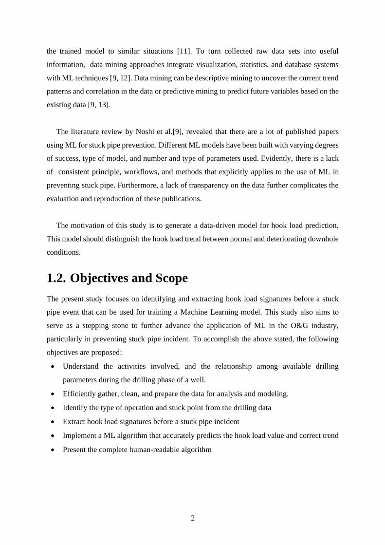
2.1. Drilling Rig System

Drilling operation is conducted to connect the surface with the reservoir, which may contain

water, oil, or natural gas. Figure 2-1 shows a typical land rotary drilling system, composed of

rotary, circulation, hoisting, power supply, and pipe handling system. The following section

briefly describes the function of each main system:

Figure 2-1. Schematic diagram of a land drilling rig.

2.1.1. Hoisting System

The hoisting system of a drilling rig is responsible for raising, lowering and suspending the

drill string, and lifting casing and tubing for installation into the well during operations. The

hoisting system consists of three major components [17]:

i. Derrick

This is a long steel tower used in the drilling rig to provide structural support for the hoist

system. It must be capable of supporting the entire load on the system. The derrick is rated

based on its ability to carry the compressive load and its height. The height of the derrick

5

determines the number of pipes that can be inserted or removed from the hole at once. The

higher the derrick, the longer the section of pipe that can be handled, the more efficient the

operation would be.

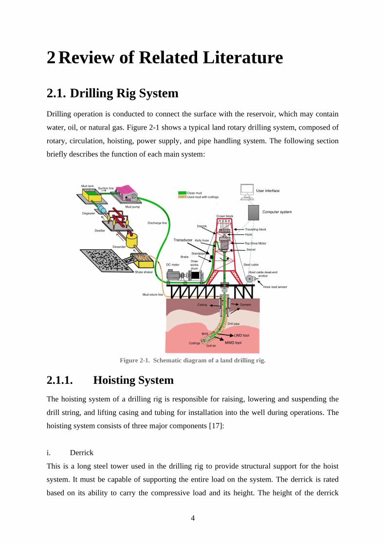
ii. Block and Tackle System

The block and tackle links the drawworks and the loads that will be lowered into or raised out

of the hole. This consists of the travelling block, crown block, and drilling line. The crown

block is stationary, while the travelling block can move up and down. Block and tackle system

provides a mechanical advantage that helps in handling large loads efficiently. The mechanical

advantage, 𝑀𝐴𝑏𝑡, of a block and tackle is the load supported by the traveling block, 𝐹𝑡𝑏, divided

by the load imposed on the drawworks which is the tension in the fast line, 𝐹𝑓𝑙 [18]:

𝑀𝐴𝑏𝑡 =𝐹𝑏𝑡

𝐹𝑓𝑙 (1)

The ideal mechanical advantage in the block and tackle can be determined from a force

analysis of the traveling block. Assuming a friction-less system, using Figure 2-2 , the tension

in the drilling line is constant throughout. Thus, a force balance in the vertical direction yields,

𝑁𝑡𝑏𝐹𝑓𝑙 = 𝐹𝑏𝑡, (2)

Where 𝑁𝑡𝑏 is the number of lines strung in the travelling block.

By inserting equation 1 to 2:

𝑀𝐴𝑏𝑡 =𝐹𝑏𝑡𝑁𝑡𝑏𝐹𝑏𝑡

= 𝑁𝑡𝑏 (3)

Where the mechanical advantage of the block-and-tackle system, 𝑀𝐴𝑏𝑡, is equal to the

number of lines strung between the crown block and traveling block. This means that the

greater number of lines and pulleys provide higher lifting power [17, 19].

6

Figure 2-2. Schematic of drawworks and block and tackle [20]

iii. Drawworks

Drawworks are the main operating component of the hoisting system. It is a winch that reels

the drilling line in or out causing the traveling block to move up or down. Drawworks consist

of brakes, mechanical and electromagnetic, used to control the weight-on-bit (WOB) during

drilling. WOB and revolutions per minute (RPM) are the two most important parameters to

optimize penetration rate. This will be discussed further in the following chapters.

2.1.2. Rotating System

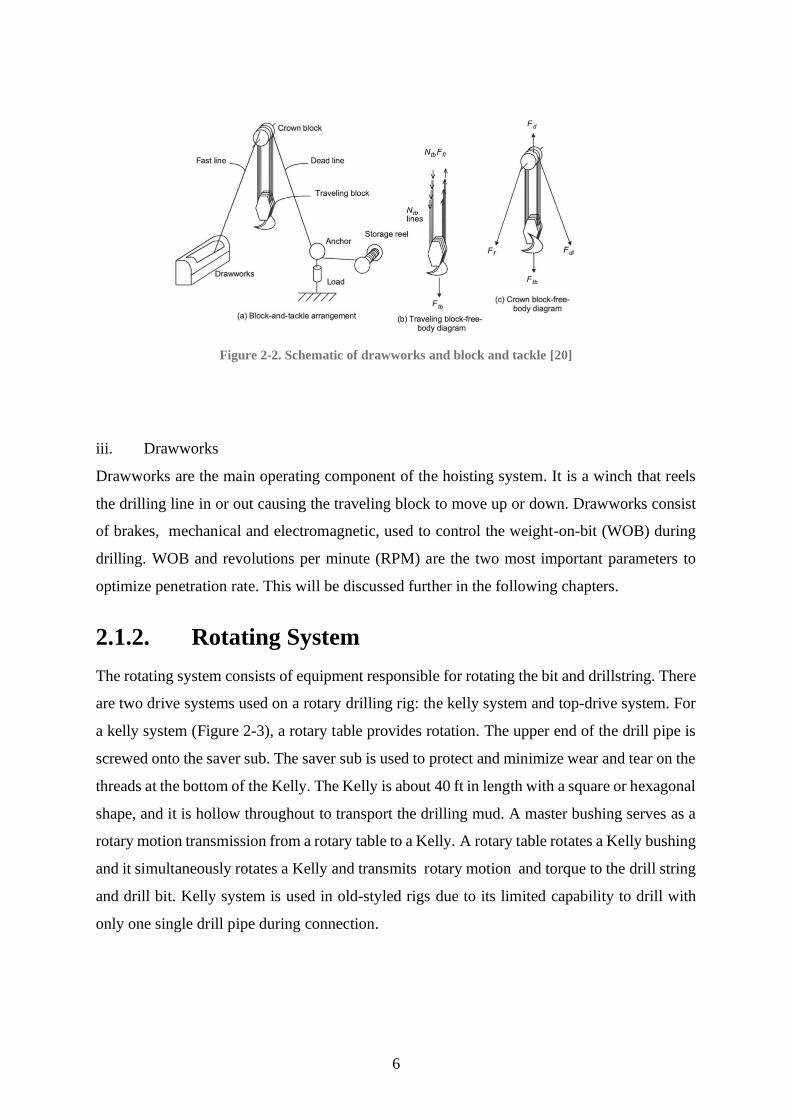
The rotating system consists of equipment responsible for rotating the bit and drillstring. There

are two drive systems used on a rotary drilling rig: the kelly system and top-drive system. For

a kelly system (Figure 2-3), a rotary table provides rotation. The upper end of the drill pipe is

screwed onto the saver sub. The saver sub is used to protect and minimize wear and tear on the

threads at the bottom of the Kelly. The Kelly is about 40 ft in length with a square or hexagonal

shape, and it is hollow throughout to transport the drilling mud. A master bushing serves as a

rotary motion transmission from a rotary table to a Kelly. A rotary table rotates a Kelly bushing

and it simultaneously rotates a Kelly and transmits rotary motion and torque to the drill string

and drill bit. Kelly system is used in old-styled rigs due to its limited capability to drill with

only one single drill pipe during connection.

7

Figure 2-3. Parts of a Kelly system [21]

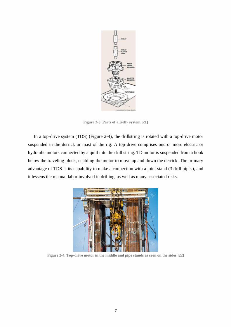
In a top-drive system (TDS) (Figure 2-4), the drillstring is rotated with a top-drive motor

suspended in the derrick or mast of the rig. A top drive comprises one or more electric or

hydraulic motors connected by a quill into the drill string. TD motor is suspended from a hook

below the traveling block, enabling the motor to move up and down the derrick. The primary

advantage of TDS is its capability to make a connection with a joint stand (3 drill pipes), and

it lessens the manual labor involved in drilling, as well as many associated risks.

Figure 2-4. Top-drive motor in the middle and pipe stands as seen on the sides [22]

8

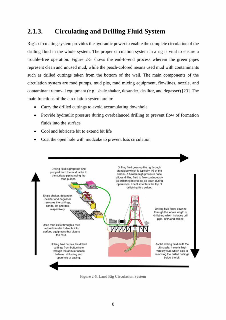
2.1.3. Circulating and Drilling Fluid System

Rig’s circulating system provides the hydraulic power to enable the complete circulation of the

drilling fluid in the whole system. The proper circulation system in a rig is vital to ensure a

trouble-free operation. Figure 2-5 shows the end-to-end process wherein the green pipes

represent clean and unused mud, while the peach-colored means used mud with contaminants

such as drilled cuttings taken from the bottom of the well. The main components of the

circulation system are mud pumps, mud pits, mud mixing equipment, flowlines, nozzle, and

contaminant removal equipment (e.g., shale shaker, desander, desilter, and degasser) [23]. The

main functions of the circulation system are to:

• Carry the drilled cuttings to avoid accumulating downhole

• Provide hydraulic pressure during overbalanced drilling to prevent flow of formation

fluids into the surface

• Cool and lubricate bit to extend bit life

• Coat the open hole with mudcake to prevent loss circulation

Figure 2-5. Land Rig Circulation System

9

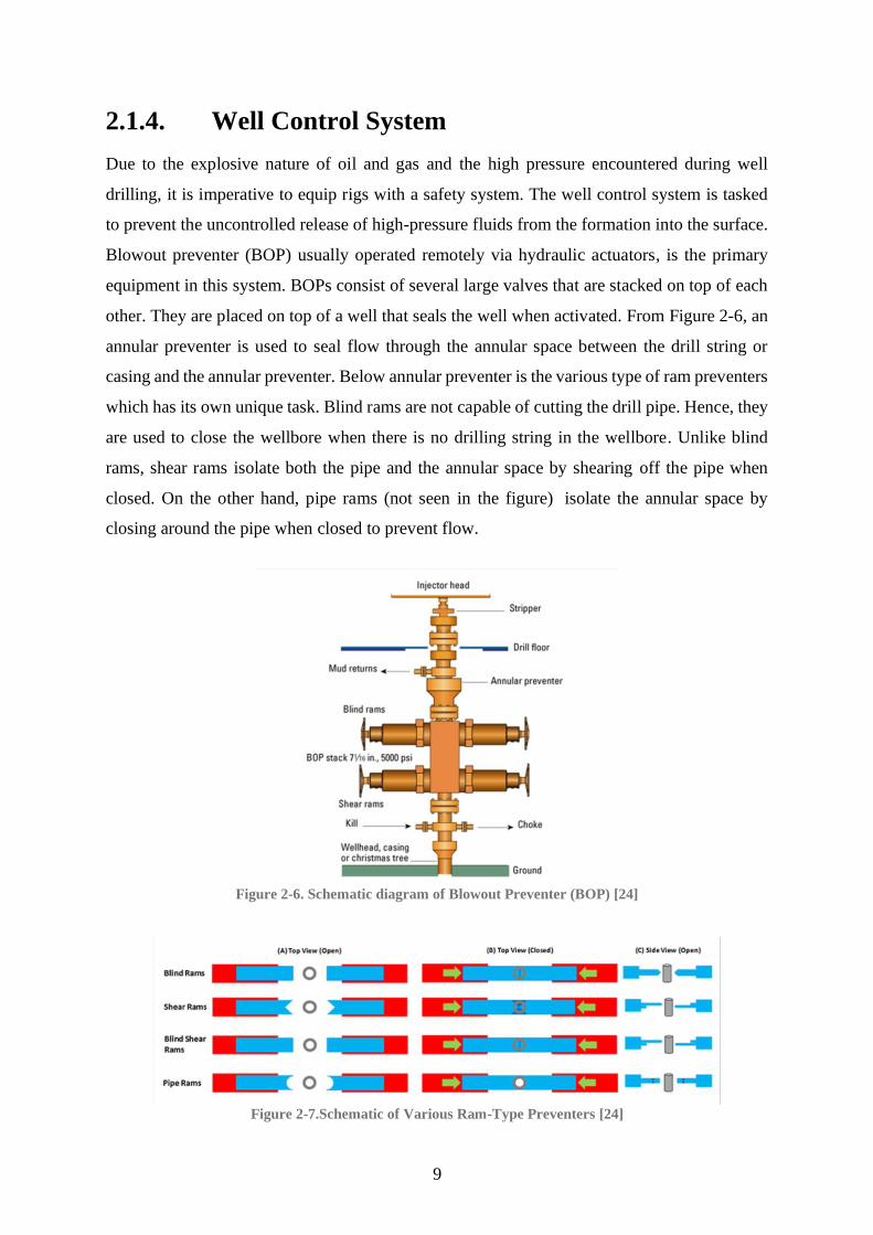
2.1.4. Well Control System

Due to the explosive nature of oil and gas and the high pressure encountered during well

drilling, it is imperative to equip rigs with a safety system. The well control system is tasked

to prevent the uncontrolled release of high-pressure fluids from the formation into the surface.

Blowout preventer (BOP) usually operated remotely via hydraulic actuators, is the primary

equipment in this system. BOPs consist of several large valves that are stacked on top of each

other. They are placed on top of a well that seals the well when activated. From Figure 2-6, an

annular preventer is used to seal flow through the annular space between the drill string or

casing and the annular preventer. Below annular preventer is the various type of ram preventers

which has its own unique task. Blind rams are not capable of cutting the drill pipe. Hence, they

are used to close the wellbore when there is no drilling string in the wellbore. Unlike blind

rams, shear rams isolate both the pipe and the annular space by shearing off the pipe when

closed. On the other hand, pipe rams (not seen in the figure) isolate the annular space by

closing around the pipe when closed to prevent flow.

Figure 2-6. Schematic diagram of Blowout Preventer (BOP) [24]

Figure 2-7.Schematic of Various Ram-Type Preventers [24]

10

2.1.5. Pipe Handling System

In the past, drill pipes are prepared and moved around the rig by manual pipe handling. To

increase the speed of operation and have a safer workplace, rig operators look for automating

pipe handling. A full range of high-performance pipe handling systems is available for onshore

and offshore applications. From NORSOK D-001 [25], automated pipe handling systems

include:

• vertical pipe handling systems

• horizontal pipe handling system

• horizontal to vertical pipe handling system

Figure 2-8 displays an automated racking board pipe handling system mounted on a rig that

mechanizes the process of lifting and moving stands of drill pipe and collars from the well

center to the racking board. This is a part of The Iron Derrickman® Pipe Handling System

designed to provide hands-free tripping of drill pipe and drill collars to maximize safety and

efficiency.

Figure 2-8. Automated pipe handling system [26]

11

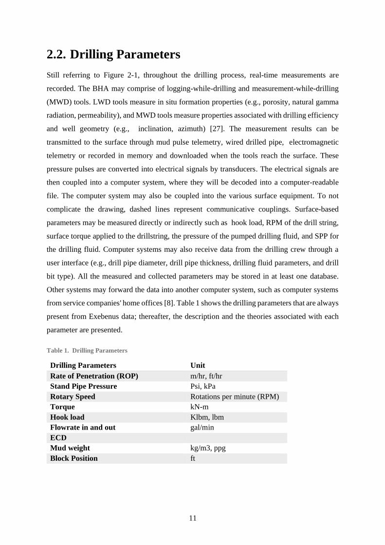
2.2. Drilling Parameters

Still referring to Figure 2-1, throughout the drilling process, real-time measurements are

recorded. The BHA may comprise of logging-while-drilling and measurement-while-drilling

(MWD) tools. LWD tools measure in situ formation properties (e.g., porosity, natural gamma

radiation, permeability), and MWD tools measure properties associated with drilling efficiency

and well geometry (e.g., inclination, azimuth) [27]. The measurement results can be

transmitted to the surface through mud pulse telemetry, wired drilled pipe, electromagnetic

telemetry or recorded in memory and downloaded when the tools reach the surface. These

pressure pulses are converted into electrical signals by transducers. The electrical signals are

then coupled into a computer system, where they will be decoded into a computer-readable

file. The computer system may also be coupled into the various surface equipment. To not

complicate the drawing, dashed lines represent communicative couplings. Surface-based

parameters may be measured directly or indirectly such as hook load, RPM of the drill string,

surface torque applied to the drillstring, the pressure of the pumped drilling fluid, and SPP for

the drilling fluid. Computer systems may also receive data from the drilling crew through a

user interface (e.g., drill pipe diameter, drill pipe thickness, drilling fluid parameters, and drill

bit type). All the measured and collected parameters may be stored in at least one database.

Other systems may forward the data into another computer system, such as computer systems

from service companies' home offices [8]. Table 1 shows the drilling parameters that are always

present from Exebenus data; thereafter, the description and the theories associated with each

parameter are presented.

Table 1. Drilling Parameters

Drilling Parameters Unit

Rate of Penetration (ROP) m/hr, ft/hr

Stand Pipe Pressure Psi, kPa

Rotary Speed Rotations per minute (RPM)

Torque kN-m

Hook load Klbm, lbm

Flowrate in and out gal/min

ECD

Mud weight kg/m3, ppg

Block Position ft

12

2.2.1. Torque and Drag

Torque is defined as the force multiplied by an arm that causes an object to rotate. To drill

holes, torque is applied to overcome the rotational friction between the drillstring, including

the bit and the borehole wall.

Drag is the friction force, which is the product of the contact force of the drilling string on

the wellbore and the coefficient of friction. The effective tension on the drill string is due to

the static weight of the drill string and the drag forces. This additional load is added to the static

weight when pulling out of the hole and deducted from the static weight when running into the

hole. Similarly, due to friction, there is a difference between the torque applied at the rig floor

and the torque available at the bit. Thus, torque and drag are often associated with each other.

Drag and Torque Along Straight Sections

Figure 2-9 shows the free body diagram of mass-friction in the inclined well geometry.

Applying equilibrium condition, Aadnøy [28] derived the force at the top of the string along

straight sections:

𝐹2 = 𝐹1 + 𝑤∆𝑠(𝑐𝑜𝑠 ∝ ± 𝜇𝑠𝑖𝑛 ∝) (4)

Where,

𝛼 : well inclination

𝐹1: force at the bottom

𝐹𝟐 ∶ force at the top

𝑤∆𝑠 𝑐𝑜𝑠𝛼 : static force (or self-weight)

±𝑤∆𝑠𝜇 𝑠𝑖𝑛𝛼 : the drag force, (+) for pulling the pipe, and (-) when lowering the pipe

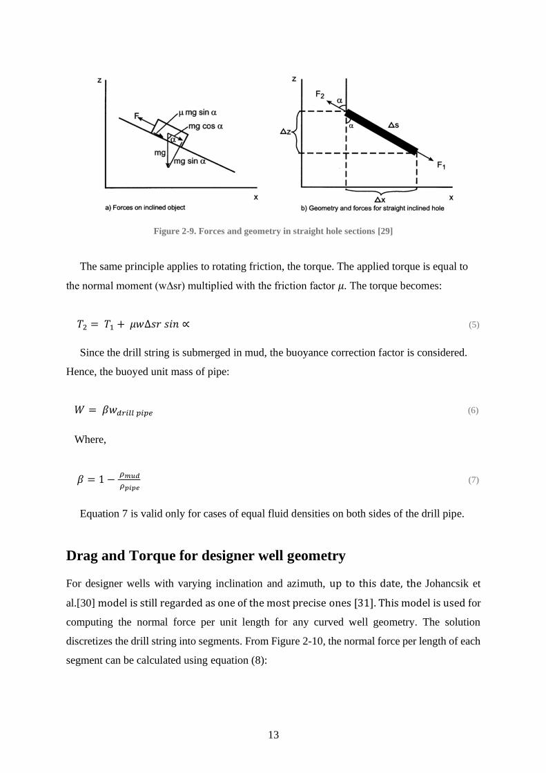
13

Figure 2-9. Forces and geometry in straight hole sections [29]

The same principle applies to rotating friction, the torque. The applied torque is equal to

the normal moment (w∆sr) multiplied with the friction factor 𝜇. The torque becomes:

𝑇2 = 𝑇1 + 𝜇𝑤∆𝑠𝑟 𝑠𝑖𝑛 ∝ (5)

Since the drill string is submerged in mud, the buoyance correction factor is considered.

Hence, the buoyed unit mass of pipe:

𝑊 = 𝛽𝑤𝑑𝑟𝑖𝑙𝑙 𝑝𝑖𝑝𝑒 (6)

Where,

𝛽 = 1 − 𝜌𝑚𝑢𝑑

𝜌𝑝𝑖𝑝𝑒

(7)

Equation 7 is valid only for cases of equal fluid densities on both sides of the drill pipe.

Drag and Torque for designer well geometry

For designer wells with varying inclination and azimuth, up to this date, the Johancsik et

al.[30] model is still regarded as one of the most precise ones [31]. This model is used for

computing the normal force per unit length for any curved well geometry. The solution

discretizes the drill string into segments. From Figure 2-10, the normal force per length of each

segment can be calculated using equation (8):

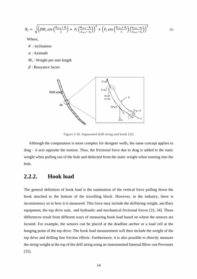
14

𝑁𝑖 = √(𝛽𝑊𝑖 𝑠𝑖𝑛 (𝜃𝑖+1+ 𝜃𝑖

2) + 𝐹𝑖 (

𝜃𝑖+1− 𝜃𝑖

𝑆𝑖+1− 𝑆𝑖))

2+ (𝐹𝑖 𝑠𝑖𝑛 (

𝜃𝑖+1+ 𝜃𝑖

2) (

𝛼𝑖+1−𝛼𝑖

𝑆𝑖+1−𝑆𝑖))

2 (8)

Where,

𝜃 : inclination

𝛼 : Azimuth

𝑊𝑖 : Weight per unit length

𝛽 : Buoyance factor

Figure 2-10. Segmented drill string and loads [32]

Although the computation is more complex for designer wells, the same concept applies to

drag – it acts opposite the motion. Thus, the frictional force due to drag is added to the static

weight when pulling out of the hole and deducted from the static weight when running into the

hole.

2.2.2. Hook load

The general definition of hook load is the summation of the vertical force pulling down the

hook attached to the bottom of the travelling block. However, in the industry, there is

inconsistency as to how it is measured. This force may include the drillstring weight, ancillary

equipment, the top drive unit, and hydraulic and mechanical frictional forces [33, 34]. These

differences result from different ways of measuring hook load based on where the sensors are

located. For example, the sensors can be placed at the deadline anchor or a load cell at the

hanging point of the top drive. The hook load measurement will then include the weight of the

top drive and drilling line friction effects. Furthermore, it is also possible to directly measure

the string weight at the top of the drill string using an instrumented Internal Blow-out Preventer

[35].

15

For simplicity, according to Aadnøy [28], the static hook load, regardless of wellbore

orientation, is equal to the buoyed pipe weight multiplied by the projected vertical height of

the well. During dynamic conditions wherein the string moves inside the well, the additional

forces due to drag must be accounted for. Drag is added to the static weight when tripping out

of the hole since forces from the weight of the drill string and friction are in the same direction.

Drag is deducted from the static weight for tripping in since friction is opposite the direction

of drillstring weight. For this case, the formula for hook load based on coulomb mass-friction

can be written as:

𝐻𝑜𝑜𝑘 𝑙𝑜𝑎𝑑 = 𝑊∆𝑠(𝑐𝑜𝑠 ∝ ± 𝜇𝑠𝑖𝑛 ∝) − 𝑊𝑂𝐵 (9)

Where,

(+) means tripping out and (−) means tripping in of the drill string.

𝑊 : buoyed weight

∆𝑠(𝑐𝑜𝑠 ∝) : projected height

WOB : non-zero weight on bit during drilling mode, and zero for tripping operations

∆𝑠 𝜇𝑠𝑖𝑛 ∝ : drag force

Generally, three main factors cause a reduction in hook load:

i. Buoyancy effect

During drilling, the drillstring is immersed in drilling fluid inside the well. Due to the up-thrust

forces, the hook load will be reduced. Also, since rocks have a higher density than mud, cuttings

in suspension will increase the effective density of the annular mud. The added density reduces

the specific string weight and thereby also the total reference string weight.

ii. Bit on bottom

A reduction in hook load could be observed when the bit touches the hole’s bottom as some of

the load is transferred into the formation.

iii. Contact friction

Particularly in-high angle wells, hook load is reduced as the drillstring makes contact on one

side of the borehole. This is similar to pack-off and differential sticking, where the

accumulation of cuttings tries to hold some of the drillstring weight.

16

Hook load is an important drilling parameter that helps the driller estimate and control the

weight on bit to maximize drilling efficiency. It also provides a vital information about the

downhole conditions. For example, abnormal hook load may indicate poor hole cleaning or

excessive tortuosity [33].

2.2.3. Standpipe Pressure

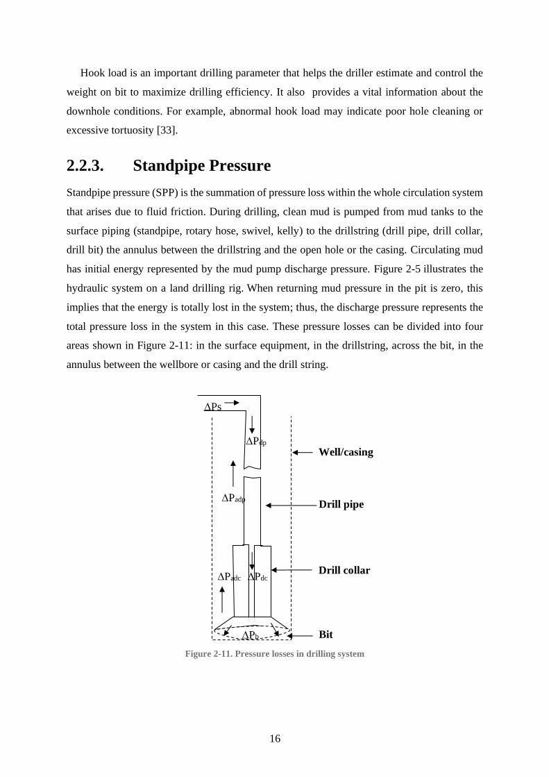
Standpipe pressure (SPP) is the summation of pressure loss within the whole circulation system

that arises due to fluid friction. During drilling, clean mud is pumped from mud tanks to the

surface piping (standpipe, rotary hose, swivel, kelly) to the drillstring (drill pipe, drill collar,

drill bit) the annulus between the drillstring and the open hole or the casing. Circulating mud

has initial energy represented by the mud pump discharge pressure. Figure 2-5 illustrates the

hydraulic system on a land drilling rig. When returning mud pressure in the pit is zero, this

implies that the energy is totally lost in the system; thus, the discharge pressure represents the

total pressure loss in the system in this case. These pressure losses can be divided into four

areas shown in Figure 2-11: in the surface equipment, in the drillstring, across the bit, in the

annulus between the wellbore or casing and the drill string.

Figure 2-11. Pressure losses in drilling system

Ps

Pdp

Pb

Padp

Padc

Bit

Drill collar

Drill pipe

Well/casing

Pdc

17

SPP can be expressed as [28]:

𝑃𝑝 = ∆𝑃𝑓𝑠 + ∆𝑃𝑓𝑑𝑝 + ∆𝑃𝑓𝑑𝑐 + ∆𝑃𝑏 + ∆𝑃𝑓𝑎𝑑𝑐 + ∆𝑃𝑓𝑎𝑑𝑝 (10)

Where,

∆𝑃fs= Pressure loss in surface flow lines.

∆𝑃fdp = pressure losses in the drill pipe.

∆𝑃fdc = Pressure losses in the drill collar.

∆𝑃b = Pressure losses in the nozzles of the drill bit.

∆𝑃fadc= Pressure losses in the annular spacing between the well and the drill collar.

∆𝑃fadp = Pressure losses in the annular spacing between the wellbore and the drill pipe.

Pressure drop equations depend on the following:

• Flow regime: laminar or turbulent

• Rheology of the circulating fluid

• The pipe and hole geometry

In general, SPP increases with drilling depth, an increase in viscosity, mud weight and

flowrate, and smaller annulus. SPP helps select the right size of bit nozzle, proper mud pump

liner, and optimum flowrate to achieve adequate hole cleaning and cuttings transport. Real-

time monitoring of SPP is of prime importance as it aids in identifying potential downhole

problems. For example, washed out pipe or bit nozzle, broken drillstring, lost circulation could

cause too low SPP. On the other hand, a high SPP could indicate plugged drill bit or increased

mud density or viscosity [36].

2.2.4. Rate of Penetration

This is the rate at which the bit crushes and moves through the formation. High ROP produces

a greater amount of cuttings; thus, mud rheology must be properly designed to avoid cutting

accumulation. ROP is measured in feet per hour or meters per hour. During tripping operations,

the penetration rate has a value of 0 or -999 that indicates no new drilled rock. This is confirmed

as well by a constant measured depth in the drilling data.

18

2.2.5. Rotary Speed

The rate at which the drill string rotation is measured in revolutions per minute (rpm). During

drilling operations, it is not always possible to rotate the drillstring. For instance, drilling a

deviated hole using a mud motor, slide drilling is performed wherein only the bit rotates.

During tripping operations, it depends on the driller’s preference to rotate the string.

2.2.6. Mud weight

Mud density expressed in lbm/gal or kg/m3. Mud weight controls the wellbore hydrostatic

pressure, thus preventing the influx of fluid during overbalanced operation. Too high mud

weight could cause formation fracture and lead to losses. Mud weight can be altered by the

addition of additives such as barite which increases the density. The presence of cuttings in

suspension in the drilling fluid also increases mud weight. Two mud weights can be measured,

mud going inside the well and the returning mud out of the well.

2.2.7. Equivalent Circulating Density

During static conditions, the pressure in the well is only provided by the mud weight. However,

during dynamic drilling, the circulation of fluids creates opposing frictional forces which

change the effective pressure exerted against the formation. This additional force must be taken

into account; thus, ECD is used rather than mud weight when measuring the bottom hole

pressure. ECD is the effective density exerted by the drilling fluid that considers the pressure

drop in the annulus above the point being considered. The ECD is calculated as [37]:

𝐸𝐶𝐷(𝑝𝑝𝑔) = 𝑀𝑊(𝑝𝑝𝑔) +∆𝑃𝑎𝑛𝑛𝑢𝑙𝑢𝑠(𝑝𝑠𝑖)

0.052 ∙𝑇𝑉𝐷 (𝑓𝑡) (11)

Where,

∆𝑃𝑎𝑛𝑛𝑢𝑙𝑢𝑠 : pressure drop in the annulus

𝑀𝑊 : static mud weight and

𝑇𝑉𝐷 : true vertical depth to the point of interest

19

2.2.8. Flow rate

This is the volume of mud being pumped in or going out of the system. Ideally, equal flowrate

in and out indicates a good well condition. This means that no losses of mud to the formation

or no addition due to an influx of formation fluids. During tripping in operations, flowrate is

attributed to filling in the pipe with mud. For tripping out, this is attributed to the pumping of

mud inside the well to accommodate the volume previously occupied by the unscrewed joint.

In any operation, the well must always be filled with mud enough to control the influx of

formation fluids.

2.2.9. Block Position

This is the height of the travelling block that ranges up to 90ft. When paired with hook load,

block position serves as a guide in determining the current activity in the rig. This will be

elaborated under Section 2.3.

2.3. Tripping Operations

Tripping operation is the act of moving the string in (tripping in) or out of the well (tripping

out). Bit are off the bottom during this operation such that the WOB and ROP are zero.

Tripping in is performed while drilling to extend the drillstring and reach the oil or gas reserve.

Similarly, running and setting in the casing are considered tripping in, except that the casing

has a larger diameter and heavier than the drill pipes. Conversely, when a bit replacement is

necessary, a survey needs to occur, or a downhole tool failure is experienced, the complete

drillstring must be tripped out and then back in. In this context, tripping out operations involves

activities in which the string moves toward the surface (e.g., back reaming, where you maintain

or enlarge the diameter of the hole by rotating the bit while tripping out). Similarly, tripping in

operation involves activities in which the string moves towards the bottom of the well (e.g.,

running in liner or casing).

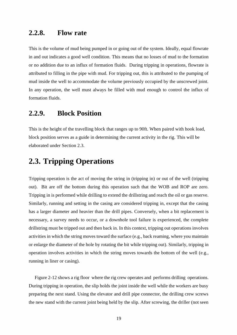
Figure 2-12 shows a rig floor where the rig crew operates and performs drilling operations.

During tripping in operation, the slip holds the joint inside the well while the workers are busy

preparing the next stand. Using the elevator and drill pipe connector, the drilling crew screws

the new stand with the current joint being held by the slip. After screwing, the driller (not seen

20

on the figure) raises the top drive to remove the slip, and then the joint is lowered inside the

hole and set back in slips again.

Figure 2-12. Rig floor [38]

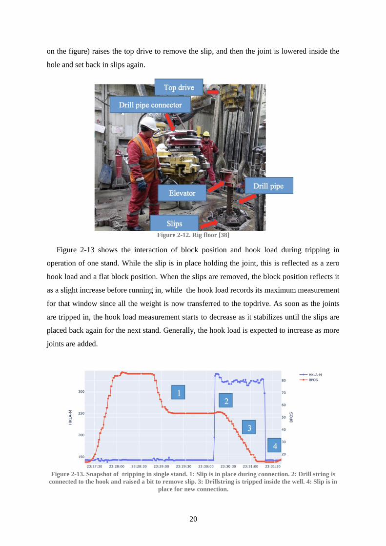
Figure 2-13 shows the interaction of block position and hook load during tripping in

operation of one stand. While the slip is in place holding the joint, this is reflected as a zero

hook load and a flat block position. When the slips are removed, the block position reflects it

as a slight increase before running in, while the hook load records its maximum measurement

for that window since all the weight is now transferred to the topdrive. As soon as the joints

are tripped in, the hook load measurement starts to decrease as it stabilizes until the slips are

placed back again for the next stand. Generally, the hook load is expected to increase as more

joints are added.

Figure 2-13. Snapshot of tripping in single stand. 1: Slip is in place during connection. 2: Drill string is

connected to the hook and raised a bit to remove slip. 3: Drillstring is tripped inside the well. 4: Slip is in

place for new connection.

21

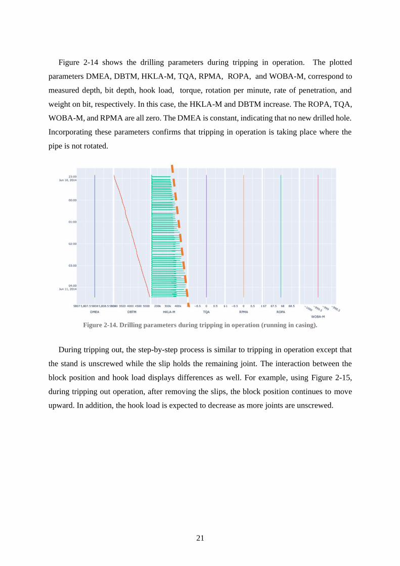
Figure 2-14 shows the drilling parameters during tripping in operation. The plotted

parameters DMEA, DBTM, HKLA-M, TQA, RPMA, ROPA, and WOBA-M, correspond to

measured depth, bit depth, hook load, torque, rotation per minute, rate of penetration, and

weight on bit, respectively. In this case, the HKLA-M and DBTM increase. The ROPA, TQA,

WOBA-M, and RPMA are all zero. The DMEA is constant, indicating that no new drilled hole.

Incorporating these parameters confirms that tripping in operation is taking place where the

pipe is not rotated.

Figure 2-14. Drilling parameters during tripping in operation (running in casing).

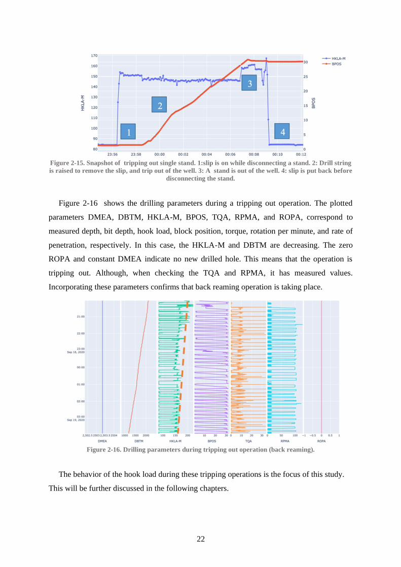
During tripping out, the step-by-step process is similar to tripping in operation except that

the stand is unscrewed while the slip holds the remaining joint. The interaction between the

block position and hook load displays differences as well. For example, using Figure 2-15,

during tripping out operation, after removing the slips, the block position continues to move

upward. In addition, the hook load is expected to decrease as more joints are unscrewed.

22

Figure 2-15. Snapshot of tripping out single stand. 1:slip is on while disconnecting a stand. 2: Drill string

is raised to remove the slip, and trip out of the well. 3: A stand is out of the well. 4: slip is put back before

disconnecting the stand.

Figure 2-16 shows the drilling parameters during a tripping out operation. The plotted

parameters DMEA, DBTM, HKLA-M, BPOS, TQA, RPMA, and ROPA, correspond to

measured depth, bit depth, hook load, block position, torque, rotation per minute, and rate of

penetration, respectively. In this case, the HKLA-M and DBTM are decreasing. The zero

ROPA and constant DMEA indicate no new drilled hole. This means that the operation is

tripping out. Although, when checking the TQA and RPMA, it has measured values.

Incorporating these parameters confirms that back reaming operation is taking place.

Figure 2-16. Drilling parameters during tripping out operation (back reaming).

The behavior of the hook load during these tripping operations is the focus of this study.

This will be further discussed in the following chapters.

23

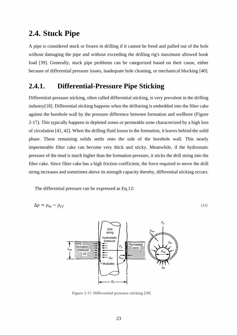
2.4. Stuck Pipe

A pipe is considered stuck or frozen in drilling if it cannot be freed and pulled out of the hole

without damaging the pipe and without exceeding the drilling rig's maximum allowed hook

load [39]. Generally, stuck pipe problems can be categorized based on their cause, either

because of differential pressure issues, inadequate hole cleaning, or mechanical blocking [40].

2.4.1. Differential-Pressure Pipe Sticking

Differential-pressure sticking, often called differential sticking, is very prevalent in the drilling

industry[18]. Differential sticking happens when the drillstring is embedded into the filter cake

against the borehole wall by the pressure difference between formation and wellbore (Figure

2-17). This typically happens in depleted zones or permeable zone characterized by a high loss

of circulation [41, 42]. When the drilling fluid losses to the formation, it leaves behind the solid

phase. These remaining solids settle onto the side of the borehole wall. This nearly

impermeable filter cake can become very thick and sticky. Meanwhile, if the hydrostatic

pressure of the mud is much higher than the formation pressure, it sticks the drill string into the

filter cake. Since filter cake has a high friction coefficient, the force required to move the drill

string increases and sometimes above its strength capacity thereby, differential sticking occurs.

The differential pressure can be expressed as Eq.12:

∆𝜌 = 𝜌𝑚 − 𝜌𝑓𝑓 (12)

Figure 2-17. Differential pressure sticking [39]

24

Whereas the force required, Fp, to free the stuck pipe:

𝐹𝑃 = 𝑓∆𝑝𝐴𝑐 (13)

From Bourgoyne A. [43], 𝐴𝑐 can be expressed as:

𝐴𝑐 = 2𝐿𝑒𝑝((𝐷ℎ

2−ℎ𝑚𝑐)

2− [

𝐷ℎ

2−ℎ𝑚𝑐(𝐷ℎ−ℎ𝑚𝑐)

𝐷ℎ−𝐷𝑜𝑝

]

2

)0.5 (14)

Where,

𝐷𝑜𝑝 ≤ (𝐷ℎ − ℎ𝑚𝑐) (15)

In these equations:

Δp : differential pressure

f : coefficient of friction, 0.04 – 0.35 for oil or water based muds with no added lubricant

Lep : length of the permeable zone

Dop : outside diameter of the pipe

Dh : diameter of the hole

hmc :mudcake thickness

Ac : area of contact between the pipe and mudcake surfaces

From equations 13 and 14, the factors that cause differential-pressure pipe sticking are high

differential pressure, thick mudcake due to high fluid loss to the formation, low-lubricity mud

cake, and the length of pipe embedded in the mudcake. When differential sticking occurs, rig

site indications can be full unrestricted circulation, mud losses, increase in torque and drag, an

inability to reciprocate the drillstring and in some cases, to rotate it [39, 44].

2.4.2. Inadequate Hole Cleaning

Drilled cuttings must be taken out of the wellbore to avoid cuttings bed inside the hole. Failure

to remove the cuttings can lead to packing off of the drillstring – another type of stuck pipe.

Accumulation starts when the circulating drilling fluid is not viscous enough or fast enough

that the gravity forces exceed the drag forces on the solids. This means that instead of up and

out of the hole, the solids flow down the hole. When this accumulation is not mitigated, the

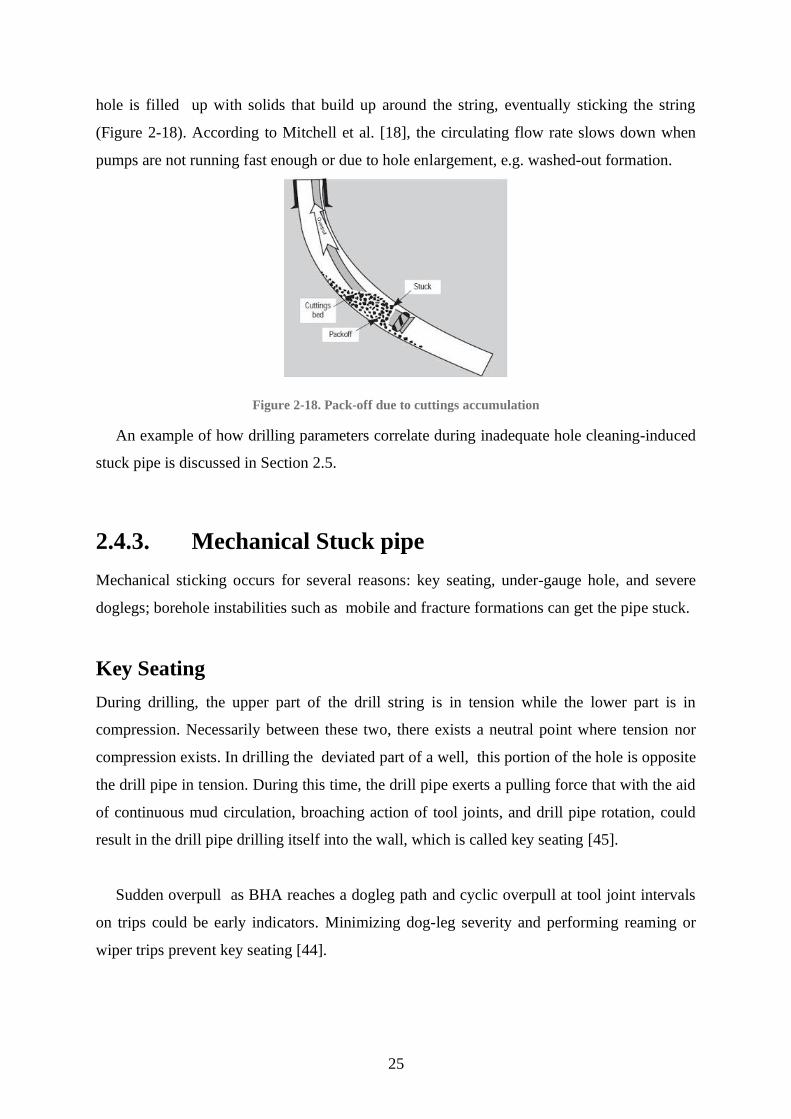
25

hole is filled up with solids that build up around the string, eventually sticking the string

(Figure 2-18). According to Mitchell et al. [18], the circulating flow rate slows down when

pumps are not running fast enough or due to hole enlargement, e.g. washed-out formation.

Figure 2-18. Pack-off due to cuttings accumulation

An example of how drilling parameters correlate during inadequate hole cleaning-induced

stuck pipe is discussed in Section 2.5.

2.4.3. Mechanical Stuck pipe

Mechanical sticking occurs for several reasons: key seating, under-gauge hole, and severe

doglegs; borehole instabilities such as mobile and fracture formations can get the pipe stuck.

Key Seating

During drilling, the upper part of the drill string is in tension while the lower part is in

compression. Necessarily between these two, there exists a neutral point where tension nor

compression exists. In drilling the deviated part of a well, this portion of the hole is opposite

the drill pipe in tension. During this time, the drill pipe exerts a pulling force that with the aid

of continuous mud circulation, broaching action of tool joints, and drill pipe rotation, could

result in the drill pipe drilling itself into the wall, which is called key seating [45].

Sudden overpull as BHA reaches a dogleg path and cyclic overpull at tool joint intervals

on trips could be early indicators. Minimizing dog-leg severity and performing reaming or

wiper trips prevent key seating [44].

26

Under gauge hole

Any hole that is considered smaller than expected is deemed to be an under-gauged hole.

Swelling formations may decrease the diameter of the hole. Using higher mud weight will

balance the rock stresses and can keep the borehole in-gauge. Another reason for under gauge

hole is bit wear as a result of drilling hard abrasive rocks. When a new in-gauge bit is run

without reaming and wiper trip, there is a potential for jam and leading to pipe stuck. A thick

filter cake and fill packing around the bottom hole assembly could cause a reduced diameter

[28, 44].

Pulled bit or stabilizers are under gauge, sudden set down weight, and circulation may be

slightly restricted could be early indicators. Using gauged bit, stabilizers, BHA, roller reamers,

and higher mud weight could keep the hole in-gauged [44].

Junk

Any object that has fallen unintentionally into the wellbore can jam the drill string. This is a

result of poor housekeeping or failure of downhole equipment. Sudden erratic torque, metal

shavings at the shaker, missing tools, and inability to make holes are the rig indicators of junk

in [44].

Collapsed casing or tubing

This happens when either the casing or tubing collapse rating is reduced due to wear, corrosion,

or excessive formation pressure exceeding the collapse pressure rating. Typically, this is

discovered when BHA is run into the hole and jams. Proper cement practices, avoiding casing

wear, and usage of corrosion inhibitors could prevent this problem [44].

Cement Sticking

Cement has two ways to cause stuck pipes. One is unstable cement blocks falling around and

accumulating at the bottomhole. Cement fragments, erratic torque with unrestricted circulation

are the rig indicators. Two is when the drill string is run before the cement curing time, and the

sudden surge in pressure results in cement to flash set. A sudden increase in torque, loss of

string weight, increase in pump pressure leading to restricted circulation and cement in mud

27

returns are the indicators of this pipe sticking problem. Knowing the right top of cement and

the cement setting time could prevent [44].

Borehole Instability

Borehole instability is the undesirable condition of an openhole that does not keep its gauge

size and structural integrity. Mechanical failure caused by in-situ stresses, erosion, and

chemical interaction between the mud and formation are the leading causes of borehole

instability. Furthermore, borehole instabilities have types: hole closure or reduced diameter,

washouts, fracturing, and collapse [39].

Reduced diameter

The reduced diameter of the openhole could be caused by drilling reactive formations such as

water-sensitive shale and reactive clays. The shale absorbs the water from the circulating mud

and swells into the wellbore. Shakers screens blind off, restricted circulation, hydrated or

mushy cavings, and an increase in pump pressure are the early indicators of drilling a swelling

formation. Using an inhibited mud system, minimized open hole time in shale, and regular

wiper trips or reaming trips could prevent this issue [39]. Some wells kept the hole stable by

using sufficiently high mud weight and minimal open hole exposure time. However, some

wells showed hole enlargement despite high mud weight used [28].

Hole Enlargement

Hole enlargement results from the hydraulic force from the bit nozzles that hydraulically erode

the borehole away, mechanical abrasion caused by drillstring and shale sloughing. As observed

in the Central North Sea, drilling at about 500m with unconsolidated formation gradually

increased that drag over several meters. This happens when little or no filter cake is present or

excessive jetting. An increase in pump pressure, fill in bottom, overpull on connections and

shakers blinding are the indicators of drilling unconsolidated formation. Avoiding pressure

surges and an adequate filter cake could help stabilize the formation [28, 39, 44].

28

Collapse

Borehole collapse happens when the ECD is too low compared to the hoop stress around the

borehole wall. Eventually, pipe sticking and loss of well could persist. The most important

remedy is to increase mud weight [28, 39].

Fractured and Faulted Formation

Fractured and faulted formations are typically found near faults. These rock fragments can fall

into the wellbore and eventually, when adequate accumulation occurs can lead to jamming the

drill string. Hole fill on connections, fault-damaged cavings at shakers, and instantaneous

sticking can be early signs of this issue. Through RPM change and BHA configuration,

minimizing drill string vibration could help prevent the rock fragments from falling [44].

2.5. Physics-Based Stuck Pipe Detection

Engineers use “roadmaps” to detect deteriorating downhole conditions. Roadmaps are made

up of precalculated physics-based models and real-time measurements displayed together

graphically [6]. These physical models are integrated with automatic calibration. Automatic

calibration provides a reliable picture of the expected well behavior and ensures that relevant

learnings are carried forward into the next time step. By analyzing the deviations between

modeled and actual measured values, an estimation of the current state of the well is derived in

real-time. When the current well conditions are deviating from normality, the drilling crew are

warned of a deteriorating well condition or if the well conditions limit the drillability of the

well [6, 46]. The difficulty in this approach is defining what "normal" is, which significantly

depends on the engineer's interpretation [7].

In particular to stuck pipe detection, hook load measurement analysis identifies any decrease

or increase in friction of the drillstring run inside the well. As mentioned previously, there is

no straightforward in measuring the “normal” friction factor. Thus, it is much more sensible to

monitor the trend of the hook load rather than one specific calculated ideal value. For this

particular approach, engineers simulate different hook load values using various friction

factors. Typically, the friction factor ranges from 0.1 to 0.5 for RIH and POOH plus one curve

with 0 friction factor for bit rotating on the bottom [7]. In practice, while this friction factor

29

approach may work, it is often unable to deal with complex situations where hook load does

not show large variations and sometimes possess hidden trends [6].

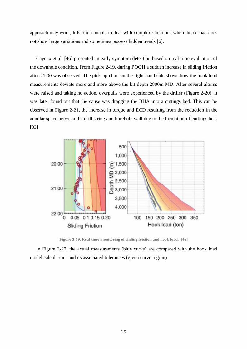
Cayeux et al. [46] presented an early symptom detection based on real-time evaluation of

the downhole condition. From Figure 2-19, during POOH a sudden increase in sliding friction

after 21:00 was observed. The pick-up chart on the right-hand side shows how the hook load

measurements deviate more and more above the bit depth 2800m MD. After several alarms

were raised and taking no action, overpulls were experienced by the driller (Figure 2-20). It

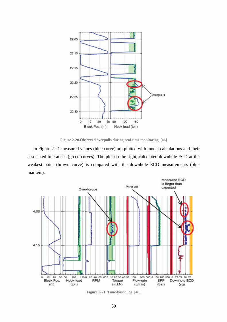
was later found out that the cause was dragging the BHA into a cuttings bed. This can be

observed in Figure 2-21, the increase in torque and ECD resulting from the reduction in the

annular space between the drill string and borehole wall due to the formation of cuttings bed.

[33]

Figure 2-19. Real-time monitoring of sliding friction and hook load. [46]

In Figure 2-20, the actual measurements (blue curve) are compared with the hook load

model calculations and its associated tolerances (green curve region)

30

Figure 2-20.Observed overpulls during real-time monitoring. [46]

In Figure 2-21 measured values (blue curve) are plotted with model calculations and their

associated tolerances (green curves). The plot on the right, calculated downhole ECD at the

weakest point (brown curve) is compared with the downhole ECD measurements (blue

markers).

Figure 2-21. Time-based log. [46]

31

2.6. Machine Learning

Arthur Samuel [47] defines Machine Learning (ML) as applying artificial intelligence that

equips systems with the ability to learn and improve through experience without being

explicitly programmed [48]. An ML system is trained with enough examples relevant to a

particular task that eventually allows the system to develop new rules for automating the task

[49]. One vital feature of ML algorithms is recognizing complex patterns with reasonable

predictive accuracy [50]. There are various types of ML algorithms that are available

depending on:

i. Objective

Algorithms could predict a discrete class label (classification problem) or predict a continuous

quantity (regression problem).

ii. Data category

From a ML perspective, data can be categorized into numerical, categorical, text, and time

series. In this context, hook load measurements are a time series data since it is collected at

regular intervals over time.

iii. Supervised or Unsupervised

Supervised learning algorithms learn from labeled datasets wherein the label is the target we

are interested in predicting. Using these labels, the model can measure its accuracy and learn

over time. On the contrary, unsupervised algorithms are designed to analyze and cluster

unlabeled datasets. This is because unlabeled data does not contain targets that the model will

try to predict. In this context, we used the past hook load measurements as input to predict the

next hook load. This predicted hook load is the target or label. This means that a supervised

algorithm is used.

Generally, the predictive model's performance depends on the database's size and the

variables selected for the analysis. A robust database model yields more accurate and feasible

results [51].

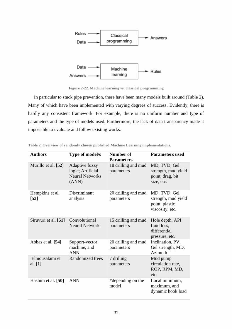
32

Figure 2-22. Machine learning vs. classical programming

In particular to stuck pipe prevention, there have been many models built around (Table 2).

Many of which have been implemented with varying degrees of success. Evidently, there is

hardly any consistent framework. For example, there is no uniform number and type of

parameters and the type of models used. Furthermore, the lack of data transparency made it

impossible to evaluate and follow existing works.

Table 2. Overview of randomly chosen published Machine Learning implementations.

Authors Type of model/s Number of

Parameters

Parameters used

Murillo et al. [52] Adaptive fuzzy

logic; Artificial

Neural Networks

(ANN)

18 drilling and mud

parameters

MD, TVD, Gel

strength, mud yield

point, drag, bit

size, etc.

Hempkins et al.

[53]

Discriminant

analysis

20 drilling and mud

parameters

MD, TVD, Gel

strength, mud yield

point, plastic

viscosity, etc.

Siruvuri et al. [51] Convolutional

Neural Network

15 drilling and mud

parameters

Hole depth, API

fluid loss,

differential

pressure, etc.

Abbas et al. [54] Support-vector

machine, and

ANN

20 drilling and mud

parameters

Inclination, PV,

Gel strength, MD,

Azimuth

Elmousalami et

al. [1]

Randomized trees 7 drilling

parameters

Mud pump

circulation rate,

ROP, RPM, MD,

etc.

Hashim et al. [50] ANN *depending on the

model

Local minimum,

maximum, and

dynamic hook load

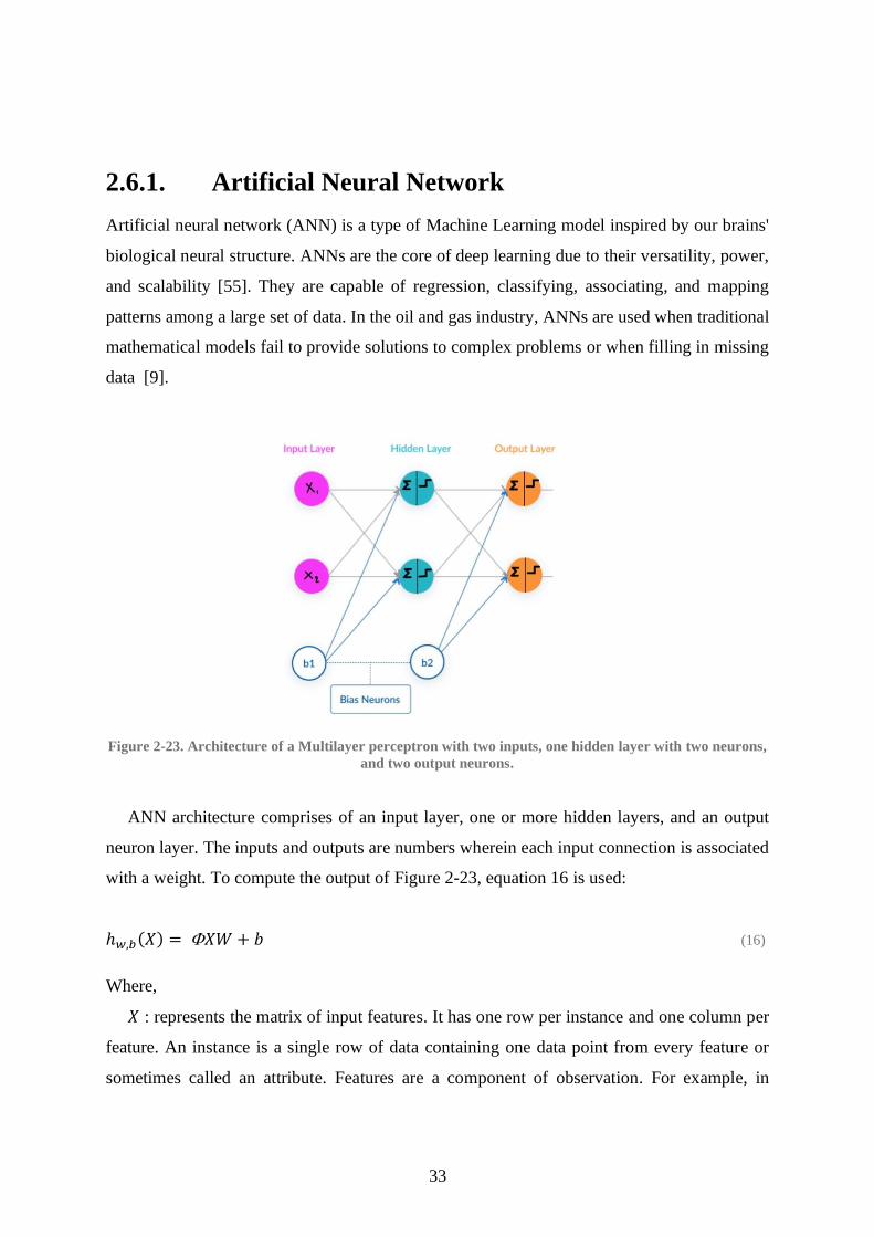
33

2.6.1. Artificial Neural Network

Artificial neural network (ANN) is a type of Machine Learning model inspired by our brains'

biological neural structure. ANNs are the core of deep learning due to their versatility, power,

and scalability [55]. They are capable of regression, classifying, associating, and mapping

patterns among a large set of data. In the oil and gas industry, ANNs are used when traditional

mathematical models fail to provide solutions to complex problems or when filling in missing

data [9].

Figure 2-23. Architecture of a Multilayer perceptron with two inputs, one hidden layer with two neurons,

and two output neurons.

ANN architecture comprises of an input layer, one or more hidden layers, and an output

neuron layer. The inputs and outputs are numbers wherein each input connection is associated

with a weight. To compute the output of Figure 2-23, equation 16 is used:

ℎ𝑤,𝑏(𝑋) = 𝑋𝑊 + 𝑏 (16)

Where,

𝑋 : represents the matrix of input features. It has one row per instance and one column per

feature. An instance is a single row of data containing one data point from every feature or

sometimes called an attribute. Features are a component of observation. For example, in

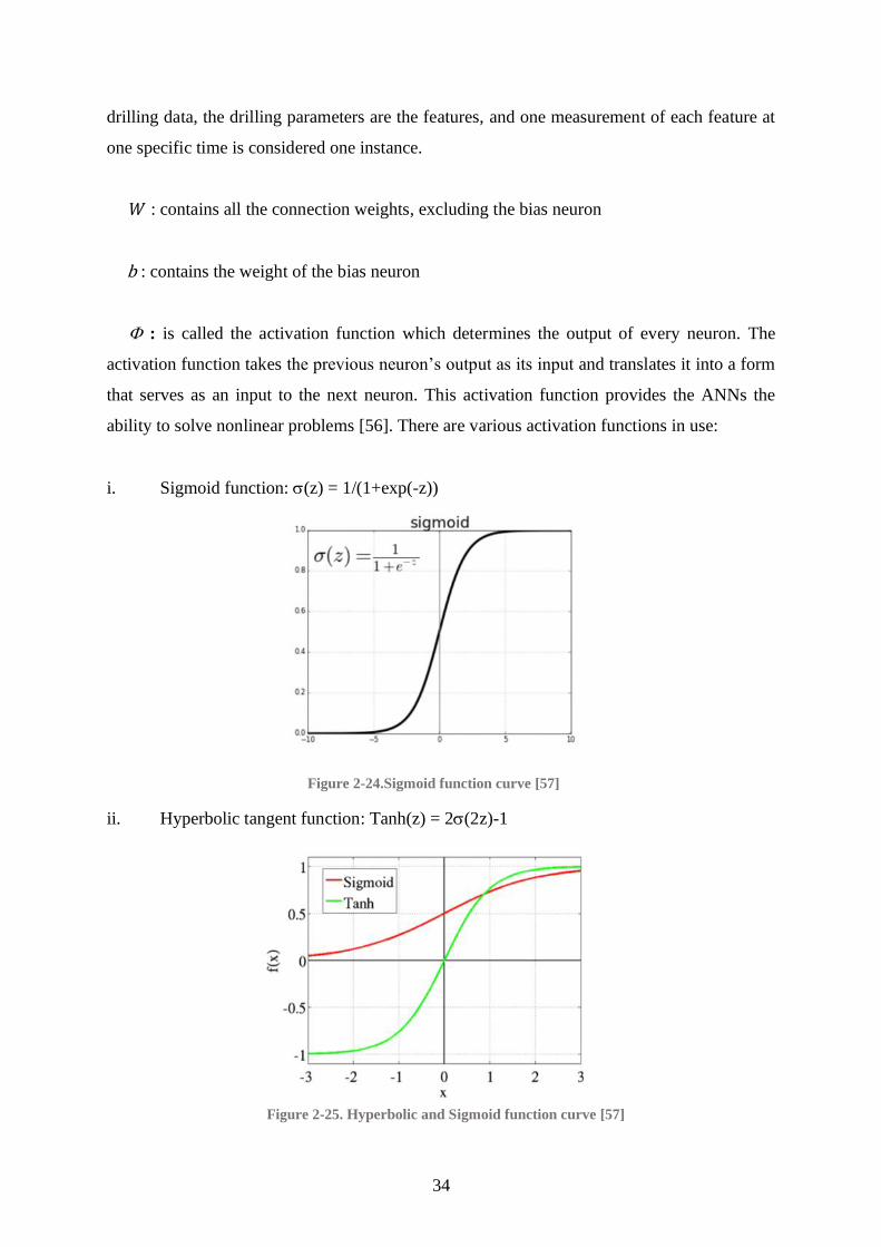
34

drilling data, the drilling parameters are the features, and one measurement of each feature at

one specific time is considered one instance.

𝑊 : contains all the connection weights, excluding the bias neuron

b : contains the weight of the bias neuron

: is called the activation function which determines the output of every neuron. The

activation function takes the previous neuron’s output as its input and translates it into a form

that serves as an input to the next neuron. This activation function provides the ANNs the

ability to solve nonlinear problems [56]. There are various activation functions in use:

i. Sigmoid function: (z) = 1/(1+exp(-z))

Figure 2-24.Sigmoid function curve [57]

ii. Hyperbolic tangent function: Tanh(z) = 2(2z)-1

Figure 2-25. Hyperbolic and Sigmoid function curve [57]

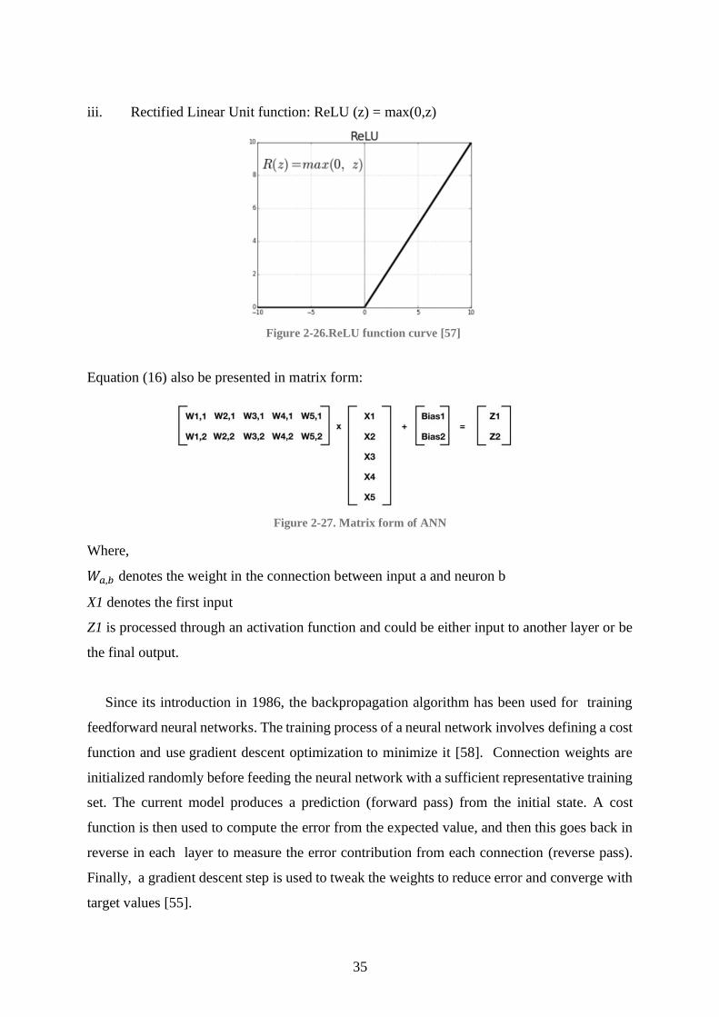
35

iii. Rectified Linear Unit function: ReLU (z) = max(0,z)

Figure 2-26.ReLU function curve [57]

Equation (16) also be presented in matrix form:

Figure 2-27. Matrix form of ANN

Where,

𝑊𝑎,𝑏 denotes the weight in the connection between input a and neuron b

X1 denotes the first input

Z1 is processed through an activation function and could be either input to another layer or be

the final output.

Since its introduction in 1986, the backpropagation algorithm has been used for training

feedforward neural networks. The training process of a neural network involves defining a cost

function and use gradient descent optimization to minimize it [58]. Connection weights are

initialized randomly before feeding the neural network with a sufficient representative training

set. The current model produces a prediction (forward pass) from the initial state. A cost

function is then used to compute the error from the expected value, and then this goes back in

reverse in each layer to measure the error contribution from each connection (reverse pass).

Finally, a gradient descent step is used to tweak the weights to reduce error and converge with

target values [55].

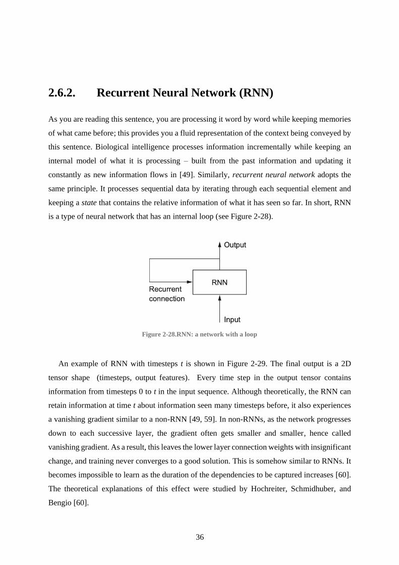
36

2.6.2. Recurrent Neural Network (RNN)

As you are reading this sentence, you are processing it word by word while keeping memories

of what came before; this provides you a fluid representation of the context being conveyed by

this sentence. Biological intelligence processes information incrementally while keeping an

internal model of what it is processing – built from the past information and updating it

constantly as new information flows in [49]. Similarly, recurrent neural network adopts the

same principle. It processes sequential data by iterating through each sequential element and

keeping a state that contains the relative information of what it has seen so far. In short, RNN

is a type of neural network that has an internal loop (see Figure 2-28).

Figure 2-28.RNN: a network with a loop

An example of RNN with timesteps t is shown in Figure 2-29. The final output is a 2D

tensor shape (timesteps, output features). Every time step in the output tensor contains

information from timesteps 0 to t in the input sequence. Although theoretically, the RNN can

retain information at time t about information seen many timesteps before, it also experiences

a vanishing gradient similar to a non-RNN [49, 59]. In non-RNNs, as the network progresses

down to each successive layer, the gradient often gets smaller and smaller, hence called

vanishing gradient. As a result, this leaves the lower layer connection weights with insignificant

change, and training never converges to a good solution. This is somehow similar to RNNs. It

becomes impossible to learn as the duration of the dependencies to be captured increases [60].

The theoretical explanations of this effect were studied by Hochreiter, Schmidhuber, and

Bengio [60].

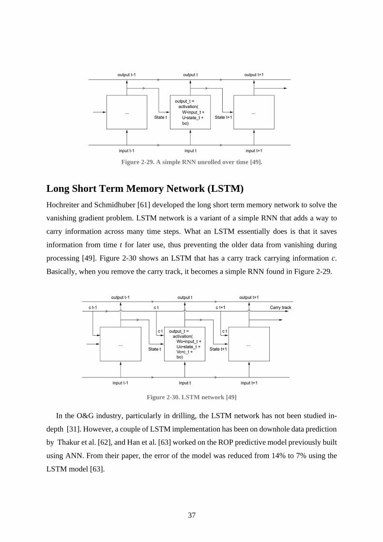
37

Figure 2-29. A simple RNN unrolled over time [49].

Long Short Term Memory Network (LSTM)

Hochreiter and Schmidhuber [61] developed the long short term memory network to solve the

vanishing gradient problem. LSTM network is a variant of a simple RNN that adds a way to

carry information across many time steps. What an LSTM essentially does is that it saves

information from time t for later use, thus preventing the older data from vanishing during

processing [49]. Figure 2-30 shows an LSTM that has a carry track carrying information c.

Basically, when you remove the carry track, it becomes a simple RNN found in Figure 2-29.

Figure 2-30. LSTM network [49]

In the O&G industry, particularly in drilling, the LSTM network has not been studied in-

depth [31]. However, a couple of LSTM implementation has been on downhole data prediction

by Thakur et al. [62], and Han et al. [63] worked on the ROP predictive model previously built

using ANN. From their paper, the error of the model was reduced from 14% to 7% using the

LSTM model [63].

38

2.6.3. Feature Scaling

Feature scaling is one of the vital steps needed when preparing data, as ML algorithms perform

poorly when data have different scales. In the context of drilling operations, we work with

different scales and units for every drilling parameter, e.g., weight on bit measurements vary

from 0 to 8 Tons, and torque measurements ranging 15-25 kN-m [31]. Although we will only

work with hook load measurements in this paper, there is a vast discrepancy in recorded hook

load during casing operations ranging from 300 – 450 klbm with operations involving only

drill pipe where hook load ranges from 140 – 300 klbm.

Min-max scaling, also known as normalization, is used when the data does not follow a

Gaussian distribution, e.g., hook load measurements [64]. Values are shifted and rescaled so

that they end up ranging between 0 and 1. To normalize data, the minimum value of the dataset

is subtracted from every single data point and divided by the difference of maximum and

minimum value (see equation 17). After normalization, the minimum value in original data

becomes 0, the maximum becomes 1, and other values are between the range of 0 and 1. For

this purpose, Scikit-Learn’s [65] transformer MinMaxScaler was used.

𝓍(𝑖)𝑛𝑜𝑟𝑚 = 𝓍𝑖− 𝓍𝑚𝑖𝑛

𝓍𝑚𝑎𝑥− 𝓍𝑚𝑖𝑛 (17)

2.6.4. Regression Metrics

Building an effective Machine Learning model requires evaluation metrics to see how good

the model is. Different evaluation metrics are used for different kinds of problems. Similarly,

evaluation metrics to be used for regression differ from those used for classification [49]. In

our context, we will build a regression model that will predict the hook load value based on

previous hook load measurements. Naturally, the concept of accuracy doesn’t apply to

regression. A common regression metric is mean absolute error (MAE) [49].

Mean Absolute Error (MAE)

The mean absolute error (MAE) of a model is the mean of the absolute values of the individual

prediction errors on all instances. MAE can be calculated using equation 18 [66]:

39

𝑀𝐴𝐸 =1

𝑛∑ |𝑦𝑗 − 𝑋𝑗|𝑛

𝑗=1 (18)

Where,

𝑦𝑗 , is the expected or true value for instance j

𝑋𝑗 , is the predicted value for instance j

n is the number of instances.

Residual Distribution

Residuals are obtained by finding the deviation between the model output with the true value

the model is trying to predict. Examining residuals is a key part of all statistical modeling. An

ideal distribution should be normal - centered on zero and narrow as possible [50]. Residual

distribution is plotted where x-axis represents the residuals, and y-axis represents the density

distribution.

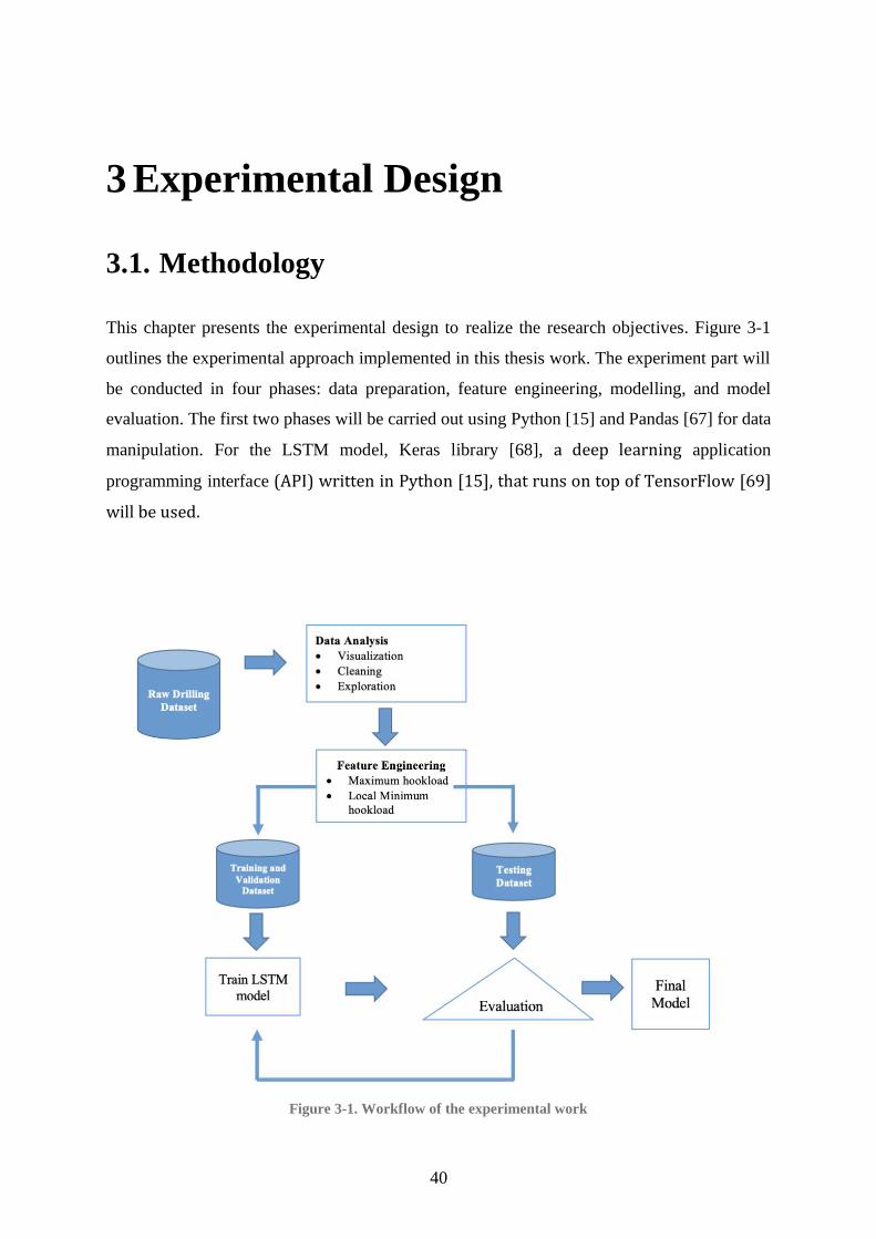
40

3 Experimental Design

3.1. Methodology

This chapter presents the experimental design to realize the research objectives. Figure 3-1

outlines the experimental approach implemented in this thesis work. The experiment part will

be conducted in four phases: data preparation, feature engineering, modelling, and model

evaluation. The first two phases will be carried out using Python [15] and Pandas [67] for data

manipulation. For the LSTM model, Keras library [68], a deep learning application

programming interface (API) written in Python [15], that runs on top of TensorFlow [69]

will be used.

Figure 3-1. Workflow of the experimental work

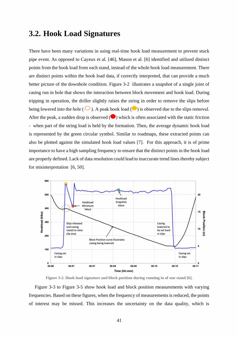
41

3.2. Hook Load Signatures

There have been many variations in using real-time hook load measurement to prevent stuck

pipe event. As opposed to Cayeux et al. [46], Mason et al. [6] identified and utilized distinct

points from the hook load from each stand, instead of the whole hook load measurement. There

are distinct points within the hook load data, if correctly interpreted, that can provide a much

better picture of the downhole condition. Figure 3-2 illustrates a snapshot of a single joint of

casing run in hole that shows the interaction between block movement and hook load. During

tripping in operation, the driller slightly raises the string in order to remove the slips before

being lowered into the hole ( ). A peak hook load ( ) is observed due to the slips removal.

After the peak, a sudden drop is observed ( ) which is often associated with the static friction

- when part of the string load is held by the formation. Then, the average dynamic hook load

is represented by the green circular symbol. Similar to roadmaps, these extracted points can

also be plotted against the simulated hook load values [7]. For this approach, it is of prime

importance to have a high sampling frequency to ensure that the distinct points in the hook load

are properly defined. Lack of data resolution could lead to inaccurate trend lines thereby subject

for misinterpretation [6, 50].

Figure 3-2. Hook load signature and block position during running in of one stand [6].

Figure 3-3 to Figure 3-5 show hook load and block position measurements with varying

frequencies. Based on these figures, when the frequency of measurements is reduced, the points

of interest may be missed. This increases the uncertainty on the data quality, which is

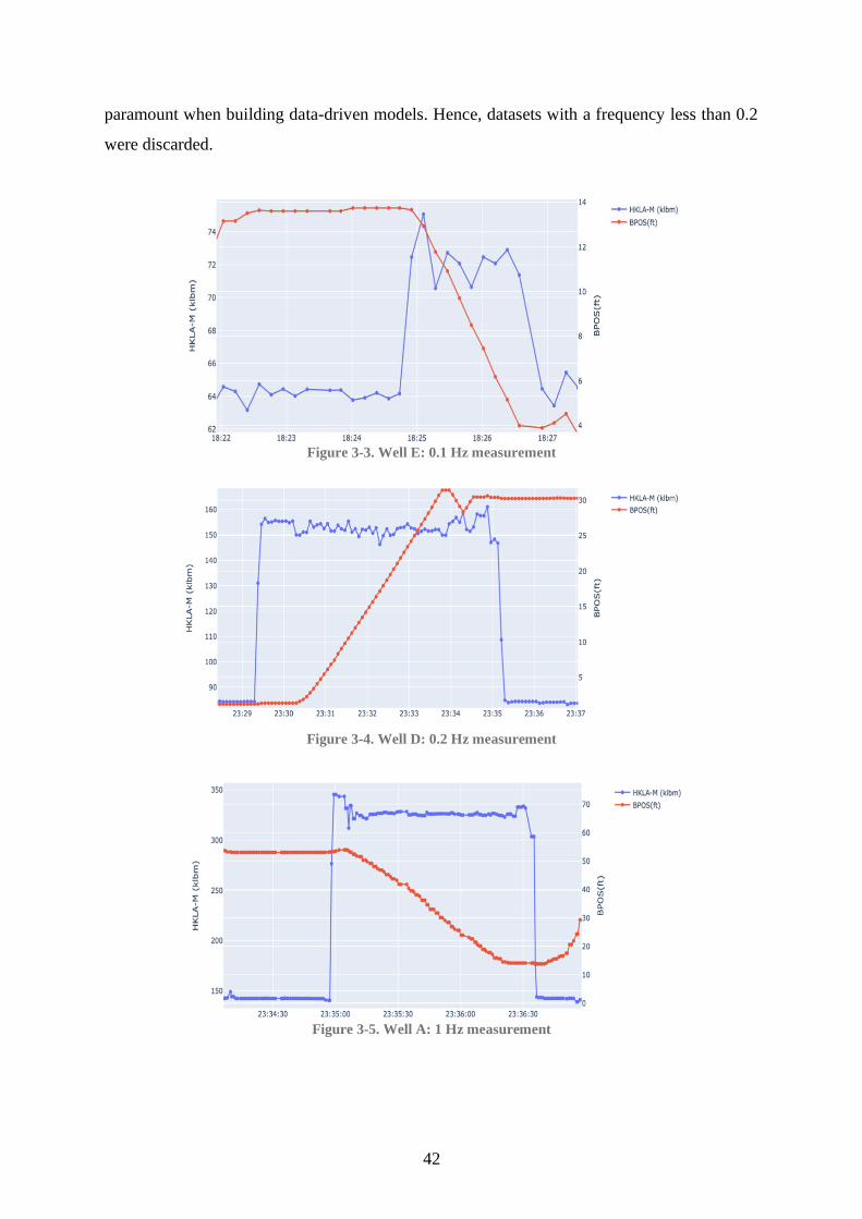
42

paramount when building data-driven models. Hence, datasets with a frequency less than 0.2

were discarded.

Figure 3-3. Well E: 0.1 Hz measurement

Figure 3-4. Well D: 0.2 Hz measurement

Figure 3-5. Well A: 1 Hz measurement

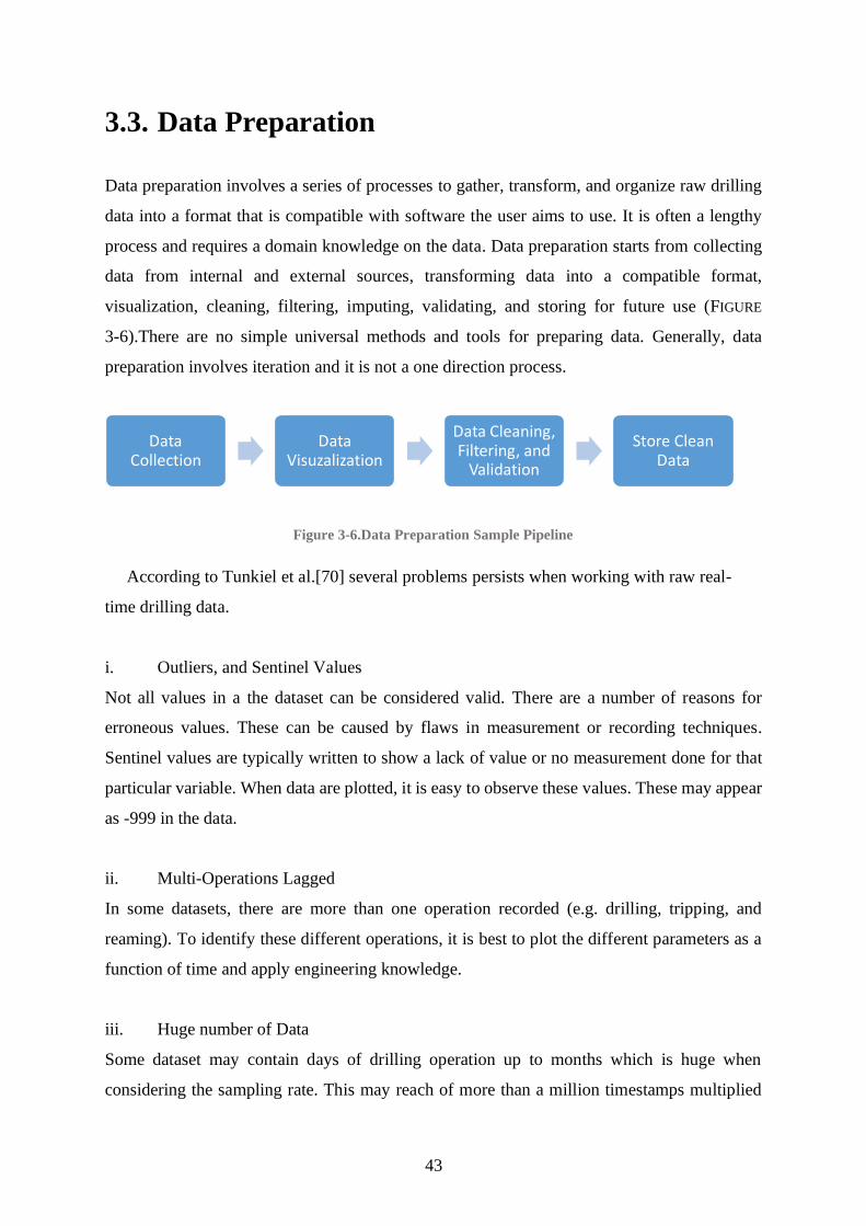
43

3.3. Data Preparation

Data preparation involves a series of processes to gather, transform, and organize raw drilling

data into a format that is compatible with software the user aims to use. It is often a lengthy

process and requires a domain knowledge on the data. Data preparation starts from collecting

data from internal and external sources, transforming data into a compatible format,

visualization, cleaning, filtering, imputing, validating, and storing for future use (FIGURE

3-6).There are no simple universal methods and tools for preparing data. Generally, data

preparation involves iteration and it is not a one direction process.

Figure 3-6.Data Preparation Sample Pipeline

According to Tunkiel et al.[70] several problems persists when working with raw real-

time drilling data.

i. Outliers, and Sentinel Values

Not all values in a the dataset can be considered valid. There are a number of reasons for

erroneous values. These can be caused by flaws in measurement or recording techniques.

Sentinel values are typically written to show a lack of value or no measurement done for that

particular variable. When data are plotted, it is easy to observe these values. These may appear

as -999 in the data.

ii. Multi-Operations Lagged

In some datasets, there are more than one operation recorded (e.g. drilling, tripping, and

reaming). To identify these different operations, it is best to plot the different parameters as a

function of time and apply engineering knowledge.

iii. Huge number of Data

Some dataset may contain days of drilling operation up to months which is huge when

considering the sampling rate. This may reach of more than a million timestamps multiplied

Data Collection

Data Visuzalization

Data Cleaning, Filtering, and

Validation

Store Clean Data

44

by the number of parameters that ranges from ten up to two hundred. Although not all data is

necessary, it is highly recommended to automate searching for relevant features from the

available data. For example to determine the type of operation, only five parameters is useful,

namely, measured depth, bit depth, hook load, rotation per minute, and torque (see Figure

2-16). Capacity of computer should also be considered when working with this amount of data.

These problems are presented and addressed in 3.3.2.

3.3.1. Data Collection

To build a data-driven model, a collection of dataset has to be available. In this project,

Exebenus provided raw real-time drilling data from 7 wells in comma-separated values (CSV)

and Microsoft excel format. Table 3 shows the information provided by Exebenus for each

well. There were no drilling report and annotations attached. All the well data were unnamed

due to data privacy and bounded by non-disclosure agreement.

Table 3. Data provided by Exebenus

Well ID Issue reported as

Well A Diff sticking

Well B Diff sticking

Well C Unknown

Well D Pack-off

Well E Hole Cleaning

Well F No Data

Well G No Data

3.3.2. Data Analysis

Our goal is to determine the type of operation, identify the stuck point, and prepare the data for

the next step which is feature engineering. This can be done by correlating the available drilling

measurements. However, data analysis is no straightforward. The raw dataset carries issues as

mentioned by Tunkiel et al.[70] that needs to be addressed before we can fulfill our main tasks.

In this thesis, two web-based applications were developed to enable efficient data analysis

given the time constraint of the project and the amount of data to analyze.

45

Visualizing data

Data visualization is the initial step in data analysis in which data analysts use visualization

tools in order to better understand the nature of the data. The purpose of this process is to help

create a clearer view of important trends and points to study in greater detail. When working

with drilling data, data visualization allows the analyst to see the available parameters, quality

and characteristics of data, and the type of operation. As discussed by Tunkiel et al. [70], dataset

may contain more than a million timestamps due to the sampling rate causing problems for

software such as Excel. One cannot simply browse through the data due to its quantity. To

address this problem, the author built a fit for purpose web-based application for data

visualization. The application is written in Python [15] and Dash [71] - a framework for

building web visual and analytical applications with customizable user interfaces in pure

Python [15]. This application allows the user to upload files in CSV and Excel format, and

plot up to 7 drilling parameters simultaneously without typing a single code. It is also possible

to zoom in details particularly when the dataset is too large to fit on the screen. Anomalous

values and data trends can be quickly observed. This application eliminated the arduous process

of manual methods of typing algorithms to visualize the data. Appendix B.1. shows the code

of the application.

Figure 3-7 shows the user interface of the visualization tool where Well B raw data was

uploaded. Seven parameters were plotted namely, DMEA, DBTM, BPOS, HKLA-M, RPMA,

SPPA, and TQA, respectively. In Figure 3-8, other available parameters are plotted, WOBA-

M, ROPA, MFIA, MDIA, and ECD_ARC_RT, respectively. See Table 4 for the full form of

these abbreviations.

Well B dataset is from July 30, 2020 to August 5, 2020. Evidently, the dataset contains

sentinel values. All the parameters have values of -999 which is an indication of no

measurement or error in sensor [70]. To better understand the data, it must be filtered first from

these values.

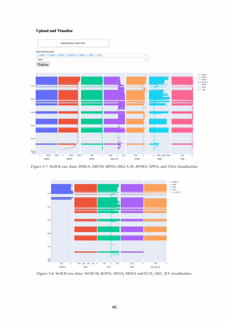
46

Figure 3-7. Well B raw data: DMEA, DBTM, BPOS, HKLA-M, RPMA, SPPA, and TQA visualization

Figure 3-8. Well B raw data: WOB-M, ROPA, MFIA, MDIA and ECD_ARC_RT visualization

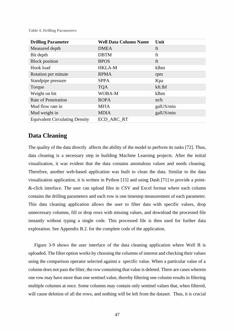
47

Table 4. Drilling Parameters

Drilling Parameter Well Data Column Name Unit

Measured depth DMEA ft

Bit depth DBTM ft

Block position BPOS ft

Hook load HKLA-M klbm

Rotation per minute RPMA rpm

Standpipe pressure SPPA Kpa

Torque TQA kft.lbf

Weight on bit WOBA-M klbm

Rate of Penetration ROPA m/h

Mud flow rate in MFIA galUS/min

Mud weight in MDIA galUS/min

Equivalent Circulating Density ECD_ARC_RT

Data Cleaning

The quality of the data directly affects the ability of the model to perform its tasks [72]. Thus,

data cleaning is a necessary step in building Machine Learning projects. After the initial

visualization, it was evident that the data contains anomalous values and needs cleaning.

Therefore, another web-based application was built to clean the data. Similar to the data

visualization application, it is written in Python [15] and using Dash [71] to provide a point-

&-click interface. The user can upload files in CSV and Excel format where each column

contains the drilling parameters and each row is one timestep measurement of each parameter.

This data cleaning application allows the user to filter data with specific values, drop

unnecessary columns, fill or drop rows with missing values, and download the processed file

instantly without typing a single code. This processed file is then used for further data

exploration. See Appendix B.2. for the complete code of the application.

Figure 3-9 shows the user interface of the data cleaning application where Well B is

uploaded. The filter option works by choosing the columns of interest and checking their values

using the comparison operator selected against a specific value. When a particular value of a

column does not pass the filter, the row containing that value is deleted. There are cases wherein

one row may have more than one sentinel value, thereby filtering one column results in filtering

multiple columns at once. Some columns may contain only sentinel values that, when filtered,

will cause deletion of all the rows, and nothing will be left from the dataset. Thus, it is crucial

48

to only consider relevant parameters according to predefined objectives. There is no fixed

configuration on which and how many parameters are considered relevant. Most of the time,

iteration and domain knowledge of the data and task at hand is needed.

In this paper, it is our primary objective to extract signature points from hook load before

stuck pipe incident. But before we proceed, it is necessary to determine the type of operation,

identify the stuck point, and prepare the data for the next step which is feature engineering.

Figure 3-9 shows Well B’s HKLA-M, BPOS, SPPA, DBTM, DMEA, RPMA, and TQA are

all filtered to have values equal or greater than zero. It is based on engineering knowledge that

these values cannot have negative values.

Figure 3-9. Cleaning Well B data

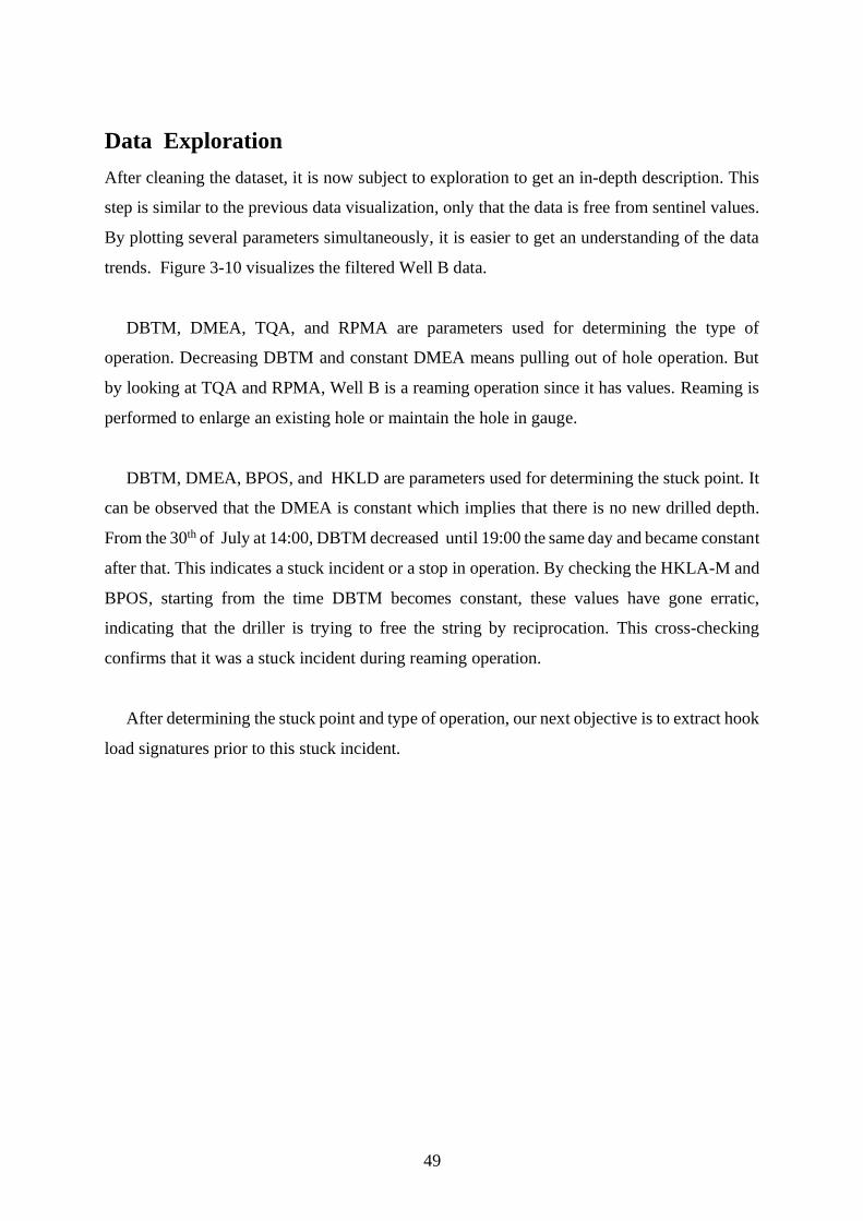
49

Data Exploration

After cleaning the dataset, it is now subject to exploration to get an in-depth description. This

step is similar to the previous data visualization, only that the data is free from sentinel values.

By plotting several parameters simultaneously, it is easier to get an understanding of the data

trends. Figure 3-10 visualizes the filtered Well B data.

DBTM, DMEA, TQA, and RPMA are parameters used for determining the type of

operation. Decreasing DBTM and constant DMEA means pulling out of hole operation. But

by looking at TQA and RPMA, Well B is a reaming operation since it has values. Reaming is

performed to enlarge an existing hole or maintain the hole in gauge.

DBTM, DMEA, BPOS, and HKLD are parameters used for determining the stuck point. It

can be observed that the DMEA is constant which implies that there is no new drilled depth.

From the 30th of July at 14:00, DBTM decreased until 19:00 the same day and became constant

after that. This indicates a stuck incident or a stop in operation. By checking the HKLA-M and

BPOS, starting from the time DBTM becomes constant, these values have gone erratic,

indicating that the driller is trying to free the string by reciprocation. This cross-checking

confirms that it was a stuck incident during reaming operation.

After determining the stuck point and type of operation, our next objective is to extract hook

load signatures prior to this stuck incident.

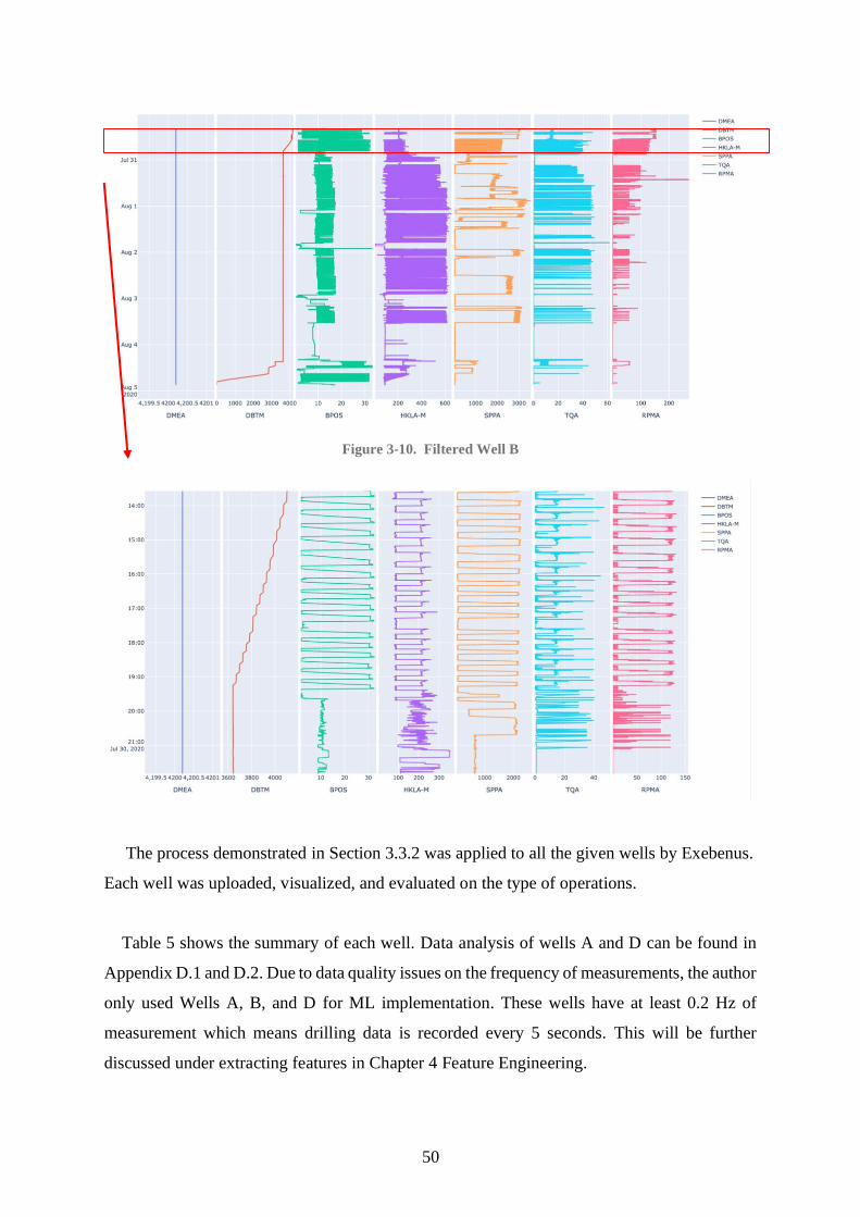
50

Figure 3-10. Filtered Well B

The process demonstrated in Section 3.3.2 was applied to all the given wells by Exebenus.

Each well was uploaded, visualized, and evaluated on the type of operations.

Table 5 shows the summary of each well. Data analysis of wells A and D can be found in

Appendix D.1 and D.2. Due to data quality issues on the frequency of measurements, the author

only used Wells A, B, and D for ML implementation. These wells have at least 0.2 Hz of

measurement which means drilling data is recorded every 5 seconds. This will be further

discussed under extracting features in Chapter 4 Feature Engineering.

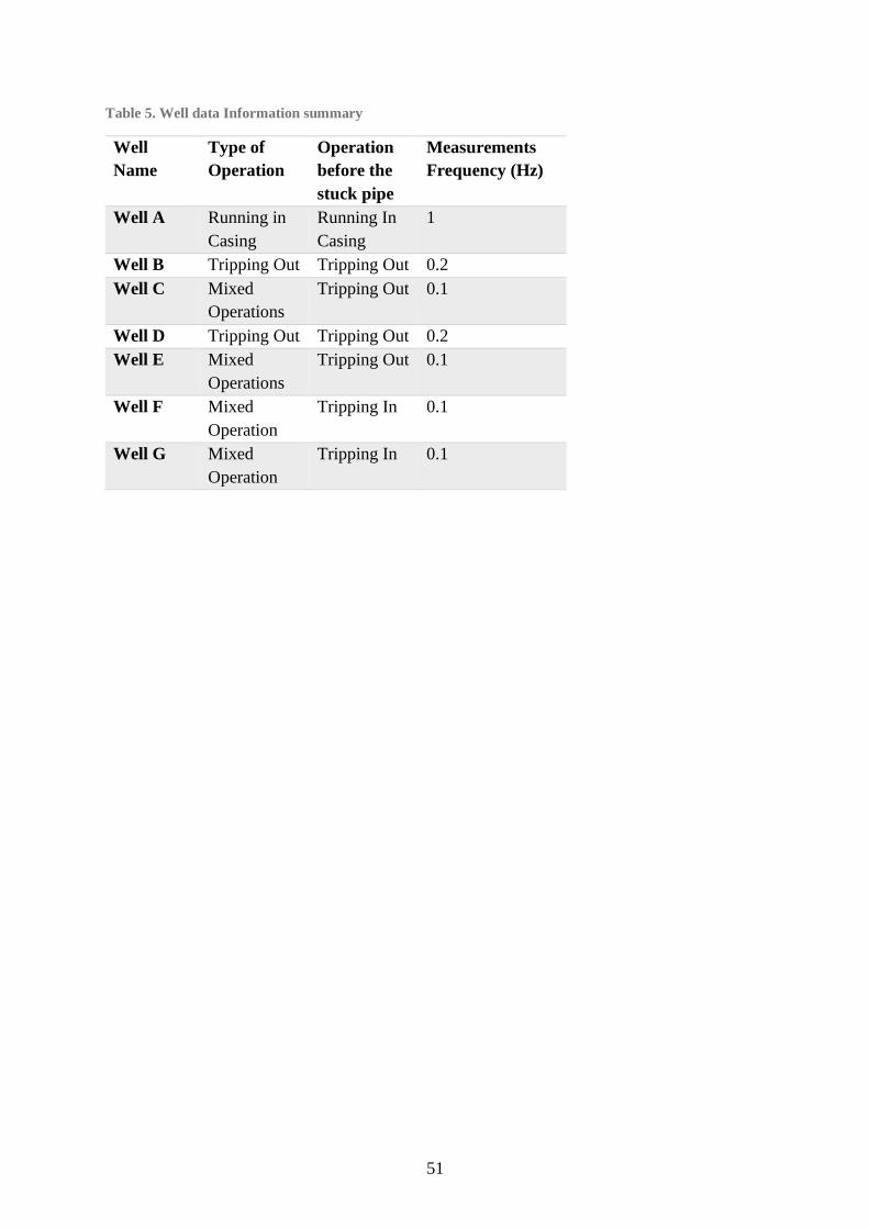
51

Table 5. Well data Information summary

Well

Name

Type of

Operation

Operation

before the

stuck pipe

Measurements

Frequency (Hz)

Well A Running in

Casing

Running In

Casing

1

Well B Tripping Out Tripping Out 0.2

Well C Mixed

Operations

Tripping Out 0.1

Well D Tripping Out Tripping Out 0.2

Well E Mixed

Operations

Tripping Out 0.1

Well F Mixed

Operation

Tripping In 0.1

Well G Mixed

Operation

Tripping In 0.1

52

4 Feature Engineering

The success of a Machine Learning project relies heavily on coming up with a good set of

features to train on [66]. No algorithm alone can supplement the information gain given by

using correct features [73]. In ML, feature engineering is the process of using your knowledge

about the data to make the algorithm work better by extracting specific features. The essence

of feature engineering is expressing the problem more straightforwardly [49].

As mentioned in Section 3.2. , hook load signatures exist before stuck pipe events. During

tripping out operations, after removing the slip to continue moving the pipe out of the well, a

force is needed to initiate movement. This required force is the hook load during the static

condition and the static friction. Because frictional forces always oppose the direction of

motion, it is added when tripping out. This hook load is referred to as the maximum hook load.

The same concept applies during tripping in operations only that static friction is deducted, and

this is referred to as the local minimum hook load. This is called local minimum because, after

this point, any further reduction in hookload is attributed to the dynamic movement of the

string. In normal operation, static friction should not vary much when monitoring consecutive

stands. This trend of frictional forces is an excellent indicator of the downhole condition as it

reflects additional forces to initiate movement [6].

It is our prime objective in feature engineering to extract these hook load signatures for each

dataset. Maximum and local minimum hook loads are extracted from wells with tripping out

and tripping in operations, respectively. These extracted hook load signatures will be used in

building a long short term memory network ML model for hook load prediction.

The processed and explored file from Section 3.3.2 is now imported to Python [15] as a

DataFrame using Pandas. Similar to CSV files, DataFrame has a tabular data structure with

labeled rows and columns. Figure 4-1 shows the elements of a DataFrame. Columns are the

drilling parameters, and each row represents measurements at each time interval. Rows are

numbered using the index, which is the default in Python [15]. Similar to rows, columns also

have indexes (not seen) where “TIME” is the 0th column, “DMEA” is the 1st column, and so

on. Individual data can be accessed through its row and column index. In Python, this is

implemented using DataFrame variable name in Python followed by a parenthesis containing

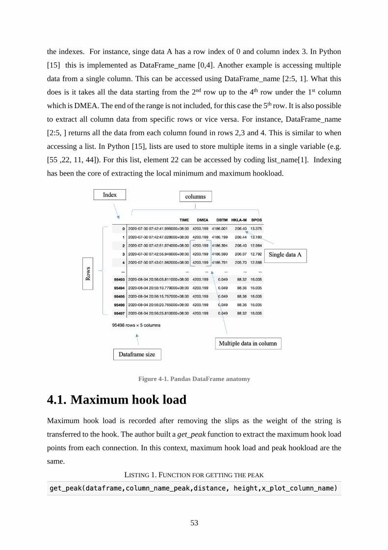
53

the indexes. For instance, singe data A has a row index of 0 and column index 3. In Python

[15] this is implemented as DataFrame_name [0,4]. Another example is accessing multiple

data from a single column. This can be accessed using DataFrame_name [2:5, 1]. What this

does is it takes all the data starting from the 2nd row up to the 4th row under the 1st column

which is DMEA. The end of the range is not included, for this case the 5th row. It is also possible

to extract all column data from specific rows or vice versa. For instance, DataFrame_name

[2:5, ] returns all the data from each column found in rows 2,3 and 4. This is similar to when

accessing a list. In Python [15], lists are used to store multiple items in a single variable (e.g.

[55 ,22, 11, 44]). For this list, element 22 can be accessed by coding list_name[1]. Indexing

has been the core of extracting the local minimum and maximum hookload.

Figure 4-1. Pandas DataFrame anatomy

4.1. Maximum hook load

Maximum hook load is recorded after removing the slips as the weight of the string is

transferred to the hook. The author built a get_peak function to extract the maximum hook load

points from each connection. In this context, maximum hook load and peak hookload are the

same.

LISTING 1. FUNCTION FOR GETTING THE PEAK

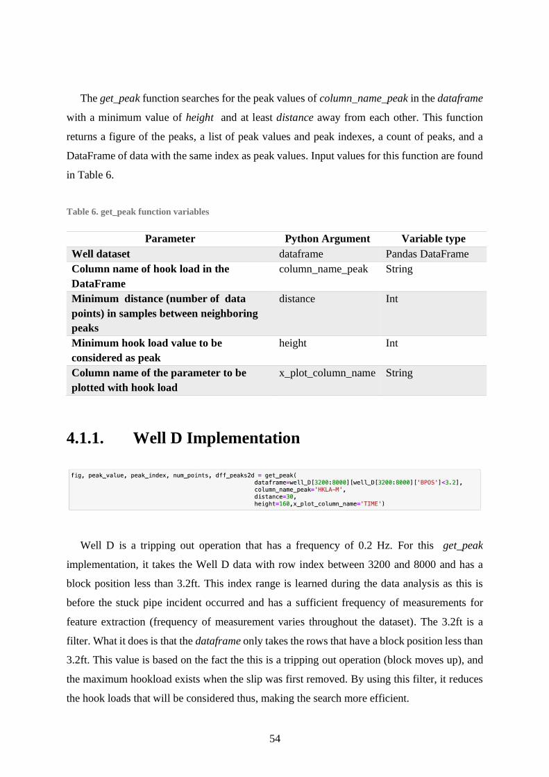
54

The get_peak function searches for the peak values of column_name_peak in the dataframe

with a minimum value of height and at least distance away from each other. This function

returns a figure of the peaks, a list of peak values and peak indexes, a count of peaks, and a

DataFrame of data with the same index as peak values. Input values for this function are found

in Table 6.

Table 6. get_peak function variables

Parameter Python Argument Variable type

Well dataset dataframe Pandas DataFrame

Column name of hook load in the

DataFrame

column_name_peak String

Minimum distance (number of data

points) in samples between neighboring

peaks

distance Int

Minimum hook load value to be

considered as peak

height Int

Column name of the parameter to be

plotted with hook load

x_plot_column_name String

4.1.1. Well D Implementation

Well D is a tripping out operation that has a frequency of 0.2 Hz. For this get_peak

implementation, it takes the Well D data with row index between 3200 and 8000 and has a

block position less than 3.2ft. This index range is learned during the data analysis as this is

before the stuck pipe incident occurred and has a sufficient frequency of measurements for

feature extraction (frequency of measurement varies throughout the dataset). The 3.2ft is a

filter. What it does is that the dataframe only takes the rows that have a block position less than

3.2ft. This value is based on the fact the this is a tripping out operation (block moves up), and

the maximum hookload exists when the slip was first removed. By using this filter, it reduces

the hook loads that will be considered thus, making the search more efficient.

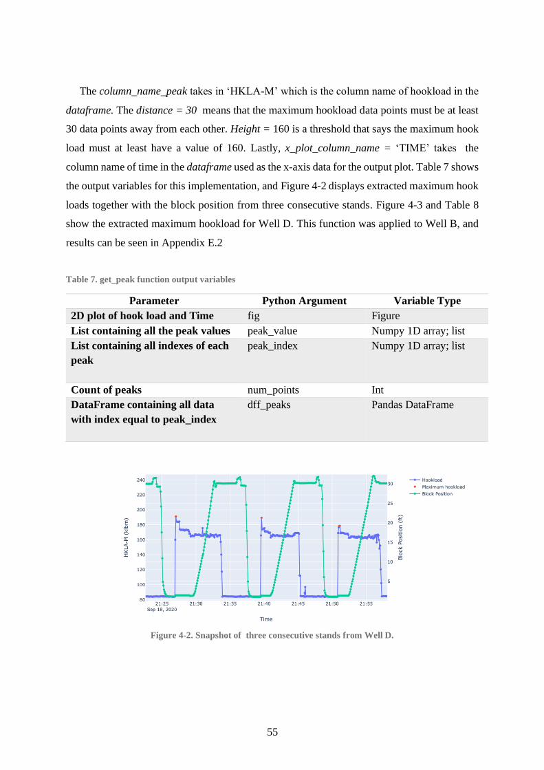
55

The column_name_peak takes in ‘HKLA-M’ which is the column name of hookload in the

dataframe. The distance = 30 means that the maximum hookload data points must be at least

30 data points away from each other. Height = 160 is a threshold that says the maximum hook

load must at least have a value of 160. Lastly, x_plot_column_name = ‘TIME’ takes the

column name of time in the dataframe used as the x-axis data for the output plot. Table 7 shows

the output variables for this implementation, and Figure 4-2 displays extracted maximum hook

loads together with the block position from three consecutive stands. Figure 4-3 and Table 8

show the extracted maximum hookload for Well D. This function was applied to Well B, and

results can be seen in Appendix E.2

Table 7. get_peak function output variables

Parameter Python Argument Variable Type

2D plot of hook load and Time fig Figure

List containing all the peak values peak_value Numpy 1D array; list

List containing all indexes of each

peak

peak_index Numpy 1D array; list

Count of peaks num_points Int

DataFrame containing all data

with index equal to peak_index

dff_peaks Pandas DataFrame

Figure 4-2. Snapshot of three consecutive stands from Well D.

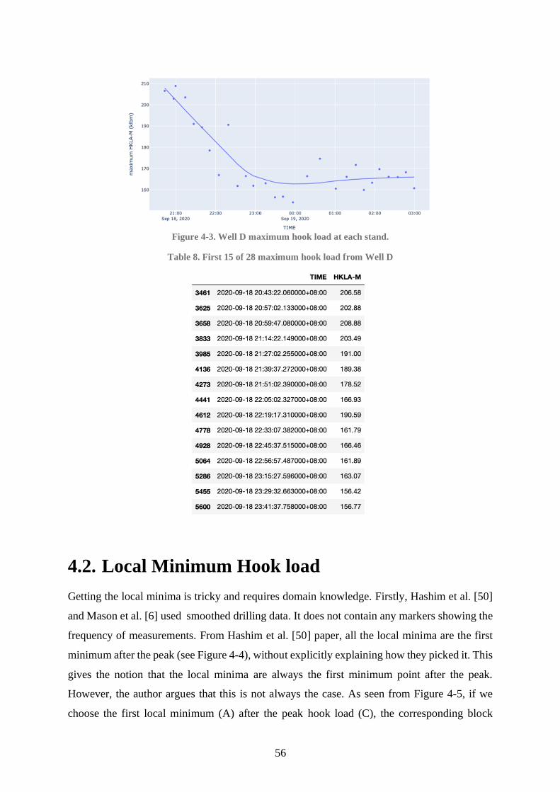
56

Figure 4-3. Well D maximum hook load at each stand.

Table 8. First 15 of 28 maximum hook load from Well D

4.2. Local Minimum Hook load

Getting the local minima is tricky and requires domain knowledge. Firstly, Hashim et al. [50]

and Mason et al. [6] used smoothed drilling data. It does not contain any markers showing the

frequency of measurements. From Hashim et al. [50] paper, all the local minima are the first

minimum after the peak (see Figure 4-4), without explicitly explaining how they picked it. This

gives the notion that the local minima are always the first minimum point after the peak.

However, the author argues that this is not always the case. As seen from Figure 4-5, if we

choose the first local minimum (A) after the peak hook load (C), the corresponding block

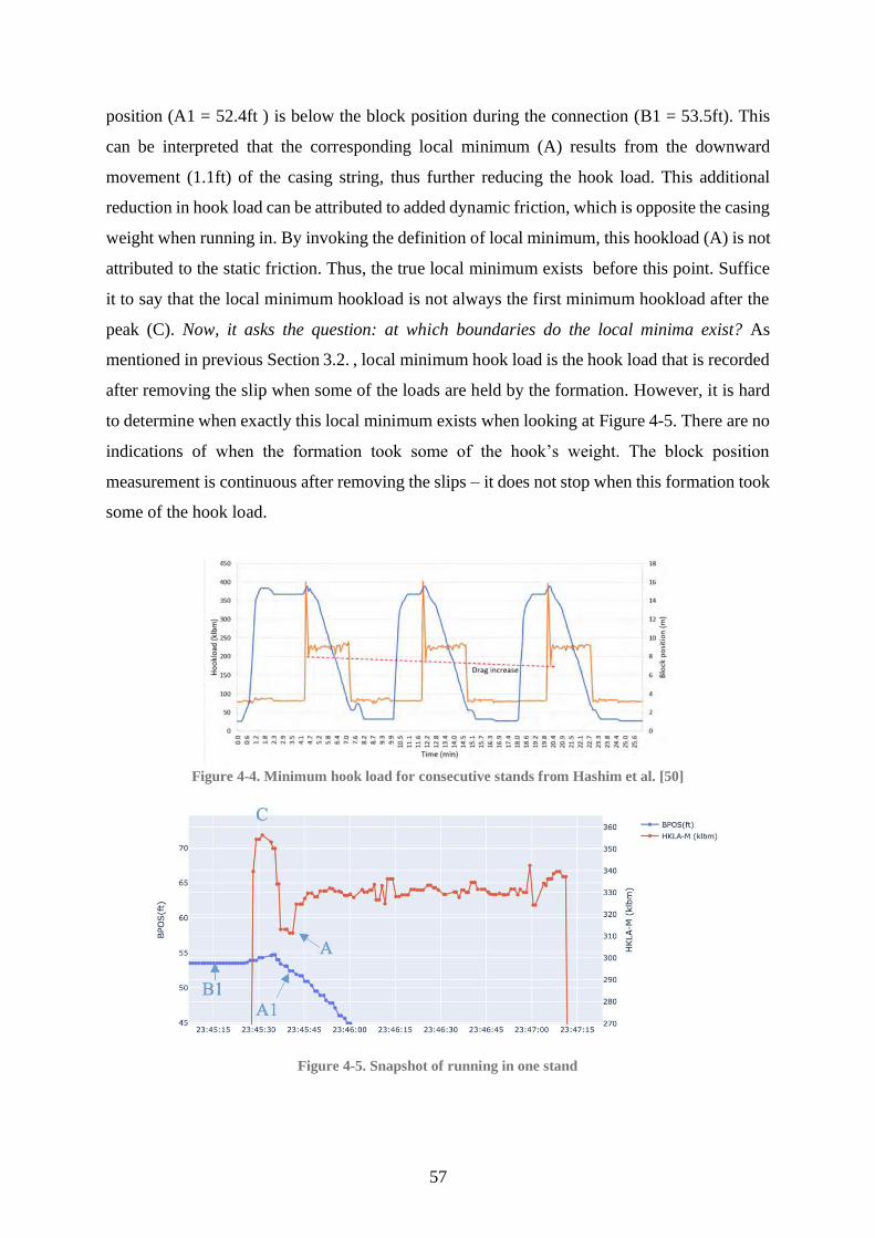
57

position (A1 = 52.4ft ) is below the block position during the connection (B1 = 53.5ft). This

can be interpreted that the corresponding local minimum (A) results from the downward

movement (1.1ft) of the casing string, thus further reducing the hook load. This additional

reduction in hook load can be attributed to added dynamic friction, which is opposite the casing

weight when running in. By invoking the definition of local minimum, this hookload (A) is not

attributed to the static friction. Thus, the true local minimum exists before this point. Suffice

it to say that the local minimum hookload is not always the first minimum hookload after the

peak (C). Now, it asks the question: at which boundaries do the local minima exist? As

mentioned in previous Section 3.2. , local minimum hook load is the hook load that is recorded

after removing the slip when some of the loads are held by the formation. However, it is hard

to determine when exactly this local minimum exists when looking at Figure 4-5. There are no

indications of when the formation took some of the hook’s weight. The block position

measurement is continuous after removing the slips – it does not stop when this formation took

some of the hook load.

Figure 4-4. Minimum hook load for consecutive stands from Hashim et al. [50]

Figure 4-5. Snapshot of running in one stand

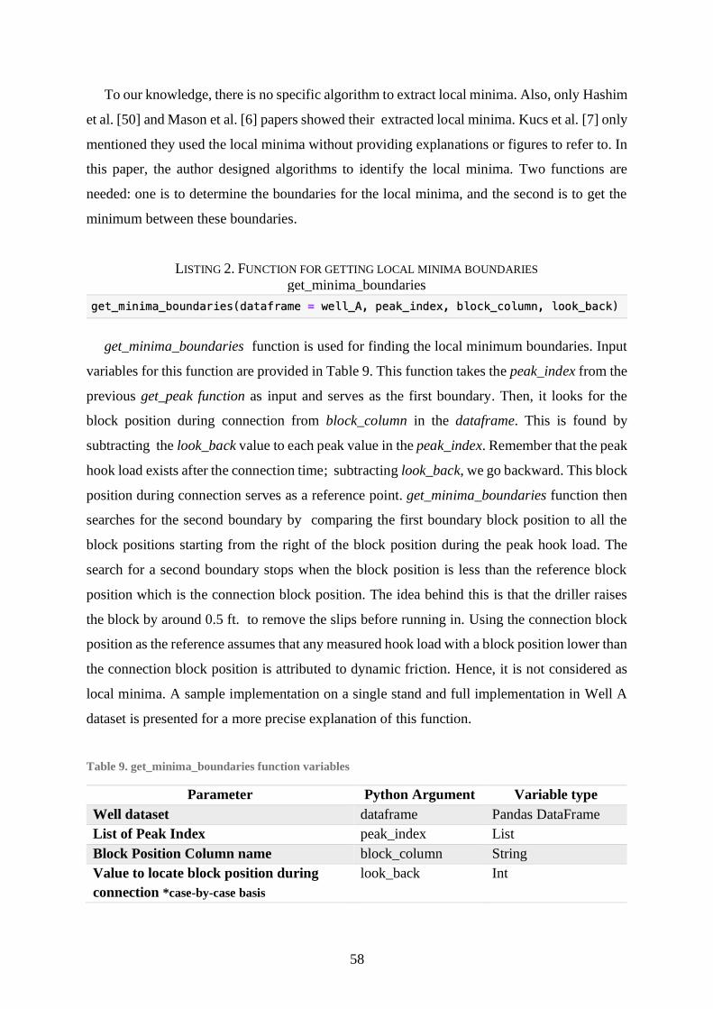
58

To our knowledge, there is no specific algorithm to extract local minima. Also, only Hashim

et al. [50] and Mason et al. [6] papers showed their extracted local minima. Kucs et al. [7] only

mentioned they used the local minima without providing explanations or figures to refer to. In

this paper, the author designed algorithms to identify the local minima. Two functions are

needed: one is to determine the boundaries for the local minima, and the second is to get the

minimum between these boundaries.

LISTING 2. FUNCTION FOR GETTING LOCAL MINIMA BOUNDARIES

get_minima_boundaries

get_minima_boundaries function is used for finding the local minimum boundaries. Input

variables for this function are provided in Table 9. This function takes the peak_index from the

previous get_peak function as input and serves as the first boundary. Then, it looks for the

block position during connection from block_column in the dataframe. This is found by

subtracting the look_back value to each peak value in the peak_index. Remember that the peak

hook load exists after the connection time; subtracting look_back, we go backward. This block

position during connection serves as a reference point. get_minima_boundaries function then

searches for the second boundary by comparing the first boundary block position to all the

block positions starting from the right of the block position during the peak hook load. The

search for a second boundary stops when the block position is less than the reference block

position which is the connection block position. The idea behind this is that the driller raises

the block by around 0.5 ft. to remove the slips before running in. Using the connection block

position as the reference assumes that any measured hook load with a block position lower than

the connection block position is attributed to dynamic friction. Hence, it is not considered as

local minima. A sample implementation on a single stand and full implementation in Well A

dataset is presented for a more precise explanation of this function.

Table 9. get_minima_boundaries function variables

Parameter Python Argument Variable type

Well dataset dataframe Pandas DataFrame

List of Peak Index peak_index List

Block Position Column name block_column String

Value to locate block position during

connection *case-by-case basis

look_back Int

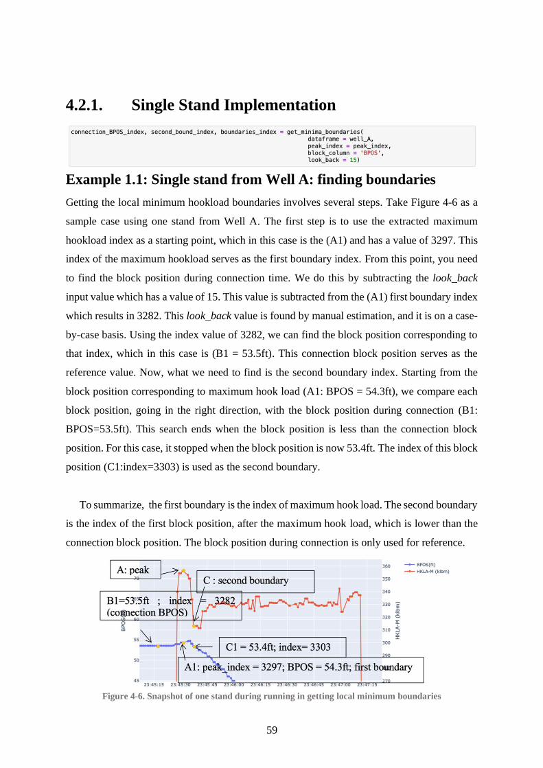
59

4.2.1. Single Stand Implementation

Example 1.1: Single stand from Well A: finding boundaries

Getting the local minimum hookload boundaries involves several steps. Take Figure 4-6 as a

sample case using one stand from Well A. The first step is to use the extracted maximum

hookload index as a starting point, which in this case is the (A1) and has a value of 3297. This

index of the maximum hookload serves as the first boundary index. From this point, you need

to find the block position during connection time. We do this by subtracting the look_back

input value which has a value of 15. This value is subtracted from the (A1) first boundary index

which results in 3282. This look_back value is found by manual estimation, and it is on a case-

by-case basis. Using the index value of 3282, we can find the block position corresponding to

that index, which in this case is (B1 = 53.5ft). This connection block position serves as the

reference value. Now, what we need to find is the second boundary index. Starting from the

block position corresponding to maximum hook load (A1: BPOS = 54.3ft), we compare each

block position, going in the right direction, with the block position during connection (B1:

BPOS=53.5ft). This search ends when the block position is less than the connection block

position. For this case, it stopped when the block position is now 53.4ft. The index of this block

position (C1:index=3303) is used as the second boundary.

To summarize, the first boundary is the index of maximum hook load. The second boundary

is the index of the first block position, after the maximum hook load, which is lower than the

connection block position. The block position during connection is only used for reference.

Figure 4-6. Snapshot of one stand during running in getting local minimum boundaries

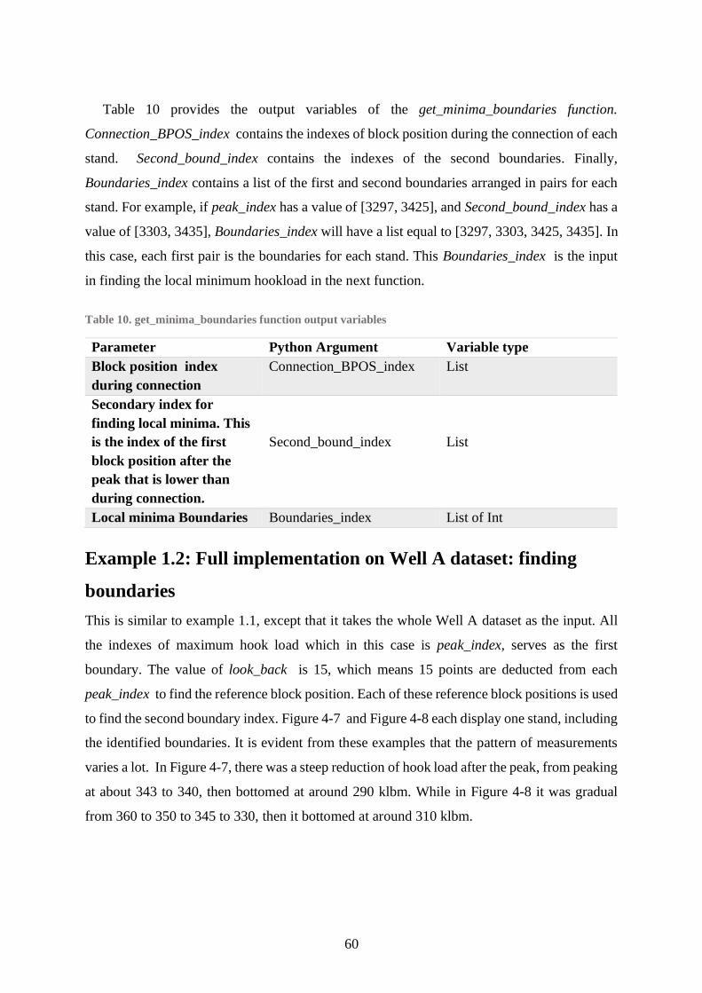
60

Table 10 provides the output variables of the get_minima_boundaries function.

Connection_BPOS_index contains the indexes of block position during the connection of each

stand. Second_bound_index contains the indexes of the second boundaries. Finally,

Boundaries_index contains a list of the first and second boundaries arranged in pairs for each

stand. For example, if peak_index has a value of [3297, 3425], and Second_bound_index has a

value of [3303, 3435], Boundaries_index will have a list equal to [3297, 3303, 3425, 3435]. In

this case, each first pair is the boundaries for each stand. This Boundaries_index is the input

in finding the local minimum hookload in the next function.

Table 10. get_minima_boundaries function output variables

Parameter Python Argument Variable type

Block position index

during connection

Connection_BPOS_index List

Secondary index for

finding local minima. This

is the index of the first

block position after the

peak that is lower than

during connection.

Second_bound_index

List

Local minima Boundaries Boundaries_index List of Int

Example 1.2: Full implementation on Well A dataset: finding

boundaries

This is similar to example 1.1, except that it takes the whole Well A dataset as the input. All

the indexes of maximum hook load which in this case is peak_index, serves as the first

boundary. The value of look_back is 15, which means 15 points are deducted from each

peak_index to find the reference block position. Each of these reference block positions is used

to find the second boundary index. Figure 4-7 and Figure 4-8 each display one stand, including

the identified boundaries. It is evident from these examples that the pattern of measurements

varies a lot. In Figure 4-7, there was a steep reduction of hook load after the peak, from peaking

at about 343 to 340, then bottomed at around 290 klbm. While in Figure 4-8 it was gradual

from 360 to 350 to 345 to 330, then it bottomed at around 310 klbm.

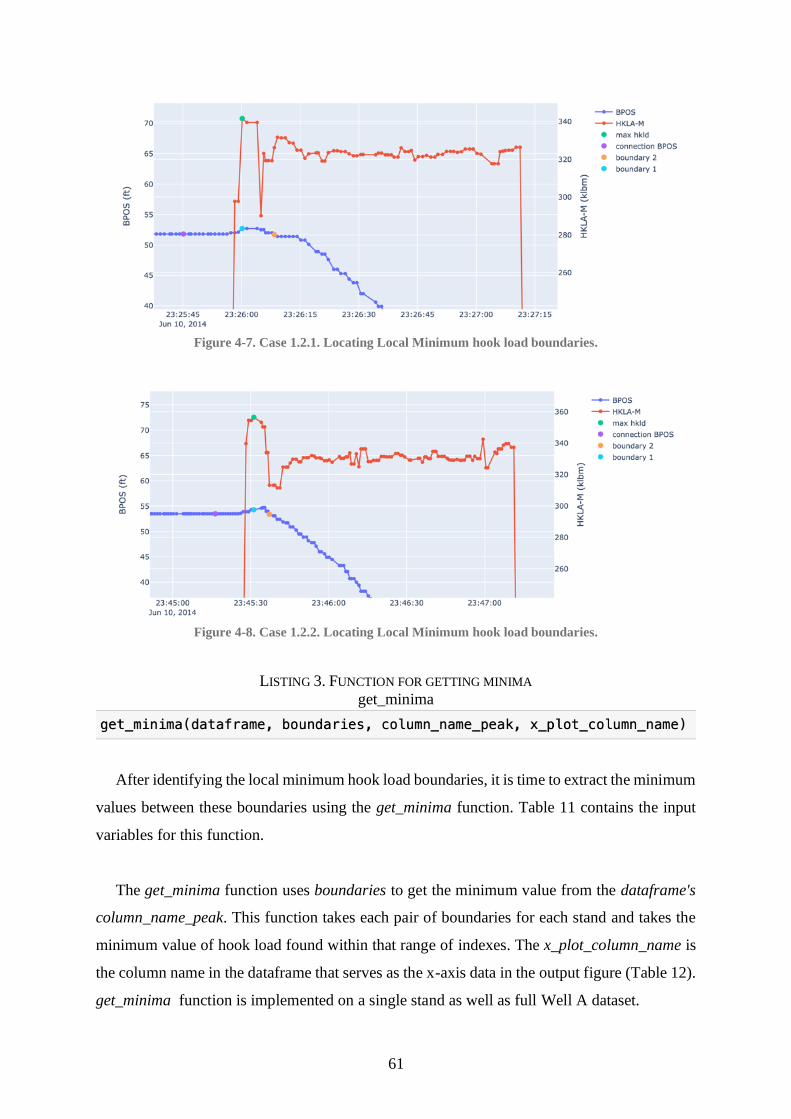
61

Figure 4-7. Case 1.2.1. Locating Local Minimum hook load boundaries.

Figure 4-8. Case 1.2.2. Locating Local Minimum hook load boundaries.

LISTING 3. FUNCTION FOR GETTING MINIMA

get_minima

After identifying the local minimum hook load boundaries, it is time to extract the minimum

values between these boundaries using the get_minima function. Table 11 contains the input

variables for this function.

The get_minima function uses boundaries to get the minimum value from the dataframe's

column_name_peak. This function takes each pair of boundaries for each stand and takes the

minimum value of hook load found within that range of indexes. The x_plot_column_name is

the column name in the dataframe that serves as the x-axis data in the output figure (Table 12).

get_minima function is implemented on a single stand as well as full Well A dataset.

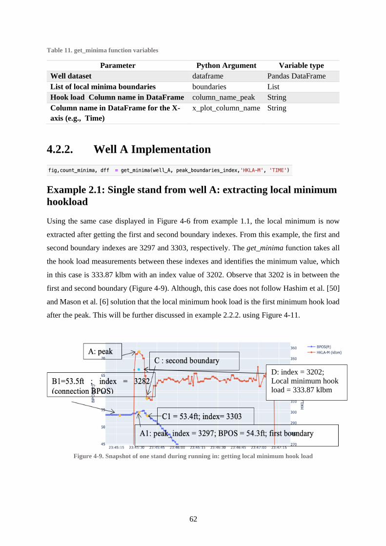
62

Table 11. get_minima function variables

Parameter Python Argument Variable type

Well dataset dataframe Pandas DataFrame

List of local minima boundaries boundaries List

Hook load Column name in DataFrame column_name_peak String

Column name in DataFrame for the X-

axis (e.g., Time)

x_plot_column_name String

4.2.2. Well A Implementation

Example 2.1: Single stand from well A: extracting local minimum

hookload

Using the same case displayed in Figure 4-6 from example 1.1, the local minimum is now

extracted after getting the first and second boundary indexes. From this example, the first and

second boundary indexes are 3297 and 3303, respectively. The get_minima function takes all

the hook load measurements between these indexes and identifies the minimum value, which

in this case is 333.87 klbm with an index value of 3202. Observe that 3202 is in between the

first and second boundary (Figure 4-9). Although, this case does not follow Hashim et al. [50]

and Mason et al. [6] solution that the local minimum hook load is the first minimum hook load

after the peak. This will be further discussed in example 2.2.2. using Figure 4-11.

Figure 4-9. Snapshot of one stand during running in: getting local minimum hook load

D: index = 3202;

Local minimum hook

load = 333.87 klbm

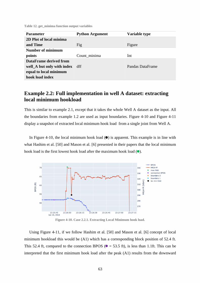
63

Table 12. get_minima function output variables

Parameter Python Argument Variable type

2D Plot of local minima

and Time

Fig

Figure

Number of minimum

points

Count_minima

Int

DataFrame derived from

well_A but only with index

equal to local minimum

hook load index

dff

Pandas DataFrame

Example 2.2: Full implementation in well A dataset: extracting

local minimum hookload

This is similar to example 2.1, except that it takes the whole Well A dataset as the input. All

the boundaries from example 1.2 are used as input boundaries. Figure 4-10 and Figure 4-11

display a snapshot of extracted local minimum hook load from a single joint from Well A.

In Figure 4-10, the local minimum hook load ( ) is apparent. This example is in line with

what Hashim et al. [50] and Mason et al. [6] presented in their papers that the local minimum

hook load is the first lowest hook load after the maximum hook load ( ).

Figure 4-10. Case 2.2.1. Extracting Local Minimum hook load.

Using Figure 4-11, if we follow Hashim et al. [50] and Mason et al. [6] concept of local

minimum hookload this would be (A1) which has a corresponding block position of 52.4 ft.

This 52.4 ft, compared to the connection BPOS ( = 53.5 ft), is less than 1.1ft. This can be

interpreted that the first minimum hook load after the peak (A1) results from the downward

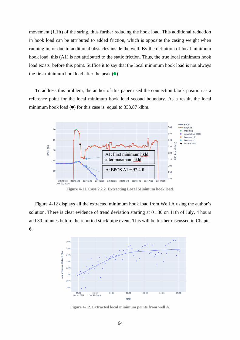
64

movement (1.1ft) of the string, thus further reducing the hook load. This additional reduction

in hook load can be attributed to added friction, which is opposite the casing weight when

running in, or due to additional obstacles inside the well. By the definition of local minimum

hook load, this (A1) is not attributed to the static friction. Thus, the true local minimum hook

load exists before this point. Suffice it to say that the local minimum hook load is not always

the first minimum hookload after the peak ( ).

To address this problem, the author of this paper used the connection block position as a

reference point for the local minimum hook load second boundary. As a result, the local

minimum hook load ( ) for this case is equal to 333.87 klbm.

Figure 4-11. Case 2.2.2. Extracting Local Minimum hook load.

Figure 4-12 displays all the extracted minimum hook load from Well A using the author’s

solution. There is clear evidence of trend deviation starting at 01:30 on 11th of July, 4 hours

and 30 minutes before the reported stuck pipe event. This will be further discussed in Chapter

6.

Figure 4-12. Extracted local minimum points from well A.

65

4.3. Summary of Extracted data

Table 13 shows the count of extracted hook load signatures. A total of 108 signature points

were extracted, consisting of 43 maximum and 65 local minimum hook loads from wells with

tripping out and tripping in operations, respectively. The data quality has been essential in this

study as three out of the seven wells were functional. These extracted points will be used in

building the ML model that will predict hook load signatures.

Table 13. Summary of extracted hook load signature points

Well Name Type of Operation Number of

Maximum hook load

Number of Local

Minimum hook

load

Well A Tripping In Not extracted 65

Well B Tripping Out 15 Not extracted

Well D Tripping Out 28 Not extracted

A table of all the extracted data points from Wells A, B, and D can be found in Appendix E.2

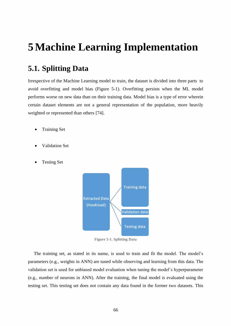
66

5 Machine Learning Implementation

5.1. Splitting Data

Irrespective of the Machine Learning model to train, the dataset is divided into three parts to

avoid overfitting and model bias (Figure 5-1). Overfitting persists when the ML model

performs worse on new data than on their training data. Model bias is a type of error wherein

certain dataset elements are not a general representation of the population, more heavily

weighted or represented than others [74].

• Training Set

• Validation Set

• Testing Set

Figure 5-1. Splitting Data

The training set, as stated in its name, is used to train and fit the model. The model’s

parameters (e.g., weights in ANN) are tuned while observing and learning from this data. The

validation set is used for unbiased model evaluation when tuning the model’s hyperparameter

(e.g., number of neurons in ANN). After the training, the final model is evaluated using the

testing set. This testing set does not contain any data found in the former two datasets. This

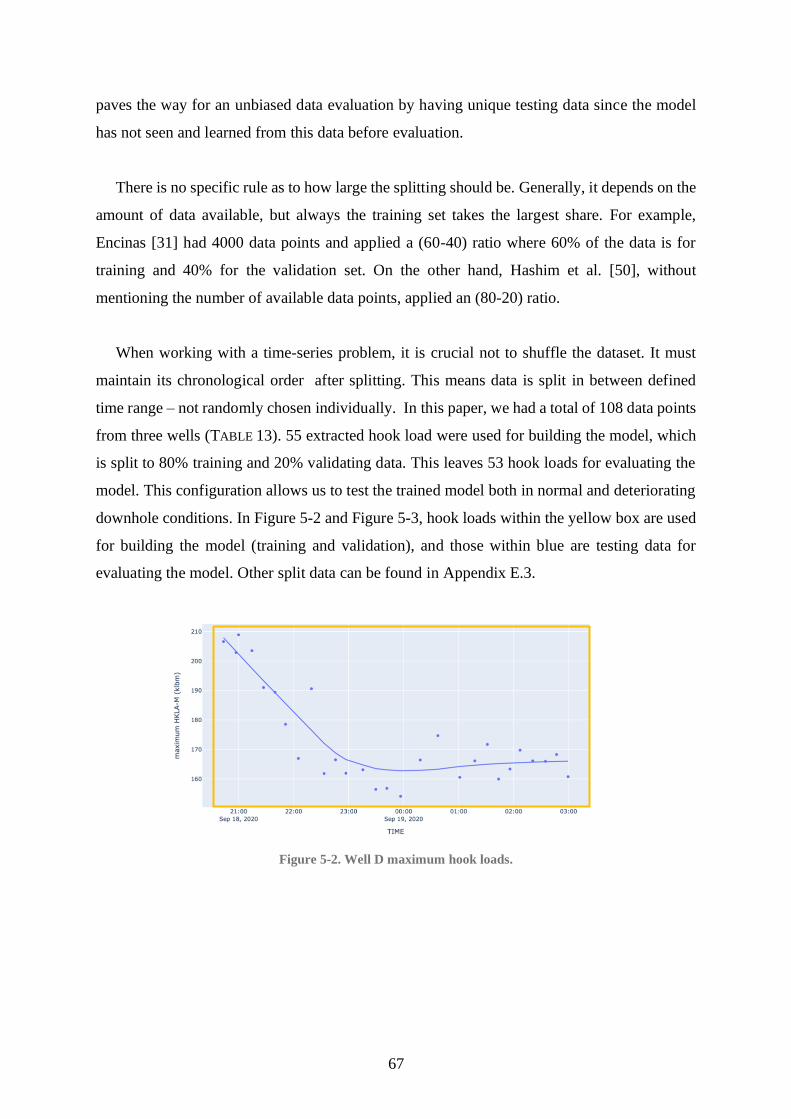
67

paves the way for an unbiased data evaluation by having unique testing data since the model

has not seen and learned from this data before evaluation.

There is no specific rule as to how large the splitting should be. Generally, it depends on the

amount of data available, but always the training set takes the largest share. For example,

Encinas [31] had 4000 data points and applied a (60-40) ratio where 60% of the data is for

training and 40% for the validation set. On the other hand, Hashim et al. [50], without

mentioning the number of available data points, applied an (80-20) ratio.

When working with a time-series problem, it is crucial not to shuffle the dataset. It must

maintain its chronological order after splitting. This means data is split in between defined

time range – not randomly chosen individually. In this paper, we had a total of 108 data points

from three wells (TABLE 13). 55 extracted hook load were used for building the model, which

is split to 80% training and 20% validating data. This leaves 53 hook loads for evaluating the

model. This configuration allows us to test the trained model both in normal and deteriorating

downhole conditions. In Figure 5-2 and Figure 5-3, hook loads within the yellow box are used

for building the model (training and validation), and those within blue are testing data for

evaluating the model. Other split data can be found in Appendix E.3.

Figure 5-2. Well D maximum hook loads.

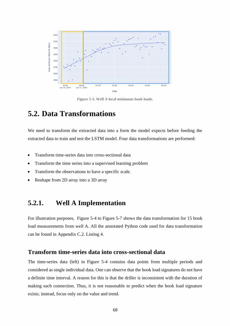
68

Figure 5-3. Well A local minimum hook loads.

5.2. Data Transformations

We need to transform the extracted data into a form the model expects before feeding the

extracted data to train and test the LSTM model. Four data transformations are performed:

• Transform time-series data into cross-sectional data

• Transform the time series into a supervised learning problem

• Transform the observations to have a specific scale.

• Reshape from 2D array into a 3D array

5.2.1. Well A Implementation

For illustration purposes, Figure 5-4 to Figure 5-7 shows the data transformation for 15 hook

load measurements from well A. All the annotated Python code used for data transformation

can be found in Appendix C.2. Listing 4.

Transform time-series data into cross-sectional data

The time-series data (left) in Figure 5-4 contains data points from multiple periods and

considered as single individual data. One can observe that the hook load signatures do not have

a definite time interval. A reason for this is that the driller is inconsistent with the duration of

making each connection. Thus, it is not reasonable to predict when the hook load signature

exists; instead, focus only on the value and trend.

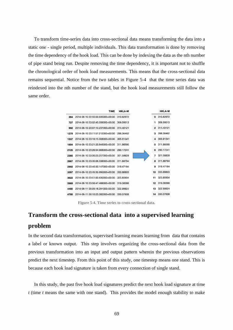
69

To transform time-series data into cross-sectional data means transforming the data into a

static one - single period, multiple individuals. This data transformation is done by removing

the time dependency of the hook load. This can be done by indexing the data as the nth number

of pipe stand being run. Despite removing the time dependency, it is important not to shuffle

the chronological order of hook load measurements. This means that the cross-sectional data

remains sequential. Notice from the two tables in Figure 5-4 that the time series data was

reindexed into the nth number of the stand, but the hook load measurements still follow the

same order.

Figure 5-4. Time series to cross-sectional data.

Transform the cross-sectional data into a supervised learning

problem

In the second data transformation, supervised learning means learning from data that contains

a label or known output. This step involves organizing the cross-sectional data from the

previous transformation into an input and output pattern wherein the previous observations

predict the next timestep. From this point of this study, one timestep means one stand. This is

because each hook load signature is taken from every connection of single stand.

In this study, the past five hook load signatures predict the next hook load signature at time

t (time t means the same with one stand). This provides the model enough stability to make

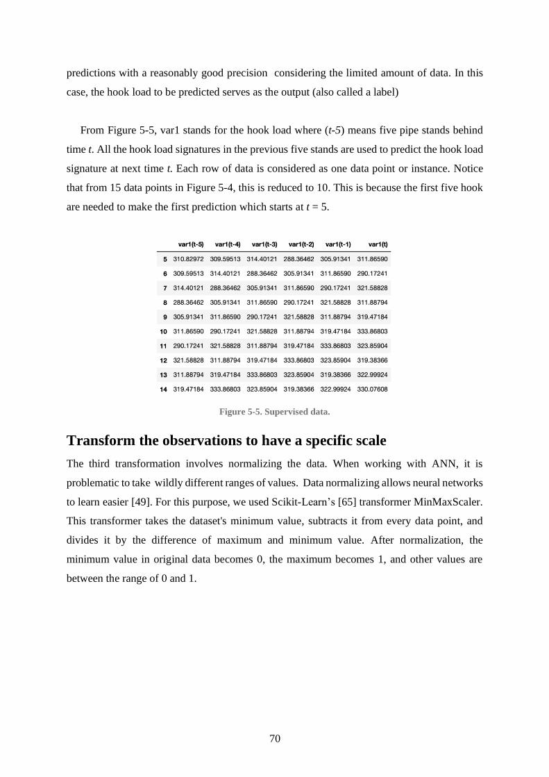
70

predictions with a reasonably good precision considering the limited amount of data. In this

case, the hook load to be predicted serves as the output (also called a label)

From Figure 5-5, var1 stands for the hook load where (t-5) means five pipe stands behind

time t. All the hook load signatures in the previous five stands are used to predict the hook load

signature at next time t. Each row of data is considered as one data point or instance. Notice

that from 15 data points in Figure 5-4, this is reduced to 10. This is because the first five hook

are needed to make the first prediction which starts at t = 5.

Figure 5-5. Supervised data.

Transform the observations to have a specific scale

The third transformation involves normalizing the data. When working with ANN, it is

problematic to take wildly different ranges of values. Data normalizing allows neural networks

to learn easier [49]. For this purpose, we used Scikit-Learn’s [65] transformer MinMaxScaler.

This transformer takes the dataset's minimum value, subtracts it from every data point, and

divides it by the difference of maximum and minimum value. After normalization, the

minimum value in original data becomes 0, the maximum becomes 1, and other values are

between the range of 0 and 1.

71

Figure 5-6. Normalized supervised data using a Scikit-learn [65] MinMaxScaler.

Reshape from 2D array into 3D array

Currently, the data is a normalized 2D data with six columns wherein the last column is the

target or to be predicted value, and each row is one instance. However, the LSTM model

expects a 3D array input. This means that the data needs to be reshaped from a 2D array (batch

size, features) into a 3D (batch size, timestep, features) array. In this context, batch size means

the number of samples or instances. For illustration purposes, referring to the transformed and

normalized data (Figure 5-6), the batch size is equal to the number of row data. In this case it

is 10 (5 to 14). Time step means every row data is one time step. For two time steps, this means

two rows of data. Features mean the number of columns, in this case, we have six wherein the

first five are the past hook load measurements.

Although when training the LSTM model, we separate the input features from the output.

In our case, the LSTM input shape is (10,1,5). This means that the model is trained on 10 data

points, wherein each timestep has five features. In this 3D data, the feature means the past

hook load measurements. For this purpose, reshape() function in NumPy [75] was used to

reshape the 2D array into a 3D array. Figure 5-7 shows the data in the 3D form in Python [15].

Figure 5-8 displays a representation of an LSTM input.

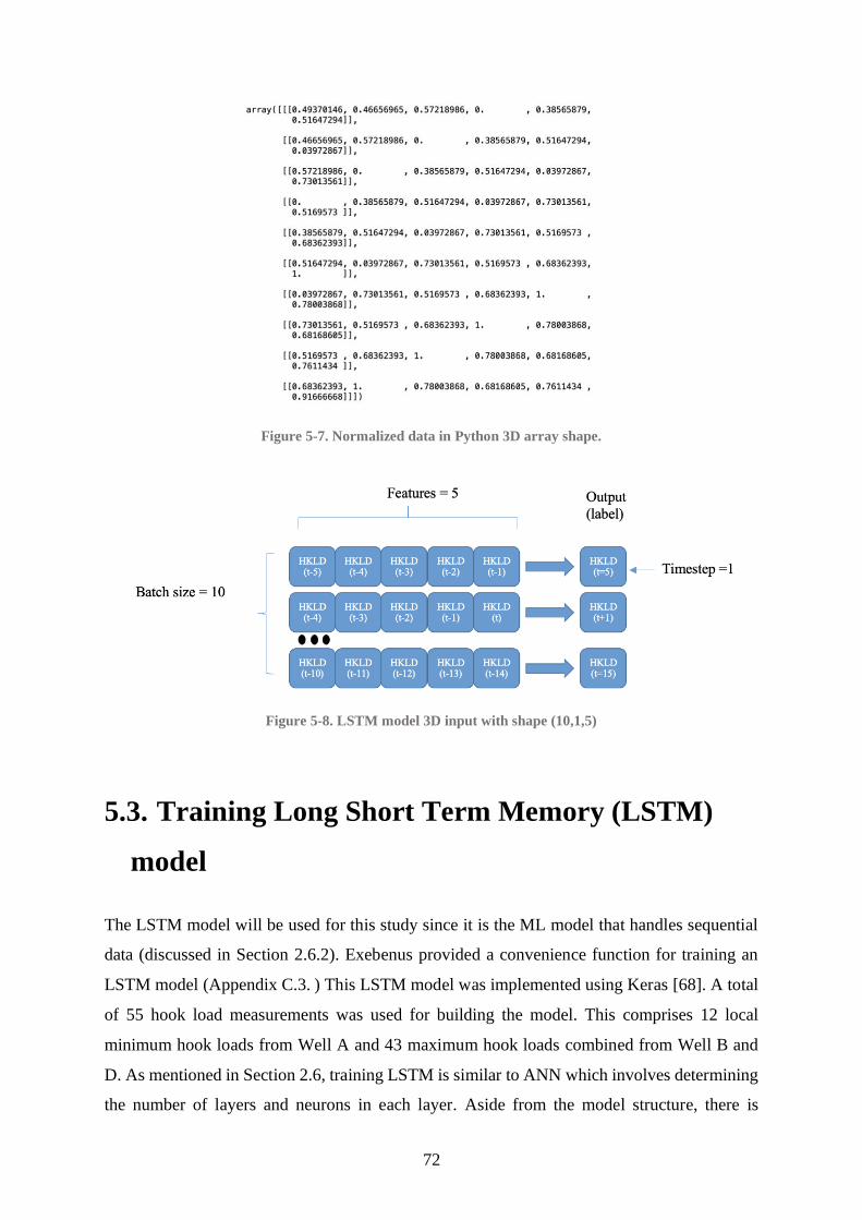
72

Figure 5-7. Normalized data in Python 3D array shape.

Figure 5-8. LSTM model 3D input with shape (10,1,5)

5.3. Training Long Short Term Memory (LSTM)

model

The LSTM model will be used for this study since it is the ML model that handles sequential

data (discussed in Section 2.6.2). Exebenus provided a convenience function for training an

LSTM model (Appendix C.3. ) This LSTM model was implemented using Keras [68]. A total

of 55 hook load measurements was used for building the model. This comprises 12 local

minimum hook loads from Well A and 43 maximum hook loads combined from Well B and

D. As mentioned in Section 2.6, training LSTM is similar to ANN which involves determining

the number of layers and neurons in each layer. Aside from the model structure, there is

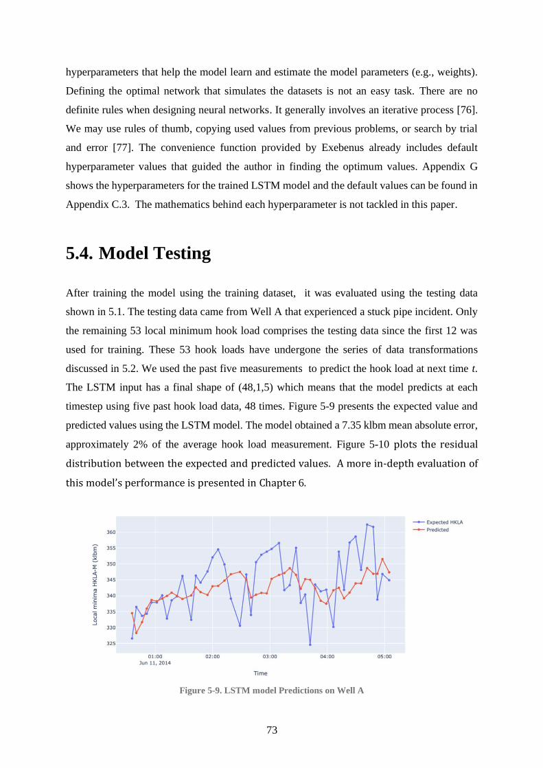
73

hyperparameters that help the model learn and estimate the model parameters (e.g., weights).

Defining the optimal network that simulates the datasets is not an easy task. There are no

definite rules when designing neural networks. It generally involves an iterative process [76].

We may use rules of thumb, copying used values from previous problems, or search by trial

and error [77]. The convenience function provided by Exebenus already includes default

hyperparameter values that guided the author in finding the optimum values. Appendix G

shows the hyperparameters for the trained LSTM model and the default values can be found in

Appendix C.3. The mathematics behind each hyperparameter is not tackled in this paper.

5.4. Model Testing

After training the model using the training dataset, it was evaluated using the testing data

shown in 5.1. The testing data came from Well A that experienced a stuck pipe incident. Only

the remaining 53 local minimum hook load comprises the testing data since the first 12 was

used for training. These 53 hook loads have undergone the series of data transformations

discussed in 5.2. We used the past five measurements to predict the hook load at next time t.

The LSTM input has a final shape of (48,1,5) which means that the model predicts at each

timestep using five past hook load data, 48 times. Figure 5-9 presents the expected value and

predicted values using the LSTM model. The model obtained a 7.35 klbm mean absolute error,

approximately 2% of the average hook load measurement. Figure 5-10 plots the residual

distribution between the expected and predicted values. A more in-depth evaluation of

this model’s performance is presented in Chapter 6.

Figure 5-9. LSTM model Predictions on Well A

74

Figure 5-10. Residuals distribution

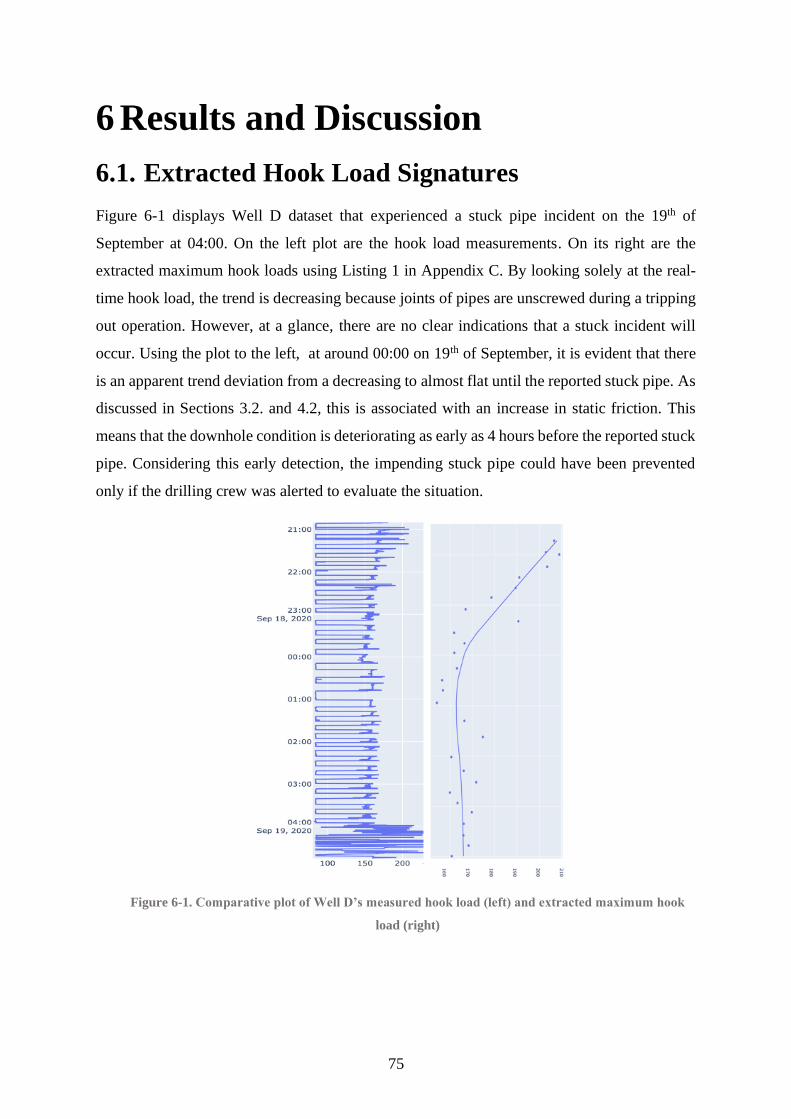
75

6 Results and Discussion

6.1. Extracted Hook Load Signatures

Figure 6-1 displays Well D dataset that experienced a stuck pipe incident on the 19th of

September at 04:00. On the left plot are the hook load measurements. On its right are the

extracted maximum hook loads using Listing 1 in Appendix C. By looking solely at the real-

time hook load, the trend is decreasing because joints of pipes are unscrewed during a tripping

out operation. However, at a glance, there are no clear indications that a stuck incident will

occur. Using the plot to the left, at around 00:00 on 19th of September, it is evident that there

is an apparent trend deviation from a decreasing to almost flat until the reported stuck pipe. As

discussed in Sections 3.2. and 4.2, this is associated with an increase in static friction. This

means that the downhole condition is deteriorating as early as 4 hours before the reported stuck

pipe. Considering this early detection, the impending stuck pipe could have been prevented

only if the drilling crew was alerted to evaluate the situation.

Figure 6-1. Comparative plot of Well D’s measured hook load (left) and extracted maximum hook

load (right)

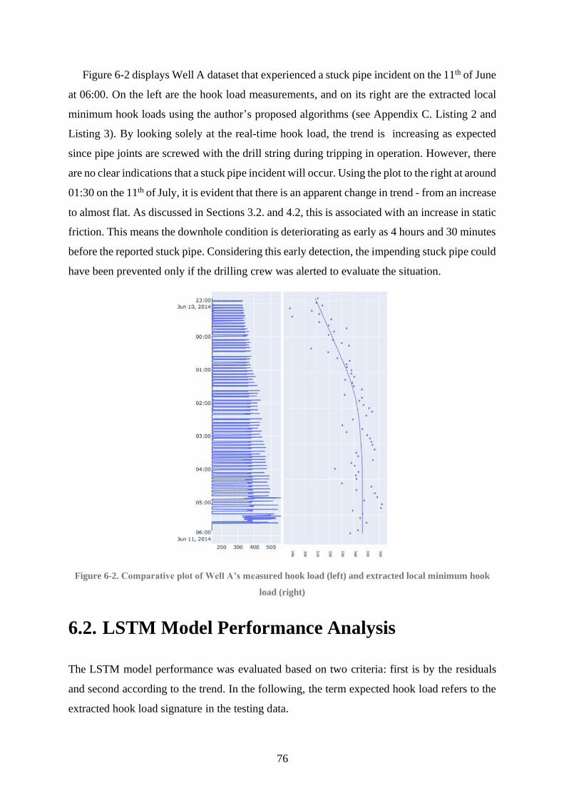
76

Figure 6-2 displays Well A dataset that experienced a stuck pipe incident on the 11th of June

at 06:00. On the left are the hook load measurements, and on its right are the extracted local

minimum hook loads using the author’s proposed algorithms (see Appendix C. Listing 2 and

Listing 3). By looking solely at the real-time hook load, the trend is increasing as expected

since pipe joints are screwed with the drill string during tripping in operation. However, there

are no clear indications that a stuck pipe incident will occur. Using the plot to the right at around

01:30 on the 11th of July, it is evident that there is an apparent change in trend - from an increase

to almost flat. As discussed in Sections 3.2. and 4.2, this is associated with an increase in static

friction. This means the downhole condition is deteriorating as early as 4 hours and 30 minutes

before the reported stuck pipe. Considering this early detection, the impending stuck pipe could

have been prevented only if the drilling crew was alerted to evaluate the situation.

Figure 6-2. Comparative plot of Well A’s measured hook load (left) and extracted local minimum hook

load (right)

6.2. LSTM Model Performance Analysis

The LSTM model performance was evaluated based on two criteria: first is by the residuals

and second according to the trend. In the following, the term expected hook load refers to the

extracted hook load signature in the testing data.

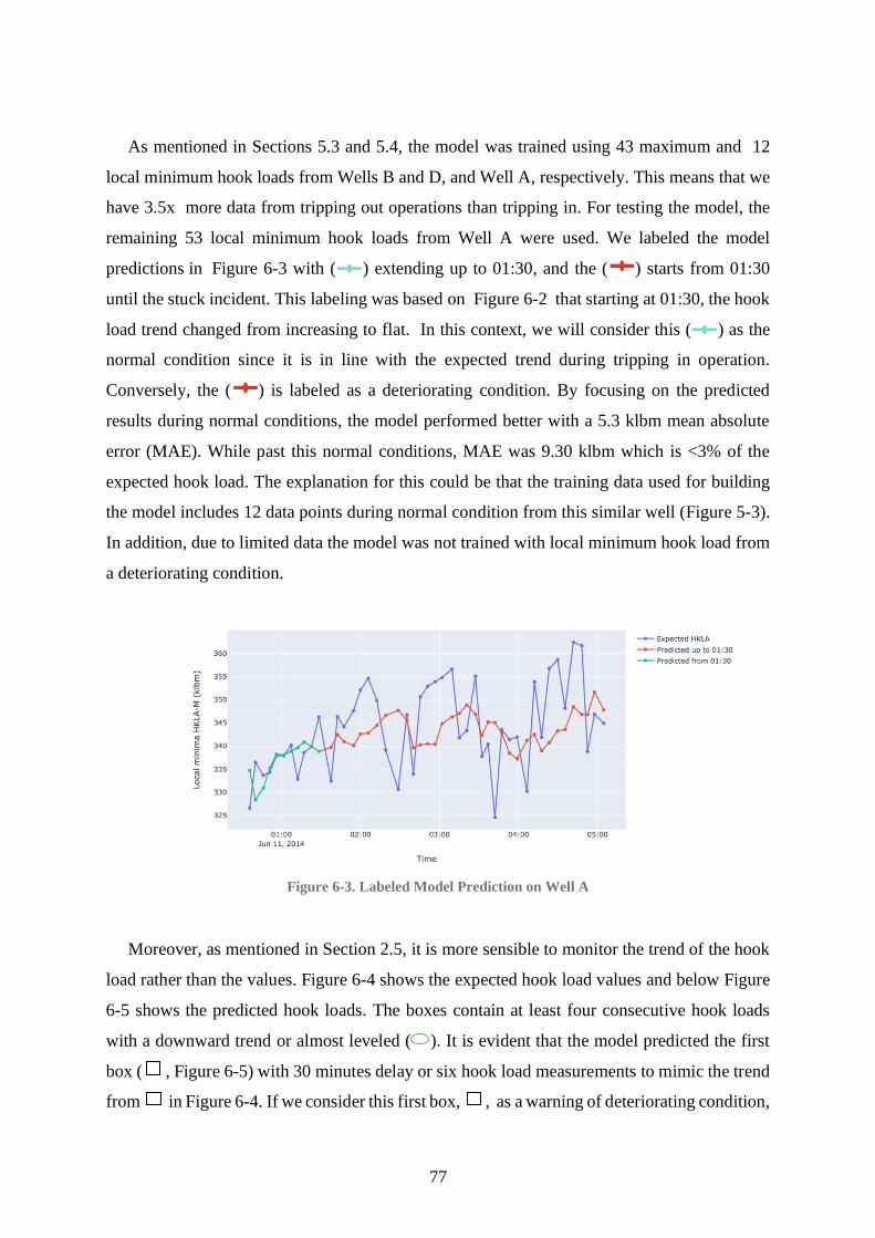
77

As mentioned in Sections 5.3 and 5.4, the model was trained using 43 maximum and 12

local minimum hook loads from Wells B and D, and Well A, respectively. This means that we

have 3.5x more data from tripping out operations than tripping in. For testing the model, the

remaining 53 local minimum hook loads from Well A were used. We labeled the model

predictions in Figure 6-3 with ( ) extending up to 01:30, and the ( ) starts from 01:30

until the stuck incident. This labeling was based on Figure 6-2 that starting at 01:30, the hook

load trend changed from increasing to flat. In this context, we will consider this ( ) as the

normal condition since it is in line with the expected trend during tripping in operation.

Conversely, the ( ) is labeled as a deteriorating condition. By focusing on the predicted

results during normal conditions, the model performed better with a 5.3 klbm mean absolute

error (MAE). While past this normal conditions, MAE was 9.30 klbm which is <3% of the

expected hook load. The explanation for this could be that the training data used for building

the model includes 12 data points during normal condition from this similar well (Figure 5-3).

In addition, due to limited data the model was not trained with local minimum hook load from

a deteriorating condition.

Figure 6-3. Labeled Model Prediction on Well A

Moreover, as mentioned in Section 2.5, it is more sensible to monitor the trend of the hook

load rather than the values. Figure 6-4 shows the expected hook load values and below Figure

6-5 shows the predicted hook loads. The boxes contain at least four consecutive hook loads

with a downward trend or almost leveled ( ). It is evident that the model predicted the first

box ( , Figure 6-5) with 30 minutes delay or six hook load measurements to mimic the trend

from in Figure 6-4. If we consider this first box, , as a warning of deteriorating condition,

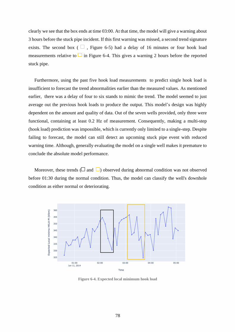
78

clearly we see that the box ends at time 03:00. At that time, the model will give a warning about

3 hours before the stuck pipe incident. If this first warning was missed, a second trend signature

exists. The second box ( , Figure 6-5) had a delay of 16 minutes or four hook load

measurements relative to in Figure 6-4. This gives a warning 2 hours before the reported

stuck pipe.

Furthermore, using the past five hook load measurements to predict single hook load is

insufficient to forecast the trend abnormalities earlier than the measured values. As mentioned

earlier, there was a delay of four to six stands to mimic the trend. The model seemed to just

average out the previous hook loads to produce the output. This model’s design was highly

dependent on the amount and quality of data. Out of the seven wells provided, only three were

functional, containing at least 0.2 Hz of measurement. Consequently, making a multi-step

(hook load) prediction was impossible, which is currently only limited to a single-step. Despite

failing to forecast, the model can still detect an upcoming stuck pipe event with reduced

warning time. Although, generally evaluating the model on a single well makes it premature to

conclude the absolute model performance.

Moreover, these trends ( and ) observed during abnormal condition was not observed

before 01:30 during the normal condition. Thus, the model can classify the well's downhole

condition as either normal or deteriorating.

Figure 6-4. Expected local minimum hook load

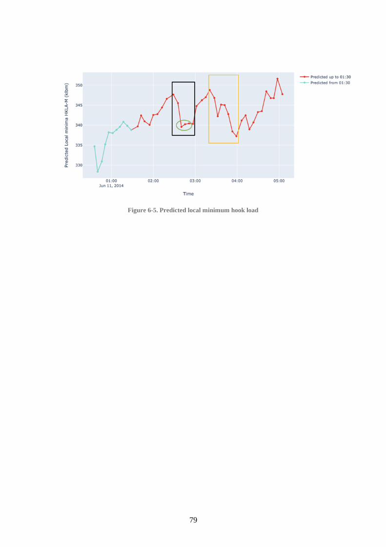
79

Figure 6-5. Predicted local minimum hook load

80

7 Conclusions and Future Work

7.1. Conclusions

It was challenging to identify published work in the Oil and Gas industry that has shown a

transparent and complete process of building a Machine Learning model – from data collection

to model evaluation. As a result, some conclusions are made about the developed LSTM model

as well as experiences while working on the project:

• The proposed concept and algorithm in extracting the local minimum hook load

accurately identified the data points of interest. Furthermore, it has shown an apparent

trend deviation 4 hours and 30 minutes before the reported stuck pipe.

• It was proved that the use of hook load signatures – maximum and local minimum hook

loads - provided a better view of the deteriorating downhole condition than relying on

the whole hook load measurement. This can be seen in Figure 6-1 and Figure 6-2. Even

without a predictive model, this is sufficient in serving as a stuck pipe indicator.

• The model was successfully tested with an acceptable mean absolute error of < 3%.

Also, it was able to mimic and produce trend signatures of an impending stuck pipe but

with 4 to 6 hook load measurement delays relative to the expected data (see Figure 6-4

and Figure 6-5).

• The majority of the time was consumed for data preparation and feature extraction.

• The two in-house web-based applications developed for data exploration and cleaning

were invaluable and paved the way for efficient data analysis.

• A single model capable of predicting hook load signatures during tripping in and

tripping out operations was built.

• Reproducible algorithms for this project were all provided.

81

7.2. Future Work

This study can be used as a stepping stone to further develop Machine Learning models in the

Oil and Gas industry, particularly for preventing non-productive time relative to stuck pipe.

But before this, it is advisable to consider the following:

• Gather more drilling data with at least 0.2 Hz of measurement frequency.

• With more training data, retrain the model to predict more hook load measurements at

each timestep. This will anticipate the trend deviations earlier than the currently

developed model.

• Extensive model testing from wells with different configurations.

• Find other parameters that are always available, which can improve hook load

prediction.

With a good and reliable multi-step hook load predictive model, it is possible to develop an

alarm system to alert the drilling crew of a deteriorating downhole condition that could lead to

a stuck pipe. The alarm can be flagged when the trend of consecutive hook load signatures

deviates from what is expected.

82

References [1] H. H. Elmousalami and M. Elaskary, "Drilling stuck pipe classification and mitigation

in the Gulf of Suez oil fields using artificial intelligence," Journal of Petroleum Exploration and Production Technology, 2020. [Online]. Available: https://doi.org/10.1007/s13202-020-00857-w.

[2] A. Pant. "Workflow of a Machine Learning project." Towards Data Science. https://towardsdatascience.com/workflow-of-a-machine-learning-project-ec1dba419b94 (accessed May 20, 2021).

[3] G. Press. "Cleaning Big Data: Most Time-Consuming, Least Enjoyable Data Science Task, Survey Says." Forbes. https://www.forbes.com/sites/gilpress/2016/03/23/data-preparation-most-time-consuming-least-enjoyable-data-science-task-survey-says/ (accessed May 20, 2021).

[4] M. A. Muqeem, A. E. Weekse, and A. A. Al-Hajji, "Stuck Pipe Best Practices – A Challenging Approach to Reducing Stuck Pipe Costs," 2012. SPE-160845-MS. [Online]. Available: https://doi.org/10.2118/160845-MS.

[5] A. L. Agbaji, "Optimizing The Planning, Design And Drilling Of Extended Reach And Complex Wells," in Abu Dhabi International Petroleum Exhibition and Conference, 2010. SPE-136901-MS. [Online]. Available: https://doi.org/10.2118/136901-MS

[6] C. J. Mason, Igland, Jan Kåre, Streeter, Edward J., Andresen, Per-Arild, "New Real-Time Casing Running Advisory System Reduces NPT," in SPE Offshore Europe Oil and Gas Conference and Exhibition, 2013, SPE-166616-MS. [Online]. Available: https://doi.org/10.2118/166616-MS. [Online].

[7] R. J. W. Kucs, H. F. Spoerker, G. Thonhauser, and P. Zoellner, "Automated Real-Time Hookload and Torque Monitoring," IADC/SPE Drilling Conference, 2008. SPE-112565-MS.

[8] R. M. Thomas Goebel, Ricardo Vilalta, Kinjal Gupta, "METHOD AND SYSTEM FOR PREDICTING A DRILL STRING STUCK PIPE EVENT," United States of America Patent US 8,752,648 B2 Patent Appl. 13/883,822, 2014.

[9] C. I. Noshi and J. J. Schubert, "The Role of Machine Learning in Drilling Operations; A Review," in SPE/AAPG Eastern Regional Meeting, October 10, 2018. SPE- 191823-18erm-ms. [Online]. Available: https://doi.org/10.2118/191823-18ERM-MS

[10] K. R. Holdaway, Harness oil and gas big data with analytics : Optimize exploration and production with data-driven models. . ProQuest Ebook Central 2014.

[11] F. Zhang et al., "Real Time Stuck Pipe Prediction by Using a Combination of Physics-Based Model and Data Analytics Approach," in Abu Dhabi International Petroleum Exhibition & Conference, November 12, 2019. SPE-197167-MS. [Online]. Available: https://doi.org/10.2118/197167-MS

[12] A. Twin. "Data Mining." https://www.investopedia.com/terms/d/datamining.asp (accessed June 20, 2021).

[13] P. Katiyar. "Difference Between Descriptive and Predictive Data Mining." https://www.geeksforgeeks.org/difference-between-descriptive-and-predictive-data-mining/ (accessed June 20, 2021).

[14] B. R.-K. Thomas Kluyver, Fernando Pérez, Brian Granger, Matthias Bussonnier, Jonathan Frederic, Kyle Kelley, Jessica Hamrick, Jason Grout, Sylvain Corlay, Paul Ivanov, Damián Avila, Safia Ab- dalla, and Carol Willing, F. L. a. B. Schmidt, Ed. Jupyter Notebooks -- a publishing format for reproducible computational workflows

83

(Positioning and Power in Academic Publishing: Players, Agents and Agendas). IOS Press, 2016.

[15] G. V. Rossum and F. L. Drake, Python 3 Reference Manual. CreateSpace, 2009. [16] S. India. "Best language for Machine Learning: Which Programming Language to

Learn." https://in.springboard.com/blog/best-language-for-machine-learning/ (accessed June 20, 2021).

[17] "Hoisting system." Petropedia. https://www.petropedia.com/definition/6723/hoisting-system (accessed March 20, 2021).

[18] R. F. Mitchell and S. Z. Miska, Fundamentals of Drilling Engineering. Richardson, UNITED STATES: Society of Petroleum Engineers, 2010.

[19] "The Hoisting System." PennState, College of Earth and Mineral Sciences. https://www.e-education.psu.edu/png301/node/725 (accessed March 20, 2021, 2021).

[20] A. T. Bourgoyne, K. K. Millheim, and M. E. Chenevert, Applied Drilling Engineering. Richardson, UNITED STATES: Society of Petroleum Engineers, 1985.

[21] "What is a Kelly Rig?" http://www.drillingformulas.com/what-is-kelly-rig/ (accessed February 13, 2021).

[22] "Top Drive System (TDS) Spinning for Oil Drilling Rig." https://www.123rf.com/photo_80732180_top-drive-system-tds-spinning-for-oil-drilling-rig.html (accessed March 20, 2021).

[23] ERITIA. "Drilling Mud Circulation System." https://drillingfluid.org/drilling-fluids-handbook-2/drilling-mud-circulation-system.html (accessed March 20, 2021).

[24] "The Well Control System (Blowout Prevention System)." PennState, College of Earth and Mineral Sciences. https://www.e-education.psu.edu/png301/node/728 (accessed March 20, 2021).

[25] NORSOK Standard D-001, third edition, N. O. a. G. Association, Norway, 2012. [26] J. Vogt, "Automated Racking Board Pipe Handling System for Drilling Rigs Ensures

Connection Integrity While Providing Safer Working Conditions and Consistent Tripping Speeds With Minimal Rig Modifications," in SPE/IATMI Asia Pacific Oil & Gas Conference and Exhibition, 2015. SPE-176336-MS. [Online]. Available: https://doi.org/10.2118/176336-MS

[27] "MWD/LWD technologies advance to meet industry needs." Offshore. https://www.offshore-mag.com/drilling-completion/article/14038994/measurementwhiledrilling-and-loggingwhiledrilling-advances-to-meet-industry-needs (accessed February 13, 2021).

[28] B. S. Aadnøy, Modern Well Design, second ed. P.O. Box 447, 2300 AK Leiden,The Netherlands: CRC Press/Balkema, 2010.

[29] K. A. Bernt S. Aadnøy, "Design of oil wells using analytical friction models," Journal of Petroleum Science and Engineering, 2001.

[30] C. A. Johancsik, D. B. Friesen, and R. Dawson, "Torque and Drag in Directional Wells-Prediction and Measurement," Journal of Petroleum Technology, 1984. SPE-11380-pa.

[31] M. A. Encinas Quisbert, D. Sui, and A. Mirhaj, "Data Driven ROP Modeling - Analysis and Feasibility Study." Master Thesis. University of Stavanger, Norway, 2020.

[32] M. Belayneh, Chapter 3B: Drill string mechanics design. Lecture Notes. University of Stavanger, Norway, 2020.

84

[33] C. Eric, H. J. Skadsem, and R. Kluge, "Accuracy and Correction of Hook Load Measurements During Drilling Operations," in SPE/IADC Drilling Conference and Exhibition, March 18, 2015. SPE-173035-MS. [Online]. Available: https://doi.org/10.2118/173035-MS

[34] Schlumberger, "Hook load," ed, 2012. https://glossary.oilfield.slb.com/en/terms/h/hook_load. (accessed February 13, 2021)

[35] R. Wylie, J. Standefer, J. Anderson, and I. Soukup, "Instrumented Internal Blowout Preventer Improves Measurements for Drilling and Equipment Optimization," in SPE/IADC Drilling Conference, 2013. SPE-163475-MS. [Online]. Available: https://doi.org/10.2118/163475-MS

[36] P. l. S. Dipankar Chowdhury, Mohammed Mahbubur Rahman, "PREDICTION OF STAND PIPE PRESSURE USING CONVENTIONAL APPROACH," Chemical Engineering Research Bulletin, 2009. [Online]. Available: http://www.ipt.ntnu.no/~pskalle/files/TechnicalPapers/31_SPP.pdf.

[37] Schlumberger, "Equivalent Circulating Density," in Schlumberger Oilfield Glossary, ed., 2012. https://glossary.oilfield.slb.com/en/terms/e/ecd (accessed February 13, 2021)

[38] C. Sena. "Get your booty on the drill floor." https://kcacod.wordpress.com/2016/03/27/get-your-booty-on-the-drill-floor/ (accessed February 13, 2021).

[39] L. W. Lake and R. F. Mitchell, Petroleum Engineering Handbook : Drilling Engineering. Richardson, UNITED STATES: Society of Petroleum Engineers, 2006.

[40] A. Brankovic et al., "A Data-Based Approach for the Prediction of Stuck-Pipe Events in Oil Drilling Operations," in Abu Dhabi International Petroleum Exhibition & Conference, November 12, 2020. SPE-202625-MS. [Online]. Available: https://doi.org/10.2118/202625-MS

[41] F. E. Dupriest, W. C. Elks, and S. Ottesen, "Design Methodology and Operational Practices Eliminate Differential Sticking," SPE Drilling & Completion, 2011. SPE-128129-pa.

[42] A. A. Alshaikh and M. Amanullah, "A Comprehensive Review of Differential Sticking, Spotting Fluids, and the Current Testing and Evaluation Methods," in SPE Kingdom of Saudi Arabia Annual Technical Symposium and Exhibition, 2018. SPE-192169-MS. [Online]. Available: https://doi.org/10.2118/192169-MS

[43] A. T. Bourgoyne, "Applied drilling engineering," (in English), 1986. [Online]. Available: http://site.ebrary.com/id/10619585.

[44] C. B. R. Procter, 1997 Drillers Stuck pipe Handbook, Ballater, Scotland, AB35 5UR: Procter & Collins Ltd, 1997.

[45] J. E. Warren, "Causes, Preventions, and Recovery of Stuck Drill Pipe," in Drilling and Production Practice, 1940, vol. All Days, API-40-030.

[46] E. Cayeux, B. Daireaux, E. Wolden Dvergsnes, and G. Sælevik, "Early Symptom Detection on the Basis of Real-Time Evaluation of Downhole Conditions: Principles and Results From Several North Sea Drilling Operations," SPE Drilling & Completion, 2012. SPE-150422-pa.

[47] M. Awad and R. Khanna, "Machine Learning," in Efficient Learning Machines: Theories, Concepts, and Applications for Engineers and System Designers. Berkeley, CA: Apress, 2015, pp. 1-18.

85

[48] E. A. Team, "What is Machine Learning? A Definition.," vol. 2021, ed, 2020. https://www.expert.ai/blog/machine-learning-definition/ (accessed February 13, 2021)

[49] F. Chollet, Deep Learning with Python. Manning Publications Co., 2017. [50] M. M. Meor Hashim et al., "Utilizing Artificial Neural Network for Real-Time

Prediction of Differential Sticking Symptoms," in International Petroleum Technology Conference, March 29, 2021. IPTC-21221-ms. [Online]. Available: https://doi.org/10.2523/IPTC-21221-MS

[51] C. Siruvuri, S. Nagarakanti, and R. Samuel, "Stuck Pipe Prediction and Avoidance: A Convolutional Neural Network Approach," in IADC/SPE Drilling Conference, 2006. SPE-98378-MS. [Online]. Available: https://doi.org/10.2118/98378-MS

[52] A. Murillo, J. Neuman, and R. Samuel, "Pipe Sticking Prediction and Avoidance Using Adaptive Fuzzy Logic Modeling," in SPE Production and Operations Symposium, 2009. SPE-120128-MS. [Online]. Available: https://doi.org/10.2118/120128-MS

[53] W. B. Hempkins, R. H. Kingsborough, W. E. Lohec, and C. J. Nini, "Multivariate Statistical Analysis of Stuck Drillpipe Situations," SPE Drilling Engineering, 1987. SPE-14181-pa.

[54] A. K. Abbas, H. Almubarak, H. Abbas, and J. Dawood, "Application of Machine Learning Approach for Intelligent Prediction of Pipe Sticking," in Abu Dhabi International Petroleum Exhibition & Conference, November 12, 2019. SPE-197396-MS. [Online]. Available: https://doi.org/10.2118/197396-MS

[55] A. Géron, Hands-on machine learning with Scikit-Learn, Keras, and TensorFlow : concepts, tools, and techniques to build intelligent systems, Second Edition. ed. (Hands-on machine learning with Scikit-Learn and TensorFlow). Sebastopol, CA: O'Reilly, 2019.

[56] V. Jain. "Everything you need to know about “Activation Functions” in Deep learning models." https://towardsdatascience.com/everything-you-need-to-know-about-activation-functions-in-deep-learning-models-84ba9f82c253 (accessed May 20, 2021).

[57] T. N. Activator. "What is An Activation Function?" https://www.neuronactivator.com/blog/what-even-is-activation-function (accessed February 10, 2021).

[58] T. Yiu. "Understanding Neural Networks." https://towardsdatascience.com/understanding-neural-networks-19020b758230 (accessed May 20, 2021).

[59] I. C. Education. "Recurrent Neural Networks." https://www.ibm.com/cloud/learn/recurrent-neural-networks (accessed May 20, 2021).

[60] Y. Bengio, P. Simard, and P. Frasconi, "Learning long-term dependencies with gradient descent is difficult," IEEE transactions on neural networks / a publication of the IEEE Neural Networks Council, vol. 5, pp. 157-66, 02/01 1994, doi: 10.1109/72.279181.

[61] S. Hochreiter and J. Schmidhuber, "Long Short-Term Memory," Neural Comput., vol. 9, no. 8, pp. 1735–1780, 1997, doi: 10.1162/neco.1997.9.8.1735.

[62] B. Thakur and R. Samuel, "Deep Learning for Downhole Data Prediction: A Cost-Effective Data Telemetry Through Data Analytics," in SPE Western Regional Meeting,

86

April 22, 2021. SPE-200870-ms. [Online]. Available: https://doi.org/10.2118/200870-MS

[63] J. Han, Y. Sun, and S. Zhang, "A Data Driven Approach of ROP Prediction and Drilling Performance Estimation," in International Petroleum Technology Conference, March 26, 2019. IPTC-19430-ms. [Online]. Available: https://doi.org/10.2523/IPTC-19430-MS

[64] A. Bhandari. "Feature Scaling for Machine Learning: Understanding the Difference Between Normalization vs. Standardization." https://www.analyticsvidhya.com/blog/2020/04/feature-scaling-machine-learning-normalization-standardization/ (accessed May 20, 2021).

[65] F. Pedregosa, Varoquaux, G., Gramfort, A., Michel, V., Thirion, B., Grisel, O., Blondel, M., Prettenhofer, P., Weiss, R., Dubourg, V., Vanderplas, J., Passos, A., Cournapeau, D., Brucher, M., Perrot, M., Duchesnay, E., "Scikit-learn: Machine Learning in Python," Journal of Machine Learning Research, vol. 12, pp. 2825 - 2830, 2011.

[66] A. Gron, Hands-On Machine Learning with Scikit-Learn and TensorFlow: Concepts, Tools, and Techniques to Build Intelligent Systems. O'Reilly Media, Inc., 2017.

[67] pandas-dev/pandas: Pandas. (2020). [Online]. Available: https://doi.org/10.5281/zenodo.3509134

[68] Chollet, F., & others. (2015). Keras. GitHub. Retrieved from https://github.com/fchollet/keras.

[69] TensorFlow: Large-Scale Machine Learning on Heterogeneous Systems. (2015). [Online]. Available: http://tensorflow.org/

[70] A. T. Tunkiel, T. Wiktorski, and D. Sui, "Drilling Dataset Exploration, Processing and Interpretation Using Volve Field Data," in ASME 2020 39th International Conference on Ocean, Offshore and Arctic Engineering, 2020. OMAE2020-18151. [Online]. Available: https://doi.org/10.1115/OMAE2020-18151

[71] Collaborative data science Publisher: Plotly Technologies Inc. (2015). Montréal, QC. [Online]. Available: https://plot.ly

[72] D. Kumar. "Introduction to Data Preprocessing in Machine Learning." https://towardsdatascience.com/introduction-to-data-preprocessing-in-machine-learning-a9fa83a5dc9d (accessed May 20,2021).

[73] E. Rençberoğlu. "Fundamental Techniques of Feature Engineering for Machine Learning." https://towardsdatascience.com/feature-engineering-for-machine-learning-3a5e293a5114 (accessed May 20, 2021).

[74] H. Lim. "7 Types of Data Bias in Machine Learning." https://lionbridge.ai/articles/7-types-of-data-bias-in-machine-learning/ (accessed May 23, 2021).

[75] K. J. M. Charles R. Harris, Stefan J., van der Walt, Ralf Gommers, Stephan Hoyer, Marten H. van Kerkwijk "Numpy," Nature, vol. 585, pp. 357-362, 2020. [Online]. Available: https://doi.org/10.1038/s41586-020-2649-2.

[76] M. M. Amer, A. S. DAHAB, and A.-A. H. El-Sayed, "An ROP Predictive Model in Nile Delta Area Using Artificial Neural Networks," in SPE Kingdom of Saudi Arabia Annual Technical Symposium and Exhibition, April 25, 2017. SPE-187969-ms. [Online]. Available: https://doi.org/10.2118/187969-MS

[77] J. Brownlee. "What is the Difference Between a Parameter and a Hyperparameter?" (accessed February 13, 2021).

87

Appendices

Appendix A

Installed Packages

88

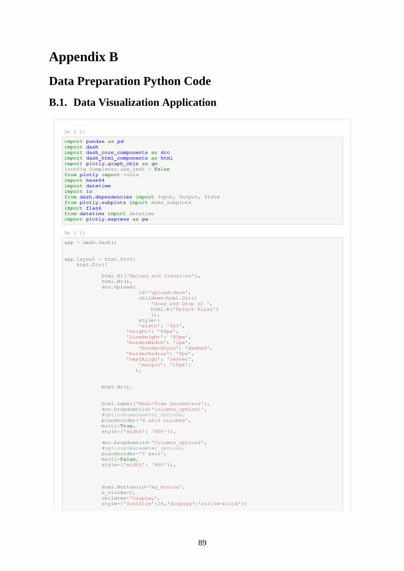
89

Appendix B

Data Preparation Python Code

B.1. Data Visualization Application

In [ ]:

importimport pandaspandas asas pdpd

importimport dashdash

importimport dash_core_componentsdash_core_components asas dccdcc

importimport dash_html_componentsdash_html_components asas htmlhtml

importimport plotly.graph_objsplotly.graph_objs asas gogo

%config Completer.use_jedi = FalseFalse

fromfrom plotlyplotly importimport tools

importimport base64base64

importimport datetimedatetime

importimport ioio

fromfrom dash.dependenciesdash.dependencies importimport Input, Output, State

fromfrom plotly.subplotsplotly.subplots importimport make_subplots

importimport flaskflask

fromfrom datetimedatetime importimport datetime

importimport plotly.expressplotly.express asas pxpx

In [ ]:

app = dash.Dash()

app.layout = html.Div([

html.Div([

html.H1('Upload and Visualize'),

html.Br(),

dcc.Upload(

id='upload-data',

children=html.Div([

'Drag and Drop or ',

html.A('Select Files')

]),

style={

'width': '40%',

'height': '60px',

'lineHeight': '60px',

'borderWidth': '1px',

'borderStyle': 'dashed',

'borderRadius': '5px',

'textAlign': 'center',

'margin': '10px'}

),

html.Br(),

html.Label('Real-Time Parameters'),

dcc.Dropdown(id='Columns_option1',

#options=parameter_options,

placeholder='X axis columns',

multi=TrueTrue,

style={'width': '80%'}),

dcc.Dropdown(id='Columns_option2',

#options=parameter_options,

placeholder='Y axis',

multi=FalseFalse,

style={'width': '80%'}),

html.Button(id='my_button',

n_clicks=0,

children='Display',

style={'fontSize':28,'display':'inline-block'})

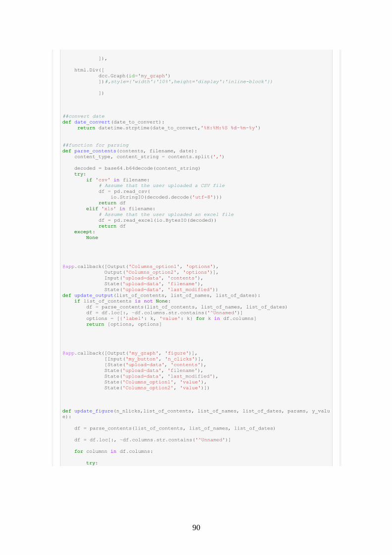
90

]),

html.Div([

dcc.Graph(id='my_graph')

])#,style={'width':'10%',height='display':'inline-block'})

])

##convert date

defdef date_convert(date_to_convert):

returnreturn datetime.strptime(date_to_convert,'%H:%M:%S %d%d-%m-%y')

##function for parsing

defdef parse_contents(contents, filename, date):

content_type, content_string = contents.split(',')

decoded = base64.b64decode(content_string)

trytry:

ifif 'csv' inin filename:

# Assume that the user uploaded a CSV file

df = pd.read_csv(

io.StringIO(decoded.decode('utf-8')))

returnreturn df

elifelif 'xls' inin filename:

# Assume that the user uploaded an excel file

df = pd.read_excel(io.BytesIO(decoded))

returnreturn df

exceptexcept:

NoneNone

@app.callback([Output('Columns_option1', 'options'),

Output('Columns_option2', 'options')],

Input('upload-data', 'contents'),

State('upload-data', 'filename'),

State('upload-data', 'last_modified'))

defdef update_output(list_of_contents, list_of_names, list_of_dates):

ifif list_of_contents isis notnot NoneNone:

df = parse_contents(list_of_contents, list_of_names, list_of_dates)

df = df.loc[:, ~df.columns.str.contains('^Unnamed')]

options = [{'label': k, 'value': k} forfor k inin df.columns]

returnreturn [options, options]

@app.callback([Output('my_graph', 'figure')],

[Input('my_button', 'n_clicks')],

[State('upload-data', 'contents'),

State('upload-data', 'filename'),

State('upload-data', 'last_modified'),

State('Columns_option1', 'value'),

State('Columns_option2', 'value')])

defdef update_figure(n_nlicks,list_of_contents, list_of_names, list_of_dates, params, y_valu

e):

df = parse_contents(list_of_contents, list_of_names, list_of_dates)

df = df.loc[:, ~df.columns.str.contains('^Unnamed')]

forfor columnn inin df.columns:

trytry:

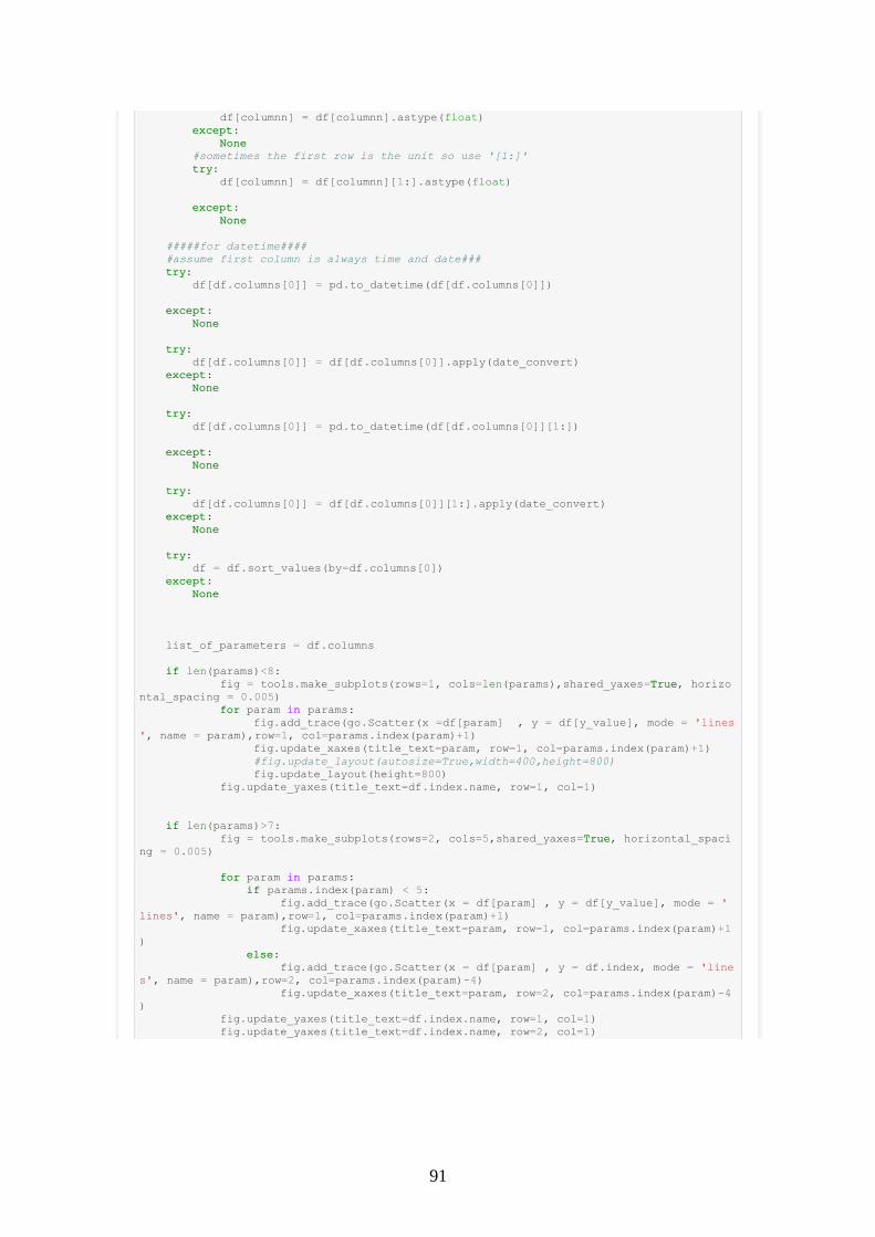
91

df[columnn] = df[columnn].astype(float)

exceptexcept:

NoneNone

#sometimes the first row is the unit so use '[1:]'

trytry:

df[columnn] = df[columnn][1:].astype(float)

exceptexcept:

NoneNone

#####for datetime####

#assume first column is always time and date###

trytry:

df[df.columns[0]] = pd.to_datetime(df[df.columns[0]])

exceptexcept:

NoneNone

trytry:

df[df.columns[0]] = df[df.columns[0]].apply(date_convert)

exceptexcept:

NoneNone

trytry:

df[df.columns[0]] = pd.to_datetime(df[df.columns[0]][1:])

exceptexcept:

NoneNone

trytry:

df[df.columns[0]] = df[df.columns[0]][1:].apply(date_convert)

exceptexcept:

NoneNone

trytry:

df = df.sort_values(by=df.columns[0])

exceptexcept:

NoneNone

list_of_parameters = df.columns

ifif len(params)<8:

fig = tools.make_subplots(rows=1, cols=len(params),shared_yaxes=TrueTrue, horizo

ntal_spacing = 0.005)

forfor param inin params:

fig.add_trace(go.Scatter(x =df[param] , y = df[y_value], mode = 'lines

', name = param),row=1, col=params.index(param)+1)

fig.update_xaxes(title_text=param, row=1, col=params.index(param)+1)

#fig.update_layout(autosize=True,width=400,height=800)

fig.update_layout(height=800)

fig.update_yaxes(title_text=df.index.name, row=1, col=1)

ifif len(params)>7:

fig = tools.make_subplots(rows=2, cols=5,shared_yaxes=TrueTrue, horizontal_spaci

ng = 0.005)

forfor param inin params:

ifif params.index(param) < 5:

fig.add_trace(go.Scatter(x = df[param] , y = df[y_value], mode = '

lines', name = param),row=1, col=params.index(param)+1)

fig.update_xaxes(title_text=param, row=1, col=params.index(param)+1

)

elseelse:

fig.add_trace(go.Scatter(x = df[param] , y = df.index, mode = 'line

s', name = param),row=2, col=params.index(param)-4)

fig.update_xaxes(title_text=param, row=2, col=params.index(param)-4

)

fig.update_yaxes(title_text=df.index.name, row=1, col=1)

fig.update_yaxes(title_text=df.index.name, row=2, col=1)

92

#if len(params)>3:

# fig.add_trace(go.Scatter(x = df[params[3]] , y = df.index, mode = 'lines',

name = params[3]),row=1, col=3)

fig.update_yaxes(title_text=df.index.name, row=1, col=1)

fig.update_yaxes(autorange="reversed")

returnreturn [fig]

ifif __name__ == '__main__':

app.run_server(port=8064)

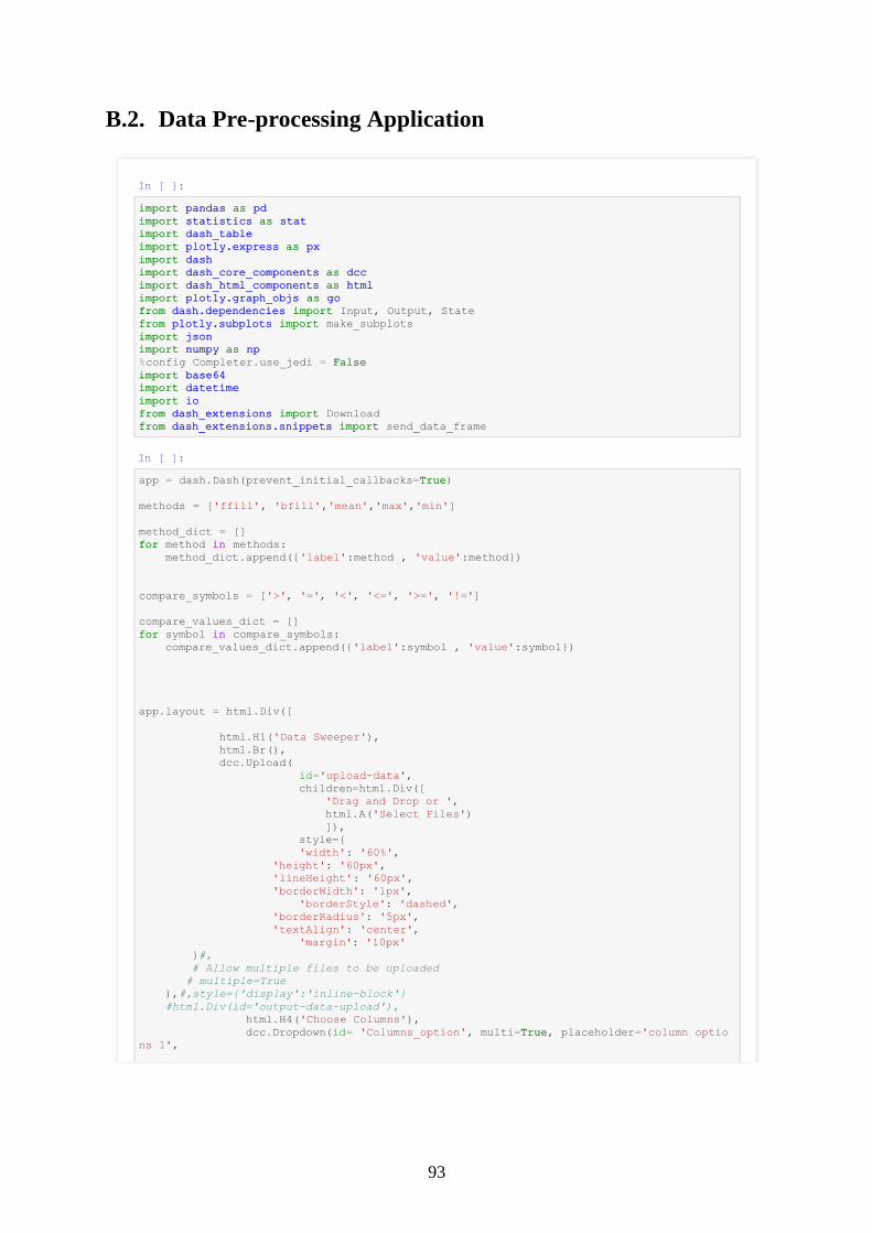
93

B.2. Data Pre-processing Application

In [ ]:

importimport pandaspandas asas pdpd

importimport statisticsstatistics asas statstat

importimport dash_tabledash_table

importimport plotly.expressplotly.express asas pxpx

importimport dashdash

importimport dash_core_componentsdash_core_components asas dccdcc

importimport dash_html_componentsdash_html_components asas htmlhtml

importimport plotly.graph_objsplotly.graph_objs asas gogo

fromfrom dash.dependenciesdash.dependencies importimport Input, Output, State

fromfrom plotly.subplotsplotly.subplots importimport make_subplots

importimport jsonjson

importimport numpynumpy asas npnp

%config Completer.use_jedi = FalseFalse

importimport base64base64

importimport datetimedatetime

importimport ioio

fromfrom dash_extensionsdash_extensions importimport Download

fromfrom dash_extensions.snippetsdash_extensions.snippets importimport send_data_frame

In [ ]:

app = dash.Dash(prevent_initial_callbacks=TrueTrue)

methods = ['ffill', 'bfill','mean','max','min']

method_dict = []

forfor method inin methods:

method_dict.append({'label':method , 'value':method})

compare_symbols = ['>', '=', '<', '<=', '>=', '!=']

compare_values_dict = []

forfor symbol inin compare_symbols:

compare_values_dict.append({'label':symbol , 'value':symbol})

app.layout = html.Div([

html.H1('Data Sweeper'),

html.Br(),

dcc.Upload(

id='upload-data',

children=html.Div([

'Drag and Drop or ',

html.A('Select Files')

]),

style={

'width': '60%',

'height': '60px',

'lineHeight': '60px',

'borderWidth': '1px',

'borderStyle': 'dashed',

'borderRadius': '5px',

'textAlign': 'center',

'margin': '10px'

}#,

# Allow multiple files to be uploaded

# multiple=True

),#,style={'display':'inline-block'}

#html.Div(id='output-data-upload'),

html.H4('Choose Columns'),

dcc.Dropdown(id= 'Columns_option', multi=TrueTrue, placeholder='column optio

ns 1',

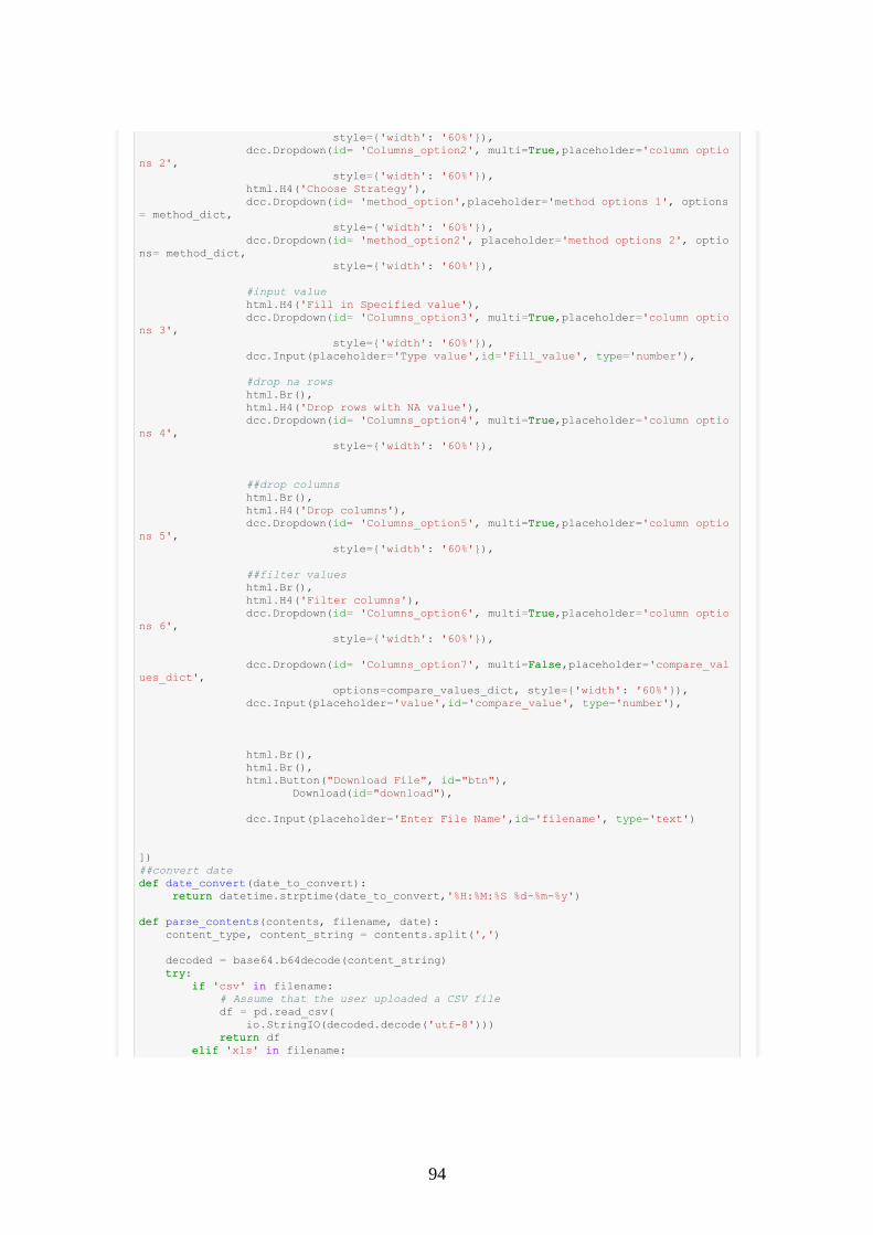
94

style={'width': '60%'}),

dcc.Dropdown(id= 'Columns_option2', multi=TrueTrue,placeholder='column optio

ns 2',

style={'width': '60%'}),

html.H4('Choose Strategy'),

dcc.Dropdown(id= 'method_option',placeholder='method options 1', options

= method_dict,

style={'width': '60%'}),

dcc.Dropdown(id= 'method_option2', placeholder='method options 2', optio

ns= method_dict,

style={'width': '60%'}),

#input value

html.H4('Fill in Specified value'),

dcc.Dropdown(id= 'Columns_option3', multi=TrueTrue,placeholder='column optio

ns 3',

style={'width': '60%'}),

dcc.Input(placeholder='Type value',id='Fill_value', type='number'),

#drop na rows

html.Br(),

html.H4('Drop rows with NA value'),

dcc.Dropdown(id= 'Columns_option4', multi=TrueTrue,placeholder='column optio

ns 4',

style={'width': '60%'}),

##drop columns

html.Br(),

html.H4('Drop columns'),

dcc.Dropdown(id= 'Columns_option5', multi=TrueTrue,placeholder='column optio

ns 5',

style={'width': '60%'}),

##filter values

html.Br(),

html.H4('Filter columns'),

dcc.Dropdown(id= 'Columns_option6', multi=TrueTrue,placeholder='column optio

ns 6',

style={'width': '60%'}),

dcc.Dropdown(id= 'Columns_option7', multi=FalseFalse,placeholder='compare_val

ues_dict',

options=compare_values_dict, style={'width': '60%'}),

dcc.Input(placeholder='value',id='compare_value', type='number'),

html.Br(),

html.Br(),

html.Button("Download File", id="btn"),

Download(id="download"),

dcc.Input(placeholder='Enter File Name',id='filename', type='text')

])

##convert date

defdef date_convert(date_to_convert):

returnreturn datetime.strptime(date_to_convert,'%H:%M:%S %d%d-%m-%y')

defdef parse_contents(contents, filename, date):

content_type, content_string = contents.split(',')

decoded = base64.b64decode(content_string)

trytry:

ifif 'csv' inin filename:

# Assume that the user uploaded a CSV file

df = pd.read_csv(

io.StringIO(decoded.decode('utf-8')))

returnreturn df

elifelif 'xls' inin filename:

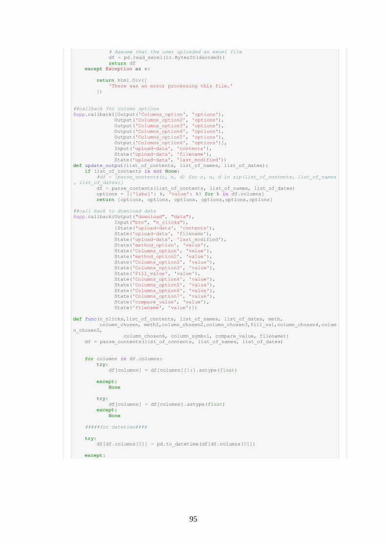
95

# Assume that the user uploaded an excel file

df = pd.read_excel(io.BytesIO(decoded))

returnreturn df

exceptexcept ExceptionException asas e:

returnreturn html.Div([

'There was an error processing this file.'

])

##callback for column options

@app.callback([Output('Columns_option', 'options'),

Output('Columns_option2', 'options'),

Output('Columns_option3', 'options'),

Output('Columns_option4', 'options'),

Output('Columns_option5', 'options'),

Output('Columns_option6', 'options')],

Input('upload-data', 'contents'),

State('upload-data', 'filename'),

State('upload-data', 'last_modified'))

defdef update_output(list_of_contents, list_of_names, list_of_dates):

ifif list_of_contents isis notnot NoneNone:

#df = [parse_contents(c, n, d) for c, n, d in zip(list_of_contents, list_of_names

, list_of_dates)]

df = parse_contents(list_of_contents, list_of_names, list_of_dates)

options = [{'label': k, 'value': k} forfor k inin df.columns]

returnreturn [options, options, options, options,options,options]

##call back to download data

@app.callback(Output("download", "data"),

Input("btn", "n_clicks"),

[State('upload-data', 'contents'),

State('upload-data', 'filename'),

State('upload-data', 'last_modified'),

State('method_option', 'value'),

State('Columns_option', 'value'),

State('method_option2', 'value'),

State('Columns_option2', 'value'),

State('Columns_option3', 'value'),

State('Fill_value', 'value'),

State('Columns_option4', 'value'),

State('Columns_option5', 'value'),

State('Columns_option6', 'value'),

State('Columns_option7', 'value'),

State('compare_value', 'value'),

State('filename', 'value')])

defdef func(n_nlicks,list_of_contents, list_of_names, list_of_dates, meth,

column_chosen, meth2,column_chosen2,column_chosen3,fill_val,column_chosen4,colum

n_chosen5,

column_chosen6, column_symbol, compare_value, filename):

df = parse_contents(list_of_contents, list_of_names, list_of_dates)

forfor columnn inin df.columns:

trytry:

df[columnn] = df[columnn][1:].astype(float)

exceptexcept:

NoneNone

trytry:

df[columnn] = df[columnn].astype(float)

exceptexcept:

NoneNone

#####for datetime####

trytry:

df[df.columns[0]] = pd.to_datetime(df[df.columns[0]])

exceptexcept:

96

NoneNone

trytry:

df[df.columns[0]] = df[df.columns[0]].apply(date_convert)

exceptexcept:

NoneNone

trytry:

df[df.columns[0]] = pd.to_datetime(df[df.columns[0]][1:])

exceptexcept:

NoneNone

trytry:

df[df.columns[0]] = df[df.columns[0]][1:].apply(date_convert)

exceptexcept:

NoneNone

trytry:

df = df.sort_values(by=df.columns[0])

exceptexcept:

NoneNone

ifif meth == 'mean':

df[column_chosen] = df[column_chosen].fillna(df[column_chosen].mean())

ifif meth == 'max':

df[column_chosen] = df[column_chosen].fillna(df[column_chosen].max())

ifif meth == 'min':

df[column_chosen] = df[column_chosen].fillna(df[column_chosen].min())

ifif meth == 'ffill':

df[column_chosen] = df[column_chosen].fillna(method='ffill')

ifif meth == 'bfill':

df[column_chosen] = df[column_chosen].fillna(method='bfill')

#####part 2####

ifif meth2:

ifif meth2 == 'mean':

df[column_chosen2] = df[column_chosen2].fillna(df[column_chosen2].mean())

ifif meth2 == 'max':

df[column_chosen2] = df[column_chosen2].fillna(df[column_chosen2].max())

ifif meth2 == 'min':

df[column_chosen2] = df[column_chosen2].fillna(df[column_chosen2].min())

ifif meth2 == 'ffill':

df[column_chosen2] = df[column_chosen2].fillna(method='ffill')

ifif meth2 == 'bfill':

df[column_chosen2] = df[column_chosen2].fillna(method='bfill')

ifif column_chosen3:

df[column_chosen3] = df[column_chosen3].fillna(fill_val)

ifif column_chosen4:

df = df.dropna(subset=column_chosen4)

ifif column_chosen5:

df = df.drop(columns=column_chosen5)

97

###filtering values

ifif column_chosen6:

ifif column_symbol == '>=':

forfor col inin column_chosen6:

df = df[df[col] >= compare_value]

elseelse:

NoneNone

returnreturn send_data_frame(df.to_csv, filename+'.csv')

ifif __name__ == '__main__':

app.run_server(port=8060)

In [ ]:

In [ ]:

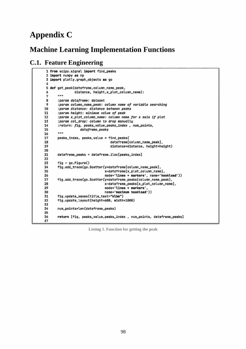
98

Appendix C

Machine Learning Implementation Functions

C.1. Feature Engineering

Listing 1. Function for getting the peak

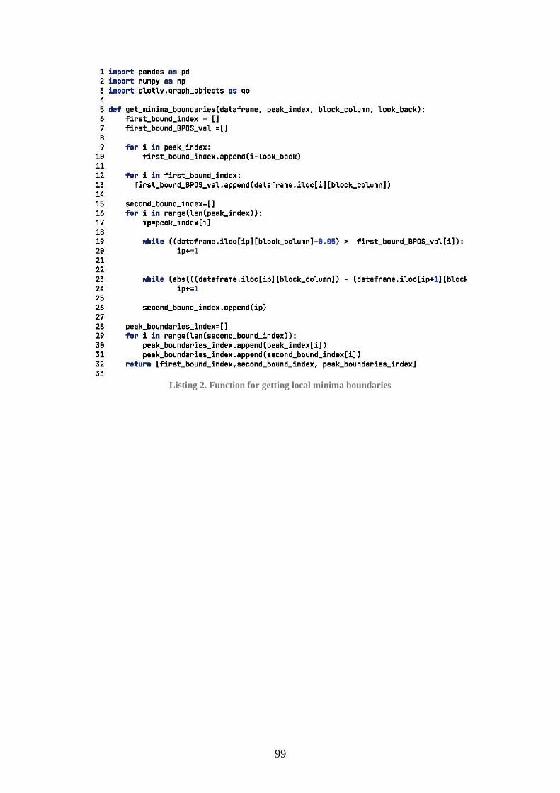
99

Listing 2. Function for getting local minima boundaries

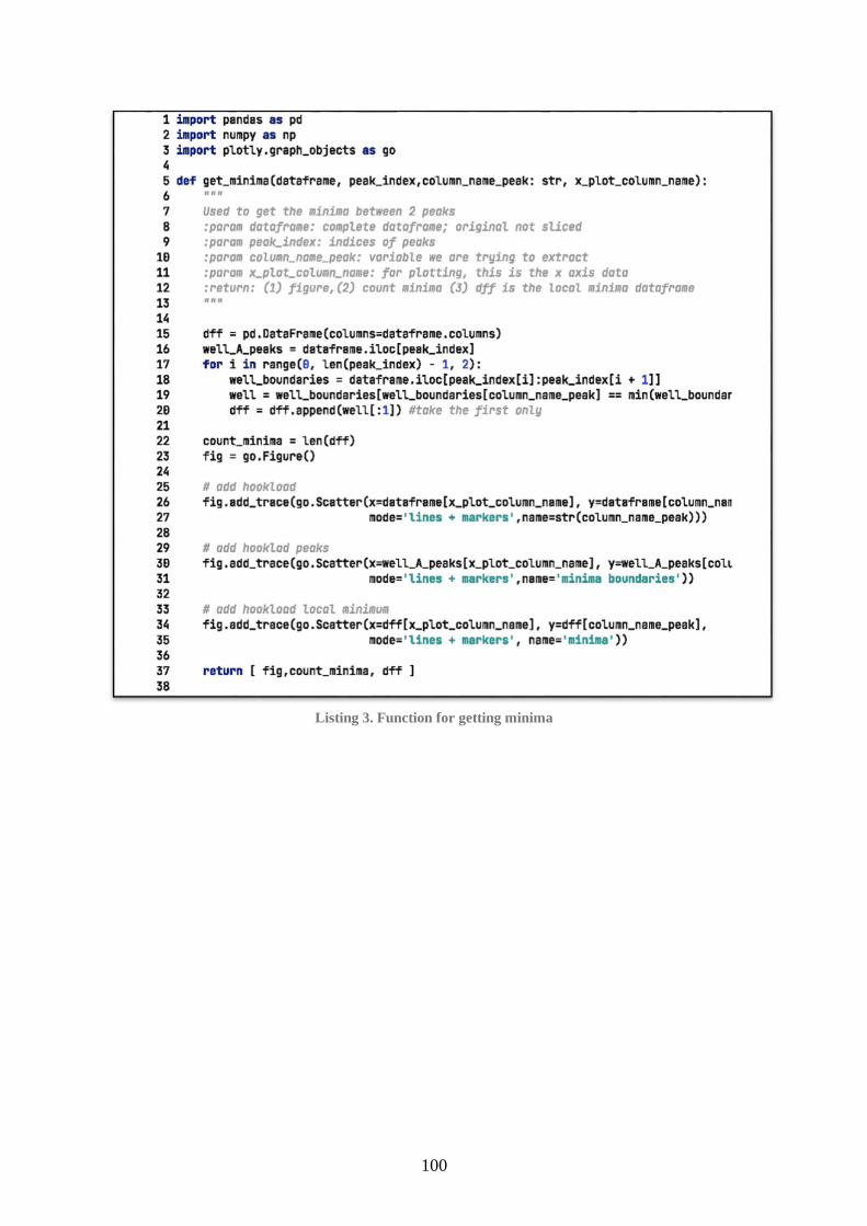
100

Listing 3. Function for getting minima

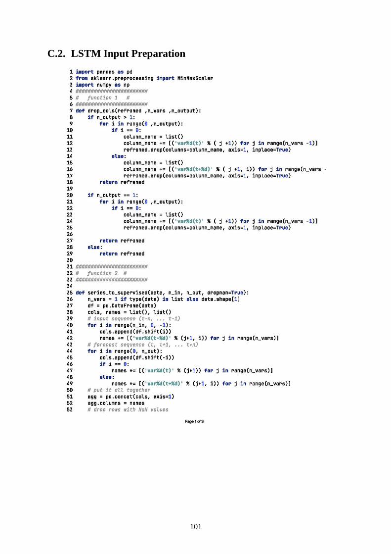
101

C.2. LSTM Input Preparation

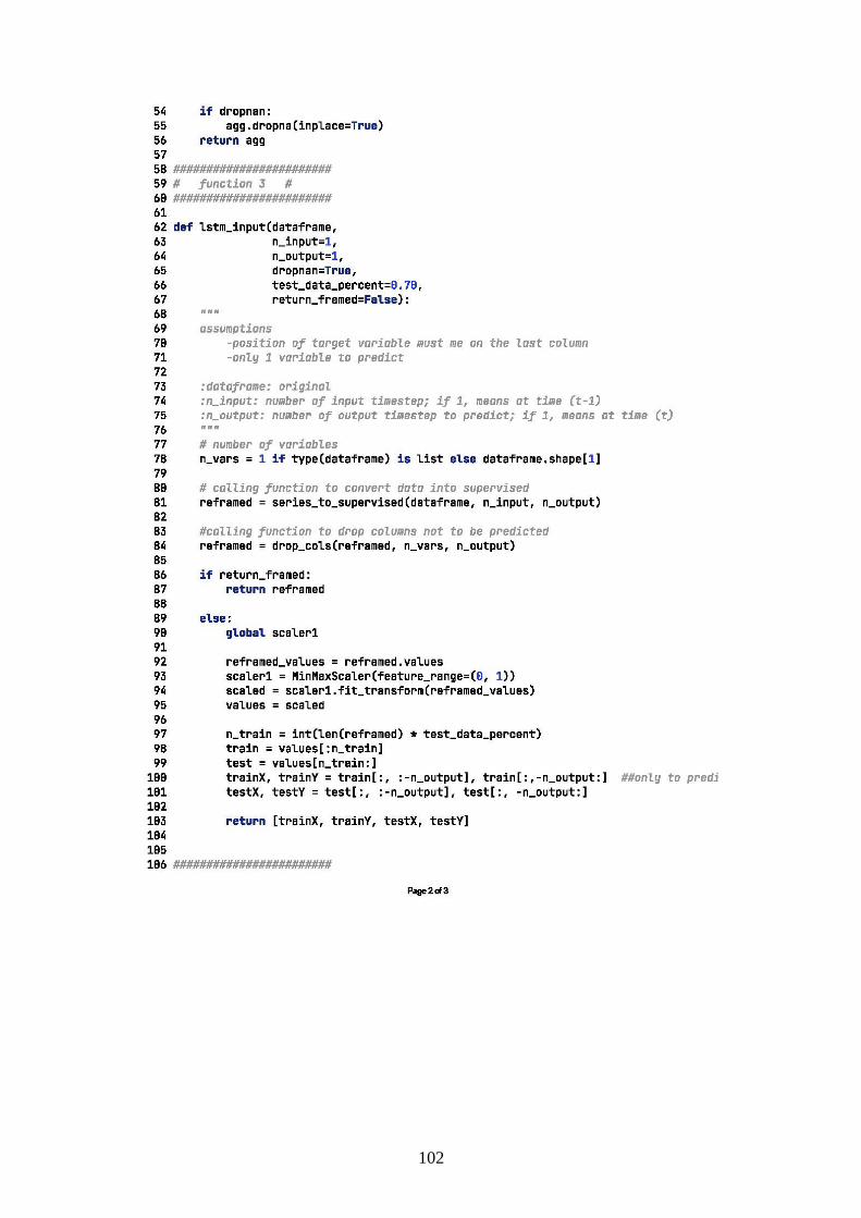
102

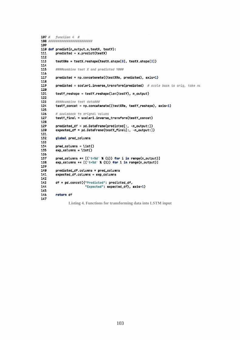
103

Listing 4. Functions for transforming data into LSTM input

104

C.3. LSTM model training

105

Listing 5. Convenience function for training LSTM model

106

C.4. LSTM model Predict

Listing 6. Function to use the trained LSTM model

107

C.5. Mean Absolute Error

Listing 7. Function for finding the mean absolute error and DataFrame containing the difference between

expected and predicted values

C.6. Residual Error Distribution

Listing 8. Function returns residual error distribution histogram

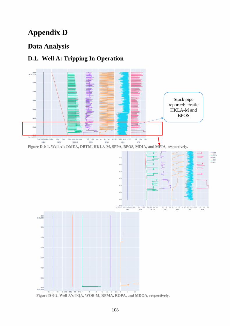
108

Figure D-0-2. Well A’s TQA, WOB-M, RPMA, ROPA, and MDOA, respectively.

Appendix D

Data Analysis

D.1. Well A: Tripping In Operation

Figure D-0-1. Well A’s DMEA, DBTM, HKLA-M, SPPA, BPOS, MDIA, and MFIA, respectively.

Stuck pipe

reported: erratic

HKLA-M and

BPOS

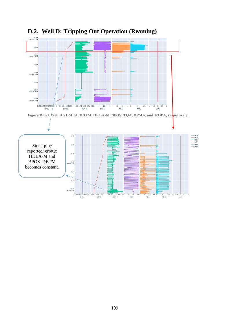
109

D.2. Well D: Tripping Out Operation (Reaming)

Figure D-0-3. Well D’s DMEA, DBTM, HKLA-M, BPOS, TQA, RPMA, and ROPA, respectively.

Stuck pipe

reported: erratic

HKLA-M and

BPOS. DBTM

becomes constant.

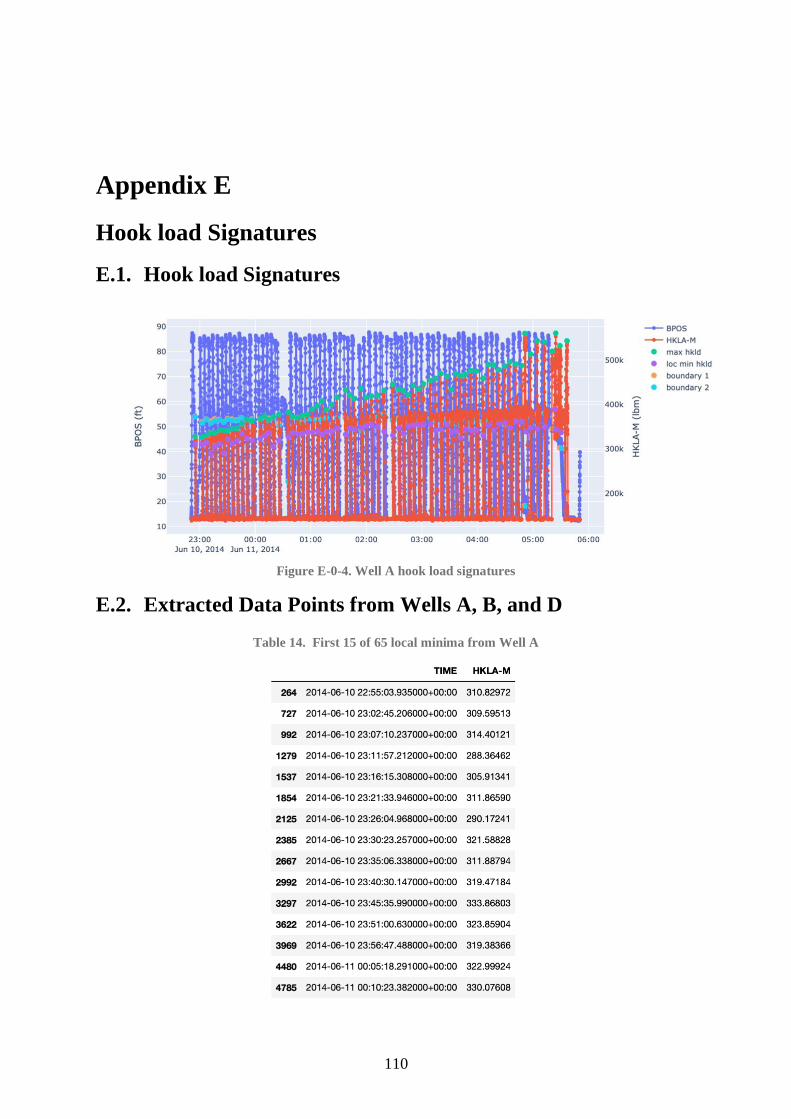
110

Appendix E

Hook load Signatures

E.1. Hook load Signatures

Figure E-0-4. Well A hook load signatures

E.2. Extracted Data Points from Wells A, B, and D

Table 14. First 15 of 65 local minima from Well A

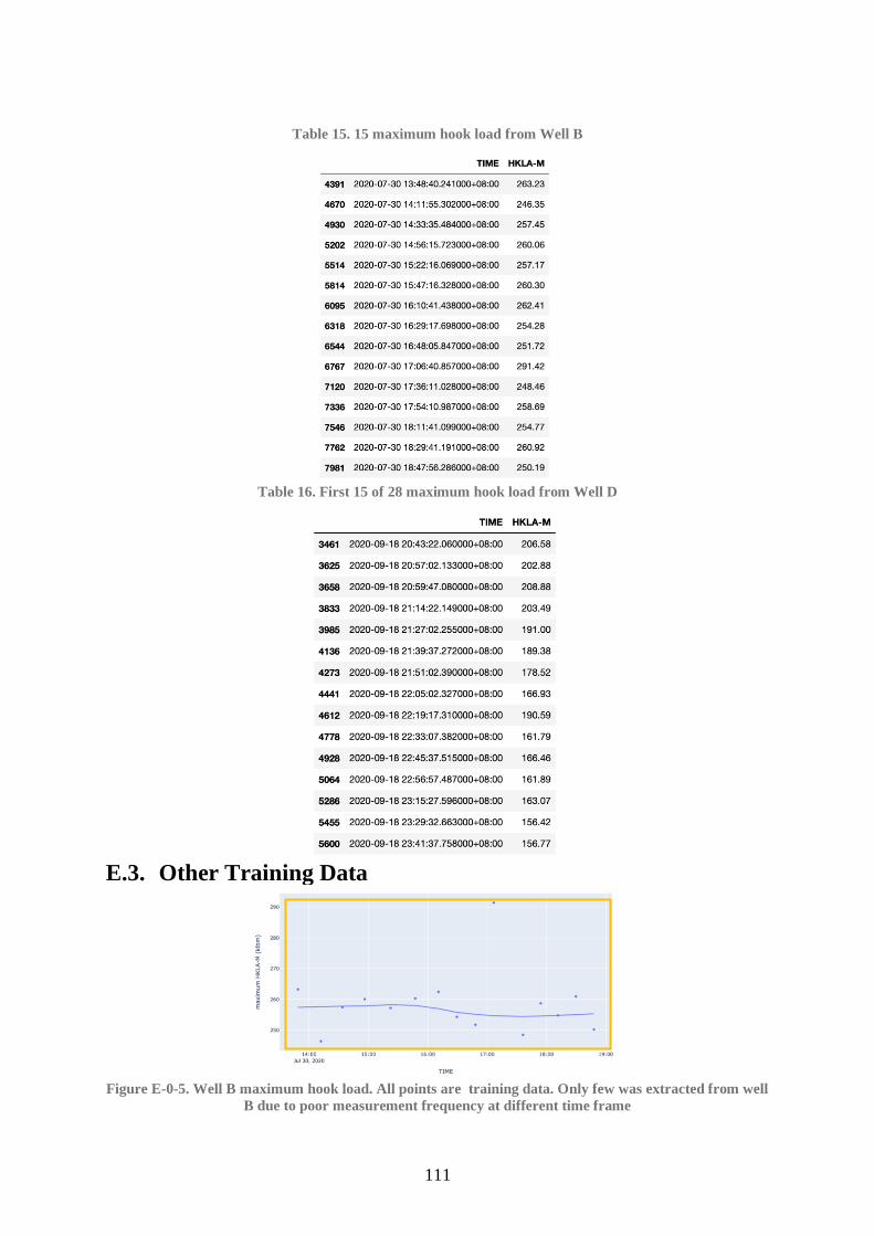
111

Table 15. 15 maximum hook load from Well B

Table 16. First 15 of 28 maximum hook load from Well D

E.3. Other Training Data

Figure E-0-5. Well B maximum hook load. All points are training data. Only few was extracted from well

B due to poor measurement frequency at different time frame

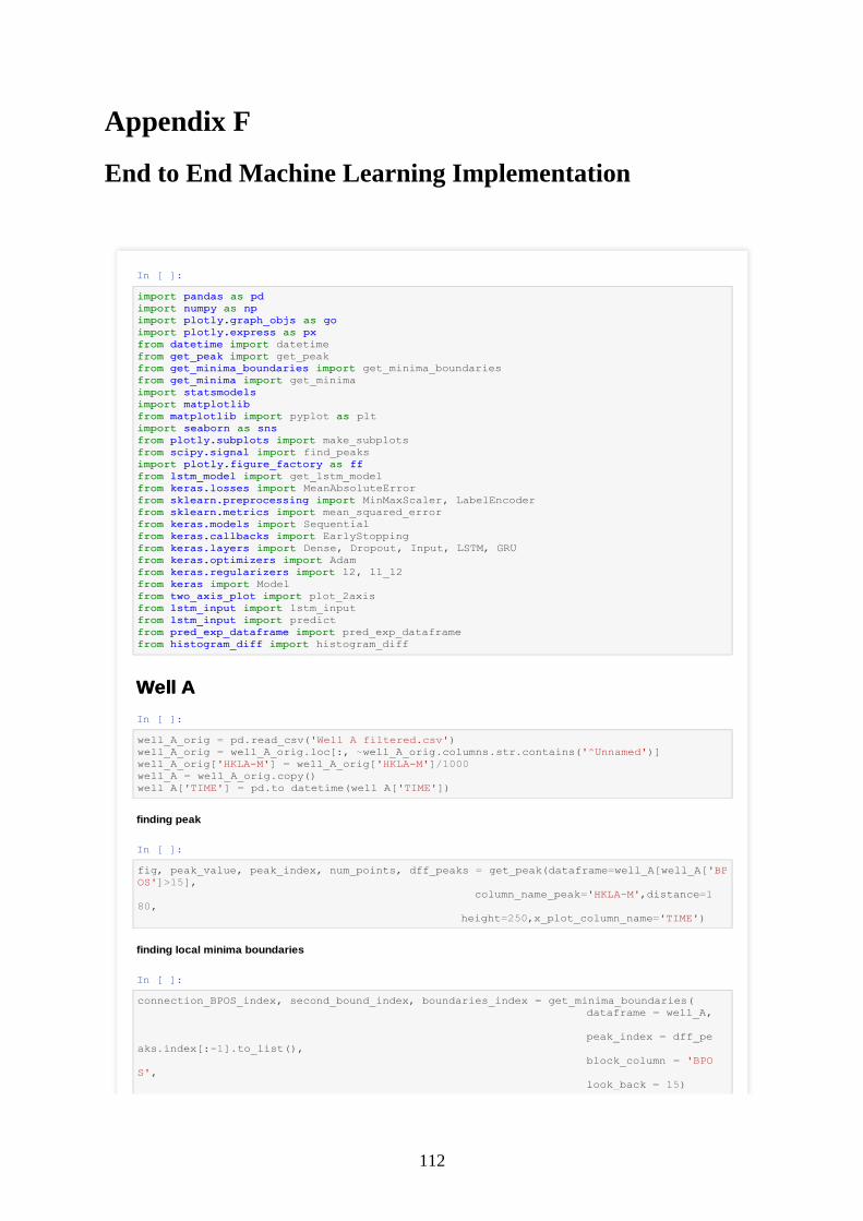
112

Appendix F

End to End Machine Learning Implementation

In [ ]:

importimport pandaspandas asas pdpd

importimport numpynumpy asas npnp

importimport plotly.graph_objsplotly.graph_objs asas gogo

importimport plotly.expressplotly.express asas pxpx

fromfrom datetimedatetime importimport datetime

fromfrom get_peakget_peak importimport get_peak

fromfrom get_minima_boundariesget_minima_boundaries importimport get_minima_boundaries

fromfrom get_minimaget_minima importimport get_minima

importimport statsmodelsstatsmodels

importimport matplotlibmatplotlib

fromfrom matplotlibmatplotlib importimport pyplot asas plt

importimport seabornseaborn asas snssns

fromfrom plotly.subplotsplotly.subplots importimport make_subplots

fromfrom scipy.signalscipy.signal importimport find_peaks

importimport plotly.figure_factoryplotly.figure_factory asas ffff

fromfrom lstm_modellstm_model importimport get_lstm_model

fromfrom keras.losseskeras.losses importimport MeanAbsoluteError

fromfrom sklearn.preprocessingsklearn.preprocessing importimport MinMaxScaler, LabelEncoder

fromfrom sklearn.metricssklearn.metrics importimport mean_squared_error

fromfrom keras.modelskeras.models importimport Sequential

fromfrom keras.callbackskeras.callbacks importimport EarlyStopping

fromfrom keras.layerskeras.layers importimport Dense, Dropout, Input, LSTM, GRU

fromfrom keras.optimizerskeras.optimizers importimport Adam

fromfrom keras.regularizerskeras.regularizers importimport l2, l1_l2

fromfrom keraskeras importimport Model

fromfrom two_axis_plottwo_axis_plot importimport plot_2axis

fromfrom lstm_inputlstm_input importimport lstm_input

fromfrom lstm_inputlstm_input importimport predict

fromfrom pred_exp_dataframepred_exp_dataframe importimport pred_exp_dataframe

fromfrom histogram_diffhistogram_diff importimport histogram_diff

Well AWell A

In [ ]:

well_A_orig = pd.read_csv('Well A filtered.csv')

well_A_orig = well_A_orig.loc[:, ~well_A_orig.columns.str.contains('^Unnamed')]

well_A_orig['HKLA-M'] = well_A_orig['HKLA-M']/1000

well_A = well_A_orig.copy()

well_A['TIME'] = pd.to_datetime(well_A['TIME'])

finding peak

In [ ]:

fig, peak_value, peak_index, num_points, dff_peaks = get_peak(dataframe=well_A[well_A['BP

OS']>15],

column_name_peak='HKLA-M',distance=1

80,

height=250,x_plot_column_name='TIME')

finding local minima boundaries

In [ ]:

connection_BPOS_index, second_bound_index, boundaries_index = get_minima_boundaries(

dataframe = well_A,

peak_index = dff_pe

aks.index[:-1].to_list(),

block_column = 'BPO

S',

look_back = 15)

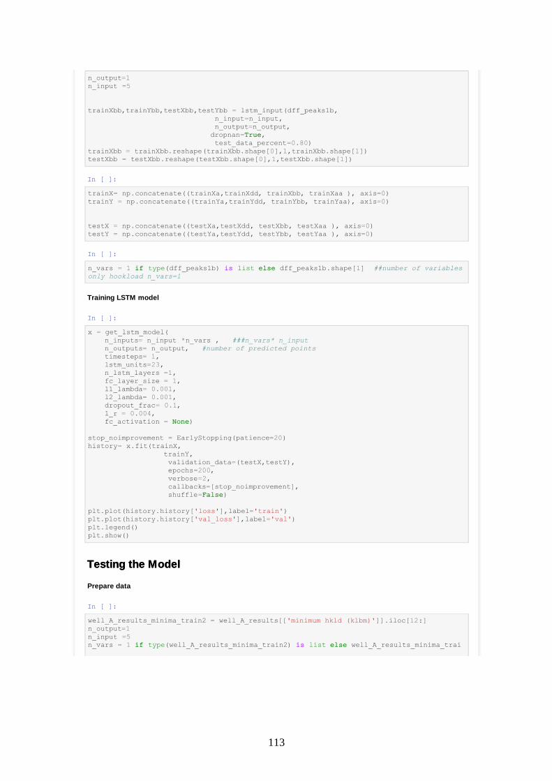
113

n_output=1

n_input =5

trainXbb,trainYbb,testXbb,testYbb = lstm_input(dff_peaks1b,

n_input=n_input,

n_output=n_output,

dropnan=TrueTrue,

test_data_percent=0.80)

trainXbb = trainXbb.reshape(trainXbb.shape[0],1,trainXbb.shape[1])

testXbb = testXbb.reshape(testXbb.shape[0],1,testXbb.shape[1])

In [ ]:

trainX= np.concatenate((trainXa,trainXdd, trainXbb, trainXaa ), axis=0)

trainY = np.concatenate((trainYa,trainYdd, trainYbb, trainYaa), axis=0)

testX = np.concatenate((testXa,testXdd, testXbb, testXaa ), axis=0)

testY = np.concatenate((testYa,testYdd, testYbb, testYaa ), axis=0)

In [ ]:

n_vars = 1 ifif type(dff_peaks1b) isis list elseelse dff_peaks1b.shape[1] ##number of variables

only hookload n_vars=1

Training LSTM model

In [ ]:

x = get_lstm_model(

n_inputs= n_input *n_vars , ###n_vars* n_input

n_outputs= n_output, #number of predicted points

timesteps= 1,

lstm_units=23,

n_lstm_layers =1,

fc_layer_size = 1,

l1_lambda= 0.001,

l2_lambda= 0.001,

dropout_frac= 0.1,

l_r = 0.004,

fc_activation = NoneNone)

stop_noimprovement = EarlyStopping(patience=20)

history= x.fit(trainX,

trainY,

validation_data=(testX,testY),

epochs=200,

verbose=2,

callbacks=[stop_noimprovement],

shuffle=FalseFalse)

plt.plot(history.history['loss'],label='train')

plt.plot(history.history['val_loss'],label='val')

plt.legend()

plt.show()

Testing the ModelTesting the Model

Prepare data

In [ ]:

well_A_results_minima_train2 = well_A_results[['minimum hkld (klbm)']].iloc[12:]

n_output=1

n_input =5

n_vars = 1 ifif type(well_A_results_minima_train2) isis list elseelse well_A_results_minima_trai

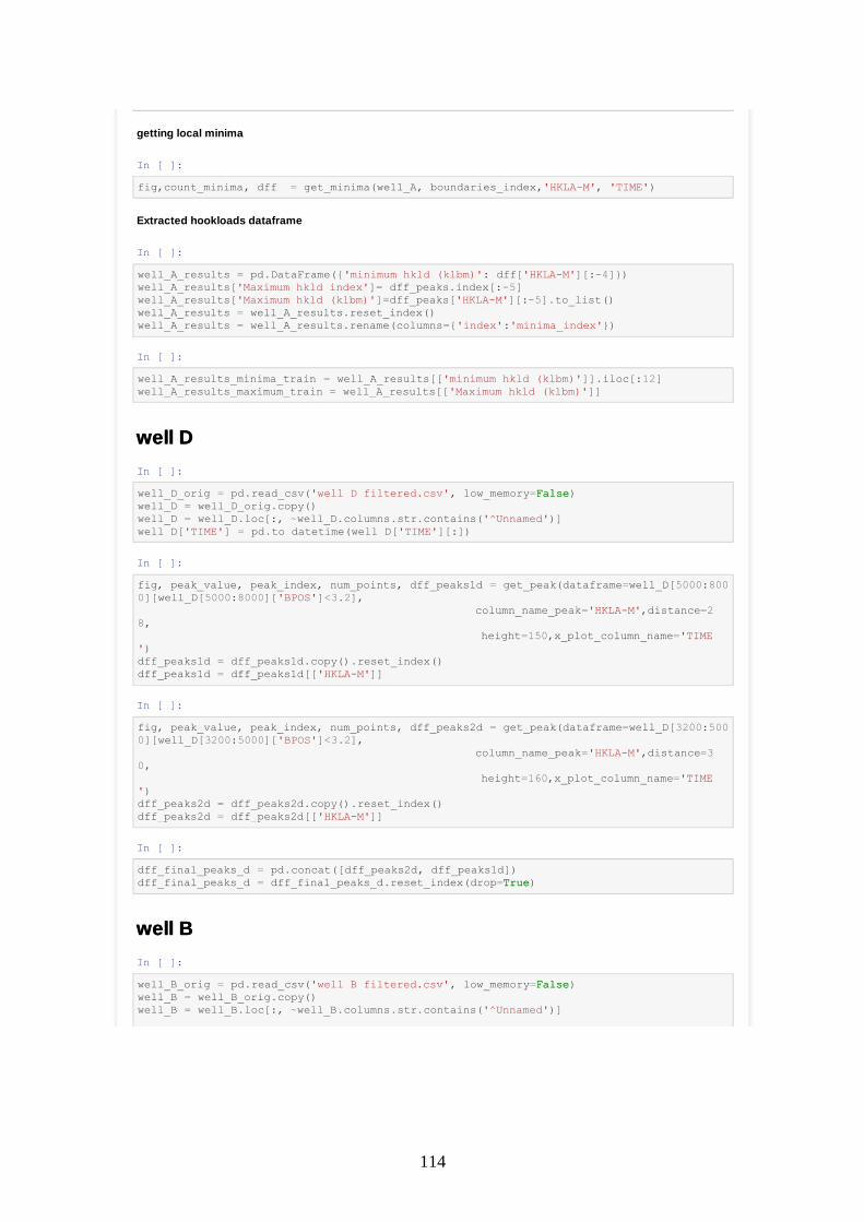
114

getting local minima

In [ ]:

fig,count_minima, dff = get_minima(well_A, boundaries_index,'HKLA-M', 'TIME')

Extracted hookloads dataframe

In [ ]:

well_A_results = pd.DataFrame({'minimum hkld (klbm)': dff['HKLA-M'][:-4]})

well_A_results['Maximum hkld index']= dff_peaks.index[:-5]

well_A_results['Maximum hkld (klbm)']=dff_peaks['HKLA-M'][:-5].to_list()

well_A_results = well_A_results.reset_index()

well_A_results = well_A_results.rename(columns={'index':'minima_index'})

In [ ]:

well_A_results_minima_train = well_A_results[['minimum hkld (klbm)']].iloc[:12]

well_A_results_maximum_train = well_A_results[['Maximum hkld (klbm)']]

well Dwell D

In [ ]:

well_D_orig = pd.read_csv('well D filtered.csv', low_memory=FalseFalse)

well_D = well_D_orig.copy()

well_D = well_D.loc[:, ~well_D.columns.str.contains('^Unnamed')]

well_D['TIME'] = pd.to_datetime(well_D['TIME'][:])

In [ ]:

fig, peak_value, peak_index, num_points, dff_peaks1d = get_peak(dataframe=well_D[5000:800

0][well_D[5000:8000]['BPOS']<3.2],

column_name_peak='HKLA-M',distance=2

8,

height=150,x_plot_column_name='TIME

')

dff_peaks1d = dff_peaks1d.copy().reset_index()

dff_peaks1d = dff_peaks1d[['HKLA-M']]

In [ ]:

fig, peak_value, peak_index, num_points, dff_peaks2d = get_peak(dataframe=well_D[3200:500

0][well_D[3200:5000]['BPOS']<3.2],

column_name_peak='HKLA-M',distance=3

0,

height=160,x_plot_column_name='TIME

')

dff_peaks2d = dff_peaks2d.copy().reset_index()

dff_peaks2d = dff_peaks2d[['HKLA-M']]

In [ ]:

dff_final_peaks_d = pd.concat([dff_peaks2d, dff_peaks1d])

dff_final_peaks_d = dff_final_peaks_d.reset_index(drop=TrueTrue)

well Bwell B

In [ ]:

well_B_orig = pd.read_csv('well B filtered.csv', low_memory=FalseFalse)

well_B = well_B_orig.copy()

well_B = well_B.loc[:, ~well_B.columns.str.contains('^Unnamed')]

115

well_B['TIME'] = pd.to_datetime(well_B['TIME'][:])

In [ ]:

well_try = well_B[4000:8000]

fig, peak_value, peak_index, num_points, dff_peaks1b = get_peak(dataframe=well_try[well_t

ry['BPOS']<4.2],

column_name_peak='HKLA-M',distance=6

0,

height=220,x_plot_column_name='TIME

')

dff_peaks1b = dff_peaks1b.copy().reset_index()

dff_peaks1b = dff_peaks1b[['HKLA-M']]

combine data for ML trainingcombine data for ML training

Training data from Well A local minima

In [ ]:

n_output=1

n_input =5

trainXa,trainYa,testXa,testYa = lstm_input(well_A_results_minima_train,

n_input=n_input,

n_output=n_output,

dropnan=TrueTrue,

test_data_percent=0.80)

print(trainXa.shape,trainYa.shape,testXa.shape,testYa.shape)

trainXa = trainXa.reshape(trainXa.shape[0],1,trainXa.shape[1])

testXa = testXa.reshape(testXa.shape[0],1,testXa.shape[1])

Training data from Well D maxima

In [ ]:

n_output=1

n_input =5

trainXdd,trainYdd,testXdd,testYdd = lstm_input(dff_final_peaks_d,

n_input=n_input,

n_output=n_output,

dropnan=TrueTrue,

test_data_percent=0.80)

trainXdd = trainXdd.reshape(trainXdd.shape[0],1,trainXdd.shape[1])

testXdd = testXdd.reshape(testXdd.shape[0],1,testXdd.shape[1])

Training data from Well B maxima

In [ ]:

n_output=1

n_input =5

trainXbb,trainYbb,testXbb,testYbb = lstm_input(dff_peaks1b,

n_input=n_input,

n_output=n_output,

dropnan=TrueTrue,

test_data_percent=0.80)

trainXbb = trainXbb.reshape(trainXbb.shape[0],1,trainXbb.shape[1])

testXbb = testXbb.reshape(testXbb.shape[0],1,testXbb.shape[1])

In [ ]:

trainX= np.concatenate((trainXa,trainXdd, trainXbb), axis=0)

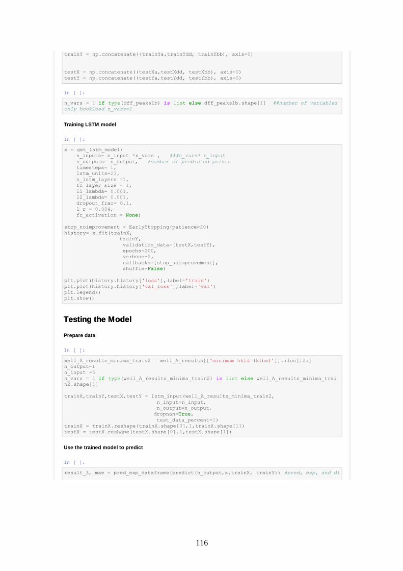
116

trainY = np.concatenate((trainYa,trainYdd, trainYbb), axis=0)

testX = np.concatenate((testXa,testXdd, testXbb), axis=0)

testY = np.concatenate((testYa,testYdd, testYbb), axis=0)

In [ ]:

n_vars = 1 ifif type(dff_peaks1b) isis list elseelse dff_peaks1b.shape[1] ##number of variables

only hookload n_vars=1

Training LSTM model

In [ ]:

x = get_lstm_model(

n_inputs= n_input *n_vars , ###n_vars* n_input

n_outputs= n_output, #number of predicted points

timesteps= 1,

lstm_units=23,

n_lstm_layers =1,

fc_layer_size = 1,

l1_lambda= 0.001,

l2_lambda= 0.001,

dropout_frac= 0.1,

l_r = 0.004,

fc_activation = NoneNone)

stop_noimprovement = EarlyStopping(patience=20)

history= x.fit(trainX,

trainY,

validation_data=(testX,testY),

epochs=200,

verbose=2,

callbacks=[stop_noimprovement],

shuffle=FalseFalse)

plt.plot(history.history['loss'],label='train')

plt.plot(history.history['val_loss'],label='val')

plt.legend()

plt.show()

Testing the ModelTesting the Model

Prepare data

In [ ]:

well_A_results_minima_train2 = well_A_results[['minimum hkld (klbm)']].iloc[12:]

n_output=1

n_input =5

n_vars = 1 ifif type(well_A_results_minima_train2) isis list elseelse well_A_results_minima_trai

n2.shape[1]

trainX,trainY,testX,testY = lstm_input(well_A_results_minima_train2,

n_input=n_input,

n_output=n_output,

dropnan=TrueTrue,

test_data_percent=1)

trainX = trainX.reshape(trainX.shape[0],1,trainX.shape[1])

testX = testX.reshape(testX.shape[0],1,testX.shape[1])

Use the trained model to predict

In [ ]:

result_3, mae = pred_exp_dataframe(predict(n_output,x,trainX, trainY)) #pred, exp, and di

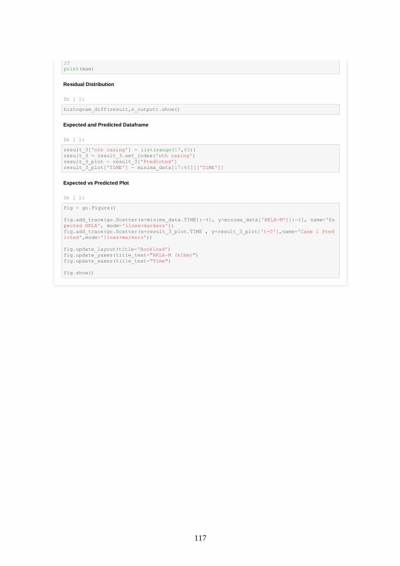
117

ff

print(mae)

Residual Distribution

In [ ]:

histogram_diff(result,n_output).show()

Expected and Predicted Dataframe

In [ ]:

result_3['nth casing'] = list(range(17,65))

result_3 = result_3.set_index('nth casing')

result_3_plot = result_3['Predicted']

result_3_plot['TIME'] = minima_data[17:65][['TIME']]

Expected vs Predicted Plot

In [ ]:

fig = go.Figure()

fig.add_trace(go.Scatter(x=minima_data.TIME[:-4], y=minima_data['HKLA-M'][:-4], name='Ex

pected HKLA', mode='lines+markers'))

fig.add_trace(go.Scatter(x=result_3_plot.TIME , y=result_3_plot['t+0'],name='Case 1 Pred

icted',mode='lines+markers'))

fig.update_layout(title='Hookload')

fig.update_yaxes(title_text="HKLA-M (klbm)")

fig.update_xaxes(title_text="Time")

fig.show()

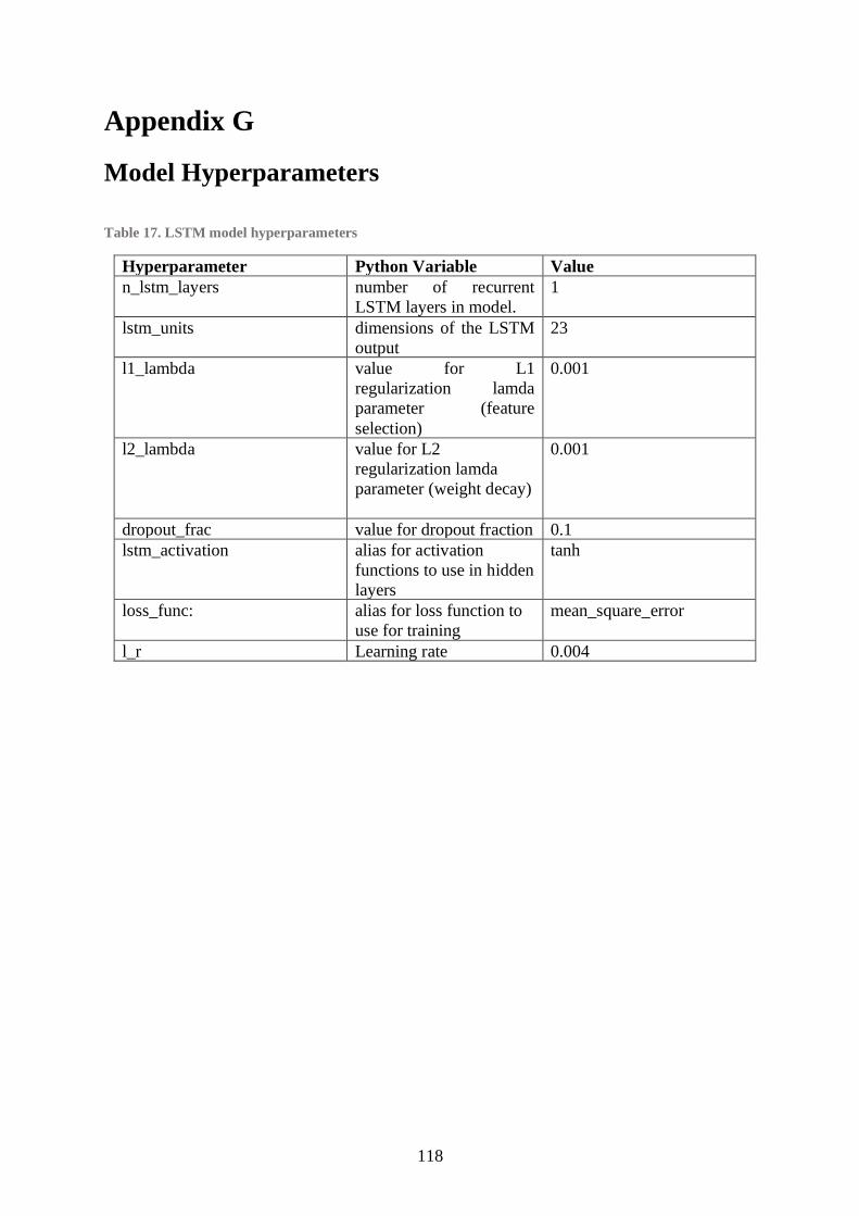
118

Appendix G

Model Hyperparameters

Table 17. LSTM model hyperparameters

Hyperparameter Python Variable Value

n_lstm_layers number of recurrent

LSTM layers in model.

1

lstm_units dimensions of the LSTM

output

23

l1_lambda value for L1

regularization lamda

parameter (feature

selection)

0.001

l2_lambda value for L2

regularization lamda

parameter (weight decay)

0.001

dropout_frac value for dropout fraction 0.1

lstm_activation alias for activation

functions to use in hidden

layers

tanh

loss_func: alias for loss function to

use for training

mean_square_error

l_r Learning rate 0.004