I am grateful to Professor Dirk Schindler for his constant support and guidance in writing this master’s thesis. Remaining errors are mine. Abstract Multinational corporations can reduce their groupwide tax liability by shifting internal debt from affiliates in low-tax countries to affiliates in high-tax countries. To counter such tax avoidance schemes many countries have implemented thin-capitalization rules over the past two decades. Contradictory to this trend, the Netherlands abolished its safe-harbor thin- capitalization rules at the start of 2013. This paper analyses the effect of this abolishment on the capital structure of Dutch affiliates of multinational corporations. The empirical analyses find that these affiliates increased their debt-to-equity ratio by 12% to 20% after the abolishment, on average. This paper is, to my knowledge, the first to include headquarters- country gravity variables in thin-capitalization research. The effects are mostly insignificant, except when headquarters located in tax-havens are excluded. Keywords: Thin-capitalization; Safe-harbor rules, Internal debt shifting JEL classification: G32, G38, H26 ERASMUS UNITVERSITY ROTTERDAM Erasmus School of Economics Master’s Thesis International Economics Abolishment of Safe-Harbor Rules and the Effect on Multinationals’ Capital Structure Name student: Gerardus Cas van Lambalgen Student ID number: 582722 Supervisor: Professor Dirk Schindler Second assessor: Professor Aksel Erbahar Date draft version: 23-09-2021

Welcome message from author
This document is posted to help you gain knowledge. Please leave a comment to let me know what you think about it! Share it to your friends and learn new things together.
Transcript

I am grateful to Professor Dirk Schindler for his constant support and guidance in writing this master’s thesis. Remaining errors are mine.
Abstract
Multinational corporations can reduce their groupwide tax liability by shifting internal
debt from affiliates in low-tax countries to affiliates in high-tax countries. To counter such tax
avoidance schemes many countries have implemented thin-capitalization rules over the past
two decades. Contradictory to this trend, the Netherlands abolished its safe-harbor thin-
capitalization rules at the start of 2013. This paper analyses the effect of this abolishment on
the capital structure of Dutch affiliates of multinational corporations. The empirical analyses
find that these affiliates increased their debt-to-equity ratio by 12% to 20% after the
abolishment, on average. This paper is, to my knowledge, the first to include headquarters-
country gravity variables in thin-capitalization research. The effects are mostly insignificant,
except when headquarters located in tax-havens are excluded.
Keywords: Thin-capitalization; Safe-harbor rules, Internal debt shifting
JEL classification: G32, G38, H26
ERASMUS UNITVERSITY ROTTERDAM
Erasmus School of Economics
Master’s Thesis International Economics
Abolishment of Safe-Harbor Rules and the Effect on Multinationals’ Capital
Structure
Name student: Gerardus Cas van Lambalgen
Student ID number: 582722
Supervisor: Professor Dirk Schindler
Second assessor: Professor Aksel Erbahar
Date draft version: 23-09-2021
2
1. Introduction
Over the past two decades, the thin capitalization of firms, tax sensitivity of debt, and internal
debt-shifting by multinational companies (henceforth MNCs), have received massive attention
from economic literature as well as from policymakers. The reason for this attention is that
the corporate income tax system contains a bias in the favor of debt. The interest expenses
paid on debt are tax-deductible for corporations, while dividends are paid out of the net-of-
tax corporate income. Thus, the corporate income tax system incentivizes firms to have higher
debt ratios (de Mooij, 2011). MNCs can capitalize on the tax benefits of debt more aggressively
than domestic firms by shifting both external as well as internal debt to increase their debt
tax shield (Møen et al., 2019).
MNCs have two comparative advantages over domestic firms when it comes to debt-
shifting. Firstly, by using excessive external debt in affiliates that are located in high-tax
countries and less in low-tax country affiliates, the MNC increases the tax benefits of interest
payments, while the group-wide amount of external debt stays equal. The second
comparative advantage that MNCs have in terms of the debt-tax shield, is the usage of internal
debt. By setting up a financial centre in a low-tax country (often a tax haven) and shifting
internal debt to affiliates in high-tax countries the MNC creates an internal debt tax shield.
The tax benefits of the interest payments on the internal debt in the high tax country are larger
than the tax payments on received interest payments in the financial centre (Ruf and
Schindler, 2015; Schindler and Schjelderup, 2012), thus creating an internal debt tax shield.
These theoretical predictions are supported by many empirical papers (Mintz and Smart,
2004; Büttner et al., 2009; Büttner and Wamser, 2013; Møen et al., 2019). These results
suggest that countries with high tax rates attract a reasonable amount of tax-deductible
interest costs (Weichenrieder and Windischbauer, 2008).
Excessive amounts of group-wide external debt lead to excessive bankruptcy costs and
risks, but internal debt suffers less from such costs. Non-regulated internal debt can therefore
create extreme tax benefits as long as there is a positive taxable income (Ruf and Schindler,
2015). Over the past two decades, most countries have implemented thin-capitalization rules
to counter excessive tax-driven internal debt financing. The implementation of such thin
capitalization rules is encouraged by the OECD (2013) in their Base Erosion and Profit Shifting
(BEPS) action plan. Thin-capitalization rules exist in two forms: safe-harbor rules and earnings

3
stripping rules (Ruf and Schindler, 2015). This paper will focus on the safe-harbor thin
capitalization rules. Safe-harbor rules restrict the tax deductibility of excessive (internal) debt.
Safe-harbor rules have a certain threshold level of (internal) debt-to-equity after which a
higher ratio does not reap more tax deductions from interest paid on debt (binding rules) or
after which it is costly to reap those tax deductions. (rules with leeway) (Gresik et al, 2017).
Over the past decades, many countries have felt the need to counter the increasingly
aggressive profit shifting by MNCs. As a response, many countries have implemented or
tightened their thin-capitalization rules since 2000 (Haufler et al., 2018). Contradictory to
these countries, the Netherlands abolished its safe-harbor rules (3:1 internal debt-to-equity
ratio) in 2013 (de Brauw Blackstone Westbroek, 2013), which allows for an interesting
empirical analysis. This abolishment and its consequences on the debt-to-equity ratio of Dutch
affiliates of MNCs are central in this paper.
This paper uses a theoretical model to predict the tax-efficient capital structure of
affiliates of MNCs. The model is based on the theoretical model provided by Møen et al. (2019)
with some slight simplifications. This paper’s model includes the expected effects of the
abolishment of the Dutch 3:1 safe-harbor rules with leeway. The most important and new
insight provided by the model is the expected increase in the internal debt-to-equity ratio for
Dutch affiliates of MNCs after the abolishment. The cost of using internal debt to profit from
the internal debt-tax shield above the 3:1 ratio drops significantly after the abolishment. The
model, therefore, predicts that MNCs increase the internal debt-to-equity ratio in their Dutch
affiliates in/after 2013.
A micro-level data sample from the Orbis database is utilized to put the model and its
predictions to the test. The data sample contains information on Dutch affiliates of MNCs and
domestic Dutch firms. The dataset only contains information on the total debt and does not
show internal or external debt separately. The empirical specification is adjusted to deal with
this issue but does not capture the effect on the internal debt-to-equity ratio fully. The main
sample includes 687 firms over a six-year period, adding up to 4122 observations. Of the 687
firms, 324 are the Dutch affiliate of an MNC, the remaining 363 firms are domestic Dutch firms.
As a robustness test, a smaller sample of the 300 largest firms is used to increase the accuracy
of the firm-level data.
The theoretical predictions from the model are supported by the empirical analysis.
The identification strategy interacts an MNC dummy with a Post-2012 dummy to examine the

4
effect of the abolishment on the debt-to-equity ratio of Dutch affiliates of MNCs in a panel
dataset. Several variables that are deemed as important capital structure predictors in the
finance literature are included to control for cross-firm differences. Headquarter-country
variables are included to control for country differences. Lastly, vectors of time and industry
fixed effects are embedded in the model to control for unobservable effects. Despite having
to use the total debt-to-equity ratio instead of the internal debt-to-equity ratio the result is
consistent with the prediction. The effect of the abolishment of the safe-harbor rule on the
debt-to-equity ratio of Dutch affiliates of MNCs is significant at the 1% level and has a value of
0.253. This means that the affiliates of the MNCs increased their debt-to-equity ratio by 0.253
after the abolishment of the safe-harbor rules. With a mean debt-to-equity ratio of roughly
1.383, this is an increase of 19.5%.
The result is consistent throughout most of the robustness checks. The model that uses
a one-year lagged period to consider capital adjustment time finds an insignificant effect in
the large sample, but still a significant effect at the 1% level in the small sample. The model
that uses the debt-to-asset ratio as the dependent variable finds insignificant effects as well.
All other robustness checks find an effect that is significant at the 1% level and in the range of
0.188 and 0.353 in the small and large samples. This is considered to be a constant result.
An additional contribution of this paper to the research in corporate debt-shifting is
the inclusion of headquarters-country (gravity) variables. The inclusion is inspired by the
inclusion of gravity variables to predict trade in financial assets (Martin and Rey, 2004; Portes
and Rey, 2000; Portes et al, 2001). Orbis provides the location of the headquarters of the MNC
of which the Dutch affiliate is a part. The log of the GDP of the country where this headquarters
is located is included in the empirical analysis. The log of the distance from the country where
the headquarters is located to the Netherlands is included, as well as the log of the import
flow from that country to the Netherlands. The logs of GDP and imports are expected to have
a positive effect on the debt-to-equity ratio since it should decrease information asymmetries
between the two countries. The opposite applies to the log of distance, which also increases
travel and communication costs.
The main results regarding the headquarters-country variables are counter-intuitive.
Where the logs of distance and imports are insignificant, the log of GDP is significant at the
1% level but has a coefficient of -0.226 which contradicts expectations. A possible explanation
for this could be the large number of headquarters located on a tax haven with low imports

5
and a low GDP. To verify this a robustness check is performed by excluding the Dutch affiliates
of MNCs of which the headquarters is located in a tax haven. The logs of distance and imports
become significant at the 1% level in both samples and have the expected negative and
positive signs, respectively. The log of GDP becomes insignificant in the large sample but stays
negative and significant at the 1% level in the small sample. This suggests that the log of GDP
of the country where the headquarters is located is negatively correlated with the debt-to-
equity ratio of Dutch affiliates of MNCs.
The remainder of this paper is organized as follows: Section 2 presents and summarizes
related literature. Section 3 defines and outlines the concept of thin-capitalization rules. The
theoretical model is explained in section 4. Section 5 highlights the data that is utilized, as well
as descriptive statistics, definitions, and the main variables. The empirical model is explained
in section 7. Section 7 presents the main results and section 8 the robustness checks. Section
9 provides a short discussion. Finally, section 10 provides the conclusion.
2. Related literature
There exists a large literature on the tax sensitivity of debt, debt shifting, and thin-
capitalization/safe-harbor rules. The tax sensitivity of debt usage has been confirmed by many
papers, theoretically as well as empirically. Mills and Newberry (2004) use a sample of U.S.
foreign-controlled corporations during 1987-1996. They find that the MNCs with a relatively
low average tax rate use more debt in their US foreign-controlled corporation than MNCs with
a relatively high average tax rate. This is due to the larger debt tax shield experienced by the
MNCs with a lower tax rate and supports their expectations regarding the tax sensitivity of
debt.
Desai et al. (2004) look at the effect of local tax rates on the composition and level of
borrowing by foreign affiliates of U.S. MNCs. Their dataset differentiates between external
borrowing and borrowing by foreign affiliates from the same parent company. By doing so
they control for parental fixed effects. As a result, they obtain clean estimates evaluating the
impact of tax rate differences on capital structure. Their study finds that a 10% rise in the local
tax rates leads to a 2.8% increase in the affiliate's debt-to-asset ratio. Furthermore, they find
that affiliates who operate in a country with underdeveloped capital markets borrow more
from their parent company. This reduces the overall interest rate faced and provides MNCs
with a comparative advantage over domestic firms.

6
Mintz and Smart (2004) create a model that explains internal debt shifting. Their
model suggests that MNCs should use internal debt to profit from the debt-tax shield.
Borrowing should be done in the affiliates that operate in high-tax jurisdictions so that the tax-
deductibility of interest expenses is the highest. The lending should be done in the affiliate
that faces the lowest tax rate so that the tax paid on interest income is the smallest. They use
Canadian firm-level data to test the predictions of their model. The firms in their data are all
domestic firms that normally are unable to profit from internal debt shifting. However, due to
the subnational corporate income system in Canada, there exist provincial differences in the
corporate tax rates. This system thus allows for internal debt shifting within a country and
provides an interesting study (Mintz and Smart, 2004). They estimate taxable income
elasticities with the standard log-linear specification and divide their sample into three groups
large corporations who shift income, large corporations who do not shift income, and small
corporations. Their study finds that the elasticity of taxable income with respect to tax rates
for income-shifting firms is 4.9, while this is 2.3 for non-shifting comparable firms. Büttner et
al. (2009) use the MiDi database of the German Bundesbank. Their sample includes foreign
affiliates of German MNCs in 26 countries from 1996 until 2003. They use an OLS regression
to estimate the impact of local tax rates on external and internal debt. The study's empirical
analysis confirms that MNCs use excessive external and internal debt in regions with a high
tax burden. Büttner and Wamser (2013) also use the MiDi database but extend the sample.
Their data covers foreign affiliates of German MNCs in 174 countries. They look at the role of
internal debt in shifting profits from one foreign affiliate of a German MNC to another foreign
affiliate of the same MNC. Their dependent variable, thus, is the amount of internal loans
received by one foreign affiliate from another foreign affiliate. They look at the effect of the
host country tax rate as well as the group-wide lowest available tax rate on the amount of
internal loans. Their study finds an implied tax-elasticity of reported profits of only 0.1% due
to profit shifting. Previous literature found estimates of 1.3% up to 2%. Büttner and Wamser
(2013) find that the small impact in their study is partly due to the German-controlled foreign
corporation (CFC) rule.
Møen et al. (2019) use a sample of 33,857 firm-year observations from the MiDi
database. Their sample includes 8191 foreign affiliates of 3660 German MNCs from 1996 to
2006. The study makes use of variation in tax rates over time and across countries to identify
the tax effect on the capital structure. Their estimation looks at the effect of the host country's
7
tax rate, the weighted tax difference with the corporate group, and the tax difference between
affiliate i and the lowest taxed affiliate on the total debt to asset ratio of affiliate i. The authors
find that MNCs use both internal and external debt to save taxes and that the usage of these
two is independent of each other. Most important for this research, they find that MNCs have
an advantage over domestic firms by shifting debt across borders to gain additional profits
from the debt tax shield.
de Mooij (2011) evaluates 267 estimates from 19 different studies in a meta-study. He
finds an average tax elasticity of debt of somewhere between 0.5 and 0.7. Feld et al. (2013)
include 1,143 estimates from 46 previous studies in their meta-study. They predict that the
marginal tax effect on the debt ratio is 0.30. Hence, if the marginal tax rate is increased by 10
percentage points, the debt-to-asset ratio would rise by 3 percentage points. This is in line
with the estimate from de Mooij (2011), who finds that the marginal tax effect on the debt
ratio is 0.17 in the narrow measures of debt and 0.28 in the broad measures of financial
leverage.
More in line with this paper is research that looks into the effects of thin-capitalization
rules on debt-shifting. Weichenrieder and Windischbauer (2008) use a panel from the MiDi
database that runs from 1996 to 2004. The sample includes 1699 German affiliates of foreign
MNCs. Their study tests the effect of the tightening of the German thin-capitalization rules in
2001 on corporations using a Diff-in-Diff specification. They use branches as a control group
since branches are unaffected by the German thin-capitalization rules. Both corporations and
branches are split into high- and low-leveraged groups. Lastly, they compare the effects of the
tightening on the affected corporations and unaffected branches. Their study finds that high-
leveraged corporations decreased their internal debt-to-equity ratio more than similarly
leveraged unaffected branches. The difference was significant at the 5% level, which shows
that the thin-capitalization rules were only somewhat effective. Weichenrieder and
Windischbauer (2008) attribute this to a loophole in the legislation. This loophole allowed
foreign MNCs to circumvent the German thin-capitalization rules.
Büttner et al. (2012) also use a panel from the MiDi database. Their sample runs from
1996 to 2004 and includes 42,950 firms. The study estimates the effects of foreign thin-
capitalization rules on the foreign affiliates of German MNCs. They estimate the effect of thin-
capitalization rules on internal debt by use of a dummy that measures the existence of thin-
capitalization rules in a country as well as a variable that measures the safe-harbor threshold

8
as tightness. The authors make use of the cross-country differences and time variation of the
existence/tightness of thin-capitalization rules. Their analysis finds that thin-capitalization
rules reduce the tax incentive to use internal debt. When a host country that has a tax rate of
34%, which is the sample average, implements a thin-capitalization rule that denies interest
deductions for internal debt exceeding an internal debt-to-equity ratio of 2:1, the ratio of
internal debt declines by 12%. If the thin-capitalization rule applies to total debt instead of
internal debt, the internal debt ratio is predicted to decline by 24% even.
This master thesis differs from the studies of Weichenrieder and Windischbauer (2008)
and Büttner et al. (2012) in multiple directions. First of all, this paper looks at the Dutch
affiliates of MNCs which is in line with Weichenrieder and Windischbauer (2008). However,
the identification strategy in this research is different. Weichenrieder and Windischbauer
(2008) make use of the difference between incorporated firms (affected by the TC rules) and
branches (unaffected by the TC rules), as well as the difference between firms above and
below the safe-haven threshold to compare the development of the debt-t-equity ratio of
corporations and branches. In contrast, this master study estimates the effect of the
abolishment of the thin-capitalization rules on the debt-to-equity ratio of Dutch affiliates of
MNCs by comparing the development of this ratio to Dutch domestic firms over the same
period. A similar identification set-up as in Weichenrieder and Windischbauer (2008) would
have been preferred in the research. However, due to data limitations from the Orbis
database, this master's thesis has employed a different identification strategy. Furthermore,
the research from Weichenrieder and Windischbauer (2008) suffers from the effects of a
loophole that biases their results, this loophole should not be present in this paper. Büttner
et al. (2012) look into foreign affiliates of German MNCs whereas this research looks into
Dutch affiliates of MNCs. Both previous pieces of research use the MiDi database with
information on German firms, whereas this research employs the Orbis database and the
information on Dutch firms over a more recent period. Moreover, Weichenrieder and
Windischbauer (2008) and Büttner et al. (2012) look at tightenings and emplacements of thin-
capitalization rules, whereas this study looks at the abolishment of such a rule. Lastly, this
paper will look into the effects of gravity measures on the debt-to-equity ratio of Dutch
affiliates of foreign MNCs. To the knowledge of the author, gravity variables have not yet been
incorporated into similar research before.

9
3. International tax-system and thin-capitalization rules
The idea behind the usage of debt to save tax payments is well known and stems from
the basic principle that interest payments on debt are tax-deductible, whereas costs of equity
are not. MNCs, as well as domestic firms, can profit from this by using excessive amounts of
external debt to finance investments. However, excessive amounts of debt go hand in hand
with excessive costs of debt, think of bankruptcy costs. For this reason, there is a limit to the
amount of external debt that a corporation can use effectively (Moen et al, 2019). MNCs profit
from the fact that they can use internal debt next to external debt and therefore shift their
debt more aggressively. The mechanism for internal debt shifting calls for an affiliate in a low-
tax country. This affiliate lends capital to one in a higher tax country. The interest income is
thus earned and taxed in a low-tax country while the tax deductions from interest payments
are larger in the high-tax country. This leads to an overall tax benefit for the MNC (Schindler
and Schjelderup, 2012). In general, governments aim to counter internal debt shifting by
imposing thin-capitalization rules that limit the deductibility of internal debt (Ruf and
Schindler, 2015).
Thin-capitalization rules exist in two main forms: earning-stripping rules and safe-
harbor rules. This paper focuses on the latter. Safe-harbor rules restrict the tax deductibility
of excessive debt by setting a certain threshold after which no more tax deductions for
interests paid on debt exists. The threshold is defined as a fixed debt-to-equity ratio (3:1 in
the Netherlands before 2013). This threshold can either be strictly binding or have leeway. If
the safe-harbor rule is strictly binding the tax-deductibility of debt after the threshold is zero.
If the safe-harbor rule has leeway to circumvent it, there is a possibility to profit from the tax-
deductibility of debt beyond the threshold, but this is costly. If the debt-to-equity ratio is
below the threshold, no restrictions on the tax deductibility are present. Hence the name
‘safe-harbor rule’ (Gresik et al, 2017).
Over the past two decades, governments have been increasing the usage of thin-
capitalization rules to counter the increasingly aggressive profit shifting by MNCs (Haufler et
al, 2018). This is in line with the OECD’s (2013) BEPS plan which aims to counter the
exploitation of mismatches in different countries’ tax systems by MNCs. Haufler et al. (2018)
provide information on the development of the thin-capitalization rules of 34 countries from
2000 (or 2004 if earlier data was unavailable) till 2014. Of those 34 countries, 14 have either

10
tightened or implemented thin-capitalization rules over that period. In contrast, only one
country out of the 34 has abolished its thin-capitalization rules in the same period. The
Netherland implemented their thin-capitalization rules in 2004 with a total debt-to-equity
threshold of 3:1. The Dutch thin-capitalization rules were aimed at limiting the deductibility
of interest on loans from affiliates within the same corporate group, thus internal debt. The
taxpayer had the choice to either test the fixed 3:1 debt-to-equity ratio or to test the
consolidated group ratio. The amount of non-deductible interest payments due to the safe-
harbor rule is capped at the amount of interest paid on loans received from related entities
(IFA et al., 2013; Tax Consultants International B.V., 2012).
Against the trend of tightening/implementing the thin-capitalization rules, the
Netherlands abolished theirs in 2013 and implemented the arm’s-length principle. Under the
arm’s-length principle, the tax-deductibility of the interest paid on internal debt can be denied
if the internal loan could not be provided with similar conditions on the external market. In
general, the arm’s-length principle is difficult to enforce and has little effect in limiting debt-
shifting (Ruf and Schindler, 2015, P.18). The Netherlands implemented earnings stripping rules
at the start of 2019 in compliance with the EU Anti-Tax-Avoidance directive. The 2013
abolishment thus provides a natural experiment that allows for an estimation of the effects of
safe-harbor rules on the capital structure of MNCs.
4. Model
The model that goes hand in hand with the information from section 3 is provided by
Møen et al. (2019), with some slight modifications to incorporate the safe-harbor rule with
leeway. An MNC is located in country p, is price taking, and has fully owned affiliates in i = 1,
…, n countries. Each affiliate has fixed assets 𝐾𝑖 and for simplicity reasons, this asset is the
capital used to produce a homogenous good with the production function 𝑦𝑖 = 𝑓(𝐾𝑖) with
decreasing marginal productivity. Capital can be financed by equity 𝐸𝑖, third party external
debt 𝐷𝑖𝐸 or internal debt from related affiliates 𝐷𝑖
𝐼. The rental costs of capital are exogenous,
constant (small country assumption), and equal to r. The rental costs of equity are, in contrast
to the rental costs of debt, not tax-deductible. This is the case in most OECD countries’ tax
codes. External leverage is defined as 𝑏𝑖𝐸 = 𝐷𝑖
𝐸/𝐾𝑖 and internal leverage as 𝑏𝑖𝐼 = 𝐷𝑖
𝐼/𝐾𝑖. The
total leverage ratio in an affiliate i therefore is: 𝑏𝑖 = 𝑏𝑖𝐸 + 𝑏𝑖
𝐼
Internal as well as external debt does lead to different types of costs for the affiliate.

11
The affiliate therefore must find an optimal trade-off between the benefits and costs of using
external/internal debt. The use of external debt can incentivize local managers to not
overspend on unnecessary perks for themselves to limit the risk of bankruptcy of the affiliate.
However, too much external debt could cause managers to disregard beneficial investments
to prevent bankruptcy (Huizinga et al., 2008). Furthermore, excessive external debt leads to
increased group-wide bankruptcy costs (Huizinga et al., 2008; Møen et al., 2019). The use of
excessive internal debt leads to increased tax engineering costs needed to circumvent tax
regulation (extra lawyers or accountants) such as thin-capitalization rules or is limited to a
fixed amount in the case of strictly binding safe-harbor rules (Overesch and Wamser, 2010;
Schindler and Schjelderup, 2012; Overesch and Wamser, 2010). Furthermore, the usage of
internal debt does not reduce agency problems between the local managers and the MNC, it
does not increase the risk of bankruptcy, and failure to repay the loan does not lead to
consequences from the outside. The costs of external debt 𝐶𝐸 = 𝐶𝐸(𝑏𝑖𝐸) and the cost of
internal debt 𝐶𝐼 = 𝐶𝐼(𝑏𝑖𝐼 , 𝛼𝑖) are, therefore, additively separable (Møen et al., 2019, p. 439).
𝛼𝑖 defines the tightness of the thin-capitalization rules in country i. If the thin-capitalization
rules are tighter, 𝛼𝑖 increases and the costs needed to circumvent the safe-harbor rule
increases. However, if the rules are abolished the costs drop since firms have to follow the
arm’s-length principle, which is less strict (see section 3). Lastly, the sum of internal loans must
be zero (no money creation).
The affiliate’s after-tax profits then become:
𝜋𝑖 = (1 − 𝑡𝑖) ∗ 𝐹(𝐾𝑖) − 𝑟 ∗ 𝐾𝑖 + 𝑡𝑖 ∗ 𝑟 ∗ (𝐷𝑖𝐸 + 𝐷𝑖
𝐼) − (1 − 𝑡𝑖)(𝐶𝐸(𝑏𝑖𝐸) + 𝐶𝐼(𝑏𝑖
𝐼)) ∗ 𝐾𝑖 (1)
Where (1 − 𝑡𝑖) ∗ 𝐹(𝐾𝑖) is the after-tax revenue. 𝑟 ∗ 𝐾𝑖 are the rental costs of capital which
are non-tax-deductible and therefore decrease the after-tax profits. 𝑡𝑖 ∗ 𝑟 ∗ (𝐷𝑖𝐸 + 𝐷𝑖
𝐼) is the
total debt tax shield. The taxes paid on the rental costs of debt are tax-deductible and are
added to the after-tax profits. Lastly, (1 − 𝑡𝑖)(𝐶𝐸(𝑏𝑖𝐸) + 𝐶𝐼(𝑏𝑖
𝐼)) ∗ 𝐾𝑖 represents the costs of
capital and therefore decreases the total revenue. In addition, the MNC faces bankruptcy costs
on the parent level, since the MNC (partly) guarantees the debt of its affiliates. These costs
depend convexly on the firm-wide external leverage 𝑏𝑓 =∑ 𝐷𝑖
𝐸𝑖
∑ 𝐾𝑖𝑖 and are proportional to the
total capital employed (Huizinga et al, 2008, p. 94; Møen et al., 2019, p 440).

12
𝐶𝑓 = 𝐶𝑓(𝑏𝑓) ∗ ∑ 𝐾𝑖𝑖
Worldwide profit of the MNC therefore becomes:
Π = ∑ 𝜋𝑖𝑖 − 𝐶𝑓 (2)
Combining and equations (1), and (2), the maximization problem for the optimal debt levels
𝐷𝑖𝐸 and 𝐷𝑖
𝐼 results as:
max Π𝑝 = ∑ [(1 − 𝑡𝑖) ∗ (𝐹(𝐾𝑖) − 𝑟 ∗ 𝐾𝑖 + 𝑡𝑖 ∗ 𝑟 ∗ (𝐷𝑖𝐸 + 𝐷𝑖
𝐼) − (1 − 𝑡𝑖)(𝐶𝐸(𝑏𝑖𝐸 ) +𝑖
𝐶𝐼(𝑏𝑖𝐼)) ∗ 𝐾𝑖] − 𝐶𝑓(𝑏𝑓) ∑ 𝐾𝑖𝑖 𝑠. 𝑡. ∑ 𝑟 ∗ 𝐷𝑖
𝐼 = 0𝑖 (3)
Where the first part is the sum of the after-tax profits of all affiliates. 𝐶𝑓(𝑏𝑓) ∑ 𝐾𝑖𝑖 are the total
bankruptcy costs faced by the MNC.
Taking the FOCs with respect to external and internal debt and rearranging them gives
equations (4) and (5). See appendix 1 for the derivations:
𝑡𝑖 ∗ 𝑟 = (1 − 𝑡𝑖) ∗𝜕𝐶𝐸(𝑏𝑖
𝐸)
𝜕𝑏𝑖𝐸 +
𝜕𝐶𝑓(𝑏𝑓)
𝜕𝑏𝑓> 0 ∀𝑖, (4)
(𝑡𝑖 − 𝜆) ∗ 𝑟 = (1 − 𝑡𝑖) ∗𝜕𝐶𝐼(𝑏𝑖
𝐼,𝛼𝑖)
𝜕𝑏𝑖𝐼 ≥ 0 ∀𝑖, (5)
where the Lagrange parameter 𝜆 is the tax payments on the shifted interest.
Equation (5) is our equation of interest. The left-hand side presents the marginal debt tax
shield of internal debt, whilst the right-hand side represents the marginal costs of using
internal debt (tax planning costs). One can see that the marginal benefits of internal debt are
the net tax savings on paying additional interest on internal loans in country i and claiming
additional interest income in a country with a lower tax rate. The tax benefits are the largest
when the difference between the tax rate of the lending country and the tax rate of the lender
country is the highest. Therefore, 𝜆 should be the lowest statutory tax rate found in the
corporate group: 𝑡1 (Schindler and Schjelderup, 2012). The costs of debt shifting depend on

13
tax engineering costs and on the thin-capitalization rules that are in place in a country. Up till
2013, the Netherlands had thin-capitalization rules with a threshold at the level 𝑏𝑖�̅� (3:1).
However, after the abolishment, MNCs had to obey the arm’s-length principle instead of the
safe-harbor rules. This decreases the tightness parameter 𝛼𝑖. This leads to a reduction in the
costs of internal debt shifting 𝐶𝐼(𝑏𝑖𝐼 , 𝛼𝑖). To highlight the effect of a decrease in parameter 𝛼𝑖
equation (6) is derived. Equation (6) is the total differential of equation (5). See appendix 2 for
the derivations.
𝑑𝑏𝑖𝐼
𝑑𝛼𝑖= −
𝜕2𝐶𝐼(𝑏𝑖𝐼,𝛼𝑖)/(𝜕𝑏𝑖
𝐼𝜕𝛼𝑖)
𝜕2𝐶𝐼(𝑏𝑖𝐼,𝛼𝑖)/(𝜕𝑏𝑖
𝐼)2 < 0 (6)
Since 𝜕2𝐶𝐼(𝑏𝑖
𝐼,𝛼𝑖)
(𝜕𝑏𝑖𝐼𝜕𝛼𝑖)
> 0 and 𝜕2𝐶𝐼(𝑏𝑖
𝐼,𝛼𝑖)
(𝜕𝑏𝑖𝐼)
2 > 0
Equation (6) Highlights how a change in the tightness parameter 𝛼𝑖 affects 𝑏𝑖𝐼 . Since both the
numerator and the denominator on the right-hand side are positive by definition, the entire
division is positive. The negative in front of the division means that the right-hand side of
equation (6) is negative. Therefore, an increase in 𝛼𝑖 leads to a decrease in 𝑏𝑖𝐼 . In economic
terms, this would mean that an increase in the tightness of the thin capitalization rules, would
lead to a decrease in the internal leverage of MNCs. In this research, the thin capitalization
rules are abolished and the tightness of parameter 𝛼𝑖 decreases. According to equation (6),
this would lead to an increase in the internal leverage of MNCs. This leads to hypothesis 1.
H1: The abolishment of the safe-harbor rules leads to an increase in the debt-to-equity
ratio of Dutch affiliates of MNCs.
5. Data
The most vital part of the data for this research is provided by the Orbis1 micro-level
database from Bureau van Dijk (Bureau van Dijk, 2021). Orbis provides financial information
on a total of 287,000,000 active firms all over the world. This study investigates a change in
the Dutch tax laws for MNCs. Therefore, only firms located in the Netherlands are of
1 Bureau van Dijk creates Orbis by combining over 170 separate databases and 100 of their own sources in one set.

14
importance. Orbis has data on 6,100,000 firms in the Netherlands. Orbis provides financial
data and information on ownership for these firms. Both are a necessity for this research.
Firms for which Orbis does not provide the necessary financial information are dropped from
the sample. Observations that lack the financial data needed to construct the debt-to-equity
ratio are excluded. The same applies to firms of which data on the standard capital structure
predictors is missing. The standard capital structure predictors included are obtained from
Frank and Goyal (2009) and Rajan and Zingales (1995). Lastly, MNCs in databases from Bureau
van Dijk often provide consolidated as well as unconsolidated statements (Huizinga et al.,
2008). A consolidated statement includes all activities in the parent company as well as in the
subsidiaries. In contrast, a non-consolidated statement only consists of the activities within
the mother firm or subsidiary. This study, therefore, includes unconsolidated statements only
and excludes consolidated statements.
The period utilized to conduct the research runs from 2011 to 2016. With the TC-rule
reform being implemented at the start of 2013, optimally the starting year would have been
earlier. However, Orbis does not provide data from before 2011. The end year is chosen in a
trade-off between the number of years and the number of firms in the sample. A longer period
leads to fewer firms. A shorter period leads to less reliable regression results.
Orbis provides the necessary data for 919 firms over the whole period. 195 of these
observations show consolidated finances, which are dropped. 724 firms remain in the sample.
37 of these are excluded because of extreme outliers in the debt-to-equity ratio. The final
sample includes 687 firms of which 324 are the Dutch affiliate of an MNC. The remaining 363
are domestic firms.
Table 1: Trimming procedures Selection criteria Number of firms.
(1) Active firms in country Netherlands 6.113.638 (2) Debt-to-equity ratio 2011-2016 53.965 (3) Standard capital structure predictors 2011-2016 919 (4) Unconsolidated finances 724 (5) Outliers 687
Final sample 687

15
5.1. Abolishment of TC rules
The main coefficient of interest is the interaction between the post-2012 dummy and the
MNC dummy. The theoretical model predicts that, after the abolishment of the TC rules in
2012, MNC should increase their internal debt usage and thus their internal debt-to-equity
ratio. This is because the abolishment leads to more leeway and reduces the costs of using
internal debt, making internal debt shifting more profitable. Since the costs and benefits of
internal and external debt are separable (see section 3), the increase in the usage of internal
debt does not lead to a decrease in the usage of external debt. The total debt-to-equity ratio
of Dutch affiliates of MNCs is, therefore, expected to increase after the abolishment. This
paper thus expects that the coefficient has a positive effect on the debt-to-equity ratio.
5.2. Dependent variable.
The dependent variable in this research is the debt-to-equity ratio. Most literature in
corporate capital structure research looks at the debt-to-asset ratio (Huizinga et al., 2008;
Møen et al., 2019). However, these studies look at the effect of tax rates and tax-rate
differences on the debt-to-asset ratio, in general. This master thesis aims to estimate the
effect of the abolishment of safe-harbor rules on the capital structure of MNCs. The Dutch
safe-harbor rules were aimed at the debt-to-equity ratio (de Brauw Blackstone Westbroek,
2013), which is why this study looks at the debt-to-equity ratio as a dependent variable. This
is in line with similar papers that estimate the effect of thin-capitalization rules. Weichenrieder
and Windischbauer (2008) use the internal debt-to-equity ratio in their research on the effect
of thin-capitalization rules. Furthermore, Büttner et al. (2012) use the ratio of liabilities from
foreign affiliates to total capital to estimate the effectiveness of thin-capitalization rules.
However, as a robustness test, this paper will run the main regression with the debt-to-asset
ratio as the dependent variable.
The Orbis database does not make a distinction between internal and external debt.
The dependent variable in each regression, therefore, is the total debt-to-equity ratio. Total
debt should work as a proxy that captures the effect on internal debt for a rather simple
reason. This paper investigates Dutch firms and Dutch affiliates of MNCs only. Factors from
the external environment that could change the optimal external debt level are therefore
similar for both groups. One external factor that possibly confounds results is related to the
external debt shifting mechanism. Since my paper only includes the maximum tax difference

16
within the group and not the weighted tax differentials for all affiliates, a change in the foreign
tax rate of an affiliate that is not the lowest is not included in the regression. Such a change
would affect the optimal external debt allocation within the MNC group and could thus affect
the amount of external debt in the Dutch affiliate (Møen et al., 2019). Since this paper uses
the total debt-to-equity ratio as a proxy for the internal ratio, a change in the external debt
level of the Dutch affiliate would affect the results. Factors from the internal environment that
drive a change in the debt-to-equity ratio should be captured by the control variables. The
coefficient of interest will, therefore, provide an approximation of the real effect. Orbis
explicitly reports the debt-to-equity ratio for 62 firms in the previously mentioned sample.
Hence an alternative debt-to-equity ratio is calculated by use of more prevalent data. Long-
term debt and current liabilities are adjoined to form the total debt of the firm. Shareholders’
funds are utilized as a proxy for equity. Dividing the first by the latter results in an alternative
more prevalent debt-to-equity ratio. Roughly 54.000 firms report the data necessary to
construct the alternative.
Table 2: Summary statistics
Full sample Small sample
Variable Nature Mean Std. Dev. Mean Std. Dev.
Debt-to-equity ratio Debt-to-asset ratio
Continuous Continuous
2.054 0.583
3.366 0.247
2.242 0.589
3.199 0.251
MNC 0/1 0.471 0.499 0.620 0.486 Max tax diff Continuous 3.147 0.165 3.095 0.211 Expected inflation Continuous 1.415 1.211 1.415 1.211 Median industry D/E Continuous 1.556 0.229 1.629 0.419 Tangibility Continuous 0.495 0.219 0.473 0.201 Sales (log) 12.10 1.561 13.31 1.504 Net income (log) 7.153 3.433 8.235 3.689 Population * MNC (log) 5.228 5.031 6.892 4.788 GDP * MNC (log) 10.94 10.34 14.33 9.676 GDP/cap*MNC (log) 5.710 5.378 7.436 4.991 Distance * MNC (log) 2.882 2.953 3.856 2.927 Imports * MNC (log) 2.089 2.005 2.666 1.848 Total assets (log) 11.84 1.649 12.91 1.744 Employees (log) 6.156 1.599 7.156 1.658 GDP/cap*MNC (log) 5.710 5.378 7.436 4.991 Population * MNC (log) 5.228 5.031 6.892 4.788 Profitability Continuous 0.027 0.193 0.026 0.177
Observations 4.122 1.800
Firms 687 300

17
5.3. Control variables
This study aims to identify the effect of a change in the Dutch tax rules for MNCs on the debt-
to-equity ratio of these MNCs. Many other factors drive the optimal capital ratio for firms as
well. These factors need to be included as control variables in the regression. The choice of
which factors to include in the model is motivated by Frank and Goyal (2009) and Rajan and
Zingales (1995). Furthermore, some unconventional MNC specific variables, like the GDP of
the country where the headquarters is located, are built into the model. The difference
between the lowest statutory tax rate in the group and the Dutch statutory tax rates is
included (𝑡1 − 𝑡𝑖). Lastly, industry and time-fixed effects are incorporated.
The standard control variables included will be discussed one by one:
The maximum tax difference (𝑡𝑖 − 𝑡1) is calculated as the difference between the Dutch
statutory tax rate and the lowest statutory tax rate found in the corporate group, which is
defined as affiliate 1. The variable takes on a value of zero if the Dutch statutory tax rate is the
lowest in the group. The relation between this variable and the debt-to-equity ratio is
expected to be positive. If the difference between these rates is larger, the incentive to borrow
from the lowest taxed affiliate becomes bigger (Møen et al., 2019). The variable is included to
make sure that potential changes in tax incentives after 2012 do not confound the
identification of the TC effect.
Expected inflation consists of only six observations (one for each year) and is gathered
from the OECD inflation forecast database. According to Frank and Goyal (2009), expected
inflation is positively related to the debt-to-equity ratio. This expectation follows from Taggart
(1985) who claims that the real value of the debt-tax shield is higher when expected inflation
is high. In contrast, other studies suggest that countries with high inflation also have a higher
business risk. This reduces external borrowing (Huizinga et al., 2008). The effect of expected
inflation on the capital structure, therefore, is ambiguous.
The median industry debt-to-equity ratio is expected to have a positive effect on the
debt-to-equity ratio. Multiple studies have confirmed that inter-industry differences in the
leverage ratios exist (Bowen et al., 1982; Scott and Martin, 1975). Two main reasons are
provided by Frank and Goyal (2009) to explain the positive effect on leverage. Firstly,
Managers could perceive the industry median as a target for their debt-to-equity ratio. Thus,
a higher industry median would result in a higher debt-to-equity ratio. Secondly, a higher

18
industry median could be caused by omitted factors that differ per industry. However, the
industry-fixed effects should capture the second effect at least partly.
Tangibility is calculated as the ratio of fixed to total assets (Rajan and Zingales, 1995).
Some studies suggest that tangibility has a positive effect on leverage (Frank and Goyal, 2009;
Rajan and Zingales, 1995). Creditors can use fixed assets as collateral more easily and
decreases the chance of bankruptcy. This should increase the borrowing capacity (Huizinga et
al., 2008). This paper, therefore, expects to find a positive relationship between the tangibility
coefficient and the debt-to-equity ratio.
Firm size is measured by the log of sales. Empirical literature often uses the log of sales
as a proxy for firm size (Frank and Goyal, 2009; Huizinga et al., 2008; Møen et al., 2019). Larger
firms can borrow funds easier in general, since they are less prone to go bankrupt and are
more diversified (Møen et al., 2019). It is therefore expected that the relation between firm
size and the debt-to-equity ratio is positive.
Profitability is proxied by the log of net income. Frank and Goyal (2009) predict that
more profitable firms have a higher debt-to-equity ratio since the benefits of a tax shield are
more valuable to a firm with higher profitability. However, in their results, they find a negative
effect of profitability on leverage. This is in line with the prediction from Titman and Wessels
(1988). Following the pecking order theory, they suggest that a firm will prefer raising capital
through retained earnings, before turning to debt, and lastly from issuing new equity. This
preference follows from the asymmetric information costs and transaction costs (Myers and
Majluf, 1984). This paper expects to find a negative correlation between profitability and the
debt-to-equity ratio.
5.4 Headquarters-country variables
One of the contributions of this paper is the inclusion of headquarters-country (gravity)
variables to the corporate capital structure literature. The headquarters-country variables are
included to account for differences between the home countries where the headquarters of
MNCs are located.
5.4.1 Standard gravity model
Tinbergen (1962) was the first to present the gravity theory of trade. The model aims
to determine variables that impact the trade flow between two countries. The size of the two
countries in terms of GDP as well as the geographical distance between them was deemed to

19
be relevant predictors of the trade flow between the countries (Burger et al., 2009). Tinbergen
(1962) used Newton’s theory of gravitation to derive the gravity equation.
𝐼𝑖,𝑗 = 𝐾𝑀𝑖𝑀𝑗
𝑑𝑖𝑗 (9)
Where 𝐼 represents the trade flow between the country i and j. M represents the size of the
economy, often measured as the GDP of the country, d represents the distance between the
trading countries and K is a constant (Burger et al., 2009). M has a positive effect on the trade
flow, a larger economy attracts more trade (Mátyás, 1997). In contrast, the potential trade
flow is limited by d, a larger distance between the trading countries decreases the trade flow
(Mátyás, 1997). The base model can be expanded by including other variables, such as having
common borders or speaking the same language (Feenstra, 2004).
5.4.2 Gravity model in financial markets
Over the past two decades, multiple papers have extended the arguments from the
standard gravity model to the financial sector (Martin and Rey, 2004; Portes and Rey, 2000;
Portes et al, 2001), who all find that gravity variables also predict trade in financial assets.
Martin and Ray (2004) develop a 2-country macroeconomic model where the size of the
economy is a predicter of the breadth of the financial markets. This is in line with the results
from Portes and Rey (2000) and Portes et al. (2001) who find that size of the economy has a
positive effect on the trade in financial assets. This effect is mostly attributed to the fact that
larger economies have better working financial markets and easier accessible information.
The latter decreases information asymmetries and the cost of information. Portes and Rey
(2000) and Portes et al. (2001) also estimate that distance has a negative effect on the trade
in financial assets. Both papers attribute this effect to increased informational asymmetries
and increased cost of information. Portes and Rey (2000) attribute these increased costs to
cultural differences and higher costs of traveling. Egger and Larch (2013) also find that time
zone differences act as a trade barrier.
5.4.3 Gravity model in debt-shifting
This paper expects the gravity model variables to be a predictor in (internal) debt-
shifting. The headquarters-country (gravity) variables included in this model are the log of
GDP, which functions as a proxy for the size of the economy, the log of distance between the
two countries, and the log of imports from the headquarters-country to the Netherlands.

20
The log of GDP of the headquarters’ country is expected to have a positive effect on
the debt lending from the headquarters to the affiliate. This expectation follows from the
previously mentioned benefits regarding better working financial markets and easier
accessible information leading to increased trade in financial assets (Portes and Rey, 2000;
Portes et al., 2001). Furthermore, Schiavo et al. (2010) find that richer countries form tighter
financial links in general. This paper expects that these effects apply to internal debt lending
as well. Ideally speaking this research would look at the internal debt-to-equity ratio to
estimate the effects of the headquarters GDP, but due to data limitations, this is not possible.
Self-explanatory the external debt-to-equity ratio is unaffected by the GDP of the
headquarters and its inclusion can therefore bias the results. Hypothesis 2.1 is formed to test
the expectations of the effect of the headquarters GDP.
H2.1: The GDP of the country where the MNCs headquarters is located has a positive effect
on the debt-to-equity ratio of the Dutch affiliate
The next headquarters-country variable to be discussed is the log of distance between
the two countries. This paper expects that the log of distance has a negative effect on the
debt-to-equity ratio of the Dutch affiliate. Distance increases the differences between two
countries in: business culture, administrative work, social behaviour, linguistics, institutions,
and economic conditions (Ghemawat, 2001). These differences present the MNC with
challenges in multiple activities amongst which, transferring knowledge, integrating foreign
acquisitions, and agency problems (Kostova and Hoenen, 2018). Kostova and Hoenen (2018)
suggest that increased distance between the two countries leads to increased agency
problems between the headquarters and the affiliate. Furthermore, Portes and Rey (2000)
suggest that the increased costs of traveling worsen the agency problem. Lastly, Egger and
Larch (2013) find that time zone differences act as a trade barrier. For these reasons, this
paper expects the distance between the headquarters and the affiliate to have a negative
effect on the debt-to-equity ratio of the affiliate. Again, ideally speaking the research would
only look at the effect on the internal debt-to-equity ratio. Hypothesis 2.2 is formulated based
on the previously mentioned arguments.
H2.2: The distance between the country where the MNCs headquarters is located and the
country where the affiliate is located has a negative effect on the debt-to-equity ratio
of the affiliate.

21
The last headquarters-country variable to be discussed in the log of imports from the
headquarters country to the Netherlands. The log of imports between the two countries is
expected to have a positive effect on the debt-to-equity ratio of the affiliate. As previously
mentioned, information asymmetries (Portes and Rey, 2000; Portes et al., 2001), as well as
agency costs (Kostova and Hoenen, 2018), are expected to have a negative effect on the debt-
to-equity ratio of the affiliate. This paper expects the import flow from the headquarters
country to the affiliate’s country to represent information flows outside of the GDP/distance
factors. Thus, if one out of two countries, who are similar in GDP and distance to the
Netherlands, has a larger import flow to the Netherlands, it is expected to have fewer
information asymmetries and agency problems. This could be due to, for example, a colonial
past or fewer linguistic issues (Feenstra, 2004). This paper, therefore, expects the log of
imports to have a positive effect on the debt-to-equity ratio of the affiliate and H2.3 is
formulated accordingly.
H2.3: The import flow from the country where the MNCs headquarters is located to the
country where the affiliate is located has a positive effect on the debt-to-equity ratio
of the affiliate.
6. Identification strategy
The purpose of this study is to estimate the effect of the abolishment of the safe-
harbor rules on the debt-to-equity ratio of Dutch affiliates of MNCs. To succeed in this a fixed-
effects OLS regression is run on a panel data set. The firm-level control variables, a tax variable,
headquarters-destination variables, and year- and industry-fixed effects are added to the
empirical model. A dummy interaction term is included to capture the effect of the
abolishment after 2012 on Dutch affiliates of MNCs. The dummy interaction term mimics a
Diff-in-Diff regression. The first difference should be captured by the Post-2012 dummy, which
is the difference between the debt-to-equity ratio before and after the abolishment for all
firms. The second difference is captured by the MNC dummy variable, which captures the
difference in the debt-to-equity ratio of MNCs and domestic firms. The interaction term
combines these differences and should mimic a Diff-in-Diff regression. This approach is used
by Davies et al. (2018) to analyze transfer pricing by MNCs and is adopted in this research to
analyze the effect of the abolishment on the debt-to-equity ratio of MNCs. The exact empirical
model specification is:

22
𝐷
𝐸𝑟𝑎𝑡𝑖𝑜𝑖𝑡 = 𝛽0 + 𝛽1𝑀𝑁𝐶𝑖 + 𝛽2𝑃𝑜𝑠𝑡2012𝑡 + 𝛽3(𝑀𝑁𝐶𝑖 ∗ 𝑃𝑜𝑠𝑡2012𝑡)
+ 𝛽4((𝐺𝐷𝑃𝑖𝑗𝑡 ∗ 𝑀𝑁𝐶𝑖) ∗ 𝑁𝑁𝑖𝑡) + 𝛽5((𝐷𝑖𝑠𝑡𝑖𝑗𝑡 ∗ 𝑀𝑁𝐶𝑖) ∗ 𝑁𝑁𝑖𝑡)
+ 𝛽6((𝐼𝑚𝑝𝑖𝑗𝑡 ∗ 𝑀𝑁𝐶𝑖) ∗ 𝑁𝑁𝑖𝑡) + 𝛽7((𝑡𝑖𝑡 − 𝑡1𝑡) ∗ 𝐿𝑇𝑖𝑡) + 𝛽8𝑋𝑡𝑖
+ 𝛼𝑖 + 𝛾𝑡 + 𝜀𝑖𝑡
The dependent variable is the debt-to-equity ratio of firm i at time t. 𝑀𝑁𝐶𝑖 is a dummy variable
that takes on 1 of the firm is a Dutch affiliate of an MNC. 𝑃𝑜𝑠𝑡2012𝑡 is a dummy variable that
takes on 1 if the year is 2013 or later. The (𝑀𝑁𝐶𝑖 ∗ 𝑃𝑜𝑠𝑡2012𝑡) interaction variable is the
variable of interest. It captures the effect of the abolishment of the safe-harbor rules on the
debt-to-equity ratio of MNCs. The (𝐺𝐷𝑃𝑖𝑗𝑡 ∗ 𝑀𝑁𝐶𝑖) interaction term captures the GDP of the
country where the headquarters of the corporate group of affiliate i is located.
(𝐷𝑖𝑠𝑡𝑖𝑗𝑡 ∗ 𝑀𝑁𝐶𝑖) is an interaction term that captures the distance between the country where
the headquarters is located and the Netherlands. The (𝐼𝑚𝑝𝑖𝑗𝑡 ∗ 𝑀𝑁𝐶𝑖) interaction term
captures the import flow from the country where the headquarters is located to the
Netherlands. The 𝑁𝑁𝑖𝑡 variable is a dummy variable that has a value of 1 if the headquarters
is not located in the Netherlands. (𝑡𝑖𝑡 − 𝑡1𝑡) is the maximum tax difference between the Dutch
statutory tax rate and the lowest statutory tax rate found in the corporate group. 𝐿𝑇𝑖𝑡 is a
dummy variable that takes on the value of 1 if the Dutch affiliate does not have the lowest tax
rate within the corporate group. 𝑋𝑡𝑖 is a vector of country and firm-level control variables. 𝛼𝑖
is a vector of time dummies and 𝛾𝑡 is a vector of industry dummies. Lastly, 𝜀𝑖𝑡 is the error term.
7. Results
This section tests the empirical predictions from the model. In this section, the main
results will be discussed. Robustness checks will be reviewed in the next section. Table 3
presents the basic regressions.
7.1. Baseline results
As previously mentioned, 687 firms are included in the sample. The data covers six consecutive
years which means that there are a total of 4122 observations in the set. The first regression
includes no fixed effects. The second regression includes time-fixed effects. The third
regression includes time and industry fixed effects. All regressions use robust standard errors.
Regression 3 which includes time and industry fixed effects is the main specification and will

23
be the focus in highlighting the results. However, it should be noted that coefficients and
significance are relatively similar across the three regressions apart from some exceptions.
Note: The dependent variable is the debt-to-equity ratio, calculated as (Long term debt + Current liabilities) / Shareholders funds. The regressions are estimated by ordinary least squares. Regression 1 has no fixed effects included. Regression 2 has year-fixed effects included. Regression 3 is the main specification and has year- and industry-fixed effects included. All regressions use robust standard errors. The sample includes 687 firms. t statistics in parentheses * p < 0.10, ** p < 0.05, *** p < 0.01
Firstly, the coefficients on the MNC and the Post-2012 dummy will be discussed. The
coefficient of the MNC dummy has a value of -0.468. This implies that the debt-to-equity ratio
of a Dutch affiliate of an MNC is 0.468 lower than that of a Dutch firm, on average. The
coefficient is significant at the 1% level and roughly similar in each of the three regressions.
The result is in line with many theoretical predictions. For example, Park et al. (2013) suggest
that MNCs have more valuable intangible assets (Patents, technology, etc) than domestic
firms. This characterization should lead to higher growth potential and profitability, which in
Table 3: Baseline regression, large sample
Dependent variable: Debt-to-equity ratio
(1) (2) (3)
MNC -0.447*** -0.446*** -0.468*** (-4.94) (-4.94) (-5.03) Post-2012 -0.143*** 1.250*** 1.247*** (-4.71) (7.31) (7.37) MNC*2012 0.253*** 0.254*** 0.253*** (4.52) (4.52) (4.46) Max tax diff 0.000241 0.000270 0.00730 (0.02) (0.02) (0.59) Expected inflation -0.00120 0.613*** 0.611*** (-0.09) (7.88) (7.96) Median industry D/E 0.276 0.276 2.267 (0.75) (0.75) (0.71) Tangibility -0.283 -0.286 -0.351 (-1.19) (-1.20) (-1.36) Log sales 0.347*** 0.346*** 0.353*** (10.17) (10.21) (10.42) Log net income -0.124*** -0.124*** -0.124*** (-3.55) (-3.55) (-3.64) Log GDP MNC -0.235*** -0.236*** -0.226*** (-21.50) (-21.79) (-19.67) Log distance MNC -0.0632 -0.0630 -0.0677*
(-1.58) (-1.58) (-1.74) Log import MNC 0.0815 0.0810 0.105 (1.19) (1.19) (1.63)
Year FE No Yes Yes Industry FE No No Yes
R2 0.0264 0.0265 0.0319 N 4122 4122 4122

24
turn should result in a lower leverage level (Park et al., 2013). Furthermore, Rajan and Zingales
(1995) suggest that MNCs’ assets tangibility is lower on average. This should lead to lower
debt-to-equity levels as well. The coefficient on the Post-2012 dummy has a value of -0.143 in
the first regression and a value of 1.250 and 1.247 in the second and third regression,
respectively. This highlights that excluding the year-fixed effects leads to a wrong
approximation of the Post-2012 coefficient. The coefficients are significant at the 1% level in
all regressions. Lastly, the coefficient shows that the firms in the sample increased their debt-
to-equity ratio by 1.250 after 2012, on average.
The main coefficient of interest is the interaction term of the MNC dummy and the
Post-2012 dummy. The interaction term estimates by how much Dutch affiliates of an MNC’s
changed their debt-to-equity in comparison to domestic Dutch firms after 2012, on average.
The coefficient is estimated to be 0.271 and is significant at the 1% level. It suggests that, after
the abolishment of the TC rules in 2012, Dutch affiliates of MNCs increased their debt-to-
equity ratio by 0.271, on average, compared to domestic firms. The debt-to-equity ratio
sample mean for MNCs is 1.383. This suggests that Dutch affiliates of MNCs increased their
debt-to-equity ratio by roughly 19.5% after the abolishment of the TC rules. Due to the
abolishment, MNCs now have more leeway to use (internal) debt more extensively. This
corresponds with the predictions from the theoretical model and the empirical evidence
supports H1.
The coefficient on the log of the maximum tax difference is insignificant in all
regressions. This is contradictory to expectations from Møen et al. (2019). Their study suggests
that a larger tax difference should increase the incentive to borrow from the lowest taxed
affiliate. That would result in a higher debt-to-equity ratio.
The coefficient on expected inflation takes on a value of 0.611 and is significant at the
1% level in regressions 2 and 3. It is insignificant in regression 1. The interpretation of this
coefficient is as follows. When firms expect inflation to be 1 point higher, they increase their
debt-to-equity ratio by 0.611. This is in line with predictions by Frank and Goyal (2009) and
Taggart (1985). According to their research, the value of the debt-tax shield is higher when
expected inflation is higher. The coefficient is contrary to the findings of Huizinga et al. (2008)
and Møen et al. (2019). Their studies find either a negative or a negative/insignificant effect
of inflation on the debt-to-equity ratio, respectively. According to Huizinga et al. (2008), this
is due to the increased risk premium and business risk caused by higher inflation. Clearly, in

25
this study, the first effect dominated the latter. This caused a positive correlation between
expected inflation and the debt-to-equity ratio.
Contrary to predictions, the median industry debt-to-equity is insignificant in all three
regressions. This would suggest that the median industry debt-to-equity ratio does not explain
any variation in the firm-specific debt-to-equity ratio. This is in contrast with findings from
Frank and Goyal (2009) who find a significant positive effect in all their specifications. This
difference could be explained by the inclusion of industry-fixed effects, which Frank and Goyal
(2009) do not include. However, regressions 1 and 2 that exclude industry-fixed effects do not
find a significant result as well. Two other reasons could explain the difference. Firstly, as
previously mentioned the calculated debt-to-equity ratio is not a perfect replacement of the
actual value. This applies to the calculated median industry debt-to-equity ratio as well, which
might not perfectly match the actual median industry debt-to-equity ratio. secondly, a total
of 17 industries are included in the sample of 687 firms. This results in an average of roughly
40 firms per industry and the smallest industry consisting of only 3 firms. These small samples
could bias results. To check this more closely, a robustness check will be performed excluding
the five smallest industries.
Next, the firm-level control variables will be discussed. Firstly, an eye will be shed on
tangibility. This paper expected to find a significant and positive effect of tangibility on the
debt-to-equity ratio in line with findings from Frank and Goyal (2009). However, tangibility has
a coefficient of -0.351 but is insignificant in all regressions. A possible explanation for this could
lay in the average firm size of my sample and the sample from Frank and Goyal (2009). Frank
and Goyal (2009) point out that tangibility has a positive effect on the debt-to-equity ratio
since it reduces the risk of bankruptcy of the firm, which is favorable for the lender. The
average The mean of total assets of the firms in my paper is twice as large as the mean of total
assets of the firms in Frank and Goyal (2009). Larger firms are less prone to go bankrupt and
tangibility therefore might be an insignificant predictor of the debt-to-equity ratio in my
sample.
Secondly, the log of sales will be discussed. The coefficient on the log sales has a value
of 0.353 and is significant at the 1% level in all regressions. A 100% increase in sales, all else
equal, leads to a 0.353 increase in the debt-to-equity ratio of the firm. This is in line with
findings from Huizinga et al. (2008), Møen et al. (2019), and Rajan and Zingales (1995) who all
find a positive relationship between the debt-to-equity ratio and log of sales. Huizinga et al.
26
(2008) and Rajan and Zingales (1995) fail to explain this relationship. Møen et al. (2019)
suggest that larger firms have easier access to external debt and are more diversified. To check
the robustness of these results the log of sales will be replaced by the log of total assets or the
log of the number of employees. Both these variables function as a proxy for firm size, similar
to the log of sales.
The last firm-level control variables to be discussed is the log of net income, which acts
as a proxy for profitability. The coefficient of the log of net income is -0.124 and significant at
the 1% level in all regressions. This means that a 100% increase in net income would lead to a
0.124 decrease in the debt-to-equity ratio. This is in line with findings from Huizinga et al.
(2008) and Rajan and Zingales (1995). Both studies find a negative and significant relationship
between profitability and the debt-to-equity ratio. A robustness check will be performed
replacing the log of net income with the calculated profitability. The profitability is calculated
as operating income divided by total assets.
The last variables to be discussed are the headquarters-country variables. The log of
GDP is significant at the 1% level in each of the regressions. The log of import is insignificant
in all the regressions. The coefficient on the log of GDP has a value of -0.226 and is roughly
similar in all three regressions. A Dutch affiliate of an MNC would decrease its debt-to-equity
ratio by 0.226 if the GDP of the country where the headquarters is located is increased by
100%. This paper expected GDP to have a positive effect on the debt-to-equity ratio, by
decreasing information asymmetries and the costs of information (Portes and Rey, 2000;
Portes et al., 2001). The result contradicts this expectation and H2.1 is rejected. A possible
explanation for this contradiction could be the large number of headquarters located in tax-
havens with a low GDP. A robustness check will be performed excluding headquarters located
in tax-havens to see if this biases the results as well as a robustness check using the log of GDP
per capita and the log of population. The log of imports is significant at the 10% level in
regression 3 and insignificant in regression 1 and 2. H2.2 is therefore rejected. The large
number of headquarters located in tax-havens could also be part of the reason why the log of
import does not provide significant results. These tax-havens have a small import flow to the
Netherlands. The aforementioned robustness check will analyze whether this is the case.
Lastly, the coefficient on the log of distance is insignificant and does not seem to be a relevant
predictor for the debt-to-equity ratio of MNCs. H2.3 is therefore rejected. The inclusion or
exclusion of headquarters located on tax havens should not alter this result.

27
8. Robustness tests
This section will discuss the robustness tests performed in this paper. Firstly, table 4
performs the three standard regressions on a smaller sample of larger firms. Table 5 until table
11 will present the remaining robustness checks. All robustness checks use regression 3 from
table 3 as the starting point and include this regression for comparison reasons. All robustness
checks will be performed on the standard and smaller sample. Several of the robustness
checks perform the standard regression on slightly adjusted samples and other robustness
checks change some of the variables within the samples. Descriptive statistics of the additional
variables used in the robustness tests can be found in table 2.
The quality of the firm-level financial data provided by Orbis drops rather quickly. To
ensure that the regression results are not influenced by incorrect data a smaller sample is used
as a robustness check. Table 4 presents the results of the same regressions as table 3 on the
smaller sample. This sample includes the 300 largest firms from the original sample over six
years, adding up to 1800 observations. Of those 300 firms, 186 are Dutch affiliates of an MNC.
The remaining 114 firms are domestic Dutch firms. What is most important to notice is the
coefficient of interest, the interaction term of the MNC, and the Post-2012 dummy. The
coefficient is significant at the 1% level in all three of the regressions and has a value of 0.239.
That is roughly the same value as in the larger sample. This confirms the robustness of H1. The
mean value of the debt-to-equity ratio in the small sample is 1.87. This suggests that Dutch
affiliates of MNCs in the small sample increased their debt-to-equity ratio by roughly 12.7%
after the abolishment of the TC rules.
Overall, most coefficients and significance stay relatively similar, which is why the
major differences will be highlighted. First, the MNC dummy stays significant at the 1% level
in all three regressions, but triples in value from roughly -0.46 to roughly -1.34. Secondly, the
coefficient on the maximal tax difference becomes significant at the 1% level in each of the
three regressions. The coefficient has a positive value which is in line with predictions from
the model. If the difference between the Dutch statutory tax rate and the lowest statutory tax
rate found in the corporate group is larger, the incentive to shift debt is higher (Møen et al.,
2019). The coefficient has a value of 0.0395, which is of a similar magnitude as Møen et al.
(2019) who find a value of 0.12. Furthermore, the median industry debt-to-equity ratio is
significant at the 1% level in regression 2 and 3 but only at the 5% level in regression 4. The

28
log of GDP remains significant and negative and H2.1 is rejected. The log of distance from the
country where the headquarters is located to the Netherlands becomes significant at the 1%
level in all regressions. The coefficient takes on the expected sign and has a value of -0.178.
this is in line with the prediction from H2.2. This means that an MNC would experience a
decrease of 0.178 in their debt-to-equity ratio if the distance was increased by 100%. Lastly,
the log of imports becomes significant at the 5% level in each regression. This is in line with
the prediction from H2.3. The coefficient has a value of 0.218 which is the expected sign.
Note: The dependent variable is the debt-to-equity ratio, calculated as (Long term debt + Current liabilities) / Shareholders funds. The regressions are estimated by ordinary least squares. Regression 2 has no fixed effects included. Regression 3 has year-fixed effects included. Regression 4 is the main specification and has year- and industry-fixed effects included. All regressions use robust standard errors. The sample includes 300 firms. Regression 1 shows the results from the main specification (table 3 regression 3). t statistics in parentheses * p < 0.10, ** p < 0.05, *** p < 0.01
Table 4: Baseline regression, small sample
Dependent variable: Debt-to-equity ratio
(1) (2) (3) (4)
MNC -0.468*** -1.232*** -1.233*** -1.346*** (-5.03) (-11.81) (-11.86) (-11.37) Post-2012 1.247*** -0.283*** 1.178*** 1.151*** (7.37) (-8.95) (7.33) (6.44) MNC*2012 0.253*** 0.239*** 0.239*** 0.239*** (4.46) (5.44) (5.43) (5.33) Max tax diff 0.00730 0.0411*** 0.0412*** 0.0395*** (0.59) (7.85) (7.89) (9.71) Expected inflation 0.611*** -0.0522* 0.614*** 0.603*** (7.96) (-1.85) (8.77) (7.72) Median industry D/E 2.267 0.911*** 0.912*** 7.835*** (0.71) (9.70) (9.71) (3.14) Tangibility -0.351 -0.378 -0.384 -0.556 (-1.36) (-1.10) (-1.12) (-1.48) Log sales 0.353*** 0.292*** 0.292*** 0.279*** (10.42) (6.35) (6.30) (4.43) Log net income -0.124*** -0.0656*** -0.0650*** -0.0685*** (-3.64) (-3.81) (-3.86) (-3.67) Log GDP MNC -0.226*** -0.366*** -0.368*** -0.349*** (-19.67) (-22.87) (-23.42) (-20.32) Log distance MNC -0.0677* -0.163*** -0.163*** -0.178*** (-1.74) (-4.47) (-4.47) (-4.36) Log import MNC 0.105 0.171** 0.171** 0.218** (1.63) (2.07) (2.07) (2.42)
Year FE Yes no Yes Yes Industry FE Yes No No Yes R2 0.0319 0.0654 0.0659 0.0786 N 4122 1800 1800 1800

29
Table 5 presents the robustness tests regarding the firm size proxies. In the original
regression, the log of sales acts as a proxy for firm size. In the robustness checks, the firm size
will be proxied by the log of total assets or by the log of the total number of employees.
Regressions 2 and 3 from table 5 use the log of total assets for the large and small samples,
respectively. Regressions 4 and 5 follow the same principle but use the log of the total number
of employees as a proxy. It is important to note that the MNC and post-2012 interaction term
remains significant at the 1% level in all regressions. Furthermore, the coefficient keeps
roughly the same size as in the original regression. This confirms the robustness of the main
coefficient of interest. The coefficient on the log of total assets is significant at the 1% level in
both regression and keeps the expected positive sign. The log of total assets has a coefficient
of 0.202 and 0.183 in the large and small samples, respectively. This is relatively similar to the
coefficients from the log of sales and therefore robust. The log of the total amount of
employees has a coefficient of roughly 0.05 but is insignificant in both regressions. This
suggests that the log of the total amount of employees does not perform well as a proxy for
firm size.

30
Table 5: Firm size proxies
Dependent variable: Debt-to-equity ratio
(1) (2) (3) (4) (5)
MNC -0.468*** -0.490*** -1.375*** -0.451*** -1.298*** (-5.03) (-4.92) (-10.94) (-4.59) (-11.48) Post-2012 1.247*** 1.398*** 1.358*** 1.503*** 1.395*** (7.37) (8.12) (6.51) (10.10) (6.61) MNC*2012 0.253*** 0.250*** 0.227*** 0.265*** 0.232*** (4.46) (4.74) (5.35) (4.79) (5.41) Log max tax diff 0.00730 0.0216* 0.0469*** 0.0379** 0.0642*** (0.59) (1.72) (6.74) (2.37) (10.01) Expected inflation 0.611*** 0.686*** 0.696*** 0.746*** 0.714*** (7.96) (8.70) (7.59) (11.32) (7.39) Median industry D/E 2.267 2.991 8.835*** 3.234 9.383*** (0.71) (0.93) (3.81) (1.02) (4.10) Tangibility -0.351 -0.722*** -0.818** -0.415* -0.472 (-1.36) (-3.28) (-2.25) (-1.72) (-1.14) Log sales 0.353*** - - - - (10.42) - - - - Log total assets - 0.202*** 0.183*** - - - (4.81) (6.58) - - Log employees - - - 0.0511 0.0318 - - - (1.57) (0.47) Log net income -0.124*** -0.103*** -0.0586*** -0.0808*** -0.0412** (-3.64) (-2.87) (-2.73) (-2.83) (-2.07) Log GDP MNC -0.226*** -0.213*** -0.347*** -0.187*** -0.331*** (-19.67) (-16.02) (-16.45) (-15.93) (-18.07) Log distance MNC -0.0677* -0.0600 -0.182*** -0.0276 -0.157*** (-1.74) (-1.39) (-4.11) (-0.75) (-3.65) Log import MNC 0.105 0.114* 0.224** 0.0861 0.206** (1.63) (1.67) (2.42) (1.32) (2.19)
Year FE Yes Yes Yes Yes Yes Industry FE Yes Yes Yes Yes Yes
R2 0.0319 0.0215 0.0739 0.0163 0.0699 N 4122 4122 1800 4122 1800
Note: The dependent variable is the debt-to-equity ratio, calculated as (Long term debt + Current liabilities) / Shareholders funds. The regressions are estimated by ordinary least squares. All regressions include year- and industry-fixed effects. All regressions use robust standard errors. Regressions 2 and 4 include 687 firms in the samples. Regressions 3 and 5 include 300 firms in the samples. Regressions 2 and 3 use the log of total assets as a proxy for firm size. Regressions 4 and 5 use the log of employees as a proxy for firm size. Regression 1 shows the results from the main specification (table 3 regression 3). t statistics in parentheses * p < 0.10, ** p < 0.05, *** p < 0.01
One of the contributions of this research is the inclusion of headquarters-country variables. Tables 6 and 7 present the robustness checks regarding these variables. In the original regression, the log of GDP is used as a proxy for country size. The proxy is significant at the 1% level but has an unexpected negative sign. The log of the population, as well as the log of GDP per capita, are therefore included as different proxies for country size in table 6. Regressions 2 and 3 include the log of the population as a proxy for firm size in the large and small samples, respectively. Regressions 4 and 5 use the log of GDP per capita as a proxy for country size. The coefficients on the log of the population stay significant at the 1% level and negative. What is interesting to notice is the coefficient on the log of imports. It was insignificant in all previous regressions but is significant at the 1% level in the regressions of

31
table 6 and has the expected sign. The coefficients have a value of 0.333 and 0.603 in the large and small samples, respectively. This suggests that a 100% increase in imports from the country where the headquarters is located to the Netherlands, leads to an increase of 0.333 in the debt-to-equity ratio of the Dutch affiliate of the MNC. The coefficient on the log of GDP per capita is significant at the 5% level only in the large sample and will therefore not be discussed. The coefficient is significant at the 1% level in the small sample and has a value of -0.292. This suggests that country size proxies are negatively related to the debt-to-equity ratio of Dutch affiliates of MNCs and that the result is robust.
Table 6: Country size proxies
Dependent variable: Debt-to-equity ratio
(1) (2) (3) (4) (5)
MNC -0.468*** -0.501*** -1.243*** -0.508*** -1.128*** (-5.03) (-5.32) (-10.97) (-5.32) (-12.06) Post-2012 1.247*** 1.235*** 0.997*** 1.205*** 0.905*** (7.37) (7.26) (5.44) (5.93) (3.29) MNC*2012 0.253*** 0.246*** 0.230*** 0.238*** 0.209*** (4.46) (3.99) (4.79) (3.55) (3.95) Log max tax diff 0.00730 0.00703 0.0360*** 0.00663 0.0341*** (0.59) (0.57) (8.72) (0.53) (8.12) Expected inflation 0.611*** 0.593*** 0.520*** 0.584*** 0.489*** (7.96) (7.66) (6.43) (6.35) (4.11) Median industry D/E 2.267 2.002 7.390*** 1.778 6.971*** (0.71) (0.62) (2.96) (0.56) (2.82) Tangibility -0.351 -0.367 -0.606 -0.375 -0.620 (-1.36) (-1.42) (-1.59) (-1.46) (-1.59) Log sales 0.353*** 0.352*** 0.284*** 0.339*** 0.252*** (10.42) (10.51) (4.58) (10.19) (3.93) Log net income -0.124*** -0.123*** -0.0682*** -0.121*** -0.0621*** (-3.64) (-3.62) (-3.59) (-3.56) (-3.17) Log GDP MNC -0.226*** - - - - (-19.67) - - - - Log population MNC - -0.124*** -0.229*** - - - (-12.43) (-16.93) - - Log GDP per capita MNC - - - -0.128** -0.292*** - - - (-2.38) (-3.38) Log distance MNC -0.0677* -0.00512 -0.0663* -0.00806 -0.0457** (-1.74) (-0.14) (-1.78) (-0.32) (-2.13) Log import MNC 0.105 0.333*** 0.603*** 0.388** 0.789*** (1.63) (4.55) (5.76) (2.54) (3.28)
Year FE Yes Yes Yes Yes Yes Industry FE Yes Yes Yes Yes Yes
R2 0.0319 0.0297 0.0751 0.0278 0.0670 N 4122 4122 1800 4122 1800
Note: The dependent variable is the debt-to-equity ratio, calculated as (Long term debt + Current liabilities) / Shareholders funds. The regressions are estimated by ordinary least squares. All regressions include year- and industry-fixed effects. All regressions use robust standard errors. Regressions 2 and 4 include 687 firms in the samples. Regressions 3 and 5 include 300 firms in the samples. Regressions 2 and 3 use the log of the population as a proxy for country size. Regressions 4 and 5 use the log of GDP per capita as a proxy for country size. Regression 1 shows the results from the main specification (table 3 regression 3). t statistics in parentheses * p < 0.10, ** p < 0.05, *** p < 0.01
32
Table 7 includes another robustness test regarding the headquarters-country
variables. The relatively large amount of headquarters located in a tax haven could bias
results2. To ensure that this is not the case, Dutch affiliates of an MNC that have its
headquarters located in a tax haven are excluded from the sample. The list with tax havens
is gathered from the Hines and Rice (1994) list. Table 14 in appendix 3 shows the tax havens
that are present in the large and small sample and the number of firms per tax haven. Firstly,
the large sample will be discussed. The log of GDP becomes insignificant after removing the
tax havens. Furthermore, the log of distance and the log of imports become significant at the
1% level and with the expected sign. The coefficients are -0.139 and 0.207, respectively. This
shows that excluding the tax havens leads to the expected effects of the headquarters-
country variables on the debt-to-equity ratio and the confirmation of H2.2 and H2.3, but the
results are not robust.
In the small sample, the coefficients, as well as the significance of the log of distance
and the log of imports, stay very similar. I will therefore not discuss them again. The
coefficient concerning the log of GDP becomes significant at the 1% level again. It keeps the
unexpected negative sign, also once the tax havens are excluded. This confirms the rejection
of hypothesis 2.1; the log of GDP does not predict the debt-to-equity ratio in the expected
direction. There are two possible reasons for this rejection. Firstly, this study only observes
the total debt-to-equity ratio whereas the gravity variables should, self-explanatory, only
affect the internal debt-to-equity ratio. Secondly, this research includes Dutch firms only,
thus the GDP of the receiving affiliate could not be included. For future research, it would be
interesting to look at the GDP of the headquarters as well as the GDP of the receiving
affiliates located in different countries.
Lastly, it is important to note the robustness of the coefficient of interest. The MNC
post-2012 interaction term stays significant at the 1% level in all regressions of table 6 and
table 7. The coefficient always stays in the range of 0.2 – 0.3. This confirms H1 and the effect
of the abolishment of the TC rules on the debt-to-equity ratio.
2 32 out of the 324 Dutch affiliates of an MNC in the large sample have their headquarters located in a tax haven. This is roughly 10%.

33
Note: The dependent variable is the debt-to-equity ratio, calculated as (Long term debt + Current liabilities) / Shareholders funds. The regressions are estimated by ordinary least squares. All regressions include year- and industry-fixed effects. All regressions use robust standard errors. Regression 2 includes 655 firms in the sample. Regression 3 includes 285 firms in the sample. Regression 1 shows the results from the main specification (table 3 regression 3). t statistics in parentheses * p < 0.10, ** p < 0.05, *** p < 0.01
Table 7: Excluding Dutch affiliates of MNCs with their headquarters located in a tax haven from the samples
Dependent variable: Debt-to-equity ratio
(1) (2) (3)
MNC -0.468*** -0.590*** -1.607*** (-5.03) (-5.59) (-10.51) Post-2012 1.247*** 1.214*** 1.358*** (7.37) (5.72) (7.22) MNC*2012 0.253*** 0.296*** 0.264*** (4.46) (4.99) (4.45) Log max tax diff 0.00730 0.0189 0.0465*** (0.59) (1.46) (10.20) Expected inflation 0.611*** 0.582*** 0.694*** (7.96) (6.48) (8.63) Median industry D/E 2.267 2.321 7.955*** (0.71) (0.73) (3.17) Tangibility -0.351 -0.492** -0.687* (-1.36) (-1.96) (-1.71) Log sales 0.353*** 0.353*** 0.299*** (10.42) (11.05) (4.16) Log net income -0.124*** -0.128*** -0.0684*** (-3.64) (-3.78) (-3.73) Log GDP MNC -0.226*** -0.0687 -0.345*** (-19.67) (-0.77) (-4.10) Log distance MNC -0.0677* -0.139*** -0.196*** (-1.74) (-7.38) (-7.42) Log import MNC 0.105 0.207*** 0.293*** (1.63) (5.67) (3.67)
Year FE Yes Yes Yes Industry FE Yes Yes Yes
R2 0.0319 0.0316 0.0818 N 4122 3930 1710

34
Table 8 checks the robustness of the profitability proxy. In the original specification,
the log of net income is included as a proxy for profitability and was found to be a significant
predictor of the debt-to-equity ratio. The coefficient was of similar size and direction as
Frank and Goyal (2009) found and thus in line with predictions. In the robustness check, a
calculated profitability proxy will be used. The profitability variable is calculated as net
income divided by total assets. The coefficient is insignificant in both regressions. The
profitability proxy does not seem to be a robust predictor of the debt-to-equity ratio. Frank
and Goyal (2009) already stated that, over the past decades, profits have experienced a
remarkable decline in their importance when it comes to predicting corporate leverage. This
decline could be an explanation of why profitability does not seem to be a robust predictor.
Important to note is the robustness of the MNC Post-2012 interaction term.
Table 8: Profitability proxy
Dependent variable: Debt-to-equity ratio
(1) (2) (3)
MNC -0.468*** -0.494*** -1.288*** (-5.03) (-3.86) (-6.84) Post-2012 1.247*** 1.624*** 1.707*** (7.37) (16.87) (9.80) MNC*2012 0.253*** 0.251*** 0.188*** (4.46) (3.78) (2.97) Log max tax diff 0.00730 -0.00350 0.0309*** (0.59) (-0.27) (6.89) Expected inflation 0.611*** 0.801*** 0.854*** (7.96) (19.08) (11.29) Median industry D/E 2.267 0.869 8.858*** (0.71) (0.28) (4.46) Tangibility -0.351 -0.326 -0.621 (-1.36) (-1.33) (-1.58) Log sales 0.353*** 0.247*** 0.177*** (10.42) (10.10) (6.68) Log net income -0.124*** - - (-3.64) - - Profitability - 0.413 2.215 - (0.42) (1.56) Log GDP MNC -0.226*** -0.206*** -0.326*** (-19.67) (-15.38) (-13.40) Log distance MNC -0.0677* -0.0647* -0.181*** (-1.74) (-1.74) (-4.65) Log import MNC 0.105 0.118* 0.231** (1.63) (1.69) (2.50)
Year FE Yes Yes Yes Industry FE Yes Yes Yes R2 0.0319 0.0205 0.0871 N 4122 4122 1800
Note: The dependent variable is the debt-to-equity ratio, calculated as (Long term debt + Current liabilities) / Shareholders funds. The regressions are estimated by ordinary least squares. All regressions include year- and industry-fixed effects. All regressions use robust standard errors. Regression 2 includes 687 firms in the sample. Regression 3 includes 300 firms in the sample. Regressions 2 and 3 use a calculated profitability proxy. The proxy is calculated as the net income divided by total assets. Regression 1 shows the results from the main specification (table 3 regression 3). t statistics in parentheses * p < 0.10, ** p < 0.05, *** p < 0.01

35
Table 9 highlights a rather interesting robustness test. Instead of the MNC Post-2012
interaction term, these regressions include the MNC Post-2013 interaction term as the
coefficient of interest. This idea is inspired by Drobetz and Wanzenried (2006), who suggest
that firms need time to adjust their optimal capital structure after an exogenous change. The
MNC Post-2013 interaction term provides MNCs with a year of capital adjustment time. The
coefficient is insignificant in the large sample. A possible explanation could be that such an
abolishment never happens overnight. The plans to abolish such a law are public knowledge
before the actual abolishment takes place. MNCs thus needed no too little capital
adjustment time. In the small sample, the interaction term is significant at the 1% level and
has a coefficient of 0.205. This suggests that larger Dutch affiliates of MNCs were adjusting
their debt-to-equity for a longer period. I am unaware of why this is the case.

36
Table 9: Lagged model
Dependent variable: Debt-to-equity ratio
(1) (2) (3)
MNC -0.468*** -0.382*** -1.289*** (-5.03) (-3.18) (-14.22) Post-2012 1.247*** - - (7.37) - - Post-2013 - 1.289*** 1.172*** - (7.43) (7.10) MNC*2012 0.253*** - - (4.46) - - MNC*2013 - 0.164 0.205*** - (1.62) (2.71) Log max tax diff 0.00730 0.00730 0.0395*** (0.59) (0.59) (9.69) Expected inflation 0.611*** 0.611*** 0.603*** (7.96) (7.95) (7.72) Median industry D/E 2.267 2.254 7.834*** (0.71) (0.70) (3.14) Tangibility -0.351 -0.351 -0.557 (-1.36) (-1.35) (-1.48) Log sales 0.353*** 0.354*** 0.279*** (10.42) (10.44) (4.43) Log net income -0.124*** -0.124*** -0.0687*** (-3.64) (-3.64) (-3.68) Log GDP MNC -0.226*** -0.226*** -0.349*** (-19.67) (-19.72) (-20.33) Log distance MNC -0.0677* -0.0679* -0.178*** (-1.74) (-1.74) (-4.36) Log import MNC 0.105 0.105 0.218** (1.63) (1.64) (2.42)
Year FE Yes Yes Yes Industry FE Yes Yes Yes
R2 0.0319 0.0317 0.0786 N 4122 4122 1800
Note: The dependent variable is the debt-to-equity ratio, calculated as (Long term debt + Current liabilities) / Shareholders funds. The regressions are estimated by ordinary least squares. All regressions include year- and industry-fixed effects. All regressions use robust standard errors. Regression 2 includes 687 firms in the sample. Regression 3 includes 300 firms in the sample. Regressions 2 and 3 use a one-year lag to take capital adjustment time into account. Regression 1 shows the results from the main specification (table 3 Regression 3). t statistics in parentheses * p < 0.10, ** p < 0.05, *** p < 0.01

37
Table 10 shows the robustness checks concerning the median industry debt-to-equity ratio. As previously mentioned, the samples include some small industries. This could bias the coefficient of the median industry debt-to-equity ratio. This robustness check thus excludes the smaller industries in both samples. In the large sample, industries with fewer than ten firms are excluded, which adds up to six industries. This leaves a total of 659 firms in the sample. In the small sample, industries with fewer than five firms are excluded, which adds up to six industries. This leaves a total of 284 firms in the sample. See table 15 in appendix 3 for more information on the industry sizes in both samples. Table 10 highlights the results from the robustness test. The coefficient of the median industry debt-to-equity ratio stays insignificant in the large sample and drops from the 5% level to the 10% level in the small sample. The median industry debt-to-equity ratio does not seem to be a predictor in the sample of this thesis. This is contradictory to the findings from Frank and Goyal (2009) and Rajan and Zingales (1995). A possible reason for this difference is the imperfectness of the calculated debt-to-equity ratio. It does not perfectly predict the median industry debt-to-equity ratio either.
Table 10: Excluding small industries
Dependent variable: Debt-to-equity ratio
(1) (2) (3)
MNC -0.468*** -0.482*** -1.475*** (-5.03) (-4.63) (-10.68) Post-2012 1.247*** 0.818*** 0.937*** (7.37) (4.27) (5.09) MNC*2012 0.253*** 0.353*** 0.315*** (4.46) (5.65) (5.06) Log max tax diff 0.00730 -0.00268 0.0413*** (0.59) (-0.18) (11.28) Expected inflation 0.611*** 0.467*** 0.523*** (7.96) (5.56) (6.87) Median industry D/E 2.267 10.55 1.612** (0.71) (1.38) (2.14) Tangibility -0.351 -0.370 -0.392 (-1.36) (-1.47) (-1.04) Log sales 0.353*** 0.361*** 0.274*** (10.42) (11.18) (4.46) Log net income -0.124*** -0.127*** -0.0735*** (-3.64) (-3.77) (-4.12) Log GDP MNC -0.226*** -0.238*** -0.375*** (-19.67) (-24.72) (-21.22) Log distance MNC -0.0677* -0.0648* -0.196*** (-1.74) (-1.76) (-5.11) Log import MNC 0.105 0.0964 0.240*** (1.63) (1.52) (2.71)
Year FE Yes Yes Yes Industry FE Yes Yes Yes
R2 0.0319 0.0308 0.0770 N 4122 3894 1704
Note: The dependent variable is the debt-to-equity ratio, calculated as (Long term debt + Current liabilities) / Shareholders funds. The regressions are estimated by ordinary least squares. All regressions include year- and industry-fixed effects. All regressions use robust standard errors. Regression 2 includes 659 firms in the sample. Regression 3 includes 284 firms in the sample. Regression 1 shows the results from the main specification (table 3 regression 3). t statistics in parentheses * p < 0.10, ** p < 0.05, *** p < 0.01

38
For the final robustness check, the dependent variable is altered. Instead of the debt-
to-equity ratio, the debt-to-asset ratio is used. The debt-to-asset ratio is more commonly
utilized in corporate capital structure literature (Huizinga et al., 2008; Møen et al., 2019) and
is therefore included as a robustness test. The debt-to-equity ratio is used by Weichenrieder
and Windischbauer (2008) among others and Büttner et al. (2012) have the debt-to-total-
capital ratio as their dependent variable. The debt-to-asset ratio has a value between zero and
one by construction and values outside this interval are dropped from the dataset (Møen et
al., 2019). From the 687 firms in the sample, 27 firms have a debt-to-asset ratio above one in
at least one of the years. Thus, a sample of 660 firms remains. From the smaller sample of 300
firms, 8 firms have a debt-to-asset ratio above one. Thus, a sample of 292 firms remains. Table
11 presents the results of this robustness check. What is first to be noticed is the insignificance
of the coefficient of interest. The MNC Post-2012 interaction term is insignificant in both
regressions and thus disproves H.1 and the robustness of the result of this paper. The debt-
to-equity ratio and the debt-to-asset ratio consist of different variables, which obviously can
lead to different results. However, an increase in the (internal) leverage should have a similar
effect on the debt-to-asset ratio. Similar logic applies to a decrease in equity (to increase the
debt-to-equity ratio), which should also have a similar effect on the debt-to-asset ratio.
Looking at the relatively large differences between the coefficients in regressions (1) and (2)
this could imply a data issue in either one (or both) of the calculated variables. However, this
master’s thesis remains unaware of why this difference in results is present. The log of GDP
remains significant at the 1% level and negative in both samples and thus confirms the
rejection of H2.1. The log of distance becomes significant at the 1% level and has the expected
sign in both samples, in line with the predictions from H2.2. Lastly, the log of imports becomes
significant at the 1% level but with an unexpected negative sign in the large sample and is
insignificant in the small sample, thus confirming the rejection of H2.3

39
Table 11: Debt-to-asset ratio
Debt-to-equity ratio Debt-to-asset ratio
(1) (2) (3)
MNC -0.468*** 0.399*** -0.00284 (-5.03) (12.57) (-0.07) Post-2012 1.247*** -0.0116* -0.114*** (7.37) (-2.39) (-13.20) MNC*2012 0.253*** 0.00721 0.00933 (4.46) (1.76) (1.57) Log max tax diff 0.00730 -0.00216*** -0.00199*** (0.59) (-6.61) (-4.50) Expected inflation 0.611*** 0.00302 -0.0403*** (7.96) (1.89) (-13.00) Median industry D/E 2.267 - - (0.71) - - Median industry D/A - 0.896 2.342*** - (1.20) (6.09) Tangibility -0.351 0.0262*** 0.0209*** (-1.36) (13.19) (15.95) Log sales 0.353*** -0.0304*** -0.106*** (10.42) (-3.61) (-12.33) Log net income -0.124*** -0.0132*** -0.00921*** (-3.64) (-18.34) (-11.40) Log GDP MNC -0.226*** -0.0271*** -0.0279*** (-19.67) (-22.22) (-15.06) Log distance MNC -0.0677* -0.0256*** -0.00836*** (-1.74) (-11.03) (-3.92) Log import MNC 0.105 -0.0744*** -0.00304 (1.63) (-13.37 (-0.42)
Year FE Yes Yes Yes Industry FE Yes Yes Yes
R2 0.0319 0.13 0.21 N 4122 3960 1752
Note: The dependent variable in regression 1 is the debt-to-equity ratio, calculated as (Long term debt + Current liabilities) / Shareholders funds. The dependent variable in regressions 2 and 3 is the debt-to-asset ratio, calculated as (Long term debt + Current liabilities) / Total assets. The regressions are estimated by ordinary least squares. All regressions include year- and industry-fixed effects. All regressions use robust standard errors. Regression 2 includes 660 firms in the sample. Regression 3 includes 292 firms in the sample. Regression 1 shows the results from the main specification (table 3 regression 3). t statistics in parentheses * p < 0.10, ** p < 0.05, *** p < 0.01

40
9. Discussion
What is first to be noted is the low R-squared value of around 3% in table 3, which is
the main regression table. This suggests that the predictor variables in the model explain
roughly 3% of the variance of the outcome variable (Miles, 2014). This is in line with Huizinga
et al. (2008) who find similar R-squared values in most of their regressions3. In table 4 the R-
squared value increases to almost 8%. This is most likely due to the increased quality of data
in the smaller sample that includes only the 300 largest firms. However, to confirm that the
predictor values are chosen correctly one is referred to table 12. The standard regressions in
this table are performed on the extremely small sample of 62 firms of which Orbis directly
reports the debt-to-equity ratio. Since the sample contains only 5 domestic firms and only 62
firms in total most coefficients are insignificant. The coefficient of interest, which is the
interaction term between the MNC and Post-2012 dummy stays significant at the 1% level and
of similar size as in previous estimations. What is most important to notice is the R-squared
value. The value increases to a much more acceptable 23.5%, which is in line with Frank and
Goyal (2009), who find that the variation in leverage is for 24% explained by their variables.
This indicates that the predictor variables are chosen correctly. However, this also highlights
that the calculated debt-to-equity ratio is not perfect.
3 Huizinga et al. (2008) employ the Amadeus database in their research. Amadeus is provided by Bureau van Dijk as well.
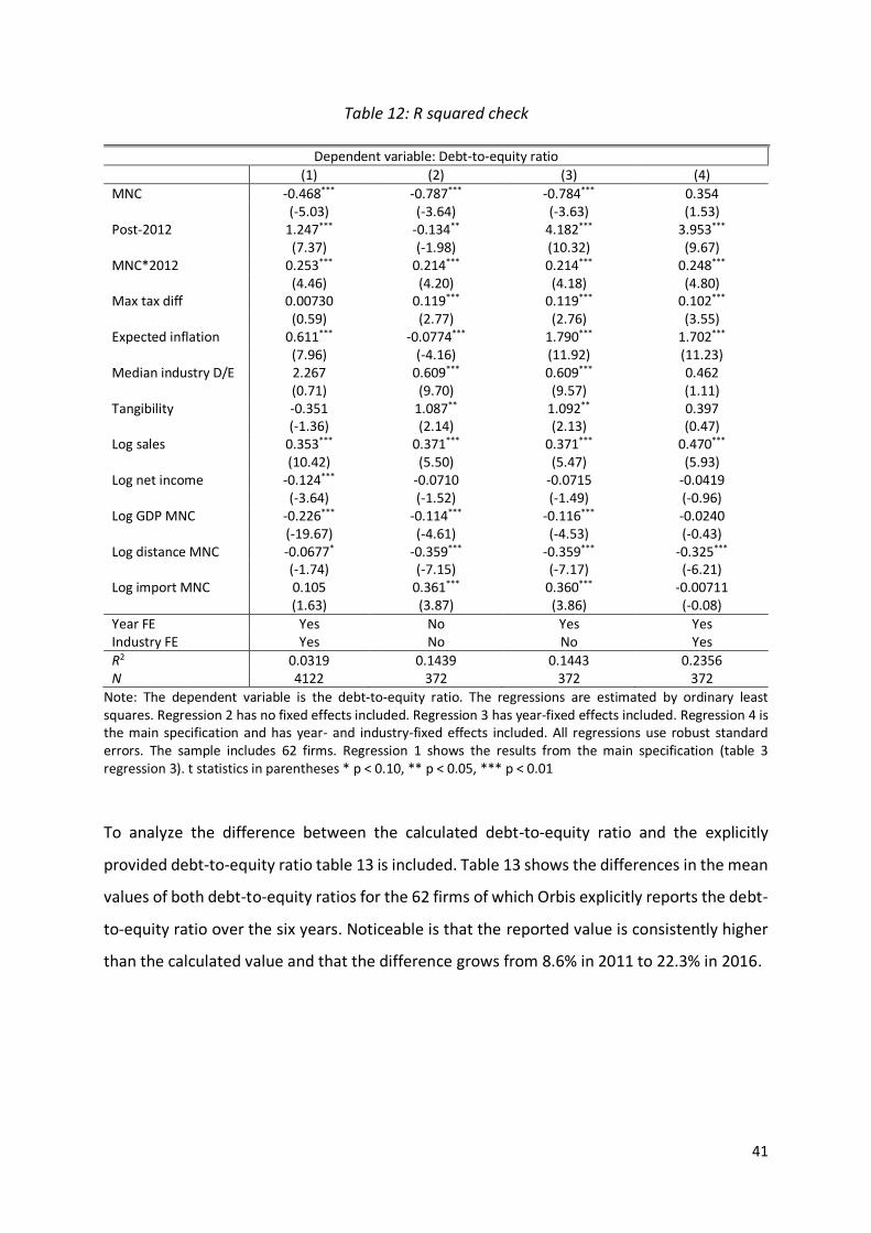
41
Table 12: R squared check
Dependent variable: Debt-to-equity ratio
(1) (2) (3) (4)
MNC -0.468*** -0.787*** -0.784*** 0.354 (-5.03) (-3.64) (-3.63) (1.53) Post-2012 1.247*** -0.134** 4.182*** 3.953*** (7.37) (-1.98) (10.32) (9.67) MNC*2012 0.253*** 0.214*** 0.214*** 0.248*** (4.46) (4.20) (4.18) (4.80) Max tax diff 0.00730 0.119*** 0.119*** 0.102*** (0.59) (2.77) (2.76) (3.55) Expected inflation 0.611*** -0.0774*** 1.790*** 1.702*** (7.96) (-4.16) (11.92) (11.23) Median industry D/E 2.267 0.609*** 0.609*** 0.462 (0.71) (9.70) (9.57) (1.11) Tangibility -0.351 1.087** 1.092** 0.397 (-1.36) (2.14) (2.13) (0.47) Log sales 0.353*** 0.371*** 0.371*** 0.470*** (10.42) (5.50) (5.47) (5.93) Log net income -0.124*** -0.0710 -0.0715 -0.0419 (-3.64) (-1.52) (-1.49) (-0.96) Log GDP MNC -0.226*** -0.114*** -0.116*** -0.0240 (-19.67) (-4.61) (-4.53) (-0.43) Log distance MNC -0.0677* -0.359*** -0.359*** -0.325*** (-1.74) (-7.15) (-7.17) (-6.21) Log import MNC 0.105 0.361*** 0.360*** -0.00711 (1.63) (3.87) (3.86) (-0.08)
Year FE Yes No Yes Yes Industry FE Yes No No Yes
R2 0.0319 0.1439 0.1443 0.2356 N 4122 372 372 372
Note: The dependent variable is the debt-to-equity ratio. The regressions are estimated by ordinary least squares. Regression 2 has no fixed effects included. Regression 3 has year-fixed effects included. Regression 4 is the main specification and has year- and industry-fixed effects included. All regressions use robust standard errors. The sample includes 62 firms. Regression 1 shows the results from the main specification (table 3 regression 3). t statistics in parentheses * p < 0.10, ** p < 0.05, *** p < 0.01
To analyze the difference between the calculated debt-to-equity ratio and the explicitly
provided debt-to-equity ratio table 13 is included. Table 13 shows the differences in the mean
values of both debt-to-equity ratios for the 62 firms of which Orbis explicitly reports the debt-
to-equity ratio over the six years. Noticeable is that the reported value is consistently higher
than the calculated value and that the difference grows from 8.6% in 2011 to 22.3% in 2016.

42
Furthermore, the estimation results by Büttner et al. (2012) and Wamser (2014)
highlight that the implementation of thin-capitalization rules encourages MNCs to substitute
internal for external debt. While the substitution is limited and the total debt-to-equity ratio
still declines after implementation, this does show a bias in the results of this paper. It is
reasonable to assume that the reverse substitution occurs after the abolishment of the thin-
capitalization rule in the Netherland. Thus, Dutch affiliates of MNCs substituting external for
internal debt. Nevertheless, the results show that the debt-to-equity ratio of Dutch affiliates
of MNCs after 2012 increased. However, the effect on the internal debt-to-equity ratio is most
likely larger than the estimated effect, which faces a downward bias due to the substitution
effect.
10. Conclusion
The thin capitalization of MNCs is a central topic in public economics and corporate
finance. Both theoretical as well as empirical studies delve into the tax-efficient financing
structures of MNCs. It has been established that MNCs use external debt as well as excessive
internal debt to profit at most from the debt-tax-shield. Governments can implement thin-
capitalization rules to counter this excessive debt usage. Multiple studies have looked at the
effects of the implementation/tightening of such rules, yet none have looked at the effect of
the abolishment of such a rule.
The theoretical model provided by this study suggests that MNCs will shift more
internal debt after the abolishment of the Dutch safe-harbor rule. The costs incurred to
circumvent the safe-harbor rule and to use internal debt above the threshold (3:1 internal
debt-to-equity ratio) cease to exist and the arm’s-length principle, with lower tax engineering
Table 13: Mean reported vs mean calculated debt-to-equity ratio
Debt to equity ratio
Variable` Mean reported Mean calc Difference Diff in %
2011 1.64 1.50 0.14 8.6%
2012
2013
2014
2015
2016
1.72
1.72
1.89
1.89
1.72
1.43
1.42
1.54
1.54
1.33
0.29
0.30
0.35
0.35
0.38
16.6%
17.5%
18.5%
18.7%
22.3%
Firms 62 62 62 62

43
costs, replaces it. Dutch affiliates of MNCs are therefore expected to increase their (internal)
debt-to-equity ratio by a larger amount than comparable domestic Dutch firms.
The empirical results from this study confirm the theoretical model. Using the Orbis
database, a sample of 687 firms is gathered that contains sufficient information to conduct
the analysis. By comparing domestic Dutch firms who are unable to profit from the
abolishment with Dutch affiliates of MNCs who can, the effect of the abolishment on thin-
capitalization is estimated. The results find that Dutch affiliates of MNCs increased their debt-
to-equity ratio by 0.253 in the large sample and by 0.239 in the smaller, more detailed sample,
compared to domestic Dutch firms. This accounts for an increase of 19.5% and 12.7% in the
mean debt-to-equity ratio, respectively. The result stays of similar size and significance in most
robustness checks. In the lagged model robustness check the result in the large sample is
insignificant. Furthermore, when using the debt-to-asset ratio instead of the debt-to-equity
ratio, the result becomes insignificant as well. This disproves the robustness of the
confirmation of hypothesis 1. Since the robustness of hypothesis 1 is disproven, this study will
refrain from providing a policy implication. A similar study that observes the internal debt-to-
equity ratio should be performed in order to confirm hypothesis 1. Such a study could also
delve into why the result on the debt-to-equity and debt-to-asset dependent variable differ.
This study is to my knowledge the first one to include headquarters-country gravity
variables in this area of research. The results in the main sample are contradictory to
expectations. The log of GDP has a negative effect on the debt-to-equity ratio and the log of
distance and import are insignificant. This disproves H2.1, H2.2, and H2.3. The effect of GDP
stays similar in the small sample, but distance as well as imports become significant (1% and
5% level, respectively) and have the expected signs. This implies that the log of distance has a
negative effect on the debt-to-equity ratio and the log of imports has a positive effect on the
debt-to-equity ratio. Thus, as the distance between the country where the headquarters is
located and the country where the affiliate is located grows, the debt-to-equity ratio of the
affiliate decreases. The reverse holds for the import flow, as the import flow from the
headquarters’ country to the affiliate’s country grows, the debt-to-equity ratio rises as well.
As an additional robustness check, Dutch affiliates of MNCs with their headquarters in a tax
haven are excluded. The results in the large sample are in line with expectations. The effect of
GDP is insignificant, but the effects of distance and imports are significant and have the
expected sign.

44
By excluding headquarters located in tax havens one decreases its sample and the
exclusion is not at random. Therefore, this is not a perfect solution to estimate the effect of
these variables. Further research should delve into the effects of the headquarter country
variables. More specifically, a data set that observes the internal debt-to-equity ratio should
be used, as this is affected by the headquarter-country variables the most. Furthermore, a
sample with affiliates and headquarters located in different countries should be utilized to
better estimate the effects of GDP, distance, and imports on the (internal) debt-to-equity
ratio.

45
Appendix 1: First-order conditions for internal and external debt
In order to derive the FOC for internal and external debt equation (3) is recovered:
max Π𝑝 = ∑ [(1 − 𝑡𝑖) ∗ (𝐹(𝐾𝑖) − 𝑟 ∗ 𝐾𝑖 + 𝑡𝑖 ∗ 𝑟 ∗ (𝐷𝑖𝐸 + 𝐷𝑖
𝐼) − (1 − 𝑡𝑖)(𝐶𝐸(𝑏𝑖𝐸) +𝑖
𝐶𝐼(𝑏𝑖𝐼)) ∗ 𝐾𝑖] − 𝐶𝑓(𝑏𝑓) ∑ 𝐾𝑖𝑖 𝑠. 𝑡. ∑ 𝑟 ∗ 𝐷𝑖
𝐼 = 0𝑖 (3)
First, the FOC for external debt will be derived and provides equation (7):
𝜕Π𝑝
𝜕𝑏𝑖𝐸 = ∑ 𝑡𝑖 ∗ 𝑟 − (1 − 𝑡𝑖) ∗
𝜕𝐶𝐸(𝑏𝑖𝐸)
𝜕𝑏𝑖𝐸 +
𝜕𝐶𝑓(𝑏𝑓)
𝜕𝑏𝑓= 0𝑖 (7)
After taking ∑ (1 − 𝑡𝑖) ∗𝜕𝐶𝐸(𝑏𝑖
𝐸)
𝜕𝑏𝑖𝐸 +
𝜕𝐶𝑓(𝑏𝑓)
𝜕𝑏𝑓𝑖 to the right-hand side and dividing by ∑ 𝑖, we are
left with equation (4). Equation (4) shows the benefits and costs of using external debt.
𝑡𝑖 ∗ 𝑟 = (1 − 𝑡𝑖) ∗𝜕𝐶𝐸(𝑏𝑖
𝐸)
𝜕𝑏𝑖𝐸 +
𝜕𝐶𝑓(𝑏𝑓)
𝜕𝑏𝑓> 0 ∀𝑖, (4)
In order to find equation (5), the FOC with respect to internal debt will be derived from
equation (3) and provides equation (8):
𝜕Π𝑝
𝜕𝑏𝑖𝐼 = ∑ 𝑡𝑖 ∗ 𝑟 − (1 − 𝑡𝑖) ∗
𝜕𝐶𝐼(𝑏𝑖𝐼)
𝜕𝑏𝑖𝐼 − 𝜆 ∗ 𝑟 = 0𝑖 (8)
After taking ∑ (1 − 𝑡𝑖) ∗𝜕𝐶𝐼(𝑏𝑖
𝐼)
𝜕𝑏𝑖𝐼𝑖 to the right-hand side and dividing by ∑ 𝑖, we are left with
equation (5). Equation (5) shows the benefits and costs of using internal debt.
(𝑡𝑖 − 𝜆) ∗ 𝑟 = (1 − 𝑡𝑖) ∗𝜕𝐶𝐼(𝑏𝑖
𝐼,𝛼𝑖)
𝜕𝑏𝑖𝐼 ≥ 0 ∀𝑖, (5)

46
Appendix 2: Effect of abolishing thin-capitalization rules
To find the effect of abolishing the thin-capitalization rules and thus lowering parameter 𝛼𝑖,
the total differential of equation (5) is derived.
(𝑡𝑖 − 𝜆) ∗ 𝑟 = (1 − 𝑡𝑖) ∗𝜕𝐶𝐼(𝑏𝑖
𝐼,𝛼𝑖)
𝜕𝑏𝑖𝐼 ≥ 0 ∀𝑖, (5)
After replacing 𝜆 by 𝑡1, the total differential of equation (5) becomes equation (9):
(𝑑𝑡𝑖 − 𝑑𝑡1) ∗ 𝑑𝑟 = (1 − 𝑑𝑡𝑖) ∗𝜕𝐶𝐼(𝑏𝑖
𝐼,𝛼𝑖)
𝜕𝑏𝑖𝐼 ∗ 𝑑𝛼𝑖 + (1 − 𝑡𝑖)
𝜕2𝐶𝐼(𝑏𝑖𝐼,𝛼𝑖)
𝜕𝑏𝑖𝐼𝜕𝑎𝑖
∗ 𝑑𝛼𝑖 + (1 − 𝑑𝑡𝑖) ∗
𝜕𝐶𝐼(𝑏𝑖𝐼,𝛼𝑖)
𝜕𝑏𝑖𝐼 ∗ 𝑑𝑏𝑖
𝐼 + (1 − 𝑡𝑖)𝜕2𝐶𝐼(𝑏𝑖
𝐼,𝛼𝑖)
𝜕𝑏𝑖𝐼𝜕𝑎𝑖
∗ 𝑑𝑏𝑖𝐼 (9)
Since 𝑑𝑡𝑖 = 𝑑𝑡1 = 𝑑𝑟 = 0 equation (9) becomes equation (10):
0 = (1 − 𝑡𝑖)𝜕2𝐶𝐼(𝑏𝑖
𝐼 ,𝛼𝑖)
𝜕𝑏𝑖𝐼𝜕𝑎𝑖
∗ 𝑑𝛼𝑖 + (1 − 𝑡𝑖)𝜕2𝐶𝐼(𝑏𝑖
𝐼,𝛼𝑖)
𝜕𝑏𝑖𝐼𝜕𝑎𝑖
∗ 𝑑𝑏𝑖𝐼 (10)
Equation (10) can straightforwardly be modified into equation (11):
−(1 − 𝑡𝑖)𝜕2𝐶𝐼(𝑏𝑖
𝐼,𝛼𝑖)
𝜕𝑏𝑖𝐼𝜕𝑎𝑖
∗ 𝑑𝑏𝑖𝐼 = (1 − 𝑡𝑖)
𝜕2𝐶𝐼(𝑏𝑖𝐼,𝛼𝑖)
𝜕𝑏𝑖𝐼𝜕𝑎𝑖
∗ 𝑑𝛼𝑖 (11)
After dividing both sides by 𝑑𝛼𝑖 equation (11) becomes equation (12):
−(1 − 𝑡𝑖)𝜕2𝐶𝐼(𝑏𝑖
𝐼,𝛼𝑖)
𝜕𝑏𝑖𝐼𝜕𝑎𝑖
∗𝑑𝑏𝑖
𝐼
𝑑𝛼𝑖= (1 − 𝑡𝑖)
𝜕2𝐶𝐼(𝑏𝑖𝐼 ,𝛼𝑖)
𝜕𝑏𝑖𝐼𝜕𝑎𝑖
(12)
After dividing both sides by −(1 − 𝑡𝑖)𝜕2𝐶𝐼(𝑏𝑖
𝐼 ,𝛼𝑖)
𝜕𝑏𝑖𝐼𝜕𝑎𝑖
equation (11) becomes equation (6):
𝑑𝑏𝑖𝐼
𝑑𝛼𝑖= −
𝜕2𝐶𝐼(𝑏𝑖𝐼,𝛼𝑖)/(𝜕𝑏𝑖
𝐼𝜕𝛼𝑖)
𝜕2𝐶𝐼(𝑏𝑖𝐼,𝛼𝑖)/(𝜕𝑏𝑖
𝐼)2 < 0 (6)

47
Appendix 3: additional tables
Table 14: Tax haven countries
Number of firms
Country Large sample Small sample
Aruba
Bahamas
1
3
0
1
Belize
Bermuda
The British Virgin Islands
Cayman Islands
Cyprus
Gibraltar
Ireland
Liechtenstein
Luxembourg
Switzerland
1
4
1
2
2
1
4
1
5
7
0
4
1
1
0
0
3
0
3
2
Total 32 15
% Of MNCs 9.9% 8.1%

48
Table 15: Industry sizes
Large sample Small sample
industry Number of firms Percentage Number of firms Percentage
1 9 1,3% 4 1,3%
2 8 1,2% 5 1,7%
3 88 12,8% 59 19,7%
4 6 0,9% 2 0,7%
5 12 1,7% 5 1,7%
6 18 2,6% 9 3,0%
7 70 10,2% 44 14,7%
8 25 3,6% 14 4,7%
9 10 1,5% 0 0,0%
10 14 2,0% 7 2,3%
11 321 46,7% 111 37,0%
12 15 2,2% 6 2,0%
13 65 9,5% 24 8,0%
14 11 1,6% 4 1,3%
15 6 0,9% 1 0,3%
16 3 0,4% 1 0,3%
17 6 0,9% 4 1,3%
Total 687 100% 300 100%

49
References
Banerjee, S., Heshmati, A., and Wihlborg, C. (1999). The dynamics of capital structure. New York
University-Salomon Center-Leonard N. Stern School of Business.
Beer, S., De Mooij, R., and Liu, L. (2020). International corporate tax avoidance: A review of the
channels, magnitudes, and blind spots. Journal of Economic Surveys, 34(3), 660-688.
Bowen, R. M., Daley, L. A., and Huber Jr, C. C. (1982). Evidence on the existence and determinants of
inter-industry differences in leverage. Financial Management, 10-20.
Buckley, P. J., and Casson, M. (1976). A long-run theory of the multinational enterprise. In The Future
of the Multinational Enterprise (pp. 32-65). Palgrave Macmillan, London.
Burger, M., Van Oort, F., & Linders, G. J. (2009). On the specification of the gravity model of trade:
Zeros, excess zeros and zero-inflated estimation. Spatial Economic Analysis, 4(2), 167-190.
Büttner, T., Overesch, M., Schreiber, U., and Wamser, G. (2009). Taxation and capital structure
choice—Evidence from a panel of German multinationals. Economics Letters, 105(3), 309-
311.
Büttner, T., Overesch, M., Schreiber, U., and Wamser, G. (2012). The impact of thin-capitalization
rules on the capital structure of multinational firms. Journal of Public Economics, 96(11-12),
930-938.
Büttner, T., Overesch, M., and Wamser, G. (2018). Anti profit-shifting rules and foreign direct
investment. International Tax and Public Finance, 25(3), 553-580.
Büttner, T., and Wamser, G. (2013). Internal debt and multinational profit shifting: Empirical
evidence from firm-level panel data. National Tax Journal, 66(1), 63-95.
Bureau van Dijk. (2021). Orbis. Retrieved from: https://orbis.bvdinfo.com/
Campello, M., and Giambona, E. (2013). Real assets and capital structure. Journal of Financial and
Quantitative Analysis, 48(5), 1333-1370.

50
CEPII. (2021). Gravity database. Retrieved from:
http://www.cepii.fr/CEPII/en/bdd_modele/presentation.asp?id=8
Davies, R. B., Martin, J., Parenti, M., and Toubal, F. (2018). Knocking on tax haven’s door:
Multinational firms and transfer pricing. Review of Economics and Statistics, 100(1), 120-134.
DeAngelo, H., and Masulis, R. W. (1980). Optimal capital structure under corporate and personal
taxation. Journal of Financial Economics, 8(1), 3-29.
De Brauw Blackstone Westbroek. (2013). Interest deductions in the Netherlands.
https://www.debrauw.com/wp-content/uploads/NEWS%20-
%20LEGAL%20ALERTS/Tax/2016/Interest-deductions-in-the-Netherlands.pdf
De Mooij, R. A. (2011). The tax elasticity of corporate debt: a synthesis of size and variations.
International Monetary Fund.
Desai, M. A., Foley, C. F., and Hines Jr, J. R. (2004). A multinational perspective on capital structure
choice and internal capital markets. The Journal of Finance, 59(6), 2451-2487.
Drobetz, W., and Wanzenried, G. (2006). What determines the speed of adjustment to the target
capital structure?. Applied Financial Economics, 16(13), 941-958.
Dunning, J. H. (1977). Trade, location of economic activity and the MNE: A search for an eclectic
approach. In The International Allocation of Economic Activity (pp. 395-418). Palgrave
Macmillan, London.
Egger, P. H., and Larch, M. (2013). Time zone differences as trade barriers. Economics Letters, 119(2),
172-175.
Feenstra, R. C. (2015). Advanced international trade: Theory and evidence. Princeton University Press.
Feld, L. P., Heckemeyer, J. H., and Overesch, M. (2013). Capital structure choice and company
taxation: A meta-study. Journal of Banking and Finance, 37(8), 2850-2866.
Frank, M. Z., and Goyal, V. K. (2009). Capital structure decisions: Which factors are reliably
important?. Financial Management, 38(1), 1-37.
Ghemawat, P. (2001). Distance still matters. Harvard Business Review, 79(8), 137-147.

51
Giannetti, M. (2003). Do better institutions mitigate agency problems? Evidence from corporate
finance choices. Journal of financial and quantitative analysis, 38(1), 185-212.
Gresik, T. A., Schindler, D., and Schjelderup, G. (2017). Immobilizing corporate income shifting:
Should it be safe to strip in the harbor?. Journal of Public Economics, 152, 68-78.
Haufler, A., Mardan, M., & Schindler, D. (2018). Double tax discrimination to attract FDI and fight
profit shifting: The role of CFC rules. Journal of International Economics, 114, 25-43.
Hines Jr, J. R., and Rice, E. M. (1994). Fiscal paradise: Foreign tax havens and American business. The
Quarterly Journal of Economics, 109(1), 149-182.
Huizinga, H., Laeven, L., and Nicodeme, G. (2008). Capital structure and international debt
shifting. Journal of Financial Economics, 88(1), 80-118.
IFA, Boterman, M., & Van der Gulik, B. (2013). IFA country report 2013_Netherlands.docx.
https://www.ifa-nl.org/asset/document/5f610253b0b90af1.pdf
Kostova, T., Nell, P. C., & Hoenen, A. K. (2018). Understanding agency problems in headquarters-
subsidiary relationships in multinational corporations: A contextualized model. Journal of
Management, 44(7), 2611-2637.
Krugman, P. (1984). Import protection as export promotion: International competition in the
presence of oligopoly and economies of scale. Monopolistic Competition and International
Trade, 180-93.
Porta, R. L., Lopez-de-Silanes, F., Shleifer, A., & Vishny, R. W. (1998). Law and finance. Journal of
Political Economy, 106(6), 1113-1155.
Martin, P., and Rey, H. (2004). Financial super-markets: size matters for asset trade. Journal of
International Economics, 64(2), 335-361.
Mátyás, L. (1997). Proper econometric specification of the gravity model. World Economy, 20(3), 363-
368.
Miles, J. R. (2014). Squared. Adjusted R Squared Wiley StatsRef: Statistics Reference Online: John
Wiley and Sons, Ltd.

52
Mills, L. F., and Newberry, K. J. (2004). Do foreign multinationals' tax incentives influence their US
income reporting and debt policy?. National Tax Journal, 57(1), 89-107.
Mintz, J., and Smart, M. (2004). Income shifting, investment, and tax competition: Theory and
evidence from provincial taxation in Canada. Journal of Public Economics, 88(6), 1149-1168.
Møen, J., Schindler, D., and Schjelderup, G. (2008). Capital structure and international debt shifting: A
comment. Beta, 24(02), 132-140.
Møen, J., Schindler, D., Schjelderup, G., and Tropina Bakke, J. (2019). International debt shifting: The
value-maximizing mix of internal and external debt. International Journal of the Economics of
Business, 26(3), 431-465.
De Mooij, R. A. (2011). The tax elasticity of corporate debt: A synthesis of size and variations.
International Monetary Fund.
Myers, S. C., and Majluf, N. S. (1984). Corporate financing and investment decisions when firms have
information that investors do not have. Journal of Financial Economics, 13(2), 187-221.
OECD. (n.d.). About - BEPS. Retrieved 11 March 2021, from https://www.oecd.org/tax/beps
OECD, (2013). Action plan on base erosion and profit shifting. OECD Publishing, Paris.
http://dx.doi.org/10.1787/9789264202719-en
OECD. (2021). Prices - Inflation forecast - OECD Data. Retrieved from:
https://data.oecd.org/price/inflation-forecast.htm
Overesch, M., & Wamser, G. (2010). Corporate tax planning and thin-capitalization rules: Evidence
from a quasi-experiment. Applied Economics, 42(5), 563-573.
Park, S. H., Suh, J., and Yeung, B. (2013). Do multinational and domestic corporations differ in their
leverage policies?. Journal of Corporate Finance, 20, 115-139.
Portes, R., Rey, H., (2000). The determinants of cross-border equity flows: The geography of
information. Revised version of CEPR Discussion paper 2225, January.
Portes, R., Rey, H., and Oh, Y. (2001). Information and capital flows: The determinants of transactions
in financial assets. European Economic Review, 45(4-6), 783-796.

53
Rajan, R. G., and Zingales, L. (1995). What do we know about capital structure? Some evidence from
international data. The Journal of Finance, 50(5), 1421-1460.
Ruf, M., and Schindler, D. S. (2015). Debt shifting and thin-capitalization rules–German experience
and alternative approaches. Nordic Tax Journal, 2015(1), 17-33.
Schiavo, S., Reyes, J., & Fagiolo, G. (2010). International trade and financial integration: A weighted
network analysis. Quantitative Finance, 10(4), 389-399.
Schindler, D., and Schjelderup, G. (2012). Debt shifting and ownership structure. European Economic
Review, 56(4), 635-647.
Scott Jr, D. F., and Martin, J. D. (1975). Industry influence on financial structure. Financial
Management, 67-73.
Taggart, R. A. (2009). 1. Secular patterns in the financing of US corporations. In Corporate Capital
Structures in the United States (pp. 13-80). University of Chicago Press.
Tax Consultants International B.V. (2012). Proposal to abolish the Dutch thin capitalization rules. Tax
Consultants International. https://www.tax-consultants-international.com/news/proposal-
to-abolish-the-dutch-thin-capitalization-rules#section_4
Tinbergen, J. (1962): Shaping the world economy, New York: The twentieth century fund.
Titman, S., and Wessels, R. (1988). The determinants of capital structure choice. The Journal of
Finance, 43(1), 1-19.
Wamser, G. (2014). The impact of thin‐capitalization rules on external debt usage–a propensity score
matching approach. Oxford Bulletin of Economics and Statistics, 76(5), 764-781.
Worldbank. (2021). World Development Indicators | DataBank. Retrieved from:
https://databank.worldbank.org/source/world-development-indicators#
Related Documents