MASTER'S THESIS - DiVA-Portal

MASTER'S THESIS

Improvement of Fatigue ResistanceThrough Box Action for I-girder Composite

Bridges

Victor Vestman2016

Master of Science in Engineering TechnologyCivil Engineering

Luleå University of TechnologyDepartment of Civil, Environmental and Natural Resources Engineering

Illustration of three generations of bridges over Öreälv by Catrin Sjölund

i

“For every bridge we build we have one less to build but one more to maintain”

Peter Collin, Professor in Composite Structures at Luleå University of Technology and Marketing Manager Bridges at Ramböll Sweden.

ii

Preface

This thesis is the final stage of my Master of Science in Civil Engineering at Luleå University of Technology (LTU). After five years I am at the end of my master education, which has been a real pleasant journey thanks to my great classmates and friends who have made these five years pass by too fast.

The thesis was initiated by LTU and Ramböll Sweden as a part of a European R&D-project ProLife (RFCS-CT-2015-00025) about strengthening of existing steel- and steel concrete composite bridges.

First of all thanks to my supervisor Jens Häggström (LTU) who has given me guidance through the work and who always have had time for my questions. I really appreciate the effort you have put in to help me complete this thesis.

Thanks to my professor and supervisor Peter Collin (Ramböll and LTU) for introducing me to the subject of steel- and composite bridges with your enthusiasm and passion on this subject.

I would like to thank the office at Statens vegvesen in Skien Norway with my supervisor Lars Farstad. Thanks also for the opportunity to be part of the organization and for all new knowledge about bridges and the impact bridges have on the society. Thanks to my supervisors in Norway and for my newly found friends.

Thanks to my dear life-companion and after this summer my wife, who I always will be thankful to for all the support and joy she is giving me.

Luleå, November 2015

Victor Vestman

iii

Abstract The increased amount of traffic combined with higher traffic loads will lead to that many bridges of today are in need of strengthening or replacement. This because of the coming rules for fatigue and because of the old design codes that did not consider such high loads that we have today.

When strengthening existing I-girder composite bridges (which are the majority of the steel bridge stock), one concept is to make the cross section act like a box section, by adding a horizontal truss between the bottom flanges. This means that the eccentric loads produce a torque that is transferred by shear forces around the section. The preferred type of truss is a K-truss, since other types will force the diagonals to take part in the global bending, which will make them sensible to buckling between the joints. This means a lot in the Ultimate Limit State (ULS), but even more in the Fatigue Limit State (FLS). In the FLS the fatigue is determined by the stress ranges in certain parts of the structure, for instance the welded details in an I-girder. If the girders can act like brothers or at least as “step-brothers”, sharing the load effects from eccentric loading, the stress ranges can be significantly reduced.

This thesis presents a study that shows the effects by these horizontal trusses between lower flanges for bridges and how the fatigue resistance is improved. Reduced stress ranges and increased amount of tolerated load cycles will extend the lifetime of the details, and by so the lifetime for the bridge.

Bergeforsen Bridge is chosen as a case study in the thesis to implement the method with horizontal trusses. The bridge is a multi-span bridge with three spans without curvature, which makes it perfect for the purpose of analysing the effects of box action introduced by K-trusses. The chosen dimensions for the trusses is180x100x8 mm, which corresponds to a cross section area of 4004 mm2 for a cold-formed rectangular hollow section. The additional weight is 1.6 % of the original steel weight and only 0.7 % of the total dead load for the bridge. The load distribution between the girders or as called in this thesis lane factor, LF is 0,74 (0,95 without a truss) which extends the lifetime of the bridge 3.5 times, with aspect to the most exposed detail for fatigue, on-site welded joints.

Keywords: Box action; composite; fatigue; framework; I-girder; 3-D; modelling; steel; strengthening; torsion.

iv

Sammanfattning Den ökade trafikmängden kombinerat med en ökad axellast kommer leda till att många gamla broar i dagens brobestånd måste förstärkas eller bytas ut. Detta på grund av de kommande utmattningsreglerna och att den trafikmängd och last vi har idag inte var medräknat i de gamla normerna.

Vid förstärkning av existerande i-balksbroar med samverkan, vilket är majoriteten av de gamla stålbroarna, är ett koncept att införa lådverkan i tvärsnittet. Det kan göras genom att införa ett horisontellt fackverk mellan de nedre flänsarna. Vilket i sin tur kommer att innebära att excentriska laster ger upphov till ett vridande moment som kommer transporteras i form av tvärkrafter runt i tvärsnittet. K-fackverk är att föredra framför andra typer av fackverk då andra typer gör så att diagonalerna medverkar i den globla nedböjningen, vilket gör de känsliga för knäckning mellan knytpunkterna. Detta betyder mycket i brottgränstillståndet, men mer i utmattningsgränstillståndet. I utmattningsgränstillståndet så bestäms utmattningen från de spänningsvariationer som uppkommer i specifika detaljer i bron, till exempel svetsade detaljer i en I-balk. Om balkarna kan agera som bröder eller åtminstone som styvbröder, genom att dela lasteffekterna från excentriska laster, kan spänningsvariationen reduceras.

I det här examensarbetet presenteras en studie där effekterna från ett horisontellt fackverk mellan de nedre flänsarna på broar och hur dessa medverkar i en ökad utmattningshållfasthet analyseras. Minskade spänningsvariationer och ett ökat antal lastcykler leder till en förlängd livstid på detaljer, vilket i sin tur ger en ökad livslängd för bron.

Bron Bergeforsen är valt som objekt för en fallstudie i examensarbetet för att testa metoden med lådverkan genom horisontalfackverk. Bron är i tre spann och utan kurvatur, vilket gör den utmärkt för analysering av effekterna från lådverkan introducerad av ett K-fackverk. Den valda dimensionen på fackverket är 180x100x8 mm vilket motsvarar en area på 4004 mm2 för ett kallformat rektangulärt tvärsnitt. Fackverket ger en ökad egenvikt på 1.6 % av den befintliga stålvikten, men bara 0.7 % av den totala vikten på konstruktionen. Lastfördelningen mellan balkarna, eller som det benämns i denna studie filfaktor, är med detta fackverk 0,74 (0,95 utan fackverk). Således förlängs brons livslängd 3,5 ggr, med avseende på de mest utsatta detaljerna för utmattning, montageskarvarna.

Sökord: Box action; composite; fatigue; framework; I-girder; 3-D; modelling; steel; strengthening; torsion.

v

Table of Contents 1 INTRODUCTION ............................................................................................................ 15

1.1 Background ................................................................................................................ 15

1.2 Aims and scopes ........................................................................................................ 16

1.3 Methodology .............................................................................................................. 16

1.4 Limitations ................................................................................................................. 16

1.5 Disposition of thesis .................................................................................................. 17

2 THEORETICAL STUDY ................................................................................................ 18

2.1 History ....................................................................................................................... 18

2.2 Fatigue ....................................................................................................................... 19

2.3 Fatigue verification in Eurocode ............................................................................... 21

2.3.1 Fatigue Load Models .......................................................................................... 21

2.3.2 Damage Accumulation Method ......................................................................... 24

2.3.3 Palmgren-Miner (Cumulative damage method) ................................................. 24

2.3.4 Lambda-coefficient method ............................................................................... 25

2.3.5 C-classes ............................................................................................................. 29

2.3.6 Equivalent stress range concept ......................................................................... 31

2.4 I-girder ....................................................................................................................... 32

2.5 Box-girder .................................................................................................................. 33

2.6 Improvements of fatigue strength .............................................................................. 33

2.7 Torsion and Warping ................................................................................................. 34

2.8 Strengthening with bracings ...................................................................................... 41

3 CASE STUDY – Bergeforsen Bridge .............................................................................. 44

3.1.1 Location and history ........................................................................................... 44

3.1.2 Geometry and materials ..................................................................................... 45

3.1.3 Cross sections ..................................................................................................... 46

3.2 FEM-setup ................................................................................................................. 48

3.2.1 Program .............................................................................................................. 48

3.2.2 Elements ............................................................................................................. 48

3.2.3 Concept design ................................................................................................... 51

vi

4 CALCULATIONS ........................................................................................................... 56

4.1 Hand-calculations ...................................................................................................... 56

4.1.1 Fictive thickness ................................................................................................. 56

4.1.2 Torsional stiffness .............................................................................................. 57

4.1.3 Composite actions .............................................................................................. 57

4.1.4 Displacement ...................................................................................................... 59

4.2 FEM-analysis of Bergeforsen Bridge ........................................................................ 62

4.2.1 Structure ............................................................................................................. 62

4.2.2 Loads .................................................................................................................. 63

4.2.3 Lane factor .......................................................................................................... 65

4.2.4 Cracking of concrete .......................................................................................... 65

5 RESULTS ......................................................................................................................... 67

5.1 Bending moment........................................................................................................ 67

5.1.1 Lane factors ........................................................................................................ 69

6 ANALYSIS ...................................................................................................................... 71

6.1 Lane factors and frame work ..................................................................................... 71

6.2 Contribution in global bending .................................................................................. 71

6.3 Stresses ...................................................................................................................... 72

6.3.1 Stress range ........................................................................................................ 75

6.4 Fatigue ....................................................................................................................... 80

6.4.1 Stress range ........................................................................................................ 80

6.4.2 Extended lifetime ............................................................................................... 82

6.5 Global bending of bracings in framework ................................................................. 83

7 DISCUSSION AND CONCLUSIONS ............................................................................ 84

7.1 Discussion .................................................................................................................. 84

7.2 Conclusions ............................................................................................................... 85

7.3 Suggestions for further research ................................................................................ 85

REFERENCES ........................................................................................................................ 87

APPENDIXES ......................................................................................................................... 89

vii

List of Figures Figure 1 - Deflection corresponding to different type of cross section .................................... 15

Figure 2 - Harmonic stress variation (Larsen, 2010) ............................................................... 19

Figure 3 - Stress states for harmonic stress history (Larsen, 2010) ......................................... 20

Figure 4 - Wöhler curve with defined areas (Bathias & Pineau, 2010) ................................... 21

Figure 5 - Fatigue Load Models, (Al-Emrani & Aygül, 2014) ................................................ 21

Figure 6 - FLM 3, (SS-EN 1991-2, 2010) ................................................................................ 22

Figure 7 - Set of lorries in FLM 4, (EN 1991-2, 2003) ............................................................ 23

Figure 8 - Variable amplitude loading with resulting simplified diagram (Al-Emrani & Aygül, 2014) ......................................................................................................................................... 24

Figure 9 - Location of mid-span- and support section ............................................................. 26

Figure 10 – λ1 for moments ...................................................................................................... 27

Figure 11 – λmax for sections subjected to bending stresses ..................................................... 29

Figure 12 - Fatigue strength curves for direct stress ranges (SS-EN 1993-1-9, 2005) ............ 31

Figure 13 - Plate welded I-girder (SteelConstruction.info, 2015) ........................................... 32

Figure 14 – Stiffeners for I-girders (SteelConstruction.info, 2015) ......................................... 33

Figure 15 –Beam with torque and distribution of torsional angle. In Right: (1): pivot plane (2): rotary volted (Nylander, 1973) ................................................................................................. 35

Figure 16 –Beam in torsion, (Nylander, 1973) ........................................................................ 36

Figure 17 – Arbitrary cross section .......................................................................................... 37

Figure 18 – To the left: Closed cross section. To the right: Open cross section ...................... 38

Figure 19 - Shear flow, (Nylander, 1973) ................................................................................ 39

Figure 20 - The profile of a HEA beam at torsion (1) and the displacement in (2) in the longitudinal direction called warping (Nylander, 1973) .......................................................... 40

Figure 21 - Lateral torsion for symmetric cross section ........................................................... 40

Figure 22 - K-trusses (Roik, 1983) ........................................................................................... 42

Figure 23 - Types of framework (Roik, 1983) ......................................................................... 43

Figure 24 - Location bridge geographically (Google maps, 2015-06-10) ............................... 44

Figure 25 –Location of Bergeforsen Bridge (Google Maps, 2015-06) .................................... 45

Figure 26 - Elevation of steel beams ........................................................................................ 45

Figure 27 - View from the northern end of the bridge (Häggström, 2012) .............................. 46

Figure 28 - Cross section Bergeforsen (Häggström, 2012) ...................................................... 47

viii

Figure 29 - Local coordinate system of beam elements (SOFiSTiK AG, 2014) ..................... 49

Figure 30 - Forces and moments of plates/quads (SOFiSTiK AG, 2014) ............................... 49

Figure 31 - Exemple of cross section, Beam 1:1, (SOFiPLUS-X 2014) ................................. 50

Figure 32 – Quad- (light blue) and beam elements (light purple) (SSD 2014) ........................ 51

Figure 33 – Computed beam sections (SOFiSTiK-SSD) ......................................................... 52

Figure 34 – Quad-/area element added (SOFiSTiK-SSD) ....................................................... 52

Figure 35 - Support condition, fully restrained (SOFiPLUS-X) .............................................. 53

Figure 36 - Load case, eccentric load ....................................................................................... 54

Figure 37 - Sectional view of load case ................................................................................... 54

Figure 38 - Full design of concept bridge (SOFiSTiK-SSD) ................................................... 55

Figure 39 – View of the framework, K-trusses (SOFiSTiK-SSD) .......................................... 55

Figure 40 – Fictive thickness with different angle and dimension, K-bracing ........................ 56

Figure 41 - Sectional parameters for composite cross section (Collin, et al., 2011) ................ 58

Figure 42 - Expression of eccentric load .................................................................................. 60

Figure 43 - Elementary case of beam bending for simply supported conditions ..................... 60

Figure 44 - Lane 10 for FLM3 (SOFiSTiK – SSD – Traffic Loader) ...................................... 64

Figure 45 - Lane 20 for FLM3 (SOFiSTiK – SSD – Traffic Loader) ...................................... 64

Figure 46 - Lane 1 for FLM3 (SOFiSTiK – SSD – Traffic Loader) ........................................ 64

Figure 47 - Lane 1-centric for FLM3 (SOFiSTiK - SSD - Traffic Loader) ............................. 65

Figure 48 - Cracking zones ...................................................................................................... 66

Figure 49 –Bending moment for the original design ............................................................... 67

Figure 50 – Bending moments for the strengthened design ..................................................... 68

Figure 51 – Comparison of bending moments in girder no.2 from the three models .............. 69

Figure 52 - Lane factors for the strengthened and original design ........................................... 70

Figure 53 – Lane factors for different dimensions on the framework ..................................... 71

Figure 54 - Global bending for K-frame work ......................................................................... 72

Figure 55 - Fatigue stresses original design ............................................................................. 73

Figure 56 - Fatigue stresses strengthened design ..................................................................... 74

Figure 57 - Fatigue stresses in 2-D model................................................................................ 74

Figure 58 - Comparison of stress ranges between models (un-cracked) .................................. 75

Figure 59 - Comparison of stress ranges between models (cracked) ....................................... 76

ix

Figure 60 - Comparison of true stress ranges ........................................................................... 77

Figure 61 - 2-D model with LF=1.19 ....................................................................................... 77

Figure 62 - 3-D model with LF=0.95 ....................................................................................... 78

Figure 63 - 3-D model with strengthening and LF=0.74 ......................................................... 79

Figure 64 - Stress ranges for true stresses with position of the on-site welded joints for models .................................................................................................................................................. 81

Figure 65 - Maximum normal force in bracing calculated in SOFiSTiK for ULS .................. 83

x

List of Tables Table 1 - The history of the fatigue phenomenon (Bathias & Pineau, 2010) .......................... 18

Table 2 - Traffic categories, (Trafikverket, 2011) ................................................................... 24

Table 3 - Recommended λ2 values ........................................................................................... 28

Table 4 - Geometry values ....................................................................................................... 38

Table 5 - Materials in main parts (Häggström, 2012) .............................................................. 46

Table 6 - Dimensions for beam sections (Häggström, 2012) ................................................... 47

Table 7 – Dimensions of the concept bridge ............................................................................ 51

Table 8 – Dimensions of composite cross section in the concept bridge ................................. 53

Table 9 - Cross section properties Concept Bridge .................................................................. 59

Table 10 - Comparison of displacement for case 1&2 in 2-D & 3-D ...................................... 62

Table 11- Support conditions Bergeforsen Bridge (Häggström, 2012) ................................... 62

Table 12 – Self-weights ............................................................................................................ 63

Table 13 - Number and width of notional lanes (SS-EN 1991-2, 2010) .................................. 63

Table 14 – Example of output for moments over elements ..................................................... 67

Table 15 - Comparison of remaining lifetime .......................................................................... 79

Table 16 - Lambda factors, [λ] (Häggström, 2012) ................................................................. 80

Table 17 – Stress range of the on-site welded joints for the models, from Figure 64 ............. 81

Table 18 - Fatigue resistance from 2-D design ........................................................................ 82

Table 19 - Reduction for strengthening in 3-D design and extended lifetime ......................... 82

xi

Nomenclature

Roman upper letters

A Area [mm2]

Ac Area of concrete [mm2]

Ac,eff Effective concrete area [mm2]

As Area of steel [mm2]

C Torsional stiffness [Nmm2]

Cc Torsional stiffness of concrete [Nmm2]

Cs Torsional stiffness of steel [Nmm2]

Cw Warping stiffness [Nmm4]

D Fatigue damage [-]

FD Cross section area of the diagonals [mm2]

FO Cross section area of the girder [mm2]

FV Cross section area of the verticals [mm2]

FU Cross section area of the girder [mm2]

G Shear modulus [MPa]

Icomp Moment of inertia composite [mm4]

Is Moment of inertia steel [mm4]

KV Torsion factor [mm4]

KV,c Torsion factor of concrete [mm4]

KV,s Torsion factor of steel [mm4]

Li Length of bridge span [m]

MT Torque [Nm]

N Number of cycles [cycles]

Nk Number of lorries per year in lane k [lorries]

NO Annual number of lorries [lorries]

NObs Total number of lorries per year in the slow lane [lorries]

xii

Qi Gross weight of the lorry, number i, in the slow lane [kN]

Qm1 Average gross weight [kN]

Qmk Number of lorries per year in lane k [lorries]

R Stress ratio [-]

Roman lower letters

a Distance between the vertical beams [mm]

b Distance between the girders [mm]

ci Length of the part i [mm]

d Length of the diagonal [mm]

e Eccentricity [mm]

ecomp Centre of gravity composite [mm]

es Centre of gravity [mm]

hc Thickness of concrete deck [mm]

hw Height of web [mm]

k number of lanes with heavy traffic [lanes]

tlf Thickness of lower flange [mm]

tuf Thickness of upper flange [mm]

tw Thickness of web [mm]

wlf Width of upper flange [mm]

wuf Width of upper flange [mm]

Greek letters

γFf Partial safety factor for fatigue [-]

γMF Partial safety factor for fatigue resistance [-]

δ Displacement [mm]

ϕ Torsional angle [rad]

ϕ’ Torsional rotation [mm-1]

λ Fatigue damage equivalent factor [-]

Φ2 Dynamic factor [-]

xiii

∆σ2-D,org Stress range for 2-D design [MPa]

∆σ3-D,org Stress range for 3-D design without frame work [MPa]

∆σ3-D,str Stress range for 3-D design with frame work [MPa]

σa Component stress [MPa]

σm Mean stress [MPa]

σmax Maximum stress [MPa]

σtrue True stress [MPa]

Δσ Stress range [MPa]

ΔσFLM Stress range due to the Fatigue Load Model [MPa]

ΔσC Reference stress range value of the fatigue strength [MPa]

ηk Value of the influence line for the internal force [-]

Abbreviations

AADT Annual Average Daily Traffic

CDB CD-Base

DAM Damage Accumulation Method

Dc Detail category

EN Eurocode

FEM Finite Element Method

FLM Fatigue Load Model

FLS Fatigue Limit State

LF Lane Factor

GDP Gross Domestic Product

ORG Original

ProLife Prolonging Life Time of Old Steel and Steel-Concrete Bridges

SLS Serviceability Limit State

SN Stress Number of cycles to failure

STR Strengthened

RHS Rectangular Hollow Section

xiv

ULS Ultimate Limit State

Introduction

15

1 INTRODUCTION 1.1 Background

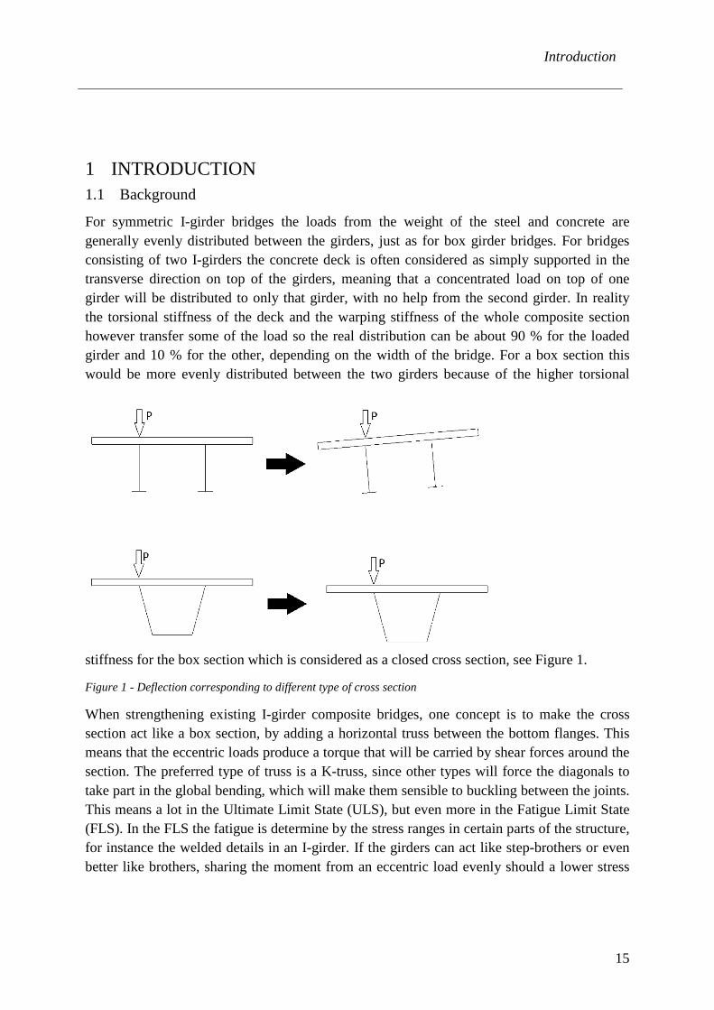
For symmetric I-girder bridges the loads from the weight of the steel and concrete are generally evenly distributed between the girders, just as for box girder bridges. For bridges consisting of two I-girders the concrete deck is often considered as simply supported in the transverse direction on top of the girders, meaning that a concentrated load on top of one girder will be distributed to only that girder, with no help from the second girder. In reality the torsional stiffness of the deck and the warping stiffness of the whole composite section however transfer some of the load so the real distribution can be about 90 % for the loaded girder and 10 % for the other, depending on the width of the bridge. For a box section this would be more evenly distributed between the two girders because of the higher torsional

stiffness for the box section which is considered as a closed cross section, see Figure 1.

Figure 1 - Deflection corresponding to different type of cross section

When strengthening existing I-girder composite bridges, one concept is to make the cross section act like a box section, by adding a horizontal truss between the bottom flanges. This means that the eccentric loads produce a torque that will be carried by shear forces around the section. The preferred type of truss is a K-truss, since other types will force the diagonals to take part in the global bending, which will make them sensible to buckling between the joints. This means a lot in the Ultimate Limit State (ULS), but even more in the Fatigue Limit State (FLS). In the FLS the fatigue is determine by the stress ranges in certain parts of the structure, for instance the welded details in an I-girder. If the girders can act like step-brothers or even better like brothers, sharing the moment from an eccentric load evenly should a lower stress

Introduction

16

range be achieved. The increased amount of load cycles that the bridge can withstand, with the new distribution between the girders (70/30) can be up to six times.

In this study it will be tested if a framework, (K-trusses) of Rectangular Hollow Shapes, RHS beams, at the bottom of the flanges, will lead to a more even distribution of the load between the I-girders. With an interaction of the I-girder from the framework of RHS beams the more evenly distributed load will hopefully give smaller fatigue stresses. With smaller stresses the lifetime of the bridge will be extended.

1.2 Aims and scopes

The aim of this thesis is to first gain knowledge of the foundations in the topic of fatigue in steel structures, mainly bridges. The theories need to be understood and implanted to the chosen structure.

The complexing of steel- and concrete composite bridges with steel-girder and concrete decks should be investigated, this to understand the basics to the substrate for design described in the Eurocode, EN

The main aim of this thesis is to investigate and if possible prove that a framework between two I-girders can provide higher torsional stiffness so that it acts more like a box-girder. If that is achieved, determine how much the life span of bridges can be extended by using the proposed method.

1.3 Methodology

To complete the thesis a literature study is made to get more knowledge in subject of torsion and the structural behaviour of a bridge according to theories and as described in the Eurocode, EN. Some FEM studies were necessary to get an understanding of the program and its behaviour of composite structures.

A FEM-analysis is used for verification and evaluation of the original and the strengthened structure considering forces, moments and lane factors where the effect of the strengthening can be evaluated.

Comparisons between models both in 2-D and 3-D, but also with different type of strengthening are made to determine the effect of that strengthening.

1.4 Limitations

This thesis is limited to multi-span steel concrete composite bridges with no inclination and radius. According to these criteria Bergeforsen Bridge is chosen for a case study. Only global effects are being analysed. The strengthening method, with bracings between the girders, is limited to one type (K-trusses) even X-trusses has been tested to verify the theory about global bending.

Introduction

17

1.5 Disposition of thesis

This thesis is divided into six chapters excluding the introduction. Following are some short summaries of the contents in each chapter.

Chapter 2 - Theory

This is a theory study performed to get the knowledge necessary to complete the aims. It is also important to be able to understand the fundamental theory behind the subject investigated. The chapter contains the history of fatigue and the Eurocodes interpretation of fatigue in structures/details and how it should be used.

Chapter 3 – Case Study

A description of the Bergeforsen Bridge used for the case study is described. Some introduction and evaluation of the modelling in the FEM-program SOFiSTiK is done. The concept bridge is designed to test the different elements and connections in the program. The theory of torsion is tested with the theory of fictive thickness in the concept design.

Chapter 4 - Calculation

Both hand- and FEM-calculations are presented here. From the hand-calculations the theory of torsion is applied to a composite cross section. The concept of fictive thickness is also applied for composite bridges. The structure and the loads from the FEM-analysis are described, like the size and where it’s applied.

Chapter 5 - Results

Results from the FEM-analysis are displayed here, such as the moment diagrams from different load cases and for the original- and strengthened bridge design. The stresses in the cross section due to the fatigue load model are explained and how cracks, due to negative moments near the internal supports are considered.

Chapter 6 - Analysis

An analysis of the results is presented here with investigations of stresses and stress ranges. The original calculation for the bridge was done in a 2-D model, which results are compared here with the results from the 3-D model in SOFiSTiK. Some analysis about the frame work and different cross section areas is also done. The difference between strengthened and unstrengthen is visualized with how the remaining lifetime will be effected by a reduction of the stress range.

Chapter 7 – Discussion and conclusions

In this chapter some attempts to answer the aims for the thesis from section 1.2 are made. Errors and confounding variables are discussed and evaluated. Furthermore, some suggestions of further research in the subject “strengthening of composite bridges" are listed. Both for the method studied in the thesis and for other previously tested methods around the world.

Theoretical Study

18

2 THEORETICAL STUDY 2.1 History

It is shown by experience that fractures of structure parts often are due to fatigue from regular service conditions, like traffic loads on bridges (Smith, 1990). The obstacle for the development by the industry has always been the integrity of the structures. Some consequences could be seen in the 19th century in the development of the railway transportation. A number of serious accidents happened due to fatigue of an axle, such as the Versailles train accident in 1842. The accident cost 60 people their lives. Another corresponding accident is the plane crashes of the Comet planes in 1954 (Smith, 1990).

The increasing number of papers about fatigue is reasonable because of the knowledge that the costs from fatigue damages of the GDP, Gross Domestic Product of engineering industry is several percent. About 2000 articles was written per year about fatigue between 1988 and 1993, so a total of 10.000 articles (Totoh, 2001).

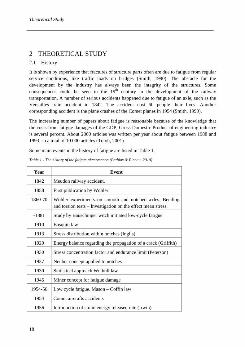
Some main events in the history of fatigue are listed in Table 1.

Table 1 - The history of the fatigue phenomenon (Bathias & Pineau, 2010)

Year Event

1842 Meudon railway accident.

1858 First publication by Wöhler

1860-70 Wöhler experiments on smooth and notched axles. Bending and torsion tests – Investigation on the effect mean stress.

-1881 Study by Bauschinger witch initiated low-cycle fatigue

1910 Basquin law

1913 Stress distribution within notches (Inglis)

1920 Energy balance regarding the propagation of a crack (Griffith)

1930 Stress concentration factor and endurance limit (Peterson)

1937 Neuber concept applied to notches

1939 Statistical approach Weibull law

1945 Miner concept for fatigue damage

1954-56 Low cycle fatigue. Mason – Coffin law

1954 Comet aircrafts accidents

1956 Introduction of strain energy released rate (Irwin)

Theoretical Study

19

1960 Servo hydraulic machines

1961 Paris law

1968 Introduction of effective stress intensity factor (Elber)

1988 Aloha B737 accident

1989 DC 10 Sioux City accident

1996 Pensacola accident

1998 ICE. Eschede railway accident

2006 Los Angeles B767 accident

2.2 Fatigue

“The process of initiation and propagation of cracks through a structural part due to action of fluctuating stress” (SS-EN 1993-1-9, 2005).

In the subject of fatigue some explanations are good to be defined for the understanding.

− Fatigue or fatigue damage is referring to the modification of the properties of materials due to the application of stress cycles whose repletion can lead to fracture.

− The amplitude of the maximum stress is the definition of uniaxial loading during a cycle, σmax.

− The stress ratio R is the ratio between the minimum stress, σmin and the maximum, σmax, so R=σmin/σmax (Bathias & Pineau, 2010).

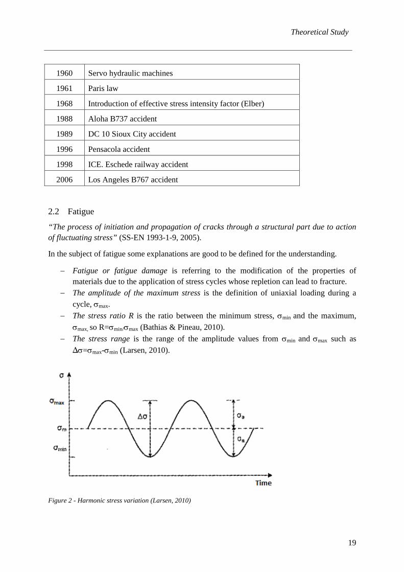
− The stress range is the range of the amplitude values from σmin and σmax such as Δσ=σmax-σmin (Larsen, 2010).

Figure 2 - Harmonic stress variation (Larsen, 2010)

Theoretical Study

20

Sometimes the alternative component (σa) have to be distinguished from the mean stress σm. These two components can with the relative values differentiate the tests under different stresses. This can be explained by:

− Fully reversed: σm=0, R=-1; − Asymmetrically reversed: 0<σm<σa, -1<R<0; − Repeated: R=0; − Alternating tension: σm>σa, 0<R<1.

These different states of fatigue stresses are shown in a stress-time diagram, see Figure 3.

Figure 3 - Stress states for harmonic stress history (Larsen, 2010)

One easy way to test a structure for fatigue is to load it periodically with a maximum amplitude at a constant frequency. The number of cycles is determined from the first time a rupture or disturbance on a structure occurs. A diagram can be achieved through the measured points for cycles and frequency. The diagram is then divided into four zones, as marked in Figure 4. This type of diagram is called a stress-number of cycle diagram, SN-curve or its more formal name Wöhler curve (Bathias & Pineau, 2010). The four zones in the figure are:

− Low cycle fatigue that can be achieved by high stresses. This zone gives fractures from low number cycles and with big amplitudes. The low cycle give a significant plastic deformation. Damage types like this has been studied for a long time by Manson and Coffin, who introduced the Coffin-Manson law (Bathias & Pineau, 2010).

− Monocycle fatigue is for lower stresses where the limit is the endurance. The fractures are initiated by a certain number of load cycles (Bathias & Pineau, 2010). The figure is showing that for lower stress amplitudes a higher number of cycles can be allowed before fractures occur.

− Endurance is region that is considered as an infinite lifetime of the steel or its safety region. In the figure this region starts around one million to 10 million cycles. In reality metals doesn’t have such a limit for endurance, which have made us to investigate the gigacycle fatigue (Bathias & Pineau, 2010).

Theoretical Study

21

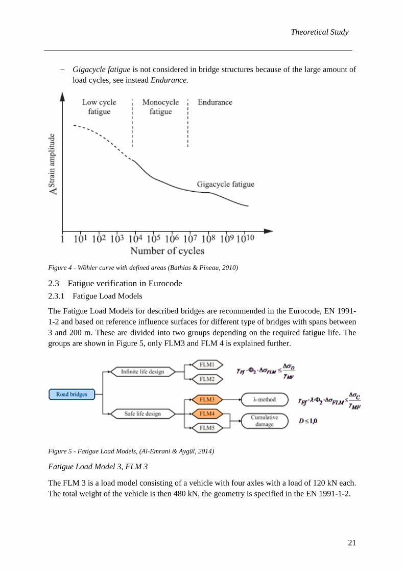
− Gigacycle fatigue is not considered in bridge structures because of the large amount of load cycles, see instead Endurance.

Figure 4 - Wöhler curve with defined areas (Bathias & Pineau, 2010)

2.3 Fatigue verification in Eurocode 2.3.1 Fatigue Load Models

The Fatigue Load Models for described bridges are recommended in the Eurocode, EN 1991-1-2 and based on reference influence surfaces for different type of bridges with spans between 3 and 200 m. These are divided into two groups depending on the required fatigue life. The groups are shown in Figure 5, only FLM3 and FLM 4 is explained further.

Figure 5 - Fatigue Load Models, (Al-Emrani & Aygül, 2014)

Fatigue Load Model 3, FLM 3

The FLM 3 is a load model consisting of a vehicle with four axles with a load of 120 kN each. The total weight of the vehicle is then 480 kN, the geometry is specified in the EN 1991-1-2.

Theoretical Study

22

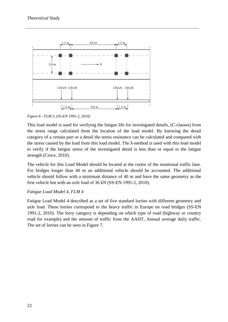
Figure 6 - FLM 3, (SS-EN 1991-2, 2010)

This load model is used for verifying the fatigue life for investigated details, (C-classes) from the stress range calculated from the location of the load model. By knowing the detail category of a certain part or a detail the stress resistance can be calculated and compared with the stress caused by the load from this load model. The λ-method is used with this load model to verify if the fatigue stress of the investigated detail is less than or equal to the fatigue strength (Croce, 2010).

The vehicle for this Load Model should be located at the centre of the notational traffic lane. For bridges longer than 40 m an additional vehicle should be accounted. The additional vehicle should follow with a minimum distance of 40 m and have the same geometry as the first vehicle but with an axle load of 36 kN (SS-EN 1991-2, 2010).

Fatigue Load Model 4, FLM 4

Fatigue Load Model 4 described as a set of five standard lorries with different geometry and axle load. These lorries correspond to the heavy traffic in Europe on road bridges (SS-EN 1991-2, 2010). The lorry category is depending on which type of road (highway or country road for example) and the amount of traffic from the AADT, Annual average daily traffic. The set of lorries can be seen in Figure 7.

Theoretical Study

23

Figure 7 - Set of lorries in FLM 4, (EN 1991-2, 2003)

The load model is recommended to be used with the Palmgren-Miner concept where it is intended to assemble stress ranges from the time-history analysis. The analysis is a cycle counting procedure where this FLM is mainly used (Al-Emrani & Aygül, 2014).

For both FLM 3 and FLM 4 it’s needed to specify the number of cycles to be able to do the fatigue verification. For road bridges the number of cycles is expressed as a traffic category. Four traffic categories are proposed with an extra category for AADT bigger than 24000, where a certain investigation has to be done of the prerequisites for the fatigue design (Al-Emrani & Aygül, 2014).

Theoretical Study

24

Table 2 - Traffic categories, (Trafikverket, 2011)

Traffic category AADT heavy traffic (ÅDT)

X <24000

1 6000≤AADT≤24000

2 1500≤AADT≤6000

3 600≤AADT≤1500

4 ≤600 2.3.2 Damage Accumulation Method

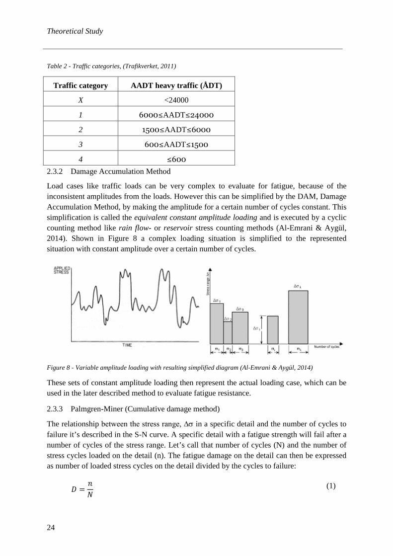
Load cases like traffic loads can be very complex to evaluate for fatigue, because of the inconsistent amplitudes from the loads. However this can be simplified by the DAM, Damage Accumulation Method, by making the amplitude for a certain number of cycles constant. This simplification is called the equivalent constant amplitude loading and is executed by a cyclic counting method like rain flow- or reservoir stress counting methods (Al-Emrani & Aygül, 2014). Shown in Figure 8 a complex loading situation is simplified to the represented situation with constant amplitude over a certain number of cycles.

Figure 8 - Variable amplitude loading with resulting simplified diagram (Al-Emrani & Aygül, 2014)

These sets of constant amplitude loading then represent the actual loading case, which can be used in the later described method to evaluate fatigue resistance.

2.3.3 Palmgren-Miner (Cumulative damage method)

The relationship between the stress range, ∆σ in a specific detail and the number of cycles to failure it’s described in the S-N curve. A specific detail with a fatigue strength will fail after a number of cycles of the stress range. Let’s call that number of cycles (N) and the number of stress cycles loaded on the detail (n). The fatigue damage on the detail can then be expressed as number of loaded stress cycles on the detail divided by the cycles to failure:

𝐷𝐷 =𝑛𝑛𝑁𝑁

(1)

Theoretical Study

25

This relationship describes how much a detail is utilized due to the fatigue damage such as:

𝐷𝐷 = 1,0 𝑤𝑤ℎ𝑒𝑒𝑛𝑛 𝑛𝑛 = 𝑁𝑁

𝐷𝐷 < 1,0 𝑤𝑤ℎ𝑒𝑒𝑛𝑛 𝑛𝑛 < 𝑁𝑁

If one loading cycle is called a block, it would mean that a detail could be subjected to a number of loading blocks ni with a constant amplitude stress ∆σi repeatedly (Al-Emrani & Aygül, 2014). The sum of all these loading blocks on the detail are therefore the total damage as:

𝐷𝐷 = �𝑛𝑛𝑖𝑖𝑁𝑁𝑖𝑖𝑖𝑖

(2)

2.3.4 Lambda-coefficient method

This method is a simplified method which uses the stress range, ∆σ to compare it to the detail category. The fatigue damage occur by the stress range ∆σE or as described in the EN like the equivalent stress range for 2 million cycles. The stress range is then called the fatigue strength (Al-Emrani & Aygül, 2014). The method is earlier implanted from the railway bridges but can be used for road bridges as well (Al-Emrani & Aygül, 2014).

It’s taken into account the different fatigue variations in the structure and applies these with an equivalent factor to control the fatigue resistance, like the stress range.

The fatigue resistance can then be compared to the stress range for the detail. To get the maximum stress range the chosen FLM is used, and the expression for the fatigue verification can be expressed as:

𝛾𝛾𝐹𝐹𝐹𝐹 = 𝜆𝜆 ∗ Φ2 ∗ ∆𝜎𝜎𝐹𝐹𝐹𝐹𝐹𝐹 ≤∆𝜎𝜎𝐶𝐶𝛾𝛾𝐹𝐹𝐹𝐹

(3)

where

γFf is the partial safety factor for fatigue

γMF is the partial safety factor for fatigue resistance

λ is the fatigue damage equivalent factor

Φ2 is the dynamic factor

ΔσFLM is the stress range due to the FLM

ΔσC is the reference stress range value of the fatigue strength

The damage equivalent factor ℷ is depending on four independent factors, λ1, λ2, λ3, λ4 and limited to λmax such as

Theoretical Study

26

𝜆𝜆 = 𝜆𝜆1 ∗ 𝜆𝜆2 ∗ 𝜆𝜆3 ∗ 𝜆𝜆4; 𝜆𝜆 ≤ 𝜆𝜆𝑚𝑚𝑚𝑚𝑚𝑚 (4)

The factors describe the traffic on a bridge in individual ways like the design life and the traffic volume. Following is described how to evaluate and calculate these factors.

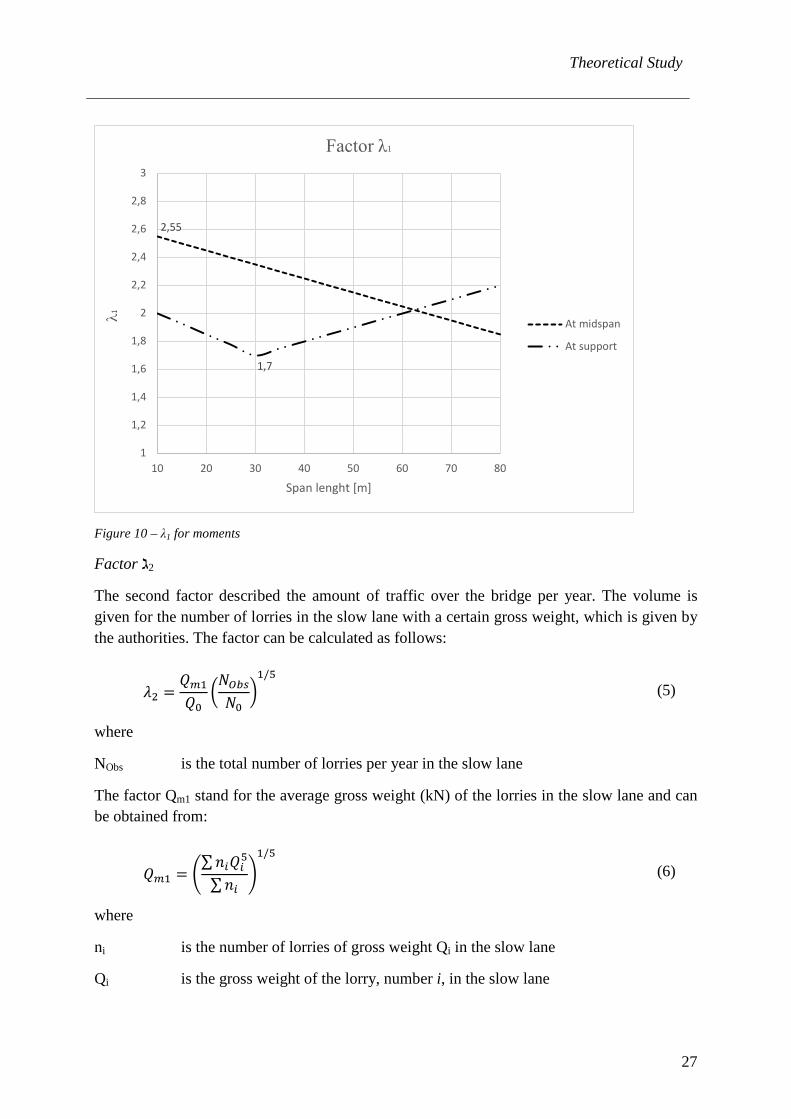
Factor ℷ1

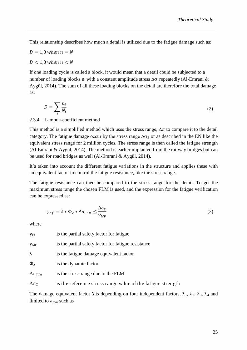
This factor describes the damage effect of traffic and depends on the length of the critical influence line or area. Depending on which maximum the bridge has it differs, like for a maximum moment the length Li is determined. The length is determined from the spans, so it is not the same for a simply supported span as it is for a bridge with more spans. The spans should be between 10 to 80 meters but for longer spans it’s accepted to do a linear extrapolation (Al-Emrani & Aygül, 2014). The Figure 9 shows how the span length can be determined.

Figure 9 - Location of mid-span- and support section

So for simply supported spans it’s the whole span length, in this case L1. For continuous spans in midsection it’s Li of the span under consideration and in support sections the Li and Lj adjacent to that support. Some special case is also considerate, for cross girder supporting stingers there the sum of the critical length of the influence is the sum of the two adjacent spans of the stiffeners carried by the cross girder.

When shear gives the maximum value the critical length can be described as the span length under consideration of the support section and 40 % of the span length for mid-span sections. Some regulations considering arch bridges can be described as well, but will not be part of this study (Al-Emrani & Aygül, 2014).

After the critical length has been defined the value for the factor can be found in Figure 10 depending on which of the span that has been evaluated.

Theoretical Study

27

Figure 10 – λ1 for moments

Factor ℷ2

The second factor described the amount of traffic over the bridge per year. The volume is given for the number of lorries in the slow lane with a certain gross weight, which is given by the authorities. The factor can be calculated as follows:

𝜆𝜆2 =

𝑄𝑄𝑚𝑚1𝑄𝑄0

�𝑁𝑁𝑂𝑂𝑂𝑂𝑂𝑂𝑁𝑁0

�1/5

(5)

where

NObs is the total number of lorries per year in the slow lane

The factor Qm1 stand for the average gross weight (kN) of the lorries in the slow lane and can be obtained from:

𝑄𝑄𝑚𝑚1 = �

∑𝑛𝑛𝑖𝑖𝑄𝑄𝑖𝑖5

∑ 𝑛𝑛𝑖𝑖�1/5

(6)

where

ni is the number of lorries of gross weight Qi in the slow lane

Qi is the gross weight of the lorry, number i, in the slow lane

2,55

1,7

1

1,2

1,4

1,6

1,8

2

2,2

2,4

2,6

2,8

3

10 20 30 40 50 60 70 80

Span lenght [m]

Factor λ1

At midspan

At support

Theoretical Study

28

The factors Q0 and N0 are given as values of the reference traffic of the equivalent weight respectively the annual number of lorries. These values are:

𝑄𝑄0 = 480 𝑘𝑘𝑁𝑁 (7)

𝑁𝑁0 = 0,5 ∗ 106 𝑙𝑙𝑙𝑙𝑙𝑙𝑙𝑙𝑙𝑙𝑒𝑒𝑙𝑙 (8)

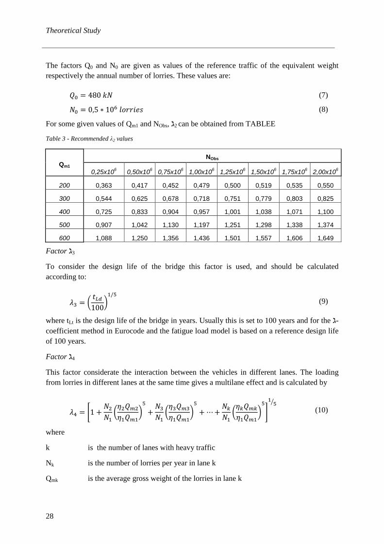
For some given values of Qm1 and NObs, ℷ2 can be obtained from TABLEE

Table 3 - Recommended λ2 values

Qm1 NObs

0,25x106 0,50x106 0,75x106 1,00x106 1,25x106 1,50x106 1,75x106 2,00x106

200 0,363 0,417 0,452 0,479 0,500 0,519 0,535 0,550

300 0,544 0,625 0,678 0,718 0,751 0,779 0,803 0,825

400 0,725 0,833 0,904 0,957 1,001 1,038 1,071 1,100

500 0,907 1,042 1,130 1,197 1,251 1,298 1,338 1,374

600 1,088 1,250 1,356 1,436 1,501 1,557 1,606 1,649

Factor ℷ3

To consider the design life of the bridge this factor is used, and should be calculated according to:

𝜆𝜆3 = �

𝑡𝑡𝐹𝐹𝐿𝐿100

�1/5

(9)

where tLt is the design life of the bridge in years. Usually this is set to 100 years and for the ℷ-coefficient method in Eurocode and the fatigue load model is based on a reference design life of 100 years.

Factor ℷ4

This factor considerate the interaction between the vehicles in different lanes. The loading from lorries in different lanes at the same time gives a multilane effect and is calculated by

𝜆𝜆4 = �1 +

𝑁𝑁2𝑁𝑁1

�𝜂𝜂2𝑄𝑄𝑚𝑚2𝜂𝜂1𝑄𝑄𝑚𝑚1

�5

+𝑁𝑁3𝑁𝑁1

�𝜂𝜂3𝑄𝑄𝑚𝑚3𝜂𝜂1𝑄𝑄𝑚𝑚1

�5

+ ⋯+𝑁𝑁𝑘𝑘𝑁𝑁1

�𝜂𝜂𝑘𝑘𝑄𝑄𝑚𝑚𝑘𝑘𝜂𝜂1𝑄𝑄𝑚𝑚1

�5

�

15�

(10)

where

k is the number of lanes with heavy traffic

Nk is the number of lorries per year in lane k

Qmk is the average gross weight of the lorries in lane k

Theoretical Study

29

ηk is the value of the influence line for the internal force that produces the stress range in the middle of lane k to be inserted in the equation with positive sign.

Factor λmax

The maximum value of the λ-factor is defined for the section subjected to the fatigue stresses caused by bending moment. This because of the shear effects in the S-N curves doesn’t have defined constant amplitude fatigue limit. Similar to the first factor λ1 the maximum value is depended on the span length and the detail under consideration of the bridge. In Figure 11 the maximum value can be determined from the span length.

-

Figure 11 – λmax for sections subjected to bending stresses

2.3.5 C-classes

To determine the fatigue resistance the detail, with a certain geometry and stress distribution due to the configuration and material effects must be evaluated (Larsen, 2010). This evaluation has been categorized in the EN, (Detail categories, Dc) from practical experiments and some of the main groups of details in bridges are here listed and explained.

− Plain members [Dc 100-160] - This category has high fatigue resistance (SS-EN 1993-1-9, 2005).

− Mechanically fastened joints [Dc -100] – Cracking from fatigue initiates around holes at the loading plate or in the base material. The bolts used for this connections has a lower category number (SS-EN 1993-1-9, 2005).

2,5

1,0

1,2

1,4

1,6

1,8

2,0

2,2

2,4

2,6

2,8

3,0

10 20 30 40 50 60 70 80

λ max

Span lenght [m]

Maximum value, λmax

At midspan

At support

Theoretical Study

30

− Bolts [Dc 50] – Bolts in tension are extremely sensitive to fatigue loads due to the stress amplitudes. To achieve a higher resistance it’s common to pre-stress the bolts to reduce the stress range (Larsen, 2010).

− Welded built-up sections [Dc 100-125] – Details in this category can be welded I-, box sections and plates with longitudinal butt welds. These welds only take loads from shear forces which leads to shear stresses. Shear stresses is the initial point for fatigue cracks and it usually is at sections where the welding has been started or interrupted. Therefore the details with intermittent longitudinal welds are in a lower category (SS-EN 1993-1-9, 2005).

− Transverse butt welds [Dc, depending on the welds] – The categorization for this category is mainly dependent on the configuration of the weld. For higher categorization it is needed to have good quality of the welds and that it’s simple to execute. In addition to that it is important to have small stress concentrations in the weld (SS-EN 1993-1-9, 2005).

− Weld attachments and stiffeners [Dc 40-90] – This are common details in bridges where e.g. shear studs and web stiffeners are used. It is also common to have these type of details in the installation phase of a structure when details for lifting is welded to the structure (Larsen, 2010).

− Load carrying welded joints [Dc 50-80] – The fatigue cracks initiate at the weld toe and continue into to the plate (Larsen, 2010).

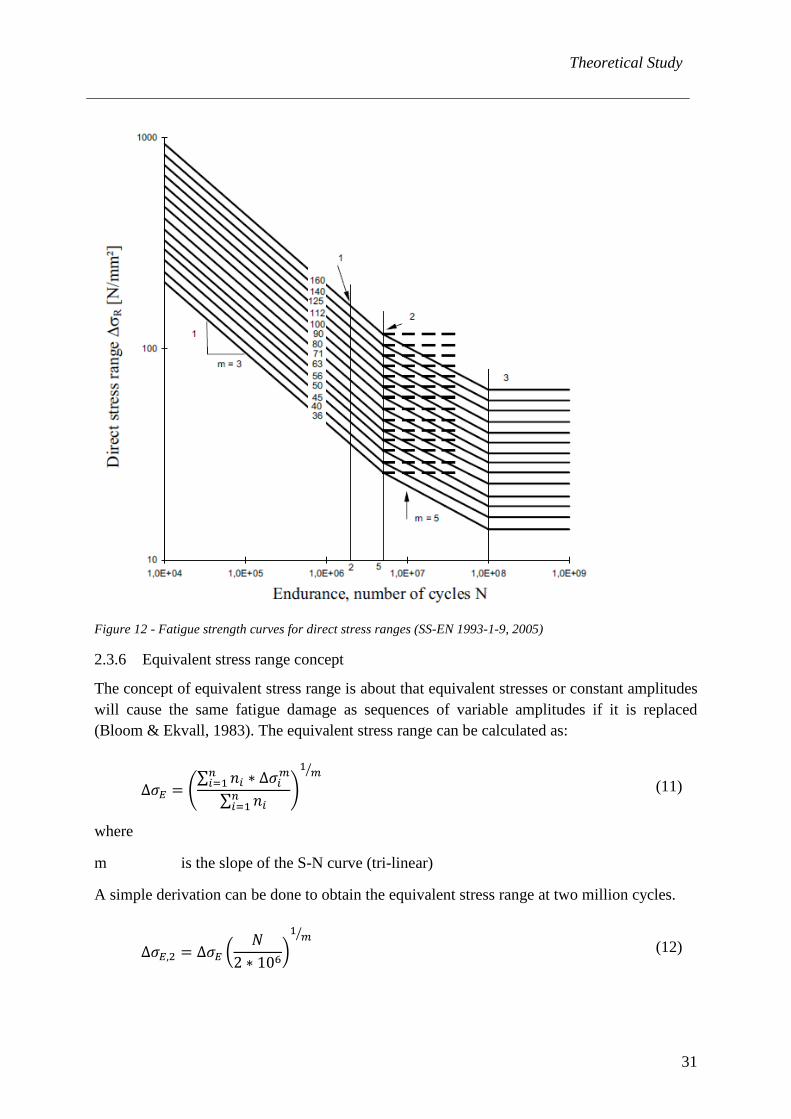
By knowing the Detail class and the number of cycles the direct stress range can be determine, see Figure 12. The curve is divided into three section as the number in top of the figure indicates as:

1. ∆σC - Detail category (up to two million cycles) 2. ∆σD - Constant amplitude fatigue limit (at five million cycles) 3. ∆σL - Cut-off limit (at 100 million cycles)

Theoretical Study

31

Figure 12 - Fatigue strength curves for direct stress ranges (SS-EN 1993-1-9, 2005)

2.3.6 Equivalent stress range concept

The concept of equivalent stress range is about that equivalent stresses or constant amplitudes will cause the same fatigue damage as sequences of variable amplitudes if it is replaced (Bloom & Ekvall, 1983). The equivalent stress range can be calculated as:

∆𝜎𝜎𝐸𝐸 = �

∑ 𝑛𝑛𝑖𝑖 ∗ ∆𝜎𝜎𝑖𝑖𝑚𝑚𝑛𝑛𝑖𝑖=1∑ 𝑛𝑛𝑖𝑖𝑛𝑛𝑖𝑖=1

�1 𝑚𝑚�

(11)

where

m is the slope of the S-N curve (tri-linear)

A simple derivation can be done to obtain the equivalent stress range at two million cycles.

∆𝜎𝜎𝐸𝐸,2 = ∆𝜎𝜎𝐸𝐸 �

𝑁𝑁2 ∗ 106

�1 𝑚𝑚�

(12)

Theoretical Study

32

With this stress range it is possible to compare the fatigue strength of a detail (Al-Emrani & Aygül, 2014) as:

∆𝜎𝜎𝐸𝐸,2 ≤ ∆σ𝐶𝐶 (13) 2.4 I-girder

A girder bridge is one of the most common bridge types and has been used for millennia. A log across a stream can be called a girder bridge (INTI, 2012). A girder bridge can be divided into two types, rolled steel girder and plate girder. The rolled steel girder is created by rolling a steel blank to create a desired shape, which means that a standardization of these types exists. Plate girders are fabricated by welding plates with different or same dimensions together, for an I-girder three plates are needed to create the girder. These parts of the girder is called top flange, bottom flange and web, see Figure 13.

Figure 13 - Plate welded I-girder (SteelConstruction.info, 2015)

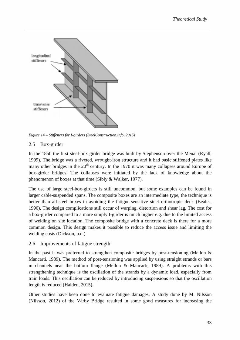
The plate welded girder is usually used for bridges because of its flexibility in dimensions and shape. One problem for girders with very high webs is that they are sensible for buckling. One way to solve this problem is to introduce stiffeners on the web, this by welding longitudinal and/or transverse stiffeners to the web (Collings, 2005).

Theoretical Study

33

Figure 14 – Stiffeners for I-girders (SteelConstruction.info, 2015)

2.5 Box-girder

In the 1850 the first steel-box girder bridge was built by Stephenson over the Menai (Ryall, 1999). The bridge was a riveted, wrought-iron structure and it had basic stiffened plates like many other bridges in the 20th century. In the 1970 it was many collapses around Europe of box-girder bridges. The collapses were initiated by the lack of knowledge about the phenomenon of boxes at that time (Sibly & Walker, 1977).

The use of large steel-box-girders is still uncommon, but some examples can be found in larger cable-suspended spans. The composite boxes are an intermediate type, the technique is better than all-steel boxes in avoiding the fatigue-sensitive steel orthotropic deck (Beales, 1990). The design complications still occur of warping, distortion and shear lag. The cost for a box-girder compared to a more simply I-girder is much higher e.g. due to the limited access of welding on site location. The composite bridge with a concrete deck is there for a more common design. This design makes it possible to reduce the access issue and limiting the welding costs (Dickson, u.d.)

2.6 Improvements of fatigue strength

In the past it was preferred to strengthen composite bridges by post-tensioning (Mellon & Mancarti, 1989). The method of post-tensioning was applied by using straight strands or bars in channels near the bottom flange (Mellon & Mancarti, 1989). A problems with this strengthening technique is the oscillation of the strands by a dynamic load, especially from train loads. This oscillation can be reduced by introducing suspensions so that the oscillation length is reduced (Halden, 2015).

Other studies have been done to evaluate fatigue damages. A study done by M. Nilsson (Nilsson, 2012) of the Vårby Bridge resulted in some good measures for increasing the

Theoretical Study

34

fatigue life of a bridge. One simple method to enhance the fatigue strength in welds between flanges and stiffeners is to use butt welds rather than fillet welds (Nilsson, 2012). According to the study the fatigue life of the weld is extended by a factor eight (Nilsson, 2012). Some other suggestions are also proposed, such as elimination of stress concentrations by considering a soft transition between stiffeners and flanges (Nilsson, 2012).

Another study have been done concerning the same issues with torsional stiffness of I-girder bridges as in this thesis but not as a post strengthening method. The study proved that lateral bracings, or as called in this thesis (horizontal framework) between lower flanges will improve the torsional stiffness (Adamakos, et al., 2011). Calculations were done both in a grid-model and in a FEM-model and both models gave the same results with very small differences in results. The bridge tested in the analysis was a steel concrete composite bridge with three I-girders and a concrete deck and it was straight and simple supported in one span (Adamakos, et al., 2011). The introduction of lateral bracings (horizontal framework) between the lower flanges led to a reduction of the stresses in the outer girder by 25 % (according to the FEM-results), (Adamakos, et al., 2011). They describe the new load distribution between the girders and the reduction of deformation in the outer girder like: “The load distribution changes and the whole bridge behaves in a way close to a box section bridge. At the same time, the maximum deformation of the extreme girder reduces significantly”, (Adamakos, et al., 2011).

2.7 Torsion and Warping

Both torsion and warping with their theories will be explained in this chapter. Some steps in the calculations have been reduced, but the steps should not be so hard to follow.

Torsion -

A beam with constant cross section and with torque at the beam ends like in Figure 15 is considered.

Theoretical Study

35

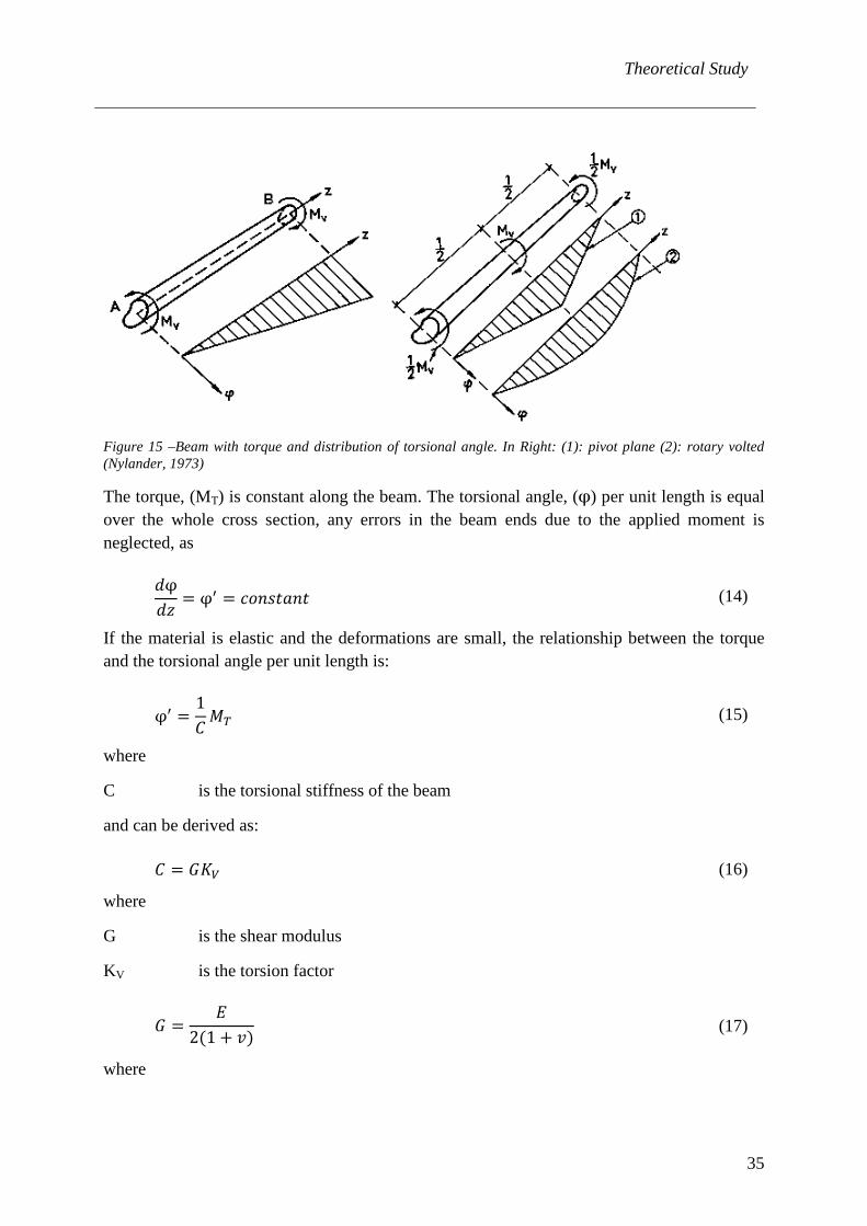
Figure 15 –Beam with torque and distribution of torsional angle. In Right: (1): pivot plane (2): rotary volted (Nylander, 1973)

The torque, (MT) is constant along the beam. The torsional angle, (φ) per unit length is equal over the whole cross section, any errors in the beam ends due to the applied moment is neglected, as

𝑑𝑑φ𝑑𝑑𝑑𝑑

= φ′ = 𝑐𝑐𝑙𝑙𝑛𝑛𝑙𝑙𝑡𝑡𝑐𝑐𝑛𝑛𝑡𝑡 (14)

If the material is elastic and the deformations are small, the relationship between the torque and the torsional angle per unit length is:

φ′ =1𝐶𝐶𝑀𝑀𝑇𝑇 (15)

where

C is the torsional stiffness of the beam

and can be derived as:

𝐶𝐶 = 𝐺𝐺𝐾𝐾𝑉𝑉 (16)

where

G is the shear modulus

KV is the torsion factor

𝐺𝐺 =𝐸𝐸

2(1 + 𝑣𝑣) (17)

where

Theoretical Study

36

ν is the Poisson’s ratio for the material

From these expressions the relationship for the torsion factor can be described as:

𝐾𝐾𝑉𝑉 =𝑀𝑀𝑇𝑇

𝐺𝐺φ′ (18)

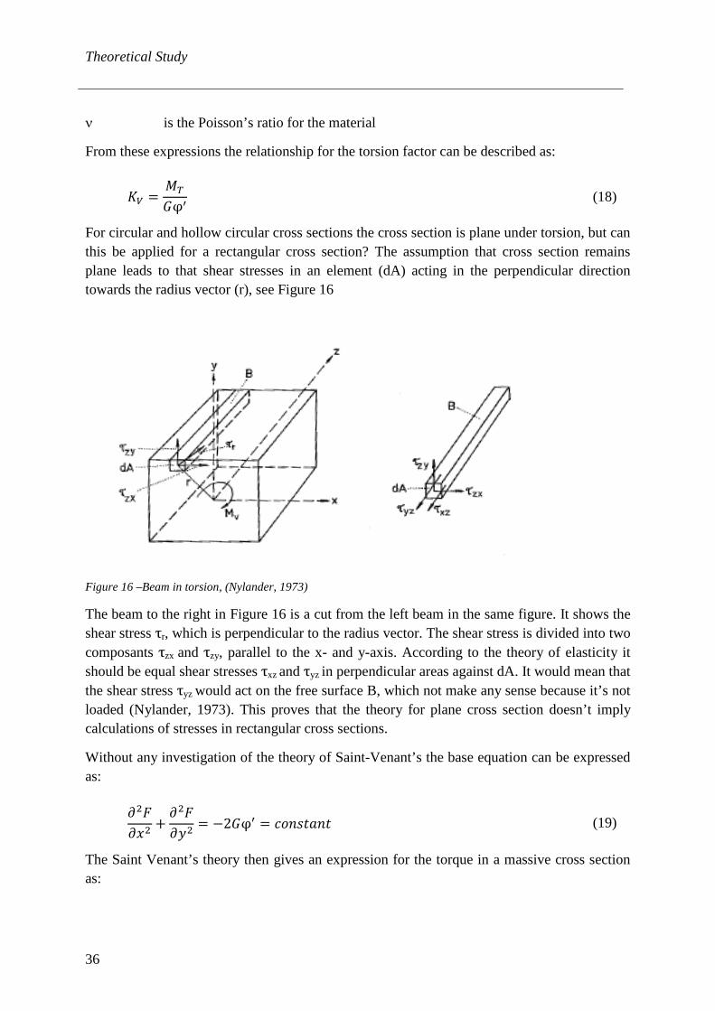
For circular and hollow circular cross sections the cross section is plane under torsion, but can this be applied for a rectangular cross section? The assumption that cross section remains plane leads to that shear stresses in an element (dA) acting in the perpendicular direction towards the radius vector (r), see Figure 16

Figure 16 –Beam in torsion, (Nylander, 1973)

The beam to the right in Figure 16 is a cut from the left beam in the same figure. It shows the shear stress τr, which is perpendicular to the radius vector. The shear stress is divided into two composants τzx and τzy, parallel to the x- and y-axis. According to the theory of elasticity it should be equal shear stresses τxz and τyz in perpendicular areas against dA. It would mean that the shear stress τyz would act on the free surface B, which not make any sense because it’s not loaded (Nylander, 1973). This proves that the theory for plane cross section doesn’t imply calculations of stresses in rectangular cross sections.

Without any investigation of the theory of Saint-Venant’s the base equation can be expressed as:

𝜕𝜕2𝐹𝐹𝜕𝜕𝑥𝑥2

+𝜕𝜕2𝐹𝐹𝜕𝜕𝑦𝑦2

= −2𝐺𝐺φ′ = 𝑐𝑐𝑙𝑙𝑛𝑛𝑙𝑙𝑡𝑡𝑐𝑐𝑛𝑛𝑡𝑡 (19)

The Saint Venant’s theory then gives an expression for the torque in a massive cross section as:

Theoretical Study

37

𝑀𝑀𝑇𝑇 = �� �𝜏𝜏𝑧𝑧𝑧𝑧𝑥𝑥 − 𝜏𝜏𝑧𝑧𝑚𝑚𝑦𝑦�𝑑𝑑𝑥𝑥𝑑𝑑𝑦𝑦𝐴𝐴

(20)

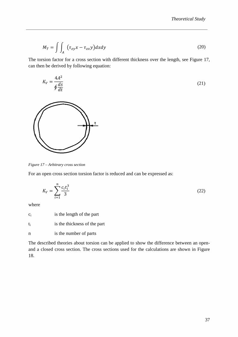
The torsion factor for a cross section with different thickness over the length, see Figure 17, can then be derived by following equation:

𝐾𝐾𝑉𝑉 =

4𝐴𝐴2

∮𝑑𝑑𝑙𝑙𝑑𝑑𝑡𝑡

(21)

Figure 17 – Arbitrary cross section

For an open cross section torsion factor is reduced and can be expressed as:

𝐾𝐾𝑉𝑉 = �

𝑐𝑐𝑖𝑖𝑡𝑡𝑖𝑖3

3

𝑛𝑛

𝑖𝑖=1

(22)

where

ci is the length of the part

ti is the thickness of the part

n is the number of parts

The described theories about torsion can be applied to show the difference between an open- and a closed cross section. The cross sections used for the calculations are shown in Figure 18.

Theoretical Study

38

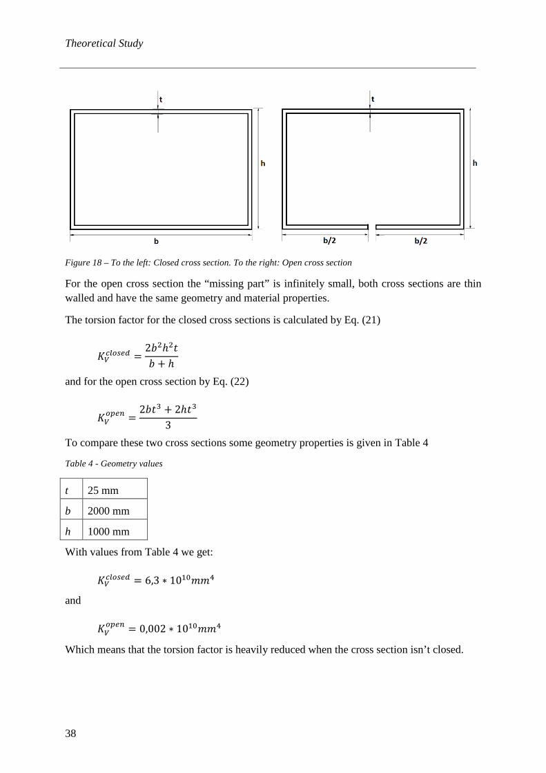
Figure 18 – To the left: Closed cross section. To the right: Open cross section

For the open cross section the “missing part” is infinitely small, both cross sections are thin walled and have the same geometry and material properties.

The torsion factor for the closed cross sections is calculated by Eq. (21)

𝐾𝐾𝑉𝑉𝑐𝑐𝑐𝑐𝑐𝑐𝑂𝑂𝑐𝑐𝐿𝐿 =

2𝑏𝑏2ℎ2𝑡𝑡𝑏𝑏 + ℎ

and for the open cross section by Eq. (22)

𝐾𝐾𝑉𝑉𝑐𝑐𝑜𝑜𝑐𝑐𝑛𝑛 =

2𝑏𝑏𝑡𝑡3 + 2ℎ𝑡𝑡3

3

To compare these two cross sections some geometry properties is given in Table 4

Table 4 - Geometry values

t 25 mm

b 2000 mm

h 1000 mm

With values from Table 4 we get:

𝐾𝐾𝑉𝑉𝑐𝑐𝑐𝑐𝑐𝑐𝑂𝑂𝑐𝑐𝐿𝐿 = 6,3 ∗ 1010𝑚𝑚𝑚𝑚4

and

𝐾𝐾𝑉𝑉𝑐𝑐𝑜𝑜𝑐𝑐𝑛𝑛 = 0,002 ∗ 1010𝑚𝑚𝑚𝑚4

Which means that the torsion factor is heavily reduced when the cross section isn’t closed.

Theoretical Study

39

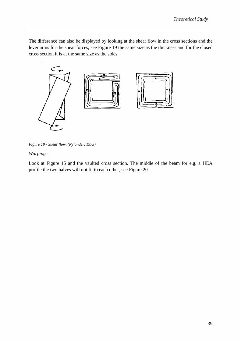
The difference can also be displayed by looking at the shear flow in the cross sections and the lever arms for the shear forces, see Figure 19 the same size as the thickness and for the closed cross section it is at the same size as the sides.

Figure 19 - Shear flow, (Nylander, 1973)

Warping -

Look at Figure 15 and the vaulted cross section. The middle of the beam for e.g. a HEA profile the two halves will not fit to each other, see Figure 20.

Theoretical Study

40

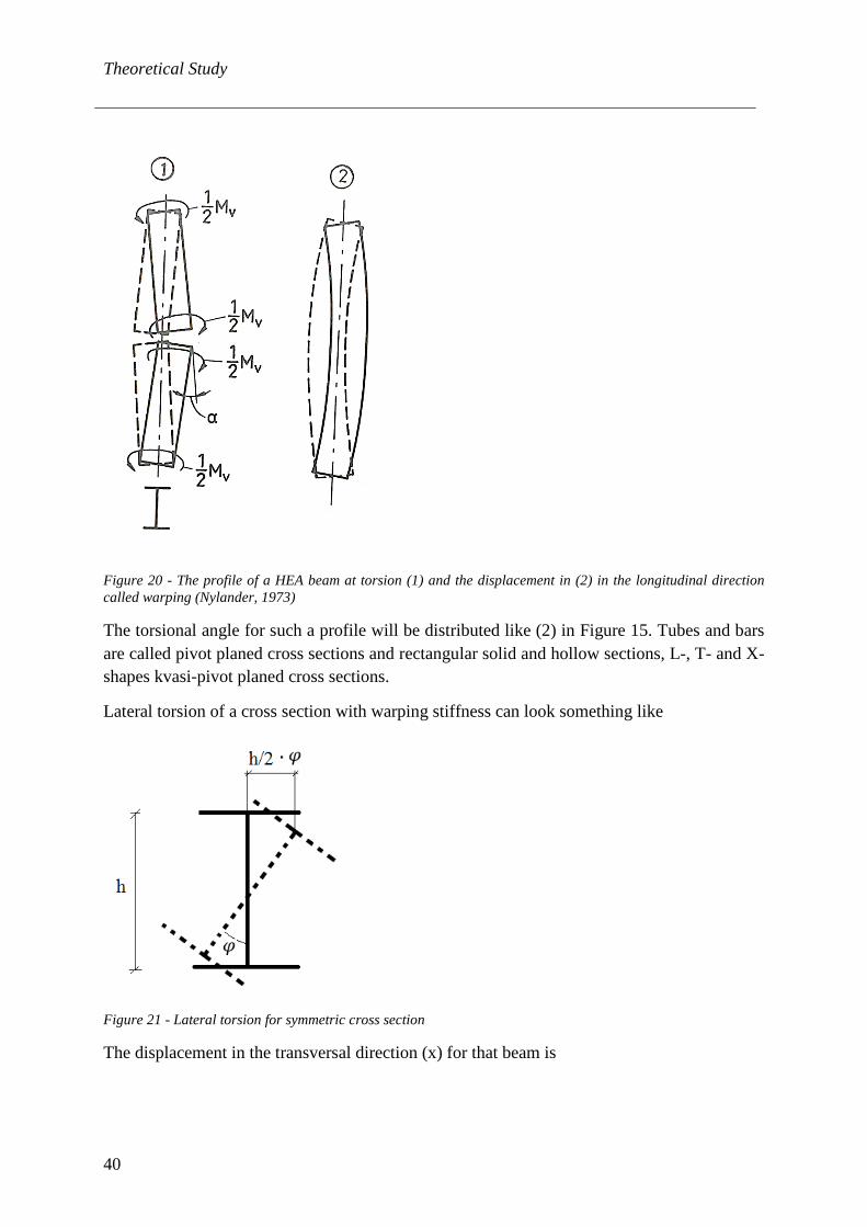
Figure 20 - The profile of a HEA beam at torsion (1) and the displacement in (2) in the longitudinal direction called warping (Nylander, 1973)

The torsional angle for such a profile will be distributed like (2) in Figure 15. Tubes and bars are called pivot planed cross sections and rectangular solid and hollow sections, L-, T- and X-shapes kvasi-pivot planed cross sections.

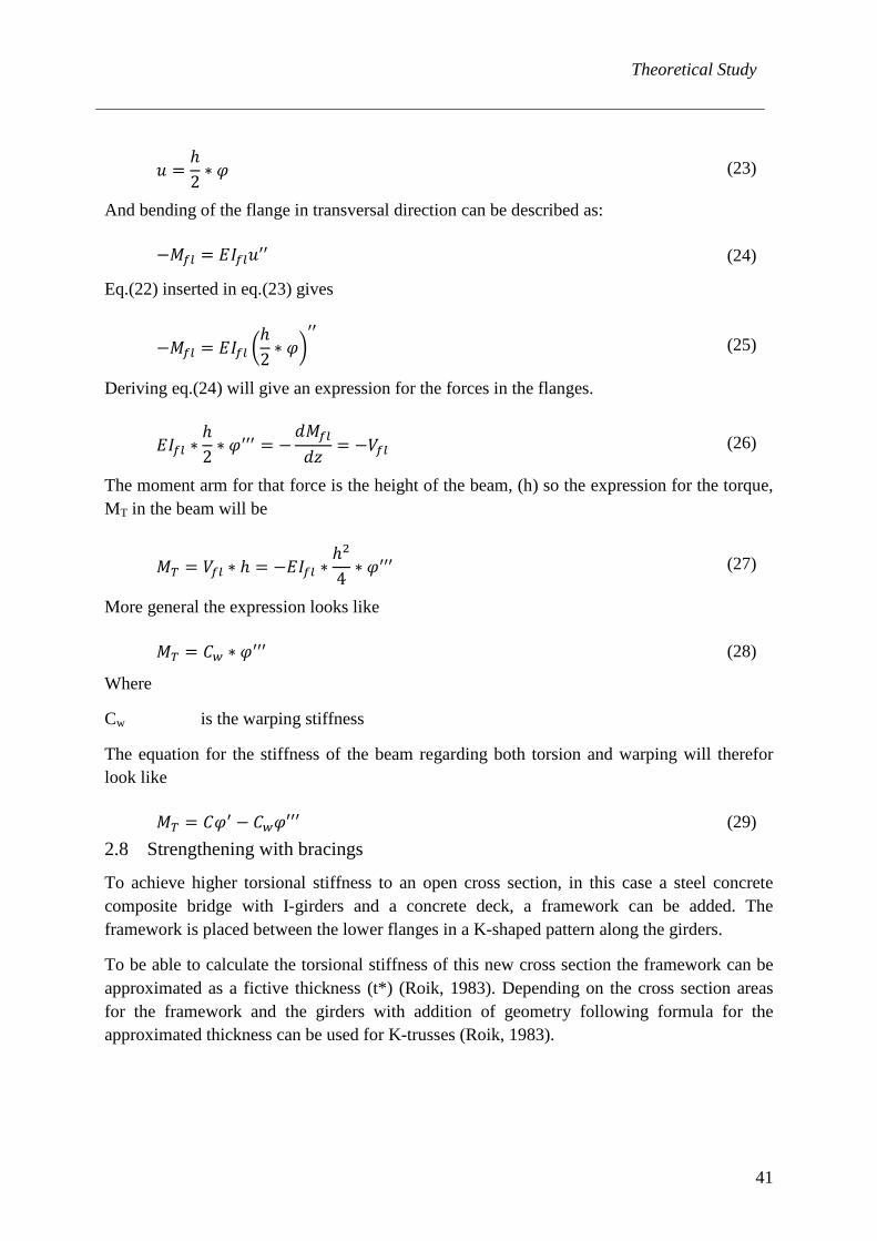
Lateral torsion of a cross section with warping stiffness can look something like

Figure 21 - Lateral torsion for symmetric cross section

The displacement in the transversal direction (x) for that beam is

Theoretical Study

41

𝑢𝑢 =

ℎ2∗ 𝜑𝜑 (23)

And bending of the flange in transversal direction can be described as:

−𝑀𝑀𝐹𝐹𝑐𝑐 = 𝐸𝐸𝐼𝐼𝐹𝐹𝑐𝑐𝑢𝑢′′ (24)

Eq.(22) inserted in eq.(23) gives

−𝑀𝑀𝐹𝐹𝑐𝑐 = 𝐸𝐸𝐼𝐼𝐹𝐹𝑐𝑐 �

ℎ2∗ 𝜑𝜑�

′′

(25)

Deriving eq.(24) will give an expression for the forces in the flanges.

𝐸𝐸𝐼𝐼𝐹𝐹𝑐𝑐 ∗

ℎ2∗ 𝜑𝜑′′′ = −

𝑑𝑑𝑀𝑀𝐹𝐹𝑐𝑐

𝑑𝑑𝑑𝑑= −𝑉𝑉𝐹𝐹𝑐𝑐 (26)

The moment arm for that force is the height of the beam, (h) so the expression for the torque, MT in the beam will be

𝑀𝑀𝑇𝑇 = 𝑉𝑉𝐹𝐹𝑐𝑐 ∗ ℎ = −𝐸𝐸𝐼𝐼𝐹𝐹𝑐𝑐 ∗

ℎ2

4∗ 𝜑𝜑′′′ (27)

More general the expression looks like

𝑀𝑀𝑇𝑇 = 𝐶𝐶𝑤𝑤 ∗ 𝜑𝜑′′′ (28)

Where

Cw is the warping stiffness

The equation for the stiffness of the beam regarding both torsion and warping will therefor look like

𝑀𝑀𝑇𝑇 = 𝐶𝐶𝜑𝜑′ − 𝐶𝐶𝑤𝑤𝜑𝜑′′′ (29) 2.8 Strengthening with bracings

To achieve higher torsional stiffness to an open cross section, in this case a steel concrete composite bridge with I-girders and a concrete deck, a framework can be added. The framework is placed between the lower flanges in a K-shaped pattern along the girders.

To be able to calculate the torsional stiffness of this new cross section the framework can be approximated as a fictive thickness (t*) (Roik, 1983). Depending on the cross section areas for the framework and the girders with addition of geometry following formula for the approximated thickness can be used for K-trusses (Roik, 1983).

Theoretical Study

42

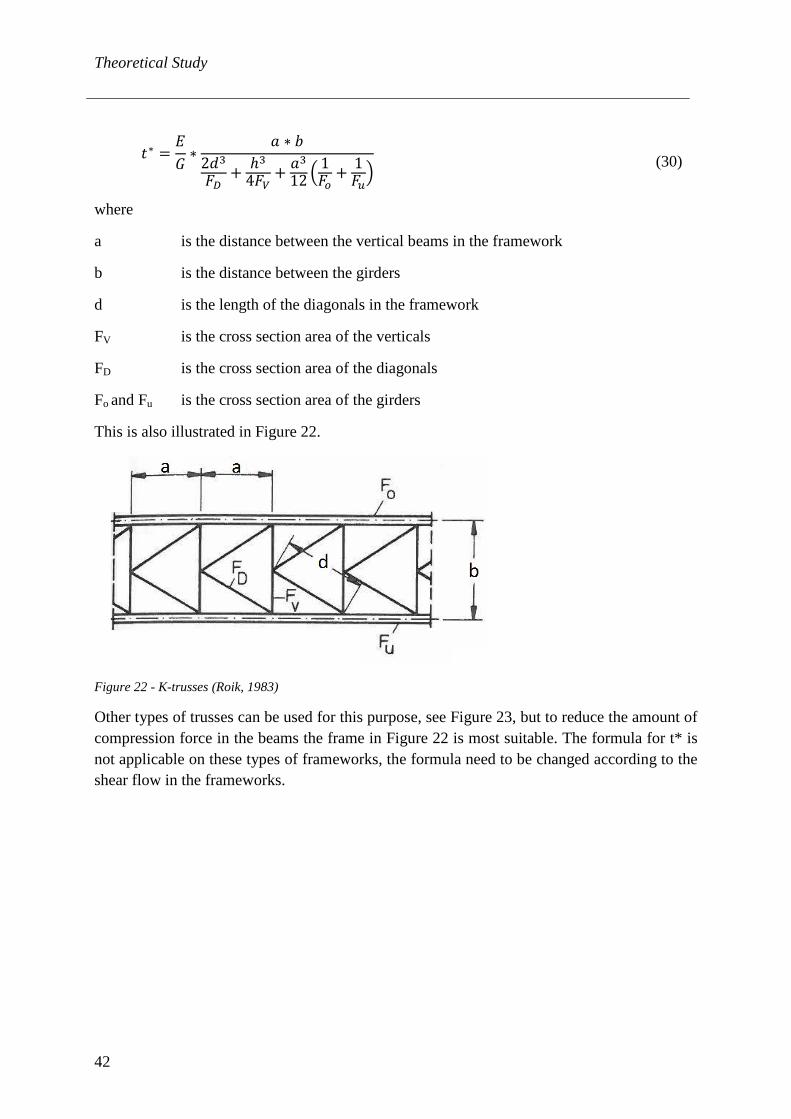
𝑡𝑡∗ =

𝐸𝐸𝐺𝐺∗

𝑐𝑐 ∗ 𝑏𝑏2𝑑𝑑3𝐹𝐹𝐷𝐷

+ ℎ34𝐹𝐹𝑉𝑉

+ 𝑐𝑐312 �

1𝐹𝐹𝑐𝑐

+ 1𝐹𝐹𝑢𝑢� (30)

where

a is the distance between the vertical beams in the framework

b is the distance between the girders

d is the length of the diagonals in the framework

FV is the cross section area of the verticals

FD is the cross section area of the diagonals

Fo and Fu is the cross section area of the girders

This is also illustrated in Figure 22.

Figure 22 - K-trusses (Roik, 1983)

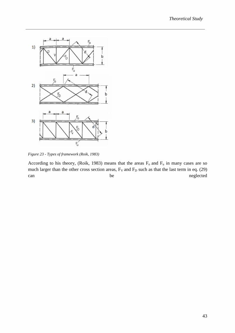
Other types of trusses can be used for this purpose, see Figure 23, but to reduce the amount of compression force in the beams the frame in Figure 22 is most suitable. The formula for t* is not applicable on these types of frameworks, the formula need to be changed according to the shear flow in the frameworks.

Theoretical Study

43

Figure 23 - Types of framework (Roik, 1983)

According to his theory, (Roik, 1983) means that the areas Fo and Fu in many cases are so much larger than the other cross section areas, FV and FD such as that the last term in eq. (29) can be neglected

Case Study

44

3 CASE STUDY – Bergeforsen Bridge 3.1.1 Location and history

Bergeforsen Bridge is a multi-span steel composite bridge located outside Sundsvall which is in the southern region of northern Sweden. In Figure 24 the location is showed and in Figure 25 a more exact location can be found. The circular area pointed out is not showing Bergeforsen Bridge, just the location. This because that the image from Google was taken under the construction stage of the bridge which is located east of the old bridge.

The design and calculations of the bridge was done by Jens Häggström at Ramböll Luleå (Häggström, 2012) and the construction by Svevia. The bridge was completed in the fall of 2012. It was built on request from Bergeforsen Kraft, because the lack of capacity in the outlet channel from Bergeforsen power station. The channel is crossing road 331 north of Indalsälven (Ramböll, Sverige, u.d.)

1. Bergeforsen Bridge

Figure 24 - Location bridge geographically (Google maps, 2015-06-10)

Case Study

45

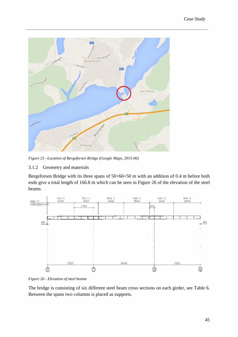
Figure 25 –Location of Bergeforsen Bridge (Google Maps, 2015-06)

3.1.2 Geometry and materials

Bergeforsen Bridge with its three spans of 50+66+50 m with an addition of 0.4 m before both ends give a total length of 166.8 m which can be seen in Figure 26 of the elevation of the steel beams.

Figure 26 - Elevation of steel beams

The bridge is consisting of six different steel beam cross sections on each girder, see Table 6. Between the spans two columns is placed as supports.

Case Study

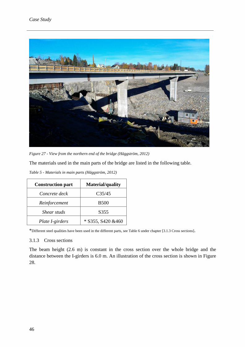
46

Figure 27 - View from the northern end of the bridge (Häggström, 2012)

The materials used in the main parts of the bridge are listed in the following table.

Table 5 - Materials in main parts (Häggström, 2012)

Construction part Material/quality

Concrete deck C35/45

Reinforcement B500

Shear studs S355

Plate I-girders * S355, S420 &460

*Different steel qualities have been used in the different parts, see Table 6 under chapter [3.1.3 Cross sections].

3.1.3 Cross sections

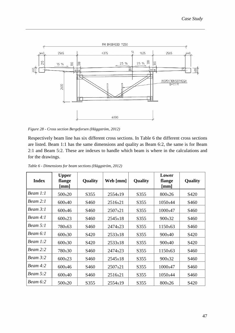
The beam height (2.6 m) is constant in the cross section over the whole bridge and the distance between the I-girders is 6.0 m. An illustration of the cross section is shown in Figure 28.

Case Study

47

Figure 28 - Cross section Bergeforsen (Häggström, 2012)

Respectively beam line has six different cross sections. In Table 6 the different cross sections are listed. Beam 1:1 has the same dimensions and quality as Beam 6:2, the same is for Beam 2:1 and Beam 5:2. These are indexes to handle which beam is where in the calculations and for the drawings.

Table 6 - Dimensions for beam sections (Häggström, 2012)

Index Upper flange [mm]

Quality Web [mm] Quality Lower flange [mm]

Quality

Beam 1:1 500x20 S355 2554x19 S355 800x26 S420 Beam 2:1 600x40 S460 2516x21 S355 1050x44 S460 Beam 3:1 600x46 S460 2507x21 S355 1000x47 S460 Beam 4:1 600x23 S460 2545x18 S355 900x32 S460 Beam 5:1 780x63 S460 2474x23 S355 1150x63 S460 Beam 6:1 600x30 S420 2533x18 S355 900x40 S420 Beam 1:2 600x30 S420 2533x18 S355 900x40 S420 Beam 2:2 780x30 S460 2474x23 S355 1150x63 S460 Beam 3:2 600x23 S460 2545x18 S355 900x32 S460 Beam 4:2 600x46 S460 2507x21 S355 1000x47 S460 Beam 5:2 600x40 S460 2516x21 S355 1050x44 S460 Beam 6:2 500x20 S355 2554x19 S355 800x26 S420

Case Study

48

3.2 FEM-setup 3.2.1 Program

The program used for the Finite Element analysis is SOFiSTiK 2014. The core of the program is an efficient database called CD-BASE. This is a set of programs which can be simple scripts or graphical interfaces. All these files and interfaces interchange their information through the database. The schedule in Appendix D shows the interaction between the programs in the CDB (SSD). The used programs from that schedule can be found below with explanations.

In the pre-processing some interactive programs can be used:

− Cross Section Editor is used for graphical input of cross sections with SOFIPLUS(-X) − SOFIPLUS(-X) the graphical input based on AutoCAD

Some of the modules/programs is explained further:

− SSD-SOFiSTiK Structural Desktop is the main module that includes the other modules within and with a good interface. The module direct, pre-processing, processing and post-processing the work (SOFiSTiK, 2014).

− SOFiLOAD is used to generate loading to the other programs which can be simple nodal and elemental loads to geometric load definitions with more complex load generators.

− ELLA-Extended Live Load Analysis “is a program for the analysis and evaluation of imposed loads that acts on spatial beam or shell structure in the form of load trains which move along certain traffic lanes” (SOFiSTiK, 2014).

− ASE-General Static Analysis of Finite Element Structures calculates the static and dynamic effects of general loading (SOFiSTiK, 2014).

− Animator is part of the interface of SSD and shows the modelled part/structure in SOFIPLUS-X.

− WINGRAF is a graphical program that allows to see the calculated results from the processing programs there included ASE. The visualization can be the shape of the structure with nodes with or without numbers, support conditions, material values and more. Loads can be showed with the resultant forces, stresses and deflections for just some examples (SOFiSTiK, 2014).

3.2.2 Elements

The FEM-model for the bridge is consisting of two different types of elements:

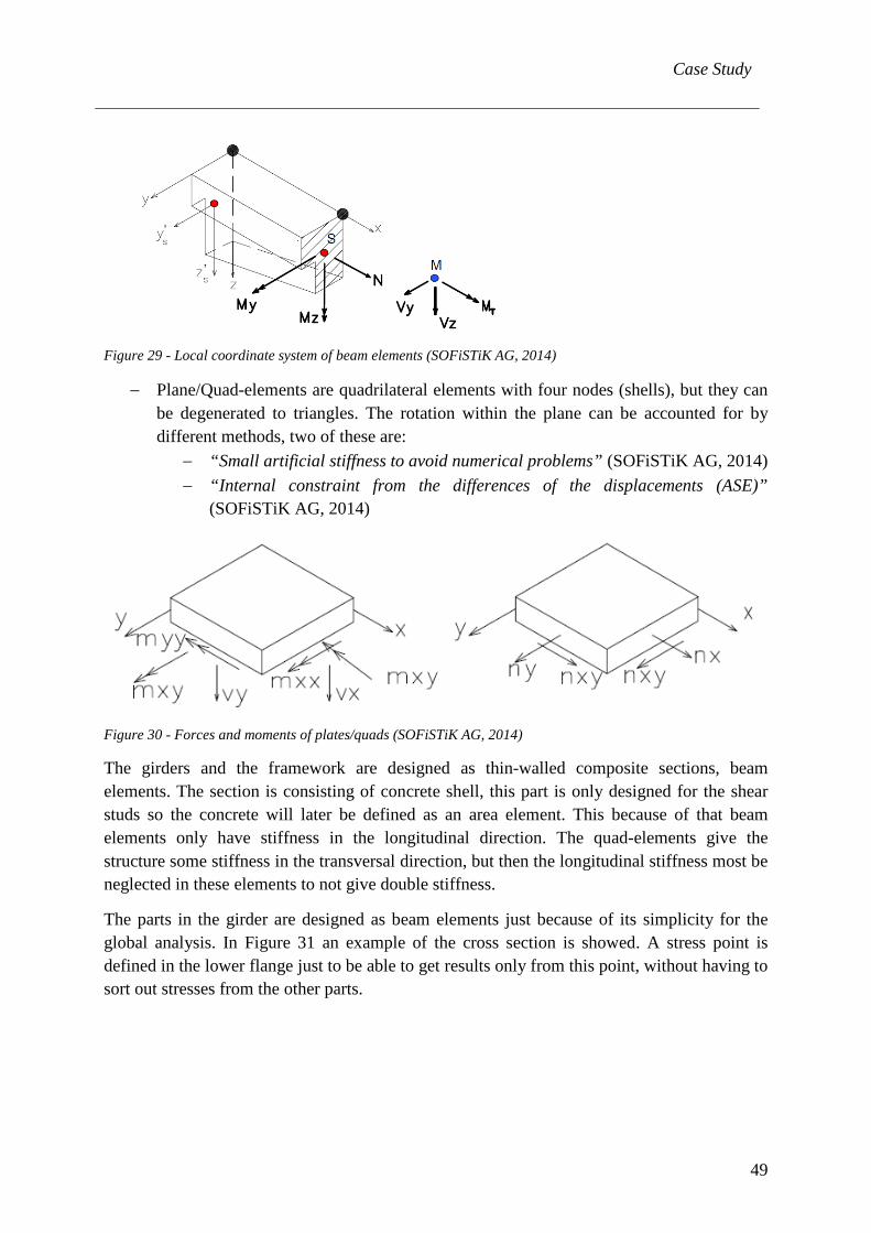
− Beam-elements “are defined by two nodes and their straight connection, which is either the centrobaric axis or the origin of the sectional coordinate system” (SOFiSTiK AG, 2014). The z-axis is the loading direction and the bending only occurs around the y-axis and z-axis.

Case Study

49

Figure 29 - Local coordinate system of beam elements (SOFiSTiK AG, 2014)

− Plane/Quad-elements are quadrilateral elements with four nodes (shells), but they can be degenerated to triangles. The rotation within the plane can be accounted for by different methods, two of these are:

− “Small artificial stiffness to avoid numerical problems” (SOFiSTiK AG, 2014) − “Internal constraint from the differences of the displacements (ASE)”

(SOFiSTiK AG, 2014)

Figure 30 - Forces and moments of plates/quads (SOFiSTiK AG, 2014)

The girders and the framework are designed as thin-walled composite sections, beam elements. The section is consisting of concrete shell, this part is only designed for the shear studs so the concrete will later be defined as an area element. This because of that beam elements only have stiffness in the longitudinal direction. The quad-elements give the structure some stiffness in the transversal direction, but then the longitudinal stiffness most be neglected in these elements to not give double stiffness.

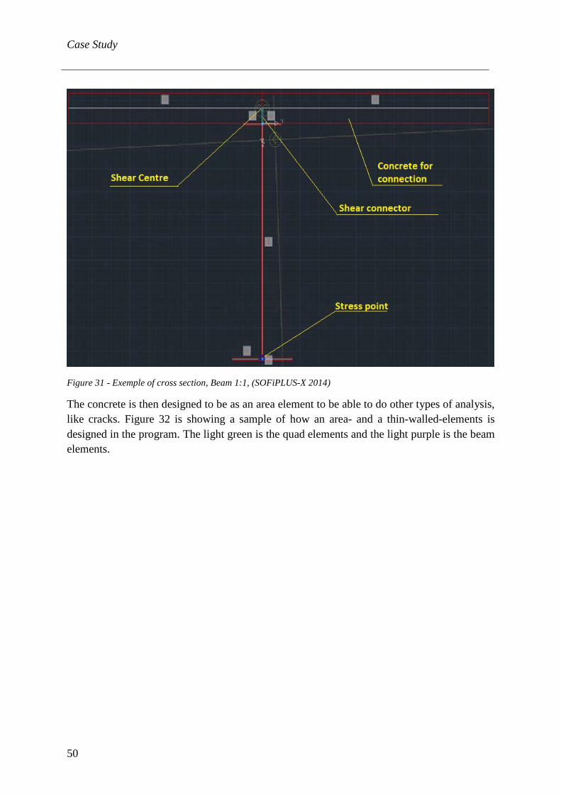
The parts in the girder are designed as beam elements just because of its simplicity for the global analysis. In Figure 31 an example of the cross section is showed. A stress point is defined in the lower flange just to be able to get results only from this point, without having to sort out stresses from the other parts.

Case Study

50

Figure 31 - Exemple of cross section, Beam 1:1, (SOFiPLUS-X 2014)

The concrete is then designed to be as an area element to be able to do other types of analysis, like cracks. Figure 32 is showing a sample of how an area- and a thin-walled-elements is designed in the program. The light green is the quad elements and the light purple is the beam elements.

Case Study

51

Figure 32 – Quad- (light blue) and beam elements (light purple) (SSD 2014)

3.2.3 Concept design

The design in SOFiSTiK was first tested for a more simplified bridge. This to understand and evaluate which type of element that should be used and how connections should be made.

The concept bridge which was used for this purpose is a one span composite bridge with the dimensions listed below.

Table 7 – Dimensions of the concept bridge

Length (L) 30 m

Width (w) 11 m

Distance between girders (B) 6 m

The most effective and also the proposed way from the support at SOFiSTiK was to use the composite function in the cross section editor. This function can be used to design composite cross sections, in this case between steel girders and concrete deck. For further information about the cross section editor and element functions see chapter 3.2.1 and 3.2.2. With this editor a cross section of beam elements is designed and the final result is shown in Figure 33.

Case Study

52

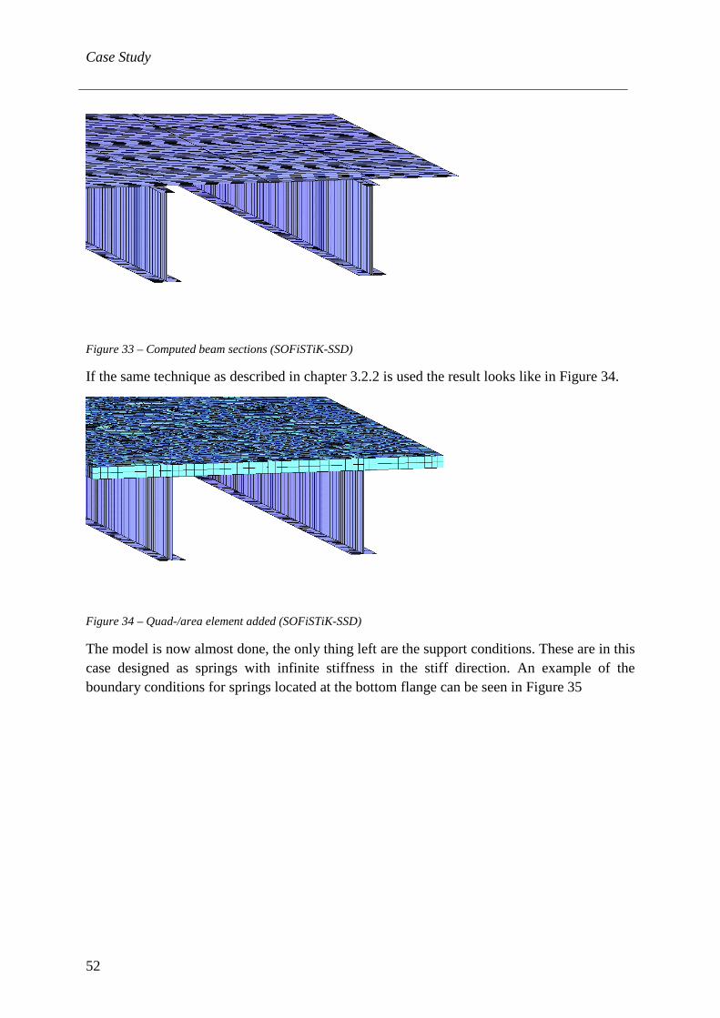
Figure 33 – Computed beam sections (SOFiSTiK-SSD)

If the same technique as described in chapter 3.2.2 is used the result looks like in Figure 34.

Figure 34 – Quad-/area element added (SOFiSTiK-SSD)

The model is now almost done, the only thing left are the support conditions. These are in this case designed as springs with infinite stiffness in the stiff direction. An example of the boundary conditions for springs located at the bottom flange can be seen in Figure 35

Case Study

53

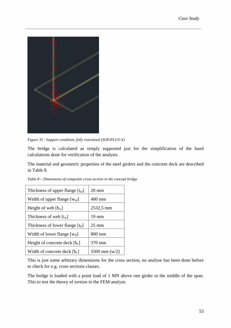
Figure 35 - Support condition, fully restrained (SOFiPLUS-X)

The bridge is calculated as simply supported just for the simplification of the hand calculations done for verification of the analysis.

The material and geometric properties of the steel girders and the concrete deck are described in Table 8.

Table 8 – Dimensions of composite cross section in the concept bridge

Thickness of upper flange [tuf] 20 mm

Width of upper flange [wuf] 400 mm

Height of web [hw] 2532,5 mm

Thickness of web [tw] 19 mm

Thickness of lower flange [tlf] 25 mm

Width of lower flange [wlf] 800 mm

Height of concrete deck [hc] 370 mm

Width of concrete deck [bc] 5500 mm (w/2)

This is just some arbitrary dimensions for the cross section, no analyse has been done before to check for e.g. cross sections classes.

The bridge is loaded with a point load of 1 MN above one girder in the middle of the span. This to test the theory of torsion in the FEM-analyse.

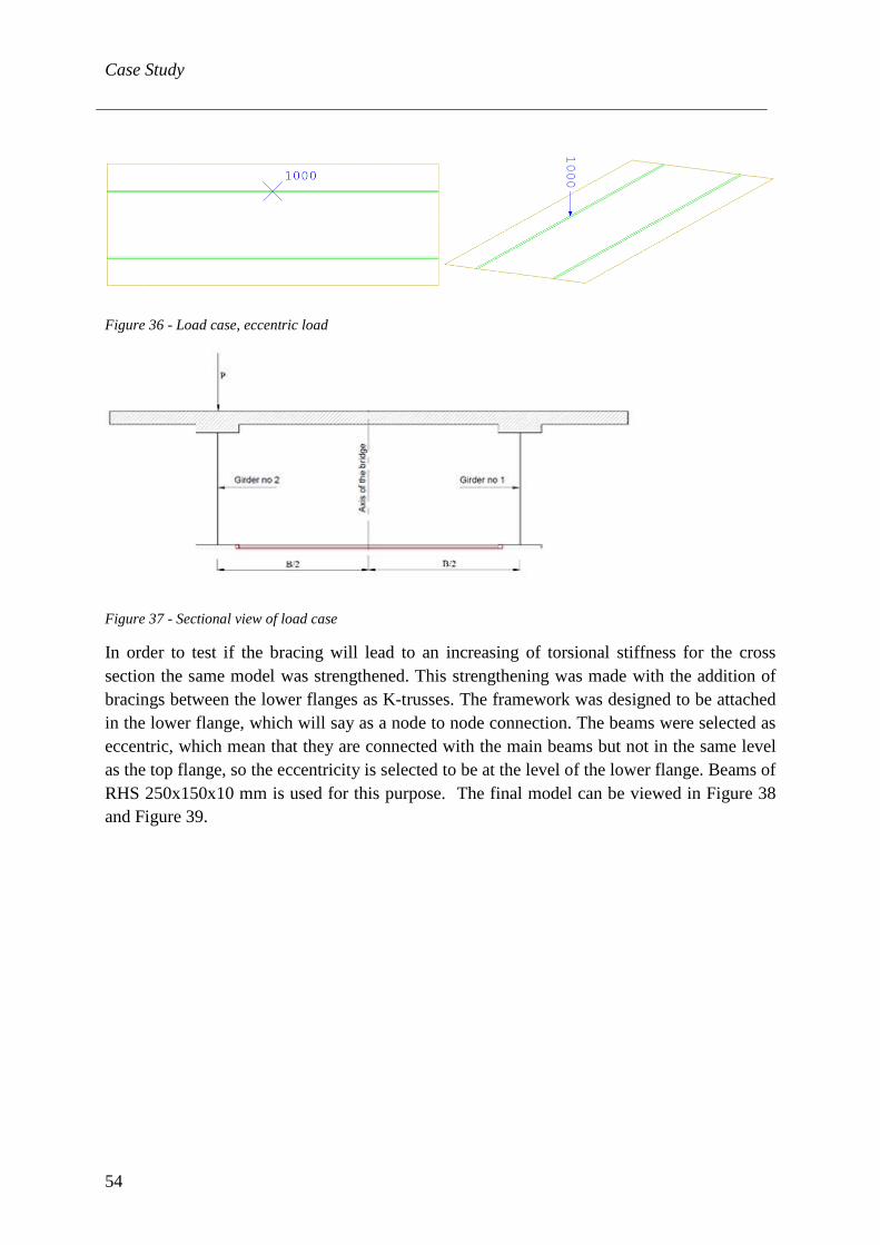
Case Study

54

Figure 36 - Load case, eccentric load

Figure 37 - Sectional view of load case

In order to test if the bracing will lead to an increasing of torsional stiffness for the cross section the same model was strengthened. This strengthening was made with the addition of bracings between the lower flanges as K-trusses. The framework was designed to be attached in the lower flange, which will say as a node to node connection. The beams were selected as eccentric, which mean that they are connected with the main beams but not in the same level as the top flange, so the eccentricity is selected to be at the level of the lower flange. Beams of RHS 250x150x10 mm is used for this purpose. The final model can be viewed in Figure 38 and Figure 39.

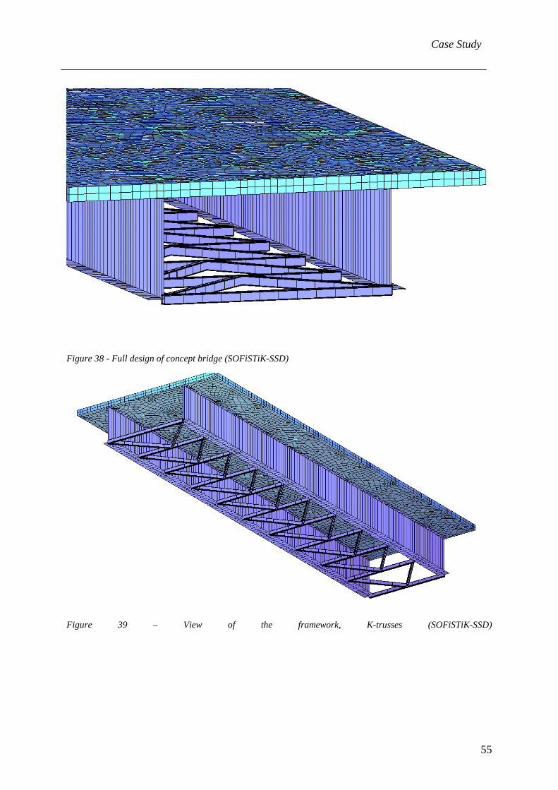
Case Study

55

Figure 38 - Full design of concept bridge (SOFiSTiK-SSD)

Figure 39 – View of the framework, K-trusses (SOFiSTiK-SSD)

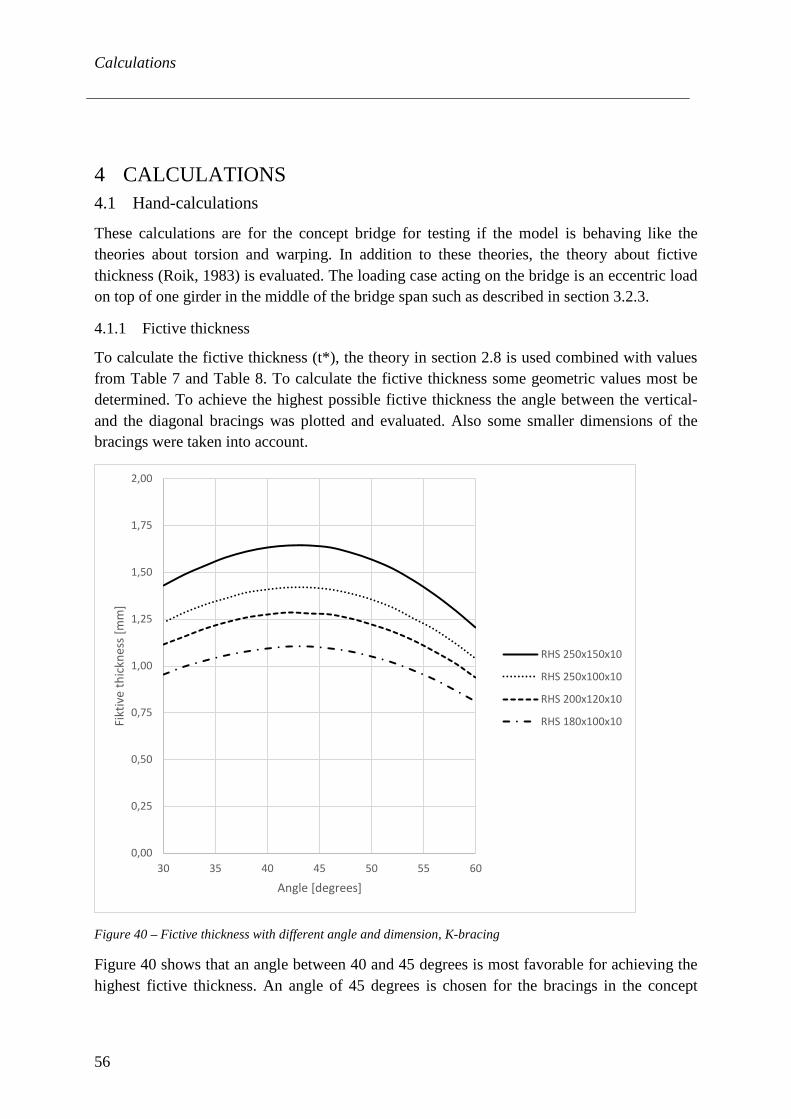
Calculations

56

4 CALCULATIONS 4.1 Hand-calculations

These calculations are for the concept bridge for testing if the model is behaving like the theories about torsion and warping. In addition to these theories, the theory about fictive thickness (Roik, 1983) is evaluated. The loading case acting on the bridge is an eccentric load on top of one girder in the middle of the bridge span such as described in section 3.2.3.

4.1.1 Fictive thickness

To calculate the fictive thickness (t*), the theory in section 2.8 is used combined with values from Table 7 and Table 8. To calculate the fictive thickness some geometric values most be determined. To achieve the highest possible fictive thickness the angle between the vertical- and the diagonal bracings was plotted and evaluated. Also some smaller dimensions of the bracings were taken into account.

Figure 40 – Fictive thickness with different angle and dimension, K-bracing

Figure 40 shows that an angle between 40 and 45 degrees is most favorable for achieving the highest fictive thickness. An angle of 45 degrees is chosen for the bracings in the concept

0,00

0,25

0,50

0,75

1,00

1,25

1,50

1,75

2,00

30 35 40 45 50 55 60

Fikt

ive

thic

knes

s [m

m]

Angle [degrees]

RHS 250x150x10

RHS 250x100x10

RHS 200x120x10

RHS 180x100x10

Calculations

57

bridge, because of the distance between the verticals then will be three meters and give an equal distance over the whole bridge.

With the given dimensions and geometry the fictive thickness is:

𝑡𝑡∗ = 1,6 𝑚𝑚𝑚𝑚 4.1.2 Torsional stiffness

The theories under section 2.7 is applied here. The first parameter which is calculated is the torsion factor (KV). It is here the fictive thickness contribution to the stiffness based on the thickness and length of the bracings. It is assumed as a plate between the girders with the thickness t*. The torsional stiffness is divided into the concrete part and the steel part.

𝐾𝐾𝑉𝑉𝑐𝑐𝑐𝑐𝑛𝑛𝑐𝑐. = 1,82 ∗ 1012𝑚𝑚𝑚𝑚4

𝐾𝐾𝑉𝑉𝑂𝑂𝑠𝑠𝑐𝑐𝑐𝑐𝑐𝑐 = 2,76 ∗ 1011𝑚𝑚𝑚𝑚4

And with the shear modulus for concrete and steel the torsional stiffness can be determine as:

𝐶𝐶 = 𝐺𝐺𝐾𝐾𝑉𝑉

and for the whole cross section as:

𝐶𝐶 = 𝐶𝐶𝑐𝑐𝑐𝑐𝑛𝑛𝑐𝑐. + 𝐶𝐶𝑂𝑂𝑠𝑠𝑐𝑐𝑐𝑐𝑐𝑐

The torsional stiffness for the cross section is therefor:

𝐶𝐶 = 4,83 ∗ 1016 𝑁𝑁𝑚𝑚𝑚𝑚2 4.1.3 Composite actions

Because the girders are connected to the concrete with shear studs the cross section properties is calculated as a composite section:

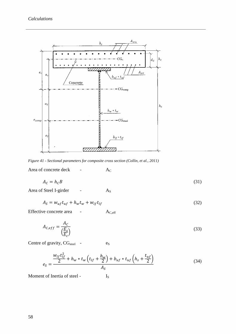
Calculations

58

Figure 41 - Sectional parameters for composite cross section (Collin, et al., 2011)

Area of concrete deck - AC

𝐴𝐴𝐶𝐶 = ℎ𝐶𝐶𝐵𝐵 (31)

Area of Steel I-girder - AS

𝐴𝐴𝑆𝑆 = 𝑤𝑤𝑢𝑢𝐹𝐹𝑡𝑡𝑢𝑢𝐹𝐹 + ℎ𝑤𝑤𝑡𝑡𝑤𝑤 + 𝑤𝑤𝑐𝑐𝐹𝐹𝑡𝑡𝑐𝑐𝐹𝐹 (32)

Effective concrete area - AC,eff

𝐴𝐴𝐶𝐶,𝑐𝑐𝐹𝐹𝐹𝐹 =𝐴𝐴𝐶𝐶

�𝐸𝐸𝑂𝑂𝐸𝐸𝑐𝑐� (33)

Centre of gravity, CGsteel - eS

𝑒𝑒𝑆𝑆 =

𝑤𝑤𝑐𝑐𝐹𝐹𝑡𝑡𝑐𝑐𝐹𝐹22 + ℎ𝑤𝑤 ∗ 𝑡𝑡𝑤𝑤 �𝑡𝑡𝑐𝑐𝐹𝐹 + ℎ𝑤𝑤

2 � + 𝑏𝑏𝑢𝑢𝐹𝐹 ∗ 𝑡𝑡𝑢𝑢𝐹𝐹 �ℎ𝑂𝑂 +𝑡𝑡𝑢𝑢𝐹𝐹2 �

𝐴𝐴𝑆𝑆 (34)

Moment of Inertia of steel - IS

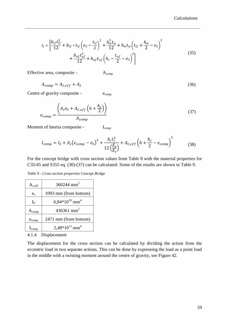
Calculations

59

𝐼𝐼𝑆𝑆 = �

𝑏𝑏𝑙𝑙𝑙𝑙𝑡𝑡𝑙𝑙𝑙𝑙3

12 + 𝑏𝑏𝑙𝑙𝑙𝑙 ∗ 𝑡𝑡𝑙𝑙𝑙𝑙 �𝑒𝑒𝑆𝑆 −𝑡𝑡𝑙𝑙𝑙𝑙2�

2+ ℎ𝑤𝑤

3 𝑡𝑡𝑤𝑤12 + ℎ𝑤𝑤𝑡𝑡𝑤𝑤 �𝑡𝑡𝑙𝑙𝑙𝑙 + ℎ𝑤𝑤

2 −𝑒𝑒𝑆𝑆�2

+𝑏𝑏𝑢𝑢𝑙𝑙𝑡𝑡𝑢𝑢𝑙𝑙3

12 + 𝑏𝑏𝑢𝑢𝑙𝑙𝑡𝑡𝑢𝑢𝑙𝑙 �ℎ𝑙𝑙 −𝑡𝑡𝑢𝑢𝑙𝑙2 −𝑒𝑒𝑆𝑆�

2�

(35)

Effective area, composite - Acomp

𝐴𝐴𝑐𝑐𝑐𝑐𝑚𝑚𝑜𝑜 = 𝐴𝐴𝐶𝐶,𝑐𝑐𝐹𝐹𝐹𝐹 + 𝐴𝐴𝑆𝑆 (36)

Centre of gravity composite - ecomp

𝑒𝑒𝑐𝑐𝑐𝑐𝑚𝑚𝑜𝑜 =�𝐴𝐴𝑂𝑂𝑒𝑒𝑆𝑆 + 𝐴𝐴𝐶𝐶,𝑐𝑐𝐹𝐹𝐹𝐹 �ℎ + ℎ𝑐𝑐

2 ��

𝐴𝐴𝑐𝑐𝑐𝑐𝑚𝑚𝑜𝑜

(37)

Moment of Inertia composite - Icomp

𝐼𝐼𝑐𝑐𝑐𝑐𝑚𝑚𝑜𝑜 = 𝐼𝐼𝑆𝑆 + 𝐴𝐴𝑂𝑂�𝑒𝑒𝑐𝑐𝑐𝑐𝑚𝑚𝑜𝑜 − 𝑒𝑒𝑆𝑆�

2+

𝑏𝑏𝑐𝑐𝑡𝑡𝑐𝑐3

12 �𝐸𝐸𝑂𝑂𝐸𝐸𝑐𝑐�

+ 𝐴𝐴𝐶𝐶,𝑐𝑐𝐹𝐹𝐹𝐹 �ℎ +ℎ𝑐𝑐2− 𝑒𝑒𝑐𝑐𝑐𝑐𝑚𝑚𝑜𝑜�

2

(38)

For the concept bridge with cross section values from Table 8 with the material properties for C35/45 and S355 eq. (30)-(37) can be calculated. Some of the results are shown in Table 9.

Table 9 - Cross section properties Concept Bridge

Ac,eff 360244 mm2

es 1093 mm (from bottom)

IS 6,84*1010 mm4

Acomp 436361 mm2

ecomp 2471 mm (from bottom)

Icomp 2,48*1011 mm4

4.1.4 Displacement

The displacement for the cross section can be calculated by dividing the action from the eccentric load in two separate actions. This can be done by expressing the load as a point load in the middle with a twisting moment around the centre of gravity, see Figure 42.

Calculations

60

Figure 42 - Expression of eccentric load

This method is used for the strengthen design, that the slab is assumed as simply supported between the girders in the analysis, the force will therefore only act on one of the girders.

For a simply supported beam with a point load in the middle the deflection can be calculated as:

𝛿𝛿 =

𝑃𝑃𝐿𝐿3

48𝐸𝐸𝐼𝐼 (39)

Figure 43 - Elementary case of beam bending for simply supported conditions

The deflection is calculated for the case with framework as strengthening (closed section). The deflection from the point load in the middle is divided to both girders.

𝛿𝛿𝑜𝑜 =

𝑃𝑃𝐿𝐿3

48𝐸𝐸𝐼𝐼𝑐𝑐𝑐𝑐𝑚𝑚𝑜𝑜 (40)

Calculations

61

𝛿𝛿1,𝑜𝑜 =

𝛿𝛿𝑜𝑜2

(41)

𝛿𝛿𝑜𝑜 = 5,41 𝑚𝑚𝑚𝑚

For the deflection the moment of inertia is the same as the one in case 1 because both girders are supposed to act together. The warping effect in case 2 is neglected, so only the torsional stiffness will be included for that case.

In addition to the point load a torque is applied, see Figure 42. With the theories described in chapter 4.1.2 the displacement from the torque can be calculated. With earlier calculated values for a closed cross section the displacement from the torque can be determined. From eq.(14) the torque is calculated with an eccentricity, e of half the distance B between girders.

𝑀𝑀𝑇𝑇 = 𝑃𝑃 ∗𝐵𝐵2

𝑀𝑀𝑇𝑇 = 3 ∗ 106 𝑘𝑘𝑁𝑁𝑚𝑚𝑚𝑚

The torque gives a rotation of the structure and the angle, earlier called torsional angle can be calculated as:

𝜑𝜑 =𝐿𝐿2∗ 𝜑𝜑′ (42)

𝜑𝜑′ =𝑀𝑀𝑇𝑇

𝐶𝐶 + 𝐶𝐶𝑤𝑤𝜋𝜋2𝐿𝐿2

(43)

The additional factor π2/L2 is from the solution for the differential equation (eq.28)

Where the torsional stiffness is

𝐶𝐶 = 4,83 ∗ 1016𝑁𝑁𝑚𝑚𝑚𝑚2

And the warping stiffness is

𝐶𝐶𝑤𝑤 = 9,40 ∗ 1023𝑁𝑁𝑚𝑚𝑚𝑚4

This gives the torsional angle of

𝜑𝜑2 = 0,0009 𝑙𝑙𝑐𝑐𝑑𝑑

The displacement of the girder due to the point load is depending on the bridge length like:

𝛿𝛿𝑇𝑇 = sin(𝜑𝜑) ∗𝐵𝐵2

(44)

𝛿𝛿𝑇𝑇 = 2,62 𝑚𝑚𝑚𝑚

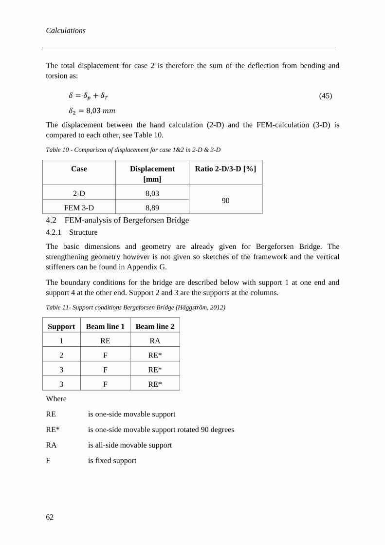
Calculations

62

The total displacement for case 2 is therefore the sum of the deflection from bending and torsion as:

𝛿𝛿 = 𝛿𝛿𝑜𝑜 + 𝛿𝛿𝑇𝑇 (45)

𝛿𝛿2 = 8,03 𝑚𝑚𝑚𝑚

The displacement between the hand calculation (2-D) and the FEM-calculation (3-D) is compared to each other, see Table 10.

Table 10 - Comparison of displacement for case 1&2 in 2-D & 3-D

Case Displacement [mm]

Ratio 2-D/3-D [%]

2-D 8,03 90

FEM 3-D 8,89 4.2 FEM-analysis of Bergeforsen Bridge 4.2.1 Structure

The basic dimensions and geometry are already given for Bergeforsen Bridge. The strengthening geometry however is not given so sketches of the framework and the vertical stiffeners can be found in Appendix G.

The boundary conditions for the bridge are described below with support 1 at one end and support 4 at the other end. Support 2 and 3 are the supports at the columns.

Table 11- Support conditions Bergeforsen Bridge (Häggström, 2012)

Support Beam line 1 Beam line 2

1 RE RA

2 F RE*

3 F RE*

3 F RE*

Where

RE is one-side movable support

RE* is one-side movable support rotated 90 degrees

RA is all-side movable support

F is fixed support

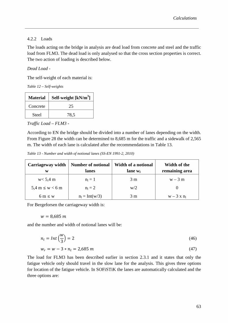
Calculations

63

4.2.2 Loads

The loads acting on the bridge in analysis are dead load from concrete and steel and the traffic load from FLM3. The dead load is only analysed so that the cross section properties is correct. The two action of loading is described below.

Dead Load -

The self-weight of each material is:

Table 12 – Self-weights

Material Self-weight [kN/m3]

Concrete 25

Steel 78,5

Traffic Load – FLM3 -

According to EN the bridge should be divided into a number of lanes depending on the width. From Figure 28 the width can be determined to 8,685 m for the traffic and a sidewalk of 2,565 m. The width of each lane is calculated after the recommendations in Table 13.

Table 13 - Number and width of notional lanes (SS-EN 1991-2, 2010)

Carriageway width w

Number of notional lanes

Width of a notional lane wl

Width of the remaining area

w< 5,4 m

5,4 m ≤ w < 6 m

6 m ≤ w

nl = 1

nl = 2

nl = Int(w/3)

3 m

w/2

3 m

w – 3 m

0

w – 3 x nl

For Bergeforsen the carriageway width is:

𝑤𝑤 = 8,685 𝑚𝑚

and the number and width of notional lanes will be:

𝑛𝑛𝑐𝑐 = 𝐼𝐼𝑛𝑛𝑡𝑡 �𝑤𝑤3� = 2 (46)

𝑤𝑤𝑟𝑟 = 𝑤𝑤 − 3 ∗ 𝑛𝑛𝑐𝑐 = 2,685 𝑚𝑚 (47)

The load for FLM3 has been described earlier in section 2.3.1 and it states that only the fatigue vehicle only should travel in the slow lane for the analysis. This gives three options for location of the fatigue vehicle. In SOFiSTiK the lanes are automatically calculated and the three options are:

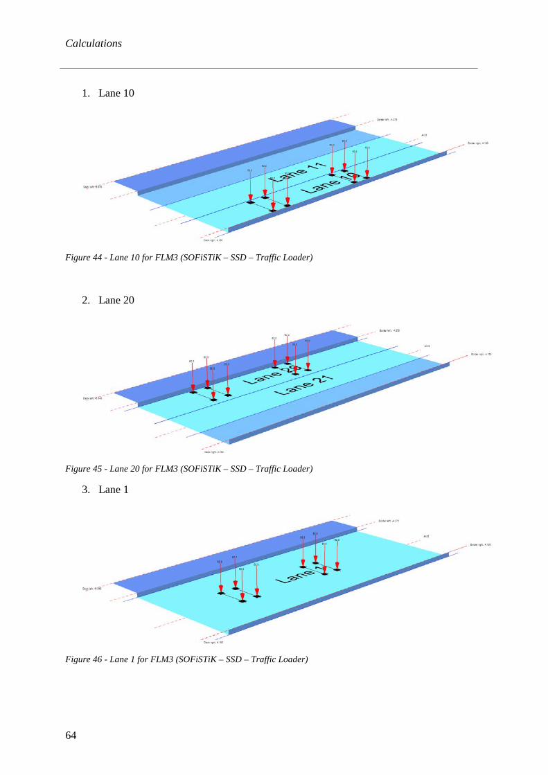
Calculations

64

1. Lane 10

Figure 44 - Lane 10 for FLM3 (SOFiSTiK – SSD – Traffic Loader)

2. Lane 20

Figure 45 - Lane 20 for FLM3 (SOFiSTiK – SSD – Traffic Loader)

3. Lane 1

Figure 46 - Lane 1 for FLM3 (SOFiSTiK – SSD – Traffic Loader)

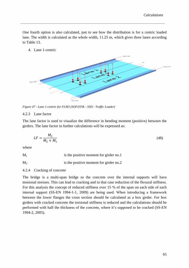
Calculations

65

One fourth option is also calculated, just to see how the distribution is for a centric loaded lane. The width is calculated as the whole width, 11.25 m, which gives three lanes according to Table 13.

4. Lane 1-centric

Figure 47 - Lane 1-centric for FLM3 (SOFiSTiK - SSD - Traffic Loader)

4.2.3 Lane factor

The lane factor is used to visualize the difference in bending moment (positive) between the girders. The lane factor in further calculations will be expressed as:

𝐿𝐿𝐹𝐹 =𝑀𝑀2

𝑀𝑀2 + 𝑀𝑀1 (48)

where

M1 is the positive moment for girder no.1

M2 is the positive moment for girder no.2

4.2.4 Cracking of concrete

The bridge is a multi-span bridge so the concrete over the internal supports will have tensional stresses. This can lead to cracking and in that case reduction of the flexural stiffness. For this analysis the concept of reduced stiffness over 15 % of the span on each side of each internal support (SS-EN 1994-1-1, 2009) are being used. When introducing a framework between the lower flanges the cross section should be calculated as a box girder. For box girders with cracked concrete the torsional stiffness is reduced and the calculations should be performed with half the thickness of the concrete, where it’s supposed to be cracked (SS-EN 1994-2, 2005).

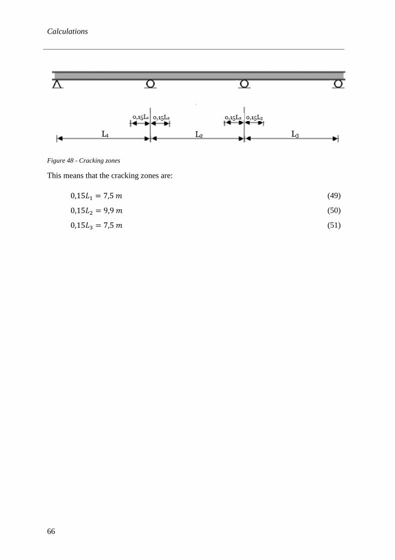
Calculations

66

Figure 48 - Cracking zones

This means that the cracking zones are:

0,15𝐿𝐿1 = 7,5 𝑚𝑚 (49)

0,15𝐿𝐿2 = 9,9 𝑚𝑚 (50)

0,15𝐿𝐿3 = 7,5 𝑚𝑚 (51)

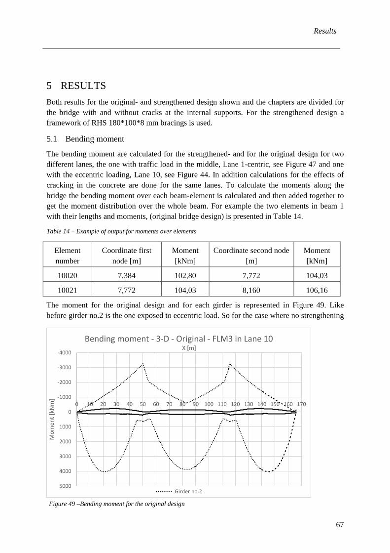
Results

67

5 RESULTS Both results for the original- and strengthened design shown and the chapters are divided for the bridge with and without cracks at the internal supports. For the strengthened design a framework of RHS 180*100*8 mm bracings is used.

5.1 Bending moment

The bending moment are calculated for the strengthened- and for the original design for two different lanes, the one with traffic load in the middle, Lane 1-centric, see Figure 47 and one with the eccentric loading, Lane 10, see Figure 44. In addition calculations for the effects of cracking in the concrete are done for the same lanes. To calculate the moments along the bridge the bending moment over each beam-element is calculated and then added together to get the moment distribution over the whole beam. For example the two elements in beam 1 with their lengths and moments, (original bridge design) is presented in Table 14.

Table 14 – Example of output for moments over elements

Element number

Coordinate first node [m]

Moment [kNm]

Coordinate second node [m]

Moment [kNm]

10020 7,384 102,80 7,772 104,03

10021 7,772 104,03 8,160 106,16

The moment for the original design and for each girder is represented in Figure 49. Like before girder no.2 is the one exposed to eccentric load. So for the case where no strengthening

-4000

-3000

-2000

-1000

0

1000

2000

3000

4000

5000

0 10 20 30 40 50 60 70 80 90 100 110 120 130 140 150 160 170

Mom

ent [

kNm

]

X [m] Bending moment - 3-D - Original - FLM3 in Lane 10

Girder no.2

Figure 49 –Bending moment for the original design

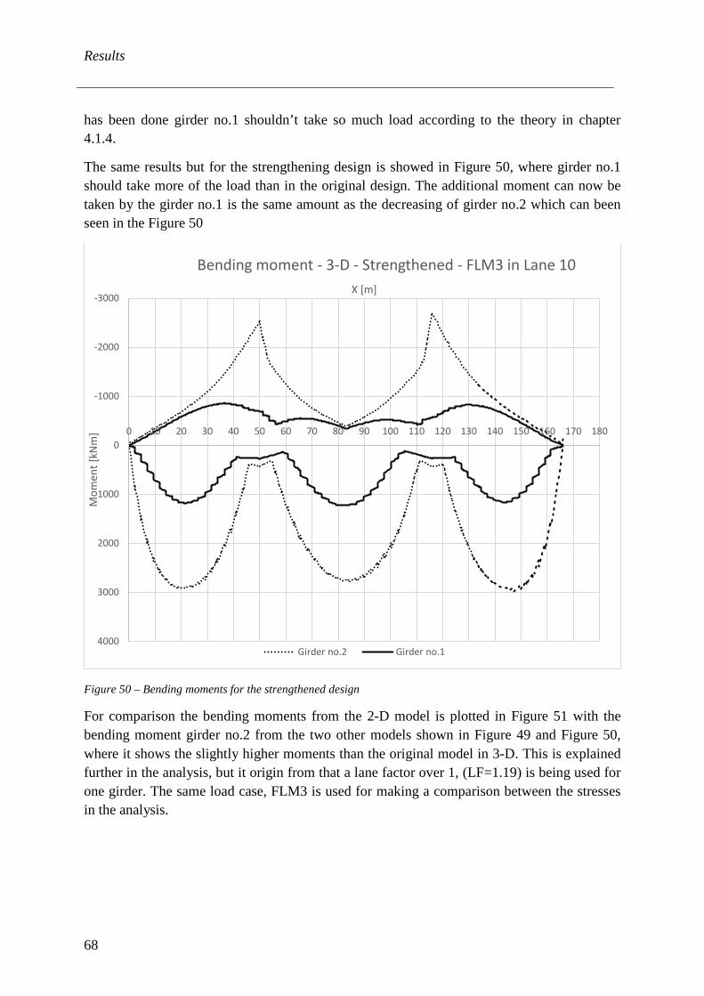
Results

68

has been done girder no.1 shouldn’t take so much load according to the theory in chapter 4.1.4.

The same results but for the strengthening design is showed in Figure 50, where girder no.1 should take more of the load than in the original design. The additional moment can now be taken by the girder no.1 is the same amount as the decreasing of girder no.2 which can been seen in the Figure 50

For comparison the bending moments from the 2-D model is plotted in Figure 51 with the bending moment girder no.2 from the two other models shown in Figure 49 and Figure 50, where it shows the slightly higher moments than the original model in 3-D. This is explained further in the analysis, but it origin from that a lane factor over 1, (LF=1.19) is being used for one girder. The same load case, FLM3 is used for making a comparison between the stresses in the analysis.

-3000

-2000

-1000

0

1000

2000

3000

4000

0 10 20 30 40 50 60 70 80 90 100 110 120 130 140 150 160 170 180

Mom

ent [

kNm

]

X [m]

Bending moment - 3-D - Strengthened - FLM3 in Lane 10

Girder no.2 Girder no.1

Figure 50 – Bending moments for the strengthened design

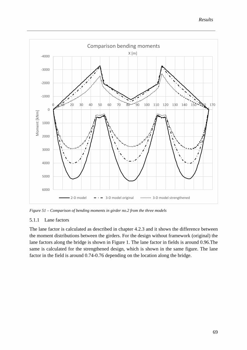
Results

69

Figure 51 – Comparison of bending moments in girder no.2 from the three models

5.1.1 Lane factors

The lane factor is calculated as described in chapter 4.2.3 and it shows the difference between the moment distributions between the girders. For the design without framework (original) the lane factors along the bridge is shown in Figure 1. The lane factor in fields is around 0.96.The same is calculated for the strengthened design, which is shown in the same figure. The lane factor in the field is around 0.74-0.76 depending on the location along the bridge.

-4000

-3000

-2000

-1000

0

1000

2000

3000

4000

5000

6000

0 10 20 30 40 50 60 70 80 90 100 110 120 130 140 150 160 170

Mom

ent [

kNm

]

X [m]

Comparison bending moments

2-D model 3-D model original 3-D model strengthened

Results

70

Figure 52 - Lane factors for the strengthened and original design

0,5

0,55

0,6

0,65

0,7

0,75

0,8

0,85

0,9

0,95

1

0 10 20 30 40 50 60 70 80 90 100 110 120 130 140 150 160 170

Lane

fact

or

X [m]

Comparison of Lane factors

Strengthened design Original design

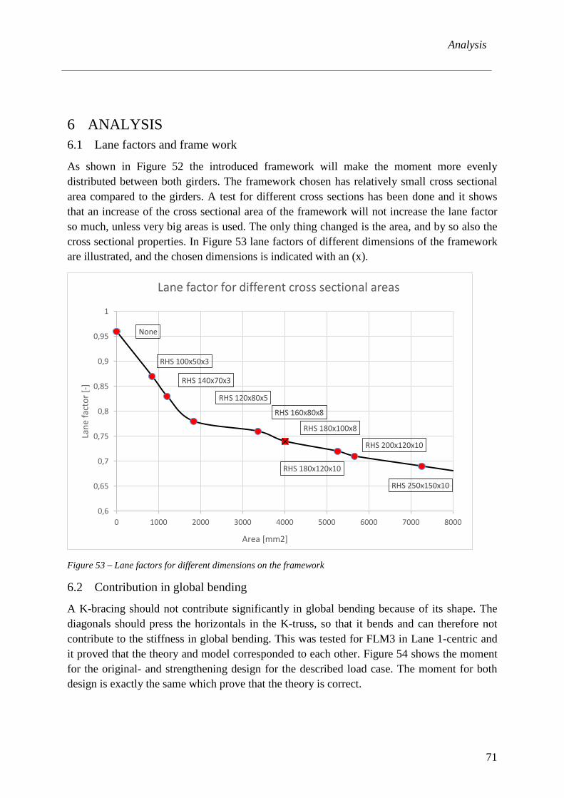
Analysis

71

6 ANALYSIS 6.1 Lane factors and frame work

As shown in Figure 52 the introduced framework will make the moment more evenly distributed between both girders. The framework chosen has relatively small cross sectional area compared to the girders. A test for different cross sections has been done and it shows that an increase of the cross sectional area of the framework will not increase the lane factor so much, unless very big areas is used. The only thing changed is the area, and by so also the cross sectional properties. In Figure 53 lane factors of different dimensions of the framework are illustrated, and the chosen dimensions is indicated with an (x).

Figure 53 – Lane factors for different dimensions on the framework

6.2 Contribution in global bending

A K-bracing should not contribute significantly in global bending because of its shape. The diagonals should press the horizontals in the K-truss, so that it bends and can therefore not contribute to the stiffness in global bending. This was tested for FLM3 in Lane 1-centric and it proved that the theory and model corresponded to each other. Figure 54 shows the moment for the original- and strengthening design for the described load case. The moment for both design is exactly the same which prove that the theory is correct.

None

RHS 100x50x3

RHS 140x70x3

RHS 120x80x5

RHS 160x80x8

RHS 180x100x8

RHS 180x120x10

RHS 200x120x10

RHS 250x150x10

0,6

0,65

0,7

0,75

0,8

0,85

0,9

0,95

1

0 1000 2000 3000 4000 5000 6000 7000 8000

Lane

fact

or [-

]

Area [mm2]

Lane factor for different cross sectional areas

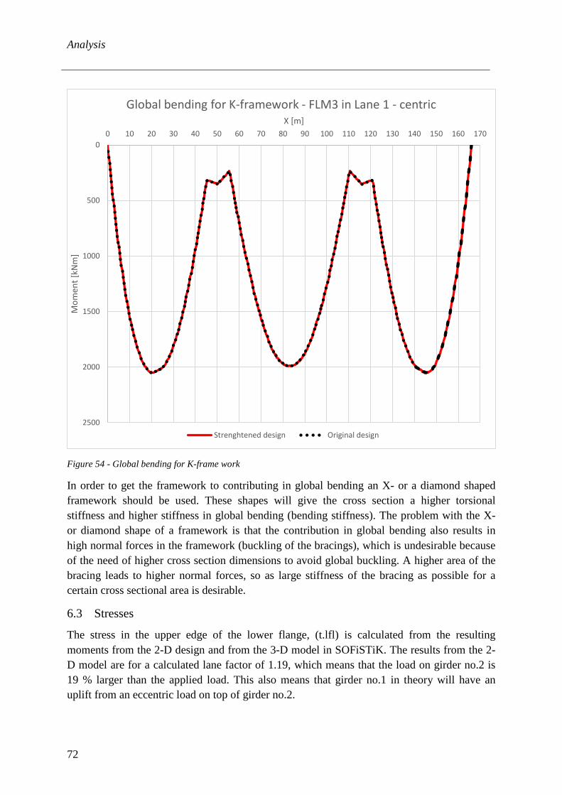
Analysis

72

Figure 54 - Global bending for K-frame work

In order to get the framework to contributing in global bending an X- or a diamond shaped framework should be used. These shapes will give the cross section a higher torsional stiffness and higher stiffness in global bending (bending stiffness). The problem with the X- or diamond shape of a framework is that the contribution in global bending also results in high normal forces in the framework (buckling of the bracings), which is undesirable because of the need of higher cross section dimensions to avoid global buckling. A higher area of the bracing leads to higher normal forces, so as large stiffness of the bracing as possible for a certain cross sectional area is desirable.

6.3 Stresses

The stress in the upper edge of the lower flange, (t.lfl) is calculated from the resulting moments from the 2-D design and from the 3-D model in SOFiSTiK. The results from the 2-D model are for a calculated lane factor of 1.19, which means that the load on girder no.2 is 19 % larger than the applied load. This also means that girder no.1 in theory will have an uplift from an eccentric load on top of girder no.2.

0

500

1000

1500

2000

2500

0 10 20 30 40 50 60 70 80 90 100 110 120 130 140 150 160 170

Mom

ent [

kNm

]

X [m]

Global bending for K-framework - FLM3 in Lane 1 - centric

Strenghtened design Original design

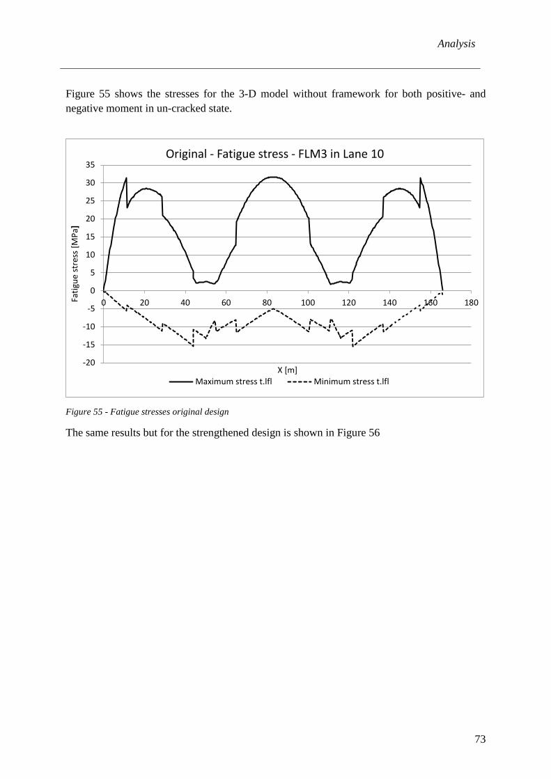
Analysis

73

Figure 55 shows the stresses for the 3-D model without framework for both positive- and negative moment in un-cracked state.

Figure 55 - Fatigue stresses original design

The same results but for the strengthened design is shown in Figure 56

-20

-15

-10

-5

0

5

10

15

20

25

30

35

0 20 40 60 80 100 120 140 160 180Fatig

ue st

ress

[MPa

]

X [m]

Original - Fatigue stress - FLM3 in Lane 10

Maximum stress t.lfl Minimum stress t.lfl

Analysis

74

Figure 56 - Fatigue stresses strengthened design

For comparison the stresses from the 2-D model is used and they are found in Figure 57.

Figure 57 - Fatigue stresses in 2-D model

-15

-10

-5

0

5

10

15

20

25

30

0 20 40 60 80 100 120 140 160 180

Fatig

ue st

ress

[MPa

]

X [m]

Strengthened - Fatigue stress - FLM3 in Lane 10

Maximum stress t.lfl Minimum stress t.lfl

-20

-15

-10

-5

0

5

10

15

20

25

30

35

40

45

50

0 20 40 60 80 100 120 140 160 180

2-D - Fatigue stress - FLM3 in Lane 10

Maximum stress t.lfl Minimum stress t.lfl

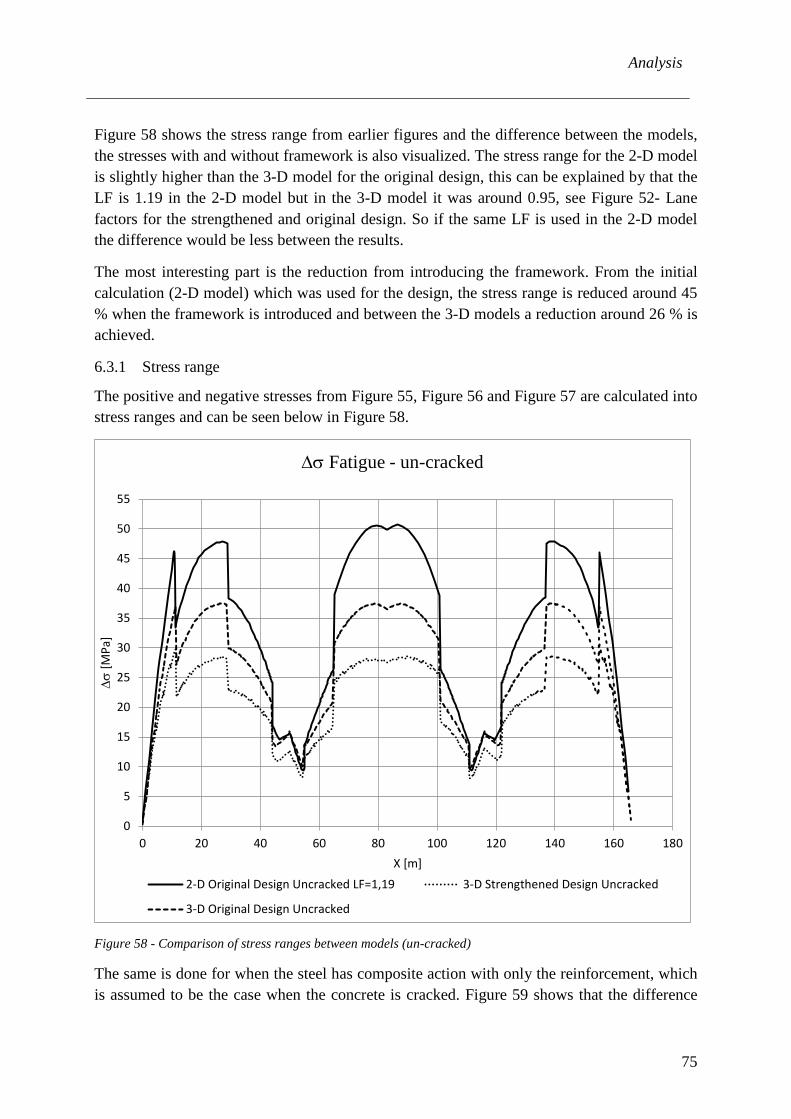
Analysis

75

Figure 58 shows the stress range from earlier figures and the difference between the models, the stresses with and without framework is also visualized. The stress range for the 2-D model is slightly higher than the 3-D model for the original design, this can be explained by that the LF is 1.19 in the 2-D model but in the 3-D model it was around 0.95, see Figure 52- Lane factors for the strengthened and original design. So if the same LF is used in the 2-D model the difference would be less between the results.

The most interesting part is the reduction from introducing the framework. From the initial calculation (2-D model) which was used for the design, the stress range is reduced around 45 % when the framework is introduced and between the 3-D models a reduction around 26 % is achieved.

6.3.1 Stress range

The positive and negative stresses from Figure 55, Figure 56 and Figure 57 are calculated into stress ranges and can be seen below in Figure 58.

Figure 58 - Comparison of stress ranges between models (un-cracked)

The same is done for when the steel has composite action with only the reinforcement, which is assumed to be the case when the concrete is cracked. Figure 59 shows that the difference

0

5

10

15

20

25

30

35

40

45

50

55

0 20 40 60 80 100 120 140 160 180

∆σ

[MPa

]

X [m]

∆σ Fatigue - un-cracked

2-D Original Design Uncracked LF=1,19 3-D Strengthened Design Uncracked

3-D Original Design Uncracked

Analysis

76

between the models is almost the same but all curves have higher stress ranges than when the concrete is un-cracked and the steel has composite action with the concrete.

Figure 59 - Comparison of stress ranges between models (cracked)

To get a more realistic stress ranges the true stress should be analysed. The true stress is when the positive moments is assumed to give stresses in a un-cracked concrete and negative moments stresses for cracked concrete. This analysis is visualized in Figure 60. If these ranges is compared to the ones in Figure 58 and Figure 59 it can be seen that the true stress is close to the un-cracked stress range in fields and close to stress range for cracked near supports.

0

5

10

15

20

25

30

35

40

45

50

55

60

65

70

0 10 20 30 40 50 60 70 80 90 100 110 120 130 140 150 160 170

Stre

ss [M

Pa]

X [m]

∆σ Fatigue - cracked

2-D Original Design Cracked LF=1,19 3-D Strengthened Design Cracked

3-D Original Design Cracked

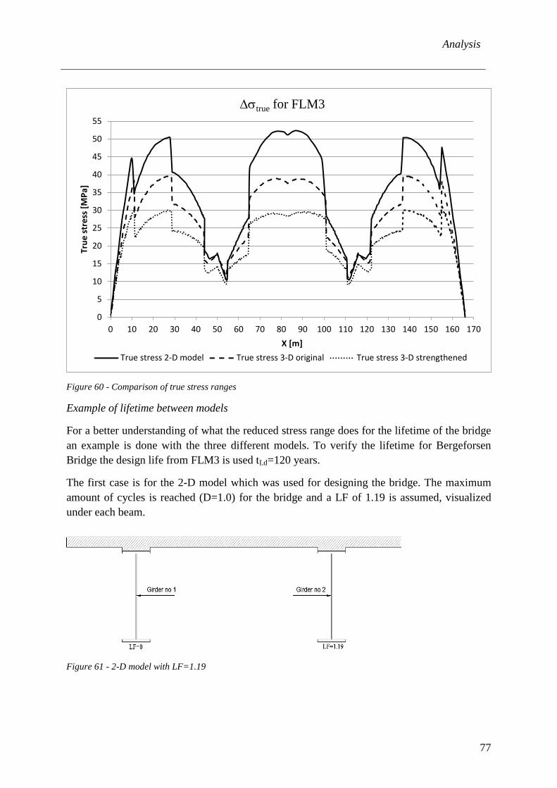
Analysis

77

Figure 60 - Comparison of true stress ranges

Example of lifetime between models

For a better understanding of what the reduced stress range does for the lifetime of the bridge an example is done with the three different models. To verify the lifetime for Bergeforsen Bridge the design life from FLM3 is used tLd=120 years.

The first case is for the 2-D model which was used for designing the bridge. The maximum amount of cycles is reached (D=1.0) for the bridge and a LF of 1.19 is assumed, visualized under each beam.

Figure 61 - 2-D model with LF=1.19

0

5

10

15

20

25

30

35

40

45

50

55

0 10 20 30 40 50 60 70 80 90 100 110 120 130 140 150 160 170

True

stre

ss [M

Pa]

X [m]

∆σtrue for FLM3

True stress 2-D model True stress 3-D original True stress 3-D strengthened

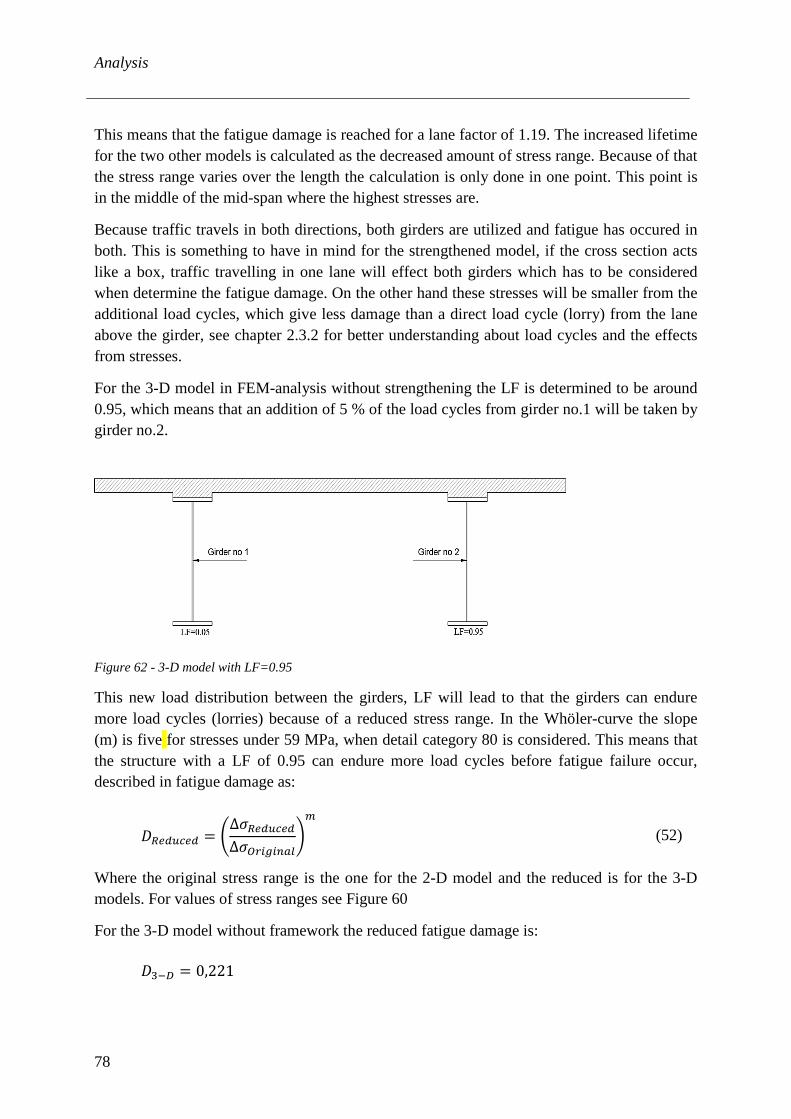
Analysis

78

This means that the fatigue damage is reached for a lane factor of 1.19. The increased lifetime for the two other models is calculated as the decreased amount of stress range. Because of that the stress range varies over the length the calculation is only done in one point. This point is in the middle of the mid-span where the highest stresses are.

Because traffic travels in both directions, both girders are utilized and fatigue has occured in both. This is something to have in mind for the strengthened model, if the cross section acts like a box, traffic travelling in one lane will effect both girders which has to be considered when determine the fatigue damage. On the other hand these stresses will be smaller from the additional load cycles, which give less damage than a direct load cycle (lorry) from the lane above the girder, see chapter 2.3.2 for better understanding about load cycles and the effects from stresses.

For the 3-D model in FEM-analysis without strengthening the LF is determined to be around 0.95, which means that an addition of 5 % of the load cycles from girder no.1 will be taken by girder no.2.

Figure 62 - 3-D model with LF=0.95

This new load distribution between the girders, LF will lead to that the girders can endure more load cycles (lorries) because of a reduced stress range. In the Whöler-curve the slope (m) is five for stresses under 59 MPa, when detail category 80 is considered. This means that the structure with a LF of 0.95 can endure more load cycles before fatigue failure occur, described in fatigue damage as:

𝐷𝐷𝑅𝑅𝑐𝑐𝐿𝐿𝑢𝑢𝑐𝑐𝑐𝑐𝐿𝐿 = �

∆𝜎𝜎𝑅𝑅𝑐𝑐𝐿𝐿𝑢𝑢𝑐𝑐𝑐𝑐𝐿𝐿∆𝜎𝜎𝑂𝑂𝑟𝑟𝑖𝑖𝑂𝑂𝑖𝑖𝑛𝑛𝑚𝑚𝑐𝑐

�𝑚𝑚

(52)

Where the original stress range is the one for the 2-D model and the reduced is for the 3-D models. For values of stress ranges see Figure 60

For the 3-D model without framework the reduced fatigue damage is:

𝐷𝐷3−𝐷𝐷 = 0,221

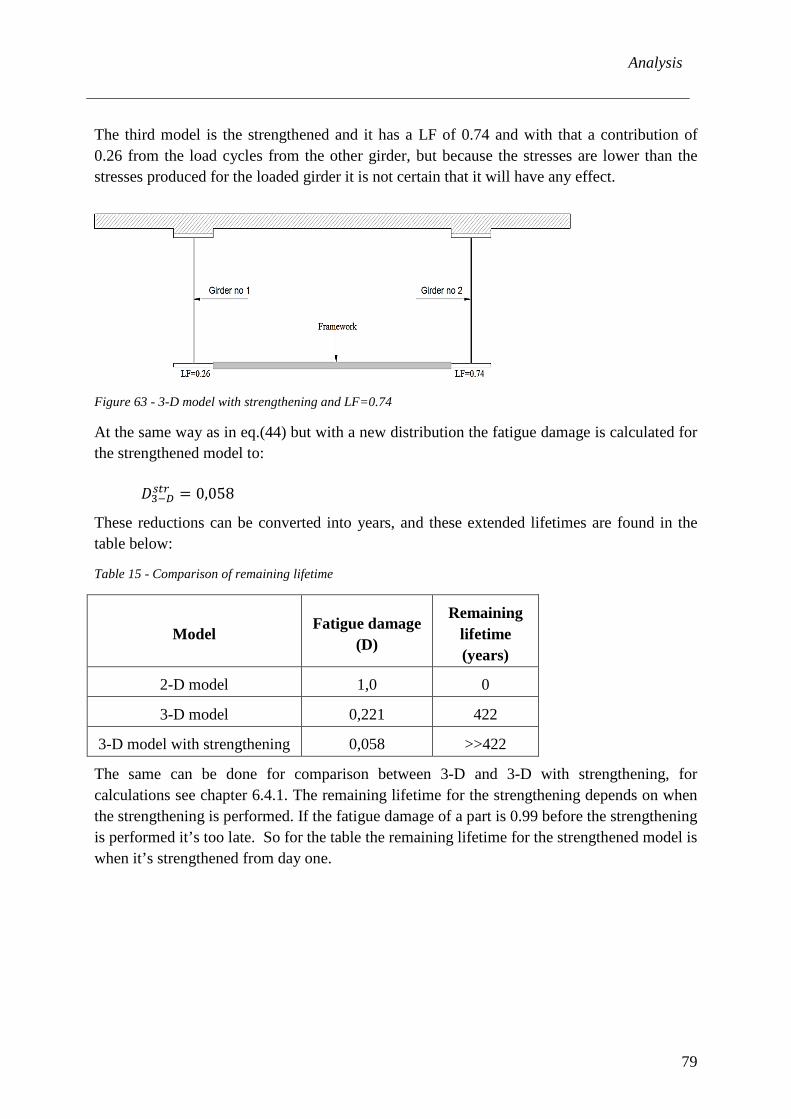
Analysis

79

The third model is the strengthened and it has a LF of 0.74 and with that a contribution of 0.26 from the load cycles from the other girder, but because the stresses are lower than the stresses produced for the loaded girder it is not certain that it will have any effect.

Figure 63 - 3-D model with strengthening and LF=0.74

At the same way as in eq.(44) but with a new distribution the fatigue damage is calculated for the strengthened model to:

𝐷𝐷3−𝐷𝐷𝑂𝑂𝑠𝑠𝑟𝑟 = 0,058

These reductions can be converted into years, and these extended lifetimes are found in the table below:

Table 15 - Comparison of remaining lifetime

Model Fatigue damage (D)

Remaining lifetime (years)

2-D model 1,0 0

3-D model 0,221 422

3-D model with strengthening 0,058 >>422

The same can be done for comparison between 3-D and 3-D with strengthening, for calculations see chapter 6.4.1. The remaining lifetime for the strengthening depends on when the strengthening is performed. If the fatigue damage of a part is 0.99 before the strengthening is performed it’s too late. So for the table the remaining lifetime for the strengthened model is when it’s strengthened from day one.

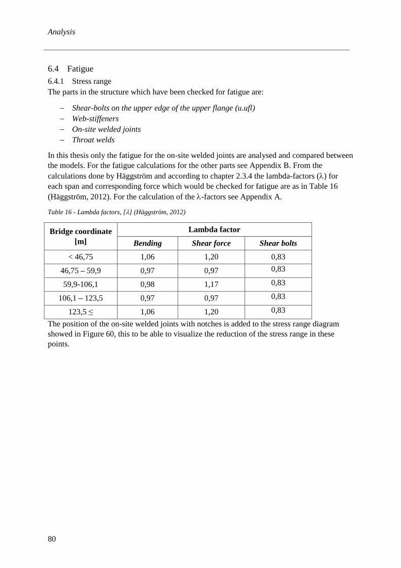
Analysis

80

6.4 Fatigue 6.4.1 Stress range The parts in the structure which have been checked for fatigue are:

− Shear-bolts on the upper edge of the upper flange (u.ufl) − Web-stiffeners − On-site welded joints − Throat welds

In this thesis only the fatigue for the on-site welded joints are analysed and compared between the models. For the fatigue calculations for the other parts see Appendix B. From the calculations done by Häggström and according to chapter 2.3.4 the lambda-factors (λ) for each span and corresponding force which would be checked for fatigue are as in Table 16 (Häggström, 2012). For the calculation of the λ-factors see Appendix A.

Table 16 - Lambda factors, [λ] (Häggström, 2012)

Bridge coordinate [m]

Lambda factor

Bending Shear force Shear bolts

< 46,75 1,06 1,20 0,83

46,75 – 59,9 0,97 0,97 0,83

59,9-106,1 0,98 1,17 0,83

106,1 – 123,5 0,97 0,97 0,83

123,5 ≤ 1,06 1,20 0,83

The position of the on-site welded joints with notches is added to the stress range diagram showed in Figure 60, this to be able to visualize the reduction of the stress range in these points.

Analysis

81

Figure 64 - Stress ranges for true stresses with position of the on-site welded joints for models

The values for the stress ranges are summarized in Table 17, where the on-site welded joints are numbered from left (1) to right (5) from Figure 64. The differences between the models are also calculated in the table and are shown as (%) with the 2-D model as reference value (100 %).

Table 17 – Stress range of the on-site welded joints for the models, from Figure 64

Beam joint ∆σ2-D

[MPa]; (% of σ2-D)

∆σ3-D,org.

[MPa]; (% of σ2-D)

∆σ3-D,str.

[MPa]; (% of σ2-D)

1 50,4; (100) 39,6; (78,6) 29,9; (59,3)

2 15,6; (100) 15,6; (100) 13,3; (85,3)

3 51,3; (100) 37,6; (73,3) 28,3; (55,2)

4 15,6; (100) 15,6; (100) 13,3; (85,3)

5 50,4; (100) 39,6; (78,6) 29,9; (59,3)

1 2 3 4 5 0

5

10

15

20

25

30

35

40

45

50

55

60

0 10 20 30 40 50 60 70 80 90 100 110 120 130 140 150 160 170

True

stre

ss [M

Pa]

X [m]

∆σtrue with marked joints

True stress 2-D model True stress 3-D original

True stress 3-D strengthened On-site welded joints

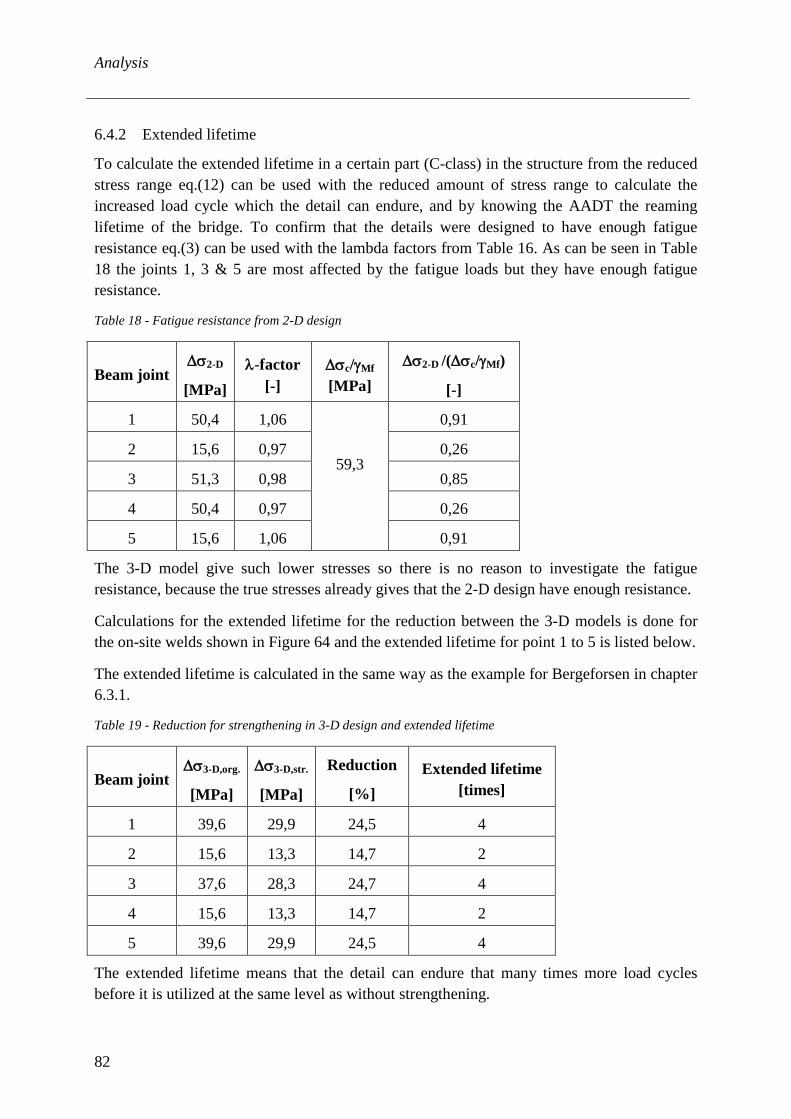
Analysis

82

6.4.2 Extended lifetime

To calculate the extended lifetime in a certain part (C-class) in the structure from the reduced stress range eq.(12) can be used with the reduced amount of stress range to calculate the increased load cycle which the detail can endure, and by knowing the AADT the reaming lifetime of the bridge. To confirm that the details were designed to have enough fatigue resistance eq.(3) can be used with the lambda factors from Table 16. As can be seen in Table 18 the joints 1, 3 & 5 are most affected by the fatigue loads but they have enough fatigue resistance.

Table 18 - Fatigue resistance from 2-D design

Beam joint ∆σ2-D

[MPa]

λ-factor [-]

∆σc/γMf

[MPa]

∆σ2-D /(∆σc/γMf)

[-]

1 50,4 1,06

59,3

0,91

2 15,6 0,97 0,26

3 51,3 0,98 0,85

4 50,4 0,97 0,26

5 15,6 1,06 0,91

The 3-D model give such lower stresses so there is no reason to investigate the fatigue resistance, because the true stresses already gives that the 2-D design have enough resistance.

Calculations for the extended lifetime for the reduction between the 3-D models is done for the on-site welds shown in Figure 64 and the extended lifetime for point 1 to 5 is listed below.

The extended lifetime is calculated in the same way as the example for Bergeforsen in chapter 6.3.1.

Table 19 - Reduction for strengthening in 3-D design and extended lifetime

Beam joint ∆σ3-D,org.

[MPa]

∆σ3-D,str.

[MPa]

Reduction

[%]

Extended lifetime [times]

1 39,6 29,9 24,5 4

2 15,6 13,3 14,7 2

3 37,6 28,3 24,7 4

4 15,6 13,3 14,7 2

5 39,6 29,9 24,5 4

The extended lifetime means that the detail can endure that many times more load cycles before it is utilized at the same level as without strengthening.

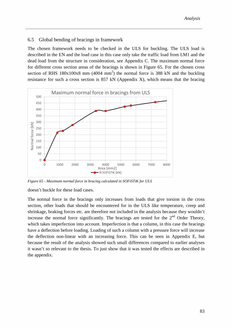
Analysis

83

6.5 Global bending of bracings in framework

The chosen framework needs to be checked in the ULS for buckling. The ULS load is described in the EN and the load case in this case only take the traffic load from LM1 and the dead load from the structure in consideration, see Appendix C. The maximum normal force for different cross section areas of the bracings is shown in Figure 65. For the chosen cross section of RHS 180x100x8 mm (4004 mm2) the normal force is 388 kN and the buckling resistance for such a cross section is 857 kN (Appendix X), which means that the bracing

doesn’t buckle for these load cases.

The normal force in the bracings only increases from loads that give torsion in the cross section, other loads that should be encountered for in the ULS like temperature, creep and shrinkage, braking forces etc. are therefore not included in the analysis because they wouldn’t increase the normal force significantly. The bracings are tested for the 2nd Order Theory, which takes imperfection into account. Imperfection is that a column, in this case the bracings have a deflection before loading. Loading of such a column with a pressure force will increase the deflection non-linear with an increasing force. This can be seen in Appendix E, but because the result of the analysis showed such small differences compared to earlier analyses it wasn’t so relevant to the thesis. To just show that it was tested the effects are described in the appendix.

0

50

100

150

200

250

300

350

400

450

500

0 1000 2000 3000 4000 5000 6000 7000 8000

Nor

mal

forc

e [k

N]

Area [mm2]

Maximum normal force in bracings from ULS

N SOFiSTiK [kN]

Figure 65 - Maximum normal force in bracing calculated in SOFiSTiK for ULS

Discussion and Conclusions

84

7 DISCUSSION AND CONCLUSIONS The results in previous chapter will be discussed and conclusions and possible errors and confounding variables will be presented. The aim of the thesis was to investigate and evaluate the effect from a horizontal framework of bracings between the lower flanges in an I-girder composite bridge. If proven that these gave effects of a more torsional stiff cross section and by so decreasing the stresses in girders the lifespan of the bridge would be prolonged. In addition analyses have been done for compression forces in the bracings for K-trusses and X-trusses with and without imperfections in ULS, to verify that the bracing doesn’t buckle so that the torsional stiffness decreases.

7.1 Discussion

The results from the concept bridge, which was compared to the theoretically calculations for the same cross sectional values shows that the FEM-model can be assumed correct by verification with the theory of torsion and warping. The calculations for the strengthened model gave similar results for both calculation methods (FEM and Hand-calculations). For the strengthened design which is a closed cross section the torsion is more dominating than the warping, like for an open cross section where the contribution is more equal between the two effects.

Disadvantages for the chosen model with the steel beams modelled as beam-element is that no local effects can be evaluated. In the beginning of the thesis only the global effect was meant to be analysed, and because it is easier to analyse moments in beam-elements than shell-elements and because of that modelling composite structures like this is proposed by the program support, these elements were chosen. The shell-elements however have the advantages of local effects from e.g. the connection point between flange and bracing, but first a good connection joint need to be decided. One proposed way can be to bolt the bracing in the flange with cover plates sliced in to the profile, a detail category of such a joint is C=112 according to the standards, if the bolts are pre-tensioned. That means that holes in un-used material are drilled and a detail category better than (C=80) is implied. (By un-used it means the material in the flange which is not effected by earlier fatigue loads and has if the structure is designed right not any plastic deformations.)

The lane factor which was used as a measurement of the load distribution showed that even small areas of the bracing have effect on the torsional stiffness. From a design perspective small areas can be used if a buckling analysis is done to verify that the bracings doesn’t buckle. The chosen dimensions of 180x100x8 (4004mm2) will not buckle according to 2nd Order Theory. The additional weight from the framework is only 1.6 % of the original steel weight so the framework gives small effect on the dead load but can almost be neglected..

Discussion and Conclusions

85

True stresses are used for verification of the fatigue resistance and the fatigue damage, these stresses is one way to determine if the concrete is cracked or un-cracked. It is a good representation of the behaviour of the concrete for positive and negative stresses and when the concrete is cracked only the reinforcement is in composite action with steel instead of the whole concrete section like it is when the concrete is un-cracked.

The differences between the 2-D and 3-D model shows that design in a 2-D analysis is on the safe side of reality regarding the distribution of eccentric loads. In terms of deciding the remaining lifetime of the structure is showed that the bridge will endure more load cycles than calculated in the design. To confirm that the bridge is good for more years than the design says a FEM-analysis can be done

7.2 Conclusions

Differences between a 2-D model and a 3-D model (FEM) show that load distribution of eccentric load is lower than 1.0 for Bergeforsen Bridge which means that both girders is effected by these loads (1,18 for 2-D and 0,95 for a 3-D model taking torsional and warping stiffnesses into account).

A framework between lower flanges is proven in this thesis to be a good method to reduce the stress range from FLM3 and by so extend the lifetime for the bridge. A chosen framework consisting of bracings (RHS) with dimensions of 180x100x8mm gives a reduction of the stress range down to 22.8 MPa for a specific detail which is a reduction with around 45 % of the design values. Even for small dimensions on the bracings a reduced stress range can be achieved and by so reduce the material costs for the performed strengthening method.

By summarising the result from this thesis the method of introducing box action into an I-girder composite bridge is shown to be a good method for strengthening old existing bridges regarding prolonging the lifetime.

7.3 Suggestions for further research

Like mentioned earlier the local effects should be analysed and results be checked by other models (element types). The global effects shouldn’t vary but the influence of stresses depending on chosen connection for the framework in the flange should be analysed. Optimization for individual bridges depending on angle and distances between the frameworks is an interesting part to investigate.

The effects from the new distribution of loads between the girders could be more analysed, there considering the effects from loads in other lanes. These stresses should be accounted for in the damage accumulation, in this thesis the stresses were assumed to be smaller than the cut-off limit needed to have an effect on the fatigue damage. But for boxes where the load distribution (lane factor) is more like 50/50 these distributions should be more explained in the EN 1991-1-2.

Discussion and Conclusions

86

An interesting thing to investigate or to be tested is the load distribution, if it can be confirmed that both girders are affected by an eccentric load on top of one girder the fatigue damage of the structure is reduced. Even more interesting is to test a bridge with horizontal bracings (K-trusses or other shapes) and compare these values with an analysis in a FEM-model. It would be very interesting to strengthen a bridge which is designed by older standards with this method and make tests on it, before and after strengthening.

References

87

REFERENCES

Adamakos, T., Vayas, I. & Iliopoulos, A., 2011. Modeling of Composite Bridges using Bar Elements. Lateral Bracing and Cross-frames Influence. EUROSTEEL, Budapest, Hungary, Augusti 31-September 2.

Al-Emrani, M. & Aygül, M., 2014. Fatigue design of steel and composite bridges, Göteborg: Chalmers University of Tchnology, Division of Structual Engineering, Steel and Timber Structure.

Bathias, C. & Pineau, A., 2010. Fatigue of Materials and Structures. Great Britian and the United States: ISTE Ltd and John Wiley & Sons, Inc.

Beales, C., 1990. Assesment of Trough to Crossbeam Connections in Orthotropic Steel Bridge Decks, Research Report 276, Crowthorne: Transport and Road Reasearch Labratory.

Bloom, J. M. & Ekvall, J. C., 1983. Probalistic Fracture Mechanics and Fatigue Methods: Applications for Structural Design and Maintenance. 798 ed. Baltimore: ASTM International.

Collings, D., 2005. Steel-Concrete Composite Bridges. 1 ed. Londom: Thomas Telfjord Publishing, Thomas Telford Ltd.

Collin, P., Johansson, B. & Sundquist, H., 2011. Steel Concrete Composire Bridges. 4th Edition ed. Stockholm, Sweden: KTH Architecture and the Built Enviroment, LTU Division of Structural Engineering.

Croce, P. e. a., 2010. Guidebook 2 - Design of Bridges. P. Croce ed. Praque: Czech Technical University.

Dickson, D. M., n.d. Poyle to M4: Alternative Steel Viaducts. Proceedings of the Institution of Civil Engineers, 82 Part 1, pp. 309-326.

Halden, J., 2015. International Workshop of Strengthening of Steel/Composite Bridges. Stockholm, s.n.

Häggström, J., 2012. 22-1675-1, Bro över utskovskanal vid Bergeforsen på väg 331, Luleå: Rambøll, orgnr: 556133-0506.

Häggström, J., 2012. Bergeforsen Bridge. [Art] (Rambøll Sverige).

INTI, N. I. o. I. T., 2012. Girder Bridge, Argentina: s.n.

Larsen, P. K., 2010. Dimensjonering av stålkonstruksjoner. 2. ed. Trondheim: Tapir Akademisk Forlag.

Mellon, F. L. & Mancarti, G. D., 1989. Memo to designers. s.l., s.n.

References

88

Nilsson, M., 2012. Secondary Strain in Web Stiffeners in Steel and Composite Bridges, Luleå: Universitetstryckeriet LTU.

Nylander, H., 1973. Grundläggande elasticitetsteori och vridning. Meddelande nr. 98 ed. Stockholm: Kungliga Tekniska Högskolan, Institutionen för Byggnadsstatik.

Ramböll, Sverige, n.d. Brokonstruktion, kontakt, Stockholm: Ramböll.

Roik, K., 1983. Vorlesungen über Stahlbau : Grundlagen. 2nd ed. Berlin: Berlag von W. Ernst & Sohn.

Ryall, M., 1999. Britannia Bridge: from concept to construction. Proceedings of the Institution of Civil Engineerings 132, May/Aug.

Sibly, P. & Walker, A., 1977. Structual Accidents and Their Causes. Proceedings of the Institution of Civil Engineers, Part 1, 62, May.

Smith, R., 1990. The Versailles railway accident of 1842 and the first research into meal fatigue. In: Birmingham: EMAS, pp. 2033-2041.

SOFiSTiK AG, 2014. SOFiMSHA - Import and Export of Finite Elements and Beam Structures, Oberschleissheim: SOFiSTiK AG.

SOFiSTiK, 2014. Manual Version 2014, Nuremberg, Germany: SOFiSTiK AG.

SS-EN 1991-2, 2010. SS-EN 1991-2, s.l.: Swedish Standards Institute.

SS-EN 1993-1-9, 2005. SS-EN 1993-1-9, Stockholm: SIS Förlag AB.

SS-EN 1994-1-1, 2009. SS-EN 1994-1-1, s.l.: Swedish Standards Institute.

SS-EN 1994-2, 2005. SS-EN 1994-2, s.l.: s.n.

SteelConstruction.info, 2015. www.steelconstruction.info. [Online] Available at: http://www.steelconstruction.info/Stiffeners [Accessed 30 November 2015].

Totoh, L., 2001. Fatigue crack growth laws and their material parameters. Mekanika vol. 269, pp. 349-368.

Trafikverket, 2011. TRVK Bro 11, s.l.: Trafikverket.

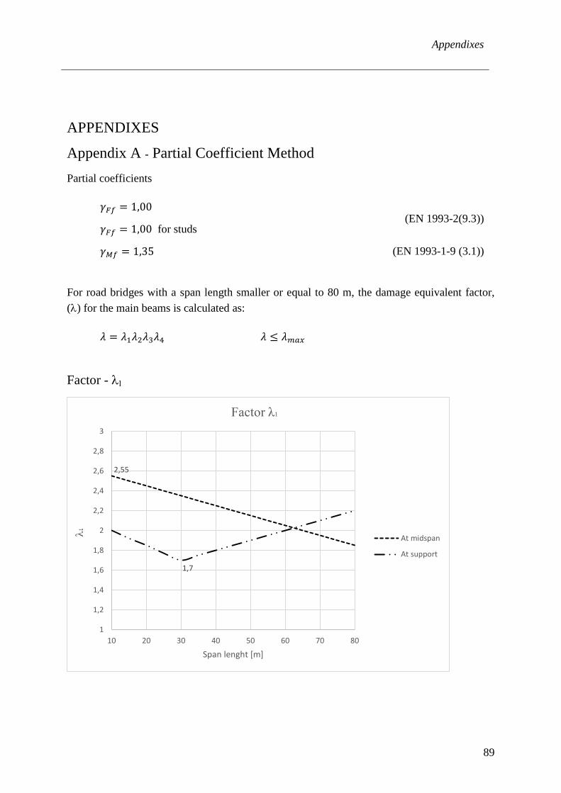
Appendixes

89

APPENDIXES

Appendix A - Partial Coefficient Method Partial coefficients

𝛾𝛾𝐹𝐹𝐹𝐹 = 1,00

𝛾𝛾𝐹𝐹𝐹𝐹 = 1,00 for studs (EN 1993-2(9.3))

𝛾𝛾𝐹𝐹𝐹𝐹 = 1,35 (EN 1993-1-9 (3.1))

For road bridges with a span length smaller or equal to 80 m, the damage equivalent factor, (λ) for the main beams is calculated as:

𝜆𝜆 = 𝜆𝜆1𝜆𝜆2𝜆𝜆3𝜆𝜆4 𝜆𝜆 ≤ 𝜆𝜆𝑚𝑚𝑚𝑚𝑚𝑚

Factor - λ1

2,55

1,7

1

1,2

1,4

1,6

1,8

2

2,2

2,4

2,6

2,8

3

10 20 30 40 50 60 70 80

Span lenght [m]

Factor λ1

At midspan

At support

Appendixes

90

The different length are:

𝐿𝐿1 = 50,0 𝑚𝑚, Bending moment in span 1,3

𝐿𝐿1 = 66,0 𝑚𝑚, Bending moment in span 2

𝐿𝐿1 = 58,0 𝑚𝑚, Bending moment at internal support

𝐿𝐿1 = 20,0 𝑚𝑚, Shear force in span 1,3

𝐿𝐿1 = 26,4 𝑚𝑚, Shear force in span 2

𝐿𝐿1 = 58,0 𝑚𝑚, Shear force at internal support

𝐿𝐿1 = 6,0 𝑚𝑚, Bending moment, cross-beams

These gives following λ1-values:

𝜆𝜆1 = 2,15 Bending moment in span 1,3

𝜆𝜆1 = 1,99 Bending moment in span 2

𝜆𝜆1 = 1,98 Bending moment at internal support

𝜆𝜆1 = 2,45, Shear force in span 1,3

𝜆𝜆1 = 2,39 Shear force in span 2

𝜆𝜆1 = 1,98 Shear force at internal support

𝜆𝜆1 = 2,59 Bending moment, cross-beams

For the shear studs the λ-value is:

𝜆𝜆𝑣𝑣,1 = 1,55 Shear studs, regardless span or support

(EN 1994-2 (6.8.6.2))

Factor - λ2

The second factor is describing the amount of traffic over the bridge per year and is calculated as:

𝜆𝜆2 =𝑄𝑄𝑚𝑚1𝑄𝑄0

�𝑁𝑁𝑂𝑂𝑂𝑂𝑂𝑂𝑁𝑁0

�1/5

Construction steel

𝜆𝜆2 =𝑄𝑄𝑚𝑚1𝑄𝑄0

�𝑁𝑁𝑂𝑂𝑂𝑂𝑂𝑂𝑁𝑁0

�1/8

Shear studs

𝑄𝑄𝑚𝑚1 = 300 𝑘𝑘𝑁𝑁 (EN 1993-2 (9.5.2 (3)))

Appendixes

91

𝑄𝑄0 = 480 𝑘𝑘𝑁𝑁 (EN 1993-2 (9.5.2 (3)))

𝑁𝑁𝑂𝑂𝑂𝑂𝑂𝑂 = 125000 (EN 1993-2 (9.5.2 (3)))

𝑁𝑁0 = 500000 (EN 1993-2 (9.5.2 (3)))

Which gives the value:

𝜆𝜆2 = 0,474 Construction steel

𝜆𝜆2 = 0,526 Shear studs

Factor - λ3

To consider the design life of the bridge this factor is calculated

𝜆𝜆3 = �

𝑡𝑡𝐹𝐹𝐿𝐿100

�1/5

Construction steel

𝜆𝜆3 = �

𝑡𝑡𝐹𝐹𝐿𝐿100

�1/8

Shear studs

The design life is set to 120 years

𝜆𝜆3 = 1,037 Construction steel

𝜆𝜆3 = 1,023 Shear studs

Factor - λ4

Is set to 1,0 by the national annex (EN 1993-2 NA)

Factor - λmax

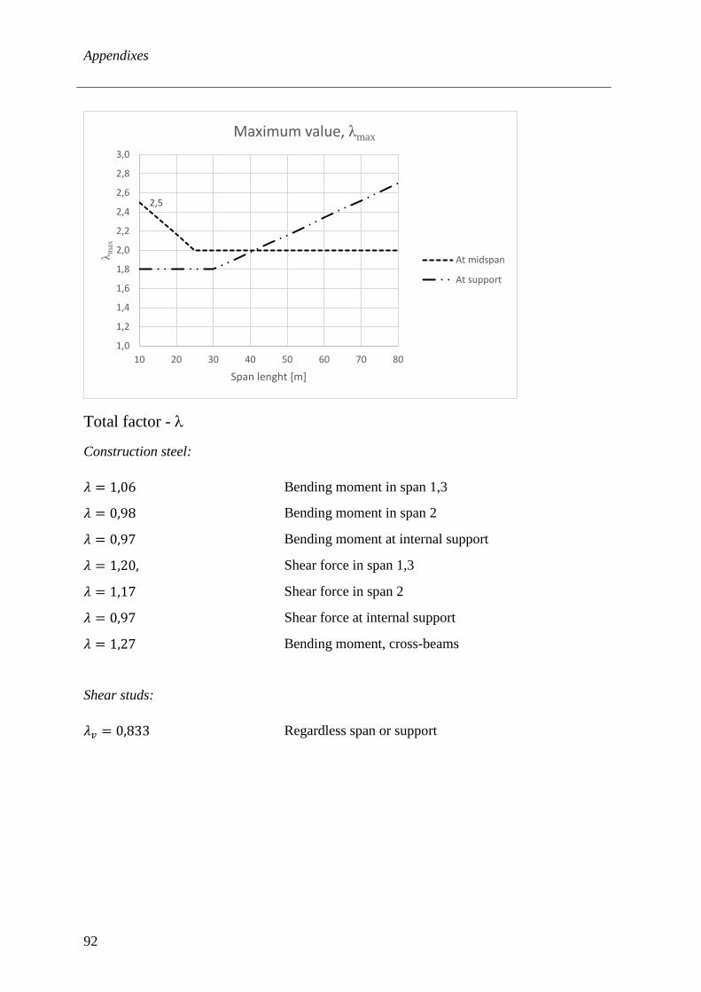
Appendixes

92

Total factor - λ

Construction steel:

𝜆𝜆 = 1,06 Bending moment in span 1,3

𝜆𝜆 = 0,98 Bending moment in span 2

𝜆𝜆 = 0,97 Bending moment at internal support

𝜆𝜆 = 1,20, Shear force in span 1,3

𝜆𝜆 = 1,17 Shear force in span 2

𝜆𝜆 = 0,97 Shear force at internal support

𝜆𝜆 = 1,27 Bending moment, cross-beams

Shear studs:

𝜆𝜆𝑣𝑣 = 0,833 Regardless span or support

2,5

1,0

1,2

1,4

1,6

1,8

2,0

2,2

2,4

2,6

2,8

3,0

10 20 30 40 50 60 70 80

λ max

Span lenght [m]

Maximum value, λmax

At midspan

At support

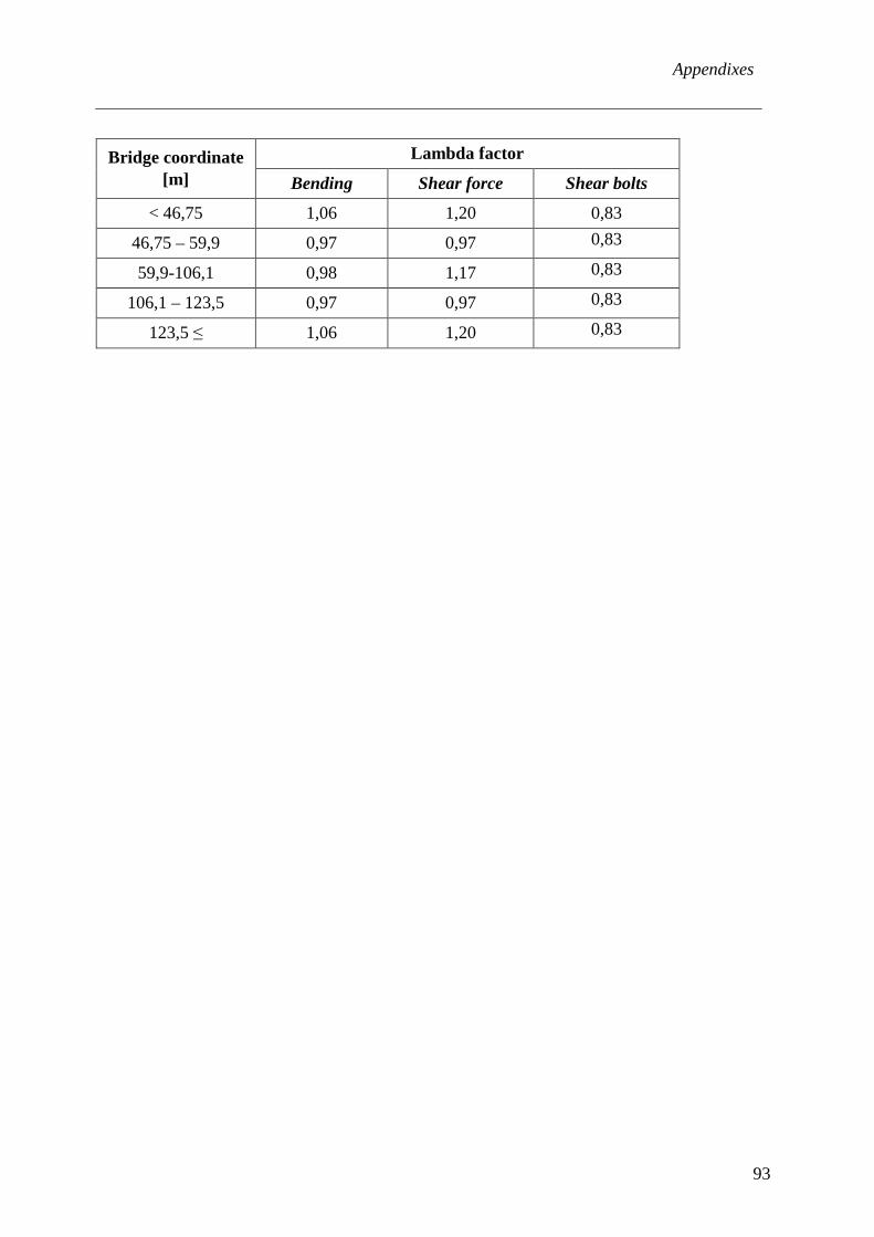
Appendixes

93

Bridge coordinate [m]

Lambda factor

Bending Shear force Shear bolts

< 46,75 1,06 1,20 0,83

46,75 – 59,9 0,97 0,97 0,83

59,9-106,1 0,98 1,17 0,83

106,1 – 123,5 0,97 0,97 0,83

123,5 ≤ 1,06 1,20 0,83

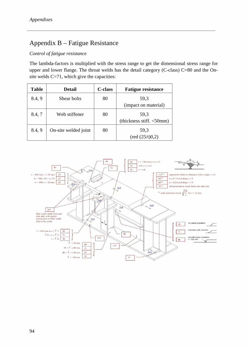
Appendixes

94

Appendix B – Fatigue Resistance Control of fatigue resistance

The lambda-factors is multiplied with the stress range to get the dimensional stress range for upper and lower flange. The throat welds has the detail category (C-class) C=80 and the On-site welds C=71, which give the capacities:

Table Detail C-class Fatigue resistance

8.4, 9 Shear bolts 80 59,3 (impact on material)

8.4, 7 Web stiffener 80 59,3 (thickness stiff. <50mm)

8.4, 9 On-site welded joint 80 59,3 (red (25/t)0,2)

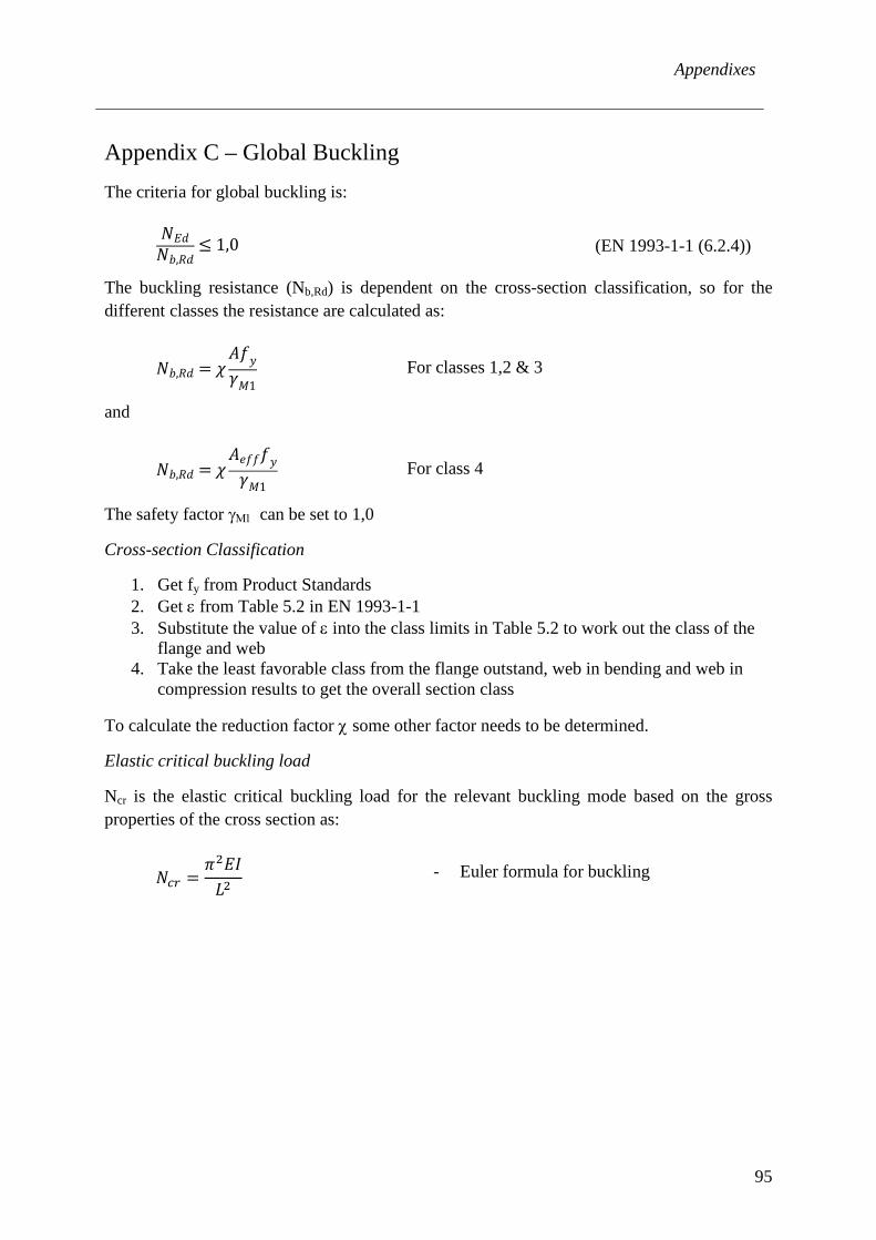
Appendixes

95

Appendix C – Global Buckling The criteria for global buckling is:

𝑁𝑁𝐸𝐸𝑑𝑑𝑁𝑁𝑏𝑏,𝑅𝑅𝑑𝑑

≤ 1,0 (EN 1993-1-1 (6.2.4))

The buckling resistance (Nb,Rd) is dependent on the cross-section classification, so for the different classes the resistance are calculated as:

𝑁𝑁𝑏𝑏,𝑅𝑅𝑑𝑑 = 𝜒𝜒

𝐴𝐴𝑙𝑙𝑦𝑦𝛾𝛾𝑀𝑀1

For classes 1,2 & 3

and

𝑁𝑁𝑏𝑏,𝑅𝑅𝑑𝑑 = 𝜒𝜒

𝐴𝐴𝑒𝑒𝑙𝑙𝑙𝑙𝑙𝑙𝑦𝑦𝛾𝛾𝑀𝑀1

For class 4

The safety factor γΜ1 can be set to 1,0

Cross-section Classification

1. Get fy from Product Standards 2. Get ε from Table 5.2 in EN 1993-1-1 3. Substitute the value of ε into the class limits in Table 5.2 to work out the class of the

flange and web 4. Take the least favorable class from the flange outstand, web in bending and web in

compression results to get the overall section class

To calculate the reduction factor χ some other factor needs to be determined.

Elastic critical buckling load

Ncr is the elastic critical buckling load for the relevant buckling mode based on the gross properties of the cross section as:

𝑁𝑁𝑐𝑐𝑟𝑟 =

𝜋𝜋2𝐸𝐸𝐼𝐼𝐿𝐿2

- Euler formula for buckling

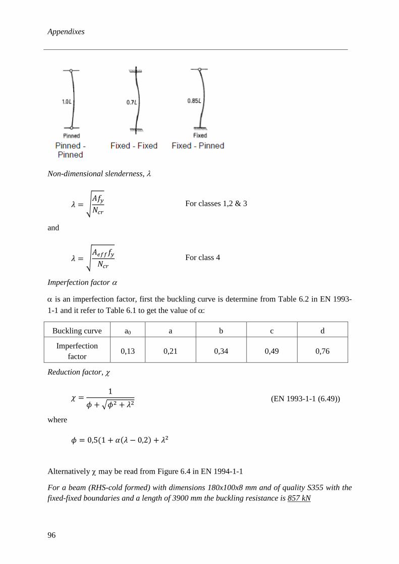
Appendixes

96

Non-dimensional slenderness, λ

𝜆𝜆 = �

𝐴𝐴𝑙𝑙𝑧𝑧𝑁𝑁𝑐𝑐𝑟𝑟

For classes 1,2 & 3

and

𝜆𝜆 = �

𝐴𝐴𝑐𝑐𝐹𝐹𝐹𝐹𝑙𝑙𝑧𝑧𝑁𝑁𝑐𝑐𝑟𝑟

For class 4

Imperfection factor α

α is an imperfection factor, first the buckling curve is determine from Table 6.2 in EN 1993-1-1 and it refer to Table 6.1 to get the value of α:

Buckling curve a0 a b c d

Imperfection factor

0,13 0,21 0,34 0,49 0,76

Reduction factor, χ

𝜒𝜒 =1

𝜙𝜙 + �𝜙𝜙2 + 𝜆𝜆2 (EN 1993-1-1 (6.49))

where

𝜙𝜙 = 0,5(1 + 𝛼𝛼(𝜆𝜆 − 0,2) + 𝜆𝜆2

Alternatively χ may be read from Figure 6.4 in EN 1994-1-1

For a beam (RHS-cold formed) with dimensions 180x100x8 mm and of quality S355 with the fixed-fixed boundaries and a length of 3900 mm the buckling resistance is 857 kN

Appendixes

97

Appendix D – SOFiSTiK Database Workflow

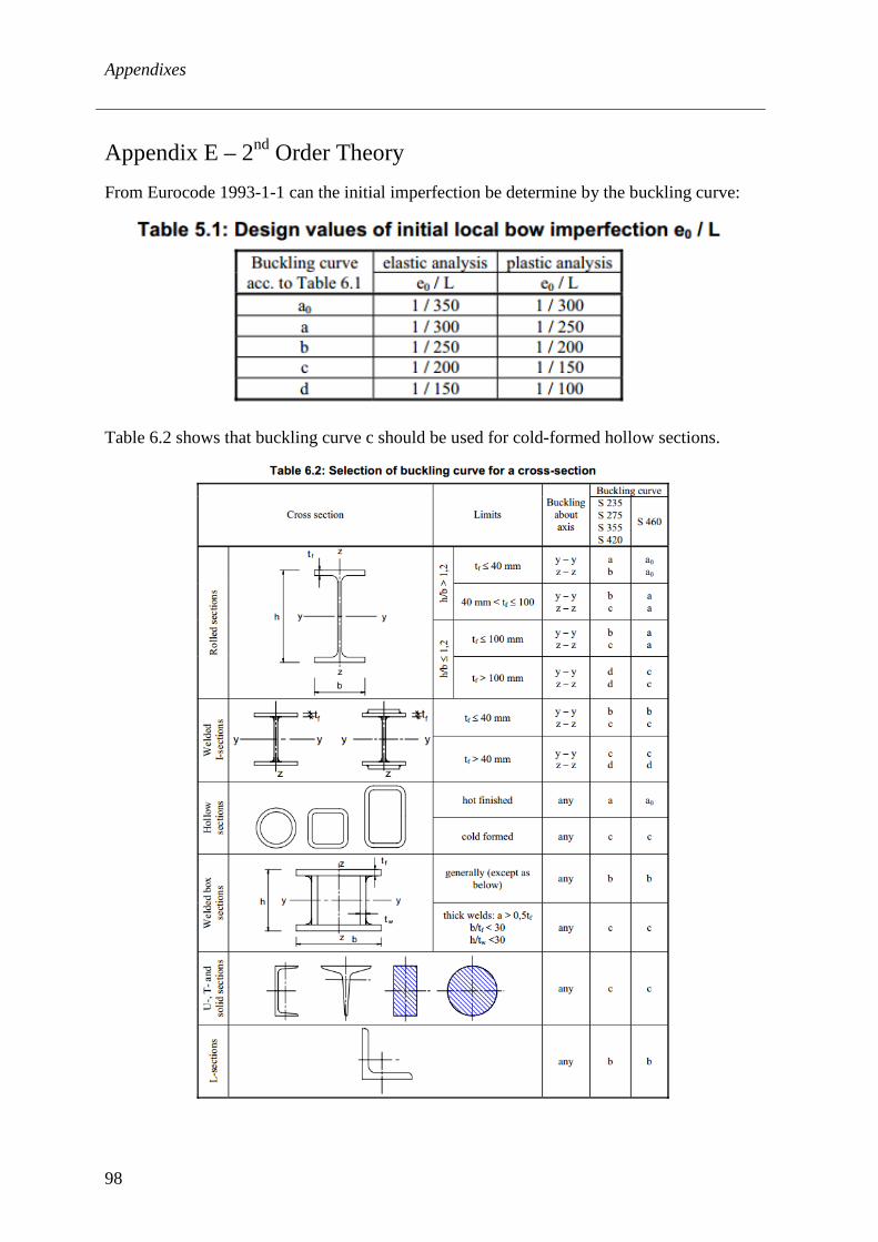
Appendixes

98

Appendix E – 2nd Order Theory From Eurocode 1993-1-1 can the initial imperfection be determine by the buckling curve:

Table 6.2 shows that buckling curve c should be used for cold-formed hollow sections.

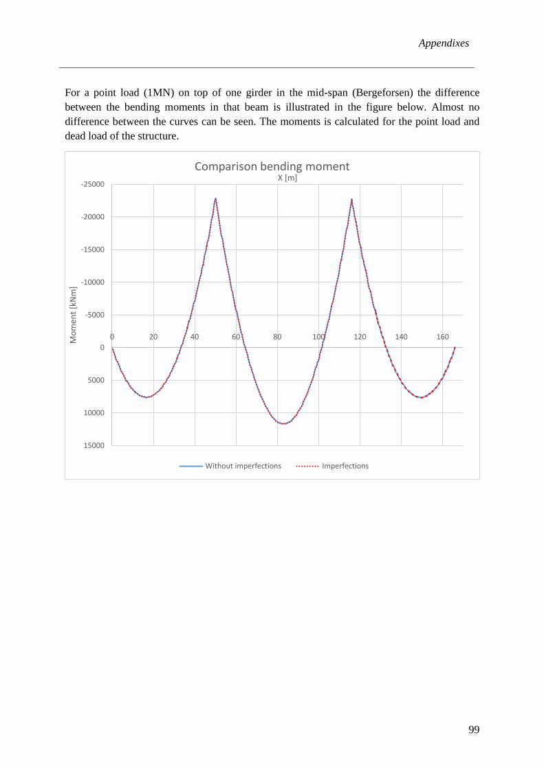
Appendixes

99

For a point load (1MN) on top of one girder in the mid-span (Bergeforsen) the difference between the bending moments in that beam is illustrated in the figure below. Almost no difference between the curves can be seen. The moments is calculated for the point load and dead load of the structure.

-25000

-20000

-15000

-10000

-5000

0

5000

10000

15000

0 20 40 60 80 100 120 140 160Mom

ent [

kNm

]

X [m] Comparison bending moment

Without imperfections Imperfections

Appendixes

100

Appendix F – Bending Moment X-trusses, Lane 1-centric

1964,17

0

500

1000

1500

2000

2500

0 10 20 30 40 50 60 70 80 90 100 110 120 130 140 150 160 170 180

Mom

ent [

kNm

]

X [m]

Global bending X-trusses for FLM3 in Lane 1-centric

X-trusses

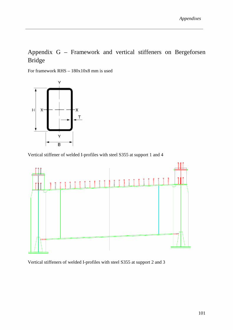
Appendixes

101

Appendix G – Framework and vertical stiffeners on Bergeforsen Bridge For framework RHS – 180x10x8 mm is used

Vertical stiffener of welded I-profiles with steel S355 at support 1 and 4

Vertical stiffeners of welded I-profiles with steel S355 at support 2 and 3

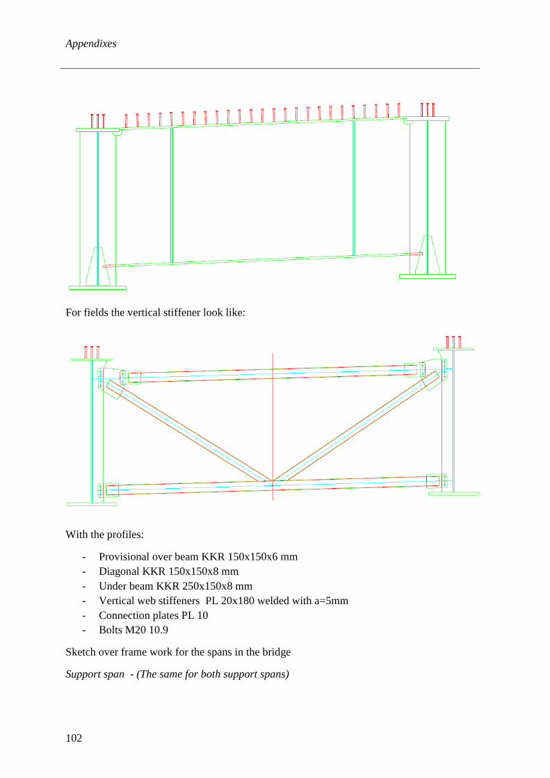
Appendixes

102

For fields the vertical stiffener look like:

With the profiles:

- Provisional over beam KKR 150x150x6 mm - Diagonal KKR 150x150x8 mm - Under beam KKR 250x150x8 mm - Vertical web stiffeners PL 20x180 welded with a=5mm - Connection plates PL 10 - Bolts M20 10.9

Sketch over frame work for the spans in the bridge

Support span - (The same for both support spans)

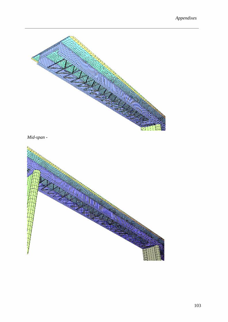
Appendixes

103

Mid-span -