Master's Thesis Deterministic Ocean Waves Fredrik Larsson

Master’s Thesis

Deterministic Ocean Waves

Fredrik Larsson

Department of Computer Science Faculty of Engineering LTH Lund University, 2012

ISSN 1650-2884 LU-CS-EX: 2012-18

M.Sc. Thesis in Computer Science

Deterministic Ocean Waves

Fredrik LarssonLund University

Institute of Technology, LTHDepartment of Computer Science

Advisors:Torbjörn Söderman, EA DICEBjörn Ottosson, EA DICE

Michael Doggett, Lund University

August 20, 2012

Abstract

In this master’s thesis a system for deterministic ocean wave simulationis presented. The target application is interactive multi-client computergames, where the system can render a visual representation of the oceansurface as well as provide surface data to other systems, such as a buoyancyphysics simulation. Ocean waves caused by wind above the water surface aresimulated by propagating waves in the Fourier domain, where a Fast FourierTransform algorithm is used for efficient computations. Additional largerindividual waves are represented by a basic particle system in an algorithminspired by Wave Particles. A prototype implementation was integratedinto an existing system for interactive water waves in the Frostbite enginedeveloped by EA DICE. The simulation can, with reasonable quality, achievesub-millisecond run times on current generation gaming consoles and PChardware.

Sammanfattning

I denna masteruppsats presenteras ett system för deterministisk oceanvågsi-mulering. Målapplikationen är interaktiva datorspel för multipla klienter,där systemet kan rendera en visuell represenation av havsytan och dess-utom kan tillhandahålla data till andra system, så som fysiksimuleringar förflytande objekt. Havsvågor som orsakas av vind ovanför havsytan simulerasgenom vågpropagering i Fourierdomänen, där en algoritm för snabb Fouri-ertransform används för att uppnå tillräcklig prestanda. Större individuellavågor representeras av ett partikelsystem där en algoritm som inspireratsav Vågpartiklar tillämpats. En prototyp har implementerats i ett existeran-de system för interaktiva vattenvågor i spelmotorn Frostbite, som utvecklasav EA DICE. Simulering kan med rimlig kvalitet uppnå beräkningstider påunder 1 millisekund på denna generations spelkonsoler och PC-hårdvara.

Contents

Abstract i

Sammanfattning ii

Contents iii

List of Figures v

1 Introduction 11.1 Scope . . . . . . . . . . . . . . . . . . . . . . . . . . . . . . . 11.2 Outline . . . . . . . . . . . . . . . . . . . . . . . . . . . . . . 2

2 Background 32.1 Fluid Simulations . . . . . . . . . . . . . . . . . . . . . . . . . 32.2 Ocean Surface Simulation . . . . . . . . . . . . . . . . . . . . 32.3 Interactive Water Surfaces . . . . . . . . . . . . . . . . . . . . 5

3 Overview 73.1 Local Interactive Simulation . . . . . . . . . . . . . . . . . . . 7

3.1.1 Level of Detail . . . . . . . . . . . . . . . . . . . . . . 73.1.2 Heightfield Generation and Propagation . . . . . . . . 83.1.3 Rendering . . . . . . . . . . . . . . . . . . . . . . . . . 9

3.2 Physics Simulation . . . . . . . . . . . . . . . . . . . . . . . . 93.2.1 Networking and Prediction . . . . . . . . . . . . . . . 9

4 Method 114.1 Ocean Waves and the Fast Fourier Transform . . . . . . . . . 11

4.1.1 Features . . . . . . . . . . . . . . . . . . . . . . . . . . 114.1.2 Notation . . . . . . . . . . . . . . . . . . . . . . . . . . 124.1.3 Wave Distribution . . . . . . . . . . . . . . . . . . . . 134.1.4 Wave Dispersion . . . . . . . . . . . . . . . . . . . . . 144.1.5 Transforming . . . . . . . . . . . . . . . . . . . . . . . 154.1.6 Additional Data . . . . . . . . . . . . . . . . . . . . . 15

4.2 Wave Entities . . . . . . . . . . . . . . . . . . . . . . . . . . . 16

iii

4.2.1 Particle System . . . . . . . . . . . . . . . . . . . . . . 164.2.2 Particles as a Heightfield . . . . . . . . . . . . . . . . 174.2.3 Water Interaction . . . . . . . . . . . . . . . . . . . . 18

5 Implementation Details 195.1 Overview . . . . . . . . . . . . . . . . . . . . . . . . . . . . . 195.2 Simulation Tasks . . . . . . . . . . . . . . . . . . . . . . . . . 20

5.2.1 Initialization . . . . . . . . . . . . . . . . . . . . . . . 215.2.2 Updating the Heightfield . . . . . . . . . . . . . . . . 225.2.3 Precomputation of Heightfields for Point Sampling . . 225.2.4 Level of Detail Preparation . . . . . . . . . . . . . . . 22

5.3 Heightfield Sampling . . . . . . . . . . . . . . . . . . . . . . . 235.4 Simulation Parameters . . . . . . . . . . . . . . . . . . . . . . 245.5 The Fast Fourier Transform . . . . . . . . . . . . . . . . . . . 24

5.5.1 Using FFTW . . . . . . . . . . . . . . . . . . . . . . . 255.6 Wave Particles . . . . . . . . . . . . . . . . . . . . . . . . . . 25

5.6.1 Particle Data . . . . . . . . . . . . . . . . . . . . . . . 255.6.2 Subdivision . . . . . . . . . . . . . . . . . . . . . . . . 26

5.7 Rendering . . . . . . . . . . . . . . . . . . . . . . . . . . . . . 26

6 Results 296.1 Renderings . . . . . . . . . . . . . . . . . . . . . . . . . . . . 296.2 Performance . . . . . . . . . . . . . . . . . . . . . . . . . . . . 32

6.2.1 Performance Improvements from Using FFTW . . . . 336.3 Modified Phillips Spectrum . . . . . . . . . . . . . . . . . . . 336.4 Wave Entities . . . . . . . . . . . . . . . . . . . . . . . . . . . 34

7 Discussion 357.1 Ocean Wave Simulation Using FFT . . . . . . . . . . . . . . . 35

7.1.1 Performance . . . . . . . . . . . . . . . . . . . . . . . 357.1.2 Spectrum Tweaks . . . . . . . . . . . . . . . . . . . . . 357.1.3 Parameter Changes . . . . . . . . . . . . . . . . . . . . 367.1.4 Shores . . . . . . . . . . . . . . . . . . . . . . . . . . . 367.1.5 Tiling Artefacts and Cracks . . . . . . . . . . . . . . . 367.1.6 Heightfield Sampling Discrepancy . . . . . . . . . . . . 37

7.2 Wave Entities . . . . . . . . . . . . . . . . . . . . . . . . . . . 387.2.1 Other Uses . . . . . . . . . . . . . . . . . . . . . . . . 38

7.3 Conclusion . . . . . . . . . . . . . . . . . . . . . . . . . . . . 39

iv

List of Figures

4.1 Particle subdivision . . . . . . . . . . . . . . . . . . . . . . . . 17

5.1 Heightfield LOD preparation . . . . . . . . . . . . . . . . . . 235.2 Quadtree LOD Hierarchy . . . . . . . . . . . . . . . . . . . . 275.3 Rendering of wave particles . . . . . . . . . . . . . . . . . . . 28

6.1 Heightfield and displacement fields . . . . . . . . . . . . . . . 306.2 Derivatives and normal map . . . . . . . . . . . . . . . . . . . 306.3 Sample rendering of water body . . . . . . . . . . . . . . . . . 316.4 Sample wireframe rendering of water body . . . . . . . . . . . 316.5 Phillips spectra . . . . . . . . . . . . . . . . . . . . . . . . . . 34

v

Chapter 1

Introduction

When simulating and rendering a physically correct world, sooner or laterone usually needs to address the issue of representing and visualizing abody of water. Such a body of water may occur in varying sizes and ap-pearances ranging from small rain puddles to vast stormy oceans. Watersimulations have over the last decades seen numerous takes, both in interac-tive applications, off-line image generation and simulation of fluid dynamics.Common to all methods is the aim of achieving a high level of physical accu-racy while maintaining low computational cost. Simulation with interactiveframe rates, which is the topic of this thesis, is of course more leaned towardskeeping the needed computational effort low and is satisfied with results ata plausible level.

1.1 ScopeIn this thesis, the simulation of ocean waves is discussed, with the targetapplication being multi-client computer games. The goal is to representtwo types of waves occurring on the ocean surface: ambient waves andlarger individual waves. The ambient waves should provide a simulatedrepresentation of a water surface of oceanic proportions under given weatherconditions. The ability to manually place large individual waves on top ofthe simulated surface can be used to design specific gameplay events, forexample a dam breaking or a tsunami.

One use of the simulation results in this application is to render a visualrepresentation of the water surface. This involves supplying the underly-ing rendering system with a mesh representation of the simulation results.Another use is to provide other systems in the application with responsesto water level queries. For example, a physics simulation system may needsuch information in order to simulate the motion of an object floating in thewater body.

A multi-client game usually involves a server application in addition to

1

CHAPTER 1. INTRODUCTION 2

the clients. It is essential that the water surface affects the game worldequally on all involved clients, including the server. To achieve this, theocean surface needs to be fully deterministic across all clients, for any givenpoint in time. The server and clients are connected via a network, usuallythe Internet, which imposes further issues in terms of latency and synchro-nization, something that also needs to be addressed by the system.

This thesis is focused on finding a suitable model for the problem formu-lation given above, and presenting a prototype implementation of it. Themain focus is obtaining an efficient implementation of a simulation of am-bient wind-driven waves that can potentially be incorporated in today’sgames. The implementation of individual wave entities is complemental andpresented as a proof of concept. The implementation will be incorporatedinto the Frostbite engine, developed by EA DICE, where it needs to inte-grate with other sub-systems of the engine. For this reason, the availableresources for the system are highly restricted, which introduces further per-formance requirements. The ocean wave simulation also needs to integratewith an existing system for water interaction. The interaction simulation islocal to each client and is used for generating and propagating waves causedby disturbances of the water surface.

For any component in a game engine it is essential that a high enoughlevel of control is exposed to the user. The user here is an artist or gamedesigner, who must be able to tweak the ocean waves to obtain the visualappearance and game experience they want. Furthermore, it is also impor-tant to be able to adjust the fidelity of the simulation for devices on bothends of the performance scale.

1.2 OutlineA brief presentation of previous research in the area is discussed in chapter2, where a number of different approaches for both ocean wave simulationand interactive wave simulation are discussed. The restrictions and featuresoffered by the target system for the reference implementation are presentedin chapter 3. These two chapters are used as a motivation for the chosenmethod, which is outlined in chapter 4. The reference implementation of themethod is presented in chapter 5, with the results in chapter 6. Finally, adiscussion on the results and suggestions for future improvements concludesthe report in chapter 7.

Chapter 2

Background

2.1 Fluid SimulationsAny work concerning simulation of fluids is almost obliged to mention theNavier-Stokes equations. These are a set of partial differential equationsdescribing the movements of a fluid. The equations are of non-linear nature,and thus very difficult to solve. In the field of computational fluid dynamics(CFD) various numerical methods are applied in order to solve the equations.The methods of CFD are often applicable for off-line simulations of fluidphenomena and require large amounts of computational power. If interactiveframe rates are the target, the methods from CFD must be discarded infavour of ones of less computational intensity. As in many other situationsin real-time computer graphics, one is forced to resort to approximations ofmore or less severity to get a good balance between computational time andresult plausibility.

As will be shown in this chapter, many of the methods aiming for in-teractive frame rates reduce the otherwise three-dimensional problem to asimilar one in two dimensions. This reduction means that only waves presenton the water surface are simulated, discarding phenomena such as verticalflow and turbulence.

Many methods presented here also use a heightfield to represent the wa-ter surface. A heightfield is a map from a two-dimensional point p to a cor-responding vertical displacement. As the heightfield is animating, the mapalso depends on time, meaning that a function h(p, t) is the mathematicalrepresentation of the heightfield. The heightfield representation introducesfurther restrictions, for example the inability to represent breaking waves.

2.2 Ocean Surface SimulationA well known and early model of the ocean surface was presented by Fournierand Reeves, which utilizes the theory of Gerstner waves. In the Gerstner

3

CHAPTER 2. BACKGROUND 4

model, water particles exhibit elliptical stationary orbits around their restingpoints. This gives the waves their characteristic shape with sharp crestsand wide troughs [FR86]. The model assumes that the ocean surface canbe described by a sum of a number of such waves. For this reason, as thenumber of waves increases the method quickly becomes expensive becauseof the need to evaluate a high number of sine functions each frame.

A more intricate solution, which successfully handles a high number ofwaves is Tessendorf’s Fourier domain method. His work is based on thefindings of Mastin, Watterberg and Mareda who use a statistical approachfor their model [MWM87]. The model originates in oceanographic research,in which observations of ocean surface lead to the derivation of a frequencyspectrum for surface waves. Using this method, the wave propagation canbe performed efficiently in the Fourier domain, to be later transformed tothe spatial domain using a Fast Fourier Transform (FFT) algorithm. Thismethod has been successfully used in both off-line renderings in movies[Tes04b], and also in interactive applications [Mit07].

Another approach worth mentioning is to use fractal noise to generatethe heightfield. With Perlin noise of different frequencies and amplitudesa plausible ocean surface can be acquired. In combination with a level ofdetail algorithm, Yang et al. used this method for rendering an unboundedocean [Yan+05]. This method lacks the foundation of a statistical observa-tion as the previously mentioned method has. However, as mentioned byYang et al., this method has the benefit of being easily implemented whilemaintaining low computational cost.

As an extension to the heightfield representation, the method describedby Thüerey et al. successfully simulates breaking waves. By using shallowwater simulations, the characteristic steepening of waves as they approacha shore or reef is simulated. Then, by detecting and tracking the steep wavefronts, a set of particles are spawned that can be used to represent a patchof wave that spills down in front of the wave [Th07].

In most cases only a small part of the ocean surface is visible in screenspace at a given time, yielding it unnecessary to render most of it. A popularmethod of limiting the rendered surface is to use a projected grid, which isdescribed in detail in Claes Johansson’s master thesis [Joh04]. The basic ideais to use a uniformly spaced grid in screen space, which is later projected ontothe water surface. In world space, this yields a fine grid resolution close tothe viewer, and coarser further away towards the horizon. This approach hasalso been used successfully by numerous other researchers [YHK07; CS09].

A good example of a practical application of water simulation techniquesfor computer games can be found in Naughty Dog’s title Uncharted. Themethod described is highly artist driven, and not so much a simulationmethod, but is still interesting because it describes actual production use oftechniques described here. The authors discarded the methods of Tessendorfdescribed above, with the motivation that the parameters offered by the sim-


ulation were difficult to interpret and tweak to get the desired appearance ofthe water surface. Instead, a few larger Gerstner waves are used to create thelarge billowing waves of the ocean, with smaller high-frequency waves super-imposed on top of those. Other techniques applied involve representing largeindividual waves, where a wave-shaped B-spline curve is used to define theshape of a wave. This wave can then be individually spawned and animatedas desired. Also, a mask encoding flow and local deviations in amplitude isused for further tweaking of the resulting water surface [GOH12].

2.3 Interactive Water SurfacesThe already present water interaction simulation in the target system ofthis thesis’ prototype implementation is based on linear wave theory anduses convolution to propagate waves over a heightfield [Ott10]. Tessendorfdescribes a similar algorithm called iWave [Tes04a], and because of the sim-ilarities the two methods are comparable in terms of visual and computa-tional performance [Ott10]. The simulation has been further optimized andparallelized to run efficiently on current gaming consoles, and use a quadtreebased LOD (Level of Detail) algorithm as described in Lennartsson’s thesis[Len12].

Also based on linear wave theory, Cords and Staadt describe a methodfor highly detailed simulation of interactive waves. They introduce mov-ing grids to efficiently limit the simulation area, instead of using a LODscheme. For rigid-body physics, a particle-based approach is used whichrealistically simulates the object-liquid and liquid-object interaction. Themethod is combined with the Fourier-based ocean wave simulation methodby Tessendorf to simulate the ambient ocean surface [CS09].

Another useful simulation method is to use the shallow water equations.These are simplifications of the Navier-Stokes equations making them usablein real-time applications. Chentanez and Müller describes a method whichis based on these equations. In addition, they use a hybrid approach whichextends the otherwise limiting heightfield representation. By using a particlebased simulation in situations where the heightfield is not enough, breakingwaves, waterfalls, vortices and other phenomena can be simulated [CM10].

Using Lattice-Boltzmann methods originating from CFD, Geist et al.present a slightly different simulation method. The method employs a two-dimensional discrete lattice in which mass can flow between neighboringpoints. Their wave propagation method uses a collision matrix to encodehow the mass flows between points. In contrast, the previously mentionediWave algorithm relies on convolution for propagation but the two methodsare comparable in terms of needed computational power [Gei+10]. The au-thors implemented their method using the compute capabilities of moderngraphics cards to obtain interactive frame rates.


A slightly different approach in simulation of interactive surface wavesis the concept of wave particles which was originally proposed by Yuksel,House and Keyser. This model takes a large number of simultaneous in-teractions into consideration and successfully simulates phenomena such aswave reflection with low computational effort. The method involves usinga simple particle system, where the particles represent perturbations on thewater surface. The particles can be treated independently from each other,meaning large amounts of particles can be present simultaneously in thesystem. Using the graphics processor, the particles can be converted to aheightfield using a simple wave form function [YHK07].

Chapter 3

Overview

This chapter gives a description of the premises for the proposed system.The local water interaction simulation that the system integrates with isdescribed, along with existing engine features such as rigid body physicssimulation and networking.

3.1 Local Interactive SimulationThe water interaction simulation consists of a number of steps which areoutlined below. The intention is not to give a full description, but ratheran overview which is needed for the following chapters. The following stepsmake up the algorithm, and are described in more detail in the followingsections.

1. Determine which area of the water surface to simulate by consideringthe client’s world position.

2. Find which objects are currently inside the volume of water and dis-place the heightfield appropriately.

3. Animate the heightfield using results from previous steps.

4. Render the total heightfield.

The simulation is run locally on each connected client with no data beinginterchanged between clients, and the server does not run the simulation atall. For this reason it is not possible for the results of this simulation toinfluence objects in the global game world, and the results are only used forlocal visual effects.

3.1.1 Level of DetailThe simulation requires a discrete grid to represent the heightfield, wherefiner resolution grids give a simulation of higher fidelity and the possibility

7

CHAPTER 3. OVERVIEW 8

to simulate waves with shorter wavelength. However, finer resolution gridsalso leads to higher computational cost per area unit of water surface. Toovercome this, it is useful to limit the resolution in areas where the simula-tion does not add any significant improvement in visual realism. The lessimportant pieces of surface area are typically ones that are far away fromthe client’s point of view. In the existing simulation system the approachused to implement such a scheme is to equip each simulated body of wa-ter with a quadtree, which gives a hierarchical representation of the waterbody’s surface area. Each node in a quad tree contains a data structure herecalled a cell, which represent a square piece of water surface. The root nodeof each quadtree is a cell with the same dimension D0, as the entire watersurface. Descendant cells at level i > 0 of the quadtree have the dimensionDi = Di+1

2 .In order to give predictable memory usage a constant number of cells

is allocated when the system starts. This means that each tree node onlyhas an implicit cell, and a cell is only explicitly added to the hierarchywhen needed. In each step of the simulation the quadtree is updated byprioritizing cells according to the client’s point of view. Cells which get ahigh enough priority are added to the tree hierarchy, while those with apriority lower than a user defined threshold are removed. Next, by usinga user defined range of dimensions R = [Ds, 2Ds, . . . , NDs] the simulationsystem can attach grids to the cells which have a dimension D ∈ R. Thesegrid-equipped cells are in a later step those to be considered by the actualsimulation.

A common problem when dealing with LOD systems is popping. Thisoccurs when swapping between different levels of detail and destroys theillusion of a seamless mesh or texture. To overcome this, the interactivewater system does not instantly remove or add grids to the hierarchy, butinstead fades the values in the grid towards or from zero over time. Thisintroduces inertia and the need for frame-to-frame persistence of LOD data.

3.1.2 Heightfield Generation and PropagationWhen the grids to use for the simulation have been determined, the nextstep is to apply disturbances to the heightfield from the previous step. Thisis done by first finding all objects that are currently inside the water vol-ume. Then, by using the object’s velocity and its approximate shape theheightfield is disturbed, taking care to preserve the water body’s total vol-ume. Next, the heightfield is propagated by convolving each grid causingthe waves to animate over time. Extra care is also taken along the bordersof each grid, as the waves generated by a disturbance must be allowed totravel between grids. For that reason, each grid has a border region which iscopied between neighboring cells. The underlying theory of this procedureis not in the scope of this thesis, but is discussed in greater detail in the


works of Ottosson and Lennartsson [Ott10; Len12].The final step before rendering the heightfield is to apply a bicubic up-

sampling step. This can be seen as adding the results of a low-resolutionsimulation to its children of higher resolution. The higher resolution gridshave twice the resolution per area unit which calls for the need of upsam-pling. Another feature of the existing simulation system is that the bordersof heightfields in quadtree cells which do not have a gridded sibling are lin-early faded to 0. The intention of this is to avoid gaps in the resulting mesh,which would otherwise be evident.

3.1.3 RenderingThe very same quadtree based approach as described above is used to obtainmore efficient rendering of the heightfield. A gridded cell with simulationdata is used to create vertices with uniform horizontal distance and with itsvertical position displaced according to the heightfield. The cells which donot have simulation data will each be rendered as a simple flat quadrilateralwith vertices in the corners of the cell. For rendering purposes the normalof each vertex is also needed. The approach used by the interactive watersystem is to approximate the normals on the GPU. The heightfield resultingfrom the simulation is rendered to a two-dimensional texture which is laterused by the shader to compute an approximate surface normal.

3.2 Physics SimulationModern game engines often have extensive systems for simulation of physicalphenomena, such as rigid body dynamics. For the purpose of this thesis theinteresting part of the rigid body physics simulation is the module handlingfloating objects. Among the information needed by this simulation is thewater surface height h(p, t), where p is a point in world space coordinatesand t is the simulation time. During an update pass of the physics simulationthe function needs to be evaluated for several different points p, which isproportional to the number of objects floating in the body of water.

3.2.1 Networking and PredictionIn a networked environment, latency is an inevitable problem that needs tobe addressed. Latency can be as high as several hundred milliseconds, which,if not handled appropriately, will cause unacceptable delays for the clients.One way of dealing with latency issues is to utilize a client-side predictionmechanism which can effectively hide such delays. As an example, if a clientissues a command to move forward in the game world, the command wouldfirst need to reach the server, where the position is updated. At a later time,the updated position is sent to all clients. The delay before the client receives


the updated position is approximately equal to its round-trip latency to theserver, which is often large enough to be noticeable.

With prediction however, the client instantly predicts the effect of acommand before sending it to the server. Assuming an authoritative server,there is a possibility that the predicted result is not equal to the correctresult computed on the server. This may occur because of commands fromother clients not having arrived to the client in question yet, and means theprediction took place with invalid premises. Such a misprediction situationcan be solved in various ways, for example temporally interpolating a po-sition from the predicted position and the actual position. Implications tokeep in mind when employing the described prediction scheme is that ob-jects controlled by the local client will live ahead of the authoritative servertime. For the purpose of the system presented here, the implications are thatthere is a possibility that the water height function needs to be evaluatedfor times in the future with respect to the actual time.

Chapter 4

Method

4.1 Ocean Waves and the Fast Fourier TransformGiven the already present representation of the water surface, the oceansurface simulation method described by Tessendorf was deemed suitable forsimulation of wind-driven waves in this application. The system in place isequipped with a quadtree organized set of uniform grids with equal resolu-tions, making it a good fit for incorporating this method. A heightfield rep-resentation of the water surface is already in place, and the chosen methodcan be incorporated with little interference with the original implementa-tion. As the method has been used successfully in both movie productionsand games, the method can provide the physical realism required.

For the rest of this section, the theory behind Tessendorf’s method isdescribed in detail. The theory is also adapted to better fit the implemen-tation aspects, such as meeting performance requirements, integration withthe present system, and being able to use the simulation deterministicallyin a multi-client environment. Another intention of this theoretical sectionis to identify and extend the set of simulation parameters available, so thatthe system can provide sufficient user control of the simulation.

4.1.1 FeaturesThe method produces a tiled discrete heightfield of the desired resolution.The tiling feature means that the generated heightfields can be placed sideby side to get a continuous water surface of the desired dimension. However,if the rendered water surface area is much larger than the tile, the repeatingtile pattern causes unwanted artefacts.

An ocean surface with a high level of realism will need to obtain thecharacteristic choppy look of ocean waves. The method can achieve this bycreating an additional two-dimensional displacement field which can be usedto add perturbations to the points of the otherwise uniform grid. Moving

11

CHAPTER 4. METHOD 12

grid points horizontally towards crests, and thus away from troughs willsimulate this behavior.

The method is also fully deterministic, which is crucial in this applica-tion. The determinism comes from the fact that for any time t, the resultingheightfield is only dependent on a fixed set of initial parameters. Also, forcomputing a heightfield at time t = t0 no information is needed from previ-ous results for times t < t0, meaning no frame-to-frame persistence of datais required.

4.1.2 NotationThe theory described in this section operates in a three-dimensional space,where the y-axis of the space’s coordinate system is pointing upwards. Thesimulated water surface thus lies in parallel with the xz-plane, with the basewater height y = y0. A wave travelling on the xz-plane can be expressedusing a function of a point p = (px, pz) on the plane and the time t:

Φ(p, t) = A cos(k · p− ωt+ θ) ,

where A is the amplitude of the wave, ω is the angular frequency and θ itsphase. In the expression above, the vector k = (kx, kz) is the wave vector,which points in the waves’ propagation direction and has the magnitude|k| = 2π

λ , inversely proportional to the wavelength λ. This number k = |k|is also called the waves’ wavenumber. Using this notation, the water surfaceheight is the function

h(p, t) = y0 +∑

kΦk(p, t) , (4.1)

which is the sum of the base water height and all waves present on the watersurface.

Another convenient notation for waves in general comes from Euler’sformula. The formula gives an expression for a sinusoidal wave in terms ofcomplex-valued functions

A cos(ωt+ θ) = Re{Aei(ωt+θ)} = Re{Aeiθ · eiωt} .

In the above, the complex number Aeiθ encodes the amplitude and phaseof the wave, and is commonly called its complex amplitude or phasor.

As stated before, the simulation works by generating smaller areas oftiling water surface. These tiles are discrete grids with a resolution Rx ×Rz discrete samples and cover an area of DxDy m2. The resolution anddimension of the tiles can be chosen depending on application, but for therest of this theoretical section a square tile with Rx = Rz = R and Dx =Dz = D will be used for simplicity’s sake. Also note that, since an FFT


algorithm will be applied to the discrete grid, it is usually convenient to keepR a power of two.

The described method works on a discrete heightfield, which is given bythe water surface height function 4.1 evaluated at the points q = D

Rr, wherer = (m,n) is an index vector with m,n ∈ [0, . . . , R− 1].

4.1.3 Wave DistributionLooking at the expression in 4.1 the summation region is all wave vectors kpresent on the water surface. This section describes how to generate a setof such wave vectors and also how to obtain the corresponding amplitudeand phase. Operating in the frequency domain a wave vector is assigned toeach of the R2 discrete grid points. With m and n being row and columnindices, a wave vector for that grid point is:

kmn = 2πD

(n− R

2 ,m−R

2 ) = 2πD

(l− R2 ) , (4.2)

where the vectors R = (R,R) and l = (n,m) are used for convenience. Theresult of this is a discrete field of wave vectors with the magnitude of thevectors increasing, and thus with wavelength decreasing, radially from thecenter of the field.

Oceanological research has lead to the observation that the complex am-plitudes for an ocean surface fluctuate spatially in the frequency domain.The only factor that influence the waves’ fluctuations is the wind veloc-ity w = (wx, wz). The fluctuations can then be described by the Phillipsspectrum [Tes04b]

Ph(k) = Ae−1/(kL)2

k4 |k · w|2 ,

where A is a scalar constant, the · operator denotes the dot product oftwo vectors, and v denotes the unit length counterpart of a vector v. Thedot product term will cause waves travelling in a direction perpendicular tothe wind to be cancelled out, while leaving those propagating in a directioncloser to the upwind and downwind directions.

This spectrum is what will determine the end result of the simulation,and from a user’s perspective it does not provide many knobs to turn. Forthis reason, a slightly altered Phillips spectrum is used in the proposedsystem. With this altered spectrum the wave distribution can be narrowedtowards the wind direction, giving a more evident directionality of the waves.This can be done by increasing the power of the dot product term. It is alsopossible to scale waves travelling in either direction, to further increase thedirectionality. By defining a scaling function d(x) and power function p(x)a modified Phillips spectrum is:

P ′h(k) = e−1/(kL)2

k4 C(k · w) , (4.3)


where C(x) = d(x) · |x|p(x). Here, a simple step function was chosen for thescaling

d(x) ={d+ if x ≥ 0,d− if x < 0,

and analoguously for the power p(x).Using the Phillips spectrum for the given set of waves, an initial field of

complex amplitudes can be generated with

h0(k) = ξ√2

√P ′h(k) ,

where ξ = ξr + iξi is a complex number and i is the complex unit i2 = −1.ξr and ξi are independent draws from a gaussian distribution with mean 1and standard deviation 0. This set of complex amplitudes constitutes thephases and amplitudes of R2 waves on the water surface. These amplitudesonly need to be computed and stored once for the simulation, and are usedin subsequent steps for animating the surface.

4.1.4 Wave DispersionTo realistically animate water surface waves, the velocity with which a wavepropagates needs to be replicated. The simple property that gives thisbehavior is concluded in the dispersion relation for water waves [Tes04b],which couples a waves’ wavelength to its angular frequency. Using the abovenotation the relation comes down to:

ω2(k) = gk tanh(kd) ,

where d is the water depth and g is the gravitational constant. For theopen ocean where d is usually very large compared to the wavelength, thehyperbolic tangent term will approach 1, yielding the even simpler relation

ω2(k) = gk .

For the purpose of this simulation this means that for any wave k, the angu-lar frequency and thus the propagation velocity is given, and also constant.

Now, using the dispersion relation, the complex amplitudes for a giventime t can be computed with

h(k, t) = h0(k)eiω(k)t + h∗0(−k)e−iω(k)t . (4.4)

Here, ∗ denotes the complex conjugate operator. This expression maintainsthe reality condition for Fourier transforms, which states that if a functionis strictly real-valued, the imaginary part of the Fourier transform exhibitsodd symmetry:

Im {f(t)} = 0 ⇒ F (−s) = F ∗(s) ,where F (s) = F {f(t)} (s), and F is the Fourier transform.


4.1.5 TransformingThe results so far are still in the frequency domain, and need to be trans-formed to the spatial domain in order to evaluate the water surface heightfunction 4.1. This transformation is obtained by [Tes04b]

h(q, t) =∑

kh(k, t)eiq·k , (4.5)

which closely resembles the definition of the inverse 2-dimensional DiscreteFourier Transform (DFT) of size N ×N

fk = 1N2

∑nFne

i 2πN

k·n ,

where the sum is nested over both indices n = (m,n), m, n ∈ [0, . . . , N−1].Recalling the expression for k in equation 4.2 and that q = D

Rr, equation 4.5can be rewritten to instead use the summation variable l, and parameter r.With this substitution, the expression is in fact the DFT, with a shift of R2in each dimension of the input signal.

h(q, t) =∑

lh(q, t)ei

2πR

r ·(l−R2 ) =

=[∑

lh(q, t)ei

2πR

r·l]e−iπ

RR·r .

By further expansion, and using that e−iπ = −1 and RR = (1, 1) the shifted

input is compensated for by multiplying with an alternating sign factor(−1)m+n:

h(q, t) =[

1R2

∑lh(k, t)ei

2πR

r·l]R2(−1)(m+n) =

= F−1{h(k, t)

}R2(−1)(m+n) .

(4.6)

4.1.6 Additional DataBy using even more Fourier transforms, additional required data can beobtained [Tes04b]. To be able to render the heightfield it is essential tohave access to the surface normals of the heightfield. Recalling the Fouriertransform of a functions derivative

F{f ′(t)

}(s) = 2πis F (s) ,

and applying this to the field of complex amplitudes

∇h(q, t) =∑

kik h(k, t)eik·q ,


yields the partial derivatives in the x and z directions. Having obtained thederivatives, the surface normal at the grid point q is

n(q, t) = (−∇hx(q, t), 1,−∇hz(q, t)) .

Finally, to obtain the choppy look of ocean waves, the horizontal dis-placement vectors also need to be computed. Again, by using even moreFourier transforms, the two-dimensional displacement vector field is com-puted with

D(q, t) =∑

k−ik h(k, t)eik·q .

The final horizontal position of the grid points is thus q + D(q, t). Apitfall when computing the displacement field is that it is possible for thedisplacement of adjacent points to overlap. While it is possible to detectsuch situations, the simple solution is to bias the displacement with a factorλ which can be set by the user, yielding q + λD(q, t).

4.2 Wave EntitiesTo represent large individual waves an algorithm inspired by the wave par-ticles, as proposed by Yuksel et al. was selected. While the method isoriginally proposed as a simulation method for interactive water surfaces[YHK07], the method has features which makes it suitable in this situationas well.

4.2.1 Particle SystemFor representing the waves on a water surface a very simple particle system isused. For efficiency reasons, the particles do not interact with other particlesin the system and most of a particles’ properties remain constant during itslifetime. An advantage to draw from this, is that if the initial position p0for a particle is known, the position at any other time t > t0 kan be easilydetermined with

p(t) = p0 + (t− t0)v , (4.7)

where v is the velocity of the particle. This makes the behavior of eachparticle completely deterministic over time. Another advantage to exploitfrom this is that there is no need to update each particle position everyframe. Instead, the position is computed as needed with the expression in4.7, greatly reducing the number of memory writes [Yuk10, p. 89].

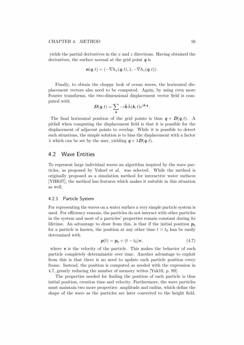
The properties needed for finding the position of each particle is thusinitial position, creation time and velocity. Furthermore, the wave particlesmust maintain two more properties: amplitude and radius, which define theshape of the wave as the particles are later converted to the height field.


lt

dtα v

Figure 4.1: Approximation of time for subdivision event for particle withvelocity v and dispersion angle α.

Also, to represent expanding wavefronts, another parameter is introducedwhich is the dispersion angle of a particle. For radially expanding waves,new wave particles must be spawned in order to preserve the shape. Thedistance between particles on the same wavefront should optimally never ex-ceed half the particle radius [YHK07], which is why subdivision of particlesis necessary. Naïvely approached, the problem of finding subdivision candi-dates can become expensive and introduce dependencies between particles.A better approach is to instead treat every particle independently, whichcan be done by introducing a few assumptions regarding particle proper-ties yielding an efficient analytical solution. Considering a particle on awavefront with speed v = |v|, dispersion angle α and radius r, the distancetravelled by the particle in t seconds is lt = t v. The length of the arc givenby the angle α and a circle of radius lt is dt = αlt = αtv, and is a roughapproximation of the distance between two neighboring particles, see figure4.1. Solving for t with dt = r

2 yields the time of the subdivision event:

r

2 = α t v ⇔ t = r

2 vα .

From the acquired time the subdivision event can be scheduled, removingthe need for finding candidates each update. The subdivision means threeparticles will spawn, one at the original particle’s position and two on eachside of that. The dispersion angle and amplitude of the new particles are onethird of the original, and the direction of the new outer particles is rotatedby α

3 and −α3 respectively.

4.2.2 Particles as a HeightfieldHaving subdivided particles accordingly, the particle system needs to beturned into the heightfield representation discussed earlier. This can be doneby properly selecting a waveform function Wi(x), yielding the heightfieldfunction

h(p, t) = y0 +∑i

aiWi(p− pi(t)) ,


where ai is the amplitude and pi(t) is the position of wave particle i. Yukselet al. suggests using the following waveform function

Wi(x) = 12

(cos

(π|x|ri

)+ 1

)Π( |x|

2ri

),

where Π(x) is the rectangle function with Π(x) = 1 for −0.5 < x < 0.5,Π(x) = 0.5 for x = ±0.5 and 0 otherwise. For simplicity’s sake it isusually convenient to keep a constant radius ri = r, which also gives aconstant waveform function Wi(p) = W (p). With this simplification Yukselet al. describe how to perform the heightfield conversion efficiently usinga convolution on the GPU. Each particle is rendered as a point primitiveto a render target, which is later filtered with the waveform function asa kernel. The filtering can be further optimized by using one-dimensionalapproximations in each direction of the otherwise two-dimensional filter.

To obtain the choppy look of waves, just as with the method describedin the previous section, a two-dimensional vector field can be obtained fordisplacing the horizontal position of the heightfield. This field is given by

D(p, t) =∑i

Li(vi)aiWi(p− pi(t)) ,

whereLi(u) = − sin

(π|u|ri

)Π( |u|

2ri

)u

4.2.3 Water InteractionTo use the described particle system for simulating water interaction, waveparticles with proper amplitude and velocity must be spawned accordingly.The authors of the wave particle algorithm describes how to accomplish thisby using a GPU-based technique. As the wave entities described in thisthesis will be primarily artist generated, these techniques are not in thescope of this thesis.

Chapter 5

Implementation Details

This chapter is meant to give a description of the implementations of thealgorithms presented earlier. Various aspects of rendering the ocean surfaceare also discussed. The implementation here refers to a reference imple-mentation made in the Frostbite engine and running on a PC under theMicrosoft Windows operating system, and on Sony’s Playstation 3 gamingconsole. The reference implementation was integrated with an existing sys-tem for water interaction, but the simulations are not tightly coupled andcould be enabled and disabled independently. A simple prototype for quickexperimentation with the chosen method was also implemented in Matlab.

5.1 OverviewCombining the two different techniques discussed in chapter 4, the simulatedwind driven waves and wave entities can be superimposed to form the finalheightfield function

H(p, t) = y0 +∑k

h(k, t) eip · k +∑i

aiWi (p− pi(t)) . (5.1)

The reference implementation consists of one system for the server andone for the client. The two implementations contain significant differences,but as it turns out much of the code from the server-side can be reused onthe client. The only information that the server needs to provide is waterheights for different points in time and space, or more precisely, evaluationsof the function in equation 5.1.

The client system needs to provide the exact same functionality as theserver, but additional work is also needed which is related to rendering. Itis assumed that the heightfield queries arrive at a different frequency thanthe rendering frame rate, and for that reason the simulation data for wind-driven waves used for queries and rendering are computed separately. Thismeans more computations on the client, but has the advantage that the two

19

CHAPTER 5. IMPLEMENTATION DETAILS 20

sets of simulation data can be processed with different parameters. Oneexample of where this advantage is used in the reference implementation,is that the simulation data used for physics queries does not need surfacenormals, nor is it equipped with any horizontal displacement data. As thesimulation data used for rendering has a horizontal displacement, there willbe a discrepancy between the water height returned by the queries and therendered mesh.

For easy integration with the interactive water system, the LODing ofthe rendered heightfield use the same quadtree based approach. To be ableto use this approach, the heightfield obtained from the simulation will needto be resampled to lower resolutions. In the reference implementation 3–4 LODs were used. As mentioned in section 3.1.2, the grids used by theinteractive water simulation have a border region on each side. This borderis not used while rendering the heightfield, which means that for a border ofsize B a mesh representation of such a grid has only (R−2B+1)×(R−2B+1)vertices. Here the +1 comes from the fact that the borders of the mesh mustmatch for tiling purposes. In order for the data from both simulations tomatch, a scaling of the ocean simulation data is applied for it to fit theunbordered grid area. The scaling uses bilinear downsampling to reach thedesired resolution, which is later copied to fill an entire R × R grid, withmaintained border properties.

For the simulation of wind-driven waves, the theory from section 4.1 isused to form the following algorithm:

1. Construct an R×R field of wave vectors k

2. Compute Phillips spectrum P ′h(k)

3. Compute initial amplitudes h0(k)

4. Apply dispersion relationship ω(k) to get h(k)

5. Transform to spatial domain to get heightfield h(p, t)

Items 1 to 3 is the initialization part of the algorithm which only needs tobe executed once any of the parameters change. The subsequent steps areperformed on each update step of the simulation.

5.2 Simulation TasksTo fully utilize the multi-core architectures of modern PCs and gaming con-soles, the simulation splits its workload among a number of tasks. At everyupdate step of the simulation, the jobs are started to later be synchronizedbefore the rendering is done. The ambient wave simulation has been splitinto three different tasks: update, precomp and prepareLod, and an addi-tional initialization procedure. The prepareLod task is only used by the


client simulation. For updating the wave particle system a subdivision taskis also required, this task is however run on the main thread because of theability to implement it very efficiently.

Running the tasks on a Microsoft Windows PC involves starting a threadwhich executes the task’s code. By relying on the operating system’s schedul-ing the multiple threads can be allowed to run in parallel on a multi-coreprocessor. To avoid the overhead of spawning new threads, a pool of workerthreads can be used.

The architecture of Sony’s Playstation 3 is slightly different though, andmulti-threading will not cause significant performance improvements com-pared to running all task in sequence on the same thread. The Playstation3’s is equipped with a Cell processor, consisting of one Power ProcessorElement (PPE) and 8 Synergetic Processor Elements (SPE). The PPE isa 64-bit PowerPC, reduced instruction set computer (RISC), which runsthe operating system and controls the SPEs. The SPEs are 128-bit RISCprocessors designed for smaller data-rich processing tasks and are the mainworkhorses of the platform. Each SPE executes its instructions on a localmemory store, in contrast to the PPE which operates on main memory.To transfer data back and forth between the local store and main mem-ory, the SPEs use direct memory accesses (DMA), which can be performedasynchronously to reduce latency [CBE09].

To utilize the SPEs for the simulation, each task needs to be compiledinto a separate small program that are started on each update step. Thememory addresses of the data to be processed are passed as parameters tothe programs, and by using DMA, the data is read from main memory intothe local storage. After the processing is complete, the data is written back.

5.2.1 InitializationThe initialization task takes the user-defined parameters and computes aninitial field of complex amplitudes and a dispersion field. This task needsonly to run once when the simulation starts, and if any of the parameterschange. Because of this, the task has not undergone any optimizations in thereference implementation as there are no critical time limits to meet. Thereason for also outputting the dispersion field is that, while the expressionlooks harmless, it does contain two square root operations for each wavevector k, if one were to compute it as needed. The set of wave vectorsis constant as long as the parameters remain unchanged, which yields theopportunity to pre-compute this data.

For the simulation to be deterministic, the initialized data needs to beprecisely equal on all involved clients and on the server. The computation ofthe initial heightfield draws from a random number generator which, for theequality to be fulfilled, must be identical. In this implementation a seededpseudo random number generator is used, with the seed being part of the


common simulation parameters that are of course identical on all clients.

5.2.2 Updating the HeightfieldThe update task contains two distinct computational sub-tasks, where thesecond depends on the results of the first. The first task consists of applyingthe dispersion to the initial grid of complex amplitudes h0. The dispersion isdone according to equation 4.4 and the dispersion relationship ω(k). Becauseequation 4.4 maintains the complex conjugation property, the bottom halfof the resulting set of amplitudes h(k, t) will be the complex conjugate ofthe horizontally and vertically flipped upper half. By exploiting this fact,the number of needed iterations for this procedure is R2/2.

To guarantee identical results between clients, the clocks used for sim-ulation must be synchronized between server and clients. This is handledby the underlying networking system of the engine and not part of this im-plementation. It works by having each client separately maintain its owntimer, which are continuosly corrected by the server, should it start to drift.A time correction from the server may cause unexpected jumps in the sim-ulation time for a client and thereby a jump in the heightfield animation.To avoid such jumps, the clock is not instantly skipped to the correct timewhen a correction arrives, but instead accelerated by a factor proportionalto the time error.

The second sub-task is to transform the results from the previous task tothe spatial domain. This is done using an FFT algorithm, discussed furtherin section 5.5. In total, 5 inverse FFTs are performed where one producesthe heightfield, two are used for horizontal displacement, and the last twoare for the computation of surface normals.

5.2.3 Precomputation of Heightfields for Point SamplingTo accommodate for the point sample queries of the water surface height,this task precomputes heightfields and stores them for later use. This per-forms a subset of the operations in the update task, where only the height-field is computed with no additional horizontal displacement or normal data.This means only one inverse FFT operation is executed for each instanceof the precomp task. The buffering scheme is described in more detail insection 5.3.

5.2.4 Level of Detail PreparationThe prepareLod task is a preparation of the data before rendering theheightfield. The task uses the data which is output from the previouslydescribed update task to prepare a single LOD of lower resolution. Thistask performs the down-sampling described in the overview section above to


R

R

H F G H F G H FC A B C AE D E DH F G H FC AE DH FC A B C A B C A

B

R−2B2

Figure 5.1: Downsampling and border copy of original heightfield of resolu-tion R to level of detail l = 1. The original heightfield is down-sampled andstored in the upper left region of the target heightfield. Next, it is copied tothe remaining three regions and the lettered sub-regions are copied to thecorresponding area of the border

reach the desired resolution

Rtarget = R− 2Bl + 1 ,

where l is the requested LOD and l = 0 is the highest resolution LOD.After obtaining the low-resolution heightifield it is copied to fill the topmostrow of the R × R tile. Next, that row is copied to fill the rest of the tile.While doing so, the borders are also copied to preserve the same data layoutas used by the interactive simulation. This procedure is depicted for l = 1in figure 5.1. The LOD preparation tasks can run in parallel with one taskinstance per LOD, as there are no dependencies between them.

5.3 Heightfield SamplingIt is assumed that for a point in time t0, the water height may be queried fora range of times t0−S ≤ t < t0 +S, where the times are discrete, uniformlyspaced time steps. To quickly be able to respond to such queries, the systemmaintains a buffer of heightfields from past and for future time steps insteadof computing them on-demand. The maximum time tmax for which a queryhas been answered is recorded, and with a buffer of size 2S, the buffer ensuresthat the heightfields for times tmax−S ≤ tmax < tmax +S are in the buffer.If the initial assumption holds, a sufficiently large buffer will guarantee thatall the heightfields needed to respond to the queries are already in the buffer.However, to be safe, a fallback on-demand computation of a heightfield canbe made if needed. At every update step of the simulation, tmax − tbuf new


heightfields are computed and buffered, where tbuf is the maximum time ofall currently buffered heightfields.

Simply fetching a buffered heightfield is not enough to respond to aquery. As a query is made for an arbitrary point p in space, the heightfieldfetched from the buffer needs to be sampled in some fashion. First of all, ifthe point is outside the bounds of the entire water surface, no further workis needed and the sampling procedure is complete. If it is inside, the offsetposition into the water surface is determined with ps = p− p0, where p0 isthe corner position of the entire water surface. This position is then usedto compute the position in the tile’s coordinate system q = R

Dps. The finalwater height is finally bilinearly interpolated from four samples from thediscrete grid points closest to q.

Superimposing individual waves is performed by simply iterating over allactive wave particles and summing evaluations of their waveform functions.

5.4 Simulation ParametersThere are several parameters that affect the outcome of the ocean simulation.Some parameters influence the general appearance of the surface waves whileothers can be used to adjust fidelity. Increasing fidelity, as usual, also meansincreasing computational cost and thereby decreasing performance.

The first two parameters to set are the simulation resolution and dimen-sion. The resolution of course has a direct relation to the computationalcost. The implication of choosing a higher simulation resolution is thatmore wave vectors will fit into the grid. The increased number of wave vec-tors will expand the heightfield outwards, and thus give waves with higherwave numbers. Recalling that the wave number is inversely proportionalto the wavelength, this will give more small surface waves. A resolutionabove around 2048 × 2048 will give such small wavelengths that numericalprecision becomes an issue [Tes04b]. During the work of this thesis the reso-lutions were usually set to 64×64 or 32×32. The dimension parameter onlycontrols the size in the world that a simulation tile covers and thus does notadd any additional computational costs for the simulation.

The modified Phillips spectrum in equation 4.3 provides an additionalfour parameters that can be set by the user. Upwind and downwind power,controls how much the propagation directions of waves will be spread outaround the wind direction. Upwind and downwind scaling factors controlsthe amplitude of waves travelling in the corresponding direction.

5.5 The Fast Fourier TransformEvaluating a DFT by definition, while maintaining interactive frame rates,is infeasible as the complexity of such an operation is O(N2) in the one-


dimensional case and at best O(N3) in two dimensions. Instead we resortto an FFT algorithm, such as the traditional one, proposed by Cooley-Tukey. This effectively reduces the complexity of the problem to a moremanageable O(N logN) in one-dimension and thus O(N2 logN) in the two-dimensional case [FJ05]. For the first prototype implementation a simple,yet naïve, implementation of the Cooley-Tukey algorithm was used to verifythe results. However, this unoptimized implementation still did not providesufficient performance, especially on consoles, which led to the use of a third-party library specialized for FFT computations.

5.5.1 Using FFTWThe problem faced in this thesis is to efficiently compute a transform of fixedand moderate size. For this reason it would be possible to write low-leveloptimized code that is tailored for that particular problem. This solutionhowever, is not very flexible. As mentioned, it is desirable to be able toadjust simulation fidelity depending on platform, which means lots of workneeds to be put into writing similar low-level optimized code for those prob-lems as well.

For these reasons a more flexible solution, to use the third-party libraryFFTW, was chosen. FFTW stands for The Fastest Fourier Transform inthe West and is a collection of C routines released both under the GNUGPL license and other non-free proprietary licenses. FFTW works with aset of codelets, which are machine generated code sequences, specialized onperforming one particular set of computations. By testing different combi-nations of the codelets, FFTW can find an optimal solution for the givenproblem. The speed of computations is comparable with “hand-optimizedsolutions” [FJ05]. With the FFTW software package, it is also possible togenerate new codelets if needed.

5.6 Wave Particles5.6.1 Particle DataTo avoid runtime allocation of memory on the heap, it is necessary to main-tain a buffer of constant size for the particle data. Each particle carries aproperty which tells if it is active and should be included in the simulation.To avoid searching the buffer for available particles when spawning new onesa simple wrapping counter tells the next index to choose. This will causeparticles, which are potentially still alive, to be overwritten. However, thebuffer can be maintained to keep the particles roughly sorted by creationtime, meaning the overwrites will only hit old particles.

The data needed for each particle is: creation time, initial position,direction, amplitude and dispersion angle. A choice can be made whether


to allow varying particle radii or use a constant global value. Allowingindividual radius properties, in combination with waveform evaluation usinga convolution kernel is problematic. This would need numerous convolutionswith different kernels and would significantly increase memory usage. Thereference implementation does not use convolution, which allows the use ofindividually set radii.

5.6.2 SubdivisionThe subdivision time table of the wave particle system can be implementedefficiently by choosing the right data structures [Yuk10, p. 90-92]. In thereference implementation, a map data structure was used to map the timeof a subdivision event to a list of particles. To avoid dynamically allocatingmemory for the particle lists, a linked list structure was used. By equippingthe particle data with a pointer to the next particle, this scheme is readilyimplemented. Thus, the time table is a map from discrete time step to awave particle pointer, pointing at the tail of the subdivision list.

Ideally, all particles subject for subdivision at a point in time should beordered sequentially in memory to improve memory access times. Subdi-viding a particle, involves creating two new particles on either side of theoriginal one, which is not optimal for memory layout. To overcome this, theoriginal particle is relocated to where the two new particles are created inthe memory buffer. This also reduces the risk of overwriting particles beforeit has been subdivided [Yuk10, p. 94].

5.7 RenderingThe heightfields obtained from the simulation of wind-driven waves are wellsuited for the already present rendering. As described in section 3.1.1, thequadtree structure will provide a number of grids of equal resolution, butdifferent dimension. To apply the height field, the different LODs of thesimulation data can be matched with a quadtree level, giving a range oflevels of where to superimpose the heightfield. The level matching can beperformed by finding the quadtree level which has grids of a dimension whichmost closely matches the dimension of the simulation data. An examplequadtree hierarchy is depicted in figure 5.2. To apply the height field togrids below the range of levels, the present system’s upsampling algorithmis used to bicubically upsample the data from the level above.

To render the wave particles, a naïve solution would be to for everyvertex in every mesh grid evaluate the waveform function for every waveparticle. This solution was deemed too expensive, which lead to a more effi-cient, yet still naïve, two-pass solution. By first determining which particlesaffect which grid, the complexity is reduced. Considering a wave particle’s


Figure 5.2: Example quadtree hierarchy for a water surface. Using 2 LODs,the simluation data for wind driven waves would be inserted at the levelsshaded with gray color, with the highest LOD in the grids of the bottommostof these levels. For quadtree levels below the LOD range, the data fromabove levels are upsampled to fit the grids.

position and the inflated two-dimensional bounding box of a grid, a point-box intersection test can tell which particles affect a given grid. The boundsof a grid must be inflated by the constant particle radius r in each directionto successfully cover the influence of all particles, which is exemplified infigure 5.3. All particles affecting a grid is appended to a list, which in thesecond pass provides each grid with the particles to consider. The secondpass is also easily parallelized, for further performance increase.


r

r

P0

r

P1

Figure 5.3: Example grid sampling of a wave particle system with twoparticles: P0 and P1, and the grid shaded in gray. The outer square repre-sents the inflated bounding box which is needed to catch influences from allrelevant particles.

Chapter 6

Results

This chapter presents the results of the implementation of the algorithms.The default set of parameters used, unless otherwise stated, is shown intable 6.1.

Resolution R = 512Dimension D = 1500 mWind direction w = (wx, wz) = (1, 0)Wind speed |w| = 30 m/sDirectionality p− = p+ = 2Scale factor d− = d+ = 1

Table 6.1: Default simulation parameters used for the results presented inchapter 6.

6.1 RenderingsUsing a 2-dimensional grayscale image, the heightfield and horizontal dis-placement maps can be represented. Such a representation is shown in figure6.1. Observing only this representation, it is not clear in which direction thewaves are propagating. But, by also taking the derivatives into account, thedirection becomes more evident. Similar renderings of the derivatives in thex and z directions, along with the resulting normal map are shown in figure6.2.

The final result can be seen in figure 6.3, where an entire water body isrendered with basic shading. Looking closely at this figure, cracks can benoticed between different LODs as the border vertices of the mesh patchesdoes not match. A repeating pattern is also evident caused by the tiledheightfield with a rather low resolution. The rendering in figure 6.4 showsthe wireframe of the same water body.

29

CHAPTER 6. RESULTS 30

(a) (b) (c)

Figure 6.1: Example two-dimensional representations of (a) height field,(b) horizontal displacement in x direction, and (c) horizontal displacementin z direction. The parameters used are those presented in table 6.1.

(a) (b) (c)

Figure 6.2: Heightfield derivatives rendered as a two-dimensional map. (a)is the x derivative, and (b) the z derivative. In (c) the resulting normal mapis rendered in color with the red, green and blue channels representing x,y and z components respectively. Simulation parameters are listed in table6.1.


Figure 6.3: Rendering of ocean surface with basic shading. The heightfieldresolution used was 64 × 64 which explains the obvious repeating patterncaused by tiling. Cracks between different LODs are also evident on closerexamination.

Figure 6.4: Wireframe rendering of the same water body as in figure 6.3.As shown in the rendering, 4 LODs are used.


PC PS3Task 32× 32 64× 64 32× 32 64× 64update 0.08 0.29 0.12 0.33Propagation 0.06 0.21 0.08 0.24Transform 0.02 0.08 0.04 0.09prepareLod 0.05 0.06 0.06 0.07precomp 0.05 0.15 0.06 0.16Propagation 0.04 0.12 0.04 0.12Transform 0.01 0.03 0.02 0.04Frame time ( 1

f ) 7.69 10.0 33.3 33.3Simulation CPU Time 0.29 0.58 0.42 0.77Wall clock time 0.13 0.35 0.18 0.40

Table 6.2: Timing measurements (in milliseconds) for each of the simulationtasks and sub-tasks. On Playstation 3 (PS3), all tasks are executed on thesynergetic processing elements (SPE). The query frequency is fq = 30 Hzand LOD count l = 4. Simulation CPU Time is computed by the formulain 6.1, and wall clock time according to 6.2.

6.2 PerformanceApart from fulfilling the requirements of deterministically generating a plau-sible mesh representation of an ocean surface, a key factor of a successfulimplementation of this method is performance. In table 6.2, processor timefor one instance of each of the simulation tasks and sub-tasks is presentedfor different resolutions, and on two different platforms: a Sony Playsta-tion 3 and a PC. The PC was equipped with an Intel Xeon X5550 with 4cores at 2.66 GHz and 12 GB of RAM. The number of LODs used duringmeasurements was l = 4, and the used query frequency was fq = 30 Hz.

On the client, the number of task instances of each task that is run everyframe is variable. This is due to the possibility of the frame rate f beingdifferent from the frequency of the heightfield queries fq. This means thatfor each frame, precisely one instance of update task needs to be executed,together with one instance of prepareLod per LOD. The most commonsituation in the reference implementation is that f ≥ fq, which means thatone instance of the precomp task executes roughly every f

fqframe. The total

CPU time spent can thus be computed with the formula

tcpu = tupdate + l · tresmaple + f

fqtprecomp , (6.1)

where l is the LOD count and ttask is the CPU time for task.The wall clock time that is needed for the entire simulation can be com-


puted with the following formula:

twall = max(tprecomp, tupdate + tprepareLod) . (6.2)

This means that the wall clock time is whichever finishes last of one instanceof the precomp task and one instance of update together with one instanceof prepareLod. The assumption is made that the tasks are allowed to run inparallel, meaning that precomp and update can be started at the same time.Also, all prepareLod tasks can be executed in parallel, yielding the aboveexpression. Note that the prepareLod task can vary slightly in run timedepending on which LOD it is computing. These differences were howeverconsidered negligible in the performed measurements.

On the server-side the total CPU time and wall clock time are tcpu =twall = tprecomp, since only one instance of the precomp task is executed everyupdate step.

6.2.1 Performance Improvements from Using FFTWReplacing the naïvely implemented FFT algorithm significantly improvedperformance on all tested platforms. For a simulation resolution of 64× 64,the measured CPU time on PC for the naïve algorithm was 0.55 ms pertransform. With FFTW, the corresponding time was improved with oneorder of magnitude to 0.05 ms. Similar improvements were also evident onthe other platforms.

It should be noted, that while there is a gain in performance, static link-ing with the FFTW library will lead to increased code size of the executable.This could potentially be alleviated by extracting or generating the neededFFTW codelets, and thus only link with those. While sacrificing flexibility,this solution could be used to produce a small amount of high-performancecode that is tailored for the given problem and platform. This could poten-tially also improve performance even further, making it a viable option forfinal builds of an application as the flexibility offered can be discarded atthat point.

6.3 Modified Phillips SpectrumThe alternative Phillips Spectrum in equation 4.3 was implemented to in-crease the user’s level of control over the simulation. In figure 6.5 threeexample spectra are represented as two-dimensional grayscale images. Withwhite color representing high amplitudes, the figure 6.5 (a) show that themaximum amplitudes in the spectrum are in the upwind, and also in thedownwind direction for the default spectrum. The spectrum is tweaked withincreased directionality in figure 6.5 (b), and with downwind amplitudesscaled down in figure 6.5 (c).


(a) (b) (c)

Figure 6.5: Three different spectra generated with the modified Phillipsspectrum with resolution, dimension and wind direction as specified in table6.1, but with wind speed 5 m/s. White color represents high amplitudes. (a)Default parameters, s− = s+ = 1 and p− = p+ = 2. (b) Increased power,p− = p+ = 8. (c) Scaled amplitudes in downwind direction p− = 3, p+ = 8and s− = 0.2, s+ = 1.

6.4 Wave EntitiesAs the reference implementation of a wave particle does not strive for highperformance, no detailed performance measurements were conducted on thisalgorithm. For completeness sake, with a maximum particle count of 4000,a parallelized waveform evaluation step, performs in roughly 5 – 6 ms wallclock time on modern PC hardware. Other steps of the algorithm can beimplemented very cheaply and does not add significant cost.

Chapter 7

Discussion

7.1 Ocean Wave Simulation Using FFTThe presented solution provides a deterministic ocean wave simulation, whichis feasible for integration into a real-time application. The simple, yet ef-fective, heightfield representation is well suited for this application as bothrendering work and individual point queries can be performed efficiently.

7.1.1 PerformanceThe measurements presented in chapter 6 show promising results in terms ofperformance. The performance level obtained indicates that a simulation ofhigher resolution is possible, without significant reduction in overall framerate. Higher resolutions were not experimented with during the work of thisthesis, mainly because of limitations imposed by the underlying interactivewater simulation.

The re-sampling and LOD preparation task and the wave propagationtask have not undergone significant optimization in the reference implemen-tation. Both these tasks are candidates for vectorization and to thereby putthe platforms’ single-instruction, multiple data (SIMD) capabilities to use.

7.1.2 Spectrum TweaksThe modified Phillips spectrum gives the opportunity for artists to bettercontrol the simulation so that the desired appearance can be achieved. Mod-ifying the spectrum does diverge the method from its foundation in studiesof actual ocean surface, but in this application the ability to control the sim-ulation was deemed more important than maintaining the highest possiblelevel of realism.

A problem with the chosen method, is that directly modifying the spec-trum can be difficult for someone not well versed in the used method. Theimplications of a tweak applied by a user can have consequences on the end

35

CHAPTER 7. DISCUSSION 36

result that are difficult to predict, making it a time consuming process tofind the right parameters [GOH12]. However, the modified Phillips spectrumis intended to alleviate the customization process.

7.1.3 Parameter ChangesThe proposed method is not well suited for changes in the parameters. Pa-rameters that are candidates for runtime changes are the wind speed anddirection, whereas the resolution and dimension parameters should be keptconstant. A change in wind direction or speed would not be instant, butrather a transition over a period of time. A transition in parameter valuesmeans that the heightfield needs to be reinitialized for numerous differentsets of parameters, which is an expensive effort and could potentially causejumps in the animation of the heightfield. A better solution would be to,as the parameter changes, initialize a new temporary simulation with thetarget parameters and blend it in linearly over time. This would cause asmooth transition, with only one needed reinitialization but with twice therequired computational effort during the transition.

7.1.4 ShoresAs the simulation is meant for the open ocean, practical handling of shore-lines is an issue that needs to be addressed. In particular, when a roughocean surface is simulated, a gently sloping shore will cause very unrealisticbehavior. If the simulation has the ability to access the geometry that repre-sents the seabed, a simple solution would be to locally apply a water depthdependent scale factor to the heightfield. Experiments have shown that byblending with another procedural wave generator, which is specialized onshore waves, a more realistic shoreline can be obtained.

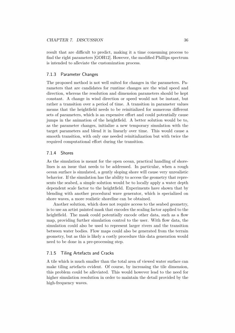
Another solution, which does not require access to the seabed geometry,is to use an artist painted mask that encodes the scaling factor applied to theheightfield. The mask could potentially encode other data, such as a flowmap, providing further simulation control to the user. With flow data, thesimulation could also be used to represent larger rivers and the transitionbetween water bodies. Flow maps could also be generated from the terraingeometry, but as this is likely a costly procedure this data generation wouldneed to be done in a pre-processing step.

7.1.5 Tiling Artefacts and CracksA tile which is much smaller than the total area of viewed water surface canmake tiling artefacts evident. Of course, by increasing the tile dimension,this problem could be alleviated. This would however lead to the need forhigher simulation resolution in order to maintain the detail provided by thehigh-frequency waves.


To keep computational cost down, a potential solution would be to per-form two heightfield computations of the same resolution but at differentdimension. The heightfield of larger dimension could be linearly up-sampledto form a higher resolution heightfield. Several of the smaller heightfieldscould then be superimposed on the larger to form the final result. The largerheightfield would break up the tiling artefacts created by the smaller. Thistechnique could of course be further extended to use as many heightfields asdesired. This would however burden users with more parameters to adjust,to obtain the right appearance.

As is evident from the rendered ocean surface in figures 6.3 and 6.4,vertices along borders between different LODs does not line up correctly,causing cracks in the resulting mesh. A solution to this is to apply someform of stitching along the edges, which is a common method of dealing withsuch problems.

7.1.6 Heightfield Sampling DiscrepancyAs mentioned in the implementation chapter, the heightfield queries will notprovide query responses that exactly match the rendered mesh. By equip-ping the buffered heightfields with horizontal displacement information, thequeries could be made more exact. However, this would not only mean morecomplicated sampling of the heightfield, but also more memory usage by thebuffer.

In the reference implementation, this discrepancy has not been foundto cause problems in terms of simulation accuracy. As buoyant objectsof significant density do not float directly on the water surface, but aresubmerged to some extent, the discrepancy is hidden. The accuracy maybecome problematic for smaller, light objects, which follow the water surfacemore precisely.

As the heightfields used for queries are separate from the rendered height-field, it is also possible to use different resolutions for the two. If a higherresolution is desired for rendering purposes, a low resolution simulation couldpotentially still be used for queries while maintaining an accurate physicssimulation. This is of course interesting for performance reasons, both interms of computational effort and memory usage.

The rendered mesh will represent the water surface at the local clienttime, meaning there will be a discrepancy between objects not controlledlocally and the water surface. As with the sampling discrepancies describedabove the buoyancy physics hides this to some extent, avoiding the floatingobject looking detached from the water surface. This is at least true formoderate network latency. Should high latencies cause unacceptable errors,solutions such as local modification of the water surface around objects couldbe employed. If the latency can be estimated, two heightfields from differentpoints in time can be radially blended with respect to the local clients camera


position. This means the water surface from the actual time is shown in thedistance, and the local time representation is used near the client.

7.2 Wave EntitiesThe implementation of wave particles is only a subset of the entire algorithmas described by the original authors. For example, no reflection step isincluded in the reference implementation, as it would need additional datafrom the geometry surrounding the water body not readily accessible.

The described way of handling subdivision events maintains the deter-minism of the system. Because future positions and subdivisions of any waveparticle can be determined another conclusion to draw is that, from a multi-client perspective, only the initial wave particles need to be synchronizedover the network. A potential problem worth noting comes from applyingthe previously described client-side prediction scheme. If the heightfield isevaluated for a future time, subdivision events occurring between the cur-rent time and this future time will not have been executed. A potentialsolution could be to temporarily fast forward the subdivision events to thedesired point in time, ensuring an accurate evaluation of the water level.However, in the reference implementation this was not deemed necessary asthe error introduced by evaluating a non-subdivided particle system was notnoticeable.

7.2.1 Other UsesUsing wave particles has proven a flexible solution that could potentially seemany applications. A basic wave generator can be implemented to providelarge wave trains, with wavelengths far larger than what the ambient simu-lation can handle. This not only adds more waves to the ocean surface, butcould also be used to break up tiling artefacts caused by a low resolutionambient simulation.

Attaching wave particle generators to objects interacting with the wa-ter surface could also be an interesting use, giving the ability to simulatethe presence of boat wakes and similar effects. Care must be taken in amulti-client environment, as initial positions of wave particles need to besynchronized in order to provide equal simulation results, which leads toincreased network bandwidth usage. As objects in the world are alreadysynchronized, the position of these could be used for determining spawnlocations for particles. This would however require a deterministic way offinding when such particle spawn events occur, that is insensitive to networklatency.


7.3 ConclusionThis thesis has presented a system for ocean simulation in real-time applica-tions. The main focus has been to obtain realistic results while maintaininghigh performance and providing a decent level of user control. The systemhas been divided into two systems: one for simulation of wind-driven wavesand the other for manually controlled individual waves on the ocean surface.

The wind-driven waves use a simulation method presented by JerryTessendorf, which is based on statistical observation of ocean surfaces. Themethod provides, if not the most, at least a very realistic simulation of openocean surface waves. To improve user control, the wave distribution spec-trum used in the method was altered to expose more parameters which affectthe outcome of the simulation. In this thesis, the integration of this methodinto a quadtree-based LOD scheme is also discussed.

Individual waves on the water surface was implemented as wave entities,with an algorithm based on Cem Yuksel’s Wave Particles. The proposed sys-tem lends the basic ideas from the original algorithm: representing waveswith a particle system, particle subdivision, and how to obtain the resultingheightfield. Particle generation in the presented system is performed man-ually by a user, as opposed to the original algorithm which approximatewater-object interactions to simulate the wave generation.

To address the steep performance requirements imposed by implement-ing the system in a game engine, the paralell processing capabilities of thetarget platform was exploited. To further improve performance, the FFTWlibrary provided a fast implementation of an FFT algorithm that could read-ily be applied to the simulation data.

Bibliography

[CBE09] Cell Broadband Engine Programming Handbook. Including thePowerXCell 8i Processor. Version 1.12. Apr. 3, 2009. url:https : / / www - 01 . ibm . com / chips / techlib / techlib .nsf/techdocs/7A77CCDF14FE70D5852575CA0074E8ED/$file/CellBE _ Handbook _ v1 . 12 _ 3Apr09 _ pub . pdf (visited on05/17/2012).

[CM10] Nuttapong Chentanez and Matthias Müller. ”Real-time sim-ulation of large bodies of water with small scale details”. In:Proceedings of the 2010 ACM SIGGRAPH/Eurographics Sym-posium on Computer Animation. SCA ’10. Eurographics Associ-ation, 2010, pp. 197–206. url: http://dl.acm.org/citation.cfm?id=1921427.1921457.

[CS09] Hilko Cords and Oliver Staadt. ”Real-Time Open Water En-vironments with Interacting Objects”. In: Proceedings of Eu-rographics Workshop on Natural Phenomena (EGWNP ’09).2009, pp. 35–42.

[FJ05] M. Frigo and S.G. Johnson. ”The Design and Implementation ofFFTW3”. In: Proceedings of the IEEE 93.2 (Feb. 2005), pp. 216–231. issn: 0018-9219. doi: 10.1109/JPROC.2004.840301.

[FR86] Alain Fournier and William T. Reeves. ”A simple model ofocean waves”. In: SIGGRAPH Comput. Graph. 20 (4 1986),pp. 75–84. issn: 0097-8930.

[Gei+10] Robert Geist et al. ”Lattice-boltzmann water waves”. In: Pro-ceedings of the 6th international conference on Advances invisual computing - Volume Part I. ISVC’10. Springer-Verlag,2010, pp. 74–85. isbn: 3-642-17288-1, 978-3-642-17288-5.

[GOH12] Carlos Gonzales Ochoa and Doug Holder. Water Technologyof Uncharted. Game Developers Conference. 2012. url: http://www.gdcvault.com/play/1015309/Water-Technology-of(visited on 05/16/2012).

[Joh04] Claes Johanson. ”Real-time water rendering”. Master’s thesis.LTH Lund Institute of Technology, Mar. 2004.

40

https://www-01.ibm.com/chips/techlib/techlib.nsf/techdocs/7A77CCDF14FE70D5852575CA0074E8ED/$file/CellBE_Handbook_v1.12_3Apr09_pub.pdf



http://dl.acm.org/citation.cfm?id=1921427.1921457

http://dl.acm.org/citation.cfm?id=1921427.1921457

http://dx.doi.org/10.1109/JPROC.2004.840301

http://www.gdcvault.com/play/1015309/Water-Technology-of

http://www.gdcvault.com/play/1015309/Water-Technology-of

BIBLIOGRAPHY 41

[Len12] Joel Lennartsson. ”Data Oriented Interactive Water”. Bache-lor’s thesis. Linköping University, 2012.

[Mit07] Martin Mittring. ”Finding next gen: CryEngine 2”. In: ACMSIGGRAPH 2007 courses. SIGGRAPH ’07. ACM, 2007,pp. 97–121. doi: 10.1145/1281500.1281671.

[MWM87] Gary A. Mastin, Peter A. Watterberg, and John F. Mareda.”Fourier Synthesis of Ocean Scenes”. In: Computer Graphicsand Applications, IEEE 7.3 (Mar. 1987), pp. 16–23. issn: 0272-1716. doi: 10.1109/MCG.1987.276961.

[Ott10] Björn Ottosson. ”Real-time Interactive Water Waves”. Mas-ter’s thesis. KTH Royal Institute of Technology, 2010. url:http : / / publications . dice . se / attachments / water %20interaction%20ottosson_bjorn.pdf.

[Tes04a] Jerry Tessendorf. ”Interactive Water Surfaces”. In: Game Pro-gramming Gems 4. Charles River Media, 2004, pp. 265–275.url: http://people.clemson.edu/~jtessen/papers_files/Interactive_Water_Surfaces.pdf (visited on 02/08/2012).

[Tes04b] Jerry Tessendorf. Simulating ocean water. SIGGRAPH 2004Course Notes. 2004. url: http : / / people . clemson . edu /~jtessen/papers_files/coursenotes2004.pdf (visited on05/16/2012).

[Th07] Nils Thürey et al. ”Real-time Breaking Waves for Shallow Wa-ter Simulations”. In: Proceedings of the Pacific Conference onComputer Graphics and Applications 2007 (Oct. 2007), p. 8.

[Yan+05] Xudong Yang et al. ”GPU-based real-time simulation and ren-dering of unbounded ocean surface”. In: Computer Aided De-sign and Computer Graphics, Ninth International Conferenceon. Dec. 2005, 6 pp. doi: 10.1109/CAD-CG.2005.45.

[YHK07] Cem Yuksel, Donald H. House, and John Keyser. ”Wave Parti-cles”. In: ACM Transactions on Graphics (Proceedings of SIG-GRAPH 2007) 26.3 (2007), p. 99.

[Yuk10] Cem Yuksel. ”Real-time Water Waves with Wave Particles”.PhD thesis. Texas A&M University, 2010.

http://dx.doi.org/10.1145/1281500.1281671

http://dx.doi.org/10.1109/MCG.1987.276961

http://publications.dice.se/attachments/water%20interaction%20ottosson_bjorn.pdf

http://publications.dice.se/attachments/water%20interaction%20ottosson_bjorn.pdf

http://people.clemson.edu/~jtessen/papers_files/Interactive_Water_Surfaces.pdf

http://people.clemson.edu/~jtessen/papers_files/Interactive_Water_Surfaces.pdf

http://people.clemson.edu/~jtessen/papers_files/coursenotes2004.pdf

http://people.clemson.edu/~jtessen/papers_files/coursenotes2004.pdf

http://dx.doi.org/10.1109/CAD-CG.2005.45

Master's Thesis Deterministic Ocean Waves Fredrik Larsson

Documents