Masterbook of Business and Industry (MBI) Muhammad Firman (University of Indonesia - Accounting ) 2 Why Study Financial Markets? Financial markets are markets in which funds are transferred from people and Firms who have an excess of available funds to people and Firms who have a need of funds The Bond Market and Interest Rates A security (financial instrument) is a claim on the issuer‘s future income or assets. A bond is a debt security that promises to make payments periodically for a specified period of time. An interest rate is the cost of borrowingor the price paid for the rental of funds. Figure 1 Interest Rates on Selected Bonds, 1950–2011 The Stock Market Common stock represents a share ofownership in a corporation. A share of stock is a claim on the residual earnings and assets of the corporation Why Study Financial Institutions and Banking? Financial Intermediaries: institutions that borrow funds from people who have saved and make loans to other people: – Banks: accept deposits and make loans – Other Financial Institutions: insurance companies, finance companies, pension funds, mutual funds and investment companies Financial Innovation: the development of new financial products and services. Can be an important force for good by makingthe financial system more efficient Figure 2 Stock Prices as Measured by the Dow Jones Industrial Average, 1950–2011 Financial Crises Financial crises are major disruptions in financial markets that are characterized by sharp declines in asset prices and the failures of many financial and nonfinancial firms. Why Study Money and Monetary Policy? Evidence suggests that money plays an important role in generating business cycles. Recessions (unemployment) and expansions affect all of us. Monetary Theory ties changes in the money supply to changes in aggregate economic activity and the price level . The aggregate price level is the average price of goods and services in an economy A continual rise in the price level (inflation) affects all economic players. Data shows a connection between the money supply and the price level Figure 3 Money Growth (M2 Annual Rate) and the Business Cycle in the United States 1950–2011 Figure 4 Aggregate Price Level and the Money Supply in the United States, 1950–2011 Figure 5 Average Inflation Rate Versus Average Rate of Money Growth for Selected Countries, 2000- 2010 CHAPTER 1 WHY STUDY MONEY, BANKING, AND FINANCIAL MARKETS ? EKONOMI MONETER

Welcome message from author
This document is posted to help you gain knowledge. Please leave a comment to let me know what you think about it! Share it to your friends and learn new things together.
Transcript
Masterbook of Business and Industry (MBI)
Muhammad Firman (University of Indonesia - Accounting ) 2
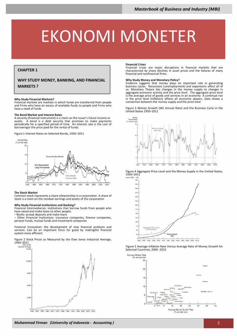
Why Study Financial Markets? Financial markets are markets in which funds are transferred from people and Firms who have an excess of available funds to people and Firms who have a need of funds The Bond Market and Interest Rates A security (financial instrument) is a claim on the issuer‘s future income or assets. A bond is a debt security that promises to make payments periodically for a specified period of time. An interest rate is the cost of borrowingor the price paid for the rental of funds. Figure 1 Interest Rates on Selected Bonds, 1950–2011
The Stock Market Common stock represents a share ofownership in a corporation. A share of stock is a claim on the residual earnings and assets of the corporation Why Study Financial Institutions and Banking? Financial Intermediaries: institutions that borrow funds from people who have saved and make loans to other people: – Banks: accept deposits and make loans – Other Financial Institutions: insurance companies, finance companies, pension funds, mutual funds and investment companies Financial Innovation: the development of new financial products and services. Can be an important force for good by makingthe financial system more efficient Figure 2 Stock Prices as Measured by the Dow Jones Industrial Average, 1950–2011
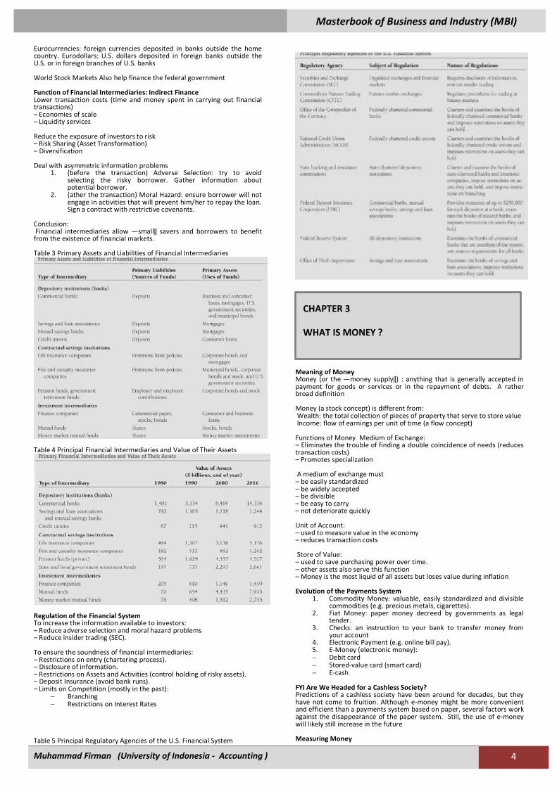
Financial Crises Financial crises are major disruptions in financial markets that are characterized by sharp declines in asset prices and the failures of many financial and nonfinancial firms. Why Study Money and Monetary Policy? Evidence suggests that money plays an important role in generating business cycles. Recessions (unemployment) and expansions affect all of us. Monetary Theory ties changes in the money supply to changes in aggregate economic activity and the price level . The aggregate price level is the average price of goods and services in an economy A continual rise in the price level (inflation) affects all economic players. Data shows a connection between the money supply and the price level Figure 3 Money Growth (M2 Annual Rate) and the Business Cycle in the United States 1950–2011
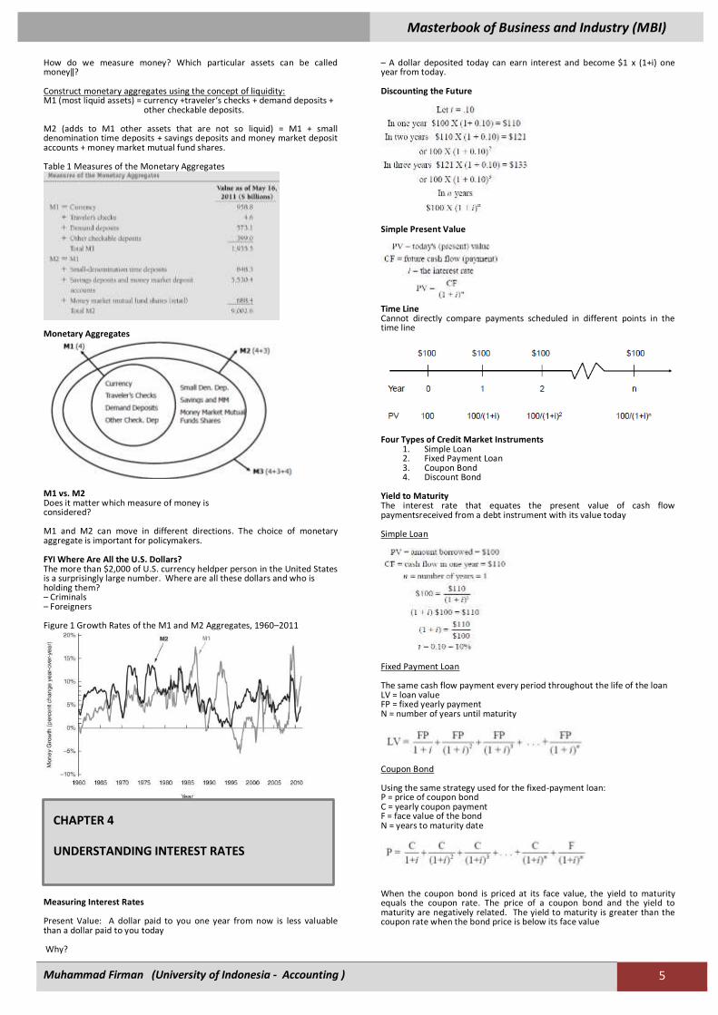
Figure 4 Aggregate Price Level and the Money Supply in the United States, 1950–2011
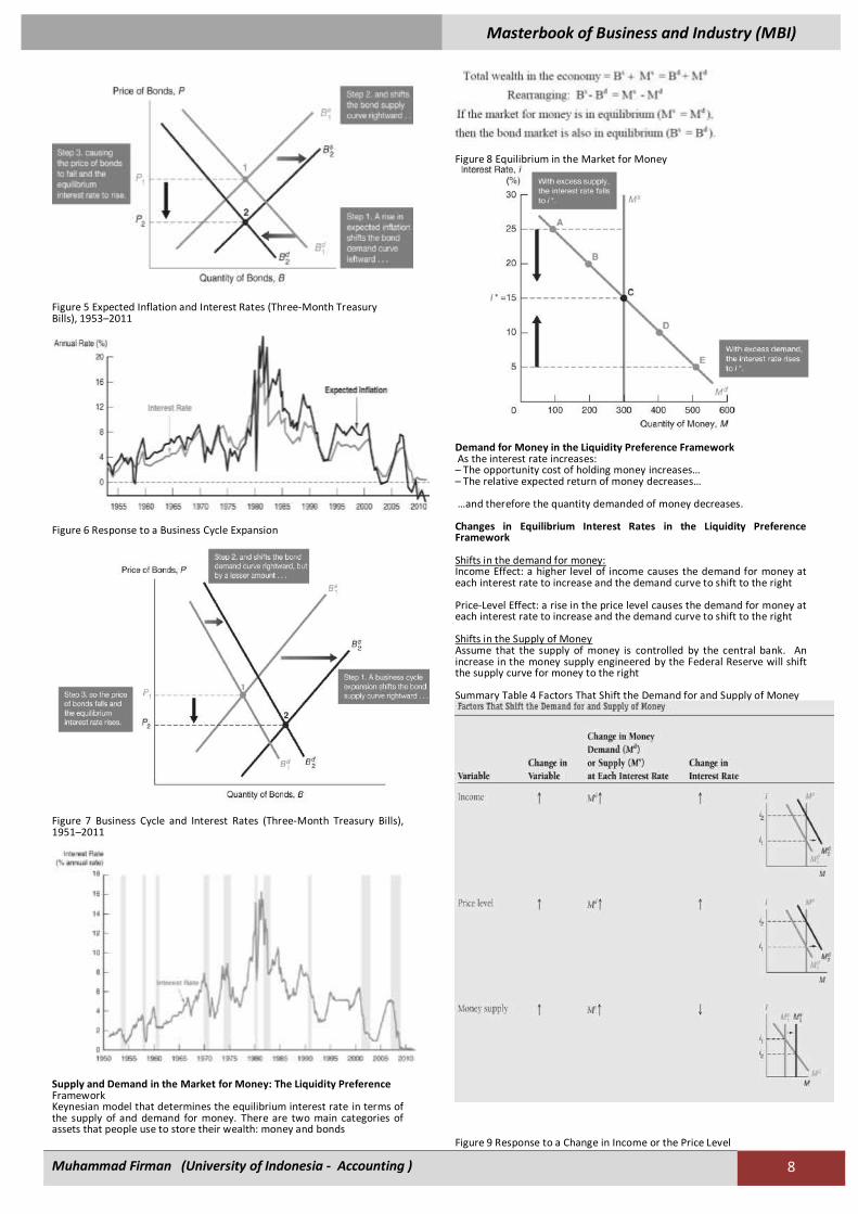
Figure 5 Average Inflation Rate Versus Average Rate of Money Growth for Selected Countries, 2000- 2010
CHAPTER 1
WHY STUDY MONEY, BANKING, AND FINANCIAL
MARKETS ?
EKONOMI MONETER

Masterbook of Business and Industry (MBI)
Muhammad Firman (University of Indonesia - Accounting ) 3
Money and Interest Rates Interest rates are the price of money. Prior to 1980, the rate of money growth and the interest rate on long-term Treasury bonds were closely tied. Since then, the relationship is less clear but the rate of money growth is still an important determinant of interest rates Figure 6 Money Growth (M2 Annual Rate) and Interest Rates (Long-Term U.S. Treasury Bonds), 1950–2011
Fiscal Policy and Monetary Policy Monetary policy is the management of the money supply and interest rates. Conducted in the U.S. by the Federal Reserve System (Fed). Fiscal policy deals with government spending and taxation. Budget deficit is the excess of expenditures over revenues for a particular year. Budget surplus is the excess of revenues over expenditures for a particular year. Any deficit must be financed by borrowing Figure 7 Government Budget Surplus or Deficit as a Percentage of Gross Domestic Product, 1950–2010
The Foreign Exchange Market The foreign exchange market is where funds are converted from one currency into. Another The foreign exchange rate is the price of one currency in terms of another currency. The foreign exchange market determines the foreign exchange rate Figure 8 Exchange Rate of the U.S. Dollar, 1970–2011
The International Financial System Financial markets have become increasingly integrated throughout the world. The international financial system has tremendous impact on domestic economies:
How a country‘s choice of exchange rate policy affect its monetary policy?
How capital controls impact domestic financial systems and therefore the performance of the economy?
Which should be the role of international financial institutions like the IMF?
How We Will Study Money, Banking, and Financial Markets
A simplified approach to the demand for assets. The concept of equilibrium Basic supply and demand to explain behavior in financial
markets The search for profits An approach to financial structure based on transaction costs
and asymmetric information Aggregate supply and demand analysis
Function of Financial Markets
1. Perform the essential function of channeling funds from economic players that have saved surplus funds to those that have a shortage of funds.
2. Direct finance: borrowers borrow funds directly from lenders in financial markets by selling them securities.
3. Promotes economic efficiency by producing an efficient allocation of capital, which increases production.
4. Directly improve the well-being of consumers by allowing them to time purchases better
Figure 1 Flows of Funds Through the Financial System
Structure of Financial Markets Debt and Equity Markets – Debt instruments (maturity) – Equities (dividends) Primary and Secondary Markets – Investment Banks underwrite securities in primary markets – Brokers and dealers work in secondary markets Exchanges and Over-the-Counter (OTC) Markets – Exchanges: NYSE, Chicago Board of Trade – OTC Markets: Foreign exchange, Federal funds Money and Capital Markets – Money markets deal in short-term debt instruments – Capital markets deal in longer-term debt and equity instruments Table 1 Principal Money Market Instruments
Table 2 Principal Capital Market Instruments
Internationalization of Financial Markets Foreign Bonds: sold in a foreign country and denominated in that country‘s currency Eurobond: bond denominated in a currency other than that of the country in which it is sold
CHAPTER 2
AN OVERVIEW OF THE FINANCIAL SYSTEM
Masterbook of Business and Industry (MBI)
Muhammad Firman (University of Indonesia - Accounting ) 4
Eurocurrencies: foreign currencies deposited in banks outside the home country. Eurodollars: U.S. dollars deposited in foreign banks outside the U.S. or in foreign branches of U.S. banks World Stock Markets Also help finance the federal government Function of Financial Intermediaries: Indirect Finance Lower transaction costs (time and money spent in carrying out financial transactions) – Economies of scale – Liquidity services Reduce the exposure of investors to risk – Risk Sharing (Asset Transformation) – Diversification Deal with asymmetric information problems
1. (before the transaction) Adverse Selection: try to avoid selecting the risky borrower. Gather information about potential borrower.
2. (ather the transaction) Moral Hazard: ensure borrower will not engage in activities that will prevent him/her to repay the loan. Sign a contract with restrictive covenants.
Conclusion: Financial intermediaries allow ―small‖ savers and borrowers to benefit from the existence of financial markets. Table 3 Primary Assets and Liabilities of Financial Intermediaries
Table 4 Principal Financial Intermediaries and Value of Their Assets
Regulation of the Financial System To increase the information available to investors: – Reduce adverse selection and moral hazard problems – Reduce insider trading (SEC). To ensure the soundness of financial intermediaries: – Restrictions on entry (chartering process). – Disclosure of information. – Restrictions on Assets and Activities (control holding of risky assets). – Deposit Insurance (avoid bank runs). – Limits on Competition (mostly in the past):
Branching Restrictions on Interest Rates
Table 5 Principal Regulatory Agencies of the U.S. Financial System
Meaning of Money Money (or the ―money supply‖) : anything that is generally accepted in payment for goods or services or in the repayment of debts. A rather broad definition Money (a stock concept) is different from: Wealth: the total collection of pieces of property that serve to store value Income: flow of earnings per unit of time (a flow concept) Functions of Money Medium of Exchange: – Eliminates the trouble of finding a double coincidence of needs (reduces transaction costs) – Promotes specialization A medium of exchange must – be easily standardized – be widely accepted – be divisible – be easy to carry – not deteriorate quickly Unit of Account: – used to measure value in the economy – reduces transaction costs Store of Value: – used to save purchasing power over time. – other assets also serve this function – Money is the most liquid of all assets but loses value during inflation Evolution of the Payments System
1. Commodity Money: valuable, easily standardized and divisible commodities (e.g. precious metals, cigarettes).
2. Fiat Money: paper money decreed by governments as legal tender.
3. Checks: an instruction to your bank to transfer money from your account
4. Electronic Payment (e.g. online bill pay). 5. E-Money (electronic money): Debit card Stored-value card (smart card) E-cash
FYI Are We Headed for a Cashless Society? Predictions of a cashless society have been around for decades, but they have not come to fruition. Although e-money might be more convenient and efficient than a payments system based on paper, several factors work against the disappearance of the paper system. Still, the use of e-money will likely still increase in the future Measuring Money
CHAPTER 3
WHAT IS MONEY ?
Masterbook of Business and Industry (MBI)
Muhammad Firman (University of Indonesia - Accounting ) 5
How do we measure money? Which particular assets can be called money‖? Construct monetary aggregates using the concept of liquidity: M1 (most liquid assets) = currency +traveler‘s checks + demand deposits + other checkable deposits. M2 (adds to M1 other assets that are not so liquid) = M1 + small denomination time deposits + savings deposits and money market deposit accounts + money market mutual fund shares. Table 1 Measures of the Monetary Aggregates
Monetary Aggregates
M1 vs. M2 Does it matter which measure of money is considered? M1 and M2 can move in different directions. The choice of monetary aggregate is important for policymakers. FYI Where Are All the U.S. Dollars? The more than $2,000 of U.S. currency heldper person in the United States is a surprisingly large number. Where are all these dollars and who is holding them? – Criminals – Foreigners Figure 1 Growth Rates of the M1 and M2 Aggregates, 1960–2011
Measuring Interest Rates Present Value: A dollar paid to you one year from now is less valuable than a dollar paid to you today Why?
– A dollar deposited today can earn interest and become $1 x (1+i) one year from today. Discounting the Future
Simple Present Value
Time Line Cannot directly compare payments scheduled in different points in the time line
Four Types of Credit Market Instruments
1. Simple Loan 2. Fixed Payment Loan 3. Coupon Bond 4. Discount Bond
Yield to Maturity The interest rate that equates the present value of cash flow paymentsreceived from a debt instrument with its value today Simple Loan
Fixed Payment Loan The same cash flow payment every period throughout the life of the loan LV = loan value FP = fixed yearly payment N = number of years until maturity
Coupon Bond Using the same strategy used for the fixed-payment loan: P = price of coupon bond C = yearly coupon payment F = face value of the bond N = years to maturity date
When the coupon bond is priced at its face value, the yield to maturity equals the coupon rate. The price of a coupon bond and the yield to maturity are negatively related. The yield to maturity is greater than the coupon rate when the bond price is below its face value
CHAPTER 4
UNDERSTANDING INTEREST RATES

Masterbook of Business and Industry (MBI)
Muhammad Firman (University of Indonesia - Accounting ) 6
Table 1 Yields to Maturity on a 10%- Coupon-Rate Bond Maturing in Ten Years (Face Value = $1,000)
Consol or Perpetuity A bond with no maturity date that does not repay principal but pays fixed coupon payments forever yield to maturity of the consol yearly interest payment price of the consol
Can rewrite above equation as this :
For coupon bonds, this equation gives the current yield, an easy to calculate approximation to the yield to maturity Discount Bond For any one year discount bond
F = Face value of the discount bond P = current price of the discount bond The yield to maturity equals the increase in price over the year divided by the initial price. As with a coupon bond, the yield to maturity is negatively related to the current bond price. The Distinction Between Interest Rates and Returns Rate of Return : The payments to the owner plus the change in value expressed as a fraction of the purchase price
The return equals the yield to maturity only if the holding period equals the time to maturity . A rise in interest rates is associated with a fall in bond prices, resulting in a capital loss if time to maturity is longer than the holding period. The more distant a bond‘s maturity, the greater the size of the percentage price change associated with an interest-rate change. The more distant a bond‘s maturity, the lower the rate of return the occurs as a result of an increase in the interest rate. Even if a bond has a substantial initial interest rate, its return can be negative if interest rates rise Table 2 One-Year Returns on Different- Maturity 10%-Coupon-Rate Bonds When Interest Rates Rise from 10% to 20%
Interest-Rate Risk
Prices and returns for long-term bonds are more volatile than those for shorter-term bonds. There is no interest-rate risk for any bond whose time to maturity matches the holding period. Nominal interest rate makes no allowance for inflation. Real interest rate is adjusted for changes in price level so it more accurately reflects the cost of borrowing. Ex ante real interest rate is adjusted for expected changes in the price level. Ex post real interest rate is adjusted for actual changes in the price level Fisher Equation
When the real interest rate is low, there are greater incentives to borrow and fewer incentives to lend. Figure 1 Real and Nominal Interest Rates (Three-Month Treasury Bill), 1953–2011
Determinants of Asset Demand
1. Wealth: the total resources owned by the individual, including all assets
2. Expected Return: the return expected over the next period on one asset relative to alternative assets
3. Risk: the degree of uncertainty associated with the return on one asset relative to alternative assets
4. Liquidity: the ease and speed with which an asset can be turned into cash relative to alternative assets
Theory of Portfolio Choice Holding all other factors constant:
1. The quantity demanded of an asset is positively related to wealth
2. The quantity demanded of an asset is positively related to its expected return relative to alternative assets
3. The quantity demanded of an asset is negatively related to the risk of its returns relative to alternative assets
4. The quantity demanded of an asset is positively related to its liquidity relative to alternative assets
Summary Table 1 Response of the Quantity of an Asset Demanded to Changes in Wealth, Expected Returns, Risk, and Liquidity
Supply and Demand in the Bond Market At lower prices (higher interest rates), ceteris paribus, the quantity demanded of bonds is higher: an inverse relationship. At lower prices (higher interest rates), ceteris paribus, the quantity supplied of bonds is lower: a positive relationship Figure 1 Supply and Demand for Bonds
CHAPTER 5
THE BEHAVIIOR OF INTEREST RATES

Masterbook of Business and Industry (MBI)
Muhammad Firman (University of Indonesia - Accounting ) 7
Market Equilibrium Occurs when the amount that people are willing to buy (demand) equals the amount that people are willing to sell (supply) at a given price. Bd = Bs defines the equilibrium (or market clearing) price and interest rate.
– When Bd > Bs , there is excess demand, price will rise and interest rate will fall
– When Bd < Bs , there is excess supply, price will fall and interest rate will rise
Changes in Equilibrium Interest Rates Shifts in the demand for bonds:
– Wealth: in an expansion with growing wealth, the demand curve for bonds shifts to the right
– Expected Returns: higher expected interest rates in the future lower the expected return for long-term bonds, shifting the demand curve to the left
– Expected Inflation: an increase in the expected rate of inflations lowers the expected return for bonds, causing the demand curve to shift to the left
– Risk: an increase in the riskiness of bonds causes the demand curve to shift to the left
– Liquidity: increased liquidity of bonds results in the demand curve shifting right
Summary Table 2 Factors That Shift the Demand Curve for Bonds
Figure 2 Shift in the Demand
Shifts in the Supply of Bonds Expected profitability of investment opportunities: in an expansion, the supply curve shifts to the right Expected inflation: an increase in expected inflation shifts the supply curve for bonds to the right Government budget: increased budget deficits shift the supply curve to the right Summary Table 3 Factors That Shift the Supply of Bonds
Figure 3 Shift in the Supply Curve for Bonds
Figure 4 Response to a Change in Expected Inflation
Masterbook of Business and Industry (MBI)
Muhammad Firman (University of Indonesia - Accounting ) 8
Figure 5 Expected Inflation and Interest Rates (Three-Month Treasury Bills), 1953–2011
Figure 6 Response to a Business Cycle Expansion
Figure 7 Business Cycle and Interest Rates (Three-Month Treasury Bills), 1951–2011
Supply and Demand in the Market for Money: The Liquidity Preference Framework Keynesian model that determines the equilibrium interest rate in terms of the supply of and demand for money. There are two main categories of assets that people use to store their wealth: money and bonds
Figure 8 Equilibrium in the Market for Money
Demand for Money in the Liquidity Preference Framework As the interest rate increases: – The opportunity cost of holding money increases… – The relative expected return of money decreases… …and therefore the quantity demanded of money decreases. Changes in Equilibrium Interest Rates in the Liquidity Preference Framework Shifts in the demand for money: Income Effect: a higher level of income causes the demand for money at each interest rate to increase and the demand curve to shift to the right Price-Level Effect: a rise in the price level causes the demand for money at each interest rate to increase and the demand curve to shift to the right Shifts in the Supply of Money Assume that the supply of money is controlled by the central bank. An increase in the money supply engineered by the Federal Reserve will shift the supply curve for money to the right Summary Table 4 Factors That Shift the Demand for and Supply of Money
Figure 9 Response to a Change in Income or the Price Level

Masterbook of Business and Industry (MBI)
Muhammad Firman (University of Indonesia - Accounting ) 9
Figure 10 Response to a Change in the Money Supply
Price-Level Effect and Expected-Inflation Effect A one time increase in the money supply will cause prices to rise to a permanently higher level by the end of the year. Theinterest rate will rise via the increased prices. Price-level effect remains even ather prices have stopped rising. A rising price level will raise interest rates because people will expect inflation to be higher over the course of the year. When the price level stops rising, expectations of inflation will return to zero. Expected-inflation effect persists only as long as the price level continues to rise. Does a Higher Rate of Growth of the Money Supply Lower Interest Rates? Liquidity preference framework leads to the conclusion that an increase in the money supply will lower interest rates: the liquidity effect. Income effect finds interest rates rising because increasing the money supply is an expansionary influence on the economy (the demand curve shifts to the right). Price-Level effect predicts an increase in the money supply leads to a rise in interest rates in response to the rise in the price level (the demand curve shifts to the right). Expected-Inflation effect shows an increase in interest rates because an increase in the money supply may lead people to expect a higher price level in the future (the demand curve shifts to the right). Figure 11 Response over Time to an Increase in Money Supply Growth
Figure 12 Money Growth (M2, Annual Rate) and Interest Rates (Three-Month Treasury Bills), 1950–2011
Risk Structure of Interest Rates Bonds with the same maturity have different interest rates due to: – Default risk – Liquidity – Tax considerations Figure 1 Long-Term Bond Yields, 1919–2011
CHAPTER 6
THE RISK AND TERM STRUCTURE OF INTEREST
RATES

Masterbook of Business and Industry (MBI)
Muhammad Firman (University of Indonesia - Accounting ) 10
– Default risk: probability that the issuer of the bond is unable or unwilling to make interest payments or pay off the face value. U.S. Treasury bonds are considered default free (government can raise taxes).
– Risk premium: the spread between the interest rates on bonds with default risk and the interest rates on (same maturity) Treasury bonds
Figure 2 Response to an Increase in Default Risk on Corporate Bonds
TABLE 1 Bond Ratings by Moody’s, Standard and Poor’s, and Fitch
Liquidity: the relative ease with which an asset can be converted into cash – Cost of selling a bond – Number of buyers/sellers in a bond market Income tax considerations – Interest payments on municipal bonds are exempt from federal income taxes. Figure 3 Interest Rates on Municipal and Treasury Bonds
Term Structure of Interest Rates Bonds with identical risk, liquidity, and tax characteristics may have different interest rates because the time remaining to maturity is different Yield curve: a plot of the yield on bonds with differing terms to maturity but the same risk, liquidity and tax considerations – Upward-sloping: long-term rates are above short-term rates – Flat: short- and long-term rates are the same – Inverted: long-term rates are below short-term rates Facts that the Theory of the Term Structure of Interest Rates Must Explain
1. Interest rates on bonds of different maturities move together over time
2. When short-term interest rates are low, yield curves are more likely to have an upward slope; when short-term rates are high, yield curves are more likely to slope downward and be inverted
3. Yield curves almost always slope upward Three Theories to Explain the Three Facts 1. Expectations theory explains the first two facts but not the third 2. Segmented markets theory explains fact three but not the first two 3. Liquidity premium theory combines the two theories to explain all three facts Figure 4 Movements over Time of Interest Rates on U.S. Government Bonds with Different Maturities
Expectations Theory The interest rate on a long-term bond will equal an average of the short-term interest rates that people expect to occur over the life of the long-term bond. Buyers of bonds do not prefer bonds of one maturity over another; they will not hold any quantity of a bond if its expected return is less than that of another bond with a different maturity. Bond holders consider bonds with different maturities to be perfect substitutes Expectations Theory: Example Let the current rate on one-year bond be 6%. You expect the interest rate on a one-year bond to be 8% next year. Then the expected return for buying two one-year bonds averages (6% + 8%)/2 = 7%. The interest rate on a two-year bond must be 7% for you to be willing to purchase it.
Expected return over the two periods from investing $1 in the two-period bond and holding it for the two periods
Masterbook of Business and Industry (MBI)
Muhammad Firman (University of Indonesia - Accounting ) 11
The n-period interest rate equals the average of the one-period interest rates expected to occur over the -period life of the bond
– Explains why the term structure of interest rates changes at different times
– Explains why interest rates on bonds with different maturities move together over time (fact 1)
– Explains why yield curves tend to slope up when short-term rates are low and slope down when short-term rates are high (fact 2)
– Cannot explain why yield curves usually slope upward (fact 3) Segmented Markets Theory Bonds of different maturities are not substitutes at all. The interest rate for each bond with a different maturity is determined by the demand for and supply of that bond. Investors have preferences for bonds of one maturity over another. If investors generally prefer bonds with shorter maturities that have less interest-rate risk, then this explains why yield curves usually slope upward (fact 3) Liquidity Premium & Preferred Habitat Theories The interest rate on a long-term bond will equal an average of short-term interest rates expected to occur over the life of the long-term bond plus a liquidity premium that responds to supply and demand conditions for that bond. Bonds of different maturities are partial (not perfect) substitutes Liquidity Premium Theory
Preferred Habitat Theory Investors have a preference for bonds of one maturity over another. They will be willing to buy bonds of different maturities only if they earn a somewhat higher expected return. Investors are likely to prefer short-term bonds over longer-term bonds Figure 5 The Relationship Between the Liquidity Premium (Preferred Habitat) and Expectations Theory
Interest rates on different maturity bonds move together over time; explained by the first term in the equation. Yield curves tend to slope upward when short-term rates are low and to be inverted when short-term rates are high; explained by the liquidity premium term in the first case and by a low expected average in the second case. Yield curves typically slope upward; explained by a larger liquidity premium as the term to maturity lengthens
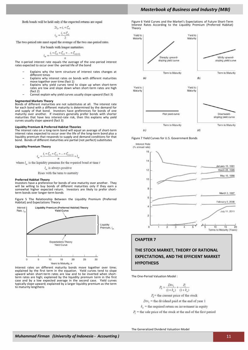
Figure 6 Yield Curves and the Market’s Expectations of Future Short-Term Interest Rates According to the Liquidity Premium (Preferred Habitat) Theory
Figure 7 Yield Curves for U.S. Government Bonds
The One-Period Valuation Model :
The Generalized Dividend Valuation Model
CHAPTER 7
THE STOCK MARKET, THEORY OF RATIONAL
EXPECTATIONS, AND THE EFFICIENT MARKET
HYPOTHESIS

Masterbook of Business and Industry (MBI)
Muhammad Firman (University of Indonesia - Accounting ) 12
The Gordon Growth Model
Dividends are assumed to continue growing at a constant rate forever. The growth rate is assumed to be less than the required return on equity How the Market Sets Prices The price is set by the buyer willing to pay the highest price. The market price will be set by the buyer who can take best advantage of the asset. Superior information about an asset can increase its value by reducing its perceived risk. Information is important for individuals to value each asset. When new information is released about a firm, expectations and prices change. Market participants constantly receive information and revise their expectations, so stock prices change frequently. Application: The Global Financial Crisis and the Stock Market Financial crisis that started in August 2007 led to one of the worst bear markets in 50 years. Downward revision of growth prospects: ↓g. Increased uncertainty: ↑ke Gordon model predicts a drop in stock prices. The Theory of Rational Expectations Adaptive expectations: Expectations are formed from past experience only. Changes in expectations will occur slowly over time as data changes. However, people use more than just past data to form their expectations and sometimes change their expectations quickly. Expectations will be identical to optimal forecasts using all available information Even though a rational expectation equals the optimal forecast using all available information, a prediction based on it may not always be perfectly accurate. It takes too much effort to make the expectation the best guess possible. Best guess will not be accurate because predictor is unaware of some relevant information Formal Statement of the Theory
Rationale Behind the Theory The incentives for equating expectations with optimal forecasts are especially strong in financial markets. In these markets, people with better forecasts of the future get rich. The application of the theory of rational expectations to financial markets (where it is called the efficient market hypothesis or the theory of efficient capital markets) is thus particularly useful Implications of the Theory If there is a change in the way a variable moves, the way in which expectations of the variable are formed will change as well. Changes in the conduct of monetary policy (e.g. target the federal funds rate). The forecast errors of expectations will, on average, be zero and cannot be predicted ahead of time. The Efficient Market Hypothesis: Rational Expectations in Financial Markets Recall : The rate of return from holding a security equals the sum of the capital gain on the security, plus any cash payments divided by the initial purchase price of the security.
The Efficient Market Hypothesis : Rational Expectations in Financial
Current prices in a financial market will be set so that the optimal forecast of a security‘s return using all available information equals the security‘s equilibrium return. In an efficient market, a security‘s price fully reflects all available information
In an efficient market, all unexploited profit opportunities will be eliminated How Valuable are Published Reports by Investment Advisors? Information in newspapers and in the published reports of investment advisers is readily available to many market participants and is already reflected in market prices. So acting on this information will not yield abnormally high returns, on average The empirical evidence for the most part confirms that recommendations from investment advisers cannot help us outperform the general market . Recommendations from investment advisors cannot help us outperform the market A hot tip is probably information already contained in the price of the stock. Stock prices respond to announcements only when the information is new and unexpected. A buy and hold‖ strategy is the most sensible strategy for the Some financial economists believe all prices are always correct and reflect market fundamentals (items that have a direct impact on future income streams of the securities) and so financial markets are efficient However, prices in markets like the stock market are unpredictable- This casts serious doubt on the stronger view that financial markets are efficient Behavioral Finance The lack of short selling (causing over-priced stocks) may be explained by loss aversion. The large trading volume may be explained by investor overconfidence. Stock market bubbles may be explained by overconfidence and social contagion
Basic Facts about Financial Structure Throughout the World This chapter provides an economic analysis of how our financial structure is designed to promote economic efficiency The bar chart in Figure 1 shows how American businesses financed their activities using external funds (those obtained from outside the business itself) in the period 1970–2000 and compares U.S. data to those of Germany, Japan, and Canada Figure 1 Sources of External Funds for Nonfinancial Businesses: A Comparison of the United States with Germany, Japan, and Canada
Eight Basic Facts
CHAPTER 8
AN ECONOMIC ANALYSIS OF FINANCIAL
STRUCTURE

Masterbook of Business and Industry (MBI)
Muhammad Firman (University of Indonesia - Accounting ) 13
1. Stocks are not the most important sources of external financing for businesses
2. Issuing marketable debt and equity securities is not the primary way in which businesses finance their operations
3. Indirect finance is many times more important than direct finance
4. Financial intermediaries, particularly banks, are the most important source of external funds used to finance businesses.
5. The financial system is among the most heavily regulated sectors of the economy
6. Only large, well-established corporations have easy access to securities markets to finance their activities
7. Collateral is a prevalent feature of debt contracts for both households and businesses.
8. Debt contracts are extremely complicated legal documents that place substantial restrictive covenants on borrowers
Transaction Costs Financial intermediaries have evolved to reduce transaction costs – Economies of scale – Expertise Asymmetric Information: Adverse Selection and Moral Hazard Adverse selection occurs before the transaction. Moral hazard arises ather the transaction. Agency theory analyses how asymmetric information problems affect economic behavior The Lemons Problem: How Adverse Selection Influences Financial Structure If quality cannot be assessed, the buyer is willing to pay at most a price that reflects the average quality. Sellers of good quality items will not want to sell at the price for average quality. The buyer will decide not to buy at all because all that is left in the market is poor quality items. This problem explains fact 2 and partially explains fact 1 Tools to Help Solve Adverse Selection Problems Private production and sale of information – Free-rider problem Government regulation to increase information – Not always works to solve the adverse selection problem,explains Fact 5. Financial intermediation – Explains facts 3, 4, & 6. Collateral and net worth – Explains fact 7. How Moral Hazard Affects the Choice Between Debt and Equity Contracts Called the Principal-Agent Problem – Principal: less information (stockholder) – Agent: more information (manager) Separation of ownership and control of the firm – Managers pursue personal benefits and power rather than the profitability of the firm Tools to Help Solve the Principal- Agent Problem Monitoring (Costly State Verification) – Free-rider problem – Fact 1 Government regulation to increase information – Fact 5 Financial Intermediation – Fact 3 Debt Contracts – Fact 1 How Moral Hazard Influences Financial Structure in Debt Markets Borrowers have incentives to take on projects that are riskier than the lenders would like. This prevents the borrower from paying back the loan. Tools to Help Solve Moral Hazard in Debt Contracts Net worth and collateral – Incentive compatible Monitoring and Enforcement of Restrictive Covenants – Discourage undesirable behavior – Encourage desirable behavior – Keep collateral valuable – Provide information Financial Intermediation – Facts 3 & 4
Summary Table 1 Asymmetric Information Problems and Tools to Solve Them
Asymmetric Information in Transition and Developing Countries Financial repression‖ created by an institutional environment characterized by: – Poor system of property rights (unable to use collateral efficiently) – Poor legal system (difficult for lenders to enforce restrictive covenants) – Weak accounting standards (less access to good information) – Government intervention through directed credit programs and state owned banks (less incentive to proper channel funds to its most productive use). Application: Financial Development and Economic Growth The financial systems in developing and transition countries face several difficulties that keep them from operating efficiently. In many developing countries, the system of property rights (the rule of law, constraints on government expropriation, absence of corruption) functions poorly, making it hard to use these two tools effectively
What is a Financial Crisis? A financial crisis occurs when there is a particularly large disruption to information flows in financial markets, with the result that financial frictions increase sharply and financial markets stop functioning Asset Markets Effects on Balance Sheets – Stock market decline Decreases net worth of corporations. – Unanticipated decline in the price level Liabilities increase in real terms and net worth decreases. – Unanticipated decline in the value of the domestic currency Increases debt denominated in foreign currencies and decreases net worth. – Asset write-downs. Factors Causing Financial Crises Deterioration in Financial Institutions‘ Balance Sheets – Decline in lending. Banking Crisis – Loss of information production and disintermediation. Increases in Uncertainty – Decrease in lending. Increases in Interest Rates – Increases adverse selection problem
CHAPTER 9
FINANCIAL CRISES
Masterbook of Business and Industry (MBI)
Muhammad Firman (University of Indonesia - Accounting ) 14
– Increases need for external funds and therefore adverse selection and moral hazard. Government Fiscal Imbalances – Create fears of default on government debt. – Investors might pull their money out of the country. Dynamics of Financial Crises in Advanced Economies
1. Stage One: Initiation of Financial Crisis Mismanagement of financial liberalization/innovation Asset price boom and bust Spikes in interest rates Increase in uncertainty
2. Stage two: Banking Crisis
3. Stage three: Debt Deflation
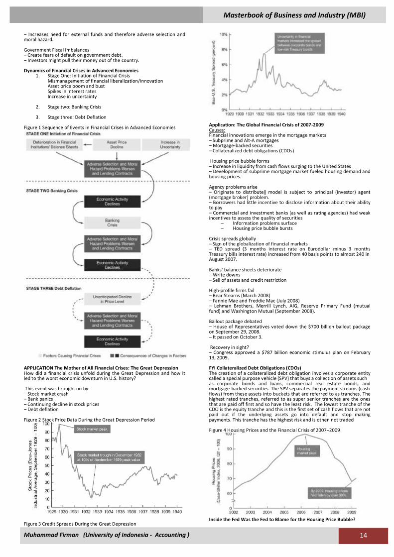
Figure 1 Sequence of Events in Financial Crises in Advanced Economies
APPLICATION The Mother of All Financial Crises: The Great Depression How did a financial crisis unfold during the Great Depression and how it led to the worst economic downturn in U.S. history? This event was brought on by: – Stock market crash – Bank panics – Continuing decline in stock prices – Debt deflation Figure 2 Stock Price Data During the Great Depression Period
Figure 3 Credit Spreads During the Great Depression
Application: The Global Financial Crisis of 2007-2009 Causes: Financial innovations emerge in the mortgage markets – Subprime and Alt-A mortgages – Mortgage-backed securities – Collateralized debt obligations (CDOs) Housing price bubble forms – Increase in liquidity from cash flows surging to the United States – Development of subprime mortgage market fueled housing demand and housing prices. Agency problems arise – Originate to distribute‖ model is subject to principal (investor) agent (mortgage broker) problem. – Borrowers had little incentive to disclose information about their ability to pay – Commercial and investment banks (as well as rating agencies) had weak incentives to assess the quality of securities
– Information problems surface – Housing price bubble bursts
Crisis spreads globally – Sign of the globalization of financial markets – TED spread (3 months interest rate on Eurodollar minus 3 months Treasury bills interest rate) increased from 40 basis points to almost 240 in August 2007. Banks‘ balance sheets deteriorate – Write downs – Sell of assets and credit restriction High-profile firms fail – Bear Stearns (March 2008) – Fannie Mae and Freddie Mac (July 2008) – Lehman Brothers, Merrill Lynch, AIG, Reserve Primary Fund (mutual fund) and Washington Mutual (September 2008). Bailout package debated – House of Representatives voted down the $700 billion bailout package on September 29, 2008. – It passed on October 3. Recovery in sight? – Congress approved a $787 billion economic stimulus plan on February 13, 2009. FYI Collateralized Debt Obligations (CDOs) The creation of a collateralized debt obligation involves a corporate entity called a special purpose vehicle (SPV) that buys a collection of assets such as corporate bonds and loans, commercial real estate bonds, and mortgage-backed securities The SPV separates the payment streams (cash flows) from these assets into buckets that are referred to as tranches. The highest rated tranches, referred to as super senior tranches are the ones that are paid off first and so have the least risk. The lowest tranche of the CDO is the equity tranche and this is the first set of cash flows that are not paid out if the underlying assets go into default and stop making payments. This tranche has the highest risk and is othen not traded Figure 4 Housing Prices and the Financial Crisis of 2007–2009
Inside the Fed Was the Fed to Blame for the Housing Price Bubble?
Masterbook of Business and Industry (MBI)
Muhammad Firman (University of Indonesia - Accounting ) 15
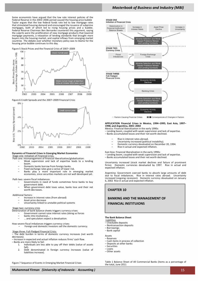
Some economists have argued that the low rate interest policies of the Federal Reserve in the 2003–2006 period caused the housing price bubble Taylor argues that the low federal funds rate led to low mortgage rates that stimulated housing demand and encouraged the issuance of subprime mortgages, both of which led to rising housing prices and a bubble. Federal Reserve Chairman Ben Bernanke countered this argument, saying the culprits were the proliferation of new mortgage products that lowered mortgage payments, a relaxation of lending standards that brought more buyers into the housing market, and capital inflows from emerging market countries The debate over whether monetary policy was to blame for the housing price bubble continues to this day. Figure 5 Stock Prices and the Financial Crisis of 2007–2009
Figure 6 Credit Spreads and the 2007–2009 Financial Crisis
Dynamics of Financial Crises in Emerging Market Economies Stage one: Initiation of Financial Crisis. Path one: mismanagement of financial liberalization/globalization:
– Weak supervision and lack of expertise leads to a lending boom.
– Domestic banks borrow from foreign banks. – Fixed exchange rates give a sense of lower risk. – Banks play a more important role in emerging market
economies, since securities markets are not well developed yet. Path two: severe fiscal imbalances:
– Governments in need of funds sometimes force banks to buy government debt.
– When government debt loses value, banks lose and their net worth decreases.
Additional factors:
– Increase in interest rates (from abroad) – Asset price decrease – Uncertainty linked to unstable political systems
Stage two: currency crisis Deterioration of bank balance sheets triggers currency crises:
– Government cannot raise interest rates (doing so forces – banks into insolvency)… – … and speculators expect a devaluation.
How severe fiscal imbalances triggers currency crises:
– Foreign and domestic investors sell the domestic currency. Stage three: Full-Fledged Financial Crisis: – The debt burden in terms of domestic currency increases (net worth decreases). – Increase in expected and actual inflation reduces firms‘ cash flow. – Banks are more likely to fail:
1. Individuals are less able to pay off their debts (value of assets fall).
2. Debt denominated in foreign currency increases (value of liabilities increase).
Figure 7 Sequence of Events in Emerging Market Financial Crises
APPLICATION Financial Crises in Mexico, 1994–1995; East Asia, 1997–1998; and Argentina, 2001–2002 Mexico: Financial liberalization in the early 1990s: – Lending boom, coupled with weak supervision and lack of expertise. – Banks accumulated losses and their net worth declined.
– Rise in interest rates abroad. – Uncertainty increased (political instability). – Domestic currency devaluated on December 20, 1994. – Rise in actual and expected inflation.
East Asia: Financial liberalization in the early 1990s: – Lending boom, coupled with weak supervision and lack of expertise. – Banks accumulated losses and their net worth declined. Uncertainty increased (stock market declines and failure of prominent firms). Domestic currencies devaluated by 1997. Rise in actual and expected inflation. Argentina: Government coerced banks to absorb large amounts of debt due to fiscal imbalances. Rise in interest rates abroad. Uncertainty increased (ongoing recession). Domestic currency devaluated on January 6, 2002 Rise in actual and expected inflation.
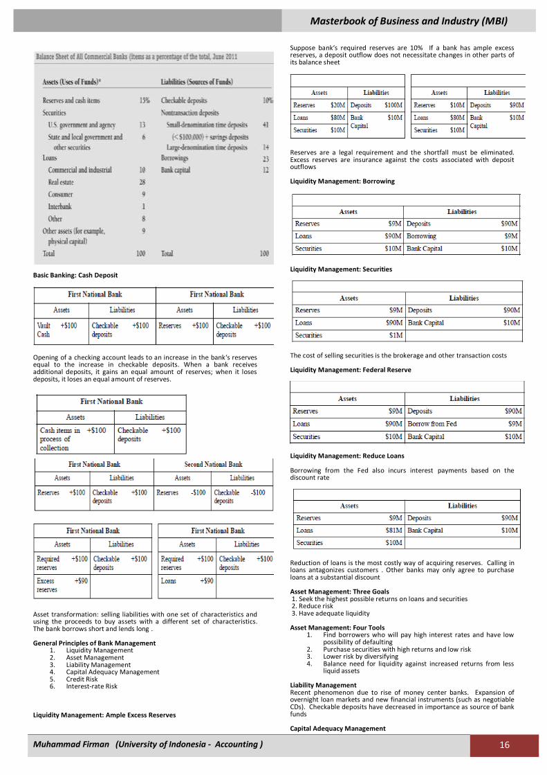
The Bank Balance Sheet Liabilities – Checkable deposits – Nontransaction deposits – Borrowings – Bank capital Assets – Reserves – Cash items in process of collection – Deposits at other banks – Securities – Loans – Other assets Table 1 Balance Sheet of All Commercial Banks (items as a percentage of the total, June 2011
CHAPTER 10
BANKING AND THE MANAGEMENT OF
FINANCIAL INSTITUIONS
Masterbook of Business and Industry (MBI)
Muhammad Firman (University of Indonesia - Accounting ) 16
Basic Banking: Cash Deposit
Opening of a checking account leads to an increase in the bank‘s reserves equal to the increase in checkable deposits. When a bank receives additional deposits, it gains an equal amount of reserves; when it loses deposits, it loses an equal amount of reserves.
Asset transformation: selling liabilities with one set of characteristics and using the proceeds to buy assets with a different set of characteristics. The bank borrows short and lends long . General Principles of Bank Management
1. Liquidity Management 2. Asset Management 3. Liability Management 4. Capital Adequacy Management 5. Credit Risk 6. Interest-rate Risk
Liquidity Management: Ample Excess Reserves
Suppose bank‘s required reserves are 10% If a bank has ample excess reserves, a deposit outflow does not necessitate changes in other parts of its balance sheet
Reserves are a legal requirement and the shortfall must be eliminated. Excess reserves are insurance against the costs associated with deposit outflows Liquidity Management: Borrowing
Liquidity Management: Securities
The cost of selling securities is the brokerage and other transaction costs Liquidity Management: Federal Reserve
Liquidity Management: Reduce Loans Borrowing from the Fed also incurs interest payments based on the discount rate
Reduction of loans is the most costly way of acquiring reserves. Calling in loans antagonizes customers . Other banks may only agree to purchase loans at a substantial discount Asset Management: Three Goals 1. Seek the highest possible returns on loans and securities 2. Reduce risk 3. Have adequate liquidity Asset Management: Four Tools
1. Find borrowers who will pay high interest rates and have low possibility of defaulting
2. Purchase securities with high returns and low risk 3. Lower risk by diversifying 4. Balance need for liquidity against increased returns from less
liquid assets Liability Management Recent phenomenon due to rise of money center banks. Expansion of overnight loan markets and new financial instruments (such as negotiable CDs). Checkable deposits have decreased in importance as source of bank funds Capital Adequacy Management
Masterbook of Business and Industry (MBI)
Muhammad Firman (University of Indonesia - Accounting ) 17
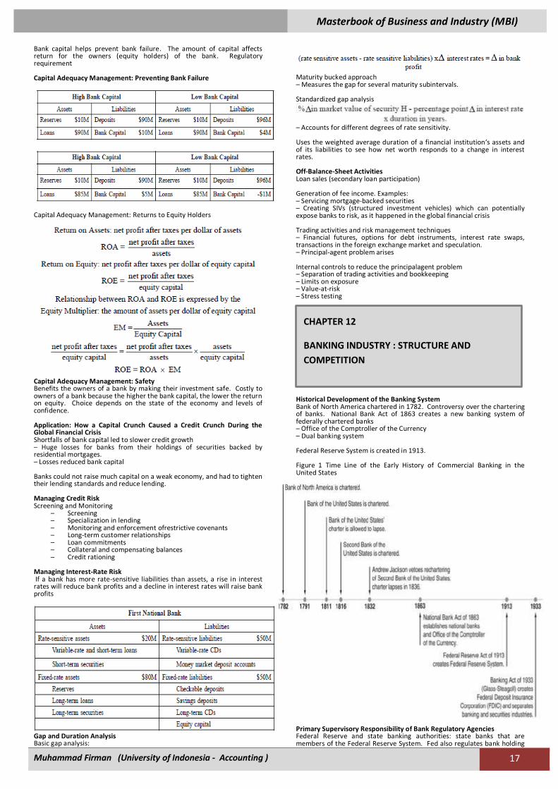
Bank capital helps prevent bank failure. The amount of capital affects return for the owners (equity holders) of the bank. Regulatory requirement Capital Adequacy Management: Preventing Bank Failure
Capital Adequacy Management: Returns to Equity Holders
Capital Adequacy Management: Safety Benefits the owners of a bank by making their investment safe. Costly to owners of a bank because the higher the bank capital, the lower the return on equity. Choice depends on the state of the economy and levels of confidence. Application: How a Capital Crunch Caused a Credit Crunch During the Global Financial Crisis Shortfalls of bank capital led to slower credit growth – Huge losses for banks from their holdings of securities backed by residential mortgages. – Losses reduced bank capital Banks could not raise much capital on a weak economy, and had to tighten their lending standards and reduce lending. Managing Credit Risk Screening and Monitoring
– Screening – Specialization in lending – Monitoring and enforcement ofrestrictive covenants – Long-term customer relationships – Loan commitments – Collateral and compensating balances – Credit rationing
Managing Interest-Rate Risk If a bank has more rate-sensitive liabilities than assets, a rise in interest rates will reduce bank profits and a decline in interest rates will raise bank profits
Gap and Duration Analysis Basic gap analysis:
Maturity bucked approach – Measures the gap for several maturity subintervals. Standardized gap analysis
– Accounts for different degrees of rate sensitivity. Uses the weighted average duration of a financial institution‘s assets and of its liabilities to see how net worth responds to a change in interest rates. Off-Balance-Sheet Activities Loan sales (secondary loan participation) Generation of fee income. Examples: – Servicing mortgage-backed securities – Creating SIVs (structured investment vehicles) which can potentially expose banks to risk, as it happened in the global financial crisis Trading activities and risk management techniques – Financial futures, options for debt instruments, interest rate swaps, transactions in the foreign exchange market and speculation. – Principal-agent problem arises Internal controls to reduce the principalagent problem – Separation of trading activities and bookkeeping – Limits on exposure – Value-at-risk – Stress testing
Historical Development of the Banking System Bank of North America chartered in 1782. Controversy over the chartering of banks. National Bank Act of 1863 creates a new banking system of federally chartered banks – Office of the Comptroller of the Currency – Dual banking system Federal Reserve System is created in 1913. Figure 1 Time Line of the Early History of Commercial Banking in the United States
Primary Supervisory Responsibility of Bank Regulatory Agencies Federal Reserve and state banking authorities: state banks that are members of the Federal Reserve System. Fed also regulates bank holding
CHAPTER 12
BANKING INDUSTRY : STRUCTURE AND
COMPETITION
Masterbook of Business and Industry (MBI)
Muhammad Firman (University of Indonesia - Accounting ) 18
companies. FDIC: insured state banks that are not Fed members. State banking authorities: state banks without FDIC insurance. Financial Innovation and the Growth of the “Shadow Banking System” Financial innovation is driven by the desire to earn profits. A change in the financial environment will stimulate a search by financial institutions for innovations that are likely to be profitable. – Financial engineering Responses to Changes in Demand Conditions: Interest Rate Volatility Adjustable-rate mortgages – Flexible interest rates keep profits high when rates rise – Lower initial interest rates make them attractive to home buyers Financial Derivatives – Ability to hedge interest rate risk – Payoffs are linked to previously issued (i.e. derived from) securities. Responses to Changes in Supply Conditions: Information Technology Bank credit and debit cards – Improved computer technology lowers transaction costs Electronic banking – ATM, home banking, ABM and virtual banking
– Junk bonds – Commercial paper market
Securitization
– To transform otherwise illiquid financial assets into marketable capital market securities.
– Securitization played an especially prominent role in the development of the subprime mortgagemarket in the mid 2000s.
Avoidance of Existing Regulations: Loophole Mining Reserve requirements act as a tax on deposits. Restrictions on interest paid on deposits led to disintermediation.
– Money market mutual funds – Sweep accounts
Financial Innovation and the Decline of Traditional Banking As a source of funds for borrowers, market share has fallen. Commercial banks‘ share of total financial intermediary assets has fallen. No decline in overall profitability. Increase in income from off-balance-sheet activities Figure 2 Bank Share of Total Nonfinancial Borrowing, 1960–2011
Decline in cost advantages in acquiring funds (liabilities) – Rising inflation led to rise in interest rates and disintermediation – Low-cost source of funds, checkable deposits, declined in importance Decline in income advantages on uses of funds (assets) – Information technology has decreased need for banks to finance short-term credit needs or to issue loans – Information technology has lowered transaction costs for other financial institutions, increasing competition Banks’ Responses Expand into new and riskier areas of lending – Commercial real estate loans – Corporate takeovers and leveraged buyouts Pursue off-balance-sheet activities – Non-interest income – Concerns about risk Structure of the U.S. Commercial Banking Industry Restrictions on branching – McFadden Act and state branching regulations.
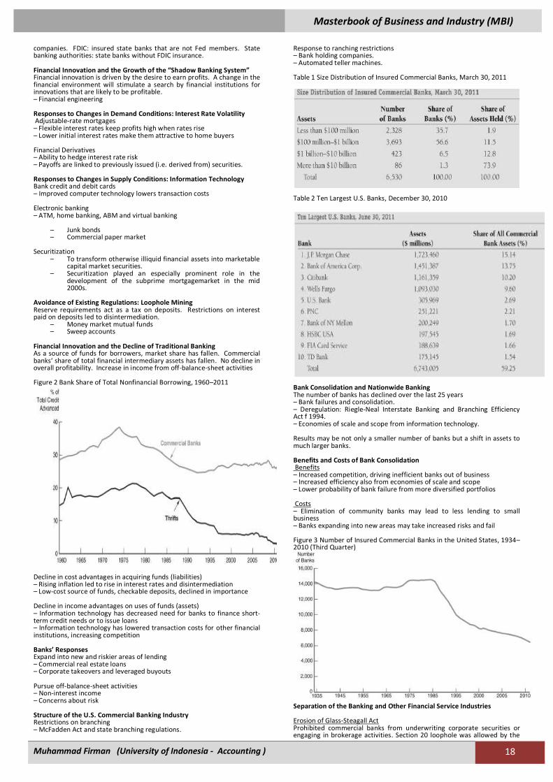
Response to ranching restrictions – Bank holding companies. – Automated teller machines. Table 1 Size Distribution of Insured Commercial Banks, March 30, 2011
Table 2 Ten Largest U.S. Banks, December 30, 2010
Bank Consolidation and Nationwide Banking The number of banks has declined over the last 25 years – Bank failures and consolidation. – Deregulation: Riegle-Neal Interstate Banking and Branching Efficiency Act f 1994. – Economies of scale and scope from information technology. Results may be not only a smaller number of banks but a shift in assets to much larger banks. Benefits and Costs of Bank Consolidation Benefits – Increased competition, driving inefficient banks out of business – Increased efficiency also from economies of scale and scope – Lower probability of bank failure from more diversified portfolios Costs – Elimination of community banks may lead to less lending to small business – Banks expanding into new areas may take increased risks and fail Figure 3 Number of Insured Commercial Banks in the United States, 1934–2010 (Third Quarter)
Separation of the Banking and Other Financial Service Industries Erosion of Glass-Steagall Act Prohibited commercial banks from underwriting corporate securities or engaging in brokerage activities. Section 20 loophole was allowed by the

Masterbook of Business and Industry (MBI)
Muhammad Firman (University of Indonesia - Accounting ) 19
Federal Reserve enabling affiliates of approved commercial banks to underwrite securities as long as the revenue did not exceed a specified amount. – U.S. Supreme Court validated the Fed‘s action in 1988 Gramm-Leach-Bliley Financial Services Modernization Act of 1999
– Abolishes Glass-Steagall – States regulate insurance activities – SEC keeps oversight of securities activities – Office of the Comptroller of the Currency regulates bank
subsidiaries engaged in securities underwriting – Federal Reserve oversees bank holding companies
Separation of Banking and Other Financial Services Industries Throughout the World Universal banking – No separation between banking and securities industries British-style universal banking – May engage in security underwriting Separate legal subsidiaries are common
1. Bank equity holdings of commercial firms are less common 2. Few combinations of banking and insurance firms
Some legal separation Allowed to hold substantial equity stakes in commercial firms but holding companies are illegal Thrift Industry: Regulation and Structure Savings and Loan Associations
– Chartered by the federal government or by states – Most are members of Federal Home Loan Bank System (FHLBS) – Deposit insurance provided by Savings Association Insurance
Fund (SAIF), part of FDIC – Regulated by the Office of Thrift Supervision
Mutual Savings Banks – Approximately half are chartered by states – Regulated by state in which they are located – Deposit insurance provided by FDIC or state insurance Credit Unions
– Tax-exempt – Chartered by federal government or by states – Regulated by the National Credit Union Administration (NCUA) – Deposit insurance provided by National Credit Union Share
Insurance Fund (NCUSIF) International Banking Rapid growth – Growth in international trade and multinational corporations – Global investment banking is very profitable – Ability to tap into the Eurodollar market Eurodollar Market Dollar-denominated deposits held in banks outside of the U.S. Most widely used currency in international trade. Offshore deposits not subject to regulations. Important source of funds for U.S. banks Structure of U.S. Banking Overseas Shell operation Edge Act corporation International banking facilities (IBFs) – Not subject to regulation and taxes – May not make loans to domestic residents Foreign Banks in the U.S. Agency office of the foreign bank – Can lend and transfer fund in the U.S. – Cannot accept deposits from domestic residents – Not subject to regulations Subsidiary U.S. bank – Subject to U.S. regulations – Owned by a foreign bank Branch of a foreign bank
– May open branches only in state designated as home state or in state that allow entry of out-of-state banks
– Limited-service may be allowed in any other state Subject to the International Banking Act of 1978 Basel Accord (1988) – Example of international coordination of bank regulation – Sets minimum capital requirements for banks Table 3 Ten Largest Banks in the World, 2011
Origins of the Federal Reserve System Resistance to establishment of a central bank – Fear of centralized power – Distrust of moneyed interests No lender of last resort – Nationwide bank panics on a regular basis – Panic of 1907 so severe that the public was convinced a central bank was needed Federal Reserve Act of 1913 – Elaborate system of checks and balances – Decentralized Structure of the Federal Reserve System The writers of the Federal Reserve Act wanted to diffuse power along regional lines, between the private sector and the government, and among bankers, business people, and the public . This initial diffusion of power has resulted in the evolution of the Federal Reserve System to include the following entities: – The Federal Reserve banks, the Board of Governors of the Federal Reserve System, the Federal Open Market Committee (FOMC), the Federal Advisory Council, and around 2,900 member commercial banks. Figure 1 Structure and Responsibility for Policy Tools in the Federal Reserve System
Figure 2 Federal Reserve System
CHAPTER 13
CENTRAL BANKS AND THE FEDERAL RESERVE
SYSTEM
Masterbook of Business and Industry (MBI)
Muhammad Firman (University of Indonesia - Accounting ) 20
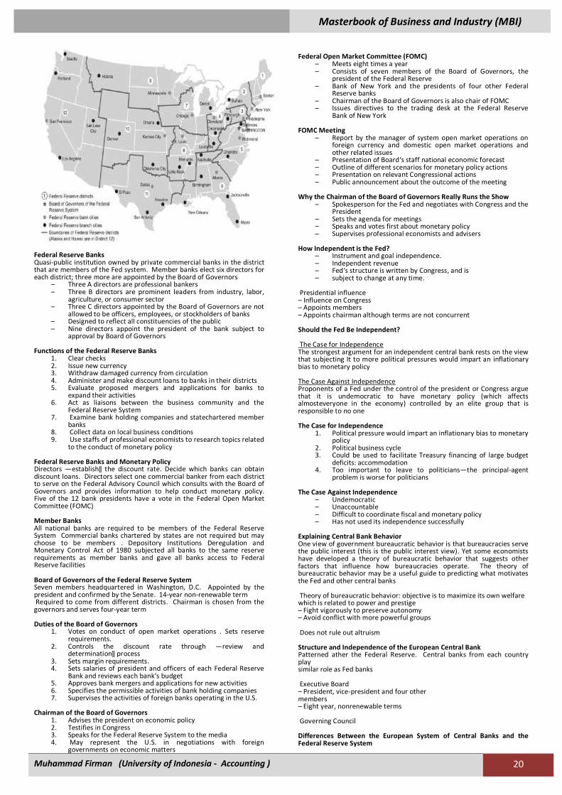
Federal Reserve Banks Quasi-public institution owned by private commercial banks in the district that are members of the Fed system. Member banks elect six directors for each district; three more are appointed by the Board of Governors
– Three A directors are professional bankers – Three B directors are prominent leaders from industry, labor,
agriculture, or consumer sector – Three C directors appointed by the Board of Governors are not
allowed to be officers, employees, or stockholders of banks – Designed to reflect all constituencies of the public – Nine directors appoint the president of the bank subject to
approval by Board of Governors Functions of the Federal Reserve Banks
1. Clear checks 2. Issue new currency 3. Withdraw damaged currency from circulation 4. Administer and make discount loans to banks in their districts 5. Evaluate proposed mergers and applications for banks to
expand their activities 6. Act as liaisons between the business community and the
Federal Reserve System 7. Examine bank holding companies and statechartered member
banks 8. Collect data on local business conditions 9. Use staffs of professional economists to research topics related
to the conduct of monetary policy Federal Reserve Banks and Monetary Policy Directors ―establish‖ the discount rate. Decide which banks can obtain discount loans. Directors select one commercial banker from each district to serve on the Federal Advisory Council which consults with the Board of Governors and provides information to help conduct monetary policy. Five of the 12 bank presidents have a vote in the Federal Open Market Committee (FOMC) Member Banks All national banks are required to be members of the Federal Reserve System Commercial banks chartered by states are not required but may choose to be members . Depository Institutions Deregulation and Monetary Control Act of 1980 subjected all banks to the same reserve requirements as member banks and gave all banks access to Federal Reserve facilities Board of Governors of the Federal Reserve System Seven members headquartered in Washington, D.C. Appointed by the president and confirmed by the Senate. 14-year non-renewable term Required to come from different districts. Chairman is chosen from the governors and serves four-year term Duties of the Board of Governors
1. Votes on conduct of open market operations . Sets reserve requirements.
2. Controls the discount rate through ―review and determination‖ process
3. Sets margin requirements. 4. Sets salaries of president and officers of each Federal Reserve
Bank and reviews each bank‘s budget 5. Approves bank mergers and applications for new activities 6. Specifies the permissible activities of bank holding companies 7. Supervises the activities of foreign banks operating in the U.S.
Chairman of the Board of Governors
1. Advises the president on economic policy 2. Testifies in Congress 3. Speaks for the Federal Reserve System to the media 4. May represent the U.S. in negotiations with foreign
governments on economic matters
Federal Open Market Committee (FOMC)
– Meets eight times a year – Consists of seven members of the Board of Governors, the
president of the Federal Reserve – Bank of New York and the presidents of four other Federal
Reserve banks – Chairman of the Board of Governors is also chair of FOMC – Issues directives to the trading desk at the Federal Reserve
Bank of New York FOMC Meeting
– Report by the manager of system open market operations on foreign currency and domestic open market operations and other related issues
– Presentation of Board‘s staff national economic forecast – Outline of different scenarios for monetary policy actions – Presentation on relevant Congressional actions – Public announcement about the outcome of the meeting
Why the Chairman of the Board of Governors Really Runs the Show
– Spokesperson for the Fed and negotiates with Congress and the President
– Sets the agenda for meetings – Speaks and votes first about monetary policy – Supervises professional economists and advisers
How Independent is the Fed?
– Instrument and goal independence. – Independent revenue – Fed‘s structure is written by Congress, and is – subject to change at any time.
Presidential influence – Influence on Congress – Appoints members – Appoints chairman although terms are not concurrent Should the Fed Be Independent? The Case for Independence The strongest argument for an independent central bank rests on the view that subjecting It to more political pressures would impart an inflationary bias to monetary policy The Case Against Independence Proponents of a Fed under the control of the president or Congress argue that it is undemocratic to have monetary policy (which affects almosteveryone in the economy) controlled by an elite group that is responsible to no one The Case for Independence
1. Political pressure would impart an inflationary bias to monetary policy
2. Political business cycle 3. Could be used to facilitate Treasury financing of large budget
deficits: accommodation 4. Too important to leave to politicians—the principal-agent
problem is worse for politicians The Case Against Independence
– Undemocratic – Unaccountable – Difficult to coordinate fiscal and monetary policy – Has not used its independence successfully
Explaining Central Bank Behavior One view of government bureaucratic behavior is that bureaucracies serve the public interest (this is the public interest view). Yet some economists have developed a theory of bureaucratic behavior that suggests other factors that influence how bureaucracies operate. The theory of bureaucratic behavior may be a useful guide to predicting what motivates the Fed and other central banks Theory of bureaucratic behavior: objective is to maximize its own welfare which is related to power and prestige – Fight vigorously to preserve autonomy – Avoid conflict with more powerful groups Does not rule out altruism Structure and Independence of the European Central Bank Patterned ather the Federal Reserve. Central banks from each country play similar role as Fed banks Executive Board – President, vice-president and four other members – Eight year, nonrenewable terms Governing Council Differences Between the European System of Central Banks and the Federal Reserve System
Masterbook of Business and Industry (MBI)
Muhammad Firman (University of Indonesia - Accounting ) 21
– National Central Banks control their own – budgets and the budget of the ECB – Monetary operations are not centralized – Does not supervise and regulate financial institutions
Governing Council
– Monthly meetings at ECB in Frankfurt, Germany – Twelve National Central Bank heads and six Executive Board
members – Operates by consensus – ECB announces the target rate and takes questions from the
media – To stay at a manageable size as new countries join, the
Governing Council will be on a system of rotation How Independent Is the ECB? Most independent in the world
– Members of the Executive Board have long terms – Determines own budget – Less goal independent – Price stability – Charter cannot by changed by legislation; only by revision of
the Maastricht Treaty Structure and Independence of Other Foreign Central Banks Bank of Canada – Essentially controls monetary policy Bank of England – Has some instrument independence. Bank of Japan – Recently (1998) gained more independence The trend toward greater independence
Three Players in the Money Supply Process
1. Central bank (Federal Reserve System) 2. Banks (depository institutions; financial intermediaries) 3. Depositors (individuals and institutions)
The Fed’s Balance Sheet
Liabilities – Currency in circulation: in the hands of the public – Reserves: bank deposits at the Fed and vault cash Assets – Government securities: holdings by the Fed that affect money supply and earn interest – Discount loans: provide reserves to banks and earn the discount rate Control of the Monetary Base High-powered money
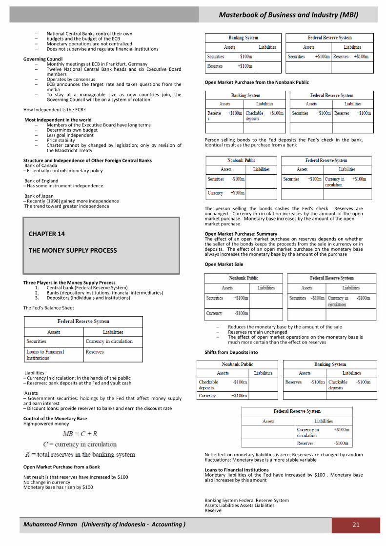
Open Market Purchase from a Bank Net result is that reserves have increased by $100 No change in currency Monetary base has risen by $100
Open Market Purchase from the Nonbank Public
Person selling bonds to the Fed deposits the Fed‘s check in the bank. Identical result as the purchase from a bank
The person selling the bonds cashes the Fed‘s check Reserves are unchanged. Currency in circulation increases by the amount of the open market purchase. Monetary base increases by the amount of the open market purchase. Open Market Purchase: Summary The effect of an open market purchase on reserves depends on whether the seller of the bonds keeps the proceeds from the sale in currency or in deposits. The effect of an open market purchase on the monetary base always increases the monetary base by the amount of the purchase Open Market Sale
– Reduces the monetary base by the amount of the sale – Reserves remain unchanged – The effect of open market operations on the monetary base is
much more certain than the effect on reserves Shifts from Deposits into
Net effect on monetary liabilities is zero; Reserves are changed by random fluctuations; Monetary base is a more stable variable Loans to Financial Institutions Monetary liabilities of the Fed have increased by $100 . Monetary base also increases by this amount Banking System Federal Reserve System Assets Liabilities Assets Liabilities Reserve
CHAPTER 14
THE MONEY SUPPLY PROCESS
Masterbook of Business and Industry (MBI)
Muhammad Firman (University of Indonesia - Accounting ) 22
Other Factors that Affect the Monetary Base
1. Float 2. Treasury deposits at the Federal Reserve 3. Interventions in the foreign exchange market
Overview of The Fed’s Ability to Control the Monetary Base Open market operations are controlled by the Fed. The Fed cannot determine the amount of borrowing by banks from the Fed. Split the monetary base into two components
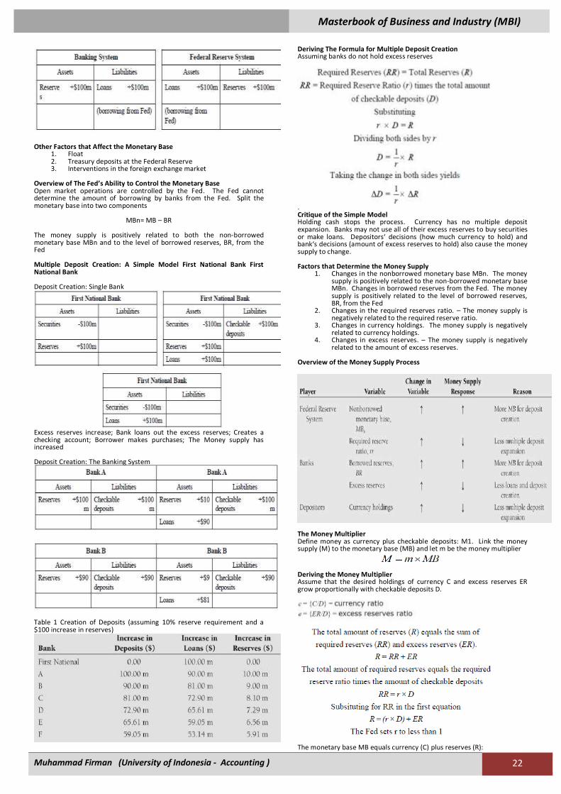
MBn= MB – BR The money supply is positively related to both the non-borrowed monetary base MBn and to the level of borrowed reserves, BR, from the Fed Multiple Deposit Creation: A Simple Model First National Bank First National Bank Deposit Creation: Single Bank
Excess reserves increase; Bank loans out the excess reserves; Creates a checking account; Borrower makes purchases; The Money supply has increased Deposit Creation: The Banking System
Table 1 Creation of Deposits (assuming 10% reserve requirement and a $100 increase in reserves)
Deriving The Formula for Multiple Deposit Creation Assuming banks do not hold excess reserves
. Critique of the Simple Model Holding cash stops the process. Currency has no multiple deposit expansion. Banks may not use all of their excess reserves to buy securities or make loans. Depositors‘ decisions (how much currency to hold) and bank‘s decisions (amount of excess reserves to hold) also cause the money supply to change. Factors that Determine the Money Supply
1. Changes in the nonborrowed monetary base MBn. The money supply is positively related to the non-borrowed monetary base MBn. Changes in borrowed reserves from the Fed. The money supply is positively related to the level of borrowed reserves, BR, from the Fed
2. Changes in the required reserves ratio. – The money supply is negatively related to the required reserve ratio.
3. Changes in currency holdings. The money supply is negatively related to currency holdings.
4. Changes in excess reserves. – The money supply is negatively related to the amount of excess reserves.
Overview of the Money Supply Process
The Money Multiplier Define money as currency plus checkable deposits: M1. Link the money supply (M) to the monetary base (MB) and let m be the money multiplier
Deriving the Money Multiplier Assume that the desired holdings of currency C and excess reserves ER grow proportionally with checkable deposits D.
The monetary base MB equals currency (C) plus reserves (R):
Masterbook of Business and Industry (MBI)
Muhammad Firman (University of Indonesia - Accounting ) 23
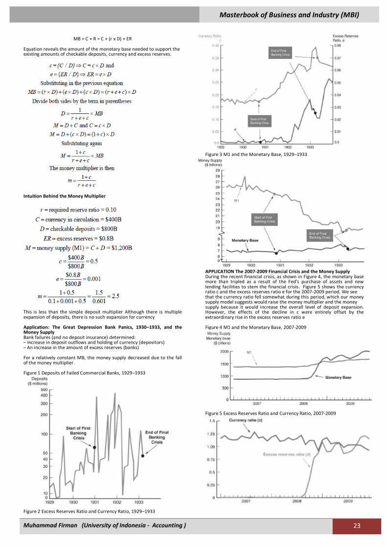
MB = C + R = C + (r x D) + ER
Equation reveals the amount of the monetary base needed to support the existing amounts of checkable deposits, currency and excess reserves.
Intuition Behind the Money Multiplier
This is less than the simple deposit multiplier Although there is multiple expansion of deposits, there is no such expansion for currency Application: The Great Depression Bank Panics, 1930–1933, and the Money Supply Bank failures (and no deposit insurance) determined: – Increase in deposit outflows and holding of currency (depositors) – An increase in the amount of excess reserves (banks) For a relatively constant MB, the money supply decreased due to the fall of the money multiplier. Figure 1 Deposits of Failed Commercial Banks, 1929–1933
Figure 2 Excess Reserves Ratio and Currency Ratio, 1929–1933
Figure 3 M1 and the Monetary Base, 1929–1933
APPLICATION The 2007-2009 Financial Crisis and the Money Supply During the recent financial crisis, as shown in Figure 4, the monetary base more than tripled as a result of the Fed's purchase of assets and new lending facilities to stem the financial crisis. Figure 5 shows the currency ratio c and the excess reserves ratio e for the 2007-2009 period. We see that the currency ratio fell somewhat during this period, which our money supply model suggests would raise the money multiplier and the money supply because it would increase the overall level of deposit expansion. However, the effects of the decline in c were entirely offset by the extraordinary rise in the excess reserves ratio e Figure 4 M1 and the Monetary Base, 2007-2009
Figure 5 Excess Reserves Ratio and Currency Ratio, 2007-2009
Masterbook of Business and Industry (MBI)
Muhammad Firman (University of Indonesia - Accounting ) 24
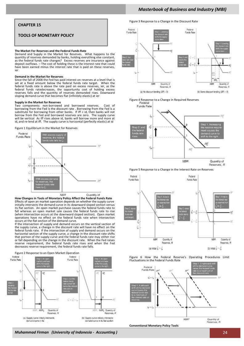
The Market For Reserves and the Federal Funds Rate Demand and Supply in the Market for Reserves. What happens to the quantity of reserves demanded by banks, holding everything else constant, as the federal funds rate changes? Excess reserves are insurance against deposit outflows. – The cost of holding these is the interest rate that could have been earned minus the interest rate that is paid on these reserves, ier Demand in the Market for Reserves Since the fall of 2008 the Fed has paid interest on reserves at a level that is set at a fixed amount below the federal funds rate target. When the federal funds rate is above the rate paid on excess reserves, ier, as the federal funds ratedecreases, the opportunity cost of holding excess reserves falls and the quantity of reserves demanded rises. Downward sloping demand curve that becomes flat (infinitely elastic) at ier Supply in the Market for Reserves Two components: non-borrowed and borrowed reserves. Cost of borrowing from the Fed is the discount rate . Borrowing from the Fed is a substitute for borrowing from other banks. If iff < id, then banks will not borrow from the Fed and borrowed reserves are zero. The supply curve will be vertical As iff rises above id, banks will borrow more and more at id, and re-lend at iff. The supply curve is horizontal (perfectly elastic) at id Figure 1 Equilibrium in the Market for Reserves
How Changes in Tools of Monetary Policy Affect the Federal Funds Rate Effects of open an market operation depends on whether the supply curve initially intersects the demand curve in its downward sloped section versus its flat section. An open market purchase causes the federal funds rate to fall whereas an open market sale causes the federal funds rate to rise (when intersection occurs at the downward sloped section). Open market operations have no effect on the federal funds rate when intersection occurs at the flat section of the demand curve. If the intersection of supply and demand occurs on the vertical section of the supply curve, a change in the discount rate will have no effect on the federal funds rate. If the intersection of supply and demand occurs on the horizontal section of the supply curve, a change in the discount rate shifts that portion of the supply curve and the federal funds rate may either rise or fall depending on the change in the discount rate. When the Fed raises reserve requirement, the federal funds rate rises and when the Fed decreases reserve requirement, the federal funds rate falls. Figure 2 Response to an Open Market Operation
Figure 3 Response to a Change in the Discount Rate
Figure 4 Response to a Change in Required Reserves
Figure 5 Response to a Change in the Interest Rate on Reserves
Figure 6 How the Federal Reserve’s Operating Procedures Limit Fluctuations in the Federal Funds Rate
Conventional Monetary Policy Tools
CHAPTER 15
TOOLS OF MONETARY POLICY

Masterbook of Business and Industry (MBI)
Muhammad Firman (University of Indonesia - Accounting ) 25
During normal times, the Federal Reserve uses three tools of monetary policy—open market operations, discount lending, and reserve requirements—to control the money supply and interest rates, and these are referred to as conventional monetary policy tools. Open Market Operations
– Dynamic open market operations – Defensive open market operations – Primary dealers – TRAPS (Trading Room Automated Processing System) – Repurchase agreements – Matched sale-purchase agreements
Advantages of Open Market Operations
1. The Fed has complete control over the 2. volume 3. Flexible and precise 4. Easily reversed 5. Quickly implemented
Discount Policy and the Lender of Last Resort
– Discount window – Primary credit: standing lending facility, Lombard facility – Secondary credit – Seasonal credit – Lender of last resort to prevent financial – Panics, Creates moral hazard problem
Advantages and Disadvantages of Discount Policy Used to perform role of lender of last resort . Important during the subprime financial crisis of 2007-2008. Cannot be controlled by the Fed; the decision maker is the bank. Discount facility is used as a backup facility to prevent the federal funds rate from rising too far above the target Reserve Requirements Depository Institutions Deregulation and Monetary Control Act of 1980 sets the reserve requirement the same for all depository institutions. 3% of the first $48.3 million of checkable deposits; 10% of checkable deposits over $48.3 million. The Fed can vary the 10% requirement between 8% to 14% Disadvantages of Reserve Requirements
– No longer binding for most banks – Can cause liquidity problems – Increases uncertainty for banks
Nonconventional Monetary Policy Tools During the Global FinancialCrisis Liquidity provision: The Federal Reserve implemented unprecedented increases in its lending facilities to provide liquidity to the financial markets – Discount Window Expansion – Term Auction Facility – New Lending Programs Asset Purchases: During the crisis the Fed started two new asset purchase programs to lower interest rates for particular types of credit: Government Sponsored Entities Purchase Program; QE2 Monetary Policy Tools of the European Central Bank Open market operations – Main refinancing operations, Weekly reverse transactions – Longer-term refinancing operations Lending to banks – Marginal lending facility/marginal lending rate – Deposit facility
The Price Stability Goal and the Nominal Anchor Over the past few decades, policy makers throughout the world have become increasingly aware of the social and economic costs of inflation and more concerned with maintaining a stable price level as a goal of economic policy. The role of a nominal anchor: a nominal variable such as the inflation rate or the money supply, which ties down the price level to achieve pricestability Other Goals of Monetary Policy Five other goals are continually mentioned by central bank officials when they discuss the objectives of monetary policy: – (1) high employment and output stability – (2) economic growth – (3) stability of financial markets – (4) interest-rate stability – (5) stability in foreign exchange markets Should Price Stability Be the Primary Goal of Monetary Policy?
Hierarchical Versus Dual Mandates: – hierarchical mandates put the goal of price stability first, and
then say that as long as it is achieved other goals can be pursued
– dual mandates are aimed to achieve two coequal objectives: price stability and maximum employment (output stability
Price Stability as the Primary, Long-Run Goal of Monetary Policy. Either type of mandate is acceptable as long as it operates to make price stability the primary goal in the long run, but not the short run Inflation Targeting Public announcement of medium-term numericaltarget for inflation. Institutional commitment to price stability as the primary, long-run goal of monetary policy and a commitment to achieve the inflation goal. Information-inclusive approach in which many variables are used in making decisions Increased transparency of the strategy. Increased accountability of the central bank New Zealand (effective in 1990)
– Inflation was brought down and remained within the target most of the time.
– Growth has generally been high and unemployment has come down significantly
Canada (1991)
– Inflation decreased since then, some costs in term ofunemployment
United Kingdom (1992)
– Inflation has been close to its target. – Growth has been strong and unemployment has been
decreasing. Advantages – Does not rely on one variable to achieve target – Easily understood – Reduces potential of falling in time inconsistency trap – Stresses transparency and accountability Disadvantages – Delayed signaling – Too much rigidity – Potential for increased output fluctuations – Low economic growth during disinflation Figure 1 Inflation Rates and Inflation Targets for New Zealand, Canada, and the United Kingdom, 1980–2011
The Federal Reserve’s Monetary Policy Strategy
CHAPTER 16
THE CONDUCT OF MONETARY POLICY :
STRATEGY AND TACTICS

Masterbook of Business and Industry (MBI)
Muhammad Firman (University of Indonesia - Accounting ) 26
The United States has achieved excellent macroeconomic performance (including low and stable inflation) until the onset of the global financial crisis without using an explicit nominal anchor such as an inflation target History: – Fed began to announce publicly targets for money supply growth in 1975 – Paul Volker (1979) focused more in nonborrowed reserves – Greenspan announced in July 1993 that the Fed would not use any monetary aggregates as a guide for conducting monetary policy There is no explicit nominal anchor in the form of an overriding concern for the Fed. Forward looking behavior and periodic , preemptive strikes‖ The goal is to prevent inflation from getting started. Advantages – Uses many sources of information – Demonstrated success Disadvantages – Lack of accountability – Inconsistent with democratic principles Advantages of the Fed‘s ―Just Do It‖ Approach: forward-looking behavior and stress on price stability also help to discourage overly expansionary monetary policy, thereby ameliorating the time-inconsistency problem Disadvantages of the Fed‘s ―Just Do It‖ Approach: lack of transparency; strong dependence on the preferences, skills, and trustworthiness of the individuals in charge of the central bank Lessons for Monetary Policy Strategy from the Global Financial Crisis 1. Developments in the financial sector have a far greater impact on
economic activity than was earlier realized 2. The zero-lower-bound on interest rates can be a serious problem 3. The cost of cleaning up ather a financial crisis is very high 4. Price and output stability do not ensure financial stability
How should Central banks respond to asset price bubbles? – Asset-price bubble: pronounced increase in asset prices that depart from fundamental values, which eventually burst. Types of asset-price bubbles – Credit-driven bubbles, Subprime financial crisis – Bubbles driven solely by irrational exuberance Should central banks respond to bubbles?
– Strong argument for not responding to bubbles driven by irrational exuberance
– Bubbles are easier to identify when asset prices and credit are increasing rapidly at the same time.
– Monetary policy should not be used to prick bubbles. Macropudential policy: regulatory policy to affect what is happening in credit markets in the aggregate. Monetary policy: Central banks and other regulators should not have a laissez-faire attitude and let credit-driven bubbles proceed without any reaction. Tactics: Choosing the Policy Instrument Tools – Open market operation – Reserve requirements – Discount rate Policy instrument (operating instrument) – Reserve aggregates – Interest rates – May be linked to an intermediate target Figure 2 Linkages Between Central Bank Tools, Policy Instruments, Intermediate Targets, and Goals of Monetary Policy
Figure 3 Result of Targeting on Nonborrowed Reserves
Figure 4 Result of Targeting on the Federal Funds Rate
Criteria for Choosing the Policy Instrument 1. Observability and Measurability 2. Controllability 3. Predictable effect on Goals
Tactics: The Taylor Rule, NAIRU, and the Phillips Curve Federal funds rate target = inflation rate + equilibrium real fed funds rate +1/2 (inflation gap) +1/2 (output gap) An inflation gap and an output gap – Stabilizing real output is an important concern – Output gap is an indicator of future inflation as shown by Phillips curve NAIRU – Rate of unemployment at which there is no tendency for inflation to change Figure 5 The Taylor Rule for the Federal Funds Rate, 1970–2011
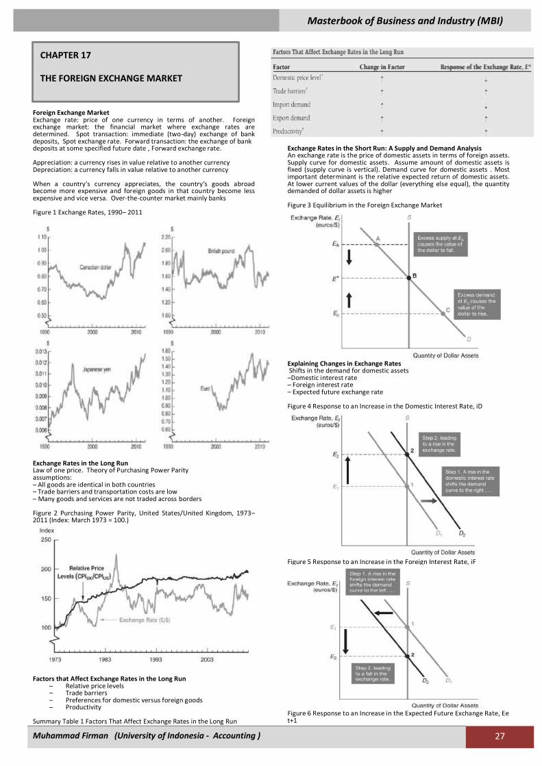
Masterbook of Business and Industry (MBI)
Muhammad Firman (University of Indonesia - Accounting ) 27
Foreign Exchange Market Exchange rate: price of one currency in terms of another. Foreign exchange market: the financial market where exchange rates are determined. Spot transaction: immediate (two-day) exchange of bank deposits, Spot exchange rate. Forward transaction: the exchange of bank deposits at some specified future date , Forward exchange rate. Appreciation: a currency rises in value relative to another currency Depreciation: a currency falls in value relative to another currency When a country‘s currency appreciates, the country‘s goods abroad become more expensive and foreign goods in that country become less expensive and vice versa. Over-the-counter market mainly banks Figure 1 Exchange Rates, 1990– 2011
Exchange Rates in the Long Run Law of one price. Theory of Purchasing Power Parity assumptions: – All goods are identical in both countries – Trade barriers and transportation costs are low – Many goods and services are not traded across borders Figure 2 Purchasing Power Parity, United States/United Kingdom, 1973–2011 (Index: March 1973 = 100.)
Factors that Affect Exchange Rates in the Long Run
– Relative price levels – Trade barriers – Preferences for domestic versus foreign goods – Productivity
Summary Table 1 Factors That Affect Exchange Rates in the Long Run
Exchange Rates in the Short Run: A Supply and Demand Analysis An exchange rate is the price of domestic assets in terms of foreign assets. Supply curve for domestic assets. Assume amount of domestic assets is fixed (supply curve is vertical). Demand curve for domestic assets . Most important determinant is the relative expected return of domestic assets. At lower current values of the dollar (everything else equal), the quantity demanded of dollar assets is higher Figure 3 Equilibrium in the Foreign Exchange Market
Explaining Changes in Exchange Rates Shifts in the demand for domestic assets –Domestic interest rate – Foreign interest rate – Expected future exchange rate Figure 4 Response to an Increase in the Domestic Interest Rate, iD
Figure 5 Response to an Increase in the Foreign Interest Rate, iF
Figure 6 Response to an Increase in the Expected Future Exchange Rate, Ee t+1
CHAPTER 17
THE FOREIGN EXCHANGE MARKET
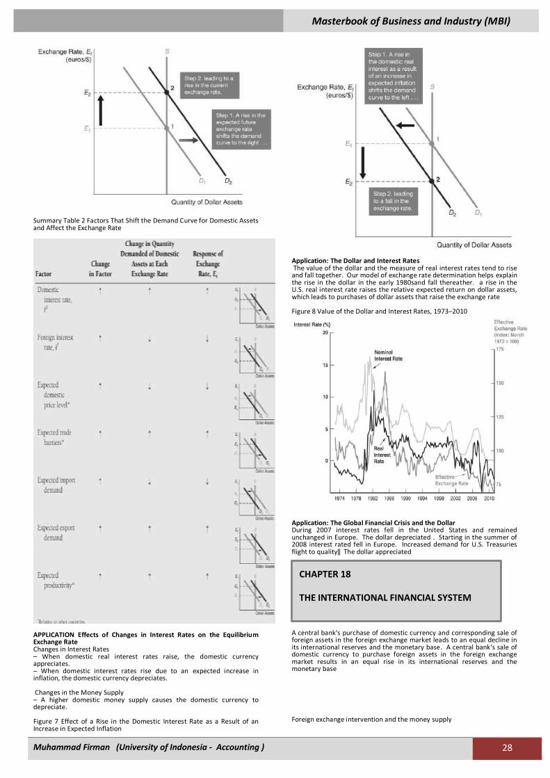
Masterbook of Business and Industry (MBI)
Muhammad Firman (University of Indonesia - Accounting ) 28
Summary Table 2 Factors That Shift the Demand Curve for Domestic Assets and Affect the Exchange Rate
APPLICATION Effects of Changes in Interest Rates on the Equilibrium Exchange Rate Changes in Interest Rates – When domestic real interest rates raise, the domestic currency appreciates. – When domestic interest rates rise due to an expected increase in inflation, the domestic currency depreciates. Changes in the Money Supply – A higher domestic money supply causes the domestic currency to depreciate. Figure 7 Effect of a Rise in the Domestic Interest Rate as a Result of an Increase in Expected Inflation
Application: The Dollar and Interest Rates The value of the dollar and the measure of real interest rates tend to rise and fall together. Our model of exchange rate determination helps explain the rise in the dollar in the early 1980sand fall thereather. a rise in the U.S. real interest rate raises the relative expected return on dollar assets, which leads to purchases of dollar assets that raise the exchange rate Figure 8 Value of the Dollar and Interest Rates, 1973–2010
Application: The Global Financial Crisis and the Dollar During 2007 interest rates fell in the United States and remained unchanged in Europe. The dollar depreciated . Starting in the summer of 2008 interest rated fell in Europe. Increased demand for U.S. Treasuries flight to quality‖ The dollar appreciated
A central bank‘s purchase of domestic currency and corresponding sale of foreign assets in the foreign exchange market leads to an equal decline in its international reserves and the monetary base. A central bank‘s sale of domestic currency to purchase foreign assets in the foreign exchange market results in an equal rise in its international reserves and the monetary base Foreign exchange intervention and the money supply
CHAPTER 18
THE INTERNATIONAL FINANCIAL SYSTEM
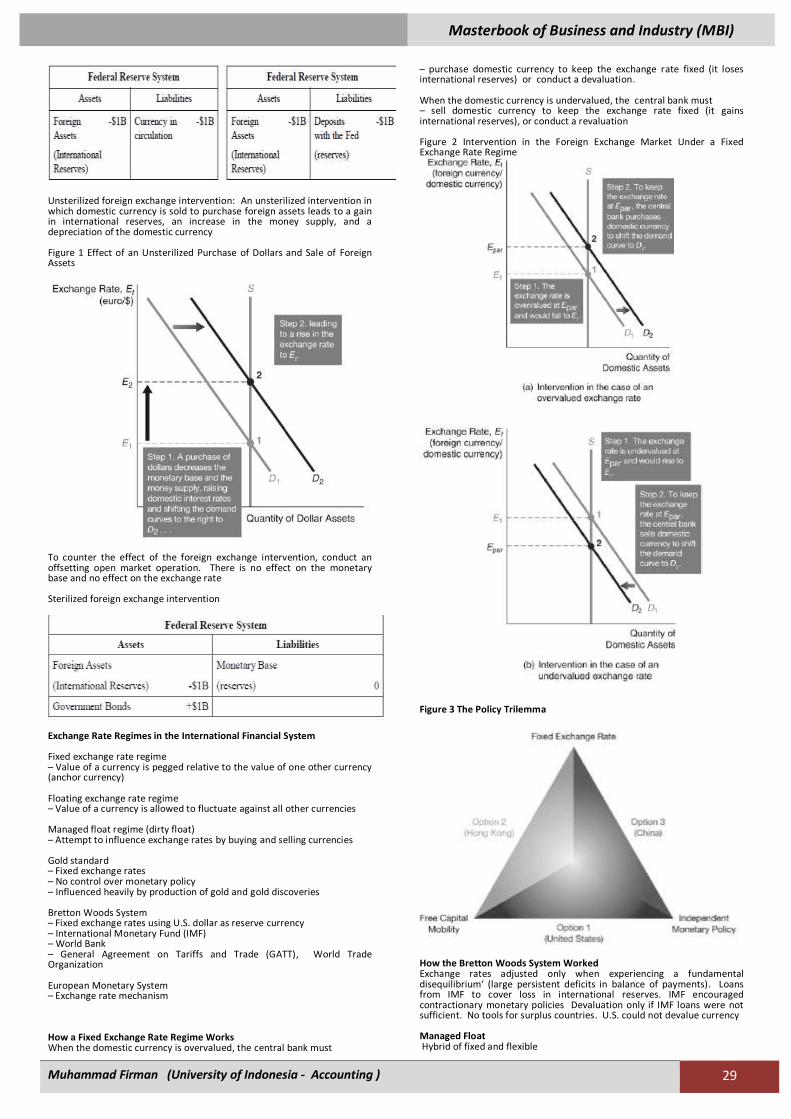
Masterbook of Business and Industry (MBI)
Muhammad Firman (University of Indonesia - Accounting ) 29
Unsterilized foreign exchange intervention: An unsterilized intervention in which domestic currency is sold to purchase foreign assets leads to a gain in international reserves, an increase in the money supply, and a depreciation of the domestic currency Figure 1 Effect of an Unsterilized Purchase of Dollars and Sale of Foreign Assets
To counter the effect of the foreign exchange intervention, conduct an offsetting open market operation. There is no effect on the monetary base and no effect on the exchange rate Sterilized foreign exchange intervention
Exchange Rate Regimes in the International Financial System Fixed exchange rate regime – Value of a currency is pegged relative to the value of one other currency (anchor currency) Floating exchange rate regime – Value of a currency is allowed to fluctuate against all other currencies Managed float regime (dirty float) – Attempt to influence exchange rates by buying and selling currencies Gold standard – Fixed exchange rates – No control over monetary policy – Influenced heavily by production of gold and gold discoveries Bretton Woods System – Fixed exchange rates using U.S. dollar as reserve currency – International Monetary Fund (IMF) – World Bank – General Agreement on Tariffs and Trade (GATT), World Trade Organization European Monetary System – Exchange rate mechanism How a Fixed Exchange Rate Regime Works When the domestic currency is overvalued, the central bank must
– purchase domestic currency to keep the exchange rate fixed (it loses international reserves) or conduct a devaluation. When the domestic currency is undervalued, the central bank must – sell domestic currency to keep the exchange rate fixed (it gains international reserves), or conduct a revaluation Figure 2 Intervention in the Foreign Exchange Market Under a Fixed Exchange Rate Regime
Figure 3 The Policy Trilemma
How the Bretton Woods System Worked Exchange rates adjusted only when experiencing a fundamental disequilibrium‘ (large persistent deficits in balance of payments). Loans from IMF to cover loss in international reserves. IMF encouraged contractionary monetary policies Devaluation only if IMF loans were not sufficient. No tools for surplus countries. U.S. could not devalue currency Managed Float Hybrid of fixed and flexible
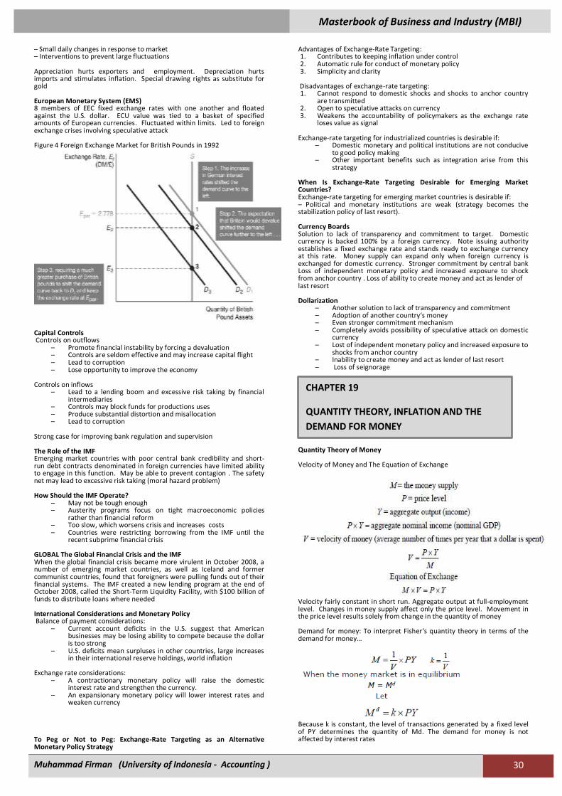
Masterbook of Business and Industry (MBI)
Muhammad Firman (University of Indonesia - Accounting ) 30
– Small daily changes in response to market – Interventions to prevent large fluctuations Appreciation hurts exporters and employment. Depreciation hurts imports and stimulates inflation. Special drawing rights as substitute for gold European Monetary System (EMS) 8 members of EEC fixed exchange rates with one another and floated against the U.S. dollar. ECU value was tied to a basket of specified amounts of European currencies. Fluctuated within limits. Led to foreign exchange crises involving speculative attack Figure 4 Foreign Exchange Market for British Pounds in 1992
Capital Controls Controls on outflows
– Promote financial instability by forcing a devaluation – Controls are seldom effective and may increase capital flight – Lead to corruption – Lose opportunity to improve the economy
Controls on inflows
– Lead to a lending boom and excessive risk taking by financial intermediaries
– Controls may block funds for productions uses – Produce substantial distortion and misallocation – Lead to corruption
Strong case for improving bank regulation and supervision The Role of the IMF Emerging market countries with poor central bank credibility and short-run debt contracts denominated in foreign currencies have limited ability to engage in this function. May be able to prevent contagion . The safety net may lead to excessive risk taking (moral hazard problem) How Should the IMF Operate?
– May not be tough enough – Austerity programs focus on tight macroeconomic policies
rather than financial reform – Too slow, which worsens crisis and increases costs – Countries were restricting borrowing from the IMF until the
recent subprime financial crisis GLOBAL The Global Financial Crisis and the IMF When the global financial crisis became more virulent in October 2008, a number of emerging market countries, as well as Iceland and former communist countries, found that foreigners were pulling funds out of their financial systems. The IMF created a new lending program at the end of October 2008, called the Short-Term Liquidity Facility, with $100 billion of funds to distribute loans where needed International Considerations and Monetary Policy Balance of payment considerations:
– Current account deficits in the U.S. suggest that American businesses may be losing ability to compete because the dollar is too strong
– U.S. deficits mean surpluses in other countries, large increases in their international reserve holdings, world inflation
Exchange rate considerations:
– A contractionary monetary policy will raise the domestic interest rate and strengthen the currency.
– An expansionary monetary policy will lower interest rates and weaken currency
To Peg or Not to Peg: Exchange-Rate Targeting as an Alternative Monetary Policy Strategy
Advantages of Exchange-Rate Targeting: 1. Contributes to keeping inflation under control 2. Automatic rule for conduct of monetary policy 3. Simplicity and clarity
Disadvantages of exchange-rate targeting: 1. Cannot respond to domestic shocks and shocks to anchor country
are transmitted 2. Open to speculative attacks on currency 3. Weakens the accountability of policymakers as the exchange rate
loses value as signal Exchange-rate targeting for industrialized countries is desirable if:
– Domestic monetary and political institutions are not conducive to good policy making
– Other important benefits such as integration arise from this strategy
When Is Exchange-Rate Targeting Desirable for Emerging Market Countries? Exchange-rate targeting for emerging market countries is desirable if: – Political and monetary institutions are weak (strategy becomes the stabilization policy of last resort). Currency Boards Solution to lack of transparency and commitment to target. Domestic currency is backed 100% by a foreign currency. Note issuing authority establishes a fixed exchange rate and stands ready to exchange currency at this rate. Money supply can expand only when foreign currency is exchanged for domestic currency. Stronger commitment by central bank Loss of independent monetary policy and increased exposure to shock from anchor country . Loss of ability to create money and act as lender of last resort Dollarization
– Another solution to lack of transparency and commitment – Adoption of another country‘s money – Even stronger commitment mechanism – Completely avoids possibility of speculative attack on domestic
currency – Lost of independent monetary policy and increased exposure to
shocks from anchor country – Inability to create money and act as lender of last resort – Loss of seignorage
Quantity Theory of Money Velocity of Money and The Equation of Exchange
Velocity fairly constant in short run. Aggregate output at full-employment level. Changes in money supply affect only the price level. Movement in the price level results solely from change in the quantity of money Demand for money: To interpret Fisher‘s quantity theory in terms of the demand for money…
Because k is constant, the level of transactions generated by a fixed level of PY determines the quantity of Md. The demand for money is not affected by interest rates
CHAPTER 19
QUANTITY THEORY, INFLATION AND THE
DEMAND FOR MONEY
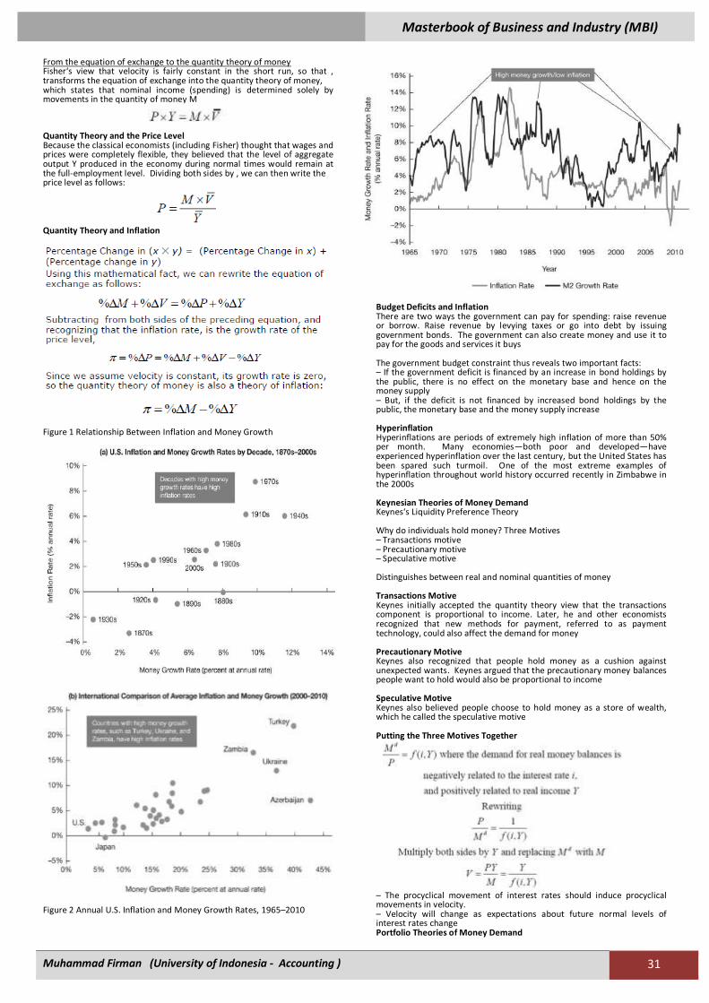
Masterbook of Business and Industry (MBI)
Muhammad Firman (University of Indonesia - Accounting ) 31
From the equation of exchange to the quantity theory of money Fisher‘s view that velocity is fairly constant in the short run, so that , transforms the equation of exchange into the quantity theory of money, which states that nominal income (spending) is determined solely by movements in the quantity of money M
Quantity Theory and the Price Level Because the classical economists (including Fisher) thought that wages and prices were completely flexible, they believed that the level of aggregate output Y produced in the economy during normal times would remain at the full-employment level. Dividing both sides by , we can then write the price level as follows:
Quantity Theory and Inflation
Figure 1 Relationship Between Inflation and Money Growth
Figure 2 Annual U.S. Inflation and Money Growth Rates, 1965–2010
Budget Deficits and Inflation There are two ways the government can pay for spending: raise revenue or borrow. Raise revenue by levying taxes or go into debt by issuing government bonds. The government can also create money and use it to pay for the goods and services it buys The government budget constraint thus reveals two important facts: – If the government deficit is financed by an increase in bond holdings by the public, there is no effect on the monetary base and hence on the money supply – But, if the deficit is not financed by increased bond holdings by the public, the monetary base and the money supply increase Hyperinflation Hyperinflations are periods of extremely high inflation of more than 50% per month. Many economies—both poor and developed—have experienced hyperinflation over the last century, but the United States has been spared such turmoil. One of the most extreme examples of hyperinflation throughout world history occurred recently in Zimbabwe in the 2000s Keynesian Theories of Money Demand Keynes‘s Liquidity Preference Theory Why do individuals hold money? Three Motives – Transactions motive – Precautionary motive – Speculative motive Distinguishes between real and nominal quantities of money Transactions Motive Keynes initially accepted the quantity theory view that the transactions component is proportional to income. Later, he and other economists recognized that new methods for payment, referred to as payment technology, could also affect the demand for money Precautionary Motive Keynes also recognized that people hold money as a cushion against unexpected wants. Keynes argued that the precautionary money balances people want to hold would also be proportional to income Speculative Motive Keynes also believed people choose to hold money as a store of wealth, which he called the speculative motive Putting the Three Motives Together
– The procyclical movement of interest rates should induce procyclical movements in velocity. – Velocity will change as expectations about future normal levels of interest rates change Portfolio Theories of Money Demand

Masterbook of Business and Industry (MBI)
Muhammad Firman (University of Indonesia - Accounting ) 32
Theory of Portfolio Choice and Keynesian Liquidity Preference. The theory of portfolio choice can justify the conclusion from the Keynesian liquidity preference function that the demand for real money balances is positively related to income and negatively related to the nominal interest rate. Other Factors That Affect the Demand for Money: Wealth, Risk, – Liquidity of other assets Empirical Evidence on the Demand for Money Summary Table 1 Factors That Determine the Demand for Money
Precautionary Demand Similar to transactions demand. As interest rates rise, the opportunity cost of holding precautionary balances rises . The precautionary demand for money is negatively related to interest rates Interest Rates and Money Demand We have established that if interest rates do not affect the demand for money, velocity is more likely to be constant—or at least predictable—so that the quantity theory view that aggregate spending is determined by the quantity of money is more likely to be true. However, the more sensitive the demand for money is to interest rates, the more unpredictable velocity will be, and the less clear the link between the money supply and aggregate spending will be Stability of Money Demand If the money demand function is unstable and undergoes substantial, unpredictable shifts as Keynes believed, then velocity is unpredictable, and the quantity of money may not be tightly linked to aggregate spending, as it is in the quantity theory. The stability of the money demand function is also crucial to whether the Federal Reserve should target interest rates or the money supply. If the money demand function is unstable and so the money supply is not closely linked to aggregate spending, then the level of interest rates the Fed sets will provide more information about the stance of monetary policy than will the money supply
Planned Expenditure and Aggregate Demand Planned expenditure is the total amount of spending on domestically produced goods and services that households, businesses, the government, and foreigners want to make. Aggregate demand is the total amount of output demanded in the economy The total quantity demanded of an economy‘s output is the sum of 4 types of spending: Consumption expenditure (C), Planned investment spending (I ), Government purchases (G ), Net exports (NX ) Consumption Expenditure and the Consumption Function
Planned Investment Spending Fixed investment: always planned
Inventory investment: can be unplanned Planned investment spending – Interest rates – Expectations Net Exports Made up of two components: autonomous net exports and the part of net exports that is affected by changes in real interest rates Net export function:
Government Purchases and Taxes The government affects aggregate demand in two ways: through its purchases and taxes Government purchases:
Government taxes:
Goods Market Equilibrium Keynes recognized that equilibrium would occur in the economy when the total quantity of output produced in the economy equals the total amount of aggregate demand (planned expenditure) . Solving for goods market equilibrium: Aggregate Output = Consumption Expenditure + Planned Investment Spending + Government Purchases + Net Exports Understanding the IS Curve What the IS curve tells us: traces out the points at which the goods market is in equilibrium . Examines an equilibrium where aggregate output equals aggregate demand. Assumes fixed price level where nominal and real quantities are the same . IS curve is the relationship between equilibrium aggregate output and the interest rate Figure 1 The IS Curve
Why the Economy Heads Toward the Equilibrium Interest rates and planned investment spending – Negative relationship Interest rates and net exports – Negative relationship IS curve: the points at which the total quantity of goods produced equals the total quantity of goods demanded. Output tends to move toward points on the curve that satisfies the goods market equilibrium Factors that Shift the IS Curve The IS curve shifts whenever there is a change in autonomous factors (factors independent of aggregate output and the real interest rate. One example is changes in government purchases, as in Figure 2 Figure 2 Shift in the IS Curve from an Increase in Government Purchases
CHAPTER 20
THE IS CURVE
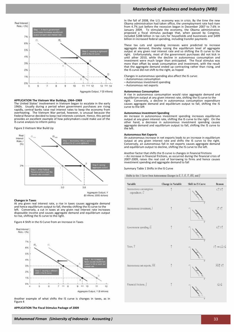
Masterbook of Business and Industry (MBI)
Muhammad Firman (University of Indonesia - Accounting ) 33
APPLICATION The Vietnam War Buildup, 1964–1969 The United States‘ involvement in Vietnam began to escalate in the early 1960s. Usually during a period when government purchases are rising rapidly, central banks raise real interest rates to keep the economy from overheating. The Vietnam War period, however, is unusual because the Federal Reserve decided to keep real interests constant. Hence, this period provides an excellent example of how policymakers could make use of the IS curve analysis to inform policy Figure 3 Vietnam War Build Up
Changes in Taxes At any given real interest rate, a rise in taxes causes aggregate demand and hence equilibrium output to fall, thereby shifting the IS curve to the left. Conversely, a cut in taxes at any given real interest rate increases disposable income and causes aggregate demand and equilibrium output to rise, shifting the IS curve to the right. Figure 4 Shift in the IS Curve from an Increase in Taxes
Another example of what shifts the IS curve is changes in taxes, as in Figure 4 APPLICATION The Fiscal Stimulus Package of 2009
In the fall of 2008, the U.S. economy was in crisis. By the time the new Obama administration had taken office, the unemployment rate had risen from 4.7% just before the recession began in December 2007 to 7.6% in January 2009. To stimulate the economy, the Obama administration proposed a fiscal stimulus package that, when passed by Congress, included $288 billion in tax cuts for households and businesses and $499 billion in increased federal spending, including transfer payments These tax cuts and spending increases were predicted to increase aggregate demand, thereby raising the equilibrium level of aggregate output at any given real interest rate and so shifting the IS curve to the right. Unfortunately, most of the government purchases did not kick in until ather 2010, while the decline in autonomous consumption and investment were much larger than anticipated. The fiscal stimulus was more than offset by weak consumption and investment, with the result that the aggregate demand ended up contracting rather than rising, and the IS curve did not shift to the right, as hoped Changes in autonomous spending also affect the IS curve: – Autonomous consumption – Autonomous investment spending – Autonomous net exports Autonomous Consumption A rise in autonomous consumption would raise aggregate demand and equilibrium output at any given interest rate, shifting the IS curve to the right. Conversely, a decline in autonomous consumption expenditure causes aggregate demand and equilibrium output to fall, shifting the IS curve to the left Autonomous Investment Spending An increase in autonomous investment spending increases equilibrium output at any given interest rate, shifting the IS curve to the right. On the other hand, a decrease in autonomous investment spending causes aggregate demand and equilibrium output to fall, shifting the IS curve to the left. Autonomous Net Exports An autonomous increase in net exports leads to an increase in equilibrium output at any given interest rate and shifts the IS curve to the right. Conversely, an autonomous fall in net exports causes aggregate demand and equilibrium output to decline, shifting the IS curve to the left. Another factor that shifts the IS curve is changes in financial frictions – An increase in financial frictions, as occurred during the financial crisis of 2007-2009, raises the real cost of borrowing to firms and hence causes investment spending and aggregate demand to fall Summary Table 1 Shifts in the IS Curve
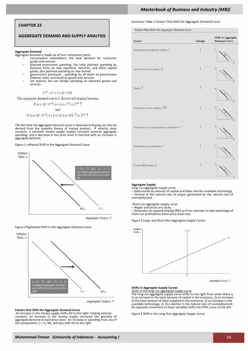
Masterbook of Business and Industry (MBI)
Muhammad Firman (University of Indonesia - Accounting ) 34
Aggregate Demand Aggregate demand is made up of four component parts:
– consumption expenditure, the total demand for consumer goods and services
– planned investment spending, the total planned spending by business firms on new machines, factories, and other capital goods, plus planned spending on new homes
– government purchases , spending by all levels of government (federal, state, and local) on goods and services
– net exports, the net foreign spending on domestic goods and services
The fact that the aggregate demand curve is downward sloping can also be derived from the quantity theory of money analysis. If velocity stays constant, a constant money supply implies constant nominal aggregate spending, and a decrease in the price level is matched with an increase in aggregate demand. Figure 1 Leftward Shift in the Aggregate Demand Curve
Figure 2 Rightward Shift in the Aggregate Demand Curve
Factors that Shift the Aggregate Demand Curve An increase in the money supply shifts AD to the right: holding velocity constant, an increase in the money supply increases the quantity of aggregate demand at each price level. An increase in spending from any of the components C, I, G, NX, will also shift AD to the right
Summary Table 1 Factors That Shift the Aggregate Demand Curve
Aggregate Supply Long-run aggregate supply curve – Determined by amount of capital and labor and the available technology – Vertical at the natural rate of output generated by the natural rate of unemployment Short-run aggregate supply curve – Wages and prices are sticky – Generates an upward sloping SRAS as firms attempt to take advantage of short-run profitability when price level rises Figure 3 Long- and Short-Run Aggregate Supply Curves
Shifts in Aggregate Supply Curves Shifts in the long run aggregate supply curve The long-run aggregate supply curve shifts to the right from when there is 1) an increase in the total amount of capital in the economy, 2) an increase in the total amount of labor supplied in the economy, 3) an increase in the available technology, or 4) a decline in the natural rate of unemployment. An opposite movement in these variables shifts the LRAS curve to the left Figure 4 Shift in the Long-Run Aggregate Supply Curve
CHAPTER 22
AGGREGATE DEMAND AND SUPPLY ANALYSIS
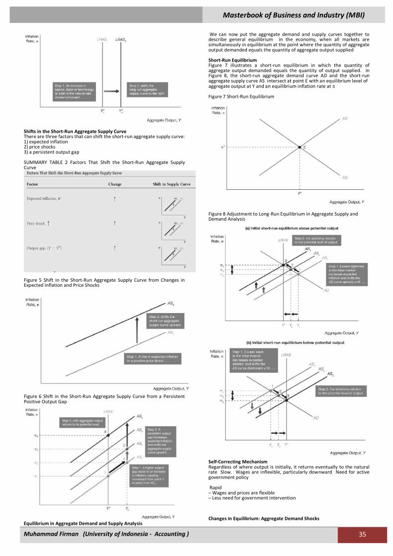
Masterbook of Business and Industry (MBI)
Muhammad Firman (University of Indonesia - Accounting ) 35
Shifts in the Short-Run Aggregate Supply Curve There are three factors that can shift the short-run aggregate supply curve: 1) expected inflation 2) price shocks 3) a persistent output gap SUMMARY TABLE 2 Factors That Shift the Short-Run Aggregate Supply Curve
Figure 5 Shift in the Short-Run Aggregate Supply Curve from Changes in Expected Inflation and Price Shocks
Figure 6 Shift in the Short-Run Aggregate Supply Curve from a Persistent Positive Output Gap
Equilibrium in Aggregate Demand and Supply Analysis
We can now put the aggregate demand and supply curves together to describe general equilibrium in the economy, when all markets are simultaneously in equilibrium at the point where the quantity of aggregate output demanded equals the quantity of aggregate output supplied Short-Run Equilibrium Figure 7 illustrates a short-run equilibrium in which the quantity of aggregate output demanded equals the quantity of output supplied. In Figure 8, the short-run aggregate demand curve AD and the short-run aggregate supply curve AS intersect at point E with an equilibrium level of aggregate output at Y and an equilibrium inflation rate at Figure 7 Short-Run Equilibrium
Figure 8 Adjustment to Long-Run Equilibrium in Aggregate Supply and Demand Analysis
Self-Correcting Mechanism Regardless of where output is initially, it returns eventually to the natural rate Slow. Wages are inflexible, particularly downward Need for active government policy Rapid – Wages and prices are flexible – Less need for government intervention Changes in Equilibrium: Aggregate Demand Shocks

Masterbook of Business and Industry (MBI)
Muhammad Firman (University of Indonesia - Accounting ) 36
With an understanding of the distinction between the short-run and long-run equilibria, you are now ready to analyze what happens when there are demand shocks, shocks that cause the aggregate demand curve to shift Figure 9 Positive Demand Shock
Figure 10 The Volcker Disinflation
Figure 11 Negative Demand Shocks, 2001–2004
Changes in Equilibrium: Aggregate Supply (Price) Shocks The aggregate supply curve can shift from temporary supply (price) shocks in which the longrun aggregate supply curve does not shift, or from permanent supply shocks in which the long-run aggregate supply curve does shift Temporary Supply Shocks: – When the temporary shock involves a restriction in supply, we refer to this type of supply shock as a negative (or unfavorable) supply shock, and it results in a rise in commodity prices – A temporary positive supply shock shifts the short-run aggregate supply curve downward and to the right, leading initially to a fall in inflation and a rise in output. In the long run, however, output and inflation will be unchanged (holding the aggregate demand curve constant) Figure 12 Temporary Negative Supply Shock
Figure 13 Negative Supply Shocks, 1973–1975 and 1978–1980
Permanent Supply Shocks and Real Business Cycle Theory A permanent negative supply shock—such as an increase in ill advised regulations that causes the economy to be less efficient, thereby reducing supply—would decrease potential output and shift the long-run aggregate supply curve to the left Because the permanent supply shock will result in higher prices, there will be an immediate rise in inflation and so the short-run aggregate supply curve will shift up and to the left. One group of economists, led by Edward Prescott of Arizona State University, believe

Masterbook of Business and Industry (MBI)
Muhammad Firman (University of Indonesia - Accounting ) 37
that business cycle fluctuations result from permanent supply shocks alone and their theory of aggregate economic fluctuations is called real business cycle theory Figure 14 Permanent Negative Supply Shock
Figure 15 Positive Supply Shocks, 1995–1999
Conclusions Aggregate demand and supply analysis yields the following conclusions: 1. A shift in the aggregate demand curve affects output only in the short run and has no effect in the long run 2. A temporary supply shock affects output and inflation only in the short run and has no effect in the long run (holding the aggregate demand curve constant) 3. A permanent supply shock affects output and inflation both in the short and the long run 4. The economy has a self-correcting mechanism that returns it to potential output and the natural rate of unemployment over time Figure 16 Negative Supply and Demand Shocks and the 2007–2009
AD/AS Analysis of Foreign Business Cycle Episodes Our aggregate demand and supply analysis also can help us understand business cycle episodes in foreign countries – Figure 17 shows the UK Financial Crisis, 2007– 2009 – Figure 18 shows China and the Financial Crisis, 2007–2009 Figure 17 UK Financial Crisis, 2007–2009
Figure 18 China and the Financial Crisis, 2007–2009

Masterbook of Business and Industry (MBI)
Muhammad Firman (University of Indonesia - Accounting ) 38
Appendix to Chapter 22: The Phillips Curve and the Short-Run Aggregate Supply Curve The Phillips Curve: the negative relationship between unemployment and inflation. The idea behind the Phillips curve is intuitive. When labor markets are tight—that is, the unemployment rate is low—firms may have difficulty hiring qualified workers and may even have a hard time keeping their present employees. Because of the shortage of workers in the labor market, firms willraise wages to attract needed workers and raise their prices at a more rapid rate Figure 1 Inflation and Unemployment in the United States, 1950–1969 and 1970–2010
Figure 2 The Short- and Long- Run Phillips Curve
Three Important Conclusions 1. There is no long-run trade-off between unemployment and inflation 2. There is a short-run trade-off between unemployment and inflation 3. There are two types of Phillips curves, long run and short run The Short-Run Aggregate Supply Curve o complete our aggregate demand and supply model, we need to use our analysis of the Phillips curve to derive a short-run aggregate supply curve,
which represents the relationship between the total quantity of output that firms are willing to produce and the inflation rate. We can translate the modern Phillips curve into a short-run aggregate supply curve by replacing the unemployment gap (U – Un) with the output gap, the difference between output and potential output (Y – YP) Okun’s Law Okun‘s law describes the negative relationship between the unemployment gap and the output gap. Okun‘s law states that for each percentage point that output is above potential, the unemployment rate is one-half of a percentage point below the natural rate of unemployment. Alternatively, for every percentage point that unemployment is above its natural rate, output is two percentage points below potential output Figure 3 Okun’s Law, 1960–2010
Response of Monetary Policy to Shocks Monetary policy should try to minimize the difference between inflation and the inflation target . In the case of both demand shocks and permanent supply shocks, policy makers can simultaneously pursue price stability and stability in economic activity Following a temporary supply shock, however, policy makers can achieve either price stability or economic activity stability, but not both. This tradeoff poses a dilemma for central banks with dual mandates Response to an Aggregate Demand Shock Policy makers can respond to this shock in two possible ways: – No policy response – Policy stabilizes economic activity and inflation in the short run In the case of aggregate demand shocks, there is no tradeoff between the pursuit of price stability and economic activity stability Figure 1 Aggregate Demand Shock: No Policy Response
Figure 2 Aggregate Demand Shock: Policy Stabilizes Output and Inflation
CHAPTER 23
MONETARY POLICY THEORY
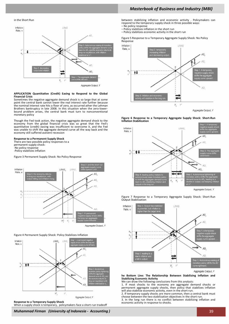
Masterbook of Business and Industry (MBI)
Muhammad Firman (University of Indonesia - Accounting ) 39
in the Short Run
APPLICATION Quantitative (Credit) Easing to Respond to the Global Financial Crisis Sometimes the negative aggregate demand shock is so large that at some point the central bank cannot lower the real interest rate further because the nominal interest rate hits a floor of zero, as occurred ather the Lehman Brothers bankruptcy in late 2008. In this situation when the zero-lower-bound problem arises, the central bank must turn to nonconventional monetary policy Though the Fed took action, the negative aggregate demand shock to the economy from the global financial crisis was so great that the Fed‘s quantitative (credit) easing was insufficient to overcome it, and the Fed was unable to shift the aggregate demand curve all the way back and the economy still suffered asevere recession Response to a Permanent Supply Shock There are two possible policy responses to a permanent supply shock: -No policy response -Policy stabilizes inflation Figure 3 Permanent Supply Shock: No Policy Response
Figure 4 Permanent Supply Shock: Policy Stabilizes Inflation
Response to a Temporary Supply Shock When a supply shock is temporary, policymakers face a short-run tradeoff
between stabilizing inflation and economic activity . Policymakers can respond to the temporary supply shock in three possible ways: – No policy response – Policy stabilizes inflation in the short run – Policy stabilizes economic activity in the short run Figure 5 Response to a Temporary Aggregate Supply Shock: No Policy Response
Figure 6 Response to a Temporary Aggregate Supply Shock: Short-Run Inflation Stabilization
Figure 7 Response to a Temporary Aggregate Supply Shock: Short-Run Output Stabilization
he Bottom Line: The Relationship Between Stabilizing Inflation and Stabilizing Economic Activity We can draw the following conclusions from this analysis: 1. If most shocks to the economy are aggregate demand shocks or permanent aggregate supply shocks, then policy that stabilizes inflation will also stabilize economic activity, even in the short run. 2. If temporary supply shocks are more common, then a central bank must choose between the two stabilization objectives in the short run. 3. In the long run there is no conflict between stabilizing inflation and economic activity in response to shocks.

Masterbook of Business and Industry (MBI)
Muhammad Firman (University of Indonesia - Accounting ) 40
How Actively Should Policy Makers Try to Stabilize Economic Activity? All economists have similar policy goals (to promote high employment and price stability), yet they othen disagree on the best approach to achieve those goals. Nonactivists believe government action is unnecessary to eliminate unemployment . Activists see the need for the government to pursue active policy to eliminate high unemployment when it develops Lags and Policy Implementation Several types of lags prevent policymakers from shifting the aggregate demand curveinstantaneously
– Data lag: the time it takes for policy makers to obtain data indicating what is happening in the economy
– Recognition lag: the time it takes for policy makers to be sure of what the data are signaling about the future course of the economy
– Legislative lag: the time it takes to pass legislation to implement a particular policy
– Implementation lag: the time it takes for policy makers to change policy instruments once they have decided on the new policy
– Effectiveness lag: the time it takes for the policy actually to have an impact on the economy
FYI The Activist/Nonactivist Debate Over the Obama Fiscal Stimulus Package Many activists argued that the government needed to do more by implementing a massive fiscal stimulus package On the other hand, nonactivists opposed the fiscal stimulus package, arguing that fiscal stimulus would take too long to work because of long implementation lags. The Obama administration came down squarely on the side of the activists and proposed the American Recovery and Reinvestment Act of 2009, a $787 billion fiscal stimulus package that Congress passed on February 13, 2009 Inflation: Always and Everywhere a Monetary Phenomenon This adage is supported by our aggregate demand and supply analysis because it shows that monetary policy makers can target any inflation rate in the long run by shifting the aggregate demand curve with autonomous monetary policy Figure 8 A Rise in the Inflation
Causes of Inflationary Monetary Policy High Employment Targets and Inflation – Cost-push inflation results either from a temporary negative supply shock or a push by workers for wage hikes beyond what productivity gains can justify – Demand-pull inflation results from policy makers pursuing policies that increase aggregate demand Figure 9 Cost-Push Inflation
Figure 10 Demand-Pull Inflation
APPLICATION The Great Inflation Now that we have examined the roots of inflationary monetary policy, we can investigate the causes of the rise in U.S. inflation from 1965 to 1982, a period dubbed the Great Inflation. Panel (a) of Figure 11 documents the rise in inflation during those years. Just before the Great Inflation started, the inflation rate was below 2% at an annual rate; by the late 1970s, it averaged around 8% and peaked at nearly 14% in 1980 ather the oil price shock in 1979. Panel (b) of Figure 11 compares the actual unemployment rate to estimates of the natural rate of unemployment Figure 11 Inflation and Unemployment, 1965-1982
Macro-econometric models—collections of equations that describe statistical relationships among economic variables are used by economists to forecast economic activity and to evaluate the potential effects of policy options. In his famous paper ‖Econometric Policy Evaluation: A Critique,‖ Robert Lucas argued that econometric models are unreliable for evaluation policy options if they do not incorporate rational expectations. According to Lucas, when policies change, public expectations will shift as well, and such changing expectations (as ignored by conventional econometric models) can have a real effect oneconomic behavior and outcomes APPLICATION The Term Structure of Interest Rates
CHAPTER 24
THE ROLE OF EXPECTATIONS IN MONETARY
POLICY
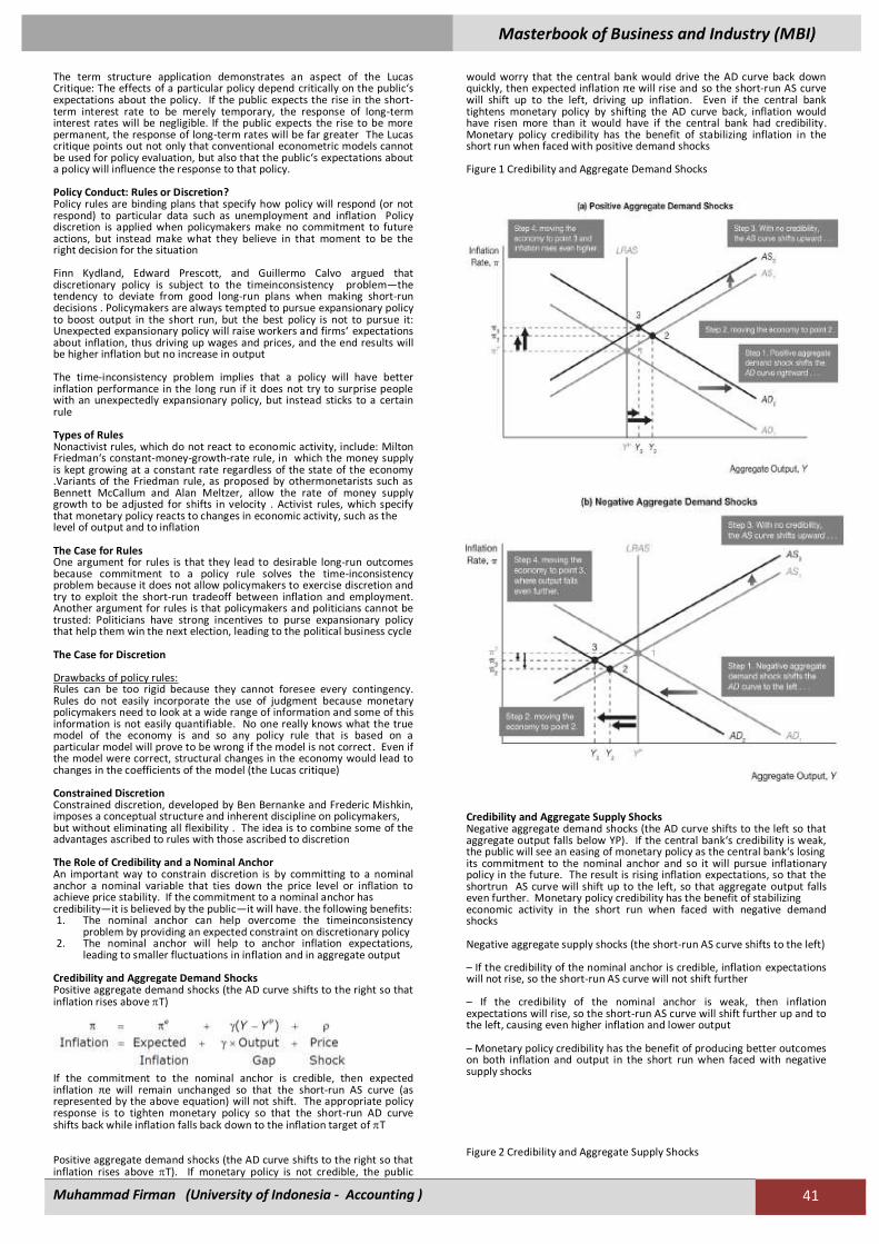
Masterbook of Business and Industry (MBI)
Muhammad Firman (University of Indonesia - Accounting ) 41
The term structure application demonstrates an aspect of the Lucas Critique: The effects of a particular policy depend critically on the public‘s expectations about the policy. If the public expects the rise in the short-term interest rate to be merely temporary, the response of long-term interest rates will be negligible. If the public expects the rise to be more permanent, the response of long-term rates will be far greater The Lucas critique points out not only that conventional econometric models cannot be used for policy evaluation, but also that the public‘s expectations about a policy will influence the response to that policy. Policy Conduct: Rules or Discretion? Policy rules are binding plans that specify how policy will respond (or not respond) to particular data such as unemployment and inflation Policy discretion is applied when policymakers make no commitment to future actions, but instead make what they believe in that moment to be the right decision for the situation Finn Kydland, Edward Prescott, and Guillermo Calvo argued that discretionary policy is subject to the timeinconsistency problem—the tendency to deviate from good long-run plans when making short-run decisions . Policymakers are always tempted to pursue expansionary policy to boost output in the short run, but the best policy is not to pursue it: Unexpected expansionary policy will raise workers and firms‘ expectations about inflation, thus driving up wages and prices, and the end results will be higher inflation but no increase in output The time-inconsistency problem implies that a policy will have better inflation performance in the long run if it does not try to surprise people with an unexpectedly expansionary policy, but instead sticks to a certain rule Types of Rules Nonactivist rules, which do not react to economic activity, include: Milton Friedman‘s constant-money-growth-rate rule, in which the money supply is kept growing at a constant rate regardless of the state of the economy .Variants of the Friedman rule, as proposed by othermonetarists such as Bennett McCallum and Alan Meltzer, allow the rate of money supply growth to be adjusted for shifts in velocity . Activist rules, which specify that monetary policy reacts to changes in economic activity, such as the level of output and to inflation The Case for Rules One argument for rules is that they lead to desirable long-run outcomes because commitment to a policy rule solves the time-inconsistency problem because it does not allow policymakers to exercise discretion and try to exploit the short-run tradeoff between inflation and employment. Another argument for rules is that policymakers and politicians cannot be trusted: Politicians have strong incentives to purse expansionary policy that help them win the next election, leading to the political business cycle The Case for Discretion Drawbacks of policy rules: Rules can be too rigid because they cannot foresee every contingency. Rules do not easily incorporate the use of judgment because monetary policymakers need to look at a wide range of information and some of this information is not easily quantifiable. No one really knows what the true model of the economy is and so any policy rule that is based on a particular model will prove to be wrong if the model is not correct. Even if the model were correct, structural changes in the economy would lead to changes in the coefficients of the model (the Lucas critique) Constrained Discretion Constrained discretion, developed by Ben Bernanke and Frederic Mishkin, imposes a conceptual structure and inherent discipline on policymakers, but without eliminating all flexibility . The idea is to combine some of the advantages ascribed to rules with those ascribed to discretion The Role of Credibility and a Nominal Anchor An important way to constrain discretion is by committing to a nominal anchor a nominal variable that ties down the price level or inflation to achieve price stability. If the commitment to a nominal anchor has credibility—it is believed by the public—it will have. the following benefits: 1. The nominal anchor can help overcome the timeinconsistency
problem by providing an expected constraint on discretionary policy 2. The nominal anchor will help to anchor inflation expectations,
leading to smaller fluctuations in inflation and in aggregate output Credibility and Aggregate Demand Shocks Positive aggregate demand shocks (the AD curve shifts to the right so that inflation rises above T)
If the commitment to the nominal anchor is credible, then expected inflation πe will remain unchanged so that the short-run AS curve (as represented by the above equation) will not shift. The appropriate policy response is to tighten monetary policy so that the short-run AD curve shifts back while inflation falls back down to the inflation target of T Positive aggregate demand shocks (the AD curve shifts to the right so that inflation rises above T). If monetary policy is not credible, the public
would worry that the central bank would drive the AD curve back down quickly, then expected inflation πe will rise and so the short-run AS curve will shift up to the left, driving up inflation. Even if the central bank tightens monetary policy by shifting the AD curve back, inflation would have risen more than it would have if the central bank had credibility. Monetary policy credibility has the benefit of stabilizing inflation in the short run when faced with positive demand shocks Figure 1 Credibility and Aggregate Demand Shocks
Credibility and Aggregate Supply Shocks Negative aggregate demand shocks (the AD curve shifts to the left so that aggregate output falls below YP). If the central bank‘s credibility is weak, the public will see an easing of monetary policy as the central bank‘s losing its commitment to the nominal anchor and so it will pursue inflationary policy in the future. The result is rising inflation expectations, so that the shortrun AS curve will shift up to the left, so that aggregate output falls even further. Monetary policy credibility has the benefit of stabilizing economic activity in the short run when faced with negative demand shocks Negative aggregate supply shocks (the short-run AS curve shifts to the left) – If the credibility of the nominal anchor is credible, inflation expectations will not rise, so the short-run AS curve will not shift further – If the credibility of the nominal anchor is weak, then inflation expectations will rise, so the short-run AS curve will shift further up and to the left, causing even higher inflation and lower output – Monetary policy credibility has the benefit of producing better outcomes on both inflation and output in the short run when faced with negative supply shocks Figure 2 Credibility and Aggregate Supply Shocks

Masterbook of Business and Industry (MBI)
Muhammad Firman (University of Indonesia - Accounting ) 42
APPLICATION A Tale of Three Oil Price Shocks In 1973, 1979, and 2007, the U.S. economy was hit by three major negative supply shocks when theprice of oil rose sharply; and yet in the first two episodes inflation rose sharply, while in the most recent episode it rose much less. We can see this in Figure 3 Figure 3 Inflation and Unemployment 1970–2010
Credibility and Anti-Inflation Policy The greater is the credibility of the central bank as an inflation fighter, the more rapid will be the decline in inflation and the lower will be the loss of output to achieve the inflation objective If the central bank has very little credibility, then the public will not be convinced that the central bank will stay the course to reduce inflation and they will not revise their inflation expectations Figure 4 Credibility and Anti- Inflation Policy
APPLICATION Credibility and the Reagan Budget Deficits The Reagan administration was strongly criticized for creating huge budget deficits by cutting taxes in the early 1980s. Although many economists agree that the Fed‘s anti-inflation program lacked credibility, not all agree that the Reagan budget deficits were the cause of that lack of credibility. The conclusion that the Reagan budget deficits helped create a more severe recession in 1981– 1982 is controversial Approaches to Establishing Central Bank Credibility Inflation Targeting, Strategy that involves:
– public announcement of medium-term numerical targets for inflation
– an institutional commitment to price stability as the primary, long-run goal of monetary policy
– an information-inclusive approach in which policymakers use many variables in making decisions about monetary policy
– increased transparency of the monetary policy strategy through communication with the public and the markets
– increased accountability of the central bank for attaining its inflation objectives
– Adopted by many countries, beginning with New Zealand, Australia, Canada and the United Kingdom
Appoint “Conservative” Central Bankers Kenneth Rogoff of Harvard University suggested that another way to establish policy credibility is for the government to appoint central bankers who have a strong aversion to inflation. The public will then expected that the conservative‖ central banker will be less tempted to pursue expansionary monetary policy and will try to keep inflation under control The problem with this approach is that it is not clear what it will work over time Inside the Fed: The Appointment of Paul Volcker, Anti-Inflation Hawk Paul Volcker is known as an inflation hawk and thus his appointment as the chairman of the Fed in October 1979 is good example of the appointment of a ―conservative‖ central banker Shortly ather he took the helm of the Fed, the federal funds rate rose by 8 percentage points to nearly 20% by April 1980. Despite the unemployment rate rose to nearly 10% in 1982, the federal funds rate remained at around 15% until the inflation rate began to fall in July 1982
Examines whether one variable affects another by using data to build a model that explains the channels through which the variable affects the other. Transmission mechanism – The change in the money supply affects interest rates – Interest rates affect investment spending – Investment spending is a component of aggregate spending (output) Traditional Interest-Rate Channels An important feature of the interest-rate transmission mechanism is its emphasis on the real (rather than the nominal) interest rate as the rate that affects consumer and business decisions. In addition, it is othen the real long-term interest rate (not the real short-term interest rate) that is viewed as having the major impact on spending Other Asset Price Channels In addition to bond prices, two other asset prices receive substantial attention as channels for monetary policy effects: -foreign exchange rates -the prices of equities (stocks)
CHAPTER 25
TRANSMISSIONS MECHANISMS OF
MONETARY POLICY
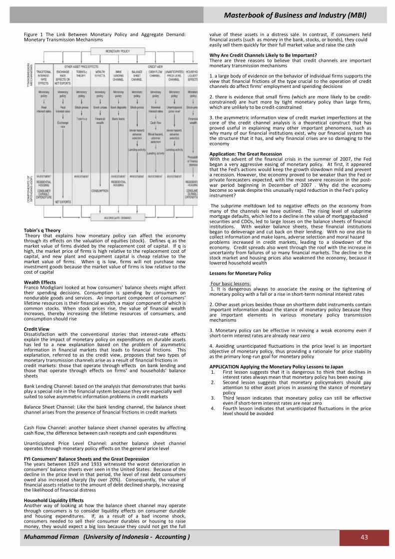
Masterbook of Business and Industry (MBI)
Muhammad Firman (University of Indonesia - Accounting ) 43
Figure 1 The Link Between Monetary Policy and Aggregate Demand: Monetary Transmission Mechanisms
Tobin’s q Theory Theory that explains how monetary policy can affect the economy through its effects on the valuation of equities (stock). Defines q as the market value of firms divided by the replacement cost of capital. If q is high, the market price of firms is high relative to the replacement cost of capital, and new plant and equipment capital is cheap relative to the market value of firms. When q is low, firms will not purchase new investment goods because the market value of firms is low relative to the cost of capital Wealth Effects Franco Modigliani looked at how consumers‘ balance sheets might affect their spending decisions. Consumption is spending by consumers on nondurable goods and services. An important component of consumers‘ lifetime resources is their financial wealth, a major component of which is common stocks. When stock prices rise, the value of financial wealth increases, thereby increasing the lifetime resources of consumers, and consumption should rise Credit View Dissatisfaction with the conventional stories that interest-rate effects explain the impact of monetary policy on expenditures on durable assets has led to a new explanation based on the problem of asymmetric information in financial markets that leads to financial frictions. This explanation, referred to as the credit view, proposes that two types of monetary transmission channels arise as a result of financial frictions in credit markets: those that operate through effects on bank lending and those that operate through effects on firms‘ and households‘ balance sheets Bank Lending Channel: based on the analysis that demonstrates that banks play a special role in the financial system because they are especially well suited to solve asymmetric information problems in credit markets Balance Sheet Channel: Like the bank lending channel, the balance sheet channel arises from the presence of financial frictions in credit markets Cash Flow Channel: another balance sheet channel operates by affecting cash flow, the difference between cash receipts and cash expenditures Unanticipated Price Level Channel: another balance sheet channel operates through monetary policy effects on the general price level FYI Consumers’ Balance Sheets and the Great Depression The years between 1929 and 1933 witnessed the worst deterioration in consumers‘ balance sheets ever seen in the United States. Because of the decline in the price level in that period, the level of real debt consumers owed also increased sharply (by over 20%). Consequently, the value of financial assets relative to the amount of debt declined sharply, increasing the likelihood of financial distress Household Liquidity Effects Another way of looking at how the balance sheet channel may operate through consumers is to consider liquidity effects on consumer durable and housing expenditures. If, as a result of a bad income shock, consumers needed to sell their consumer durables or housing to raise money, they would expect a big loss because they could not get the full
value of these assets in a distress sale. In contrast, if consumers held financial assets (such as money in the bank, stocks, or bonds), they could easily sell them quickly for their full market value and raise the cash Why Are Credit Channels Likely to Be Important? There are three reasons to believe that credit channels are important monetary transmission mechanisms 1. a large body of evidence on the behavior of individual firms supports the view that financial frictions of the type crucial to the operation of credit channels do affect firms‘ employment and spending decisions 2. there is evidence that small firms (which are more likely to be credit-constrained) are hurt more by tight monetary policy than large firms, which are unlikely to be credit-constrained 3. the asymmetric information view of credit market imperfections at the core of the credit channel analysis is a theoretical construct that has proved useful in explaining many other important phenomena, such as why many of our financial institutions exist, why our financial system has the structure that it has, and why financial crises are so damaging to the economy Application: The Great Recession With the advent of the financial crisis in the summer of 2007, the Fed began a very aggressive easing of monetary policy. At first, it appeared that the Fed‘s actions would keep the growth slowdown mild and prevent a recession. However, the economy proved to be weaker than the Fed or private forecasters expected, with the most severe recession in the post-war period beginning in December of 2007 . Why did the economy become so weak despite this unusually rapid reduction in the Fed‘s policy instrument? The subprime meltdown led to negative effects on the economy from many of the channels we have outlined. The rising level of subprime mortgage defaults, which led to a decline in the value of mortgagebacked securities and CDOs, led to large losses on the balance sheets of financial institutions. With weaker balance sheets, these financial institutions began to deleverage and cut back on their lending. With no one else to collect information and make loans, adverse selection and moral hazard problems increased in credit markets, leading to a slowdown of the economy. Credit spreads also went through the roof with the increase in uncertainty from failures of so many financial markets. The decline in the stock market and housing prices also weakened the economy, because it lowered household wealth Lessons for Monetary Policy Four basic lessons: 1. It is dangerous always to associate the easing or the tightening of monetary policy with a fall or a rise in short-term nominal interest rates 2. Other asset prices besides those on shortterm debt instruments contain important information about the stance of monetary policy because they are important elements in various monetary policy transmission mechanisms 3. Monetary policy can be effective in reviving a weak economy even if short-term interest rates are already near zero 4. Avoiding unanticipated fluctuations in the price level is an important objective of monetary policy, thus providing a rationale for price stability as the primary long-run goal for monetary policy APPLICATION Applying the Monetary Policy Lessons to Japan 1. First lesson suggests that it is dangerous to think that declines in
interest rates always mean that monetary policy has been easing 2. Second lesson suggests that monetary policymakers should pay
attention to other asset prices in assessing the stance of monetary policy
3. Third lesson indicates that monetary policy can still be effective even if short-term interest rates are near zero
4. Fourth lesson indicates that unanticipated fluctuations in the price level should be avoided
Related Documents