Forecasting Realized Volatility A. Nabbi Introduction Long-Memory Models of RV Proposed Models Forecast Measure Univariate Models on S&P500 What’s Next . . . . . . . . . . . . . . . . . . . . . . . . . . . . . . . . . . . . . . . . . . . . Forecasting Realized Volatility Univariate and Multivariate Heterogeneous Autoregressive Model of Realized Volatility with Jump processes A. Nabbi Department of Quantitative Economics School of Business and Economics Maastricht University April 22, 2016

Welcome message from author
This document is posted to help you gain knowledge. Please leave a comment to let me know what you think about it! Share it to your friends and learn new things together.
Transcript
ForecastingRealizedVolatility
A. Nabbi
Introduction
Long-MemoryModels of RV
ProposedModels
ForecastMeasure
UnivariateModels onS&P500
What’s Next
.
.
.
.
.
.
.
.
.
.
.
.
.
.
.
.
.
.
.
.
.
.
.
.
.
.
.
.
.
.
.
.
.
.
.
.
.
.
.
.
.
.
.
.
Forecasting Realized VolatilityUnivariate and Multivariate Heterogeneous Autoregressive
Model of Realized Volatility with Jump processes
A. Nabbi
Department of Quantitative EconomicsSchool of Business and Economics
Maastricht University
April 22, 2016

ForecastingRealizedVolatility
A. Nabbi
Introduction
Long-MemoryModels of RV
ProposedModels
ForecastMeasure
UnivariateModels onS&P500
What’s Next
.
.
.
.
.
.
.
.
.
.
.
.
.
.
.
.
.
.
.
.
.
.
.
.
.
.
.
.
.
.
.
.
.
.
.
.
.
.
.
.
.
.
.
.
Outline
1 IntroductionFinancial Data, Models and IssuesVolatility EstimatorsVolatility Components
2 Long-Memory Models of RVHeterogeneous AR and AR Quarticity Models
3 Proposed Models
4 Forecast Measure
5 Univariate Models on S&P500Model EstimationsIn-sample Forecast Performance
6 What’s Next

ForecastingRealizedVolatility
A. Nabbi
Introduction
Financial Data,Models andIssues
VolatilityEstimators
VolatilityComponents
Long-MemoryModels of RV
ProposedModels
ForecastMeasure
UnivariateModels onS&P500
What’s Next
.
.
.
.
.
.
.
.
.
.
.
.
.
.
.
.
.
.
.
.
.
.
.
.
.
.
.
.
.
.
.
.
.
.
.
.
.
.
.
.
.
.
.
.
IntroductionFinancial Data, Models and Issues
Financial Data Characteristics:
Persistent Autocorrelation of square returns.
Return Distribution: fat-tailed and leptokurtic.
Slow convergence to Normal distribution.
Volatility Models:
Short-Memory Models: GARCH and SV Models.
Long-Memory Models: FIGARCH and ARFIMA.
Issues in Modeling:
Unable to reproduce data characteristics, Loss ofObservations, Lack of Economic interpretation.
Under-performance to estimate high-frequent data.

ForecastingRealizedVolatility
A. Nabbi
Introduction
Financial Data,Models andIssues
VolatilityEstimators
VolatilityComponents
Long-MemoryModels of RV
ProposedModels
ForecastMeasure
UnivariateModels onS&P500
What’s Next
.
.
.
.
.
.
.
.
.
.
.
.
.
.
.
.
.
.
.
.
.
.
.
.
.
.
.
.
.
.
.
.
.
.
.
.
.
.
.
.
.
.
.
.
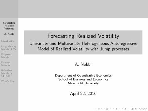
IntroductionVolatility Estimators
Daily Realized Variance
Let rt,i be high-frequency intraday return, then:
RV(d)t = RVt ≡
M∑i=1
r2t,i (1)
where ∆ = 1d/M and ∆-frequency return is defined byrt,i = log(Pt−1+i .∆)− log(Pt−1+(i−1).∆).
Jump robust estimators:
Bipower Variation: BPVt ≡ π2
(M−1M
)∑Mi=2 |rt,i ||rt,i−1|.
Median Truncated Realized Variance:MedRVt ≡ π
π−2
(M
M−1
)∑M−1i=2 Med(|rt,i+1|, |rt,i |, |rt,i−1|)2.
ForecastingRealizedVolatility
A. Nabbi
Introduction
Financial Data,Models andIssues
VolatilityEstimators
VolatilityComponents
Long-MemoryModels of RV
ProposedModels
ForecastMeasure
UnivariateModels onS&P500
What’s Next
.
.
.
.
.
.
.
.
.
.
.
.
.
.
.
.
.
.
.
.
.
.
.
.
.
.
.
.
.
.
.
.
.
.
.
.
.
.
.
.
.
.
.
.
IntroductionVolatility Estimators
Daily Realized Variance
Let rt,i be high-frequency intraday return, then:
RV(d)t = RVt ≡
M∑i=1
r2t,i (1)
where ∆ = 1d/M and ∆-frequency return is defined byrt,i = log(Pt−1+i .∆)− log(Pt−1+(i−1).∆).
Jump robust estimators:
Bipower Variation: BPVt ≡ π2
(M−1M
)∑Mi=2 |rt,i ||rt,i−1|.
Median Truncated Realized Variance:MedRVt ≡ π
π−2
(M
M−1
)∑M−1i=2 Med(|rt,i+1|, |rt,i |, |rt,i−1|)2.

ForecastingRealizedVolatility
A. Nabbi
Introduction
Financial Data,Models andIssues
VolatilityEstimators
VolatilityComponents
Long-MemoryModels of RV
ProposedModels
ForecastMeasure
UnivariateModels onS&P500
What’s Next
.
.
.
.
.
.
.
.
.
.
.
.
.
.
.
.
.
.
.
.
.
.
.
.
.
.
.
.
.
.
.
.
.
.
.
.
.
.
.
.
.
.
.
.
IntroductionVolatility Components
Highly persistent process and consistent.
No access to Intraday data.
True long-memory processes versus simple componentmodels.
Volatility components: Short-, medium- and long-term.
Realized Variance over different time horizon
RV over time horizon h is defined by,
RV(h)t−i = RVt−i |t−h ≡ 1
h
h∑k=i
RVt−k (2)
For time horizons daily, weekly and monthly: h = 1, 5, 22.

ForecastingRealizedVolatility
A. Nabbi
Introduction
Long-MemoryModels of RV
HeterogeneousAR and ARQuarticityModels
ProposedModels
ForecastMeasure
UnivariateModels onS&P500
What’s Next
.
.
.
.
.
.
.
.
.
.
.
.
.
.
.
.
.
.
.
.
.
.
.
.
.
.
.
.
.
.
.
.
.
.
.
.
.
.
.
.
.
.
.
.
Long-Memory Models of Realized VolatilityHeterogeneous AR and AR Quarticity Models
Heterogeneous Autoregressive (HAR) - Corsi(2009)
The following model labeled as HAR(3)-RV which captures theapproximate long-memory dynamic dependencies conveniently.
RVt = β0 + β1RV(d)t−1 + β2RV
(w)t−1 + β3RV
(m)t−1 + ϵt (3)
RV refers to Realized Volatility.
Extensions to HAR:
HAR-J:
RVt = β0 + β1RV(d)t−1 + β2RV
(w)t−1 + β3RV
(m)t−1 + β4Jt−1 + ϵt
(4)
Continuous HAR:
RVt = β0+β1BPV(d)t−1+β2BPV
(w)t−1 +β3BPV
(m)t−1 + ϵt (5)

ForecastingRealizedVolatility
A. Nabbi
Introduction
Long-MemoryModels of RV
HeterogeneousAR and ARQuarticityModels
ProposedModels
ForecastMeasure
UnivariateModels onS&P500
What’s Next
.
.
.
.
.
.
.
.
.
.
.
.
.
.
.
.
.
.
.
.
.
.
.
.
.
.
.
.
.
.
.
.
.
.
.
.
.
.
.
.
.
.
.
.
Long-Memory Models of Realized VolatilityHeterogeneous AR and AR Quarticity Models
Consider drt = µtdt + σtdWt then QVt = IVt + ηt whereIVt =
∫ tt−1 σ
2s ds.
RVt as consistent estimator of QVt .
In absence of jumps:√M(RV − IV )
D−→ N(0, 2IQ) whereIQt =
∫ tt−1 σ
4s ds.
RQt =M3
∑Mi=1 r
4t,i as consistent estimator of IQt .
Autoregressive Quarticity(ARQ) - Bollerslev (2015)
RVt = β0 +(β1 + β1QRQ
1/2t−1
)RVt−1 + ϵt (6)
which has a time-varying parameter.

ForecastingRealizedVolatility
A. Nabbi
Introduction
Long-MemoryModels of RV
HeterogeneousAR and ARQuarticityModels
ProposedModels
ForecastMeasure
UnivariateModels onS&P500
What’s Next
.
.
.
.
.
.
.
.
.
.
.
.
.
.
.
.
.
.
.
.
.
.
.
.
.
.
.
.
.
.
.
.
.
.
.
.
.
.
.
.
.
.
.
.
Long-Memory Models of Realized VolatilityHeterogeneous AR and AR Quarticity Models
Demeaned RQ1/2 results in comparable interpretation toautoregressive coefficient in AR(1)-RV.
RQ is highly imprecise and requires forth moments.
Non-robustness.
In presence of jumps: RV is not consistent and RQdiverges as M grows.
HAR on Realized Volatility and ARQ on Realized Variance.
ARQ models extensions:
Can be extended to Heterogeneous ARQ.
HARQ Full model.

ForecastingRealizedVolatility
A. Nabbi
Introduction
Long-MemoryModels of RV
ProposedModels
ForecastMeasure
UnivariateModels onS&P500
What’s Next
.
.
.
.
.
.
.
.
.
.
.
.
.
.
.
.
.
.
.
.
.
.
.
.
.
.
.
.
.
.
.
.
.
.
.
.
.
.
.
.
.
.
.
.
Proposed Models
Time-varying Autoregressive Model + Jump component
RVt = β0 + (β1 + β1J .Jt−1)RVt−1 + ϵt (7)
We term this specification the ARJ for short.
Heterogeneous ARJ
RVt = β0+(β1+β1J .Jt−1)RV(d)t−1+β2RV
(w)t−1+β3RV
(m)t−1+ϵt (8)
And respectively, HARJ full model is considered as a candidate.

ForecastingRealizedVolatility
A. Nabbi
Introduction
Long-MemoryModels of RV
ProposedModels
ForecastMeasure
UnivariateModels onS&P500
What’s Next
.
.
.
.
.
.
.
.
.
.
.
.
.
.
.
.
.
.
.
.
.
.
.
.
.
.
.
.
.
.
.
.
.
.
.
.
.
.
.
.
.
.
.
.
Forecast MeasuresIn-Sample and Out-of-Sample Forecast
In-Sample forecast.
Out-of-Sample forecast (Horizons and moving window)
Volatility Models Performance (unbiasedness andaccuracy):
Diebold-Mariano test.Mincer-Zarnowitz regression.
Mincer-Zarnowitz Regression (1969)
RVt = β0 + β1R̂V t|t−1 + ϵt (9)

ForecastingRealizedVolatility
A. Nabbi
Introduction
Long-MemoryModels of RV
ProposedModels
ForecastMeasure
UnivariateModels onS&P500
ModelEstimations
In-sampleForecastPerformance
What’s Next
.
.
.
.
.
.
.
.
.
.
.
.
.
.
.
.
.
.
.
.
.
.
.
.
.
.
.
.
.
.
.
.
.
.
.
.
.
.
.
.
.
.
.
.
Univariate Models on S&P500Model Estimation
HAR(3) on Realized Variance:

ForecastingRealizedVolatility
A. Nabbi
Introduction
Long-MemoryModels of RV
ProposedModels
ForecastMeasure
UnivariateModels onS&P500
ModelEstimations
In-sampleForecastPerformance
What’s Next
.
.
.
.
.
.
.
.
.
.
.
.
.
.
.
.
.
.
.
.
.
.
.
.
.
.
.
.
.
.
.
.
.
.
.
.
.
.
.
.
.
.
.
.
Univariate Models on S&P500Model Estimation
HAR(3)-J on Realized Variance:

ForecastingRealizedVolatility
A. Nabbi
Introduction
Long-MemoryModels of RV
ProposedModels
ForecastMeasure
UnivariateModels onS&P500
ModelEstimations
In-sampleForecastPerformance
What’s Next
.
.
.
.
.
.
.
.
.
.
.
.
.
.
.
.
.
.
.
.
.
.
.
.
.
.
.
.
.
.
.
.
.
.
.
.
.
.
.
.
.
.
.
.
Univariate Models on S&P500Model Estimation
CHAR on Realized Variance:

ForecastingRealizedVolatility
A. Nabbi
Introduction
Long-MemoryModels of RV
ProposedModels
ForecastMeasure
UnivariateModels onS&P500
ModelEstimations
In-sampleForecastPerformance
What’s Next
.
.
.
.
.
.
.
.
.
.
.
.
.
.
.
.
.
.
.
.
.
.
.
.
.
.
.
.
.
.
.
.
.
.
.
.
.
.
.
.
.
.
.
.
Univariate Models on S&P500Model Estimation
ARJ on Realized Variance:

ForecastingRealizedVolatility
A. Nabbi
Introduction
Long-MemoryModels of RV
ProposedModels
ForecastMeasure
UnivariateModels onS&P500
ModelEstimations
In-sampleForecastPerformance
What’s Next
.
.
.
.
.
.
.
.
.
.
.
.
.
.
.
.
.
.
.
.
.
.
.
.
.
.
.
.
.
.
.
.
.
.
.
.
.
.
.
.
.
.
.
.
Univariate Models on S&P500Model Estimation
HARJ on Realized Variance:

ForecastingRealizedVolatility
A. Nabbi
Introduction
Long-MemoryModels of RV
ProposedModels
ForecastMeasure
UnivariateModels onS&P500
ModelEstimations
In-sampleForecastPerformance
What’s Next
.
.
.
.
.
.
.
.
.
.
.
.
.
.
.
.
.
.
.
.
.
.
.
.
.
.
.
.
.
.
.
.
.
.
.
.
.
.
.
.
.
.
.
.
Univariate Models on S&P500Model Estimation
HARJ Full model on Realized Variance:

ForecastingRealizedVolatility
A. Nabbi
Introduction
Long-MemoryModels of RV
ProposedModels
ForecastMeasure
UnivariateModels onS&P500
ModelEstimations
In-sampleForecastPerformance
What’s Next
.
.
.
.
.
.
.
.
.
.
.
.
.
.
.
.
.
.
.
.
.
.
.
.
.
.
.
.
.
.
.
.
.
.
.
.
.
.
.
.
.
.
.
.
Univariate Models on S&P500Model Estimation
Autocorrelation and Partial Autocorrelation:

ForecastingRealizedVolatility
A. Nabbi
Introduction
Long-MemoryModels of RV
ProposedModels
ForecastMeasure
UnivariateModels onS&P500
ModelEstimations
In-sampleForecastPerformance
What’s Next
.
.
.
.
.
.
.
.
.
.
.
.
.
.
.
.
.
.
.
.
.
.
.
.
.
.
.
.
.
.
.
.
.
.
.
.
.
.
.
.
.
.
.
.
Univariate Models on S&P500In-sample Forecast Performance
Models R2 MAE RMSE
HAR(3) 0.5308 0.5968 1.7874HAR-J 0.5528 0.5764 1.7454CHAR 0.5575 0.5781 1.7359ARJ 0.5329 0.6206 1.7791HARJ 0.5649 0.5845 1.7216HARJ-F 0.5769 0.5893 1.6980
Table: In-sample forecast performance

ForecastingRealizedVolatility
A. Nabbi
Introduction
Long-MemoryModels of RV
ProposedModels
ForecastMeasure
UnivariateModels onS&P500
What’s Next
.
.
.
.
.
.
.
.
.
.
.
.
.
.
.
.
.
.
.
.
.
.
.
.
.
.
.
.
.
.
.
.
.
.
.
.
.
.
.
.
.
.
.
.
What’s Next
Out-of-sample forecast performance.
HAR Realized Variance vs. Realized Volatility
Multivariate Models.
Missing values in multivariate case.
Volatility signals, Timezones.
Granger-Causality and Cointegration.
Partial prediction of jumps from other indexes.

ForecastingRealizedVolatility
A. Nabbi
Introduction
Long-MemoryModels of RV
ProposedModels
ForecastMeasure
UnivariateModels onS&P500
What’s Next
.
.
.
.
.
.
.
.
.
.
.
.
.
.
.
.
.
.
.
.
.
.
.
.
.
.
.
.
.
.
.
.
.
.
.
.
.
.
.
.
.
.
.
.
Q&A

ForecastingRealizedVolatility
A. Nabbi
Introduction
Long-MemoryModels of RV
ProposedModels
ForecastMeasure
UnivariateModels onS&P500
What’s Next
.
.
.
.
.
.
.
.
.
.
.
.
.
.
.
.
.
.
.
.
.
.
.
.
.
.
.
.
.
.
.
.
.
.
.
.
.
.
.
.
.
.
.
.
Thank youfor
your attention
ForecastingRealizedVolatility
A. Nabbi
Appendix
References
.
.
.
.
.
.
.
.
.
.
.
.
.
.
.
.
.
.
.
.
.
.
.
.
.
.
.
.
.
.
.
.
.
.
.
.
.
.
.
.
.
.
.
.
References I
F. CorstA simple approximation Long-memory model of realizedvolatility, 2009.
T. Bollerslev, A.J. Patton and R. Quaedvlieg.Exploiting the Errors: A simple approach for improvedvolatility forecasting, 2015.
Related Documents