Master Thesis JPEG 2000 Encoder Development x KTH ...ingo/MasterThesis/Delente2006.pdf · Department of Information Technology and Microelectronics ... While the JPEG standard is

1/60

Master Thesis

JPEG 2000 Encoder Development x

KTH

Department of Information Technology and Microelectronics

Author Jérémie Delente Period 2005/9-2006/2 Thales Supervisor Michel Sarlotte KTH Supervisor Ingo Sander

2/60

Acknowledgments Firstly, I would like to thank Bernard Candaele who welcomed me into his service for my internship. I also want to thank Michel Sarlotte for the opportunity he gave me to work in his laboratory. Besides, I really appreciate the behavior of the SIE service that have welcomed me easily and made my integration simpler. I also want to thank Cédric Le Barz and Didier Nicholson for their help and patience when I went to them and asked a lot of questions about the JPEG2000. I shall not forget Bertrand Mercier whose advices were accurate. I enjoyed working there, thanks for all.

3/60

Abstract In computing, JPEG is one of the most commonly used standards of compression for photographic images. However, some of its inherent weaknesses are starting to be a real trouble for specific applications such as medical imagery. The need for a new standard arose several years ago and the JPEG2000 has been created. It shall solve the JPEG weaknesses and introduce new features that others standards either don't address efficiently or don't address at all. The aim of the present document is to think over how a JPEG2000 encoder can be implemented in a hardware/software structure. The targeted platform is a FPGA with an embedded processor core in order to mix both hardware and software. After an overview of the JPEG2000 standard, the requirements and the methodology are presented; eventually the modules will be presented.

4/60

Table of Contents Acknowledgments ...................................................................................................................... 2

Abstract ...................................................................................................................................... 3

Table of Contents ....................................................................................................................... 4

List of Figures ............................................................................................................................ 6

List of Tables.............................................................................................................................. 7

1. The JPEG2000 standard ..................................................................................................... 8

1.1. Introduction ................................................................................................................ 8

1.1.1. JPEG2000 main requirements ............................................................................ 9 1.1.2. Advantages and drawbacks ................................................................................ 9

1.2. Overview of the encoding process ........................................................................... 10

1.2.1. Color transform ................................................................................................ 10 1.2.2. Tiling ................................................................................................................ 11 1.2.3. DWT................................................................................................................. 11 1.2.4. Quantization ..................................................................................................... 15 1.2.5. Entropy Coder .................................................................................................. 16 1.2.6. Rate allocation.................................................................................................. 17 1.2.7. Syntax............................................................................................................... 17

2. Objectives of the thesis .................................................................................................... 20

2.1. Outline...................................................................................................................... 20

2.2. Hardware/Software mapping.................................................................................... 20

2.3. General architecture ................................................................................................. 22

3. Design Methodology ........................................................................................................ 24

3.1. Requirements............................................................................................................ 24

3.2. VHDL development ................................................................................................. 24

3.3. Validation ................................................................................................................. 24

3.4. Synthesis................................................................................................................... 25

3.5. Place and route ......................................................................................................... 25

3.6. Final Validation........................................................................................................ 25

4. Module descriptions ......................................................................................................... 26

4.1. The DWT module..................................................................................................... 26

4.1.1. Algorithmic specification................................................................................. 26 4.1.2. Hardware specification..................................................................................... 26 4.1.3. Architecture ...................................................................................................... 27

5/60

4.1.4. Validation ......................................................................................................... 30 4.1.5. Synthesis results ............................................................................................... 30

4.2. The quantization module.......................................................................................... 30

4.2.1. Algorithmic specification................................................................................. 30 4.2.2. Hardware specification..................................................................................... 31 4.2.3. Architecture ...................................................................................................... 32 4.2.4. Validation ......................................................................................................... 32 4.2.5. Synthesis results ............................................................................................... 33

4.3. The EC abstraction module (qtt2ec)......................................................................... 33

4.3.1. Hardware specification..................................................................................... 33 4.3.2. Architecture ...................................................................................................... 33 4.3.3. Validation ......................................................................................................... 34 4.3.4. Synthesis results ............................................................................................... 34

4.4. The modules altogether ............................................................................................ 34

4.4.1. Architecture ...................................................................................................... 34 4.4.2. Validation ......................................................................................................... 35 4.4.3. Final results ...................................................................................................... 35

5. Sequencer Study............................................................................................................... 37

5.1. General Architecture ................................................................................................ 37

5.1.1. Zoom on EC ..................................................................................................... 37 5.1.2. Global Architecture .......................................................................................... 39

5.2. Options lie in the EC arbiter and the EC unloader ................................................... 40

5.2.1. Global pool of ECs........................................................................................... 40 5.2.2. Four subband-dedicated pools of ECs with a polling writing .......................... 41 5.2.3. Four subband-dedicated pools of ECs without a polling writing..................... 42

5.3. Entering the sequencer ............................................................................................. 43

5.3.1. The address translator....................................................................................... 44 5.3.2. The feeder......................................................................................................... 46 5.3.3. The DWT watcher ............................................................................................ 51 5.3.4. The EC arbiter .................................................................................................. 51 5.3.5. The EC unloader............................................................................................... 53 5.3.6. The communication unit................................................................................... 54

6. Conclusion........................................................................................................................ 56

6.1. ROI implementation ................................................................................................. 56

6.2. Clusters..................................................................................................................... 57

7. Glossary............................................................................................................................ 59

8. References ........................................................................................................................ 60

6/60

List of Figures

Figure 1: Comparison JPEG vs JPEG2000 ................................................................................ 8

Figure 2: Structure of the encoder............................................................................................ 10

Figure 3: Tile generation .......................................................................................................... 11

Figure 4: Lifting scheme for the [9,7] transformation ............................................................. 13

Figure 5: Multiple decomposition process ............................................................................... 14

Figure 6: Frequency partition in code-blocks .......................................................................... 16

Figure 7: 3D representation of a code-block............................................................................ 16

Figure 8: Layer (quality) progression....................................................................................... 18

Figure 9: Resolution progression ............................................................................................. 18

Figure 10: Position progression................................................................................................ 19

Figure 11: Hardware/software mapping................................................................................... 21

Figure 12: General Architecture of the encoder....................................................................... 22

Figure 13: Validation process .................................................................................................. 25

Figure 14: Lifting scheme for the [9,7] transformation ........................................................... 26

Figure 15: 2 different architectures for the DWT module ....................................................... 27

Figure 16: General architecture of the DWT module .............................................................. 28

Figure 17: Structure of the DWT-1D block ............................................................................. 29

Figure 18: Controller implementation...................................................................................... 29

Figure 19: Architecture of the quantization module ................................................................ 32

Figure 20: Reading order for the EC........................................................................................ 33

Figure 21: Architecture of the EC abstraction module ............................................................ 34

Figure 22: Global architecture.................................................................................................. 35

Figure 23: structural overview of a EC line ............................................................................. 37

Figure 24: FSM structure of the post-EC controller ................................................................ 38

Figure 25: Memory mapping in the external RAM.................................................................. 39

Figure 26: Architecture of the sequencer ................................................................................. 39

Figure 27: Dedicated pool of ECs ............................................................................................ 41

Figure 28: Tiling fragmentation ............................................................................................... 44

Figure 29: Grid and virtual address of the input ...................................................................... 45

Figure 30: Structure of the feeder FSM ................................................................................... 46

Figure 31: boundary conditions of the tile block ..................................................................... 48

Figure 32: Read sequence without symmetry operation .......................................................... 49

Figure 33: Read sequence with a left symmetry operation ...................................................... 49

7/60

Figure 34: Read sequence with a top symmetry operation ...................................................... 50

Figure 35: Structure of the FSM for the arbiter ....................................................................... 52

Figure 36: Illustration of the address space.............................................................................. 54

Figure 37: ROI shift up ............................................................................................................ 57

Figure 38: ROI example ........................................................................................................... 57

List of Tables

Table 1: Reversible filter taps .................................................................................................. 12

Table 2: Irreversible filter taps ................................................................................................. 12

Table 3: Lifting scheme coefficients for irreversible DWT..................................................... 14

Table 4: Gain values in the quantization.................................................................................. 15

Table 5: Hardware/software mapping ...................................................................................... 21

Table 6: External memory needs.............................................................................................. 23

Table 7: Gain values by subband ............................................................................................. 31

8/60

1. The JPEG2000 standard

1.1. Introduction The JPEG2000 standard [1], as the JPEG standard, is an international standard for encoding and decoding static pictures. While the JPEG standard is highly based on a discrete cosine transform (DCT) and a Huffman coder, the JPEG2000 is based on a discrete wavelet transform and an arithmetic coder. The JPEG is the widespread standard for digital image compression. The JPEG2000 has been designed to be its successor. But one question would be why we need a new standard. Firstly, the old standard has relevant weaknesses:

• it is restricted to 8 bits/pixel inputs • it provides a low quality image at low bit-rates. The shows a illustration of this issue

and compares it to what would do a JPEG2000 compression with the same ratio. The difference is striking : one can hardly guess the boat on the left picture while one can almost read the name of the boat with a JPEG2000 compression. One should notice that both compressed images has the same size.

• the maximal image size is 64k x 64k in the JPEG standard • it suffers of a block affect as the DCT is applied on 8x8 block.

Figure 1: Comparison JPEG vs JPEG2000

Despite these weaknesses, the JPEG standard is widespread in the digital picture world. It is quite common to have digital cameras that use the JPEG baseline system. One key to this phenomenal success is obviously attributed to its royalty-free nature. Therefore a new committee has decided to create a new standard that is scheduled on 6 parts. Actually we could focus on the first part, which is [1], because it mainly deals with what we have done. The 6 parts are:

• Part1: JPEG2000 Image Coding System: Core Coding System (scheduled for December 2000)

• Part2: JPEG2000 Image Coding System: Extensions (scheduled for November 2001) • Part3: Motion JPEG2000 (scheduled for November 2001) • Part4: Conformance Testing (scheduled for March 2002) • Part5: Reference Software (scheduled for November 2001) • Part6: Compound Image File Format (scheduled for March 2002)

Those parts are mostly completed now, however they filled in new extensions that are not completed yet, so the whole standard is still in evolution but the main baseline system is fixed.

9/60

1.1.1. JPEG2000 main requirements These weaknesses have lead people to think over a new standard that would fulfill them. Thus the main requirements for the JPEG 2000 are:

• Superior low bit-rate performance: this standard should offer performance superior to the current standard at low bit-rates (i.e. below 0.25 bpp (bits per pixel) for highly detailed gray-scale pictures). This shall not be achieved with sacrificing performance on the rest of the rate-distortion spectrum. This feature is needed by applications like network image transmission and remote sensing.

• Lossless and lossy compression: Some applications such as medical imagery require a lossless compression so the standard shall also provide it. Moreover, it shall also provide the capacity of creating embedded bit-stream and allow progressive lossy to lossless build-up.

• Multiple resolution representation: this feature allows the user to order the code-stream so that the picture can be decoded with an increasing resolution. That means it begins to decode a small complete image and as long as the decoding runs, the resolution increases up to the original image resolution.

• Tiling: This feature allows the capacity to split a big image into smaller pieces that will be encoded independently.

• Region of interest coding: Often some areas of a picture have more interest than others, so the standard shall allow users to define certain Region Of Interest’s (ROI) in the image to be coded and transmitted with a better quality and less distortion than the rest of the image.

• Error resilience: It is desirable to consider robustness to bit-errors while designing the code-stream. One application where this feature would be important is transmission over wireless communication channels.

• Random code-stream access and processing: This feature allows user defined ROI's in the image to be randomly accessed/decompressed with less distortion than the rest of the image. Also random code-stream processing could allow operations such as rotation, translation, filtering, feature extraction and scaling.

• Improved performance to multiple compression/decompression cycles: This feature means that in the case of a lossy transformation, the new standard has better performance than the old one, in multiple compression/decompressions cycles.

• A more flexible file format • Large and complex image support: the maximal size of a picture is (232-1) x (232-1)

with a maximal bit-depth of 38 bits and the maximal number of components is 16384. These requirements are more deeply explained in [2], [3] and [5].

1.1.2. Advantages and drawbacks The advantages are more or less the requirements because they correct the weaknesses of the old standard. The main drawback is that this standard requires a lot more computation power. The encoding process is very complex and time consuming. This higher complexity was predictable due to the wanted higher compression ratio. Nevertheless, many of its abilities shall make it the new reference standard. It integrates functionalities, which make it relevant in a lot of transmission applications, and as it has security features, which are compatible with Digital Right Management. So, it may become quickly the new standard.

10/60

1.2. Overview of the encoding process The main steps of the encoding process are described in the below figure which summarizes the following references [1], [2], [3] and [4]:

Color

transform DWT Quantization

Arithmetic coder

Coefficient Bit Modeling

Input picture

Jpeg2000 codestream

Tiling

Syntax

Rate allocation

Figure 2: Structure of the encoder

The input image is commonly the output of a digital camera or of a captor. Its format may vary, but it is more likely to be either the RGB (Red Green Blue) format or a luminance based format if the picture is multi-chromatic. Then, the input stream will be unsigned coefficients. Basically, a preprocessing happens with the first two steps ( Color transform and Tiling ); these are optional steps but the former helps to obtain better results in the process while the latter allows to reduce the amount of memory needed to encode the picture and to execute a parallel encoding. The Discrete Wavelet Transform is used to de-correlate the input image into a frequency space. No compression is performed in this step. The quantization step is used to scaled down the coefficient if we want to, so that the encoding will be faster, but it leads to loss of information. The coefficient bit modeling and the arithmetic coder are the main parts of the Entropy Coder (EC), they perform the actual compression of the data. Based on information about the compression given by the EC and what the user wants, the rate allocation selects what data can be discarded. The syntax step is just ordering the data into a specific order to make clear to decode. We are now going to explain deeply every step of the encoding process in order to apprehend the concepts and the algorithmic requirements we had.

1.2.1. Color transform This step might be optional depending on the format of the input image. Anyhow, if we apply a color transform, the unsigned input coefficients need to be level shifted into signed coefficients to make their values more symmetric around zero. This step simplifies some implementation issues such as numerical overflows, but has no effect on the coding efficiency. Finally, the level shifted values can be subjected to a forward color transformation to de-correlate the color data. This only applies on components that have identical bit-depths and dimensions. Two transformations are available in the baseline JPEG2000 codec: the irreversible color transform and the reversible color transform. The former is non reversible and real-to-real in nature whereas the latter is reversible and integer-to-integer. Both of theses transformations map image data from the RGB to YCrCb color space. The ICT (Irreversible

11/60

Color Transform) can only be used in a lossy transformation while the RCT (Reversible Color Transform) can be used in both cases, but it is more likely used in reversible transformations only. The ICT can be shown to be:

)(713.0)(564.0

)(114.0)(299.0

YRCYBC

GBGGRY

r

b

−∗=−∗=

−∗++−∗=

The irreversibility lies in the fact that a real implementation can never be achieved in hardware or in software. Besides the RCT can be shown to be:

GBVGRU

BGRY

−=−=

⎥⎦⎥

⎢⎣⎢ ++

=4

2

Where ⎣ ⎦x means the greatest integer less or equal to x.

1.2.2. Tiling The tiling is also an optional preprocessing step. It allows the user to split the original picture into smaller pieces that have the same size except maybe around the edges of the picture. This is used to reduce the memory needs during the encoding. A grid can be drawn over the picture (see Figure 3)

Original picture

tile

Figure 3: Tile generation

.

1.2.3. DWT The JPEG DCT transformation has been replaced with a full frame DWT (Discrete Wavelet Transform) in JPEG2000. The DWT has several characteristics that make it more suitable for fulfilling some of the main JPEG2000 requirements. Among them, we can point out:

• It has an inherent multi-resolution image representation.

12/60

• The full frame nature of the transform de-correlates the image across a larger scale and thus eliminates blocking artifacts at high compression ratio.

• The use of integer-to-integer DWT filters allows for both lossless and lossy compression in a single bit-stream.

The result of the DWT on a tile is the following dyadic decompositions, assuming a multiple level decomposition (see Figure 5). We will focus on the one-dimensional DWT for two reasons: because it is the one recommended by the standard and because it is the one we implemented. However, the two-dimensional DWT is worth to mention. But it may have lower precision in the computation. We will focus on the one-dimensional transformation then, on the way to perform a two-dimensional transformation with two one-dimensional transformation block.

1.2.3.1. One-dimensional transformation The forward one-dimensional DWT at the encoder is best understood as successive applications of a pair of low-pass and high-pass filters, followed by down sampling by a factor 2 (i.e. discarding the odd indexed samples). Basically, the low-pass filter shall preserve the low frequencies and thus returns a blurred version of the original data while the high-pass filter shall preserve the high frequencies and thus returns the details, the edges in the original picture. The JPEG2000 standard [1] defines 2 types of DWT transformations; both of them are symmetrical bi-orthogonal filter-banks:

• A reversible one, which is an integer-to-integer transformation. It is a [5,3] filter-bank that means that the low-pass filter has 5 coefficients whereas the high-pass filter has only 3 coefficients. The transformation is summarized by the following table:

i Low-pass filter High-pass filter 0 ¾ 1

±1 ¼ ½ ±2 - ⅛

Table 1: Reversible filter taps

• An irreversible transformation, which is a real to real transformation. As it is not possible to implement it as real, it can be either with a floating point or with a fixed point representation. It is a [9,7] filter-bank which coefficients are summarized in the below table.

i Low-pass filter High-pass filter 0 0.602949018236360 1.115087052457000

±1 0.266864118442875 0.591271763114250 ±2 -0.078223266528990 -0.05754526228500 ±3 -0.016864118442875 -0.091271763114250 ±4 0.026748757410810

Table 2: Irreversible filter taps

13/60

The irreversible filter-bank has better performance, but it can only be used in lossy compression.

1.2.3.2. Lifting scheme The most effective hardware implementation is the lifting scheme implementation which is described in [2]. It reduces the memory needs in the implementation. The lifting scheme consists of several steps. The basic idea is to first compute a trivial wavelet transform, also referred to as the “lazy wavelet transform”, by splitting the original 1D signal into odd and even indexed subsequences, and then modifying these values using prediction and updating steps. We would denote the odd and even subsequences respectively as {si

0} and {di0}.

A prediction step would consist of predicting each odd sample as a linear combination of the even samples and subtracting it from the odd sample to form the prediction error {di

1}. The update step would consist of updating the even samples by adding to them a linear combination of the already modified odd samples {di

1} to form the updated sequence {si1}.

For the reversible transformation, the output of this stage {si

1} is the result of the low-pass filter, while the sequence {di

1} is the result of the high-pass filter. But the process can be iterated on the output sequence to form a more complex scheme. Fortunately, the irreversible transform requires only 2 stages (see Figure 4). In Figure 4, x refers to the input data and each level is referred with a Greek letter. Note that if we only want to perform the reversible transformation, then the output shall be α and β. The outputs are correct up to a scaling factor, which happens to be 1 in the reversible transformation but it is different in the irreversible one.

x

α

β

γ

δ

Figure 4: Lifting scheme for the [9,7] transformation

The prediction and update coefficients are quite simple for the reversible transformation:

( ) ( ) ( ) ( )

( ) ( ) ( )⎥⎦⎥

⎢⎣⎢ +++−

−=

⎥⎦⎥

⎢⎣⎢ +−

−+=+

421212)2(2

22221212

nnnxn

nxnxnxn

ααβ

α

For the irreversible transformation, the coefficients are real numbers:

14/60

).().(

).().(

112

2211

31122

42133

+−

+++

++++

++++

++=++=++=++=

nnnn

nnnn

nnnn

nnnn

UPUx

xxPx

γγβδββαγααβ

α

With P1 -1.586134342059924 U1 -0.052980118572961 P2 0.882911075530934 U2 0.443506852043971

Table 3: Lifting scheme coefficients for irreversible DWT

1.2.3.3. Two-dimensional transformation The two-dimensional transformation is extended from the one-dimensional by applying the same filter-bank in a separable manner. At each level of the wavelet decomposition, each column of a 2D image is first transformed using a one-dimension filter-bank, and then the same filter-bank is applied on each row of the filtered and sub-sampled data. The result of one-level wavelet decomposition is four filtered and sub-sampled images, referred as subbands. The subband is named using 2 letters from the set {H, L}; the former letter refers to the horizontal transformation, and the latter to the vertical one. For instance, the LH subband is the result of a high-pass filter vertically and a low-pass filter horizontally. The standard imposes the first transformation to be vertical, and the second to be horizontal. Besides a multiple level decomposition transformation would use the 2D DWT, but for each level of decomposition, we re-apply the transformation to the LL subband, which gives the dyadic decomposition. The below figure (Figure 5) illustrates this process with 2 levels of decomposition.

Tile-component

data

1L

1H 1HL 1HH

1LH1LL

2L

2H

1HL 1HH

1LH

1HL 1HH

1LH

2LL

2HL

2HH

2LH

Figure 5: Multiple decomposition process

15/60

1.2.4. Quantization The quantization is a step which purpose is to reduce the dynamic of the data so as to speed up the process in the rest of the data-path. It allows a greater compression to be achieved. However, the quantization is the one of the two primary sources of information loss in the coding path. The quantization uses a central dead-zone. Obviously this implies an irreversible transformation, in the case of the reversible transformation, the quantization step is fixed to 1. Every subband at each level of decomposition shall have their quantization step.

( ) ( )( ) ( )⎥⎦

⎥⎢⎣

⎢

Δ=

b

bbb

vuyvuysignvuq

,,,

The scaling down part is a process by which the transform coefficients are reduced in precision. For a reversible transformation the quantization step size is always 1, in other words, nothing is done in this case. However, if it is an irreversible transformation, the quantization step Δb for the subband b is calculated from the dynamic range Rb of the subband b, the exponent εb and the mantissa μb as given in the following equation:

⎟⎠⎞

⎜⎝⎛ +=Δ −

11212 bR

bbb

με

And Rb is computed from the following formula and table (Table 4):

)(log2 bIb gainRR += Where RI is then number of bits used to represent the original picture sample. The exponent εb and the mantissa μb are user defined and are concatenated in a 16-bit coefficient (the mantissa has the 11th LSB (Least Significant Bits) and the exponent the 5th MSB(Most Significant Bits)).

Subband b Gainb Log2(gainb) LL 1 0 LH 2 1 HL 2 1 HH 4 2

Table 4: Gain values in the quantization

There are two ways to give the value of the quantization step. A complete table can be given as a parameter to the encoder or a single value of (ε0, μ0) is given for the LL subband and the others values are derived from this couple. This latter method might appear interesting, but it leads to a lower quality result. Besides, there is a representation shift between the input and the output of the quantization block, the inputs are represented by the genuine signed representation, while the outputs must be represented with a new representation: This new representation is rather simple; the most

16/60

significant bit is a sign bit (0 means positive, 1 means negative); the others bits are used to define the absolute value of the number to represent.

1.2.5. Entropy Coder The entropy coder has two main steps: the coefficient bit modeling and the arithmetic coder. The entropy coder allows creating a bit-stream. The entropy coder only uses a code block (see Figure 6) paradigm to function; that means that every code-block is encoded independently with respect to its subband or level of decomposition.

Figure 6: Frequency partition in code-blocks

1.2.5.1. Coefficient bit modeling The coefficient bit modeling uses a bitplane representation of the code block, it is a kind of 3D view of a code block (see Figure 7). The symbols that represent the quantized coefficients are encoded one bit at a time starting with the MSB and proceeding to the LSB. A quantized coefficient is called insignificant if the quantized coefficient index is still 0. Once the first nonzero bit is encoded, the coefficient becomes significant and its sign is encoded. As soon as a coefficient becomes significant, all subsequent bits are referred as refinement bits.

A 16 bitsCoefficient

Sign bit-planeMSB bit-plane

LSB bit-plane

Figure 7: 3D representation of a code-block

17/60

With exception of the sign bit plan and the first bitplane with at least one 1, every bitplane is encoded in three sub-bitplane passes. Each bit can only be part of a unique pass. The value of the bit and its context are sent to the arithmetic coder. The different passes are:

• Significance propagation pass: it encodes the bits that have the highest probability of becoming significant in the current bitplane. They are those, which have at least one neighbor that is significant.

• Refinement pass: the magnitude bit of a coefficient that has already become significant in a previous bitplane is encoded.

• Cleanup pass: all the remaining bits of the current bitplane are encoded in this pass. In order to be more efficient, the number of MSB planes that are full of 0s is signaled in the bit-stream. Since the significance state of all the coefficients in the first non-zero MSB is zero, only the cleanup pass is applied to this first non-zero bitplane. The number of MSB planes that contains only 0s, is called the IMSB (Insignificant Most Significant Bits). A MSE (Mean Square Error) computation is also performed for every pass; this would be used for the rate allocation step. This value is used to qualify the distortion from the original image.

1.2.5.2. Arithmetic coder Arithmetic coding uses a fundamentally different approach from the Huffman coding in that the entire sequence of source symbols is mapped into a single codeword. Basically, it encodes the bits and their context into this codeword. The context of the bit allows the coder to estimate the symbol probabilities of the less probable symbol and the most probable symbol. Note that these symbols represent either 0 or 1 in this case.

1.2.6. Rate allocation There is no method specified in the standard for this step, thus only its purpose will be presented here. The rate allocation shall analyze the information data produced by the EC (Entropy Coder) to determine which passes it shall include in the JPEG2000 code-stream and which ones it can discard. This is the second primary source of information loss. Obviously, this step is rather trivia if a lossless encoding is required: nothing is discarded. The selection is performed code-block after code-block so that it shall minimize the image distortion for a fixed bit-rate. Therefore, the most important information it uses is the MSE computation and the number of encoded octets every pass represents.

1.2.7. Syntax The syntax step is basically a reordering of the data into a JPEG2000 code-stream. It shall create the different headers, and order the data. The concept of progression order is defined to better apprehend this step: it is the order in which the packets appear in the code-stream. Some others concepts are defined like the quality layers structure: within a code-block encoded data, it represents a quality improvement and contains a certain amount of consecutive coding passes (it can be 0). Several progression orders are defined by the standard ( see [1], [2] and [3]):

18/60

• Layer-Resolution-Component–Position progression (Figure 8): it is useful in image database browsing application where a low quality image can be used to perform a pre-selection. The more you decode the stream, the more the quality of the picture increases.

Figure 8: Layer (quality) progression

• Resolution-Layer-Component-Position progression (Figure 9): it is useful in client-

server application where several clients may require different resolutions. The more you decode the stream, the more the resolution increases up to be the original image resolution.

• Resolution-Position-Component-Layer progression: it can be used where resolution scalability is needed.

• Position-Component-Resolution-Layer progression (Figure 10): it can be used if it is desirable to refine the picture quality at a particular spatial location. The more you decode the stream, the more the image will be revealed.

• Component-Position-Resolution-Layer progression: it can be used if it is desirable to obtain a highest quality for one component at a specific spatial location.

Figure 9: Resolution progression

19/60

Figure 10: Position progression

Thus, we have seen why this new standard has been created. The bases of the encoding steps of the JPEG2000 have been presented, we can now proceed with the actual objectives of the thesis, before being more specific about the implementation.

20/60

2. Objectives of the thesis

2.1. Outline The internship was focused on the encoding part of the JPEG2000 standard. I have worked on the implementation of a JPEG2000 encoder that can be used as an intellectual property (IP). Thus it shall be portable and developed for an ASIC (Application Specific Integrated Circuit) or FPGA (Field Programmable Gate Array) target. The targeted application is a real-time JPEG2000 encoder that is able to process at least a SDTV (Standard Definition TeleVision) flow. This means:

• 720 x 576 pictures • 3 components with an 8-bit depth • A frame rate of 25 per second • A 4:4:4 format

However, the specifications are not limited to that, it shall handle:

• Input coefficients, which bit depth is up to 12 • Picture size larger than 720x576 • Format picture that can be 4:4:4, 4:2:2 and 4:2:0

The maximal frame rate, it can handle, may vary depending on the parameter of the input picture.

2.2. Hardware/Software mapping One could ask himself why a hardware implementation should be developed instead of a pure software implementation. The answer is quite simple: the performance you can get with a software solution is too low. Moreover, a dedicated hardware solution is more likely to have a lower power consumption than a pure software solution. Actually software encoders, which are compliant with the standard, already exist in public domain or within Thales, but the main issue with these software solutions is their speed. For instance in software, the encoding of such a flow is possible up to 6.6 frames per second if the flow has one component (monochromatic pictures). As the JPEG2000 process involves a lot of computation, a hardware implementation is a natural choice. However a processor should be added to handle some of the encoding because some steps require a lot of decisions to be taken dynamically. Therefore, a hardware/software design has been proposed. For the internship, the target of this IP will be a programmable component, an FPGA which is more suitable for a quick demonstration. Actually, a Xilinx FPGA has been chosen as the target. There are two ways of doing this, the former is to add a processor, a general purpose one or a specific one such as a DSP (Digital Signal Processor), on the same board; the latter is to find a FPGA that has an embedded processor core available. The advantages of the latter solution is to have a complete system within a chip, and it can be plugged into a bigger product more easily than if you have to add an external processor. However, it is obviously more expensive. Anyhow, the FPGA, we target, would be one of the

21/60

Xilinx Virtex4 FX family. These FPGAs have up to four embedded Power PC 405 cores, though we would only use one of them. The standard logic element in such a device is a Look Up Table (LUT) with 4 inputs and one output, therefore the results I shall give would imply a number of LUTs. Moreover, those devices have a limited amount of dedicated RAM blocks and multipliers within the chip, so it is important to know how many of them we need. From Figure 2, we have seen the different steps of the encoding process. The first step, the color transform, is optional and has not been implemented because the picture source may perform this kind of transformation. As usual, the critical steps have been mapped to hardware in order to speed up the process, and the steps, which parameters are more dynamic and may heavily vary between pictures, have been mapped to software. The following table sums up this mapping.

Step Mapped to Color transform (Would be hardware) Tiling Software DWT Hardware Quantization Hardware EC Hardware Rate allocation Software Syntax Software

Table 5: Hardware/software mapping

From Table 5, it clearly appears that the communication between the hardware and the software will not be a major issue, even if there will be some. Actually, the dataflow is mainly performed by the hardware and there is no exchange between the software and the hardware but the parameters for the processing of a picture.

Color transform

DWT Quantization

Arithmetic coder

Coefficient Bit Modeling

Input picture

Jpeg2000 codestream

Hardware

Tiling

Rate allocation

Syntax

Software

Figure 11: Hardware/software mapping

The software cuts the picture into smaller pieces called tiles and then it waits for the main processing to complete before putting everything into order at the end. Moreover, the JPEG2000 standard [1] allows us to encode the different components independently so the encoder will consider each component as a different picture. The hardware part of the encoder

22/60

shall not be aware of the image format or the number of components. This information stays in the software part of the encoder. The main constraint about the encoder, apart from the performance requirement we have seen earlier, is that the encoder has to be equivalent to a reference C program that performs a JPEG2000 encoding.

2.3. General architecture All these thoughts have lead to the following general architecture (see Figure 12).

Figure 12: General Architecture of the encoder

The encoder needs several storage facilities in order to work, and as the picture (or the tile) size might be quite huge, the memory required to process such a picture would never fit in the available local memory. An overview of the memory needs is given in the below table (Table 6). Of course, these values may vary due to the picture format and the kind of code-stream we require in output, but it gives an idea of the need in memory.

DWT

RAM1

RAM2

EC

EC

EC

EC

RAM3

µP

Input image

Jpeg2000 code-stream

RAM0

SequencerQ

uant

izat

ion

FPGA

23/60

RAM Size RAM0 2 * size of picture RAM1 ¼ * size of a color component RAM2 2048 16-bit words RAM3 Varies from 2 * (size of a component + size

of information) to 6 * (size of a component + size of information)

Table 6: External memory needs

Let's follow the flow to better understand what is going on in this architecture:

• First the picture is sampled by a captor and sent to the optional color transform. • Then it is written into a RAM (RAM0). • The global sequencer reads this RAM block by block, and the blocks are sent to

the DWT. • Depending on the number of decompositions, the data that went through both the

low-filters is either written in the RAM1 to be sent back to the DWT, or sent forward in the flow.

• After the DWT, a quantization may happen to reduce the dynamic of the data and thus speed up the EC encoding.

• The data is then processed by an EC; the output data can be split into information about the encoding and compressed data. Both of them are written into an external RAM, RAM3.

• The processor is warned to process the data as soon as a tile has been processed, so that it can compute the rate allocation, select the data it will keep and create the code-stream syntax that it may send directly out or write into another RAM which is not drawn in the above figure.

Besides, this general architecture also shows that the encoder can be easily partitioned into separate modules. When I arrived, the Entropy Coder was already developed as an IP. These modules shall be designed following a method that is to be explained.

24/60

3. Design Methodology

3.1. Requirements Before the pure development part, one need to write a design specification document that lists all the critical items of the module. It also gives the hierarchy, the interface and all the details one might need to develop the module. The basic idea is that if any developer and you would develop the module without concurring, then the final result would be the same. It basically forces you to plan how the functions will be implemented, how to make them interact with other modules or within the module and what kind of interface you will need. With this document, at least the skeleton of the module is drawn and that helps the designer to clarify a lot of issues before actually facing them. From this step, you can estimate the resources you will need to develop the module in terms of area.

3.2. VHDL development Then, after writing the previous document, the implementation can begin. I used the VHDL (Very high speed Hardware Description Language) language (version 93) to describe the module behavior. The simulation tool, which was used to simulate the module, was Modelsim®. Besides, the company has its own design rules about how to write VHDL code, but I will not enter into much detail about them. Basically, these rules guarantee the portability, a more efficient use of tools and a better re-use of the code.

3.3. Validation After a debug period, the RTL (Register Transfer Logic) code had to be validated. As there was a C reference program that has been validated, the RTL code and this reference program shall give the same results on some significant test patterns. The hardware model has to be bit true with the reference program in order to be able to apply the characteristics of the software to the hardware in terms of algorithmic performance. Besides this algorithmic validation, we also check the scheduling of the module. In order to structure all these tests and validations, a validation plan has to be filled in. It is very useful because it instantly gives an overview of the tests the module has faced. Thus, it is easy to see whether some tests were forgotten or not. Moreover, the validation plan ends on a matrix where for every requirements we indicate which pattern or tests tested this requirement. The bit-true validation process can be sum up by the below figure (see Figure 13). Both the reference software and the hardware model are fed with the same input pattern, their respective outputs must match in order to pass the validation.

25/60

data.dat

Module reference (C code)

Module (VHDL)

output.ref

output.log

diff Result

Figure 13: Validation process

3.4. Synthesis I used Synplify_pro® as the synthesis tool. The synthesis step analyzes the written code and maps it depending of the targeted FPGA. It also gives results on space and timing on the module, but those results are not so accurate.

3.5. Place and route This would be the final step of the actual development process, as the result of this step is a bit-stream that will be use to configure the FPGA. At the end of this step, you get results about the space occupied and the real timing of the FPGA. It is the real timing because as the netlist has been routed, you have access to the propagation time through wires of the circuit.

3.6. Final Validation From the results of the place and route step, you ought to know if the performance matches your requirements, if not then you get back to the coding step. If you have access to a test board you can test the system directly and see if it globally works. Otherwise you launch post route simulations that will allow you to check whether the actual circuit you are to put in the FPGA functionally behaves as the RTL code you had before synthesis with the timing requirement achieved. And as the RTL code must be bit-true with a reference software in our case, then the circuit ought to be bit-true also.

26/60

4. Module descriptions In this part, the different modules I have implemented shall be explained more deeply. The structure of every subpart shall be the same for every module, the points shall be:

• The algorithmic specification • The hardware specification • The architecture • The validation • The synthesis results

4.1. The DWT module

4.1.1. Algorithmic specification The DWT module shall be an implementation of the discrete wavelet transform. Several implementations of the DWT are possible. In order to stick to the software implementation that is the simulation reference and to the recommendations of the standard [1], the DWT module shall use 2 one-dimensional transforms following a lifting scheme, which structure is reminded below. Therefore, a bi-orthogonal filter bank filters the data first vertically and then horizontally.

x

α

β

γ

δ

Figure 14: Lifting scheme for the [9,7] transformation

Besides, the module shall handle both the reversible transform and the irreversible one. In order to minimize the risk of computational approximation, we shall use shifted coefficients in the filter parameters. The values of the shifts ought to be the same as in the software implementation but before the output of the module, we have to shift back the results. As you can see from the figure, I chose to limit the amount of memory needed to compute the next stage in the lifting scheme by storing the temporary results that are marked with an circle. Therefore, only 6 coefficients shall be store instead of 9 in the irreversible transformation.

4.1.2. Hardware specification As the 2-dimensional transform is reduced to two one-dimensional transformations, the module shall be pipelined between these stages. However, the temporary data has to be stored

27/60

in 2 local RAMs because the reading and the writing are not performed in the same order: the data from the 1st stage is received by columns and it shall be sent by rows. Thus, the intermediate RAMs shall be doubled so that the 1st stage can write in one while the 2nd stage is reading the other. Moreover, the processor shall give the DWT coefficients before the processing; the module is then flexible if the values of these coefficients change. The module has been designed so that it is unaware of the current level of decomposition. Actually, there is no need for it to have this kind of information, that means it is not in charge of fetching the data in one of the external RAMs and it shall not know if the output data on the LL subband shall go to RAM1 (a.k.a. LL RAM) or to the quantization module. Eventually, the module shall handle the fact that the tile coefficients may be received in an un-continuous way. In that case, the module will be as fast as it can. The registers of the dataflow have a data enable that allow complying this requirement.

4.1.3. Architecture With all these specifications, there were two possible architectures for implementing a two one dimensional transforms. The former would use 2 one-dimensional transform blocks whereas the latter would use 3 one-dimensional transform blocks.

1D 1D

1D

1D

1D

Figure 15: 2 different architectures for the DWT module

I chose the latter architecture for the DWT module (see Figure 16). As we were required to be fast, I gave more credits to the time than to the space. Actually with this architecture we are faster than with the former architecture: Assuming an M x N tile block as an input the transformation time is:

• With the former architecture: ( )TMNT +=1

• With the latter architecture: TMNT ⎟⎠⎞

⎜⎝⎛ +=

22

28/60

Where T is the time needed to transform one pixel. Within the one-dimensional transform block, a lifting scheme is implemented, this lifting scheme is hybrid which means that with the same scheme both the reversible and the irreversible transforms may be performed, the outputs are just at different levels: the outputs are:

• Reversible: low = β; high = α • Irreversible: low = δK0; high = γK1

The Greek characters refer to the nomenclature of the Figure 14.

DWT–1D

DWT–1D

DWT–1D

Buffer_dwt-L

Buffer_dwt-H

Input data

To RAM or EC

To EC

To EC

To EC

DWT controller

0

0

1

1

Figure 16: General architecture of the DWT module

4.1.3.1. One-dimensional DWT block This block shall perform a one-dimensional transformation on its inputs. Its internal structure is the lifting scheme, we have mentioned earlier. The implementation of this block is perfectly summed up by the below formulas:

).().(

).().(

112

2211

31122

42133

+−

+++

++++

++++

++=++=++=++=

nnnn

nnnn

nnnn

nnnn

UPUx

xxPx

γγβδββαγααβ

α

From these formulas, we see that we need 6 registers to store the input values, the first two levels of the lifting scheme and 3 registers to store the third level. This is exactly how it is implemented.

29/60

To be compliant with inputs, which bit-depth may vary up to 12, those registers are 16-bit large, that is sufficient to keep a good approximation. The dynamic increase in the DWT has been explained in [5] by J.Hara.

+

*

+

+

*

+

+

*

+

+

*

+

ST

OR

AG

E

xn+4

xn+2

P1

xn+3

αn+1 αn+3

U1

Xn+2

βn+2

βn

P2

U2

γn+1

γn-1

δn

βn

αn+1

*

*

K1

K0

Figure 17: Structure of the DWT-1D block

4.1.3.2. DWT controller The architecture is quite classical; the dataflow is controlled by a local controller that sets up the parameters for every item on the dataflow. It is also in charge of indicating that the module is ready to receive a new tile block, depending on the status of the RAMs that are before the ECs and the status of the buffers. Basically, the implementation of this controller is two FSMs (Finite State Machines) that communicate: the former is for the writing of the buffers and the latter is for the reading (see Figure 18).

Waitb0 state

Waitb1 state

Init DWT1

DWT1 to b0

Init DWT1

DWT1 to b1 Block request

& b0 free

When finished

Block request & b1 free

When finished

Wait for b0 full

Wait for b1 full

Init DWT2

DWT2 from b0

Init DWT2

DWT2 from b1 b0 full & Rams free

When finished

b1 full & Rams free

When finished

Figure 18: Controller implementation

30/60

There ought to be signals that indicate the status of a buffer to the FSMs, the writing FSM shall lock a buffer to indicate that it has finished to write values in it, and the latter shall release this lock as soon as it has performed the read.

4.1.4. Validation The validation of this module is done in 3 steps:

• A validation of the DWT-1D block behavior both sequentially and algorithmically • An algorithmic validation of the DWT module • A sequentially validation of the DWT module

For all these validations, the methodology was the one presented in the previous chapter. An algorithmic validation is a validation of the algorithm, it means that we send the data without interruption and the module shall output the same values than the software. However, in a sequential validation, we introduce interruptions in the input flow in order to check the robustness of the module to this type of inputs as it has been specified as a requirement; we also check that the module behavior, other than the algorithmic behavior, matches the specifications. We used reference patterns generated from the software implementation. In order to check the module in different situations, the size of the input block has varied: we used size from its maximal value: 72x72 to its minimal value: 9x9 and we check on intermediate even and odd values. All the validations were positive, we tested the module with the sample of 4 consecutive blocks, which were randomly chosen within the patterns we had. For each input pattern, there were one output reference for both the reversible and the irreversible transforms.

4.1.5. Synthesis results After the synthesis step, the module without the internal RAMs, which would be on dedicated blocks in a Xilinx Virtex4 FPGA, has the following features:

• It runs up to 117 MHz • It needs 1941 LUTs (Look Up Tables) and 18 multipliers

Besides it requires 12 RAM blocks.

4.2. The quantization module

4.2.1. Algorithmic specification As we have seen in the section 1.2.4, the coefficient that are output by the DWT might be scaled down in order to speed up the EC process. Obviously, the encoding is no more reversible and thus no longer lossless. This module is in charge of performing this scaling. The processor shall give the parameters of the scaling before that a new tile is sampled, but the sequencer shall dispatch them when appropriate. Those parameters may change between the levels of decomposition and between the subbands.

31/60

In addiction to this possible scaling, we switch from the genuine signed representation to a new representation. This new representation is rather simple: the most significant bit is a sign bit (0 means positive, 1 means negative); the others bits are used to define the absolute value of the number to represent. The scaling down part is a process by which the transform coefficients are reduced in precision. For a reversible transformation the quantization step size is always 1, in other words, nothing is done in this case. However, if it is an irreversible transformation, the quantization step Δb for the subband b is calculated from the dynamic range Rb of the subband b, the exponent εb and the mantissa μb as given in the following equation:

⎟⎠⎞

⎜⎝⎛ +=Δ −

11212 bR

bbb

με

And Rb is computed from the following formula and table:

Subband b Gainb Log2(gainb)

LL 1 0

LH 2 1

HL 2 1

HH 4 2

Table 7: Gain values by subband

)(log2 bIb gainRR +=

Where RI is then number of bits used to represent the original picture sample. One shall remember that we shall divide the transform coefficient by the quantization step. Besides, in our implementation, we arbitrary decide that whatever may happen the quantization step must be within the following interval:

163 22 <Δ≤−b

Which means that the exponent may be between –3 and 15.

4.2.2. Hardware specification The module shall receive four 16-bit coefficients by level of decomposition that represents the concatenation of the exponent εb and the mantissa μb. However, if the overall transform is said to be reversible, the module shall only perform the shift in representation. In an irreversible transform, the quantization must be applied before the representation shift. The main issue is that we would have to divide the coefficient output by the DWT by the quantization step Δb and a division is definitely not what we want to implement. Therefore, we have used a LUT to store the result of these divisions; now the division becomes a multiplication, which is more acceptable. However, we are not to store in this LUT the value of the inverse of the quantization step, because it would require a huge amount of memory and it's quite trivial to compute the inverse of a shift. What is stored is:

32/60

1

1113

212

−

⎟⎠⎞

⎜⎝⎛ + bμ

Therefore there are only 211 possible input of the LUT that is to say 2048 coefficients, which is bearable. As the LUT shall be implemented in an internal RAM used as a ROM (Read Only Memory), we chose to implement it as a dual port ROM and thus to share it between 2 units. In your case, we have 16-bit coefficients so with this representation we switch from the standard signed representation which represents every number from –215 to (215 –1), to the new representation that allow us to represent every integer from –(215 –1) to (215 –1). One should notice that we lost an integer in the transformation: we cannot represent exactly –215 but we shall consider it as –(215 –1).

4.2.3. Architecture The architecture shall be described hereafter (see Figure 19). Inside the quantization unit, if it is a reversible transformation then the data can bypass the quantization block in order to get directly into the representation shift.

Quantization

unit LL

Quantization

unit HL

Quantization

unit LH

Quantization

unit HH

RomL

RomH

Figure 19: Architecture of the quantization module

4.2.4. Validation Actually the validation of this module was performed at a higher level of hierarchy. As the module was not that large, and the functionality was not that difficult, it was quicker to proceed like that.

33/60

4.2.5. Synthesis results After the synthesis step, the module without the internal RAMs, which would be on dedicated blocks in a Xilinx Virtex4 FPGA, has the following features:

• It runs up to 123.7 MHz • It needs 1148 LUTs (Look Up Tables) and 4 multipliers

Besides, it requires 4 RAM blocks.

4.3. The EC abstraction module (qtt2ec)

4.3.1. Hardware specification This module is used as an abstraction of the EC, which means that it is basically an advanced storage facility between the quantization and the EC (it is also called qtt2ec). One important point is that there are 4 modules like that in the dataflow: one for each subband flow. Let's be more detailed about the functionality of one module:

• It is a storage facility because it has a RAM to store the coefficients that come out of the quantization block before sending them to an EC.

• It is an abstraction of the EC because from the DWT and quantization point of view, there is no difference between sending a code block to that entity and sending it to an EC. Furthermore, the DWT module will have to stall sometimes because it is able to cope with a higher flow than what we need whereas the number of ECs would be dimensioned so that it just copes with the requirements. Therefore, the DWT module would somehow have to know how the EC are organized to determine whether it has to wait or not. This storage facility allows us to bypass this constraint because the DWT only focus on the status of this RAM.

• It is called advanced because it writes the data row by row, but reads it to an EC in a weird way described in the figure hereafter.

Figure 20: Reading order for the EC

4.3.2. Architecture The architecture is quite simple and described in the figure below (see Figure 21)

34/60

RAM Controller

RAM

Parameters

Input coefficientOutput coefficient

Figure 21: Architecture of the EC abstraction module

The Ram shall be able to store a whole code block; consequently its storage capacity has to be 1024 16-bit coefficients.

4.3.3. Validation The functionality of this module was straightforward so we did not feel like testing it alone, we validated it at a higher level of hierarchy. However, we debugged it first to see if it seems to work.

4.3.4. Synthesis results After the synthesis step, the module without the internal RAMs, which would be on dedicated blocks in a Xilinx Virtex4 FPGA, has the following features:

• It runs up to 170.9 MHz • It needs 94 LUTs (Look Up Tables)

Besides, it requires one RAM block.

4.4. The modules altogether

4.4.1. Architecture The global architecture of these modules put altogether would look like the following (see Figure 22). We notice that the routing of the LL subband coefficient is performed by a multiplexer that either send the data to an external RAM or to the quantization module. This routing depends on the fact that it is or not the last level of decomposition.

35/60

Figure 22: Global architecture

4.4.2. Validation The validation of this aggregate of modules is quite important because it shall also validate the quantization and the EC abstraction modules of a lower level of hierarchy. We used tile inputs for a reversible transformation with different block size. Actually, it was the same 15 input patterns than for the reversible transform validation of the DWT block. This means that an example of every situation of size has been run. Moreover for the irreversible transformation validation we only used maximal tile size in order to test have a lot of pattern for the quantization validation. Both these tests have 8-bit and 12-bit input coefficients. And the aggregate of modules passed them all. We also test the routing feature: the resulting behavior was the one we predicted; that is to say that the module either send the LL data to an external ram or to the quantization module.

4.4.3. Final results After the synthesis step, the module without the internal RAMs, which would be on dedicated blocks in a Xilinx Virtex4 FPGA, has the following features:

• It runs up to 117 MHz • It needs 3394 LUTs (Look Up Tables) and 22 multipliers

It requires 20 RAM blocks. We also made a place and route step for the top unit, to have a better idea on how much space it would need and which would be the frequency of this aggregate. This step was only made for the Virtex2 Pro technology, but it shows the following:

• It would run up to 99.6 MHz • It needs 2336 slices (4672 LUTs), 20 special RAM units and 22 multipliers

DWT Q

LL Qtt2ec

HH Qtt2ec

LH Qtt2ec

HL Qtt2ecMux

Ram1

36/60

Besides, the estimated power on such a FPGA is 1.1W. However, this result is just an estimate from the manufacturer of the FPGA, and the encoder is not complete, it has not taken into account the PPC (Power PC) core, the sequencer and the ECs.

37/60

5. Sequencer Study

5.1. General Architecture

5.1.1. Zoom on EC

5.1.1.1. General structure The structure of the EC wrapping will be discussed here. Basically, the EC is not deterministic, there is no way to know when it is going to output some results. Therefore, we need to insert some storage facilities between the output of the EC and the external RAM. The EC has two main steps: the coefficient bit modeling and the arithmetic coder. In order to use the pipeline implemented between these two steps, we need to double the storage size.

EC Ram

Post-EC controller

Figure 23: structural overview of a EC line

The controller is the module that shall handle the gathering of the results and put them all together into a define structure.

5.1.1.2. Storage facilities The storage facility shall contain:

• The IMSB, the number of bit plans that are full with 0s. (8 bits) • The 43 possible values of MSE (Mean Square Error) (44 bits each) • The size of the picture (2 times 8 bits) • The extra-bits (43 times 8 bits) • The number of compressed octets (43 times 16 bits) • The compressed octets (max 2048 octets)

The storage is here represented by one RAM but actually it would be more accurate to consider 2 areas: the former shall be used to store the compressed data and therefore its size shall be 2048 octets, which is the maximal possible size meaning that no compression could be performed. The latter shall be used to store the information and shall be a 16-bit Ram. The reason of 16 bits is to reduce the number of access while unloading the contents. So the former Ram shall be an 8-bit one whereas the latter is a 16-bit one. Anyhow, the external RAM, we will unload into, shall be either a 16- or 32-bit one. In the case of the implementation with the PowerPC integrated in the targeted FPGA, we have to use a 32-bit Ram because of the architecture of such a processor. Therefore during the reading phase, we have to hold up the values in order to make the data as wide as it is requested.

38/60

5.1.1.3. The post-EC controller The controller is in charge of telling whether the EC is ready or not. As soon as all the data is written into one of the RAMs and the other is empty then it shall allow the sample of a new block in order to benefit from the 2 RAMs. This means that we basically allow the processing of a new code block before we actually write the results of the previous one into the external Ram. The controller should be structured as follows (see Figure 24): it should have 3 FSMs (Finite State Machine) to handle the writing and reading of the data. As there is no synchronicity between the output of the information and the output of the compressed data, we have to use 2 different FSMs that write into 2 different RAMs.

Wait 1

Wait 2

Write 1 Write 2

Wait 1

Wait 2

Write 1 Write 2

Wait 1

Wait 2

Read 1 Read 2

Data FSM Info FSM

Read FSM

Figure 24: FSM structure of the post-EC controller

In order to keep some coherence, the FSMs shall not be entirely independent. The reading cannot happen before both of the corresponding writes have completed. Moreover, as we may receive information about the code block almost whenever the EC can cope with it, we might want to store several values like the size of the block and the IMSB in some registers until we reach the corresponding writing state. Actually, the IMSB is available a lot sooner than the compressed data or other information; as the EC is pipelined, the new IMSB may arrived while the compressed data from the previous code block is being written. Eventually, the synchronization between these FSMs should not be easy because it is more likely that some compressed data from a code block shall be stored while some information of the next code block are output.

5.1.1.4. External Ram The compressed data may not be a multiple of 32 or even 16 bits. The external RAM shall be structured like the following (see Figure 25). The memory shall be written in Big Endian.

39/60

Even when the last word we have to send is incomplete, we would need to flush the remaining data.

HH 1

HL 1

HH 2

LH 1

HL 2

LH 2

Info HH

Info HL

Info LH

Info LL

Figure 25: Memory mapping in the external RAM

5.1.2. Global Architecture The architecture shall be the one depicted in the figure below (see Figure 26).

Feeder

DW

T W

atch

er

EC Arbiter

EC Unloader

µP communication

unit

Add

ress

tra

nsla

tor

Figure 26: Architecture of the sequencer

40/60

We can extract 6 main blocks in the sequencer: a feeder, a DWT watcher, an EC arbiter, an EC reader, an address translator and a microprocessor communication unit. The full description of these blocks shall be given later. Some blocks have to communicate between each other's and some may run independently. The microprocessor communication unit shall be in charge of the reception and the sending of messages from the processor.

5.2. Options lie in the EC arbiter and the EC unloader The JPEG2000 encoder has some performance requirements such as to be real-time on the processing of a SDTV stream. As the EC will limit the speed and we have to know the minimal bit rate of the EC for 8-bit coefficients, the allocation and the unload of an EC will be the critical point. Three implementation options have been considered and shall be explained in this part.

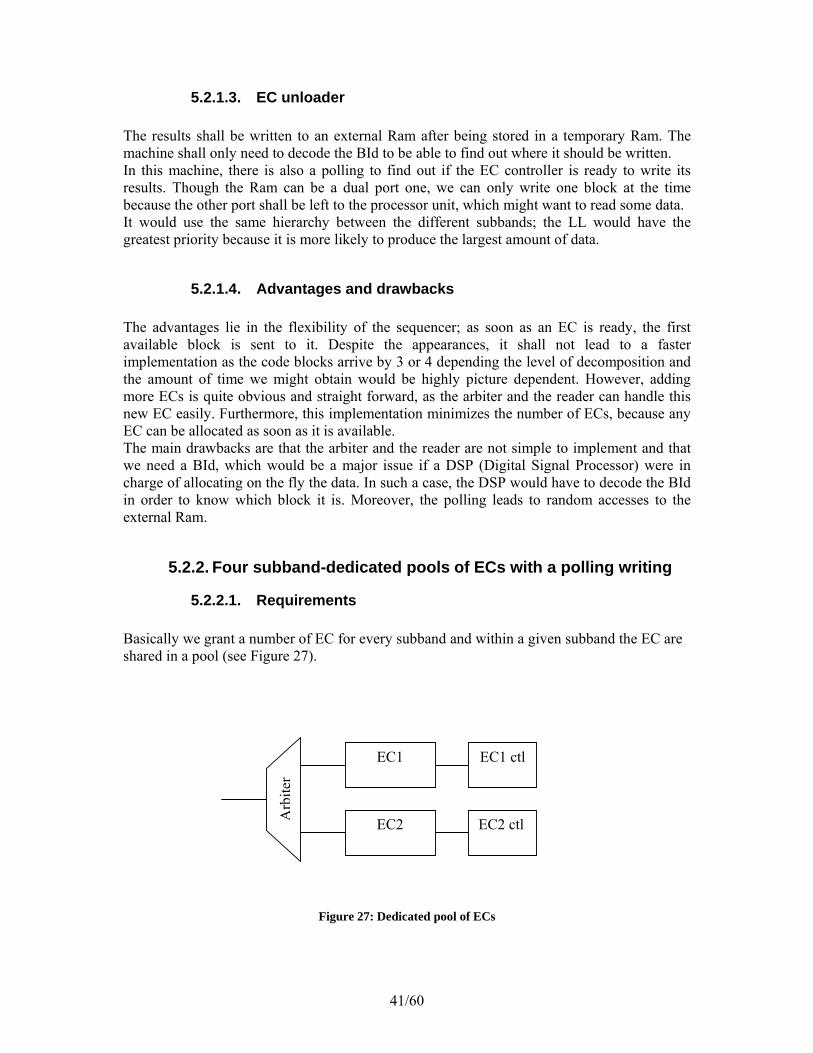
5.2.1. Global pool of ECs

5.2.1.1. Requirements This implementation has a global pool of ECs. That means that each EC can process any subband code block. With this implementation, we definitely need BId (Block Identification) to identify a block so as to write at the right place the correct data and to trace where the blocks are. Such identification would then be a data structure that contains a block number, a level of decomposition and the subband information. To write the data in the external memory, we shall use a polling to detect whether the EC has finished its computations. As it needs a BId, we have to keep track of which blocks are in the flow. That means that we need a register structure that looks like the real flow: there would be DWT registers, quantization registers, EC registers. And inside those registers, we would be storing the BId to track down the blocks.

5.2.1.2. EC arbiter As there is a global pool, the arbiter shall grant every available subband code block that has been output by the DWT to the first available EC. Thus, it shall be a FSM that scan in a round robin way every EC controller to check if they are available or not. We shall use 4 different check units, and the hierarchy to grant an EC shall be LL>LH>HL>HH. This hierarchy is arbitrary but based upon the fact that the LL subband ought to get the most information than the others, and somehow, the HH ought to be the one with the least information. The routine we choose for the checking is rather simple and allows a minimal waiting time: We can check them 4 by 4. In this way the 4 check units work together, but we could also imagine a solution that would be based upon the same hierarchy with 4 independent check units. The arbiter shall read the quantization registers and write into the EC registers. It writes the values corresponding to the data sent to the EC.

41/60

5.2.1.3. EC unloader The results shall be written to an external Ram after being stored in a temporary Ram. The machine shall only need to decode the BId to be able to find out where it should be written. In this machine, there is also a polling to find out if the EC controller is ready to write its results. Though the Ram can be a dual port one, we can only write one block at the time because the other port shall be left to the processor unit, which might want to read some data. It would use the same hierarchy between the different subbands; the LL would have the greatest priority because it is more likely to produce the largest amount of data.

5.2.1.4. Advantages and drawbacks The advantages lie in the flexibility of the sequencer; as soon as an EC is ready, the first available block is sent to it. Despite the appearances, it shall not lead to a faster implementation as the code blocks arrive by 3 or 4 depending the level of decomposition and the amount of time we might obtain would be highly picture dependent. However, adding more ECs is quite obvious and straight forward, as the arbiter and the reader can handle this new EC easily. Furthermore, this implementation minimizes the number of ECs, because any EC can be allocated as soon as it is available. The main drawbacks are that the arbiter and the reader are not simple to implement and that we need a BId, which would be a major issue if a DSP (Digital Signal Processor) were in charge of allocating on the fly the data. In such a case, the DSP would have to decode the BId in order to know which block it is. Moreover, the polling leads to random accesses to the external Ram.

5.2.2. Four subband-dedicated pools of ECs with a polling writing

5.2.2.1. Requirements Basically we grant a number of EC for every subband and within a given subband the EC are shared in a pool (see Figure 27).

Arb

iter

EC1 EC1 ctl

EC2 EC2 ctl

Figure 27: Dedicated pool of ECs

42/60

We also need a block identification (BId) in order to write the data at the correct location in the external Ram. As it needs a BId, we have also to keep track of which blocks are in the flow. That means that we also need a register structure that looks like the real flow: there would be DWT registers, quantization registers, EC registers.

5.2.2.2. EC arbiter The arbiter shall be pretty much the same than in the previous implementation (see section 5.2.1) except that the arbiter would be simpler due to the fact that only 1 block is incoming per subband. Every subband shall be granted a fixed number of ECs and there would be 4 arbiters, one for each subband. It would only have to find out if one of the ECs is ready to get one block. That would lead to 4 independent FSMs, which check the status of their respective ECs, and read and write their respective registers.

5.2.2.3. EC unloader It would be the same than in the section 5.2.1.3. It would be a polling machine that checks the status of all the EC controllers and writes the results into an external RAM at an address decoded from the BId.

5.2.2.4. Advantages and drawbacks It has globally the same drawbacks than the previous implementation. However, the arbiter may be a bit simpler but we have to use more ECs in order to reach our objectives. We need a fixed number of ECs per subband to cope with the flow, even for the LL if we consider that forcing a one level decomposition is an option. One advantage would also be that as soon as an EC is ready to receive a block, it is more likely to get one because of the dedicated pools by subband.

5.2.3. Four subband-dedicated pools of ECs without a polling writing

5.2.3.1. Requirements The arbiter in this case would even simpler; it is based on dedicated polls of ECs. This approach would not need a BId and we would just insure that the order of the code blocks is respected. We do not know which blocks are being processed, as shown in Figure 27, the arbiter only insures us that assuming there are 4 consecutive blocks, then the first and the third are mapped to the former EC, while the second and the fourth are mapped to the latter EC (in the example of Figure 27). We cannot know though if they belong to the same level of decomposition.

43/60

5.2.3.2. EC arbiter The arbiter is very simple in this case; it is just a mere FSM that keeps a pointer on the next EC that shall be fed or the last one that was fed (we shall stick to the former choice for the rest of the study). With this implementation, adding one new EC is just adding a state in the FSM. Assuming we have a block that shall be sent to the second EC, we shall wait until the EC is ready to sample a new block even if there is another EC, which is ready. We have to respect this requirement in order to preserve the order of the blocks.

5.2.3.3. EC unloader The writing machine is now different than the polling machine we have seen previously. Now, we would build a systematic machine, which unload every EC results at a determined time. This time would be the time at which the last EC of the pool was loaded incremented by the maximal amount of time the EC needs to process a block. At this specific time we are sure that every EC of the pool is finished and that the results are waiting to be written. This is the critical item of the implementation. As the implementation only insures a local timing coherence, we need an address generator that is able to detect the shift between the levels of decomposition.

5.2.3.4. Advantages and drawbacks The main issues would be:

• To know where to write the data, because there is no BId • To handle the 4 different subband writing processes

To deal with the latter issue, one may think of attributing levels of priority between the subbands, like HH>HL>LH>LL. One should notice that this might lead to a lot of waste time waiting for the writing of the result. This time may affect the global speed of the system, as the DWT might have to stall. Some stalling can be avoided if we double the temporary RAM, which we obviously do. Nevertheless, some stalling may happen due to the fact that the mapping of tile blocks to an EC is not flexible. To answer the former issue, we need an address generator that remembers where we last wrote something for each subband and which level we stand. It shall also be able to find out if a complete level of decomposition has been processed and then re-compute a new address for the next level. A general view of the memory mapping is given in Figure 25.

5.3. Entering the sequencer As we have seen previously, there were 3 options and we chose the last one as the most likely to be implemented, the one with a dedicated pool and a deterministic unloading. We are to focus more deeply into the different modules in this part so as to point out the main issues and how to solve them.

44/60

5.3.1. The address translator

5.3.1.1. Why should we need one? In order to have a modular component and to be able to use it in various ways, we may want to deal with pictures, which size is larger than 720 x 576. That is where the concept of tiling becomes so important; it allows the fragmentation of the original picture into smaller pieces, which shall be encoded independently. We would use that, if we want to use the component on larger picture. Thus, the processor shall give us at least a start address of the tile (the address of the top left corner) and the pitch of the picture, as the fragmentation ought to be done by the software. However, the tile size is a fixed parameter.

Pitch

Start address

Figure 28: Tiling fragmentation

5.3.1.2. Virtual Address Space To locate a block at a level of decomposition, we consider a grid formed by the blocks 64x64 (or less on the right and bottom edges) and we use the coordinates row number and column number. Here an example of how we consider the current decomposition input picture (see Figure 29). We are forced to use an abstraction layer in the addresses, so every module within the sequencer will deal with a virtual address, and there must be an address translator to get the real address. As we receive from the processor a pitch and a starting address, we shall manage to convert the virtual address into the real address. The local address within the block is a 12-bit address; the 6 most significant bits are called Ma and the 6 least significant La.

45/60

64

64

Block StartAddress

0 1 2 3 4 5 6 7 8

0

1

2

3

4

5

6

Row Col

Address within the block

Virtual address Ma La

2 7 0 0

Figure 29: Grid and virtual address

We have arbitrarily constrained the virtual address to 20 bits. The main reasons are the following:

• For the targeted application we need up to 10 blocks per row, this implies that we must have at least 4 bits for the number of rows.

• To handle square pictures we force the same amount of bits for the number of columns.

• A maximal tile which size is 1024x1024 was good enough and doesn't appear like a heavy restriction for most applications. However, this can be changed for particular application if bigger tiles are required.

Eventually the virtual address will be: Field Row Col Ma La Number of bits

4 4 6 6 Total 20 bits

5.3.1.3. Shift back to the real address space The main goal of the address translator is to perform the translation from the virtual address space into the real address space. Actually, the sequencer is to use 2 different virtual address spaces: the former is for the feeder and the reading of the input for the DWT module; the latter is for the unloader and the writing of the compressed data and the information into an external Ram. So there shall be 2 independent translators that run in parallel within the module. Their functionality is the same; it is just not the same parameters.

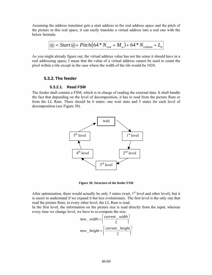
46/60

Assuming the address translator gets a start address in the real address space and the pitch of the picture in this real space, it can easily translate a virtual address into a real one with the below formula:

( ) acolumnarow LNMNPitchStart ++++= *64*64.@@ As you might already figure out, the virtual address value has not the sense it should have in a real addressing space, I mean that the value of a virtual address cannot be used to count the pixel within a tile except in the case where the width of the tile would be 1024.

5.3.2. The feeder

5.3.2.1. Read FSM The feeder shall contain a FSM, which is in charge of reading the external data. It shall handle the fact that depending on the level of decomposition, it has to read from the picture Ram or from the LL Ram. There should be 6 states: one wait state and 5 states for each level of decomposition (see Figure 30).

wait

1st level

2nd level

3rd level

4th level

5th level

Figure 30: Structure of the feeder FSM

After optimization, there would actually be only 3 states (wait, 1st level and other level), but it is easier to understand if we expand it but less evolutionary. The first level is the only one that read the picture Ram; in every other level, the LL Ram is read. In the first level, the information on the picture size is read directly from the input, whereas every time we change level, we have to re-compute the size.

⎥⎥⎤

⎢⎢⎡=

⎥⎥⎤

⎢⎢⎡=

2__

2__

heightcurrentheightnew

widthcurrentwidthnew

47/60

5.3.2.2. Local toolbox The feeder handles the feeding of the DWT block so it shall need a lot of little blocks that compute some basic functions in order to send correct information. This paragraph shall enumerate the most important ones.

• Find out the number of blocks per line and per column in this level of decomposition Those numbers are quite easy to compute as 64 is a power of 2 and we are looking for the number of 64x64 blocks. We have arbitrarily limited the number of bits to 4 for both numbers as we have seen previously. But, it might be changed if the application requires tiles to be larger.

[ ][ ]0:1?)0]0:5[(6__

0:1?)0]0:5[(6__>+>>=

>+>>=HeightHeightheightblockNb

WidthWidthwidthblockNb

• Find out the number of blocks in this level of decomposition

We just have to multiply the previous 2 numbers.

• Find out the size of the block we are to send to the DWT module

The default value is 72x72, which means that the original size of the block was 64x64. So we can implement the following pseudo code:

BlWidth = 72; BlHeight = 72; If(Width[5:0]!=0 AND count_col == Nb_block_width –1) BlWidth = Width[5:0] + 8; If(Height[5:0]!=0 AND count_row == Nb_block_height –1) BlHeight = Height[5:0] + 8;

• Find out if there is some symmetry we should do

One shall notice that there are tricky cases where we might have to do a symmetry operation on blocks that are not at the edges. We are to do the symmetry from the edge of the picture or the tile and not from the edge of the tile block.

If(startAddress.row == 0) Symmetry.top = TRUE; else Symmetry.top = FALSE; If(startAddress.col > Height – 68) Symmetry.bottom = TRUE; else Symmetry.bottom = FALSE; If(startAddress.row == 0) Symmetry.left = TRUE; else Symmetry.left = FALSE; If(startAddress.col > Width – 68) Symmetry.right = TRUE; else Symmetry.right = FALSE;

48/60

5.3.2.3. Read address generator This is one of the biggest issues in the sequencer. It is such a big issue because we have to deal with the possible symmetries. Firstly, let's recall the basic rules about the symmetry operations.

• The main basic rule is : within a tile, if the data exist (i.e. there are tile blocks around the current block) we have to use this data, else we have to perform a symmetry

• What is meant with the terms symmetry is a mirroring of data with reference to the edge of the tile

As it is illustrated in the Figure 31, the boundary conditions are centered on the tile block we want to send to the DWT module.

Tile block to be transformed

Boundary conditions

Figure 31: boundary conditions of the tile block

Let's assume we consider an NxM tile block, which doesn’t need any symmetry. Then, the tile block, we have to send to the DWT module, is centered on the NxM tile block and has a size is (N+8)x(M+8). As there is no symmetry to perform, we have to send existing data that belong to the surrounding blocks. The figures below will illustrate what we have to do in such a case, when we have a left symmetry and when we have a top symmetry ; the number refers to the reading order (see Figure 32, Figure 33 and Figure 34). As we mentioned earlier, the symmetry is done from the edge of the tile.

49/60

Picture block

1 2 3 4 5 6 7 8 Without any symmetry operation

Figure 32: Read sequence without symmetry operation

Picture block

1 2 3 4 5

6 7 8 With a left symmetry operation

Figure 33: Read sequence with a left symmetry operation

50/60

Picture block

1 2 3 4 5 6 7 8

With a top symmetry operation

Figure 34: Read sequence with a top symmetry operation

5.3.2.4. Local knowledge The feeder shall have access to:

• A signal that indicates that the DWT is ready to sample a new block • The original tile size • The number of decomposition requested by the user

It shall:

• Compute the current decomposition level, and thus indicates to the dataflow if the data that belongs to the LL subband shall be written in the LL Ram or sent to the quantization.

• Compute the total number of blocks, the amount by row and by column in the current level of decomposition

• Find out the size of the tile block that is to send • Find out if there is some symmetry to perform for the current block • Compute the virtual addresses for the writing in the external Ram • Compute the virtual read addresses for the reading of the tile block

It shall drive:

• The current decomposition signal and a signal that indicates if it is the last level of decomposition

• The virtual address for reading • The starting addresses for the output external ram • The block width and block height signals for the size of the tile block • A signal that indicates that the data at the input of the DWT module is valid

51/60

5.3.3. The DWT watcher

5.3.3.1. Function The DWT watcher is a small module. Its only role is to send the quantization parameters when we change the level of decomposition. But it shall change it only when the first tile block corresponding to the new decomposition level is processed by the 2nd stage of the DWT and is about to go through the quantization module.. Besides, the DWT watcher shall generate the write addresses for the LL RAM. Those addresses do not need a translation because there is only one tile being processed at the time. Therefore, it does not need any virtual address space. The basic idea is to overwrite the previous data with the new data, there will not be any trouble because the size of the LL subband in the next level of decomposition is a quarter of the LL subband size at the current level of decomposition.

5.3.3.2. Local knowledge It shall have access to:

• The quantization parameter table • The dynamic • The size of the next LL subband • The starting address for the write of current block • The size of the current block (to compute the LL contribution)

The processor communication unit drives both signals about quantization. The feeder shall give the rest of the information. It shall receive to:

• The level of decomposition (given by the feeder module) • A signal that indicates when it has started the 2nd stage of the transformation (given by

the DWT module) It shall drive the quantization parameter signals and the dynamic signal to the quantization module, and the write address for the LL Ram and the associate enable signal.

5.3.4. The EC arbiter

5.3.4.1. Function The arbiter is quite an independent module inside the sequencer. Actually, it is 4 different arbiters that we join into a global module. Its main function is to grant an EC to the code blocks, which are temporary, stored after the quantization. As we have seen in §5.2.3.2, the arbiter has a quite simple function, it shall be implemented as a FSM, which state determine the EC to grant:

52/60

Grant EC1

Grant EC2

Grant EC3

Figure 35: Structure of the FSM for the arbiter

In this way, we can insure a deterministic sequence. Adding new ECs means adding more states; so it is not a major issue.

5.3.4.2. Local knowledge The arbiter shall be able to know the status of the temporary Ram ( located after the quantization) that is linked to it, the status of the EC controller, which is the next to be loaded. Thus, every independent arbiter shall have access to:

• A signal that indicates whether that Ram is empty or not • The signals from the EC controllers that indicates we can store the results of a new

block • The EC ready signals

Here is one small point, which needs to be emphasized: Among the signals driven by the EC, there are 2 control signals, EC_Ready and EC_Finish. The former is a signal that indicates that the EC is likely to receive one coefficient. It may be active as soon as the coefficient bit modeling is over. In other words, the EC may ask for a new block before that the processing of the current block ends. The latter is a signal that indicates that a complete processing is finished, but it doesn't mean that the EC is not already processing the next block. Actually, it means that the arithmetic encoding is over. As you may recall, the EC processing has two main steps: the coefficient bit modeling and the arithmetic encoding. Thus, our implementation will only focus on the EC_Ready signals because we are also sensitive to a post-EC controller's signal, which indicates that at least one of the 2 temporary Rams is free. We can decide if a new block can be sampled just with these 2 signals. Though, the EC_Finish may be used by the controller to determine if we have reached the end of the processing and if needed flush its buffers. Every independent arbiter shall drive for its own pool:

• A signal that select the routing between the incoming data and the selected EC

53/60

• The corresponding signal that would activate the reading of the Ram located before the EC

5.3.5. The EC unloader

5.3.5.1. Function The EC unloader shall generate the virtual addresses used to the storage of the compressed data and of the encoding information into an external Ram. It shall receive the start addresses of all the areas (see Figure 25) at the beginning of the tile processing. In the worst case, the EC does not compress anything and thus the maximal output data is 1024 16-bit coefficients. In order to handle every possibility, we have to allocate this amount of memory for every code block. Once again, we are using a virtual address space within the EC unloader; the address translator is in charge of the translation into the real address space.

5.3.5.2. Local knowledge The EC unloader shall have access to:

• The table of start addresses for all the subbands ( there are 2 sets: the former for the data, the latter for the information)

• The EC_Finish signals from all the ECs • A signal that indicates if it is the last level of decomposition: if it is the last level, that

means that the LL subband has data, therefore we have to check also the status of these dedicated ECs to know if the unload can be performed. Otherwise, the status of the LL ECs shall be ignored.

It shall keep:

• The last addresses that have been written to (8 addresses)

It shall drive:

• A tile finish signal that indicates the end of the tile processing • A read signal to indicate one EC controller that it shall enter the reading state • A select signal to select the EC to be unloaded • An address which is virtual but shall be translated before being output of the

sequencer

5.3.5.3. Implementation solutions To make it as simpler as it could be, we plan to force the EC controller and thus the EC unloader to go through all the addresses within the possible space allocated to a code block. This means the following: assuming a 32x32 code block, the compressed data is 523 octets, which should be compared to the 2048 it might have produced in the worst case, and the number of passes is 29 (the maximal number of passes would be 43 due to our EC implementation when the dynamic is 16 bits). The temporary ram, which stores the results, would not be full. When the unloading time occurs, we would be tempted to optimize the

54/60

transfer, just by allowing the valid data to be sent. However this would lead to a bigger complexity that might cost an unbearable hardware overhead. Therefore, we plan to use a deterministic unloading and the whole contents, even if it is not valid. The unloading time ought to be 2048+218 (2266) cycles, as it should not lead to a huge waiting time. As it keeps the table with all the starting addresses, it shall know that a level of decomposition is over for a given subband, when the next address for the next code block in this subband equals the starting address of another subband at the same level of decomposition (see Figure 36). In the below figure, we know that the HH subband at the 1st level of decomposition is finished when the current address HH1 (big red arrow) equals the starting address HL1.

HH 1

HL 1

Start address HH1

Current address HH1

Starting address HL1

Start address LH1

Figure 36: Illustration of the address space

5.3.6. The communication unit

5.3.6.1. Function This module shall handle the communication with the microprocessor. Basically, it shall receive parameters at the beginning of every tile and warn the processor that the tile processing is completed. Due to the mapping between hardware and software of the JPEG2000 encoder, there is no need of a lot of communication between the software and the hardware. Both areas are distinct and they occur sequentially, without a lot of communication. That explains why this module is really simple.

5.3.6.2. Local knowledge The processor shall give the following information before the beginning of a new tile:

• The tile width and height • The dynamic of the tile

55/60

• The number of decomposition in the wavelet transform • The pitch and start address of the tile in the input memory • The reversibility of the transform and the DWT coefficients • The EC options • The two start addresses of the memory that stores the compressed data and the

information from the EC. They are used to compute the start addresses of every subband with their level of decomposition

• The quantization parameters for every subband and every level of decomposition. Every parameter is a 16-bit coefficient

Besides, the module raises a signal to indicate that the processing of the tile is over; the most probable would be that it generates an interruption for the processor.

56/60

6. Conclusion Eventually, the whole dataflow is developed, implemented and validated. The VHDL model is bit-true with the reference software. The performance requirements are met for the whole aggregate. Although the main results are obtained after the synthesis step and are not very reliable, the results after the place and route step on a older technology are optimistic as the frequency almost reaches the required frequency. Moreover, the area space needed for the implementation of this aggregate is not too large in terms of multipliers, Ram blocks and LUTs. Besides, the sequencer has been studied and it needs to be developed, validated and integrated. After that, there would still be some development to make the hardware and the software interact as we planned. The integration is not an easy part, but as the interaction is not that important, it should not be so hard. However, this shall not prevent us from thinking about what could be done in order to improve and include other features. In the possible evolutions, I was thinking about 2 main ideas: the ROI implementation and the ability of creating clusters of encoders.

6.1. ROI implementation Basically, it is the ability to select one or several area of the image so that they shall be encoded at a higher level of quality relative to the rest of the image (called background). First, a binary mask has to be created in the wavelet domain, this mask corresponds to the area that have been selected. This mask is trivial, the coefficient has a value of one if it is inside the ROI and zero otherwise. Prior to the entropy coding, the bitplanes of coefficients belonging to the ROI mask are shifted up by a desired amount that can vary from one ROI to another within the same image. Therefore, the coefficients shall be encoded first and they would appear in the beginning of the compressed data. Of course, some additional information needs to be stored in the code-stream so that the decoder can work properly. The below figures illustrate this. In the imagined implementation there is no real ROI implementation. Surely, one can be faked using the tiling. This would mean that it is far from being optimum. So what I was suggesting previously, is that with minor changes in the software, we can emulate a basic ROI implementation. The main restriction would be:

• Rectangular shape only • Only one ROI would be highly recommended

Basically, the ROI would become the basic tile, and the whole splitting would be performed with this base. The software shall be in charge of modeling the quantization parameters and the rate allocation so that the ROI encoding would take place. The main drawback would be that the tiling might be too important, so block artifacts might appear. A better solution might be to work on ROI encoding that happens after the EC.

57/60

Coefficientsincludedin ROI

Figure 37: ROI shift up

ROI

Figure 38: ROI example

6.2. Clusters It is based of the fact that the FPGA might have 2 available processor cores, though we plan to only use one of them. Basically, if the application requires a very important flow to be encoded, I would think of Digital Cinema or satellite application, where the image can be very large and/or the number of components can be high. The standard [1] allows up to 38-bit inputs and up to 16384 components. In these critical cases, if we want to still have a comfortable image rate then we shall need several encoders that work in parallel within a global cluster. The main issue with clusters is the communication between the units. My guess

58/60

would be to implement is as a network. One unit might be the one that coordinate the others or an external resource can do that. Anyhow, the other core shall be used to handle the communication with the others and the external world. Eventually, the idea would be: if it is not fast enough, you just have to plug another board (or to add an encoder on the board, but it is less flexible) and the image rate increases.

59/60

7. Glossary Acronyms Meaning

BId Block Identification bpp Bit per pixel CBM Coefficient Bit Modeling DCT Discrete Cosine Transform DWT Discrete Wavelet Transform EC Entropy Coder FPGA Field Programmable Gate Array FSM Finite State Machine ICT Irreversible Color Transform IMSB Insignificant Most Significant Bit IP Intellectual Property JPEG Joint Photographic Expert Group LUT Look Up Table LSB Least Significant Bit MSB Most Significant Bit MSE Mean Square Error qtt2ec Quantization to EC module (it is the EC abstraction module) RAM Random Access Memory RCT Reversible Color Transform ROI Region Of Interest ROM Read Only Memory RTL Register Transfer Logic SDTV Standard Definition TeleVision SQ Signal Quantization VHDL Very high speed Hardware Description Language

60/60

8. References [1] JPEG 2000 Image Coding System, ISO/IEC 154444-1 – last revised July 24th, 2002 [2] Coding of Still Pictures, An overview of the JPEG 2000 Still Image Compression Standard, M.Rabbani and R.Joshi, ISO/IEC JTC 1/SC 29/WG1 N2233 - July 19th, 2001 [3] The JPEG 2000 Still Image Coding System: An Overview, C.Christopoulos, A.Skodras and T.Ebrahimi – November 2000 [4] The JPEG-2000 Still Image Compression Standard, M.D.Adams – December 25th, 2002 [5] JPEG2000 Coding of still pictures: Guard Bit Requirements for JPEG2000 Part 1 Filters, J.Hara, ISO/IEC JTC 1/SC 29/WG 1 N2133 [6] JPEG 2000: The next generation still image compression standard, C.Christopoulos, A.Skrodras, Ericsson presentation Wikipedia site: http://en.wikipedia.org