École Centrale de Nantes MASTER ARIA - ROBA “AUTOMATIQUE, ROBOTIQUE ET INFORMATIQUE APPLIQUÉE” 2015/ 2016 Thesis Report Presented by Muhammad Qumar Zaman Tufail On 30 / 08 / 2016 Title Visual Servoing of a High Speed Parallel Robot Jury President: Philippe Martinet Professor, Ecole Centrale de Nantes Evaluators: Sebastien Briot Full-time CNRS researcher at IRRCyN Philippe Martinet Professor, ECN Olivier Kermorgant Assistant Professor, ECN Abdelhamid Chriette Assistant Professor, ECN Supervisors: Sebastien Briot and Olivier Kermorgant Laboratory : Institut de Recherche en Communications et Cybernétique de Nantes

Welcome message from author
This document is posted to help you gain knowledge. Please leave a comment to let me know what you think about it! Share it to your friends and learn new things together.
Transcript

École Centrale de Nantes
MASTER ARIA - ROBA
“AUTOMATIQUE, ROBOTIQUE ET INFORMATIQUE APPLIQUÉE”
2015/ 2016
Thesis Report
Presented by
Muhammad Qumar Zaman Tufail
On 30 / 08 / 2016
Title
Visual Servoing of a High Speed Parallel Robot
Jury
President: Philippe Martinet Professor, Ecole Centrale de Nantes
Evaluators: Sebastien Briot Full-time CNRS researcher at IRRCyN
Philippe Martinet Professor, ECN
Olivier Kermorgant Assistant Professor, ECN
Abdelhamid Chriette Assistant Professor, ECN
Supervisors:
Sebastien Briot and Olivier Kermorgant
Laboratory : Institut de Recherche en Communications et Cybernétique de Nantes
Abstract
This thesis work is aimed at investigating the possibilities of controllinga high speed parallel robot using computer vision techniques. For thispurpose, different methods that have been proposed in the literature, arestudied.Different possibilities like controlling by observation of leg directionsand leg edges are considered here. The efficacy of these models with andwithout noise has been studied.
For the purposes of simulation, a model of the robot has been de-veloped in ADAMS and linked with MATLAB/Simulink in order tocontrol. At the end of the thesis work, reader can get an idea that thecontrol of parallel robot using vision is indeed an innovative and usefulway and the information provided can be used to further improve the results
2
Contents
List of Figures 5
1 Introduction 81.1 Structure of the report . . . . . . . . . . . . . . . . . . . . . . 81.2 Objective . . . . . . . . . . . . . . . . . . . . . . . . . . . . . 9
2 Pose and Velocity 122.1 Pose in robotics literature . . . . . . . . . . . . . . . . . . . . 132.2 Pose estimation using vision . . . . . . . . . . . . . . . . . . . 15
2.2.1 Estimating Pose . . . . . . . . . . . . . . . . . . . . . 182.2.2 Velocity estimation . . . . . . . . . . . . . . . . . . . . 19
3 State of the art in Robotics 203.1 Concept of a robot . . . . . . . . . . . . . . . . . . . . . . . . 203.2 Classification of robots . . . . . . . . . . . . . . . . . . . . . . 21
3.2.1 Serial robotic architectures . . . . . . . . . . . . . . . 213.2.2 Parallel Robotic architectures . . . . . . . . . . . . . . 22
3.3 Classical Control algorithms . . . . . . . . . . . . . . . . . . . 263.3.1 PID Control . . . . . . . . . . . . . . . . . . . . . . . 263.3.2 Computed Torque Control . . . . . . . . . . . . . . . . 26
3.4 Joint space or Cartesian space . . . . . . . . . . . . . . . . . . 28
4 Vision Based Control 304.1 Basics of Vision based control . . . . . . . . . . . . . . . . . . 314.2 Different techniques in visual servoing . . . . . . . . . . . . . 31
4.2.1 Image based visual servoing . . . . . . . . . . . . . . . 314.2.2 Position based visual servoing . . . . . . . . . . . . . . 32
4.3 Vision based computed torque control of parallel kinematicmachines[2] . . . . . . . . . . . . . . . . . . . . . . . . . . . . 33
4.4 Problems with vision based control . . . . . . . . . . . . . . . 34
3
4.5 MIMO predictive controller . . . . . . . . . . . . . . . . . . . 354.6 Techniques based on Regions of Interest acquisition . . . . . . 36
4.6.1 3D Pose and Velocity Visual Tracking Based on Se-quential Region of Interest Acquisition[3] . . . . . . . 36
4.6.2 Efficient High-speed Vision-based Computed TorqueControl of the Orthoglide Parallel Robot [19] . . . . . 41
5 Visual servoing using legs observation 435.1 Plucker coordinates for visual servoing . . . . . . . . . . . . . 435.2 Leg Observation . . . . . . . . . . . . . . . . . . . . . . . . . 44
5.2.1 Line Modelling . . . . . . . . . . . . . . . . . . . . . . 445.2.2 Cylindrical leg observation . . . . . . . . . . . . . . . 46
5.3 Simulator Design . . . . . . . . . . . . . . . . . . . . . . . . . 465.3.1 Linking ADAMS and MATLAB/Simulink . . . . . . . 48
5.4 Control Algorithms developed . . . . . . . . . . . . . . . . . . 495.4.1 Leg orientation based visual servoing . . . . . . . . . . 495.4.2 Results without noise . . . . . . . . . . . . . . . . . . 545.4.3 Results with noise . . . . . . . . . . . . . . . . . . . . 585.4.4 Leg edges based visual servoing . . . . . . . . . . . . . 605.4.5 Results without noise . . . . . . . . . . . . . . . . . . 645.4.6 Results with noise . . . . . . . . . . . . . . . . . . . . 69
5.5 Practical Edge detection on robot . . . . . . . . . . . . . . . . 735.5.1 Practical setup . . . . . . . . . . . . . . . . . . . . . . 735.5.2 Camera calibration . . . . . . . . . . . . . . . . . . . . 745.5.3 Technique used for edge detection . . . . . . . . . . . 77
6 Conclusion and Future work proposal 82
7 Bibliography 83
4

List of Figures
2.1 Transformation from frame G to H . . . . . . . . . . . . . . . 142.2 Perspective projection, taken from [10] . . . . . . . . . . . . . 152.3 Pinhole camera with real and virtual images, taken from [10] 162.4 Geometric view of pinhole camera model, taken from [10] . . 162.5 From 3D to image coordinates, taken from [10] . . . . . . . . 17
3.1 Visual description of serial robots, taken from [4] . . . . . . . 213.2 Visual description of Parallel robots, taken from [5] . . . . . 223.3 Comparison of serial and parallel robots,taken from [4] . . . . 243.4 Planar RRRP mechanism in type1 singualrity,taken from [5] . 253.5 Planar RRRP mechanism in type2 singualrity ,taken from [5] 253.6 PID Controller schematic . . . . . . . . . . . . . . . . . . . . 263.7 Computed Torque Controller schematic,taken from[7] . . . . 28
4.1 General schematic for sensor based control,taken from[5] . . 304.2 Cartesian space computed torque control,where ω = X[2] . . 334.3 60mm circle at 3ms−2 achieved by the Cartesian space com-
puted torque control with the forward kinematic model andthe vision-based computed torque control in the XY plane . . 34
4.4 High speed vision system chronogram where processing isbased on the sequential acquisition of small sub-images con-taining the features. . . . . . . . . . . . . . . . . . . . . . . . 37
4.5 Control scheme using ROI acquisition . . . . . . . . . . . . . 404.6 3D trajectories from robot joint sensors and Vision, taken
from [3] . . . . . . . . . . . . . . . . . . . . . . . . . . . . . . 41
5.1 Plucker Coordinates and edges of a cylinder [16] . . . . . . . 455.2 IRSBot-2 Architecture of 1 leg[24] . . . . . . . . . . . . . . . 475.3 ADAMS model of IRSBot-2 . . . . . . . . . . . . . . . . . . 485.4 Simulation setup in simulink . . . . . . . . . . . . . . . . . . 49
5

5.5 IRSBot-2 Schematic . . . . . . . . . . . . . . . . . . . . . . . 505.6 Error on Leg11 . . . . . . . . . . . . . . . . . . . . . . . . . . 555.7 Error on Leg21 . . . . . . . . . . . . . . . . . . . . . . . . . . 565.8 Error on Leg11 . . . . . . . . . . . . . . . . . . . . . . . . . . 575.9 Error on Leg21 . . . . . . . . . . . . . . . . . . . . . . . . . . 575.10 Error on Leg11 . . . . . . . . . . . . . . . . . . . . . . . . . . 585.11 Error on Leg21 . . . . . . . . . . . . . . . . . . . . . . . . . . 595.12 Error on pose of end-effector . . . . . . . . . . . . . . . . . . 605.13 Error on edge1 of Leg11 . . . . . . . . . . . . . . . . . . . . . 655.14 Error on edge2 of Leg11 . . . . . . . . . . . . . . . . . . . . . 665.15 Error on first edge of Leg21 . . . . . . . . . . . . . . . . . . . 665.16 Error on second edge of Leg21 . . . . . . . . . . . . . . . . . . 675.17 Error on first edge of Leg11 . . . . . . . . . . . . . . . . . . . 685.18 Error on second edge of Leg11 . . . . . . . . . . . . . . . . . . 685.19 Error on first edge of Leg21 . . . . . . . . . . . . . . . . . . . 695.20 Error on second edge of Leg21 . . . . . . . . . . . . . . . . . . 695.21 Error on edge1 of Leg11 . . . . . . . . . . . . . . . . . . . . . 715.22 Error on edge2 of Leg11 . . . . . . . . . . . . . . . . . . . . . 715.23 Error on first edge of Leg21 . . . . . . . . . . . . . . . . . . . 725.24 Error on second edge of Leg21 . . . . . . . . . . . . . . . . . . 725.25 Error on pose of end-effector . . . . . . . . . . . . . . . . . . 735.26 Process of Camera Calibration . . . . . . . . . . . . . . . . . 745.27 Reprojection error in pixels . . . . . . . . . . . . . . . . . . . 755.28 Extrinsic visualization . . . . . . . . . . . . . . . . . . . . . . 765.29 Original Image from Camera . . . . . . . . . . . . . . . . . . 775.30 Sub Images from the original . . . . . . . . . . . . . . . . . . 775.31 Edge detection . . . . . . . . . . . . . . . . . . . . . . . . . . 795.32 Sobel Edge detection . . . . . . . . . . . . . . . . . . . . . . . 805.33 Edges (green) and projection-line vectors (red) . . . . . . . . 80
6
Acronyms
POS Pose from orthography and scaling
POSIT POS with iterations
RRRP Revolute Revolute Revolute Prismatic joints
PID Proportional Integral Derivative
DOF Degrees of Freedom
MIMO Multi input Multi Output
ROI Regions of Interest
GS Gough Stewart
STL Stereolithography
IRRCyN Institut de Recherche en Communications et Cybernetique deNantes
7
Chapter 1
Introduction
1.1 Structure of the report
This thesis work is divided into two parts. In part 1 ,basic concepts andtechniques related to robotics,vision, visual servoing and control are pre-sented. In part 2 , the work that has been performed during this project ispresented. In third part, conclusion is presented and possible future work issuggested.
• In chapter 2 , basics of pose and velocity in the robotics literature arecovered. How these parameters can be estimated using vision
• In chapter 3 ,state of the art in Robotics is described. Differentrobotics architectures and different control algorithms available in lit-erature, are described briefly.
• In chapter 4 , the concepts of Vision based control are described. Whatis the basis of such kind of control . What kind of techniques are beingused in literature to achieve vision based control, all this is covered inthis chapter.
• Chapter 5 describes all the work that has been done in the context ofthis project. The results are presented and analyzed.
• Chapter 6 concludes the work done and describes the future work thatcould be done on the basis of this work
8
1.2 Objective
Aim is to propose a vision-based controller for IRSBot-2 , a high speedparallel robot designed at IRCCyN, based on the observation of the legs,rather than using the proprioceptive sensors.
To achieve this objective, during the first phase of this project, bibli-ographic study was performed in order to get acquainted with the workbeing done in this field and algorithms available in literature. In the secondphase of the project, different vision based algorithms have been developedand investigated for the robot.
9

Part 1
10
Preliminary Concepts & Literature Review
11

Chapter 2
Pose and Velocity
Pose and velocity information about a body in space can help understandthe motion of the body better. Pose of a body defines the complete positionand orientation of a body in space. Velocity of a body defines how fast thispose is changing with respect to time. Depending on the physical resourcesavailable, there can be different methods to estimate these parameters.Nature has blessed different organisms with different kind of sensors to helpthem evolve and survive in their respective environments.The animals evolving in the environments where light is not sufficient, tendto use other means. It is necessary for them to localise and estimate themotion of other animals, in order to survive and hunt. They usually usemethods based on sound waves. Equipped with sensors that respond tosound waves, they send sound signals and then capture it back. From thecaptured signal, they are able to localise other animals, how far they areand their motion profile.The animals evolving in suitable light conditions tend to depend more onthe light based sensors,mainly vision. Human beings are also equippedwith vision sensors,in the form of eyes. Our vision system is binocular,because of the difference of position of eyes on the head. The vision systemof humans is a very efficient one,at the same time being a complicated one.
Another technology available for determining the pose and velocity ofan object is RADAR technology. Radar is an object-detection system thatuses radio waves to determine the range, angle, or velocity of objects. Aradar transmits radio waves or microwaves that reflect from any objectin their path. A receive radar, which is typically the same system as thetransmit radar, receives and processes these reflected waves to determine
12

properties of the object(s)[1]. It basically uses the Doppler effect.Based onthe Doppler shifts,it can estimate the velocity of the objects. It is beingused in many different applications in the world,such as:
• Air traffic Control and Air Defence
• Police Department
• Geology
• Weather prediction
To emulate any kind of system in real life, we need to have a thoroughunderstanding of its working. Unfortunately, the vision system of humansis not understandable to a level of being able to completely emulate it. Theissues of processing a huge amount of information while communicatingbetween many different modules in real time is well performed by humans,but not well understood. The artificial correspondence to the naturalsystem of eyes is camera. But there are many issues that need to beaddressed while using the camera,such as:
• Limited Processing power
• Interfacing the camera with other processing units(Brain of the sys-tem)
• Operating frequency of the system
• Accuracy
These and many other issues related to artificial vision system are dealtwith in the field of computer vision. The aim of this project is to extractthe information related to the pose and velocity of an object in a scene, fromthe images provided by the camera,using the field of computer vision. Thenwe can use this information for our purpose (Designing a controller for therobot).
2.1 Pose in robotics literature
Since a robot uses its end-effector to manipulate different objects andinteract with its environment, it is necessary to know the exact coordinates
13
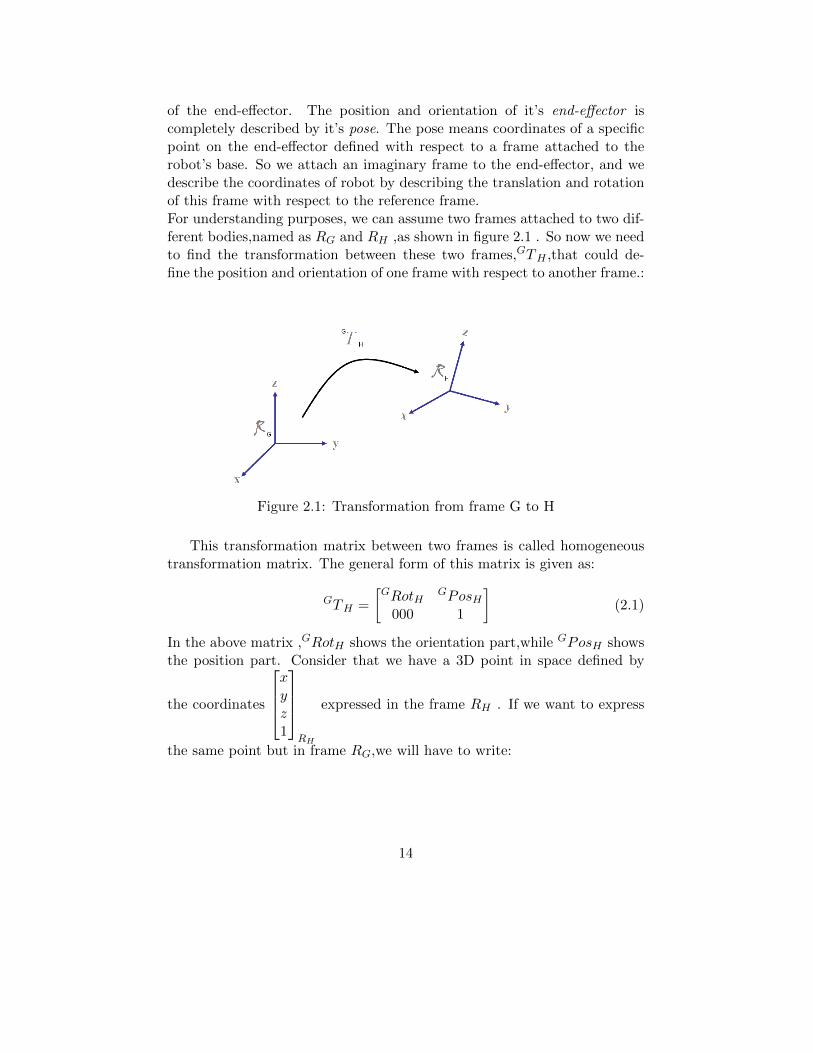
of the end-effector. The position and orientation of it’s end-effector iscompletely described by it’s pose. The pose means coordinates of a specificpoint on the end-effector defined with respect to a frame attached to therobot’s base. So we attach an imaginary frame to the end-effector, and wedescribe the coordinates of robot by describing the translation and rotationof this frame with respect to the reference frame.For understanding purposes, we can assume two frames attached to two dif-ferent bodies,named as RG and RH ,as shown in figure 2.1 . So now we needto find the transformation between these two frames,GTH ,that could de-fine the position and orientation of one frame with respect to another frame.:
Figure 2.1: Transformation from frame G to H
This transformation matrix between two frames is called homogeneoustransformation matrix. The general form of this matrix is given as:
GTH =
[GRotH
GPosH000 1
](2.1)
In the above matrix ,GRotH shows the orientation part,while GPosH showsthe position part. Consider that we have a 3D point in space defined by
the coordinates
xyz1
RH
expressed in the frame RH . If we want to express
the same point but in frame RG,we will have to write:
14
xyz1
RG
= GTH
xyz1
RH
(2.2)
The rotation part of the homogeneous transformation matrix can be definedin several ways. In literature,there exist many different parametrizations ,like Euler angles , direction cosines, quaternions,Bryant angles,Roll pitchyaw angles, Rodrigues’rotation formula etc.
2.2 Pose estimation using vision
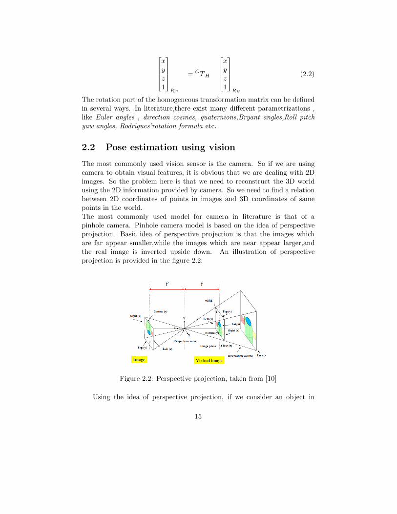
The most commonly used vision sensor is the camera. So if we are usingcamera to obtain visual features, it is obvious that we are dealing with 2Dimages. So the problem here is that we need to reconstruct the 3D worldusing the 2D information provided by camera. So we need to find a relationbetween 2D coordinates of points in images and 3D coordinates of samepoints in the world.The most commonly used model for camera in literature is that of apinhole camera. Pinhole camera model is based on the idea of perspectiveprojection. Basic idea of perspective projection is that the images whichare far appear smaller,while the images which are near appear larger,andthe real image is inverted upside down. An illustration of perspectiveprojection is provided in the figure 2.2:
Figure 2.2: Perspective projection, taken from [10]
Using the idea of perspective projection, if we consider an object in
15
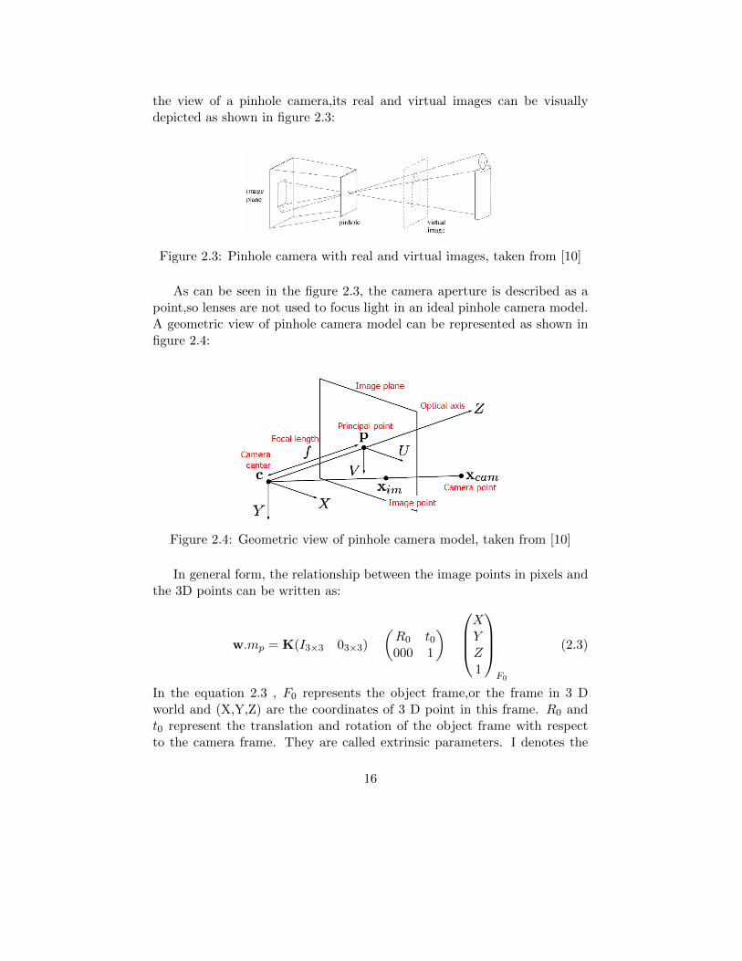
the view of a pinhole camera,its real and virtual images can be visuallydepicted as shown in figure 2.3:
Figure 2.3: Pinhole camera with real and virtual images, taken from [10]
As can be seen in the figure 2.3, the camera aperture is described as apoint,so lenses are not used to focus light in an ideal pinhole camera model.A geometric view of pinhole camera model can be represented as shown infigure 2.4:
Figure 2.4: Geometric view of pinhole camera model, taken from [10]
In general form, the relationship between the image points in pixels andthe 3D points can be written as:
w.mp = K(I3×3 03×3)
(R0 t0000 1
) XYZ1
F0
(2.3)
In the equation 2.3 , F0 represents the object frame,or the frame in 3 Dworld and (X,Y,Z) are the coordinates of 3 D point in this frame. R0 andt0 represent the translation and rotation of the object frame with respectto the camera frame. They are called extrinsic parameters. I denotes the
16

identity matrix. K is the collineation matrix, which is composed of theinertial parameters of the camera. w is the scaling factor ,which is inverselyproportional to the depth of 3 D point.mp are the coordinates of the pointin the image plane, in pixels. The figure 2.5 provides a general overview ofhow we obtained the equation 2.3.
Figure 2.5: From 3D to image coordinates, taken from [10]
The collineation matrix K is a matrix of the following form:
K =
fu γ u00 fv v00 0 1
where:fu, fv:Focal lengths in pixelsγ:Skew factoru0 and v0 :Principal point
Camera calibration
If we define a matrix P, which is composed of intrinsic as well as extrinsicparameters,we can write:
P = K(I3×3 03×3)
(R0 t0000 1
)(2.4)
So equation 2.3 can be written as:
w.mpi = P.mi (2.5)
17
where mpi =
xpiypi1
is the image point of i-th point. mi =
Xi
YiZi1
represents
the 3 D coordinates of i-th point of the object. So P will be a 3× 4 matrix.Hence we need to estimate 12 unknowns,which means that by estmating Pmatrix, we can extract the matrix K, R0 and t0. So from equation 2.5,wecan estimate P , taking number of images n≥ 6 ,knowing the model of objectmi and image coordinates mpi.This was the linear approach for camera calibration. There also exists anon-linear approach. The basic idea behind non-linear approach is that itinitializes from the estimate provided by linear approach. Then a correctionis computed at each iteration until the convergence of the system. Conver-gence of the system is defined by minimization of a chosen criteria.
Distortion
Generally, there exists some distortion when we are considering pinholecamera model. So this also needs to be taken into account. For thispurpose, two kinds of distortions are defined [10]:
• Radial distortion
• Tangential distortion
Radial distortion results because of the failure of a lens to image straightlines as straight lines. It is composed of three components,which can bedenoted as k1,k2 and k3. Tangential distortion is produced when a lens isnot parallel to the imaging plane. It is composed of two components,whichcan be denoted by p1 and p2. In this case, the equation for pinhole cameramodel will be modified to take into account the distortions. The equationis not detailed here. Interested reader can find it in [10].
2.2.1 Estimating Pose
With a calibrated camera, the pose can be estimated using different algo-rithms available in literature. The most commonly used algorithm in caseof non-planar objects is Dementhon algorithm [11] . The basic idea of De-menthon algorithm is this :The algorithm is defined to estimate the pose of a non coplanar object froma single object. The model of object must be known. Four or more non-coplanar feature points of the object are used. In this method, basically two
18
algorithms algorithms are used, namely POS(Pose from orthography andscaling) and POSIT(POS with iterations) .POS algorithm considers a scaled orthographic projection and finds the ro-tation matrix and translation vector by solving a linear system. Scaledorthographic projection means that we assume that all the points on theobject have same depth and we replace Zi for each point by just a valueZ . In POSIT algorithm, first an estimation of pose is obtained using thePOS algorithm. Then in the iteration loop, applies POS to scaled ortho-graphic projections of feature points ,rather than to original image projec-tions. POSIT converges to good accuracy within few iterations. As shown in[11] , POSIT can be written in 25 lines of code in Mathematica. Dementhonalgorithm was used in [2] by Paccot et al. in order to estimate the pose. Thismethod is not feasible in our case, because the required operating frequencyof robot is quite high . So other ways to estimate pose will be explored innext chapters.
2.2.2 Velocity estimation
A precise estimate of velocity along with pose information can help us tounderstand the motion better and design a more efficient controller in termsof twist associated.In literature, even though efficient algorithms exist forpose estimation, but those algorithms do not provide a way to estimatevelocities. In many research works, like [2], velocity estimation is producedby direct numerical differentiation of pose information. THis introducesnoise,which at high speeds could become very high. Hence this way ofcomputing velocity information is not suitable for our cause and alternatemethods will be explored in order to obtain it in a more useful way.
19

Chapter 3
State of the art in Robotics
3.1 Concept of a robot
A robot can be described as a mechanical assembly of different parts whosecombined action allows it to perform motions with a certain degree ofautonomy. It is a programmable device and the region it can operate in, isdefined by its workspace. It is different from automated machines in thefact that it does not necessarily perform same motion again and again andit can be programmed to do different tasks.The different segments or links in a robot are connected to eachother with the help of joints .These joints could be of manytypes,namely,prismatic,revolute,cylindrical,spherical,universal etc. Thetype of joints determine the kind of motion that could be performed. Thecombined effect of these series of segments helps the robot to place andmanoeuvre it’s end-effector in the environment.
While giving us many advantages over automated machines, robotsare limited in their operation by different constraints imposed by physicallimits of different parts being used. This fact makes the design and controlof robots an interesting research and engineering field. While a good designand control algorithm can provide the industry with a very useful tool, theconstraints and limits imposed could also pose a great challenge.In the following sections of this chapter, a general classification of robotswill be described,that is currently being used in literature. Also,differentconstraints imposed by physical parts will be described and different controlstrategies being used will be briefly covered.
20

3.2 Classification of robots
Robots can be generally classified on the basis of types of joints,numberof joints, types of motions that it can perform etc. Here we will describethe two general classifications made in literature,namely serial and parallelrobots. These classifications are made on the basis of the way a robot’s end-effector is connected to it’s base. We will see that both classes have quitedifferent properties and constraints. This fact leads us to adopt differentcontrol strategies for both classes.
3.2.1 Serial robotic architectures
In serial robots, the end-effector of the robot is attached to it’s base withthe help of several links,connected to each other in a serial way. Thisarchitecture is analogous to serial circuits in electrical engineering. A closeresemblance to serial architecture can be thought of a human arm,wherethe links are connected in a serial way. A serial architecture is shown in thefigure 3.1a and a serial robot in 3.1b :
(a) Serial architecture
(b) Serial Robot
Figure 3.1: Visual description of serial robots, taken from [4]
Serial robots are widely used in the industry. The main reason of theirwidespread use is that they have a large workspace and relatively simplestructure.However, serial robots have their own disadvantages. Because of their serialarchitecture , each actuator has to carry the inertia of it’s link as well asinertia of the following links and actuators. This leads to a very high inertiaat the last link and hence relatively small load can be manipulated by the
21
robot. This means that serial robots have high less payload to mass ratio ascompare to their parallel counterparts. Also, the errors tend to accumulatein serial robots because of their architecture. This leads to a reduced accu-racy. These facts urge us to look for alternative solutions and hence the roleof parallel robots becomes very important.
3.2.2 Parallel Robotic architectures
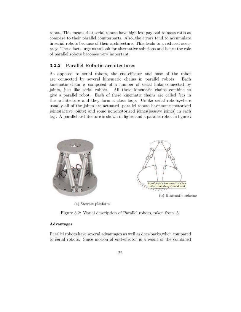
As opposed to serial robots, the end-effector and base of the robotare connected by several kinematic chains in parallel robots. Eachkinematic chain is composed of a number of serial links connected byjoints, just like serial robots. All these kinematic chains combine togive a parallel robot. Each of these kinematic chains are called legs inthe architecture and they form a close loop. Unlike serial robots,whereusually all of the joints are actuated, parallel robots have some motorizedjoints(active joints) and some non-motorized joints(passive joints) in eachleg . A parallel architecture is shown in figure and a parallel robot in figure :
(a) Stewart platform
(b) Kinematic scheme
Figure 3.2: Visual description of Parallel robots, taken from [5]
Advantages
Parallel robots have several advantages as well as drawbacks,when comparedto serial robots. Since motion of end-effector is a result of the combined
22

motion of several light weight kinematic chains, parallel robots are able tohandle weights more than their weights so their payload to mass ratio ishigher. Actuators can be mounted onto the base and this results in fastermovements and light weight kinematic chains.Another advantage of parallel robots is that the errors tend to average outas opposed to the serial case,where they tend to accumulate. Also,becauseof several supporting chains, the stiffness of the structure is high.
Drawbacks
However, parallel robots are not without their disadvantages. Theworkspace of parallel robots is smaller as compared to serial robots.Another disadvantage is that their workspace is constrained by manykind of singularities which leads to a complex design analysis and hence acomplex structure. At a singularity, the robot loses one or more degreesof freedom or the motion in a particular direction becomes uncontrollable.Hence singularity analysis is a major challenge for the designer and effec-tiveness of a robot can be described in terms of singularities in its workspace.
Another drawback is that the forward kinematic model of the parallelrobots is usually complex and does not have an analytical form. Hencewe have to resort to numerical methods which can introduce errors in themodelling and these small errors can lead to major problems in model basedcontrol algorithms. Hence the problem of control of parallel manipulatorsis a research issue and will be briefly covered in the following sections.We can see a non-exhaustive comparison of serial and parallel robots infigure3.3 :
23
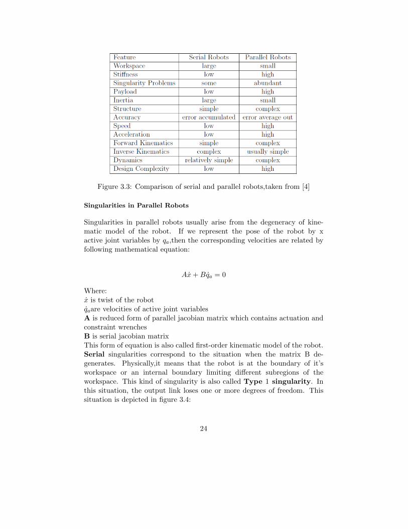
Figure 3.3: Comparison of serial and parallel robots,taken from [4]
Singularities in Parallel Robots
Singularities in parallel robots usually arise from the degeneracy of kine-matic model of the robot. If we represent the pose of the robot by xactive joint variables by qa,then the corresponding velocities are related byfollowing mathematical equation:
Ax+Bqa = 0
Where:x is twist of the robotqaare velocities of active joint variablesA is reduced form of parallel jacobian matrix which contains actuation andconstraint wrenchesB is serial jacobian matrixThis form of equation is also called first-order kinematic model of the robot.Serial singularities correspond to the situation when the matrix B de-generates. Physically,it means that the robot is at the boundary of it’sworkspace or an internal boundary limiting different subregions of theworkspace. This kind of singularity is also called Type 1 singularity. Inthis situation, the output link loses one or more degrees of freedom. Thissituation is depicted in figure 3.4:
24
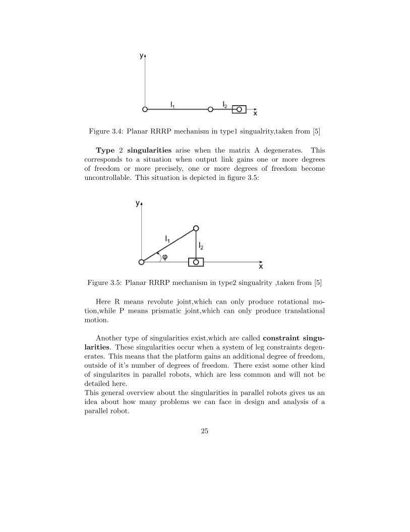
Figure 3.4: Planar RRRP mechanism in type1 singualrity,taken from [5]
Type 2 singularities arise when the matrix A degenerates. Thiscorresponds to a situation when output link gains one or more degreesof freedom or more precisely, one or more degrees of freedom becomeuncontrollable. This situation is depicted in figure 3.5:
Figure 3.5: Planar RRRP mechanism in type2 singualrity ,taken from [5]
Here R means revolute joint,which can only produce rotational mo-tion,while P means prismatic joint,which can only produce translationalmotion.
Another type of singularities exist,which are called constraint singu-larities. These singularities occur when a system of leg constraints degen-erates. This means that the platform gains an additional degree of freedom,outside of it’s number of degrees of freedom. There exist some other kindof singularites in parallel robots, which are less common and will not bedetailed here.This general overview about the singularities in parallel robots gives us anidea about how many problems we can face in design and analysis of aparallel robot.
25
3.3 Classical Control algorithms
3.3.1 PID Control
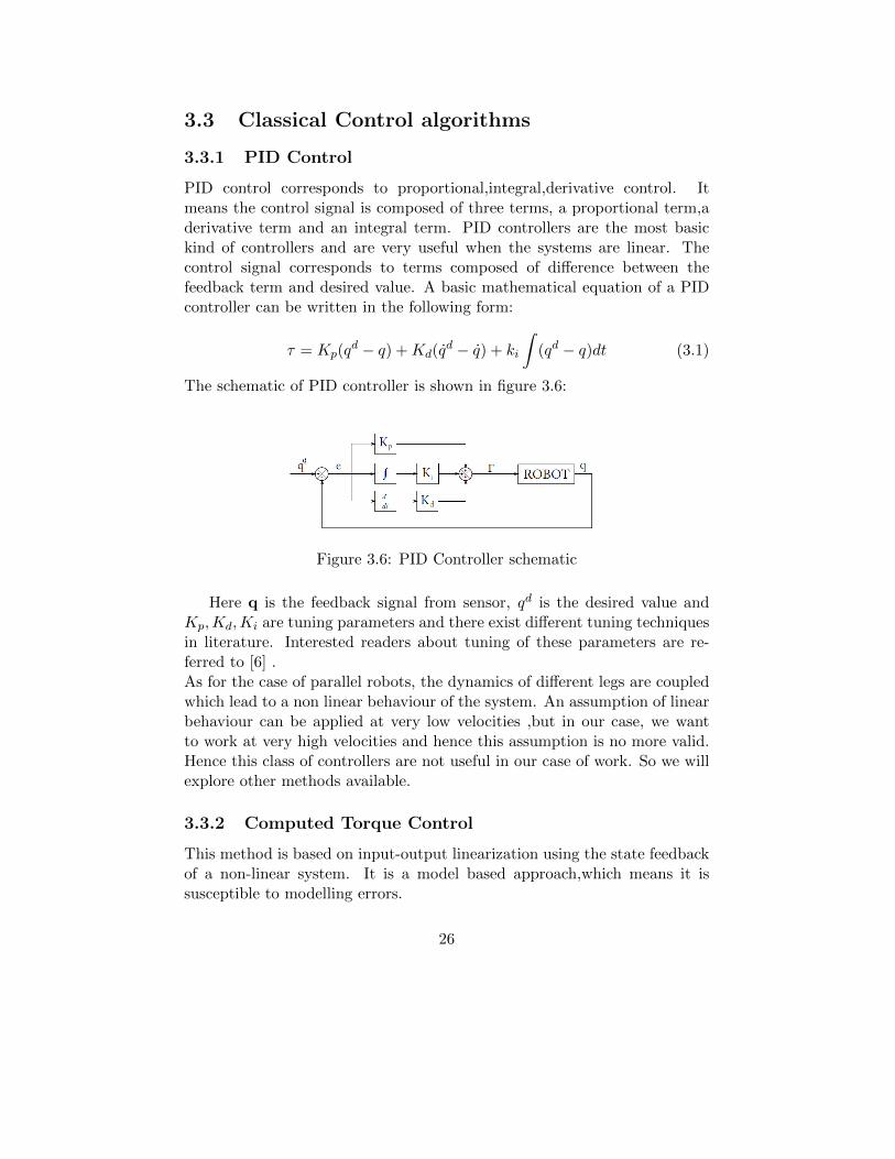
PID control corresponds to proportional,integral,derivative control. Itmeans the control signal is composed of three terms, a proportional term,aderivative term and an integral term. PID controllers are the most basickind of controllers and are very useful when the systems are linear. Thecontrol signal corresponds to terms composed of difference between thefeedback term and desired value. A basic mathematical equation of a PIDcontroller can be written in the following form:
τ = Kp(qd − q) +Kd(q
d − q) + ki
∫(qd − q)dt (3.1)
The schematic of PID controller is shown in figure 3.6:
Figure 3.6: PID Controller schematic
Here q is the feedback signal from sensor, qd is the desired value andKp,Kd,Ki are tuning parameters and there exist different tuning techniquesin literature. Interested readers about tuning of these parameters are re-ferred to [6] .As for the case of parallel robots, the dynamics of different legs are coupledwhich lead to a non linear behaviour of the system. An assumption of linearbehaviour can be applied at very low velocities ,but in our case, we wantto work at very high velocities and hence this assumption is no more valid.Hence this class of controllers are not useful in our case of work. So we willexplore other methods available.
3.3.2 Computed Torque Control
This method is based on input-output linearization using the state feedbackof a non-linear system. It is a model based approach,which means it issusceptible to modelling errors.
26

Considering the general form of dynamic model of a robot,given by equationbelow:
τ = A(q)q +H(q, q) (3.2)
Where:τ is the torqueA(q) denotes the Inertia matrix of the robotq is the set of joint variablesH denotes the matrix taking into account the gravitational,Coriolis andcentrifugal effectsConsidering the torque control law described by:
τ = ˆA(q)w(t) + H(q, q) (3.3)
So a straightforward linearization is obtained by having q = w(t) . Thismeans that the system has become a double integrator. We can considerdifferent cases ,as described in the following sections.
Motion completely specified
In the case,motion is completely specified, means we know the desired jointpositions, velocities and accelerations, we can write the control law as:
w(t) = qd +Kv(qd − q) +Kp(q
d − q) (3.4)
Then:
q = qd +Kv(qd − q) +Kp(q
d − q)
If we write error as:
e = (qd − q)
Then ,using equation 3.3 ,the control signal becomes:
τ = A(qd +Kv e+Kpe) + H(q, q) (3.5)
where:Kv is derivative gain tuning termKp is proportional gain tuning term
27
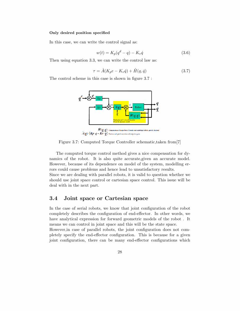
Only desired position specified
In this case, we can write the control signal as:
w(t) = Kp(qd − q)−Kv q (3.6)
Then using equation 3.3, we can write the control law as:
τ = A(Kpe−Kv q) + H(q, q) (3.7)
The control scheme in this case is shown in figure 3.7 :
Figure 3.7: Computed Torque Controller schematic,taken from[7]
The computed torque control method gives a nice compensation for dy-namics of the robot. It is also quite accurate,given an accurate model.However, because of its dependence on model of the system, modelling er-rors could cause problems and hence lead to unsatisfactory results.Since we are dealing with parallel robots, it is valid to question whether weshould use joint space control or cartesian space control. This issue will bedeal with in the next part.
3.4 Joint space or Cartesian space
In the case of serial robots, we know that joint configuration of the robotcompletely describes the configuration of end-effector. In other words, wehave analytical expression for forward geometric models of the robot . Itmeans we can control in joint space and this will be the state space.However,in case of parallel robots, the joint configuration does not com-pletely specify the end-effector configuration. This is because for a givenjoint configuration, there can be many end-effector configurations which
28
correspond to that same joint configuration. For example, in case of Gough-Stewart platform, a single joint configuration may correspond to 40 realconfigurations. So in the case of parallel robots, it is desirable to control incartesian space. This was shown in [8] . Also the superiority of computedtorque control law was shown in this paper.However,as shown previously,computed torque control law is a model basedapproach and hence it is susceptible to errors. In the next chapter, controltechniques which do not depend on models,will be explored.
29
Chapter 4
Vision Based Control
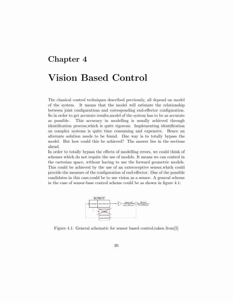
The classical control techniques described previously, all depend on modelof the system. It means that the model will estimate the relationshipbetween joint configurations and corresponding end-effector configuration.So in order to get accurate results,model of the system has to be as accurateas possible. This accuracy in modelling is usually achieved throughidentification process,which is quite rigorous. Implementing identificationon complex systems is quite time consuming and expensive. Hence analternate solution needs to be found. One way is to totally bypass themodel. But how could this be achieved? The answer lies in the sectionsahead.In order to totally bypass the effects of modelling errors, we could think ofschemes which do not require the use of models. It means we can control inthe cartesian space, without having to use the forward geometric models.This could be achieved by the use of an exteroceptive sensor,which couldprovide the measure of the configuration of end-effector. One of the possiblecandidates in this case,could be to use vision as a sensor. A general schemein the case of sensor-base control scheme could be as shown in figure 4.1:
Figure 4.1: General schematic for sensor based control,taken from[5]
30
4.1 Basics of Vision based control
The basic idea in vision based control is to minimize an error defined bythe following equation [9]:
e(t) = s(m(t), a)− s∗ (4.1)
Here s denotes the set of visual features that we are interested in. Itdepends on the set of image measurements,m, as well as the intrinsicparameters or the knowledge about the object model a.s∗ represents thedesired visual featuresIn vision based control,usually a velocity controller is designed based onthe concept of interaction matrix An interaction matrix relates the rate ofchange of visual features with the instantaneous relative motion betweenthe camera and scene. If we denote the interaction matrix by Ls , then wecan write:
s = LsVc (4.2)
Here Vc represents the instantaneous relative motion between the cameraand scene. So it can be defined as Vc =c vc − cvs. Herecvc and cvsrepresent the kinematic screw of the camera and the scene respectively,both represented in camera frame.Then if we want to impose exponential decay of the error,we can writee = −λe . If we assume that desired visual features are not changingwith respect to time, then we can define a velocity controller given by thefollowing equation:
Vc = −λ L+s (s(m(t), a)− s∗) (4.3)
4.2 Different techniques in visual servoing
4.2.1 Image based visual servoing
The basic idea in image based visual servoing is to achieve servoing in theimage. We do not know how the robot will move in 3 D space, we try toachieve convergence in image space. For this purpose, a relation between2D points in the image in pixel coordinates and velocity of camera mustbe defined. This relationship is defined by an interaction matrix. If werepresent image point coordinates in pixels as mp ,from [17]we can write:
31
mp =
−fu/Z 0 u/Z (u ∗ v)/fv −fu − u2/fu (−fu ∗ v)/fv
0 −fv/Z v/Z fv + v2/fv −(u ∗ v)/fu (−fv ∗ u)/fu
Vc
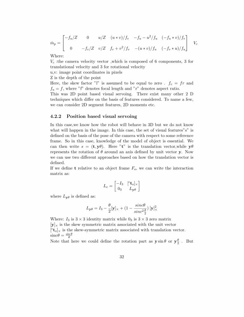
Where:Vc :the camera velocity vector ,which is composed of 6 components, 3 fortranslational velocity and 3 for rotational velocityu,v: image point coordinates in pixelsZ is the depth of the pointHere, the skew factor ”l” is assumed to be equal to zero . fv = fr andfu = f , where ”f” denotes focal length and ”r” denotes aspect ratio.This was 2D point based visual servoing. There exist many other 2 Dtechniques which differ on the basis of features considered. To name a few,we can consider 2D segment features, 2D moments etc.
4.2.2 Position based visual servoing
In this case,we know how the robot will behave in 3D but we do not knowwhat will happen in the image. In this case, the set of visual features”s” isdefined on the basis of the pose of the camera with respect to some referenceframe. So in this case, knowledge of the model of object is essential. Wecan then write s = (t,yθ). Here ”t” is the translation vector,while yθrepresents the rotation of θ around an axis defined by unit vector y. Nowwe can use two different approaches based on how the translation vector isdefined.If we define t relative to an object frame Fo, we can write the interactionmatrix as:
Le =
[−I3 [cto]×03 Lyθ
]where Lyθ is defined as:
Lyθ = I3 −θ
2[y]× + (1− sincθ
sinc2 θ2) [y]2×
Where: I3 is 3× 3 identity matrix while 03 is 3× 3 zero matrix[y]× is the skew symmetric matrix associated with the unit vector[cto]× is the skew-symmetric matrix associated with translation vector.sincθ = sin θ
θ
Note that here we could define the rotation part as y sin θ or y θ2 . But
32
those parametrizations have singularities,while yθ parametrization has nosingularity.
4.3 Vision based computed torque control of par-allel kinematic machines[2]
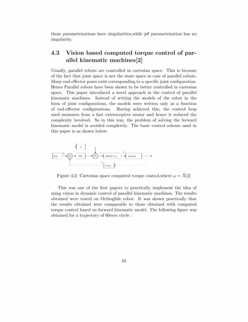
Usually, parallel robots are controlled in cartesian space. This is becauseof the fact that joint space is not the state space in case of parallel robots.Many end-effector poses exist corresponding to a specific joint configuration.Hence Parallel robots have been shown to be better controlled in cartesianspace. This paper introduced a novel approach in the control of parallelkinematic machines. Instead of writing the models of the robot in theform of joint configurations, the models were written only as a functionof end-effector configurations. Having achieved this, the control loopused measures from a fast exteroceptive sensor and hence it reduced thecomplexity involved. So in this way, the problem of solving the forwardkinematic model is avoided completely. The basic control scheme used inthis paper is as shown below:
Figure 4.2: Cartesian space computed torque control,where ω = X[2]
This was one of the first papers to practically implement the idea ofusing vision in dynamic control of parallel kinematic machines. The resultsobtained were tested on Orthoglide robot. It was shown practically thatthe results obtained were comparable to those obtained with computedtorque control based on forward kinematic model. The following figure wasobtained for a trajectory of 60mm circle :
33

Figure 4.3: 60mm circle at 3ms−2 achieved by the Cartesian space computedtorque control with the forward kinematic model and the vision-based com-puted torque control in the XY plane
We can see that the results obtained using visual sensor are comparable.But this method is not useful for our purposes. In this method, Dementhonalgorithm is used for computing the pose and then velocity is derived bysimple numerical derivation. Since we are interested in working at highfrequencies, the numerical derivation is not a useful option in our case, hencethis method will not be useful. Nevertheless, it encourages the use of visionas sensor and with more precise visual sensors and at lower velocities, thismethod can provide useful results.
4.4 Problems with vision based control
Since we have clearly established the advantages associated with using vi-sion based control, we are hopeful to get an improvement in results. Theproblem in vision based control comes when we look into the practical imple-mentation of these techniques. We see that the dynamic control frequencyis usually quite high,in our case we want to operate the robot at 1 kHz. The problem is that we have to synchronize the vision sensor with therobot. The vision sensors usually operate at lower frequencies. Even with
34

high technology cameras, the problem of huge amount of data to be trans-mitted and processed cannot be ignored. Moreover,the transferring systemwill have limited bandwidth. All this results in loss of speed of vision basedcontroller. One solution is proposed in [12] , where the authors designeda multivariable predictive controller for a 6 DOF manipulator robot. Thenext section will describe this controller briefly.
4.5 MIMO predictive controller
MIMO stands for multi-input,multi-output .This work is based on the lin-earized model of the dynamics of a robot. The purpose of this controllerwas to increase the bandwidth of servo loop.In the visual servo loop, thereference pose vector is compared with estimated pose obtained using thevision system.The controller is a velocity controller, means that it generatesa control signal that is a velocity vector of size 6×1 . It represents a velocityreference signal for each component of pose. The open loop model of visualservoing can be considered as a multi-input,multi-output (MIMO) system,whose input is a reference velocity vector and whose output is an estimatedvector of pose, having 6 components. The controller is predictive controllerbecause it takes into account the future references.It was shown in this paper, with the help of practical implementations, thatpredctive controller always yields a larger bandwidth as compared to PID.However,In this work, the authors did not consider the torque control. Inour case, while dealing with higher dynamics, we have to use the torquecontrol . So this type of approach is not valid for torque control,because inthat case, the model of the robot cannot be linearized.
35

4.6 Techniques based on Regions of Interest ac-quisition
4.6.1 3D Pose and Velocity Visual Tracking Based on Se-quential Region of Interest Acquisition[3]
This method is based on non-simultaneous sub-images acquisition. Insteadof grabbing the whole image and using it for the purpose of visual servoing,this paper introduces the concept of regions of interest. Sequential acqui-sition of regions of interest(ROI) means that we capture only the parts ofthe image which have useful information. This method has many benefitsas compared to classical visual servoing schemes, in terms of visual controlsampling frequency. It allows to increase the visual control sampling fre-quency as well as manages to reduce the amount of data to be acquired andsent by camera. Also ,the associated image projection model depends onpose and velocity of observed object. Based on this property, a new controllaw was defined in this paper, whose outputs are kinematic and dynamictwists.
A very important assumption taken by the authors in this paper wasthat the velocity of the tracked object is constant during the image acqui-sition. In other words, the velocity was considered piecewise constant ,andimage acquisition period was considered small enough to make this assump-tion valid. Practically, the algorithm was implemented using two threads,asshown in figure 4.4. One thread was dedicated to ROI acquisition and an-other thread was dedicated to control processing and pose prediction. Thisidea allowed to achieve 4kHz ROI acquisition frequency and 400Hz visioncontrol sampling frequency.
36

Figure 4.4: High speed vision system chronogram where processing is basedon the sequential acquisition of small sub-images containing the features.
Proposed visual servoing approach
We consider a camera and a rigid known object in its visual field. Theobject can be represented by a set of 3D points. The motion of thisobject can be analysed by sequentially grabbing one single sub-imagewhere just one point is located. The cartesian coordinates of the set ofpoints with respect to the object frame is represented as oPi, ∀i = 1, ..., n.Their corresponding image projections in the camera frame are denoted bymi = (ui, vi)
T .If we use the pinhole projection model, then we can computethe coordinates of these points in camera frame as:
∀i = 1, ..., n, wimi(ti) = K(cRoictoi)
oPi (4.4)
where:cRoi is rotation between the reference and grabbing timesctoi is translation between the reference and grabbing timesK is the intrinsic parameters matrix of cameraoPi = (P Ti , 1)T is the homogeneous representation of oPimi = (mT
i , 1)T is the homogeneous representation of mi
wi is the scale factor ,which is inverse of the depth of 3D pointNow considering the assumption of constant velocity between the image
37

acquisitions, we can obtain the translation of the object by simple integra-tion:
cδt =
∫ ti
t0
cV dt =c V∆ti (4.5)
The rotation can be defined using Rodrigues formula,expressed in the formof rotational velocities:
oδRi = I +sin(‖ oω‖∆ti)‖ oω‖
[oω]× +1− cos2(‖ oω‖∆ti)
‖ oω‖2[oω]2× (4.6)
where:‖ oω‖ represents the magnitude of rotational velocity oω[oω]× represents the skew symmetric matrix associated with the rotationalvelocity vector∆ti is the integration time, or the time elapsed between each acquisitionIn order to define the aim of this method, a corresponding task functionwas defined. A task function of the general form was defined as below:
e = C(s(r, τ0)− s∗(t)) (4.7)
where s(r, τ0) is the vector of features in the image plane. It depends on theobject pose ’r’ as well as the kinematic twist τ0(translational and rotationalvelocities). C is the combination matrix. We should note here that taskfunction defined here will have 12 entries, 6 for pose and 6 for velocity.Combination matrix will correspondingly be a 12x2n matrix, where n is thenumber of features. As shown in [3] , we can take the time derivative ofequation 4.7,and write it as:
e =∂e
∂r
dr
dt+
∂e
∂τ0
dτ0dt
+∂e
∂t(4.8)
After some simplifications ,equation 4.8 can be written as:
e = CL2d
[ττ
]− Cds
∗(t)
dt(4.9)
Here L2d is an interaction matrix which will be of size 2nx12 . It willrelate the velocities of n image features to translational and rotationalvelocities and acceleration of the object. It should be noted here that in
38

classical vision based algorithms, size of interaction matrix is usually 2nx6because in that case we only relate translational and rotational velocities tothe features. Here, we also have a relation of rotational and translationalaccelerations. A first order exponential decrease of the task function wasimposed,which could be mathematically expressed as:
e = −λe (4.10)
where λ was defined as a positive proportional gain parameter which willdetermine the convergence speed of this law.From equations 4.9 and 4.10, we can write :[
ττ
]= (CL2d)
−1(−λe+ Cs∗(t)) (4.11)
The condition for convergence of this control law can be written as:
C = L2d+
where L2d+
is the pseudo inverse of the estimate of interaction matrix L2d.If we assume that estimate of interaction matrix is correct i.e,:
L2d+L2d = I
where I is the identity matrix, then the control law can be written in thefollowing form: [
ττ
]= −λL2d
+(s(r, τ0)− s∗(t)) + L2d
+s∗(t)) (4.12)
The proposed control scheme based on ROI acquisition is as shown infigure4.5:
39

Figure 4.5: Control scheme using ROI acquisition
In this control method, the control output provided 12 elements, 6 forkinematic twise and 6 for dynamic twist. So integration of kinematic twistprovides the estimation of current pose, and integration of dynamic twistprovides an estimation of current velocity. The relative target velocity withrespect to the camera was then estimated by integrating the dynamic twistover the sampling period .Interaction matrix is computed on the basic principles of vision based controldescribed previously. It is detailed in [3] .
Results
The virtual visual servoing scheme was implemented by authors in [3] inC++ language . The acquisition process was performed using a ”Photonfocus Track Cam” based on ROI grabbing method. The algorithm wastested on ”Orthoglide” robot. Maximum speed reached was 1m/s andmaximum tangential acceleration of the robot was 5m/s2 . The resultsobtained were as shown in the figure 4.6:
40
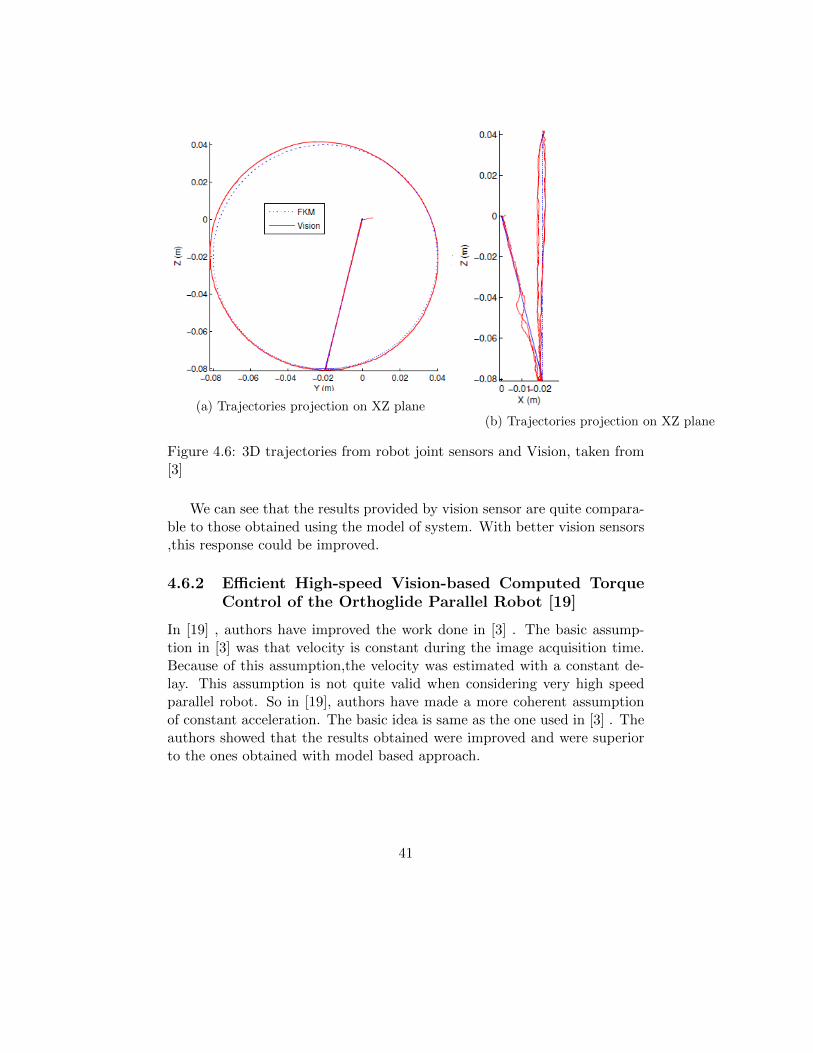
(a) Trajectories projection on XZ plane(b) Trajectories projection on XZ plane
Figure 4.6: 3D trajectories from robot joint sensors and Vision, taken from[3]
We can see that the results provided by vision sensor are quite compara-ble to those obtained using the model of system. With better vision sensors,this response could be improved.
4.6.2 Efficient High-speed Vision-based Computed TorqueControl of the Orthoglide Parallel Robot [19]
In [19] , authors have improved the work done in [3] . The basic assump-tion in [3] was that velocity is constant during the image acquisition time.Because of this assumption,the velocity was estimated with a constant de-lay. This assumption is not quite valid when considering very high speedparallel robot. So in [19], authors have made a more coherent assumptionof constant acceleration. The basic idea is same as the one used in [3] . Theauthors showed that the results obtained were improved and were superiorto the ones obtained with model based approach.
41

Part 2
42
Chapter 5
Visual servoing using legsobservation
We have seen in the previous chapters that classically, computed torquecontrol law is used to control parallel robots. This control law performs wellin joint space,in case of serial robots. However,in case of parallel robots,we usually try to avoid working in joint space because one has to solve forforward kinematic problem at each step.So in case of parallel robots, we try to work in cartesian space,as was shownin previous chapter. One way to control in cartesian space is to estimatethe end-effector pose and estimate its velocity directly,using different poseestimation algorithms available in literature. But these pose estimationalgorithms are costly in terms of computations and hence not very feasiblein very high speed manipulators.
5.1 Plucker coordinates for visual servoing
Plucker coordinates are another way to represent a line in space. We knowthat a line L in 3-dimesnional Euclidean space can be determined by two dis-tinct points. If we consider x1 = (x1, y1, z1)and x2 = (x2, y2, z2) be the twopoints on line L, then the vector displacement from x1 to x2 represents thedirection of the line. by this definition, every displacement between pointson L is a scalar multiple of d = x2−x1. If we suppose that a physical parti-cle of unit mass moves from x1 to x2, it would have a moment about origin.The geometric equivalent is a vector with the direction perpendicular to theplane containing line L and the origin, with the length equal to double the
43
area of triangle formed by the segment of displacement and origin. There-fore, moment is the vector cross product m = P× d, where P is any pointon the line. The area of triangle is proportional to the length of segmentbetween x1 and x2. By definition, the moment vector is perpendicular toeach displacement along the line, so the vector dot product is d ·m = 0.The two vectors, the direction vector of the line and the moment vector, aresufficient to uniquely determine line L. Therefore, plucker coordinates aregiven by :(d : m) = (d1 : d2 : d3 : m1 : m2 : m3).
5.2 Leg Observation
The control schemes developed and studied during this work i.e, line ori-entation and edges based, are defined based on the fact that it is possibleto control by observing the legs of the robot. The following subsectionsdescribe the ways to extract leg orientation and edges, using geometricalrelations.
5.2.1 Line Modelling
A line L expressed in the camera frame, is define by its binormalized pluckercoordinates [21] :
L = (cu, ch, ch)
Here, cu is the unit vector giving the spatial orientation of the line, ch isthe unit vector defining the interpretation plane of line L and ch is a nonnegative scalar. The latter are defined by chch = cP × cu , where cP isposition of any point P on the line, expressed in camera frame. Using thisnotation, the well known normalized plucker coordinates [22] are the couple(cu, chch).
44

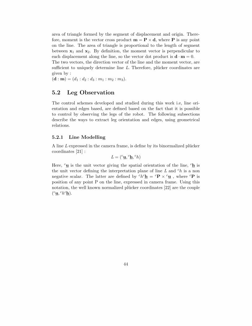
Figure 5.1: Plucker Coordinates and edges of a cylinder [16]
The projection of such a line in the image plane, expressed in the cameraframe, has for characteristic equation [21]:
chT cp = 0 (5.1)
where cp are the coordinates of a point P lying on the line, in the imageplane, expressed in camera frame.If we denote the intrinsic parameter matrix of the camera as K , we canobtain the line equation in pixel coordinates ph from:
phT pp = 0 (5.2)
Replacing pp with Kcp in this expression yields:
phTKcp = 0
From equations 5.1 and 5.2, we can write:
ph =K−T ch
‖K−T ch‖(5.3)
ch =K−T ph
‖K−T ph‖(5.4)
45
5.2.2 Cylindrical leg observation
The legs of parallel robots usually have cylindrical cross-sections [23]. Edgesof i-th cylindrical leg in the camera frame, are given by [16] (Fig 5.1):
cn1i = − cos θi
chi − sin θicui × chi
cn2i = + cos θi
chi − sin θicui × chi
Where:
cos θi =
√ch2i −R2
i
chisin θi =
Richi
Ri is the radius of the cylinder and (cu, ch, ch) are the binormalized Pluckercoordinates of the cylinder axis.We can also write a relationship between the leg orientation and its edges,expressed in camera frame, as given by [16]:
cui =cn1
i × cn2i
‖cn1i × cn2
i ‖
5.3 Simulator Design
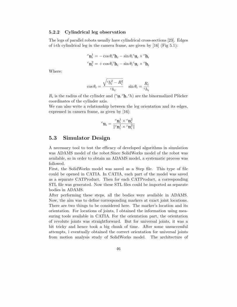
A necessary tool to test the efficacy of developed algorithms in simulationwas ADAMS model of the robot.Since SolidWorks model of the robot wasavailable, so in order to obtain an ADAMS model, a systematic process wasfollowed.First, the SolidWorks model was saved as a Step file. This type of filecould be opened in CATIA. In CATIA, each part of the model was savedas a separate CATProduct. Then for each CATProduct, a correspondingSTL file was generated. Now these STL files could be imported as separatebodies in ADAMS.After performing these steps, all the bodies were available in ADAMS.Now, the aim was to define corresponding markers at exact joint locations.There are two things to be considered here. The marker’s location and itsorientation. For locations of joints, I obtained the information using mea-suring tools available in CATIA. For the orientation part, the orientationof revolute joints was straightforward. But for universal joints, it was abit tricky and hence took a big chunk of time. After some unsuccessfulattempts, i eventually obtained the correct orientation for universal jointsfrom motion analysis study of SolidWorks model. The architecture of
46

a leg of IRSBot-2 is shown in figure 5.2,with all the joints.The lengthsl1 = l2 = 321mm, l41 = l42 = 458mm . The angle β = 45.
Figure 5.2: IRSBot-2 Architecture of 1 leg[24]
47
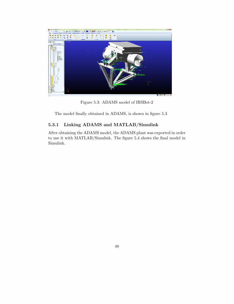
Figure 5.3: ADAMS model of IRSBot-2
The model finally obtained in ADAMS, is shown in figure 5.3
5.3.1 Linking ADAMS and MATLAB/Simulink
After obtaining the ADAMS model, the ADAMS plant was exported in orderto use it with MATLAB/Simulink. The figure 5.4 shows the final model inSimulink.
48
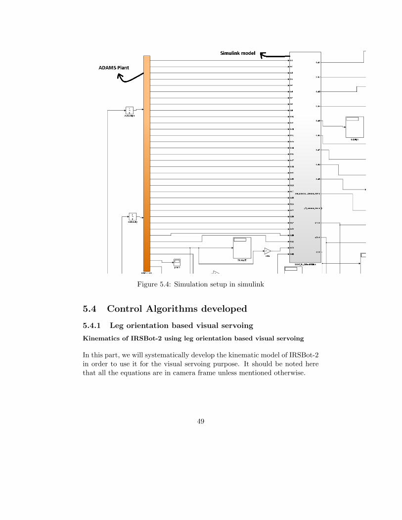
Figure 5.4: Simulation setup in simulink
5.4 Control Algorithms developed
5.4.1 Leg orientation based visual servoing
Kinematics of IRSBot-2 using leg orientation based visual servoing
In this part, we will systematically develop the kinematic model of IRSBot-2in order to use it for the visual servoing purpose. It should be noted herethat all the equations are in camera frame unless mentioned otherwise.
49

Figure 5.5: IRSBot-2 Schematic
The figure 5.5 shows the simplified architecture of IRSBot-2 and will beused to develop a kinematic model. IRSBot-2 is a two degrees of trans-lational parallel manipulator. The robot can be basically categorized ascomposed of two legs. Each leg can be further subdivided into a proximalpart and distal part, linked by an elbow. The proximal part is a parallelo-gram as shown in figure 5.5.In this part, the revolute joints that are actuatedare located at point Ai, which move the arm attached at points Ai and Bi.The direction vector of this arm is given by the vector xi. The distal partcan be further split into two distal bars or cylinders. An elbow joints thedistal part with the proximal part and the end-effector. A distal leg, orcylinder is attached at points Cij and Dij with the help of universal joints.Here, i= 1, 2 denotes the index of the proximal part and j= 1, 2 denotes theindex of the distal part.
50
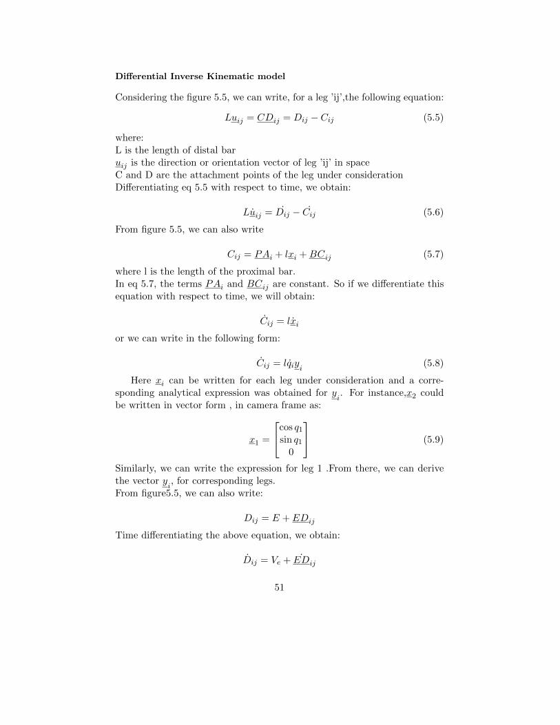
Differential Inverse Kinematic model
Considering the figure 5.5, we can write, for a leg ’ij’,the following equation:
Luij = CDij = Dij − Cij (5.5)
where:L is the length of distal baruij is the direction or orientation vector of leg ’ij’ in spaceC and D are the attachment points of the leg under considerationDifferentiating eq 5.5 with respect to time, we obtain:
Luij = Dij − Cij (5.6)
From figure 5.5, we can also write
Cij = PAi + lxi +BCij (5.7)
where l is the length of the proximal bar.In eq 5.7, the terms PAi and BCij are constant. So if we differentiate thisequation with respect to time, we will obtain:
Cij = lxi
or we can write in the following form:
Cij = lqiyi (5.8)
Here xi can be written for each leg under consideration and a corre-sponding analytical expression was obtained for y
i. For instance,x2 could
be written in vector form , in camera frame as:
x1 =
cos q1sin q1
0
(5.9)
Similarly, we can write the expression for leg 1 .From there, we can derivethe vector y
i, for corresponding legs.
From figure5.5, we can also write:
Dij = E + EDij
Time differentiating the above equation, we obtain:
Dij = Ve + ˙EDij
51

Since ED is constant, the above equation simplifies to:
Dij = Ve (5.10)
Putting 5.8 and 5.10 in equation 5.6, we obtain:
Luij = Ve − lqiyi (5.11)
Since u is a unit vector , so the following relation holds:
uTij uij = 0
Hence we can obtain the following relation after simplification:
qi =uTijVe
lyTiuij
(5.12)
This could be written in simplified form as:
qi = J invi Ve (5.13)
Where J invi is the inverse jacobian matrix relating the end-effector velocityto the joint value of the leg considered.
Interaction Matrix Computation
Since we want to use visual servoing, determination of interaction matrixrelating the rate of change of features to the end effector velocity is essential.For this purpose,if we insert eq 5.12 into eq 5.11, we obtain:
uij =1
L
(I3 −
yiuTij
yTiuij
)Ve
The above equation can be written in simplified form as:
uij = MijVe (5.14)
Here, Mij denotes the interaction matrix relating the rate of change of fea-tures to the end effector velocity.
52

Control Law
Since we are dealing with unit vectors, geodesic error is a better way toconsider error as compared to the difference of vectors. If we consider thatuij is our current leg direction at some point in time and u∗ij is our desiredleg direction, then we can write the error as:
eij = uij × u∗ijTaking the time derivative of above equation, we can write:
˙eij = −[u∗ij ]×uij
Using equation 5.14, we can write the above equation as:
˙eij = −[u∗ij ]×MijVe
or˙eij = NijVe (5.15)
where:
Nij = −[u∗ij ]×Mij
For a simple control strategy, if we impose proportional decrease of theerror, we can write:
˙eij = −λeijUsing this in eq 5.15, we get following pseudo control law:
Ve = −λN+e (5.16)
Notice that matrix N is a compound matrix obtained by stacking individualmatrices Nij of each leg and e is the compound error matrix obtained bystacking the individual errors of each leg. Using eq 5.13 in eq 5.16, we havethe final control law of the form:
q = −λJ invN+e
where q is a vector obtained by stacking the values from both actuators.J inv is the matrix obtained by stacking the inverse jacobian matrices ofboth legs.
53

5.4.2 Results without noise
The following section shows some of the results obtained using the Simulink/ ADAMS View based simulator. Noise is not added in this part. Thedesired leg orientation vectors of both legs are provided, which correspondto a certain pose of end-effector. For simulation purposes, as shown infigure 5.5, the camera is supposed to be placed at some location away fromthe robot and the camera frame is rotated for 90◦ around x-axis. Thegeneral form of homogeneous transformation matrix between camera andbase frame can be written as:
cTo =
[cRo
cto0 0 0 1
]So the homogeneous transformation matrix between the robot and
camera frame is as follows:
cTo =
1 0 0 2500 0 −1 −2500 1 0 10000 0 0 1
The translation part of the homogeneous transformation matrix is inmillimetres.The initial leg orientations of each leg were:
u21 =
−0.80560.50920.3032
u11 =
0.51500.80190.3032
These initial leg orientations correspond to the initial end effector pose of:
X =
xyz
=
100342.91000
The desired orientations of each leg are as shown below:
u∗21 =
−0.71310.63220.3032
u∗11 =
0.41630.85730.3032
54

These desired leg orientations correspond to the end effector pose of:
X =
xyz
=
88.1413.11000
It should be noted that all the vectors described here are in cameraframe.Figure 5.6 demonstrates the results obtained for leg11.
Figure 5.6: Error on Leg11
Similarly, figure 5.7 shows the error and norm of error on the leg 21. Itcan be noted that in both cases, the desired leg orientation was achievedand there was an exponential decay of error, as desired.
55
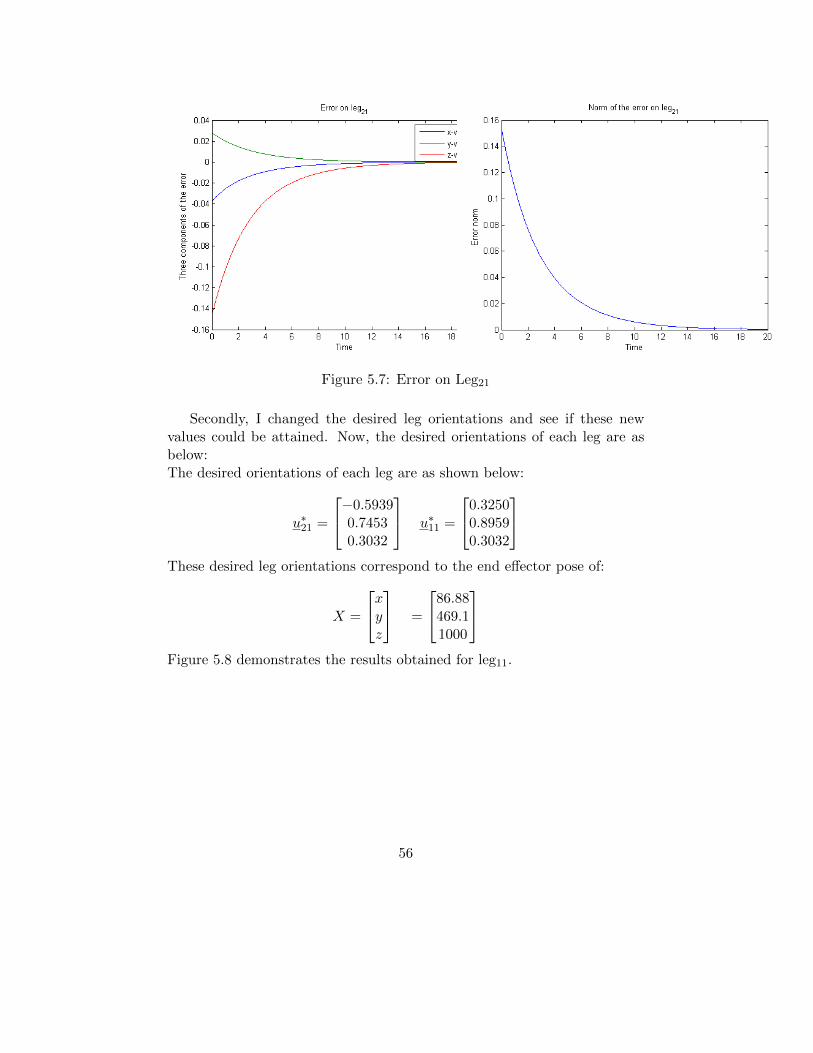
Figure 5.7: Error on Leg21
Secondly, I changed the desired leg orientations and see if these newvalues could be attained. Now, the desired orientations of each leg are asbelow:The desired orientations of each leg are as shown below:
u∗21 =
−0.59390.74530.3032
u∗11 =
0.32500.89590.3032
These desired leg orientations correspond to the end effector pose of:
X =
xyz
=
86.88469.11000
Figure 5.8 demonstrates the results obtained for leg11.
56

Figure 5.8: Error on Leg11
Similarly, figure 5.9 shows the error and norm of error on the leg 21. Itcan be noted that in both cases, the desired leg orientation was achievedand there was an exponential decay of error, as desired.
Figure 5.9: Error on Leg21
57

5.4.3 Results with noise
In this subsection, we will observe the effect of a small noise added. Thiswill be closer to practical scenario, since there will be some noise indetermination of leg edges or leg orientation in real life.This effect was mimicked in simulation by introducing additive whitegaussian noise in our model, at the location where we are determining theorientation vectors. The noise was added with a variance of 0.001 to theoriginal vector measured. The results are as shown below in the figures:
Figure 5.10: Error on Leg11
Similarly, figure 5.11 shows the error and norm of error on the leg 21.It can be noted that in both cases, the desired leg orientation was achievedand there was an exponential decay of error, as desired.
58

Figure 5.11: Error on Leg21
The pose reached by end-effector in this case was
X =
xyz
=
87.78412.81000
As described previously the desired pose was :
X =
xyz
=
88.1413.11000
The figure 5.12 shows that despite the noise introduced in the measurementof orientation vectors, the desired end-effector pose was reached withminimal error.
59
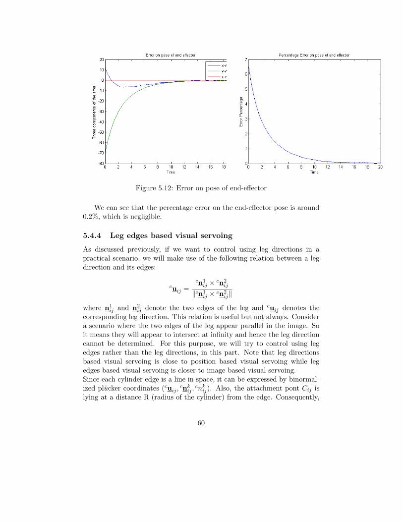
Figure 5.12: Error on pose of end-effector
We can see that the percentage error on the end-effector pose is around0.2%, which is negligible.
5.4.4 Leg edges based visual servoing
As discussed previously, if we want to control using leg directions in apractical scenario, we will make use of the following relation between a legdirection and its edges:
cuij =cn1
ij × cn2ij
‖cn1ij × cn2
ij‖
where n1ij and n2
ij denote the two edges of the leg and cuij denotes thecorresponding leg direction. This relation is useful but not always. Considera scenario where the two edges of the leg appear parallel in the image. Soit means they will appear to intersect at infinity and hence the leg directioncannot be determined. For this purpose, we will try to control using legedges rather than the leg directions, in this part. Note that leg directionsbased visual servoing is close to position based visual servoing while legedges based visual servoing is closer to image based visual servoing.Since each cylinder edge is a line in space, it can be expressed by binormal-ized plucker coordinates (cuij ,
cnkij ,cnkij). Also, the attachment pont Cij is
lying at a distance R (radius of the cylinder) from the edge. Consequently,
60
a cylinder edge can be fully defined by following constraints [16]:
CTijnkij = −R (5.17)
nkTij nkij = 1 (5.18)
uTijnkij = 0 (5.19)
The interaction matrix W relating the end effector velocity to the edges inthe pixel frame can be written as:
nk = WVe (5.20)
The matrix R can be decomposed into three parts, as follows:
W = pQcnQuM (5.21)
The matrix M, as derived previously, relates the time rate of change ofleg orientation to the end effector velocity. The matrix nQu relates the legorientation velocities and leg edges velocities, in camera frame. The matrixpQc is used to change from camera to pixel frame. The two latter matriceswill be derived in the following sections.
Edge velocity in the camera frame
Here, we will derive the time derivative of a cylinder edge, in camera frame,under the kinematic constraint that cylinder is attached at point Cij .For that purpose, taking time derivative of the constraints expressed inequations 5.17, 5.18 and 5.19, we have the following relations. Note thatthe legs index ’ij ’ is dropped from following calculations for simplicity:
nkTC = 0 (5.22)
nkTnk = 0 (5.23)
nkTu+ nkT u = 0 (5.24)
Using the equation 5.18 and the fact that the vectors (u,n,u×n) form theorthonormal basis (Andreff et al. 2002), we can state that:
nk = αu+ βu× nk
Now inserting this expression into equations 5.17 and 5.19 yields :
α = −nku, β =CTu
CT (u× nk)(nkT u)
61
Consequently, we obtain the relationship between the time derivative of aleg edge, expressed in the camera frame, and the time derivative of the legorientation:
nk = nQuu = nQuMVe
where:
nQu =
(CTu
CT (u× nk)(u× nk)− u
)nkT
Image line velocity in pixel coordinates
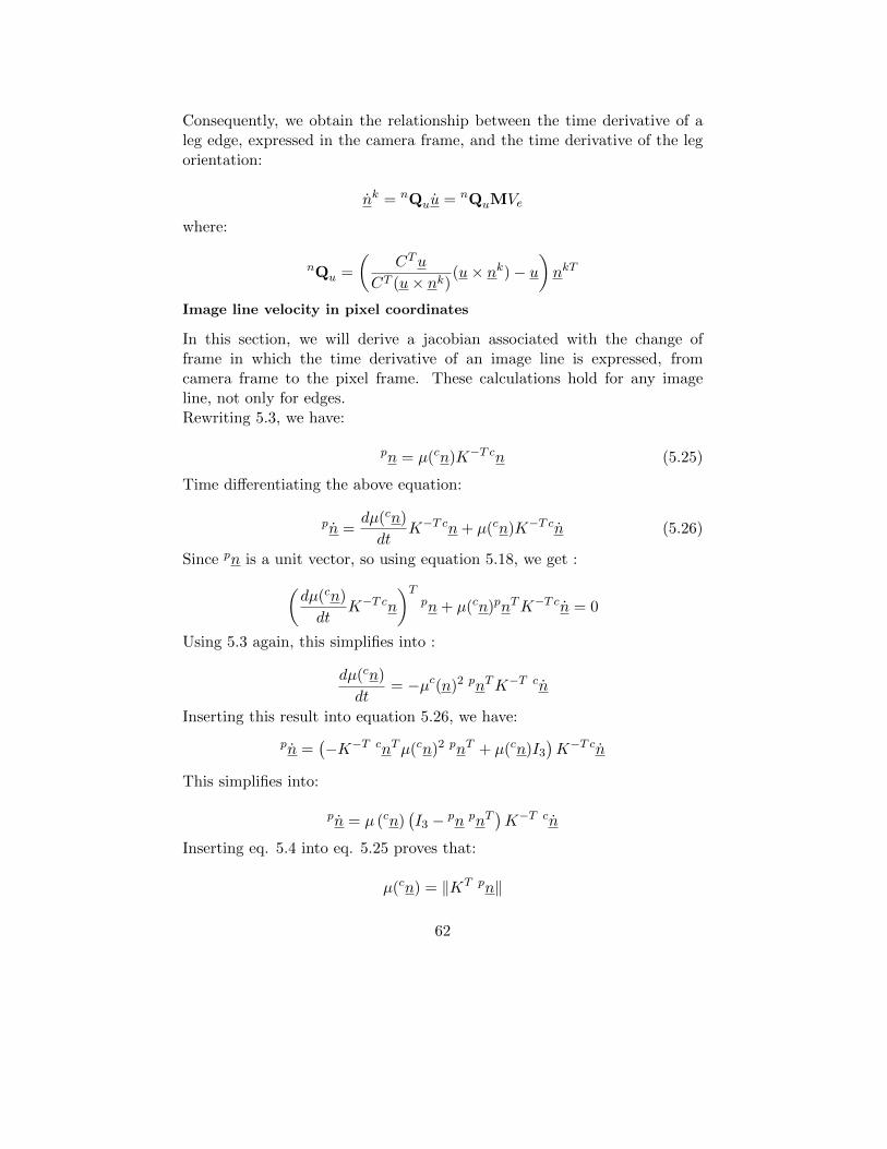
In this section, we will derive a jacobian associated with the change offrame in which the time derivative of an image line is expressed, fromcamera frame to the pixel frame. These calculations hold for any imageline, not only for edges.Rewriting 5.3, we have:
pn = µ(cn)K−T cn (5.25)
Time differentiating the above equation:
pn =dµ(cn)
dtK−T cn+ µ(cn)K−T cn (5.26)
Since pn is a unit vector, so using equation 5.18, we get :(dµ(cn)
dtK−T cn
)Tpn+ µ(cn)pnTK−T cn = 0
Using 5.3 again, this simplifies into :
dµ(cn)
dt= −µc(n)2 pnTK−T cn
Inserting this result into equation 5.26, we have:
pn =(−K−T cnTµ(cn)2 pnT + µ(cn)I3
)K−T cn
This simplifies into:
pn = µ (cn)(I3 − pn pnT
)K−T cn
Inserting eq. 5.4 into eq. 5.25 proves that:
µ(cn) = ‖KT pn‖
62

From this, we finally obtain the relationship between the time derivative ofa line, expressed in the pixel frame and in camera frame:
pn = pQccn
pQc = ‖KT pn‖(I3 − pnpnT
)K−T
Thus we have all the matrices needed to use equation 5.21.
Controlling in pixel coordinates
In our case,geodesic error is a better way to consider error as compared tothe difference of vectors. If we consider that nkij is one of our current leg
edge at some point in time and nk∗ij is our desired leg edge , then we canwrite the error as:
ekij = nkij × nk∗ijTaking the time derivative of above equation, we can write:
ekij = −[nk∗ij ]×nkij
Using equation 5.20, we can write the above equation as:
ekij = −[nk∗ij ]×WkijVe
orekij = SkijVe (5.27)
where:
Skij = −[nk∗ij ]×Wkij
For a simple control strategy, if we impose proportional decrease of theerror, we can write:
˙eij = −λeijUsing this in eq 5.27, we get following pseudo control law:
Ve = −λS+ije (5.28)
Notice that matrix S is a compound matrix obtained by stacking individualmatrices Skij of all the edges of all legs and e is the compound error matrixobtained by stacking the individual errors of each edge. Using eq 5.13 in eq
63
5.28, we have the final control law of the form:
q = −λJ invS+e
where q is a vector obtained by stacking the values from both actuators.J inv is the matrix obtained by stacking the inverse jacobian matrices ofboth legs.
5.4.5 Results without noise
The following section shows some of the results obtained using theSimulink / ADAMS View based simulator. Noise is not added in this part.The desired leg edges vectors of both legs are provided, which correspondto a certain pose of end-effector. The initial values of the edges of leg11 were:
n111 =
0.8091−0.5715
0.137
n111 =
−0.79310.5799−0.1865
Similarly, for leg21, the initial values for edges were:
n121 =
0.38840.8401−0.3788
n121 =
−0.4082−0.84770.3388
These initial values for leg edges correspond to the initial end effector
pose of:
X =
xyz
=
100342.91000
The desired edges of leg11 are as shown below:
n1∗11 =
0.49730.7611−0.4165
n2∗11 =
−0.5195−0.7670.3765
Similarly, for leg21, the desired values for edges were:
n1∗21 =
0.38840.8401−0.3788
n2∗21 =
−0.4082−0.84770.3388
64
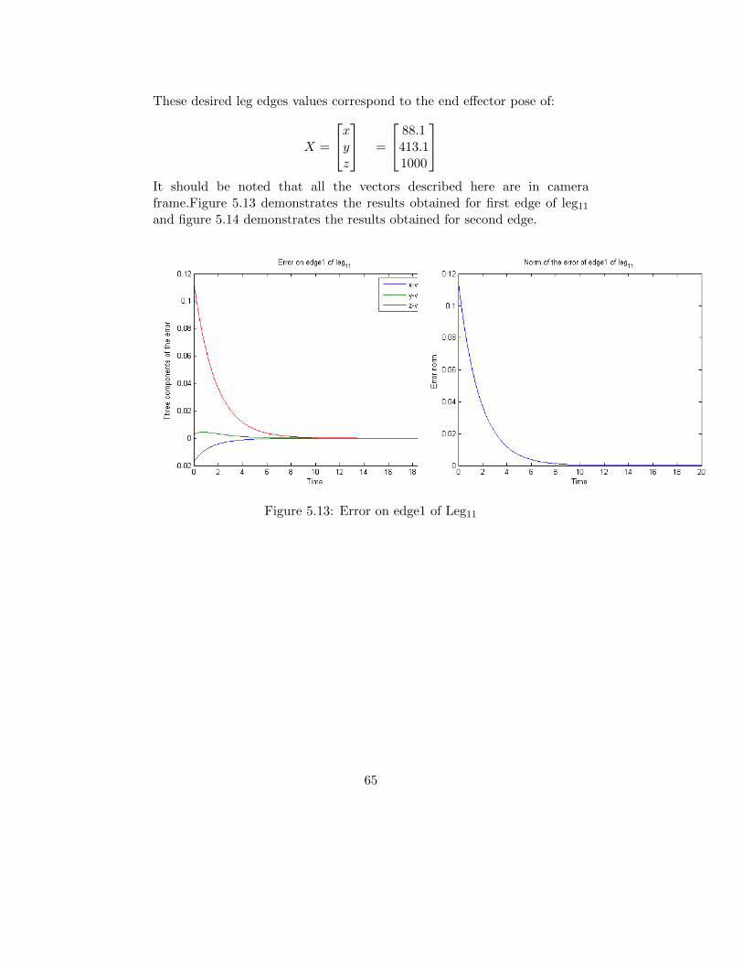
These desired leg edges values correspond to the end effector pose of:
X =
xyz
=
88.1413.11000
It should be noted that all the vectors described here are in cameraframe.Figure 5.13 demonstrates the results obtained for first edge of leg11and figure 5.14 demonstrates the results obtained for second edge.
Figure 5.13: Error on edge1 of Leg11
65

Figure 5.14: Error on edge2 of Leg11
Similarly, figure 5.15 shows the error and norm of error on the first edgeof leg 21 and 5.16 shows the error and norm of error on the second edge.It can be noted that in both cases, the desired leg orientation was achievedand there was an exponential decay of error, as desired.
Figure 5.15: Error on first edge of Leg21
66

Figure 5.16: Error on second edge of Leg21
Secondly, I changed the desired leg edges and see if these new valuescould be attained. Now, the desired edges of each leg are as below:The desired orientations of leg11 are as shown below:
n1∗11 =
0.8946−0.4228
0.145
n2∗11 =
−0.87930.434−0.1959
Similarly, for leg21, the desired values for edges were:
n1∗21 =
0.52630.7424−0.4146
n2∗21 =
−0.549−0.7475
0.374
These desired leg edges correspond to the end effector pose of:
X =
xyz
=
86.88469.11000
Figures 5.17 and 5.18 demonstrates the results obtained for first and secondedges of leg11 respectively.
67

Figure 5.17: Error on first edge of Leg11
Figure 5.18: Error on second edge of Leg11
Similarly, figures 5.19 and 5.20 show the error and norm of error on firstand second edges of leg 21 respectively. It can be noted that in both cases,the desired leg orientation was achieved and there was an exponential decayof error, as desired.
68

Figure 5.19: Error on first edge of Leg21
Figure 5.20: Error on second edge of Leg21
5.4.6 Results with noise
In this case also, additive white gaussian noise was added with a varianceof 0.001.The initial values of the edges of leg11 were:
69

n111 =
0.8091−0.5715
0.137
n111 =
−0.79310.5799−0.1865
Similarly, for leg21, the initial values for edges were:
n121 =
0.38840.8401−0.3788
n121 =
−0.4082−0.84770.3388
These initial values for leg edges correspond to the initial end effector
pose of:
X =
xyz
=
100342.91000
The desired edges of leg11 are as shown below:
n1∗11 =
0.49730.7611−0.4165
n2∗11 =
−0.5195−0.7670.3765
Similarly, for leg21, the desired values for edges were:
n1∗21 =
0.38840.8401−0.3788
n2∗21 =
−0.4082−0.84770.3388
These desired leg edges values correspond to the end effector pose of:
X =
xyz
=
88.1413.11000
It should be noted that all the vectors described here are in cameraframe.Figure 5.21 demonstrates the results obtained for first edge of leg11and figure 5.22 demonstrates the results obtained for second edge.
70
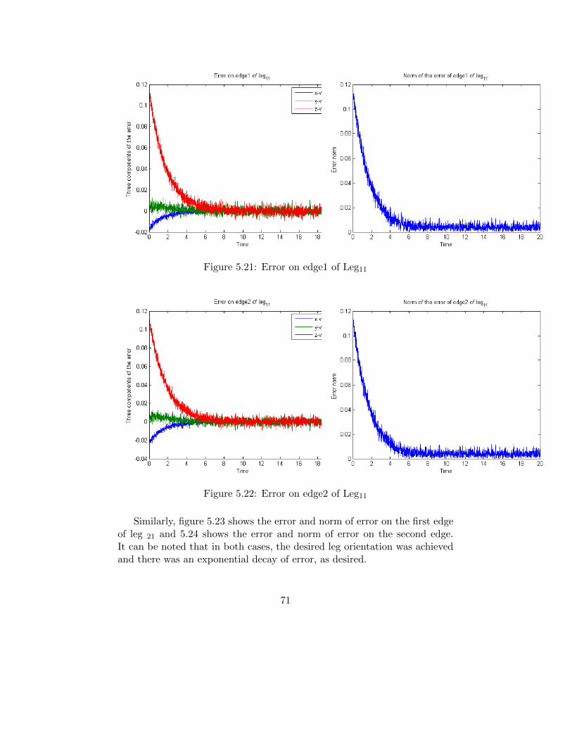
Figure 5.21: Error on edge1 of Leg11
Figure 5.22: Error on edge2 of Leg11
Similarly, figure 5.23 shows the error and norm of error on the first edgeof leg 21 and 5.24 shows the error and norm of error on the second edge.It can be noted that in both cases, the desired leg orientation was achievedand there was an exponential decay of error, as desired.
71
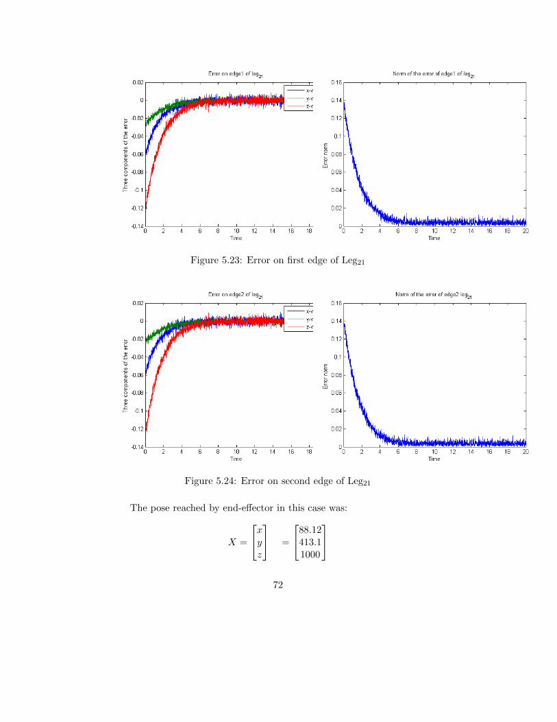
Figure 5.23: Error on first edge of Leg21
Figure 5.24: Error on second edge of Leg21
The pose reached by end-effector in this case was:
X =
xyz
=
88.12413.11000
72
The desired pose was :
X =
xyz
=
88.1413.11000
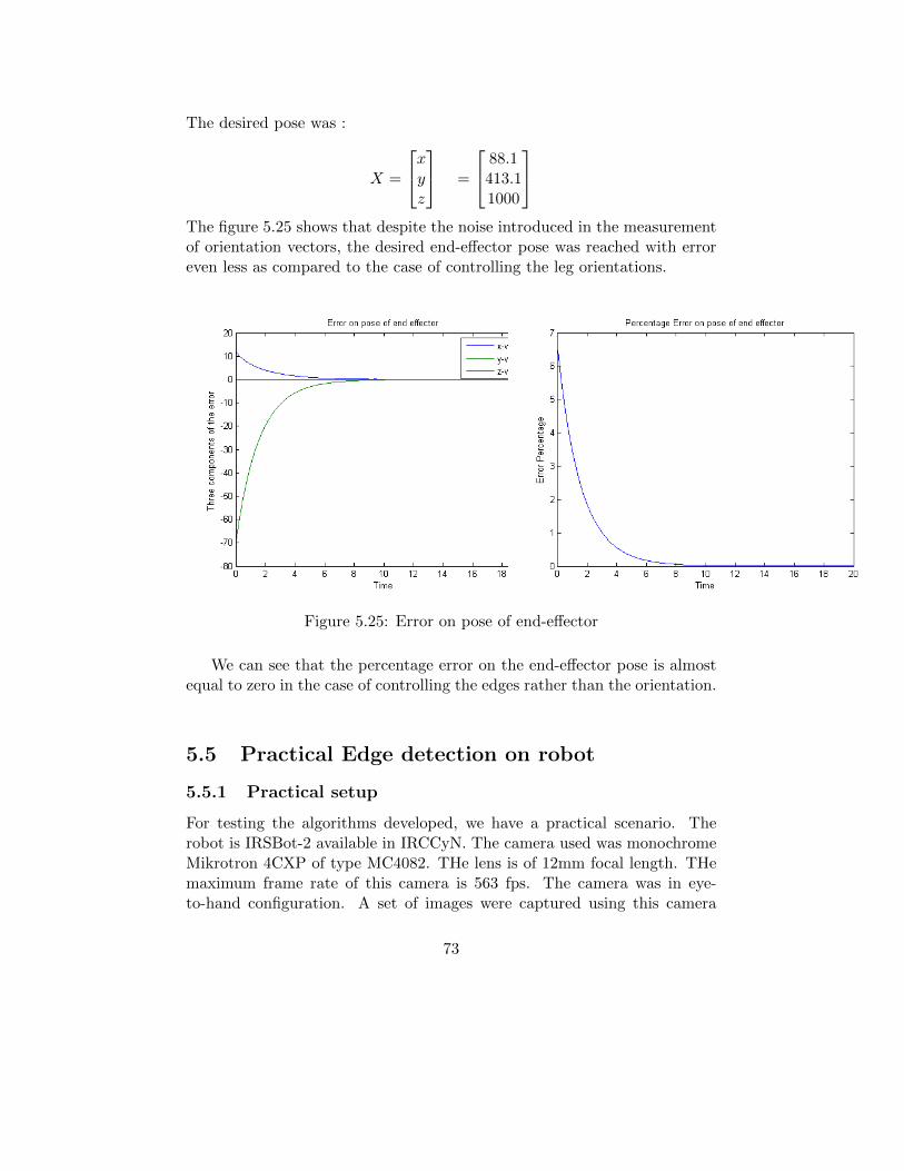
The figure 5.25 shows that despite the noise introduced in the measurementof orientation vectors, the desired end-effector pose was reached with erroreven less as compared to the case of controlling the leg orientations.
Figure 5.25: Error on pose of end-effector
We can see that the percentage error on the end-effector pose is almostequal to zero in the case of controlling the edges rather than the orientation.
5.5 Practical Edge detection on robot
5.5.1 Practical setup
For testing the algorithms developed, we have a practical scenario. Therobot is IRSBot-2 available in IRCCyN. The camera used was monochromeMikrotron 4CXP of type MC4082. THe lens is of 12mm focal length. THemaximum frame rate of this camera is 563 fps. The camera was in eye-to-hand configuration. A set of images were captured using this camera
73
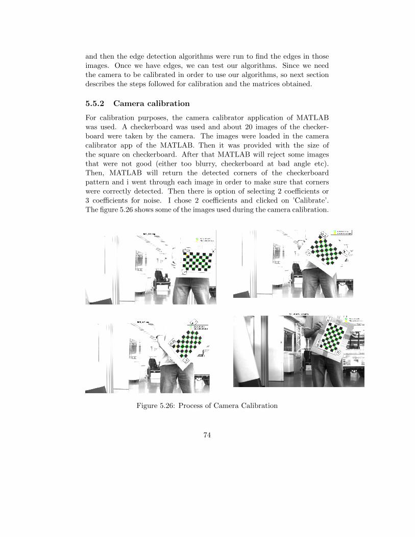
and then the edge detection algorithms were run to find the edges in thoseimages. Once we have edges, we can test our algorithms. Since we needthe camera to be calibrated in order to use our algorithms, so next sectiondescribes the steps followed for calibration and the matrices obtained.
5.5.2 Camera calibration
For calibration purposes, the camera calibrator application of MATLABwas used. A checkerboard was used and about 20 images of the checker-board were taken by the camera. The images were loaded in the cameracalibrator app of the MATLAB. Then it was provided with the size ofthe square on checkerboard. After that MATLAB will reject some imagesthat were not good (either too blurry, checkerboard at bad angle etc).Then, MATLAB will return the detected corners of the checkerboardpattern and i went through each image in order to make sure that cornerswere correctly detected. Then there is option of selecting 2 coefficients or3 coefficients for noise. I chose 2 coefficients and clicked on ’Calibrate’.The figure 5.26 shows some of the images used during the camera calibration.
Figure 5.26: Process of Camera Calibration
74
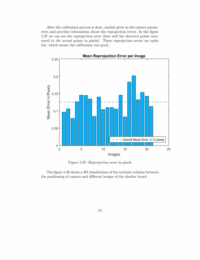
After the calibration process is done, matlab gives us the camera param-eters and provides information about the reprojection errors. In the figure5.27 we can see the reprojection error (how well the detected points mea-sured to the actual points in pixels). These reprojection errors are quitelow, which means the calibration was good.
Figure 5.27: Reprojection error in pixels
The figure 5.28 shows a 3D visualization of the extrinsic relation betweenthe positioning of camera and different images of the checker board.
75

Figure 5.28: Extrinsic visualization
Next, we click on “export camera parameters” (this will be importedinto MATLAB workspace). Then, we can go to MATLAB workspace andfind cameraParameters file. Here, we can find the intrinsic parameters andthe radial distortions needed to undistort an image. The values returnedby MATLAB were:
K =
fu γ u00 fv v00 0 1
=
1812.3 0 1231.40 1817.5 497.420 0 1
The radial distortion parameters determined were:
76
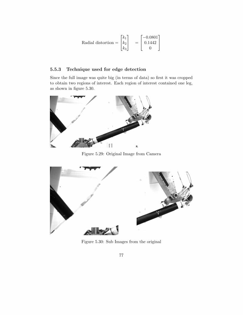
Radial distortion =
k1k2k3
=
−0.08010.1442
0
5.5.3 Technique used for edge detection
Since the full image was quite big (in terms of data) so first it was croppedto obtain two regions of interest. Each region of interest contained one leg,as shown in figure 5.30.
Figure 5.29: Original Image from Camera
Figure 5.30: Sub Images from the original
77

Then on each image, the edge detection was applied simultaneously.Since we had a MATLAB model of the robot, so Computer vision toolboxof MATLAB was used to do image processing. For the detection of edges,an edge detection block was used, which is available in computer visiontoolbox. Initially, the technique selected was using the Sobel filter, althoughthis could be changed later. The basic idea in Sobel filter is to determinethe approximations of derivatives in horizontal and vertical direction. Fordoing so, it uses a 3 × 3 Kernel and convolves it with a given image. Thiscan be mathematically represented as follows:
M1 =
−1 0 1−2 0 2−1 0 1
M2 =
1 2 10 0 0−1 −2 −1
If we define I as the source image, and Gx and Gy as two images which ateach point contain the horizontal and vertical derivative approximationsrespectively, the computations can be represented as follows:
Gx = M1 ∗ I, Gy = M2 ∗ I
Here ‘*’ operator denotes the 2-dimensional signal processing convolutionoperation.At each point in the image, the resulting gradient approximationscan be combined to give the gradient magnitude, using:
G =√G2x +G2
y
Using this information, the gradient’s direction is calculated as:
θ = arctanGyGx
The images after the edge detection are shown in figure 5.31.
78
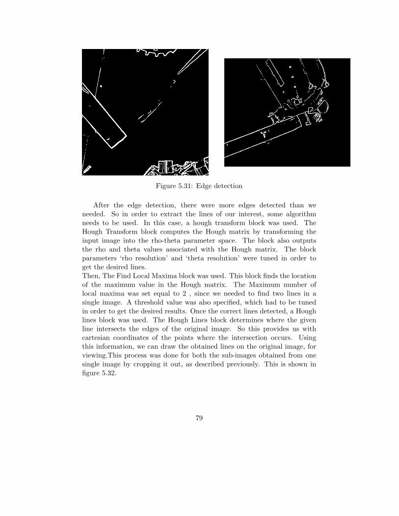
Figure 5.31: Edge detection
After the edge detection, there were more edges detected than weneeded. So in order to extract the lines of our interest, some algorithmneeds to be used. In this case, a hough transform block was used. TheHough Transform block computes the Hough matrix by transforming theinput image into the rho-theta parameter space. The block also outputsthe rho and theta values associated with the Hough matrix. The blockparameters ‘rho resolution’ and ‘theta resolution’ were tuned in order toget the desired lines.Then, The Find Local Maxima block was used. This block finds the locationof the maximum value in the Hough matrix. The Maximum number oflocal maxima was set equal to 2 , since we needed to find two lines in asingle image. A threshold value was also specified, which had to be tunedin order to get the desired results. Once the correct lines detected, a Houghlines block was used. The Hough Lines block determines where the givenline intersects the edges of the original image. So this provides us withcartesian coordinates of the points where the intersection occurs. Usingthis information, we can draw the obtained lines on the original image, forviewing.This process was done for both the sub-images obtained from onesingle image by cropping it out, as described previously. This is shown infigure 5.32.
79

Figure 5.32: Sobel Edge detection
Finally the projection line vectors for each leg can be found from edges,as shown in figure 5.33.
Figure 5.33: Edges (green) and projection-line vectors (red)
80

Part 3
81
Chapter 6
Conclusion and Future workproposal
In the previous chapters, state of the art in robotics,vision and control hasbeen briefly covered. Different techniques to estimate the pose and velocityfor parallel robots have been analysed and different control algorithms inthe literature were covered.Then the work done in the context of this thesis has been presented indetail. It has been shown that it is possible to control this robot using 2out of the 4 legs of the robot. The methods using the leg orientations andleg edges have been investigated and validated in simulations.Secondly, the way has been paved for practically testing the algorithms onrobot. The edge detection has been performed on images obtained througha calibrated camera.
Future Recommendations
For building the future work based on this thesis, following points could beinvestigated:
• Practically testing the algorithms on the robot
• Improving the control algorithms by introducing the dynamic controlwhile taking into account the high speed of robot
82

Chapter 7
Bibliography
[1] https://en.wikipedia.org/wiki/Radar
[2] Flavien Paccot, Philippe Lemoine, Nicolas Andreff, Damien
Chablat and Philippe Martinet. A vision-based computed
torque control for parallel kinematic machines. In IEEE
International Conference on Robotics and Automation, 2008.
[3] Redwan Dahmouche, Nicolas Andreff, Youcef Mezouar, Philippe
Martinet, LASMEA, CNRS, Universite Blaise Pascal. 3d pose
and velocity visual tracking based on sequential region of
interest acquisition. In The 2009 IEEE/RSJ International
Conference on Intelligent Robots and Systems October 11-15,
2009 St. Louis, USA. IEEE, 2009.
[4] Optimal Kinematic Design of Robots by Mr Philippe
Wenger,EMARO II Course, Ecole Centrale de Nantes
[5] Victor Rosenzvig, Sensor Based design and control of
high-speed manipulators, PhD Thesis 2015, IRCCyN,Ecole
Centrale de Nantes,Nantes
[6] P.Srinivas,K.Vijaya Lakshmi,V.Naveen Kumar.A comparison
of PID Controller Tuning Methods for three tank
level process. International Journal of Advanced
Research in Electrical,Electronics and Instrumentation
Engineering,January 2014
[7] Modelling and Control of Manipulator Robots by Professor
Philippe Martinet,EMARO-ARIA Master 1,Ecole Centrale de
83

Nantes. Slides available at http://www.irccyn.ec-nantes.fr/
~martinet/MoCom.html
[8] Flavien Paccot ,Nicolas Andreff, Philippe Martinet.A review
on dynamic control of parallel kinematic machines:Theory
and experiments. The International Journal of Robotics
Research
[9] Chaumette, F. and Hutchinson, S. (2008). Handbook of
Robotics - Visual Servoing and Visual Tracking pages
563-583
[10] Slides of Computer Vision course by Professor Philippe
Martinet . Slides can be found at http://www.irccyn.
ec-nantes.fr/~martinet/
[11] Daniel F. DeMenthon and Larry S. Davis. Model-based object
pose in 25 lines of code. International Journal of Computer
Vision, 15:123{141, 1995
[12] J.A. Gangloff and M.F. de Mathelin. High speed visual
servoing of a 6 DOF manipulator using multivariable
predictive control,October 7,2003
[13] Seth Hutchinson, Gregory D Hager, Peter I. Corke. A
tutorial on visual servo control.IEEE transactions on
Robotics and Automation,Volume 12, No.5, October 1996
[14] D. Stewart. A platform with six degrees of freedom.
Proceedings of the Institution of Mechanical Engineers
[15] N. Andreff, A. Marchadier, and P. Martinet. Vision-based
control of a Gough-Stewart parallel mechanism using
legs observation. In Robotics and Automation, 2005.
ICRA 2005. Proceedings of the 2005 IEEE International
Conference on, pages 2535{2540, april 2005. doi:
10.1109/ROBOT.2005.1570494
[16] Nicolas Andref, Tej Dallej, Philippe Martinet. Image-based
Visual Servoing of a Gough- Stewart Parallel Manipulator
using Leg Observations. International Journal of Robotics
Re- search. Special Issue on Vision and Robotics - Joint
with the International Journal of Computer Vision, 2007, 26
(7), pp.677-687. <hal-00520165>
84
[17] Slides of Vision based control course by Professor
Philippe Martinet . Slides can be found at http://www.
irccyn.ec-nantes.fr/~martinet/VisionBasedControl.html
[18] S. Briot and P. Martinet. "Minimal Representation for the
Control of Gough-Stewart Platforms via Leg Observation
Considering a Hidden Robot Model", Proceedings of the 2013
IEEE International Conference on Robotics and Automation
(ICRA 2013), May 6-10, 2013, Karlsruhe, Germany
[19] Redwan Dahmouche, Nicolas Andreff, Youcef Mezouar and
Philippe Martinet.Efficient High-speed Vision-based
Computed Torque Control of the Orthoglide Parallel
Robot. 2010 IEEE International Conference on Robotics and
Automation Anchorage Convention District May 3-8, 2010,
Anchorage, Alaska, USA
[20] Tej Dallej, Nicolas Andreff and Philippe Martinet.
Image-Based Visual Servoing of the I4R parallel robot
without Proprioceptive Sensors. 2007 IEEE International
Conference on Robotics and Automation Roma, Italy, 10 − 14April 2007
[21] N. Andreff, B. Espiau, and R. Horaud. Visual servoing from
lines. International Journal of Robotics Research, 21(8):
679–700, 2002
[22] J. Plucker. On a new geometry of space. Philosophical
Transactions of the Royal Society of London, 155:725–791,1865.
[23] J.P. Merlet. Parallel Robots. Springer, 2nd edition, 2006.
[24] Coralie Germain. Conception d’un robot parallele a deux
degres de liberte pour des operations de prise et de
depose. Automatique / Robotique. Ecole Centrale de Nantes,
2013. Francais. <tel-01108739>
[25] Erol Ozgur. From lines to dynamics of parallel robots.
Other. Universite Blaise Pascal, Clermont-Ferrand II, 2012
[26] Alessia Vignolo, Master Thesis(2014). Visual servoing of
the Monash Epicyclic-parallel manipulator,Ecole Centrale de
Nantes.
85
[27] Giovanni Claudio, Master Thesis(2013). Pose and velocity
estimation for high speed robot control, Ecole Centrale de
Nantes.
[28] Redwan Dahmouche, These de doctorat. Contributions a
l’estimation de mouvement 3D et a la commande par vision
rapide, Universite Blaise Pascal - Clermont II.
[29] Tej Dallej, These de doctorat. Contributions a
un modele generique pour l’asservissement visuel
des robots paralleles par observation des elements
cinematiques,Universite Blaise Pascal - Clermont II.
[30] Flavien Paccot, These de doctorat. Contributions a la
commande dynamique referencee capteur de robots paralleles,
Universite Blaise Pascal - Clermont II.
86
Related Documents
![á ÖÝf¼ ~ò¨¼ 5f Ò Ö¨¼ f¼ ¨½ ¨¼ - Philips · f h ¨Ò Òó Òfr r 8 P Ò ¼ ¨á ¼ f] ¥½Ã·Ã ¨ f f ·¨¼ ¨½~Ò f~ Ò Ö¨¼ ¨¨] ¥½Ã·Ã ¨ fS ~Ϩ fh](https://static.cupdf.com/doc/110x72/5e5dfd1578ee94483575284b/-f-5f-f-philips-f-h-fr-r-8-p.jpg)