Massively compositional model for cross-project defect ...

Singapore Management University Singapore Management University

Institutional Knowledge at Singapore Management University Institutional Knowledge at Singapore Management University

Research Collection School Of Information Systems School of Information Systems

10-2016

HYDRA: Massively compositional model for cross-project defect HYDRA: Massively compositional model for cross-project defect

prediction prediction

Xin XIA Zhejiang University

David LO Singapore Management University, [email protected]

Sinno Jialin PAN Nanyang Technological University

Nachiappan NAGAPPAN Microsoft Research

Xinyu WANG Zhejiang University

Follow this and additional works at: https://ink.library.smu.edu.sg/sis_research

Part of the Software Engineering Commons, and the Theory and Algorithms Commons

Citation Citation XIA, Xin; David LO; PAN, Sinno Jialin; NAGAPPAN, Nachiappan; and WANG, Xinyu. HYDRA: Massively compositional model for cross-project defect prediction. (2016). IEEE Transactions on Software Engineering. 42, (10), 977-998. Research Collection School Of Information Systems. Available at:Available at: https://ink.library.smu.edu.sg/sis_research/3415

This Journal Article is brought to you for free and open access by the School of Information Systems at Institutional Knowledge at Singapore Management University. It has been accepted for inclusion in Research Collection School Of Information Systems by an authorized administrator of Institutional Knowledge at Singapore Management University. For more information, please email [email protected].

https://ink.library.smu.edu.sg/

https://ink.library.smu.edu.sg/sis_research

https://ink.library.smu.edu.sg/sis_research

https://ink.library.smu.edu.sg/sis

https://ink.library.smu.edu.sg/sis_research?utm_source=ink.library.smu.edu.sg%2Fsis_research%2F3415&utm_medium=PDF&utm_campaign=PDFCoverPages

http://network.bepress.com/hgg/discipline/150?utm_source=ink.library.smu.edu.sg%2Fsis_research%2F3415&utm_medium=PDF&utm_campaign=PDFCoverPages

http://network.bepress.com/hgg/discipline/151?utm_source=ink.library.smu.edu.sg%2Fsis_research%2F3415&utm_medium=PDF&utm_campaign=PDFCoverPages

mailto:[email protected]

HYDRA: Massively Compositional Modelfor Cross-Project Defect Prediction

Xin Xia,Member, IEEE, David Lo,Member, IEEE, Sinno Jialin Pan,

Nachiappan Nagappan, and Xinyu Wang

Abstract—Most software defect prediction approaches are trained and applied on data from the same project. However, often a new

project does not have enough training data. Cross-project defect prediction, which uses data from other projects to predict defects in a

particular project, provides a new perspective to defect prediction. In this work, we propose a HYbrid moDel Reconstruction Approach

(HYDRA) for cross-project defect prediction, which includes two phases: genetic algorithm (GA) phase and ensemble learning (EL)

phase. These two phases create a massive composition of classifiers. To examine the benefits of HYDRA, we perform experiments on

29 datasets from the PROMISE repository which contains a total of 11,196 instances (i.e., Java classes) labeled as defective or clean.

We experiment with logistic regression as the underlying classification algorithm of HYDRA. We compare our approach with the most

recently proposed cross-project defect prediction approaches: TCA+ by Nam et al., Peters filter by Peters et al., GP by Liu et al., MO by

Canfora et al., and CODEP by Panichella et al. Our results show that HYDRA achieves an average F1-score of 0.544. On average,

across the 29 datasets, these results correspond to an improvement in the F1-scores of 26.22 , 34.99, 47.43, 28.61, and 30.14 percent

over TCA+, Peters filter, GP, MO, and CODEP, respectively. In addition, HYDRA on average can discover 33 percent of all bugs if

developers inspect the top 20 percent lines of code, which improves the best baseline approach (TCA+) by 44.41 percent. We also find

that HYDRA improves the F1-score of Zero-R which predict all the instances to be defective by 5.42 percent, but improves Zero-R by

58.65 percent when inspecting the top 20 percent lines of code. In practice, Zero-R can be hard to use since it simply predicts all of the

instances to be defective, and thus developers have to inspect all of the instances to find the defective ones. Moreover, we notice the

improvement of HYDRA over other baseline approaches in terms of F1-score and when inspecting the top 20 percent lines of code are

substantial, and in most cases the improvements are significant and have large effect sizes across the 29 datasets.

Index Terms—Cross-project defect prediction, transfer learning, genetic algorithm, ensemble learning

Ç

1 INTRODUCTION

SOFTWARE defect prediction can help in allocating testresources by predicting defect-prone classes, files, or

modules prior to the testing phase [52]. A number of defectprediction approaches have been proposed which leveragemachine learning techniques to build a prediction modelfrom historical data stored in software repositories [10],[20], [25], [34], [35], [57]. These approaches typically use var-ious features, e.g., process metrics, previous-defect metrics,source code metrics, etc., to characterize a class/file/mod-ule and employ a classification algorithm to predict if aclass/file/module is defective or not. Most defect predictionapproaches are trained and applied on classes/files/mod-ules from the same project. These within-project defect pre-diction approaches require sufficient training (historical)data from a project.

However, in practice, it is rare that sufficient trainingdata is available for a new project, but there is plenty ofdata from other projects. For example, the PROMISE reposi-tory [33] provides many publicly released defect predictiondatasets. Cross-project defect prediction, which uses train-ing data from other projects (aka. source projects) to predictdefective instances (i.e., classes/files/ modules) in a partic-ular project of interest (aka. target project), provides a newperspective to defect prediction [9], [28], [36], [41], [42], [58].In this paper, we refer to defect prediction approaches thatare trained and applied on instances from the same projectas within-project defect prediction approaches. On the otherhand, we refer to approaches that also use training datafrom other projects as cross-project defect prediction approaches.

Cross-project defect prediction is a challenging tasksince a prediction model that is trained on one or a set ofprojects might not generalize well to other projects [58].The challenge is how to create a model to better capturegeneralizable properties of defective instances that willwork for the target project, and (fully or partly) ignore non-generalizable properties that do not hold for the target proj-ect. In the machine learning literature, to overcome the dif-ference in data distributions between domains, transferlearning [13], [15], [39], [40] which extracts common knowl-edge from the one domain and transfers it to anotherdomain, has been proposed. Cross-project defect predictioncan be viewed as a specific case of transfer learning, whichextracts knowledge from a set of source projects and trans-fers it to a target project.

� X. Xia and X. Wang are with the College of Computer Science and Tech-nology, Zhejiang University Hangzhou, Zhejiang 310000, China.E-mail: {xxkidd, wangxinyu}@zju.edu.cn.

� D. Lo is with the School of Information Systems, Singapore ManagementUniversity, Singapore 17890. E-mail: [email protected].

� S. Jialin Pan is with the School of Computer Engineering, Nanyang Tech-nological University, Singapore. E-mail: [email protected].

� N. Nagappan is with the Testing, Verification and Measurement Research,Microsoft Research, Redmond, WA 98052. E-mail: [email protected].

Manuscript received 12 Feb. 2015; revised 1 Mar. 2016; accepted 6 Mar. 2016.Date of publication 16 Mar. 2016; date of current version 21 Oct. 2016.Recommended for acceptance by T. Menzies.For information on obtaining reprints of this article, please send e-mail to:[email protected], and reference the Digital Object Identifier below.Digital Object Identifier no. 10.1109/TSE.2016.2543218

IEEE TRANSACTIONS ON SOFTWARE ENGINEERING, VOL. 42, NO. 10, OCTOBER 2016 977

0098-5589� 2016 IEEE. Personal use is permitted, but republication/redistribution requires IEEE permission.See http://www.ieee.org/publications_standards/publications/rights/index.html for more information.

Published in IEEE Transactions on Software Engineering, October 2016, Volume 42, Issue 10, Pages 977-998.http://doi.org/10.1109/TSE.2016.2543218

mailto:

mailto:

mailto:

mailto:

In this paper, we propose our HYbrid moDel Reconstruc-tion Approach (HYDRA) which addresses the above chal-lenge by iteratively learning new classifiers and compositionsof classifiers to collectively better capture generalizable prop-erties in every new iteration. Rather than learning only one ora few classifiers, HYDRA tunes a two-layer hierarchical com-position of a massive number of classifiers. The tuning pro-cess is done in many iterations, with the help of GeneticAlgorithm (GA) and Ensemble Learning (EL), which gradu-ally steers the composite model to better capture generalizableproperties; this is done by learning new classifiers and newcompositions of classifiers, and by assigning weights to theseclassifiers, compositions of classifiers, and training instances.Our approach is different from the existing studies on cross-defect prediction which only build one classifier [9], [28], [36],[42] or unify a few classifiers [41].

HYDRA considers the setting where there are numerouslabeled data from multiple source projects, however there isonly a limited amount of labeled data (e.g., 5 percent of thedata are labeled) from a target project. This limited amountof labeled data from a target project is referred to as trainingtarget data. HYDRA includes two phases: genetic algorithm(GA) phase and ensemble learning (EL) phase. In the GAphase, we first build a classifier for each source project datamerged with the training target data, and another classifierfor the training target data alone. Next, we build a GA clas-sifier by assigning different weights to the multiple classi-fiers using genetic algorithm. Genetic algorithm will searchfor the best weights which optimize F1-score [19] on thetraining target data. The goal is to reduce training error toapproximate the generalization error since there are not suf-ficient instances in training target data to be divided intotraining and validation sets [46]. In the EL phase, we iteratethe GA phase many times. For each iteration, we build a GAclassifier, and assign a weight to the GA classifier accordingto its prediction error rate on the training target data; also,we increase the weights of instances in source projects andthe training target data if they are wrongly classified by theGA classifier built in the previous iteration. At the end ofthe GA and EL phases, we have a massive composition ofclassifiers and we use it to predict defective instances in thetarget project.

We evaluate our approach against seven existingapproaches [9], [15], [28], [36], [41], [42], [58] using 29 data-sets from the PROMISE data repository which contains atotal of 11,196 instances. Our results show that HYDRAachieves the best performance. HYDRA achieves an averageF1-scores of 0.544. On average, across the 29 datasets, ourapproach improves the F1-scores of Zimmermann et al.’sapproach [58] by 40.21 percent, of TCA+ [36] by 26.22 per-cent, of Peters filter [42] by 34.99 percent, of GP [28] by47.43 percent, of MO [9] by 28.61 percent, and of CODEP [41]by 30.14 percent, respectively. We also compare ourapproach with TransferBoost [15] which is recently proposedin the machine learning literature by Eaton and desJardins,and the results show that our approach improves Transfer-Boost by 39.49 percent. In addition, HYDRA on average candiscover 33 percent of all bugs if developers only inspectthe top 20 percent lines of code, which improves the bestbaseline approach (TCA+) by 44.41 percent. We address thefollowing research questions:

RQ1: How effective is HYDRA? How much improvement canit achieve over the baseline approaches?

On average across the 29 projects, the average F1 andPofB20 scores for HYDRA are 0.544 and 33.0 percent, whichimproves the baseline approaches by a substantial margin.

RQ2: Can HYDRA outperform conventional within-projectdefect prediction?

On average across the 29 datasets, HYDRA outperformsthe within-project defect prediction with 5 percent labeleddata in terms of F1-score and PofB20 by 19.46, and 62.40 per-cent, respectively. Moreover, HYDRA achieves similarresults as within-project defect prediction with 90 percentlabeled data.

RQ3: Do different percentages of labeled instances from a tar-get project affect the performance of HYDRA?

We notice that for small number of instances, such as 1-3 percent of the total number of instances, the F1-score islow. With more labeled instances from the target projects,the performance is improved. Also the average percentagesof bugs detected when inspecting 20% of code is relativelystable, and it varies from 31.5-35.5 percent.

RQ4: How much time does it take for HYDRA to run?We find that the model building and prediction time for

HYDRA are reasonable. On average, HYDRA needs1.5 minutes to train a model, and 1.7 seconds to predict thelabels of instances in the testing set using the model.

The main contributions of this paper are:

1) We propose a novel cross-project defect predictionapproach named HYDRA, which utilizes the advan-tages of genetic algorithm (GA) and ensemble learn-ing (EL) to build and iteratively tune a massivelycompositional model.

2) We evaluate our approach and those proposed byZimmermann et al., Nam et al., Peters et al., Liuet al., Canfora et al., Panichella et al., and Eaton anddesJardins on 29 datasets containing a total of 11,196instances. The experiment results show that ourapproach can achieve a substantial improvementover these baseline approaches.

The remainder of the paper is organized as follows. Wedescribe the motivation of building a compositional modeland the high-level architecture of HYDRA in Section 2. Weelaborate HYDRA in Section 3. We present our experimentsin Section 4. We discuss the other settings of HYDRA, andthreats to validity in Section 5. We briefly review relatedwork in Section 6. We conclude this work and point outpotential future directions in Section 7.

2 MOTIVATION AND ARCHITECTURE

In this section, we present the motivation of building a com-positional model, followed by the architecture of HYDRA.

2.1 Why Compositional Model?

If a single model built from one source project, using a state-of-the-art defect prediction approach, can perform very wellacross a wide-variety of target projects, there is no need fora compositional model. To validate the need for a composi-tional model, we investigate how models learned from dif-ferent source projects affect the performance of a state-of-the-art cross-project defect prediction approach.

978 IEEE TRANSACTIONS ON SOFTWARE ENGINEERING, VOL. 42, NO. 10, OCTOBER 2016

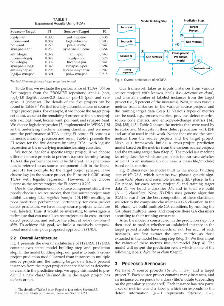
To do this, we evaluate the performance of TCA+ [36] onfive projects from the PROMISE repository: ant-1.4 (ant),log4j-1.0 (log4j), lucene-2.0 (lucene), poi-1.5 (poi), and syn-apse-1.0 (synapse). The details of the five projects can befound in Table 3.1We first identify all combinations of source-target project pairs. For example, if we choose the target proj-ect as ant,we select the remaining 4 projects as the source proj-ects, i.e., log4j)ant, lucene)ant, poi)ant, and synapse)ant.We choose logistic regression [7] implemented in WEKA [18]as the underlying machine learning classifier, and we mea-sure the performance of TCA+ using F1-score.2 F1-score is aharmonic mean of precision and recall. Table 1 presents theF1-scores for the five datasets by using TCA+ with logisticregression as the underlyingmachine learning classifier.

We notice that for a specific target project, if we choosedifferent source projects to perform transfer learning (usingTCA+), the performance would be different. This phenome-non is referred to as source component shift in the litera-ture [51]. For example, for the target project synapse, if wechoose log4j as the source project, the F1-score is 0.301 usingTCA+ with logistic regression. However, if we chooselucene as the source project, the F1-score is 0.202.

Due to the phenomenon of source component shift, if wepoorly choose a source project, then this source project mayinhibit learning (aka. negative transfer [15], [40]) resulting inpoor prediction performance. Fortunately, for cross-projectdefect prediction, we have many source projects which arewell labeled. Thus, it would be interesting to investigate atechnique that can use all source projects to do cross-projectdefect prediction, and reduce the effect of source componentshift. To achieve this goal, we build a massively composi-tional model using our proposed approach HYDRA.

2.2 Overall Architecture

Fig. 1 presents the overall architecture of HYDRA. HYDRAcontains two steps: model building step and predictionstep. In the model building step, our goal is to build a cross-project prediction model learned from instances in multiplesource projects and the training target data (i.e., 5 percentinstances from the target project that are labeled as defectiveor clean). In the prediction step, we apply this model to pre-dict if a new class/file/module in the target project hasdefects or not.

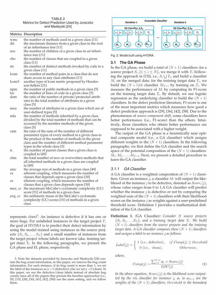
Our framework takes as inputs instances from varioussource projects with known labels (i.e., defective or clean),and a small number of labeled instances from the targetproject (i.e., 5 percent of the instances). Next, it uses variousmetrics from instances in the various source projects andthe training target data (Step 1). Various types of metricscan be used, e.g., process metrics, previous-defect metrics,source code metrics, and entropy-of-change metrics [14],[26], [38], [43]. Table 2 shows the metrics that were used byJureczko and Madeyski in their defect prediction work [24]and are also used in this work. Notice that we use the samemetrics from the source projects and the target project.Next, our framework builds a cross-project predictionmodel based on the metrics from the various source projectsand the training target data (Step 2). The model is a machinelearning classifier which assigns labels (in our case: defectiveor clean) to an instance (in our case: a class/file/module)based on its metrics.

Fig. 2 illustrates the model built in the model buildingstep of HYDRA, which contains two phases: genetic algo-rithm (GA) phase and ensemble learning (EL) phase. In theGA phase, for each source project Si and training targetdata Tt, we build a classifier Mi, and in total we buildðN þ 1Þ classifiers. Next, HYDRA uses genetic algorithm(GA) to search for the best composition of these classifiers;we refer to the composite classifier as a GA classifier. In theEL phase, we build multiple GA classifiers, by running theGA phase multiple times, and compose these GA classifiersaccording to their training error rate.

After the model is constructed, in the prediction step, it isthen used to predict whether an unlabeled instance in thetarget project would have defects or not. For each of suchinstances, we first extract the same metrics as thoseextracted in the model building step (Step 3). We then inputthe values of these metrics into the model (Step 4). Themodel will output the prediction result which is one of thefollowing labels: defective or clean (Step 5).

3 PROPOSED APPROACH

We have N source projects fS1; S2; . . . ; SNg and a targetproject T . Each source project contains many instances, andan instance corresponds to a class/file/module (dependingon the granularity considered). Each instance has two parts:a set of metrics x and a label y which corresponds to thedefect information (y ¼ 1 represents defective, y ¼ 0

TABLE 1Experiment Results Using TCA+

Source)Target F1 Source)Target F1

log4j)ant 0.300 ant)lucene 0.536lucene)ant 0.359 log4j)lucene 0.503poi)ant 0.275 poi)lucene 0.547synapse)ant 0.256 synapse)lucene 0.556

ant)log4j 0.372 ant)poi 0.563lucene)log4j 0.378 log4j)poi 0.578poi)log4j 0.339 lucene)poi 0.541synapse)log4j 0.343 synapse)poi 0.594ant)synapse 0.208 lucene)synapse 0.202log4j)synapse 0.301 poi)synapse 0.215

The best F1-scores for each target project are in bold. Fig. 1. Overall architecture of HYDRA.

1. The details of Table 3 is on Page 8 to just before Section 3.3.2. For the details of F1-score, please see Section 4.2.1.

XIA ET AL.: HYDRA: MASSIVELY COMPOSITIONAL MODEL FOR CROSS-PROJECT DEFECT PREDICTION 979

represents clean)3. An instance is defective if it has one ormore bugs. For unlabeled instances in the target project T ,the goal of HYDRA is to predict their defect information byusing the model trained using instances in the source proj-ects fS1; S2; . . . ; SNg and a small number of instances fromthe target project whose labels are known (aka. training tar-get data) Tt. In the following paragraphs, we present theGA phase and EL phase, respectively.

3.1 The GA Phase

In the GA phase, we build a total of ðN þ 1Þ classifiers: for asource project Si; f1 � i � Ng, we merge it with Tt (follow-ing the approach in [15]), i.e., Si

STt, and build a classifier

Mi on the merged data; for the training target data Tt, webuild the ðN þ 1Þth classifier MNþ1 by training on Tt. Wemeasure the performance of Mi by computing its F1-scoreon the training target data Tt. By default, we use logisticregression as the underlying classifier to build the ðN þ 1Þclassifiers. In the defect prediction literature, F1-score is oneof the most important metrics which measures how good adefect prediction approach is [29], [36], [42], [58]. Due to thephenomenon of source component shift, some classifiers havebetter performance (i.e., F1-score) than the others. Intui-tively, those classifiers who obtain better performance aresupposed to be associated with a higher weight.

The output of the GA phase is a heuristically near opti-mal composite model (i.e., a GA classifier) which assignsdifferent weights to the ðN þ 1Þ classifiers. In the followingparagraphs, we first define the GA classifier and the searchspace of the potential composition of the ðN þ 1Þ classifiers:M1;M2; . . . ;MNþ1. Next, we present a detailed procedure tolearn the GA classifier.

3.1.1 GA Classifier

A GA classifier is a weighted composition of ðN þ 1Þ classi-fiers. Given an instance j, a classifierMi will output the like-lihood of the instance j to be defective, denoted as ScoreiðjÞ,whose value ranges from 0 to 1.A GA classifier will predictwhether the instance j is defective or not by comparing theweighted sum of the ðN þ 1Þ classifiers with their likelihoodscores on the instance j as weights against a user-predefinedthreshold score. Definition 1 provides a mathematical defi-nition of the GA classifier.

Definition 1. (GA Classifier) Consider N source projectsfS1; S2;. . . ; SNg, and a training target data Tt. We buildðN þ 1Þ classifiers from the source projects and the trainingtarget data. A GA classifier composes these ðN þ 1Þ classifiersand assigns a label to an instance j as follows:

LabelðjÞ ¼ 1 (i.e., defective);

0 (i.e., clean);

if CompðjÞ � threshold

Otherwise;

�

where,

CompðjÞ ¼PNþ1

i¼1 ai � ScoreiðjÞLOCðjÞ : (1)

In the above equation, ScoreiðjÞ is the likelihood score output-ted by the ith classifier for instance j, a1 to aNþ1 are theweights of the ðN þ 1Þ classifiers, threshold is the boundary

TABLE 2Metrics for Defect Prediction Used by Jureczko

and Madeyski [24]

Metrics Description

wmc the number of methods used in a given class [11]dit the maximum distance from a given class to the root

of an inheritance tree [11]noc the number of children of a given class in an inheri-

tance tree [11]cbo the number of classes that are coupled to a given

class [11]rfc the number of distinct methods invoked by code in a

given class [11]lcom the number of method pairs in a class that do not

share access to any class attributes [11]lcom3 another type of lcom metric proposed by Hender-

son-Sellers [21]npm the number of public methods in a given class [5]loc the number of lines of code in a given class [5]dam the ratio of the number of private/protected attrib-

utes to the total number of attributes in a givenclass [5]

moa the number of attributes in a given class which are ofuser-defined types [5]

mfa the number of methods inherited by a given classdivided by the total number of methods that can beaccessed by the member methods of the givenclass [5]

cam the ratio of the sum of the number of differentparameter types of every method in a given class tothe product of the number of methods in the givenclass and the number of different method parametertypes in the whole class [5]

ic the number of parent classes that a given class iscoupled to [49]

cbm the total number of new or overwritten methods thatall inherited methods in a given class are coupledto [49]

amc the average size of methods in a given class [49]ca afferent coupling, which measures the number of

classes that depends upon a given class [30]ce efferent coupling, which measures the number of

classes that a given class depends upon [30]max_cc the maximumMcCabe’s cyclomatic complexity (CC)

score [31] of methods in a given classavg_cc the arithmetic mean of the McCabe’s cyclomatic

complexity (CC) scores [31] of methods in a givenclass

Fig. 2. Model built using HYDRA.

3. Note the datasets provided by Jureczko and Madeyski [24] con-tain the bug count information, in this paper, we remove the bug countinformation. For each instance, if its bug count is more than 1, we setthe label of the instances as y = 1 (defective); else we set y = 0 (clean). Inthis paper, we use the defective/clean labels instead of absolute bugcounts since all of the papers that present the baseline approaches (i.e.,[9], [15], [28], [36], [41], [42], [58]) use the same setting, and we followthem.


used to decide whether an instance is defective or not, andLOCðjÞ is the number of lines of codes for instance j. Instancej would be classified as defective (i.e., y ¼ 1) if its compositescore CompðjÞ is larger than or equal to threshold; otherwiseit is classified as clean. Note that a1 to aNþ1 and threshold arethe parameters of a GA classifier. Thus, We denote a GA classi-

fier as (PNþ1

i¼1 aiMi, threshold) where each Mi is a classifier,ai is the weight ofMi, and threshold is the defect boundary.

The search space of all possible compositions corre-sponds to the various assignments of values to the weightsfa1;a2; . . . ;aNþ1g, and the defect boundary threshold. Eachweight is a real number from zero to one and threshold is areal number from zero to N þ 1.

We include LOC in Equation (1) to maximize the numberof buggy instances found given a budget (e.g., inspectingonly 20 percent of the number of LOC). If two instanceshave equal likelihood to be buggy and one of them has ahigher LOC, to find as many bugs as possible within thebudget, we need to pick the instance with the lower LOC.

Notice in the GA phase, we use training target data Tt tobuild a classifierMNþ1. Since the number of instances in Tt issmall, and we do not have a separate validation set, we eval-uate the error rate ofMNþ1 by using the same set Tt. We findthat MNþ1 does not yield the best error rate on Tt, since thenumber of instances in Tt is small and MNþ1 does not getenough training. Thus, during the GA phase, the weights ofthe other classifiers fa1;a2; . . . ;aNg are not zeroes.

3.1.2 Detailed Procedure

To learn the weights and the threshold, we employ geneticalgorithm. Genetic algorithm is a well-known search algo-rithm which models solutions in a search space as chromo-somes. In our setting, a solution is a set of values for theweights and the threshold of a GA classifier. A chromosomecontains a set of genes where a gene corresponds to a part ofa solution (e.g., a value of a weight, in our setting). Geneticalgorithm starts with a random selection of chromosomes,referred to as the initial population. It then evolves the popu-lation by generating subsequent generations, where eachgeneration is a population of chromosomes. GA evolves thepopulation by three operations: (1) selection operator,which selects parent chromosomes according to their fitnessscores; (2) crossover operator, where the selected parentsexchange their genes with a given probability; (3) mutationoperator, where the genes of new chromosomes would bemodified according to a given probability. More detailsabout GA can be found in [17], [48].

We use a simple GA [17], [48] implemented in jgap [32]in this paper. Chromosomes are represented as an array ofðN þ 2Þ doubles whose values—the first ðN þ 1Þ doublesrepresent the weights fa1;a2; . . . ;aNþ1g, and the last doublerepresents the threshold whose value ranges from zero toN þ 1. We use the Roulette wheel selection procedure [17],[48] as the selection operator. It assigns a higher probabilityto a chromosome with a higher fitness score to be selected.Fitness score measures the quality of a solution in a searchspace. We set the fitness score as the F1-score of the GA clas-sifier on the training target data Tt, i.e., after we choose theweights and the threshold, we use the composite model(i.e., GA classifier) to predict the label of instances in Tt and

compute the resulting F1-score. For the crossover operator,we use the single point crossover operator. It processespairs of chromosomes and for each pair, with a certain prob-ability, it randomly picks a gene (i.e., a double value) from aparent chromosome and swaps that gene and the subse-quent ones with corresponding genes from the other parentchromosome. For the mutation operator, we use randommutation. For each gene in the first N genes, with a certainprobability, it randomly swaps the gene with another dou-ble value in the range of zero to one. And for the ðN þ 1Þthgene, with a certain probability, it randomly swaps the genewith another double value in the range of zero to ðN þ 1Þ.

Algorithm 1. The GA Phase of HYDRA

1: GAPhase(fS1; S2; . . . ; SNg, Tt, PopSize,MaxGen)2: Input:3: fS1; S2; . . . ; SNg: Source Projects4: Tt: Training target data5: PopSize: Number of chromosomes in a population. One

chromosome is represented by an array of ðN þ 2Þdoubles.

6: MaxGen: Maximum number of generations7: Output: Composite GA Classifier (

PNþ1i¼1 aiMi, threshold).

8: Method:9: for all Si � fS1; S2; . . . ; SNg do10: Build a classifierMi by using Si

STt;

11: end for12: Build a classifierMNþ1 by using Tt;13: Let P = Initial population with PopSizemembers;14: Evaluate P and record the best solution (i.e., the solution

with the maximum F1-score on Tt) found so far;15: Let curGen = 0, and set P

0 ¼ P ;16: while curGen < MaxGen do17: Let P

0 ¼ selectðP 0 Þ;18: P

0 ¼ crossoverðP 0 Þ;19: P

0 ¼ mutationðP 0 Þ;20: Evaluate P

0and record the best solution so far;

21: curGen = curGen + 1;22: end while23: Output (

PNþ1i¼1 aiMi, threshold) which achieves the highest

F1-score.

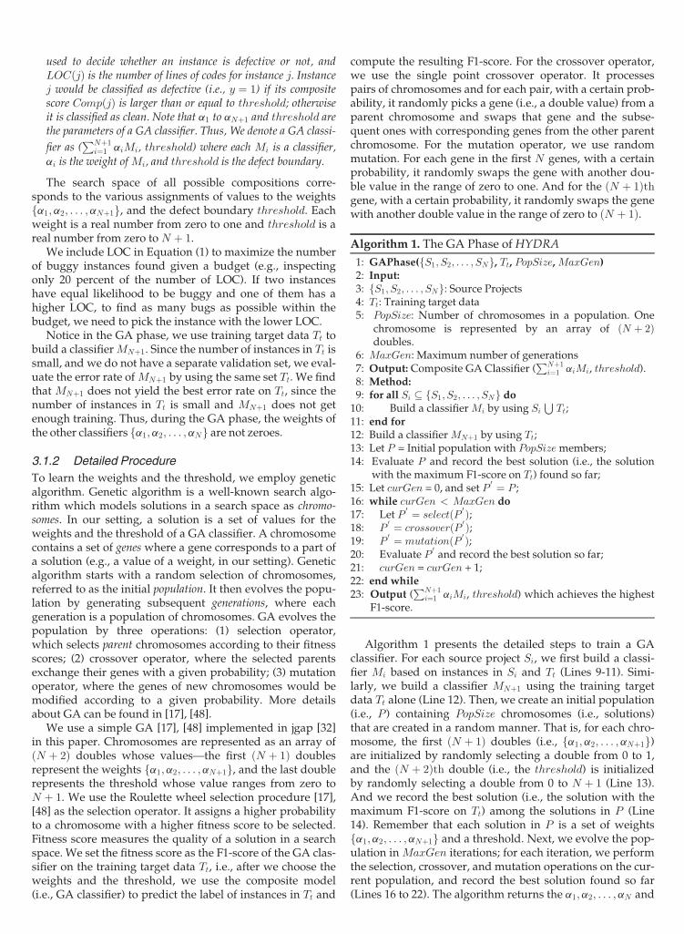
Algorithm 1 presents the detailed steps to train a GAclassifier. For each source project Si, we first build a classi-fier Mi based on instances in Si and Tt (Lines 9-11). Simi-larly, we build a classifier MNþ1 using the training targetdata Tt alone (Line 12). Then, we create an initial population(i.e., P ) containing PopSize chromosomes (i.e., solutions)that are created in a random manner. That is, for each chro-mosome, the first ðN þ 1Þ doubles (i.e., fa1;a2; . . . ;aNþ1g)are initialized by randomly selecting a double from 0 to 1,and the ðN þ 2Þth double (i.e., the threshold) is initializedby randomly selecting a double from 0 to N þ 1 (Line 13).And we record the best solution (i.e., the solution with themaximum F1-score on Tt) among the solutions in P (Line14). Remember that each solution in P is a set of weightsfa1;a2; . . . ;aNþ1g and a threshold. Next, we evolve the pop-ulation in MaxGen iterations; for each iteration, we performthe selection, crossover, and mutation operations on the cur-rent population, and record the best solution found so far(Lines 16 to 22). The algorithm returns the a1;a2; . . . ;aN and


threshold values which maximize the F1-score on Tt (i.e., thebest solution among solutions in the initial population andthe populations generated in theMaxGen generations).

3.2 The EL Phase

In the EL phase, we iterate the GA phase a number of timesto learn a composition of GA classifiers. To do this, weadapt AdaBoost [16], which is one of the most famous andwidely used ensemble learning algorithms. AdaBoost pro-ceeds in a number of iterations and generates one classifierin each iteration. In each iteration, the classifier built istweaked such that instances that get misclassified by previ-ous classifiers get a higher weight and thus are deemed tobe more important to be classified correctly. AdaBoost canbe used with any underlying/base classification algorithms.In the EL phase, we follow the principle of AdaBoost to gen-erate multiple GA classifiers. However, there are severaldifferences between our EL phase and AdaBoost: (1) Ada-Boost is not for transfer learning—it is designed for tradi-tional supervised learning, while our approach is fortransfer learning. (2) To adapt AdaBoost for transfer learn-ing, we modify the way in which Adaboost [16] assignsweights to instances and evaluates the effectiveness of aclassifier. Different from AdaBoost, where instances comesfrom one domain, for our setting, we have instances fromsource projects and those from training target data. Our ELphase adjusts the weights of instances from source projectsdifferently from those from training target data. During theiterations, the focus of our EL phase is to minimize errorson the prediction of instances in the training target data,while AdaBoost tries to minimize prediction errors of alltraining instances.

The details of the EL phase is as follows. For each iterationk, we build a composite GA classifier GAk using instances infS1; S2; . . . ; SNg and Tt. Next, we assign different weights tothe data instances in fS1; S2; . . . ; SNg and Tt. For data instan-ces that GAk predicts correctly, we assign lower weights tothem, and for data instances whichGAk predicts wrongly, weassign higher weights to them. Also, we assign weights toinstances in training target data differently from those insource projects since our goal is to minimize errors on instan-ces in the training target data.4 In the next iteration kþ 1, sincedifferent data instances have different weights, GAkþ1 willprioritize data instances with higher weights. The underlyingclassifiers (i.e., logistic regression), which are parts of the GAclassifier, are able to process weighted instances in the train-ing data andwill prioritize thosewith higherweights.

Notice that in the EL phase, we create an ensemble ofmultiple GA classifiers. We choose this design rather thanusing only the best performing GA classifier to preventoverfitting [19], i.e., the model that fits best on the trainingdata may not show good performance when it is applied tothe testing data.

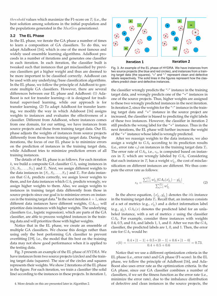
Fig. 3 presents an example of the EL phase ofHYDRA. Wehave instances from two source projects (circles) and the train-ing target data (squares). The size of the circles and squaresrepresents their weights.We show 2 iterations of the EL phasein the figure. For each iteration, we train a classifier (the solidline) according to the instances in these projects. In iteration 1,

the classifier wrongly predicts the “-” instance in the trainingtarget data, and wrongly predicts one of the “+” instances inone of the source projects. Thus, higher weights are assignedto these two wrongly predicted instances in the next iteration.In iteration 2, since theweights for the “-” instance in the train-ing target data and “+” instance in the source project areincreased, the classifier is biased to predicting the right labelsof these two instances. However, the classifier in iteration 2still predicts the wrong label for the “+” instance. Thus in thenext iterations, the EL phase will further increase the weightof the “+” instancewhose label iswrongly predicted.

After we reassign weights to the data instances, we alsoassign a weight to GAk according to its prediction results(i.e., error rate �k) on instances in the training target data Tt.The error rate of GAk, i.e., �k, is computed based on instan-ces in Tt which are wrongly labeled by GAk. Considering

that each instance in Tt has a weight wiTt, the cost of misclas-

sification on different instances are different. We thus com-pute the error rate as follows:

�k ¼PjTtj

i¼1 wiTtjGAkðxi

TtÞ � yiTt jPjTtj

j¼1 wjTt

: (2)

In the above equation, fxiTt; yiTtg denotes the ith instance

in the training target data Tt. Recall that, an instance consists

of a set of metrics (e.g., xiTt) and a defect information label

(e.g., yiTt ). GAkðxÞ denotes the predicted label for an unla-

beled instance, with a set of metrics x using the classifierGAk. For example, consider three instances with weights0.4, 0.5, and 0.6, and labels 1, 1, and 0. After we run the GAk

classifier, the predicted labels are 1, 0, and 1. Then, the errorrate for GAk would be:

�ðkÞ ¼ 0:4 � j1� 1j þ 0:5 � j0� 1j þ 0:6 � j1� 0j0:4þ 0:5þ 0:6

¼ 0:73:

Notice that we use a different optimization criteria in theEL phase (i.e., error rate) and GA phase (F1-score). In the ELphase, we follow the principle of AdaBoost [16], and Ada-Boost also uses error rate as the optimization criteria. In theGA phase, since our GA classifier combines a number ofclassifiers, if we set the fitness function as the error rate (i.e.,minimize the error rate), due to the imbalance distributionof defective and clean instances in the source projects, the

Fig. 3. An example of the EL phase of HYDRA. We have instances fromtwo source projects (the blue and red circles), and instances from a train-ing target data (the squares). “+” and “-” represent clean and defectivelabels respectively. The solid lines in the figures represent how the clas-sifiers predict clean and defective instances.

4. More details on this are presented later in Algorithm 2.


GA classifier is likely to be prone to predict all of the instan-ces to be of the majority class.

At the end of the K iterations, we have a total of K GAclassifiers, and each GA classifier has a weight. We refer tothe combination of the K classifiers as an ensemble classifier.For a new instance in the target project, we input it into theensemble classifier, and the ensemble classifier will outputa predicted label.

Algorithm 2 presents the detailed steps of the EL phaseof HYDRA. In the algorithm, the ith source project isdenoted as Si and the jth instance of Si is denoted as

fxjSi; yjSig where xj

Siis the set of metrics of the jth instance

and yjSi is its defect information (i.e., defective or clean).

Moreover, we denote the weight of the jth instance in the

ith source project as wjSi, and the weight of the jth instance

in the training target data Tt as wjTt. We use the instances in

the source projects and training target data as proxies to theunlabeled data in the target project. The EL phase buildsmultiple models that can predict the labels of these proxiesin varying amount of accuracies, and then ensemble thesestrong and weak classifiers together.

Algorithm 2. The EL Phase of HYDRA

1: ELPhase(fS1; S2; . . . ; SNg, Tt,K)2: Input:3: fS1; S2; . . . ; SNg: Source projects4: Tt: Training target data5: K: Maximum number of iterations6: Output: Ensemble Classifier

PKk¼1 bk GAk.

7: Method:8: Compute the number of instances: ns ¼

PNi¼1 jSij, and

n ¼ ns þ jTtj;9: Set bs ¼ 1

2 lnð1þffiffiffiffiffiffiffiffiffiffiffiffi2 ln ns

K

p);

10: Initialize the weights of instances in fS1; S2; . . . ; SNg, andTt. We set the weights equally, i.e., wj

Si¼ 1

n, and wjTt

¼ 1n;

11: for all iteration k from 1 toK do12: Normalize the weights in fS1; S2; . . . ; SNg, and Tt such

that the summation of all the weight equals to 1;13: Input fS1; S2; . . . ; SNg, and Tt into the GA phase (i.e.,

Algorithm 1) to get a GA classifier GAk;14: Let �k denote the error rate of GAk on Tt according to

Equation (2):15: If �k > 1

2, Break;16: Set bk ¼ �k

1��k, with �k � 1

2;17: Reassign the weights in fS1; S2; . . . ; SNg, and Tt:

wjSi

¼ wjSiexp

�bsjGAkðxjSi Þ�yjSij; 1 � i � N; 1 � j � jSij

wjTt

¼ wjTtexp

�bkjGAkðxjTt Þ�yjTtj; 1 � j � jTtj

18: end for19: Output Ensemble Classifier

PKk¼1 bkGAk.

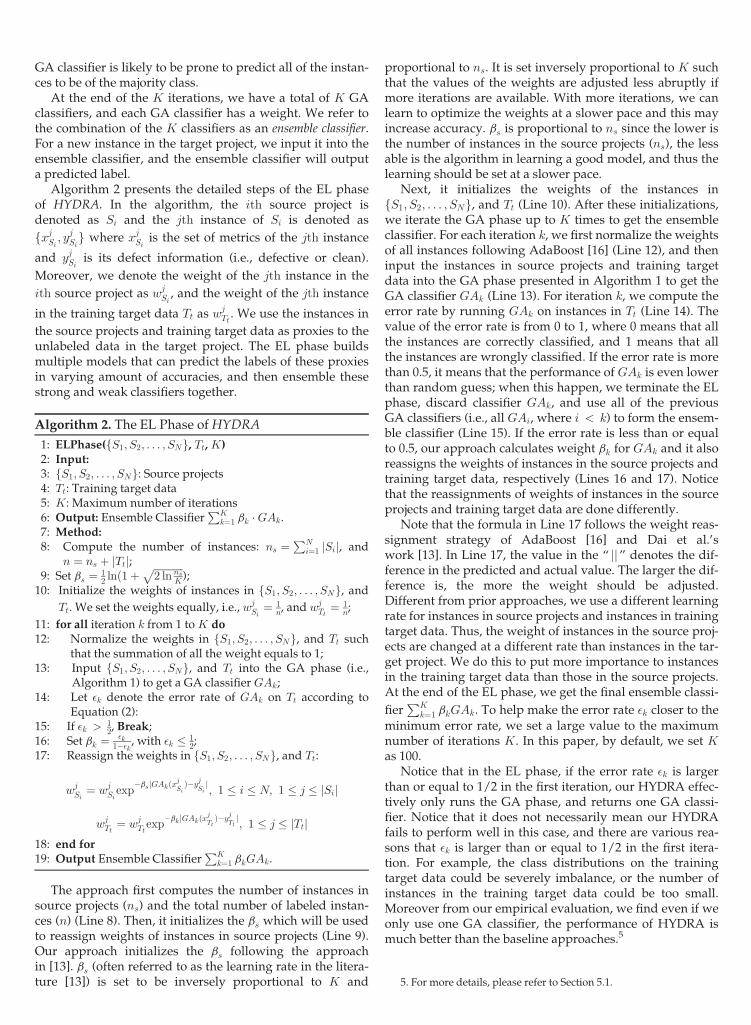
The approach first computes the number of instances insource projects (ns) and the total number of labeled instan-ces (n) (Line 8). Then, it initializes the bs which will be usedto reassign weights of instances in source projects (Line 9).Our approach initializes the bs following the approachin [13]. bs (often referred to as the learning rate in the litera-ture [13]) is set to be inversely proportional to K and

proportional to ns. It is set inversely proportional to K suchthat the values of the weights are adjusted less abruptly ifmore iterations are available. With more iterations, we canlearn to optimize the weights at a slower pace and this mayincrease accuracy. bs is proportional to ns since the lower isthe number of instances in the source projects (ns), the lessable is the algorithm in learning a good model, and thus thelearning should be set at a slower pace.

Next, it initializes the weights of the instances infS1; S2; . . . ; SNg, and Tt (Line 10). After these initializations,we iterate the GA phase up to K times to get the ensembleclassifier. For each iteration k, we first normalize the weightsof all instances following AdaBoost [16] (Line 12), and theninput the instances in source projects and training targetdata into the GA phase presented in Algorithm 1 to get theGA classifier GAk (Line 13). For iteration k, we compute theerror rate by running GAk on instances in Tt (Line 14). Thevalue of the error rate is from 0 to 1, where 0 means that allthe instances are correctly classified, and 1 means that allthe instances are wrongly classified. If the error rate is morethan 0.5, it means that the performance of GAk is even lowerthan random guess; when this happen, we terminate the ELphase, discard classifier GAk, and use all of the previousGA classifiers (i.e., all GAi, where i < k) to form the ensem-ble classifier (Line 15). If the error rate is less than or equalto 0.5, our approach calculates weight bk for GAk and it alsoreassigns the weights of instances in the source projects andtraining target data, respectively (Lines 16 and 17). Noticethat the reassignments of weights of instances in the sourceprojects and training target data are done differently.

Note that the formula in Line 17 follows the weight reas-signment strategy of AdaBoost [16] and Dai et al.’swork [13]. In Line 17, the value in the “ jj ” denotes the dif-ference in the predicted and actual value. The larger the dif-ference is, the more the weight should be adjusted.Different from prior approaches, we use a different learningrate for instances in source projects and instances in trainingtarget data. Thus, the weight of instances in the source proj-ects are changed at a different rate than instances in the tar-get project. We do this to put more importance to instancesin the training target data than those in the source projects.At the end of the EL phase, we get the final ensemble classi-

fierPK

k¼1 bkGAk. To help make the error rate �k closer to theminimum error rate, we set a large value to the maximumnumber of iterations K. In this paper, by default, we set Kas 100.

Notice that in the EL phase, if the error rate �k is largerthan or equal to 1/2 in the first iteration, our HYDRA effec-tively only runs the GA phase, and returns one GA classi-fier. Notice that it does not necessarily mean our HYDRAfails to perform well in this case, and there are various rea-sons that �k is larger than or equal to 1/2 in the first itera-tion. For example, the class distributions on the trainingtarget data could be severely imbalance, or the number ofinstances in the training target data could be too small.Moreover from our empirical evaluation, we find even if weonly use one GA classifier, the performance of HYDRA ismuch better than the baseline approaches.5

5. For more details, please refer to Section 5.1.


3.3 Complexity Analysis

Notice our HYDRA can employ different underlying classi-fiers, and we denote the time complexity for the underlyingclassifier as U . In the GA phase, we denote the populationsize as P , number of generations as G, the number of classi-fiers as ðN þ 1Þ (N refers to the number of source projects),and the length of the chromosomes is ðN þ 2Þ. Then thetime complexity for the GA phase is OðGAÞ ¼ OðN � U þP �G�NÞ. In the EL phase, if we denote the number ofiteration as T , then the time complexity for the EL phase isOðT �GAÞ. Thus, the time complexity for HYDRA isOðT � ðN � U þ P �G�NÞÞ.

4 EXPERIMENTS

In this section, we evaluate the performance of HYDRA. Theexperimental environment is a Windows 7, 64-bit, IntelXeon 2.53 GHz server with 24 GB RAM.

4.1 Experiment Setup

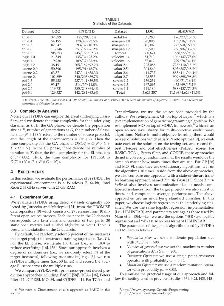
We evaluate HYDRA using defect datasets originally col-lected by Jureczko and Madeyski [24] from the PROMISEdata repository [8] which consists of 29 releases from 10 dif-ferent open-source projects. Each instance in the 29 datasetscorresponds to a Java class and consists of two parts: 20static code metrics and a label (defective or clean). Table 3presents the statistics of the 29 datasets.

By default, we randomly select 5 percent of the instancesin a target project to construct a training target data (i.e., Tt).For the EL phase, we iterate 100 times (i.e., K ¼ 100) toreduce overfitting [16], [56]. Since our approach involves adegree of randomness (i.e., we randomly select 5% of thetarget instances), following past studies, e.g., [3], we runHYDRA multiple times (i.e., 50 times) and record the aver-age F1-score across the multiple runs.

We compare HYDRA with prior cross-project defect pre-diction approaches including: BASIC [58]6, TCA+ [36], Petersfilter [42], GP [28], MO [9], and CODEP [41]. For TCA+ and

TransferBoost, we use the source code provided by theauthors. We re-implement GP on top of Leyan,7 which is ajava implementation of genetic programming algorithm. Were-implement MO on top of MOEA framework,8 which is anopen source Java library for multi-objective evolutionaryalgorithms. Notice in multi-objective learning, there wouldbe a set of solutionswhich satisfy Pareto optimal [9], we eval-uate each of the solution on the testing set, and record thebest F1-score and cost effectiveness (PofB20) scores. ForBASIC, TCA+, Peters filter, and CODEP, these approachesdo not involve any randomness, i.e., the results would be thesame no matter how many times they are run. For GP [28]and MO [9], since they use evolutionary algorithms, we runthe algorithms 10 times. Aside from the above approaches,we also compare our approach with a state-of-the-art trans-fer learning approach named TransferBoost [15]. Since Trans-ferBoost also involves randomization (i.e., it needs somelabeled instances from the target project), we also run it 50times, and compute its average performance. The aboveapproaches use an underlying standard classifier. In thispaper, we choose logistic regression as this underlying clas-sifier. We use the same logistic regression implementation(i.e., LIBLINEAR) and parameters settings as those used byNam et al. [36],—i.e., we use the options “-S 0 (use logisticregression) and “-B -1 (use no bias term) of LIBLINEAR.

The parameters of the genetic algorithm used by HYDRAand MO are as follows:

� Population size: we set a moderate population sizewith PopSize ¼ 500.

� Number of generations: we set the maximum numberof generationsMaxGen ¼ 200.

� Crossover Operator: we use a single point crossoveroperator with probability pc ¼ 0:35.

� Mutation Operator: we use a random mutation opera-tor with probability pm ¼ 0:08.

To simulate the practical usage of our approach and fol-low the setting used in previous studies [36], [42], [43], [45],

TABLE 3Statistics of the Datasets

Dataset LOC #I/#D/%D Dataset LOC #I/#D/%D

ant-1.3 37,699 125/20/16% redaktor 59,280 176/27/15.3%ant-1.4 54,195 178/40/22.5% synapse-1.0 28,806 157/16/10.2%ant-1.5 87,047 293/32/10.9% synapse-1.1 42,302 222/60/27.0%ant-1.6 113,246 351/92/26.2% synapse-1.2 53,500 256/86/33.6%ant-1.7 208,653 745/166/22.3% tomcat 300,674 858/77/9.0%log4j-1.0 21,549 135/34/25.2% velocity-1.4 51,713 196/147/75.0%log4j-1.1 19,938 109/37/33.9% velocity-1.6 57,012 229/78/34.1%log4j-1.2 38,191 205/189/92.2% xalan-2.4 225,088 723/110/15.2%lucene-2.0 50,596 195/91/46.7% xalan-2.5 304,860 803/387/48.2%lucene-2.2 63,571 247/144/58.3% xalan-2.6 411,737 885/411/46.4%lucene-2.4 102,859 340/203/59.7% xalan-2.7 428,555 909/898/98.8%poi-1.5 55,428 237/141/59.5% xerces-1.2 159,254 440/71/16.1%poi-2.0 93,171 314/37/11.8% xerces-1.3 167,095 453/69/15.2%poi-2.5 119,731 385/248/64.4% xerces-1.4 141,180 588/437/74.3%poi-3.0 129,327 442/281/63.6% Total 3,626,257 11,196/4,629/41.3%

LOC denotes the total number of LOC. #I denotes the number of instances. #D denotes the number of defective instances. %D denotes theproportion of defective instances.

6. We refer to Zimmermann et al.’s approach as BASIC in thissection

7. http://www.leyan.org/Genetic+Programming8. http://www.moeaframework.org/


http://www.leyan.org/Genetic

http://www.moeaframework.org/

[52], when we consider a release of a project as a target proj-ect, we choose releases of other projects as the source proj-ects. For example, if we choose ant-1.5 as the target project,we use all releases of other projects (i.e., log4j, lucene, poi,redaktor, synapse, tomcat, velocity, xalan, and xerces) asthe source projects, and exclude other releases from thesame project (i.e., ant). For HYDRA and TransferBoost, wetake all instances from the source projects and 5 percent ofthe instances in the target project (with their labels), to pre-dict the labels of the remaining 95 percent of the instancesin the target project. For the other approaches, to ensurethat we use the same test set to evaluate all approaches for afair comparison, we remove the same 5 percent of theinstances in the target project, and predict the labels of thesame remaining 95 percent of the instances in the targetproject. Also, for some baseline approaches, such as BASICand TCA+, we adapt them so that they can benefit from alldatasets (rather than only one dataset, which is the settingused in the original paper) so that the setting is similar tothat of our approach and other baselines.

4.2 Evaluation Metrics

We use two evaluation metrics: F1-score and cost effective-ness. F1-score is useful when there are sufficient resourcesto inspect all of the predicted buggy changes. Cost effective-ness is useful when there are limited resources to inspect alimited amount of code due to a hectic schedule ofdevelopment.

4.2.1 F1-Score

There are four possible outcomes for an instance in a targetproject: An instance can be classified as defective when it istruly defective (true positive, TP); it can be classified asdefective when it is actually clean (false positive, FP); it canbe classified as clean when it is actually defective (false neg-ative, FN); or it can be classified as clean and it is truly clean(true negative, TN). Based on these possible outcomes, pre-cision, recall and F1-score are defined as:

Precision: the proportion of instances that are correctlylabeled as defective among those labeled as defective,

P ¼ TP=ðTP þ FP Þ: (3)

Recall: the proportion of defective instances that are cor-rectly labeled,

R ¼ TP=ðTP þ FNÞ: (4)

F1-Score: a summary measure that combines both precisionand recall—it evaluates if an increase in precision (recall)outweighs a reduction in recall (precision),

F ¼ ð2� P �RÞ=ðP þRÞ: (5)

There is a trade-off between precision and recall. Thetrade-off causes difficulties to compare the performance ofseveral prediction models by using only precision orrecall [19]. For this reason, we compare the predictionresults using F1-score, which is a harmonic mean of preci-sion and recall. This follows the setting used in many defectprediction studies [25], [36] and other software analyticsstudies [37], [50], [55].

4.2.2 Cost Effectiveness

Cost effectiveness is a widely used evaluation metric fordefect prediction [4], [23], [43], [44], [45], which evaluatesprediction performance given a cost limit. In our setting, thecost is the lines of code to inspect, and the benefit is thenumber of bugs detected. We use the same cost effective-ness setup as the one used by Jiang et al. [23]. They measurethe percentage of bugs that a developer can identify byinspecting the top 20 percent lines of code. They refer to thisnumber as PofB20.

To compute PofB20 we sort instances in the test databased on the confidence levels that a defect prediction tech-nique outputs for each of them. An instance with a higherconfidence level is deemed to be more likely to be buggy bythe defect prediction technique. We then simulate a devel-oper that inspects these potentially buggy instances one at atime. As the instances are inspected one at a time, we accu-mulate the number of lines of code that are inspected andthe number of bugs identified. We stop the process when20 percent of the lines of code have been inspected and out-put the percentage of bugs that are identified. This numberis the PofB20 score. A higher cost effectiveness score repre-sents that a developer can detect more bugs when inspect-ing a limited number of LOC.

In our HYDRA, suppose we have n GA classifier. For anew instance new, each GA classifier GAk will compute acomposite score that indicates the likelihood that new isbuggy, i.e., CompkðnewÞ. Then, the final confidence scorethat HYDRA outputs for new can be computed asPn

k¼1 bk � CompkðnewÞ. In this paper, for each instance inthe test set, we get its confidence score. Next, we rank theinstances based on their confidence scores to compute thePofB20 score.

4.3 Research Questions

RQ1 How effective is HYDRA? How much improvement can itachieve over the baseline approaches?

In this RQ, we investigate the extent HYDRA advancesthe state-of-the-art approaches. To answer this researchquestion, we compare HYDRA with BASIC, TCA+, Petersfilter, GP, MO, CODEP, and TransferBoost. We compute F1-scores and cost effectiveness (NofB20) to evaluate the per-formance of these five approaches on the 29 datasets fromthe PROMISE repository. For each dataset, by default, werun HYDRA and the baseline approaches 50 times. To checkif the differences in the performance of HYDRA and thebaseline approaches are statistically significant, for the eachdataset, we apply the Wilcoxon signed-rank test [54] at95 percent significance level on two 50 paired data whichcorresponds to the F1-scores and PofB20 scores of two com-peting approaches respectively. Since we run the test manytimes (twice for each dataset), we also use Bonferroni cor-rection [1] to counteract the results of multiple comparisons.

We also use Cliff’s delta (d) [12], which is a non-paramet-ric effect size measure that quantifies the amount of differ-ence between two approaches. In our context, we use Cliff’sdelta to compare HYDRA with the baseline approaches.The delta values range from -1 to 1, where d ¼ �1 or 1 indi-cates the absence of overlap between two approaches (i.e.,all values of one group are higher than the values of the


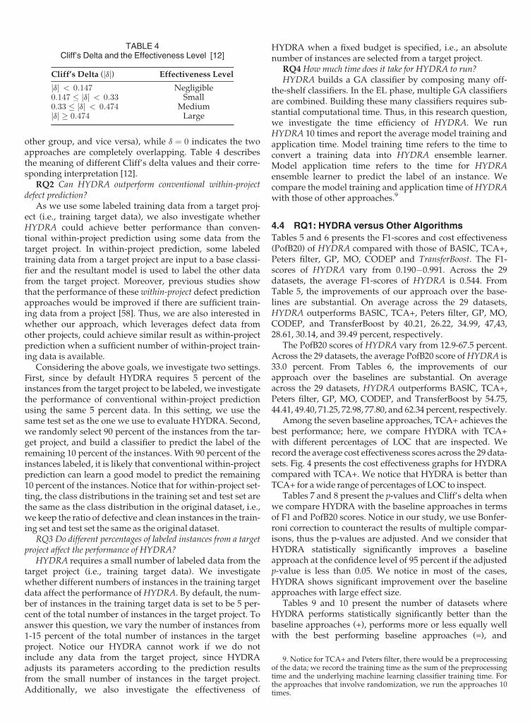
other group, and vice versa), while d ¼ 0 indicates the twoapproaches are completely overlapping. Table 4 describesthe meaning of different Cliff’s delta values and their corre-sponding interpretation [12].

RQ2 Can HYDRA outperform conventional within-projectdefect prediction?

As we use some labeled training data from a target proj-ect (i.e., training target data), we also investigate whetherHYDRA could achieve better performance than conven-tional within-project prediction using some data from thetarget project. In within-project prediction, some labeledtraining data from a target project are input to a base classi-fier and the resultant model is used to label the other datafrom the target project. Moreover, previous studies showthat the performance of these within-project defect predictionapproaches would be improved if there are sufficient train-ing data from a project [58]. Thus, we are also interested inwhether our approach, which leverages defect data fromother projects, could achieve similar result as within-projectprediction when a sufficient number of within-project train-ing data is available.

Considering the above goals, we investigate two settings.First, since by default HYDRA requires 5 percent of theinstances from the target project to be labeled, we investigatethe performance of conventional within-project predictionusing the same 5 percent data. In this setting, we use thesame test set as the one we use to evaluate HYDRA. Second,we randomly select 90 percent of the instances from the tar-get project, and build a classifier to predict the label of theremaining 10 percent of the instances. With 90 percent of theinstances labeled, it is likely that conventional within-projectprediction can learn a good model to predict the remaining10 percent of the instances. Notice that for within-project set-ting, the class distributions in the training set and test set arethe same as the class distribution in the original dataset, i.e.,we keep the ratio of defective and clean instances in the train-ing set and test set the same as the original dataset.

RQ3 Do different percentages of labeled instances from a targetproject affect the performance of HYDRA?

HYDRA requires a small number of labeled data from thetarget project (i.e., training target data). We investigatewhether different numbers of instances in the training targetdata affect the performance ofHYDRA. By default, the num-ber of instances in the training target data is set to be 5 per-cent of the total number of instances in the target project. Toanswer this question, we vary the number of instances from1-15 percent of the total number of instances in the targetproject. Notice our HYDRA cannot work if we do notinclude any data from the target project, since HYDRAadjusts its parameters according to the prediction resultsfrom the small number of instances in the target project.Additionally, we also investigate the effectiveness of

HYDRA when a fixed budget is specified, i.e., an absolutenumber of instances are selected from a target project.

RQ4 How much time does it take for HYDRA to run?HYDRA builds a GA classifier by composing many off-

the-shelf classifiers. In the EL phase, multiple GA classifiersare combined. Building these many classifiers requires sub-stantial computational time. Thus, in this research question,we investigate the time efficiency of HYDRA. We runHYDRA 10 times and report the average model training andapplication time. Model training time refers to the time toconvert a training data into HYDRA ensemble learner.Model application time refers to the time for HYDRAensemble learner to predict the label of an instance. Wecompare the model training and application time ofHYDRAwith those of other approaches.9

4.4 RQ1: HYDRA versus Other Algorithms

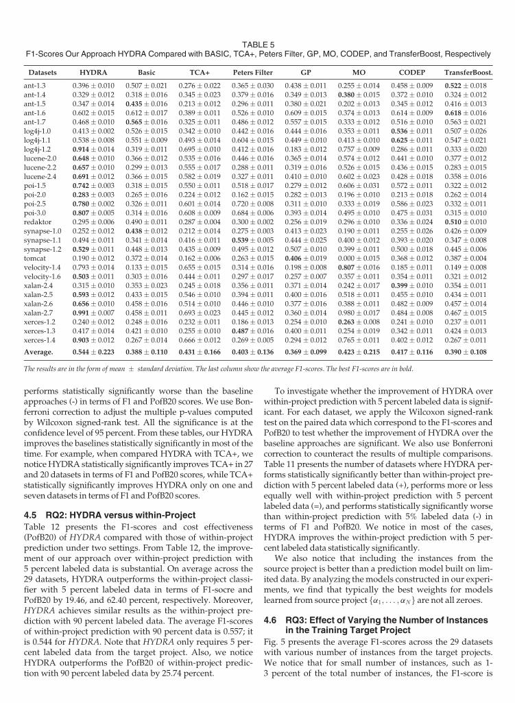
Tables 5 and 6 presents the F1-scores and cost effectiveness(PofB20) of HYDRA compared with those of BASIC, TCA+,Peters filter, GP, MO, CODEP and TransferBoost. The F1-scores of HYDRA vary from 0.190�0.991. Across the 29datasets, the average F1-scores of HYDRA is 0.544. FromTable 5, the improvements of our approach over the base-lines are substantial. On average across the 29 datasets,HYDRA outperforms BASIC, TCA+, Peters filter, GP, MO,CODEP, and TransferBoost by 40.21, 26.22, 34.99, 47,43,28.61, 30.14, and 39.49 percent, respectively.

The PofB20 scores of HYDRA vary from 12.9-67.5 percent.Across the 29 datasets, the average PofB20 score ofHYDRA is33.0 percent. From Tables 6, the improvements of ourapproach over the baselines are substantial. On averageacross the 29 datasets, HYDRA outperforms BASIC, TCA+,Peters filter, GP, MO, CODEP, and TransferBoost by 54.75,44.41, 49.40, 71.25, 72.98, 77.80, and 62.34 percent, respectively.

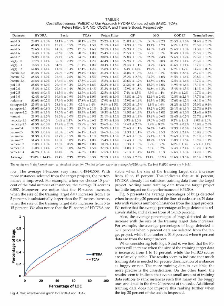
Among the seven baseline approaches, TCA+ achieves thebest performance; here, we compare HYDRA with TCA+with different percentages of LOC that are inspected. Werecord the average cost effectiveness scores across the 29 data-sets. Fig. 4 presents the cost effectiveness graphs for HYDRAcompared with TCA+. We notice that HYDRA is better thanTCA+ for awide range of percentages of LOC to inspect.

Tables 7 and 8 present the p-values and Cliff’s delta whenwe compare HYDRA with the baseline approaches in termsof F1 and PofB20 scores. Notice in our study, we use Bonfer-roni correction to counteract the results of multiple compar-isons, thus the p-values are adjusted. And we consider thatHYDRA statistically significantly improves a baselineapproach at the confidence level of 95 percent if the adjustedp-value is less than 0.05. We notice in most of the cases,HYDRA shows significant improvement over the baselineapproaches with large effect size.

Tables 9 and 10 present the number of datasets whereHYDRA performs statistically significantly better than thebaseline approaches (+), performs more or less equally wellwith the best performing baseline approaches (=), and

TABLE 4Cliff’s Delta and the Effectiveness Level [12]

Cliff’s Delta (jdj) Effectiveness Level

jdj < 0:147 Negligible0:147 � jdj < 0:33 Small0:33 � jdj < 0:474 Mediumjdj � 0:474 Large

9. Notice for TCA+ and Peters filter, there would be a preprocessingof the data; we record the training time as the sum of the preprocessingtime and the underlying machine learning classifier training time. Forthe approaches that involve randomization, we run the approaches 10times.


performs statistically significantly worse than the baselineapproaches (-) in terms of F1 and PofB20 scores. We use Bon-ferroni correction to adjust the multiple p-values computedby Wilcoxon signed-rank test. All the significance is at theconfidence level of 95 percent. From these tables, our HYDRAimproves the baselines statistically significantly inmost of thetime. For example, when compared HYDRA with TCA+, wenoticeHYDRA statistically significantly improves TCA+ in 27and 20 datasets in terms of F1 and PofB20 scores, while TCA+statistically significantly improves HYDRA only on one andseven datasets in terms of F1 and PofB20 scores.

4.5 RQ2: HYDRA versus within-Project

Table 12 presents the F1-scores and cost effectiveness(PofB20) of HYDRA compared with those of within-projectprediction under two settings. From Table 12, the improve-ment of our approach over within-project prediction with5 percent labeled data is substantial. On average across the29 datasets, HYDRA outperforms the within-project classi-fier with 5 percent labeled data in terms of F1-socre andPofB20 by 19.46, and 62.40 percent, respectively. Moreover,HYDRA achieves similar results as the within-project pre-diction with 90 percent labeled data. The average F1-scoresof within-project prediction with 90 percent data is 0.557; itis 0.544 for HYDRA. Note that HYDRA only requires 5 per-cent labeled data from the target project. Also, we noticeHYDRA outperforms the PofB20 of within-project predic-tion with 90 percent labeled data by 25.74 percent.

To investigate whether the improvement of HYDRA overwithin-project predictionwith 5 percent labeled data is signif-icant. For each dataset, we apply the Wilcoxon signed-ranktest on the paired data which correspond to the F1-scores andPofB20 to test whether the improvement of HYDRA over thebaseline approaches are significant. We also use Bonferronicorrection to counteract the results of multiple comparisons.Table 11 presents the number of datasets where HYDRA per-forms statistically significantly better than within-project pre-diction with 5 percent labeled data (+), performs more or lessequally well with within-project prediction with 5 percentlabeled data (=), and performs statistically significantly worsethan within-project prediction with 5% labeled data (-) interms of F1 and PofB20. We notice in most of the cases,HYDRA improves the within-project prediction with 5 per-cent labeled data statistically significantly.

We also notice that including the instances from thesource project is better than a prediction model built on lim-ited data. By analyzing themodels constructed in our experi-ments, we find that typically the best weights for modelslearned from source project fa1; . . . ;aNg are not all zeroes.

4.6 RQ3: Effect of Varying the Number of Instancesin the Training Target Project

Fig. 5 presents the average F1-scores across the 29 datasetswith various number of instances from the target projects.We notice that for small number of instances, such as 1-3 percent of the total number of instances, the F1-score is

TABLE 5F1-Scores Our Approach HYDRA Compared with BASIC, TCA+, Peters Filter, GP, MO, CODEP, and TransferBoost, Respectively

Datasets HYDRA Basic TCA+ Peters Filter GP MO CODEP TransferBoost.

ant-1.3 0.396 0.010 0.507 0.021 0.276 0.022 0.365 0.030 0.438 0.011 0.255 0.014 0.458 0.009 0.522 0.018ant-1.4 0.329 0.012 0.318 0.016 0.345 0.023 0.379 0.016 0.349 0.013 0.380 0.015 0.372 0.010 0.324 0.012ant-1.5 0.347 0.014 0.435 0.016 0.213 0.012 0.296 0.011 0.380 0.021 0.202 0.013 0.345 0.012 0.416 0.013ant-1.6 0.602 0.015 0.612 0.017 0.389 0.011 0.526 0.010 0.609 0.015 0.374 0.013 0.614 0.009 0.618 0.016ant-1.7 0.468 0.010 0.565 0.016 0.325 0.011 0.486 0.012 0.557 0.015 0.333 0.012 0.516 0.010 0.563 0.021log4j-1.0 0.413 0.002 0.526 0.015 0.342 0.010 0.442 0.016 0.444 0.016 0.353 0.011 0.536 0.011 0.507 0.026log4j-1.1 0.538 0.008 0.551 0.009 0.493 0.014 0.604 0.015 0.449 0.010 0.413 0.010 0.625 0.011 0.547 0.021log4j-1.2 0.914 0.014 0.319 0.011 0.695 0.010 0.412 0.016 0.183 0.012 0.757 0.009 0.286 0.011 0.333 0.020lucene-2.0 0.648 0.010 0.366 0.012 0.535 0.016 0.446 0.016 0.365 0.014 0.574 0.012 0.441 0.010 0.377 0.012lucene-2.2 0.657 0.010 0.299 0.013 0.555 0.017 0.288 0.011 0.319 0.016 0.526 0.015 0.436 0.015 0.283 0.015lucene-2.4 0.691 0.012 0.366 0.015 0.582 0.019 0.327 0.011 0.410 0.010 0.602 0.023 0.428 0.018 0.358 0.016poi-1.5 0.742 0.003 0.318 0.015 0.550 0.011 0.518 0.017 0.279 0.012 0.606 0.031 0.572 0.011 0.322 0.012poi-2.0 0.283 0.003 0.265 0.016 0.224 0.012 0.162 0.015 0.282 0.013 0.196 0.010 0.213 0.018 0.262 0.014poi-2.5 0.780 0.002 0.326 0.011 0.601 0.014 0.720 0.008 0.311 0.010 0.333 0.019 0.586 0.023 0.332 0.011poi-3.0 0.807 0.005 0.314 0.016 0.608 0.009 0.684 0.006 0.393 0.014 0.495 0.010 0.475 0.031 0.315 0.010redaktor 0.295 0.006 0.490 0.011 0.287 0.004 0.300 0.002 0.256 0.019 0.296 0.010 0.336 0.024 0.510 0.010synapse-1.0 0.252 0.012 0.438 0.012 0.212 0.014 0.275 0.003 0.413 0.023 0.190 0.011 0.255 0.026 0.426 0.009synapse-1.1 0.494 0.011 0.341 0.014 0.416 0.011 0.539 0.005 0.444 0.025 0.400 0.012 0.393 0.020 0.347 0.008synapse-1.2 0.529 0.011 0.448 0.013 0.435 0.009 0.495 0.012 0.507 0.010 0.399 0.011 0.500 0.018 0.445 0.006tomcat 0.190 0.012 0.372 0.014 0.162 0.006 0.263 0.015 0.406 0.019 0.000 0.015 0.368 0.012 0.387 0.004velocity-1.4 0.793 0.014 0.133 0.015 0.655 0.015 0.314 0.016 0.198 0.008 0.807 0.016 0.185 0.011 0.149 0.008velocity-1.6 0.503 0.011 0.303 0.016 0.444 0.011 0.297 0.017 0.257 0.007 0.357 0.011 0.354 0.011 0.321 0.012xalan-2.4 0.315 0.010 0.353 0.023 0.245 0.018 0.356 0.011 0.371 0.014 0.242 0.017 0.399 0.010 0.354 0.011xalan-2.5 0.593 0.012 0.433 0.015 0.546 0.010 0.394 0.011 0.400 0.016 0.518 0.011 0.455 0.010 0.434 0.011xalan-2.6 0.656 0.010 0.458 0.016 0.514 0.010 0.446 0.010 0.377 0.016 0.388 0.011 0.482 0.009 0.457 0.014xalan-2.7 0.991 0.007 0.458 0.011 0.693 0.023 0.445 0.012 0.360 0.014 0.980 0.017 0.484 0.008 0.467 0.015xerces-1.2 0.240 0.012 0.248 0.016 0.232 0.011 0.186 0.013 0.254 0.010 0.263 0.008 0.241 0.010 0.237 0.011xerces-1.3 0.417 0.014 0.421 0.010 0.255 0.010 0.487 0.016 0.400 0.011 0.254 0.019 0.342 0.011 0.424 0.013xerces-1.4 0.903 0.012 0.267 0.014 0.666 0.012 0.269 0.005 0.294 0.012 0.765 0.011 0.402 0.012 0.267 0.011

Average. 0.544 0.223 0.388 0.110 0.431 0.166 0.403 0.136 0.369 0.099 0.423 0.215 0.417 0.116 0.390 0.108

The results are in the form of mean standard deviation. The last column show the average F1-scores. The best F1-scores are in bold.


low. The average F1-scores vary from 0.484-0.558. Withmore instances selected from the target projects, the perfor-mance is improved. For example, when we choose 15 per-cent of the total number of instances, the average F1-score is0.557. Moreover, we notice that the F1-scores increase,when the size of the training target data increases from 1 to5 percent, is substantially larger than the F1-scores increase,when the size of the training target data increases from 5 to15 percent. We also notice that the F1-scores of HYDRA are

stable when the size of the training target data increasesfrom 10 to 15 percent. This indicates that at 10 percent,HYDRA already has sufficient training data from the targetproject. Adding more training data from the target projecthas little impact on the performance of HYDRA.

Fig. 6 presents the average percentages of bugs detectedwhen inspecting 20 percent of the lines of code across 29 data-sets with various number of instances from the target projects.We notice that the average percentages of bugs detected is rel-atively stable, and it varies from 31.5-35.5 percent.

Also, the average percentages of bugs detected do notincrease with the size of the training target data increases.For example, the average percentages of bugs detected is32.7 percent when 5 percent data are selected from the tar-get project, while the number is 31.8 percent when 6 percentdata are from the target project.

When considering both Figs. 5 and 6, we find that the F1-scores will increase when the size of the training target datais increased from 1 to 15 percent, while the PofB20 scoresare relatively stable. The results seem to indicate that muchtraining data is needed for precise classification of instancesas buggy or not. The more training data is available, themore precise is the classification. On the other hand, theresults seem to indicate that even a small amount of trainingdata suffices to rank instances such that many of the buggyones are listed in the first 20 percent of the code. Additionaltraining data does not improve this ranking further whenthe top 20 percent of the code is inspected.Fig. 4. Cost effectiveness graph for HYDRA and TCA+.

TABLE 6Cost Effectiveness (PofB20) of Our Approach HYDRA Compared with BASIC, TCA+,

Peters Filter, GP, MO, CODEP, and TransferBoost, Respectively

Datasets HYDRA Basic TCA+ Peters Filter GP MO CODEP TransferBoost.

ant-1.3 20.0% 1.0% 35.1% 1.1% 20.1% 2.2% 25.2% 1.3% 20.0% 1.0% 35.0% 2.2% 25.5% 1.6% 31.6% 2.5%ant-1.4 46.8% 1.2% 17.2% 1.5% 32.2% 1.5% 21.5% 1.4% 14.9% 1.6% 19.1% 1.2% 6.5% 1.2% 25.5% 1.0%ant-1.5 28.6% 1.0% 14.5% 2.2% 17.6% 1.6% 20.1% 1.6% 22.9% 1.6% 14.3% 1.4% 22.6% 1.0% 14.3% 1.0%ant-1.6 14.4% 1.0% 23.6% 1.5% 20.5% 1.0% 25.4% 2.2% 25.5% 1.8% 9.2% 1.5% 30.4% 1.0% 22.5% 1.2%ant-1.7 24.8% 0.8% 29.1% 1.6% 24.3% 1.0% 30.0% 1.6% 27.8% 1.9% 32.8% 2.4% 27.6% 1.2% 27.3% 1.0%log4j-1.0 19.7% 1.1% 36.0% 2.3% 37.7% 1.2% 42.4% 1.8% 27.9% 1.2% 29.5% 0.8% 31.2% 1.1% 28.3% 1.3%log4j-1.1 16.5% 1.2% 34.5% 1.2% 31.4% 1.0% 30.4% 1.8% 24.4% 1.1% 33.7% 1.6% 33.6% 1.1% 16.7% 1.6%log4j-1.2 54.8% 1.4% 11.6% 1.4% 17.1% 1.2% 15.8% 1.5% 6.4% 1.0% 19.7% 1.1% 6.7% 1.7% 14.2% 0.6%lucene-2.0 35.4% 1.0% 29.9% 2.2% 19.4% 1.8% 34.3% 1.3% 34.0% 1.6% 3.4% 1.1% 20.8% 2.5% 25.7% 1.2%lucene-2.2 38.5% 1.0% 26.6% 2.6% 16.0% 1.5% 19.9% 1.6% 25.2% 2.3% 33.7% 1.0% 24.5% 1.4% 27.8% 1.6%lucene-2.4 39.5% 1.0% 17.6% 1.0% 17.5% 2.3% 15.8% 1.1% 20.6% 1.2% 13.8% 1.0% 12.5% 1.6% 13.7% 1.6%poi-1.5 35.6% 1.0% 20.4% 1.2% 23.2% 1.6% 22.3% 1.1% 20.2% 1.1% 15.2% 1.0% 14.9% 1.6% 13.1% 1.7%poi-2.0 15.8% 1.2% 20.6% 1.4% 30.9% 1.4% 23.3% 1.6% 17.9% 1.8% 38.5% 1.2% 15.4% 1.3% 11.1% 1.2%poi-2.5 49.6% 0.4% 11.5% 1.6% 12.9% 1.3% 22.5% 1.0% 7.4% 1.5% 9.9% 1.4% 6.2% 1.2% 10.7% 1.4%poi-3.0 42.4% 0.3% 10.6% 1.9% 24.5% 1.0% 16.6% 1.0% 13.8% 1.2% 12.4% 2.4% 12.8% 2.1% 17.7% 1.6%redaktor 50.0% 0.2% 17.9% 0.3% 17.8% 1.2% 17.9% 1.3% 17.9% 1.4% 14.3% 1.5% 17.6% 1.2% 48.1% 1.7%synapse-1.0 23.8% 1.1% 28.8% 1.3% 0.2% 1.4% 9.6% 1.5% 33.3% 1.5% 4.8% 1.6% 38.2% 1.3% 35.0% 0.4%synapse-1.1 33.0% 0.8% 27.3% 1.3% 25.5% 2.1% 24.2% 2.1% 27.3% 1.6% 18.2% 2.5% 26.1% 1.3% 24.7% 0.4%synapse-1.2 24.8% 1.3% 19.5% 1.4% 18.6% 1.0% 19.3% 3.2% 14.5% 1.6% 13.8% 1.0% 24.9% 1.0% 21.6% 0.2%tomcat 21.9% 1.5% 26.3% 1.0% 22.8% 0.8% 21.1% 1.2% 21.9% 1.4% 15.8% 0.6% 26.4% 0.5% 25.7% 0.7%velocity-1.4 67.5% 0.5% 5.4% 1.4% 36.7% 0.6% 21.9% 1.0% 3.3% 1.5% 29.5% 0.4% 0.2% 1.4% 8.0% 1.5%velocity-1.6 46.3% 0.3% 17.4% 2.1% 35.8% 0.5% 23.6% 0.5% 17.4% 2.6% 7.9% 0.5% 14.7% 0.2% 13.0% 2.6%xalan-2.4 12.9% 0.2% 28.2% 1.5% 21.8% 1.3% 26.9% 1.2% 25.6% 1.1% 36.5% 1.4% 17.9% 0.6% 17.3% 2.5%xalan-2.5 38.5% 0.4% 20.3% 1.6% 26.4% 1.4% 16.6% 0.5% 14.3% 1.1% 27.9% 1.5% 16.5% 2.4% 16.0% 1.0%xalan-2.6 31.5% 1.2% 23.7% 1.5% 18.6% 1.1% 20.3% 1.5% 20.6% 1.0% 25.1% 1.1% 20.6% 1.5% 28.1% 1.2%xalan-2.7 51.4% 1.0% 18.3% 1.0% 15.4% 1.0% 15.4% 1.6% 12.4% 1.0% 18.2% 1.5% 13.8% 1.6% 19.9% 1.1%xerces-1.2 15.8% 1.0% 12.5% 0.5% 18.3% 1.0% 10.1% 1.4% 10.3% 1.0% 5.2% 1.6% 6.0% 1.3% 7.5% 1.1%xerces-1.3 13.0% 1.4% 22.8% 1.0% 34.2% 1.5% 32.1% 1.0% 14.0% 1.6% 2.1% 1.2% 12.4% 2.4% 10.2% 3.0%xerces-1.4 44.7% 1.3% 13.4% 1.1% 26.5% 1.0% 17.5% 1.1% 17.1% 1.4% 14.1% 1.1% 12.6% 1.5% 14.2% 1.1%

Average. 33.0% 14.4% 21.4% 7.9% 22.9% 8.3% 22.1% 7.1% 19.3% 7.6% 19.1% 10.9% 18.6% 9.3% 20.3% 9.2%

The results are in the form of mean standard deviation. The last column show the average PofB20 scores. The best PofB20 scores are in bold.


Table 13 presents the F1-scores and cost effectiveness(PofB20) of HYDRA when there are only 10, 20, 30, 40, 50,and 60 instances in the training target project. We randomlyselect these 10, 20, 30, 40, 50, and 60 instances, and repeat theprocess 10 times and record the average F1 and cost effective-ness scores. The F1-scores and PofB20 vary from 0.529-0.580,and 30.6-35.1 percent, respectively. We notice the perfor-mance of HYDRA increases when the number of instances inthe training target project increases from 10 to 50, anddecreases when the number of instances from 50 to 60. Evenwith a smaller number of instances in the training target proj-ect, the performance of HYDRA is better than the other base-line approaches. For example, when we label only 20instances in the target project, HYDRA could achieve F1-score and PofB20 up to 0.559, and 35.1 percent, respectively.

4.7 RQ4: Time Efficiency of HYDRA

Table 14 presents the averagemodel training and applicationtime across the 29 datasets. Due to the space limitation,we donot list the time for each individual datasets. From Table 14,we notice that the model training and application time ofHYDRA is reasonable, e.g., on average, we need about1.5 minutes to train a model, and 1.7 seconds to predict thelabels of instances in the testing set using the model. Notethat themodel does not need to be updated all the time and itcan be used to label many instances. HYDRAmodel trainingtime is longer than those of BASIC, Peters filter, and

TransferBoost but shorter than that of TCA+, GP, andCODEP.The training time for TCA+ is long (i.e., nearly 1 hour to trainamodel) because TCA+ needs to performmanymatrix oper-ations. HYDRA model application time is longer than thoseof the other approaches but we believe it is still acceptable (itcan label thousands of instances in seconds).

5 DISCUSSIONS

5.1 Impact of the Number of Iterations in the ELPhase

By default, we set the number of iterations of HYDRA as100. Here, we also investigate other numbers of itera-tions, i.e., we increase the number of iterations from 1,10, 20, 30, . . . , 200. Fig. 7 presents the average F1 andPofB20 scores of HYDRA with different number of itera-tions. We notice that the performance of HYDRAincreases when we increase the number of iterationsfrom 1 to 100, and it is stable when we increase thenumber of iterations from 100 to 200. Thus, in practice,we suggest users to set the number of iteration as 100,since more iterations translates to higher runtime cost.Moreover, when we set the number of iterations as 1, itmeans we only have the GA phase, and the F1 andPofB20 scores of HYDRA are 0.501 and 0.28, respectively.These scores are much less than those of HYDRA withenough iterations. Thus, combining the GA and ELphases improves the performance of HYDRA.

TABLE 7P-Value and Cliff’s Delta (d) for HYDRA Compared with the Baseline Approaches in Terms of F1-Score

DatasetsH. vs. Basic H. vs. TCA+ H. vs. Peters

FilterH. vs. GP H. vs. MO H. vs. CODEP H. vs. Tr.Bo.

p-value d p-value d p-value d p-value d p-value d p-value d p-value d

ant-1.3 1.2e�9 -0.65 6.2e�12 0.52 0.0014 0.43 0.0003 -0.31 5.3e�15 0.87 1.1e�9 -0.56 5.8e�13 -0.86ant-1.4 0.02 0.08 0.0004 -0.15 0.0005 -0.46 0.072 -0.11 1.5e�9 -0.84 2.4e�7 -0.76 0.123 0.04ant-1.5 1.9e�15 0.83 4.3e�11 0.66 1.4e�6 0.55 0.0001 -0.35 1.5e�6 0.86 0.234 0.04 1.8e�15 -0.91ant-1.6 0.014 -0.10 5.5e�15 0.94 1.3e�7 0.66 0.234 -0.02 2.2e�15 0.96 0.224 -0.03 0.0012 -0.12ant-1.7 1.4e�14 -0.62 4.6e�13 0.73 0.055 -0.12 3.6e�8 -0.66 1.8e�15 0.78 1.3e�13 -0.78 2.4e�14 -0.77log4j-1.0 5.8e�13 -0.69 3.4e�9 0.68 1.2e�12 -0.44 2.4e�13 0.45 1.8e�9 0.56 2.4e�14 -0.82 2.3e�13 -0.71log4j-1.1 0.05 -0.14 0.0014 0.45 1.1e�13 -0.65 1.2e�9 0.87 4.3e�11 0.68 5.4e�13 -0.78 0.128 -0.04log4j-1.2 2.2e�13 1.00 3.4e�15 0.96 2.2e�13 1.00 3.5e�16 1.00 1.1e�13 0.91 2.2e�13 1.00 2.8e�13 1.00lucene-2.0 3.3e�11 1.00 3.2e�13 0.77 2.6e�13 0.93 4.5e�15 1.00 1.2e�6 0.81 2.4e�10 0.88 2.1e�10 0.98lucene-2.2 2.2e�16 1.00 4.2e�13 0.86 2.2e�16 1.00 2.2e�16 1.00 5.4e�10 0.78 2.4e�11 0.89 2.2e�16 1.00lucene-2.4 2.2e�16 1.00 3.2e�15 0.92 2.2e�16 1.00 5.4e�13 0.92 2.3e�6 0.68 2.9e�13 0.92 2.2e�16 1.00poi-1.5 2.2e�16 1.00 5.6e�13 0.89 3.4e�14 0.91 2.2e�16 1.00 3.6e�8 0.74 3.4e�14 0.95 2.2e�16 1.00poi-2.0 1.4e�6 0.51 4.8e�13 0.61 2.2e�16 1.00 0.346 0.00 5.5e�8 0.84 4.5e�10 0.75 0.045 0.12poi-2.5 2.2e�16 1.00 5.4e�13 0.91 4.3e�10 0.72 5.1e�13 1.00 3.8e�16 1.00 3.4e�13 0.95 2.2e�16 1.00poi-3.0 2.2e�16 1.00 2.4e�15 0.95 1.3e�9 0.71 2.2e�16 1.00 2.2e�16 1.00 2.5e�15 1.00 2.2e�16 1.00redaktor 2.2e�16 -1.00 0.432 0.08 0.312 -0.01 1.4e�10 0.65 0.112 0.02 0.0003 -0.55 2.2e�16 -1.00synapse-1.0 2.5e�11 -0.98 1.5e�13 0.51 0.0003 -0.35 1.4e�13 -0.64 6.6e�10 0.65 0.129 -0.01 1.8e�13 -0.86synapse-1.1 2.4e�13 0.65 3.2e�12 0.68 2.1e�7 -0.54 1.8e�13 0.58 2.5e�15 0.72 3.5e�12 0.78 3.2e�14 0.81synapse-1.2 3.9e�15 0.85 5.4e�15 0.82 0.0001 0.55 0.0001 0.52 3.2e�12 1.00 0.0004 0.42 2.4e�8 0.65tomcat 2.2e�15 -0.97 1.9e�7 0.53 1.8e�15 -0.76 2.2e�16 -1.00 2.2e�16 1.00 1.8e�15 -1.00 2.2e�16 -1.00velocity-1.4 2.2e�16 1.00 6.9e�12 0.90 2.2e�16 1.00 2.2e�16 1.00 0.0001 -0.14 2.2e�16 1.00 2.2e�16 1.00velocity-1.6 2.2e�16 1.00 3.5e�16 0.98 2.2e�16 1.00 2.2e�16 1.00 2.2e�16 1.00 2.2e�16 1.00 2.2e�16 1.00xalan-2.4 0.0001 -0.45 1.8e�12 0.56 1.2e�5 -0.32 1.7e�12 -0.54 1.8e�13 0.67 2.4e�12 -0.72 0.0001 -0.45xalan-2.5 2.4e�12 0.95 1.8e�10 0.82 2.2e�15 1.00 2.4e�11 1.00 1.9e�12 0.95 6.4e�12 0.91 2.9e�15 0.90xalan-2.6 2.2e�13 1.00 3.5e�13 0.98 2.2e�16 1.00 2.2e�16 1.00 2.8e�15 1.00 3.2e�15 0.96 2.5e�15 0.96xalan-2.7 2.2e�16 1.00 2.2e�16 1.00 2.2e�16 1.00 2.2e�16 1.00 2.2e�16 1.00 2.2e�16 1.00 2.2e�16 1.00xerces-1.2 0.2490 -0.02 0.123 0.05 1.8e�12 0.62 0.112 0.12 0.0001 -0.31 0.4561 0.00 0.3210 -0.01xerces-1.3 0.1345 -0.03 9.2e�12 0.78 1.8e�12 -0.82 0.1720 0.13 3.5e�13 0.92 1.2e�5 0.91 0.1023 -0.04xerces-1.4 2.2e�16 1.00 5.4e�12 1.00 2.2e�16 1.00 2.2e�16 1.00 2.2e�12 1.00 2.2e�16 1.00 2.2e�16 1.00


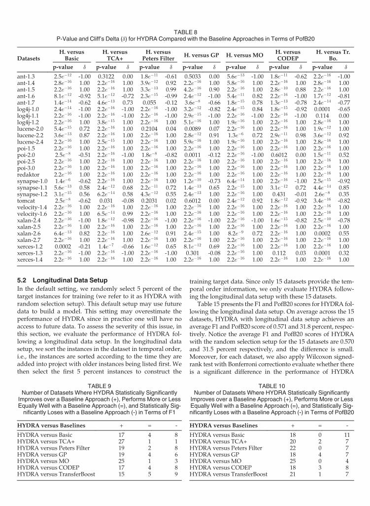
5.2 Longitudinal Data Setup

In the default setting, we randomly select 5 percent of thetarget instances for training (we refer to it as HYDRA withrandom selection setup). This default setup may use futuredata to build a model. This setting may overestimate theperformance of HYDRA since in practice one will have noaccess to future data. To assess the severity of this issue, inthis section, we evaluate the performance of HYDRA fol-lowing a longitudinal data setup. In the longitudinal datasetup, we sort the instances in the dataset in temporal order,i.e., the instances are sorted according to the time they areadded into project with older instances being listed first. Wethen select the first 5 percent instances to construct the

training target data. Since only 15 datasets provide the tem-poral order information, we only evaluate HYDRA follow-ing the longitudinal data setup with these 15 datasets.

Table 15 presents the F1 and PofB20 scores for HYDRA fol-lowing the longitudinal data setup. On average across the 15datasets, HYDRA with longitudinal data setup achieves anaverage F1 and PofB20 score of 0.571 and 31.8 percent, respec-tively. Notice the average F1 and PofB20 scores of HYDRAwith the random selection setup for the 15 datasets are 0.570and 31.5 percent respectively, and the difference is small.Moreover, for each dataset, we also apply Wilcoxon signed-rank test with Bonferroni correctionto evaluate whether thereis a significant difference in the performance of HYDRA

TABLE 9Number of Datasets Where HYDRA Statistically Significantly

Improves over a Baseline Approach (+), Performs More or LessEqually Well with a Baseline Approach (=), and Statistically Sig-nificantly Loses with a Baseline Approach (-) in Terms of F1

HYDRA versus Baselines + = -

HYDRA versus Basic 17 4 8HYDRA versus TCA+ 27 1 1HYDRA versus Peters Filter 19 2 8HYDRA versus GP 19 4 6HYDRA versus MO 25 1 3HYDRA versus CODEP 17 4 8HYDRA versus TransferBoost 15 5 9

TABLE 10Number of Datasets Where HYDRA Statistically Significantly

Improves over a Baseline Approach (+), Performs More or LessEqually Well with a Baseline Approach (=), and Statistically Sig-nificantly Loses with a Baseline Approach (-) in Terms of PofB20


HYDRA versus Basic 18 0 11HYDRA versus TCA+ 20 2 7HYDRA versus Peters Filter 22 0 7HYDRA versus GP 18 4 7HYDRA versus MO 25 0 4HYDRA versus CODEP 18 3 8HYDRA versus TransferBoost 21 1 7

TABLE 8P-Value and Cliff’s Delta (d) for HYDRA Compared with the Baseline Approaches in Terms of PofB20

DatasetsH. versusBasic

H. versusTCA+

H. versusPeters Filter

H. versus GP H. versus MOH. versusCODEP

H. versus Tr.Bo.

p-value d p-value d p-value d p-value d p-value d p-value d p-value d

ant-1.3 2.5e�12 -1.00 0.3122 0.00 1.8e�11 -0.61 0.5033 0.00 5.6e�13 -1.00 1.8e�11 -0.62 2.2e�16 -1.00ant-1.4 2.8e�16 1.00 2.2e�16 1.00 3.9e�12 0.92 2.2e�16 1.00 5.8e�16 1.00 2.2e�16 1.00 2.8e�16 1.00ant-1.5 2.2e�16 1.00 2.2e�16 1.00 3.3e�13 0.99 4.2e�16 0.90 2.2e�16 1.00 2.8e�10 0.88 2.2e�16 1.00ant-1.6 8.1e�12 -0.92 5.1e�12 -0.72 2.3e�15 -0.99 2.4e�12 -1.00 5.4e�11 0.82 2.2e�16 -1.00 1.7e�12 -0.81ant-1.7 1.4e�14 -0.62 4.6e�13 0.73 0.055 -0.12 3.6e�8 -0.66 1.8e�15 0.78 1.3e�13 -0.78 2.4e�14 -0.77log4j-1.0 2.4e�14 -1.00 2.2e�16 -1.00 2.2e�16 -1.00 3.2e�12 -0.82 2.4e�15 0.84 1.8e�15 -0.92 0.0001 -0.65log4j-1.1 2.2e�16 -1.00 2.2e�16 -1.00 2.2e�16 -1.00 2.9e�15 -1.00 2.2e�16 -1.00 2.2e�16 -1.00 0.114 0.00log4j-1.2 2.2e�16 1.00 3.8e�15 1.00 2.2e�16 1.00 5.1e�16 1.00 1.9e�16 1.00 2.2e�16 1.00 2.8e�16 1.00lucene-2.0 5.4e�15 0.72 2.2e�16 1.00 0.2104 0.04 0.0089 0.07 2.2e�16 1.00 2.2e�16 1.00 1.9e�12 1.00lucene-2.2 3.6e�13 0.87 2.2e�16 1.00 2.2e�16 1.00 2.8e�12 0.91 1.3e�6 0.72 2.9e�11 0.98 3.6e�12 0.92lucene-2.4 2.2e�16 1.00 2.5e�15 1.00 2.2e�16 1.00 5.9e�16 1.00 1.9e�16 1.00 2.2e�16 1.00 2.8e�16 1.00poi-1.5 2.2e�16 1.00 2.2e�16 1.00 2.2e�16 1.00 2.2e�16 1.00 2.2e�16 1.00 2.2e�16 1.00 2.2e�16 1.00poi-2.0 2.5e�8 -0.51 2.2e�16 -1.00 1.8e�8 -0.82 0.0011 -0.12 2.2e�16 -1.00 0.6012 0.00 1.5e�11 0.52poi-2.5 2.2e�16 1.00 2.2e�16 1.00 2.2e�16 1.00 2.2e�16 1.00 2.2e�16 1.00 2.2e�16 1.00 2.2e�16 1.00poi-3.0 2.2e�16 1.00 2.2e�16 1.00 2.2e�16 1.00 2.2e�16 1.00 2.2e�16 1.00 2.2e�16 1.00 2.2e�16 1.00redaktor 2.2e�16 1.00 2.2e�16 1.00 2.2e�16 1.00 2.2e�16 1.00 2.2e�16 1.00 2.2e�16 1.00 2.2e�16 1.00synapse-1.0 1.4e�6 -0.62 2.2e�16 1.00 2.2e�16 1.00 1.2e�10 -0.73 6.4e�14 1.00 2.2e�16 -1.00 2.5e�15 -0.92synapse-1.1 5.6e�13 0.58 2.4e�12 0.68 2.2e�11 0.72 1.4e�13 0.65 2.2e�15 1.00 3.1e�12 0.72 4.4e�14 0.85synapse-1.2 3.1e�15 0.56 6.2e�14 0.58 4.3e�12 0.55 2.4e�13 1.00 2.2e�16 1.00 0.431 -0.01 2.6e�8 0.35tomcat 2.5e�8 -0.62 0.031 -0.08 0.2031 0.02 0.6012 0.00 2.4e�12 0.92 1.8e�12 -0.92 3.4e�16 -0.82velocity-1.4 2.2e�16 1.00 2.2e�16 1.00 2.2e�16 1.00 2.2e�16 1.00 2.2e�16 1.00 2.2e�16 1.00 2.2e�16 1.00velocity-1.6 2.2e�16 1.00 6.5e�14 0.99 2.2e�16 1.00 2.2e�16 1.00 2.2e�16 1.00 2.2e�16 1.00 2.2e�16 1.00xalan-2.4 2.2e�16 -1.00 1.8e�12 -0.98 2.2e�16 -1.00 2.2e�16 -1.00 2.2e�16 -1.00 1.6e�15 -0.82 2.5e�10 -0.78xalan-2.5 2.2e�16 1.00 2.2e�16 1.00 2.2e�16 1.00 2.2e�16 1.00 2.2e�16 1.00 2.2e�16 1.00 2.2e�16 1.00xalan-2.6 6.4e�13 0.82 2.2e�16 1.00 2.6e�12 0.91 2.4e�15 1.00 8.2e�9 0.72 2.2e�16 1.00 0.0002 0.55xalan-2.7 2.2e�16 1.00 2.2e�16 1.00 2.2e�16 1.00 2.2e�16 1.00 2.2e�16 1.00 2.2e�16 1.00 2.2e�16 1.00xerces-1.2 0.0002 -0.21 1.4e�7 -0.66 1.6e�12 0.65 8.1e�12 0.69 2.2e�16 1.00 2.2e�16 1.00 2.2e�16 1.00xerces-1.3 2.2e�16 -1.00 2.2e�16 -1.00 2.2e�16 -1.00 0.301 -0.08 2.2e�16 1.00 0.112 0.03 0.0001 0.32xerces-1.4 2.2e�16 1.00 2.2e�16 1.00 2.2e�16 1.00 2.2e�16 1.00 2.2e�16 1.00 2.2e�16 1.00 2.2e�16 1.00


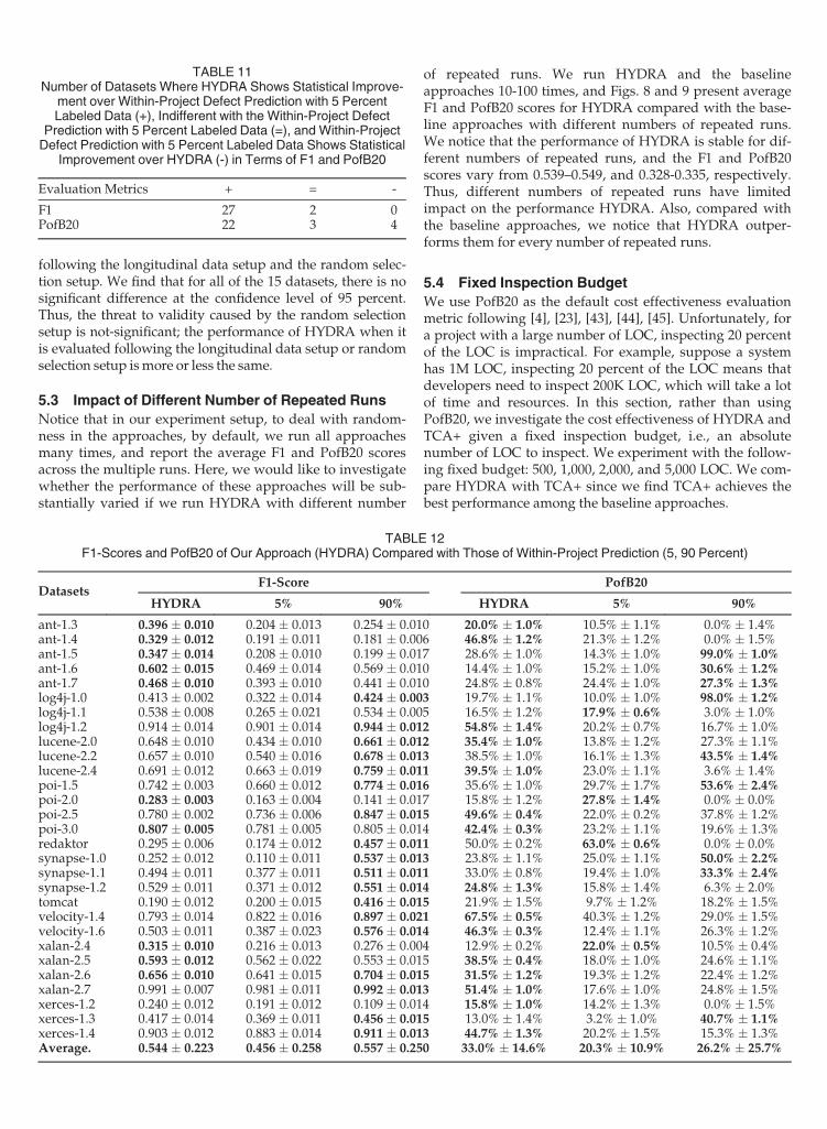
following the longitudinal data setup and the random selec-tion setup. We find that for all of the 15 datasets, there is nosignificant difference at the confidence level of 95 percent.Thus, the threat to validity caused by the random selectionsetup is not-significant; the performance of HYDRA when itis evaluated following the longitudinal data setup or randomselection setup ismore or less the same.

5.3 Impact of Different Number of Repeated Runs

Notice that in our experiment setup, to deal with random-ness in the approaches, by default, we run all approachesmany times, and report the average F1 and PofB20 scoresacross the multiple runs. Here, we would like to investigatewhether the performance of these approaches will be sub-stantially varied if we run HYDRA with different number

of repeated runs. We run HYDRA and the baselineapproaches 10-100 times, and Figs. 8 and 9 present averageF1 and PofB20 scores for HYDRA compared with the base-line approaches with different numbers of repeated runs.We notice that the performance of HYDRA is stable for dif-ferent numbers of repeated runs, and the F1 and PofB20scores vary from 0.539–0.549, and 0.328-0.335, respectively.Thus, different numbers of repeated runs have limitedimpact on the performance HYDRA. Also, compared withthe baseline approaches, we notice that HYDRA outper-forms them for every number of repeated runs.

5.4 Fixed Inspection Budget

We use PofB20 as the default cost effectiveness evaluationmetric following [4], [23], [43], [44], [45]. Unfortunately, fora project with a large number of LOC, inspecting 20 percentof the LOC is impractical. For example, suppose a systemhas 1M LOC, inspecting 20 percent of the LOC means thatdevelopers need to inspect 200K LOC, which will take a lotof time and resources. In this section, rather than usingPofB20, we investigate the cost effectiveness of HYDRA andTCA+ given a fixed inspection budget, i.e., an absolutenumber of LOC to inspect. We experiment with the follow-ing fixed budget: 500, 1,000, 2,000, and 5,000 LOC. We com-pare HYDRA with TCA+ since we find TCA+ achieves thebest performance among the baseline approaches.

TABLE 11Number of Datasets Where HYDRA Shows Statistical Improve-

ment over Within-Project Defect Prediction with 5 PercentLabeled Data (+), Indifferent with the Within-Project Defect

Prediction with 5 Percent Labeled Data (=), and Within-ProjectDefect Prediction with 5 Percent Labeled Data Shows Statistical

Improvement over HYDRA (-) in Terms of F1 and PofB20

Evaluation Metrics + = -

F1 27 2 0PofB20 22 3 4

TABLE 12F1-Scores and PofB20 of Our Approach (HYDRA) Compared with Those of Within-Project Prediction (5, 90 Percent)

DatasetsF1-Score PofB20

HYDRA 5% 90% HYDRA 5% 90%

ant-1.3 0.396 0.010 0.204 0.013 0.254 0.010 20.0% 1.0% 10.5% 1.1% 0.0% 1.4%ant-1.4 0.329 0.012 0.191 0.011 0.181 0.006 46.8% 1.2% 21.3% 1.2% 0.0% 1.5%ant-1.5 0.347 0.014 0.208 0.010 0.199 0.017 28.6% 1.0% 14.3% 1.0% 99.0% 1.0%ant-1.6 0.602 0.015 0.469 0.014 0.569 0.010 14.4% 1.0% 15.2% 1.0% 30.6% 1.2%ant-1.7 0.468 0.010 0.393 0.010 0.441 0.010 24.8% 0.8% 24.4% 1.0% 27.3% 1.3%log4j-1.0 0.413 0.002 0.322 0.014 0.424 0.003 19.7% 1.1% 10.0% 1.0% 98.0% 1.2%log4j-1.1 0.538 0.008 0.265 0.021 0.534 0.005 16.5% 1.2% 17.9% 0.6% 3.0% 1.0%log4j-1.2 0.914 0.014 0.901 0.014 0.944 0.012 54.8% 1.4% 20.2% 0.7% 16.7% 1.0%lucene-2.0 0.648 0.010 0.434 0.010 0.661 0.012 35.4% 1.0% 13.8% 1.2% 27.3% 1.1%lucene-2.2 0.657 0.010 0.540 0.016 0.678 0.013 38.5% 1.0% 16.1% 1.3% 43.5% 1.4%lucene-2.4 0.691 0.012 0.663 0.019 0.759 0.011 39.5% 1.0% 23.0% 1.1% 3.6% 1.4%poi-1.5 0.742 0.003 0.660 0.012 0.774 0.016 35.6% 1.0% 29.7% 1.7% 53.6% 2.4%poi-2.0 0.283 0.003 0.163 0.004 0.141 0.017 15.8% 1.2% 27.8% 1.4% 0.0% 0.0%poi-2.5 0.780 0.002 0.736 0.006 0.847 0.015 49.6% 0.4% 22.0% 0.2% 37.8% 1.2%poi-3.0 0.807 0.005 0.781 0.005 0.805 0.014 42.4% 0.3% 23.2% 1.1% 19.6% 1.3%redaktor 0.295 0.006 0.174 0.012 0.457 0.011 50.0% 0.2% 63.0% 0.6% 0.0% 0.0%synapse-1.0 0.252 0.012 0.110 0.011 0.537 0.013 23.8% 1.1% 25.0% 1.1% 50.0% 2.2%synapse-1.1 0.494 0.011 0.377 0.011 0.511 0.011 33.0% 0.8% 19.4% 1.0% 33.3% 2.4%synapse-1.2 0.529 0.011 0.371 0.012 0.551 0.014 24.8% 1.3% 15.8% 1.4% 6.3% 2.0%tomcat 0.190 0.012 0.200 0.015 0.416 0.015 21.9% 1.5% 9.7% 1.2% 18.2% 1.5%velocity-1.4 0.793 0.014 0.822 0.016 0.897 0.021 67.5% 0.5% 40.3% 1.2% 29.0% 1.5%velocity-1.6 0.503 0.011 0.387 0.023 0.576 0.014 46.3% 0.3% 12.4% 1.1% 26.3% 1.2%xalan-2.4 0.315 0.010 0.216 0.013 0.276 0.004 12.9% 0.2% 22.0% 0.5% 10.5% 0.4%xalan-2.5 0.593 0.012 0.562 0.022 0.553 0.015 38.5% 0.4% 18.0% 1.0% 24.6% 1.1%xalan-2.6 0.656 0.010 0.641 0.015 0.704 0.015 31.5% 1.2% 19.3% 1.2% 22.4% 1.2%xalan-2.7 0.991 0.007 0.981 0.011 0.992 0.013 51.4% 1.0% 17.6% 1.0% 24.8% 1.5%xerces-1.2 0.240 0.012 0.191 0.012 0.109 0.014 15.8% 1.0% 14.2% 1.3% 0.0% 1.5%xerces-1.3 0.417 0.014 0.369 0.011 0.456 0.015 13.0% 1.4% 3.2% 1.0% 40.7% 1.1%xerces-1.4 0.903 0.012 0.883 0.014 0.911 0.013 44.7% 1.3% 20.2% 1.5% 15.3% 1.3%Average. 0.544 0.223 0.456 0.258 0.557 0.250 33.0% 14.6% 20.3% 10.9% 26.2% 25.7%


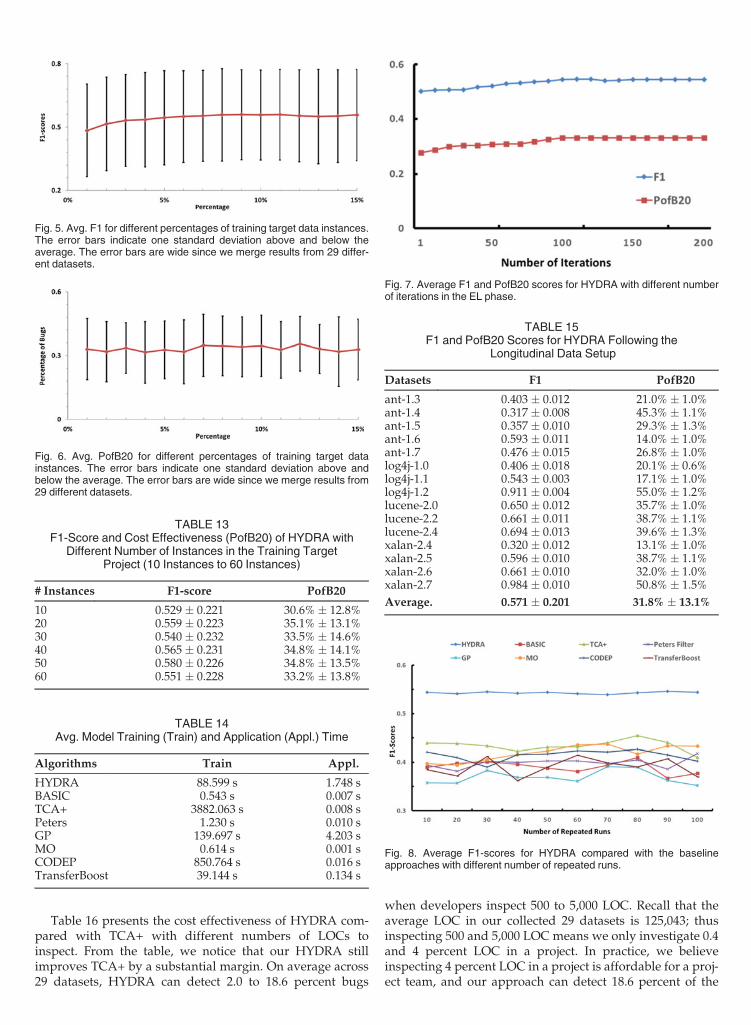
Table 16 presents the cost effectiveness of HYDRA com-pared with TCA+ with different numbers of LOCs toinspect. From the table, we notice that our HYDRA stillimproves TCA+ by a substantial margin. On average across29 datasets, HYDRA can detect 2.0 to 18.6 percent bugs

when developers inspect 500 to 5,000 LOC. Recall that theaverage LOC in our collected 29 datasets is 125,043; thusinspecting 500 and 5,000 LOC means we only investigate 0.4and 4 percent LOC in a project. In practice, we believeinspecting 4 percent LOC in a project is affordable for a proj-ect team, and our approach can detect 18.6 percent of the

Fig. 5. Avg. F1 for different percentages of training target data instances.The error bars indicate one standard deviation above and below theaverage. The error bars are wide since we merge results from 29 differ-ent datasets.

Fig. 6. Avg. PofB20 for different percentages of training target datainstances. The error bars indicate one standard deviation above andbelow the average. The error bars are wide since we merge results from29 different datasets.

TABLE 13F1-Score and Cost Effectiveness (PofB20) of HYDRA with

Different Number of Instances in the Training TargetProject (10 Instances to 60 Instances)

# Instances F1-score PofB20

10 0.529 0.221 30.6% 12.8%20 0.559 0.223 35.1% 13.1%30 0.540 0.232 33.5% 14.6%40 0.565 0.231 34.8% 14.1%50 0.580 0.226 34.8% 13.5%60 0.551 0.228 33.2% 13.8%

TABLE 14Avg. Model Training (Train) and Application (Appl.) Time

Algorithms Train Appl.

HYDRA 88.599 s 1.748 sBASIC 0.543 s 0.007 sTCA+ 3882.063 s 0.008 sPeters 1.230 s 0.010 sGP 139.697 s 4.203 sMO 0.614 s 0.001 sCODEP 850.764 s 0.016 sTransferBoost 39.144 s 0.134 s

Fig. 7. Average F1 and PofB20 scores for HYDRA with different numberof iterations in the EL phase.

TABLE 15F1 and PofB20 Scores for HYDRA Following the

Longitudinal Data Setup

Datasets F1 PofB20

ant-1.3 0.403 0.012 21.0% 1.0%ant-1.4 0.317 0.008 45.3% 1.1%ant-1.5 0.357 0.010 29.3% 1.3%ant-1.6 0.593 0.011 14.0% 1.0%ant-1.7 0.476 0.015 26.8% 1.0%log4j-1.0 0.406 0.018 20.1% 0.6%log4j-1.1 0.543 0.003 17.1% 1.0%log4j-1.2 0.911 0.004 55.0% 1.2%lucene-2.0 0.650 0.012 35.7% 1.0%lucene-2.2 0.661 0.011 38.7% 1.1%lucene-2.4 0.694 0.013 39.6% 1.3%xalan-2.4 0.320 0.012 13.1% 1.0%xalan-2.5 0.596 0.010 38.7% 1.1%xalan-2.6 0.661 0.010 32.0% 1.0%xalan-2.7 0.984 0.010 50.8% 1.5%

Average. 0.571 0.201 31.8% 13.1%

Fig. 8. Average F1-scores for HYDRA compared with the baselineapproaches with different number of repeated runs.


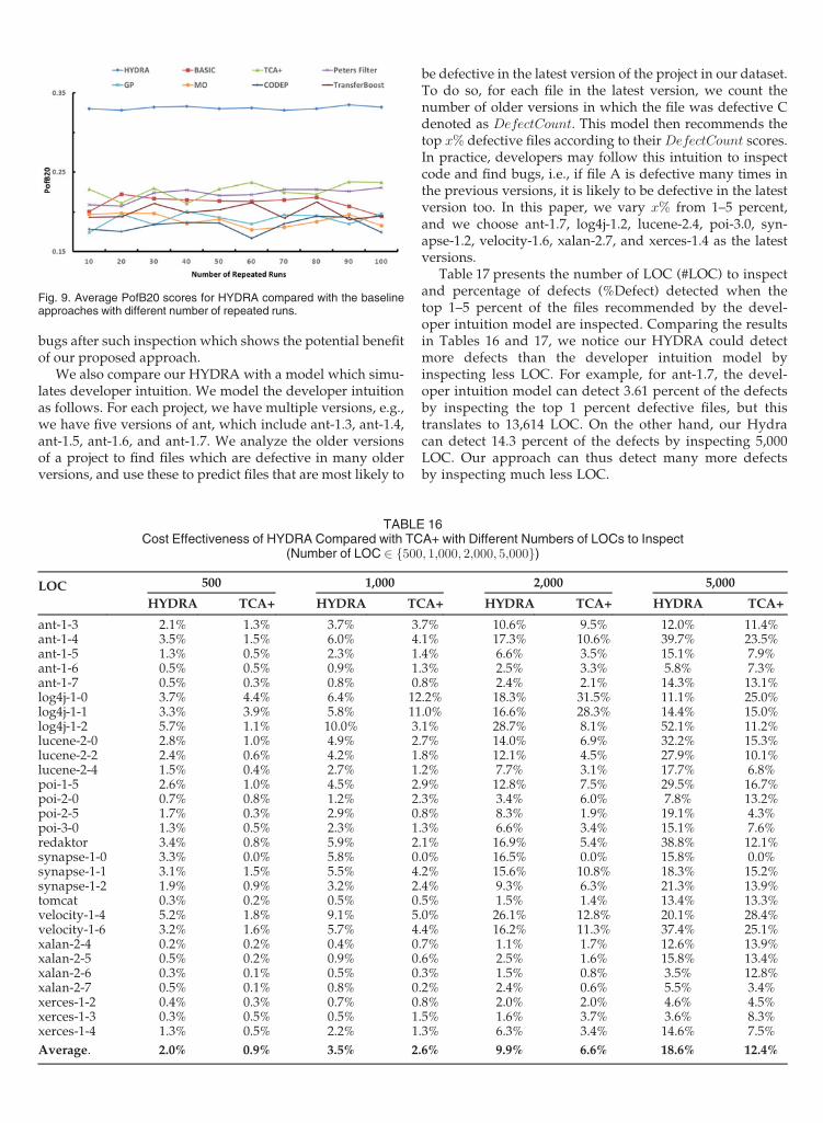
bugs after such inspection which shows the potential benefitof our proposed approach.

We also compare our HYDRA with a model which simu-lates developer intuition. We model the developer intuitionas follows. For each project, we have multiple versions, e.g.,we have five versions of ant, which include ant-1.3, ant-1.4,ant-1.5, ant-1.6, and ant-1.7. We analyze the older versionsof a project to find files which are defective in many olderversions, and use these to predict files that are most likely to

be defective in the latest version of the project in our dataset.To do so, for each file in the latest version, we count thenumber of older versions in which the file was defective Cdenoted as DefectCount. This model then recommends thetop x% defective files according to theirDefectCount scores.In practice, developers may follow this intuition to inspectcode and find bugs, i.e., if file A is defective many times inthe previous versions, it is likely to be defective in the latestversion too. In this paper, we vary x% from 1–5 percent,and we choose ant-1.7, log4j-1.2, lucene-2.4, poi-3.0, syn-apse-1.2, velocity-1.6, xalan-2.7, and xerces-1.4 as the latestversions.

Table 17 presents the number of LOC (#LOC) to inspectand percentage of defects (%Defect) detected when thetop 1–5 percent of the files recommended by the devel-oper intuition model are inspected. Comparing the resultsin Tables 16 and 17, we notice our HYDRA could detectmore defects than the developer intuition model byinspecting less LOC. For example, for ant-1.7, the devel-oper intuition model can detect 3.61 percent of the defectsby inspecting the top 1 percent defective files, but thistranslates to 13,614 LOC. On the other hand, our Hydracan detect 14.3 percent of the defects by inspecting 5,000LOC. Our approach can thus detect many more defectsby inspecting much less LOC.

Fig. 9. Average PofB20 scores for HYDRA compared with the baselineapproaches with different number of repeated runs.

TABLE 16Cost Effectiveness of HYDRA Compared with TCA+ with Different Numbers of LOCs to Inspect

(Number of LOC 2 f500; 1;000; 2;000; 5;000g)

LOC 500 1,000 2,000 5,000

HYDRA TCA+ HYDRA TCA+ HYDRA TCA+ HYDRA TCA+

ant-1-3 2.1% 1.3% 3.7% 3.7% 10.6% 9.5% 12.0% 11.4%ant-1-4 3.5% 1.5% 6.0% 4.1% 17.3% 10.6% 39.7% 23.5%ant-1-5 1.3% 0.5% 2.3% 1.4% 6.6% 3.5% 15.1% 7.9%ant-1-6 0.5% 0.5% 0.9% 1.3% 2.5% 3.3% 5.8% 7.3%ant-1-7 0.5% 0.3% 0.8% 0.8% 2.4% 2.1% 14.3% 13.1%log4j-1-0 3.7% 4.4% 6.4% 12.2% 18.3% 31.5% 11.1% 25.0%log4j-1-1 3.3% 3.9% 5.8% 11.0% 16.6% 28.3% 14.4% 15.0%log4j-1-2 5.7% 1.1% 10.0% 3.1% 28.7% 8.1% 52.1% 11.2%lucene-2-0 2.8% 1.0% 4.9% 2.7% 14.0% 6.9% 32.2% 15.3%lucene-2-2 2.4% 0.6% 4.2% 1.8% 12.1% 4.5% 27.9% 10.1%lucene-2-4 1.5% 0.4% 2.7% 1.2% 7.7% 3.1% 17.7% 6.8%poi-1-5 2.6% 1.0% 4.5% 2.9% 12.8% 7.5% 29.5% 16.7%poi-2-0 0.7% 0.8% 1.2% 2.3% 3.4% 6.0% 7.8% 13.2%poi-2-5 1.7% 0.3% 2.9% 0.8% 8.3% 1.9% 19.1% 4.3%poi-3-0 1.3% 0.5% 2.3% 1.3% 6.6% 3.4% 15.1% 7.6%redaktor 3.4% 0.8% 5.9% 2.1% 16.9% 5.4% 38.8% 12.1%synapse-1-0 3.3% 0.0% 5.8% 0.0% 16.5% 0.0% 15.8% 0.0%synapse-1-1 3.1% 1.5% 5.5% 4.2% 15.6% 10.8% 18.3% 15.2%synapse-1-2 1.9% 0.9% 3.2% 2.4% 9.3% 6.3% 21.3% 13.9%tomcat 0.3% 0.2% 0.5% 0.5% 1.5% 1.4% 13.4% 13.3%velocity-1-4 5.2% 1.8% 9.1% 5.0% 26.1% 12.8% 20.1% 28.4%velocity-1-6 3.2% 1.6% 5.7% 4.4% 16.2% 11.3% 37.4% 25.1%xalan-2-4 0.2% 0.2% 0.4% 0.7% 1.1% 1.7% 12.6% 13.9%xalan-2-5 0.5% 0.2% 0.9% 0.6% 2.5% 1.6% 15.8% 13.4%xalan-2-6 0.3% 0.1% 0.5% 0.3% 1.5% 0.8% 3.5% 12.8%xalan-2-7 0.5% 0.1% 0.8% 0.2% 2.4% 0.6% 5.5% 3.4%xerces-1-2 0.4% 0.3% 0.7% 0.8% 2.0% 2.0% 4.6% 4.5%xerces-1-3 0.3% 0.5% 0.5% 1.5% 1.6% 3.7% 3.6% 8.3%xerces-1-4 1.3% 0.5% 2.2% 1.3% 6.3% 3.4% 14.6% 7.5%

Average. 2.0% 0.9% 3.5% 2.6% 9.9% 6.6% 18.6% 12.4%


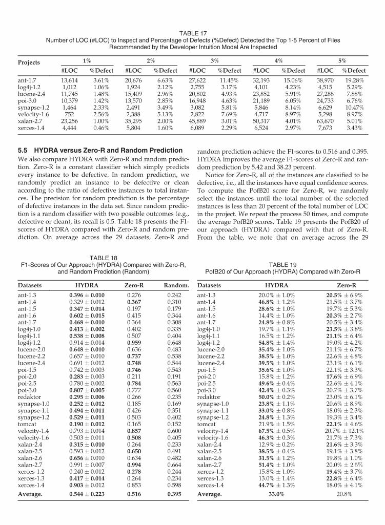
5.5 HYDRA versus Zero-R and Random Prediction

We also compare HYDRA with Zero-R and random predic-tion. Zero-R is a constant classifier which simply predictsevery instance to be defective. In random prediction, werandomly predict an instance to be defective or cleanaccording to the ratio of defective instances to total instan-ces. The precision for random prediction is the percentageof defective instances in the data set. Since random predic-tion is a random classifier with two possible outcomes (e.g.,defective or clean), its recall is 0.5. Table 18 presents the F1-scores of HYDRA compared with Zero-R and random pre-diction. On average across the 29 datasets, Zero-R and

random prediction achieve the F1-scores to 0.516 and 0.395.HYDRA improves the average F1-scores of Zero-R and ran-dom prediction by 5.42 and 38.23 percent.

Notice for Zero-R, all of the instances are classified to bedefective, i.e., all the instances have equal confidence scores.To compute the PofB20 score for Zero-R, we randomlyselect the instances until the total number of the selectedinstances is less than 20 percent of the total number of LOCin the project. We repeat the process 50 times, and computethe average PofB20 scores. Table 19 presents the PofB20 ofour approach (HYDRA) compared with that of Zero-R.From the table, we note that on average across the 29

TABLE 17Number of LOC (#LOC) to Inspect and Percentage of Defects (%Defect) Detected the Top 1-5 Percent of Files

Recommended by the Developer Intuition Model Are Inspected

Projects 1% 2% 3% 4% 5%

#LOC %Defect #LOC %Defect #LOC %Defect #LOC %Defect #LOC %Defect

ant-1.7 13,614 3.61% 20,676 6.63% 27,622 11.45% 32,193 15.06% 38,970 19.28%log4j-1.2 1,012 1.06% 1,924 2.12% 2,755 3.17% 4,101 4.23% 4,515 5.29%lucene-2.4 11,745 1.48% 15,409 2.96% 20,802 4.93% 23,852 5.91% 27,288 7.88%poi-3.0 10,379 1.42% 13,570 2.85% 16,948 4.63% 21,189 6.05% 24,733 6.76%synapse-1.2 1,464 2.33% 2,491 3.49% 3,082 5.81% 5,846 8.14% 6,629 10.47%velocity-1.6 752 2.56% 2,388 5.13% 2,822 7.69% 4,717 8.97% 5,298 8.97%xalan-2.7 23,256 1.00% 35,295 2.00% 45,889 3.01% 50,317 4.01% 63,670 5.01%xerces-1.4 4,444 0.46% 5,804 1.60% 6,089 2.29% 6,524 2.97% 7,673 3.43%

TABLE 18F1-Scores of Our Approach (HYDRA) Compared with Zero-R,

and Random Prediction (Random)

Datasets HYDRA Zero-R Random.

ant-1.3 0.396 0.010 0.276 0.242ant-1.4 0.329 0.012 0.367 0.310ant-1.5 0.347 0.014 0.197 0.179ant-1.6 0.602 0.015 0.415 0.344ant-1.7 0.468 0.010 0.364 0.308log4j-1.0 0.413 0.002 0.402 0.335log4j-1.1 0.538 0.008 0.507 0.404log4j-1.2 0.914 0.014 0.959 0.648lucene-2.0 0.648 0.010 0.636 0.483lucene-2.2 0.657 0.010 0.737 0.538lucene-2.4 0.691 0.012 0.748 0.544poi-1.5 0.742 0.003 0.746 0.543poi-2.0 0.283 0.003 0.211 0.191poi-2.5 0.780 0.002 0.784 0.563poi-3.0 0.807 0.005 0.777 0.560redaktor 0.295 0.006 0.266 0.235synapse-1.0 0.252 0.012 0.185 0.169synapse-1.1 0.494 0.011 0.426 0.351synapse-1.2 0.529 0.011 0.503 0.402tomcat 0.190 0.012 0.165 0.152velocity-1.4 0.793 0.014 0.857 0.600velocity-1.6 0.503 0.011 0.508 0.405xalan-2.4 0.315 0.010 0.264 0.233xalan-2.5 0.593 0.012 0.650 0.491xalan-2.6 0.656 0.010 0.634 0.482xalan-2.7 0.991 0.007 0.994 0.664xerces-1.2 0.240 0.012 0.278 0.244xerces-1.3 0.417 0.014 0.264 0.234xerces-1.4 0.903 0.012 0.853 0.598

Average. 0.544 0.223 0.516 0.395

TABLE 19PofB20 of Our Approach (HYDRA) Compared with Zero-R

Datasets HYDRA Zero-R

ant-1.3 20.0% 1.0% 20.5% 6.9%ant-1.4 46.8% 1.2% 21.5% 3.7%ant-1.5 28.6% 1.0% 19.7% 5.3%ant-1.6 14.4% 1.0% 20.3% 2.7%ant-1.7 24.8% 0.8% 20.5% 3.4%log4j-1.0 19.7% 1.1% 23.5% 3.8%log4j-1.1 16.5% 1.2% 21.1% 6.4%log4j-1.2 54.8% 1.4% 19.0% 4.2%lucene-2.0 35.4% 1.0% 21.1% 6.7%lucene-2.2 38.5% 1.0% 22.6% 4.8%lucene-2.4 39.5% 1.0% 23.1% 6.1%poi-1.5 35.6% 1.0% 22.1% 3.3%poi-2.0 15.8% 1.2% 17.6% 6.9%poi-2.5 49.6% 0.4% 22.6% 4.1%poi-3.0 42.4% 0.3% 20.7% 3.7%redaktor 50.0% 0.2% 23.0% 6.1%synapse-1.0 23.8% 1.1% 20.6% 8.9%synapse-1.1 33.0% 0.8% 18.0% 2.3%synapse-1.2 24.8% 1.3% 19.3% 3.4%tomcat 21.9% 1.5% 22.1% 4.6%velocity-1.4 67.5% 0.5% 20.7% 12.1%velocity-1.6 46.3% 0.3% 21.7% 7.3%xalan-2.4 12.9% 0.2% 21.6% 3.3%xalan-2.5 38.5% 0.4% 19.1% 3.8%xalan-2.6 31.5% 1.2% 19.8% 1.0%xalan-2.7 51.4% 1.0% 20.0% 2:5%xerces-1.2 15.8% 1.0% 19.4% 3.7%xerces-1.3 13.0% 1.4% 22.8% 6.4%xerces-1.4 44.7% 1.3% 18.0% 4.1%

Average. 33.0% 20.8%


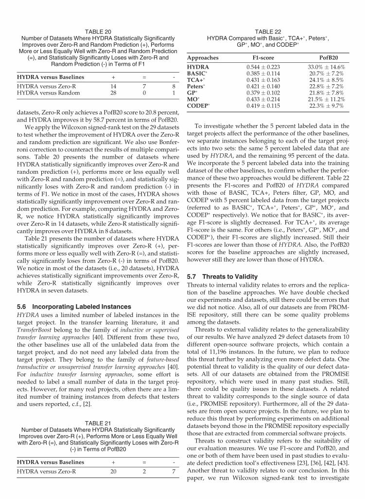
datasets, Zero-R only achieves a PofB20 score to 20.8 percent,and HYDRA improves it by 58.7 percent in terms of PofB20.

We apply theWilcoxon signed-rank test on the 29 datasetsto test whether the improvement of HYDRA over the Zero-Rand random prediction are significant. We also use Bonfer-roni correction to counteract the results of multiple compari-sons. Table 20 presents the number of datasets whereHYDRA statistically significantly improves over Zero-R andrandom prediction (+), performs more or less equally wellwith Zero-R and random prediction (=), and statistically sig-nificantly loses with Zero-R and random prediction (-) interms of F1. We notice in most of the cases, HYDRA showsstatistically significantly improvement over Zero-R and ran-dom prediction. For example, comparing HYDRA and Zero-R, we notice HYDRA statistically significantly improvesover Zero-R in 14 datasets, while Zero-R statistically signifi-cantly improves overHYDRA in 8 datasets.

Table 21 presents the number of datasets where HYDRAstatistically significantly improves over Zero-R (+), per-forms more or less equally well with Zero-R (=), and statisti-cally significantly loses from Zero-R (-) in terms of PofB20.We notice in most of the datasets (i.e., 20 datasets), HYDRAachieves statistically significant improvements over Zero-R,while Zero-R statistically significantly improves overHYDRA in seven datasets.

5.6 Incorporating Labeled Instances

HYDRA uses a limited number of labeled instances in thetarget project. In the transfer learning literature, it andTransferBoost belong to the family of inductive or supervisedtransfer learning approaches [40]. Different from these two,the other baselines use all of the unlabeled data from thetarget project, and do not need any labeled data from thetarget project. They belong to the family of feature-basedtransductive or unsupervised transfer learning approaches [40].For inductive transfer learning approaches, some effort isneeded to label a small number of data in the target proj-ects. However, for many real projects, often there are a lim-ited number of training instances from defects that testersand users reported, c.f., [2].

To investigate whether the 5 percent labeled data in thetarget projects affect the performance of the other baselines,we separate instances belonging to each of the target proj-ects into two sets: the same 5 percent labeled data that areused by HYDRA, and the remaining 95 percent of the data.We incorporate the 5 percent labeled data into the trainingdataset of the other baselines, to confirm whether the perfor-mance of these two approaches would be different. Table 22presents the F1-scores and PofB20 of HYDRA comparedwith those of BASIC, TCA+, Peters filter, GP, MO, andCODEP with 5 percent labeled data from the target projects(referred to as BASIC�, TCA+�, Peters�, GP�, MO�, andCODEP� respectively). We notice that for BASIC�, its aver-age F1-score is slightly decreased. For TCA+�, its averageF1-score is the same. For others (i.e., Peters�, GP�, MO�, andCODEP�), their F1-scores are slightly increased. Still theirF1-scores are lower than those of HYDRA. Also, the PofB20scores for the baseline approaches are slightly increased,however still they are lower than those of HYDRA.

5.7 Threats to Validity

Threats to internal validity relates to errors and the replica-tion of the baseline approaches. We have double checkedour experiments and datasets, still there could be errors thatwe did not notice. Also, all of our datasets are from PROM-ISE repository, still there can be some quality problemsamong the datasets.

Threats to external validity relates to the generalizabilityof our results. We have analyzed 29 defect datasets from 10different open-source software projects, which contain atotal of 11,196 instances. In the future, we plan to reducethis threat further by analyzing even more defect data. Onepotential threat to validity is the quality of our defect data-sets. All of our datasets are obtained from the PROMISErepository, which were used in many past studies. Still,there could be quality issues in these datasets. A relatedthreat to validity corresponds to the single source of data(i.e., PROMISE repository). Furthermore, all of the 29 data-sets are from open source projects. In the future, we plan toreduce this threat by performing experiments on additionaldatasets beyond those in the PROMISE repository especiallythose that are extracted from commercial software projects.

Threats to construct validity refers to the suitability ofour evaluation measures. We use F1-score and PofB20, andone or both of them have been used in past studies to evalu-ate defect prediction tool’s effectiveness [23], [36], [42], [43].Another threat to validity relates to our conclusion. In thispaper, we run Wilcoxon signed-rank test to investigate

TABLE 20Number of Datasets Where HYDRA Statistically SignificantlyImproves over Zero-R and Random Prediction (+), Performs

More or Less Equally Well with Zero-R and Random Prediction(=), and Statistically Significantly Loses with Zero-R and

Random Prediction (-) in Terms of F1


HYDRA versus Zero-R 14 7 8HYDRA versus Random 28 0 1

TABLE 21Number of Datasets Where HYDRA Statistically SignificantlyImproves over Zero-R (+), Performs More or Less Equally Wellwith Zero-R (=), and Statistically Significantly Loses with Zero-R

(-) in Terms of PofB20


HYDRA versus Zero-R 20 2 7

TABLE 22HYDRA Compared with Basic�, TCA+�, Peters�,

GP�, MO�, and CODEP�

Approaches F1-score PofB20

HYDRA 0.544 0.223 33.0% 14.6%BASIC� 0.385 0.114 20.7% 7.2%TCA+� 0.431 0.163 24.1% 8.5%Peters� 0.421 0.140 22.8% 7.2%GP� 0.379 0.102 21.8% 7.8%MO� 0.433 0.214 21.5% 11.2%CODEP� 0.419 0.115 22.3% 9.7%


whether the improvements of HYDRA over the baselineapproaches are significant. To counteract the bias due tomultiple comparisons, we employ Bonferroni correction.Both Wilcoxon signed-rank test and Bonferroni correctionare classical statistical methods.

6 RELATED WORK

There have been a number of studies on defect predic-tion [14], [23], [25], [29], [36], [38], [42], [47], [52], [52], [57],[58]. Most of these studies predict defect by leveragingmachine learning techniques and are evaluated in within-project defection prediction setting [14], [23], [25], [38], [47],[57]. In this setting, defect prediction approaches are trainedand applied on classes/files/modules from the same proj-ect. Koru et al. perform an empirical study on two commer-cial systems, and find that smaller modules will beproportionally more defect-prone compared to largerones [27]. Bettenburg et al. use an algorithm called MARSwhich is a global model that has local consideration toimprove the performance of defect prediction [6]. Kim et al.propose the change classification problem, and use supportvector machines (SVM) to classify a change to be buggy orclean [25]. However, in practice, it is rare that sufficienttraining data is available for a new project, but there areplenty of data from other projects.

To address the limitation of within-project defect predic-tion, recently, a number of cross-project defect predictionapproaches have been proposed. Turhan et al. employ a k-nearest neighbor approach to select instances from sourceprojects to be used as training data; for every unlabeledinstance in a target project, they select 10 nearest instancesfrom source projects [52]. Ma et al. propose transfer naiveBayes (TNB) which addresses the difference in the datadistribution between source and target projects by weight-ing training instances [29]. Similar to the work by Turhanet al., Peters et al. also use a nearest neighbor approach toselect instances from source projects; however, a differentinstance selection mechanism is employed [42]. Nam et al.extends TCA, which transforms data from source and tar-get projects to a latent space where the two data sets areclose to each other [36]. They propose TCA+ which extendsTCA with some data pre-processing options and a heuris-tic to decide the best pre-processing option to use. Liuet al. propose a genetic programming based approach (GP)which constructs a classification model in the form of atree considering defect data from multiple software reposi-tories [28]. Canfora et al. construct a classification model(MO) by using multi-objective genetic algorithm for cross-project defect prediction [9]. Panichella et al. propose anapproach named CODEP that uses a classification modelto combine results of six classification algorithms (i.e.,logistic regression, RBF network, multi-layer perceptron,etc.) for cross-project defect prediction [41]. Turhan et al.perform an empirical study on the effectiveness of thecombination of within and cross (i.e. mixed) project datafor binary defect prediction [53].

In the machine learning community, there have been anumber of studies on transfer learning [13], [15], [39], [40].The previous studies on transfer learning can be classifiedinto two categories: (1) a small amount of labeled data are

available in the target task10 [13], [15], i.e., supervised trans-fer learning; or (2) only some unlabeled data are available inthe target task [22], [39], i.e., unsupervised transfer learning.TransferBoost [15] is one the state-of-the-art multi-sourcesupervised transfer learning algorithms, where multiplesource domains (i.e. source projects in our context) are avail-able to learn an adaptive prediction model for a targetdomain (i.e. target project). It also builds a model followingthe AdaBoost framework, but our HYDRA is different fromTransferBoost in several aspects: (1) In each iteration,HYDRA builds multiple classifiers for each source projectand training target data, and leverages GA to search for asemi-optimal composition of these classifiers; on the otherhand, TransferBoost builds one classifier from all instancesin source projects and training target data; (2) The strategyto assign weights to the instances in the source projects andtraining target data is different. We have demonstrated thatHYDRA outperforms TransferBoost.

7 CONCLUSION AND FUTURE WORK

In this paper, we propose a new cross-project defect predic-tion approach named HYDRA. HYDRA includes twophases: genetic algorithm (GA) phase and ensemble learn-ing (EL) phase. In the GA phase, HYDRA first builds a clas-sifier for each source project and the target project. Next,HYDRA builds a composite classifier, referred to as a GAclassifier, by assigning different weights, learned usinggenetic algorithm, to each classifier. In the EL phase,HYDRA iterates the GA phase many times to create manyGA classifiers. In each iteration, HYDRA builds a GA classi-fier, and assigns a weight to the GA classifier according toits prediction error rate in the training data. In the end, wehave a massive composition of classifiers which is used topredict defective instances in the target project. We evaluateour approach on 29 datasets from 10 different open-sourcesoftware projects. The results show that HYDRA achievesan average F1-scores of 0.544. On average, across the 29datasets, these results correspond to an improvement in theF1-scores of 26.22, 34.99, 47.43, 28.61, 30.14, and 39.49 per-cent over TCA+, Peters filter, GP, MO, and CODEP, andTransferBoost, respectively. In addition, HYDRA, on aver-age, can discover 33 percent of all bugs if developers inspectthe top 20 percent lines of code, which improves the bestbaseline approach (TCA+) by 44.41 percent. Notice HYDRAonly improves the F1-score of Zero-R which predict all theinstances to be defective by 5.42 percent, but it improves thePofB20 of Zero-R by 58.65 percent. Although the improve-ment of F1-score is relatively small compared with PofB20,in practice, Zero-R is hard to use since it simply predicts allof the instances to be defective, and thus developers have toinspect all of the instances to find the defective ones. More-over, we notice the improvement of HYDRA over otherbaseline approaches in terms of F1-score and when inspect-ing the top 20 percent lines of code are substantial, and inmost cases the improvements are significant and have largeeffect sizes across the 29 datasets.

In the future, we plan to evaluate HYDRA with datasetsfrommore software projects, and develop a better technique

10. In our setting, a target task is a target software project.


which can improve the prediction performance further. Wealso plan to extend this work to predict the number of bugsin each instance (instead of only predicting defective/cleanlabels) by leveraging the bug count information.

ACKNOWLEDGMENTS

We thank Jaechang Nam and Sunghun Kim for providingus the source code of TCA+, and Eric Eaton for providingus the source code of TransferBoost. XinyuWang is the corre-sponding author. This research was supported by theNational Basic Research Program of China (the 973 Pro-gram) under grant 2015CB352201, NSFC Program(No.61572426), and National Key Technology R&D Programof the Ministry of Science and Technology of China undergrant 2015BAH17F01. The source code and datasets ofHYDRA can be downloaded from: https://github.com/xin-xia1986/TSE-Code_HYDRA.

REFERENCES

[1] H. Abdi, “Bonferroni and �sid�ak corrections for multiplecomparisons” in Encyclopedia of Measurement and Statistics, N. J. Sal-kind, Ed. Newbury Park, CA, USA: Sage, 2007, Available: http://www. utdallas.edu/herve/abdi-bonferroni2007-pretty. pdf

[2] J. Anvik, L. Hiew, and G. C. Murphy, “Coping with an open bugrepository,” in Proc. OOPSLA Workshop Eclipse Technol. eXchange,2005, pp. 35–39.

[3] A. Arcuri and L. C. Briand, “A practical guide for using statisticaltests to assess randomized algorithms in software engineering,”in Proc. 33rd Int. Conf. Software Eng., 2011, pp. 1–10.

[4] E. Arisholm, L. C. Briand, and M. Fuglerud, “Data mining techni-ques for building fault-proneness models in telecom Java software,”inProc. 18th IEEE Int. Symp. Software Reliability, 2007, pp. 215–224.

[5] J. Bansiya and C. G. Davis, “A hierarchical model for object-ori-ented design quality assessment,” IEEE Trans. Softw. Eng., vol. 28,no. 1, pp. 4–17, Jan. 2002.

[6] N. Bettenburg, M. Nagappan, and A. E. Hassan, “Think locally, actglobally: Improving defect and effort prediction models,” in Proc.9th IEEEWork. Conf. Mining Softw. Repositories, 2012, pp. 60–69.

[7] C. M. Bishop and N. M. Nasrabadi, Pattern Recognition andMachine Learning, vol. 1. New York, NY, USA: Springer, 2006.

[8] T. Menzies, R. Krishna, and D. Pryor, “The promise repository ofempirical software engineering data,” Dept. Comput. Sci., NorthCarolina State University, 2015, http://openscience.us/repo

[9] G. Canfora, A. De Lucia, M. Di Penta, R. Oliveto, A. Panichella,and S. Panichella, “Multi-objective cross-project defect pre-diction,” in Proc. IEEE 6th Int. Conf. Softw. Testing, Verification Vali-dation, 2013, pp. 252–261

[10] C. Catal and B. Diri, “Investigating the effect of dataset size, met-rics sets, and feature selection techniques on software fault predic-tion problem,” Inf. Sci., vol. 179, no. 8, pp. 1040–1058, 2009.

[11] S. R. Chidamber and C. F. Kemerer, “A metrics suite for object ori-ented design,” IEEE Trans. Softw. Eng., vol. 20, no. 6, pp. 476–493,Jun. 1994.

[12] N. Cliff. Ordinal Methods for Behavioral Data Analysis. PsychologyPress, New York, USA, 2014.

[13] W. Dai, Q. Yang, G.-R. Xue, and Y. Yu, “Boosting for transferlearning,” in Proc. 24th Int. Conf. Mach. Learning, 2007, pp. 193–200.

[14] M. D’Ambros, M. Lanza, and R. Robbes, “An extensive compari-son of bug prediction approaches,” in Proc. 7th IEEE Working Conf.Mining Softw. Repositories, 2010, pp. 31–41.

[15] E. Eaton and M. des Jardins, “Selective transfer between learningtasks using task-based boosting,” in Proc. 25th AAAI Conf. Artif.Intell., 2011, pp. 337–342.

[16] Y. Freund and R. E. Schapire, “A decision-theoretic generalizationof on-line learning and an application to boosting,” in Proc. 2ndEur. Conf. Comput. Learning Theory, 1995, pp. 23–37.

[17] D. E. Goldberg and J. H. Holland, “Genetic algorithms andmachine learning,”Mach. Learning, vol. 3, no. 2, pp. 95–99, 1988.

[18] M. Hall, E. Frank, G. Holmes, B. Pfahringer, P. Reutemann, andI. H. Witten, “The weka data mining software: An update,” ACMSIGKDD Explorations Newslett., vol. 11, no. 1, pp. 10–18, 2009.

[19] J. Han, M. Kamber, and J. Pei, Data Mining: Concepts and Techni-ques. Burlington, MA, USA: Morgan Kaufmann, 2006.

[20] A. E. Hassan, “Predicting faults using the complexity of codechanges,” in Proc. 31st Int. Conf. Softw. Eng., 2009, pp. 78–88.

[21] B. Henderson-Sellers, Object-Oriented Metrics, Measures of Complex-ity. Englewood Cliffs, NJ, USA: Prentice-Hall, 1996.

[22] J. Jiang and C. Zhai, “Instance weighting for domain adaptation inNLP,” in Proc. 45th Annu. Meeting Assoc. Comput. Linguistics, 2007,pp. 22.

[23] T. Jiang, L. Tan, and S. Kim, “Personalized defect prediction,” inProc. 28th Int. Conf. Autom. Softw. Eng., 2013, pp. 279–289.

[24] M. Jureczko and L. Madeyski, “Towards identifying softwareproject clusters with regard to defect prediction,” in Proc. 6th Int.Conf. Predictive Models Softw. Eng., 2010, pp. 9.

[25] S. Kim, E. J. Whitehead, and Y. Zhang, “Classifying softwarechanges: Clean or buggy?” IEEE Trans. Softw. Eng., vol. 34, no. 2,pp. 181–196, Mar./Apr. 2008.

[26] S. Kim, H. Zhang, R. Wu, and L. Gong, “Dealing with noise indefect prediction,” in Proc. 33rd Int. Conf. Softw. Eng., 2011,pp. 481–490.

[27] A. G. Koru, K. El Emam, D. Zhang, H. Liu, and D. Mathew,“Theory of relative defect proneness,” Empirical Softw. Eng.,vol. 13, no. 5, pp. 473–498, 2008.

[28] Y. Liu, T. M. Khoshgoftaar, and N. Seliya, “Evolutionary optimiza-tion of software quality modeling with multiple repositories,”IEEE Trans. Softw. Eng., vol. 36, no. 6, pp. 852–864, Nov./Dec. 2010.

[29] Y. Ma, G. Luo, X. Zeng, and A. Chen, “Transfer learning for cross-company software defect prediction,” Inf. Softw. Technol., vol. 54,no. 3, pp. 248–256, 2012.

[30] R. Martin, “OO design quality metrics—An analysis of depend-encies,” in Proc. Workshop Pragmatic and Theoretical Directions inObject-Oriented Software Metrics, 1994, pp. 151–170.

[31] T. McCabe, “A complexity measure,” IEEE Trans. Softw. Eng.,vol. 2, no. 4, pp. 308–320, Dec. 1976.

[32] K. Meffert, N. Rotstan, C. Knowles, and U. Sangiorgi. (2011). Jgap-java genetic algorithms and genetic programming package[Online]. Available: http://jgap.sourceforge.net/

[33] T. Menzies, R. Krishna, and D. Pryor, “The promise repository ofempirical software engineering data,” Dept. Comput. Sci., NorthCarolina State University, 2015, http://openscience.us/repo

[34] T. Menzies, J. Greenwald, and A. Frank, “Data mining static codeattributes to learn defect predictors,” IEEE Trans. Softw. Eng.,vol. 33, no. 1, pp. 2–13, Jan. 2007.

[35] T. Menzies, B. Turhan, A. Bener, G. Gay, B. Cukic, andY. Jiang, “Implications of ceiling effects in defect predictors,”in Proc. 4th Int. Workshop Predictor Models Softw. Eng., 2008,pp. 47–54.

[36] J. Nam, S. J. Pan, and S. Kim, “Transfer defect learning,” in Proc.Int. Conf. Soft. Eng., 2013, pp. 382–391.

[37] A. T. Nguyen, T. T. Nguyen, H. A. Nguyen, and T. N. Nguyen,“Multi-layered approach for recovering links between bug reportsand fixes,” in Proc. ACM SIGSOFT 20th Int. Symp. Found. Softw.Eng., 2012, pp. 63.

[38] N. Ohlsson and H. Alberg, “Predicting fault-prone software mod-ules in telephone switches,” in IEEE Trans. Softw. Eng., vol. 22,no. 12, pp. 886–894, Dec. 1996.

[39] S. J. Pan, I. W. Tsang, J. T. Kwok, and Q. Yang, “Domain adapta-tion via transfer component analysis,” IEEE Trans. Neural Netw.,vol. 22, no. 2, pp. 199–210, Feb. 2011.

[40] S. J. Pan and Q. Yang, “A survey on transfer learning,”IEEE Trans. Knowl. Data Eng., vol. 22, no. 10, pp. 1345–1359,Oct. 2010.

[41] A. Panichella, R. Oliveto, and A. De Lucia, “Cross-project defectprediction models: L’nion fait la force,” in Proc. Softw. EvolutionWeek—IEEE Conf. Softw. Maintenance, Reengineering Reverse Eng.,2014, pp. 164–173.

[42] F. Peters, T. Menzies, and A. Marcus, “Better cross companydefect prediction,” in Proc 10th Int. Workshop Mining Softw. Reposi-tories, 2013, pp. 409–418.

[43] F. Rahman and P. Devanbu, “How, and why, process metrics arebetter,” in Proc. Int. Conf. Softw. Eng, 2013, pp. 432–441.

[44] F. Rahman, D. Posnett, and P. Devanbu, “Recalling the impreci-sion of cross-project defect prediction,” in Proc. ACM SIGSOFT20th Int. Symp. Found. Softw. Eng, 2012, p. 61.

[45] F. Rahman, D. Posnett, I. Herraiz, and P. Devanbu, “Sample sizevs. bias in defect prediction,” in Proc. 9th Joint Meeting FoundationsSoftw. Eng., 2013, pp. 147–157.


[46] R. E. Schapire, Y. Freund, P. Barlett, and W. S. Lee, “Boosting themargin: A new explanation for the effectiveness of voting meth-ods,” in Proc. 14th Int. Conf. Mach. Learn., 1997, pp. 322–330.

[47] S. Shivaji, J. E. J. Whitehead, R. Akella, and S. Kim, “Reducing fea-tures to improve bug prediction,” in Proc. IEEE/ACM Int. Conf.Autom. Softw. Eng., 2009, pp. 600–604.

[48] S. Sivanandam and S. Deepa, Introduction to Genetic Algorithms.New York, NY, USA: Springer, 2007.

[49] M. Tang, M. Kao, and M. Chen, “An empirical study on object-ori-ented metrics,” in Proc. 6th Int. Softw. Metrics Symp., 2009, pp. 242–249.

[50] Y. Tian, J. Lawall, and D. Lo, “Identifying Linux bug fixingpatches,” in Proc. 34th Int. Conf. Softw. Eng., 2012, pp. 386–396.

[51] B. Turhan, “On the dataset shift problem in software engineeringprediction models,” Empirical Softw. Eng., vol. 17, no. 1/2, pp. 62–74, 2012.

[52] B. Turhan, T. Menzies, A. B. Bener, and J. Di Stefano, “On the rela-tive value of cross-company and within-company data for defectprediction,” Empirical Softw. Eng., vol. 14, no. 5, pp. 540–578, 2009.

[53] B. Turhan, A. T. Mısırlı, and A. Bener, “Empirical evaluation ofthe effects of mixed project data on learning defect predictors,”Inf. Softw. Technol., vol. 55, no. 6, pp. 1101–1118, 2013.

[54] F. Wilcoxon, “Individual comparisons by ranking methods,” Bio-metrics, vol. 1, no. 6, pp. 80–83, 1945.

[55] R. Wu, H. Zhang, S. Kim, and S.-C. Cheung, “Relink: Recoveringlinks between bugs and changes,” in Proc. 19th ACM SIGSOFTSymp., 13th Eur. Conf. Foundations Softw. Eng., 2011, pp. 15–25.

[56] Z.-H. Zhou, Ensemble Methods: Foundations and Algorithms. BocaRaton, FL, USA: CRC Press, 2012.

[57] T. Zimmermann and N. Nagappan, “Predicting defects using net-work analysis on dependency graphs,” in Proc. 30th Int. Conf.Softw. Eng., 2008, pp. 531–540.

[58] T. Zimmermann, N. Nagappan, H. Gall, E. Giger, and B. Murphy,“Cross-project defect prediction: A large scale experiment on datavs. domain vs. process,” in Proc. 7th Joint Meeting Eur. Softw. Eng.Conf. ACM SIGSOFT Symp. Found. Softw. Eng., 2009, pp. 91–100.

Xin Xia received the PhD degree from the Collegeof Computer Science and Technology, ZhejiangUniversity, China, in 2014. He is currently aresearch assistant professor in theCollege of Com-puter Science and Technology, Zhejiang Univer-sity. His research interests include softwareanalytic, empirical study, and mining softwarerepository. He is amember of IEEE.

David Lo received the PhD degree from theSchool of Computing, National University of Sin-gapore in 2008. He is currently an assistant pro-fessor in the School of Information Systems,Singapore Management University. He has about10 years of experience in software engineeringand data mining research and has more than 130publications in these areas. He received the LeeFoundation Fellow for Research Excellence fromthe Singapore Management University in 2009.He received number of research awards including

an ACM Distinguished Paper Award for his work on bug report manage-ment. He has published in many top international conferences in soft-ware engineering, programming languages, data mining and databases,including ICSE, FSE, ASE, PLDI, KDD, WSDM, TKDE, ICDE, andVLDB. He has also served on the program committees of ICSE, ASE,KDD, VLDB, and many others. He is a steering committee member ofthe IEEE International Conference on Software Analysis, Evolution, andReengineering (SANER) which is a merger of the two major conferencesin software engineering, namely CSMR andWCRE. He will also serve asthe general chair of ASE 2016. He is a leading researcher in the emerg-ing field of software analytics and has been invited to give keynotespeeches and lectures on the topic in many venues, such as the 2010Workshop on Mining Unstructured Data, the 2013 Gnie Logiciel Empiri-que Workshop, the 2014 International Summer School on Leading EdgeSoftware Engineering, and the 2014 Estonian Summer School in Com-puter and Systems Science. He is member of the IEEE.

Sinno Jialin Pan received the PhD degree incomputer science from the Hong Kong Universityof Science and Technology in 2010. He is aNanyang assistant professor at the School ofComputer Engineering, Nanyang TechnologicalUniversity (NTU), Singapore. Prior to joiningNTU, he was a scientist and lab head of text ana-lytics with the Data Analytics Department, Insti-tute for Infocomm Research, Singapore. Hisresearch interests include transfer learning, andits applications to wireless-sensor-based data

mining, text mining, sentiment analysis, software engineering and Bioin-formatics. For more details about his research, please visit his home-page at http://www.ntu.edu.sg/home/sinnopan/.

Nachiappan Nagappan receive the PhD degreefrom the North Carolina State University. He is aprincipal researcher at Microsoft Research wherehe works in the Empirical Software EngineeringResearch Group (ESE) in RiSE. He also holds anadjunct faculty appointment at Indraprastha Insti-tute of Information Technology, New Delhi, India.His research interests include data analytics forsoftware engineering focusing on software reli-ability, software metrics, software testing andempirical software processes. More broadly he

works on software analytics for improving software engineering practicesand developer productivity. He is an ACM distinguished scientist.

Xinyu Wang received the bachelor’s and PhDdegrees in computer science from the ZhejiangUniversity of China, in 2002 and 2007. He was aresearch assistant in Zhejiang University, during2002–2007. He is currently an associate profes-sor in the College of Computer Science, ZhejiangUniversity. His research interests include soft-ware engineering, formal methods, and verylarge information systems.

" For more information on this or any other computing topic,please visit our Digital Library at www.computer.org/publications/dlib.


http://www.ntu.edu.sg/home/sinnopan/

Massively compositional model for cross-project defect ...

Documents