Mass dimension one fermions - arXiv

arX

iv:2

007.

1509

8v2

[he

p-th

] 3

1 Ju

l 202

0

Mass dimension one fermions

———————————–

Dharam Vir Ahluwalia

Centre for the Studies of the Glass Bead Game

iii

.

dedicated to the Journeyers to the East

in the tradition of Hermann Hesse’s The Glass Bead Game

Contents

Preface page 1

Acknowledgements 8

1 Introduction 12

2 A trinity of duplexities 17

2.1 From emergence of spin, to antiparticles, to dark matter 17

3 From elements of Lie symmetries to Lorentz algebra 22

3.1 Introduction 22

3.2 Generator of a Lie symmetry 24

3.3 A beauty of abstraction and a hint for the quantum

nature of reality 25

3.4 A unification of the microscopic and the macroscopic 28

3.5 Lorentz algebra 29

3.6 Further abstraction: Un-hinging the Lorentz algebra . . . 31

4 Representations of Lorentz Algebra 33

4.1 Poincare algebra, mass, and spin 33

4.1.1 A cautionary remark 35

4.2 Representations of Lorentz algebra 35

4.2.1 Notational remark 37

4.2.2 Accidental Casimir 37

Contents v

4.3 Simplest representations of Lorentz algebra 38

4.4 Spacetime: Its construction . . . 41

4.5 A few philosophic remarks 43

5 Discrete symmetries: Part 1 (Parity) 45

5.1 Discrete symmetries 45

5.2 Weyl spinors 46

5.3 Parity operator for the general four-component spinors 47

5.4 The parity constraints on spinors, locality phases . . . 52

6 Discrete symmetries: Part 2 (Charge conjugation) 56

6.1 Magic of Wigner time reversal operator 56

6.2 Charge conjugation operator for the general four-

component spinors 58

6.3 Transmutation of P eigenvalues by C, and related results 59

7 Eigenspinors of charge conjugation operator, Elko 62

7.1 Elko 62

7.2 Restriction on local gauge symmetries 64

8 Construction of Elko 66

8.1 Elko at rest 66

8.2 Elko are not Grassmann nor are they Weyl in disguise 68

8.3 Elko for any momentum 68

9 A hint for mass dimension one fermions 71

10 CPT for Elko 74

11 Elko in Shirokov-Trautman, Wigner, and Lounesto clas-

sifications 76

12 Rotation induced effects on Elko 77

12.1 Setting up an orthonormal cartesian coordinate system

with p as one of its axis 77

12.2 Generators of the rotation in the new coordinate system 79

12.3 The new effect 80

vi Contents

13 Elko-Dirac interplay, a temptation and a departure 82

13.1 Null norm of massive Elko and Elko-Dirac interplay 82

13.2 Further on Elko-Dirac interplay 84

13.3 A temptation, and a departure 85

14 An ab initio journey into duals 89

14.1 Motivation and a brief outline 89

14.2 The dual of spinors: constraints from the scalar invari-

ants 90

14.3 The Dirac and Elko dual: a preview 91

14.4 Constraints on the metric from Lorentz, and discrete,

symmetries 91

14.4.1 A freedom in the definition of the metric 93

14.4.2 The Dirac dual 94

14.5 The Elko dual 96

14.6 The dual of spinors: constraint from the invariance . . . 98

14.7 The IUCAA breakthrough 99

15 Mass dimension one fermions 104

15.1 A quantum field with Elko as its expansion coefficient 104

15.2 A hint that the new field is fermionic 105

15.3 Amplitude for propagation 107

15.4 Mass dimension one fermions 109

15.5 Locality structure of the new field 112

15.5.1 Majorana-isation of the new field 113

16 Mass dimension one fermions as a first principle dark

matter 115

16.1 Mass dimension one fermions as dark matter 115

16.2 A conjecture on a mass dimension transmuting symmetry 116

16.3 Elko inflation and Elko dark energy 117

16.4 Darkness is relative, not self referential 119

Contents vii

17 Continuing the story 120

17.1 Constructing the spacetime metric from Lorentz algebra 120

17.2 The [R⊗L]s=1/2 representation space 122

17.3 Maxwell equations and beyond 123

Appendix: Further reading 124

References 127

Preface

We report an unexpected theoretical discovery of a spin one half matter

field with mass dimension one.

Ahluwalia and Grumiller (2005a)

We provide the first details on the unexpected theoretical discovery of a

spin-one-half matter field with mass dimension one.

Ahluwalia and Grumiller (2005b)

With these opening lines Daniel Grumiller and I introduced an entirely

new class of fermions. They carry mass dimension one. That is, they do

not satisfy Dirac equation, but only the spinorial Klein-Gordon equation for

spin one half. In the intervening decade and a half, the issues of non-locality,

and Lorentz symmetry violation, have been completely resolved. But a self

contained and an ab initio treatment of such an unexpected theoretical

discovery is missing. It is therefore necessary to lift a logical version of this

development from the pages of various journals to a monograph.

I present here what we know of the subject at the present moment (late

2018). In making this selection I have strictly confined, with a minor excep-

tion, to that part of the existing literature which has passed through my own

pen and paper. This is not to negate the contributions of my collaborators,

and many others who have worked on the subject, but to take full personal

responsibility for the presented formalism.1

1 Of the reader it is assumed that she is at home with the theory of special relativity, and firstfew chapters of books on the theory of quantum fields. With that background she would beready for the journey through this monograph

2 Preface

Not unexpectedly, there is a group of physicists who have siezed upon the

new construct and based much of their careers on exploiting the physical

consequences and studying the underlying mathematical structure of the

new theoretical discovery. This is evident from some one hundred papers,

and several doctoral thesis, that are entirely devoted to the new spinors and

the associated fermions.

Then there is a group of physicists who simply dismiss the subject as an

impossibility. For the latter, I can only suggest that they first construct the

eigenspinors of the (1/2, 0) ⊕ (0, 1/2) charge conjugation operator – with

eigenvalues ±1 – and show that neither (γµpµ +mI4) nor (γµp

µ −mI4) an-

nihilates these spinors. Having done this preliminary exercise carefully, with-

out falling into the temptation of Grassmann-isaton of the new spinors, they

may start with Chapter 5 – returning to the earlier chapters only for nota-

tional details – and come to the end of chapter 13. At that stage, they would

have enough information to develop their own theory and to see if their cal-

culations produce something similar to what follows in the remainder of the

monograph.

The rest of the Preface provides a brief scientific journey of the author. It

provides a context in which the reported results were obtained. What follows

may thus be seen as a brief scientific autobiography that excludes, with the

exception of the next paragraph, large parts of my work on the interface of

the gravitational and quantum realms, and on neutrino oscillations.

————–

Sometime in the early 1980’s, on the banks of Charles river in Boston,

my quantum mechanics teacher was scheduled to give three fifty-minutes

lectures, thrice a week. Instead, to my pleasure, I was exposed to five lec-

tures a week, each of three hours duration with a five minutes water break

half the way through each of the lectures. And these continued for three

trimesters. I learned many things, among them, significance of phases in the

quantum description of reality. Years later, it was, in part, for that reason

that a day after Christmas of 1995, seeing falling snow flakes on a road trip

by car from the Maulbronn Monastery, Germany, to the French border, that

I asked myself as to what is the difference between classical snow and quan-

tum snow. I realised that each of the snow flakes had a different mass. Each

flake thus picked up a different gravitationally induced phase.2 Soon, within

2 I now realise that this inference requires a revision due to the inevitable modification of thewave particle duality in the Planck realm (Kempf et al., 1995; Ahluwalia, 2000): going from asnow flake to the neutrino mass eigenstates one goes from the Planck-scale inducedgravitational modifications of the wave particle duality to the low energy realm of quantum

Preface 3

minutes, I was thinking of solar neutrinos instead of snow flakes and a back

of the envelope calculation rolled through me. It became clear that neutrino

oscillations provide a set of flavour oscillation clocks and that these clocks

redshift according to the general relativistic expectation, and suffer Zeeman

like splitting in the oscillation frequencies for generalised flavour oscillations

clocks. In the process I came to realise that there are instances when the

gravitationally induced forces may be zero, but not the gravitationally in-

duced phases. All this, in collaboration with Christoph Burgard, led to a

shared 1996 First Prize from the Gravity Research Foundation (GRF), a

Fourth Prize for 1997, and a series of other publications that inspired a few

hundred papers devoted to the interface of the gravitational and quantum

realms and won the third, in 2004, and the fifth in 2000, prizes from GRF.

When my quantum mechanics teacher moved from the east coast to the

mid west, I returned with him to my original host university (which has been

utterly flexible and graceful to me), I considered him as a natural advisor for

my doctoral thesis. Gradually it dawned on me that my questions in Physics

were different from his. For my teacher one must start a conversation with

a Lagrangian, while for me I needed a more systematic approach to arrive

at Lagrangians – be they be for the Maxwell field, or the Dirac, or any

other matter or gauge field. In fact one cannot even fully formulate gauge

covariance without knowing the kinematical description of the matter fields.

I now know that once the Lagrangian is given then the principles of quan-

tum mechanics and inhomogeneous Lorentz symmetries – coupled with the

operations of parity, time reversal, and charge conjugation – intermingle to

make a theory predictable in the resulting S-matrix formalism.3 My aim

was to understand the opening chapters of any quantum field theory text

better. Given a representation space associated with the Lorentz algebra,

and the behaviour under discrete symmetries, my desire was to derive La-

grangians for the objects inhabiting these spaces. I expected nothing more

than to arrive at the standard results, but in my own way. This is already

done by Steven Weinberg in his classic on quantum fields (Weinberg, 2005;

Weinberg, S., 2013)

During the year I started working on my doctoral thesis, Lewis Ryder’s

mechanics where the de Broglie’s wave particle duality holds to a great accuracy(Hackermueller et al., 2003). For C60F48 molecule the experiment finds fringe visibility lowerthan expected. It may be indicative that the modification to the de Broglie wave particleduality may become significant at a much lower energy.

3 This is the quantum field theoretic formalism presented in (Weinberg, 2005; Weinberg, S.,2013). Its origins go back to (Weinberg, 1964a,b, 1969). Its most celebrated offspring is thestandard model of high energy physics.

4 Preface

book on quantum field theory arrived on the scene. It provided a derivation

of Dirac equation.4 I could easily extend his derivation to obtain Maxwell

equations. So, I was happy for sometime that I could make progress in

obtaining the kinematical structure of matters fields, and understand gauge

fields from my own perspective. At this juncture, I arranged for a series of

breakfast/lunch conversations with a nuclear physicist who had been my

teacher for a wonderfully-taught course from Jackson’s electrodynamics. As

a result of these conversations, I realised that I could be useful to the nuclear

physics community by formulating a pragmatic approach to dealing with

higher spin baryonic and mesonic resonances. These were copiously produced

at the then new Continuous Electron Beam Accelerator Facility in Virginia.5

As soon I submitted my doctoral work to the thesis clerk, came Christoph

Burgard, and declared to me that Ryder’s derivation of Dirac equation is

‘all wrong.’6 And it turned out that Christoph was correct, as always. This

is now explained in my review of Ryder’s book (written a few years later)

and by Gaioli and Garcia Alvarez in their Am. J. Phys. paper.7 To me, it is

again a story that weaves important phases in the analysis: for Dirac spinors

the right and left transforming components of the particle and antiparticle

rest-spinors have opposite relative phases. This important fact can be read

off from Steven Weinberg’s analysis of the Dirac field. The result follows

without invoking Dirac equation.

Soon after my arrival at the Los Alamos Meson Physics Facility8 in the

July of 1992, I started to look at Majorana neutrinos. There was a significant

element of confusion on the subject and I requested LAMPF to obtain for me

an English translation of the 1937 paper of Majorana. I thus found out that

in the 1937 paper there was no notion of Majorana spinors: The Majorana

field was still the Dirac field, expanded in terms of the Dirac spinors, but

with particle and antiparticle creation operators identified with each other.

On the other hand, I found in Pierre Ramond’s primer a systematic de-

4 Dirac equation, as originally introduced and as now understood are two very different things.The original acted (iγµ∂µ −mI4) on a spinor, while that of the standard model of highenergy physics the same very operator acts on a spinorial quantum field.

5 Now called Thomas Jefferson National Accelerator Facility.6 To be fair to Lewis Ryder, his derivation, in essence reproduced the then-existing literature

on the subject. For a parallel treatment as Ryder’s our reader may consult (Hladik, 1999). Itapparently began in the Istanbul lectures in early 1960’s with Feza Gursey hosting thetheoretical physics school.

7 At the time I wrote my book review I was not aware of the analysis of Gaioli and GarciaAlvarez. I only learned of their work when, unexpectedly one day, they walked into my officeat the Los Alamos National Laboratory (as by then I was a Director’s Fellow there) and toldme about their publication. Lewis Ryder in the second edition of his book does cite Gaioliand Garcia Alvarez, but without attending to the raised concerns.

8 Now named Los Alamos Neutron Science Center.

Preface 5

velopment of Majorana spinors: their origin resided in the fact that if φ

transformed as a left-handed Weyl spinor then σ2φ∗ transformed as a right-

handed Weyl spinor (σ2 = ‘second’ Pauli matix). But φ, and consequently

the Majorana spinor, had to be treated as a Grassmann variable. Further-

more, Majorana spinors were looked upon as Weyl spinors in disguise.

I was uncomfortable with both of the mentioned elements. For the Dirac

spinors, understood as a direct sum of the right and left transforming Weyl

spinors, no such Grassmann-isation was necessary – at least in the operator

formalism of quantum field theory. Another matter that concerned me was

that for higher spin generalisation of the φ-σ2φ∗ argument a replacement of

σ2 by its higher spin counterparts failed to do the magic of Pauli matrices,

as Ramond had called it. For a while, this seemed to make a higher spin

generalisation of Majorana spinors untenable.

I resolved these problems by taking note of the fact that for spin one

half the charge conjugation operator has four, rather than two, independent

eigenspinors. And that the φ-σ2φ∗ argument works magically well for all

spins if σ2 was instead recognised, up to a phase, as Wigner’s time reversal

operator, Θ, for spin one half: if φ transforms as an (0, j) object then Θφ∗

transforms as a (j, 0) object – with Θ now a spin-j Wigner time reversal

operator. As a consequence the (j, 0) ⊕ (0, j) object

(a phase×Θφ∗

φ

)(0.1)

becomes an eigenvector of the spin-j charge conjugation operator if the

indicated phases are chosen correctly to satisfy the self/anti-self conjugacy

condition. This generalised Majorana spinors to all spins. And such new

objects were not (j, 0), or (0, j) objects in disguise: there were 2j, and not

j, independent (j, 0)⊕ (0, j) vectors. Half of them were self-conjugate under

charge conjugation, and other half were anti self-conjugate. Later new names

were to be invented to avoid confusion with the newly constructed (j, 0) ⊕(0, j) vectors.

During this phase, I also began to suspect that the dynamics associated

with these new objects would carry unexpected features. It was as true for

spin one half, as for higher spins.

All these observations were essentially a mathematical science fiction. In

addition, I encountered the same problem as Aitchison and Hey did in their

attempt to construct a Lagrangian for the c-number Majorana spinors. With

6 Preface

some caveats, without the Lagrangian the story cannot unfold, cannot come

to fruition.

Bringing back the focus to spin one half, I expressed some of my frustration

in an unpublished e-print where, towards a resolution of the problem, I

initiated a work to construct dual space for the new set of four-component

spinors. It allowed to define an adjoint for the quantum field with the new

spinors as expansion coefficients. At this stage Daniel Grumiller joined my

efforts and we calculated the vacuum expectation value of the time ordered

product of the field with the newly defined adjoint – that is, the Feynman-

Dyson propagator. This gave us a most startling result: the new spin one

half fermionic field carried mass dimension one. This we presented as an

“unexpected theoretical discovery” in JCAP and PRD – the two 2004 e-

prints, were published in 2005, almost back to back due to a long, but

constructive, refereeing process.

Soon after the publication of these papers, I moved from Zacatecas in Mex-

ico to Canterbury in New Zealand. There, I formed a very active research

group till it dismantled in the aftermath of the Christchurch earthquakes.

The most active members of this group were my doctoral students: Cheng-

Yang Lee, Sebastian Horvath, Dimitri Schritt, and Tom Watson. Though

Tom stayed in the group only for a short time, he made an interesting

contribution. The most important of these was that Ryder’s definition of

the Dirac quantum field, as was the case with many other authors, was

not consistent with the construction of quantum fields formulated by Steven

Weinberg. This fact, along with what I’ll later describe as the IUCAA break-

through in Section 14.7 of this monograph led to evaporating the problems

of non-locality and Lorentz-symmetry violation.

After the Canterbury earthquakes, I took a two-year detour to Campinas

in Brasil, and returned to India more or less permanently. Thus by 2017, in

India I had on my hands a spin one half fermionic field that was local and

did not suffer from the violation of the Lorentz symmetry.

————–

With this background, this monograph presents the new theory at a level

that should be easily accessible to any good graduate student. An outstand-

ing question that still remains is to reformulate Weinberg’s construction

of quantum fields so as to accommodate this new field. My preliminary

thoughts on evading the no-go result of Weinberg can be found in my lat-

est paper in Europhysics Letters (EPL) written under the title, “Evading

Preface 7

Weinberg’s no-go theorem to construct mass dimension one fermions: Con-

structing darkness.”

Acknowledgements

Projects like these often evolve over years if not decades. In the process

one’s scientific style takes birth, often in a merging of one’s own genius and

an inspiration owed to least one great teacher. The latter for me was Dick

Arnowitt. I am immensely grateful to him for teaching me many things of the

quantum realm and for his absolute accessibility. Steven Weinberg’s books

are another source of my inspiration, as is Dirac’s classic on quantum me-

chanics. While for Arnowitt a story begins with the Lagrangian density, for

me once the Lagragian density is given one gives essentially the whole story.

And so my quest was for the logical path that leads to Lagrangian densities.

This monograph is a reflection of that quest, and that path taken. Arnowitt,

in the very first lecture I attended by him, told us all that Dirac’s classic

was the best book written in one hundred years (Dirac, 1930). Weinberg, in

my opinion does for quantum field theory what Dirac did for quantum me-

chanics. I am grateful to these scholars. I took Arnowitt’s emphasis on the

importance of phases in quantum mechanics to heart and there is perhaps

not a single publication of mine where this is not apparent.

My gratefulness also includes numerous referees and one in particular. He

is Louis Michel. I urge the reader to read my indebtedness to him published

as an acknowledgement (Ahluwalia, 1995). I am thankful to Peter Herczeg

for bringing certain sentiments of Louis Michel to me and for his friendship

and scholarship during my 1992-1998 stay at Los Alamos.

Very special thanks go to Daniel Grumiller for joining my seed efforts

in a 2003 preprint (Ahluwalia, 2003) and evolving them collaboratively into

an ‘unexpected theoretical discovery’ reported in (Ahluwalia and Grumiller,

2005a,b). My students, Cheng-Yang Lee, Sebastian Horvath, and Dimitri

Schritt, became my close friends and collaborators and contributed im-

Acknowledgements 9

mensely in creating a warm scholarly ambiance in our research group at

the University of Canterbury (Christchurch, New Zealand) and in develop-

ing the formalism of mass dimension one fermions. I am grateful to them,

and to numerous other students who either attended my lectures at Can-

terbury and Zacatecas (Mexico) or/and worked under my supervision for

projects or thesis.

For securing a continuing academic position at the University of Can-

terbury I am grateful to Matt Visser and to David Wiltshire and equally

thankful for making that decade a very productive and pleasant one. For my

two-year long detour to Brasil I am grateful to Marco Dias, Saulo Pereira,

Julio Marny Hoff da Silva, Alberto Saa, and to Roldao da Rocha for their

friendship and many insightful discussions on subject of this monograph.

Zacatecas is a beautiful small city in northern Mexico at roughly two thou-

sand and five hundred meters. I very much enjoyed my tenure at Universidad

Autonoma de Zacatecas and the city. The papers with Daniel Grumiller were

published from there. Gema Mercado, then Director of the Department of

Mathematics, not only invited me back from India to Zacatecas but she also

provided an inspired scholarly ambiance, and a friendship and leadership of

unprecedented selflessness. I am utterly grateful to Gema for that and for

allowing me to pursue my work without hindrance and with encouragement

and support.

I thank Llohann Speranca for discussions in the initial stages of this

manuscript at Unicamp (Sao Paulo, Brasil). The breakthrough on the Lorentz

symmetry and locality presented here began in late 2015 during a three-

month long visit to the Inter-University Centre for Astronomy and Astro-

physics (IUCAA, Pune) where I gave a series of lectures on mass dimen-

sion one fermions. For their insightful questions and the ensuing discus-

sions, I thank the participants of those lectures and in particular Sourav

Bhattachaya, Sumanta Chakraborty, Swagat Mishra, Karthik Rajeev, and

Krishnamohan Parattu and my host Thanu Padmanabhan. Raghu Rangara-

jan (Physical Research Laboratory, Allahabad) carefully read the entire first

draft of an important manuscript (Ahluwalia, 2017c) and provided many in-

sightful suggestions. I am grateful to him for his generosity and for engaging

in long insightful discussions. The calculations that led to the reported re-

sults were done at Centre for the Studies of the Glass Bead Game and

Physical Research Laboratory.

Chia-Ren Hu and George Kattawar brought me to Texas A&M University

(College Station, USA) for me to pursue my doctoral degree and supported

10 Acknowledgements

me through my entire 1983-1991 stay there. I am immensely indebted to

them for their conviction that a man could enter a Ph.D. program at age

31 and take his time reflecting to secure a Ph.D. at just a little shy of his

39th birthday. My gratefulness also goes to my supervisor for the Ph.D.

degree, Dave Ernst. My tenure at Texas A&M was made particularly mean-

ingful by the inspired friendship and collaboration with Christoph Burgard.

I treasured and treasure his warmth, his insights, and many things zimpoic.

At the Los Alamos National Laboratory, Terry Goldman, Peter Herczeg,

Mikkel Johnson, Hewyl White, among so many other friends like Cy Hoff-

man, George Glass and Nu Xu, kept their faith in my studies and supported

my independence with warmth and scholarship. I am grateful to them, and

those others who know who they are. Who sat down on mesas or walked

with me, and shared their insights and wisdom.

My return to India has been warmly supported by Pankaj Jain through

an Institute Fellowship at the Indian Institute of Technology Kanpur, and

through similar grants and invitations by T. P. Singh (Tata Institute of

Fundamental Research, Mumbai), Sudhakar Panda (Institute of Physics,

Bhubaneshwar), Thanu Padmanbhan (IUCAA), Mohammad Sami (Jamia

Milia Islamia, New Delhi). I thank them for welcoming me back and for

opening doors for me.

The scene where the reported work took place changed from Los Alamos

National Laboratory in the States, to Universidad Autonoma de Zacatecas

(UAZ) in Mexico, to the University of Canterbury in New Zealand, to Uni-

versidade Estadual de Campinas (Unicamp) in Brasil, to Inter-University

Centre for Astronomy and Astrophysics (IUCAA) and to the Centre for the

Studies of the Glass Bead Game in Bir, Himachal Pradesh. I am indebted

to these institutions for reasons too many to enumerate.

Yeluripati Rohin and Suresh Chand read the final draft of the manuscript

and caught several typos, and helped me improve the presentation. I thank

them both. I thank Shreyas Tiruvaskar for his suggestions on an earlier draft.

I am utterly thankful to my editor, Simon Capelin, and Roisin Munnelly,

and Sarah Lambert in the role of of Editorial Assistants. Without their

patience and advice, and without the personal invitation of Simon, this

monograph would simply not have come to exist.

Last, but not least my warm thanks go to my children Jugnu, Vikram,

Shanti, and Wellner, and to my father Bikram Singh Ahluwalia. They all

have been sages of wisdom and affection to me. Karan and Bobby, my broth-

Acknowledgements 11

ers and their families, provided a home when I had none, for that and their

warmth I am grateful. Sangeetha Siddheswaran is a constant source of af-

fection and encouragement, and I am equally grateful to her for helping me

bring this monograph to completion.

While writing this monograph works of J. M. Coetzee, Hermann Hesse

and Carl Jung provided the poetic and moral background. The monograph

is dedicated to Hermann Hesse’s Journeyers to the East.

During writing of this work Sweta Sarmah became an inspired inspiration

in the ways of the Golu Molu. Many butter scotch ice creams to her.

1

Introduction

In a broad brush, the grand metamorphosis that has created the astrophys-

ical and cosmic structures arise from an interplay of (a) Wigner’s work on

unitary representations of the inhomogeneous Lorentz group including re-

flections, (b) Yang-Mills-Higgs framework for understanding interactions,

and (c) an expanding universe governed by Einstein’s theory of general

relativity. The wood is provided by the spacetime symmetries. These tell

us whatever matter exists, it must be one representation or the other of

the extended Lorentz symmetries (Wigner, 1939, 1964). The fire and the

glue is provided by the principle of local gauge symmetries a la Yang and

Mills (Yang and Mills, 1954) and by general relativistic gravity. TheWigner-

Yang-Mills framework, as implemented in the standard model of the high

energy physics, then provides the right hand side of the Einstein’s field equa-

tions to determine the evolution of that very spacetime which these matter

and gauge fields give birth to in a mutuality yet not completely formulated

to its quantum completion. Dark energy, thought to be needed for the ac-

celerated expansion of the universe, and dark matter, required by data on

the velocities of the stars in galaxies, the motion of galaxies in galactic clus-

ters, and cosmic structure formation, keeps roughly ninety five percent of

the universe dark, and of yet to be understood origin.

It is nothing less than the most sublime poetry and primal magic that this

picture can explain the rise of mountains and flow of water in the rivers,

and go as deep as to invoke metamorphosis of light into the water and

the mountains, the stars and galaxies. Where a scientist knows where and

how the water first came to be (Hogerheijde et al., 2011; Podio et al., 2013),

and a poet asks if there was thirst when the water first rose. The origin of

biological structures remains an inspiring open subject.

Introduction 13

It is within this framework, that we wish to add a new chapter and show

how to construct dark matter and understand its darkness from first princi-

ples. It is thus, in this monograph we present an unexpected theoretical dis-

covery of new fermions of spin one half. The fermions of the standard model,

be they leptons or quarks, carry mass dimension three halves. The mass di-

mension of the new fermions is one. Their quartic self interaction, despite

being fermions, is a mass dimension four operator as is their interaction with

the Higgs. Their interaction with the standard model fermions is suppressed

by one power of the Planck scale and because they couple to Higgs, quantum

corrections can bring about tiny magnetic moments for the new fermions.

These aspects make them natural dark matter candidate and can provide

tiny interaction between matter and gauge fields of the standard model –

something that is already suggested observationally (Barkana, 2018). Stud-

ies in cosmology hint that the quantum field associated with the new parti-

cles may also play an important role in inflation and accelerated expansion

of the universe (Boehmer, 2007b; Boehmer et al., 2010; Basak et al., 2013;

Basak and Shankaranarayanan, 2015; Pereira et al., 2014, 2017a,b; Bueno Rogerio et al.,

2018).

We thus weave a story of how the non-locality of the first effort evap-

orated (Ahluwalia and Grumiller, 2005a,b; Ahluwalia, 2017a,c). We tell of

the evaporation of the violation of Lorentz symmetry. In the process, we

construct a quantum field that is local and fermionic. It finds not its de-

scription in the Dirac formalism, but in a new formalism appropriate for its

own nature. Beyond the immediate focus it makes explicit many insights,

otherwise hidden in the work of Weinberg (Weinberg, 2005).

The meandering path from non-locality to locality, from Lorentz symme-

try violation to preserving Lorentz symmetry, owes its existence to certain

wide-spread errors and misconceptions in most textbook presentations of

quantum field theory (and we had to learn, and correct these), and the

eventual breakthrough to certain phases that affect locality and to a con-

struction of a theory of duals and adjoints.

In the first volume, in chapters 2 to 5 of (Weinberg, 2005) Steven Weinberg

proves what may be called a no-go theorem: a Lorentz and parity covari-

ant local theory of spin half fermions must be based on a field expanded

in terms of the eigenspinors of the parity operator, that is Dirac spinors –

and nothing else. Furthermore, these expansion coefficients must come with

certain relative phases. And in addition, there must be a specific pairing be-

14 Introduction

tween the expansion coefficients and the annihilation and creation operators

satisfying fermionic statistics.

A reader who finds these remarks mysterious, may undertake the exercise

of comparing “coefficient functions at zero momentum” which Weinberg ar-

rives at in his equations (5.5.35) and (5.5.36) with their counterparts written

by some of the other popular authors, for example (Ryder, 1986 and 1996;

Folland, 2008; Schwartz, 2014a). The book by Srednicki avoids these errors

with profound consequences for the consistency of the theory with Lorentz

symmetry and locality (Srednicki, 2007).

In arriving at the canonical spin one half fermionic field, Weinberg does

not use or invoke Dirac equation, or the Dirac Lagrangian density. These

follow by evaluating the vacuum expectation value of the time ordered prod-

uct of the field and its adjoint at two spacetime points (x, x′). The resulting

Feynman-Dyson propagator determines the mass dimensionality of the field

to be three halves.9

Thus, information about the mass dimensionality of a quantum field is

spread over two objects: the field, and its adjoint. Weinberg first derives

the field from general quantum mechanical considerations consistent with

spacetime symmetries, cluster decomposition principle, and then as just in-

dicated, uses this field to arrive at the Lagrangian density through evaluating

the vacuum expectation value of the time ordered product of the field and its

adjoint at two spacetime points (x, x′). The powers of spacetime derivatives

that enter the Lagrangian density is not assumed, but it is determined by

the representation space, and the mentioned formalism, in which the field

resides. The broad brush lesson is: Given a spin, it is naive to propose a

Lorentz covariant Lagrangian density. It must be derived a la Weinberg.

The expansion coefficient, fα and f ′α, of a quantum field, ψ, are determined

by an appropriate finite dimensional representation of the Lorentz algebra

and the symmetry of spacetime translation

ψ =∑

α

[fαaα + f ′αb

†α

]

where aα and bα satisfy canonical fermionic or bosonic commutators or an-

ticommutators. For simplicity of our argument we have suppressed the usual

integration on four momentum, and it may be considered absorbed in the

summation sign. As is clear from Weinberg’s work, though not explicitly

stated by him, if fα and f ′α satisfy a wave equation, so do uα = eiζαfα

9 See chapter 12 of Weinberg’s cited monograph for a rigorous definition of mass dimensionalityof a quantum field.

Introduction 15

and vα = eiξαf ′α, with ζα, ξα ∈ ℜ. If the field ψ has to respect Lorentz co-

variance, locality, and certain discrete symmetries then the phases, eiζα and

eiξα cannot be arbitrary, but must acquire certain values. Up to an overall

phase factor, these are determined uniquely in the Weinberg formalism. Fur-

thermore, the pairing of the uα and vα with the annihilation and creation

operators is also not arbitrary. A concrete example of all this can be found

in (Ahluwalia, 2017a). The second subtle element is: how to define dual of

uα and vα, and the adjoint of ψ (see below). We develop a general theory

of these elements in this monograph suspecting that mathematicians may

have already addressed this issue in one form or another – that said, a tourist

guide by a mathematician has missed the issues that we point out (Folland,

2008).

Once these observations are taken into account, if one were to envisage a

new fermionic field of spin one half and evade Weinberg’s no-go theorem then

something non-trivial has to be done. Our approach would be to combine el-

ements of Weinberg’s approach and that of a naive one indicated above. We

shall take the fα and f ′α not to be complete set of eigenspinors of the spinorial

parity operator but that of the spin one half charge conjugation operator.

We shall fix the phases eiζα and eiξα to control the covariance under various

symmetries, and to satisfy locality. We will find that each of the eigenspinors

of the charge conjugation operator has a zero norm under the canonical Dirac

dual. This would lead us to an ab initio analysis of constructing duals and

adjoints. In the process, we find that if the eigenspinors of the parity oper-

ators in the Dirac field are replaced by a complete set of the eigenspinors of

the charge conjugation operator, and one chooses appropriate relative phases

between the “coefficient functions at zero momentum,” and follows a Wein-

berg analogue of pairing of the expansion coefficients with the annihilation

and creation operators, then the resulting field on evaluating the vacuum

expectation value of the time ordered product of the field and its adjoint

at two spacetime points (x, x′) is found to be endowed with mass dimen-

sion one. Thus, giving a fundamentally new fermionic field of spin one half.

————–

One of my younger friends, and a physicist in his own right, explains

to me the new fermions with the following wisdom (Mishra, 2017), “Why

should Parity get all the privilege? Charge Conjugation has equal rights.”

We will see here that he captures the essence of one of the main results of

this monograph.

The monograph may also be seen as chapters envisaged by a referee of a

16 Introduction

2006 Marsden Funding Application to the Royal Society of New Zealand.

The referee report read, in part (Anonymous Referee, 2006):

The problem has fueled intense debates in recent years and is generally

considered fundamental for the advancement in the field. As for the pro-

posed solution [by Ahluwalia], I find the approach advocated in the project

a very solid one, and, remarkably, devoid of speculative excesses common

in the field; the whole program is firmly rooted in quantum field theo-

retic fundamentals, and can potentially contribute to them. If Elko and

its siblings can be shown to account for dark matter, it will be a major

theoretical advancement that will necessitate the rewriting of the first few

chapters in any textbook in quantum field theory. If not, the enterprise will

still have served its purpose in elucidating the role of all representations

of the extended Poincare group.

Thus this monograph presents the first long chapter envisaged by the

referee and contains much that has been discovered since.

From time to time, a junior reader would come across a remark that is

not immediately obvious. For example, after equation (4.20), there suddenly

appears a paragraph reading, “Without the existence of two, rather than

one, representations for each J one would not be able to respect causality in

quantum field theoretic formalism respecting Poincare symmetries, or have

antiparticles required to avoid causal paradoxes.” In such an instance our

reader may simply go past such matters and continue. The chances are in

the course of her studies, she will come to appreciate the insight, or perhaps

disagree with it. I hope such liberties shall serve their purpose in the spirit

of Hermann Hesse’s journeyers to the east, to whom this monograph is

dedicated.

2

A trinity of duplexities

A view is presented in which dark matter is seen as a continuation of his-

torical emergence of spin and antiparticles.

2.1 From emergence of spin, to antiparticles, to dark matter

Arguing for “some incompleteness” in the earlier works of Darwin and

Pauli, Dirac confronts a “duplexity” phenomena: a discrepancy that the

observed number of stationary states of an electron in an atom being twice

the number given by the then-existing theory (Dirac, 1928; Darwin, 1927;

Pauli, 1927; Uhlenbeck and Goudsmit, 1925, 1926).10 The solution he pro-

posed, with the subsequent development of the theory of quantum fields,

not only resolved the discrepancy but it also introduced a new unexpected

duplexity (Tomonaga, 1946; Feynman, 1949; Dyson, 1949; Schwinger, 1951;

Weinberg, 1964a; ’t Hooft, 1973; Weinberg, 2005): For each spin one half

particle, the Dirac theory predicted an antiparticle. Associated with this

prediction was the charge conjugation symmetry – a notion that soon after-

wards was generalised to all spins. This symmetry shall play a pivotal role

in this monograph.

The doubling of the degrees of freedom, for spin one half fermions of

Dirac, can be traced to the parity covariance built into the formalism. This

symmetry requires not only the left-handed Weyl spinors but also the right-

handed Weyl spinors. In the process for a spin one half particle we are forced

to deal with four, rather than two, degrees of freedom. The antiparticles of

the Dirac formalism may be interpreted as a consequence of this doubling.

10 For the contribution of Otto Stern to this story, see (Pakvasa, 2018).

18 A trinity of duplexities

Parenthetic remarks:

• The existence of antiparticles is not confined to spin one half as is beau-

tifully argued by Feynman in his 1986 Dirac memorial lecture delivered

under the title, “The reason for antiparticles” (Feynman and Weinberg,

1999). It is based on a calculation of amplitudes for sources with strictly

positive energy superpositions. A related argument by Weinberg empha-

sises that antiparticles are required to avoid causal paradoxes (Weinberg,

1972, chap. 2, Sec. 13).

• For each spin, Lorentz algebra provides two separate representation spaces.

These transmute into each other under the operation of parity. The exis-

tence of two separate representation spaces is important for the existence

of antiparticles. It allows the doubling in the degrees of freedom required

by the existence of antiparticles. That in turn allows to build a causal

theory.11

Fast forward a few decades, with the intervening years placing Dirac’s

work on a more systematic footing, the new astrophysical and cosmological

observations have now introduced a new duplexity. With the exception of

interaction with gravity, these observations strongly hint that there exists a

new form of matter which carries no, or limited, interactions with the matter

and gauge fields of the standard model of high energy physics (Bertone and Hooper,

2018). To distinguish it from the matter fields of the standard model of high

energy physics the new form of matter has come to be called dark matter.

For some decades now supersymmetry was thought to provide precisely

such a duplexity in a natural manner by introducing a symmetry that trans-

muted mass dimensionality and statistics of particles (Coleman and Mandula,

1967; Haag et al., 1975). However, at the date of this writing, despite intense

searches there is no observational evidence for its existence.

Here I suggest that its origin instead lies in a new duplexity. And that

dark matter is simply not yet another familiar particle of the types found

in the standard model of the high energy physics and the standard general

relativistic cosmology. The new duplexity, I suggest, is provided by mass

dimension one fermions. Unlike supersymmetry I suspect that there exists

a new symmetry that transmutes only the mass dimension of the fermions,

and not the statistics.

11 A departure from this remark must be made when dealing with massless particles, and parityviolation.

2.1 From emergence of spin, to antiparticles, to dark matter 19

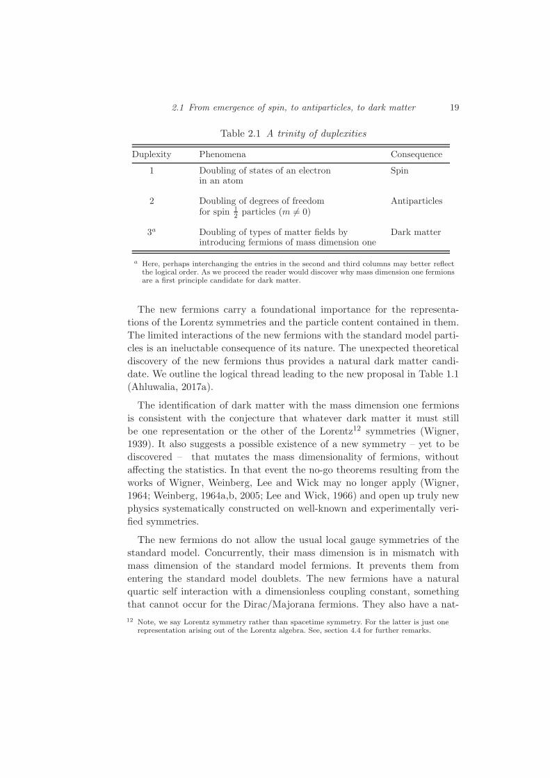
Table 2.1 A trinity of duplexities

Duplexity Phenomena Consequence

1 Doubling of states of an electron Spinin an atom

2 Doubling of degrees of freedom Antiparticlesfor spin 1

2particles (m 6= 0)

3a Doubling of types of matter fields by Dark matterintroducing fermions of mass dimension one

a Here, perhaps interchanging the entries in the second and third columns may better reflectthe logical order. As we proceed the reader would discover why mass dimension one fermionsare a first principle candidate for dark matter.

The new fermions carry a foundational importance for the representa-

tions of the Lorentz symmetries and the particle content contained in them.

The limited interactions of the new fermions with the standard model parti-

cles is an ineluctable consequence of its nature. The unexpected theoretical

discovery of the new fermions thus provides a natural dark matter candi-

date. We outline the logical thread leading to the new proposal in Table 1.1

(Ahluwalia, 2017a).

The identification of dark matter with the mass dimension one fermions

is consistent with the conjecture that whatever dark matter it must still

be one representation or the other of the Lorentz12 symmetries (Wigner,

1939). It also suggests a possible existence of a new symmetry – yet to be

discovered – that mutates the mass dimensionality of fermions, without

affecting the statistics. In that event the no-go theorems resulting from the

works of Wigner, Weinberg, Lee and Wick may no longer apply (Wigner,

1964; Weinberg, 1964a,b, 2005; Lee and Wick, 1966) and open up truly new

physics systematically constructed on well-known and experimentally veri-

fied symmetries.

The new fermions do not allow the usual local gauge symmetries of the

standard model. Concurrently, their mass dimension is in mismatch with

mass dimension of the standard model fermions. It prevents them from

entering the standard model doublets. The new fermions have a natural

quartic self interaction with a dimensionless coupling constant, something

that cannot occur for the Dirac/Majorana fermions. They also have a nat-

12 Note, we say Lorentz symmetry rather than spacetime symmetry. For the latter is just onerepresentation arising out of the Lorentz algebra. See, section 4.4 for further remarks.

20 A trinity of duplexities

ural coupling with the Higgs and gravity. Additional interactions arise from

quantum corrections.

As this monograph was composed a new unexpected aspect of the new

fermions under rotation came to attention. It has important cosmological

consequences. This is now the subject of Chapter 12.

Like the Majorana fermions the symmetry of charge conjugation plays a

central role for the new fermions: while for the Majorana field the coefficient

functions are eigenspinors of the parity operator, the field itself equals its

charge conjugate. For the new fermions the field is expanded in terms of the

eigenspinors of the charge conjugation operator. Once that is done, one may

choose to impose the Majorana condition, but it is not mandated.

Thus the new formalism, in a parallel with the Dirac formalism, allows

for darkly-charged fermions, and Majorana-like neutral fields.

To avoid possible confusion we remind the reader that both the Dirac

and Majorana quantum field are expanded in terms of Dirac spinors. These

are eigenspinors of the parity operator: m−1γµpµ, see Chapter 5 below,

and (Speranca, 2014). Eigenspinors of the charge conjugation operator are

thought to provide no Lagrangian description in a quantum field theoretic

construct (Aitchison and Hey, 2004, App. P). Thus placing the parity and

charge conjugation symmetries on an asymmetric footing – that is, as far

as their roles in constructing spin one half quantum fields are concerned.

Here I show that the Aitchison and Hey claim is in error (it seems to be

edited out in later editions). It has remained hidden in a lack of full appre-

ciation as to how one is to construct duals for spinors, and the associated

adjoints – that is, in the mathematics underlying the definition of the dual

spinors via ψ(p) = ψ(p)†γ0 (Ahluwalia, 2017a,c). The resolution occurs

through a generalisation of the Dirac dual presented here in chapter 14.

To develop the physics hinted above we are forced to complete the de-

velopment of this mathematics. Taken to its logical conclusion it leads to

the doubling of the fundamental form of matter fields. One form of matter

is described by the Dirac formalism, while the other, that of the dark sec-

tor, by the new fermions reported here. For each sector the needed matter

fields require a complete set of four, four-component spinors. For the former

these are eigenspinors of the parity operator while for the latter these are

eigenspinors of the charge conjugation operator (Elko).13

13 As noted earlier: Elko is a German acronym for Eigenspinoren desLadungskonjugationsoperators introduced in (Ahluwalia and Grumiller, 2005a,b). In English,it translates to eigenspinors of the charge conjugation operator.

2.1 From emergence of spin, to antiparticles, to dark matter 21

Global phases associated with these eigenspinors, and the pairing of these

eigenspinors with the creation and annihilation operators influence the Lorentz

covariance and locality of the fields (as already discussed at some length in

the Preface). This last observation, often ignored in textbooks, when cou-

pled with the discovery of a freedom in defining spinorial duals accounts for

the removal of the non-locality and restores the Lorentz symmetry for the

mass dimension one fermions (Ahluwalia, 2017c,a).

3

From elements of Lie symmetries to Lorentz algebra

Our first exposure to Lorentz algebra often happens in the context of some

course on the theory of special relativity. Because of historical reasons one

often thinks of the two in the same breath. On some planet endowed with

individuals who reflect on their origins one may arrive at Lorentz algebra

by looking at the spectrum of the hydrogen atom. At another planet, obser-

vations on light may lead thinking beings to arrive at Maxwell equations,

and then Lorentz algebra – and may be even at conformal algebra. Thus,

Lorentz algebra is a unifying theme underlying all attempts to understand

associated matter and gauge fields, and the very spacetime in which the as-

sociated quanta propagate. Somewhat poetically, that which walks and that

in which it walks are determined by each other (this thread continues fur-

ther in chapter 17). With this being so, we here take the view that Lorentz

algebra is deeper than the symmetries of the Minkowski space (where the

additional symmetry of spacetime translations exist). Its different solutions

furnish different representation spaces. Minkowski spacetime being just one

of them.

This chapter develops the needed concepts in a pedagogic manner. Its

pace is to the point, and leisurely, and exploits the opportunity to present

a point of view that to my knowledge contains several novel points of view.

This chapter is written for an advanced undergraduate student to provide

her a simple entry into the subject at hand.

3.1 Introduction

At Texas A&M University, I did not begin work on my doctoral thesis till

such time I came to know of Eugene Wigner’s 1939 work and of Steven Wein-

3.1 Introduction 23

berg’s 1964 papers (Wigner, 1939; Weinberg, 1964a,b). Not that I instantly

understood them, or even appreciated their depth in the first encounter.

But I realised that the Dirac equation in its 1928 form and Maxwell equa-

tions of classical electrodynamics are so utterly simple to arrive at. Modulo

a careful handling of the discrete symmetries, all one needs is the unifying

theme provided by the Loretnz algebra.14 And if the latter were to change,

say at the Planck scale, so would these equations. Assertions such as ‘let

us take a Lagrangian density that depends only on one or two spacetime

derivatives of the fields,’ as I was to learn in the process, often led to myste-

rious pathologies for once the representation space to which a field belonged

to was specified, one lost the freedom to invoke simplicity and convenience

to choose how many spacetime derivatives entered the Lagrangian density.

Many, if not all, such pathologies disappear if one is careful at the starting

point: the Lagrangian density.

In other words, and as already alluded to above, my trouble with the

quantum field theory courses as a doctoral student was that one had to pro-

vide a Lagrangian density, and even at the free field level it amounted to

invoking the genius of Dirac or that of Maxwell coupled with a set of associ-

ated experiments and data. But theoretical physics to me was to be a logical

exercise which depended on as few experiments as possible and explained

all the relevant phenomena. This approach, if it existed, would then provide

the unifying thread from which wave equations and Lagrangian densities

would emerge. The hosts of experimental results would then simply be a

logical consequence of this unifying theme and these Lagrangian densities.

Additional formal structure would then be built from additional principles,

such as that of local gauge invariance and the technology of the S-matrix

theory would help extract many of the observables.15

Roughly two decades later I have a better understanding as to from where

do the Lagrangian densities come from and how one may evade certain no-

go theorems of Weinberg (Ahluwalia, 2017a). This is the story I want to

develop. In the process we shall arrive at several known, and some totally

unexpected, results. Very often the manner in which we arrive at the known

14 In a quantum field theoretic context significantly more structure needs to be introduced toarrive at the Dirac and Maxwell equation for the fields (Weinberg, 2005).

15 Unknown to me for sometime, similar questions were being asked by Steven Weinberg in1960’s. In 1980’s when I was to take quantum field theory courses, not too far from TexasA&M, he was offering quantum field theory courses at the University of Texas at Austin. HadI attended those courses this monograph would not have come to be written. The beauty ofhis formalism, how he viewed and views quantum field theory, and its seduction was toointense to think that a couple places needed to be explored deeper leading to the resultspresented in this monograph.

24 From elements of Lie symmetries to Lorentz algebra

results shall be significantly different from their presentation elsewhere in

the physics literature. The role played by various symmetries shall be trans-

parent, or so I hope. I make significant effort to keep the presentation at a

level that makes the presented material easily accessible to the advanced un-

dergraduate students and the beginning doctoral students of Physics. Some

mathematicians may frown upon it but even for them it is hoped that there

is, at times, new mathematics, and a lesson in the importance of phase

factors in physics.

The first thing, then, is to introduce the notion of symmetry generators

for a Lie algebra towards the eventual aim to facilitate bringing Lorentz

algebra on the scene. To introduce the said notion it suffices to begin with the

rotational symmetry in the familiar landscape of three spatial dimensions.

With rotational symmetry in our focus we would not forgo the opportunity

to emphasise the unavoidable inevitability of the quantum structure of the

physical reality – or at least, make it more plausible.

3.2 Generator of a Lie symmetry

By a Lie symmetry we mean a symmetry that depends on a continuous

parameter. These are to be distinguished from the discrete symmetries, such

as that of parity. The familiar rotational symmetry in the ordinary space is

one simple and important example. We will use it to introduce the notion

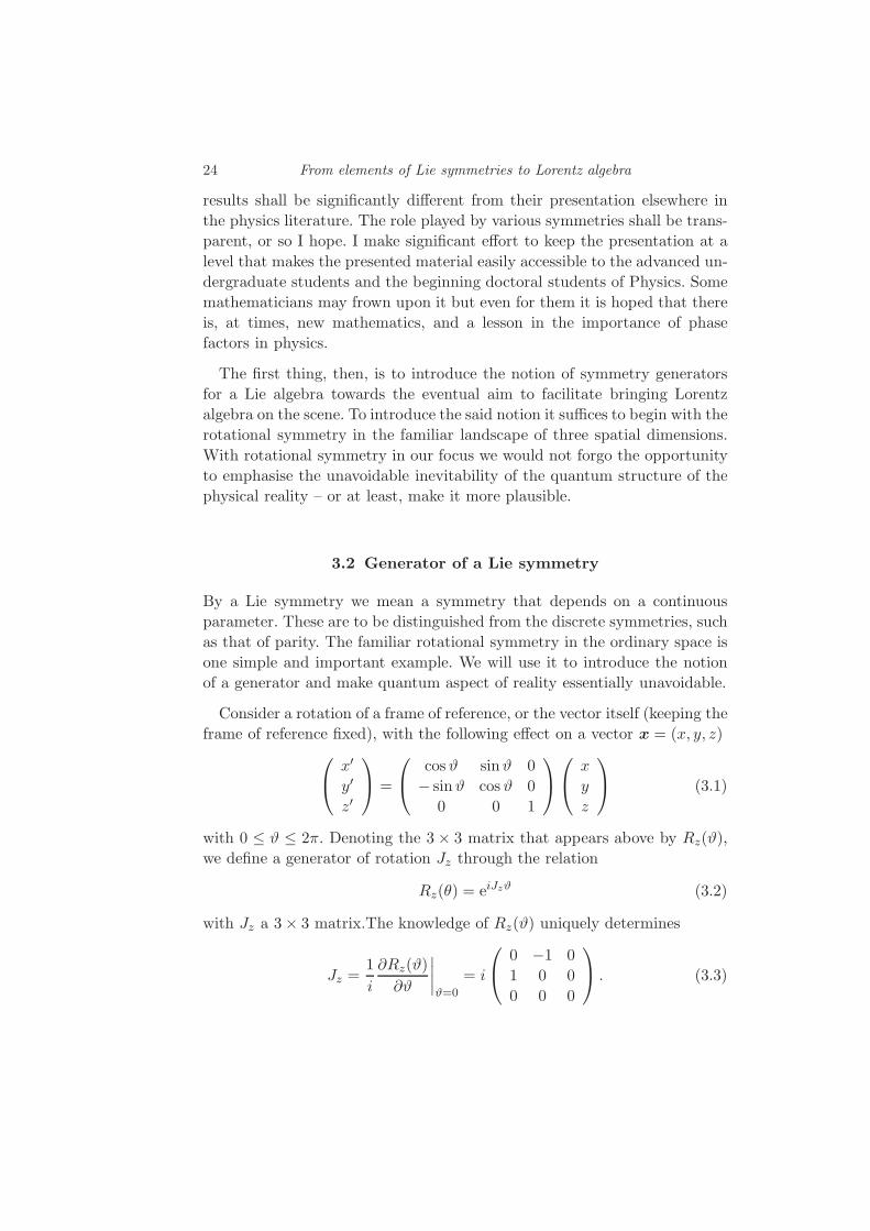
of a generator and make quantum aspect of reality essentially unavoidable.

Consider a rotation of a frame of reference, or the vector itself (keeping the

frame of reference fixed), with the following effect on a vector x = (x, y, z)

x′

y′

z′

=

cos ϑ sinϑ 0

− sinϑ cos ϑ 0

0 0 1

x

y

z

(3.1)

with 0 ≤ ϑ ≤ 2π. Denoting the 3× 3 matrix that appears above by Rz(ϑ),

we define a generator of rotation Jz through the relation

Rz(θ) = eiJzϑ (3.2)

with Jz a 3× 3 matrix.The knowledge of Rz(ϑ) uniquely determines

Jz =1

i

∂Rz(ϑ)

∂ϑ

∣∣∣∣ϑ=0

= i

0 −1 0

1 0 0

0 0 0

. (3.3)

3.3 A beauty of abstraction and a hint for the quantum nature of reality 25

The factor of i in the exponential of the definition (3.2) is often omitted by

mathematicians. We shall keep the factor of i. It makes Jz hermitian. In the

process it becomes a candidate for an observable in the quantum formalism.

The interval dr2 = dx2 + dy2 + dz2, besides other symmetry transforma-

tions of the Galilean group, is invariant not only under the transformation

Rz(θ) but also under two additional transformations associated with rota-

tions

Ry(ψ) =

cosψ 0 − sinψ

0 1 0

sinψ 0 cosψ

def Jy

= eiJyψ (3.4)

and

Rx(φ) =

1 0 0

0 cosφ sinφ

0 − sinφ cosφ

def Jx= eiJxφ (3.5)

leading to the associated generators of the rotations

Jy =1

i

∂Ry(ψ)

∂ψ

∣∣∣∣ψ=0

= i

0 0 1

0 0 0

−1 0 0

(3.6)

and

Jx =1

i

∂Rx(φ)

∂φ

∣∣∣∣φ=0

= i

0 0 0

0 0 −1

0 1 0

. (3.7)

This is very elementary. But it allows us to introduce the important notion

of generators of Lie symmetries in a familiar landscape. For the moment we

refrain from studying boosts and spacetime translations.

3.3 A beauty of abstraction and a hint for the quantum nature

of reality

Now comes an unreasonable beauty of abstraction. Since the matrices do

not commute, the generators of rotations given by equations (3.3), (3.6),

and (3.7) satisfy the algebraic relationship, or simply the algebra (or, Lie

algebra)

[Jx, Jy ] = iJz , and cyclic permutations. (3.8)

26 From elements of Lie symmetries to Lorentz algebra

The abstraction, well known to physicists and mathematicians, consists of

the following. Let us momentarily forget how this algebra has arisen, and in-

stead marvel at the infinitely many solutions that exist for this algebra. Each

of these solutions is called a representation of the algebra, and the spaces

on which the elements of the representation act are called representation

spaces.

All of us know that (3.8) also follows from the fundamental commutator,

but we now ask: Does the fundamental commutator follow from rotational

symmetry?

Continuing the thread, not only are there finite-dimensional matrix rep-

resentations of (3.8), infinitely many of them (this thought continues in

chapter 4), but there is also an infinite-dimensional representation that is

made of differential operators, with

Jx =1

i

(y∂

∂z− z

∂

∂y

), Jy =

1

i

(z∂

∂x− x

∂

∂z

), (3.9)

Jz =1

i

(x∂

∂y− y

∂

∂x

). (3.10)

Many students of Physics encounter this result in the context of their first

quantum mechanics course. Starting with the Heisenberg fundamental com-

mutator, they are taught that taking the classical definition of the angular

momentum and replacing the position and momentum by their quantum

counterparts, one obtains (3.8), followed by (3.9) and (3.10).

Given our discussion above, we ask the question: Does quantum aspect

of reality spring from rotational symmetry and the implicit assumption of a

continuous spacetime? The answer we adopt would then tell us if the quan-

tum gravity spacetime would be discrete, not covered by Lorentz algebra and

what modifications would the Heisenberg algebra and the deBroglie wave

particle duality suffer. This view is supported by the Kempf, Mangano, and

Mann (Kempf et al., 1995) and by my own work (Ahluwalia, 2000, 1994).

Taking this view has the consequence that quantum mechanical founda-

tions are seen as an inevitable consequence of the rotational symmetry. The

primary result is the Heisenberg algebra, and from that follows the secondary

result: the de Broglie wave particle duality We thus rewrite (3.9) and (3.10)

as

Jx =1

~× ~

i

(y∂

∂z− z

∂

∂y

), Jy =

1

~× ~

i

(z∂

∂x− x

∂

∂z

), (3.11)

3.3 A beauty of abstraction and a hint for the quantum nature of reality 27

Jz =1

~× ~

i

(x∂

∂y− y

∂

∂x

). (3.12)

with ~ = h/2π as the reduced Planck’s constant. Identifying

x and~

i

∂

∂x, y and

~

i

∂

∂y, z and

~

i

∂

∂z(3.13)

as position and momentum operators naturally leads to the Heisenberg’s

fundamental commutators

[x, px] = i~, [y, py] = i~, [z, pz] = i~ (3.14)

with [x, y] = 0, etc. Now the eigenfunctions of the momentum operator

p =~

i∇ (3.15)

have the form

exp

(ip′ · x′

~

)(3.16)

where p′ and x′ denote eigenvalues of the operators p and x. We find this

Dirac-Schwinger notation useful but only invoke it when an ambiguity is

likely to arise. The eigenfunctions (3.16) have the spatial periodicity

λ =h

p(3.17)

with p = |p′|. We are thus required that we associate a wave length λ with

momentum p a la de Broglie.16

In this interpretation the foundations of classical mechanics are at odds

with the rotational symmetry and echo considerations related to the lack of

stability of the algebra underling classical mechanics (Flato, 1982; Faddeev,

1989; Vilela Mendes, 1994; Chryssomalakos and Okon, 2004).

To emphasise we repeat that the argument of the conventional courses

on quantum mechanics begins with the fundamental commutator and re-

sults in the ‘angular momentum commutators.’ It is generally not realised

that the de Broglie’s λ = h/p is a direct consequence of the Heisenberg’s

fundamental commutator. Whereas here we reverse that argument and see

the fundamental commutator, and hence the wave particle duality, as a con-

sequence of rotational symmetry. It makes it clear, or opens a discussion,

that the classical description of reality is incompatible with the rotational

16 We shall often set ~ and the speed of light c to be unity.

28 From elements of Lie symmetries to Lorentz algebra

symmetry. Quantum aspect of realty thus seem to spring from the rotational

symmetry of the space in which events occur.

The presence of the momentum operator in the Heisenberg algebra intro-

duces kinetic energy in the measurement process. It induces inevitable gravi-

tational effects through the modification of the local curvature. These effects

make position measurements non-commutative (Ahluwalia, 1994; Doplicher et al.,

1994). The implicit assumption of the commuting position operators of the

arrived at quantum nature of reality must, therefore, undergo a modification

at the Planck scale where gravitational effects become important. But ro-

tational symmetry seems to make the fundamental commutator inevitable.

This paradoxical circumstance can be averted if we entertain the possibility

that quantum-gravity requires a non-commutative spacetime accompanied

by a modified Heisenberg algebra.

In the argument above we can easily take ~ as some unknown constant

with the dimension of angular momentum and then obtain its chosen identi-

fication by, say, looking at the spectrum of a system governed by the hamil-

tonian H = p2/2m+(1/2)mω2x2. The fundamental commutator yields the

energy spectrum of such systems to be equidistant lines with separation ~ω,

and a zero point energy of 12~ω.

3.4 A unification of the microscopic and the macroscopic

All this is not mathematical science fiction. Because of its simplicity and

its manifest importance, it is good to recall that the stability of the Earth

beneath us and Avogadro number of primal entities in a palmful of water

speak of it. Take the simplest of the simple systems, the hydrogen atom.

Classically, if one minimises the energy, E =(p2/2m

)−e2/r, of the hydrogen

atom then one immediately sees that the energy is minimised at r = 0. The

atom collapses to size zero. In contrast the fundamental commutator in

(3.14) requires that E be minimised to the constraint r p ∼ ~. To implement

this constraint one may set r ∼ ~/p and get E =(p2/2m

)− e2p/~. Setting,

∂E/∂p = 0, then gives the E-minimising p, p0 ∼ me2/~, for which E takes

its minimum value E0 ∼ −me4/2~2 ≈ −13.6 eV. The r instead of collapsing

to zero, is now constrained to r0 = ~2/me2 = 0.5 × 10−8 cm. It is a good

measure of the size of most atoms. The reason being that for heavier nuclei

with atomic number Z, for the outermost electron the (Z − 1) electrons

screen the nucleus in such a way that the effective nuclear charge remains

e (Weinberg, 2012). In this simple manner we not only understand the origin

3.5 Lorentz algebra 29

of the ionisation energy of the hydrogen atom but we also obtain the order

of magnitude for the Avagadro’s number (∼ (1/r0)3).

These simple argument unify the microscopic, the hydrogen atom, with

the macroscopic, the Earth. Beyond the stability of the planets, and burning

of the stars, quantum nature of reality leaves its imprints in the entire cosmos

and to possible physics beyond. Beyond, where rotational symmetry either

ceases to be, or takes a new – not yet known – form in discreteness of

spacetime (Padmanabhan, 2016).

3.5 Lorentz algebra

On the planet Earth, the Lorentz algebra is usually arrived at by con-

sidering the transformations of the spatial and temporal specifications of

events. Elsewhere in the cosmos one may arrive at the very same alge-

bra by studying the spectrum of hydrogen atom, instead through the null

result of the terrestrially famous 1887 experiment of Michelson and Mor-

ley (Michelson and Morley, 1887).

The folklore that the 1887 experiment requires Lorentz symmetries is,

strictly speaking, not true (Cohen and Glashow, 2006). The Lorentz sym-

metries follow only if one requires in addition any of the four discrete sym-

metries. One of these discrete symmetries is Parity – a symmetry known to

be violated in the electroweak interactions (Lee and Yang, 1956; Wu et al.,

1957). Remaining three are: time reversal, and charge conjugation conju-

gated with parity, or time reversal.

The most familiar way to arrive at the Lorentz algebra is to simply note

that absolute space and absolute time are now empirically untenable. While

a rotation, say about the z-axis, does not mix time and space (units: speed

of light is now taken as unity)

t′

x′

y′

z′

=

1 0 0 0

0 cos ϑ sinϑ 0

0 − sinϑ cos ϑ 0

0 0 0 1

t

x

y

z

. (3.18)

a boost, say along the x-axis does

t′

x′

y′

z′

=

coshϕ sinhϕ 0 0

sinhϕ coshϕ 0 0

0 0 1 0

0 0 0 1

t

x

y

z

(3.19)

30 From elements of Lie symmetries to Lorentz algebra

where the rapidity parameter, ϕ = ϕ p, is defined as

coshϕ = E/m = γ = 1/√

1− v2

sinhϕ = p/m = γv (3.20)

with all symbols carrying their usual meaning. Denoting the 4 × 4 boost

matrix in (3.19) by Bx(ϕ). The generator of the boost along the x-axis is

thus

Kx =1

i

∂Bx(ϕ)

∂ϕ

∣∣∣∣ϕ=0

= −i

0 1 0 0

1 0 0 0

0 0 0 0

0 0 0 0

. (3.21)

This is complemented by the remaining two generators of the boosts

Ky = −i

0 0 1 0

0 0 0 0

1 0 0 0

0 0 0 0

, Kz = −i

0 0 0 1

0 0 0 0

0 0 0 0

1 0 0 0

(3.22)

and the three generators of the rotations. These are directly read off from

our work earlier with the added observation that under rotations t and t′

are identical

Jx = −i

0 0 0 0

0 0 0 0

0 0 0 1

0 0 −1 0

, (3.23)

Jy = −i

0 0 0 0

0 0 0 −1

0 0 0 0

0 1 0 0

, Jz = −i

0 0 0 0

0 0 1 0

0 −1 0 0

0 0 0 0

. (3.24)

The six generators satisfy the following algebra

[Jx, Jy] = iJz and cyclic permutations (3.25)

[Kx,Ky ] = −iJz, and cyclic permutations (3.26)

[Jx,Kx] = 0, etc. (3.27)

[Jx,Ky] = iKz, and cyclic permutations. (3.28)

It is named Lorentz algebra.

3.6 Further abstraction: Un-hinging the Lorentz algebra . . . 31

3.6 Further abstraction: Un-hinging the Lorentz algebra from its

association with Minkowski spacetime

To underline the mysteries of nature coded in the algebra just arrived at

let us take the liberty of imagining that we forget how we arrived at this

algebra. Each civilisation in the cosmos, sooner or later, is likely to arrive at

this truth, this reflection of low-energy reality, in one way or another. Some

in a way similar to ours, others in ways different, even ways we have not yet

dreamed of. Lorentz algebra is a powerful unifying element in unearthing

the nature of reality. Its various aspects thread through this monograph,

with Physics as our primary focus.

We thus symbolically unhinge the Lorentz algebra from spacetime sym-

metries and express it as an abstract reality expressed through the following

abstraction

J → J, K → K (3.29)

such that J and K are no longer confined to being identified with the 4 ×4 matrices given in (3.21) to (3.24), or with their unitarily transformed

expressions, but still satisfy

[Jx,Jy] = iJz , and cyclic permutations (3.30)

[Kx,Ky] = −iJz, and cyclic permutations (3.31)

[Jx,Kx] = 0, etc. (3.32)

[Jx,Ky] = iKz, and cyclic permutations. (3.33)

The Ji and Kj, i, j = x, y, z, represent generators of rotations and boosts –

in an abstract space. Their exponentiations

exp (iJ · θ) , exp (iK ·ϕ) (3.34)

give the group transformations under rotations and boosts for the ‘vectors’

spanning the associated representation space. While the underlying alge-

braic structure remains the same, each of the group transformations – cho-

sen by a specific choice of J and K in (3.34) – defines a new group. These

group transformations act on vectors that inhabit the associated representa-

tion spaces. Upto a convention related freedom of a unitary transformation,

the transformations of four vectors, to transformations of Dirac spinors, to

‘other vectors’ in infinitely many other representation spaces, are all ob-

tained from (3.34).

To cast the Lorentz algebra in a manifestly covariant form, we recall the

32 From elements of Lie symmetries to Lorentz algebra

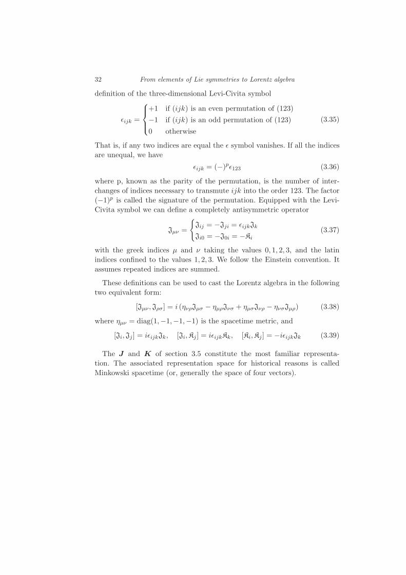
definition of the three-dimensional Levi-Civita symbol

ǫijk =

+1 if (ijk) is an even permutation of (123)

−1 if (ijk) is an odd permutation of (123)

0 otherwise

(3.35)

That is, if any two indices are equal the ǫ symbol vanishes. If all the indices

are unequal, we have

ǫijk = (−)pǫ123 (3.36)

where p, known as the parity of the permutation, is the number of inter-

changes of indices necessary to transmute ijk into the order 123. The factor

(−1)p is called the signature of the permutation. Equipped with the Levi-

Civita symbol we can define a completely antisymmetric operator

Jµν =

Jij = −Jji = ǫijkJk

Ji0 = −J0i = −Ki(3.37)

with the greek indices µ and ν taking the values 0, 1, 2, 3, and the latin

indices confined to the values 1, 2, 3. We follow the Einstein convention. It

assumes repeated indices are summed.

These definitions can be used to cast the Lorentz algebra in the following

two equivalent form:

[Jµν ,Jρσ ] = i (ηνρJµσ − ηµρJνσ + ηµσJνρ − ηνσJµρ) (3.38)

where ηµν = diag(1,−1,−1,−1) is the spacetime metric, and

[Ji,Jj ] = iǫijkJk, [Ji,Kj ] = iǫijkKk, [Ki,Kj ] = −iǫijkJk (3.39)

The J and K of section 3.5 constitute the most familiar representa-

tion. The associated representation space for historical reasons is called

Minkowski spacetime (or, generally the space of four vectors).

4

Representations of Lorentz Algebra

4.1 Poincare algebra, mass, and spin

For the purposes of a physicist a ‘representation of an algebra’ is simply a

specific solution to the symmetry algebra under consideration.

Thus the six 4×4 matrices given in equations (3.21) to (3.24) form a rep-

resentation of the Lorentz algebra. It is a finite dimensional representation,

and there are infinitely many of them. We will start considering them in the

next section.

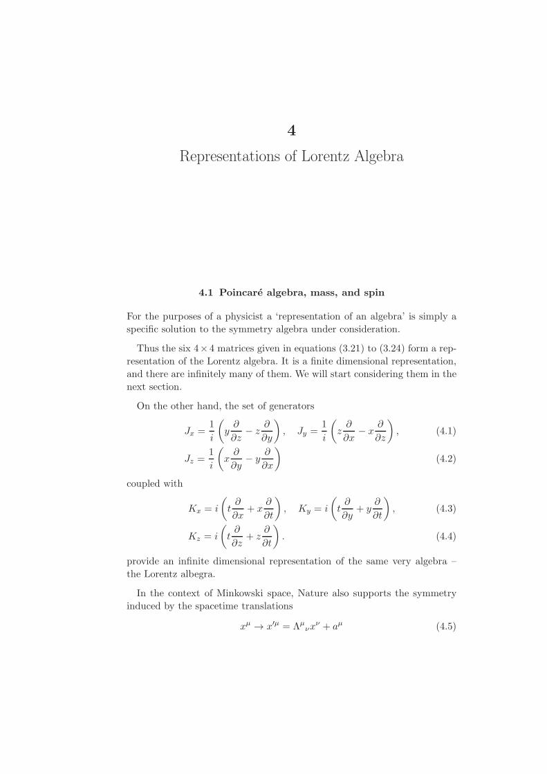
On the other hand, the set of generators

Jx =1

i

(y∂

∂z− z

∂

∂y

), Jy =

1

i

(z∂

∂x− x

∂

∂z

), (4.1)

Jz =1

i

(x∂

∂y− y

∂

∂x

)(4.2)

coupled with

Kx = i

(t∂

∂x+ x

∂

∂t

), Ky = i

(t∂

∂y+ y

∂

∂t

), (4.3)

Kz = i

(t∂

∂z+ z

∂

∂t

). (4.4)

provide an infinite dimensional representation of the same very algebra –

the Lorentz albegra.

In the context of Minkowski space, Nature also supports the symmetry

induced by the spacetime translations

xµ → x′µ = Λµνxν + aµ (4.5)

34 Representations of Lorentz Algebra

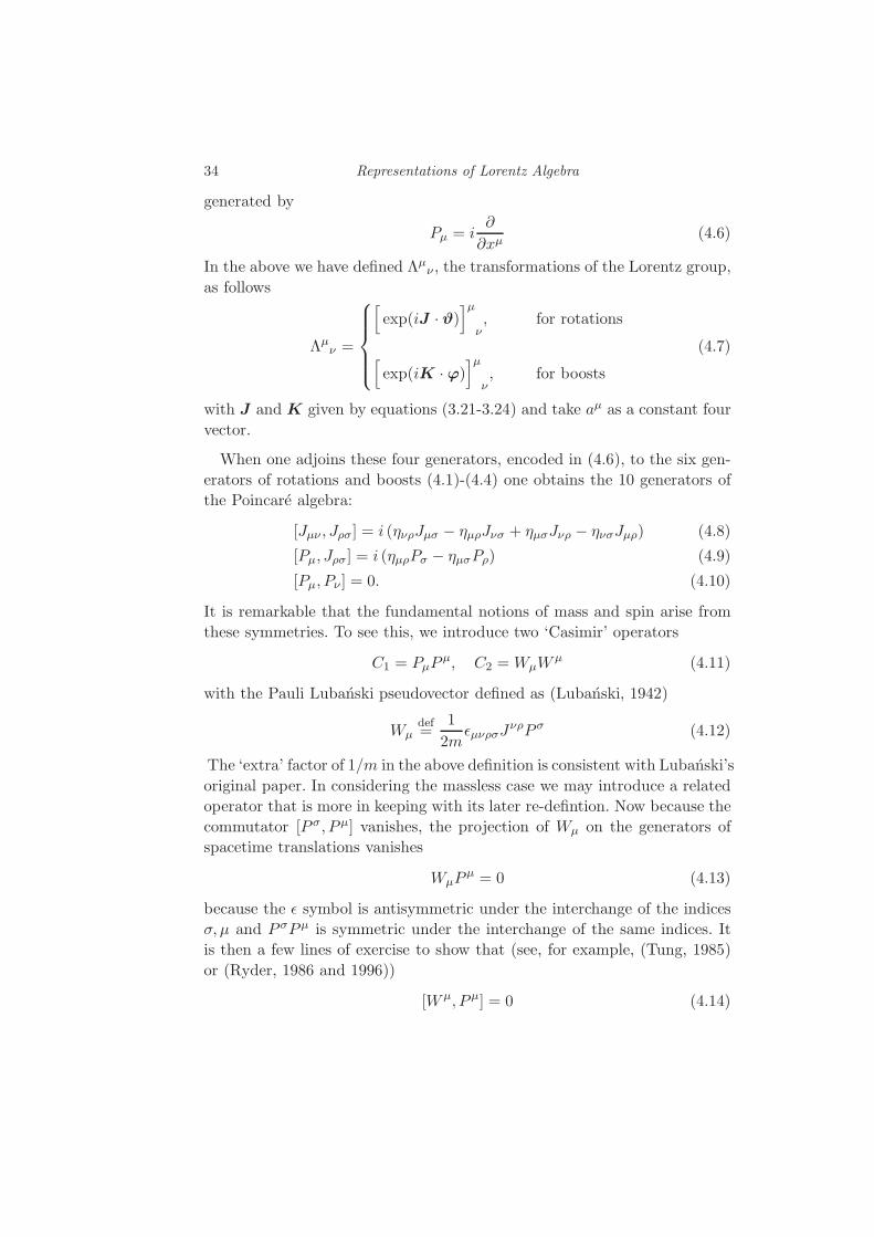
generated by

Pµ = i∂

∂xµ(4.6)

In the above we have defined Λµν , the transformations of the Lorentz group,

as follows

Λµν =

[exp(iJ · ϑ)

]µν, for rotations

[exp(iK · ϕ)

]µν, for boosts

(4.7)

with J and K given by equations (3.21-3.24) and take aµ as a constant four

vector.

When one adjoins these four generators, encoded in (4.6), to the six gen-

erators of rotations and boosts (4.1)-(4.4) one obtains the 10 generators of

the Poincare algebra:

[Jµν , Jρσ ] = i (ηνρJµσ − ηµρJνσ + ηµσJνρ − ηνσJµρ) (4.8)

[Pµ, Jρσ ] = i (ηµρPσ − ηµσPρ) (4.9)

[Pµ, Pν ] = 0. (4.10)

It is remarkable that the fundamental notions of mass and spin arise from

these symmetries. To see this, we introduce two ‘Casimir’ operators

C1 = PµPµ, C2 =WµW

µ (4.11)

with the Pauli Lubanski pseudovector defined as (Lubanski, 1942)

Wµdef=

1

2mǫµνρσJ

νρP σ (4.12)

The ‘extra’ factor of 1/m in the above definition is consistent with Lubanski’s

original paper. In considering the massless case we may introduce a related

operator that is more in keeping with its later re-defintion. Now because the

commutator [P σ, Pµ] vanishes, the projection of Wµ on the generators of

spacetime translations vanishes

WµPµ = 0 (4.13)

because the ǫ symbol is antisymmetric under the interchange of the indices

σ, µ and P σPµ is symmetric under the interchange of the same indices. It

is then a few lines of exercise to show that (see, for example, (Tung, 1985)

or (Ryder, 1986 and 1996))

[W µ, Pµ] = 0 (4.14)

4.2 Representations of Lorentz algebra 35

with the consequence that not only WµWµ is invariant under the Lorentz

transformation but also under spacetime translations. And thus it commutes

with all the ten generators of the Poincare algebra. A parallel of the same

argument tells us that PµPµ also commutes with all the ten generators of the

Poincar’e algebra. The eigenvalues of the latter are identified with the square

of the mass parameter m, and modulo a sign the eigenvalues of the former

can be easily identified with the eigenvalues of the square of the generators

of rotations: −s(s+ 1).17 It is for these reasons that mass and spin arise in

the description of the physical reality. Once one inertial observer measures

them, all inertial observers related by Poincare symmetries measure the same

value.

We generally assume that electron has the same ‘mass’ and same ‘spin,’

here in our solar system as in a far away distant galaxy going back to the

dawn of our universe – despite the fact that in earlier epochs Poincare sym-

metries may have suffered a modification. But perhaps where and when these

departures occur we enter another realm, the realm of massless particles,

with hypothetical massless observers. These observers have no rest frame,

and to us they lie in a realm where spacetime dimensionality changes, and

time as we generally define does not exist. Such a dramatic change arises

from singularities of length contraction and time dilation for truly massless

particles.

4.1.1 A cautionary remark

Except in the rest frame, the s(s+1) encountered above is not an eigenvalue

of J2. It is C2 whose eigenvalues remain invariant under Poincare transfor-

mations and not the eigenvalues of J2 except in the rest frame – or, in an

accidental situation to be discussed below.

4.2 Representations of Lorentz algebra

To identify various representations of Lorentz algebra one often starts with

introducing two su (2) generators:

A =1

2(J+ iK) , B =

1

2(J− iK) (4.15)

17 In making this identification with J2 we implicitly assume the abstraction explicitly noted inequation (3.29) that allows s to take half integral and integral values.

36 Representations of Lorentz Algebra

and studies representations of su (2)⊗ su (2), keeping in mind that

[Ax,Ay] = iAz , and cyclic permutations (4.16)

[Bx,By] = iBz, and cyclic permutations (4.17)

[Ai,Bj ] = 0, i, j = x, y, z. (4.18)

In this way one labels the resulting representation space by two labels (a, b),

with a(a + 1) and b(b + 1) being eigenvalues of A2 and B2, respectively.

We find this complexification of the generators unnecessary. I mention it

here because our reader may encounter it in her/his studies often. If due

interpretational caution is not exercised all this can cause confusion as J2 too

is not a Casimir invariant of the Lorentz algebra (as just cautioned above),

but only of the rotational subalgebra represented by the first of the equations

in (3.39). Introducing two su (2) algebras through complexifications of the

generators – when one is permitted only real linear combination – strictly

speaking, takes us away from the Lorentz algebra and it is avoidable.

————–

To avoid conceptual confusion we do not follow this potentially misleading

traditional approach but instead follow a straight forward method. For this

we note that once a representation of J is found18 that satisfies the first

part of (3.39) an inspection of the remainder of the Lorentz algebra shows

that for each representation of J there exist two independent primordial

representations for the boost generators

K = −iJ, K = +iJ (4.19)

The sets

J,K = −iJ︸ ︷︷ ︸R type

and J,K = iJ︸ ︷︷ ︸L type

(4.20)

provide two independent representations of the Lorentz algebra. As indi-

cated, we call these representaions as R type and L type, respectively. The

reason for this nomenclature shall become apparent in section 4.3 below.

Without the existence of two, in contrast to one, representations for each

J one would not be able to respect causality in quantum field theoretic

formalism respecting Poincare symmetries, or have massive antiparticles re-

quired to avoid causal paradoxes. And thus this doubling of representations

18 To find explicit form of J a junior reader may consult any good book on quantum mechanicsranging from Dirac’s classic (Dirac, 1930), to recent lectures by Weinberg (Weinberg, 2012),or to a very pedagogically written two volume set by Cohen-Tannoudji etal. (Cohen-Tannoudji et al., 1977).

4.2 Representations of Lorentz algebra 37

is more than an oddity, or a coincidence. It is a reflection a deep underly-

ing thread of symmetries, causality, and degrees of freedom encountered in

quantum fields.

In accordance with (3.34), the associated symmetry transformations are

implemented as follows

R :

Rotations by : exp[iJ · ϑ]Boosts by : exp[i(−iJ) ·ϕ] = exp[J · ϕ]

(4.21)

and

L :

Rotations by : exp[iJ · ϑ]Boosts by : exp[i(iJ) ·ϕ] = exp[−J · ϕ]

(4.22)

For these primordial representations the knowledge of J completely deter-

mines the rotation, parameterised by ϑ, and the boost, parameterised by ϕ,

transformations.

The boosts do not carry the imaginary i in the exponentiation. It is not

that we have suddenly changed to the convention of the mathematics liter-

ature but because the i in the exponentiation for the boost operator when

encountered with the ±i in the expression for K in (4.20) results in ∓1. I

make this parenthetic note because again and again in my seminars I en-

counter a question to this effect.

4.2.1 Notational remark

In the language of the traditional approach of labelling representation spaces,

theR and L stand for the (j, 0) and (0, j) representation spaces, respectively:

R ↔ (j, 0),L ↔ (0, j).

4.2.2 Accidental Casimir

For the primordial representations introduced above – despite the general

remark made above about J2 after equations (4.18) – J2 does commute with

all the generators given in (4.20). For this reason, in the restricted context

of the R and L representation spaces, we introduce the term ‘accidental

Casimir operator’ for J2. Its invariant eigenvalue s(s + 1) coincides with

that of the C2 in all inertial frames.

38 Representations of Lorentz Algebra

4.3 Simplest representations of Lorentz algebra

With our focus on (4.21) and (4.22), the simplest non trivial J that satisfies

the Lorentz algebra (3.39) is formed from the Pauli matrices

σx =

(0 1

1 0

), σy =

(0 −ii 0

), σz =

(1 0

0 −1

)(4.23)

and is given by

J = σ/2. (4.24)

Through (4.20), it introduces two independent representations spaces of spin

one half.

Referring to equations (4.21) and (4.22) the group transformations for

rotations and boosts for these representation spaces are given by

RR,L(ϑ) = exp[iσ

2· ϑ

](4.25)

BR,L(ϕ) = exp[±σ

2·ϕ

](4.26)

where the upper sign is for the R type boosts, while the lower sign is for

the L type boosts. The expression for the transformation for rotation is the

same for both type of primordial representations.

Writing ϑ = ϑ n, with ϑ representing the angle of rotation and n denoting

a unit vector along the axis of rotation, the transformation for rotations

(4.25) takes the form

RR,L(ϑ) = I+ iσ · nϑ2− 1

2!(σ · n)2

(ϑ

2

)2

− i1

3!(σ · n)3

(ϑ

2

)3

+1

4!(σ · n)4

(ϑ

2

)4

+ i1

5!(σ · n)5

(ϑ

2

)5

+ . . . (4.27)

Using the identity (σ · n)2 = I, the above expansion reduces to

RR,L(ϑ) =

[1− 1

2!

(ϑ

2

)2

+1

4!

(ϑ

2

)4

− . . .

]I

+ iσ · n[ϑ

2− 1

3!

(ϑ

2

)3

+1

5!

(ϑ

2

)5

− . . .

](4.28)

and simplifies to yield

RR,L(ϑ) = cos

(ϑ

2

)I+ iσ · n sin

(ϑ

2

)(4.29)

4.3 Simplest representations of Lorentz algebra 39

An exactly similar calculation as above yields the boosts noted in (4.26)

to be given by

BR,L(ϕ) = cosh(ϕ2

)I± σ · p sinh

(ϕ2

)(4.30)

= cosh(ϕ2

) [I± σ · p tanh

(ϕ2

)](4.31)

where the the upper sign on the righthand side of the above result holds

for the R type representations, and the lower sign holds for the L type

representations. To further simplify (4.31) we use the identities

cosh(ϕ2

)=

√coshϕ+ 1

2=

√E +m

2m(4.32)

tanh(ϕ2

)=

sinhϕ

coshϕ+ 1=

p

E +m(4.33)

for the rapidity parameter defined in (3.20) and rewrite (4.31) as

BR,L(ϕ) =

√E +m

2m

[I± σ · p

E +m

](4.34)

Now note that the spin-1/2 helicity operator is defined as

hdef=

σ

2· p (4.35)

and thus σ · p that appears in BR,L(ϕ) can be written as 2ph. This allows

us to re-write (4.34) in the form

BR,L(ϕ) =

√E +m

2m

[I± 2ph

E +m

](4.36)

The transformations RR,L(θ) and BR,L(ϕ) act on the two-dimensional

representation spaces. For historical reasons the ‘vectors’ in these spaces are

called R-type and L-type Weyl spinors. To gain insights into these repre-

sentation spaces we work out the effect of the boosts and rotations on the

eigenspinors of h. For an arbitrary four-momentum pµ these are defined as

hφR,L± (pµ) = ±1

2φR,L± (pµ) (4.37)

Introducing the standard four momentum vector for massive particles

kµ =

(m

0

), 0

def= p

∣∣p→0

(4.38)

40 Representations of Lorentz Algebra

the Weyl spinors for a particle at rest φR,L± (kµ) also satisfy (4.37)

hφR,L± (kµ) = ±1

2φR,L± (kµ) (4.39)

Once φR,L± (kµ) are chosen, the boosted φR,L± (pµ) follow immediately by the

application of the boost operators (4.36). To avoid keeping track of two

many ± and ∓ signs, consider R type Weyl spinors first

φR±(pµ) = BR(ϕ)φ

R±(k

µ) (4.40)

=

√E +m

2m

[I± p

E +mI

]φR±(k

µ) (4.41)

To explore the high-energy limit we note that for p≫ m,

p

E +m≈ 1− m

p(4.42)

As a result we have

BR (ϕ)φR±(kµ) ≈

√E +m

2m

[1±

(1− m

p

)]φR±(k

µ) (4.43)

Implementing the high-energy limit by taking the massless limit one thus

arrives at the result that for the R type Weyl spinors only the positive

helicity degree of freedom survives. While for the L type Weyl spinors the

counterpart of (4.43) reads

BL (ϕ)φL±(kµ) ≈

√E +m

2m

[1∓

(1− m

p

)]φL±(k

µ) (4.44)

As a consequence, in the high energy limit only the negative helicity spinors

survive.

The nomenclature of R and L type Weyl spinors arises from these high

energy limits. For the m = 0 case the helicity is an invariant under boosts,

and from there arose the nomenclature of the right-handed (R type) and

left-handed (L type) Weyl spinors. But for the massive case helicity is not

an invariant and thus one must be careful. The R and L must be taken as

labels for the representation spaces under consideration unless one wishes to

restrict one’s calculations to a preferred frame for convenience. Both the Rtype and the L type Weyl spinors support positive helicity and the negative

helicity spinors. A similar exercise for higher spins tells us that in the high

energy limit only the maximal helicity (±j) associated with the j-vectors

survives. By j-vectors we mean (2j+1) column vectors with (2j+1) complex

4.4 Spacetime: Its construction . . . 41

entries – either in the R or L representation space. In this language massive

Weyl spinors are 1/2-vectors.

Equation (4.29) implies that the action of RR,L(ϑ) on Weyl spinors for

ϑ = 2π, irrespective of the axis of rotation n, introduces a phase factor equal

to −1. It requires a 4π rotation for a spinor to return to itself. In general

Weyl spinors pick up a helicity-dependent phase factor

φ(pµ) →e+iϑ/2φ(pµ), for the positive helicity Weyl spinor

e−iϑ/2φ(pµ), for the negative helicity Weyl spinor(4.45)

We shall discover in Chapter 12 that these phase factors play a dramatic

role for Elko, the eigenspinors of the charge conjugation operator.

4.4 Spacetime: Its construction from the simplest

representations of Lorentz algebra

The simplest representations of the Lorentz algebra provide the basic ele-

ments to describe the matter fields that we encounter around us, the basic

blocks from which we are constructed from. The gauge fields that keep them

interacting, glue them and add fire, carry a ‘vector’ spacetime index. This

section is devoted to construct this vector index, in essence by constructing

spacetime itself.

Towards this end, using the the R and L type generators for spin one halfζR = σ/2,κR = −iσ/2

,

ζL = σ/2,κL = iσ/2

(4.46)

we introduce the following six generators for the R⊗L representation space

Ji =[(ζR)i ⊗ I

]+

[I⊗ (ζL)i

](4.47)

Ki =[(κR)i ⊗ I

]+

[I⊗ (κL)i

](4.48)

with i = x, y, z. These generators correspond to rotation and boost trans-

formations given by

R(ϑ)def= RR(ϑ)⊗RL(ϑ), B(ϕ)

def= BR(ϕ)⊗BL(ϕ). (4.49)

The definitions (4.49), and (4.47) and (4.48) mutually define each other

Ji =1

i

∂

∂ϑR(ϑ)

∣∣∣∣ϑ→0

(4.50)

42 Representations of Lorentz Algebra

Each of the Ji corresponds to taking n in the defintion ϑ = ϑ n along each

of the three spatial axes. Similarly,

Ki =1

i

∂

∂ϕB(ϕ)

∣∣∣∣ϕ→0

(4.51)

Each of the Ki corresponds to taking p in the defintion ϕ = ϕ p along each

of the three spatial axes.

We now show that modulo a convention-related unitary transformation U

given below in equation (4.56), the R(ϑ) and B(ϕ) are precisely the special

relativistic transformations of the rotation and boosts.

To establish this claim all we have to do is to obtain Ji and Ki defined

in (4.47) and (4.48) and show that a unitary transformation U exists such

that the U -transformed Ji and Ki reduce to Ji and Ki of special relativity.

The U simply implements the convention that the temporal coordinate is

placed on top of the spatial co-ordinates in the standard sequence so that

xµ equals (t,x).

Implementing the definitions (4.46)-(4.48) explicitly, and using Pauli ma-

trices in the representation (4.23) we obtain

Jx =1

2

0 1 1 0

1 0 0 1

1 0 0 1

0 1 1 0

, (4.52)

Jy =1

2

0 −i −i 0

i 0 0 −ii 0 0 −i0 i i 0

, Jz =

1 0 0 0

0 0 0 0

0 0 0 0

0 0 0 −1

(4.53)

and

Kx =1

2

0 i −i 0

i 0 0 −i−i 0 0 i

0 −i i 0

, (4.54)

Ky =1

2

0 1 −1 0

−1 0 0 −1

1 0 0 1

0 1 −1 0

, Kz =

0 0 0 0

0 −i 0 0

0 0 i 0

0 0 0 0

(4.55)

4.5 A few philosophic remarks 43

A straight forward calculation now shows that with the U defined as

Udef=

1√2

0 i −i 0

−i 0 0 i

1 0 0 1

0 i i 0

(4.56)

we have the required result

UJiU−1 → Ji (4.57)

UKiU−1 → Ki (4.58)

with Ji and Ki of special relativity given in (3.21) to (3.24). The usual 4×4

transformation matrices of the special relativity are nothing but one or the

other of the following

[Λµν ] = U

R(ϑ)

B(ϕ)

U−1 (4.59)

The square brackets on the left hand side indicates that the expression is to

be understood as the matrix Λ defined by the elements enclosed.

The construction presented here may be interpreted as a parallel to Atiyah’s

suggestion of a spinor being a square root of geometry (Atiyah, 2013).

4.5 A few philosophic remarks

It would become apparent as we open deeper into our discourse that the

R⊕ L representation space, in contrast to the R⊗ L representation space

just explored, supports all the fermionic matter fields of the standard model

of the high energy physics. So that which walks – the matter fields – and

that in which it walks, that is spacetime, are determined by each other. The

unifying theme being the underlying Lorentz algebra. From a philosophic

point of view the theory that deals with the measurement of spatial and

temporal distances through the proverbial rods and clocks in fact explores

the universality of symmetries that determine the very substance those very

rods and clocks are made of. I believe that this point of view is very similar

to the one adopted by Harvey Brown in his monograph (Brown, 2005).

It also assures us that the Planck-scale expected departures from the

Lorentz algebra are likely to alter foundational principles that spring from

the low-energy phenomena that we human are able to observe and study

44 Representations of Lorentz Algebra

so far. Some of these principles and notions are those of Heisenberg al-

gebra, wave particle duality, causality, particle-antiparticle symmetry, and

the Lagrangians that govern matter and gauge fields in a Lorentz covariant

framework. Any such departure may also be able to incorporate such notions

as consciousness, and phenomena that are presently considered outside the

realm of physics proper.

We make this observation because one can easily argue that non-commutati-

vity of spacetime measurements already follows from the merger of quantum

mechanics and the theory of general relativity (Ahluwalia, 1994; Doplicher et al.,

1994; Kempf et al., 1995; Ahluwalia, 2000). In reference to the beautiful

analysis of (Chryssomalakos and Okon, 2004) we note that in their analysis

relativistic symmetries and Heisenberg algebra are considered as two sepa-

rate entities to be merged together whereas in the approach taken in this

monograph Heisenberg algebra is seen as implicitly contained in the Lorentz

algebra.

However, incorporating the still deeper issues into the physics proper

may require a unification of physics-related phenomena and consciousness-

endowed biological systems (Ahluwalia, 2017b).

5

Discrete symmetries: Part 1 (Parity)

Adapting the approach of (Speranca, 2014), this chapter presents a first-

principle discussion of the parity operator. We will find that the 1928-Dirac

equation expresses the fact that the associated spinors are the eigenspinors

of the parity operator, and that m−1γµpµ is the covariant parity operator.

We will show that for the Dirac spinors the right- and left- transforming

components necessarily carry the same helicity, and bring to attention a

phase factor that determines whether a spinor is a particle spinor, or an

antiparticle spinor. Our results coincide with that of (Weinberg, 2005), while

pointing out a flaw in the standard treatment of the subject in books such

as (Ryder, 1986 and 1996; Hladik, 1999).

5.1 Discrete symmetries

Our description of the nature of reality divides one unified whole into parts.

These are connected with each other by being one representation or the

other of the Lorentz algebra.

An example of this broadbrush observation is that each of the transfor-

mation for rotations and boosts (4.21) and (4.22) contains in it a reference

to two type of spaces: one from the familiar four-vector space of Minkowski

through θ and ϕ (see section 4.4), and second to the spaces on which the

generators of rotations and boosts act (this time, Minkowski being just one

of them). The latter are bifurcated in two types, the R and L type. These

can transmute into each other if there exists a discrete transformation such

that exp[iJ · ϑ], exp[±J · ϕ]

exp[iJ · ϑ], exp[∓J · ϕ]

(5.1)

46 Discrete symmetries: Part 1 (Parity)

Or, equivalently

R L (5.2)

There are two known ways in which this can be done. Each of these introduce

a discrete symmetry. These merge seamlessly with the continuous kinemat-

ical symmetries and provide additional needed structure and understanding

of reality. These are the symmetries of parity and charge conjugation:

• In the Minkowski four-vector space, parity is defined as the map:

P : xµ = (t,x) → x′µ = (t,−x). (5.3)

Under it the J and ϑ remain unaltered but the rapidity parameter ϕ

changes sign. As a consequence parity interchanges the two representation

spaces and implements (5.1). In this chapter I start a discussion of the

image of (5.3) in the R⊕L representation space for s = 1/2 and develop

the associated mathematical structure that gives us two identities, leading

to the 1928 Dirac equation in the momentum space.19

• A distinct discrete symmetry arises if the transmutation (5.1) is imple-

mented by complex conjugating a spin s representation space and acting

it with the Wigner time reversal operator Θ defined as

ΘJΘ−1 def= −J

∗ (5.4)

It introduces a new discrete symmetry, that of charge conjugation. Again,

taking s = 1/2 as an example, I develop this discrete symmetry in detail

in chapter 6.

5.2 Weyl spinors

To bring a sharper focus to spin one half we first gather together what we

have learned so far in a compact form. Under the Lorentz boosts the right-

and left-handed Weyl spinors transform as20

φR(pµ) = exp

(+σ

2· ϕ

)φR(k

µ), φL(pµ) = exp

(−σ

2·ϕ

)φL(k

µ) (5.5)

where σ represents the set of Pauli matrices σx, σy, σz in their standard

representation given in (4.23); and the boost parameter ϕ is defined so that

19 The genesis of this chapter goes back to a pizza and hand written explanation by LlohannSperanca on a paper napkin one evening in Barao Geraldo in Campinas. This was during thetwo years I spent at IMECC, Unicamp, on a long term visit.

20 The placing of R and L as a superscript or as a subscript is purely for convenience in a givencontext.

5.3 Parity operator for the general four-component spinors 47

exp (iK · ϕ) acting on the standard four momentum equals the general four

momentum pµ = (E, p sin θ cosφ, p sin θ sinφ, p cos θ). This yields coshϕ =

E/m, sinhϕ = p/m with ϕ = p [in agreement with (3.20)], while K are the

4× 4 matrices for the generators of boosts in Minkowski space as per their

definition in equations (3.21) and (3.22).

The reader may recall that (5.5) follow from the fact that −iσ/2 are

the generators of the boosts for the right-handed Weyl representation space,

while +iσ/2 are for the left-handed Weyl representation space. For the direct

sum of the right- and left-Weyl representation spaces, to be motivated below,

the boost and rotation generators thus read

κ =

[−iσ/2 O

O +iσ/2

], ζ =

[σ/2 O

O σ/2

]. (5.6)

The set of generators K,J and κ, ζ, separately, satisfy the same

unifying algebra, the Lorentz algebra – given in equations (3.39) – and are

simply its different representations.

The [Λµν ]def= Λ representing boosts and rotations in Minkowski space is

thus given by

Λdef=

exp (iK · ϕ) for Lorentz boosts

exp (iJ · ϑ) for rotations. (5.7)

If K,J are in their canonical form the elements of Λ, K, and J are of

the form aµν , where the 4 × 4 matrix a stands generically for either one of

them. Their indices may then be raised and lowered by the spacetime metric

ηµν = diag1,−1,−1,−1.

5.3 Parity operator for the general four-component spinors

To construct the image of parity operator for s = 1/2 the discussion above

suggests to define a four-component spinor in the R⊕L representation space

ψ(pµ) =

(φR(p

µ)

φL(pµ)

)(5.8)

with

ψ(pµ) = exp(iκ ·ϕ)ψ(kµ). (5.9)

where pµ = [exp (iK · ϕ)]µνkν .The ψ(kµ) are generally called “rest spinors,” while the ψ(pµ) are often

48 Discrete symmetries: Part 1 (Parity)

named “boosted spinors.” However, since no frame is a preferred frame, the

ψ(kµ) and the infinitely many ψ(pµ) reside in every frame.

These ψ(pµ) spinor may be eigenspinors of the parity operator, or that of

the charge conjugation operator, or any other operator in the [R⊕L]s=1/2

representation space. A physically important classification of spinors is by

Lounesto (Lounesto, 2001, Chapter 12). For ready reference we remind that

the rotation on ψ(pµ) is implemented by

ψ(p′µ

)= exp (iζ · ϑ)ψ (pµ) (5.10)

where p′µ = [exp (iJ · ϑ)]µνpν .

Thus for massive particles incorporating parity covariance doubles the

degrees of freedom for a spin one half representation space from 2 to 4.

This doubling brings in a new degree of freedom, that of antiparticles. The

argument has a natural extension for all spins.

A parenthetic remark —

Historically, antiparticles entered the theoretical physics scene through

this doubling in the degrees of freedom. Later, it was realised that in a

merger of quantum mechanical formalism and the theory of special relativ-

ity, causality could only be preserved if one introduced antiparticles, for all

spins. For massive particles of spin one half, it is done by doubling of the

degrees of freedom inherent in the definition of ψ(pµ), while for the massless

particles the doubling happens through incorporating both helicities degrees

of freedom – one from the massless R and the opposite from the massless Lrepresentation space. In a sense, the parity eigenvalues act as a charge under

the charge conjugation operator, while helicity takes over the role of charge

for massless particles and it gets interchanged by the charge conjugation

operator.

Parity need not be invoked to incorporate antiparticles in the massless

case, helicity picks up that role in the m 6= 0 to the m = 0 transition.

In fact the R and L representation spaces get decoupled in the indicated

transition. It is natural to conjecture if helicity of massless particles, irre-

spective of spin, from neutrinos to photons to gravitons acts as a new type

of charge. If so, does it couple to torsion, or a fundamentally new field? In a

cosmological setting, it may suggest tiny difference in the cosmic background

temperatures associated with the different helicities and it could also lead

to matter-antimatter asymmetry.

5.3 Parity operator for the general four-component spinors 49

An examination of the question, “How does P affect ψ(pµ)?” yields the

Dirac operator (Speranca, 2014). The argument is as follows.

In accordance with the opening discussion of this chapter, the parity op-

erator interchanges the right- and left- handed Weyl representation spaces.

The effect of P on ψ(pµ) is thus realised by a 4× 4 matrix P:

a. which up to a global phase must contain purely off-diagonal 2×2 identity

matrices I, and

b. which in addition implements the action of P on pµ.

Up to a global phase, chosen to be 1 (unless needed otherwise), the effect of

P on ψ(pµ) is therefore given by

P ψ(pµ) =

(O I

I O

)

︸ ︷︷ ︸γ0

ψ(p′µ) = γ0ψ(p′µ). (5.11)

Here, p′µ is the P transformed pµ while O and I represent 2 × 2 null and

identity matrices, respectively. This is where the general textbook consid-

erations on P stop. To be precise, the usual treatments arrive at P only

after they introduce Dirac equation, and not at the primitive level we are

pursuing. We will shortly see that the 1928 Dirac equation lies a short way

ahead on the track.

For a general spinor, Speranca has noted that it provides a better under-

standing of P if in (5.11) we note that ψ(p′µ) may be related to ψ(pµ) as

follows (Speranca, 2014)

ψ(p′µ

)= exp

[iκ · (−ϕ)

]ψ(kµ) (5.12)

with κ defined in (5.6). But since from (5.9), ψ(kµ) = exp (−iκ · ϕ)ψ(pµ)the above equation can be re-written as

ψ(p′µ

)= exp (−iκ · ϕ) exp (−iκ · ϕ)ψ(pµ) = exp(−2iκ ·ϕ)ψ(pµ). (5.13)

Substituting ψ (p′µ) from the above equation in the P-defining equation (5.11),

and on using the anti-commutativity of γ0 with each of the generators of

the boost κ,

γ0,κi = 0, with i = x, y, z (5.14)

equation (5.11) becomes

Pψ(pµ) = exp(2iκ ·ϕ)γ0ψ(pµ). (5.15)

50 Discrete symmetries: Part 1 (Parity)

Using the definition of κ given in equation (5.6) and recalling from (3.20)

that ϕ = ϕ p, the exp(2iκ · ϕ)γ0 factor in the above equation can be re-

written as

exp(2iκ ·ϕ)γ0 = exp

[(σ · p O

O −σ · p

)ϕ

]γ0 (5.16)

Taking note of the identity

(σ · p O

O −σ · p

)2

=

(I O

O I

)(5.17)

we immediately obtain

exp

[(σ · p O

O −σ · p

)ϕ

]

=

(I coshϕ+ σ · p sinhϕ O

O I coshϕ− σ · p sinhϕ

)(5.18)

With γ0 defined in (5.11), this result transforms (5.16) to

exp(2iκ ·ϕ)γ0 =(

O I coshϕ+ σ · p sinhϕ

I coshϕ− σ · p sinhϕ O

)(5.19)

Making the substitutions

coshϕ→ p0

m

sinhϕ→ p

m(5.20)

and using the identifications

γ0def=

(O I

I O

), γ

def=

(O σ

−σ O

). (5.21)

where γµ = (γ0,γ), γdef= γ1, γ2, γ3, are the canonical Dirac matrices in the

Weyl representation, yields

exp (2iκ · ϕ) γ0 = m−1γµpµ (5.22)

Thus (5.15) now takes the form

P ψ(pµ) = m−1γµpµ ψ(pµ). (5.23)

5.3 Parity operator for the general four-component spinors 51

Up to a global phase this exercise yields the parity operator for the

[R⊕L]s=1/2 representation space to be

P = m−1γµpµ. (5.24)

In this manner the ‘recipe’ contained in the discussion surrounding equation

(5.11) transforms into a clear-cut mathematical operator and makes the

physical content of the 1928 Dirac equation transparent. The P applies

to all the [R⊕L]s=1/2 4-component spinors of the type ψ(pµ). Only its

eigenspinors, despite wide spread misconceptions to the contrary, are Dirac

spinors – for, they alone satisfy the Dirac equation.

The eigenvalues of P are ±1. Each of these has a two fold degeneracy

P ψSσ (pµ) = +ψSσ (p

µ), P ψAσ (pµ) = −ψAσ (pµ). (5.25)

The subscript σ is the degeneracy index, while the superscripts refer to

self and anti-self conjugacy of ψ(pµ) under P. With the help of Eq. (5.24),

Eq. (5.25) translates to

(γµpµ −mI)ψSσ (p

µ) = 0, (γµpµ +mI)ψAσ (p

µ) = 0. (5.26)

Notational remark—

The Dirac’s (Dirac, 1928) uσ(pµ) and vσ(p

µ) spinors are thus seen as

the eigenspinors of the parity operator, P, with eigenvalues +1 and −1,

respectively:

ψSσ (pµ) → uσ(p

µ), ψAσ (pµ) → vσ(p

µ). (5.27)

At this stage equations (5.26) should not be given a higher status than

that of identities. This is not to undermine their eventual importance but

that importance, history aside, resides in a quantum field theoretic con-

text with ψSσ (pµ) and ψAσ (p

µ) serving as expansion coefficients of the Dirac

field (Weinberg, 2005) and not as wave functions in momentum space.

We end this part of the discussion on the spinorial parity operator by

noting that P2 = I4, and that the form of equation (5.26) is preserved under

a global transformation

ψσ(pµ) → ψ′

σ(pµ) = exp(iα)ψσ(p

µ), ∀σ (5.28)

with α ∈ R.

52 Discrete symmetries: Part 1 (Parity)

5.4 The parity constraint on spinors, locality phases, and

constructing the Dirac spinors

To obtain the explicit form of the Dirac spinors we use the following strategy

(a) first we obtain the constraint put on a general four-component spinor

for pµ = kµ, and construct ψ(kµ)

(b) then act the boost operator

exp(iκ ·ϕ) =√E +m

2m

[I+ σ·p

E+m O

O I− σ·pE+m

](5.29)

on ψ(kµ).

To accomplish this calculation we re-write equations (5.25) into the form

m−1

[(O I

I O

)p0 +

(O σ · p

−σ · p O

)p

](φR(p

µ)

φL(pµ)

)

= ±(φR(p

µ)

φL(pµ)

)(5.30)

For pµ = kµ this reduces to the constraint(φL(k

µ)

φR(kµ)

)= ±

(φR(k

µ)

φL(kµ)

)(5.31)

Thus, keeping the notation introduced in (5.27) in mind, we have

φR(kµ) =

+φL(k

µ), for uσ(kµ) spinors

−φL(kµ), for vσ(kµ) spinors

(5.32)

That is, for a four-component spinor ψ(pµ) to be an eigenspinor of the Pthe relative phase between the left- and right- transforming Weyl spinors at

rest must be the same for the self-conjugate spinors and opposite for the

anti-self conjugate spinors.

This result stands in conflict with the well-known textbook treatments of

the subject (Ryder, 1986 and 1996; Hladik, 1999) and must be corrected (Gaioli and Garcia Alvarez,

1995; Ahluwalia, 1998). Christoph Burgard arrived at this result simply by

examining the form of the rest spinors as found in most textbooks (Burgard,

1992). Specifically, Ryder and Hladik assume that φR(kµ) = φL(k

µ) and

claim that this in conjunction with the results (5.5) yields Dirac equation:

(iγµ∂µ −m)ψ(x) = 0. Their construct yields (γµp

µ −m)ψ(pµ) = 0, but

5.4 The parity constraints on spinors, locality phases . . . 53

misses (γµpµ +m)ψ(pµ) = 0. With the latter missing one must make two

mistakes to arrive at the Dirac equation – this thread continues in refer-

ence (Ahluwalia, 2017a).

The constraint (5.32) is consistent with Weinberg’s analysis (Weinberg,

2005). His analysis contains two additional elements:

• one, in each of the ψ(kµ) the spin projections – or helicities – for φR(kµ)

and φL(kµ) must be the same; and

• second, when these are used to construct the expansion coefficients of a

quantum field the ψσ(kµ) cannot have arbitrary global phases but must

have specific values.21

The first of the mentioned results, in conjunction with (4.45), implies that

under rotation by an angle ϑ the Dirac spinors pick up a global phase e±iϑ/2

depending on the helicity of the Weyl components involved. It ought to be

emphasised that this result is specific to Dirac spinors. It does not hold for

general four-component spinors. An example of this assertion is found in

Chapter 12.

To incorporate the phase factors constraints coded in (5.32) into the eigen-

spinors of the P we define the Weyl spinors at rest φ(kµ)

σ · pφ±(kµ) = ±φ±(kµ) (5.33)

and take

φ+(kµ) =

√meiϑ1

(cos(θ/2) exp(−iφ/2)sin(θ/2) exp(+iφ/2)

)(5.34)

φ−(kµ) =

√meiϑ2

(sin(θ/2) exp(−iφ/2)

− cos(θ/2) exp(+iφ/2)

)(5.35)

with ϑ1, ϑ2 ∈ ℜ. In contrast to our 2005 work (Ahluwalia and Grumiller,

2005a,b) where we set ϑ1 = ϑ2 = 0, we now take ϑ1 = 0, ϑ2 = π. These are

part of the locality phase factors, the phase factors responsible for removing

non-locality of the cited earlier works. With this choice of phase factors the

φ(kµ) read

φ+(kµ) =

√m

(cos(θ/2) exp(−iφ/2)sin(θ/2) exp(+iφ/2)

)(5.36)

φ−(kµ) =

√m

(− sin(θ/2) exp(−iφ/2)cos(θ/2) exp(+iφ/2)

). (5.37)

21 These observations, though not explicitly stated, can be easily read off from the mentionedanalysis.

54 Discrete symmetries: Part 1 (Parity)

In terms of these two-component rest spinors, we define the four-component

rest spinors

u+(kµ) = eiλ1

(φ+(k

µ)

φ+(kµ)

), u−(k

µ) = eiλ2(φ−(k

µ)

φ−(kµ)

)(5.38)

v+(kµ) = eiλ3

(φ−(k

µ)

−φ−(kµ)

), v−(k

µ) = eiλ4(

φ+(kµ)

−φ+(kµ)

)(5.39)

with λ1, λ2, λ3, λ4 ∈ ℜ. We set λ1 = λ2 = λ3 = 0 and λ4 = π,

u+(kµ) =

(φ+(k

µ)

φ+(kµ)

), u−(k

µ) =

(φ−(k

µ)

φ−(kµ)

)(5.40)

v+(kµ) =

(φ−(k

µ)

−φ−(kµ)

), v−(k

µ) =

(−φ+(kµ)φ+(k

µ)

). (5.41)

to be consistent with equations (5.5.35) and (5.5.36) of Weinberg’s analy-

sis (Weinberg, 2005). That analysis ensures correct incorporation of Lorentz

symmetries, parity covariance, and locality. Apart from the chosen phases,

it is φ+(kµ) which enters the definition of v−(k

µ), and φ−(kµ) which enters

the definition of v+(kµ). In contrast, it is φ−(k

µ) which enters the definition

of u−(kµ), and φ+(k

µ) which enters the definition of u+(kµ). This is impor-

tant for the correct pairing of the creation and annihilation operators with

u±(kµ) and v±(k

µ) when constructing the Dirac quantum field.

Following item (b) of the strategy that opened this section, the uσ(pµ)

and vσ(pµ) for an arbitrary pµ follow by acting the [R⊕L]s=1/2 boost given

in equation (5.29) on the rest spinors just enumerated. This exercise yields

u+(pµ) = α

(α+ φ+(k

µ)

α− φ+(kµ)

)(5.42)

u−(pµ) = α

(α− φ−(k

µ)

α+ φ−(kµ)

)(5.43)

and

v+(pµ) = α

(α− φ−(k

µ)

−α+ φ−(kµ)

)(5.44)

v−(pµ) = α

(−α+ φ+(k

µ)

α− φ+(kµ)

)(5.45)

where

α =

√E +m

2m, α± =

(1± p

E +m

)(5.46)

5.4 The parity constraints on spinors, locality phases . . . 55

The task is done: On the one hand we have constructed the constraint

that a R ⊕ L spinor must satisfy for it to be an eigenspinor of the parity

operator m−1γµpµ and unearthed how Dirac spinors follow when working

through this approach. On the other hand we have also introduced certain

phase factors that affect the Lorentz and parity covariance, and locality, of

the quantum field these spinors allow to be constructed.

Dirac spinors are known since 1928. What we have added to the subject

is its simple underlying structure, an act that leads us to look at the charge

conjugation operator and its eigenspinors in the next chapter. It is there that

a reader to whom all this is fairly well known would encounter her folkloric

wisdom challenged, unexpectedly.

6

Discrete symmetries: Part 2 (Charge conjugation)

We now embark on developing a second discrete symmetry implied by the

transmutation (5.1). It is the symmetry of charge conjugation. The reader

is likely to have encountered it before, in particular, in the context of the

1928-Dirac equation. Here, we will see it arise in a manner that unifies its

origin to the transmutation (5.1) and the symmetry of parity discussed in the

previous chapter. It spawns by complex conjugating R, or L, representationspaces for spin one half followed by the operation of the Wigner time reversal

operator. The extension of the argument to all spins – or more precisely, to

all representation spaces of the type [R⊕L]j=any – follows in a parallel

manner. We show that the the charge conjugation operator transmutes the

parity eigenvalues. This in turn leads to the anti-commutativity of the parity

and charge conjugation operators.

6.1 Magic of Wigner time reversal operator

For spin s, given a J the Wigner time reversal operator is defined as:

Θ[s]JΘ−1[s]

def= −J∗ (6.1)

with Θ[s] = (−1)s+σδσ′,−σ and Θ∗[s]Θ[s] = (−1)2s. We abbreviate Θ[1/2] to Θ.

In Θ we mark the rows and columns in the order −1/2, 1/2.

For spin one half J = σ/2. As such, the Wigner time reversal operator

acts on the Pauli matrices as follows

ΘσΘ−1 = −σ∗ (6.2)

6.1 Magic of Wigner time reversal operator 57

with

Θ =

(0 −1

1 0

), Θ−1 = −Θ. (6.3)

It allows the following ‘magic’ to happen:

• If φR(pµ) transforms as a right-handed Weyl spinor then ζρΘφ

∗R(p

µ) – with ζρan arbitrary phase factor – transforms as a left-handed Weyl spinor.

• If φL(pµ) transforms as a left-handed Weyl spinor then ζλΘφ

∗L(p

µ) – with ζλ anarbitrary phase factor – transforms as a right-handed Weyl spinor.

The way this comes about is as follows. First complex conjugate both

the equations in (5.5), then multiply from the left by Θ, and use the above

defining feature of the Wigner time reversal operator. This sequence of ma-

nipulations – after using the freedom to multiply these equations by phase

factors ζρ and ζλ respectively – ends up with the result[ζρΘφ

∗R(p

µ)]= exp

(−σ

2·ϕ

) [ζρΘφ

∗R(k

µ)]

(6.4)

and [ζλΘφ

∗L(p

µ)]= exp

(+σ

2·ϕ

) [ζλΘφ

∗L(k

µ)]

(6.5)

yielding the claimed magic of the Wigner time reversal operator. This cru-

cial observation motivates the introduction of two sets of four-component

spinors (Ahluwalia, 1996; Ahluwalia and Grumiller, 2005b)

ρ(pµ) =

(φR(p

µ)

ζρΘφ∗R(p

µ)

), λ(pµ) =

(ζλΘφ

∗L(p

µ)

φL(pµ)

). (6.6)

The ρ(pµ) do not provide an additional independent set of spinors. For that

reason we do not consider them further and confine our attention to λ(pµ)

only (Ahluwalia, 1996).

Confining to spin one half, Ramond (Ramond, 1981) introduces this result

as ‘magic of Pauli matrices’ where Θ gets concealed in Pauli’s σy, which

equals iΘ. More importantly, his analysis misses the full multiplicity of the

phase factor ζλ. Our argument in terms of the Wigner time reversal operator

Θ has the advantage that it immediately generalises to higher spin R ⊕ Lrepresentation spaces.

In λ(pµ) we have four, rather than two, independent four-component

spinors. The helicities of the right and left transforming components of λ(pµ)

58 Discrete symmetries: Part 2 (Charge conjugation)

are opposite (see Section 7.1) – in sharp contrast to the eigenspinors of the

parity operator. This circumstance allows the λ(pµ) to escape their inter-

pretation as Weyl spinors in a four-component disguise. This doubling is

more than of an academic interest. It is required, as we shall see later in

this monograph, to incorporate antiparticles when the λ(pµ) are used as

expansion coefficients of a quantum field.

6.2 Charge conjugation operator for the general four-component

spinors

With the just made observations at hand we are led to entertain the pos-

sibility that in addition to the symmetry operator P there exists a second

symmetry operator from (5.1), which up to a global phase factor, has the

form

C def=

(O αΘ

βΘ O

)K (6.7)

where K complex conjugates to its right. The arguments that lead to (6.7)

are similar to the ones that give (5.11). Requiring C2 to be an identity

operator determines α = i, β = −i (where we have used K2 = 1). It results

in

C =

(O iΘ

−iΘ O

)K = γ2K (6.8)

with

γ2 =

(O σy

−σy O

). (6.9)

There also exists a second solution with α = −i, β = i. But this does not

result in a physically different operator and in any case the additional minus

sign can be absorbed in the indicated global phase. This is the same operator

that appears in the particle-antiparticle symmetry associated with the 1928

Dirac equation.

We have thus arrived at the charge conjugation operator from the analysis

of the symmetries of the 4-component representation space of spinors. This

perspective has the advantage of immediate generalisation to any spin: if

Θ[s] is taken as Wigner time reversal operator for spin s then the spin-

s charge conjugation operator in the 2(2s + 1) dimensional representation

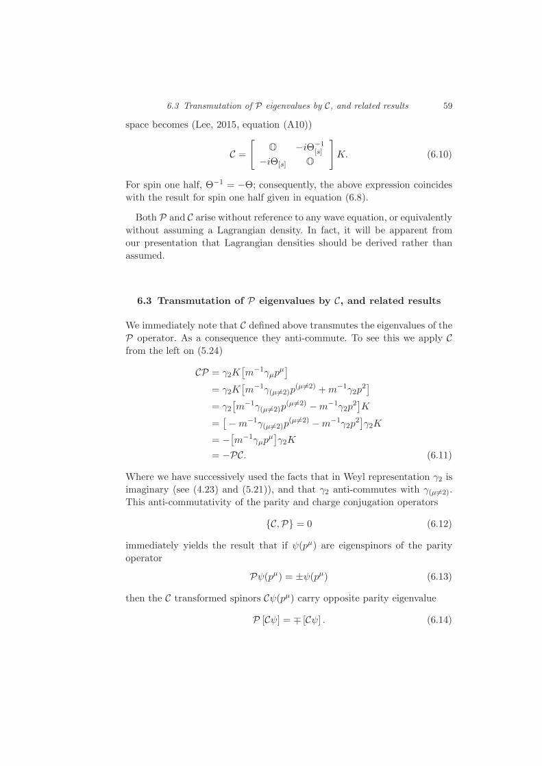
6.3 Transmutation of P eigenvalues by C, and related results 59

space becomes (Lee, 2015, equation (A10))

C =

[O −iΘ−1

[s]

−iΘ[s] O

]K. (6.10)

For spin one half, Θ−1 = −Θ; consequently, the above expression coincides

with the result for spin one half given in equation (6.8).

Both P and C arise without reference to any wave equation, or equivalently

without assuming a Lagrangian density. In fact, it will be apparent from

our presentation that Lagrangian densities should be derived rather than

assumed.

6.3 Transmutation of P eigenvalues by C, and related results

We immediately note that C defined above transmutes the eigenvalues of the

P operator. As a consequence they anti-commute. To see this we apply Cfrom the left on (5.24)

CP = γ2K[m−1γµp

µ]

= γ2K[m−1γ(µ6=2)p

(µ6=2) +m−1γ2p2]

= γ2[m−1γ(µ6=2)p

(µ6=2) −m−1γ2p2]K

=[−m−1γ(µ6=2)p

(µ6=2) −m−1γ2p2]γ2K

= −[m−1γµp

µ]γ2K

= −PC. (6.11)

Where we have successively used the facts that in Weyl representation γ2 is

imaginary (see (4.23) and (5.21)), and that γ2 anti-commutes with γ(µ6=2).

This anti-commutativity of the parity and charge conjugation operators

C,P = 0 (6.12)

immediately yields the result that if ψ(pµ) are eigenspinors of the parity

operator

Pψ(pµ) = ±ψ(pµ) (6.13)

then the C transformed spinors Cψ(pµ) carry opposite parity eigenvalue

P [Cψ] = ∓ [Cψ] . (6.14)

60 Discrete symmetries: Part 2 (Charge conjugation)

Stated differently, (5.26) changes as follows

(γµpµ −mI)ψSσ (p

µ) = 0, (γµpµ +mI)ψAσ (p

µ) = 0︸ ︷︷ ︸↓

︷ ︸︸ ︷(γµp

µ +mI)[CψSσ (pµ)

]= 0, (γµp

µ −mI)[CψAσ (pµ)

]= 0 . (6.15)

In this sense, the relative eigenvalues of the P may be identified as a charge

under the charge conjugation operator.

The result on the anti-commutativity of the C and P operators arrived

at (6.12) may be obtained in another manner and it checks the internal

consistency of various choices of phase factors. For this analysis we note

that (5.27) together with (6.15) imply

vσ(pµ) ∝ Cuσ(pµ), uσ(p

µ) ∝ Cvσ(pµ) (6.16)

where the proportionality constants may depend on σ. We wish to find the

proportionality constant(s), so we act C on each of the uσ(pµ) and vσ(p

µ).

With expression for C given by (6.8) and for u+(pµ) given by (5.42) we work

through first of the calculations as follows

Cu+(pµ) = i

√E +m

2m

(1− p

E+m

)Θφ∗+(k

µ)

−(1 + p

E+m

)Θφ∗+(k

µ)

(6.17)

and since Θφ∗+(kµ) = φ−(k

µ)

Cu+(pµ) = i

√E +m

2m

(1− p

E+m

)φ−(k

µ)

−(1 + p

E+m

)φ−(k

µ).

(6.18)

Use of (5.44) then yields

Cu+(pµ) = iv+(pµ). (6.19)

The use of another identity Θφ∗−(kµ) = −φ+(k

µ) and calculations similar

to as above then tells us that

Cu±(pµ) = iv±(pµ), Cv±(pµ) = iu±(p

µ). (6.20)

As a consequence,

C2 = I4, C,P = 0 (6.21)

for the eigenspinors of the parity operator. This is so because

CP u−(pµ) = Cu−(pµ) = iv−(p

µ) (6.22)

6.3 Transmutation of P eigenvalues by C, and related results 61

PC u−(pµ) = P (iv−(pµ)) = −iv−(pµ). (6.23)

Together, they yield the claimed anti-commutativity of the C and P for the

eigenspinors of the parity operator P.

Introducing the time reversal operator T = iγC, with γ given by equation

(7.15) below, an explicit calculation gives the result

T u+(pµ) = −u−(pµ), T u−(pµ) = u+(pµ) (6.24)

T v+(pµ) = v−(pµ), T v−(pµ) = −v+(pµ). (6.25)

The introduced time reversal operator commutes with the charge conjuga-

tion operator and also with the parity operator

[C,T ] = 0, [P,T ] = 0 (6.26)

In conjunction with the facts that

P2 = I4, T 2 = −I4 (6.27)

all the results obtained above combine to yield

(CPT )2 = I4 (6.28)

for the Dirac spinors.

7

Eigenspinors of charge conjugation operator, Elko

In the usual language, the 1937 Majorana field starts with the Dirac field

and identifies the b†σ(p) with the a†σ(p). In the process Majorana constructed

a fundamentally neutral field. Later Majorana spinors were introduced as

eigenspinors of the charge conjugation operator, see for example Ramond’s

primer (Ramond, 1981). But as soon these were motivated by the ‘magic

of Pauli matrices,’ they were elevated to Grassmann variables. Further-

more, they were simply considered as Weyl spinors in a four component

form – giving rise to the ‘disguise’ argument. Nothing similar is required

of the Dirac spinors – at least, in the operator formalism of quantum field

theory, which in our opinion is an unambiguous conceptual continuation

of the quantum formalism (Dirac, 1930). Finding the grassmann-isation

of doubtful validity, at least for the reasons given in (Ramond, 1981) and

elsewhere (Aitchison and Hey, 2004), we here construct eigenspinors of the

charge conjugation operator. We not only avoid the ‘disguise’ argument,

but we also refrain from grassmann-isation. The result is a set of four four-

component spinors which stand at par with the Dirac spinors. Taken to their

logical consequence the new spinors lead to mass dimension one fermions.

To avoid a possible confusion from arising we call the new spinors as Elko

(Eigenspinoren des Ladungskonjugationsoperators) – or, simply as eigen-

spinors of the charge conjugation operator.

7.1 Elko

We have at our disposal the charge conjugation operator from equation (6.8)

and the new spinors suggested by the magic of the Wigner time reversal

7.1 Elko 63

operator from equation (6.6):

C =

(O iΘ

−iΘ O

)K, (7.1)

λ(pµ) =

(ζλΘφ

∗L(p

µ)

φL(pµ)

). (7.2)

We now establish the following two results:

• The λ(pµ) become eigenspinors of the charge conjugation operator with

doubly degenerate eigenvalues, ±1, if the phase ζλ that appears in λ(pµ)

is set to ±i.• In contrast to the eigenspinors of the parity operator, the right- and left-

transforming components of the new spinors have opposite helicities.

To establish the first of the two enumerated results we act the charge

conjugation operator on the new spinors. After the action of K in C, theresult reads

Cλ(pµ) =(

O iΘ

−iΘ O

)(ζ∗λΘφL(p

µ)

φ∗L(pµ)

)(7.3)

Exploiting the property Θ2 = −I simplifies the above expression into

Cλ(pµ) =(iΘφ∗L(p

µ)

iζ∗λφL(pµ)

). (7.4)

The choice ζλ = ±i makes λ(pµ) become eigenspinors of C with doubly

degenerate eigenvalues ±1:

CλS(pµ) = +λS(pµ), CλA(pµ) = −λA(pµ), (7.5)

where

λ(pµ) =

λS(pµ) =

(iΘφ∗L(p

µ)

φL(pµ)

)for ζλ = +i

λA(pµ) =

(−iΘφ∗L(pµ)φL(p

µ)

)for ζλ = −i

(7.6)

To establish the second of the two enumerated results we proceed as fol-

lows. With the structure ζλΘφ∗L(p

µ) in mind, we complex conjugate (5.33)

to get (suppressing the subscript L)

σ∗ · pφ∗±(kµ) = ±φ∗±(kµ) (7.7)

64 Eigenspinors of charge conjugation operator, Elko

and then replace σ∗ by −ΘσΘ−1 in accordance with (6.2)

ΘσΘ−1 · pφ∗±(kµ) = ∓φ∗±(kµ) (7.8)

Next we use the fact that Θ−1 −Θ to replace ΘσΘ−1 by Θ−1σΘ

Θ−1σΘ · pφ∗±(kµ) = ∓φ∗±(kµ) (7.9)

A left multiplication by Θ furnishes us the result

σ · p[Θφ∗±(k

µ)]= ∓

[Θφ∗±(k

µ)]

(7.10)

The result (6.5) immediately translates the validity of the above expression

for all pµ

σ · p[Θφ∗±(p

µ)]= ∓

[Θφ∗±(p

µ)]

(7.11)

Thus, the right- and left- transforming components of λ(kµ) are constrained

to have opposite helicities – in sharp contrast to the constraints (5.32) for

the eigenspinors of the parity operator P. We will see in Chapter 12 that

this fact endows Elko with an unusual property under rotation. Exploiting

(4.45) it results in an unexpected cosmological effect.

7.2 Restriction on local gauge symmetries

Because of the presence of the operator K in Eq. (6.8) a global transforma-

tion of the type

λ(pµ) → λ′(pµ) = exp(iaα)λ(pµ) (7.12)

with a† = a, a 4 × 4 matrix and α ∈ R, does not preserve the self/anti-self

conjugacy of λ(pµ) under C unless the matrix a satisfies the condition

γ2a∗ + aγ2 = 0 (7.13)

The general form of a satisfying this requirements is

a =

ǫ β λ 0

β∗ δ 0 λ

λ∗ 0 −δ β

0 λ∗ β∗ −ǫ

(7.14)

with ǫ, δ ∈ R and β, λ ∈ C (with no association with the same symbols used

elsewhere in this work).

For a field constructed with the eigenspinors of C as expansion coeffi-

cients, the usual local U(1) interaction is ruled out as the form of a given

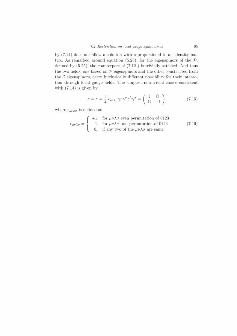
7.2 Restriction on local gauge symmetries 65

by (7.14) does not allow a solution with a proportional to an identity ma-

trix. As remarked around equation (5.28), for the eigenspinors of the P,

defined by (5.25), the counterpart of (7.12 ) is trivially satisfied. And thus

the two fields, one based on P eigenspinors and the other constructed from

the C eigenspinors, carry intrinsically different possibility for their interac-

tion through local gauge fields. The simplest non-trivial choice consistent

with (7.14) is given by

a = γ =i

4!ǫµνλσγ

µγνγλγσ =

(I O

O −I

)(7.15)

where ǫµνλσ is defined as

ǫµνλσ =

+1, for µνλσ even permutation of 0123

−1, for µνλσ odd permutation of 0123

0, if any two of the µνλσ are same

(7.16)

8

Construction of Elko

With Elko defined in the previous chapter we now provide explicit construc-

tion of the new spinors and discuss the subtle departure from our 2005 publi-

cations (Ahluwalia and Grumiller, 2005a,b). These departure, when coupled

with the new dual introduced in Chapter 13, lie at the heart of evaporating

away the non-locality and a lack of full Lorentz covariance of our earlier

works. The arguments that follow are adapted from (Ahluwalia, 2017c,a).

8.1 Elko at rest

To obtain an explicit form of Elko requires the ‘rest’ spinors λ(kµ). That

done, we then have for an arbitrary pµ

λ(pµ) =

√E +m

2m

[I+ σ·p

E+m O

O I− σ·pE+m

]λ(kµ) (8.1)

with the boost operator above the same as in (5.29).

To construct λ(kµ) we have to choose global phases for each of the two

φ±(kµ) as discussed after equations (5.34) and (5.35). With that choice made

we are still left with the additional phase freedom

λS+(kµ) = eiξ1

[iΘ [φ+(k

µ)]∗

φ+(kµ)

], λS−(k

µ) = eiξ2[iΘ [φ−(k

µ)]∗

φ−(kµ)

](8.2)

and

λA+(kµ) = eiξ3

[−iΘ [φ−(k

µ)]∗

φ−(kµ)

], λA−(k

µ) = eiξ4[−iΘ [φ+(k

µ)]∗

φ+(kµ)

](8.3)

8.1 Elko at rest 67

Table 8.1 A comparison of λ(pµ) with those used in earlier work.

Here In reference (Ahluwalia and Grumiller, 2005a,b)a

λS+(kµ) λS−,+(k

µ)

λS−(kµ) −λS+,−(k

µ)

λA+(kµ) −λA+,−(k

µ), and not − λA−,+(kµ)

λA−(kµ) −λA−,+(k

µ), and not − λA+,−(kµ)

a The 0 there carries the same meaning as kµ here.

with ξ1, ξ2, ξ3, ξ4 ∈ ℜ. We set ξ1 = ξ2 = ξ3 = 0 and ξ4 = π

λS+(kµ) =

[iΘ [φ+(k

µ)]∗

φ+(kµ)

], λS−(k

µ) =

[iΘ [φ−(k

µ)]∗

φ−(kµ)

](8.4)

λA+(kµ) =

[−iΘ [φ−(k

µ)]∗

φ−(kµ)

], λA−(k

µ) =

[iΘ [φ+(k

µ)]∗

−φ+(kµ)

](8.5)

This choice of phases, coupled with advances in understanding duals and

adjoints (Ahluwalia, 2017c,a), completely resolves the lingering problems

with locality and Lorentz covariance encountered in (Ahluwalia and Grumiller,

2005a,b; Ahluwalia et al., 2010, 2011b; Ahluwalia and Horvath, 2010). Table

7.1 tabulates the differences just mentioned explicitly.

For the Dirac field, the counterpart of these observations follow seamlessly

in the Weinberg’s formalism. Since Weinberg does not note these details

explicitly they seem to have escaped many of the recent textbook expositions

on the theory of quantum fields. This has the consequence that the Dirac

field, as presented, for example, in (Ryder, 1986 and 1996; Folland, 2008;

Schwartz, 2014a), hides violation of locality and Lorentz symmetry. The

former can be seen by locality analysis of the those fields on Majorana-

isation, while the latter only becomes apparent on comparing the rest spinors

with those of Weinberg’s analysis. One way of understanding part of this

story is to realise that in a quantum field the complete set of spinors enter as

expansion coefficients and the freedom of a global phase that each of these

carried before – by, say satisfying the Dirac equation – is lost under the

usual summation on the helicity degrees of freedom.

68 Construction of Elko

8.2 Elko are not Grassmann nor are they Weyl in disguise

Under the Dirac dual, as would be seen in Chapters 13 and 14, the naive

mass term for Elko identically vanishes. So one would be tempted to treat

Elko as grassmann numbers – see, for example, (Aitchison and Hey, 2004).

As already remarked in Chapter 7, we find this transition from the complex

valued Elko to their grassmann-isation as mathematically untenable. We

would treat Elko as one treated the Dirac spinors in the operator formalism

of quantum field theory.

Similarly, one should not be tempted to consider Elko as Weyl spinors in

disguise. This is because I include the neglected ζλ = −1 in our formalism.

It would be seen as we proceed that just as the Dirac spinors span a four

dimensional representation space, the Elko too are endowed with a com-

pleteness relation in the same four dimensional representation space (see

equation (14.77)). Furthermore, we can exploit the algebraic identity

Θφ∗±(kµ) = ±φ∓(k

µ) (8.6)

to rewrite the Elko at rest, given by equations (8.2) and (8.3), into

λS+(kµ) =

(iφ−(k

µ)

φ+(kµ)

), λS−(k

µ) =

(−iφ+(kµ)φ−(k

µ)

)(8.7)

λA+(kµ) =

(iφ+(k

µ)

φ−(kµ)

), λA−(k

µ) =

(iφ−(k

µ)

−φ+(kµ)

)(8.8)

and compare these with the Dirac spinors at rest given in equations (5.40)

and (5.41) in the same degrees of freedom: φ±(kµ). Written in this form all

the phase choices, relative between the right- and left- transforming compo-

nents, and global for each of the spinors, along with their helicities become

manifest and stand in contrast to their Dirac counterpart.

8.3 Elko for any momentum

The interplay of the result (7.10) with the boost (5.29) and the chosen form

of λ(kµ) in (8.4) to (8.5) results in the following form for λ(pµ)

λS+(pµ) =

√E +m

2m

(1− p

E +m

)λS+(k

µ), (8.9)

λS−(pµ) =

√E +m

2m

(1 +

p

E +m

)λS−(k

µ) (8.10)

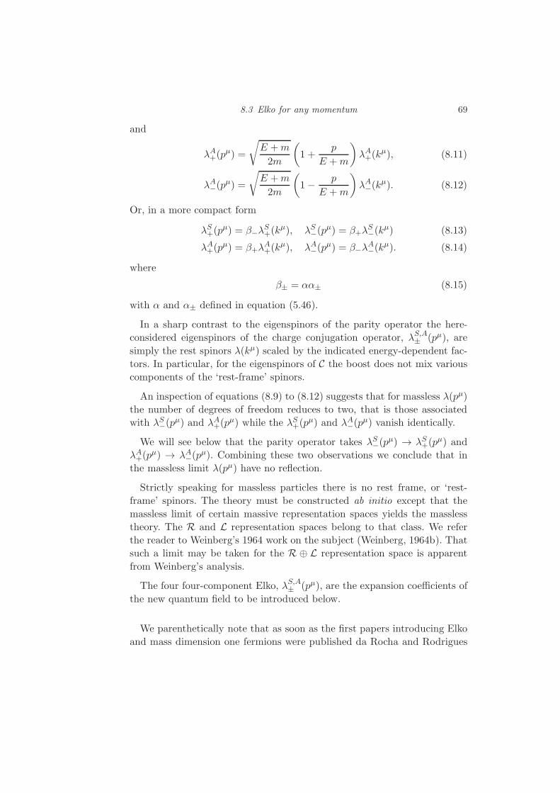
8.3 Elko for any momentum 69

and

λA+(pµ) =

√E +m

2m

(1 +

p

E +m

)λA+(k

µ), (8.11)

λA−(pµ) =

√E +m

2m

(1− p

E +m

)λA−(k

µ). (8.12)

Or, in a more compact form

λS+(pµ) = β−λ

S+(k

µ), λS−(pµ) = β+λ

S−(k

µ) (8.13)

λA+(pµ) = β+λ

A+(k

µ), λA−(pµ) = β−λ

A−(k

µ). (8.14)

where

β± = αα± (8.15)

with α and α± defined in equation (5.46).

In a sharp contrast to the eigenspinors of the parity operator the here-

considered eigenspinors of the charge conjugation operator, λS,A± (pµ), are

simply the rest spinors λ(kµ) scaled by the indicated energy-dependent fac-

tors. In particular, for the eigenspinors of C the boost does not mix various

components of the ‘rest-frame’ spinors.

An inspection of equations (8.9) to (8.12) suggests that for massless λ(pµ)

the number of degrees of freedom reduces to two, that is those associated

with λS−(pµ) and λA+(p

µ) while the λS+(pµ) and λA−(p

µ) vanish identically.

We will see below that the parity operator takes λS−(pµ) → λS+(p

µ) and

λA+(pµ) → λA−(p

µ). Combining these two observations we conclude that in

the massless limit λ(pµ) have no reflection.

Strictly speaking for massless particles there is no rest frame, or ‘rest-

frame’ spinors. The theory must be constructed ab initio except that the

massless limit of certain massive representation spaces yields the massless

theory. The R and L representation spaces belong to that class. We refer

the reader to Weinberg’s 1964 work on the subject (Weinberg, 1964b). That

such a limit may be taken for the R ⊕ L representation space is apparent

from Weinberg’s analysis.

The four four-component Elko, λS,A± (pµ), are the expansion coefficients of

the new quantum field to be introduced below.

We parenthetically note that as soon as the first papers introducing Elko

and mass dimension one fermions were published da Rocha and Rodrigues

70 Construction of Elko

Jr. noted that Elko belong to class 5 spinors (da Rocha and Rodrigues, 2006)

in the Lounesto classification (Lounesto, 2001, Chapter 12).

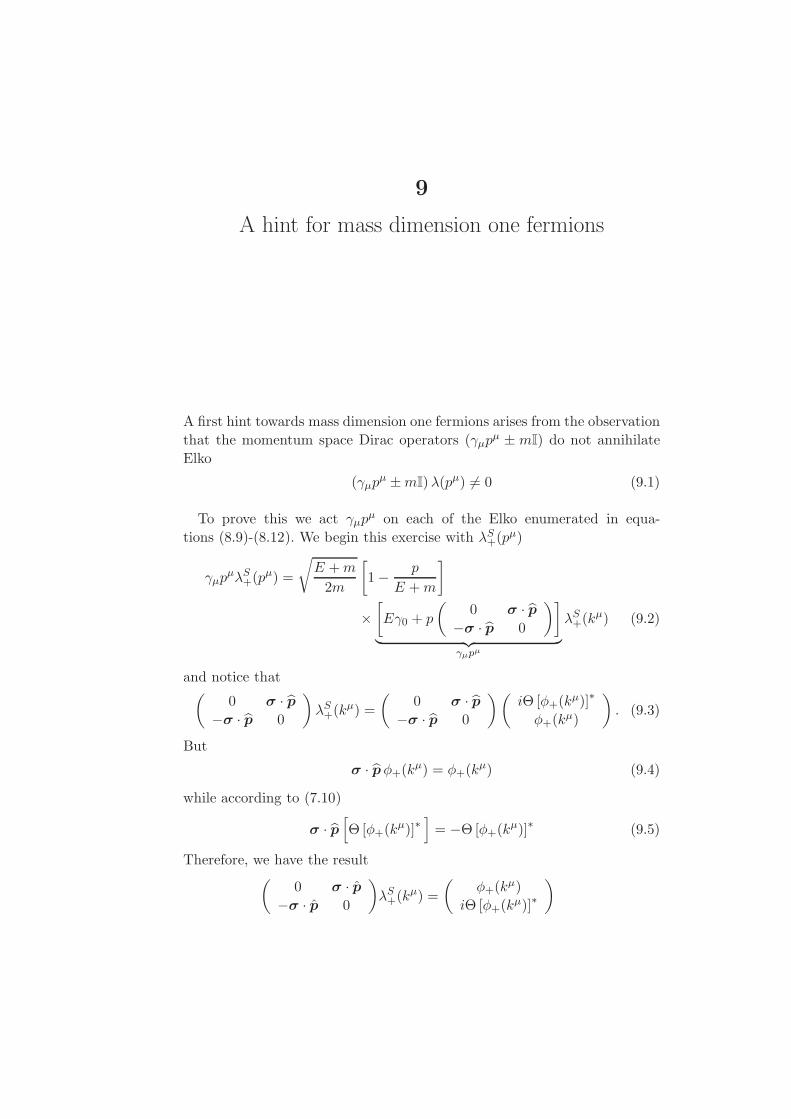
9

A hint for mass dimension one fermions

A first hint towards mass dimension one fermions arises from the observation

that the momentum space Dirac operators (γµpµ ± mI) do not annihilate

Elko

(γµpµ ±mI)λ(pµ) 6= 0 (9.1)

To prove this we act γµpµ on each of the Elko enumerated in equa-

tions (8.9)-(8.12). We begin this exercise with λS+(pµ)

γµpµλS+(p

µ) =

√E +m

2m

[1− p

E +m

]

×[Eγ0 + p

(0 σ · p

−σ · p 0

)]

︸ ︷︷ ︸γµpµ

λS+(kµ) (9.2)

and notice that(

0 σ · p−σ · p 0

)λS+(k

µ) =

(0 σ · p

−σ · p 0

)(iΘ [φ+(k

µ)]∗

φ+(kµ)

). (9.3)

But

σ · pφ+(kµ) = φ+(kµ) (9.4)

while according to (7.10)

σ · p[Θ [φ+(k

µ)]∗]= −Θ [φ+(k

µ)]∗ (9.5)

Therefore, we have the result(

0 σ · p−σ · p 0

)λS+(k

µ) =

(φ+(k

µ)

iΘ [φ+(kµ)]∗

)

72 A hint for mass dimension one fermions

=

(O I

I O

)(iΘ [φ+(k

µ)]∗

φ+(kµ)

)(9.6)

That is (0 σ · p

−σ · p 0

)λS+(k

µ) = γ0λS+(k

µ). (9.7)

As a consequence (9.2) simplifies to

γµpµλS+(p

µ) =

√E +m

2m

(1− p

E +m

)(E + p) γ0λ

S+(k

µ). (9.8)

The standard dispersion relation allows for the replacement(1− p

E +m

)(E + p) → m

(1 +

p

E +m

)(9.9)

To evaluate γ0λS+(k

µ) we first expand it as

γ0λS+(k

µ) =

(φ+(k

µ)

iΘφ∗+(kµ)

)(9.10)

and exploit the algebraic result (8.6) to make the following substitutions

φ+(kµ) → i

(iΘφ∗−(k

µ)), iΘφ∗+(k

µ) → iφ−(kµ) (9.11)

to obtain the identity

γ0λS+(k

µ) = iλS−(kµ) (9.12)

Combined, these two observations reduce (9.8) to

γµpµλS+(p

µ) = im

√E +m

2m

(1 +

p

E +m

)λS−(k

µ). (9.13)

Using (8.10) in the right-hand side of (9.13) gives

γµpµλS+(p

µ) = imλS−(pµ). (9.14)

An exactly similar exercise complements (9.14) with

γµpµλS−(p

µ) = −imλS+(pµ) (9.15)

γµpµλA−(p

µ) = imλA+(pµ) (9.16)

γµpµλA+(p

µ) = −imλA−(pµ). (9.17)

These results are consistent with those of (Dvoeglazov, 1995a,b). Trans-

lated in words these equations combine to yield the following pivotal result:

(γµpµ ±m) do not annihilate λ(pµ).

A hint for mass dimension one fermions 73

Equations (9.14) to (9.17), coupled with the discussion surrounding (7.12),

contain the rudimentary seeds for the kinematical and dynamical content of

the quantum field built upon λ(pµ) as its expansion coefficients: first, λ(pµ)

are annihilated by the spinorial Klein-Gordon operator (and not by the Dirac

operator), and second, the resulting kinematic structure cannot support the

usual gauge symmetries of the standard model of the high energy physics.

To prove the the former claim, we multiply (9.14) from the left by γνpν and

use (9.14) and (9.15) in succession

γνpνγµp

µλS+(pµ) = imγνp

νλS−(pµ) = im

(−imλS+(pµ)

)= m2λS+(p

µ) (9.18)

and then utilise the fact that the left hand side of the above equation can be

rewritten exploiting γµ, γν = 2ηµνI4 – where ηµν is the space-time metric

with signature (+1,−1,−1,−1)) – as

γνpνγµp

µ =1

2γµ, γνpµpν = ηµνp

µpνI4. (9.19)

Substituting this result in (9.18), and rearranging gives

(ηµνpµpνI4 −m2

I4)λS+(p

µ) = 0. (9.20)

Repeating the same exercise with (9.15) to (9.17) as the starting point, yields

(ηµνpµpνI4 −m2

I4)λ(pµ) = 0. (9.21)

where λ(pµ) stands for any of the four eigenspinors of the charge conjugation

operator, λS,A± (pµ).

Lest the appearances betray, the λS,A± (pµ) are not a set of four scalars,

disguised in four-component form repeated four times, but spinors in the

R ⊕ L representation space of spin one half. Under boosts these spinors

contract or dilate by factors of

β± =

√E +m

2m

[1± p

E +m

](9.22)

in accord with equations (8.9) to (8.12) and pick up a minus sign under 2π

rotation as dictated by (5.10).22

22 See, Chapter 12 for departures from Dirac spinors.

10

CPT for Elko

Since P = m−1γµpµ the results obtained in the previous chapter also trans-

late to the action of P on the eigenspinors of the charge conjugation operator

C

PλS+(pµ) = iλS−(pµ) (10.1)

PλS−(pµ) = −iλS+(pµ) (10.2)

PλA−(pµ) = iλA+(pµ) (10.3)

PλA+(pµ) = −iλA−(pµ). (10.4)

The above can be compacted into the following

PλS±(pµ) = ±iλS∓(pµ), PλA±(pµ) = ∓iλA∓(pµ) (10.5)

and lead to

P2 = I4 (10.6)

Acting C from the left on the first of the above equations gives

CPλS+(pµ) = −iCλS−(pµ) = −iλS−(pµ). (10.7)

On the other hand

PCλS+(pµ) = PλS+(pµ) = iλS−(pµ). (10.8)

Adding the above two results leads to anti-commutativity for the C and Pfor λS+(p

µ). Repeating the same exercise for λS−(pµ) and λA±(p

µ) establishes

that C and P anticommute for all the eigenspinors of the charge conjugation

operator

C,P = 0 (10.9)

CPT for Elko 75

just as seen before in (6.21) for the eigenspinors of the parity operator P.

The action of the time reversal operator on λ(pµ) is as follows (as an

explicit calculation shows):

T λS+(pµ) = iλA−(pµ), T λS−(pµ) = −iλA+(pµ) (10.10)

T λA+(pµ) = iλS−(pµ), T λA−(pµ) = −iλS+(pµ) (10.11)

with the square of T acting on Elko giving, −I4

T 2 = −I4 (10.12)

In addition, we find that

[C,T ] = 0, [P,T ] = 0 (10.13)

hold for Elko, as for the Dirac spinors. In consequence, for Elko (CPT )2 = I4.

This contrasts with contrary results reported in our own earlier work, and

those of several other authors. The difference can be traced to an unam-

biguous treatment P for Elko, and to the differences tabulated in Table

7.1.

11

Elko in Shirokov-Trautman, Wigner, and Lounestoclassifications

In the Shirokov-Trautman classification (Shirokov, 1960; Trautman, 2005)

a spinor is classified by the possible choices of signs λ, µ, ν ∈ +,− in the

relations

PT = λ T P, P2 = µ I4, T 2 = ν I4 (11.1)

Commutativity of P and T as given in equation (10.13) gives λ = +, while

results (10.6) and (10.12) give µ = + and ν = −. Thus Elko belongs to

(λ, µ, ν) class identified as (+,+,−).

In the Wigner classification one may go beyond the relative intrinsic parity

of the particles and antiparticles to be same for bosons, and opposite for

fermions (Wigner, 1964). The anti-commutativity of C and P reached in

equation (10.9) places Elko in the same class as the Dirac spinors. This

should not make the reader infer that all other properties of Elko and Dirac

spinors are the same but only that both of these spinors have particles and

antiparticles with the opposite relative intrinsic parity.

Lounesto classification is based on the bilinear invariants associated with

the spinors under the standard Dirac dual (Lounesto, 2001). An early analy-

sis given in reference (da Rocha and Rodrigues, 2006) established that Elko

belong to class 5 in this classification. The cited work has been extended in a

series of later papers, see for example in (Hoff da Silva and Cavalcanti, 2017;

Hoff da Silva et al., 2016b), with additional new structure unearthed by the

use of the dual appropriate for Elko. This classification may be particularly

helpful for studying currents associated with Dirac spinors and Elko, and

the gauge symmetries they arise from. However, Lounesto did not consider

the issue of associated Lagrangian densities for each of the classes that he

proposed.

12

Rotation induced effects on Elko

Despite its simple roots in the spin one half representation of the Lorentz

algebra the celebrated minus sign that a 2π rotation induces on Dirac spinors

has intrigued the physicist and the lay scholar alike (Aharonov and Susskind,

1967; Dowker, 1969; Rauch et al., 1974; Werner et al., 1975; Silverman, 1980;

Horvathy, 1985; Klein and Opat, 1976). For a general rotation about an axis,

say p, by an angle ϑ the effect of rotation is simply a multiplication of the

original spinor by a phase factor exp(±iϑ/2) – the sign determined by the

helicity of the spinor.

In sharp contrast to the Dirac spinors, Elko not only acquire a minus sign

for the same 2π rotation but the effect of a general rotation is to create a

specific admixture of the self-conjugate and anti-self conjugate spinors – the

resulting spinors are still eigenspinors of the charge conjugation operator.

This apparent paradox is resolved. This property is a direct consequence of

the fact that the right and left transforming components of Elko are endowed

with opposite helicities (see equation (7.11), and each of these picks up an

opposite phase in accordance with the result (4.45).23

12.1 Setting up an orthonormal cartesian coordinate system

with p as one of its axis

Understanding the new spinors vastly simplifies in the basis we have chosen

for them. Their right- and left- transforming components have their spin

projections assigned not with respect an external z-axis but to a self refer-

ential unit vector associated with their motion: that is p. To establish the

23 This chapter is an adapted version of (Ahluwalia and Sarmah, 2018)

78 Rotation induced effects on Elko

result outlined above we find it convenient to erect an orthonormal cartesian

coordinate system with p as one of its axis. With p chosen as24

(sθcφ, sθsφ, cθ) (12.1)

we introduce two more unit vectors

η+def=

1√2 + a2

(1, 1, a) , a ∈ ℜ (12.2)

η−def=

p× η+√(p× η+) · (p× η+)

(12.3)

and impose the requirement

η+ · η− = 0, η+ · p = 0, η− · p = 0 (12.4)

η+ · η+ = 1, η− · η− = 1. (12.5)

Requiring η+ · p to vanish reduces η+ to

η+ =1√

2 + (1 + s2φ)t2θ

(1, 1,−(cφ + sφ)tθ

). (12.6)

Definition (12.3) then immediately yields

η− =1√

2 + (1 + s2φ)t2θ

(− cθ − sθsφ(cφ + sφ)tθ, (12.7)

cθ + sθcφ(cφ + sφ)tθ, sθ(cφ − sφ)). (12.8)

In the limit when both the θ and φ tend to zero, the above-defined unit

vectors take the form

η+∣∣θ→0,φ→0

=1√2(1, 1, 0) (12.9)

η−∣∣θ→0,φ→0

=1√2(−1, 1, 0) (12.10)

and orthonormal system (η−, η+, p) does not reduce to the standard carte-

sian coordinate system (x, y, z). For this reason, without destroying the

orthonormality of the introduced unit vectors and guided by (12.9) and

(12.10), we exploit the freedom of a rotation about the p axis (in the plane

defined by η+ and η−) and introduce

p±def=

1√2(η+ ± η−) (12.11)

24 Where sin[θ] is abbreviated as sθ with obvious extension to other trigonometric function.

12.2 Generators of the rotation in the new coordinate system 79

The set of axes(p−, p+, p

)do indeed form a right-handed coordinate system

that reduces to the standard cartesian system in the limit both the θ and

the φ tend to zero.

12.2 Generators of the rotation in the new coordinate system

We now introduce three generators of rotations about each of the three axes

J−def=

σ

2· p−, J+

def=

σ

2· p+, Jp

def=

σ

2· p (12.12)

Jp coincides with the helicity operator h defined in (4.35). As a check, a

straightforward exercise shows that the three J′s satisfy the su(2) algebra

needed for generators of rotation

[J−, J+] = iJp, [Jp, J−] = iJ+, [J+, Jp] = iJ− (12.13)

Since Elko reside in the R⊕ L representation space and as far as rotations

are concerned both the R and L spaces are served by the same generators

of rotations. We therefore introduce

h− =

(J− 0202 J−

), h+ =

(J+ 0202 J+

), hp =

(Jp 0202 Jp

)(12.14)

where 02 is a 2 × 2 null matrix. A straight forward calculation then yields

the result

hp λS+(p

µ) = −1

2λA−(p

µ), hp λS−(p

µ) = −1

2λA+(p

µ) (12.15)

hp λA+(p

µ) = −1

2λS−(p

µ), hp λA−(p

µ) = −1

2λS+(p

µ) (12.16)

with the consequence that each of the Elko is an eigenspinor of h2p

h2p λS,A± (pµ) =

1

4λS,A± (pµ) (12.17)

The action of h− and h+ on Elko is more involved, for instance

h+ λS+(p

µ) = −1

2

(αλS−(p

µ) + βλA+(pµ))

(12.18)

with

α = − im(m+ E)(cosφ(1 + sec θ) + (−1 + sec θ) sinφ

)√

4 + 2(1 + sin 2φ) tan2 θ(12.19)

β = −m(m+ E)(cosφ(−1 + sec θ) + (1 + sec θ) sinφ

)√

4 + 2(1 + sin 2φ) tan2 θ(12.20)

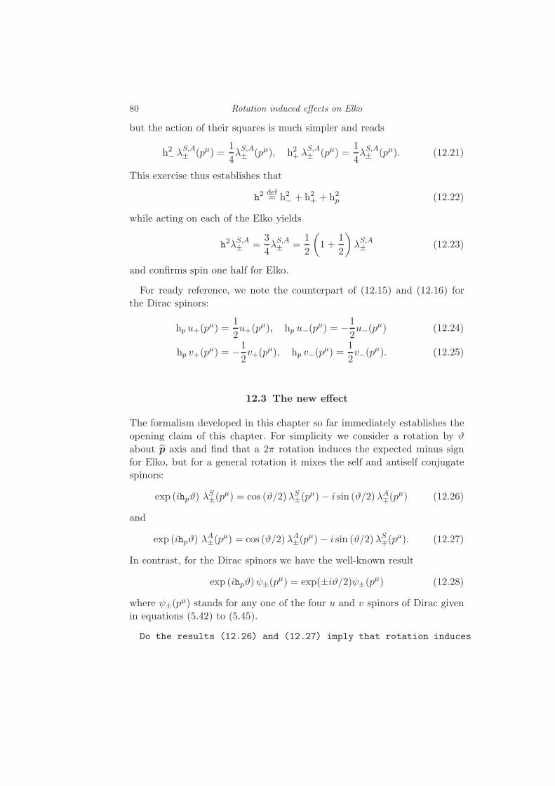
80 Rotation induced effects on Elko

but the action of their squares is much simpler and reads

h2− λS,A± (pµ) =

1

4λS,A± (pµ), h2+ λ

S,A± (pµ) =

1

4λS,A± (pµ). (12.21)

This exercise thus establishes that

h2def= h2− + h2+ + h2p (12.22)

while acting on each of the Elko yields

h2λS,A± =3

4λS,A± =

1

2

(1 +

1

2

)λS,A± (12.23)

and confirms spin one half for Elko.

For ready reference, we note the counterpart of (12.15) and (12.16) for

the Dirac spinors:

hp u+(pµ) =

1

2u+(p

µ), hp u−(pµ) = −1

2u−(p

µ) (12.24)

hp v+(pµ) = −1

2v+(p

µ), hp v−(pµ) =

1

2v−(p

µ). (12.25)

12.3 The new effect

The formalism developed in this chapter so far immediately establishes the

opening claim of this chapter. For simplicity we consider a rotation by ϑ

about p axis and find that a 2π rotation induces the expected minus sign

for Elko, but for a general rotation it mixes the self and antiself conjugate

spinors:

exp (ihpϑ) λS±(p

µ) = cos (ϑ/2)λS±(pµ)− i sin (ϑ/2)λA∓(p

µ) (12.26)

and

exp (ihpϑ) λA±(p

µ) = cos (ϑ/2)λA±(pµ)− i sin (ϑ/2)λS∓(p

µ). (12.27)

In contrast, for the Dirac spinors we have the well-known result

exp (ihpϑ)ψ±(pµ) = exp(±iϑ/2)ψ±(p

µ) (12.28)

where ψ±(pµ) stands for any one of the four u and v spinors of Dirac given

in equations (5.42) to (5.45).

Do the results (12.26) and (12.27) imply that rotation induces

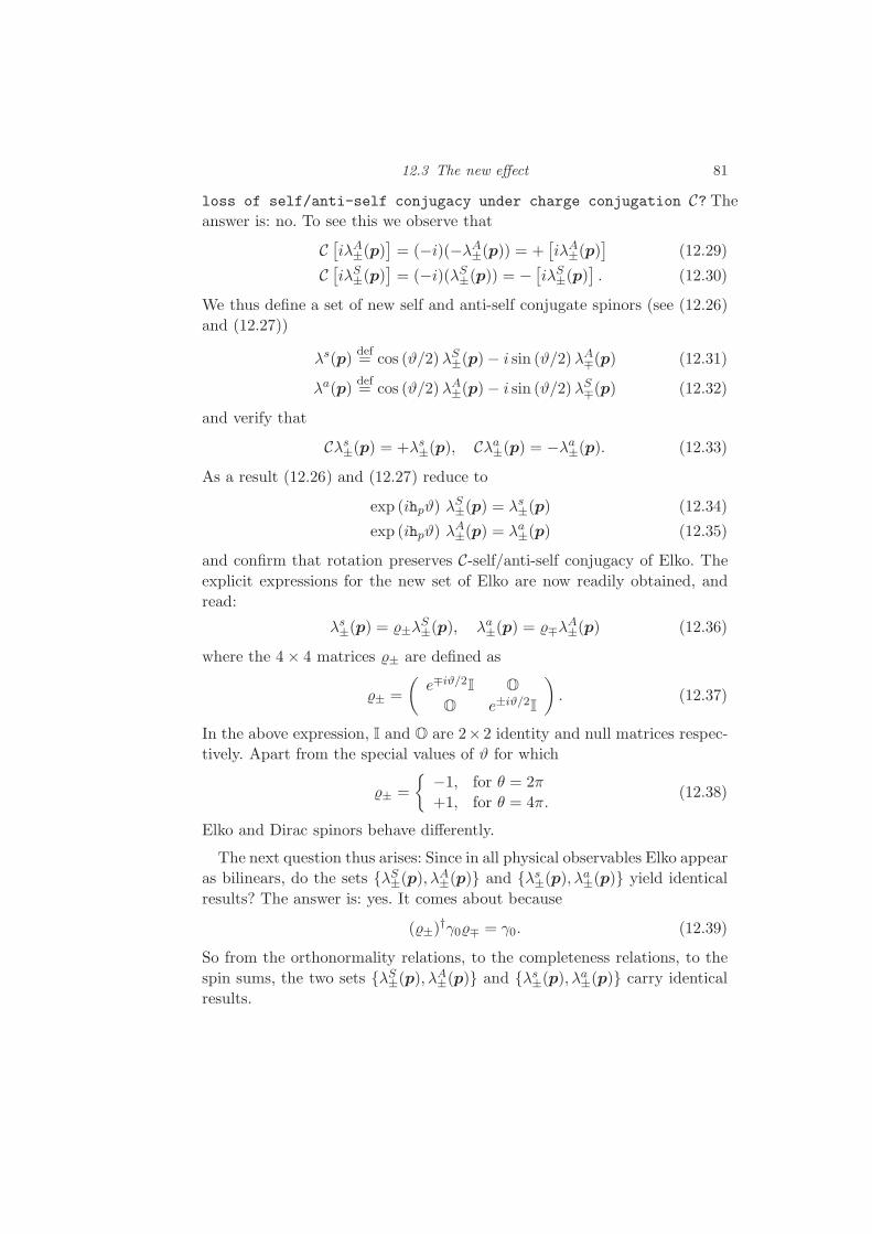
12.3 The new effect 81

loss of self/anti-self conjugacy under charge conjugation C? Theanswer is: no. To see this we observe that

C[iλA±(p)

]= (−i)(−λA±(p)) = +

[iλA±(p)

](12.29)

C[iλS±(p)

]= (−i)(λS±(p)) = −

[iλS±(p)

]. (12.30)

We thus define a set of new self and anti-self conjugate spinors (see (12.26)

and (12.27))

λs(p)def= cos (ϑ/2) λS±(p)− i sin (ϑ/2)λA∓(p) (12.31)

λa(p)def= cos (ϑ/2) λA±(p)− i sin (ϑ/2)λS∓(p) (12.32)

and verify that

Cλs±(p) = +λs±(p), Cλa±(p) = −λa±(p). (12.33)

As a result (12.26) and (12.27) reduce to

exp (ihpϑ) λS±(p) = λs±(p) (12.34)

exp (ihpϑ) λA±(p) = λa±(p) (12.35)

and confirm that rotation preserves C-self/anti-self conjugacy of Elko. The

explicit expressions for the new set of Elko are now readily obtained, and

read:

λs±(p) = ±λS±(p), λa±(p) = ∓λ

A±(p) (12.36)

where the 4× 4 matrices ± are defined as

± =

(e∓iϑ/2I O

O e±iϑ/2I

). (12.37)

In the above expression, I and O are 2×2 identity and null matrices respec-

tively. Apart from the special values of ϑ for which

± =

−1, for θ = 2π

+1, for θ = 4π.(12.38)

Elko and Dirac spinors behave differently.

The next question thus arises: Since in all physical observables Elko appear

as bilinears, do the sets λS±(p), λA±(p) and λs±(p), λa±(p) yield identical

results? The answer is: yes. It comes about because

(±)†γ0∓ = γ0. (12.39)

So from the orthonormality relations, to the completeness relations, to the

spin sums, the two sets λS±(p), λA±(p) and λs±(p), λa±(p) carry identical

results.

13

Elko-Dirac interplay, a temptation and a departure

13.1 Null norm of massive Elko and Elko-Dirac interplay

The result that the spin one-half eigenspinors of the charge conjugation

operator satisfy only the Klein Gordon equation would suggest that at the

‘classical level’ the Lagrangian density for the λ(x) would simply be

L(x) = ∂µλ(x) ∂µλ(x)−m2λ(x)λ(x) (13.1)

where λ(x) is a classical field with λS,A(pµ) as its Fourier coefficients. This

apparently natural choice is too naive. Its validity is challenged by an explicit

calculation which shows that under the Dirac dual

λS,Aα (pµ)

def=

[λS,Aα (pµ)

]†γ0 (13.2)

the norm of each of the four λS,Aα (pµ) identically vanishes (Ahluwalia, 1996)

λSα(p

µ)λSα(pµ) = 0, λ

Aα (p

µ)λAα (pµ) = 0. (13.3)

At the simplest, one may use the λ(pµ) enumerated in equations (8.9) to

(8.12) and verify null norm (13.3) by a brute force algebraic calculation.

Here we follow a more detailed route to arrive at the null norm of massive

Elko. In the process we would not only see how precisely this comes about

but also gain deeper insight into the relation between the Dirac spinors and

Elko.

Since both the Dirac spinors and Elko reside in the same R ⊕ L|s=1/2

representation space, we can expand Elko in terms of the Dirac spinors

as (Ahluwalia and Sawicki, 1993; Ahluwalia and Grumiller, 2005b)

ea =

4∑

b=1

Ωabdb, a, b = 1, 2, 3, 4 (13.4)

13.1 Null norm of massive Elko and Elko-Dirac interplay 83

where we have abbreviated Elko and Dirac spinors as

e1e2e3e4

def=

λS+(pµ)

λS−(pµ)

λA+(pµ)

λA−(pµ)

,

d1d2d3d4

def=

u+(pµ)

u−(pµ)

v+(pµ)

v−(pµ)

(13.5)

and

Ωab =

+(1/2m)dbea, for b=1,2

−(1/2m)dbea, for b=3,4(13.6)

An explicit calculation using equations (8.9) to (8.12) for the Elko and equa-

tions (5.42) to (5.45) for the Dirac spinors yields

Ω =1

2

1 i i 1

−i 1 −1 i

i 1 −1 −i−1 i i −1

(13.7)

where rows are enumerated as a = 1, 2, 3, 4 and columns as b = 1, 2, 3, 4.

With this formulation at hand we immediately see that we may explicitly

write any of the Elko in terms of Dirac spinors. For instance

λS+(pµ) =

1

2

(u+(p

µ) + iu−(pµ) + iv+(p

µ) + v−(pµ)

(13.8)

which yields under the Dirac dual reads

λS+(p

µ) =1

2

(u+(p

µ)− iu−(pµ)− iv+(p

µ) + v−(pµ)). (13.9)

Thus, using the orthonormality of the Dirac spinors under the Dirac dual,

we get two positive and two negative contributions – each equaling 2m in

magnitude – to the norm of λS+(pµ) under the Dirac dual. With the result

that λS(pµ)λS(pµ) vanishes. Exactly the same pattern and result holds for

the remaining three Elko.

So the mass matrix in the Lagrangian density (13.1) would have vanishing

diagonal elements. The off diagonal elements would either vanish identically,

or would be pure imaginary because, for instance

λS−(p

µ) =1

2

(iu+(p

µ) + u−(pµ)− v+(p

µ)− iv−(pµ))

(13.10)

and it results in

λS−(p

µ)λS+(pµ) = i2m (13.11)

84 Elko-Dirac interplay, a temptation and a departure

13.2 Further on Elko-Dirac interplay

The above discussed Elko-Dirac structure makes it clear that the inclusion

of anti self conjugate spinors is necessary for a proper understanding of the

eigenspinors of the charge conjugation operator.

The result that Elko cannot satisfy Dirac equation, as encoded in equa-

tions (10.1) to (10.4), can now be derived in a way which makes transparent

inevitability of the conclusion. To see this one may act the parity operator

P, m−1γµpµ, on equation (13.8) to the effect

m−1γµpµ λS+(p

µ) =1

2

(m−1γµp

µ u+(pµ)︸ ︷︷ ︸

u+(pµ)

+im−1γµpµ u−(p

µ)︸ ︷︷ ︸u−(pµ)

+ im−1γµpµ v+(p

µ)︸ ︷︷ ︸−v+(pµ)

+m−1γµpµ v−(p

µ)︸ ︷︷ ︸−v−(pµ)

)

=1

2

(u+(p

µ) + iu−(pµ)− iv+(p

µ)− v−(pµ))

)

= i1

2

(− iu+(p

µ) + u−(pµ)− v+(p

µ) + iv−(pµ)

︸ ︷︷ ︸λS−(pµ)

)

= iλS−(pµ). (13.12)

That is PλS+(pµ) = iλS−(pµ). Results (10.2) to (10.4) follow similarly.

Finally, it is insightful to check how the results (10.10) and (10.11) on

time reversal come from the Elko-Dirac relationship. Towards this end one

may act the time reversal operator T , iγC, on λS+(pµ) expanded in terms of

Dirac spinors in (13.8) to the effect

T λS+(pµ) =

1

2iγC

(u+(p

µ) + iu−(pµ) + iv+(p

µ) + v−(pµ))

=1

2iγ(Cu+(pµ)− iCu−(pµ)− iCv+(pµ) + Cv−(pµ)

). (13.13)

The action of the charge conjugation operator C can now be implemented

through equations (6.20) to obtain

T λS+(pµ) =

1

2iγ(iv+(p

µ) + v−(pµ) + u+(p

µ) + iu−(pµ)). (13.14)

This requires us to note that γ acts on the Dirac spinors as follows

γ u±(pµ) = ∓ v∓(p

µ), γ v±(pµ) = ±u∓(p

µ). (13.15)

13.3 A temptation, and a departure 85

As a consequence we have

T λS+(pµ) =

1

2i(iu−(p

µ)− u+(pµ)− v−(p

µ) + iv+(pµ)

= i1

2

(− u+(p

µ) + iu−(pµ) + iv+(p

µ)− v−(pµ))

︸ ︷︷ ︸λA−(pµ)

(13.16)

That is

T λS+(pµ) = iλA−(p

µ) (13.17)

in agreement with (10.10). The check for the remainder of the results in

(10.10) and (10.11) follows exactly the same calculational flow.

These calculations provide an intimate dependence of Elko on Dirac spinors,

and of Dirac spinors on Elko. Since Elko are superposition of the particle

and antiparticle Dirac spinors, which in configuration space have different

time evolutions, Elko and Dirac spinors cannot be governed by the same

Lagrangian density.

13.3 A temptation, and a departure

One may thus be tempted to suggest that we introduce, instead, a Majo-

rana mass term and treat the components of λ(x) as anticommuting numbers

(that is, as Grassmann numbers). This, in effect – but with doubtful mathe-

matical justification – would immediately promote a c-number classical field

to the quantum field of Majorana and demand that the kinetic term be re-

stored to that of Dirac. In the process we will be forced to abandon Elko as

possible expansion coefficients of a quantum field, and return to a field with

Dirac spinors as its expansion coefficients

ψ(x) =

∫d3p

(2π)31√

2E(p)

×∑

σ

[aσ(p)uσ(p) exp(−ipµxµ) + b†σ(p)vσ(p) exp(ipµx

µ)]

(13.18)

which on setting

b†σ(p) = a†σ(p), (Majorana, 1937) (13.19)

and introducing R and L transforming components, ψR(x) and ψL(x), can

be written as

ψ(x) =

(ψR(x)

ψL(x)

)(13.20)

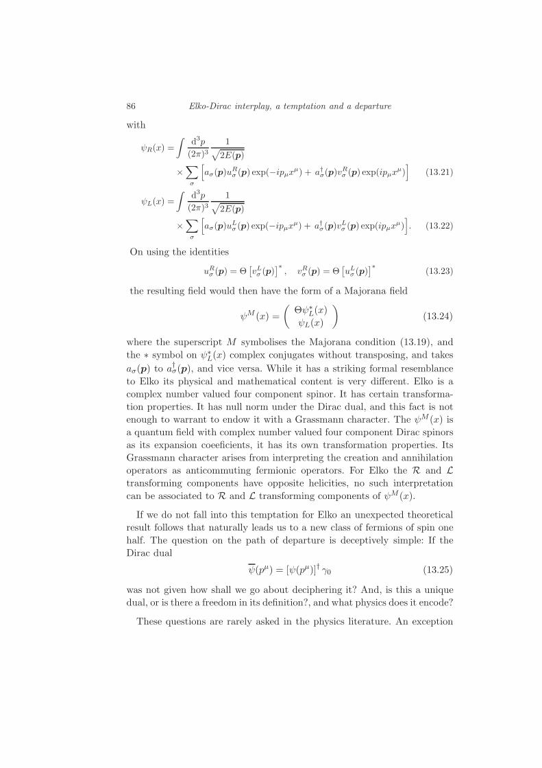
86 Elko-Dirac interplay, a temptation and a departure

with

ψR(x) =

∫d3p

(2π)31√

2E(p)

×∑

σ

[aσ(p)u

Rσ (p) exp(−ipµxµ) + a†σ(p)v

Rσ (p) exp(ipµx

µ)]

(13.21)

ψL(x) =

∫d3p

(2π)31√

2E(p)

×∑

σ

[aσ(p)u

Lσ (p) exp(−ipµxµ) + a†σ(p)v

Lσ (p) exp(ipµx

µ)]. (13.22)

On using the identities

uRσ (p) = Θ[vLσ (p)

]∗, vRσ (p) = Θ

[uLσ (p)

]∗(13.23)

the resulting field would then have the form of a Majorana field

ψM (x) =

(Θψ∗

L(x)

ψL(x)

)(13.24)

where the superscript M symbolises the Majorana condition (13.19), and

the ∗ symbol on ψ∗L(x) complex conjugates without transposing, and takes

aσ(p) to a†σ(p), and vice versa. While it has a striking formal resemblance

to Elko its physical and mathematical content is very different. Elko is a

complex number valued four component spinor. It has certain transforma-

tion properties. It has null norm under the Dirac dual, and this fact is not

enough to warrant to endow it with a Grassmann character. The ψM (x) is

a quantum field with complex number valued four component Dirac spinors

as its expansion coeeficients, it has its own transformation properties. Its

Grassmann character arises from interpreting the creation and annihilation

operators as anticommuting fermionic operators. For Elko the R and Ltransforming components have opposite helicities, no such interpretation

can be associated to R and L transforming components of ψM (x).

If we do not fall into this temptation for Elko an unexpected theoretical

result follows that naturally leads us to a new class of fermions of spin one

half. The question on the path of departure is deceptively simple: If the

Dirac dual

ψ(pµ) = [ψ(pµ)]† γ0 (13.25)

was not given how shall we go about deciphering it? And, is this a unique

dual, or is there a freedom in its definition?, and what physics does it encode?

These questions are rarely asked in the physics literature. An exception

13.3 A temptation, and a departure 87

for the definition, called a “convenience” by Weinberg, is to note that the

counterpart of Λ in (5.7) for the R⊕L|s=1/2 representation space

D(Λ)def=

exp (iκ ·ϕ) for Lorentz boosts

exp (iζ · ϑ) for rotations(13.26)

is not unitary, but pseudounitary25

γ0D(Λ)†γ0 = D(Λ)−1. (13.27)

Weinberg uses this observation to motivate the definition (13.25).

For Elko the completion of (13.3) and (13.11) is given by

λS±(p

µ)λS±(pµ) = 0, λ

S±(p

µ)λA±(pµ) = 0, λ

S±(p

µ)λA∓(pµ) = 0 (13.28)

λA±(p

µ)λA±(pµ) = 0, λA±(p

µ)λS±(pµ) = 0, λ

A±(p

µ)λS∓(pµ) = 0 (13.29)

and

λS±(p

µ)λS∓(pµ) = ∓ 2im, λ

A±(p

µ)λA∓(pµ) = ± 2im. (13.30)

Because of (13.30), we can define – see below – a new dual and make it con-

venient to formulate and calculate the physics of quantum fields with Elko

as their expansion coefficients. Once a lack of uniqueness of the Dirac dual

is discovered, the new way to accommodate the pseudounitarity captured

by (13.27) is introduced. It opens up concrete new possibilities to go beyond

the Dirac and Majorana fields for spin one half fermions without violating

Lorentz covariance and without introducing non-locality. The programme

now is as follows:

• Introduce a new dual so that not only the norm of Elko is Lorentz invariant

(and ∈ ℜ), but also the spins sums.

• Define a quantum field in terms of Elko, with the creation and annihilation

operators satisfying the usual fermionic anticommutators.

• Using the new dual, define a new adjoint for the quantum field. Calculate

the vacuum expectation value of the time ordered product of the field and

its adjoint.

• From the Feynman-Dyson propagator thus obtained, decipher the mass

dimensionality of the new field, and check the Schwinger locality by cal-

culating the relevant anticommutators.

25 Strictly speaking, Weinberg’s discussion is for a spin one half quantum field but it readilyadapts to the c-number spinors, ψ(pµ), in the R⊕ L|s=1/2 representation space.

88 Elko-Dirac interplay, a temptation and a departure

With the exception of this chapter, we consciously refrained from intro-

ducing a dual of the spinors. The reason was simple. The Elko had to be

obtained in a linear fashion. Its full poetry and beauty revealed without the

shadows of the intricacies of the dual space. The inevitability of the final

result hinted, and exposed, in its utter simplicity. That done we could then

take our reader through the more amorphous cloud of duals and adjoints,

to establishing the hint in its full maturing, knowing that others may refine

it further but not alter its essence.

This shared with the reader, we proceed to developing the theory of dual

spaces. Its flow holds as good for the representation space of our imme-

diate interest as for any other representation space. But by confining to

the indicated space we are able to make our argument less heavy, nota-

tionally. Beginning in the next chapter the reader would learn the deeper

structure from which (13.25) arises, and why there is no proper metric for

Weyl spinors, and for R and L representation spaces, separately, in general.

We would also learn to construct the metric for many other representation

spaces. In particular, we would easily see how the Lorentz algebra – with-

out reference to any other fact – gives the metric for the Minkowski space,

with the twist of a multiplicative phase factor. This phase may help us to

understand four-vector spaces at a deeper quantum level. In the process we

will discover how to construct the needed metric, with symmetries as the

starting point.

14

An ab initio journey into duals

14.1 Motivation and a brief outline

A n dimensional representation space may be spanned by n independent

vectors ζ1, ζ2, . . . ζn. These could be Weyl spinors, four-component spinors,

four-vectors, or ‘vectors’ spanning any representation. Our task is to intro-

duce a unified approach to constructing dual spaces, and a metric that helps

define bi-linear invariants.

Our starting point is Lorentz algebra, and the representation spaces on

which the symmetry transformations act through exponentiation of the gen-

erators in the sense defined in the opening chapters. Our motivation to look

at the duals ab initio resides in the null norm of Elko under the Dirac dual.

While considering a representation space, we look at each of the basis

vectors ζα, α = 1, 2, . . . n, as a complex number valued column vector. Our

task is to define a dual that allows us to construct scalars (or more generally

bilinears), that are invariant (covariant) under a set of physically interest-

ing symmetry transformations. These, besides the Lorentz transformations,

would include the discrete transformations, of parity, of time reversal, and

of charge conjugation. For this task we generate a mechanism that trans-

forms each of the ζα into a row. We identify this mechanism, in part, with

the complex conjugation of each of the ζα and transposing it. In addition,

motivated by the null norm of Elko under the Dirac dual, we introduce a

pairing operator that uniquely pairs (with the freedom to multiply with an

α dependent phase factor) each of these newly generated rows in an invert-

ible manner with each of the ζα. Say, the αth column with the βth row and

90 An ab initio journey into duals

generate the set of row vectors, ζ ′1, ζ ′2, . . . ζ ′n

ζ ′αdef= (Ξ ζα)

† (14.1)

where we have taken the liberty of first pairing and then implementing the

complex conjugation and transposition. Of Ξ we require that its inverse

exists, and that its square is an identity operator, Ξ2 = In.

To construct scalars from the ζ ′α and ζα we introduce a n × n matrix η,

and define a dual vector, or just a dual

∼

ζαdef= ζ ′αη (14.2)

We call η the metric for the representation space under consideration. It is

constrained to keep the bi-linear product

χα =∼

ζα ζα (14.3)

invariant under a chosen set of transformation, or symmetries. These con-

straints, as we will discover, generally take the form of commutators/anticom-

mutators of η, with the relevant generators of the symmetry algebra, to

vanish.

Additional constraints —

It turns out that the dual as defined above still has an element of freedom.

This freedom we shall discuss in detail.

It is this general procedure that we now implement for the spinor spaces.

14.2 The dual of spinors: constraints from the scalar invariants

Consider a general set of 4-component massive spinors (pµ). We would like

these to be orthonormal under the dual we are seeking. These do not have

to be eigenspinors of P, that is, Dirac spinors, or the eigenspinors of C –

that is, Elko. As a specific implementation of the preceding discussion, we

examine a general form of the dual defined as

∼

α(pµ)

def=

[Ξ(pµ) α(p

µ)]†η (14.4)

where η is a 4 × 4 matrix, with its elements ∈ C. The task of Ξ(pµ) is to

take any one of the α(pµ) and transform it, up to a phase, into one of the

spinors α′(pµ) from the same set. It is not necessary that the indices α′ and

α be the same. We require Ξ(pµ) to define an invertible map, with Ξ2 = I4

(possibly, up to a phase).

14.3 The Dirac and Elko dual: a preview 91

14.3 The Dirac and Elko dual: a preview

The Dirac dual arises when we identify the pairing matrix with the identity

matrix

Ξ(pµ) = I4 (14.5)

for which β = α

α(pµ) → α(p

µ), ∀α (14.6)

and identifying α(pµ) with the eigenspinors of the parity operator, that is

with the uσ(pµ) and vσ(p

µ).

The starting point for the Elko dual goes back to an early unpublished

preprint before it was fully realised that these provide expansion coefficients

for a mass dimension one fermionic field of spin one half (Ahluwalia, 2003).

The hint arose from the results found here in equations (13.28) to (13.30).

That early choice was shown by Speranca to arise from the pairing ma-

trix (Speranca, 2014)

Ξ(pµ)def=

1

2m

∑

α=±

[λSα(p

µ)λSα(pµ)− λAα (p

µ)λAα (pµ)]. (14.7)

It induces the needed map

λS+(pµ) → iλS−(p

µ) (14.8)

λS−(pµ) → −iλS+(pµ) (14.9)

λA+(pµ) → −iλA−(pµ) (14.10)

λA−(pµ) → +iλS+(p

µ). (14.11)

if α(pµ) are identified with Elko, λα(p

µ). That is

Ξ(pµ)λS±(pµ) = ±iλS∓(pµ) (14.12)

Ξ(pµ)λA±(pµ) = ∓iλA∓(pµ). (14.13)

14.4 Constraints on the metric from Lorentz, and discrete,

symmetries

We now wish to determine the metric η, and Ξ(pµ) – explicitly. We will

see that the choices (14.5), (14.12) and (14.13), are indeed allowed. For the

92 An ab initio journey into duals

boosts, the requirement of a Lorentz invariant norm translates to

[Ξ(kµ)(kµ)

]†η (kµ)

︸ ︷︷ ︸χ(kµ)

=[Ξ(pµ)(pµ)

]†η (pµ)

︸ ︷︷ ︸χ(pµ)

(14.14)

with a similar expression for the rotations. Expressing (pµ) as exp(iκ ·ϕ)(kµ), and using κ† = −κ (for an explicit form of κ see Eq. (5.6)), the

right-hand side of the above expression can be re-written as

[Ξ(pµ)(pµ)

]†η (pµ) = †(kµ) eiκ·ϕ Ξ†(pµ) η eiκ·ϕ (kµ). (14.15)

Since

Ξ(pµ) = eiκ·ϕ Ξ(kµ) e−iκ·ϕ (14.16)

the Ξ†(pµ) evaluates to

Ξ†(pµ) → eiκ†·ϕ Ξ†(kµ) e−iκ

†·ϕ = e−iκ·ϕ Ξ†(kµ) eiκ·ϕ. (14.17)

Using this result in (14.15) yields

[Ξ(pµ)(pµ)

]†η (pµ) = †(kµ)Ξ†(kµ)eiκ·ϕη eiκ·ϕ(kµ)

=[Ξ(kµ)(kµ)

]†eiκ·ϕη eiκ·ϕ(kµ). (14.18)

Using the just derived result into the right hand side of (14.14) gives

[Ξ(kµ)(kµ)

]†η (kµ) =

[Ξ(kµ)(kµ)

]†eiκ·ϕη eiκ·ϕ(kµ). (14.19)

Up to a caveat to be noted below in section 14.4.1, it gives the constraint

η = eiκ·ϕη eiκ·ϕ (14.20)

That is, the metric η must anticommute with each of boost generators κ

κi, η = 0, i = x, y, z. (14.21)

Implementing the above constraint with i = z, y, z in succession reduces η

to have the form

0 0 a+ ib 0

0 0 0 a+ ib

c+ id 0 0 0

0 c+ id 0 0

(14.22)

where a, b, c, d ∈ ℜ. This is valid for all four-component spinors.

14.4 Constraints on the metric from Lorentz, and discrete, symmetries 93

14.4.1 A freedom in the definition of the metric

Strictly speaking the equality in (14.20) is up to a freedom of an operator

which carries the (pµ) as its eigenspinor with eigenvalue unity:

η = eiκ·ϕη eiκ·ϕΓ (14.23)

with Γ(pµ) = (pµ). Existence of Γ operator(s) is an important freedom as

it may reduce the symmetries under consideration, possibly to a subgroup

of Lorentz.

Apart from our Elko experience (Ahluwalia and Horvath, 2010) that we

shall further share with our reader in this chapter, the above remark arises

from a 2006 Cohen and Glashow observation (Cohen and Glashow, 2006)

that, “Indeed, invariance under HOM(2), rather than (as is often taught)

the Lorentz group, is both necessary and sufficient to ensure that the speed of

light is the same for all observers, and inter alia, to explain the null result to

the Michelson-Morley experiment and its more sensitive successors.” These

subgroups are defined by the four algebras summarised in Table 11.1. The

generators

T1def= Kx + Jy, T2

def= Ky − Jx (14.24)

form the group T(2) – a group isomorphic to the group of translations in a

plane.

Following Cohen and Glashow a relativity formed by adjoining four space-

time translations with any of these groups is termed Very Special Relativity

(VSR). While each of the four VSRs have distinct physical characters they

all share the remarkable defining property that incorporation of either P , T ,

CP , or CT enlarges these subgroups to the full Lorentz group. At present,

VSR does not violate any of the existing tests of Special Relativity and

provides an unexpected realm for the investigation of spacetime symmetries

including violation of discrete symmetries, and isotropy of space.

A detailed discussion of VSR can be found in a Masters thesis by Gustavo

Salinas De Souza (de Souza, 2015) and in the context of Elko in (Ahluwalia and Horvath,

2010). Our analysis of Elko provides a concrete example of a VSR quantum

field that exhibits non-locality governed by a VSR operator

G(pµ) def=

0 0 0 −ie−iφ0 0 ieiφ 0

0 −ie−iφ 0 0

ieiφ 0 0 0

. (14.25)

94 An ab initio journey into duals

Table 14.1 Algebras associated with the four VSR subgroups

Name Generators Sub algebra

t(2) T1,T2 [T1,T2] = 0e(2) T1,T2, Jz [T1,T2] = 0, [T1, Jz] = −iT2, [T2, Jz] = iT1

hom(2) T1,T2,Kz [T1,T2] = 0, [T1,Kz] = iT1, [T2,Kz ] = iT2

sim(2) T1,T2, Jz,Kz [T1,T2] = 0, [T1,Kz] = iT1, [T2,Kz ] = iT2

[T1, Jz] = −iT2, [T2, Jz] = iT1, [Jz,Kz ] = 0

This result is consistent with the claim of Cohen and Glashow that a de-

parture from SR to VSR introduces non-locality. In its character G(pµ) is

similar to Γ becuase G(pµ)λS(pµ) = λS(pµ), and G(pµ)λA(pµ) = −λA(pµ).

As a parenthetic remark we note that Nakayama shows a way to circum-

vent the no-go locality result of VSR (Nakayama, 2018a,b) while Ilderton

shows how non-locality and VSR symmetries appear on averaging observ-

ables over rapid field oscillations of a Lorentz covariant theory (Ilderton,

2016). Cheng-Yang Lee circumvents the non-locality problem by introduc-

ing a configuration space G(pµ) at the cost of introducing fractional deriva-

tives (Lee, 2016a).

Given our experience with Elko we conjecture that Γ encodes a theoret-

ical mechanism of Lorentz symmetry breaking in a generic manner to the

subgroups summarised in Table 11.1. After we have developed the notion of

Elko dual further, we shall pick up this thread in section 14.7

14.4.2 The Dirac dual

The simplest choice for Ξ(pµ) is the identity operator as in (14.5). We will

now show that the well-known Dirac dual corresponds to this choice. With

Ξ(pµ) = I4, the counterpart of (14.14) for rotations reads

†(pµ) η (pµ) = †(p′µ) η (p′µ) (14.26)

where (p′µ) = eiζ·θ(pµ). Using ζ† = ζ (for an explicit form of ζ see

Eq. (5.6)) translates (14.26) to

†(pµ) η (pµ) = †(pµ) e−iζ·θ ηeiζ·θ (pµ). (14.27)

Modulo a freedom noted in section 14.4.1, it gives the constraint

η = e−iζ·θ ηeiζ·θ. (14.28)

14.4 Constraints on the metric from Lorentz, and discrete, symmetries 95

That is, the metric η must commute with each of rotation generators ζ

[ζi, η] = 0, i = x, y, z. (14.29)

The constraint that η must commute with ζi does not reduce η constrained

by its anticommutativity with each of the boost generators, κi.

However, following an analysis paralleling the two previous calculations

the demand for the norm to be invariant under the parity transformation Pis readily obtained to be

η = m−2 [γµpµ]† η γµp

µ (14.30)

A direct evaluation of the right hand side of the parity constraint (14.30)

with η given by (14.22) gives the result

m−2 [γµpµ]† η γµp

µ =

0 0 c+ id 0

0 0 0 c+ id

a+ ib 0 0 0

0 a+ ib 0 0

(14.31)

thus requiring c = a, and d = b. In consequence, the parity constraint further

reduces the metric η to

η =

0 0 a+ ib 0

0 0 0 a+ ib

a+ ib 0 0 0

0 a+ ib 0 0

(14.32)

Requiring the norm of the Dirac spinors to be real forces the choice b = 0,

and then a is simply a scale factor. It may be chosen to be unity

η =

0 0 1 0

0 0 0 1

1 0 0 0

0 1 0 0

(14.33)

We thus reproduce the canonical Dirac dual: it is defined by the choice of

Ξ(pµ) = I4, and the constraints on η given by (14.21), (14.29) and (14.30).

On the path of our departure we learn that the Dirac dual has additional

underlying structure. In particular, it gives us a choice to violate parity, or to

preserve it, depending on whether we choose a/c in η of (14.22) to be unity,

or different from unity. With the former choice we reproduce the standard

result (13.25), while the latter choice gives us a first-principle control on

the extent to which parity may be violated in nature, or in a given physical

process.

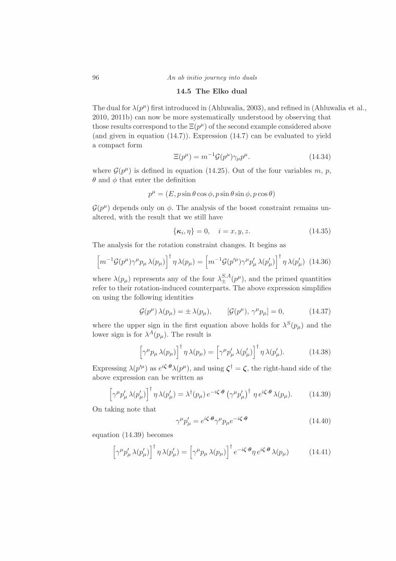
96 An ab initio journey into duals

14.5 The Elko dual

The dual for λ(pµ) first introduced in (Ahluwalia, 2003), and refined in (Ahluwalia et al.,

2010, 2011b) can now be more systematically understood by observing that

those results correspond to the Ξ(pµ) of the second example considered above

(and given in equation (14.7)). Expression (14.7) can be evaluated to yield

a compact form

Ξ(pµ) = m−1G(pµ)γµpµ. (14.34)

where G(pµ) is defined in equation (14.25). Out of the four variables m, p,

θ and φ that enter the definition

pµ = (E, p sin θ cosφ, p sin θ sinφ, p cos θ)

G(pµ) depends only on φ. The analysis of the boost constraint remains un-

altered, with the result that we still have

κi, η = 0, i = x, y, z. (14.35)

The analysis for the rotation constraint changes. It begins as[m−1G(pµ)γµpµ λ(pµ)

]†η λ(pµ) =

[m−1G(p′µ)γµp′µ λ(p′µ)

]†η λ(p′µ) (14.36)

where λ(pµ) represents any of the four λS,A± (pµ), and the primed quantities

refer to their rotation-induced counterparts. The above expression simplifies

on using the following identities

G(pµ)λ(pµ) = ±λ(pµ), [G(pµ), γµpµ] = 0, (14.37)

where the upper sign in the first equation above holds for λS(pµ) and the

lower sign is for λA(pµ). The result is

[γµpµ λ(pµ)

]†η λ(pµ) =

[γµp′µ λ(p

′µ)]†η λ(p′µ). (14.38)

Expressing λ(p′µ) as eiζ·θλ(pµ), and using ζ† = ζ, the right-hand side of the

above expression can be written as[γµp′µ λ(p

′µ)]†η λ(p′µ) = λ†(pµ) e

−iζ·θ(γµp′µ

)†η eiζ·θ λ(pµ). (14.39)

On taking note that

γµp′µ = eiζ·θγµpµe−iζ·θ (14.40)

equation (14.39) becomes[γµp′µ λ(p

′µ)]†η λ(p′µ) =

[γµpµ λ(pµ)

]†e−iζ·θη eiζ·θ λ(pµ) (14.41)

14.5 The Elko dual 97

Comparing the above expression with (14.38) gives the constraint

η = e−iζ·θη eiζ·θ (14.42)

That is, the metric η must commute with each of rotation generators ζ

[ζi, η] = 0, i = x, y, z (14.43)

Despite a non-trivial Ξ(pµ), this is the same result as before.

It is readily seen that [Ξ(pµ)]2 = I and [Ξ(pµ)]−1 indeed exists and equals

Ξ(pµ) itself. Thus, the dual for λ(pµ) is defined by the choice of Ξ(pµ) given

by (14.34).

So far the constraints on η turn out to be same as for the Dirac dual. To

distinguish it from other possibilities the new dual at the intermediate state

of our calculations is represented by

∼

λα(pµ)

def=

[Ξ(pµ)λα(p

µ)]†η (14.44)

with η given by (14.4.2). This choice of η is purely for convenience at the mo-

ment. If the new particles to be introduced here are indeed an element of the

physical reality then the ratio a/c must not be set to unity but determined

by appropriate observations/experiments.

Using (14.12) and (14.13), (14.44) translates to

∼

λS

+(pµ) = −i

[λS−(p

µ)]†η

∼

λS

−(pµ) = i

[λS+(p

µ)]†η

∼

λA

+(pµ) = i

[λA−(p

µ)]†η

∼

λA

−(pµ) = −i

[λA+(p

µ)]†η (14.45)

We can thus rewrite the results (13.28), (13.29), and (13.30) into the

following orthonormality relations

∼

λS

α(pµ)λSα′(pµ) = 2mδαα′

∼

λA

α (pµ)λAα′(pµ) = −2mδαα′

∼

λS

α(pµ)λAα′(pµ) = 0 =

∼

λA

α (pµ)λSα′(pµ) (14.46)

with α and α′ = ±.

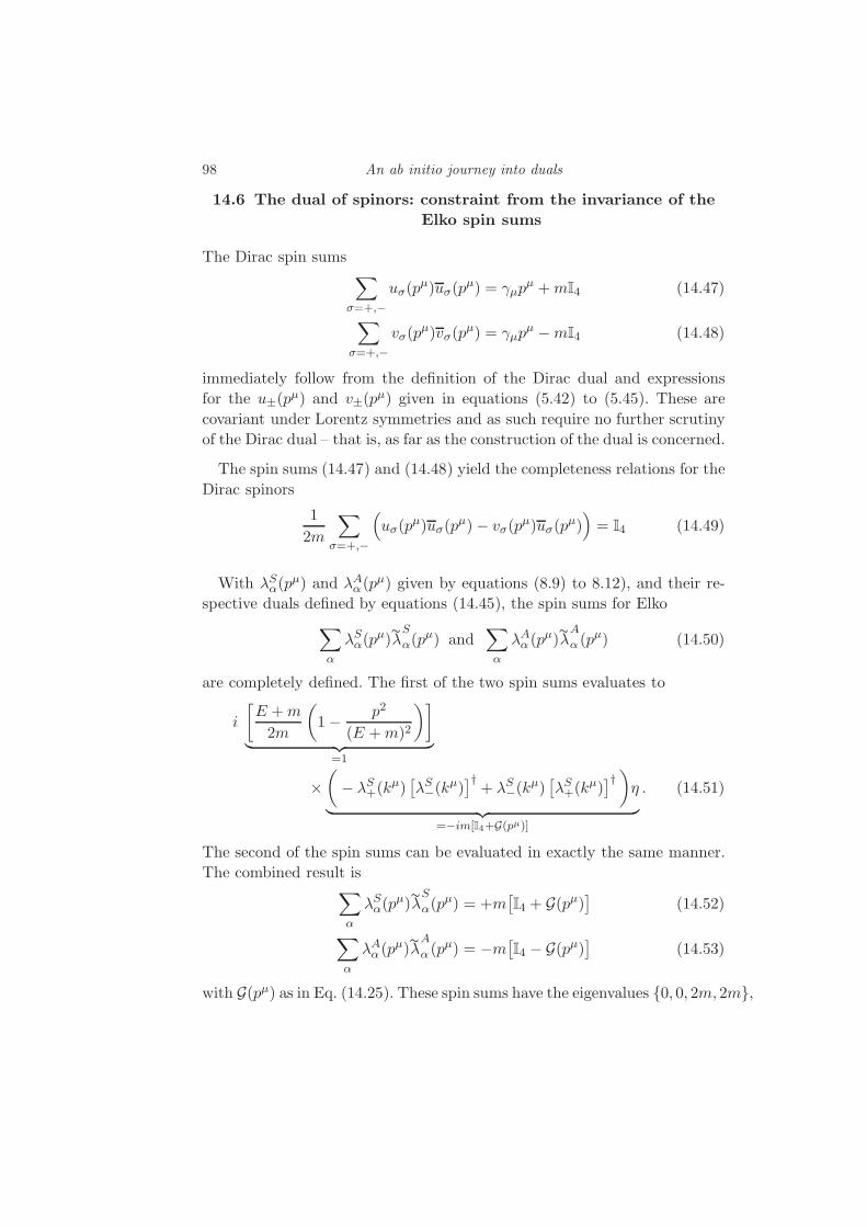
98 An ab initio journey into duals

14.6 The dual of spinors: constraint from the invariance of the

Elko spin sums

The Dirac spin sums∑

σ=+,−

uσ(pµ)uσ(p

µ) = γµpµ +mI4 (14.47)

∑

σ=+,−

vσ(pµ)vσ(p

µ) = γµpµ −mI4 (14.48)

immediately follow from the definition of the Dirac dual and expressions

for the u±(pµ) and v±(p

µ) given in equations (5.42) to (5.45). These are

covariant under Lorentz symmetries and as such require no further scrutiny

of the Dirac dual – that is, as far as the construction of the dual is concerned.

The spin sums (14.47) and (14.48) yield the completeness relations for the

Dirac spinors

1

2m

∑

σ=+,−

(uσ(p

µ)uσ(pµ)− vσ(p

µ)uσ(pµ))= I4 (14.49)

With λSα(pµ) and λAα (p

µ) given by equations (8.9) to 8.12), and their re-

spective duals defined by equations (14.45), the spin sums for Elko

∑

α

λSα(pµ)

∼

λS

α(pµ) and

∑

α

λAα (pµ)

∼

λA

α (pµ) (14.50)

are completely defined. The first of the two spin sums evaluates to

i

[E +m

2m

(1− p2

(E +m)2

)]

︸ ︷︷ ︸=1

×(− λS+(k

µ)[λS−(k

µ)]†

+ λS−(kµ)

[λS+(k

µ)]†)η

︸ ︷︷ ︸=−im[I4+G(pµ)]

. (14.51)

The second of the spin sums can be evaluated in exactly the same manner.

The combined result is∑

α

λSα(pµ)

∼

λS

α(pµ) = +m

[I4 + G(pµ)

](14.52)

∑

α

λAα (pµ)

∼

λA

α (pµ) = −m

[I4 − G(pµ)

](14.53)

with G(pµ) as in Eq. (14.25). These spin sums have the eigenvalues 0, 0, 2m, 2m,

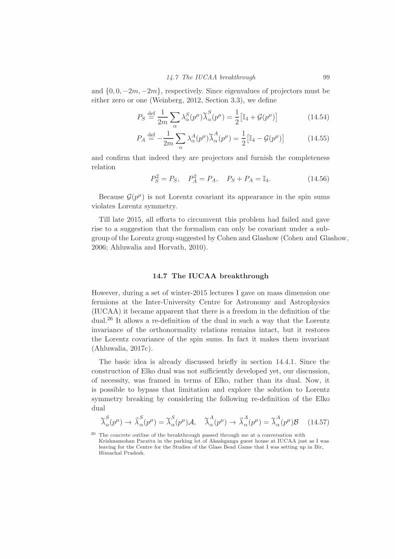
14.7 The IUCAA breakthrough 99

and 0, 0,−2m,−2m, respectively. Since eigenvalues of projectors must be

either zero or one (Weinberg, 2012, Section 3.3), we define

PSdef=

1

2m

∑

α

λSα(pµ)

∼

λS

α(pµ) =

1

2

[I4 + G(pµ)

](14.54)

PAdef= − 1

2m

∑

α

λAα (pµ)

∼

λA

α (pµ) =

1

2

[I4 − G(pµ)

](14.55)

and confirm that indeed they are projectors and furnish the completeness

relation

P 2S = PS , P 2

A = PA, PS + PA = I4. (14.56)

Because G(pµ) is not Lorentz covariant its appearance in the spin sums

violates Lorentz symmetry.

Till late 2015, all efforts to circumvent this problem had failed and gave

rise to a suggestion that the formalism can only be covariant under a sub-

group of the Lorentz group suggested by Cohen and Glashow (Cohen and Glashow,

2006; Ahluwalia and Horvath, 2010).

14.7 The IUCAA breakthrough

However, during a set of winter-2015 lectures I gave on mass dimension one

fermions at the Inter-University Centre for Astronomy and Astrophysics

(IUCAA) it became apparent that there is a freedom in the definition of the

dual.26 It allows a re-definition of the dual in such a way that the Lorentz

invariance of the orthonormality relations remains intact, but it restores

the Lorentz covariance of the spin sums. In fact it makes them invariant

(Ahluwalia, 2017c).

The basic idea is already discussed briefly in section 14.4.1. Since the

construction of Elko dual was not sufficiently developed yet, our discussion,

of necessity, was framed in terms of Elko, rather than its dual. Now, it

is possible to bypass that limitation and explore the solution to Lorentz

symmetry breaking by considering the following re-definition of the Elko

dual∼

λS

α(pµ) → ¬

λS

α(pµ) =

∼

λS

α(pµ)A, ∼

λA

α (pµ) → ¬

λA

α (pµ) =

∼

λA

α (pµ)B (14.57)

26 The concrete outline of the breakthrough passed through me at a conversation withKrishnamohan Parattu in the parking lot of Akashganga guest house at IUCAA just as I wasleaving for the Centre for the Studies of the Glass Bead Game that I was setting up in Bir,Himachal Pradesh.

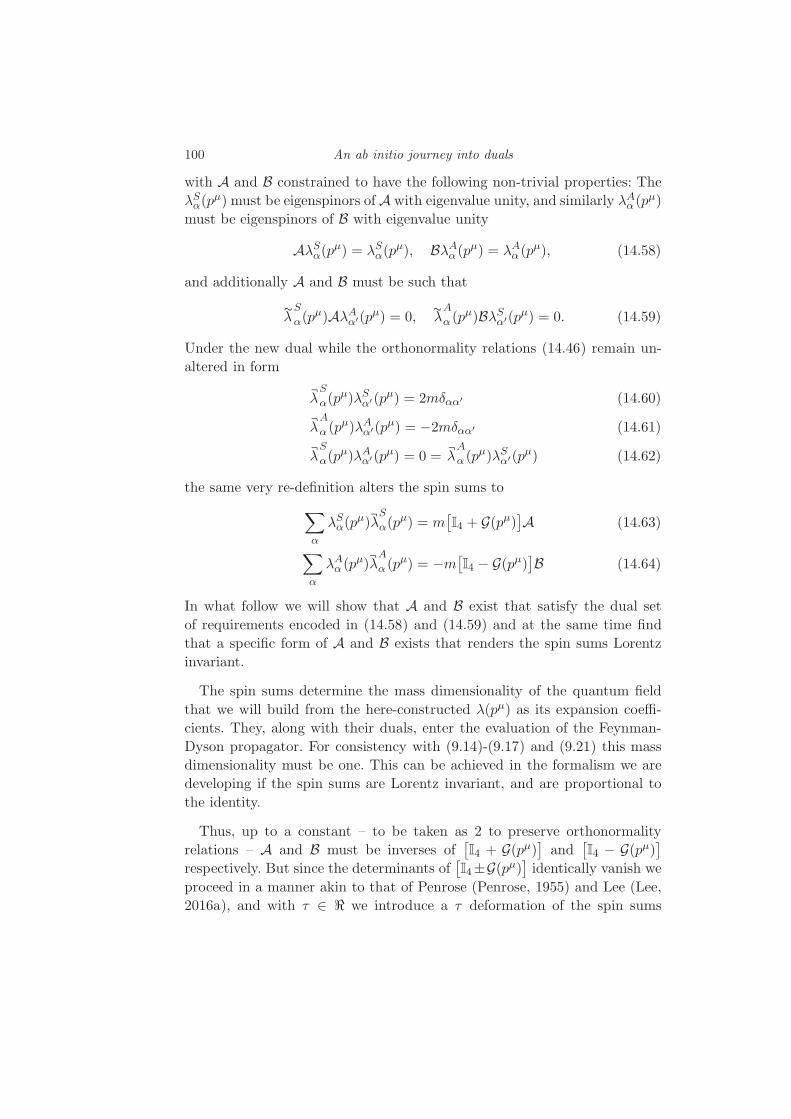
100 An ab initio journey into duals

with A and B constrained to have the following non-trivial properties: The

λSα(pµ) must be eigenspinors of A with eigenvalue unity, and similarly λAα (p

µ)

must be eigenspinors of B with eigenvalue unity

AλSα(pµ) = λSα(pµ), BλAα (pµ) = λAα (p

µ), (14.58)

and additionally A and B must be such that

∼

λS

α(pµ)AλAα′(pµ) = 0,

∼

λA

α (pµ)BλSα′(pµ) = 0. (14.59)

Under the new dual while the orthonormality relations (14.46) remain un-

altered in form

¬

λS

α(pµ)λSα′(pµ) = 2mδαα′ (14.60)

¬

λA

α (pµ)λAα′(pµ) = −2mδαα′ (14.61)

¬

λS

α(pµ)λAα′(pµ) = 0 =

¬

λA

α (pµ)λSα′(pµ) (14.62)

the same very re-definition alters the spin sums to

∑

α

λSα(pµ)

¬

λS

α(pµ) = m

[I4 + G(pµ)

]A (14.63)

∑

α

λAα (pµ)

¬

λA

α (pµ) = −m

[I4 − G(pµ)

]B (14.64)

In what follow we will show that A and B exist that satisfy the dual set

of requirements encoded in (14.58) and (14.59) and at the same time find

that a specific form of A and B exists that renders the spin sums Lorentz

invariant.

The spin sums determine the mass dimensionality of the quantum field

that we will build from the here-constructed λ(pµ) as its expansion coeffi-

cients. They, along with their duals, enter the evaluation of the Feynman-

Dyson propagator. For consistency with (9.14)-(9.17) and (9.21) this mass

dimensionality must be one. This can be achieved in the formalism we are

developing if the spin sums are Lorentz invariant, and are proportional to

the identity.

Thus, up to a constant – to be taken as 2 to preserve orthonormality

relations – A and B must be inverses of[I4 + G(pµ)

]and

[I4 − G(pµ)

]

respectively. But since the determinants of[I4±G(pµ)

]identically vanish we

proceed in a manner akin to that of Penrose (Penrose, 1955) and Lee (Lee,

2016a), and with τ ∈ ℜ we introduce a τ deformation of the spin sums

14.7 The IUCAA breakthrough 101

(14.63) and (14.64)27

∑

α

λSα(pµ)

¬

λS

α(pµ) = m

[I4 + τG(pµ)

]A∣∣∣τ→1

(14.65)

∑

α

λAα (pµ)

¬

λA

α (pµ) = −m

[I4 − τG(pµ)

]B∣∣∣τ→1

. (14.66)

We will see that the τ → 1 limit is non pathological in the infinitesimal small

neighbourhood of τ = 1 in the sense we shall make explicit. We choose Aand B to be

A = 2[I4 + τG(pµ)

]−1= 2

(I4 − τG(pµ)

1− τ2

)(14.67)

B = 2[I4 − τG(pµ)

]−1= 2

(I4 + τG(pµ)

1− τ2

). (14.68)

Making use of the identity G2(pµ) = I4, Eqs. (14.65) and (14.66) simplify to:

∑

α

λSα(pµ)

¬

λS

α(pµ) = 2m

[I4 + τG(pµ)

](I4 − τG(pµ)1− τ2

) ∣∣∣∣τ→1

= 2mI4

(1− τ2

1− τ2

) ∣∣∣∣τ→1

= 2mI4 (14.69)

∑

α

λAα (pµ)

¬

λA

α (pµ) = 2m

[I4 − τG(pµ)

](I4 + τG(pµ)1− τ2

) ∣∣∣∣τ→1

= 2mI4

(1− τ2

1− τ2

) ∣∣∣∣τ→1

= −2mI4 (14.70)

We now return to the orthonormality relations. Since from the first equation

in (14.37), G(pµ)λS(pµ) = λS(pµ) while G(pµ)λA(pµ) = −λA(pµ), we have

the result demanded by the requirement (14.58)

AλSα(pµ) = 2

(I4 − τG(pµ)

1− τ2

)λSα(p

µ) = 2

(1− τ

1− τ2

)λSα(p

µ)

=

(2

1 + τ

) ∣∣∣∣τ→1

λSα(pµ)

= λSα(pµ) (14.71)

and

BλAα (pµ) = 2

(I4 + τG(pµ)

1− τ2

)λAα (p

µ) = 2

(1− τ

1− τ2

)λAα (p

µ)

27 Unlike Lee (Lee, 2016a) we refrain from introducing configuration counterpart of G(pµ) toavoid brining in the theory fractional derivatives.

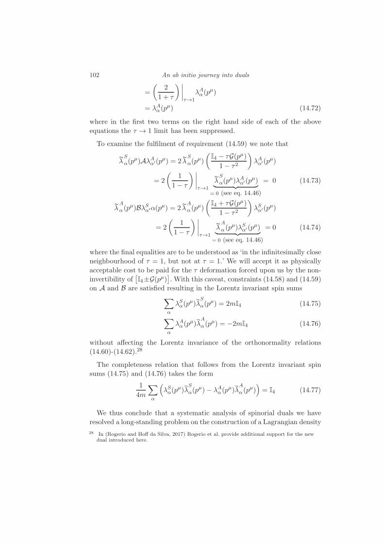
102 An ab initio journey into duals

=

(2

1 + τ

) ∣∣∣∣τ→1

λAα (pµ)

= λAα (pµ) (14.72)

where in the first two terms on the right hand side of each of the above

equations the τ → 1 limit has been suppressed.

To examine the fulfilment of requirement (14.59) we note that

∼

λS

α(pµ)AλAα′(pµ) = 2

∼

λS

α(pµ)

(I4 − τG(pµ)

1− τ2

)λAα′(pµ)

= 2

(1

1− τ

) ∣∣∣∣τ→1

∼

λS

α(pµ)λAα′(pµ)︸ ︷︷ ︸

= 0 (see eq. 14.46)

= 0 (14.73)

∼

λA

α (pµ)BλSα′α(pµ) = 2

∼

λA

α (pµ)

(I4 + τG(pµ)

1− τ2

)λSα′(pµ)

= 2

(1

1− τ

) ∣∣∣∣τ→1

∼

λA

α (pµ)λSα′(pµ)︸ ︷︷ ︸

= 0 (see eq. 14.46)

= 0 (14.74)

where the final equalities are to be understood as ‘in the infinitesimally close

neighbourhood of τ = 1, but not at τ = 1.’ We will accept it as physically

acceptable cost to be paid for the τ deformation forced upon us by the non-

invertibility of[I4±G(pµ)

]. With this caveat, constraints (14.58) and (14.59)

on A and B are satisfied resulting in the Lorentz invariant spin sums∑

α

λSα(pµ)

¬

λS

α(pµ) = 2mI4 (14.75)

∑

α

λAα (pµ)

¬

λA

α (pµ) = −2mI4 (14.76)

without affecting the Lorentz invariance of the orthonormality relations

(14.60)-(14.62).28

The completeness relation that follows from the Lorentz invariant spin

sums (14.75) and (14.76) takes the form

1

4m

∑

α

(λSα(p

µ)¬

λS

α(pµ)− λAα (p

µ)¬

λA

α (pµ))= I4 (14.77)

We thus conclude that a systematic analysis of spinorial duals we have

resolved a long-standing problem on the construction of a Lagrangian density

28 In (Rogerio and Hoff da Silva, 2017) Rogerio et al. provide additional support for the newdual introduced here.

14.7 The IUCAA breakthrough 103

for the c-number Majorana spinors, extended here into Elko. The sought

after Lagrangian density is not as given in equation (13.1), or as conjectured

and found not to exist in (Aitchison and Hey, 2004, App. P), but

L(x) = ∂µ¬

λ(x) ∂µλ(x)−m2 ¬

λ(x)λ(x). (14.78)

Strictly speaking, this result should be taken as suggestive till it is fully

established in its quantum field theoretic incarnation in the next chapter.

15

Mass dimension one fermions

15.1 A quantum field with Elko as its expansion coefficient

We now use the eigenspinors of the charge conjugation operator, Elko:

λSα(pµ) and λAα (p

µ), as expansion coefficients to define a new quantum field

of spin one half

f(x)def=

∫d3p

(2π)31√

2mE(p)

×∑

α

[aα(p)λ

Sα(p)e

−ip·x + b†α(p)λAα (p)e

ip·x]

(15.1)

where we have taken the liberty to notationally replace the λ(pµ) by λ(p).

To decipher the mass dimensionality of f(x) and to develop a quantum field

theoretic formalism for the new field we define its adjoint

¬

f (x)def=

∫d3p

(2π)31√

2mE(p)

×∑

α

[a†α(p)

¬

λS

α(p)eip·x + bα(p)

¬

λA

α (p)e−ip·x

](15.2)

The creation and annihilation operators, at this stage, are left free to obey

fermionicaα(p), a

†α′(p

′)= (2π)3 δ3

(p− p′

)δαα′ (15.3)

aα(p), aα′(p′)

= 0,

a†α(p), a

†α′(p

′)= 0 (15.4)

or bosonic[aα(p), a

†α′(p

′)]= (2π)3 δ3

(p− p′

)δαα′ (15.5)

15.2 A hint that the new field is fermionic 105

[aα(p), aα′(p′)

]= 0,

[a†α(p), a

†α′(p

′)]= 0 (15.6)

statistics. We assume similar anti-commutativity/commutativity for bα(p)

and b†α(p). Under the assumption that the vacuum state | 〉 is normalised to

unity, they fix the normalisation of one particle states

|p, α, a〉 def= a†α(p)| 〉, |p, α, b〉 def

= b†α(p)| 〉 (15.7)

to be

〈p′, α′, a|p, α, a〉 = (2π)3 δ3(p− p′

)δαα′

〈p′, α′, b|p, α, b〉 = (2π)3 δ3(p− p′

)δαα′ (15.8)

In the above expressions, we use the key

a = particle, b = antiparticle (15.9)

15.2 A hint that the new field is fermionic

A Lie algebraically stable theoretical framework requires that position and

momentum measurements do not commute: theories with special relativis-

tic symmetries must be quantum in nature (Flato, 1982; Faddeev, 1989;

Vilela Mendes, 1994; Chryssomalakos and Okon, 2004).29 With the ensuing

irreducible product of ~/2 between the uncertainties in the position and the

momentum measurements this necessity forces non-vanishing amplitude for

the propagation of a particle from an emission event x to a space-like sepa-

rated absorption event y – that is to a classically forbidden region. But since

time ordering of events is not preserved for space-like separations, causal

paradoxes come to exist unless the same very process that was interpreted as

a particle propagation for the set of observers with y0 > x0 is re-interpreted

as propagation of an antiparticle for observers for whom y0 < x0 (Weinberg,

1972, Ch. 2, Sec.13). In the quantum field theoretic framework – only known

way to merge quantum and relativistic realms – the processes that connect

space-like separated events are mediated by virtual particles, particles that

are off shell, that is, with energy, momentum, and mass that deviate from:

E2 = p2 +m2. The time-energy uncertainty relation intervenes to protect

the energy-momentum conservation for fluctuations off the mass shell.

With this background, to decipher the statistics for the f(x) and¬

f (x)

system we now consider two space-like separated events, x and y, along the

29 A weaker version of this argument based solely on the rotational symmetry is given insection 3.3.

106 Mass dimension one fermions

lines of (Ahluwalia and Nayak, 2015). Referring to the observation on the

lack of time ordering preservation for such a set-up we recognise the existence

of two sets of inertial frames, ones in which y0 > x0 and the ones in which

the reverse is true, x0 > y0. We call these sets of inertial frame as O and

O′ respectively. In O, we calculate the amplitude for a particle to propagate

from x to y and in O′ the amplitude for an antiparticle to propagate from y

to x. Causality requires that these two amplitudes may only differ, at most,

by a phase factor:30

Amp(x→ y,particle)∣∣O= eiθAmp(y → x, antiparticle)

∣∣O′

(15.10)

with θ ∈ R. The definition of f(x) and its adjoint¬

f (x) given in equations

(15.1) and (15.2), respectively, allow us to obtain the following concrete

results for the needed amplitudes:

Amp(x→ y,particle)∣∣O= 〈 |f(y) ¬

f (x)| 〉

=

∫d3p

(2π)3

(1

2mE(p)

)e−ip·(y−x)

∑

α

λSα(p)¬

λS

α(p) (15.11)

and

Amp(y → x, antiparticle)∣∣O′

= 〈 | ¬f (x)f(y)| 〉∣∣O′

=[〈 | ¬f (x)f(y)| 〉

∣∣O

](x−y)→(y−x)

=

∫d3p

(2π)3

(1

2mE(p)

)e−ip·(y−x)

∑

α

λAα (p)¬

λA

α (p) (15.12)

The Elko spin sums (14.75) and (14.76) when substituted in the above calcu-

lated amplitudes, yields the result that the phase factor in (15.10) is minus

one: eiθ = −1. Furthermore, a direct calculation shows that

Amp(y → x, antiparticle)∣∣O′

= Amp(y → x, antiparticle)∣∣O

(15.13)

Combined, the above two results translate the relation (15.10) to

Amp(x→ y,particle)∣∣O= −Amp(y → x, antiparticle)

∣∣O

(15.14)

That is ¬

f (x), f(y)= 0 (15.15)

This is a hint, a strong hint, that the new field must be fermionic. We

thus take the choice (15.4) as part of the definition of the f(x).

30 For the smoothness of the discussion, we suppress a normalisation factor with the dimensionsof inverse length squared till equation (15.16).

15.3 Amplitude for propagation 107

In the standard S-matrix theory the events that we detect at ‘spatial

infinity’ – that is, at distances far away from the interaction region – contain

contribution from virtual particles as well as from on-sell particles. This

amplitude is the Feynman-Dyson propagator. It is considered in the next

section.

However, before we undertake that study we explicitly substitute the spin

sum from (14.75) into (15.11), do the resulting integration, and introduce

the normalisation constant alluded to above31

Amp(x→ y,particle)∣∣O=i

2m2

∫d3p

(2π)3

(1

E(p)

)e−ip·(y−x) I4

=i

4π2m3

√ǫ2 − τ2

K1(m√ǫ2 − τ2) (15.16)

where ǫdef= |x′ − x|, τ def

= |x0′ − x0|, ǫ > τ so that y and x represent events

separated by space-like interval, and Kν(. . .) is the modified Bessel function

of the second kind of order one, that is with ν = 1.

For a historical thread (in the context of Dirac fermions), involving Dirac,

Pauli, and Feynman, we refer our reader to the discussion following equation

(2.13) of (Ahluwalia et al., 2011a).

15.3 Amplitude for propagation

We now study amplitude of propagation from x to x′ without spacetime

interval being restricted to space-like separations. It would reveal the mass

dimensionality of the new field to be one. We would be mindful that causal

paradoxes can only be avoided for contributions from space-like separations

if we allow particles to be replaced by antiparticles whenever time ordering

of the events is reversed. In the interaction region we do not measure space-

time coordinates, x and x′ – all our measurements in the scattering/collision

processes take place in ‘far away regions.’ This creates an unavoidable ambi-

guity in time ordering of the absorption and emission of the virtual particles.

This is incorporated in our calculations, as in the standard quantum field

theoretic formalism, by adding all possible amplitudes that connect x and x′,

at the same time we keep in mind the time ordering.

With this background, we note that:

31 The far from trivial integration was done by Sebastian Horvath in our collaborativework (Ahluwalia et al., 2011a).

108 Mass dimension one fermions

• The fermionic statistics requires the amplitude for the x→ x′ propagation

to be antisymmetric under the exchange x↔ x′.

• Causality requires that a particle, or an antiparticle, cannot be absorbed

before it is emitted, and vice versa.

In the S-matrix formulation of quantum field theory, amplitude for a particle

to propagate from x to x′ incorporates all these facts by giving it the general

form

Ax→x′ = Amp(x→ x′,particle)∣∣t′>t

−Amp(x′ → x, antiparticle)∣∣t>t′

= ξ(〈 |f(x′) ¬

f (x)| 〉θ(t′ − t)− 〈 | ¬f (x)f(x′)| 〉θ(t− t′)︸ ︷︷ ︸〈 |T(f(x′)

¬f (x)| 〉

)(15.17)

where ξ ∈ C is to be determined from the normalisation condition that

Ax→x′ integrated over all possible separations x−x′ be unity,32 and T is the

time ordering operator. The two vacuum expectation values that appear in

Ax→x′ can be evaluated as before but with the care that (x−x′) is no longer

restricted to a space-like separation, the result is

〈 |f(x′) ¬

f (x)| 〉 =∫

d3p

(2π)3

(1

2mE(p)

)e−ip·(x

′−x)∑

α

λSα(p)¬

λS

α(p) (15.18)

〈 | ¬f (x)f(x′)| 〉 = −∫

d3p

(2π)3

(1

2mE(p)

)eip·(x

′−x)∑

α

λAα (p)¬

λA

α (p). (15.19)

The two Heaviside step function can be replaced by their integral represen-

tations

θ(t′ − t) = limǫ→0+

∫dω

2πi

eiω(t′−t)

ω − iǫ(15.20)

θ(t− t′) = limǫ→0+

∫dω

2πi

eiω(t−t′)

ω − iǫ(15.21)

where ǫ, ω ∈ R. Using these results, and

• substituting ω → p0 = −ω+E(p) in the first term and ω → p0 = ω−E(p)

in the second term

• and using the results (14.75) and (14.76) for the spin sums

we get

Ax→x′ = i 2ξ

∫d4p

(2π)4e−ipµ(x

′µ−xµ) I4

pµpµ −m2 + iǫ(15.22)

32 Or, more precisely eiγ , with γ ∈ R.

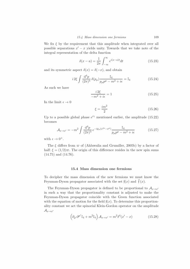
15.4 Mass dimension one fermions 109

We fix ξ by the requirement that this amplitude when integrated over all

possible separations x′ − x yields unity. Towards that we take note of the

integral representation of the delta function

δ(x − a) =1

2π

∫ ∞

−∞ei(x−a)tdt (15.23)

and its symmetric aspect δ(x) = δ(−x), and obtain

i 2ξ

∫d4p

(2π)4δ(pµ)

I4

pµpµ −m2 + iǫ= I4 (15.24)

As such we havei 2ξ

−m2 + iǫ= 1 (15.25)

In the limit ǫ→ 0

ξ =im2

2(15.26)

Up to a possible global phase eiγ mentioned earlier, the amplitude (15.22)

becomes

Ax→x′ = −m2

∫d4p

(2π)4e−ipµ(x

′µ−xµ) I4

pµpµ −m2 + iǫ(15.27)

with ǫ→ 0+.

The ξ differs from of (Ahluwalia and Grumiller, 2005b) by a factor of

half: ξ = (1/2). The origin of this difference resides in the new spin sums

(14.75) and (14.76).

15.4 Mass dimension one fermions

To decipher the mass dimension of the new fermions we must know the

Feynman-Dyson propagator associated with the set f(x) and¬

f (x).

The Feynman-Dyson propagator is defined to be proportional to Ax→x′

in such a way that the proportionality constant is adjusted to make the

Feynman-Dyson propagator coincide with the Green function associated

with the equation of motion for the field f(x). To determine this proportion-

ality constant we act the spinorial Klein-Gordon operator on the amplitude

Ax→x′ (∂µ′∂

µ′I4 +m2

I4

)Ax→x′ = m2δ4(x′ − x) (15.28)

110 Mass dimension one fermions

So we define the Feynman-Dyson propagator

SFD(x′ − x)

def= − 1

m2Ax→x′

=

∫d4p

(2π)4e−ipµ(x

′µ−xµ) I4

pµpµ −m2 + iǫ(15.29)

With this definition(∂µ′∂

µ′I4 +m2

I4

)SFD(x

′ − x) = −δ4(x′ − x) (15.30)

and the Feynman-Dyson propagator in terms of the new field and its adjoint

takes the form

SFD(x′ − x) = − i

2

⟨ ∣∣∣T(f(x′) ¬

f (x)∣∣∣⟩

(15.31)

Following the canonical discussion on the mass dimensionality of quantum

fields given in (Weinberg, 2005, Section 12.1) we find that mass dimension

of the field f(x) is one

Df = 1 (15.32)

and not three-half, as is the case for the Dirac field: for large momenta p,

SFD(x′ − x) ∝ p−1 for the latter, while for the new field SFD(x

′ − x) ∝ p−2.

This result is precisely what was hinted at by our discussion in section 9.

The discussion of section 9, when coupled with the results encoded in

equations (15.29) and (15.30), suggests the following free field Lagrangian

density for the new field

L0(x) =1

2

(∂a

¬

f ∂af(x)−m2 ¬

f (x)f(x))

(15.33)

where we have taken liberty to let a, b, . . . take the flat space values (0, 1, 2, 3),

and reserve µ, ν, etc to take on the values for the names of the co-ordinates

in the gravitational context, for example (t, x, y, z). The motivation to in-

troduce the factor of half resides in our desire to obtain canonical form of

the locality anticommutators. It does not alter the equation of motion.

Like the Dirac fermions, the new fermions, are of spin one half. Both

satisfy Klein-Gordon equation. For the former the “factorisation” of the

Klein-Gordon operator occurs through the Dirac operator, while for the

latter it occurs through equations (9.14) to (9.17). The expansion coefficients

of the former are a complete set of eigenspinors of the parity operator, while

for the latter the expansion coefficients are a complete set of eigenspinors of

the charge conjugation operator. Both the fields are local as we shall soon

discover in section 15.5.

15.4 Mass dimension one fermions 111

Gravity enters the realm of Elko and mass dimension one fermions by

introducing tetrads eaµ through eaµebνηab = gµν . Here gµν is the spacetime

metric and ηab = diag(1,−1,−1,−1). Thus, for example, space-time Dirac

matrices are connected with their flat space counterpart by γµ = eµaγa, which

consequently satisfy

γµ, γν = 2gµν (15.34)

The Latin indices – a, b, . . . = 0, 1, . . ., called non-holonomic indices – refer

to a local inertial frame. Greek indices – µ, ν, . . . = t, . . ., called holonomic

indices – refer to a generic non-inertial frame.

The Lagrangian density (15.33) for the mass dimension one fermions in a

torsion-free gravitational field follows the prescription

∂af(x) → ∇µf(x)def= ∂µf(x)− Γµf(x) (15.35)

∂a¬

f (x) → ∇µ¬

f (x)def= ∂µ

¬

f +¬

f (x)Γµ (15.36)

where

Γµ =i

2ωabµ

(Jab

∣∣∣(R⊕L)s=1/2

)(15.37)

and the spin connection is defined as

ωabµ = eaν

(∂µe

νb + eσbΓνµσ

)(15.38)

with Γνµσ denoting the Christoffel symbol associated with gµν . In addition

Jab

∣∣∣(R⊕L)s=1/2

=

Jij = −Jji = ǫijkζk

Ji0 = −J0i = −κi(15.39)

Equation (5.6) provides explicit expressions for κ and ζ, respectively the

boost and rotation generators in the R ⊕ L representations space for spin

one half.

This prescription is as valid for Elko as for the Dirac spinors because the

spinorial covariant derivative depends on the generators of the Lorentz alge-

bra for spin one half in the indicated fashion. Bohmer has verified this obser-

vation independently, without invoking our argument, in (Boehmer, 2007b).

The physics of Elko and torsion is discussed at length in (Fabbri, 2011a;

Kouwn et al., 2013; Fabbri and Vignolo, 2014; Pereira and Guimares, 2017;

Pereira et al., 2017a). In the presence of torsion, denoted by a ‘tilde’ above

the symbols, the spinorial covariant derivatives no longer commute[∇µ, ∇ν

]6= O (15.40)

112 Mass dimension one fermions

and (15.33) is modified to

L(x) =1

2

(∇µ ¬

f ∇µf(x)−m2 ¬

f (x)f(x))

(15.41)

allowing for such additional interactions as

1

2∇µ

¬

f (x)σµν∇νf(x) (15.42)

with

σµνdef=

1

4

[γµ, γν

](15.43)

This was first noted by Luca Fabbri in (Fabbri, 2011a).

Despite formal similarity, Elko and Dirac spinors experience gravity dif-

ferently. From a physical point of view the R and L transforming com-

ponents of Elko pick up different, and in certain circumstances opposite,

gravitationally-induced phase factors. This is apparent from their helicity

structure (Ahluwalia, 2004).

Another distinguishing feature of Elko arises from the contribution to

the energy-momentum tensor from the variation of spin connection. For the

Dirac spinors this contribution identically vanishes. In contrast, for Elko

it idoes not. This was first noted by Christian Bohmer in (Boehmer et al.,

2010).

15.5 Locality structure of the new field

Now that we have L0(x) we can calculate the momentum conjugate to f(x)

p(x) =∂L0(x)

∂ f(x)=

1

2

∂

∂t

¬

f (x). (15.44)

To establish that the new field is local we calculate the standard equal-time

anti-commutators. The first of the three anti-commutators we calculate is

the ‘f-p’ anti-commutator

f(t,x), p(t,x′)

. (15.45)

With the defintion

∑

α,p

def=

∫d3p

(2π)31√

2mE(p)

∑

α

(15.46)

15.5 Locality structure of the new field 113

it expands to

1

2

∑

α,p

∑

α′,p′

(iE(p′

) [aα(p), a

†α′(p

′)λSα(p)

¬

λS

α′(p′)e−ip·x+ip′·x′

−bα(p), b

†α′(p

′)λAα (p)

¬

λA

α′(p′)eip·x−ip′·x′

](15.47)

Replacing each of the anticommutators by (2π)3 δ3(p− p′) δαα′ and perform-

ing the p′ integration, and α′ summation, followed by (a) change of variables

p → −p in the second integration, and (b) noting that the t dependence in

the exponentials cancels out, we get

i

4m

∫d3p

(2π)3eip·(x−x′)

∑

α

(λSα(p)

¬

λS

α(p)− λAα (−p)¬

λA

α (−p))

(15.48)

The first spin sum evaluates to 2mI, while the second equals −2mI, giving

the result 4mI for the summation over α. This gives usf(t,x), p(t,x′)

= iδ3

(x− x′

)I4. (15.49)

Had we not included a factor 1/2 in the definition of the Lagrangian density

in (15.33) we would have gotten an additional factor of 2 multiplying the

delta function in the above result.

A still simpler calculation shows that the remaining two, that is, ‘f-f’ and

‘p-p’, equal time anti-commutators vanishf(t,x), f(t,x′)

= 0,

p(t,x), p(t,x′)

= 0. (15.50)

The field f(x) is thus local in the sense of Schwinger (Schwinger, 1951, Sec.

II, Eqs. 2.82). It is a much stronger condition of locality than that adopted

by Schwartz (Schwartz, 2014b, Sec. 24.4).

15.5.1 Majorana-isation of the new field

Even though field f(x) is uncharged under local U(1) supported by the Dirac

fields of the standard model of high energy physics, it may carry a charge

under a different local U(1) gauge symmetry such as the one suggested in

the discussion around (7.14). This gives rise to the possibility of having a

fundamentally neutral field in the sense of Majorana (Majorana, 1937)

m(x) =

∫d3p

(2π)31√

2mE(p)

114 Mass dimension one fermions

×∑

α

[aα(p)λ

S(p) exp(−ipµxµ) + a†α(p)¬

λA(p) exp(ipµx

µ)]

(15.51)

with momentum conjugate

q =1

2

∂

∂t

¬

m(x). (15.52)

The calculation for the ‘m-q’ equal time anti-commutators goes through

exactly as before and one getsm(t,x), q(t,x′)

= iδ3

(x− x′

)I4. (15.53)

The calculation of the remaining two anti-commutators requires knowledge

of the following ‘twisted’ spin sums∑

α

[λSα(p)

[λAα (p)

]T+ λAα (−p)

[λSα(−p)

]T ](15.54)

∑

α

[[¬

λS

α(p)]T

¬

λA

α (p) +[

¬

λA

α (−p)]T

¬

λS

α(−p)

]. (15.55)

One finds that each of these vanishes. With this result at hand, we immedi-

ately decipher vanishing of the ‘m-m’ and ‘q-q’, equal time anti-commutators

m(t,x), m(t,x′)

= 0,

q(t,x), q(t,x′)

= 0. (15.56)

The field m(x), like f(x), is thus local in the sense of Schwinger (Schwinger,

1951, Sec. II, Eqs. 2.82).

16

Mass dimension one fermions as a first principledark matter

16.1 Mass dimension one fermions as dark matter

• A mass dimension mismatch between the new fermions and the standard

model matter fields – one versus three halves – forbids them to enter

the standard model doublets. In the process their interaction with the

standard model fields is severely restricted.

One exception is the dimension four operators

λfφ¬

f (x)f(x)φ†(x)φ(x), λmφ¬

m(x)m(x)φ†(x)φ(x) (16.1)

where λfφ and λmφ are dimensionless coupling constant, and φ(x) is the

Higgs doublet. For the Dirac field, a similar interaction is a dimension five

operator. It is thus suppressed by one power of the unification/Planck

scale.

Therefore, mass dimension one fermions are natural dark matter can-

didate. Compared to bosonic dark matter a fermionic dark matter brings

with it Pauli exclusion principle to affect structure formation.

• The system of mass dimension one fermions further supports perturba-

tively re-normalisable dimension-four quartic self interactions

λf

(¬

f (x)f(x))2, λm

(¬

m(x)m(x))2

(16.2)

where λf and λm are dimensionless coupling constants. A similar quar-

tic self interaction for the Dirac field, with or without Majorana-isation,

is a dimension six operator. It is thus suppressed by two power of the

unification/Planck scale.

Observational evidence that favours self interacting dark matter is re-

viewed in (Tulin and Yu, 2018) and in a Ph.D. thesis by Robertson (Robertson,

116 Mass dimension one fermions as a first principle dark matter

2017). An early reference is (Spergel and Steinhardt, 2000). Following

these references we simply note that self interacting dark matter pro-

vides a heat transport mechanism from the outer hotter to the cooler

inner region of dark matter halos. It thermalises the inner halo and leads

to a uniform velocity distribution as one moves outward in the halo.

• The very definition of Elko does not allow covariance under local phase

transformations of the standard model (see, section 7.2 for local U(1)).

This endows the new fermions with a natural darkness with respect to

the standard model fields while leaving open the possibility of new gauge

symmetries that apply to mass dimension one fermions.

Beyond the dimension-four interactions mentioned above one may also in-

troduce the following Yukawa couplings of dimension three and half (Dasgupta,

2016)

λ1 ϕ(x)ψ(x)f(x), λ2 ϕ(x)¬

f (x)ψ(x) (16.3)

λ3 ϕ(x)ψ(x)m(x), λ4 ϕ(x)¬

m(x)ψ(x) (16.4)

where ψ(x) is a Dirac/Majorana field, ϕ(x) is a scalar field, and λ′s are

dimensionfull coupling constants. These may be used to violate conserva-

tion of all three of the following: lepton number, electric charge, and dark

charges33

The interactions of the form

ǫ¬

f (x)[γa, γb

]f(x)Fab(x), ε

¬

m(x)[γa, γb

]m(x)Fab(x) (16.5)

with dimensionless couplings ǫ and ε are severely restricted due to strin-

gent limits on photon mass (Accioly and Paszko, 2004; Luo et al., 2003;

Bonetti et al., 2016). Nevertheless, they could have significant astrophysi-

cal and cosmological implications where the smallness of the couplings may

be compensated by huge dark matter densities. One crucial arena where

such couplings may manifest are in 21-cm cosmology (Barkana et al., 2018).

16.2 A conjecture on a mass dimension transmuting symmetry

A single component dark matter sector is likely to be an oversimplified view

of the cosmological reality with the possibility of distorting our intuitions.

33 A similar mass dimension four coupling, without a quartic self interaction term, ofDirac/Majorana fermions to a scalar can be found in (Kainulainen et al., 2016).

16.3 Elko inflation and Elko dark energy 117

We conjecture that the realm of dark matter is populated by a set of fields

of the f(x) type and its Majorana-ised form m(x). We envisage the possi-

bility that a mass dimension transmuting symmetry exists. It takes mass

dimension one fermions to mass dimension three halves fermions, and vice

versa. Unlike supersymmetry the conjectured new symmetry does not alter

the statistics, but only the mass dimensionality.

In this possibility for every standard model fermion there exists a mass di-

mension one fermion, and vice versa. The possibility that Higgs is shared by

both the sectors is the simplest unifying theme we can envisage. To complete

our conjecture we suggest that dark gauge fields mirror the standard model

gauge fields. The coupling constants and masses we leave as free parameters,

but we would be surprised if they were not related to those of the standard

model. Echoing the arguments of (Hardy et al., 2015; McDermott, 2017):

Combined, the dark sector may support some sort of dark fusion leading to

dark nucleosynthesis.

A parenthetic remark —

For reasons to be soon encountered the dark sector supported by Elko

has distinctive gravitational signatures with torsion revealing aspects that

are absent with the Dirac spinors. Elko cosmology is still in its infancy,

and given its first principle origins it holds promise to give us observational

signatures not yet anticipated by cosmologists. Observations can be easily

misinterpreted in the absence of a systematic development of a cosmology

that fully incorporates the new fermions. Such a process was begun by Chris-

tian Bohmer, and is now an active realm of researches by a new generation

of physicists mostly from South America, Europe, and Asia.

16.3 Elko inflation and Elko dark energy

Echoing the closing remarks of the last section, Christian Bohmer was the

first cosmologist to realise that:

• Elko not only help formulate mass dimension one fermions for dark matter,

as Daniel Grumiller and I had argued, but also that Elko could serve as

as a source of inflation and could drive the accelerated expansion of the

universe (Boehmer, 2007a,b, 2008).

• In a stark contrast to Dirac spinors, Elko energy momentum tensor Tµν

118 Mass dimension one fermions as a first principle dark matter

has an important non-vanishing contribution from the variation of spin

connection (Boehmer et al., 2010).

These early works inspired a series of efforts to explore Elko as a source

inflation, dark matter, and dark energy. Christian Bohmer was also the first

to note that the spin angular momentum tensor associated with Elko can-

not be entirely expressed as an axial torsion vector (Boehmer, 2007a). He

emphasised that this important difference from the Dirac spinors arises due

to different helicity structures of the Elko and Dirac spinors. His ground-

breaking paper also put forward a tiny coupling of Elko to Yang-Mills fields

and discussed its implications for consistently coupling massive spin one

field to the Einstein-Cartan theory. Restricting to the Einstein-Elko system

he constructed analytical ghost Elko solutions with the property of a van-

ishing energy-momentum tensor (Boehmer, 2007a). This was done to make

the analytical calculations possible34 and he showed that, “the Elko . . . are

not only prime dark matter candidates but also prime candidates for in-

flation.” With his collaborators Bohmer has placed Elko cosmology on a

firm footing with an eye on the available data. We refer the reader to ref-

erences (Boehmer and Mota, 2008; Boehmer, 2008; Boehmer and Burnett,

2008, 2010; Boehmer et al., 2010) for details. While building Elko cosmology

he has coined the term “dark spinors” for Elko.

The group of Julio Hoff da Silva and Saulo Pereira, focusing on ex-

act analytical solutions, have taken Elko cosmology significantly beyond

Bohmer’s initial pioneering efforts. We refer the reader to their publica-

tions (Hoff da Silva and Pereira, 2014; Pereira et al., 2014; dos Santos Souza et al.,

2015; Pereira and S., 2014). Concurrently extending the work of Bohmer,

Gredat and Shankaranarayanan have considered an Elko-condensate driven

inflation and shown that it is favoured by existing observational data (Gredat and Shankaranarayanan,

2010). This work has been followed by Basak and Shankaranarayanan to

prove that, “Elko driven inflation can generate growing vector modes even

in the first order.” This allows them to generate vorticity during inflation to

produce primordial magnetic field (Basak and Shankaranarayanan, 2015).

Basak et al. show that Elko cosmology provides two sets of attractor

points. These correspond to slow and fast-roll inflation. The latter being

unique to Elko (Basak et al., 2013). For earlier contribution to Elko cos-

mology from this group we refer the reader to (Shankaranarayanan, 2010,

2009). The cosmological coincidence problem in the context of Elko is dis-

cussed by Hao Wei in reference (Wei, 2011), and has been revisited in

34 This assumption was later placed on a more natural footing by (Chang et al., 2015) et al.

16.4 Darkness is relative, not self referential 119

(Bahamonde et al., 2017, Sec. 7.1). One of the early papers on stability of

de Sitter solution in the context of Elko is (Chee, 2010).

Elko cosmology has gained a significant and independent boost through

a recent study of phantom dark-energy Elko/dark-spinors undertaken by

Yu-Chiao Chang et al. In the context of Einstein-Cartan theory it resolves

a host of problems with phantom dark energy models and predicts a final

de Sitter phase for our universe at late time with or without dark mat-

ter (Chang et al., 2015). Their work not only makes Elko and mass dimen-

sion one fermions more physically viable but it also lends concrete physicality

to torsion as an important possible element of reality.

16.4 Darkness is relative, not self referential

To avoid confusion, a clarifying remark seems necessary: The dark sector

need not be self referentially dark. To dark matter, and to the all pervading

field – dark energy – responsible for the accelerated expansion of the uni-

verse, we are dark. But, darkness is relative, and the dark sector may not

be self referentially dark. It may support its own gauge fields, and carry its

own luminosity. Our luminosity arises from the gauge fields supported by

the matter fields which use eigenspinors of the parity operator as its expan-

sion coefficients. A self referentially luminous dark sector may arise from the

gauge fields that matter fields based on Elko support.

17

Continuing the story

In this closing chapter, I take the liberty of suggesting what in essence are

research projects that a beginning students may pursue. Most of these have

been developed in detail in my private notes. I would be happy to share the

details with anyone interested in pursuing them further.

17.1 Constructing the spacetime metric from Lorentz algebra

Returning to section 4.4 we continue an ab initio examination of four vectors

spanning the R⊗L|s=1/2 representation space. We denote these vectors by

χ, and take them in the form of four-component columns with their elements

in C. We shall assume that we have implemented the rotation defined by

U of equation (4.56), then if χ represents the position of an event then the

elements take values in ℜ but otherwise this restriction is not necessary.

Following the discussion in chapter 14 the simplest dual for χ is

χdef= χ†η (17.1)

In order that χχ is an invariant for observers connected by Lorentz trans-

formations, the metric η must satisfy

Ki, η = 0, [Ji, η] = 0, i = x, y.z (17.2)

with the boost and rotation generators, Ki and Ji, defined by equations

(3.21) to (3.24).

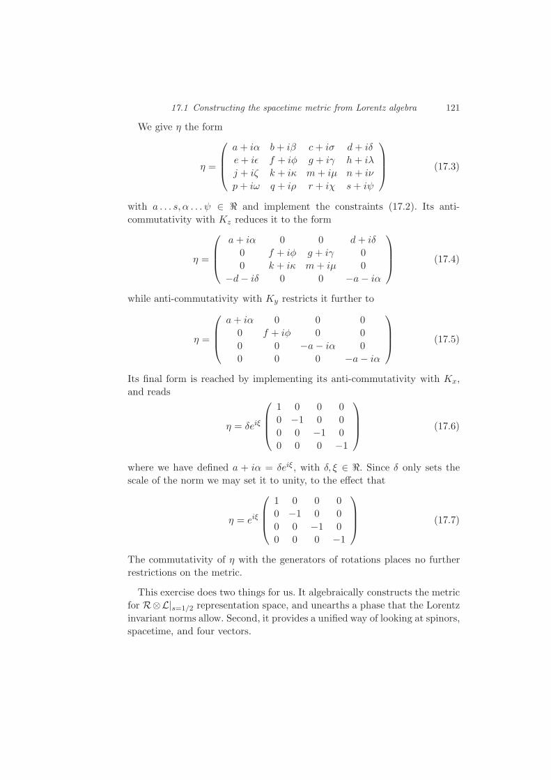
17.1 Constructing the spacetime metric from Lorentz algebra 121

We give η the form

η =

a+ iα b+ iβ c+ iσ d+ iδ

e+ iǫ f + iφ g + iγ h+ iλ

j + iζ k + iκ m+ iµ n+ iν

p+ iω q + iρ r + iχ s+ iψ

(17.3)

with a . . . s, α . . . ψ ∈ ℜ and implement the constraints (17.2). Its anti-

commutativity with Kz reduces it to the form

η =

a+ iα 0 0 d+ iδ

0 f + iφ g + iγ 0

0 k + iκ m+ iµ 0

−d− iδ 0 0 −a− iα

(17.4)

while anti-commutativity with Ky restricts it further to

η =

a+ iα 0 0 0

0 f + iφ 0 0

0 0 −a− iα 0

0 0 0 −a− iα

(17.5)

Its final form is reached by implementing its anti-commutativity with Kx,

and reads

η = δeiξ

1 0 0 0

0 −1 0 0

0 0 −1 0

0 0 0 −1

(17.6)

where we have defined a + iα = δeiξ , with δ, ξ ∈ ℜ. Since δ only sets the

scale of the norm we may set it to unity, to the effect that

η = eiξ

1 0 0 0

0 −1 0 0

0 0 −1 0

0 0 0 −1

(17.7)

The commutativity of η with the generators of rotations places no further

restrictions on the metric.

This exercise does two things for us. It algebraically constructs the metric

for R⊗L|s=1/2 representation space, and unearths a phase that the Lorentz

invariant norms allow. Second, it provides a unified way of looking at spinors,

spacetime, and four vectors.

122 Continuing the story

If we require a reality of the norm for χ, with all its four elements ∈ ℜ,the phase angle ξ can be restricted as follows

ξ =

0, to yield η in the West coast form

π, to give the East coast version of η(17.8)

This is useful for spacetime vectors. On the other hand, in a quantum context

where χ may be a vector field, a non-vanishing ξ, 0 ≤ ξ ≤ π, opens a

discussion which was not possible hitherto: that is, before the discovery of

the phase eiξ in (17.7).

17.2 The [R⊗L]s=1/2 representation space

A field transforming according to [R⊗L]s=1/2 representations can be bi-

furcated into two Casimir sectors: one, with eigenvalue 2 = 1(1 + 1), and

the other with eigenvalue 0 = 0(0 + 1). The eigenvalue 2 sector is three

fold degenerate, which in the rest frame can be distinguished with eigen-

values +1, 0,−1 of spin one Jz. The Casimir sector with eigenvalue 0 is

non-degenerate.

A quantum field defined with the three degrees of freedom associated

with the Casimir sector of eigenvalue 2 is known to violate unitarity at high

energies. The unitarity is restored to construct a renormalisable theory in the

form of the standard model of high energy physics at the cost of introducing

Higgs through spontaneous symmetry breaking. Historically, it served as a

departure to develop gauge theories.

It is and was conventional to project out the Casimir sector with the

vanishing eigenvalue. But, can one project out degrees of freedom from a

representation space without violating something deep about the symmetries

that gives birth to the very representation space on which a quantum field

is built upon?

To cosnider this question we backtrack to our discussion in Section 2.2

of (Ahluwalia and Grumiller, 2005b) that a similar projecting out from the

[R⊕L]s=1/2 representation space would have excluded antiparticles from

the Dirac’s theory. Mass dimension one fermions come to exist because we do

not ignore the two degrees of freedom associated with the anti-self conjugate

spinors. Incorporating them in the theory brings about dark matter, or at

least a first principle candidate for dark matter with quartic self interaction,

and an unusual property associated with rotation of dark matter clouds

based on Elko.

17.3 Maxwell equations and beyond 123

With that background we suspect that something similar may be happen-

ing in the conventional treatment of the [R⊗L]s=1/2 representation space.

Inadvertently, we may be projecting out something that could morph into

a Higgs.

One can now define a field that contains expansion coefficients correspond-

ing to the three degrees of freedom associated with the Casimir invariant

2 sector, and one from the Casimir invariant 0 sector. The dual of the ex-

pansion coefficients is so defined that the two Casimir sectors have their

own phase angle ξ. This modifies the adjoint of the field. As a result the

the phase angles end up showing in the vacuum expectation value of the

calculated Feynman-Dyson propagator and can be so adjusted as to ob-

tain a well-behaved propagator that does not lead to unitarity violation at

high energies, or to the negative norm states. The latter aspect is related

to the fact that the creation and destruction operators satisfy the bosonic

commutators.

The result is that the resulting field contains, what in the rest frame,

can be called spin one and spin zero. Such a scenario can serve as an ab

initio starting point to better understand origin of the Higgs mechanism

and spontaneous symmetry breaking.35 Extended to ‘spin 2’, the argument

suggests ‘spin 1’ and ‘spin 0’ Higgs like bosons.

17.3 Maxwell equations and beyond

When one extends the work of Chapter 5 to the R⊕L representation space

of spin one and two, and takes the massless limit, one reaches a deeper

understanding of Maxwell equations and Einstein’s gravity in the weak field

limit. A helpful reference is (Weinberg, 1964b), but care must be taken to

check the invertibility of J · ∇ operator (Ahluwalia and Ernst, 1992).

35 The just outlined calculation for the new field has been a subject of various discussions withSebastian Horvath, Cheng-Yang Lee, and Dimitri Schritt as is the extension to higher spins.It must be considered preliminary.

Appendix: Further reading

Recently Saulo Pereira and R. C. Lima have shown that an asymptotically

expanding universe creates low-mass mass dimension one fermions much

more copiously than Dirac fermions (of the same mass) (Pereira and Lima,

2017). If their preliminary results remain essentially unaffected by the new

results presented here it would significantly help us to develop a first-principle

cosmology based on Elko and mass dimension one fermions.

Various Brazilian-Italian group of physicists have examined such impor-

tant topics as Hawking radiation of mass dimension one fermions (da Rocha and Hoff da Silva,

2014), and continue to develop mathematical physics underlying Elko (da Rocha and Pereira,

2007; da Rocha and Hoff da Silva, 2007, 2010; Hoff da Silva and da Rocha,

2009; da Rocha et al., 2011a,b; Bernardini and da Rocha, 2012; Hoff da Silva and da Rocha,

2013; da Rocha et al., 2013; Cavalcanti et al., 2014; da Rocha and Hoff da Silva,

2014; Bonora and da Rocha, 2016; da Rocha and Cavalcanti, 2016; Bueno Rogerio et al.,

2016; Hoff da Silva et al., 2016a, 2017; Neto, 2017). Of these we draw par-

ticular attention to mass-dimension transmuting operators considered in

(da Rocha and Hoff da Silva, 2007; Hoff da Silva and da Rocha, 2009). It

would help define a new symmetry between the Dirac field and the field as-

sociated with mass dimension one fermions if mass-dimension transmuting

operators could be placed on a rigorous footing after incorporating locality

and Lorentz covariance.36

Max Chaves and Doug Singleton have suggested that mass dimension

one fermions of spin one half may have a possible connection with mass-

dimension-one vector particles with fermionic statistics (Chaves and Singleton,

2008). It may be worth examining if a new fundamental symmetry may be

36 The need for a mass-dimension transmuting symmetry was first suggested by the presentauthor to Roldao da Rocha several years ago and is briefly mentioned in section 16.2.

Appendix: Further reading 125

constructed that relates the works of (da Rocha and Hoff da Silva, 2007;

Hoff da Silva and da Rocha, 2009) with those of Chaves and Singleton.

Localisation of Elko in the brane has been considered in references (Liu et al.,

2012; Jardim et al., 2015; Zhou et al., 2017). Elko in the presence of torsion

has been a subject of several insightful papers by Luca Fabbri. We refer the

reader to these and related publications (Fabbri, 2010; Fabbri and Vignolo,

2012b; Fabbri, 2011a,b, 2012; Fabbri and Vignolo, 2012a, 2014). Cosmolog-

ical solutions of 5D Einstein equations with Elko condensates were obtained

by Tae Hoon Lee where it was found that there exist exponentially expanding

cosmological solution even in the absence of a cosmological constant (Lee,

2012).

We parenthetically note that all the works discussed so far remain essen-

tially unchanged with the new developments reported here. In view of the

new results on locality and Lorentz covariance it is important to revisit the

analysis and claims of (Basak and Bhatt, 2011) and also those calculations

that use full apparatus of the theory of quantum fields, and not merely

Elko. In the same thread, given the interest in mass dimension one fermions

a number of S-matrix calculations were done and published (Dias et al.,

2012; Lee and Dias, 2016; Alves et al., 2014, 2015; Agarwal et al., 2015; Lee,

2016b; Alves et al., 2018). These need to be revisited also.

References

Accioly, Antonio, and Paszko, Ricardo. 2004. Photon mass and gravitational de-flection. Phys. Rev. D, 69(May), 107501.

Agarwal, B., Jain, P., Mitra, S., Nayak, A. C., and Verma, R. K. 2015. Elko fermionsas dark matter candidates. Phys. Rev., D92, 075027. arXiv: 1407.0797[hep-ph].

Aharonov, Yakir, and Susskind, Leonard. 1967. Observability of the sign change ofspinors under 2π rotations. Phys. Rev., 158, 1237–1238.

Ahluwalia, D. V. 1994. Quantum measurement, gravitation, and locality. Phys.Lett., B339, 301–303. arXiv: gr-qc/9308007.

Ahluwalia, D. V. 1995. A new type of massive spin one boson: And Its relationwith Maxwell equations. In: The present status of the quantum theory of light.Proceedings, Symposium in Honour of Jean-Pierre Vigier, Toronto, Canada,August 27-30, 1995.

Ahluwalia, D. V. 1996. Theory of neutral particles: McLennan-Case construct forneutrino, its generalization, and a fundamentally new wave equation. Int. J.Mod. Phys., A11, 1855–1874. arXiv: hep-th/9409134[hep-th].

Ahluwalia, D. V. 1998. Book review of Quantum Field Theory by Lewis H. Ryder.Foundations of Physics, 28, 527–529.

Ahluwalia, D. V. 2000. Wave particle duality at the Planck scale: Freezing ofneutrino oscillations. Phys. Lett., A275, 31–35. arXiv: gr-qc/0002005.

Ahluwalia, D. V. 2003. Extended set of Majorana spinors, a new dispersion relation,and a preferred frame. arXiv: hep-ph/0305336 (unpublished)[hep-ph].

Ahluwalia, D. V. 2004. Charge conjugation and Lense-Thirring effect: A New asym-metry. Int. J. Mod. Phys., D13, 2361–2367. arXiv: gr-qc/0405112[gr-qc]. [Gen.Rel. Grav. 36, 2581 (2004)].

Ahluwalia, D. V. 2017a. Evading Weinberg’s no-go theorem to construct massdimension one fermions: Constructing darkness. EPL, 118(6), 60001. arXiv:1605.04224[hep-th].

Ahluwalia, D. V. 2017b. Reflections of the observer and the observed in quantumgravity. Int. J. Mod. Phys., D26(12), 1743001. arXiv: 1706.05927[gr-qc].

Ahluwalia, D. V. 2017c. The theory of local mass dimension one fermions of spin onehalf. Adv. Appl. Clifford Algebras, 27(3), 2247–2285. arXiv: 1601.03188[hep-th].

Ahluwalia, D. V., and Grumiller, D. 2005a. Dark matter: A spin one half

128 References

fermion field with mass dimension one? Phys. Rev., D72, 067701. arXiv:hep-th/0410192[hep-th].

Ahluwalia, D. V., and Grumiller, D. 2005b. Spin half fermions with mass dimensionone: Theory, phenomenology, and dark matter. JCAP, 0507, 012. arXiv:hep-th/0412080[hep-th].

Ahluwalia, D. V., and Horvath, S. P. 2010. Very special relativity as relativity ofdark matter: The Elko connection. JHEP, 11, 078. arXiv: 1008.0436[hep-ph].

Ahluwalia, D. V., and Nayak, A. C. 2015. Elko and mass dimension one field ofspin one half: causality and fermi statistics. Int. J. Mod. Phys., D23, 1430026.arXiv: 1502.01940[hep-th].

Ahluwalia, D. V., and Sawicki, M. 1993. Front form spinors in the Weinberg-Soperformalism and generalized Melosh transformations for any spin. Phys. Rev.,D47, 5161–5168. arXiv: nucl-th/9603019[nucl-th].

Ahluwalia, D. V., Lee, Cheng-Yang, and Schritt, D. 2010. Elko as self-interactingfermionic dark matter with axis of locality. Phys. Lett., B687, 248–252. arXiv:0804.1854[hep-th].

Ahluwalia, D. V., Horvath, S. P., and Schritt, D. 2011a. Amplitudes for space-likeseparations and causality. arXiv: 1110.1162[hep-ph].

Ahluwalia, D. V., Lee, Cheng-Yang, and Schritt, D. 2011b. Self-interacting Elkodark matter with an axis of locality. Phys. Rev., D83, 065017. arXiv:0911.2947[hep-ph].

Ahluwalia, Dharam Vir, and Ernst, D. J. 1992. Paradoxical kinematic acausalityin Weinberg’s equations for massless particles of arbitrary spin. Mod. Phys.Lett., A7, 1967–1974.

Ahluwalia, Dharam Vir, and Sarmah, Sweta. 2018. Behaviour of the eigen-spinors of the charge conjugation operator under spatial rotations. arXiv:1810.04985[hep-th].

Aitchison, I. J. R., and Hey, A. J. G. 2004. Gauge theories in particle physics:A practical introduction. Vol. 2: Non-Abelian gauge theories: QCD and theelectroweak theory. Bristol, UK: IOP (2004) 454 p. The citations in themonograph refer to this edition.

Alves, A., Dias, M., and de Campos, F. 2014. Perspectives for an Elko Phenomenol-ogy using monojets at the 14 TeV LHC. Int. J. Mod. Phys., D23, 1444005.arXiv: 1410.3766[hep-ph].

Alves, A., de Campos, Fernando, Dias, M., and Hoff da Silva, J. M. 2015. Searchingfor Elko dark matter spinors at the CERN LHC. Int. J. Mod. Phys., A30,1550006. arXiv: 1401.1127[hep-ph].

Alves, Alexandre, Dias, M., de Campos, F., Duarte, L., and Hoff da Silva, J. M.2018. Constraining Elko dark matter at the LHC with monophoton Events.EPL, 121(3), 31001. arXiv: 1712.05180[hep-ph].

Anonymous Referee. 2006. Referee report for Marsden application 07-UOC-055(Royal Society of New Zealand) “Dark Matter and its Darkness”.

Atiyah, Michael. 2013. What is a spinor?https://www.youtube.com/watch?v=SBdW978Ii_E.

Bahamonde, S., Boehmer, C. G., Carloni, S., Copeland, E. J., Fang, Wei, andTamanini, Nicola. 2017. Dynamical systems applied to cosmology: dark energyand modified gravity. arXiv: 1712.03107[gr-qc].

Barkana, R., Outmezguine, N. J., Redigolo, D., and Volansky, T. 2018. Signs ofDark Matter at 21-cm? arXiv: 1803.03091[hep-ph].

References 129

Barkana, Rennan. 2018. Possible interaction between baryons and dark-matterparticles revealed by the first stars. Nature, 555(7694), 71–74. arXiv:1803.06698[astro-ph.CO].

Basak, A., and Bhatt, J. R. 2011. Lorentz invariant dark-spinor and inflation.JCAP, 1106, 011. arXiv: 1104.4574[astro-ph.CO].

Basak, A., and Shankaranarayanan, S. 2015. Super-inflation and generation of firstorder vector perturbations in Elko. JCAP, 1505, 034. arXiv: 1410.5768[hep-ph].

Basak, A., Bhatt, Jitesh R., Shankaranarayanan, S., and Prasantha Varma, K. V.2013. Attractor behaviour in Elko cosmology. JCAP, 1304, 025. arXiv:1212.3445[astro-ph.CO].

Bernardini, A. E., and da Rocha, R. 2012. Dynamical dispersion relation for Elkodark spinor fields. Phys. Lett., B717, 238–241. arXiv: 1203.1049[hep-th].

Bertone, Gianfranco, and Hooper, Dan. 2018. A History of Dark Matter. Rev. Mod.Phys., 90(4), 045002. arXiv: 1605.04909[astro-ph.CO].

Boehmer, C. G. 2007a. The Einstein-Cartan-Elko system. Annalen Phys., 16,38–44. arXiv: gr-qc/0607088[gr-qc].

Boehmer, C. G. 2007b. The Einstein-Elko system: Can dark matter drive inflation?Annalen Phys., 16, 325–341. arXiv: gr-qc/0701087[gr-qc].

Boehmer, C. G. 2008. Dark spinor inflation: Theory primer and dynamics. Phys.Rev., D77, 123535. arXiv: 0804.0616[astro-ph].

Boehmer, C. G., and Burnett, J. 2008. Dark spinors with torsion in cosmology.Phys. Rev., D78, 104001. arXiv: 0809.0469[gr-qc].

Boehmer, C. G., and Burnett, J. 2010. Dark energy with dark spinors. Mod. Phys.Lett., A25, 101–110. arXiv: 0906.1351[gr-qc].

Boehmer, C. G., and Mota, D. F. 2008. CMB anisotropies and inflation from non-standard Spinors. Phys. Lett., B663, 168–171. arXiv: 0710.2003[astro-ph].

Boehmer, C. G., Burnett, J., Mota, D. F., and Shaw, D. J. 2010. Dark spinor modelsin gravitation and cosmology. JHEP, 07, 053. arXiv: 1003.3858[hep-th].

Bonetti, L., Ellis, J., Mavromatos, N. E., Sakharov, A. S., Sarkisyan-Grinbaum,Edward K. G., and Spallicci, Alessandro D. A. M. 2016. Photon mass limitsfrom fast radio bursts. Phys. Lett., B757, 548–552. arXiv: 1602.09135[astro-ph.HE].

Bonora, L., and da Rocha, R. 2016. New spinor fields on Lorentzian 7-manifolds.JHEP, 01, 133. arXiv: 1508.01357[hep-th].

Brown, H. R. 2005. Physical relativity: Space-time structure from a dynamicalperspective. Oxford University Press.

Bueno Rogerio, R. J., Hoff da Silva, J. M., Pereira, S. H., and da Rocha, R. 2016. Aframework to a mass dimension one fermionic sigma model. Europhys. Lett.,113(6), 60001. arXiv: 1603.09183[hep-th].

Bueno Rogerio, R. J., Hoff da Silva, J. M., Dias, M., and Pereira, S. H. 2018. Effec-tive lagrangian for a mass dimension one fermionic field in curved spacetime.JHEP, 02, 145. arXiv: 1709.08707[hep-th].

Burgard, Christoph. 1992. private communication.Cavalcanti, R. T., Hoff da Silva, J. M., and da Rocha, R. 2014. VSR symmetries

in the DKP algebra: the interplay between Dirac and Elko spinor fields. Eur.Phys. J. Plus, 129, 246. arXiv: 1401.7527[hep-th].

Chang, Yu-Chiao, Bouhmadi-Lopez, M., and Chen, P. 2015. Phantom dark energyspinors in Einstein-Cartan gravity. arXiv: 1507.07571[gr-qc].

130 References

Chaves, M., and Singleton, D. 2008. A unified model of phantom energy and darkMatter. SIGMA, 4, 009. arXiv: 0801.4728[hep-th].

Chee, G. 2010. Stability of de Sitter solutions sourced by dark spinors. arXiv:1007.0554[gr-qc].

Chryssomalakos, C., and Okon, E. 2004. Generalized quantum relativistic kine-matics: A stability point of view. Int. J. Mod. Phys., D13, 2003–2034. arXiv:hep-th/0410212[hep-th].

Cohen, A. G., and Glashow, Sheldon L. 2006. Very special relativity. Phys. Rev.Lett., 97, 021601. arXiv: hep-ph/0601236[hep-ph].

Cohen-Tannoudji, C., Diu, B., and Laloe, F. 1977. Quantum mechanics, Vol. I andVol. II. Wiley Interscience.

Coleman, S. R., and Mandula, J. 1967. All possible symmetries of the S Matrix.Phys. Rev., 159, 1251–1256.

da Rocha, R., and Cavalcanti, R. T. 2016. Flag-dipole and flagpole spinors fluidflows in Kerr spacetimes. arXiv: 1602.02441[hep-th].

da Rocha, R., and Hoff da Silva, J. M. 2010. Elko, flagpole and flag-dipole spinorfields, and the instanton Hopf fibration. Adv. Appl. Clifford Algebras, 20,847–870. arXiv: 0811.2717[math-ph].

da Rocha, R., and Hoff da Silva, J. M. 2014. Hawking radiation from Elko Particlestunnelling across black strings horizon. Europhys. Lett. (EPL), 107, 50001.arXiv: 1408.2402[hep-th].

da Rocha, R., and Hoff da Silva, Julio M. 2007. From Dirac spinor fields to Elko.J. Math. Phys., 48, 123517. arXiv: 0711.1103[math-ph].

da Rocha, R., and Pereira, J. G. 2007. The quadratic spinor Lagrangian, axialtorsion current, and generalizations. Int. J. Mod. Phys., D16, 1653–1667.arXiv: gr-qc/0703076[GR-QC].

da Rocha, R., and Rodrigues, Jr., W. A. 2006. Where are Elko spinor fields inLounesto spinor field classification? Mod. Phys. Lett., A21, 65–74. arXiv:math-ph/0506075[math-ph].

da Rocha, R., Hoff da Silva, J. M., and Bernardini, A. E. 2011a. Elko spinor fieldsas a tool for probing exotic topological spacetime features. Int. J. Mod. Phys.Conf. Ser., 3, 133–142.

da Rocha, R., Bernardini, Alex E., and Hoff da Silva, J. M. 2011b. Exotic darkspinor fields. JHEP, 04, 110. arXiv: 1103.4759[hep-th].

da Rocha, R., Fabbri, L., Hoff da Silva, J. M., Cavalcanti, R. T., and Silva-Neto,J. A. 2013. Flag-Dipole spinor fields in ESK Gravities. J. Math. Phys., 54,102505. arXiv: 1302.2262[gr-qc].

Darwin, C. G. 1927. The electron as a vector wave. Nature, 119, 282–284.Dasgupta, Arnab. 2016. Private communication.de Souza, Gustavo Salinas. 2015. The representations of HOM(2) and SIM(2)

in the context of Very Special Relativity. M.Phil. thesis, State University ofCampinas (Unicamp), Sao Paulo, Brasil.

Dias, M., de Campos, F., and Hoff da Silva, J. M. 2012. Exploring Elko typicalsignature. Phys. Lett., B706, 352–359. arXiv: 1012.4642[hep-ph].

Dirac, P. A. M. 1928. The quantum theory of the electron. Proc. Roy. Soc. Lond.,A117, 610–624.

Dirac, P. A. M. 1930. The principles of quantum mechanics. Oxford UniversityPress.

Doplicher, S., Fredenhagen, K., and Roberts, J. E. 1994. Space-time quantizationinduced by classical gravity. Phys. Lett., B331, 39–44.

References 131

dos Santos Souza, A. P., Pereira, S. H., and Jesus, J. F. 2015. A new approachon the stability analysis in Elko cosmology. Eur. Phys. J., C75, 36. arXiv:1407.3401[gr-qc].

Dowker, J. S. 1969. Is the sign change of spinors under 2π rotations observable? J.Phys. A, 2, 267–273.

Dvoeglazov, V. V. 1995a. Lagrangian for the Majorana-Ahluwalia construct. NuovoCim., A108, 1467–1476. arXiv: hep-th/9506083[hep-th].

Dvoeglazov, V. V. 1995b. Neutral particles in light of the Majorana-Ahluwaliaideas. Int. J. Theor. Phys., 34, 2467–2490. arXiv: hep-th/9504158[hep-th].

Dyson, F. J. 1949. The S matrix in quantum electrodynamics. Phys. Rev., 75,1736–1755.

Fabbri, L. 2010. Causal propagation for Elko fields. Mod. Phys. Lett., A25, 151–157. arXiv: 0911.2622[gr-qc]. [Erratum: Mod. Phys. Lett.A25,1295(2010)].

Fabbri, L. 2011a. The most general cosmological dynamics for Elko matter Fields.Phys. Lett., B704, 255–259. arXiv: 1011.1637[gr-qc].

Fabbri, L. 2011b. Zero energy of plane-waves for Elkos. Gen. Rel. Grav., 43,1607–1613. arXiv: 1008.0334[gr-qc].

Fabbri, L. 2012. Conformal gravity with the most general Elko matter. Phys. Rev.,D85, 047502. arXiv: 1101.2566[gr-qc].

Fabbri, L., and Vignolo, S. 2012a. A modified theory of gravity with torsion andits applications to cosmology and particle physics. Int. J. Theor. Phys., 51,3186–3207. arXiv: 1201.5498[gr-qc].

Fabbri, L., and Vignolo, S. 2012b. The most general Elko matter in torsional f(R)-theories. Annalen Phys., 524, 77–84. arXiv: 1012.4282[gr-qc].

Fabbri, L., and Vignolo, S. 2014. Elko and Dirac spinors seen from torsion. Int. J.Mod. Phys., D23, 1444001. arXiv: 1407.8237[gr-qc].

Faddeev, L. D. 1989. Mathematician’s view on the development of physics (inFrontiers in physics, high technology and mathematics edited by H. A. Cerdeiraand S. Lundqvist). 238–246. Also see: L. D. Faddeev, 1988 Asia-Pacific News,Vol. 3, page 21 .

Feynman, R. P. 1949. The theory of positrons. Phys. Rev., 76(Sep), 749–759.Feynman, R. P., and Weinberg, S. 1999. Elementary particles and the laws of

physics: the 1986 Dirac memorial lectures. Cambridge University Press. (SeeFeynman in).

Flato, M. 1982. Deformation view of physical theories. Czech. J. Phys., B32, 472–475. Note: While the general physical ideas of this important paper remainvalid, some of the pessimistic remarks have been proved by experiments to beunfounded.

Folland, Gerald B. 2008. Quantum field theory: A tourist guide for mathematicians.Gaioli, F. H., and Garcia Alvarez, E. T. 1995. Some remarks about intrinsic parity

in Ryder’s derivation of the Dirac equation. Am. J. Phys., 63, 177–178. arXiv:hep-th/9807211[hep-th].

Gredat, D., and Shankaranarayanan, S. 2010. Modified scalar and tensor spectrain spinor driven inflation. JCAP, 1001, 008. arXiv: 0807.3336[astro-ph].

Haag, R., Lopuszanski, Jan T., and Sohnius, M. 1975. All possible generators ofsupersymmetries of the S Matrix. Nucl. Phys., B88, 257.

Hackermueller, L., Uttenthaler, S., Hornberger, K., Reiger, E., Brezger, Bjoern,Zeilinger, A., and Arndt, M. 2003. Wave nature of biomolecules and fluoro-fullerenes. Phys. Rev. Lett., 91(Aug), 090408.

132 References

Hardy, E., Lasenby, R., March-Russell, J., and West, S. M. 2015. Big bang synthesisof nuclear dark matter. JHEP, 06, 011. arXiv: 1411.3739[hep-ph].

Hladik, J. 1999. Spinors in physics. Graduate Texts in Contemporary Physics.New York: Springer.

Hoff da Silva, J. M., and Cavalcanti, R. T. 2017. Revealing how different spinors canbe: the Lounesto spinor classification. Mod. Phys. Lett., A32(35), 1730032.arXiv: 1708.06222[physics.gen-ph].

Hoff da Silva, J. M., and da Rocha, R. 2013. Unfolding Physics from the alge-braic classification of spinor fields. Phys. Lett., B718, 1519–1523. arXiv:1212.2406[hep-th].

Hoff da Silva, J. M., and da Rocha, Roldao. 2009. From Dirac action to Elko action.Int. J. Mod. Phys., A24, 3227–3242. arXiv: 0903.2815[math-ph].

Hoff da Silva, J. M., and Pereira, S. H. 2014. Exact solutions to Elko spinorsin spatially flat Friedmann-Robertson-Walker spacetimes. JCAP, 1403, 009.arXiv: 1401.3252[hep-th].

Hoff da Silva, J. M., Coronado Villalobos, C. H., and da Rocha, Roldao. 2016a.Black holes and exotic spinors. Universe, 2(2), 8.

Hoff da Silva, J. M., Coronado Villalobos, C. H., Bueno Rogerio, R. J., and Scatena,E. 2016b. On the bilinear covariants associated to mass dimension one spinors.Eur. Phys. J., C76(10), 563. arXiv: 1608.05365[hep-th].

Hoff da Silva, J. M., Villalobos, C. H. Coronado, Rogerio, R. J. Bueno, andda Rocha, R. 2017. On the spinor Representation. arXiv: 1702.05034[math-ph].

Hogerheijde, Michiel R., et al. 2011. Detection of the water reservoir in a formingplanetary system. Science, 334, 338–340. arXiv: 1110.4600[astro-ph.SR].

Horvathy, P. A. 1985. The observability of 2π rotations around an Aharonov-Bohmsolenoid. Phys. Rev., A31, 1151–1153.

Ilderton, Anton. 2016. Very special relativity as a background field theory. Phys.Rev., D94(4), 045019. arXiv: 1605.04967[hep-th].

Jardim, I. C., Alencar, G., Landim, R. R., and Costa Filho, R. N. 2015. Solutionsto the problem of Elko spinor localization in brane models. Phys. Rev., D91,085008. arXiv: 1411.6962[hep-th].

Kainulainen, K., Tuominen, K., and Vaskonen, V. 2016. Self-interacting dark matterand cosmology of a light scalar mediator. Phys. Rev., D93(1), 015016. arXiv:1507.04931[hep-ph]. [Erratum: Phys. Rev. D95, no.7, 079901(2017)].

Kempf, A., Mangano, G., and Mann, R. B. 1995. Hilbert space representation ofthe minimal length uncertainty relation. Phys. Rev., D52, 1108–1118. arXiv:hep-th/9412167[hep-th].

Klein, A. G., and Opat, G. I. 1976. Observation of 2π rotations by Fresnel diffractionof neutrons. Phys. Rev. Lett., 37, 238.

Kouwn, S., Lee, J., Lee, T. H., and Oh, P. 2013. Dark spinor model with torsionand cosmology. Mod. Phys. Lett., A28, 1350121. arXiv: 1211.2981[gr-qc].

Lee, Cheng-Yang. 2015. Self-interacting mass-dimension one fields for any spin.Int. J. Mod. Phys., A30, 1550048. arXiv: 1210.7916[hep-th].

Lee, Cheng-Yang. 2016a. A Lagrangian for mass dimension one fermionic darkmatter. Phys. Lett., B760, 164–169. arXiv: 1404.5307[hep-th].

Lee, Cheng-Yang. 2016b. Symmetries and unitary interactions of mass dimensionone fermionic dark matter. Int. J. Mod. Phys., A31(35), 1650187. arXiv:1510.04983[hep-th].

References 133

Lee, Cheng-Yang, and Dias, M. 2016. Constraints on mass dimension one fermionicdark matter from the Yukawa interaction. Phys. Rev., D94(6), 065020. arXiv:1511.01160[hep-ph].

Lee, T. D., and Wick, G. C. 1966. Space inversion, time Reversal, and other discretesymmetries in local field theories. Phys. Rev., 148(Aug), 1385–1404.

Lee, T. D., and Yang, Chen-Ning. 1956. Question of parity conservation in weakInteractions. Phys. Rev., 104, 254–258.

Lee, T. H. 2012. Some cosmological solutions of 5D Einstein equations with darkspinor condensate. Phys. Lett., B712, 6–9.

Liu, Yu-Xiao, Zhou, Xiang-Nan, Yang, K., and Chen, Feng-Wei. 2012. Localizationof 5D Elko spinors on Minkowski branes. Phys. Rev., D86, 064012. arXiv:1107.2506[hep-th].

Lounesto, P. 2001. Clifford algebras and spinors. Lond. Math. Soc. Lect. Note Ser.,286, 1–338.

Lubanski, J. K. 1942. Sur la theorie des particules elementaires de spin quelconque.I. Physica, 9. (in French).

Luo, Jun, Tu, Liang-Cheng, Hu, Zhong-Kun, and Luan, En-Jie. 2003. New Ex-perimental Limit on the Photon Rest Mass with a Rotating Torsion Balance.Phys. Rev. Lett., 90(Feb), 081801.

Majorana, E. 1937. Theory of the symmetry of electrons and positrons. NuovoCim., 14, 171–184.

McDermott, S. D. 2017. Is self-interacting dark matter undergoing dark fusion?arXiv: 1711.00857[hep-ph].

Michelson, A. A., and Morley, E. W. 1887. On the relative motion of the Earthand the luminiferous ether. Am. J. Sci., 34, 333–345.

Mishra, S. S. 2017. private communication.Nakayama, Yu. 2018a. Local field theory construction of Very Special Conformal

Symmetry. arXiv: 1802.06489[hep-th].Nakayama, Yu. 2018b. Very special conformal field theories and their holographic

duals. Phys. Rev., D97(6), 065003. arXiv: 1707.05423[hep-th].Neto, J. A. Silva. 2017. f(R) gravity with torsion and Lorentz violation. Ph.D.

thesis.Padmanabhan, T. 2016. The atoms of space, gravity and the cosmological constant.

Int. J. Mod. Phys., D25(07), 1630020. arXiv: 1603.08658[gr-qc].Pakvasa, Sandip. 2018. The Stern-Gerlach Experiment and the Electron Spin.

arXiv: 1805.09412[physics.hist-ph].Pauli, W. 1927. Zur quantenmechanik des magnetischen elektrons. Zeitschrift fur

Physik, 43, 601–623.Penrose, R. 1955. A generalized inverse for matrices. Mathematical Proceedings of

the Cambridge Philosophical Society, 51(7), 406–413.Pereira, S. H., and Guimares, T. M. 2017. From inflation to recent cosmic acceler-

ation: The fermionic Elko field driving the evolution of the universe. JCAP,1709(09), 038. arXiv: 1702.07385[gr-qc].

Pereira, S. H., and Lima, Rodrigo C. 2017. Creation of mass dimension one fermionicparticles in asymptotically expanding universe. Int. J. Mod. Phys., D26(12),1730028. arXiv: 1612.02240[hep-th].

Pereira, S. H., and S., A. Pinho S. 2014. Elko applications in cosmology. Int. J.Mod. Phys., D23(14), 1444008.

134 References

Pereira, S. H., Pinho, S. S., and Hoff da Silva, J. M. 2014. Some remarks on theattractor behaviour in Elko cosmology. JCAP, 1408, 020. arXiv: 1402.6723[gr-qc].

Pereira, S. H., Holanda, R. F. L., and Souza, A. Pinho S. 2017a. Evolution of theuniverse driven by a mass dimension one fermion field. EPL, 120(3), 31001.arXiv: 1703.07636[gr-qc].

Pereira, S. H., S. S., A. Pinho, Hoff da Silva, J. M., and Jesus, J. F. 2017b. Λ(t)cosmology induced by a slowly varying Elko field. JCAP, 1701(01), 055. arXiv:1608.02777[gr-qc].

Podio, L., et al. 2013. Water vapor in the protoplanetary disk of DG Tau. Astrophys.J., 766, L5. arXiv: 1302.1410[astro-ph.SR].

Ramond, P. 1981. Field theory: A modern primer. Benjamin/Cummings PublishingCompany, USA.

Rauch, H., Treimer, W., and Bonse, U. 1974. Test of a single crystal neutroninterferometer. Physics Letters A, 47(5), 369 – 371.

Robertson, Andrew. 2017. The Cosmological Implications of Self-Interacting DarkMatter. Ph.D. thesis, Durham U.

Rogerio, R. J. Bueno, and Hoff da Silva, J. M. 2017. The local vicinity of spinssum for certain mass dimension one spinors. Europhys. Lett., 118(1), 10003.arXiv: 1602.05871[hep-th].

Ryder, L. H. 1986 and 1996. Quantum field theory. Cambridge University Press.Schwartz, M. D. 2014a. Quantum field theory and the standard model. Cambridge

University Press.Schwartz, M. D. 2014b. Quantum field theory and the standard model. Cambridge

University Press.Schwinger, J. 1951. The theory of quantized fields. I. Phys. Rev., 82, 914–927.Shankaranarayanan, S. 2009. What-if inflaton is a spinor condensate? Int. J. Mod.

Phys., D18, 2173–2179. arXiv: 0905.2573[astro-ph.CO].Shankaranarayanan, S. 2010. Dark spinor driven inflation. Pages 1237–1240 of:

On recent developments in theoretical and experimental general relativity, as-trophysics and relativistic field theories. Proceedings, 12th Marcel GrossmannMeeting on General Relativity, Paris, France, July 12-18, 2009. Vol. 1-3.

Shirokov, Yu. M. 1960. Space and time reflections in relativistic theory. Nucl. Phys.B, 15, 1–12.

Silverman, M. P. 1980. The curious problem of spinor rotation. Eur. J. Phys., 1,116–123.

Speranca, L. D. 2014. An identification of the Dirac operator with the parityoperator. Int. J. Mod. Phys., D23, 1444003. arXiv: 1304.4794[math-ph].

Spergel, D. N., and Steinhardt, P. J. 2000. Observational evidence for self-interacting cold dark matter. Phys. Rev. Lett., 84, 3760–3763. arXiv:astro-ph/9909386[astro-ph].

Srednicki, M. 2007. Quantum field theory. Cambridge University Press.’t Hooft, G. 1973. Dimensional regularization and the renormalization group. Nucl.

Phys., B61, 455–468.Tomonaga, S. 1946. On a relativistically invariant formulation of the quantum

theory of wave fields. Prog. Theor. Phys., 1, 27–42. This is a translation ofthe original 1943 paper in Japanese.

Trautman, A. 2005. On eight kinds of spinors. Acta Phys. Polon., B36, 121–130.Tulin, Sean, and Yu, Hai-Bo. 2018. Dark matter self-interactions and small scale

structure. Phys. Rept., 730, 1–57. arXiv: 1705.02358[hep-ph].

References 135

Tung, W. K. 1985. Group theory in Physics. Singapore, Singapore: World Scientific( 1985) 344p.

Uhlenbeck, G. E., and Goudsmit, S. 1925. Die Intensitat der Zeemankomponenten.Naturwissenschaften, 13, 90.

Uhlenbeck, G. E., and Goudsmit, S. 1926. Spinning electrons and the structure ofspectra. Nature, 117, 264–265.

Vilela Mendes, R. 1994. Deformations, stable theories and fundamental constants.J. Phys., A27, 8091–8104.

Wei, Hao. 2011. Spinor dark energy and cosmological coincidence Problem. Phys.Lett., B695, 307–311. arXiv: 1002.4230[gr-qc].

Weinberg, S. 1964a. Feynman rules for any spin. Phys. Rev., 133, B1318–B1332.Weinberg, S. 1964b. Feynman rules for any spin. II . massless particles. Phys. Rev.,

134, B882–B896.Weinberg, S. 1972. Gravitation and cosmology: Principles and applications of the

general theory of relativity. John Wiley & Sons.Weinberg, S. 2005. The quantum theory of fields. Vol. 1: Foundations. Cambridge

University Press.Weinberg, S. 2012. Lectures on quantum mechanics. Cambridge University Press.Weinberg, Steven. 1969. Feynman rules for any spin: III. Phys. Rev., 181, 1893–

1899.Weinberg, S. 2013. The quantum theory of fields. Vol. 2: Modern applications.

Cambridge University Press.Werner, S. A., Colella, R., Overhauser, A. W., and Eagen, C. F. 1975. Observation

of the phase shift of a neutron due to precession in a magnetic field. Phys.Rev. Lett., 35, 1053–1055.

Wigner, E. P. 1939. On unitary representations of the inhomogeneous Lorentzgroup. Annals Math., 40, 149–204. [Reprint: Nucl. Phys. Proc. Suppl. 6,9(1989)].

Wigner, E. P. 1964. Unitary representations of the inhomogeneous Lorentz groupincluding reflection. In: Group theoretical concepts and methods in elementaryparticle Physics: Lectures of the Istanbul Summer School of theoretical physics,1962, edited by F. Gursey; (Gordon and Breach).

Wu, C. S., Ambler, E., Hayward, R. W., Hoppes, D. D., and Hudson, R. P. 1957.Experimental test of parity conservation in beta decay. Phys. Rev., 105, 1413–1414.

Yang, Chen-Ning, and Mills, R. L. 1954. Conservation of Isotopic Spin and IsotopicGauge Invariance. Phys. Rev., 96, 191–195.

Zhou, Xiang-Nan, Du, Yun-Zhi, Zhao, Hua-Zhen, and Liu, Yu-Xiao. 2017. Local-ization of five-dimensional Elko spinors with non-minimal coupling on thickbranes. arXiv: 1710.02842[hep-th].