Martingaleunobservedcomponentmodels - Full-time MBA, Part ...

Martingale unobserved component models

Neil Shephard∗

Nuffield College, New Road, Oxford OX1 1NF, UK and

Department of Economics, University of Oxford

[email protected]

10th February 2013

Abstract

I discuss models which allow the local level model, which rationalised exponentially weightedmoving averages, to have a time-varying signal/noise ratio. I call this a martingale componentmodel. This makes the rate of discounting of data local. I show how to handle such modelseffectively using an auxiliary particle filter which deploys M Kalman filters run in parallelcompeting against one another. Here one thinks of M as being 1, 000 or more. The model isapplied to inflation forecasting. The model generalises to unobserved component models whereGaussian shocks are replaced by martingale difference sequences.

Keywords: auxiliary particle filter; EM algorithm; EWMA; forecasting; Kalman filter; likelihood;martingale unobserved component model; particle filter; stochastic volatility.

JEL codes: C01; C14; C58; D53; D81

1 Introduction

When I went to the LSE in 1986 as a new graduate student I wanted to study time series. My first

supervisor was Jim Durbin, who was excited about his new paper Harvey and Durbin (1986) which

used time series unobserved component models to estimate the size of a public policy intervention.

Jim was about to retire and so when Andrew Harvey returned from sabbatical I asked if I could

work with him as a Ph.D. student.

The central unobserved component model is the Gaussian “random walk plus noise model”

or “local level model”. This is a profoundly important model for it (1) rationalises exponentially

weighted moving average forecasting; (2) is the simplest state space model which can be handled

through the Kalman filter and (3) through its analysis lead to the rational expectations school

of forward looking expectations in macroeconomics (for good and for bad). I learnt time series

modelling from Andrew through thinking about this model and its extensions and what it implies for

the degree of “discounting the data.” Such models should be flexible but sensible and importantly

∗This paper was written in honour of Andrew C. Harvey’s 65 birthday. I am grateful to James W. Taylor forintroducing me to the non-model based EWMA literature which allows the discount parameter to change throughtime as a function of past data. The detailed comments of S.J. Koopman and two referees were also very helpful, aswell as suggestions from Mike Pitt.

1

should fit the data. Much of the flavour of this approach can be seen in my still favourite time

series book Harvey (1981), the exhaustive Harvey (1989) and was elegantly broadcast in Durbin

and Koopman (2001, Ch. 2). The question answered here is how should one allow this rate of

discounting to change through time?

I advocate the following solution. Replace the random walk with a martingale and the inde-

pendent and identically distribution (i.i.d.) noise with a martingale difference sequence. I call this

class of models “Martingale unobserved component models”. These martingales are parameterised

through stochastic volatility (SV) processes.

I started working on stochastic volatility before I left the LSE in 1991. Charles Goodhart

asked for thoughts on how to remove the time varying diurnality seen in the volatility in exchange

rate markets, which had been clearly revealed by the work of Richard Olsen and his colleagues in

Zurich. Andrew and Esther Ruiz were working on seasonality and so we discussed this challenge.

To put it into their framework we came up with a “stochastic variance model”, where the returns

could be transformed into a linear state space form and so handled using their methods. Once

we had that we went back to the simplest model as being interesting in its own right (and forgot

about the diurnality). This model is now most accurately called a log-normal stochastic volatility

model. At the time we thought “stochastic variance models” were new but we found from Stephen

Taylor the existing work on the topic. Our initial multivariate work was published in Harvey, Ruiz,

and Shephard (1994). A discussion of the history of SV models is given in Shephard (2005, Ch.

1). The linkage of SV with both realised volatility (e.g. Barndorff-Nielsen and Shephard (2002)

and Barndorff-Nielsen, Hansen, Lunde, and Shephard (2008)) and simulation based inference has

meant that SV models are now extremely popular in econometrics and have been a common theme

to much of my research in the last 20 years.

Martingale unobserved component models parameterised through stochastic volatility innova-

tions are related to Harvey, Ruiz, and Sentana (1992) and Fiorentini, Sentana, and Shephard (2004),

but my direct past connections to it include Shephard (1994) and, for example, Bos and Shephard

(2006). The latter paper has an extensive discussion of the literature on this topic. I thought

about writing this paper after reading Stock and Watson (2007). Intellectually, one can think of

the contribution of this paper as arguing for a different parameterisation from that used by Stock

and Watson (2007), as well as employing a different computational device. I think there are also

some attractions in thinking about the models as martingale unobserved component models, rather

than starting with the default Gaussian model associated with the Kalman filter.

Computationally I handle the model using an auxiliary particle filter, implementing it by run-

ning thousands of Kalman filters in parallel, allowing the data to select which ones blossom as time

2

evolves. I will use the particular structure of the model to do this statistically efficiently, the most

related work to this is Chen and Liu (2000) as well as Fearnhead and Clifford (2003). I should

also note the work of Koopman and Bos (2004) and Creal (2012) around this topic, while Stock

and Watson (2007) use the Kim, Shephard, and Chib (1998) approach to SV. The related work

in macroeconomics includes Cogley, Primiceri, and Sargent (2010), D’Agostino, Gambetti, and

Giannone (2013), Fernandez-Villaverde, Guerron, Rudio-Ramirez, and Uribe (2010) and Caldara,

Fernandez-Villaverde, Guerron, Rudio-Ramirez, and Wen (2012).

The rest of this paper has the following form. In Section 2 a martingale unobserved component

model is defined and various special cases are discussed. A key feature of this model is that it has

a simple conditional probabilistic structure. This is discussed in Section 3, where the relations to

the Kalman filter are brought out. Section 4 focuses on how the model can be handled using a

particular type of particle filter, which allows both state and parameter estimation. In Section 5

the model is used to analyse a time series of quarterly inflation from the United States. In Section

6 some conclusions are made.

2 Martingale unobserved component models

2.1 A first example

I start by considering a local level version of the martingale unobserved component model

yt = µt + ε∗t ,µt+1 = µt + η∗t , t = 1, 2, ..., n,

with

E

(ε∗tη∗t

)|Fε∗,η∗,µ0

t−1 =

(00

),

where Fxt generically denotes the past and current information of an arbitrary x process, that

is Fx0 , x1, ..., xt, where Fx

0 is some prior. So here ε∗t and η∗t are martingale difference sequences

with respect to their joint natural filtration Fε∗,η∗,µ0 , while µt is a Fε∗,η∗,µ0-martingale. The key

idea in martingale unobserved component models is that the filtration is not with respect to the

observables but with respect to the components.

2.2 Parameterising the model

An elegant and mainstream way of parameterising martingales is through stochastic volatility, e.g.

Harvey, Ruiz, and Shephard (1994), Ghysels, Harvey, and Renault (1996) and Shephard (2005).

Although at first sight the use of SV looks at ad hoc it is well known that large classes of martingales

(i.e. basically continuous sample path martingales with absolutely continuous quadratic variation)

can be represented in this way, e.g. Shephard (2005, Ch. 1).

3

Here two “discrete time stochastic volatility” models are used, with

yt = µt + σε,tεt, (εt, ηt)′ iid∼ N (0, I2) ,

µt+1 = µt + ση,tηt,(1)

where t = 1, 2, ..., n. I will call σε,t and ση,t transitory and permanent component volatilities.

Throughout I will assume that the non-negative (σε,t, ση,t) as a process is probabilistically inde-

pendent from (εt, ηt) as a process. More sophisticated dependence is possible, allowing features

such as statistical leverage, but that will not be attempted here.

The model is completed by a prior on the initial location. Here I decided to put this on µ2 and

use a simple prior. This is built by making inference conditional on an initial datapoint y1 and so

take the prior

µ2|Fy,σε,ση

1 ∼ N(y1, σ2ε,1 + σ2η,1). (2)

This prior can be motivated by noting that µ2 = y1 − σε,1ε1 + ση,1η1. Of course more rigourous

treatment of initial conditions can be provided, see for example, de Jong (1991) and Durbin and

Koopman (2001, Ch. 2).

The following are important special cases:

• Random walk plus strict white noise model. This is where σε,t and ση,t are both constant,

meaning the model is Gaussian. This is the traditional model which can be computationally

efficiently handled by the Kalman filter. It is sometimes called the local level model.

• Martingale plus strict white noise model. This is where σε,t = σε but ση,t can vary through

time. This means that the location is a martingale, rather than a random walk.

• Random walk plus SV scale. This is where ση,t = q1/2σε,t, but σε,t can vary through time

allowing the scale of the volatilities of change through time but the model has a fixed signal

to noise ratio q. This model is studied in, for example, Koopman and Bos (2004) who develop

special computational methods to handle it.

Various local models for the volatilities will be defined and analysed in a moment.

This martingale unobserved component model class extends to cover all Gaussian state space

models replacing all i.i.d. noise terms with martingale difference sequences. Here we detail two

classic examples.

4

2.3 Other martingale unobserved component models

2.3.1 Local linear trend plus cycle

To be explicit, the univariate local linear trend plus cycle version of a martingale unobserved

component model would have

yt = µt +√

1− ρ2ψt + ε∗t ,µt+1 = µt + βt + η∗t ,βt+1 = βt + ζ∗t ,(ψt+1.ψt+1

)= ρ

(cos(λc) sin(λc)− sin(λc) cos(λc)

)(ψt.ψt

)+

(κ∗t.κ∗t

).

(3)

In this model µt is interpreted as the trend, βt as a time varying slope and√1− ρ2ψt as the

cycle. In some applications researchers have preferred to use a “smooth trend” component, which

imposes a priori η∗t = 0 (which connects to the literature on cubic splines). In the martingale

unobserved component model the vector(ε∗t , η

∗t , ζ

∗t , κ

∗t ,

.κ∗t

)′is a martingale difference sequence

with respect to its own natural filtration conditional on β0, µ0, ψ0,.ψ0. Here ρ ∈ (0, 1), which

means that if(κ∗t ,

.κ∗t

)′is weak white noise then ψt has a linear ARMA(2,1) representation with

the complex autoregressive roots. Further λc is a frequency in radians. I have parameterised it so

that Var(√

1− ρ2ψt) = Var(κ∗t ) = Var(.κ∗t ), and thus does not vary with ρ or λc. The martingale

difference sequences can be parameterised as SV processes

ε∗t = σε,tεt, η∗t = ση,tηt, ζ∗t = σζ,tζt, κ∗t = σκ,tκt,.κ∗t = σκ,t

.κt, (4)

where(εt, ηt, ζt, κt,

.κt)′ iid∼ N (0, I5) and stochastically independent from (σε,t, ση,t, σζ,t, σκ,t)

′.

Of course a related simpler model writes

yt = µt + ψt,

ψt+1 = ρψt +√

1− ρ2κ∗t , ρ ∈ (−1, 1) ,(5)

which has an autoregressive measurement error (whose marginal distribution does not depend upon

ρ), while a moving average measurement error version can be achieved by writing

yt = µt + (1 0)ψt,

ψt+1 =

(0 10 0

)ψt +

(1λ

)1√1+λ2

κ∗t , λ ∈ (−1, 1) .(6)

Again (1 0)ψt is setup so that the implied marginal distribution does not depend upon λ.

2.3.2 Multivariate martingale unobserved component local level model

Likewise a d-dimensional vector martingale unobserved component version of the local level model

would have the form

yt = µt + ε∗t ,µt+1 = µt + η∗t ,

(7)

5

which is parameterise as ε∗t = σε,tεt and η∗t = ση,tηt, with (ε′t, η

′t)′ iid∼ N (0, I2d) which are stochasti-

cally independent from (σε,t, ση,t)′. Here σε,t and ση,t are d×d dimensional time-varying volatility

matrices.

3 Conditional properties

3.1 General case

This stochastic volatility parameterisation of the martingale unobserved component model is a

special case of the partially or conditionally Gaussian time series, a class of state space models

defined in Shephard (1994). The core feature of this model is that it can be placed into a Gaussian

state space form by conditioning on, in this special case, the volatilities (note there is a significant

and influential literature on the case where we condition on variables with discrete support to deliver

a Gaussian state space form, e.g. Ackerson and Fu (1970), Akashi and Kumamoto (1977) and

Carter and Kohn (1994)). To start the discussion, focus on the local level martingale unobserved

component model (1) and assume that σε,t, ση,t > 0 for all t.

A key characteristic of this model is the “signal/noise ratio process”

qt = σ2η,t/σ2ε,t. (8)

Throughout q1:t = (q1, ..., qt)′.

Remark 1 In the univariate martingale local linear trend plus cycle model (3) there are three

signal/noise processes qη,t = σ2η,t/σ2ε,t, qζ,t = σ2ζ,t/σ

2ε,t, qκ,t = σ2κ,t/σ

2ε,t. This has the virtue that the

signal/noise processes are invariant to rescaling the data. In the smooth trend plus cycle model

there are only two signal/noise processes qζ,t and qκ,t.

Remark 2 In the multivariate martingale local level unobserved component model (7) there is a

matrix signal/noise process Qt = Σ−1/2ε,t Ση,tΣ

−1/2′ε,t , where Σε,t = σε,tσ

′ε,t and Ση,t = ση,tσ

′η,t =

Σ1/2ε,t QtΣ

1/2′ε,t . This signal/noise process is invariant to rescaling and rotation of the data.

3.2 Gaussian state space models

Now take a step backwards and recall the general d-dimensional Gaussian state space form (e.g.

Durbin and Koopman (2001, p. 67)), where µt is the general state. This takes on the form of

observing

yt = Ztµt + εt, εt ∼ N(0,Ht), (9)

µt+1 = Ttµt +Rtηt, ηt ∼ N(0, Qt), (10)

6

where the sequences Zt, Ht, Qt, Tt and Rt are assumed to be non-stochastic and the ε1, ..., εn,

η1, ..., ηn are stochastically independent. The conditional model is completed by the prior µ1|Fy0 ∼

N(m1|0, P1|0).

Then µt+1|Fyt ∼ N(mt+1|t, Pt+1|t), where the mean and variance updates according to the

Kalman filter recursions

mt+1|t = Ttmt|t−1 + TtPt|t−1Z′tF

−1t (yt − Ztmt|t−1) (11)

= Ttmt|t−1 +Ktvt, Kt = TtPt|t−1Z′tF

−1t (12)

= Ktyt + Ltmt|t−1, Lt = Tt −KtZt (13)

= Tt{Wtyt + (I −WtZt)mt|t−1

}, Wt = Pt|t−1Z

′tF

−1t , (14)

Pt+1|t = TtPt|t−1T′t − TtPt|t−1Z

′tF

−1t ZtPt|t−1T

′t +RtQtR

′t (15)

= TtPt|t−1L′t +RtQtR

′t, Lt = Tt(I −WtZt) (16)

= TtPt|t−1(I −WtZt)′T ′

t +RtQtR′t, (17)

Ft = ZtPt|t−1Z′t +Ht, (18)

and as a side product

yt|Fyt−1 ∼ N(Ztmt|t−1, Ft). (19)

Remark 3 In the important special case were Ht = σ2ε,tI, Rt = σε,t and I write Pt|t−1 = σ2ε,tP∗t|t−1,

where σε,t is a non-stochastic sequence, then

Ft = σ2ε,t

(ZtP

∗t|t−1Z

′t + I

), Wt = P ∗

t|t−1Z′t

(ZtP

∗t|t−1Z

′t + I

)−1(20)

Pt+1|t = σ2ε,t

{TtP

∗t|t−1(I −WtZt)

′T ′t +Qt

}, (21)

and so P ∗t+1|t =

σ2ε,t

σ2ε,t+1

{TtP

∗t|t−1(I −WtZt)

′T ′t +Qt

}. Hence the P ∗

t+1|t process, and so Wt and

mt|t−1, depends not on the level of volatility but on the change in the level of volatility. In the

special univariate case with Zt = Tt = I, then this can be more compactly written as

mt+1|t = mt|t−1 +pt|t−1

pt|t−1 + ht(yt −mt|t−1), pt+1|t =

pt|t−1σ2ε,t

pt|t−1 + σ2ε,t+ σ2ε,tqt. (22)

3.3 Conditioning on the volatilities

For the local level version of the martingale unobserved component model it is useful to condition

on the stochastic volatility processes (σε,t, ση,t). This conditional model can be handled computa-

tionally efficiently using the Kalman filter which becomes

mt+1|t = (1− ωt)mt|t−1 + ωtyt, (23)

7

where E(µt+1|F

y,σε,ση

t

)= mt+1|t. This is driven off the simple recursions

ωt =pt|t−1

pt|t−1 + σ2ε,t, pt+1|t = σ2ε,t (ωt + qt) . (24)

Of course here pt+1|t = E{(µt+1 −mt+1|t

)2 |Fy,σε,ση

t

}. The conditional likelihood is, via the

prediction decomposition

log f(y2, ..., yn|Fy1 ,F

σε,σηn ) (25)

= −1

2

n∑

t=2

log(pt|t−1 + σ2ε,t

)− 1

2

n∑

t=2

(yt −mt|t−1

)2

pt|t−1 + σ2ε,t(26)

= −1

2

n∑

t=2

log σ2ε,t −1

2

n∑

t=2

log(p∗t|t−1 + 1

)− 1

2

n∑

t=2

(yt −mt|t−1

)2

σ2ε,t

(p∗t|t−1 + 1

) . (27)

Remark 4 For the local linear trend plus cycle model in section 2.3.1 and Remark 1 the conditional

state space form becomes

Zt = (1, 0,√

1− ρ2, 0), ht = σ2ε,t, rt = σε,t, Qt = diag(qη,t, qζ,t, qκ,t, qκ,t),

Tt =

1 1 00 1 0

0 0 ρ

(cos(λc) sin(λc)− sin(λc) cos(λc)

)

,

and hence (20) and (21) applies.

3.4 Gaussian case, no volatility clustering

Suppose there is no volatility clustering, so σ2ε,t = σ2ε and σ2η,t = σ2η. This reproduces the celebrated

Gaussian random walk plus noise model which can be handled efficiently by the Kalman filter. All

the following is well known.

If t is large and then σ2ε, σ2η > 0 then the updating recursion converges to the solution to the

Riccati equation

limt→∞

p∗t|t−1 = p∗ = q +p∗

p∗ + 1=q +

√q2 + 4q

2∈ [0,∞) , (28)

where, again, pt|t−1 = σ2t,εp∗t|t−1, which means that the updating equation for the conditional mean

has the form of

mt+1|t = (1− ω)mt|t−1 + ωyt, ω =p∗

p∗ + 1=

q +√q2 + 4q

2 + q +√q2 + 4q

∈ [0, 1] , (29)

a simple discount of the past data. Hence the local level model rationalises the EWMA updating

recursion (Muth (1960))

mt+1|t = ω

∞∑

j=0

(1− ω)j yt−j . (30)

8

Of course the first difference of the local level model can be written as a first order moving

average model ∆yt = ς t + ψςt−1 where ςt is strict white noise and

ψ = ω − 1 =−2

2 + q +√q2 + 4q

∈ [−1, 0] . (31)

Breaking away from the time-invariant model the

ψt =−2

2 + qt +√q2t + 4qt

∈ [−1, 0] , (32)

is defined here as a “psi process”. One way of directly measuring the the relative weight of a data

point at time t compared to at time t− j is through (1− ω)j in (30). I determine when j is large

enough for (1− ω)j to be around 0.1, which means this is long enough for the data not to have

much impact on the forecast. I will call this the “life span process”, which may vary through time

as

st = log 0.1/ log(1− ωt) (33)

= log 0.1/ log(−ψt) ∈ [0,∞) .

When st is close to zero the forecast is approximately a martingale, while when it is for example

20, it roughly averages the data over the last 20 periods.

When there is no transitory component volatility clustering, that is σ2ε,t = σ2ε, then this model is

called the martingale plus strict white noise model. This model has a some flexibility for forecasting

and is still relatively easy to handle. Now, recalling qt = σ2η,t/σ2ε,

mt+1|t = (1− ωt)mt|t−1 + ωtyt, p∗t+1|t = qt + ωt, ωt =p∗t|t−1

p∗t|t−1 + 1, (34)

where mt+1|t and p∗t+1|t are invariant to σ2ε. Clearly µt+1|Fy,q

t , σ2ε ∼ N(mt+1|t, σ2εp

∗t+1|t).

3.5 Volatility models

For the martingale unobserved component models the signal/noise (qt) and volatility processes

(σt = σε,t) can evolve. I focus on the local level type model and initially make these two processes

stochastically independently with each following log-Gaussian processes

log qt+1 = log qt + θqξq,t,

(ξq,tξσ,t

)iid∼ N(0, I2), (35)

log σ2t+1 = log σ2t + θσξσ,t. (36)

This means that qt+1

qt= exp(θqξq,t). Hence for moderate θq the proportional change is roughly

(qt+1 − qt) /qt ≃ θqξq,t, which makes sense whatever the current value of the volatility due to its

attractive scale invariance. In particular then the expected percentage change at any time point is

roughly E |(qt+1 − qt) /qt| ≃ θq√

π2 .

9

This model implies that the level

µt+1 = µt + σtqtηt = µt + σµ,tηt, (37)

is like an integrated stochastic volatility model from financial econometrics, although these models

are typically setup with a small degree of mean reversion in σµ,t — e.g. Harvey, Ruiz, and Shephard

(1994), Ghysels, Harvey, and Renault (1996) and Shephard (2005).

Now this model implies that

log σ2µ,t+1 = log σ2µ,t + θµξµ,t, ξµ,t ∼ N(0, 1), (38)

and θµξµ,t = θσξσ,t + θqξq,t. This means that θµ =√θ2σ + θ2q. Of course, this model implies

Cov(ξµ,t, ξσ,t

)= θσ/θµ, Cov

(ξµ,t, ξq,t

)= θq/θµ.

3.6 Encompasses

Stock and Watson (2007) parameterise their changing volatilies using independent random walks

log σ2µ,t+1 = log σ2µ,t + θµξµ,t, log σ2t+1 = log σ2t + θσξσ,t,(ξµ,t, ξσ,t

)′ iid∼ N(0, I2), (39)

This means that

log qt+1 = log σ2µ,t+1 − log σ2t+1 = log qt + θµξµ,t − θσξσ,t = log qt + θqξq,t, (40)

where ξq,tiid∼ N(0, 1), while

Var

(θqξq,tθσξσ,t

)=

(θ2µ + θ2σ −θ2σ−θ2σ θ2σ

). (41)

This means that a priori θ2q ≥ θ2σ, while the shocks are negatively correlated. This is a little

concerning for if there is a great deal of volatility clustering then this model implies the signal/noise

process must also move around a great deal.

To reconcile the two parameterisation an extended SW parameterisation can be introduced

which writes

(ξµ,tξσ,t

)=

(1 0

ρ√

1− ρ2

)(u1,tu2,t

)=

(u1,tρu1,t +

√1− ρ2u2,t

), (42)

for this then encompasses our alternative. We will see later that allowing a correlation between

these two innovations will be supported by the data. Then

θqξq,t = (θµ − ρθσ)u1,t − θσ√

1− ρ2u2,t,

θq =

√(θµ − ρθσ)

2 + θ2σ (1− ρ2) =√θ2µ + θ2σ − 2ρθµθσ,

Cov(θqξq,t, θσξσ,t) = θσρ (θµ − ρθσ)− θ2σ(1− ρ2

)= θσ (ρθµ − θσ)

10

Cor(θqξq,t, θσξσ,t) =ρθµ − θσ

θq=

ρθµ − θσ√θ2µ + θ2σ − 2ρθµθσ

.

Hence if ρ is incorrectly imposed to be zero then the implied θq will be too high if the true

ρ > 0. This is crucial as this parameter determines the degree of discounting used in forecasting.

We will see this is exactly what happens empirically.

Remark 5 Suppose the Gaussian local level model is parameterised as

yt = µt + σεt, µt+1 = µt + q1/2σηt, µt ∼ N(m0, P0), (εt, ηt)′ iid∼ N (0, I2) . (43)

It is helpful to write this time series as the vector using the notation y ∼ LLM(σ, q,m0, P0). Then

if a and b are scalar constants a + by ∼ LLM(bσ, q, a + bm0, b2P0), so the model is closed under

location shifts and rescaling and the impact of rescaling is just to scale up and down σ (as well as

some impact on the prior). It has no impact on the key time series properties of the model, which

are governed through q. If the model is setup as

yt = µt + σεεt, µt+1 = µt + σηηt, µt ∼ N(m0, P0), (εt, ηt)′ iid∼ N (0, I2) . (44)

then a+ by ∼ LLM(bσε, bση, a+ bm0, b2P0). This shows that under a scale shift the two volatilities

σε and ση must move together, for the implied q will otherwise change. This suggests it is not so

attractive to place independent priors on σε and ση (i.e. these two parameters should move together

to reflect the scaling of the data), while it may make some sense to make q and σ independent.

This observation is also key in the dynamic case, where scaling of economic data can vary through

time. This persuades me to prefer the parameterisation (43) to (44). Of course in practice it is an

empirical question as to which model is empirically more successful in terms of fit and parsimony.

3.7 EWMA and adaptive discounting

The Gaussian local level model provides a statistical rational for EWMA forecasting

mt+1|t = (1− ω)mt|t−1 + ωyt. (45)

The above models allow the discount parameter to change through time as an unobservable process

which can be efficiently learnt using data and Bayes theory.

There is another literature which has directly allowed the discount factor to move in response

to past data. The most well known approach is Trigg and Leach (1967) who specify

ωt =|At||Mt|

, At = φet−1 + (1− φ)At−1, Mt = φ |et−1|+ (1− φ)Mt−1, (46)

where et = yt − mt|t−1. Typically φ = 0.2, but this does not enforce ωt ∈ (0, 1). Discussions of

alternatives are given in, for example, Taylor (2004).

11

Related to this work is the so-called generalised autoregressive score based models of Creal,

Koopman, and Lucas (2008, Section 4.4) which builds an observation driven model based upon a

Stock and Watson (2007) type parameterisation.

4 Particle filter based analysis

4.1 Basics of filtering

In this paper I have decided to use a particle filter as the basis of sequential Bayesian inference on

µt, σt and qt. Particle filters are now the established extension of the Kalman filter to deal with

non-Gaussian and non-linear state space models. They use simulation to provide filtered estimates

of the states and an unbiased estimator of the likelihood. Particle filters can be implemented

in various ways, which effect their Monte Carlo statistical efficiency. Early contributions to this

include, for example, Gordon, Salmond, and Smith (1993), Liu and Chen (1998), Pitt and Shephard

(1999) and Doucet, de Freitas, and Gordon (2001). Modern surveys include, for example, Doucet

and Johansen (2011) and Creal (2012).

In this section I assume a Markov model qt+1, σ2t+1|qt, σ2t , θ, from which I can simulate. The

simplest case is (35)-(36). For now assume that the value of θ is known and return to that issue

in the next subsection.

The conditional Gaussian structure of the model can be used to improve upon the bootstrap

particle filter of Gordon, Salmond, and Smith (1993), integrating out the conditionally Gaussian

µt for the complete model

yt = µt + σtεt, µt+1 = µt + q1/2t σtηt,

(εt, ηt, ξq,t, ξσ,t

)′ ∼ N (0, I4) ,

log qt+1 = log qt + θqξq,t, log σ2t+1 = log σ2t + θσξσ,t.

In this approach the only “particle state variable” is

αt =(σ2t , qt

)′. (47)

The genesis of this appears in the auxiliary particle filter of Pitt and Shephard (1999), but it is

dealt with more extensively by Doucet, Godsill, and Andrieu (2000) and in particular Chen and Liu

(2000) and Fearnhead and Clifford (2003). It has also been used by Creal (2012) in this context

and by Creal, Koopman, and Zivot (2010). This approach is sometimes called a mixture Kalman

filter and is also related to Rao-Blackwellisation.

In effect this auxiliary particle filter simply runs M Kalman filters in parallel, each with an

individual signal/noise ratio and volatility process which nudges the signal/noise rate and volatility

in random directions at each time increment. Some of these Kalman filters will run up pretty high

likelihoods through time, others will perform poorly — as they have uncompetitive signal/noise

12

ratios or volatilities. When there is sufficient imbalance in the likelihoods between the different

filters, the Kalman filters are resampled. Resampling samples with probability in proportion to

the likelihood to produce a new set of M Kalman filters from their parents. Thus Kalman filters

which generate large likelihoods survive and replicate, those which have poor fit die. The particles

α(j)t are indexed by j = 1, 2, ...,M . Like the Kalman filter, the particle filter is run conditioned on

θ = (θq, θσ)′.

Algorithmically it takes on the following form.

Auxiliary particle filter

1. Set t = 1, draw α(j)1 from a prior f(α1). Here I have taken

q(j)1

L= 0.3χ2

1, σ2(j)1

L= 0.25χ2

1, (48)

whereL= denotes being equal in law (i.e. distribution). Set

m(j)2|1 = y1, p

(j)2|1 = σ

2(j)1

(1 + q

(j)1

), w

(j)2|1 = 0 (49)

and sample α(j)2 ∼ α2|α(j)

1 , θ.

2. Set t = t+ 1. Compute for each j = 1, 2, ...,M in parallel the conditional Kalman filter (23)

and (24), recording

l(j)t = −1

2log(p(j)t|t−1 + σ

2(j)t

)− 1

2

(yt −m

(j)t|t−1

)2(p(j)t|t−1 + σ

2(j)t

) . (50)

updating w(j)t+1|t = w

(j)t|t−1 + l

(j)t and computing

ω(j)t =

p(j)t|t−1

p(j)t|t−1 + σ

2(j)t

, (51)

then

m(j)t+1|t =

(1− ω

(j)t

)m

(j)t|t−1 + ω

(j)t yt, p

(j)t+1|t = σ

2(j)t

(q(j)t + ω

(j)t

). (52)

Then simulate forward the particle state

α(j)t+1 ∼ αt+1|α(j)

t , θ. (53)

3. Record some summary results if desired. This will be discussed in a moment.

4. Resample every 3 (an ad hoc choice) increments in time, by resampling with replacement

from the

{α(1)t ,m

(1)t+1|t, p

(1)t+1|t

}, ...,

{α(M)t ,m

(M)t+1|t, p

(M)t+1|t

}(54)

13

with probability proportional to w∗(1)t+1|t, ..., w

∗(M)t+1|t , where w

∗(j)t|t−1 is given in (55) below. Having

done this set w(j)t = 0 for j = 1, 2, ...,M .

5. Goto 2.

The fact that the key step 2 is entirely parallel in j means it can be implemented using matrix

computations. This is important as M may be quite large.

Finally, we note that for the Stock-Watson parameterisation discussed in Section 3.6 the only

change would be that αt = (σ2ε,t, σ2η,t)

′, σ2(j)η,1 = σ

2(j)1 q

(j)1 , p

(j)t+1|t = σ

2(j)η,t + σ

2(j)ε,t ω

(j)t and replacing

σ2(j)t by σ

2(j)ε,t everywhere.

4.2 Recording some output

As the particle filter steps through time the output needs to be recorded. Here I highlight some

important quantities which can be saved, the extension to many others is straightforward.

3. Record some output.

(a) Compute

w∗(j)t|t−1 =

exp(w(j)t|t−1)

∑Mi=1 exp(w

(i)t|t−1)

. (55)

(b) Then a variety of things can be estimated, such as

i. Particle estimates of the log-likelihood contribution

log f(yt|Fyt−1, θ) = log

M∑

j=1

w∗(j)t|t−1 exp

{l(j)t

} , (56)

ii. Particle estimates of the level E(µt|Fyt−1, θ) =

∑Mj=1w

∗(j)t|t−1m

(j)t|t−1.

iii. Particle estimates of the state process E(αt|Fyt−1, θ) =

∑Mj=1w

∗(j)t|t−1α

(j)t .

In practice it is often better to use quantiles as summaries of αt|Fyt−1, θ and µt|Fy

t−1, θ. To

do this recall that the distribution of the posterior µt|Fyt−1, θ can be estimated as F (µt|Fy

t−1, θ) =∑M

j=1w∗(j)t|t−1FN (µt;m

(j)t|t−1, P

(j)t|t−1), where FN is the normal distribution function. The composition

method can be used to simulate from this and then the corresponding empirical quantiles can be

calculated. Alternatively this distribution can be first analytically marginalised (i.e. using the

properties of the normal distribution) and then numerically inverted to compute the quantiles. To

estimate the quantiles of αt|Fyt−1, θ the weighted particles w

∗(j)t|t−1, α

(j)t can be resampled and the

corresponding empirical quantiles computed.

14

4.3 Particle MCMC

The particle filter delivers an unbiased estimator of the likelihood. This property is important

and so it is worthwhile reflecting upon it for a moment. Here I draw upon Andrieu, Doucet, and

Holenstein (2010) and the exposition in Flury and Shephard (2011). See also Pitt, Silva, Giordani,

and Kohn (2012).

Think of all the uniform random numbers behind a run of a particle filter as u, then the particle

filter based estimated likelihood can be thought of as

Lu(θ|y) = f(y|θ, u), (57)

an artificial conditional density, which has the property that

EU

{LU (θ|y)

}=

∫f(y|θ, u)f(u)du, (58)

where f(u) ∝ 1 is the density of the uniforms.

This means that an artificial joint posterior can be constructed as

f(u, θ|y) ∝ Lu(θ|y)f(u)f(θ), (59)

by thinking of u as a set of auxiliary variables. Hence inference can be carried out by simulating

from u, θ|y and discarding the draws from u. This approach is called particle MCMC and is due to

Andrieu, Doucet, and Holenstein (2010), while outside the particle context it can be traced back

to Beaumont (2003). It simply makes a proposal to move θ by drawing a proposed move to θ′ but

where the likelihood is estimated using a particle filter based upon some draws u′. If the proposal

is accepted both θ′, u′ are accepted. The resulting chain is a correct draw from θ|y even though an

estimated likelihood is being used. This contrasts markedly with the maximum simulated likelihood

literature discussed by, for example, Gourieroux and Monfort (1996).

5 Illustration using inflation data

5.1 The complete model

I follow an example given in Harvey (1981) on a time series of inflation, which he modelled by a

Gaussian random walk plus noise model. Here the martingale unobserved component model

yt = µt + σtεt, µt+1 = µt + σtq1/2t ηt,

log σ2t+1 = log σ2t + θσζσ,t, log qt+1 = log qt + θqζq,t,(60)

will be used where σt is called “SV scaling”, as it effects all aspect of the scale of movements in

the series, and assume(εt, ηt, ζσ,t, ζq,t

)′ iid∼ N (0, I4). The virtue of the martingale unobserved

component model here is that it produces rather simple forecasts of inflation a few steps out, say

15

1950 1955 1960 1965 1970 1975 1980 1985 1990 1995 2000 2005 2010

-2

-1

0

1

2

3

4 Extended quarterly inflation

In sample

Out ofsample

Figure 1: Computed quarterly US inflation series, measured through CPI-U. This is constructedas 100 times the first difference of the log of the average of the price index during the quarter. Thevertical line indicates when the out of sample new data starts, which is the first quarter of 2005.

1 year, just extrapolating the current estimate of the level µt. At that time horizon it is likely to

be somewhat robust to any moderate unmodelled serially correlation in εt.

Here the addition of the time varying q allows the EWMA type forecasts implied by the local

level model to adapt the rate of discounting to the recent data.

This model is indexed by three “parameters” with priors which are integrated directly over:

µ2|y1, q1, σ21 ∼ N(m1, p2|1), where m1 = y1 and p2|1 = σ21 (1 + q1) and the independent initial

conditions

q1L= 0.3χ2

1, σ21L= 0.25χ−2

1 . (61)

The focus here will be on the last parameters θσ and θq and they will be assumed to be a priori

independent and that

θσL= 0.15

(1

3χ23

), θq

L= 0.3

(1

3χ23

). (62)

These are ad hoc choices, but I selected them to ensure the mode is away from zero, centred on

roughly plausible values and the tails of these prior are quite thin to crush implausible values.

Stock and Watson (2007) also focused on this problem but they used a different parameterisation

(the results for their model will be given at the end of Section 5.3). However, I will use the same

data as them. The series is the main US inflation series CPI-U and starts in January 1947. The

Stock and Watson version of the data finishes December 2004. I follow them in computing quarterly

price levels as the average monthly price level in each quarter. In our graphs of the raw quarterly

16

0.01 0.1 1

78

80

82

84

M = 250

0.01 0.1 1

78

80

82

84

M = 500

0.01 0.1 1

78

80

82

84

M = 1000

0.01 0.1 1

78

80

82

84

M = 5000

0.01 0.1 1

78

80

82

84

Quantiles: M = 250

0.01 0.1 1

78

80

82

84

Quantiles: M = 500

0.01 0.1 1

78

80

82

84

Quantiles: M = 1000

0.01 0.1 1

78

80

82

84

Quantiles: M = 5000

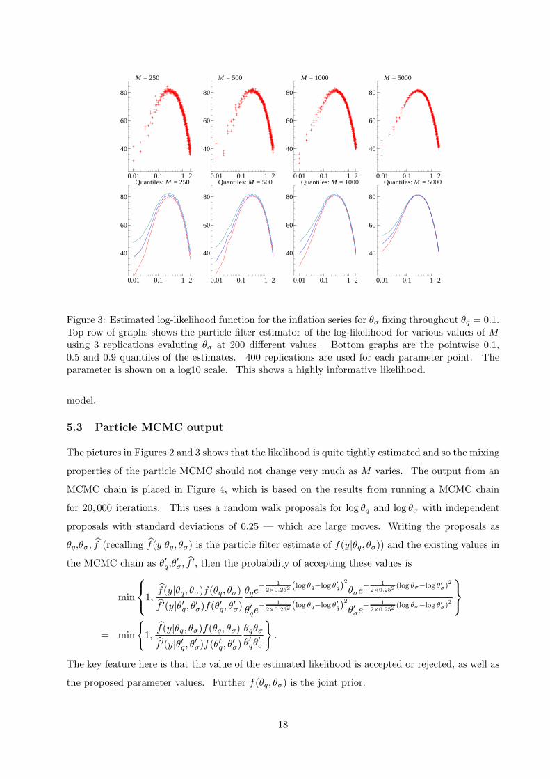
Figure 2: Estimated log-likelihood function for the inflation series for θq fixing throughout θσ =0.25. Top row of graphs shows the particle filter estimator of the log-likelihood for various valuesof M using 3 replications evaluting θq at 200 different values. Bottom graphs are the pointwise0.1, 0.5 and 0.9 quantiles of the estimates. 400 replications are used for each parameter point inestimating the quantiles. The likelihood is quite flat for this parameter.

data, estimated volatilities and diagnostics will be extended to August 2012, keeping the estimated

parameters θσ and θq fixed at the December 2004 estimates.

Throughout the series analysed will be 100 times the first difference of the log of the series,

which is roughly the percentage quarterly inflation series. This raw series is given in Figure 1,

where the updating of the series to reflect new data is indicated by the vertical line.

5.2 Estimated likelihood

The first step to understanding the empirical content of the model will be to graph the particle

filter based estimates of the log-likelihood as a function of the two parameters in θ. For the plot as

a function of θq I fixed θσ = 0.25 and when the function in θσ is drawn I took θq = 0.1. The particle

filter is run using M as 250, 500, 1000 and 5000. Figures 2 and 3 shows the results and indicate,

as expected, that the filter becomes more precise as M increases. The top row of graphs shows

the particle filter estimates of the log-likelihood, throughout using a log10 scale for θq and θσ. It

indicates quite a flat likelihood for θq but with some support for a value of away form θq = 0, which

is the random walk plus SV scale model special case. It shows quite a heavily peaked likelihood for

θσ away from θσ = 0. Taken together this suggests a full martingale unobserved component model

is needed, but volatility clustering in the scale is the main feature to be added to the Gaussian

17

0.01 0.1 1 2

40

60

80

M = 250

0.01 0.1 1 2

40

60

80

M = 500

0.01 0.1 1 2

40

60

80

M = 1000

0.01 0.1 1 2

40

60

80

M = 5000

0.01 0.1 1 2

40

60

80

Quantiles: M = 250

0.01 0.1 1 2

40

60

80

Quantiles: M = 500

0.01 0.1 1 2

40

60

80

Quantiles: M = 1000

0.01 0.1 1 2

40

60

80

Quantiles: M = 5000

Figure 3: Estimated log-likelihood function for the inflation series for θσ fixing throughout θq = 0.1.Top row of graphs shows the particle filter estimator of the log-likelihood for various values of Musing 3 replications evaluting θσ at 200 different values. Bottom graphs are the pointwise 0.1,0.5 and 0.9 quantiles of the estimates. 400 replications are used for each parameter point. Theparameter is shown on a log10 scale. This shows a highly informative likelihood.

model.

5.3 Particle MCMC output

The pictures in Figures 2 and 3 shows that the likelihood is quite tightly estimated and so the mixing

properties of the particle MCMC should not change very much as M varies. The output from an

MCMC chain is placed in Figure 4, which is based on the results from running a MCMC chain

for 20, 000 iterations. This uses a random walk proposals for log θq and log θσ with independent

proposals with standard deviations of 0.25 — which are large moves. Writing the proposals as

θq,θσ, f (recalling f(y|θq, θσ) is the particle filter estimate of f(y|θq, θσ)) and the existing values in

the MCMC chain as θ′q,θ′σ, f

′, then the probability of accepting these values is

min

1,

f(y|θq, θσ)f(θq, θσ)f ′(y|θ′q, θ′σ)f(θ′q, θ′σ)

θqe− 1

2×0.252(log θq−log θ′q)

2

θσe− 1

2×0.252(log θσ−log θ′σ)

2

θ′qe− 1

2×0.252(log θq−log θ′q)

2

θ′σe− 1

2×0.252(log θσ−log θ′σ)

2

= min

{1,f(y|θq, θσ)f(θq, θσ)f ′(y|θ′q, θ′σ)f(θ′q, θ′σ)

θqθσθ′qθ

′σ

}.

The key feature here is that the value of the estimated likelihood is accepted or rejected, as well as

the proposed parameter values. Further f(θq, θσ) is the joint prior.

18

In all 8 such chains are run independently in parallel, using a multicore processor. The output

is then thought of as a cross-section of long independent time series with the same marginal distri-

bution. The Figure shows the path from a single chain, while the autocorrelation function is the

average autocorrelation function from the 8 independent chains.

0 10000 20000

0.25

0.50

0.75

1.00 M = 250

θq

0 10000 20000

0.5

1.0

M = 500

0 10000 20000

0.5

1.0

M = 1000

0 10000 20000

0.5

1.0M = 5000

0 10000 20000

0.2

0.4

0.6 θσ

0 10000 20000

0.2

0.4

0 10000 20000

0.2

0.4

0 10000 20000

0.2

0.4

θq θσ

0 500 1000

0.0

0.5

1.0θq θσ

0 500 1000

0.0

0.5

1.0

0 500 1000

0.0

0.5

1.0

0 500 1000

0.0

0.5

1.0

Figure 4: Particle MCMC inference for the θq and θσ parameters for the inflation series. ResultingMCMC chain for a variety of values of M being 250, 500, 1000 and 5000. Suggests the mixing ofthe chain is relatively fast.

The posteriors are typically summarised using quantiles. This is carried out by computing the

quantile for each chain separately and then cross-sectionally averaging the resulting quantiles. The

uncertainty of this estimate can be measured by using the standard error of this arithmetic mean,

but when I did this the errors are so small there is little utility in reporting them here.

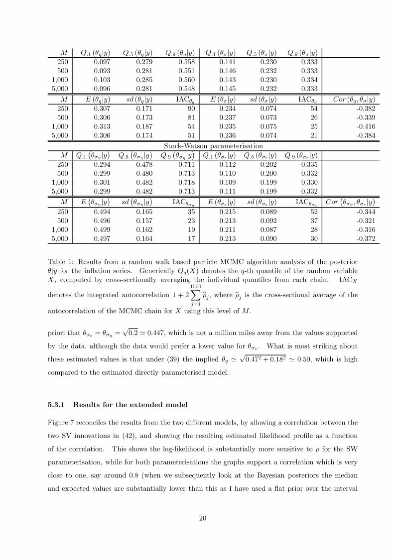
Table 1 shows quantile summaries of θ|y for different values of M , showing that the results are

entirely comparable. There is an improvement in precision as M increases, but the computational

cost of running the algorithm is proportional to M . The results suggest that using a small value

of M maybe the most computationally effective for this problem.

The posterior θq|y shows quite a high degree of spread and non-symmetry, with 80% of the

mass roughly between 0.09 and 0.55. The posterior θσ|y is much tighter and symmetric, with 80%

of the mass roughly between 0.14 and 0.33. The posterior means are θq = 0.37 and θσ = 0.23

respectively, while the standard deviation measures reflect the results from the quantiles. The

posterior correlation between the parameters is around −0.4.

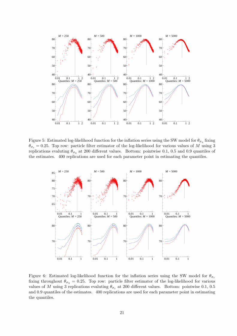
Table 1 also shows summaries for the fitted Stock-Watson parameterisation (note the corre-

sponding likelihood profiles are given in Figure 5 and 6). In their empirical work they impose a

19

M Q.1 (θq|y) Q.5 (θq|y) Q.9 (θq|y) Q.1 (θσ|y) Q.5 (θσ|y) Q.9 (θσ|y)250 0.097 0.279 0.558 0.141 0.230 0.333500 0.093 0.281 0.551 0.146 0.232 0.333

1,000 0.103 0.285 0.560 0.143 0.230 0.3345,000 0.096 0.281 0.548 0.145 0.232 0.333

M E (θq|y) sd (θq|y) IACθq E (θσ|y) sd (θσ|y) IACθσ Cor (θq, θσ|y)250 0.307 0.171 90 0.234 0.074 54 -0.382500 0.306 0.173 81 0.237 0.073 26 -0.339

1,000 0.313 0.187 54 0.235 0.075 25 -0.4165,000 0.306 0.174 51 0.236 0.074 21 -0.384

Stock-Watson parameterisation

M Q.1

(θση |y

)Q.5

(θση |y

)Q.9

(θση |y

)Q.1 (θσε |y) Q.5 (θσε |y) Q.9 (θσε |y)

250 0.294 0.478 0.711 0.112 0.202 0.335500 0.299 0.480 0.713 0.110 0.200 0.332

1,000 0.301 0.482 0.718 0.109 0.199 0.3305,000 0.299 0.482 0.713 0.111 0.199 0.332

M E(θση |y

)sd(θση |y

)IACθση E (θσε |y) sd (θσε |y) IACθσε

Cor(θση , θσε |y

)

250 0.494 0.165 35 0.215 0.089 52 -0.344500 0.496 0.157 23 0.213 0.092 37 -0.321

1,000 0.499 0.162 19 0.211 0.087 28 -0.3165,000 0.497 0.164 17 0.213 0.090 30 -0.372

Table 1: Results from a random walk based particle MCMC algorithm analysis of the posteriorθ|y for the inflation series. Generically Qq(X) denotes the q-th quantile of the random variableX, computed by cross-sectionally averaging the individual quantiles from each chain. IACX

denotes the integrated autocorrelation 1 + 2

1500∑

j=1

ρj, where ρj is the cross-sectional average of the

autocorrelation of the MCMC chain for X using this level of M .

priori that θσε = θση =√0.2 ≃ 0.447, which is not a million miles away from the values supported

by the data, although the data would prefer a lower value for θσε . What is most striking about

these estimated values is that under (39) the implied θq ≃√0.472 + 0.182 ≃ 0.50, which is high

compared to the estimated directly parameterised model.

5.3.1 Results for the extended model

Figure 7 reconciles the results from the two different models, by allowing a correlation between the

two SV innovations in (42), and showing the resulting estimated likelihood profile as a function

of the correlation. This shows the log-likelihood is substantially more sensitive to ρ for the SW

parameterisation, while for both parameterisations the graphs support a correlation which is very

close to one, say around 0.8 (when we subsequently look at the Bayesian posteriors the median

and expected values are substantially lower than this as I have used a flat prior over the interval

20

0.01 0.1 1 240

50

60

70

80M = 250

0.01 0.1 1 240

50

60

70

80M = 500

0.01 0.1 1 240

50

60

70

80M = 1000

0.01 0.1 1 240

50

60

70

80M = 5000

0.01 0.1 1 240

50

60

70

80Quantiles: M = 250

0.01 0.1 1 240

50

60

70

80Quantiles: M = 500

0.01 0.1 1 240

50

60

70

80Quantiles: M = 1000

0.01 0.1 1 240

50

60

70

80Quantiles: M = 5000

Figure 5: Estimated log-likelihood function for the inflation series using the SW model for θση fixingθσε = 0.25. Top row: particle filter estimator of the log-likelihood for various values of M using 3replications evaluting θση at 200 different values. Bottom: pointwise 0.1, 0.5 and 0.9 quantiles ofthe estimates. 400 replications are used for each parameter point in estimating the quantiles.

0.01 0.1 1

65

70

75

80

85 M = 250

0.01 0.1 1

70

80

M = 500

0.01 0.1 1

70

80

M = 1000

0.01 0.1 1

70

80

M = 5000

0.01 0.1 1

70

80

Quantiles: M = 250

0.01 0.1 1

70

80

Quantiles: M = 500

0.01 0.1 1

70

80

Quantiles: M = 1000

0.01 0.1 1

70

80

Quantiles: M = 5000

Figure 6: Estimated log-likelihood function for the inflation series using the SW model for θσε

fixing throughout θση = 0.25. Top row: particle filter estimator of the log-likelihood for variousvalues of M using 3 replications evaluting θσε at 200 different values. Bottom: pointwise 0.1, 0.5and 0.9 quantiles of the estimates. 400 replications are used for each parameter point in estimatingthe quantiles.

21

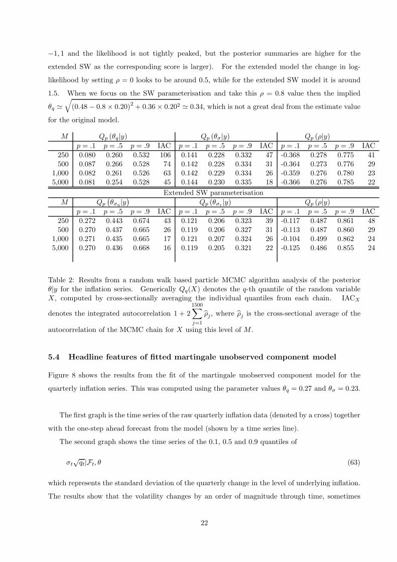
−1, 1 and the likelihood is not tightly peaked, but the posterior summaries are higher for the

extended SW as the corresponding score is larger). For the extended model the change in log-

likelihood by setting ρ = 0 looks to be around 0.5, while for the extended SW model it is around

1.5. When we focus on the SW parameterisation and take this ρ = 0.8 value then the implied

θq ≃√

(0.48 − 0.8 × 0.20)2 + 0.36 × 0.202 ≃ 0.34, which is not a great deal from the estimate value

for the original model.

M Qp (θq|y) Qp (θσ|y) Qp (ρ|y)p = .1 p = .5 p = .9 IAC p = .1 p = .5 p = .9 IAC p = .1 p = .5 p = .9 IAC

250 0.080 0.260 0.532 106 0.141 0.228 0.332 47 -0.368 0.278 0.775 41500 0.087 0.266 0.528 74 0.142 0.228 0.334 31 -0.364 0.273 0.776 29

1,000 0.082 0.261 0.526 63 0.142 0.229 0.334 26 -0.359 0.276 0.780 235,000 0.081 0.254 0.528 45 0.144 0.230 0.335 18 -0.366 0.276 0.785 22

Extended SW parameterisation

M Qp

(θση |y

)Qp (θσε |y) Qp (ρ|y)

p = .1 p = .5 p = .9 IAC p = .1 p = .5 p = .9 IAC p = .1 p = .5 p = .9 IAC

250 0.272 0.443 0.674 43 0.121 0.206 0.323 39 -0.117 0.487 0.861 48500 0.270 0.437 0.665 26 0.119 0.206 0.327 31 -0.113 0.487 0.860 29

1,000 0.271 0.435 0.665 17 0.121 0.207 0.324 26 -0.104 0.499 0.862 245,000 0.270 0.436 0.668 16 0.119 0.205 0.321 22 -0.125 0.486 0.855 24

Table 2: Results from a random walk based particle MCMC algorithm analysis of the posteriorθ|y for the inflation series. Generically Qq(X) denotes the q-th quantile of the random variableX, computed by cross-sectionally averaging the individual quantiles from each chain. IACX

denotes the integrated autocorrelation 1 + 2

1500∑

j=1

ρj, where ρj is the cross-sectional average of the

autocorrelation of the MCMC chain for X using this level of M .

5.4 Headline features of fitted martingale unobserved component model

Figure 8 shows the results from the fit of the martingale unobserved component model for the

quarterly inflation series. This was computed using the parameter values θq = 0.27 and θσ = 0.23.

The first graph is the time series of the raw quarterly inflation data (denoted by a cross) together

with the one-step ahead forecast from the model (shown by a time series line).

The second graph shows the time series of the 0.1, 0.5 and 0.9 quantiles of

σt√qt|Ft, θ (63)

which represents the standard deviation of the quarterly change in the level of underlying inflation.

The results show that the volatility changes by an order of magnitude through time, sometimes

22

-1.0 -0.5 0.0 0.5 1.072

73

74

75

76

77

78

79

80

81

82 Extended SW: Quantiles, M = 5000

-1.0 -0.5 0.0 0.5 1.0

73

74

75

76

77

78

79

80

81

82 Extended model: Quantiles M = 5000

ρ

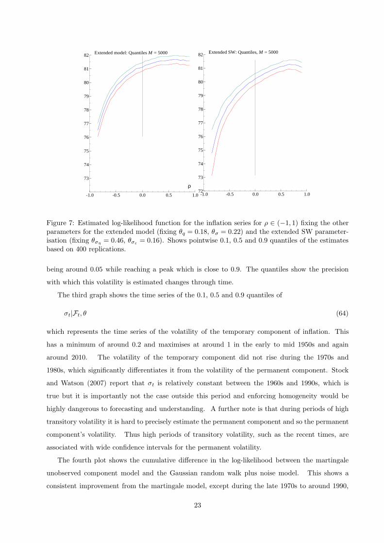
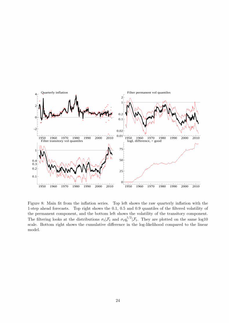
Figure 7: Estimated log-likelihood function for the inflation series for ρ ∈ (−1, 1) fixing the otherparameters for the extended model (fixing θq = 0.18, θσ = 0.22) and the extended SW parameter-isation (fixing θση = 0.46, θσε = 0.16). Shows pointwise 0.1, 0.5 and 0.9 quantiles of the estimatesbased on 400 replications.

being around 0.05 while reaching a peak which is close to 0.9. The quantiles show the precision

with which this volatility is estimated changes through time.

The third graph shows the time series of the 0.1, 0.5 and 0.9 quantiles of

σt|Ft, θ (64)

which represents the time series of the volatility of the temporary component of inflation. This

has a minimum of around 0.2 and maximises at around 1 in the early to mid 1950s and again

around 2010. The volatility of the temporary component did not rise during the 1970s and

1980s, which significantly differentiates it from the volatility of the permanent component. Stock

and Watson (2007) report that σt is relatively constant between the 1960s and 1990s, which is

true but it is importantly not the case outside this period and enforcing homogeneity would be

highly dangerous to forecasting and understanding. A further note is that during periods of high

transitory volatility it is hard to precisely estimate the permanent component and so the permanent

component’s volatility. Thus high periods of transitory volatility, such as the recent times, are

associated with wide confidence intervals for the permanent volatility.

The fourth plot shows the cumulative difference in the log-likelihood between the martingale

unobserved component model and the Gaussian random walk plus noise model. This shows a

consistent improvement from the martingale model, except during the late 1970s to around 1990,

23

1950 1960 1970 1980 1990 2000 2010

-2

0

2

4 Quarterly inflation

0.01

0.02

0.1

0.2

1

2

1950 1960 1970 1980 1990 2000 2010

Filter permanent vol quantiles

0.1

0.2

0.30.4

1

1950 1960 1970 1980 1990 2000 2010

Filter transitory vol quantiles

1950 1960 1970 1980 1990 2000 20100

25

50

75

logL difference, > good

Figure 8: Main fit from the inflation series. Top left shows the raw quarterly inflation with the1-step ahead forecasts. Top right shows the 0.1, 0.5 and 0.9 quantiles of the filtered volatility ofthe permanent component, and the bottom left shows the volatility of the transitory component.

The filtering looks at the distributions σt|Ft and σtq1/2t |Ft. They are plotted on the same log10

scale. Bottom right shows the cumulative difference in the log-likelihood compared to the linearmodel.

24

where the models fitted roughly similarly.

5.5 Analysis

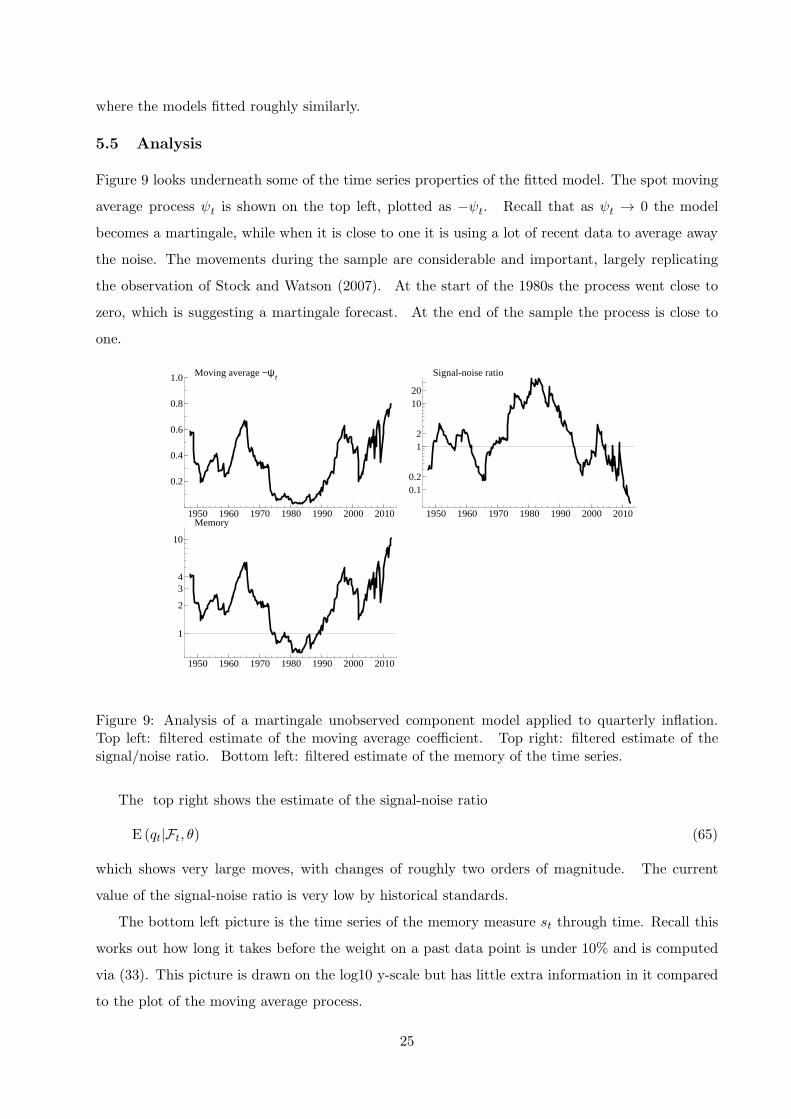
Figure 9 looks underneath some of the time series properties of the fitted model. The spot moving

average process ψt is shown on the top left, plotted as −ψt. Recall that as ψt → 0 the model

becomes a martingale, while when it is close to one it is using a lot of recent data to average away

the noise. The movements during the sample are considerable and important, largely replicating

the observation of Stock and Watson (2007). At the start of the 1980s the process went close to

zero, which is suggesting a martingale forecast. At the end of the sample the process is close to

one.

1950 1960 1970 1980 1990 2000 2010

0.2

0.4

0.6

0.8

1.0 Moving average −ψt

0.10.2

12

1020

1950 1960 1970 1980 1990 2000 2010

Signal-noise ratio

1

2

34

10

1950 1960 1970 1980 1990 2000 2010

Memory

Figure 9: Analysis of a martingale unobserved component model applied to quarterly inflation.Top left: filtered estimate of the moving average coefficient. Top right: filtered estimate of thesignal/noise ratio. Bottom left: filtered estimate of the memory of the time series.

The top right shows the estimate of the signal-noise ratio

E (qt|Ft, θ) (65)

which shows very large moves, with changes of roughly two orders of magnitude. The current

value of the signal-noise ratio is very low by historical standards.

The bottom left picture is the time series of the memory measure st through time. Recall this

works out how long it takes before the weight on a past data point is under 10% and is computed

via (33). This picture is drawn on the log10 y-scale but has little extra information in it compared

to the plot of the moving average process.

25

5.6 Diagnostic statistics

Figure 10 shows some plots to diagnose the empirical effectiveness of the models. The first column

of figures looks at the innovations from the fitted model

vt = E

yt −mt|t−1

σt√p∗t|t−1 + 1

|Ft−1

, (66)

where the posterior mean is averaged over q1:t and σ1:t. This should be roughly i.i.d. standard

normal if the model fits well. In the top plot vt is drawn against t and there is little apparent

structure visible to the eye. The bottom plot shows the correlogram for vt, drawn using an index

plot, together with the correlogram for |vt| which is shown by a series of dots. The latter is

designed to pick up any missing volatility clustering in the innovations, the former looks for linear

dependence in the innovations. The results are somewhat encouraging, there seems very little

volatility clustering. There are some quite large autocorrelations appearing for vt in lags 2 and 3,

while the results for |vt| look very strong. This indicates the model could be improved for very

short-term forecasting by allowing some very short memory into εt.

The second column looks at the plot of the probability integral transforms

Ut = E

Φ

yt −mt|t−1

σt√p∗t|t−1 + 1

|Ft−1

(67)

against time, where Φ is the standard normal distribution function. The Ut should be an i.i.d.

U(0, 1) sequence if the model is correctly specified and so the plot should appear like the scatter of a

two dimensional homogenous Poisson process on [0, 1]× [1, n]. These types of transforms have been

used by many researchers, e.g. Rosenblatt (1952), Shephard (1994) and Diebold, Gunther, and Tay

(1998). The correlogram of the Ut and the so-called reflected uniforms 2 |Ut − 1/2| (see Shephard

(1994) who introduced them to check for volatility clustering, realising they should also be i.i.d.

U(0, 1) if the model is well fitting) are given in the plot below. These correlograms should be less

effected by outliers than the corresponding ones for vt, but in this case there is little difference.

The same diagnostics are also reported for the Gaussian random walk plus noise model in the

third and fourth columns. Here there are some obvious failings, most dramatically due to volatility

clustering. The correlogram in the third column also shows a very high correlation at lag 2 for

the vt (much higher than for the martingale plus noise model, and this feature also appears in the

corresponding results for Ut). Overall the fit of the linear model is quite poor.

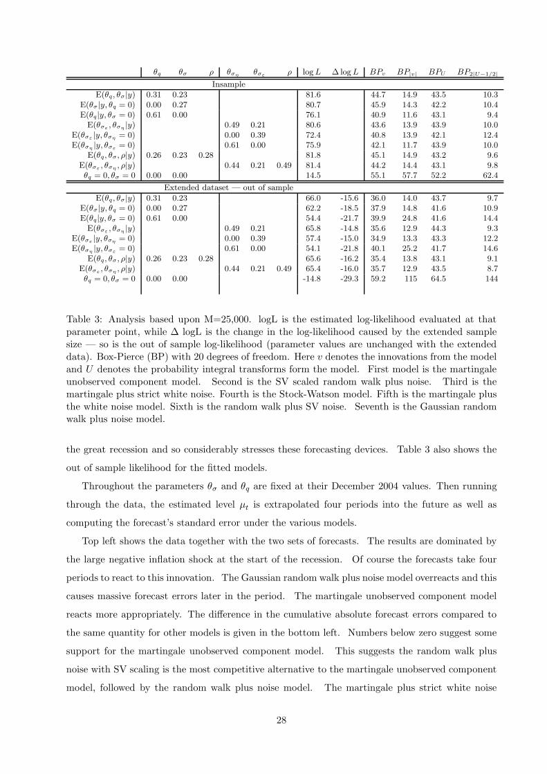
All of these results are summarised in Table 3, which shows the fitted martingale unobserved

component model’s parameters, the corresponding log-likelihood and Box-Pierce summarises from

the above correlograms. These were computed using 20 lags. Also given is the result from the

26

linear model (which is where θq = θσ = 0), which has a poorer likelihood and worse dependence

measures. Most of the gain is made by dealing with the heteroskedasticity in the data. The Table

also reports results from the random walk plus SV noise model (θq = 0) and the martingale plus

strict white noise model (θσ = 0). These models have parameters which need to be estimated and

this is carried out using particle MCMC in the usual way. Note that these two constrained models

1950 1975 2000

-5.0

-2.5

0.0

2.5SV based inn

1950 1975 2000

0.25

0.50

0.75

1.00 SV based U

1950 1975 2000

-5.0

-2.5

0.0

2.5 N based inn

1950 1975 2000

0.25

0.50

0.75

1.00 N based U

Innovations Abs innov

0 10 20-0.4

-0.2

0.0

0.2

0.4 acf: SV inn

Innovations Abs innov

0 10 20-0.4

-0.2

0.0

0.2

0.4 acf: SV U

0 10 20-0.4

-0.2

0.0

0.2

0.4 acf: N inn

0 10 20-0.4

-0.2

0.0

0.2

0.4 acf: N U

Figure 10: Diagnostics from the model for the extended inflation series. Top are raw innovationsand probability integral transforms (U), for two models: martingale plus noise and random walkplus noise. Bottom denotes correlograms either of the raw series or the absolute value or reflectedversion 2 |U − 1/2|. Estimation is based on data up until 2004, log-likelihood is computed at theseestimated parameter points and includes all data up to 2012.

deliver parameter estimates which are considerably higher than for the martingale unobserved

component model, as they try to use their flexibility to deal with the heteroskedasticity in the data.

That the parameters jump upwards is not surprising given the posterior for the general model is

negatively correlated and these model simplifications wrongly impose one of the parameters as zero.

Overall the martingale unobserved component model is slightly better than the random walk plus

SV noise model. This is in turn better than the martingale plus strict white noise model, but the

degree of difference is surprisingly small. This latter model boosts up θq to such a large degree

that it can deal with some of the heteroskedasticity in the data.

5.7 Multistep out of sample forecasting

I finish by looking at how the models perform out of sample, forecasting a year ahead, that is four

steps ahead. The results are given in Figure 11 for the martingale unobserved component model

and the Gaussian random walk plus noise model. This out of sample period includes the start of

27

θq θσ ρ θσηθσε

ρ logL ∆ logL BPv BP|v| BPU BP2|U−1/2|

Insample

E(θq, θσ|y) 0.31 0.23 81.6 44.7 14.9 43.5 10.3E(θσ|y, θq = 0) 0.00 0.27 80.7 45.9 14.3 42.2 10.4E(θq|y, θσ = 0) 0.61 0.00 76.1 40.9 11.6 43.1 9.4E(θσε

, θση|y) 0.49 0.21 80.6 43.6 13.9 43.9 10.0

E(θσε|y, θση

= 0) 0.00 0.39 72.4 40.8 13.9 42.1 12.4E(θση

|y, θσε= 0) 0.61 0.00 75.9 42.1 11.7 43.9 10.0

E(θq, θσ, ρ|y) 0.26 0.23 0.28 81.8 45.1 14.9 43.2 9.6E(θσε

, θση, ρ|y) 0.44 0.21 0.49 81.4 44.2 14.4 43.1 9.8

θq = 0, θσ = 0 0.00 0.00 14.5 55.1 57.7 52.2 62.4

Extended dataset — out of sample

E(θq, θσ|y) 0.31 0.23 66.0 -15.6 36.0 14.0 43.7 9.7E(θσ|y, θq = 0) 0.00 0.27 62.2 -18.5 37.9 14.8 41.6 10.9E(θq|y, θσ = 0) 0.61 0.00 54.4 -21.7 39.9 24.8 41.6 14.4E(θσε

, θση|y) 0.49 0.21 65.8 -14.8 35.6 12.9 44.3 9.3

E(θσε|y, θση

= 0) 0.00 0.39 57.4 -15.0 34.9 13.3 43.3 12.2E(θση

|y, θσε= 0) 0.61 0.00 54.1 -21.8 40.1 25.2 41.7 14.6

E(θq, θσ, ρ|y) 0.26 0.23 0.28 65.6 -16.2 35.4 13.8 43.1 9.1E(θσε

, θση, ρ|y) 0.44 0.21 0.49 65.4 -16.0 35.7 12.9 43.5 8.7

θq = 0, θσ = 0 0.00 0.00 -14.8 -29.3 59.2 115 64.5 144

Table 3: Analysis based upon M=25,000. logL is the estimated log-likelihood evaluated at thatparameter point, while ∆ logL is the change in the log-likelihood caused by the extended samplesize — so is the out of sample log-likelihood (parameter values are unchanged with the extendeddata). Box-Pierce (BP) with 20 degrees of freedom. Here v denotes the innovations from the modeland U denotes the probability integral transforms form the model. First model is the martingaleunobserved component model. Second is the SV scaled random walk plus noise. Third is themartingale plus strict white noise. Fourth is the Stock-Watson model. Fifth is the martingale plusthe white noise model. Sixth is the random walk plus SV noise. Seventh is the Gaussian randomwalk plus noise model.

the great recession and so considerably stresses these forecasting devices. Table 3 also shows the

out of sample likelihood for the fitted models.

Throughout the parameters θσ and θq are fixed at their December 2004 values. Then running

through the data, the estimated level µt is extrapolated four periods into the future as well as

computing the forecast’s standard error under the various models.

Top left shows the data together with the two sets of forecasts. The results are dominated by

the large negative inflation shock at the start of the recession. Of course the forecasts take four

periods to react to this innovation. The Gaussian random walk plus noise model overreacts and this

causes massive forecast errors later in the period. The martingale unobserved component model

reacts more appropriately. The difference in the cumulative absolute forecast errors compared to

the same quantity for other models is given in the bottom left. Numbers below zero suggest some

support for the martingale unobserved component model. This suggests the random walk plus

noise with SV scaling is the most competitive alternative to the martingale unobserved component

model, followed by the random walk plus noise model. The martingale plus strict white noise

28

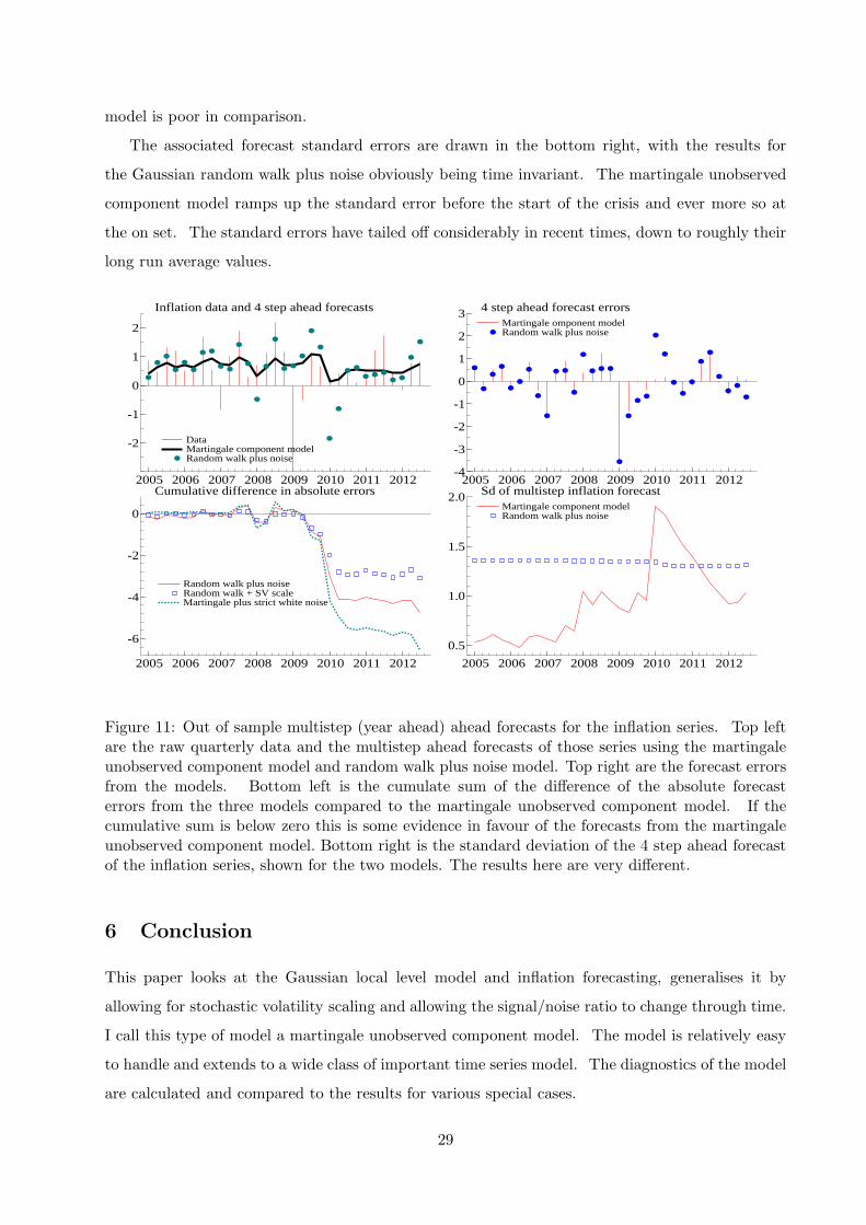
model is poor in comparison.

The associated forecast standard errors are drawn in the bottom right, with the results for

the Gaussian random walk plus noise obviously being time invariant. The martingale unobserved

component model ramps up the standard error before the start of the crisis and ever more so at

the on set. The standard errors have tailed off considerably in recent times, down to roughly their

long run average values.

Data Martingale component model Random walk plus noise

2005 2006 2007 2008 2009 2010 2011 2012

-2

-1

0

1

2

Inflation data and 4 step ahead forecasts

Data Martingale component model Random walk plus noise

Martingale omponent model Random walk plus noise

2005 2006 2007 2008 2009 2010 2011 2012-4

-3

-2

-1

0

1

2

3 4 step ahead forecast errorsMartingale omponent model Random walk plus noise

Random walk plus noise Random walk + SV scale Martingale plus strict white noise

2005 2006 2007 2008 2009 2010 2011 2012

-6

-4

-2

0

Cumulative difference in absolute errors

Random walk plus noise Random walk + SV scale Martingale plus strict white noise

Martingale component model Random walk plus noise

2005 2006 2007 2008 2009 2010 2011 2012

0.5

1.0

1.5

2.0 Sd of multistep inflation forecastMartingale component model Random walk plus noise

Figure 11: Out of sample multistep (year ahead) ahead forecasts for the inflation series. Top leftare the raw quarterly data and the multistep ahead forecasts of those series using the martingaleunobserved component model and random walk plus noise model. Top right are the forecast errorsfrom the models. Bottom left is the cumulate sum of the difference of the absolute forecasterrors from the three models compared to the martingale unobserved component model. If thecumulative sum is below zero this is some evidence in favour of the forecasts from the martingaleunobserved component model. Bottom right is the standard deviation of the 4 step ahead forecastof the inflation series, shown for the two models. The results here are very different.

6 Conclusion

This paper looks at the Gaussian local level model and inflation forecasting, generalises it by

allowing for stochastic volatility scaling and allowing the signal/noise ratio to change through time.

I call this type of model a martingale unobserved component model. The model is relatively easy

to handle and extends to a wide class of important time series model. The diagnostics of the model

are calculated and compared to the results for various special cases.

29

The particle filter is used to handle the model, which extends the Kalman filter to allow for

non-Gaussianity and non-linearity. The particle filter is used to generate an estimate of the log-

likelihood which is used inside a MCMC algorithm, in order to make inference on the parameters

of the model. The MCMC chains are quite well behaved and are simple to parallelise to exploit

multicore computers or indeed GPUs.

The martingale unobserved component model generalises in various ways, to allow for trends,

cycles and for seasonal components. The methods developed here can be extended in the same

way. The martingale unobserved component model can also be set in continuous time and used to

look at high frequency financial data, where stochastic volatility scaling is clearly very important.

Likewise non-parametric regression can be analysed using this kind of model, as noted by for

example Wecker and Ansley (1983), Kohn, Ansley, and Wong (1992) and Harvey and Koopman

(2000). By allowing for the signal/noise ratio to change through time, the approach discussed here

allows the smoothing to be carried out with in effect a local bandwidth which might be important

for some applications.

References

Ackerson, G. A. and K. S. Fu (1970). On state estimation in switching environments. IEEE Transactionson Automatic Control 15, 10–17.

Akashi, H. and H. Kumamoto (1977). Random sampling approach to state estimation in switching envi-ronments. Automatica 13, 429–434.

Andrieu, C., A. Doucet, and R. Holenstein (2010). Particle Markov chain Monte Carlo methods (withdiscussion). Journal of the Royal Statistical Society, Series B 72, 1–33.

Barndorff-Nielsen, O. E., P. R. Hansen, A. Lunde, and N. Shephard (2008). Designing realised kernels tomeasure the ex-post variation of equity prices in the presence of noise. Econometrica 76, 1481–1536.

Barndorff-Nielsen, O. E. and N. Shephard (2002). Econometric analysis of realised volatility and its use inestimating stochastic volatility models. Journal of the Royal Statistical Society, Series B 64, 253–280.

Beaumont, M. (2003). Estimation of population growth or decline in genetically monitored populations.Genetics 164, 1139.

Bos, C. and N. Shephard (2006). Inference for adaptive time series models: stochastic volatility andconditionally Gaussian state space form. Econometric Reviews 25, 219–244.

Caldara, D., J. Fernandez-Villaverde, P. Guerron, J. F. Rudio-Ramirez, and Y. Wen (2012). Computingdsge models with recursive preferences and stochastic volatility. Review of Economic Dynamics 15,188–206.

Carter, C. K. and R. Kohn (1994). On Gibbs sampling for state space models. Biometrika 81, 541–553.

Chen, R. and J. S. Liu (2000). Mixture Kalman filters. Journal of the Royal Statistical Society, SeriesB 62, 493–508.

Cogley, T., G. Primiceri, and T. J. Sargent (2010). Inflation-gap persistence in the U.S. American Eco-nomic Journal: Macroeconomics 2, 43–69.

Creal, D. (2012). A survey of sequential Monte Carlo methods for economics and finance. EconometricReviews 31, 245–296.

Creal, D., S. J. Koopman, and A. Lucas (2008). A general framework for observation driven time-varyingparameter models. Unpublished paper: Tinbergen Institute Discussion Paper 108.

Creal, D., S. J. Koopman, and E. Zivot (2010). Extracting a robust U.S. business cycle using a time-varyingmultivariate model-based bandpass filter. Journal of Applied Econometrics 25, 695–719.

30

D’Agostino, A., L. Gambetti, and D. Giannone (2013). Macroeconomic forecasting and structural change.Journal of Applied Econometrics 28, 82–101.

de Jong, P. (1991). The diffuse Kalman filter. Annals of Statistics 19, 1073–1083.

Diebold, F. X., T. A. Gunther, and T. S. Tay (1998). Evaluating density forecasts with applications tofinancial risk management. International Economic Review 39, 863–883.

Doucet, A., N. de Freitas, and N. J. Gordon (Eds.) (2001). Sequential Monte Carlo Methods in Practice.New York: Springer-Verlag.

Doucet, A., S. J. Godsill, and C. Andrieu (2000). On sequential Monte Carlo sampling methods forBayesian filtering. Statistics and Computing 10, 197–208.

Doucet, A. and A. Johansen (2011). A tutorial on particle filtering and smoothing: fifteen years later.In D. Crisan and B. Rozovsky (Eds.), The Oxford Handbook of Nonlinear filtering. Oxford UniversityPress.

Durbin, J. and S. J. Koopman (2001). Time Series Analysis by State Space Methods. Oxford: OxfordUniversity Press.

Fearnhead, P. and P. Clifford (2003). On-line inference for hidden Markov models via particle filters.Journal of the Royal Statistical Society, Series B 65, 887–899.

Fernandez-Villaverde, J., P. Guerron, J. F. Rudio-Ramirez, and M. Uribe (2010). Risk matters: The realeffects of volatility shocks. American Economic Review 101, 2530–2561.

Fiorentini, G., E. Sentana, and N. Shephard (2004). Likelihood-based estimation of latent generalisedARCH structures. Econometrica 72, 1481–1517.

Flury, T. and N. Shephard (2011). Bayesian inference based only on simulated likelihood: particle filteranalysis of dynamic economic models. Econometric Theory 27, 933–956.

Ghysels, E., A. C. Harvey, and E. Renault (1996). Stochastic volatility. In C. R. Rao and G. S. Maddala(Eds.), Statistical Methods in Finance, pp. 119–191. Amsterdam: North-Holland.

Gordon, N. J., D. J. Salmond, and A. F. M. Smith (1993). A novel approach to nonlinear and non-GaussianBayesian state estimation. IEE-Proceedings F 140, 107–113.

Gourieroux, C. and A. Monfort (1996). Simulation Based Econometric Methods. Oxford: Oxford UniversityPress.

Harvey, A. C. (1981). Time Series Models (1 ed.). New York: Philip Allan.

Harvey, A. C. (1989). Forecasting, Structural Time Series Models and the Kalman Filter. Cambridge:Cambridge University Press.

Harvey, A. C. and J. Durbin (1986). The effects of seat belt legislation on British road casualties: Acase study in structural time series modelling. Journal of the Royal Statistical Society, Series B 149,187–227.

Harvey, A. C. and S. J. Koopman (2000). Signal extraction and the formulation of unobserved componentsmodels. Econometrics Journal 3, 84–107.

Harvey, A. C., E. Ruiz, and E. Sentana (1992). Unobserved component time series models with ARCHdisturbances. Journal of Econometrics 52, 129–158.

Harvey, A. C., E. Ruiz, and N. Shephard (1994). Multivariate stochastic variance models. Review ofEconomic Studies 61, 247–264.

Kim, S., N. Shephard, and S. Chib (1998). Stochastic volatility: likelihood inference and comparison withARCH models. Review of Economic Studies 65, 361–393.

Kohn, R., C. F. Ansley, and C.-M. Wong (1992). Nonparametric spline regression with autoregressivemoving average errors. Biometrika 79, 335–346.

Koopman, S. J. and C. Bos (2004). State space models with a common stochastic variance. Journal ofBusiness and Economic Statistics 22, 346–357.

Liu, J. S. and R. Chen (1998). Sequential Monte Carlo methods for dynamic systems. Journal of theAmerican Statistical Association 93, 1032–1044.

Muth, J. F. (1960). Optimal properties of exponentially weighted forecasts. Journal of the AmericanStatistical Association 55, 299–306.

31

Pitt, M. K. and N. Shephard (1999). Filtering via simulation: auxiliary particle filter. Journal of theAmerican Statistical Association 94, 590–599.

Pitt, M. K., R. Silva, P. Giordani, and R. Kohn (2012). On some properties of Markov chain Monte Carlosimulation methods based on the particle filter. Journal of Econometrics . Forthcoming.

Rosenblatt, M. (1952). Remarks on a multivariate transformation. Annals of Mathematical Statistics 23,470–472.

Shephard, N. (1994). Partial non-Gaussian state space. Biometrika 81, 115–131.

Shephard, N. (Ed.) (2005). Stochastic Volatility: Selected Readings. Oxford: Oxford University Press.

Stock, J. H. and M. W. Watson (2007). Why has U.S. inflation become harder to forecast? Journal ofMoney, Credit, and Banking 39, 3–34.

Taylor, J. W. (2004). Smooth transition exponential smoothing. Journal of Forecasting 23, 385–394.

Trigg, D. W. and A. G. Leach (1967). Exponential smoothing with an adaptive response rate. OperationalResearch Quarterly 18, 53–59.

Wecker, W. E. and C. F. Ansley (1983). The signal extraction approach to nonlinear regression and splinesmoothing. Journal of the American Statistical Association 78, 81–89.

32