JOURNAL OF GEOPHYSICAL RESEARCH, VOL. 98, NO. E2, PAGES 3125-3148, FEBRUARY 25, 1993 Mars Atmospheric Dynamics as Simulated by the NASA Ames General Circulation Model 2. Transient Baroclinic Eddies JEFFREY R. BARNES, JAMES B. POLLACK, ROBERT M. HABERLE, CONWAY B. LEOVY, RICHARD W. ZUREK, HILDA LEE, AND JAMES SCHAEFFER A largesetof experiments performed with the NASA AmesMarsgeneral circulation model(GCM) havebeen analyzed to determine the properties, structure, and dynamics of thesimulated transient baroclinic eddies. The Mars GCM simulations span a wide range of seasonal dates and dust loadings and include a number of special sensitivity experiments (e.g.,withflat topography). There is strong transient baroclinic eddy activity in theextratropics of the northern hemisphere during the northern autumn, winter, and spring seasons. The eddyactivity remains strong for verylargedust loadings, though it shifts northward. The eastward propagating eddies arecharacterized by zonal wavenumbers of 1-4and periods of-2-10 days. In several simulations, theeddy variance is dominated by a single zonal wavenumber and a narrow range of periods. Thelonger (wavenumbers 1 and 2) transient eddies have a very deep vertical structure, exhibiting a maximum kinetic energy density atthemodel top(-45-50 km) in many of the simulations. In a simulation for earlynorthern spring theeddies arequite shallow, however.The transient eddies generate the bulkof their energy baroclincally vialarge meridional and vertical heat fluxes, atboth lowerand upper levels.This isdespite the factthat their vertical structure istypically close toequivalent barotropic above the lowest 10 km. The eddies alsoappear to generate a substantial amount of energy barotropically, via large meridional momentum fluxes at both lower and upper levels. In the tropics and northern subtropics atupper levels (-25-50 km) there are strong transient eddy motions withstructures resembling those characterisitic ofinertially unstable modes. This eddy activity appears tobearesponse tothe forcing of aregion of marginal inertial stability by theextratropical transient baroclinic eddies, as the wavenumbers andperiods are the same as those in the extratropics. A major surprise is the presence of very weak transient eddy activityin a number of the southern winter simulations. It appears that this ispartly a consequence of thestabilizing effects of thezonally symmetric topography in theGCM, butit also must beassociated withcertain aspects of thezonal-mean circulation in southern winter. Thisis indicated by the presence of relatively largeamplitude eddies in simulations for earlysouthern autumn andspring andin a southern wintersolstice simulation incorporating a different topography (derived from the Mars Digital Terrain Model).This topography differs from that used in •nost ofthe GCM ,imulations in not being characterized bysteep symmetric slopes (which arestabilizing to baroclinic instability) in southern highlatitudes. It is hypothesized that the verylargeextent of the southern seasonal polar capand highelevations in thesouth both mightcontribute to weakening the transient eddy activity.Large zonally symmetric topography in thenorthern hemisphere of theMars GCM also appears to have a strong impacton the transient eddies, actingto increase the dominant zonal wavenumbers andphase speeds. The properties of the GCM baroclinic eddies in the northern extratropics are compared in detail withanalogous properties inferred fromVikingLander meteorology observations. The GCM eddies are found tobevery similar tothose observed in most respects. A notable exception isthat the eddy amplitudes in the highly dusty GCM simulations are much larger than those observed byVikingduring the1977 winter solstice dust storm. This is almost certainly at least partlydueto the relatively smalllatitudinal expansion of the Hadley circulation in thehighlydusty GCM experiments. 1. INTRODUCTION Despite the present scarcity of observations it is known that extratropical transient eddies play an important role in the general circulation of the Martian atmosphere. In particular, these eddies produce substantial heat and momentum fluxes that strongly influ- ence the zonal-mean circulation and climate [Pollack et al., 1981, 1990]. The importance of the heat transports is greatest at the climatically sensitive polar latitudes: it appears that they can be large enough in northem winter, especially under highly dusty conditions, to significantly reduce volatile condensation in the outer portions of the seasonal polarcap [Pollack eta/., 1990]. •Atmospheric Sciences, Oregon State University, Corvallis. 2Space Sciences Division, NASA Ames Research Center, Moffett Field, California. 3Department of Atmospheric Sciences, University of Washington, Seattle. 4Jet Propulsion Laboratory, Pasadena, California. 5Sterling Software, Incorporated, Palo Alto,California. Copyright 1993 by the American Geophysical Union. Papernumber 9ZIE02935. 0148-0227/93/9ZIE-02935 $05.00 The transient baroclinic eddies appear to have important roles in the dustandwater cycles of the Mars climatesystem. Observations have shown that these disturbances act to raise dust in winter mid- latitudes [Briggs and Leovy,1974;Briggs et al., 1979]. It hasbeen hypothesized thatthe baroclinic eddy activity could becrucial to the interannual variabilityof globalduststorm genesis [Leovy et al., 1985; Haberle, 1986]. Transports of water bythe transient eddies are almost certainly of some significance in the water cycle [e.g., Haberle and Jakosky, 1990]. The transient baroclinic eddies are also of considerable intrinsic interest, especially in the framework of comparative atmospheric dynamics. Such eddies areveryprominent in Earth's atmosphere, buttheMartian atmosphere represents a rather different "parameter regime" for these eddies.Furthermore, Marsoffers a remarkably wide range of atmospheric conditions: the winter and summer hemispheres are far more different than on Earth, and the atmo- spheric thermal forcingchanges tremendously asthe dust loading varies between relativelylow and very highlevels (onboth seasonal and interannual time scales). The Martian baroclinic eddies are known to have someproperties that are especially interesting in comparison with their terrestrial counterparts. In particular, the Mars eddies appear to be remarkably "regular" at times, with a single 3125

Welcome message from author
This document is posted to help you gain knowledge. Please leave a comment to let me know what you think about it! Share it to your friends and learn new things together.
Transcript
JOURNAL OF GEOPHYSICAL RESEARCH, VOL. 98, NO. E2, PAGES 3125-3148, FEBRUARY 25, 1993
Mars Atmospheric Dynamics as Simulated by the NASA Ames General Circulation Model
2. Transient Baroclinic Eddies
JEFFREY R. BARNES, JAMES B. POLLACK, ROBERT M. HABERLE, CONWAY B. LEOVY, RICHARD W. ZUREK, HILDA LEE, AND JAMES SCHAEFFER
A large set of experiments performed with the NASA Ames Mars general circulation model (GCM) have been analyzed to determine the properties, structure, and dynamics of the simulated transient baroclinic eddies. The Mars GCM simulations span a wide range of seasonal dates and dust loadings and include a number of special sensitivity experiments (e.g., with flat topography). There is strong transient baroclinic eddy activity in the extratropics of the northern hemisphere during the northern autumn, winter, and spring seasons. The eddy activity remains strong for very large dust loadings, though it shifts northward. The eastward propagating eddies are characterized by zonal wavenumbers of 1-4 and periods of-2-10 days. In several simulations, the eddy variance is dominated by a single zonal wavenumber and a narrow range of periods. The longer (wavenumbers 1 and 2) transient eddies have a very deep vertical structure, exhibiting a maximum kinetic energy density at the model top (-45-50 km) in many of the simulations. In a simulation for early northern spring the eddies are quite shallow, however. The transient eddies generate the bulk of their energy baroclincally via large meridional and vertical heat fluxes, at both lower and upper levels. This is despite the fact that their vertical structure is typically close to equivalent barotropic above the lowest 10 km. The eddies also appear to generate a substantial amount of energy barotropically, via large meridional momentum fluxes at both lower and upper levels. In the tropics and northern subtropics at upper levels (-25-50 km) there are strong transient eddy motions with structures resembling those characterisitic ofinertially unstable modes. This eddy activity appears to be a response to the forcing of a region of marginal inertial stability by the extratropical transient baroclinic eddies, as the wavenumbers and periods are the same as those in the extratropics. A major surprise is the presence of very weak transient eddy activity in a number of the southern winter simulations. It appears that this is partly a consequence of the stabilizing effects of the zonally symmetric topography in the GCM, but it also must be associated with certain aspects of the zonal-mean circulation in southern winter. This is indicated by the presence of relatively large amplitude eddies in simulations for early southern autumn and spring and in a southern winter solstice simulation incorporating a different topography (derived from the Mars Digital Terrain Model). This topography differs from that used in •nost of the GCM ,imulations in not being characterized by steep symmetric slopes (which are stabilizing to baroclinic instability) in southern high latitudes. It is hypothesized that the very large extent of the southern seasonal polar cap and high elevations in the south both might contribute to weakening the transient eddy activity. Large zonally symmetric topography in the northern hemisphere of the Mars GCM also appears to have a strong impact on the transient eddies, acting to increase the dominant zonal wavenumbers and phase speeds. The properties of the GCM baroclinic eddies in the northern extratropics are compared in detail with analogous properties inferred from Viking Lander meteorology observations. The GCM eddies are found tobe very similar tothose observed in most respects. A notable exception is that the eddy amplitudes in the highly dusty GCM simulations are much larger than those observed by Viking during the 1977 winter solstice dust storm. This is almost certainly at least partly due to the relatively small latitudinal expansion of the Hadley circulation in the highly dusty GCM experiments.
1. INTRODUCTION
Despite the present scarcity of observations it is known that extratropical transient eddies play an important role in the general circulation of the Martian atmosphere. In particular, these eddies produce substantial heat and momentum fluxes that strongly influ- ence the zonal-mean circulation and climate [Pollack et al., 1981, 1990]. The importance of the heat transports is greatest at the climatically sensitive polar latitudes: it appears that they can be large enough in northem winter, especially under highly dusty conditions, to significantly reduce volatile condensation in the outer portions of the seasonal polar cap [Pollack eta/., 1990].
•Atmospheric Sciences, Oregon State University, Corvallis. 2Space Sciences Division, NASA Ames Research Center, Moffett Field,
California.
3Department of Atmospheric Sciences, University of Washington, Seattle. 4Jet Propulsion Laboratory, Pasadena, California. 5Sterling Software, Incorporated, Palo Alto, California.
Copyright 1993 by the American Geophysical Union.
Paper number 9ZIE02935. 0148-0227/93/9ZIE-02935 $05.00
The transient baroclinic eddies appear to have important roles in the dust and water cycles of the Mars climate system. Observations have shown that these disturbances act to raise dust in winter mid-
latitudes [Briggs and Leovy, 1974; Briggs et al., 1979]. It has been hypothesized that the baroclinic eddy activity could be crucial to the interannual variability of global dust storm genesis [Leovy et al., 1985; Haberle, 1986]. Transports of water by the transient eddies are almost certainly of some significance in the water cycle [e.g., Haberle and Jakosky, 1990].
The transient baroclinic eddies are also of considerable intrinsic
interest, especially in the framework of comparative atmospheric dynamics. Such eddies are very prominent in Earth's atmosphere, but the Martian atmosphere represents a rather different "parameter regime" for these eddies. Furthermore, Mars offers a remarkably wide range of atmospheric conditions: the winter and summer hemispheres are far more different than on Earth, and the atmo- spheric thermal forcing changes tremendously as the dust loading varies between relatively low and very high levels (on both seasonal and interannual time scales). The Martian baroclinic eddies are known to have some properties that are especially interesting in comparison with their terrestrial counterparts. In particular, the Mars eddies appear to be remarkably "regular" at times, with a single
3125
3126 B^•Es ET AL.: MARTIAN TRANSIENT BAROCUNIC EDDIES
global mode of approximately constant period and amplitude domi- nating the circulation [e.g., Barnes, 1981; Murphy et al., 1990].
Currently available observations allow only a very limited defini- tion of the structure and dynamics of the transient baroclinic eddies [e.g., Barnes, 1980, 1981; Murphy eta/., 1990]. It is not known whether the transient eddies are even present in the southern hemi- sphere during winter. Very little is known about the vertical structure of the transient eddies, though Mariner 9 Infrared interferometer spectrometer (IRIS) observations may provide a partial picture [Conrath, 1981 ].
V adous theoretical in vesti gations o f the trans ient eddies, focusin g upon linear baroclinic instability in the Martian atmosphere, have been pursued [e.g., Leovy, 1969; Blumsack and Gierasch, 1972; Barnes, 1984, 1986]. General circulation model (GCM) experi- ments have provided fully nonlinear simulations of the eddy dynam- ics, with relatively complete representations of the physical pro- cesses of importance. Previous Mars GCM simulations were char- acterized by large-amplitude transient baroclinic eddies in the winter extratropics: Though some of the most basic aspects of the structure and dynamics of these eddies were examined [Leovy and Mintz, 1969; Pollack eta/., 1981], detailed analyses were not performed. The primary objective of the current study has been to carry out such analyses, on a large set of simulations generated with a significantly improved version of the Mars GCM. The current GCM incorporates
levels the grid spacing is roughly uniform at about one-half scale height.
The horizontal resolution adopted for most of the current simula- tions is somewhat coarser than that used previously [Pollack et al., 1981]: 7.5 ø latitude by 9 ø longitude. Since the bulk of the Martian eddy activity is at planetary or near-planetary scales, it is believed that this resolution is adequate. A higher resolution (5øx6 ø) sensitiv- ity experiment has been performed to assess the effects of horizontal resolution on the simulated circulation.
The major change in the model physics is the incorporation of effects of atmospheric dust on both solar and thermal radiation. The presence of significant amounts of dust greatly alters the thermal forcing of the Martian atmosphere and changes the atmospheric circulation considerably. In the present experiments the dust is "static," influencing the thermal forcing but not being transported by the circulation. In the simulations here the horizontal distribution of
dust is uniform except for effects of topography. Simulations with horizontally non-uniform dust distributions have also been per- formed, and these will be reported on in a later paper. The vertical distribution of dust is approximately uniform in the lower atmo- sphere, but falls off at higher levels; in the current simulations most of the dust is confined below ~25 km [see Pollack eta/., 1990].
Other important changes in the GCM physics include allowing condensation of carbon dioxide within the atmosphere and incorpo-
the radiative effects of atmospheric dust, as well as a number of rating spatially varying fields of surface thermal inertia, albedo, and improvements in the model physics [Pollack et al., 1990]. Of topography as derived from the Mars Consortium data sets (an particularimportance for simulations ofeddy structure and dynamics experiment has also been performed using the newer Mars Digital is the fact that the current GCM has a deeper vertical domain Terrain Model topography). The current GCM has a Rayleigh (extending to 45-50 km altitude) than previous versions, with much better vertical resolution in the lower atmosphere. The focus of the analyses reported on here is the extratropical transient baroclinic eddies; analyses of thermal tides and quasi-stationary eddies present in the simulations will be reported on in future papers.
The analyses of the eddy structure and dynamics in the GCM
friction "sponge layer" near the model top to help dissipate upward propagating waves and minimize problems associated with spurious reflections from the upper boundary. In the simulations here the Rayleigh friction time constant in the top layer is 2 days, with the time constants in the next two layers down increasing quadratically with increasing pressure. The top of the current GCM is located near
simulations have been compared with existing observations wher- • levels where thermal tides and gravity waves may break in the ever possible. In particular, Viking meteorology data provide key constraints on the properties of the transient eddies. Detailed comparison of GCM data with these data constitutes perhaps the best "validation" of the Mars GCM that is possible in advance of new observational data. The latter will become available in the near future: data from Mars observer should allow the basic structure and
dynamics of the extratropical transient eddies to be very well defined. The GCM data can be a very valuable aid in the design and testing of data reduction and analysis schemes for Mars observer, particularly to the extent that the GCM circulations are indeed "Mars-like."
2. THE MODEL AND EXPERIMENTS
The Mars GCM employed for the simulations analyzed here is a modified version of the model used by Leovy and Mintz [ 1969] and Pollack et al. [1981]. Pollack et al. [1990] presented a detailed description of the current version of this model. We thus give only a brief overview of the model, emphasizing the aspects that differ from the earlier versions and are particularly relevant to the transient eddies.
The NASA Ames Mars GCM is a finite difference model based on
the primitive equations in sigma-coordinates. The version utilized for the present simulations permits the use of an arbitrary number of vertical layers of arbitrary thickness. Thirteen vertical layers, ex- tending from the surface to about 47 km, have been used in the simulations here. This vertical grid provides excellent resolution near the surface, with 5-6 layers in the lowest scale height; at higher
Martian atmosphere [Zurek, 1986; Barnes, 1990]. At least some relatively long-wavelength gravity waves are certainly present in the GCM, along with large-amplitude thermal fides at upper levels; tidal and gravity wave breaking at high levels in the GCM is presumably handled by the convective adjustment scheme in the model (which mixes momentum as well as heat). The Mars GCM has no explicit diffusion (vertical or horizontal); it does, however, employ a longi- tudinal smoothing at higher latitudes to suppress linear computa- tional instability.
The set of numerical simulations that has been analyzed for th':s study spans a wide range of seasonal dates (of the start of the simulations) and globally averaged, visible dust opacities (x). In all of the simulations the model is started from an isothermal and
motionless state and run with a continuously varying seasonal date. Because of the very short radiative relaxation time scales character- istic of the Martian atmosphere, the circulation "spins up" very rapidly, within ~ 15-20 days. All of the experiments examined are 50 days in length, and data from the last 30 days of each simulation have been analyzed. The GCM history data are available at intervals of 1/16th of a Mars solar day or "sol" (88,775 s). Table 1 provides a summary of all the Mars GCM experiments that are analyzed and reported on in this paper.
For a number of the analyses performed in this study, the GCM data have been interpolated from the model sigma levels to constant pressure levels (the two can differ considerably with the very large Mars topography). This has been done to facilitate comparison with theory, other models, and observations.
B^RNES ET ̂ L.: M^RT•AN TR^NSmNT B^ROCHNIC EDDtES 3127
TABLE 1. Mars GCM Experiments
Special Season L s Range '• Condifons
NH winter 268-286 ø 0 none NH winter 268-286 ø 0.3 none NH winter 268-286 ø 1 none NH winter 268-286 ø 2.5 none NH winter 268-286 ø 5 none
NH autunm-SH spring 202-220 ø 0.3 none NH late winter 332-348 ø 0.3 none NH late winter 332-348 ø 1 none
NH spring-SH autunm 10-24 ø 0.3 none SH winter 94-107 ø 0.3 none SH autumn 35-48 ø 0.3 none
NH late winter 332-348 ø 1 high-resolution NH winter 268-286 ø 1 smooth planet SH autumn 35-48 ø 0.3 flat topography SH winter 94-107 ø 0.3 DTM topography
The L s ranges above correspond to the 30 day periods used for analysis. L s is the Mars-centered solar longitude, defined such that 90 ø corresponds to northern hemisphere (NH) summer solstice, 180 ø to NH autumnal equinox, etc. SH denotes southern hemisphere.
3. ZONALLY AVERAGED STATES
In this section we summarize some of the basic aspects of the zonally averaged model circulations. The emphasis is on the zonal- mean flows as basic states upon which the transient eddies are present and with which they interact; it is not on the dynamics of the zonal- mean circulation itself. This is the subject of a study by Haberle et al. [this issue].
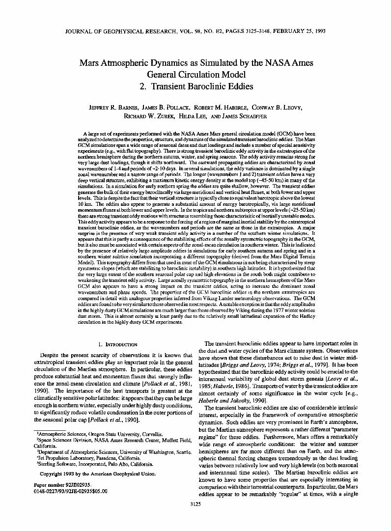
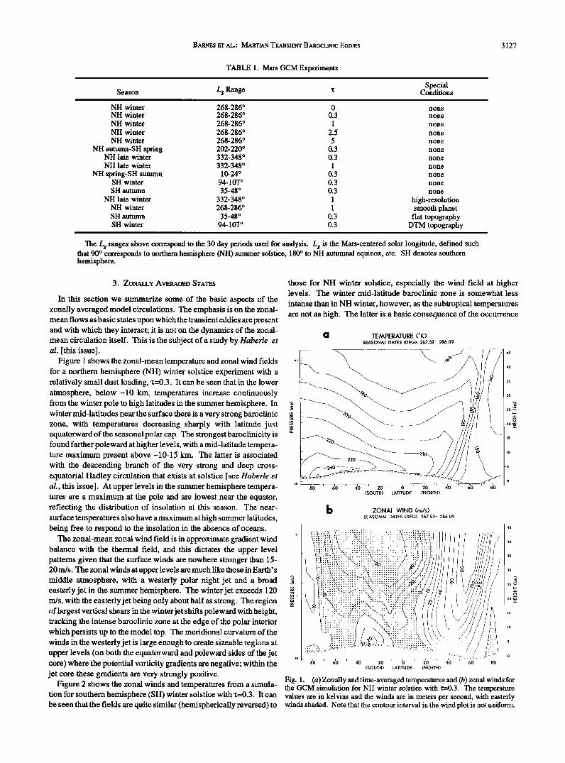
Figure 1 shows the zonal-mean temperature and zonal wind fields for a northern hemisphere (NH) winter solstice experiment with a relatively small dust loading, x--0.3. It can be seen that in the lower atmosphere, below ~10 km, temperatures increase continuously from the winter pole to high latitudes in the summer hemisphere. In winter mid-latitudes near the surface there is a very strong baroclinic zone, with temperatures decreasing sharply with latitude just equatorward of the seasonal polar cap. The strongest baroclinicity is found farther poleward at higher levels, with a mid-latitude tempera- ture maximum present above -10-15 km. The latter is associated with the descending branch of the very strong and deep cross- equatorial Hadley circulation that exists at solstice [see Haberle et a/., this issue]. At upper levels in the summer hemisphere tempera- tures are a maximum at the pole and are lowest near the equator, reflecting the distribution of insolation at this season. The near- surface temperatures also have a maximum at high summer latitudes, being free to respond to the insolation in the absence of oceans.
The zonal-mean zonal wind field is in approximate gradient wind balance with the thermal field, and this dictates the upper level patterns given that the surface winds are nowhere stronger than 15- 20 m/s. The zonal winds at upper levels are much like those in Earth' s middle atmosphere, with a westerly polar night jet and a broad easterly jet in the summer hemisphere. The winter jet exceeds 120 m/s, with the easterly jet being only about half as strong. The region of largest vertical shears in the winter jet shifts poleward with height, tracking the intense baroclinic zone at the edge of the polar interior which persists up to the model top. The meridional curvature of the winds in the westerly jet is large enough to create sizeable regions at upper levels (on both the equatorward and poleward sides of the jet core) where the potential vorticity gradients are negative; within the jet core these gradients are very strongly positive.
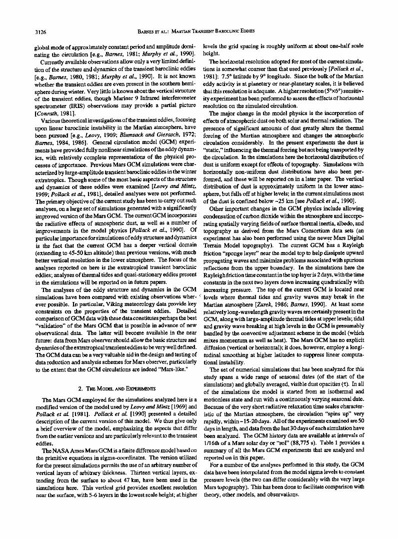
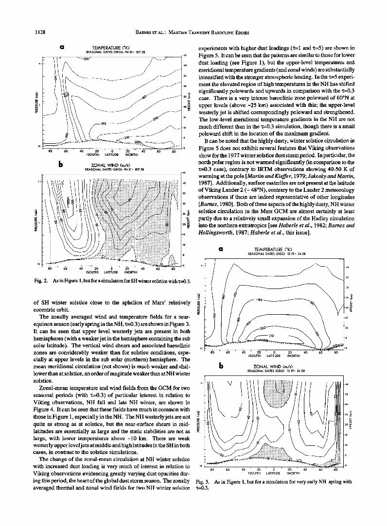
Figure 2 shows the zonal winds and temperatures from a simula- tion for southern hemisphere (SH) winter solstice with •=0.3. It can be seen that the fields are quite similar (hemispherically reversed) to
those for NH winter solstice, especially the wind field at higher levels. The winter mid-latitude baroclinic zone is somewhat less
intense than in NH winter, however, as the subtropical temperatures are not as high. The latter is a basic consequence of the occurrence
TEMPERATURE (*K) SEASONAL DATES (DEG)= 267.52- 286.09
Fig. 1. (a) Zonally and t•me-averaged temperatures and (b) zonal winds for the GCM simulation for NH winter solstice with x=0.3. The temperature values are in kelvins and the winds are in meters per second, with easterly winds shaded. Note that the contour interval in the wind plot is not uniform.
3128 BARNES ET AL.: MARTIAN TRANSIENT BAROCLINIC EI>I>IES
o!
a TEMPERATURE (øK) SEASONAL DATES (DEG): 9,4.01- 107.38
v •1õo / --
oo 6o 4o 2o o 2o 4o 6o •o
• ZONAL WIND (m/s) s•so•r o•t•s (o•e): •.ol-
o!
4O
35
30
•5
•0
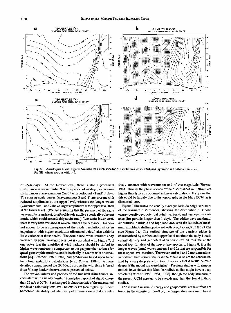
experiments with higher dust loadings (x=l and x=5) are shown in Figure 5. It can be seen that the patterns are similar to those for lower dust loading (see Figure 1), but the upper-level temperatures and meridional temperature gradients (and zonal winds) are substantially intensified with the stronger atmospheric heating. In the'r=5 experi- ment the elevated region of high temperatures in the NH has shifted significantly polewards and upwards in comparison with the 'r=0.3 case. There is a very intense baroclinic zone poleward of 60øN at upper levels (above -25 kin) associated with this' the upper-level westerly jet is shifted correspondingly poleward and strengthened. The low-level meridional temperature gradients in the NH are not much different than in the 'r=0.3 simulation, though there is a small poleward shift in the location of the maximum gradient.
It can be noted that the highly dusty, winter solstice circulation in Figure 5 does not exhibit several features that Viking observations show for the 1977 winter solstice dust storm period. In particular, the north polar region is not warmed significantly (in comparison to the x=0.3 case), contrary to IRTM observations showing 40-50 K of warming at the pole [Martin and Kieffer, 1979; Jakosky and Martin,
-,o 1987]. Additionally, surface easterlies are not present at the latitude
-. of Viking Lander 2 (- 48øN), contrary to the Lander 2 meteorology observations if these are indeed representative of other longitudes
3o [Barnes, 1980]. Both of these aspects of the highly dusty, NH winter '• solstice circulation in the Mars GCM are almost certainly at least ,,- partly due to a relatively small expansion of the Hadley circulation o
-20 •: into the northern extratropics [see Haberle et al., 1982; Barnes and -,3 Hullingsworth, 1987' Haberle et al., this issue].
-io
a TEMPERATURE (OK) • SEASONAL DATES (DEG) 10 15- 24 28
o'o do 4•- -•---)•o 6 TM 2'0 4o •,o •o (SOUTH) LATITUDE (NORTH)
Fig. 2. As in Figure 1, but for a simulation for SH winter solstice with'r=0.3.
of SH winter solstice close to the aphelion of Mars' relatively eccentric orbit.
The zonally averaged wind and temperature fields for a near- equinox season (early spring in the NH, 'r=0.3) are shown in Figure 3. It can be seen that upper level westerly jets are present in both hemispheres (with a weaker jet in the hemisphere containing the sub solar latitude). The vertical wind shears and associated baroclinic zones are considerably weaker than for solstice conditions, espe- cially at upper levels in the sub solar (northern) hemisphere. The mean meridional circulation (not shown) is much weaker and shal- lower than at solstice, an order of magitude weaker than at NH winter solstice.
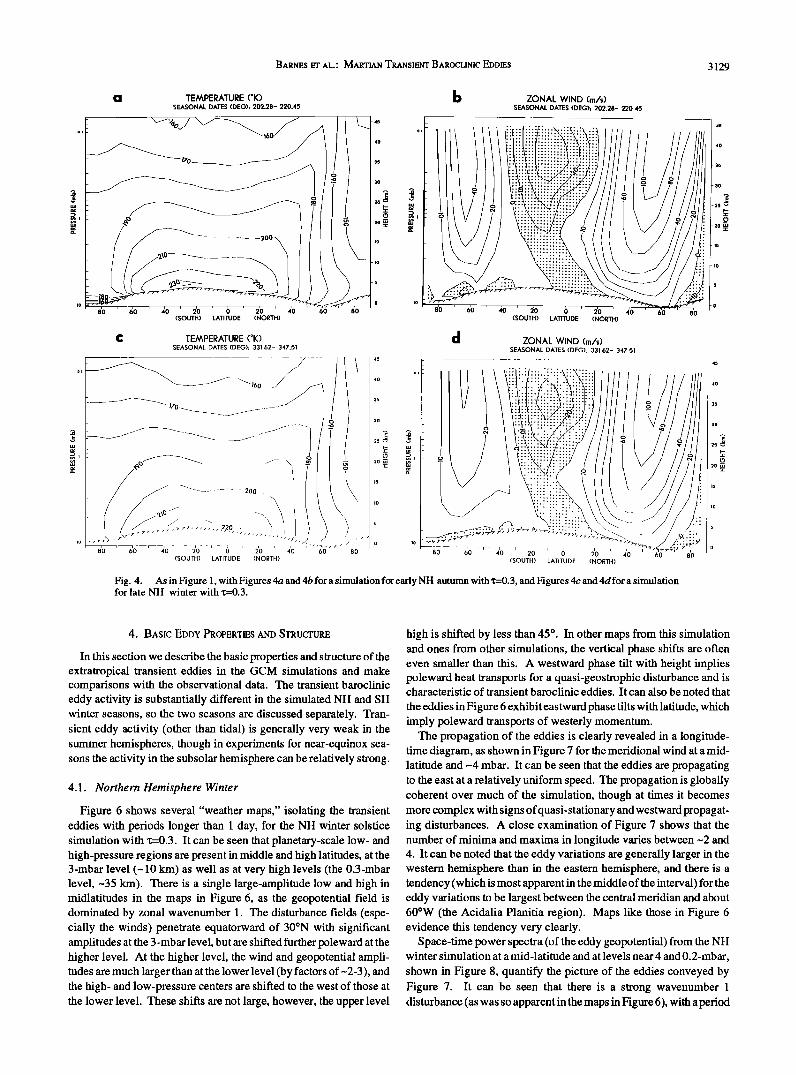
Zonal-mean temperature and wind fields from the GCM for two seasonal periods (with 'r=0.3) of particular interest in relation to Viking observations, NH fall and late NH winter, are shown in Figure 4. It can be seen that these fields have much in common with those in Figure 1, especially in the NH. The NH westerly jets are not quite as strong as at solstice, but the near-surface shears in mid- latitudes are essentially as large and the static stabilities are not as large, with lower temperatures above ~10 km. There are weak westerly upper leveljets atmiddle and high latitudes in the SH in both cases, in contrast to the solstice simulations.
The change of the zonal-mean circulation at NH winter solstice
-40
- 35
-- -20 •
•o •o •o 2o ' 6 •o •o ' d6'"' •'o (SOUTH) LATITUDE (NORTH)
• ZONAL WIND (m/s) SEASONAL DATES (DEG)• 10,15- 24.28
with increased dust loading is v•ry much of interest in r•lation to •o •o •o :o o :o •'o •o •'o Vih•g observations •vid•cing gr•ady v•ying dust opaciti•s dur- •sou• •muo• •o•.• ins •is •riod, •e he•t of the global dust storm season. %e zonally Fig. 3. • i• Figur• 1, but for a simulafio• for wry •ly NH •ri•g wi• averaged •e•al and zonal wind fields for two NH winter solstice •=0.3.
BARNES ET AL.: MARTIAN TRANSIENT BARDCLINIC EDDIES 3129
a TEMPERATURE (øK) [• ZONAL WIND (m/s) SEASONAL DATES (DEO): 202.28- 220.45 SEASONAL DATES (DEO): 202.28- 220.45
- 45 45
=o 30 E O , • i 2• •
930•• - •o •o
.•--•. -15,•-• - o 8'0 ' •0 40 20 0 20 40 •0 80
(SOUTH) LATITUDE(NORTH) • )3 35
25 • 25 •
• • • • 71• • I 'ø ' •o• • • • • •oo
80 ' ' ' 4'0 60 80 8• gO 4'0 2'0 6 2'0 4'0 60 80 (SOUTH) LATITUDE (NORTH) (SOUTH) LATITUDE (NORTH)
Fig. 4. As in Figure 1, with Figures 4a and 4b for a simulation for early NH autumn with'm=0.3, and Figures 4c and 4dfor a simulation for late NH winter with '•=0.3.
4. BASIC EDDY PROPERTIES AND STRUCTURE
In this section we describe the basic properties and structure of the extratropical transient eddies in the GCM simulations and make comparisons with the observational data. The transient baroclinic eddy activity is substantially different in the simulated NH and SH winter seasons, so the two seasons are discussed separately. Tran- sient eddy activity (other than tidal) is generally very weak in the summer hemispheres, though i n experiments for near-equinox sea- sons the activity in the subsolar hemisphere can be relatively strong.
4.1. Northern Hemisphere Winter
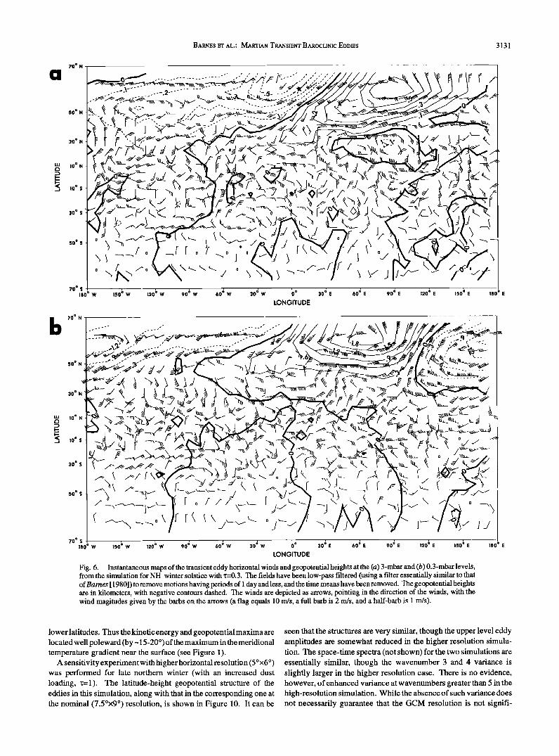
Figure 6 shows several "weather maps," isolating the transient eddies with periods longer than 1 day, for the NH winter solstice simulation with 'c=0.3. It can be seen that planetary-scale low- and high-pressure regions are present in middle and high latitudes, at the 3-mbar level (~ 10 km) as well as at very high levels (the 0.3-mbar level, -35 km). There is a single large-amplitude low and high in midlatitudes in the maps in Figure 6, as the geopotential field is dominated by zonal wavenumber 1. The disturbance fields (espe- cially the winds) penetrate equatorward of 30øN with significant amplitudes at the 3-mbar level, but are shifted further poleward at the higher level. At the higher level, the wind and geopotential ampli- tudes are much larger than at the lower level (by factors of --2-3), and the high- and low-pressure centers are shifted to the west of those at the lower level. These shifts are not large, however, the upper level
high is shifted by less than 45 ø . In other maps from this simulation and ones from other simulations, the vertical phase shifts are often even smaller than this. A westward phase tilt with height implies poleward heat transports for a quasi-geostrophic disturbance and is characteristic of transient baroclinic eddies. It can also be noted that
the eddies in Figure 6 exhibit eastward phase tilts with latitude, which imply poleward transports of westerly momentum.
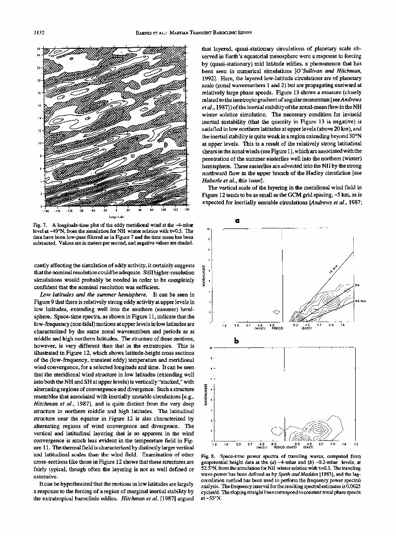
The propagation of the eddies is clearly revealed in a longitude- time diagram, as shown in Figure 7 for the meridional wind at a mid- latitude and ~4 mbar. It can be seen that the eddies are propagating to the east at a relatively uniform speed. The propagation is globally coherent over much of the simulation, though at times it becomes more complex with signs of quasi-stationary and westward propagat- ing disturbances. A close examination of Figure 7 shows that the number of minima and maxima in longitude varies between -2 and 4. It can be noted that the eddy variations are generally larger in the western hemisphere than in the eastern hemisphere, and there is a tendency (which is most apparent in the middle of the interval) for the eddy variations to be largest between the central meridian and about 60øW (the Acidalia Planitia region). Maps like those in Figure 6 evidence this tendency very clearly.
Space-time power spectra (of the eddy geopotential) from the NH winter simulation at a mid-latitude and at levels near 4 and 0.2-mbar,
shown in Figure 8, quantify the picture of the eddies conveyed by Figure 7. It can be seen that there is a strong wavenumber 1 disturbance (as was so apparent in the maps in Figure 6), with a period
3130 BARNES ET AL.: MARTIAN TRANSIENT BAROCLINIC EDDIES
a TEAAPERATURE (:øK) b ZONAL WIND SEASONAL DATES (DEG).. 267.õ2- 286.09 SEASONAL DATES (DEG): 267.õ2- 286.09
0, :
o
•o • • •o •:
o!
40
•o •o •o b •o •o •o eo e'o •o •o •'o • •'o •o •o <SOUTH• L^T•TUDE <NO.TH• CSC:)UTH• L^T•TUC•E CNC:)•TH•
Fiõ. 5. As inFiõure ], withFiõures •a and 5bœorasimu]ationfor NH wJnterso]sticewith•=], andFJõures 5œ and 5dfor asJmu]•tion for NH winter solstice with x=5.
of ~5-6 days. At the 4-mbar level, there is also a prominent disturbance at wavenumber 3 with a period of ~2 days, and weaker disturbances at wavenumbers 2 and 4 with periods of-3 and 1.4 days. The shorter-scale waves (wavenumbers 3 and 4) are present with reduced amplitudes at the upper level, whereas the longer waves (wavenumbers 1 and 2) have larger amplitudes at the upper level than at the lower level. (We are assuming that the presence of the same wavenumbers and periods at both levels implies a vertically coherent mode, which could conceivably not be true.) Even at the lower level, there is very little variance at wavenumbers greater than 5. This does not appear to be a consequence of the model resolution, since an experiment with higher resolution (discussed below) also exhibits little variance at these scales. The dominance of the transient eddy variance by zonal wavenumbers 1-4 is consistent with Figure 7, if one notes that the meridional wind variance should be shifted to
higher wavenumbers in comparison to the geopotential variance for quasi-geostrophic motions, and is basically in accord with observa- tions [e.g., Barnes, 1980, 1981] and predictions based upon linear baroclinic instability calculations [e.g., Barnes, 1984]. A more detailed comparison of the GCM eddy properties with those inferred from Viking lander observations is presented below.
The wavenumbers and periods of the transient disturbances are consistent with a nearly constant zonal phase speed, of slightly more than 25 m/s at 50øN. Such a speed is characteristic of the mean zonal winds at a relatively low level, below ~5 km (see Figure 1). Linear baroclinic instability calculations yield phase speeds that are rela-
tively constant with wavenumber and of this magnitude [Barnes, 1984], though the phase speeds of the disturbances in Figure 8 are higher than typically obtained in linear calculations. It appears that this could be largely due to the topography in the Mars GCM, as is discussed later.
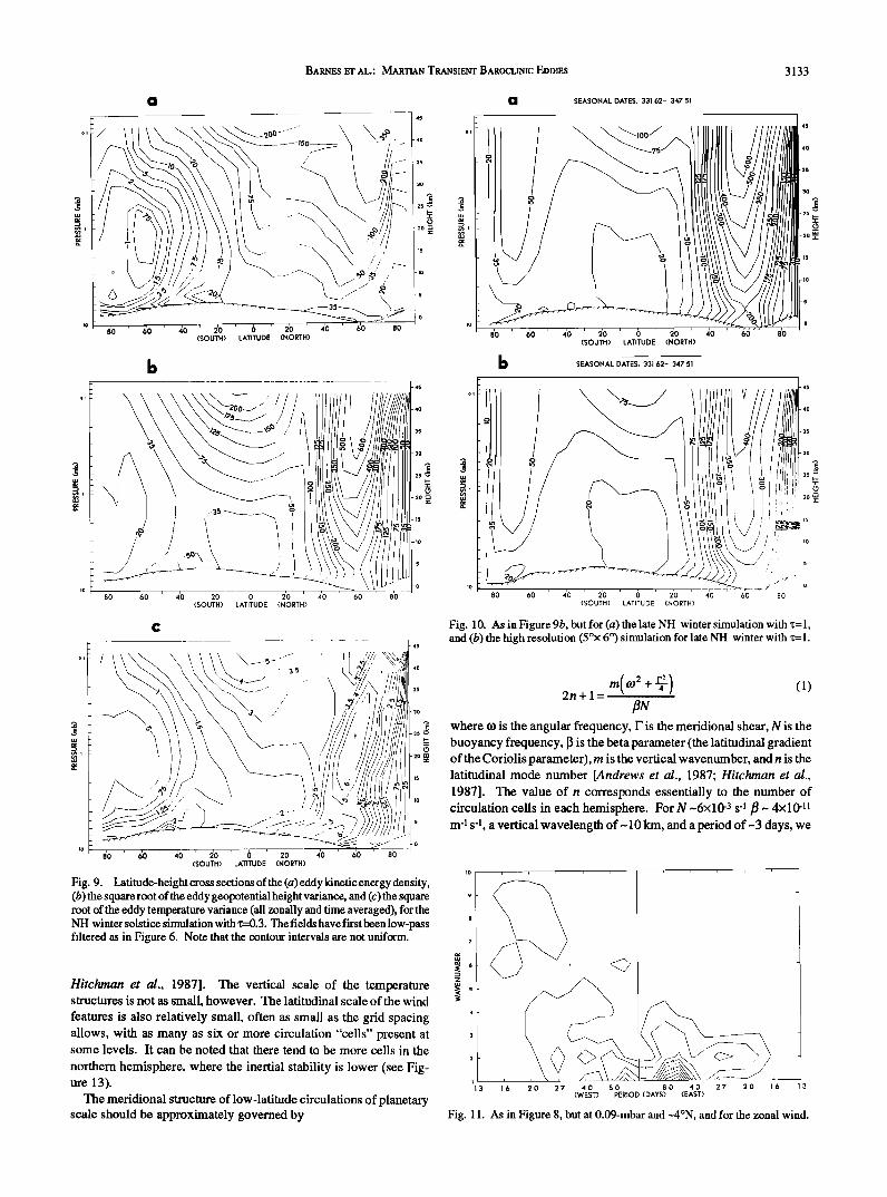
Figure 9 illustrates the zonally averaged latitude-height structure of the transient disturbances, showing the distribution of kinetic energy density, geopotential height variance, and temperature vari- ance (for periods longer than 1 day). The eddies have maximum amplitudes in middle and high latitudes, with the latitude of maxi- mum amplitude shifting poleward with height along with the jet axis (see Figure 1). The vertical structure of the transient eddies is characterized by surface and upper level maxima; the eddy kinetic energy density and geopotential variance exhibit maxima at the model top. In view of the space-time spectra in Figure 8, it is the longer waves (zonal wavenumbers 1 and 2) that are responsible for these upper level maxima. The wavenumber 1 and 2 transient eddies in northern hemisphere winter in the Mars GCM are thus character- ized by a very deep structure (and it appears that it would be even deeper if the model top were higher). Previous studies with simpler models have shown that Mars baroclinic eddies might have a deep structure [Barnes, 1983, 1984, 1986], though the eddy structure in the present GCM appears to be even deeper than that found in these studies.
The maxima in kinetic energy and geopotential at the surface are found in the vicinity of 55-60øN; the temperature maximum lies at
BARNES ET AL.: MARTIAN TRANSIENT BAROCLINIC EDDIES 3131
70 ø N
a
50 ø N
30 ø N
LU I0 ø N :=)
• I0 ø S
30 ø S
•50 ø S
70 ø $
b 70 ø N
õ0 ø N
30 ø N
I0 ø N
i0 ø S
180 ø W 150 ø W 120 ø W 90 ø W 60 ø W 30 ø W 0 ø 30 ø E 60 ø E 90 ø E 120 ø E Iõ0 ø E 180 ø E LONGITUDE
30 ø S
õ0 ø S
70 ø S
'"-'--1
180 ø W Iõ0 ø W 120 ø W 90 ø W 60 ø W 30 ø W 0 ø 30 ø E 60 ø E 90 ø E 120 ø E Iõ0 ø E 180 ø E LONGITUDE
Fig. 6. Instantaneous maps of the transient eddy horizontal winds and geopotential heights at the (a) 3-mbar and (b) 0.3-mbar levels, from the simulation for NH winter solstice with •:=0.3. The fields have been low-pass filtered (using a filter essentially similar to that of Barnes [ 1980]) to remove motions having periods of 1 day and less, and the time means have been removed. The geopotenfial heights are in kilometers, with negative contours dashed. The winds are depicted as arrows, pointing in the direction of the winds, with the wind magitudes given by the barbs on the arrows (a flag equals 10 m/s, a full barb is 2 m/s, and a half-barb is 1 m/s).
lower latitudes. Thus the kinetic energy and geopotential maxima are located well poleward (b y -15-20 ø) of the maxim um in the meridional temperature gradient near the surface (see Figure 1).
A sensitivity experiment with higher horizontal resolution (5øx6 ø) was performed for late northern winter (with an increased dust loading, 'c=l). The latitude-height geopotential structure of the eddies in this simulation, along with that in the corresponding one at the nominal (7.5øx9 ø) resolution, is shown in Figure 10. It can be
seen that the structures are very similar, though the upper level eddy amplitudes are somewhat reduced in the higher resolution simula- tion. The space-time spectra (not shown) for the two simulations are essentially similar, though the wavenumber 3 and 4 variance is slightly larger in the higher resolution case. There is no evidence, however, of enhanced variance at wavenumbers greater than 5 in the high-resolution simulation. While the absence of such variance does not necessarily guarantee that the GCM resolution is not signifi-
3132 B^•s ET AL.: MART•N TRANSIENT B^ROCLINIC E•t•ms
that layered, quasi-stationary circulations of planetary scale ob- served in Earth's equatorial mesosphere were a response to forcing by (quasi-stationary) mid latitude eddies, a phenomenon that has been seen in numerical simulations [O'Sullivan and Hitchman, 1992]. Here, the layered low-lat:.tude circulations are of planetary scale (zonal wavenumbers 1 and 2) but are propagating eastward at relatively large phase speeds. Figure 13 shows a measure (closely related to the isentropic gradient of angular momentum [see Andrews eta/., 1987]) of the inertial stability of the zonal-mean flow in the NH winter solstice simulation. The necessary condition for inviscid inertial instability (that the quantity in Figure 13 is negative) is satisfied in low northern latitudes at upper levels (above 20 km), and the inertial stability is quite weak in a region extending beyond 30øN at upper levels. This is a result of the relatively strong latitudinal shears in the zonal winds (see Figure 1), which are associated with the penetration of the summer easterlies well into the northern (winter) hemisphere. These easterlies are advected into the NH by the strong northward flow in the upper branch of the Hadley circulation [see Haberle et al., this issue].
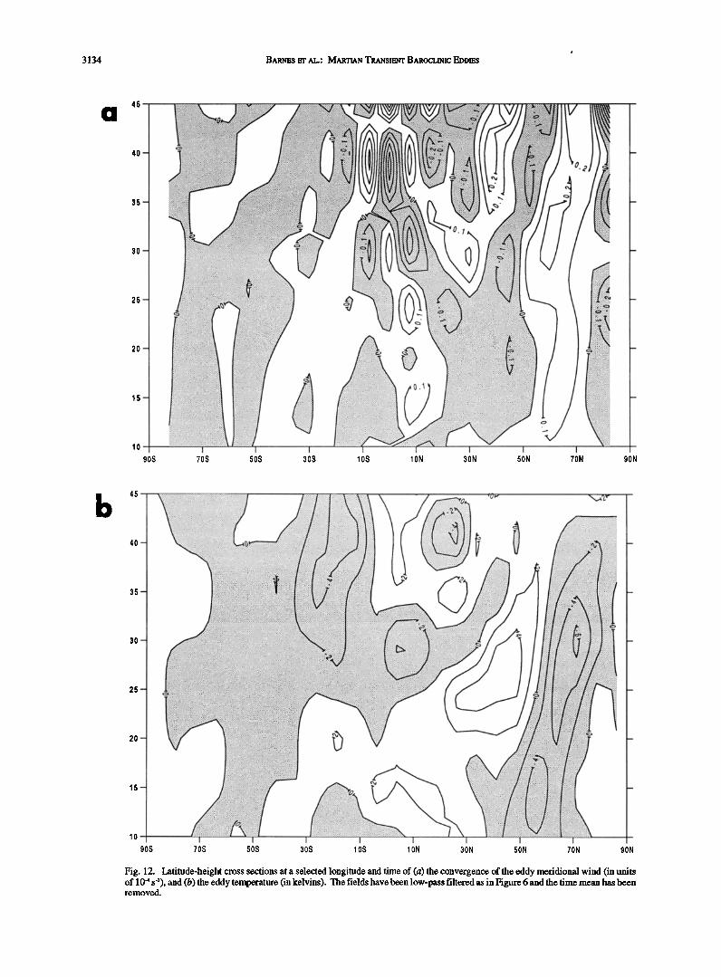
The vertical scale of the layering in the meridional wind field in Figure 12 tends to be as small as the GCM grid spacing, -5 km, as is expected for inertially unstable circulations [Andrews et al., 1987;
Long• tude
Fig. 7. A longitude-time plot of the eddy meridional wind at the -4-mbar level at -49øN, from the simulation for NH winter solstice with x=0.3. The data have been low-pass filtered as in Figure 7 and the time mean has been subtracted. Values are in meters per second, and negative values are shaded.
canfly affecting the simulation of eddy activity, it certainly suggests that the nominal resolution could be adequate. Still higher-resolution simulations would probably be needed in order to be completely confident that the nominal resolution was sufficient.
Low latitudes and the summer hemisphere. It can be seen in Figure 9 that there is relatively strong eddy activity at upper levels in low latitudes, extending well into the southern (summer) hemi- sphere. Space-time spectra, as shown in Figure 11, indicate that the low-frequency (non tidal) motions at upper levels in low latitudes are characterized by the same zonal wavenumbers and periods as at middle and high northern latitudes. The structure of these motions, however, is very different than that in the extratropics. This is illustrated in Figure 12, which shows latitude-height cross sections of the (low-frequency, transient eddy) temperature and meridional wind convergence, for a selected longitude and time. It can be seen that the meridional wind structure in low latitudes (extending well into both the NH and SH at upper levels) is vertically "stacked," with alternating regions of convergence and divergence. Such a structure resembles that associated with inertially unstable circulations [e.g., Hitchman et al., 1987], and is quite distinct from the very deep structure in northern middle and high latitudes. The latitudinal structure near the equator in Figure 12 is also characterized by alternating regions of wind convergence and divergence. The vertical and latitudinal layering that is so apparent in the wind convergence is much less evident in the temperature field in Fig- ure 11. The thermal field is characterized by distinctly larger vertical and latitudinal scales than the wind field. Examination of other
cross-sections like those in Figure 12 shows that these structures are fairly typical, though often the layering is not as well defined or extensive.
It can be hypothesized that the motions in low latitudes are largely a response to the forcing of a region of marginal inertial stability by the extratropical baroclinic eddies. Hitchman et al. [1987] argued
8 0 4.0 2.7 2.0 16 PERIOD (EAST)
1.6 2.0 2.7 4.0 8.0 (WEST)
40 m/s
1
1.3 1.6 2.0 2.7 4.0 1.3 (WEST)
8.0 8.0 4.0 2.7 2.0 1.6 PERIOD (DAYS) (EAST)
Fig. 8. Space-time power spectra of traveling waves, computed from geopotential height data at the (a) -4-mbar and (b) -0.2-mbar levels, at 52.5øN, from the simulation for NH winter solstice with x=0.3. The traveling wave power has been defined as by Speth and Madden [ 1983], and the lag- correlation method has been used to perform the frequency power spectral analysis. The frequency interval for the resulting spectral estimates is 0.0625 cycles/d. The sloping straight lines correspond to constant zonal phase speeds at -53øN.
BARNES ET AL.: MARTIAN TRANSIENT BAROCLINIC EDDIES 3133
a a SEASONAL DATES, 331.62- 347.õ1
••• c• 3o
(SOUTH) LATITUDE (NORTH)
(SOUTH) LATITUDE (NORTH)
9
8
7
Z
Fig. 9. Latitude-height cross sections of the (a) eddy kinetic energy density, (b) the square root of the eddy geopotenfial height variance, and (c) the square root of the eddy temperature variance (all zonally and time averaged), for the NH winter solstice simulation with'c=0. 3. The fields have first been low-pass filtered as in Figure 6. Note that the contour intervals are not uniform.
Hitchman et al., 1987]. The vertical scale of the temperature structures is not as small, however. The latitudinal scale of the wind
features is also relatively small, often as small as the grid spacing allows, with as many as six or more circulation "cells" present at some levels. It can be noted that there tend to be more cells in the
northern hemisphere, where the inertial stability is lower (see Fig- ure 13).
The meridional structure of low-latitude circulations of planetary scale should be approximately governed by
I1. 3 1.3 1.6 2.0 2.7 4.0 8.0 (WEST)
8.0 4.0 2.7 2.0 1.6 PERIOD (DAYS) (EAST)
Fig. 11. As in Figure 8, but at 0.09-mbar and -4øN, and for the zonal wind.
3134 BARNES ET ̂ L.: MARTIAN TRANSIENT B^ROCLINIC EDDIES
i i i
90s 70s 50s 30s 10s 1ON 30N 50N 70N 90N
b 45
35
Fig. 12. Latitude-height cross sections at a selected longitude and time of (a) the convergence of the eddy meridional wind (in units of 10 -4 s-•), and (b) the eddy temperature (in kelvins). The fields have been low-pass filtered as in Figure 6 and the time mean has been removed.
BARNES ET AL.: MARTIAN TRANSIENT BAROCLINIC EDDIES 3135
I I I I I I I I
90S 70S 50S 30S 10$ 10N 30N 50N 70N 90N
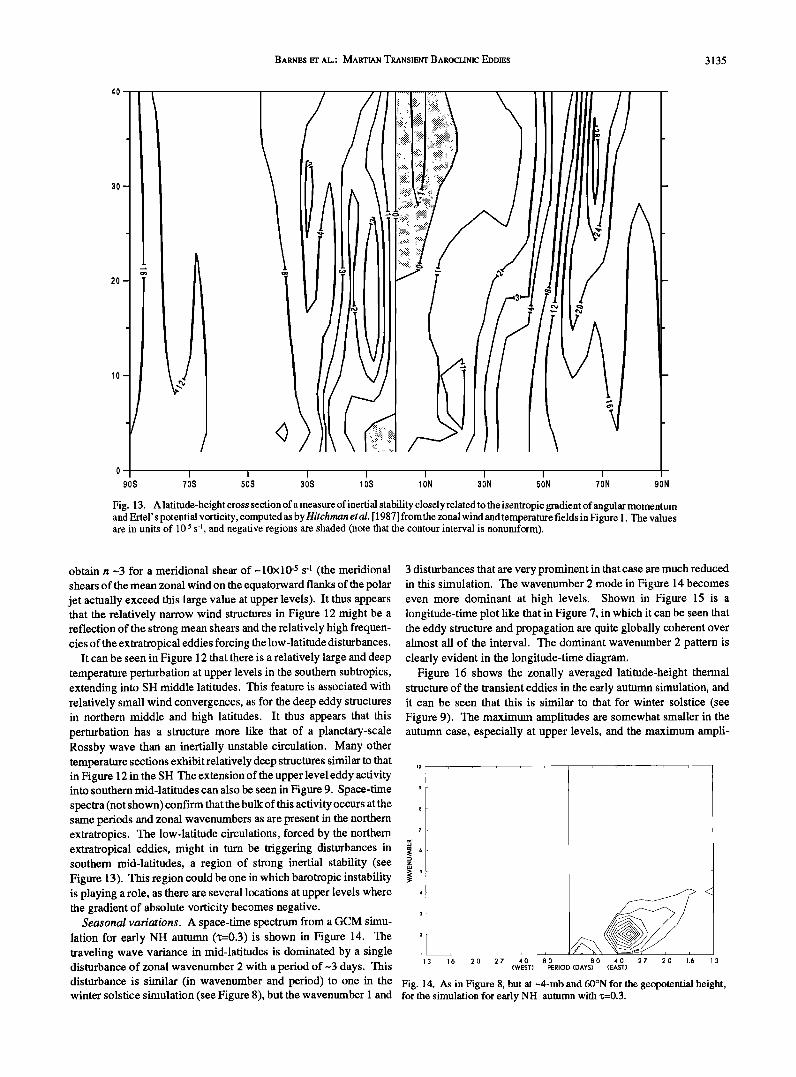
Fig. 13. A latitude-height cross section of a measure of inertial stability closely related to the isentropic gradient of angular momentum and Ertel' s potential vorticity, computed as by Hitch man et al. [ 1987] from the zonal wind and temperature fields in Figure 1. The values are in units of 10 -5 s -l, and negative regions are shaded (note that the contour interval is nonuniform).
obtain n -3 for a meridional shear of-10xlff 5 s -• (the meridional shears of the mean zonal wind on the equatorward flanks of the polar jet actually exceed this large value at upper levels). It thus appears that the relatively narrow wind structures in Figure 12 might be a reflection of the strong mean shears and the relatively high frequen- cies of the extratropical eddies forcing the low-latitude disturbances.
It can be seen in Figure 12 that there is a relatively large and deep temperature perturbation at upper levels in the southern subtropics, extending into SH middle latitudes. This feature is associated with relatively small wind convergences, as for the deep eddy structures in northern middle and high latitudes. It thus appears that this perturbation has a structure more like that of a planeta13•-scale Rossby wave than an inertially unstable circulation. Many other temperature sections exhibit relatively deep structures similar to that in Figure 12 in the SH The extension of the upper level eddy activity into southern mid-latitudes can also be seen in Figure 9. Space-time spectra (not shown) confirm that the bulk of this activity occurs at the same periods and zonal wavenumbers as are present in the northern extratropics. The low-latitude circulations, forced by the northern extratropical eddies, might in turn be triggering disturbances in southern mid-latitudes, a region of strong inertial stability (see Figure 13). This region could be one in which barotropic instability is playing a role, as there are several locations at upper levels where the gradient of absolute vorticity becomes negative.
Seasonal variations. A space-time spectrum from a GCM simu- lation for early NH autumn (x=0.3) is shown in Figure 14. The traveling wave variance in mid-latitudes is dominated by a single disturbance of zonal wavenumber 2 with a period of--3 days. This
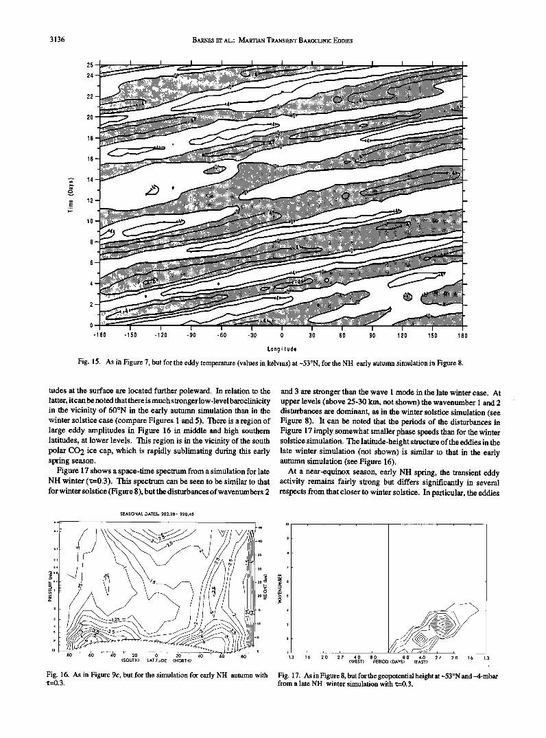
3 disturbances that are very prominent in that case are much reduced in this simulation. The wavenumber 2 mode in Figure 14 becomes even more dominant at high levels. Shown in Figure 15 is a longitude-time plot like that in Figure 7, in which it can be seen that the eddy structure and propagation are quite globally coherent over almost all of the interval. The dominant wavenmnber 2 pattern is clearly evident in the longitude-time diagram.
Figure 16 shows the zonally averaged latitude-height thermal structure of the transient eddies in the early autumn simulation, and it can be seen that this is similar to that for winter solstice (see
Figure 9). The maximum amplitudes are somewhat smaller in the autumn case, especially at upper levels, and the maximum ampli-
ua
1.3 1.6 2.0 2.7 4.0 8.0 (WEST) PERIOD (DAYS)
8.0 4.0 2.7 2.0 1.6 1.3 (EAST)
disturbance is similar (in wavenumber and period) to one in the Fig. 14. As in Figure 8, but at •-4-mb and 60øN for the geopotential height, winter solstice simulation (see Figure 8), but the wavenumber 1 and for the simulation for early NH autumn with '•=0.3.
3136 B^RNES ET AL.: MARTIAN TRANSIENT BAROCLINIC EVVIES
25
24
14
12
0
-180 -150 -120 -90 -60 -30 0 30 60 90 120 150 180
Longi t ude
Fig. 15. As in Figure 7, but for the eddy temperature (values in kelvins) at --53øN, for the NH early autumn simulation in Figure 8.
tudes at the surface are located further poleward. In relation to the latter, it can be noted that there is much stronger low-level baroclinicity in the vicinity of 60øN in the early autumn simulation than in the winter solstice case (compare Figures 1 and 5). There is a region of large eddy amplitudes in Figure 16 in middle and high southern latitudes, at lower levels. This region is in the vicinity of the south polar CO 2 ice cap, which is rapidly sublimating during this early spring season.
Figure 17 shows a space-time spectrum from a simulation for late NH winter (x=0.3). This spectrum can be seen to be similar to that for winter solstice (Figure 8), but the disturbances of wavenumbers 2
and 3 are stronger than the wave 1 mode in the late winter case. At upper levels (above 25-30 km, not shown) the wavenumber 1 and 2 disturbances are dominant, as in the winter solstice simulation (see Figure 8). It can be noted that the periods of the disturbances in Figure 17 imply somewhat smaller phase speeds than for the winter solstice simulation. The latitude-height structure of the eddies in the late winter simulation (not shown) is similar to that in the early autumn simulation (see Figure 16).
At a near-equinox season, early NH spring, the transient eddy activity remains fairly strong but differs significantly in several respects from that closer to winter solstice. In particular, the eddies
SEASONAL DATES: 202.28- 220.45
z
2
1.3 1.6 2.o 2.7 •.o 8.o 8.0 •.o 2.7 2.o 1.6 1.3 (SOUTH) LATITUDE (NORTH) (WEST) PERIOD (DAYS) (EAST)
Fig. 16. As in Figure 9c, but for the simulation for early NH autumn with Fig. 17. As in Figure 8, butforthegeopotentialheightat.-53øNand,-4-mbar 'r=0.3. from a late NH winter simulation with 'r=0.3.
BARNES E'r AL.' MARTIAN TRANSIENT BAROCLINIC EDDIES 3137
SEASONAL DATES: 10.1õ- 24.28
(SOUTH) LATITUDE (NORTH)
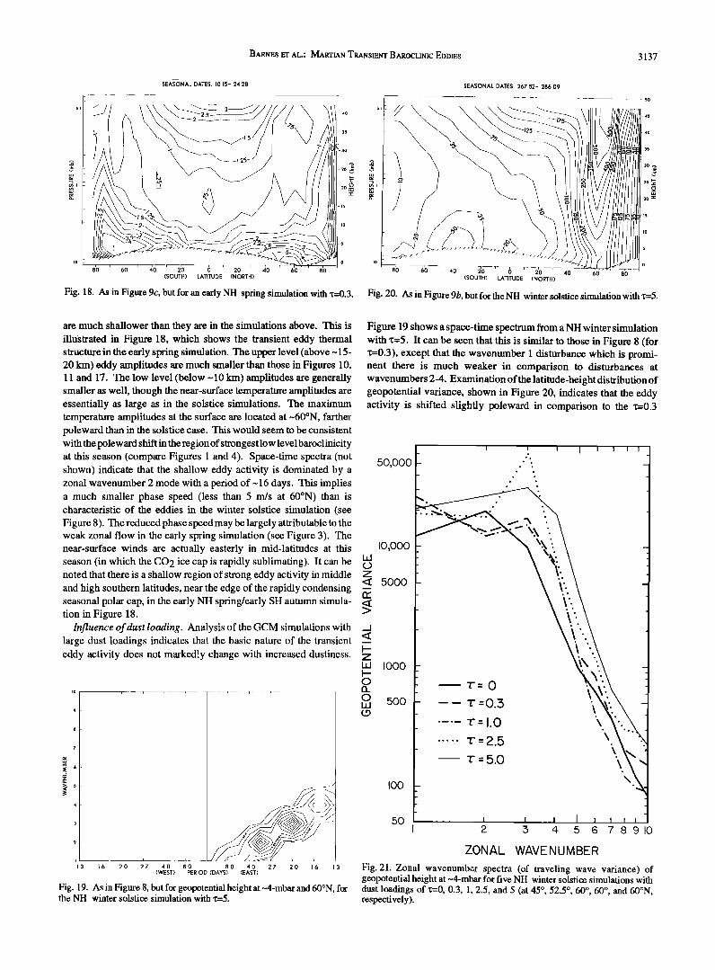
Fig. 18. As in Figure 9c, but for an early NH spring simulation with x=0.3.
SEASONAL DATES.. 267.õ2- 286.09
- - 50
80 60 40 20 I• 20 d(•--- 60 80 (SOUTH) LATITUDE (NORTH)
Fig. 20. As in Figure 9b, but for the NH winter solstice simulation with x=5.
are much shallower than they are in the simulations above. This is illustrated in Figure 18, which shows the transient eddy thermal structure in the early spring simulation. The upper level (above -15- 20 km) eddy amplitudes are much smaller than those in Figures 1 O, 11 and 17. The low level (below -10 km) amplitudes are generally smaller as well, though the near-surface temperature amplitudes are essentially as large as in the solstice simulations. The maximum temperature amplitudes at the surface are located at -60øN, farther poleward than in the solstice case. This would seem to be consistent with the poleward shift in the region of strongestlow levelbaroclinicity at this season (compare Figures 1 and 4). Space-time spectra (not shown) indicate that the shallow eddy activity is dominated by a zonal wavenumber 2 mode with a period of-16 days. This implies a much smaller phase speed (less than 5 m/s at 60øN) than is characteristic of the eddies in the winter solstice simulation (see Figure 8). The reduced phase speed may be largely attributable to the weak zonal flow in the early spring simulation (see Figure 3). The near-surface winds are actually easterly in mid-latitudes at this season (in which the CO 2 ice cap is rapidly sublimating). It can be Lgl noted that there is a shallow region of strong eddy activity in middle Z
<• 5000 and high southern latitudes, near the edge of the rapidly condensing seasonal polar cap, in the early Nit spring/early SH autumn simula- tion in Figure 18.
Influence of dust loading. Analysis of the GCM simulations with large dust loadings indicates that the basic nature of the transient eddy activity does not markedly change with increased dustiness.
9
7
Z
2
1.3 1.6 2.0 2.7 4.0 8.0 8.0 4.0 2.7 2.0 1.6 1.3 (WEST) PERIOD (DAYS) (EA$1)
Fig. 19. As in Figure 8, but for geopotential height at ~4-mbar and 60øN, for the NH winter solstice simulation with x=5.
Figure 19 shows a space-time spectrum from a NH winter simulation with x--5. It can be seen that this is similar to those in Figure 8 (for x=0.3), except that the wavenmnber 1 disturbance which is promi- nent there is much weaker in comparison to disturbances at wavenumbers 2-4. Examination of the latitude-height distribution of g•potential variance, shown in Figure 20, indicates that the eddy activity is shifted slightly poleward in comparison to the x=0.3
50,000 .'; ß .
o
ß
ß
ß
I0,000
i,i 1000
o
o 500
Ioo
r=O \ -- r=O.3 '
.... 'r= 1.0 '\ ß
..... 'r :2.5 \ r: 5.0 '
50 • • • I • I 2_ 3 4 5 6 78910
ZONAL WAVE NUMBER
Fig. 21. Zonal wavenumber spectra (of traveling wave variance) of geopotential height at ~4-mbar for five NH winter solstice simulations with dust loadings of x=0, 0.3, 1, 2.5, and 5 (at 45 ø, 52.5 ø, 60 ø, 60 ø, and 60øN, respectively).
3138 BARNES ET AL.' MARTIAN TRANSIENT BAROCLINIC EDDIES
simulation (see Figure 9). This corresponds to the poleward shift in the maximum baroclinicity of the zonally averaged circulation (compare Figures 1 and 6). The maximum geopotential values, at the surface and aloft, are essentially similar to those in the x=0.3 solstice simulation. It can be noted that the low-latitude upper level region of eddy activity has shifted somewhat northward, and does not appear to be as separate from the middle- and high-latitude activity as in the x=0.3 simulation. In a solstice simulation with x=l (not shown) this is also the case, and the upper level eddy amplitudes are substantially larger than in both the x=0.3 and x=5 cases.
An interesting aspect of the NH winter solstice experiments is that there appears to be a systematic shift in the dominant wavenumbers of the transient eddies with increasing dust loading. This is illus- trated in Figure 21, which shows wavenumber power spectra of the traveling eddies (the tidal variance constitutes a very small compo- nent in all these spectra) from several NH winter simulations with different dust loadings. It can be seen that the dominant wavenumbers in the highly dusty simulations are larger (-3) than those in the less dusty cases (which are as low as 1). (It must be noted, however, that it is possible that the global or hemispheric eddy kinetic energy spectra might not show the same trend as the local spectra in Figure 21.) An increase in dominant wavenumber with decreases in the thermal (radiative) damping time scale has been found in simu- lations with the Mars climate model [Houben et al., 1989]. If the radiative/thermal damping time scale in the Mars GCM decreases with increasing dust loading, as is expected, then the decrease in scale of the transient eddies in both models is associated with an increase
in thermal dissipation/forcing. How increased dissipation/forcing shortens the zonal scales of the dominant eddies is not clear. Analy- ses of the climate model simulations indicate that the direct effect of
the thermal dissipation on the long-wave modes (especially wave 1) is important, as are changes in the structure of the mean flow (R.M. Haberle, personal communication, 1991).
4.2. Southern Hemisphere Winter
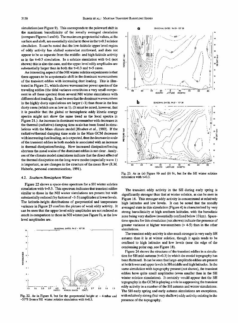
Figure 22 shows a space-time spectrum for a SH winter solstice simulation with x=0.3. This spectrum indicates that transient eddies similar to those in the NH winter simulations are present but with substantially reduced (by factors of-3-5) amplitudes at lower levels. The latitude-height distributions of geopotential and temperature variance in Figure 23 confirm the picture of weak eddy activity. It can be seen that the upper level eddy amplitudes are not reduced as much in comparison to those in NH winter (see Figure 9), as the low level amplitudes are.
SEASONAL DATES, 94.01- 107.38
I i
i.3 i.6 2.0 2.7 4.0 1.6 1.3 (WEST)
8.0 8.0 4.0 2.7 2.0 PERIOD (DAYS) (EAST)
Fig. 22. As in Figure 8, but for the geopotential height at - 4-mbar and -53øS from a SH winter solstice simulation with x=0.3.
• SEASONAL DATES: 94.01- 107.38
'
D . 1-
2o •
15
10
80 60 40 20 0 20 4'0 60 80 (SOUTH) LATITUDE (NORTH)
Fig. 23. As in (a) Figure 9b and (b) 9c, but for the SH winter solstice simulation with 'c=0.3.
The transient eddy activity in the SH during early spring is significantly stronger than that at winter solstice, as can be seen in Figure 16. This stronger eddy activity is concentrated at relatively high latitudes and low levels. It can be noted that the zonally averaged state in this simulation (Figure 4) is characterized by very strong baroclinicity at high southern latitudes, with the baroclinic zone being very shallow (essentially confined below 10 km). Space- time spectra for this simulation (not shown) indicate the presence of greater variance at higher wavenumbers (> 4-5) than in the other simulations.
The transient eddy activity is also much stronger in very early SH autumn than it is at winter solstice, though it again tends to be confined to high latitudes and low levels (near the edge of the condensing polar cap, see Figure 18).
Figure 24 shows the structure of the transient eddies in a simula- tion for SH mid-autumn (x=0.3) in which the model topography has been flattened. It can be seen that large-amplitude eddies are present at both lower and upper levels in SH middle and high latitudes. In the same simulation with topography present (not shown), the transient eddies have quite small amplitudes (even smaller than in the SH winter solstice simulation). It certainly would appear that the SH topography in the GCM is playing a role in suppressing the transient eddy activity in a number of the SH autumn and winter simulations. The SH early spring and early autumn simulations are exceptions, with relatively strong (but very shallow) eddy activity existing in the presence of the topography.
BARNES ET AL.: MARTIAN TRANSIENT BAROCLINIC EDDIES 3139
SEASONAL DATES: 34.66- 48.02
4o
g o
80 6•0 -r 40 7- 2•0 •) 2'0 4•0 60 8'0 (SOUTH) LATITUDE (NORTH)
Fig. 24. As in Figure 9b, but for a simulation for SH midautumn with flat topography and x=0.3.
4.3. Comparison With Viking Observations
long-period activity, while waves 2-4 are associated with the short- period motions (see Figures 9, 15, 18, and 20).
The amplitudes of the GCM eddies in mid-latitudes are generally very comparable to those seen by Viking Lander 2, though somewhat larger. This is illustrated in Table 2, which gives the GCM variances (at periods longer than 1 sol) at the model grid points closest to the Viking Lander 2 location for several of the winter solstice simula- tions, along with the observed Lander 2 variances (also for periods
SEASONAL DATES: 267.52- 286.09 4oo o
300 o
200 o
It is of interest to compare the properties of the extratropical .... transient eddies in the GCM simulations with those inferred from Viking lander observations. Such a comparison provides one of the best "validations" of the Mars GCM that is possible with existing data.
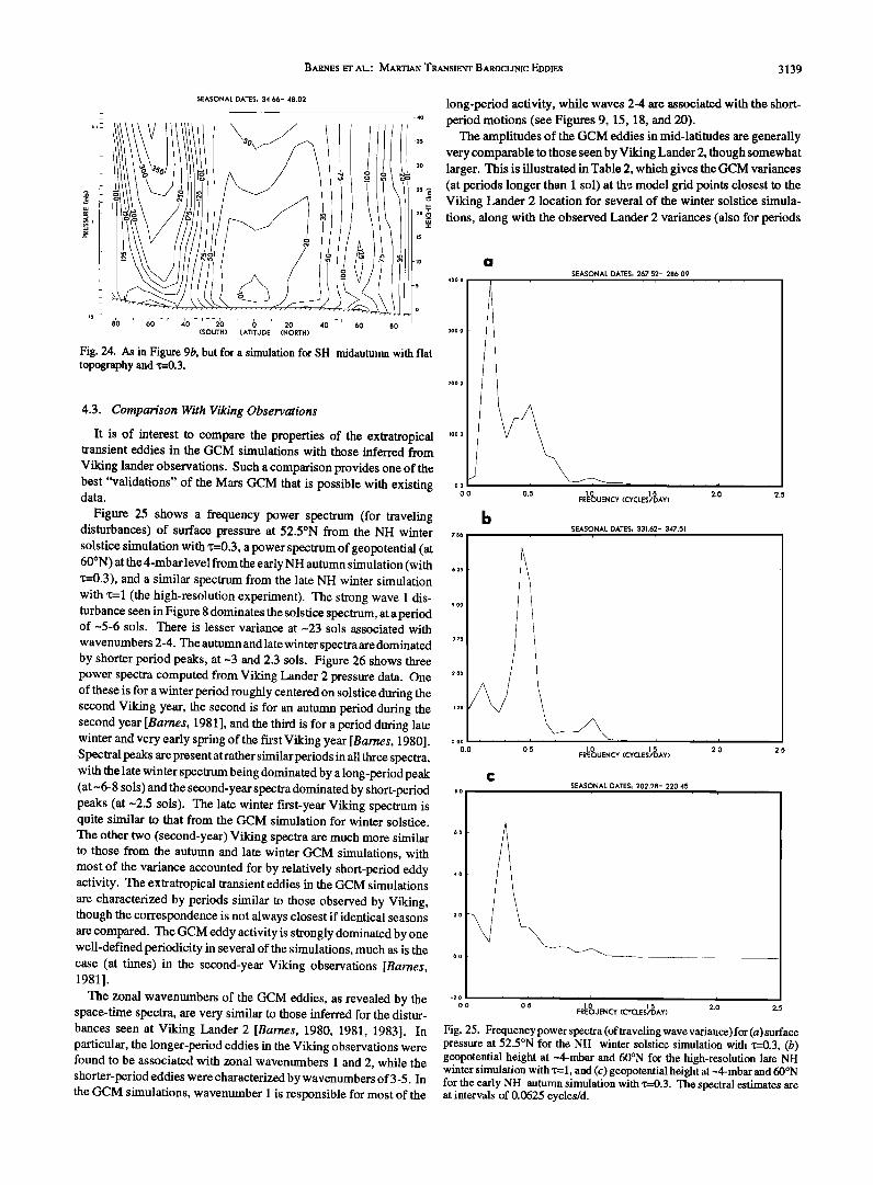
Figure 25 shows a frequency power spectrum (for traveling disturbances) of surface pressure at 52.5øN from the NH winter solstice simulation with 'c=0.3, a power spectrum of geopotential (at 60øN) at the 4-mbar level frøm the early NH autumn simulation ( with 67, 'c=0.3), and a similar spectrum from the late NH winter simulation with 'c=l (the high-resolution experiment). The strong wave 1 dis- 500
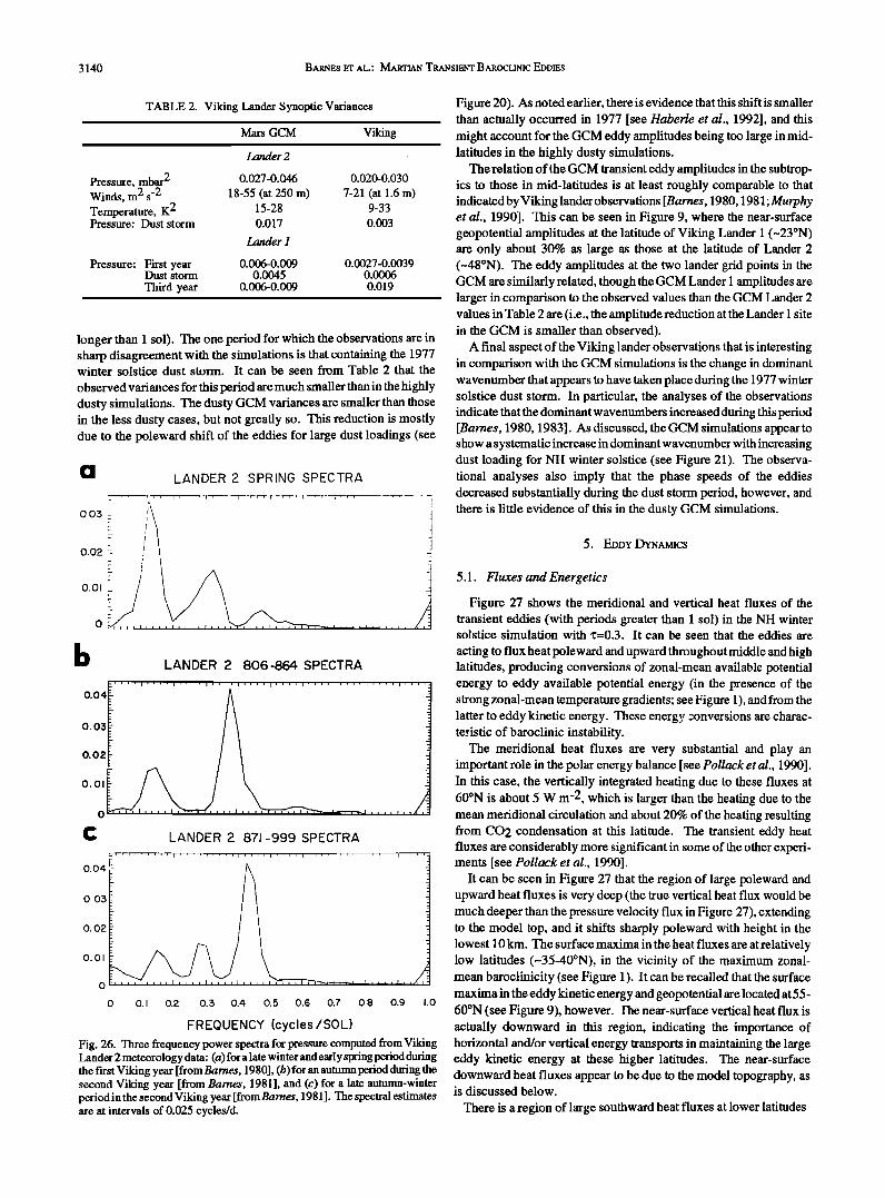
turbance seen in Figure 8 dominates the solstice spectrum, at a period of-5-6 sols. There is lesser variance at -23 sols associated with wavenumbers 2-4. The autumn and late winter spectra are dominated by shorter period peaks, at -3 and 2.3 sols. Figure 26 shows three power spectra computed from Viking Lander 2 pressure data. One 7,0 of these is for a winter period roughly centered on solstice during the second Viking year, the second is for an autumn period during the second year [Barnes, 1981 ], and the third is for a period during late winter and very early spring of the first Viking year [Barnes, 1980]. Spectral peaks are present at rather similar periods in all three spectra, with the late winter spectrum being dominated by a long-period peak (at -6-8 sols) and the second-year spectra dominated by short-period peaks (at -2.5 sols). The late winter first-year Viking spectrum is quite similar to that from the GCM simulation for winter solstice. The other two (second-year) Viking spectra are much more similar 6.0 to those from the autumn and late winter GCM simulations, with most of the variance accounted for by relatively short-period eddy 4.0 activity. The extratropical transient eddies in the GCM simulations are characterized by periods similar to those observed by Viking, though the correspondence is not always closest if identical seasons 7.0 are compared. The GCM eddy activity is strongly dominated by one well-defined periodicity in several of the simulations, much as is the
0.0
case (at times) in the second-year Viking observations [Barnes, 1981].
The zonal wavenumbers of the GCM eddies, as revealed by the space-time spectra, are very similar to those inferred for the distur- bances seen at Viking Lander 2 [Barnes, 1980, 1981, 1983]. In particular, the longer-period eddies in the Viking observations were found to be associated with zonal wavenumbers 1 and 2, while the shorter-period eddies were characterized by wavenumbers of 3-5. In the GCM simulations, wavenmnber 1 is responsible for most of the
00
0.0 0.5 1.0 1.5 2.0 2.5 FREQUENCY (CYCLES/DAY)
SEASONAL DATES: 331.62- 347.51 7.50 ß , , . , . -
000 " , i , = I , = = ,
0.0 1.5 2.0 2.5 FREQUENCY (CYCLES/DAY)
0.5 1.0
SEASONAL DATES: 202.28- 220.45 ,
0.0 0.5 10 1.5 2.0 FREQUENCY (CYCLES/DAY) 2.5
Fig. 25. Frequency power spectra (of traveling wave variance) for (a)surface pressure at 52.5øN for the NH winter solstice simulation with 'c=0.3, (b) geopotential height at --4-mbar and 60øN for the high-resolution late NH winter simulation with'c= I, and (c) geopotential height at --4-mbar and 60øN for the early NH autumn simulation with x=0.3. The spectral estimates are at intervals of 0.0625 cycles/d.
3140 BARNES ET AL.: MARTIAN TRANSIEI'Cr BAROCLINIC EDDIES
TABLE 2. Viking Lander Synoptic Variances
Mars GCM Viking
Lander 2
Pressure, mbar 2 0.027-0.046 0.020-0.030 Winds, m 2 s -2 18-55 (at 250 m) 7-21 (at 1.6 m) Temperature, K 2 15-28 9-33 Pressure: Dust storm 0.017 0.003
Lander I
Pressure: First year 0.006-0.009 0.0027-0.0039 Dust storm 0.0045 0.0006
Third year 0.006-0.009 0.019
longer than 1 sol). The one period for which the observations are in sharp disagreement with the simulations is that containing the 1977 winter solstice dust storm. It can be seen from Table 2 that the
observed variances for this period are much smaller than in the highly dusty simulations. The dusty GCM variances are smaller than those in the less dusty cases, but not greafiy so. This reduction is mosfiy due to the poleward shift of the eddies for large dust loadings (see
0.03
0.02
0.01
b
LANDER 2 SPRING SPECTRA
LANDER 2 806-864 SPECTRA
•,, ,, i,,,,i,, ,, i,, ,,i,,•,1,•,, i,,,,1,, ,, i ,,,,i,, •,-
o.o,i 0 •' 'l ''''' ',,m,l,, I, I,, ,, I, III I,, - -
LANDER 2 871-999 SPECTRA
o. o4 i- .................................. • '"' '1 0.03
0.02
0.01
0 0.1 0.2 0.3 0.4 0.5 0.6 0.7 0.8 0.9 1.0
FREQUENCY (cycles/SOL) Fig. 26. Three frequency power spectra for pressure computed from Viking Lander 2 meteorology data: (a)for a late winter and early spring period during the first Viking year [from Barnes, 1980], (b) for an autumn period during the second Viking year [from Barnes, 1981], and (c) for a late autumn-winter period in the second Viking year [from Barnes, 1981 ]. The spectral estimates are at intervals of 0.025 cycles/d.
Figure 20). As noted earlier, there is evidence that this shift is smaller than actually occurred in 1977 [see Haberle et al., 1992], and this might account for the GCM eddy amplitudes being too large in mid- latitudes in the highly dusty simulations.
The relation of the GCM transient eddy amplitudes in the subtrop- ics to those in mid-latitudes is at least roughly comparable to that indicated by Viking lander observations [Barnes, 1980,1981; Murphy et al., 1990]. This can be seen in Figure 9, where the near-surface geopotential amplitudes at the latitude of Viking Lander 1 (-23øN) are only about 30% as large as those at the latitude of Lander 2 (-48øN). The eddy amplitudes at the two lander grid points in the GCM are similarly related, though the GCM Lander 1 amplitudes are larger in comparison to the observed values than the GCM Lander 2 values in Table 2 are (i.e., the amplitude reduction atthe Lander 1 site in the GCM is smaller than observed).
A final aspect of the Viking lander observations that is interesting in comparison with the GCM simulations is the change in dominant wavenumber that appears to have taken place during the 1977 winter solstice dust storm. In particular, the analyses of the observations indicate that the dominant wavenumbers increased during this period [Barnes, 1980, 1983]. As discussed, the GCM simulations appear to show a systematic increase in dominant wavenumber with increasing dust loading for NH winter solstice (see Figure 21). The observa- tional analyses also imply that the phase speeds of the eddies decreased substantially during the dust storm period, however, and them is little evidence of this in the dusty GCM simulations.
5. EDDY DYNAMICS
5.1. Fluxes and Energetics
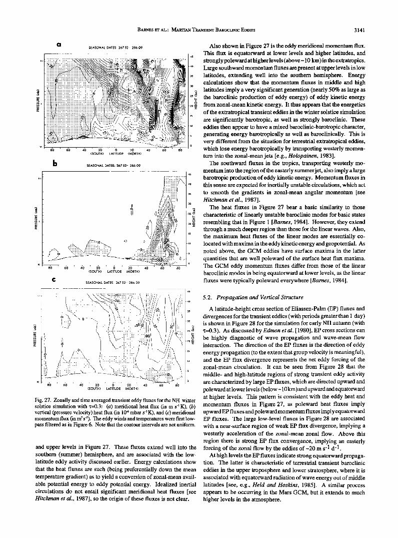
Figure 27 shows the meridional and vertical heat fluxes of the transient eddies (with periods greater than 1 sol) in the NH winter solstice simulation with 'r=0.3. It can be seen that the eddies are
acting to flux heat poleward and upward throughout middle and high latitudes, producing conversions of zonal-mean available potential energy to eddy available potential energy (in the presence of the strong zonal-mean temperature gradients; see Figure 1), and from the latter to eddy kinetic energy. These energy conversions are charac- teristic of baroclinic instability.
The meridional heat fluxes are very substantial and play an important role in the polar energy balance [see Pollack et al., 1990]. In this case, the vertically integrated heating due to these fluxes at 60øN is about 5 W m -2, which is larger than the heating due to the mean meridional circulation and about 20% of the heating resulting from CO2 condensation at this latitude. The transient eddy heat fluxes are considerably more significant in some of the other experi- ments [see Pollack et al., 1990].
It can be seen in Figure 27 that the region of large poleward and upward heat fluxes is very deep (the true vertical heat flux would be much deeper than the pressure velocity flux in Figure 27), extending to the model top, and it shifts sharply poleward with height in the lowest 10 km. The surface maxima in the heat fluxes are at relatively low latitudes (~35-40øN), in the vicinity of the maximum zonal- mean baroclinicity (see Figure 1). It can be recalled that the surface maxima in the eddy kinetic energy and geopotential are located at55- 60øN (see Figure 9), however. llae near-surface vertical heat flux is actually downward in this region, indicating the importance of horizontal and/or vertical energy transports in maintaining the large eddy kinetic energy at these higher latitudes. The near-surface downward heat fluxes appear to be due to the model topography, as is discussed below.
There is a region of large southward heat fluxes at lower latitudes
BARNES ET AL.: I¾IARTIAN TRANSIENT BAROCLINIC EDDIES 3141
SEASONAL DATES: 267.52- 286.09
• , , , [ ] [ [ [ ] ] • •,•-•"---'"'T, •'•_• 60 40 20 0 20 40 60 80
(SOUTH) LATITUDE (NORTH)
SEASONAL DATES, 267.52- 286.09
80 60 40 20 0 20 40 60 8'0 (SOUTH) LATITUDE (NORTH)
2o •
15
5
SEASONAL DATES. 267.52- 286 09
Also shown in Figure 27 is the eddy meridional momentum flux. This flux is equatorward at lower levels and higher latitudes, and strongly poleward at higher levels (above ~ 10 kin) in the extratropics.
,0 Large southward momentum fluxes are present at upper levels in low 3• latitudes, extending well into the southern hemisphere. Energy
calculations show that the momentum fluxes in middle and high 3O
• latitudes imply a very significant generation (nearly 50% as large as 2, * the baroclinic production of eddy energy) of eddy kinetic energy 20 •: from zonal-mean kinetic energy. It thus appears that the energetics
of the extratropical transient eddies in the winter solstice simulation are significantly barotropic, as well as strongly baroclinic. These
,0 eddies then appear to have a mixed baroclinic-barotropic character, , generating energy barotropically as well as baroclinically. This is
very different from the situation for terrestrial extratropical eddies, 0
which lose energy barotropically by transporting westerly momen- tum into the zonal-mean jets [e.g., Holopainen, 1983].
The southward fluxes in the tropics, transporting westerly mo- mentum into the region of the easterly summerj et, also imply a large barotropic production of eddy kinetic energy. Momentum fluxes in this sense are expected for inertially unstable circulations, which act to smooth the gradients in zonal-mean angular momentum [see Hitchman et al., 1987].
The heat fluxes in Figure 27 bear a basic similarity to those characteristic of linearly unstable baroclinic modes for basic states resembling that in Figure 1 [Barnes, 1984]. However, they extend through a much deeper region than those for the linear waves. Also, the maximum heat fluxes of the linear modes are essentially co- located with maxima in the eddy kinetic energy and geopotential. As noted above, the GCM eddies have surface maxima in the latter
quantities that are well poleward of the surface heat flux maxima. The GCM eddy momentum fluxes differ from those of the linear baroclinic modes in being equatorward at lower levels, as the linear fluxes were typically poleward everywhere [Barnes, 1984].
Fig. 27. Zonally and time averaged transient eddy fluxes for the NH winter solstice simulation with •:=0.3: (a) meridional heat flux (in m s '• K), (b) vertical (pressure velocity) heat flux (in 10 • mbar s '• K), and (c) meridional momentum flux (in m2s-2). The eddy winds and temperatures were first low- pass filtered as in Figure 6. Note that the contour intervals are not uniform.
and upper levels in Figure 27. These fluxes extend well into the southern (summer) hemisphere, and are associated with the low- latitude eddy activity discussed earlier. Energy calculations show that the heat fluxes are such (being preferentially down the mean temperature gradient) as to yield a conversion of zonal-mean avail- able potential energy to eddy potential energy. Idealized inertial circulations do not entail significant meridional heat fluxes [see Hitchman et al., 1987], so the origin of these fluxes is not clear.
5.2. Propagation and Vertical Structure
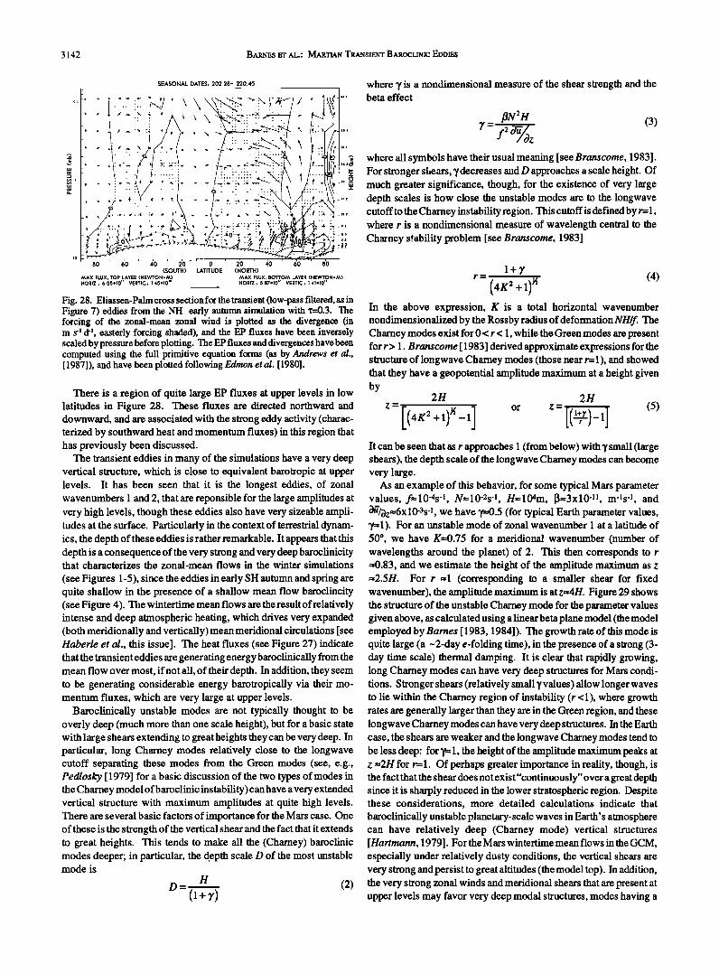
A latitude-height cross section of Eliassen-Pahn (EP) fluxes and divergences for the transient eddies (with periods greater than 1 day) is shown in Figure 28 for the simulation for early NH autumn (with 'c=0.3). As discussed by Edmon et al. [ 1980], EP cross sections can be highly diagnostic of wave propagation and wave-mean flow interaction. The direction of the EP fluxes is the direction of eddy energy propagation (to the extent that group velocity is meaningful), and the EP flux divergence represents the net eddy forcing of the zonal-mean circulation. It can be seen from Figure 28 that the middle- and high-latitude regions of strong transient eddy activity are characterized by large EP fluxes, which are directed upward and poleward at lower levels (below -- 10 km) and upward and equatorward at higher levels. This pattern is consistent with the eddy heat and momentum fluxes in Figure 27, as poleward heat fluxes imply upward EP fluxes and poleward momentum fluxes imply equatorw ard EP fluxes. The large low-level fluxes in Figure 28 are associated with a near-surface region of weak EP flux divergence, implying a westerly acceleration of the zonal-mean zonal flow. Above this region there is strong EP flux convergence, implying an easterly forcing of the zonal flow by the eddies of ~20 m s -1 d -1.
At high levels the EP fluxes indicate strong equatorward propaga- tion. The latter is characteristic of terrestrial transient baroclinic
eddies in the upper troposphere and lower stratosphere, where it is associated with equatorward radiation of wave energy out of middle latitudes [see, e.g., Held and Hoskins, 1985]. A similar process appears to be occurring in the Mars GCM, but it extends to much higher levels in the atmosphere.
3142 BARNES ET AL.: MARTIAN TRANSIENT BAROCLINIC EDDIES
SEASONAL DATES, 202.28- 220.4.5
80 60 40 20 (SOUTH)
MAX FLUX. TOP LAYER (NEWTON-M) HORIZ.: 6.0õe10 '• VERTIC., 1.4õ-I0"
0 20 40 LATITUDE (NORTH)
p d •,• 44 i
o 8o
MAX FLUX. BOTTOM LAYER (NEWTON-M) HORIZ., 5.B7e10 '•' VERTIC., 1.41el0'"
Fig. 28. Eliassen-Palm cross section for the transient (low-pass filtered, as in Figure 7) eddies from the NH early autumn simulation with •:=0.3. The forcing of the zonal-mean zonal wind is plotted as the divergence (in m s 4 d 4, easterly forcing shaded), and the EP fluxes have been inversely scaled by pressure before plotting. The EP fluxes and divergences have been computed using the full primitive equation forms (as by Andrews et al., [1987]), and have been plotted following Edmon etal. [1980].
There is a region of quite large EP fluxes at upper levels in low latitudes in Figure 28. These fluxes are directed northward and downward, and are associated with the strong eddy activity (charac- terized by southward heat and momentum fluxes) in this region that has previously been discussed.
The transient eddies in many of the simulations have a very deep vertical structure, which is close to equivalent barotropic at upper levels. It has been seen that it is the longest eddies, of zonal wavenumbers 1 and 2, that are reponsible for the large amplitudes at very high levels, though these eddies also have very sizeable ampli- tudes at the surface. Particularly in the context of terrestrial dynam- ics, the depth of these eddies is rather remarkable. It appears that this depth is a consequence of the very strong and very deep baroclinicity that characterizes the zonal-mean flows in the winter simulations
(see Figures 1-5), since the eddies in early SH autumn and spring are quite shallow •_n the presence of a shallow mean flow baroclincity (see Figure 4). The wintertime mean flows are the result ofrelatively intense and deep atmospheric heating, which drives very expanded (both meridionally and vertically) mean meridional circulations [see Haberle et al., this issue]. The heat fluxes (see Figure 27) indicate that the transient eddies are generating energy baroclinically from the mean flow over most, ifnot a!l, of their depth. In addition, they seem to be generating considerable energy barotropically via their mo- mentum fluxes, which are very large at upper levels.
Baroclinically unstable modes are not typically thought to be overly deep (much more than one scale height), but for a basic state with large shears extending to great heights they can be very deep. In particular, long Charney modes relatively close to the longwave cutoff separating these modes from the Green modes (see, e.g., Pedlosky [ 1979] for a basic discussion of the two types of modes in the Charney model ofbaroclinic instability) can have a very extended vertical structure with maximum amplitudes at quite high levels. There are several basic factors of importance for the Mars case. One of these is the strength of the vertical shear and the fact that it extends to great heights. This tends to make all the (Charney) baroclinic modes deeper; in particular, the depth scale D of the most unstable mode is
D = H (2) (l+r)
where T is a nondimensional measure of the shear strength and the beta effect
fiN2H (3)
where all symbols have their usual meaning [see Branscome, 1983]. For stronger slsears, •tdecreases told D approaches a scale height. Of much greater significance, though, for the existence of very large depth scales is how close the unstable modes are to the longwave cutoffto the Charney instability region. This cutoffis defined by r= 1, where r is a nondimensional measure of wavelength central to the Charney s•.ability problem [see Branscome, 1983]
1+7
r= ( 4K2 + 1)){ (4) In the above expression, K is a total horizontal wavenumber nondimensionalized by the Rossby radius of deformation NH/f. The Charney modes exist for 0 < r < 1, while the Green modes are present for r> 1. Branscome [ 1983] derived approximate expressions for the structure of longwave Chamey modes (those near r=- 1), and showed that they have a geopotential amplitude maximum at a height given by
2H 2H
It can be seen that as r approaches 1 (from below) with •/small (large shears), the depth scale of the longwave Chamey modes can become very large.
As an example of this behavior, for some typical Mars parameter values, f=10'4s '1, N=10-2s -•, H=lO4m, [l--3x10 -•, m-•s -•, and •t7/•z--6xlO-3s-•, we have T=0.5 (for typical Earth parameter values, 'F• 1). For an unstable mode of zonal wavenumber 1 at a latitude of 50 ø, we have K--0.75 for a meridional wavenumber (number of wavelengths around the planet) of 2. This then corresponds to r =0.83, and we estimate the height of the amplitude maximum as z --2.5H. For r =1 (corresponding to a smaller shear for fixed wavenumber), the amplitude maximum is atz=4H. Figure 29 shows the structure of the unstable Charney mode for the parameter values given above, as calculated using a linear beta plane model (the model employed by Barnes [ 1983, 1984]). The growth rate of this mode is quite large (a ~2-day e-folding time), in the presence of a strong (3- day time scale) thermal damping. It is clear that rapidly growing, long Chamey modes can have very deep structures for Mars condi- tions. Stronger shears (relatively small •tvalues) allow longer waves to lie within the Chamey region of instability (r <1), where growth rates are generally larger than they are in the Green region, and these longwave Charney modes can have very deep stxuctures. In the Earth case, the shears are weaker and the longwave Charney modes tend to be less deep: for T= 1, the height of the amplitude maximum peaks at z =2H for r=-l. Of perhaps greater importance in reality, though, is the fact that the shear does not exist"continuously" over a great depth since it is sharply reduced in the lower stratospheric region. Despite these considerations, more detailed calculations indicate that
baroclinically unstable planetary-scale waves in Earth's atmosphere can have relatively deep (Charney mode) vertical structures [Hartmann, 1979]. For the Mars wintertime mean flows in the GCM, especially under relatively dusty conditions, the vertical shears are very strong and persist to great altitudes (the model top). In addition, the very strong zonal winds and meridional shears that are present at upper levels may favor very deep modal structures, modes having a
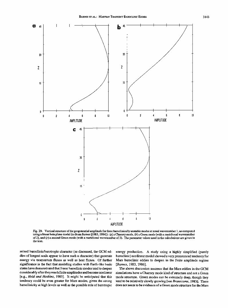
BARNES ET AL.: MARTIAN TRANSIENT BAROCLINIC EDDIES 3143
• 45
3o
z
b 45
0 2 4 6 8 10 0 2 4 6 8 10
AMPLITUDE AMPLITUDE
C 45
30
z
0 2 4 6 8 10
AMPLITUDE
Fig. 29. Vertical structure of the geopotential amplitude for three baroclinically unstable modes at zonal wavenumber 1, as computed using a linear beta plane model (as from Barnes [ 1983, 1984]): (a) a Charhey mode, (b) a Green mode (with a meridional wavenumber of 2), and (c) a second Green mode (with a meridional wavenumber of 3). The parameter values used in the calculations are given in the text.
mixed baroclinic/barotropic character (as discussed, the GCM ed- dies of longest scale appear to have such a character) that generate energy via momentum fluxes as well as heat fluxes. Of further significance is the fact that modeling studies with Earth-like basic states have demonstrated that linear baroclinic modes tend to deepen considerably after they reach finite amplitudes and become nonlinear [e.g., Held and Hoskins, 1985]. It might be anticipated that this tendency could be even greater for Mars modes, given the strong baroclinicity at high levels as well as the possible role of barotropic
energy production. A study using a highly simplified (purely baroclinic) nonlinear model showed a very pronounced tendency for Mars baroclinic eddies to deepen in the finite amplitude regime [Barnes, 1983, 1986].
The above discussion assumes that the Mars eddies in the GCM
simulations have a Charney mode kind of structure and not a Green mode structure. Green modes can be extremely deep, though they tend to be relatively slowly growing [see Branscome, 1983]. There does not seem to be evidence of a Green mode structure for the Mars
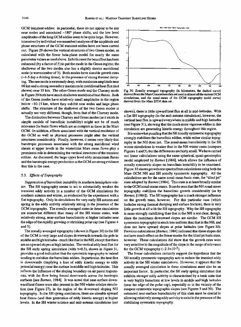
3144 B^•-s Er AL.: MART•N T•^•s•.•r B^•ocL•mC EDDmS
GCM transient eddies: in particular, there do not appear to be any near nodes and assoc•iated ~180 ø phase shifts, and the low level amplitudes ofthe long GCM eddies seem to be quite large. However, intensive (by individual wavenumber) analyses of the amplitude and phase structures of the GCM transient eddies have not been carried out. Figure 29 shows the vertical structures of two Green modes, as calculated with the linear beta-plane model for nearly the same parameter values as used above. In both cases the beta effect has been enhanced (by a factor of 5) to put the mode in the Green regime; the shallower of the two modes also has a slightly shorter meridional scale (a wavenumber of 3). Both modes have sizeable growth rates (-4-5 day e-folding times), in the presence of strong thermal damp- ing. The one mode is extremely deep, with maximum amplitude near 60 km and a strong secondary maximum in meridional heat flux (not shown) near 35 km. The other Green mode and the Charney mode in Figure 29 both have much shallower meridional heat fluxes. Both of the Green modes have relatively small amplitudes in the region below ~10-15 km, where they exhibit near nodes and large phase shifts. The structure of the shallower of the two Green modes is
actually not very different, though, from that of the Chamey mode. The distinction between Charney and Green modes (as it exists in
simple models of baroclinic instability) might not be of much relevance for basic flows which are as complex as those in the Mars GCM. In addition, effects associated with the vertical resolution of
the GCM as well as physical processes might alter the vertical structures considerably. Finally, however, it seems very likely that barotropic processes associated with the strong meridional wind shears at upper levels in the wintertime Mars mean flows play a prominent role in determining the vertical structures of the transient eddies. As discussed, the large upper level eddy momentum fluxes and the barotropic energy production in the GCM are strong evidence that this is the case.
5.3. Effects of Topography
Suppression of baroclinic instability in southern hemisphere win- ter. The SH topography seems to act to substantially weaken the transient eddy activity in a number of the GCM simulations for southern autumn and winter, as evidenced by the experiment with a flat topography. Only in simulations for very early SH autumn and spring is the eddy activity relatively strong in the presence of the GCM topography. The zonally averaged states in these simulations are somewhat different than many of the SH winter states, with relatively strong, near-surface baroclinicity at higher latitudes near the edge of the rapidly growing or shrinking polar cap (see Figures 4 and 5).
The zonally averaged topography (shown in Figure 30) in the SH of the GCM is very large and slopes downwards towards the pole in middle and high latitudes - much like that in the NH, except that there are no upward slopes at high latitudes. The vertical eddy heat flux for the SH early spring simulation (with x=0.3), shown in Figure 31, provides a good indication that the symmetric topography is indeed tending to stabilize the baroclinic eddies. In particular, the heat flux is downwards (implying a loss of eddy kinetic energy to eddy potential energy) near the surface in middle and high latitudes. This reflects the influence of the sloping boundary on air parcel trajecto- ties, with the flow being forced downwards across the isentropic surfaces [see Barnes, 1984]. It was noted that near-surface down- ward heat fluxes were also present in the NH winter solstice simula- tion (see Figure 27), in the region of the downward sloping NH topography. In the SH spring simulation, there are sizeable upward heat fluxes (and thus generation of eddy kinetic energy) at higher levels. In the SH winter solstice and mid-autumn simulations (not
Mars GCM Zonal Mean Topography (km)
5/ i i i i i i i I i i a i
ß
90s ,;s s;s .,;s ,;s ,;. ' i , i ,
5ON 70N 90N
Fig. 30. Zonally averaged topography (in kilometers, the dashed curve) derived from the Mars Consortium data set used in almost all the current GCM
simulations, and the zonal-mean of the GCM topography (solid curve) derived from the Mars DTM data set.
shown), there is little upward heat flux at all in mid-latitudes. With a flat SH topography (in the mid-autumn simulation), however, the vertical heat flux is upward everywhere in middle and high latitudes (see Figure 31), showing that the much more vigorous eddies in this simulation are generating kinetic energy throughout this region.
It is somewhat puzzling that the SH zonally symmetric topography strongly stabilizes the baroclinic eddies, while rather similar topog- raphy in the NH does not. The zonal-mean baroc!inicity in the SH winter simulations is weaker than in the NH winter cases (compare Figures 1 and 3), but the differences are fairly small. We have carried out linear calculations using the same spherical, quasi-geostrophic model employed by Barnes [ 1984], which allows the influence of zonally symmetric slopes on baroclinic instability to be examined. Figure 32 shows growth rate spectra from calculations using both the Mars GCM NH and SH zonally symmetric topography. All the calculations are for the same zonal-mean basic state, the "tilted jet" state adopted by Barnes [ 1984]. This state is at least broadly similar to the GCM zonal-mean states. Itcan be seen that the NH zonal-mean
topography stabilizes the baroclinic growth considerably (as by Barnes, [ 1984]). The SH topography has a much stronger influence on the growth rams, however. For this particular case (which includes strong thermal damping and surface friction), there is very little growth at all with the SH topography. Why the SH topography is more strongly stabilizing than that in the NH is not clear, though, since the maximum downward slopes are similar. The GCM SH symmetric topography is much less uniform than that in the NH, and does not have upward slopes at polar latitudes (see Figure 30). Previous calculations [Barnes, 1984] indicated tha• these slopes did not have much effect on the linear modes for the tilted jet basic state, however. These calculations did show that the growth rates were very sensitive to the magnitude of the slope in the range of relevance for the GCM topography (-2-3x10⁻³).
The linear calculations certainly support the hypothesis that the SH zonally symmetric topography acts to reduce the transient eddy activity in the SH winter simulations. However, it appears that the zonally averaged circulation in these simulations must also be an important factor. In particular, the SH early spring simulation that exhibits stronger eddy activity is characterized by a basic state that is very highly baroclinic at low levels in middle and high latitudes (near the edge of the polar cap), especially so in the vicinity of the steepest symmetric topographic slopes (see Figures 5 and 30). The enhanced near-surface baroclinicity of this state must be crucial in allowing relatively strong eddy activity to exist in the presence of the stabilizing symmetric topography.
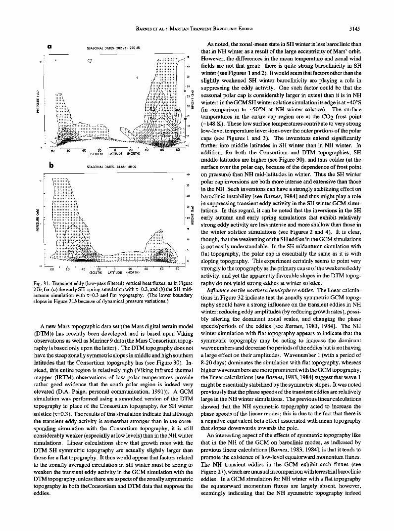
BARNES E-'I' AL.: •ARTIAN TRANSIENT BAROCLINIC EDDIES 3145
SEASONAL DATES: 202.28- 220.4õ
80 60 40 20 0 20 40 60 80 (SOUTH) LATITUDE (NORTH)
b SEASONAL DATES: 34.66- 48.02
30
2• •
•o • _
15
80 60 40 20 0 20 40 60 80 (SOUTH) LATITUDE (NORTH)
Fig. 31. Transient eddy (low-pass filtered) vertical heat fluxes, as in Figure 27b, for (a) the early SH spring simulation with x=0.3, and (b) the SH mid- autumn simulation with x=0.3 and flat topography. (The lower boundary slopes in Figure 3 lb because of dynamical pressure variations.)
A new Mars topographic data set (the Mars digital terrain model (DTM)) has recently been developed, and is based upon Viking observations as well as Mariner 9 data (the Mars Consortium topog- raphy is based only upon the latter). The DTM topography does not have the steep zonally symmetric slopes in middle and high southern latitudes that the Consortium topography has (see Figure 30). In- stead, this entire region is relatively high (Viking infrared thermal mapper (IRTM) observations of low polar temperatures provide rather good evidence that the south polar region is indeed very elevated (D.A. Paige, personal communication, 1991)). A GCM simulation was performed using a smoothed version of the DTM topography in place of the Consortium topography, for SH winter solstice (x=0.3). The results of this simulation indicate that although the transient eddy activity is somewhat stronger than in the corre- sponding simulation with the Consortium topography, it is still considerably weaker (especially at low levels) than in the NH winter simulations. Linear calculations show that growth rates with the DTM SH symmetric topography are actually slightly larger than those for a flat topography. It thus would appear that factors related to the zonally averaged circulation in SH winter must be acting to weaken the transient eddy activity in the GCM simulation with the DTM topography, unless there are aspects of the zonally asymmetric topography in both theConsortium and DTM data that suppress the eddies.
As noted, the zonal-mean state in SH winter is less baroclinic than
that in NH winter as a result of the large eccentricity of Mars' orbit. However, the differences in the mean temperature and zonal wind fields are not that great: there is quite strong baroclinicity in SH winter (see Figures 1 and 2). It would seem that factors other than the slightly weakened SH winter baroclinicity are playing a role in suppressing the eddy activity. One such factor could be that the seasonal polar cap is considerably larger in extent than it is in NH winter: in the GCM SH winter solstice simulation its edge is at-40øS (in comparison to -50øN at NH winter solstice). The surface temperatures in the entire cap region are at the CO 2 frost point (- 148 K). These low surface temperatures contribute to very strong low-level temperature inversions over the outer portions of the polar caps (see Figures 1 and 3). The inversions extend significantly further into middle latitudes in SH winter than in NH winter. In
addition, for both the Consortium and DTM topographies, SH middle latitudes are higher (see Figure 30), and thus colder (at the surface over the polar cap, because of the dependence of frost point on pressure) than NH mid-latitudes in winter. Thus the SH winter polar cap inversions are both more intense and extensive than those in the NH Such inversions can have a strongly stabilizing effect on baroclinic instability [see Barnes, 1984] and thus might play a role in suppressing transient eddy activity in the SH winter GCM simu- lations. In this regard, it can be noted that the inversions in the SH early autumn and early spring simulations that exhibit relatively strong eddy activity are less intense and more shallow than those in the winter solstice simulations (see Figures 2 and 4). It is clear, though, that the weakening ofthe SH eddies in the GCM simulations is not easily understandable. In the SI-i midautumn simulation with flat topography, the polar cap is essentially the same as it is with sloping topography. This experiment certainly seems to point very strongly to the topography as the primary cause ofthe weakened eddy activity, and yet the apparently favorable slopes in the DTM topog- raphy do not yield strong eddies at winter solstice.
Influence on the northern hemisphere eddies. The linear calcula- tions in Figure 32 indicate that the zonally symmetric GCM topog- raphy should have a strong influence on the transient eddies in NH winter: reducing eddy amplitudes (by reducing growth rates), possi- bly altering the dominant zonal scales, and changing the phase speeds/periods of the eddies [see Barnes, 1983, 1984]. The NH winter simulation with flat topography appears to indicate that the symmetric topography may be acting to increase the dominant wavenumbers and decrease the periods of the eddies but is not having a large effect on their amplitudes. Wavenmnber 1 (with a period of 8-20 days) dominates the simulation with flat topography, whereas higher wavenumbers are more prominent with the GCM topography; the linear calculations [see Barnes, 1983, 1984] suggest that wave 1 might be essentially stabilized by the symmetric slopes. It was noted previously that the phase speeds of the transient eddies are relatively large in the NH winter simulations. The previous linear calculations showed that the NH symmetric topography acted to increase the phase speeds of the linear modes; this is due to the fact that there is a negative equivalent beta effect associated with mean topography that slopes downwards towards the pole.
An interesting aspect of the effects of symmetric topography like that in the NH of the GCM on baroclinic modes, as indicated by previous linear calculations [Barnes, 1983, 1984], is that it tends to promote the existence of low-level equatorward momentum fluxes. The NH transient eddies in the GCM exhibit such fluxes (see Figure 27), which are unusual in comparison with terrestrial baroclinic eddies. In a GCM simulation for NH winter with a flat topography the equatorward momentum fluxes are largely absent, however, seemingly indicating that the NH symmetric topography indeed

3146 B^RNES ET AL.: MARTIAN TRANSIENT BAROCLINIC EDDIES
0.7
0,6--
0,5 I
0,4 I
0,3 I
0,2 I
0,1 i
flat
NH
o i
SH
2 3 4
Zonal Wavenumber
Fig. 32. Growth rate spectra from linear instability calculations with the spherical, quasi-geostrophic model of Barnes [1984]. The spectra are for calculations with the GCM (Consortium) NH zonal-mean topography, the GCM SH zonal-mean topography, and flat topography. All of the calcula- tions are otherwise the same (the same basic state, dissipation, etc.).
tends to promote these fluxes. The polar mean easterlies seen in Figure 1 are also absent, supporting the hypothesis that these are driven largely by the equatorward momentum fluxes. In flat topog- raphy simulations that have been carried out with the NASA Ames Mars climate model, however, the transient eddies do exhibit strong low level equatorward momentum fluxes (R.M. Haberle, personal communications, 1991). Also, such fluxes have been obtained in
recent linear calculations (being performed by J.R. Barnes using a primitive equation model) in the absence of symmetric slopes. It thus appears that while the NH symmetric topography may indeed pro- mote the equatorward momentum fluxes (and the polar easterlies) in the GCM simulations, there are aspects of baroclinic instability in the Mars atmosphere that can yield such fluxes in the absence of any topography.
6. D•SCUSS•ON
6.1. Eddy Structure and Dynamics
The NASA Ames Mars GCM simulations exhibit transient
baroclinic eddy activity in middle and high latitudes during the autumn, winter and spring seasons. This activity is present for very high dust loadings, as well as without dust. The baroclinic eddies are characterized by planetary scales, with zonal wavenumbers 1-4 accounting for a very large fraction of the variance. The periods of the eddies range from -1.5 to 20 days (typically from -2-8 days),
corresponding to eastward zonal phase speeds of -5-30 rn/s (in mid- latitudes). These wavenumbers and periods are very similar to those inferred from Viking observations. The surface eddy amplitudes in most of the simulations, at both lander locations, are also quite comparable to those observed by Viking. An exception is the amplitude in several highly dusty NH winter simulations: this is much larger than seen by Viking during the 1977 winter solstice dust storm (though not much larger than those during the 1977 autumn dust storm). It seems very likely that this is at least partially due to an insufficient expansion of the zonal-mean circulation in the highly dusty GCM experiments.
The most interesting aspect of the structure of the transient eddies in the current GCM simulations is their very large vertical extent. In many of the simulations the planetary scale (wavenumber 1 and 2) eddies have their greatest amplitudes at the model top, at 45-50 km altitude, and the heat and momentum fluxes associated with these eddies are large at high levels. At upper levels the structure of these eddies approaches an equivalent barotropic one, but the heat fluxes are still sufficiently large (given the large magnitudes of the wind and temperature perturbations) to produce substantial baroclinic energy conversions. At upper levels there are quite substantial barotropic energy conversions as well, such that a sizeable fraction of the total eddy energy in the winter extratropics is generated barotropically.
The great vertical extent and the planetary scales of the winter transient eddies in the Mars GCM distinguish them from their terrestrial counterparts. The very deep structure of the GCM eddies is associated with the deep structure of the wintertime zonal-mean circulation [see Haberle et al., this issue]. At least in part it is a reflection of the fundamental tendency for long baroclinic modes to become very deep in the presence of strong mean shears existing through a deep region. In addition, however, the substantial barotropic energy production by the eddies indicates that they have a mixed baroclinic-barotropic character, for which large upper level ampli- tudes are probably favored. Relatively deep eddy structures were indicated by previous linear and simplified nonlinear modeling of baroclinic instability in the Mars atmosphere [Barnes, 1983, 1984, 1986]; the nonlinear studies showed that the vertical structures of the eddies became nearly equivalent barotropic. Simulations with the NASA Ames Mars climate model have also shown a very deep vertical structure for the winter transient eddies, with very large momentum fluxes at high levels (R.M. Habefie, personal communi- cation, 1991).
Available observations may provide evidence for such a deep eddy structure: the Mariner 9 IRIS detected a large-scale wave with a temperature maximum at upper levels, in the same height range as for the transient eddies in the Mars GCM [Conrath, 1981]. These observations do not, unfortunately, permit the wavenumber and frequency of the disturbance to be unambiguously determined. Transient (eastward traveling) wavenumber 1 and 2 modes are possible fits to the IRIS data, as is a stationary mode. Confirmation of a deep structure for the Mars transient eddies will have to await Mars observer.
In low latitudes and the NH subtropics most ofthe upper level eddy energy appears to be produced barotropically, much of it by circula- tions that resemble those characteristic of inertially unstable modes. The low-latitude activity eppears to largely be a response to the forcing of a region of marginal inertial stability by the extratropical transient eddies, as it is characterized by the same wavenumbers and periods. These wavenumbers and periods also dominate the nontidal eddy activity at upper levels in mid-latitudes in the summer hemi- sphere, but the eddy structure in this region is rather different (being much deeper) than that in the tropics and the inertial stability of the mean flow is quite strong. It can be speculated that unstable (perhaps
BARNES Err AL.: MARTIAN TRANSIEI•rr BAROCLINIC EDDIES 3147
barotropic) modes are being "triggered" in this region by the inertial oscillations in low latitudes.
6,2. Comparison With Viking Observations
The basic properties of the NH transient eddies in the GCM simulations are very similar to those inferred from Viking observa- tions. In particular, the eddies are characterized by planetary and near-planetary scales (zonal wavenumbers 1-4), and periods of -2- 10 days. In some simulations shorter-scale (wavenumbers 3 and 4) eddies of shorter period are dominant, whereas in others longer (wavenumbers 1 and 2) eddies of longer period are more prominent. In a few simulations (several with flat topography and one without dust) the wavenumber 1 disturbances are strongly dominant. Analy- ses of the Viking Lander 2 observations show a similar behavior, with the short-scale modes sometimes of largest amplitude and the long-scale modes dominant at other times [Barnes, 1980, 1981, 1983]. These analyses do not show a dominant role for zonal wavenumber 1 for any extended interval, but they do indicate that such a mode might be present with significant amplitude; analyses of the Viking Lander 1 data do seem to show a strong wavenumber 1 signal, though these estimates are more uncertain because of prob- lems with the wind data [Murphy etal., 1990].
Several GCM simulations are dominated by a single eddy distur- bance, at one zonal wavenumber with a well-defined period. Such a situation seems to be strikingly similar to that indicated by Viking observations for several -20-50 sol intervals [Barnes, 1981, 1983; Murphy et al., 1990]. The current version of the GCM thus appears to be capable of simulating at least some aspects of the regularity that the Mars eddies can exhibit. The factors involved in this behavior in
the GCM are unclear, however. It can be hoped that more intensive analyses of the GCM simulations together with mechanistic studies of nonlinear baroclinic instability in the Martian atmosphere will allow the key factors to be elucidated.
The variation of the transient eddy activity with season and dust loading in the simulations warrants comparison with the observa- tions. The winter solstice eddies in the simulations do not diminish
in amplitude for very large dust loading but do shift somewhat farther poleward so as to yield a reduction in amplitude (at the surface) in middle latitudes and the subtropics. This reduction is qualitatively consistent with Viking lander observations during the winter solstice dust storm of 1977 but is much smaller. As noted, this is almost
certainly due at least in part to the fact that the zonal-mean circulation in the GCM does not shift as far poleward with large dust loading as the actual Mars circulation appeared to during the 1977 storm [Haberle et al., 1982; Barnes and Hollingsworth, 1987; Haberle et al., this issue]. However, it might also be the case that the eddy activity diminished everywhere during the 1977 winter solstice dust storm. This does not occur in the highly dusty GCM simulations, but experiments with spatially nonuniform dust loadings do exhibit eddy activity that is weaker everywhere (R.M. Haberle, personal commu- nication, 1991).
The GCM simulations show a systematic change in the dominant zonal wavenumbers of the transient eddies with dust loading: the zonal scale of the eddies shortens with increasing dustiness. Viking observations indicate that such a shortening occurred during the 1977 winter dust storm [Barnes, 1980, 1983]. On the other hand, the Viking data show that the shorter eddies (wavenumbers 3 and 4) were dominant during the second Viking year and much less so in the first [Barnes, 1981 ]. It is believed that the second year was generally less dusty than the first [e.g., Leovy et al., 1985], so the interannual changes in the transient eddy activity observed by Viking do not seem to be readily understandable on the basis of the present set of
GCM simulations. However, changes in the dust distribution, both in the vertical and the horizontal, certainly might have been impor- tant in producing the interannual changes observed by Viking.
6.3. Effects of Topography
The lack of strong transient eddy activity in a number of the SH autumn and winter simulations is a major surprise in the current GCM studies, since strong eddy activity was present in experiments performed (for SH winter solstice) with the previous version of the Mars GCM [Pollack eta/., 1981]. It appears that the relatively weak SH eddy activity in the current simulations is at least partially due to the topography in the present version of the model, but it appears that it also is related to the nature of the zonally averaged climate in SH winter. The zonally averaged topography in the current GCM has very steep slopes in middle and high southern latitudes, and these appear to act to stabilize the baroclinic eddies in SH winter. The previous Mars GCM SH topography was not characterized by such steep symmetric slopes [see Pollacket al., 1981]. However, a winter solstice simulation with a new topography (derived from the Mars DTM) that does not have steep symmetric slopes in the SH also exhibits relatively weak eddy activity. (Yet, a mid-autumn simula- tion with flat topography shows strong eddies.) This simulation demonstrates that factors other than the symmetric slopes must also be important - as is indicated by the presence of relatively strong eddies in simulations for early SH autumn and spring. We have hypothesized that two significant factors could be the relatively large extent of the seasonal polar cap in SH winter and relatively high elevations in extratropical southern latitudes. Both factors appear to contribute to the existence of strong low-level inversions in winter over the very extensive polar cap, which could (along with a somewhat weakened baroclinicity) reduce the instability of the zonal-mean states in SH winter. It can be noted that the previous Mars GCM had only three vertical levels and thus was not really able to resolve the kind of low level inversions that the current GCM
produces. The NH zonally symmetric topography in the current GCM also
appears to exert a strong influence on the transient eddies in NH winter, though it does not seem to suppress them significantly. The NH topography appears to act to shorten the periods and increase the dominant zonal wavenumbers of the eddies. It also seems to promote low level equatorward eddy momentum fluxes, which drive mean easterlies at polar latitudes.
The Mars topography will remain uncertain (given the large possible errors in the available data sets) until Mars observer. The strength of the transient eddy activity in SH winter will also remain unknown until Mars Observer, as none of the available observations
allow it to be defined. If it turns out that the eddy activity during southern winter is indeed relatively weak, this would constitute a significant asymmetry between the Mars hemispheres. In view ofthe importance of the transient eddy heat transports for the energy balance in the north polar region in the GCM simulations [Pollack et al., 1990], it seems plausible that weak SH eddies might be a significant factor in the maintenance of a permanent CO2 ice cap at the Mars south pole.
Acknowledgments. The lead author would especially like to acknowledge the assistance of D. Vickers at Oregon State University with some of the analyses and graphics. Conversations with J. Murphy, H. Houben, R. Young, M. Hitchman, and J. Hollingsworth have contributed to this study. Support for the lead author's participation in the study was provided by the NASA Planetary Atmospheres Program (NAGW-1127 and NAGW-2445) and NASA Ames (Cooperative Agreement NCC 2-661). The Mars GCM project has
3148 BARNES Err AL.: MARTIAN TRANSIENT BAROCLINIC EDDIES
been supported by the Planetary Atmospheres Program under grant 154-20- 80-16. Extensive computer time for the simulations and analyses was provided by the Numerical Aerodynamic Simulation (NAS) Facility at NASA Ames.
REFERENCES
Andrews, D.G., J.R. Holton, and C.B. Leovy, MiddleAtmosphere Dynamics, Academic, San Diego, Calif.,1987.
Barnes, J.R., Time spectral analysis of midlatitude disturbances in the Martian atmosphere, J. Atmos. Sci., 37, 2002-2015, 1980.
Barnes, J.R., Midlatitude disturbances in the Martian atmosphere: A second Mars year, J. Atmos. Sci., 38, 225-234, 1981.
Barnes, J.R., Baroclinic waves in the atmosphere of Mars: Observations, linear instability, and finite-amplitude evolution, Ph.D. Thesis, Univ. of Wash., Seattle, 1983.
Barnes, J.R., Linear baroclinic instability in the Martian atmosphere, J. Atmos. Sci., 41, 1536-1550, 1984.
Barnes, J.R., Finite-amplitude behavior of a single baroclinic wave with multiple vertical modes: Effects of thermal damping, J. Atmos. Sci., 43, 58-71, 1986.
Barnes, J.R., Possible effects of breaking gravity waves on the circulation of the middle atmosphere of Mars, J. Geophys. Res., 95, 1401-1421, 1990.
Barnes, J.R. and J.L. Hollingsworth, Dynamical modeling of a planetary wave mechanismfor a Martian polar warming, lcarus, 71,313-334,1987.
Blumsack, S.L. and P.J. Gierasch, Mars: The effects of topography on baroclinic instability, J. Atmos. Sci., 29, 1081-1089, 1972.
Branscome, L.E., The Charney baroclinic stability problem: Approximate solutions and modal structures, J. Atrnos. Sci., 40, 1393-1409, 1983.
Briggs, G.A., and C.B. Leovy, Mariner 9 observations of the Mars north polar hood, Bull. Am. Met. Soc., 55, 278-296, 1974.
Briggs, G.A., W.A. Baum, and J.R. Barnes, Viking orbiter imagingobser- vations of dust in the Martian atmosphere, J. Geophys. Res., 84, 2795- 2820, 1979.
Conrath, B.J., Planetary-scale wave structure in the Martian atmosphere, Icarus, 48, 246-255, 1981.
Edmon, H.J., B.J. Hoskins, and M.E. Mcintyre, Eliassen-Palm cross sections for the troposphere, J. Atmos. Sci., 37, 2600-2612, 1980.
Haberle, R.M., Interannual variability of global dust storms on Mars, Science, 234, 459-461, 1986.
Haberle, R.M., and B.M. Jakosky, Sublimation and transport of water from the north residual polar cap on Mars, J. Atmos. Sci., 95, 1423-1437, 1990.
Haberle, R.M., C.B. Leovy, and J.B. Pollack, Some effects of global dust storms on the atmospheric circulation of Mars, Icarus, 50, 322-367,1982.
Haberle, R.M., J.B. Pollack, J.R. Barnes, R.W. Zurek, C.B. Leovy, J. Murphy, H. Lee, and J. Schaeffer, Mars atmospheric dynamics as simulated by the NASA Ames Mars general circulation model, 1, The zonal-mean circu- lation, J. Geophys. Res., this issue.
Hartmann, D.L., Baroclinic instability of realistic zonal-mean states to planetary waves, J. Atmos. Sci., 36, 2336-2349, 1979.
Held, I.M. and B.J. Hoskins, Large-scale eddies and the general circulation of the troposphere, in Issues in Atmospheric and Oceanic Modeling Part A: Climate Dynamics, edited by S. Manabe, Adv. Geophys. 28, 3-31, 1985.
Hitchman, M.H., C.B. Leovy, J.C. GiIle, and P.L. Bailey, Quasi-stationary zonally asymmetric circulations in the equatorial lower mesosphere, J. Atmos. Sci., 44, 2219-2236, 1987.
Holopainen, E.O., Transient eddies in mid-latitudes: Obserations and inter- pretation, in l arg e-Scale Dynamical Processes in theAtmosphe re, pp. 201- 233, Academic, San Diego, Calif., 1983.
Houben, H., R.M. Habede, and R.E. Young, Mars 3-D climate model, Eos Trans. AGU, 70 (43), 1179-1180, 1989.
Jakosky, B.M. and T.Z. Martin, Mars: North polar atmospheric warming during dust storms, Icarus, 72, 528-534, 1987.
Leovy, C.B., Mars: Theoretical aspects of meteorology, Appl. Opt., 8, 1279- 1286, 1969.
Leovy, C.B., and Y. Mintz, Numerical simulations of the weather and climate of Mars, J. Atmos. Sci.,26, 1167-1190, 1969.
Leovy, C.B., J.E. Tillman, W.R. Guest, and J.R. Barnes, Interannual variabil- ity of Martian weather, in Recent Advances in Planetary Meteorology, pp. 69-84, Cambridge University Press, New York, 1985.
Martin, T.Z., and H.H. Kieffer, Thermal infrared properties of the Martian atmosphere, 2, The 15-mm band measurements, J. Geophys. Res., 84, 2843-2852, 1979.
Murphy, J.R., C.B. Leovy, and J.E. Tillman, Observations of Martian surface winds at the Viking Lander 1 site, J. Geophys. Res., 95, 14555-14576, 1990.
O'Sullivan, D.J., and M.H. Hitchman, Inertial instability and Rossby wave breaking in a numerical model, J. Atmos. Sci., 49, 991-1002, 1992.
Pedlosky, J., Geophysical Fluid Dynamics, 624 pp., Springer-Verlag, New York, 1979.
Pollack, J.B., C.B. Leovy, P.W. Greiman, and Y. Mintz, A Martian general circulation experiment with large topography, J. Atmos. Sci., 38, 3-29, 1981.
Pollack, J.B., R.M. Habede, J. Schaeffer, and H. Lee, Simulations of the general circulation of the Martian atmosphere, I, Polar processes, J. Geophys. Res., 95, 1447-1474, 1990.
Speth, P., and R.A. Madden, Space-time spectral analyses of northern hemisphere geopotential heights, J. Atmos. Sci., 40, 1086-1100, 1983.
Zurek, R.W., Atmospheric tidal forcing of the zonal-mean circulation: The Martian dusty atmosphere, J. Atmos. Sci., 43, 652-670, 1986.
J. R. Barnes, Atmospheric Sciences, Strand Agriculture Hall 326, Oregon State University, Corvallis, OR 97331-2209.
R. M. Habefie and J. B. Pollock, Space Sciences Division, MS 245-3, NASA Ames Research Center, Moffett Field, CA 94035.
H. Lee andJ. Schaeffer, Stealing Software, Inc., 1121 San Antonio Road, Palo Alto, CA 94303.
C. Leovy, Department of Atmospheric Sciences, University of Washington, Seattle, WA 98195.
R. W. Zurek, MS 169-237, Jet Propulsion Laboratory, 4800 Oak Grove Drive, Pasadena, CA 91109.
(Received January 31, 1992; revised December 15, 1992;
accepted December 15, 1992.)
Related Documents