Marriage Institutions and Sibling Competition - National ...

NBER WORKING PAPER SERIES

MARRIAGE INSTITUTIONS AND SIBLING COMPETITION:EVIDENCE FROM SOUTH ASIA

Tom Vogl

Working Paper 18319http://www.nber.org/papers/w18319

NATIONAL BUREAU OF ECONOMIC RESEARCH1050 Massachusetts Avenue

Cambridge, MA 02138August 2012

An earlier draft of this paper circulated under the title, “Sisters, Schooling, and Spousal Search: Evidencefrom South Asia.” I am grateful to Erica Field, Michael Kremer, and especially David Cutler, ClaudiaGoldin, and Lawrence Katz for their guidance throughout this research project. I thank Ruchir Agarwal,Anne Case, Amitabh Chandra, Joyce Chen, Tom Cunningham, Supreet Kaur, Michal Kolesar, EdGlaeser, Seema Jayachandran, Kyle Meng, Sendhil Mullainathan, Daniele Paserman, Nancy Qian,Monica Singhal, and seminar participants at BU, Harvard, Princeton, RAND, Yale, UCLA, UT Austin,and the World Bank for helpful comments and suggestions. Bishnu Thapa provided excellent researchassistance and sage insights into Nepali society. This research was supported by the MultidisciplinaryProgram on Inequality and Social Policy (NSF IGERT Grant 0333403) and the NBER Aging Program(NIA Grant T32-AG000186). The views expressed herein are those of the author and do not necessarilyreflect the views of the National Bureau of Economic Research.

NBER working papers are circulated for discussion and comment purposes. They have not been peer-reviewed or been subject to the review by the NBER Board of Directors that accompanies officialNBER publications.

© 2012 by Tom Vogl. All rights reserved. Short sections of text, not to exceed two paragraphs, maybe quoted without explicit permission provided that full credit, including © notice, is given to the source.

Marriage Institutions and Sibling Competition: Evidence from South AsiaTom VoglNBER Working Paper No. 18319August 2012JEL No. I25,J12,O12

ABSTRACT

Using data from South Asia, this paper examines how arranged marriage cultivates rivalry amongsisters. During marriage search, parents with multiple daughters reduce the reservation quality foran older daughter's groom, rushing her marriage to allow sufficient time to marry off her younger sisters.Relative to younger brothers, younger sisters increase a girl’s marriage risk; relative to younger singletonsisters, younger twin sisters have the same effect. These effects intensify in marriage markets withlower sex ratios or greater parental involvement in marriage arrangements. In contrast, older sistersdelay a girl’s marriage. Because girls leave school when they marry and face limited earnings opportunitieswhen they reach adulthood, the number of sisters has well-being consequences over the lifecycle. Youngersisters cause earlier school-leaving, lower literacy, a match to a husband with less education and aless-skilled occupation, and (marginally) lower adult economic status. Data from a broader set of countriesindicate that these cross-sister pressures on marriage age are common throughout the developing world,although the schooling costs vary by setting.

Tom VoglDepartment of EconomicsPrinceton University363 Wallace HallPrinceton, NJ 08544and [email protected]

1 Introduction

Economic, social, and cultural change occur unevenly, with some behaviors and institutions lagging

behind technological progress. Social scientists have long been interested in how these slowly-

evolving traditions interact with the process of development (e.g., Weber 1905; Grief 1994; Guiso et

al. 2006). One such tradition is arranged marriage. While this tradition has gradually given way

to love marriage in some societies over the past millennium, it remains prevalent in many parts

of the world (Goode 1970; Goody 1983). For example, among Indian women born in the 1950s,

1960s, and 1970s, only 5 percent report having arranged their marriages independently of their

families (Desai and Andrist 2010). This paper uses data from South Asia to study how the family’s

continued influence over marriage arrangements creates tradeoffs among siblings, such that one

sibling’s presence in the family affects another sibling’s marriage and human capital outcomes. The

interaction of this tradition with recent expansions in mobility and educational opportunity appears

to magnify these tradeoffs.

Competition among siblings has received much attention for its potential to have a lasting

impact on the outcomes of children, but the typical economic treatment of this issue places little

emphasis on institutions like arranged marriage. In the standard framework, siblings compete for

limited resources within the household, so that an increase in the number of children decreases

average child investment.1 But sibling rivalry also occurs in arenas that are not fully captured

by a conventional budget constraint. For instance, siblings of the same gender participate in the

same marriage market, sharing a pool of potential spouses. In some ways, they are like any other

participants on the same side of the market, but their membership in the same family introduces

special constraints on their marriages. Indeed, these constraints are particularly severe in societies

with arranged marriage, where for a variety of reasons parents seek to marry children of the same

sex in order of birth. When search for a suitable spouse takes time, this practice implies that same-

sex siblings constrain each other’s marriage arrangements. A girl’s presence in the family leads

her parents to hurry the marriage arrangements of her older sisters and delay those of her younger

sisters, both at the expense of groom quality. The logic is similar for boys but probably more acute1The classic model of the tradeoff between child quality and quantity is due to Becker and Lewis (1973). Early evidence

of the negative association between childhood family size and adult outcomes can be found in Leibowitz (1974) and Blake(1983). Despite this association, Black et al. (2005) and Angrist et al. (2010) find no evidence in data from Norway andIsrael that an exogenous increase in the number of younger siblings affects adult outcomes. But Li et al. (2008) andRosenzweig and Zhang (2009) estimate negative family size effects on schooling outcomes in China.

1

for girls, who in many parts of the world (including South Asia) leave school if they marry young

(Field and Ambrus 2008). Since women’s economic status depends heavily on age at marriage,

schooling, and spousal attributes, the impact of these sibling effects may be felt well into adulthood.

This paper focuses on measuring that impact, but it begins by describing the practice of

marrying daughters in order of birth and by outlining a simple marriage search framework to clarify

how this practice leads to cross-sibling effects. The search framework predicts that the presence

of older sisters delays the marriages of their younger sisters; that the presence of younger sisters

hastens the marriages of their older sisters; and that the presence of any sisters reduces expected

groom quality. Using data primarily from the Demographic and Health Surveys (DHS), the paper

then analyzes sister effects in South Asia’s four largest countries, which together comprise more

than a fifth of the world’s population. Much of the analysis centers on a simple natural experiment

within the family. If a girl has at least x younger siblings, then in the absence of sex selection, one

can treat the gender of her xth-younger sibling as exogenous.2 A comparison of girls with next-born

brothers and sisters thus identifies the effect of the next-born sibling’s gender. The analysis has

two parts. The first uses data from Bangladesh, India, Nepal, and Pakistan that indicate whether

a girl has left her natal home, with no information on her outcomes afterward. Home-leaving is

tantamount to marriage for South Asian women, so parental coresidence serves as a useful proxy

for never-marriage. The second part of the analysis uses data from Nepal with more extensive

information on adult outcomes.

Across all four countries, teenage girls with next-youngest sisters are roughly 3 percent-

age points more likely to have left their natal homes than their counterparts with next-youngest

brothers. The effects are stronger in rural areas, where marriage markets are thinner; in areas with

more parental involvement in marriage arrangements, where cross-sister constraints would be ex-

pected to be stronger; and in marriage markets with low ratios of marriageable men to marriage-

able women, consistent with the idea that a scarcity of grooms intensifies parents’ fear that they

will fail to find a husband for their younger daughter. A complementary analysis of twin births,

though underpowered due to the rarity of twins, gives suggestive evidence that younger brothers

(the comparison group in the main analysis) serve mainly as buffers between sisters. Relative to

a singleton female birth, the birth of twin girls raises home-leaving among older sisters, whereas

2The paper takes seriously the possibility that the gender of the xth-younger sibling is endogenous. As Section 5.1.1discusses, the data do not show consistent evidence of sex selection across the four countries.

2

twin boys have no effect relative to a singleton boy. Also, as the search framework predicts, girls

with next-oldest sisters marry later than those with next-oldest brothers. Because endogenous fer-

tility confounds comparisons based on the sex composition of older siblings, the paper assesses the

extent of selection bias using both Heckman’s (1974) selection correction model and Lee’s (2009)

non-parametric bounds estimator.3 Both methods give results consistent with the hypothesis that

the presence of an older sister causes a girl to leave home later, although the 95 percent confidence

interval of the bounds estimator includes zero. The data thus suggest that older and younger sisters

have opposite effects on home-leaving risk.

These sister effects on home-leaving have lasting consequences. To examine these conse-

quences, I analyze DHS data from Nepal in which adult women report all of their siblings ever

born. Consistent with the results on home-leaving, women with younger sisters marry earlier and

initiate childbearing half a year earlier than women with younger brothers. The earlier transition

to married life comes at the expense of human capital and spousal quality. Next-youngest sisters

cause lower school attendance among marriage-age teenagers, as well as lower educational attain-

ment and literacy among adult women. The effects on school attendance among current teenagers

are especially large: 7 percentage points, or nearly 40 percent of the gender gap in teen school atten-

dance. Furthermore, compared to women with next-youngest brothers, women with next-youngest

sisters have husbands with less education and lower skill occupations, and they live in marginally

poorer households.

How siblings affect adult outcomes is an enduring question in the social sciences, so the re-

sults are of interest independent of the mechanism mediating them. But collectively, the results

suggest a prominent role for marriage search and are inconsistent with leading alternative theo-

ries of the effects of sibling composition on adult wellbeing. In this respect, the queuing of girls to

leave the household is perhaps the most distinguishing result. Neither models in which the gender

of a child is a generic wealth shock, nor models in which parents substitute resources from girls

to boys, nor models of son-biased fertility stopping behavior, nor models of the demand for male

and female labor in the household predict on their own that older sisters have the opposite effect

of younger sisters. Many of these theories also predict effects of sibling sex composition in earlier

childhood, which the data do not show. After these explanations, one prominent alternative re-

3Both methods assume monotonicity in the effect of treatment on selection. I discuss the appropriateness of thisassumption below.

3

mains, also rooted in the marriage market. This alternative theory posits that liquidity-constrained

families adjust their daughters’ marriage ages because they cannot afford to pay two dowries in

close succession. But the data indicate that the effects of younger sisters on marriage risk are if

anything weaker in regions known to have large and burdensome dowries than in regions where

dowries are rare and small. Sister effects on age at marriage are also evident in societies outside

South Asia, some of which exchange brideprice rather than dowry. The interaction of marriage

costs with liquidity constraints is thus unlikely to explain the results.

Because the results appear to be driven by the number of sisters rather than the number

of brothers, they have implications for the effects of both sibling sex composition and family size.

Much of my empirical work makes comparisons based on the sex of the next-youngest sibling,

which speaks most directly to the literature on sibling sex composition. A few papers in this lit-

erature have considered the role of patrilineal and matrilineal inheritance norms (see Fafchamps

and Quisumbing 2007), but on the whole, the economics literature has tended to emphasize more

generic theories of intra-household resource distribution, without regard to specific institutions like

arranged marriage.4 In an early paper on the topic, Parish and Willis (1993) note that oldest daugh-

ters in Taiwanese families marry and leave school early, which they interpret through the lens of

credit constraints.5 Relative to their paper and others in the earlier literature, this paper makes a

contribution by paying close attention to which causal parameters within the family are identifiable

in observational data.

Because an increase in family size on average increases the number of sisters, the paper also

relates to research on the effects of family size. Recent results from Norway suggest that although

an increase in the number of younger siblings does not affect adult outcomes, an increase in the

number of older siblings (i.e., an increase in birth order) reduces educational attainment and adult

economic status (Black et al. 2005). These results stand in contrast to South Asia, where having older

sisters allows a girl to remain in school, whereas having younger sisters forces her to leave. The

mechanisms underlying the Norwegian findings remain unknown, but these differences remind us

that varying constraints on household decisions lead to varying forms of sibling competition.4The literature on the effects of sibling sex composition has varied results; see Steelman et al. (2001) for a review.

Edmonds (2006) studies various aspects of sibling differences in child labor in Nepal. Garg and Morduch (1997) andMorduch (2000) find mixed evidence that African girls with a greater share of female siblings display better health andeducation outcomes. In work on the United States, Butcher and Case (1994) report that women with brothers attain moreeducation than women with sisters, although Kaestner (1997) finds no such evidence in later birth cohorts.

5In related work, Chen et al. (2010) do not find that the sex of a Taiwanese girl’s twin affects her health or education.

4

Even so, given the prevalence of arranged marriage in many parts of the world, the cross-

sibling marriage pressures documented in South Asia are likely to carry to other settings. Indeed,

the penultimate section of the paper shows that sister effects on age at marriage are evident across

much of the developing world, although they are much smaller in world regions with less arranged

marriage.6 Meanwhile, the effects on schooling surface only in societies where marriage occurs suf-

ficiently early, and school-leaving occurs sufficiently late. In this sense, the results contribute to the

research effort towards understanding the ramifications of various marriage institutions, especially

during times of social, economic, and demographic change (e.g., Edlund 1999; Edlund and Lager-

löf 2006; Tertilt 2006; Anderson 2007; Jacoby and Mansuri 2010). More broadly, they relate to the

recent literature on how variation in the cultural importance of family ties shapes both individual

and aggregate economic outcomes (Bertrand and Schoar 2006; Alesina and Giuliano 2010).

2 Sex-Specific Birth Order and Marriage: Background

Historical texts from both inside and outside South Asia contain many references to the practice of

marrying daughters in strict order of birth. In the Hebrew Bible, Laban deceives Jacob into marrying

his daughter Leah instead of her younger sister Rachel, under the defense, “This is not done in our

country—giving the younger before the firstborn” (Gen. 29:26 New Oxford Annotated Bible). The

Mahabharata, one of the two major ancient Hindu epics, takes yet a stronger position, putting the

marriage of a younger daughter before her elder sister in the same list of sins as arson, breach of

contract, and the murder of a teacher, a woman, or a member of a high caste.7 In a more recent text,

Shakespeare’s The Taming of the Shrew, Baptista refuses to allow his daughter Bianca to marry before

her elder sister Katherina. Note the role of parents in enforcing the practice. Indeed, demographers

have shown that sisters married disproportionately in order of birth in several historical Western

contexts; they have interpreted the decline of this practice as evidence of waning parental authority

in marriage decisions (Smith 1976; Dillon 2010).

This practice may have evolved as a social norm, or it may simply reflect a family’s optimal

behavior in the marriage market. First, it addresses issues of fairness and competition within the

6Importantly, the degree to which the family of origin controls marriage arrangements is continuous, rather thanbinary. Even in societies that no longer formally adhere to arranged marriage, the family of origin still may influencespouse selection (Goode 1970; Goody 1983; Caldwell et al. 1988).

7The father of the sisters is particularly at fault for the out-of-order marriages of his daughters.

5

family. It equalizes outcomes among daughters by ensuring that parents will find a groom for an

unattractive elder daughter even if her younger sister has many suitors, and it minimizes compe-

tition between sisters over grooms. Second, the practice can arise in a simple consumption model.

If weddings are costly and families face credit constraints, a younger sister’s marriage prevents her

elder sister from marrying for quite some time. As a result, liquidity-constrained parents who wish

to marry all daughters in their youth feel compelled to marry their daughters in strict order of birth.

Third, the practice is optimal when search for grooms takes time. Because the probability of finding

a willing mate declines rapidly after youth, an unmarried younger daughter’s option value to her

parents is greater than her older sister’s. Parents thus marry their older daughter first.

The importance of marriage by order of birth in South Asia is apparent in DHS data from

Bangladesh, India, Nepal, and Pakistan, which Section 4 introduces in greater detail. Specific data

on sisters’ marriage ages are not available, but because South Asian newlyweds move in with the

groom’s parents, one can gauge the importance of marriage by sex-specific birth order by examining

what fraction of girls leave home before their older sisters. If parents are constrained to marry

their daughters in order of birth, then the fraction of girls who leave home out of order will be

lower than the fraction predicted based on their ages alone. To implement this test, I restrict the

sample to families with exactly two daughters, estimate a regression of parental coresidence on age

indicators, and then predict the probability that each daughter lives at home. Among families with

two daughters aged 15-24, the predicted probability that the younger daughter has left home but

her older sister remains is 12 percent, but the actual probability is 3 percent. If one repeats this

exercise for families with three daughters, the predicted probability that a daughter has left home

while her older sister remains is 27 percent, compared to an actual probability of 7 percent.

Figure 1, which uses the same data to plot rates of parental coresidence by age and sex-

specific birth order, gives further evidence that sex-specific birth order matters for marriage. The

figure presents graphs for families with two, three, and four girls. Each graph shows clear evidence

that sex-specific birth order influences age at marriage. At each age, the oldest sister is most likely

to have left home, followed by the next-oldest, the third-oldest, and then the youngest. The differ-

ences between older and younger sisters are substantial; among families with two daughters, the

median younger daughter leaves home roughly two years older than the median older daughter. A

regression of a parental coresidence indicator on the number of older brothers, the number of older

6

sisters, age effects, and maternal fixed effects confirms that these patterns reflect sex-specific birth

order, rather than birth order generally. The coefficient on the number of older sisters is 0.060 [S.E.

= 0.010], whereas the coefficient on the number of older brothers is 0.007 [S.E. = 0.011].

3 Sister Effects in a Model of Search for Grooms

This section develops a simple search framework for understanding how the practice of marrying

daughters in order of birth, which features prominently in most systems of arranged marriage, af-

fects marriage timing and spousal choice. The framework rests on three basic assumptions: parents

wish to marry their daughters in their youth, parents care about the quality of their daughters’ hus-

bands, and potential husbands of variable quality arrive at the household at a slow rate. As shown

below, these three assumptions provide one rationalization for marriage by birth order, although

the empirical work does not address the origins of the practice. The framework’s main takeaway

points would hold even if the practice arose partly for other reasons.

In the framework, a family has either one or two daughters. Daughters vary only in age ai,

with i = o for an only daughter and i = y, e for the younger and elder daughters in a two-daughter

family. Let ∆ ≡ ae − ay be the age gap between the elder and younger daughters. Daughters

are marriageable only until age a, after which they transition to spinsterhood.8 In each period, a

groom arrives with probability λ ∈ (0, 1). Each groom is characterized by quality q, drawn from

a distribution F with full support on [Q, Q], Q ≤ 0 < Q. If a groom arrives, the parents decide

whether to accept him, and if so, which daughter to marry (irreversibly). If the parents reject, the

process repeats in the next period. In each period, parents obtain payoff q if a daughter is married

to a husband of quality q and zero if she remains unmarried. This setup is highly stylized—for

instance, it assumes that groom quality is equally valuable for all daughters and that the arrival rate

of grooms is invariant to the number of daughters—but perturbations to these assumptions to not

alter the framework’s first-order implications.9

As is standard in optimal stopping problems, the parents accept a groom if and only if his

8In much of South Asia, once a woman reaches her later twenties, a suitable spouse is extremely hard to find.9In a model with a variable arrival rate of grooms, one can obtain the main results by assuming that the arrival rate

increases less than one-for-one with the number of daughters in the household. That assumption is reasonable in manyparts of rural South Asia, where the groom’s search party arrives at a village and then visits households within the villagethat have potential brides. Additionally, parents typically only offer their oldest daughter (as is implied by the model),so in equilibrium, each groom has access to only one daughter per household.

7

quality exceeds a reservation level. Because the problem is non-stationary, reservation quality varies

with age. The Theory Appendix derives the optimal policy for the one-daughter family by back-

wards induction, yielding a recursive solution:

qo(a)− qo(a + 1) = λψ (qo(a + 1))

qo(a) = 0(1)

where qo(a) is the reservation quality at age a for an only daughter, and ψ(·), defined formally in

the appendix, equals the chance that a random groom exceeds the reservation quality times his ex-

pected gain over the reservation quality. Therefore, the transition function, λψ(·), is the product of

the probability that an acceptable groom arrives and the expected excess quality of that groom. Since

λψ(·) > 0, reservation quality decreases with age until a, when the parents are indifferent between

a spouse of quality zero and a never-married daughter. Additionally, if quality is log-concavely

distributed, then ψ′(q) < 0, so that reservation quality declines more steeply as the daughter ap-

proaches spinsterhood.10

This solution changes in an intuitive way when the family has two daughters. Note first

that the option value of an unmarried younger daughter always exceeds that of an unmarried el-

der daughter, so the parents will always marry the elder daughter first (as long as she remains of

marriageable age). As a result, the practice of marrying daughters in order of birth arises endoge-

nously in the model. After the elder daughter is out of the way, the parents’ problem reduces to the

only-daughter problem, so that qo(a) = qy(a). In contrast, the elder daughter’s marriage problem

embeds the cost to her younger sister of waiting another period. The optimal policy is now:

qe(a, ∆)− qe(a + 1, ∆) = λψ (qe(a + 1, ∆))−(qy(a− ∆)− qy(a− ∆ + 1)

)qe(a, ∆) = 0

(2)

where qe(a, ∆) is the reservation quality at age a for an elder daughter with an age gap of ∆. The term

qy(a− ∆)− qy(a− ∆ + 1) is the cost (in terms of expected spousal quality) of forcing the younger

sister to postpone entering the marriage market for another period. This cost is positive, so an elder

daughter’s reservation groom quality is less than a younger daughter’s for all a < a.

10Log-concavity is a standard assumption in the economics of search because it rules out pathological cases. A randomvariable is log-concave if the logarithm of its density function is concave. Examples include the uniform, normal, logistic,and exponential distributions. See Bagnoli and Bergstrom (2005).

8

Equations (1) and (2) have implications for marriage timing and spousal quality. Because the

reservation quality for an older daughter is always less than that of an only daughter, she marries

earlier than an only daughter and to a lower quality groom. Meanwhile, a younger daughter has

the same age-specific reservation quality as an only daughter, but she enters the marriage market

at a later age and thus marries later. Because reservation quality declines with age, her late entry

implies lower expected spousal quality. The Theory Appendix confirms this intuition: compared to

a girl with no sisters, a girl with a younger sister has higher cumulative marriage risk at any age,

a girl with an older sister has lower cumulative marriage risk at any age, and a girl with either an

older or younger sister has lower expected spousal quality.

The bulk of the empirical application focuses on the effect of having a younger sister on

marriage outcomes. Because the transition function for an elder daughter differs from that of an

only daughter solely through the cost of delaying a younger sister, we gain insight into comparative

statics on the younger sister effect by examining the properties of this cost. Equations (1) and (2)

imply that this cost is qy(a− ∆)− qy(a− ∆ + 1) = λψ(qy(a− ∆ + 1)). For the purpose of deriving

comparative statics, assume that q is log-concavely distributed. Then ψ′(·) < 0, implying that the

effect of a younger sister on marriage risk decreases in the age gap (∆). Empirically, the absence of

exogenous variation in birth spacing makes this comparative static difficult to test. Even so, it may

offer useful implications for family planning policies that seek to increase birth spacing. Meanwhile,

the arrival rate (λ) has an ambiguous influence on the younger sister effect. For a given qy(·), higher

λ increases the rate of change. But an increase in λ also raises qy(·) for all a < a, which decreases

ψ(qy(·)). The intuition is that, with high λ, the younger sister’s reservation quality declines slowly

for most of her lifetime and then drops precipitously in the last few periods before a; with low λ,

her reservation quality declines more steadily because her parents expect fewer chances to sample

from the groom distribution. If the age gap is sufficiently large, the cost of delaying a younger sister

decreases in the arrival rate, so that lower arrival rates lead to larger sister effects.

The introduction of love marriage would decouple the sisters’ problem, thus eliminating

cross-sister effects. Note that the arrival rate and distribution of grooms would change in equi-

libirum, so the one-sided framework does not allow comparisons of aggregate welfare under ar-

ranged marriage and love marriage. In any event, marriage institutions are not binary. The family

of origin may have influence over the marriage decision long after the transition to love marriage.

9

4 Data and Methods

4.1 Sibling Data from the Demographic and Health Surveys

To examine how sisters affect one another’s marriage and human capital outcomes, I primarily use

data from the Demographic and Health Surveys in Bangladesh, India, Nepal, and Pakistan, which

share several features in marriage institutions.11 Arranged marriage is widespread, non-marriage is

a taboo, dowries are commonplace, and post-marital residence is virilocal—the couple resides with

the husband’s extended family. Appendix Table 1 reports the specific survey years for each country.

I analyze two types of data. The first type derives from the DHS fertility history module, in

which women list all of their live births. For each live birth, women report on a series of outcomes,

including current parental coresidence.12 Because South Asian societies are almost uniformly virilo-

cal, home-leaving is a good proxy for marriage among young women.13 However, these data suffer

from the important drawback that they do not track a mother’s children after they have left the

household. For more information on teenagers and adult women, I turn to the DHS sibling history

module, which asks respondents to list all children ever born to their biological mothers. Nepal’s

2006 DHS is the only survey in South Asia with nationally-representative sibling history data on

all women of childbearing age (15-49), rather than ever-married women. The absence of adult sib-

ling data for other South Asian countries is unfortunate, but Nepal’s marriage market has a similar

structure to those elsewhere in the region, so one might expect to find similar patterns in other

countries. I use the Nepal data to analyze the effect of sibling structure on the ages of first marriage

and first birth, school enrollment and attainment, literacy, height, weight, and spousal attributes.

Because the analysis of spousal attributes necessarily focuses on ever-married women, I minimize

selection bias by restricting the sample for this analysis to ever-married women over age 30, who

represent over 98 percent of all women over age 30. For statistical power, I supplement these data

with the 30-plus sample from the 1996 Nepal DHS, which interviewed ever-married women.

11The surveys I use represent 13 of the 14 Standard DHS surveys ever conducted in South Asia. The only survey Iomit is Sri Lanka’s 1987 DHS, a small sample with relatively few variables. Marriage institutions in Sri Lanka differsubstantially from those elsewhere in South Asia (Caldwell et al. 1988). Compared to other South Asian societies, theSinhalese marry much later, have far less parental involvement in spousal choice, and exchange far smaller dowries. TheSinhalese also do not adhere to virilocal post-marital residence.

12For girls who have left home, the data do not contain the age at home-leaving.13Among women aged 15-24 in the India 2005-06 DHS, 15 percent of those who lived in a household headed by a parent

or a grandparent were married, compared to 90 percent of those with non-parent/grandparent household heads. Othersurveys in the region show a similar pattern, which suggests that most young women leave their natal homes to marryrather than to work or study while remaining unmarried.

10

Although the empirical work relies mainly on South Asian DHS data, supplementary anal-

yses draw on several other data sources, including the 2001 Census of Nepal, the India Human

Development Survey, and Demographic and Health Surveys conducted elsewhere in the world.

4.2 Empirical Strategy

For both the Fertility Histories and the Sibling Histories, the basic estimation strategy takes ad-

vantage of variation in younger siblings’ genders. Conditional on a girl having at least x younger

siblings, the gender of her xth younger (ever-born) sibling may be taken as random. A comparison

of girls with next-born sisters to those with next-born brothers (or of those with second-subsequent

sisters and brothers) therefore allows a causal interpretation. Similarly, conditional on a mother

having at least x more pregnancies, the occurrence of a twin birth instead of a singleton birth in the

xth-subsequent pregnancy may be taken as random. As a result, a comparison of girls with next-

born twin sisters to those with next-born singleton sisters (or of those with second-subsequent twins

and singletons) also allows a causal interpretation.14 Because twin births are rare (less than 1 percent

of the sample) and thus limit statistical power, most of the analyses focus on the sister-brother com-

parison rather than the twin-singleton comparison. Additionally, most of the analyses study the

outcome of the mother’s next pregnancy (conditional on at least one more pregnancy), but some

also show results for second-subsequent pregnancy (conditional on at least two more pregnancies).

Although outcome of a given birth is random in ideal circumstances, it may in reality be

correlated with pre-birth characteristics. This threat to identification applies mainly to the sister-

brother comparison, due to the prevalence of sex-selective abortion in South Asia (Arnold, Kishor,

and Roy 2002; Bhalotra and Cochrane 2010).15 Because of the uneven spread of prenatal sex de-

tection technologies, some birth cohorts and countries in this study are subject to concerns about

sex-selective abortion, while others are not.16 Nevertheless, respondents may be more likely to re-

member deceased boys than deceased girls, which may also lead to selection bias. Additionally, the

Trivers-Willard hypothesis proposes that a woman’s status affects the sex of her offspring (Trivers

14Rosenzweig and Wolpin (1980) were the first researchers to use twins to identify family size effects. More recentexamples include Black et al. (2005) and Angrist et al. (2010).

15In theory, threats to identification may also apply to the secondary analysis of twin births. However, the data showno evidence that twinning probabilities are correlated with parental characteristics or the composition of older siblings.

16Prenatal sex detection technologies became available in India in the mid-1980s and in Bangladesh and Pakistan some-what later. Their penetration in Nepal remains low.

11

and Willard 1973). Section 5.1.1 shows that evidence of sex-selection is absent in some estimation

samples and quantitatively small in others. Still, I control for the exact permutation of older sib-

lings by sex (e.g., BG, GG, GBG, etc.) as well as the birth interval between the individual and her

next-youngest sibling. The likelihood of sex selection declines in the number of older brothers due

to a demand for sons, and it increases in the birth interval because longer birth intervals allow for

more terminated pregnancies between births (Pörtner 2010). For all of the outcomes of interest,

Appendix Table 2 reports unadjusted mean differences between women with younger sisters and

brothers. The unadjusted estimates are all similar in magnitude and significance to the regression

results below.

For a girl of family i and older sibling composition j, I run the following basic regression:

yij = δj + βsistersij + X′ijγ + ε ij (3)

The central variables are yij, a marriage or human capital outcome, and sistersij, the number of girls

born in a subsequent pregnancy (first- or second-subsequent, depending on the analysis). For the

sister-brother experiment, sistersij varies between 0 (for a next brother) and 1 (for a next sister). For

the twins experiment, sistersij varies between 1 (for a singleton sister) and 2 (for twin sisters). The

fixed effect δj is unique to each permutation of older siblings. The vector Xij contains covariates

that vary by sample based on availability. In the analysis of the Fertility Histories, Xij includes the

birth interval, maternal and paternal educational attainment, and maternal age, as well as indicators

for the girl’s age or birth year, the mother’s region and sector of residence, household religion, and

survey.17 In the analysis of the Sibling Histories, it includes the birth interval and indicators for birth

year, the decade that the woman’s mother initiated childbearing, household religion, and survey.

As one would expect in a quasi-experimental setting, the results are not sensitive to the exclusion

of these covariates or the δj fixed effect. For ease of interpretation, I omit girls who are themselves

twins (less than 1 percent of the sample). Although serial correlation across households is likely

minimal in this natural experiment, I estimate standard errors conservatively by clustering at the

primary sampling unit (PSU) level. I report results from regressions that are weighted using survey

weights, but in unweighted regressions produced identical results.

17The Pakistan DHS surveys do not include a question about religion. Because over 96 percent of Pakistanis are Muslim(Pew Research Center 2009), I code the entire Pakistan sample as Muslim.

12

5 Sister Effects on Marriage and Human Capital

5.1 Evidence on Home-Leaving

The analysis first focuses on the process of female home-leaving in the Fertility Histories. The

Fertility Histories establish basic patterns across all four countries and allow a detailed examination

of how sister effects differ across sub-samples and differ between older and younger sisters.

5.1.1 Younger Sister Effects on Home-Leaving

The basic home-leaving result appears in Figure 2, which plots the share of girls living with their

parents by age and sex of the next-youngest sibling. Similar patterns emerge in all four countries.

Starting in the mid-teenage years, female rates of parental coresidence decline precipitously, as girls

leave their natal homes and move in with their husbands’ families. Precisely when rates of parental

coresidence begin their steep decline (and rates of marriage increase), a persistent gap emerges

between girls with younger brothers and sisters. Compared to girls with next-youngest brothers,

girls with next-youngest sisters are a few percentage points less likely to be living with their parents.

Table 1 places magnitudes on these graphical differences with ordinary least squares (OLS)

estimates of the effect of next-youngest sisters on parental coresidence between ages 15 and 24.

In each panel, the first row reports the coefficient on the younger sister dummy, and the second

row reports the control group mean, or the share of girls with younger brothers who still live with

their parents. Relative to their counterparts with next-youngest brothers, girls with next-youngest

sisters are roughly 3 percentage points more likely to have left home (Panel A). Additionally, girls

with second-youngest sisters are roughly 1.5 percentage points more likely to have left home than

those with second-youngest brothers (Panel B). Many of the second-youngest sister coefficients are

not statistically significant at the individual country level, but a pooled regression with country-by-

year fixed effects yields a significant coefficient of -0.015 [S.E. = 0.003]. The weaker effects of second-

youngest sisters are consistent with the search framework’s prediction that sister effects decline in

the age gap between sisters, but because of compositional differences across samples, the results in

Panels A and B are not directly comparable. The point estimates in both panels show some variation

across countries, with Bangladesh and Nepal showing lower average rates of parental coresidence

and larger effects. However, the basic patterns are similar across all countries.

13

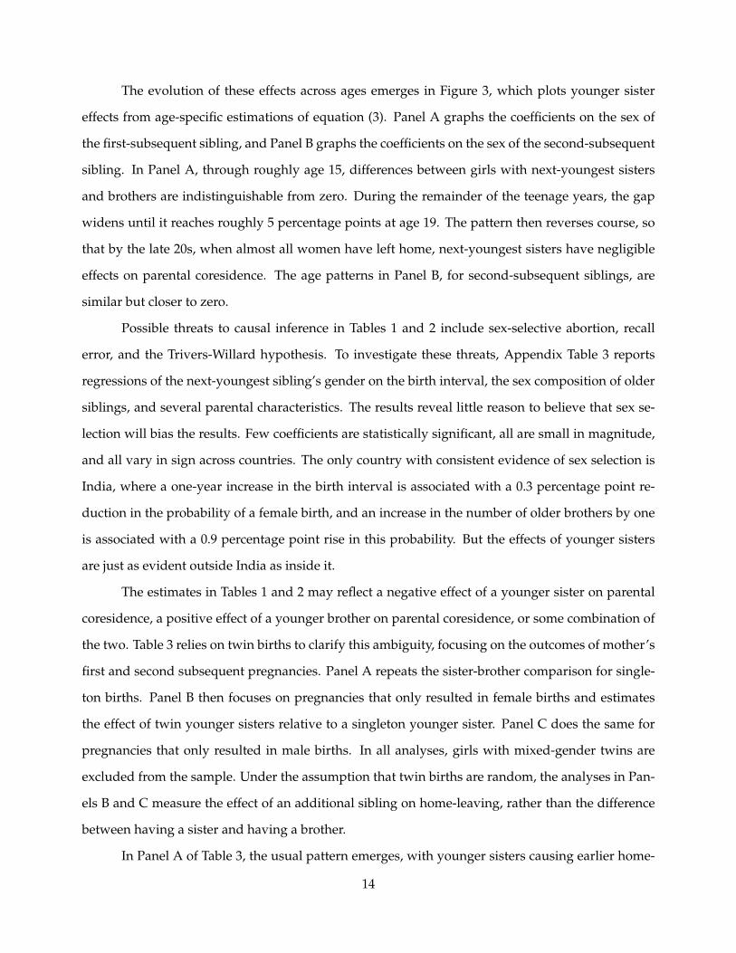
The evolution of these effects across ages emerges in Figure 3, which plots younger sister

effects from age-specific estimations of equation (3). Panel A graphs the coefficients on the sex of

the first-subsequent sibling, and Panel B graphs the coefficients on the sex of the second-subsequent

sibling. In Panel A, through roughly age 15, differences between girls with next-youngest sisters

and brothers are indistinguishable from zero. During the remainder of the teenage years, the gap

widens until it reaches roughly 5 percentage points at age 19. The pattern then reverses course, so

that by the late 20s, when almost all women have left home, next-youngest sisters have negligible

effects on parental coresidence. The age patterns in Panel B, for second-subsequent siblings, are

similar but closer to zero.

Possible threats to causal inference in Tables 1 and 2 include sex-selective abortion, recall

error, and the Trivers-Willard hypothesis. To investigate these threats, Appendix Table 3 reports

regressions of the next-youngest sibling’s gender on the birth interval, the sex composition of older

siblings, and several parental characteristics. The results reveal little reason to believe that sex se-

lection will bias the results. Few coefficients are statistically significant, all are small in magnitude,

and all vary in sign across countries. The only country with consistent evidence of sex selection is

India, where a one-year increase in the birth interval is associated with a 0.3 percentage point re-

duction in the probability of a female birth, and an increase in the number of older brothers by one

is associated with a 0.9 percentage point rise in this probability. But the effects of younger sisters

are just as evident outside India as inside it.

The estimates in Tables 1 and 2 may reflect a negative effect of a younger sister on parental

coresidence, a positive effect of a younger brother on parental coresidence, or some combination of

the two. Table 3 relies on twin births to clarify this ambiguity, focusing on the outcomes of mother’s

first and second subsequent pregnancies. Panel A repeats the sister-brother comparison for single-

ton births. Panel B then focuses on pregnancies that only resulted in female births and estimates

the effect of twin younger sisters relative to a singleton younger sister. Panel C does the same for

pregnancies that only resulted in male births. In all analyses, girls with mixed-gender twins are

excluded from the sample. Under the assumption that twin births are random, the analyses in Pan-

els B and C measure the effect of an additional sibling on home-leaving, rather than the difference

between having a sister and having a brother.

In Panel A of Table 3, the usual pattern emerges, with younger sisters causing earlier home-

14

leaving relative to younger brothers. The effect is stronger for the first subsequent pregnancy than

the second, which is consistent with the idea that younger sister effects diminish in the age gap

between sisters. As before, however, the difference in coefficients is confounded by differential

selection into the samples with at least one or two subsequent pregnancies.

Panels B and C then give suggestive evidence that the sister-brother difference is due solely

to an effect of the number of sisters. Because twin births are rare (200-300 in each regression, or less

than 1 percent of the sample), the standard errors are large and the estimates noisy. Even so, in Panel

B, the coefficients on the number of girls born in subsequent pregnancies are both negative and, in

one out of two cases, statistically significant. The coefficient is larger for the second subsequent

pregnancy than for the first, which is surprising, but this is likely the result of sampling error. Cer-

tainly, the coefficients are not statistically distinguishable. Meanwhile, Panel C yields coefficients of

zero for the number of boys born in subsequent pregnancies. An exogenous increase in the number

of younger sisters increases marriage risk, whereas an exogenous increase in the number of younger

brothers does not. This result suggests that the sister-brother comparison solely reflects the effect of

an additional sister, rather than offsetting (non-zero) effects of sisters and brothers.

5.1.2 Heterogeneity in Younger Sister Effects on Home Leaving

A comparison of the next-youngest sister effects across selected subsamples sheds some light on the

mechanisms behind the basic result.

A. Younger Sister Effects by Demographic Group Table 2 pools data from all four countries and

then divides the sample by several relevant characteristics.18 As a basis for comparison, column (1)

reports the baseline estimate of the younger sister effect in the pooled data. Because India’s sample

is so large relative to other countries’, the baseline estimate in the pooled data, -0.028, is very close

to the estimate for India in Table 1, Panel A.19

18The search model has no specific predictions for how sister effects vary with religion, so Table 2 does not report effectsby religion. For completeness, I analyzed Hindus and Muslims separately and found no significant difference betweenthe two in the pooled sample. The effects are larger for Hindus than for Muslims in Bangladesh, India, and Nepal, butPakistan (which is predominantly Muslim) exhibits large effects.

19One could argue that the coefficient on the gender of the next-youngest ever-born sibling is not the estimand ofinterest. If the effects operate through a marriage search channel, then one should take interest in the effect of a youngersister who is still alive when her older sister reaches marriageable age. In a a two-stage least squares (2SLS) regressionthat uses the gender of the next-youngest ever-born sibling as an instrument for a surviving next-youngest sister at agefifteen, the effect estimate is 14 percent larger than OLS estimate. This estimator assumes that the effect of the youngersibling’s gender operates only through circumstances in young adulthood. While this exclusion restriction may not hold

15

Columns (2) and (3) of Table 2 show that the effects are stronger for girls who grew up in

rural areas than for their urban counterparts. This result suggests that a low arrival rate of grooms

intensifies the observed effects because parents fear they will fail to find a spouse for their younger

daughter. Urban areas are likely characterized by higher arrival rates than rural areas. In urban

areas, marriage markets are thick, matchmakers and newspaper classifieds are easily accessible,

and the search process does not involve (sometimes arduous) travel to neighboring villages. The

theoretical framework reveals that cross-sister effects on marriage risk vary ambiguously with the

arrival rate, so one can interpret the urban/rural difference as preliminary evidence on the sign of

this comparative static. Section 5.1.3 estimates the arrival rate comparative static more formally.

The remainder of Table 2 examines heterogeneity by parental socioeconomic status and the

age gap between sisters. Columns (4) and (5) show that the effects are stronger among girls whose

fathers have above-median educational attainment, implying that the effects are not driven by eco-

nomic constraints affecting only poor families. Finally, columns (6)-(8) subdivide the sample based

on the next birth interval. The model predicts stronger effects of younger sisters when the age gap

is small. Indeed, the effect estimates decrease with the age gap, but the differences in coefficients

are statistically insignificant. Importantly, birth spacing is associated with parental socioeconomic

status, so the comparison across subsamples does not isolate the comparative static of interest.

B. Younger Sister Effects and the Arrival Rate of Grooms Intuition suggests that the a younger

sister’s effect on marriage risk may be especially strong when grooms arrive at a slow rate because

parents fear that they will fail to find their younger daughter a groom while she is still desirable on

the marriage market. The model clarifies that this comparative static is in fact ambiguous, because

the slow arrival rate also decreases the rate at which the younger daughter loses value in her final

years of her marriageable age span. How cross-sister effects vary with the arrival rate is an empirical

question.

The true arrival rate is unobservable, but one can use marriage market demographics as

proxies. The starting point is a meeting function, m(M, F), which gives the number of meetings per

unit of time as a function of the number of marriageable men (M) and women (F).20 The literature

exactly, the estimate is nonetheless informative.20I refer to m(·) as a “meeting function” rather than a “matching function” to emphasize that a meeting does not

necessarily translate to a match.

16

commonly specifies this function as a Cobb-Douglas technology, so that m(M, F) = MαFβ. Then

from a female perspective, the arrival rate of grooms is:

λ(M, F) =m(M, F)

F=

(MF

)α

Fα+β−1 (4)

Equation (5) expresses the arrival rate of grooms as a function of observable features of the marriage

market: namely, the sex ratio and the number of women. Research on search in both the labor

and marriage markets points to two empirical regularities.21 First, the arrival rate increases in the

tightness of the market (here measured by the sex ratio), so that α > 0. Second, the meeting (or

matching) function is typically characterized by constant returns to scale, so that α + β = 1. This

implies that doubling the size of the market leads to a doubling of the number of meetings.

To use equation (5) in a linear regression, take logs to obtain:

ln λ = α ln(

MF

)+ (α + β− 1) ln F (5)

One can implement this specification of the log arrival rate using basic data on the demographics

of the marriage market. Not all DHS samples can be linked to data on local marriage markets, but

the 2001 and 2006 Nepal DHS samples are geocoded, allowing a merge to district-level information

from the 2001 Census of Nepal (Nepal Central Bureau of Statistics 2010). Using this linked Nepal

dataset, I interact the next-youngest sister dummy with the logarithms of the marriage market sex

ratio and the number of women in the marriage market. Most marriages in Nepal take place within

district and within caste or ethnicity, so I aggregate marriage markets at the district-by-ethnicity

level.22 Men marry at ages 20-24, and women marry at ages 15-19. For each of three 5-year female

marriage cohorts that were aged 15-19 in 1996, 2001, and 2006, I use the 11% census micro-sample to

estimate the number of women in the cohort, as well as the ratio of men in the next-oldest five-year

cohort to women in the cohort.23 To avoid bias from a badly measured sex ratio denominator, I omit

21On labor markets, see the review by Petrongolo and Pissarides (2001). On marriage markets, see Angrist (2002),Botticini and Siow (2009), and Abramitzky et al. (2010).

22I assume that cross-district marriage-related migration is minimal, although I do not have specific data on this issue.Marriage-related migration would tend to bias the coefficients towards zero.

23Respondents reported their district of residence 5 years before, so for the 1996 cohort, I use the ratio of men age 20-24to women 15-19 five years before the census. For the 2001 cohort, I use the current ratio men age 20-24 to women age15-19. For the 2006 cohort, I use the current ratio of men age 15-19 to girls age 10-14 in the current district of residence.The 1996 and 2006 sex ratio estimates will be accurate if mortality and international emigration are minimal.

17

district/ethnicity-level cohorts with fewer than fifteen women in the micro-sample.24 The resulting

marriage market sex ratio has a mean of 0.8 and a standard deviation of 0.26. The mean sex ratio is

below 1 because population growth implies that the number of 15-19 year-olds exceeds the number

of 20-24 year-olds.

Table 4 adds these measures and their interactions with the next-youngest sister dummy to

specification (3). The new specification also includes fixed effects at the 5-year marriage cohort,

district, and caste-ethnicity level. To ease interpretation, I run one regression as specified above,

with both marriage market variables in logs, and one regression that uses the level of the sex ratio

rather than its logarithm. The dependent variable is an indicator for parental coresidence.

Younger sister effects on home-leaving are stronger when grooms are scarce but do not de-

pend on the scale of the marriage market. The levels and logs specifications of the sex ratio lead

to similar estimates, which is unsurprising because sex ratios are on average close to 1, so that

ln(M

F

)≈ M

F − 1. The coefficient of 0.138 in column (1) implies that a move from the 75th percentile

(0.96) to the 25th percentile (0.64) of sex ratio distribution increases the younger sister effect on

home-leaving by 4 percentage points. Note also that the probability of parental coresidence tends

to decrease in the relative supply of grooms (i.e., the main effect of the sex ratio), implying that the

risk of non-marriage is high when grooms are scarce. Interestingly, both specifications indicate little

role for the absolute number of women of the marriage market, which is suggestive evidence of

constant returns to scale in the meeting function.

The preceding analysis is based on cross-sectional variation in marriage market demograph-

ics, which poses some concerns about identification. Variation in marriage market sex ratios results

from variation in population growth, (pre- and post-natal) sex selection, and migration. Unfor-

tunately, no credible instrument exists for marriage market sex ratios in Nepal. Nonetheless, the

strength of the association between younger sister effects and the relative supply of grooms rein-

forces a marriage market interpretation of the main results.

C. Younger Sister Effects and the Prevalence of Arranged Marriage Although sisters may con-

strain one another’s marriage timing even in the absence of formal arranged marriage, the con-

straints are likely to be especially important when parents have a strong say in their daughters’

24The results are not sensitive to modifications of the fifteen woman cutoff.

18

marriages. The DHS contains no information on parental involvement in marriage arrangements,

but another survey, the India Human Development Survey (IHDS), does. A nationally represen-

tative household survey, the IHDS includes a fertility history module similar to that found in the

DHS, a marriage history module asking adult women to report how their marriages were arranged,

and a marriage practices module asking women to describe some aspects of marriage practice in

their communities. I use the IHDS data to measure whether the next-youngest sister effect varies

with the prevalence of arranged marriage.

Because the data on marriage arrangements are self-reported but the data on home-leaving

and sibling composition are mother-reported, I cannot estimate individual heterogeneity in sister ef-

fects by type of marriage arrangement.25 However, I can aggregate self-reported marriage arrange-

ments of young women at the district level and ask whether sister effects vary with the district-level

prevalence of arranged marriage.26 To measure the district-level prevalence of arranged marriage,

I calculate the shares of young women age 25-29 who arranged their own marriages, arranged their

marriages jointly with their parents, and had no input into their marriage arrangements. I then in-

teract the next-youngest sister dummy in specification (3) with the share self-arranged and the share

with no say. Looking across districts, the share self-arranged has a mean of 0.06 and first, second,

and third quartiles of 0.00, 0.00, and 0.07, respectively. The share with no say has a mean of 0.36 and

first, second, and third quartiles of 0.00, 0.30, and 0.60, respectively.

The results of this exercise, presented in Table 5, show that younger sister effects on home

leaving are significantly weaker in districts with a greater share of self-arranged marriages.27 At

the same time, relative to joint marriage arrangements, parent-only marriage arrangements do not

significantly change the magnitude of the younger sister effects. In the full specification in column

(4), the coefficient on the interaction of the next-youngest sister dummy with the share self-arranged

0.19 [S.E. = 0.09]. A move from the median to the 75th percentile of the share self-arranged shrinks

the younger sister effect by 1.3 percentage points, and a move from the 75th percentile to the 90th

percentile shrinks it by a further 2.3 percentage points.

25Individual-level variation in the type of marriage arrangement may also be endogenous to sibling composition.26Unlike the 11% census sample from Nepal, the IHDS sample is too small to disaggregate districts by caste.27The uninteracted coefficient in column (1) of Table 6 may appear large relative to the DHS results for India. However,

when the regressions are estimated with sampling weights, the coefficients are much closer. In the India DHS data, theweighted regression coefficient is 0.034. In the India Human Development Survey data, the weighed regression coefficientis 0.039. The IHDS survey weights are not representative at the district level, so the weights are not helpful for the analysisin Table 6.

19

These results strongly imply that sister effects intensify with more family involvement in

marriage arrangements. But we should note that the prevalence of arranged marriage is likely

correlated with social conservatism more generally. If conservatism is associated with strong social

norms for marriage by birth order, then arranged marriage may not be the culprit per se. In either

case, however, adherence to orthodox marriage practices is key to putting sisters’ interests at odds

with each other.

5.1.3 Older Sister Effects on Home-Leaving

The search framework has the important prediction that the effects of older and younger sisters have

opposite sign. Parents hasten to marry an older daughter but delay in marrying her younger sister.

However, mean differences between girls with older brothers and girls with older sisters may reflect

selective fertility, rather than the effects of older siblings. Because of the demand for sons, parents

are far more likely to continue having children after a female birth than after a male birth (Filmer et

al. 2010). For young women with at least one older sibling in the pooled sample, Appendix Table

4 regresses the gender of the next-oldest sibling on family characteristics. Girls with next-oldest

sisters have fewer older brothers (not counting the next-oldest birth), shorter birth intervals, more

educated and older mothers, and later birth years than girls with next-oldest brothers. This implies

that a mean comparison between girls with next-oldest brothers and sisters may yield a biased

estimate of the effect of an older sister.

The selection problem is most intuitive if we view the older sibling as the unit of observation.

As before, consider a child from family i with older sibling composition j. Let femaleij, Sij, and Yij

be indicators for the child’s gender, the presence of a next-youngest sister, and the presence of a

next-youngest sister who lives with her parents, respectively. In more general language, femaleij is

the treatment indicator, Sij is the sample selection indicator, and Yij is the outcome. Then:

Sij = S1ij(femaleij) + S0

ij(1− femaleij)

Yij = Sij ·{

Y1ij(femaleij) + Y0

ij(1− femaleij)} (6)

where (S1ij, S0

ij) are potential sample selection probabilities and (Y1ij, Y0

ij) are potential outcomes. We

observe only (femaleij, Sij, Yij) but wish to make inferences about moments of Y1ij −Y0

ij: the effect of a

child’s sex on a younger sister’s propensity to live with her parents, were a younger sister to exist.20

The econometrics literature suggests a few ways to estimate treatment effects under endoge-

nous sample selection. Horowitz and Manski (2000) propose making worst-case assumptions about

the missing outcomes to generate treatment effect bounds that require no assumptions about the se-

lection process. But if both the treatment and control groups select out of the sample at reasonably

high rates, as is the case here, Horowitz-Manski bounds become uninformative.28 However, Heck-

man (1974, 1979) and Lee (2009) show that added structure on the selection process can improve

identification. Both approaches depend heavily on a latent variable threshold-crossing model of

sample selection, which is equivalent to the monotonicity condition that S1ij − S0

ij has weakly the

same sign for all children (Vytlacil 2002). Heckman’s parametric selection correction model yields a

point estimate of the treatment effect but is only robust when an instrument for selection—a variable

that affects selection but bears no direct effect on the outcome—exists. In contrast, the procedure of

Lee provides non-parametric bounds on the treatment effect without requiring such an exclusion re-

striction. This procedure involves identifying the excess number of observations in the group with a

higher selection rate and then trimming the left and right tails of that group’s outcome distribution

by this excess number of observations.

I use the methods of both Heckman (1974) and Lee (2009) to assess the extent of selection bias

in OLS estimates of the older sister effect on parental coresidence.29 As a first step to implementing

these methods, one must justify the monotonicity assumption. In South Asia, where parents have a

demand for sons, the monotonicity condition generally implies that all couples who stopped child-

bearing after a girl would have also stopped after a boy. This condition may not hold exactly for all

families, but because son-biased fertility stopping behavior is so pervasive in South Asia (Filmer et

al. 2010), it is a reasonable approximation.30 Nonetheless, if parents also have a demand for gen-

der diversity, a female birth may decrease fertility in families with many boys but without many

girls. To account for this possibility, I allow the effect of a girl on fertility continuation to differ

by the exact composition of older siblings in both the selection correction and bounds estimations.28Because we only observe outcomes for girls, who represent roughly half of next-born children, the attrition rate

would be approximately one-half even in the absence of fertility cessation.29In implementing both estimation procedures, I account for clustering in the DHS survey design. The maximum

likelihood version of Heckman’s selection correction model is easier to adjust for clustering than the two-step version, soI use the former. For consistency with the other results in the paper, I use a linear probability model for the second-stageequation. For the bounds estimator, Lee provides formulas for asymptotic standard errors only in the i.i.d. case, so Iblock-bootstrap the bounds estimator at the PSU-level.

30Son-biased fertility stopping behavior reflects the tendency to desire more sons than daughters. For example, inIndia’s 2005-06 DHS, 22 percent of women desire more sons than daughters, 76 percent of women desire the same number,and less than 3 percent desire more daughters than sons.

21

In the selection correction model estimations, I interact the gender dummy with indicators for the

exact composition of older siblings. In the bounds estimations, I compute separate bounds for each

composition of older siblings and then average across them, weighting by sample size.

The monotonicity condition requires a careful choice of the analysis sample. One sample of

interest is every individual in the fertility histories over age 15, which includes every older sibling of

the 15-24 age group. But the inclusion of individuals aged 26 and above may violate the monotonic-

ity condition, since an initial spike in parental fertility following a female birth may then decrease

the probability that a younger sibling lands in the 15-24 age group. As a result, I analyze how the

genders of individuals aged 16-25 affect rates of parental coresidence among their younger sisters

aged 15-24. This approach exacerbates sample selectivity because it leaves a short period for the

birth of a younger sibling, but it makes the monotonicity condition plausible.

A second step to implementing the Heckman selection correction model is the choice of an

instrument for sample selection. Based on the logic that women become less likely to continue

childbearing as they age, I use the mother’s age at the older sibling’s birth as an instrument for

whether a younger sibling is born. Because the mother’s age at a given child’s birth is correlated

with her age at first birth, I control for her age at first birth in both the selection equation and the

outcome equation.31 I also report a specification that controls for the mother’s age at first birth,

age at first marriage, and educational attainment, as well as the father’s educational attainment. In

both specifications, the exclusion restriction—that absent selection, children born longer after their

mothers’ first births would have similar home-leaving propensities to those born sooner after their

mothers’ first births—is strong, but the results are nonetheless instructive. The DHS does not offer

an obviously superior instrument for selection.

Table 6 exhibits the uncorrected OLS estimates, the Heckman selection-corrected estimates,

and the Lee bounds. To clarify the selection process, Table 6 presents separate estimations for birth

orders 1-5. For comparison, column (1) presents estimates the effect of next-youngest sibling gender.

Column (2)-(7) contain estimates of the effect of next-oldest sibling gender. These effects do not

apply to first-born children (who have no older siblings), and the Heckman models are not estimable

for second-born children (for whom the mother’s age at first birth is the same as the mother’s age

at the next-oldest sibling’s birth).

31The results are also robust to omitting the mother’s age at first birth.

22

The results support the queuing theory’s prediction that younger and older sisters have op-

posite effects. Column (1) shows that the presence of a younger sister has a robust negative effect

on parental coresidence across all birth orders. In contrast, the results in columns (2)-(7) strongly

suggest that the presence of an older sister has a positive effect on parental coresidence. The uncor-

rected OLS results in column (2), which use the full sample of women aged 15-24 who have at least

one older sibling, indicate that younger women with older sisters exhibit significantly higher rates

of parental coresidence than their counterparts with older brothers. Selection bias is possible, how-

ever, so columns (3)-(7) perform the selection-correction and bounding procedures. The selection-

corrected estimates (columns [3]-[4]) are broadly similar to the uncorrected OLS estimates in both

magnitude and statistical significance. The nonparametric bounds are necessarily less precise, but

they too support the hypothesis that younger and older sisters have opposite effects. Column (5)

shows the average proportion of observations trimmed from each older sibling composition stra-

tum, and columns (6) and (7) display the trimmed bounds. Except among 5th-born women, for

whom the trimming proportion is fully 11 percent, both the lower and upper bounds on the older

sister effect are positive. Unfortunately, the lower bound is too close to zero to statistically reject a

zero effect. Coupled with the OLS and Heckman results, however, the results are strongly consistent

with positive older sister effects on parental coresidence—compelling evidence that girls queue to

leave the household.

5.2 Evidence on Marriage Age, Human Capital, and Spousal Quality

The Fertility History results establish some compelling facts about how sisters affect each other’s

home-leaving. But because the Fertility Histories fail to track these women after they leave home,

they cannot provide answers to several key questions. Do the effects of younger sisters on home-

leaving indeed correspond to effects on marriage? If so, does the earlier marriage of women with

younger sisters come at the expense of their education? And what are the implications for spousal

quality? This section explores these questions using women’s Sibling Histories from Nepal. The

Sibling History data do not provide enough information to compute selection-corrected estimates

of the effects of older sisters, so the section focuses only on the effects of younger sisters.

23

5.2.1 Younger Sister Effects on Marriage Age and Human Capital among Teenagers

Figure 4 plots rates of parental coresidence, never-marriage, and school attendance by age and

younger sibling gender. The top panel shows rates of parental coresidence in a graph analogous

to Figure 2, this time focusing only on the 2006 Nepal Fertility History data. The middle panel

displays rates of never-marriage among young women in the same survey’s Sibling History data.

The bottom panel combines Fertility History data on coresident daughters with self-reported data

on women fifteen and older. By combining the samples in this way, one can observe precisely when

schooling gaps emerge between girls with younger brothers and sisters.32

The patterns in Figure 4 match a theory in which same-sex sibling competition emerges only

when girls are at risk of marriage. From age three to age fifteen, girls with younger brothers and

sisters have identical school attendance rates. This pattern holds both for ten-year-olds, who have

high school attendance rates, and for three- to five-year-olds, who do not. At age sixteen, a large

gap in school attendance emerges between girls with younger brothers and sisters, only to close at

age 19, when school attendance rates become quite low. These are precisely the ages at which girls

are most likely to marry.

Based on these patterns, Table 7 estimates younger sister effects on marriage, childbearing,

school enrollment, and literacy among women aged 15-19. A younger sister increases a teenage

girl’s probability of marriage by 5½ percentage points and decreases her probability of attending

school in the previous year by 6½ percentage points. Girls often leave school in advance of their

weddings, so the larger effect on school attendance does not necessarily imply that non-marital

forces are at work. (In any event, the effects are not statistically distinguishable.) The effects on

literacy and fertility are small and insignificant, which may be due to the low rates of illiteracy and

maternity in this young sample.

5.2.2 Younger Sister Effects on Marriage Age and Human Capital among Adults

Similar effects on marriage risk and human capital are also evident among women later in the

lifecycle. Panel A of Table 8 presents analyses based on all women aged 15-49. The first two columns

32Changes in sample composition pose a potential problem for this approach. Girls in the Fertility Histories all havemothers younger than 50, whereas those in the Sibling Histories have mothers of any age. However, adjustment for theyear of the mother’s first birth does not change the patterns in Figure 2. (The year of the mother’s first birth serves as aproxy for her age; her actual age is not available in the Sibling Histories.)

24

report Cox hazard regressions based on equation (3).33 The presence of a younger sister raises a

woman’s risk of marriage and childbearing by slightly over 10 percent. In the time metric, this

represents an average effect of approximately half a year. Younger sisters cause earlier marriage,

which also appears to hasten childbearing.

The remaining columns in Panel A of Table 8 examine the effects of younger sisters on other

female outcomes in adulthood. Column (3) shows a moderate (but only marginally significant)

negative effect on the highest grade completed, while column (4) indicates a large, statistically sig-

nificant, positive effect on illiteracy. Of women with younger brothers, 44 percent are illiterate,

compared to 47 percent of women with younger sisters. This finding is consistent with the results

of Field and Ambrus (2008), who find that early marriage reduces female literacy in Bangladesh.

Women with younger sisters also display slightly lower body mass indices (BMIs) than women

with younger brothers (p < 0.08).34 However, younger sisters have no effect on height, an indicator

of early-childhood conditions. This result supports the hypothesis that the effects of younger sisters

emerge only in young adulthood.

5.2.3 Younger Sister Effects on Spousal Attributes

Shorter search time implies lower spousal quality. For obvious reasons, data on spousal quality are

available only for ever-married women. I thus restrict attention to women over age 30, whose rates

of never-marriage are extremely low (less than 2 percent).35 Because this reduces the sample size

substantially, I supplement the 2006 sample with data from the 1996 Nepal DHS. The 1996 survey

also included a sibling history module, but it only interviewed ever-married women, making it

inappropriate for some of the preceding analyses. Nonetheless, the sample design introduces no

new biases for the study of spousal quality.

Panel B of Table 8 analyzes this sample of women aged 30-49. For completeness, the table first

verifies that younger sisters increase the hazards of marriage and childbirth in this sample of older

women. The effects remain positive and statistically significant, although they are smaller than in

the 2006 full-sample results.36 The human capital effects are similar to before, and the coefficient for

33To avoid possibly inappropriate proportionality restrictions, the Cox models stratify by the composition of oldersiblings, instead of including fixed effects. Otherwise, the specification is identical to equation (3).

34The standard deviations of BMI and height are 3 and 6, respectively.35Nearly all ever-married women in the sample reported their husbands’ characteristics.36Appendix Figure 1 shows that secular change across cohorts may account for the different results in the main sample

25

educational attainment is now significant at the 5 percent level.

Columns (11)-(14) then show that younger sisters also reduce spousal quality and house-

hold wealth in adulthood. The husbands of women with younger sisters have completed 0.2 fewer

grades and are 4 percentage points less likely to have skilled occupations than their counterparts

whose wives have younger brothers. Durable goods ownership, measured in an index normed

to have mean 0 and standard deviation 1, is also slightly lower in the households of women with

younger sisters. However, although the effects on spousal education and occupation are statisti-

cally significant at the 5 percent level, the effect on household wealth is only statistically significant

at the 10 percent level. Finally, younger sisters do not affect the age of their older sisters’ husbands,

a result consistent with the small, insignificant estimates of the value of a groom’s age that arise

in hedonic dowry regressions (e.g., Rao 1993). These results suggest that the constraints younger

sisters place on their older sisters’ marriage arrangements lead to reductions in spousal quality.

6 Alternative Explanations for Sister Effects

The results in Section 5 are strongly consistent with a marriage search framework, but several alter-

native theories also predict that women’s outcomes vary with the sex composition of their siblings.

The leading alternatives focus on marriage costs, the demand for male and female labor, son-biased

resource allocation, and son-biased fertility stopping behavior. Sections 6.1-6.3 discuss the alterna-

tive mechanisms and explore whether their implications match the data.37 The basic conclusion is

that no single alternative theory can account for all the patterns observed in the data.

6.1 Dowry and Liquidity Constraints

The first alternative explanation for the patterns in Section 5 remains firmly rooted in the marriage

market but concentrates on the family consumption problem rather than search. To marry their

daughters, South Asian families pay dowries that regularly reach several times their annual income

and the over-30 sample. For four decadal birth cohorts, the figure plots the share of women married by ages 14, 15, 16,17, and 18. Younger sisters increase marriage risk only among cohorts born after 1970. This coincides with populationgrowth, which raised marriage market sex ratios, and also with the rapid growth of the Nepali public school system,which increased the dispersion of groom quality and the value of parental coresidence for teenage daughters.

37Sections 6.1-6.3 discuss mainly economic mechanisms, rather than gender-specific personality effects, which arise inthe literature on industrialized countries (Butcher and Case 1994). The link between such personality effects and marriagerisk is unclear. Additionally, personality theories give little reason to expect the effects to vary with the prevalence ofarranged marriage and the demographics of the marriage market.

26

(Anderson 2007a). A liquidity-constrained family must delay its younger daughter’s marriage to

allow time to accumulate a second dowry. Because dowries increase with bridal age (Field and

Ambrus 2008), the delay increases her dowry, which the family may offset by marrying her older

sister at a younger age. Like the search framework, this simple theory predicts opposite effects of

older and younger sisters on marriage age.

The sub-sample analyses in Table 2 already provide suggestive evidence against the dowry

theory. Girls whose fathers have above-median educational attainment display stronger effects than

girls whose fathers are less educated. If dowries and liquidity constraints were important, then the

effects would presumably be stronger in poorer households (with less educated fathers), where

borrowing constraints are more likely to bind. Without more information on the size of the dowry

and the nature of borrowing constraints, this pattern remains suggestive. Nonetheless, the stronger

effects in better-off households are difficult to reconcile with a model of liquidity constraints.

The data offer two testing grounds for the dowry theory. The first is Nepal, which exhibits

significant regional variation in marriage institutions. In the terai lowlands, where nearly half of

Nepal’s population lives, dowry is a deep-seated institution (Niraula and Morgan 1996; Sah 2008).

Dowries are large and widespread in terai marriages, and parents take on overwhelming debt to

marry their daughters. In contrast, dowries are smaller and less common in Nepal’s other two

ecological regions, the hills and mountains. If the interaction of dowry and liquidity constraints

drives the home-leaving patterns, then these patterns should be stronger in the terai than in the hills

and mountains. As column (1) of Table 9 reveals, the opposite is true. In the hills and mountains,

younger sisters decrease parental coresidence in early adulthood by over 8 percentage points. This

compares with an effect of less than 2 percentage points in the terai.38 This stark regional difference

suggests that dowry cannot play a primary role in explaining the main results of the paper.39

The second testing ground is India, where the IHDS data allow for more precise measure-

ment of dowry. The IHDS features a module on marriage practices, including a series of questions

on the types of “gifts” typically transferred during a daughter’s wedding, from precious metals, to

38The younger sister effect is also smaller in the terai than in the hills and mountains if one omits Tharu women fromthe sample. The Tharu, an ethnic group from the western terai, do not exchange dowries (Gurung and Kittelsen 1996).

39The size and direction of the regional difference was unexpected, but one can easily reconcile it with the searchframework. Because of the rugged terrain in the hills and mountains, communities are more isolated than in the terai.Travel to neighboring communities is more cumbersome, which may intensify search frictions. Additionally, young menmigrate from the hills and mountains to the terai for work; as a result, the terai has marriage market sex ratios that areapproximately 10 percentage points higher than the hills and mountains.

27

livestock, to cash. I use the responses of the young woman’s mother, although the results are similar

if one instead uses a district-level average that leaves out the young woman’s mother due to endo-

geneity concerns. To aggregate the various gifts, I take the first principal component of the vector of

the mother’s responses. I then interact this measure of dowry with the next-youngest sister dummy.

The results, in column (2) of Table 9, show no evidence that sister effects are more pronounced in

communities with larger dowries.40

6.2 Household Labor Demand

Apart from the marriage market explanations, sibling sex composition may affect marriage age be-

cause of complementarities in household production. If opposite-sex siblings are complements in

household production, but same-sex siblings are substitutes, then a sister’s presence in the house-

hold decreases the demand for female labor, whereas a brother’s presence increases it. However,

while this theory predicts higher home-leaving (and marriage) among young women with sisters, it

gives no reason for the opposite effects of older and younger sisters that are suggested by the data.

Furthermore, Table 3 shows that the birth of twin brothers relative to a singleton brother does not

affect female home-leaving. Finally, the school attendance differences in Figure 4 are also inconsis-

tent with the labor demand theory. Girls with brothers are more likely to attend school than girls

with sisters; the labor demand theory predicts that they should be working rather than studying.41

Household demand for male and female labor is unlikely to account for the patterns in Section 5.

6.3 Son Bias

The existing literature on the effects of sibling sex composition in resource-poor settings has empha-

sized yet another mechanism: a bias for sons in both intrahousehold resource allocation and fertility

stopping.42 Families may substitute resources from girls to boys, so that a girl benefits from the birth

of a sister rather than a brother. However, brothers raise per capita resources in the household, both

40The size of the dowry may be correlated with household income, which in turn may be inversely related to theincidence of liquidity constraints. In unreported results, I control for the education of the young woman’s father and forthe interaction of his education with dowry size. The results still fail to support the dowry theory.

41Using data from Nepal, Edmonds (2006) finds that both boys’ and girls’ labor supply decreases if the next-youngestsibling is female, with the effect substantially larger among boys. However, this effect is concentrated only among closelyspaced children, whereas the effects on marriage risk are evident at wider birth spacing as well. Furthermore, in un-reported estimates, teenage boys with younger sisters have lower home-leaving risk than those with younger brothers,which is opposite the result for girls. This difference is at odds with Edmonds’s labor supply estimates.

42See Garg and Morduch (1998), Morduch (2000), and Chen et al. (2010).

28

directly—through productivity—and indirectly—because families are more likely to continue fer-

tility after a girl than after a boy (Filmer et al. 2009).43 As a result, sibling sex composition may have

multiple countervailing effects.

Many results in Section 5 address these theories. As a starting point, note that women with

younger sisters appear to be worse-off than women with younger brothers, which makes allocative

bias for sons an unlikely explanation for the effects. Son-biased fertility stopping rules, which are

evident in Table 3, are more likely to play a role. However, several findings suggest that fertility

stopping rules also fail to explain the sister effects observed in Section 5.44 First, the data suggest that

older sisters have opposite effects from younger sisters on home-leaving. The alternative theories

in the previous paragraph might predict that only older or younger siblings would matter—for

example, because younger siblings do not yet work—but they do not give a natural interpretation

for opposite effects.45 Second, the increase in family size due to twin boys is similar to that due to

twin girls, but only the latter affect female home-leaving. These results imply that the younger sister

effect is due to the presence of a sister rather than the absence of a brother.46 Third, in Figure 4, the

gap in school attendance between girls with younger sisters and brothers emerges only when girls

are of marriageable age. Theories based on the value of sons would predict gaps in earlier childhood

as well. For a broader look at this issue, Appendix Table 5 considers the effects of next-youngest

sibling gender on four outcomes in earlier life: under-5 mortality, height and weight for two- to four-

year-olds, and school enrollment for five- to nine-year-olds.47 The results reveal little systematic

evidence that the gender of a girl’s next-youngest sibling affects her wellbeing in childhood.

7 Sister Effects on Marriage Outside South Asia

Because the family of origin is involved in marriage arrangements in many parts of the world,

younger sisters may affect women’s marriage age more globally. One would expect these sister

43The presence of a son may also improve a mother’s bargaining power, with benefits to his sisters. The next paragraphdiscusses empirical patterns that reject this explanation.

44In addition to the findings discussed in this paragraph, the inclusion of childhood family size as a covariate did notsubstantively change the results. I do not report this finding in a table because completed family size is endogenous.

45The confidence intervals on the nonparametric bounds include zero, but the bounds themselves are both positive,and the OLS and selection-corrected estimates reject zero.

46Table 3 indicates that son-biased stopping rules are widespread, but they do explain the home-leaving patterns.47Some of these variables do not appear in every survey. I analyze the heights and weights of two to four year-olds

because the DHS only collects anthropometric data on children under 5, and few one-year-olds have a younger sibling.The height and weight z-scores have mean zero and standard deviation one in a “healthy” population.

29

effects to be strongest in regions with the strictest adherence to parental arranged marriage, such

as the Middle East, North Africa, Central Asia, and South Asia. In other world regions—such as

Africa, East Asia, and Latin America—where the role of the family in marriage arrangements has

declined, the effects may be smaller. Apart from Nepal, 40 other countries in Africa, Asia, and Latin

America have conducted DHS surveys with questions on siblings, marriage, and education. Table

10 presents estimates of next-youngest sister effects on marriage risk and educational attainment in

five world regions other than South Asia, using data on these 40 other countries.48

Column (1) reveals that younger sister effects on age at marriage are surprisingly prevalent

throughout the developing world. As one would expect, in Afghanistan, Jordan, and Morocco,

the Cox hazard ratios are similar in magnitude to those found in South Asia, ranging from 1.06 to

1.08. For Latin America, the Pacific, and Sub-Saharan Africa, the hazard ratios remain significantly

greater than one, but they all lie between 1.01 and 1.02. These regional differences are consistent

with the global diffusion of liberal attitudes towards marriage. Notably, dowry payments (net trans-

fers from the bride’s family) are extremely rare outside South Asia (Anderson 2007a), so the results

reinforce the conclusion that dowry payments do not by themselves explain why younger sisters

cause earlier marriage.

The table then examines whether these marriage age effects to translate into schooling effects,

as they do in South Asia. For the schooling effects to operate, two conditions must be met: (1)

marriage must occur at a sufficiently early age, and (2) school-leaving must occur at a sufficiently

late age. As such, along with the hazard ratios for marriage and the OLS coefficients for educational

attainment, the table reports the fraction of women who were married by age 16 and the fraction of

women with no schooling.

Column (3) indicates that younger sisters have significant negative effects on educational

attainment only in Sub-Saharan Africa. This result is easily squared with the distributions of mar-

riage age and educational attainment. In Afghanistan, girls marry young but do not attend school

for long, with an average of less than the second grade. In the Middle East and North Africa, they

obtain more schooling but marry late. Early marriage is also fairly rare in Latin America and the

Pacific. But the conditions are right for schooling effects in Sub-Saharan, where both early marriage

and adolescent schooling are common. The effects on schooling are small, one-tenth the size of the

48The data from Indonesia and Jordan only include ever-married women, so I restrict both these samples to womenover the age of 30. For all other countries, the data include both married and unmarried women.

30

effects in Nepal, but the effects on marriage risk are also small.

8 Conclusions

Traditional institutions interact in interesting ways with social and economic change. This paper

studies how traditional marriage practices induce tradeoffs among sisters, tradeoffs most intense

at intermediate levels of female schooling. Across four large South Asian countries, parents rush

a daughter’s marriage search if she has younger sisters and delay her marriage search if she has

older sisters, at the expense of spousal quality. These effects are especially strong in settings where

grooms are scarce, search frictions are large, and arranged marriage is common. Because girls leave

school when they marry and depend on their husbands for economic support in adulthood, the

effects have long-term consequences. In Nepal, where data on adult women are available, younger

sisters cause earlier school-leaving, lower educational attainment and adult literacy, lower spousal

educational attainment and spousal occupational status, and marginally lower adult household

economic status. Sibling rivalry over leaving the nest has effects that last long after all siblings have

left it.

These findings augment previous research on the lifecycle consequences of the marriage deci-

sion. In a notable paper on this topic, Field and Ambrus (2008) use age at menarche as an instrument

for marriage age in rural Bangladesh, where girls may only enter the marriage market after reaching

menarche. They find that women who started menstruating early married young and left school

young but saw no change in spousal quality. Their different results on spousal quality highlight

an important difference in the variation driving marriage age. In their study, early menarche leads

to early marriage by expanding the opportunity set, thus allowing parents to find a weakly better

groom. In mine, younger sisters lead to early marriage because they restrict the opportunity set.49

The policy implications of this result depend on the nature of the marriage market and the

production function. If schooling has decreasing returns, then the cost of an older sister’s lost time

in school is greater than the benefit of her younger sister’s gain. But perhaps more importantly, the

theory predicts that the presence of any sister, older or younger, decreases expected spousal quality.

49Also consistent with my results, Field and Ambrus (2008) report that age at menarche has smaller effects on marriageage among women with more older sisters. However, their data only include siblings who survived to adulthood and asa result do not allow a more careful examination of sibling effects.

31

If grooms attributes are equally valuable to all women, then the results imply a transfer of high-

quality grooms from large families to small. But if marriages are characterized by match-specific

quality, then a large number of daughters per family may cause aggregate mismatch in the marriage

market. Along these lines, the findings may provide a new justification for family planning policies

(which on average reduce the number of daughters per family and increase the spacing between

them), for the promotion of love marriage, or for the development of search technologies (e.g.,

matchmakers and websites).

The apparent role of search in explaining the results is surprising because it implies that

for a large swath of the world’s population, conventional budget constraint considerations fail to

describe a principal cause of sibling rivalry. This finding suggests an interesting direction for fu-

ture research, concerning how the interaction of persistent institutions with a changing economy

shapes the effects of family structure on children’s outcomes. It also calls attention to the question

of why some institutions evolve slowly, a topic raised by Roland (2005) and Guiso et al. (2006). A

deeper understanding of these institutions and their effects may shed light on a range of social and

economic phenomena, both across and within families.

References

Abramitzky, Ran, Adeline Delavande and Luís Vasconcelos. (2010). “Marrying Up: The Role of SexRatio in Assortative Matching.” Mimeo, Stanford University.

Alesina, Alberto and Paola Giuliano. (2010). “The Power of the Family.” Journal of Economic Growth15(2): 93-125.

Ambrus, Attila, Erica Field and Máximo Torero. (2010). “Muslim Family Law, Prenuptial Agree-ments, and the Emergence of Dowry in Bangladesh.” Quarterly Journal of Economics 125(3): 1349-1397.

Anderson, Siwan. (2007a). "The Economics of Dowry and Brideprice." Journal of Economic Perspec-tives 21(4): 151-174.

Angrist, Josh. (2002). “How Do Sex Ratios Affect Marriage and Labor Markets? Evidence fromAmerica’s Second Generation.” Quarterly Journal of Economics 117(3): 997-1038.

Angrist, Joshua, Victor Lavy, and Analia Schlosser. (2010). “Multiple Experiments for the CausalLink between the Quantity and Quality of Children.” Journal of Labor Economics 28(4): 773-824.

32

Arnold, Fred, Sunita Kishor, and T. K. Roy. 2002. "Sex-Selective Abortions in India." Population andDevelopment Review 28(4): 759-785.

Bagnoli, Mark, and Ted Bergstrom. (2005). “Log-concave Probability and its Applications.” Eco-nomic Theory 26(2): 445-469.

Becker, Gary S., and H. Gregg Lewis. (1973). “On the Interaction between the Quantity and Qualityof Children.” Journal of Political Economy 81: S279-S288.

Bertrand, Marianne, and Antoinette Schoar. (2006). “The Role of Family in Family Firms.” Journalof Economic Perspectives 20(2): 73-96.

Bhalotra, Sonia, and Tom Cochrane. (2010). “Where Have All the Young Girls Gone? Identificationof Sex Selection in India.” Mimeo, Bristol University.

Black, Sandra, Paul J. Devereux, and Kjell G. Salvanes. (2005). “The More the Merrier? The Effect ofFamily Composition on Children’s Education.” Quarterly Journal of Economics 120: 669-700.

Blake, Judith. (1983). “Family Size and the Quality of Children.” Demography 18: 421-442.

Botticini, Maristella, and Aloysius Siow. (2009). “Are There Increasing Returns to Scale in MarriageMarkets?” Mimeo, Università Bocconi.

Butcher, Kristin F., and Anne Case. (1994). “The Effect of Sibling Sex Composition on Women’sEducation and Earnings.” Quarterly Journal of Economics 109(3): 531-563.

Caldwell, John C., Pat Caldwell, Bruce K. Caldwell, and Idrani Pieres. (1998). “The Constructionof Adolescence in a Changing World: Implications for Sexuality, Reproduction, and Marriage.”Studies in Family Planning 29(2): 137-153.

Chen, Stacey H., Yen-Chien Chen, and Jin-Tan Liu. (2010). “The Effects of Sibling Sex Compositionon Child Mortality and Education.” Mimeo, Royal Holloway University of London.

Desai, Sonalde, and Lester Andrist. (2010). “Gender Scripts and Age at Marriage in India.” Demog-raphy 47(3): 667-687.

Dillon, Lisa. (2010). “Parental and Sibling Influences on the Timing of Marriage, 17th and 18th-Century Quebec.” Annales de Dèmographie Historique 119: 139-180.

Edlund, Lena. (1999). “Son Preference, Sex Ratios, and Marriage Patterns.” Journal of Political Econ-omy 107(6): 1275-1304.

Edlund, Lena, and Nils-Petter Lagerlöf. (2006). “Individual vs. Parental Consent in Marriage: Im-plications for Intra-Household Resource Allocation and Growth.” Mimeo, Columbia University.

Edmonds, Eric. (2006). “Understanding Sibling Differences in Child Labor.” Journal of PopulationEconomics 19: 795-821.

33

Fafchamps, Marcel, and Agnes R. Quisumbing. (2007). “Household Formation and Marriage Mar-kets in Rural Areas.” In T. Paul Schultz and John A. Strauss, eds., Handbook of DevelopmentEconomics, Volume 4. Amsterdam: Elsevier.

Field, Erica, and Attila Ambrus. (2008). “Early Marriage, Age of Menarche, and Female SchoolingAttainment in Bangladesh.” Journal of Political Economy 116(5): 881-930.

Filmer, Deon, Jed Friedman, and Norbert Schady. (2009). “Development, Modernization, and Child-bearing: The Role of Family Sex Composition.” World Bank Economic Review 23(3): 371-398.

Garg, Ashish, and Jonathan Morduch. (1998). “Sibling Rivalry and the Gender Gap: Evidence fromChild Health Outcomes in Ghana.” Journal of Population Economics 11(4): 471-493.

Goldberger, Arthur. (1983). “Abnormal Selection Bias.” In Samuel Karlin, Takeshi Amemiya, andLeo A. Goodman, eds., Studies in Econometrics, Time Series, and Multivariate Statistics. NewYork:Academic Press, pp. 67–84.

Goode, William Josiah. (1970). World Revolution and Family Patterns. New York: Free Press.

Goody, Jack R. (1983). The Development of the Family and Marriage in Europe. New York: CambridgeUniversity Press.

Greif, Avner. (1994). “Cultural Beliefs and the Organization of Society: a Historical and TheoreticalReflection on Collectivist and Individualist Societies.” Journal of Political Economy 102: 912-950.

Guiso, Luigi, Paola Sapienza, and Luigi Zingales. 2006. “Does Culture Affect Economic Outcomes?”Journal of Economic Perspectives 20(2): 23-48.

Gurung, Ganesh Man and Tove C. Kittelsen. (1986). “Kurma, Kola, and Kuli as Community Con-cepts: Patrilineage, Deities, and Inside-Outside Dichotomy among the Rana Tharus.” In Emerg-ing Ethnicity and Aspects of Community Adaptation. Kathmandu: Central Department of Sociologyand Anthropology, Tribhuvan University, pp. 78-93.

Heckman, James J. (1974). “Shadow Prices, Market Wages and Labor Supply.” Econometrica 42: 679-694.

Heckman, James. (1979). “Sample Selection Bias as a Specification Error.” Econometrica 47(1): 153-162.

Horowitz, Joel L., and Charles F. Manski. (2000). “Nonparametric Analysis of Randomized Experi-ments with Missing Covariate and Outcome Data.” Journal of the American Statistical Association95: 77-84.

Jacoby, Hanan and Ghazala Mansuri. (2010). “Watta Satta: Exchange Marriage and Women’s Wel-fare in rRural Pakistan.” American Economic Review 100(4): 1804-25.

Kaestner, Robert. (1997). “Are Brothers Really Better? Sibling Sex Composition and EducationalAttainment Revisited.” Journal of Human Resources 32: 250-84.

34

Lee, David S. (2009). “Training, Wages, and Sample Selection: Estimating Sharp Bounds on Treat-ment Effects.” Review of Economic Studies 76(3): 1071-1102.

Li, Hongbin, Junsen Zhang, and Yi Zhu. (2008). “The Quantity-Quality Tradeoff of Children in aDeveloping Country: Identification Using Chinese Twins.” Demography 45(1): 223-243.

Majupuria, Indra and Trilok Chandra Majupuria. (1978). Marriage Customs in Nepal: Ethnic Groups,their Marriage Customs and Traditions. Kathmandu: Indra Majupuria.

Morduch, Jonathan. (2000). “Sibling Rivalry in Africa.” American Economic Review 90(2): 405-409.

Munshi, Kaivan, and Mark Rosenzweig. (2006). “Traditional Institutions Meet the Modern World:Caste, Gender, and Schooling Choice in a Globalizing Economy.” American Economic Review96(4): 1225–1252.

Nepal Central Bureau of Statistics. (2010). National Population Census 2001. In Minnesota Popu-lation Center, Integrated Public Use Microdata Series, International: Version 6.0 [Machine-readabledatabase]. Minneapolis: University of Minnesota.

Niraula, Bhanu B., and S. Philip Morgan. (1996). “Marriage Formation, Post-Marital Contact withNatal Kin and Autonomy of Women: Evidence from Two Nepali Settings.” Population Studies 50:35-50.

Parish, William L., and Robert J. Willis. (1993). “Daughters, Education, and Family Budgets: TaiwanExperiences.” Journal of Human Resources 28(4): 863-898.

Petrongolo, Barbara, and Christopher A. Pissarides. (2001). “Looking into the Black Box: A Surveyof the Matching Function.” Journal of Economic Literature 39(2): 390-431.

Pew Research Center. (2009). Mapping the Global Muslim Population: A Report on the Size and Distri-bution of the World’s Muslim Population. Washington, DC.

Pörtner, Claus. (2010). “Sex-Selective Abortions, Fertility, and Birth Spacing.” Mimeo, University ofWashington.

Rao, Vijayendra. (1993). “The Rising Price of Husbands: A Hedonic Analysis of Dowry Increases inRural India.” Journal of Political Economy 101(4): 666-677.

Roland, Gérard. (2003). “Understanding Institutional Change: Fast-Moving and Slow-Moving In-stitutions.” Studies in Comparative International Development 38(4): 109-131.

Rosenzweig, Mark R., and Kenneth I. Wolpin. (1980). “Testing the Quantity-Quality Fertility Model:The Use of Twins as a Natural Experiment.” Econometrica 48: 227-240.

Rosenzweig, Mark R., and Junsen Zhang. (2009). “Do Population Control Policies Induce MoreHuman Capital Investment? Twins, Birth Weight, and China’s ‘One Child’ Policy.” Review ofEconomic Studies 76: 1149-74.

35

Sah, Nepali. “How Useful are the Demographic Surveys in Explaining the Determinants of EarlyMarriage of Girls in the Terai of Nepal?” Journal of Population Research 25(2): 207-222.

Smith, Daniel Scott. (1973). “Parental Power and Marriage Patterns: An Analysis of HistoricalTrends in Hingham, Massachusetts.” Journal of Marriage and the Family 35 (3): 406-415.

Steelman, Lala Carr, Brian Powell, Regina Werum, and Scott Carter. (2002). “Reconsidering theEffects of Sibling Configuration: Recent Advances and Challenges.” Annual Review of Sociology28: 243-269.

Tertilt, Michele. (2005). “Polygyny, Fertility, and Savings.” Journal of Political Economy 113(6): 1341-71.

Trivers, Robert L., and Dan E. Willard. (1973). “Natural Selection of Parental Ability to Vary theSex-Ratio of Offspring.” Science 179(4068): 90-92.

United Nations Children’s Fund (UNICEF). (2001). Early Marriage: Child Spouses. Florence, Italy:UNICEF, Innocenti Research Center.

Vytlacil, Edward. (2002). “Independence, Monotonicity, and Latent Index Models: An EquivalenceResult.” Econometrica 70: 331-341.

Weber, Max. (1905). The Protestant Ethic and the Spirit of Capitalism. London: Routledge Classic.

36

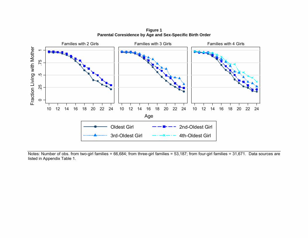
Figure 1 Parental Coresidence by Age and Sex-Specific Birth Order

0.2

5.5

.75

1

10 12 14 16 18 20 22 24 10 12 14 16 18 20 22 24 10 12 14 16 18 20 22 24

Families with 2 Girls Families with 3 Girls Families with 4 Girls

Oldest Girl 2nd-Oldest Girl

3rd-Oldest Girl 4th-Oldest Girl

Frac

tion

Livi

ng w

ith M

othe

r

Age

Notes: Number of obs. from two-girl families = 66,684; from three-girl families = 53,187; from four-girl families = 31,671. Data sources are listed in Appendix Table 1.

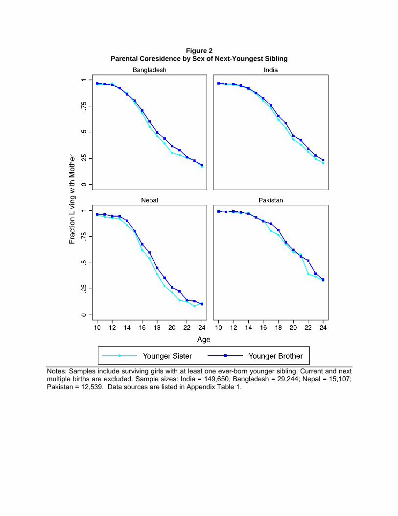
Figure 2 Parental Coresidence by Sex of Next-Youngest Sibling

Notes: Samples include surviving girls with at least one ever-born younger sibling. Current and next multiple births are excluded. Sample sizes: India = 149,650; Bangladesh = 29,244; Nepal = 15,107; Pakistan = 12,539. Data sources are listed in Appendix Table 1.

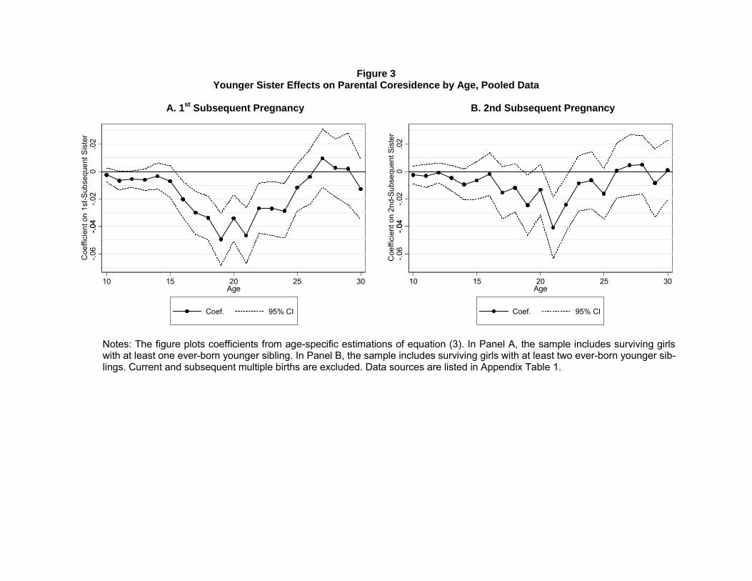
Figure 3 Younger Sister Effects on Parental Coresidence by Age, Pooled Data

A. 1st Subsequent Pregnancy B. 2nd Subsequent Pregnancy

0.0

2-.0

6-.0

4-.0

4-.0

2C

oeffi

cien

t on

1st-S

ubse

quen

t Sis

ter

10 15 20 25 30Age

Coef. 95% CI

0.0

2-.0

6-.0

4-.0

4-.0

2C

oeffi

cien

t on

2nd-

Sub

sequ

ent S

iste

r

10 15 20 25 30Age

Coef. 95% CI

Notes: The figure plots coefficients from age-specific estimations of equation (3). In Panel A, the sample includes surviving girls with at least one ever-born younger sibling. In Panel B, the sample includes surviving girls with at least two ever-born younger sib-lings. Current and subsequent multiple births are excluded. Data sources are listed in Appendix Table 1.

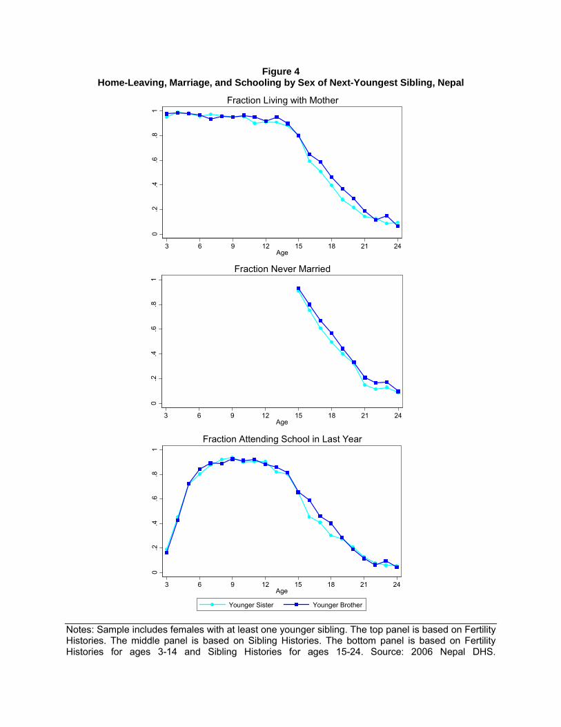
Figure 4 Home-Leaving, Marriage, and Schooling by Sex of Next-Youngest Sibling, Nepal

0.2

.4.6

.81

3 6 9 12 15 18 21 24Age

Fraction Living with Mother

0.2

.4.6

.81

3 6 9 12 15 18 21 24Age

Fraction Never Married

0.2

.4.6

.81

3 6 9 12 15 18 21 24Age

Younger Sister Younger Brother

Fraction Attending School in Last Year

Notes: Sample includes females with at least one younger sibling. The top panel is based on Fertility Histories. The middle panel is based on Sibling Histories. The bottom panel is based on Fertility Histories for ages 3-14 and Sibling Histories for ages 15-24. Source: 2006 Nepal DHS.

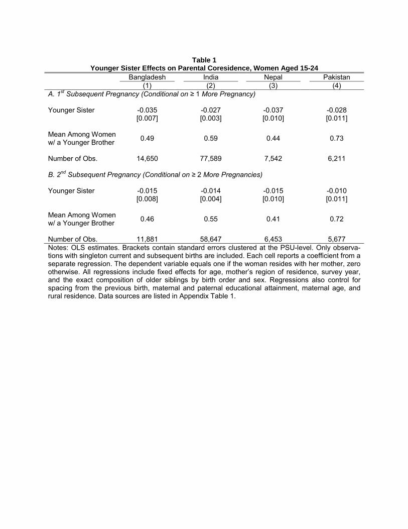
Table 1

Younger Sister Effects on Parental Coresidence, Women Aged 15-24 Bangladesh India Nepal Pakistan (1) (2) (3) (4) A. 1st Subsequent Pregnancy (Conditional on ≥ 1 More Pregnancy) Younger Sister -0.035 -0.027 -0.037 -0.028 [0.007] [0.003] [0.010] [0.011] Mean Among Women w/ a Younger Brother 0.49 0.59 0.44 0.73

Number of Obs. 14,650 77,589 7,542 6,211 B. 2nd Subsequent Pregnancy (Conditional on ≥ 2 More Pregnancies) Younger Sister -0.015 -0.014 -0.015 -0.010 [0.008] [0.004] [0.010] [0.011] Mean Among Women w/ a Younger Brother 0.46 0.55 0.41 0.72

Number of Obs. 11,881 58,647 6,453 5,677 Notes: OLS estimates. Brackets contain standard errors clustered at the PSU-level. Only observa-tions with singleton current and subsequent births are included. Each cell reports a coefficient from a separate regression. The dependent variable equals one if the woman resides with her mother, zero otherwise. All regressions include fixed effects for age, mother’s region of residence, survey year, and the exact composition of older siblings by birth order and sex. Regressions also control for spacing from the previous birth, maternal and paternal educational attainment, maternal age, and rural residence. Data sources are listed in Appendix Table 1.

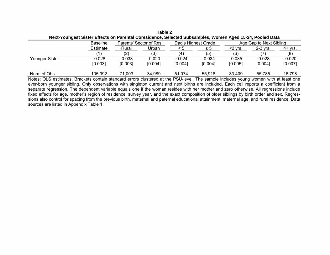
Table 2 Next-Youngest Sister Effects on Parental Coresidence, Selected Subsamples, Women Aged 15-24, Pooled Data

Baseline Parents’ Sector of Res. Dad’s Highest Grade Age Gap to Next Sibling Estimate Rural Urban < 5 ≥ 5 <2 yrs. 2-3 yrs. 4+ yrs. (1) (2) (3) (4) (5) (6) (7) (8) Younger Sister -0.028 -0.033 -0.020 -0.024 -0.034 -0.035 -0.028 -0.020 [0.003] [0.003] [0.004] [0.004] [0.004] [0.005] [0.004] [0.007] Num. of Obs. 105,992 71,003 34,989 51,074 55,918 33,409 55,785 16,798

Notes: OLS estimates. Brackets contain standard errors clustered at the PSU-level. The sample includes young women with at least one ever-born younger sibling. Only observations with singleton current and next births are included. Each cell reports a coefficient from a separate regression. The dependent variable equals one if the woman resides with her mother and zero otherwise. All regressions include fixed effects for age, mother’s region of residence, survey year, and the exact composition of older siblings by birth order and sex. Regres-sions also control for spacing from the previous birth, maternal and paternal educational attainment, maternal age, and rural residence. Data sources are listed in Appendix Table 1.

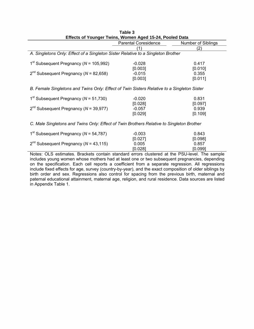
Table 3 Effects of Younger Twins, Women Aged 15-24, Pooled Data

Parental Coresidence Number of Siblings (1) (2) A. Singletons Only: Effect of a Singleton Sister Relative to a Singleton Brother 1st Subsequent Pregnancy (N = 105,992) -0.028 0.417 [0.003] [0.010] 2nd Subsequent Pregnancy (N = 82,658) -0.015 0.355 [0.003] [0.011] B. Female Singletons and Twins Only: Effect of Twin Sisters Relative to a Singleton Sister 1st Subsequent Pregnancy (N = 51,730) -0.020 0.831 [0.028] [0.097] 2nd Subsequent Pregnancy (N = 39,977) -0.057 0.939 [0.029] [0.109] C. Male Singletons and Twins Only: Effect of Twin Brothers Relative to Singleton Brother 1st Subsequent Pregnancy (N = 54,787) -0.003 0.843 [0.027] [0.098] 2nd Subsequent Pregnancy (N = 43,115) 0.005 0.857 [0.028] [0.099] Notes: OLS estimates. Brackets contain standard errors clustered at the PSU-level. The sample includes young women whose mothers had at least one or two subsequent pregnancies, depending on the specification. Each cell reports a coefficient from a separate regression. All regressions include fixed effects for age, survey (country-by-year), and the exact composition of older siblings by birth order and sex. Regressions also control for spacing from the previous birth, maternal and paternal educational attainment, maternal age, religion, and rural residence. Data sources are listed in Appendix Table 1.

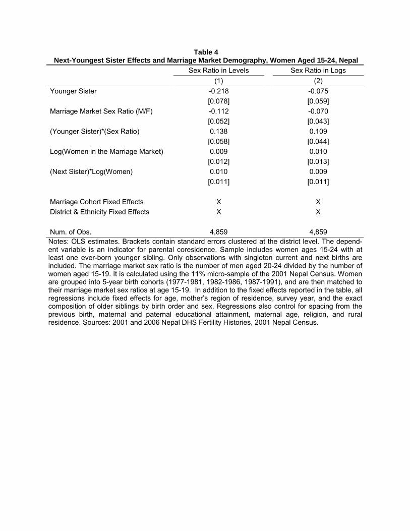
Table 4 Next-Youngest Sister Effects and Marriage Market Demography, Women Aged 15-24, Nepal

Sex Ratio in Levels Sex Ratio in Logs

(1) (2) Younger Sister -0.218 -0.075

[0.078] [0.059] Marriage Market Sex Ratio (M/F) -0.112 -0.070

[0.052] [0.043] (Younger Sister)*(Sex Ratio) 0.138 0.109

[0.058] [0.044] Log(Women in the Marriage Market) 0.009 0.010

[0.012] [0.013] (Next Sister)*Log(Women) 0.010 0.009

[0.011] [0.011]

Marriage Cohort Fixed Effects X X District & Ethnicity Fixed Effects X X

Num. of Obs. 4,859 4,859 Notes: OLS estimates. Brackets contain standard errors clustered at the district level. The depend-ent variable is an indicator for parental coresidence. Sample includes women ages 15-24 with at least one ever-born younger sibling. Only observations with singleton current and next births are included. The marriage market sex ratio is the number of men aged 20-24 divided by the number of women aged 15-19. It is calculated using the 11% micro-sample of the 2001 Nepal Census. Women are grouped into 5-year birth cohorts (1977-1981, 1982-1986, 1987-1991), and are then matched to their marriage market sex ratios at age 15-19. In addition to the fixed effects reported in the table, all regressions include fixed effects for age, mother’s region of residence, survey year, and the exact composition of older siblings by birth order and sex. Regressions also control for spacing from the previous birth, maternal and paternal educational attainment, maternal age, religion, and rural residence. Sources: 2001 and 2006 Nepal DHS Fertility Histories, 2001 Nepal Census.

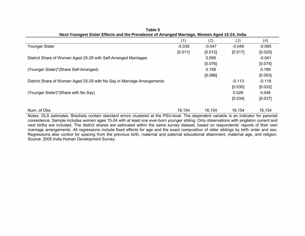
Table 5 Next-Youngest Sister Effects and the Prevalence of Arranged Marriage, Women Aged 15-24, India

(1) (2) (3) (4) Younger Sister -0.039 -0.047 -0.049 -0.065

[0.011] [0.012] [0.017] [0.020] District Share of Women Aged 25-29 with Self-Arranged Marriages 0.056 -0.041 [0.076] [0.074] (Younger Sister)*(Share Self-Arranged) 0.158 0.189

[0.086] [0.093] District Share of Women Aged 25-29 with No Say in Marriage Arrangements -0.113 -0.118 [0.030] [0.032] (Younger Sister)*(Share with No Say) 0.028 0.048 [0.034] [0.037]

Num. of Obs. 16,154 16,154 16,154 16,154 Notes: OLS estimates. Brackets contain standard errors clustered at the PSU-level. The dependent variable is an indicator for parental coresidence. Sample includes women ages 15-24 with at least one ever-born younger sibling. Only observations with singleton current and next births are included. The district shares are estimated within the same survey dataset, based on respondents’ reports of their own marriage arrangements. All regressions include fixed effects for age and the exact composition of older siblings by birth order and sex. Regressions also control for spacing from the previous birth, maternal and paternal educational attainment, maternal age, and religion. Source: 2005 India Human Development Survey.

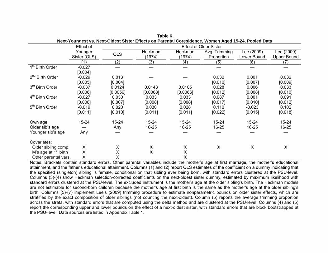
Table 6 Next-Youngest vs. Next-Oldest Sister Effects on Parental Coresidence, Women Aged 15-24, Pooled Data

Effect of Effect of Older Sister

Younger Sister (OLS) OLS Heckman

(1974) Heckman (1974) Avg. Trimming

Proportion Lee (2009) Lower Bound Lee (2009)

Upper Bound (1) (2) (3) (4) (5) (6) (7) 1st Birth Order -0.027 — — — — — — [0.004] 2nd Birth Order -0.029 0.013 — — 0.032 0.001 0.032 [0.005] [0.004] [0.010] [0.007] [0.009] 3rd Birth Order -0.037 0.0124 0.0143 0.0105 0.028 0.006 0.033 [0.006] [0.0056] [0.0068] [0.0066] [0.012] [0.008] [0.010] 4th Birth Order -0.027 0.030 0.033 0.033 0.087 0.001 0.091 [0.008] [0.007] [0.008] [0.008] [0.017] [0.010] [0.012] 5th Birth Order -0.019 0.020 0.030 0.028 0.110 -0.023 0.102 [0.011] [0.010] [0.011] [0.011] [0.022] [0.015] [0.018] Own age 15-24 15-24 15-24 15-24 15-24 15-24 15-24 Older sib’s age — Any 16-25 16-25 16-25 16-25 16-25 Younger sib’s age Any — — — — — — Covariates: Older sibling comp. X X X X X X X M’s age at 1st birth X X X X Other parental vars. X X X Notes: Brackets contain standard errors. Other parental variables include the mother’s age at first marriage, the mother’s educational attainment, and the father’s educational attainment. Columns (1) and (2) report OLS estimates of the coefficient on a dummy indicating that the specified (singleton) sibling is female, conditional on that sibling ever being born, with standard errors clustered at the PSU-level. Columns (3)-(4) show Heckman selection-corrected coefficients on the next-oldest sister dummy, estimated by maximum likelihood with standard errors clustered at the PSU-level. The excluded instrument is the mother’s age at the older sibling’s birth. The Heckman models are not estimable for second-born children because the mother's age at first birth is the same as the mother's age at the older sibling's birth. Columns (5)-(7) implement Lee’s (2009) trimming procedure to estimate nonparametric bounds on older sister effects, which are stratified by the exact composition of older siblings (not counting the next-oldest). Column (5) reports the average trimming proportion across the strata, with standard errors that are computed using the delta method and are clustered at the PSU-level. Columns (4) and (5) report the corresponding upper and lower bounds on the effect of a next-oldest sister, with standard errors that are block bootstrapped at the PSU-level. Data sources are listed in Appendix Table 1.

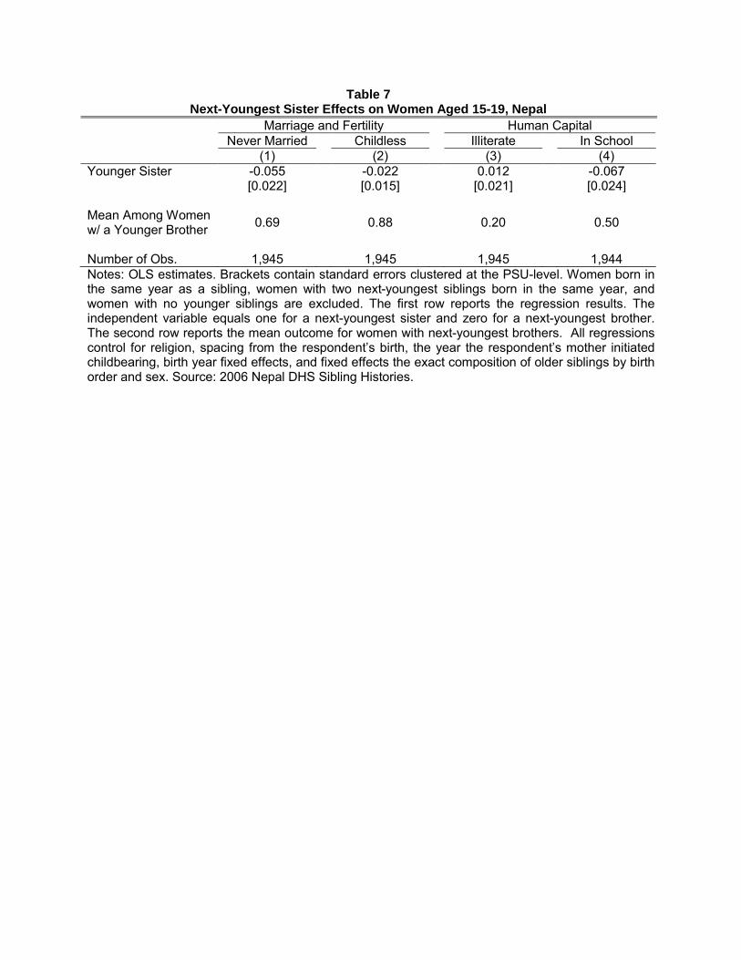
Table 7 Next-Youngest Sister Effects on Women Aged 15-19, Nepal

Marriage and Fertility Human Capital Never Married Childless Illiterate In School (1) (2) (3) (4) Younger Sister -0.055 -0.022 0.012 -0.067 [0.022] [0.015] [0.021] [0.024] Mean Among Women w/ a Younger Brother 0.69 0.88 0.20 0.50

Number of Obs. 1,945 1,945 1,945 1,944 Notes: OLS estimates. Brackets contain standard errors clustered at the PSU-level. Women born in the same year as a sibling, women with two next-youngest siblings born in the same year, and women with no younger siblings are excluded. The first row reports the regression results. The independent variable equals one for a next-youngest sister and zero for a next-youngest brother. The second row reports the mean outcome for women with next-youngest brothers. All regressions control for religion, spacing from the respondent’s birth, the year the respondent’s mother initiated childbearing, birth year fixed effects, and fixed effects the exact composition of older siblings by birth order and sex. Source: 2006 Nepal DHS Sibling Histories.

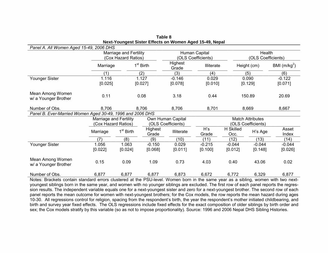
Table 8

Next-Youngest Sister Effects on Women Aged 15-49, Nepal Panel A. All Women Aged 15-49, 2006 DHS

Marriage and Fertility (Cox Hazard Ratios) Human Capital

(OLS Coefficients) Health (OLS Coefficients)

Marriage 1st Birth Highest Grade Illiterate Height (cm) BMI (m/kg2)

(1) (2) (3) (4) (5) (6) Younger Sister 1.116 1.127 -0.146 0.029 0.090 -0.122 [0.025] [0.027] [0.078] [0.010] [0.129] [0.071] Mean Among Women w/ a Younger Brother 0.11 0.08 3.18 0.44 150.89 20.69

Number of Obs. 8,706 8,706 8,706 8,701 8,669 8,667 Panel B. Ever-Married Women Aged 30-49, 1996 and 2006 DHS

Marriage and Fertility (Cox Hazard Ratios) Own Human Capital

(OLS Coefficients) Match Attributes (OLS Coefficients)

Marriage 1st Birth Highest Grade Illiterate H’s

Grade H Skilled Occ. H’s Age Asset

Index (7) (8) (9) (10) (11) (12) (13) (14) Younger Sister 1.056 1.063 -0.150 0.029 -0.215 -0.044 -0.044 -0.044 [0.022] [0.024] [0.068] [0.011] [0.100] [0.012] [0.148] [0.026] Mean Among Women w/ a Younger Brother 0.15 0.09 1.09 0.73 4.03 0.40 43.06 0.02

Number of Obs. 6,877 6,877 6,877 6,873 6,672 6,772 6,329 6,877 Notes: Brackets contain standard errors clustered at the PSU-level. Women born in the same year as a sibling, women with two next-youngest siblings born in the same year, and women with no younger siblings are excluded. The first row of each panel reports the regres-sion results. The independent variable equals one for a next-youngest sister and zero for a next-youngest brother. The second row of each panel reports the mean outcome for women with next-youngest brothers; for the Cox models, the row reports the mean hazard during ages 10-30. All regressions control for religion, spacing from the respondent’s birth, the year the respondent’s mother initiated childbearing, and birth and survey year fixed effects. The OLS regressions include fixed effects for the exact composition of older siblings by birth order and sex; the Cox models stratify by this variable (so as not to impose proportionality). Source: 1996 and 2006 Nepal DHS Sibling Histories.

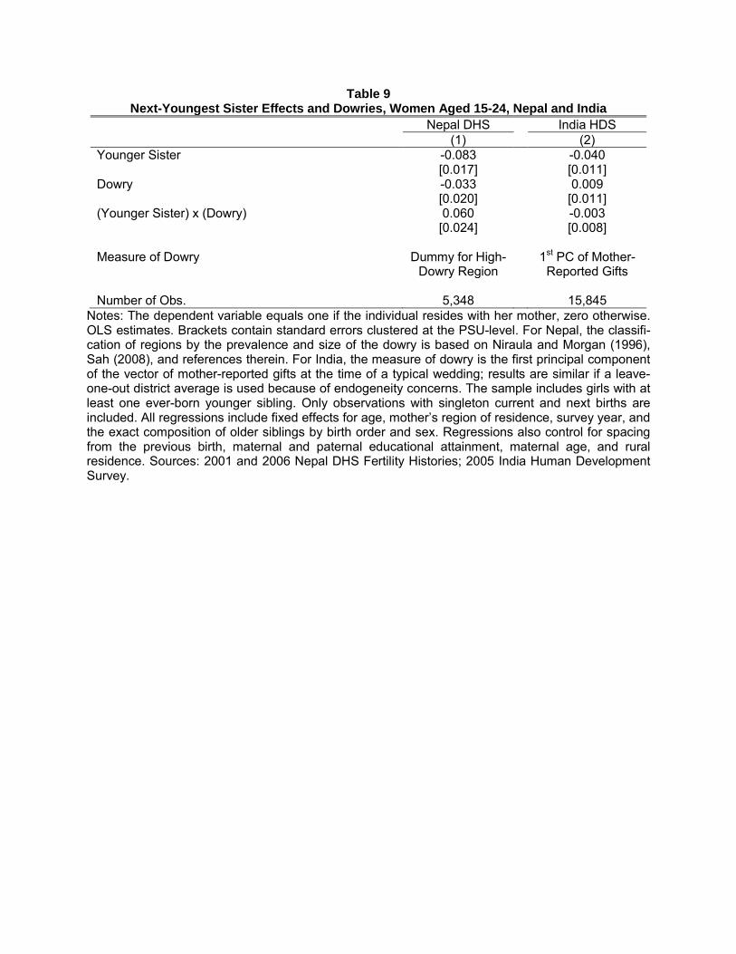
Table 9 Next-Youngest Sister Effects and Dowries, Women Aged 15-24, Nepal and India

Nepal DHS India HDS (1) (2) Younger Sister -0.083 -0.040 [0.017] [0.011] Dowry -0.033 0.009 [0.020] [0.011] (Younger Sister) x (Dowry) 0.060 -0.003 [0.024] [0.008] Measure of Dowry Dummy for High- 1st PC of Mother- Dowry Region Reported Gifts Number of Obs. 5,348 15,845

Notes: The dependent variable equals one if the individual resides with her mother, zero otherwise. OLS estimates. Brackets contain standard errors clustered at the PSU-level. For Nepal, the classifi-cation of regions by the prevalence and size of the dowry is based on Niraula and Morgan (1996), Sah (2008), and references therein. For India, the measure of dowry is the first principal component of the vector of mother-reported gifts at the time of a typical wedding; results are similar if a leave-one-out district average is used because of endogeneity concerns. The sample includes girls with at least one ever-born younger sibling. Only observations with singleton current and next births are included. All regressions include fixed effects for age, mother’s region of residence, survey year, and the exact composition of older siblings by birth order and sex. Regressions also control for spacing from the previous birth, maternal and paternal educational attainment, maternal age, and rural residence. Sources: 2001 and 2006 Nepal DHS Fertility Histories; 2005 India Human Development Survey.

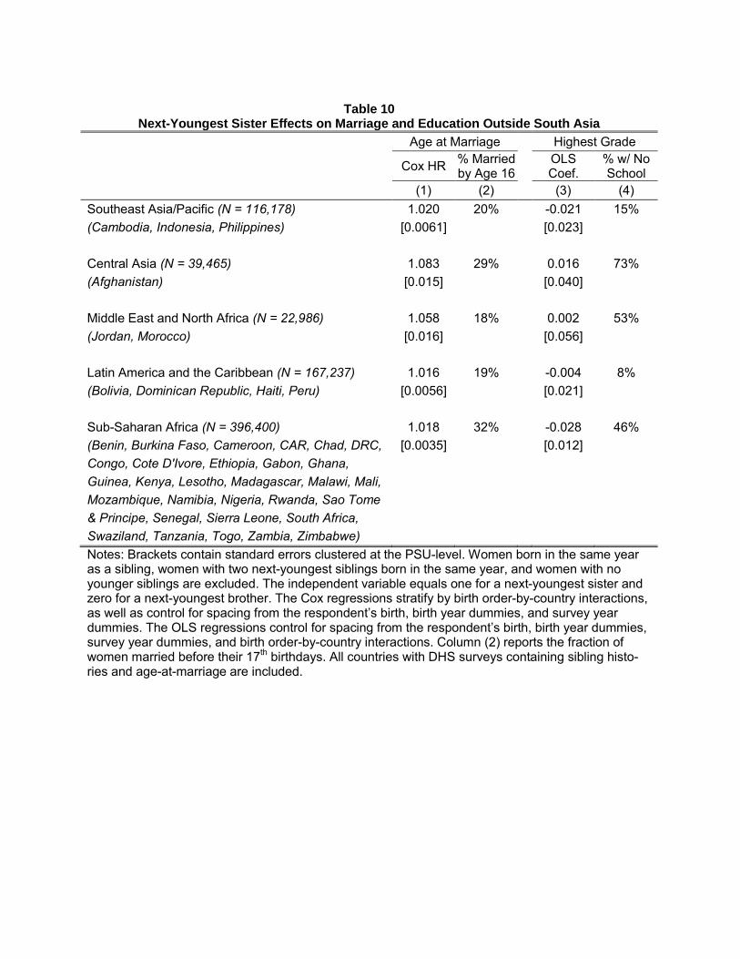
Table 10

Next-Youngest Sister Effects on Marriage and Education Outside South Asia Age at Marriage Highest Grade

Cox HR % Married by Age 16 OLS

Coef. % w/ No School

(1) (2) (3) (4) Southeast Asia/Pacific (N = 116,178) 1.020 20% -0.021 15% (Cambodia, Indonesia, Philippines) [0.0061] [0.023] Central Asia (N = 39,465) 1.083 29% 0.016 73% (Afghanistan) [0.015] [0.040] Middle East and North Africa (N = 22,986) 1.058 18% 0.002 53% (Jordan, Morocco) [0.016] [0.056] Latin America and the Caribbean (N = 167,237) 1.016 19% -0.004 8% (Bolivia, Dominican Republic, Haiti, Peru) [0.0056] [0.021] Sub-Saharan Africa (N = 396,400) 1.018 32% -0.028 46% (Benin, Burkina Faso, Cameroon, CAR, Chad, DRC, [0.0035] [0.012] Congo, Cote D'Ivore, Ethiopia, Gabon, Ghana, Guinea, Kenya, Lesotho, Madagascar, Malawi, Mali, Mozambique, Namibia, Nigeria, Rwanda, Sao Tome & Principe, Senegal, Sierra Leone, South Africa, Swaziland, Tanzania, Togo, Zambia, Zimbabwe) Notes: Brackets contain standard errors clustered at the PSU-level. Women born in the same year as a sibling, women with two next-youngest siblings born in the same year, and women with no younger siblings are excluded. The independent variable equals one for a next-youngest sister and zero for a next-youngest brother. The Cox regressions stratify by birth order-by-country interactions, as well as control for spacing from the respondent’s birth, birth year dummies, and survey year dummies. The OLS regressions control for spacing from the respondent’s birth, birth year dummies, survey year dummies, and birth order-by-country interactions. Column (2) reports the fraction of women married before their 17th birthdays. All countries with DHS surveys containing sibling histo-ries and age-at-marriage are included.

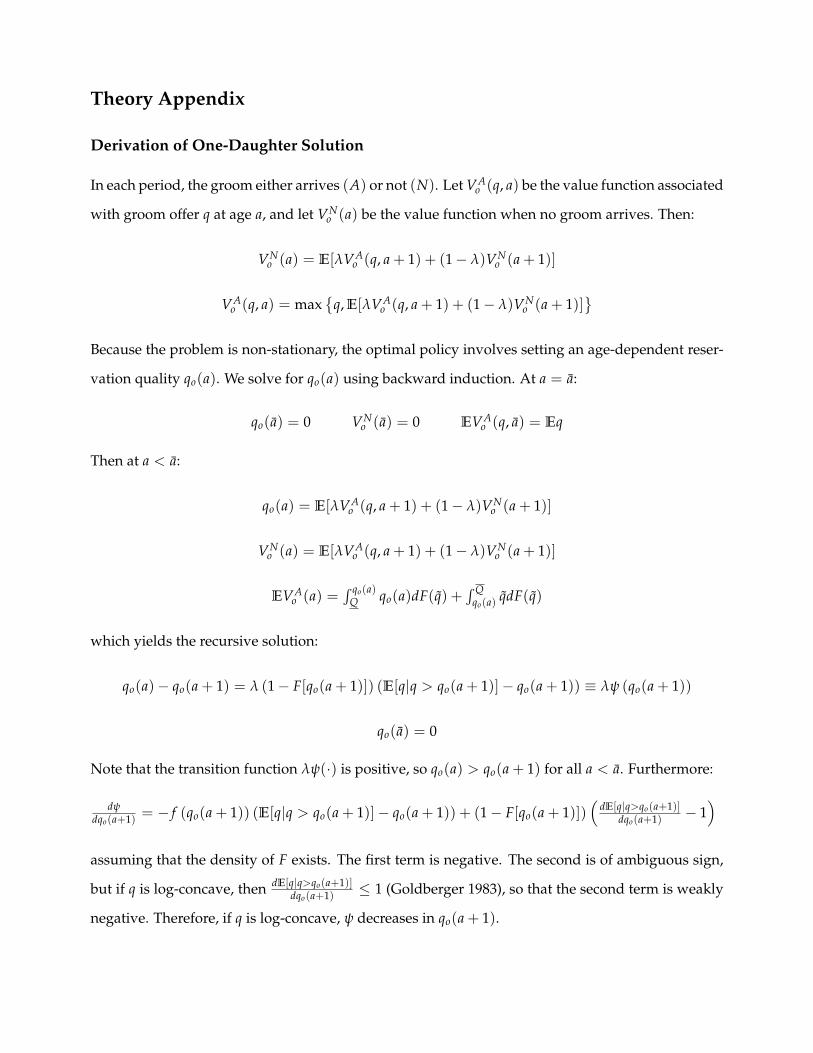
Theory Appendix

Derivation of One-Daughter Solution

In each period, the groom either arrives (A) or not (N). Let VAo (q, a) be the value function associated

with groom offer q at age a, and let VNo (a) be the value function when no groom arrives. Then:

VNo (a) = E[λVA

o (q, a + 1) + (1− λ)VNo (a + 1)]

VAo (q, a) = max

{q, E[λVA

o (q, a + 1) + (1− λ)VNo (a + 1)]

}Because the problem is non-stationary, the optimal policy involves setting an age-dependent reser-

vation quality qo(a). We solve for qo(a) using backward induction. At a = a:

qo(a) = 0 VNo (a) = 0 EVA

o (q, a) = Eq

Then at a < a:

qo(a) = E[λVAo (q, a + 1) + (1− λ)VN

o (a + 1)]

VNo (a) = E[λVA

o (q, a + 1) + (1− λ)VNo (a + 1)]

EVAo (a) =

´ qo(a)Q qo(a)dF(q) +

´ Qqo(a) qdF(q)

which yields the recursive solution:

qo(a)− qo(a + 1) = λ (1− F[qo(a + 1)]) (E[q|q > qo(a + 1)]− qo(a + 1)) ≡ λψ (qo(a + 1))

qo(a) = 0

Note that the transition function λψ(·) is positive, so qo(a) > qo(a + 1) for all a < a. Furthermore:

dψdqo(a+1) = − f (qo(a + 1)) (E[q|q > qo(a + 1)]− qo(a + 1)) + (1− F[qo(a + 1)])

(dE[q|q>qo(a+1)]

dqo(a+1) − 1)

assuming that the density of F exists. The first term is negative. The second is of ambiguous sign,

but if q is log-concave, then dE[q|q>qo(a+1)]dqo(a+1) ≤ 1 (Goldberger 1983), so that the second term is weakly

negative. Therefore, if q is log-concave, ψ decreases in qo(a + 1).

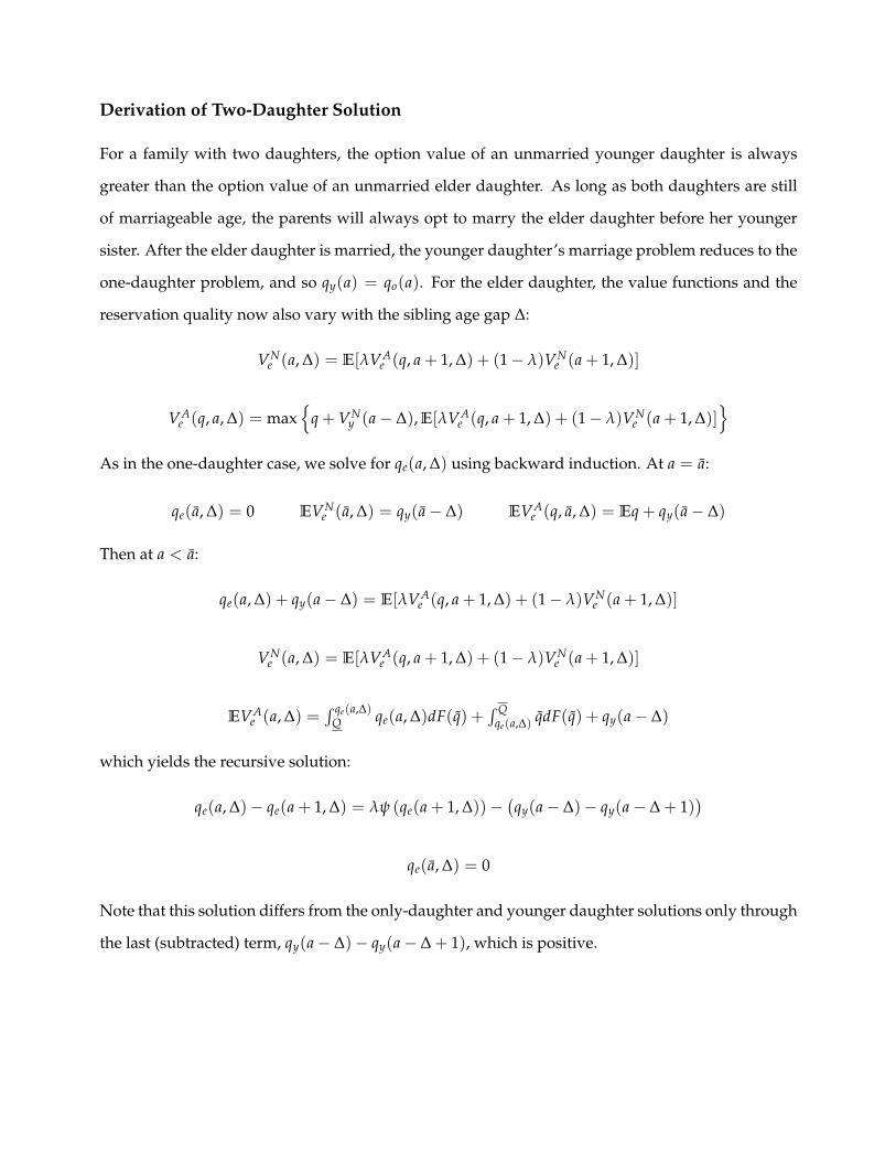
Derivation of Two-Daughter Solution

For a family with two daughters, the option value of an unmarried younger daughter is always

greater than the option value of an unmarried elder daughter. As long as both daughters are still

of marriageable age, the parents will always opt to marry the elder daughter before her younger

sister. After the elder daughter is married, the younger daughter’s marriage problem reduces to the

one-daughter problem, and so qy(a) = qo(a). For the elder daughter, the value functions and the

reservation quality now also vary with the sibling age gap ∆:

VNe (a, ∆) = E[λVA

e (q, a + 1, ∆) + (1− λ)VNe (a + 1, ∆)]

VAe (q, a, ∆) = max

{q + VN

y (a− ∆), E[λVAe (q, a + 1, ∆) + (1− λ)VN

e (a + 1, ∆)]}

As in the one-daughter case, we solve for qe(a, ∆) using backward induction. At a = a:

qe(a, ∆) = 0 EVNe (a, ∆) = qy(a− ∆) EVA

e (q, a, ∆) = Eq + qy(a− ∆)

Then at a < a:

qe(a, ∆) + qy(a− ∆) = E[λVAe (q, a + 1, ∆) + (1− λ)VN

e (a + 1, ∆)]

VNe (a, ∆) = E[λVA

e (q, a + 1, ∆) + (1− λ)VNe (a + 1, ∆)]

EVAe (a, ∆) =

´ qe(a,∆)Q qe(a, ∆)dF(q) +

´ Qqe(a,∆) qdF(q) + qy(a− ∆)

which yields the recursive solution:

qe(a, ∆)− qe(a + 1, ∆) = λψ (qe(a + 1, ∆))−(qy(a− ∆)− qy(a− ∆ + 1)

)qe(a, ∆) = 0

Note that this solution differs from the only-daughter and younger daughter solutions only through

the last (subtracted) term, qy(a− ∆)− qy(a− ∆ + 1), which is positive.

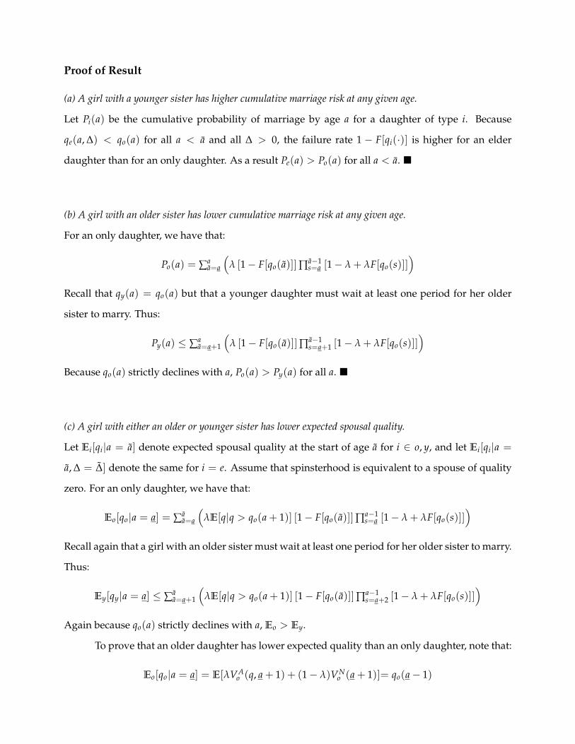
Proof of Result

(a) A girl with a younger sister has higher cumulative marriage risk at any given age.

Let Pi(a) be the cumulative probability of marriage by age a for a daughter of type i. Because

qe(a, ∆) < qo(a) for all a < a and all ∆ > 0, the failure rate 1 − F[qi(·)] is higher for an elder

daughter than for an only daughter. As a result Pe(a) > Po(a) for all a < a. �

(b) A girl with an older sister has lower cumulative marriage risk at any given age.

For an only daughter, we have that:

Po(a) = ∑aa=a

(λ [1− F[qo(a)]]∏a−1

s=a [1− λ + λF[qo(s)]])

Recall that qy(a) = qo(a) but that a younger daughter must wait at least one period for her older

sister to marry. Thus:

Py(a) ≤ ∑aa=a+1

(λ [1− F[qo(a)]]∏a−1

s=a+1 [1− λ + λF[qo(s)]])

Because qo(a) strictly declines with a, Po(a) > Py(a) for all a. �

(c) A girl with either an older or younger sister has lower expected spousal quality.

Let Ei[qi|a = a] denote expected spousal quality at the start of age a for i ∈ o, y, and let Ei[qi|a =

a, ∆ = ∆] denote the same for i = e. Assume that spinsterhood is equivalent to a spouse of quality

zero. For an only daughter, we have that:

Eo[qo|a = a] = ∑aa=a

(λE[q|q > qo(a + 1)] [1− F[qo(a)]]∏a−1

s=a [1− λ + λF[qo(s)]])

Recall again that a girl with an older sister must wait at least one period for her older sister to marry.

Thus:

Ey[qy|a = a] ≤ ∑aa=a+1

(λE[q|q > qo(a + 1)] [1− F[qo(a)]]∏a−1

s=a+2 [1− λ + λF[qo(s)]])

Again because qo(a) strictly declines with a, Eo > Ey.

To prove that an older daughter has lower expected quality than an only daughter, note that:

Eo[qo|a = a] = E[λVAo (q, a + 1) + (1− λ)VN

o (a + 1)]= qo(a− 1)

For an elder daughter:

Ee[qe + VNo (a + 1)|a = a, ∆ = ∆] = E[λVA

e (q, a + 1, ∆) + (1− λ)VNo (a + 1, ∆)]

= qe(a− 1, ∆) + qy(a− 1− ∆)

And thus:

Ee[qe|a = a, ∆ = ∆] = qe(a− 1, ∆)

Because qe(a− 1, ∆) < qo(a− 1) for all ∆ > 0, we have that Eo > Ee. �

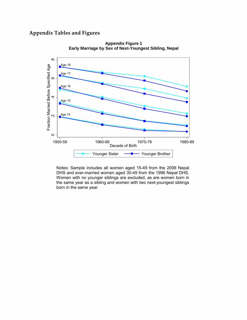
Appendix Tables and Figures

Appendix Figure 1 Early Marriage by Sex of Next-Youngest Sibling, Nepal

Age 14

Age 18

Age 17

Age 16

Age 15

0.2

.4.6

.8Fr

actio

n M

arrie

d B

efor

e S

peci

fied

Age

1950-59 1960-69 1970-79 1980-89Decade of Birth

Younger Sister Younger Brother

Notes: Sample includes all women aged 15-49 from the 2006 Nepal DHS and ever-married women aged 30-49 from the 1996 Nepal DHS. Women with no younger siblings are excluded, as are women born in the same year as a sibling and women with two next-youngest siblings born in the same year.

Appendix Table 1 Demographic and Health Surveys Used in the Fertility History Analysis

Country: Survey year:

Bangladesh

1993-94, 1996-97, 1999-2000, 2004, 2007

India

1992-93, 1998-99, 2005-06

Nepal

1996, 2001, 2006

Pakistan 1990-91, 2006-07

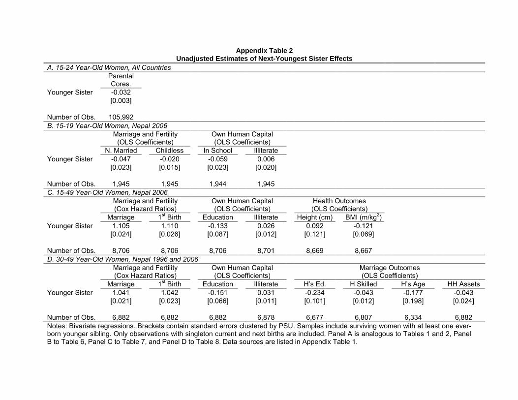
Appendix Table 2 Unadjusted Estimates of Next-Youngest Sister Effects

A. 15-24 Year-Old Women, All Countries

Parental Cores.

Younger Sister -0.032 [0.003] Number of Obs. 105,992 B. 15-19 Year-Old Women, Nepal 2006

Marriage and Fertility (OLS Coefficients) Own Human Capital

(OLS Coefficients)

N. Married Childless In School Illiterate Younger Sister -0.047 -0.020 -0.059 0.006 [0.023] [0.015] [0.023] [0.020] Number of Obs. 1,945 1,945 1,944 1,945 C. 15-49 Year-Old Women, Nepal 2006

Marriage and Fertility (Cox Hazard Ratios) Own Human Capital

(OLS Coefficients) Health Outcomes (OLS Coefficients)

Marriage 1st Birth Education Illiterate Height (cm) BMI (m/kg2) Younger Sister 1.105 1.110 -0.133 0.026 0.092 -0.121 [0.024] [0.026] [0.087] [0.012] [0.121] [0.069] Number of Obs. 8,706 8,706 8,706 8,701 8,669 8,667 D. 30-49 Year-Old Women, Nepal 1996 and 2006

Marriage and Fertility (Cox Hazard Ratios) Own Human Capital

(OLS Coefficients) Marriage Outcomes (OLS Coefficients)

Marriage 1st Birth Education Illiterate H’s Ed. H Skilled H’s Age HH Assets Younger Sister 1.041 1.042 -0.151 0.031 -0.234 -0.043 -0.177 -0.043 [0.021] [0.023] [0.066] [0.011] [0.101] [0.012] [0.198] [0.024] Number of Obs. 6,882 6,882 6,882 6,878 6,677 6,807 6,334 6,882 Notes: Bivariate regressions. Brackets contain standard errors clustered by PSU. Samples include surviving women with at least one ever-born younger sibling. Only observations with singleton current and next births are included. Panel A is analogous to Tables 1 and 2, Panel B to Table 6, Panel C to Table 7, and Panel D to Table 8. Data sources are listed in Appendix Table 1.

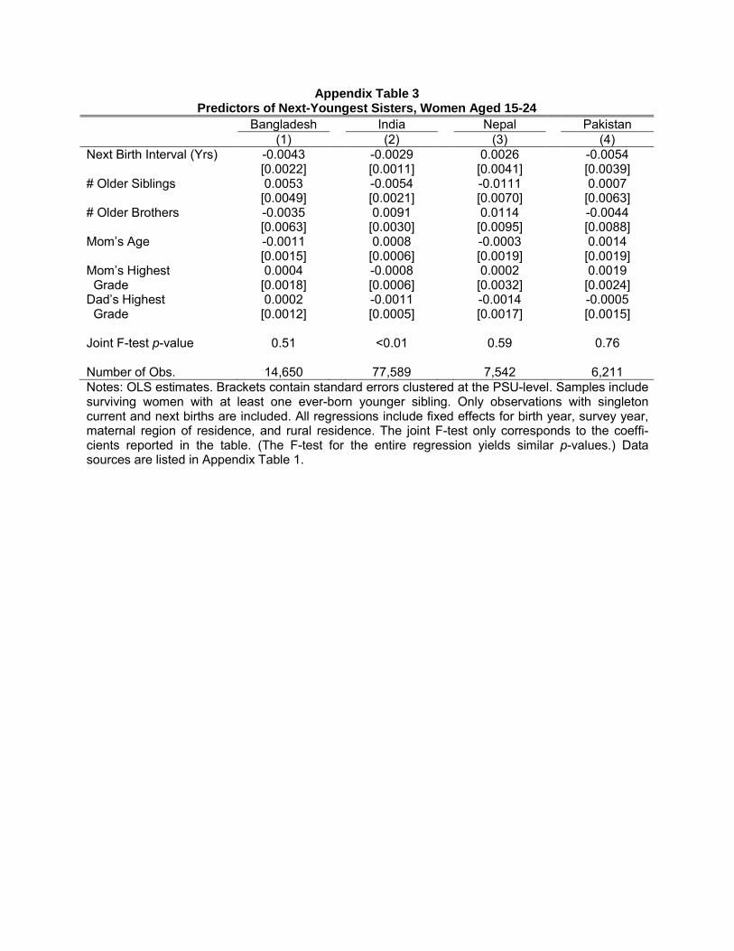
Appendix Table 3 Predictors of Next-Youngest Sisters, Women Aged 15-24

Bangladesh India Nepal Pakistan (1) (2) (3) (4) Next Birth Interval (Yrs) -0.0043 -0.0029 0.0026 -0.0054 [0.0022] [0.0011] [0.0041] [0.0039] # Older Siblings 0.0053 -0.0054 -0.0111 0.0007 [0.0049] [0.0021] [0.0070] [0.0063] # Older Brothers -0.0035 0.0091 0.0114 -0.0044 [0.0063] [0.0030] [0.0095] [0.0088] Mom’s Age -0.0011 0.0008 -0.0003 0.0014 [0.0015] [0.0006] [0.0019] [0.0019] Mom’s Highest 0.0004 -0.0008 0.0002 0.0019 Grade [0.0018] [0.0006] [0.0032] [0.0024] Dad’s Highest 0.0002 -0.0011 -0.0014 -0.0005 Grade [0.0012] [0.0005] [0.0017] [0.0015] Joint F-test p-value 0.51 <0.01 0.59 0.76 Number of Obs. 14,650 77,589 7,542 6,211 Notes: OLS estimates. Brackets contain standard errors clustered at the PSU-level. Samples include surviving women with at least one ever-born younger sibling. Only observations with singleton current and next births are included. All regressions include fixed effects for birth year, survey year, maternal region of residence, and rural residence. The joint F-test only corresponds to the coeffi-cients reported in the table. (The F-test for the entire regression yields similar p-values.) Data sources are listed in Appendix Table 1.

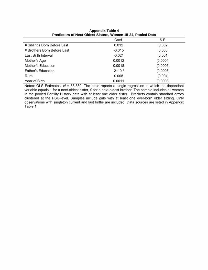
Appendix Table 4

Predictors of Next-Oldest Sisters, Women 15-24, Pooled Data

Coef. S.E. # Siblings Born Before Last 0.012 [0.002] # Brothers Born Before Last -0.015 [0.003] Last Birth Interval -0.021 [0.001] Mother's Age 0.0012 [0.0004] Mother's Education 0.0018 [0.0006] Father's Education -2∗10⁻⁵ [0.0005] Rural 0.005 [0.004] Year of Birth 0.0011 [0.0003] Notes: OLS Estimates. N = 83,330. The table reports a single regression in which the dependent variable equals 1 for a next-oldest sister, 0 for a next-oldest brother. The sample includes all women in the pooled Fertility History data with at least one older sister. Brackets contain standard errors clustered at the PSU-level. Samples include girls with at least one ever-born older sibling. Only observations with singleton current and last births are included. Data sources are listed in Appendix Table 1.

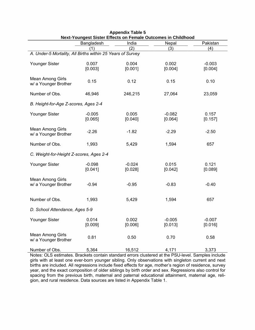
Appendix Table 5 Next-Youngest Sister Effects on Female Outcomes in Childhood

Bangladesh India Nepal Pakistan (1) (2) (3) (4) A. Under-5 Mortality, All Births within 25 Years of Survey Younger Sister 0.007 0.004 0.002 -0.003 [0.003] [0.001] [0.004] [0.004] Mean Among Girls w/ a Younger Brother

0.15 0.12 0.15 0.10

Number of Obs. 46,946 246,215 27,064 23,059 B. Height-for-Age Z-scores, Ages 2-4 Younger Sister -0.005 0.005 -0.082 0.157 [0.065] [0.040] [0.064] [0.157] Mean Among Girls w/ a Younger Brother

-2.26 -1.82 -2.29 -2.50

Number of Obs. 1,993 5,429 1,594 657 C. Weight-for-Height Z-scores, Ages 2-4 Younger Sister -0.098 -0.024 0.015 0.121 [0.041] [0.028] [0.042] [0.089] Mean Among Girls w/ a Younger Brother

-0.94 -0.95 -0.83 -0.40

Number of Obs. 1,993 5,429 1,594 657 D. School Attendance, Ages 5-9 Younger Sister 0.014 0.002 -0.005 -0.007 [0.009] [0.006] [0.013] [0.016] Mean Among Girls w/ a Younger Brother

0.81 0.50 0.70 0.58

Number of Obs. 5,364 16,512 4,171 3,373 Notes: OLS estimates. Brackets contain standard errors clustered at the PSU-level. Samples include girls with at least one ever-born younger sibling. Only observations with singleton current and next births are included. All regressions include fixed effects for age, mother’s region of residence, survey year, and the exact composition of older siblings by birth order and sex. Regressions also control for spacing from the previous birth, maternal and paternal educational attainment, maternal age, reli-gion, and rural residence. Data sources are listed in Appendix Table 1.