Markov Random Field Models for High-Dimensional Parameters in Simulations of Fluid Flow in Porous Media

Markov Random Field Models for High-Dimensional Parameters in

Simulations of Fluid Flow in Porous Media

Herbert Lee, David Higdon, Zhuoxin Bi, Marco Ferreira, and Mike West, Duke University

November 22, 2000

Abstract

We give an approach for using flow information from a system of wells to characterize hydrologic

properties of an aquifer. In particular, we consider experiments where an impulse of tracer fluid is injected

along with the water at the input wells and its concentration is recorded over time at the uptake wells.

We focus on characterizing the spatially varying permeability field which is a key attribute of the aquifer

for determining flow paths and rates for a given flow experiment. As is standard for estimation from such

flow data, we make use of complicated subsurface flow code which simulates the fluid flow through the

aquifer for a particular well configuration and aquifer specification, which includes the permeability field

over a grid. This ill-posed problem requires that some regularity be imposed on the permeability field.

Typically this is accomplished by specifying a stationary Gaussian process model for the permeability

field. Here we use an intrinsically stationary Markov random field which compares favorably and offers

some additional flexibility and computational advantages. Our interest in quantifying uncertainty leads

us to take a Bayesian approach, using Markov chain Monte Carlo for exploring the high-dimensional

posterior distribution. We demonstrate our approach with several examples.

Key Words: Bayesian Statistics, Markov Chain Monte Carlo, Computer Model, Inverse Problem

1 Introduction

The problem of studying the flow of liquids, particularly groundwater, through an aquifer is an important

engineering problem with applications in contaminant cleanup and oil production. The engineering commu-

nity has a good handle on the solution to the forward problem, i.e. determining the flow of water when the

physical characteristics of the aquifer (such as permeability and porosity) are known. A problem of interest

to statisticians and engineers alike is the inverse problem, that of inferring the permeability of the aquifer

from flow data. It is this inverse problem that we address in this paper. A review of the inverse problem

can be found in Yeh (1986).

Applications of this work include contaminant cleanup and oil production. In the case of environmental

cleanup, permeability estimates are critical to two phases: in identifying the likely location and distribution

of the contaminant, and for designing the remediation operation (James et al., 1997; Jin et al., 1995). The

1

contaminants can be extracted in situ by pumping water containing a surfactant through the affected area.

The water can then be treated to remove the contaminants, a much quicker and less costly operation than

excavating and treating the soil itself. However, effective use of this procedure requires good knowledge of

the permeabilities in both phases and so the inverse problem is of utmost importance. In oil production,

secondary and tertiary recovery requires increasing pressure within the oil field to cause the oil to rise to the

surface. Effective recovery procedures rely on good permeability estimates, as one must be able to identify

high permeability channels and low permeability barriers (Xue and Datta-Gupta, 2000).

Most previous studies of the inverse problem have focused on finding a single estimate of the perme-

abilities, without getting a good measure of uncertainty in this estimate. In fact, there is typically a large

amount of variability in permeability realizations consistent with a set of flow data because the number of

parameters in the permeability field is large relative to the number of available data points. Thus we find

the Bayesian approach to be compelling, both because it naturally provides an estimate of the variability,

as well as allowing us to build enough structure into the prior to allow us to fit the model with a relatively

small amount of data without unduly constraining the model.

Bayesian methods for the hydrology inverse problem have been in the literature for some time now. An

early reference is Neuman and Yakowitz (1979). Floris et al. (1999) provide a discussion of several approaches

to solving the inverse problem in the context of oil production, as well as attempts at quantifying uncertainty

in production forecasts. Other approaches to the inverse problem with an interest in uncertainty include

those of Hegstad and Omre (1997), Vasco and Datta-Gupta (1999), Oliver (1994), Oliver et al. (1997), and

Craig et al. (1996). Where our paper differs from these is our more fully-Bayesian treatment of the problem.

The above papers fix the parameters governing the spatial dependence of the permeability field a priori. The

underlying permeability field is then estimated conditional on these pre-specified parameters. Our approach

induces regularity in the permeability field through a simple Markov random field prior on the permeability

field. The parameter(s) controlling the strength of spatial regularity are then treated as unknown so that

inference regarding the permeabilities includes uncertainty about the strength of spatial dependence.

The setup of the problem in this paper is as follows. We have an aquifer with unknown permeability.

There are one or more injection wells which force water underground into the aquifer at a fixed rate. Multiple

producer wells extract water such that the pressure at the bottom of the well is held constant. Water

is pumped through this system until equilibrium is reached, and then a tracer (such as a fluorescent or

radioactive dye) is injected at the injection well(s) and the concentration of the tracer is measured over time

at each of the producer wells. The breakthrough time is the first time of arrival of the tracer at a given

well, and this time has been found to be a useful summary of the entire concentration curve (Vasco et al.,

1998; Yoon et al., 1999a). We have found that for a unimodal concentration curve the breakthrough time is

practically a sufficient statistic, so we use the breakthrough times as our data. Throughout this paper, we

assume an incompressible medium and fluid, and an ideal tracer.

To be more concrete, the setup in our first two examples is the classic “inverted 9-spot” pattern. It is

a square field with single injection well in the center of the field. Eight producer wells are arranged along

the edges of the field, one at each corner, and one on the middle of each edge. Thus our data are the eight

2

breakthrough times, one for each well.

The primary parameter of interest is the permeability field. Permeability is a measure of how easily

liquid flows through the aquifer at that point, and this value varies over space. Permeability can be measured

directly by taking a core sample to a lab and measuring flow rates, but this is both expensive and destructive

(the soil is now in the lab, not the ground). Furthermore, there can be significant problems with measurement

error, and the value is only measured at the point of the sample — even with multiple core samples one still

has a problem with inferring the rest of the spatial distribution. Tracer flow experiments are a method for

gathering relevant data on permeabilities in a non-destructive way. Our current research focuses on two-

dimensional fields, although the methods are easily extended to three dimensions. We use a discrete grid for

the permeabilities. In this paper we use several different grid sizes: 64 by 64 (4096 unknown permeabilities

to estimate), 32 by 32, and 33 by 42.

Porosity is another important physical quantity of an aquifer. It measures the fraction of the material

that is not physical rock (i.e. air or water), and thus the proportion which can be filled with water. We

take the porosity of the aquifer to be a known constant, a common practice in inverse problems because the

variation in porosity is typically at least an order of magnitude smaller than the variation in permeability,

and porosity can be more easily measured than permeability.

Our likelihood is based on previous solutions to the forward problem. Conditional on the values of the

permeabilities over a grid, the breakthrough times can be found from the solution of differential equations

given by physical laws, i.e., conservation of mass, Darcy’s Law, and Fick’s Law. Reliable computer code can

be found that gives the breakthrough times, and we have chosen to use the S3D streamtube code of Datta-

Gupta (King and Datta-Gupta, 1998). The code is fast enough to make Markov chain Monte Carlo solutions

practical. We take our likelihood for the breakthrough times to be Gaussian, with each breakthrough time

conditionally independent with mean equal to the value from the forward solution and common unknown

variance. It is worth pointing out several things about this likelihood. First, it is a “black-box” likelihood

in the sense that we cannot write down the likelihood analytically, although we do have code that will

compute it. Thus there is no hope of having any conjugacy in the model, other than for the error variance

in the likelihood. Second, the code that produces the fitted values for the likelihood is relatively slow and

computationally expensive relative to the rest of the MCMC steps. Thus we need to be somewhat intelligent

about our update steps during MCMC so that we do not spend too much time computing likelihoods for

poor candidates.

In Section 2 we discuss two choices of prior for the unknown permeability field: Markov random fields

(MRFs) and Gaussian process models (GPs) typical of kriging applications. While most previous publications

have used GPs, we find that MRFs have several advantages over GPs as will be discussed throughout this

paper. Section 3 discusses implementation issues with both MRFs and GPs. Finally we present some

examples and conclusions.

3

2 Bayes Formulation

2.1 Likelihood

To help motivate the model formulation, we consider the artificial two-dimensional flow experiment cor-

responding to Figure 1. The image in the centers shows a m = m1 × m2 array of permeabilities x =

(x1, . . . , xm)T over a rectangular field. Here a single pixel xi corresponds to the permeability over an 8 ft ×8 ft area, with darker pixels denoting higher permeability. For this particular experiment, there is a single

injector well at the center of the field with eight producer wells arranged along the edges of the field, one at

each corner, and one on the middle of each edge.

The graphs surrounding the field show the tracer concentration as a function of time for the n = 8

corresponding producer wells. These traces were produced by running the flow simulator on the pictured

permeability field with the central well injecting at a constant rate and the n uptake wells producing at

constant pressure. Of particular interest are the n breakthrough times t = (t1, . . . , tn)T (i.e. the time when

the tracer first reaches each producer well). So, for a given permeability input x, the simulator will give n

breakthrough times t(x) = (t1(x), . . . , tn(x))T , as well as much additional output.

In addition to the flow data, we might also have direct permeability measurements which may inform

about the permeabilities at a small number sites i1, . . . , iL, or which give information regarding the average

permeability over the field. Since we prefer to work with permeabilities on the log scale, we specify the sam-

pling distributions with respect to ψ = log(x). In the first case, measured log-permeabilities p = p1, . . . , pL,

typically taken from well core samples, inform about the corresponding log permeabilities ψi1 , . . . , ψiL . In

the second case, more general geologic information is used to require that the average log permeability be

near a pre-specified value p1.

We take y = (t, p) to denote the data, which includes the breakthrough times as well as permeability

measurements. We use a Gaussian specification of the sampling distribution for y of the form

L(y|x) ∝ exp{

− 1

2

(

t− t(x))T

Σ−1t

(

t− t(x))

}

× exp{

− 1

2(p−Hψ)

TΣ−1p (p−Hψ)

}

(1)

where the covariances Σt and Σp are fixed constants and the observation matrix H describes how the log-

permeabilities ψ are related to p. In the case where we have L site specific permeability measurements, H is

a L×m incidence matrix. In the case when p is a scalar denoting the average log-permeability, H is a 1×mmatrix of 1

m’s. We advocate fixing Σt and Σp to ensure the differences t − t and p −Hψ are “small,” but

not necessarily zero. An alternative we have tried is to use an informative prior for the covariance matrices.

Discrepancies in the breakthrough times may be due to uncertainty in the concentration measurements as well

as the mismatch between the simulator and physical reality. Also, the lab based permeability measurements

are conducted on a sample that is typically at a much smaller scale than the permeability pixels in the

model. This, along with the fact that the process of drilling can leave a core sample greatly altered as

compared to its original state, lead us to to allow some discrepancy between the measurement p` and its

model counterpart ψi` .

For the applications in this paper, we use the very simple specification of Σt = σ2t Im and Σp = σ2

pIL

4

Time

0 10 20 30 40 50 60

0.0

0.10

0.25

Time

0 10 20 30 40 50 60

0.0

0.10

0.25

Time

0 10 20 30 40 50 60

0.0

0.10

0.25

Time

0 10 20 30 40 50 60

0.0

0.10

0.25

Permeabilities

0 20 40 60

020

4060

Time

0 10 20 30 40 50 60

0.0

0.10

0.25

Time

0 10 20 30 40 50 60

0.0

0.10

0.25

Time

0 10 20 30 40 50 60

0.0

0.10

0.25

Time

0 10 20 30 40 50 60

0.0

0.10

0.25

Figure 1: Concentration Curves for Eight Wells with the Permeability Field Shown at Center

since any additional structure in the covariance matrices would have very little effect. As regards to the

breakthrough times, the recording wells are fairly evenly spaced, so that any spatial structure on Σt will have

little effect on the likelihood. As for direct information regarding the permeability, it is typically very scarce

in flow applications such as this. We use a single, fairly vague specification of the mean log-permeability.

Hence L = 1. Equivalently, this particular component of the likelihood could be relegated to the permeability

prior. In applications where wells and direct measurements are more numerous and less evenly distributed,

models for Σt and Σp allow covariance to depend on physical distance.

The actual choice of σt is still somewhat of an art. It must be fixed apriori since treating σt as an

unknown parameter results in an unacceptably large estimate. Hegstad and Omre (1997) suggest a value

that depends on the sum of squared residuals of the breakthrough times. In other papers, the value is simply

user specified (see Oliver et al. (1997), Craig et al. (1996), and Floris et al. (1999), for example). We’ve found

that taking σt to be between 1% and 5% of the smallest breakthrough time works well in the applications

we’ve worked with.

5

2.2 Spatial priors for permeability

We now specify the prior distribution for the underlying permeability field which resides on a m = m1×m2

lattice of grid blocks. At any given site, the permeability is most generally described by a tensor. In our

application, we assume the tensor to be diagonal with the same value in each component direction. Therefore

a single scalar controls the permeability at each grid block or site, though the permeability value may differ

at each of sites x1, . . . , xm. It is standard practice to model the log-permeabilities ψ = log(x) as multivariate

normal

π(ψ|µ, θ) ∝ |Σθ|−m

2 exp{

− 1

2(ψ − µ)TΣ−1

θ (ψ − µ)}

(2)

where µ controls the prior mean for ψ = log(x) and θ controls the covariance matrix Σθ, determining the

spatial dependence structure of ψ.

We consider two approaches for specifying the nature of the spatial dependence structure in ψ. First

is a Gaussian process approach which models the covariance between two sites i and j as a function of

distance between the two sites, dij , so that Σij = C(dij) — see Ripley (1981), Section 4.4 or Cressie (1991),

Part I for example. Second is to specify a Gaussian Markov random field (MRF) prior for ψ. This prior

formulation specifies the conditional distribution of each ψi given all the remaining permeability components

ψ−i = (ψ1, . . . , ψi−1, ψi+1, . . . , ψm)T . Such priors are used to inject spatial regularity in applications ranging

from image reconstruction (Weir, 1997; Higdon et al., 1997) to epidemiology (Besag et al., 1991; Waller et

al., 1996; Knorr-Held, 2000). We discuss the two approaches below.

2.2.1 Gaussian process models

A common specification for log-permeabilities is ordinary kriging-type models in which ψ is a restriction of

a Gaussian process with a constant mean µ and a correlation function ρ(d), called correlogram, which gives

the correlation between any ψi and ψj as a function of the distance between them dij . Because it is required

that the correlation function ρ(d) be positive definite, a number of simple parametric forms are commonly

used such as the exponential correlogram ρ(d) = e−d; the Gaussian correlogram ρ(d) = e−d2

; or the two-

dimensional spherical correlogram ρ(d) = {1− 2

π[r√

1− d2 + sin−1(d)]}I [d < 1]. The parameter θ can then

be used to control the marginal variance and the range of spatial dependence so that Σθij = θ1ρ(dij/θ2).

Typically, the choice of correlation model and values of θ will need to be chosen apriori since the flow

information obtained will not be very informative in this regard.

2.2.2 Markov Random Fields

For a continuous valued process ψ, defined over a m1 ×m2 = m lattice, we consider Gaussian MRF models

π(ψ|θ) of the form

π(ψ) ∝ θm

2 |W |1

2 exp{− 1

2θψTWψ} (3)

where θ is a precision parameter controlling the scale and the sparse matrix W = {wij} controls the spatial

dependence structure of ψ. The precision matrix W must be positive semi-definite and symmetric. We also

specify that wii = −wi+ for all i = 1, . . . ,m, where wi+ =∑

j wij . This results in an improper distribution

6

for ψ since π(ψ) = π(ψ + c1¯) for any constant c. In general these models may have other improprieties as

well (see section 3.4 of Besag and Kooperberg (1995) for an example).

For any site i = (i1, i2) on the lattice, θ andW determine its full conditional — the conditional distribution

of ψi given all the remaining components of ψ, denoted by ψ−i. For the general formulation above, the full

conditional for ψi is

ψi|ψ−i ∼ N

(−∑

j 6=i wijψj

wii,

1

θwii

)

.

The behavior of realizations from π(ψ) is determined by the values wij . The simplest choice of W —

which we use in the examples in this paper — is given by the “locally planar” model which specifies that

E(zi|z−i) is simply the average of site i’s four (or fewer for edges and corner sites) nearest neighbors. In this

case

wij =

−1 if i and j are adjacent

ni if i = j

0 otherwise

where ni is the number of neighbors adjacent to site i. This model, described in Besag and Kooperberg

(1995), has a single impropriety corresponding to its level. An important distinction between this MRF

specification and the GP specification is that the MRF model has no marginal variance while the precision

parameter θ in (3) effectively controls the variance of differences ψi −ψj . In the GP model, two parameters

control the variance of such differences. This often makes the MCMC implementation problematic in the

GP case since there is little information in the flow data to distinguish between the two parameters.

3 Posterior Exploration

The resulting posterior distribution is proportional to the product of the likelihood and the prior

π(x, θ|y) ∝ L(y|x)× π(x|θ) × π(θ).

We explore this complicated, high dimensional posterior distribution using MCMC. The MCMC updates for

the permeabilities x, or the log-permeabilities ψ, are particularly cumbersome since they require evaluation

of the posterior density which requires a run of the forward simulator. We give details related to updating

ψ (and hence x) and θ under the MRF and GP specifications below.

3.1 Updating MRFs

The Markov random fields that we use in this paper are given a symmetric first-order neighborhood structure,

so the only parameter controlling the MRF is the scalar θ. In addition to updating the error precision λy, the

MCMC algorithm will also need to update the log-permeabilities ψ = log(x) and θ. If we give θ a conjugate

Γ(aθ, bθ) prior, the resulting full conditional for θ is a Γ(aθ+m/2, bθ+1

2ψTWψ) distribution. When possible,

we try to specify aθ and bθ to reflect prior information about the dependence in the permeabilities; when no

such information is available, we use “default” values which give a diffuse prior — we’ve taken default values

7

of (aθ, bθ) = (1, .005) in the examples presented here. In either case, the update for θ is straightforward; it

is the permeability field update that presents challenges.

Finding an efficient method for updating the permeability field turns out to be an interesting problem.

Since the likelihood is not analytically tractable, one is forced to use Metropolis-Hastings updates during

MCMC, so the key is to generate good candidate values. Good candidates are a compromise between

updating the entire field as a single multivariate update and updating the grid elements one at a time. In

general, there is a computational efficiency trade-off when updating a multivariate parameter. Single-site

candidate updates are much more likely to be accepted in the accept/reject step of Metropolis-Hastings.

Theoretically, one can attempt to update the entire field with a multivariate candidate — see Rue (2000) for

efficient generation of MRFs. However, the larger the dimension of the candidate (the more sites updated

at the same time), the harder it is to generate a candidate with a reasonable chance of being accepted. This

is because it is difficult to incorporate information regarding the likelihood in choosing the candidate. For

good mixing of the chain and full exploration of the posterior, one needs to balance having many small steps

with high probability of acceptance against having fewer large steps with lower probability of acceptance.

We face two additional complications because of the particular likelihood. First, the likelihood is compli-

cated. Computing the value of the likelihood takes one to two orders of magnitude longer than all the rest

of the calculations that go into an MCMC iteration. Thus likelihood calculations are relatively expensive,

so one does not want to have too many small steps. Nor does one want to have too many candidates with

low probability of acceptance. Furthermore, the black-box nature of the likelihood means that we have no

information with which to help create clever candidate values. However we are currently developing code to

efficiently obtain derivative information on the forward simulator so that we can use the local sensitivities

of the output with respect to the permeabilities to guide our candidate choice (see Henninger et al. (1996)

or Oliver et al. (1997), for example).

The second complication of the likelihood is its nonlinear sensitivity to changes in the permeability field.

For a reasonably large field (such as a 32 × 32 grid; it is much more of a problem in 64 × 64 grids we

have tried), changing the permeability at a single grid cell has almost no effect on the breakthrough times.

Intuitively, this makes sense, because if a single, small location had a much lower permeability, the water

would simply go around that one spot, and it would still arrive at the production wells at about the same

time, despite large changes in the permeability at that one location. Hence single-site updating results in very

slow mixing even if the prohibitive computational burden could be overcome. On the other hand, changing

a large number of permeabilities at once can cause large and unpredictable changes in the likelihood, and

thus typically leads to rejection of the candidate if one tries to update too many sites at once.

Our solution is to use two types of group updates. Both are based on subdividing the permeability field

into blocks. For grids of size 32 × 32 or 64 × 64, we have found partitioning the large grid into blocks of

8× 8 to work well. The first type of block update is to propose a candidate which shifts a whole block by an

additive constant on the log scale. The amount added is normally distributed with mean 1

nedge

∑

(ψj − ψi)

and variance 1

nedgeθ, where the sum is over all adjacent pairs of log permeabilities ψi and ψj , where ψi is

inside the block, and ψj is outside the block, and nedge is the number of such adjacencies. For an 8 × 8

8

interior block, nedge = 32; if the block is along the edge of the whole field, it will have fewer adjacencies.

This proposal ensures that the candidate is still reasonably consistent with the MRF prior, while allowing

enough permeabilities to change together to have an impact on the likelihood.

The second type of step is to update half of a block with a draw from the prior. Specifically, we update

a checkerboard pattern (every other square) in the block, half of the time changing the “red” squares, the

other half of the time changing the “black” squares. For a first-order neighborhood structure MRF, the

permeabilities on the checkerboard are conditionally independent given the values of the the rest of the

permeability field. Thus we can draw a candidate for each grid cell from a univariate normal with mean

equal to the mean of the surrounding cells (on the log scale) and variance (niθ)−1 where ni is the number of

surrounding cells (4 unless the cell is on the edge of the large grid). This update allows the individual cells

to change values while having some impact on the likelihood.

3.2 Updating GPs

Updating a kriging type Gaussian process requires parameter values for the variogram (power and range

parameters), as well as overall scale parameters (a mean and scale). In principle, all of these can be treated

as random, given priors, and fit using MCMC. In practice, we find it extremely difficult to get chains to

mix properly for the variogram parameters. We note that other papers in the literature which use GPs (for

example Oliver et al. (1997)) normally specify the power and range ahead of time rather than trying to

treat them as unknown parameters. From discussions with engineers, we have found there are occasions

where they are satisfied to treat the variogram parameters as known, based on previous investigation at that

particular site. Thus we follow their example and treat the power and range as known.

After experimenting with a variety of approaches, we found one similar to that of Oliver et al. (1997) to

work best. Given the values of the variogram parameters (power and range) and the overall scale parameter,

we can easily write down the covariance matrix, C, of the permeability field. We then take the Cholesky

decomposition to get C = LLt. If no pivoting is used, L will be lower triangular. However, to increase

efficiency, we do use pivoting within the Cholesky algorithm, and thus L is lower triangular only after its

columns have been permuted. Writing the permeability field as a vector of permeabilities, m, the GP prior is

then m ∼ N(m0, C) where m0 is the mean level of the field. If we generate a vector, z, of random realizations

from a standard normal distribution, then

m = m0 + Lz (4)

is a random realization of a GP with the given parameters. Thus we can easily draw samples from the prior

distribution, which can then be used as candidates for Metropolis-Hastings steps within MCMC.

Oliver et al. discuss the relative merits of sampling z as a single multivariate draw versus drawing each

element of z in a separate Metropolis-Hastings step. The trade-off is that each sample requires a likelihood

calculation, and this calculation is far more computationally expensive, so one needs to balance the number

of likelihood computations with the probability of accepting the candidate. It could be more efficient to

sample the entire vector at once instead of re-computing the likelihood after each individual element is

updated separately. However, changing the entire z vector often results in a very low value of the likelihood

9

and thus low probability of acceptance. Changing a single element of this vector leads to a candidate more

likely to be accepted, but it requires more likelihood calculations for the chain to around its space. Oliver

et al. also discuss a method of local perturbations for generating candidates.

Our approach is to use pivoting during the Cholesky decomposition, which selects the pivots in decreasing

order of importance, so that we have an ordering of the elements of z from most to least important. During

pivoting, we can also set a tolerance level such that pivots which are numerically very close to zero are

set to zero. When the covariance matrix is close to singular (as it often is for a Gaussian variogram) this

technique has the advantage of improving the numerical stability of the procedure as well as speeding up the

MCMC algorithm as the elements of z that correspond to zero pivots do not need to be updated. For the

nonzero pivots, we updated the associated elements of z in the pivot order. The most important elements

have the most effect on the permeability field realization and thus on the likelihood, and so more care must

be taken when updating them. Thus we use Metropolis-Hastings steps, with candidates generated from a

normal distribution centered at the current value of the element and standard deviation less than one. For

intermediate pivots, we draw individual standard normals as candidates. For the least important pivots, we

update several pivots at a time, with independent standard normal candidates for the elements of z. Thus we

have a method of effectively balancing the desire to generate candidates with a reasonable rate of acceptance

and the desire to limit the number of separate likelihood calculations (by sampling the elements in groups).

In addition to updating z, and hence the permeability field, we also treat the overall mean level and the

overall scale as parameters and update these with Metropolis-Hastings steps. Finally, the error variance in

the likelihood can be updated with a Gibbs sample.

3.3 Assessing the MCMC output

We initialize the MCMC at permeabilities x that give breakthrough times within 2σt of the recorded values

and also that give a match between p and Hψ to within 2σp. This initialization can most simply be done

by fixing θ at a plausible value and initializing the components of ψ to p1, then cycling through the MCMC

updates for ψ, but accepting any proposal that increases the likelihood, rather than using the Hastings

acceptance rule. This initialization typically takes a few minutes for the applications considered here.

In order to assess how well we’ve explored the posterior distribution, we save the values of θ, the like-

lihood, the posterior density, and a subset of components from the permeability x after each update cycle.

From considering these sequences, it appears that the chain burns in within about 10,000 cycles after the

initialization. An additional 50,000 update cycles appear sufficient to explore the posterior in the worst

behaved of the applications we consider. Note if we considered only the likelihood and/or posterior, the

chain behavior seems to stabilize much sooner. Only by considering permeability traces can we detect that

important parts of the posterior remain unexplored. Stopping the MCMC run based solely on the likelihood

and posterior would have given an underestimate of the uncertainty in the permeability field. The entire

MCMC run can be carried out overnight using a high end workstation. This large number of iterations is

possible since flow simulator takes advantage of the fact the flow is in steady state and the flow is typically

simulated over a few days. In contrast, matching production histories as in Barker et al. (2000) typically

10

requires simulations over years which will necessitate far more computing time.

We’ve found that the typical setup of constant rate injector wells coupled with constant pressure producer

wells results in a near singularity in the likelihood. In this case the likelihood is quite insensitive to constant

shifts in the permeability field. This happens since a uniform shift in permeability is compensated by and

increase in the production pressure to maintain a constant rate of injection. Hence some information about

the overall permeability is required to keep this near singularity out of the posterior. Either a single direct

observation p1, or prior information on the mean level elicited from a geologist, is sufficient to remedy this

problem. Lastly we note that the Cholesky based updating described in Section 3.2 is also appropriate for

updating the ψ in the MRF formulation. For the MRF specification, we’ve found the updating rules of

Section 3.1 give significantly better MCMC performance.

4 Examples

4.1 Example 1

The first example is a synthetic data set where the permeability increases with a constant gradient along

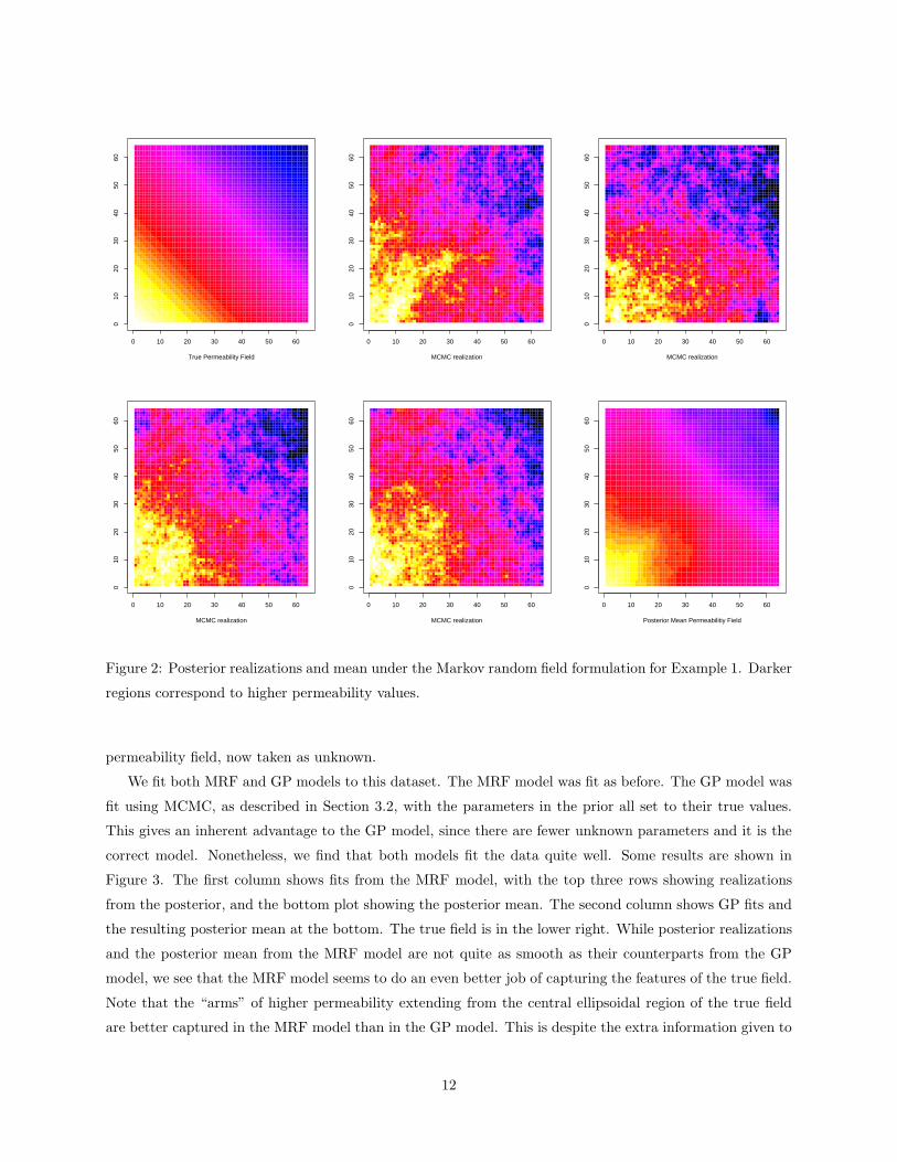
a northeast-southwest axis, as shown in the upper left plot of Figure 2. Darker regions indicate higher

permeability values in the plots. A 64 by 64 grid of square blocks with sides of length 8 feet was used for

this example. The true permeability field was used to generate eight concentration curves, and the eight

breakthrough times from these curves were then used as the data to infer the permeability field to see if we

could recover the original field.

We fit a Markov random field prior model using MCMC as described in the Section 3.1. Some results

are shown in Figure 2. The upper left plot is the true field, taken as unknown during the fitting stage. The

next four plots show samples from the posterior distribution for the field, i.e., MCMC realizations. These

samples are each consistent with the given breakthrough times, and taken together they give some idea of

the variability in the posterior. One can see that each sample does capture the main features of the true

field, although there is a large amount of variability between the samples. The plot in the lower right is

the posterior mean (the average of the MCMC samples). It is remarkable how well the posterior mean field

matches the true permeability field.

It was straightforward to fit this dataset with a Markov random field, since the smoothness parameter can

also be fit with the data. In contrast, MCMC exploration of the posterior resulting from the GP specification

is problematic if the covariance parameters are treated as unknown. In this case the sampler becomes quite

slow mixing so that a much longer run is required.

4.2 Example 2

Our second example is a dataset generated from a Gaussian process with an isotropic Gaussian covariogram

with a range of 10 grid blocks. We generated a 32 by 32 grid of permeabilities from this GP, as shown in the

lower right plot of Figure 3. Again we took only the breakthrough times and tried to recover the original

11

True Permeability Field

0 10 20 30 40 50 60

010

2030

4050

60

MCMC realization

0 10 20 30 40 50 60

010

2030

4050

60MCMC realization

0 10 20 30 40 50 60

010

2030

4050

60

MCMC realization

0 10 20 30 40 50 60

010

2030

4050

60

MCMC realization

0 10 20 30 40 50 60

010

2030

4050

60

Posterior Mean Permeabilitiy Field

0 10 20 30 40 50 60

010

2030

4050

60

Figure 2: Posterior realizations and mean under the Markov random field formulation for Example 1. Darker

regions correspond to higher permeability values.

permeability field, now taken as unknown.

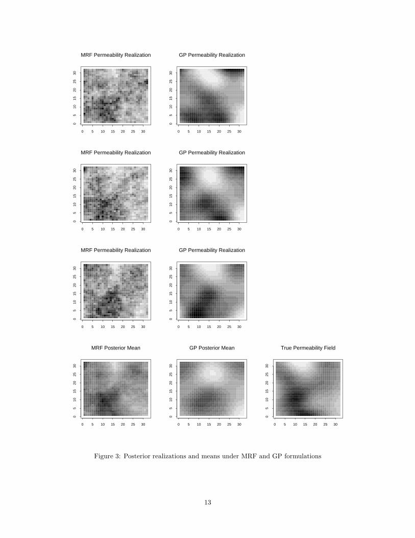
We fit both MRF and GP models to this dataset. The MRF model was fit as before. The GP model was

fit using MCMC, as described in Section 3.2, with the parameters in the prior all set to their true values.

This gives an inherent advantage to the GP model, since there are fewer unknown parameters and it is the

correct model. Nonetheless, we find that both models fit the data quite well. Some results are shown in

Figure 3. The first column shows fits from the MRF model, with the top three rows showing realizations

from the posterior, and the bottom plot showing the posterior mean. The second column shows GP fits and

the resulting posterior mean at the bottom. The true field is in the lower right. While posterior realizations

and the posterior mean from the MRF model are not quite as smooth as their counterparts from the GP

model, we see that the MRF model seems to do an even better job of capturing the features of the true field.

Note that the “arms” of higher permeability extending from the central ellipsoidal region of the true field

are better captured in the MRF model than in the GP model. This is despite the extra information given to

12

MRF Permeability Realization

0 5 10 15 20 25 30

05

1015

2025

30

GP Permeability Realization

0 5 10 15 20 25 30

05

1015

2025

30

MRF Permeability Realization

0 5 10 15 20 25 30

05

1015

2025

30

GP Permeability Realization

0 5 10 15 20 25 30

05

1015

2025

30

MRF Permeability Realization

0 5 10 15 20 25 30

05

1015

2025

30

GP Permeability Realization

0 5 10 15 20 25 30

05

1015

2025

30

MRF Posterior Mean

0 5 10 15 20 25 30

05

1015

2025

30

GP Posterior Mean

0 5 10 15 20 25 30

05

1015

2025

30

True Permeability Field

0 5 10 15 20 25 30

05

1015

2025

30

Figure 3: Posterior realizations and means under MRF and GP formulations

13

the GP prior. In the individual realizations shown, the “arms” are also better captured by the MRF model

realizations than the GP versions. Thus we are quite pleased with the performance of the MRF model.

4.3 Example 3

This example is of real flow data obtained from an experiment run at Hill Air Force Base in Utah, and is

part of a larger, more complex experiment (Annable et al., 1998; Yoon, 2000). The ground at this site holds

a number of contaminants. Multiple tracer experiments were run to discover the aquifer characteristics in

order to aid clean-up efforts. We focus on the experiment which uses the conservative tracer which does

not appreciably interact with the contaminants. Thus our simple flow simulator should satisfactorily model

this physical process. The test site measures 14 feet by 11 feet, and involves four injection wells along one

short edge, three production wells along the opposite edge, and five sampling wells in the middle where the

concentration of the tracer is measured (see the upper left plot of Figure 4). Note that we do not have tracer

measurements at the production wells in this example.

The permeabilities are modeled on a 42 by 33 grid. We specify σt = .01 days, σp = .05, and the mean

of the log permeabilities p1 = 9.9 (this mean coming from geologists familiar with the site). Posterior

realizations and a posterior mean estimate of the permeabilities are shown in Figure 4. Note that the lower

and central sampling wells have the earliest and latest breakthrough times respectively. In order to be

consistent with this data, the posterior permeability realizations must show a high permeability path from

the injectors to the lower sampling well, and a fairly abrupt decrease near the central sampling well.

5 Discussion

We have demonstrated how the Bayesian framework, with the use of MCMC, can be used to characterize

an aquifer based on flow data. Of course, a fast flow simulator is required for the approach we described.

A valuable product of this approach is posterior realizations of the permeability field which can be used

to address more pressing questions involved with environmental remediation. For example: Where are we

the least certain about the aquifer? Where are regions of high and low flow? Where should an additional

sampling well be placed to minimize posterior variability or some other functional of the posterior? A second

feature of this approach is that MCMC explores the probable regions of the posterior. Since the posterior

distribution is almost certain to have local modes, an MCMC-based approach will visit these local modes in

accordance to their posterior probability. In contrast, mode finding approaches can only locate local maxima,

without achieving an idea of the probability associated with each maximum.

In other more complicated flow applications, the simplifying assumptions which speed up the streamline

based simulator will be inappropriate. In this case, a slower, more detailed simulator will be required.

Here one may try to speed up the MCMC by reducing the dimensionality of the permeabilities as well as

attempting to parallelize the slow, but detailed simulation code. We are currently looking at both approaches

in cases when the forward simulation is too slow. For a Bayesian approach on a much lower dimensional

representation of the permeability field which doesn’t rely on MCMC, we refer the readers to Craig et al.

14

Well Layout

0.42

0.34 0.93 0.52

0.17

P

P

P

I

I

I

I

MCMC realization

0 10 20 30 40

010

2030

MCMC realization

0 10 20 30 40

010

2030

MCMC realization

0 10 20 30 40

010

2030

MCMC realization

0 10 20 30 40

010

2030

Posterior Mean Permeabilitiy Field

0 10 20 30 40

010

2030

Figure 4: Layout of wells, posterior realizations, and posterior mean for the Hill Air Force Base data. In

the upper left plot, the wells are labeled “I” for injectors, “P” for producers, and the samplers are shown

with numbers where the value is the breakthrough time (in days) for each well. For the permeability plots,

darker regions correspond to higher permeability values. A single image pixel corresponds to a 1/3 ft. by

1/3 ft. area.

(1996) and O’Hagan et al. (1998).

The actual amount of information contained in the tracer concentration is relatively small. Hence the

resulting inference will be somewhat sensitive to specifications in both the likelihood and the spatial prior

model. In the likelihood specification, of key importance is how closely must the breakthrough time from a

given permeability realization tk(x) match the actual data tk. If the likelihood is too “loose,” the data have

very little influence on plausible permeability fields x; if the likelihood is too “tight,” the resulting posterior

becomes very spiky and multimodal, so that a straightforward MCMC run can become stuck at a local mode

(one fix we’ve used employs simulated tempering (Marinari and Parisi, 1992)). These considerations, along

with the recording error in the breakthrough times and mismatch between the flow simulator and reality,

make the likelihood specification important.

As we mentioned before, the choice of prior for the spatial regularity parameter λψ in the MRF specifi-

cation can influence results, particularly when the dynamic flow data results in only weak information. The

15

small scale structure of the permeability field x is governed almost completely by the prior or other data

sources. The use of our “default,” flat Γ(1, .005) prior puts most of the prior mass on relatively large values

of λψ. This may result in overly smooth posterior realizations if the data are relatively uninformative about

λψ . If this is the case in a particular application, an informative prior regarding λψ would be appropriate.

Even though the applications shown here use only flow data and a single estimate of the mean permeability

for generating plausible permeability realizations, we note that it is usually straightforward to incorporate

additional information regarding the permeability field. For example, information about permeability near a

particular well, but on a larger scale, may be obtained from slug tests or from other sources, such as seismic

information. This sort of information can be built into either the prior (Ferreira et al., 2000) or the likelihood

(Tjelmeland and Omre, 1997; Yoon et al., 1999b). Thus the framework of this paper can be generalized to

a variety of applications.

Acknowledgments

We would like to thank Akhil Datta-Gupta for many helpful suggestions and assistance with implementing

the S3D flow simulator. Thanks also to John Trangenstein for many helpful comments regarding simulation

of flow through porous media. This work was supported by National Science Foundation grant DMS 9873275.

References

Annable, M. D., Rao, P. S. C., Hatfield, K., Graham, W. D., Wood, A. L., and Enfield, C. G. (1998). “Par-

titioning Tracers for Measuring Residual NAPL: Field-Scale Test Results.” Journal of Environmental

Engineering , 124, 498–503.

Barker, J. W., Cuypers, M., and Holden, L. (2000). “Quantifying Uncertainty in Production Forecasts:

Another Look at the PUNQ-S3 Problem.” Society of Petroleum Engineers 2000 Annual Technical

Conference, SPE 62925.

Besag, J. and Kooperberg, C. (1995). “On Conditional and Intrinsic Autoregressions.” Biometrika, 82,

733–746.

Besag, J., York, J., and Mollie, A. (1991). “Bayesian image restoration, with two applications in spatial

statistics (with discussion).” Annals of the Institute of Statistical Mathematics , 43, 1–59.

Craig, P. S., Goldstein, M., Seheult, A. H., and Smith, J. A. (1996). “Bayes Linear Strategies for History

Matching of Hydrocarbon Reservoirs.” In Bayesian Statistics 5 , eds. J. M. Bernardo, J. O. Berger,

A. P. Dawid, and A. F. M. Smith, 69–95. Oxford: Clarendon Press.

Cressie, N. A. C. (1991). Statistics for Spatial Data. Wiley-Interscience.

Ferreira, M. A. R., West, M., Lee, H., and Higdon, D. (2000). “A Class of Multi-Scale Time Series Models.”

Unpublished manuscript: Duke University, Institute of Statistics and Decision Sciences.

16

Floris, F. J. T., Bush, M. D., Cuypers, M., Roggero, F., and Syversveen, A.-R. (1999). “Comparison of

Production Forecast Uncertainty Quantification Methods — An Integrated Study.” 1st Symposium on

Petroleum Geostatistics, Toulouse, 20–23 April 1999.

Hegstad, B. K. and Omre, H. (1997). “Uncertainty assessment in history matching and forecasting.” In

Geostatistics Wollongong ’96, Vol. 1., ed. E. Y. Baafi and N. A. Schofield, 585–596. Kluwer Academic

Publishers.

Henninger, R. L., Maudlin, P. J., Rightley, M. L., and Hanson, K. M. (1996). “Application of forward and

adjoint techniques to hydrocode sensitivity analysis.” In Proceedings of the 9th Nuclear Exploratory

Code Development Conference, ed. F. Graviana, et al. Lawrence Livermore National Laboratory.

Higdon, D. M., Johnson, V. E., Bowsher, J. E., Turkington, T. G., Gilland, D. R., and Jaszczack, R. J.

(1997). “Fully Bayesian estimation of Gibbs hyperparameters for emission computed tomography data.”

IEEE Transactions on Medical Imaging , 16, 516–526.

James, A. I., Graham, W. D., Hatfield, K., Rao, P. S. C., and Annable, M. D. (1997). “Optimal Estimation of

Residual Non-aqueous Phase Liquid Saturation Using Partitioning Tracer Concentration Data.” Water

Resources Research, 33, 2621–2636.

Jin, M., Delshad, M., Dwarakanath, V., McKinney, D. C., Pope, G. A., Sepehrnoori, K., Tilburg, C. E.,

and Jackson, R. E. (1995). “Partitioning Tracer Test for Detection, Estimation, and Remediation

Performance Assessment of Subsurface Non-aqueous Phase Liquids.” Water Resources Research, 31,

1201–1211.

King, M. J. and Datta-Gupta, A. (1998). “Streamline Simulation: A Current Perspective.” In Situ, 22, 1,

91–140.

Knorr-Held, L. (2000). “Bayesian Modelling of Inseparable Space-Time Variation in Disease Risk.” Statistics

in Medicine, 19, 2555–2567.

Marinari, E. and Parisi, G. (1992). “Simulated tempering: a new Monte Carlo scheme.” Europhysics Letters ,

19, 451–458.

Neuman, S. P. and Yakowitz, S. (1979). “A Statistical Approach to the Problem of Aquifer Hydrology: 1.

Theory.” Water Resources Research, 15, 845–860.

O’Hagan, A., Kennedy, M. C., and Oakley, J. E. (1998). “Uncertainty Analysis and other Inference Tools for

Complex Computer Codes.” In Bayesian Statistics 6 , eds. J. M. Bernardo, J. O. Berger, A. P. Dawid,

and A. F. M. Smith, 503–524. Oxford University Press.

Oliver, D. S. (1994). “Incorporation of Transient Pressure Data into Reservoir Characterization.” In Situ,

18, 243–275.

17

Oliver, D. S., Cunha, L. B., and Reynolds, A. C. (1997). “Markov Chain Monte Carlo Methods for Condi-

tioning a Permeability Field to Pressure Data.” Mathematical Geology , 29, 1, 61–91.

Ripley, B. D. (1981). Spatial Statistics . John Wiley & Sons.

Rue, H. (2000). “Fast Sampling of Gaussian Markov Random Fields with Applications.” Statistics no. 1,

Department of Mathematical Sciences, Norwegian University of Science and Technology, Trondheim,

Norway.

Tjelmeland, H. and Omre, H. (1997). “A complex sand-shale facies model conditioned on observations from

wells, seismics and production.” In Geostatistics Wollongong ’96, Vol. 1., ed. E. Y. Baafi and N. A.

Schofield. Kluwer Academic Publishers.

Vasco, D. W. and Datta-Gupta, A. (1999). “Asymptotic Solutions for Solute Transport: A Formalism for

Tracer Tomography.” Water Resources Research, 35, 1, 1–16.

Vasco, D. W., Yoon, S., and Datta-Gupta, A. (1998). “Integrating Dynamic Data Into High-Resolution

Reservoir Models Using Streamline-Based Analytic Sensitivity Coefficients.” Society of Petroleum En-

gineers 1998 Annual Technical Conference, SPE 49002.

Waller, L. A., Carlin, B. P., Xia, H., and Gelfand, A. (1996). “Hierarchical spatio-temporal mapping of

disease rates.” Journal of the American Statistical Association, 92, 607–617.

Weir, I. (1997). “Fully Bayesian Reconstructions from single photon emission computed tomography.” Jour-

nal of the American Statistical Association, 92, 49–60.

Xue, G. and Datta-Gupta, A. (2000). “A New Approach to Seismic Data Integration Using Optimal Non-

parametric Transformations.” SPE Formation Evaluation, accepted, SPE 36500.

Yeh, W. W. (1986). “Review of Parameter Identification in Groundwater Hydrology: the Inverse Problem.”

Water Resources Research, 22, 95–108.

Yoon, S. (2000). “Dynamic Data Integration Into High Resolution Reservoir Models Using Streamline-Based

Inversion.” Ph.D. thesis, Texas A&M University, Department of Petroleum Engineering.

Yoon, S., Barman, I., Datta-Gupta, A., and Pope, G. A. (1999a). “In-Situ Characterization of Residual NAPL

Distribution Using Streamline-Based Inversion of Partitioning Tracer Tests.” SPE/EPA Exploration and

Production Environmental Conference, SPE 52729.

Yoon, S., Malallah, A. H., Datta-Gupta, A., Vasco, D. W., and Behrens, R. A. (1999b). “A Multiscale

Approach to Production Data Integration Using Streamline Models.” Society of Petroleum Engineers

1999 Annual Technical Conference, SPE 56653.

18