Markov Properties and the Multivariate Gaussian Distribution · university of copenhagendepartment of mathematical sciences Overview of lectures Lecture 1 Markov Properties and the

un i v er s i ty of copenhagen department of mathemat i ca l s c i ence s

Faculty of Science

Markov Properties and the Multivariate GaussianDistribution

Steffen LauritzenDepartment of Mathematical Sciences

Minikurs TUM 2016 — Lecture 1

Slide 1/42


Overview of lectures

Lecture 1 Markov Properties and the MultivariateGaussian Distribution

Lecture 2 Likelihood Analysis of Gaussian GraphicalModels

Lecture 3 Gaussian Graphical Models with AdditionalRestrictions; structure identification.

For reference, if nothing else is mentioned, see Lauritzen(1996), Chapters 3 and 4.

Steffen Lauritzen — Markov Properties and the Multivariate Gaussian Distribution — Minikurs TUM 2016 — Lecture 1

Slide 2/42


Independence

We recall that two random variables X and Y areindependent if

P(X ∈ A |Y = y) = P(X ∈ A)

or, equivalently, if

P{(X ∈ A) ∩ (Y ∈ B)} = P(X ∈ A)P(Y ∈ B).

For continuous variables the requirement is a factorization ofthe joint density:

fXY (x , y) = fX (x)fY (y).

When X and Y are independent we write X ⊥⊥ Y .


Slide 3/42


Formal definition

Random variables X and Y are conditionally independentgiven the random variable Z if

L(X |Y ,Z ) = L(X |Z ).

We then write X ⊥⊥ Y |Z (or X ⊥⊥P Y |Z )

Intuitively: Knowing Z renders Y irrelevant for predicting X .

Factorisation of densities:

X ⊥⊥ Y |Z ⇐⇒ fXYZ (x , y , z)fZ (z) = fXZ (x , z)fYZ (y , z)

⇐⇒ ∃a, b : f (x , y , z) = a(x , z)b(y , z).


Slide 4/42


Undirected graphical models

3 6

1 5 7

2 4

u uu u u

u u@@@

��

@@@

@@@

@@@

��

��

For several variables, complex systems of conditionalindependence can for example be described by undirectedgraphs.

Then a set of variables A is conditionally independent of aset B, given the values of a set of variables C , if C separatesA from B.

For example in picture above

1 ⊥⊥ {4, 7} | {2, 3}, {1, 2} ⊥⊥ 7 | {4, 5, 6}.Steffen Lauritzen — Markov Properties and the Multivariate Gaussian Distribution — Minikurs TUM 2016 — Lecture 1

Slide 5/42


Fundamental properties

For random variables X , Y , Z , and W it holds

(C1) If X ⊥⊥ Y |Z then Y ⊥⊥ X |Z ;

(C2) If X ⊥⊥ Y |Z and U = g(Y ), then X ⊥⊥ U |Z ;

(C3) If X ⊥⊥ Y |Z and U = g(Y ), thenX ⊥⊥ Y | (Z ,U);

(C4) If X ⊥⊥ Y |Z and X ⊥⊥W | (Y ,Z ), thenX ⊥⊥ (Y ,W ) |Z ;

If density w.r.t. product measure f (x , y , z ,w) > 0 also

(C5) If X ⊥⊥ Y | (Z ,W ) and X ⊥⊥ Z | (Y ,W ) thenX ⊥⊥ (Y ,Z ) |W .


Slide 6/42


Conditional independence can be seen as encoding abstractirrelevance: Knowing C , A is irrelevant for learning B,(C1)–(C4) translate into:

(I1) If, knowing C , learning A is irrelevant forlearning B, then B is irrelevant for learning A;

(I2) If, knowing C , learning A is irrelevant forlearning B, then A is irrelevant for learning anypart D of B;

(I3) If, knowing C , learning A is irrelevant forlearning B, it remains irrelevant having learntany part D of B;

(I4) If, knowing C , learning A is irrelevant forlearning B and, having also learnt A, D remainsirrelevant for learning B, then both of A and Dare irrelevant for learning B.


Slide 7/42


Semi-graphoidAn independence model (Studeny, 2005) ⊥σ is a ternaryrelation over subsets of a finite set V . It is a graphoid if forall disjoint subsets A, B, C , D:

(S1) if A⊥σ B |C then B ⊥σ A |C (symmetry);

(S2) if A⊥σ (B ∪ D) |C then A⊥σ B |C andA⊥σ D |C (decomposition);

(S3) if A⊥σ (B ∪ D) |C then A⊥σ B | (C ∪ D)(weak union);

(S4) if A⊥σ B |C and A⊥σ D | (B ∪ C ), thenA⊥σ (B ∪ D) |C (contraction);

(S5) if A⊥σ B | (C ∪ D) and A⊥σ C | (B ∪ D) thenA⊥σ (B ∪ C ) |D (intersection).

Semigraphoid if only (S1)–(S4). It is compositional if

(S6) if A⊥σ B |C and A⊥σ D |C thenA⊥σ (B ∪ D) |C (composition).


Slide 8/42


Separation in undirected graphs

Let G = (V ,E ) be finite and simple undirected graph (noself-loops, no multiple edges).

For subsets A,B,S of V , let A⊥G B | S denote that Sseparates A from B in G, i.e. that all paths from A to Bintersect S .

Fact: The relation ⊥G on subsets of V is a compositionalgraphoid.

This fact is the reason for choosing the name ‘graphoid’ forsuch independence model.


Slide 9/42


Probabilistic Independence Model

For a system V of labeled random variables Xv , v ∈ V , weuse

A ⊥⊥ B |C ⇐⇒ XA ⊥⊥ XB |XC ,

where XA = (Xv , v ∈ A) denotes the variables with labels inA.

The properties (C1)–(C4) imply that ⊥⊥ satisfies thesemi-graphoid axioms and the graphoid axioms if the jointdensity of the variables is strictly positive.

A regular multivariate Gaussian distribution defines acompositional graphoid independence model, as we shall seelater.


Slide 10/42


Geometric orthogonalityLet L, M, and N be linear subspaces of a Hilbert space H and

L ⊥ M |N ⇐⇒ (L N) ⊥ (M N),

where L N = L ∩ N⊥.L and M are said to meetorthogonally in N.

(O1) If L ⊥ M |N then M ⊥ L |N;

(O2) If L ⊥ M |N and U is a linear subspace of L,then U ⊥ M |N;

(O3) If L ⊥ M |N and U is a linear subspace of M,then L ⊥ M | (N + U);

(O4) If L ⊥ M |N and L ⊥ R | (M + N), thenL ⊥ (M + R) |N.

Intersection does not hold in general whereas composition(S6) does.Steffen Lauritzen — Markov Properties and the Multivariate Gaussian Distribution — Minikurs TUM 2016 — Lecture 1

Slide 11/42


Markov properties for undirected graphs

G = (V ,E ) simple undirected graph; An independence model⊥σ satisfies

(P) the pairwise Markov property if

α 6∼ β =⇒ α⊥σ β |V \ {α, β};

(L) the local Markov property if

∀α ∈ V : α⊥σ V \ cl(α) | bd(α);

(G) the global Markov property if

A⊥G B | S =⇒ A⊥σ B | S .


Slide 12/42


Pairwise Markov property

3 6

1 5 7

2 4

u uu u u

u u@@@

��

@@@

@@@

@@@

��

��

Any non-adjacent pair of random variables are conditionallyindependent given the remaning.

For example, 1⊥σ 5 | {2, 3, 4, 6, 7} and 4⊥σ 6 | {1, 2, 3, 5, 7}.


Slide 13/42


Local Markov property

3 6

1 5 7

2 4

u uu u u

u u@@@

��

@@@

@@@

@@@

��

��

Every variable is conditionally independent of the remaining,given its neighbours.

For example, 5⊥σ {1, 4} | {2, 3, 6, 7} and7⊥σ {1, 2, 3} | {4, 5, 6}.


Slide 14/42


Global Markov property

3 6

1 5 7

2 4

u uu u u

u u@@@

��

@@@

@@@

@@@

��

��

To find conditional independence relations, one should lookfor separating sets, such as {2, 3}, {4, 5, 6}, or {2, 5, 6}

For example, it follows that 1⊥σ 7 | {2, 5, 6} and2⊥σ 6 | {3, 4, 5}.


Slide 15/42


Structural relations among Markov properties

For any semigraphoid it holds that

(G) =⇒ (L) =⇒ (P)

If ⊥σ satisfies graphoid axioms it further holds that

(P) =⇒ (G)

so that in the graphoid case

(G) ⇐⇒ (L) ⇐⇒ (P).

The latter holds in particular for ⊥⊥, when f (x) > 0.


Slide 16/42


The multivariate Gaussian

A d-dimensional random vector X = (X1, . . . ,Xd) has amultivariate Gaussian distribution or normal distribution onRd if there is a vector ξ ∈ Rd and a d × d matrix Σ suchthat

λ>X ∼ N (λ>ξ, λ>Σλ) for all λ ∈ Rd . (1)

We then write X ∼ Nd(ξ,Σ).

Taking λ = ei or λ = ei + ej where ei is the unit vector withi-th coordinate 1 and the remaining equal to zero yields:

Xi ∼ N (ξi , σii ), Cov(Xi ,Xj) = σij .

Hence ξ is the mean vector and Σ the covariance matrix ofthe distribution.


Slide 17/42


The definition (1) makes sense if and only if λ>Σλ ≥ 0, i.e.if Σ is positive semidefinite. Note that we have alloweddistributions with variance zero.

The multivariate moment generating function of X can becalculated using the relation (1) as

md(λ) = E{eλ>X} = eλ>ξ+λ>Σλ/2

where we have used that the univariate moment generatingfunction for N (µ, σ2) is

m1(t) = etµ+σ2t2/2

and let t = 1, µ = λ>ξ, and σ2 = λ>Σλ.

Thus a multivariate Gaussian distribution is determined by itsmean vector and covariance matrix.


Slide 18/42


A simple example

Assume X> = (X1,X2,X3) with Xi independent andXi ∼ N (ξi , σ

2i ). Then

λ>X = λ1X1 + λ2X2 + λ3X3 ∼ N (µ, τ2)

with

µ = λ>ξ = λ1ξ1 + λ2ξ2 + λ3ξ3, τ2 = λ21σ

21 + λ2

2σ22 + λ2

3σ23.

Hence X ∼ N3(ξ,Σ) with ξ> = (ξ1, ξ2, ξ3) and

Σ =

σ21 0 0

0 σ22 0

0 0 σ23

.


Slide 19/42


Density of multivariate Gaussian

If Σ is positive definite, i.e. if λ>Σλ > 0 for λ 6= 0, thedistribution has density on Rd

f (x | ξ,Σ) = (2π)−d/2(detK )1/2e−(x−ξ)>K(x−ξ)/2, (2)

where K = Σ−1 is the concentration matrix of thedistribution. Since a positive semidefinite matrix is positivedefinite if and only if it is invertible, we then also say that Σis regular.

If X1, . . . ,Xd are independent and Xi ∼ N (ξi , σ2i ) their joint

density has the form (2) with Σ = diag(σ2i ) and

K = Σ−1 = diag(1/σ2i ).

Hence vectors of independent Gaussians are multivariateGaussian.


Slide 20/42


A counterexample

The marginal distributions of a vector X can all be Gaussianwithout the joint being multivariate Gaussian:

For example, let X1 ∼ N (0, 1), and define X2 as

X2 =

{X1 if |X1| > c−X1 otherwise.

Then, using the symmetry of the univariate Gausssiandistribution, X2 is also distributed as N (0, 1).


Slide 21/42


Counterexample continued

The joint distribution is not Gaussian unless c = 0 since, forexample, Y = X1 + X2 satisfies

P(Y = 0) = P(X2 = −X1) = P(|X1| ≤ c) = Φ(c)− Φ(−c).

Note that for c = 0, the correlation ρ between X1 and X2 is1 whereas for c =∞, ρ = −1.

It follows that there is a value of c so that X1 and X2 areuncorrelated, and still not jointly Gaussian.


Slide 22/42


Adding two independent Gaussians yields a Gaussian:

If X ∼ Nd(ξ1,Σ1) and X2 ∼ Nd(ξ2,Σ2) and X1 ⊥⊥ X2

X1 + X2 ∼ Nd(ξ1 + ξ2,Σ1 + Σ2).

To see this, just note that

λ>(X1 + X2) = λ>X1 + λ>X2

and use the univariate addition property.


Slide 23/42


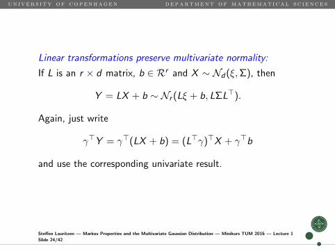
Linear transformations preserve multivariate normality:

If L is an r × d matrix, b ∈ Rr and X ∼ Nd(ξ,Σ), then

Y = LX + b ∼ Nr (Lξ + b, LΣL>).

Again, just write

γ>Y = γ>(LX + b) = (L>γ)>X + γ>b

and use the corresponding univariate result.


Slide 24/42


Marginal distributions

Partition X into into XA and XB , where XA ∈ RA andXB ∈ RB with A ∪ B = V . Partition mean vector,concentration and covariance matrix accordingly as

ξ =

(ξAξB

), K =

(KAA KAB

KBA KBB

), Σ =

(ΣAA ΣAB

ΣBA ΣBB

).

Then, if X ∼ N (ξ,Σ) it holds that

XB ∼ Ns(ξB ,ΣBB).

This follows simply from the previous fact using the matrix

L = (0AB IB) .

with 0AB a matrix of zeros and IB the B × B identity matrix.


Slide 25/42


Conditional distributions

If ΣBB is regular, it further holds that

XA |XB = xB ∼ NA(ξA|B ,ΣA|B),

where

ξA|B = ξA+ΣABΣ−1BB(xB−ξB) and ΣA|B = ΣAA−ΣABΣ−1

BBΣBA.

In particular, ΣAB = 0 if and only if XA and XB areindependent.


Slide 26/42


To see this, we simply calculate the conditional density.

f (xA | xB) ∝ fξ,Σ(xA, xB)

∝ exp{−(xA − ξA)>KAA(xA − ξA)/2− (xA − ξA)>KAB(xB − ξB)

}.

The linear term involving xA has coefficient equal to

KAAξA − KAB(xA − ξB) = KAA

{ξA − K−1

AAKAB(xB − ξB)}.

Using the matrix identities

K−1AA = ΣAA − ΣABΣ−1

BBΣBA (3)

andK−1AAKAB = −ΣABΣ−1

BB , (4)


Slide 27/42


we find

f (xA | xB) ∝ exp{−(xA − ξA|B)>KAA(xA − ξA|B)/2

}and the result follows.

From the identities (3) and (4) it follows in particular thatthen the conditional expectation and concentrations also canbe calculated as

ξA|B = ξA − K−1AAKAB(xB − ξB) and KA|B = KAA.

Note that the marginal covariance is simply expressed interms of Σ whereas the conditional concentration is simplyexpressed in terms of K .


Slide 28/42


Further, since

ξA|B = ξA − K−1AAKAB(xB − ξB) and KA|B = KAA,

XA and XB are independent if and only if KAB = 0, givingKAB = 0 if and only if ΣAB = 0.

More generally, if we partition X into XA,XB ,XC , theconditional concentration of XA∪B given XC = xC is

KA∪B|C =

(KAA KAB

KBA KBB

),

soXA ⊥⊥ XB |XC ⇐⇒ KAB = 0.

It follows that a Gaussian independence model is acompositional graphoid.


Slide 29/42


An example

Consider N3(0,Σ) with covariance matrix

Σ =

1 1 11 2 11 1 2

.

The concentration matrix is

K = Σ−1 =

3 −1 −1−1 1 0−1 0 1

.


Slide 30/42


The marginal distribution of (X2,X3) has covariance andconcentration matrix

Σ23 =

(2 11 2

), (Σ23)−1 =

1

3

(2 −1−1 2

).

The conditional distribution of (X1,X2) given X3 hasconcentration and covariance matrix

K12 =

(3 −1−1 1

), Σ12|3 = (K12)−1 =

1

2

(1 11 3

).

Similarly, V(X1 |X2,X3) = 1/k11 = 1/3, etc.


Slide 31/42


Consider X = (Xv , v ∈ V ) ∼ NV (0,Σ) with Σ regular andK = Σ−1.

The concentration matrix of the conditional distribution of(Xα,Xβ) given XV \{α,β} is

K{α,β} =

(kαα kαβkβα kββ

),

Henceα ⊥⊥ β |V \ {α, β} ⇐⇒ kαβ = 0.

Thus a regular Gaussian distribution is pairwise, local, andglobally Markov w.r.t. the graph G(K ) given by

α 6∼ β ⇐⇒ kαβ = 0.


Slide 32/42


Gaussian graphical model

S(G) denotes the symmetric matrices A with aαβ = 0 unlessα ∼ β and S+(G) their positive definite elements.

A Gaussian graphical model for X specifies X as multivariatenormal with K ∈ S+(G) and otherwise unknown.

Note that the density then factorizes as

log f (x) = constant− 1

2

∑α∈V

kααx2α −

∑{α,β}∈E

kαβxαxβ,

hence no interaction terms involve more than pairs..


Slide 33/42


Mathematics marks

Examination marks of 88 students in 5 differentmathematical subjects. The empirical concentrations (on orabove diagonal) and partial correlations (below diagonal) are

Mechanics Vectors Algebra Analysis StatisticsMechanics 5.24 −2.44 −2.74 0.01 −0.14Vectors 0.33 10.43 −4.71 −0.79 −0.17Algebra 0.23 0.28 26.95 −7.05 −4.70Analysis −0.00 0.08 0.43 9.88 −2.02Statistics 0.02 0.02 0.36 0.25 6.45


Slide 34/42


Graphical model for mathmarks

Mechanics

Vectors

Algebra

Analysis

Statistics

��

��

PPPPPP ��

��

PPPPPPcc

ccc

This analysis is from Whittaker (1990).

We have An, Stats ⊥⊥ Mech,Vec |Alg.


Slide 35/42


Gaussian likelihoodsConsider the case where ξ = 0 and a sampleX 1 = x1, . . . ,X n = xn from a multivariate Gaussiandistribution Nd(0,Σ) with Σ regular. Using the expressionfor the density, we get the likelihood function

L(K ) = (2π)−nd/2(detK )n/2e−∑n

ν=1(xν)>Kxν/2

∝ (detK )n/2e−∑n

ν=1 tr{Kxν(xν)>}/2

= (detK )n/2e− tr{K∑n

ν=1 xν(xν)>}/2

= (detK )n/2e− tr(Kw)/2. (5)

where

W =n∑ν=1

X ν(X ν)>

is the matrix of sums of squares and products.Steffen Lauritzen — Markov Properties and the Multivariate Gaussian Distribution — Minikurs TUM 2016 — Lecture 1

Slide 36/42


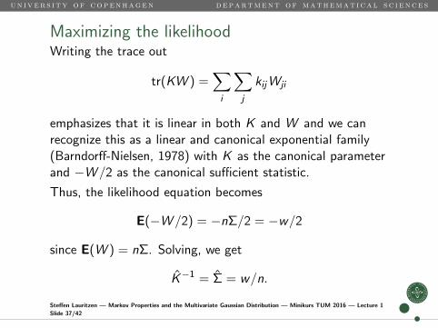
Maximizing the likelihoodWriting the trace out

tr(KW ) =∑i

∑j

kijWji

emphasizes that it is linear in both K and W and we canrecognize this as a linear and canonical exponential family(Barndorff-Nielsen, 1978) with K as the canonical parameterand −W /2 as the canonical sufficient statistic.

Thus, the likelihood equation becomes

E(−W /2) = −nΣ/2 = −w/2

since E(W ) = nΣ. Solving, we get

K−1 = Σ = w/n.


Slide 37/42


Rewriting the likelihood function as

log L(K ) =n

2log(detK )− tr(Kw)/2

we can of course also differentiate to find the maximum,leading to the equation

∂

∂kijlog(detK ) = wij/n,

which in combination with the previous result yields

∂

∂Klog(detK ) = K−1.

The latter can also be derived directly by writing out thedeterminant, and it holds for any non-singular square matrix,i.e. one which is not necessarily positive definite.


Slide 38/42


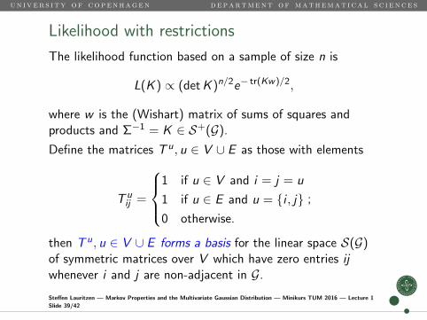
Likelihood with restrictions

The likelihood function based on a sample of size n is

L(K ) ∝ (detK )n/2e− tr(Kw)/2,

where w is the (Wishart) matrix of sums of squares andproducts and Σ−1 = K ∈ S+(G).

Define the matrices T u, u ∈ V ∪ E as those with elements

T uij =

1 if u ∈ V and i = j = u

1 if u ∈ E and u = {i , j}0 otherwise.

;

then T u, u ∈ V ∪ E forms a basis for the linear space S(G)of symmetric matrices over V which have zero entries ijwhenever i and j are non-adjacent in G.


Slide 39/42


Further, as K ∈ S(G), we have

K =∑v∈V

kvTv +

∑e∈E

keTe (6)

and hence

tr(Kw) =∑v∈V

kv tr(T vw) +∑e∈E

ke tr(T ew);

leading to the log-likelihood function

l(K ) = log L(K ) ∼ n

2log(detK )− tr(Kw)/2

=n

2log(detK )

−∑v∈V

kv tr(T vw)/2 +∑e∈E

ke tr(T ew)/2.


Slide 40/42


Hence we can identify the family as a (regular and canonical)exponential family with − tr(T uW )/2, u ∈ V ∪ E ascanonical sufficient statistics.

The likelihood equations can be obtained from this fact or bydifferentiation, combining the fact that

∂

∂kulog det(K ) = tr(T uΣ)

with (6).

This eventually yields the likelihood equations

tr(T uw) = n tr(T uΣ), u ∈ V ∪ E .


Slide 41/42


The likelihood equations

tr(T uw) = n tr(T uΣ), u ∈ V ∪ E .

can also be expressed as

nσvv = wvv , nσαβ = wαβ, v ∈ V , {α, β} ∈ E .

Remember the model restriction K = Σ−1 ∈ S+(G).

This ‘fits variances and covariances along nodes and edges inG’ so we can write the equations as

nΣcc = wcc for all cliques c ∈ C(G).

General theory of exponential families ensure the solution tobe unique, provided it exists.


Slide 42/42


Barndorff-Nielsen, O. E. (1978). Information and ExponentialFamilies in Statistical Theory. John Wiley and Sons, NewYork.

Lauritzen, S. L. (1996). Graphical Models. Clarendon Press,Oxford, United Kingdom.

Studeny, M. (2005). Probabilistic Conditional IndependenceStructures. Information Science and Statistics.Springer-Verlag, London.

Whittaker, J. (1990). Graphical Models in AppliedMultivariate Statistics. John Wiley and Sons, Chichester,United Kingdom.


Slide 42/42

Markov Properties and the Multivariate Gaussian Distribution · university of copenhagendepartment of mathematical sciences Overview of lectures Lecture 1 Markov Properties and the

Documents