Markov chains in a field of traps: theory and simulation

UNIVERSIDADE ESTADUAL DE CAMPINAS

MS777 PROJECT

Markov chains in a field of traps: theory andsimulation

Author:Marina VASQUES MOREIRA

Supervisor:Marina VACHKOVSKAIA

Abstract

In this work we make a review of the main ideas of Markov chains theory, giving some examples as motiva-tion.We then proceed in examining some statements related to Markov chains in quenched and annealed fields.After that, we present computer simulations and compare these results with the ones proved theoretically.

1

Contents1 Introduction 3

2 Markov Chains 42.1 Basic ideas and definitions . . . . . . . . . . . . . . . . . . . . . . . . . . . . . . . . . . . . . . 42.2 Classification of states . . . . . . . . . . . . . . . . . . . . . . . . . . . . . . . . . . . . . . . . 82.3 Long term behavior . . . . . . . . . . . . . . . . . . . . . . . . . . . . . . . . . . . . . . . . . . 9

3 Markov chains in a field of traps 113.1 Introduction . . . . . . . . . . . . . . . . . . . . . . . . . . . . . . . . . . . . . . . . . . . . . . 113.2 A criterion for trapping . . . . . . . . . . . . . . . . . . . . . . . . . . . . . . . . . . . . . . . . 123.3 A necessary and sufficient condition for trapping . . . . . . . . . . . . . . . . . . . . . . . . . . 14

4 Simulation 144.1 Gambler’s ruins . . . . . . . . . . . . . . . . . . . . . . . . . . . . . . . . . . . . . . . . . . . . 154.2 Drunkard walk – one dimensional random walk . . . . . . . . . . . . . . . . . . . . . . . . . . . 18

4.2.1 Quenched field . . . . . . . . . . . . . . . . . . . . . . . . . . . . . . . . . . . . . . . . 194.2.2 Annealed field . . . . . . . . . . . . . . . . . . . . . . . . . . . . . . . . . . . . . . . . 20

5 Conclusions 22

6 References 22

2

1 Introduction“Predictions can be very difficult – especially about the future.”Niels Bohr

In everyday life, we deal with probabilistic phenomena: even those among us without formal mathematicaltraining are acquainted with some features of the theory of probability. People in general develop an intuitivesense of chance and randomness while dealing with such things as tossing coins, lottery games and weather fore-casting. The last one is a good example of this intuitive sense: while most of us are not aware of all the mechanismsinvolved in weather forecasting, we accept that a 95% accurate prediction of a sunny day is a good reason not towear a raincoat (bear in mind here the difference between accuracy and precision: while accuracy refers to howclose the measured value is to the true or accepted value, precision refers to how close together a group of mea-surement actually are to each other. Precision is usually expressed trough significant digits. In the case of weatherforecasting, an accurate forecasting is usually preferable over a precise one: if we are told that the temperaturetomorrow may vary from 20◦C to 25 ◦C, and it turns out that we measure it as 23◦C, that is just ok. On the otherhand, a very precise forecasting may predict a temperature of 23.43◦C for tomorrow, and if it turns out to be 32◦C,that was a very precise but highly inaccurate – not to mention useless – prediction). More than that: we also carrywith us the intuitive notion that, regardless of geographical location or time of the year, we can make a good guessthat the weather tomorrow is somehow related to the weather today (of course location and time of the year matter,but we do make statements about the weather tomorrow based on the weather today). In theory, one could say thatthe current weather is a result of all the climate processes that have taken place on Earth since its origin billions ofyears ago1, but even if we had access to this enormous amount of information, that would not make quite a veryuseful model. Instead, let’s try to think of a model where the predictability of the weather today is influenced bythe weather observed yesterday, and so on.

With that in mind, we could define some possible weather states (such as “rainy”, “sunny”, “cloudy”) and makeup some probabilities. The way we defined our model, the probabilities should be of the kind

“As today is sunny, P is the probability that the weather tomorrow is going to be rainy”.

After computing all the probabilities that describe a transition from one weather state to the other, we couldpredict, for any two given weather states i and j, the probability of the weather – today in state i – being tomorrowin state j. We could also repeat the same calculations and try to predict the weather some days ahead with theinformation we have today; we could go further and, carrying on this result, have an idea of the long term prediction(which is just a prediction for the weather a big lot of days ahead!).

Strange as it may seem, the apparent simplicity of the model we have just outlined is in fact its great advantage:different phenomena can be modeled in such a way, as this model doesn’t carry many assumptions on the nature ofthe problem, provided only that we can define some states, and the outcome of one experiment is influenced solelyby the previous one. This is the heart of the definition of a Markov chain, named after the Russian mathematicianAndrey Markov. We shall discuss some of the main ideas and definitions of Markov chains in the next section.

1This is usually referred to as determinism. Laplace is often misquoted as having said“give me the positions and velocities of all the atomsin the universe, and the forces acting upon them, one can predict the future course of the universe.” But what he truly said is somehow deeperthan that, as it can be seen on this excerpt from one of his works: “Thus, we must consider the present state of the universe as the effect of itsprevious state and as the cause of those states to follow. An intelligent being which, for a given point in time, knows all the forces acting uponthe universe and the positions of the objects of which it is composed, supplied with facilities large enough to submit these data to numericalanalysis, would include in the same formula the movements of the largest bodies of the universe and those of the lightest atom. Nothing wouldbe uncertain for it, and the past and future would be known to it. (...) All the efforts of human intellect to search for the truth tend to bring itsteadily closer to the intelligent being described above, but this being will remain always infinitely distant.”

3

2 Markov Chains

2.1 Basic ideas and definitions

In this chapter, we define Markov chains and discuss some of its properties. The fundamentals of this theory havebeen widely discussed on many good books; most of the definitions given here are adpated from “The Theory ofProbability”, written by B. V. Gnedenko.A Markov chain is a collection of random variables {Xt} (where the index t runs through 0, 1, ...) having theproperty that, given the present, the future is conditionally independent of the past. Frequently, Markov chainsare defined in terms of a given physical system S, which at each instant of time can be in one of the statesA1, A2, ..., Ak and alters its state only at times t1, t2, ..., tn, .... For Markov chains, the probability of passing tosome state Ai(i = 1, 2, ..., k) at a time τ(ts < τ < ts+1) depends only on the state the system was in at timet(ts−1 < t < ts) and does not change if we learn what its states were at earlier times. This is the same as sayingthat Markov chains are memoryless (“future” is independent of “past” given “present”).

In the following examples we illustrate this definition:

Example 1. Gambler’s ruin – Let two players each have a finite number of cents (say, nA for player A and nBfor player B). Now, flip one of the cents (from either player), with each player having 50% probabilityof winning, and transfer a cent from the loser to the winner. Repeat the process until one player has all thecents. In this example, we may define a collection of random variablesAt, in which we store the informationof the amount of cents with player A at time t, where the index t represents the successive tossing of thecoins, t = 1, 2, .... Similarly, define Bt the amount of cents with player B at time t. Then, the possiblestates for this system are represented by the ordered pairs (At, Bt), which we may call Xt = (At, Bt).Observe that the game stops when one of the players has all the cents, there is, the game stops when Xt =

(nA + nB , 0) or Xt = (0, nA + nB). 2

This is an example of a random walk, which is a mathematical formalisation of a trajectory that consists oftaking successive random steps. Random walks are usually assumed to be Markov chains. Other examplesinclude the path traced by a molecule as it travels in liquid or gas, the search path of a foraging animal(assuming that the animal takes random steps and does not retrieve information from the past), the price ofa fluctuating stock.

Example 2. Hydrogen atom – In Bohr’s model of the hydrogen atom, the electron can be in one of the allowedorbits. Denote by Ai the event that the electron lies on the ith orbit. Further, assume that changes in the stateof the atom can only occur at times t1, t2, ... (actually, these times are random quantities). The probabilityof transition from the ith orbit to the jth at time ts depends only on i and j (the difference j − i depends onthe amount of energy by which the charge of the atom changed at time ts) and does not depend on the orbitsthe electron occupied in the past.

Example 3. Branching process Suppose that a population evolves in generations, and let Zn be the number ofmembers of the nth generation. Each member of the nth generation giver birth to a family, possibly empty,of members of the (n+ 1) th generation; the size of this family is a random variable. We make the followingassumptions about these family sizes:

(a) the family sizes of the individuals of the branching process form a collection of independent randomvariables;

2The probability that one of the players will eventually lose all his money approaches 100% as time increases. It can be shown that thechances PA and PB that the players A and B, respectively, will end with no cents are: PA = nB/(nA + nB), PB = nA/(nA + nB).Thus, the player starting with the smallest number of cents has the greater chance of going bankrupt. The longer you gamble, the longer thechance that the player who started with more cents will win the game. That’s why casinos always come out ahead in the long run, as they startwith more money than the players.

4

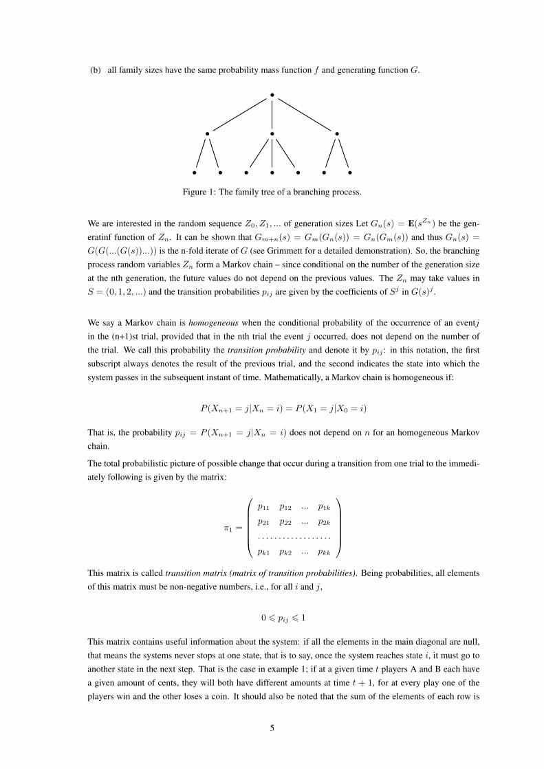
(b) all family sizes have the same probability mass function f and generating function G.

•

•

• •

•

• • •

•

• •

Figure 1: The family tree of a branching process.

We are interested in the random sequence Z0, Z1, ... of generation sizes Let Gn(s) = E(sZn) be the gen-eratinf function of Zn. It can be shown that Gm+n(s) = Gm(Gn(s)) = Gn(Gm(s)) and thus Gn(s) =

G(G(...(G(s))...)) is the n-fold iterate of G (see Grimmett for a detailed demonstration). So, the branchingprocess random variables Zn form a Markov chain – since conditional on the number of the generation sizeat the nth generation, the future values do not depend on the previous values. The Zn may take values inS = (0, 1, 2, ...) and the transition probabilities pij are given by the coefficients of Sj in G(s)j .

We say a Markov chain is homogeneous when the conditional probability of the occurrence of an eventjin the (n+1)st trial, provided that in the nth trial the event j occurred, does not depend on the number ofthe trial. We call this probability the transition probability and denote it by pij : in this notation, the firstsubscript always denotes the result of the previous trial, and the second indicates the state into which thesystem passes in the subsequent instant of time. Mathematically, a Markov chain is homogeneous if:

P (Xn+1 = j|Xn = i) = P (X1 = j|X0 = i)

That is, the probability pij = P (Xn+1 = j|Xn = i) does not depend on n for an homogeneous Markovchain.

The total probabilistic picture of possible change that occur during a transition from one trial to the immedi-ately following is given by the matrix:

π1 =

p11 p12 ... p1k

p21 p22 ... p2k

. . . . . . . . . . . . . . . . . .

pk1 pk2 ... pkk

This matrix is called transition matrix (matrix of transition probabilities). Being probabilities, all elementsof this matrix must be non-negative numbers, i.e., for all i and j,

0 6 pij 6 1

This matrix contains useful information about the system: if all the elements in the main diagonal are null,that means the systems never stops at one state, that is to say, once the system reaches state i, it must go toanother state in the next step. That is the case in example 1; if at a given time t players A and B each havea given amount of cents, they will both have different amounts at time t + 1, for at every play one of theplayers win and the other loses a coin. It should also be noted that the sum of the elements of each row is

5

equal to unity. This comes from the fact that from state Ai at time t, the system must go to one and only oneof the states Aj . This fact can be written as:

k∑j=1

pij = 1(i = 1, 2, ..., k)

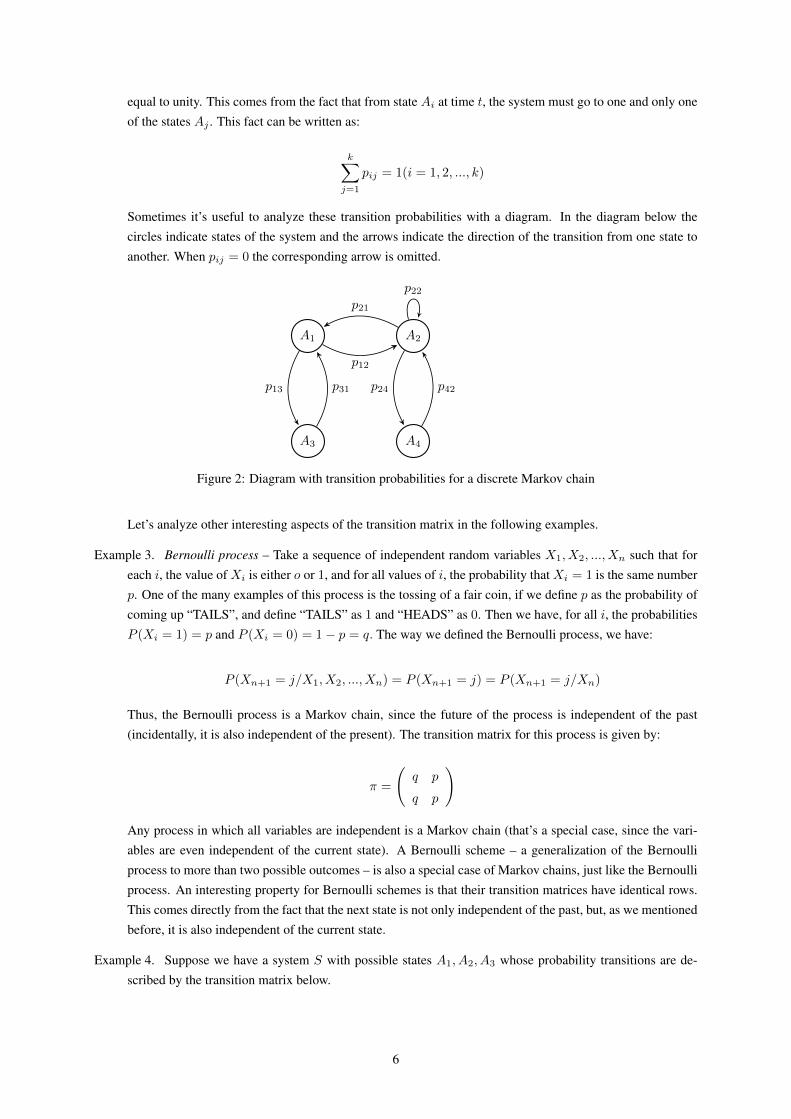
Sometimes it’s useful to analyze these transition probabilities with a diagram. In the diagram below thecircles indicate states of the system and the arrows indicate the direction of the transition from one state toanother. When pij = 0 the corresponding arrow is omitted.

A1 A2

p21

p12

A3

p13 p31

A4

p22

p24 p42

Figure 2: Diagram with transition probabilities for a discrete Markov chain

Let’s analyze other interesting aspects of the transition matrix in the following examples.

Example 3. Bernoulli process – Take a sequence of independent random variables X1, X2, ..., Xn such that foreach i, the value of Xi is either o or 1, and for all values of i, the probability that Xi = 1 is the same numberp. One of the many examples of this process is the tossing of a fair coin, if we define p as the probability ofcoming up “TAILS”, and define “TAILS” as 1 and “HEADS” as 0. Then we have, for all i, the probabilitiesP (Xi = 1) = p and P (Xi = 0) = 1− p = q. The way we defined the Bernoulli process, we have:

P (Xn+1 = j/X1, X2, ..., Xn) = P (Xn+1 = j) = P (Xn+1 = j/Xn)

Thus, the Bernoulli process is a Markov chain, since the future of the process is independent of the past(incidentally, it is also independent of the present). The transition matrix for this process is given by:

π =

(q p

q p

)

Any process in which all variables are independent is a Markov chain (that’s a special case, since the vari-ables are even independent of the current state). A Bernoulli scheme – a generalization of the Bernoulliprocess to more than two possible outcomes – is also a special case of Markov chains, just like the Bernoulliprocess. An interesting property for Bernoulli schemes is that their transition matrices have identical rows.This comes directly from the fact that the next state is not only independent of the past, but, as we mentionedbefore, it is also independent of the current state.

Example 4. Suppose we have a system S with possible states A1, A2, A3 whose probability transitions are de-scribed by the transition matrix below.

6

π =

p11 p12 p13

p21 p22 p23

p31 p32 p33

Suppose also that the Markov chain is homogeneous, that is, the transition probabilities have no relation withthe number of the trial. We are interested in knowing the probability that the system will be at state A3 twosteps ahead if it starts at state A1. We shall denote this probability as p(2)13 . A quick look shows us that stateA3 can be reached through states A1 and A2, and the probability we look for can be found considering thepossible ways we may get from state 1 to 3 passing through the other states. Then, the probability p(2)13 is:

p(2)13 = p11p13 + p12p23 + p13p33

In general, for a system with k states, we have:

p(2)ij =

k∑r=1

pirprj

It can be shown that if a Markov chain has a transition matrix π, the ijth element p(n)ij of the matrix πn givesthe probability that the Markov chain will be in state j, starting from state i, after n steps. An outline of thedemonstration is given: Suppose we have a systems which has states A1, A2, ..., Ak.Let’s denote as A(s)

i theevent that the system is in state i at time s. We want to find the probability that the system will be at statej after n steps, that is, we want to find the probability of the event A(s+n)

j . This probability was denotedabove as p(n)ij . We now examine some intermediate trial with the number (s+m). One of the possible eventsA(s+m)r , com (1 6 r 6 k) will occur in this trial, with probability p(m)

ir . The probability of transition fromstate A(s+m)

r to state A(s+n)j is p(n−m)

rj . By the formula of total probability,

p(n)ij =

k∑r=1

p(m)ir p

(n−m)rj (2.1)

This is the Kolmogorov-Chapman equation.

We denote by πn the transition matrix after n trials:

πn =

p(n)11 p

(n)12 ... p

(n)1k

p(n)21 p

(n)22 ... p

(n)2k

. . . . . . . . . . . . . . . . . . . .

p(n)k1 p

(n)k2 ... p

(n)kk

According to the formula of the total probability given above, the following relation holds between thematrices πs with different subscripts:

πn = πm · πn−m(0 < m < n)

In particular, for n = 2, we find:

π2 = π1 · π1 = π21

For n=3:

7

π3 = π1 · π2 = π1 · π21 = π3

1

And generally, for any n:

πn = πn1

We note a special case of formula (1) for m = 1:

p(n)ij =

k∑r=1

p(m)ir p

(n−1)rj (2.2)

2.2 Classification of states

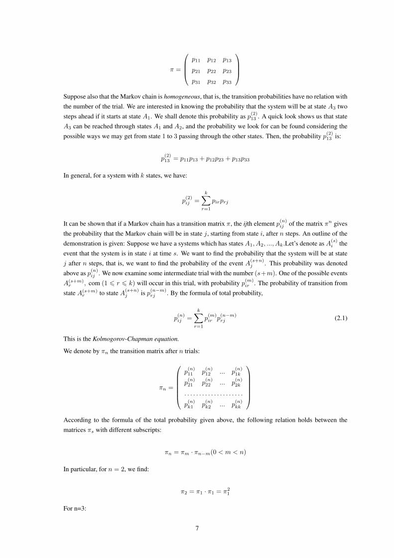
A state Ai of a Markov chain is called absorbing if it is impossible to leave it (i.e., pii = 1 and pij =

0 for i 6= j). A Markov chain is absorbing if it has at least one absorbing state, and if from every state itis possible to go to an absorbing state (not necessarily in one step). In Example 1 (the gambler’s ruin), wehave two absorbing states, one corresponding to the situation when player A gets all the cents and wins thegame, and the other is the situation when player B wins. Note that this is an example of an absorbing Markovchain: at any moment of the game, we can say that, with some probability, one of the players will get all thecents at a time (tn), thus winning the game and reaching an absorbing state. We may not all argue that thiswill eventually happen – otherwise, there wouldn’t be so many ruined gamblers! – but it is clear that it ispossible, at any given moment, that one of the players will win the game after a numbers of plays. In fact, itcan be proven that for an absorbing Markov chain, the probability that the process will be absorbed is 1.

A1

A2 A3

p31p21

p23

p32

Figure 3: State A1 is an absorbing state.

We say a state Aj is accessible from a state Ai (Ai ←→ Aj) if a system started in state Ai has a non-zeroprobability of transitioning into state Aj at some point; that is, for some n > 0:

p(n)ij > 0

A state Ai has period d if any return to state Ai must occur in multiples of d time steps. If d = 1, then thestate is said to be aperiodic: returns to state Ai can occur at irregular times.

A stateAi is called unessential (or transient) if there existAj and n such that p(ij)(n) > 0, but p(ji)(m) = 0

for all m. Thus, an unessential state possesses the property that it is possible, with positive probability, topass from it to another state, but it is no longer possible to return from that state to the original (unessential)state.

8

A1 A2

p12

A3

p13

A4

p22

p24 p42

p34

p43

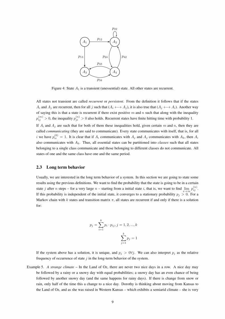
Figure 4: State A1 is a transient (unessential) state. All other states are recurrent.

All states not transient are called recurrent or persistent. From the definition it follows that if the statesAi and Aj are recurrent, then for all j such that (Ai ←→ Aj), it is also true that (Aj ←→ Ai). Another wayof saying this is that a state is recurrent if there exist positive m and n such that along with the inequalityp(m)ij > 0, the inequality p(n)ji > 0 also holds. Recurrent states have finite hitting time with probability 1.

If Ai and Aj are such that for both of them these inequalities hold, given certain m and n, then they arecalled communicating (they are said to communicate). Every state communicates with itself, that is, for alli we have p(0)ii = 1. It is clear that if Ai communicates with Aj and Aj communicates with Ak, then Aialso communicates with Ak. Thus, all essential states can be partitioned into classes such that all statesbelonging to a single class communicate and those belonging to different classes do not communicate. Allstates of one and the same class have one and the same period.

2.3 Long term behavior

Usually, we are interested in the long term behavior of a system. In this section we are going to state someresults using the previous definitions. We want to find the probability that the state is going to be in a certainstate j after n steps – for a very large n – starting from a initial state i, that is, we want to find lim

x→∞p(n)ij .

If this probability is independent of the initial state, it converges to a stationary probability pj > 0. For aMarkov chain with k states and transition matrix π, all states are recurrent if and only if there is a solutionfor:

pj =

k∑i=1

pi · pij , j = 1, 2, ..., k

k∑j=1

pj = 1

If the system above has a solution, it is unique, and pj > 0∀j. We can also interpret pj as the relativefrequency of occurrence of state j in the long-term behavior of the system.

Example 5. A strange climate – In the Land of Oz, there are never two nice days in a row. A nice day maybe followed by a rainy or a snowy day with equal probabilities; a snowy day has an even chance of beingfollowed by another snowy day (and the same happens for rainy days). If there is change from snow orrain, only half of the time this a change to a nice day. Dorothy is thinking about moving from Kansas tothe Land of Oz, and as she was raised in Western Kansas – which exhibits a semiarid climate – she is very

9

curious about the strange climate of the Land of Oz, so she asked the wonderful wizard of Oz to do somecalculations for her – because matrix multiplication is one of the wonderful things he does. What is the longterm behavior of the climate in the Land of Oz?

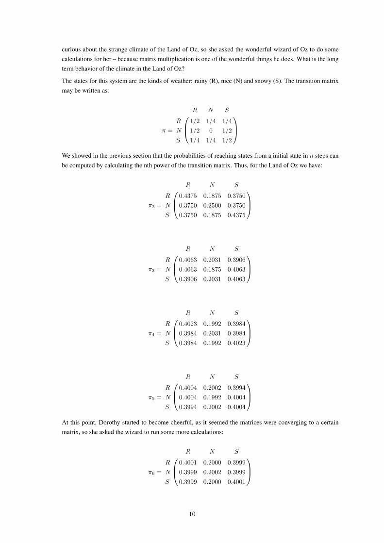
The states for this system are the kinds of weather: rainy (R), nice (N) and snowy (S). The transition matrixmay be written as:

π =

R N S

R 1/2 1/4 1/4

N 1/2 0 1/2

S 1/4 1/4 1/2

We showed in the previous section that the probabilities of reaching states from a initial state in n steps canbe computed by calculating the nth power of the transition matrix. Thus, for the Land of Oz we have:

π2 =

R N S

R 0.4375 0.1875 0.3750

N 0.3750 0.2500 0.3750

S 0.3750 0.1875 0.4375

π3 =

R N S

R 0.4063 0.2031 0.3906

N 0.4063 0.1875 0.4063

S 0.3906 0.2031 0.4063

π4 =

R N S

R 0.4023 0.1992 0.3984

N 0.3984 0.2031 0.3984

S 0.3984 0.1992 0.4023

π5 =

R N S

R 0.4004 0.2002 0.3994

N 0.4004 0.1992 0.4004

S 0.3994 0.2002 0.4004

At this point, Dorothy started to become cheerful, as it seemed the matrices were converging to a certainmatrix, so she asked the wizard to run some more calculations:

π6 =

R N S

R 0.4001 0.2000 0.3999

N 0.3999 0.2002 0.3999

S 0.3999 0.2000 0.4001

10

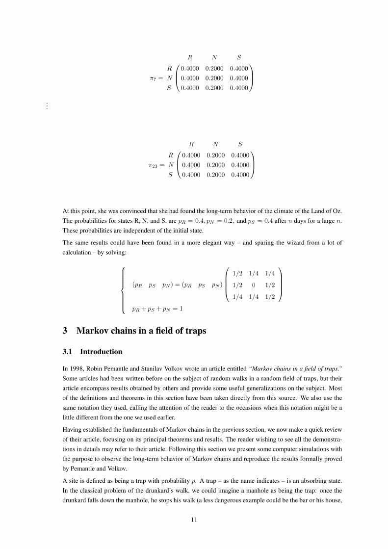
π7 =

R N S

R 0.4000 0.2000 0.4000

N 0.4000 0.2000 0.4000

S 0.4000 0.2000 0.4000

...

π23 =

R N S

R 0.4000 0.2000 0.4000

N 0.4000 0.2000 0.4000

S 0.4000 0.2000 0.4000

At this point, she was convinced that she had found the long-term behavior of the climate of the Land of Oz.The probabilities for states R, N, and S, are pR = 0.4, pN = 0.2, and pS = 0.4 after n days for a large n.These probabilities are independent of the initial state.

The same results could have been found in a more elegant way – and sparing the wizard from a lot ofcalculation – by solving:

(pR pS pN ) = (pR pS pN )

1/2 1/4 1/4

1/2 0 1/2

1/4 1/4 1/2

pR + pS + pN = 1

3 Markov chains in a field of traps

3.1 Introduction

In 1998, Robin Pemantle and Stanilav Volkov wrote an article entitled “Markov chains in a field of traps.”

Some articles had been written before on the subject of random walks in a random field of traps, but theirarticle encompass results obtained by others and provide some useful generalizations on the subject. Mostof the definitions and theorems in this section have been taken directly from this source. We also use thesame notation they used, calling the attention of the reader to the occasions when this notation might be alittle different from the one we used earlier.

Having established the fundamentals of Markov chains in the previous section, we now make a quick reviewof their article, focusing on its principal theorems and results. The reader wishing to see all the demonstra-tions in details may refer to their article. Following this section we present some computer simulations withthe purpose to observe the long-term behavior of Markov chains and reproduce the results formally provedby Pemantle and Volkov.

A site is defined as being a trap with probability p. A trap – as the name indicates – is an absorbing state.In the classical problem of the drunkard’s walk, we could imagine a manhole as being the trap: once thedrunkard falls down the manhole, he stops his walk (a less dangerous example could be the bar or his house,

11

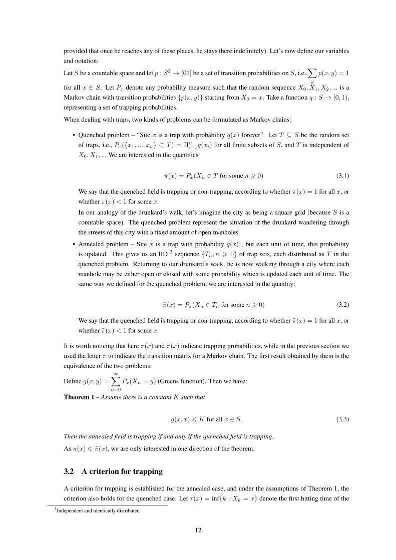
provided that once he reaches any of these places, he stays there indefinitely). Let’s now define our variablesand notation:

Let S be a countable space and let p : S2 → [01] be a set of transition probabilities on S, i.e.,∑y

p(x, y) = 1

for all x ∈ S. Let Px denote any probability measure such that the random sequence X0, X1, X2, ... is aMarkov chain with transition probabilities {p(x, y)} starting from X0 = x. Take a function q : S → [0, 1),representing a set of trapping probabilities.

When dealing with traps, two kinds of problems can be formulated as Markov chains:

• Quenched problem – “Site x is a trap with probability q(x) forever”. Let T ⊆ S be the random setof traps, i.e., Px({x1, ..., xn} ⊂ T ) = Πn

i=1q(xi) for all finite subsets of S, and T is independent ofX0, X1, ... We are interested in the quantities

π(x) = Px(Xn ∈ T for some n > 0) (3.1)

We say that the quenched field is trapping or non-trapping, according to whether π(x) = 1 for all x, orwhether π(x) < 1 for some x.

In our analogy of the drunkard’s walk, let’s imagine the city as being a square grid (because S is acountable space). The quenched problem represent the situation of the drunkard wandering throughthe streets of this city with a fixed amount of open manholes.

• Annealed problem – Site x is a trap with probability q(x) , but each unit of time, this probabilityis updated. This gives us an IID 3 sequence {Tn, n > 0} of trap sets, each distributed as T in thequenched problem. Returning to our drunkard’s walk, he is now walking through a city where eachmanhole may be either open or closed with some probability which is updated each unit of time. Thesame way we defined for the quenched problem, we are interested in the quantity:

π̃(x) = Px(Xn ∈ Tn for some n > 0) (3.2)

We say that the quenched field is trapping or non-trapping, according to whether π̃(x) = 1 for all x, orwhether π̃(x) < 1 for some x.

It is worth noticing that here π(x) and π̃(x) indicate trapping probabilities, while in the previous section weused the letter π to indicate the transition matrix for a Markov chain. The first result obtained by them is theequivalence of the two problems:

Define g(x, y) =

∞∑n=0

Px(Xn = y) (Greens function). Then we have:

Theorem 1 – Assume there is a constant K such that

g(x, x) 6 K for all x ∈ S. (3.3)

Then the annealed field is trapping if and only if the quenched field is trapping.

As π(x) 6 π̃(x), we are only interested in one direction of the theorem.

3.2 A criterion for trapping

A criterion for trapping is established for the annealed case, and under the assumptions of Theorem 1, thecriterion also holds for the quenched case. Let τ(x) = inf{k : Xk = x} denote the first hitting time of the

3Independent and identically distributed

12

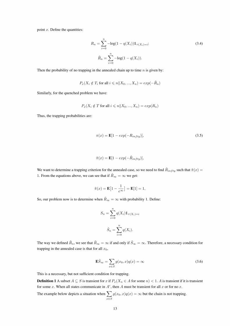
point x. Define the quantities:

Rn =

n∑i=0

−log(1− q(Xi))1τ(Xi)=i; (3.4)

R̃n =

n∑i=0

−log(1− q(Xi)).

Then the probability of no trapping in the annealed chain up to time n is given by:

Px(Xi /∈ Ti for all i 6 n‖X0, ..., Xn) = exp(−R̃n)

Similarly, for the quenched problem we have:

Px(Xi /∈ T for all i 6 n‖X0, ..., Xn) = exp(Rn)

Thus, the trapping probabilities are:

π(x) = E[1− exp(−Rinfty)], (3.5)

π̃(x) = E[1− exp(−R̃infty)],

We want to determine a trapping criterion for the annealed case, so we need to find R̃infty such that π̃(x) =

1. From the equations above, we can see that if R̃∞ =∞ we get:

π̃(x) = E[1− 1

e∞]

= E[1] = 1,

So, our problem now is to determine when R̃∞ =∞ with probability 1. Define:

Sn =

n∑i=0

q(Xi)1τ(Xi)=i

S̃n =

n∑i=0

q(Xi).

The way we defined R̃n, we see that R̃∞ =∞ if and only if S̃∞ =∞. Therefore, a necessary condition fortrapping in the annealed case is that for all x0,

ES̃∞ =∑x∈S

g(x0, x)q(x) =∞ (3.6)

This is a necessary, but not sufficient condition for trapping.

Definition 1 A subsetA ⊆ S is transient for x if Px(Xn ∈ A for some n) < 1. A is transient if it is transientfor some x. When all states communicate in Ac, then A must be transient for all x or for no x.

The example below depicts a situation when∑x∈S

g(x0, x)q(x) =∞ but the chain is not trapping.

13

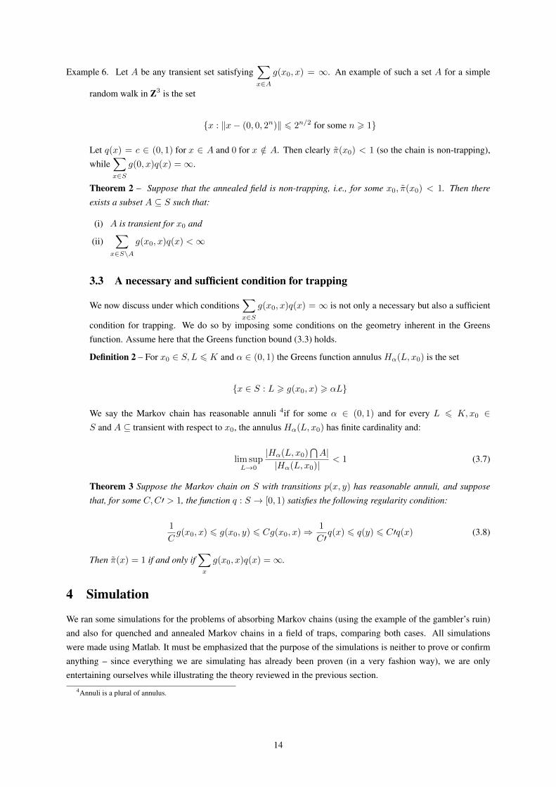
Example 6. Let A be any transient set satisfying∑x∈A

g(x0, x) = ∞. An example of such a set A for a simple

random walk in Z3 is the set

{x : ‖x− (0, 0, 2n)‖ 6 2n/2 for some n > 1}

Let q(x) = c ∈ (0, 1) for x ∈ A and 0 for x /∈ A. Then clearly π̃(x0) < 1 (so the chain is non-trapping),while

∑x∈S

g(0, x)q(x) =∞.

Theorem 2 – Suppose that the annealed field is non-trapping, i.e., for some x0, π̃(x0) < 1. Then there

exists a subset A ⊆ S such that:

(i) A is transient for x0 and

(ii)∑

x∈S\A

g(x0, x)q(x) <∞

3.3 A necessary and sufficient condition for trapping

We now discuss under which conditions∑x∈S

g(x0, x)q(x) = ∞ is not only a necessary but also a sufficient

condition for trapping. We do so by imposing some conditions on the geometry inherent in the Greensfunction. Assume here that the Greens function bound (3.3) holds.

Definition 2 – For x0 ∈ S,L 6 K and α ∈ (0, 1) the Greens function annulus Hα(L, x0) is the set

{x ∈ S : L > g(x0, x) > αL}

We say the Markov chain has reasonable annuli 4if for some α ∈ (0, 1) and for every L 6 K,x0 ∈S and A ⊆ transient with respect to x0, the annulus Hα(L, x0) has finite cardinality and:

lim supL→0

|Hα(L, x0)⋂A|

|Hα(L, x0)|< 1 (3.7)

Theorem 3 Suppose the Markov chain on S with transitions p(x, y) has reasonable annuli, and suppose

that, for some C,C′ > 1, the function q : S → [0, 1) satisfies the following regularity condition:

1

Cg(x0, x) 6 g(x0, y) 6 Cg(x0, x)⇒ 1

C′q(x) 6 q(y) 6 C′q(x) (3.8)

Then π̃(x) = 1 if and only if∑x

g(x0, x)q(x) =∞.

4 Simulation

We ran some simulations for the problems of absorbing Markov chains (using the example of the gambler’s ruin)and also for quenched and annealed Markov chains in a field of traps, comparing both cases. All simulationswere made using Matlab. It must be emphasized that the purpose of the simulations is neither to prove or confirmanything – since everything we are simulating has already been proven (in a very fashion way), we are onlyentertaining ourselves while illustrating the theory reviewed in the previous section.

4Annuli is a plural of annulus.

14

4.1 Gambler’s ruins

As mentioned in example (number), two players each have a finite number of coins, say n1 and n2. A coin isflipped. If the result is TAILS, player 1 gives one of his coins to player 2. If the result is HEADS, player 2 givesone of his coins to player 1. The game stops when one of the players runs out of coins. The probability that aplayer will go bankrupt is equal to the ratio of the amount of coins his opponent have to the total amount of coins.Calling Pi the probability that player i will go bankrupt (which we shall refer as “failure”), we have:

P1 =n2

n1 + n2

P2 =n1

n1 + n2

We wrote a small code in Matlab to examine the probabilities above. We do this by running the code severaltimes and comparing the frequencies FN1 and FN2 of failure for each player with the calculated probabilities.Matlab has special commands to generate pseudo-random numbers and arrays. Some of them worth mentioningare:

• rand – Basic syntax: rand(n) returns an n-by-n matrix containing pseudo-random values drawn from thestandard uniform distribution on the open interval (0,1).

• randi – Basic syntax: r = randi(imax,n)returns an n-by-n matrix containing pseudo-random integer valuesdrawn from the discrete uniform distribution on 1:imax.

• randn – Basic syntax: r = randn(n) returns an n-by-n matrix containing pseudo-random values drawn fromthe standard normal distribution.

• binornd – Basic syntax: binornd(N,P). This command generates random numbers from the binomial distri-bution with parameters specified by the number of trials, N, and probability of success for each trial, P. Nand P can be vectors, matrices, or multidimensional arrays that have the same size, which is also the size ofR. A scalar input for N or P is expanded to a constant array with the same dimensions as the other input.

• sprandsym – Basic syntax: sprandsym(S) returns a symmetric random matrix whose lower triangle anddiagonal have the same structure as S. Its elements are normally distributed, with mean 0 and variance 1.

• sprand – Basic syntax: sprand(S)has the same sparsity structure as S, but uniformly distributed randomentries.

• sprandn – Basic syntax: sprandn(S)has the same sparsity structure as S, but normally distributed randomentries with mean 0 and variance 1.

• randsrc – Basic syntax: randsrc(m)generates an m-by-m matrix, each of whose entries independently takesthe value -1 with probability 1/2, and 1 with probability 1/2. This command can also be used to generatea random matrix using prescribed alphabet. This is done by the elements of the alphabet, and the prob-abilities of occurrence of each element. Then, a m × n random matrix is generated with the commandrandsrc(m,n,[alphabet; prob]).

Each of these commands have many possibilities as to parameters input; ore information on the syntax of eachcommand and some examples can be found at the MathWorks website (see references).

Below is the pseudo-code for our program. The inputs are the quantities of coins n1 and n2 each player hasat the beginning of the game and p, the probability of a coin turning HEADS (the probability that player 1 wins acoin from player 2) and m, the desired number of matches. The output is: N1, the number of failures for player

15

1 out of m matches; N2, the number of failures for player 2; v, a vector of length m which stores informationof the number of steps at each match until one of the players wins the game, and mv, which is just the mean ofvector v. When mv is not an integer, we simply take the closest integer, since the purpose of this part of the code isjust to give a glimpse at the magnitude of the number of steps until the end of the game as the initial conditions vary.

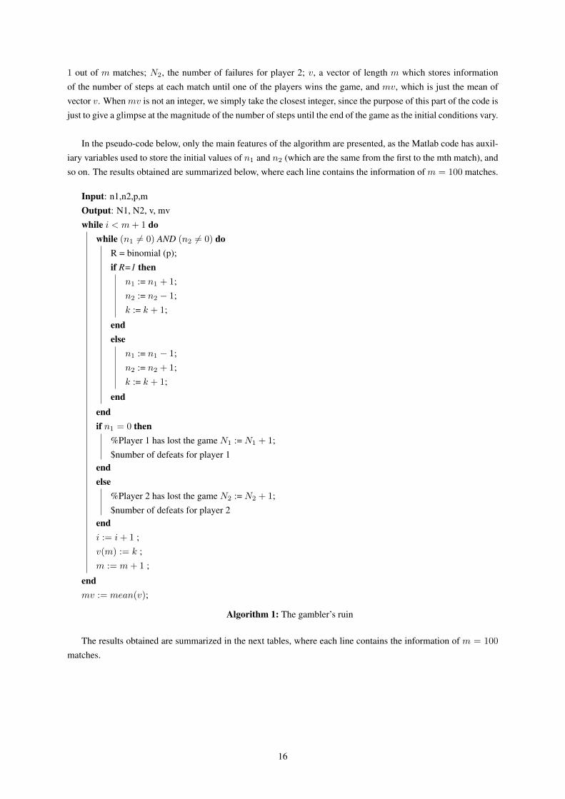
In the pseudo-code below, only the main features of the algorithm are presented, as the Matlab code has auxil-iary variables used to store the initial values of n1 and n2 (which are the same from the first to the mth match), andso on. The results obtained are summarized below, where each line contains the information of m = 100 matches.

Input: n1,n2,p,mOutput: N1, N2, v, mvwhile i < m+ 1 do

while (n1 6= 0) AND (n2 6= 0) doR = binomial (p);if R=1 then

n1 := n1 + 1;n2 := n2 − 1;k := k + 1;

endelse

n1 := n1 − 1;n2 := n2 + 1;k := k + 1;

endendif n1 = 0 then

%Player 1 has lost the game N1 := N1 + 1;$number of defeats for player 1

endelse

%Player 2 has lost the game N2 := N2 + 1;$number of defeats for player 2

endi := i+ 1 ;v(m) := k ;m := m+ 1 ;

endmv := mean(v);

Algorithm 1: The gambler’s ruin

The results obtained are summarized in the next tables, where each line contains the information of m = 100

matches.

16

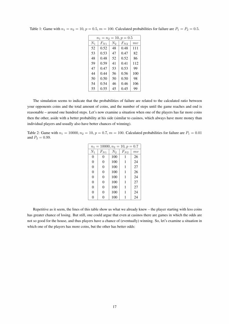
Table 1: Game with n1 = n2 = 10, p = 0.5, m = 100. Calculated probabilities for failure are P1 = P2 = 0.5.

n1 = n2 = 10, p = 0.5

N1 FN1 N2 FN2 mv

52 0.52 48 0.48 11153 0.53 47 0.47 8248 0.48 52 0.52 8659 0.59 41 0.41 11247 0.47 53 0.53 9944 0.44 56 0.56 10050 0.50 50 0.50 9854 0.54 46 0.46 10655 0.55 45 0.45 99

The simulation seems to indicate that the probabilities of failure are related to the calculated ratio betweenyour opponents coins and the total amount of coins, and the number of steps until the game reaches and end isreasonable – around one hundred steps. Let’s now examine a situation when one of the players has far more coinsthen the other, aside with a better probability at his side (similar to casinos, which always have more money thanindividual players and usually also have better chances of winning).

Table 2: Game with n1 = 10000, n2 = 10, p = 0.7, m = 100. Calculated probabilities for failure are P1 = 0.01and P2 = 0.99.

n1 = 10000, n2 = 10, p = 0.7

N1 FN1 N2 FN2 mv

0 0 100 1 260 0 100 1 240 0 100 1 270 0 100 1 260 0 100 1 240 0 100 1 270 0 100 1 270 0 100 1 240 0 100 1 24

Repetitive as it seem, the lines of this table show us what we already knew – the player starting with less coinshas greater chance of losing. But still, one could argue that even at casinos there are games in which the odds arenot so good for the house, and thus players have a chance of (eventually) winning. So, let’s examine a situation inwhich one of the players has more coins, but the other has better odds:

17

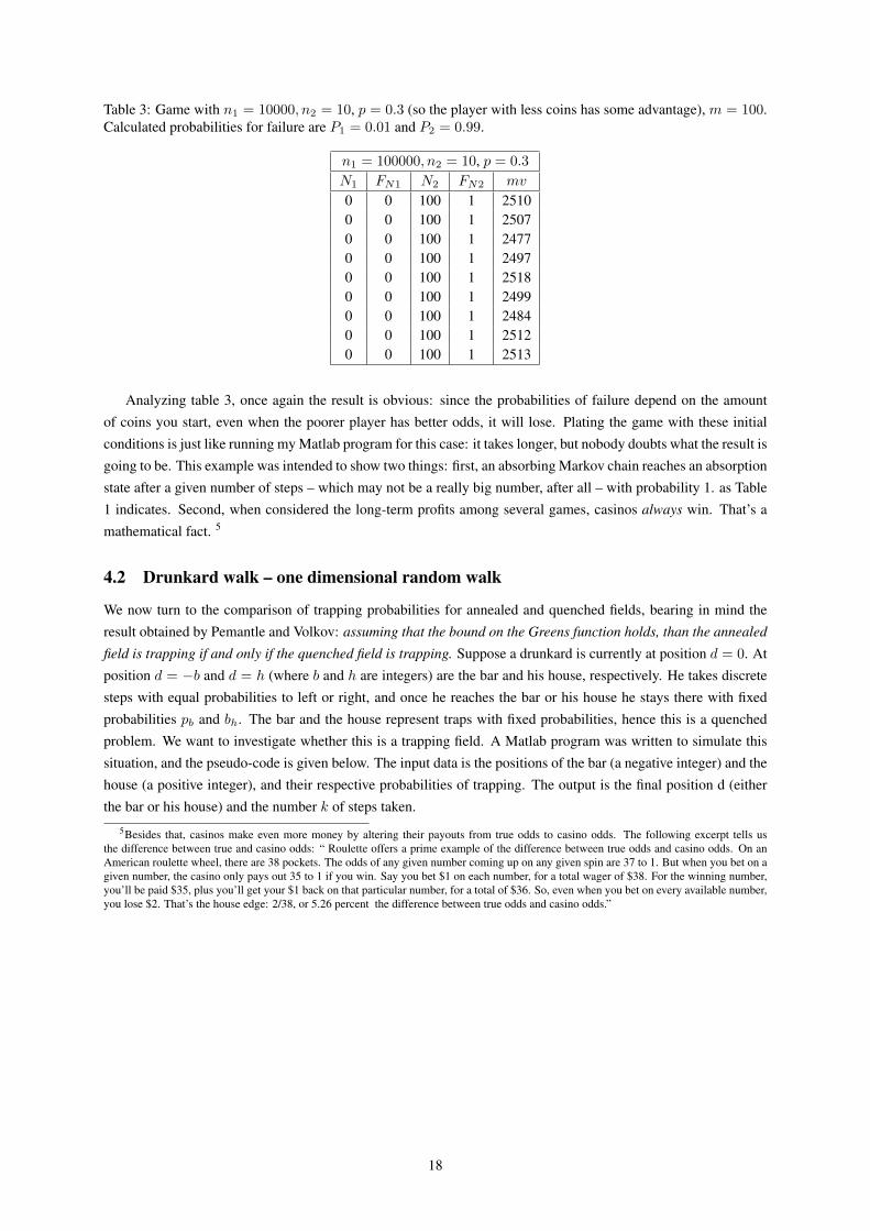
Table 3: Game with n1 = 10000, n2 = 10, p = 0.3 (so the player with less coins has some advantage), m = 100.Calculated probabilities for failure are P1 = 0.01 and P2 = 0.99.

n1 = 100000, n2 = 10, p = 0.3

N1 FN1 N2 FN2 mv

0 0 100 1 25100 0 100 1 25070 0 100 1 24770 0 100 1 24970 0 100 1 25180 0 100 1 24990 0 100 1 24840 0 100 1 25120 0 100 1 2513

Analyzing table 3, once again the result is obvious: since the probabilities of failure depend on the amountof coins you start, even when the poorer player has better odds, it will lose. Plating the game with these initialconditions is just like running my Matlab program for this case: it takes longer, but nobody doubts what the result isgoing to be. This example was intended to show two things: first, an absorbing Markov chain reaches an absorptionstate after a given number of steps – which may not be a really big number, after all – with probability 1. as Table1 indicates. Second, when considered the long-term profits among several games, casinos always win. That’s amathematical fact. 5

4.2 Drunkard walk – one dimensional random walk

We now turn to the comparison of trapping probabilities for annealed and quenched fields, bearing in mind theresult obtained by Pemantle and Volkov: assuming that the bound on the Greens function holds, than the annealed

field is trapping if and only if the quenched field is trapping. Suppose a drunkard is currently at position d = 0. Atposition d = −b and d = h (where b and h are integers) are the bar and his house, respectively. He takes discretesteps with equal probabilities to left or right, and once he reaches the bar or his house he stays there with fixedprobabilities pb and bh. The bar and the house represent traps with fixed probabilities, hence this is a quenchedproblem. We want to investigate whether this is a trapping field. A Matlab program was written to simulate thissituation, and the pseudo-code is given below. The input data is the positions of the bar (a negative integer) and thehouse (a positive integer), and their respective probabilities of trapping. The output is the final position d (eitherthe bar or his house) and the number k of steps taken.

5Besides that, casinos make even more money by altering their payouts from true odds to casino odds. The following excerpt tells usthe difference between true and casino odds: “ Roulette offers a prime example of the difference between true odds and casino odds. On anAmerican roulette wheel, there are 38 pockets. The odds of any given number coming up on any given spin are 37 to 1. But when you bet on agiven number, the casino only pays out 35 to 1 if you win. Say you bet $1 on each number, for a total wager of $38. For the winning number,you’ll be paid $35, plus you’ll get your $1 back on that particular number, for a total of $36. So, even when you bet on every available number,you lose $2. That’s the house edge: 2/38, or 5.26 percent the difference between true odds and casino odds.”

18

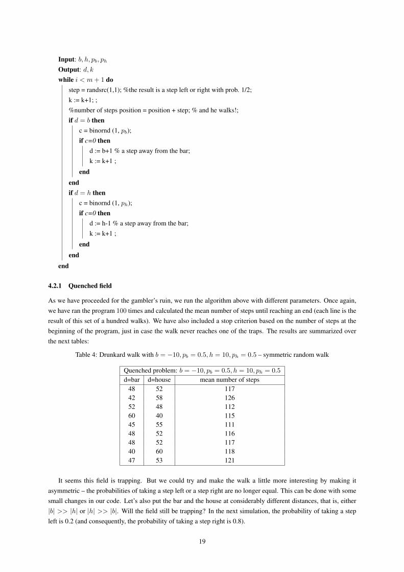
Input: b, h, pb, phOutput: d, kwhile i < m+ 1 do

step = randsrc(1,1); %the result is a step left or right with prob. 1/2;k := k+1; ;%number of steps position = position + step; % and he walks!;if d = b then

c = binornd (1, pb);if c=0 then

d := b+1 % a step away from the bar;k := k+1 ;

endendif d = h then

c = binornd (1, ph);if c=0 then

d := h-1 % a step away from the bar;k := k+1 ;

endend

end

4.2.1 Quenched field

As we have proceeded for the gambler’s ruin, we run the algorithm above with different parameters. Once again,we have ran the program 100 times and calculated the mean number of steps until reaching an end (each line is theresult of this set of a hundred walks). We have also included a stop criterion based on the number of steps at thebeginning of the program, just in case the walk never reaches one of the traps. The results are summarized overthe next tables:

Table 4: Drunkard walk with b = −10, pb = 0.5, h = 10, ph = 0.5 – symmetric random walk

Quenched problem: b = −10, pb = 0.5, h = 10, ph = 0.5

d=bar d=house mean number of steps48 52 11742 58 12652 48 11260 40 11545 55 11148 52 11648 52 11740 60 11847 53 121

It seems this field is trapping. But we could try and make the walk a little more interesting by making itasymmetric – the probabilities of taking a step left or a step right are no longer equal. This can be done with somesmall changes in our code. Let’s also put the bar and the house at considerably different distances, that is, either|b| >> |h| or |h| >> |b|. Will the field still be trapping? In the next simulation, the probability of taking a stepleft is 0.2 (and consequently, the probability of taking a step right is 0.8).

19

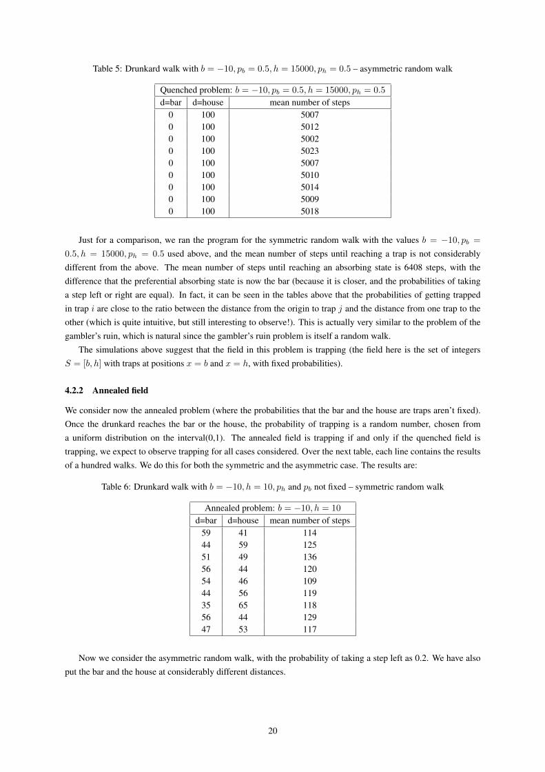
Table 5: Drunkard walk with b = −10, pb = 0.5, h = 15000, ph = 0.5 – asymmetric random walk

Quenched problem: b = −10, pb = 0.5, h = 15000, ph = 0.5

d=bar d=house mean number of steps0 100 50070 100 50120 100 50020 100 50230 100 50070 100 50100 100 50140 100 50090 100 5018

Just for a comparison, we ran the program for the symmetric random walk with the values b = −10, pb =

0.5, h = 15000, ph = 0.5 used above, and the mean number of steps until reaching a trap is not considerablydifferent from the above. The mean number of steps until reaching an absorbing state is 6408 steps, with thedifference that the preferential absorbing state is now the bar (because it is closer, and the probabilities of takinga step left or right are equal). In fact, it can be seen in the tables above that the probabilities of getting trappedin trap i are close to the ratio between the distance from the origin to trap j and the distance from one trap to theother (which is quite intuitive, but still interesting to observe!). This is actually very similar to the problem of thegambler’s ruin, which is natural since the gambler’s ruin problem is itself a random walk.

The simulations above suggest that the field in this problem is trapping (the field here is the set of integersS = [b, h] with traps at positions x = b and x = h, with fixed probabilities).

4.2.2 Annealed field

We consider now the annealed problem (where the probabilities that the bar and the house are traps aren’t fixed).Once the drunkard reaches the bar or the house, the probability of trapping is a random number, chosen froma uniform distribution on the interval(0,1). The annealed field is trapping if and only if the quenched field istrapping, we expect to observe trapping for all cases considered. Over the next table, each line contains the resultsof a hundred walks. We do this for both the symmetric and the asymmetric case. The results are:

Table 6: Drunkard walk with b = −10, h = 10, ph and pb not fixed – symmetric random walk

Annealed problem: b = −10, h = 10

d=bar d=house mean number of steps59 41 11444 59 12551 49 13656 44 12054 46 10944 56 11935 65 11856 44 12947 53 117

Now we consider the asymmetric random walk, with the probability of taking a step left as 0.2. We have alsoput the bar and the house at considerably different distances.

20

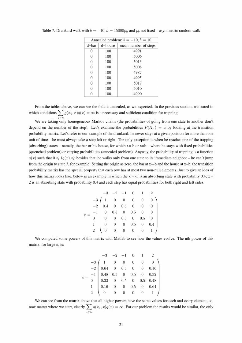
Table 7: Drunkard walk with b = −10, h = 15000ph and pb not fixed – asymmetric random walk

Annealed problem: b = −10, h = 10

d=bar d=house mean number of steps0 100 49910 100 50060 100 50130 100 50080 100 49870 100 49950 100 50170 100 50100 100 4990

From the tables above, we can see the field is annealed, as we expected. In the previous section, we stated inwhich conditions

∑x∈S

g(x0, x)q(x) =∞ is a necessary and sufficient condition for trapping.

We are taking only homogeneous Markov chains (the probabilities of going from one state to another don’tdepend on the number of the step). Let’s examine the probabilities P (Xn) = x by looking at the transitionprobability matrix. Let’s refer to our example of the drunkard: he never stays at a given position for more than oneunit of time – he must always take a step left or right. The only exception is when he reaches one of the trapping(absorbing) states – namely, the bar or his house, for which x=-b or x=h – where he stays with fixed probabilities(quenched problem) or varying probabilities (annealed problem). Anyway, the probability of trapping is a functionq(x) such that 0 6 1q(x) 6; besides that, he walks only from one state to its immediate neighbor – he can’t jumpfrom the origin to state 3, for example. Setting the origin as zero, the bar at x=-b and the house at x=h, the transitionprobability matrix has the special property that each row has at most two non-null elements. Just to give an idea ofhow this matrix looks like, below is an example in which the x = -3 is an absorbing state with probability 0.4; x =2 is an absorbing state with probability 0.4 and each step has equal probabilities for both right and left sides.

π =

−3 −2 −1 0 1 2

−3 1 0 0 0 0 0

−2 0.4 0 0.5 0 0 0

−1 0 0.5 0 0.5 0 0

0 0 0 0.5 0 0.5 0

1 0 0 0 0.5 0 0.4

2 0 0 0 0 0 1

We computed some powers of this matrix with Matlab to see how the values evolve. The nth power of this

matrix, for large n, is:

π =

−3 −2 −1 0 1 2

−3 1 0 0 0 0 0

−2 0.64 0 0.5 0 0 0.16

−1 0.48 0.5 0 0.5 0 0.32

0 0.32 0 0.5 0 0.5 0.48

1 0.16 0 0 0.5 0 0.64

2 0 0 0 0 0 1

We can see from the matrix above that all higher powers have the same values for each and every element, so,

now matter where we start, clearly∑x∈S

g(x0, x)q(x) =∞. For our problem the results would be similar, the only

21

difference being the size of the matrix. As most Markov chains, a simple random walk has reasonable annuli (see[7]), and so our condition is sufficient and enough for trapping.

5 Conclusions

The simulations all showed the same results that were proved theoretically. Also, while writing the code used to runthe simulations we confirmed the simplicity and power of modeling phenomena as Markov chains: the algorithmsare very simple and can easily be changed to study more complex phenomena (provided that this is still a Markovchain, of course), as all it takes to run these programs is essentially a random number generator.

6 References

[1] Drie, John H. Van. “What Laplace really said - the myth of Laplacian determinism”

[2] Gnedenko, B. V. The Theory of Probability. Mir Publishers, Moscow, 1969.

[3] Grimmett, G. , David Stirzaker Probability and Random Processes. Oxford University Press, New York, 3rdedition 2001.

[4] Hannun, Robert C. “A Guide to Casino Mathematics”.

[5] MATLAB version 7.0.0. The MathWorks Inc, Natick, Massachusetts, 2004.

[6] MathWorks Product Documentation

[7] Pemantle, R. , Stanislav Volkov,“Markov Chains in a Field of Traps”.Journal of Theoretical Probability, 1April 1998, 561-569.

[8] Shiryaev, A. N. Probability. Springer 2nd. edition 1996.

[9] Weisstein, Eric W. “Gambler’s Ruin.” From MathWorld–A Wolfram Web Resource.

[10] Schneider, Meg E. ‘Playing Against the House”.

22