Markov analysis and Kramers--Moyal expansion of the ...

Markov analysis and Kramers–Moyal expansion of the ballistic deposition and restricted solid-

on-solid models

This article has been downloaded from IOPscience. Please scroll down to see the full text article.

J. Stat. Mech. (2008) P02010

(http://iopscience.iop.org/1742-5468/2008/02/P02010)

Download details:

IP Address: 134.106.40.32

The article was downloaded on 18/06/2012 at 12:37

Please note that terms and conditions apply.

View the table of contents for this issue, or go to the journal homepage for more

Home Search Collections Journals About Contact us My IOPscience

J.Stat.M

ech.(2008)

P02010

ournal of Statistical Mechanics:An IOP and SISSA journalJ Theory and Experiment

Markov analysis and Kramers–Moyalexpansion of the ballistic deposition andrestricted solid-on-solid models

S Kimiagar1, G R Jafari2,3 and M Reza Rahimi Tabar4,5

1 Plasma Physics Research Center, Science and Research Campus, Islamic AzadUniversity, Tehran, Iran2 Department of Physics, Shahid Beheshti University, Evin, Tehran 19839, Iran3 Department of Nano-Science, IPM, PO Box 19395-5531, Tehran, Iran4 Department of Physics, Sharif University of Technology, PO Box 11365-9161,Tehran, Iran5 Carl von Ossietzky University, Institute of Physics, D-26111 Oldenburg,GermanyE-mail: [email protected], [email protected] [email protected]

Received 29 July 2007Accepted 6 February 2008Published 26 February 2008

Online at stacks.iop.org/JSTAT/2008/P02010doi:10.1088/1742-5468/2008/02/P02010

Abstract. It is well known that the ballistic deposition and the restricted solid-on-solid models belong to the same universality class, having the same roughnessand growth exponents. In this paper, we determine some new statisticalproperties of the two models, such as the Kramers–Moyal coefficients and theMarkov length scale, and show them to be distinct for the two models.

Keywords: self-affine roughness (theory), stochastic processes (theory)

c©2008 IOP Publishing Ltd and SISSA 1742-5468/08/P02010+13$30.00

J.Stat.M

ech.(2008)

P02010

Markov analysis and Kramers–Moyal expansion

Contents

1. Introduction 2

2. The Markov nature of the height fluctuations: the drift and diffusion coefficients 3

3. The Kramers–Moyal coefficients of the BD and RSOS increments 10

4. Markov length scale and roughness exponent of the surface 10

Acknowledgment 12

References 12

1. Introduction

The study of the statistical properties of surfaces growing under the deposition ofparticles has attracted many researchers over the last two decades [1]–[7]. The theoreticaldescription of the surface growth processes has been accomplished using a number ofdiscrete and continuous models that belong mainly to three groups: the Edwards–Wilkinson model [8], the Kardar–Parisi–Zhang equation (KPZ) [9], and models basedon molecular beam epitaxy [10]. The focus of such studies has been the statisticalcharacterization of the growing surface. This is achieved by estimating the roughnessexponent of the steady-state surface, the growth exponent [11], and the scaling functionsassociated with the steady-state evolution of the surface [12]–[16].

The simplest quantitative characteristic of a given surface or interface is its roughness,also called the interface width, defined as the root mean square fluctuation of the heightaround its average position. The width w is usually averaged over different configurations,and its scaling with the time and length of the substrate is used to characterize the growthprocess. Consider a sample of size L and define the mean height of the growing film hand its roughness w by the following expressions:

w(L, t) = (〈(h − h)2〉)1/2, (1)

where t is proportional to the deposition time and 〈· · ·〉 denotes an averaging over differentsamples. For simplicity, and without loss of generality, we assume that h = 0. Startingfrom a flat interface (one of the possible initial conditions), it was conjectured by Familyand Vicsek that a scaling of space by factor b and of time by factor bz (z is the dynamicalscaling exponent) rescales the roughness w by the factor bα as [17]

w(bL, bzt) = bαw(L, t), (2)

which implies that

w(L, t) = Lαf(t/Lz). (3)

If for large t and fixed L(t/Lz → ∞), w saturates, then f(x) −→ g as x −→ ∞. However,for fixed and large L and t � Lz, one expects correlations of the height fluctuations toexist only within a distance t1/z and, thus, they must be independent of L. This implies

doi:10.1088/1742-5468/2008/02/P02010 2

J.Stat.M

ech.(2008)

P02010

Markov analysis and Kramers–Moyal expansion

that for x � 1, f(x) ∼ xβg′ with β = α/z. Thus, for dynamic scaling one postulates that

w(L, t) =

{tβg ∼ tβ, t � Lz;

Lαg′ ∼ Lα, t � Lz.(4)

The roughness exponent α and the dynamic exponent z characterize the self-affinegeometry of the surface and its dynamics, respectively. The dependence of the roughnessw on h or t indicates that w has a fixed value for a given time.

A main problem in this area of research has been the scaling behavior of the momentsof the height difference, Δh = h(x1)− h(x2), and the evolution of the probability densityfunction (PDF) of Δh, i.e., P (Δh, Δx), in terms of the length scale Δx. Recently, Friedrichand Peinke were able to derive a Fokker–Planck equation which describes the evolutionof the probability distribution function in terms of the length scale, for several stochasticphenomena, such as rough surfaces [18]–[20], turbulent flows [21], financial data [22, 23],heart interbeats [24], etc. They pointed out that the conditional probability densityof the field increments (velocity field, etc) satisfies the Chapman–Kolmogorov equation.Mathematically, this is a necessary condition for the fluctuating data to follow a Markovprocess in the length scales [5].

In this paper we compute the Kramers–Moyal (KM) coefficients for the fluctuatingfield Δh = h(x + Δx) − h(x) of the restricted solid-on-solid (RSOS) and the ballisticdeposition (BD) models, and show that their first and second KM coefficients havewell-defined values, whereas their third- and fourth-order KM coefficients tend to zero.Although the models have the same roughness and dynamical exponents, we show thatthey have distinct KM coefficients, and are described by distinct stochastic Langevinequations [25]. Hence, our computations make it possible to better distinguish the twomodels.

2. The Markov nature of the height fluctuations: the drift and diffusion coefficients

The first model analyzed here is the RSOS model [26] in which the incident particle sticksat the top of a growing column only if the differences of heights of all pairs of neighboringcolumns do not exceed ΔHmax = 1. Otherwise, the attempt for the growth of the surfaceis rejected. The second model was proposed for etching of a crystalline solid, by Mello et al[27]: in each growth attempt a randomly chosen column i, with current height h(i) = h0,has its height increased by one unit [h(i) → h0 + 1], and all the neighboring columnswhose heights are smaller than h0 grow to h0 (this may be called the growth version ofthe etching model [28]).

In the simplest version of the BD model, particles are released from a randomly chosenposition above a d-dimensional substrate, follow trajectories perpendicular to the surfaceand stick to it upon first contact with a nearest-neighbor occupied site. The resultingaggregate is porous and has a rough surface. Several applications of the BD model or itsextensions to real growth processes have already been proposed, which justify the presentanalysis (see, for example, the recent applications in [29, 30]).

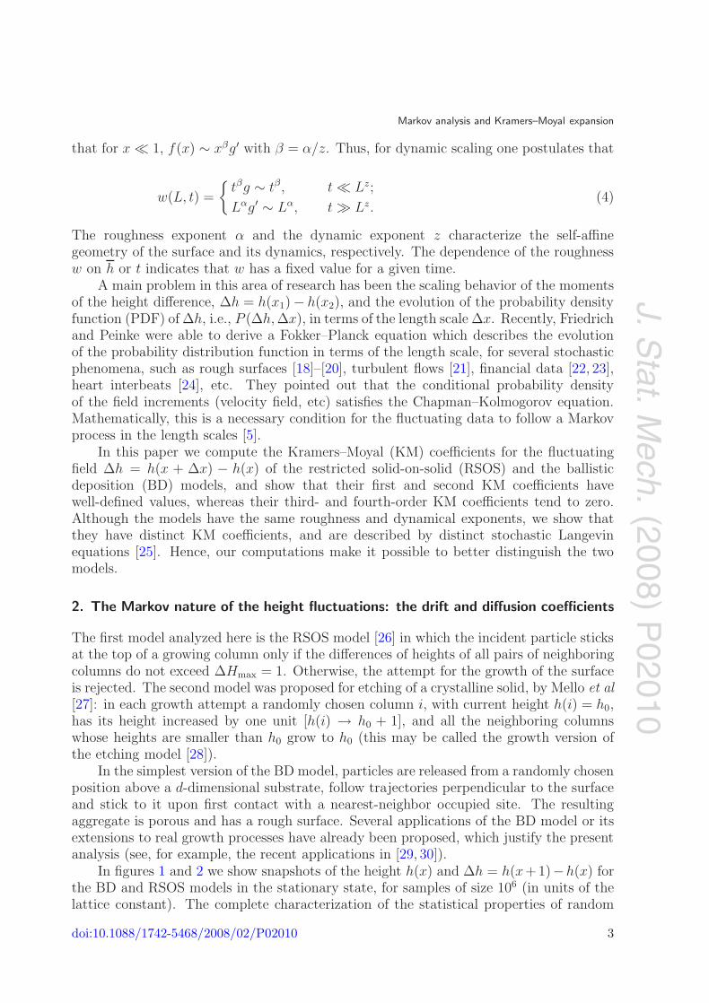
In figures 1 and 2 we show snapshots of the height h(x) and Δh = h(x+1)−h(x) forthe BD and RSOS models in the stationary state, for samples of size 106 (in units of thelattice constant). The complete characterization of the statistical properties of random

doi:10.1088/1742-5468/2008/02/P02010 3

J.Stat.M

ech.(2008)

P02010

Markov analysis and Kramers–Moyal expansion

Figure 1. Snapshots of the height fluctuations of h(x) and Δh = h(x + 1)−h(x)for the BD model, after saturation.

fluctuations of a quantity, such as the height h of the surface in the two models, in termsof a parameter x requires evaluation of the joint PDF, i.e., PN(h1, x1, . . . , hN , xN ), foran arbitrary N . If the process is a Markov process, an important simplification arises,since in this case PN can be generated by a product of the conditional probabilitiesP (hi+1, xi+1|hi, xi), for i = 1, . . . , N − 1. As a necessary condition for the fluctuationbeing a Markov process, the Chapman–Kolmogorov equation [5],

P (h2, x2|h1, x1) =

∫d(hi) P (h2, x2|hi, xi) P (hi, xi|h1, x1), (5)

should hold for any value of xi, in the interval x2 < xi < x1.Let us first check that the height fluctuations represent a Markov process, and

determine their corresponding Markov length scales LM. The Markov length scale LM

is the minimum length over which the data can be considered as a Markov process. Here,

doi:10.1088/1742-5468/2008/02/P02010 4

J.Stat.M

ech.(2008)

P02010

Markov analysis and Kramers–Moyal expansion

Figure 2. Same as figure 1, but for the RSOS model.

we use the least-squares method to determine the Markov length scale of the height h(x).If h(x) is a Markov process, then, one finds

P (h3, x3|h2, x2; h1, x1) = P (h3, x3|h2, x2). (6)

We compare the three-point PDF with that obtained on the basis of the Markov process.The joint three-point PDF, in terms of the conditional probability functions, is given by

P (h3, x3; h2, x2; h1, x1) = P (h3, x3|h2, x2; h1, x1)P (h2, x2; h1, x1). (7)

Using the properties of the Markov process and substituting in equation (7), we obtain

PMar(h3, x3; h2, x2; h1, x1) = P (h3, x3|h2, x2)P (h2, x2; h1, x1). (8)

In order to check the condition for the data being a Markov process, we must computethe three-point joint PDF through equation (7) and compare the result with equation (8).

doi:10.1088/1742-5468/2008/02/P02010 5

J.Stat.M

ech.(2008)

P02010

Markov analysis and Kramers–Moyal expansion

Figure 3. The χ2 tests for estimating the Markov length scales of the BD andRSOS models, indicating that the Markov length scales are, respectively, 8 and28 for the BD and RSOS models.

We define χ2 by [23]

χ2 =

∫dh3 dh2 dh1[P (h3, x3; h2, x2; h1, x1)

− PMar(h3, x3; h2, x2; h1, x1)]2/[σ3.joint + σMar], (9)

where σ3.joint and σMar are the variances of P (h3, x3; h2, x2; h1, x1) and PMar(h3, x3; h2, x2;h1, x1), respectively. To compute the Markov length scale, we also used the likelihoodstatistical analysis. In the absence of a prior constraint, the probability of the set ofthree-point joint PDFs is given by a product of Gaussian functions:

p(x3 − x1) = Πh3,h2,h1

1√(σ2

3.joint + σ2Mar)

2

× exp

[[P (h3, x3; h2, x2; h1, x1) − PMar(h3, x3; h2, x2; h1, x1)]

2

2(σ23.joint + σ2

Mar)

]. (10)

doi:10.1088/1742-5468/2008/02/P02010 6

J.Stat.M

ech.(2008)

P02010

Markov analysis and Kramers–Moyal expansion

Figure 4. Typical test of the Chapman–Kolmogorov equation for several values,Δh1 = −2, Δh1 = 0, and Δh1 = 2. The bold and dashed lines represent theleft and right side of equation (5), respectively. The length scales Δx1, Δx2, andΔx3 are 180, 320, and 260, respectively. For clarity of presentation the PDFshave been shifted on the Δh-axis.

This probability distribution must be normalized. Evidently, when, for a set of values ofthe parameters, χ2

ν attains its minimum, the probability is at its maximum value. Figure 3shows the normalized χ2

ν as a function of L = x3 − x1, where χ2ν = χ2/N , with N being

the number of degrees of freedom. χ2ν has its minimum at L ≈ 40 and L ≈ 80 for the BD

and RSOS models, respectively, hence yielding the corresponding Markov length scalesLM.

The process Δh = h(x + 1) − h(x) is also Markov. Using the method describedabove, one can show that Δh has a Markov length scale of 1 and 6 (in units of the latticeconstant) for the BD and RSOS models, respectively. At this step we can check also theMarkov nature of the height increments in scales, i.e., Δh = h(x+Δx)−h(x). We checkedthe validity of the Chapman–Kolmogorov equation for several Δh1 triplets by comparingthe directly evaluated conditional probability distribution P (Δh2, Δx2|Δh1, Δx1) withthose calculated according to the right-hand side of equation (5). In figure 4 the directlycomputed and the integrated PDFs are superimposed, for the purpose of illustration, forthe BD and RSOS models. The bold and dashed lines represent, respectively, the left andright sides of equation (5).

It is well known that the Chapman–Kolmogorov equation yields an equation for theevolution of the distribution function P (Δh, Δx) across the scales Δx. The Chapman–Kolmogorov equation, when formulated in differential form, yields a master equationwhich takes on the form of a Fokker–Planck equation [5]:

∂

∂xP (Δh, Δx) =

[− ∂

∂ΔhD(1)(Δh, Δx) +

∂2

∂Δh2D(2)(Δh, Δx)

]P (Δh, Δx). (11)

doi:10.1088/1742-5468/2008/02/P02010 7

J.Stat.M

ech.(2008)

P02010

Markov analysis and Kramers–Moyal expansion

Figure 5. Comparing the drift coefficients of the BD (top) and RSOS models.

The drift and diffusion coefficients, D(1)(Δh, Δx) and D(2)(Δh, Δx), are estimated directlyfrom the data and the moments M (k) of the conditional probability distributions:

D(k)(Δh, Δx) =1

k!limr→0M

(k),

M (k) =1

r

∫dh′(Δh′ − Δh)kP (Δh′, Δx + r|Δh, Δx). (12)

The coefficients D(k)(Δh, Δx) are known as the KM coefficients. According to the Pawulatheorem [5], the KM expansion can be truncated after the second term, provided thatthe fourth-order coefficient, D(4)(Δh, Δx), vanishes [5]. The fourth-order coefficientsD(4) in our analysis were found to be about D(4) 10−4D(2), for both models. Thus,in this approximation, we ignore the coefficients D(k) for k ≥ 3. We note that the

doi:10.1088/1742-5468/2008/02/P02010 8

J.Stat.M

ech.(2008)

P02010

Markov analysis and Kramers–Moyal expansion

Figure 6. Comparing the diffusion coefficients of the BD (top) and RSOS models.

Fokker–Planck equation is equivalent to the following Langevin equation (using the Itointerpretation [5]):

∂

∂ΔxΔh(Δx) = D(1)(Δh, Δx) +

√D(2)(Δh, Δx)f(Δx), (13)

where f(Δx) is a random force, with zero mean and Gaussian statistics, δ-correlatedin Δx, i.e., 〈f(Δx)f(Δx′)〉 = 2δ(Δx − Δx′). Furthermore, given the last expression,it should be clear that we are able to separate the deterministic and the stochasticcomponents of the surface height fluctuations, in terms of the coefficients D(1)

and D(2).

doi:10.1088/1742-5468/2008/02/P02010 9

J.Stat.M

ech.(2008)

P02010

Markov analysis and Kramers–Moyal expansion

Figure 7. Markov length scale versus roughness or Hurst exponents.

3. The Kramers–Moyal coefficients of the BD and RSOS increments

Using the statistical parameters introduced in the previous sections, it is now possible toobtain some quantitative information about the BD and RSOS models. We computed thedrift coefficient, D(1)(Δh), and the diffusion coefficient, D(2)(Δh); the results are displayedin figures 5 and 6. It turns out that the drift D(1) is a linear function of Δh, whereasthe diffusion coefficient D(2) is a quadratic function of Δh. For large values of Δh, ourestimates become poor and, thus, the uncertainty increases. From the analysis of the dataset we obtain the following approximation for the BD model:

D(1)(Δh, Δx) = [−1.04(Δx)−1]Δh, (14)

D(2)(Δh, Δx) = (2.6 × 10−4)(Δh)2 + [(−1.6 × 10−3)(Δx)0.5 + 0.062]Δh,

and for the RSOS model, we find that

D(1)(Δh, Δx) = [−0.84(Δx)−1]Δh, (15)

D(2)(Δh, Δx) = (4.1 × 10−4)(Δh)2 + [(−2.4 × 10−4)(Δx)0.5 + 0.012]Δh.

Thus, apart from their Markov length scales being distinct for the BD and RSOS models,we see that the drift and diffusion coefficients of the two models are also distinct. Thediffusion coefficient of the BD model is greater than that of the RSOS model. Accordingto the Langevin equation, it is multiplied by the random white noise f , which means thatthe random part of the corresponding Langevin equation for BD model is stronger. Thisis related to the existence of jumps in the surface generated by the BD model.

4. Markov length scale and roughness exponent of the surface

In this section we wish to determine the relation between the roughness exponent of arough surface and the Markov length scale LM, and the consequence of the relation for

doi:10.1088/1742-5468/2008/02/P02010 10

J.Stat.M

ech.(2008)

P02010

Markov analysis and Kramers–Moyal expansion

Figure 8. Comparing the drift and diffused coefficients for surfaces with differentroughness or Hurst exponents.

the drift and diffusion coefficients. We generated a rough surface by using the Fourierfiltering algorithm with various Hurst exponents H and unit roughness [31]. For H < 1the roughness and Hurst exponents are equal. First, we calculate the dependence of theMarkov length scale LM on the Hurst exponent of the surface. The results are shownin figure 7. It is evident that LM is an increasing function of roughness exponent H . Incorrelated data series, the height differences between the neighbors are small, which is dueto the fact that such series have persistent nature. As the correlation or Hurst exponentincreases, the height difference decreases. This means that data series have long memory.One can translate the memory to the physical meaning of the Markov length scale: thedata with larger H also have long Markov length scale LM. We note, however, that fora process with a given Hurst exponent one finds a unique LM, whereas, in general, theopposite is not true. One may fit the functional dependence of LM on H using different

doi:10.1088/1742-5468/2008/02/P02010 11

J.Stat.M

ech.(2008)P

02010

Markov analysis and Kramers–Moyal expansion

functions. The simplest functions are exponential and power-law functions. We obtainLM = 0.01 exp(10.48H) and LM = 56.58H8.94 as the candidates.

Moreover, the same effect can also be analyzed for the drift and diffusion coefficients.Figure 8(a) presents the calculated drift coefficient for the generated surfaces using severalHurst exponents. It is seen that the drift coefficient exhibits a linear dependence onH . Increasing the Hurst exponent results in a decreasing drift coefficient. We findthat the drift coefficient behaves as D(1)(h, H) = −f1(H)h, where f1(H) is given byf1(H) = 0.255 + 1.810H − 1.643H2. The dependence of the diffusion coefficient of thegenerated rough surface on the Hurst exponents is shown in figure 8(b). A decreasingdiffusion coefficient with increasing Hurst exponent is seen. The diffusion coefficientsexhibit quadratic dependence on the height h given by D(2)(h, H) = f2(H)h2, wheref2(H) is fitted by 0.02 + 0.54H + 0.57H2.

In summary, we showed that the probability densities of the height increments inthe BD and RSOS models satisfy a Fokker–Planck equation, which encodes the Markovproperty of these fluctuations in a necessary way. We computed the Kramers–Moyalcoefficients for the field Δh = h(x + Δx) − h(x), and determined their correspondingLangevin equations. We showed that the Markov length scales of the two models aredifferent, and that they also have distinct KM coefficients. In addition, we investigatedthe dependence of the Markov Length scale on the roughness exponents of a rough surface.

Acknowledgment

We would like to thank M Sahimi for useful discussions and comments.

References

[1] Krug J and Spohn H, 1990 Solids Far from Equilibrium Growth, Morphology and Defectsed C Godreche (New York: Cambridge University Press)

Barabasi A L and Stanley H E, 1995 Fractal Concepts in Surface Growth (New York: CambridgeUniversity Press)

Halpin-Healy T and Zhang Y C, 1995 Phys. Rep. 245 218Sahimi M, 2003 Heterogeneous Materials II (Berlin: Springer)

[2] Friedrich R and Peinke J, 1997 Phys. Rev. Lett. 78 863[3] Friedrich R, Peinke J and Renner C, 2000 Phys. Rev. Lett. 84 5224[4] Friedrich R, Marzinzik K and Schmigel A, 1997 A Perspective Look at Nonlinear Media (Springer Lecture

Notes in Physics vol 503) ed J Parisi, S C Muller and W Zimmermann (Berlin: Springer) p 313Friedrich R et al , 2000 Phys. Lett. A 271 217

[5] Risken H, 1984 The Fokker–Planck Equation (Berlin: Springer)[6] Waechter M, Riess F, Schimmel Th, Wendt U and Peinke J, 2004 Eur. Phys. J. B 41 259

Jafari G R, Saberi A A, Azimirad R, Moshfegh A Z and Rouhani S, 2006 J. Stat. Mech. P09017Jafari G R, Mahdavi S M, Iraji Zad A and Kaghazchi P, 2005 Surf. Interface Anal. 37 641Jafari G R, Kaghazchi P, Dariani R S, Iraji Zad A, Mahdavi S M, Rahimi Tabar M R and Taghavinia1 N,

2005 J. Stat. Mech. P04013[7] Ausloos M and Kowalskit J M, 1992 Phys. Rev. B 45

Ausloos M and Berman D H, 1985 Proc. R. Soc. Lond. A 400 331[8] Edwards S F and Wilkinson D R, 1982 Proc. R. Soc. Lond. A 381 17

Vvedensky D D, 2003 Phys. Rev. E 67 025102(R)[9] Kardar M, Parisi G and Zhang Y C, 1986 Phys. Rev. Lett. 56 889

[10] Wolf D E and Villain J, 1990 Europhys. Lett. 13 389[11] Wolf D E and Kertesz J, 1987 Europhys. Lett. 4 651

Haselwandter C A and Vvedensky D D, 2006 Phys. Rev. E 73 040101(R)[12] Kim J M and Kosterlitz J M, 1989 Phys. Rev. Lett. 62 2289[13] Schwartz M and Edwards S F, 2002 Physica A 312 363

doi:10.1088/1742-5468/2008/02/P02010 12

J.Stat.M

ech.(2008)

P02010

Markov analysis and Kramers–Moyal expansion

[14] Colaiori F and Moore M A, 2001 Phys. Rev. E 63 57103[15] Colaiori F and Moore M A, 2002 Phys. Rev. E 65 17105[16] Katzav E and Schwartz M, 2004 Phys. Rev. E 69 052603[17] Marsilli M, Maritan A, Toigoend F and Banavar J R, 1996 Rev. Mod. Phys. 68 963[18] Jafari G R, Fazeli S M, Ghasemi F, Vaez Allaei S M, Rahimi Tabar M R, Iraji Zad A and Kavei G, 2003

Phys. Rev. Lett. 91 226101Baggio C, Vardavas R and Vvedensky D D, 2001 Phys. Rev. E 64 045103(R)

[19] Waechter M, Riess F, Schimmel T, Wendt U and Peinke J, 2004 Eur. Phys. J. B 41 259[20] Sangpour P, Jafari G R, Akhavan O, Moshfegh A Z and Rahimi Tabar M R, 2005 Phys. Rev. B 71 155423

Jafari G R, Rahimi Tabar M R, Iraj Zad A and Kavei G, 2007 Physica A 375 239[21] Renner C, Peinke J and Friedrich R, 2001 J. Fluid Mech. 433 383409[22] Renner C, Peinke J and Friedrich R, 2001 Physica A 298 499[23] Ghasemi F, Sahimi M, Peinke J, Friedrich R, Jafari G R and Rahimi Tabar M R, 2007 Phys. Rev. E

75 060102(R)[24] Ghasemi F, Peinke J, Sahimi M and Rahimi Tabar M R, 2005 Eur. Phys. J. B 47 411[25] Chua A L-S, Haselwandter C A, Baggio C and Vvedensky D D, 2005 Phys. Rev. E 72 051103[26] Kim J M and Kosterlitz J M, 1989 Phys. Rev. Lett. 62 2289[27] Mello B A, Chaves A S and Oliveira F A, 2001 Phys. Rev. E 63 41113[28] Aarao Reis F D A, 2004 Phys. Rev. E 69 021610[29] Trojan K and Ausloos M, 2003 Physica A 326 492[30] Grzegorczyk M, Rybaczuk M and Maruszewski K, 2004 Chaos Solitons Fractals 19 1003[31] Peitgen H and Saupe D, 1988 The Science of Fractal Images (Berlin: Springer)

doi:10.1088/1742-5468/2008/02/P02010 13