Munich Personal RePEc Archive Market Procyclicality and Systemic Risk Tasca, Paolo and Battiston, Stefano Swiss Federal Institute of Technology March 2013 Online at https://mpra.ub.uni-muenchen.de/45156/ MPRA Paper No. 45156, posted 17 Mar 2013 03:31 UTC

Welcome message from author
This document is posted to help you gain knowledge. Please leave a comment to let me know what you think about it! Share it to your friends and learn new things together.
Transcript

Munich Personal RePEc Archive
Market Procyclicality and Systemic Risk
Tasca, Paolo and Battiston, Stefano
Swiss Federal Institute of Technology
March 2013
Online at https://mpra.ub.uni-muenchen.de/45156/
MPRA Paper No. 45156, posted 17 Mar 2013 03:31 UTC

http://www.sg.ethz.ch
P. Tasca, S. Battiston:Market Procyclicality and Systemic Risk
Submitted March 16, 2013
Market Procyclicality and Systemic Risk
Paolo Tasca, Stefano Battiston
Chair of Systems Design, ETH Zurich, Weinbergstrasse 58, 8092 Zurich, Switzerland
Abstract
We model the systemic risk associated with the so-called balance-sheet amplification
mechanism in a system of banks with interlocked balance sheets and with positions in real-
economy-related assets. Our modeling framework integrates a stochastic price dynamics with
an active balance-sheet management aimed to maintain the Value-at-Risk at a target level.
We find that a strong compliance with capital requirements, usually alleged to be procyclical,
does not increase systemic risk unless the asset market is illiquid. Conversely, when the asset
market is illiquid, even a weak compliance with capital requirements increases significantly
systemic risk. Our findings have implications in terms of possible macro-prudential policies
to mitigate systemic risk.
Keywords : Systemic risk, Procyclicality, Leverage, Market liquidity, Network models
JEL classification: G20, G28
1 Introduction
In a mark-to-market financial system, asset price movements have an instantaneous impact on
the net worth of the market participants who hold those assets. This effect is amplified when
financial institutions use borrowing to leverage their exposure to risky assets. Moreover, there
are also indirect spillover effects on market participants who hold claims on those holding the
assets. Therefore, aggregate asset-price shocks can propagate through the financial system via
both direct and indirect linkages. A recent body of research has investigated the relation between
price changes and subsequent balance sheet adjustments resulting from the fact that institutions
actively manage their Value-at-Risk (Adrian and Shin, 2010, 2011b; Shin, 2008). This practice
leads to spirals of asset devaluation (or overvaluation). Accordingly, a debate has developed
regarding the appropriate policy instruments to use to mitigate the procyclical effects arising
0We are grateful to Andrea Collevecchio, Martino Grasselli, Iman Lelyveld, Loriana Pelizzon, Paolo Pellizzari,
Frank Schweitzer, Jean-Charles Rochet, Didier Sornette, Claudio J. Tessone. The authors acknowledge financial
support from the ETH Competence Center “Coping with Crises in Complex Socio-Economic Systems” CHIRP
1 (grant no. CH1-01-08-2), the European Commission FET Open Project “FOC” (grant no. 255987), and the
Swiss National Science Foundation project “OTC Derivatives and Systemic Risk in Financial Networks” (grant
no. CR12I1-127000/1). Correspondence to Paolo Tasca, [email protected].
1/30

http://www.sg.ethz.ch
P. Tasca, S. Battiston:Market Procyclicality and Systemic Risk
Submitted March 16, 2013
from the interplay between leverage and mark-to-market asset valuation (see e.g., BIS, 2010;
EC, 2011).
Our goal is to asses how systemic risk depends on the interaction between (1) the level of
bank compliance with capital requirements and (2) asset market liquidity in the presence of
an unexpected common price shock.1 Unlike previous works focusing on price volatility, we
characterize risk in terms of time-to-default in a system context by combining a balance sheet
approach with a dynamic stochastic framework.
First, we model a financial system that is composed of leveraged financial institutions (hereafter,
“banks”) that manage diversified but possibly overlapping portfolios of real-economy-related as-
sets (hereafter, “external assets”). Banks hold claims on each other (hereafter, “interbank claims”),
the value of which depend on the obligor’s leverage. Finally, banks borrow funds from market
players outside the banking network (hereafter, “external funds”). Second, we model dynamic
balance-sheet management. As noted by Adrian and Shin (2010), the practice of adjusting the
Value-at-Risk (VaR) to a given target level is equivalent to maintaining leverage close to a con-
stant value of financial reporting leverage (hereafter, “target leverage”). The paper formalizes
an accounting rule in support of Adrian and Shin (2010) findings, whereby banks sell or buy
external assets in response to price movements. An increase (decrease) in prices induces an ex-
pansion (contraction) of the balance sheets, which generates further price movements in the
same direction. Consequently, prices exhibit a stochastic dynamics whose return is influenced
by bank trades. In other words, the combination of (1) balance-sheet management and (2) the
price response generates a positive feedback loop between leverage and prices (i.e., leverage-price
cycle) that may amplify the effects of common shocks into a spiral of asset price devaluation or
over-valuation.
We thus introduce a table of market procyclicality in the exogenous parameters ε and γ. The
parameter ε represents the level of bank compliance with capital requirements, i.e., promptness
in adjusting leverage deviations from the target level. Values of ε that are close to zero denote
banks’ sluggish adjustments, whereas values of ε that are close to one mean that banks react very
promptly. In other words, ε can be understood as a scaling factor of the trading size engendered
by the accounting rule. The parameter γ captures the market impact (i.e., the average price
response to bank trades). γ is also related to the market liquidity risk. We define a liquid market
as a market where participants can execute large transactions at short notice with minimal impact
on the price. An asset will be liquid if it is traded in a liquid market. Therefore, low (high) values
of γ imply a liquid (illiquid) market. Thus, the market is said to be weakly (strongly) procyclical
when both ε and γ are small (large).
1“Systemic risk” is meant here as the risk of a systemic default and in the following it will be used interchange-
ably with the term “probability of systemic default”.
2/30

http://www.sg.ethz.ch
P. Tasca, S. Battiston:Market Procyclicality and Systemic Risk
Submitted March 16, 2013
Although the model can accommodate various market microstructures and heterogeneous players,
in the analysis we focus on a scenario that includes a homogeneous and tightly-knit financial
system. In this context, we test the resilience of the system by introducing a common market-wide
price shock (hereafter, “price shock”). The price shock is generic because we do not distinguish
between fundamental and non-fundamental shocks. In addition, the asset market is incomplete
in the sense that banks cannot insure themselves against the price shock (i.e., there are no Arrow
securities that are contingent on the shock).
Our findings are as follows. A negative shock to asset prices depletes capital and increases lever-
age. When ε is not too small and γ is sufficiently high, (i.e., when the price response to bank
trades is more rapid than the adjustment in leverage), banks continue pursuing their target
leverage without reaching it. In so doing, banks generally amplify the effect of the initial price
shock. Therefore, the probability of systemic default is higher. Conversely, when ε is high and
γ is very close to zero (i.e., when the market is so liquid that the price response to bank trades
is considerably weaker than the adjustments in leverage), banks manage to promptly track their
target leverage without triggering an amplification of the initial price shock. In this case, the
probability of systemic default remains low. In addition, the mix of funding sources is not irrel-
evant: the probability of systemic default increases with the average bank exposures to external
funds relative to interbank funds.
Overall, this paper sheds light on the mechanisms that govern the emergence of the tension
between (1) the individual incentive to target a given VaR (relative to its economic capital) and
(2) systemic risk. In terms of their policy implications, our results are significant because they
suggest that in the presence of price shocks, counter-cyclical policies should take into account the
interplay between banks’ procyclical behavior and the time-variation of asset market liquidity.
This paper is structured as follows. We begin with a review of the related literature. Then,
Section 2 introduces the model. In Section 3, we simplify the modeling framework using mean-
field approximation and conduct a numerical analysis of the probability of systemic default.
Section 4 presents the results. Section 5 concludes and considers the policy implications of the
results.
1.1 Related Literature
This paper is related to the following discussions in the literature. Several authors have inves-
tigated financial contagion in the interbank market (see e.g., Allen and Gale, 2001; Battiston
et al., 2012a,b; Elsinger et al., 2006; Freixas et al., 2000; Furfine, 2003; Tasca and Battiston, 2011).
Other studies have investigated contagion effects mediated by common asset holding (see e.g.,
Allen et al., 2012; Kiyotaki and Moore, 2002). As our paper adopts a balance-sheet approach, the
results are pertinent to the literature on the amplification of financial shocks via balance sheet
3/30

http://www.sg.ethz.ch
P. Tasca, S. Battiston:Market Procyclicality and Systemic Risk
Submitted March 16, 2013
transmission mechanisms (Brunnermeier, 2008; Kashyap and Stein, 2000) – a literature review
on this topic is carried out in Krishnamurthy (2010). Moreover, the paper offers a first attempt
to link the balance-sheet approach to a dynamic stochastic setting in a network context. Using
this framework, we model the procyclicality of leverage, the empirical evidence of which has been
documented mainly in Adrian and Shin (2008a, 2010) and Greenlaw et al. (2008). In particular,
we study the macro-level consequences of procyclical leverage and analyze the mutual influence
between the contraction and expansion of banks’ balance sheets and asset prices. In a different
setting, Adrian and Shin (2011b) offer a two-stage principal-agent model for use in studying
the relationship between balance sheet leverage and the riskiness of bank assets. Instead, our
network approach is more related to the recent literature on the network-based “leverage accel-
erator” mechanism (see e.g., Bargigli et al., 2012). Moreover, as liquidity risk is embedded in our
model, the paper complements a growing literature on funding and market liquidity problems
that in the recent U.S. crisis (2007-2009) started the systemic liquidity spirals (see e.g., Gârleanu
and Pedersen, 2007). Our model partially resorts to the assumptions of “equity rationing”(see
e.g., Stiglitz and Weiss, 1981) and “debt overhang”, the idea that, under certain conditions, it is
difficult or inconvenient for banks to raise new equity; evidence and possible causes are discussed
in Adrian and Shin (2011a). Moreover, the idea that capital scarcity may lead to a “credit crunch”
has been investigated by Bernanke et al. (1991); Calomiris and Wilson (1998), among others.
Finally, the problem of the procyclical effects of capital adequacy regulation is a classic conflict
between the micro and macro perspectives on financial stability (see e.g., Acharya, 2009). This
issue has been widely discussed in the context of the Basel accords (see e.g., Blum and Hellwig,
1995; Estrella, 2004).
2 Model
2.1 The Interbank Network
Let time be indexed as t ∈ [0, T ], and consider an interbank market composed of a set Ωn of n
risk-averse banks bound by market risk-based capital requirements. To keep the notation simple,
whenever it is unambiguous given the context that a variable is time-dependent, we will omit
the index t. The balance-sheet identity of bank i ∈ Ωn is given by
ai = hi + bi + ei . (1)
where ai is the market value of bank i’s assets, hi is the book value of bank i’s obligations to
other banks in the network (e.g., zero-coupon bonds),2 bi is the book value of bank i’s external
2More specifically, hi is the value of the payment at maturity that each obligor i has promised to its lenders.
The equation implicitly assumes that, for all of the banks in the system, there is only one type of debt with the
same maturity date and seniority.
4/30
http://www.sg.ethz.ch
P. Tasca, S. Battiston:Market Procyclicality and Systemic Risk
Submitted March 16, 2013
funds with actors outside the banking system, and ei is the equity value. It is assumed that
each bank invests in two asset classes composed of: (i) n − 1 obligations, each issued by one of
the other banks in the system and (ii) m homogeneous investment opportunities that belong to
the set Ωm of external assets related to the real side of the economy. Hereafter, for the sake of
simplicity, we omit the lower and upper bounds of the summations. It remains understood that,
in the summation for external assets, the index ranges from 1 to m, and that, in the summation
for banks, the index ranges from 1 to n. The asset side in Eq. (1) reads
ai :=∑
l
Qilsl +∑
j
Wij~j . (2)
In the equation above, Qil (≥ 0) is the quantity of the external asset l held by i; sl is the price
of the external assets l; Wij (≥ 0) (with Wii = 0) is the quantity of debt issued by j and held by
i; and ~j is the present market value of bank j’s debts, defined as the discounted value of future
payoffs:
~j := hj [1 + rj ]−t ,
where rj is the rate of return on t-years maturity obligations, which are assumed to be continu-
ously rolled over at every time t. Correspondingly, bank i’s balance sheet can be represented as
follows.
Bank-i balance-sheet
Assets Liabilities∑
j Qilsl hi∑
j Wij~j biei
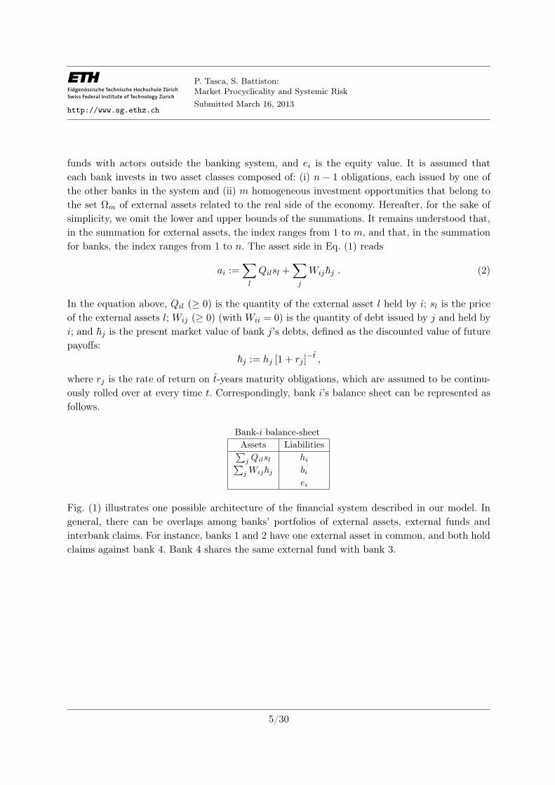
Fig. (1) illustrates one possible architecture of the financial system described in our model. In
general, there can be overlaps among banks’ portfolios of external assets, external funds and
interbank claims. For instance, banks 1 and 2 have one external asset in common, and both hold
claims against bank 4. Bank 4 shares the same external fund with bank 3.
5/30

http://www.sg.ethz.ch
P. Tasca, S. Battiston:Market Procyclicality and Systemic Risk
Submitted March 16, 2013
Figure 1: Illustration example of a stylized architecture of the financial system.
2.2 Leverage
The bank i’s leverage is defined as its debt-asset ratio.3 From Eq. (1) and Eq. (2) we have,
φi := (hi + bi)/ai (3a)
= (hi + bi)/
∑
l
Qilsl +∑
j
Wij~j
(3b)
= (hi + bi)/
∑
l
Qilsl +∑
j
Wijhj [1 + rj ]−t
∈ (0, 1]. (3c)
We assume that the rate of return on claims on other banks depends linearly upon the obligor’s
credit worthiness as measured by its leverage. In particular, as in Tasca and Battiston (2011),
we assume that for each obligor j, the following relationship holds:
rj := rf + βφj , (4)
where rf is the risk-free rate, and where βφj denotes the credit spread associated with the j
issuer. The parameter β ∈ (0, 1) is the factor loading on j’s leverage and can be understood
as the responsiveness of the rate of return to the bank’s financial condition. After substituting
Eq. (4) into Eq. (3c), we obtain a system of coupled equations in which bank i’s leverage is a
positive function of the leverage of all of the obligors of i:
φi = (hi + bi)/
∑
l
Qilsl +∑
j
Wijhj [1 + rf + βφj ]−t
. (5)
3Notice that the leverage is always bigger than zero since banks are by definition debt-financed.
6/30

http://www.sg.ethz.ch
P. Tasca, S. Battiston:Market Procyclicality and Systemic Risk
Submitted March 16, 2013
2.3 Target Leverage. An Accounting Rule
The VaR is widely considered by financial institutions as part of their risk management procedure.
As in Shin (2008), we assume that each bank i ∈ Ωn adjusts its balance sheet to maintain
“economic capital” (equity ei) equal to its VaR. In other words, the VaR is the equity capital
that a bank must hold to remain solvent with probability c. As explained below, this practice
is equivalent to targeting a reference leverage φ∗
i . Let us use Vi to denote the VaR per dollar
of assets held by i. If bank i maintains equity capital ei to meet total VaR, then we have
ei = Vi × ai ⇒ ai − hi + bi = Vi × ai ⇒ hi + bi = ai × (1− Vi). This implies that i has a target
leverage φ∗
i = (hi + bi)/ai = (1− Vi).
The accounting rule that allows bank i to keep its leverage close to φ∗
i over time finds its economic
ground in Adrian and Shin (2008a, 2010) and operates as follows. In a falling market (i.e., under
slumping external asset prices), the leverage increases (i.e., φi > φ∗
i ). In this scenario, the bank
shrinks its balance sheet by selling (a portion of) its external assets and paying back (a portion
of) its external debts with the proceeds. In a rising market (i.e., under booming external asset
prices), the leverage decreases (i.e., φi < φ∗
i ). In such a scenario, the bank expands its balance
sheet by taking on additional external funds to invest the “fresh” cash in external activities.
Therefore, the dynamics of banks’ balance sheets may reinforce cyclical upturns and downturns.
To derive a formal accounting rule, we make the following assumptions:
1. Bank i can neither issue new equity or replace equity with debts.4
2. The notional value of bank i’s interbank debts is constant over time, i.e., hi(t) = hi for all
t ≥ 0.5
Note that the second assumption does not prevent bank i from changing counterparties or ad-
justing their relative shares in i’s interbank debts. Moreover, it does not prevent the market value
of the interbank claims from changing over time based on the time-varying credit worthiness of
the debt issuer (see Eq. 4). The two assumptions above, together with the balance sheet identity
in Eq. (1), imply that any variation in the external assets held by bank i will correspond to an
equal amount of variation in the external funds on the liability side.
Formally, under the accounting constraints Qi =∑
l Qil; dQi ≥ −Qi; dbi ≥ −bi, we obtain the
following accounting rule (whose derivation is provided in Appendix A).
dbibi
=
(
εiκiφi
)(
φ∗
i − φi
1− φ∗
i
)
, (6)
4Some candidate explanations in support of the fact that equity remains “sticky” are explained in Adrian and
Shin (2011a).5Because our aim is to model the leverage-price cycle, this hypothesis allows us to better capture the spillover
effect on the real economy that results from the re-adjustments of banks’ claims against real-economy-related
activities.
7/30

http://www.sg.ethz.ch
P. Tasca, S. Battiston:Market Procyclicality and Systemic Risk
Submitted March 16, 2013
dQil
Qil
=
(
εiαil
)(
φ∗
i − φi
1− φ∗
i
)
. (7)
The parameter εi ∈ (0, 1] measures the promptness of i in pursuing the target level of leverage φ∗
i .
It can also be seen as a scaling factor of i’s trading size. The parameter κi := bi/(bi+hi) ∈ (0, 1]
is the ratio of external funds to total debts, and αil := Qilsl/(∑
l Qilsl +∑
j Wij~j) ∈ (0, 1] is
the ratio of the external asset l to total assets.
2.4 Leverage-Price Cycle and Market Liquidity
In this section, we formalize the leverage-price cycle and link it to the notion of market liquidity.
Inspired by the empirical research on the leverage-asset price cycle (Adrian and Shin, 2008b,
2010), we now model how the accounting rule in Eq. (7) impacts the price of (non-paying-
dividend) external assets whose dynamics are driven by a standard GBM6
dslsl
= µldt+ σldBl , ∀l ∈ ΩM . (8)
The (bid-ask) trading sizes serve as measures of the strength of the (demand-supply) pressures on
external assets at a given time. A large bid size indicates a strong demand for the external asset. A
large ask size shows that there is a large supply of the external asset. Banks act as “active”traders
because they demand immediacy and push prices in the direction of their trading. Instead, players
outside the banking system act as “passive” traders who act as liquidity providers. These players
are “contrarian” who take the opposite side of the banks’ transactions: they sell when the price
is high and buy when the price is low. For a given external asset l ∈ Ωm with trading volume
Ql =∑
iQil, if banks place a bid on the order book, then the demand for the asset is larger than
the supply (i.e., dQl > 0); therefore, the price sl is likely to go up. If banks place an ask on the
order book, then the supply of the asset is larger than the demand (i.e., dQl < 0); therefore, the
price sl is likely to drop. In order to isolate the non-linear impact of the dynamic balance-sheet
management on the asset price dynamics in Eq. (8), we consider a linear relationships between
asset returns and trading volume:
E
(
dslsl
)
= γl
(
dQl
Ql
)
. (9)
The parameter γl ≥ 0 captures the market impact, i.e., the average price response to trade size.
This concept is closely related to the demand elasticity of price and is typically measured as
6Where Bl ∼ N(0, dt) is a standard Brownian motion defined on a complete filtered probability space
(Ω;F ; Ft;P) where Ft = σB(s) : s ≤ t, µl is the instantaneous risk-adjusted expected growth rate, σl > 0 is
the volatility of the growth rate and d(Bl, Bk) = ρlk.
8/30

http://www.sg.ethz.ch
P. Tasca, S. Battiston:Market Procyclicality and Systemic Risk
Submitted March 16, 2013
the price return following a transaction of a given volume. In other words, it is the effect that
market participants have on price when they buy or sell an external asset. It is the extent to
which buying or selling moves the price against the buyer or seller, i.e., upward during buying
and downward during selling. Market liquidity (as we will refer to it here) measures the size of
the price response to trades and is inversely proportional to the scale of the market impact: 1/γl.7
If trading a given quantity only produces a small price change, the market is said to be liquid.
If the trade produces a substantial price change, the market is said to be illiquid. Combining
Eq. (8) and Eq. (9), we can rewrite the price dynamics as follows:
dslsl
= γl
(
dQl
Ql
)
dt+ σldBl , ∀l ∈ ΩM . (10)
Eq. (10), together with Eq. (6)-(7), represents the leverage-price cycle. We can describe this
positive feedback loop between leverage and prices as follows. At the beginning, the leverage φi
is set equal to the target φ∗
i at a given “reference” price s∗l (see Eq. 5). Therefore, any deviation of
sl from s∗l leads to a deviation of φi from φ∗
i , which indirectly results from the deviation of ei from
e∗i . This event triggers the previously described accounting rule. When ei > e∗i (ei < e∗i ), the bank
has a “surplus” (“deficit”) of capital to allocate to external assets. More specifically, when prices
rise (i.e., sl > s∗l ), the upward adjustment in leverage entails the purchase of external assets. The
greater (aggregate) demand for external assets tends to put upward pressure on prices, and the
reference price increases. In a downtrend, this mechanism is reversed. In a downtrend market
(i.e., sl < s∗l ), the downward adjustment of leverage to the target level entails (forced) sales of
external assets.8 The lower (aggregate) demand for external assets puts downward pressure on
prices, and the reference price decreases.
2.5 The Financial System in a Nutshell
In summary, the dynamics of the financial market can be described by the following 3× n+m
system of coupled equations with indeces range as follows l = 1, ...,m; i = 1, ..., n, and parameter
values reported in Table 1.
dslsl
= γl
(
dQl
Ql
)
dt+ σdBl
dQil
Qil=
(
εiαil
)(
φ∗i−φi
1−φ∗i
)
dt
dbibi
=(
εiκiφi
)(
φ∗i−φi
1−φ∗i
)
dt
φi = (hi + bi)/(
∑
l Qilsl +∑
j Wijhj
(1+rf+βφj)t
)
.
(11)
7For the sake of simplicity, in our model, γl does not change with trading volume.8 This “flight to quality” process leads to a price decrease, which in turn forces further selling and further price
decreases.
9/30

http://www.sg.ethz.ch
P. Tasca, S. Battiston:Market Procyclicality and Systemic Risk
Submitted March 16, 2013
In this scheme, procyclicality is caused by a chain reaction triggered by an exogenous shock
(for example, a fall in house prices) and amplified by the interplay between the shock and asset
market dynamics. The propagating factor is leverage: when banks are highly leveraged, the initial
shock and the ensuing reduction in asset prices induce massive asset liquidation, accentuating
the price fall and possibly starting a vicious circle.
Parameters Description Set of Values
φ∗ Target leverage φ∗ ∈ R : 0 < φ∗ < 1
σ Variance of external assets σ ∈ R : 0 < σ < 1
ε Bank reaction to the accounting rule ε ∈ R : 0 ≤ ε ≤ 1
γ Price response of assets to banks’ trades γ ∈ R : γ > 0
h Face value of interbank obligations h ∈ R : h > 0
b Face value of external funds b ∈ R : b > 0
β Sensitivity of interbank obligations to leverage β ∈ R : 0 < β < 1
rf Risk-free rate rf ∈ R : rf ≥ 0
Table 1: Range of values for each of the parameters in the model. For the sake of simplicity, we omitted the
indices of banks and assets.
3 Analysis
The system of Eq. (11) represents a general framework based on which a number of exercises can
be conducted and several issues can be investigated. In the present paper, we focus on a specific
question that has recently risen to the top of the policy agenda:
RQ: “How does the risk of a systemic default depend on the interplay between the level of
bank compliance with capital requirements and asset-market liquidity in the presence of a
price shock? ”
Toward this end, we first simplify the above modeling framework using mean-field approximation.
Then, we provide a formal definition of systemic risk. Finally, we perform a numerical analysis
of the probability of systemic default.
3.1 Mean-field Approximation
The theoretical literature shows that the exact propagation of shocks within the interbank market
depends on the specific architecture of bank-to-bank financial linkages (see e.g., Allen and Gale,
2001; Freixas et al., 2000). However, the range of possible different architectures shrinks as
network density increases. Therefore, when the network density is relatively high, the probability
10/30

http://www.sg.ethz.ch
P. Tasca, S. Battiston:Market Procyclicality and Systemic Risk
Submitted March 16, 2013
of systemic breakdown depends only weakly on the specific network architecture. Indeed, network
density has been found to be a major driver of systemic risk (see e.g., Battiston et al., 2012a,b;
Tasca and Battiston, 2011). There is also a body of empirical evidence that suggests that financial
networks typically display a core-periphery structure with a dense core and a sparsely connected
periphery (see e.g., Battiston et al., 2012c; Cont et al., 2011; Iori et al., 2006; Vitali et al., 2011).
In the following, our aim is to describe the dynamics of the banks in the core of a core-periphery
structure.
It has been argued that the financial sector has undergone increasing levels of homogeneity
because of the spread of similar risk management models (e.g., VaR) and investment strategies
– “[...]The level playing field resulted in everyone playing the same game at the same time, often
with the same ball.”, Haldane (2009). As a result, one might reason that, banks’ balance sheet
structures and portfolios tend to look alike. In particular, in this scenario, banks’ leverage values
may differ across banks and over time, but they will remain close to the average value.
Based on these considerations, we conduct a mean-field analysis of the model, attempting to
study the behavior of the system in the neighborhood of a state in which the banks are close
to homogeneous in terms of balance sheet management and interact with each other via the
interbank network. Toward this end, we make the following three assumptions:
1. Banks set a similar reporting leverage targets, i.e., φ∗
i ≈ φ∗.
2. There exists a simplified market in which the external assets are indistinguishable and
uncorrelated and have identical initial values, i.e., s1(0) = s2(0) = ... = sl(0). In particular,
this means that (i) all of the external assets have the same expected returns and the same
volatility, (ii) the pairwise correlations are all zero (i.e., ρlk = 0, ∀ l, k ∈ Ωm), and (iii)
the external assets have the same market impact (i.e., γl = γ, ∀ l ∈ Ωm). The dynamics
of the average price9, s = 1m
∑
l sl, is ds/s = µdt + σdB. In the absence of transaction
costs, the 1/m heuristic is the optimal diversification strategy. Therefore, at time t = 0,
each bank i composes an equally weighted portfolio of external assets, denoted as pi, with
pi =∑
l Qilsl = Qis where Qi =∑
l Qil with Qi1 = Qi2 = ... = Qil =Qi
m. Moreover, we
assume that agents have comparable market power, i.e., that their portfolios of external
assets are of a similar size, s.t. Qi ≈1n
∑
j Qj := Q. Therefore, pi ≈1n
∑
j pj := p = Qs.
In addition, the agents are assumed to have the same level of compliance with capital
requirements, i.e., εi = ε, ∀ i ∈ Ωn.
3. The agents also have similar nominal total obligations in the interbank market, i.e., hi ≈1n
∑
j hj := h, and similar total debt to external creditors, i.e., bi ≈1n
∑
j bj := b.
9Where the expected return is µ = 1
m
∑lµl with µ1 = µ2 = ... = µl, while σ = σ√
mwith σ = 1
m
∑lσl and
B ∼ N(0, dt) is derived from the linear combination of B1,...,l,...,m uncorrelated processes.
11/30

http://www.sg.ethz.ch
P. Tasca, S. Battiston:Market Procyclicality and Systemic Risk
Submitted March 16, 2013
The first and the second assumptions imply Eq. (13), which reads the same for both individual
trades of size Q and the aggregate trade of size nQ. The second assumption also implies that the
expected return on the average price is proportional to the relative change in the average trading
size, i.e., µ = γ (dQ/Q), which therefore implies Eq. (12). The first and third assumptions imply
that the mark-to-market value of interbank claims is similar across banks, i.e., ~i :=∑
j Wij~j ≈1n
∑
j ~j := ~ = h/[1 + rf + φ]−t. The second and third assumptions imply that the ratio of
external assets to total assets is homogeneous across banks, i.e., αi =∑
l αil = p/(p + ~) := α.
The third assumption implies that the ratio of external funds to total liabilities is homogeneous
across banks, i.e., κi = b/(b+h) := κ. In totality, the three assumptions above imply that Eq. (5)
simplifies to φ = (h+b)/(
Qs+ h[1 + rf + βφ]−t)
, which is a quadratic expression in φ. Without
loss of generality, we set the risk-free rate equal to zero (i.e., rf = 0). We also set t = 1, which
means that banks issue 1-year maturity obligations. Then, solving for φ and taking the positive
root, we obtain Eq. (15).
In conclusion, under the above approximations and assumptions, the system of Eq. (11) simplifiesto the following system of four coupled equations that will be studied in the remainder of ouranalysis
ds
s= γ
(
dQ
Q
)
dt+ σdB
dQ
Q=
( ε
α
)
(
φ∗ − φ
1− φ∗
)
dt
db
b=
(
ε
κφ
)(
φ∗ − φ
1− φ∗
)
dt
φ =h(β − 1) + βb−Qs+
(
4β(b+ h)Qs+ (h− β(b+ h) +Qs)2)1/2
2βQs
(12)
(13)
(14)
(15)
In this scenario, the balance sheet of each bank in the core can be represented as follows.
Balance-sheet
Assets Liabilities
~ h
p b
e
3.2 Systemic Risk
We model the default event as a first passage time problem. An individual bank is assumed
to default whenever the market value of its assets falls below the book value of its debts, even
before their maturity. Accordingly, the default occurs whenever the bank’s leverage is equal to
or greater than one.
12/30

http://www.sg.ethz.ch
P. Tasca, S. Battiston:Market Procyclicality and Systemic Risk
Submitted March 16, 2013
However, the mean-field analysis enables us to assign a systemic meaning to the single bank
default event. Indeed, banks manage overlapped portfolios composed of external assets and in-
terbank claims. Consequently, banks are subject to similar sources of risk. Moreover, the leverage
of each bank is close to the mean value across banks, i.e., φi ≈ φ, ∀i ∈ Ωn. Hence, the failure of
one bank i in the core is likely to coincide with the failure of all of the other banks. This is also
consistent with recent empirical studies (see e.g., Battiston et al., 2012c). We define systemic
default as an event in which, at any time t ≥ 0, the leverage φ is equal to or greater than one.
Formally,
A systemic default occurs whenever φ(t) ≥ 1, given that ∀ t′ < t , 0 < φ(t′) < 1.
If the set Ωn of banks is populated at a constant rate at each time interval dt, then the probability
of systemic default P[systemic default] is related to the expected default time τ(φ) and can
be approximated as P[systemic default] ≈ dt/τ(φ) with dt << τ(φ).10 In the following, the
probability of systemic default event is also referred to as systemic risk.
3.3 Simulation Framework
Before conducting the numerical experiments, we appropriately design the simulation framework
with respect to the following: (1) the price shock, (2) the range of γ and ε, and (3) the capital
structure.
Aggregate shock. To assess the level of balance-sheet amplification, the exogenous aggregate price
shock is assumed to have the following properties: (i) it is common, i.e., the shock is not asset-
specific and cannot be diversified away; (ii) it is a single shock, i.e., it hits the external assets
only once at the beginning of the simulation process; and (iii) it is uniform, i.e., the strength of
the shock is homogeneous across assets.
Range of γ and ε. It is convenient to generate a table P(ε×γ) that represents the level of market
procyclicality as a function of bank compliance with capital requirements ε and asset-market
impact γ. Accordingly, the market can be weakly, moderately or strongly procyclical (see Fig.2).
For the former parameter, we choose a set of values that span the entire range of variation:
ε := 0.1, 0.2, ..., 1. Because our preliminary tests indicated that for values of γ that are approx-
imately larger than five, the results of the analysis do not change, so we choose the following set
of values γ := 0.1, 0.2, ..., 5.
Capital structure. First, note that under the assumption (2) used to derive the accounting rule
in Eq. (6)-(7), h(t) = h for all t ≥ 0. Hereafter, for the sake of simplicity, we impose the initial
condition b+h = 1 and consider three different funding policies based on the imbalance towards
10A formal definition of τ(φ) is provided in Appendix B.
13/30

http://www.sg.ethz.ch
P. Tasca, S. Battiston:Market Procyclicality and Systemic Risk
Submitted March 16, 2013
Figure 2: Table of Market Procyclicality. The left-bottom region of weak procyclicality represents a context
in which the asset market is highly liquid (i.e., γ ' 0) and in which the banks loosely react to a asset-price
changes (i.e., ε ' 0). The left-upper region of medium procyclicality represents a context in which the asset
market is very liquid (i.e., γ ' 0) and in which the banks react promptly to asset-price changes (i.e., ε / 1).
The right-bottom region of medium procyclicality represents a context in which the asset market is illiquid (i.e.,
γ / 5) and in which the banks loosely react to asset-price changes (i.e., ε ' 0). The right-upper region of strong
procyclicality represents a context in which the asset market is highly illiquid (i.e., γ / 5) and in which the
banks react promptly to asset-price changes (i.e., ε / 1).
external funds versus funds from the interbank market: high imbalance (b = 0.9 > h = 0.1),
medium imbalance (b = 0.5 ≡ h = 0.5), low imbalance (b = 0.1 < h = 0.9). We also consider
three different levels of target leverage: low target (φ∗ = 0.7), medium target (φ∗ = 0.8), high
target (φ∗ = 0.9). As a result, we have nine different capital structures, as illustrated in Tab. 2.
The remaining accounting entries for the balance sheets at time t = 0 are obtained by solving
the following system of equations:
p+ ~ = h+ b+ e (balance-sheet identity)
~ = h/(1 + βφ∗) (market value of interbank claims)
with p = Qs. As β ∈ (0, 1), we use β = 0.5 to represent a scenario in which interest rates on
interbank claims have an intermediate level of sensitivity to the obligors’ credit worthiness.
3.4 Monte Carlo Simulations
To compute the probability of systemic default, we first estimate the mean time to default τ(φ)
based on the output of two thousand Monte Carlo simulations (N = 2.000) according to Eq. (12-
14/30

http://www.sg.ethz.ch
P. Tasca, S. Battiston:Market Procyclicality and Systemic Risk
Submitted March 16, 2013
15).11 Each realization lasts a number of steps T = 50.000 with a step size of ∆t = 0.01. The
mean time to default is obtained for all of the pairs (ε, γ) in the table P(ε,γ) and all nine capital
structures in Tab. 2. The leverage-price cycle, summarized by the flow-chart in Fig. 3, is the
central part of our Monte Carlo analysis. In brief, at the beginning (t = 0), the leverage φ of
the banks is set equal the target level φ∗. To this value corresponds the “reference”price value
s∗ := [b+ h+ φ∗(bβ − h+ βh)]/[φ∗Q(1 + βφ∗)] as derived from Eq.(15). The initial price shock
(−10%) moves the banks out of “equilibrium” by deviating s from s∗ and φ from φ∗. To drive the
leverage back toward φ∗, banks adjust their external asset holdings and external funds according
to the accounting rule in Eq. (13)-(14). The re-sizing of banks’ balance sheets has a market
impact on asset prices (see Eq. 12), which in turn further influence the balance sheet entries.
This effect completes the leverage-asset price cycle (see Fig. 3). Systemic risk is then computed
using the approximation in Section 3.2.
4 Results
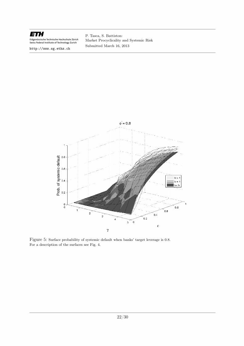
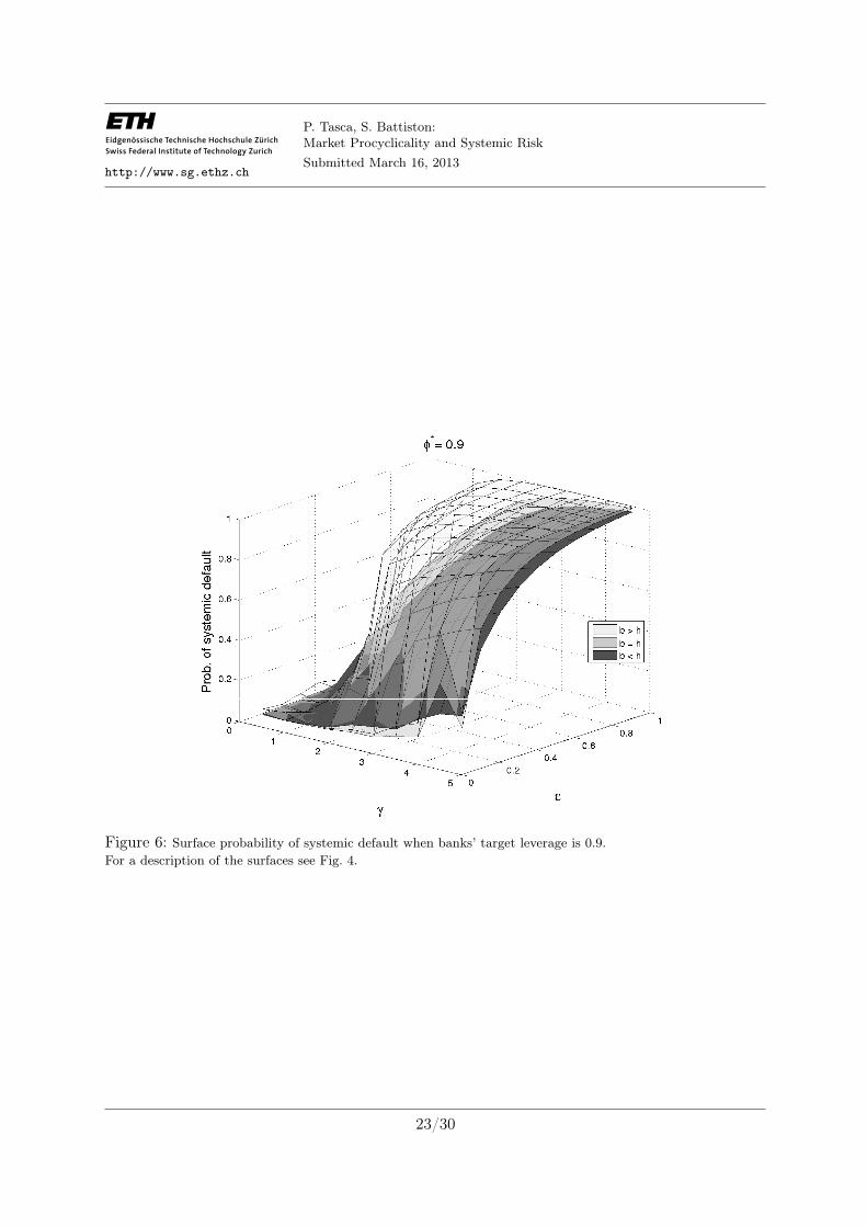
Fig. 4-5-6 show the probability surface of the systemic default event as a function of (1) the level
of market procyclicality and (2) the banks’ capital structure. The capital structure, instead, refers
to the balance between external and interbank funding sources. Finally, each figure corresponds
to a different level of target leverage: φ∗ = 0.7, 0.8, 0.9.
(1) Market Procyclicality In connection with the areas of the table P(ε×γ) of market pro-
cyclicality in Fig. 2, the systemic risk in Fig. 4-5-6 varies as follows.
Weak procyclicality – left lower corner of P(ε×γ) Systemic risk is at its minimum level.
Banks are in the region of weak market procyclicality characterized by a liquid asset market
(i.e., γ ' 0) and a weak adjustment of any leverage deviation from the target level (i.e., ε ' 0).
An example of sample path of leverage is illustrated in Fig. 7-c. Even though the price shock
induces some asset liquidations, it is immediately absorbed by the system because of a sluggish
balance-sheet management and a liquid asset market. Eventually, systemic risk remains at low
levels.
Medium procyclicality – left upper corner of P(ε×γ) Systemic risk is at a moderate level.
On the one side, banks promptly comply with capital requirements (i.e., ε / 1) and react to
price shocks by selling orders of large size. Therefore, massive liquidation of banks’ assets may
put further downward pressure on asset prices. On the other side, the asset market is very
liquid (i.e., γ ' 0). Therefore, potentially large quantities of the assets can be sold or bought
without significant impact on their market price. Systemic risk remains at medium levels until
11The values of the parameters used in the simulations are reported in Tab. 3, and the procedure is described
in greater detail in Appendix C.
15/30

http://www.sg.ethz.ch
P. Tasca, S. Battiston:Market Procyclicality and Systemic Risk
Submitted March 16, 2013
the liquidity does not “evaporate” from the market. An example of sample path of the leverage
is illustrated in Fig. 7-a.
Medium procyclicality – right lower corner of P(ε×γ) Systemic risk is at a moderate level.
The asset-market is illiquid (i.e., γ / 5), and banks loosely comply with capital requirements (i.e.,
ε ' 0). In this situation, the selling orders executed by the banks in response to the price shock are
limited in size. Combined with a liquidity shock, these trades produce only a small price change,
which is sufficient, however, to trigger a weak spiral of asset-price devaluation. This spiral further
degenerates the banks’ balance sheets and deteriorates the leverage. As a consequence, systemic
risk slightly increases. An example of sample path of the leverage is illustrated in Fig. 7-d.
Strong procyclicality – right upper corner of P(ε×γ) Systemic risk is at its maximum level.
Banks are in the region of strong market procyclicality characterized by the extremely dangerous
combination of a highly illiquid asset market (i.e., γ / 5) and prompt responses to any deviation
of the leverage from the target level (i.e., ε / 1). An example of sample path of the leverage
is illustrated in Fig. 7-b. In this context, banks react to the price shock via selling orders of a
significant size. If at the same time a liquidity shock materializes such that buyers temporarily
retreat from the market, external assets can only be sold at “fire-sale prices”. Eventually, the
market crash degrades the balance sheets and both leverage and the default risk increase.
(2) Capital Structure Banks’ capital structures also play an important role in systemic risk
except under weak market procyclicality. Indeed, when banks’ exposure to external funds is
greater (i.e., b > h), a price shock will have a greater effect on banks’ net worth, and systemic
risk will be higher (as indicated by the light-gray surfaces in Fig. 4-5-6). In contrast, when banks’
positions are more tilted towards the interbank market, the price shock is damped down because
it mainly propagates via a drop in the market value of the interbank claims (as indicated by
the dark-gray surfaces in Fig. 4-5-6). In this case, the systemic risk is lower. Interestingly, the
gaps between the levels of systemic risk associated with the three different funding policies are
amplified at high levels of market procyclicality (see the border between the surfaces in Fig. 4-
5-6). Finally, the higher the target leverage level is, the more pronounced the effects (compare
Fig. 4-5-6). Indeed, leverage is the propagating factor of a price shock: if banks did not target
leverage, letting equity absorb the shock, the vicious circle would be mitigated or even eliminated.
Overall, the results suggest that to mitigate the systemic effects of an unexpected price shock,
two complementary policy rules can be implemented: (1) one can allow banks to weaken their
compliance in adjusting their leverage to meet the target level (i.e., ε will decrease toward zero);12
or (2) one can set up financing facilities to increase market liquidity (i.e., γ will decrease toward
12Based on our Monte Carlo trials, we find that the leverage follows a slower mean reversion process toward the
target level. Interestingly, this effect could explain the empirical puzzle recently discovered by Adrian and Shin
(2008b) concerning the slow mean reversion over time exhibited by the (reported) leverage ratios.
16/30

http://www.sg.ethz.ch
P. Tasca, S. Battiston:Market Procyclicality and Systemic Risk
Submitted March 16, 2013
zero). If one (both) of these two policy rules is put in place, the market will transition into the
region of medium (weak) procyclicality. If, moreover, one can reduce banks’ imbalance towards
the external market and set a cap to the target leverage, the systemic risk will further decrease.13
Indeed, for containing macro-prudential risks, leverage caps could be helpful if other solutions
based on capital or contingent rules turn out to be too costly or difficult to implement. However,
one drawback of this rule lies in its difficulty to be harmonized among different business models
and cross-border banks. Moreover, leverage caps should be robust to: (i) the accounting treat-
ment of off-balance operations (incl., derivatives and hedges); and (ii) the treatment of leverage
embedded in structured finance products.
5 Concluding Remarks
In this paper, we combined a balance sheet approach with a dynamic stochastic setting to
investigate the impact of market procyclicality on systemic risk. One of the novelties of our work
is that it provides a quantitative representation of the notion of market procyclicality using a
table whose dimensions correspond to (1) the level of bank compliance with capital requirements
(controlled by the parameter ε) and (2) the degree of asset market liquidity (controlled by the
parameter γ).
The general approach is to perturb the system with an aggregate price shock and analyze the
probability of systemic default in critical regions of the table of market procyclicality. In our
model, systemic defaults are a result of drops in asset prices, which are endogenously driven by
bank trades. Thus, the leverage-asset price cycle is characterized by a “self-fulfilling” dynamics.
Essentially, over-leveraged banks (which are more likely to default) tend to liquidate their assets
after negative price variations. However, their market impact further decreases asset prices. Thus,
balance-sheet management may amplify the effect of an initial shock, turning it into a spiral of
asset price devaluation. Hence, at the heart of our model are pecuniary externalities in the form
of direct asset price contagion (via overlapping portfolios) and indirect asset price contagion (via
interbank claims). In particular, we stress the policy implications of the interplay between bank
capital requirements and asset market liquidity. When the asset market is very liquid, even a
strong compliance with capital requirements, which are usually alleged to be procyclical, do not
in fact increase the probability of systemic default. Conversely, when the asset market is very
illiquid, even a weak compliance with capital requirements increase the probability of systemic
default.
13The G20 group of leading countries agreed on September 2012 to introduce a leverage ratio on banks by the
end of 2012, as part of the Basel III reform from the global Basel Committee on Banking Supervision, to make
the sector less risky.
17/30
http://www.sg.ethz.ch
P. Tasca, S. Battiston:Market Procyclicality and Systemic Risk
Submitted March 16, 2013
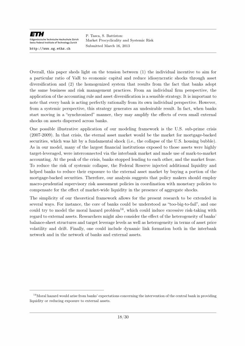
Overall, this paper sheds light on the tension between (1) the individual incentive to aim for
a particular ratio of VaR to economic capital and reduce idiosyncratic shocks through asset
diversification and (2) the homogenized system that results from the fact that banks adopt
the same business and risk management practices. From an individual firm perspective, the
application of the accounting rule and asset diversification is a sensible strategy. It is important to
note that every bank is acting perfectly rationally from its own individual perspective. However,
from a systemic perspective, this strategy generates an undesirable result. In fact, when banks
start moving in a “synchronized” manner, they may amplify the effects of even small external
shocks on assets dispersed across banks.
One possible illustrative application of our modeling framework is the U.S. sub-prime crisis
(2007-2009). In that crisis, the eternal asset market would be the market for mortgage-backed
securities, which was hit by a fundamental shock (i.e., the collapse of the U.S. housing bubble).
As in our model, many of the largest financial institutions exposed to those assets were highly
target-leveraged, were interconnected via the interbank market and made use of mark-to-market
accounting. At the peak of the crisis, banks stopped lending to each other, and the market froze.
To reduce the risk of systemic collapse, the Federal Reserve injected additional liquidity and
helped banks to reduce their exposure to the external asset market by buying a portion of the
mortgage-backed securities. Therefore, our analysis suggests that policy makers should employ
macro-prudential supervisory risk assessment policies in coordination with monetary policies to
compensate for the effect of market-wide liquidity in the presence of aggregate shocks.
The simplicity of our theoretical framework allows for the present research to be extended in
several ways. For instance, the core of banks could be understood as “too-big-to-fail”, and one
could try to model the moral hazard problem14, which could induce excessive risk-taking with
regard to external assets. Researchers might also consider the effect of the heterogeneity of banks’
balance-sheet structures and target leverage levels as well as heterogeneity in terms of asset price
volatility and drift. Finally, one could include dynamic link formation both in the interbank
network and in the network of banks and external assets.
14Moral hazard would arise from banks’ expectations concerning the intervention of the central bank in providing
liquidity or reducing exposure to external assets.
18/30

http://www.sg.ethz.ch
P. Tasca, S. Battiston:Market Procyclicality and Systemic Risk
Submitted March 16, 2013
φ∗ = 0.7 φ∗ = 0.8 φ∗ = 0.9
b > h
Assets Liabilities
~ = 0.074 h = 0.1
p = 1.354 b = 0.9
e = 0.428
Assets Liabilities
~ = 0.071 h = 0.1
p = 1.179 b = 0.9
e = 0.25
Assets Liabilities
~ = 0.069 h = 0.1
p = 1.041 b = 0.9
e = 0.11
b = h
Assets Liabilities
~ = 0.37 h = 0.5
p = 1.058 b = 0.5
e = 0.428
Assets Liabilities
~ = 0.357 h = 0.5
p = 0.893 b = 0.5
e = 0.25
Assets Liabilities
~ = 0.345 h = 0.5
p = 0.765 b = 0.5
e = 0.11
b < h
Assets Liabilities
~ = 0.66 h = 0.9
p = 0.768 b = 0.1
e = 0.428
Assets Liabilities
~ = 0.643 h = 0.9
p = 0.607 b = 0.1
e = 0.25
Assets Liabilities
~ = 0.620 h = 0.9
p = 0.490 b = 0.1
e = 0.11
Table 2: Banks’ capital structures at time t = 0 as used in the Monte Carlo simulations, based on three differ-
ent funding policies and three different levels of target leverage.
Model Parameters Simulation Setting Initial Conditions
σ = 0.1 shock= −10% b0 = 0.1, 0.5, 0.9
rf = 0 N = 2.000 Q0 = 1
β = 0.5 ∆t = 0.01 s0 = s∗ × (shock + 1)
ε = 0.1 : 0.1 : 1 T = 50.000
γ = 0.1 : 0.1 : 5
h = 0.1, 0.5, 0.9
Table 3: Range of values and initial conditions used in the simulation analysis.
19/30

http://www.sg.ethz.ch
P. Tasca, S. Battiston:Market Procyclicality and Systemic Risk
Submitted March 16, 2013
Figure 3: Flow-chart of the numerical simulation of the financial system in Eq. (12-15) with an emphasis on
the leverage-price cycle. Note that we use pk to denote the new portfolio value after the price shock.
20/30

http://www.sg.ethz.ch
P. Tasca, S. Battiston:Market Procyclicality and Systemic Risk
Submitted March 16, 2013
Figure 4: Surface probability of systemic default when banks’ target leverage is 0.7. In the x-axis, γ represents
the average price response to trades. In the y-axis, ε represents the intensity of bank compliance with capital
requirements. The light gray surface shows the probability of systemic default when banks have high imbalance
towards external funds (b > h). The gray surface shows the probability of systemic default when banks have
medium imbalance towards external funds (b = h). The dark gray surface shows the probability of systemic
default when banks have high imbalance towards external funds (b > h).
21/30
http://www.sg.ethz.ch
P. Tasca, S. Battiston:Market Procyclicality and Systemic Risk
Submitted March 16, 2013
Figure 5: Surface probability of systemic default when banks’ target leverage is 0.8.
For a description of the surfaces see Fig. 4.
22/30
http://www.sg.ethz.ch
P. Tasca, S. Battiston:Market Procyclicality and Systemic Risk
Submitted March 16, 2013
Figure 6: Surface probability of systemic default when banks’ target leverage is 0.9.
For a description of the surfaces see Fig. 4.
23/30

http://www.sg.ethz.ch
P. Tasca, S. Battiston:Market Procyclicality and Systemic Risk
Submitted March 16, 2013
2000 4000 6000 8000 10000 120000.5
0.6
0.7
0.8
0.9
1
ε = 1 , γ =0.3
Time
φ
(a)
500 1000 1500 20000.6
0.65
0.7
0.75
0.8
0.85
0.9
0.95
1
ε = 1 , γ = 3
Time
φ
(b)
2 4 6 8 10
x 104
0.4
0.5
0.6
0.7
0.8
0.9
1
ε =0.1 , γ = 0.1
Time
φ
(c)
2000 4000 6000 8000 10000 12000 140000.6
0.65
0.7
0.75
0.8
0.85
0.9
0.95
1
ε = 0.1 , γ =3
Time
φ
(d)
Figure 7: Sample paths for the leverage with target leverage φ∗ = 0.6. The target leverage works as a constant
long-run mean. However, the leverage follows a process that is non-stationary. Indeed, the leverage dynamics is
derived by the non-linear system in Section 3.1 in which the price process in Eq.12 is non-stationary. Neverthe-
less, in case (c) of weak procyclicality in which both ε and γ approximate zero, the path resembles a stationary
process with mean reversion level equal to 0.6. In this case, the dynamics of: (1) the price process in Eq.12;
(2) the bank asset trading in Eq.13, and (3) the external funds in Eq.14 are damped down by the parameter
ε ≡ γ = 0.1.
24/30

http://www.sg.ethz.ch
P. Tasca, S. Battiston:Market Procyclicality and Systemic Risk
Submitted March 16, 2013
A An Accounting Rule Based on Target Leverage
In this section we derive the accounting rule in Eq. (6-7), according to which a generic bank i ∈ Ωn adjusts
its balance sheet entries in response to an asset price change. At time t=0, bank i starts its activity with a
target leverage, φi(0) ≡ φ∗i . As pointed out in Section 2.3, the accounting rule is based on the underlying
assumption that bank i keeps its debt/credit positions fixed in the interbank market: the bank only
adjusts the quantity of external assets and external funds: hi(0) = hi and∑
j Wij(0)~j(0) =∑
j Wij~j
for all t ≥ 0 and all i, j ∈ Ωn. Thus, the initial leverage can be written as φi(0) =hi+bi(0)∑
lQil(0)sl(0)+
∑jWij~j
.
At time t=1, for the sake of simplicity, let only one external asset l ∈ Ωm be shocked. Ceteris paribus
(i.e., bi and Qil remain as they were at time t=0), the new price value sl(1) implies the following leverage:
φi(1) = hi+bi(0)∑lQil(0)sl(1)+
∑jWij~j
6= φ∗i . After the price shock, at time t=2, the bank is able to adjust its
leverage to the target level by changing the quantity of external asset l held on the asset side – i.e.,∑
l Qil(0) →∑
l Qil(2), and of the external debts on the liability side – i.e., bi(0) → bi(2). As a result,
the new leverage at time t=2 is equal to the target level, i.e., φi(2) ≡ φ∗i . Expanding the equivalence
φi(2) ≡ φi(0) ≡ φ∗i yields
φi(2) =hi + bi(2)
∑
l Qil(2)sl(1) +∑
j Wij~j≡
hi + bi(0)∑
l Qil(0)sl(0) +∑
j Wij~j≡ φ∗
i . (16)
Now, the equation for leverage at time t=1 can be re-written as∑
j Wij~j +∑
l Qil(0)sl(1) =hi+bi(0)φi(1)
⇒∑
j Wij~j =hi+bi(0)φi(1)
−∑
l Qil(0)sl(1), which we substitute into the equation for the leverage at time t=2
as follows:
φi(2) =hi + bi(2)
∑
l Qil(2)sl(1) +hi+bi(0)φi(1)
−∑
l Qil(0)sl(1)=
hi + bi(2)hi+bi(0)φi(1)
+∆Qil(2)sl(1), (17)
where ∆Qil indicates the variation in the quantity of external assets in bank i’s portfolio due to a change
in its holdings of external asset l. Eq. (17) can be re-written as
hi + bi(0)
φi(1)+ ∆Qil(2)sl(1) ≡
hi + bi(2)
φ∗i
. (18)
Based on the assumptions associated with the accounting rule as indicated in Section 2.3, the following
identity holds true:
bi(2) = bi(0) + ∆Qil(2)sl(1) . (19)
Then, substituting (19) into (18) yields hi+bi(0)φi(1)
+∆Qil(2)sl(1) =hi+bi(0)+∆Qil(2)sl(1)
φ∗
i
, from which, with
little arrangements we obtain
∆Qil(2)sl(1) =hi + bi(0)
φi(1)
(
φ∗i − φi(0)
1− φ∗i
)
. (20)
Therefore, the rate of change in the demand for asset l from bank i is:
Qil(2)−Qil(0)
Qil(0)=
∑
j Wij~ij +Qil(0)sl(1)
Qil(0)sl(1)
(
φ∗i − φi(0)
1− φ∗i
)
=1
αil
(
φ∗i − φi(0)
1− φ∗i
)
, (21)
25/30

http://www.sg.ethz.ch
P. Tasca, S. Battiston:Market Procyclicality and Systemic Risk
Submitted March 16, 2013
where αil =Qil(0)sl(1)
ai(1)is the ratio of the value of the external asset l to the total asset value held by the
bank. The relative change in debts is easily obtained from Eq. 19:
bi(2)− bi(0)
bi(0)=
hi + bi(0)
bi(0)φi(0)
(
φ∗i − φi(0)
1− φ∗i
)
=1
κiφi(0)
(
φ∗i − φi(0)
1− φ∗i
)
, (22)
where κi =bi(0)
hi+bi(0)is the ratio of external debts to the total debts. In the presence of market frictions,15
the bank may react with a certain (in)elasticity εi ∈ (0, 1] to deviations in leverage φi from the target level.
Heuristically, in continuous time, the accounting rule implies the following (rates of) change, respectively,
for the demand for external assets and the amount of external debts:
dQil
Qil=
(
εiαil
)(
φ∗i − φi
1− φ∗i
)
dt (23)
dhi
hi=
(
εiκiφi
)(
φ∗i − φi
1− φ∗i
)
dt . (24)
The boundary conditions are: (i) dQi
Qi=
∑
l
(
dQil
Qil
)
s.t. dQil
Qil= 0 for some l ∈ Ωm; (ii) dQil ≥ −Qil for
all l ∈ Ωm and i ∈ Ωn, and (iii) dhi ≥ −hi for all i ∈ Ωn. The accounting rule in Eq. (23) can be easily
generalized if bank i changes the quantity of more than one external asset. For example, the rule for
changing the quantity of all of the assets in Ωm is
dQi
Qi=
(
εiαi
)(
φ∗i − φi
1− φ∗i
)
dt (25)
where Qi =∑
l Qil and αi =∑
l αil.
B Expected time-to-default
The first time to default τ(φ), is defined as the first time the process φt≥0 touches the upper bound
of the set Ωφ := (0, 1]. Namely, τ(φ) = inft ≥ 0 : φ(t) ≥ 1 with inf∅ = T if one is never reached.
The full characterization of τ(φ) is its transition probability density function fφ(1, t | φ0, 0) conditional
to the initial value φ(0) := φ0 ∈ (0, 1). Then, the mean time to default is
τ(φ) :=
∫ T
0
tfφ(1, t | φ0, 0)dt (26)
which is the mean first hitting time for φt≥0 to reach the absorbing default barrier before the terminal
date T .
15I.e., market and (or) firm structures that prevent banks from instantly adjusting their balance sheets using
the accounting rule.
26/30

http://www.sg.ethz.ch
P. Tasca, S. Battiston:Market Procyclicality and Systemic Risk
Submitted March 16, 2013
C Numerical Analysis
In this section, we show how to obtain the mean time to default from the system (11), through simulations
of the SDEs. The first step is to simulate the standard Brownian motion. Then, we look at stochastic
differential equations, after which we compute the exit time for the process φt≥0 through the upper
barrier fixed at one.
Simulation of Brownian Motion We begin by considering a discretized version of Brownian
motion. We set the step-size as ∆t and let Bℓ denote B(tℓ) with tℓ = ℓ∆t. According to the properties of
Brownian motion, we find
Bℓ = Bℓ−1 + dBj ℓ = 1, ..., L. (27)
Here, L denotes the number of steps that we take with t0, t1, ..., tL as a discretization of the interval [0, T ],
and dBℓ is a normally distributed random variable with zero mean and variance ∆t. Expression (27) can
be seen as a numerical recipe to simulate Brownian motion.
Simulation of the SDEs We use the Euler-Maruyama method. First, we discretize the dynamics of
the processes st≥0, Qt≥0 and bt≥0. Then, we substitute the value of s, b and Q into the discrete
time version of Eq.(15). It is unnecessary to derive the dynamics of φt≥0 via Ito’s Lemma from the
dynamics of st≥0, Qt≥0 and bt≥0. We directly use the expression in Eq.(15), which is the closed-
form solution for φ in terms of s, Q and b. Therefore, the discrete version of the system of equations in
Section 3.1 reads as follows:
sℓ = sℓ−1 + µs(φℓ−1, sℓ−1, φ∗, γ, ε, αℓ)∆t+ σ(sℓ−1)dBℓ , s(0) = s0
Qℓ = Qℓ−1 + µQ(φℓ−1, φ∗, ε, αℓ)∆t , Q(0) = Q0
bℓ = bℓ−1 + µb(φℓ−1, bℓ−1, φ∗, ε, κℓ)∆t , b(0) = b0
φℓ =h(β − 1) + βbℓ −Qℓsℓ +
√
4β(bℓ + h)Qℓsℓ + (h− β(bℓ + h) +Qℓsℓ)2
2βQℓsℓ
where αℓ = (Qℓ−1sℓ−1)/(Qℓ−1sℓ−1 + ~ℓ), ~ℓ = h/(1 + βφℓ−1), κℓ = bℓ−1/(bℓ−1 + h). Here φℓ, sℓ , bℓ,
αℓ, ~ℓ, Qℓ and κℓ are the approximation to φ(ℓ∆t), s(ℓ∆t), b(ℓ∆t), α(ℓ∆t), ~(ℓ∆t), Q(ℓ∆t) and κ(ℓ∆t).
While, ∆t is the step size, dBℓ = Bℓ −Bℓ−1 and L is the number of steps we take.
Estimation of expected time to default The expected exit time can be estimated in the fol-
lowing manner. We simulate a single sample path for st≥0, Qt≥0, bt≥0 and compute the value φℓ.
Then, we observe the time at which the process φt≥0 crossed the default boundary fixed at one. Once
this point has been reached, we halt the simulation. The observed time approximates the exit time in
the current sample path. If the trajectory of φt≥0 does not exit through one before T , we set the exit
time equal to T , i.e., the economy terminal date. By using the Monte Carlo method, we estimate the
expected exit time for the system by simulating a total of N sample paths within [0, T ]. We keep track
of the fraction of trajectories that did not cross the default boundary before T and make sure to set T
to keep this a fraction as small as possible (i.e., < 5%). Let the r-th realization of the path of φt≥0 be
denoted as φrt≥0 with r = 1, ..., N . For each of these paths, the random variable that represents the
27/30

http://www.sg.ethz.ch
P. Tasca, S. Battiston:Market Procyclicality and Systemic Risk
Submitted March 16, 2013
exit time through the default boundary is defined as: τr = inft ≥ 0 : φrt ≥ 1. The expected default
time τ(φ) is approximated by τ(φ) as the total sum of the exit times divided by the number N of paths:
τ(φ) =1
N
N∑
r
τr(11φrt=1) ≈ τ(φ) =
∫ T
0
tfφ(1, t | φ0, 0)dt . (28)
References
Acharya, V., 2009. A theory of systemic risk and design of prudential bank regulation. Journal
of Financial Stability 5 (3), 224–255.
Adrian, T., Shin, H. S., 2008a. Financial intermediary leverage and value at risk. Federal Reserve
Bank of New York Staff Reports 338.
Adrian, T., Shin, H. S., 2008b. Liquidity and financial cycles. BIS Working Papers 256.
Adrian, T., Shin, H. S., 2010. Liquidity and leverage. Journal of Financial Intermediation 19 (3),
418–437.
Adrian, T., Shin, H. S., 2011a. Financial intermediary balance sheet management. Federal Reserve
Bank of New York, Staff Reports No. 532.
Adrian, T., Shin, H. S., 2011b. Procyclical leverage and value-at-risk. FRB of New York Staff
Report No. 338.
Allen, F., Babus, A., Carletti, E., 2012. Asset commonality, debt maturity and systemic risk.
Journal of Financial Economics 104 (3), 519–534.
Allen, F., Gale, D., Feb. 2001. Financial contagion. Journal of Political Economy 108 (1), 1–33.
Bargigli, L., Gallegati, M., Riccetti, L., Russo, A., 2012. Network analysis and calibration of
the’leveraged network-based financial accelerator’. Available at SSRN 2160254.
Battiston, S., Gatti, D. D., Gallegati, M., Greenwald, B., Stiglitz, J. E., 2012a. Default cascades:
When does risk diversification increase stability? Journal of Financial Stability 8 (3), 138 –
149.
Battiston, S., Gatti, D. D., Gallegati, M., Greenwald, B. C. N., Stiglitz, J. E., 2012b. Liaisons
dangereuses: Increasing connectivity, risk sharing and systemic risk. Journal of Economic Dy-
namics and Control (forthcoming), early version NBER Working Paper Series n.15611.
28/30
http://www.sg.ethz.ch
P. Tasca, S. Battiston:Market Procyclicality and Systemic Risk
Submitted March 16, 2013
Battiston, S., Puliga, M., Kaushik, R., Tasca, P., Caldarelli, G., 2012c. Debtrank: Too central to
fail? financial networks, the fed and systemic risk. Sci. Rep. 2 (541).
Bernanke, B., Lown, C., Friedman, B., 1991. The credit crunch. Brookings Papers on Economic
Activity 1991 (2), 205–247.
BIS, Apr. 2010. International framework for liquidity risk measurement, standards and monitor-
ing. Consultative document, Basel Committee on Banking Supervision, Bank for International
Settlements, CH-4002 Basel, Switzerland.
Blum, J., Hellwig, M., 1995. The macroeconomic implications of capital adequacy requirements
for banks. European Economic Review 39 (3-4), 739–749.
Brunnermeier, M., 2008. Deciphering the 2007-08 Liquidity and Credit Crunch. Journal of Eco-
nomic Perspectives 23 (1), 77–100.
Calomiris, C., Wilson, B., 1998. Bank capital and portfolio management: The 1930’s capital
crunch and scramble to shed risk.
Cont, R., Moussa, A., Santos, E., 2011. Network structure and systemic risk in banking systems.
New York.
EC, Jul. 2011. Proposal for a directive of the european parliament and of the cuncil. EU Directive
COM(2011) 453 final, DG Internal Market and Services, Banking and Financial Conglomerates
Unit, European Commission, SPA2 4/29, B–1049 Brussels.
Elsinger, H., Lehar, A., Summer, M., 2006. Risk Assessment for Banking Systems. Management
Science 52 (9), 1301–1314.
Estrella, A., 2004. The cyclical behavior of optimal bank capital. Journal of Banking & Finance
28 (6), 1469–1498.
Freixas, X., Parigi, B. M., Rochet, J.-C., 2000. Systemic risk, interbank relations, and liquidity
provision by the central bank. Journal of Money, Credit & Banking 32, 611–638.
Furfine, C., 2003. Interbank Exposures: Quantifying the Risk of Contagion. Journal of Money,
Credit & Banking 35 (1), 111–129.
Gârleanu, N., Pedersen, L., 2007. Liquidity and risk management. The American Economic
Review 97 (2), 193–197.
Greenlaw, D., Hatzius, J., Kashyap, A., Shin, H., 2008. Leveraged losses: lessons from the mort-
gage market meltdown. US Monetary Policy Forum Report No.2.
29/30
http://www.sg.ethz.ch
P. Tasca, S. Battiston:Market Procyclicality and Systemic Risk
Submitted March 16, 2013
Haldane, A., 2009. Rethinking the financial network. Speech delivered at the Financial Student
Association, Amsterdam, April.
Iori, G., Jafarey, S., Padilla, F., 2006. Systemic risk on the interbank market. Journal of Economic
Behaviour and Organization 61 (4), 525–542.
Kashyap, A., Stein, J., 2000. What do a million observations on banks say about the transmission
of monetary policy? The American Economic Review, 407–428.
Kiyotaki, N., Moore, J., 2002. Balance-Sheet Contagion. American Economic Review 92 (2),
46–50.
Krishnamurthy, A., 2010. Amplification mechanisms in liquidity crises. American Economic Jour-
nal: Macroeconomics 2 (3), 1–30.
Shin, H., 2008. Risk and liquidity in a system context. Journal of Financial Intermediation 17 (3),
315–329.
Stiglitz, J., Weiss, A., 1981. Credit rationing in markets with imperfect information. The Amer-
ican economic review 71 (3), 393–410.
Tasca, P., Battiston, S., 2011. Diversification and financial stability. Working Paper Series CCSS-
11-001.
Vitali, S., Glattfelder, J., Battiston, S., 2011. The network of global corporate control. PloS one
6 (10), e25995.
30/30
Related Documents