Market Microstructure Knowledge Needed for Controlling an ...

Market Microstructure Knowledge Needed forControlling an Intra-Day Trading Process

Charles-Albert Lehalle∗

February 20, 2013

Abstract

A great deal of academic and theoretical work has been dedicated to optimalliquidation of large orders these last twenty years. The optimal split of an or-der through time (‘optimal trade scheduling’) and space (‘smart order routing’) isof high interest to practitioners because of the increasing complexity of the mar-ket micro structure because of the evolution recently of regulations and liquidityworldwide. This chapter translates into quantitative terms these regulatory issuesand, more broadly, current market design.

It relates the recent advances in optimal trading, order-book simulation andoptimal liquidity to the reality of trading in an emerging global network of liquidity.

Contents1 Market Microstructure Modeling and Payoff Understanding are Key Ele-

ments of Quantitative Trading 2

2 From Market Design to Market Microstructure: Practical Examples 5

3 Forward and Backward Components of the Price Formation Process 15

4 From Statistically Optimal Trade Scheduling to Microscopic Optimizationof Order Flows 174.1 Replacing market impact by statistical costs . . . . . . . . . . . . . . . 184.2 An order-flow oriented view of optimal execution . . . . . . . . . . . . 24

5 Perspectives and Future Work 29∗Global Head of Quantitative Research, Credit Agricole Cheuvreux, [email protected]

1

arX

iv:1

302.

4592

v1 [

q-fi

n.T

R]

19

Feb

2013

1 Market Microstructure Modeling and Payoff Under-standing are Key Elements of Quantitative Trading

As is well known, optimal (or quantitative) trading is about finding the proper balancebetween providing liquidity in order to minimize the impact of the trades, and consum-ing liquidity in order to minimize the market risk exposure, while taking profit throughpotentially instantaneous trading signals, supposed to be triggered by liquidity ineffi-ciencies.

The mathematical framework required to solve this kind of optimization problemneeds:

• a model of the consequences of the different ways of interacting with liquidity(such as the market impact model (Almgren et al., 2005; Wyart et al., 2008;Gatheral, 2010));

• a proxy for the ‘market risk’ (the most natural of them being the high frequencyvolatility (Aıt-Sahalia and Jacod, 2007; Zhang et al., 2005; Robert and Rosen-baum, 2011));

• and a model for quantifying the likelihood of the liquidity state of the market(Bacry et al., 2009; Cont et al., 2010).

A utility function then allows these different effects to be consolidated with respect tothe goal of the trader:

• minimizing the impact of large trades under price, duration and volume con-straints (typical for brokerage trading (Almgren and Chriss, 2000));

• providing as much liquidity as possible under inventory constraints (typical formarket-makers Avellaneda and Stoikov (2008) or Gueant et al. (2011));

• or following a belief about the trajectory of the market (typical of arbitrageurs(Lehalle, 2009)).

Once these key elements have been defined, rigorous mathematical optimizationmethods can be used to derive the optimal behavior (Bouchard et al., 2011; Predoiuet al., 2011). Since the optimality of the result is strongly dependent on the phenomenonbeing modeled, some understanding of the market microstructure is a prerequisite forensuring the applicability of a given theoretical framework.

The market microstructure is the ecosystem in which buying and selling interestsmeet, giving birth to trades. Seen from outside the microstructure, the prices of thetraded shares are often uniformly sampled to build time series that are modeled viamartingales (Shiryaev, 1999) or studied using econometrics. Seen from the inside of

2

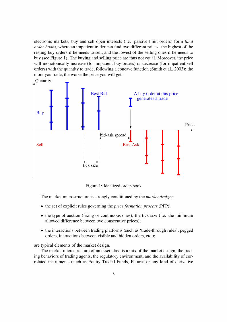
electronic markets, buy and sell open interests (i.e. passive limit orders) form limitorder books, where an impatient trader can find two different prices: the highest of theresting buy orders if he needs to sell, and the lowest of the selling ones if he needs tobuy (see Figure 1). The buying and selling price are thus not equal. Moreover, the pricewill monotonically increase (for impatient buy orders) or decrease (for impatient sellorders) with the quantity to trade, following a concave function (Smith et al., 2003): themore you trade, the worse the price you will get.

6Quantity

-Price

Buy

Best Bid A buy order at this pricegenerates a trade

Sell Best Ask

?

-�bid-ask spread

-�

tick size

Figure 1: Idealized order-book

The market microstructure is strongly conditioned by the market design:

• the set of explicit rules governing the price formation process (PFP);

• the type of auction (fixing or continuous ones); the tick size (i.e. the minimumallowed difference between two consecutive prices);

• the interactions between trading platforms (such as ‘trade-through rules’, peggedorders, interactions between visible and hidden orders, etc.);

are typical elements of the market design.The market microstructure of an asset class is a mix of the market design, the trad-

ing behaviors of trading agents, the regulatory environment, and the availability of cor-related instruments (such as Equity Traded Funds, Futures or any kind of derivative

3

products). Formally, the microstructure of a market can be seen as several sequencesof auction mechanisms taking place in parallel, each of them having its own particularcharacteristics. For instance the German market place is mainly composed (as of 2011)of the Deutsche Borse regulated market, the Xetra mid-point, the Chi-X visible orderbook, Chi-delta (the Chi-X hidden mid-point), Turquoise Lit and Dark Pools, BATSpools. The regulated market implements a sequence of fixing auctions and continuousauctions (one open fixing, one continuous session, one mid-auction and one closing auc-tion); others implement only continuous auctions, and Turquoise mid-point implementsoptional random fixing auctions.

To optimize his behavior, a trader has to choose an abstract description of the mi-crostructure of the markets he will interact with: this will be his model of market mi-crostructure. It can be a statistical ‘macroscopic’ one as in the widely-used Almgren–Chriss framework (Almgren and Chriss, 2000), in which the time is sliced into intervalsof 5 or 10 minutes duration during which the interactions with the market combine twostatistical phenomena:

• the market impact as a function of the ‘participation rate’ of the trader;

• and the volatility as a proxy of the market risk.

It can also be a microscopic description of the order book behavior as in the Alfonsi–Schied proposal (Alfonsi et al., 2010) in which the shape of the order book and itsresilience to liquidity-consuming orders is modeled.

This chapter will thus describe some relationships between the market design andthe market microstructure using European and American examples since they have seenregulatory changes (in 2007 for Europe with the MiFI Directive, and in 2005 for theUSA with the NMS regulation) as much as behavioral changes (with the financial crisisof 2008). A detailed description of some important elements of the market microstruc-ture will be conducted:

• dark pools;

• impact of fragmentation on the price formation process;

• tick size;

• auctions, etc.

Key events like the 6 May 2010 flash crash in the US market and some European marketoutages will also receive attention.

To obtain an optimal trading trajectory, a trader needs to define its payoff. Here also,choices have to be made from a mean-variance criterion (Almgren and Chriss, 2000) tostochastic impulse control (Bouchard et al., 2011) going through stochastic algorithms

4

(Pages et al., 2012). This chapter describes the statistical viewpoint of the Almgren–Chriss framework, showing how practitioners can use it to take into account a largevariety of effects. It ends with comments on an order-flow oriented view of optimalexecution, dedicated to smaller time-scale problems, such as ‘Smart Order Routing’(SOR).

2 From Market Design to Market Microstructure: Prac-tical Examples

The recent history of the French equity market is archetypal in the sense that it wentfrom a highly concentrated design with only one electronic platform hosted in Paris(Muniesa, 2003) to a fragmented pan-European one with four visible trading pools andmore than twelve ‘dark ones’, located in London, in less than four years.

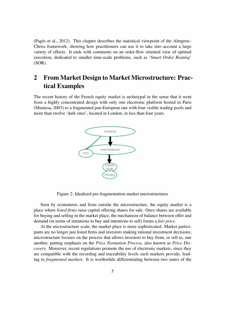
Figure 2: Idealized pre-fragmentation market microstructures

Seen by economists and from outside the microstructure, the equity market is aplace where listed firms raise capital offering shares for sale. Once shares are availablefor buying and selling in the market place, the mechanism of balance between offer anddemand (in terms of intentions to buy and intentions to sell) forms a fair price.

At the microstructure scale, the market place is more sophisticated. Market partici-pants are no longer just listed firms and investors making rational investment decisions;microstructure focuses on the process that allows investors to buy from, or sell to, oneanother, putting emphasis on the Price Formation Process, also known as Price Dis-covery. Moreover, recent regulations promote the use of electronic markets, since theyare compatible with the recording and traceability levels such markets provide, lead-ing to fragmented markets. It is worthwhile differentiating between two states of the

5

microstructure: pre- and post-fragmentation, see Figure 2 and 4:

• Pre-fragmented microstructure: before Reg NMS in the US and MiFID in Europe,the microstructure can be pictured as three distinct layers:

– investors, taking buy or sell decisions;

– intermediaries, giving unbiased advice (through financial analysts or strate-gists) and providing access to trading pools they are members of; low fre-quency market makers (or maker-dealers) can be considered to be part ofthis layer;

– market operators: hosting the trading platforms, NYSE Euronext, NAS-DAQ, BATS, Chi-X, belong to this layer. They are providing matching en-gines to other market participants, hosting the Price Formation Process.

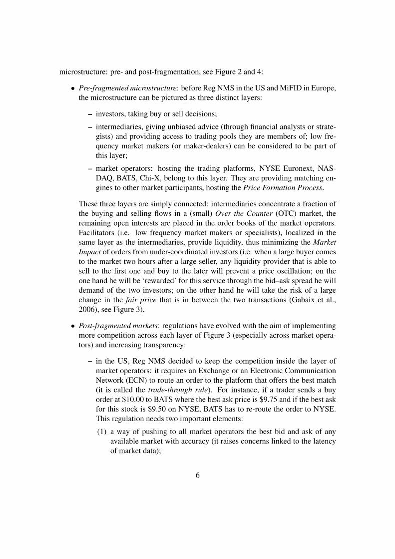
These three layers are simply connected: intermediaries concentrate a fraction ofthe buying and selling flows in a (small) Over the Counter (OTC) market, theremaining open interests are placed in the order books of the market operators.Facilitators (i.e. low frequency market makers or specialists), localized in thesame layer as the intermediaries, provide liquidity, thus minimizing the MarketImpact of orders from under-coordinated investors (i.e. when a large buyer comesto the market two hours after a large seller, any liquidity provider that is able tosell to the first one and buy to the later will prevent a price oscillation; on theone hand he will be ‘rewarded’ for this service through the bid–ask spread he willdemand of the two investors; on the other hand he will take the risk of a largechange in the fair price that is in between the two transactions (Gabaix et al.,2006), see Figure 3).

• Post-fragmented markets: regulations have evolved with the aim of implementingmore competition across each layer of Figure 3 (especially across market opera-tors) and increasing transparency:

– in the US, Reg NMS decided to keep the competition inside the layer ofmarket operators: it requires an Exchange or an Electronic CommunicationNetwork (ECN) to route an order to the platform that offers the best match(it is called the trade-through rule). For instance, if a trader sends a buyorder at $10.00 to BATS where the best ask price is $9.75 and if the best askfor this stock is $9.50 on NYSE, BATS has to re-route the order to NYSE.This regulation needs two important elements:

(1) a way of pushing to all market operators the best bid and ask of anyavailable market with accuracy (it raises concerns linked to the latencyof market data);

6

-Quantity

6Price

-Quantity

6Price

-Quantity

6Price

-Quantity

6Price

-Quantity

6Price

-Quantity

6Price

@@@���

Large Sell Order (A1) ���

@@@

Large Buy Order (A2)

Poor Market Depth (A3)

Preserved Market Depth (B3)

@@��

Large Sell Order (B1)��@@

Large Buy Order (B2)

Figure 3: Idealized kinematics of market impact caused by bad synchronization (A1–A2–A3 sequence) and preservation of the market depth thanks to a market maker agree-ing to support market risk (B1–B2-B3 sequence).

(2) that buying at $9.50 on NYSE is always better for a trader than buying at$9.75 on BATS, meaning that the other trading costs (especially clearingand settlement costs) are the same.

The data conveying all the best bid and asks is called the consolidated pre-trade tape and its best bid and offer is called the National Best-Bid and Offer(NBBO).

– in Europe, mainly because of the diversity of the clearing and settlementchannels, MiFID allows the competition to be extended to the intermedi-aries: they are in charge of defining their Execution Policies describing howand why they will route and split orders across market operators. The Euro-pean Commission thus relies on competition between execution policies asthe means of selecting the best way of splitting orders, taking into accountall trading costs. As a consequence, Europe does not have any officiallyconsolidated pre-trade tape.

7

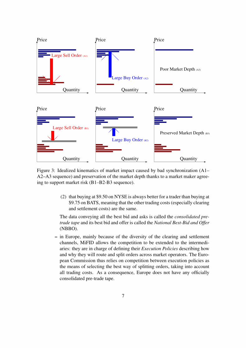
Figure 4: Idealized post-fragmentation market microstructure.

Despite these differences, European and US electronic markets have a lot in com-mon: their microstructures evolved similarly to a state where latency is crucial andHigh Frequency Market-Makers (also called High Frequency Traders) became themain liquidity providers of the market.

Figure 4 gives an idealized view of this fragmented microstructure:

– A specific class of investors: the High Frequency Traders (HFT) are an es-sential part of the market; by investing more than other market participantsin technology, thus reducing their latency to markets, they have succeededin:

∗ implementing market-making-like behaviors at high frequency;∗ providing liquidity at the bid and ask prices when the market has low

probability of moving (thanks to statistical models);∗ being able to cancel very quickly resting orders in order to minimize the

market risk exposure of their inventory;

they are said to be feature in 70% of the transactions in US Equity markets,

8

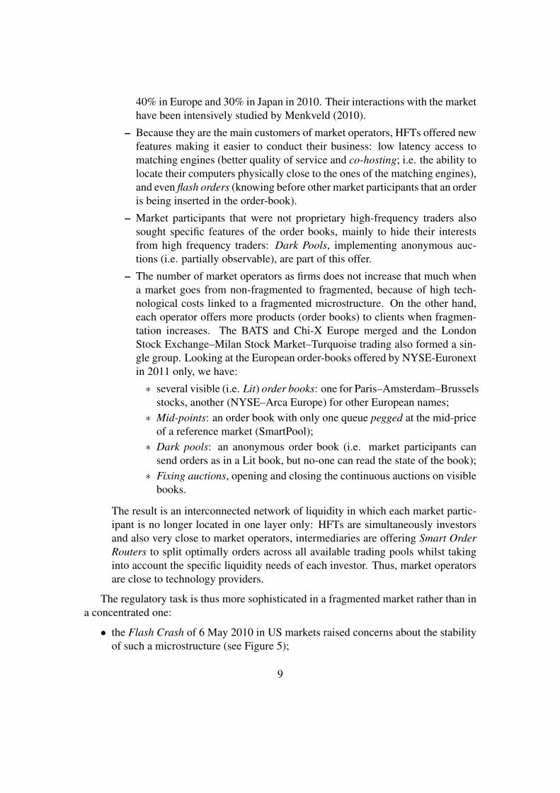
40% in Europe and 30% in Japan in 2010. Their interactions with the markethave been intensively studied by Menkveld (2010).

– Because they are the main customers of market operators, HFTs offered newfeatures making it easier to conduct their business: low latency access tomatching engines (better quality of service and co-hosting; i.e. the ability tolocate their computers physically close to the ones of the matching engines),and even flash orders (knowing before other market participants that an orderis being inserted in the order-book).

– Market participants that were not proprietary high-frequency traders alsosought specific features of the order books, mainly to hide their interestsfrom high frequency traders: Dark Pools, implementing anonymous auc-tions (i.e. partially observable), are part of this offer.

– The number of market operators as firms does not increase that much whena market goes from non-fragmented to fragmented, because of high tech-nological costs linked to a fragmented microstructure. On the other hand,each operator offers more products (order books) to clients when fragmen-tation increases. The BATS and Chi-X Europe merged and the LondonStock Exchange–Milan Stock Market–Turquoise trading also formed a sin-gle group. Looking at the European order-books offered by NYSE-Euronextin 2011 only, we have:

∗ several visible (i.e. Lit) order books: one for Paris–Amsterdam–Brusselsstocks, another (NYSE–Arca Europe) for other European names;∗ Mid-points: an order book with only one queue pegged at the mid-price

of a reference market (SmartPool);∗ Dark pools: an anonymous order book (i.e. market participants can

send orders as in a Lit book, but no-one can read the state of the book);∗ Fixing auctions, opening and closing the continuous auctions on visible

books.

The result is an interconnected network of liquidity in which each market partic-ipant is no longer located in one layer only: HFTs are simultaneously investorsand also very close to market operators, intermediaries are offering Smart OrderRouters to split optimally orders across all available trading pools whilst takinginto account the specific liquidity needs of each investor. Thus, market operatorsare close to technology providers.

The regulatory task is thus more sophisticated in a fragmented market rather than ina concentrated one:

• the Flash Crash of 6 May 2010 in US markets raised concerns about the stabilityof such a microstructure (see Figure 5);

9

Figure 5: The ‘Flash Crash’: 6 May 2010, US market rapid down-and-up move byalmost 10% was only due to market microstructure effects.

• the cost of surveillance of trading flows across a complex network is higher thanin a concentrated one.

Moreover, elements of the market design play many different roles: the tick size forinstance, is not only the minimum between two consecutive different prices, i.e., a con-straint on the bid-ask spread, it is also a key in the competition between market opera-tors. In June 2009, European market operators tried to gain market shares by reducingthe tick size on their order books. Each time one of them offered a lower tick thanothers, it gained around 10% of market shares (see Figure 6). After a few weeks ofcompetition on the tick, they limited this kind of infinitesimal decimation of the tickthanks to a gentleman’s agreement obtained under the umbrella of the FESE (Federa-tion of European Security Exchanges): such a decimation had been expensive in CPUand memory demand for their matching engines.

An idealized view of the ‘Flash Crash’. The flash crash was accurately described inKirilenko et al. (2010). The sequence of events that led to a negative jump in price anda huge increase in traded volumes in few minutes, followed by a return to normal in less

10

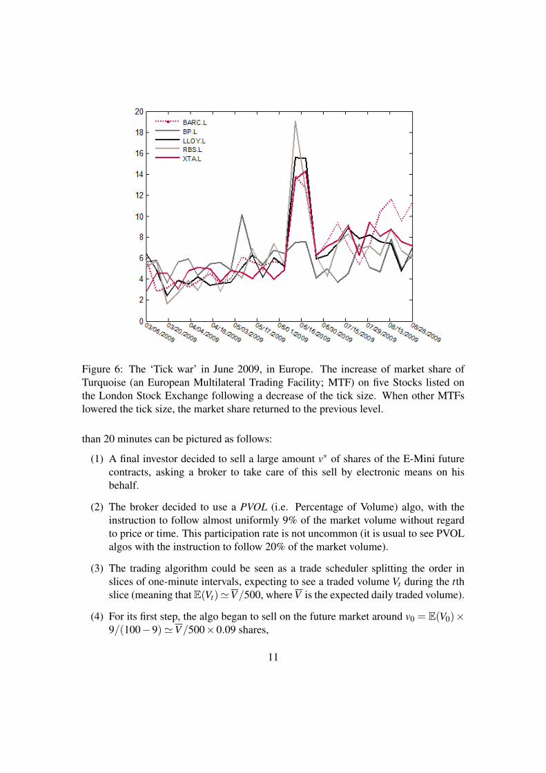
Figure 6: The ‘Tick war’ in June 2009, in Europe. The increase of market share ofTurquoise (an European Multilateral Trading Facility; MTF) on five Stocks listed onthe London Stock Exchange following a decrease of the tick size. When other MTFslowered the tick size, the market share returned to the previous level.

than 20 minutes can be pictured as follows:

(1) A final investor decided to sell a large amount v∗ of shares of the E-Mini futurecontracts, asking a broker to take care of this sell by electronic means on hisbehalf.

(2) The broker decided to use a PVOL (i.e. Percentage of Volume) algo, with theinstruction to follow almost uniformly 9% of the market volume without regardto price or time. This participation rate is not uncommon (it is usual to see PVOLalgos with the instruction to follow 20% of the market volume).

(3) The trading algorithm could be seen as a trade scheduler splitting the order inslices of one-minute intervals, expecting to see a traded volume Vt during the tthslice (meaning that E(Vt)'V/500, where V is the expected daily traded volume).

(4) For its first step, the algo began to sell on the future market around v0 = E(V0)×9/(100−9)'V/500×0.09 shares,

11

(5) The main buyers of these shares had been intra-day market makers; say that theybought (1−q) of them.

(6) Because the volatility was quite high on 6 May 2010, the market makers did notfeel comfortable with such an imbalanced inventory, and so decided to hedge iton the cash market, selling (1− q)× vt shares of a properly weighted basket ofequities.

(7) Unfortunately the buyers of most of these shares (say (1−q) of them again) wereintra-day market makers themselves, who decided in their turn to hedge their riskon the future market.

(8) It immediately increased the traded volume on the future market by (1− q)2v0shares.

(9) Assuming that intra-day market makers could play this hot potato game (as itwas called in the SEC–CFTC report), N times in 1 minute, the volume traded onthe future market became ∑n≤N(1−q)2nv0 larger than expected by the brokeragealgo.

(10) Back to step (4) at t + 1, the PVOL algo is now late by ∑n≤N(1− q)2nv0 ×8/(100−8), and has to sell V/500×8/(100−8) again; i.e. selling

vt+1 '(

N× vt +V

500

)×0.08.

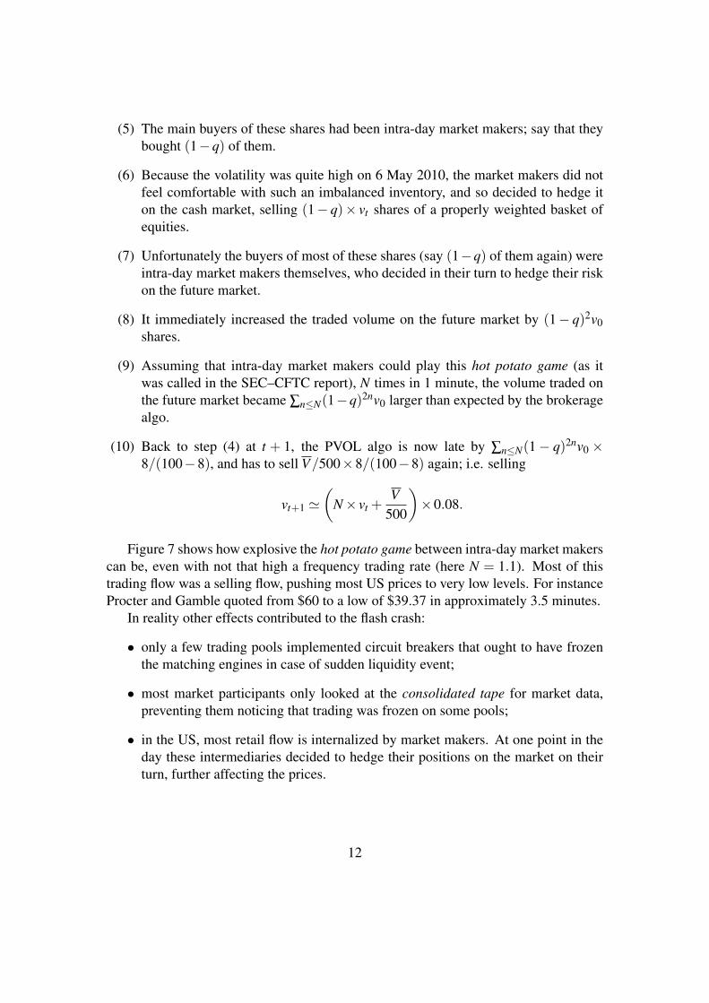
Figure 7 shows how explosive the hot potato game between intra-day market makerscan be, even with not that high a frequency trading rate (here N = 1.1). Most of thistrading flow was a selling flow, pushing most US prices to very low levels. For instanceProcter and Gamble quoted from $60 to a low of $39.37 in approximately 3.5 minutes.

In reality other effects contributed to the flash crash:

• only a few trading pools implemented circuit breakers that ought to have frozenthe matching engines in case of sudden liquidity event;

• most market participants only looked at the consolidated tape for market data,preventing them noticing that trading was frozen on some pools;

• in the US, most retail flow is internalized by market makers. At one point in theday these intermediaries decided to hedge their positions on the market on theirturn, further affecting the prices.

12

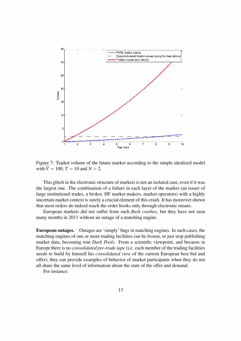
Figure 7: Traded volume of the future market according to the simple idealized modelwith V = 100, T = 10 and N = 2.

This glitch in the electronic structure of markets is not an isolated case, even if it wasthe largest one. The combination of a failure in each layer of the market (an issuer oflarge institutional trades, a broker, HF market-makers, market operators) with a highlyuncertain market context is surely a crucial element of this crash. It has moreover shownthat most orders do indeed reach the order books only through electronic means.

European markets did not suffer from such flash crashes, but they have not seenmany months in 2011 without an outage of a matching engine.

European outages. Outages are ‘simply’ bugs in matching engines. In such cases, thematching engines of one or more trading facilities can be frozen, or just stop publishingmarket data, becoming true Dark Pools. From a scientific viewpoint, and because inEurope there is no consolidated pre-trade tape (i.e. each member of the trading facilitiesneeds to build by himself his consolidated view of the current European best bid andoffer), they can provide examples of behavior of market participants when they do notall share the same level of information about the state of the offer and demand.

For instance:

13

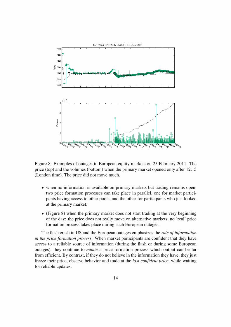
Figure 8: Examples of outages in European equity markets on 25 February 2011. Theprice (top) and the volumes (bottom) when the primary market opened only after 12:15(London time). The price did not move much.

• when no information is available on primary markets but trading remains open:two price formation processes can take place in parallel, one for market partici-pants having access to other pools, and the other for participants who just lookedat the primary market;

• (Figure 8) when the primary market does not start trading at the very beginningof the day: the price does not really move on alternative markets; no ‘real’ priceformation process takes place during such European outages.

The flash crash in US and the European outages emphasizes the role of informationin the price formation process. When market participants are confident that they haveaccess to a reliable source of information (during the flash or during some Europeanoutages), they continue to mimic a price formation process which output can be farfrom efficient. By contrast, if they do not believe in the information they have, they justfreeze their price, observe behavior and trade at the last confident price, while waitingfor reliable updates.

14

3 Forward and Backward Components of the Price For-mation Process

The literature on market microstructure can be split in two generic subsets:

• papers with a Price Discovery viewpoint, in which the market participants areinjecting into the order book their views on a fair price. In these papers (seefor instance Biais et al. (2005); Ho and Stoll (1981); Cohen et al. (1981)), the fairprice is assumed to exist for fundamental reasons (at least in the mind of investors)and the order books are implementing a Brownian-bridge-like trajectory targetingthis evolving fair price. This is a backward view of the price dynamics: theinvestors are updating assumptions on the future value of tradeable instruments,and send orders in the electronic order books according to the distance betweenthe current state of the offer and demand and this value, driving the quoted priceto some average of what they expect.

Figure 9 shows a price discovery pattern: the price of the stock changes for funda-mental reasons, and the order book dynamics react accordingly generating morevolume, more volatility, and a price jump.

• Other papers rely on a Price Formation Process viewpoint. For their authors(most of them econophysicists, see for instance Smith et al. (2003); Bouchaudet al. (2002) or Chakraborti et al. (2011) for a review of agent based models oforder books) the order books are building the price in a forward way. The marketparticipants take decisions with respect to the current orders in the books makingassumptions of the future value of their inventory; it is a forward process.

Following Lehalle et al. (2010), one can try to crudely model these two dynamicssimultaneously. In a framework with an infinity of agents (using a Mean Field Gameapproach, see Lasry and Lions (2007) for more details), the order book at the bid (re-spectively at the ask), is a density mB(t, p) (resp. mA(t, p)) of agents agreeing at timet to buy (resp. sell) at price p. In such a continuous framework, there is no bid–askspread and the trading price p∗(t) is such that there is no offer at a price lower thanp∗(t) (and no demand at a price greater then p∗(t)). Assuming diffusivity, the two sidesof the order book are subject to the following simple partial differential equations:

∂tmB (t, p)− ε2

2∂

2ppmB(t, p) = λ (t)δp=p∗(t)

∂tmA (t, p)− ε2

2∂

2ppmA(t, p) = λ (t)δp=p∗(t).

15

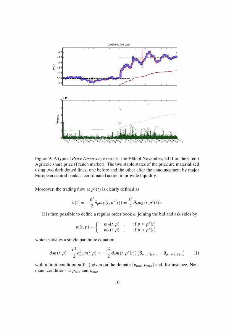
Figure 9: A typical Price Discovery exercise: the 30th of November, 2011 on the CreditAgricole share price (French market). The two stable states of the price are materializedusing two dark dotted lines, one before and the other after the announcement by majorEuropean central banks a coordinated action to provide liquidity.

Moreover, the trading flow at p∗(t) is clearly defined as

λ (t) =−ε2

2∂pmB (t, p∗(t)) =

ε2

2∂pmA (t, p∗(t)) .

It is then possible to define a regular order book m joining the bid and ask sides by

m(t, p) ={

mB(t, p) , if p≤ p∗(t)−mA(t, p) , if p > p∗(t)

which satisfies a single parabolic equation:

∂tm(t, p)− ε2

2∂

2ppm(t, p) =−ε2

2∂pm(t, p∗(t))

(δp=p∗(t)−a−δp=p∗(t)+a

)(1)

with a limit condition m(0, ·) given on the domain [pmin, pmax] and, for instance, Neu-mann conditions at pmin and pmax.

16

0 200 400 600 800 1000 12009.97

9.98

9.99

10

10.01

10.02

10.03

10.04

10.05

10.06

Time (seconds)

Price

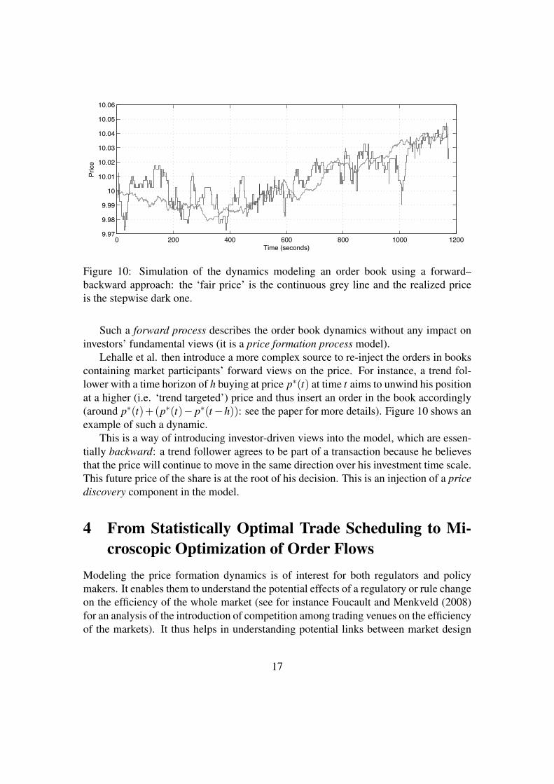
Figure 10: Simulation of the dynamics modeling an order book using a forward–backward approach: the ‘fair price’ is the continuous grey line and the realized priceis the stepwise dark one.

Such a forward process describes the order book dynamics without any impact oninvestors’ fundamental views (it is a price formation process model).

Lehalle et al. then introduce a more complex source to re-inject the orders in bookscontaining market participants’ forward views on the price. For instance, a trend fol-lower with a time horizon of h buying at price p∗(t) at time t aims to unwind his positionat a higher (i.e. ‘trend targeted’) price and thus insert an order in the book accordingly(around p∗(t)+(p∗(t)− p∗(t−h)): see the paper for more details). Figure 10 shows anexample of such a dynamic.

This is a way of introducing investor-driven views into the model, which are essen-tially backward: a trend follower agrees to be part of a transaction because he believesthat the price will continue to move in the same direction over his investment time scale.This future price of the share is at the root of his decision. This is an injection of a pricediscovery component in the model.

4 From Statistically Optimal Trade Scheduling to Mi-croscopic Optimization of Order Flows

Modeling the price formation dynamics is of interest for both regulators and policymakers. It enables them to understand the potential effects of a regulatory or rule changeon the efficiency of the whole market (see for instance Foucault and Menkveld (2008)for an analysis of the introduction of competition among trading venues on the efficiencyof the markets). It thus helps in understanding potential links between market design

17

and systemic risk.In terms of risk management inside a firm hosting trading activities, it is more im-

portant to understand the trading cost of a position, which can be understood as itsliquidation risk.

From the viewpoint of one trader versus the whole market, three key phenomenahave to be controlled:

• the market impact (see Kyle (1985); Lillo et al. (2003); Engle et al. (2012); Alm-gren et al. (2005); Wyart et al. (2008)) which is the market move generated byselling or buying a large amount of shares (all else being equal); it comes fromthe forward component of the price formation process, and can be temporary ifother market participants (they are part of the backward component of the pricediscovery dynamics) provide enough liquidity to the market to bring back theprice to its previous level;

• adverse selection, capturing the fact that providing too much (passive) liquidityvia limit orders enables the trader to maintain the price at an artificial level; not alot of literature is available about this effect, which has been nevertheless identi-fied by practitioners (Altunata et al., 2010);

• and the uncertainty on the fair value of the stock that can move the price duringthe trading process; it is often referred as the intra-day market risk.

4.1 Replacing market impact by statistical costsA framework now widely used for controling the overall costs of the liquidation of aportfolio was proposed by Almgren and Chriss in the late 1990s Almgren and Chriss(2000). Applied to the trade of a single stock, this framework:

• cuts the trading period into an arbitrary number of intervals N of a chosen durationδ t,

• models the fair price moves thanks to a Gaussian random walk:

Sn+1 = Sn +σn+1√

δ t ξn+1 (2)

• models the temporary market impact ηn inside each time bin using a power law ofthe trading rate (i.e. the ratio of the traded shares vn by the trader over the markettraded volume during the same period Vn):

η(vn) = aψn +κ σn√

δ t(

vn

Vn

)γ

(3)

where a, κ and γ are parameters, and ψ is the half bid-ask spread;

18

• assumes the permanent market impact is linear in the participation rate;

• uses a mean–variance criterion and minimizes it to obtain the optimal sequenceof shares to buy (or sell) through time.

It is important first to notice that there is an implicit relationship between the timeinterval δ t and the temporary market impact function: without changing η and simplyby choosing a different time slice, the cost of trading can be changed. It is in fact notpossible to choose (a,κ,γ) and δ t independently; they have to be chosen according tothe decay of the market impact on the stock, provided that most of the impact is keptin a time bin of size δ t. Not all the decay functions are compatible with this view (seeGatheral and Schied (2012) for details about available market impact models and theirinteractions with trading). Up to now the terms in

√δ t have been ignored. Note also

that the parameters (a,κ,γ) are relevant at this time scale.One should not regard this framework as if it were based on structural model as-

sumptions (i.e. that the market impact really has this shape, or that the price movesreally are Brownian), rather, as if it were a statistical one. With such a viewpoint, anypractitioner can use the database of its past executed orders and perform an econometricstudy of its ‘trading costs’ on any interval, δ t, of time (see Engle et al. (2012) for ananalysis of this kind on the whole duration of the order). If a given time scale succeedsin capturing, with enough accuracy, the parameters of a trading cost model, then thatmodel can be used to optimize trading. Formally, the result of such a statistical ap-proach would be the same as that of a structural one, as we will show below. But it ispossible to go one step further, and to take into account the statistical properties of thevariables (and parameters) of interest.

Going back to the simple case of the liquidation of one stock without any permanentmarket impact, the value (which is a random variable) of a buy of v∗ shares in N bins ofsize v1,v2, . . . ,vN is

W (v1,v2, . . . ,vN) =N

∑n=1

vn(Sn +ηn(vn))

= S0v∗+N

∑n=1

σnξnxn︸ ︷︷ ︸market move

+N

∑n=1

aψn(xn− xn+1)+κσn

V γn(xn− xn+1)

γ+1

︸ ︷︷ ︸market impact

, (4)

using the remaining quantity to buy: that is, xn = ∑k≥n vk instead of the instantaneousvolumes vn. To obtain an answer in as closed a form as possible, γ will be taken equal to

19

1 (i.e. linear market impact). (See Bouchard et al. (2011) for a more sophisticated modeland more generic utility functions rather than the idealized model which we adopt herein order to obtain clearer illustrations of phenomena of interest.)

To add a practitioner-oriented flavor to our upcoming optimization problems, justintroduce a set of independent random variables (An)1≤n≤N to model the arbitrage op-portunities during time slices. It will reflect our expectation that the trader will be ableto buy shares at price Sn−An during slice n rather than at price Sn.

Such an effect can be used to inject a statistical arbitrage approach into optimaltrading or to take into account the possibility of crossing orders at mid price in DarkPools or Broker Crossing Networks (meaning that the expected trading costs should besmaller during given time slices). Now the cost of buying v∗ shares is:

W (v) = S0v∗+N

∑n=1

σnξnxn +N

∑n=1

(aψn−An)vn +κσn

Vnv2

n (5)

Conditioned expectation optimization. The expectation of this cost,

E(W |(Vn,σn,ψn)1≤n≤N),

given the market state, can be written as

C0 = S0v∗+N

∑n=1

(aψn−EAn)vn +κσn

Vnv2

n, (6)

A simple optimization under constraint (to ensure ∑Nn=1 vn = v∗) gives

vn = wn

(v∗+

1κ

((EAn−

N

∑`=1

w`EA`

)−a

(ψn−

N

∑`=1

w`ψ`

))), (7)

where wn are weights proportional to the inverse of the market impact factor:

wn =Vn

σn

(N

∑`=1

V`

σ`

)−1

.

Simple effects can be deduced from this first idealization.

(1) Without any arbitrage opportunity and without any bid-ask cost (i.e. EAn = 0 forany n and a = 0), the optimal trading rate is proportional to the inverse of themarket impact coefficient: vn = wn ·v∗. Moreover, when the market impact has nointra-day seasonality, wn = 1/N implying that the optimal trading rate is linear.

20

(2) Following formula (7) it can be seen that the greater the expected arbitrage gain(or the lower the spread cost) on a slice compared to the market-impact-weightedexpected arbitrage gain (or spread cost) over the full trading interval, the largerthe quantity to trade during this slice. More quantitatively:

∂vn

∂EAn=

wn

2κ(1−wn)> 0,

∂vn

∂ψn=− a

2κ(1−wn)wn < 0.

This result gives the adequate weight for applying to the expected arbitrage gainin order to translate it into an adequate trading rate so as to profit on arbitrage op-portunities on average. Just note that usually the expected arbitrage gains increasewith market volatility, so the wn-weighting is consequently of interest to balancethis effect optimally.

Conditioned mean-variance optimization. Going back to a mean–variance optimiza-tion of the cost of buying progressively v∗ shares, the criterion for minimizing (using arisk aversion parameter λ ) becomes

Cλ = E(W |(Vn,σn,ψn)1≤n≤N)+λV(W |(Vn,σn,ψn)1≤n≤N)

= S0v∗+N

∑n=1

(aψn−EAn)(xn− xn+1)+

(κ

σn

Vn+λVAn

)(xn− xn+1)

2 +λσ2n x2

n. (8)

To minimize Cλ when it is only constrained by terminal conditions on x (i.e. x0 = v∗

and vN+1 = 0), it is enough to cancel its derivatives with respect to any xn, leading tothe recurrence relation(

σn

Vn+

λ

κVAn

)xn+1 =

12κ

(a(ψn−1−ψn)− (EAn−1−EAn))

+

(λ

κσ

2n +

(σn

Vn+

λ

κVAn +

σn−1

Vn−1+

λ

κVAn−1

))xn

−(

σn−1

Vn−1+

λ

κVAn−1

)xn−1. (9)

This shows that the variance of the arbitrage has an effect similar to that of themarket impact (through a risk-aversion rescaling), and that the risk-aversion parameteracts as a multiplicative factor on the market impact, meaning that within an arbitrage-free and spread-costs-free framework (i.e. a = 0 and EAn = 0 for all n), the marketimpact model for any constant b has no effect on the final result as long as λ is replacedby bλ .

Figure 11 compares optimal trajectories coming from different criteria and parame-ter values.

21

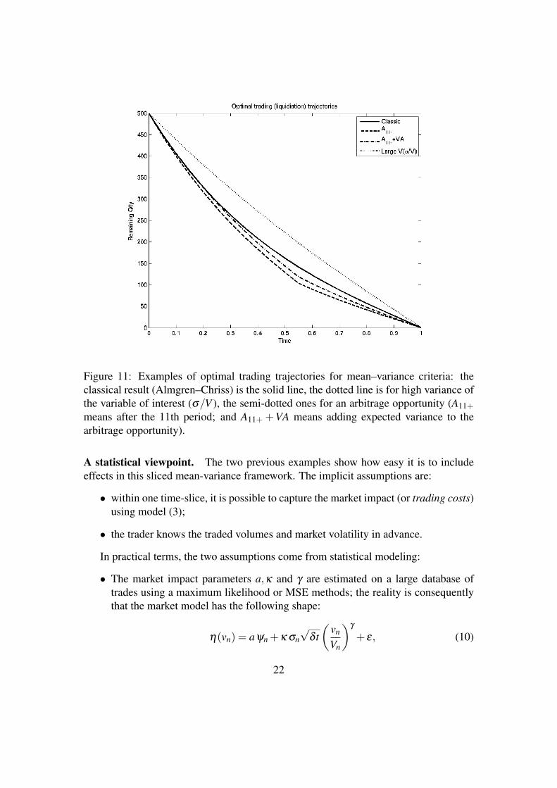
Figure 11: Examples of optimal trading trajectories for mean–variance criteria: theclassical result (Almgren–Chriss) is the solid line, the dotted line is for high variance ofthe variable of interest (σ/V ), the semi-dotted ones for an arbitrage opportunity (A11+means after the 11th period; and A11+ +VA means adding expected variance to thearbitrage opportunity).

A statistical viewpoint. The two previous examples show how easy it is to includeeffects in this sliced mean-variance framework. The implicit assumptions are:

• within one time-slice, it is possible to capture the market impact (or trading costs)using model (3);

• the trader knows the traded volumes and market volatility in advance.

In practical terms, the two assumptions come from statistical modeling:

• The market impact parameters a,κ and γ are estimated on a large database oftrades using a maximum likelihood or MSE methods; the reality is consequentlythat the market model has the following shape:

η(vn) = aψn +κ σn√

δ t(

vn

Vn

)γ

+ ε, (10)

22

where ε is an i.i.d. noise.

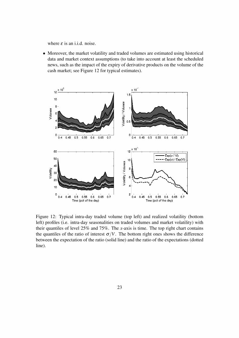
• Moreover, the market volatility and traded volumes are estimated using historicaldata and market context assumptions (to take into account at least the schedulednews, such as the impact of the expiry of derivative products on the volume of thecash market; see Figure 12 for typical estimates).

Figure 12: Typical intra-day traded volume (top left) and realized volatility (bottomleft) profiles (i.e. intra-day seasonalities on traded volumes and market volatility) withtheir quantiles of level 25% and 75%. The x-axis is time. The top right chart containsthe quantiles of the ratio of interest σ/V . The bottom right ones shows the differencebetween the expectation of the ratio (solid line) and the ratio of the expectations (dottedline).

23

Taking these statistical modeling steps into account in the classical mean–variancecriterion of (8), changes that equation into its unconditioned version:

Cλ = E(W )+λV(W )

= S0v∗+N

∑n=1

(aEψn−EAn)(xn− xn+1)

+

(κ E(

σn

Vn

)+λ (a2Vψn +VAn +Vε)

)(xn− xn+1)

2

+λσ2n x2

n +λκ2V(

σn

Vn

)(xn− xn+1)

4. (11)

The consequences of using this criterion rather than the conditioned one are clear:

• the simple plug-in of empirical averages of volumes and volatility in criterion(8) instead of the needed expectation of the overall trading costs leads us to use(Eσn)/(EVn) instead of E(σn/Vn). Figure 12 shows typical differences betweenthe two quantities.

• If the uncertainty on the market impact is huge (i.e. the Vε term dominates allothers), then the optimal trading strategy is to trade linearly, which is also the solu-tion of a purely expectation-driven minimization with no specific market behaviorlinked with time.

Within this new statistical trading framework, the inaccuracy of the models and thevariability of the market context are taken into account: the obtained optimal trajectorieswill no longer have to follow sophisticated paths if the models are not realistic enough.

Moreover, it is not difficult to solve the optimization program associated to this newcriterion; the new recurrence equation is a polynomial of degree 3. Figure 11 givesillustrations of the results obtained.

Many other effects can be introduced in the framework, such as auto-correlations onthe volume–volatility pair. This statistical framework does not embed recent and worth-while proposals such as the decay of market impact (Gatheral and Schied, 2012) or aset of optimal stopping times that avoid a uniform and a priori sampled time (Bouchardet al., 2011). It is nevertheless simple enough so that most practitioners can use it inorder to include their views of the market conditions and the efficiency of their inter-actions with the market on a given time scale; it can be compared to the Markowitzapproach for quantitative portfolio allocation (Markowitz, 1952).

4.2 An order-flow oriented view of optimal executionThough price dynamics in quantitative finance are often modeled using diffusive pro-cesses, just looking at prices of transactions in a limit order book convinces one that

24

a more discrete and event-driven class of model ought to be used; at a time scale ofseveral minutes or more, the assumptions of diffusivity used in equation (2) to modelthe price are not that bad, but even at this scale, the ‘bid–ask bounce’ has to be takeninto account in order to be able to estimate with enough accuracy the intra-day volatil-ity. The effect on volatility estimates of the rounding of a diffusion process was firststudied in Jacod (1996); since then other effects have been taken into account, such asan additive microstructure noise (Zhang et al., 2005), sampling (Aıt-Sahalia and Jacod,2007) or liquidity thresholding – also known as uncertainty zones – (Robert and Rosen-baum, 2011). Thanks to all these models, it is now possible to use high frequency datato estimate the volatility of an underlying diffusive process generating the prices with-out being polluted by the signature plot effect (i.e. an explosion of the usual empiricalestimates of volatility when high frequency data are used).

Similarly, advances have been made in obtaining accurate estimates of the correla-tions between two underlying prices thereby avoiding the drawback of the Epps effect(i.e. a collapse of usual estimates of correlations at small scales (Hayashi and Yoshida,2005)).

To optimize the interactions of trading strategies with the order-books, it is necessaryto zoom in as much as possible and to model most known effects taking place at thistime scale (see Wyart et al. (2008); Bouchaud et al. (2002)). Point processes have beensuccessfully used for this purpose, in particular because they can embed short-termmemory modeling (Large, 2007; Hewlett, 2006). Hawkes-like processes have most ofthese interesting properties and exhibit diffusive behavior when the time scale is zoomedout (Bacry et al., 2009). To model the prices of transactions at the bid Nb

t and at theask Na

t , two coupled Hawkes processes can be used. Their intensities Λbt and Λa

t arestochastic and are governed by

Λa/bt = µ

a/b + c∫

τ<te−k(t−τ) dNb/a

t ;

here µb and µa are constants. In such a model the more transactions at the bid (resp.ask), the more likely will there be one at the opposite price in the near future.

The next qualitative step is to link the prices with the traded volumes. It has recentlybeen shown that under some assumptions that are almost always true for very liquidstocks in a calm market context (a constant bid–ask spread and no dramatic change inthe dynamics of liquidity-providing orders), there is a correspondence between a two-dimensional point process of the quantities available at the first limits and the price ofthe corresponding stock (Cont et al., 2010; Cont and De Larrard, 2011).

To understand the mechanism underlined by such an approach, just notice that theset of stopping times defined by the instants when the quantity at the first ask crosseszero (i.e. T a = {τ : Qa

τ = 0}) exactly maps the increases of prices (if the bid–ask spreadis constant). Similarly the set T b = {τ : Qb

τ = 0} maps the decreases of the price.

25

Despite these valuable proposals for modeling the dynamics of the order book atsmall time scales, they have not yet been directly used in an optimal trading framework.The most sophisticated approaches for optimal trading including order book dynamicsare based on continuous and martingale assumptions (Alfonsi and Schied, 2010) or onPoisson-like point processes (Gueant et al., 2011).

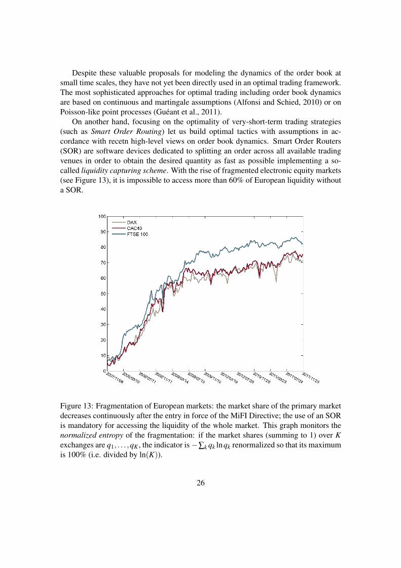
On another hand, focusing on the optimality of very-short-term trading strategies(such as Smart Order Routing) let us build optimal tactics with assumptions in ac-cordance with recetn high-level views on order book dynamics. Smart Order Routers(SOR) are software devices dedicated to splitting an order across all available tradingvenues in order to obtain the desired quantity as fast as possible implementing a so-called liquidity capturing scheme. With the rise of fragmented electronic equity markets(see Figure 13), it is impossible to access more than 60% of European liquidity withouta SOR.

Figure 13: Fragmentation of European markets: the market share of the primary marketdecreases continuously after the entry in force of the MiFI Directive; the use of an SORis mandatory for accessing the liquidity of the whole market. This graph monitors thenormalized entropy of the fragmentation: if the market shares (summing to 1) over Kexchanges are q1, . . . ,qK , the indicator is−∑k qk lnqk renormalized so that its maximumis 100% (i.e. divided by ln(K)).

26

Optimal policies for SOR have been proposed in Pages et al. (2012) and Ganchevet al. (2010). The latter used censored statistics to estimate liquidity available and tobuild an optimization framework on top of it; the former built a stochastic algorithmand proved that it asymptotically converges to a state that minimizes a given criterion.

To get a feel for the methodology associated with the stochastic algorithm viewpoint,just consider the following optimization problem.

Optimal liquidity seeking: the expected fast end criterion. To define the criterionto be optimized, first assume that K visible order books are available (for instance BATS,Chi-X, Euronext, Turquoise for an European stock). At time t, a buy order of size Vthas to be split over the order books according to a key (r1, . . . ,rK), given that on the kthorder book:

• the resting quantity ‘cheaper’ than a given price S is Ikt (i.e. the quantity at the bid

side posted at a price higher or equals to S, or at a lower price at the ask);

• the incoming flow of sell orders consuming the resting quantity at prices cheaperthan S follows a Poisson process Nk

t of intensity λ k, i.e.

E(Nkt+δ t−Nk

t ) = δ t ·λ k;

• the waiting time on the kth trading destination to consume a volume v added onthe kth trading destination at price S in t is denoted ∆T k

t (v); it is implicitly definedby:

∆T kt (v) = argmin

τ{Nk

t+τ −Nkt ≥ Ik

t + v}.

Assuming that there is no specific toxicity in available trading platforms, a traderwould like to split an incoming order at time t of size Vt according to an allocation key(r1, . . . ,rK) in order to minimize the waiting time criterion. Thus:

C (r1, . . . ,rK) = Emaxk{∆T k

t (rkVt)}. (12)

This means that the trader aims at optimizing the following process:

(1) an order of size Vτ(u) is to be split at time τ(u), the set of order arrival times beingS = {τ(1), . . . ,τ(n), . . .};

(2) it is split over the K available trading venues thanks to an ‘allocation key’, R =(r1, . . . ,rK): a portion rkVτ(u) is sent to the kth order book (all the quantity isspread, i.e. ∑k≤K rk = 1);

(3) the trader waits the time needed to consume all the sent orders.

27

The criterion C (R) defined in (12) reflects the fact that the faster the allocation keylets us obtain liquidity, the better: the obtained key is well suited for a liquidity-seekingalgorithm.

First denote by k∗t (R) the last trading destination to consume the order sent at t:

k∗t (R) = argmaxk{∆T k

t (rkVt)}.

A gradient approach to minimizing C (R) means we must compute ∂∆T ut (r

uVt)/∂ rk forany pair (k,u). To respect the constraint, just replace an arbitrary r` by 1−∑u 6=` ru.Consequently,

∂∆T ut (r

uVt)

∂ rk =∂∆T k

t (rk)

∂ rk 11k∗t (R)=k +∂∆T `

t (r`)

∂ rk 11k∗t (R)=`

where 11 is a delta function. With the notation ∆Nkt = Nk

t −Nkt−, we can write that any

allocation key R such that, for any pair (`,k),

E(

Vt ·Dkt (r

k) ·11k∗t (R)=k

)= E

(Vt ·D`

t (r`) ·11k∗t (R)=`

)(13)

whereDk

t (rk) =

1∆Nk

t+∆T kt (rk)

11(∆Nk

t+∆T kt (rk)

>0)

is a potential minimum for the criterion C (R) (the proof of this result will not be pro-vided here). Equation (13) can also be written as:

E(

Vt ·Dkt (r

k) ·11k∗t (R)=k

)=

1K

K

∑`=1

E(

Vt ·D`t (r

`) ·11k∗t (R)=`

).

It can be shown (see Lelong (2011) for generic results of this kind) that the asymp-totic solutions of the following stochastic algorithm on the allocation weights throughtime

∀k, rk(n+1) = rk(n)− γk+1

(Vτ(n) ·Dk

τ(n)(rk(n)) ·11k∗

τ(n)(R(n))=k−

1K

K

∑`=1

Vτ(n) ·D`τ(n)(r

`(n)) ·11k∗τ(n)(R(n))=`

)(14)

minimize the expected fast end criterion C (R), provided there are strong enough ergod-icity assumptions on the (V,(Nk)1≤k≤K,(Ik)1≤k≤K)-multidimensional process.

Qualitatively, we read this update rule to mean that if a trading venue k demandsmore time to execute the fraction of the volume that it receives (taking into account thecombination of I and N) than the average waiting time on all venues, then the fractionrk of the orders to send to k has to be decreased for future use.

28

5 Perspectives and Future WorkThe needs of intra-day trading practitioners are currently focused on optimal executionand trading risk control. Certainly some improvements on what is actually availablehave been proposed by academics, in particular:

• provide optimal trading trajectories taking into account multiple trading desti-nations and different type of orders: liquidity-providing (i.e. limit) ones andliquidity-consuming (i.e. market) ones;

• the analysis of trading performances is also an important topic; models are neededto understand what part of the performance and risk are due to the planned schedul-ing, the interactions with order books, the market impact and the market moves;

• stress testing: before executing a trading algorithm in real markets, we must un-derstand its dependence on different market conditions, from volatility or mo-mentum to bid–ask spread or trading frequency. The study of the ‘Greeks’ of thepayoff of a trading algorithm is not straightforward since it is inside a closed loopof liquidity: its ‘psi’ should be its derivative with respect to the bid–ask spread,its ‘phi’ with respect to the trading frequency, and its ‘lambda’ with respect to theliquidity available in the order book.

For the special case of portfolio liquidity studied in this chapter (using the payoffCλ defined by equality (11)), these trading Greeks would be:

Ψ =

(∂Cλ

∂ψ`

)1≤`≤N

, Φ =∂Cλ

∂N, Λ =

∂Cλ

∂κ.

Progress in the above three directions will provide a better understanding of theprice formation process and the whole cycle of asset allocation and hedging, taking intoaccount execution costs, closed loops with the markets, and portfolio trajectories at anyscales.

Acknowledgments Most of the data and graphics used here come from the work ofCredit Agricole Cheuvreux Quantitative Research group.

ReferencesAıt-Sahalia, Y. and Jacod, J. (2007). Volatility estimators for discretely sampled Levy

processes. Annals of Statistics 35 355–392.

Alfonsi, A., Fruth, A., and Schied, A. (2010). Optimal execution strategies in limit orderbooks with general shape functions. Quantitative Finance 10 (2) 143–157.

29

Alfonsi, A. and Schied, A. (2010). Optimal execution and absence of price manipula-tions in limit order book models. SIAM J. Finan. Math. 1 490–522.

Almgren, R., Thum, C., Hauptmann, E., and Li, H. (2005). Direct estimation of equitymarket impact. Risk 18 57–62.

Almgren, R. F. and Chriss, N. (2000). Optimal execution of portfolio transactions.Journal of Risk 3 (2) 5–39.

Altunata, S., Rakhlin, D., and Waelbroeck, H. (2010). Adverse selection vs. opportunis-tic savings in dark aggregators. Journal of Trading 5 16–28.

Avellaneda, M. and Stoikov, S. (2008). High-frequency trading in a limit order book.Quantitative Finance 8 (3) 217–224.

Bacry, E., Delattre, S., Hoffman, M., and Muzy, J. F. (2009). Deux modeles de bruitde microstructure et leur inference statistique. Preprint, CMAP, Ecole Polytechnique,France.

Biais, B., Glosten, L., and Spatt, C. (2005). Market microstructure: a survey of micro-foundations, empirical results, and policy implications. Journal of Financial Markets2 (8) 217–264.

Bouchard, B., Dang, N.-M., and Lehalle, C.-A. (2011). Optimal control of tradingalgorithms: a general impulse control approach. SIAM J. Financial Mathematics 2404–438.

Bouchaud, J. P., Mezard, M., and Potters, M. (2002). Statistical properties of stockorder books: empirical results and models. Quantitative Finance 2 (4) 251–256.

Chakraborti, A., Toke, I. M., Patriarca, M., and Abergel, F. (2011). Econophysics re-view: II. agent-based models. Quantitative Finance 11 (7) 1013–1041.

Cohen, K. J., Maier, S. F., Schwartz, R. A., and Whitcomb, D. K. (1981). Transactioncosts, order placement strategy, and existence of the bid–ask spread. The Journal ofPolitical Economy 89 (2) 287–305.

Cont, R. and De Larrard, A. (2011). Price dynamics in a Markovian limit order bookmarket. Social Science Research Network Working Paper Series.

Cont, R., Kukanov, A., and Stoikov, S. (2010). The price impact of order book events.Social Science Research Network Working Paper Series.

Engle, R. F., Ferstenberg, R., and Russell, J. R. (2012). Measuring and modeling exe-cution cost and risk. The Journal of Portfolio Management 38 (2) 14–28.

30

Foucault, T. and Menkveld, A. J. (2008). Competition for order flow and smart orderrouting systems. The Journal of Finance 63 (1) 119–158.

Gabaix, X., Gopikrishnan, P., Plerou, V., and Stanley, H. E. (2006). Institutional in-vestors and stock market volatility. Quarterly Journal of Economics 121 (2) m461–504.

Ganchev, K., Nevmyvaka, Y., Kearns, M., and Vaughan, J. W. (2010). Censored explo-ration and the dark pool problem. Commun. ACM 53 (5) 99–107.

Gatheral, J. (2010). No-dynamic-arbitrage and market impact. Quantitative Finance 10(7) 749–759.

Gatheral, J. and Schied, A. (2012). Dynamical models of market impact and algorithmsfor order execution. Handbook of Systemic Risk. Fouque, J.-P. and Langsam, J., (eds).Cambridge University Press.

Gueant, O., Lehalle, C. A., and Fernandez-Tapia, J. (2011). Optimal execution withlimit orders. Working paper.

Hayashi, T. and Yoshida, N. (2005). On covariance estimation of non-synchronouslyobserved diffusion processes. Bernoulli 11 (2) 359–379.

Hewlett, P. (2006). Clustering of order arrivals, price impact and trade path optimisation.In Workshop on Financial Modeling with Jump processes. Ecole Polytechnique.

Ho, T. and Stoll, H. R. (1981). Optimal dealer pricing under transactions and returnuncertainty. Journal of Financial Economics 9 (1) 47–73.

Jacod, J. (1996). La variation quadratique moyenne du brownien en presence d’erreursd’arrondi. In Hommage a P. A. Meyer et J. Neveu, Asterisque, 236.

Kirilenko, A. A., Kyle, A. P., Samadi, M., and Tuzun, T. (2010). The flash crash: theimpact of high frequency trading on an electronic market. Social Science ResearchNetwork Working Paper Series.

Kyle, A. P. (1985). Continuous auctions and insider trading. Econometrica 53 (6)1315–1335.

Large, J. (2007). Measuring the resiliency of an electronic limit order book. Journal ofFinancial Markets 10 (1) 1–25.

Lasry, J.-M. and Lions, P.-L. (2007). Mean field games. Japanese Journal of Mathe-matics 2 (1) 229–260.

31

Lehalle, C.-A. (2009). Rigorous strategic trading: balanced portfolio and mean-reversion. The Journal of Trading 4 (3) 40–46.

Lehalle, C.-A., Gueant, O., and Razafinimanana, J. (2010). High frequency simulationsof an order book: a two-scales approach. In Econophysics of Order-Driven Markets,Abergel, F., Chakrabarti, B. K., Chakraborti, A., and Mitra, M., (eds), New EconomicWindows. Springer.

Lelong, J. (2011). Asymptotic normality of randomly truncated stochastic algorithms.ESAIM: Probability and Statistics (forthcoming).

Lillo, F., Farmer, J. D., and Mantegna, R. (2003). Master curve for price–impact func-tion. Nature, 421, 129–130.

Markowitz, H. (1952). Portfolio selection. The Journal of Finance 7 (1) 77–91.

Menkveld, A. J. (2010). High frequency trading and the new-market makers. SocialScience Research Network Working Paper Series.

Muniesa, F. (2003). Des marches comme algorithmes: sociologie de la cotationelectronique a la Bourse de Paris. PhD thesis, Ecole Nationale Superieure des Minesde Paris.

Pages, G., Laruelle, S., and Lehalle, C.-A. (2012). Optimal split of orders across liquid-ity pools: a stochatic algorithm approach. SIAM Journal on Financial Mathematics2 (1) 1042–1076.

Predoiu, S., Shaikhet, G., and Shreve, S. (2011). Optimal execution of a general one-sided limit-order book. SIAM Journal on Financial Mathematics 2 183–212.

Robert, C. Y. and Rosenbaum, M. (2011). A new approach for the dynamics of ultra-high-frequency data: the model with uncertainty zones. Journal of Financial Econo-metrics 9 (2) 344–366.

Shiryaev, A. N. (1999). Essentials of Stochastic Finance: Facts, Models, Theory, 1stedition. World Scientific Publishing Company.

Smith, E., Farmer, D. J., Gillemot, L., and Krishnamurthy, S. (2003). Statistical theoryof the continuous double auction. Quantitative Finance 3 (6) 481–514.

Wyart, M., Bouchaud, J.-P., Kockelkoren, J., Potters, M., and Vettorazzo, M. (2008).Relation between bid–ask spread, impact and volatility in double auction markets.Quantitative finance 8 41–57.

32

Zhang, L., Mykland, P. A., and Sahalia, Y. A. (2005). A tale of two time scales: deter-mining integrated volatility with noisy high-frequency data. Journal of the AmericanStatistical Association 100 (472) 1394–1411.

33