Market Discipline and the Use of Stock Market Data to Predict ...

1

Market Discipline and the Use of Stock Market Data to Predict Bank Financial Distress

Isabelle Distinguin, Philippe Rous, Amine Tarazi*

Université de Limoges, LAPE, 4 place du Présidial, 87000 Limoges, France

March 2005

Abstract : The aim of this paper is to assess the extent to which stock market information can be used to estimate leading indicators of bank financial distress. This issue is of importance because of the increased emphasis on market forces by the Basel II committee (pillar 3). We specify a Logit early warning model, designed for European banks, which is used to test if market based indicators add predictive value to models relying on accounting data. Tests are also conducted to study the robustness of the link between market information and financial downgrading in the light of the too-big-too-fail (safety net) and the bank opacity (asymmetric information) hypotheses. Whereas some of our results support the use of market related indicators (in line with those previously obtained in the literature), we show that the accuracy of the predictive power is dependent on the extent to which bank liabilities are market traded. For banks which heavily rely on (insured) deposits, the market seems unable to convey useful information and the amount of subordinated debt issued by banks does not contribute to any improvement in the expected link.

Key words : Bank, Market Discipline, Bank Risk, Market Prices

JEL Classification : G21, G28

1. Introduction

Until the early 90’s early warning models of bank financial distress essentially relied

on public information contained in financial statements (accounting data) and on

macroeconomic variables. In recent years recommendations have aimed to enlarge the role of

market forces to promote safe and sound banking systems as well as the use of market

information by bank supervisors to improve the assessment of bank financial conditions

(Berger, Davies and Flannery [2000], Flannery [1998, 2001]).

This increased emphasis on market forces is at the heart of the new regulatory

framework developed by the Basel Committee on Banking and Supervision (Basel II Accord)

* Corresponding author. Tel. : +33-555-43-69-34; fax : +33-555-43-69-34 E-mail address: [email protected] (A. Tarazi).

2

which includes market discipline as one of its three pillars (BIS [2003]). By imposing greater

disclosure the aim is to improve the quality of the information provided by banks to investors

and market forces are therefore assumed to reinforce bank capital regulation and supervision

to ensure safety. Under market discipline market prices and returns reflect the accurate level

of individual bank risk because unlike insured depositors market investors will require a risk

premium which may increase banks’ cost of funding and therefore reduce risk taking

incentives. Consequently, it has been suggested that market prices could be used by

supervisors as signals and also complement accounting data in the design of early warning

systems.

Under such an approach, as noted by Feldman and Levonian [2001], a major issue is

whether the benefits from employing market information outweighs the costs and therefore

ensure an efficient allocation of supervisory resources. Therefore, because the cost of using

market information can be very high, a central question is whether market prices convey

additional information which is not already included in accounting data (Curry, Elmer and

Fissel [2002]).

Recent papers studying US banks have investigated the predictive power of models in

which market variables are added to standard call report financial data (Curry, Elmer and

Fissel [2002, 2003], Evanoff and Wall [2001]). Their findings support the idea that market

variables improve the assessment of bank financial health. In the European context Gropp,

Vesala and Vulpes [2005] focused on selected market indicators and their use as leading

indicators of bank financial distress. Their results show that indicators derived from market

prices are able to predict changes in bank financial health at a relatively long time horizon.

They also insist on the additional contribution of market indicators relatively to an average

indicator based on accounting data.

The objective of this paper is two-fold : firstly, to construct an early warning system of

bank financial distress specifically designed for European banks, and secondly to raise further

issues, in the light of modern intermediation theory ignored by the existing literature. More

precisely we start by building an early warning model based on downgrades by three rating

agencies Moody’s, Standard and Poors et Fitch and a large set of accounting and market

indicators. We then raise the issue of the additional contribution of market indicators based on

stock prices and specifically as regards the information conveyed by market prices for

banking institutions which are inherently opaque firms (asymmetric information). We also

question the opportunity of relying on market information in the light of the too-big-to-fail

3

issue and the reliance on a safety net, that is the likelihood that a bank receives support from

official or other sources (systemic risk).

The rest of the paper is laid out as follows. Section 2 discusses the issue and relates it

to the existing literature. Section 3 presents our methodology to estimate an early warning

model and to test our different propositions. Section 4 defines our sample and shows how our

leading indicators were constructed. Section 5 presents our empirical findings and section 6

concludes.

2. Issue and related literature

The issue of the reliance on market prices either to assess bank individual risk, the

accuracy of market discipline in banking, or to specifically predict bank financial distress has

been widely addressed in the literature (see Flannery [1998, 2001]). In a strand of this

literature the prices of different types of securities issued by banks (shares, bonds,

subordinated bonds, certificates of deposits…) have been used to study the link between

market variables and bank risk. Building on the findings of these papers another issue focused

on the potential for market prices to serve as early signals of bank failures or financial

distress.

Most of the existing literature focused on the prediction of large events such as actual

bank closures or sharp downgrades by rating agencies or by official sources (Supervisory

ratings). Studying US banks, Curry, Elmer and Fissel [2003] showed that the prediction of a

CAMEL (supervisory) rating downgrade to the lowest levels can be significantly improved by

adding market variables to a set of accounting indicators. However, this predictive power was

found to be significant only for banks in the greatest financial distress. Similarly, Gunther,

Levonian and Moore [2001] showed that the inclusion of a market indicator such as the

expected default frequency (EDF) improves the predictive power of a model based on

accounting ratios and CAMEL ratings.

To our knowledge only one study was dedicated to the case of European banks (Gropp,

Vesala and Vulpes [2005]). Based on a panel of 15 countries, their aim was to compare the

properties of stock market and subordinated debt data as early indicators of Fitch/IBCA

downgrades to C or below reflecting severe financial distress. They also showed that, beyond

the information conveyed by a composite score variable based on accounting data, the equity

market-based distance to default (KMV [2003]) significantly improves predictions up to an 18

months time horizon.

4

This paper extends the earlier studies in several directions by proposing a framework

which can be implemented for European banks and which enables to further raise two

theoretical issues neglected in the existing literature.

Firstly, based on a broad panel of European banks our approach combines different

frequency data (annual for accounting data and daily for market data) without imposing

underlying restrictive assumptions implicit to some of the existing empirical models which

are discussed in the next section.

Secondly, we focus on the predictive power of a large number of market indicators

estimated solely from stock prices. Because European markets for other securities issued by

banks (such as bonds or subordinated bonds) generally suffer from insufficient liquidity

(inactive trading) our analysis is restricted to equityholders incentives and uses, in contrast to

earlier studies, a greater variety of market indicators.

Thirdly, instead of focusing on bank failures or on severe financial distress we consider

the prediction of any downward change in a bank’s financial health. In this sense our view is

that early detection of downgrades may play a major role in the implementation of prompt

corrective action by regulators without jeopardizing strategic orientations followed by bank

managers. In this sense we deal with the issue of identifying banks’ future financial health by

considering the information contained in the changes in indicators (financial ratios and/or

market variables) rather than in their level as in previous studies.

Fourthly, our objective is also to test the robustness of results in the light of modern

financial intermediation theory developed in the steps of Leland and Pyle [1977], Diamond

and Dybvig [1983] and Diamond [1984]. Banks and financial intermediaries are considered as

agents that play a major role in the financial system as information intermediaries. They

collect and process information namely about loan customers (Diamond 1984, 1991) which

implies that they possess private information. As such, market participants (outsiders) should

have limited ability to monitor banks and market discipline in the banking industry should not

play a prominent role. Therefore, due to the inherent opacity of banks (opacity effect) and the

need to support large banking institutions (too-big-to-fail effect) we question the ability of

market indicators to accurately predict future financial distress for different types of banks

and financial institutions.

5

3. Methodology

As a first step, we implement a procedure to test for the specific and additional

contribution of various market indicators to the prediction of bank financial distress. We then

study the stability of the predictive power of early warning market indicators with respect to

bank size and balance sheet structure.

3.1. Identifying the additional contribution of market indicators

Assessing the ability of market indicators to predict bank financial distress requires

the choice of an event capturing the changing status of each bank. In the absence of actual

bankruptcies in the European banking industry in sufficient number we identify changes in a

bank’s financial condition through downgrading announcements by three rating agencies

(Fitch, Standard & Poors, and Moody’s). Most studies on US banks considered either explicit

bank failures or supervisory ratings (Curry, Elmer and Fissel [2003], Gunther, Levonian and

Moore [2004]). Because of the lack of access to explicit supervisory ratings in Europe which

are confidential in most countries we rely on public information disclosed by private agencies.

In this sense the selection of our events is close to the method developed by Gropp, Vesala

and Vulpes [2005] who use downgrades of Fitch individual ratings to C or below as a proxy

of bank failure. In contrast to their study, and because we are more concerned by the actual

information content of stock prices than their ability to forecast failures, we consider that any

downgrading announcement should be retained in our study. This implies that a deterioration

in a bank’s financial health is captured in our study by a downgrading from any initial level

and down to any level below. Identifying both narrow and broad changes is essential for the

robustness of results and provides a more general framework for early warning models

estimation.

We then define two sets of variables : accounting indicators and equity market based

indicators likely to predict a future downgrade in a bank’s financial condition. When

assessing the link between the dependent variable and early warning indicators several

shortcomings need to be tackled. Firstly, the different variables are not available at the same

frequencies (daily for market indicators, yearly for accounting indicators). Whereas some

studies proceed by linear or more advanced interpolation of low frequency data (i.e. Gropp et

alii [2005]) we consider that such a procedure is not convenient because it implies that in

some cases future information may be used to explain current downgrades. Therefore instead

of departing from each event (downgrade by a rating agency) to then compute all the relevant

6

accounting and market indicators on a backward given time horizon we deal with the issue of

predictability departing from each date at which accounting data information is available. In

the case of European banks this date is 31 December of each year. We then consider events

taking place in the four subsequent quarters following this date.

Formally, consider that for each of the N banks of the sample, there are T observations

through time for accounting indicators. These dates are retained as the starting point for the

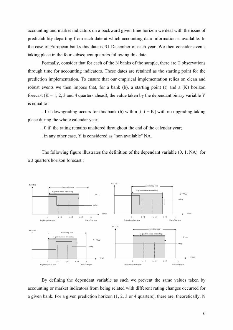
prediction implementation. To ensure that our empirical implementation relies on clean and

robust events we then impose that, for a bank (b), a starting point (t) and a (K) horizon

forecast (K = 1, 2, 3 and 4 quarters ahead), the value taken by the dependant binary variable Y

is equal to :

. 1 if downgrading occurs for this bank (b) within [t, t + K] with no upgrading taking

place during the whole calendar year;

. 0 if the rating remains unaltered throughout the end of the calendar year;

. in any other case, Y is considered as "non available" NA.

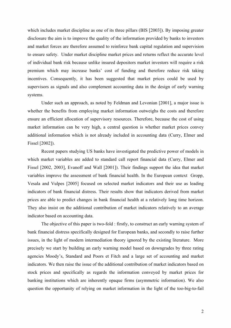
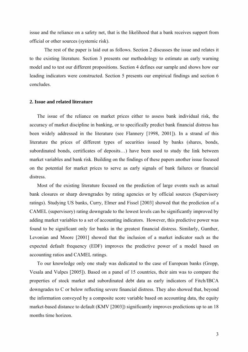
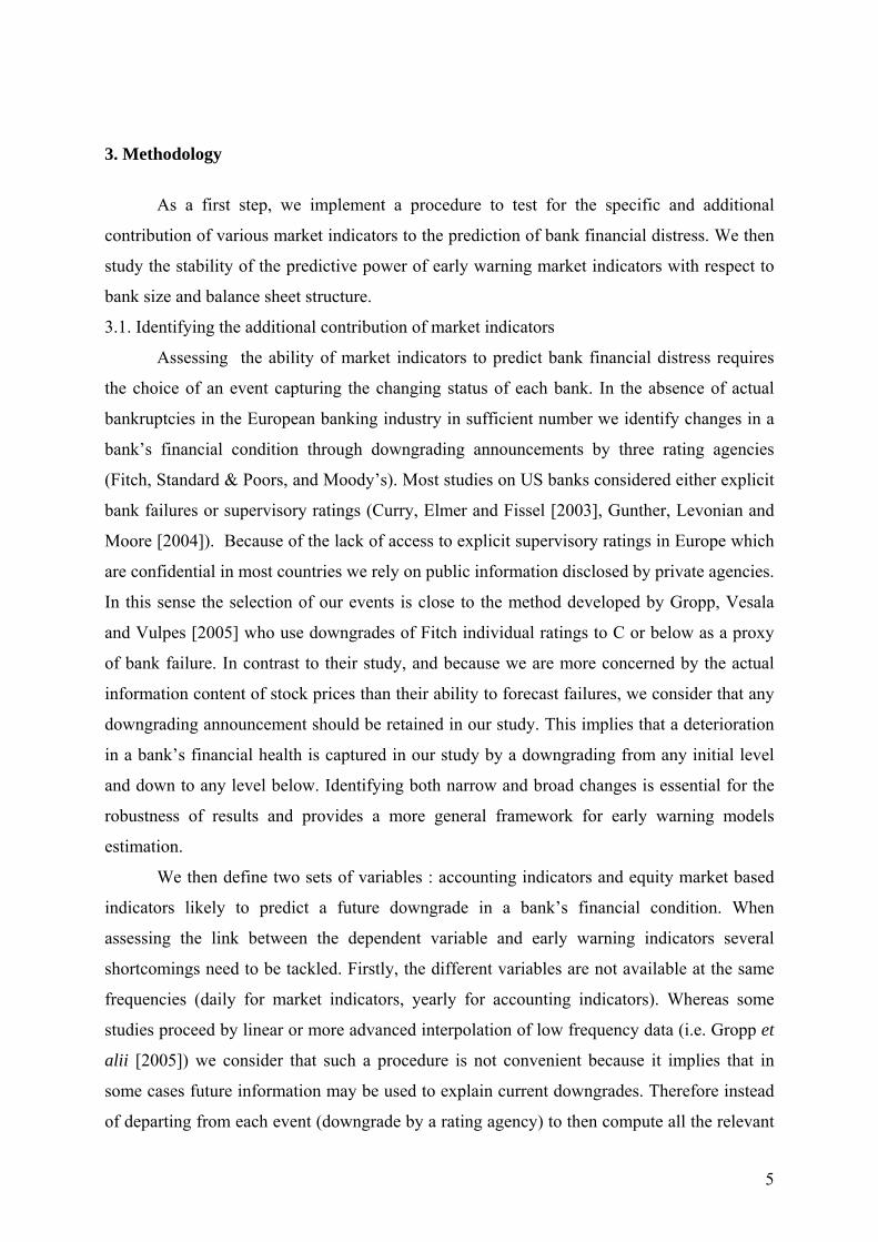
The following figure illustrates the definition of the dependant variable (0, 1, NA) for

a 3 quarters horizon forecast :

TIME

RATING

t1

Begining of the year

t1 +1 t1 +2 t1 +3 t2

End of the year

Accounting year

3 quarters ahead forecasting

Y = 1

rating

TIME

RATING

t1

Beginning of the year

t1 +1 t1 +2 t1 +3 t2

End of the year

Accounting year

3 quarters ahead forecasting

Y = "NA"

rating

TIME

RATING

t1

Beginning of the year

t1 +1 t1 +2 t1 +3 t2

End of the year

Accounting year

3 quarters ahead forecasting

Y = "NA"

rating

TIME

RATING

t1

Beginning of the year

t1 +1 t1 +2 t1 +3 t2

End of the year

Accounting year

3 quarters ahead forecasting

Y = 0

rating

By defining the dependant variable as such we prevent the same values taken by

accounting or market indicators from being related with different rating changes occurred for

a given bank. For a given prediction horizon (1, 2, 3 or 4 quarters), there are, theoretically, N

7

× T observations Yi for the explained binary variable where i refers to a bank (b), a starting

prediction point (t) and a forecasting horizon (K):

i = i(b, t, K)

Accounting Cji(b, t, K) and market Mli(b, t, K) indicators are computed at a starting point

(t), that is on December 31th of each year. Consequently, the interpolation of the missing

accounting data as implemented by Gropp, Vesala and Vulpes [2005] to estimate their

distance to default indicator is suitably avoided ensuring that the information content of

accounting data based indicators is not inappropriately upward biased.

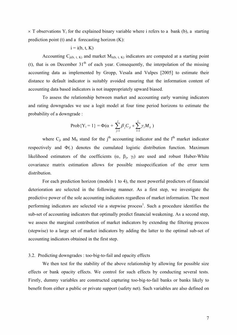
To assess the relationship between market and accounting early warning indicators

and rating downgrades we use a logit model at four time period horizons to estimate the

probability of a downgrade :

Prob{Yi = 1} = Φ(α + 1 1= =

+∑ ∑J L

j ji l lij l

C Mβ γ )

where Cji and Mli stand for the jth accounting indicator and the lth market indicator

respectively and Φ(.) denotes the cumulated logistic distribution function. Maximum

likelihood estimators of the coefficients (α, βj, γl) are used and robust Huber-White

covariance matrix estimation allows for possible misspecification of the error term

distribution.

For each prediction horizon (models 1 to 4), the most powerful predictors of financial

deterioration are selected in the following manner. As a first step, we investigate the

predictive power of the sole accounting indicators regardless of market information. The most

performing indicators are selected via a stepwise process1. Such a procedure identifies the

sub-set of accounting indicators that optimally predict financial weakening. As a second step,

we assess the marginal contribution of market indicators by extending the filtering process

(stepwise) to a large set of market indicators by adding the latter to the optimal sub-set of

accounting indicators obtained in the first step.

3.2. Predicting downgrades : too-big-to-fail and opacity effects

We then test for the stability of the above relationship by allowing for possible size

effects or bank opacity effects. We control for such effects by conducting several tests.

Firstly, dummy variables are constructed capturing too-big-to-fail banks or banks likely to

benefit from either a public or private support (safety net). Such variables are also defined on

8

the basis of a set of standard financial ratios which are generally used as opacity proxies in the

literature. Dummies are then introduced in the different models (models 1 to 4) to conduct a

series of stability tests. Secondly, tests are also carried out by estimating the different models

on restricted samples of banks.

4. Sample and indicators

4.1. Sample

The sample consists of events (downgrades or absence of downgrades) related to 64

European banks regularly listed on the stock market and for which ratings from at least one of

the three major rating agencies (Fitch, Moody's or Standard and Poors) are available during

the 1995-2002 period. Table 1 presents the distribution of these banks by country and

specialisation.

Table 1 : distribution of banks by country and specialisation

Country NumbersGermany 7Denmark 1

Spain 5France 8Greece 2Ireland 1

Italy 15Luxemburg 1

Norway 2The Netherlands 4

Portugal 4United Kingdom 11

Sweden 1Switzerland 2

Specialisation Numberscommercial bank 31cooperative bank 7

medium and long term credit bank 2real estate and mortgage bank 6

savings bank 2investment bank 3

bank holding and holding coimpany 9non banking credit institution 4

Daily market data (bank stock prices) are taken from Datastream International and

annual income statements and balance sheets come from Bankscope Fitch IBCA. Our sample

of banks is restricted to EU banks for which market data is reliable for the purpose of our

study. Only actively and regularly traded stocks were considered. Table 2 shows descriptive

statistics on our sample of banks which exhibits a relatively high level of heterogeneity. This

enables us to investigate further on the robustness of the relationship between early indicators

and the probability of financial deterioration with respect to differences in size or balance

1 As a common rule of thumb, we retained a 5 % level for type 1 error ; a Max (Min) LR statistic was used as a

9

sheet structure. Also this raises the problem of observations which may be considered as

outliers.

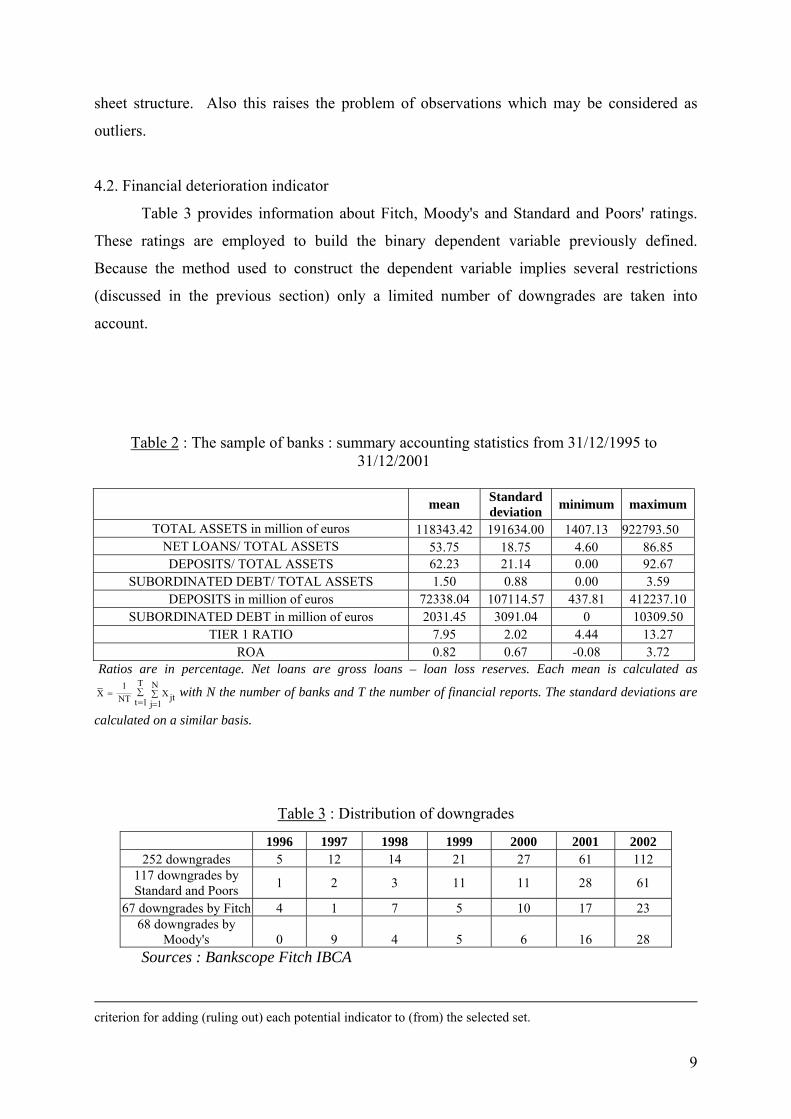
4.2. Financial deterioration indicator

Table 3 provides information about Fitch, Moody's and Standard and Poors' ratings.

These ratings are employed to build the binary dependent variable previously defined.

Because the method used to construct the dependent variable implies several restrictions

(discussed in the previous section) only a limited number of downgrades are taken into

account.

Table 2 : The sample of banks : summary accounting statistics from 31/12/1995 to 31/12/2001

mean Standard

deviation minimum maximum

TOTAL ASSETS in million of euros 118343.42 191634.00 1407.13 922793.50 NET LOANS/ TOTAL ASSETS 53.75 18.75 4.60 86.85 DEPOSITS/ TOTAL ASSETS 62.23 21.14 0.00 92.67

SUBORDINATED DEBT/ TOTAL ASSETS 1.50 0.88 0.00 3.59 DEPOSITS in million of euros 72338.04 107114.57 437.81 412237.10

SUBORDINATED DEBT in million of euros 2031.45 3091.04 0 10309.50 TIER 1 RATIO 7.95 2.02 4.44 13.27

ROA 0.82 0.67 -0.08 3.72 Ratios are in percentage. Net loans are gross loans – loan loss reserves. Each mean is calculated as

T N1X X jtNT t 1 j 1

∑= ∑= =

with N the number of banks and T the number of financial reports. The standard deviations are

calculated on a similar basis.

Table 3 : Distribution of downgrades

1996 1997 1998 1999 2000 2001 2002 252 downgrades 5 12 14 21 27 61 112

117 downgrades by Standard and Poors 1 2 3 11 11 28 61

67 downgrades by Fitch 4 1 7 5 10 17 23 68 downgrades by

Moody's 0 9 4 5 6 16 28 Sources : Bankscope Fitch IBCA

criterion for adding (ruling out) each potential indicator to (from) the selected set.

10

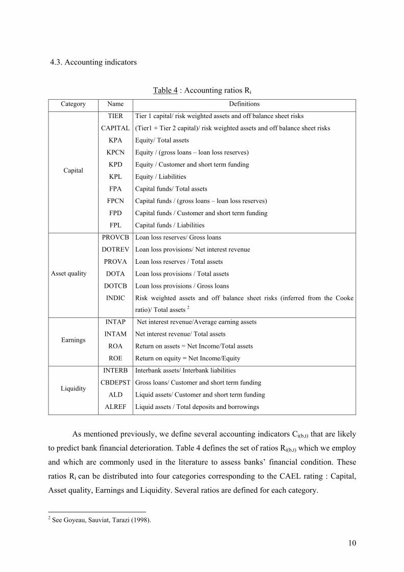
4.3. Accounting indicators

Table 4 : Accounting ratios Ri

Category Name Definitions

TIER Tier 1 capital/ risk weighted assets and off balance sheet risks

CAPITAL (Tier1 + Tier 2 capital)/ risk weighted assets and off balance sheet risks

KPA Equity/ Total assets

KPCN Equity / (gross loans – loan loss reserves)

KPD Equity / Customer and short term funding

KPL Equity / Liabilities

FPA Capital funds/ Total assets

FPCN Capital funds / (gross loans – loan loss reserves)

FPD Capital funds / Customer and short term funding

Capital

FPL Capital funds / Liabilities

PROVCB Loan loss reserves/ Gross loans

DOTREV Loan loss provisions/ Net interest revenue

PROVA Loan loss reserves / Total assets

DOTA Loan loss provisions / Total assets

DOTCB Loan loss provisions / Gross loans

Asset quality

INDIC Risk weighted assets and off balance sheet risks (inferred from the Cooke

ratio)/ Total assets 2

INTAP Net interest revenue/Average earning assets

INTAM Net interest revenue/ Total assets

ROA Return on assets = Net Income/Total assets Earnings

ROE Return on equity = Net Income/Equity

INTERB Interbank assets/ Interbank liabilities

CBDEPST Gross loans/ Customer and short term funding

ALD Liquid assets/ Customer and short term funding Liquidity

ALREF Liquid assets / Total deposits and borrowings

As mentioned previously, we define several accounting indicators Ci(b,t) that are likely

to predict bank financial deterioration. Table 4 defines the set of ratios Ri(b,t) which we employ

and which are commonly used in the literature to assess banks’ financial condition. These

ratios Ri can be distributed into four categories corresponding to the CAEL rating : Capital,

Asset quality, Earnings and Liquidity. Several ratios are defined for each category.

2 See Goyeau, Sauviat, Tarazi (1998).

11

Accounting ratios can be introduced in such prediction models either in level or in

variation (first order difference). Most of the previous studies considered these ratios in level

(Gunther, Levonian and Moore [2001], Curry, Elmer and Fissel [2002]) which can be justified

when it comes to predict an event like a failure. However, if the aim is rather to predict a

change in financial health it seems more appropriate to introduce not the values taken by the

ratios, but their time changes. Besides, in this study, all banks are treated equally regardless of

their initial financial strength. This means that the downgrade of a sound and safe bank (as

might be reflected by the level of financial ratios) can only be captured by changes in the

values of ratios. Also, because our sample consists of banks with a broad range of ratings,

considering the values taken by financial indicators would be inappropriate. Therefore we

define Cji(b, t), the change in the value of the accounting ratio Rji as : Cji(b,t) = ∆Rji(b,t) = Rji(b, t) -

Rji(b,t-1). Accounting indicators used in this study are these changes further denoted by Cji(b,t).

4.4. Market indicators

We can reasonably assume that the equity market conveys useful information to

predict financial deterioration. If the market is efficient, prices and returns should incorporate

the risk exposure of banks and thus their default risk. Table 5 presents the market based

indicators used in this study which are constructed from daily equity prices. In contrast with

previous literature we cover a broad range of indicators to compare their relative predictive

power. The variables LNP, RCUM, EXCRCUM, RCUM_NEG, EXCRCUM_NEG, RAC are

used to capture the effects of shocks or the presence of abnormal returns in event studies. The

variables ∆ECTYP, ∆BETA and ∆RISKSPEC are employed to detect risk changes and ∆Z

and ∆DD changes in the probability of failure. Some of the variables used in this study have

already been introduced in similar models of bank distress to test the additional predictive

contribution of stock market prices. Market excess return (EXCRCUM) and durably negative

market excess return (EXCRCUM_NEG) were introduced by Elmer and Fissel [2001].

Gropp, Vesala and Vulpes [2005] used the value taken by the distance to default variable. In

this study, several market indicators are introduced in difference in the predictive equation

(variables reflecting market assessment of risk or the probability of failure).

12

Table 5 : Market indicators

Indicators Definition Expected sign of the coefficient

LNP Difference between the natural logarithm of market price and its moving average calculated on 261 days. Negative

RCUM

Cumulative return :

( )65

, 11

1 1bt b t kk

RCUM r − +

=

= + −⎛⎛ ⎞ ⎞⎜⎜ ⎟ ⎟⎝⎝ ⎠ ⎠

∏ with rb,t+1 = , 1 , ,( /)b t b t b tP P P+ − where rbt is the daily return of the stock b; this cumulative return is

calculated on the fourth quarter of the accounting period (financial year) preceding the event, Pbt is the daily stock price of bank b.

Negative

RCUM_NEG Dummy variable equal to 1 if the cumulative return is negative in the two last quarters of the accounting period (financial year) preceding the event and 0 otherwise. Positive

EXCRCUM

Cumulative market excess return : ( ) ( )

65 65

, , 1 , 11 1

1 1 1 1− + − += =

⎛ ⎞ ⎛ ⎞⎛ ⎞ ⎛ ⎞⎜ ⎟ ⎜ ⎟⎜ ⎟ ⎜ ⎟⎜ ⎟ ⎜ ⎟⎜ ⎟ ⎜ ⎟⎜ ⎟ ⎜ ⎟⎝ ⎠ ⎝ ⎠⎝ ⎠ ⎝ ⎠

= + − − + −∏ ∏b t b t k m t kk k

EXCRCUM r r

with rm the daily market return calculated from market index extracted from Datastream International for the fourth quarter of the financial exercise preceding the event.

Negative

EXCRCUM_NEG Dummy variable equal to 1 if the cumulative market excess return is negative in the two last quarters of the accounting period (financial year) preceding the event and 0 otherwise. Positive

RAC

Cumulative abnormal returns on the fourth quarter of the accounting period (financial year) preceding the event:

RACbt= 65

, 11

b t kk

RA − +

=

∑ with RAbt=Rbt-( ˆˆmtRα β+ ) , the market model is estimated on the third quarter of the accounting period (financial

year) preceding the event

Negative

∆ECTYP Change in the standard deviation of daily returns between the third and fourth quarter of the accounting period (financial year) preceding the event Positive

∆BETA Change in the market model beta ( ˆˆˆmtbt RR α β+= ) between the third and fourth quarter of the accounting period (financial year)

preceding the event Positive

∆RISKSPEC Change in specific risk : standard deviation of the market model residual between the third and fourth quarter of the accounting period (financial year) preceding the event. Positive

∆Z Change in the Z-score between the third and fourth quarter of the accounting period (financial year) preceding the event with : Z= ( )1 /b rr σ+ where br is the mean return of stock b on the preceding quarter and rσ the standard deviation of the return. Negative

∆DD Change in the distance to default between the third and fourth quarter of the accounting period (financial year) preceding the event. The distance to default is inferred from the market value of a risky debt (Merton (1977)) based on the Black and Scholes (1973) option pricing formula. Details on the estimation method and on the data are presented in appendix.

Negative

13

5. Empirical results

As a preliminary stage we consider the predictive power of each indicator by running

logistic regressions in which each explanatory variable is introduced separately. We then

present the best performing accounting based models for the different prediction horizons.

The additional contribution of market indicators is then assessed by augmenting each model

with market indicators which are selected by the stepwise procedure. Eventually, tests are

conducted to study the robustness of the predictive power of market indicators with respect to

bank size (too-big-to-fail effect) and bank balance sheet structure (opacity effect).

5.1. Individual contribution of indicators

Table 6 shows the results obtained for each horizon (models 1 to 4), when each early

indicator is separately introduced in the model. Results are only reported when coefficients

are at least significant at the 10% level. The last column of table 6 (model 5) shows the results

that are obtained when the dependent binary variable Y is based on sharp downgrades

reflecting severe financial distress (failure or quasi-failure).

On the whole, the coefficients associated to changes in profitability ratios (∆ROA et

∆ROE) or to loan loss provisions (∆DOTCB) are significant only for the longer horizons (2, 3

and 4 quarters). Inversely changes in capital ratios (∆KPCN et ∆KPD) perform significantly

only for the shortest horizon (1 quarter). These results suggest that income statement

information (flows) allows earlier prediction of financial downgrades whereas balance sheet

information (stocks) which is by definition less flexible might only be useful for relatively

shorter horizons. The negative (expected sign) and significant contribution of the change in

the liquidity ratio (∆ALREF) for the shortest horizon solely suggests that downgrades are

shortly preceded by a partial liquidation of liquid assets. However, similarly to balance sheet

information this signal can only be employed at a short horizon. On the whole, these

preliminary results favour indicators which combine information contained in both balance

sheets and income statements for longer horizons predictions.

The results obtained in table 6 for market indicators show that for every time horizon a

number of market based variables significantly predict financial deterioration (downgrades).

In each logistic regression (for every prediction horizon) the coefficients of the variables

capturing downward or upward trends in stock prices or negative cumulative returns (LNP

and RCUM_NEG) are highly significant with the expected sign. Cumulative excess returns

14

(EXCRCUM) are significant for three out of four horizons. If we consider the longest

horizon (1 year) the coefficient of the cumulative return variable (RCUM) and the coefficient

of the negative cumulative market excess return (EXCRCUM_NEG) are also significantly

different from 0. These preliminary results suggest that market based indicators may well

contribute to predict financial difficulties at a relatively long time horizon.

Table 6 : Financial deterioration and early indicators : simple regressions Model specification : Prob{Yi = 1} = Φ(α + β Xi)

Model 1 Model 2 Model 3 Model 4 Model 5

∆KPCN 0.137** (1.970)

∆KPD -0.170* (-1.808) -0.139*

(-1.854) Capital

∆CAPITAL 0.263** (2.267)

∆DOTREV 0.020* (1.845)

0.019* (1.787)

Asset quality ∆DOTCB 0.928**

(2.023) 1.019** (2.257)

0.786** (2.040)

∆INTAM -1.606** (-1.988)

∆INTAP -1.670** (-2.550)

∆ROA -0.661** (-2.024)

-0.649* (-1.947)

Earnings

∆ROE -0.070** (-2.436)

-0.061** (-2.325)

-0.053** (-2.356)

Liquidity ∆ALREF -0.075** (-2.221)

EXCRCUM -3.039** (-2.250)

-2.378** (-1.994)

-2.466** (-2.522)

-5.663*** (-3.600)

EXCRCUM_NEG 0.550*

(1.720)

LNP -2.869* (-1.951)

-2.996** (-2.464)

-3.333*** (-2.804)

-3.693*** (-3.416)

-6.183*** (-2.827)

RCUM -2.769** (-2.396)

-2.409* (-1.917)

Market indicators

RCUM_NEG 1.311** (2.388)

1.180*** (2.794)

0.968** (2.424)

0.991*** (2.890)

1.744*** (3.283)

This table reports simple logit estimation results : for each model, the dependent variable is separately regressed on each explanatory variable and a constant. Models 1, 2, 3 and 4 explain downgradings (whatever their extent) occurring respectively in less than 1, 2, 3 and 4 quarters. Model 5 explains only downgradings occurring in less than 4 quarters and reflecting quasi-insolvency. Standard errors are adjusted using the Huber-White method. *, ** and *** indicate significance respectively at 10%, 5% and 1% levels. Z-statistics are shown in parenthesis.

15

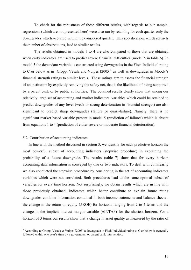
To check for the robustness of these different results, with regards to our sample,

regressions (which are not presented here) were also ran by retaining for each quarter only the

downgrades which occurred within the considered quarter. This specification, which restricts

the number of observations, lead to similar results.

The results obtained in models 1 to 4 are also compared to those that are obtained

when early indicators are used to predict severe financial difficulties (model 5 in table 6). In

model 5 the dependant variable is constructed using downgrades in the Fitch Individual rating

to C or below as in Gropp, Vesala and Vulpes [2005]3 as well as downgrades in Moody’s

financial strength ratings to similar levels. These ratings aim to assess the financial strength

of an institution by explicitly removing the safety net, that is the likelihood of being supported

by a parent bank or by public authorities. The obtained results clearly show that among our

relatively large set of accounting and market indicators, variables which could be retained to

predict downgrades of any level (weak or strong deterioration in financial strength) are also

significant to predict sharp downgrades (failure or quasi-failure). Namely, there is no

significant market based variable present in model 5 (prediction of failures) which is absent

from equations 1 to 4 (prediction of either severe or moderate financial deterioration).

5.2. Contribution of accounting indicators

In line with the method discussed in section 3, we identify for each predictive horizon the

most powerful subset of accounting indicators (stepwise procedure) in explaining the

probability of a future downgrade. The results (table 7) show that for every horizon

accounting data information is conveyed by one or two indicators. To deal with collinearity

we also conducted the stepwise procedure by considering in the set of accounting indicators

variables which were not correlated. Both procedures lead to the same optimal subset of

variables for every time horizon. Not surprisingly, we obtain results which are in line with

those previously obtained. Indicators which better contribute to explain future rating

downgrades combine information contained in both income statements and balance sheets :

the change in the return on equity (∆ROE) for horizons ranging from 2 to 4 terms and the

change in the implicit interest margin variable (∆INTAP) for the shortest horizon. For a

horizon of 3 terms our results show that a change in asset quality as measured by the ratio of

3 According to Gropp, Vesala et Vulpes [2005] a downgrade in Fitch Individual rating to C or below is generally followed within one year’s time by a government or parent bank intervention.

16

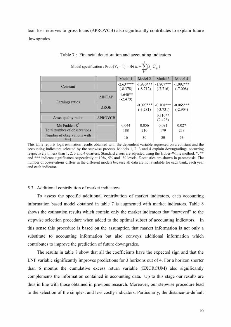
loan loss reserves to gross loans (∆PROVCB) also significantly contributes to explain future

downgrades.

Table 7 : Financial deterioration and accounting indicators

Model specification : Prob{Yi = 1} = Φ(J

j jij 1

C=

α + β∑ )

Model 1 Model 2 Model 3 Model 4

Constant -2.637***(-8.378)

-1.930***(-8.712)

-1.807*** (-7.716)

-1.092*** (-7.008)

∆INTAP -1.640** (-2.479)

Earnings ratios ∆ROE -0.093***

(-3.281) -0.108*** (-3.731)

-0.065*** (-2.904)

Asset quality ratios ∆PROVCB 0.310** (2.423)

0.044 0.056 0.091 0.027 Mc Fadden R2

Total number of observations 188 210 179 238

Number of observations with Y=1 16 30 30 63

This table reports logit estimation results obtained with the dependent variable regressed on a constant and the accounting indicators selected by the stepwise process. Models 1, 2, 3 and 4 explain downgradings occurring respectively in less than 1, 2, 3 and 4 quarters. Standard errors are adjusted using the Huber-White method. *, ** and *** indicate significance respectively at 10%, 5% and 1% levels. Z-statistics are shown in parenthesis. The number of observations differs in the different models because all data are not available for each bank, each year and each indicator.

5.3. Additional contribution of market indicators

To assess the specific additional contribution of market indicators, each accounting

information based model obtained in table 7 is augmented with market indicators. Table 8

shows the estimation results which contain only the market indicators that “survived” to the

stepwise selection procedure when added to the optimal subset of accounting indicators. In

this sense this procedure is based on the assumption that market information is not only a

substitute to accounting information but also conveys additional information which

contributes to improve the prediction of future downgrades.

The results in table 8 show that all the coefficients have the expected sign and that the

LNP variable significantly improves predictions for 3 horizons out of 4. For a horizon shorter

than 6 months the cumulative excess return variable (EXCRCUM) also significantly

complements the information contained in accounting data. Up to this stage our results are

thus in line with those obtained in previous research. Moreover, our stepwise procedure lead

to the selection of the simplest and less costly indicators. Particularly, the distance-to-default

17

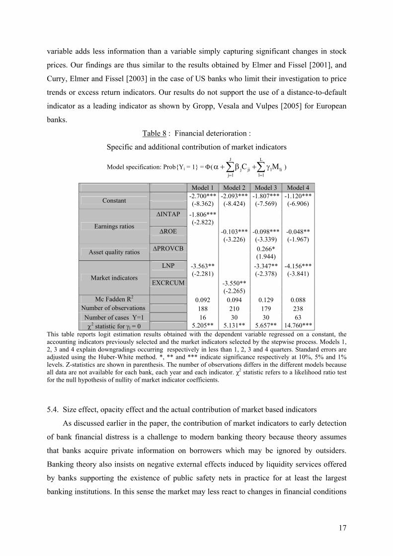
variable adds less information than a variable simply capturing significant changes in stock

prices. Our findings are thus similar to the results obtained by Elmer and Fissel [2001], and

Curry, Elmer and Fissel [2003] in the case of US banks who limit their investigation to price

trends or excess return indicators. Our results do not support the use of a distance-to-default

indicator as a leading indicator as shown by Gropp, Vesala and Vulpes [2005] for European

banks.

Table 8 : Financial deterioration :

Specific and additional contribution of market indicators

Model specification: Prob{Yi = 1} = Φ(J L

j ji l lij 1 l 1

C M= =

α + β + γ∑ ∑ )

Model 1 Model 2 Model 3 Model 4 Constant

-2.700***(-8.362)

-2.093***(-8.424)

-1.807*** (-7.569)

-1.120*** (-6.906)

∆INTAP

-1.806***(-2.822)

∆ROE Earnings ratios

-0.103***(-3.226)

-0.098*** (-3.339)

-0.048** (-1.967)

∆PROVCBAsset quality ratios

0.266* (1.944)

LNP

-3.563** (-2.281)

-3.347** (-2.378)

-4.156*** (-3.841)

EXCRCUMMarket indicators

-3.550** (-2.265)

Mc Fadden R2 0.092 0.094 0.129 0.088 Number of observations 188 210 179 238 Number of cases Y=1 16 30 30 63

χ2 statistic for γl = 0 5.205** 5.131** 5.657** 14.760*** This table reports logit estimation results obtained with the dependent variable regressed on a constant, the accounting indicators previously selected and the market indicators selected by the stepwise process. Models 1, 2, 3 and 4 explain downgradings occurring respectively in less than 1, 2, 3 and 4 quarters. Standard errors are adjusted using the Huber-White method. *, ** and *** indicate significance respectively at 10%, 5% and 1% levels. Z-statistics are shown in parenthesis. The number of observations differs in the different models because all data are not available for each bank, each year and each indicator. χ2 statistic refers to a likelihood ratio test for the null hypothesis of nullity of market indicator coefficients.

5.4. Size effect, opacity effect and the actual contribution of market based indicators

As discussed earlier in the paper, the contribution of market indicators to early detection

of bank financial distress is a challenge to modern banking theory because theory assumes

that banks acquire private information on borrowers which may be ignored by outsiders.

Banking theory also insists on negative external effects induced by liquidity services offered

by banks supporting the existence of public safety nets in practice for at least the largest

banking institutions. In this sense the market may less react to changes in financial conditions

18

for large institutions implying a lower contribution of market prices to predict future failure.

Conversely, one could assume that the market mainly focuses on the largest institutions

because information may be less reliable for smaller banks. Identically, bank opacity may also

affect the marginal contribution of market indicators. In the banking literature, private

information is often captured by assessing the structure of financial statements. In theory,

opacity comes from the intermediation function of banks and is often proxied by the ratio of

loans to total assets. Since deposits are insured and deposit interest rates are not marked to

market alternatively the ratio of deposits to total assets is also another frequently employed

proxy. Conversely, large issues of non insured securities such as bonds or subordinated bonds

(market funded liabilities) should induce market discipline hence contributing to improve the

quality of the information conveyed by the market. Because liquidity is essential for market

signals to transmit accurate information, the extent to which liabilities are market funded is

crucial. Therefore the proportion of market funding on the liability side of the balance sheet is

also considered as a determinant variable in several studies.

The size effect and the opacity effect are assessed by first estimating for each horizon

an augmented model specified as follows :

Prob{Yi = 1} = Φ(α + α' Di + 1 1= =

+∑ ∑J L

j ji l lij l

C Mβ γ + 1

'=∑

L

l i lil

D Mγ )

where Di is a dummy variable, capturing either the size effect (DBIGi) or the opacity effect

(DOPACi). Two tests are then conducted first to determine the effectiveness of each effect

(H0 : α' = 0 and γ’l = 0 ∀ l) and then to assess the assumption that size or opacity outweighs

or neutralizes the predictive power of each market indicator (H0 : γl + γ’l = 0 ∀ l).

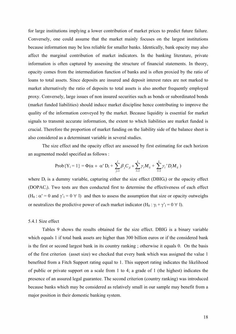
5.4.1 Size effect

Tables 9 shows the results obtained for the size effect. DBIG is a binary variable

which equals 1 if total bank assets are higher than 300 billion euros or if the considered bank

is the first or second largest bank in its country ranking ; otherwise it equals 0. On the basis

of the first criterion (asset size) we checked that every bank which was assigned the value 1

benefited from a Fitch Support rating equal to 1. This support rating indicates the likelihood

of public or private support on a scale from 1 to 4; a grade of 1 (the highest) indicates the

presence of an assured legal guarantee. The second criterion (country ranking) was introduced

because banks which may be considered as relatively small in our sample may benefit from a

major position in their domestic banking system.

19

Table 9 : Contribution of market indicators and bank size

Model specification : Prob{Yi = 1} = Φ(J L L

i j ji l li l i lij 1 l 1 l 1

' DBIG C M ' (DBIG M= = =

α + α + β + γ + γ ×∑ ∑ ∑ )

Model 1 Model 2 Model 3 Model 4 Constant

-3.397*** (-7.186)

-2.643*** (-7.545)

-2.266*** (-6.973)

-1.221*** (-6.472)

DBIG

1.478*** (2.224)

1.421*** (2.957)

1.130** (2.519)

0.355 (0.991)

∆INTAP

-2.482*** (-3.500)

∆ROE

-0.092*** (-2.842)

-0.096** (-3.060)

-0.048* (-1.935)

∆PROVCB

0.227* (1.714)

LNP

-1.485 (-1.068) -2.365

(-1.151) -3.374*** (-2.668)

LNP × DBIG

-5.608* (-1.828) -2.218

(-0.785) -2.657

(-1.148) EXCRCUM

-4.833** (-2.148)

EXCRCUM × DBIG

1.388 (0.407)

Mc Fadden R2 0.190 0.148 0.177 0.098 Total number of observations 188 210 179 238

Number of observations of type Y=1 16 30 30 63 Risk level to reject : α'= 0 et γl'=0 ∀l 0.13 %*** 0.95 %*** 2.66 %** 24 %

Risk level to reject : γl + γl' =0 ∀ l 1.03 %** 18 % 2.02 %** 0.19%*** This table reports logit estimation results obtained with the dependent variable regressed on a constant, the accounting indicators and the market indicators previously selected. Size effect is taken into account with a dummy variable (DBIG) associated with the constant and the market indicators. DBIG is equal to 1 if bank's total assets is greater than 300 billions of euros or if the bank is ranked first or second in its country, and 0 otherwise. Models 1, 2, 3 and 4 explain downgradings occurring respectively in less than 1, 2, 3 and 4 quarters. Standard errors are adjusted using the Huber-White method. *, ** and *** indicate significance respectively at 10%, 5% and 1% levels. Z-statistics are shown in parenthesis. The number of observations differs in the different models because all data are not available for each bank, each year and each indicator.

The results show that for a horizon up to 9 months, DBIG is significant and positive

which suggests that the size effect may well be attributable to other factors such as closer

scrutiny of rating agencies for the largest banks. For relatively smaller banks LNP is no longer

significant except for a 12 months horizon. EXCRCUM is only significant for smaller banks

(level 2 test) for a 6 months horizon. On the whole, whereas Gropp, Vesala et Vulpes [2005]

show that safety net issues do not alter the predictive power of market indicators, suggesting

that stockholders do not expect to be rescued along with debtholders in case of default, our

results are more mitigated.

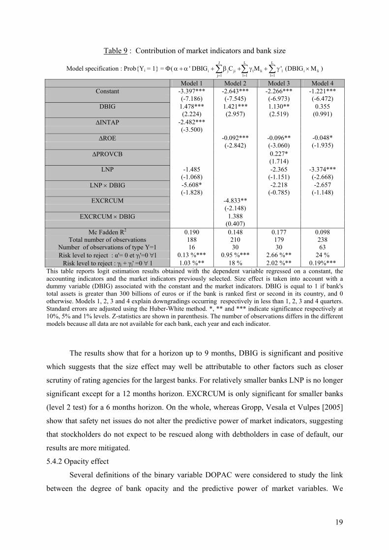
5.4.2 Opacity effect

Several definitions of the binary variable DOPAC were considered to study the link

between the degree of bank opacity and the predictive power of market variables. We

20

considered the ratio of Net Loans to Total Assets, the ratio of Deposits to Total Assets, the

ratio of Subordinated Debt to Total Assets, and the ratio of Market Funded Liabilities to Total

Assets4. Only the results obtained with the ratio of Deposits to Total Assets and the ratio of

Market Funded Liabilities to Total Assets are conclusive in discriminating the predictive

power of market variables in a very similar way. Therefore we solely report in table 10 the

results obtained when DOPAC equals 1 if the ratio of market funded liabilities is lower than

its median (equal to 25.63%). Market funded liabilities are measured as : Total Assets –

Deposits – Total Equity.

Table 10 : Contribution of market indicators and bank opacity

Model specification : Prob{Yi = 1} = Φ(J L L

i j ji l li l i lij 1 l 1 l 1

' DOPAC C M ' DOPAC M= = =

α + α + β + γ + γ ×∑ ∑ ∑ )

Model 1 Model 2 Model 3 Model 4 constant

-2.460*** (-6.054)

-1.797*** (-5.474)

-1.459*** (-4.594)

-0.577*** (-2.733)

DOPAC

-0.518 (-0.943)

-0.894* (-1.890)

-0.798* (-1.767)

-1.402*** (-3.995)

∆INTAP

-1.844*** (-2.996)

∆ROE

-0.103*** (-3.610)

-0.104*** (-3.308)

-0.060** (-2.465)

∆PROVCB

0.200 (1.436)

LNP

-4.161* (-1.915)

-4.676** (-2.336)

-5.329*** (-3.667)

EXCRCUM

-6.663*** (-3.443)

LNP ×DOPAC

3.132 (1.114)

4.228* (1.724)

5.747*** (2.853)

EXCRCUM × DOPAC

7.369*** (3.055)

Mc Fadden R2 0.109 0.184 0.164 0.177 Total number of observations 188 210 179 238

Number of observations of type Y=1 16 30 30 63 Risk level to reject : α'= 0 et γl'=0 ∀l 32.40 % 0.05%*** 3.52%** 0%***

Risk level to reject : γl + γl' =0 ∀ l 57.08 % 61.96% 74.69% 76.44% This table reports logit estimation results obtained with the dependent variable regressed on a constant, the accounting indicators and the market indicators previously selected. Opacity effect is taken into account with a dummy variable (DOPAC) associated with the constant and the market indicators. DOPAC is equal to 1 if the value of the ratio market funded liabilities / total assets is lower than its median (25.63%), and 0 otherwise. Models 1, 2, 3 and 4 explain downgradings occurring respectively in less than 1, 2, 3 and 4 quarters. Standard errors are adjusted using the Huber-White method. *, ** and *** indicate significance respectively at 10%, 5% and 1% levels. Z-statistics are shown in parenthesis. The number of observations differs in the different models because all data are not available for each bank, each year and each indicator.

4 One can refer to Goyeau, Sauviat and Tarazi (2001) and Crouzille, Lepetit and Tarazi (2004) for a discussion on the use of these ratios as private information proxies.

21

The results in table 10 show that the significance of both DOPAC and LNPxDOPAC

increases with the prediction horizon and reaches the 1% level in model 4 which suggests that

opacity is more likely to alter the predictive power of market variables for the longest

horizons. In almost all cases (models 2, 3, 4) the coefficients of market indicators (LNP and

EXCRUM) and the coefficients of the same market indicators multiplied by the dummy

variable (LNPxDOPAC and EXCRUMxDOPAC) are of opposite sign and significant.

Therefore a higher degree of opacity tends to weaken the existing link between market

indicators and the probability of a future downgrade. Based on the results of the γl + γl' = 0

test, the predictive power of market indicators is totally outweighed by bank opacity, a result

which holds for the 4 models. A similar result which is not presented here is obtained when

the dummy variable is constructed on the basis of the ratio of Deposits to Total Assets.

However, tests conducted with the subordinated debt ratio were not conclusive indicating that

the predictive power of market variables is independent of the amount of subordinated debt

issued by banks.

To check for robustness the augmented models 1 to 4 were also estimated on 4

different panels of banks on the basis of the structure of their balance sheets (table 11) to

isolate the impact of marked to market assets and liabilities. Panel A consists of banks

exhibiting a high degree of loan activity (low proportion of marked to market assets) weakly

funded by insured deposits (high proportion of market funded liabilities); 2/ Panel B is limited

to banks with a relatively high proportion of loans and weakly reliant on market debt; 3/ Panel

C contains banks with a low loan activity funded to a large extent with insured deposits; 4/

Panel D is relative to banks with a low degree of loan activity mainly funded with market

debt. More precisely, 2 criteria are taken into account to discriminate banks : the ratio of net

loans to total assets (the extent to which assets are not marked to market) and the ratio of

market funded liabilities to total assets (the extent to which a bank relies on insured and non

marked to market liabilities). The medians of both ratios were used to define the 4 panels

(25.63% for the ratio of market funded liabilities and 54.32% for the loan ratio).

Our main objective here is to assess the extent to which abundant market debt is likely to

induce changes in the opacity of bank assets. In other words, does the predictive power of

market indicators solely depend on the structure of bank liabilities (amount of market debt)?

Are market participants (who should have strong incentives to discipline heavily market

funded banks) able to process information when bank assets are, to a large extent, not market

priced? The results in table 11 show that market indicators are powerful to predict future

downgrades as long as the proportion of market debt in bank liabilities is relatively high,

22

independently of the percentage of loans in bank assets (panels A and D). Moreover, when the

proportion of (uninsured) market debt is low (panels B and C) market indicators tend to loose

their predictive power which confirms the results obtained in table 10. This result holds for

any asset profile (proportion of loans) and thus for any degree of transparency of the asset

side of the balance sheet. Moreover, this result is unchanged with respect to the amount of

subordinated debt issued by banks : when banks are heavily reliant on insured and non market

priced deposits, larger subordinated debt issues do not contribute to improve prediction (table

12, H0 : γl + γl' = 0 ∀ l). Conversely the results obtained in table 12 (H0 : γl = 0 ∀ l) show that

larger subordinated debt issues significantly reinforce the role of market indicators when bank

liabilities are to a large extent market based (low proportion of insured deposits in the balance

sheet). It is worthwhile also to note (panels B and C in table 11) that when bank liabilities are

essentially composed of non market debt (insured deposits) neither accounting nor market

indicators are able to predict future downgrades.

6. Conclusion

The objective of this paper was to assess the extent to which stock market prices can

contribute to improve the prediction of future bank financial distress and thus to question the

role and effectiveness of market discipline in the banking industry. By implementing a logit

econometric model specifically designed for European banks we tested for the additional

contribution of market based indicators (relatively to public financial statements) using a large

set of accounting and stock market indicators. Whereas some of our results support the use of

market related indicators (in line with those previously obtained in the literature), we show

that the accuracy of the predictive power is dependent on the extent to which bank liabilities

are market traded. For banks which heavily rely on (insured) deposits, the market seems

unable to convey useful information and the amount of subordinated debt issued by banks

does not contribute to any improvement in the expected link.

23

Table 11 : Degree of securitization of assets and liabilities and contribution of market indicators

Model specification: Prob{Yi = 1} = Φ(J L

i j ji l lij 1 l 1

C M= =

α + β + γ∑ ∑ )

Panel A : (net loans/ total assets) high and (market funded liabilities/ total liabilities) high

Panel B : (net loans/ total assets) high and (market funded liabilities/ total liabilities) low

Panel C : (net loans/ total assets) low and (market funded liabilities/ total liabilities) low

Panel D : (net loans/ total assets) low and (market funded liabilities/ total liabilities) high

Model 1 Model 2 Model 3 Model 4 Model 1 Model 2 Model 3 Model 4 Model 1 Model 2 Model 3 Model 4 Model 1 Model 2 Model 3 Model 4 Constant -2.165***

(-2.946) -2.605***(-3.750)

-3.853*** (-3.012)

-0.618* (-1.832)

-3.405*** (-4.777)

-2.786*** (-5.249)

-2.196***(-4.934)

-2.304*** (-5.399)

-2.555*** (-4.408)

-2.338*** (-4.519)

-2.196*** (-3.297)

-1.790*** (-4.354)

-3.182***(-4.682)

-1.513***(-3.538)

-1.040*** (-2.712)

-0.576* (-1.954)

∆INTAP -1.577 (-1.047)

-1.787 (-1.207)

-0.989 (-0.716)

-3.382***(-3.940)

∆ROE -0.191***(-2.762)

-0.417*** (-2.576)

-0.082 (-1.403)

-0.056 (-0.553)

0.064 (0.503)

0.073 (0.640)

-0.023 (-0.202)

-0.079 (-0.845)

-0.004 (-0.051)

-0.115***(-3.552)

-0.101*** (-2.795)

-0.076*** (-2.592)

∆PROVCB 3.547** (2.528)

0.258 (0.325)

1.549* (1.824)

-0.174 (-0.541)

LNP -5.641 (-1.107)

-14.020*** (-2.734)

-5.443***(-2.721)

2.358 (0.915)

2.524 (1.166)

4.725* (1.905)

-2.885 (-1.251)

-5.236** (-2.452)

-3.237* (-1.817)

-4.720** (-2.330)

-4.775** (-2.349)

-5.263** (-2.380)

EXCRCUM -9.497** (-2.068)

-0.337 (-0.118)

1.333 (0.915)

-5.999***(-2.722)

Mc Fadden R2

0.089 0.268 0.545 0.148 0.043 0.006 0.021 0.054 0.034 0.017 0.196 0.033 0.318 0.226 0.219 0.183

Total number of observations

35 42 32 56 61 65 56 66 51 53 46 56 41 50 45 60

Number of observations with Y=1

5 8 5 24 3 4 6 8 4 5 5 8 4 13 14 23

This table reports logit estimation results obtained with the dependent variable regressed on a constant, the accounting indicators and the market indicators previously selected. Four sub-samples

are taken into account on the basis of two ratios ; net loans/ total assets and market funded liabilities/ total liabilities. These ratios are considered high if their value is higher than the median

(25.63% for market funded liabilities/ total liabilities and 54.32% for net loans/ total assets). Models 1, 2, 3 and 4 explain downgradings occurring respectively in less than 1, 2, 3 and 4 quarters.

Standard errors are adjusted using the Huber-White method. *, ** and *** indicate significance respectively at 10%, 5% and 1% levels. Z-statistics are shown in parenthesis.

24

Table 12 : Structure of bank liabilities, subordinated debt and contribution of market

indicators Model specification:

Prob{Yi = 1} = Φ(J L L

i j ji l li l i lij 1 l 1 l 1

' DUMSUBA C M ' DUMSUBA M= = =

α + α + β + γ + γ ×∑ ∑ ∑ )

Test of the null hypothesis of absence of predictive contribution of market indicators when the ratio subordinated debt/ total assets is lower than its median, H0 : γl + γl' = 0 ∀ l Test of the null hypothesis of absence of predictive contribution of market indicators when the ratio subordinated debt/ total assets is higher than its median, H0 : γl = 0 ∀ l

Sample with high ratio of deposits/ total assets Sample with low ratio of deposits/ total assets Model 1 Model 2 Model 3 Model 4 Model 1 Model 2 Model 3 Model 4

Constant -3.645*** (-3.258)

-2.129*** (-4.093)

-1.721*** (-3.443)

-1.446*** (-3.391)

-2.543*** (-3.890)

-2.489*** (-4.545)

-1.876*** (-3.386)

-0.824** (-2.235)

∆INTAP -1.194 (-0.947)

-2.853*** (-2.580)

∆ROE 0.063 (0.803)

0.024 (0.262)

0.076 (0.994)

-0.177*** (-3.539)

-0.161*** (-3.308)

-0.085*** (-2.978)

∆PROVCB 0.724* (1.937)

-0.097 (-0.237)

DUMSUBA 0.607 (0.543)

-0.296 (-0.461)

-0.557 (-0.802)

-0.563 (-1.015)

-0.219 (-0.234)

0.625 (0.906)

-0.233 (-0.266)

0.306 (0.629)

LNP -1.285 (-1.287)

-2.774* (-1.673)

-3.160 (-1.465)

-2.941 (-1.264)

-8.393** (-2.542)

-6.713*** (-2.944)

EXCRCUM 0.080 (0.060)

-10.149*** (-3.328)

LNP × DUMSUBA

2.859 (0.782)

6.336 (1.537)

4.604 (1.282)

-8.053** (-2.069)

3.677 (0.760)

1.333 (0.425)

EXCRCUM ×

DUMSUBA

0.737 (0.209)

3.150 (0.801)

Mc Fadden R2

0.029 0.010 0.096 0.033 0.267 0.295 0.306 0.188

Total number of observations

106 114 99 118 74 83 71 105

Number of observations with Y=1

5 10 12 17 10 18 16 42

Risk level to reject : γl + γl' =0 ∀ l

65.34% 80.26% 30.18% 62.22% 0.05%*** 1.24%** 16.79% 1.01%**

This table reports logit estimation results obtained with the dependent variable regressed on a constant, the accounting

indicators and the market indicators previously selected. Two sub-samples are taken into account depending on the value of

the ratio deposits/ total assets. This ratio is considered high if it is higher than the median (67.57%). The dummy variable

DUMSUBA associated with the constant and the market indicators is equal to 1 if the value of the ratio subordinated debt/

total assets is lower than its median (1.51%). Models 1, 2, 3 and 4 explain downgradings occurring respectively in less than

1, 2, 3 and 4 quarters. Standard errors are adjusted using the Huber-White method. *, ** and *** indicate significance

respectively at 10%, 5% and 1% levels. Z-statistics are shown in parenthesis. The last line of the table gives the levels of risk

to reject the null hypothesis of absence of predictive contribution of market indicators when the ratio subordinated debt/ total

assets is lower than 1.51%.

25

APPENDIX : DISTANCE TO DEFAULT The distance to default indicator DD that is the number of standard deviations the asset value is away from default (where the asset value = the book value of total liabilities) is5 :

T

TrDV

DDt

tf

t

t

t σ

σ⎟⎟⎠

⎞⎜⎜⎝

⎛−+⎟⎟

⎠

⎞⎜⎜⎝

⎛

=2

log2

where : Vt : bank's asset value in t Dt : book value of the bank's liabilities due at time t T : expiration debt of the option rf : risk free rate σt : bank's asset value volatility and where equity is considered as a call option on the underlying assets with a strike price equal to the book value of the bank's liabilities. Hence, the market value and volatility of the bank's underlying assets can be derived from the equity's market value (VE) and volatility (σE) by solving :

)1()2(

dNdNeDVE

VTr

ttt

f−+=

)1(

,

dNV

VEtE

t

t

t

σσ =

where :

T

TrDV

dt

tf

t

t

σ

σ⎟⎟⎠

⎞⎜⎜⎝

⎛++⎟⎟

⎠

⎞⎜⎜⎝

⎛

=2

log1

2

Tdd tσ−= 12 Daily market value of the bank's equity (VE) are taken from Datastream. The volatility of the bank's equity (σE) is calculated on the quarter preceding the end of the calendar year (ie 65 trading days) as the standard deviation of the daily equity returns multiplied by 365 . The expiry date of the option (T) is in this case equal to the maturity of the debt. A common assumption is set to it to 1 (one year)6. We took the 12 months interbank rates from Datastream to compute risk free rates except for Greece where we used the 6 months interbank rate. Data on debt liabilities were taken from Bankscope. The total amount of liabilities is calculated as the total amount of deposits, money market funding, bonds, subordinated debt and hybrid capital.

5 For details see Crosbie (1999), Gropp, Vesala and Vulpes (2005). 6 See Crosbie (1999), Gropp, Vesala and Vulpes (2005).

26

REFERENCES

BANK FOR INTERNATIONAL SETTLEMENTS, (2003), "Overview of the New Basel Capital Accord", Consultative Document April BERGER A. N., DAVIES S. M., FLANNERY M. J., (2000), "Comparing Market and Supervisory Assessments of Bank Performance : Who Knows What When ?", Journal of Money, Credit and Banking, pp 641-667 BLACK F., SCHOLES M., (1973), "The Pricing of Options and Corporate Liabilities", Journal of Political Economy, pp 637-654 CROSBIE P. J., (1999), "Modeling Default Risk", KMV Corporation CROUZILLE C., LEPETIT L., TARAZI A. (2004) : « Bank Stock Volatility, News and Asymmetric Information in Banking : an Empirical Investigation », Journal of Multinational Financial Management, vol 14, pp 443-461 CURRY T. J., ELMER P. J., FISSEL G. S., (2002), "Regulator Use of Market Data to Improve the Identification of Bank Financial Health", FDIC Working Paper CURRY T. J., ELMER P. J., FISSEL G. S., (2003), "Using Market Information to Help Identify Distressed Institutions : A Regulatory Perspective", FDIC Banking Review, vol. 15, n°3 DIAMOND D. W., (1984), "Financial Intermediation and Delegated Monitoring", Review of Economic Studies 54, pp 393-414 DIAMOND D. W., DYBVIG P. H., (1983), "Bank runs, deposit insurance and liquidity", Journal of Political Economy, vol. 91, pp 401-419 ELMER P. J., FISSEL G., (2001), "Forecasting Bank Failure From Momentum Patterns in Stock Returns", Federal Deposit Insurance Corp. Working Paper ESTRELLA A., PARK S., PERISTANI S., (2000), "Capital Ratios as Predictors of bank Failure", Economic Policy Review,July EVANOFF D. D., WALL L. D., (2000), "Subordinated Debt and Bank Capital Reform", Federal Reserve Bank of Chicago, Working Papers EVANOFF D. D., WALL L. D., (2001), "Sub-debt yield spreads as bank risk measures", Federal Reserve Bank of Chicago, Working Papers EVANOFF D. D., WALL L. D., (2002), "Measures of the Riskiness of Banking Organisations : Subordinated Debt Yields, Risk-Based Capital, and Examination Ratings", Journal of Banking and Finance

27

EVANOFF D. D., WALL L. D., (2002), "Subordinated Debt and Prompt Corrective Regulatory Action", Federal Reserve Bank of Atlanta, Working Paper Series , August FELDMAN R., LEVONIAN M., (2001), "Market Data and Bank Supervision: The Transition to Practical Use", Federal Reserve Bank of Minneapolis The Region, pp 11-13, 46-54 FLANNERY M. J., (1998), "Using Market Information in Prudential Bank Supervision: A Review of the U.S. Empirical Evidence", Journal of Money Credit and Banking, vol. 30(3) pp 273-30 FLANNERY M. J., (2001), "The Faces of Market Discipline", Journal of Financial Services Research October/December, pp 107-119 GOYEAU D., SAUVIAT A., TARAZI A. (1998), "Taille, rentabilité et risque bancaire, évaluation empirique et perspectives pour la réglementation prudentielle", Revue d'Economie Politique vol. 108, n°3, pp 339-361 GOYEAU D., SAUVIAT A., TARAZI A., (2001), "Marché financier et évaluation du risque bancaire. Les agences de notation contribuent-elles à améliorer la discipline de marché ?", Revue Economique 52, mars, pp 265-283 GOYEAU D., TARAZI A., (1992), "Evaluation du risque de défaillance bancaire en Europe", Revue d'Economie Politique, 102 pp 250-280 GROPP R., VESALA J., VULPES G., (2005), "Equity and Bond Market Signals as Leading Indicators of Bank Fragility", Journal of Money Credit and Banking, forthcoming. GUNTHER J. W., LEVONIAN M. E., MOORE R. R., (2001), "Can the Stock Market tell Bank Supervisors Anything They Don't Already Know ?", Federal Reserve Bank of Dallas JAGTIANI J., KAUFMAN G., LEMIEUX C., (1999), "Do Markets Discipline Banks and Bank Holding Companies ? Evidence from Debt Pricing", Federal Reserve Bank of Chicago JAGTIANI J., LEMIEUX C., (2001), "Market Discipline Prior to Bank Failure", Journal of Economics and Business vol. 53, pp 313-324 KRAINER J., LOPEZ J. A., (2004), "Using Securities Market Information for Bank Supervisory Monitoring", Federal Reserve Bank of San Francisco Working paper KMV Corporation (2003) : “Modelling Risk”, San Francisco : KMV Corporation LELAND H. E., PYLE D. H., (1977), "Informational Asymmetries, Financial Structure, and Financial Intermediation", The Journal of Finance vol. 32, pp 371-387 LOGAN A., (2000), "G10 Seminar on Systems for assessing Banking System Risk", Financial Stability Review, June MERTON R. C., (1977), "On the Pricing of Contingent Claims and the Modigliani-Miller Theorem", Journal of Financial Economics 5, pp 241-249

28

RONN E. I., VERMA A. K., (1986), "Pricing Risk-Adjusted Deposit Insurance : An Option-Based Model", Journal of Finance, pp 871-895 SAHAJWALA R., VAN DEN BERGH P., (2000), "Supervisory Risk Assessment and Early Warning Systems", Basel Committee on Banking Supervision working papers no. 4 SIRONI A., (2003), "Testing for Market Discipline in the European Banking Industry : Evidence from Subordinated Debt Issues", Jounal of Money, Credit and Banking, vol. 35, pp 443-472 WHALEN G., THOMSON J. B., (1988), "Using Financial Data to Identify Changes in Bank Condition", Federal Reserve Bank of Cleveland Economic Review, pp 18-26