Mark recapture abundance estimates and distribution of ...

Mark recapture abundance estimates and distribution of bottlenose dolphins (Tursiops truncatus) using the southern

coastline of the outer Moray Firth, NE Scotland.

Thesis submitted for the degree of Master of Science

By

Ross M. Culloch

School of Biological Sciences University of Wales, Bangor

In association with the Cetacean Research & Rescue Unit

November 2004

i

Pho

to c

redi

t: K

evin

Rob

inso

n / C

RR

U

“There is about as much educational benefit to be gained in studying dolphins

in captivity as there would be studying mankind by only observing prisoners

held in solitary confinement”.

- Jacques Cousteau

ii

Declaration

This work has not previously been accepted in substance for any degree and is not being

concurrently submitted in candidature for any degree.

Signed………………………………………………(candidate)

Date………………………………………………….

Statement 1

This dissertation is being submitted in partial fulfilment of the requirements for the degree of

M.Sc.

Statement 2

This dissertation is the result of my own independent work/investigation, except where

otherwise stated. Other sources are acknowledged by footnotes giving explicit references. A

bibliography is appended.

Statement 3

I hereby give consent for my dissertation, if accepted, to be available for photocopying and for inter-library loan, and for the title and summary to be made available to outside organisations.

Signed………………………………………………(candidate)

Date…………………………………………………

i

Acknowledgements

The completion of this thesis is the direct result of the assistance, encouragement and support

of several truly incredible people to whom I am indebted.

My biggest thanks goes to my supervisor and friend, Dr. Kevin Robinson, director of the

Cetacean Research & Rescue Unit (CRRU), without whom this project would not have been

possible. He provided the initial data, sound advice, guidance, expert knowledge, moral

support and taught me so much about working in the field of cetology. Thanks for everything

Kev, you and the CRRU have been an inspiration and it has been a pleasure working

alongside you and the team over the past 6 months.

Special thanks also goes to my supervisor at the University of Wales, Bangor, Dr.

Chris Gliddon, for providing sound advice and guidance throughout this project, it was much

appreciated, thanks Chris.

I would also like to thank the numerous volunteers, friends and staff of the CRRU for all their help in 2004, in alphabetical order: Alison Atherton, Hanna Bostrom, Virginie Campos, Bob Carter, Sandra Donkervoort, Louise Ellis, Elaine Galston, Tracy Guild, Silvia Haering-Fabiani, Rhiannon Hersee, Eva-Maria Irek, Saskia Juinen, Kirsten Lattewitz, Nathalie Lautier, Christine Low, Michelle Maki, Jackie Maud, Cameron McPherson, Michael Moerzinger, Xavier Senel, Phillippe Soulet, Christine O'Sullivan, Theo Pados, Caroline Passingham, Vicky Smolen, Mike Tetley, Sai Tiptus, Jo Torres, Eva Van Meervenne, Tessa van Ree, Laura Vereecken, Katja Wagner, Serena Weber, Dave & Barbi White, Elanor Whythe and Frank Zanderink.

Finally, thanks to all my friends and family for their encouragement and support, especially my parents, Dorothy and James, without whom, I could never have undertaken this M.Sc, thank you both for this opportunity.

i

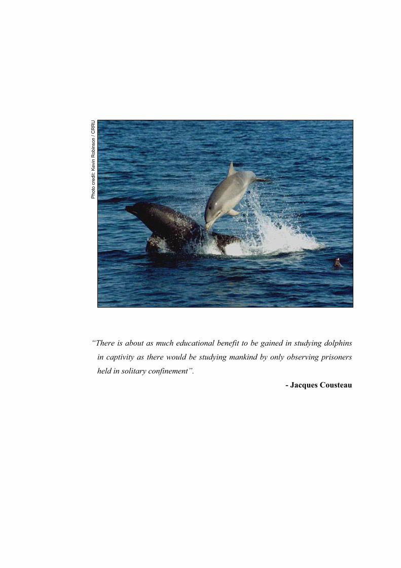
Abstract

Distribution, relative abundance, group composition, and site fidelity of bottlenose dolphins

(Tursiops truncatus) using the southern coastline of the outer Moray Firth, NE Scotland, were

investigated using systematic boat surveys and photo-identification / mark-recapture

techniques. Results showed that bottlenose dolphins were present in the southern outer Moray

Firth throughout the summer months, with the highest number of encounters occurring in

July. Further analysis of relative abundance revealed two areas that were intensively used by

the dolphins. Both of these areas contained river mouths, which are used by spawning salmon

(Salmo salar). There were a high number of neonate calves first sighted between July and

September, and 81% of the total numer of groups encountered had at least one calf. These

results strongly imply that the outer Moray Firth is an important feeding ground and

nursery/calving ground for this population.

Computer-assisted photo-identification techniques were applied to the existing bottlenose

dolphin database held by the host organisation. This process revealed a total of 2 false

positive and 22 false negative errors. Subsequently, 9.2% of the total number of marked

individuals used in the analysis were defined as resident to the outer Moray Firth. Residency

was calculated on an annual basis, with the number of residents per year varying between 3

and 9. This variablity in the composition and number of residents was attributed to the social

ecology of the dolphins, prey abundance, and boat traffic. Finally, using a closed population

model, the abundance estimate of bottlenose dolphins using the outer Moray Firth was 108

(95% CI = 99-117).

In view of these findings, the current management scheme is discussed, with the

recommendation that the current boundaries of the candidate Special Area of Conservation

(cSAC) be revised in order to afford a greater level of protection to this already vulnerable

population.

ii

Table of Contents

Acknowledgements ................................................................................................................... i

Abstract..................................................................................................................................... ii

Table of Contents .................................................................................................................... iii

List of Figures.......................................................................................................................... iv

List of Tables ........................................................................................................................... vi

List of Appendices.................................................................................................................. vii

1. Introduction.........................................................................................................................1

2. The Study Area ...................................................................................................................9

3. Methods..............................................................................................................................11

3.1. Data Collection ..............................................................................................................11

3.2. Photo-Identification .......................................................................................................13

3.3. Definition of Age Classes ..............................................................................................14

3.4. Handling Photographs, Matching Animals and Record Keeping..................................17

3.5. Removing False Negatives & False Positives & Data Selection...................................19

3.6. Estimations of Population Size ......................................................................................22

3.7. GIS & Statistical Analysis .............................................................................................23

4. Results ................................................................................................................................24

4.1. Survey Effort..................................................................................................................24

4.2. Distribution & Abundance of Animals..........................................................................24

4.3. Group Size / Composition..............................................................................................32

4.4. Mark Recapture & Estimation of Population Size.........................................................34

5. Discussion ...........................................................................................................................42

5.1. Distribution, Density & Habitat Selection.....................................................................42

5.2. Site Fidelity and Abundance Estimates .........................................................................47

5.3. Conservation & the candidate Special Area of Conservation........................................50

6. Summary & Conclusions..................................................................................................53

References................................................................................................................................55

Appendices………………………………………………...…………………………………67

iii

List of Figures Figure 1.1. Schematic diagram showing the taxonomy of cetacean classification……. 2 Figure 1.2.

Map showing the global distribution of Tursiops truncatus………………. 3

Figure 2.1.

Map of north east Scotland showing the location of the Moray Firth……... 10

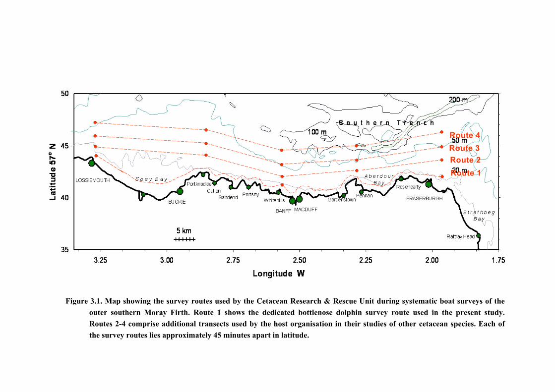
Figure 3.1.

Map showing the survey routes used by the Cetacean Research & Rescue Unit during systematic boat surveys of the outer southern Moray Firth…... 12

Figure 3.2.

Schematic diagram showing the data entry forms constituting the CRRU’s bottlenose dolphin database……………………………………………….. 15

Figure 3.3.

Photographs illustrating the features used in the present study in the categorisation of age class in bottlenose dolphins………………………… 16

Figure 3.4.

Program screen captures showing (a) the FinEx dorsal extraction program and (b) the FinMatch automated matching program used in the present study for the reanalysis of all “marked” animals………………………….. 21

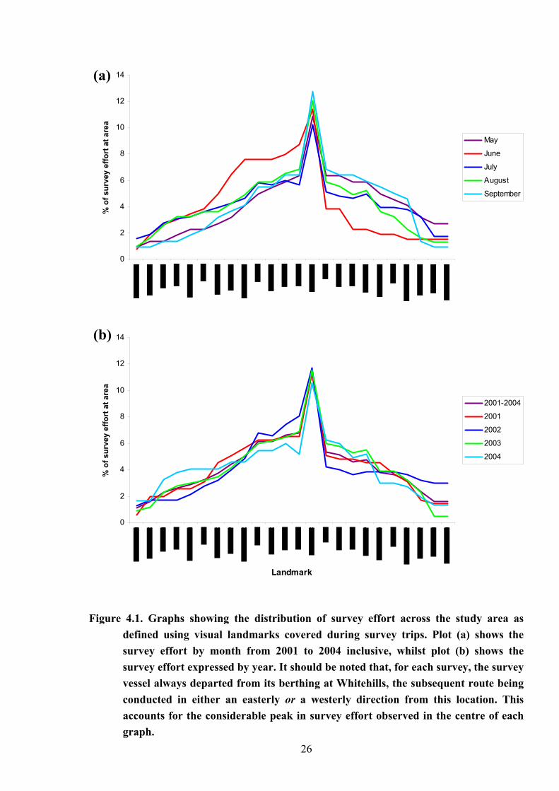
Figure 4.1.

Graphs showing the distribution of survey effort across the study area as defined using visual landmarks covered during survey trips……………… 26

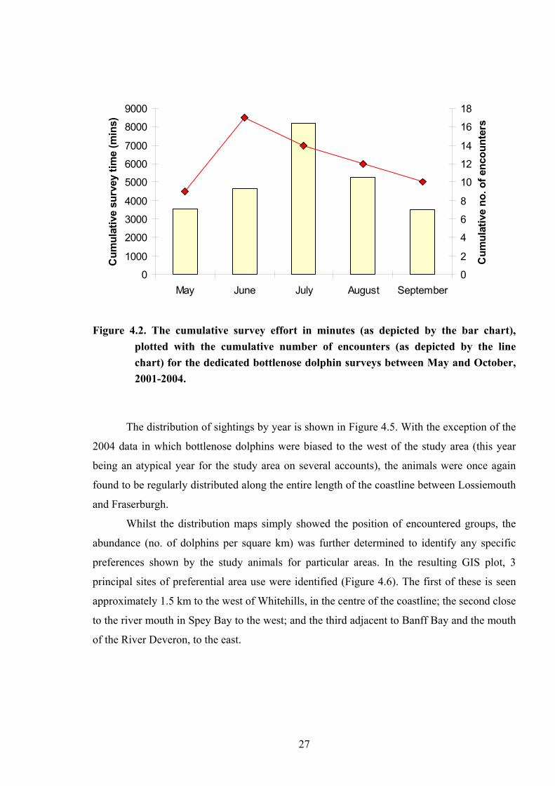
Figure 4.2.

The cumulative survey effort in minutes plotted with the cumulative number of encounters for the dedicated bottlenose dolphin surveys between May and October, 2001-2004……………………………………. 27

Figure 4.3.

Map of the outer southern Moray Firth showing the distribution of all bottlenose dolphin sightings recorded by the CRRU between May and October of 2001 to 2004 inclusive (n = 62)……………………………….. 28

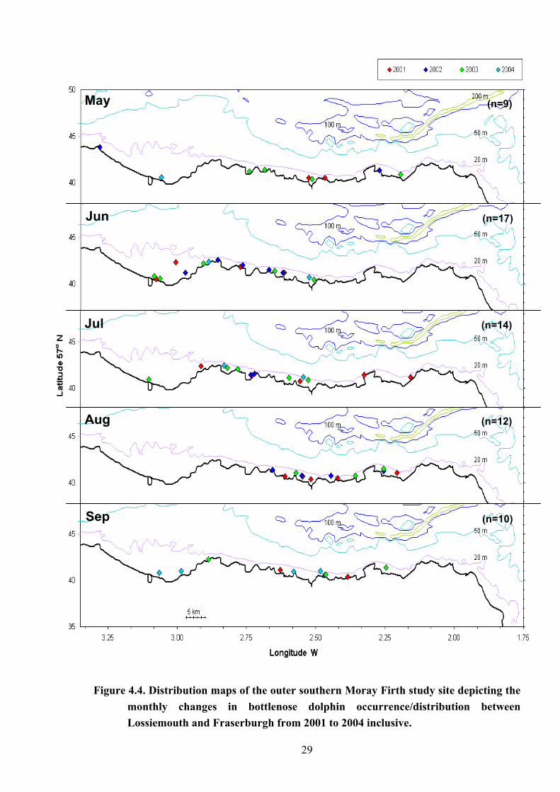
Figure 4.4.

Distribution maps of the outer southern Moray Firth study site depicting the monthly changes in bottlenose dolphin occurrence/distribution between Lossiemouth and Fraserburgh from 2001 to 2004 inclusive.......... 29

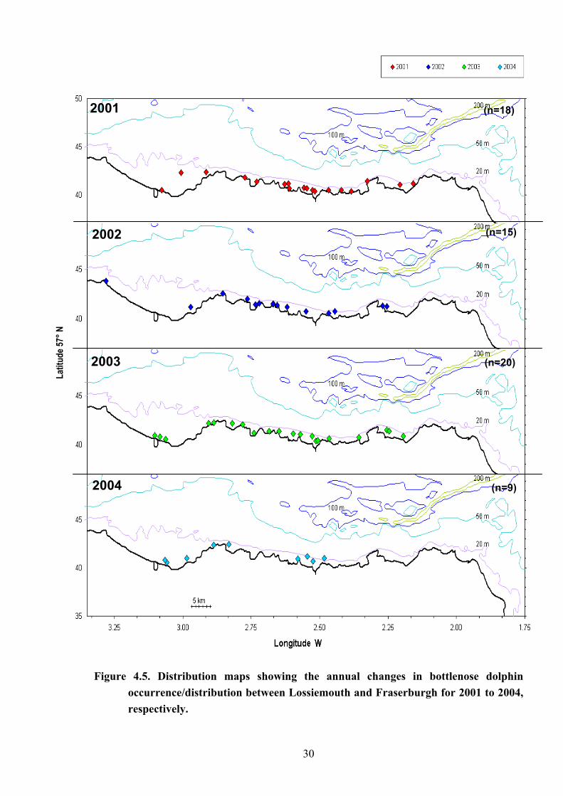
Figure 4.5.

Distribution maps showing the annual changes in bottlenose dolphin occurrence/distribution between Lossiemouth and Fraserburgh for 2001 to 2004, respectively………………………………………………………….. 30

iv

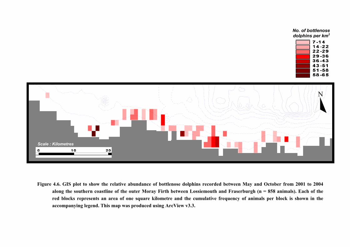
Figure 4.6.

GIS plot to show the relative abundance of bottlenose dolphins recorded between May and October from 2001 to 2004 along the southern coastline of the outer Moray Firth between Lossiemouth and Fraserburgh…………. 31

Figure 4.7.

Histogram showing the distribution of recapture frequencies for all marked bottlenoses identified in the present study between May and October 2001 to 2004……………………………………………………… 35

Figure 4.8.

Histograms showing the occurrence and distribution of marked bottlenose dolphins using the study area……………………………………………… 39

Figure 4.9.

Discovery curve of the cumulative number of all individually marked bottlenoses recorded throughout the study period (n=76) plotted against the cumulative number of dolphins encountered (n=858)…………………

40 Figure 5.1.

A distribution map showing the bottlenose dolphin encounters within Spey Bay between 1997 and 1998 during a pilot study carried out by the CRRU (n=80)……………………………………………………………… 48

v

List of Tables Table 3.1 Naturally occurring markings used in the present study for the photo-

identification of individual bottlenose dolphins (adapted and expanded from Wilson, 1995)………………………………………………………………... 18

Table 4.1 Showing the survey effort for dedicated bottlenose surveys conducted between May and October 2001 to 2004……………………………………. 25

Table 4.2

The relative abundance or density of bottlenose dolphins (no. animals per km2) in each of the designated sub-areas, from Halliman Skerries, in Lossiemouth, to Kannaird Head, in Fraserburgh……………………………. 33

Table 4.3 Showing the first sightings of individual neonate records from 2001 to 2004 and the percentages of groups containing calves (n=60)……………………. 34

Table 4.4

Showing the annual frequencies of seasonal residence by bottlenose dolphins from 2001 to 2004…………………………………………………. 36

Table 4.5

Marked bottlenoses recorded during 3 or more of the 5 survey months (May to October) in any single study year, from 2001 to 2004 inclusive…………. 37

Table 4.6

The results of the population estimations for each year using: (a) the Chao time-dependency model; (b) the Darroch time-dependency model; and (c) the Chao time-dependent heterogeneity model……………………………… 40

Table 4.7

The results of the corrected population estimate for each of the study years 2001 to 2004 using the results from the Chao time-dependence model…….. 41

vi

List of Appendices

Appendix 1 A systematic list of the cetacean species recorded in northeast Scottish waters and their occurrence (adapted from Evans, 1996)...... 67

Appendix 2

Showing examples of the Trip and Encounter log sheets (a & b respectively) used in the present study during boat surveys………… 68

Appendix 3

An example of a Film Sheet used during an encounter to assist in the subsequent organisation and identification of photographs taken…... 69

Appendix 4

An example of a Bottlenose Dolphin Survey Sheet onto which the general data from each trip and encounter (where applicable) was recorded from the respective Trip & Encounter logs………………... 70

Appendix 5

Showing the Encounter Grid used in the present analysis. The grid is simply used to separate individual dolphins photographed during each encounter……………………………………………………….. 71

Appendix 6

A completed Summary Encounter Sheet for a group of 12 bottlenose dolphins. Note the mother-calf pairs identified, depicted by brackets. 72

Appendix 7

The following pages show the “marked” individual dolphins used in the present study for the estimation of population size (n=76)……… 73

Appendix 8

Table showing encounter histories of the 7 resident dolphins encountered during 3 or more of the 5 months……………………… 79

Appendix 9

The results obtained from the Chao (Mth) models for population sizes, using CAPTURE run through MARK v4.1, for the years 2001 to 2004, respectively………………………………………………… 80

Appendix 10

Statistical Analysis…………………………………………………... 83

vii

1. Introduction

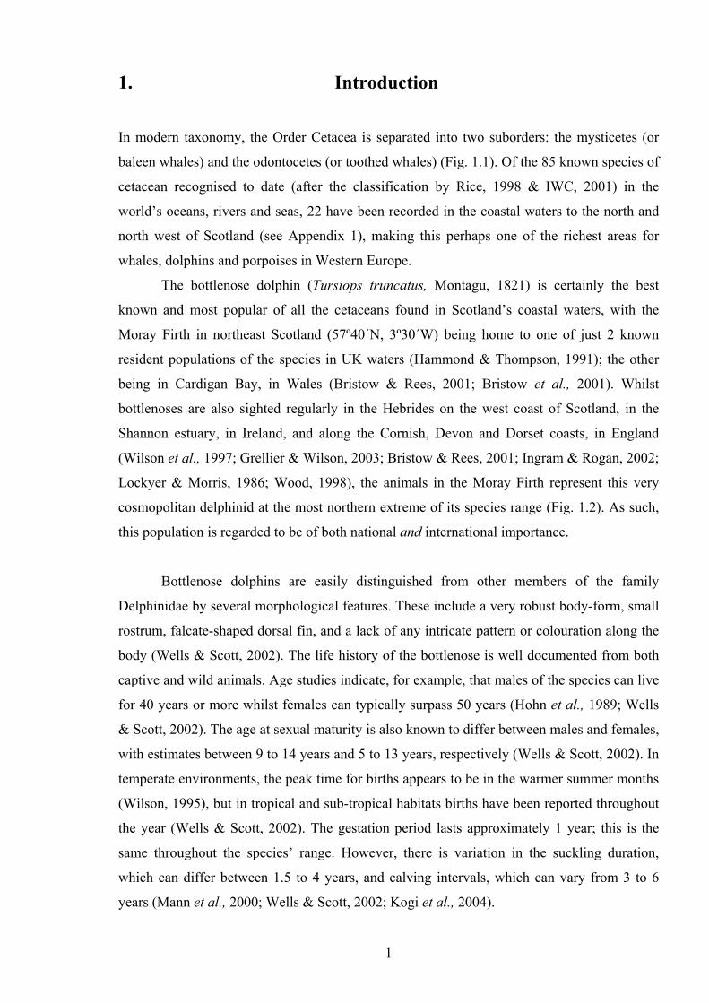
In modern taxonomy, the Order Cetacea is separated into two suborders: the mysticetes (or

baleen whales) and the odontocetes (or toothed whales) (Fig. 1.1). Of the 85 known species of

cetacean recognised to date (after the classification by Rice, 1998 & IWC, 2001) in the

world’s oceans, rivers and seas, 22 have been recorded in the coastal waters to the north and

north west of Scotland (see Appendix 1), making this perhaps one of the richest areas for

whales, dolphins and porpoises in Western Europe.

The bottlenose dolphin (Tursiops truncatus, Montagu, 1821) is certainly the best

known and most popular of all the cetaceans found in Scotland’s coastal waters, with the

Moray Firth in northeast Scotland (57º40´N, 3º30´W) being home to one of just 2 known

resident populations of the species in UK waters (Hammond & Thompson, 1991); the other

being in Cardigan Bay, in Wales (Bristow & Rees, 2001; Bristow et al., 2001). Whilst

bottlenoses are also sighted regularly in the Hebrides on the west coast of Scotland, in the

Shannon estuary, in Ireland, and along the Cornish, Devon and Dorset coasts, in England

(Wilson et al., 1997; Grellier & Wilson, 2003; Bristow & Rees, 2001; Ingram & Rogan, 2002;

Lockyer & Morris, 1986; Wood, 1998), the animals in the Moray Firth represent this very

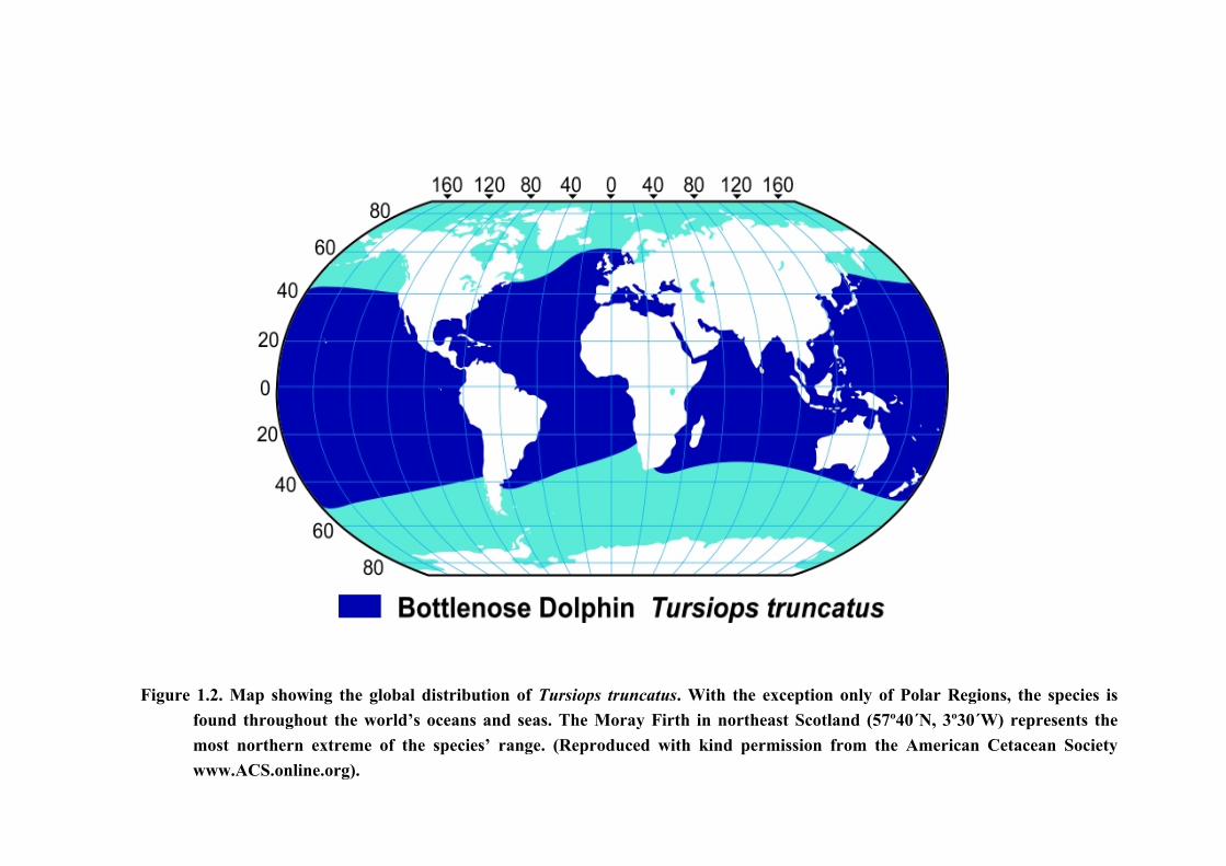
cosmopolitan delphinid at the most northern extreme of its species range (Fig. 1.2). As such,

this population is regarded to be of both national and international importance.

Bottlenose dolphins are easily distinguished from other members of the family

Delphinidae by several morphological features. These include a very robust body-form, small

rostrum, falcate-shaped dorsal fin, and a lack of any intricate pattern or colouration along the

body (Wells & Scott, 2002). The life history of the bottlenose is well documented from both

captive and wild animals. Age studies indicate, for example, that males of the species can live

for 40 years or more whilst females can typically surpass 50 years (Hohn et al., 1989; Wells

& Scott, 2002). The age at sexual maturity is also known to differ between males and females,

with estimates between 9 to 14 years and 5 to 13 years, respectively (Wells & Scott, 2002). In

temperate environments, the peak time for births appears to be in the warmer summer months

(Wilson, 1995), but in tropical and sub-tropical habitats births have been reported throughout

the year (Wells & Scott, 2002). The gestation period lasts approximately 1 year; this is the

same throughout the species’ range. However, there is variation in the suckling duration,

which can differ between 1.5 to 4 years, and calving intervals, which can vary from 3 to 6

years (Mann et al., 2000; Wells & Scott, 2002; Kogi et al., 2004).

1

(Chine

Fig

Class Mammalia

Suborder Mysticeti

(Baleen Whales)

Suborder Odontoceti

(Toothed Whales)

Family Balaenopteridae

(Rorquals)

Family Eschrichtiidae(Gray Whale)

Family Neobalaenidae

(Pygmy Right Whale)

Family Physeteridae

(Sperm Whale)

Family Iniidae

(Amazon River-dolphin)

Family Platanistidae

(Indian River Dolphin)

Family Kogiidae

(Pygmy Sperm Whales)

Family Ziphiidae

(Beaked Whales)

Family Lipotidae

se River-dolphin)

Family Pontoporiidae

(La Plata Dolphin)

Family Monodontidae

(Beluga and Narwhal)

Family Delphinidae (Dolphins)

Family Phocoenidae (Porpoises)

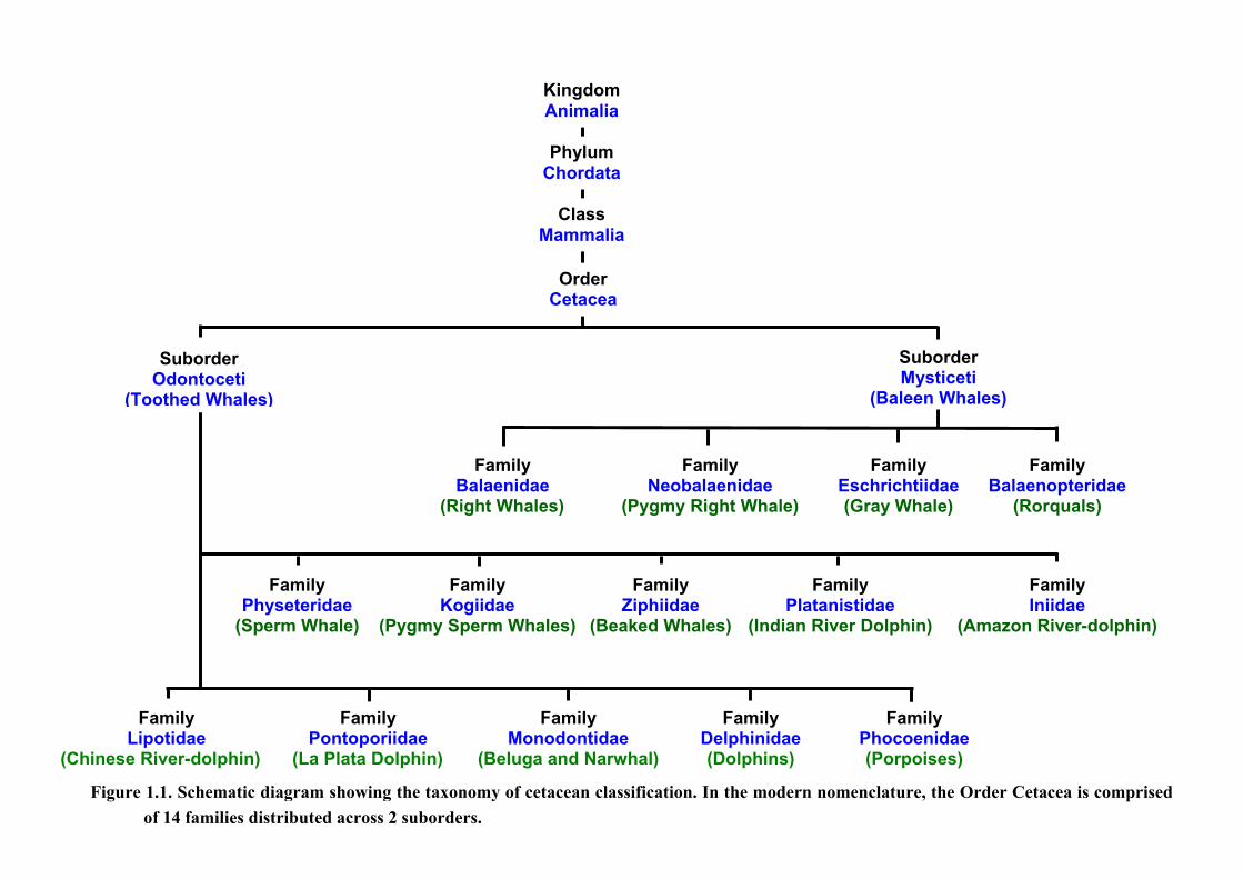
ure 1.1. Schematic diagram showing the taxonomy of cetacean classification. In the modern nomenclature, the Order Cetacea is comprised

of 14 families distributed across 2 suborders.

Family Balaenidae

(Right Whales)

Order Cetacea

Phylum Chordata

Kingdom Animalia

3

Figure 1.2. Map showing the global distribution of Tursiops truncatus. With the exception only of Polar Regions, the species isfound throughout the world’s oceans and seas. The Moray Firth in northeast Scotland (57º40´N, 3º30´W) represents themost northern extreme of the species’ range. (Reproduced with kind permission from the American Cetacean Societywww.ACS.online.org).

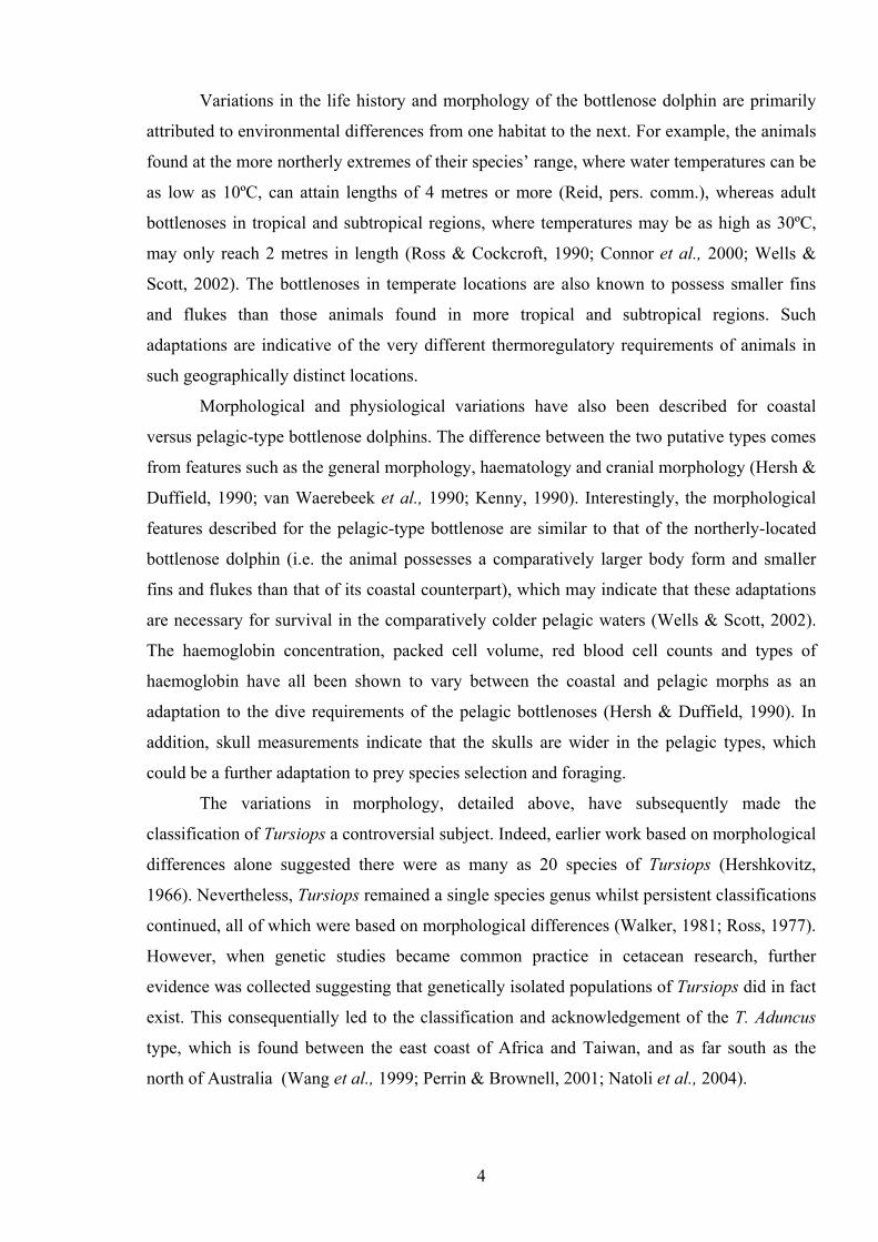
Variations in the life history and morphology of the bottlenose dolphin are primarily

attributed to environmental differences from one habitat to the next. For example, the animals

found at the more northerly extremes of their species’ range, where water temperatures can be

as low as 10ºC, can attain lengths of 4 metres or more (Reid, pers. comm.), whereas adult

bottlenoses in tropical and subtropical regions, where temperatures may be as high as 30ºC,

may only reach 2 metres in length (Ross & Cockcroft, 1990; Connor et al., 2000; Wells &

Scott, 2002). The bottlenoses in temperate locations are also known to possess smaller fins

and flukes than those animals found in more tropical and subtropical regions. Such

adaptations are indicative of the very different thermoregulatory requirements of animals in

such geographically distinct locations.

Morphological and physiological variations have also been described for coastal

versus pelagic-type bottlenose dolphins. The difference between the two putative types comes

from features such as the general morphology, haematology and cranial morphology (Hersh &

Duffield, 1990; van Waerebeek et al., 1990; Kenny, 1990). Interestingly, the morphological

features described for the pelagic-type bottlenose are similar to that of the northerly-located

bottlenose dolphin (i.e. the animal possesses a comparatively larger body form and smaller

fins and flukes than that of its coastal counterpart), which may indicate that these adaptations

are necessary for survival in the comparatively colder pelagic waters (Wells & Scott, 2002).

The haemoglobin concentration, packed cell volume, red blood cell counts and types of

haemoglobin have all been shown to vary between the coastal and pelagic morphs as an

adaptation to the dive requirements of the pelagic bottlenoses (Hersh & Duffield, 1990). In

addition, skull measurements indicate that the skulls are wider in the pelagic types, which

could be a further adaptation to prey species selection and foraging.

The variations in morphology, detailed above, have subsequently made the

classification of Tursiops a controversial subject. Indeed, earlier work based on morphological

differences alone suggested there were as many as 20 species of Tursiops (Hershkovitz,

1966). Nevertheless, Tursiops remained a single species genus whilst persistent classifications

continued, all of which were based on morphological differences (Walker, 1981; Ross, 1977).

However, when genetic studies became common practice in cetacean research, further

evidence was collected suggesting that genetically isolated populations of Tursiops did in fact

exist. This consequentially led to the classification and acknowledgement of the T. Aduncus

type, which is found between the east coast of Africa and Taiwan, and as far south as the

north of Australia (Wang et al., 1999; Perrin & Brownell, 2001; Natoli et al., 2004).

4

Whilst defining the bottlenose dolphin with reference to genetic evidence is extremely

important for conservation and management of a species, it is also important, for the same

reasoning, to define parameters such as distribution and density. In these types of studies, and

particularly when population estimates are required, a researcher needs to be able to

distinguish between individual animals; a technique often referred to as mark capture-

recapture or mark-recapture for short. In early studies of coastal cetaceans, artificial tagging

methods, such as freeze-branding, tattooing, flag tags, button tags, and spaghetti tags, were all

used to identify individuals within a population (Evans et al., 1972; White et al., 1981; Irvine

et al., 1982; Hobbs, 1982). Whilst some of these methods are still being used today (for

example, Scott et al., 1990a; Silva & Martin, 2000), artificial tagging has been largely

superseded by the more modern application of photo-identification.

In simple definition, photo-identification is a technique used to identify individual

animals from photographs of distinctive, naturally occurring markings. This technique was

first applied to bottlenose dolphins by Caldwell (1955), Irvine & Wells (1972) and Würsig &

Würsig (1977), and to date, still remains one of the best and least intrusive (non-invasive)

methods used for gathering information about cetacean societies in the wild. Since its

introduction in the 1950’s, it has been used to provide information on occurrence and intra-

group affiliation patterns in a great variety of cetacean species, including: the killer whale

(Orcinus orca) (Bain, 1990), bottlenose whale (Hyperoodon ampullatus) (Hooker et al.,

2002), humpback whale (Megaptera novaeangliae) (Gowans & Whitehead, 2001), blue whale

(Balaenoptera musculus) (Calambokidis & Barlow, 2004), minke whale (Balaenoptera

acutorostrata) (Dorsey et al., 1990), fin whale (Balaenoptera physalus) (Agler et al., 1990),

gray whale (Eschrichtius robustus) (Jones, 1990) and sperm whale (Physeter macrocephalus)

(Whitehead, 1990), to name but a few.

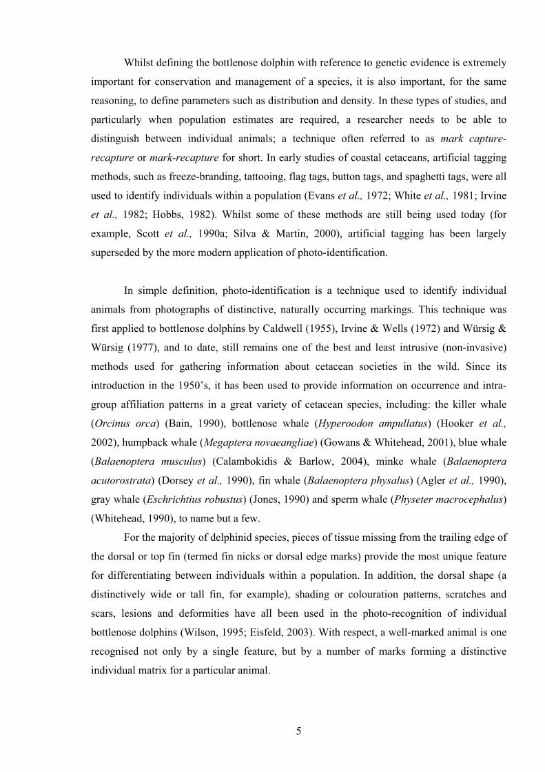
For the majority of delphinid species, pieces of tissue missing from the trailing edge of

the dorsal or top fin (termed fin nicks or dorsal edge marks) provide the most unique feature

for differentiating between individuals within a population. In addition, the dorsal shape (a

distinctively wide or tall fin, for example), shading or colouration patterns, scratches and

scars, lesions and deformities have all been used in the photo-recognition of individual

bottlenose dolphins (Wilson, 1995; Eisfeld, 2003). With respect, a well-marked animal is one

recognised not only by a single feature, but by a number of marks forming a distinctive

individual matrix for a particular animal.

5

The uniqueness of photo-ID as a central tool for the recognition of individual whales

and dolphins is its ability as a technique to document the life history and ecology of animals,

as well as making estimations of population size within a given survey area (Whitehead et al.,

2000). When photographs of animals are obtained at more than one location, distribution,

short-term movement patterns, and migrations can be determined (Weigle, 1990; Wells et al.,

1990; Würsig & Harris, 1990). Recognisable dolphins further allow for a more thorough

description of inter-individual behaviours, especially if sex and reproductive conditions are

known (Connor & Smolker, 1985; Wells et al., 1987; Connor et al., 2000). They also allow

for the basic description of surfacing-respiration-dive cycles and their correlation to general

behaviour patterns such as resting, socialising, travelling and feeding (Tayler & Saayman,

1972; Würsig, 1978; Shane, 1990; Balance, 1990).

Whilst fine-scale studies of distribution and habitat use may provide fundamental data

for the management and conservation of a species in a given area, life history and population

determinants are also crucial to our understanding of mortality, fecundity, immigration and

emigration rates within a population. A greater understanding of the dynamics of a dolphin

population can thus be obtained when individuals are followed for a number of years during

long-term mark-recapture studies utilising photo-identification (Wilson et al., 1999; Rogan et

al., 2000).

In order to estimate the population size in wild cetacean societies using mark capture-

recapture models, the population under analysis must be defined as either open or closed. In

general, closed models assume that no births, deaths, or permanent immigration or emigration

occurs during the sampling period, whereas open models allow for, and even quantify, these

parameters (Wilson et al., 1999). The assumption that a population is demographically closed

is often achieved by reducing the study period; meaning that a five-year study, for example, is

divided into five annual data sets for individual analysis. However, demographic closure is

only one of four specific assumptions that need to be met in order to apply a closed

population model to a dataset with confidence, the full set of assumptions (after Campbell et

al., 2002; Shirakihara et al., 2002; Chilvers & Cockeron, 2003; Irwin & Würsig, 2004) being

that: 1) every marked animal present in the population at time (i) has the same probability of

recapture (pi) (part of the demographic assumption); 2) every marked animal in the population after time (i) has the same probability of

surviving to time (i+1);

6

3) marks are not lost or missed during the study period; and 4) all samples are instantaneous, relative to the interval between occasion (i) and (i+1),

and each release is made immediately after the sample.

With long-lived animals such as dolphins, assumption 2 can be met with confidence.

Assumption 3 can be met by using high quality photographs and experienced observers, and

assumption 4 can be met if the research conducted in the field is efficient, i.e. minimal time is

spent with the animals during an encounter. Assumption 1, however, can easily be broken as

it assumes that all individuals within a population will react in the same manner. As this is

very unlikely, it is important to counter this assumption with a model that can relax certain

aspects of the supposition; as well as reducing demographic parameters.

In UK and Irish waters, estimates assuming population closure have been made for

bottlenose dolphin populations in the Moray Firth and the Outer Hebrides, in Scotland

(Wilson et al., 1999; Grellier & Wilson, 2004), New Quay, in Cardigan Bay, in Wales

(Bristow & Rees, 2001), and the Shannon estuary, in Ireland (Rogan et al., 2000).

Interestingly, genetic analyses of Tursiops from these areas, and from another area in the

south of England, showed that the animals in the Moray Firth were more closely related to

those in Cardigan Bay, rather than their nearest neighbouring population from the west coast

of Scotland (Parsons et al., 2002). This study also indicated that the within-population genetic

diversity of the Moray Firth dolphins was markedly lower, and therefore more genetically

isolated than the populations in the other sampling regions. This, encompassed with the most

pessimistic scenario by Wilson et al., (1999) suggesting a population decline of more than 5%

a year, clearly indicates that the population in northeast Scotland is undoubtedly vulnerable to

extinction.

The bottlenose dolphin is currently listed under Annex II of the 1992 European

Community’s “Habitats Directive” (Council directive 92/43/EEC) and the “inner” Moray

Firth has been put forward as a candidate Special Area of Conservation (cSAC); as hosting

one of just two known resident populations of bottlenose dolphins in UK waters and featuring

sub-tidal sandbanks as an additional qualifying interest (MFP, 2001). Designation as an SAC

requires an effective management plan for the co-operative management of anthropogenic

impacts within the Firth (MFP, 2003). As such, one of the conservation objectives of this

management scheme is the “establishment and maintenance of a viable population of

bottlenose dolphins within the Firth”. However, the physical boundaries of the cSAC only

cover the “inner” area of the Moray Firth at present (shown in Fig. 2.1 in the following

section), and recent studies have indicated that the home range of this population extends well

7

beyond the Moray Firth, even as far south as Tyneside in the north of England (Wilson et al.,

2004). Whilst the SAC need not cover the entire home range of the population, it should

however encompass a large enough area pertinent to the “physical or biological factors

essential to life and reproduction” (MFP, 2003). Indeed, Eisfeld & Robinson (in press) advise

that the southern coastline of the outer Moray Firth may provide crucial habitats for a

significant proportion of this North Sea population which may be particularly significant in

view of the management proposals currently aimed at their protection (Curran et al., 1996;

MFP, 2003). Consequently, whilst earlier studies concentrated in the inner Moray Firth have

been fundamental to our understanding of the biology, behaviour and ecology of this

population as a whole, interpretation of some of these data would certainly benefit from

studies of the animals in other focal areas within their home range.

Using original data collectied in 2004 combined with earlier data collected by the host

organisation from 2001 to 2003 inclusive, the principal objectives of this study aimed:

i). to determine the distribution and site fidelity of bottlenose dolphins using the

southern coastline of the outer Moray Firth;

ii). to ascertain the composition of animals using this coastline and the relative

importance of the area in terms of “physical or biological factors essential to life and

reproduction”;

iii). to estimate the number of animals utilising the study area, using mark-recapture

models for evaluation;

iv). and to discuss the significance of the outer Moray Firth in view of current

boundaries of the existing cSAC.

8

2. The Study Area The Moray Firth is a large triangular embayment in the north east of Scotland. Measuring

approximately 5,230 km2, it is generally defined as the area of sea to the west of Duncansby

Head on the north coast and Fraserburgh on the south coast (Harding-Hill, 1993). It is the

largest firth of its kind on the east coast of Scotland, and contains within it four smaller firths,

the Dornoch, Cromarty, Beauly and the Inverness Firths. The area west of Helmsdale in the

North to Lossiemouth in the South is generally referred to as the “inner” Moray Firth, whilst the

area to the North and East of these landmarks is known as the “outer” Moray Firth (Fig. 2.1).

On a large scale, the bathymetry of the Moray Firth is relatively simple. From the

inner Firth, the seabed slopes gently from the coast to a depth of around 50 m, approximately

15 km from the shoreline (Admiralty Chart C22, 1997). The coastline of this area consists of

dune systems, cliffs and tidally exposed mudflats. In contrast, the outer Moray Firth where the

present study is focused more resembles the open sea. Here the seabed slopes much more

rapidly to depths greater than 200 metres within 26 km of the shoreline (Admiralty Chart C22,

1997). The characteristically rugged coastline of the outer firth is formed by a composite of

headlands and small bays, which is consistent with the more irregular topography of the

seabed in this area.

On a fine scale, however, the transition from the inner to the outer Moray Firth is

much less distinct. Prominent submarine banks in the outer Firth create shallow areas that

reduce the depth to just 33 m in some places. Conversely, the narrow mouths of the Cromarty,

Beauly and Inverness Firths within the inner Firth are composed of steeply sided basins

creating depths of over 50 m only 1 km offshore (Admiralty Chart C22, 1997).

The sediment in the Moray Firth is predominantly sandy, with grain size being

inversely correlated to depth making the shallower areas of the Firth primarily coarse sands,

whilst the deepest areas off the southern shoreline are more typically composed of mud (Reid

& McManus, 1987).

A combination of coastal and mixed waters (coastal and oceanic) are found in the

Moray Firth, the major part of the mixed waters being brought down from the north by the

Dooley current which circulates in a clockwise direction within the embayment (Adams,

1987). There are also 12 major rivers flowing into the Moray Firth, 10 of which discharge

freshwater into the inner Firth creating an estuarine-like environment that changes to the

North and East (Adams & Martin, 1986). Because of this major freshwater input into the

9

inner Firth, the salinity is substantially reduced, particularly during the winter when salinity

levels are less than 34 psu (practical salinity units). These permanent estuarine conditions

gradually decrease with increasing distance from the inner Moray Firth, reaching salinity

concentrations that generally exceed 34.8 psu in the outer Moray Firth (Wilson, 1995).

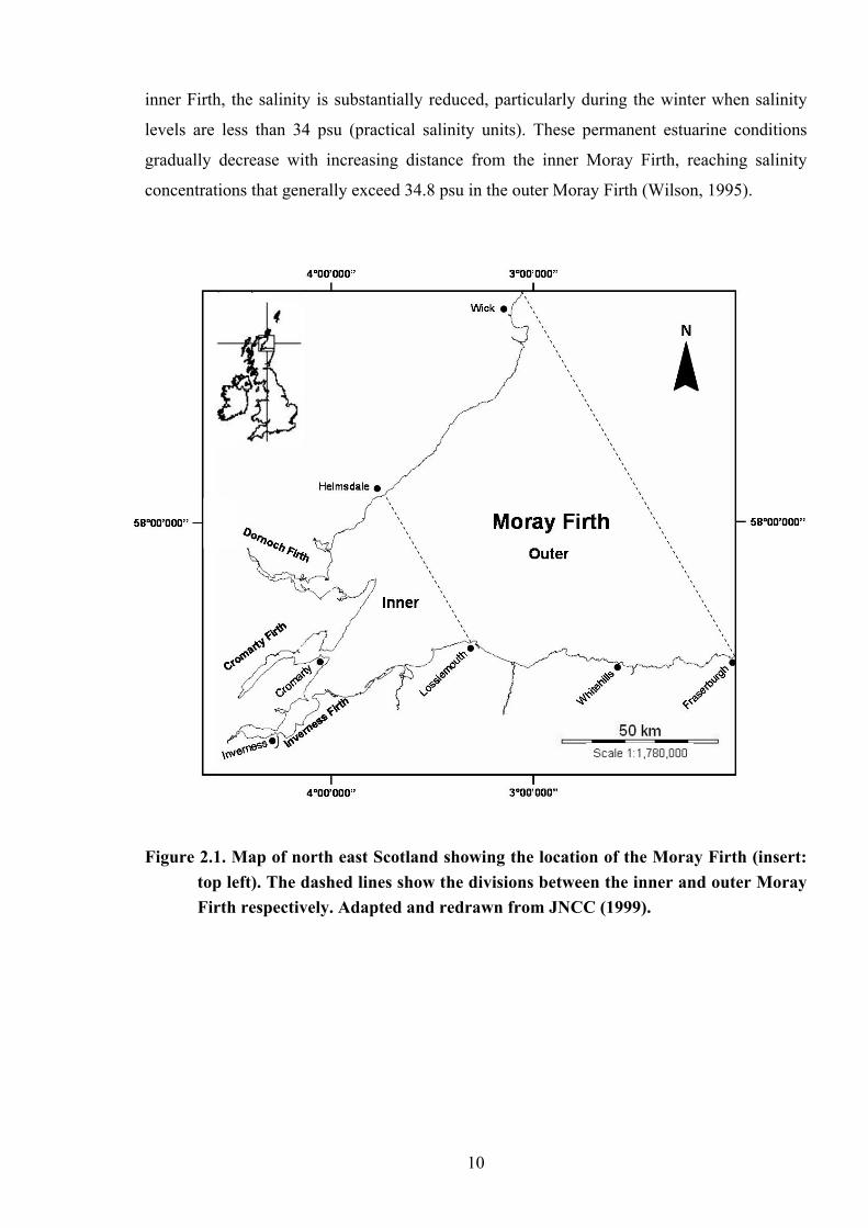
Figure 2.1. Map of north east Scotland showing the location of the Moray Firth (insert:

top left). The dashed lines show the divisions between the inner and outer Moray Firth respectively. Adapted and redrawn from JNCC (1999).

10

3. Methods 3.1. Data Collection Data were collected from systematic boat surveys along the southern coastline of the outer

Moray Firth between May and October from 2001 to 2004 inclusive. The survey route is

illustrated in Figure 3.1 as Route 1, which covers approximately 80 km of coastline between

the costal ports of Lossiemouth and Fraserburgh. This route was divided into two part survey

routes: an eastwards route to Fraserburgh and a westwards route to Lossiemouth originating

from the centrally-located port of Whitehills where the survey vessel used in the present study

was berthed. The surveys were conducted using a 5.4 m Avon Searider Rigid Inflatable Boat

(RIB) with a 90 hp Johnston Evinrude outboard engine. A Lowrance 330C combined GPS

Plotter / Sonar Unit was used for navigation during boat surveys with a crew of 4 to 7 people

acting as observers. The surveys were conducted at speeds of 8-12 km h-1 in sea states of

Beaufort 3 or less and during good light conditions. If the sea state increased above this or if

weather conditions worsened such that heavy or continuous rain occurred, then the survey

was aborted.

At the beginning of each survey trip, a Trip Log was filled out to record the start time,

GPS start position and crewmembers onboard (example shown in Appendix 2). Accordingly,

on the completion of each survey, the end time and end GPS position were also recorded,

along with a summary of the sea state and other environmental conditions. If bottlenose

dolphins were sighted (referred to as an encounter), the boat was gradually slowed and the

camera equipment and recording sheets prepared. An Encounter Log Sheet was used to record

the start time of the encounter, the GPS position of the animals encountered, and the general

landmark along the coastline (for example, see Appendix 2). Encountered dolphins were

always approached cautiously at a shallow angle to their direction of travel so that the boat

would eventually run parallel with the animals, approximately 20 to 50 metres from their

track. Once the boat was in position, the direction and momentum of the boat were maintained

as carefully as possible. If the dolphins naturally changed course, the boat was slowed

accordingly and steered gently behind the animals, rather than in front, to prevent any

unnecessary disturbance. If they stopped to forage or feed at any point during an encounter,

the boat was slowed to idle as appropriate and maintained at a respectable distance until the

group reformed and continued to transit. Hence, throughout the encounter, any alterations in

speed or course were kept to the barest minimum and of utmost predictability for the animals

present. Moreover, the time spent with bottlenoses was always kept to a minimum. This

11

Route 2Route 3Route 4

Route 1

Figure 3.1. Map showing the survey routes used by the Cetacean Research & Rescue Unit during systematic boat surveys of the

outer southern Moray Firth. Route 1 shows the dedicated bottlenose dolphin survey route used in the present study. Routes 2-4 comprise additional transects used by the host organisation in their studies of other cetacean species. Each of the survey routes lies approximately 45 minutes apart in latitude.

12

meant that the research team were only with the dolphins for as long as was necessary to

collect the required data and photograph the individuals present. If this was not possible,

however, or if the team felt that the animals were showing any adverse reaction to the

presence of the survey vessel, the encounter was terminated immediately. All manoeuvres

were conducted in accordance with the principals of the Moray Firth voluntary guidelines on

handling boats around dolphins (Scottish National Heritage, 1993) and the methods laid down

by the Universities of Aberdeen and St. Andrews.

3.2. Photo-Identification During encounters, photographs were taken with a 35mm Nikon F5 auto focus camera with a

F2.8 100-300 mm zoom lens. All photographs were taken using Fuji 400 or 800 ASA colour

print film. Colour film was selected over black and white as the medium was considered to be

more useful in recording the variety of different markings on the bodies of dolphins.

The aim during an encounter was to take sequential photographs of the dorsal fins of

those individuals present. The most efficient method of doing this was to pre-focus the camera

on the sea where the subject was anticipated to surface, thus minimising the time required to

focus on the subject itself and allowing the photographer more time to select between desired

individuals. The capture of both left and right dorsal fins of individuals was not considered

necessary, so long as each individual was photographed on at least one side or the other. This

was regarded as an important protocol to ensure that encounter durations, and therefore any

subsequent disturbance, was minimised. In instances where group sizes were particularly

large, positive identifications of known marked animals were made by eye by experienced

observers. This allowed the photographer more time to photograph unknown or more subtly

marked individuals, thereby reducing the time spent with groups.

If possible, the positioning of the boat adjacent to the dolphins was made in relation to

the sun. Ideally, the sun would be behind the photographer so that the sunlight lit up the

desired features of the dorsal fin and back of selected subjects. If the sun was behind the

subject in relation to the photographer then the dorsal fin appeared as a silhouette, obscuring

any markings, such as identifying scratches or lesions, on the fin and back.

Whilst the photographer was taking pictures, a note taker recorded the content of each

exposure using a simple Film Sheet (Appendix 3). This was also used to detail mother-calf

relationships, intra-group associations and sub-group compositions as observed. A separate

film sheet was used for each film; the number of films required was dependent on the size of

the group encountered, behaviour of the dolphins present and to some extent the

13

environmental conditions at the time of the encounter. A group of foraging animals, for

example, would be typically dispersed with affiliates changing direction frequently, resulting

in a greater number of photographs being taken. On the other hand, a travelling school of 8 to

10 closely associated dolphins surfacing in a regular, predictable manner could be

photographed in a relatively short space of time using no more than two 36-exposure films.

At the end of an encounter, the number of adults, sub-adults, calves and neonates (new

born calves) present were totalled (for age definitions, see section 3.3) and the information on

sub-group structures recorded. This required good communication between the boat driver,

photographer, note taker and other observers present to record this information accurately. A

summary of the behaviour of the dolphins, the time, GPS end position and a visual landmark

was then recorded accordingly. Finally, a photograph of something other than the dolphins or

the sea (usually a photograph of the crew) was taken to separate any additional photos from

subsequent encounters made on the same film. In the case that more than one group of

dolphins was encountered during a single survey trip, each encounter was treated as a separate

sample and recorded on a separate Encounter Log. Back on shore, the data from the Trip and

Encounter Logs were transferred to a generalised Bottlenose Dolphin Survey Form (Appendix

4) and this information was subsequently entered into a relational database system (illustrated

in Figure 3.2).

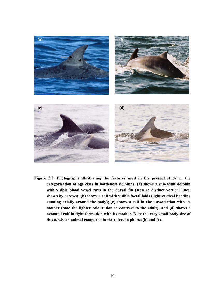
3.3. Definition of Age Classes For the purposes of this study, bottlenose dolphins were divided into four age classes. Based

on their appearance, these were: adult (A), sub-adult (SA), calf (C) and neonate (N). Sub-

adults were defined as individuals of a similar size to adults, but with a slightly lighter, olive

colouration and visible blood vessel rays through the dorsal fin; calves were defined as

approximately two-thirds or less the length of an adult, very light in colouration, often with

discernable foetal folds, and usually swimming in close association with their mothers;

whereas neonates were defined by their very small size (less than one third the length of an

adult), very pale colouration with bold foetal folds, often with a droopy dorsal fin and very

close association with their mother (Robinson, pers. com; Shane, 1990) (Fig, 3.3).

14

Enc ID

ID #

Trip ID

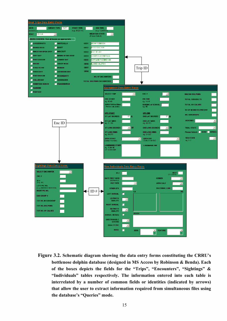
Figure 3.2. Schematic diagram showing the data entry forms constituting the CRRU’s

bottlenose dolphin database (designed in MS Access by Robinson & Benda). Each of the boxes depicts the fields for the “Trips”, “Encounters”, “Sightings” & “Individuals” tables respectively. The information entered into each table is interrelated by a number of common fields or identities (indicated by arrows) that allow the user to extract information required from simultaneous files using the database’s “Queries” mode.

15

(c) (d)

(a) (b)

Figure 3.3. Photographs illustrating the features used in the present study in the

categorisation of age class in bottlenose dolphins: (a) shows a sub-adult dolphin with visible blood vessel rays in the dorsal fin (seen as distinct vertical lines, shown by arrows); (b) shows a calf with visible foetal folds (light vertical banding running axially around the body); (c) shows a calf in close association with its mother (note the lighter colouration in contrast to the adult); and (d) shows a neonatal calf in tight formation with its mother. Note the very small body size of this newborn animal compared to the calves in photos (b) and (c).

16

3.4. Handling Photographs, Matching Animals and Record Keeping Once the photographs from each encounter had been developed, the negatives were cut into

strips and stored in transparent A4 sleeves for protection. Each sleeve was marked with a

unique identification code; beginning with the initials of the photographer and the film

number, and followed by the year and the film reference number as supplied by the developer

i.e. KR22/04-1126. Next, the individual photographs from each processed film were

labelled with the encounter date, encounter start time, the GPS position of the encounter, and

the frame number and film code respectively. This allowed the photographs to be traced to

source should they become mixed-up during the matching process.

An Encounter Grid was used to assist in the sorting procedure for photographs to the

individual level. Each print was examined using a magnifying lamp over a well-lit table with

a protective surface that prevented up-turned photographs getting scratched. Photographs

were always handled from the corners to prevent fingerprints being left on the surface

obscuring any subtle identifying marks. Photo quality was considered paramount to the

subsequent method, and as such only photographs deemed to be of medium to high quality

were used in the following analysis. Hence, if a subject was found to be out of focus,

obscured in any way or too distant then the photograph was discarded.

The natural markings used in the subsequent recognition of individual bottlenoses are

detailed in Table 3.1. The duration for which these natural-occurring marks remained useful

in the process of photo-identification was variable. Dorsal edge marks (DEM’s), deformities

and unusual fin shapes, for example, were all considered unique and permanent markings. In

contrast, minor scratches and lesions healed relatively quickly and were sometimes useful for

only several weeks to months (as described by Wilson et al., 1999). However, given the short

duration of each field season used in the present study (May to September), animals with

markings known to last longer than one field season were considered to be marked herein.

Using the encounter grid, photographs of each distinctive “marked” dolphin from an

encounter was assigned a temporary unique symbol (e.g. * ♥ ☺ , etc) or identification

number depending on whether the animal was already known or not. The photographs for

each individual were subsequently laid out and matched by left and right dorsal profile. Once

complete, the Encounter Grid provided a summary table for all the individual dolphins

recorded on a particular encounter (see Appendix 5 for a compiled example). These

individuals could then be cross-matched with known individuals from the established CRRU

archive; the procedure being assisted through the use of specific search queries within the

purpose-designed database (utilising descriptors based on the number and position of DEM’s)

17

Table 3.1. Naturally occurring markings used in the present study for the photo-

identification of individual bottlenose dolphins (adapted and expanded from Wilson, 1995).

Dorsal fin nicks or tears Pieces of tissue missing from the trailing, and occasionally leading, edges of the dorsal fin

Unusual dorsal shapes Distinctively broad, narrow, tall, short or leaning dorsal fins

Major scratches or scars Large scratches or scars on the fins and body flanks of animals

Minor scratches or scars As with major scratches or scars, but less pronounced and superficial marks from interactions with conspecifics

White fin fringes / areas of depigmentation

Depigmented areas usually observed around the edges of the dorsal fin. Albino animals are also included in this category

Active lesions Areas of black, cloudy, lunar or orange lesions

Healed lesions Pale epidermal lesions / skin blemishes often used as an additional feature for differentiating individuals

Deformities (Natural & unnatural)

Distortions of the normal body contours, such as a kinked peduncle or tailstock, for example. May be congenital or otherwise, and therefore includes inflicted injuries such as those caused from boat collisions or propeller strikes, for example.

18

to locate animals with unique or distinctive features. Once a potential match was made from a

digital image within the archive, the appropriate hanging file could be retrieved in hard copy

for closer inspection of all previous photographs.

On confirmation of a positive match, the best photograph(s) of the right and/or left

dorsal fin were added to the respective hanging file, along with information on the date,

encounter start time, frame number and code. If no match could be found, then the unknown

animal was assigned a new identification number and hanging file, and its details added to the

Individuals file in the database accordingly. Finally, the entire encounter was recorded on a

Summary Encounter Sheet (shown in Appendix 6), from which the information on each

recognisable individual could be inputted into the Sightings table in the relational database for

completion.

3.5. Removing False Negatives & False Positives & Data Selection In order to estimate the number of animals using the study area in the following part of this

investigation as accurately as possible, a further procedure was used to ensure the greatest

confidence in the dataset being used. This involved the use of a computer-assisted

identification / automated matching software package currently under development by Leiden

University as part of the EC EuroPhlukes Initiative (www.europhlukes.net). As contributors

to the Europhlukes Project and partners in the EC Consortium, the CRRU undertook to trial

the new software on its extensive bottlenose archive with the application of a two-stage

extraction/matching procedure in the form of FinEx and FinMatch™.

For each of the marked animals archived in the CRRU’s bottlenose dolphin catalogue

(from 2001 to 2004 inclusive), the above software was used to isolate errors resulting from

misidentification. The two error types which most typically occur during the matching

process are those of false positive errors, when two sightings of different individuals are

classed as one and the same individual and, false negative errors, when two images of the

same individual are classed as two different animals; both resulting in bias in population

estimations (Gunnlaugsson & Sigurjónsson, 1990; Stevick et al., 2001). With respect, the

application of this computer-assisted matching software to the existing dataset, although time

consuming, was considered to be an integral process for the subsequent analysis of marked

individuals for predictions of the number of animals using the study area.

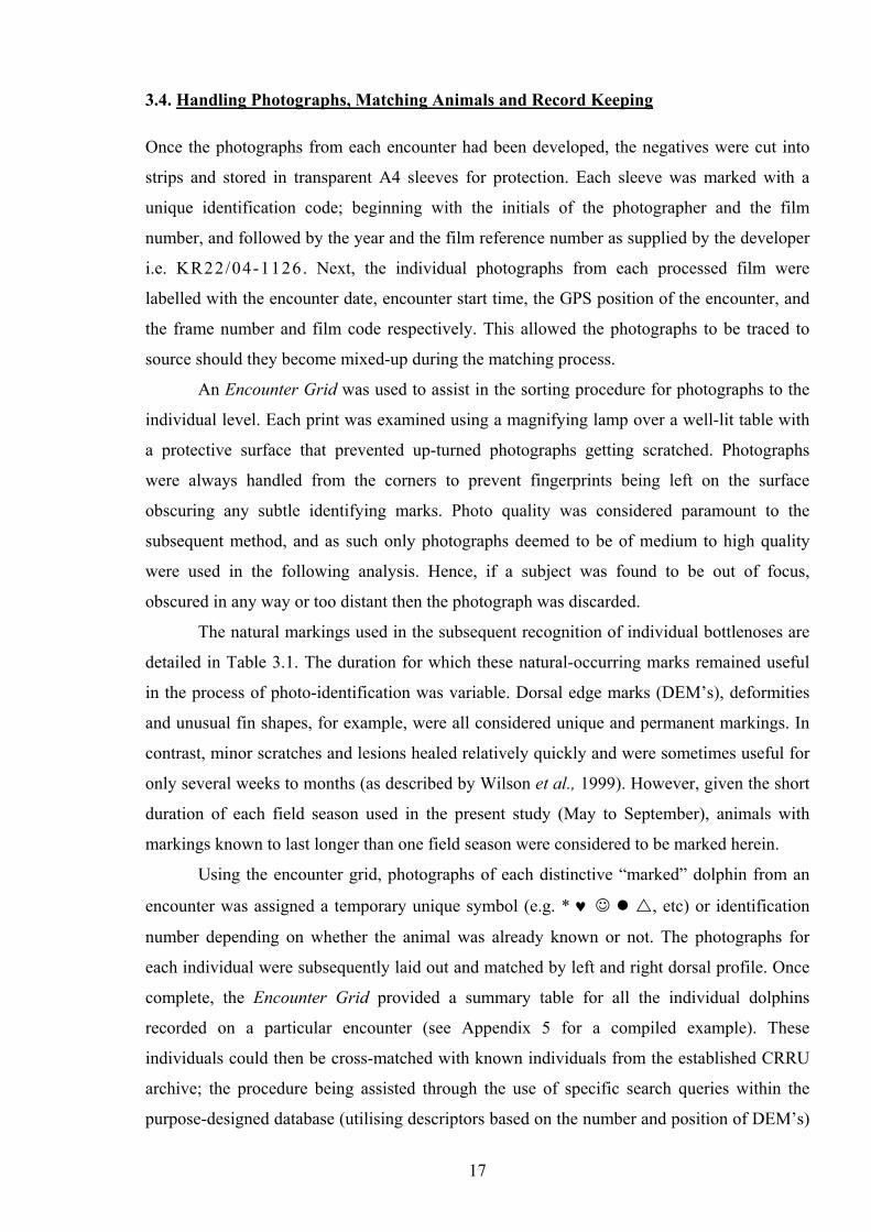
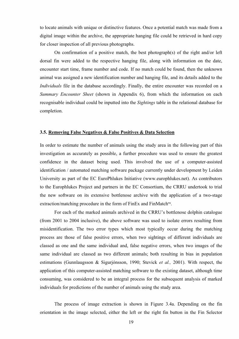
The process of image extraction is shown in Figure 3.4a. Depending on the fin

orientation in the image selected, either the left or the right fin button in the Fin Selector

19

(a)

5

3

4

2

last point first point

brighness/contrast Threshold Panel

Image Display Panel

View Panel Project Panel

Fin Selector

Contour Display Panel Project Panel

(iii)

(ii)

(i)

(b)

20

Figure 3.4. Program screen captures showing (a) the FinEx dorsal extraction program and(b) the FinMatch automated matching program used in the present study for thereanalysis of all “marked” animals (developed by the National Research Institute forMathematics and Computer Science Department of Mathematics (CWI),Amsterdam, for the EC EuroPhlukes Project). The algorithm extractions describedin the text are shown in 3.4b for: (i) the subject image, (ii) the selected match, and(iii) the overlay of the two extractions.

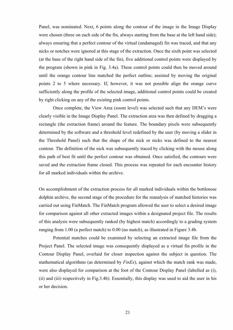
Panel, was nominated. Next, 6 points along the contour of the image in the Image Display

were chosen (three on each side of the fin, always starting from the base at the left hand side);

always ensuring that a perfect contour of the virtual (undamaged) fin was traced, and that any

nicks or notches were ignored at this stage of the extraction. Once the sixth point was selected

(at the base of the right hand side of the fin), five additional control points were displayed by

the program (shown in pink in Fig. 3.4a). These control points could then be moved around

until the orange contour line matched the perfect outline; assisted by moving the original

points 2 to 5 where necessary. If, however, it was not possible align the orange curve

sufficiently along the profile of the selected image, additional control points could be created

by right clicking on any of the existing pink control points.

Once complete, the View Area (zoom level) was selected such that any DEM’s were

clearly visible in the Image Display Panel. The extraction area was then defined by dragging a

rectangle (the extraction frame) around the feature. The boundary pixels were subsequently

determined by the software and a threshold level redefined by the user (by moving a slider in

the Threshold Panel) such that the shape of the nick or nicks was defined to the nearest

contour. The definition of the nick was subsequently traced by clicking with the mouse along

this path of best fit until the perfect contour was obtained. Once satisfied, the contours were

saved and the extraction frame closed. This process was repeated for each encounter history

for all marked individuals within the archive.

On accomplishment of the extraction process for all marked individuals within the bottlenose

dolphin archive, the second stage of the procedure for the reanalysis of matched histories was

carried out using FinMatch. The FinMatch program allowed the user to select a desired image

for comparison against all other extracted images within a designated project file. The results

of this analysis were subsequently ranked (by highest match) accordingly to a grading system

ranging from 1.00 (a perfect match) to 0.00 (no match), as illustrated in Figure 3.4b.

Potential matches could be examined by selecting an extracted image file from the

Project Panel. The selected image was consequently displayed as a virtual fin profile in the

Contour Display Panel, overlaid for closer inspection against the subject in question. The

mathematical algorithms (as determined by FinEx), against which the match rank was made,

were also displayed for comparison at the foot of the Contour Display Panel (labelled as (i),

(ii) and (iii) respectively in Fig.3.4b). Essentially, this display was used to aid the user in his

or her decision.

21

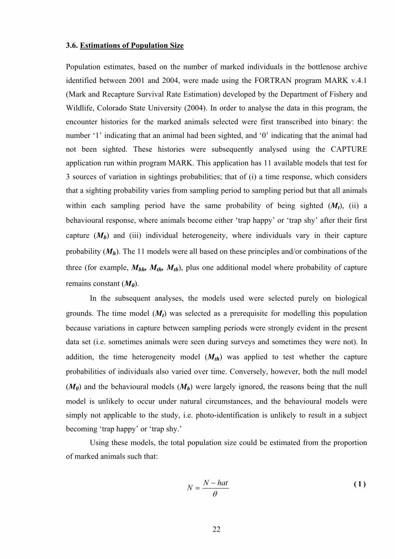
3.6. Estimations of Population Size Population estimates, based on the number of marked individuals in the bottlenose archive

identified between 2001 and 2004, were made using the FORTRAN program MARK v.4.1

(Mark and Recapture Survival Rate Estimation) developed by the Department of Fishery and

Wildlife, Colorado State University (2004). In order to analyse the data in this program, the

encounter histories for the marked animals selected were first transcribed into binary: the

number ‘1’ indicating that an animal had been sighted, and ‘0’ indicating that the animal had

not been sighted. These histories were subsequently analysed using the CAPTURE

application run within program MARK. This application has 11 available models that test for

3 sources of variation in sightings probabilities; that of (i) a time response, which considers

that a sighting probability varies from sampling period to sampling period but that all animals

within each sampling period have the same probability of being sighted (Mt), (ii) a

behavioural response, where animals become either ‘trap happy’ or ‘trap shy’ after their first

capture (Mb) and (iii) individual heterogeneity, where individuals vary in their capture

probability (Mh). The 11 models were all based on these principles and/or combinations of the

three (for example, Mbh, Mth, Mtb), plus one additional model where probability of capture

remains constant (M0).

In the subsequent analyses, the models used were selected purely on biological

grounds. The time model (Mt) was selected as a prerequisite for modelling this population

because variations in capture between sampling periods were strongly evident in the present

data set (i.e. sometimes animals were seen during surveys and sometimes they were not). In

addition, the time heterogeneity model (Mth) was applied to test whether the capture

probabilities of individuals also varied over time. Conversely, however, both the null model

(M0) and the behavioural models (Mb) were largely ignored, the reasons being that the null

model is unlikely to occur under natural circumstances, and the behavioural models were

simply not applicable to the study, i.e. photo-identification is unlikely to result in a subject

becoming ‘trap happy’ or ‘trap shy.’

Using these models, the total population size could be estimated from the proportion

of marked animals such that:

( 1 )

θhatNN −

=

22

−

+

−−

=θθ

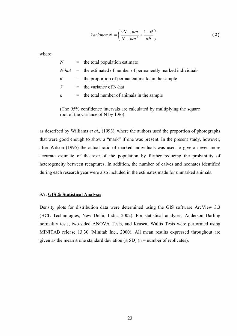
nhatNhatvNVariance N 1 2

( 2 )

where:

N = the total population estimate

N-hat = the estimated of number of permanently marked individuals

θ = the proportion of permanent marks in the sample

V = the variance of N-hat

n = the total number of animals in the sample

(The 95% confidence intervals are calculated by multiplying the square root of the variance of N by 1.96).

as described by Williams et al., (1993), where the authors used the proportion of photographs

that were good enough to show a “mark” if one was present. In the present study, however,

after Wilson (1995) the actual ratio of marked individuals was used to give an even more

accurate estimate of the size of the population by further reducing the probability of

heterogeneity between recaptures. In addition, the number of calves and neonates identified

during each research year were also included in the estimates made for unmarked animals.

3.7. GIS & Statistical Analysis Density plots for distribution data were determined using the GIS software ArcView 3.3

(HCL Technologies, New Delhi, India, 2002). For statistical analyses, Anderson Darling

normality tests, two-sided ANOVA Tests, and Kruscal Wallis Tests were performed using

MINITAB release 13.30 (Minitab Inc., 2000). All mean results expressed throughout are

given as the mean ± one standard deviation (± SD) (n = number of replicates).

23

4. Results

4.1. Survey Effort

Between May and October 2004, a total of 42 survey trips were carried out on 28 survey days.

The survey effort for this period totalled 92 hours and 13 minutes, of which 11 hours and 43

minutes were spent observing and photographing dolphins during 9 encounters. From May to

October 2001 to 2003 inclusive, an additional 151 surveys were conducted on a further 146

days producing an overall survey effort of 437 hours and 40 minutes for the entire study

period. Thus, from May 2001 to Oct 2004, a total of 78 hours and 30 minutes were spent with

dolphins from 62 encounters (Table 4.1).

Figure 4.1 shows that the survey effort throughout the study period from May to Oct

was relatively even across the study area, between Lossiemouth to Fraserburgh (Fig.4.1a), and

from one annual field season to the next (Fig.4.1b). Only two notable exceptions were

observed, both of which express a bias in survey effort to the area west of Whitehills. The first

of these occurred during the month of June, and the second across the 2001 field season. In

both cases it seems that a greater number of surveys were carried out between Whitehills and

Lossiemouth than between Whitehills and Fraserburgh, which may have influenced the

observed patterns of distribution. Statistical analysis using a Kruskal-Wallis Test found a

significant variation between monthly survey effort (p = 0.00, d.f. = 4, H = 36.14), this result

was undoubtedly caused by the survey effort in July, which was indicated by the

comparatively higher median, however, there was no significant variation in survey effort

between the survey years (p = 0.4.06, d.f. = 3, H = 2.91). Variation in the number of

encounters between months was also observed; however, further analysis showed that this

was not attributed to survey effort (Fig 4.2).

4.2. Distribution & Abundance of Animals The distribution of bottlenose dolphins between May and October 2001 to 2004 is shown in

Figure 4.3 Animals were typically found throughout the study area at depths of between 5 and

25 metres. When plotted by month (as shown in Figure 4.4), their distribution was seen to be

variable with no particular preferences shown for specific areas of the coastline from one

month to another. Whilst the dispersal of groups appeared to be comparatively even during

the months of May, July and September, however, this distribution was found to be skewed to

the west in June then to the east in August respectively.

24

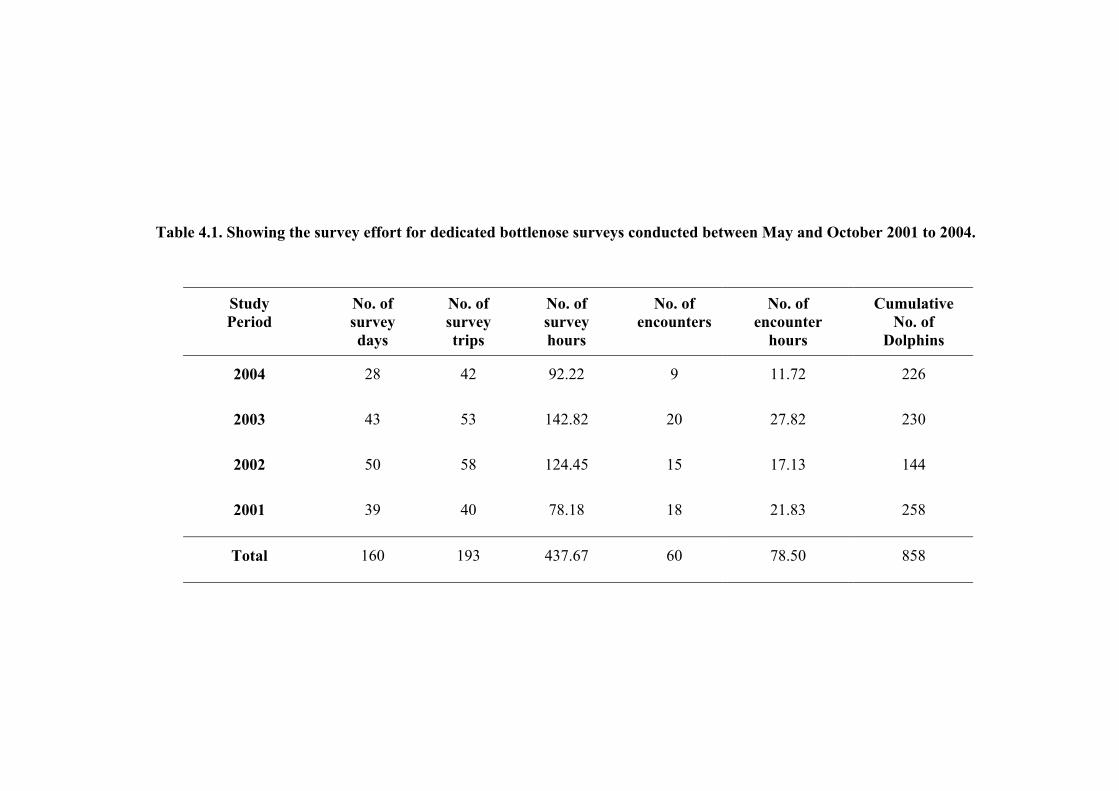
Table 4.1. Showing the survey effort for dedicated bottlenose surveys conducted between May and October 2001 to 2004.

25

Study Period

No. of survey days

No. of survey trips

No. of survey hours

No. of encounters

No. of encounter

hours

Cumulative No. of

Dolphins

2004 28 42 92.22 9 11.72 226

2003 43

53 142.82 20 27.82 230

2002 50 58 124.45 15 17.13 144

2001 39 40 78.18 18 21.83 258

Total 160 193 437.67 60 78.50 858

0

2

4

6

8

10

12

14

Landmark

% o

f sur

vey

effo

rt a

t are

a

May

June

July

August

September

0

2

4

6

8

10

12

14

Landmark

% o

f sur

vey

effo

rt a

t are

a

2001-2004

2001

2002

2003

2004

(a)

(b)

Figure

4.1. Graphs showing the distribution of survey effort across the study area asdefined using visual landmarks covered during survey trips. Plot (a) shows thesurvey effort by month from 2001 to 2004 inclusive, whilst plot (b) shows thesurvey effort expressed by year. It should be noted that, for each survey, the surveyvessel always departed from its berthing at Whitehills, the subsequent route beingconducted in either an easterly or a westerly direction from this location. Thisaccounts for the considerable peak in survey effort observed in the centre of eachgraph.

26

0

1000

2000

3000

4000

5000

6000

7000

8000

9000

May June July August September

Cum

ulat

ive

surv

ey ti

me

(min

s)

0

2

4

6

8

10

12

14

16

18

Cum

ulat

ive

no. o

f enc

ount

ers

Figure 4.2. The cumulative survey effort in minutes (as depicted by the bar chart),

plotted with the cumulative number of encounters (as depicted by the line chart) for the dedicated bottlenose dolphin surveys between May and October, 2001-2004.

The distribution of sightings by year is shown in Figure 4.5. With the exception of the

2004 data in which bottlenose dolphins were biased to the west of the study area (this year

being an atypical year for the study area on several accounts), the animals were once again

found to be regularly distributed along the entire length of the coastline between Lossiemouth

and Fraserburgh.

Whilst the distribution maps simply showed the position of encountered groups, the

abundance (no. of dolphins per square km) was further determined to identify any specific

preferences shown by the study animals for particular areas. In the resulting GIS plot, 3

principal sites of preferential area use were identified (Figure 4.6). The first of these is seen

approximately 1.5 km to the west of Whitehills, in the centre of the coastline; the second close

to the river mouth in Spey Bay to the west; and the third adjacent to Banff Bay and the mouth

of the River Deveron, to the east.

27

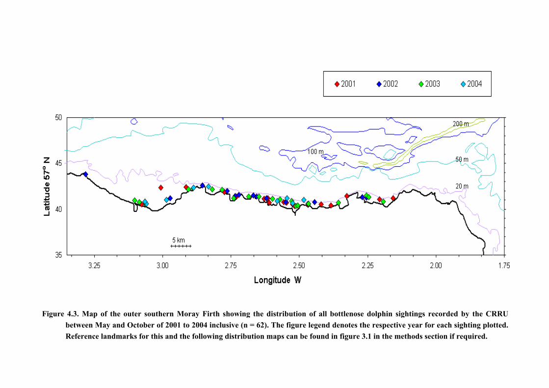
28

Figure 4.3. Map of the outer southern Moray Firth showing the distribution of all bottlenose dolphin sightings recorded by the CRRUbetween May and October of 2001 to 2004 inclusive (n = 62). The figure legend denotes the respective year for each sighting plotted.Reference landmarks for this and the following distribution maps can be found in figure 3.1 in the methods section if required.

(n=17)

(n=10)

(n=12)

(n=14)

(n=9)

Jun

Sep

Aug

Jul

May

Figure 4.4. Distribution maps of the outer southern Moray Firth study site depicting the

monthly changes in bottlenose dolphin occurrence/distribution between Lossiemouth and Fraserburgh from 2001 to 2004 inclusive.

29

Latit

ude 5

7° N

2004 (n=9)

2003 (n=20)

2002 (n=15)

2001 (n=18)

Figure 4.5. Distribution maps showing the annual changes in bottlenose dolphin occurrence/distribution between Lossiemouth and Fraserburgh for 2001 to 2004, respectively.

30

Scale : Kilometres

31

Figure 4.6. GIS plot to show the relative abundance of bottlenose dolphins recorded balong the southern coastline of the outer Moray Firth between Lossiemouth anred blocks represents an area of one square kilometre and the cumulative freaccompanying legend. This map was produced using ArcView v3.3.

No. of bottlenosedolphins per km2

N

etween May and October from 2001 to 2004d Fraserburgh (n = 858 animals). Each of thequency of animals per block is shown in the

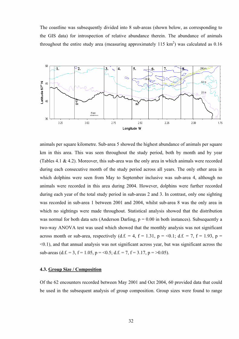
The coastline was subsequently divided into 8 sub-areas (shown below, as corresponding to

the GIS data) for introspection of relative abundance therein. The abundance of animals

throughout the entire study area (measuring approximately 115 km2) was calculated as 0.16

8. 7.6.5.4.3.1. 2.

animals per square kilometre. Sub-area 5 showed the highest abundance of animals per square

km in this area. This was seen throughout the study period, both by month and by year

(Tables 4.1 & 4.2). Moreover, this sub-area was the only area in which animals were recorded

during each consecutive month of the study period across all years. The only other area in

which dolphins were seen from May to September inclusive was sub-area 4, although no

animals were recorded in this area during 2004. However, dolphins were further recorded

during each year of the total study period in sub-areas 2 and 3. In contrast, only one sighting

was recorded in sub-area 1 between 2001 and 2004, whilst sub-area 8 was the only area in

which no sightings were made throughout. Statistical analysis showed that the distribution

was normal for both data sets (Anderson Darling, p = 0.00 in both instances). Subsequently a

two-way ANOVA test was used which showed that the monthly analysis was not significant

across month or sub-area, respectively (d.f. = 4, f = 1.31, p = <0.1; d.f. = 7, f = 1.93, p =

<0.1), and that annual analysis was not significant across year, but was significant across the

sub-areas (d.f. = 3, f = 1.05, p = <0.5; d.f. = 7, f = 3.17, p = >0.05).

4.3. Group Size / Composition

Of the 62 encounters recorded between May 2001 and Oct 2004, 60 provided data that could

be used in the subsequent analysis of group composition. Group sizes were found to range

32

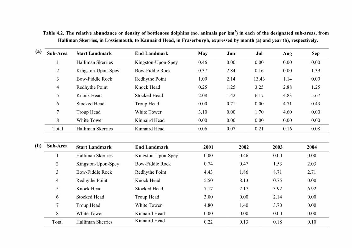
Table 4.2. The relative abundance or density of bottlenose dolphins (no. animals per km2) in each of the designated sub-areas, from Halliman Skerries, in Lossiemouth, to Kannaird Head, in Fraserburgh, expressed by month (a) and year (b), respectively.

(a) Sub-Area Start Landmark End Landmark May Jun Jul Aug Sep

1 Halliman Skerries Kingston-Upon-Spey 0.46 0.00 0.00 0.00 0.00

2

Kingston-Upon-Spey Bow-Fiddle Rock 0.37 2.84 0.16 0.00 1.39

3 Bow-Fiddle Rock Redhythe Point 1.00 2.14 13.43 1.14 0.00

4 Redhythe Point Knock Head 0.25 1.25 3.25 2.88 1.25

5 Knock Head Stocked Head 2.08 1.42 6.17 4.83 5.67

6 Stocked Head Troup Head 0.00 0.71 0.00 4.71 0.43

7 Troup Head White Tower 3.10 0.00 1.70 4.60 0.00

8 White Tower Kinnaird Head 0.00 0.00 0.00 0.00 0.00

Total Halliman Skerries Kinnaird Head 0.06 0.07 0.21 0.16 0.08

(b) (b) Sub-Area Start Landmark End Landmark 2001 2002 2003 2004

1 Halliman Skerries Kingston-Upon-Spey 0.00 0.46 0.00 0.00

2

Kingston-Upon-Spey Bow-Fiddle Rock 0.74 0.47 1.53 2.03

3 Bow-Fiddle Rock Redhythe Point 4.43 1.86 8.71 2.71

4 Redhythe Point Knock Head 5.50 8.13 0.75 0.00

5 Knock Head Stocked Head 7.17 2.17 3.92 6.92

6 Stocked Head Troup Head 3.00 0.00 2.14 0.00

7 Troup Head White Tower 4.80 1.40 3.70 0.00

8 White Tower Kinnaird Head 0.00 0.00 0.00 0.00

Total Halliman Skerries Kinnaird Head 0.22 0.13 0.18 0.10 33

between 2 and 44, with only 5 solatary animals being encountered throughout the entire study

period, which accounted for just 3.3% of the total encounters. The largest school of 44

animals was recorded in September 2002.

Eighty one percent of all groups recorded contained calves. Those groups containing

calves, both excluding calves from the analysis (median group size = 15) and including calves

(median group size = 10), were significantly larger than those without calves (median group

size = 4) (d.f. = 107, f = 8.18, p = > 0.001, one-way ANOVA). Calves were sighted across all

months of the study period. Newborn or neonatal calves, however, were only recorded from

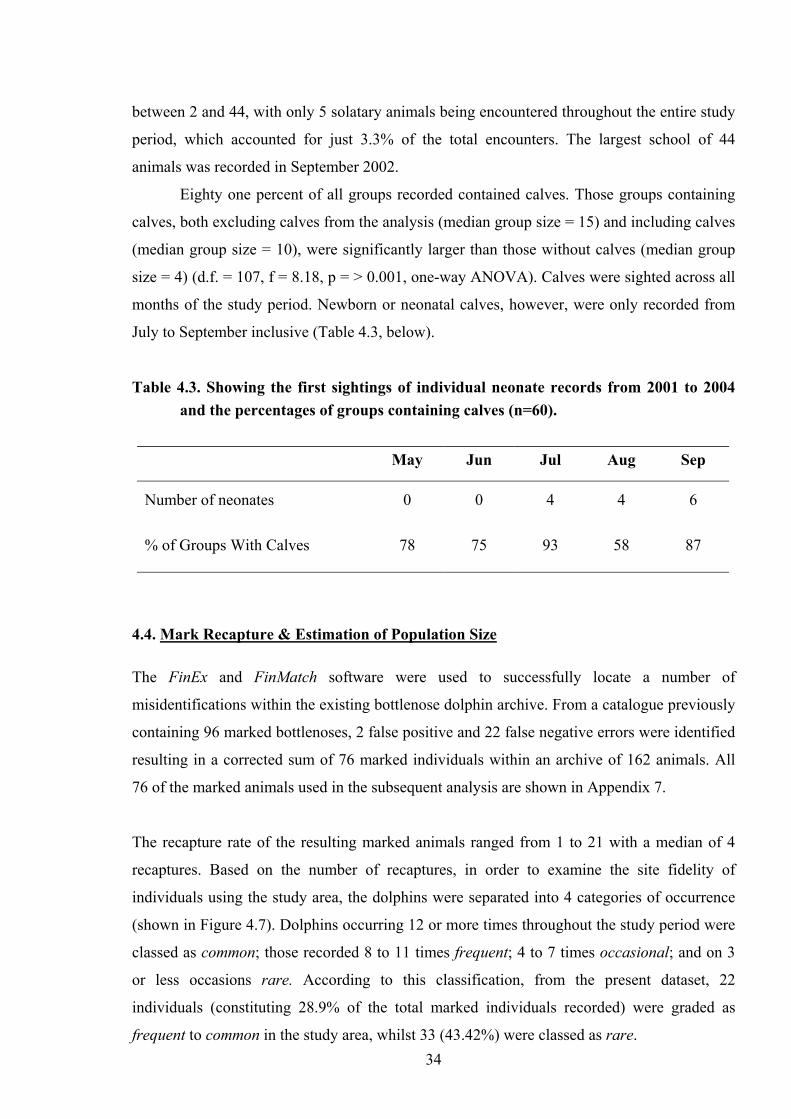
July to September inclusive (Table 4.3, below).

Table 4.3. Showing the first sightings of individual neonate records from 2001 to 2004 and the percentages of groups containing calves (n=60).

May Jun Jul Aug Sep

Number of neonates 0 0 4 4 6

% of Groups With Calves 78 75 93 58 87

4.4. Mark Recapture & Estimation of Population Size The FinEx and FinMatch software were used to successfully locate a number of

misidentifications within the existing bottlenose dolphin archive. From a catalogue previously

containing 96 marked bottlenoses, 2 false positive and 22 false negative errors were identified

resulting in a corrected sum of 76 marked individuals within an archive of 162 animals. All

76 of the marked animals used in the subsequent analysis are shown in Appendix 7.

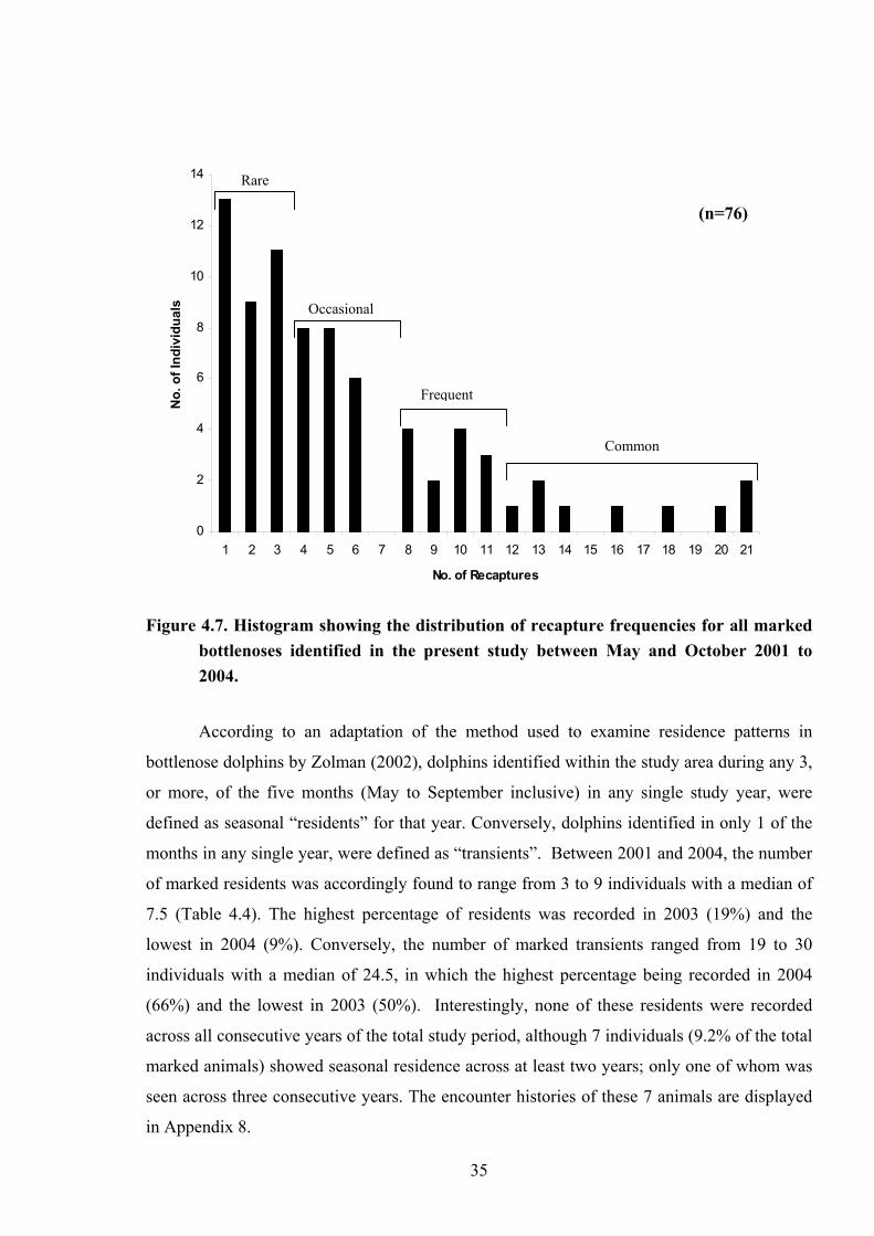
The recapture rate of the resulting marked animals ranged from 1 to 21 with a median of 4

recaptures. Based on the number of recaptures, in order to examine the site fidelity of

individuals using the study area, the dolphins were separated into 4 categories of occurrence

(shown in Figure 4.7). Dolphins occurring 12 or more times throughout the study period were

classed as common; those recorded 8 to 11 times frequent; 4 to 7 times occasional; and on 3

or less occasions rare. According to this classification, from the present dataset, 22

individuals (constituting 28.9% of the total marked individuals recorded) were graded as

frequent to common in the study area, whilst 33 (43.42%) were classed as rare. 34

0

2

4

6

8

10

12

14

1 2 3 4 5 6 7 8 9 10 11 12 13 14 15 16 17 18 19 20 21

No. of Recaptures

No.

of I

ndiv

idua

ls

(n=76)

Common

Frequent

Occasional

Rare Figure 4.7. Histogram showing the distribution of recapture frequencies for all marked

bottlenoses identified in the present study between May and October 2001 to 2004.

According to an adaptation of the method used to examine residence patterns in

bottlenose dolphins by Zolman (2002), dolphins identified within the study area during any 3,

or more, of the five months (May to September inclusive) in any single study year, were

defined as seasonal “residents” for that year. Conversely, dolphins identified in only 1 of the

months in any single year, were defined as “transients”. Between 2001 and 2004, the number

of marked residents was accordingly found to range from 3 to 9 individuals with a median of

7.5 (Table 4.4). The highest percentage of residents was recorded in 2003 (19%) and the

lowest in 2004 (9%). Conversely, the number of marked transients ranged from 19 to 30

individuals with a median of 24.5, in which the highest percentage being recorded in 2004

(66%) and the lowest in 2003 (50%). Interestingly, none of these residents were recorded

across all consecutive years of the total study period, although 7 individuals (9.2% of the total

marked animals) showed seasonal residence across at least two years; only one of whom was

seen across three consecutive years. The encounter histories of these 7 animals are displayed

in Appendix 8.

35

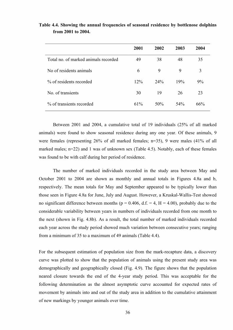
Table 4.4. Showing the annual frequencies of seasonal residence by bottlenose dolphins from 2001 to 2004.

2001 2002 2003 2004

Total no. of marked animals recorded 49 38 48 35

No of residents animals 6 9 9 3

% of residents recorded 12% 24% 19% 9%

No. of transients 30 19 26 23

% of transients recorded 61% 50% 54% 66%

Between 2001 and 2004, a cumulative total of 19 individuals (25% of all marked

animals) were found to show seasonal residence during any one year. Of these animals, 9

were females (representing 26% of all marked females; n=35), 9 were males (41% of all

marked males; n=22) and 1 was of unknown sex (Table 4.5). Notably, each of these females

was found to be with calf during her period of residence.

The number of marked individuals recorded in the study area between May and

October 2001 to 2004 are shown as monthly and annual totals in Figures 4.8a and b,

respectively. The mean totals for May and September appeared to be typically lower than

those seen in Figure 4.8a for June, July and August. However, a Kruskal-Wallis-Test showed

no significant difference between months (p = 0.406, d.f. = 4, H = 4.00), probably due to the

considerable variability between years in numbers of individuals recorded from one month to

the next (shown in Fig. 4.8b). As a result, the total number of marked individuals recorded

each year across the study period showed much variation between consecutive years; ranging

from a minimum of 35 to a maximum of 49 animals (Table 4.4).

For the subsequent estimation of population size from the mark-recapture data, a discovery

curve was plotted to show that the population of animals using the present study area was

demographically and geographically closed (Fig. 4.9). The figure shows that the population

neared closure towards the end of the 4-year study period. This was acceptable for the

following determination as the almost asymptotic curve accounted for expected rates of

movement by animals into and out of the study area in addition to the cumulative attainment

of new markings by younger animals over time.

36

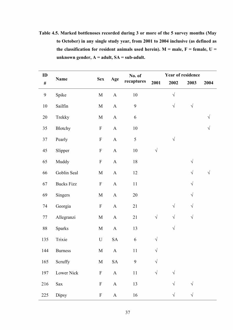
Table 4.5. Marked bottlenoses recorded during 3 or more of the 5 survey months (May

to October) in any single study year, from 2001 to 2004 inclusive (as defined as

the classification for resident animals used herein). M = male, F = female, U =

unknown gender, A = adult, SA = sub-adult.

Year of residence

ID

# Name Sex Age

No. of recaptures

2001 2002 2003 2004

9 Spike M A 10 √

10 Sailfin M A 9 √ √

20 Trekky M A 6 √

35 Blotchy F A 10 √

37 Pearly F A 5 √

45 Slipper F A 10 √

65 Muddy F A 18 √

66 Goblin Seal M A 12 √ √

67 Bucks Fizz F A 11 √

69 Singers M A 20 √

74 Georgia F A 21 √ √

77 Allegranzi M A 21 √ √ √

88 Sparks M A 13 √

135 Trixie U SA 6 √

144 Burness M A 11 √

165 Scruffy M SA 9 √

197 Lower Nick F A 11 √ √

216 Sax F A 13 √ √

225 Dipsy F A 16 √ √

37

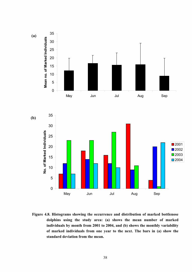
0

5

10

15

20

25

30

35

May Jun Jul Aug Sep

Mea

n no

. of M

arke

d In

divi

dual

s(a)

0

5

10

15

20

25

30

35

May Jun Jul Aug Sep

No.

of M

arke

d In

divi

dual

s

2001200220032004

(b)

Figure 4.8. Histograms showing the occurrence and distribution of marked bottlenose

dolphins using the study area: (a) shows the mean number of marked individuals by month from 2001 to 2004, and (b) shows the monthly variability of marked individuals from one year to the next. The bars in (a) show the standard deviation from the mean.

38

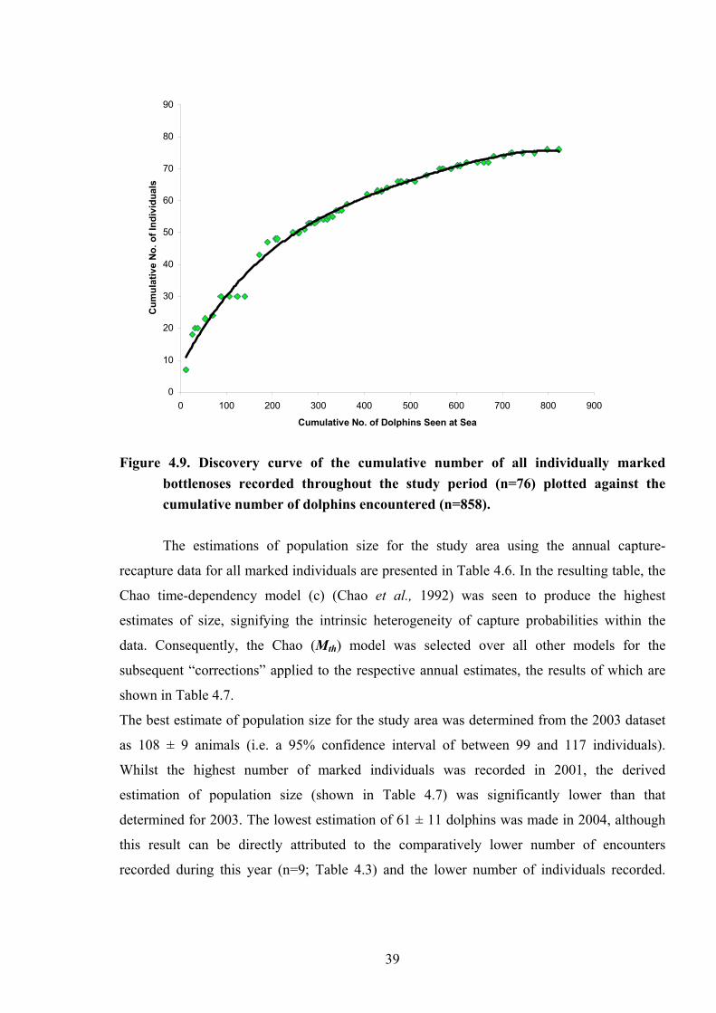
0

10

20

30

40

50

60

70

80

90

0 100 200 300 400 500 600 700 800 900

Cumulative No. of Dolphins Seen at Sea

Cum

ulat

ive

No.

of I

ndiv

idua

ls

Figure 4.9. Discovery curve of the cumulative number of all individually marked

bottlenoses recorded throughout the study period (n=76) plotted against the cumulative number of dolphins encountered (n=858).

The estimations of population size for the study area using the annual capture-

recapture data for all marked individuals are presented in Table 4.6. In the resulting table, the

Chao time-dependency model (c) (Chao et al., 1992) was seen to produce the highest

estimates of size, signifying the intrinsic heterogeneity of capture probabilities within the

data. Consequently, the Chao (Mth) model was selected over all other models for the

subsequent “corrections” applied to the respective annual estimates, the results of which are

shown in Table 4.7.

The best estimate of population size for the study area was determined from the 2003 dataset

as 108 ± 9 animals (i.e. a 95% confidence interval of between 99 and 117 individuals).

Whilst the highest number of marked individuals was recorded in 2001, the derived

estimation of population size (shown in Table 4.7) was significantly lower than that

determined for 2003. The lowest estimation of 61 ± 11 dolphins was made in 2004, although

this result can be directly attributed to the comparatively lower number of encounters

recorded during this year (n=9; Table 4.3) and the lower number of individuals recorded.

39

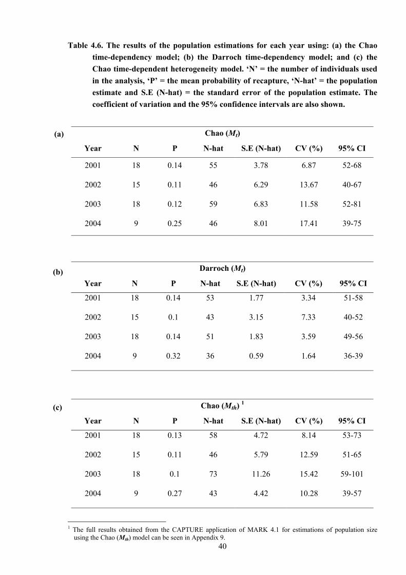
Table 4.6. The results of the population estimations for each year using: (a) the Chao time-dependency model; (b) the Darroch time-dependency model; and (c) the Chao time-dependent heterogeneity model. ‘N’ = the number of individuals used in the analysis, ‘P’ = the mean probability of recapture, ‘N-hat’ = the population estimate and S.E (N-hat) = the standard error of the population estimate. The coefficient of variation and the 95% confidence intervals are also shown.

Chao (Mt)

Year N P N-hat S.E (N-hat) CV (%) 95% CI

2001 18 0.14 55 3.78 6.87 52-68

2002 15 0.11 46 6.29 13.67 40-67

2003 18 0.12 59 6.83 11.58 52-81

2004 9 0.25 46 8.01 17.41 39-75

(a)

Darroch (Mt)

Year N P N-hat S.E (N-hat) CV (%) 95% CI

2001 18 0.14 53 1.77 3.34 51-58

2002 15 0.1 43 3.15 7.33 40-52

2003 18 0.14 51 1.83 3.59 49-56

2004 9 0.32 36 0.59 1.64 36-39

(b)

Chao (Mth) 1

Year N P N-hat S.E (N-hat) CV (%) 95% CI

2001 18 0.13 58 4.72 8.14 53-73

2002 15 0.11 46 5.79 12.59 51-65

2003 18 0.1 73 11.26 15.42 59-101

2004 9 0.27 43 4.42 10.28 39-57

(c)

40

1 The full results obtained from the CAPTURE application of MARK 4.1 for estimations of population size

using the Chao (Mth) model can be seen in Appendix 9.

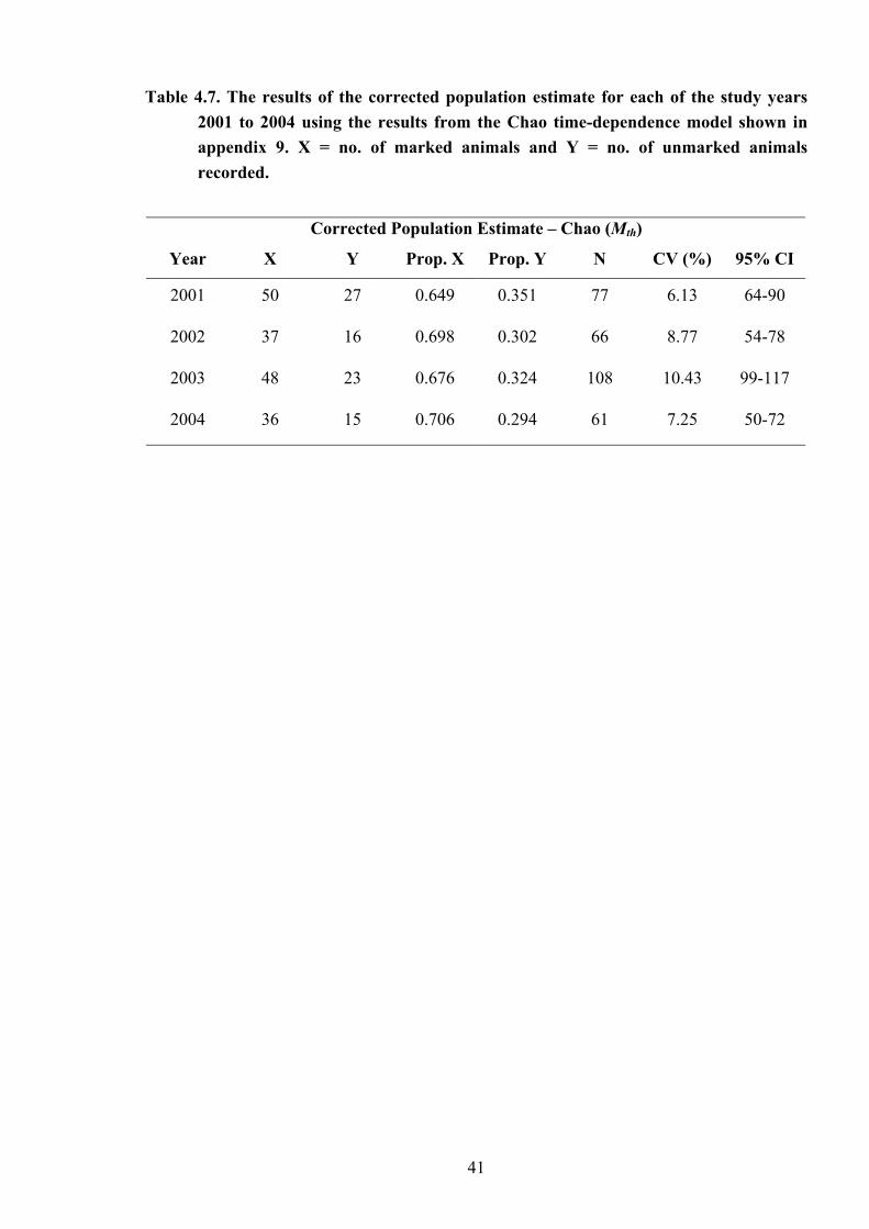
Table 4.7. The results of the corrected population estimate for each of the study years 2001 to 2004 using the results from the Chao time-dependence model shown in appendix 9. X = no. of marked animals and Y = no. of unmarked animals recorded.

Corrected Population Estimate – Chao (Mth)

Year X Y Prop. X Prop. Y N CV (%) 95% CI

2001 50 27 0.649 0.351 77 6.13 64-90

2002 37 16 0.698 0.302 66 8.77 54-78

2003 48 23 0.676 0.324 108 10.43 99-117

2004 36 15 0.706 0.294 61 7.25 50-72

41

5. Discussion

5.1. Distribution, Density & Habitat Selection

In the present study, bottlenose dolphins were encountered along the entire coastline of the

southern outer Moray Firth, at depths ranging between 5 and 25 metres. The maximum depth

showed an interesting contrast with the data from studies in the inner Moray Firth where

dolphins were found in their highest abundance at depths in excess of 50 metres (Hastie et al.,

2003a; Hastie et al., 2004). Similarly, in the Shannon estuary, in Ireland, bottlenoses were

typically found at depths ranging between 30 and 50 meters (Ingram & Rogan, 2002). Whilst

the inner Moray Firth and the Shannon estuary are examples of an enclosed estuarine-type

environment, the outer Moray Firth more resembles the open ocean. Conversely, other studies

of the species in more open ocean locations such as Florida, California and Argentina have

also noted preferences for shallower depths, comparable to those found in the present study

(Defran & Weller, 1999; Scott et al., 1990b; Würsig & Harris, 1990).

Nevertheless, variability in depth preference is not uncommon within bottlenose

dolphin communities. For example, in the Gulf of Mexico, bottlenoses have been recorded in

depths ranging from 65 metres to 1,316 metres (Mullin et al., 2004). It is in these regions

(where depth ranges vary significantly), that the community is often putatively segregated

into coastal and pelagic populations. However, in the present study, and from studies in other

areas of the home range of this population in the north east of Scotland, the animals have only

been recorded coastally and at relatively shallow depths (Wilson et al., 1999; Weir & Stockin,

2001). Therefore pelagic-type bottlenoses are not known to occur in this population.

Encounters with bottlenoses in the present study were highest in the month of June, and

lowest in the month of May. Interestingly, there was a gradual decrease in the number of

encounters between June and September, which suggests that the majority of animals are only

using the outer Moray Firth in the summer months. In this case, it is most likely that many of

these individuals do leave the survey area, particularly during the winter months, moving to

other areas where important resources, such as prey, for example, may be in higher

abundance. This pattern in seasonal distribution has been observed in the inner Moray Firth

(Wilson et al., 1997), with the converse pattern occurring along the Aberdeen coastline (Weir

& Stockin, 2001). Similar trends in distribution have also been described in other regions,

such as Wales, Texas, Mexico and Florida (Bristow & Rees, 2001; Maze & Würsig, 1999;

Shane, 1980; Balance, 1990; Weigle, 1990). Therefore, changes in seasonal distribution are

42

not an uncommon observation in coastal bottlenose populations. Nevertheless, the results

from the present study and from previous studies in other regions of the population’s home

range do indicate that the bottlenoses are most prevalent in the Moray Firth during the warmer

summer months. After this point the majority of these animals appear to travel south in the

winter, and return to the north in the spring.

The distribution of bottlenose groups within the southern outer Moray Firth varied spatially

and temporally. These observations could be attributed to survey effort, particularly for the

month of July. However, other factors may also have had a direct impact on the observed

distribution, these being most commonly attributed to mating, calving, predation, prey

distribution and anthropogenic impacts (Wilson, 1995; Wilson et al., 2004).

Results from the present study clearly indicate that the outer Moray Firth is an area

important for mother and calf pairs. The percentage of groups encountered with calves in the

outer Moray Firth between 2001 and 2004 was 81%. This is comparable to Carrigaholt, in the

Shannon Estuary, in Ireland (79.4%) (Berrow & O’Brien, 2003), but was far higher than any

other percentages given for other areas in UK waters, such as the Aberdeen coastline, in

Scotland (58%) (Weir & Stockin, 2001) and New Quay, in Cardigan Bay, in Wales (66%)

(Bristow & Rees, 2001). Indeed, as the Aberdeen coastline has a far small percentage of

groups with calves, it is evident that the majority of females with calves must preferentially

use the outer Moray Firth. Furthermore, Bristow & Rees (2001) termed New Quay as a

nursery ground based on the percentage of groups with calves. Therefore, by Bristow & Rees

definition, the outer Moray Firth must be a nursery ground for this population of bottlenose

dolphins.

In addition, the high numbers of neonates first sighted in July, August and September

gives further support as to the importance of the outer Moray Firth as a nursery ground, and

perhaps even a calving ground for pregnant females. However, in more tropical regions, births

are recorded throughout the year (Wells & Scott, 2002), yet this does not appear to be the case

for more temperate waters, as the same trend in first sightings of neonates was similar for the

inner Moray Firth (Wilson, 1995) and for the Shannon estuary, in Ireland (Rogan et al.,

2000). This suggests that the time in which females are in oestrus in temperate waters is

shorter than that of other populations in more tropical regions. This was reflected in the group

sizes with calves, as these groups were significantly larger than those without calves, even

when calves were excluded from the calculation. This indicates that males join groups of

females with calves in search of females in oestrus. However, the larger group sizes when

calves are present can also be attributed to allo-maternal care, which is an important factor in

43

shaping the group sizes within this population, as male-inflicted infanticide has been reported

along the entire east coast of Scotland (Patterson et al., 1998; Wilson et al., 2004). Therefore,

allo-maternal care can help to protect the calves of affiliates against aggressive males,

meaning that females may favour larger schools in return for the added protection and care of

their young (Norris & Dohl, 1980).

The diet of bottlenoses in Scottish waters is diverse, as shown by a study of the

stomach contents of stranded and by-caught animals, where the remains of several species

including salmon (Salmo salar), cod (Gadus morhua), saithe (Pollachius virens), and whiting

(Merlangius merlangus) were found (Santos et al., 2001). Indeed, bottlenose dolphins are

renowned throughout their global distribution as opportunistic feeders (Gannon & Waples,

2004; Wells & Scott, 2002), although they do demonstrate a clear preference when given a

choice of prey items (Cockeron et al., 1990). Interestingly, the feeding behaviour of

bottlenoses is just as diverse as the diet itself. For example, a common tactic for many fish or

squid in an open, uniform environment is to aggregate together, resulting in a patchy

distribution of prey, consequently, the dolphins take advantage of conspecifics to lessen the

difficulties in locating and controlling such patches (see Norris & Dohl, 1980). This situation

is likely to occur in the outer Moray Firth, particularly in the deeper range preferences of the

bottlenoses. This foraging technique would also account for the larger, more dispersed groups

typically encountered in the open waters of the outer Moray Firth, as larger groups of

dolphins would be better able to control and feed on the prey source, and a dispersed group is

more likely to find patchy aggregations of prey (e.g. Evans, 1987; Similä & Ugarte, 1993).

Conversely, in more shallow waters, bottlenoses are known to trap fish against the shoreline.

This behaviour has been observed to occur cooperatively and solitarily (Hoese, 1971; Hogan,

1975; Bel’kovich et al., 1978). Indeed, this is also a likely method used in the outer Moray

Firth by bottlenoses in the shallower depths of their range. Interestingly, the foraging methods

described for the inner Firth are also based on topographic features, where the dolphins are

thought to take advantage of the deep and steep areas within the inner Firth, which are heavily

influenced by the effects of currents (Hastie et al., 2004). The striking differences between the

areas used by the dolphins in the Moray Firth may be an indication of opportunistic foraging,

or it could be that specialised feeders have adapted to a specific niche, such that the dolphins

found in the shallows may be exploiting different prey species to those in the comparably

deeper depths, for example.

The direct anthropogenic impacts that are most abundant in the outer Moray Firth are

trawlers and tourist boats, both of which can cause significant disturbance to cetacean

communities (Constantine et al., 2004; Lusseau & Higham, 2004; Chilvers & Cockeron,

44

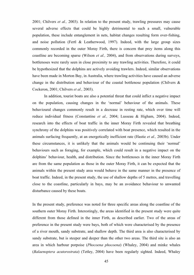
2001; Chilvers et al., 2003). In relation to the present study, trawling pressures may cause

several adverse effects that could be highly detrimental to such a small, vulnerable

population, these include entanglement in nets, habitat changes resulting form over-fishing,

and noise pollution (Fertl & Leatherwood, 1997). Indeed, with the large group sizes

commonly recorded in the outer Moray Firth, there is concern that prey items along this

coastline are becoming sparse (Wilson et al., 2004), and from observations during surveys,

bottlenoses were rarely seen in close proximity to any trawling activities. Therefore, it could

be hypothesized that the dolphins are actively avoiding trawlers. Indeed, similar observations

have been made in Morton Bay, in Australia, where trawling activities have caused an adverse

change in the distribution and behaviour of the coastal bottlenose population (Chilvers &

Cockeron, 2001; Chilvers et al., 2003).

In addition, tourist boats are also a potential threat that could inflict a negative impact

on the population, causing changes in the ‘normal’ behaviour of the animals. These

behavioural changes commonly result in a decrease in resting rate, which over time will

reduce individual fitness (Constantine et al., 2004; Lusseau & Higham, 2004). Indeed,

research into the effects of boat traffic in the inner Moray Firth revealed that breathing

synchrony of the dolphins was positively correlated with boat presence, which resulted in the

animals surfacing frequently, at an energetically inefficient rate (Hastie et al., 2003b). Under

these circumstances, it is unlikely that the animals would be continuing their ‘normal’

behaviours such as foraging, for example, which could result in a negative impact on the

dolphins’ behaviour, health, and distribution. Since the bottlenoses in the inner Moray Firth

are from the same population as those in the outer Moray Firth, it can be expected that the

animals within the present study area would behave in the same manner in the presence of

boat traffic. Indeed, in the present study, the use of shallow depths of 5 metres, and travelling

close to the coastline, particularly in bays, may be an avoidance behaviour to unwanted

disturbance caused by these boats.

In the present study, preference was noted for three specific areas along the coastline of the

southern outer Moray Firth. Interestingly, the areas identified in the present study were quite

different from those defined in the inner Firth, as described earlier. Two of the areas of

preference in the present study were bays, both of which were characterised by the presence

of a river mouth, sandy substrate, and shallow depth. The third area is also characterised by

sandy substrate, but is steeper and deeper than the other two areas. The third site is also an

area in which harbour porpoise (Phocoena phocoena) (Whaley, 2004) and minke whales

(Balaenoptera acutorostrata) (Tetley, 2004) have been regularly sighted. Indeed, Whaley

45

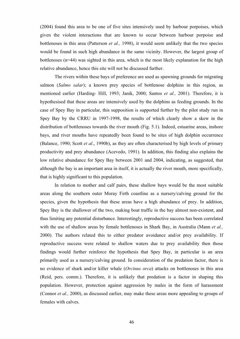
(2004) found this area to be one of five sites intensively used by harbour porpoises, which

given the violent interactions that are known to occur between harbour porpoise and

bottlenoses in this area (Patterson et al., 1998), it would seem unlikely that the two species

would be found in such high abundance in the same vicinity. However, the largest group of

bottlenoses (n=44) was sighted in this area, which is the most likely explanation for the high

relative abundance, hence this site will not be discussed further.

The rivers within these bays of preference are used as spawning grounds for migrating

salmon (Salmo salar); a known prey species of bottlenose dolphins in this region, as

mentioned earlier (Harding- Hill, 1993; Janik, 2000; Santos et al., 2001). Therefore, it is

hypothesised that these areas are intensively used by the dolphins as feeding grounds. In the

case of Spey Bay in particular, this supposition is supported further by the pilot study run in

Spey Bay by the CRRU in 1997-1998, the results of which clearly show a skew in the

distribution of bottlenoses towards the river mouth (Fig. 5.1). Indeed, estuarine areas, inshore

bays, and river mouths have repeatedly been found to be sites of high dolphin occurrence

(Balance, 1990; Scott et al., 1990b), as they are often characterised by high levels of primary

productivity and prey abundance (Acevedo, 1991). In addition, this finding also explains the

low relative abundance for Spey Bay between 2001 and 2004, indicating, as suggested, that

although the bay is an important area in itself, it is actually the river mouth, more specifically,

that is highly significant to this population.

In relation to mother and calf pairs, these shallow bays would be the most suitable

areas along the southern outer Moray Firth coastline as a nursery/calving ground for the

species, given the hypothesis that these areas have a high abundance of prey. In addition,

Spey Bay is the shallower of the two, making boat traffic in the bay almost non-existent, and

thus limiting any potential disturbance. Interestingly, reproductive success has been correlated

with the use of shallow areas by female bottlenoses in Shark Bay, in Australia (Mann et al.,

2000). The authors related this to either predator avoidance and/or prey availability. If

reproductive success were related to shallow waters due to prey availability then those

findings would further reinforce the hypothesis that Spey Bay, in particular is an area

primarily used as a nursery/calving ground. In consideration of the predation factor, there is

no evidence of shark and/or killer whale (Orcinus orca) attacks on bottlenoses in this area

(Reid, pers. comm.). Therefore, it is unlikely that predation is a factor in shaping this

population. However, protection against aggression by males in the form of harassment

(Connor et al., 2000), as discussed earlier, may make these areas more appealing to groups of

females with calves.

46

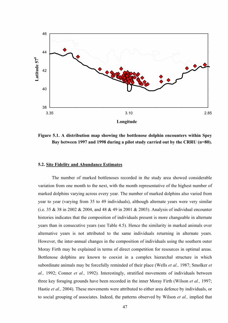
38

40

42

44

46

2.853.103.35

Lat

itude

570

Longitude

Figure 5.1. A distribution map showing the bottlenose dolphin encounters within Spey Bay between 1997 and 1998 during a pilot study carried out by the CRRU (n=80).

5.2. Site Fidelity and Abundance Estimates

The number of marked bottlenoses recorded in the study area showed considerable

variation from one month to the next, with the month representative of the highest number of

marked dolphins varying across every year. The number of marked dolphins also varied from

year to year (varying from 35 to 49 individuals), although alternate years were very similar

(i.e. 35 & 38 in 2002 & 2004, and 48 & 49 in 2001 & 2003). Analysis of individual encounter

histories indicates that the composition of individuals present is more changeable in alternate

years than in consecutive years (see Table 4.5). Hence the similarity in marked animals over

alternative years is not attributed to the same individuals returning in alternate years.

However, the inter-annual changes in the composition of individuals using the southern outer

Moray Firth may be explained in terms of direct competition for resources in optimal areas.

Bottlenose dolphins are known to coexist in a complex hierarchal structure in which

subordinate animals may be forcefully reminded of their place (Wells et al., 1987; Smolker et

al., 1992; Conner et al., 1992). Interestingly, stratified movements of individuals between

three key foraging grounds have been recorded in the inner Moray Firth (Wilson et al., 1997;

Hastie et al., 2004). These movements were attributed to either area defence by individuals, or

to social grouping of associates. Indeed, the patterns observed by Wilson et al., implied that

47

not all individuals within the population had equal access to all parts of the inner Moray Firth.

Therefore, it is highly likely that the same social factors will occur along the southern

coastline of the outer Moray Firth, where the most probable key areas with these optimum

resources are the two areas of highest relative abundance, Spey Bay and Banff Bay.

The number of captures of marked individuals ranged from 1 to 22. Further analysis of

individual capture histories revealed that 9.2% of these marked individuals demonstrated a

seasonal residence in the summer months over at least two consecutive years. These findings

indicate that a significant number of particular individuals may use the outer Moray Firth

almost exclusively across the summer months. Of these resident animals, approximately 50%

were found to be of female gender. Interestingly, every one of these females was found to be

with calf during her period of residency. In other words, 100% of resident females were

identified with a calf, which strongly supports the earlier supposition that areas along the

southern outer Moray Firth coastline must be important as nursery/calving grounds for the

species. Furthermore, the 50:50 ratio of males and females also supports the other previous

hypothesis that males will remain with groups of females, waiting for their opportunity to

mate with females entering oestrus.

As not all animals considered residents are resident over the full study period, it seems

highly likely that the aforementioned social factors play a prominent role in which individuals

use the area. In the present study the changes in composition of individuals and residents inter

annually can be termed as a ‘substitution effect’, whereby an individual that uses the area

almost exclusively in one year may be ‘substituted’, or displaced by another individual in the

subsequent year. As a result, the number of resident animals in any one year varied from 3 to

9. This may be an indication as to the quality and quantity of resources available to the

animals, i.e. if the resources in one year can support 9 resident dolphins, the area would be

expected to support 9 resident dolphins in the following year. However, the number of

residents was not constant, and given the hierarchal structure of bottlenoses it is unlikely that

animals would not use these areas if resources were plentiful. Therefore, resources such as

prey, for example, may be significantly variable between years, and hence unstable and

undependable to the dolphins. Alternatively, it may be disturbance factors such as trawlers or

tourist boats, causing the animals to move to other, more desirable areas where these

disturbance factors are reduced. Indeed, it could be a combination of these factors, and

perhaps other underlying environmental factors such as temperature and salinity, for example;

both of which have been related to changes in distribution and social structure of bottlenose

dolphin populations (Lusseau et al., 2004; Wilson, 1995).

48

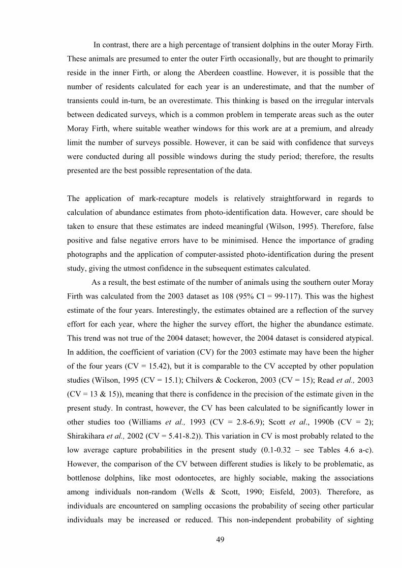
In contrast, there are a high percentage of transient dolphins in the outer Moray Firth.

These animals are presumed to enter the outer Firth occasionally, but are thought to primarily

reside in the inner Firth, or along the Aberdeen coastline. However, it is possible that the

number of residents calculated for each year is an underestimate, and that the number of

transients could in-turn, be an overestimate. This thinking is based on the irregular intervals

between dedicated surveys, which is a common problem in temperate areas such as the outer

Moray Firth, where suitable weather windows for this work are at a premium, and already

limit the number of surveys possible. However, it can be said with confidence that surveys

were conducted during all possible windows during the study period; therefore, the results

presented are the best possible representation of the data.

The application of mark-recapture models is relatively straightforward in regards to

calculation of abundance estimates from photo-identification data. However, care should be

taken to ensure that these estimates are indeed meaningful (Wilson, 1995). Therefore, false

positive and false negative errors have to be minimised. Hence the importance of grading

photographs and the application of computer-assisted photo-identification during the present

study, giving the utmost confidence in the subsequent estimates calculated.

As a result, the best estimate of the number of animals using the southern outer Moray

Firth was calculated from the 2003 dataset as 108 (95% CI = 99-117). This was the highest

estimate of the four years. Interestingly, the estimates obtained are a reflection of the survey

effort for each year, where the higher the survey effort, the higher the abundance estimate.

This trend was not true of the 2004 dataset; however, the 2004 dataset is considered atypical.

In addition, the coefficient of variation (CV) for the 2003 estimate may have been the higher

of the four years (CV = 15.42), but it is comparable to the CV accepted by other population

studies (Wilson, 1995 (CV = 15.1); Chilvers & Cockeron, 2003 (CV = 15); Read et al., 2003

(CV = 13 & 15)), meaning that there is confidence in the precision of the estimate given in the

present study. In contrast, however, the CV has been calculated to be significantly lower in

other studies too (Williams et al., 1993 (CV = 2.8-6.9); Scott et al., 1990b (CV = 2);

Shirakihara et al., 2002 (CV = 5.41-8.2)). This variation in CV is most probably related to the

low average capture probabilities in the present study (0.1-0.32 – see Tables 4.6 a-c).

However, the comparison of the CV between different studies is likely to be problematic, as

bottlenose dolphins, like most odontocetes, are highly sociable, making the associations

among individuals non-random (Wells & Scott, 1990; Eisfeld, 2003). Therefore, as

individuals are encountered on sampling occasions the probability of seeing other particular

individuals may be increased or reduced. This non-independent probability of sighting

49

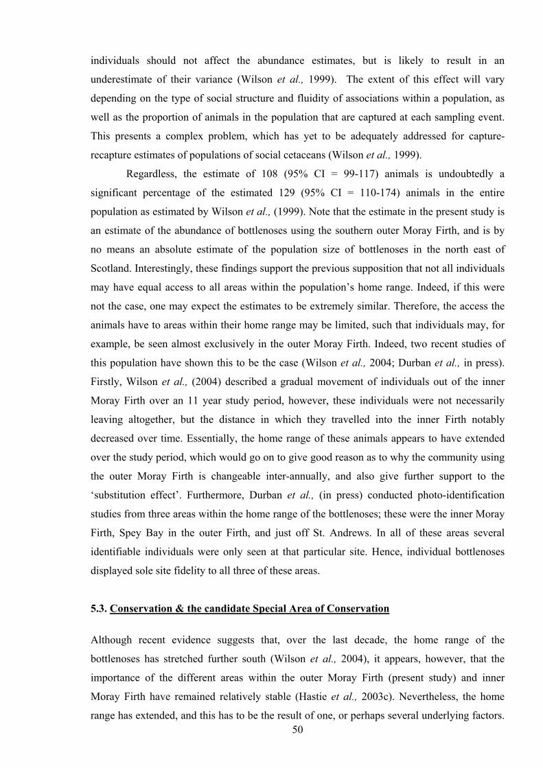
individuals should not affect the abundance estimates, but is likely to result in an

underestimate of their variance (Wilson et al., 1999). The extent of this effect will vary

depending on the type of social structure and fluidity of associations within a population, as

well as the proportion of animals in the population that are captured at each sampling event.

This presents a complex problem, which has yet to be adequately addressed for capture-

recapture estimates of populations of social cetaceans (Wilson et al., 1999).

Regardless, the estimate of 108 (95% CI = 99-117) animals is undoubtedly a

significant percentage of the estimated 129 (95% CI = 110-174) animals in the entire

population as estimated by Wilson et al., (1999). Note that the estimate in the present study is

an estimate of the abundance of bottlenoses using the southern outer Moray Firth, and is by

no means an absolute estimate of the population size of bottlenoses in the north east of

Scotland. Interestingly, these findings support the previous supposition that not all individuals

may have equal access to all areas within the population’s home range. Indeed, if this were

not the case, one may expect the estimates to be extremely similar. Therefore, the access the

animals have to areas within their home range may be limited, such that individuals may, for

example, be seen almost exclusively in the outer Moray Firth. Indeed, two recent studies of

this population have shown this to be the case (Wilson et al., 2004; Durban et al., in press).

Firstly, Wilson et al., (2004) described a gradual movement of individuals out of the inner

Moray Firth over an 11 year study period, however, these individuals were not necessarily

leaving altogether, but the distance in which they travelled into the inner Firth notably

decreased over time. Essentially, the home range of these animals appears to have extended

over the study period, which would go on to give good reason as to why the community using

the outer Moray Firth is changeable inter-annually, and also give further support to the

‘substitution effect’. Furthermore, Durban et al., (in press) conducted photo-identification

studies from three areas within the home range of the bottlenoses; these were the inner Moray

Firth, Spey Bay in the outer Firth, and just off St. Andrews. In all of these areas several

identifiable individuals were only seen at that particular site. Hence, individual bottlenoses

displayed sole site fidelity to all three of these areas.

5.3. Conservation & the candidate Special Area of Conservation

50

Although recent evidence suggests that, over the last decade, the home range of the

bottlenoses has stretched further south (Wilson et al., 2004), it appears, however, that the

importance of the different areas within the outer Moray Firth (present study) and inner

Moray Firth have remained relatively stable (Hastie et al., 2003c). Nevertheless, the home

range has extended, and this has to be the result of one, or perhaps several underlying factors.

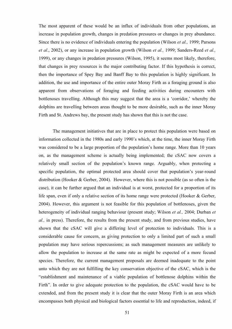
The most apparent of these would be an influx of individuals from other populations, an

increase in population growth, changes in predation pressures or changes in prey abundance.

Since there is no evidence of individuals entering the population (Wilson et al., 1999; Parsons

et al., 2002), or any increase in population growth (Wilson et al., 1999; Sanders-Reed et al.,

1999), or any changes in predation pressures (Wilson, 1995), it seems most likely, therefore,

that changes in prey resources is the major contributing factor. If this hypothesis is correct,

then the importance of Spey Bay and Banff Bay to this population is highly significant. In

addition, the use and importance of the entire outer Moray Firth as a foraging ground is also

apparent from observations of foraging and feeding activities during encounters with

bottlenoses travelling. Although this may suggest that the area is a ‘corridor,’ whereby the

dolphins are travelling between areas thought to be more desirable, such as the inner Moray

Firth and St. Andrews bay, the present study has shown that this is not the case.

The management initiatives that are in place to protect this population were based on

information collected in the 1980s and early 1990’s which, at the time, the inner Moray Firth

was considered to be a large proportion of the population’s home range. More than 10 years

on, as the management scheme is actually being implemented; the cSAC now covers a

relatively small section of the population’s known range. Arguably, when protecting a

specific population, the optimal protected area should cover that population’s year-round

distribution (Hooker & Gerber, 2004). However, where this is not possible (as so often is the

case), it can be further argued that an individual is at worst, protected for a proportion of its

life span, even if only a relative section of its home range were protected (Hooker & Gerber,

2004). However, this argument is not feasible for this population of bottlenoses, given the

heterogeneity of individual ranging behaviour (present study; Wilson et al., 2004; Durban et

al., in press). Therefore, the results from the present study, and from previous studies, have

shown that the cSAC will give a differing level of protection to individuals. This is a

considerable cause for concern, as giving protection to only a limited part of such a small

population may have serious repercussions; as such management measures are unlikely to

allow the population to increase at the same rate as might be expected of a more fecund

species. Therefore, the current management proposals are deemed inadequate to the point

unto which they are not fulfilling the key conservation objective of the cSAC, which is the

“establishment and maintenance of a viable population of bottlenose dolphins within the

Firth”. In order to give adequate protection to the population, the cSAC would have to be

extended, and from the present study it is clear that the outer Moray Firth is an area which

encompasses both physical and biological factors essential to life and reproduction, indeed, if

51

the majority of the animals do travel further south during the winter then surely those areas

must also encompass physical or biological factors essential to life and reproduction.

Therefore, a different approach to the conservation and management initiatives in place

should be considered in order to afford much needed additional protection to this vulnerable

population of bottlenose dolphins.

52

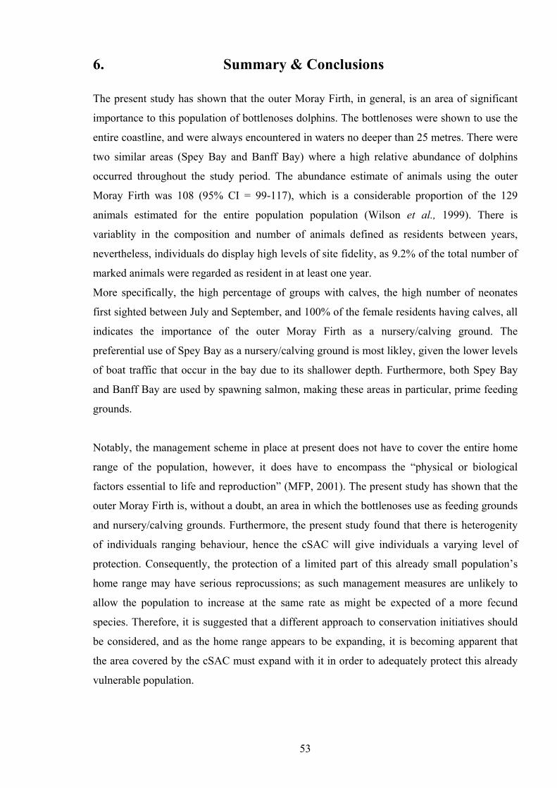
6. Summary & Conclusions

The present study has shown that the outer Moray Firth, in general, is an area of significant

importance to this population of bottlenoses dolphins. The bottlenoses were shown to use the

entire coastline, and were always encountered in waters no deeper than 25 metres. There were

two similar areas (Spey Bay and Banff Bay) where a high relative abundance of dolphins

occurred throughout the study period. The abundance estimate of animals using the outer

Moray Firth was 108 (95% CI = 99-117), which is a considerable proportion of the 129

animals estimated for the entire population population (Wilson et al., 1999). There is

variablity in the composition and number of animals defined as residents between years,

nevertheless, individuals do display high levels of site fidelity, as 9.2% of the total number of

marked animals were regarded as resident in at least one year.

More specifically, the high percentage of groups with calves, the high number of neonates

first sighted between July and September, and 100% of the female residents having calves, all

indicates the importance of the outer Moray Firth as a nursery/calving ground. The

preferential use of Spey Bay as a nursery/calving ground is most likley, given the lower levels

of boat traffic that occur in the bay due to its shallower depth. Furthermore, both Spey Bay

and Banff Bay are used by spawning salmon, making these areas in particular, prime feeding

grounds.

Notably, the management scheme in place at present does not have to cover the entire home

range of the population, however, it does have to encompass the “physical or biological

factors essential to life and reproduction” (MFP, 2001). The present study has shown that the

outer Moray Firth is, without a doubt, an area in which the bottlenoses use as feeding grounds

and nursery/calving grounds. Furthermore, the present study found that there is heterogenity

of individuals ranging behaviour, hence the cSAC will give individuals a varying level of

protection. Consequently, the protection of a limited part of this already small population’s

home range may have serious reprocussions; as such management measures are unlikely to

allow the population to increase at the same rate as might be expected of a more fecund

species. Therefore, it is suggested that a different approach to conservation initiatives should

be considered, and as the home range appears to be expanding, it is becoming apparent that

the area covered by the cSAC must expand with it in order to adequately protect this already

vulnerable population.

53

There is much known about cetacean species in the inner Moray Firth, with the initial studies

on bottlenoses now over a decade old (Hammond & Thompson, 1991), and with the number

of cetacean studies in the outer Moray Firth growing (Eisfeld, 2003; Whaley, 2004; Tetley,

2004), so is our understanding of these complex communities. However, it is evident that

greater collaberation between researchers, both in the Moray Firth and elsewhere, is required

in order to maximise the outcome of fieldwork addressing fundamental questions about the

Moray Firth population. The most beneficial colaberation would come from the merging of

photo-identification catalogues. Arguably, this is a lengthy process, with several questions

raised about possible false negative and false positive errors that may already be present in the

existing catalogues. However, the use of computer-assisted photo-identification has been

shown in the present study to reduce these erorr types. Therefore, the application of such

programs to existing catalogues previous to merging, and during merging would greatly

reduce the potential for erorrs. As mentioned earlier, this would be a lengthy process, but the

information gained on an individual’s presence or absence from an area, which potentially

encompasses the majority of its home range, would be invaluable in further understanding the

use of these areas by individuals. Indeed, the information gained would not only be on

distribution of individuals, but it would also encompass behavioural observations and

associations with other animals, thus giving researchers the potential to understand further,

the complex social ecology of these animals across their entire home range.

This study has broadened the range of environmental conditions in which the bottlenose has

been studied; therefore, the findings presented here serve to further our understanding of the

factors influencing distribution patterns and habitat use of this and other small, coastal

cetacean populations in temperate, open ocean environments. Furthermore, monitoring the

use of particular habitats that are of known importance to bottlenose dolphins, and other

cetacean communities, is essential for the successful management and conservation of a

species. It is clear that marine protected areas (MPAs) are important to small, coastal cetacean

communites, but their successful implementation requires careful consideration regarding the

underlying uses of the habitat by these communities. In conclusion, the findings of the present

study can be applied to improve the current management scheme for this, and other small,

coastal cetacean communites in other regions.

54

References

Acevedo, A. (1991). Behaviour and movement s of bottlenose dolphins, Tursiops truncatus, in the entrance to Ensenda De La Paz, Mexico. Aquatic Mammals, 17(3): 137-147.

Adams, J.A. (1987). The primary ecological sub-divisions of the North Sea: some aspects of

their plankton communities: In: Development in Fisheries Research in Scotland. (R.S. Bailey & B. B. Parish, eds.). Fishing News Books, Farnham. pp 165-181.

Adams, J.A., Martin, J.H. (1986). The hydrography and plankton of the Moray Firth. In: The

Marine Environment of the Moray Firth. (J Hawthorn, ed.). Proceedings of the Royal Society of Edinburgh,91B: 37-56.

Agler, B.A., Beard, J.L., Bowman, R.S., Corbett, H.D., Frohock, S.E., Hawvermale, M.P.,

Katona, S.K., Sadove, S.S., Seipt, I.E. (1990). Fin whale (Balaenoptera physalus) photographic identification: methodology and preliminary results from the Western North Atlantic. In: Individual Recognition of Cetaceans: Use of Photo-identification and other Techniques to Estimate Population Parameters. (P.S. Hammond, S.A. Mizroch & G.P. Donovan, eds.). Report of the International Whaling Commission Special Issue 12: pp. 349-356.

Bain, D. (1990). Examining the validity of inferences drawn from photo-identification data,

with special reference to studies of the killer whale (Orcinus orca) in British Columbia. In: Individual Recognition of Cetaceans: Use of Photo-identification and other Techniques to Estimate Population Parameters. (P.S. Hammond, S.A. Mizroch & G.P. Donovan, eds.). Report of the International Whaling Commission Special Issue 12: pp. 93-100.

Balance, L.T. (1990). Residence patterns, group organization, and surfacing associations of

bottlenose dolphins in Kino Bay, Gulf of California, Mexico. In: The Bottlenose Dolphin. (S. Leatherwood & R. R. Reeves, eds.). Academic Press, San Diego, CA. pp. 267 – 283.

Bel’kovich, V.M., Ivanova, Y., Yefremenkova, O.V., Kozarovitskiy, L.B., Kharitonov, S.P.

(1978). Description of the searching-hunting behaviour of dolphins. In: Behaviour and bioacoustics of dolphins (V.M. Bel’kovich, ed), FBIS-JPRS L/8786.

Berrow, S,. O’Brien, J. (2003). Shannon dolphin tour boat monitoring report – 2003 Shannon

Dolphin and Wildlife Foundation, Merchants Quay, Kilrush, Co. Clare. 9 pp.

55

Bristow, T., Rees, E.I.S. (2001). Site fidelity and behaviour of bottlenose dolphins (Tursiops truncatus) in Cardigan Bay, Wales. Aquatic Mammals, 27: 1-10.

Bristow, T., Glanville, N., Hopkins, J. (2001). Shore-based monitoring of bottlenose dolphins

(Tursiops truncatus) by trained volunteers in Cardigan Bay, Wales. Aquatic Mammals, 27 (2): 115-120.

Calambokidis, J. and Barlow, J. (2004). Abundance of blue and humpback whales in the

Eastern North Pacific estimated by capture-recapture and line-transect methods. Marine Mammal Science, 20 (1): 63-85.

Campbell, G.S., Bilgre, B.A., Defran, R.H. (2002) Bottlenose dolphins (Tursiops truncatus)

in Turneffe Atoll, Belize: occurrence, site fidelity, group size, and abundance. Aquatic Mammals, 28 (2): 170-180.

Carlson, C.A., Mayo, C.A., Whitehead, H. (1990). Changes in the ventral fluke pattern of

humpback whale (Megaptera novaeangliae), and its effect on matching; evaluation of its significance to photo-identification research. In: Individual Recognition of Cetaceans: Use of Photo-identification and other Techniques to Estimate Population Parameters. (P.S. Hammond, S.A. Mizroch & G.P. Donovan, eds.). Report of the International Whaling Commission Special Issue 12: pp. 105-111.

Chao, A., Lee, S.M., Jeng, S.L. (1992). Estimating population size for capture-recapture data

when capture probabilities vary by time and individual animal. Biometrics, 48: 201-216.

Chilvers, B.L., Corkeron, P.J. (2001). Trawling and bottlenose dolphins’ social structure.

Proceedings of the Royal Society London B, 268: 1901 – 1905. Chilvers, B.L., Corkeron, P.J., Puotinen, M.L. (2003). Influence of trawling on the behaviour

and spatial distribution of Indo-Pacific bottlenose dolphins (Tursiops aduncus) in Morton Bay, Australia. Canadian Journal of Zoology, 81; 1947-1955.

Chilvers, B.L., Cockeron, P.J. (2003). Abundance of Indo-Pacific bottlenose dolphins,

Tursiops aduncus, off Point Lookout, Queensland, Australia. Marine Mammal Science, 19 (1): 85-95.

Connor, R.C., Smolker, R.A. (1985). Habituated dolphins (Tursiops sp.) in western Australia.

Journal of Mammalogy, 66: 398 – 400.

56

Connor, R.C., Smolker, R.A., Richards, A.F. (1992). Two levels of alliance formation among male bottlenose dolphins (Tursiops sp.). Proceedings of the National Academy of Science, USA, 89: 987 – 990.

Connor, R.C., Wells, R.S., Mann, J., Read, A.J. (2000). The bottlenose dolphin. Social

relationships in a fission-fusion society. In: Cetacean Society. Field studies of dolphins and whales. (J. Mann, R. C. Connor, P. L. Tyack, H. Whitehead, eds.). University of Chicago Press. Chicago & London. pp. 91 – 126.

Constantine, R., Bunton, D.H., Dennis, T. (2004). Dolphin-watching tour boats change

bottlenose dolphin (Tursiops truncatus) behaviour. Biological Conservation, 117: 299-307.

Corkeron, P.J., Bryden, M.M., Hedstrom, K.E., (1990). Feeding by bottlenose dolphins in

association with trawling operations in Moreton Bay, Australia. In: The Bottlenose Dolphin. (S. Leatherwood & R. R. Reeves, eds.). Academic Press, San Diego, CA. pp. 329 – 336.

Curran, S, Wilson, B., Thompson, P.M. (1996). Recommendations for the sustainable management of the bottlenose dolphin population in the Moray Firth. Scottish Natural Heritage Review, No 56. 74 pp.

Defran, R.H., Weller, D.W. (1999). Occurrence, distribution, site fidelity, and school size of bottlenose dolphins (Tursiops truncatus) off San Diego, California. Marine Mammal Science, 15 (2); 366-380.

Dorsey, E.M., Stern, S.J., Hoelzel, A.R., Jacobsen, J. (1990). Minke whales (Balaenoptera

acutorostrata) from the west coast of North America: individual recognition and small-scale site fidelity. In: Individual Recognition of Cetaceans: Use of Photo-identification and other Techniques to Estimate Population Parameters. (P.S. Hammond, S.A. Mizroch & G.P. Donovan, eds.). Report of the International Whaling Commission Special Issue 12: pp. 357-368.

Durban, J.W., Elston, D.A., Ellifrit, D.K., Dickson, E., Hammond, P.S., Thompson, P.M. In

Press. Multi-state mark-recapture for cetaceans: population estimates with Bayesian model averaging. Marine Mammal Science.

Eisfeld, S.M. (2003). The social affiliation and group composition of bottlenose dolphins

(Tursiops truncatus) in the outer Moray Firth, NE Scotland. MSc. Thesis. University of Wales, Bangor. 84 pp.

57

Eisfeld, S.M., Robinson, K.P. (in press). The sociality of bottlenose dolphins in the outer southern Moray Firth, NE Scotland: Implications for current management proposals? European Research on Cetaceans, 17.

Evans, W.E., Hall, J.D., Irvine, A.B., Leatherwood, J.S. (1972). Methods for tagging small

cetaceans. Fisheries Bulletin, 70 (1): 61-65. Evans, D. (1987). Dolphins as beaters for gulls. Bird Behaviour, 7: 47 – 48. Evans, P.G.H. (1996). Whales, Dolphins and Porpoises. Chapter 5.15. pp. 131-134. In: Coasts

and Seas of the United Kingdom, Region 3. North-east Scotland: Cape Wrath to St. Cyrus. (J.H. Barnesm C.F. Robson, S.S. Kaznowska & J.P Doody, eds.). Joint Nature Conservation Committee, Peterborough. 219 pp.

Fertl, D., Leatherwood, S. (1997). Cetacean interaction with trawls: a preliminary review.

Journal of the Northwest Atlantic Fisheries Science, 22: 219 – 248. Gannon, D.P., Waples, D.M. (2004). Diets of coastal bottlenose dolphins from the U.S. Mid-

Atlantic coast differ by habitat. Marine Mammal Science, 20(3): 527-545. Grellier, K., Wilson, B. (2003). Bottlenose dolphins using the Sound of Barra, Scotland.

Aquatic Mammals, 29: 378-382. Gowans, S., Whitehead, H. (2001). Photographic identification of northern bottlenose whales

(Hyperdoon ampullatus): sources of heterogeneity from natural marks. Marine Mammal Science, 17 (1): 76-93.

Gunnlaugsson, T., Sigurjónsson, J. (1990). A note on the problem of false positives in the use

of natural marking data and abundance estimation. In: Individual Recognition of Cetaceans: Use of Photo-identification and other Techniques to Estimate Population Parameters. (P.S. Hammond, S.A. Mizroch & G.P. Donovan, eds.). Report of the International Whaling Commission Special Issue 12: pp. 143-145.

Hammond, P.S., Thompson, P.M. (1991). Minimum estimate of the number of bottlenose

dolphins Tursiops truncatus in the Moray Firth, NE Scotland. Biological Conservation, 56: 79-87.

Harding-Hill, R. (1993). The Moray Firth Review. Scottish National Heritage, north-west

region, Scotland. 257 pp.

58

Hastie, G.D., Wilson, B., Thompson, P.M. (2003a). Fine-scale selection by coastal bottlenose dolphins: application of a new land-based video-montage technique. Canadian Journal of Zoology, 81: 469-478.

Hastie, G.D., Wilson, B., Tufft, L.H., Thompson, P.M. (2003b). Bottlenose dolphins increase

breathing synchrony in response to boat traffic. Marine Mammal Science, 19 (1): 74-84.

Hastie, G.D., Barton, T.R., Grellier, K., Hammond, P.S., Swift, R.J., Thompson, P.M.,

Wilson, B. (2003c). Distribution of small cetaceans within a candidate Special Area of Conservation; implications for management. Journal of Cetacean Research and Management, 5(3): 261-266.

Hastie, G.D., Wilson, B., Parsons, K.M., Thompson, P.M. (2004). Functional mechanisms

underlying cetacean distribution patterns: hotspots for bottlenose dolphins are linked to foraging. Marine Biology, 144: 397-403.

Hersh, S.L., Duffield, D.A. (1990). Distinctive between Northwest Atlantic offshore and

coastal bottlenose dolphins based on haemoglobin profile and morphometry. In: The Bottlenose Dolphin. (S. Leatherwood & R.R. Reeves, eds.). Academic Press, San Diego. pp. 129-139.

Hershkovitz, P. (1966). Catalog of living whales. US National Museum Bulletin, 246.

Smithsonian Institute, Washington, D.C. Hobbs. L. (1982). Tags on Whales, Dolphins, and Porpoises. Appendix A. In: Whales,

Dolphins, and Porpoises of the Eastern North Pacific and Adjacent Arctic Waters. (S. Leatherwood, R.R. Reeves, W.F. Perrin & W.E. Evans, eds.). Academic Press, San Diego, CA. pp 218-230.

Hoese, H. D. (1971). Dolphin feeding out of water in a salt marsh. Journal of Mammalogy, 52

(1): 222 – 223. Hogan, T. (1975). Movements and behaviour of the bottlenose dolphin in the Savannah River

mouth area. Unpublished manuscript, University of Rhode Island, Kingston, RI, 42 pp.

Hohn, A.A., Scott, M.D., Wells, R.S., Sweeney, J.C., Irvine., A.B. (1989). Growth layers in

teeth from known-age, free-ranging bottlenose dolphins. Marine Mammal Science, 5 (4): 315-342.

59

Hooker, S.K., Whitehead, H., Gowans, S., Baird, R.W. (2002). Fluctuations in distributions and patterns of individual range use of northern bottlenose whales. Marine Ecology Progress Series, 225: 287-297.

Hooker, S.K., Gerber, L.H. (2004). Marine reserves as a tool for ecosystem-based

management: the potential importance of megafauna. BioScience, 54(1): 27-39. Ingram, S.N., Rogan, E. (2002). Identifying critical areas and habitat preferences of

bottlenose dolphins (Tursiops truncatus). Marine Ecology Progress Series, 244: 247-255.

International Whaling Commission (IWC). (2001). Annex U. Report of the working group of

nomenclature. Journal of Cetacean Research and Management, 3 (Suppl.): 363-365. Irvine, A.B., Wells, R.S., Scott, M.D. (1982). An evaluation of techniques for tagging small

odontocete cetaceans. Fisheries Bulletin, 80 (1): 135-143. Irwin, L., Würsig, B. (2004). A small resident community of bottlenose dolphins, Tursiops

truncatus, in Texas: Monitoring recommendations. Gulf of Mexico Science, 1: 13-21. Janik, V.M. (2000). Food-related bray calls in wild bottlenose dolphins (Tursiops truncatus).

Proceedings of the Royal Society of London, 267: 923-927. JNCC. (1999). Coastal Directories Electronic Platform (phase 1) Version 1. Joint Nature

Conservation Committee. Jones, M.L. (1990). The reproductive cycle in gray whales based on photographic resightings

of females on the breeding grounds from 1977-1982. In: Individual Recognition of Cetaceans: Use of Photo-identification and other Techniques to Estimate Population Parameters. (P.S. Hammond, S.A. Mizroch & G.P. Donovan, eds.). Report of the International Whaling Commission Special Issue 12: pp. 177-182.

Kaufman, G.D., Osmond, M.G., Ward, A.J., Forestell, P.H. (1990). Photographic

documentation of the migratory movement of a Humpback Whale (Megaptera novaeangliae) between East Australia and Antarctic Area V. In: Individual Recognition of Cetaceans: Use of Photo-identification and other Techniques to Estimate Population Parameters. (P.S. Hammond, S.A. Mizroch & G.P. Donovan, eds.). Report of the International Whaling Commission Special Issue 12: pp. 265-268.

60

Kenny, R.D. (1990). Bottlenose dolphins off the north-eastern United States. In: The Bottlenose Dolphin. (S. Leatherwood & R.R. Reeves, eds.). Academic Press, San Diego, CA. pp. 369-386.

Kogi, K., Hishii, T., Imamura, A., Iwatani, T., Dudzinski, K.M. (2004). Demographic

parameters of Indo-Pacific bottlenose dolphins (Tursiops aduncus) around Mikura Island, Japan. Marine Mammal Science, 20 (3): 510-526.

Lockyer, C.H., Morris, R.J. (1986). The history and behaviour of a wild, sociable dolphin

(Tursiops truncatus) off the north coast of Cornwall. Aquatic Mammals, 12: 3-12. Lusseau, D., Higham, J.E.S. (2004). Managing the impacts of dolphin-based tourism

throughout the definition of critical habitats: the case of bottlenose dolphins (Tursiops spp). In Doubtful Sound, New Zealand. Tourism Management, 25: 657-667.

Lusseau, D., Williams, R., Wilson, B., Grellier, K., Barton, T.R., Hammond, P.S., Thompson,

P.M. (2004). Parallel influence of climate on behaviour of Pacific killer whales and Atlantic bottlenose dolphins. Ecology Letters, 7: 1-9.

Mann, J., Connor, R.C., Barre, L.M., Heithaus, M.R. (2000). Female reproductive success in

bottlenose dolphins (Tursiops sp.): life history, habitat, provisioning, and group size effects. Behavioural Ecology, 11 (2): 210-219.

Maze, K.S., Würsig, B. (1999). Bottlenose dolphins of San Luis Pass, Texas: Occurrence

patterns, site-fidelity, and habitat use. Aquatic Mammals, 25 (2): 91-103. Moray Firth Partnership (2001). The Moray Firth candidate Special Area of Conservation

Management Scheme. 89 pp. Moray Firth Partnership. (2003). The Moray Firth candidate Special Area of Conservation

Management Scheme, Revision 1. 120 pp. Mullin, K.D., Hoggard, W., Hansen, L.J. (2004). Abundance and seasonal occurrence of

cetaceans in Outer Continental Shelf and slope waters of the North-Central and Northwestern Gulf of Mexico. Gulf of Mexico Science, 1: 62-73.

Natoli, A., Peddemors, V.M., Hoelzel, A.R. (2003). Population structure and speciation in the

genus Tursiops based on microsatellite and mitochondrial DNA analyses. Journal of Evolutionary Biology, 17: 363-375.

61

Norris, K. S., Dohl, T. P. (1980). The structure and function of cetacean schools. In: Cetacean Behavior: Mechanisms and Functions. 2nd ed. (L. M. Herman, ed.). Robert E. Krieger Publishing Company, Malabar, Florida. pp. 211 – 262.

Parsons, K.M., Noble, L.R., Reid, R.J., Thompson, P.M. (2002). Mitochondrial genetic

diversity and population structuring of UK bottlenose dolphins (Tursiops truncatus): is the NE Scotland population demographically and geographically isolated? Biological Conservation, 108: 175-182.

Patterson, I. A. P., Reid, R. J., Wilson, B., Grellier, K., Ross, H. M., Thompson, P. M. (1998).

Evidence for infanticide in bottlenose dolphins: an explanation for violent interactions with harbour porpoise? Proceedings of the Royal Society London B, 265: 1167 – 1170.

Read, A.J., Urian, K.W., Wilson, B., Waples, D.M. (2003). Abundance of bottlenose dolphins

in the bays, sounds, and estuaries of North Carolina. Marine Mammal Science, 19 (1): 59-73.

Reid, G., McManus, J. (1987). Sediment exchanges along the coastal margin of the Moray

Firth, eastern Scotland. Journal of the Geological Society London (A), 144: 179-185.

Rice, D.W. (1998). Marine Mammals of the World. Systematics and Distribution. Special Publication No.4. The Society for Marine Mammalogy.

Rogan, E., Ingram, S., Holmes, B., O’Flanagan, C. (2000). A survey of bottlenose dolphins (Tursiops truncatus) in the Shannon estuary. 49 pp.

Ross, G.J.B. (1977). The taxonomy of bottlenosed dolphins Tursiops species in South African

waters, with notes on their biology. Annals of the Cape Provincial Museums (Natural History), 11: 135-194.

Ross, G.J.B., Cockcroft, V.G. (1990). Comments on Australian bottlenose dolphins and the

taxonomic status of Tursiops aduncus (Ehrenberg, 1832). In: The Bottlenose Dolphin. (S. Leatherwood & R.R. Reeves, eds.). Academic Press, San Diego. Pp. 101-128.

Sanders-Reed, C.A., Hammond, P.S., Grellier, K., Thompson, P.M. (1999). Development of a

population model for bottlenose dolphins. SNH Research, Survey and Monitoring Report, No. 56.

62

Santos, M.B., Pierce, G.J., Reid, R.J., Patterson, I.A.P., Ross, H.M., Mente, E. (2001). Stomach contents of bottlenose dolphins (Tursiops truncatus) in Scottish waters. Journal of the Marine Biological Association of the United Kingdom 81: 873-878.

Scott, M.D., Wells, R.S., Irvine, A.B., Mate, B.R. (1990a). Tagging and marking studies on

small cetaceans. In: The Bottlenose Dolphin. (S. Leatherwood & R.R Reeves, eds.). Academic Press, San Diego, CA. pp. 489-514.

Scott, M.D., Wells, R.S., Irvine, A.B. (1990b). A long-term study of bottlenose dophins on

the West coast of Florida. In: The Bottlenose Dolphin. (S. Leatherwood & R.R Reeves, eds.). Academic Press, San Diego, CA. pp. 235-244.

Scottish Natural Heritage. (1993). Dolphin Awareness: Dolphins, Porpoises and Whales of

the Moray Firth. SNH publication. ISBN: 1 85397 091. 70 pp. Sears, R.J., Wiliamson, M., Wenzel, F.W., Bérubé, M., Gendron, D., Jones, P. (1990).

Photographic identification of the blue whale (Balaenoptera musculus) in the Gulf of St. Lawrence, Canada. In: Individual Recognition of Cetaceans: Use of Photo-identification and other Techniques to Estimate Population Parameters. (P.S. Hammond, S.A. Mizroch & G.P. Donovan, eds.). Report of the International Whaling Commission Special Issue 12: pp. 105-111.

Shane, S.H. (1980). Occurrence, movements, and distribution of bottlenose dolphins,

Tursiops truncatus, in southern Texas. Fishery Bulletin (U.S.), 78: 593-601. Shane, S.H. (1990). Behaviour and ecology of the bottlenose dolphin at Sanibel Island,

Florida. In: The Bottlenose Dolphin. (S. Leatherwood & R.R. Reeves, eds.). Academic Press, San Diego, CA. pp. 245-265.

Shirakihara, M., Shirakihara, K., Tomonaga, J., Takatsuki, M. (2002). A resident population

of Indo-Pacific bottlenose dolphins (Tursiops aduncus) in Amakusa, Western Kyushu, Japan. Marine Mammal Science, 18 (1): 30-41.

Silvia, V.M.F., Martin, A.R. (2000). A study of the boto, or Amazon River dolphin (Inia

geoffrensis), in the Mamiraua reserve, Brazil, operation and techniques. Biology and Conservation of Freshwater Cetaceans in Asia, 23: 121-131.

Similä, T., Ugarte, F. (1993). Surface and underwater observations of cooperatively feeding

killer whales in northern Norway. Canadian Journal of Zoology, 71: 2311 – 2318.

63

Smolker, R.A., Richards, A.F., Connor, R.C., Pepper, J.W. (1992). Sex differences in patterns of associations among Indian Ocean bottlenose dolphins. Behaviour, 123: 38 – 69.

Stevick, P.T., Palsbøll, P.J., Smith, T.D., Bravington, M.V., Hammond, P.S. (2001). Errors in

identification using natural markings: rates, sources, and effects on capture-recapture estimates of abundance. Canadian Journal of Fisheries and Aquaculture Science, 58: 1861-1870.

Tayler, C.K., Saayman, G.S. (1972). A method for determining the composition, development

and stability of groups of free-ranging dolphins. Zeitschrift für Säugetierkunde, 37: 116 – 119.

Tetley, M.J. (2004). The Distribution and Habitat Preference of the North Atlantic Minke

Whale (Balaenoptera acutorostrata acutorostrata) in the Southern Outer Moray Firth, NE Scotland. MSc Thesis, University of Wales Bangor. 111 pp.

Walker, W.A. (1981). Geographical variation in morphology and biology of bottlenose

dolphins (Tursiops) in the eastern North Pacific. NOAA, US Department of Commerce, Administrative Report LJ-81-03C. NMFS, Southwest Fisheries Center, La Jolla, California. 21 pp.

Waerebeek, K.V., Reyes, J.C., Read, A.J., McKinnin, J.S. (1990). Preliminary observations of

bottlenose dolphins from the Pacific coast of South America. In: The Bottlenose Dolphin. (S. Leatherwood & R.R. Reeves, eds.). Academic Press, San Diego. pp. 143-154.

Wang, J.Y., Chou, L.S., White, B.N. (1999). Mitochondrial DNA analysis of sympatric

morphotypes of bottlenose dolphins (genus: Tursiops) in Chinese waters. Molecular Ecology, 8: 1603-1612.

Weigle, B. (1990). Abundance, distribution and movements of bottlenose dolphins (Tursiops

truncatus) in Lower Tampa Bay, Florida. In: Individual Recognition of Cetaceans: Use of Photo-identification and other Techniques to Estimate Population Parameters. (P. S. Hammond, S. A. Mizroch, G. P. Donovan, eds.). Report of the International Whaling Commission, Special Issue 12. pp. 195 – 201.

Weir, C.R., Stockin, K.A. (2001). The occurrence and distribution of bottlenose dolphin

(Tursiops truncatus) and other cetacean species in the coastal waters of Aberdeenshire, Scotland. Report of the Sea Watch Foundation, Oxford. 68 pp.

64

Wells, R. S., Scott, M. D., Irvine, A. B. (1987). The social structure of free-ranging bottlenose dolphins. In: Current Mammalogy Vol. 1. (H. H. Genoways, ed.). Plenum Press, New York. pp. 247 – 305.

Wells, R.S., Scott, M.D. (1990). Estimating bottlenose dolphin population parameters from

individual identification and capture-release techniques. In: Individual Recognition of Cetaceans: Use of Photo-identification and other Techniques to Estimate Population Parameters. (P.S. Hammond, S.A. Mizroch & G.P. Donovan, eds.). Report of the International Whaling Commission Special Issue 12: pp. 407-415.

Wells, R.S., Scott, M.D. (2002). Bottlenose dolphins Tursiops truncatus and T. aduncus. In:

Encyclopedia of Marine Mammals (W.F. Perrin, B. Würsig & J.G.M. Thewissen, eds.). Academic Press. San Diego – Tokyo. pp. 122-128.

Whaley, A. (2004) The distribution and relative abundance of harbour porpoises (Phocoena

phocoena) in the outer southern Moray Firth. B.Sc. Dissertation. University of London.

White, M. J., Jr., Jennings, J.G., Gandy, W.F., Cornell, L.H. (1981). An evaluation of tagging,

marking, and tattooing techniques for small delphinids. NOAA Technical Memorandum, NOAA-TM-NMFS-SWFC-16. 142 pp.

Whitehead, H. (1990). Assessing sperm whale populations using natural markings: recent

progress. In: Individual Recognition of Cetaceans: Use of Photo-identification and other Techniques to Estimate Population Parameters. (P.S. Hammond, S.A. Mizroch & G.P. Donovan, eds.). Report of the International Whaling Commission Special Issue 12: pp. 377-382.

Whitehead, H., Christal, J., Tyack, P.L. (2000). Studying cetacean social structure in space

and time. In: Field Studies of Dolphins and Whales. (J. Mann, R.C. Connor, P.L. Tyack & H. Whitehead, eds.). Cetacean Societies. The University of Chicago Press. Chicago & London. pp. 65-87.

Willams, J.A., Dawson, S.M., Slooten, E. (1993). The abundance and distribution of

bottlenose dolphins (Tursiops truncatus) in Doubtful Sound, New Zealand. Canadian Journal of Zoology, 71: 2080-2088.

Wilson, B. (1995). The ecology of the bottlenose dolphins in the Moray Firth, Scotland: a

population at the northern extreme of the species’ range. PhD thesis, University of Aberdeen. 201 pp.

65

Wilson, B., Thompson, P.M., Hammond, P.S. (1997). Habitat use by bottlenose dolphins: seasonal distribution and stratified movement patterns in the Moray Firth, Scotland. Journal of Applied Ecology, 34: 1365-1374.

Wilson, B., Hammond, P.S., Thompson, P.M. (1999). Estimating size and assessing trends in

a coastal bottlenose dolphin population. Ecological Applications, 9: 288-300. Wilson, B., Grellier, K., Hammond, P.S., Brown, G., Thompson, P.M. (2000). Changing

occurrence of epidermal lesions in wild bottlenose dolphins. Marine Ecology Progress Series, 205: 283-290.

Wilson, B., Reid, R.J., Grellier, K., Thompson, P.M., Hammond, P.S. (2004). Considering the

temporal when managing the spatial: a population range expansion impacts protected areas-based management for bottlenose dolphins. Animal Conservation, 7: 1-8.

Wood, C.J. (1998). Movements of bottlenose dolphins around the south-west coast of Britain.

Journal of Zoology 246, (2): 155-164. Würsig, B., Würsig, M. (1977). The photographic determination of group size, composition

and stability of coastal porpoises (Tursiops truncatus). Science, 198: 755-756. Würsig, B. (1978). Occurrence and group organisation of Atlantic bottlenose porpoise

(Tursiops truncatus) in an Argentine bay. Biology Bulletin, 154: 348 – 359. Würsig, B., Harris, G. (1990). Site and association fidelity in bottlenose dolphins off

Argentina. In: The Bottlenose Dolphin. (S. Leatherwood & R. R. Reeves, eds.). Academic Press, San Diego, CA. pp. 361 – 365.

Würsig, B., Jefferson, T.A. (1990). Methods of photo-identification for small cetaceans. In:

Individual Recognition of Cetaceans: Use of Photo-identification and other Techniques to Estimate Population Parameters. (P.S. Hammond, S.A. Mizroch & G.P. Donovan, eds.). Report of the International Whaling Commission Special Issue 12: pp. 43-50.

Zoolman, E.S. (2002). Residence patterns of bottlenose dolphins (Tursiops truncatus) in the

Stono River Estuary, Charleston County, South Carolina, U.S.A. Marine Mammal Science, 18 (4): 879-892.

66

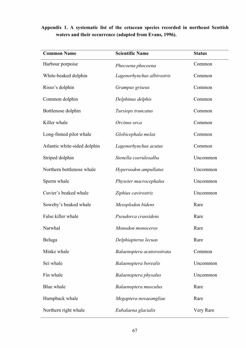
Appendix 1. A systematic list of the cetacean species recorded in northeast Scottish waters and their occurrence (adapted from Evans, 1996).

Common Name Scientific Name Status

Harbour porpoise Phocoena phocoena Common

White-beaked dolphin Lagenorhynchus albirostris Common

Risso’s dolphin Grampus griseus Common

Common dolphin Delphinus delphis Common

Bottlenose dolphin Tursiops truncatus Common

Killer whale Orcinus orca Common

Long-finned pilot whale Globicephala melas Common

Atlantic white-sided dolphin Lagenorhynchus acutus Common

Striped dolphin Stenella coeruleoalba Uncommon

Northern bottlenose whale Hyperoodon ampullatus Uncommon

Sperm whale Physeter macrocephalus Uncommon

Cuvier’s beaked whale Ziphius cavirostris Uncommon

Soweby’s beaked whale Mesoplodon bidens Rare

False killer whale Pseudorca crassidens Rare

Narwhal Monodon monoceros Rare

Beluga Delphiapterus lecuas Rare

Minke whale Balaenoptera acutorostrata Common

Sei whale Balaenoptera borealis Uncommon

Fin whale Balaenoptera physalus Uncommon

Blue whale Balaenoptera musculus Rare

Humpback whale Megaptera novaeangliae Rare

Northern right whale Eubalaena glacialis Very Rare

67

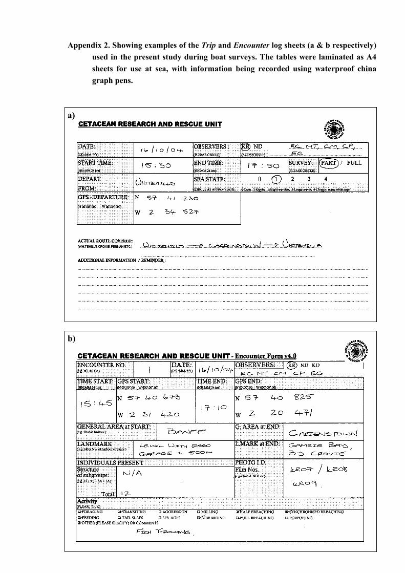
68

b)

Appendix 2. Showing examples of the Trip and Encounter log sheets (a & b respectively) used in the present study during boat surveys. The tables were laminated as A4 sheets for use at sea, with information being recorded using waterproof china graph pens.

a)

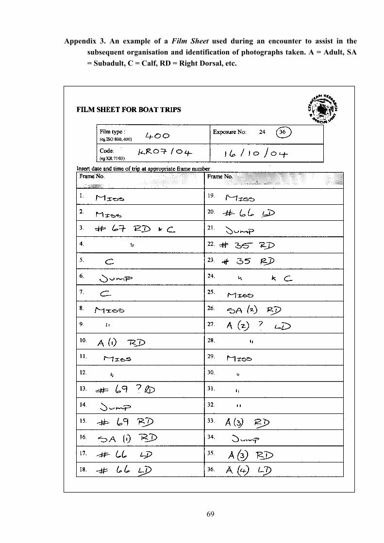
Appendix 3. An example of a Film Sheet used during an encounter to assist in the subsequent organisation and identification of photographs taken. A = Adult, SA = Subadult, C = Calf, RD = Right Dorsal, etc.

69

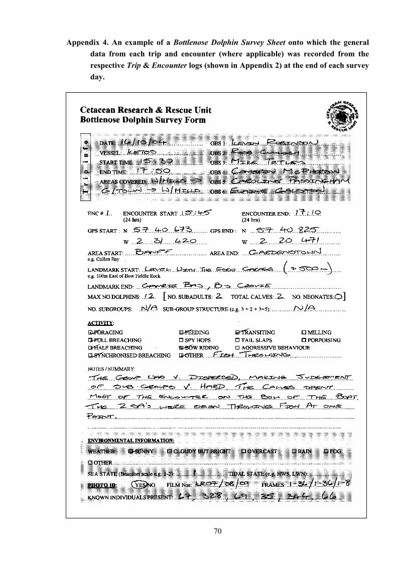
Appendix 4. An example of a Bottlenose Dolphin Survey Sheet onto which the general data from each trip and encounter (where applicable) was recorded from the respective Trip & Encounter logs (shown in Appendix 2) at the end of each survey day.

70

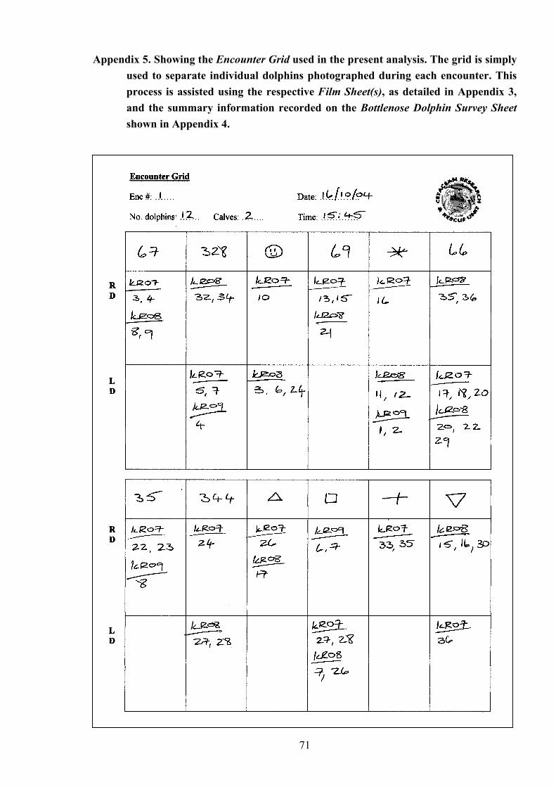
Appendix 5. Showing the Encounter Grid used in the present analysis. The grid is simply used to separate individual dolphins photographed during each encounter. This process is assisted using the respective Film Sheet(s), as detailed in Appendix 3, and the summary information recorded on the Bottlenose Dolphin Survey Sheet shown in Appendix 4.

71

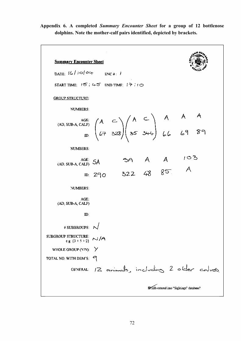
Appendix 6. A completed Summary Encounter Sheet for a group of 12 bottlenose dolphins. Note the mother-calf pairs identified, depicted by brackets.

72

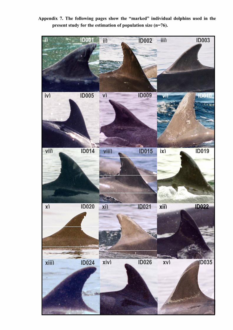
Appendix 7. The following pages show the “marked” individual dolphins used in the

present study for the estimation of population size (n=76).

73

i) ID001 iii) ID003 ii) ID002

v) ID009 iv) ID005 vi) ID010 vii) ID014 ix) ID019 viii) ID015 x) ID020 xi) ID021 xii) ID022

xiv) ID026 xv) ID035 xiii) ID024

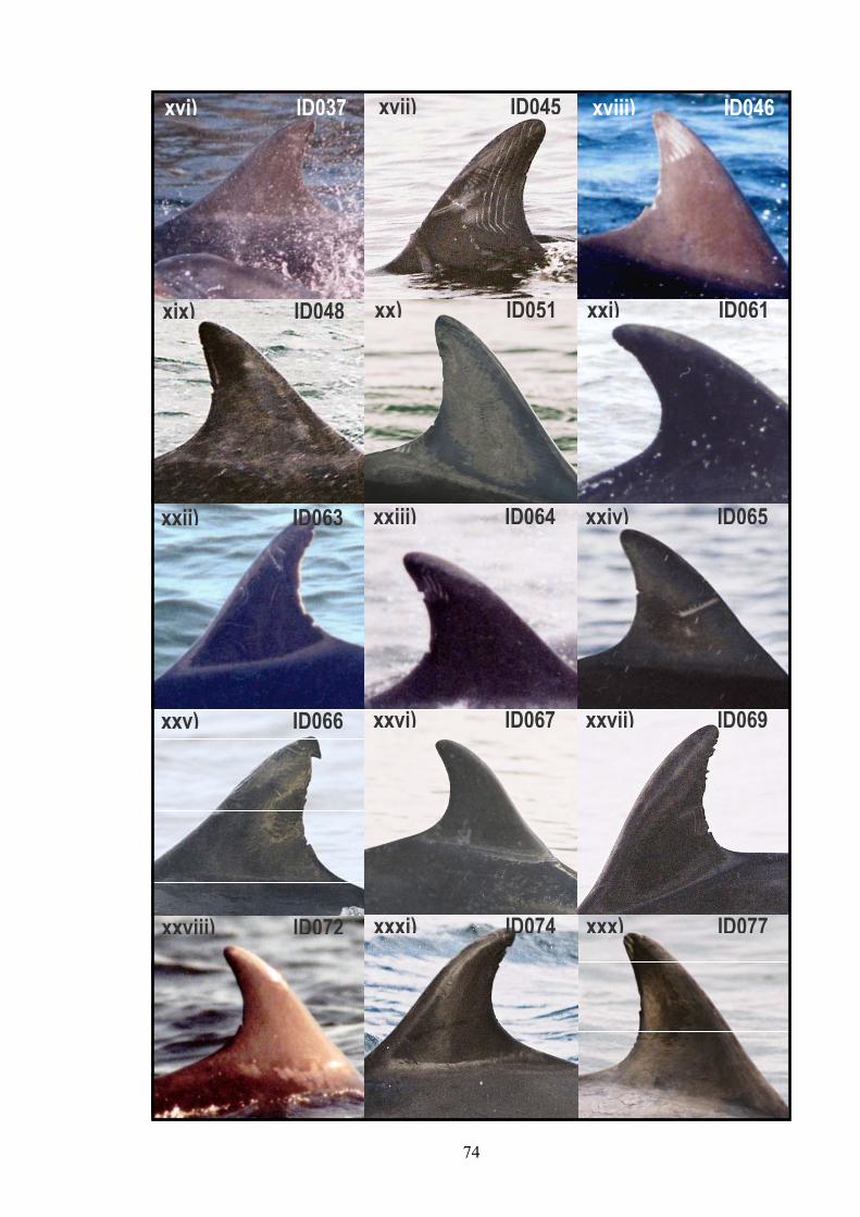
xxxi) ID074 xxx) ID077 xxviii) ID072

xxvi) ID067 xxvii) ID069 xxv) ID066

xvii) ID045 xviii) ID046 xvi) ID037

xxiii) ID064 xxiv) ID065 xxii) ID063

xx) ID051 xxi) ID061 xix) ID048

74

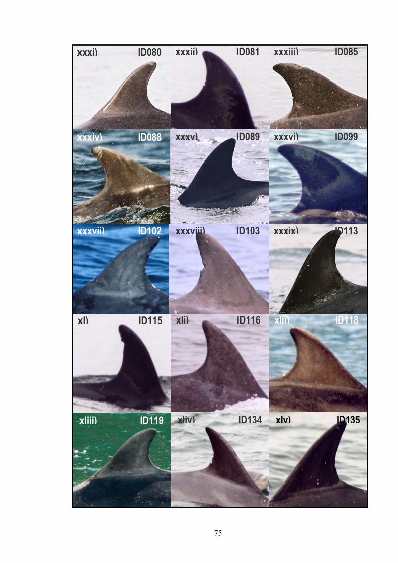
xxxi) ID080 xxxiii) ID085 xxxii) ID081

xxxiv) ID088 xxxvi) ID099 xxxv) ID089

xxxvii) ID102 xxxix) ID113 xxxviii) ID103

xl) ID115 xlii) ID118 xli) ID116

xliii) ID119 xlv) ID135 xliv) ID134

75

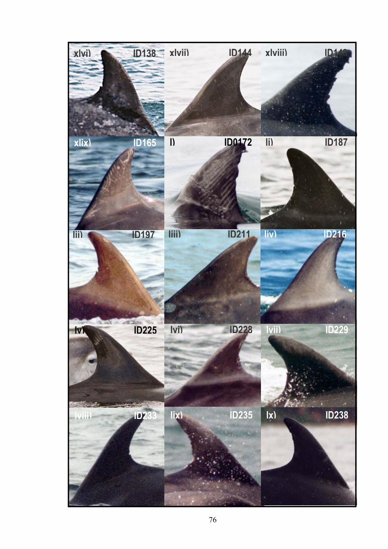
xlvi) ID138 xlviii) ID149 xlvii) ID144

xlix) ID165 li) ID187 l) ID0172

lii) ID197 liv) ID216 liii) ID211

lv) ID225 lvii) ID229 lvi) ID228

lviii) ID233 lx) ID238 lix) ID235

76

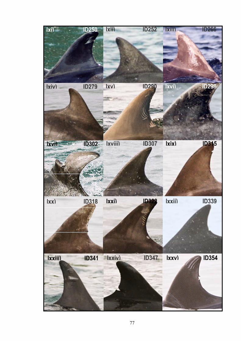
lxi) ID250 lxiii) ID266 lxii) ID252

lxiv) ID279 lxvi) ID298 lxv) ID290

l

l

l

xvi) ID302 lxix) ID315 lxviii) ID307

xx) ID318 lxxii) ID339 lxxi) ID322

xxiii) ID341 lxxv) ID354 lxxiv) ID347

77

lxxvi) ID362

78

Appendix 8. Table showing encounter histories for the 7 resident dolphins encountered during 3 or more of the 5 months (May to September inclusive) for at least two consecutive years of the study period, 2001 to 2004 inclusive.

79

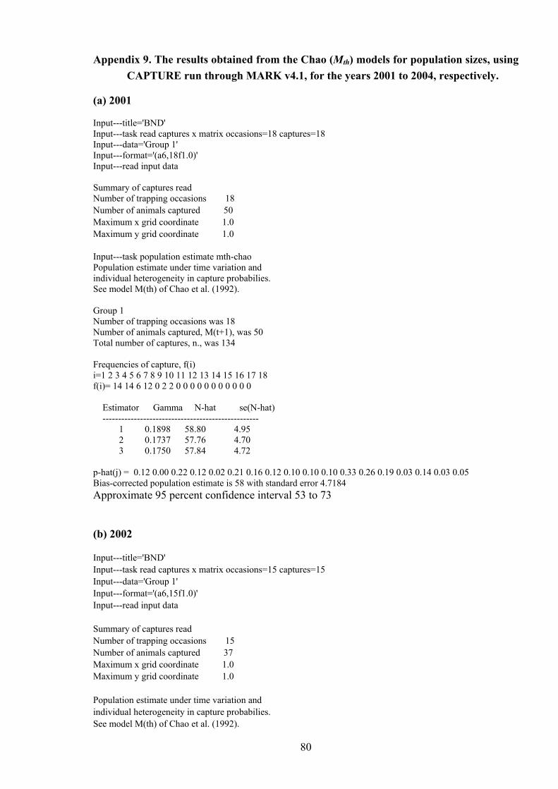
Appendix 9. The results obtained from the Chao (Mth) models for population sizes, using CAPTURE run through MARK v4.1, for the years 2001 to 2004, respectively.

(a) 2001 Input---title='BND' Input---task read captures x matrix occasions=18 captures=18 Input---data='Group 1' Input---format='(a6,18f1.0)' Input---read input data Summary of captures read Number of trapping occasions 18 Number of animals captured 50 Maximum x grid coordinate 1.0 Maximum y grid coordinate 1.0 Input---task population estimate mth-chao Population estimate under time variation and individual heterogeneity in capture probabilies. See model M(th) of Chao et al. (1992). Group 1 Number of trapping occasions was 18 Number of animals captured, M(t+1), was 50 Total number of captures, n., was 134 Frequencies of capture, f(i) i=1 2 3 4 5 6 7 8 9 10 11 12 13 14 15 16 17 18 f(i)= 14 14 6 12 0 2 2 0 0 0 0 0 0 0 0 0 0 0 Estimator Gamma N-hat se(N-hat) -------------------------------------------------- 1 0.1898 58.80 4.95 2 0.1737 57.76 4.70 3 0.1750 57.84 4.72 p-hat(j) = 0.12 0.00 0.22 0.12 0.02 0.21 0.16 0.12 0.10 0.10 0.10 0.33 0.26 0.19 0.03 0.14 0.03 0.05 Bias-corrected population estimate is 58 with standard error 4.7184 Approximate 95 percent confidence interval 53 to 73

(b) 2002 Input---title='BND' Input---task read captures x matrix occasions=15 captures=15 Input---data='Group 1' Input---format='(a6,15f1.0)' Input---read input data Summary of captures read Number of trapping occasions 15 Number of animals captured 37 Maximum x grid coordinate 1.0 Maximum y grid coordinate 1.0 Population estimate under time variation and individual heterogeneity in capture probabilies. See model M(th) of Chao et al. (1992).

80

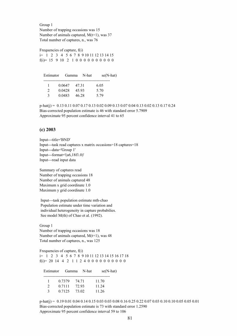
Group 1 Number of trapping occasions was 15 Number of animals captured, M(t+1), was 37 Total number of captures, n., was 76 Frequencies of capture, f(i) i= 1 2 3 4 5 6 7 8 9 10 11 12 13 14 15 f(i)= 15 9 10 2 1 0 0 0 0 0 0 0 0 0 0 Estimator Gamma N-hat se(N-hat) -------------------------------------------------- 1 0.0647 47.31 6.05 2 0.0428 45.93 5.70 3 0.0483 46.28 5.79 p-hat(j) = 0.13 0.11 0.07 0.17 0.13 0.02 0.09 0.13 0.07 0.04 0.13 0.02 0.13 0.17 0.24 Bias-corrected population estimate is 46 with standard error 5.7909 Approximate 95 percent confidence interval 41 to 65

(c) 2003 Input---title='BND' Input---task read captures x matrix occasions=18 captures=18 Input---data='Group 1' Input---format='(a6,18f1.0)' Input---read input data Summary of captures read Number of trapping occasions 18 Number of animals captured 48 Maximum x grid coordinate 1.0 Maximum y grid coordinate 1.0 Input---task population estimate mth-chao Population estimate under time variation and individual heterogeneity in capture probabilies. See model M(th) of Chao et al. (1992). Group 1 Number of trapping occasions was 18 Number of animals captured, M(t+1), was 48 Total number of captures, n., was 125 Frequencies of capture, f(i) i= 1 2 3 4 5 6 7 8 9 10 11 12 13 14 15 16 17 18 f(i)= 20 14 4 2 1 1 2 4 0 0 0 0 0 0 0 0 0 0 Estimator Gamma N-hat se(N-hat) -------------------------------------------------- 1 0.7379 74.71 11.70 2 0.7111 72.93 11.24 3 0.7125 73.02 11.26 p-hat(j) = 0.19 0.01 0.04 0.14 0.15 0.03 0.03 0.08 0.16 0.25 0.22 0.07 0.03 0.10 0.10 0.05 0.05 0.01 Bias-corrected population estimate is 73 with standard error 1.2590 Approximate 95 percent confidence interval 59 to 106

81

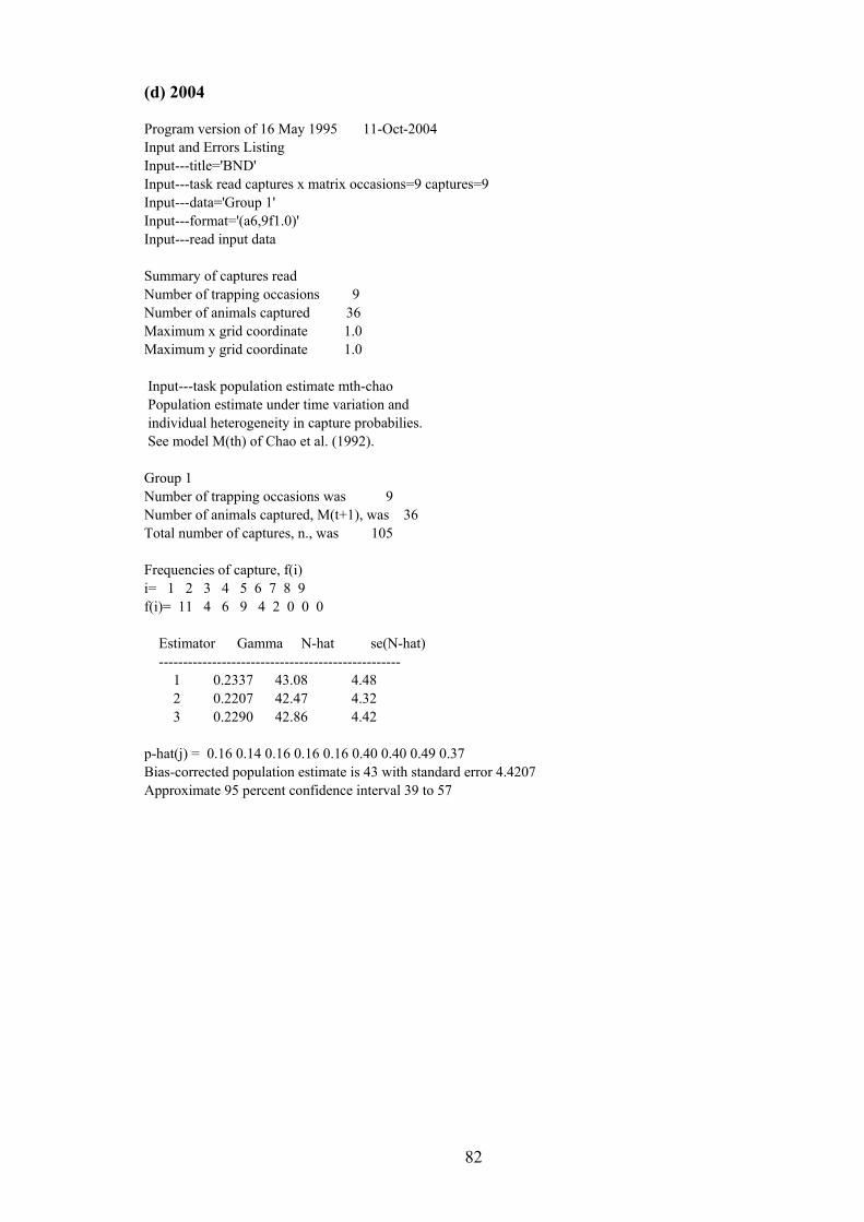
(d) 2004 Program version of 16 May 1995 11-Oct-2004 Input and Errors Listing Input---title='BND' Input---task read captures x matrix occasions=9 captures=9 Input---data='Group 1' Input---format='(a6,9f1.0)' Input---read input data Summary of captures read Number of trapping occasions 9 Number of animals captured 36 Maximum x grid coordinate 1.0 Maximum y grid coordinate 1.0 Input---task population estimate mth-chao Population estimate under time variation and individual heterogeneity in capture probabilies. See model M(th) of Chao et al. (1992). Group 1 Number of trapping occasions was 9 Number of animals captured, M(t+1), was 36 Total number of captures, n., was 105 Frequencies of capture, f(i) i= 1 2 3 4 5 6 7 8 9 f(i)= 11 4 6 9 4 2 0 0 0 Estimator Gamma N-hat se(N-hat) -------------------------------------------------- 1 0.2337 43.08 4.48 2 0.2207 42.47 4.32 3 0.2290 42.86 4.42 p-hat(j) = 0.16 0.14 0.16 0.16 0.16 0.40 0.40 0.49 0.37 Bias-corrected population estimate is 43 with standard error 4.4207 Approximate 95 percent confidence interval 39 to 57

82

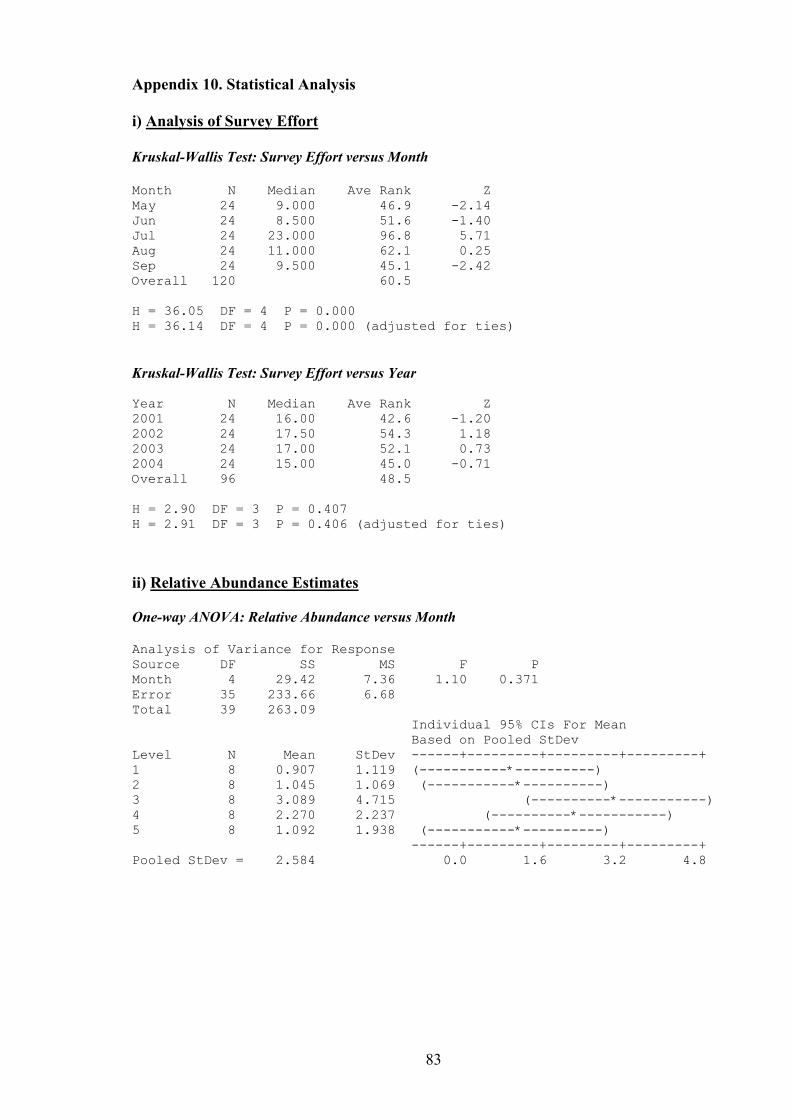
Appendix 10. Statistical Analysis i) Analysis of Survey Effort Kruskal-Wallis Test: Survey Effort versus Month Month N Median Ave Rank Z May 24 9.000 46.9 -2.14 Jun 24 8.500 51.6 -1.40 Jul 24 23.000 96.8 5.71 Aug 24 11.000 62.1 0.25 Sep 24 9.500 45.1 -2.42 Overall 120 60.5 H = 36.05 DF = 4 P = 0.000 H = 36.14 DF = 4 P = 0.000 (adjusted for ties) Kruskal-Wallis Test: Survey Effort versus Year Year N Median Ave Rank Z 2001 24 16.00 42.6 -1.20 2002 24 17.50 54.3 1.18 2003 24 17.00 52.1 0.73 2004 24 15.00 45.0 -0.71 Overall 96 48.5 H = 2.90 DF = 3 P = 0.407 H = 2.91 DF = 3 P = 0.406 (adjusted for ties)

ii) Relative Abundance Estimates One-way ANOVA: Relative Abundance versus Month Analysis of Variance for Response Source DF SS MS F P Month 4 29.42 7.36 1.10 0.371 Error 35 233.66 6.68 Total 39 263.09 Individual 95% CIs For Mean Based on Pooled StDev Level N Mean StDev ------+---------+---------+---------+ 1 8 0.907 1.119 (-----------*----------) 2 8 1.045 1.069 (-----------*----------) 3 8 3.089 4.715 (----------*-----------) 4 8 2.270 2.237 (----------*-----------) 5 8 1.092 1.938 (-----------*----------) ------+---------+---------+---------+ Pooled StDev = 2.584 0.0 1.6 3.2 4.8

83

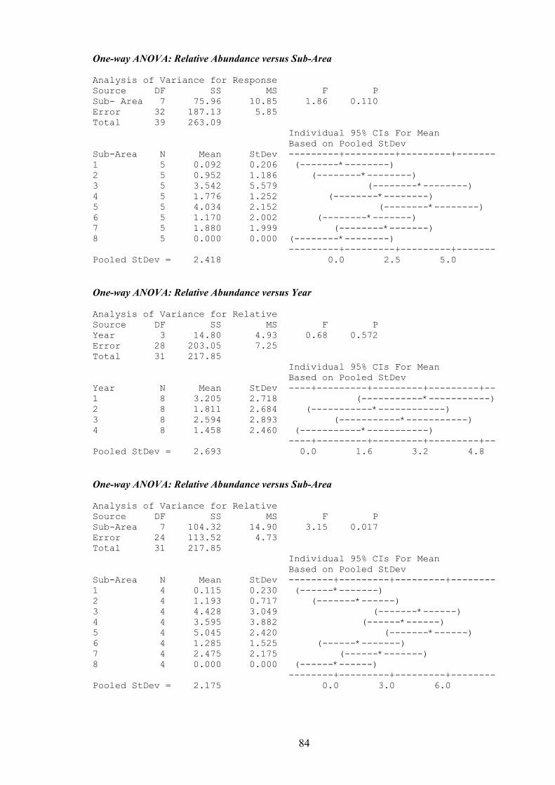
One-way ANOVA: Relative Abundance versus Sub-Area Analysis of Variance for Response Source DF SS MS F P Sub- Area 7 75.96 10.85 1.86 0.110 Error 32 187.13 5.85 Total 39 263.09 Individual 95% CIs For Mean Based on Pooled StDev Sub-Area N Mean StDev ---------+---------+---------+------- 1 5 0.092 0.206 (-------*--------) 2 5 0.952 1.186 (--------*--------) 3 5 3.542 5.579 (--------*--------) 4 5 1.776 1.252 (--------*--------) 5 5 4.034 2.152 (--------*--------) 6 5 1.170 2.002 (--------*-------) 7 5 1.880 1.999 (--------*-------) 8 5 0.000 0.000 (--------*--------) ---------+---------+---------+------- Pooled StDev = 2.418 0.0 2.5 5.0 One-way ANOVA: Relative Abundance versus Year Analysis of Variance for Relative Source DF SS MS F P Year 3 14.80 4.93 0.68 0.572 Error 28 203.05 7.25 Total 31 217.85 Individual 95% CIs For Mean Based on Pooled StDev Year N Mean StDev ----+---------+---------+---------+-- 1 8 3.205 2.718 (-----------*-----------) 2 8 1.811 2.684 (-----------*------------) 3 8 2.594 2.893 (-----------*-----------) 4 8 1.458 2.460 (-----------*-----------) ----+---------+---------+---------+-- Pooled StDev = 2.693 0.0 1.6 3.2 4.8 One-way ANOVA: Relative Abundance versus Sub-Area Analysis of Variance for Relative Source DF SS MS F P Sub-Area 7 104.32 14.90 3.15 0.017 Error 24 113.52 4.73 Total 31 217.85 Individual 95% CIs For Mean Based on Pooled StDev Sub-Area N Mean StDev --------+---------+---------+-------- 1 4 0.115 0.230 (------*-------) 2 4 1.193 0.717 (-------*------) 3 4 4.428 3.049 (-------*------) 4 4 3.595 3.882 (------*------) 5 4 5.045 2.420 (-------*------) 6 4 1.285 1.525 (------*-------) 7 4 2.475 2.175 (------*-------) 8 4 0.000 0.000 (------*------) --------+---------+---------+-------- Pooled StDev = 2.175 0.0 3.0 6.0

84

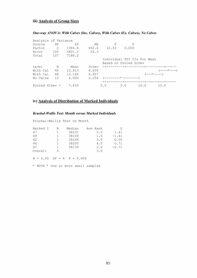
iii) Analysis of Group Sizes One-way ANOVA: With Calves (Inc. Calves), With Calves (Ex. Calves), No Calves Analysis of Variance Source DF SS MS F P Factor 2 1384.9 692.4 12.53 0.000 Error 105 5801.3 55.3 Total 107 7186.2 Individual 95% CIs For Mean Based on Pooled StDev Level N Mean StDev -+---------+---------+---------+----- With Cal 48 15.813 8.634 (----*---) With Cal 48 12.146 6.907 (---*----) No Calve 12 4.000 2.256 (--------*--------) -+---------+---------+---------+----- Pooled StDev = 7.433 0.0 5.0 10.0 15.0 iv) Analysis of Distribution of Marked Individuals Kruskal-Wallis Test: Month versus Marked Individuals Kruskal-Wallis Test on Month Marked I N Median Ave Rank Z 47 1 38231 5.0 1.41 49 1 38108 1.0 -1.41 62 1 38169 3.0 0.00 64 1 38200 4.0 0.71 67 1 38139 2.0 -0.71 Overall 5 3.0 H = 4.00 DF = 4 P = 0.406 * NOTE * One or more small samples

85