University of Montana University of Montana ScholarWorks at University of Montana ScholarWorks at University of Montana Graduate Student Theses, Dissertations, & Professional Papers Graduate School 2016 MULE DEER POPULATION DYNAMICS IN SPACE AND TIME: MULE DEER POPULATION DYNAMICS IN SPACE AND TIME: ECOLOGICAL MODELING TOOLS FOR MANAGING UNGULATES ECOLOGICAL MODELING TOOLS FOR MANAGING UNGULATES Mark A. Hurley Follow this and additional works at: https://scholarworks.umt.edu/etd Let us know how access to this document benefits you. Recommended Citation Recommended Citation Hurley, Mark A., "MULE DEER POPULATION DYNAMICS IN SPACE AND TIME: ECOLOGICAL MODELING TOOLS FOR MANAGING UNGULATES" (2016). Graduate Student Theses, Dissertations, & Professional Papers. 10892. https://scholarworks.umt.edu/etd/10892 This Dissertation is brought to you for free and open access by the Graduate School at ScholarWorks at University of Montana. It has been accepted for inclusion in Graduate Student Theses, Dissertations, & Professional Papers by an authorized administrator of ScholarWorks at University of Montana. For more information, please contact [email protected].

Welcome message from author
This document is posted to help you gain knowledge. Please leave a comment to let me know what you think about it! Share it to your friends and learn new things together.
Transcript
University of Montana University of Montana
ScholarWorks at University of Montana ScholarWorks at University of Montana
Graduate Student Theses, Dissertations, & Professional Papers Graduate School
2016
MULE DEER POPULATION DYNAMICS IN SPACE AND TIME: MULE DEER POPULATION DYNAMICS IN SPACE AND TIME:
ECOLOGICAL MODELING TOOLS FOR MANAGING UNGULATES ECOLOGICAL MODELING TOOLS FOR MANAGING UNGULATES
Mark A. Hurley
Follow this and additional works at: https://scholarworks.umt.edu/etd
Let us know how access to this document benefits you.
Recommended Citation Recommended Citation Hurley, Mark A., "MULE DEER POPULATION DYNAMICS IN SPACE AND TIME: ECOLOGICAL MODELING TOOLS FOR MANAGING UNGULATES" (2016). Graduate Student Theses, Dissertations, & Professional Papers. 10892. https://scholarworks.umt.edu/etd/10892
This Dissertation is brought to you for free and open access by the Graduate School at ScholarWorks at University of Montana. It has been accepted for inclusion in Graduate Student Theses, Dissertations, & Professional Papers by an authorized administrator of ScholarWorks at University of Montana. For more information, please contact [email protected].
i
MULE DEER POPULATION DYNAMICS IN SPACE AND TIME: ECOLOGICAL
MODELING TOOLS FOR MANAGING UNGULATES
by
MARK A. HURLEY
B.S. Wildlife Biology, University of Montana, Missoula, 1988
M.S. Wildlife Resources, University of Idaho, Moscow, Idaho, 1994
Dissertation
presented in partial fulfillment of the requirements
for the degree of
Doctor of Philosophy
in Fish and Wildlife Biology
The University of Montana
Missoula, MT
May 2016
Approved by:
Scott Whittenburg, Dean of the Graduate School
Graduate School
Mark Hebblewhite, Co-Chair
Department of Ecosystem and Conservation Sciences
Michael S. Mitchell, Co-Chair
Montana Cooperative Wildlife Research Unit
Jean-Michel Gaillard
University Claude Bernard - Lyon I
Department of Laboratoire Biométrie & Biologie Évolution
Paul M. Lukacs
Department of Ecosystem and Conservation Sciences
Winsor Lowe
Department of Organismal Biology and Ecology

ii
© COPYRIGHT
by
Mark A. Hurley
2016
All Rights Reserved
iii
Hurley, Mark, Ph.D., Spring 2016 Fish and Wildlife Biology
Mule Deer Population Dynamics in Space And Time: Ecological Modeling Tools For
Managing Ungulates
Co-Chairperson: Mark Hebblewhite
Co-Chairperson: Michael S. Mitchell
ABSTRACT
Ecologists aim to understand and predict the effect of management actions on population
dynamics of animals, a difficult task in highly variable environments. Mule deer
(Odocoileus hemionus) occupy such variable environments and display volatile
population dynamics, providing a challenging management scenario. I first investigate
the ecological drivers of overwinter juvenile survival, the most variable life stage in this
ungulate. I tested for both direct and indirect effects of spring and fall phenology on
winter survival of 2,315 mule deer fawns from 1998 – 2011 across a wide range of
environmental conditions in Idaho, USA. I showed that early winter precipitation and
direct and indirect effects of spring and especially fall plant productivity (NDVI)
accounted for 45% of observed variation in overwinter survival. I next develop predictive
models of overwinter survival for 2,529 fawns within 11 Population Management Units
in Idaho, 2003 – 2013. I used Bayesian hierarchical survival models to estimate survival
from remotely-sensed measures of summer NDVI and winter snow conditions (MODIS
snow and SNODAS). The multi-scale analysis produced well performing models,
predicting out-of-sample data with a validation R2 of 0.66. Next, I ask how predation risk
and deer density influences neonatal fawn survival. I developed a spatial coyote predation
risk model and tested the effect on fawn mortality. I then regressed both total fawn
mortality and coyote-caused mortality on mule deer density to test the predation-risk
hypothesis that coyote predation risk increased as deer density increased as low predation
risk habitats were filled, forcing maternal females to use high predation risk habitats.
Fawn mortality did not increase with density, but coyote predation increased with
increasing deer density, confirming density-dependence in fawn mortality was driven by
coyote behavior, not density per se. Finally, I use integrated population models (IPM) to
collate the previous findings into a model that simultaneously estimates all mule deer
vital rates to test ecological questions concerning population drivers. I test whether
density-dependence or environmental stochasticity (weather) drives mule deer population
dynamics. The vital rate most influenced by density was recruitment, yet across most
populations, weather was the predominant force affecting mule deer dynamics. These
IPM’s will provide managers with a means to estimate population dynamics with
precision and flexibility.
iv
ACKNOWLEDGEMENTS
Funding was provided by Idaho Department of Fish and Game (IDFG), Federal Aid in
Wildlife Restoration Grant number W-160-R-37, NASA grant number NNX11AO47G,
University of Montana, Mule Deer Foundation, Safari Club International, Deer Hunters
of Idaho, Universite Lyon1, and Foundation Edmund Mach. I owe a great deal of
gratitude to the multitude of private landowners and sportsmen in Idaho who not only
granted access to their property, but provided invaluable labor during capture operations.
Cal Groen, Virgil Moore, Jim Unsworth, Jeff Gould, Lonn Kuck, Brad Compton,
Gary Power, Mike Scott, Jon Rachael, and Pete Zager provided leadership, guidance, and
policy support without which this project would not have been possible; and they allowed
me to pursue this professional development opportunity (PhD) as an active Idaho
Department of Fish and Game (IDFG) employee. They also had the foresight to extend
me the encouragement to meld research and management programs providing the
opportunity to ask ecological questions while providing crucially necessary management
tools. Amongst them are my oldest and dearest colleagues, which I truly appreciate their
friendship. Thank you.
I thank IDFG wildlife technicians, biologists, and managers for high-quality data
collection. I am also indebted to those wildlife biologists and managers that have
supported all the “new ideas”: Daryl Meints, Paul Atwood, Jessie Thiel-Shallow, Hollie
Miyasaki, Carl Anderson, Tom Keegan, Jim Hayden, Jay Crenshaw, Craig White, Steve
Nadeau, Randy Smith, Regan Berkley, Martha Wackenhut, Curtis Hendricks, George
Pauley, Wayne Wakkinen, Jason Husseman, Jennifer Struthers, Toby Boudreau, Chad
Bishop, and the entire rest of the IDFG crew. I have been graced with the best data
coordinators possible; Hollie Miyasaki, Jessie Thiel-Shallow, Cindy Austin-McClellan,
and Nikie Bilodeau, all of whom are as professional in maintaining data quality as
mugging deer, with the added benefit of each weighing the equivalent of 16 gallons of jet
fuel, whereas I weigh 26. Capture and data collection efforts were largely successful
because of the assistance I received from professional field technicians Trent Brown, Jon
Muir, and Brett Panting. Special thanks to my ever dependable capture colleagues and
friends, Jim Juza and John Nelson for their tireless work and countless hours of
entertainment. Thanks to the IDFG research crew: Bruce Ackerman, Dave Ausband, Scott
Bergan, Frances Cassirer, Summer Crea, Mike Elmer, Jon Horne, Dave Musil, and Shane
Roberts for critical input to all projects and keeping other projects moving while I was
absent analyzing data and preparing this dissertation.
Thank you to Wildlife Health Lab staff for their unfailing willingness to lend their
expertise in animal processing and biological sample collection: Dr. Mark Drew, Stacey
Dauwalter, Trisha Hosch-Hebdon, Katy Keeton, and Julie Mulholland. This project
required 1000s of hours in helicopters and airplanes, special thanks to pilots and friends,
Ron Gipe, Dave Savage, Bob Hawkins, Carl Anderson, Dave Shallow, and John Romero.
I thank my co-advisors Dr. Mark Hebblewhite and Dr. Mike Mitchell. Mark with
his boundless energy and creative thinking has been a friend throughout this process. He
has kept me excited about science and has opened the doors (both literally and in my own
mind) for many opportunities that have enriched my professional and personal life. Mike
paved the way for my work here and provided countless hours of discussion and
v
friendship as we worked though scientific and logistical issues. I am very fortunate to
have had such a talented committee to work with: Jean-Michel Gaillard, Paul Lukacs,
Scott Mills (an early member replaced by Lukacs), and Winsor Lowe. Every interaction
with them has been a valuable learning experience. One of the highlights of this
experience was the opportunity to collaborate with my European colleagues, Christophe
Bonenfant, Jean-Michel Gaillard, and Wibke Peters opening my mind to new thought
processes and possibilities.
The successful completion of this dissertation, given the complex nature of the
data and questions, was only possible through an intense collaborative effort. My co-
authors; Mark Hebblewhite, Jean-Michel Gaillard, Christophe Bonenfant, Paul Lukacs,
Josh Nowak, Kyle Taylor, Stéphane Dray, Bill Smith, and Pete Zager, spent countless
hours discussing, editing, and analyzing data for these publications. Their combined skill
and knowledge along with their absolute wizardry with large and complicated data sets
and R-coding has been critical to answering the questions I posed. Thanks to Angie
Hurley and Nikie Bilodeau for formatting and technical editing help with this
dissertation.
I have been very fortunate to be associated with two University labs -both the
Mitchell Lab members: Ben Jimenez, Barb McCall-Moore, Jeff Stetz, Dave Ausband,
Lindsey Rich, and Sarah Sells; as well as the Hebblewhite Lab members: Sonya
Christiansen, Shawn Cleveland, Nick DeCesare, Scott Eggeman, Josh Goldberg, Lacey
Greene, Michel Kohl, Matt Metz, Clay Miller, Wibke Peters, Jean Polfus, Derek Spitz,
Robin Steenweg, Dan Eacker, Tshering Tempa, and Hugh Robinson. The discussions
concerning details of projects or general ecological principles were a very special part of
my time at University of Montana, thank you.
Special thanks to Ben, Shawn, Hugh, Bob Weisner, Adam and Shannon
Sepulveda, and Mike Thompson for providing a place for me to stay with entertaining
and educational evening discussions. And thanks to Dan Pletcher, my undergraduate
advisor and longtime mentor and associate who was so fond of introducing several
graduate seminars with: “Let me tell you a story about Hurley, he was here at the
University of Montana when I came here 30 years ago and he is still here!” Thanks Dan.
Now my longtime friend and colleague, Chad Bishop, takes his place. University of
Montana will not miss a beat. Thanks to Jeanne Franz, Robin Hamilton, Vanetta Burton,
and Tina Anderson for keeping me straight with academic and the financial
administrative needs of Sponsored Programs.
Most importantly, I would like to thank Angie, Erin, and Tess for their support of
this extreme adventure. They endured the hardship of my months (years) of absence and
welcomed me home with loving arms each time. I also couldn’t have done this without
the support and encouragement from my mother, Darleen, father, Lloyd, and brother and
sister, Mike and Net. Thank you, family.
This Dissertation is dedicated to two men who have had a profound impact on my
life. First, my father, Lloyd E. Hurley, who loved the wild country of Idaho and missed
his son receiving a PhD by a scant two months, something he dearly wanted to witness.
And second, Ron Gipe, friend and one the most intuitive and capable helicopter pilots I
have had the honor to fly with. We experienced many adventures in our nearly 30 years
together in the sky.

vi
TABLE OF CONTENTS
ABSTRACT ……………………………………………………………………………iii ACKNOWLEDGEMENTS ……………………………………………………………iv TABLE OF CONTENTS ……………………………………………………………vi
LIST OF TABLES ………………………………………………………..…………viii LIST OF FIGURES ………………………………………………………….………..xii CHAPTER 1. DISSERTATION OVERVIEW AND INTRODUCTION ……….…….1
LITERATURE CITED.................................................................................................... 8 CHAPTER 2. FUNCTIONAL ANALYSIS OF NDVI CURVES REVEALS
OVERWINTER MULE DEER SURVIVIAL IS DRIVEN BY BOTH SPRING AND
FALL PHENOLOGY ……………………………………………………………………15
INTRODUCTION ……………………………………………………………………15 MATERIALS AND METHODS ……………………………………………………21
(a) Study Areas ......................................................................................................... 21 (b) Mule deer monitoring ......................................................................................... 22
(c) Defining Population Ranges of Mule Deer ........................................................ 23 (d) Functional Analysis of NDVI curves ................................................................. 23
(e) PRISM Weather Data ......................................................................................... 27 (f) Environmental Effects on Body Mass and Overwinter Survival of Fawns ........ 27
RESULTS ……………………………………………………………………………29
(a) Functional Analysis of NDVI Curves................................................................. 29 (b) Environmental Effects on Body Mass and Overwinter Survival of Fawns ....... 30
DISCUSSION ……………………………………………………………………32 LITERATURE CITED ……………………………………………………………38
TABLES ……………………………………………………………………………56 FIGURES ……………………………………………………………………………63
APPENDIX A. SUPPLEMENTAL MATERIALS ……………………………69 2-S4: Technical description of the Functional Principal Component Analysis ............ 72 2-S5: R code for Bayesian Hierarchical data analysis .................................................. 74
CHAPTER 3: GENERALITY AND PRECISION OF REGIONAL-SCALE SURVIVAL
MODELS FOR PREDICTING OVERWINTER SURVIVAL OF JUVENILE
UNGULATES ……………………………………………………………………………76 INTRODUCTION ……………………………………………………………………77
STUDY AREA ……………………………………………………………………82 METHODS …....……………………………………………………………………83
(a) Capture and Survival Monitoring ....................................................................... 83
(b) Defining Seasons and Herd Unit Home Ranges ................................................ 84 (c) Survival Variable Development .......................................................................... 85
Individual covariates ........................................................................................... 85 Spatial forage and weather covariates ................................................................ 85
(d) Survival Modeling .............................................................................................. 88 (e) Model Selection .................................................................................................. 91 (f) Evaluating the Precision, Accuracy and Generality of Survival Models ............ 93
RESULTS ……………………………………………………………………………94

vii
(a) Observed survival ............................................................................................... 94
(b) Covariate and random effects for overall model ................................................ 94 (c) Overall survival model validation, prediction, and complexity ......................... 95 (d) Ecotype survival models and covariate effects .................................................. 97
DISCUSSION ……………………………………………………………………98 MANAGEMENT IMPLICATIONS …………………………………………..107 LITERATURE CITED …………………………………………………………..107 TABLES …………………………………………………………………………..116 FIGURES …………………………………………………………………………..120
APPENDIX B. SUPPLEMENTAL MATERIALS ………………………..…131 3-S1: Summer Range Ecotype Classification ........................................................ 131
CHAPTER 4: HABITAT-MEDIATED DENSITY DEPENDENCE IN NEONATAL
SURVIVAL OF MULE DEER FAWNS …………………………………………..143
INTRODUCTION …………………………………………………………………..143 MATERIALS AND METHODS 146
(a) Data collection .................................................................................................. 146 (b) Statistical analysis ............................................................................................ 148
RESULTS …………………………………………………………………………..149 DISCUSSION …………………………………………………………………..151 LITERATURE CITED …………………………………………………………..154
TABLES …………………………………………………………………………..158 FIGURES …………………………………………………………………………..159
CHAPTER 5: DISENTANGLING CLIMATE AND DENSITY-DEPENDENT EFFECTS
ON UNGULATE POPULATION DYNAMICS …………………………………..163 INTRODUCTION …………………………………………………………………..164
STUDY AREA …………………………………………………………………..170
METHODS ……………………………………………………………….….172 (a) Integrated Population Model Development...................................................... 172
Population estimates .......................................................................................... 173
Age and Sex ratio estimates ............................................................................... 173 Survival monitoring ........................................................................................... 174
Harvest estimation ............................................................................................. 175 (b) Integrated Population Model Parameterization ................................................ 175
Testing for Density Dependence ........................................................................ 179 Testing for Density Independence in Climatic Drivers ...................................... 180 Bayesian Model Fitting ...................................................................................... 181
RESULTS …………………………………………………………………………..182
(a) Density dependence on vital rates .................................................................... 182 (b) Strength of density dependence on recruitment ............................................... 182 (c) Density or weather ............................................................................................ 183
(d) Effects of Weather ............................................................................................ 184 TABLES …………………………………………………………………………..198 FIGURES …………………………………………………………………………..204 APPENDIX C. SUPPLEMENTAL MATERIALS …………………………..210
viii
LIST OF TABLES
Table 2-1. A brief literature survey of the studies that investigated relationships between
NDVI metrics and life history traits linked to performance and population abundance.
The literature survey was performed using ISI web of knowledge using the key-words
“NDVI and survival”, “NDVI and body mass”, “NDVI and body weight”, “NDVI and
reproductive success”, “NDVI and recruitment”, “NDVI and population growth”, and
“NDVI and population density”. Only studies performed on vertebrate species were
retained. For each case study, the table displays the focal trait(s), the focal species, the
NDVI metric(s) used, the outcome (“+”: positive association between NDVI and
performance, “-“: negative association between NDVI and performance”, “0”: no
statistically significant association between NDVI and performance”), the reference, and
the location of the study………….……………………………………………………..57
Table 3-1. Model selection results for the overall, overwinter Hierarchical Bayesian
survival model for mule deer (Odocoileus hemionus) fawns based on 2529 individuals
from 2003 - 2013 in Idaho, USA. The overall models contain data from all Population
Management Units (PMU) and all years, and the full models contain all of the covariates.
For each model, we report the model structure with covariates, Deviance Information
Criterion (DIC), Difference from lowest DIC (ΔDIC), Effective Number of Parameters
(pD), Deviance, and validation metrics. We conducted two forms of model validation;
cross-validation within the observed data (R2cv) and external validation (R
2EV) with
withheld survival data collected on n = 403 mule deer fawns in years 2007-2008 in the
same study areas. The best model identified by each of the criteria (ΔDIC , R2cv , R
2EV)

ix
are bolded. Covariates include mean snow cover in November and December
(ND%snow), mean snow cover in January to March (W%snow), mean snow cover in
April (A%snow), Functional analysis principal components for fall (FPC), functional
analysis principal components for spring (SPC), number of weeks with >90% snow cover
in November and December (FWeeks), and average snow depth in January – March
(Depth). ……………………………………………………………………………….117
Table 3-2. Model selection results for the ecotype specific, overwinter Hierarchical
Bayesian survival models for mule deer (Odocoileus hemionus) fawns based on 2529
individuals, including all years of data from 2003 - 2013 in Idaho, USA. The full models
contain all of the covariates. For each model we report, the model structure with
covariates, Deviance Information Criterion (DIC), Difference from lowest DIC (ΔDIC),
Effective Number of Parameters (pD), Deviance, and validation metrics (Cross validation
R2). The best model identified by each of the criteria (ΔDIC , R
2cv ) are bolded.
Covariates are; mean snow cover in November and December (ND%snow), mean snow
cover in January to March (W%snow), mean snow cover in April (A%snow), Functional
analysis principal components for fall (FPC), functional analysis principal components
for spring (SPC), number of weeks with >90% snow cover in November and December
(FWeeks), and average snow depth in January – March (Depth)………………………119

x
Table 4-1. Parameter estimates of the top coyote (Canis latrans) predation risk model in
southern Idaho, 1998 – 2002, used to estimate exposure of neonatal mule deer
(Ocodoileus hemionus) fawns to coyote predation risk……………………………158
Table 5-1. Integrated Population Model (IPM) model selection for mule deer (Odocoileus
hemionus) for 6 Population Management Unit (PMU), Idaho, 2001 – 2013. Shown is the
model structure with density dependent (dd) terms added on each vital rate (R-
recruitment, jS – juvenile survival, fS – adult female survival, mS – adult male survival)
and the prefix denotes dd = density dependence, c = vital rate varies within a given
distribution of the global mean for the PMU, and t = vital rate varies within a given
distribution for an annual mean. Model diagnostics are the Deviance Information
Criteria (DIC), effective number of parameters (pD), Deviance, and parameter estimates
for density dependence (DD), and the standard deviation of density dependence (DD
SD)…………………………………………………………………………………..198
Table 5-2. Integrated Population Model (IPM) model selection for mule deer (Odocoileus
hemionus) in 6 Population Management Units (PMU), Idaho, years 2001 – 2013. The
model structure includes a density dependent term on recruitment, time-varying juvenile
survival, constant adult female survival, and constant adult male survival. Parameter
estimates for density dependence (DD) and standard deviations (SD) are provided for
density dependence (DD). Model fitting diagnostic are Deviance Information Criteria
(DIC), effective number of parameters (pD) and Deviance. In this instance ΔDIC
describes the relationship to the PMU specific model set to illustrate departure from the

xi
best model when another model is used for constancy of model structure for DD
covariate comparisons………………………………………………………………200
Table 5-3: Model selection results for integrated population models comparing model fit
for models with density dependence on recruitment only (DDO), effect of weather and
density dependence on recruitment (WDD), and the effect of weather without density
dependence (WO). We present the top models for each model type in each PMU to test
between factors driving population dynamics; density dependence, weather, or both. For
models including weather, we report the covariates in each model. Model fitting
diagnostic are the Deviance Information Criterion (DIC), Difference from lowest DIC
(ΔDIC), Effective Number of Parameters (pD), Deviance, and validation metrics…..202
xii
LIST OF FIGURES
Figure 2-1. Results of Functional Principal Component Analysis of the typology of NDVI
curves in Idaho, USA, from 1998 – 2011 from April (A) to November (N) for each
population-year (dot) identifying two key periods, the spring (2nd
FPCA component, the
Y-axis) and the fall components (1st FPCA component, X-axis). a) Variation in NDVI
curves among populations and years was best explained by FPCA 1, which explained
48.9% of the variation, and characterized primary production from June to October (e.g.,
summer/fall). b) FPCA 2 (Y-axis) characterized primary production in May and June and
explained 27% of the seasonal variation. c) NDVI typology was best characterized by 5
clusters, shown in different colors that corresponded to different patterns of spring and
fall primary production, compared to the mean NDVI curve across all of Idaho. For
example, typology 5 was characterized by low NDVI intensity in both spring and fall,
typology 3 by high NDVI intensity in both spring and fall, and typology 4 by high NDVI
intensity in spring, but low in fall, etc. ……………………….…………………………63
Figure 2-2. Distribution of the 5 NDVI typologies shown in Figure 1, with corresponding
colors (inset) across the 13 mule deer populations (GMU’s) in Idaho, USA, from 1998 -
2011. The size of the pie wedge is proportional to the frequency of occurrence of each
NDVI typology within that mule deer population. For example, population 56 had all but
one population-year occurring in NDVI typology 4 (Figure 1) indicating low primary
productivity during spring but higher during fall. ………………………………………65

xiii
Figure 2-3. Hierarchical Bayesian Path Analysis of the effects of spring and fall growing
season functional components (from Figure 1) and winter precipitation on mule deer
fawn body mass and overwinter survival from 1998 – 2011 in Idaho, USA. This model
explained 44.5% of the variation in survival. Beta coefficients and their standard
deviation are shown, with solid lines indicating the indirect effects of NDVI on survival
mass through their effects on body mass, and dashed lines indicate the direct effects of
NDVI on survival. ………………………………………………...……………………..66
Figure 2-4. Results of hierarchical Bayesian path analysis showing the standardized direct
effects of a) FPCA component 1 from the functional analysis (Fall NDVI), and b) FPCA
component 2 (Spring NDVI) on body mass (kg) mule deer fawns in Idaho, USA, from
1998 – 2011. ………………………………………………………………………….…67
Figure 2-5. Results of hierarchical Bayesian path analysis showing standardized direct
effects of a) body mass (kg), b) cumulative winter precipitation (in mm), c) FPCA
component 1 from the functional analysis (Fall NDVI), and d) FPCA component 2
(Spring NDVI) on the overwinter survival of mule deer fawns in Idaho, USA, from 1998
– 2011. ……………………………………………………………..……………………68
Figure 3-1. Annual survival cycle for mule deer fawns in year t from birth, through
summer and winter survival to recruitment into the population in relation to the
management setting of mule deer harvest in year t+1 in Idaho, USA. Winter begins in
November or December and winter fawn survival is measured from 15 December to June
xiv
1 (dashed line). Season setting for harvest management begins in early January and final
seasons are set in early March of each year……………………………………………120
Figure 3-2. (A) Hierarchical relationship between Mule deer seasonal summer and winter
ranges within the deer sampling unit at the Game Management Unit (GMU) and the
larger-scale Population Management Unit (PMU), and largest-scale Ecotype in central
and southern Idaho, USA, years 2003-2013. Spatial covariates for weather (summer
precipitation, NDVI, snow-cover) were extracted from seasonal ranges estimated from
radio telemetry data during summer and winter, and then associated with individual mule
deer within each GMU, nested within each PMU. (B) Expected overwinter survival of
fawns in each PMU estimated from the mean of the annual posterior distributions. (C)
Parameter estimate for the random effect of winter snow cover for the best fitting random
effect model (Table 1). Green colors denote minimal effect of winter and orange to red
colors denote increasing effect of winter……………………………………………….121
Figure 3-3. Effects of covariates on mule deer (Odocoileus hemionus) overwinter survival
in Idaho, 2003-2013, from the top 6 Bayesian hierarchical models showing the mean,
75% and 95% Bayesian credible intervals for the following covariates: mean snow cover
in November and December (ND%snow), mean snow cover in January to March
(W%snow), mean snow cover in April (A%snow), Functional analysis principal
components for fall (FPC), functional analysis principal components for spring (SPC),
Number of Weeks with >90% snow cover in November and December (FWeeks), and
average snow depth in January – March (Depth)………………………………………123

xv
Figure 3-4. Observed (Kaplan-Meier survival, x axis) versus predicted (modeled y axis)
overwinter survival of 6-month old mule deer (Odocoileus hemionus) fawns in southern
and central Idaho for each PMU, 2003-2013. Survival was predicted for 2529 mule deer
fawns using a hierarchical Bayesian survival model that accounted for spatial and
temporal variation in covariates. Panel figures for the numbering scheme of Table 1 a)
Model 10, b) Model 1, c) Model 6, d) Model 5, e) Model 3, f) Model 9. The first model is
the only model that includes mass. The blue line is a spline fit to illustrate bias of
modeled survival estimates from observed estimates……………………………….125
Figure 3-5. External validation of the overall models of mule deer (Odocoileus hemionus)
fawn survival in Idaho, 2003-2013. We conducted external validation by withholding
survival data collected on 403 mule deer fawns in years 2007-2008. We used the models
to predict survival of fawns and then compared the estimate (green circle) to observed
survival (Kaplan-Meier estimate) in the same study areas. First and 4th
models include a
random effect of winter % snow cover the others only random intercept and correspond
to model numbers in Table 1. The blue line is a spline fit to illustrate bias of modeled
survival estimates from observed estimates……………………………………………127

xvi
Figure 3-6. Observed (Kaplan-Meier; x axis) versus predicted (modeled; y axis)
overwinter survival of 6-month old mule deer (Odocoileus hemionus) fawns within a,b)
Aspen c, d) Conifer, and e, f) Shrub-Steppe ecotypes in southern Idaho, 2003-2013. The
most supported 2 models are presented. The blue line is a spline fit to illustrate bias of
modeled survival estimates from observed estimates….………………………..……..129
Figure 4-1. Spatial predictions from the resource selection function based model of
coyote (Canis latrans) predation risk for mule deer (Odocoileus hemionus) neonatal
predation risk in southern Idaho, 1998 – 2002, showing the two Game Management Units
56 and 73A where neonatal mule deer were monitored. The spatial distribution of coyote
transects used to develop the model in a wider spatial area are depicted by black
circles…………………………………………………………………………………..159
Figure 4-2. Relationship between coyote (Canis latrans) predation risk (estimated from a
resource selection functions based on scat transects) and mule deer (Odocoileus
hemionus) fawn survival (estimated with Cox-proportional hazards models) in mule deer
in southern Idaho, 1998 – 2002…………………………………………………………160
Figure 4-3. Relationship between mule deer (Ocodoileus hemionus) density and a) overall
fawn mortality rates and b) fawn mortality caused by coyotes (Canis latrans) including
average density and mortality for two Game Management Units (GMU 73A, 56) in
southern Idaho, 1998 – 2002………………………………………………………….161
xvii
Figure 4-4. Relationship between mule deer (Ocodoileus hemionus) population size and
a) overall fawn mortality rates and b) fawn mortality caused by coyotes (Canis latrans)
including independent measures of density and mortality in 2 Game Management Units
(GMU 73A, 56) in southern Idaho, 1998 - 2002……………………………………..162
Figure 5-1. Basic age-structured life-cycle for the post-breeding birth pulse matrix model
used as the basis for the Integrated Population Model (IPM) for mule deer in Idaho. Here,
we start the recruitment of individuals as 6 month olds as estimated from fawn to adult
female ratio counts in December, estimate survival through winter and summer, and
recruit into the adult population at age 18 months. Only adults reproduce as the age of
first reproduction is 2 in mule deer………….……………….…………………..…..204
Figure 5-2. Spatial map of the strength of density-dependent population growth rate for
Mule deer (Odocoileus hemionus) populations estimated with an integrated population
model in Idaho, 2001-2013……………………………………………………...........205
Figure 5-3. Integrated population model (IPM) projections for mule deer (Odocoileus
hemionus) in the Bannock population management unit (PMU), 2001-2013, showing
time varying juvenile survival, constant female survival, and population abundance
estimates consistent with a density-dependent effect on recruitment only. Lines indicate
posterior mean estimate with 95% credible interval (grey shading). Points are field data
with 95% confidence interval…………………………………………………………206

xviii
Figure 5-4. Integrated population model (IPM) projections for Mule deer in the Bannock
population management unit (PMU), 2001 - 2013, weather modeled juvenile survival,
constant female survival, and population abundance estimates consistent with a density-
dependent effect on recruitment. Lines indicate posterior mean estimate with 95%
credible interval (grey shading). Points are field data with 95% confidence interval…207
Figure 5-5. Comparisons of parameter estimates for standardized density dependence in
vital rates (recruitment) and the best density-independent (weather, forage) covariates on
mule deer populations in Idaho, 2001 – 2013……………………………………….208
Figure 5-6. Spatial map of the strength of density-independent effects on population
growth rate from annual variation in late summer forage quality for mule deer
(Odocoileus hemionus) populations estimated with an integrated population model in
Idaho, 2001-2013……………………………………………………………………..209
1
CHAPTER 1. DISSERTATION OVERVIEW AND INTRODUCTION
A complex suite of biotic and abiotic processes drives ungulate population growth across
varying environmental conditions. Our goal as ecologists is to understand and predict the
effect of the environment in concert with management actions on population dynamics of
animals, a particularly difficult task in highly variable environments. Across species,
ungulate population growth is often driven by variation in recruitment (Gaillard et al.
2000) modified by the interplay of summer vs. winter nutrition, weather, and predation
(Nilsen et al. 2009). The population growth of my study species, mule deer (Odocoileus
hemionus), is sensitive to adult female survival (Unsworth et al. 1999, Hurley et al.
2011), but juvenile survival shows the widest variation, often in response to weather
(Bishop et al. 2005), similar to juvenile survival across many ungulate species (Portier et
al. 1998, Gaillard et al. 2000, Coulson et al. 2001). This variation in juvenile survival
often drives mule deer population dynamics (Unsworth et al. 1999) and many other
temperate ungulates (Festa-Bianchet and Smith 1994, Raithel et al. 2007). Recruitment
may also vary spatially, depending on the effect of weather on nutritional quality
(Pettorelli et al. 2005), winter energy expenditure (Bartmann et al. 1992, Parker et al.
2009), and spatial variation in predation (Mackie et al. 1998, Bishop et al. 2009). This
spatial variation suggests that site-specific ecotype productivity was modified by weather
and local predation conditions (Lukacs et al. 2009). Given this complexity, a clear
understanding of the interaction between forage quality, winter weather, and predation
2
risk is necessary to accurately predict population performance with environmental
change.
Prediction, however, is complicated by many factors as ungulates exist over a
wide range of environmental conditions, with their densities driven by a combination of
these large-scale processes, life-history trade-offs and resource selection (Senft et al.
1987, Bowyer and Kie 2006). Densities of ungulates are positively correlated with both
primary productivity (Crete and Daigle 1999, Melis et al. 2009) and the spatial variation
in forage because this increases access to high quality forage (Fryxell 1988, Wang et al.
2006). Forage quality alone, however, does not determine ungulate density on landscapes
with predation. Ungulates may adopt behavioral strategies to avoid predation, reducing
the actual nutrition given the constraints of predation risk, resulting in a lower realized
nutrition and thus lower growth rates (Hopcraft et al. 2010). Effects of predation are also
strongest in lower productivity (Melis et al. 2009), and the degree to which predation is
compensatory or additive depends on the interaction of forage quality and density
(Bartmann et al. 1992, Ballard et al. 2001). Such trade-offs may also be influenced by
both density-independent forces (i.e., weather) or density-dependence (Hopcraft et al.
2010).
It has long been known that increasing density reduces the strength of selection
for high-quality patches because of density-dependent competition for forage (Fretwell
and Calver 1969, McLoughlin et al. 2010). It is through such density-dependent changes
in habitat selection that changes in population dynamics ultimately occur, although the
effects of density-dependent resource selection on populations are unclear for many
ungulate species (McLoughlin et al. 2010). Despite the uncertainty about how density-
3
dependence in resource selection translates to population growth, density dependence is
perhaps the most important paradigm in ungulate population ecology (Eberhardt 2002,
Bonenfant et al. 2009). As ungulate density increases under this paradigm, we expect
declines in juvenile survival first, followed by fecundity, and finally, adult survival
(Gaillard et al. 2000). Density-dependent changes in resource selection likely drive these
widespread patterns in ungulate demography, but it has been challenging to link resource
selection to fitness consequences (McLoughlin et al. 2010). Regardless, understanding
the underlying mechanism of density effects on vital rates is difficult to measure because
each rate is dependent on other vital rates. After decades of research on mule deer,
scientists have been similarly unable to link habitat to population growth because of
uncertainty in the relative role of summer versus winter forage quality, and the interacting
effects of predation (Ballard et al. 2001).
The wide annual variation of mule deer populations also poses a challenge for
their conservation and management. Mule deer are an economically important harvested
species in western North America necessitating intensive monitoring of population status.
Because juvenile survival and recruitment are the most variable, these key vital rates have
become the monitoring priority of wildlife managers attempting to predict changes in
ungulate populations (e.g., Montana Adaptive Harvest Management 2001, Idaho Mule
Deer Management Plan 2008, Lukacs et al. 2009). Neonate survival (birth to 6 months of
age) may be adequately measured via age ratio surveys (December fawn ratios) when
coupled with estimates of adult female age structure and age-specific fecundity (Harris et
al. 2008). But wildlife managers must still rely on expensive radiotelemetry-based
estimates of overwinter survival combined with population models to make ungulate
4
harvest decisions (White and Bartmann 1998, Montana Adaptive Harvest Plan 2001,
Idaho Mule Deer Management Plan 2008). Another challenge is that wildlife managers
must often submit harvest recommendations for the upcoming year by early January,
limiting the information available on overwinter survival estimate at the time of season
setting. Ideally, managers would benefit from some reliable way of predicting overwinter
survival based on weather and an ecologically-based definition of ungulate habitat
quality. Ultimately, population models that link summer forage quality and winter
weather to populations are critically needed for understanding the ecology and
management of ungulates. An applied goal of my Dissertation is to provide statistical
tools to meet that need. The following chapters progressively identify the underlying
mechanisms of mule deer population dynamics and then use these relationships to predict
population growth, with the ultimate goal of improving harvest management.
My Dissertation focuses on mule deer populations in Idaho, but my goal was to
elucidate relationships applicable throughout western North America to improve
management of this species. I also hope that my approach to develop large-scale
predictive models of ungulate population dynamics can be expanded across species. I
incorporated intrinsic (behavior, density) and extrinsic processes (weather, forage quality,
and predation risk) into stochastic survival and population models to predict growth rates
across a diverse range of habitat quality, predation, and weather conditions. In most
chapters, I develop statistical models using large sample sizes (>2,000 individuals) of
different age-classes of mule deer (juveniles, adult females) across large spatial scales
usually from 6 to 13 populations over long temporal scales from 1995–2014. These large
5
spatiotemporal datasets provide a unique opportunity to test fundamental and applied
questions about mule deer ecology and management.
In Chapter 2, I seek to understand the mechanisms driving fawn survival in
winter, the most variable vital rate for mule deer across 13 populations of mule deer in
Idaho. Despite the importance of nutrition, proximate causes of mule deer fawn mortality
during winter is predation or malnutrition (Ballard et al. 2001, Hurley et al. 2011) in
interaction with weather (Portier et al. 1998, Colman et al. 2001, Mech et al. 2001).
Because of this interaction, the relative effects of predation and forage on ungulate
survival are difficult to isolate (Kjellander et al. 2004, Pierce et al. 2004, Kauffman et al.
2007, Bishop 2009). Recent field studies on ungulates, however, emphasized the critical
importance of late summer and fall nutritional ecology to the population performance of
large herbivores. Important barriers to understanding the complex influence of growing
season dynamics on ungulate survival are how to disentangle correlated plant phenology
metrics and the time series nature of NDVI data in a quantitative approach that describes
variation in plant quality across an entire growing season or discriminates between sites.
To solve these issues, we jointly used functional analysis (Ramsay and Silverman 2005)
to characterize seasonal variation in NDVI curves and path analyses (Shipley 2009) to
assess the interplay of plant phenology and winter severity and disentangled relationships
of nutrition and weather and their effects on population dynamics of ungulates.
In Chapter 3, I explore prediction in both a management and ecological context by
developing fawn survival models that balance precision, bias and generality across space
and time (Levins 1966). The ecological relationships I illuminated from Chapter 2 were
used to create predictive models testing both the importance of remotely-sensed summer
6
forage quality or winter snow conditions and the generality of models to predict winter
fawn survival across a broad range of environments. One challenge in the development of
predictive statistical models for survival is the complexity of dealing with integrating
survival data across populations that are hierarchically structured in space and time
(Lukacs et al. 2009). My solution was to use Bayesian hierarchical modeling, enabling
the development of spatially structured, hierarchical and flexible statistical models (Royle
and Dorazio 2006, Kery and Schaub 2012) which are inherently well-suited to prediction
of animal movements and population ecology (Heisey et al. 2010, Geremia et al. 2014,
Mouquet et al. 2015). I then developed general models appropriate for use by managers
to estimate fawn survival in the absence of annual radiocollar data.
Chapter 4 combines predation risk with resource selection to describe potential
reductions in carrying capacity of the landscape. Because of the challenge of estimating
predation risk at large spatial scales, I focus on two populations in southern Idaho where I
developed fine-scale measures of predation risk to mule deer fawns from their main
predator, coyotes (Canis latrans). Assuming that predation risk can be spatially
decomposed to depict the probability of death given a set of landscape features (Lima and
Dill 1990, Hebblewhite 2005, Kauffman et al. 2007), maternal females should select
lower risk habitats. However, if exclusive space use of adult females during fawn rearing
created a despotic distribution with dominant females occupying both high forage quality
and low predation risk habitats, fawn survival sink may be created as subordinate female
mule deer are forced into lower quality forage and increased predation risk habitat at
higher deer density. This density-dependent resource selection may reduce population
productivity, negating the value of additional productive females on the landscape as total

7
adult female numbers increase. To test this hypothesis, I first modeled occurrence of
coyotes with a spatial model to estimate predation risk, and evaluate the relationship of
coyote predation risk to neonate mule deer mortality. Next, I tested whether this
relationship changed as mule deer populations increased and higher quality habitats were
filled. I use two Game Management Units, one with active coyote removal (removal) and
one without (reference; as described in detail in Hurley et al. 2011), predicting the effect
of density would be increased in the reference (no coyote removals) area. In keeping with
this prediction, survival of mule deer fawns did not change in the reference area and
declined in the removal area with increasing mule deer density. Cause-specific mortality
from coyotes, however, increased with deer density in the reference and to a lower degree
in the removal area suggesting density-dependence driven by expansion of deer into
lower quality habitat that was highly selected by coyotes. Thus overall changes in
density-dependent mortality were compensatory. This enforces the idea that density
dependence and compensatory mortality may operate on a despotic distribution caused by
conspecific exclusion of maternal females from low predation risk habitats.
Through the use of integrated population models (IPM, Schaub et al. 2007) in
Chapter 5, I then apply the results from the previous chapters to model population
dynamics in six of my study areas with consistently high quality vital rate data. I use
these models to understand the relative contribution of density-dependent and density-
independent drivers of ungulate population dynamics, as well as their possible
interaction. Many processes, such as predation or weather, can mimic density dependence
by acting on vital rates in the same progression as expected by density often through
density-climate interactions (Saether 1997, Clutton–Brock and Coulson 2002,

8
Hebblewhite 2005, Hurley et al. 2011). To separate the effects of weather versus density,
I used an IPM approach to identify the properties of mule deer populations that would
suggest regulation by density dependence or limitation by weather. I estimated the effect
of density with the addition of a density term on each of our measured vital rates,
recruitment (fawn ratios in December), winter fawn survival, and adult female survival. I
then added weather covariates identified as important in previous chapters to the time
varying estimate of winter fawn survival to increase model fit and test if density
dependence is evident in the populations or if weather was mimicking the effect of
density dependence. In all chapters, my search for factors that regulate or limit mule deer
population size provides tools for harvest management and increases understanding
population ecology of a high value ungulate.
Throughout the rest of this Dissertation, I use the second-person voice, we,
reflecting the highly collaborative nature of my Dissertation research. I recognize the
contributions of my co-authors in each chapter. Moreover, each chapter is formatted for
publication in a different peer-reviewed journal, and Chapter 2 is already published in
Philosophical Transactions of the Royal Society B. Chapter 3 is formatted with the intent
to submit to Journal of Wildlife Management, Chapter 4 for submission to Biology
Letters, and Chapter 5 for submission to Oecologia.
LITERATURE CITED
Ballard, W. B., D. Lutz, T. W. Keegan, L. H. Carpenter, and J. C. deVos, Jr. 2001. Deer-
Predator Relationships: A Review of Recent North American Studies with
Emphasis on Mule and Black-Tailed Deer. Wildlife Society Bulletin 29:99-115.
9
Bartmann, R. M., G. C. White, and L. H. Carpenter. 1992. Compensatory Mortality in a
Colorado Mule Deer Population. Wildlife Monographs 121:3-39.
Bishop, C. J., G. C. White, D. J. Freddy, B. E. Watkins, and T. R. Stephenson. 2009.
Effect of Enhanced Nutrition on Mule Deer Population Rate of Change. Wildlife
Monographs 172:1-28.
Bishop, C. J., J. W. Unsworth, and E. O. Garton. 2005. Mule Deer Survival among
Adjacent Populations in Southwest Idaho. The Journal of Wildlife Management
69:311-321.
Bonenfant, C., J. M. Gaillard, T. Coulson, M. Festa‐Bianchet, A. Loison, M. Garel, L. E.
Loe, P. Blanchard, N. Pettorelli, and N. Owen‐Smith. 2009. Empirical evidence of
density‐dependence in populations of large herbivores. Advances in ecological
research 41:313-357.
Bowyer, R. T. and J. G. Kie. 2006. Effects of scale on interpreting life-history
characteristics of ungulates and carnivores. Diversity and Distributions 12:244-
257.
Clutton–Brock, T. and T. Coulson. 2002. Comparative ungulate dynamics: the devil is in
the detail. Philosophical Transactions of the Royal Society of London B:
Biological Sciences 357:1285-1298.
Colman, J. E., B. W. Jacobsen, and E. Reimers. 2001. Summer Response Distances of
Svalbard Reindeer Rangifer Tarandus Platyrhynchus to Provocation by Humans
on Foot. Wildlife Biology 7:275-283.
10
Coulson, T., E. A. Catchpole, S. D. Albon, B. J. T. Morgan, J. M. Pemberton, T. H.
Clutton-Brock, M. J. Crawley, and B. T. Grenfell. 2001. Age, Sex, Density, Winter
Weather, and Population Crashes in Soay Sheep. Science 292:1528-1531.
Crete, M. and C. Daigle. 1999. Management of indigenous North American deer at the
end of the 20th century in relation to large predators and primary production. Acta
Veterinaria Hungarica 47:1-16.
Eberhardt, L. L. 2002. A Paradigm for Population Analysis of Long-Lived Vertebrates.
Ecology 83:2841-2854.
Festa-Bianchet, M. U., Martin and K. G. Smith. 1994. Mountain goat recruitment: kid
production and survival to breeding age. Canadian Journal of Zoology 72:22-27.
Fretwell, S. D. and J. S. Calver. 1969. On territorial behavior and other factors
influencing habitat distribution in birds. Acta Biotheoretica 19:16-36.
Fryxell, J. M. 1988. Population dynamics of Newfoundland moose using cohort analysis.
Journal of Wildlife Management 52:14-21.
Gaillard, J. M., M. Festa-Bianchet, N. G. Yoccoz, A. Loison, and C. Toigo. 2000.
Temporal variation in fitness components and population dynamics of large
herbivores. Annual Review of Ecology and Systematics 31:367-393.
Gaillard, J. M. and N. G. Yoccoz. 2003. Temporal Variation in Survival of Mammals: a
Case of Environmental Canalization? Ecology 84:3294-3306.
Geremia, C., P. J. White, J. A. Hoeting, R. L. Wallen, F. G. R. Watson, D. Blanton, and N.
T. Hobbs. 2014. Integrating population and individual-level information in a
movement model of Yellowstone bison. Ecological Applications 24:346-362.
11
Harris, N. C., M. J. Kauffman, and L. S. Mills. 2008. Inferences About Ungulate
Population Dynamics Derived From Age Ratios. Journal of Wildlife Management
72:1143-1151.
Hebblewhite, M. 2005. Predation by Wolves Interacts with the North Pacific Oscillation
(NPO) on a Western North American Elk Population. Journal of Animal Ecology
74:226-233.
Heisey, D. M., E. E. Osnas, P. C. Cross, D. O. Joly, J. A. Langenberg, and M. W. Miller.
2010. Linking process to pattern: estimating spatiotemporal dynamics of a
wildlife epidemic from cross-sectional data. Ecological Monographs 80:221-241.
Hopcraft, J. G. C., H. Olff, and A. R. E. Sinclair. 2010. Herbivores, resources and risks:
alternating regulation along primary environmental gradients in savannas. Trends
in Ecology & Evolution 25:119-128.
Hurley, M. A., J. W. Unsworth, P. Zager, M. Hebblewhite, E. O. Garton, D. M.
Montgomery, J. R. Skalski, and C. L. Maycock. 2011. Demographic response of
mule deer to experimental reduction of coyotes and mountain lions in
southeastern Idaho. Wildlife Monographs 178:1-33.
Kauffman, M. J., N. Varley, D. W. Smith, D. R. Stahler, D. R. Macnulty, and M. S.
Boyce. 2007. Landscape Heterogeneity Shapes Predation in a Newly Restored
Predator-Prey System. Ecology Letters 10:690-700.
Kery, M. and M. Schaub. 2012. Bayesian population analysis using WinBUGS: a
hiearchical perspective. Acadmic Press, San Diego, CA.
Kjellander, P., J. M. Gaillard, M. Hewison, and O. Liberg. 2004. Predation Risk and
Longevity Influence Variation in Fitness of Female Roe Deer (Capreolus

12
Capreolus L.). Proceedings of the Royal Society of London Series B-Biological
Sciences 271:S338-S340.
Levins, R. 1966. The strategy of model building in population biology. American
Scientist 54:421-431.
Lima, S. L. and L. M. Dill. 1990. Behavioral decisions made under the risk of predation:
a review and prospectus. Canadian Journal of Zoology 68:619-640.
Lukacs, P. M., G. C. White, B. E. Watkins, R. H. Kahn, B. A. Banulis, D. J. Finley, A. A.
Holland, J. A. Martens, and J. Vayhinger. 2009. Separating Components of
Variation in Survival of Mule Deer in Colorado. The Journal of Wildlife
Management 73:817-826.
Mackie, R. J., D. F. Pac, K. L. Hamlin, and G. L. Ducek. 1998. Ecology and Management
of Mule Deer and White-tailed Deer in Montana. Federal Aid Project W-120-R,
Montana Fish, Wildlife and Parks, Helena.
McLoughlin, P. D., D. W. Morris, D. Fortin, E. Vander Wal, and A. L. Contasti. 2010.
Considering ecological dynamics in resource selection functions. Journal of
Animal Ecology 79:4-12.
Mech, L. D., D. W. Smith, K. M. Murphy, and D. R. Macnulty. 2001. Winter Severity and
Wolf Predation on a Formerly Wolf-Free Elk Herd. Journal of Wildlife
Management 65:998-1003.
Melis, C., B. Jędrzejewska, M. Apollonio, K. A. Bartoń, W. Jędrzejewski, J. D. Linnell, I.
Kojola, J. Kusak, M. Adamic, and S. Ciuti. 2009. Predation has a greater impact
in less productive environments: variation in roe deer, Capreolus capreolus,
population density across Europe. Global Ecology and Biogeography 18:724-734.
13
Mouquet, N., Y. Lagadeuc, V. Devictor, L. Doyen, A. Duputié, D. Eveillard, D. Faure, E.
Garnier, O. Gimenez, P. Huneman, F. Jabot, P. Jarne, D. Joly, R. Julliard, S. Kéfi,
G. J. Kergoat, S. Lavorel, L. Le Gall, L. Meslin, S. Morand, X. Morin, H. Morlon,
G. Pinay, R. Pradel, F. M. Schurr, W. Thuiller, and M. Loreau. 2015. Predictive
Ecology In A Changing World. Journal of Applied Ecology 52: 1293-1310.
Nilsen, E. B., J.-M. Gaillard, R. Andersen, J. Odden, D. Delorme, G. Van Laere, and J. D.
C. Linnell. 2009. A slow life in hell or a fast life in heaven: demographic analyses
of contrasting roe deer populations. Journal of Animal Ecology 78:585-594.
Parker, K. L., P. S. Barboza, and M. P. Gillingham. 2009. Nutrition Integrates
Environmental Responses of Ungulates. Functional Ecology 23:57-69.
Pettorelli, N., J. M. Gaillard, N. G. Yoccoz, P. Duncan, D. Maillard, D. Delorme, G. Van
Laere, and C. Toigo. 2005. The Response of Fawn Survival to Changes in Habitat
Quality Varies According to Cohort Quality and Spatial Scale. Journal of Animal
Ecology 74:972-981.
Pierce, B. M., R. T. Bowyer, and V. C. Bleich. 2004. Habitat Selection by Mule Deer:
Forage Benefits or Risk of Predation? Journal of Wildlife Management 68:533-
541.
Portier, C., M. Festa-Bianchet, J.-M. Gaillard, J. T. Jorgenson, and N. G. Yoccoz. 1998.
Effects of density and weather on survival of bighorn sheep lambs (Ovis
canadensis). Journal of Zoology, London 245:271-278.
Raithel, J., M. Kauffman, and D. Pletscher. 2007. Impact of Spatial and Temporal
Variation in Calf Survival on the Growth of Elk Populations. Journal of Wildlife
Management 71:795-803.

14
Ramsay, R. and B. W. Silverman. 2005. Functional data analysis., New York, NY.
Royle, J. A. and R. M. Dorazio. 2006. Hierarchical models of animal abundance and
occurrence. Journal of Agricultural Biological and Environmental Statistics
11:249-263.
Saether, B. E. 1997. Environmental Stochasticity and Population Dynamics of Large
Herbivores: a Search for Mechanisms. Trends in Ecology & Evolution 12:143-
149.
Schaub, M., O. Gimenez, A. Sierro, and R. Arlettaz. 2007. Use of Integrated Modeling to
Enhance Estimates of Population Dynamics Obtained from Limited Data.
Conservation Biology 21:945-955.
Senft, R. L., M. B. Coughenour, D. W. Bailey, L. R. Rittenhouse, O. E. Sala, and D. M.
Swift. 1987. Large Herbivore Foraging and Ecological Hierarchies. BioScience
37:789-795.
Shipley, B. 2009. Confirmatory path analysis in a generalized multilevel context. Ecology
90:363-368.
Unsworth, J. A., D. F. Pac, G. C. White, and R. M. Bartmann. 1999. Mule deer survival in
Colorado, Idaho, and Montana. Journal of Wildlife Management 63:315-326.
Wang, G., N. T. Hobbs, R. B. Boone, A. W. Illius, I. J. Gordon, J. E. Gross, and K. L.
Hamlin. 2006. Spatial and Temporal Variability Modify Density Dependence in
Populations of Large Herbivores. Ecology 87:95-102.
White, G. C. and R. M. Bartmann. 1998. Effect of Density Reduction on Overwinter
Survival of Free-Ranging Mule Deer Fawns. The Journal of Wildlife Management
62:214-225.

15
CHAPTER 2. FUNCTIONAL ANALYSIS OF NDVI CURVES REVEALS
OVERWINTER MULE DEER SURVIVIAL IS DRIVEN BY BOTH SPRING AND
FALL PHENOLOGY1
Mark A. Hurley1,2
, Mark Hebblewhite2,3
, Jean-Michel Gaillard4, Stéphane Dray
4, Kyle A.
Taylor1,5
, W. K. Smith6, Pete Zager
7, Christophe Bonenfant
4
1Idaho Department of Fish and Game, Salmon, ID, USA
2Wildlife Biology Program, Department of Ecosystem and Conservation Sciences,
University of Montana, Missoula, Montana, USA.
3Deptartment of Biodiversity and Molecular Ecology, Research and Innovation Centre
Fondazione Edmund Mach, San Michele all'Adige, Trentio, Italy
4Laboratoire Biometrie & Biologie Evolution, CNRS-UMR-5558, Univ. C. Bernard -
Lyon I Villeurbanne, France
5Department of Botany, University of Wyoming, Laramie, Wyoming, USA.
6Numerical Terradynamics Simulation Group, Department of Ecosystem and
Conservation Sciences, University of Montana, Missoula, Montana, USA.
7Idaho Department of Fish and Game, Lewiston, ID, USA.
INTRODUCTION
1 This chapter is published as: Hurley, M. A., M. Hebblewhite, J. M. Gaillard, S. Dray, K. A.
Taylor, W. K. Smith, P. Zager, and C. Bonenfant. 2014. Functional analysis of
normalized difference vegetation index curves reveals overwinter mule deer survival is
driven by both spring and autumn phenology. Philosophical Transactions of the Royal
Society of London B: Biological Sciences 369:20130196.
16
A major challenge for the application of remote sensing to monitoring biodiversity
responses to environmental change is connecting remote sensing data to large-scale field
ecological data on animal and plant populations and communities (Turner et al. 2003).
Large herbivores such as ungulates are an economically and ecologically important group
of species (Gordon et al. 2004) with a global distribution and varied life-history responses
to climate that are very sensitive to the timing and duration of plant growing seasons
(Senft et al. 1987). Until recently, monitoring plant phenology and the nutritional
influences on ungulate life histories have been impossible at large spatial scales due to
the intense effort necessary to estimate even localized plant phenology. The remote
sensing community has largely solved this issue with by partnering with ecologists to
provide circumpolar remotely sensed vegetation indices, fueling the recent explosion of
the integration of remote sensing data into wildlife research and conservation (Turner et
al. 2003, Pettorelli et al. 2005c, Pettorelli et al. 2011). With satellites like AVHRR,
MODIS, SPOT (Huete et al. 2002, Running et al. 2004), and growing tool sets for
ecologists (Dodge et al. 2013), derived metrics are being commonly used to analyze the
ecological processes driving wildlife distribution and abundance (Pettorelli et al. 2011).
Indices such as the Normalized Difference Vegetation Index (NDVI) and the Enhanced
Vegetation Index (EVI) strongly correlate with vegetation productivity, track growing
season dynamics (Zhang et al. 2003, Zhao et al. 2005) and differences between landcover
types at moderate resolutions over broad spatio-temporal scales (Huete et al. 2002).
Indices extracted from NDVI correlate with forage quality and quantity (Hamel et al.
2009b, Cagnacci et al. 2011, Pettorelli et al. 2011) and thus have become invaluable for
indexing habitat quality for a variety of ungulates (Hebblewhite et al. 2008, Hamel et al.

17
2009b, Ryan et al. 2012). For example, only this technology can track a landscape scale
plant growth stage that ungulates often select to maximize forage quality (Fryxell et al.
1988). Because of this spatial and temporal link to forage quality, NDVI can be predictive
of ungulate nutritional status (Hamel et al. 2009b), home range size (Morellet et al.
2013), migration and movements (Hebblewhite et al. 2008, Cagnacci et al. 2011, Sawyer
and Kauffman 2011). An increasing number of studies have also linked NDVI to body
mass and demography of a wider array of vertebrates. While there have been recent
reviews of the link between NDVI and animal ecology (Pettorelli et al. 2011), few
provided examples where fall phenology was considered. We conducted a brief review of
recent studies to expose readers working at the interface of remote sensing and
biodiversity conservation to the preeminent focus on spring phenology using a-priori
defined variables. From the literature review we performed, 16 out of 22 case studies in
temperate areas focused on spring, while 3 used a growing season average, and only 3
considered both spring and fall phenology (Table 2-1). Most studies were based on NDVI
metrics describing the active vegetation period, such as; start, end, and duration of
growing season (Table 2-1). Moreover, all but one (see Table 2-1, Tveraa et al. 2013)
were based on a-priori defined NDVI metrics assumed to provide a reliable description of
plant phenology through the growing season. From this empirical evidence so far
reported (see Table 2-1 for details) spring phenology appears as an important period in
temperate systems. However, recent field studies on ungulates emphasized the critical
importance of late summer and fall nutritional ecology, suggesting vegetation conditions
during this period will also influence population performance of large herbivores. Our
18
brief review complements that of Pettorelli et al. (2011) and illustrates the importance of
considering phenological dynamics over the entire growing season.
Despite this focus on spring phenology, the best existing approach is to use a number
of standardized growing season parameters derived from NDVI describing the onset,
peak, and cessation of plant growth. Unfortunately, these useful parameters are often
highly correlated. In Wyoming for example, the start of the growing season was delayed
and the rate of green-up was slower than average following winters with high snow cover
(2013), but these ecologically different processes were highly correlated. Thus, an
important barrier to understanding the complex influence of growing season dynamics on
ungulate survival is how to disentangle correlated plant phenology metrics. Another
underappreciated barrier is the challenge of harnessing the time series nature of NDVI
data, which requires specific statistical tools; no previous study has attempted to describe
how the NDVI function varies across an entire growing season or discriminates between
sites. To fill this important gap, the joint use of functional analysis (Ramsay and
Silverman 2005) to characterize seasonal variation in NDVI curves and path analyses
(Shipley 2009) to assess both direct and indirect effects of plant phenology offers a
powerful way to address entangled relationships of plant quality and their effects on
population dynamics of ungulates.
Pioneering experimental work on elk (Cervus elaphus) (Cook et al. 2004)has led to a
growing recognition that in temperate areas, late summer and fall nutrition are important
drivers of overwinter survival and demography of large herbivores (Cook et al. 2004,
Monteith et al. 2013). Summer nutrition first affects adult female body condition
(Monteith et al. 2013), which predicts pregnancy rates (Cook et al. 2004, Stewart et al.
19
2005, Monteith et al. 2013), overwinter adult survival rates (Bender et al. 2007, Monteith
et al. 2013), litter size (Tollefson et al. 2010), as well as birth mass and early juvenile
survival (Lomas and Bender 2007, Bishop et al. 2009, Tollefson et al. 2010). The
addition of lactation during summer increases nutritionally demand and thus is an
important component of the annual nutritional cycle (Sadleir 1982, Simard et al. 2010).
Nutrition during winter (energy) minimizes body fat loss (Bishop et al. 2009), but rarely
changes the importance of late summer and fall nutrition for survival of both juveniles
and adults (Cook et al. 2004). Winter severity then interacts with body condition to shape
winter survival of ungulates (Singer et al. 1997, Monteith et al. 2013), and can, in severe
winters, overwhelm the effect of summer/fall nutrition through increase energy
expenditure, driving overwinter survival of juveniles.
Like most other large herbivores of temperate and northern areas, mule deer
(Odocoileus hemionus) population growth is more sensitive to change in adult female
survival than to equivalent change in other demographic parameters. Survival of adult
female mule deer, however, tends to vary little (Unsworth et al. 1999, Hurley et al. 2011);
see (Gaillard and Yoccoz 2003) for a general discussion. In contrast, juvenile survival
shows the widest temporal variation in survival, often in response to variation in weather
(Portier et al. 1998, Gaillard et al. 2000, Coulson et al. 2001) and population density
(Bartmann et al. 1992). This large variation in juvenile survival, especially overwinter,
often drives population growth of mule deer (Unsworth et al. 1999, Bishop et al. 2009,
Hurley et al. 2011). Fawns accumulate less fat than adults during the summer, which
increases their mortality because variation in late summer nutrition interacts with winter
severity (White and Bartmann 1998, Unsworth et al. 1999). While previous studies have
20
shown that spring plant phenology correlates with early juvenile survival in ungulates,
summer survival is not necessarily more important than overwinter survival. Yet, to date,
the effect of changes in fall plant phenology on overwinter juvenile survival remains
unexplored.
Our first goal was to identify the annual variation of plant primary production and
phenology among mule deer population summer range, measured using NDVI curves of
the growing season. Second, with annual plant phenology characterized, we assessed
both direct and indirect (through fawn body mass) effects of these key-periods on
overwinter survival of mule deer fawns. We used a uniquely long-term (1998 – 2011) and
large-scale dataset to disentangle plant phenology effects on mule deer survival,
encompassing 13 different populations spread over the entire southern half Idaho, USA
while most previous studies have focused only within 1 or 2 populations. These
populations represent diversity of elevations, habitat quality, and climatological
influences. We focused on overwinter fawn survival because previous studies (Unsworth
et al. 1999, Hurley et al. 2011) have demonstrated that this parameter is the primary
driver of population growth.
Mysterud et al. (2008) used a path analysis to separate independent effects of summer
versus winter on body mass. We present a novel methodological framework in which we
analyze NDVI measurements using functional principal component analysis to
discriminate among study areas in Idaho with differing fall and spring phenology. We
then use hierarchical Bayesian path analysis to identify factors of overwinter mule deer
survival. Based on previous studies, we expected that plant phenology should be strongly
associated with body mass of mule deer at 6 months of age, and that body mass and
21
winter severity should interact to determine overwinter survival. We expected direct
effects of plant phenology on winter survival to be weaker than winter severity because
severe conditions may overwhelm nutritional improvements to fawn quality. We also
expected early winter severity would affect overwinter fawn survival more than late
winter (Hurley et al. 2010).
MATERIALS AND METHODS
(a) Study Areas
The study area spanned ~ 160,000km2, representing nearly the entire range of climatic
conditions and primary productivity of mule deer in Idaho. We focused on 13 populations
with winter ranges corresponding to 13 Idaho game management units (GMUs); hereafter
we use GMU synonymous with population (Figure 2-2). There are three main habitat
types (called ecotypes hereafter) based on the dominant overstory canopy species on
summer range; coniferous forests, shrub-steppe, and aspen woodlands. The populations
were distributed among the ecotypes (Figure 2-2) with 5 populations in conifer ecotype
(GMUs 32, 33, 36B, 39, 60A), 2 in shrub-steppe ecotype (GMUs 54, 58), and 6 in aspen
(GMUs 56, 67, 69, 72, 73A, 76). Elevation and topographic gradients within GMUs
affect snow depths and temperature in winter, and precipitation and growing season
length in the summer, with elevation increasing from the southwest to the northeast.
Conifer GMUs ranged in elevation from 1001 – 1928m, but most were <1450m. Winter
precipitation (winter severity) varied widely (from 10 to 371mm) in coniferous GMUs.
Coniferous ecotype summer ranges are dominated by conifer species interspersed with
cool season grasslands, sagebrush, and understory of forest shrubs. Shrub-steppe GMUs

22
ranged from 1545 to 2105 m, with winter precipitation from 24 to 105 mm. Summer
range within shrub steppe ecotypes was dominated by mesic shrubs (e.g., bitterbrush
(Purshia tridentate), sagebrush (Artemisia spp.), rabbitbrush (Chrysothamnus spp.), etc.).
Aspen ecotype GMUs were located in the east and south with winter use areas ranging
from 1582 to 2011m, with 5 of the 6 GMUs above 1700m with early winter precipitation
ranging from 25 to 146mm. In summer, productive mesic Aspen (Populus tremuloides)
woodlands were interspersed with mesic shrubs.
(b) Mule deer monitoring
We radiocollared mule deer fawns at 6 months of age in the 13 GMUs (Figure 2-1),
resulting in 2,315 mule deer fawns from 1998-2011. We captured fawns primarily using
helicopters to move deer into drive nets (Beasom et al. 1980), but occasionally by
helicopter netgun (Barrett et al. 1982) or clover traps (Clover 1954). Mule deer capture
and handling methods were approved by IDFG (Animal Care and Use Committee, IDFG
Wildlife Health Laboratory) and University of Montana IACUC (protocol #02-
11MHCFC-031811). Fawns were physically restrained and blindfolded during processing
with an average handling time of < 6 minutes. We measured fawn mass to the nearest 0.4
kilogram with a calibrated spring scale. Collars weighed 320 - 400 grams (< 2% of deer
mass), were equipped with mortality sensors and fastened with temporary attachment
plates or surgical tubing, allowing the collars to fall off the animals after approximately
8-10 months. We monitored between 20 and 34 mule deer fawns in each study area for a
total of 185 to 253 annually from 1998-2011.
23
We monitored fawns with telemetry for mortality from the ground every 2 days
between capture and 15 May through 2006, and then once at the 1st of each month during
2007-2011. We located missing fawns aerially when not found during ground monitoring.
When a mortality signal was detected, we determined cause of death using a standard
protocol (Wade and Bowns 1982). In addition, we kept a minimal annual sample of ~
600 adult females with radiocollars, using the same capture techniques as fawns. We used
the composite sample of monthly aerial and mortality locations over the entire study
period from these deer to estimate mule deer population ranges.
(c) Defining Population Ranges of Mule Deer
We used the mule deer winter and summer ranges for each GMU as the main spatial units
of analysis, and we extracted NDVI data from summer range and winter weather from
winter range for each year from each population. We combined relocation points for all
individuals and years in a single study site to estimate a 95% adaptive kernel home range
for both summer and winter (Worton 1989) for mule deer captured within a population.
All deer populations were migratory with an average winter range size of 430 km2 and
average summer range size of 3360 km2. Migratory periods, 1 April to 1 June and 1
October to 15 November, were excluded from the home range estimates and remaining
animal locations between 1 June and 30 September were used for summer, 1 December to
31 March for winter. Climate and habitat information was then summarized by the
aggregate home range of radio-collared deer for winter and summer within each
population.
(d) Functional Analysis of NDVI curves
24
We measured growing season phenology for each population-year using 1-km resolution,
7-day composite AVHRR NDVI data obtained from the NOAA-14,-16, and -17 AVHRR,
and maintained by the USGS (http://phenology.cr.usgs.gov/index.php) (Eldenshink
2006). AVHRR NDVI data extends over the full temporal extent of our mule deer
monitoring effort and has been shown to correspond well with MODIS NDVI data
(Eldenshink 2006). Radiometric sensor anomalies, atmospheric effects, and geometric
registration accuracies were previously accounted for according to Eldenshink (2006).
Further, the data were accompanied by a cloud contamination mask, which was generated
using an adaptation of the cloud clearing of AVHRR data (CLAVR) algorithm (Worton
1989). We then rescaled the processed data from the USGS 0-200 classification, with 100
corresponding to vegetated/nonvegetated threshold to the standard NDVI scale of -1 to 1,
with 0 as the threshold. All cloud contaminated pixels were thus removed by applying
this previously generated cloud contamination mask, and the resulting data gaps were
infilled using a simple temporal interpolation method (Zhao et al. 2005). Finally, a
minimum NDVI threshold value of 0 was applied to define periods of little to no
photosynthetic activity and filter any pixels containing ice and snow from the analysis.
Since phenological changes in NDVI only directly represent ungulate forage dynamics in
non-forested vegetation types, we extracted NDVI values from only, grass and shrub
vegetation types (not burned within 5 years), which we characterized using SAGEMAP
landcover data (2005 USGS, Forest and Rangeland Ecosystem Science Center, Snake
River Field Station, Boise, ID). Masking in this fashion directly parallels nutritional
ecology as mule deer are adapted to feeding in open vegetation types and actively select
these types during the growing season (Hamlin and Mackie 1989, Mackie et al. 1998,

25
Thiel 2012). To encompass the entire growing season for each population-year, but
excluding winter anomalies caused by varying snow condition, we restricted NDVI data
to 15 March to 15 November. This time period provided a standardized measure of
growing season while capturing the variability both within and between populations for
comparing curves.
We first assessed among population-year variation in NDVI curves to test direct
and indirect (i.e., through body mass) effects of changes in plant phenology on
overwinter survival of fawns. In most previous studies (see table 2-1 for a review),
ecologists have either used a-priori summary statistics of NDVI. Unfortunately, this
approach has led to the use of only a few variables to define the growing season in any
ecosystem, thus to more completely assess vegetation phenology, we proposed a new
approach to identify the key-periods along the NDVI curve. Instead of defining these
periods a priori, our approach is based on a multivariate functional analysis of variation
in observed NDVI curves.
We used a functional principal component analysis (FPCA), a type of functional
data analysis (FDA) to analyze among-population and among-year variation in NDVI
curves. FDA is specifically designed to characterize information in multivariate time
series (Ramsay and Silverman 2005). FPCA techniques are relatively recent (Ramsay and
Silverman 2005) and surprisingly rarely used in ecology and remote sensing [but see
(Embling et al. 2012)] even if they offer a very powerful way to analyze temporal
ecological data such as NDVI time series. FPCA was applied to NDVI curves to identify
spatiotemporal patterns of vegetation changes. While a-priori defined metrics estimated
from NDVI data have occasionally been analyzed using PCA (Herfindal et al. 2006),
26
standard PCA is not optimal for time series data. In PCA, weeks would be considered as
independent vectors of values whereas FPCA explicitly accounts for the chronology of
weeks by treating the statistical unit as the individual NDVI curve. This ensures that the
patterns identified by FPCA are constrained to be temporal trends within the growing
period (i.e., portions of the curve) and not due to few independent NDVI values. FPCA
produces eigenvalues (measuring variation explained by each dimension) and principal
component scores for sampling units (summarizing similarities among NDVI curves).
However, eigenvectors are replaced by eigenfunctions (harmonics) that show the major
functional variations associated to each dimension.
To facilitate the application of FPCA by ecologists and remote sensing scientists
we provided in electronic supplementary materials the data and the full R code (based on
the fda package) to reproduce the analysis performed in the paper. As these methods are
poorly known in ecology and remote sensing, we also provided an expanded description
of the mathematical theory but the reader could consult the original books (Ramsay and
Silverman 2005, Ramsay et al. 2009) for additional information.
Sampling units (population-years) were partitioned using the k-means algorithm
applied on the first two principal component scores. We computed the Calinski &
Harabasz criterion for partitions between 2 and 10 groups and select the optimal number
of clusters that maximizes the criterion. We also computed the amount of variation in the
first two principal component scores (NDVI curves) that were explained by space (i.e.,
population) and time (year). This allowed us to understand which source of variation
contributed most to differences in growing season dynamics. We then used principal
component scores in subsequent analyses as explanatory variables of mule deer fawn
27
mass and survival.
(e) PRISM Weather Data
We characterized winter (1 November to 31 March) weather conditions using 4km
gridded PRISM observations of minimum monthly temperature and total monthly
precipitation from 1995 – 2011 (Daly et al. 1997)(available from
http://www.prism.oregonstate.edu). Temperature and precipitation data were averaged
across the winter range for each population, and then summed (averaged) across months
for precipitation (temperature) to produce climate covariates that represented measures of
winter severity, respectively. We produced variables for early winter (November –
December) and late winter (January-March) for both precipitation and temperature. These
variables were highly correlated (r > 0.4), thus we selected the variable with the highest
first order correlation to our response variable, overwinter survival of fawns, as our
winter severity index.
(f) Environmental Effects on Body Mass and Overwinter Survival of Fawns
We estimated population- and year-specific estimates of overwinter fawn survival (from
16 December to 1 June) using staggered Kaplan-Meier non-parametric survival models.
We then employed path analysis (Shipley 2009) to test the population-level effects of
body mass and winter weather, and to tease apart the direct from the indirect effects
(through fawn body mass, see Figure 2-3) of key periods of NDVI on overwinter
survival. For the path analysis, we transformed our response variable with an empirical
logit function (Warton and Hui 2010) because average survival for each population-year
is a proportion bounded between 0 and 1 (Zar 1995). We used mass of female fawns in
28
December to measure the cohort quality of the birth year (Hamel et al. 2009a) and
eliminate the effect of sexual size dimorphism (Hurley et al. 2011). A first, indirect,
mechanistic link between environmental conditions early in life and overwinter survival
could be that variation plant phenology and nutritional quality affects the body
development of fawns, which in turn, drives overwinter survival. An alternative could be
that variation in plant phenology is directly related to overwinter survival as a result of
the availability and quality of winter forage. Because winter precipitation was recorded in
November-December at the same time as the weighing of fawns, we could not test for an
indirect effect of winter precipitation through body mass on overwinter survival. Our
model included a population effect entered as a random factor on the intercept to account
for the repeated measurements of overwinter survival in different years within a
population.
We used a Bayesian framework to fit the path analyses to our data (Gelman and
Hill 2007). We used non-informative normal (mean of 0 and a standard deviation of 100)
and uniform (range between 0 and 100) priors for the regression coefficients and variance
parameters respectively. Using JAGS (Plummer 2003), we generated 50,000 samples
from Monte-Carlo Markov Chains (MCMC) to build the posterior distributions of
estimated parameters after discarding the first 5,000 iterations as a burn in. We checked
convergence graphically and based on Gelman's statistics (Gelman and Hill 2007).
Estimated parameters were given by computing the mean of the posterior distribution,
and the 2.5th and 97.5th percentiles of the distribution provided its 95% credibility
interval. We considered a variable as statistically significant if the credibility interval of
its posterior distribution excluded 0. We assessed the fit of the model by computing the

29
squared correlation coefficient between observed and predicted values (Zheng and
Agresti 2000). Finally, to compare the relative effect sizes of the explanatory variables on
overwinter survival we replicated the analyses using standardized coefficients.
RESULTS
(a) Functional Analysis of NDVI Curves
Functional PCA analysis of NDVI data led to the identification of two independent
eigenfunctions (hereafter FPCA components), which reflected contrasting patterns of
plant phenology in spring and fall. Both FPCA components corresponded to continuums
of increasing NDVI intensity, in early and late growing seasons, and were used as
explanatory variables of overwinter survival of mule deer fawns.
The first FPCA component described the late season phenology, after peak value
and accounted for 48.9 % of the total variation in NDVI curves. The second FPCA
component represented the early season phenology and accounted for approximately half
as much variation as the first FPCA component (27 %; Fig 2-1). FPCA components can
be interpreted as the amount of deviation from the overall average NDVI curve in terms
of overall primary productivity at different times within the growing season. For
example, high FPCA component 1 scores mean both high primary productivity in open
habitats in fall, but also a longer fall growing season compared to lower FPCA
component 1 scores (Figure 2-1a, c). Similarly, positive values of FPCA component 2
reflect both higher spring primary productivity and early onset of plant growth (e.g., Fig
2-1b, c; Type 4 dark green).

30
Combining both continuums in a factorial plane allowed us to distinguish five
NDVI types of curves in reference to the overall mean trend (Figure 2-1c). For example,
NDVI in fall was close to the average for the NDVI curve type 2 (dark blue, Figure 2-1c)
but NDVI in spring was the lowest of all curve types in Figure 2-1c. Conversely, NDVI
curve type 3 (light green, Figure 2-1c) has NDVI values above average in both spring and
fall. The NDVI curve type 1 (light blue, Figure 2-1c) has the highest NDVI in fall, while
NDVI curve type 5 (red, Figure 2-1c) had lowest fall productivity. Generally, a given
population displayed one NDVI curve type, with some extreme values belonging to a
different type (Figure 2-2, Appendix A Figure 2-S1). Decomposition of the among-
population and among-year variance in NDVI curves in fact shows that most (73.8 %) of
the observed variation in NDVI curves was accounted for by population (i.e., spatial
variation), and much less (20.8 %) by annual variation within a population, with a high
degree of synchrony between populations within a year (only 5.4 % of the variation in
NDVI curves is unexplained). This suggests that the 5 NDVI types we identified (Figure
2-1) strongly reflect the distribution of ecotypes and vegetation characteristics among
populations (Figure 2-2).
(b) Environmental Effects on Body Mass and Overwinter Survival of Fawns
The average body mass of female fawns in December was 34.0 kg (SE = 2.55). In
agreement with our hypothesis, body mass of 6-month-old fawns was positively related
to NDVI in both spring and fall (Fig 2-3 & 2-4). From the estimated standardized
regression coefficients, the effect of NDVI in fall (FPCA component 1) on autumn body
mass of fawns (standardized = 0.694, SE = 0.209) was greater the effect of NDVI in
31
spring (FPCA component 2; standardized =0.652, SE = 0.206). FPCA component in the
fall explained more variance in body mass than traditional estimates of phenology such
as, start, end or peak date of growing season (Appendix A Table 2-S3). The fall was thus
of more importance to the body development of mule deer fawns at the onset of winter
than spring (Fig 2-3 & 2-4).
The annual overwinter survival of mule deer fawns averaged 0.55 (SE = 0.24,
range = 0 to 0.94) across populations. Our best model accounted for 44.5% of the
observed variation in overwinter survival, including the additive effects of autumn body
mass of female fawns, early winter precipitation, and of spring and fall NDVI. As
expected when mean body mass reflects the average demographic performance of a given
cohort, the annual overwinter survival of fawns was associated positively with the mean
cohort body mass in late autumn (Figure 2-3 & 2-5A). Total precipitation during early
winter from November to December (ranging from 11 to 372 mm) was associated with
decreased fawn survival (Figure 2-3 & 2-5B). Once the effect of body mass and winter
precipitations were accounted for, spring had negative impacts on the overwinter survival
of fawns (Figure 2-3, 2-5D), so that survival was lower with higher NDVI during the
spring plant growth season. Fall was not significantly related to overwinter survival
beyond the positive effect on body mass. Winter precipitation has the greatest effect size
on overwinter survival of fawns (standardized = -1.138, SD = 0.200), followed by
spring (standardized = -0.587, SD = 0.217) and fall (standardized =-0.369, SD =
0.247), while fawn body mass in fall has the smallest relative effect size (standardized
= 0.350, SD = 0.146). The observed relationships between environmental conditions and

32
overwinter survival of fawns differed slightly among populations but differences were not
statistical significance (Appendix A Figure 2-S2).
DISCUSSION
Our results linked variation in observed plant phenology to body mass and survival of
juvenile mule deer during winter across populations and years, demonstrating the benefits
of connecting remote sensing and biological information to understand consequences of
environmental change on biodiversity. We used a new statistical approach to identify
plant phenology from NDVI curves encompassing the entire growing season. Previous
studies have reported effects of plant phenology on body mass and demographic
parameters in several species of mammals and birds (see Table 2-1 for a review).
However, all these studies but (Tveraa et al. 2013)’s one were based on a-priori defined
metrics mostly focusing on indexes of spring phenology, thus spring metrics appear to
explain population parameters, but the relative role of late plant growth season has rarely
be investigated. Our approach provides a compelling example and motivation for
functional analysis of remote sensing derived measures of plant growth as a first step to
help identify plant phenological periods most affecting population dynamics of animals.
Our results emphasized that the relative role of spring versus fall phenology is
unclear for ungulate species adapted to more arid environments. By defining the period’s
a-posteriori, we found that mule deer fawns survived better in populations with higher
NDVI during fall, and thus longer fall growing seasons. The effect size of fall NDVI was
stronger than the effect size of spring NDVI for predicting 6-month old body mass. Body
mass was positively related to overwinter survival, but precipitation during early winter

33
decreased survival with an effect size almost 3 times as strong as early winter body mass,
similar to other studies of winter ungulate survival (Bartmann 1984, Bishop et al. 2005,
Hurley et al. 2011). Previous studies on large herbivores reported an effect of the
preceding winter conditions when the juvenile was in utero (Post et al. 1997, Herfindal et
al. 2006, Mysterud et al. 2008, Tveraa et al. 2013), or an effect of spring conditions
(Herfindal et al. 2006) on body mass. The patterns of variation in NDVI curves translated
to spatial variation in plant growth during fall, and hence mule deer body mass and
survival. First, we found almost twice as much variation in the NDVI curves occurred in
the fall (FPCA component 1, Figure 2-1a) compared to spring (FPCA component 2,
Figure 2-1a). Thus, plant phenology during the fall was more variable than spring in our
semi-arid system. Second, we found almost three times the variation in NDVI curves
was explained by spatial variation among populations in a given year compared to
among-year variation. The high proportion of the variance explained among populations
indicates that variation among NDVI curves within a population was consistent year-to-
year and also synchronous between units within a year. These patterns of stronger
variation during fall (vs. spring) and among populations (vs. among years) contributed to
fall NDVI having double the effect size on body mass, and hence survival. Thus, the
most variable period of the growing season (e.g. fall) had the strongest effect size on
mass and survival. These results mirror results from studies of just the spatial variance in
survival (Lukacs et al. 2009) and suggest that plant phenology may also synchronize
population dynamics. With the recent focus on fall nutrition of elk (Cook et al. 2004),
however, many ungulate managers in North America are focusing increasingly on fall
nutrition. Our results emphasize that, at least for large herbivores, focusing a priori on
34
just one season, spring or fall, without explicit consideration of the spatiotemporal
variation in the entire curve of plant phenology could be misleading.
Forage availability for large herbivores varied by vegetation cover type,
precipitation, and temperature during the growing season (Marshal et al. 2005, Stewart et
al. 2005). Increased rainfall in summer, reflected in increased NDVI in fall, will promote
growth of forbs (Marshal et al. 2005) a highly selected forage for mule deer (Hobbs et al.
1983, Marshal et al. 2005) and can promote new growth in fall germinating annual
graminoids (e.g., Cheatgrass Bromus tectorum) and delay senescence, prolonging access
to higher quality forage (Hebblewhite et al. 2008). Increased summer-fall nutrition
improved calf and adult female survival, fecundity rates, and age of first reproduction in
captive elk (Cook et al. 2004). Rainfall during the growing season also increases quality
and quantity of winter forage (Marshal et al. 2005), which increases survival of fawns
and adult female mule deer (Bishop et al. 2009). Tollefson et al. (2010) showed that
summer forage has the greatest impact on mule deer juvenile survival and overall
population growth rate in a penned experiment in eastern Washington, USA. In our study
area, effects of climate and plant phenology certainly varied across our southeast to
northwest gradient (electronic supplemental materials), but will require individual-level
analyses of individual radiocollared mule deer to most clearly separate out local
influences on overwinter survival. Therefore, especially in arid or semi-arid systems, we
expect that future studies will identify strong signatures of fall NDVI and climate on
demographic parameters of large herbivore populations, similar to our results.
One obvious difference between our arid study system and previous studies of NDVI
and large herbivores is that NDVI curves were not a classic bell shape. Instead, plants in
35
open-habitats had a left-skewed growth curve, with a rapid green up in spring, but then a
long right tail in the NDVI distribution, and, occasionally, secondary growth peaks in late
summer and fall (e.g., Figure 2-1c). Most other studies that examined NDVI curves
found more symmetrical shapes, with a rapid plant green up and senescence (Herfindal et
al. 2006, Pettorelli et al. 2007). However, (Martinez-Jauregui et al. 2009) found the
classic bell-shaped NDVI curve for Norwegian and Scottish Red deer (Cervus elaphus),
but a similarly earlier and flatter NDVI curve in southern Spain. We believe our right-
skewed fall growing season dynamics may be characteristic of arid or semi-arid systems
where precipitation and growing seasons cease during summer. Nonetheless, the
variability among studies in the shape of the NDVI curves emphasize the importance of
identifying key periods of the growing season a-posteriori.
One unexpected result from our study was the negative direct effects of spring NDVI
on overwinter survival of mule deer fawns, in contrast to the stronger positive effect of
both spring and fall NDVI on body mass, and of body mass on overwinter fawn survival.
There could be several competing explanations for this puzzling result. First, despite the
power of path analysis at disentangling complex relationships (Shipley 2009), there could
still remain some confounding effects of body mass or winter severity. Although we
attempted to control for spatial variability with random effects of study site, there could
also be negative covariance between winter severity, which, because spring NDVI is
correlated to winter severity of the preceding winter (Christianson et al. 2013), could lead
to negative correlation between spring NDVI and subsequent winter severity. The effect
of this general relationship may downscale to study site differently if snow depth passes a
threshold where few fawns survive regardless of mass, as is the case sporadically in some
36
of our higher elevation study sites (67, 69, 72) that typically display the most productive
NDVI curve types. Mysterud and Austrheim (Mysterud and Austrheim 2013) provide a
very plausible explanation based on the negative effect of a later spring (Axis 2) will
increase winter survival through prolong access to high quality forage. Alternatively,
viability selection operating on mule deer cohorts may explain this pattern (Fisher 1930).
Counter-intuitively, if good spring growing conditions enhance summer survival, a large
proportion of the cohort will survive until the onset of the winter, including frail (Vaupel
et al. 1979) individuals that would experience increased mortality during winter (Wilson
and Nussey 2010), and the opposite during harsh springs. As individual early mortality in
populations of large herbivores is tightly linked with maternal condition (Gaillard et al.
2000), fawns surviving to the winter will be mostly high quality fawns enjoying high
maternal condition. Those fawns would thus be expected to be robust enough to survive
winter. Bishop et al. (Bishop et al. 2009) suggested this exact viability selection process
for mule deer fawns in Colorado, supporting our interpretation of this counterintuitive
spring NDVI effect. Viability selection could also be compounded through the interaction
between winter severity and the preponderance of predator-caused mortality in winter
(Hurley et al. 2011). There might also be negative covariance between neonate and
overwinter survival (Bishop et al. 2009), driven as we suggest here by different spring
and fall phenology patterns. Regardless, many plausible biological processes exist to
explain the effect of early season plant growth on winter survival of fawns.
Functional analysis provides a powerful approach to identify the key-periods of the
growing season from remote sensing data and to assess their differential effects on life
history traits. Our functional analysis applied to year- and population-specific NDVI
37
curves allowed us to identify two distinct components of variation that corresponded
closely to contrasting spring and fall phenology. Of course, many remote sensing studies
have used NDVI for decades to examine differences in spring and fall phenology (Huete
et al. 2002). Yet despite the primacy of multivariate approaches in remote sensing, only a
few studies have used even standard Principle Components Analysis (PCA) to examine
spatial trends in NDVI (Hall-Beyer 2003) or identify NDVI anomalies (Lasaponara
2006). Functional analysis allowed us to identify phenological patterns a-posteriori and
to summarize NDVI curves into only 2 independent components instead of 5-12 a-priori
defined metrics that are strongly correlated (see Table 2-1). Moreover, our FPCA axes
explained variation similarly or better than pre-defined parameters based on previous
studies (e.g., Axis 1 versus senescence date, Appendix A Table 2-S3). Functional analysis
provides a novel and powerful approach for studies of the ecological effects of plant
phenology, and arose out of the productive collaboration between remote sensing
scientists and ecologists. We anticipate the benefits of functional analyses to extend far
beyond NDVI, to ecological analyses of variation in the other remotely sensed vegetation
indices (e.g., fPAR, EVI), MODIS snow and temperature datasets, and aquatic measures
like sea surface temperature, chlorophyll, and other important ecological drivers.
In conclusion, in large parts of world that are semi-arid or deserts, our results
strongly show that it may not be just spring phenology that matters to ungulate population
dynamics. Our new approach using functional analysis of the entire NDVI curve provides
a powerful method to identify first key periods within the growing season and then
disentangle their respective role on demographic traits when combined with hierarchical
path analysis. Our approach thus allowed us to determine the most likely pathways that

38
plant growth influenced mule deer overwinter survival of fawns. Finally, and perhaps
most importantly, we demonstrated a novel approach to first identify different temporal
components of remote sensing datasets that are the key drivers of large-scale population
responses, aiding the broad objective of enhancing our ability to monitor responses of
biodiversity to environmental change at global scales.
LITERATURE CITED
Ambrosini, R., V. Orioli, D. Massimino, and L. Bani. 2011. Identification of putative
wintering areas and ecological determinants of population dynamics of common
house-martin (Delichon urbicum) and common swift (Apus apus) breeding in
northern Italy. Avian Conservation and Ecology 6:3.
Andreo, V., C. Provensal, M. Scavuzzo, M. Lamfri, and J. Polop. 2009. Environmental
factors and population fluctuations of Akodon azarae (Muridae: Sigmodontinae)
in central Argentina. Austral Ecology 34:132-142.
Ballard, W. B., D. Lutz, T. W. Keegan, L. H. Carpenter, and J. C. deVos, Jr. 2001. Deer-
Predator Relationships: A Review of Recent North American Studies with
Emphasis on Mule and Black-Tailed Deer. Wildlife Society Bulletin 29:99-115.
Barrett, M., J. Nolan, and L. Roy. 1982. Evaluation of hand held net-gun to capture large
mammals. Wildlife Society Bulletin 10:108-114.
Bartmann, R. M. 1984. Estimating Mule Deer Winter Mortality in Colorado. The Journal
of Wildlife Management 48:262-267.
Bartmann, R. M., G. C. White, and L. H. Carpenter. 1992. Compensatory Mortality in a
Colorado Mule Deer Population. Wildlife Monographs 121:3-39.

39
Beasom, S., W. Evans, and L. Temple. 1980. The drive net for capturing western big
game. Journal of Wildlife Management 44:478-480.
Bender, L. C., L. A. Lomas, and J. Browning. 2007. Condition, Survival, and Cause-
Specific Mortality of Adult Female Mule Deer in North-Central New Mexico. The
Journal of Wildlife Management 71:1118-1124.
Bishop, C. J., G. C. White, D. J. Freddy, B. E. Watkins, and T. R. Stephenson. 2009.
Effect of Enhanced Nutrition on Mule Deer Population Rate of Change. Wildlife
Monographs 172:1-28.
Bishop, C. J., J. W. Unsworth, E. O. Garton, and Ransom. 2005. Mule deer survival
among adjacent populationsin Southwest Idaho. Journal of Wildlife Management
69:311-321.
Bowyer, R. T. and J. G. Kie. 2006. Effects of scale on interpreting life-history
characteristics of ungulates and carnivores. Diversity and Distributions 12:244-
257.
Cagnacci, F., S. Focardi, M. Heurich, A. Stache, A. J. M. Hewison, N. Morellet, P.
Kjellander, J. D. C. Linnell, A. Mysterud, M. Neteler, L. Delucchi, F. Ossi, and F.
Urbano. 2011. Partial migration in roe deer: migratory and resident tactics are end
points of a behavioural gradient determined by ecological factors. Oikos
120:1790-1802.
Calvete, C., R. Estrada, J. Lucientes, A. Estrada, and I. Telletxea. 2003. Correlates of
helminth community in the red-legged partridge (Alectoris rufa L.) in Spain.
Journal of Parasitology 89:445-451.
40
Christianson, D., R. Klaver, A. Middleton, and M. Kauffman. 2013. Confounded winter
and spring phenoclimatology on large herbivore ranges. Landscape Ecology
28:427-437.
Clover, M. R. 1954. A portable deer trap and catch net. California Fish and Game 40:367-
373.
Clutton–Brock, T. and T. Coulson. 2002. Comparative ungulate dynamics: the devil is in
the detail. Philosophical Transactions of the Royal Society of London B:
Biological Sciences 357:1285-1298.
Colman, J. E., B. W. Jacobsen, and E. Reimers. 2001. Summer Response Distances of
Svalbard Reindeer Rangifer Tarandus Platyrhynchus to Provocation by Humans
on Foot. Wildlife Biology 7:275-283.
Cook, J. G., B. K. Johnson, R. C. Cook, R. A. Riggs, T. Delcurto, L. D. Bryant, and L. L.
Irwin. 2004. Effects of Summer-Autumn Nutrition and Parturition Date on
Reproduction and Survival of Elk. Wildlife Monographs:1-61.
Coulson, T., E. A. Catchpole, S. D. Albon, B. J. T. Morgan, J. M. Pemberton, T. H.
Clutton-Brock, M. J. Crawley, and B. T. Grenfell. 2001. Age, Sex, Density, Winter
Weather, and Population Crashes in Soay Sheep. Science 292:1528-1531.
Couturier, S., S. D. Coˆte, J. Huot, and R. D. Otto. 2008. Body-condition dynamics in a
northern ungulate gaining fat in winter. Canadian Journal of Zoology 87:367-378.
Couturier, S., S. D. Côté, R. D. Otto, R. B. Weladji, and J. Huot. 2009. Variation in Calf
Body Mass in Migratory Caribou: The Role of Habitat, Climate, and Movements.
Journal of Mammalogy 90:442-452.
41
Crete, M. and C. Daigle. 1999. Management of indigenous North American deer at the
end of the 20th century in relation to large predators and primary production. Acta
Veterinaria Hungarica 47:1-16.
Daly, C., G. Taylor, and W. Gibson. 1997. The PRISM approach to mapping precipitation
and temperature. Pages 10-12 in Proceedings, 10th Conference on Applied
Climatology, American Meteorology Society.
Diaz, G. B., R. A. Ojeda, and E. L. Rezende. 2006. Renal morphology, phylogenetic
history and desert adaptation of South American hystricognath rodents. Functional
Ecology 20:609-620.
Dodge, S., G. Bohrer, R. Weinzierl, S. Davidson, R. Kays, D. Douglas, S. Cruz, J. Han,
D. Brandes, and M. Wikelski. 2013. The environmental-data automated track
annotation (Env-DATA) system: linking animal tracks with environmental data.
Movement Ecology 1:3.
Eberhardt, L. L. 2002. A Paradigm for Population Analysis of Long-Lived Vertebrates.
Ecology 83:2841-2854.
Eldenshink, J. 2006. A 16-year time series of 1 km AVHRR satellite data of the
conterminous United States and Alaska. Photogrammetric Engineering and
Remote Sensing 72:1027.
Embling, C. B., J. Illian, E. Armstrong, J. van der Kooij, J. Sharples, K. C. J.
Camphuysen, and B. E. Scott. 2012. Investigating fine-scale spatio-temporal
predator-prey patterns in dynamic marine ecosystems: a functional data analysis
approach. Journal of Applied Ecology 49:481-492.
42
Festa-Bianchet, M. U., Martin and K. G. Smith. 1994. Mountain goat recruitment: kid
production and survival to breeding age. Canadian Journal of Zoology 72:22-27.
Fisher, R. A. 1930. The genetical theory of natural selection. Oxford University Press,
Oxford.
Fretwell, S. D. and J. S. Calver. 1969. On territorial behavior and other factors
influencing habitat distribution in birds. Acta Biotheoretica 19:16-36.
Fryxell, J. M. 1988. Population dynamics of Newfoundland moose using cohort analysis.
Journal of Wildlife Management 52:14-21.
Fryxell, J. M., J. Greever, and A. R. E. Sinclair. 1988. Why are migratory ungulates so
abundant? The American Naturalist 131:781-798.
Gaillard, J. M., M. Festa-Bianchet, N. G. Yoccoz, A. Loison, and C. Toigo. 2000.
Temporal variation in fitness components and population dynamics of large
herbivores. Annual Review of Ecology and Systematics 31:367-393.
Gaillard, J. M. and N. G. Yoccoz. 2003. Temporal Variation in Survival of Mammals: a
Case of Environmental Canalization? Ecology 84:3294-3306.
Garel, M., J.-M. Gaillard, J.-M. Jullien, D. Dubray, D. Maillard, and A. Loison. 2011.
Population abundance and early spring conditions determine variation in body
mass of juvenile chamois. Journal of Mammalogy 92:1112-1117.
Gelman, A. and A. Hill. 2007. Data analysis using regression and multilevel/hierarchical
models Cambridge University Press, Cambridge.
Geremia, C., P. J. White, J. A. Hoeting, R. L. Wallen, F. G. R. Watson, D. Blanton, and N.
T. Hobbs. 2014. Integrating population and individual-level information in a
movement model of Yellowstone bison. Ecological Applications 24:346-362.

43
Giralt, D., L. Brotons, F. Valera, and A. Krištin. 2008. The role of natural habitats in
agricultural systems for bird conservation: the case of the threatened Lesser Grey
Shrike. Biodiversity and Conservation 17:1997-2012.
Gordon, I. J., A. J. Hester, and M. Festa-Bianchet. 2004. The Management of Wild Large
Herbivores to Meet Economic, Conservation and Environmental Objectives.
Journal of Applied Ecology 41:1021-1031.
Grande, J. M., D. Serrano, G. Tavecchia, M. Carrete, O. Ceballos, R. Diaz-Delgado, J. L.
Tella, and J. A. Donázar. 2009. Survival in a long-lived territorial migrant: effects
of life-history traits and ecological conditions in wintering and breeding areas.
Oikos 118:580-590.
Guttery, M. R., D. K. Dahlgren, T. A. Messmer, J. W. Connelly, K. P. Reese, P. A.
Terletzky, N. Burkepile, and D. N. Koons. 2013. Effects of landscape-scale
environmental variation on greater sage-grouse chick survival. PLoS ONE
8:e65582.
Hall-Beyer, M. 2003. Comparison of single-year and multiyear NDVI time series
principal components in cold temperate biomes. Geoscience and Remote Sensing,
IEEE Transactions on 41:2568-2574.
Hamel, S., S. D. Cote, J. M. Gaillard, and M. Festa-Bianchet. 2009a. Individual variation
in reproductive costs of reproduction: high-quality females always do better.
Journal of Animal Ecology 78:143-151.
Hamel, S., M. Garel, M. Festa-Bianchet, J.-M. Gaillard, and S. D. Côté. 2009b. Spring
Normalized Difference Vegetation Index (NDVI) predicts annual variation in

44
timing of peak faecal crude protein in mountain ungulates. Journal of Applied
Ecology 46:582-589.
Hamlin, K. L. and R. J. Mackie. 1989. Mule deer in the Missouri River breaks, Montana.
A study of populaiton dynamics in a fluctuating environment. Federal Aid Project
W-120-R-7-18, Montana Fish, Wildlife and Parks, Bozeman.
Harris, N. C., M. J. Kauffman, and L. S. Mills. 2008. Inferences About Ungulate
Population Dynamics Derived From Age Ratios. Journal of Wildlife Management
72:1143-1151.
Hebblewhite, M. 2005. Predation by Wolves Interacts with the North Pacific Oscillation
(NPO) on a Western North American Elk Population. Journal of Animal Ecology
74:226-233.
Hebblewhite, M., E. Merrill, and G. McDermid. 2008. A Multi-Scale Test of the Forage
Maturation Hypothesis in a Partially Migratory Ungulate Population. Ecological
Monographs 78:141-166.
Heisey, D. M., E. E. Osnas, P. C. Cross, D. O. Joly, J. A. Langenberg, and M. W. Miller.
2010. Linking process to pattern: estimating spatiotemporal dynamics of a
wildlife epidemic from cross-sectional data. Ecological Monographs 80:221-241.
Herfindal, I., B.-E. SÆTher, E. J. Solberg, R. Andersen, and K. A. HØGda. 2006.
Population characteristics predict responses in moose body mass to temporal
variation in the environment. Journal of Animal Ecology 75:1110-1118.
Hobbs, N. T., D. L. Baker, and R. B. Gill. 1983. Comparative Nutritional Ecology of
Montane Ungulates During Winter. Journal of Wildlife Management 47:1-16.

45
Hopcraft, J. G. C., H. Olff, and A. R. E. Sinclair. 2010. Herbivores, resources and risks:
alternating regulation along primary environmental gradients in savannas. Trends
in Ecology & Evolution 25:119-128.
Huete, A., K. Didan, T. Miura, E. P. Rodriguez, X. Gao, and L. G. Ferreira. 2002.
Overview of the Radiometric and Biophysical Performance of the Modis
Vegetation Indices. Remote Sensing of Environment 83:195-213.
Hurley, M. A., Mark Hebblewhite, James W. Unsworth, Peter Zager, Hollie Miyasaki,
Micheal S. Scott, Craig White and John R. Skalski. 2010. Survival and population
modeling of mule deer.in I. D. o. F. a. Game, editor. Bradly B. Compton, Boise,
ID.
Hurley, M. A., J. W. Unsworth, P. Zager, M. Hebblewhite, E. O. Garton, D. M.
Montgomery, J. R. Skalski, and C. L. Maycock. 2011a. Demographic response of
mule deer to experimental reduction of coyotes and mountain lions in
southeastern Idaho. Wildlife Monographs 178:1-33.
Kauffman, M. J., N. Varley, D. W. Smith, D. R. Stahler, D. R. Macnulty, and M. S.
Boyce. 2007. Landscape Heterogeneity Shapes Predation in a Newly Restored
Predator-Prey System. Ecology Letters 10:690-700.
Kery, M. and M. Schaub. 2012. Bayesian population analysis using WinBUGS: a
hiearchical perspective. Acadmic Press, San Diego, CA.
Kjellander, P., J. M. Gaillard, M. Hewison, and O. Liberg. 2004. Predation Risk and
Longevity Influence Variation in Fitness of Female Roe Deer (Capreolus
Capreolus L.). Proceedings of the Royal Society of London Series B-Biological
Sciences 271:S338-S340.
46
Lasaponara, R. 2006. On the use of principal component analysis (PCA) for evaluating
interannual vegetation anomalies from SPOT/VEGETATION NDVI temporal
series. Ecological Modelling 194:429-434.
Levins, R. 1966. The strategy of model building in population biology. American
Scientist 54:421 - 431.
Lima, S. L. and L. M. Dill. 1990. Behavioral decisions made under the risk of predation:
a review and prospectus. Canadian Journal of Zoology 68:619-640.
Lomas, L. A. and L. C. Bender. 2007. Survival and Cause-Specific Mortality of Neonatal
Mule Deer Fawns, North-Central New Mexico. Journal of Wildlife Management
71:884-894.
Lukacs, P. M., G. C. White, B. E. Watkins, R. H. Kahn, B. A. Banulis, D. J. Finley, A. A.
Holland, J. A. Martens, and J. Vayhinger. 2009. Separating Components of
Variation in Survival of Mule Deer in Colorado. The Journal of Wildlife
Management 73:817-826.
Mackie, R. J., D. F. Pac, K. L. Hamlin, and G. L. Ducek. 1998. Ecology and Management
of Mule Deer and White-tailed Deer in Montana. Federal Aid Project W-120-R,
Montana Fish, Wildlife and Parks, Helena.
Marshal, J. P., P. R. Krausman, and V. C. Bleich. 2005. Rainfall, Temperature, and Forage
Dynamics Affect Nutritional Quality of Desert Mule Deer Forage. Rangeland
Ecology & Management 58:360-365.
Martinez-Jauregui, M., A. San Miguel-Ayanz, A. Mysterud, C. Rodriguez-Vigal, T.
Clutton-Brock, R. Langvatn, and T. Coulson. 2009. Are local weather, NDVI and
47
NAO consistent determinants of red deer weight across three contrasting
European countries? Global Change Biology 15:1727-1738.
McLoughlin, P. D., D. W. Morris, D. Fortin, E. Vander Wal, and A. L. Contasti. 2010.
Considering ecological dynamics in resource selection functions. Journal of
Animal Ecology 79:4-12.
Mech, L. D., D. W. Smith, K. M. Murphy, and D. R. Macnulty. 2001. Winter Severity and
Wolf Predation on a Formerly Wolf-Free Elk Herd. Journal of Wildlife
Management 65:998-1003.
Melis, C., I. Herfindal, K. Kauhala, R. Andersen, and K.-A. Høgda. 2010. Predicting
animal performance through climatic and plant phenology variables: the case of
an omnivore hibernating species in Finland. Mammalian Biology 75:151-159.
Melis, C., B. Jędrzejewska, M. Apollonio, K. A. Bartoń, W. Jędrzejewski, J. D. Linnell, I.
Kojola, J. Kusak, M. Adamic, and S. Ciuti. 2009. Predation has a greater impact
in less productive environments: variation in roe deer, Capreolus capreolus,
population density across Europe. Global Ecology and Biogeography 18:724-734.
Monteith, K. L., T. R. Stephenson, V. C. Bleich, M. M. Conner, B. M. Pierce, and R. T.
Bowyer. 2013. Risk-sensitive allocation in seasonal dynamics of fat and protein
reserves in a long-lived mammal. Journal of Animal Ecology 82:377-388.
Morellet, N., C. Bonenfant, L. Börger, F. Ossi, F. Cagnacci, M. Heurich, P. Kjellander, J.
D. C. Linnell, S. Nicoloso, P. Sustr, F. Urbano, and A. Mysterud. 2013.
Seasonality, weather and climate affect home range size in roe deer across a wide
latitudinal gradient within Europe. Journal of Animal Ecology: 82:1326-1339.

48
Mouquet, N., Y. Lagadeuc, V. Devictor, L. Doyen, A. Duputié, D. Eveillard, D. Faure, E.
Garnier, O. Gimenez, P. Huneman, F. Jabot, P. Jarne, D. Joly, R. Julliard, S. Kéfi,
G. J. Kergoat, S. Lavorel, L. Le Gall, L. Meslin, S. Morand, X. Morin, H. Morlon,
G. Pinay, R. Pradel, F. M. Schurr, W. Thuiller, and M. Loreau. 2015. Predictive
Ecology In A Changing World. Journal of Applied Ecology: 52: 1293-1310
Mysterud, A. and G. Austrheim. 2013. Lasting effects of snow accumulation on summer
performance of large herbivores in alpine ecosystems may not last. Journal of
Animal Ecology: 83: 712-719.
Mysterud, A., P. Tryjanowski, M. Panek, N. Pettorelli, and N. C. Stenseth. 2007. Inter-
specific synchrony of two contrasting ungulates: wild boar (Sus scrofa) and roe
deer (Capreolus capreolus). Oecologia 151:232-239.
Mysterud, A., N. G. Yoccoz, R. Langvatn, N. Pettorelli, and N. C. Stenseth. 2008.
Hierarchical path analysis of deer responses to direct and indirect effects of
climate in northern forest. Philosophical Transactions of the Royal Society B:
Biological Sciences 363:2357-2366.
Nilsen, E. B., J.-M. Gaillard, R. Andersen, J. Odden, D. Delorme, G. Van Laere, and J. D.
C. Linnell. 2009. A slow life in hell or a fast life in heaven: demographic analyses
of contrasting roe deer populations. Journal of Animal Ecology 78:585-594.
Parker, K. L., P. S. Barboza, and M. P. Gillingham. 2009. Nutrition Integrates
Environmental Responses of Ungulates. Functional Ecology 23:57-69.
Pettorelli, N., J. M. Gaillard, A. Mysterud, P. Duncan, N. C. Stenseth, D. Delorme, G.
Van Laere, C. Toigo, and F. Klein. 2006. Using a Proxy of Plant Productivity

49
(Ndvi) to Find Key Periods for Animal Performance: the Case of Roe Deer. Oikos
112:565-572.
Pettorelli, N., J. M. Gaillard, N. G. Yoccoz, P. Duncan, D. Maillard, D. Delorme, G. Van
Laere, and C. Toigo. 2005a. The Response of Fawn Survival to Changes in
Habitat Quality Varies According to Cohort Quality and Spatial Scale. Journal of
Animal Ecology 74:972-981.
Pettorelli, N., A. Mysterud, N. G. Yoccoz, R. Langvatn, and N.-C. Stenseth. 2005b.
Importance of climatological downscaling and plant phenology for red deer in
heterogenous environments. Proceedings of the Royal Society B 272:2357-2364.
Pettorelli, N., F. Pelletier, H. Achaz von, M. Festa-Bianchet, and S. D. Côté. 2007a. Early
Onset of Vegetation Growth vs. Rapid Green-Up: Impacts on Juvenile Mountain
Ungulates. Ecology 88:381-390.
Pettorelli, N., F. Pelletier, A. von Hardenberg, M. Festa-Biachet, and S. D. Cote. 2007b.
Early onset of vegetation growth vs. rapid green-up: impacts on juvenile mountain
ungulates. Ecology 88:381-390.
Pettorelli, N., S. Ryan, T. Mueller, N. Bunnefeld, B. a. Jedrzejewska, M. Lima, and K.
Kausrud. 2011. The normalized difference vegetation index (NDVI): unforeseen
successes in animal ecology. Climate Research 46:15-27.
Pettorelli, N., J. O. Vik, A. Mysterud, J.-M. Gaillard, C. J. Tucker, and N. C. Stenseth.
2005c. Using the satellite-derived NDVI to assess ecological responses to
environmental change. Trends in Ecology & Evolution 20:503-510.

50
Pierce, B. M., R. T. Bowyer, and V. C. Bleich. 2004. Habitat Selection by Mule Deer:
Forage Benefits or Risk of Predation? Journal of Wildlife Management 68:533-
541.
Plummer, M. 2003. JAGS: A Program for Analysis of Bayesian Graphical Models Using
Gibbs Sampling.in Proceedings of the 3rd International Workshop on Distributed
Statistical Computing (DSC 2003), Vienna, Austria.
Pople, A. R., G. C. Grigg, S. R. Phinn, N. Menke, C. McAlpine, and H. P. Possingham.
2010. Macropods: the biology of kangaroos, wallabies, and rat-kangaroos. Page
197 in G. Coulson and M. Eldridge, editors. Csiro publishing.
Portier, C., M. Festa-Bianchet, J.-M. Gaillard, J. T. Jorgenson, and N. G. Yoccoz. 1998.
Effects of density and weather on survival of bighorn sheep lambs (Ovis
canadensis). Journal of Zoology, London 245:271-278.
Post, E., N. C. Stenseth, R. Langvatn, and J.-M. Fromentin. 1997. Global climate change
and phenotypic variation among red deer cohorts. Proceedings of the Royal
Society of London, Series B. 263:1317-1324.
Raithel, J., M. Kauffman, and D. Pletscher. 2007. Impact of Spatial and Temporal
Variation in Calf Survival on the Growth of Elk Populations. Journal of Wildlife
Management 71:795-803.
Ramsay, J. O., G. Hooker, and S. Graves. 2009. Functional data analysis with R and
MATLAB. . Springer, New York, NY.
Ramsay, R. and B. W. Silverman. 2005. Functional data analysis., New York, NY.
51
Royle, J. A. and R. M. Dorazio. 2006. Hierarchical models of animal abundance and
occurrence. Journal of Agricultural Biological and Environmental Statistics
11:249-263.
Running, S. W., R. R. Nemani, F. A. Heinsch, M. S. Zhao, M. Reeves, and H. Hashimoto.
2004. A Continuous Satellite-Derived Measure of Global Terrestrial Primary
Production. BioScience 54:547-560.
Ryan, S. J., P. C. Cross, J. Winnie, C. Hay, J. Bowers, and W. M. Getz. 2012. The utility
of normalized difference vegetation index for predicting African buffalo forage
quality. The Journal of Wildlife Management 76:1499-1508.
Sadleir, R. M. F. S. 1982. Energy consumption and subsequent partitioning in lactating
black-tailed deer. Canadian Journal of Zoology 60:382-386.
Saether, B. E. 1997. Environmental Stochasticity and Population Dynamics of Large
Herbivores: a Search for Mechanisms. Trends in Ecology & Evolution 12:143-
149.
Saino, N., T. Szép, R. Ambrosini, M. Romano, and A. P. Møller. 2004. Ecological
conditions during winter affect sexual selection and breeding in a migratory bird.
Proceedings of the Royal Society of London B 271:681-686.
Sawyer, H. and M. J. Kauffman. 2011. Stopover ecology of a migratory ungulate. Journal
of Animal Ecology 80:1078-1087.
Schaub, M., O. Gimenez, A. Sierro, and R. Arlettaz. 2007. Use of Integrated Modeling to
Enhance Estimates of Population Dynamics Obtained from Limited Data.
Conservation Biology 21:945-955.

52
Schaub, M., W. Kania, and U. Köppen. 2005. Variation of primary production during
winter induces synchrony in survival rates in migratory white storks Ciconia
ciconia. Journal of Animal Ecology 74:656-666.
Schaub, M., T. S. Reichlin, F. Abadi, M. Kéry, L. Jenni, and R. Arlettaz. 2012. The
demographic drivers of local population dynamics in two rare migratory birds.
Oecologia 168:97-108.
Senft, R. L., M. B. Coughenour, D. W. Bailey, L. R. Rittenhouse, O. E. Sala, and D. M.
Swift. 1987. Large Herbivore Foraging and Ecological Hierarchies. BioScience
37:789-795.
Shipley, B. 2009. Confirmatory path analysis in a generalized multilevel context. Ecology
90:363-368.
Simard, M. A., T. Coulson, A. Gingras, and S. D. Coté. 2010b. Influence of Density and
Climate on Population Dynamics of a Large Herbivore Under Harsh
Environmental Conditions. The Journal of Wildlife Management 74:1671-1685.
Singer, F. J., A. Harting, K. K. Symonds, and M. B. Coughenour. 1997. Density
dependence, compensation and environmental effects on elk calf mortality in
Yellowstone National Park. Journal of Wildlife Management 61:12-25.
Stewart, K. M., R. T. Bowyer, B. L. Dick, B. K. Johnson, and J. G. Kie. 2005. Density-
Dependent Effects on Physical Condition and Reproduction in North American
Elk: An Experimental Test. Oecologia 143:85-93.
Szép, T., A. P. Møller, S. Piper, R. Nuttall, Z. D. Szabó, and P. L. Pap. 2006. Searching
for potential wintering and migration areas of a Danish Barn Swallow population

53
in South Africa by correlating NDVI with survival estimates. Journal of
Ornithology 147:245-253.
Texeira, M., J. M. Paruelo, and E. Jobbagy. 2008. How do forage availability and climate
control sheep reproductive performance?: An analysis based on artificial neural
networks and remotely sensed data. Ecological Modelling 217:197-206.
Thiel, J. R. 2012. Forage selection by maternal mule deer: body condition of maternal
females, and birth characteristics and survival of neonates. Idaho State University,
Pocatello.
Tollefson, T. N., L. A. Shipley, W. L. Myers, D. H. Keisler, and N. Dasgupta. 2010.
Influence of Summer and Autumn Nutrition on Body Condition and Reproduction
in Lactating Mule Deer. The Journal of Wildlife Management 74:974-986.
Turner, W., S. Spector, N. Gardiner, M. Fladeland, E. Sterling, and M. Steininger. 2003.
Remote sensing for biodiversity science and conservation. Trends in ecology and
conservation 18:306-314.
Tveraa, T., P. Fauchald, N. Gilles Yoccoz, R. Anker Ims, R. Aanes, and K. Arild Høgda.
2007. What regulate and limit reindeer populations in Norway? Oikos 116:706-
715.
Tveraa, T., A. Stien, B.-J. Bårdsen, and P. Fauchald. 2013. Population Densities,
Vegetation Green-Up, and Plant Productivity: Impacts on Reproductive Success
and Juvenile Body Mass in Reindeer. PLoS ONE 8:e56450.
Unsworth, J. A., D. F. PAc, G. C. White, and R. M. Bartmann. 1999. Mule deer survival
in Colorado, Idaho, and Montana. Journal of Wildlife Management 63:315-326.
54
Vaupel, J. W., K. G. Manton, and E. Stallard. 1979. The impact of heterogeneity in
individual frailty on the dynamics of mortality. Demography 16:439-454.
Wade, D. A. and J. E. Bowns. 1982. Procedures for evaluating predation on livestock and
wildlife. Texas Agricultural Extension Service, Texas Agricultural Experiment
Station, Texas A & M University System.
Wang, G., N. T. Hobbs, R. B. Boone, A. W. Illius, I. J. Gordon, J. E. Gross, and K. L.
Hamlin. 2006. Spatial and Temporal Variability Modify Density Dependence in
Populations of Large Herbivores. Ecology 87:95-102.
Warton, D. I. and F. K. C. Hui. 2010. The arcsine is asinine: the analysis of proportions in
ecology. Ecology 92:3-10.
White, G. C. and R. M. Bartmann. 1998. Effect of Density Reduction on Overwinter
Survival of Free-Ranging Mule Deer Fawns. The Journal of Wildlife Management
62:214-225.
Wilson, A. J. and D. H. Nussey. 2010. What is individual quality? An evolutionary
perspective. Trends in Ecology & Evolution 25:207-214.
Wilson, S., S. L. LaDeau, A. P. Tøttrup, and P. P. Marra. 2011. Range-wide effects of
breeding-and nonbreeding-season climate on the abundance of a Neotropical
migrant songbird. Ecology 92:1789-1798.
Wittemyer, G. 2011. Effects of economic downturns on mortality of wild African
Elephants. Conservation Biology 25:1002-1009.
Worton, B. J. 1989. Kernel Methods for Estimating the Utilization Distribution in Home-
Range Studies. Ecology 70:164-168.
Zar, J. H., editor. 1995. Biostatistical analysis. Prentice Hall, London, UK.
55
Zhang, X. Y., M. A. Friedl, C. B. Schaaf, A. H. Strahler, J. C. F. Hodges, F. Gao, B. C.
Reed, and A. Huete. 2003. Monitoring Vegetation Phenology Using Modis.
Remote Sensing of Environment 84:471-475.
Zhao, M. S., F. A. Heinsch, R. R. Nemani, and S. W. Running. 2005. Improvements of
the Modis Terrestrial Gross and Net Primary Production Global Data Set. Remote
Sensing of Environment 95:164-176.
Zheng, B. and A. Agresti. 2000. Summarizing the predictive power of a generalized linear
model. Statistics in Medicine 19:1771-1781.

56
TABLES
Table 2-1. A brief literature survey of the studies that investigated relationships between
NDVI metrics and life history traits linked to performance and population abundance.
The literature survey was performed using ISI web of knowledge using the key-words
“NDVI and survival”, “NDVI and body mass”, “NDVI and body weight”, “NDVI and
reproductive success”, “NDVI and recruitment”, “NDVI and population growth”, and
“NDVI and population density”. Only studies performed on vertebrate species were
retained. For each case study, the table displays the focal trait(s), the focal species, the
NDVI metric(s) used, the outcome (“+”: positive association between NDVI and
performance, “-” : negative association between NDVI and performance, “0”: no
statistically significant association between NDVI and performance”), the reference, and
the location of the study.
57
Trait Species NDVI metrics Outcome Location Reference
Protein mass
Body mass
Carcass mass
Body fat
Caribou
Rangifer tarandus
Average NDVI in June Protein mass: +
Other traits: 0
Québec-
Labrador
(Canada)
(Couturier et al.
2008)
Birth mass
Juvenile autumn
mass
Caribou
Rangifer tarandus
Average NDVI in June
+
Québec-
Labrador
(Canada)
(Couturier et al.
2008)
Population density
Juvenile body
mass
Semi-domesticated
reindeer
Rangifer tarandus
Summed NDVI over the
breeding season
Juvenile mass: 0
Population density: + (in
populations with poor
winter ranges only)
Norway
(across
populations)
(Tveraa et al.)
2007
Population size Lesser grey shrike
Lanius minor
NDVI in May-June
(breeding areas)
NDVI in January-March
(wintering areas)
+
France
Spain
(breeding
areas)
Kalahari
(wintering
areas)
(Giralt et al. 2008)
58
Reproductive
performance
(lamb/ewe in
December)
Sheep
Ovis aries
NDVI in March-May
NDVI in May
NDVI in May: +
NDVI in March-May: 0
North
Western
Patagonia
(Texeira et al.
2008)
Survival African elephant
Loxodonta africana
Seasonal maximum
NDVI
Juvenile survival: +
Adult survival: 0
Kenya (Wittemyer 2011)
Parasite loading Red-legged
partridge
Alectoris rufa
Yearly mean NDVI
+
Spain (Calvete et al.
2003)
Body mass Red deer
Cervus elaphus
Monthly NDVI Spring NDVI: + (Spain
only)
Other
metrics/populations: 0
Europe
(across
population)
(Martinez-
Jauregui et al.
2009)
Wing length
Tail length
Clutch size
Body mass
(Males and
females)
Barn swallow
Hirundo rustica
NDVI in December-
February
(wintering areas)
Male wing length, male
and female tail length,
clutch size: +
Other traits: 0
Italy
(breeding
area)
Africa
(wintering
areas)
(Saino et al. 2004)
Juvenile and adult
Survival
White stork
Ciconia ciconia
NDVI in October-
November (Sahel)
NDVI in December-
February (Eastern
southern Africa)
+
Eastern
Germany
Poland
(breeding
areas)
(Schaub et al.
2005)
Adult survival Barn swallow
Hirundo rustica
NDVI in September-
November
NDVI in December-
February
NDVI in March-May
+
Denmark (Szép et al. 2006)

59
(wintering areas in
Africa)
Conception rates African elephant
Loxodonta africana
Seasonal NDVI (wet vs.
dry seasons)
+
Kenya (Wittenmyer et al.
2007 ;
Rasmussen et al.
2006)
Juvenile and adult
survival
Egyptian vulture
Neophora
percnopterus
Yearly NDVI (wintering
areas)
NDVI in September-June
(breeding areas)
+
Spain (Grande et al.
2009)
Survival
Reproductive
success
Red-backed shrike
Lanius collurio
NDVI in September-
October (Sahel)
NDVI in December-
March (South Africa)
NDVI in April (Germany)
Survival: + (NDVI in
December to March)
Reproductive success: +
(NDVI in September-
October)
Germany (Schaub et al.
2012)
Juvenile survival Greater sage grouse
Centrocercus
urophasianus
NDVI in May-August
NDVI and Max NDVI in
May, June, July, and
August
+ (trends only)
Strong co-variation
among NDVI metrics
Idaho
Utah
(USA)
(Guttery et al.
2013)
Body mass Red deer
Cervus elaphus
NDVI in the 1st of May
+
Norway (Pettorelli et al.
2005)
Juvenile body
mass
Roe deer
Capreolus
capreolus
Summed NDVI in April-
May
Summed NDVI in
August-October
+ (Chizé population)
0 (Trois Fontaines
population)
France (Pettorelli et al.
2006)
Kidney mass Hystricognath
rodents
Yearly NDVI (calculated
from monthly NDVI)
-
South
America
(across
species
(Diaz et al. 2006)
Body mass Moose 7 NDVI metrics Norway (Herfindal et al.
60
Alces alces (PCA) + 2006)
Body mass Wild boar
Sus scrofa
Roe deer
Capreolus
capreolus
Summed NDVI over the
growing season
Roe deer: 0
Wild boar: 0
Poland (Mysterud et al.
2007)
Body condition Raccoon dog
Nyctereutes
procyonoides
4 NDVI metrics (onset of
spring, peak NDVI,
Summed NDVI over the
growing season, and rate
of NDVI increase in
spring)
Onset of spring: -
Peak NDVI and Summed
NDVI: +
Rate of NDVI increase: 0
Finland (Melis et al. 2010)
Juvenile body
mass
Reproductive
success
Reindeer
Rangifer tarandus
EVI (Enhanced
Vegetation Index)
Modelled using a double
logistic function. Use of
the parameters S (onset of
spring), mS (rate of EVI
increase), and mEVI
(plant productivity)
S and mEVI on both
mass and reproductive
success: +
Norway (Tveraa et al.
2013)
Juvenile body
mass
Pregnancy rate
Elk
Cervus elaphus
NDVI correlated with bi-
weekly forage biomass
and quality over the
previous growing season
Exposure to higher
predicted forage quality :
+ juvenile body mass
+ female pregnancy
Canada (Hebblewhite et
al. 2008)
Juvenile mass Sheep
Ovis aries
(2 breeds)
NDVI in late May
Summed NDVI in June-
August
NDVI in late May: +
Summed NDVI in June-
August: 0 or – depending
on the breed
Norway (Nielsen et al.
2012 ;
Nielsen et al.
2013)
Population size Common House-
Martin
Delichon urbicum
NDVI in December-
February
(wintering areas in
+
Italy (Ambrosini et al.
2011)
61
Common swift
Apus apus
Africa)
Juvenile body
mass
Chamois
Rupicapra
rupicapra
5 NDVI metrics
(NDVI slope in spring,
NDVI maximum slope in
spring, maximum NDVI,
date of NDVI peak,
Summed NDVI in March
+
(Summed NDVI in
March the best predictor)
France (Garel et al. 2011)
Juvenile growth
Juvenile survival
Mountain Goat
Oreamnos
americana
Bighorn sheep
Ovis canadensis
Alpine ibex
Capra ibex
Summed NDVI in May
Summed NDVI over the
growing season
Rate of NDVI change
Rate of NDVI change: -
Other metrics: 0
Canada
Italy
(Pettorelli et al.
2007)
Population
abundance
American redstarts
Setophage ruticilla
NDVI in December-
March
(wintering areas)
+
North
America
(breeding
areas)
Carribean –
Cuba
(wintering
areas)
(Wilson et al.
2011)
Reproductive
success
Survival
White-tailed deer
Odocoileus
virginianus
Summed NDVI in May-
August
Rate of NDVI change
between May and June
Maximum change
between May and June
Summed NDVI in May-
August on reproductive
success: +
Rate of NDVI change and
Maximum change on
reproductive success: -
Anticosti
Québec
(Canada)
(Simard et al.
2010)
62
Effects on Survival: 0
Population density Murine rodent
Akodon azarae
Seasonal NDVI
+
Argentina (Andreo et al.
2009)
Population rate of
increase
Kangaroos
Macropus sp.
NDVI for 6 months and
12 months
+
(but not better predictor
than rainfall)
Australia (Pople et al. 2010)
63
FIGURES
Figure 2-1. Results of Functional Principal Component Analysis of the typology of NDVI
curves in Idaho, USA, from 1998-2011 from April (A) to November (N) for each
population-year (dot) identifying two key periods, the spring (2nd FPCA component, the
Y-axis) and the fall components (1st FPCA component, X-axis). a) Variation in NDVI
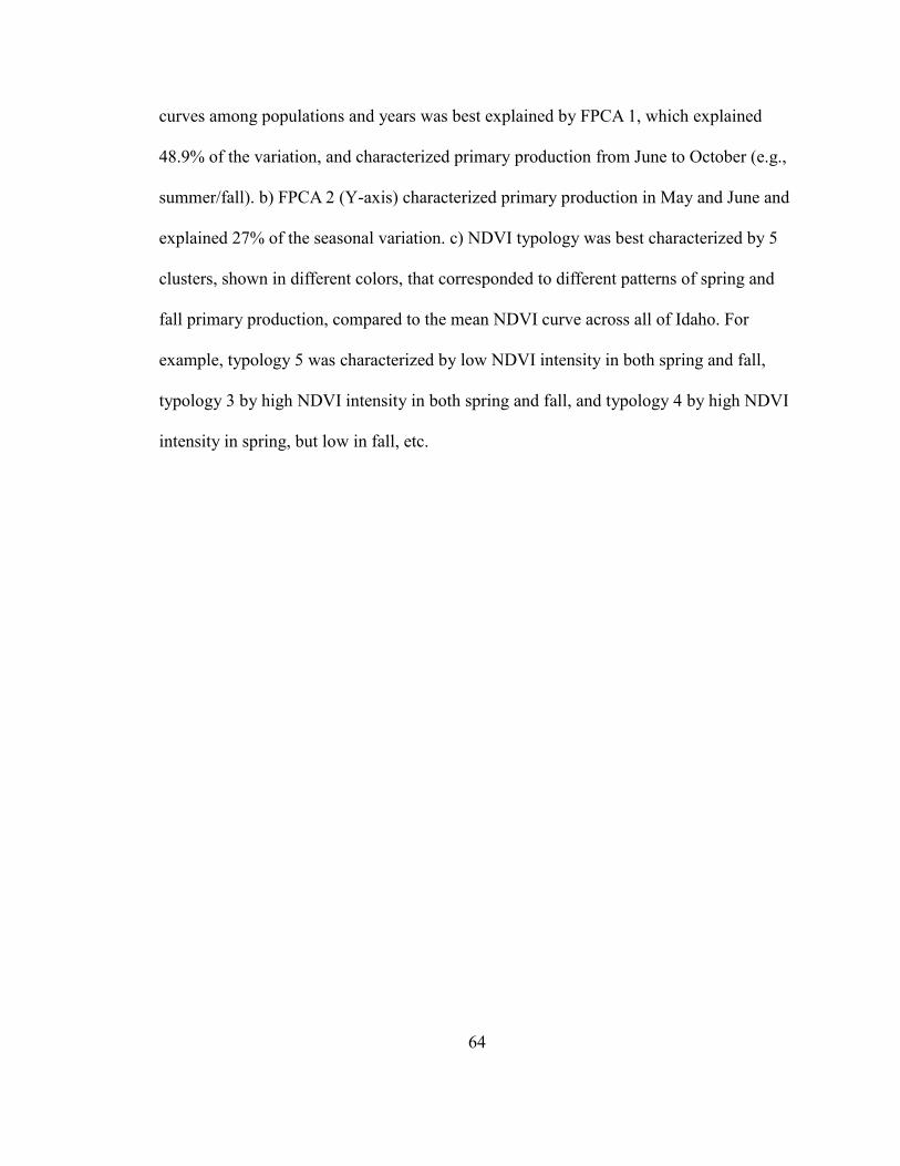
64
curves among populations and years was best explained by FPCA 1, which explained
48.9% of the variation, and characterized primary production from June to October (e.g.,
summer/fall). b) FPCA 2 (Y-axis) characterized primary production in May and June and
explained 27% of the seasonal variation. c) NDVI typology was best characterized by 5
clusters, shown in different colors, that corresponded to different patterns of spring and
fall primary production, compared to the mean NDVI curve across all of Idaho. For
example, typology 5 was characterized by low NDVI intensity in both spring and fall,
typology 3 by high NDVI intensity in both spring and fall, and typology 4 by high NDVI
intensity in spring, but low in fall, etc.

65
Figure 2-2. Distribution of the 5 NDVI typologies shown in Figure 1, with corresponding
colors (inset) across the 13 mule deer populations (GMU’s) in Idaho, USA, from 1998-
2011. The size of the pie wedge is proportional to the frequency of occurrence of each
NDVI typology within that mule deer population. For example, population 56 had all but
one population-year occurring in NDVI typology 4 (Figure 2-1) indicating low primary
productivity during spring but higher during fall.
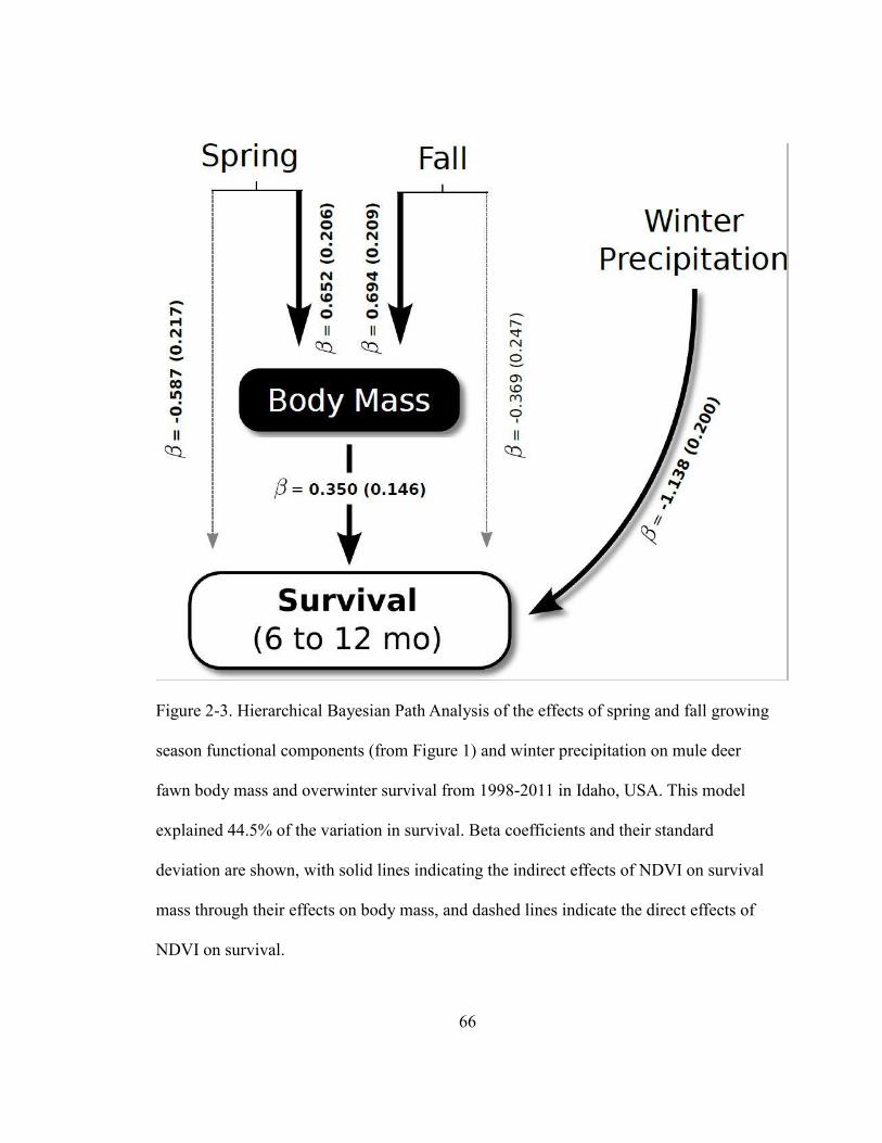
66
Figure 2-3. Hierarchical Bayesian Path Analysis of the effects of spring and fall growing
season functional components (from Figure 1) and winter precipitation on mule deer
fawn body mass and overwinter survival from 1998-2011 in Idaho, USA. This model
explained 44.5% of the variation in survival. Beta coefficients and their standard
deviation are shown, with solid lines indicating the indirect effects of NDVI on survival
mass through their effects on body mass, and dashed lines indicate the direct effects of
NDVI on survival.

67
Figure 2-4. Results of hierarchical Bayesian path analysis showing the standardized direct
effects of a) FPCA component 1 from the functional analysis (Fall NDVI), and b) FPCA
component 2 (Spring NDVI) on body mass (kg) mule deer fawns in Idaho, USA, from
1998-2011.

68
Figure 2-5. Results of hierarchical Bayesian path analysis showing standardized direct
effects of a) body mass (kg), b) cumulative winter precipitation (in mm), c) FPCA
component 1 from the functional analysis (Fall NDVI), and d) FPCA component 2
(Spring NDVI) on the overwinter survival of mule deer fawns in Idaho, USA, from 1998-
2011.
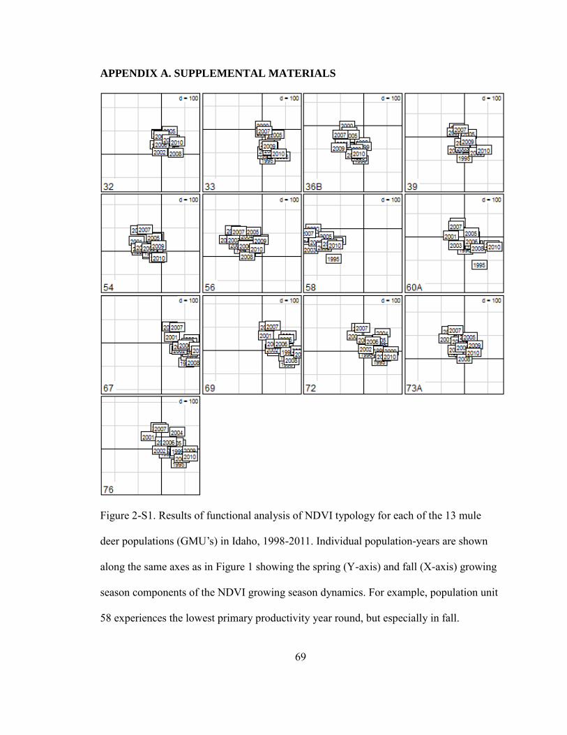
69
APPENDIX A. SUPPLEMENTAL MATERIALS
Figure 2-S1. Results of functional analysis of NDVI typology for each of the 13 mule
deer populations (GMU’s) in Idaho, 1998-2011. Individual population-years are shown
along the same axes as in Figure 1 showing the spring (Y-axis) and fall (X-axis) growing
season components of the NDVI growing season dynamics. For example, population unit
58 experiences the lowest primary productivity year round, but especially in fall.
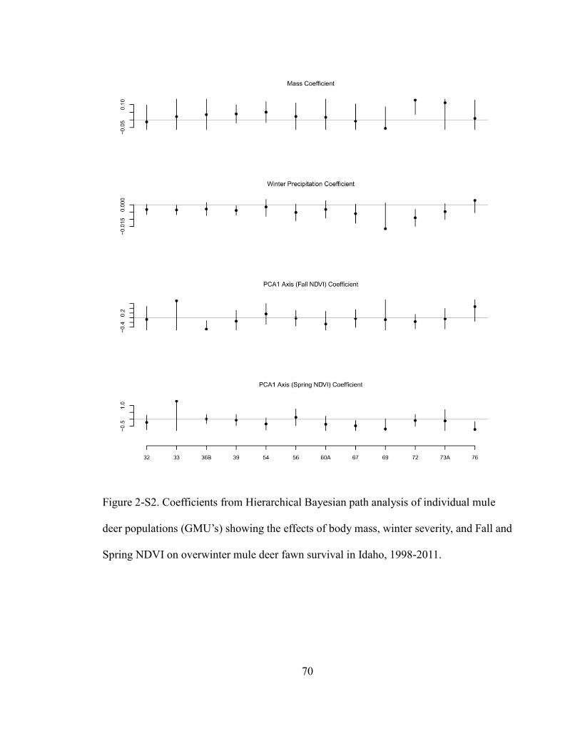
70
Figure 2-S2. Coefficients from Hierarchical Bayesian path analysis of individual mule
deer populations (GMU’s) showing the effects of body mass, winter severity, and Fall and
Spring NDVI on overwinter mule deer fawn survival in Idaho, 1998-2011.
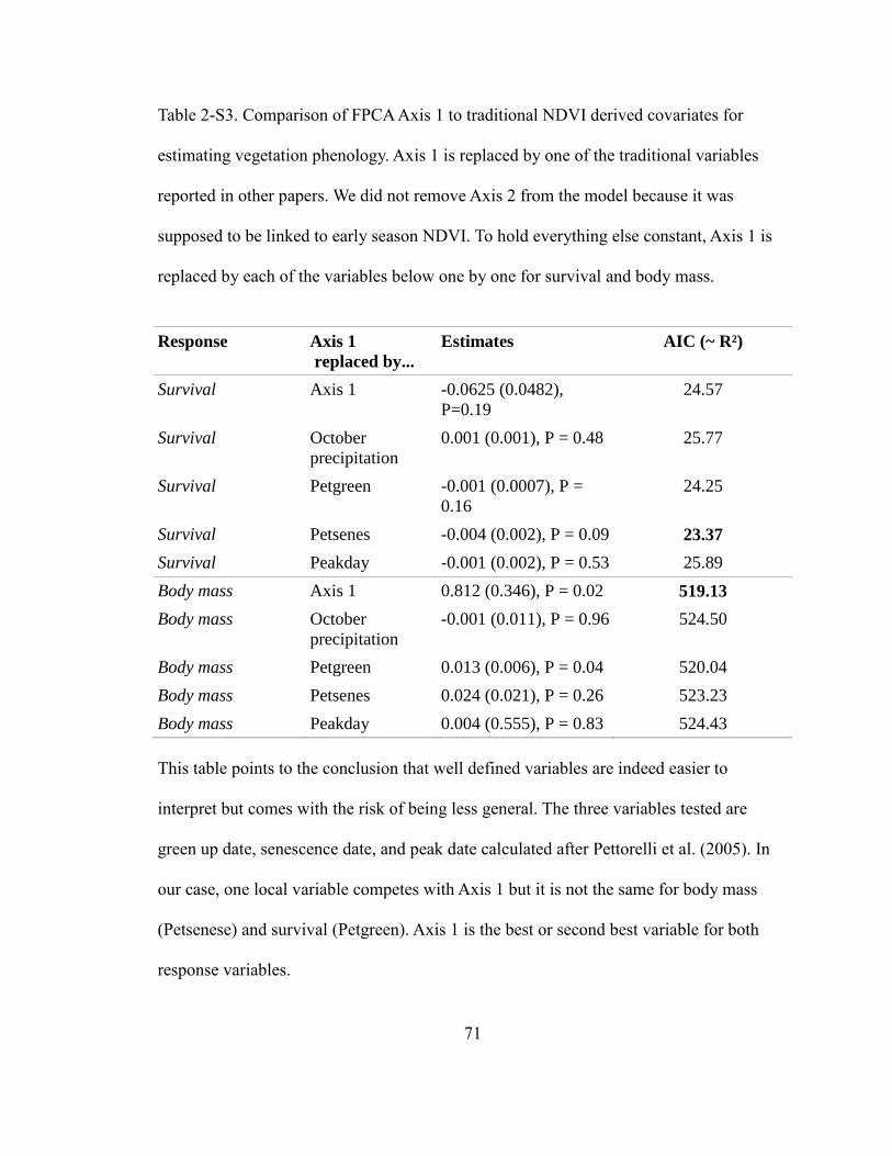
71
Table 2-S3. Comparison of FPCA Axis 1 to traditional NDVI derived covariates for
estimating vegetation phenology. Axis 1 is replaced by one of the traditional variables
reported in other papers. We did not remove Axis 2 from the model because it was
supposed to be linked to early season NDVI. To hold everything else constant, Axis 1 is
replaced by each of the variables below one by one for survival and body mass.
Response Axis 1
replaced by...
Estimates AIC (~ R²)
Survival Axis 1 -0.0625 (0.0482),
P=0.19
24.57
Survival October
precipitation
0.001 (0.001), P = 0.48 25.77
Survival Petgreen -0.001 (0.0007), P =
0.16
24.25
Survival Petsenes -0.004 (0.002), P = 0.09 23.37
Survival Peakday -0.001 (0.002), P = 0.53 25.89
Body mass Axis 1 0.812 (0.346), P = 0.02 519.13
Body mass October
precipitation
-0.001 (0.011), P = 0.96 524.50
Body mass Petgreen 0.013 (0.006), P = 0.04 520.04
Body mass Petsenes 0.024 (0.021), P = 0.26 523.23
Body mass Peakday 0.004 (0.555), P = 0.83 524.43
This table points to the conclusion that well defined variables are indeed easier to
interpret but comes with the risk of being less general. The three variables tested are
green up date, senescence date, and peak date calculated after Pettorelli et al. (2005). In
our case, one local variable competes with Axis 1 but it is not the same for body mass
(Petsenese) and survival (Petgreen). Axis 1 is the best or second best variable for both
response variables.
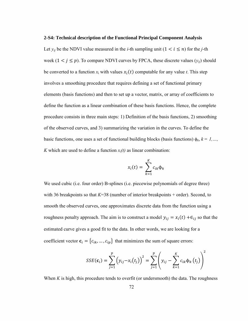
72
2-S4: Technical description of the Functional Principal Component Analysis
Let yij be the NDVI value measured in the i-th sampling unit (1 < 𝑖 ≤ 𝑛) for the j-th
week (1 < 𝑗 ≤ 𝑝). To compare NDVI curves by FPCA, these discrete values (yij) should
be converted to a function xi with values 𝑥𝑖(𝑡) computable for any value t. This step
involves a smoothing procedure that requires defining a set of functional primary
elements (basis functions) and then to set up a vector, matrix, or array of coefficients to
define the function as a linear combination of these basis functions. Hence, the complete
procedure consists in three main steps: 1) Definition of the basis functions, 2) smoothing
of the observed curves, and 3) summarizing the variation in the curves. To define the
basic functions, one uses a set of functional building blocks (basis functions) ϕk, k = 1,…,
K which are used to define a function xi(t) as linear combination:
𝑥𝑖(𝑡) = ∑ 𝑐𝑖𝑘ϕ𝑘
𝐾
𝑘=1
We used cubic (i.e. four order) B-splines (i.e. piecewise polynomials of degree three)
with 36 breakpoints so that K=38 (number of interior breakpoints + order). Second, to
smooth the observed curves, one approximates discrete data from the function using a
roughness penalty approach. The aim is to construct a model 𝑦𝑖𝑗 = 𝑥𝑖(𝑡) +∈𝑖𝑗 so that the
estimated curve gives a good fit to the data. In other words, we are looking for a
coefficient vector 𝐜𝑖 = {𝑐𝑖𝑘, … , 𝑐𝑖𝑝} that minimizes the sum of square errors:
𝑆𝑆𝐸(𝐜𝑖) =∑(𝑦𝑖𝑗−𝑥𝑖(𝑡𝑗))2
𝑝
𝑗=1
=∑(𝑦𝑖𝑗 −∑𝑐𝑖𝑘ϕ𝑘
𝐾
𝑘=1
(𝑡𝑗))
2𝑝
𝑗=1
When K is high, this procedure tends to overfit (or undersmooth) the data. The roughness
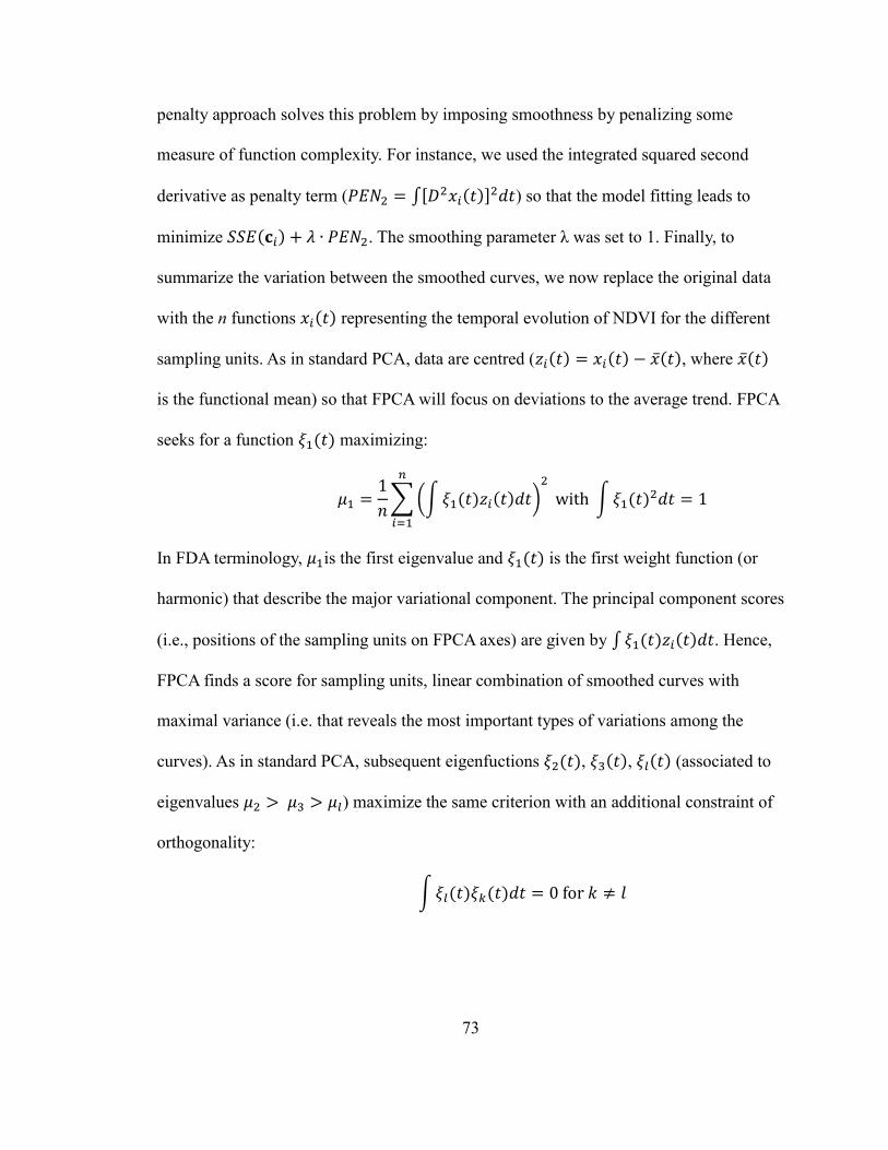
73
penalty approach solves this problem by imposing smoothness by penalizing some
measure of function complexity. For instance, we used the integrated squared second
derivative as penalty term (𝑃𝐸𝑁2 = ∫[𝐷2𝑥𝑖(𝑡)]
2𝑑𝑡) so that the model fitting leads to
minimize 𝑆𝑆𝐸(𝐜𝑖) + 𝜆 ∙ 𝑃𝐸𝑁2. The smoothing parameter λ was set to 1. Finally, to
summarize the variation between the smoothed curves, we now replace the original data
with the n functions 𝑥𝑖(𝑡) representing the temporal evolution of NDVI for the different
sampling units. As in standard PCA, data are centred (𝑧𝑖(𝑡) = 𝑥𝑖(𝑡) − ��(𝑡), where ��(𝑡)
is the functional mean) so that FPCA will focus on deviations to the average trend. FPCA
seeks for a function 𝜉1(𝑡) maximizing:
𝜇1 =1
𝑛∑(∫𝜉1(𝑡)𝑧𝑖(𝑡)𝑑𝑡)
2𝑛
𝑖=1
with ∫ 𝜉1(𝑡)2𝑑𝑡 = 1
In FDA terminology, 𝜇1is the first eigenvalue and 𝜉1(𝑡) is the first weight function (or
harmonic) that describe the major variational component. The principal component scores
(i.e., positions of the sampling units on FPCA axes) are given by ∫ 𝜉1(𝑡)𝑧𝑖(𝑡)𝑑𝑡. Hence,
FPCA finds a score for sampling units, linear combination of smoothed curves with
maximal variance (i.e. that reveals the most important types of variations among the
curves). As in standard PCA, subsequent eigenfuctions 𝜉2(𝑡), 𝜉3(𝑡), 𝜉𝑙(𝑡) (associated to
eigenvalues 𝜇2 > 𝜇3 > 𝜇𝑙) maximize the same criterion with an additional constraint of
orthogonality:
∫𝜉𝑙(𝑡)𝜉𝑘(𝑡)𝑑𝑡 = 0 for 𝑘 ≠ 𝑙

74
2-S5: R code for Bayesian Hierarchical data analysis
# Model specification using JAGS language used to produce Figure 3, 4 and 5.
model
{
# Variable definition
# N : number of site and year estimates of overwinter
survival (integer)
# Y : observed overwinter survival, arcsin-square root
tranformed (covariate)
# GMU : categorical variable (range from 1 to 13)
# mass : body mass of female fawns in late autumn
# winP : average winter precipitation in November –
December
# axis1 : first axis scores of the functional PCA
# axis2 : second axis scores of the functional PCA
# Estimated parameters are alphas (from 1 to 13, plus
alpha_mass) and betas (from 1 to 6)
for(i in 1:N) {
Y[i] ~ dnorm(mu[i], tau)
# Declare response variable as normal
#for survival
# Direct effects of body mass, winter precipitation, axis
1 and axis 2 of the functional PCA.
mu[i] <- alpha[GMU[i]] + beta1 * mass[i] + beta2
* winP[i] +
beta3 * axis1[i] + beta4 *
axis2[i]
mass[i] ~ dnorm(mu_mass[i], tau_mass)
# Declare response variable
# for body mass
# Indirect effects of NDVI on body mass
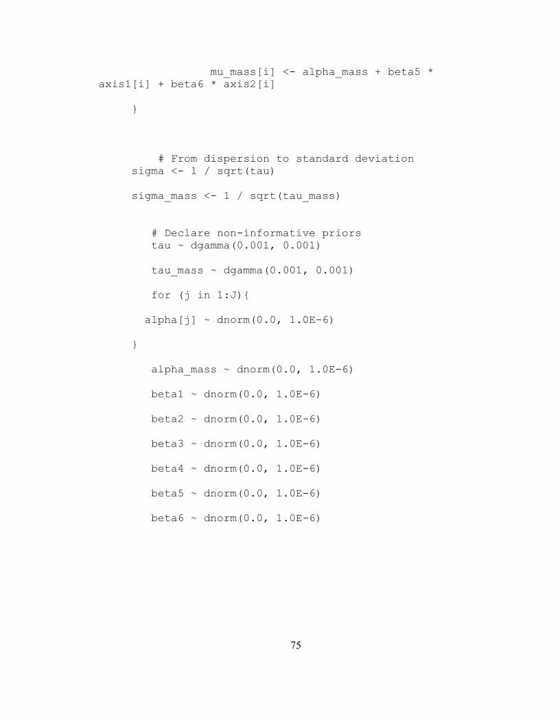
75
mu_mass[i] <- alpha_mass + beta5 *
axis1[i] + beta6 * axis2[i]
}
# From dispersion to standard deviation
sigma <- 1 / sqrt(tau)
sigma_mass <- 1 / sqrt(tau_mass)
# Declare non-informative priors
tau ~ dgamma(0.001, 0.001)
tau_mass ~ dgamma(0.001, 0.001)
for (j in 1:J){
alpha[j] ~ dnorm(0.0, 1.0E-6)
}
alpha_mass ~ dnorm(0.0, 1.0E-6)
beta1 ~ dnorm(0.0, 1.0E-6)
beta2 ~ dnorm(0.0, 1.0E-6)
beta3 ~ dnorm(0.0, 1.0E-6)
beta4 ~ dnorm(0.0, 1.0E-6)
beta5 ~ dnorm(0.0, 1.0E-6)
beta6 ~ dnorm(0.0, 1.0E-6)
76
CHAPTER 3: GENERALITY AND PRECISION OF REGIONAL-SCALE
SURVIVAL MODELS FOR PREDICTING OVERWINTER SURVIVAL OF
JUVENILE UNGULATES2
MARK A. HURLEY, Idaho Department of Fish and Game, P.O. Box 1336, 99 Highway
93 N, Salmon, ID 83467, USA
MARK HEBBLEWHITE, Wildlife Biology Program, Department of Ecosystem and
Conservation Sciences, College of Forestry and Conservation, University of
Montana, Missoula, Montana, 59812, USA
PAUL M. LUKACS, Wildlife Biology Program, Department of Ecosystem and
Conservation Sciences, College of Forestry and Conservation, University of
Montana, Missoula, Montana, 59812, USA
JOSH NOWAK, Wildlife Biology Program, College of Forestry and Conservation,
University of Montana, Missoula, Montana, 59812, USA
JEAN-MICHEL GAILLARD, Laboratoire Biométrie & Biologie Évolutive,
CNRSUMR-CNRS 5558, University Claude Bernard - Lyon I, 69622
Villeurbanne Cedex, France
CHRISTOPHE BONENFANT, Laboratoire Biométrie & Biologie Évolutive,
CNRSUMR-CNRS 5558, University Claude Bernard - Lyon I, 69622
Villeurbanne Cedex, France
2 Formatted for submission to Journal of Wildlife Management.
77
INTRODUCTION
Interest in improving ecological prediction has recently surged because of the growing
need to project the effects of land use and climate change (Mouquet et al. 2015). In
wildlife ecology and management, prediction has played an increasingly important role,
for example in predicting the spatial location of suitable habitat for species
reintroductions (Mladenoff et al. 1999, Boyce and Waller 2003), identifying spatial
human-wildlife conflict areas (Bradley and Pletscher 2005), predicting spatial wildlife-
vehicle collisions (Hurley et al. 2009), nutritional condition and pregnancy of ungulates
(Cook et al. 2004), spatial models of wolf abundance (Rich et al. 2013), and spatial nest
success and survival of birds based on habitat (Aldridge and Boyce 2007). Wildlife
applications have commonly focused on developing technology for spatial predictions,
while rigorous attempts to predict population dynamics and harvest are limited
(Jenouvrier et al. 2009). An exception is perhaps the much-lauded North American
waterfowl program that formally integrates predictions about population size into an
adaptive harvest management framework (Nichols et al. 2007).
While there have been some attempts to formally predict future population
dynamics in harvested ungulates with statistical models (Freddy 1982, Peek et al. 2002,
White and Lubow 2002), prediction is rare in the population management of ungulates,
although the relevance to state wildlife agencies for harvest management programs is
undeniable. One challenge in development of predictive statistical models for survival is
the complexity of dealing with integrating survival data across populations that are
hierarchically structured in space and time (e.g., Lukacs et al. 2009). As wildlife survival
78
studies have increased scope and spatial range, pooling data across multiple populations
has increased model complexity from single season, single population models (Bartmann
and Bowden 1984, White et al. 1987), to populations across multiple years, populations
and ecological regions (Griffin et al. 2011, Brodie et al. 2013). The recent growth of
hierarchical modeling in ecology has furthered the use of Bayesian methods for wildlife
ecologists to enable the development of spatially structured, hierarchical and flexible
statistical models (Royle and Dorazio 2006, Kery and Schaub 2012). Bayesian models
are inherently well-suited to prediction as well, with many recent examples in the
ecological and wildlife literature about prediction of spatially and temporally hierarchical
phenomenon such as epidemiology, animal movements and population ecology (Heisey
et al. 2010a, Geremia et al. 2014, Mouquet et al. 2015). A remaining challenge in
prediction is that not all models can be all things to all needs at all times. Levins (1966)
was amongst the first ecologists to point out that modeling of any sort inherently requires
trade-offs between variance/precision, bias, and generality (the ability of a model to
predict accurately across a range of conditions) and that any model cannot maximize all
three.
In most recent wildlife survival analyses, the best model is usually selected using
a model selection criterion, such as a maximum-likelihood (e.g., Akaike Information
Criteria, AIC) or a Bayesian (e.g., BIC, DIC) approach (Barker and Link 2015). The
entire purpose of model selection methods is hence to select the best statistical model that
approximates performance in out-of-sample prediction. Unfortunately, evaluating future
predictions with independent data is rarely done, but is needed to produce robust
predictive models. Some researchers (Franklin et al. 2000, Frair et al. 2007, Hebblewhite

79
and Merrill 2011) have evaluated the predictive performance of climate or habitat-based
ungulate survival models using data that were used to build the statistical model,
essentially model goodness-of-fit, but not with out-of-sample data sets. Assessing the
predictive power of a model in this fashion, however, often provides an optimistic view
of the model's forecasting ability (Hastie et al. 2001). This lack of external validation is
undoubtedly because of the expense and difficulty in collecting survival data.
Survival is especially difficult to measure in the field, but the ability to predict
future survival of ungulates would greatly improve population dynamics modeling and
thereby, management prescriptions of harvested populations. Vital rates have varying
importance to populations. For example, juvenile survival often drives population
dynamics for large and long-lived species because it is the most variable rate in space and
time (Gaillard et al. 2000). This life-history model has prompted wildlife managers to
prioritize juvenile survival and recruitment monitoring as a means to predict changes in
ungulate population dynamics (White and Bartmann 1998b, Morellet et al. 2007, Lukacs
et al. 2009). Unfortunately, for many species affected by overwinter juvenile survival,
estimates are not available until after harvest regulations are developed. Thus, wildlife
managers do not have the information needed at the time of season setting to make the
best management decisions (Figure 3-1). It would be ideal if wildlife managers had some
reliable way of predicting future overwinter survival based on other drivers of survival,
such as weather variables or habitat characteristics, without the need to capture and
monitor animals.
As a test case, we used a unique data set of mule deer juvenile survival in Idaho to
evaluate the predictive performance of large-scale survival models, from simple to
80
complex, with the ultimate objective of integrating them into harvest management
policies. We aimed to test the predictive performance of overwinter survival models for
mule deer fawns subjected to a large range of habitat quality, climate and predation
regimes in Idaho. We evaluated both model fit (within sample or internal validation) to
identify the main drivers of survival and to assess our capacity (out-of-sample or external
validation) to develop a model that best predicts survival from these drivers. Our goal
was to develop predictive models based on readily available climate and forage
productivity covariates that would enable wildlife managers to predict overwinter
survival, and thus population dynamics and harvest, without having to radiocollar
juveniles.
First we develop models to estimate survival based on freely available remote
sensed weather data. We developed hierarchical Bayesian (H-B) survival models (Lukacs
et al. 2009, Kery and Schaub 2012) that integrate spatial and temporal variation in
summer and winter weather (Hurley et al. 2014), across 11 years and 11 population
management units for mule deer. These models include individual body mass because of
the overwhelming importance of body mass to overwinter survival in juvenile mule deer
repeatedly reported (Bartmann et al. 1992, Unsworth et al. 1999, Bishop et al. 2009,
Hurley et al. 2011, Hurley et al. 2014). We then remove body mass to build predictive
models that do not require animal capture to evaluate the loss of information without
mass. We expanded upon Hurley et al. (2014) by measuring snow cover (MODIS
SNOW) and depth (SNODAS) during three winter periods, early winter (November –
December), winter (January – March) and late winter (April). Increased snow values in
each of these periods should increase energy expenditure and thereby deplete stored fat,

81
thus decreasing survival. We also incorporate the effect of previous growing season with
functional analysis of NDVI (Hurley et al. 2014) to evaluate the effect of early and late
season nutrition, which should positively correlate with subsequent winter survival.
Second, to test the predictive capacity of large-scale survival models, we conduct
both within and out-of-sample validation. We evaluated predicted population-level
survival using in-sample cross-validation (internal validation) by comparing modeled
survival with a non-parametric Kaplan-Meier survival (Kaplan and Meier 1958)
estimated with the same empirical data. We use Kaplan-Meier as a base for this
comparison because it is a widely used metric of survival estimation in wildlife
management agencies and, being non-parametric and non-distributional, is the simplest
descriptive estimator for survival.
We then validated our best empirical models with out-of-sample data to reliably
predict overwinter survival for years not used to fit the model. We test the ability of each
of these models to make predictions across populations and years to evaluate the
precision/generality trade-off in relation to complexity. Specifically, we hypothesized that
if climate-alone drives overwinter mule deer fawn survival, then models of survival only
based on climate covariates should reliably predict observed survival across populations.
Alternately, if unmeasured variables, such as predation or habitat quality, play a crucial
role, not including habitat-climate interaction should weaken the predictive capacity of
climate-only survival models. Therefore, we subset our regional survival model into three
ecotype-specific survival models to test if both predictive performance and predictors of
survival differed at the regional and ecotype levels (Hurley et al. 2014).

82
STUDY AREA
Our study area covered a wide climatic, predation and habitat gradient of mule deer range
in Idaho. We monitored overwinter survival of fawns in 11 Population Management Units
(PMU) across central and southern Idaho that were themselves comprised of 28 different
Game Management Units (GMU’s; Figure 3-2). In Idaho, GMUs are nested within
PMU’s that are grouped together to represent ecological (interbreeding) populations,
which form the basis for management. Through a hierarchical cluster analysis we
classified GMUs into three groups and identified common habitat characteristics of these
groups (called ecotypes hereafter) based on the dominant canopy species on summer
range; coniferous forests, shrub-steppe, and aspen woodlands (Figure 3-2; Appendix B
Figure 3-S1). We then assigned the PMUs to an ecotype classification based on the
classified GMUs. GMUs within PMUs were of the same ecotype with the exception of
one PMU, Mountain Valley, subsequently split into respective shrub and conifer ecotypes
for analysis (Figure 3-2). Elevation and topographic gradients within PMUs affect snow
depths and temperature in winter, and precipitation and growing season length in the
summer, with elevation increasing from the southwest to the northeast. Areas used by
mule deer in the winter in conifer ecotypes ranged in elevation from 1001 to 1928m, but
most were <1450m. Winter precipitation (winter severity) varied widely (from 10 to
371mm) in coniferous GMUs. Coniferous ecotype summer ranges are dominated by
conifer species interspersed with cool season grasslands, sagebrush, and understory of
forest shrubs. Semi-desert Shrub-steppe PMUs ranged from 1545 to 2105m, with winter
precipitation from 24 to 105mm. Summer range within shrub-steppe ecotypes was
dominated by mesic shrubs [e.g., bitterbrush (Purshia tridentata), sagebrush (Artemsia
83
spp.), rabbitbrush (Chrysothamnus spp.)]. Aspen ecotype PMUs were located in the east
and south with winter use areas ranging from 1582 to 2011m, with two of the three PMUs
above 1700m with winter precipitation ranging from 25 to 146mm. In summer,
productive mesic aspen (Populus tremuloides) woodlands were interspersed with mesic
shrubs.
METHODS
(a) Capture and Survival Monitoring
We modeled survival probability of 2,529 fawns within 11 Population Management Units
in southern Idaho, 2003–2013 (Table 3-S1). We varied capture methods depending on
winter range density of deer. In concentrated winter ranges, we used helicopters to herd
deer into drive nets as our primary capture method (Thomas and Novak 1991), but in
dispersed winter ranges we captured fawns with a netgun fired from a helicopter (Barrett
et al. 1982) or clover traps (Clover 1954). Fawns were physically restrained and
blindfolded during processing with an average handling time of < 6 minutes. Two types
of radio-collars were used: expandable collars (Telonics model 500 with CB-5 Telonics
Inc. 932 E. Impala Avenue, Mesa, AZ) and belt collars (Lotek model LMRT-3, Lotek
Wireless Inc., 115 Pony Drive Newmarket, Ontario Canada). Collars weighed 320–400
grams, were equipped with mortality sensors, and fastened with temporary attachment
plates or surgical tubing allowing the collars to fall off the animals after approximately 8–
10 months. We measured fawn mass to the nearest 0.4 kilogram with a calibrated spring
scale to assess early winter body size and condition. An Idaho Department of Fish and
84
Game (IDFG) veterinarian or veterinary technician was on site during most captures to
assist with sampling and assure animal welfare. Animal capture protocols were approved
by the Animal Care and Use Committee, IDFG Wildlife Health Laboratory, Caldwell,
Idaho, USA, and University of Montana IACUC (protocol #02-11MHCFC-031811).
Fawns were monitored with telemetry for mortality from the ground every 2 days
between capture and 1 June. If radio signals could not be detected from the ground within
1 week, animals were located via aircraft. When a mortality signal was detected, the fawn
was located and cause of death was determined using a standard protocol (Wade and
Bowns 1982). Animals that lost radio-collars or with radiocollars that failed were
removed (censored) from the analysis at the point of failure.
(b) Defining Seasons and Herd Unit Home Ranges
Because we wanted to associate individual deer to the weather and spatial covariates
associated with its seasonal range, we estimated within-GMU level seasonal ranges
across all 11 PMU’s (Figure 3-2). Deer were captured within each PMU in each primary
winter range within a GMU (range 1–6 different winter ranges) in proportion to the
distribution of deer and abundance (IDFG unpublished data) in each GMU within the
PMU. To exclude migratory periods from the seasonal home range estimates we only
used locations between 1 June and 30 September for summer ranges and between 1
December and 31 March for winter ranges (Sawyer et al. 2005). We created combined
seasonal 95% kernel density utilization distributions using a bandwidth of H = 0.05 to
minimize the inclusion of unused habitat (Worton 1989). We used all telemetry and
85
mortality locations collected, 1999–2013 (median = 96, range = 21 to 876) to create
winter and summer utilization distributions for each GMU in the study areas. Climate and
habitat information was then summarized within the seasonal home ranges of radio-
collared deer for winter and summer within each GMU, the basis of the spatial covariates.
(c) Survival Variable Development
Individual covariates
Previous studies in Idaho reported only little between-sex differences in overwinter
survival of mule deer fawns (Unsworth et al. 1999, Bishop et al. 2005a, Hurley et al.
2011). In contrast, the overwinter survival of mule deer fawns strongly increases with
their body mass (Hurley et al. 2011). Thus, we included body mass (kg) of mule deer
fawns at capture, as the only individual covariate for comparison purposes.
Spatial forage and weather covariates
We used remotely sensed and modeled measures of summer plant productivity
[Normalized Difference Vegetation Index, NDVI (Pettorelli 2013)] and winter snow
conditions (Snow cover and SNODAS) as spatial covariates for assessing the effects of
climate and habitat on fawn winter survival. We chose remotely sensed spatial measures
of these covariates because remotely sensed data are spatially explicit and generally
available to wildlife managers with a shorter delay than PRISM data, allowing a rapid
integration into harvest management programs.
We calculated NDVI from 16-day composite MODIS (Moderate Resolution

86
Infrared Spectroscopy) obtained from the MOD13Q1 NASA (250m2) data product (from
the NASA Land Products Distributed Active Archive Center LPDAAC,
https://lpdaac.usgs.gov/) (Huete et al. 2002). Radiometric sensor anomalies, atmospheric
effects, cloud contamination and geometric registration accuracies were corrected using a
simple temporal interpolation method (Zhao et al. 2005). We used a minimum NDVI
threshold value of 0 to define periods of little to no photosynthetic activity, and filtered
pixels containing ice and snow data flags from the analysis. Since phenological changes
in NDVI directly represent ungulate forage dynamics only in non-forested vegetation
types, we extracted NDVI values from only open canopied grass and shrub vegetation
types (not burned within five years), which we characterized using SAGEMAP land
cover data (2005 USGS, Forest and Rangeland Ecosystem Science Center, Snake River
Field Station, Boise, ID, USA, described in the supplemental materials). We also
restricted NDVI data to 15 March to 15 November to encompass the entire growing
season for each population-year, and excluded winter anomalies caused by varying snow
conditions.
We then used a Functional Analysis to assess the shapes of the growing season
curves for each population-year according to the methods of Hurley et al. (2014).
However, unlike Hurley et al. (2014) who performed this Functional Analysis on NDVIg
from the AVHRR (Advanced Very High Resolution Radiometer) / NDVI gimms dataset
(Zeng et al. 2013) from 1998-2011, here we used MODIS NDVI. This was because
MODIS NDVI is available at a finer resolution (250m) than AVHRR and is available to
present, where the NDVI gimms dataset ends in 2011, allowing us to include additional
data. Functional analysis was based on a multivariate functional analysis of variation in

87
observed NDVI curves of NDVI values over time. We used the first two principal
component scores of the NDVI curves, which accounted for 74% of the variance and
could be interpreted as a measure of annual fall (post NDVI peak) and spring plant
growth (early growing season). Each of the remaining three other PC scores accounted
for 10% or less of the variance and provided little additional information to explain the
NDVI phenology curves.
To measure winter snow cover, critical for determining energy expenditure and
limiting access to forage, we used two different remotely sensed snow products from the
MODIS satellite platform, and the Snow Data Assimilation System, SNODAS (Hall et al.
2002, Barrett 2003). The MODIS (MOD10A2) snow data product measures complete
snow coverage in 8-day composites at a 250m resolution. We measured snow cover during
three winter periods, early winter (November – December), winter (January – March) and
late winter (April), in two different ways. First, we estimated the percentage of each winter
period each pixel was covered by snow as a measure of fractional snow cover. Second, we
used the number of weeks > 90% of the winter use area was covered by snow. As another
measure of snow effects on survival, we used two measures of SNODAS, which predicts
snow depth at 1km2 daily resolution. SNOWDAS is a numeric model prediction based on air
temperature, relative humidity, wind speed and precipitation downscaled from broad 13km2
scales to the 1-km2. The two measures were average depth during the period and the
cumulative daily measures through the period. The final variables for the survival models
included the following remotely-sensed variables; functional analysis principal
components for fall (FPC), functional analysis principal components for spring (SPC),
mean % snow cover in November and December (ND%snow), mean % snow cover in

88
January to March (W%snow), mean % snow cover in April (A%snow), number of weeks
with >90% snow cover in November and December (FWeeks), number of weeks with
>90% snow cover in January to March (WWeeks), number of weeks with >90% snow
cover in April (AWeeks), average and cumulative snow depth in November and
December (FDepth, FCum), average and cumulative snow depth in January – March
(WDepth, WCum), average and cumulative snow depth in April (ADepth, ACum).
Our goal was to develop a small set of predictive covariates and because these
covariates were derived from similar data sources, we expect them to be highly
correlated. Ideally we wanted to keep the best predictive covariate from each period. To
accomplish this, we screened all covariates for collinearity and retained the individual
covariates of collinear pairs with significant relationship (P < 0.05) to simple discrete
time, known-fate models of overwinter fawn survival. Using these two criteria, we
removed seven covariates from our analysis and retained seven spatial covariates
ecologically related to mule deer ecology and survival; FPC, SPC, ND%snow, W%snow,
A%snow, FWeeks, and WDepth. None of the retained seven covariates had a correlation
coefficient > 0.7 (Appendix B, Table 3-S2).
(d) Survival Modeling
We used Bayesian hierarchical survival models (Royle and Dorazio 2006, Kery and
Schaub 2012) to estimate overwinter fawn survival from 16 December to 1 June,
including covariates at the appropriate spatial and temporal resolution for each
hierarchical level: individual, seasonal range (GMU, j=1….j), and Population

89
Management Unit (PMU, k=1…k; Figure 3-2). We treated survival in a known-fate (with
detection probability = 1 with radio-collars), discrete-time formulation (Murray and
Patterson 2006) in 24 weekly (7-day) intervals from 16 December to 1 June, and
accommodated left and right staggered entry (capture) and exit (mortality, censor)
common in wildlife studies (Pollock et al. 1989). Overwinter survival was estimated as
the product of each weekly interval, seasonal study area, and PMU following the
discrete-time survival paradigm using a generalized linear model with a logit-link
function following:
𝑙𝑜𝑔𝑖𝑡(∅𝑖) = 𝜇 + 𝜀𝑖 Eq. 1
where 𝑙𝑜𝑔𝑖𝑡(𝜙) is the overwinter survival (0, 1) of individual mule deer i=1…n that is a
function of a linear combination of covariates (see Eq. 2 for how we specify covariates),
𝜇, and Bernoulli distributed error 𝜀. Here, we added hierarchical structure to the survival
estimator with different covariate effects hypothesized to manifest at the individual GMU
by season and PMU levels. First, we considered body mass in full models by adding the
individual body mass for each individual mule deer to Eq. 1. This provided us with a way
of measuring the difference in predictive performance between models with and without
body mass. Next we considered the hierarchical spatial structure of seasonal ranges
nested within PMUs using hierarchical random effects (Lukacs et al. 2009, Zuur et al.
2009). We considered a fixed-intercept difference in survival between GMUs to be nested
within a random-intercept difference in survival at the PMU level. We chose to place the
random intercept at the PMU, not GMU level because ostensibly spatial forage and
weather covariates were already incorporated at the GMU level, but a random intercept at
the PMU level allowed for the effect of these GMU-level covariates to vary across PMUs

90
(Zuur et al. 2009). Next we included a random intercept for year to allow for temporal
variation. We then included a combination of our spatial climate covariates measured at
the seasonal-range (GMU) scale. Finally, some covariate effects likely differed between
GMUs in a manner consistent with random coefficients. However, because of
computational difficulty, we only explored one random coefficient at a time in models for
the strongest covariate measured by effect size and precision. Thus, the most complex
formulation for our hierarchical survival model was:
𝑙𝑜𝑔𝑖𝑡( ��𝑖𝑗𝑘|𝑡) = 𝛽0𝑗 + 𝜁0𝑡 + 𝜁0𝑘 + 𝛽1𝑀𝑎𝑠𝑠𝑖 + [𝐁𝐗𝒊𝒋] + 𝜁1𝑘 ∗ 𝑥𝑖𝑗 + 𝜀𝑖𝑗𝑘|𝑡
Eq. 2
where ��𝑖𝑗𝑘|𝑡 is survival of individual mule deer i=1…n in seasonal GMU area j=1…j in
PMU k=1…k in year t=1…11 and 𝜇 in Eq. 1 = 𝛽0𝑗 + 𝜁0𝑡 + 𝜁0𝑘that we define here; 𝛽0𝑗
is the fixed-effect (intercept) of each seasonal range at the GMU level; 𝜁0𝑡 is the random
intercept of year t; 𝜁0𝑘 is the random intercept of PMU; 𝛽1 is the coefficient of individual
body mass; [𝐵𝑋𝑖𝑗] is the vector of seasonal range-level spatial climate covariates (FPC,
SPC, W%snow, etc.) at GMU j; 𝜁1𝑘 is the random coefficient (slope) at the PMU level on
the GMU-level covariate 𝑥𝑖𝑗; and 𝜀𝑖𝑗𝑘∨𝑡 is the error at the level of individual, GMU and
PMU in year t. We assumed all random effects were distributed with mean equal to zero
and unknown variance, e.g., ~ Normal(0, 2).
As a final step to estimating unbiased PMU-level survival, 𝜙𝑘∨𝑡, for evaluation of
predictive capacity at the PMU-level, we applied a weighting scheme to the estimate
obtained with Eq. 2 to weight GMU-level sampling variation in sample sizes according to
91
the estimated mule deer population size (IDFG, unpublished data, Chapter 5) at the PMU
level. Thus, we estimated ��𝑘|𝑡 following:
��𝑘|𝑡 = 𝑛𝑗
𝑛𝑘
∗ ��𝑖𝑗𝑘|𝑡 Eq. 3
where nj = the number of individual mule deer in GMU j (Chapter 5) that is nested in
PMU k.
We fit Bayesian hierarchical survival models with JAGS (Plummer 2003) using a
Metropolis-Hastings Gibbs Markov chain Monte Carlo algorithm (Gelman et al. 2014).
We used non-informative prior distributions for all covariates in Eq. 2 and centered and
scaled (e.g., standardized) all covariates with mean = 0. We ran each model across three
different chains for 20,000 iterations each, with a burn-in of 5,000 iterations (Plummer
2003, Gelman et al. 2014), and obtained posterior distributions, means and medians for
all estimated parameters.
(e) Model Development
Taking advantage of our unusually large sample sizes, we relied on out-of-sample
predictive performance for model selection. We also calculated commonly used metrics
including the Deviance Information Criteria (DIC), the mean Deviance (over all retained
simulations) and the pD, a Bayesian measure of the effective number of parameters
(Gelman et al. 2014). Thus, for each model, we report cross-validation R2CV, the out-of-
sample external validation R2
EV, DIC, Deviance and pD, but strongly favored R2
diagnostics for model selection.

92
We developed a limited candidate set of models considering both summer and
winter seasons for a total of 13 models. We developed models for all animals in the data
set (hereafter overall models), and then partitioned the animals by ecotypes (i.e. ecotype
models for aspen, conifer and shrub-steppe included only data from those PMUs within
each ecotype). We also developed two models (early prediction) using data available
prior to 1 January to assess our ability to predict survival prior to winter, one with a
random effect of FWeeks and one without. For candidate model development, we first fit
a model with all seven covariates (including mass, herein called the full model). We then
removed mass to evaluate a set of prediction-only models. From the full model without
mass we proceeded to remove the least informative parameters, based on credible
intervals overlapping 0 and effect size of the standardized covariates, in a purposeful
backward stepwise fashion (retaining each successive model) until reaching a reduced
model where all parameters were highly informative (Gelman et al. 2014). Because of the
high diversity of the climate and of the habitat across our study area, we then added a
random effect (coefficient) for slope for each of the covariates identified in the reduced
model as the most informative parameters (only one for each model) to the full models
and reduced models. Random effects of covariates were not applied to ecotypes models
because covariate effects were expected to be similar within ecotypes. Our final step was
to predict survival with data collected prior to 1 January as a truly predictive model for
practical use in the harvest season setting process. We evaluated early prediction models
comprised of the most important covariates identified during overall model development.

93
(f) Evaluating the Precision, Accuracy and Generality of Survival Models
We evaluated models using both internal validation and external validation for our overall
set of models, prediction-only models (e.g., no body mass), and ecotype models (Hastie
et al. 2001). We considered internal validation as a measure of the model’s goodness-of-
fit and external (e.g., out-of-sample) validation as the strongest measure of a model’s
generality, accuracy and precision (Hastie et al. 2001), as well as the ultimate model
selection diagnostic (Hooten and Hobbs 2015). We first predicted the expected survival
for each animal given a set of covariates using Eq. 2, using all data for internal cross-
validation. We conducted internal validation for all models (overall, ecotype, etc.).
Second, we conducted external validation withholding all survival data for 2007 and
2008 to estimate predictive performance. We did not externally validate ecotype models
due to small sample sizes, but compared ecotype models’ internal validation to our
overall models to evaluate if using finer-scale ecotype models would increase
explanatory power of survival models.
We compared predicted survival rates from each Bayesian survival model against
observed survival rates within each year and PMU. Observed survival rates were
estimated using the simple non-parametric, non-distributional Kaplan-Meier (K-M)
estimator (Kaplan and Meier 1958):
𝑆𝑡,�� = ∏ (𝑛𝑖−𝑑𝑖
𝑛𝑖)𝑡,𝑘
𝑖=1 Eq. 4
and 𝑆𝑡,𝑘 is the estimated survival of mule deer in year i=1…t, and PMU k=1…k, ni is the
number of animals starting each weekly interval, di is the number of deaths, and the
product of the weekly survival rates provides the non-parametric estimator of survival.

94
We used Pearson’s correlation coefficient between observed and predicted survival to
estimate precision (R2). We also assessed the bias of the regression between observed and
predicted (i.e., a slope of 1 indicates equality of both) using spline curves. The JAGS
code for our hierarchical survival models is presented in Appendix B (Table 3-S4).
RESULTS
(a) Observed survival
We captured and monitored a total of 2,529 fawns, averaging ~ 30 fawns/year/PMU
(range 14 to 75) per year from 2003–2013 to develop survival models (Appendix B,
Table 3-S1). Statewide survival of fawns ranged from 0.32 (SE = 0.032) to 0.71 (SE =
0.034) during 2003–2013, and mean survival for all years varied across PMUs (Figure 3-
2b; Appendix B, Table 3-S1, for PMU-year specific KM estimates).
(b) Covariate and random effects for overall model
Male fawns were heavier than females (mean = 37.1 kg vs. 34.2 kg, t = -13.1, P < 0.005)
and survival increased with mass in the full overall Bayesian survival model
(standardized coefficient, = 0.457, SE = 0.037). In our overall models, winter survival
increased with higher fall plant productivity later in the fall (Figure 3-3, Appendix B,
Table 3-S2). Higher snow cover during January through March and higher number of
weeks in autumn with >90% snow cover both decreased fawn survival (Figure 3-3,
Appendix B, Table 3-S2). Survival also increased with higher spring functional analysis
values but this effect was more variable between models than the effects of plant
95
productivity in fall (Figure 3-3, Appendix B, Table 3-S2) and thus SPC was not included
in the final model. Winter snow depth and snow cover in April had minimal relationship
to winter fawn survival for the overall models (Figure 3-3, Appendix B, Table 3-S2).
The high spatial heterogeneity of the study area was highlighted by the strength of
both random intercepts and random slopes (Figure 3-2c, Appendix B, Table 3-S2). There
was support for variation between PMUs in overall survival and also in the effects of
winter on survival (Table 3-1, Figure 3- 4) as all the top five models in terms of internal
validation included random slopes of one other most influence top three covariates (Table
3-1). However, these models add complexity and parameters thus were not considered
amongst the top models according to DIC or validation diagnostics. Covariate effects also
varied considerably across PMUs. For example, the influence of winter snow cover on
survival varied across PMUs, with the strongest influence in the high elevation
southeastern PMUs and least in the low elevation western PMUs (Figure 3-2c).
(c) Overall survival model validation, prediction, and complexity
Ranking overall survival models using internal validation, external validation or DIC
produced contrasting perspectives on what is the ‘best’ model. The best-supported overall
survival model in terms of internal explanatory capacity (R2cv = 0.814) was a model
including all covariates (excluding body mass) with a random effect (slope) for winter
percent snow cover (Table 3-1, Figure 3-4). If we were to rank models using DIC,
however, a model with all covariates including mass was most supported (Table 3-1),
despite the substantially lower explanatory capacity (R2cv = 0.695).

96
Overall model predictions correlated well with the Kaplan-Meier survival
estimates for the external validation, when 403 mule deer fawns from 2007-2008 were
left out (Figure 3-5). Although the highest R2
CV was obtained with the most complex
model with a random effect of snow cover in winter, the R2
EV was substantially lower
when these two validation years were including in the re-parameterization of this top
model (Figures 4 & 5, R2 = 0.814 for all years vs. 0.698 with 2007 and 2008 excluded
and predicted). Without mass included, the most parsimonious model with the highest
external predictive power (R2
EV = 0.704) was a function of three covariates, winter
percent snow cover, fall NDVI, and the number of weeks with complete snow cover in
November and December (Table 3-1, Figure 3-5). The most supported early prediction
model (only covariates before 1 January) included three covariates with a random slope
for Fall Weeks with > 90% snow cover with high explanatory capacity (R2cv = 0.818),
but low external predictive power (R2
EV = 0.590).
The reduced model produced a slightly lower R2 (0.785) between KM and
modeled estimates, suggesting a trade-off between generality and precision when
predicting survival. Although, the R2 of the model fit must increase as covariates are
added, the opposite was true in the validation (Figure 3-4 vs. 3-5). Validation of these
models suggested that the best performing model in terms of predictive power was not
necessarily the best explanatory model. Interestingly, the top model that did not include
mass ranked by DIC was also the best non-random effects survival model to successfully
predict out-of-sample mule deer survival (Figure 3-5). Our most parsimonious model
predicted better than the more complex models, likely due to overfitting the data with the
additional parameters included by DIC. This suggests that for generality of true

97
prediction, the more complex models were becoming more and more overfit. Thus, the
absolutely best model from an external validation and prediction perspective in this case
was the simplest function of three covariates (model 2 in Table 3-1).
(d) Ecotype survival models and covariate effects
Model selection results were similar among vegetative ecotypes as the top models from a
DIC perspective in all ecotypes were the full models including mass (Table 3-2, Figures
3-3 to 3-6). In the aspen ecotype, there was a perfect correspondence between the ‘best’
model selected from a traditional DIC perspective and the internal validation (Table 3-2).
However, the best model from DIC in the conifer ecotype had the poorest predictive
performance. The overall predictive performance of the shrub-steppe models was lower
than conifer or aspen, and the top predictive model had two fewer covariates than the
best-selected model from DIC. The covariate effect of body mass was similar in each
ecotype model where it was retained in to the overall survival model reported above; =
0.504, SD = 0.071 in aspen, = 0.429, SD = 0.046 in conifer, and = 0.397, SD = 0.095
in shrub-steppe. Mass only improved predictive performance for aspen. Inclusion of mass
in conifer resulted in the worst predictive performance, and in shrub-steppe, mass
reduced prediction again. The models we would select to predict ecotype survival without
mass would be model 5 in aspen with two covariates; model 5 in conifer, and model 1 in
shrub-steppe (Table 3-2).
Models without mass had equivalent predictive performance as other, more
complicated models (e.g., R2
CV of 0.859 for aspen model 2 with seven covariates versus
R2
CV of 0.853 for the two covariate model). Internal validation R2
CV of all aspen models

98
were > 0.851, suggesting an improved fit over the most parsimonious overall model
(Table 3-1, Figure 3-4). The best internally validated model for conifer ecotype was the
full model, excluding Mass (Table 3-2, Figure 3-6). This conifer model explained 0.803
of the variance in overwinter fawn survival. The best internally validated model for
shrub-steppe was the 6-covariate model, excluding Mass and WDepth, accounting for
60.4% of the variance (Table 3-2, Figure 3- 6). The effect of summer range quality did
not have the strength in ecotype specific model as in the overall likely due to similar
values within the ecotype, whereas winter snow conditions will be more site-specific. Our
prediction of lower performance in more carnivore-driven systems is supported by both
the lower R2 of the top conifer model than the aspen and our survival prediction
consistently biased low when predicting high survival in the conifer models versus the
aspen models.
DISCUSSION
By combining Bayesian hierarchical survival models with spatio-temporal data on forage
and winter conditions derived from remote sensing, we successfully developed powerful
explanatory mule deer survival models across most of the state of Idaho. This supports
our general working hypothesis that climatic variation and primary production are the
major determinants of juvenile mule deer overwinter survival. Our overall models were
able to externally predict out-of-sample survival with R2EV values that ranged from 0.59 –
0.71 across time and space. This is a novel approach because there have been few if any
tests of the predictive capacity of such a large-scale model to predict the survival of a key
99
demographic trait for a harvested species. The modeling approach we advocated should
enable wildlife managers to estimate the key vital rate of a population in a large range of
ecological contexts. The first step should be to identify this critical vital rate. As
recruitment is often the most important vital rate for ungulates (Gaillard et al. 2000), the
key component should be either the summer or the winter juvenile survival. In mule deer,
like in other ungulates living in northern temperate areas such as bighorn sheep (King et
al. 2006, Eacker 2015), identifying the drivers of overwinter survival might allow
reducing the need to capture and monitor ungulates annually. Instead, a monitoring
system incorporating survival prediction with periodic monitoring for model calibration
would save considerable funds with minimal loss in accuracy. Our most general survival
model predicted overwinter survival of mule deer fawns through Idaho’s wide variety of
vegetation, climate, and predator communities with easily obtainable remote-sensed data
pertaining to vegetation quality and winter snow estimates.
The success of our approach based on Bayesian hierarchical models requires
matching the spatial or temporal scale of covariates to the appropriate survival period
(Heisey et al. 2010a, Heisey et al. 2010b, Heisey 2012). In this case we measured
MODIS-based NDVI and snow covariates derived from MODIS and SNOWDAS
products defined by the fawn habitat use in the population of interest in specific summer
and winter ranges. In addition to these spatiotemporal remote sensing covariates, we also
accounted for variation related to large-scale processes, such major vegetative differences
through the use of random-effect terms for these unmeasured, but important, latent
variables. PMUs in Idaho were developed from movement data of radio-collared animals
representing putatively interbreeding populations that overlapped in their distribution on
100
summer and fall ranges (Idaho Mule Deer Management Plan 2008). These PMU
designations did not necessarily consider differences in vegetation quality, winter
severity, and predation risk between specific summer and winter ranges. Allowing these
effects to vary across winter ranges (GMU scale) within PMUs and across PMUs allowed
covariates to account for the biological processes involved while minimizing the noise of
inherent differences in PMUs. Our Bayesian hierarchical survival models provided an
efficient means to capture this mix of measured and unmeasured drivers of overwinter
fawn survival across scales.
The importance of scale to regional hierarchical models was best exemplified by
the inconsistent importance of body mass in the survival models. Body mass is a very
strong predictor of juvenile ungulate survival across a multitude of studies (Bartmann and
Bowden 1984, Unsworth et al. 1999, Pettorelli et al. 2002, Bishop et al. 2009, Griffin et
al. 2011, Hurley et al. 2014). Increased mass-at-capture strongly increased overwinter
survival of mule deer fawns as expected. However, our best overall survival models that
included mass (Table 3-1, models 9 and 11) had poorer predictive power than even our
simplest survival models, accounting for ~ 10% less variation. We suggest this disparity
is caused by spatial differences in vegetation quality and winter severity that were
effectively captured by remotely-sensed measures of habitat. For example, fawn mass in
the Palisades PMU was generally higher (39.5 kg, SE = 2.46) than elsewhere in the state
because of high quality spring and summer range that also enabled higher body growth
rates through the summer. However, winter snow cover and depth was often also the
highest in this region (Figure 3-2b), resulting in high fawn mortality and overriding the
benefit of higher mass arising from higher summer forage. In contrast, Boise River PMU
101
fawn body mass was generally the lower (Male mean = 36.1kg, SE=1.52) because of
poorer quality spring/summer forage and low precipitation. Despite these lower ‘quality’
fawns, the Boise River PMU experienced the least snow and mild winters; thus, perhaps
counter-intuitively, survival was often high in this PMU without the low survival
experienced in the higher elevation PMUs during severe winters. This contrast between
summer and winter determinants of overwinter survival is interesting, but not ultimately
why we think mass performed more poorly as a predictive covariate at our broadest scale
of winter models. When averaging across different PMUs with high and low fawn body
mass, body mass could not ultimately predict survival as well as PMU-level spatial and
temporally varying covariates which ultimately drove differences in both starting body
mass at the beginning of winter (e.g., summer forage) and the response, e.g., mortality or
hazard rate of fawns in response to winter severity. This discussion also highlights that
viability selection (Fisher 1930), whereby the lightest individuals are more likely to die
either summer or winter, especially in lower quality habitat, may also be operating and
another reason why body mass predicts individual overwinter survival well, but loses
predictive strength at the population-level. Viability selection normally operates strongest
on summer (neonatal) survival, reducing poor quality individuals before winter, but can
also operate on the remaining cohort entering winter. Our weather covariates and the
Bayesian hierarchical modeling framework will control for most of these differences, but
extreme conditions may decouple the relationship when applied within the same model.
The importance of spatial variation in forage and winter snow cover influencing
overwinter survival was also displayed in the top explanatory model (Table 3-1). This
model included a random slope for winter snow instead of body mass, and accounted for

102
the highest proportion of variance in our overall model set (R2
CV =0.814). For example,
in Boise PMU there was no effect of winter (Figure 3-2c), whereas in all the southeastern
PMUs (e.g., Bannock, Caribou, and Palisades), the strength of the winter snow effect was
nearly double that of those in the central conifer PMUs (Figure 3-2c, Central Mountains,
Island Park, Smoky/Bennett, Weiser/McCall). We interpret that the random coefficient
accounted for some of the variation at the PMU or GMU-level in the hazard rate caused
by winter snow, which reflects spatial variation across PMUs in the realized effect body
mass had on overwinter survival. For example, in the Bannock, Caribou, and Palisades
PMUs, fawns with relatively high body mass often experienced greater overwinter
mortality not because of a stronger effect of winter snow per se, but merely because of
absolute winter severity, which was almost double the amount of snow as other PMUs
(Figure 3-2c). However, even this random coefficient could not predict out-of-sample
survival as well as the most parsimonious model that simply included the spatial variation
in three key covariates directly. This discussion highlights that inferences from our
Bayesian hierarchical survival models will vary depending on the scale of application,
and also the challenges of interpreting random coefficients in complex models, again,
emphasizing a parsimonious approach (Bolker et al. 2009, Zuur et al. 2009).
There was additional evidence in our survival modeling that ecotypes provided a
biologically relevant scale for considering mechanisms affecting survival. Differences in
snow cover between PMUs followed the ecotype divisions based solely on vegetation
cluster analysis (Figure 3-2). This suggests that ecotype could be a strong driver of
survival through nutrition or predator habitat and good partitioning metric. This is similar
to a recent continental-scale synthesis of elk calf recruitment (which includes overwinter

103
survival) reporting that ecotype differences accounted for more observed variation in
recruitment than state-level or administrative boundaries (Lukacs et al. In Review).
Moreover, in contrast to the overall mule deer survival models, body mass was included
in the top ecotype models for all three ecotypes, aspen, conifer and shrub-steppe (Table 3-
2) with a consistent positive effect between ecotypes on survival.
The ecotype-specific effects of summer/fall forage and winter snow on mule deer
overwinter survival varied between ecotypes in ways that corresponded to important
differences between PMUs. This is similar to many previous studies of mule deer, and
other ungulates, that used a variety of different measures of forage and winter severity
(Bishop et al. 2005a, Bishop et al. 2009, Hurley et al. 2011). Our approach evaluated the
same consistent set of predictors across a wide geographical gradient and revealed
important between-ecotype differences. For example, fall phenology (FPC) was observed
to be important in the conifer communities, but not in the eastern aspen communities
where only Nov-Dec weeks with complete snow and winter snow cover predicted
survival quite closely (R2
CV=0.853, Table 3-2, Figure 3-4). Yet, winter snow cover had
similar magnitude effects on fawn survival in both aspen and conifer (Figure 3-3), but
Nov-Dec snow cover only negatively affected survival in conifer. The forage production
and quality of shrub-steppe communities was highly influenced by precipitation, more so
than communities with canopy tree (aspen or conifer) cover as evidenced by the positive
relationship of most types of precipitation (including snow) and summer phenology to
survival. It appears that in these xeric shrub-steppe ecotypes, any moisture, except early
winter snow (which we interpret as indicating the end of the fall growing season), will
have a positive effect on survival in this ecotype as these open areas may require winter

104
snow moisture for plant growth in early spring. In general across all ecotypes, vegetation
phenology as measured by NDVI had much weaker effect sizes than the two primary
snow covariates (W%snow and Fweeks, Figure 3-3). Snow accumulation is a more fine-
scale process than vegetation phenology because minimal changes in temperature and
aspect will change snowfall to rain. This may explain why FPC and SPC were important
in the statewide models, but lose importance in the aspen ecotype model. Phenology is
similar across this region, limiting its effectiveness to differentiate survival among PMUs
within ecotypes. In the aspen ecotype, snow depth was important, likely due to the higher
elevation areas and increased average snow depth. The full model including mass was the
best fitting model for aspen, again suggesting that mass is a finer-scale process and
related to snow conditions.
The regional variation we found in remotely-sensed measures of winter snow may
also reflect differences in spatial resolution. For example, the higher resolution of the
MODIS data at 250m as opposed to SNODAS at 1km may likely explain greater
importance of snow cover compared to snow depth. The higher resolution may more
accurately capture the effect of elevation and aspect in our topographically variable
winter ranges by reflecting the snow free areas of a winter range at lower elevation.
Regardless of which remotely sensed measure of winter severity was retained in our
survival models, both allowed spatial variation in the measure of snow to improve
predictions of overwinter survival.
Our challenge in producing predictive models of survival was to balance the
precision, bias, and generality trade-offs (Levins 1966) while using readily obtainable
covariates that describe the complexity of our spatially diverse system. This approach

105
allowed us to select the most parsimonious model that maximized generality across large
regional areas while minimizing model complexity (i.e. our simplest model has higher
out-of-sample predictive capacity as our most complex model). This simple model with
just three covariates, one summer vegetation quality and 2 two winter snow measures,
should be general enough to estimate overwinter fawn survival in much of the arid west,
given the data for model development was obtained from the diverse vegetation types.
Interestingly, the inclusion of body mass decreased predictive capacity across ecotypes,
likely because mass is related to individual survival, but the random sample of mean
mass as used when predicting survival is a weaker measure of population level effects.
The flexibility of a general model is important because Bishop et al. (2005) observed
winter survival of fawns was not spatially synchronous even in adjacent winter ranges
and cautioned that extrapolating survival to other populations can lead to erroneous
population estimates, a problem we solved with our modeling approach.
Beyond statistical reasons, the potential discrepancies between predictions and
observations might involve predation, which could also result in lower than predicted
survival. We exclusively used vegetation quality and snow covariates to model survival,
but this may not successfully capture predation-related drivers of fawn survival over the
winter. For example, in our system, 21% (10% - 60%) of the fawns are killed by
predators during winter (M. Hurley, unpublished data). Thus we only modelled 79% of
the variation in overwinter survival when ignoring predation. Moreover, the interaction of
weather conditions and habitat may influence fawn survival through predation risk
(Griffin et al. 2011). Our predictive models also ignored possible density-dependence
(Bonenfant et al. 2009). Understanding the mechanism by which forage-risk trade-offs

106
translate to mortality may be the last critical step needed to integrate density and
predation into survival models. While including covariates representing density and
predation appeals ecologically, from a practical viewpoint, wildlife managers often will
not have access to this information over large regions. Instead, as our ecotype-scale
models demonstrate, some of this potential bias between observed and predicted survival
seems to be diminished in the ecotype-scale models with lower predictive performance
occurring in our highest predation risk ecotype, conifer.
We conclude that wildlife population studies should put more effort into testing
the predictive performance of their models to understand their generality. Previous large-
scale demographic syntheses of neonatal elk calf survival (Griffin et al. 2011), adult
female elk survival (Brodie et al. 2013), and calf:cow ratios (Lukacs et al. 2015) all
developed relatively parsimonious models to explain spatio-temporal variation of vital
rates over large regions, far greater than our study. For example, Griffin et al. (2011)
predicted 90-day elk calf survival using a fairly basic model of the number of predator
species, previous summer precipitation, and May precipitation. This model accounted for
a reasonable percentage of the variation (42%), but the out-of-sample predictive
performance had never been tested so far. Conversely, many study-area specific survival
models tend to often be so highly parameterized that we can question their predictive
potential in other systems. Very few wildlife survival studies address any aspect of either
internal or external validation. Internal validation may be limited by methodology
because to date, discrete time survival modeling approaches still do not provide any
measure of goodness-of-fit for evaluating internal model fit from a known-fate survival
model (White and Burnham 1999).
107
MANAGEMENT IMPLICATIONS
We have developed models to predict mule deer fawn overwinter survival from 16
December to 1 June in Idaho’s semi-arid intermountain habitats. The models exclude
information related to cause-specific mortality and mass of deer because this information
is not commonly available to managers. Once these models are validated or modified for
different vegetation communities, mule deer managers will realize extensive cost savings
if winter fawn survival is now included in their monitoring program (radiocollared
fawns). Modeling winter fawn survival with periodic fawn captures to empirically
estimate fawn survival and calibrate the models can be included within integrated
population models for harvest prescriptions. We suggest using the reduced overall model
as the generality will likely transfer to different environments. Using the early prediction
models will provide managers the ability to predict survival in the current winter, prior to
harvest season development. Survival predictions can then be verified with the overall
models for the entire winter season. We invite mule deer managers and researchers to
evaluate performance of our models against their current monitoring program as further
validation.
LITERATURE CITED
Ballard, W. B., D. Lutz, T. W. Keegan, L. H. Carpenter, and J. C. deVos, Jr. 2001. Deer-
Predator Relationships: A Review of Recent North American Studies with
Emphasis on Mule and Black-Tailed Deer. Wildlife Society Bulletin 29:99-115.

108
Barker, R. J. and W. A. Link. 2015. Truth, models, model sets, AIC, and multimodel
inference: A Bayesian perspective. The Journal of Wildlife Management.
Barrett, A. 2003. National Operational Hydrologic Remote Sensing Center SNOw Data
Assimilation System (SNODAS) Products at NSIDC. . NSIDC Special Report 11.
Boulder, CO, USA: National Snow and Ice Data Center. Digital media.
Barrett, M., J. Nolan, and L. Roy. 1982. Evaluation of hand held net-gun to capture large
mammals. Wildlife Society Bulletin 10:108-114.
Bartmann, R. M. and D. C. Bowden. 1984. Predicting mule deer mortality from weather
in Colorado. Wildlife Society Bulletin 12:246-248.
Bartmann, R. M., G. C. White, and L. H. Carpenter. 1992. Compensatory Mortality in a
Colorado Mule Deer Population. Wildlife Monographs:3-39.
Bishop, C. J., J. W. Unsworth, E. O. Garton, and Ransom. 2005. Mule deer survival
among adjacent populationsin Southwest Idaho. Journal of Wildlife Management
69:311-321.
Bishop, C. J., G. C. White, D. J. Freddy, B. E. Watkins, and T. R. Stephenson. 2009.
Effect of Enhanced Nutrition on Mule Deer Population Rate of Change. Wildlife
Monographs 172:1-28.
Bolker, B. M., M. E. Brooks, C. J. Clark, S. W. Geange, J. R. Poulsen, M. H. H. Stevens,
and J.-S. S. White. 2009. Generalized linear mixed models: a practical guide for
ecology and evolution. Trends in Ecology & Evolution 24:127-135.
Boyce, M. S. and J. S. Waller. 2003. Grizzly Bears for the Bitterroot: Predicting Potential
Abundance and Distribution. Wildlife Society Bulletin 31:670-683.

109
Bradley, E. H. and D. H. Pletscher. 2005. Assessing Factors Related to Wolf Depredation
of Cattle in Fenced Pastures in Montana and Idaho. Wildlife Society Bulletin
33:1256-1265.
Brodie, J., H. Johnson, M. Mitchell, P. Zager, K. Proffitt, M. Hebblewhite, M. Kauffman,
B. Johnson, J. Bissonette, C. Bishop, J. Gude, J. Herbert, K. Hersey, M. Hurley, P.
M. Lukacs, S. McCorquodale, E. McIntire, J. Nowak, H. Sawyer, D. Smith, P. J.
White, and P. Stephens. 2013. Relative influence of human harvest, carnivores,
and weather on adult female elk survival across western North America. Journal
of Applied Ecology 50:295-305.
Clover, M. R. 1954. A portable deer trap and catch net. California Fish and Game 40:367-
373.
Cook, J. G., B. K. Johnson, R. C. Cook, R. A. Riggs, T. Delcurto, L. D. Bryant, and L. L.
Irwin. 2004b. Effects of summer‐autumn nutrition and parturition date on
reproduction and survival of elk. Wildlife Monographs 155:1-61.
Eacker, D. R. 2015. Linking the effects of risk factors on annual calf survival to elk
population dynamics in the Bitterroot Valley, Montana. The University of
Montana Missoula.
Fisher, R. A. 1930. The genetical theory of natural selection. Oxford University Press,
Oxford.
Frair, J. L., E. H. Merrill, J. R. Allen, and M. S. Boyce. 2007. Know Thy Enemy:
Experience Affects Elk Translocation Success in Risky Landscapes. Journal of
Wildlife Management 71:541-554.
110
Franklin, A. B., D. R. Anderson, R. Gutiérrez, and K. P. Burnham. 2000. Climate, habitat
quality, and fitness in northern spotted owl populations in northwestern
California. Ecological Monographs 70:539-590.
Freddy, D. J. 1982. Predicting mule deer harvest in Middle Park, Colorado. Journal of
Wildlife Management 46:801-806.
Gaillard, J.-M., M. Festa-Bianchet, N. G. Yoccoz, A. Loison, and C. Toigo. 2000.
Temporal variation in fitness components and population dynamics of large
herbivores. Annual Review of Ecology and Systematics 31:367-393.
Gelman, A., J. B. Carlin, H. S. Stern, D. B. Dunson, A. Vehtari, and D. Rubin. 2014.
Bayesian data analysis. CRC Press, Taylor & Francis Group, Chapman and Hall,
New York, NY.
Geremia, C., P. J. White, J. A. Hoeting, R. L. Wallen, F. G. R. Watson, D. Blanton, and N.
T. Hobbs. 2014. Integrating population and individual-level information in a
movement model of Yellowstone bison. Ecological Applications 24:346-362.
Griffin, K., M. Hebblewhite, P. Zager, H. R. Robinson, S. Barber-Meyer, D. Christenson,
S. Creel, N. Harris, M. Hurley, D. Jackson, B. Johnson, L. D. Mech, W. L. Myers,
J. Raithel, M. Schlegel, B. Smith, and P. J. White. 2011. Neonatal mortality of elk
driven by climate, predator phenology and predator diversity. Journal of Animal
Ecology 80:1246–1257.
Hall, D. K., G. A. Riggs, V. V. Salomonson, N. E. DiGirolamo, and K. J. Bayr. 2002.
MODIS snow-cover products. Remote Sensing of Environment 83:181-194.
Hastie, T., T. Tibshirani, and J. Freidman, editors. 2001. The elements of statistical
learning: data mining, inference, and prediction. Springer, New York.

111
Hebblewhite, M. and E. H. Merrill. 2011. Fitness balancing in a partially migratory
ungulate through risk-forage trade-offs. Oikos 120:1860-1870.
Heisey, D. 2012. Bayesian shared frailty models for regional inference about wildlife
survival. Animal Conservation 15:127-128.
Heisey, D. M., E. E. Osnas, P. C. Cross, D. O. Joly, J. A. Langenberg, and M. W. Miller.
2010a. Linking process to pattern: estimating spatiotemporal dynamics of a
wildlife epidemic from cross-sectional data. Ecological Monographs 80:221-241.
Heisey, D. M., E. E. Osnas, P. C. Cross, D. O. Joly, J. A. Langenberg, and M. W. Miller.
2010b. Rejoinder: sifting through model space. Ecology 91:3503-3514.
Hooten, M. and N. Hobbs. 2015. A guide to Bayesian model selection for ecologists.
Ecological Monographs 85:3-28.
Huete, A., K. Didan, T. Miura, E. P. Rodriguez, X. Gao, and L. G. Ferreira. 2002a.
Overview of the Radiometric and Biophysical Performance of the Modis
Vegetation Indices. Remote Sensing of Environment 83:195-213.
Hurley, M. A., M. Hebblewhite, J. M. Gaillard, S. Dray, K. A. Taylor, W. K. Smith, P.
Zager, and C. Bonenfant. 2014. Functional analysis of normalized difference
vegetation index curves reveals overwinter mule deer survival is driven by both
spring and autumn phenology. Philos Trans R Soc Lond B Biol Sci
369:20130196.
Hurley, M. A., J. W. Unsworth, P. Zager, M. Hebblewhite, E. O. Garton, D. M.
Montgomery, J. R. Skalski, and C. L. Maycock. 2011. Demographic response of
mule deer to experimental reduction of coyotes and mountain lions in
southeastern Idaho. Wildlife Monographs 178:1-33.
112
Hurley, M. V., E. K. Rapaport, and C. J. Johnson. 2009. Utility of Expert-Based
Knowledge for Predicting Wildlife-Vehicle Collisions. Journal of Wildlife
Management 73:278-286.
Jenouvrier, S., H. Caswell, C. Barbraud, M. Holland, J. Strœve, and H. Weimerskirch.
2009. Demographic models and IPCC climate projections predict the decline of
an emperor penguin population. Proceedings of the National Academy of
Sciences 106:1844-1847.
Kaplan, E. L. and D. B. Meier. 1958. Nonparametric estimation from incomplete
observations. Journal of the American Statistical Association 53:457-481.
Kery, M. and M. Schaub. 2012. Bayesian population analysis using WinBUGS: a
hiearchical perspective. Acadmic Press, San Diego, CA.
King, R., S. P. Brooks, B. J. Morgan, and T. Coulson. 2006. Factors influencing soay
sheep survival: a Bayesian analysis. Biometrics 62:211-220.
Levins, R. 1966. The strategy of model building in population biology. American
Scientist 54:421 - 431.
Lukacs, P. M., G. C. White, B. E. Watkins, R. H. Kahn, B. A. Banulis, D. J. Finley, A. A.
Holland, J. A. Martens, and J. Vayhinger. 2009. Separating Components of
Variation in Survival of Mule Deer in Colorado. The Journal of Wildlife
Management 73:817-826.
Mladenoff, D. J., T. A. Sickley, and A. P. Wydeven. 1999. Predicting Gray Wolf
Landscape Recolonization: Logistic Regression Models Vs. New Field Data.
Ecological Applications 9:37-44.
113
Morellet, N., J. M. Gaillard, A. Hewison, P. Ballon, Y. Boscardin, P. Duncan, F. Klein,
and D. Maillard. 2007. Indicators of ecological change: new tools for managing
populations of large herbivores. Journal of Applied Ecology 44:634-643.
Mouquet, N., Y. Lagadeuc, V. Devictor, L. Doyen, A. Duputié, D. Eveillard, D. Faure, E.
Garnier, O. Gimenez, P. Huneman, F. Jabot, P. Jarne, D. Joly, R. Julliard, S. Kéfi,
G. J. Kergoat, S. Lavorel, L. Le Gall, L. Meslin, S. Morand, X. Morin, H. Morlon,
G. Pinay, R. Pradel, F. M. Schurr, W. Thuiller, and M. Loreau. 2015. Predictive
Ecology In A Changing World. Journal of Applied Ecology 52:1293-1310.
Nichols, J. D., M. C. Runge, F. A. Johnson, and B. K. Williams. 2007. Adaptive harvest
management of North American waterfowl populations: a brief history and future
prospects. Journal of Ornithology 148:S343-S349.
Peek, J. M., B. Dennis, and T. Hershey. 2002. Predicting Population Trends of Mule Deer.
Journal of Wildlife Management 66:729-736.
Pettorelli, N. 2013. The Normalized Difference Vegetation Index. Oxford University
Press, Oxford, UK.
Pettorelli, N., J.-M. Gaillard, G. Van Laere, P. Duncan, P. Kjellander, O. Liberg, D.
Delorme, and D. Maillard. 2002. Variations in adult body mass in roe deer: the
effects of population density at birth and of habitat quality. Proceedings of the
Royal Society of London B: Biological Sciences 269:747-753.
Plummer, M. 2003a. JAGS: A program for analysis of Bayesian graphical models using
Gibbs sampling.in 2003 Distributed Statistical Computing 2003 Working Papers,
Vienna, Austria.
114
Pollock, K. H., S. R. Winterstein, and M. J. Conroy. 1989. Survival analysis in telemetry
studies: the staggered entry design. Journal of Wildlife Management 53:7-15.
Rich, L. N., R. E. Russell, E. M. Glenn, M. S. Mitchell, J. A. Gude, K. M. Podruzny, C.
A. Sime, K. Laudon, D. E. Ausband, and J. D. Nichols. 2013. Estimating
occupancy and predicting numbers of gray wolf packs in Montana using hunter
surveys. The Journal of Wildlife Management 77:1280-1289.
Royle, J. A. and R. M. Dorazio. 2006. Hierarchical models of animal abundance and
occurrence. Journal of Agricultural Biological and Environmental Statistics
11:249-263.
Sawyer, H., F. Lindzey, and D. Mcwhirter. 2005. Mule Deer and Pronghorn Migration in
Western Wyoming. Wildlife Society Bulletin 33:1266-1273.
Thomas, R. and B. Novak. 1991. Helicopter drive-netting techniques for mule deer
capture on Great Basin ranges. California Fish and Game 77:194-200.
Unsworth, J. A., D. F. Pac, G. C. White, and R. M. Bartmann. 1999. Mule deer survival in
Colorado, Idaho, and Montana. Journal of Wildlife Management 63:315-326.
Wade, D. A. and J. E. Bowns. 1982. Procedures for evaluating predation on livestock and
wildlife. Texas Agricultural Extension Service, Texas Agricultural Experiment
Station, Texas A & M University System.
White, G. C. and R. M. Bartmann. 1998. Mule deer management—what should be
monitored. Pages 104-118 in Proceedings of the 1997 Deer/Elk Workshop, Rio
Rico, Arizona. Arizona Game and Fish Department. Phoenix, USA.
White, G. C. and K. P. Burnham. 1999. Program MARK: survival estimation from
populations of marked animals. Bird study 46:S120-S139.

115
White, G. C., R. A. Garrott, R. M. Bartmann, L. H. Carpenter, and A. W. Alldredge. 1987.
Survival of mule deer in Northwest Colorado. Journal of Wildlife Management
51:852-859.
White, G. C. and B. C. Lubow. 2002. Fitting population models to multiple sources of
observed data. The Journal of Wildlife Management 66:300-309.
Worton, B. J. 1989. Kernel Methods for Estimating the Utilization Distribution in Home-
Range Studies. Ecology 70:164-168.
Zhao, M. S., F. A. Heinsch, R. R. Nemani, and S. W. Running. 2005. Improvements of
the Modis Terrestrial Gross and Net Primary Production Global Data Set. Remote
Sensing of Environment 95:164-176.
Zuur, A. E., E. N. Leno, N. J. Walker, A. A. Saveliev, and G. M. Smith. 2009. Mixed-
effects models and extensions in ecology in R. Springer, New York, NY.

116
TABLES
Table 3-1. Model selection results for the overall, overwinter Hierarchical Bayesian
survival model for mule deer (Odocoileus hemionus) fawns based on 2529 individuals
from 2003-2013 in Idaho, USA. The overall models contain data from all Population
Management Units (PMU) and all years, and the full models contain all of the covariates.
For each model, we report the model structure with covariates, Deviance Information
Criterion (DIC), Difference from lowest DIC (ΔDIC), Effective Number of Parameters
(pD), Deviance, and validation metrics. We conducted two forms of model validation;
cross-validation within the observed data (R2cv) and external validation (R
2EV) with
withheld survival data collected on n = 403 mule deer fawns in years 2007-2008 in the
same study areas. The best model identified by each of the criteria (ΔDIC , R2cv , R
2EV)
are bolded. Covariates include mean snow cover in November and December
(ND%snow), mean snow cover in January to March (W%snow), mean snow cover in
April (A%snow), functional analysis principal components for fall (FPC), functional
analysis principal components for spring (SPC), number of weeks with >90% snow cover
in November and December (FWeeks), and average snow depth in January – March
(Depth).

117
Model ΔDIC DIC pD Deviance R2
CV R2
EV
1 W%snow(random)+FPC+FWeeks 122.9 11197.6 2409.1 8788.4 0.806 0.705
2 W%snow+FPC+FWeeks 71.4 11146.1 2358.0 8788.1 0.785 0.704
3 Full with random % W%snow 162.6 11237.3 2451.0 8786.3 0.814 0.698
4 ND%snow+W%snow+A%snow+FPC+SPC+FWeeks+Depth 228.8 11303.5 2517.6 8785.8 0.795 0.677
5 ND%snow +W%snow+A%snow+FPC+SPC+FWeeks 101.1 11175.8 2391.4 8784.4 0.796 0.675
6 ND%snow +W%snow+A%snow+FPC+FWeeks 228.7 11303.4 2515.0 8787.5 0.789 0.671
7 Full with random FWeeks 186.4 11261.1 2473.9 8789.1 0.808 0.667
8 W%snow+FPC(random)+FWeeks 123.3 11198.0 2415.1 8779.9 0.800 0.649
9 Full with random W%snow + Mass 176.3 11251.0 2650.4 8600.6 0.719 0.644
10 Full with random FPC 162.1 11236.8 2454.9 8781.8 0.806 0.628
11 ND%snow+W%snow+A%snow+FPC+SPC+FWeeks+Depth+Mass 0.0 11074.7 2472.1 8602.6 0.695 0.620
12 FPC+SPC+FWeeks (early prediction) 174.8 11249.5 2480.6 8768.9 0.816 0.620
13 FPC+SPC+FWeeks(random) (early prediction) 176.5 11251.2 2478.1 8773.0 0.818 0.590
R2
CV = Cross validation; R2
EV = Validation with external data
118
Table 3-2. Model selection results for the ecotype specific, overwinter Hierarchical
Bayesian survival models for mule deer (Odocoileus hemionus) fawns based on 2529
individuals, including all years of data from 2003-2013 in Idaho, USA. The full models
contain all of the covariates. For each model we report, the model structure with
covariates, Deviance Information Criterion (DIC), Difference from lowest DIC (ΔDIC),
Effective Number of Parameters (pD), Deviance, and validation metrics (Cross validation
R2). The best model identified by each of the criteria (ΔDIC , R
2cv ) are bolded.
Covariates are; mean snow cover in November and December (ND%snow), mean snow
cover in January to March (W%snow), mean snow cover in April (A%snow), functional
analysis principal components for fall (FPC), functional analysis principal components
for spring (SPC), number of weeks with >90% snow cover in November and December
(FWeeks), and average snow depth in January – March (Depth).
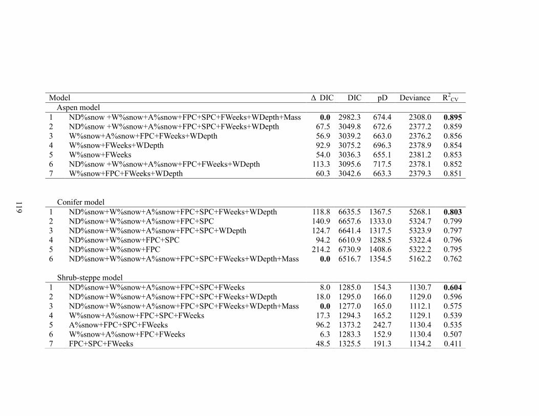
119
Model Δ DIC DIC pD Deviance R2
CV
Aspen model
1 ND%snow +W%snow+A%snow+FPC+SPC+FWeeks+WDepth+Mass 0.0 2982.3 674.4 2308.0 0.895
2 ND%snow +W%snow+A%snow+FPC+SPC+FWeeks+WDepth 67.5 3049.8 672.6 2377.2 0.859
3 W%snow+A%snow+FPC+FWeeks+WDepth 56.9 3039.2 663.0 2376.2 0.856
4 W%snow+FWeeks+WDepth 92.9 3075.2 696.3 2378.9 0.854
5 W%snow+FWeeks 54.0 3036.3 655.1 2381.2 0.853
6 ND%snow +W%snow+A%snow+FPC+FWeeks+WDepth 113.3 3095.6 717.5 2378.1 0.852
7 W%snow+FPC+FWeeks+WDepth 60.3 3042.6 663.3 2379.3 0.851
Conifer model
1 ND%snow+W%snow+A%snow+FPC+SPC+FWeeks+WDepth 118.8 6635.5 1367.5 5268.1 0.803
2 ND%snow+W%snow+A%snow+FPC+SPC 140.9 6657.6 1333.0 5324.7 0.799
3 ND%snow+W%snow+A%snow+FPC+SPC+WDepth 124.7 6641.4 1317.5 5323.9 0.797
4 ND%snow+W%snow+FPC+SPC 94.2 6610.9 1288.5 5322.4 0.796
5 ND%snow+W%snow+FPC 214.2 6730.9 1408.6 5322.2 0.795
6 ND%snow+W%snow+A%snow+FPC+SPC+FWeeks+WDepth+Mass 0.0 6516.7 1354.5 5162.2 0.762
Shrub-steppe model
1 ND%snow+W%snow+A%snow+FPC+SPC+FWeeks 8.0 1285.0 154.3 1130.7 0.604
2 ND%snow+W%snow+A%snow+FPC+SPC+FWeeks+WDepth 18.0 1295.0 166.0 1129.0 0.596
3 ND%snow+W%snow+A%snow+FPC+SPC+FWeeks+WDepth+Mass 0.0 1277.0 165.0 1112.1 0.575
4 W%snow+A%snow+FPC+SPC+FWeeks 17.3 1294.3 165.2 1129.1 0.539
5 A%snow+FPC+SPC+FWeeks 96.2 1373.2 242.7 1130.4 0.535
6 W%snow+A%snow+FPC+FWeeks 6.3 1283.3 152.9 1130.4 0.507
7 FPC+SPC+FWeeks 48.5 1325.5 191.3 1134.2 0.411
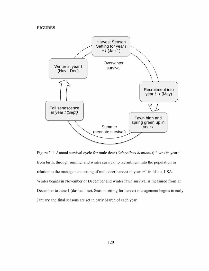
120
FIGURES
Figure 3-1. Annual survival cycle for mule deer (Odocoileus hemionus) fawns in year t
from birth, through summer and winter survival to recruitment into the population in
relation to the management setting of mule deer harvest in year t+1 in Idaho, USA.
Winter begins in November or December and winter fawn survival is measured from 15
December to June 1 (dashed line). Season setting for harvest management begins in early
January and final seasons are set in early March of each year.
Harvest Season Setting for year t
+1 (Jan 1)
Winter in year t (Nov - Dec)
Fall senescence in year t (Sept)
Fawn birth and spring green up in
year t
Recruitment into year t+1 (May)
Summer
(neonate survival)
Overwinter
survival

121
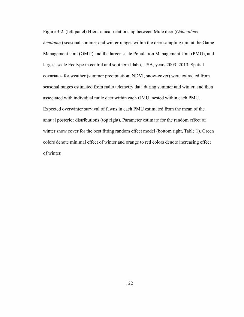
122
Figure 3-2. (left panel) Hierarchical relationship between Mule deer (Odocoileus
hemionus) seasonal summer and winter ranges within the deer sampling unit at the Game
Management Unit (GMU) and the larger-scale Population Management Unit (PMU), and
largest-scale Ecotype in central and southern Idaho, USA, years 2003–2013. Spatial
covariates for weather (summer precipitation, NDVI, snow-cover) were extracted from
seasonal ranges estimated from radio telemetry data during summer and winter, and then
associated with individual mule deer within each GMU, nested within each PMU.
Expected overwinter survival of fawns in each PMU estimated from the mean of the
annual posterior distributions (top right). Parameter estimate for the random effect of
winter snow cover for the best fitting random effect model (bottom right, Table 1). Green
colors denote minimal effect of winter and orange to red colors denote increasing effect
of winter.

123
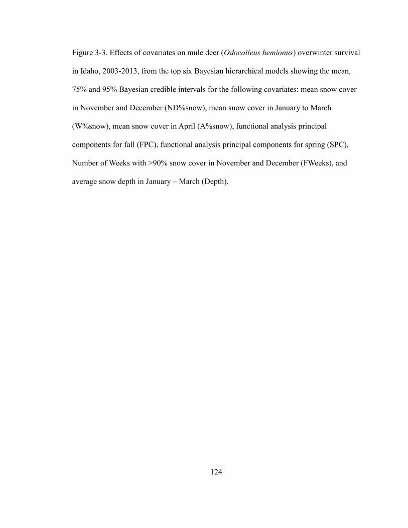
124
Figure 3-3. Effects of covariates on mule deer (Odocoileus hemionus) overwinter survival
in Idaho, 2003-2013, from the top six Bayesian hierarchical models showing the mean,
75% and 95% Bayesian credible intervals for the following covariates: mean snow cover
in November and December (ND%snow), mean snow cover in January to March
(W%snow), mean snow cover in April (A%snow), functional analysis principal
components for fall (FPC), functional analysis principal components for spring (SPC),
Number of Weeks with >90% snow cover in November and December (FWeeks), and
average snow depth in January – March (Depth).

125
Figure 3-4. Observed (Kaplan-Meier survival, x axis) versus predicted (modeled y axis)
overwinter survival of 6-month old mule deer (Odocoileus hemionus) fawns in southern
and central Idaho for each PMU, 2003-2013. Survival was predicted for 2529 mule deer
fawns using a hierarchical Bayesian survival model that accounted for spatial and

126
temporal variation in covariates. Panel figures for the numbering scheme of Table 1 a)
Model 10, b) Model 1, c) Model 6, d) Model 5, e) Model 3, f) Model 9. The first model is
the only model that includes mass. The blue line is a spline fit to illustrate bias of
modeled survival estimates from observed estimates.
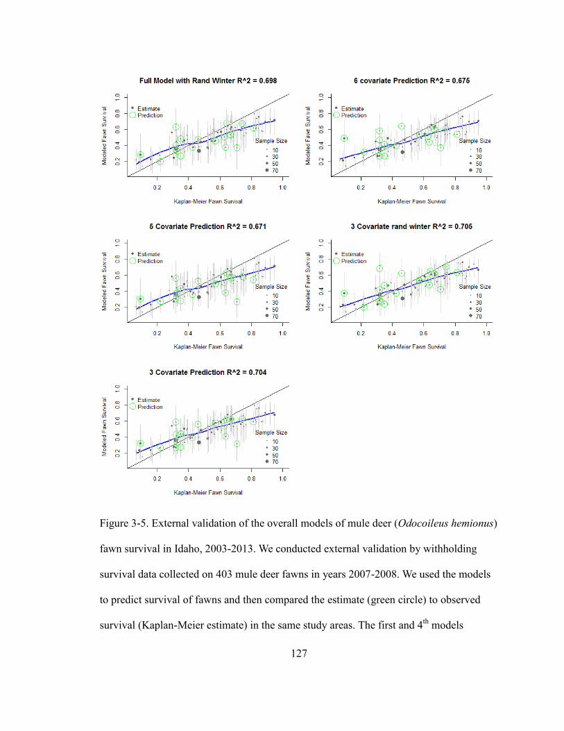
127
Figure 3-5. External validation of the overall models of mule deer (Odocoileus hemionus)
fawn survival in Idaho, 2003-2013. We conducted external validation by withholding
survival data collected on 403 mule deer fawns in years 2007-2008. We used the models
to predict survival of fawns and then compared the estimate (green circle) to observed
survival (Kaplan-Meier estimate) in the same study areas. The first and 4th
models

128
include a random effect of winter % snow cover the others only random intercept and
correspond to model numbers in Table 1. The blue line is a spline fit to illustrate bias of
modeled survival estimates from observed estimates.

129
Figure 3-6. Observed (Kaplan-Meier x axis) versus predicted (modeled y axis) overwinter
survival of 6-month old mule deer (Odocoileus hemionus) fawns within a, b) Aspen c, d)
Conifer, and e, f) Shrub-Steppe ecotypes in southern Idaho, 2003-2013. The two most
supported models are presented.
a b
f e
d c

130
The blue line is a spline fit to illustrate bias of modeled survival estimates from observed
estimates.
131
APPENDIX B. SUPPLEMENTAL MATERIALS
December 26, 2015
Hurley, M., Hebblewhite, M., et al. 2015. Generality and precision of regional-
scale survival models for predicting overwinter survival of mule deer fawns
Journal of Wildlife Management, In Review.
3-S1: Summer Range Ecotype Classification
We used summer range as the basis for clusters as these season ranges show the greatest
potential variance is nutritional quality and vegetation types. Vegetation variables were
developed from the SAGEMAP vegetation layer (2005 USGS, Forest and Rangeland
Ecosystem Science Center, Snake River Field Station, Boise, ID). The layer contained
126 land cover classes with a minimum mapping unit (MMU) of approximately 1 acre
(0.4 ha). We reclassified the image into 18 vegetation classes with importance to mule
deer ecology. These vegetation classes included; aspen woodland, riparian, other
deciduous woodland, juniper woodland, mahogany woodland, coniferous forest,
deciduous shrub land, mesic sagebrush shrub land, xeric sagebrush shrub land, wet
meadow, mesic grassland, xeric grassland (includes Conservation Reserve Program
lands), invasive grassland, agriculture, recent burn, open water, developed, and
unavailable. The weighted mean accuracy assessment of the reclassification was 84.4%.
We used a hierarchical weighted means cluster analysis based on summer range
vegetation types within summer home ranges used by the wintering herd unit (Figure 3-
S1) to identify vegetation community clusters. Defining differences identified in the three

132
primary clusters were % conifer (>40%), %aspen (6 to 13%), and % mesic sagebrush
(>60%) on summer range. The GMUs were distributed among the ecotypes with five in
conifer ecotype (GMUs 32, 33, 36B, 39, 60A), two in shrub-steppe ecotype (GMUs 54,
58), and six in aspen (GMUs 56, 67, 69, 72, 73A, 76). PMUs were assigned to group
depending on the designation of GMUs in each PMU.
Supplement Figure 3-S1. Hierarchical weighted means grouping of GMUs based on
percent of vegetation types within deer sub-population summer range.
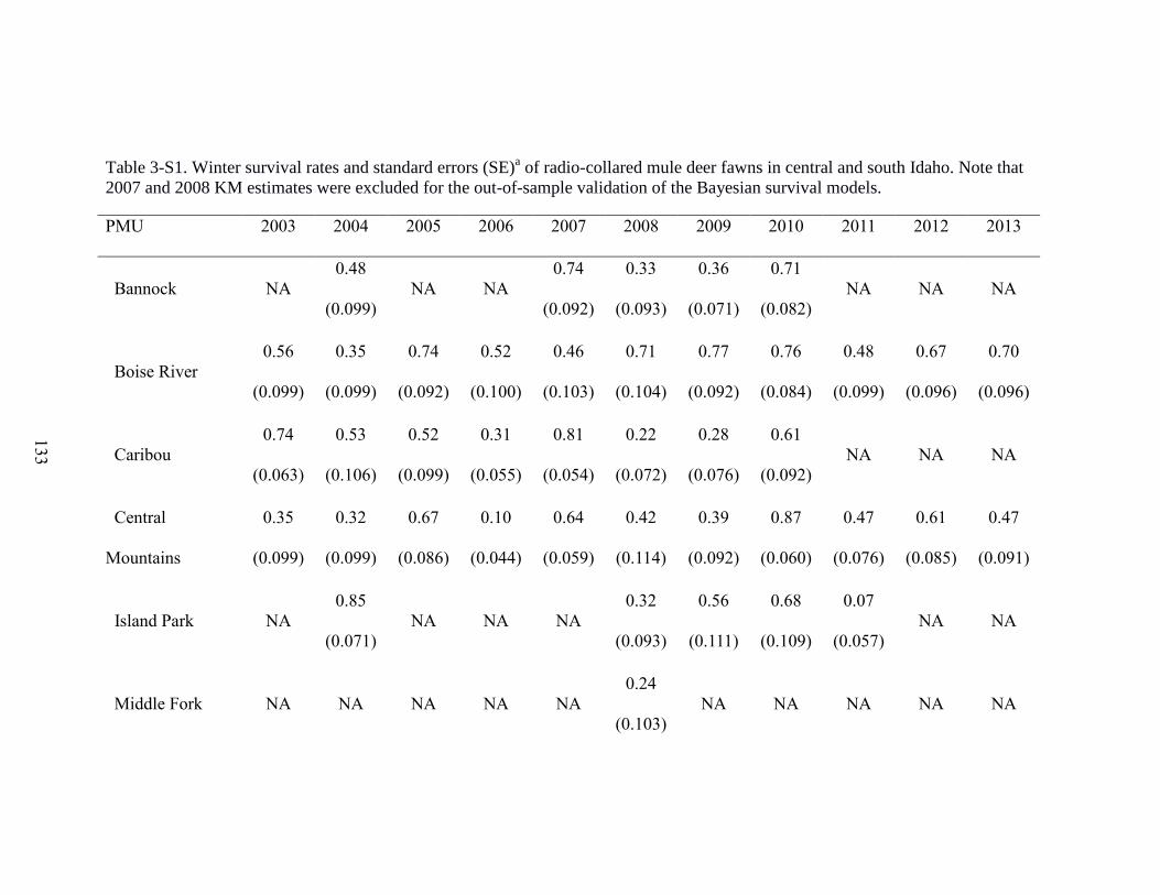
133
Table 3-S1. Winter survival rates and standard errors (SE)a of radio-collared mule deer fawns in central and south Idaho. Note that
2007 and 2008 KM estimates were excluded for the out-of-sample validation of the Bayesian survival models.
PMU 2003 2004 2005 2006 2007 2008 2009 2010 2011 2012 2013
Bannock NA
0.48
(0.099)
NA NA
0.74
(0.092)
0.33
(0.093)
0.36
(0.071)
0.71
(0.082)
NA NA NA
Boise River
0.56
(0.099)
0.35
(0.099)
0.74
(0.092)
0.52
(0.100)
0.46
(0.103)
0.71
(0.104)
0.77
(0.092)
0.76
(0.084)
0.48
(0.099)
0.67
(0.096)
0.70
(0.096)
Caribou
0.74
(0.063)
0.53
(0.106)
0.52
(0.099)
0.31
(0.055)
0.81
(0.054)
0.22
(0.072)
0.28
(0.076)
0.61
(0.092)
NA NA NA
Central
Mountains
0.35
(0.099)
0.32
(0.099)
0.67
(0.086)
0.10
(0.044)
0.64
(0.059)
0.42
(0.114)
0.39
(0.092)
0.87
(0.060)
0.47
(0.076)
0.61
(0.085)
0.47
(0.091)
Island Park NA
0.85
(0.071)
NA NA NA
0.32
(0.093)
0.56
(0.111)
0.68
(0.109)
0.07
(0.057)
NA NA
Middle Fork NA NA NA NA NA
0.24
(0.103)
NA NA NA NA NA
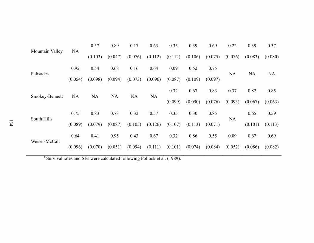
134
Mountain Valley NA
0.57
(0.103)
0.89
(0.047)
0.17
(0.076)
0.63
(0.112)
0.35
(0.112)
0.39
(0.106)
0.69
(0.075)
0.22
(0.076)
0.39
(0.083)
0.37
(0.080)
Palisades
0.92
(0.054)
0.54
(0.098)
0.68
(0.094)
0.16
(0.073)
0.64
(0.096)
0.09
(0.087)
0.52
(0.109)
0.75
(0.097)
NA NA NA
Smokey-Bennett NA NA NA NA NA
0.32
(0.099)
0.67
(0.090)
0.83
(0.076)
0.37
(0.093)
0.82
(0.067)
0.85
(0.063)
South Hills
0.75
(0.089)
0.83
(0.079)
0.73
(0.087)
0.32
(0.105)
0.57
(0.126)
0.35
(0.107)
0.30
(0.113)
0.85
(0.071)
NA
0.65
(0.101)
0.59
(0.113)
Weiser-McCall
0.64
(0.096)
0.41
(0.070)
0.95
(0.051)
0.43
(0.094)
0.67
(0.111)
0.32
(0.101)
0.86
(0.074)
0.55
(0.084)
0.09
(0.052)
0.67
(0.086)
0.69
(0.082)
a Survival rates and SEs were calculated following Pollock et al. (1989).

135
Table 3-S2. Correlation matrix of weather covariates 2003 to 2013. Covariates included MODIS snow, SNOWDAS, and NDVI. Snow
covariates were developed from the time periods; November-December, January-March, and April.
AFD FC AWD WC AAD AC FW WW F% W% A% FPC SPC
Ave. Fall Depth (AFD) 1 0.96 0.63 0.63 0.39 0.48 0.48 0.27 0.52 0.41 0.40 0.28 -0.14
Fall Cumulative Snow (FC) 0.96 1 0.64 0.64 0.44 0.53 0.52 0.32 0.54 0.45 0.45 0.27 -0.12
Ave. Winter Depth (AWD) 0.63 0.64 1 0.98 0.59 0.69 0.36 0.55 0.4 0.63 0.40 0.26 -0.02
Winter Cumulative Snow (WC) 0.63 0.64 0.98 1 0.61 0.69 0.36 0.55 0.4 0.63 0.40 0.26 -0.02
Ave. April Depth (AAD) 0.39 0.44 0.59 0.61 1 0.95 0.26 0.22 0.28 0.35 0.49 0.22 -0.13
April Cumulative Snow (AC) 0.48 0.53 0.69 0.69 0.95 1 0.27 0.26 0.27 0.38 0.52 0.20 -0.14
Fall Weeks(FW) 0.48 0.52 0.36 0.36 0.26 0.27 1 0.57 0.69 0.58 0.35 0.31 -0.10
Winter Weeks (WW) 0.27 0.32 0.55 0.55 0.22 0.26 0.57 1 0.51 0.91 0.36 0.25 0.12
Fall %Snow Cover (F%) 0.52 0.54 0.40 0.40 0.28 0.27 0.69 0.51 1 0.63 0.39 0.38 -0.18
Winter %Snow Cover (W%) 0.41 0.45 0.63 0.63 0.35 0.38 0.58 0.91 0.63 1 0.46 0.32 -0.02
April %Snow Cover (A%) 0.41 0.45 0.40 0.40 0.49 0.52 0.35 0.36 0.39 0.46 1 0.28 -0.09
FallPC (FPC) 0.28 0.27 0.26 0.26 0.22 0.20 0.31 0.25 0.38 0.32 0.28 1 -0.04
SpringPC (SPC) -0.14 -0.12 -0.02 -0.02 -0.13 -0.14 -0.10 0.12 -0.18 -0.02 -0.09 -0.04 1
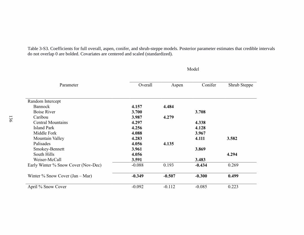
136
Table 3-S3. Coefficients for full overall, aspen, conifer, and shrub-steppe models. Posterior parameter estimates that credible intervals
do not overlap 0 are bolded. Covariates are centered and scaled (standardized).
Model
Parameter Overall Aspen Conifer Shrub Steppe
Random Intercept
Bannock
Boise River
Caribou
Central Mountains
Island Park
Middle Fork
Mountain Valley
Palisades
Smokey-Bennett
South Hills
Weiser-McCall
4.157
3.700
3.987
4.297
4.256
4.088
4.283
4.056
3.961
4.056
3.591
4.484
4.279
4.135
3.708
4.338
4.128
3.967
4.111
3.869
3.483
3.582
4.294
Early Winter % Snow Cover (Nov-Dec)
-0.088 0.193 -0.434 0.269
Winter % Snow Cover (Jan – Mar)
-0.349 -0.507 -0.300 0.499
April % Snow Cover -0.092 -0.112 -0.085 0.223
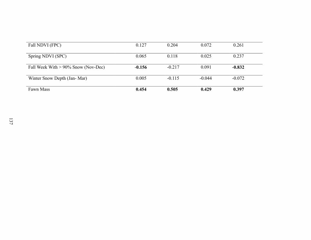
137
Fall NDVI (FPC) 0.127 0.204 0.072 0.261
Spring NDVI (SPC) 0.065 0.118 0.025 0.237
Fall Week With > 90% Snow (Nov-Dec) -0.156 -0.217 0.091 -0.832
Winter Snow Depth (Jan- Mar) 0.005 -0.115 -0.044 -0.072
Fawn Mass 0.454 0.505 0.429 0.397
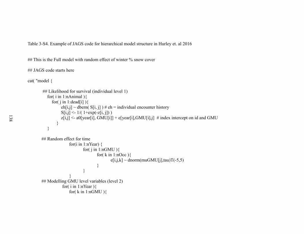
138
Table 3-S4. Example of JAGS code for hierarchical model structure in Hurley et. al 2016
## This is the Full model with random effect of winter % snow cover
## JAGS code starts here
cat( "model {
## Likelihood for survival (individual level 1)
for( i in 1:nAnimal ){
for( j in 1:dead[i] ){
eh[i,j] ~ dbern( S[i, j] ) # eh = individual encounter history
S[i,j] <- 1/( 1+exp(-z[i, j]) )
z[i,j] <- a0[year[i], GMU[i]] + e[year[i],GMU[i],j] # index intercept on id and GMU
}
}
## Random effect for time
for(i in 1:nYear) {
for( j in 1:nGMU ){
for( k in 1:nOcc ){
e[i,j,k] ~ dnorm(muGMU[j],tau)T(-5,5)
}
}
}
## Modelling GMU level variables (level 2)
for( i in 1:nYear ){
for( k in 1:nGMU ){

139
a0[i, k] <- alpha0[PMUlevel3[k]] + alpha1 * fallCenter[i, k]
+ alpha2[PMUlevel3[k]] * winterCenter[i, k]
+ alpha3 * aprilCenter[i, k] + alpha4 * fallPCC[i, k] + alpha5 * springPCC[i, k]
alpha6 * fallWeeksCenter[i, k] + alpha7 * winterDepthC[i, k]
}
}
## Metaparameters for random effects (level 3)
for( p in 1:nPMU ){
alpha0[p] ~ dnorm(muPMU, tauPMU)
alpha2[p] ~ dnorm(muCov1, tauCov1)
}
## Get predicted values at the PMU level
for(i in 1:nPMU){
for(k in 1:nYear){
for(l in 1:nOcc){
for( m in 1:nGMU ){
tempProb[i,k,m,l] <- (1/( 1+exp(- (a0[k,m ] + e[k,m,l]))))
}
phiPMUOcc[i,k,l] <- tempProb[i,k,,l]%*% weightGMU[i, , k] # weighting
#occasion specific survival by GMU sample size
}
}
}
for(i in 1:nPMU){
for(k in 1:nYear){
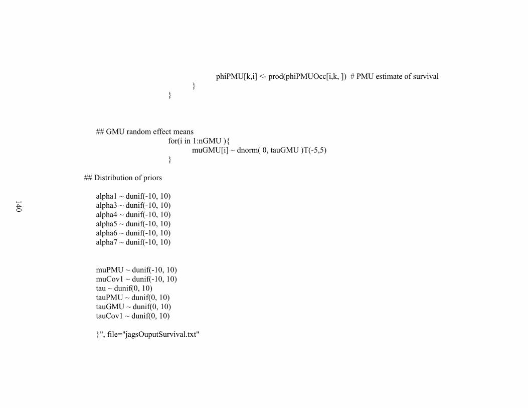
140
phiPMU[k,i] <- prod(phiPMUOcc[i,k, ]) # PMU estimate of survival
}
}
## GMU random effect means
for(i in 1:nGMU ){
muGMU[i] ~ dnorm( 0, tauGMU )T(-5,5)
}
## Distribution of priors
alpha1 ~ dunif(-10, 10)
alpha3 ~ dunif(-10, 10)
alpha4 ~ dunif(-10, 10)
alpha5 ~ dunif(-10, 10)
alpha6 ~ dunif(-10, 10)
alpha7 ~ dunif(-10, 10)
muPMU ~ dunif(-10, 10)
muCov1 ~ dunif(-10, 10)
tau ~ dunif(0, 10)
tauPMU ~ dunif(0, 10)
tauGMU ~ dunif(0, 10)
tauCov1 ~ dunif(0, 10)
}", file="jagsOuputSurvival.txt"

141
)
##
## JAGS model code ends
##
############## JAGS input variables
sp.data <- list( eh=eh, nAnimal=nAnimal, dead=dead,
year = year, nOcc = 24, nYear = nYear, nGMU = nGMU, nPMU = nPMU,
GMU = as.numeric(GMU),
fallCenter = fallCenter,
aprilCenter = aprilCenter,
winterCenter = winterCenter,
fallPCC = fallPCC,
springPCC = springPCC,
fallWeeksCenter = fallWeeksCenter,
winterDepthC = winterDepthC,
PMUlevel3 = PMUlevel3,
weightGMU = weightGMU
) # data
sp.params <- c(#"a0",
"alpha0",
"alpha1",
"alpha2",
"alpha3",
"alpha4",
"alpha5",
"alpha6",

142
"alpha7",
"phiPMU",
"tau"
) # parameters to track
sp.inits <- function() { # starting values
beta1guess <- runif( 1, 0, 1 )
alphaGuess <- runif(11, 0, 1)
gammaGuess <- rep(0, 11)
Tauguess <- runif( 1, 0, 1 )
Muguess <- runif( 1, 0, 1 )
list(alpha1 = beta1guess, alpha2 = alphaGuess, alpha3 = beta1guess,
alpha4 = beta1guess, alpha5 = beta1guess, alpha6 = beta1guess, alpha7 = beta1guess,
muPMU = Muguess, muCov1 = Muguess,
tauPMU = Tauguess, tauCov1 = Tauguess, tau = Tauguess)
}
surv.res <- jags(sp.data, sp.inits, sp.params, "jagsOuputSurvival.txt",
n.chains=3, n.iter=20000, n.burnin=5000, n.thin=1)
143
CHAPTER 4: HABITAT-MEDIATED DENSITY DEPENDENCE IN NEONATAL
SURVIVAL OF MULE DEER FAWNS3
MARK A. HURLEY, Idaho Department of Fish and Game, 600 S. Walnut Street, Boise,
Idaho, 83707, USA
MARK HEBBLEWHITE, Wildlife Biology Program, College of Forestry and
Conservation, University of Montana, Missoula, Montana, 59812, USA
JEAN-MICHEL GAILLARD, Laboratoire Biométrie & Biologie Évolutive,
CNRSUMR-CNRS 5558, University Claude Bernard - Lyon I, 69622
Villeurbanne Cedex, France
INTRODUCTION
Resource limitation is the primary mechanism governing the process of density
dependence (Sinclair 1989, Bonenfant et al. 2009). In most species including large
herbivores, both pattern- (through the analysis of time series of counts) and process-
(through direct analysis of life history traits in response to change in density) oriented
approaches have demonstrated evidence of density-dependence as populations approach
or exceed nutritional carrying capacity (Abrahams and Dill 1989, Saether et al. 1998,
Gaillard et al. 2000, Bergman et al. 2015). A decrease of the per capita food resources has
been cited as the key mechanism involved in density-dependence. However, at the
individual level, behavioral responses to disturbance and especially the avoidance of
3 Formatted for submission to Biology Letters
144
predation should modify the per capita resource availability by shifting habitat selection,
and thereby change the strength of density-dependence. Current theory of risk-sensitive
foraging predicts that a tradeoff should occur between fitness benefits through nutrition
and fitness costs through predation (Abrahams and Dill 1989, Hebblewhite and Merrill
2009) when habitats with greater forage quality or biomass are more risky. If prey are
distributed in an ideal free manner, increasing density should also reduce the strength of
selection for high-quality patches because of density-dependent competition for food
(Fretwell and Calver 1969, McLoughlin et al. 2010). Density-dependent changes in
habitat selection are thus expected to drive population dynamics through an overall
decrease in survival. In contrast, prey displaying despotic distribution may exclude
conspecifics from high quality habitat thereby creating segments of the population with
disparate resource selection and population demography. For example, White and Warner
(2007) observed density-dependence in mortality mediated by habitat based on refugia
within corral for reef fishes as mortality increased when refugia were filled. Yet for many
large herbivores, our understanding of density-dependent mortality arising from this
interaction between space and predation is unknown (Bonenfant et al. 2009, McLoughlin
et al. 2010).
Differential vulnerability of life-history stages to predation could also provide a
mechanism for such density dependent predation mortality. Indeed, for many species, it is
the juvenile life-history stage where the first signals of density dependence occur
(Bonenfant et al. 2009). For example, a juvenile survival sink may be created if the
maternal female is forced into lower quality habitats with lower forage quality and higher
risk. This habitat selection may reduce the population productivity rate as total adult

145
female numbers increase. In the case of large herbivores like mule deer (Odocoileus
hemionus), juveniles remain with their mothers throughout the first year of their life, and
so are dependent on the habitat selection strategies of their mothers (Shallow et al. 2015).
If a mule deer fawn survival sink is driving density-dependent survival, we would expect
that neonate mule deer mortality would be positively related to the predation risk from
their main predators, coyotes (Canis latrans; Hurley et al. 2011). Under the classical
model of density dependence where density is driven by food competition, we predict
that overall fawn mortality will increase with increasing density (Bonenfant et al. 2009).
However, if density dependence is driven instead by predator-mediated risk in lower
quality habitat, we would instead predict that only predator-related fawn mortality will be
density-dependent, and that overall fawn mortality need not be necessarily related to
density. This might arise because non-predator related mortality is compensatory (White
and Bartmann 1998).
To test these predictions of density-dependent mortality, we monitored neonatal
survival and cause-specific mortality of mule deer fawns for the first 6 months of life. We
took advantage of an ongoing management experimental reduction in coyotes (Hurley et
al. 2011) in one of two adjacent populations of mule deer in southern Idaho, and
compared response to both changes in density and coyote abundance in neonatal
mortality. First, to test whether fawn mortality occurred because of the habitat use of
lower quality, higher coyote predation risk areas at higher density, we developed a spatial
model for coyote predation risk (Hebblewhite et al. 2005). We then tested whether higher
coyote predation risk was correlated with fawn survival using Cox-proportional hazards
survival models (Hebblewhite and Merrill 2011). Finally we tested for density-

146
dependence in survival (mortality) of mule deer fawns with increasing density, and then,
just coyote-caused fawn survival for the study area as a whole and each unit individually
to assess the influence of lower coyote density due to coyote removal. If risk-sensitive
foraging was driving neonatal mortality, then we predicted a decline in overall mortality
at high density in the experimental coyote removal treatment, but not necessarily a
decline in coyote-caused mortality. In contrast, in the reference population, we predicted
no relationship between mortality and density, but a stronger (than the coyote removal
area) relationship between coyote caused mortality and mule deer density (sensu Sinclair
and Arcese 1995).
MATERIALS AND METHODS
(a) Data collection
We monitored neonate mule deer (Odocoileus hemionus) fawns in Game Management
Units (GMU) 56 (2,338 km2) and 73A (1,128 km
2) from 1998–2002 in southeastern
Idaho. These two GMUs are within the Bannock mule deer population management unit
used in Chapters 3 and 5. Elevations ranged from 1,350 m to 2,666 m. Each GMU
encompassed a mountain range in its entirety and provided suitable yearlong habitat for a
distinct subpopulation of deer with minimal interchange between the two GMUs. As
methods for another management experiment conducted by Idaho Fish and Game
(IDFG), coyotes were actively removed from GMU 73A (herein after removal area) and
GMU 56 was designated a reference area (reference), see Hurley et al. (2011) for a
detailed description of study areas and coyote removal treatments. We used aerial surveys

147
via a Bell 47 helicopter to estimate mule deer population size from late March to mid-
April each year from 1997 to 2003. We captured neonate fawns from 1 June to 18 June
by observing fawning behavior of adult females (for details of capture methods see
Hurley et al. 2011). Fawns were fitted with brown or black expandable radio collars
designed to break away 6 to 8 months after capture. Animal capture protocols were
approved by the Animal Care and Use Committee, Idaho Department of Fish and Game
Wildlife Health Laboratory, Caldwell, Idaho, USA, and University of Montana IACUC
(protocol #02-11MHCFC-031811). We monitored telemetry signals for mortality of
neonate deer via aerial (fixed-wing aircraft) or ground telemetry at 1 to 2 day intervals
during summer and twice weekly throughout autumn until collars were shed. We
identified the cause of death within 24 hours using criteria developed by Wade and
Bowns (1982), and categorized mortalities as coyote, mountain lion, bobcat, unknown
predator, malnutrition, natural, other, and unknown.
We developed a spatial model of coyote predation risk (the main cause of
mortality, see results) using a resource selection function (RSF; Manly et al. 2002),
framework based on coyote scat transects (e.g., Hebblewhite et al. 2005). We conducted
coyote scat surveys annually to estimate coyote occurrence or absence (Knowlton 1985).
Eighty 1-mile transects were randomly selected in each GMU and surveyed from May to
June 1998–2002 (Figure 1) the key temporal window for most neonatal fawn mortality
(Shallow et al. 2015). Landcover types were defined from the SAGEMAP vegetation
(Chapter 3). From the 126 land cover classes with a minimum mapping unit (MMU) of
approximately 1 acre (0.4 ha), we identified 18 habitat types based on mule deer ecology,
leading to a weighted mean accuracy of 84.4%. We placed a 1,000 m buffer around
148
coyote transects and intersected the resulting polygon with the cover type and digital
elevation models using a Geographical Information System (ArcGIS ver. 9.3.1, ESRI Inc.
2009). We then measured the proportion of each habitat type within the buffer.
(b) Statistical analysis
We first estimated survival of mule deer neonates in each year using non-parametric
Kaplan-Meier survival estimation (Kaplan and Meier 1958, Hosmer and Lemeshow
1999). We used left- and right- staggered entry to account for different capture times and
losses due to emigration or collar malfunction. We used estimated birth date as beginning
at risk time (origin), then enter the analysis on capture date (enter the risk set), and end
time at death or censored from shed collar or end of study (30 November; see Hurley et
al. 2011,for details). Next, we estimated cause-specific mortality rates using cumulative
incidence functions in a competing risks format (Heisey and Patterson 2006).
Second, we developed our model of coyote predation risk estimated using a used-
unused resource selection probability function (RSPF) design with a random intercept
accounting for intra-annual variation and dependency within transects (Manly et al. 2002,
Gillies et al. 2006). The sample unit was the coyote transect, and the dependent variable,
presence or absence, was modeled using logistic regression. This approach assumes
predation risk is driven by the relative abundance of coyotes, which has been borne out in
studies of other canids preying on ungulates (Hebblewhite and Merrill 2009). Coyote scat
transects were conducted in both GMU 56 and 73A, as well as neighboring GMU’s
(Hurley et al. 2011). We treated year as a random effect to control for year-to-year
variance in coyote use of transects and non-independence of repeated trials of transects
149
each year (Gillies et al. 2006). Models were developed with purposeful forward and
backward stepwise variable selection (Hosmer and Lemeshow 1999). We compared
models with and without the random effect using AICc (Burnham and Anderson 1998)
and validated the most supported coyote RSPF model with k-folds cross validation
(Boyce et al. 2002). We developed coyote predation risk models based on the landcover
model, a digital elevation model for elevation, and a measure of terrain ruggedness
(Sappington et al. 2007).
We measured probability of presence of coyotes from our predation risk model at
the neonate fawn capture site buffered by 500 m and included the probability as a
covariate in Cox-proportional hazards models (Hosmer and Lemeshow 1999,
Hebblewhite and Merrill 2011) to test the influence of coyote predation risk on fawn
survival. We regressed mortality against mule deer density in each year (previous spring
survey) using linear regression to test the first prediction of the classic hypothesis of
density dependence. We next tested the relationship between the percent of marked fawns
killed by coyotes and mule deer population density in both GMUs to test the hypothesis
of a coyote predation-mediated density-dependence in mule deer.
RESULTS
Mule deer population size fluctuated substantially over the study period, increasing from
2,810 (GMU 56= 1878, 73A = 932) in 1998 to 4,695 in 2001 (GMU 56= 2932, 73A =
1763) and then decreased to 3,067 (GMU 56= 1496, 73A = 1571) in 2002 due to severe
climatic conditions. We captured 251 neonatal fawns from 1998–2002, median 58 / year
in total, evenly distributed between GMUs. Cause-specific mortality rates of these fawns
150
were 0.13 in GMU 56 and 0.11 in 73A due to coyotes, 0.11 in GMU 56 and 0.07 in 73A
due to mountain lions, 0.08 in GMU 56 and 0.05 in 73A due to unknown predation, and
the remainder due to all other causes (see Hurley et al. 2011). Thus, coyotes were the
leading cause of mortality. Overall neonatal survival rates (1 – mortality) varied from
0.20 – 0.74, consistent with previous studies of neonatal mule deer fawn survival (Pojar
and Bowden 2004).
Coyote scats were recorded on 527 of 1035 coyote scat transects, providing a
balanced used versus unused logistic regression based RSPF. The random intercept model
had a lower AICc than the best logistic regression without random effects (ΔAICc = 25.5)
or the full model (ΔAICc = 34.2). Coyotes selected habitat with low elevation and mesic
sage and avoided high elevation and aspen habitats (Table 4-1, Figure 4-1). The top
model was validated with a 5-fold cross validation which yielded a mean rs = 0.829,
indicating the model performed well at predicting coyote presence.
Mule deer fawn mortality increased with our coyote predation risk model (β =
0.938, χ2 = 4.0, P = 0.045). The spatial distribution of mule deer fawns with respect to
coyote presence was markedly bimodal, opposing locations with rare (< 0.05) vs.
abundant (> 0.3, Figure 4-2) coyote probability of presence. The hazard ratio for the
effect of coyote presence on neonate mortality was 2.56 (95% CI = 0.993 to 6.58)
indicating fawns with 100% probably of coyotes would die at 2.56 times the rate of fawns
born in areas of 0% probability of coyote presence. Applying this ratio to the range of
predicted probability of coyote presence in our study (0.014 to 0.72) suggests neonates
were about as likely to die if born in habitats highly frequented by coyotes (Figure 4-2).

151
To test our first prediction of density dependence for the entire study area, we
found no clear or strong relationship between mule deer fawn mortality and population
density when both GMUs were treated as one study area for mortality and population
density (Fig. 4-3a; = 0.008, F1,3 = 0.001 p = 0.98, R2 = 0.0001). Our second
prediction of habitat mediated density dependence provided a clear signal as the
contribution of coyote predation to fawn mortality increased significantly with mule deer
density (R2 = 0.90) when the 2 GMUs were treated as one population (Fig. 4-3b; =
0.328, F1,3 = 27.2 p = 0.01, R2 = 0.90).
We also observed no clear relationship between mule deer fawn mortality and
population density when the GMUs were separated in GMU 56 ( = 0.11, F1,3 = 0.19, p
= 0.69, R 2
= 0.06, Figure 4-4a), and a negative, but weak, relationship in GMU 73A ( =
-0.540, F1,3 = 1.67 p = 0.29, R 2
= 0.36, Figure 4-4b), suggesting total fawn mortality was
declining with density in the coyote removal area. Again, our second prediction of
density dependent predation risk, was borne out when GMUs were separated. The pattern
persists and coyotes killed more fawns as the population density increased, even though
the overall mortally was constant or slightly decreasing (Figure 4-4a). The relationship
was stronger in GMU 56 ( = 0.251, F1,8 = 5.74, p = 0.09,, R 2
= 0.65; Figure 4-4b), but
still positive in GMU 73A ( = 0.125, F1,8 = 0.86, p = 0.42, R 2
= 0.21; Figure 4-4b)
where coyotes were actively removed.
DISCUSSION
152
We have demonstrated differential survival of neonate mule deer fawns based on an
interaction of mule deer behavior and resource selection and resource selection by their
primary predator, coyotes. We observed a density-dependent increase in mule deer fawn
mortality caused by coyotes with increasing mule deer density, but, critically, not an
increase in overall mortality (e.g., Figure 4-3a, 4-3b). This supports our hypothesis that
predation interacting with mule deer behavior may be the mechanism generating the
density-dependent signature of observed in these populations (Chapter 5). We suggest
that predation interacting with competition for space, not competition for food, may be
the primary mechanism limiting these same populations at lower density as in Chapter 5.
This is especially likely because we saw some evidence for declining overall mortality
with increasing densities, whereas coyote-caused mortality increased. More generally,
this supports the importance of density-dependent trade-offs between risk and forage in
driving patterns of density-dependence in large herbivores (Sinclair and Arcese 1995,
Hebblewhite and Merrill 2011).
The next step would be to directly test whether female mule deer resource
selection follows the same avoidance pattern of resource selection for higher coyote
predation risk. Previous studies have shown that mule deer select aspen habitats for fawn
rearing in direct contrast to our coyote resource selection (Hurley, unpublished data).
However, these habitats occur at higher elevations with lower primary prey density for
coyotes. In these systems, primary prey for coyotes are not mule deer, but lagomorphs
(Mills and Knowlton 1991). Resource use by coyotes and resulting density has been
linked to lagomorph abundance and the differential density by habitat type is likely
related to resource use of their primary prey, lagomorphs. To successfully breed, coyotes
153
must be holding a territory prior to denning season in April and most of the aspen habitats
are covered in deep snow at that time (Chapter 2), whereas, white-tailed jackrabbits
(Lepus townsendii) are most abundant in the mid-elevation mountain shrub communities
(mesic sage) in our study area. Accordingly, we observed higher survival of neonates and
lower probability of coyote use in aspen habitats than in mesic sage. Our results are
similar to Byers (1997) who reported pronghorn antelope (Antilocapra antilocapra)
maternal behaviors are driven by anti-coyote behaviors, and that in turn, coyote foraging
is driven by small mammal abundance. The differential mortality of neonatal mule deer
as a function of coyote predation risk suggests that neonate fawns are alternate prey in
this system, and are killed opportunistically and coyotes do not move to the higher
quality aspen habitats, with higher deer density, to forage.
Aspen is a rare cover type in the study area, comprising 5% of the total landscape
with 72% of the adult females selecting this habitat at low densities in 1998 at study
initiation (Hurley, unpublished data). Females actively exclude conspecifics from fawn
rearing habitat as observed in this study and by Taylor (2013), thereby limiting
subdominant females’ use of the highest quality cover types for fawn rearing (Shallow et
al. 2015). Mountain shrub cover types may provide adequate maternal nutrition in some
years with adequate precipitation, but senescence of forage will be earlier in the summer
than the higher elevation aspen and conifer types (Chapter 2). Mortality of neonates may
increase in these habitats through nutrition, disease, contact with livestock, or increased
predation risk. We suggest that the decrease in mule deer productivity as populations
increase may be related to fill of the high quality habitat and the resulting increased use
of lower quality, high predation risk habitat. We conclude that the appearance of density
154
dependent effects were the result of mule deer behavior and not forage biomass
limitation.
LITERATURE CITED
Abrahams, M. V. and L. M. Dill. 1989. A determination of the energetic equivalence of
the risk of predation. Ecology 70:999-1007.
Bergman, E. J., P. F. Doherty Jr, G. C. White, and A. A. Holland. 2015. Density
dependence in mule deer: a review of evidence. Wildlife Biology 21:18-29.
Bonenfant, C., J. M. Gaillard, T. Coulson, M. Festa‐Bianchet, A. Loison, M. Garel, L. E.
Loe, P. Blanchard, N. Pettorelli, and N. Owen‐Smith. 2009. Empirical evidence of
density‐dependence in populations of large herbivores. Advances in ecological
research 41:313-357.
Boyce, M. S., P. R. Vernier, S. E. Nielsen, and F. K. A. Schmiegelow. 2002. Evaluating
resource selection functions. Ecological Modelling 157:281-300.
Burnham, K. P. and D. R. Anderson, editors. 1998. Model selection and inference: a
practical information-theoretic approach. Springer-Verlag, New York.
Byers, J. A. 1997. American pronghorn: social adaptations and the ghosts of predators
past. University of Chicago Press.
Fretwell, S. D. and J. S. Calver. 1969. On territorial behavior and other factors
influencing habitat distribution in birds. Acta Biotheoretica 19:16-36.

155
Gaillard, J. M., M. Festa-Bianchet, N. G. Yoccoz, A. Loison, and C. Toigo. 2000.
Temporal variation in fitness components and population dynamics of large
herbivores. Annual Review of Ecology and Systematics 31:367-393.
Gillies, C. S., M. Hebblewhite, S. E. Nielsen, M. A. Krawchuk, C. L. Aldridge, J. L.
Frair, D. J. Saher, C. E. Stevens, and C. L. Jerde. 2006. Application of random
effects to the study of resource selection by animals. Journal of Animal Ecology
75:887-898.
Hebblewhite, M. and E. H. Merrill. 2009. Trade-offs between predation risk and forage
differ between migrant strategies in a migratory ungulate. Ecology 90:3445-3454.
Hebblewhite, M. and E. H. Merrill. 2011. Demographic balancing of migrant and resident
elk in a partially migratory population through forage–predation tradeoffs. Oikos
120:1860-1870.
Hebblewhite, M., E. H. Merrill, and T. L. McDonald. 2005. Spatial decomposition of
predation risk using resource selection functions: an example in a wolf–elk
predator–prey system. Oikos 111:101-111.
Heisey, D. M. and B. R. Patterson. 2006. A Review of Methods to Estimate Cause-
Specific Mortality in Presence of Competing Risks. Journal of Wildlife
Management 70:1544-1555.
Hosmer, D. W. and S. Lemeshow, editors. 1999. Applied survival analysis: regression
modeling of time to event data. Wiley, New York, NY, USA.
Hurley, M. A., J. W. Unsworth, P. Zager, M. Hebblewhite, E. O. Garton, D. M.
Montgomery, J. R. Skalski, and C. L. Maycock. 2011. Demographic response of
156
mule deer to experimental reduction of coyotes and mountain lions in
southeastern Idaho. Wildlife Monographs 178:1-33.
Kaplan, E. L. and P. Meier. 1958. Nonparametric estimation from incomplete
observations. Journal of the American Statistical Association 53:457-481.
Manly, B. F. J., L. L. McDonald, D. L. Thomas, T. L. McDonald, and W. P. Erickson,
editors. 2002. Resource selection by animals: statistical analysis and design for
field studies. Nordrecht, The Netherlands, Kluwer.
McLoughlin, P. D., D. W. Morris, D. Fortin, E. Vander Wal, and A. L. Contasti. 2010.
Considering ecological dynamics in resource selection functions. Journal of
Animal Ecology 79:4-12.
Mills, L. S. and F. F. Knowlton. 1991. Coyote space use in relation to prey abundance.
Canadian Journal of Zoology-Revue Canadienne De Zoologie 69:1516-1521.
Pojar, T. M. and D. C. Bowden. 2004. Neonatal Mule Deer Fawn Survival in West-
Central Colorado. Journal of Wildlife Management 68:550-560.
Saether, B. E., S. Engen, J. E. Swenson, O. Bakke, and P. Sandegren. 1998. Assessing the
Viability of Scandinavian Brown Bear, Ursus Arctos, Populations: the Effects of
Uncertain Parameter Estimates. Oikos 83:403-416.
Sappington, J. M., K. M. Longshore, and D. B. Thompson. 2007. Quantifying Landscape
Ruggedness for Animal Habitat Analysis: A Case Study Using Bighorn Sheep in
the Mojave Desert. Journal of Wildlife Management 71:1419-1426.
Shallow, J. R., M. A. Hurley, K. L. Monteith, and R. T. Bowyer. 2015. Cascading effects
of habitat on maternal condition and life-history characteristics of neonatal mule
deer. Journal of Mammalogy 96:194-205.
157
Sinclair, A. R. E. 1989. Population regulation of animals. Pages 197-241 in J. M. Cherret,
editor. Ecological Concepts. Blackwell, Oxford.
Sinclair, A. R. E. and P. Arcese. 1995. Population Consequences of Predation-Sensitive
Foraging: The Serengeti Wildebeest. Ecology 76:882-891.
Taylor, C. A. 2013. Behavior and casue specific mortality of mule deer (Odocoileus
hemionus) fawns on the National Rifle Association Whittington Center of North
Central New Mexico. Texas Tech University.
Wade, D. A. and J. E. Bowns. 1982. Procedures for evaluating predation on livestock and
wildlife. Texas Agricultural Extension Service, Texas Agricultural Experiment
Station, Texas A & M University System.
White, G. C. and R. M. Bartmann. 1998. Effect of Density Reduction on Overwinter
Survival of Free-Ranging Mule Deer Fawns. The Journal of Wildlife Management
62:214-225.
White, J. W. and R. R. Warner. 2007. Safety in numbers and the spatial scaling of density
dependent mortality in a coral reef fish. Ecology 88:3044-3054.
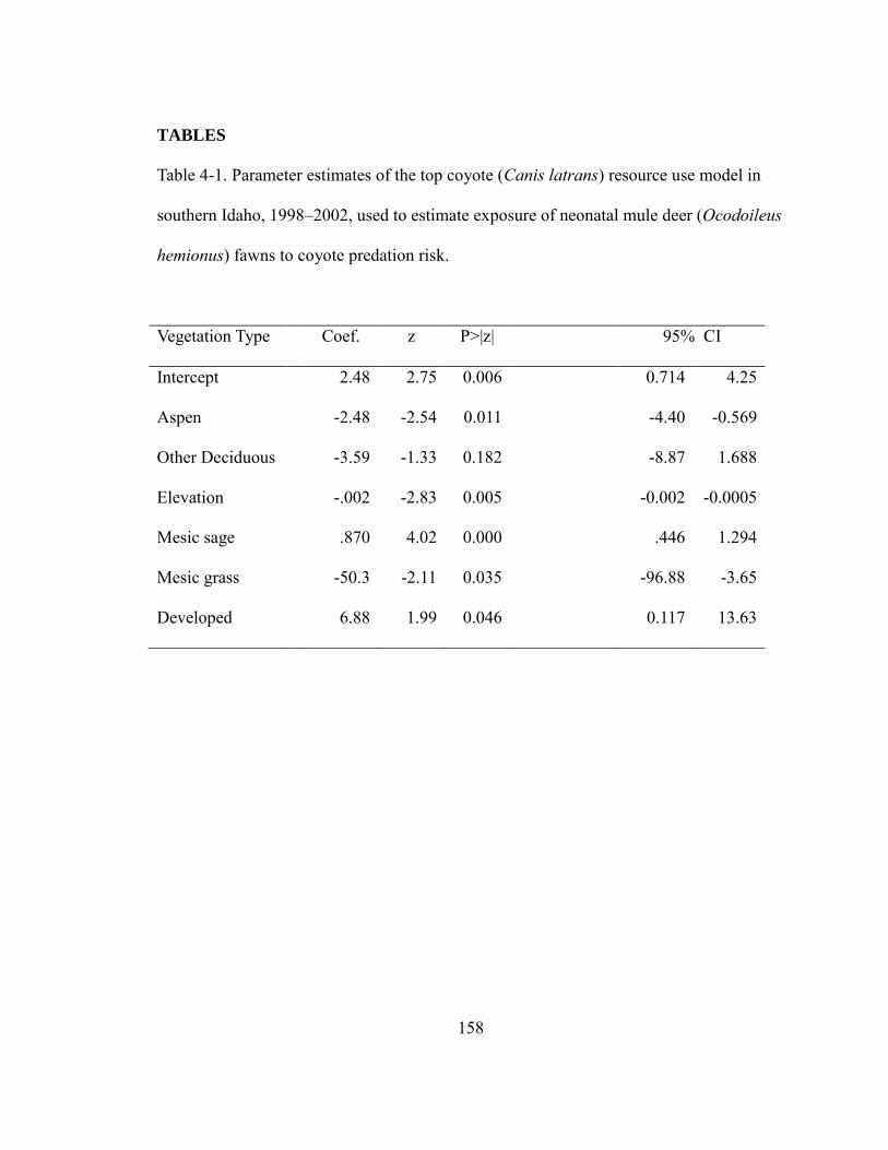
158
TABLES
Table 4-1. Parameter estimates of the top coyote (Canis latrans) resource use model in
southern Idaho, 1998–2002, used to estimate exposure of neonatal mule deer (Ocodoileus
hemionus) fawns to coyote predation risk.
Vegetation Type Coef. z P>|z| 95% CI
Intercept 2.48 2.75 0.006 0.714 4.25
Aspen -2.48 -2.54 0.011 -4.40 -0.569
Other Deciduous -3.59 -1.33 0.182 -8.87 1.688
Elevation -.002 -2.83 0.005 -0.002 -0.0005
Mesic sage .870 4.02 0.000 .446 1.294
Mesic grass -50.3 -2.11 0.035 -96.88 -3.65
Developed 6.88 1.99 0.046 0.117 13.63

159
FIGURES
Figure 4-1. Spatial predictions from the resource selection function based model of
coyote (Canis latrans) predation risk for mule deer (Odocoileus hemionus) neonatal
predation risk in southern Idaho, 1998–2002, showing the two Game Management Units
56 and 73A where neonatal mule deer were monitored. The spatial distribution of coyote
transects used to develop the model in a wider spatial area are depicted by black circles.

160
Figure 4-2. Relationship between coyote (Canis latrans) predation risk (estimated from a
resource selection functions based on scat transects) and mule deer (Odocoileus
hemionus) fawn survival (estimated with Cox-proportional hazards models) in mule deer
in southern Idaho, 1998–2002.
.2
.4
.6
.8
1
Pre
dic
ted
Ne
on
ate
Fa
wn
Su
rviv
al
0 .2 .4 .6 .8
Probability of Coyote Presence
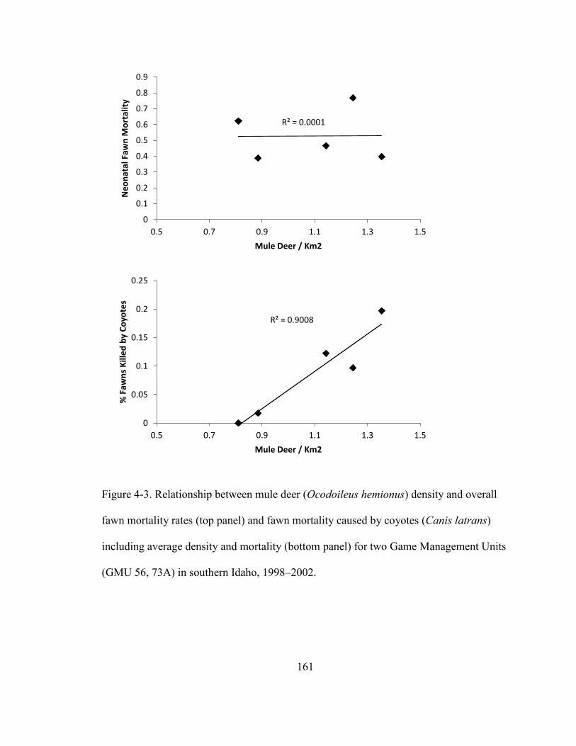
161
Figure 4-3. Relationship between mule deer (Ocodoileus hemionus) density and overall
fawn mortality rates (top panel) and fawn mortality caused by coyotes (Canis latrans)
including average density and mortality (bottom panel) for two Game Management Units
(GMU 56, 73A) in southern Idaho, 1998–2002.
R² = 0.0001
0
0.1
0.2
0.3
0.4
0.5
0.6
0.7
0.8
0.9
0.5 0.7 0.9 1.1 1.3 1.5
Ne
on
atal
Faw
n M
ort
alit
y
Mule Deer / Km2
R² = 0.9008
0
0.05
0.1
0.15
0.2
0.25
0.5 0.7 0.9 1.1 1.3 1.5
% F
awn
s K
ille
d b
y C
oyo
tes
Mule Deer / Km2
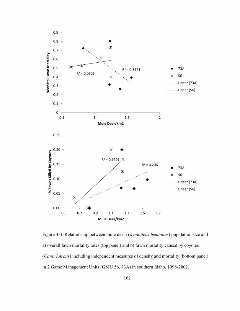
162
Figure 4-4. Relationship between mule deer (Ocodoileus hemionus) population size and
a) overall fawn mortality rates (top panel) and b) fawn mortality caused by coyotes
(Canis latrans) including independent measures of density and mortality (bottom panel)
in 2 Game Management Units (GMU 56, 73A) in southern Idaho, 1998-2002.
R² = 0.3571 R² = 0.0606
0
0.1
0.2
0.3
0.4
0.5
0.6
0.7
0.8
0.9
0.5 1 1.5 2
Ne
on
atal
Faw
n M
ort
alit
y
Mule Deer/km2
73A
56
Linear (73A)
Linear (56)
R² = 0.206
R² = 0.6501
0.00
0.05
0.10
0.15
0.20
0.25
0.5 0.7 0.9 1.1 1.3 1.5 1.7
% F
awn
s K
ille
d b
y C
oyo
tes
Mule Deer/km2
73A
56
Linear (73A)
Linear (56)

163
CHAPTER 5: DISENTANGLING CLIMATE AND DENSITY-DEPENDENT
EFFECTS ON UNGULATE POPULATION DYNAMICS4
MARK A. HURLEY, Idaho Department of Fish and Game, P.O. Box 1336, 99 Highway
93 N, Salmon, ID 83467, USA
JOSH NOWAK, Wildlife Biology Program, College of Forestry and Conservation,
University of Montana, Missoula, Montana, 59812, USA
PAUL LUKACS, Wildlife Biology Program, College of Forestry and Conservation,
University of Montana, Missoula, Montana, 59812, USA
JEAN-MICHEL GAILLARD, Laboratoire Biometrie & Biologie Evolution, CNRS-
UMR-5558, University C. Bernard - Lyon I Villeurbanne, France
MARK HEBBLEWHITE, Wildlife Biology Program, Department of Ecosystem and
Conservation Sciences, College of Forestry and Conservation, University of
Montana, Missoula, Montana, 59812, USA
4 Formatted for submission to Oecologia.

164
INTRODUCTION
The search for density-dependence in population dynamics is one of the fundamental
questions of ecology (Andrewartha and Birch 1954, Krebs 1994). Without limits to
growth, populations are predicted to grow exponentially and quickly surpass
ecological carrying capacity. Thus, understanding the strength and mechanisms of
density-dependence in population growth is a primary effort for population
ecologists. In this paper, we view of density-dependence based on the logistic growth
model that predicts linear density-dependence driven by intraspecific competition for
resources (space, food, etc.) with increasing density (Krebs 1994). Density-
dependence need not only be linear, and can either be concave (strong response only
at low density) or convex (at high density) by extending the logistic model to the
theta-logistic model (Krebs 1994). Regardless of form, the strength of density-
dependent feedbacks to population growth are generally expected to be stronger, and
more convexly non-linear, in large, longer-lived species, compared to smaller, more
r-selected species (Fowler 1981, Caughley and Krebs 1983). Life-history strategies,
pace of life, and other factors often reduce the generality of this continuum, but
empirical evidence supports stronger density-dependence in large mammals (Fowler
1981, Eberhardt et al. 2003). Furthermore, many processes, such as predation or
weather, can mimic density dependence by acting on vital rates in the same
progression as expected by density often through density-climate interactions
(Saether 1997, Clutton–Brock and Coulson 2002, Hebblewhite 2005, Hurley et al.
2011).
165
Nutritional limitation by conspecifics is hypothesized to be the primary
mechanism governing density dependence in ungulates (McCullough 1979). Density-
dependent effects (e.g., reduced survival or fecundity leading to decreased population
growth) are expected as populations approach or exceed nutritional carrying capacity,
especially in non-linear density dependence that manifests only at high density
(Stewart et al. 2005). In large mammals, density dependence is expected to first act in
parallel to the responses of vital rates to environmental variation, affecting first
juveniles, then reproduction, and finally adult female survival (Fowler 1981,
Eberhardt 2002, Gaillard & Yoccoz 2003). Ungulates conform quite well across
species to this predicted sequence (Bonenfant et al. 2009). Ungulate populations near
carrying capacity are thus expected to exert negative impacts through herbivory on
plants (Mysterud 2006), and through competition withother species.
Population dynamics are also limited by factors unrelated to population
density, and, the interaction of density-dependent and independent factors(Bonenfant
et al. 2009). Understanding the relationship between density-dependent (i.e.,
regulatory) and density-independent (i.e., limiting, sensu Sinclair 1989) drivers of
population dynamics remains an important challenge of population ecology.
Environmental stochasticity in resource availability and climate can affect population
dynamics a multitude of different ways (Saether 1997). A single species can exhibit
density-dependent responses in one population and not another, as evident in elk
(Cervus elaphus) and caribou/reindeer (Rangifer spp.) in relation to latitude (Post
2005, Ahrestani et al. 2013). Thus, despite the general evidence for density-
166
dependence in large mammal populations, the strength of density dependent and
independent factors vary across populations.
Interactions of weather, forage quality, and predation may prevent
manifestation of density-dependence on this predicted sequence of changes in vital
rates if densities are kept low by density-independent factors. This is especially true
for non-linear density dependence (convex) where a critical threshold may need to be
reached before density dependent changes to vital rates are evident. For instance,
density dependence was weak at high latitudes or under predation, suggesting weather
and predation limited densities below where density-dependence would be important
in these low productivity environments (Wilmers et al. 2006, Wang et al. 2009).
Similarly, roe deer (Capreolus capreolus) density was lower at higher latitude, low
productivity environments in Europe, and experienced stronger top-down effects of
predation in these same environments (Melis et al. 2009). Larger bodied ungulates are
also generally less vulnerable to predation, and thus experience stronger effects of
density-dependence (Sinclair and Pech 1996, Sinclair et al. 2003). However,
avoidance of predation may cause smaller bodied ungulates to select resources
inconsistent with nutritional carrying capacity alone, leading to a lower density than
predicted by nutritional carrying capacity. Population growth rate becomes difficult to
predict if the functional relationships between survival and habitat quality (forage and
predation risk) changes with density. Therefore, rigorous statistical approaches are
often required to test between competing hypotheses about regulating or limiting
factors.

167
Unfortunately, identifying mechanisms of density-dependence in population
dynamics has been statistically challenging. Most researchers have focused on testing
for density dependence using time-series of population counts (Taper and Gogan
2002, Turchin 2003), but criticisms of non-independence between axes (Elkington
2000)has caused researchers to develop statistical approaches to address this
limitation (Dennis and Taper 1994, Sibly and Smith 1998). Models have been
developed to test for linear, non-linear, and higher-order forms of density-dependence
that represent different competing hypotheses of the mechanisms of density-
dependence (Elkington 2000, Bjornstad and Grenfell 2001). These more complex
models often, unfortunately, exceed the resolution of the data to distinguish between
because of the quality of count data, as well as the limiting effect of time-series length
on detecting density dependence (De Valpine and Hastings 2002, Brook and
Bradshaw 2006). More recently, researchers have started to appreciate that these
pattern-based approaches based on count data have limited value at exposing the
underlying mechanisms of density-dependence (Saether et al. 2007, Abadi et al.
2012).
An alternative approach is to understand the underlying processes (e.g.,
changes in vital rates) driving patterns of density-dependence. The development of
state-space models (Royle et al. 2007, Kery and Schaub 2012) offer a promising
solution to some of these statistical and conceptual challenges (Abadi et al. 2012).
The ability to integrate the biology and sampling variance while estimating vital rates
simultaneously allows us to share information across data types and quality,
providing more realistic demographic estimates, including for time-series missing

168
data (Royle et al. 2007, Kery and Schaub 2012). Most studies have applied such state-
space models to estimating the strength of density dependence and density
independence only with time-series of counts, though, limiting their ability to identify
the vital rate mechanisms driving population changes (Ahrestani et al. 2013, Koons et
al. 2015, Lee et al. 2015). Developing state-space models using vital rates would be
especially useful to identify the most density-dependent vital rate. This approach has
been used successfully by combining both information about counts and vital rates
(survival, fecundity) for Red-backed shrikes (Lanius collurio) to estimate the strength
of density dependence in an integrated population model (Abadi et al. 2012). In
ungulates, time-series counts have been combined with climatic effects to estimate
both density dependence and density independence (Koons et al. 2015, Lee et al.
2015). But, to date, there have been only a few studies that combined counts, vital
rate data, and climate data to estimate both density-dependence and density-
dependent forces in an integrated population modeling framework for ungulates
(Johnson et al. 2010).
Understanding the relative contribution of density-dependent and density-
independent drivers of ungulate population dynamics, as well as their possible
interaction, is important because of their ecological and economic importance
(Gordon et al. 2004). In particular, for mule deer, the evidence for density-
dependence seems contradictory (Peek et al. 2002, Bergman et al. 2015). For
example, in one study, Peek et al. (2002) showed that both density dependence and
climatic variation explained their dynamics, but climatic factors dwarfed the effect of
density. White and Bartmann (1998) showed that overwinter survival of fawns
169
interacted strongly with density at extreme densities. However, the bulk of the
literature paints only a weak picture of density dependence in both time-series counts,
and vital rates (reviewed by Bergman et al. 2015). The relatively weak support for
density-dependence in mule deer is especially puzzling given the strong experimental
field evidence for it in their close relative, the white-tailed deer (Odocoileus
virginianus; McCullough 1979, Patterson and Power 2002). A plausible explanation
is that across the semi-arid west, mule deer may be a species for which the relative
interplay between density-independent and dependent factors is in favor of density-
independent climatic variation.
In this study, our objectives were to test for the relative strength of density-
dependent and density-independent forces in driving mule deer population dynamics
across six population units in Idaho, USA. We developed an integrated population
model (IPM, sensu Abadi et al. 2012) and incorporate density dependent effects on
each of our measured vital rates and weather effects on the most variable vital rate,
winter fawn survival. We hypothesize that mule deer populations are limited by
frequent weather-caused die-offs, limiting our ability to detect density-dependence.
We expect density effects first in recruitment to 6 months of age, then overwinter
juvenile survival, and lastly adult survival and thus predict negative density
dependence will be strongest in either recruitment or winter fawn survival (Hurley et
al. 2011; Bergman et al. 2015). We predict that density dependence should be
strongest on recruitment (fawn:adult female ratio in December) due to the interaction
of predation and density especially at high density (Chapter 4). Alternatively, density-
dependence should be strongest on winter fawn survival (6 months to 12 months old)
170
because of competition on winter range (Bartmann et al. 1992, White and Bartmann
1998). For weather related limitations on vital rates, we hypothesized that the patterns
observed with density related reduction and weather reduction will be similar. If this
is true, we predict that the addition of an important weather variable to an IPM
containing a density dependent term will reduce the density dependent effect. We
predict populations that experience the mildest climate will show the strongest effect
of density. We predict that populations least likely to show density dependence
should be those areas of contiguous good quality habitat that show a strong effect of
weather related reductions in fawn survival.
STUDY AREA
Our study area covered a wide climate, predation and habitat gradient of mule deer
range in Idaho and is fully described in (Hurley et al. 2016, Chapter 3). We monitored
population size, age and sex composition, survival of fawns and adult females, and
harvest in six Population Management Units (PMU) across central and southern
Idaho. In Idaho, Game Management Units (GMUs) are nested within Population
Management Units (PMUs) that are grouped together to represent ecological
(interbreeding) populations, which form the basis for management. Through a
hierarchical cluster analysis we identified three main habitat types (called ecotypes
hereafter) based on the dominant overstory canopy species on summer range;
coniferous forests, shrub-steppe, and aspen woodlands and assigned each PMU to a
ecotype (Chapter 3). Elevation and topographic gradients within PMUs affect snow
depths and temperature in winter, and precipitation and growing season length in the

171
summer, with elevation increasing from the southwest to the northeast. Areas used by
mule deer in the winter in conifer ecotypes (Boise River, Central Mountains, and
Weiser-McCall) ranged in elevation from 1001 to 1928m, but most were <1450m.
Winter precipitation (winter severity) varied widely (from 10 to 371mm) in
coniferous GMUs. Coniferous ecotype summer ranges are dominated by conifer
species interspersed with cool season grasslands, sagebrush, and understory of forest
shrubs. Shrub-steppe PMUs (South Hills) were semi-desert and ranged from 1545 to
2105m, with winter precipitation from 24 to 105 mm. Summer range within shrub-
steppe ecotypes was dominated by mesic shrubs (e.g., bitterbrush (Purshia
tridentata), sagebrush (Artemsia spp.), rabbitbrush (Chrysothamnus spp.), etc). Aspen
ecotype PMUs (Bannock and Caribou) were located in the east and south with winter
use areas ranging from 1582 to 2011m, and winter precipitation ranging from 25 to
146 mm. In summer, productive mesic aspen (Populus tremuloides) woodlands were
interspersed with mesic shrubs.
Because we wanted to associate individual deer to the weather and spatial
covariates associated with its seasonal range, we estimated within-GMU level
seasonal ranges across all six PMUs (Figure 5-2, Chapter 3). Deer were captured
within each PMU in each primary winter range (range 1-6 different winter ranges) in
proportion to the distribution of deer and abundance (IDFG unpublished data).
Migratory periods were excluded from the seasonal home range estimates; locations
between 1 June and 30 September were used for summer ranges and 1 December to
31 March for winter ranges (e.g., Sawyer et al. 2005). We created combined seasonal
95 % kernel density utilization distributions for deer from each winter and summer
172
range by using telemetry locations from all individuals and years for the entire study
area (Chapter 3). Climate and habitat information was then summarized within the
seasonal home ranges of radiocollared deer for winter and summer, the basis of the
spatial covariates.
METHODS
(a) Integrated Population Model Development
We used an integrated population model (IPM) to evaluate the relative strength of
density-dependent and density-independent forces on mule deer population dynamics
across our six populations. IPMs allow for the incorporation of many different types
of population data of varying quality that are integrated into a population model to
provide improved rigor in both population estimates and projections (Besbeas et al.
2002, Johnson et al. 2010, Kery and Schaub 2012). Our mule deer data included
annual estimates of survival and fecundity from marked individuals, annual harvest
data, but only infrequent sightability-adjusted aerial surveys, obviously a key
component for evaluating density dependence. To solve the problem of estimating
density-dependent effects with only infrequent density estimates, we developed and
fit an IPM to six PMUs with varying amounts of empirical data to estimate an annual
population density given age-class specific vital rates. We then used this model to test
the influence and strength of density on each individual vital rate in the following
predicted order from strongest to weakest; fall recruitment, overwinter fawn survival,
adult survival. We will first describe the data sources used to parameterize the IPM
and then the model structure of the IPM and the methods used to evaluate density
173
dependence and the influence of weather covariate on model fit and the strength of
density dependence.
Population estimates
We conducted PMU-wide population surveys using sightability models corrected for
visibility bias once every 4-5 years (Unsworth et al. 1994). Surveys were conducted
via a Bell 47 helicopter during mid-winter (January - February) for total deer numbers
only. We surveyed 100% of subunits (quadrats) that were occupied by deer.
Age and Sex ratio estimates
Early winter fawn:adult female ratios are a measure of age-specific fecundity and
fawn survival for the first six months of life. We used helicopter surveys to estimate
age and sex composition for each PMU every December (Unsworth et al. 1994). We
surveyed a previously defined stratified random sample of medium to high-density
subunits. Sampling emphasized obtaining an adequate sample size and representative
geographic distribution across each PMU. Adult male:adult female ratios were
obtained concurrently with fawn:adult female ratios, however survey design and
emphasis was placed on obtaining accurate and precise estimates of fawn:adult
female ratios for all PMUs. Adult male:adult female ratios were included in the model
when additional survey effort was expended to obtain similar accuracy and precision
of fawn ratios To maintain repeatability across PMUs and years, age and sex
classification procedure was limited to only three or four primary observers, one of
whom would be on every flight along with secondary regional observers. Surveys

174
were conducted between1 December and 31 December, prior to antler shed, with a
Bell 47 helicopter.
Survival monitoring
We monitored survival of 1,961 six-month-old male and females and 1,061 adult
females (4,776 adult years) within six Population Management Units in southern
Idaho, 2001–2013. We varied capture methods as described previously in Hurley et
al. (2014; Chapter 2, 3), and deployed 320– 400 gram collars on adults that were
permanently affixed, and for female fawns, permanent collars with a temporary pleat
or surgical tubing for male fawns that allowed collars to drop off after approximately
8-10 months. All collars had a mortality signal. An Idaho Department of Fish and
Game (IDFG) veterinarian or veterinary technician was on site during most captures
to assist with sampling and assure animal welfare. Animal capture protocols were
approved by the Animal Care and Use Committee, Idaho Department of Fish and
Game Wildlife Health Laboratory, Caldwell, Idaho, USA, and University of Montana
IACUC (protocol #02-11MHCFC-031811). Deer were monitored with telemetry for
mortality from the ground at least once a month between capture (7 December to 15
January) and 1 June. If radio signals could not be detected from the ground within 1
week, animals were located via aircraft. When a mortality signal was detected, cause
of death was determined using a standard protocol (Wade and Bowns 1982). Animals
that lost radiocollars or with radiocollars that failed were removed (censored) from
the analysis at the point of failure.
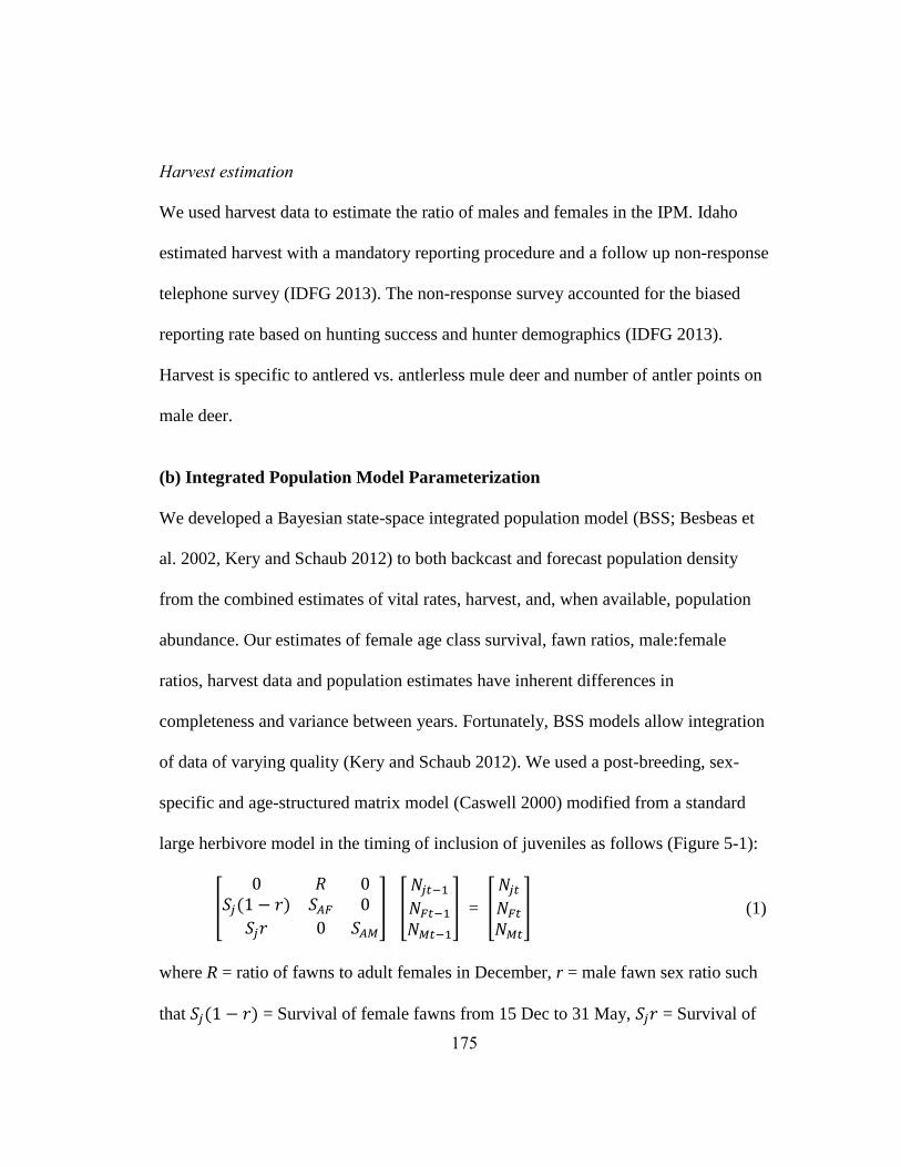
175
Harvest estimation
We used harvest data to estimate the ratio of males and females in the IPM. Idaho
estimated harvest with a mandatory reporting procedure and a follow up non-response
telephone survey (IDFG 2013). The non-response survey accounted for the biased
reporting rate based on hunting success and hunter demographics (IDFG 2013).
Harvest is specific to antlered vs. antlerless mule deer and number of antler points on
male deer.
(b) Integrated Population Model Parameterization
We developed a Bayesian state-space integrated population model (BSS; Besbeas et
al. 2002, Kery and Schaub 2012) to both backcast and forecast population density
from the combined estimates of vital rates, harvest, and, when available, population
abundance. Our estimates of female age class survival, fawn ratios, male:female
ratios, harvest data and population estimates have inherent differences in
completeness and variance between years. Fortunately, BSS models allow integration
of data of varying quality (Kery and Schaub 2012). We used a post-breeding, sex-
specific and age-structured matrix model (Caswell 2000) modified from a standard
large herbivore model in the timing of inclusion of juveniles as follows (Figure 5-1):
[
0 0𝑆𝑗(1 − ) 𝑆 0
𝑆𝑗 0 𝑆
] [
𝑁𝑗𝑡−1𝑁 𝑡−1𝑁 𝑡−1
] = [
𝑁𝑗𝑡𝑁 𝑡𝑁 𝑡
] (1)
where R = ratio of fawns to adult females in December, r = male fawn sex ratio such
that 𝑆𝑗(1 − ) = Survival of female fawns from 15 Dec to 31 May, 𝑆𝑗 = Survival of
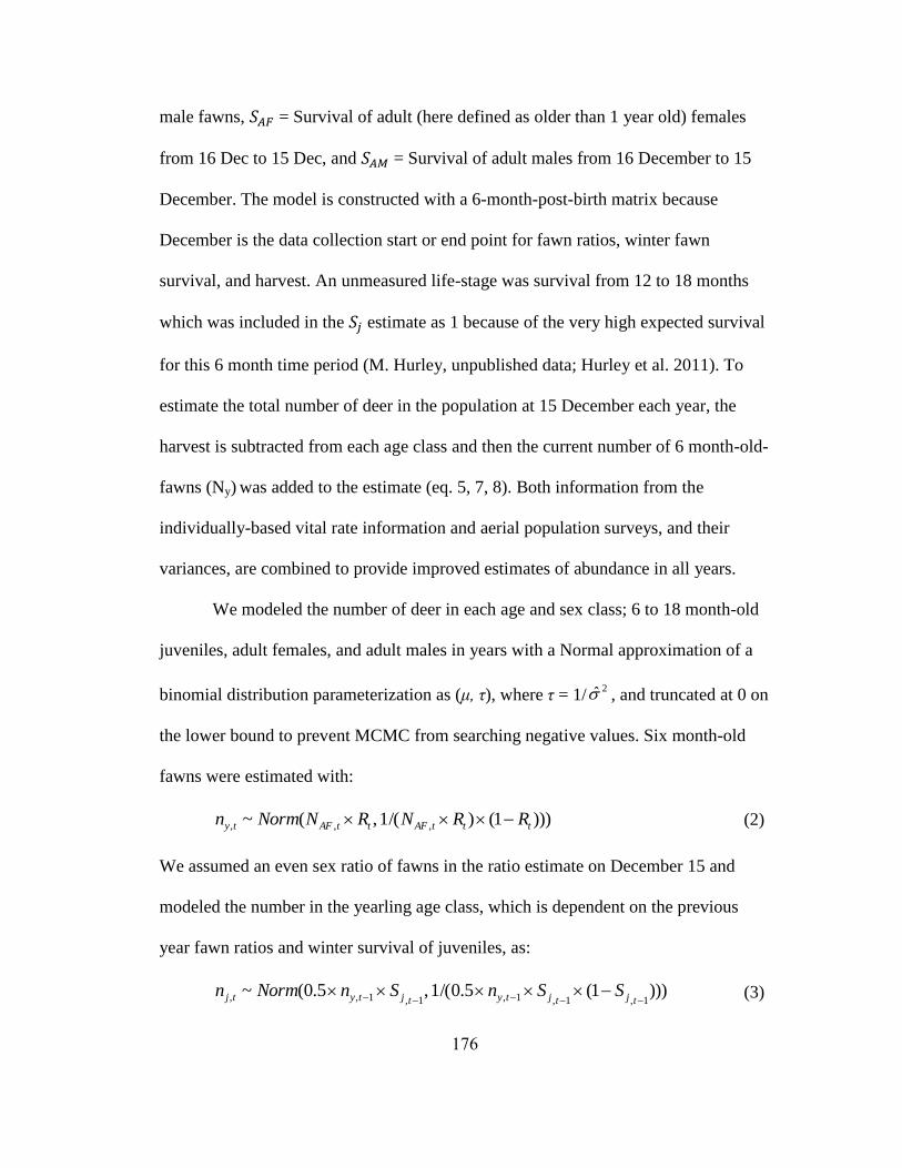
176
male fawns, 𝑆 = Survival of adult (here defined as older than 1 year old) females
from 16 Dec to 15 Dec, and 𝑆 = Survival of adult males from 16 December to 15
December. The model is constructed with a 6-month-post-birth matrix because
December is the data collection start or end point for fawn ratios, winter fawn
survival, and harvest. An unmeasured life-stage was survival from 12 to 18 months
which was included in the 𝑆𝑗 estimate as 1 because of the very high expected survival
for this 6 month time period (M. Hurley, unpublished data; Hurley et al. 2011). To
estimate the total number of deer in the population at 15 December each year, the
harvest is subtracted from each age class and then the current number of 6 month-old-
fawns (Ny) was added to the estimate (eq. 5, 7, 8). Both information from the
individually-based vital rate information and aerial population surveys, and their
variances, are combined to provide improved estimates of abundance in all years.
We modeled the number of deer in each age and sex class; 6 to 18 month-old
juveniles, adult females, and adult males in years with a Normal approximation of a
binomial distribution parameterization as (μ, τ), where τ = 1/ , and truncated at 0 on
the lower bound to prevent MCMC from searching negative values. Six month-old
fawns were estimated with:
(2)
We assumed an even sex ratio of fawns in the ratio estimate on December 15 and
modeled the number in the yearling age class, which is dependent on the previous
year fawn ratios and winter survival of juveniles, as:
(3)
2
)))1()/(1,(~ ,,, tttAFttAFty RRNRNNormn
)))1(5.0/(1,5.0(~1,1,1,1,1,,
tjtjtytjtytj SSnSnNormn

177
We estimated the number of deer in the adult female class by first estimating the
survival of adult females from the previous year as:
(4)
We then estimated the total number of adult females in the current year by adding the
yearling class (4) and subtracting harvest of both adult and yearling females ( ):
(5)
We estimated the number of deer in the adult male class by first estimating the
survival of adult males from the previous year as:
(6)
Total estimate of adult males is then calculated to include the addition of the yearling
class (4) and reductions due to harvest of both adult and yearling males ( ):
(7)
The estimate of total population size is then calculated as the summation of young of
year, adult females and adult males:
(8)
To account for sampling error in the observed data, we modeled the count and
survival using the mean of the data estimated precision as 1/ . We used binomial
distribution for survival data, and assumed a Normal distribution for the observation
model abundance estimates, where abundance estimates were the outcome of a
Normal distribution with mean equal to model parameter and the precision parameter
was approximated by the estimated standard error from the sightability correction
)))1(/(1,(~ 1,1,1,1,1,, tAFtAFtAFtAFtAFtAF SSNSNNormn
tFH ,
tFtjtAFtAF HnnN ,,,,
)))1(/(1,(~ 1,1,1,1,1,, tAMtAMtAMtAMtAMtAM SSNSNNormn
tMH ,
tMtjtAMtAM HnnN ,,,,
tAMtAFtyt NNnN ,,,
2
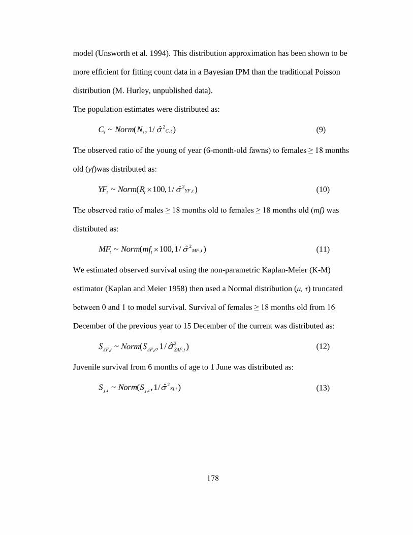
178
model (Unsworth et al. 1994). This distribution approximation has been shown to be
more efficient for fitting count data in a Bayesian IPM than the traditional Poisson
distribution (M. Hurley, unpublished data).
The population estimates were distributed as:
(9)
The observed ratio of the young of year (6-month-old fawns) to females ≥ 18 months
old (yf)was distributed as:
(10)
The observed ratio of males ≥ 18 months old to females ≥ 18 months old (mf) was
distributed as:
(11)
We estimated observed survival using the non-parametric Kaplan-Meier (K-M)
estimator (Kaplan and Meier 1958) then used a Normal distribution (μ, τ) truncated
between 0 and 1 to model survival. Survival of females ≥ 18 months old from 16
December of the previous year to 15 December of the current was distributed as:
(12)
Juvenile survival from 6 months of age to 1 June was distributed as:
(13)
)ˆ/1,(~ ,2
tCtt NNormC
)ˆ/1,100(~ ,2
tYFtt RNormYF
)ˆ/1,100(~ ,2
tMFtt mfNormMF
SAF,t ~ Norm(SAF,t, 1/ s 2
SAF,t )
)ˆ/1,(~ ,2
,, tSjtjtj SNormS
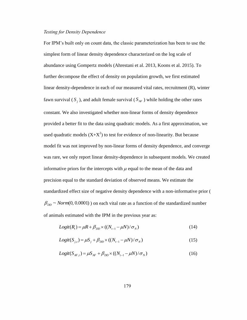
179
Testing for Density Dependence
For IPM’s built only on count data, the classic parameterization has been to use the
simplest form of linear density dependence characterized on the log scale of
abundance using Gompertz models (Ahrestani et al. 2013, Koons et al. 2015). To
further decompose the effect of density on population growth, we first estimated
linear density-dependence in each of our measured vital rates, recruitment (R), winter
fawn survival ( ), and adult female survival ( ) while holding the other rates
constant. We also investigated whether non-linear forms of density dependence
provided a better fit to the data using quadratic models. As a first approximation, we
used quadratic models (X+X2) to test for evidence of non-linearity. But because
model fit was not improved by non-linear forms of density dependence, and converge
was rare, we only report linear density-dependence in subsequent models. We created
informative priors for the intercepts with equal to the mean of the data and
precision equal to the standard deviation of observed means. We estimate the
standardized effect size of negative density dependence with a non-informative prior (
) on each vital rate as a function of the standardized number
of animals estimated with the IPM in the previous year as:
(14)
(15)
(16)
jS AFS
)0001.0,0(~ NormDD
)/)(()( 1 NtDDt NNRRLogit
)/)(()( 1, NtDDjtj NNSSLogit
)/)(()( 1, NtDDAFtAF NNSSLogit
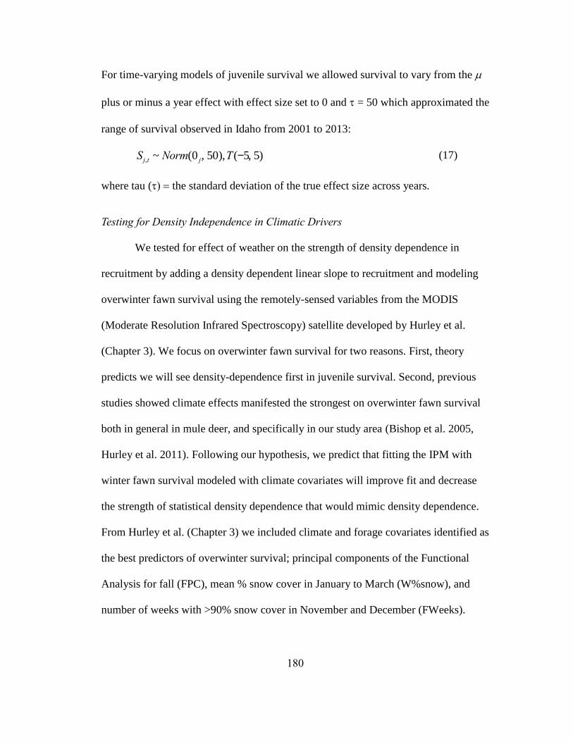
180
For time-varying models of juvenile survival we allowed survival to vary from the
plus or minus a year effect with effect size set to 0 and = 50 which approximated the
range of survival observed in Idaho from 2001 to 2013:
(17)
where tau (the standard deviation of the true effect size across years.
Testing for Density Independence in Climatic Drivers
We tested for effect of weather on the strength of density dependence in
recruitment by adding a density dependent linear slope to recruitment and modeling
overwinter fawn survival using the remotely-sensed variables from the MODIS
(Moderate Resolution Infrared Spectroscopy) satellite developed by Hurley et al.
(Chapter 3). We focus on overwinter fawn survival for two reasons. First, theory
predicts we will see density-dependence first in juvenile survival. Second, previous
studies showed climate effects manifested the strongest on overwinter fawn survival
both in general in mule deer, and specifically in our study area (Bishop et al. 2005,
Hurley et al. 2011). Following our hypothesis, we predict that fitting the IPM with
winter fawn survival modeled with climate covariates will improve fit and decrease
the strength of statistical density dependence that would mimic density dependence.
From Hurley et al. (Chapter 3) we included climate and forage covariates identified as
the best predictors of overwinter survival; principal components of the Functional
Analysis for fall (FPC), mean % snow cover in January to March (W%snow), and
number of weeks with >90% snow cover in November and December (FWeeks).
S j,t ~ Norm(0 j, 50),T(-5, 5)
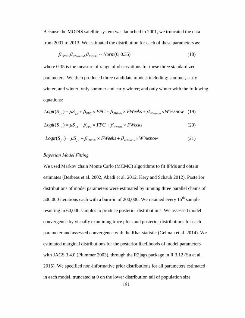
181
Because the MODIS satellite system was launched in 2001, we truncated the data
from 2001 to 2013. We estimated the distribution for each of these parameters as:
(18)
where 0.35 is the measure of range of observations for these three standardized
parameters. We then produced three candidate models including: summer, early
winter, and winter; only summer and early winter; and only winter with the following
equations:
(19)
(20)
(21)
Bayesian Model Fitting
We used Markov chain Monte Carlo (MCMC) algorithms to fit IPMs and obtain
estimates (Besbeas et al. 2002, Abadi et al. 2012, Kery and Schaub 2012). Posterior
distributions of model parameters were estimated by running three parallel chains of
500,000 iterations each with a burn-in of 200,000. We retained every 15th
sample
resulting in 60,000 samples to produce posterior distributions. We assessed model
convergence by visually examining trace plots and posterior distributions for each
parameter and assessed convergence with the Rhat statistic (Gelman et al. 2014). We
estimated marginal distributions for the posterior likelihoods of model parameters
with JAGS 3.4.0 (Plummer 2003), through the R2jags package in R 3.12 (Su et al.
2015). We specified non-informative prior distributions for all parameters estimated
in each model, truncated at 0 on the lower distribution tail of population size
)35.0,0(~,, % NormFWeekssnowWFPC
snowWFWeeksFPCSSLogit snowWFWeeksFPCtjtj %)( %,,
FWeeksFPCSSLogit FWeeksFPCtjtj ,, )(
snowWFWeeksSSLogit snowWFWeekstjtj %)( %,,
182
estimates and truncated between 0 and 1 for survival estimates. We initialized
population size of each age class using the mean total counts and the proportion
animals in each age class determined by ratio estimates. We used a normal
distribution with a vague precision (Brooks et al. 2004). We also used normal priors
with mean recruitment or survival data and vague precision (0.0001).
RESULTS
(a) Density dependence on vital rates
We first estimated the influence of density on vital rates by applying density
dependent (DD) terms on each of the individual vital rates for all PMUs. Of the
simple models we evaluated (one DD term each) density dependence effects on
recruitment was the most supported vital rate, followed by juvenile survival through
winter, and then adult female survival (Table 5-1). Boise River was the exception
where density dependence on juvenile survival was most supported with a lower DIC
(∆ DIC = 4.5). Applying density dependence to adult female survival increased the
DIC > 40% from the best model in all PMUs suggesting poorer overall IPM fit.
(b) Strength of density dependence on recruitment
We used the most supported model from Table 1, density dependence of
recruitment and time varying juvenile survival to compare the strength of density
across our environmentally diverse study areas. The strength of density dependence
(effect size) declined in this order: South Hills, Boise River, Bannock, Central
Mountains, Weiser-McCall, and Caribou (Table 5-2, Figure 5-2). Boise River and
183
South Hills were both predicted to have the strongest negative density dependence as
we observed, βDD = -0.759, SD = 0.692 and βDD = -0.165, SD = 0.81 respectively.
Caribou (βDD = 0.085, SD = 0.046) was the only PMUs that displayed no negative
density dependence in recruitment (Table 5-2, Figure 5-2, 5-6) as we predicted.
(c) Density or weather
We used the best model from each of 3 model sets; 1) density dependence on
recruitment and time varying juvenile survival (density only), 2) time varying
recruitment and juvenile survival modeled with weather covariates (weather only),
and 3) density dependence on recruitment and juvenile survival modeled with
weather covariates (density + weather) to test the effects density and weather across
the 6 PMUs. For four of the six PMUs, the most supported model considered a
density dependent term on recruitment and time varying winter fawn survival (DDO;
Table 5-3). The two exceptions were Boise River and Central Mountains, where the
weather effects on juvenile survival with time varying recruitment models were most
supported (weather only; Table 5-3). The addition of weather covariates to the density
dependent models decreased the magnitude of the effect of density dependence on
recruitment in all PMUs with the exception of Caribou, where the effect changed
from slightly positive to a highly variable negative effect(βDD = 0.085, SD = 0.046 vs.
βDD = -0.389, SD = 0.493; Table 5-3). The resulting weather plus density models fit
the data poorly in contrast to the density only models as displayed in Figures 5-3 and
5-4. In general, we found density of the previous year depressed recruitment in the
following year, thereby limiting population growth in most populations in Idaho.
184
(d) Effects of Weather
We found variation between PMUs in density-independent weather effects,
and the strength or each weather covariate on population growth (Table 5-3, Figure 5-
5). For the late summer forage quality (FPCA) measure, we found a strong negative
effect on mule deer abundance in Boise River, and a weak effect on the Central
Mountains and Weiser-McCall PMUs. In Bannock, Caribou, and South Hills, late
summer forage conditions increased mule deer abundance (Table 5-3, Figure 5-6).
Similarly, the number of fall weeks covered by snow had no consistent effects on
Bannock, Caribou, Central Mountains, but negative effects on abundance in Boise,
South Hills and Weiser-McCall (Figure 5-5). Finally, winter snow cover from
January to March had strong negative effects only on the Boise PMU where density-
dependence was also strong. In all other units, even when winter severity was
included as a covariate in some models, the effect was weak with posterior estimates
overlapping zero (Figure 5-5).
Contrary to our predictions, we did not observe a clear pattern of weather
effects in relation to effect size of density dependence in recruitment. There was no
clear negative relationship between the strength of density-dependence and the
strength of density-independence within a PMU for any of the climatic covariates
considered here (Figure 5-5). In fact, if anything, there was some evidence for
interactive effects of density and climate insomuch that the units that experienced the
strongest signs of density dependence (Boise, South Hills) also experienced the
strongest climatic effects (Figure 5-2, 5-6).

185
DISCUSSION
Our first prediction, that mule deer populations are primarily weather limited and thus
will not experience density dependent reductions in vital rate was only partially
supported. Weather effects were more important than density in 2 of our 6
populations, the remaining showed some evidence that density was more important.
We observed the strongest density dependent effect in recruitment, followed by
winter fawn survival and finally adult survival constant with our predictions. The
pattern of density dependence within these vital rates were consistent with those
predicted and documented for a variety of ungulate species (Eberhardt 2002, Gaillard
and Yoccoz 2003). We observed a reduction in the strength of density parameter when
weather covariates were added but at the same time a significant overall reduction in
model fit, clouding the interpretation of this prediction. The effect of density-
dependence was not replaced with weather effects as we predicted. It was unclear
whether this change in parameter strength was a biological effect or reduction in
model fit, it could also be due to the interaction of density and weather effects. Lastly,
density dependent effects decreased with increasing environmental severity, as we
predicted.
Our empirical evidence is similar to Coulson (2000) in that density
dependence in ungulates was population specific, especially in the highly variable
environmental conditions. In addition to being population-specific, within a
population we observed one year experiencing density effects and effects related to
weather in the next. The interactive effects of age, weather, and predation can in some
cases mimic density effects and combinations of age structure, weather, and density
186
dependence can lead to similar population sizes with very different trajectories
(Coulson et al. 2001). Environmental stochasticity in resource availability and climate
can affect population dynamics though reduced quality of summer forage, thereby
reducing pregnancy and juvenile survival (Cook et al. 2004, Chapter 2). Two studies
reported single species exhibiting density dependence in one population and not
another based on latitude (Post 2005, Ahrestani et al. 2013). Therefore, predicting
ungulate population dynamics may depend on idiosyncratic knowledge of the relative
strength of density-dependent and independent drivers on a population specific basis.
The pattern of density dependence within our observed vital rates, recruitment
> overwinter survival > adult survival, was consistent with those predicted and
documented for a variety of ungulate species (Eberhardt 2002, Gaillard and Yoccoz
2003). This is not unexpected because our recruitment measure, fawn ratio in
December, is a measure of pregnancy, fetal rate, and young survival of both
primiparous and multiparous mothers. These are the vital rates assumed to be first
affected by density in ungulates (Bonenfant et al. 2009). As evidence, we have
observed highly variable yearling pregnancy rates in our study area, varying from
12% to 80% although pregnancy is stable for older animals (M. Hurley, Unpublished
data). These results have been echoed across temperate ungulate species (Gaillard et
al. 2000), and despite the equivocal evidence for density-dependence in vital rates
leading to density-dependence in population dynamics of mule deer (Bergman et al.
2015), our study shows that indeed, mule deer populations do respond predictably to
increasing density similar to other species.

187
Another aspect of recruitment, summer neonate fawn survival, may be
depressed by density under a predator-mediated density effect discussed in Chapter 4.
Effects of density may differ depending if mule deer summer resource selection is
best described by an ideal free versus an ideal despotic (territorial) model of habitat
selection(McLoughlin et al. 2009). Territoriality during early fawn rearing occurs in
many small- to mid-sized ungulates, including mule deer (Mackie et al. 1998).
Exclusive space use (territoriality) during fawn rearing may increase recruitment of
juveniles by dominant females through exclusive access to high quality forage and
low predation risk habitats while displacing subdominant females to lower quality
habitat. The described behavior may create a despotic distribution of parturient
females across summer range, with an overall reduction of fawn survival as densities
increase. In addition to predation risk, the quality of this secondary habitat may be
variable with respect to weather conditions, adequate for fawn rearing with high
precipitation but nutritionally limited in low precipitation years, as has been observed
in roe deer (Capreolus capreolus; Pettorelli et al. 2005) suggesting density
dependence in one year and not the next. Given the strong relationship between
winter fawn survival and weather (Hurley et al. 2011, Bishop et al. 2005, Bartmann et
al. 1992, Chapter 3) we did not expect overwinter fawn survival to exhibit a strong
density effect, consistent with our results. This vital is highly variable (Figure 5-3)
and significantly related to weather (Chapter 3), unless latent effect of the resource
use described above.
Our results corroborated those of Post (2005) confirming the strength of
density dependence decreased as environmental conditions became more severe.
188
Whereas Post (2005) evaluated the effect of latitude, we observed the same reduction
in the strength of negative density dependent strength in our study areas (Caribou,
Bannock, and Weiser-McCall) where severe winters or decrease summer forage
quality are common, resulting in variable fawn survival and population fluctuation.
We did not explicitly test interactions here because of the modeling complexity
involved in fitting interactions between density and up to 3 climate covariates, adding
another 3-9 parameters to complex IPM models. We recognize this as an important
limitation of our study, given the recognized importance of climate-density
interactions in ungulate ecology (Portier et al. 1998; Hebblewhite 2005). Regardless,
there was only weak evidence for effects of density changing when in the presence of
weather covariates in IPM models. Our best models were either density dependent or
weather dependent, and spatially distinct. The weather-limited populations were in
similar habitats in Central Idaho. We predicted that if populations were truly density
independent the addition of weather covariates would decrease the strength of density
dependence as we observed. However, the addition of weather covariates to model
fawn survival from 6 months to 1 year old to our density dependence models
decreased the model fit in all of the PMUs.
We have used an integrated population model to test the effects of density and
weather on mule deer populations 6 spatial distinct mule deer populations. The
resulting models separated vital rate specific effects of density and weather while
simultaneously estimating other vital rates given these effects. These models will
vastly improve our understanding of the importance of each vital rate to population
dynamics. We conclude that mule deer population dynamics are similar to other

189
ungulates, experiencing the density dependent influences as modified by both
summer nutrition and winter energy expenditure.
LITERATURE CITED
Abadi, F., O. Gimenez, H. Jakober, W. Stauber, R. Arlettaz, and M. Schaub. 2012.
Estimating the strength of density dependence in the presence of observation
errors using integrated population models. Ecological Modelling 242:1-9.
Ahrestani, F. S., M. Hebblewhite, and E. Post. 2013. The importance of observation
versus process error in analyses of global ungulate populations. Scientific
reports 3.
Andrewartha, H. G. and L. C. Birch, editors. 1954. The distribution and abundance of
animals. University of Chicago Press, Chicago, Illinois, USA.
Bartmann, R. M., G. C. White, and L. H. Carpenter. 1992. Compensatory mortality in
a Colorado mule deer population. Wildlife Monographs:3-39.
Bergman, E. J., P. F. Doherty, G. C. White, and A. A. Holland. 2015. Density
dependence in mule deer: a review of evidence. Wildlife Biology 21:18-29.
Besbeas, P., S. N. Freeman, B. J. Morgan, and E. A. Catchpole. 2002. Integrating
mark–recapture–recovery and census data to estimate animal abundance and
demographic parameters. Biometrics 58:540-547.
Bishop, C. J., J. W. Unsworth, and E. O. Garton. 2005. Mule Deer Survival among
Adjacent Populations in Southwest Idaho. The Journal of Wildlife
Management 69:311-321.

190
Bjornstad, O. N. and B. T. Grenfell. 2001. Noisy Clockwork: Time Series Analysis of
Population Fluctuations in Animals. Science 293:638-643.
Bonenfant, C., J. M. Gaillard, T. Coulson, M. Festa‐Bianchet, A. Loison, M. Garel, L.
E. Loe, P. Blanchard, N. Pettorelli, N. Owen‐Smith, J. Du Toit, and P. Duncan.
2009. Empirical Evidence of Density‐Dependence in Populations of Large
Herbivores. Advances in Ecological Research 41:313-357.
Brook, B. W. and C. J. Bradshaw. 2006. Strength of evidence for density dependence
in abundance time-series of 1198 species. Ecology 87:1445-1451.
Brooks, S., R. King, and B. Morgan. 2004. A Bayesian approach to combining animal
abundance and demographic data. Animal Biodiversity and Conservation
27:515-529.
Caswell, H. 2000. Prospective and retrospective perturbation analyses: their roles in
conservation biology. Ecology 81:619-627.
Caughley, G. and C. J. Krebs. 1983. Are big mammals simply little mammals writ
large? Oecologia 59:7-17.
Clutton–Brock, T. and T. Coulson. 2002. Comparative ungulate dynamics: the devil is
in the detail. Philosophical Transactions of the Royal Society of London B:
Biological Sciences 357:1285-1298.
Cook, J. G., B. K. Johnson, R. C. Cook, R. A. Riggs, T. Delcurto, L. D. Bryant, and L.
L. Irwin. 2004. Effects of Summer-Autumn Nutrition and Parturition Date on
Reproduction and Survival of Elk. Wildlife Monographs:1-61.
Coulson, T., E. A. Catchpole, S. D. Albon, B. J. T. Morgan, J. M. Pemberton, T. H.
Clutton-Brock, M. J. Crawley, and B. T. Grenfell. 2001. Age, Sex, Density,

191
Winter Weather, and Population Crashes in Soay Sheep. Science 292:1528-
1531.
Coulson, T., E. J. Milner-Gulland, and T. Clutton-Brock. 2000. The relative roles of
density and climatic variation on population dynamics and fecundity rates in
three contrasting ungulate species. Proceedings of the Royal Society, B.
267:1771-1779.
Coulson, T., E. A. Catchpole, S. D. Albon, B. J. T. Morgan, J. M. Pemberton, T. H.
Clutton-Brock, M. J. Crawley, and B. T. Grenfell. 2001. Age, Sex, Density,
Winter Weather, and Population Crashes in Soay Sheep. Science 292:1528-
1531.
De Valpine, P. and A. Hastings. 2002. Fitting Population Models Incorporating
Process Noise and Observation Error. Ecological Monographs 72:57-76.
Dennis, B. and M. L. Taper. 1994. Density dependence in time series observations of
natural populations: estimation and testing. Ecological Monographs 64:205-
224.
Eberhardt, L. L. 2002. A paradigm for population analysis of long-lived vertebrates.
Ecology 83:2841-2854.
Eberhardt, L. L., R. A. Garrott, D. W. Smith, P. J. White, and R. O. Peterson. 2003.
Assessing the Impact of Wolves on Ungulate Prey. Ecological Applications
13:776-783.
Elkington, J. S. 2000. Detecting stability and causes of change in population density.
Pages 191-209 in L. Boitani and T. K. Fuller, editors. Research Techniques in

192
Animal Ecology: Controversies and Consequences. Columbia University
Press, New York.
Fowler, C. W. 1981. Density dependence as related to life-history strategy. Ecology
62:602-610.
Gaillard, J. M. and N. G. Yoccoz. 2003. Temporal Variation in Survival of Mammals:
a Case of Environmental Canalization? Ecology 84:3294-3306.
Gelman, A., J. B. Carlin, H. S. Stern, and D. B. Rubin. 2014. Bayesian data analysis.
Taylor & Francis.
Gordon, I. J., A. J. Hester, and M. Festa-Bianchet. 2004. The Management of Wild
Large Herbivores to Meet Economic, Conservation and Environmental
Objectives. Journal of Applied Ecology 41:1021-1031.
Hebblewhite, M. 2005. Predation by Wolves Interacts with the North Pacific
Oscillation (NPO) on a Western North American Elk Population. Journal of
Animal Ecology 74:226-233.
Hurley, M. A., J. W. Unsworth, P. Zager, M. Hebblewhite, E. O. Garton, D. M.
Montgomery, J. R. Skalski, and C. L. Maycock. 2011. Demographic response
of mule deer to experimental reduction of coyotes and mountain lions in
southeastern Idaho. Wildlife Monographs 178:1-33.
Hurley, M. A., M. Hebblewhite, J. M. Gaillard, S. Dray, K. A. Taylor, W. K. Smith, P.
Zager, and C. Bonenfant. 2014. Functional analysis of normalized difference
vegetation index curves reveals overwinter mule deer survival is driven by
both spring and autumn phenology. Philos Trans R Soc Lond B Biol Sci
369:20130196.

193
IDFG. 2013. Big Game Harvest Statewide.in I. D. o. F. a. Game, editor., Boise.
Johnson, H. E., L. Scott Mills, J. D. Wehausen, and T. R. Stephenson. 2010.
Combining ground count, telemetry, and mark–resight data to infer population
dynamics in an endangered species. Journal of Applied Ecology 47:1083-
1093.
Kery, M. and M. Schaub. 2012. Bayesian population analysis using WinBUGS: a
hiearchical perspective. Acadmic Press, San Diego, CA.
Koons, D. N., F. Colchero, K. Hersey, and O. Gimenez. 2015. Disentangling the
effects of climate, density dependence, and harvest on an iconic large
herbivore's population dynamics. Ecological Applications 25:956-967.
Krebs, C. J., editor. 1994. Ecology: the experimental analysis of distribution and
abundance. HarperCollins College Publishers, New York, NY.
Lee, A. M., E. M. Bjørkvoll, B. B. Hansen, S. D. Albon, A. Stien, B. E. Sæther, S.
Engen, V. Veiberg, L. E. Loe, and V. Grøtan. 2015. An integrated population
model for a long‐lived ungulate: more efficient data use with Bayesian
methods. Oikos 124:806-816.
Mackie, R. J., D. F. Pac, K. L. Hamlin, and G. L. Ducek. 1998. Ecology and
Management of Mule Deer and White-tailed Deer in Montana. Federal Aid
Project W-120-R, Montana Fish, Wildlife and Parks, Helena.
McCullough, D. R., editor. 1979. The George Reserve Deer Herd: Population ecology
of a K-selection species. Univerisity of Michigan Press, Ann Arbor.
Melis, C., B. Jędrzejewska, M. Apollonio, K. A. Bartoń, W. Jędrzejewski, J. D.
Linnell, I. Kojola, J. Kusak, M. Adamic, and S. Ciuti. 2009. Predation has a
194
greater impact in less productive environments: variation in roe deer,
Capreolus capreolus, population density across Europe. Global Ecology and
Biogeography 18:724-734.
Mysterud, A. 2006. The concept of overgrazing and its role in management of large
herbivores. Wildlife Biology 12:129-141.
Patterson, B. R. and V. A. Power. 2002. Contributions of forage competition, harvest,
and climate fluctuation to changes in population growth of northern white-
tailed deer. Oecologia 130:62-71.
Peek, J. M., Brian Dennis and Terry Hershey. 2002. Predicting population trends in
mule deer. Journal of Wildlife Management 66:729-736.
Pettorelli, N., J. M. Gaillard, N. G. Yoccoz, P. Duncan, D. Maillard, D. Delorme, G.
Van Laere, and C. Toigo. 2005. The Response of Fawn Survival to Changes in
Habitat Quality Varies According to Cohort Quality and Spatial Scale. Journal
of Animal Ecology 74:972-981.
Plummer, M. 2003. JAGS: A Program for Analysis of Bayesian Graphical Models
Using Gibbs Sampling.in Proceedings of the 3rd International Workshop on
Distributed Statistical Computing (DSC 2003), Vienna, Austria.
Portier, C., M. Festa-Bianchet, J.-M. Gaillard, J. T. Jorgenson, and N. G. Yoccoz.
1998. Effects of density and weather on survival of bighorn sheep lambs (Ovis
canadensis). Journal of Zoology, London 245:271-278.
Post, E. 2005. Large-scale spatial gradients in herbivore population dynamics.
Ecology 86:2320-2328.
195
Royle, J. A., M. Kery, R. Gautier, and H. Schmid. 2007. Hierarchical spatial models
of abundance and occurrence from imperfect survey data. Ecological
Monographs 77:465-481.
Saether, B. E. 1997. Environmental Stochasticity and Population Dynamics of Large
Herbivores: a Search for Mechanisms. Trends in Ecology & Evolution
12:143-149.
Saether, B. E., M. Lillegard, V. Grotan, F. Filli, and S. Engen. 2007. Predicting
fluctuations of reintroduced ibex populations: the importance of density
dependence, environmental stochasticity and uncertain population estimates.
Journal of Animal Ecology 76:326-336.
Sawyer, H., F. Lindzey, and D. Mcwhirter. 2005. Mule Deer and Pronghorn Migration
in Western Wyoming. Wildlife Society Bulletin 33:1266-1273.
Sibly, R. M. and R. H. Smith. 1998. Identifying key factors using lambda contribution
analysis. Journal of Animal Ecology 67:17-24.
Sinclair, A. R. E. 1989. Population regulation of animals. Pages 197-241 in J. M.
Cherret, editor. Ecological Concepts. Blackwell, Oxford.
Sinclair, A. R. E., S. Mduma, and J. S. Brashares. 2003. Patterns of Predation in a
Diverse Predator-Prey System. Nature 425:288-290.
Sinclair, A. R. E. and R. P. Pech. 1996. Density dependence, stochasticity,
compensation and predator regulation. Oikos 75:164-173.
Stewart, K. M., R. T. Bowyer, B. L. Dick, B. K. Johnson, and J. G. Kie. 2005.
Density-Dependent Effects on Physical Condition and Reproduction in North
American Elk: An Experimental Test. Oecologia 143:85-93.

196
Su, Y.-S., M. Yajima, M. Y.-S. Su, and J. SystemRequirements. 2015. Package
‘R2jags’.
Taper, M. L. and P. J. Gogan. 2002. The northern yellowstone elk: density
dependence and climatic conditions. Journal of Wildlife Management 66:106-
122.
Turchin, P., editor. 2003. Complex population dynamics: a theoretical/empirical
synthesis. Princeton University Press, Princeton, NJ.
Unsworth, J. A., F. A. Leban, D. J. Leptich, E. O. Garton, and P. Zager, editors. 1994.
Aerial Survey: User's Manual. Second Edition. Idaho Department of Fish and
Game, Biose, ID.
Wade, D. A. and J. E. Bowns. 1982. Procedures for evaluating predation on livestock
and wildlife. Experiment Station, Texas A&M University, College Station TX.
Wang, G., N. T. Hobbs, S. Twombly, R. B. Boone, A. W. Illius, I. J. Gordon, and J. E.
Gross. 2009. Density dependence in northern ungulates: interactions with
predation and resources. Population Ecology 51:123-132.
White, G. C. and R. M. Bartmann. 1998a. Effect of density reduction on overwinter
survival of free-ranging mule deer fawns. Journal of Wildlife Management
62:214-225.
White, G. C. and R. M. Bartmann. 1998b. Effect of Density Reduction on Overwinter
Survival of Free-Ranging Mule Deer Fawns. The Journal of Wildlife
Management 62:214-225.

197
Wilmers, C. C., E. Post, R. O. Peterson, and J. A. Vucetich. 2006. Predator disease
out‐break modulates top‐down, bottom‐up and climatic effects on herbivore
population dynamics. Ecology Letters 9:383-389.

198
TABLES
Table 5-1. Integrated Population Model (IPM) model selection for mule deer (Odocoileus hemionus) for 6 Population Management
Unit (PMU), Idaho, 2001 – 2013. Shown is the model structure with density dependent (dd) terms added on each vital rate (R-
recruitment, jS – juvenile survival, fS – adult female survival, mS – adult male survival) and the prefix denotes dd = density
dependence, c = vital rate varies within a given distribution of the global mean for the PMU, and t = vital rate varies within a given
distribution for an annual mean. Model diagnostics are the Deviance Information Criteria (DIC), effective number of parameters
(pD), Deviance, and parameter estimates for density dependence (DD), and the standard deviation of density dependence (DD SD).
PMU Model DD DD SD DIC pD Deviance
Bannock ddR_tjS_cfS_cmS -0.139 0.043 201.2 22.6 178.5
Bannock tR_ddjS_cfS_cmS -0.402 0.063 235.4 21.4 214.0
Bannock cR_ddjS_cfS_cmS -0.434 0.057 260.7 14.8 245.9
Bannock ddR_cjS_cfS_cmS 0.067 0.063 282.8 16.2 266.6
Bannock cR_cjS_ddfS_cmS 0.076 0.059 283.9 11.7 272.1
Boise River tR_ddjS_cfS_cmS 0.332 0.064 668.1 76.6 591.5
Boise River ddR_tjS_cfS_cmS -0.759 0.692 672.6 106.2 566.4
Boise River cR_cjS_ddfS_cmS -4.164 0.812 903.7 74.4 829.3
Boise River cR_ddjS_cfS_cmS 0.284 0.080 1,075.0 105.7 969.2
Boise River ddR_cjS_cfS_cmS -0.085 0.032 1,100.7 125.3 975.4
Caribou ddR_tjS_cfS_cmS 0.085 0.046 209.3 20.6 188.7
199
Caribou tR_ddjS_cfS_cmS -2.304 0.445 298.0 34.9 263.1
Caribou cR_ddjS_cfS_cmS -3.514 0.749 465.2 63.3 401.9
Caribou cR_cjS_ddfS_cmS 1.411 0.233 608.1 44.4 563.6
Caribou ddR_cjS_cfS_cmS 0.106 0.075 619.2 34.0 585.2
Central Mountains ddR_tjS_cfS_cmS -0.076 0.044 232.7 22.2 210.5
Central Mountains tR_ddjS_cfS_cmS -0.159 0.058 244.3 22.5 221.8
Central Mountains ddR_cjS_cfS_cmS 0.086 0.084 309.5 8.8 300.8
Central Mountains cR_ddjS_cfS_cmS -0.002 0.081 312.6 9.3 303.3
Central Mountains cR_cjS_ddfS_cmS 0.225 0.209 313.6 8.8 304.8
South Hills ddR_tjS_cfS_cmS -0.165 0.081 76.3 14.4 61.9
South Hills tR_ddjS_cfS_cmS -0.585 0.130 89.7 20.7 69.0
South Hills cR_ddjS_cfS_cmS -0.393 0.043 107.2 13.1 94.1
South Hills ddR_cjS_cfS_cmS -0.353 0.073 137.2 28.2 109.0
South Hills cR_cjS_ddfS_cmS 0.274 0.098 188.6 61.7 126.8
Weiser McCall ddR_tjS_cfS_cmS -0.119 0.050 340.6 58.6 282.0
Weiser McCall tR_ddjS_cfS_cmS -0.966 0.099 401.6 60.2 341.4
Weiser McCall cR_ddjS_cfS_cmS -1.385 0.067 538.6 85.9 452.8
Weiser McCall cR_cjS_ddfS_cmS 1.261 0.260 647.1 42.0 605.1
Weiser McCall ddR_cjS_cfS_cmS -0.061 0.077 658.7 54.7 604.0
200
Table 5-2. Integrated Population Model (IPM) model selection for mule deer (Odocoileus hemionus) in 6 Population Management
Units (PMU), Idaho, years 2001 – 2013. The model structure includes a density dependent term on recruitment, time-varying juvenile
survival, constant adult female survival, and constant adult male survival. Parameter estimates for density dependence (DD) and
standard deviations (SD) are provided for density dependence (DD). Model fitting diagnostic are Deviance Information Criteria (DIC),
effective number of parameters (pD) and Deviance. In this instance ΔDIC describes the relationship to the PMU specific model set to
illustrate departure from the best model when another model is used for constancy of model structure for DD covariate comparisons.
PMU Model DD DD SD ΔDIC DIC Deviance pD
Boise River Recruitment DD -0.759 0.692 4.5 672.6 566.4 106.2
South Hills Recruitment DD -0.165 0.081 0.0 76.3 61.9 14.4
Bannock Recruitment DD -0.139 0.043 0.0 201.2 178.5 22.6
Weiser McCall Recruitment DD -0.119 0.050 0.0 340.6 282.0 58.6
Central Mtns. Recruitment DD -0.076 0.044 0.0 232.7 210.5 22.2
Caribou Recruitment DD 0.085 0.046 0.0 209.3 188.7 20.6
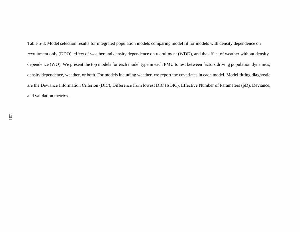
201
Table 5-3: Model selection results for integrated population models comparing model fit for models with density dependence on
recruitment only (DDO), effect of weather and density dependence on recruitment (WDD), and the effect of weather without density
dependence (WO). We present the top models for each model type in each PMU to test between factors driving population dynamics;
density dependence, weather, or both. For models including weather, we report the covariates in each model. Model fitting diagnostic
are the Deviance Information Criterion (DIC), Difference from lowest DIC (ΔDIC), Effective Number of Parameters (pD), Deviance,
and validation metrics.
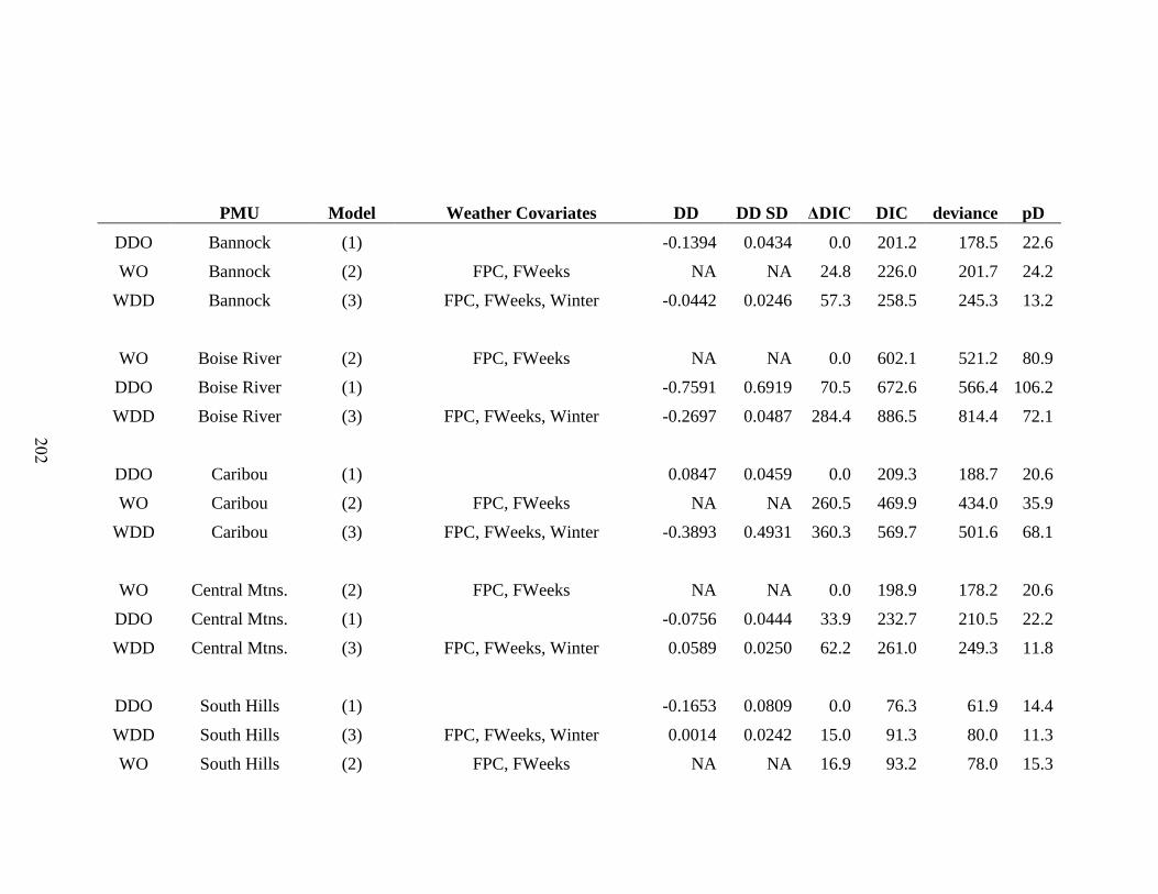
202
PMU Model Weather Covariates DD DD SD ΔDIC DIC deviance pD
DDO Bannock (1) -0.1394 0.0434 0.0 201.2 178.5 22.6
WO Bannock (2) FPC, FWeeks NA NA 24.8 226.0 201.7 24.2
WDD Bannock (3) FPC, FWeeks, Winter -0.0442 0.0246 57.3 258.5 245.3 13.2
WO Boise River (2) FPC, FWeeks NA NA 0.0 602.1 521.2 80.9
DDO Boise River (1) -0.7591 0.6919 70.5 672.6 566.4 106.2
WDD Boise River (3) FPC, FWeeks, Winter -0.2697 0.0487 284.4 886.5 814.4 72.1
DDO Caribou (1) 0.0847 0.0459 0.0 209.3 188.7 20.6
WO Caribou (2) FPC, FWeeks NA NA 260.5 469.9 434.0 35.9
WDD Caribou (3) FPC, FWeeks, Winter -0.3893 0.4931 360.3 569.7 501.6 68.1
WO Central Mtns. (2) FPC, FWeeks NA NA 0.0 198.9 178.2 20.6
DDO Central Mtns. (1) -0.0756 0.0444 33.9 232.7 210.5 22.2
WDD Central Mtns. (3) FPC, FWeeks, Winter 0.0589 0.0250 62.2 261.0 249.3 11.8
DDO South Hills (1) -0.1653 0.0809 0.0 76.3 61.9 14.4
WDD South Hills (3) FPC, FWeeks, Winter 0.0014 0.0242 15.0 91.3 80.0 11.3
WO South Hills (2) FPC, FWeeks NA NA 16.9 93.2 78.0 15.3

203
Model Structure: 1. Density dependence on recruitment and time varying juvenile survival.
2. Time varying recruitment and juvenile survival modeled with weather covariates.
3. Density dependence on recruitment and juvenile survival modeled with weather covariates.
DDO Weiser McCall (1) -0.1191 0.0498 0.0 340.6 282.0 58.6
WO Weiser McCall (2) FPC, FWeeks NA NA 72.1 412.7 359.8 52.9
WDD Weiser McCall (3) FPC, FWeeks, Winter -0.0376 0.0198 271.1 611.7 553.6 58.1

204
FIGURES
Figure 5-1. Basic age-structured life-cycle for the post-breeding birth pulse matrix
model used as the basis for the Integrated Population Model (IPM) for mule deer
(Odocoileus hemionus) in Idaho. Here, we start the recruitment of individuals as 6
month olds as estimated from fawn to adult female ratio counts in December, estimate
survival through winter and summer, and recruit into the adult population at age 18
months. Only adults reproduce as the age of first reproduction is 2 in mule deer.
205
Figure 5-2. Spatial map of the strength of density-dependent population growth rate
for Mule deer (Odocoileus hemionus) populations estimated with an integrated
population model in Idaho, 2001-2013.

206
Figure 5-3. Integrated population model (IPM) projections for Mule deer
(Odocoileus hemionus) in the Bannock population management unit (PMU),
Idaho, 2001-2013, showing time varying juvenile survival, constant female
survival, and population abundance estimates consistent with a density-dependent
effect on recruitment only. Lines indicate posterior mean estimate with 95%
credible interval (grey shading). Points are field data with 95% confidence
interval.

207
Figure 5-4. Integrated population model (IPM) projections for mule deer
(Odocoileus hemionus) in the Bannock population management unit (PMU),
Idaho, 2001 - 2013, weather modeled juvenile survival, constant female
survival, and population abundance estimates consistent with a density-dependent
effect on recruitment. Lines indicate posterior mean estimate with 95% credible
interval (grey shading). Points are field data with 95% confidence interval.
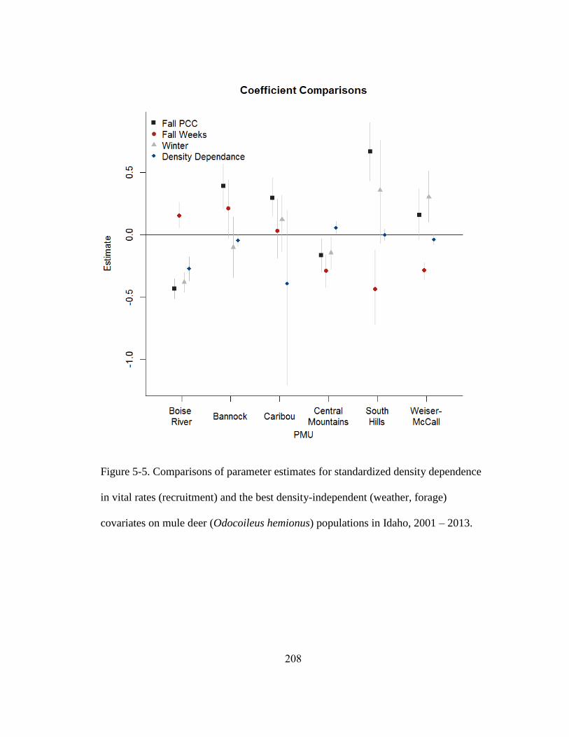
208
Figure 5-5. Comparisons of parameter estimates for standardized density dependence
in vital rates (recruitment) and the best density-independent (weather, forage)
covariates on mule deer (Odocoileus hemionus) populations in Idaho, 2001 – 2013.

209
Figure 5-6. Spatial map of the strength of density-independent effects on population
growth rate from annual variation in late summer forage quality for mule deer
(Odocoileus hemionus) populations estimated with an integrated population model in
Idaho, 2001-2013.

210
APPENDIX C. SUPPLEMENTAL MATERIALS
Table 5_S1: Model selection results for integrated population models for mule deer (Odocoileus hemionus) with weather covariates.
The overall models contain data from all Population Management Units (PMU) and all years. Table A compares the best fitting
models with varying covariates. Table B compares only the shorter model with covariates Fall PCC and Fall Weeks for each PMU.
The models compare the effects of weather on time varying recruitment and constant juvenile and adult survival with no density
dependence. For all models, we report the Deviance Information Criterion (DIC), Difference from lowest DIC (ΔDIC), Effective
Number of Parameters (pD), Deviance, and validation metrics.
A.
PMU Model Covariates DIC deviance pD
Bannock tR_cjS_cfS_cmS_pe_vars.txt Fall PCC,Fall Weeks 225.9528 201.7095 24.24338
Boise River tR_cjS_cfS_cmS_pe_vars.txt Fall PCC,Fall Weeks,Winter 562.5027 491.7094 70.79338
Caribou tR_cjS_cfS_cmS_pe_vars.txt Fall PCC,Fall Weeks 469.8585 433.963 35.89542
Central Mtns. tR_cjS_cfS_cmS_pe_vars.txt Fall PCC,Fall Weeks 198.8568 178.2267 20.63008
South Hills tR_cjS_cfS_cmS_pe_vars.txt Fall PCC,Fall Weeks,Winter 90.2703 74.40333 15.86698
Weiser McCall tR_cjS_cfS_cmS_pe_vars.txt Fall PCC,Fall Weeks 412.6944 359.8169 52.87749
Best with just weather (No DD)
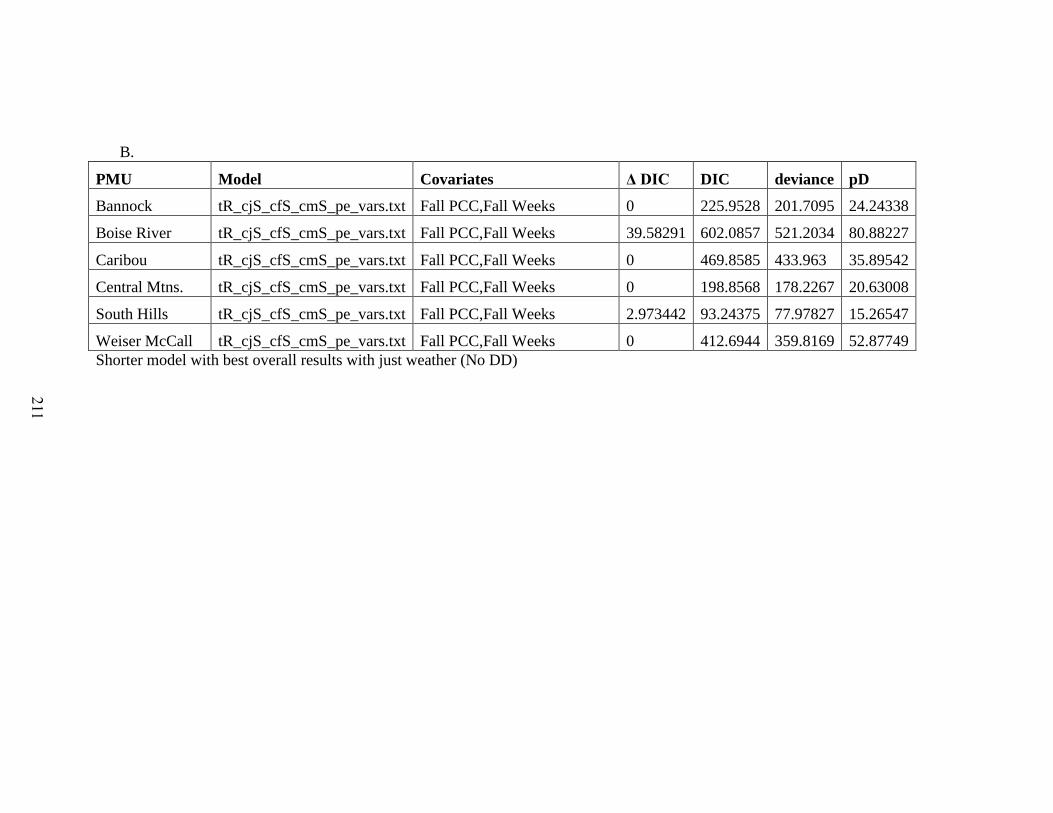
211
B.
PMU Model Covariates Δ DIC DIC deviance pD
Bannock tR_cjS_cfS_cmS_pe_vars.txt Fall PCC,Fall Weeks 0 225.9528 201.7095 24.24338
Boise River tR_cjS_cfS_cmS_pe_vars.txt Fall PCC,Fall Weeks 39.58291 602.0857 521.2034 80.88227
Caribou tR_cjS_cfS_cmS_pe_vars.txt Fall PCC,Fall Weeks 0 469.8585 433.963 35.89542
Central Mtns. tR_cjS_cfS_cmS_pe_vars.txt Fall PCC,Fall Weeks 0 198.8568 178.2267 20.63008
South Hills tR_cjS_cfS_cmS_pe_vars.txt Fall PCC,Fall Weeks 2.973442 93.24375 77.97827 15.26547
Weiser McCall tR_cjS_cfS_cmS_pe_vars.txt Fall PCC,Fall Weeks 0 412.6944 359.8169 52.87749
Shorter model with best overall results with just weather (No DD)

212
Table 5_S2: Model selection results for overall winter mule deer (Odocoileus hemionus) fawn survival with weather density
dependence and covariates. The overall models contain data from all Population Management Units (PMU) and all years. The models
compare the effects of weather density dependence on recruitment with constant juvenile and adult survival. For all models, we report
the Deviance Information Criterion (DIC), Effective Number of Parameters (pD), Deviance, and validation metrics.
PMU Model Covariates DD DD SD DIC deviance pD
Boise River Weather DD Fall PCC,Fall Weeks,Winter -0.270 0.049 886.5 814.4 72.1
South Hills Weather DD Fall PCC,Fall Weeks,Winter 0.001 0.024 91.3 80.0 11.3
Caribou Weather DD Fall PCC,Fall Weeks 0.048 0.018 544.6 505.2 39.4
Central Mtns. Weather DD Fall PCC,Fall Weeks,Winter 0.059 0.025 261.0 249.3 11.8
Bannock Weather DD Fall PCC,Fall Weeks 0.128 0.052 251.4 238.9 12.6
Weiser McCall Weather DD Fall PCC,Fall Weeks 0.237 0.042 609.8 515.1 94.7
Best overall model for Weather with DD

213
Table 5_S3: Model selection results for overall winter mule deer (Odocoileus hemionus) fawn survival with weather density
dependence and covariates. The overall models contain data from all Population Management Units (PMU) and all years. The models
compare the effects of weather density dependence on recruitment with constant juvenile and adult survival. These results are based
on the full model as compared to Table 5_3 where the “best” models were chosen for each PMU. For all models, we report the
Deviance Information Criterion (DIC), Difference from lowest DIC (ΔDIC), Effective Number of Parameters (pD), Deviance, and
validation metrics.
PMU Model Covs DD DD SD ΔDIC DIC deviance pD
Caribou Weather DD Fall PCC,Fall Weeks,Winter -0.389 0.493 25.1 569.7 501.6 68.1
Boise River Weather DD Fall PCC,Fall Weeks,Winter -0.270 0.049 0.0 886.5 814.4 72.1
Bannock Weather DD Fall PCC,Fall Weeks,Winter -0.044 0.025 7.1 258.5 245.3 13.2
Weiser McCall Weather DD Fall PCC,Fall Weeks,Winter -0.038 0.020 1.9 611.7 553.6 58.1
South Hills Weather DD Fall PCC,Fall Weeks,Winter 0.001 0.024 0.0 91.3 80.0 11.3
Central Mts. Weather DD Fall PCC,Fall Weeks,Winter 0.059 0.025 0.0 261.0 249.3 11.8
Full model for Weather with DD, seemed to work the best for a majority of the PMUs’.
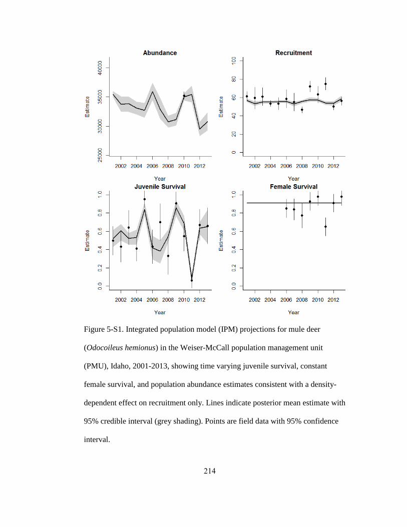
214
Figure 5-S1. Integrated population model (IPM) projections for mule deer
(Odocoileus hemionus) in the Weiser-McCall population management unit
(PMU), Idaho, 2001-2013, showing time varying juvenile survival, constant
female survival, and population abundance estimates consistent with a density-
dependent effect on recruitment only. Lines indicate posterior mean estimate with
95% credible interval (grey shading). Points are field data with 95% confidence
interval.
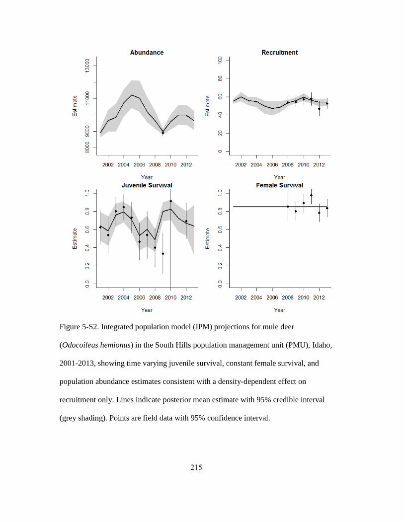
215
Figure 5-S2. Integrated population model (IPM) projections for mule deer
(Odocoileus hemionus) in the South Hills population management unit (PMU), Idaho,
2001-2013, showing time varying juvenile survival, constant female survival, and
population abundance estimates consistent with a density-dependent effect on
recruitment only. Lines indicate posterior mean estimate with 95% credible interval
(grey shading). Points are field data with 95% confidence interval.
Related Documents