Marine Vibrators: Synthetic Data Study - UiO - DUO

Marine Vibrators: Synthetic

Data Study

Sander Wågønes Losnedahl

Master’s Thesis, Spring 2019

Abstract

The traditional airgun source has for a long time been the preferred type of source in

marine seismic data acquisition due to its high impulsive pressure output. However, this

impulsive energy has recently been of concern with regards to the health of marine life.

Therefore, restrictions have been put in place such that airgun surveying is prohibited in

areas where marine life may be sensitive to high pressure levels. An example of such an

area is the Great Australian Bight where seismic survey applications have been rejected

several times. Another example is the Lofoten area located on the coast in the northern

part of Norway facing the Norwegian Sea. Seismic exploration is not allowed in this area

because of the concern that the pressure created from the seismic airgun may harm the

�sheries which is the main industry of the region. An alternative seismic source is the

marine vibrator which aims to spread the pressure output over time thus creating a non-

impulsive wave�eld that is not as harmful to marine life. The output of such a source is

more manageable than that of the airgun and the generation of low-frequencies without

bubble pulse contamination is an additional bene�t. These are the motivations behind

the revival of the marine vibrator. This thesis work will �rst derive the fundamental

equations describing such a non-impulsive wave�eld generated by a marine vibrator. Fur-

thermore, this thesis work will investigate what happens when motion is introduced into

the non-impulsive source wave�eld by deriving the aforementioned equations with respect

to motion. These equations represents the source signature of a marine vibrator and will

be used to generate synthetic data. Further processing and imaging will be employed in

an attempt to better isolate the e�ects of motion on the data and the limits of resolution

of the marine vibrator source will be investigated. Finally, controlled marine vibrator

data will be compared with corresponding airgun data in order to establish the validity

of the marine vibrator.

i

Contents

1 Introduction 1

1.1 A brief history of seismic sources . . . . . . . . . . . . . . . . . . . . . . . 1

1.2 Airguns and the environment . . . . . . . . . . . . . . . . . . . . . . . . . 4

1.3 Marine seismic vibrators . . . . . . . . . . . . . . . . . . . . . . . . . . . . 4

1.4 MV-IPN . . . . . . . . . . . . . . . . . . . . . . . . . . . . . . . . . . . . . 7

1.5 PGS' marine vibrator . . . . . . . . . . . . . . . . . . . . . . . . . . . . . . 9

1.6 Geokinetics' marine vibrator . . . . . . . . . . . . . . . . . . . . . . . . . . 10

1.7 Previous work in source wave�eld modeling and synthetic data generation . 11

2 Pressure Output from a Marine Seismic Vibrator - Theoretical Model 13

2.1 Euler's equation of motion . . . . . . . . . . . . . . . . . . . . . . . . . . . 13

2.2 Conservation of mass . . . . . . . . . . . . . . . . . . . . . . . . . . . . . . 14

2.3 The reciprocity theorem . . . . . . . . . . . . . . . . . . . . . . . . . . . . 16

2.4 The representation theorem . . . . . . . . . . . . . . . . . . . . . . . . . . 18

3 Modeling the Source Wave�eld from a Marine Vibrator 22

3.1 Sweep design . . . . . . . . . . . . . . . . . . . . . . . . . . . . . . . . . . 22

3.2 Generating stationary synthetic data . . . . . . . . . . . . . . . . . . . . . 28

3.3 Survey con�guration . . . . . . . . . . . . . . . . . . . . . . . . . . . . . . 29

3.4 Raw data . . . . . . . . . . . . . . . . . . . . . . . . . . . . . . . . . . . . 31

4 Data Processing and Migration 33

4.1 Cross-correlation . . . . . . . . . . . . . . . . . . . . . . . . . . . . . . . . 33

4.2 Wave equation based �nite-di�erence migration of cross-correlated data . . 37

ii

5 Introducing a Moving Source Wave�eld 45

5.1 Wave equation for a moving source . . . . . . . . . . . . . . . . . . . . . . 45

5.2 Modeling a moving source . . . . . . . . . . . . . . . . . . . . . . . . . . . 51

5.3 Generating synthetic data with a moving source . . . . . . . . . . . . . . . 58

6 Comparing Vibrator and Airgun Data 61

7 Discussion 65

7.1 Frequency dependent illumination . . . . . . . . . . . . . . . . . . . . . . . 65

7.2 The Doppler e�ect and dipping re�ectors . . . . . . . . . . . . . . . . . . . 67

7.3 Sweep length and deep targets . . . . . . . . . . . . . . . . . . . . . . . . . 69

7.4 Multi-vibrator systems . . . . . . . . . . . . . . . . . . . . . . . . . . . . . 70

7.5 The marine vibrator in shallow waters . . . . . . . . . . . . . . . . . . . . 72

8 Conclusion and Future Work 73

References 75

Appendixes 79

iii

Acknowledgements

I would like to extend my sincere appreciation to Prof. Leiv-J. Gelius, Dr. Okwudili Orji,

Dr. Walter Söllner and Dr. Endrias Asgedom for their excellent supervision and support

during the making of this master's thesis. A special thanks is given to PGS, Oslo o�ce

for their support and hospitality to me as a student as well as their generous sharing of

resources and software.

iv

Chapter 1

Introduction

1.1 A brief history of seismic sources

The �rst successful attempts of seismic exploration started in the early 1920s. No devel-

oped seismic source existed at that time so the scientist had to employ explosive charges

both for land and marine surveys. These explosives created an impulsive seismic wavelet

perfect for basic re�ection seismic and additionally, were relatively easy to handle.

However, the explosive charges had a severe �aw regarding bubble pulses in marine sur-

veys since no digital �ltering were available at that time. The solution was to detonate

the explosives at very shallow depths to avoid the bubble pulses entirely which resulted

in loosing much of the impulsive energy.

Early versions of the airgun and seismic vibrator were developed in the 1950s and 1960s

and they soon outperformed the explosive charges in both quality and cost. It seemed

that the airgun was preferred over the vibrator as it resembled the old explosive charge

where the technology was already available. A typical airgun is shown in �gure 1.1 (top)

and the output from multiple airguns (airgun array) are shown in �gure 1.1 (bottom).

1

Figure 1.1: Example of what an airgun could look like (top) and what the output frommultiple airguns could look like (bottom) (Emma Technologies) (Western Geco, 2010).

Basically, an airgun is a container with a �xed volume V able to hold overpressured air

P which is released almost instantaneously creating an impulsive pressure wave in the

2

surrounding acoustic medium. As in the case of the explosive charge, the airgun creates

a bubble that oscillates with a period T and is described by the modi�ed Rayleigh-Willis

formula (Parkes & Hatton, 1986)

T = kP

13V

13

P56hyd

Phyd = Patm + ρgD

(1.1)

where k is a unit dependent constant, ρ is the density of water, g is the gravitational

constant, Phyd is the hydro-static pressure from the overlying water column with Patm

being the atmospheric pressure and D the depth of the airgun. From equation 1.1, one

may alternatively solve for the frequency f. Taking the inverse of equation 1.1 yields a

term for the frequency (f = 1/T )

f =P

56hyd

kP13V

13

(1.2)

Equation 1.2 shows that more low frequencies are created when the volume of the container

and/or the pressure output from the container increases. To obtain frequencies within

the seismic bandwidth (< 500Hz), one typically adjusts the pressure within the container

since increasing the volume itself is not very cost e�cient. Increasing the contained

pressure increases the strength of the signal and consequently the signal to noise ratio

(S/N). This is because the power of the ambient noise stays the same while the power of

the signal increases. These bubble pulses are expanding and collapsing in a low frequency

fashion creating low frequency radiation. This low-frequency radiation causes notches in

the low-frequency part of the airgun source signature. Therefore, many airguns of di�erent

variations and depths are often clustered together in an attempt to remove the e�ects of

the bubble pulse and to increase the strength of the impulse. However, the notches created

from the bubble are not completely removed and still in�uence the low-frequency part

of the airgun source signature (Landrø & Amundsen, 2014). The low frequencies are in

many cases discarded when processing seismic data.

3

1.2 Airguns and the environment

The pressure wave emitted from a typical airgun array may damage the environment,

especially the health of marine mammals (International Association of Geophysical Con-

tractors, 2002). Some mammals, particularly large baleen whales, may su�er auditory

damage by lower frequencies within the seismic bandwidth (< 900Hz). These mammals,

having adapted their hearing to such low frequencies, may su�er both temporary and

permanent hearing damage since much of the seismic energy typically lies below 500Hz.

(International Association of Geophysical Contractors, 2002).

For a large baleen whale to su�er any hearing damage from a seismic vessel, it would

have to stay within a 20◦ cone of a marine airgun source (the optimal angle of pressure

emission) for a longer period of time, which is unlikely (International Association of Geo-

physical Contractors, 2002).

What pressure levels cause hearing damage are very species speci�c so if a pressure level is

damaging to one species, it can not be extrapolated to another (International Association

of Geophysical Contractors, 2002). It is noteworthy that the science behind most of ma-

rine mammal hearing are just extrapolation of terrestrial mammal hearing (International

Association of Geophysical Contractors, 2002).

Marine mammals that su�er permanent or even temporary hearing damage from an airgun

array source may change their behavioral patterns. This may change how these marine

mammals breed and may over a longer period of time harm the species population. The

science is very limited in this �eld of study, but political precautions are likely to be

taken if marine seismic acquisition is to take place in areas where some marine mammal

populations can be scarce or vulnerable.

1.3 Marine seismic vibrators

This thesis will focus on one type of environmentally friendly marine seismic source, the

marine seismic vibrator, and more speci�cally, the modular marine vibrator which con-

sists of vibrating plates emitting a pressure wave within a certain bandwidth. Unlike the

4

airgun, a seismic vibrator does not create an impulse, but aims to emit a signal with the

same energy as an airgun array but spread over a longer period of time. Usually the

frequency vary over the interval of emission, known as a sweep. There are three highly

advantageous aspects of the marine vibrator:

1. The release of energy is much more manageable due to full control over the rate of

vibration of the plates.

2. Lower peak source strength due to the spread of energy over time, lowering the risk of

potentially damaging marine mammals.

3. It is possible to reach very low frequencies (2 − 6Hz) which is useful in several types

of inversions.

Both the amount of energy released and the direction of release can be controlled to a

high degree. The direction of emission is called directivity and is achieved by having

several di�erent vibrating plates lined up and controlled in such a way that they would

constructively interfere in the vertical direction, and destructively interfere in the radial

direction.

Land surveys have been utilizing vibrator sources for a long time, but adapting the tech-

nology to marine surveys has proven to be a di�cult task. One problem is the di�erence

in how the surveys are typically executed. Source and receivers in a land survey are placed

on the surface (�gure 1.2), e�ectively removing all ghosts from the signal. In a marine

survey however, both the source and receivers are usually placed beneath the sea surface

giving rise to source and receiver ghosts. These ghosts are further ampli�ed due to the

high re�ection coe�cients of the water/air interface (sea surface) and the sea bottom.

5

Figure 1.2: Land survey where the vibrating source is attached to a truck. Receivers areplaced in a line with equal spacing away from the truck (Innoseis, 2018).

Another di�erence is that both the source and receivers are towed behind a ship in a

marine survey. In a land survey, both the source and receivers are stationary during

recording (�gure 1.2). A moving receiver distorts the measurement, but a moving source

distorts the wave �eld itself (Hampson & Jakubowicz, 1995). Vibrating sources in motion

causes a phase shift of the wave�eld due to the Doppler e�ect. In addition to a phase

shift, the moving source also slants the signal which must be corrected for (Hampson &

Jakubowicz, 1995). These e�ects will be investigated further in this work.

A large advantage of having moving source and receivers is that the survey can cover a

larger area within a given time compared to a land survey. In addition, the truck can not

access areas with a di�cult terrain, meaning other methods of acquisition must be used.

This will never be a problem in marine acquisition since there is no terrain to consider.

Many companies have seen the potential of the seismic marine vibrator and are currently

developing various kinds of vibrators. Examples of such companies are PGS, Western

Geco, CGG and BP. Some companies have joined forces to investigate the feasability of

6

the marine vibrator source. An example of this would be the MV-JIP (Marine Vibrator

Joint Industry Program) which is sponsored by Shell, Exxon and Total.

1.4 MV-IPN

The MV-JIP, or Marine Vibrator Joint Industry Program, is a collaborative e�ort sup-

ported by Shell, Exxon and Total and aims to develop a market competitive and en-

vironmentally friendly seismic marine vibrator source for both commercial and military

use. The MV-JIP has developed multiple vibrator sources, but only the MV-IPN (Marine

Vibrator Integrated Projector Node) will be covered in this thesis.

The MV-IPN uses magnetic �uxes created by electrical currents to rapidly drive pistons

back and forth creating displacements in the surrounding medium (Roy et. al., 2018).

The vibrator is shown in �gure 1.3.

7

Figure 1.3: The MV-IPN in full power testing (Feltham et. al., 2018).

There are three main housings in the vibrator as can be seen from �gure 1.3. The left

housing holds all power control equipment, the middle housing holds the actual transducer

(the circle in �gure 1.3) and the right housing holds the pressure compensation system and

control and monitoring equipment (Feltham et. al., 2018). During a test, this particular

transducer is able to emit a spectral density level shown in �gure 1.4

8

Figure 1.4: Decibel spectrogram of the MV-IPN during testing of sweep from 5− 100Hzover 5 seconds (Feltham et. al., 2018).

Figure 1.4 shows that harmonic frequencies are occurring. This was later found out to

be caused by the spring resonance which should be corrected for before a new test takes

place (Feltham et. al., 2018).

These decibel levels proved su�cient for the MV-JIP (190dB re. 1µPA/Hz @ 1m for

5 − 10Hz and 200dB re. 1µPa/Hz @ 1m for 10 − 100Hz) to declare the test a success

and that the MV-IPN is ready for seismic testing. Such testing is estimated to proceed

in 2019 (Feltham et. al., 2018).

1.5 PGS' marine vibrator

PGS is currently working on two di�erent concepts of a seismic marine vibrator. The �rst

one being the Flextensional Marine Vibrator (left in �gure 1.5). This type of vibrator

9

utilizes electric drivers and magnets to oscillate a spring that makes a �berglass plate

vibrate and cause displacements in the surrounding medium. Two of these vibrators are

often paired together so that the amplitude output is uniform within 5 − 100Hz (PGS,

2017).

Figure 1.5: The two types of vibrators currently under development at PGS (PGS, 2017).

The second type of marine vibrator is called a Modular Marine Vibrator that also utilizes

electrical drivers to move small cylindrical plates (to the right in �gure 1.5) to create

displacements in the surrounding water. These plates have a smaller surface area than

the Flextensional Marine Vibrator, but multiple plates stacked together are able to cause

su�cient displacements in the water (PGS, 2017).

1.6 Geokinetics' marine vibrator

Similar to PGS, Geokinetics are also developing a Flextensional marine vibrator called

AquaVib. The main advantage of the AquaVib is that the vibrator is tuned for shallow

marine acquisition. The vibrator can be placed as shallow as 1m below the sea surface

while still maintaining its output signal. Shallow waters tend to have fragile ecosystems

10

which an airgun source may harm. The size of the AquaVib is drastically smaller than

any airgun on the market today, making them easier to handle from a logistical point of

view (Archer, 2017).

Figure 1.6: The AquaVib in action (Archer, 2017).

Compared to many other marine seismic vibrators, the AquaVib is ready for production

and has already entered the market (Archer, 2017). Figure 1.6 gives an overview of the

AquaVib in action.

1.7 Previous work in source wave�eld modeling and

synthetic data generation

Synthetic data generation using a marine vibrator source has previously been done with

di�erent models and survey con�gurations. An example would be the synthetic data

11

generated by Hampson & Jakubowicz (1995) which consisted of a single di�ractor in a

medium with constant velocity (Hampson & Jakubowicz, 1995). This article demon-

strated what the e�ects of motion would be on a continuous vibroseis signal and the

recorded data using the described model. Hampson & Jakubowicz also presents a method

of compensating for such e�ects. Additionally, the article shows the synthetic data after

the appropriate corrections have been made. However, that article does not introduce the

modeling of the source signature used in generating the synthetic data.

On the other hand, Kramer et al. (1969) proposed a method of calculating the output

from a marine vibrator source using Bernoulli's equation (Kramer et al., 1969). Walker

et al. (1996) used this proposed equation to drive a marine vibrator in a real �eld test

which yielded good results (Walker et al., 1996). However, this article did not isolate

e�ects that are native to the marine vibrator.

This thesis will attempt to derive the fundamental equations describing the source sig-

nature of a marine vibrator and will use these equations in order to model synthetic

data. The source wave�eld modeling has of this thesis work was accepted as an extended

abstract to the SEG2019 annual meeting. Furthermore, the e�ects native to a marine

vibrator with or without motion will be isolated in order to investigate the feasibility of

such a vibrating source.

12

Chapter 2

Pressure Output from a Marine

Seismic Vibrator - Theoretical Model

To model the pressure �eld generated from a marine seismic vibrator, the motions of the

medium have to be derived for an isotropic, non-viscous �uid. The combination of Euler's

equation of motion and the constitutive law describe the reaction of an acoustic medium

when a wave propagates through. These two equations can then be used to derive the

representation theorem which compares two pressure �elds within a volume. Through the

representation theorem, the far �eld (also near �eld) can be found.

2.1 Euler's equation of motion

Euler's equation of motion of an in�nitesimal �uid volume can be derived using Newton's

second law, or in other words, conservation of momentum. This law states that the

total momentum of a closed system (mv) with no external or internal force is preserved

regardless of how complicated the system is. If one assumes that (i) pressure gradients are

the driving forces and (ii) the convection term can be neglected, the linearized equation

of motion takes the form

5p = ρ∂v

∂t(2.1)

13

with p being the pressure, ρ is the density of the medium and v is the particle velocity. For

a complete derivation of the linearized Euler's equation of motion, the reader is referred

to Appendices A and B.

2.2 Conservation of mass

Consider again a small in�nitesimal �uid volume, but this time apply the consitutive law

describing mass balance when a pressure wave propagates through the medium.

Figure 2.1: Rate of mass �ow into and out of the volume in the x-direction.

The volume of this in�nitesimal �uid element is ∆V = ∆x∆y∆z and the particle velocity

is denoted v = {vx, vy, vz}. From �gure 2.1 it follows that the net in�ux of mass resulting

from �ow in the x-direction is (ρt being the total density)

14

[ρtvx − (ρtvx +∂(ρtvx)

∂x∆x)]∆y∆z = −∂(ρtvx)

∂x∆V (2.2)

Similar expressions give the net in�ux for the y and z directions, so that the total in�ux

must be

− [∂(ρtvx)

∂x+∂(ρtvy)

∂y+∂(ρtvz)

∂z]∆V = −5 ·(ρtv)∆V (2.3)

The rate at which the mass increases in the volume can be written formally as

[(∂ρt∂t

)∆V + ρtQ∆V ] (2.4)

where the second term represents an injection term (Q being injected volume �ow per

unit volume). The net in�ux must equal the rate of increase

∂ρt∂t

+5 · (ρtv) = −ρtQ (2.5)

Equation 2.5 can be further expanded to obtain

1

ρt

∂ρt∂t

+1

ρt(v · 5)ρt +5 · v = −Q (2.6)

where the identity 5 · (ρtv) = ρt(5 · v) + v · 5ρt has been applied (Salby, 2012). Let

ρ0 represent the equilibrium density (no wave interaction). Then the perturbed density ρ

follows from the equation

ρt = ρ0 + ρ (2.7)

Combination of equations 2.6 and 2.7 gives

1

ρt

∂ρ

∂t+

1

ρt(v · 5)ρ+5 · v = −Q (2.8)

Assume now a linear relationship between the perturbed density and the wave pressure

expressed as dρ = 1c2dp. Substitution of this expression in equation 2.8 leads to

15

1

K[∂p

∂t+ (v · 5)p] +5 · v = −Q (2.9)

with K = ρtc2 being the bulk modulus.

In case of the seismic wave, it is demonstrated in Appendix B that equation 2.9 can be

further approximated to give its �nal version

∂p

∂t= −K 5 ·v−KQ = −K 5 ·v+K

∂iV∂t

(2.10)

with iV being the volume density of volume injection.

2.3 The reciprocity theorem

The temporal Fourier transform of a space and time dependent quantity f(x, t) is de�ned

as

F (x, ω) =

∫ ∞−∞

f(x, t)e(−iωt)dt (2.11)

By applying such a Fourier transform to the equation of motion (equation 2.1) and the

constitutive law (2.10) gives

5 P (x, ω) = iωρV(x, ω) (2.12)

iωP (x, ω) = iωKiV −K 5 ·V(x, ω) (2.13)

Equation 2.12 can be modi�ed as

5 ·(1

ρ5 P (x, ω)) = iω5 ·V(x, ω) (2.14)

which in combination with equation 2.13 gives

−5 ·(5P (x, ω)

ρ) +

ω2

KP (x, ω) = S(x, ω) (2.15)

16

where S = ω2iV . We continue investigating the relationship between the two solutions of

equation 2.15

−5 · (5P1(x, ω)

ρ) +

ω2

KP1(x, ω) = S1(x, ω) (2.16)

−5 · (5P2(x, ω)

ρ) +

ω2

KP2(x, ω) = S2(x, ω) (2.17)

where P1(x, ω) and P2(x, ω) are the pressure �elds generated from the di�erent source

injections. Next, multiply equation 2.16 with P2(x, ω) and equation 2.17 with P1(x, ω),

and subtract one from the other to obtain

S2P1(x, ω)− S1P2(x, ω) = P2(x, ω)5 ·(5P1(x, ω)

ρ)

−(P1(x, ω)5 ·(5P2(x, ω)

ρ)

(2.18)

The above equation determines the relationship between the two pressure �elds at any

point in the system, but it is also possible to relate the two pressure �elds within a given

volume V

∫V

(S2P1(x, ω)− S1P2(x, ω))dV

=

∫V

(P2(x, ω)5 ·(5P1(x, ω)

ρ)− (P1(x, ω)5 ·(5P2(x, ω)

ρ))dV

(2.19)

The above equation can be simpli�ed by applying the following product rule for divergence

stating that f2 5 ·(5f1) = 5 · (f2 5 f1) −5f1 5 f2, where f1 and f2 are P1(x, ω) and

P2(x, ω) in this case (Arfken et. al., 2012, A). Equation 2.19 then reduces to

∫V

S2P1(x, ω)− S1P2(x, ω)dV =

∫V

[5 · (P2(x, ω)5 P1(x, ω)

ρ)− 5P1(x, ω)5 P2(x, ω)

ρ]

−[5 · (P1(x, ω)5 P2(x, ω)

ρ)− 5P1(x, ω)5 P2(x, ω)

ρ]dV

=1

ρ

∫V

[5 · (P2(x, ω)5 P1(x, ω))−5 · (P1(x, ω)5 P2(x, ω))]dV

(2.20)

By applying the divergence theorem∫V5 · fdV =

∫Sf · ~ndS (Arfken et. al., 2012, A) to

17

the right hand side of equation 2.20, it transforms to

∫V

[S2P1(x, ω)− S1P2(x, ω)]dV =1

ρ

∫S

[P2(x, ω)5 P1(x, ω)− P1(x, ω)5 P2(x, ω)] · ~ndS

(2.21)

which is the acoustic reciprocity theorem in its most general form.

2.4 The representation theorem

The reciprocity theorem (equation 2.21) gives the relationship between two di�erent wave-

�eld states acting within a volume V with an outer surface S. By carefully de�ning these

states, the pressure at any point within that volume can be calculated for a given problem.

Figure 2.2: Physical state (left) and Green's state (right) where xR in the latter acts asa point source (Söllner & Orji, 2017).

In the following, the problem is to solve for the pressure �eld generated from two closeby

vibrating plates (�gure 2.2). The �rst state corresponds to a physical point source δ(x)

that is injected at an arbitrary point x. This type of source generates a pressure �eld

P (xR, ω) recorded at a point xR (left in �gure 2.2). This will be referred to as the physical

state from here on.

18

The second state corresponds to a point source δ(x − xR), located at the point xR and

will be referred to as the Green's state (right in �gure 2.2). The sources can be written

explicitly as (S(ω) being the spectrum of a physical source)

S1 =1

ρδ(x)S(ω) (2.22)

and

S2 =1

ρδ(x− xR) (2.23)

The corresponding wave�elds are

P1(x, ω) = P (x, ω) (2.24)

and

P2(x, ω) = G(x,xR, ω) (2.25)

with G(x,xR, ω) representing the Green's function. By substituting equations 2.22 - 2.25

into equation 2.21 the pressure �eld at point xR can be calculated

1

ρ

∫V

[P (x, ω)δ(x− xR)−G(x,xR, ω)δ(x)S(ω)]dV

=1

ρ

∫S

[G(x,xR, ω)5 P (x, ω)− P (x, ω)5G(x,xR, ω)] · ~ndS

⇒ P (xR, ω) =

∫V

G(x,xR, ω)δ(x)S(ω)dV∫S

[G(x,xR, ω)5 P (x, ω)− P (x, ω)5G(x,xR, ω)] · ~ndS

(2.26)

The pressure term P (xR, ω) arises from the identity∫VP (x, ω)δ(x − xR)dV = P (xR, ω)

(Arfken et. al., 2012, B ). Assume that physical point source δ(x) does not contribute to

the pressure �eld which implies

19

P (xR, ω) =

∫S

[G(x,xR, ω)5 P (x, ω)− P (x, ω)5G(x,xR, ω)] · ~ndS (2.27)

The contribution to the surface integral comes from both the outer surface S and the inner

surface A. If the Sommerfeld radiation condition (when the radius of the outer surface S

goes to in�nity) is applied, the contribution to the surface integral from the outer surface

S goes to zero (Peters & Stoker, 1954). This means that the only contribution to the

surface integral comes from the inner surface A

P (xR, ω) =

∫A

[G(x,xR, ω)5 P (x, ω)− P (x, ω)5G(x,xR, ω)] · ~ndA (2.28)

Assume now that the inner surface A is actually a vibrating plate with two surfaces with

opposite normal vectors, with an in�nitesimal distance between them, as shown in �gure

2.2. The surface integral in equation 2.28 can then be divided into two di�erent parts,

one for each side of the inner surface

P (xR, ω) =

∫A+

[G(x,xR, ω)5 P (x, ω)− P (x, ω)5G(x,xR, ω)] · ~ndA+

−∫A−

[G(x,xR, ω)5 P (x, ω)− P (x, ω)5G(x,xR, ω)] · ~ndA−(2.29)

The subtraction of the second integral arises from the opposite normal vectors. This

results in the cancellation of the second term in each surface integral since the Green's

function and its gradient and the pressure �eld are continuous across the plates. However,

the pressure gradients are opposite of each other due to the two vibrating plates pushing

the surrounding medium in opposite directions. The equation is then reduced to

P (xR, ω) =

∫A

G(x,xR, ω)5 [P (x, ω)]A+A− · ~ndA (2.30)

where the notation []A+

A−denotes the di�erence in pressure gradient between the upper

20

and lower inner surface. The pressure term in the above equation can be replaced by an

acceleration term (a(x, ω) = iωV (x, ω)) scaled with density from the equation of motion

(equation 2.12), yielding

P (xR, ω) = ρ

∫A

(G(x,xR, ω)5 [a(x, ω)]A+A− · ~ndA (2.31)

The pressure �eld can be calculated at any point xR in a volume if the solution to the

Green's function and the di�erence in acceleration between the two sides of the vibrating

plates are known. Since the medium is water, the Green's function has the analytical

solution

G(x,xR, ω) =1

4πReikR, R =| x− xR | (2.32)

in the frequency domain, where k = ωcis the wave number and R is the distance from

source to the point of interest. The time domain equivalent is 14πR

δ(t − Rc) (Howell,

2001, A). In Appendix C, fundamental concepts related to sweep design and acceleration

response are discussed in detail.

21

Chapter 3

Modeling the Source Wave�eld from

a Marine Vibrator

3.1 Sweep design

The pressure wave �eld generated from a marine vibrator is described by equation 2.31

where both the density of the water column and the Green's function at any point in the

system are known. The only missing part is the acceleration term which in general can

be described as (no spatial variations along the vibrating plates)

a(t) = esin[2π(φ0 + φ(t))] (3.1)

where e is the envelope function and φ(t) is the phase function. It is assumed here that

the initial phase φ0 is zero. This thesis will focus on a linear upsweep which means that

the sweep will start from a low frequency f0 and increase linearly to a higher frequency

f1 over a period of time T known as the sweep length

f(t) = f0 + bt

b =f1 − f0

T

(3.2)

Taking the integral of the instantaneous frequency f(t) yields the instantaneous phase

function φ(t)

22

φ(t) =

∫ t

0

f(t)dt

φ(t) =

∫ t

0

(f0 + bt)dt =

∫ t

0

(f0 + (f1 − f0

T)t)dt

⇒ φ(t) = [f0t+ (f1 − f0

2T)t2]

(3.3)

Substituting φ(t) into the acceleration equation 3.1 yields

a(t) = esin[2π(f0t+ (f1 − f0

2T)t2)] (3.4)

The phase is now determined by sin(φ(t)), but the strength or amplitude of the signal is

determined by the envelope function e. For a linear sweep, putting e as a constant will

give rise to �at amplitude spectra of acceleration and pressure due to equation 3.4 and

2.31.

Determining the value of the envelope function analytically can be done for a single point

since the distance from that point to the point of measurement is constant. For a single

point on a vibrating plate, the integral from equation 2.31 vanishes and the pressure

is then just a scaled version of the acceleration. Since the density and the solution

to Green's function are known (equation 2.32), the acceleration can then be used as a

control-parameter to obtain the pressure output of interest at any given distance (cf.

equation 3.5)

P (xR, ω) = ρG(x,xR, ω)A(x, ω)z

→ A(x, ω)z =P (xR, ω)

ρG(x,xR, ω)

=10000Pa ∗ 4π

m

1000kg/m3

= 125.66m/s2

(3.5)

By then using 125.66m/s2 as the envelope function, the pressure output at 1 meter gives

10000Pa (or 0.1bar) and also yields a �at amplitude spectrum of acceleration (cf. discus-

sion in Appendix C).

This has been applied to �gure 3.1 and 3.2 to ensure a pressure output of 0.1bar at 1 meter

23

away in the frequency band of f0 = 0Hz and f1 = 20Hz. Calculating the plate velocity

and plate motion numerically is done by taking the Fourier transform of the acceleration

and then divide by iω to obtain plate velocity (V (ω) = A(ω)/iω), and divide by −ω2 to

obtain plate motion (U(ω) = A(ω)/− ω2).

It is numerically possible to calculate the plate acceleration for an entire stack of plates

using e = 125.66m/s2. By using the above relations and equation 2.31 the results shown

in �gure 3.1 were obtained.

Figure 3.1: The normalized output from 11 plates 1 meter away from the center of thestack of plates.

The pressure output shown in �gure 3.1 is the pressure from 11 plates stacked together

with 0.2m spacing between them measured at 1 meter away from the center of the middle

plate. A taper has been applied to the signal to remove the ringing in the amplitude

spectra caused by Gibb's phenomenon. However, the pressure is normalized by dividing

the total pressure output by the number of points on a single plate and the number of

plates (11 in this case). The results should be the amount of pressure output equal to a

single point on a vibrating plate

24

Figure 3.2: The output from a single point 1 meter away from the center of the stack ofplates.

When comparing the pressure output in �gure 3.1 with the actual pressure output from

a single point shown in �gure 3.2 one can observe that they are not equal. This is due

to the fact that the envelope function was calculated for a single point, meaning that the

normalization does not take into account the areal extent of the plates. As the distance

from the plates to a point of measure increases, the di�erence in pressure output should

approach zero. This means that by measuring far enough away from the source, the source

can be thought of as a point source.

Since the signal is de�ned as the plate acceleration a(t), the plate motion shown in �gures

3.1 and 3.2 comes as a consequence of the envelope function. This means that in order

to obtain a �at amplitude spectrum of acceleration, the plate has to behave in a certain

manner in practice. It is observed from �gures 3.1 and 3.2 that the plate has to move

signi�cantly in the beginning of the sweep in order to maintain the �at amplitude of

acceleration.

25

Figure 3.3: Comparative phase spectra plots between plate motion/plate accelerationand plate acceleration/pressure output from �gure 3.1.

When comparing the phase of the plate motion and plate acceleration in �gure 3.3, one

can observe that they are completely out of phase. This is because the plate motion is

given by the double time integral (or division by (iω)2 in the frequency domain).

The opposite is the case when comparing the phase of plate acceleration and pressure

output (�gure 3.3). As previously mentioned, the pressure can be though of as a scaled

version of plate acceleration when the pressure output is normalized to a single point. The

point of measurement for the pressure output is 1m away from the plates, which actually

causes a slight shift due to the Green's function (equation 2.32). The exponential part

of the Green's function determines the phase of the pressure output and it is distance

dependent (r). This phase shift is only about 6◦ at 1m away from the source.

Figures 3.1 and 3.3 show the characteristics of a generated sweep between 0 and 20Hz

recorded close to the source. It will therefore be assumed in this work that this is the

true output from a vibrating stack of plates. This assumption does not take into account

directivity, but this aspect has already been discussed by Nguyen, (2017). Nevertheless,

the frequency band and sweep length as seen in �gure 3.1 will now be extended from

0 − 20Hz over 4 seconds to 5 − 100Hz over 5 seconds. This output will be used as a

26

notional source signature when modeling synthetic data in the next section.

27

3.2 Generating stationary synthetic data

Synthetic data can now be modelled by utilizing the notional source signature found in

section 3.1. This will be done using the Nucleus+ which is a PGS in house modeling

software where the user can freely create many di�erent models with a variety of survey

con�gurations. The survey con�guration includes vessel position and velocity, number

of sources and receivers, what type of source and the extent of the survey among many

other options. Di�erent types of modeling may be used as well, but only �nite di�erence

modeling were used in this thesis as this type of modeling can accommodate for motion

which will be relevant for later discussions in this thesis work.

The amplitude spectrum of the sweep in section 3.1 has now been extended to range from

5 to 100Hz as a broader frequency band is of interest in case of shallower reservoirs as

in the Barents Sea. A basic model consisting of two di�ractors within a homogenious

medium as seen in �gure 3.4 has been employed to investigate resolution aspects.

28

Figure 3.4: A 10000m wide and 4000m deep model consisting of only two di�ractorslocated at 1000m depth, 150m apart. The grid size is 4x4m.

This model was chosen primarily for its simplicity which makes it possible to isolate the

e�ects of a continues wave�eld. Having a more complex model would introduce other

e�ects not related to a marine vibrator sweep. Such e�ects, i.e. multiples, already have

well known corrections. Another reason for this choice of model was to check the limit of

resolution for a sweep wavelet. The resolution obtained after migration is also investigated

for this data set.

3.3 Survey con�guration

Initially, the survey con�guration will only include 200 stationary sources recorded by a

single streamer containing 960 receivers. This con�guration is quite simplistic, but allows

for a better understanding of the sweep. In addition, deblending and motion correction

do not need to be applied with this survey con�guration. Figure 3.5 illustrates this survey

29

con�guration.

Figure 3.5: Survey con�guration of sequentially �red stationary sources (red) andrecorded by a streamer (green) over the model (blue).

The red dots in �gure 3.5 shows where each shot is located. The source emits the sweep

(�gure 3.2) sequentially starting from left. When one shot is �red, there is a delay in which

the pressure wave �eld propagates for some time before the next sweep is emitted. The

�rst sweep is emitted at 4375m and the last sweep is emitted at 5625m relative to origo,

for a total of 200 shots spaced 6.25m apart covering 1250m. As mentioned in the previous

section, the sweep is now de�ned between frequencies f0 = 5Hz and f1 = 100Hz.

The receiver array consist of 960 receivers also spaced 6.25m apart covering a total of

6000m starting from 2000m from origo. The receiver array and the source array were

located at a depth of respectively 480m and 490m. This is very unrealistic, but this

choice together with the shear size of the model make it possible to neglect the boundary

issues of the modeling software. In addition, no sea surface re�ections are included in the

30

modeling as the main purpose is to investigate the e�ects of a sweep wavelet.

3.4 Raw data

The given model and survey con�guration were used to generate a dataset using 2D �nite-

di�erence modeling with a 4x4m grid size and the raw data generated is displayed in �gure

3.6 in case of shot number 100 (mid shot).

Figure 3.6: Raw data generated from model in �gure 3.4 and survey con�guration in�gure 3.5. This shot gather is taken from shot number 100 from the record.

It can be observed from �gure 3.6 that the direct wave�eld is not removed from the data

as the zero-o�set trace has large amplitudes at time = 0. The direct wave�eld is of course

recorded at later times with increasing o�set.

Since this dataset is synthetically generated, it is possible to remove the direct wave�eld

by simply creating a new dataset, but using a model where the di�ractors are removed

and then subtracting one dataset from the other. This is obviously not possible with real

data, but has been performed here for time saving reasons. Removing the direct wave�eld

from real data can actually be a challenge as parts of the direct wave�eld often blend with

primary re�ections.

31

Figure 3.7: Shot gather as shown in �gure 3.6 but without the direct wave�eld.

It can be observed from �gure 3.7 that there is no longer an amplitude present at time

t = 0 at zero o�set which means the direct wave�eld has been removed. By comparing

�gures 3.6 and 3.7 it is clear that the direct wave�eld dominated the raw dataset. What

is left of the data must then be the re�ected energy from the two di�ractors.

The data seen in �gure 3.7 is a convolution between the source wavelet and the re�etivity

series (Todoeschuck & Jensen, 1989). How to remove the phase of the source wavelet from

the data will be discussed in the next section.

32

Chapter 4

Data Processing and Migration

Now that the data has been modeled, it needs to be properly processed in order to obtain

an image of the scatteres. The cross-correlation process is now applied to the data in

�gure 3.7 in order to compress the sweep signal. Furthermore, the cross-correlated data

will then be imaged by a �nite di�erence migration which will allow us to obtain an image

of the scatterers.

4.1 Cross-correlation

Cross-correlation is a way to compare two signals with each other and identify possible

similarities. The mathematical de�nition in the time domain is as follows (Howell, 2001,

B)

f × g(n) =

∫ ∞−∞

f(m)g(m+ n) (4.1)

where f and g are two di�erent signals, f denotes the time reversal of the signal f , ×

denotes cross-correlation, m is the length of the signal and n is the "lag" of the cross-

correlation process. The process of cross-correlation as seen from its de�nition (4.1)

resembles the convolutional process, but with the �rst signal being time reversed. The

general idea behind the process of cross-correlation in the time domain is sketched in

�gure 4.1.

33

Figure 4.1: Sketch of how cross-correlation is performed in the time domain. The cross-correlation (green) is a step wise multiplication and summation between the �ipped signalsignal f (blue) and a di�erent signal g (red) in the time domain.

As can be seen from �gure 4.1, the signal f is multiplied with signal g in steps. When

moving to the next step, denoted in �gure 4.1 as elongated arrows pointing right, the

signal g shift to the right. Each step is called a lag and is de�ned in equation 4.1. One

can observe from �gure 4.1 that the �rst and third step yields no product, meaning the

signal has no correlation in these steps. On step two however, there are some correlation,

marked in �gure 4.1 as a �lled triangle.

When performing cross-correlation on two identical signals, the operation is called auto-

correlation. The auto-correlation has the most signi�cant correlation when the signal is

aligned with itself.

A seismic signal is of course much more complex than what is showed in �gure 4.1, but the

principle is exactly the same. When cross-correlation is performed between the vibroseis

data and the source wavelet, the e�ects of the sweep on the data will be minimized. This

is because the recorded seismic trace for a given source receiver u(xg,xs, t) (synthetic

seismic in this thesis) is a convolution between the sweep wavelet s(t) and the re�ectivity

response r(xg,xs, t)

u(xg,xs, t) = s(t) ∗ r(xg,xs, t) (4.2)

where ∗ denoted the mathematical process of convolution. The re�ectivity response

34

r(xg,xs, t) represents the data recorded for the same source receiver location in case of

an impulsive source (e.g. S(ω) = 1). In the frequency domain, the convolution becomes

a multiplication

U(xg,xs, f) = S(f)R(xg,xs, f)

= ASeiφSARe

iφR = (ASAR)ei(φS+φR)

(4.3)

where the amplitude and phase terms of the sweep and earth's re�ectivity response have

been introduced. Cross-correlation between the recorded data and the sweep wavelet

(U ′(xg,xs, f)) is then a multiplication of equation 4.3 with the complex conjugated sweep

wavelet (Howell, 2001, A)

U ′(xg,xs, f) = (ASAR)ei(φS+φR)ASe−iφS

= (A2SAR)eiφR

(4.4)

From equation 4.4 it is seen that the amplitude of the sweep is squared and the phase of

the sweep is removed as a result of the cross-correlation. What is left of the phase in the

recorded data is the phase of the earth's re�ectivity response.

The result shown in �gure 4.2 was obtained when cross-correlation is applied to the data

in �gure 3.7.

35

Figure 4.2: Source gather after cross-correlation has been performed (source number100).

As can be seen from �gure 4.2, the phase of the sweep has been successfully removed.

To further investigate the quality of the controlled data after cross-correlation, a �nite

di�erence migration was employed. This will be topic in the next section.

36

4.2 Wave equation based �nite-di�erence migration

of cross-correlated data

A shot-point driven �nite-di�erence wave equation migration scheme developed by PGS

was employed to migrate the cross-correlated data. The algorithm does not only require

the data set itself, but also a velocity model and a wavelet for propagation on the �nite

di�erence grid. As this is synthetic data, the background velocity model is known. The

propagation wavelet needs to be an auto-correlation of the source sweep wavelet. This is

because the data now have been cross-correlated with the sweep (cf. equation 4.4).

The single-source acquisition aperture, which is the lateral extent covered by the receivers

for a �xed source, will be considered in the further analysis. This migration aperture can

again be related to the Rayleigh criterion

The Rayleigh criterion gives an estimate of the size of aperture needed be able to separate

and image two points (sources of emission). Figure 4.3 gives a schematics of the general

idea.

Figure 4.3: The general idea of the Rayleigh criterion where a given aperture will beable to completely resolve (left), barely resolve (middle) or not resolve (right) two events(modi�ed version from Kallweit & Wood, 1982).

These two points can be though of as points of emission recorded by one receiver where

d is the distance between the di�ractors (150m in our case), L is the vertical distance

from the receiver array to the di�ractor depth (510m in our case), θ is the average angle

between the two di�ractors and the receiver considered and x de�nes the total receiver

outlay (aperture) as shown in �gure 4.4.

37

Figure 4.4: Di�ractors as two points of emission (stars) recorded at a receiver (circle).Green lines represent shortest distances between respectively the di�ractors and the re-ceiver considered.

With some basic trigonometry and the small angle approximation the following relation

holds

tan(θ) ≈ sin(θ) =x

L(4.5)

The di�erence in path length from the two scatterers to the outer receiver considered

should be an integer number of λ (wavelength) if constructive interference is to occur.

This implies that (cf. �gure 4.4) that (lowest order)

dsin(φ) ≈ dsin(θ) = λ (4.6)

38

which in combination with equation 4.5 gives

dx

L= λ

x =λL

d=vL

fd

(4.7)

where λ has been replaced by vf. Here, v can be though of as a RMS-velocity and f can be

considered as a center frequency of the signal. Figure 4.5 summarizes the key parameters

of the Rayleigh criterion in case of the single-source geometry.

Figure 4.5: Single-source geometry and the Rayleigh criterion related to seismic aperturex and a given angle θ.

Split-spread con�guration is considered in this work but since the model is symmetric

around the mid shot point (#100), we only need to consider the aperture to be one-sided

(single-spread) (x in �gure 4.5) in the following resolution analysis.

As can be seen from equation 4.7, the migration aperture is inversely proportional to both

the frequency and the distance between the di�ractors. However, both depth and RMS-

39

velocity are proportional to the migration aperture. Increasing the distance between the

di�ractors or increasing the frequency allows for a lower migration aperture while higher

RMS-velocity or large depth increases the migration aperture needed in order to resolve

the two scatterers.

It is now possible to estimate a minimum migration aperture needed to resolve both

di�ractors in the model (�gure 3.4). Since our model is homogeneous, the RMS-velocity

is just equal to the interval velocity of the water vRMS = vi = 1500m/s. The choice

of frequency is more di�cult since the amplitude spectrum of the sweep (�gure 3.1) is

�at. However, since each frequency contribute equally much to the signal, the highest

frequency of 100Hz can be chosen as it determines the limit of what can be resolved

according to equation 4.7. The receivers are located at a depth of 490m and di�ractors at

1000m depth, so L in this case would be 1000m− 490m = 510m. The distance between

the di�ractors are 150m as seen in �gure 3.4. The minimum migration aperture that is

needed is therefore

x =vL

fd=

1500m/s ∗ 510m

100Hz ∗ 150m= 51m (4.8)

Figure 4.6 shows migrated sections of the data seen in �gure 4.2 using di�erent migration

apertures

40

Figure 4.6: Migrated sections using 400m (top left), 200m (top right), 100m (bottomleft) and 50m (bottom right) migration aperture with only 1 shot (source #100).

Figure 4.6 clearly shows that the two di�ractors are resolved for a 400m migration aper-

ture. It is however hard to see if the smaller apertures resolve the scatterers. To be

able to analyze the horizontal resolution in more detail, an image slice was taken at the

approximate depth location of the scatterers for various apertures (cf. �gure 4.7).

41

Figure 4.7: Depth slice of migrated data using 100m, 50m, 25m and 12.5m migrationaperture. Blue vertical lines indicates actual position of the di�ractors.

It can be observed from �gure 4.7 that the two di�ractors are resolved using both 100m

and 50m apertures. One could also argue that the 25m and 12.5m depth slices are at

least partially resolved for this ideal case. The reason for why these two points are being

resolved at these low apertures may be a result of (i) the Rayleigh criterion only being

an approximation and/or (ii) the limit of resolution is not strictly limited by the highest

frequency in the band. This exercise in resolution was simply to test if the sweep would

be able to resolve two point di�ractors (which it can). Thus, no further investigation will

be considered.

It is obvious that the number of shots also contributes to the horizontal resolution. As

evidence for this, the cross-correlated section was migrated using only a 30m migration

aperture, but with both a single (mid) and all 200 shots as shown in �gures 4.8 and 4.9.

42

Figure 4.8: Migrated sections using a 30m migration aperture with the middle shot.

Figure 4.9: Migrated sections using a 30m migration aperture with 200 shots.

Figure 4.9 shows that the section migrated using all 200 shots have been able to resolve

the two di�ractors well. The reason for this is that the �rst and the last shots in the

survey con�guration (�gure 3.5) gives additional angle information similar to an extended

migration aperture even when only a few traces are migrated. This is in contrast to �gure

43

4.8 where the two di�ractors are imaged as one re�ection event due to lack of angle

information.

All the sections shown so far display strong migration smiles. These smiles comes as an

e�ect of the �nite-length apertures. To minimize such distortions, longer receiver lines

are needed such as those employed in a seismic study. By using the more typical value of

a 3000m aperture and all 200 shots, the image shown in �gure 4.10 was obtained.

Figure 4.10: Migrated sections using 3000m migration aperture with all 200 shots.

The migration smiles are now removed as seen in �gure 4.10. The use of smaller migration

apertures in this section only served the purpose of illustrating fundamental limits with

regards to resolution and migration e�ects (migration smiles). From here on, only the

aperture of 3000m will be used to migrate data.

44

Chapter 5

Introducing a Moving Source

Wave�eld

Up until now, this work has only considered a stationary source, but motion will now be

imposed on the source wave�eld. The main problem related to motion and a continuous

pressure wave�eld (sweep) is that the wave�eld experiences a time varying phase shift as

it moves relative to a given point. This is because the distance the wave has to travel

down to the di�ractor and then back to the receiver is changing with time. To be able to

correct for this motion, we need to consider the wave equation for a moving source.

5.1 Wave equation for a moving source

Let us consider a source moving along a horizontal line as showed in �gure 5.1

45

Figure 5.1: Sketch of a source initially emitting a sweep at time te followed by horizontalmotion.

The source starts emitting a sweep at a time te in position xs = vte and the distance

the pressure wave travels to a point O is called R(t). The distance R(t) changes with

time as the source moves along the horizontal line and can therefore be described by

R(t) = c(t − te), where t is the time the source has been moving and c is the medium

velocity. If the source travels at a velocity v over a time t, the source is positioned at a

point x′s = vt. Hence, the total distance traveled by the source is given by vt − vte =

v(t − te) = vcR(t) = MR(t). Here M is the Mach number which in the subsonic case

(seismic case) is much smaller than 1.

Any additional travel the source makes is then given by x − vt, where x is any position

after x′s. The total distance the source has traveled when point O is directly above the

source is given by (x− vt) +MR(t). If the vertical distance to point O is given by r, the

distance from source to point O at any time is given by

R(t)2 = [(x− vt) +MR(t)]2 + r2 (5.1)

46

By rearranging equation 5.1, it can easily be solved as a second order polynomial

R(t)2 = (x− vt)2 + 2MR(t)(x− vt) +M2R(t)2 + r2

→ R(t)2(1−M2)− 2MR(t)(x− vt)− (x− vt)2 − r2 = 0

(5.2)

Equation 5.2 is then solved for R(t) to give

R(t) =M(x− vt)±

√(x− vt)2 + (1−M2)r2

(1−M2)(5.3)

In the following, a positive sign is considered since only this gives positive values for R(t)

if the subsonic case is considered (M < 1). By de�ning R1(t) =√

(x− vt)2 + (1−M2)r2,

equation 5.3 becomes

R(t) =M(x− vt) +R1(t)

(1−M2)(5.4)

It is also of interest to �nd R(t) as a function of angle θ (�gure 5.1)

M(x− vt) = M(x− vt+ vte − vte)

= M((x− vte)− v(t− te))

= MR(t)(cos(θ)−M)

(5.5)

Equations 5.4 and 5.5 allow for de�ning R1 as

R1(t) = R(t)(1−M2)−M(x− vt)

= R(t)−M2R(t)−MR(t)(cos(θ)−M)

= R(t)(1−Mcos(θ))

(5.6)

We will return to the result in equation 5.6 later. To see how this change in distance to

point O a�ects the pressure wave �eld, the wave equation for a moving source along the

x-axis should be investigated.

52 p− 1

c2

∂2p

∂t2= s(t)δ(x− vt)δ(y)δ(z) (5.7)

where s(t) is the notional source signature (Morse & Ingard, 1968, A). Here, we only

47

assume motion in the x-direction and leave y and z to be constant.

Let us now introduce a frame of relative movement through a Lorentz coordinate trans-

formation where the new coordinates are given by

x′ = γ(x− vt) (5.8)

y′ = y (5.9)

z′ = z (5.10)

t′ = γ(t− v

c2x) (5.11)

where γ is the Lorentz factor which relates the actual time in the still frame to the relative

time in the moving frame. When the frame of motion moves relative to the still frame, this

factor is given by γ = 1√1− v2

c2

(Morse & Ingard, 1968, A). By substituting the coordinates

for a moving frame (equations 5.8,5.9,5.10 and 5.11) into equation 5.7 one arrives at

5′2 p− 1

c2

∂2p

∂t′2= s(γ(t′ +

x′v

c2))δ(

x′

γ)δ(y′)δ(z′) (5.12)

Since the source is moving very slowly compared to the pressure wave �eld, the term x′vc2

can be neglected, implying that t′ + x′vc2

= t′ + x′Mc

= t′. By also applying the identity

δ(ua) = aδ(u) (Arfken et.al, 2012, C), equation 5.12 is reduced to

5′2 p− 1

c2

∂2p

∂t′2= γs(γt′)δ(x′)δ(y′)δ(z′) (5.13)

By introducing another coordinate transformation de�ned by t′′ = γt′,x′′ = γx′, y′′ = γy′

and z′′ = γz′ equation 5.13 becomes

γ25′′2 p− 1

c2

∂2p

∂t′′2= γs(t′′)δ(

x′′

γ)δ(

y′′

γ)δ(

z′′

γ)

→5′′2p− 1

c2

∂2p

∂t′′2= γ2s(t′′)δ(x′′)δ(y′′)δ(z′′)

(5.14)

where 5′ = γ5′′ has been used. Also, the identity δ(ua) = aδ(u) (Arfken et.al, 2012, C)

has again been applied.

48

As suggested by Morse and Ingard, (1968, A), the solution to equation 5.14 is given by

p(r′′, t′′) = γ2 s(t′′ ± r′′

c)

4πr′′(5.15)

where r′′ = γr′ = γ2R1(t). Since the solution has now been found in the transformed

system, it is only a matter of applying the inverse Lorentz transform to equation 5.15. To

simplify the calculation, consider �rst

t′′ ± r′′

c

= γt′ ± γr′

c

= γ(t

γ− vx′

c2)± γ2R1

c

= t− γ2v(x− vt)c2

± γ2

c

√(x− vt)2 + (1−M2)r2

(5.16)

where t = γ(t′ + vx′

c2) → t′ = t

γ− γv(x−vt)

c2is the inverse Lorentz transform. Rearranging

equation 5.16 yields (using γ2 = 1(1− v

c2)

= 1(1−M2)

)

t− γ2M(x− vt)c

± γ2

c

√(x− vt)2 + (1−M2)r2

= t−M(x− vt)±

√(x− vt)2 + (1−M2)r2

c(1−M2)

= t− R(t)

c

(5.17)

It can be observed that equation 5.17 has an imaginary component in the supersonic case.

However, only the subsonic case is of interest since the velocity of the vessel in a seismic

survey is much lower than the speed of the wave. The entire Green's function solution

can now be written as

p(r′′, t′′) = γ2 s(t′′ ± r′′

c)

4πr′′

→ p(r, t) = γ2 s(t−R(t)c

)

4πγ2R1(t)

=s(t− R(t)

c)

4πR(t)(1−Mcos(θ))

(5.18)

where the de�nition of R1(t) is given in equation 5.6. Comparing equation 5.18 to equation

49

2.32 it is clear that they appear similar. What is di�erent is that R(t) in equation 5.18

is time dependent as it moves with a velocity v. However, if the velocity of the source is

set to 0 (stationary case), it can be observed that the two equations describe the same

pressure wave�eld

R(t) =0 +

√(x− 0)2 + (1− 0)r2

(1− 0)= R (5.19)

Keep in mind that when v is 0, so is M since M = vc. Thus in the limit of no motion,

equation 5.18 takes the form

p(R, t) =s(t− R

c)

4πR(1−Mcos(θ))

=s(t− R

c)

4πR(1− 0 ∗ cos(θ))

=s(t− R

c)

4πR

(5.20)

50

5.2 Modeling a moving source

An equation describing a pressure wave�eld emitted by a moving source has now been

derived (equation 5.18), and it is time to generate synthetic data using the numerical

implementation of that equation.

The simplest modeling case was considered when testing the implementation of a moving

source which is the direct wave �eld. By simply taking a single source and a single receiver,

the e�ects of motion can be isolated when compared to the stationary case. The data

was generated using both the numerical implementation of the analytical solution given

by equation 5.18, but also by �nite di�erence modeling for quality control. A sketch of

the general set up is shown in �gure 5.2.

Figure 5.2: Sketch of the direct wave�eld experiment. The top half of the �gure showsa single stationary source (red) and a single stationary receiver (green). The bottom halfof the �gure shows a single moving source (red) relative to a single stationary receiver(green).

In the stationary reference experiment a single source is located 1000m away from a single

receiver as shown in �gure 5.2. In the moving source experiment, the source moves at a

velocity of 50m/s towards the same receiver. The numerical implementation of the latter

case involves solving equation 5.18 with the given velocity and initial distance parameters.

51

The source in the �nite-di�erence modeling, however, simply emits the stationary sweep

over a horizontal discretized distance given by the speed of the vessel times the sweep

length 50m/s ∗ 5s = 250m. In this case, the total of 250m of motion was discretized into

127 steps. The emitted sweep as implemented in �nite-di�erence is plotted in �gure 5.3.

Figure 5.3: The moving source output in �nite di�erence where the sweep is distributedover time and distance.

The velocity of the source has in this simpli�ed case been exaggerated to 50m/s to see the

e�ects of motion much more clearly. The result shown in �gure 5.4 was obtained utilizing

both the numerical implementation of equation 5.18 and by �nite di�erence modeling.

52

Figure 5.4: The �rst 2 seconds of the recorded direct wave �eld with a moving source forboth the analytical solution (blue) and the �nite di�erence modeled (red).

As can be observed in �gure 5.4, the two approaches yields practically the same result.

However, the analytical solution has a DC shift at the very �rst sample which comes as a

consequence of the numerical implementation. This DC shift is not considered a problem

since both the �nite-di�erence and analytical data behave in the same manner as seen on

�gure 5.4.

As the numerical implementation of equation 5.18 and the �nite-di�erence implementa-

tion yields practically the same result, it increases our con�dence in the modeled source

wave�eld. It is now time to compare the data generated by a moving source (moving

data) to the data generated by a stationary source (stationary data). Thus, we continue

our direct wave�eld experiment, this time implementing the stationary source as well.

53

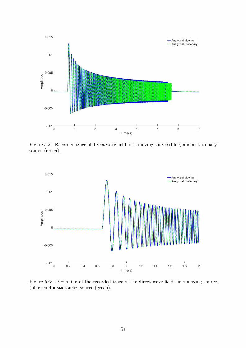
Figure 5.5: Recorded trace of direct wave �eld for a moving source (blue) and a stationarysource (green).

Figure 5.6: Beginning of the recorded trace of the direct wave �eld for a moving source(blue) and a stationary source (green).

54

Figure 5.7: End of the recorded trace of the direct wave �eld for a moving source (blue)and a stationary source (green).

Figure 5.5 show the full recorded trace and �gures 5.6 and 5.7 show the beginning and

end of the recording respectively. It can be seen from �gure 5.6 that the direct wave�elds

are initially recorded at the same time. This is because the start of the sweep for both the

stationary and the moving sources are emitted at the exact same location. The traveltime

of the initial output can easily be calculated to distancevelocity

= 1000m1500m/s

= 0.667s which coincides

with �gure 5.6.

As the source moves towards the receiver, the two traces start to behave di�erently. There

is a clear phase di�erence only after a few milliseconds which is a result of the moving

source coming closer to the receiver. This can be veri�ed by inspecting the wave equations

for both the stationary (equation 2.32) and the moving (equation 5.18) case. The phase

term in the frequency domain eikr when given two di�erent distances would yield di�erent

angles of phase as seen on the phase spectrum of the recorded data in �gure 5.8.

55

Figure 5.8: Phase spectra of the direct wave �eld for a stationary and a moving source.Both the FD and analytical approach have been plotted for quality control reasons.

As previously explained, there is little or no phase di�erence between the stationary

and moving source at low frequencies as this corresponds to the beginning of the sweep

(linear upsweep) when the moving source is still close to the stationary source. However,

at higher frequencies (or additional time), the phases recorded from the stationary and

moving source start to deviate. As mentioned, this is because the higher frequencies are

emitted when the moving source is closer to the receiver.

It can also be observed from �gure 5.7 that there is an amplitude di�erence between the

stationary and moving sources towards the end of the traces. This di�erence is also due

to the moving source getting closer to the receiver as a function of time and therefore has

less space to decay.

56

Figure 5.9: Amplitude spectra of the direct wave �eld for stationary and moving source.Both the FD and analytical approach have been plotted.

Similar to the phase spectrum, the amplitude spectrum (cf. �gure 5.9) shows that the

amplitudes are similar at low frequencies, but deviates at higher frequencies (later times

in the sweep). However, this di�erence is minor compared to the di�erence in phase.

Moreover, the moving source seems to emit higher frequencies. This is not because the

sweeps are di�erent, but because the wave�eld is compressed in the direction of motion

(and dialated in the opposite direction). When the source is moving towards the receiver at

50m/s, the wave �eld compresses which generates higher frequencies. This is the Doppler

frequency shift which can be calculated by the following equation (Morse & Ingard, 1968,

B)

f ′ = f(1

1± v

c

) (5.21)

where plus or minus is chosen whether the motion is towards the receiver (-) or away

from the receiver (+). Moreover, f is the original frequency contained within the wave,

v is the speed of the source, c is the wave velocity of the medium and f ′ is the frequency

generated by wave �eld compression or dialation which in our case is (taking f = 100Hz)

57

f ′ = 100Hz(1

1− 50m/s1500m/s

) = 103.45Hz (5.22)

The frequency shift is not very large in this case. One would actually expect an even

lower shift in reality, as the vessel usually moves at under 3m/s. This would correspond

to a frequency of f ′ = 100Hz( 1

1− 3m/s1500m/s

) = 100.2Hz. Having the vessel move at such

traditional speeds would not give such signi�cant change as in �gures 5.8 and 5.9. Thus,

the high vessel speed was only employed for the purpose of demonstration. However, from

here on, a vessel speed of 2.67m/s will be used as this is considered more of a standard.

Additionally, only the �nite-di�erence method will be used as we now have increased

con�dence in the �nite di�erence implementation.

5.3 Generating synthetic data with a moving source

The previous analysis characterized the e�ects of motion from a direct wave�eld as well

as introducing motion into the sweep wavelet. In this section, synthetic data is generated

using such a sweep along with the same model containing two scatterers (�gure 3.4) and

the same survey con�guration as shown in �gure 3.5. However, the source will move to-

wards the right as it is emitting the sweep. When the sweep has �nished and the wave�eld

has been recorded, the next sweep will start to emit at the next shot point location. As

previously mentioned, the source will now move at 2.67m/s which is considered a more

realistic vessel speed.

The data was then processed the same way as with the stationary data (section 4.1) with-

out any motion correction being applied. In fact, we want to test if the moving data can

be processed and imaged without taking the motion into account. The processed data for

the moving source was then migrated using all 200 shots and the full 3000m migration

aperture and the result is shown in �gure 5.10.

58

Figure 5.10: Migrated section of moving source data using 3000m migration aperture.

When comparing �gure 4.10 to �gure 5.10, it is hard tell if any di�erences exist. To obtain

a better idea of the image quality, an image slice was again taken at the di�ractor depth

for both the moving and stationary case (cf. �gure 5.11).

Figure 5.11: Depth slice taken of stationary data (blue) and moving data (red dotted)together with their di�erence (green) (residual).

59

Figure 5.11 shows that there is a slight di�erence in the two images which was calculated

to be at most 3.15% with a normalized root mean square (NRMS) of 2.87%. Figures

5.8 and 5.9 provide some basic understanding of how this di�erence occurs, but this is

investigated further in Appendix D.

60

Chapter 6

Comparing Vibrator and Airgun

Data

Two migrated sections have now been obtained using both a moving (�gure 5.10) and a

stationary (�gure 4.10) source emitting a continuous wave�eld. To estimate the quality of

these images, they will now be compared to the standard airgun case. The chosen airgun

in this thesis is a standard PGS airgun array already implemented into Nucleus+. This

particular gun array is called 4130G_ 080_ 2000_ 080 where 4130 refers to the volume

of the gun given in cubic inches, 8 refers to the source depth and 2000 to the air pressure

given in psi. However, the frequency band of this particular airgun is much wider than

the vibrator (equation 1.2) so for this to be a fair comparison, the two types of sources

have to emit a wave�eld containing the same range of frequencies. To achieve this, the

airgun was �ltered down to only contain frequencies between 5 and 100Hz. Additionally,

the airgun was scaled down to the amplitude level of the vibrator. The �nal airgun source

far�eld signature used can be seen in �gure 6.1.

61

Figure 6.1: The far�eld signature of an airgun array recorded 9000m away from theactual array.

The corresponding amplitude spectra of the vibrator source and the airgun are shown in

�gure 6.2.

Figure 6.2: Comparison of the amplitude spectrum of the airgun (red) with that of thevibrator (blue).

It can be observed from �gure 6.1 that the output from the airgun is not a perfect impulse

(i.e. it contain the bubble pulse). However, we indent to preserve the inherent nature

62

of the airgun array signature. Thus, some of the bubble pulse still remains within the

signature.

The far�eld signature represents the propagation distance when the source signature starts

to be stationary (9000m in this case). In order to �nd the actual output, or the notional

source signature, the far�eld signature in �gure 6.1 was propagated back to the position

of the source thus compensating for geometrical spreading and phase. This notional

signature was then used to generate synthetic data the same way as shown in section 3.2

with the same survey con�guration (�gure 3.5) and the same model (�gure 3.4).

The data was then migrated using the same �nite-di�erence depth migration as previously

used and the result is shown in �gure 6.3.

Figure 6.3: Migrated section of airgun data using 3000m migration aperture.

It can be observed from �gure 6.3 that the image is blurry in comparison to the image

produced using a marine vibrator (�gures 4.10 and 5.10). However, the two di�ractors

are still properly resolved. To get a better comparison, an image slice at the di�ractor

location was taken and is displayed in �gure 6.4 together with the results obtained in case

of sweep data (both stationary and moving source).

63

Figure 6.4: Normalized amplitude image slice taken of the migrated section in �gure 6.3at a depth of 508m.

The amplitudes shown in �gure 6.4 have been normalized in order to obtain a better

comparison. It can be observed from �gure 6.4 that the airgun data is not resolving the

two di�ractors as well as both the moving and stationary vibrator data. This may come

as an e�ect of the low frequencies being the most dominant in the airgun signature (�gure

6.2). A better comparison could be obtained by applying designature and including noise

in the computed data. However, no designature or additional signature alterations will

be considered in this work as the main point was to show that both source types are able

to generate data with su�cient energy and frequency output in order to resolve the two

di�ractors.

64

Chapter 7

Discussion

7.1 Frequency dependent illumination

Only a single-source �ring system has been considered in this work. In the stationary

case, this single source emits frequencies that all originate from the same source location.

Therefore, all frequencies illuminate the same areas of the subsurface. When motion is

introduced however, di�erent frequencies will illuminate di�erent parts of the subsurface

as the source changes its position with time. This is not a practical problem for the sweep

length and vessel speed used in this thesis work. But, long sweep lengths and/or high

vessel speeds will cause di�erent points in the subsurface to be illuminated by di�erent

frequencies.

Assume now a single vibrating source emitting a linear upsweep which is recorded by a

single receiver both located above a plane interface. The receiver is stationary while the

source moves at 2.67m/s towards the receiver emitting a sweep over 5 seconds. The largest

di�erence in midpoints caused by the motion can then be shown to be 6.675 meters. In

order for the midpoint to vary signi�cantly at these vessel speeds, the sweep length have

to be extremely long. If the same experiment were to be repeated with a sweep length of

20 seconds, the di�erence in midpoints on the plane interface would be 26.7 meters.

Large di�erences in midpoint location may introduce further problems when the wave

propagates down into the subsurface beneath the plane interface. If the underlying layer

includes strong lateral velocity variations, di�erent frequencies will propagate with dif-

65

ferent wave velocities. This may imply that the traveltimes for di�erent frequencies vary

disproportionally to the propagation distance. More speci�cally, one frequency may prop-

agate in a high velocity part of a layer while another frequency may propagate in a lower

velocity part of the same layer. The underlying layer may therefore be illuminated by

di�erent frequencies giving the wrong impression of the extent of that layer. This may

be critical when trying to locate typical thin layers like cap rocks. If the extent of the

cap rock is underestimated due to di�erent resolution in di�erent parts of the section, a

potential reservoir may go unnoticed. Furthermore, this e�ect may echo throughout the

subsurface thus having data resolved partly by di�erent frequencies.

Di�erent propagation paths for di�erent frequencies means they are recorded at di�erent

times disproportional to the propagation distance. The time di�erence in recording the

lowest and highest frequencies (assuming linear upsweep) emitted by the vibrator is then

given by the sweep length plus the additional traveltime caused by lateral velocity vari-

ations. This additional traveltime can either be negative or positive depending on the

direction of the lateral velocity gradient and the direction of motion of the source.

A type of lateral velocity variations are dipping re�ectors. The next section will discuss

how such a dipping re�ector a�ects the data with regards to the Doppler e�ect.

66

7.2 The Doppler e�ect and dipping re�ectors

It has been shown in �gure 5.11 in section 5.3 that the e�ects of motion on the source

wave�eld is minimal when moving at typical vessel speeds (< 3m/s). This is further

explored in Appendix D where the amplitude ratio in common receiver domain (CRD) is

shown to be very small as well. However, a phase di�erence of over 300 degrees between

the stationary and moving data prior to cross-correlation at high frequencies and large

o�sets is shown in �gure D-3. As described by Dragoset (1988), the Doppler e�ect arise

from the compression or dilation of the wave�eld thereby generating higher frequencies or

lower frequencies respectively. Even a small frequency shift of less than 1Hz will cause a

large phase distortion (Dragoset, 1988). Dragoset then proposed an equation to calculate

the phase shift resulting from the Doppler e�ect:

φ(f) = 360◦δTf 2

(f2 − f1)(7.1)

where T is the sweep length, f is a given frequency within the frequency band, f2 and

f1 is the highest and lowest frequency within that frequency band respectively and δ is

the Doppler factor. This Doppler factor is the ratio of vessel speed and the velocity of

the medium, but also contain angle information and is given as δ = vc[sin(αr)− sin(αs)].

Where αr and αs are the angles of incidence of the receiver and source respectively. From

this equation it is observed that the Doppler factor is 0 when the angles of incidence

are equal for both source and receiver. This only happens for the zero-o�set trace on

a common receiver gather when using the middle receiver with the model and survey

con�guration used in this thesis work. Therefore, it can be seen on �gure D-3 in Appendix

D that the zero o�set trace has a zero degree phase shift. This is con�rmed on �gure D-1

in Appendix D where there is no di�erence between the stationary and moving datasets at

zero o�set. Furthermore, the di�erence between these two angles in our case increase as

the shot point deviates from the receiver location meaning that higher o�set would yield

a higher Doppler factor and phase shift which is con�rmed in �gure D-3. The Doppler

factor can be calculated to be ±0.0017 for the largest o�set using the survey con�guration

67

and model in this work. Substituting the values used in this thesis work into equation 7.1

yields

φ(f) = 360◦ ∗ (±0.0017) ∗ 5s ∗ 100Hz2

(100Hz − 5Hz)≈ ±322.1◦ (7.2)

where f1 = 5Hz, f2 = 100Hz and f = 100Hz has been used. With the values for maxi-

mum o�set and frequency used, this corresponds well to what is seen at the bottom left

and right in �gure D-3.

It can be observed from equation 7.1 that a stationary source yields a Doppler factor

of zero meaning a zero degree phase shift. Even a small velocity such as the one used

here (2.67m/s) will yield a phase shift of several hundred degrees. Additionally, a plane

re�ector will experience no Doppler phase shift as the angles of incidence are equal.

The two-di�ractor model used in this work limits the ability to see the e�ects introduced

by complex geology, but dipping re�ectors will according to equation 7.1 cause the Doppler

e�ect to increase as the di�erence in angles of incidence increase (Dragoset, 1988). How-

ever, the phase of the sweep will be removed from the dataset when cross-correlation is

performed, thereby eliminating these Doppler phase shift e�ects.

It can be seen from equation 7.1 that increased sweep length will result in an increase of

the Doppler phase shift. The next section will discuss the advantages and disadvantages

of having a shorter sweep length.

68

7.3 Sweep length and deep targets

Short sweep lengths produce lower pressure output than longer sweeps. This is because

the longer sweep would "dwell" longer on each frequency, creating more pressure output

per frequency according to equations 2.31 and 3.4. This allows the pressure wave to

propagate to deeper targets before being too attenuated. As previously discussed in

section 7.1 however, long sweep length cause frequency dependent illumination of the

subsurface. This means that only parts of the deeper subsurface will be illuminated as

the higher frequencies will attenuate faster. Thus, long sweeps can only illuminate parts

of the deep targets in areas where the low frequencies will propagate.

However, it is not of interest to obtain the highest pressure output possible, but to do

so while under some given threshold which is set according to environmental regulations.

While under this threshold, the pressure output should be maximized. According to MV-

JIP (section 1.4), this threshold is set to 200dB re. 1µPa/Hz @ 1m for 10− 100Hz for a

5 second signal (Feltham et. al., 2018). This value means that each frequency in the band

is only allowed to contain 200dB of pressure relative to reference level of 1 micro Pascal

when measured 1 meter away from the source. Obtaining 200dB per frequency is in theory

possible for both an airgun and a marine vibrator (�gure 6.2). It is therefore important

to see how the amplitudes are distributed in time. The amplitude and frequency content

of the airgun is contained within a short period of time (see �gure 6.1), while the marine

vibrator is spreading this amplitude over a longer period of time. Therefore, the airgun

is considered more dangerous to marine life as all of this energy is concentrated into a

single wavefront (in the ideal case). In other words, the peak amplitude of the airgun is

much higher than that of the marine vibrator.

It may be possible to increase the total pressure output from short sweeps by introducing

a multi-vibrator system, thereby avoiding the disadvantages of having a longer sweep

length. How several marine vibrators each emitting shorter sweeps can be utilized will be

the topic of the next section.

69

7.4 Multi-vibrator systems

Until now, it has been discussed how short sweeps are preferred in order to avoid a sec-

tion partly illuminated by di�erent frequencies. However, these short sweeps have lower

pressure output than the longer sweeps, making deep surface resolution impossible due

to attenuation. This section will discuss how multiple vibrator sources emitting shorter

sweeps may be utilized to obtain a higher pressure output while keeping a shorter sweep

length. Additionally, having multiple vibrator shooting simultaneously lowers survey cost

as more data can be collected.

When multiple sources are introduced into a survey, it increases the pressure output equal

to the number of sources (in the ideal case). However, it is a challenge to separate the

signals recorded by the receivers. The process of signal separation is called deblending

and is well understood when it comes to airgun sources. However, deblending for marine

vibrator sources are performed di�erently from what is done in the airgun case. Marine

vibrator deblending takes advantage of knowing the output of the source as well as the

ability to encode the sweep.

A coded sweep is a type of sweep that consists of smaller sequentially ordered sub-sweeps.

The number of sweep types within a coded sweep are often referred to as code-members.

A binary coded sweep consists of two code members which could be upsweeps and down-

sweeps (Bernhardt & Peacock, 1978). Phase encoded sweeps are often used for deblending

purposes as well as increasing the signal to noise ratio which further act to suppress the

noise associated with the cross-correlation process (Bernhardt & Peacock, 1978). Fur-

thermore, it has been shown that a sub-sweep length of 1 second yields good results when

suppressing such correlation noise (Edelmann & Werner, 1982). However, the longer the

entire coded sweep (i.e. more sub-sweeps) the better the suppression of noise in the cross-

correlation process. The sub-sweeps within a coded sweep can in theory be chosen freely

such that the sub-sweeps all contain the same frequencies. Another options would be to

have the sub-sweeps have di�erent frequency bands, possibly with overlapping frequen-

cies.

70

A method utilizing phase encoded sweeps for deblending purposes was proposed by Silver-

man (1979). This type of con�guration aims to obtain two shot gathers from two di�erent

vibrators each emitting a phase encoded sweep of di�erent polarities (Silverman, 1979).

Due to the harmonic interference of the Silverman con�guration, another con�guration

proposed by Ward et al. may be considered. This con�guration expands upon the Silver-

man con�guration by adding additional sub-sweeps, with a 45◦ phase shift between the

sub-sweeps, to the coded sweeps for both vibrator sources, but with the direction of phase

shift reversed for the second source. This con�guration has proved to suppress all lower

order harmonics up to the seventh harmonic (Ward et al., 1990).

Most marine vibrator deblending methods rely on a phase di�erence between the output

from di�erent vibrator sources, but some deblending methods does not rely on the sweep

to be coded. These methods simply lets the initial phase of non-coded sweeps to vary

from shot to shot. Halliday et al. (2017) proposed such a method where six shots with a

60◦ phase shift for each source is recorded, sorted into a common receiver gather (CRG)

and then transformed to frequency-wavenumber domain. By utilizing this phase di�er-

ence separation, the deblending yielded less cross-talk than using a simple time-dithered

separation method (Halliday et al., 2017). This example shows how valuable the control

of the source signature is when trying to deblend the data. Moreover, this means that it

is possible to perform surveys using multiple sources which makes it possible to illuminate

deeper targets as well as saving both time and money.

The Halliday deblending method does not imply that any speci�c type of sweep is needed

and therefore opens up for di�erent types of sweeps to be used within the same survey.

This would imply that the bene�ts of several types of sweeps may be utilized in a multi-

vibrator system. Moreover, high pressure output may not be necessary if the target area

is shallow thereby eliminating the need for a multi-vibrator system. The next section will

discuss how marine vibrators may be utilized in shallow waters.

71

7.5 The marine vibrator in shallow waters

Airgun sources in marine surveys are usually placed at some depth below the sea surface

in order to minimize loss of energy. If the airgun source is placed at too shallow depth,

most of the energy will simply disappear into the air above. However, even at an opti-

mal depth, some of the energy will still propagate upwards and be re�ected o� the sea

surface and create the source ghost. The deeper the airgun source is �red, the larger the

di�erence in traveltimes between the primary re�ection and the source ghost itself, thus

loosing resolution.

The marine vibrator does not su�er to the same degree as the airgun when it comes to

depth limitations. As described in section 1.6, the AquaVib marine vibrator by GeoMe-

chanics can handle depths down to 1m below the sea surface, thereby making it possible

to handle very shallow prospects. Smith et.al. have shown that the output from the

Industrial Vehicles International marine vibrator is independent for depths between 8 and

1.5m. Shallower depths than 1.5m gave rise to amplitude loss on the scale of 3 − 6dB

(Smith et. al., 1998). A test of a marine vibrator engineered by Total, Mobil and Geco-

Prakla in 1994 showed that the marine vibrator was able to produce su�cient output

down to 1m depth. However, it was also shown that the source ghost dominated the data

for sources located closer to the sea surface (Walker et. al, 1996). Walker et. al. showed

that a simple ghost �lter could remove the e�ects of such a source ghost. Overall, it is safe

to say that the marine vibrator can operate at shallower waters than the airgun making

them a good alternative in such areas. This would make it possible to survey areas closer

to the shore as these areas are often shallow.

It just so happens that the shallower waters tend to have the most sensitive marine life

(Archer, 2017). The lower peak pressure output of the marine vibrator in combination

with the ability to operate at shallower waters makes the marine vibrator a good candidate

for the choice of source in these areas.

72

Chapter 8

Conclusion and Future Work

This work has shown that a term for the pressure output from a pair of vibrating plates

within a homogeneous medium can be derived (equation 2.31). A term for the moving

source wave�eld was derived as well (equation 5.18). From these two equations it has

been shown that the acceleration of the plates are directly related to the pressure out-

put and can in theory be con�gured to emit any frequency band using any sweep length

(Appendix C). However, the choice of sweep length must be chosen carefully as very long

sweeps length will result in a section partly resolved by di�erent frequencies at di�erent

depths.

The introduction of motion upon the vibrator source has been showed to cause small

amplitude di�erences, but large phase shifts which is caused by a Doppler e�ect (�gures

D-2 and D-3). However, the process of cross-correlating the synthetic data with the sta-

tionary sweep wavelet has shown to be an e�ective procedure to remove the phase of the

sweep thereby making the data interpretable. Moreover, is has been shown that the data

generated using a moving source can be treated equally to a stationary source in the ideal

case presented in this thesis work (�gure 5.11).

As a result of the choice of background model used in this work (�gure 3.4), we are not

able to see the e�ects that complex geology and a non-impulsive source wave�eld have on

the data. Therefore, a new model containing more complex geology like dipping re�ectors

alongside other re�ection events should be made in order to investigate further. If the

data generated using a moving source can still be treated as a stationary case, it can be

73

concluded that the e�ect of motion is corrected for by the cross-correlation and migration

process. Additionally, it may be possible to perform this cross-correlation in the migration

itself by utilizing a cross-correlation imaging condition.

The limit of resolution for a marine vibrator has also been tested where the generated

synthetic data for the stationary case has been cross-correlated and migrated using dif-

ferent migration apertures (�gure 4.6). The results shown in �gure 4.7 does not correlate

with values in equation 4.7, however, it was demonstrated that a marine vibrator source

was able to resolve two di�erent points separately.

Finally, synthetic airgun data was generated using a �ltered airgun source signature. The

generated data was then migrated and the image was then compared to the marine vibra-

tor image. The main di�erence between these two images was that the lower frequencies

dominated the airgun image, thereby making it seem more blurry. However, both types

of sources are able to generate an image that easily resolved the two nearby di�ractors.

What can be done further is to deconvolve the wavelet from the data which should give

a closer resemblance to the true amplitude of the re�ection events. This would make for

a more complete comparison of the marine vibrator and the airgun than what is shown

in chapter 6.

74

References

• Archer, J, 2017, A safe alternative to the seismic airgun, o�shore technology, [Inter-

net], Available from: https://www.o�shore-technology.com/features/featurea-safe-

alternative-to-the-seismic-airgun-5834997/

• Arfken, G., B., Weber, H., J., Harris, F., E., 2012, A, Mathematical Methods for

Physicists, chapter 3, 7th edition, Academic Press: Elsevier Inc., pp 164, ISBN:

978-0-12-384654-9

• Arfken, G., B., Weber, H., J., Harris, F., E., 2012, B, Mathematical Methods for

Physicists, chapter 10, 7th edition, Academic Press: Elsevier Inc., pp 448, ISBN:

978-0-12-384654-9

• Arfken, G., B., Weber, H., J., Harris, F., E., 2012, C, Mathematical Methods for

Physicists, chapter 1, 7th edition, Academic Press: Elsevier Inc., pp 78, ISBN:

978-0-12-384654-9

• Berkhout, A.J., 1980, Seismic Migration, imaging of acoustic energy by wave �eld

extrapolation, Appendix C: Wave Equation for Inhomogeneous Fluids, 355 Jan van

Galenstraat: Elsevier Scienti�c Publishing Company, pp. 320-325

• Bernhardt T., Peacock J. H., 1978, Encoding Techniques for the Vibroseis* Sys-

tem**, Geophysical Prospecting 26, pp. 184-193, DOI: https://doi.org/10.1111/j.1365-

2478.1978.tb01585.x

• Dragoset, W., H., 1988, Marine vibrators and the Doppler e�ect, Geophysics, 1988,

Vol.53(11), pp.1388-1398, DOI: 10.1190/1.1442418

75

• Edelmann, H., A., K., Werner, H., 1982, Combined Sweep Signals for Correla-

tion Noise Suppression*, Geophysical Prospecting, Vol.30(6), pp 786-812, DOI:

10.1111/j.1365-2478.1982.tb01339.x

• Emma Technologies, Seismic, [Internet], Available from:

https://www.emma-technologies.com/products/seismic/

• Feltham A., Jernerson M., Henderson N., Girard M., Nechayuk V., Cozzens A.,

2018, Geophysical Testing of a Marine Vibrator Integrated Projector Node (MV-

IPN) at Seneca Lake, 80th EAGE Conference and Exhibition, DOI: 10.3997/2214-

4609.201800996

• Halliday D. F., Laws R., Özbek A., Schlumberger Gould Research, 2017, Phase

sequencing, marine vibrators, and high-multiplicity simultaneous sources, Society of

Exploration Geophysicists, DOI: https://doi.org/10.1190/segam2017-17660035.1

• Hampson G., Jakubowicz H., 1995, The e�ects of source and receiver motion on

seismic data, Geophysical Prospecting, Vol.43(2), pp.221-244, DOI: 10.1111/j.1365-

2478.1995.tb00133.x

• Howell, K., B., 2001, A, Principles of Fourier Analysis, CRC Press; 1 edition (May

18, 2001), pp 755-756, ISBN: 0849382750

• Howell, K., B., 2001, B, Principles of Fourier Analysis, CRC Press; 1 edition (May

18, 2001), pp 395, ISBN: 0849382750

• Innoseis, 2018, Seismic Surveys, [Internet], Available from:

http://www.innoseis.com/seismic-surveying/

• International Association of Geophysical Contractors, 2002, Airgun Arrays and Ma-

rine Mammals, 2550 North Loop West, Suite 104, Houston, Texas 77092 USA

• Kadry, S., 2014, Mathematical Formulas for Industrial and Mechanical Engineering,

Elsevier Scienti�c Publishing Company, pp 60, ISBN: 978-0-12-420222-1

76

• Kallweit, R., S., Wood, L., C., 1982, The limits of resolution of zero-phase wavelets,

GEOPHYSICS, Vol.47(7), pp 1035-1046, DOI: 10.1190/1.1441367

• Kramer, F. S., Peterson, R.A., Walter, W.C., 1969, Seismic Energy Sources, O�-

shore Technology Conference, 18-21 May, Houston, Texas,

DOI: https://doi.org/10.4043/1119-MS

• Landrø, M., Amundsen, L., 2014, Is it optimal to tow air guns shallow to enhance

low frequencies?, Geophysics, Vol.79(3), pp.13-18, DOI: 10.1190/GEO2013-0348.1

• Morse, P., M., Ingard, K., U., 1968, A, Theoretical Acoustics, New-York, McGraw-

Hill Book Company , pp 717-724, ISBN: 0070433305

• Morse, P., M., Ingard, K., U., 1968, B, Theoretical Acoustics, New-York, McGraw-

Hill Book Company, pp 699, ISBN: 0070433305

• Nguyen, D., L., 2017, Seismic Wave�eld Modelling From Marine Vibrator Sources,

Department of Geosciences, Faculty of Mathematics and Natural Sciences, Univer-

sity of Oslo

• Parkes, G., Hatton, L., 1986, The marine seismic source, Dordrecht, Springer

Netherlands : Imprint: Springer, ISBN: 94-017-3385-6

• Peters, A., S., Stoker, J., J., 1954, A uniqueness theorem and a new solution for

Sommerfeld's and other di�raction problems, Communications on Pure and Applied

Mathematics, Vol.7(3), pp 565-585,

DOI: https://doi-org.ezproxy.uio.no/10.1002/cpa.3160070307

• PGS, 2017, Marine Vibrators Get Closer to Reality, [Internet], Available from:

https://www.pgs.com/publications/feature-stories/marine-vibrators/

• Rietsch E., 1977, Computerized Analysis of Vibroseis Signal Similarity, Geophysical

Prospecting, Vol.25(3), pp 541-552, DOI: 10.1111/j.1365-2478.1977.tb01186.x

77

• Roy D., Brideau C., Lawry T., Ratli� C., Rekos R., 2018, The Applied Physical

Sciences Marine Vibrator: An Overview, 80th EAGE Conference and Exhibition,

DOI: 10.3997/2214-4609.201801625

• Salby, M., L., 2012, Physics of the Atmosphere and Climate, Cambridge University

Press, Appendix D: Vector Identities, pp 620,

DOI: https://doi-org.ezproxy.uio.no/10.1017/CBO9781139005265.024

• Silverman, D., 1979, Method of Three Dimensional Seismic Prospecting, United

States Patent 4,159,463

• Smith, J., G., Jenkerson, M., R., Mobil Exploration, Producing Technical Center,

1998, Acquiring and Processing Marine Vibrator Data in the Transition Zone, So-

ciety of Exploration Geophysicists, DOI: http://dx.doi.org/10.1190/1.1820159

• Söllner, W., Orji, O., 2017, Marine vibrator source acceleration and pressure, US

Patent Application, Pub. No. US2018/0052245 A1

• Todoeschuck, J., P., Jensen, O., G., 1989, Scaling geology and seismic deconvo-

lution, Pure and applied geophysics: Volume 131, Issue 1-2, pp 273-287, DOI:

10.1007/BF00874491

• Walker, L., Potter, G., Jenkerson, M., Rodriguez, J., M., Total Research and Tech-

nology Center, 1996, The acoustic output of a marine vibrator, Society of Explo-

ration Geophysicists, DOI: http://dx.doi.org/10.1190/1.1826485

• Ward, R. M., Brune, R.H., Ross, A., Kumamoto, L. H., 1990, Phase encoding of Vi-

broseis signals for simultaneous multisource acquisition, 60th Annual International

Meeting, SEG, Expanded Abstracts, pp. 938-941

• Western Geco, 2010, Geo ExPro Vol. 7 No. 1, [Internet], Available from:

https://www.geoexpro.com/magazine/vol-7-no-1

78

Appendixes

Appendix A: Derivation of Euler's equation of motion

Consider an in�nitesimal �uid volume and let it interact with a propagating pressure �eld

as shown in �gure A-1.

Figure A-1: Translated in�nitesimal �uid element (Berkhout, 1980).

This implies compression and expansion as well as translation of the �uid element. The

acting forces can be written as:

Fx = (∂p

∂tdt+

∂p

∂x∆x)∆y∆z =

∂p

∂xV

Fy = (∂p

∂tdt+

∂p

∂y∆y)∆x∆z =

∂p

∂yV

Fz = (∂p

∂tdt+

∂p

∂z∆z)∆x∆y =

∂p

∂zV

(A-1)

or in vector form (assuming dt→ 0)

79

F = V 5 p (A-2)

In equation A-1 ∆x, ∆y and ∆z denote the three surface areas of the �uid element and

V is the volume of the �uid element. Note that the observation time dt in equation A-1

is assumed so small that the pressure change over time can be neglected.

Considering the same �uid element, the acceleration term may also be decomposed into

time and spatial components employing the total derivative dv (v being velocity):

dv =∂v

∂tdt+

∂v

∂x∆x+

∂v

∂y∆y +

∂v

∂z∆z

→ dv

dt=∂v

∂t

dt

dt+∂v

∂x

∆x

dt+∂v

∂y

∆y

dt+∂v

∂z

∆z

dt

=∂v

∂t+∂v

∂xvx +

∂v

∂yvy +

∂v

∂zvz

=∂v

∂t+ (v · 5)v

(A-3)

where v ·5 is called a convection term. Substituting equations A-2 and A-3 into Newton's

second law gives the �nal result

V 5 p = m(∂v

∂t+ (v · 5)v)

→5p = ρ(∂v

∂t+ (v · 5)v)

(A-4)

In Appendix B it is demonstrated that the convection term in equation A-4 can be ne-

glected in the seismic case.

80

Appendix B: Linearization of the equation of motion

and the constitutive law for a plane wave

The equation of motion and the constitutive law describe the motions of the isotropic, non-

viscous medium when a pressure wave propagates through. The plane-wave assumption

will allow these equations to be linearized.

A linear relation between pressure and velocity for a plane-wave is written as (in 1D)

p = (ρc)v (B-1)

The term vcis the unitless Mach Number and gives the relation between the wave velocity

and the particle velocity of the medium. Solving equation B-1 for the Mach Number

yields

v

c=

p

ρc2(B-2)

In this paper, water is the medium of interest and by substituting in values for density

and medium velocity of water, the equation becomes

v

c= (0.4p)10−9 (B-3)

where c = 1500m/s and ρ = 1000kg/m3. In the seismic case, the pressure p typically

< 103Pa, making the Mach Number close to

v

c= (0.4)10−6 (B-4)

which is much less than 1 (Berkhout, 1980). The fact that the Mach Number is so small

makes it possible to neglect the convection term in both the equation of motion and the

constitutive law. Consider �rst the equation of motion, and introduce the approximation

81

|(v · 5)v| = |vx∂v

∂x|+ |vy

∂v

∂y|+ |vz

∂v

∂z|

= |vxc

∂v

∂t|+ |vy

c

∂v

∂t|+ |vz

c

∂v

∂t| << |∂v

∂t|

(B-5)

where the absolute value is taken since only the magnitude of the derivative is of interest.

Thus, by use of equation B-5, equation A-4 in Appendix A simpli�es to

5 p = ρ∂v

∂t(B-6)

The same analysis can also be applied to the constitutive law (equation 2.9 in the main

text)

|(v · 5)p| = |vx∂p

∂x|+ |vy

∂p

∂y|+ |vz

∂p

∂z|

= |vxc

∂p

∂t|+ |vy

c

∂p

∂t|+ |vz

c

∂p

∂t| << |∂p

∂t|

(B-7)

simplifying equation 2.9 to

∂p

∂t= −K 5 ·v−KQ (B-8)

Which is the same as equation 2.10 in the main text.

82

Appendix C: Sweep design and acceleration response

We start by considering a phase dependent sweep signal of the form

s(t) = A(t)cos[2π(φ(t) + φ0)] (C-1)

where A(t) is the time dependent amplitude, φ0 is the initial phase and φ(t) is the time

dependent phase function given by (linear sweep)

φ(t) = f0t+(f1 − f0)t2

2T(C-2)

where f0 and f1 are respectively the lowest and highest frequency of the sweep and T is

the total duration for one sweep (sweep length). The signal s(t) in the frequency domain

can be obtained through the Fourier transform resulting in

S(ω) =

∫ T

0

s(t)e(−iωt)dt =

∫ T

0

A(t)cos[2π(φ(t) + φ0)][cos(ωt)− isin(ωt)]dt (C-3)

Through the identities cos(a+ b)cos(c) = 12[cos(a+ b− c) + cos(a+ b+ c)] and −cos(a+

b)sin(c) = 12[sin(a+ b− c)− sin(a+ b+ c)] (Kadry, 2014) equation C-3 becomes

S(ω) =

∫ T

0

A(t)1

2{cos[2π(φ(t) + φ0)− ωt] + cos[2π(φ(t) + φ0) + ωt]+

isin[2π(φ(t) + φ0)− ωt]− isin[2π(φ(t) + φ0) + ωt]}dt

=1

2

∫ T

0

A(t)[ei[2π(φ(t)+φ0)−ωt] + e−i[2π(φ(t)+φ0)+ωt]]dt

(C-4)

With phase spectrum

Φ(ω, t) = 2π(φ(t) + φ0)− ωt (C-5)

being introduced such that equation C-4 becomes

83

S(ω) =1

2

∫ T

0

A(t)[eiΦ(ω,t) + e−iΦ(−ω,t)]dt (C-6)

The original signal s(t) is a real signal which means that the following relation holds

S(ω) = S∗(−ω) (Rietsch, 1977). Therefore, the signal S(ω) can be de�ned by positive

frequencies only

S(ω) =1

2

∫ T

0

A(t)eiΦ(ω,t)dt (C-7)

The phase function Φ(ω, t) oscillates so rapidly compared to the amplitude function A(t)

that only the vicinity around its stationary points contribute to the actual signal. All

other points cancel out in the integration. The stationary points are found by setting the

time-derivative of the phase spectrum Φ(ω, t) equal to 0

dΦ

dt= 2π

dφ(t)

dt− ω = 0

→ 2π(f0 +(f1 − f0)t

T)− ω = 0

(C-8)

where the phase function in C-2 has been substituted in. Solving equation C-8 for t yields

the stationary points tw

tw = (ω

2π− f0)

T

(f1 − f0)(C-9)

By substituting tw (from equation C-9) into the phase function φ(t) gives the contributing

parts of the phase:

φ(tw) = f0tw +(f1 − f0)t2w

2T

=f0T

(f1 − f0)(ω

2π− f0) +

(f1 − f0)

2T[

T

(f1 − f0)(ω

2π− f0)]2

=f0T

(f1 − f0)(ω

2π− f0) +

T

2(f1 − f0)(ω

2π− f0)2

(C-10)

and correspondingly for the phase spectrum (equation C-5) while assuming no initial

phase φ0 yields

84

Φ(ω, tw) = 2πφ(tw)− ωtw

= 2π[f0T

(f1 − f0)(ω

2π− f0) +

T

2(f1 − f0)(ω

2π− f0)2]− ωT

(f1 − f0)(ω

2π− f0)

=ω0T

(f1 − f0)(ω

2π− f0) +

Tπ

(f1 − f0)(ω

2π− f0)2 − ωT

(f1 − f0)(ω

2π− f0)

(C-11)

Keep in mind that for a linear sweep, the angular frequency ω can be expressed as a linear

equation ω = ω0 + (ω1−ω0)twT

. Substitution of this expression in the last term in equation

C-11 gives

Φ(ω, tw) =ω0T

(f1 − f0)(ω

2π− f0) +

Tπ

(f1 − f0)(ω

2π− f0)2

− ω0T

(f1 − f0)(ω

2π− f0)− (ω1 − ω0)twT

(f1 − f0)T(ω

2π− f0)

=Tπ

(f1 − f0)(ω

2π− f0)2 − 2πtw(

ω

2π− f0)

=Tπ

(f1 − f0)(ω

2π− f0)2 − 2πT

(f1 − f0)(ω

2π− f0)2

= − πT

(f1 − f0)(ω

2π− f0)2

(C-12)

The stationary phase solution to equation C-7 is now given as (Rietsch, 1977)

S(ω) =A(tw)

2√| Φ′′(ω, tw) |

ei[2π(φ(tw)+φ0)−ωt+π/4] (C-13)

where Φ′′ means taking the second derivative with respect to time. Assume now that

the sweep signal in equation C-1 represents the velocity of the vibrating plates. From

equation C-13 it follows that the amplitude spectrum of the velocity is given as

| V (ω) |= A(tw)

2√| Φ′′(ω, tw) |

(C-14)

The corresponding amplitude spectrum of the acceleration is obtained by multiplication

with instantaneous frequency ω(t) in equation C-14 (and a factor of i in the phase):

| a(ω) |= A(tw)ω(t)

2√| Φ′′(ω, tw) |

(C-15)

85

A good design criterion will be to ensure a �at amplitude spectrum of the acceleration.

This implies that we introduce the following constraint in equation C-15 (D being a

constant)

D =A(tw)ω(t)

2√| Φ′′(ω, tw) |

⇒ Φ′′(ω, t) =A2(tw)ω(t)2

4D2=dω(t)

dt

→ 1

ω(t)2dω(t) =

A2(tw)

4D2dt

(C-16)

where the relationship Φ(ω, t) = 2π(φ(t) + φ0)− ωt, dΦdt

= ddt

(2πφ(t))− ω = ω(t)− ω and

d2Φdt2

= dω(t)dt

has been applied. This is a �rst order di�erential equation with solution

∫1

ω(t)2dω(t) =

∫A2(tw)

4D2dt

→ − 1

ω(t)=A2(tw)t

4D2+ C

(C-17)

where C is the integration constant. This integral can be evaluated between two times

t = 0 with corresponding frequency ω1 and t = T with corresponding frequency ω2, where

T is the length of the sweep. In a sweep, the frequency changes with time such that

ω1 6= ω2

− 1

ω1

= C, t = 0

− 1

ω2

=A2(tw)T

4D2+ C =

A2(tw)T

4D2− 1

ω1

, t = T

→ A2(tw)

4D2=

1

Tω1

− 1

Tω2

(C-18)

Substituting A2(tw)4D2 and C into equation C-17 yields

− 1

ω(t)= t(

1

Tω1

− 1

Tω2

)− 1

ω1

=t(ω2 − ω1)

Tω1ω2

− Tω2

Tω1ω2

=t(ω2 − ω1)− Tω2

Tω1ω2

⇒ ω(t) =Tω1ω2

Tω2 − t(ω2 − ω1)

(C-19)

Equation C-19 describes how frequency changes with time between ω1 and ω2. When

t = 0, the equation reduces to ω1 and when t = T , the equation reduces to ω2. To �nd

86

the phase function, the relation ω(t) = d(2πφ(t))dt

can be used

φ(t) = φ(0) +1

2π

∫ T

0

ω(t)dt

= φ(0) + [Tω1ω2

(ω1 − ω2)ln(1 +

t(ω1 − ω2)

Tω2

)]1

2π

(C-20)

where φ(0) denotes the initial phase at t = 0 and the second term denotes how the

phase will change over time. If we set φ(0) = 0 and introduce a Taylor expansion of the

logarithmic function to 2nd order, the phase function in equation C-20 is equal to that in

equation C-2. If we again let equation C-1 represent the velocity of the vibrating plates,

the phase term can be written as

v(t) = cos(2πφ(t)) (C-21)

Substituting the expression for the phase from equation C-20 into equation C-21 yields

v(t) = cos(2πφ(0) +Tω1ω2

(ω1 − ω2)ln(1 +

t(ω1 − ω2)

Tω2

)) (C-22)

Taking the time derivative of equation C-22 yields the particle acceleration caused by a

vibrating plate

a(t) =dv(t)

dt=dcos(u)

du

du

dt(C-23)

if we set u = 2πφ(0) + Tω1ω2

(ω1−ω2)ln(1 + t(ω1−ω2)

Tω2) then

= −sin(u)d

dt(2πφ(0) +

Tω1ω2

(ω1 − ω2)ln(1 +

t(ω1 − ω2)

Tω2

))

= −sin(u)[Tω1ω2

(ω1 − ω2)

1

(1 + t(ω1 − ω2))(ω1 − ω2

Tω2

)]

= −sin(u)(Tω1ω2

Tω2 + t(ω1 − ω2))

= −sin(2πφ(0) +Tω1ω2

(ω1 − ω2)ln(1 +

(ω1 − ω2)t

ω2T))

Tω1ω2

Tω2 − (ω2 − ω1)t

(C-24)

The acceleration obtained here (equation C-23) can be used to calculate the pressure wave

�eld in equation 2.31 in the main text. In the same manner, the displacement caused by

87

a vibrating plate can be found by integrating equation C-22.

88

Appendix D: Di�erence between moving and station-

ary sweep data

To further investigate the di�erence between the stationary and moving sweep data sets,

these data were subtracted from each other. For simplicity, only the middle receiver was

chosen and plotted by source number (cf �gure D-1).

Figure D-1: Mid-receiver section of di�erence between moving and stationary data.

It can be observed from �gure D-1 that there is a di�erence in data across all source

numbers (except for source number 100). Since the middle receiver was chosen, the

shortest propagation distance is is represented by source number 100 as this is the shot

directly positioned above the di�ractors. The propagation distance increases as the shot

number increases or decrease away from shot number 100.

To obtain a more accurate representation of the di�erences in data, two Fourier transforms

were applied to the data. The �rst one from time to frequency and the second one from

space to horizontal wavenumber kx (from TX-domain to FK-domain). Then, the ratio of

amplitudes spectra between the two data sets were plotted as shown in �gure D-2.

89

Figure D-2: Ratio in amplitude spectra between moving and stationary data sets in theFK-domain. The horizontal axis represents the horizontal wavenumber.

It can be observed from �gure D-2 that there are no amplitude di�erence below 60Hz,

but some di�erences above 60Hz at large horizontal wavenumber (large o�sets). It can

be observed that some numerical errors have occurred in the process, especially in the

middle of the plot. The corresponding phase spectrum of the di�erences in the two data

sets is given in �gure D-3.

90

Figure D-3: Di�erence in phase between moving and stationary data sets in the FK-domain. The horizontal axis represents the horizontal wavenumber.

The phase spectrum in �gure D-3 shows a more dramatic change than the amplitude

spectrum. There is basically no phase di�erence at zero-o�set (kx = 0), but it increases

with increasing kx at the higher frequencies. Hence, the phase di�erence increases drasti-

cally with o�set. Furthermore, �gure D-3 shows that the problem with a moving source

is essentially a phase correction problem which applies particularly to the large o�sets.

However, even if the phase errors may be signi�cant, the corresponding amplitude errors

are very low. Thus the overall e�ect of motion is fairly negligible in case of a standard

vessel speed except for the high frequencies (above 60.70Hz) at large o�sets.

91

Appendix E: Accepted article to SEG2019

92

Marine Vibrator: Source Wavefield Modeling Sander W. Losnedahl*(PGS/UIO), Okwudili C. Orji (PGS), Leiv J. Gelius (UIO), Walter Söllner (PGS)

Summary Traditional marine seismic sources are facing increasingly strict regulation due to their non-negligible environmental foot print. However, marine vibrators are easy to control, are more efficient and have lower environmental foot print. Here we demonstrate source wavefield modeling for marine

vibrators, discuss the source signature requirements and important processing and imaging steps.

Introduction The marine geophysical community proactively seeks to be environmentally responsible. Low environmental footprint in terms of Sound Pressure Level (SPL) and Sound Exposure Level (SEL) especially in locations marked as “sensitive

areas” is a major goal for the industry. In addition, though conventional air-gun sources can deliver low frequencies that may be used in some specialized processing (e.g. full waveform inversion), such procedures would work even better if the low frequencies could be further enhanced, which could be achieved using marine vibrators. As a result, several alternatives to conventional air-gun sources have been developed. Tenghamn and Long (2006) present a

marine vibrator with a flextensional shell. Dellinger et al. (2016) present a marine vibrator that generates low frequencies. Roy et al. (2018) present a marine vibrator source capable of emitting energy from 10-100Hz. One common feature of these sources is that the output pressure is based on the oscillation of their plates. In this work, we present a method for modeling the output

pressure wavefield for a marine vibrator that is based on stacks of oscillating plates. An example of the measured amplitude spectrum of a marine vibrator source which generates acoustic wavefield by actuating a vibrator surface to produce a volume change in the surrounding water is shown in Figure 1 (Oscarsson et al., 2019). The basic element of the source consists of two parallel plates actuated towards and away from each other. When a multitude of

these elements are arranged in proximity to each other, they form a modular projector system. The full system is divided into Low Frequency (LF) and High Frequency (HF) modules. The LF module is specially designed to drive a large radiating area at small displacements and was operated from 1-45Hz while the HF module was operated from 35-100Hz for 30s. The equivalence of 5s notional was computed based on Rietsch (1977).

Figure 1: Amplitude spectra of the measured LF and HF sources.

Since marine vibrators are non-impulsive and are in motion

during data acquisition, synthetic data was computed and imaged for stationary and moving sources in order to investigate the performance of these types of sources with respect to data acquisition, processing and imaging.

Theory The modeling method is based on the reciprocity theorem

and relates the acceleration of the plates directly to the output pressure. Hence, the required plate motion can be computed. The building element of the marine vibrator source is composed of an oscillating pair of plates in water, which enclose a volume of air under pressure. The seismic wavefield everywhere outside this volume may be derived from the motion of the vibrator plates, which leads to increasing and decreasing of the enclosed volume (see

Figure 2). Inside the plates the acoustic laws may fail and this volume will be removed from the model.

S+

|r’|∞

S-

xR

Figure 2: Single vibrator: Plate surface with normal vector across

the inner surface

We start from the acoustic representation theorem. The

pressure wavefield inside the model enclosed by the spherical surface as outer border and an idealized surface surrounding the oscillating plates, as inner border, is expressed for a model free of body forces by surface

integrals of the free space Green’s function 𝑔, the pressure

𝑝, and the gradients of these wavefields on the outer and

Source Wavefield Modeling

inner surfaces (Morse and Feshbach, 1953). By letting the outer surface go to infinity and applying Sommerfeld’s radiation condition (Sommerfeld, 1949), the pressure may be written as a surface integral enclosing the plate volume:

𝑝(𝒙𝑅 , 𝑡) = ∫ (𝑔(𝒙, 𝒙𝑹, 𝑡) ∗ ∇𝑝𝑆++ 𝑆−

(𝒙, 𝑡) − ∇𝑔(𝒙, 𝒙𝑹, 𝑡) ∗

𝑝(𝒙, 𝑡))𝑑𝒙 (1) In equation 1 we have assumed that the surface surrounding the total volume that is removed is given solely by the plate

surfaces 𝑆+ and 𝑆− (i.e., the distance between the plates is much smaller than the plate size). Defining the direction of

the normal vector to point from 𝑆− to 𝑆+ (as indicated in Figure 1), the integral over the entire surface may be

expressed as:

𝑝(𝒙𝑅 , 𝑡) = ∫ (𝑔(𝒙, 𝒙𝑹, 𝑡) ∗ ∇𝑝𝑆+

(𝒙, 𝑡) − ∇𝑔(𝒙, 𝒙𝑹, 𝑡) ∗

𝑝(𝒙, 𝑡))𝑑𝒙 − ∫ (𝑔(𝒙, 𝒙𝑹, 𝑡) ∗ ∇𝑝𝑆−

(𝒙, 𝑡) − ∇𝑔(𝒙, 𝒙𝑹, 𝑡) ∗

𝑝(𝒙, 𝑡))𝑑𝒙. (2)

So far no assumptions are made about Green’s functions or wavefields on the plate surfaces. If we now assume continuity of the pressure fields across the surfaces, which is a valid assumption for thin synchronously oscillating plates separated by a very small distance, and we also impose continuity for the Green’s functions and their derivatives we obtain:

𝑝(𝒙𝑅, 𝑡) = ∫ 𝑔(𝒙, 𝒙𝑹, 𝑡) ∗ [∇𝑝𝑆+

(𝒙, 𝑡)]𝑑𝒙. (3)

The bracket [.] in equation 3 denotes the difference of values, in this case of the gradients of the pressure wavefield across the plate surfaces. Since an accurate measurement of the pressure gradients at the plate surfaces might be difficult, we

replace the pressure gradients by particle accelerations from the equation of motion:

𝑝(𝒙𝑅, 𝑡) = 𝜌 ∫ 𝑔(𝒙, 𝒙𝑹, 𝑡) ∗ [𝒂𝑆+

(𝒙, 𝑡)]𝑑𝒙. (4)

Equation 4 is our final expression for calculating the emitted pressure wavefield from a surface integral of the free space Green’s function and the particle acceleration difference across the surfaces of one pair of synchronously oscillating plates. By using the continuity of the normal particle velocity at the plate water contact, the particle acceleration is obtained from the induced plate oscillation (Söllner and Orji, 2018). As a consequence of equation 4 the derived pressure

wavefield everywhere in the model will be in phase with the acceleration of the plate oscillation.If we aim for a flat spectral farfield pressure emitted by the source, the time function of the plate motion needs to be designed such that the acceleration becomes a flat function in the frequency

domain. If instead plate motion with a flat spectral behavior were generated, this would automatically lead to an emitted pressure wavefield with strongly suppressed low frequencies.

Marine Vibrator Source Wavefield Using equation 4, the source wavefield was computed for a pair of circular vibrating plates with 0.5m radius. The source wavefield was modeled for 1-20 Hz 4s long sweeps. The output was computed for a receiver located 100m from the center of the oscillating plates. The condition of flat amplitude spectrum of the acceleration was imposed. Figure

3 show the time plot of plate motion (left panel), the plate acceleration (middle panel) and computed pressure (right panel). Figure 4 and 5 show the corresponding amplitude and phase spectra respectively. Observe that, as equation 4 suggests, the amplitude spectrum of the plate motion is proportional to 1/f 2 since the amplitude spectrum of the plate acceleration is flat (see Figure 4). Note also from Figure 5 (top panel), that the plate motion and the acceleration are 180

degrees out of phase while the pressure and acceleration are in phase (lower panel).

Figure 3: Time plots of the modeled source wavefield.

Figure 4: Amplitude spectra of the modeled source wavefield.

Source Wavefield Modeling

Figure 5: Phase spectra of the modeled source wavefield.

As Figure 4 suggests, much more work is needed to generate the low frequencies in comparison to higher frequencies. Hence, in order to achieve a desired constant pressure output over the entire frequency band, the source could be divided into low frequency (LF) and high frequency (HF) modules (see Figure 1).

Synthetic Data Generation and Imaging

In order to generate enough output, marine vibrator source signatures are inherently long. Unlike air-gun sources, marine vibrators are moving while generating their wavefields. Hence, the wavefields have motion effects. In order to demonstrate the effect of this motion on imaged targets, synthetic data was generated for stationary and moving sources using on 2D Finite Difference modeling (2DFD).

The data was computed using a homogenous background model consisting of water with two diffractors that are 150m apart and located at a depth of 1000m. Data was computed for a total of 200 shots for 960 receivers that were placed 490m away from the sea surface in a split-spread configuration. The source was placed 480m from the sea surface and both the shot and receiver intervals were 6.25m.

The modeled source wavelet was a 5-100Hz 5s linear sweep. Two data sets were computed for a stationary source and a source moving at 2.67m/s (5.19 knots) while the receivers were stationary. To reduce artefacts from 2DFD modeling, a Perfectly Matched Layers, PML, absorbing boundary was used and the sea surface reflection was turned off.

Figure 6: Common receiver gather of moving and stationary datasets

scaled by 10 for visualization in TX domain (a), the amplitude ratio

in FK-domain (b) and the phase difference in FK-domain (c).

Figure 6a shows a common receiver gather of the difference between the moving and the stationary source data in time and space. The amplitude ratio as shown in Figure 6b is negligible (less than about -35dB). Figure 6c shows the spectrum of the phase difference between moving and stationary sources. The plots show that the problem of a moving source is essentially a phase correction problem. Observe also that since the source is moving from left to

right and passing through the top of the diffractors, when the source is located vertically above the diffractors, there is zero net difference in phase and amplitude between the two data sets (see Figure 6a & 6c) which is as expected according to Doppler effects. Moreover, there is a polarity reversal as the source passes the diffractors’ locations (Figure 6a and

(a)

(b)

(c)

Source Wavefield Modeling

6c) Figure 6c shows that the phase difference increases with propagation angle which implies that the difference in the time series (Figure 6a) increases with offset. Moreover the difference in amplitude increase from lower time to higher times which is an indication that a linear up sweep was used.

In order to analyse the effect of motion in the final image, the computed data sets were cross-correlated using the pilot trace (that is the modeled source wavefield for a stationary source). This is correct for a stationary source but will introduce errors for the moving source data set (see Figure 6). Subsequently the data sets were migrated using 2D Full Finite Difference Migration, 2DFFDMIG with correlation

imaging condition (Schleicher et al., 2008). Figure 7 shows depth slices of the imaged output at the target location for both data sets. The differences obtained from the two images shown in green (see Figure 7) shows that the percentage amplitude difference is at most 3.15% (or normalized root mean square (NRMS) of 2.85% NRMS). One may argue that this type of difference may be significant in the context of 4D processing. In such cases, motion could be corrected for

by utilizing deconvolution techniques (Hampson and Jakubowicz, 1995; Asgedom et.al., 2019). Nevertheless, the simplified model used in the synthetic data computation and the acquistion configuration may be limitations to a broad interpretation of the results.

Figure 7: Imaged results for data computed for stationary source

(blue), a source moving at speed of 2.67m/s (5.19 knots) (red) and

the difference (green).

Discussion and Conclusions The theory of reciprocity was used to derive an equation (equation 4) describing a continuous wavefield emitted from

a point source. Such a sweep was in this case designed to have a flat amplitude spectrum (Figure 4) which is advantageous for many aspects of seismic data processing. However, the plate motion must behave in a specific manner to sustain such an amplitude spectrum across all frequencies. This causes the phase of the plate motion to be 180 degrees out of phase with the plate acceleration as seen in Figure 5. The linear sweep was used both as a stationary and moving

source in finite difference modeling of a simple

homogeneous model containing two diffractors. To see the effects of motion on the generated data, the stationary data set was subtracted from the moving data set. The results are shown in Figures 6a-6c. From these figures it can be seen that the amplitude differences are minor, but the phase can

vary by up to 180 degrees. This phase change is due to the source moving relative to the diffractors, in contrast to a stationary source. The direction of motion of the source can be inferred from the data - with increasing shot number, the source moves closer to the diffractors and passes directly above them, then moves away from the diffractors’ location. This is important as the direction of motion relative to the target determines if the pressure wavefield is compressed or

dilated. Compressing the wavefield will generate higher frequencies, while dilation will generate lower frequencies. However, given the very low source speeds in marine seismic acquisition, any shift towards new frequencies by compression and dilation may not be visible as Figure 7 shows. Significant phase differences were observed between the

receiver gather of the stationary and the moving sources. Moreover, the source motion was not taken into account during processing and imaging. However, the net difference between the two migrated data sets is at most 3.15%. Nevertheless, a simplified geological model was used in this study, a further study with a more complex geology is ongoing.

Acknowledgements The authors would like to thank PGS for permission to publish this work. A special thanks to the University of Oslo for their support.

Asgedom, E., Orji, O.C. and Söllner W., 2019, Marine Vibrator Sources: Motion Correction, Deghosting

and Designature: 81st Conference and Exhibition, Extended Abstracts

Dellinger, J., Ross, A., Meaux, D., Brenders, A., Gesoff, G. and Etgen, J., 2016, Wolfspar®, an “FWI-

friendly” ultralow-frequency marine seismic source: 86th Annual International Meeting, SEG, Expanded

Abstracts, p. 4891 – 4895.

Hampson, G. and Jakubowicz, H., 1995, The effects of source and receiver motion on seismic data:

Geophysical Prospecting, 43, p. 221-244.

Morse, P.M. and Feshbach, H., 1953, Methods of Theoretical Physics: McGraw-Hill Book Comp., Inc.

Oscarsson-Nagel, C., Söllner W., Trætten, Ø., Armstrong, B., Nams, D. and Yeatman, P., 2019, Marine

Vibrator Source: Modular system with folded oscillating surface: 81th Conference and Exhibition,

Extended Abstracts.

Rietsch, E., 1977, Computerized Analysis of Vibroseis Signal Similarity: Geophysical Prospecting, 25, p.

541-552.

Roy, D., Brideau C., Lawry, T., Ratliff, C. and Rekos, R., 2018, A Marine Vibrator to Meet the Joint

Industry Project Specification: 88th SEG Technical Program, Expanded Abstracts, 97-101.

Schleicher, J., Costa C. J. and Novais, A., 2008, A comparison of imaging condition for wave-equation

shot-profile migration: Geophysics, Vol. 73, No. 6, p. S129-S227.

Sommerfeld, A., 1949, Partial differential equations in physics: Academic Press Inc.

Söllner W. and Orji O.C., 2018, Marine vibrator source acceleration and pressure. US Patent Application

Publication, Pub. No. US2018/0052245 A1

Tenghamn, R. and Long, A., 2006, PGS shows off electrical marine vibrator to capture ‘alternative’ seismic

source market: First Break, 24, 33-36.