CHAPTER 1 INTRODUCTION Marginal Costing - Definition Marginal costing is formally defined as: ‘The accounting system in which variable costs are charged to cost units and the fixed costs of the period are written-off in full against the aggregate contribution. Its special value is in decision making’. Marginal costing distinguishes between fixed costs and variable costs as conventionally classified. Variable costing is another name of marginal costing. Marginal costing may be defined as the technique of presenting cost data where invariable costs and fixed costs are shown separately for managerial decision-making. It should be clearly understood that marginal costing is not a method of costing like process costing or job costing. Rather it is simply a method or technique of the analysis of cost information for the guidance of management which tries to find out an effect on profit due to changes in the volume of output. MARGINAL COST The marginal cost of a product –“is its variable cost”. This is normally taken to be; direct labor, direct material, direct expenses and the variable part of overheads. Marginal cost means the cost of the marginal or last unit produced. It is also defined as the cost of one more or one less unit produced besides existing level of production The marginal cost varies directly with the volume of production and marginal cost per unit remains 1

Welcome message from author
This document is posted to help you gain knowledge. Please leave a comment to let me know what you think about it! Share it to your friends and learn new things together.
Transcript
CHAPTER 1
INTRODUCTION
Marginal Costing - Definition
Marginal costing is formally defined as: ‘The accounting system in which variable costs are
charged to cost units and the fixed costs of the period are written-off in full against the aggregate
contribution. Its special value is in decision making’. Marginal costing distinguishes between
fixed costs and variable costs as conventionally classified. Variable costing is another name
of marginal costing. Marginal costing may be defined as the technique of presenting cost data
where invariable costs and fixed costs are shown separately for managerial decision-making. It
should be clearly understood that marginal costing is not a method of costing like process
costing or job costing. Rather it is simply a method or technique of the analysis of cost
information for the guidance of management which tries to find out an effect on profit due to
changes in the volume of output.
MARGINAL COST
The marginal cost of a product –“is its variable cost”. This is normally taken to be; direct labor,
direct material, direct expenses and the variable part of overheads. Marginal cost means the cost
of the marginal or last unit produced. It is also defined as the cost of one more or one less unit
produced besides existing level of production The marginal cost varies directly with the volume
of production and marginal cost per unit remains the same. It consists of prime cost, i.e. cost of
direct materials, directlabour and all variable overheads. It does not contain any element of
fixed cost which is kept separate under marginal cost technique. The term ‘contribution’
mentioned in the formal definition is the term given to the difference between Sales and
Marginal cost. Thus MARGINAL COST =VARIABLE COST DIRECT LABOUR + DIRECT
MATERIAL+ DIRECT EXPENSE+ VARIABLE OVERHEADS Marginal costing technique has given
birth to a very useful concept of contribution where contribution is given by: Sales revenue less
variable cost (marginal cost)Contribution may be defined as the profit before the recovery of
fixed costs. Thus, contribution goes toward the recovery of fixed cost and profit, and is equal to
fixed cost plus profit (C = F + P). In case a firm neither makes profit nor suffers loss,
contribution will be just equal to fixed cost (C = F). This is known as breakeven point. The
1

concept of contribution is very useful in marginal costing. It has a fixed relation with sales.
The proportion of contribution to sales is known as P/V ratio which remains the same
under given conditions of production and sales.
Theory of Marginal Costing
The theory of marginal costing as set out in “A report on Marginal Costing” published by CIMA,
London is as follows: In relation to a given volume of output, additional output can normally be
obtained artless than proportionate cost because within limits, the aggregate of certain items of
cost will tend to remain fixed and only the aggregate of the remainder will tend to
rise proportionately with an increase in output. Conversely, a decrease in the volume of output
will normally be accompanied by less than proportionate fall in the aggregate cost. The theory of
marginal costing may, therefore, by understood in the following two steps:1. If the volume of
output increases, the cost per unit in normal circumstances reduces. Conversely, if an output
reduces, the cost per unit increases. If a factory produces 1000units at a total cost of $3,000 and
if by increasing the output by one unit the cost goes up to $3,002, the marginal cost of additional
output will be $.2.2. If an increase in output is more than one, the total increase in cost divided
by the total increase in output will give the average marginal cost per unit. If, for example, the
output is increased to 1020 units from 1000 units and the total cost to produce these units is
$1,045, the average marginal cost per unit is $2.25. It can be described as follows:
Additional cost = $ 45 = $2.25
Additional units 20
The principles of marginal costing are as follows: a. For any given period of time, fixed costs
will be the same, for any volume of sales and production (provided that the level of activity is
within the ‘relevant range’).Therefore, by selling an extra item of product or service the
following will happen:
•Revenue will increase by the sales value of the item sold.
•Costs will increase by the variable cost per unit.
•Profit will increase by the amount of contribution earned from the extra item. b. Similarly, if the
volume of sales falls by one item, the profit will fall by the amount of contribution earned from
the item’s. Profit measurement should therefore be based on an analysis of total contribution.
Since fixed costs relate to a period of time, and do not change with increases or decreases in
2

sales volume, it is misleading to charge units of sale with a share of fixedcosts.d. When a unit
of product is made, the extra costs incurred in its manufacture are the variable production costs.
Fixed costs are unaffected, and no extra fixed costs are incurred when output is increased.
In economics and finance, marginal cost is the change in the total cost that arises when the
quantity produced has an increment by unit. That is, it is the cost of producing one more unit of a
good. In general terms, marginal cost at each level of production includes any additional costs
required to produce the next unit. For example, if producing additional vehicles requires building
a new factory, the marginal cost of the extra vehicles includes the cost of the new factory. In
practice, this analysis is segregated into short and long-run cases, so that over the longest run, all
costs become marginal. At each level of production and time period being considered, marginal
costs include all costs that vary with the level of production, whereas other costs that do not vary
with production are considered fixed.
If the good being produced is infinitely divisible, so the size of a marginal cost will change with
volume, as a non-linear and non-proportional cost function includes the following:
variable terms dependent to volume, constant terms independent to volume and occurring with
the respective lot size, jump fix cost increase or decrease dependent to steps of volume increase.
In practice the above definition of marginal cost as the change in total cost as a result of an
increase in output of one unit is inconsistent with the differential definition of marginal cost for
virtually all non-linear functions. This is as the definition finds the tangent to the total cost curve
at the point q which assumes that costs increase at the same rate as they were at q. A new
definition may be useful for marginal unit cost (MUC) using the current definition of the change
in total cost as a result of an increase of one unit of output defined as: TC(q+1)-TC(q) and re-
defining marginal cost to be the change in total as a result of an infinitesimally small increase in
q which is consistent with its use in economic literature and can be calculated differentially.
If the cost function is differentiable joining, the marginal cost is the cost of the next unit
produced referring to the basic volume.
3
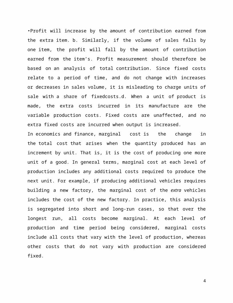
If the cost function is not differentiable, the marginal cost can be expressed as follows.
A number of other factors can affect marginal cost and its applicability to real world problems.
Some of these may be considered market failures. These may includeinformation asymmetries,
the presence of negative or positive externalities, transaction costs, price discrimination and
others.
Cost functions and relationship to average cost
In the simplest case, the total cost function and its derivative are expressed as follows, where Q
represents the production quantity, VC represents variable costs, FC represents fixed costs and
TC represents total costs.
Since (by definition) fixed costs do not vary with production quantity, it drops out of the
equation when it is differentiated. The important conclusion is that marginal cost is not related
to fixed costs. This can be compared with average total cost or ATC, which is the total cost
divided by the number of units produced and does include fixed costs.
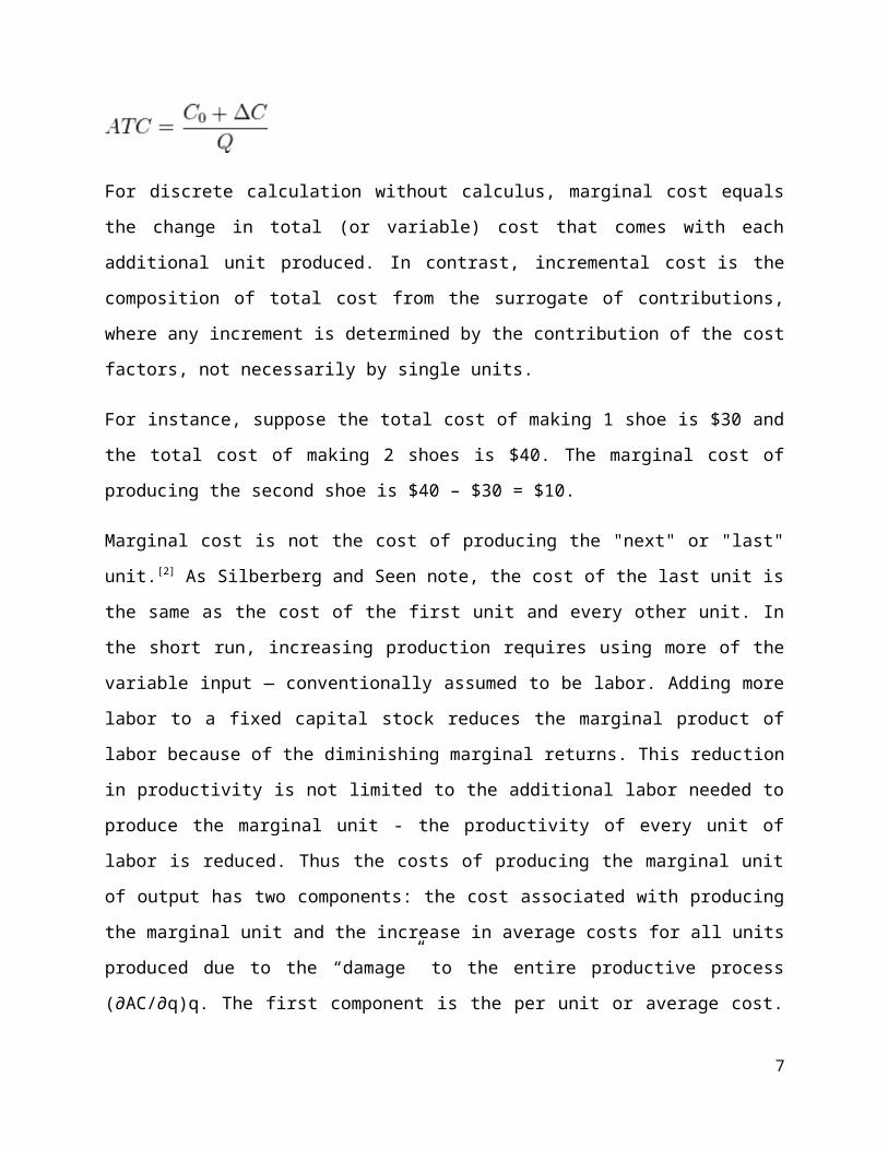
For discrete calculation without calculus, marginal cost equals the change in total (or variable)
cost that comes with each additional unit produced. In contrast, incremental cost is the
composition of total cost from the surrogate of contributions, where any increment is determined
by the contribution of the cost factors, not necessarily by single units.
For instance, suppose the total cost of making 1 shoe is $30 and the total cost of making 2 shoes
is $40. The marginal cost of producing the second shoe is $40 – $30 = $10.
4

Marginal cost is not the cost of producing the "next" or "last" unit. [2] As Silberberg and Seen
note, the cost of the last unit is the same as the cost of the first unit and every other unit. In the
short run, increasing production requires using more of the variable input — conventionally
assumed to be labor. Adding more labor to a fixed capital stock reduces the marginal product of
labor because of the diminishing marginal returns. This reduction in productivity is not limited to
the additional labor needed to produce the marginal unit - the productivity of every unit of labor
is reduced. Thus the costs of producing the marginal unit of output has two components: the cost
associated with producing the marginal unit and the increase in average costs for all units
produced due to the “damage” to the entire productive process (∂AC/∂q)q. The first component
is the per unit or average cost. The second unit is the small increase in costs due to the law of
diminishing marginal returns which increases the costs of all units of sold. Therefore, the precise
formula is: MC = AC + (∂AC/∂q)q.
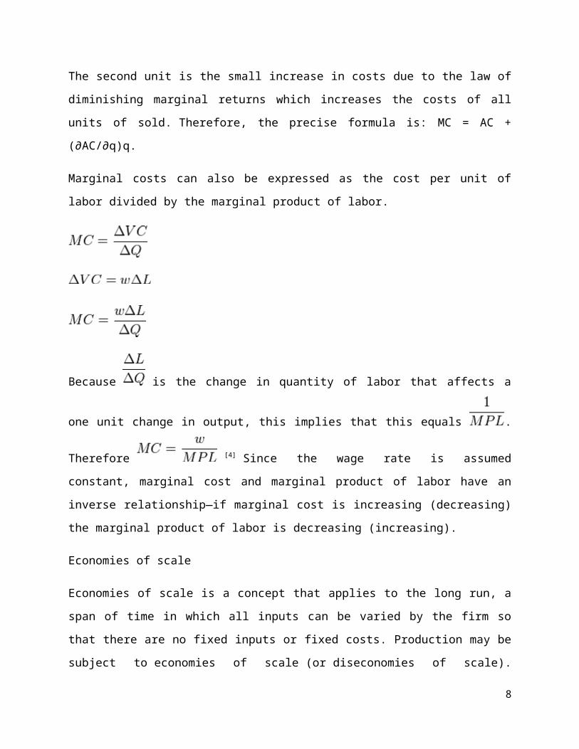
Marginal costs can also be expressed as the cost per unit of labor divided by the marginal
product of labor.
Because is the change in quantity of labor that affects a one unit change in output, this
implies that this equals . Therefore [4] Since the wage rate is assumed
constant, marginal cost and marginal product of labor have an inverse relationship—if marginal
cost is increasing (decreasing) the marginal product of labor is decreasing (increasing).
Economies of scale
Economies of scale is a concept that applies to the long run, a span of time in which all inputs
can be varied by the firm so that there are no fixed inputs or fixed costs. Production may be
5
subject to economies of scale (or diseconomies of scale). Economies of scale are said to exist if
an additional unit of output can be produced for less than the average of all previous units— that
is, if long-run marginal cost is below long-run average cost, so the latter is falling. Conversely,
there may be levels of production where marginal cost is higher than average cost, and average
cost is an increasing function of output. For this generic case, minimum average cost occurs at
the point where average cost and marginal cost are equal (when plotted, the marginal cost curve
intersects the average cost curve from below); this point will not be at the minimum for marginal
cost if fixed costs are greater than 0.
Perfectly competitive supply curve
The portion of the marginal cost curve above its intersection with the average variable cost curve
is the supply curve for a firm operating in a perfectly competitive market. (the portion of the MC
curve below its intersection with the AVC curve is not part of the supply curve because a firm
would not operate at price below the shut down point) This is not true for firms operating in
other market structures. For example, while a monopoly "has" an MC curve it does not have a
supply curve. In a perfectly competitive market, a supply curve shows the quantity a seller's
willing and able to supply at each price - for each price there is a unique quantity that would be
supplied. The one-to-one relationship simply is absent in the case of a monopoly. With a
monopoly there could be an infinite number of prices associated with a given quantity. It all
depends on the shape and position of the demand curve and its accompanying marginal revenue
curve.
Decisions taken based on marginal costs
In perfectly competitive markets, firms decide the quantity to be produced based on marginal
costs and sale price. If the sale price is higher than the marginal cost, then they supply the unit
and sell it. If the marginal cost is higher than the price, it would not be profitable to produce it.
So the production will be carried out until the marginal cost is equal to the sale price. In other
words, firms refuse to sell if the marginal cost is higher than the market price.
6
Relationship to fixed costs
Marginal costs are not affected by changes in fixed cost. Marginal costs can be expressed as
∆C(q)∕∆Q. Since fixed costs do not vary with (depend on) changes in quantity, MC is ∆VC∕∆Q.
Thus if fixed cost were to double MC would not be affected and consequently the profit
maximizing quantity and price would not change. This can be illustrated by graphing the short
run total cost curve and the short run variable cost curve. The shape of the curves are identical.
Each curve initially decreases at a decreasing rate, reaches an inflection point, then increases at
an increasing rate. The only difference between the curves is that the SRVC curve begins from
the origin while the SRTC curve originates on the y-axis. The distance of the origin of the SRTC
above the origin represents the fixed cost - the vertical distance between the curves. This distance
remains constant as the quantity produced, Q, increases. MC is the slope of the SRVC curve. A
change in fixed cost would be reflected by a change in the vertical distance between the SRTC
and SRVC curve. Any such change would have no effect on the shape of the SRVC curve and
therefore its slope at any point - MC.
Externalities
Externalities are costs (or benefits) that are not borne by the parties to the economic transaction.
A producer may, for example, pollute the environment, and others may bear those costs. A
consumer may consume a good which produces benefits for society, such as education; because
the individual does not receive all of the benefits, he may consume less than efficiency would
suggest. Alternatively, an individual may be a smoker or alcoholic and impose costs on others. In
these cases, production or consumption of the good in question may differ from the optimum
level.
Negative externalities of production
7
Negative Externalities of Production
Much of the time, private and social costs do not diverge from one another, but at times social
costs may be either greater or less than private costs. When marginal social costs of production
are greater than that of the private cost function, we see the occurrence of a negative
externality of production. Productive processes that result in pollution are a textbook example of
production that creates negative externalities.
Such externalities are a result of firms externalizing their costs onto a third party in order to
reduce their own total cost. As a result of externalizing such costs we see that members of
society will be negatively affected by such behavior of the firm. In this case, we see that an
increased cost of production on society creates a social cost curve that depicts a greater cost than
the private cost curve.
In an equilibrium state we see that markets creating negative externalities of production will
overproduce that good. As a result, the socially optimal production level would be lower than
that observed.
Positive externalities of production
Positive Externalities of Production
When marginal social costs of production are less than that of the private cost function, we see
the occurrence of a positive externality of production. Production of public goods are a textbook
example of production that create positive externalities. An example of such a public good,
which creates a divergence in social and private costs, includes the production of education. It is
8
often seen that education is a positive for any whole society, as well as a positive for those
directly involved in the market.
Examining the relevant diagram we see that such production creates a social cost curve that is
less than that of the private curve. In an equilibrium state we see that markets creating positive
externalities of production will under produce that good. As a result, the socially optimal
production level would be greater than that observed.
Social costs
Of great importance in the theory of marginal cost is the distinction between the
marginal private and social costs. The marginal private cost shows the cost associated to the firm
in question. It is the marginal private cost that is used by business decision makers in their profit
maximization goals. Marginal social cost is similar to private cost in that it includes the cost of
private enterprise but also any other cost (or offsetting benefit) to society to parties having no
direct association with purchase or sale of the product. It incorporates all negative and
positive externalities, of both production and consumption. Examples might include a social cost
from air pollution affecting third parties or a social benefit from flu shots protecting others from
infection.
The main features of marginal costing are as follows:
1. Cost Classification
The marginal costing technique makes a sharp distinction between variable costs and fixed costs.
It is the variable cost on the basis of which production and sales policies are designed by a firm
following the marginal costing technique.2. Stock/Inventory Valuation Under marginal costing,
inventory/stock for profit measurement is valued at marginal cost. It is in sharp contrast to the
total unit cost under absorption costing method.3. Marginal Contribution Marginal costing
technique makes use of marginal contribution for marking various decisions. Marginal
contribution is the difference between sales and marginal cost. It forms the basis for judging the
profitability of different products or departments.
9

Advantages and Disadvantages of Marginal Costing Technique
Advantages:
1. Marginal costing is simple to understand.
2. By not charging fixed overhead to cost of production, the effect of varying charges per unit is
avoided.
3. It prevents the illogical carry forward in stock valuation of some proportion of current year’s
fixed overhead.4. The effects of alternative sales or production policies can be more readily
available and assessed, and decisions taken would yield the maximum return to business.5.
It eliminates large balances left in overhead control accounts which indicate the difficulty of
ascertaining an accurate overhead recovery rate.6. Practical cost control is greatly facilitated. By
avoiding arbitrary allocation of fixed overhead, efforts can be concentrated on maintaining a
uniform and consistent marginal cost. It is useful to various levels of management.7. It helps
in short-term profit planning by breakeven and profitability analysis, both inters of quantity and
graphs. Comparative profitability and performance between two or more products and divisions
can easily be assessed and brought to the notice of management for decision making.
Disadvantages:
1. The separation of costs into fixed and variable is difficult and sometimes gives misleading
results
2. Normal costing systems also apply overhead under normal operating volume and this
shows that no advantage is gained by marginal costing.
3. Under marginal costing, stocks and work in progress are understated. The exclusion of
fixed costs from inventories affect profit, and true and fair view of financial affairs of an
organization may not be clearly transparent.
4. Volume variance in standard costing also discloses the effect of fluctuating output unfixed
overhead. Marginal cost data becomes unrealistic in case of highly fluctuating levels of
production, e.g., in case of seasonal factories.
5. Application of fixed overhead depends on estimates and not on the actual and as such there
may be under or over absorption of the same.
6. Control affected by means of budgetary control is also accepted by many. In order to know
the net profit, we should not be satisfied with contribution and hence, fixed overhead is also
10
a valuable item. A system which ignores fixed costs is less effective since a major portion
of fixed cost is not taken care of under marginal costing.
7. In practice, sales price, fixed cost and variable cost per unit may vary. Thus, the
assumptions underlying the theory of marginal costing sometimes becomes unrealistic. For
long term profit planning, absorption costing is the only answer.
OBJECTIVE OF THE STUDY
1. To study about Marginal Costing
2. To study and analyze Financial statements of Larsen & Toubro
SCOPE OF THE STUDY
It covers the information about Marginal Costing
It covers the information about Financial Statements of Larsen & Toubro
RESEARCH DESIGN
For the purpose of the present study only secondary data were used. Secondary data are
collected from books and websites
LIMITATIONS OF THE STUDY
During the study there was lack of information available for the study.
No proper source on the topic
CHAPTER 2
COMPANY PROFILE
11

Traded as NSE: LT
BSE: 500510
BSE SENSEX Constituent
Industry Conglomerate
Founded Mumbai then Bombay,Maharastra,
India (1938)
Founder Søren Kristian Toubro
Henning Holck-Larsen
Headquarters L&T House, Ballard Estate,
Mumbai, Maharashtra, India
Area served India, Middle East, East Asia andSoutheast
Asia
Key people K. Venkataramanan (CEO & MD)
A. M. Naik (Executive Chairman)
Products Construction
Heavy equipment
Electrical equipment
Power
Shipbuilding
Financial services
IT Services
Revenue US$ 14 Billion (2014)[1]
Operating US$ 1.07 Billion (2014)[1]
12

income
Net income US$ 952.638 Million (2013)[1]
Total assets US$ 26.188 Billion (2013)[1]
Total equity US$ 6.6818 Billion (2013)[1]
Number of
employees
84,027 (Mar 2014)[2]
Divisions Technology, engineering, construction,
manufacturing
Subsidiaries L&T Infotech, L&T Mutual Fund,L&T
Infrastructure Finance Company, L&T
Finance Holdings, L&T Technology Services,
L&T MHPS
Website www.larsentoubro.com
Larsen & Toubro Limited (L&T) is a technology, engineering, construction and manufacturing
company. It is one of the largest and most respected companies in India's private sector.
More than seven decades of a strong, customer-focused approach and the continuous quest for
world-class quality have enabled it to attain and sustain leadership in all its major lines of
business.
L&T has an international presence, with a global spread of offices. A thrust on international
business has seen overseas earnings grow significantly. It continues to grow its global
footprint, with offices and manufacturing facilities in multiple countries.
The company's businesses are supported by a wide marketing and distribution network, and
have established a reputation for strong customer support.
L&T believes that progress must be achieved in harmony with the environment. A
commitment to community welfare and environmental protection are an integral part of the
13
corporate vision.
In response to changing market dynamics, L&T has gone through a phased process of
redefining its organisation model to facilitate growth through greater levels of empowerment.
The new structure is built around multiple businesses that serve the needs of different
industries.
The evolution of L&T into the country's largest engineering and construction organization is
among the most remarkable success stories in Indian industry.
L&T was founded in Bombay (Mumbai) in 1938 by two Danish engineers, Henning Holck-
Larsen and Soren Kristian Toubro. Both of them were strongly committed to developing
India's engineering capabilities to meet the demands of industry.
Henning Holck-Larsen and Soren Kristian Toubro, school-mates in Denmark, would not
have dreamt, as they were learning about India in history classes that they would, one
day, create history in that land.
In 1938, the two friends decided to forgo the comforts of working in Europe, and started
their own operation in India. All they had was a dream. And the courage to dare.
Their first office in Mumbai (Bombay) was so small that only one of the partners could
use the office at a time!
In the early years, they represented Danish manufacturers of dairy equipment for a
modest retainer. But with the start of the Second World War in 1939, imports were
restricted, compelling them to start a small work-shop to undertake jobs and provide
service facilities.
Germany's invasion of Denmark in 1940 stopped supplies of Danish products. This crisis
forced the partners to stand on their own feet and innovate. They started manufacturing
dairy equipment indigenously. These products proved to be a success, and L&T came to
14
be recognised as a reliable fabricator with high standards.
The war-time need to repair and refit ships offered L&T an opportunity, and led to the
formation of a new company, Hilda Ltd., to handle these operations. L&T also started
two repair and fabrication shops - the Company had begun to expand.
Again, the sudden internment of German engineers (because of the War) who were to put
up a soda ash plant for the Tatas, gave L&T a chance to enter the field of installation - an
area where their capability became well respected.
History
A company was founded in Bombay (Mumbai) in 1938 by two Danish
engineers, Henning Holck-Larsen and Soren Kristian Toubro. The company began as a
representative of Danish manufacturers of dairy equipment. However, with the start of
the Second World War in 1939 and the resulting restriction on imports, the partners
started a small workshop to undertake jobs and provide service facilities.[9]
Germany's invasion of Denmark in 1940 stopped supplies of Danish products.[9] The war-
time need to repair and refit ships offered L&T an opportunity, and led to the formation
of a new company, Hilda Ltd., to handle these operations.[9] L&T also started to repair
and fabrication shops signalling the expansion of the company.[9]
The sudden internment of German engineers in British India (due to suspicions caused
by the War), who were to put up a soda ash plant for the Tatas, gave L&T a chance to
enter the field of installation.[9]
In 1944, ECC was incorporated by the partners; the company at this time was focused on
construction projects (Presently, ECC is the construction division of L&T). L&T decided
to build a portfolio of foreign collaborations. By 1945, the company represented British
manufacturers of equipment used to manufacture products such as hydrogenated oils,
biscuits, soaps and glass.[9]
In 1945, the company signed an agreement with Caterpillar Tractor Company, USA, for
marketing earth moving equipment. At the end of the war, large numbers of war-surplus
15

Caterpillar equipment were available at attractive prices, but the finances required were
beyond the capacity of the partners. This prompted them to raise additional equity
capital, and on 7 February 1946, Larsen & Toubro Private Limited was incorporated.[9]
Post-independence
Offices were set up in Kolkata (Calcutta), Chennai (Madras) and New Delhi. In 1948,
fifty-five acres of undeveloped marsh and jungle was acquired in Powai, Mumbai. That
uninhabitable swamp subsequently became the site of its main manufacturing hub.[9]
In December 1950, L&T became a public company with a paid-up capital of Rs.
20 lakhs (2 million rupees) (2,000,000). The sales turnover in that year was Rs.
1.09 crore (10.9 million rupees).[9] In 1956, a major part of the company's Mumbai office
moved to ICI House in Ballard Estate, Mumbai; which would later be purchased by the
company and renamed as L&T House, its present corporate office.[9]
The sixties witnessed the formation of many new ventures: UTMAL (set up in 1960),
Audco India Limited (1961), Eutectic Welding Alloys (1962) and TENGL (1963).[9]
Operating divisions
L&T has delivered Engineering, Procurement and Construction (EPC) services for many
projects in the upstream hydrocarbon sector over the last two decades, in India, Middle
East, Africa, South-East Asia and Australia.
L&T has formed a joint venture with SapuraCrest Petroleum Berhad, Malaysia for
providing services to offshore construction industry worldwide. The joint venture will
own and operate the LTS 3000, a Heavy Lift cum Pipelay Vessel.
L&T Power has set up an organization focused on coal-based, gas-based and nuclear
power projects. L&T has formed two joint ventures with Mitsubishi Heavy Industries,
Japan to manufacture super critical boilers and steam turbine generators.
L&T is among the top five fabrication companies in the world. L&T has a shipyard
capable of constructing vessels of up to 150 meters long and displacement of 20,000
tons at its heavy engineering complex at Hazira. The shipyard is geared up to take up
16

construction of niche vessels such as specialized Heavy lift Cargo Vessels, CNG carriers,
Chemical tankers, defense & para military vessels, submarines and other role specific
vessels.
The design wing of L&T ECC is called EDRC (Engineering Design and Research
Centre). EDRC provides consultancy, design and total engineering solutions to
customers. It carries out basic and detailed design for both residential and commercial
projects.
L&T Solar
L&T Construction a subsidiary of the Larsen & Toubro conglomerate also undertakes
solar projects. In April ’12, L&T commissioned India's largest solar photo voltaic-based
power plant (40 MWp) owned by Reliance Power at Jaisalmer, Rajasthan from concept
to commissioning in 129 days. In 2011, L&T entered into a partnership with Sharp for
EPC (engineering, procurement and construction) in megawatt solar project and plan to
construct about 100 MW in the next 12 months in most of the metros. L&T Infra
Finance, promoted by the parent L&T Ltd, is also active in the funding of solar projects
in India. ≤
Electrical and automation
L&T is an international manufacturer of a wide range of electrical and electronic
products and systems. L&T also manufactures custom-engineered switchboards for
industrial sectors like power, refineries, petrochemicals and cement. In the electronic
segment, L&T offers a range of meters and provides control and automation systems for
industries. Medical Equipment.
Information technology
Main article: Larsen & Toubro Infotech
L&T Infotech focuses on information technology and software services. Larsen &
Toubro Infotech Limited, a 100 per cent subsidiary of the L&T, offers software and
services with a focus on Manufacturing, BFSI and Communications and Embedded
Systems. It also provides services in the embedded intelligence and engineering space.
17

Machinery and industrial products
L&T manufactures, markets and provides service support for construction and mining
machinery, surface miners, hydraulic excavators, aggregate crushers, loader backhoes
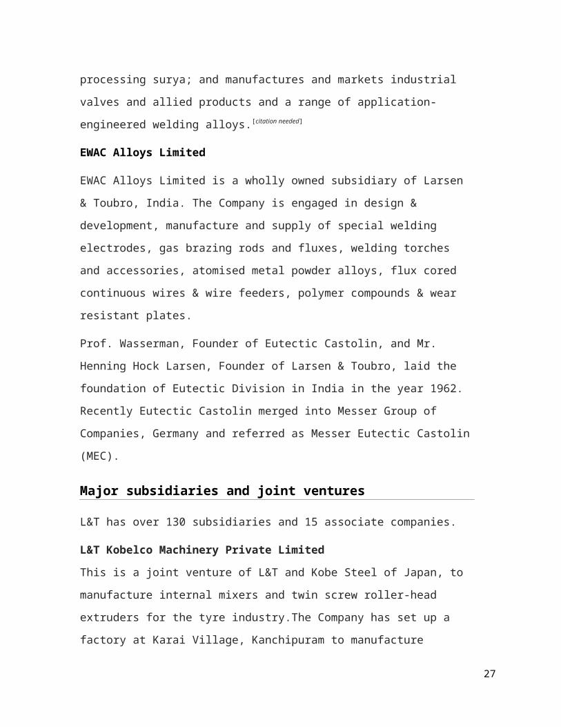
and vibratory compactors; supplies a wide range of rubber processing surya; and
manufactures and markets industrial valves and allied products and a range of
application-engineered welding alloys.[citation needed]
EWAC Alloys Limited
EWAC Alloys Limited is a wholly owned subsidiary of Larsen & Toubro, India. The
Company is engaged in design & development, manufacture and supply of special
welding electrodes, gas brazing rods and fluxes, welding torches and accessories,
atomised metal powder alloys, flux cored continuous wires & wire feeders, polymer
compounds & wear resistant plates.
Prof. Wasserman, Founder of Eutectic Castolin, and Mr. Henning Hock Larsen, Founder
of Larsen & Toubro, laid the foundation of Eutectic Division in India in the year 1962.
Recently Eutectic Castolin merged into Messer Group of Companies, Germany and
referred as Messer Eutectic Castolin (MEC).
Major subsidiaries and joint ventures
L&T has over 130 subsidiaries and 15 associate companies.
L&T Kobelco Machinery Private Limited
This is a joint venture of L&T and Kobe Steel of Japan, to manufacture internal mixers
and twin screw roller-head extruders for the tyre industry.The Company has set up a
factory at Karai Village, Kanchipuram to manufacture Internal Mixers and Twin Screw
Roller head Extruders for the tyre industry and commenced its commercial operations in
December 1, 2012.
L&T – Komatsu Limited
Having its registered office at Mumbai, India and focusing on construction
equipment and mining equipment, L&T-Komatsu Limited is a joint venture of Larsen
and Toubro, and Komatsu Asia Pacific Pte Limited, Singapore, a wholly owned
18

subsidiary of Komatsu Limited, Japan. Komatsu is the world’s second largest
manufacturer of hydraulic excavators and has manufacturing and marketing facilities.
The plant was started in the year 1975 by L&T to manufacture Hydraulic Excavators for
the first time in India. In 1998, it became a joint venture. L&T–Komatsu Limited’s
manufacturing facility—The Bangalore Works—comprises Machinery Works and
Hydraulics Works. Machinery Works has a manufacturing facility for design,
manufacture and servicing of earthmoving equipment. Hydraulics Works, with a
precision machine shop, manufactures the complete range of high pressure hydraulic
components and systems, and design, development, manufacturing and servicing of
hydraulic pumps, motors, cylinders, turning joints, hose assemblies, valve blocks,
hydraulic systems and power drives as well as allied gear boxes.In April 2013, L&T
bought the 50% stake held by Komatsu Asia & Pacific. The company's name was
changed to L&T Construction Equipment Limited.[25] [26]
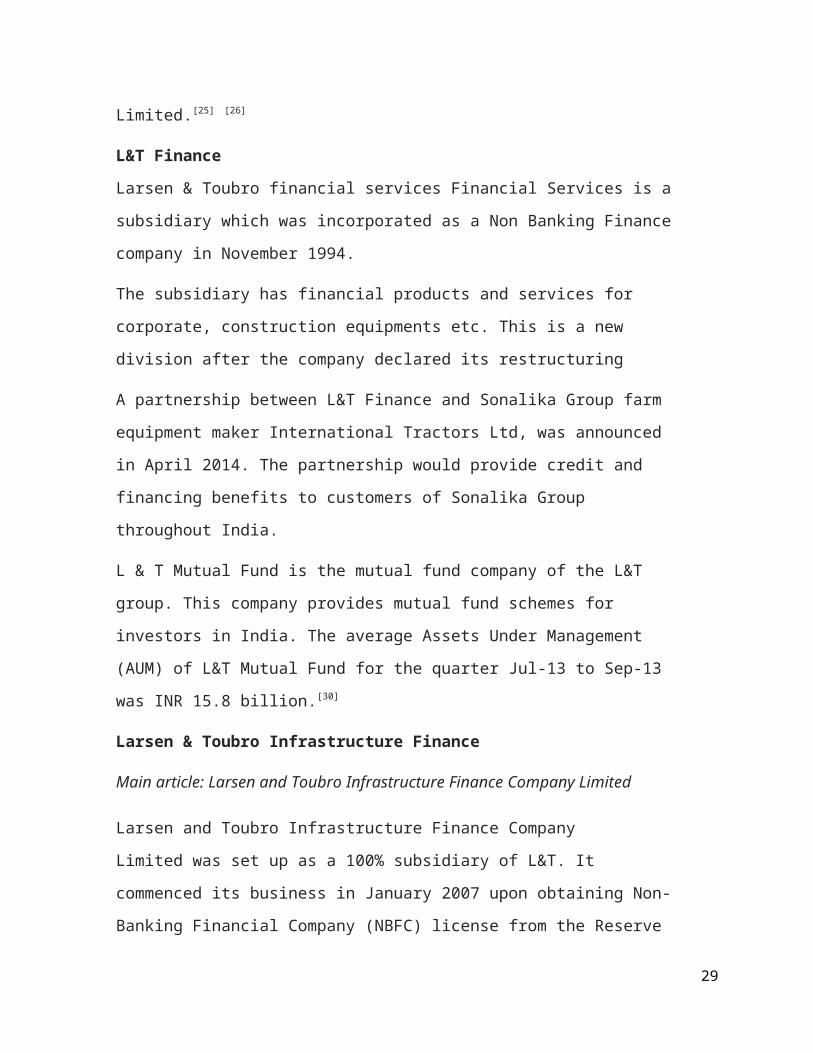
L&T Finance
Larsen & Toubro financial services Financial Services is a subsidiary which was
incorporated as a Non Banking Finance company in November 1994.
The subsidiary has financial products and services for corporate, construction equipments
etc. This is a new division after the company declared its restructuring
A partnership between L&T Finance and Sonalika Group farm equipment maker
International Tractors Ltd, was announced in April 2014. The partnership would provide
credit and financing benefits to customers of Sonalika Group throughout India.
L & T Mutual Fund is the mutual fund company of the L&T group. This company
provides mutual fund schemes for investors in India. The average Assets Under
Management (AUM) of L&T Mutual Fund for the quarter Jul-13 to Sep-13 was INR
15.8 billion.[30]
Larsen & Toubro Infrastructure Finance
Main article: Larsen and Toubro Infrastructure Finance Company Limited
Larsen and Toubro Infrastructure Finance Company Limited was set up as a 100%
19

subsidiary of L&T. It commenced its business in January 2007 upon obtaining Non-
Banking Financial Company (NBFC) license from the Reserve Bank of India (RBI).
As of 31 March 2008, L&T Infrastructure Finance has approved financing of more than a
billion USD to select projects in the infrastructure sector.
L&T Infrastructure Finance has received the status of "Infrastructure Finance Company"
from the Reserve Bank of India within the overall classification of "Non-Banking
Financial Company".
L&T (TS)
L&T Technology Services (previously known as Integrated Engineering Services or
L&T IES), a business unit of L&T, offers a combination of mechanical, electrical and
electronic design (mechatronics/embedded systems), civil and architectural services.
L&T TS has its design and delivery locations in Vadodara, Chennai, Bangalore, Mysore
and Mumbai in India.
L&T TS services also encompass architectural, civil, structural design and building
utility systems design. Practices include both product and plant engineering services in
the automotive, trucks and off-highway vehicles, industrial .
Mysore based campus of Electronic design unit of TS works predominantly for
Embedded systems with a variety of range of operations from Avionics, Automotive,
Industrial automation and metering, Medical and more.
L&T Valves
L&T’s Valves Business Group markets valves manufactured by L&T's Valve
Manufacturing Unit and L&T's joint ventures, Audco India Limited, India and Larsen &
Toubro Valves Manufacturing Unit, Coimbatore as well as allied products from major
international manufacturers.
The company's valve manufacturing Unit in Coimbatore manufactures industrial valves
specifically for the Power Industry. It also sells value-added flow control solutions to oil
and gas, refining, petrochemical, chemical and power industries, industrial valves and
customized products for major Refinery, LNG, GTL, Petrochemical and Power projects.
L&T Valves Business Group has offices in the USA, South Africa, Dubai, Abu Dhabi,
20

India and China, and alliances with valve distributors and agents in these countries.
L&T MHPS Boiler
LMB is the joint venture between L&T and Mitsubishi Hitachi Power Systems. The
group specializes in Engineering, Manufacturing, Erecting & Commissioning of Super
Critical Boilers used in Mega and Ultra Mega power plants. It is mainly headquartered in
Faridabad with Manufacturing facility in Hazira and an Engineering Centre in Chennai &
Faridabad. Currently the group is engaged in projects for JVPL, MAHAGENCO,
NABHA Power & RRVUNL.
L&T MHPS Turbine Generators Pvt.Ltd
In 2007, Larsen & Toubro Limited (“L&T”) and Mitsubishi Heavy Industries Limited
(“MHI”), headquartered in Tokyo, Japan inked a Joint Venture Agreement for setting up
a manufacturing facility to supply super-critical Steam Turbine & Generator facility in
Hazira, Surat, India, . This follows a Technology Licensing and Technical Assistance
Agreement for manufacture of super-critical Turbine & Generator, signed between L&T,
MHI, and Mitsubishi Electric Corporation (MELCO), headquartered in Tokyo, Japan.In
February 2014, MHI and Hitachi Ltd integrated the business centered on thermal power
generation systems (gas turbines, steam turbines, coal gasification generating equipment,
boilers, thermal power control systems, generators, fuel cells, environmental equipment
and so on) and started a new company as Mitsubishi Hitachi Power Systems Ltd.
(“MHPS”), headquartered in Yokohama, Japan .
L&T Howden Pvt.Ltd
L&T Howden Pvt. Ltd. is a joint venture between L&T and Howden to cater Axial Fans
and Air Preheaters of range 120-1200 MW to thermal power plants. L&T Howden is an
ISO -9001 and 5001 certified organisation, Plant is located in Surat Hazira and marketing
office in Faridabad.
L&T Special Steels and Heavy Forgings Pvt. Ltd.
LTSSHF is a joint venture between L&T and NPCIL. Headquartered at Hazia, LTSSHF
is recognized as India's largest integrated steel plant and heavy forging unit. With state-
of-the art facilities, LTSSHF is capable of producing forgings weighing 120MT each.
21

LTSSHF currently is engaged in projects from Nuclear, Hydrocarbon, Power and Oil &
Gas sectors.
THE JOURNEY
In 1944, ECC was incorporated. Around then, L&T decided to build a portfolio of foreign
collaborations. By 1945, the Company represented British manufacturers of equipment
used to manufacture products such as hydrogenated oils, biscuits, soaps and glass.
In 1945, L&T signed an agreement with Caterpillar Tractor Company, USA, for
marketing earthmoving equipment. At the end of the war, large numbers of war-surplus
Caterpillar equipment were available at attractive prices, but the finances required were
beyond the capacity of the partners. This prompted them to raise additional equity capital,
and on 7th February 1946, Larsen & Toubro Private Limited was born.
Independence and the subsequent demand for technology and expertise offered L&T the
opportunity to consolidate and expand. Offices were set up in Kolkata (Calcutta), Chennai
(Madras) and New Delhi. In 1948, fifty-five acres of undeveloped marsh and jungle was
acquired in Powai. Today, Powai stands as a tribute to the vision of the men who
transformed this uninhabitable swamp into a manufacturing landmark.
PUBLIC LIMITED COMPANY
In December 1950, L&T became a Public Company with a paid-up capital of Rs.2
million. The sales turnover in that year was Rs.10.9 million.
Prestigious orders executed by the Company during this period included the Amul Dairy
at Anand and Blast Furnaces at Rourkela Steel Plant. With the successful completion of
22
these jobs, L&T emerged as the largest erection contractor in the country.
In 1956, a major part of the company's Bombay office moved to ICI House in Ballard
Estate. A decade later this imposing grey-stone building was purchased by L&T, and
renamed as L&T House - its Corporate Office.
The sixties saw a significant change at L&T - S. K. Toubro retired from active
management in 1962.
The sixties were also a decade of rapid growth for the company, and witnessed the
formation of many new ventures: UTMAL (set up in 1960), Audco India Limited (1961),
Eutectic Welding Alloys (1962) and TENGL (1963).
EXPANDING HORIZONS
By 1964, L&T had widened its capabilities to include some of the best technologies in the
world. In the decade that followed, the company grew rapidly, and by 1973 had become
one of the Top-25 Indian companies.
In 1976, Holck-Larsen was awarded the Magsaysay Award for International
Understanding in recognition of his contribution to India's industrial development. He
retired as Chairman in 1978.
In the decades that followed, the company grew into an engineering major under the
guidance of leaders like N. M. Desai, S.R. Subramaniam, U. V. Rao, S. D. Kulkarni and
A. M. Naik.
Today, L&T is one of India's biggest and best known industrial organisations with a
reputation for technological excellence, high quality of products and services, and strong
customer orientation. It is also taking steps to grow its international presence.
23
For an institution that has grown to legendary proportions, there cannot and must not be
an 'end'. Unlike other stories, the L&T saga continues....
CHAPTER 3
FINANCIAL STATEMENTS
Standalone Profit & Loss
account------------------- in Rs. Cr. -------------------
Mar '13 Mar '12 Mar '11 Mar '10 Mar '09
12 mths 12 mths 12 mths 12 mths 12 mths
Income
Sales Turnover 60,873.26 53,170.52 43,905.87 37,187.50 34,249.85
Excise Duty 0.00 0.00 0.00 317.31 393.31
Net Sales 60,873.26 53,170.52 43,905.87 36,870.19 33,856.54
Other Income 2,104.96 1,393.28 1,480.37 2,321.67 1,612.58
Stock Adjustments 1,132.03 539.77 532.64 -422.99 105.11
Total Income 64,110.25 55,103.57 45,918.88 38,768.87 35,574.23
Expenditure
Raw Materials 15,243.62 14,133.98 11,208.01 9,593.53 9,316.38
Power & Fuel Cost 758.99 638.79 420.27 334.08 456.39
Employee Cost 4,436.32 3,663.45 2,830.08 2,379.14 1,998.02
Other Manufacturing Expenses 33,081.82 26,787.18 22,372.53 16,913.31 15,659.17
Selling and Admin Expenses 0.00 0.00 0.00 1,854.23 1,844.83
Miscellaneous Expenses 2,077.48 2,204.28 1,968.05 325.58 569.32
Preoperative Exp Capitalised 0.00 0.00 0.00 -36.25 -24.48
Total Expenses 55,598.23 47,427.68 38,798.94 31,363.62 29,819.63
24

Mar '13 Mar '12 Mar '11 Mar '10 Mar '09
12 mths 12 mths 12 mths 12 mths 12 mths
Operating Profit 6,407.06 6,282.61 5,639.57 5,083.58 4,142.02
PBDIT 8,512.02 7,675.89 7,119.94 7,405.25 5,754.60
Interest 982.40 666.10 619.25 995.37 770.00
PBDT 7,529.62 7,009.79 6,500.69 6,409.88 4,984.60
Depreciation 818.47 699.46 599.22 383.65 284.83
Other Written Off 0.00 0.00 0.00 30.95 21.16
Profit Before Tax 6,711.15 6,310.33 5,901.47 5,995.28 4,678.61
Extra-ordinary items 0.00 0.00 0.00 -45.13 -21.09
PBT (Post Extra-ord Items) 6,711.15 6,310.33 5,901.47 5,950.15 4,657.52
Tax 1,800.50 1,853.83 1,943.58 1,577.02 1,176.19
Reported Net Profit 4,910.65 4,456.50 3,957.89 4,375.52 3,481.66
Total Value Addition 40,354.61 33,293.70 27,590.93 21,770.09 20,503.25
Preference Dividend 0.00 0.00 0.00 0.00 0.00
Equity Dividend 1,138.47 1,010.46 882.84 752.75 614.97
Corporate Dividend Tax 85.86 101.44 112.82 110.25 101.83
Per share data (annualised)
Shares in issue (lakhs) 6,153.86 6,123.99 6,088.52 6,021.95 5,856.88
Earning Per Share (Rs) 79.80 72.77 65.01 72.66 59.45
Equity Dividend (%) 925.00 825.00 725.00 625.00 525.00
Book Value (Rs) 473.57 411.87 358.81 303.28 212.32
Balance Sheet of Larsen and Toubro ------------------- in Rs. Cr. -------------------
25

Mar '13 Mar '12 Mar '11 Mar '10 Mar '09
12 mths 12 mths 12 mths 12 mths 12 mths
Sources Of Funds
Total Share Capital 123.08 122.48 121.77 120.44 117.14
Equity Share Capital 123.08 122.48 121.77 120.44 117.14
Share Application Money 0.00 0.00 0.00 25.09 0.00
Preference Share Capital 0.00 0.00 0.00 0.00 0.00
Reserves 29,019.64 25,100.54 21,724.49 18,142.82 12,317.96
Revaluation Reserves 0.00 0.00 0.00 23.29 24.59
Networth 29,142.72 25,223.02 21,846.26 18,311.64 12,459.69
Secured Loans 1,234.01 1,453.34 1,063.04 955.73 1,102.38
Unsecured Loans 6,771.55 6,813.44 5,268.54 5,845.10 5,453.65
Total Debt 8,005.56 8,266.78 6,331.58 6,800.83 6,556.03
Total Liabilities 37,148.28 33,489.80 28,177.84 25,112.47 19,015.72
Mar '13 Mar '12 Mar '11 Mar '10 Mar '09
12 mths 12 mths 12 mths 12 mths 12 mths
Application Of Funds
Gross Block 11,864.73 10,455.23 8,872.71 7,235.78 5,575.00
Less: Accum. Depreciation 3,559.59 2,850.25 2,228.52 1,727.68 1,421.39
Net Block 8,305.14 7,604.98 6,644.19 5,508.10 4,153.61
Capital Work in Progress 596.84 758.68 771.34 857.66 1,040.99
Investments 16,103.39 15,871.90 14,684.82 13,705.35 8,263.72
26
Inventories 2,064.18 1,776.62 1,577.15 1,415.37 5,805.05
Sundry Debtors 22,613.01 18,729.84 12,427.61 11,163.70 10,055.52
Cash and Bank Balance 1,455.66 1,778.12 1,729.55 1,104.89 693.13
Total Current Assets 26,132.85 22,284.58 15,734.31 13,683.96 16,553.70
Loans and Advances 21,035.99 21,172.82 19,275.34 12,662.55 7,198.85
Fixed Deposits 0.00 0.00 0.00 326.98 82.16
Total CA, Loans & Advances 47,168.84 43,457.40 35,009.65 26,673.49 23,834.71
Deffered Credit 0.00 0.00 0.00 0.00 0.00
Current Liabilities 32,656.20 31,816.07 26,687.98 19,443.77 15,211.04
Provisions 2,369.73 2,387.09 2,244.18 2,188.36 3,066.53
Total CL & Provisions 35,025.93 34,203.16 28,932.16 21,632.13 18,277.57
Net Current Assets 12,142.91 9,254.24 6,077.49 5,041.36 5,557.14
Miscellaneous Expenses 0.00 0.00 0.00 0.00 0.26
Total Assets 37,148.28 33,489.80 28,177.84 25,112.47 19,015.72
Contingent Liabilities 12,987.97 10,309.19 7,761.66 1,719.39 1,371.86
Book Value (Rs) 473.57 411.87358.81
303.28 212.32
Cash Flow of Larsen and Toubro ------------------- in Rs. Cr. -------------------
Mar '13 Mar '12 Mar '11 Mar '10 Mar '09
12 mths 12 mths 12 mths 12 mths 12 mths
Net Profit Before Tax 6457.09 6255.33 5568.56 5880.67 3940.41
Net Cash From Operating Activities 2114.75 1081.58 3833.30 5482.75 1478.57
Net Cash (used in)/from 464.93 -1922.28 -2409.98 -6071.73 -3308.53
27

Investing Activities
Net Cash (used in)/from Financing Activities -2990.26 1015.61 -1124.84 1245.56 1640.79
Net (decrease)/increase In Cash and Cash
Equivalents-410.58 174.91 298.48 656.58 -189.17
Opening Cash & Cash Equivalents 1905.26 1730.35 1431.87 775.29 964.46
Closing Cash & Cash Equivalents 1494.68 1905.26 1730.35 1431.87 775.29
Marginal cost sheet of Larsen & Toubro
Particulars Rs (In Cr.)
Sales Revenue 60,873.26
Less Marginal Cost of Sales
Contribution
Less Fixed Cost
Marginal Costing Profit/Loss
28
Chapter 4
Findings, Suggestions and Conclusion
Findings
Marginal cost is the cost of the next unit or one additional unit of volume or output.
The marginal cost varies directly with the volume of production and marginal cost per
unit remains the same. It consists of prime cost, i.e. cost of direct materials, direct labor
and all variable overheads.
L & T is diversified company, which operates in national as well as international level.
Company is going for new ventures in the market so , we can assume that it has greater
scope in future.
Earnings per share of the company Rs 56, which shoes the positive trend.
Operating income of the company is showing positive trend in the 2011,which shows the
positive trend.
Net profit of the company is showing the negative slope, which is risky for the company.
Long term debt and equity of the company is showing the negative slop, which is good
for the company.
Fixed assets of the company are showing the decline slop which is alarming situation for
the company.
Current ratio of the company is showing the giz-gaz trend which is not suitable for the
company.
Total exports of the company are declining at high rate which is alarming for the
company.
29

CHAPTER V
CONCLUSION
From the above information, we can conclude that company is having sound financial position,
with reference to debt equity ratio, earning per share, and operating income .But net profit, net
export, fixed assets and current ratio is showing negative trend .L&T need to pay attention
towards the cost reduction so that profitability of the company can be maintained, and control the
liabilities
30

BIBLIOGRAPHY
The information is obtained from the listed sources
www.moneycontrol.com
www.wikipedia.com
www.timesofindia.com
Financial Management- Khan and Jain
31
Related Documents