Marginal Cost, Revenue Allocation, and Residential Rate Design for San Diego Gas & Electric Company ERRATA Prepared testimony of William B. Marcus JBS Energy, Inc. 311 D Street West Sacramento California, USA 95605 916.372.0534 on behalf of San Diego Consumers Action Network California Public Utilities Commission Application 11-10-002 August 15, 2012

Welcome message from author
This document is posted to help you gain knowledge. Please leave a comment to let me know what you think about it! Share it to your friends and learn new things together.
Transcript

Marginal Cost, Revenue Allocation, and Residential Rate Design for San Diego Gas & Electric Company ERRATA
Prepared testimony of
William B. Marcus
JBS Energy, Inc. 311 D Street
West Sacramento
California, USA 95605
916.372.0534
on behalf of
San Diego Consumers Action Network
California Public Utilities Commission
Application 11-10-002
August 15, 2012
i
Table of Contents
I. INTRODUCTION AND SUMMARY .................................................................... 1
II. MARGINAL CUSTOMER COSTS ........................................................................ 2
A. INTRODUCTION ...................................................................................................... 2 B. THEORETICAL CONSIDERATIONS: ONE-TIME HOOKUP COST METHOD VS.
RENTAL METHOD ............................................................................................................ 4 1. Interchangeability of Use across Customers .................................................... 5 2. Discussion of Marginal Cost Theory as it Relates to Customer-Hookup
Equipment ................................................................................................................... 6 3. Unreasonable Barriers to Entry ....................................................................... 7
4. Achieving Commission Goals Regarding Cost Causation, Timing, and
Demand Sensitivity...................................................................................................... 9
5. OTHC: An Approximation .............................................................................. 10 6. Discussion of the Over- vs. Under-Charge Issue ........................................... 10
7. Conclusion ...................................................................................................... 11 C. CUSTOMER COUNTS ............................................................................................ 11
D. MARGINAL CUSTOMER-RELATED DISTRIBUTION O&M COSTS .......................... 12 E. CUSTOMER ACCOUNTING AND CUSTOMER SERVICE O&M ................................. 13
1. Meter Reading ................................................................................................ 14
2. Revenue Offsets from Tariffed Service Charges ............................................. 15 3. Accounts 907-910 (Customer Service and Information) ................................ 15
F. CUSTOMER COST RESULTS ..................................................................................... 21
III. MARGINAL DISTRIBUTION DEMAND COSTS ......................................... 23
A. ADDITIONAL VEGETATION MANAGEMENT FUNCTIONALIZED AS DISTRIBUTION
DEMAND ........................................................................................................................ 23
IV. MARGINAL GENERATION CAPACITY COST AND MARGINAL
ENERGY COST.............................................................................................................. 23
V. DISTRIBUTION REVENUE ALLOCATION .................................................... 24
I. RESIDENTIAL CUSTOMER CHARACTERIZATION ................................... 26
A. REASON FOR ERRATA .......................................................................................... 29 B. RELATIONSHIP OF USAGE TO INCOME, SIZE AND TYPE OF DWELLING, AND
APPLIANCES ................................................................................................................... 30
1. Income ............................................................................................................ 31 2. Single vs. Multi-Family................................................................................... 33 3. Square Footage............................................................................................... 36 4. Air Conditioning ............................................................................................. 40
5. Swimming Pools ............................................................................................. 41 6. CONCLUSION ........................................................................................................... 45

ii
List of Tables
Table 13: Un-Weighted number of RASS Surveys by Climate Zone .............................. 52 Table 14: SDG&E Summer Tier Groups used in CEC RASS Analysis .......................... 53
List of Figures
Figure 1: Average Income by Summer Tier Group and Climate Group ......................... 31 Figure 3: Percent of Single-Family and Multi-Family Households within Tier Groups and
Climate Zones SDGE ........................................................................................................ 33 Figure 5: Percent of Single-Family and Multi-Family Households within Income Groups
SDGE ................................................................................................................................ 35
Figure 6: Percent of Single-Family and Multi-Family Households across Income Groups
SDGE ................................................................................................................................ 35 Figure 7: Percent of Households by Square Footage ........................................................ 36
Figure 9: Percentage in Tiers 2-5 (Average Summer Monthly Use) by Square Footage of
Dwelling SDGE ................................................................................................................ 38 Figure 11: Average Income by Climate Group and Square Footage SDGE .................... 39
Figure 13: Average Summer Monthly Usage by Air Conditioner Type and Climate Zone
Group SDGE ..................................................................................................................... 41
Figure 15: Single-Family Pool Groups by Summer Tier Groups and Climate Group
SDGE ................................................................................................................................ 43 Figure 17: Average Income by Swimming Pool Group and Climate Group SDGE ........ 44
Figure 18: CEC Climate Zone Map .................................................................................. 53
Figure 19: SDG&E Electric Baseline Zone Map .............................................................. 54

Prepared Testimony of William B. Marcus on behalf of SDCAN 1 SDG&E 2012 Test Year General Rate Case Phase II (CPUC App. A. 11-10-002)
I. Introduction and Summary 1
This testimony is presented on behalf of San Diego Consumers’ Action Network 2
(SDCAN) by William B. Marcus, Principal Economist of JBS Energy, Inc. Mr. Marcus 3
has 34 years of energy experience and has appeared before this Commission on many 4
occasions, and has filed testimony or formal comments before about 40 federal, state, 5
provincial, and local courts and regulatory bodies in the U.S. and Canada. His 6
qualifications are attached. 7
SDCAN proposes major changes to SDG&E’s proposed marginal customer costs. We 8
use the One-Time Hookup Cost (OTHC) or New Customer Only (NCO) method, to 9
calculate marginal customer costs instead of SDG&E’s rental method. SDCAN’s method 10
has been previously adopted by the Commission in a number of recent cases. 11
However the largest change to customer costs involves customer service O&M costs, 12
where SDCAN specifically removes non-distribution energy efficiency costs and non-13
marginal costs of demand response, the California Solar Initiative, and the Self-14
Generation Incentive Program. SDCAN also reduces meter reading costs to reflect AMI 15
deployment (consistent with SDG&E’s inclusion of AMI meters in customer-related 16
capital costs), and functionalizes only 2% of vegetation management costs as customer 17
costs instead of SDG&E’s 12-13%. 18
As a result of the changes to marginal customer costs, SDCAN proposes a reduction to 19
residential distribution charges of almost 18% relative to current rates. Essentially, 20
SDG&E dramatically “overshot” in the last case, and the changes recommended here – 21
particularly to remove costs in Accounts 907-910 that were improperly included in 22
marginal costs – have a significant effect. 23
Finally this testimony provides evidence regarding the load and usage patterns of 24
residential customers in support of MRW’s testimony on residential rate design on behalf 25
of SDCAN. Load research data indicate that apartment dwellers and small users have 26
less peaked load patterns than single-family residents. A review of data from the 27

Prepared Testimony of William B. Marcus on behalf of SDCAN 2 SDG&E 2012 Test Year General Rate Case Phase II (CPUC App. A. 11-10-002)
Residential Appliance Saturation Survey (RASS) indicates that small users have lower 1
incomes, live in smaller units and have fewer peak-oriented appliances (central air 2
conditioning and swimming pools) than larger users. 3
II. Marginal Customer Costs 4
A. Introduction 5
Table 1 presents a comparison of SDG&E’s, DRA’s, and SDCAN’s class average 6
Marginal Customer Cost results. We present a more-detailed comparison (by schedule), 7
below. 8
Table 1: Comparison of Marginal Customer Cost Results 9
SDG&E
(RECC1)
DRA (OTHC
or NCO2)
UCAN
(OTHC or
NCO)
SDG&E >
UCAN
Residential Class 259.05 78.22 89.85 169.21
Small Commercial Class 600.15 292.99 261.11 339.04
Commercial & Industrial Class 2,187.08 1,286.57 1,059.72 1,127.37
Agricultural Class 728.19 438.30 309.42 418.77
Lighting Class (Cost Per Lamp) 19.64 13.12 3.91 15.73
1 RECC is the Real Economic Carrying Charge, which is discussed below.2 OTHC is the One-time Hookup Cost (also called New Customer, Only or NCO), which
is discussed below. 10
SDCAN has identified four issues regarding SDG&E’s calculation of marginal customer 11
costs. 12
First, SDG&E continues the practice of submitting the rental method, which is discussed 13
below, as its preferred method of calculating marginal customer costs. As DRA points 14
out, this is contrary for long-held Commission policy and should not be adopted. In its 15
place, the Commission should adopt the one-time hookup cost method (OTHC), also 16
called “new customer only”, or NCO. DRA also supports the use of the OTHC method. 17
Second, the OTHC calculation relies on forecasts of customer counts. Although it 18
continues to prefer the rental method, SDG&E did provide workpapers with OTHC 19
calculations in its November 2011 filing. SDG&E’s calculation used unreasonably-20
optimistic estimates of customer counts, which should be adjusted downward. DRA is 21

Prepared Testimony of William B. Marcus on behalf of SDCAN 3 SDG&E 2012 Test Year General Rate Case Phase II (CPUC App. A. 11-10-002)
making this recommendation, but, whereas DRA uses a lower estimate of customer 1
growth to make its recommendation, SDCAN uses estimates of construction units within 2
SDG&E’s service territory calculated from SDG&E’s July, 2011 DRI forecast (and 3
recommended by SDCAN in Phase 1 of the Sempra GRC) and arrives at a slightly 4
different result than DRA. 5
Third, SDG&E has included all of Account 908 costs in its calculation of customer-6
related O&M, which highly inappropriate. SDCAN removes about 90% of Account 908 7
from consideration of marginal cost to account for the following: (1.) costs of energy 8
efficiency programs are not even distribution-related and (2.) other activities that we 9
remove (e.g., demand response, Self Generation Incentive Program, California Solar 10
Initiative) are not marginal costs even if included in Account 908. A portion of the 11
Account 908 costs (for the Commercial, Industrial and Government program) are also 12
assigned to non-residential customers. 13
Fourth, SDG&E functionalizes too much of the distribution O&M costs related to 14
vegetation management as customer-related (and too little as demand-related). SDCAN 15
recommends that the Commission increase the amount of tree trimming costs that are 16
functionalized to primary and secondary lines (distribution demand) from approximately 17
88% to 98% and reduce the functionalization to service drops (customer costs) from 12% 18
to 2%... 19
DRA also makes recommendations regarding (1.) Customer Service Costs; (2.) 20
adjustments to SDG&E’s Transformer, Service and Meter (TSM) costs to reflect 21
applicant contributions; (3.) adjustments for residential infill; and (4.) the definition for 22
Small Commercial Class. As noted above, SDCAN provides an alternative 23
recommendation on customer accounting and customer service costs to DRA’s, with 24
additional reasoning beyond that contained in DRA’s case. We have no position in this 25
testimony on the DRA’s second and third recommendations. As for the fourth point, 26
while we believe DRA’s position is well-reasoned, we did not account for it in our 27
marginal cost calculations, since such a definition change for the Small Commercial 28
Class would have no effect on revenue allocation at least at the level between residential 29
and non-residential customers. 30

Prepared Testimony of William B. Marcus on behalf of SDCAN 4 SDG&E 2012 Test Year General Rate Case Phase II (CPUC App. A. 11-10-002)
SDCAN discusses in turn each of its issues and recommendations, as follows, and then 1
shows a comparison of results for each rate schedule, below. 2
B. Theoretical Considerations: One-Time Hookup Cost Method vs. Rental 3
Method 4
There are two alternate methods for treatment of customer-related investments in 5
calculating marginal customer costs. The first method is the one-time hookup cost 6
(OTHC) method, also called “new customer only” or NCO. This method has been 7
adopted by the California PUC in a number of recent cases identified below. The OTHC 8
method multiplies the total cost of investment in a new hookup by the number of new and 9
replacement customers added to the system. 10
The alternative method multiplies the cost of a new investment by the real economic 11
carrying charge rate (RECC) and then multiplies this cost by the total number of 12
customers in each class. This approach is equivalent to developing a rental charge for the 13
customer access equipment and is referred to as the “rental method”. The rental method, 14
developed in the 1970s and 1980s, is based on an environment where a competitive rental 15
market for customer access equipment exists but where purchase or up-front payment for 16
that equipment is prohibited. Instead of simulating a competitive market,1 it prohibits 17
purchasing equipment, or paying for it up front in hookup charges, and, thus, simulates a 18
market with extreme barriers to entry by relevant participants in that market. The 19
Commission has not adopted the rental method in recent years. 20
While SDG&E continues to attempt to convince the Commission of the theoretical 21
superiority of the rental method in determining customer costs in this case, SDCAN 22
recommends that the Commission continue its practice of adopting the OTHC method for 23
calculating marginal customer costs in this proceeding, which aligns with DRA’s 24
position. The Commission has adopted the OTHC method in prior litigated cases for all 25
of the major electric and gas utilities in the state with the exception of SDG&E’s electric 26
department, where settlements have simply averaged revenue allocation numbers from 27
four different cost studies including both Rental and OTHC. The OTHC method has 28
been adopted in three PG&E BCAPs and two litigated PG&E electric cases, the 1996 rate 29
1 Marginal cost pricing is theoretically designed to simulate the operation of a competitive market.

Prepared Testimony of William B. Marcus on behalf of SDCAN 5 SDG&E 2012 Test Year General Rate Case Phase II (CPUC App. A. 11-10-002)
design case for SDG&E, and the 1996 SDG&E gas BCAP, and the 1999 consolidated 1
SoCal and SDG&E BCAP.2 2
1. Interchangeability of Use across Customers 3
SDG&E offers the following in support for its preference for the rental method: 4
SDG&E feels that the “rental” method sends the most accurate price signal to all 5
customers with similar hookups, not just new customers (under NCO).” In the 6
practical application of customer electricity rates, all customers pay a “rental” 7
for the distribution demand-related equipment and other services necessary to 8
maintain an account. The rental method follows the same process by applying the 9
annualized investment cost and ongoing costs required to maintain the account of 10
all customers. 11
In other words, SDG&E contends that because the cost of non-customer-related electric 12
distribution equipment is calculated for purposes of revenue allocation on the basis of the 13
rental method—through the RECC—it is proper to apply the rental method to customer-14
related equipment. 15
The conceptual lumping of customer-related equipment with other, non-customer related 16
equipment when making marginal cost calculations using the RECC is incorrect, 17
however. This is because the use of customer equipment, unlike that of equipment above 18
the line transformer, is not interchangeable across customers. 19
When one customer reduces his or her load there is more capacity on equipment that is 20
above the line transformer available for other customers to use as they increase their load 21
without the utility having to increase capacity. This is the reason that it is correct to give 22
customers ongoing price signals for their use of above-the-line-transformer distribution 23
equipment through the implementation of a rental charge (i.e., the application of the 24
RECC). 25
On the other hand, once customer-hookup equipment is installed it is uniquely and 26
indivisibly used by the customer at that location; other customers would not gain access 27
2 PG&E GRCs D.92-12-057 and D.97-03-017; SDG&E GRC D.96-04-050; 1999 SoCal Gas/SDG&E
BCAP D.00-04-060.
Prepared Testimony of William B. Marcus on behalf of SDCAN 6 SDG&E 2012 Test Year General Rate Case Phase II (CPUC App. A. 11-10-002)
to electrons if a particular customer reduced his or her use of the meter.3 As such, rental 1
price signals designed to reduce customers’ use of customer equipment, or somehow 2
“price it correctly,” make little sense, even if one appeals to efficiency arguments. 3
Indeed, it is more efficient to charge customers an up-front amount that correctly signals 4
to the customer the cost of installing the equipment in the first place. 5
2. Discussion of Marginal Cost Theory as it Relates to Customer-6
Hookup Equipment 7
In addition to the issue of interchangeability of use across customers, other parties have 8
traditionally contended that a rental charge is appropriate because customers derive 9
benefits (of access) even after customer-hookup equipment is installed. This 10
construction, however, conflates the notions of costs to the utility with the benefits to the 11
consumer. 12
In theory, marginal cost is the change in total cost that results from a one-unit change in 13
output, not a change in the benefit that customers derive.4 In the case of customer 14
hookup equipment, the “output” is the equipment itself, not the electrons it allows 15
SDG&E to sell. Marginal cost directly deals with the supply (i.e., production) side of the 16
demand-supply concept, and is only indirectly related to customer demand; if a customer 17
demands a unit of, in this case, utility access, then the utility has the obligation to 18
increase the quantity of the equipment it provides to customers by one unit.5 But the 19
marginal cost resulting from the utility’s decision to supply the extra unit of customer-20
hookup equipment is only a function of the change in the total cost to the company 21
resulting from procuring and installing the extra unit to a single dwelling. The amount 22
3 Meters and transformers do have salvage value associated them, but 100% of the installation costs are
unavoidable once the equipment is installed.
4 In theory, the “one unit” is infinitesimally small.
5 More generally, for non-utility companies, which do not have an obligation to serve, if a customer
demands an additional unit at a given price (i.e., his marginal benefit from obtaining the good or service is
at least equal to the price), the company will only produce the unit if the marginal cost of its production is
not more than revenue it can derive from selling it to the demanding customer.

Prepared Testimony of William B. Marcus on behalf of SDCAN 7 SDG&E 2012 Test Year General Rate Case Phase II (CPUC App. A. 11-10-002)
and timing of any benefits that its customers may derive is irrelevant to the calculation of 1
the utility’s marginal cost.6 2
In other words, marginal cost has nothing to do with whether the customer continues to 3
derive benefit from the equipment, once the utility installs it. In fact, the last (supplier) 4
company entrant in a perfectly-competitive market has no ability to extract a price higher 5
than the market’s prevailing marginal cost, regardless of the degree of usefulness to the 6
customer and longevity of the service-providing equipment, even if the customer would 7
be willing to pay more and/or pay over a longer period of time than just at the time of 8
installation.7, 8
9
3. Unreasonable Barriers to Entry 10
The OTHC method logically follows from marginal cost theory and achieves many of the 11
Commission’s oft-stated goals for using marginal cost pricing to achieve economic 12
efficiency. 13
The rental method, on the other hand, derives from a peculiar theoretical framework, 14
where extreme barriers to entry are assumed and benefits to customers that induce those 15
customers to demand and consume electrons must continually be paid for, even if the cost 16
of providing those customers access has already been realized. The rental method simply 17
dresses up sunk embedded costs in marginal cost trappings. 18
As an analogy, the customer-hookup equipment market can be compared to the market 19
for housing. Housing can be obtained (or dispensed with) either through purchase (or 20
6 In fact, individual consumers use their estimations of the marginal benefit they will derive from gaining
access to electric service and compare it to the cost of the access equipment in order to decide to undertake
the transaction.
7 Indeed, in a perfectly-competitive market—a market with many participants and no barriers to entry to or
exit from the market on the supply side—producers are price takers, and any and all of the benefits that the
consumer can derive if the sale price is less than the consumer would otherwise be willing and able to
pay—what economists call consumer surplus—is available to consumers. Only in markets with barriers to
supplier entry and where producers are able to exert market power can producers extract any of the
consumer surplus from the consumer. Regulation is meant to simulate the perfectly-competitive market,
not approximate market power, for the utility.
8 Even if the correct definition of Marginal Cost was “a change in cost for a change in service provided”
were correct, which it is not, such a definition would result in a Marginal Cost of zero, once the equipment
were installed, because there would be no change in cost after the initial installation were completed.

Prepared Testimony of William B. Marcus on behalf of SDCAN 8 SDG&E 2012 Test Year General Rate Case Phase II (CPUC App. A. 11-10-002)
sale) or rental agreement. Moreover, those renters who accumulate sufficient capital can 1
then purchase housing, if they so desire, based on the long-run benefits of a purchase. 2
However, the economic theory supporting SDG&E’s rental methodology is based on a 3
construct that is equivalent to assuming that there are perhaps 100 landlords—i.e., 4
enough so that there is a competitive rental market—who own all the property in, say, 5
San Diego, such that anyone who wants to live in San Diego must rent from one of these 6
owners. No one is allowed to buy property in this contrived scenario. 7
By definition, the above example does not describe a competitive market. Rather, this is 8
a market with extreme barriers to entry that prevent true competition. It reflects neither a 9
competitive market nor economic reality. Instead, this model places an anti-competitive 10
constraint on consumers that would limit their economic choices while protecting the 11
profits of the landlord—or the utility, in this case—as lessor from the vagaries of 12
competition. 13
In addition to positing an uncompetitive market, any analogy between rental housing and 14
the rental method for determining the marginal cost of customer-hookup equipment also 15
confuses the opportunity costs of the building to which the customer access equipment is 16
attached with that of the equipment itself. The opportunity costs of a building are 17
substantial, in contrast to the opportunity costs of the hookup, which are negligible. 18
Furthermore, access equipment is useless apart from the building to which it is attached. 19
Therefore, in general, people do not rent dwelling-affixed equipment (e.g., furnaces, 20
water heaters, etc.) that cost similar amounts to the customer-access equipment at issue, 21
here. Customer-hookup equipment is no different. 22
The market for access to propane provides a further example of the contradiction inherent 23
in SDG&E’s concept of customer access. In areas that are not piped for natural gas 24
delivery, it is common for people to fit their houses, businesses, etc., with propane tanks 25
so that they can take regular propane delivery, as needed. This is an example of a fixture 26
that is relatively more expensive than those items cited in the previous paragraph as types 27
of fixtures that are generally purchased (e.g., furnaces, water heaters, etc.). Given their 28
relatively-higher price, propane companies provide prospective customers with the option 29
to either purchase or rent their propane tank without making the strange leap of 30

Prepared Testimony of William B. Marcus on behalf of SDCAN 9 SDG&E 2012 Test Year General Rate Case Phase II (CPUC App. A. 11-10-002)
preventing purchase of the propane tank as a way of forcing consumers to continually pay 1
for the value they receive from the tank, over time. But the propane delivery company 2
would never allow the customer to purchase the tank if the analogy of the rental method 3
of customer cost estimation were applied. As such, the OTHC method better 4
approximates the ability of customers in a competitive market to purchase their access 5
equipment, just as propane customers can are given the option to purchase their propane 6
tanks. 7
4. Achieving Commission Goals Regarding Cost Causation, Timing, 8
and Demand Sensitivity 9
The use of the OTHC method achieves many of the Commission’s oft-stated goals for 10
using marginal cost pricing to achieve economic efficiency. As discussed, the only time 11
the cost of customer access is in fact marginal is when the customer is making the 12
decision to connect to the system. A hookup charge improves economic efficiency, vis-13
à-vis the rental method, by influencing customer behavior at the one point in time when 14
society can avoid spending money on those costs—the time when the customer chooses 15
to access the system—thereby accurately reflecting the timing of the cost causation. 16
Once the customer has decided to hookup, costs become sunk and society cannot avoid 17
them (except through the salvage value associated with removable equipment, such as, 18
transformers and meters).9 19
Second, the Commission has stated that marginal costs should reflect the timing of new 20
additions.10
Clearly, the hookup method reflects the timing of new additions because it is 21
based on the number of new customer additions during that period, and is not spread over 22
the utility’s average number of existing customers as the rental method would do. 23
Third, the Commission has also the stated goal that marginal costs should be sensitive to 24
demand.11
The OTHC method is more sensitive to demand than the rental method, since 25
the OTHC reflects new demand for new installations of customer-hookup equipment, 26
9 Even for meters and transformers, 100% of the installation costs are unavoidable once the equipment is
installed.
10 D. 90-07-055, and D. 92-12-057.
11 D. 92-12-058, p. 20 and 47 CPUC 2d 438, p. 454.

Prepared Testimony of William B. Marcus on behalf of SDCAN 10 SDG&E 2012 Test Year General Rate Case Phase II (CPUC App. A. 11-10-002)
whereas, it is the demand for the services provided by customer-hookup equipment, and 1
not the actual installation of new equipment, which the rental method calculates. 2
5. OTHC: An Approximation 3
In a competitive market, the customer would actually purchase the customer hookup 4
equipment at the time that it was installed by paying the actual purchase price of the 5
equipment, which would approximate marginal cost. This is the way in which consumers 6
purchase many of the durable goods that are affixed to their premises and have no other 7
uses apart from the premises—e.g., curtains, ceiling insulation, central air conditioning 8
units, etc. Therefore, the most economically-efficient method for capturing the costs of 9
electric customer-access equipment would be in the form of a customer hookup fee that 10
would charge the utility’s access equipment costs to the customer at the time that the 11
equipment is first installed. This is, in fact, a common means of dealing with new utility 12
hookups. For example, many local governments and private water utilities collect the 13
cost of hooking up new customers to water and sewer systems through one-time fees. 14
The hookup method of marginal customer cost calculation, which assigns hookup charges 15
to customer classes that cause them, is a more limited proposal. Assigning hookup 16
charges to the class, while a second-best solution from the point of view of economic 17
efficiency, avoids subsidies among classes for these customer hookup charges because it 18
assures that each class pays for its own hookups. 19
6. Discussion of the Over- vs. Under-Charge Issue 20
Some, including SDG&E, claim that, because it only includes the costs of hooking up 21
new customers, the OTHC method undercharges existing customers and overcharges new 22
customers. This claim has its basis in the notion that customers who continue to derive 23
economic value from the hookup equipment should continue to pay for that value. We 24
debunked this notion in the discussion, above. To the contrary, existing customers were 25
systematically overcharged for the costs of access equipment for years when the 26
Commission used the rental method. Customer classes would be charged far more than 27
the full cost of hooking up all of their new customers under the rental method. There is 28
not any possible underpayment under the hookup method because rental method marginal 29

Prepared Testimony of William B. Marcus on behalf of SDCAN 11 SDG&E 2012 Test Year General Rate Case Phase II (CPUC App. A. 11-10-002)
costs used in the past more than covered the costs of new hook-ups and the OTHC 1
method fully covers the cost of new hook-ups. 2
Alleged overcharges to new customers are also not present. In a perfectly competitive 3
market, new customers would have a choice to pay up-front for their own access 4
equipment, financing the hook-up cost as part of the cost of their dwelling, and locking in 5
the price. According to SDG&E’s calculations, the RECC for customer facilities—6
10.04%—is far above current mortgage interest rates plus property taxes. Moreover, the 7
rental price of the hook-up escalates year after year with inflation while the financed 8
hookup would be locked in. New customers are only overcharged if one ignores the 9
cheapest alternatives that would prevail in a truly competitive market by adopting the 10
rental method. 11
In recent cases, CMTA has proposed a “mortgage method” for computing marginal 12
customer costs as an alternative to the OTHC method. While the CMTA method is 13
clearly an improvement over the pure rental method, it still manages to confuse the cost 14
(which is only avoidable at the time that it is incurred, regardless of any long-term 15
economic value arising from it) with the method by which a typical customer would 16
finance the cost (e.g., a mortgage). We agree that the cost would be financed by most 17
customers if a customer were required to pay the full cost through a line extension 18
hookup fee. However, the physical cost is avoidable only when the hookup is either 19
installed or replaced, because a customer facility is dedicated to its location. 20
7. Conclusion 21
The Commission has no reason to reverse its position from its well-established and 22
reasoned logic in a long series of past cases, and should continue to use the economically 23
sound OTHC (or NCO) method for calculating marginal customer costs. 24
C. Customer Counts 25
SDCAN agrees with the direction of DRA’s recommendation regarding the number of 26
customer hookups SDG&E will install during the rate-effective period, but not the 27
magnitude. 28

Prepared Testimony of William B. Marcus on behalf of SDCAN 12 SDG&E 2012 Test Year General Rate Case Phase II (CPUC App. A. 11-10-002)
Although DRA uses a more-reasonable estimate of changes to customer count (by using a 1
five-year average of historical counts, rather than SDG&E’s unreasonable forecasts), the 2
use of customer counts—which SDG&E also uses, but to more exaggerated effect—3
rather than construction-unit estimates is problematic. Essentially, the OTHC method is 4
supposed to estimate the number of new customer hookups. Using SDG&E’s definition, 5
a construction unit is the hookup of a new customer. The difference in the number of 6
customers is not all caused by new hookups but is affected by other factors such as 7
changes in the vacancy rate (which is affected by the recession and by foreclosures at the 8
present time) and destruction of dwellings. In other words, focusing on changes in 9
customer counts ignores the fact that the number of customers can change on the basis of 10
many factors besides actual construction. An example of the difference would be to 11
consider a change in vacancy rate or the number of premises in bank-owned properties. 12
Such changes could increase (or decrease) the number of customers, but not necessarily 13
the number of customer hookups. 14
SDCAN properly uses the number of construction units that SDG&E currently expects in 15
its service territory to estimate the number of hookups. This is a forecast based on 16
SDG&E’s building permit forecast from Global Insight from July, 2011 – the latest data 17
available from SDG&E. This forecast used in this Phase 2 proceeding is SDCAN’s 18
estimate of construction units for capital budgeting purposes in Phase 1 of the Sempra 19
GRC.12
20
D. Marginal Customer-Related Distribution O&M Costs 21
SDCAN proposes two changes to distribution customer O&M costs. 22
First, SDG&E made a mistake in its own customer-demand weighting for services for the 23
year 2009. SDG&E’s formula for 2009 improperly used 2005 estimates of plant for 24
accounts 364, 365, 366, and 367, while using 2009 estimates of plant for Accounts 369.1 25
and 369.2, thus overstating the customer component in its five year average. SDG&E 26
12
In the GRC SDG&E uses a higher forecast of construction units, from an outdated Global Insight
forecast produced in 2010 and claims that the Commission cannot use recent data under the rate case plan.
However, SDG&E has never claimed that the more recent forecast used by SDCAN is not a reasonable
projection. It only claimed that the Commission should ignore it and give SDG&E more money.

Prepared Testimony of William B. Marcus on behalf of SDCAN 13 SDG&E 2012 Test Year General Rate Case Phase II (CPUC App. A. 11-10-002)
acknowledged this error in response to UCAN DR 9-8. We have reflected SDG&E’s 1
correction in this testimony. 2
Second, SDG&E’s method of calculation, which uses accumulated costs as the weighting 3
factor between customer and demand, assigns too many costs for tree trimming and 4
vegetation management as customer-related. The Commission’s tree-trimming clearance 5
rules apply to primary distribution lines. Trimming of service drops is incidental. In the 6
2008 rate-design window, SDG&E stated that it was reasonable to assign 2% of 7
vegetation management costs to service drops and 98% to other lines. UCAN DR 4-10 in 8
2008 rate design window, and its responses to data requests in the current case (such as 9
UCAN DRs 9-03 and 9-04) show that service drop trimming is still incidental. 10
We followed SDG&E’s methodology for calculating customer and demand-related costs 11
entirely, except for dividing Account 593 between vegetation management and other 12
costs (with vegetation management costs provided in UCAN DR 9-2), and using the 98-2 13
allocation for vegetation management. The total amount of 2009 customer-related 14
distribution is reduced from $54.3 million to $50.7 million. 15
SDCAN’s customer-related distribution O&M costs (2009 dollars) are compared to 16
SDG&E’s by customer class below. 17
Table 2: Customer-Related Distribution O&M Costs (2009$) by Customer Class 18
Residential Small Commercial Large Commercial Agricultural Lighting System
SDG&E 27.37 122.02 516.23 75.64 858.22 75.64
UCAN 25.58 114.04 482.47 70.70 802.09 70.70
SDG&E>UCAN 1.79 7.98 33.76 4.95 56.13 4.95 19
E. Customer Accounting and Customer Service O&M 20
SDCAN’s estimates of customer accounting and customer service O&M expenses are 21
substantially below those of SDG&E. There are two reasons. First, SDG&E accounted 22
for metering costs, inconsistently. Specifically, SDG&E used Advanced Metering 23
Infrastructure (AMI) costs for meter capital costs it used 2009 costs recorded in FERC 24
Form 1 for its meter-reading cost estimate. The 2009 recorded costs are the costs of 25
reading old meters that will not exist in the test year, when AMI meters will largely 26
obviate meter-reading requirements. 27

Prepared Testimony of William B. Marcus on behalf of SDCAN 14 SDG&E 2012 Test Year General Rate Case Phase II (CPUC App. A. 11-10-002)
Second, SDG&E made an even more serious error in estimating the costs of FERC 1
Account 908 – SDG&E’s estimate essentially turned that are not even distribution costs 2
under the Commission’s unbundling rules (energy efficiency, etc.) not only into 3
distribution costs but into marginal distribution costs! 4
1. Meter Reading 5
SDG&E’s workpapers (provided as part of the response to UCAN DR 4-44) state “Only 6
AMI meters used for calculations.” The note on the workpaper is also confirmed by 7
UCAN DR 8-3. That is reasonable, because AMI meters will be installed for new 8
customers. 9
In the workpapers to Chapter 6, the Customer Accounts and Services costs are referenced 10
back to the 2009 FERC Form 1. AMI was not installed in 2009 for SDG&E. Therefore, 11
SDG&E includes $10,313,011 of 2009 meter reading expenses, most of which will no 12
longer exist in 2012 because AMI meters eliminate them. These costs cannot possibly be 13
marginal costs because they will not exist in the test year of this rate case. SDG&E’s 14
Phase I rate case testimony (Exhibit 12-R) acknowledges that meter reading costs will be 15
zero in 2012. 16
The result of SDG&E’s inconsistency is that customer costs include both the higher cost 17
of AMI meters and the cost of meter reading expense that will be dispensed with due to 18
AMI. 19
Mr. Pruschki’s testimony indicates a total reduction in metering costs of $5,318,000 from 20
2009 to 2012 due to AMI.13
DRA’s proposed reduction in Phase I was $956,000 higher 21
than SDG&E’s proposal for 2012.14
For purposes of this case, since there is no decision 22
in the GRC Phase 1, we use the average of DRA and SDG&E’s estimates or a reduction 23
of $5,796,000 from SDG&E’s figures. Our estimate of costs related to meter reading is 24
thus $4,517,011 – SDG&E’s figure minus $5,796,000. Depending upon the resolution in 25
the Phase 1 portion of this case, this number may be subject to modification. 26
13
Exhibit SDG&E-12R, page PCP-3.
14 Exhibit DRA-15, page 2.
Prepared Testimony of William B. Marcus on behalf of SDCAN 15 SDG&E 2012 Test Year General Rate Case Phase II (CPUC App. A. 11-10-002)
2. Revenue Offsets from Tariffed Service Charges 1
SDG&E has not included revenue offsets for several different types of miscellaneous 2
revenue that it receives from tariffed service charges to customers (for service 3
establishment, field collection, and returned checks). These revenue credits offset costs 4
paid by SDG&E for customer accounting and customer-related distribution O&M 5
accounts. In a number of recent past cases prior to when cost allocation cases started to 6
be settled,15
the Commission has required that these costs be treated as an offset to 7
marginal costs because they are costs collected from specific customers and not the 8
general body of ratepayers. 9
Based on the testimony of Mr. Cahill (Exhibit SDG&E-39)16
in the phase 1 case, we 10
identify the following electric tariffed service charge revenue. We use 2009 data 11
(consistent with SDG&E’s FERC account analysis) except for service establishment 12
charges, which will be reduced because of AMI, where we use SDG&E’s 2012 revenue 13
forecast (which was not contested in Phase 1). These figures are: 14
Service Establishment $3,082,000 15
Collection Charges $2,181,000 16
Returned Check Charges $ 241,000 17
Total $5,504,000 18
The result is a revenue offset to marginal customer accounting costs of $4.64 per 19
customer per year. 20
3. Accounts 907-910 (Customer Service and Information) 21
SDG&E includes $153,340,153 in these three accounts as marginal customer costs. Of 22
this amount, the bulk ($151,617,640) was in Account 908. These costs were assigned as 23
an equal number of dollars per customer across the system. SDG&E’s witness appears to 24
15
See, for example, D. 89-12-057, 34 CPUC 2d 199 at 320, D. 95-12-053 (PG&E BCAP) slip op. at 33,
and D. 96-04-054, slip op. at 71 (where the principle was not at issue, but the allocation of the revenue
credit to classes was at issue).
16 SDG&E-39, Workpaper TJC-2.

Prepared Testimony of William B. Marcus on behalf of SDCAN 16 SDG&E 2012 Test Year General Rate Case Phase II (CPUC App. A. 11-10-002)
have been following some wooden mechanical process of reading FERC accounts, 1
checking boxes, and putting them in marginal cost categories without knowing what costs 2
are actually in these accounts (particularly Account 908). 3
So SDCAN had to elicit the information from data requests, which result in our 4
proposing reductions in excess of 90% to marginal costs in these categories. Attachment 5
B contains copies of the entirety of UCAN DR 8-6 through 8-11 to support our 6
contentions. We will explain our findings further below. 7
UCAN DR 8-7 identifies 2009 costs in FERC Form 1 Account 907-910 by type. We 8
have extracted the table from that data requests and added subtotals and percentages. 9
Table 3: 2009 FERC Form 1 Account 907-910 Costs, by Type 10
907E 908E 910E Subtotal %
a.) Energy Efficiency 94,614,508 94,614,508 61.7%
b.) Demand Response 14,639,400 14,639,400 9.5%
c.) Other non base rate items
California Solar Initiative 23,845,141 23,845,141 15.6%
Self-Generation Ioncentive Program 204,723 204,723 0.1%
d.) Costs included in base rates 138,333 18,313,868 1,584,180 20,036,381 13.1%
138,333 151,617,640 1,584,180 153,340,153 100.0% 11
Only 13% of the costs in this account are included in base rates. Almost $95 million (or 12
62%) of the so-called “marginal” costs in this account are related to energy efficiency. 13
However, energy efficiency costs are not included in distribution costs at all, so how 14
could they possibly be marginal distribution costs? SDG&E simply did not understand 15
what it was doing when assigning FERC Account numbers to cost categories. That is 16
clear from the response to UCAN DR 8-10, where SDG&E denied that it was advocating 17
the result that its mathematical mechanics created: 18
UCAN DR 8-10 Please provide an narrative explanation as to why SDG&E 19
believes that it is reasonable to (a) include energy efficiency expenses in marginal 20
customer costs and (b) allocate energy efficiency expenses in marginal 21
distribution costs and to allocate them as an equal number of dollars per 22
customer in each customer class. 23

Prepared Testimony of William B. Marcus on behalf of SDCAN 17 SDG&E 2012 Test Year General Rate Case Phase II (CPUC App. A. 11-10-002)
SDG&E Response 10: 1
SDG&E is not proposing that energy efficiency expenses be included in marginal 2
customer costs or that energy efficiency expenses be allocated in marginal 3
distribution costs on an equal number of dollars per customer in each customer 4
class. 5
In sum, SDG&E includes energy-efficiency expenses in marginal customer costs as 6
proven by the numbers provided in the response to UCAN DR 8-7. A mere three 7
questions later SDG&E denies in categorical terms that is proposing that energy 8
efficiency expenses be included in marginal customer costs (in response to UCAN DR 8-9
10). The only fair conclusion that can be drawn is that SDG&E is unclear on the costs 10
contained in these FERC accounts. 11
There is Commission precedent dating back to 1986 that energy efficiency, load 12
management (the terminology for what is called demand response today) and similar 13
costs undertaken for policy-related reasons to supplant other forms of electric generation 14
are not customer costs. SDG&E admitted that it could not find any Commission 15
precedent to the contrary: “SDG&E is not aware of any Commission precedents that 16
support either (a) the inclusion of energy efficiency expenses in marginal customer costs; 17
and/or (b) the allocation of energy efficiency expenses as an equal number of dollars per 18
customer in each customer class.”17
However, in Decision 86-08-083, made over 25 19
years ago, the Commission rejected including energy-efficiency costs as marginal 20
customer costs, and has never adopted their inclusion, since.18
21
Similarly, SDG&E included costs related to demand response (DR), the California Solar 22
Initiative (CSI), and Self-Generation Incentive Program (SGIP), which are all part of 23
Account 908, in marginal distribution costs. At least these costs are actually distribution 24
costs, unlike energy efficiency. But they are certainly not marginal costs and they should 25
certainly not be assigned 90% to residential customers. 26
There is a critical reason why none of these costs (DR, CSI, nor SGIP) is marginal. 27
These costs are incurred as a matter of Commission and state government policy to 28
17
UCAN DR 8-9.
18 D. 86-08-083 21 CPUC 2d 613 at 649 (Finding of Fact 41) and 650 (Conclusion of Law 25).

Prepared Testimony of William B. Marcus on behalf of SDCAN 18 SDG&E 2012 Test Year General Rate Case Phase II (CPUC App. A. 11-10-002)
reduce the need for generation costs. If DR is a marginal customer cost assigned over 1
90% to residential customers as a customer cost, then residential customers would much 2
rather build power plants than pay for DR programs. None of the other utilities include 3
these costs as marginal costs. 4
It is also noteworthy that Mr. Saxe’s testimony specifically states that costs of DR and 5
SGIP are not even allocated by equal percent of marginal cost of distribution because of 6
the nature of the costs.19
Yet Mr. Ehlers ignores Mr. Saxe and treats them as customer-7
related marginal distribution costs. 8
Finally, we turn to the allocation of all these non-marginal costs by number of customers 9
(almost 90% residential) in SDG&E’s study. It is again apparent that the witness (and the 10
writer of the report after the 2008 settlement on which the witness relies) never bothered 11
to check who any of these programs served. All of these programs serve far more than 12
10% of non-residential customers (the approximate allocation to non-residential 13
customers assumed by SDG&E). 14
So what could conceivably be marginal customer costs in Accounts 908 to 910? All that 15
should be included, at a maximum, is the $20 million of costs in base rates and nothing 16
more. We review those remaining costs more closely below based on information from 17
the 2012 Sempra General Rate case. 18
To do that, we turn, for the moment, to another document that SDG&E’s witness never 19
bothered to review to when preparing testimony (UCAN DR 8-06b), the testimony of Ms. 20
Cordova in the Sempra Rate Case Phase 1 (Exhibit SDG&E-15). This testimony 21
identifies seven categories of customer service and information cost. Therefore, we 22
asked SDG&E (in SDCAN DR 8-08) what the 2009 costs were that corresponded to the 23
seven categories and how they mapped to FERC Accounts 907, 908, and 910. The 24
answer is given below: 25
19
See Saxe Direct Testimony, Attachment A.2.

Prepared Testimony of William B. Marcus on behalf of SDCAN 19 SDG&E 2012 Test Year General Rate Case Phase II (CPUC App. A. 11-10-002)
Table 4: 2009 FERC Account 907, 908, and 910 Costs, by Specified Category 1
2009 Adjusted
-Recorded *FERC Mapping FERC 907-910
Customer Assistance 1,058 100% FERC 908 1,058
Customer Programs 799 100% FERC 908 799
Clean Energy Programs 994 100% FERC 908 994
Electric Clean Transportation 717 100% FERC 910 717
Commercial, Industrial & Governmental
Customer Services 4,837 90.99% FERC 908 4,401
Customer Communications & Research 5,211 100% FERC 908 5,211
Research Development & Demonstration 1,526 0% FERC 907,908,910
TOTAL 15,142 13,180 2
This data response thus identifies $13,180,000 of the $20,036,000 of base rate costs in 3
2009. 4
And after reviewing the descriptions of these programs provided in Ms. Cordova’s Phase 5
I testimony (an excerpt of which is included as Attachment C), we find the following: 6
Customer Assistance is a customer-related cost that should be directly assigned to 7
the residential class. 8
According to Ms. Cordova, Customer Programs “is primarily responsible for the 9
administration of social programs, such as Energy efficiency and Demand 10
Response programs.” But such costs are not marginal, just as these programs 11
themselves are not marginal. 12
According to Ms. Cordova, Clean Energy Programs involve items such as 13
“Sustainable Communities” and running the California Solar Initiative and Self-14
Generation incentive programs. But such costs are also not marginal, just as the 15
programs themselves are not marginal. 16
Electric Clean Transportation is a policy-related program related to plug-in 17
electric vehicles. Again, this not a marginal cost or program. 18
The Commercial, Industrial, and Government program is a customer-related 19
program, but one that should not be assigned to the residential class –These 20
programs have been around for many years, so the 2008 rate case report on which 21
SDG&E’s witness relies for an allocation in equal dollars per customer was 22

Prepared Testimony of William B. Marcus on behalf of SDCAN 20 SDG&E 2012 Test Year General Rate Case Phase II (CPUC App. A. 11-10-002)
simply slipshod in ignoring the existence of this program and assigning costs 1
based on numbers of customers across the board. We assign this cost based on 2
weighted customers, with each small commercial and lighting customer and each 3
agricultural customer under 20 kW assigned a weighting of 1, and each large 4
commercial customer and each agricultural customer above 20 kW assigned a 5
weighting of 5. This weighting recognizes that major account executives – a 6
significant component of this program - largely serve the biggest customers on the 7
system. 8
Customer Communications and Research is a customer-related program. 9
We simply assume that the remaining base-rate costs are customer related, though 10
we do not know what they actually are given differences in mapping costs 11
between the rate case and FERC Form 1. 12
Therefore, SDCAN recommends the following allocation of customer service costs: 13
Table 5: SDCAN-Recommended Customer Service Costs and their Allocation 14
2009 Adjusted
-Recorded *FERC Mapping FERC 907-910 Marginal Allocation
Customer Assistance 1,058 100% FERC 908 1,058 1,058 Residential only
Customer Programs 799 100% FERC 908 799 0 N/A
Clean Energy Programs 994 100% FERC 908 994 0 N/A
Electric Clean Transportation 717 100% FERC 910 717 0 N/A
Commercial, Industrial & Governmental
Customer Services 4,837 90.99% FERC 908 4,401 4,401
Weighted non-res only
(> 20 kW weight of 5)
Customer Communications & Research 5,211 100% FERC 908 5,211 5,211 Equal per customer
All Other 907-910 6,856 6,856 6,856 Equal per customer
TOTAL 20,472 20,036 17,526 15
The table below compares SDCAN’s and SDG&E’s total marginal O&M costs in dollars 16
per customer for customer accounts and services (before A&G). The only changes are 17
meter reading, tariffed service charges, and Accounts 907-910, described above. 18
Prepared Testimony of William B. Marcus on behalf of SDCAN 21 SDG&E 2012 Test Year General Rate Case Phase II (CPUC App. A. 11-10-002)
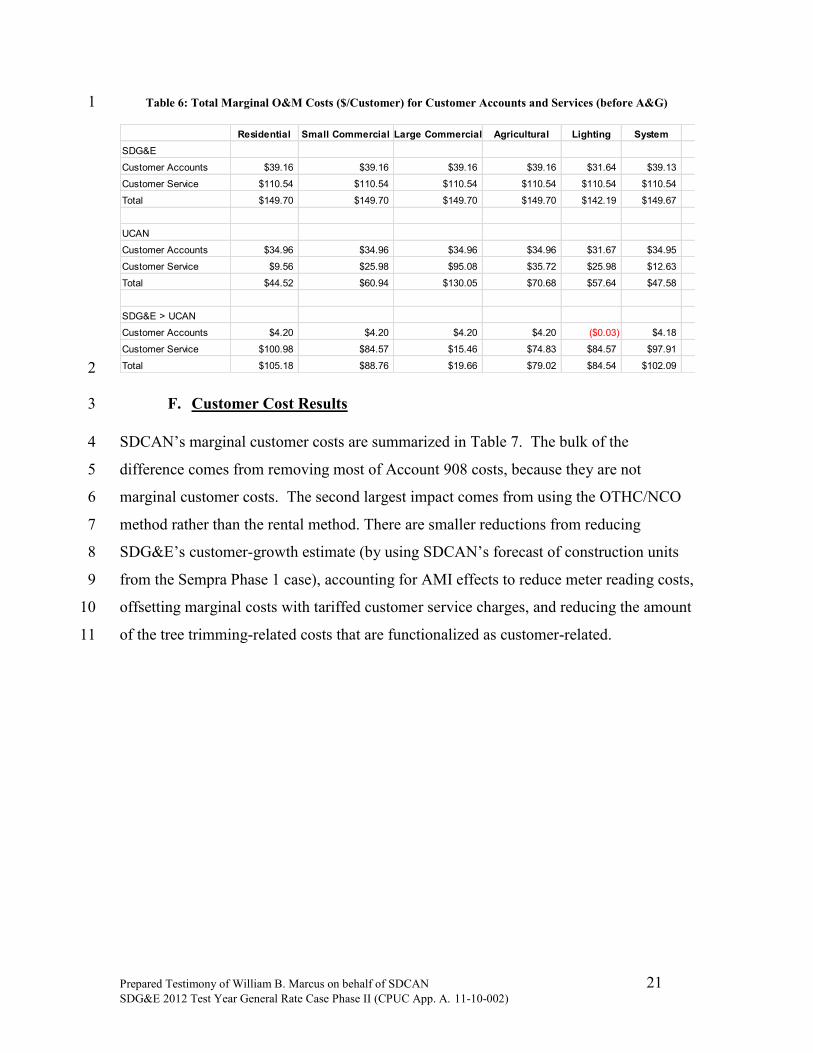
Table 6: Total Marginal O&M Costs ($/Customer) for Customer Accounts and Services (before A&G) 1
Residential Small Commercial Large Commercial Agricultural Lighting System
SDG&E
Customer Accounts $39.16 $39.16 $39.16 $39.16 $31.64 $39.13
Customer Service $110.54 $110.54 $110.54 $110.54 $110.54 $110.54
Total $149.70 $149.70 $149.70 $149.70 $142.19 $149.67
UCAN
Customer Accounts $34.96 $34.96 $34.96 $34.96 $31.67 $34.95
Customer Service $9.56 $25.98 $95.08 $35.72 $25.98 $12.63
Total $44.52 $60.94 $130.05 $70.68 $57.64 $47.58
SDG&E > UCAN
Customer Accounts $4.20 $4.20 $4.20 $4.20 ($0.03) $4.18
Customer Service $100.98 $84.57 $15.46 $74.83 $84.57 $97.91
Total $105.18 $88.76 $19.66 $79.02 $84.54 $102.09 2
F. Customer Cost Results 3
SDCAN’s marginal customer costs are summarized in Table 7. The bulk of the 4
difference comes from removing most of Account 908 costs, because they are not 5
marginal customer costs. The second largest impact comes from using the OTHC/NCO 6
method rather than the rental method. There are smaller reductions from reducing 7
SDG&E’s customer-growth estimate (by using SDCAN’s forecast of construction units 8
from the Sempra Phase 1 case), accounting for AMI effects to reduce meter reading costs, 9
offsetting marginal costs with tariffed customer service charges, and reducing the amount 10
of the tree trimming-related costs that are functionalized as customer-related. 11

Prepared Testimony of William B. Marcus on behalf of SDCAN 22 SDG&E 2012 Test Year General Rate Case Phase II (CPUC App. A. 11-10-002)
Table 7: Marginal Customer Cost Comparison (by Rate Schedule)
Rental (RECC) Rental (RECC) OTHC (NCO) OTHC (NCO) RECC (SDG&E) > RECC (UCAN) >
(SDG&E) (UCAN) (DRA) (UCAN) OTHC (UCAN) OTHC (UCAN)
(A) (B) (C) (D) (E) (F)
Residential Class
Schedule DR 257.43 137.87 77.53 89.10 168.33 48.77
Schedule DR-TOU 297.70 177.36 95.68 99.17 198.53 78.19
Schedule DR-SES 257.56 138.00 78.74 89.16 168.40 48.83
Schedule DM 319.05 198.30 105.83 107.99 211.06 90.31
Schedule DS 931.93 799.33 376.51 361.04 570.89 438.29
Schedule DT 3,793.93 3,606.03 1,669.92 1,542.91 2,251.02 2,063.11
Schedule DT-RV 1,801.41 1,652.01 709.93 720.00 1,081.42 932.01
Schedule EV-TOU 1 215.74 96.98 56.05 69.00 146.73 27.98
Schedule EV-TOU 2 344.07 222.83 108.97 130.82 213.25 92.01
Residential Class Average 259.05 139.46 78.22 89.85 169.21 49.61
Small Commercial Class
Schedule A 623.29 514.25 305.30 271.86 351.43 242.39
Under 20 kW 518.12 409.08 211.75 244.54 273.57 164.53
Over 20 kW 1,699.13 1,590.09 1,262.37 551.33 1,147.80 1,038.76
Schedule A-TC 244.27 142.55 105.27 98.43 145.84 44.13
Schedule A-TOU 460.81 354.91 206.38 183.45 277.37 171.47
Schedule UM 526.10 423.31 223.05 228.50 297.61 194.81
Small Commercial Class Average 600.15 491.55 292.99 261.11 339.04 230.44
Commercial & Industrial Class
Schedule AD 2,251.54 2,185.13 1,308.94 1,092.01 1,159.53 1,093.12
Primary 969.78 903.37 998.48 759.44 210.34 143.93
Secondary 2,264.66 2,198.25 1,312.12 1,095.41 1,169.25 1,102.84
Schedule AL-TOU 0.00
Secondary Voltage Service 2,197.16 2,131.77 1,291.51 1,067.37 1,129.79 1,064.40
Under 500 KW 2,189.94 2,124.55 1,282.22 1,065.49 1,124.45 1,059.05
Over 500 KW 6,530.56 6,465.16 6,867.30 2,192.65 4,337.91 4,272.51
Primary Voltage Service 443.73 412.21 501.49 262.71 181.02 149.51
Under 500 KW 436.19 404.67 464.88 260.74 175.44 143.93
Over 500 KW 494.84 463.33 5,011.94 276.01 218.84 187.32
Over 12 MW 3,266.10 3,234.59 5,685.18 997.16 2,268.94 2,237.43
Transmission 7,770.44 7,597.35 3,885.59 3,629.25 4,141.19 3,968.10
Under 500 KW 7,770.44 7,597.35 3,885.59 3,629.25 4,141.19 3,968.10
Schedule DGR
Secondary Voltage Service 2,235.23 2,169.10 1,380.37 1,085.98 1,149.25 1,083.12
Under 500 KW 2,220.98 2,154.84 1,298.36 1,082.27 1,138.70 1,072.57
Over 500 KW 2,933.87 2,867.73 5,482.12 1,267.68 1,666.19 1,600.06
Primary Voltage Service 433.03 401.72 769.49 257.92 175.11 143.80
Under 500 KW 433.03 401.72 461.74 257.92 175.11 143.80
Schedule AY-TOU 1,962.66 1,901.80 921.66 877.48 1,085.18 1,024.31
Secondary Voltage Service 2,020.75 1,958.76 932.20 901.48 1,119.28 1,057.29
Primary Voltage Service 433.03 401.72 644.02 245.71 187.32 156.01
Schedule PAT-1 3,151.84 3,067.99 1,482.22 1,507.41 1,644.43 1,560.58
Secondary Voltage Service 3,253.13 3,167.32 1,505.81 1,553.96 1,699.17 1,613.36
Primary Voltage Service 433.03 401.72 848.87 257.92 175.11 143.80
Schedule A6-TOU 2,450.98 2,284.06 7,223.22 2,173.53 277.45 110.53
Primary Voltage Service
Over 500kW 547.70 514.18 5,030.09 293.12 254.58 221.06
Primary at Sub Voltage Service
Transmission
Over 500kW 14,353.74 14,053.43 10,815.44 6,001.22 8,352.52 8,052.20
Commercial & Industrial Class
Average 2,187.08 2,121.88 1,286.57 1,059.72 1,127.37 1,062.17
Agricultural Class
Schedule PA 728.19 632.53 438.30 309.42 418.77 323.11
Under 20 KW 534.04 438.39 340.65 271.78 262.27 166.61
Over 20 KW 1,781.93 1,686.27 968.30 513.72 1,268.20 1,172.55
Agricultural Class Average 728.19 632.53 438.30 309.42 418.77 323.11
Lighting Class Average (Cost Per
Lamp) 19.64 10.27 13.12 3.91 15.73 6.36

Prepared Testimony of William B. Marcus on behalf of UCAN 23 SDG&E 2012 Test Year General Rate Case Phase II (CPUC App. A. 11-10-002)
III. Marginal Distribution Demand Costs
A. Additional Vegetation Management Functionalized as Distribution
Demand
SDCAN makes only one change to marginal demand distribution costs. The change in
functionalization of vegetation management costs from approximately 12-13% customer-
related to 2% customer related raises the demand distribution O&M for feeders and local
distribution from $17.45 to $18.32 per kW-year (2012 $) when that change is
incorporated into SDG&E’s demand distribution O&M workpaper.
After accounting for loading factors, the total feeder and local distribution costs are given
in Table 8. Total costs are increased from $74.06 to $75.06 per kW including changes to
both O&M and the A&G loader. SDCAN proposes no changes to substation costs.
Table 8: SDCAN and SDG&E Feeder and Local Distribution Demand Costs
Line No Description Value Units Source Factor Line No
1 Distribution Investment 526.55 $/kW 1
2 General Plant Loading 11.59 $/kW L1 x Factor 2.201% 2
3 Working Capital Loading 2.78 $/kW (L1 + L2) x Factor 0.517% 3
4 Subtotal Distribution Investment 540.92 $/kW L1 + L2 + L3 4
5 RECC Annualized Investment 50.17 $/kW/Yr L4 x Factor 9.274% 5
6 A&G Loading Applicable to Plant Loading 0.96 $/kW/Yr L5 x Factor 1.908% 6
7 Fixed O&M Overhead Cost 18.32 $/kW/Yr O&M Workpapers 7
8 A&G on Fixed O&M Loading 2.88 $/kW/Yr L7 x Factor 15.699% 8
9 Escalated Total Annual Unit Investment Cost 75.06 $/kW/Yr (L5+L6)*Factor+L7+L8 1.0537 9
Unit Feeders and Local Distribution Marginal Distribution Demand Costs
NERA Regression Method
IV. Marginal Generation Capacity Cost and Marginal Energy Cost
SDCAN generally agrees with much of SDG&E’s general framework for analysis of the
value of capacity, where the cost of a capacity resource—in SDG&E’s case, a
combustion turbine—is calculated in real dollar terms, and energy and ancillary services
value associated with the CT, which are Economic Rents, are subtracted from the
capacity cost.

Prepared Testimony of William B. Marcus on behalf of UCAN 24 SDG&E 2012 Test Year General Rate Case Phase II (CPUC App. A. 11-10-002)
However, we also agree with the theoretical principle advanced by DRA that the timing
of need for capacity should be considered when establishing marginal capacity costs.
In the context of SDG&E, the levels of capacity versus energy costs do not have large
impacts on the revenue allocation, though they may impact rate design and the cost-
effectiveness of demand-side programs.
We therefore do not address these issues further in this direct testimony, as part of our
attempts to coordinate with and not duplicate DRA, though we may have further
comments, if needed in response to other parties’ proposals in rebuttal testimony.
V. Distribution Revenue Allocation
We calculated a distribution revenue allocation equivalent to that provided by SDG&E
with SDCAN’s marginal customer and demand costs (see Table 9). Additional
supporting tables are contained in Attachment D
Table 9: SDCAN’s Uncapped Distribution Revenue Allocation
Current
Total Total
Distribution Non Marginal Marginal Distribution Distribution
Allocation Distribution Distribution Revenue Revenue Percentage
Factors Revenue Revenue Allocation Allocation Change
Line Customer Class (%) ($000) ($000) ($000) ($000) (%) Line
No. (A) (B) (C) (D) (E) (F) (G) No.
1 Residential 46.0% $471,369 $471,369 $573,261 -17.8% 1
2 2
3 Small Commercial 12.3% $126,129 $126,129 $119,152 5.9% 3
4 4
5 Medium/Large Commercial & Industrial 40.9% $6,536 $419,783 $426,319 $330,455 29.0% 5
6 6
7 Agricultural 0.4% $4,240 $4,240 $5,189 -18.3% 7
8 8
9 Lighting 0.4% $4,600 $3,791 $8,391 $8,391 0.0% 9
10 10
11 System 100.0% $11,136 $1,025,312 $1,036,448 $1,036,448 0.0% 11
12 12
13 Distribution Revenue Requirement ($000): $1,036,448 13
14 14
15 Non Marginal Revenue Requirement Components ($000): 15
16 Lighting Facilities Charges: $4,600 16
17 Standby Revenue: $4,183 17
18 Distance Adjustment Fees: $2,353 18
Note:
(1) Updated Allocation of Total Distribution Revenue: allocation of the current distribution revenue requirement based on the marginal Distribution Allocation Factors presented in this Application.
(2) Current Total Distribution Revenue Allocation: allocation of current distribution revenue requirement based on the current class distribution allocation percentages reflected in current rates; rates .
effective January 1, 2012, pursuant to SDG&E Advice Letter 2323-E.
(3) Distribution Revenue Requirement: the $1,036,448,000 Distribution Revenue Requirement reflects the current distribution revenues being collected in rates effective January 1, 2012,
excluding revenues that have separate allocation treatment such as Self Generation Incentive Program (SGIP) and Demand Response costs.
(4) Lighting Updated Total Distribution Revenue Allocation: as stated in footnote 3 of the testimony of William G. Saxe (Chapter 3), circuit and substation load data is not available for the
lighting class. For this reason, the Updated Total Distribution Revenue Allocation for lighting is set equal to its Current Distribution Revenue Allocation, using the Goal Seek Factor in Cell O26.
Updated Distribution Revenue Allocation
SAN DIEGO GAS & ELECTRIC COMPANY - ELECTRIC DEPARTMENT
2012 GRC PHASE 2 (A.11-10-002)
UCAN's DISTRIBUTION REVENUE ALLOCATION
Uncapped Distribution Revenue Allocation by Customer Class

Prepared Testimony of William B. Marcus on behalf of UCAN 25 SDG&E 2012 Test Year General Rate Case Phase II (CPUC App. A. 11-10-002)
Current rates and SDG&E’s and SDCAN’s uncapped distribution allocation results are
compared in Table 10.
Table 10: Comparison of SDG&E and SDCAN Distribution Revenue Allocation
Current Rate SDG&E UCAN SDG&E > UCAN
Residential $573,261 $534,119 $471,369 $62,750
Small Commercial $119,152 $131,836 $126,129 $5,708
Medium/Large C & I $330,455 $357,687 $426,319 -$68,633
Agricultural $5,189 $4,414 $4,240 $174
Lighting $8,391 $8,391 $8,391 $0
SDCAN’s allocation to residential customers is $63 million lower; the small commercial
allocation is nearly $6 million less, with larger customers receiving increases. It is also
likely that a lower allocation to residential customers will mechanically cause the CARE
discount to be reduced, thus reducing costs to non-residential classes.
It is likely that caps will be required with this type of allocation change. However, when
considering caps, it is important to look at the total rate changes (given that commodity
and CTC allocations are increasing for residential and decreasing for large customers,
and to look at changes both in percentage terms and in cents per kWh.

Prepared Testimony of William B. Marcus on behalf of UCAN 26 SDG&E 2012 Test Year General Rate Case Phase II (CPUC App. A. 11-10-002)
I. Residential Customer Characterization
To provide support to the work by SDCAN witness Laura Norin of MRW and
Associates, we are providing information on differences in load pattern by size of
customer (from SDG&E’s residential load research sample) and on economic and
demographic factors that affect customer usage in the SDG&E service territory (from the
Residential Appliance Saturation Survey or RASS data base). The work done here is
similar to work that JBS Energy has done for all of the California utilities on several
occasions, as well as for utilities in Nevada.
Our findings from SDG&E’s load research data are that smaller customers have better
load patterns than larger ones. This finding is consistent with SDCAN’s finding in
previous cases dating back to 2000. The RASS analysis shows that usage, while not in
lockstep with income, has a significant association with income; in particular that the
richest customers on average use more energy. This association arises in part because of
strong correlations between income and the square footage and type of dwelling and the
presence of energy-consuming equipment such as central air conditioning and swimming
pools.

Prepared Testimony of William B. Marcus on behalf of SDCAN 29 SDG&E 2012 Test Year General Rate Case Phase II (CPUC App. A. 11-10-002)
A. Reason for Errata
These errata correct the analysis of the California Energy Commission (CEC) Residential
Appliance Saturation Survey (RASS) for the SDG&E service territory by using SDG&E
Baseline zones instead of CEC Title 24 climate zones to climatically group customers.
This change affects none of our conclusions, and affects the quantitative results by only a
few percentage points in most cases.
In general, because the mid climate zone using baseline quantities was larger and
included portions of cooler CEC climate zones, both the cool zone and mid zone had
slightly less energy use per customer because the customers used more than average for
the cool zone and less than average for the mid zone. We stand by the general
conclusions presented in testimony but wish to accept SDG&E’s help in assuring that this
analysis is correct.
During rebuttal to Mr. Marcus’ testimony, SDG&E pointed out that the RASS portion of
our analysis used California Energy Commission (C EC) Title 24 climate zones to group
customers instead of SDG&E baseline zones, even though SDG&E provided SDGE
baseline zones for each customer.
We appreciate SDG&E telling us that a variable for the baseline zones was assigned to
each customer, a field that we overlooked in the nearly 800 data fields contained in the
dataset, as it was given the name UTILSDGE. The Title 24 Climate zones were identified
three times in both sets of consumption data (gas and electric) and additionally in the
RASS data using fieldnames such as “T24CZ”, and correspond closely to the baseline
zones, so the effect on the results is minimal. The late delivery of the dataset also hurried
our initial review.
The following updates the original testimony section titled “Relationship of Usage to
Income, Size and Type of Dwelling, and Appliances” beginning on page 29 and the
associated “Attachment E: Methodology for Analysis of Residential Appliance Saturation
Survey”.

Prepared Testimony of William B. Marcus on behalf of SDCAN 30 SDG&E 2012 Test Year General Rate Case Phase II (CPUC App. A. 11-10-002)
B. Relationship of Usage to Income, Size and Type of Dwelling, and
Appliances
We next examine the reasons why small customers use less energy and have better load
patterns than larger customers. We also examine relationships of consumption, among
single-family and multi-family customers by income.
At a high level, consumption is not in lockstep with income. However, there are
relatively strong correlations between consumption, size of dwelling, whether the
dwelling is single and multi-family, saturation of energy consuming appliances such as
central air conditioners and swimming pools, and income. As a result, the proposals by
SDG&E will give disproportionate rate breaks to large customers who are more likely to
have central air conditioners and swimming pools that contribute to peak loads and who
tend – on average - to be more affluent, while raising rates to CARE customers and many
other smaller customers who own less peak-heavy equipment.
We divided the SDG&E system into three climate zones groups – Cool, Mid, and Hot,
based on the SDG&E baseline zones and associated weather stations that each customer
was assigned to. The cool zone was SDG&E zone 1: the coastal baseline zone The Mid
climate group was the SDG&E inland (SDG&E zone 2) and mountain (SDGE zone 4)
baseline zones which had similar baseline quantities. The Hot Zone Group was SDG&E
baseline zone 3: low desert). We have not reported results for SDG&E’s hot zone, due to
a statistically insignificant number of RASS survey responses (only 20 respondents).
We broke the customers in each climate zone into groupings based on the average use of
the four inner summer months (June-September 2008). Each grouping was roughly
based on the average monthly summer quantities in the Cool and Mid zones (less than
130% of average basic baseline, 130-200%, 200-300%, and over 300%) rounded to the
nearest 10 kWh per month.
Our definition of which tier group a customer falls into is based on a monthly average of
the four peak summer months. In our analysis, a customer is in a Summer Tier Group if
the monthly average of the four summer months’ consumption falls within the Summer
Tier Group range. These groups roughly correspond to usage in each tier (though there

Prepared Testimony of William B. Marcus on behalf of SDCAN 31 SDG&E 2012 Test Year General Rate Case Phase II (CPUC App. A. 11-10-002)
may be some small amounts of spillover into the higher tier in the warmest summer
months).
We cross-tabulated and analyzed income by tier grouping, and by whether customers
were single-family and multi-family in each of the climate zones. We also analyzed the
saturation of central air conditioning and swimming pools by income and by tier
grouping and analyzed the relationship of the square footage of dwellings to tier grouping
and income.
More methodological information is contained in Attachment E.
1. Income
In the SDG&E zones, usage (measured by Summer Tier Group) increases with income in
the cool and mid climate zones.
Figure 1: Average Income by Summer Tier Group and Climate Group
The percentage of customers with income under $30,000 who had Tier 4 or 5 usage
(average monthly use above 200% of baseline in those four summer months) was 8% in
the cool zone and 6% in the mid zone. By comparison the percentage of customers over
$100,000 with Tier 4 use was 41% in the cool zone and 48% in the mid zone.

Prepared Testimony of William B. Marcus on behalf of SDCAN 32 SDG&E 2012 Test Year General Rate Case Phase II (CPUC App. A. 11-10-002)
Figure 2: Income Percentages by Summer Tier Group and Climate Group SDGE

Prepared Testimony of William B. Marcus on behalf of SDCAN 33 SDG&E 2012 Test Year General Rate Case Phase II (CPUC App. A. 11-10-002)
The reason is clear. Higher incomes are associated with larger dwellings, more saturation
of central air conditioning, and more swimming pools, as shown below. We start with an
examination of usage, income, and type of dwelling as related to square footage.
2. Single vs. Multi-Family
Multifamily customers use considerably less than single-family customers as shown in
the two figures below. Over 70% of multi-family customers use less than 130% of
baseline on average while very few use more than 200% of baseline.
Figure 3: Percent of Single-Family and Multi-Family Households within Tier Groups and Climate Zones SDGE

Prepared Testimony of William B. Marcus on behalf of SDCAN 34 SDG&E 2012 Test Year General Rate Case Phase II (CPUC App. A. 11-10-002)
Figure 4: Summer Average Monthly Kwh by Single-Family and Multi-Family Households
Multifamily customers use about 45% to 48% less than single-family customers in both
of the major climate zones. This phenomenon can be expected because of the smaller
size of the dwellings and common walls that reduce heat gain and loss, as well as income
differences that may affect usage.
There also are large differences in income between single-family and multi-family
dwellers. While a majority of households in all income groups live in single-family
dwellings in SDG&E’s service area as a whole, the proportion rises from 32% to 87% as
income rises.

Prepared Testimony of William B. Marcus on behalf of SDCAN 35 SDG&E 2012 Test Year General Rate Case Phase II (CPUC App. A. 11-10-002)
Figure 5: Percent of Single-Family and Multi-Family Households within Income Groups SDGE
Figure 6: Percent of Single-Family and Multi-Family Households across Income Groups SDGE
On the SDG&E system as a whole, 55% of single-family dwellers earned more than
$75,000, compared to 20% of multi-family households. Both climate zones showed a
disproportionate percentage of households under $30,000 in multifamily units as
expected.

Prepared Testimony of William B. Marcus on behalf of SDCAN 36 SDG&E 2012 Test Year General Rate Case Phase II (CPUC App. A. 11-10-002)
3. Square Footage
Figure 7 shows the percentage of dwellings by square footage. The more urbanized cool
area has more dwellings under 1500 square feet than the suburban inland area.
Figure 7: Percent of Households by Square Footage
Average usage generally increases with square footage. (Figure 8).

Prepared Testimony of William B. Marcus on behalf of SDCAN 37 SDG&E 2012 Test Year General Rate Case Phase II (CPUC App. A. 11-10-002)
Figure 8: Average Summer Monthly KWh Usage by Climate Group and Square Footage SDGE
Figure 9 computes the percentage of customers with usage in each tier with dwellings of
a given size. For those in dwellings less than 1000 square feet, 77% in cool zones and
95% in mid zones were at or below Tier 2 levels. Only 6.1% of those in cool zone
dwellings over 2500 square feet and 34% in mid zones were in the Tier 2 range. In these
large dwellings, 53% in the mid zone and 65% in the cool zone had average summer
usage that fell into Tier 4 or Tier 5.

Prepared Testimony of William B. Marcus on behalf of SDCAN 38 SDG&E 2012 Test Year General Rate Case Phase II (CPUC App. A. 11-10-002)
Figure 9: Percentage in Tiers 2-5 (Average Summer Monthly Use) by Square Footage of Dwelling SDGE

Prepared Testimony of William B. Marcus on behalf of SDCAN 39 SDG&E 2012 Test Year General Rate Case Phase II (CPUC App. A. 11-10-002)
There is a strong correlation between square footage of dwellings and income. Of those
in dwellings over 2500 square feet, 47 to 75% (depending on climate zone) earned more
than $100,000. Very few people earning over $100,000 lived in dwellings under 1,000
square feet – 13% in the more urbanized cool zone, and 9% in the mid zone (Figure 10).
Figure 10: Square Footage within Income Groups by Climate Zone SDGE E
Figure 11: Average Income by Climate Group and Square Footage SDGE

Prepared Testimony of William B. Marcus on behalf of SDCAN 40 SDG&E 2012 Test Year General Rate Case Phase II (CPUC App. A. 11-10-002)
4. Air Conditioning
Appliance such as air conditioners and swimming pools also affect summer peak usage
and saturation of these appliances is correlated with income.
The average income of a central air conditioning user is higher in all climate zones. See
Figure 12.
Figure 12: Average Income by Air Conditioner Type and Climate Group SDGE
Relative to having no air conditioner, a central air conditioner increases average monthly
summer usage by 74% in the cool zone (an increase of 284 kWh per month) and about
51% in the mid zone (an increase of 248 kWh per month).

Prepared Testimony of William B. Marcus on behalf of SDCAN 41 SDG&E 2012 Test Year General Rate Case Phase II (CPUC App. A. 11-10-002)
Figure 13: Average Summer Monthly Usage by Air Conditioner Type and Climate Zone Group SDGE
5. Swimming Pools
Swimming pools also are correlated with energy use and income. Customers must have
and pay for the energy it uses before they are counted as having a pool. Pools in common
areas are grouped with those without a pool. It should be noted that virtually no one in a
multifamily dwelling has a pool. Thirteen percent of households have pools. They use
more energy and have higher incomes than other households. Pool users tend to fall into
higher tier groups, and their usage is higher.

Prepared Testimony of William B. Marcus on behalf of SDCAN 42 SDG&E 2012 Test Year General Rate Case Phase II (CPUC App. A. 11-10-002)
Figure 14: Pool Ownership across Income Groups SDGE
As expected, there are very few swimming pool owners at the low end of income; it rises
to 17-19% for incomes over $75,000.
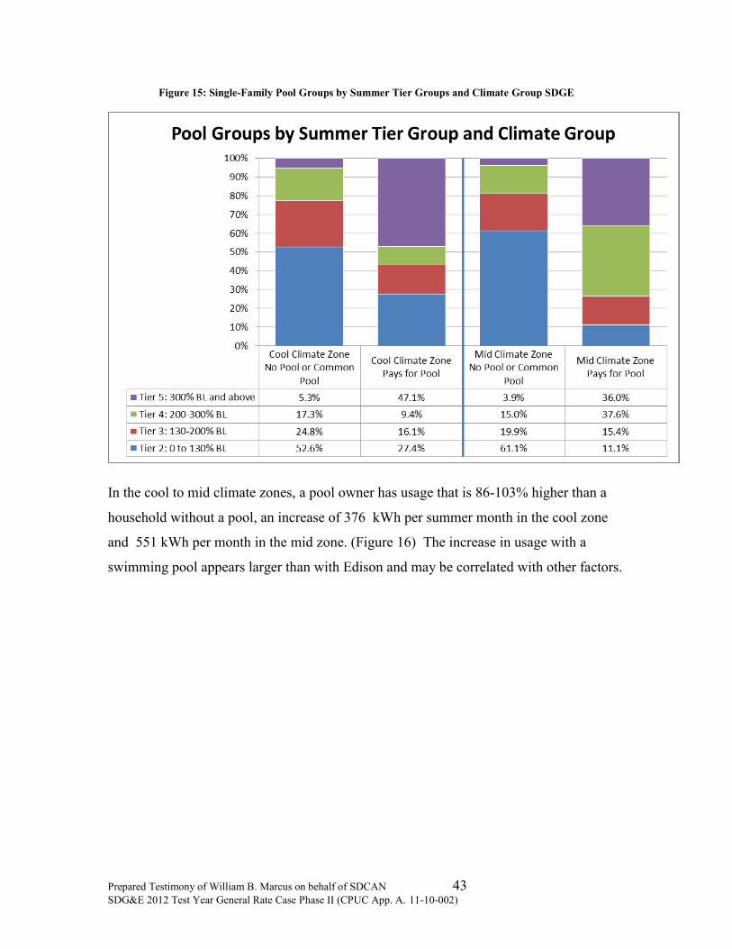
Prepared Testimony of William B. Marcus on behalf of SDCAN 43 SDG&E 2012 Test Year General Rate Case Phase II (CPUC App. A. 11-10-002)
Figure 15: Single-Family Pool Groups by Summer Tier Groups and Climate Group SDGE
In the cool to mid climate zones, a pool owner has usage that is 86-103% higher than a
household without a pool, an increase of 376 kWh per summer month in the cool zone
and 551 kWh per month in the mid zone. (Figure 16) The increase in usage with a
swimming pool appears larger than with Edison and may be correlated with other factors.

Prepared Testimony of William B. Marcus on behalf of SDCAN 44 SDG&E 2012 Test Year General Rate Case Phase II (CPUC App. A. 11-10-002)
Figure 16: Average Summer Monthly Kwh Usage by Pool Group and Climate Group SDGE
As shown in Figure 17, average incomes of pool owners are 26-33% higher than of those
without swimming pools.
Figure 17: Average Income by Swimming Pool Group and Climate Group SDGE

Prepared Testimony of William B. Marcus on behalf of SDCAN 45 SDG&E 2012 Test Year General Rate Case Phase II (CPUC App. A. 11-10-002)
6. Conclusion
The RASS data provided by SDG&E provides support for the contentions that lower
users who will be charged more by a customer charge are of lower income, are more
likely to live in apartments and smaller dwellings in general, and do not have as much
peak-oriented energy consuming equipment (central air conditioners and swimming
pools). This information will be used by the MRW witnesses in support of their
residential rate design recommendations.
Attachments

Prepared Testimony of William B. Marcus on behalf of SDCAN 46 SDG&E 2012 Test Year General Rate Case Phase II (CPUC App. A. 11-10-002)
Attachment A: Qualifications of William B. Marcus
Principal Economist, JBS Energy, Inc.
William B. Marcus has 28 years of experience in analysis of electric and gas utilities.
Mr. Marcus graduated from Harvard College with an A.B. magna cum laude in
economics in 1974 and was elected to Phi Beta Kappa. In 1975, he received an M.A. in
economics from the University of Toronto.
In July, 1984, Mr. Marcus became Principal Economist for JBS Energy, Inc. In this
position, he is the company’s lead economist for utility issues.
Mr. Marcus is the co-author of a book on electric restructuring prepared for the
National Association of Regulatory Utility Commissioners. He wrote a major report on Performance Based Ratemaking for the Energy Foundation. He analyzed restructuring
and stranded costs in eight states and provinces for environmental, consumer, and
independent power clients.
Mr. Marcus has prepared testimony and formal comments submitted to the Federal Energy Regulatory Commission, the National Energy Board of Canada, the Bonneville
Power Administration, the U.S. Bureau of Indian Affairs, U.S. District Court in San
Diego, Nevada County Municipal Court, committees of the Nevada, Ontario and California legislatures and the Los Angeles City Council, the California Energy
Commission (CEC), the Sacramento Municipal Utility District (SMUD), the
Transmission Agency of Northern California, the State of Nevada’s Colorado River Commission, two arbitration cases, environmental boards in Ontario, Manitoba, and
Nova Scotia; and regulatory commissions in Alberta, Arizona, Arkansas, British
Columbia, California, Colorado, Connecticut, District of Columbia, Hawaii, Manitoba, Maryland, Massachusetts, Nevada, New Jersey, New Mexico, North Carolina,
Northwest Territories, Nova Scotia, Ohio, Oklahoma, Ontario, Oregon, South Carolina,
Texas, Utah, Vermont, Virginia, Washington, Wisconsin, and Yukon. He testified on issues including utility restructuring, stranded costs, Performance-Based Ratemaking,
resource planning, load forecasts, need for powerplants and transmission lines,
environmental effects of electricity production, evaluation of conservation potential and programs, utility affiliate transactions, mergers, other revenue requirement issues,
avoided cost, utility business risks, regulated retail return margins, and electric and gas
cost of service and rate design.
From April, 1982, through June, 1984, Mr. Marcus was principal economist at
California Hydro Systems, Inc., an alternative energy consulting and development
company. He prepared financial analyses of projects, negotiated utility contracts, and
provided consulting services on utility economics and resources.
From July, 1978 through April, 1982, Mr. Marcus was an economist at the CEC, first in the energy development division and later as a senior economist in the CEC’s
Executive Office. He prepared testimony and economic studies on purchased power
pricing, transmission projects, renewable resources and conservation programs, and
managed interventions in utility rate cases.

Prepared Testimony of William B. Marcus on behalf of SDCAN 47 SDG&E 2012 Test Year General Rate Case Phase II (CPUC App. A. 11-10-002)
From 1975 to 1978, Mr. Marcus was a research analyst at the Kennedy School of
Government, Harvard University.
Mr. Marcus served on the 1991-92 SMUD Rate Advisory Committee, which made cost allocation and rate design recommendations to the SMUD Board. He has served on
several advisory committees for local governments in California.

Prepared Testimony of William B. Marcus on behalf of SDCAN 48 SDG&E 2012 Test Year General Rate Case Phase II (CPUC App. A. 11-10-002)
Attachment B: Responses to SDCAN Data Requests 8-6 to 8-11

Prepared Testimony of William B. Marcus on behalf of SDCAN 49 SDG&E 2012 Test Year General Rate Case Phase II (CPUC App. A. 11-10-002)
Attachment C: Excerpts from Prepared Testimony of Kathleen Cordova in Sempra GRC, Phase 1 (Exhibit SDG&E-15)

Prepared Testimony of William B. Marcus on behalf of SDCAN 50 SDG&E 2012 Test Year General Rate Case Phase II (CPUC App. A. 11-10-002)
Attachment D: Supporting Tables for Calculation of Distribution Revenue Allocation

Attachment E: Methodology for Analysis of Residential Appliance
Saturation Survey
San Diego Gas and Electric (SCE) provided the dataset used in this analysis. The
California Energy Commission (CEC) produced the dataset used in this analysis from data collected in the 2009 Residential Appliance Saturation Survey or RASS and
provided the dataset to SDG&E. SDG&E also provided gas and electric consumption
customer keyed to the RASS responses. SDG&E provided JBS with a comma separated value file with the orinal CEC RASS survey responses converted to string values. These
string values had to be converted back to the original CEC RASS ordinal values for
proper analysis. JBS combined the RASS survey with the billing consumption data. Each sample data point is weighted by the CEC to compensate for the sampling methodology;
we used the same RASS weighting factors in all of our analysis.
The statistical package SPSS (now owned by IBM) was used for the analysis to create a
combination of weighted crosstab and summary tables. Additional SDG&E related variables were created from the existing RASS variables and added to CEC RASS Survey
and Billing dataset. The RASS data was filtered to exclude incomplete electric
consumption data for the year June of 2008 through July of 2009, average monthly consumption during the summer months of June to September under 50 Kwh, bill days
for June 2008 under 25 days, household sizes equal to zero, seasonally occupied
residences, net metered homes, and all-electric homes.
All Electric homes include those with no gas consumption identified in the consumption
variable “yr1useg”that provides one years’ therm usage.
The single-family and multi-family group was created (SFMF variable) with two groups.
Mobile homes were grouped with Multi-Family households.
Air Conditioning (AC) Groups (ACGroup variable) were created from the RASS
variables for identifying Central AC, Room AC and Central Evaporative Coolers: No
AC, Room AC or a Central Evaporative Cooler, and Central AC.
The swimming pool groups (PoolPay variable) were created from the RASS “pltype” for
swimming pools to identify locations where the customer has and pays for the pool
energy (not a common area pool).
Square Footage and Income Groups were created by re-categorizing the more numerous
CEC groups into a smaller number of categories. Average incomes were assigned the
average of the income range (IncAvg variable) with the exception of the $150,000 and
more category, which was given the same average value of $175,000 as the CEC used. When used in this analysis, this value may understate some of income averages using
the highest income category values.
SDG&E Baseline Zones 1-4, were combined into three Climate Zone Groups: Cool, Mid,
and Hot. The Cool zone represents the immediate cool coastal area baseline zone, the Mid zone combines coastal influenced warmer coastal areas zones and mountain

baseline zones, and the Hot Zone which includes the El Centro dessert baseline climate
zone only. Hot Zone results were not reported in this analysis as the small number of surveyed customers might distort the results. The following table presents the number
of surveyed customers by climate zone. Note that due to the data validation and filtering
discussed above, the number of surveyed customers used in this analysis would likely
be lower than those reported below.
Table 11: Un-Weighted number of RASS Surveys by Climate Zone
SDGE Baseline Climate Zone Group Case Summaries
SDGE Baseline Zones N % of Total N
1 - Coastal 2313 56.70%
2 - Inland 60 1.50%
3 - Desert 20 0.50%
4 - Mountain 1688 41.40%
Total 4081 100.00%
The KWh consumption of the four summer months of June through September 2008 was
added into the SumKWh69 variable (data in the first monthly consumption variable in
the dataset not from June in 2008 was excluded). The average of the four months was placed in the SumKwhAvg variable. This was used to establish the upper tier level of
consumption in each Climate Group for the four summer months using SDG&E’s tier
criteria. Table 12 shows the derivation of Climate Zone Groups and Summer Tier Groups by Climate Zone Group and Figure 18 is a Map of CEC climate Zones. While not
sharing the exact geospatial boundaries, the CEC Title 24 climate zones correspond well
to the SDG&E Baseline zones.

Table 12: SDG&E Summer Tier Groups used in CEC RASS Analysis
SDGE Schedule DR
Summer: June to September Tier Groups Tier 2 Tier 3 Tier 4 Tier 5bCEC Title 24
Zone Baseline Zone Tier Group
Baseline
Allowance
Monthly
Baseline
Summer
Baseline Total 130% 200% 300% 500%
5 Santa Maria 5 0 0 - - - - -
6 Los Angeles 6 Cool 9.6 293 1,171 381 586 878 1,464
7 San Diego 7 Cool 9.6 293 1,171 381 586 878 1,464
8 El Toro 8 Cool 9.6 293 1,171 381 586 878 1,464
9 Pasedena 9 0 0 - - - - -
10 Riverside 10 Mid 11.2 342 1,366 444 683 1,025 1,708
13 Fresno 13 0 0 - - - - -
14 China Lake 14 Mid 14.8 451 1,806 587 903 1,354 2,257
15 El Centro 15 Hot 16.4 500 2,001 650 1,000 1,501 2,501
16 Mount Shasta 16 0 0 - - - - -
Calculated Tier Groups
Cool 9.6 292.8 1,171 381 586 878 1,464
Mid 13.0 396.5 1,586 515 793 1,190 1,983
Hot 16.4 500.2 2,001 650 1,000 1,501 2,501
Tier Groups Rounded to 10 Kwh
Cool 290 380 590 880 1460
Mid 400 520 790 1190 1980
Hot 500 650 1000 1500 2500 Figure 18: CEC Climate Zone Map

Figure 19: SDG&E Electric Baseline Zone Map
Related Documents