Neurocomputing 57 (2004) 313 – 344 www.elsevier.com/locate/neucom Margin maximization with feed-forward neural networks: a comparative study with SVM and AdaBoost Enrique Romero ∗ , Llu s M arquez , Xavier Carreras Departament de Llenguatges i Sistemes Inform atics, Universitat Polit ecnica de Catalunya, Campus Nord, C6-210, Barcelona 08034, Spain Received 30 April 2003; accepted 7 October 2003 Abstract Feed-forward Neural Networks (FNN) and Support Vector Machines (SVM) are two machine learning frameworks developed from very dierent starting points of view. In this work a new learning model for FNN is proposed such that, in the linearly separable case, it tends to obtain the same solution as SVM. The key idea of the model is a weighting of the sum-of-squares error function, which is inspired by the AdaBoost algorithm. As in SVM, the hardness of the margin can be controlled, so that this model can be also used for the non-linearly separable case. In addition, it is not restricted to the use of kernel functions, and it allows to deal with multiclass and multilabel problems as FNN usually do. Finally, it is independent of the particular algorithm used to minimize the error function. Theoretic and experimental results on synthetic and real-world problems are shown to conrm these claims. Several empirical comparisons among this new model, SVM, and AdaBoost have been made in order to study the agreement between the predictions made by the respective classiers. Additionally, the results obtained show that similar performance does not imply similar predictions, suggesting that dierent models can be combined leading to better performance. c 2003 Elsevier B.V. All rights reserved. Keywords: Margin maximization; Feed-forward Neural Networks; Support Vector Machines; AdaBoost; NLP classication problems ∗ Corresponding author. Tel.: +34-934015613; fax: +34-934017014. E-mail addresses: [email protected] (E. Romero), [email protected] (L. M arquez), [email protected] (X. Carreras). 0925-2312/$ - see front matter c 2003 Elsevier B.V. All rights reserved. doi:10.1016/j.neucom.2003.10.011

Welcome message from author
This document is posted to help you gain knowledge. Please leave a comment to let me know what you think about it! Share it to your friends and learn new things together.
Transcript
Neurocomputing 57 (2004) 313–344www.elsevier.com/locate/neucom
Margin maximization with feed-forward neuralnetworks: a comparative study with
SVM and AdaBoost
Enrique Romero∗ , Llu12s M3arquez , Xavier CarrerasDepartament de Llenguatges i Sistemes Inform�atics, Universitat Polit�ecnica de Catalunya,
Campus Nord, C6-210, Barcelona 08034, Spain
Received 30 April 2003; accepted 7 October 2003
Abstract
Feed-forward Neural Networks (FNN) and Support Vector Machines (SVM) are two machinelearning frameworks developed from very di:erent starting points of view. In this work a newlearning model for FNN is proposed such that, in the linearly separable case, it tends to obtainthe same solution as SVM. The key idea of the model is a weighting of the sum-of-squareserror function, which is inspired by the AdaBoost algorithm. As in SVM, the hardness of themargin can be controlled, so that this model can be also used for the non-linearly separablecase. In addition, it is not restricted to the use of kernel functions, and it allows to deal withmulticlass and multilabel problems as FNN usually do. Finally, it is independent of the particularalgorithm used to minimize the error function. Theoretic and experimental results on synthetic andreal-world problems are shown to con=rm these claims. Several empirical comparisons amongthis new model, SVM, and AdaBoost have been made in order to study the agreement betweenthe predictions made by the respective classi=ers. Additionally, the results obtained show thatsimilar performance does not imply similar predictions, suggesting that di:erent models can becombined leading to better performance.c© 2003 Elsevier B.V. All rights reserved.
Keywords: Margin maximization; Feed-forward Neural Networks; Support Vector Machines; AdaBoost;NLP classi=cation problems
∗ Corresponding author. Tel.: +34-934015613; fax: +34-934017014.E-mail addresses: [email protected] (E. Romero), [email protected] (L. M3arquez), [email protected]
(X. Carreras).
0925-2312/$ - see front matter c© 2003 Elsevier B.V. All rights reserved.doi:10.1016/j.neucom.2003.10.011
314 E. Romero et al. / Neurocomputing 57 (2004) 313–344
1. Introduction
Feed-forward Neural Networks (FNN) and Support Vector Machines (SVM) are twoalternative machine learning frameworks for approaching classi=cation and regressionproblems developed from very di:erent starting point of view. The minimization ofthe sum-of-squares (or cross-entropy) error function performed by FNN and the maxi-mization of the margin by SVM lead to a di:erent inductive bias with very interestingproperties [1,6].
This work is focused on classi=cation tasks. Its main contribution is to propose a newlearning model for FNN that, in the linearly separable case, tends to obtain the samesolution as SVM. Looking at the similarities and di:erences between FNN and SVM,it can be observed that the main di:erence between the sum-of-squares minimizationproblem of an FNN and the margin maximization problem of an SVM (1-Norm SoftMargin) lies on the constraints related to the objective function. Since these constraintsare responsible for the existence of the support vectors, their behavior will give the keyto propose the new learning model. Aiming to obtain support vectors, a weighting of thesum-of-squares error function is proposed. This weighting function is inspired by theAdaBoost algorithm [12], and it consists of modifying the contribution of every pointto the total error depending on its margin. In the linearly separable case, the hyper-plane that maximizes the normalized margin also minimizes asymptotically the weightedsum-of-squares error function proposed. The hardness of the margin can be controlled,as in SVM, so that this model can be used for the non-linearly separable case as well.
The classical FNN architecture of the new proposed scheme presents some advan-tages. The =nal solution is neither restricted to have an architecture with as manyhidden units as examples in the data set (or any subset of them) nor to use kernelfunctions. The weights in the =rst layer are not restricted to be a subset of the data set.In addition, it allows to deal with multiclass and multilabel problems as FNN usuallydo. This is a non-trivial problem for SVM, since they are initially designed for binaryclassi=cation problems. Finally, it is independent of the particular algorithm used tominimize the error function.
Both theoretic and experimental results are shown to con=rm these claims. Severalexperiments have been conducted on synthetic and two real-world problems from theNatural Language Processing domain, namely Word Sense Disambiguation and TextCategorization. Several comparisons among the new proposed model, SVM, and Ad-aBoost have been made in order to see the agreement of the predictions made by therespective classi=ers. Additionally, the evidence that there exist important di:erencesin the predictions of several models with good performance suggests that they can becombined in order to obtain better results than every individual model. This idea hasbeen experimentally con=rmed in the Text Categorization domain.
The overall organization of the paper is as follows. Some preliminaries about FNN,SVM, and AdaBoost can be found in Section 2. In Section 3, the similarities anddi:erences between FNN and SVM are discussed. Section 4 is devoted to describethe new learning model and some theoretic results. The whole experimental work isdescribed in Sections 5–7. Finally, Section 8 concludes and outlines some directionsfor further research.
E. Romero et al. / Neurocomputing 57 (2004) 313–344 315
2. Preliminaries
To =x notation, consider the classi=cation task given by a data set (the trainingset) X = {(x1; y1); : : : ; (xL; yL)}, where each instance xi belongs to an input spaceX; yi ∈{−1;+1}C , and C is the number of classes. 1 Without distinction, we willrefer to the elements of X as instances, points, examples, or vectors. A point xi be-longs to a class c when the cth component of yi (the target value) is +1. The learningalgorithm trained on the data set outputs a function or classi=er f :X → RC , wherethe sign of every component of f(x) is interpreted as the membership of x∈X toevery class. The magnitude of every component of f(x) is interpreted as a measure ofcon=dence in the prediction. Usually, X = RN .
2.1. Feed-forward Neural Networks (FNN)
The well-known architecture of an FNN is structured by layers of units, with con-nections between units from di:erent layers in forward direction [1]. A fully connectedFNN with one output unit and one hidden layer of Nh units computes the function:
fFNN(x) = ’0
(Nh∑i=1
�i’i(!i; bi; x) + b0
); (1)
where �i; bi; b0 ∈R and x; !i ∈RN . For convenience, we will divide the weights intocoe5cients (�i)
Nhi=1, frequencies (!i)
Nhi=1 and biases (bi)
Nhi=0. The most common acti-
vation functions ’i(!; b; x) in the hidden units are sigmoidal for Multi-layer Percep-trons (MLP) and radially symmetric for Radial Basis Function Networks (RBFN),although many other functions may be used [19,24]. Output activation functions ’0(u)are usually sigmoidal or linear.
The goal of the training process is to choose adequate parameters (coeLcients, fre-quencies and biases) to minimize a predetermined cost function. The sum-of-squareserror function is the most usual:
E(X ) =L∑
i=1
12(fFNN(xi)− yi)2: (2)
As it is well known, the sum-of-squares error function E(X ) is an approximation to thesquared norm of the error function fFNN(x)− y(x) in the Hilbert space L2 of squaredintegrable functions, where the integral is de=ned with regard to the probability measureof the problem represented by X . For C-class problems, architectures with C outputunits are used [1], and the objective is recast to minimize
EC(X ) =L∑
i=1
C∑c=1
12(fc
FNN(xi)− yci )
2; (3)
1 For 2-class problems, usually yi ∈{−1;+1}.
316 E. Romero et al. / Neurocomputing 57 (2004) 313–344
where fcFNN is the cth component of the output function. The architecture of the network
(i.e. connections, number of hidden units and activation functions) is usually =xed inadvance, whereas the weights are learned during the training process. Note that theappearance of the output function given by (1) is determined by the architecture ofthe FNN model.
2.2. Support Vector Machines (SVM)
According to [6,37], SVM can be described as follows: the input vectors are mappedinto a (usually high-dimensional) inner product space through some non-linear mapping�, chosen a priori. In this space (the feature space), an optimal hyperplane is con-structed. By using a kernel function K(u; v) the mapping can be implicit, since the innerproduct de=ning the hyperplane can be evaluated as 〈�(u); �(v)〉=K(u; v) for every twovectors u; v∈RN . In the SVM framework, an optimal hyperplane means a hyperplanewith maximal normalized margin with respect to the data set. The (functional) marginof a point (xi; yi) with respect to a function f is de=ned as mrg(xi; yi; f) = yif(xi).The margin of a function f with respect to a data set X is the minimum of the mar-gins of the points in the data set. If f is a hyperplane, the normalized (or geometric)margin is de=ned as the margin divided by the norm of the orthogonal vector to thehyperplane. Thus, the absolute value of the geometric margin is the distance to the hy-perplane. Using Lagrangian and Kuhn-Tucker theory, the maximal margin hyperplanefor a binary classi=cation problem given by X has the form:
fSVM(x) =L∑
i=1
yi�iK(xi; x) + b; (4)
where the vector (�i)Li=1 is the (1-Norm Soft Margin) solution of the following con-strained optimization problem in the dual space:
Maximize W (X ) =−12
L∑i; j=1
yi�iyj�jK(xi; xj) +L∑
i=1
�i
subject toL∑
i=1
yi�i = 0 (bias constraint);
06 �i6C; i = 1; : : : ; L:
(5)
In many implementations b is treated apart (=xed a priori, for example) in order toavoid the bias constraint. A point is well classi=ed if and only if its margin with respectto fSVM is positive. The points xi with �i ¿ 0 (active constraints) are support vectors.Bounded support vectors have �i = C. Regarding their margin value, non-boundedsupport vectors have margin 1, while bounded support vectors have margin less than1. The parameter C allows to control the trade-o: between the margin and the numberof training errors. By setting C=∞, one obtains the hard margin hyperplane. The costfunction −W (X ) is (plus a constant) the squared norm of the error function fSVM(x)−y(x) in the Reproducing Kernel Hilbert Space associated to K(u; v) [6, p. 41]. Themost usual kernel functions K(u; v) are polynomial, Gaussian-like or some particular
E. Romero et al. / Neurocomputing 57 (2004) 313–344 317
sigmoids. In contrast to FNN, note that the form of the solution is a consequence ofthe way the problem is solved.
2.3. AdaBoost
The purpose of AdaBoost is to =nd a highly accurate classi=cation rule by combiningmany weak classi;ers (or weak hypotheses), each of which may be only moderatelyaccurate [12,30]. The weak hypotheses are learned sequentially, one at a time. Concep-tually, at each iteration the weak hypothesis is biased to classify the examples whichwere most diLcult to classify by the preceding weak hypotheses. After a certain num-ber of iterations, the resulting weak hypotheses are linearly combined into a single rulecalled the combined hypothesis.
The generalized AdaBoost algorithm for binary classi=cation [30] maintains a vectorof weights as a distribution Dt over examples. At round t, the goal of the weak learneralgorithm is to =nd a weak hypothesis ht :X → R with moderately low error withrespect to the weights Dt . In this setting, weak hypotheses ht(x) make real-valuedcon=dence-rated predictions. Initially, the distribution D1 is uniform, but after eachiteration, the boosting algorithm increases (or decreases) the weights Dt(i) for whichht(xi) makes a bad (or good) prediction, with a variation proportional to the con=dence|ht(xi)|. The =nal hypothesis, fT :X → R, computes its predictions using a weightedvote of the weak hypotheses fT (x)=
∑Tj=1 �jhj(x). The concrete weight updating rule
can be expressed as
Dt+1(i) =Dt(i) · e−�tyiht(xi)
Zt
=e−
∑tj=1 �jyihj(xi)
L ·∏tj=1 Zj
=e−yift(xi)
L ·∏tj=1 Zj
=e−mrg(xi ;yi ;ft)
L ·∏tj=1 Zj
: (6)
Schapire and Singer [30] prove that the training error of the AdaBoost algorithm expo-nentially decreases with the normalization factor Zt computed at round t. This propertyis used in guiding the design of the weak learner, which attempts to =nd a weak hy-pothesis ht that minimizes Zt =
∑Li=1 Dt(i) · exp(−�tyiht(xi)). In the same work the
calculation of weak hypotheses is derived, which are domain partitioning rules withreal-valued predictions. In its simplest form it leads to the construction of decisionstumps, but it also can be seen as a natural splitting criterion used for performingdecision-tree induction.
From (6) and the previous expression of Zt , it can be said that AdaBoost is astage-wise procedure for minimizing a certain error function which depends on the func-tional margin −mrg(xi; yi; f). In particular, AdaBoost is trying to minimize∑
i exp(−yi
∑t �tht(xi)
), which is the negative exponential of the margin of the com-
bined classi=er. The learning bias of AdaBoost is proven to be very aggressive atmaximizing the margin of the training examples and this makes a clear connection tothe SVM learning paradigm [30]. More details about the relation between AdaBoostand SVM can be found in [26].
318 E. Romero et al. / Neurocomputing 57 (2004) 313–344
3. A Comparison between FNN and SVM
In this section, a comparison between FNN and SVM is performed. After comparingthe respective output and cost functions, it can be observed that the main di:erencelies on the presence or absence of constraints in the optimization problem.
3.1. Comparing the output functions
As pointed out elsewhere (see, for example, [38]), the output function (4) of anSVM can be expressed with a fully connected FNN with one output unit and onehidden layer of units (1) with the following identi=cations:
• Number of hidden units: L (the number of examples in X ),• Coe5cients: �i = yi�i,• Frequencies: !i = xi,• Biases: every bi vanishes, and b0 = b,• Activation functions:◦ Hidden layer: ’i(xi; bi; x) = K(xi; x).◦ Output layer: ’0 linear.
As in SVM, the only parameters to be learned in such an FNN would be the coeLcientsand the biases. Thus, the main di:erences between FNN and SVM rely both on thecost function to be optimized and the constraints, since speci=c learning algorithms area consequence of the optimization problem to be solved.
3.2. Comparing the cost functions
The =rst observation has to do with the similarities between the respective cost func-tions. De=ning KL=(K(xi; xj))Li; j=1; y=(y1; : : : ; yL)T; y�=(y1�1; : : : ; yL�L)T, neglectingthe bias term b, and considering the identi=cations stated in Section 3.1, we have thatfFNN(xj), which is equal to fSVM(xj), is the jth row of the vector y�T ·KL. Therefore,we can express the respective cost functions (2) and (5) on the data set X as
E(X ) =L∑
i=1
12fFNN(xi)2 −
L∑i=1
yifFNN(xi) +L∑
i=1
12y2i
=12y�T · KL · KL · y�− y�T · KL · y +
12L;
W (X ) =−12y�T · KL · y�+ y�T · y:
Regardless of their apparent similarity, we wonder whether there is any direct rela-tionship between the minima of E(X ) and the maxima of W (X )—or, equivalently, theminima of −W (X ). The next result partially answers this question.
E. Romero et al. / Neurocomputing 57 (2004) 313–344 319
Proposition 1. Consider the identi;cations in Section 3.1 without the bias term b. IfKL is non-singular, then the respective cost functions E(X) and −W (X ) attain theirunique minimum (without constraints) at the same point
(y1�∗1 ; : : : ; yL�∗L)T = K−1
L (y1; : : : ; yL)T:
Proof. As E(X ) and −W (X ) are convex functions, a necessary and suLcient conditionfor y�∗ to be a global minimum is that their derivative with respect to y� vanishes:
@E(X )@y�
= KL · KL · y�− KL · y = 0;
−@W (X )@y�
= KL · y�− y = 0:
Since KL is non-singular, both equations have the same solution.
If KL is singular, there will be more than one point where the optimum value isattained, but all of them are equivalent. In addition, KL has rows which are linearlydependent among them. This fact indicates that the information provided (via the innerproduct) by a point in the data set is redundant, since it is a linear combination of theinformation provided by other points. If the bias b is =xed a priori, the same resultholds.
4. An FNN that maximizes the margin
The optima of E(X ) and W (X ) can be very di:erent depending on the absence orpresence of the constraints. In this section, we explore the e:ect of the constraints inthe solution obtained by the SVM approach. Since these constraints are responsiblefor the existence of the support vectors, their behavior will give the key to propose aweighting of the sum-of-squares error function, inspired by the AdaBoost algorithm.
4.1. Contribution of every point to the cost function
The existence of linear constraints in the optimization problem to be solved in SVMhas a very important consequence: only some of the �i will be di:erent from zero.These coeLcients are associated with the so-called support vectors. Thus, the remain-ing vectors can be omitted, both to optimize W (X ) and to compute output (4). Theproblem is that we do not know them in advance. In the linearly separable case, withhard margin solutions, support vectors have margin 1 (i.e., fSVM(xi) = yi), while theremaining points (that will be referred to as superclassi;ed points) have a marginstrictly greater than 1. By linearly separable we mean “linearly separable in a certainspace”, either in the input space or in the feature space.
In contrast, for FNN minimizing the sum-of-squares error function, every point makesa certain contribution to the total error. The greater is the squared error, the greater willbe the contribution, independently of whether the point is well or wrongly classi=ed.
320 E. Romero et al. / Neurocomputing 57 (2004) 313–344
With linear output units, there may be points (very) well classi=ed with a (very)large squared error. Superclassi=ed points are a clear example of this type. Sigmoidaloutput units can help to solve this problem, but they can also create new ones (in thelinearly separable case, for example, the solution is not bounded). An alternative ideato sigmoidal output units could be to reduce the contribution of superclassi=ed pointsand reinforce those of misclassi=ed points, as explained in the next section.
4.2. Weighting the contribution
Unfortunately, we do not know in advance which points will be =nally superclassi=edor misclassi=ed. But during the FNN learning process it is possible to treat everypoint in a di:erent way depending on its error (or, equivalently, its margin). In orderto simulate the behavior of an SVM, the learning process could be guided by thefollowing heuristics:
• Any well classi=ed point contributes less to the error than any misclassi=ed point.• Among well classi=ed points, the contribution is larger for smaller errors in absolute
value (or, equivalently, smaller margins).• Among misclassi=ed points, the contribution is larger for larger errors in absolute
value (or, equivalently, smaller margins).
These guidelines reinforce the contribution of misclassi=ed points and reduces the con-tribution of well classi=ed ones. As can be seen, this is exactly the same idea asdistribution (6) for AdaBoost. Similarly, the contribution of every point to the errorcan be modi=ed simply by weighting it individually as a function of the margin withrespect to the output function fFNN(x). In order to allow more Sexibility to the model,two parameters �+; �−¿ 0 can be introduced into the weighting function as follows:
D(xi; yi; �+; �−) =
e−|mrg|�+ if mrg¿ 0;
e+|mrg|�− if mrg¡ 0 and �− = 0;
1 otherwise;
(7)
where the margin mrg=mrg(xi; yi; fFNN)=yifFNN(xi). There are (at least) two di:erentways of obtaining the behavior previously described:
• Weighting the sum-of-squares error:
Ep =12(fFNN(xi)− yi)2 · D(xi; yi; �+; �−); (8)
• Weighting the sum-of-squares error derivative (when the derivative is involved inthe learning process):
Ep such that@Ep
@fFNN= (fFNN(xi)− yi) · D(xi; yi; �+; �−); (9)
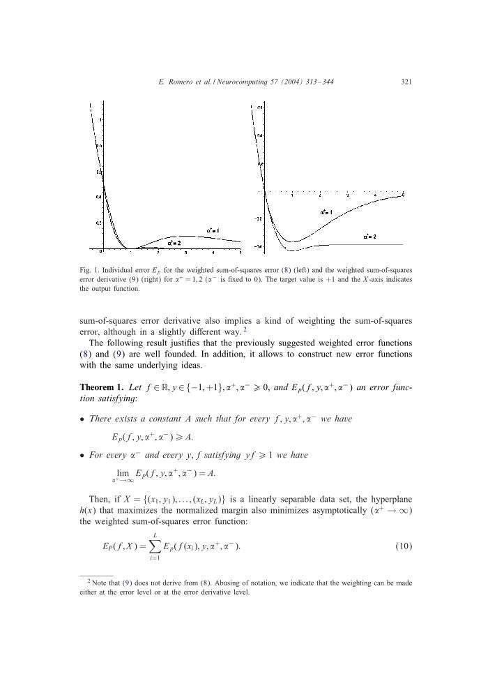
where Ep = Ep(fFNN(xi); yi; �+; �−). Graphically, the right branch of the squarederror parabola is bended to a horizontal asymptote, as shown in Fig. 1. Weighting the
E. Romero et al. / Neurocomputing 57 (2004) 313–344 321
Fig. 1. Individual error Ep for the weighted sum-of-squares error (8) (left) and the weighted sum-of-squareserror derivative (9) (right) for �+ = 1; 2 (�− is =xed to 0). The target value is +1 and the X -axis indicatesthe output function.
sum-of-squares error derivative also implies a kind of weighting the sum-of-squareserror, although in a slightly di:erent way. 2
The following result justi=es that the previously suggested weighted error functions(8) and (9) are well founded. In addition, it allows to construct new error functionswith the same underlying ideas.
Theorem 1. Let f∈R; y∈{−1;+1}; �+; �−¿ 0, and Ep(f; y; �+; �−) an error func-tion satisfying:
• There exists a constant A such that for every f; y; �+; �− we have
Ep(f; y; �+; �−)¿A:
• For every �− and every y, f satisfying yf¿ 1 we have
lim�+→∞
Ep(f; y; �+; �−) = A:
Then, if X = {(x1; y1); : : : ; (xL; yL)} is a linearly separable data set, the hyperplaneh(x) that maximizes the normalized margin also minimizes asymptotically (�+ → ∞)the weighted sum-of-squares error function:
EP(f; X ) =L∑
i=1
Ep(f(xi); y; �+; �−): (10)
2 Note that (9) does not derive from (8). Abusing of notation, we indicate that the weighting can be madeeither at the error level or at the error derivative level.
322 E. Romero et al. / Neurocomputing 57 (2004) 313–344
Proof. Since A is a lower bound for Ep, we have EP(f; X )¿L · A for any functionf(x). Since X is linearly separable, h(x) satis=es that support vectors have marginyih(xi)=1, whereas yih(xi)¿ 1 for non-support vectors. The second hypothesis impliesthat, for every xi ∈X , Ep(h(xi); y; �+; �−) = A asymptotically (�+ → ∞).
Remark.
• The theorem holds true independently of whether the data set X is linearly separableeither in the input space or in the feature space.
• The previously suggested weighted error functions (8) and (9) satisfy the hypothesesof the theorem, with the additional property that the absolute minimum of Ep isattained when the margin equals 1.
• The reciprocal may not be necessarily true, since there can be many di:erent hy-perplanes which asymptotically minimize EP(f; X ). However, the solution obtainedby minimizing EP(f; X ) is expected to have a similar behavior than the hyperplaneof maximal margin. In particular, using (8) or (9):◦ It is expected that a large �+ will be related to a hard margin.◦ For the linearly separable case, the expected margin for every support vector
is 1.◦ For the non-linearly separable case, points with margin less or equal than 1 are
expected to be support vectors.Experimental results with several synthetic and real-world problems suggest thatthese hypotheses seem to be well founded (see Sections 5–7).
The relation among �+, the learning algorithm, and the hardness of the margin de-serves special attention. Suppose that EP is minimized with an iterative procedure, suchas Back-Propagation (BP) [29], and the data set is linearly separable. For large �+,the contribution of superclassi=ed points to EP can be ignored. Far away from theminimum there exist points whose margin is smaller than 1 − &, for a certain small&¿ 0. Very close to the minimum, in contrast, the margin value of every point isgreater than 1− &. Using the same terminology that in the SVM approach, the numberof bounded support vectors decreases as the number of iterations increases, leadingto a solution without bounded support vectors. In other words, for linearly separabledata sets and large �+, the e:ect of an iterative procedure minimizing EP is the in-crease of the hardness of the solution with regard to the number of iterations. Forsmall �+, in contrast, the contribution of superclassi=ed points to EP cannot be ig-nored, and the solutions obtained probably share more properties with the regressionsolution.
For non-linearly separable data sets, it seems that the behavior could be very similarto the linearly separable case (in the sense of the hardness of the solution). In thiscase, the existence of misclassi=ed points will lead to solutions having a balancedcombination of bounded and non-bounded support vectors. As a consequence, solutionsclose to the minimum may lead to over=tting, since they are being forced to concentrateon the hardest points to classify, which may be outliers or wrongly labeled points. Thesame sensitivity to noise was observed for the AdaBoost algorithm in [7].
E. Romero et al. / Neurocomputing 57 (2004) 313–344 323
4.3. Practical considerations
Some bene=ts can be obtained by minimizing an error function as the one de=nedin (10), since there is no assumption about the architecture of the FNN:
• In the =nal solution, there is no need to have as many hidden units as points in thedata set (or any subset of them), nor the frequencies must be the points in the dataset.
• There is no need to use kernel functions, since there is no inner product to computein the feature space.
In addition, it allows to deal with multiclass and multilabel problems as FNN usuallydo:
• For C-class problems, an architecture with C output units may be constructed, sothat the learning algorithm minimizes the weighted multiclass sum-of-squares error,de=ned as usual [1]:
ECP (f
cFNN; X ) =
L∑i=1
C∑c=1
Ep(fcFNN(xi); y
ci ; �
+; �−): (11)
• The error function de=ned in (11) also allows to deal with multilabel problems withthe same architecture.
Finally, it is independent of the particular algorithm used to minimize the error function.In fact, it is even independent of using FNN to minimize EP(f; X ).
4.4. Related work
From a theoretical point of view, SVM for regression have been shown to be equiv-alent, in certain cases, to other models such as Sparse Approximation [13] or Regular-ization Networks [33]. The theoretical analysis that states the relation between one-classSVM and AdaBoost can be found in [26]. These results are obtained by means of theanalysis and adaptation of the respective cost functions to be optimized. But the errorfunctions used in these works are qualitatively di:erent from the one proposed in thepresent work.
For linearly separable data sets, a single-layer perceptron learning algorithm thatasymptotically obtains the maximum margin classi=er is presented in [27]. The archi-tecture used is an MLP with sigmoidal units in the output layer and without hiddenunits, trained with BP. In order to work, the learning rate should be increased exponen-tially, leading to weights arbitrarily large. In contrast to our approach, no modi=cationof the error function is done.
In [35], a training procedure for MLP based on SVM is described. The activationfunction is not necessarily a kernel function, as in our model. However, there aremany other di:erences, since the learning process is guided by the minimization of theestimation of an upper bound of the Vapnik–Chervonenkis dimension.
324 E. Romero et al. / Neurocomputing 57 (2004) 313–344
The work in [40] investigates learning architectures in which the kernel function canbe replaced by more general similarity measures that can have internal parameters. Thecost function is also modi=ed to be dependent on the margin, as in our scheme. Inparticular, the cost function E(X ) =
∑Li=1 [0:65− tanh(mrg(xi; yi; f))]2 is used in the
experiments presented. Another di:erence with our work relies in the fact that in [40]the frequencies are forced to be a subset of the points in the data set.
5. Experimental motivation
We performed some experiments on both arti=cial (Section 6) and real data (Section7) in order to test the validity of the new model and the predicted behavior explainedin Section 4. All experiments were performed with FNN trained with standard BPweighting the sum-of-squares error derivative (9). From now on, we will refer to thismethod as BPW. The parameter �− was set to 0 in all experiments, so that misclassi=edpoints had always a weight equal to 1. If not stated otherwise, every architecturehave linear output units, the initial frequencies were 0 and the initial range for thecoeLcients was 0:00001. Synthetic problems were trained in batch mode, whereasreal-world problems were trained in pattern mode.
Regarding the FNN training model proposed in this paper, we were interested intesting:
• Whether learning is possible or not with a standard FNN architecture when a weightedsum-of-squares error EP(f; X ) is minimized with standard methods.
• Whether the use of non-kernel functions can lead to a similar behavior to that ofkernel functions or not.
• The e:ect of large �+, together with the number of iterations, on the hardness ofthe margin.
• The identi=cation of the “support vectors”, simply by comparing their margin valuewith 1.
• The behavior of the model in multiclass and multilabel problems minimizing theerror function de=ned in (11).
• The behavior of the model in both linearly and non-linearly separable cases, withlinear and non-linear activation functions.
In real-world problems, we made several comparisons among FNN trained with BPW(for several activation functions and number of epochs), SVM with di:erent kernels,and AdaBoost with domain partitioning weak learners. Our main interest was to in-vestigate the similarities among the partitions that every model induced on the inputspace. We can approximately do that by comparing the outputs of the di:erent learnedclassi=ers on a test set, containing points never used during the construction of theclassi=er. There are several motivations for these comparisons. First, testing the hy-potheses claimed for the new model regarding its similarities to SVM (Section 4),when the parameters are properly chosen. Second, comparing di:erent paradigms ofmargin maximization (e.g., SVM and AdaBoost), and di:erent parameters within the
E. Romero et al. / Neurocomputing 57 (2004) 313–344 325
same paradigm. Finally (Section 7.2.3), the discovery of very di:erent models withgood performance may lead to signi=cant improvements in the predictions on newdata, since larger di:erences among models may be related to more independence inthe errors made by the systems [25,1].
6. Experiments on synthetic data
In this section, the experiments on arti=cial data are explained. With these problems,the predicted behavior described in Section 4 is con=rmed.
6.1. Two linearly separable classes
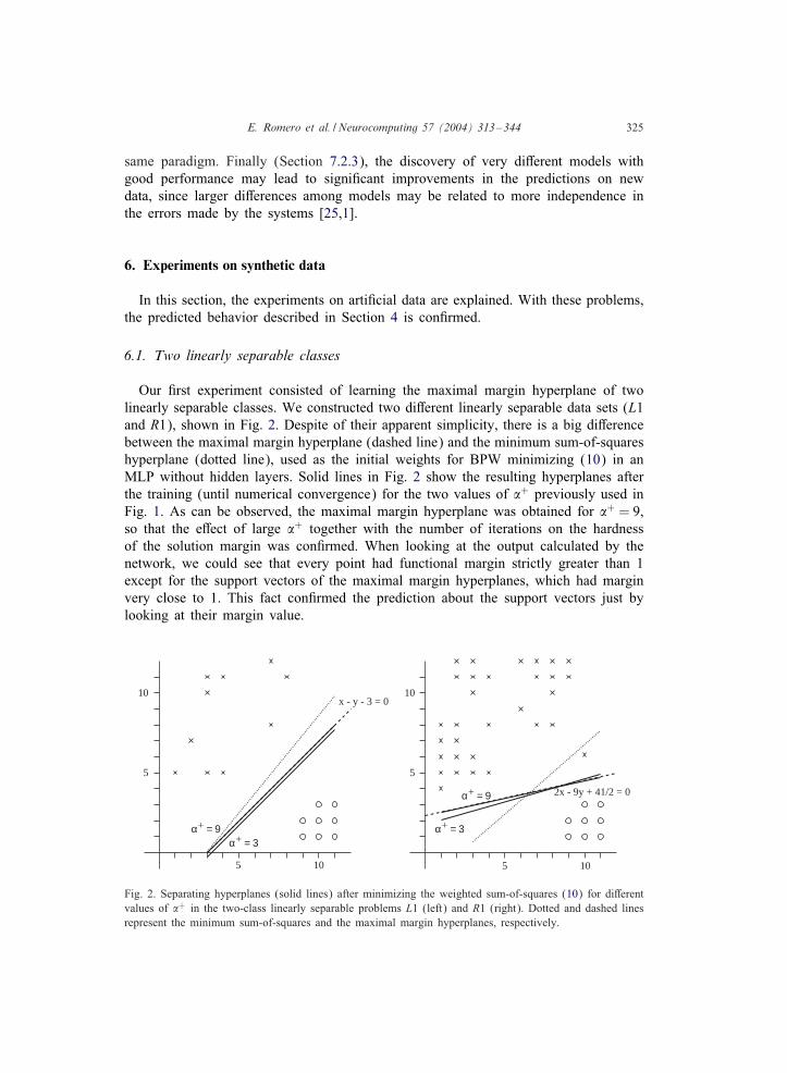
Our =rst experiment consisted of learning the maximal margin hyperplane of twolinearly separable classes. We constructed two di:erent linearly separable data sets (L1and R1), shown in Fig. 2. Despite of their apparent simplicity, there is a big di:erencebetween the maximal margin hyperplane (dashed line) and the minimum sum-of-squareshyperplane (dotted line), used as the initial weights for BPW minimizing (10) in anMLP without hidden layers. Solid lines in Fig. 2 show the resulting hyperplanes afterthe training (until numerical convergence) for the two values of �+ previously used inFig. 1. As can be observed, the maximal margin hyperplane was obtained for �+ = 9,so that the e:ect of large �+ together with the number of iterations on the hardnessof the solution margin was con=rmed. When looking at the output calculated by thenetwork, we could see that every point had functional margin strictly greater than 1except for the support vectors of the maximal margin hyperplanes, which had marginvery close to 1. This fact con=rmed the prediction about the support vectors just bylooking at their margin value.
α+ = 9
α+ = 9α+ = 3
α+ = 3
5
10
5
5 10
10
5
x - y - 3 = 0
10
2x - 9y + 41/2 = 0
Fig. 2. Separating hyperplanes (solid lines) after minimizing the weighted sum-of-squares (10) for di:erentvalues of �+ in the two-class linearly separable problems L1 (left) and R1 (right). Dotted and dashed linesrepresent the minimum sum-of-squares and the maximal margin hyperplanes, respectively.
326 E. Romero et al. / Neurocomputing 57 (2004) 313–344
5 10
10
5
5 10
10
5
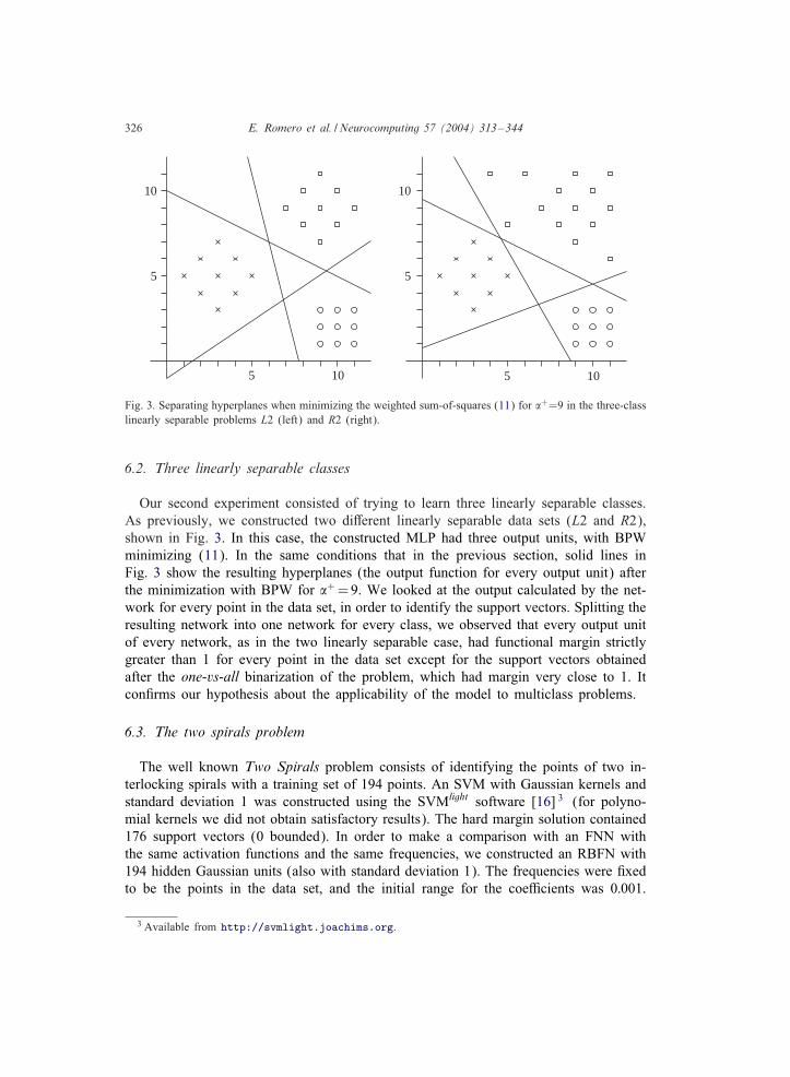
Fig. 3. Separating hyperplanes when minimizing the weighted sum-of-squares (11) for �+=9 in the three-classlinearly separable problems L2 (left) and R2 (right).
6.2. Three linearly separable classes
Our second experiment consisted of trying to learn three linearly separable classes.As previously, we constructed two di:erent linearly separable data sets (L2 and R2),shown in Fig. 3. In this case, the constructed MLP had three output units, with BPWminimizing (11). In the same conditions that in the previous section, solid lines inFig. 3 show the resulting hyperplanes (the output function for every output unit) afterthe minimization with BPW for �+=9. We looked at the output calculated by the net-work for every point in the data set, in order to identify the support vectors. Splitting theresulting network into one network for every class, we observed that every output unitof every network, as in the two linearly separable case, had functional margin strictlygreater than 1 for every point in the data set except for the support vectors obtainedafter the one-vs-all binarization of the problem, which had margin very close to 1. Itcon=rms our hypothesis about the applicability of the model to multiclass problems.
6.3. The two spirals problem
The well known Two Spirals problem consists of identifying the points of two in-terlocking spirals with a training set of 194 points. An SVM with Gaussian kernels andstandard deviation 1 was constructed using the SVMlight software [16] 3 (for polyno-mial kernels we did not obtain satisfactory results). The hard margin solution contained176 support vectors (0 bounded). In order to make a comparison with an FNN withthe same activation functions and the same frequencies, we constructed an RBFN with194 hidden Gaussian units (also with standard deviation 1). The frequencies were =xedto be the points in the data set, and the initial range for the coeLcients was 0:001.
3 Available from http://svmlight.joachims.org.
E. Romero et al. / Neurocomputing 57 (2004) 313–344 327
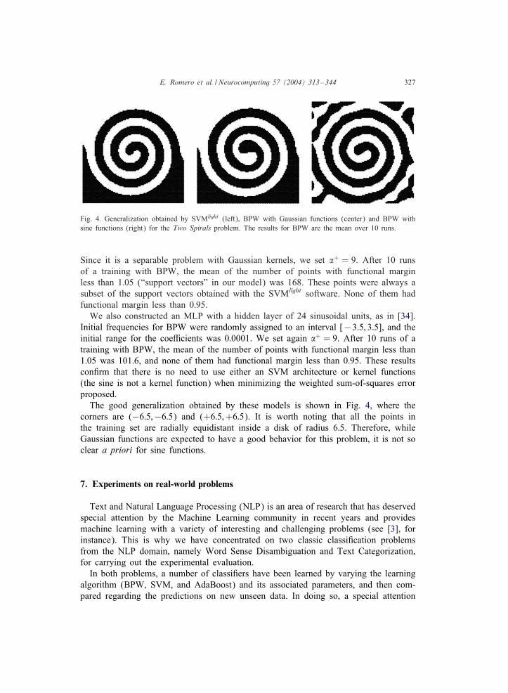
Fig. 4. Generalization obtained by SVMlight (left), BPW with Gaussian functions (center) and BPW withsine functions (right) for the Two Spirals problem. The results for BPW are the mean over 10 runs.
Since it is a separable problem with Gaussian kernels, we set �+ = 9. After 10 runsof a training with BPW, the mean of the number of points with functional marginless than 1:05 (“support vectors” in our model) was 168. These points were always asubset of the support vectors obtained with the SVMlight software. None of them hadfunctional margin less than 0:95.
We also constructed an MLP with a hidden layer of 24 sinusoidal units, as in [34].Initial frequencies for BPW were randomly assigned to an interval [−3:5; 3:5], and theinitial range for the coeLcients was 0:0001. We set again �+ = 9. After 10 runs of atraining with BPW, the mean of the number of points with functional margin less than1:05 was 101:6, and none of them had functional margin less than 0:95. These resultscon=rm that there is no need to use either an SVM architecture or kernel functions(the sine is not a kernel function) when minimizing the weighted sum-of-squares errorproposed.
The good generalization obtained by these models is shown in Fig. 4, where thecorners are (−6:5;−6:5) and (+6:5;+6:5). It is worth noting that all the points inthe training set are radially equidistant inside a disk of radius 6:5. Therefore, whileGaussian functions are expected to have a good behavior for this problem, it is not soclear a priori for sine functions.
7. Experiments on real-world problems
Text and Natural Language Processing (NLP) is an area of research that has deservedspecial attention by the Machine Learning community in recent years and providesmachine learning with a variety of interesting and challenging problems (see [3], forinstance). This is why we have concentrated on two classic classi=cation problemsfrom the NLP domain, namely Word Sense Disambiguation and Text Categorization,for carrying out the experimental evaluation.
In both problems, a number of classi=ers have been learned by varying the learningalgorithm (BPW, SVM, and AdaBoost) and its associated parameters, and then com-pared regarding the predictions on new unseen data. In doing so, a special attention
328 E. Romero et al. / Neurocomputing 57 (2004) 313–344
is devoted to the comparison between the BPW model presented in this paper andSVM. By studying the agreement rates between both models and the importance ofthe training vectors in the induced classi=ers we con=rm the already stated relationsbetween the margin maximization process performed in both models.
7.1. Word sense disambiguation
Word Sense Disambiguation (WSD) or lexical ambiguity resolution is the problemof automatically determining the appropriate meaning (aka sense) to each word in atext or discourse. As an example, the word age in a sentence like “his age was 71”refers to the length of time someone has existed (sense 1), while in a sentence like“we live in a litigious age” refers to a concrete historic period (sense 2). Thus, anautomatic WSD system should be able to pick the correct sense of the word “age”in the previous two sentences basing the decision on the context in which the wordoccurs.
Resolving the ambiguity of words is a central problem for NLP applications andtheir associated tasks, including, for instance, natural language understanding, machinetranslation, and information retrieval and extraction [14]. Although far from obtainingsatisfactory results [17], the best WSD systems up to date are based on supervisedmachine learning algorithms. Among others, we =nd Decision Lists [42], Neural Net-works [36], Bayesian learning [2], Examplar Based learning [22], AdaBoost [8], andSVM [18] in the recent literature.
Since 1998, the ACL’s SIGLEX group has carried out the SensEval initiative, whichconsists of a series of international workshops on the evaluation of Word Sense Dis-ambiguation systems. It is worth noting that in the last edition of SensEval 4 we can=nd (AdaBoost and SVM)-based classi=ers among the top performing systems.
7.1.1. SettingData set: We have used a part of the English SensEval-2 corpus (available through
the conference Web site), consisting of a set of annotated examples for 4 words (oneadjective, one noun, and two verbs), divided into a training set and a test set for eachword. Each example is provided with a context of several sentences around the wordto be disambiguated. Each word is treated as an independent disambiguation problem.
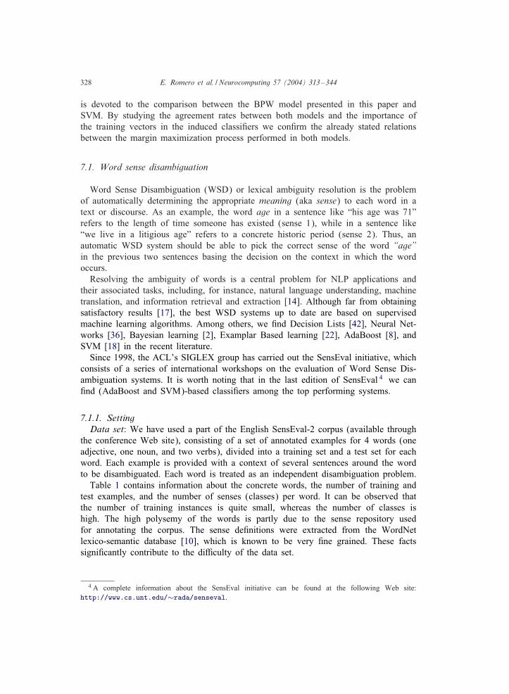
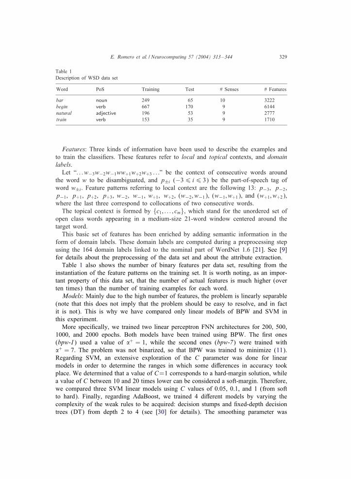
Table 1 contains information about the concrete words, the number of training andtest examples, and the number of senses (classes) per word. It can be observed thatthe number of training instances is quite small, whereas the number of classes ishigh. The high polysemy of the words is partly due to the sense repository usedfor annotating the corpus. The sense de=nitions were extracted from the WordNetlexico-semantic database [10], which is known to be very =ne grained. These factssigni=cantly contribute to the diLculty of the data set.
4 A complete information about the SensEval initiative can be found at the following Web site:http://www.cs.unt.edu/∼rada/senseval.
E. Romero et al. / Neurocomputing 57 (2004) 313–344 329
Table 1Description of WSD data set
Word PoS Training Test # Senses # Features
bar noun 249 65 10 3222begin verb 667 170 9 6144natural adjective 196 53 9 2777train verb 153 35 9 1710
Features: Three kinds of information have been used to describe the examples andto train the classi=ers. These features refer to local and topical contexts, and domainlabels.
Let “: : : w−3w−2w−1ww+1w+2w+3 : : :” be the context of consecutive words aroundthe word w to be disambiguated, and p±i (−36 i6 3) be the part-of-speech tag ofword w±i. Feature patterns referring to local context are the following 13: p−3; p−2,p−1; p+1, p+2; p+3, w−2; w−1, w+1; w+2, (w−2; w−1), (w−1; w+1), and (w+1; w+2),where the last three correspond to collocations of two consecutive words.
The topical context is formed by {c1; : : : ; cm}, which stand for the unordered set ofopen class words appearing in a medium-size 21-word window centered around thetarget word.
This basic set of features has been enriched by adding semantic information in theform of domain labels. These domain labels are computed during a preprocessing stepusing the 164 domain labels linked to the nominal part of WordNet 1.6 [21]. See [9]for details about the preprocessing of the data set and about the attribute extraction.
Table 1 also shows the number of binary features per data set, resulting from theinstantiation of the feature patterns on the training set. It is worth noting, as an impor-tant property of this data set, that the number of actual features is much higher (overten times) than the number of training examples for each word.Models: Mainly due to the high number of features, the problem is linearly separable
(note that this does not imply that the problem should be easy to resolve, and in factit is not). This is why we have compared only linear models of BPW and SVM inthis experiment.
More speci=cally, we trained two linear perceptron FNN architectures for 200, 500,1000, and 2000 epochs. Both models have been trained using BPW. The =rst ones(bpw-1) used a value of �+ = 1, while the second ones (bpw-7) were trained with�+ = 7. The problem was not binarized, so that BPW was trained to minimize (11).Regarding SVM, an extensive exploration of the C parameter was done for linearmodels in order to determine the ranges in which some di:erences in accuracy tookplace. We determined that a value of C=1 corresponds to a hard-margin solution, whilea value of C between 10 and 20 times lower can be considered a soft-margin. Therefore,we compared three SVM linear models using C values of 0.05, 0.1, and 1 (from softto hard). Finally, regarding AdaBoost, we trained 4 di:erent models by varying thecomplexity of the weak rules to be acquired: decision stumps and =xed-depth decisiontrees (DT) from depth 2 to 4 (see [30] for details). The smoothing parameter was
330 E. Romero et al. / Neurocomputing 57 (2004) 313–344
Table 2Description and accuracy results of all models trained on the WSD problem
Identi=er Algorithm Activ.Fun. Epochs Accuracy (%)
bpw-1-200 BPW lin 200 72.45bpw-1-500 BPW lin 500 73.99bpw-1-1000 BPW lin 1000 73.37bpw-1-2000 BPW lin 2000 73.37bpw-7-200 BPW lin 200 72.76bpw-7-500 BPW lin 500 73.68bpw-7-1000 BPW lin 1000 74.30bpw-7-2000 BPW lin 2000 73.37
Identi=er Software Kernel C-value Accuracy (%)
svm-C005 SVMlight lin 0.05 73.37svm-C01 SVMlight lin 0.1 73.99svm-C1 SVMlight lin 1 72.45
Identi=er Algorithm Weak Rules Rounds Accuracy (%)
ab-stumps AdaBoost stumps 300 73.37ab-depth1 AdaBoost DT(1) 100 73.68ab-depth2 AdaBoost DT(2) 50 72.13ab-depth3 AdaBoost DT(3) 25 73.07
set to the default value [30], whereas the number of rounds has been empirically setto achieve an error-free classi=cation of the training set (the BPW and SVM modelsalso achieved 100% learning of the training set). Both the SVM and AdaBoost modelswere trained on a one-vs-all binarized version of the training corpus.
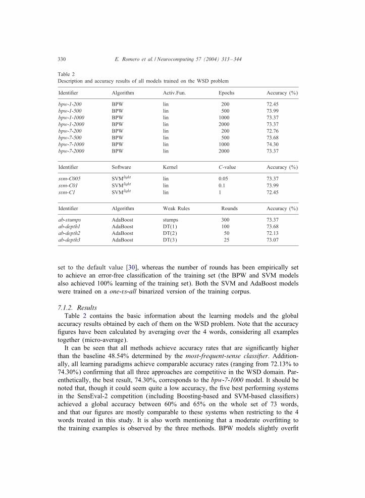
7.1.2. ResultsTable 2 contains the basic information about the learning models and the global
accuracy results obtained by each of them on the WSD problem. Note that the accuracy=gures have been calculated by averaging over the 4 words, considering all examplestogether (micro-average).
It can be seen that all methods achieve accuracy rates that are signi=cantly higherthan the baseline 48.54% determined by the most-frequent-sense classi;er. Addition-ally, all learning paradigms achieve comparable accuracy rates (ranging from 72.13% to74.30%) con=rming that all three approaches are competitive in the WSD domain. Par-enthetically, the best result, 74.30%, corresponds to the bpw-7-1000 model. It should benoted that, though it could seem quite a low accuracy, the =ve best performing systemsin the SensEval-2 competition (including Boosting-based and SVM-based classi=ers)achieved a global accuracy between 60% and 65% on the whole set of 73 words,and that our =gures are mostly comparable to these systems when restricting to the 4words treated in this study. It is also worth mentioning that a moderate over=tting tothe training examples is observed by the three methods. BPW models slightly over=t
E. Romero et al. / Neurocomputing 57 (2004) 313–344 331
Table 3Agreement and Kappa values between linear BPW, AdaBoost and linear SVM models trained on the WSDproblem (test set)
svm-C005 svm-C01 svm-C1
Agreement Kappa Agreement Kappa Agreement Kappa(%) (%) (%)
bpw-1-200 94.74 0.8964 93.48 0.8787 91.64 0.8481bpw-1-500 96.28 0.9286 95.98 0.9279 93.50 0.8855bpw-1-1000 96.28 0.9309 95.98 0.9256 93.81 0.8882bpw-1-2000 94.43 0.8972 95.36 0.9136 93.50 0.8827
bpw-7-200 96.90 0.9397 95.35 0.9164 93.18 0.8810bpw-7-500 96.28 0.9305 97.21 0.9527 95.67 0.9291bpw-7-1000 94.74 0.8994 96.90 0.9428 96.59 0.9406bpw-7-2000 93.19 0.8717 95.67 0.9199 96.28 0.9341
ab-stumps 82.35 0.6940 80.81 0.6762 80.81 0.6785ab-depth1 83.28 0.7193 82.66 0.7169 82.66 0.7165ab-depth2 82.66 0.7024 82.97 0.7132 83.59 0.7217ab-depth3 82.97 0.7055 83.59 0.7209 84.21 0.7298
with the number of epochs, SVM with the hardness of the margin (i.e., high values ofthe C parameter), and AdaBoost with the number of rounds (=gures not included inTable 2) and with the depth of the decision trees.
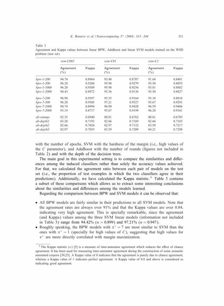
The main goal in this experimental setting is to compare the similarities and di:er-ences among the induced classi=ers rather than solely the accuracy values achieved.For that, we calculated the agreement ratio between each pair of models on the testset (i.e., the proportion of test examples in which the two classi=ers agree in theirpredictions). Additionally, we have calculated the Kappa statistic. 5 Table 3 containsa subset of these comparisons which allows us to extract some interesting conclusionsabout the similarities and di:erences among the models learned.
Regarding the comparison between BPW and SVM models it can be observed that:
• All BPW models are fairly similar in their predictions to all SVM models. Note thatthe agreement rates are always over 91% and that the Kappa values are over 0.84,indicating very high agreement. This is specially remarkable, since the agreement(and Kappa) values among the three SVM linear models (information not includedin Table 3) range from 94.42% () = 0:899) and 97.21% () = 0:947).
• Roughly speaking, the BPW models with �+ = 7 are most similar to SVM than theones with �+ = 1 (specially for high values of C), suggesting that high values for�+ are more directly correlated with margin maximization.
5 The Kappa statistic ()) [5] is a measure of inter-annotator agreement which reduces the e:ect of chanceagreement. It has been used for measuring inter-annotator agreement during the construction of some semanticannotated corpora [39,23]. A Kappa value of 0 indicates that the agreement is purely due to chance agreement,whereas a Kappa value of 1 indicates perfect agreement. A Kappa value of 0.8 and above is considered asindicating good agreement.
332 E. Romero et al. / Neurocomputing 57 (2004) 313–344
• Restricting to bpw-7 models, another connection can be made between the number ofepochs and the hardness of the margin. On the one hand, comparing to the svm-C005models (SVM with a soft margin) the less number of epochs performed the higheragreement rates are achieved. On the other hand, this trend is inverted when com-paring to the hard-margin model of SVM (svm-C1). 6 Put in another way, restrictingto the bpw-7-2000 row, the more harder the SVM margin is, the more similar themodels are, whereas in the bpw-7-200 row the tendency is completely the opposite.
• Note that the behavior described in the last point is not so evident in the bpw-1model, and that in some cases it is even contradictory. We think that this fact isgiving more evidence to the idea that high values of �+ are required to resemble theSVM model, and that the hardness of the margin can be controlled with the numberof iterations.
Regarding the comparison between AdaBoost and SVM models it can be observedthat:
• Surprisingly, the similarities observed among all models are signi=cantly lower thanthose between BPW and SVM. Now, the agreement rates (and Kappa values) rangefrom 80.81% ()=0:676) to 84.21% ()=0:730), i.e., 10 points lower than the formerones. This fact suggests that, even the theoretical modeling of AdaBoost seems tohave strong connections with the SVM paradigm, there are practical di:erences thatmakes the induced classi=ers to partition the input space into signi=cantly di:erentareas.
• A quite clear relation can be observed between the complexity of the weak rules andthe hardness of the margin of the SVM model. The predictions of the AdaBoost mod-els with low-complexity weak rules (say ab-stumps and ab-depth1), are more similarto svm-C005 than to svm-C1. While the predictions of the AdaBoost models withhigh-complexity weak rules (ab-depth2 and ab-depth3) are more similar to svm-C1than to svm-C001. However, given that the absolute agreement rates are so low, wethink that this evidence should be considered weak and only moderately relevant.
• The inSuence of the complexity of the weak rules is signi=cant in the WSD prob-lem. It can be observed that the disagreement among the four AdaBoost models isalso very high in many cases (results not present in Table 3). The agreement ratesvary from 84.83% () = 0:751) to 91.02% () = 0:855), being the most di:erent theextreme models ab-stumps and ab-depth3 (although they are almost equivalent interms of accuracy).
7.2. Text categorization
Text categorization (TC), or classi=cation, is the problem of automatically assign-ing text documents to a set of pre-speci=ed categories, based on their contents. Since
6 Note that there are two cells in the table that seems to contradict this statement, since the agreementbetween bpw-7-2000 and svm-C1 should not be lower than the agreement between bpw-7-1000 and svm-C1,and this is not the case. However, note that the di:erence in agreement is due to the di:erent classi=cationof a unique example, and therefore they can be considered almost equivalent.
E. Romero et al. / Neurocomputing 57 (2004) 313–344 333
the seminal works in the early 1960s, TC has been used in a number of applications,including, among others: automatic indexing for information retrieval systems, docu-ment organization, text =ltering, hierarchical categorization of Web pages, and topicdetection and tracking. See [32] for an excellent survey on text categorization.
From the 1990s, many statistical and machine learning algorithms have been suc-cessfully applied to the text categorization task, including, among others: rule induc-tion, decision trees, Bayesian classi=ers, neural networks [41], on-line linear classi=ers,instance-based learning, boosting-based committees [31], support vector machines [15],and regression models. There is a general agreement in that support vector machinesand boosting-based committees are among the top-notch performance systems.
7.2.1. SettingData set: We have used the publicly available Reuters-21578 collection of docu-
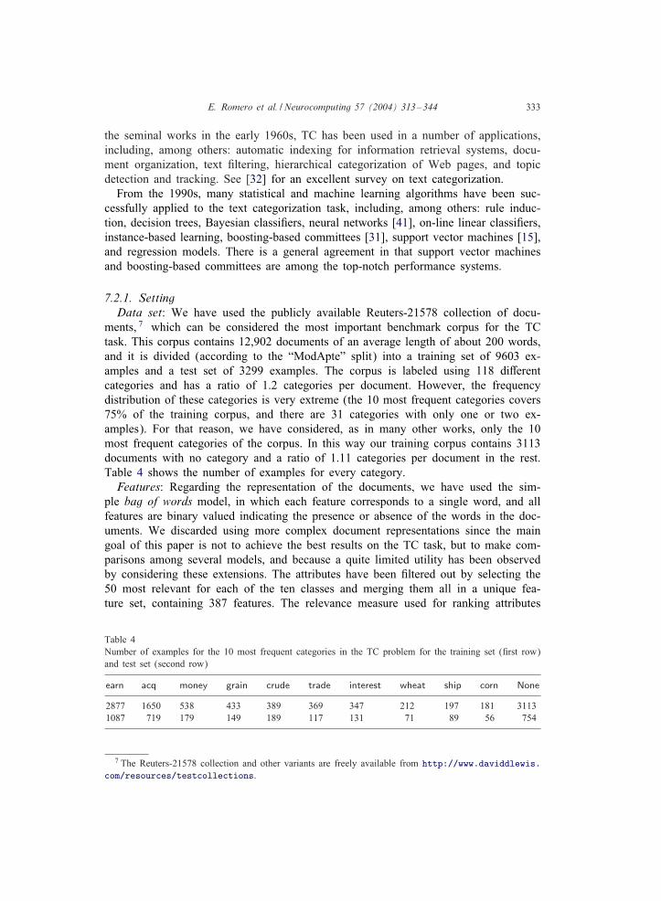
ments, 7 which can be considered the most important benchmark corpus for the TCtask. This corpus contains 12,902 documents of an average length of about 200 words,and it is divided (according to the “ModApte” split) into a training set of 9603 ex-amples and a test set of 3299 examples. The corpus is labeled using 118 di:erentcategories and has a ratio of 1.2 categories per document. However, the frequencydistribution of these categories is very extreme (the 10 most frequent categories covers75% of the training corpus, and there are 31 categories with only one or two ex-amples). For that reason, we have considered, as in many other works, only the 10most frequent categories of the corpus. In this way our training corpus contains 3113documents with no category and a ratio of 1.11 categories per document in the rest.Table 4 shows the number of examples for every category.Features: Regarding the representation of the documents, we have used the sim-
ple bag of words model, in which each feature corresponds to a single word, and allfeatures are binary valued indicating the presence or absence of the words in the doc-uments. We discarded using more complex document representations since the maingoal of this paper is not to achieve the best results on the TC task, but to make com-parisons among several models, and because a quite limited utility has been observedby considering these extensions. The attributes have been =ltered out by selecting the50 most relevant for each of the ten classes and merging them all in a unique fea-ture set, containing 387 features. The relevance measure used for ranking attributes
Table 4Number of examples for the 10 most frequent categories in the TC problem for the training set (=rst row)and test set (second row)
earn acq money grain crude trade interest wheat ship corn None
2877 1650 538 433 389 369 347 212 197 181 31131087 719 179 149 189 117 131 71 89 56 754
7 The Reuters-21578 collection and other variants are freely available from http://www.daviddlewis.com/resources/testcollections.
334 E. Romero et al. / Neurocomputing 57 (2004) 313–344
is the RLM entropy-based distance function used for feature selection in decision-treeinduction [20].Evaluation measures: Note that TC is a multiclass multilabel classi=cation problem,
since each document may be assigned a set of categories (which may be empty). Thus,one may think that a yes/no decision must be taken for each pair (document, category),in order to assign categories to the documents. The most standard way of evaluatingTC systems is in terms of precision (P), recall (R), and a combination of both (e.g.,the F1 measure). Precision is de=ned as the ratio between the number of correctlyassigned categories and the total number of categories assigned by the system. Recallis de=ned as the ratio between the number of correctly assigned categories and the totalnumber of real categories assigned to examples. The F1 measure is the harmonic meanof precision and recall: F1(P; R) = 2PR=(P+ R). It is worth noting that a di:erence of1 or 2 points in F1 should be considered signi=cant, due to the size of the corpus andthe number of binary decisions.Models: The description of the models tested can be seen in Table 5, together with
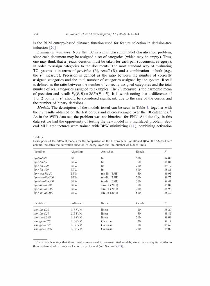
the F1 results obtained on the test corpus and micro-averaged over the 10 categories. 8
As in the WSD data set, the problem was not binarized for FNN. Additionally, in thisdata set we had the opportunity of testing the new model in a multilabel problem. Sev-eral MLP architectures were trained with BPW minimizing (11), combining activation
Table 5Description of the di:erent models for the comparison on the TC problem. For BP and BPW, the “Activ.Fun.”column indicates the activation function of every layer and the number of hidden units
Identi=er Algorithm Activ.Fun. Epochs F1
bp-lin-500 BP lin 500 84.09bpw-lin-50 BPW lin 50 88.84bpw-lin-200 BPW lin 200 89.12bpw-lin-500 BPW in 500 88.81bpw-tnh-lin-50 BPW tnh-lin (35H) 50 89.93bpw-tnh-lin-200 BPW tnh-lin (35H) 200 89.77bpw-tnh-lin-500 BPW tnh-lin (35H) 500 89.41bpw-sin-lin-50 BPW sin-lin (20H) 50 89.87bpw-sin-lin-200 BPW sin-lin (20H) 200 88.93bpw-sin-lin-500 BPW sin-lin (20H) 500 88.30
Identi=er Software Kernel C-value F1
svm-lin-C20 LIBSVM linear 20 88.20svm-lin-C50 LIBSVM linear 50 88.85svm-lin-C200 LIBSVM linear 200 89.09svm-gau-C20 LIBSVM Gaussian 20 89.14svm-gau-C50 LIBSVM Gaussian 50 89.62svm-gau-C200 LIBSVM Gaussian 200 89.02
8 It is worth noting that these results correspond to non-over=tted models, since they are quite similar tothose obtained when model-selection is performed (see Section 7.2.3).
E. Romero et al. / Neurocomputing 57 (2004) 313–344 335
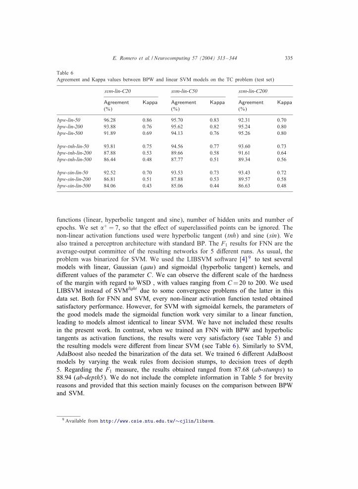
Table 6Agreement and Kappa values between BPW and linear SVM models on the TC problem (test set)
svm-lin-C20 svm-lin-C50 svm-lin-C200
Agreement Kappa Agreement Kappa Agreement Kappa(%) (%) (%)
bpw-lin-50 96.28 0.86 95.70 0.83 92.31 0.70bpw-lin-200 93.88 0.76 95.62 0.82 95.24 0.80bpw-lin-500 91.89 0.69 94.13 0.76 95.26 0.80
bpw-tnh-lin-50 93.81 0.75 94.56 0.77 93.60 0.73bpw-tnh-lin-200 87.88 0.53 89.66 0.58 91.61 0.64bpw-tnh-lin-500 86.44 0.48 87.77 0.51 89.34 0.56
bpw-sin-lin-50 92.52 0.70 93.53 0.73 93.43 0.72bpw-sin-lin-200 86.81 0.51 87.88 0.53 89.57 0.58bpw-sin-lin-500 84.06 0.43 85.06 0.44 86.63 0.48
functions (linear, hyperbolic tangent and sine), number of hidden units and number ofepochs. We set �+ = 7, so that the e:ect of superclassi=ed points can be ignored. Thenon-linear activation functions used were hyperbolic tangent (tnh) and sine (sin). Wealso trained a perceptron architecture with standard BP. The F1 results for FNN are theaverage-output committee of the resulting networks for 5 di:erent runs. As usual, theproblem was binarized for SVM. We used the LIBSVM software [4] 9 to test severalmodels with linear, Gaussian (gau) and sigmoidal (hyperbolic tangent) kernels, anddi:erent values of the parameter C. We can observe the di:erent scale of the hardnessof the margin with regard to WSD , with values ranging from C=20 to 200. We usedLIBSVM instead of SVMlight due to some convergence problems of the latter in thisdata set. Both for FNN and SVM, every non-linear activation function tested obtainedsatisfactory performance. However, for SVM with sigmoidal kernels, the parameters ofthe good models made the sigmoidal function work very similar to a linear function,leading to models almost identical to linear SVM. We have not included these resultsin the present work. In contrast, when we trained an FNN with BPW and hyperbolictangents as activation functions, the results were very satisfactory (see Table 5) andthe resulting models were di:erent from linear SVM (see Table 6). Similarly to SVM,AdaBoost also needed the binarization of the data set. We trained 6 di:erent AdaBoostmodels by varying the weak rules from decision stumps, to decision trees of depth5. Regarding the F1 measure, the results obtained ranged from 87.68 (ab-stumps) to88.94 (ab-depth5). We do not include the complete information in Table 5 for brevityreasons and provided that this section mainly focuses on the comparison between BPWand SVM.
9 Available from http://www.csie.ntu.edu.tw/∼cjlin/libsvm.
336 E. Romero et al. / Neurocomputing 57 (2004) 313–344
7.2.2. ResultsWe can see that the perceptron with standard BP obtained a poor performance,
whereas the other linear classi=ers (BPW and SVM) clearly outperformed this model(see Table 5). Therefore, it seems that the inductive bias provided by the maximizationof the margin has a positive e:ect in this problem, when linear classi=ers are used. Incontrast, for non-linear functions this e:ect was not observed (we also trained severalarchitectures with standard BP and non-linear activation functions, leading to similarresults to those of non-linear models of Table 5). As in WSD , a slight over=tting waspresent at every non-linear model tested: BPW with regard to the number of epochs,SVM with regard to the hardness of the margin and AdaBoost (although slightly) withregard to the number of rounds.
In Table 6 it can observed the comparison of the predictions in the test set (agree-ment 10 and Kappa values) among several SVM models with linear kernels and thesolutions obtained with BPW:
• Looking only at linear BPW models, a strong correlation between the number ofepochs and the hardness of the margin can be observed. It can be checked by simplylooking at the table by rows: BPW models with 50 epochs tend to be more di:erentas the hardness of the margin increases, whereas BPW models with 500 epochs tendto be more similar to hard margin SVM models. This con=rms again the relationbetween the hardness of the margin and the number of iterations, provided �+ hasa large value. For BPW with non-linear activation functions this behavior is not soclear, although there also exist similar tendencies in some cases (see, for example,the rows of the models with 500 epochs).
• Looking at the table by columns, the tendency of the SVM model with C = 20 isto be more similar to the BPW models with 50 epochs. However, the SVM modelwith the hardest margin (C200) signi=cantly tends to be more similar to models withmany epochs only for linear BPW activation functions. For non-linear functions, thetendency is the opposite. Looking at the most similar models between SVM andBPW, we can see that, as expected, the most similar models to svm-lin are those ofbpw-lin, with very signi=cant di:erences over the non-linear ones. The di:erencesdecrease as the margin becomes harder.
The comparison of BPW models with SVM with Gaussian kernels can be seen inTable 7. A similar behavior can be observed, but with some di:erences:
• The tendency of linear BPW models changes: the less similar model to those with200 and 500 epochs is now svm-gau-C200, the model with hardest margin. In con-trast, non-linear BPW models have the same tendency previously shown, leading toa situation where the agreement rates between svm-gau-C200 and any other modelis low. This may be indicating that the harder the margin (either with a larger C inSVM or more epochs in BPW), the highest the importance of the kernel is.
10 Due to the vast majority of negatives in all the (document, category) binary decision of the TC problem,the negative–negative predictions have not been taken into account to compute agreement ratios betweenclassi=ers.
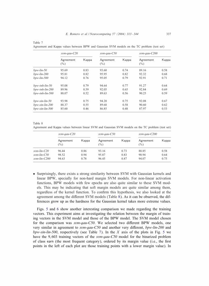
E. Romero et al. / Neurocomputing 57 (2004) 313–344 337
Table 7Agreement and Kappa values between BPW and Gaussian SVM models on the TC problem (test set)
svm-gau-C20 svm-gau-C50 svm-gau-C200
Agreement Kappa Agreement Kappa Agreement Kappa(%) (%) (%)
bpw-lin-50 95.69 0.83 93.60 0.74 89.16 0.58bpw-lin-200 95.81 0.82 95.95 0.82 92.32 0.68bpw-lin-500 94.12 0.76 95.05 0.79 92.91 0.71
bpw-tnh-lin-50 95.08 0.79 94.64 0.77 91.27 0.64bpw-tnh-lin-200 89.96 0.59 92.05 0.65 92.84 0.69bpw-tnh-lin-500 88.07 0.52 89.63 0.56 90.25 0.59
bpw-sin-lin-50 93.98 0.75 94.20 0.75 92.08 0.67bpw-sin-lin-200 88.37 0.55 89.68 0.58 90.60 0.62bpw-sin-lin-500 85.60 0.46 86.85 0.48 87.97 0.53
Table 8Agreement and Kappa values between linear SVM and Gaussian SVM models on the TC problem (test set)
svm-gau-C20 svm-gau-C50 svm-gau-C200
Agreement Kappa Agreement Kappa Agreement Kappa(%) (%) (%)
svm-lin-C20 96.44 0.86 93.16 0.73 88.85 0.58svm-lin-C50 98.52 0.94 95.87 0.83 90.94 0.64svm-lin-C200 94.63 0.78 96.45 0.87 94.07 0.75
• Surprisingly, there exists a strong similarity between SVM with Gaussian kernels andlinear BPW, specially for non-hard margin SVM models. For non-linear activationfunctions, BPW models with few epochs are also quite similar to these SVM mod-els. This may be indicating that soft margin models are quite similar among them,regardless of the kernel function. To con=rm this hypothesis, we also looked at theagreement among the di:erent SVM models (Table 8). As it can be observed, the dif-ferences grow up as the hardness for the Gaussian kernel takes more extreme values.
Figs. 5 and 6 show another interesting comparison we made regarding the trainingvectors. This experiment aims at investigating the relation between the margin of train-ing vectors in the SVM model and those of the BPW model. The SVM model chosenfor the comparison was svm-gau-C50. We selected two di:erent BPW models, onevery similar in agreement to svm-gau-C50 and another very di:erent, bpw-lin-200 andbpw-sin-lin-500, respectively (see Table 7). In the X axis of the plots in Fig. 5 wehave the 9; 603 training vectors of the svm-gau-C50 model for the binarized problemof class earn (the most frequent category), ordered by its margin value (i.e., the =rstpoints in the left of each plot are those training points with a lower margin value). In
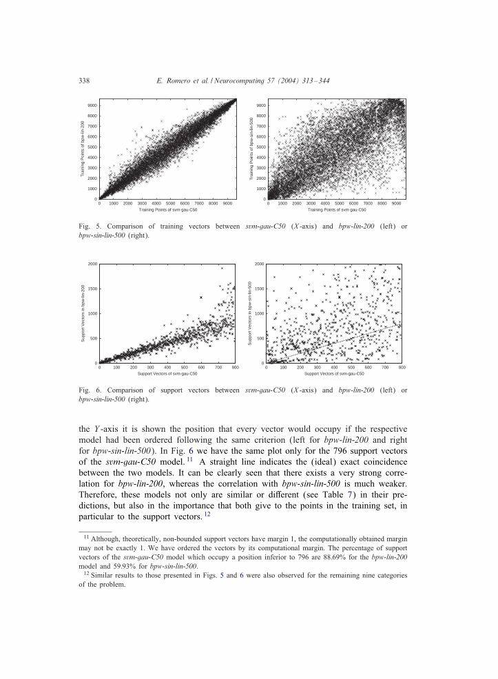
338 E. Romero et al. / Neurocomputing 57 (2004) 313–344
0
1000
2000
3000
4000
5000
6000
7000
8000
9000
0 1000 2000 3000 4000 5000 6000 7000 8000 9000
Tra
inin
g P
oint
s of
bpw
-lin-
200
Training Points of svm-gau-C50
0
1000
2000
3000
4000
5000
6000
7000
8000
9000
0 1000 2000 3000 4000 5000 6000 7000 8000 9000
Tra
inin
g P
oint
s of
bpw
-sin
-lin-
500
Training Points of svm-gau-C50
Fig. 5. Comparison of training vectors between svm-gau-C50 (X -axis) and bpw-lin-200 (left) orbpw-sin-lin-500 (right).
0
500
1000
1500
2000
0 100 200 300 400 500 600 700 800
Sup
port
Vec
tors
in b
pw-li
n-20
0
Support Vectors of svm-gau-C50
0
500
1000
1500
2000
0 100 200 300 400 500 600 700 800
Sup
port
Vec
tors
in b
pw-s
in-li
n-50
0
Support Vectors of svm-gau-C50
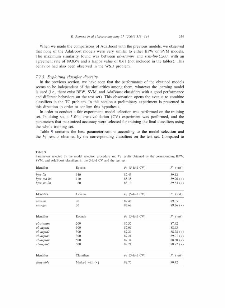
Fig. 6. Comparison of support vectors between svm-gau-C50 (X -axis) and bpw-lin-200 (left) orbpw-sin-lin-500 (right).
the Y -axis it is shown the position that every vector would occupy if the respectivemodel had been ordered following the same criterion (left for bpw-lin-200 and rightfor bpw-sin-lin-500). In Fig. 6 we have the same plot only for the 796 support vectorsof the svm-gau-C50 model. 11 A straight line indicates the (ideal) exact coincidencebetween the two models. It can be clearly seen that there exists a very strong corre-lation for bpw-lin-200, whereas the correlation with bpw-sin-lin-500 is much weaker.Therefore, these models not only are similar or di:erent (see Table 7) in their pre-dictions, but also in the importance that both give to the points in the training set, inparticular to the support vectors. 12
11 Although, theoretically, non-bounded support vectors have margin 1, the computationally obtained marginmay not be exactly 1. We have ordered the vectors by its computational margin. The percentage of supportvectors of the svm-gau-C50 model which occupy a position inferior to 796 are 88:69% for the bpw-lin-200model and 59:93% for bpw-sin-lin-500.
12 Similar results to those presented in Figs. 5 and 6 were also observed for the remaining nine categoriesof the problem.
E. Romero et al. / Neurocomputing 57 (2004) 313–344 339
When we made the comparisons of AdaBoost with the previous models, we observedthat none of the AdaBoost models were very similar to either BPW or SVM models.The maximum similarity found was between ab-stumps and svm-lin-C200, with anagreement rate of 89.83% and a Kappa value of 0.61 (not included in the tables). Thisbehavior had also been observed in the WSD problem.
7.2.3. Exploiting classi;er diversityIn the previous section, we have seen that the performance of the obtained models
seems to be independent of the similarities among them, whatever the learning modelis used (i.e., there exist BPW, SVM, and AdaBoost classi=ers with a good performanceand di:erent behaviors on the test set). This observation opens the avenue to combineclassi=ers in the TC problem. In this section a preliminary experiment is presented inthis direction in order to con=rm this hypothesis.
In order to conduct a fair experiment, model selection was performed on the trainingset. In doing so, a 5-fold cross-validation (CV) experiment was performed, and theparameters that maximized accuracy were selected for training the =nal classi=ers usingthe whole training set.
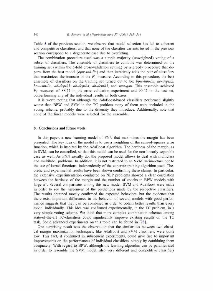
Table 9 contains the best parameterizations according to the model selection andthe F1 results obtained by the corresponding classi=ers on the test set. Compared to
Table 9Parameters selected by the model selection procedure and F1 results obtained by the corresponding BPW,SVM, and AdaBoost classi=ers in the 5-fold CV and the test set
Identi=er Epochs F1 (5-fold CV) F1 (test)
bpw-lin 140 87.45 89.12bpw-tnh-lin 110 88.38 89.96 (∗)bpw-sin-lin 60 88.19 89.84 (∗)
Identi=er C-value F1 (5-fold CV) F1 (test)
svm-lin 70 87.48 89.05svm-gau 30 87.68 89.36 (∗)
Identi=er Rounds F1 (5-fold CV) F1 (test)
ab-stumps 200 86.35 87.92ab-depth1 100 87.09 88.63ab-depth2 300 87.29 88.78 (∗)ab-depth3 300 87.21 89.01 (∗)ab-depth4 500 87.34 88.50 (∗)ab-depth5 500 87.21 88.97 (∗)
Identi=er Classi=ers F1 (5-fold CV) F1 (test)
Ensemble Marked with (∗) 88.77 90.42
340 E. Romero et al. / Neurocomputing 57 (2004) 313–344
Table 5 of the previous section, we observe that model selection has led to coherentand competitive classi=ers, and that none of the classi=er variants tested in the previoussection correspond to a degenerate case due to over=tting.
The combination procedure used was a simple majority (unweighted) voting of asubset of classi=ers. The ensemble of classi=ers to combine was determined on thetraining set (within the 5-fold cross-validation setting) by a greedy procedure that de-parts from the best model (bpw-tnh-lin) and then iteratively adds the pair of classi=ersthat maximizes the increase of the F1 measure. According to this procedure, the bestensemble of classi=ers on the training set turned out to be: bpw-tnh-lin, ab-depth2,bpw-sin-lin, ab-depth3, ab-depth4, ab-depth5, and svm-gau. This ensemble achievedF1 measures of 88.77 in the cross-validation experiment and 90.42 in the test set,outperforming any of the individual results in both cases.
It is worth noting that although the AdaBoost-based classi=ers performed slightlyworse than BPW and SVM in the TC problem many of them were included in thevoting scheme, probably due to the diversity they introduce. Additionally, note thatnone of the linear models were selected for the ensemble.
8. Conclusions and future work
In this paper, a new learning model of FNN that maximizes the margin has beenpresented. The key idea of the model is to use a weighting of the sum-of-squares errorfunction, which is inspired by the AdaBoost algorithm. The hardness of the margin, asin SVM, can be controlled, so that this model can be used for the non-linearly separablecase as well. As FNN usually do, the proposed model allows to deal with multiclassand multilabel problems. In addition, it is not restricted to an SVM architecture nor tothe use of kernel functions, independently of the concrete training algorithm used. The-oretic and experimental results have been shown con=rming these claims. In particular,the extensive experimentation conducted on NLP problems showed a clear correlationbetween the hardness of the margin and the number of epochs in BPW models withlarge �+. Several comparisons among this new model, SVM and AdaBoost were madein order to see the agreement of the predictions made by the respective classi=ers.The results obtained mostly con=rmed the expected behaviors, but the evidence thatthere exist important di:erences in the behavior of several models with good perfor-mance suggests that they can be combined in order to obtain better results than everymodel individually. This idea was con=rmed experimentally, in the TC problem, in avery simple voting scheme. We think that more complex combination schemes amongstate-of-the-art TC-classi=ers could signi=cantly improve existing results on the TCtask. Some advanced experiments on this topic can be found in [28].
One surprising result was the observation that the similarities between two classi-cal margin maximization techniques, like AdaBoost and SVM classi=ers, were quitelow. This fact, if con=rmed in subsequent experiments, could give rise to importantimprovements on the performances of individual classi=ers, simply by combining themadequately. With regard to BPW, although the learning algorithm can be parametrizedin order to resemble the SVM model, also very di:erent and competitive classi=ers
E. Romero et al. / Neurocomputing 57 (2004) 313–344 341
can be learned. In fact, the performance of the obtained models seems to be indepen-dent of their similarities to the SVM model (i.e., there exist models with a very goodperformance and very di:erent of the best SVM models).
The weighting functions proposed in this work are only a =rst proposal to weightthe sum-of-squares error function. We think that this issue deserves further research. Inparticular, we are interested in de=ning weighting functions more robust to over=ttingeither by relaxing the importance of the error of the very bad classi=ed examples (e.g.,following the idea of the BrownBoost algorithm [11]), which are probably outliers ornoisy examples, or by including a regularization term in the weighted sum-of-squareserror function (10).
Although in this work we have only considered classi=cation problems, the sameidea can be applied to regression problems, just by changing the condition of theweighting function (7) from mrg(xi; yi; fFNN)¿ 0 to |fFNN(xi)− yi|6 &, where & is anew parameter that controls the resolution at which we want to look at the data, as inthe &-insensitive cost function proposed in [37]. We are currently working in how toadapt the weighted sum-of-squares error function to this new regression setting.
Acknowledgements
The authors thank the anonymous reviewers for their valuable comments and sug-gestions in order to prepare the =nal version of the paper.
This research has been partially funded by the Spanish Research Department (CI-CYT’s projects: DPI2002-03225, HERMES TIC2000-0335-C03-02, and PETRATIC2000-1735-C02-02), by the European Commission (MEANING IST-2001-34460),and by the Catalan Research Department (CIRIT’s consolidated research group2001SGR-00254 and research grant 2001FI-00663).
References
[1] C.M. Bishop, Neural Networks for Pattern Recognition, Oxford University Press Inc, New York, 1995.[2] R.F. Bruce, J.M. Wiebe, Decomposable Modeling in Natural Language Processing, Comput. Linguistics
25 (2) (1999) 195–207.[3] C. Cardie, R. Mooney (Guest Eds.) Introduction: machine learning and natural language, Machine
Learning (Special Issue on Natural Language Learning) 34 (1–3) (1999) 5–9.[4] C.C. Chang, C.J. Lin, LIBSVM: A Library for Support Vector Machines, http://www.csie.ntu.edu.
tw/∼cjlin/libsvm, 2002.[5] J. Cohen, A coeLcient of agreement for nominal scales, J. Educational Psychol. Measure. 20 (1960)
37–46.[6] N. Cristianini, J. Shawe-Taylor, An Introduction to Support Vector Machines, Cambridge University
Press, UK, 2000.[7] T.G. Dietterich, An experimental comparison of three methods for constructing ensembles of decision
trees: bagging, boosting, and randomization, Mach. Learning 40 (2) (2000) 139–157.[8] G. Escudero, L. M3arquez, G. Rigau, Boosting Applied to Word Sense Disambiguation in: R. L1opez
de M1antaras, E. Plaza (Eds.), Proceedings of the 11th European Conference on Machine Learning,ECML-2000, Springer LNAI 1810, Barcelona, Spain, 2000, pp. 129–141.
342 E. Romero et al. / Neurocomputing 57 (2004) 313–344
[9] G. Escudero, L. M3arquez, G. Rigau, Using LazyBoosting for Word Sense Disambiguation, in:Proceedings of the Second Senseval Workshop on the Evaluation of WSD Systems, Tolouse, France,2001, pp. 71–74.
[10] C. Fellbaum (Ed.), WordNet. An Electronic Lexical Database, MIT Press, 1998.[11] Y. Freund, An adaptive version of the boost by majority algorithm, Mach. Learning 43 (3) (2001)
293–318.[12] Y. Freund, R.E. Schapire, A decision-theoretic generalization of on-line learning and an application to
boosting, J. Comput. System Sci. 55 (1) (1997) 119–139.[13] F. Girosi, An equivalence between sparse approximation and support vector machines, Neural Comput.
10 (6) (1998) 1455–1480.[14] N. Ide, J. V1eronis, Introduction to the special issue on word sense disambiguation: the state of the art,
Comput. Linguistics 24 (1) (1998) 1–40.[15] T. Joachims, Text Categorization with Support Vector Machines: Learning with Many Relevant Features,
in: C. N1edellec, C. Rouveirol, Proceedings of the 10th European Conference on Machine Learning,ECML-1998, LNAI-1398, Chemnitz, Germany, 1998, pp. 137–142.
[16] T. Joachims, Making large-scale SVM learning practical, in: B. SchYolkopf, C. Burges, A. Smola (Eds.),Advances in Kernel Methods—Support Vector Learning, The MIT Press, Cambridge MA, 1999, pp.169–184.
[17] A. Kilgarri:, J. Rosenzweig, English SENSEVAL: report and results, in: Proceedings of the SecondInternational Conference on Language Resources and Evaluation, LREC-2000, Athens, Greece, 2000,pp. 1239–1243.
[18] Y.K. Lee, H.T. Ng, An empirical evaluation of knowledge sources and learning algorithms for wordsense disambiguation, in: Proceedings of the Seventh Conference on Empirical Methods in NaturalLanguage Processing, EMNLP-2002, Philadelphia, PA, 2002, pp. 41–48.
[19] M. Leshno, V.Y. Lin, A. Pinkus, S. Schocken, Multilayer feedforward networks with a nonpolynomialactivation function can approximate any function, Neural Networks 6 (6) (1993) 861–867.
[20] R. L1opez de M1antaras, A distance-based attribute selection measure for decision tree induction, Mach.Learning 6 (1) (1991) 81–92.
[21] B. Magnini, G. Cavaglia, Integrating subject =eld codes into wordnet, in: Proceedings of the SecondInternational Conference on Language Resources and Evaluation, LREC-2000, Athens, Greece, 2000,pp. 1413–1418.
[22] H.T. Ng, Exemplar-based word sense disambiguation: some recent improvements, in: Proceedings of theSecond Conference on Empirical Methods in Natural Language Processing, EMNLP-1997, Providence,RI, 1997, pp. 208–213.
[23] H.T. Ng, C.Y. Lim, S.K. Foo, A case study on inter-annotator agreement for word sense disambiguation,in: Proceedings of the ACL SIGLEX Workshop: Standardizing Lexical Resources, SIGLEX-1999,College Park, MD, 1999, pp. 9–13.
[24] J. Park, I.W. Sandberg, Approximation and radial-basis-function networks, Neural Comput. 5 (2) (1993)305–316.
[25] M.P. Perrone, L.N. Cooper, When networks disagree: ensemble methods for hybrid neural networks,in: R.J. Mammone (Ed.), Arti=cial Neural Networks for Speech and Vision, Chapman & Hall, London,1993, pp. 126–142.
[26] G. RYatsch, S. Mika, B. SchYolkopf, K.-R. MYuller, Constructing boosting algorithms from SVMs: anapplication to one-class classi=cation, IEEE Trans. Pattern Anal. Mach. Intell. 24 (9) (2002) 1184–1199.
[27] S. Raudys, Evolution and generalization of a single neurone: I. Single-layer perceptron as seven statisticalclassi=ers, Neural Networks 11 (2) (1998) 283–296.
[28] E. Romero, X. Carreras, L. M3arquez, Exploiting diversity of margin-based classi=ers research report,LSI-03-49-R, LSI Department, Universitat Polit3ecnica de Catalunya, Barcelona, 2003.
[29] D.E. Rumelhart, G.E. Hinton, R.J. Williams, Parallel Distributed Processing, Vol. 1, The MIT Press,Cambridge, MA, 1986.
[30] R.E. Schapire, Y. Singer, Improved boosting algorithms using con=dence-rated predictions, Mach.Learning 37 (3) (1999) 297–336.
E. Romero et al. / Neurocomputing 57 (2004) 313–344 343
[31] R.E. Schapire, Y. Singer, BOOSTEXTER: a boosting-based system for text categorization, Mach. Learning39 (2–3) (2000) 135–168.
[32] F. Sebastiani, Machine learning in automated text categorization, ACM Comput. Surveys 34 (1) (2002)1–47.
[33] A.J. Smola, B. SchYolkopf, K.R. MYuller, The connection between regularization operators and supportvector kernels, Neural Networks 11 (4) (1998) 637–650.
[34] J.M. Sopena, E. Romero, R. Alqu1ezar, Neural networks with periodic and monotonic activationfunctions: a comparative study in classi=cation problems, in: Proceedings of the Ninth InternationalConference on Arti=cial Neural Networks, ICANN-1999, Edinburgh, Scotland, pp. 323–328.
[35] J.A.K. Suykens, J. Vandewalle, Training multilayer perceptron classi=ers based on a modi=ed supportvector method, IEEE Trans. Neural Networks 10 (4) (1999) 907–911.
[36] G. Towell, E.M. Voorhees, Disambiguating highly ambiguous words, Comput. Linguistics 24 (1) (1998)125–146.
[37] V. Vapnik, The Nature of Statistical Learning Theory, Springer, New York, 1995.[38] V. Vapnik, The support vector method of function estimation, in: C. Bishop (Ed.), Neural Networks
and Machine Learning, Springer, Berlin, 1998, pp. 239–268.[39] J. V1eronis, A study of polysemy judgements and inter-annotator agreement, in: Programme and
Advanced Papers of the First Senseval Workshop, Herstmonceux Castle, Sussex, England, 1998,pp. 2–4.
[40] P. Vincent, Y. Bengio, A neural support vector architecture with adaptive kernels, in: Proceedings of theIEEE International Joint Conference on Neural Networks, IJCNN-2000, Como, Italy, 2000, pp. 187–192.
[41] Y. Yang, X. Liu, A Re-examination of Text Categorization Methods, in: Proceedings of the 22ndAnnual ACM SIGIR Conference on Research and Development in Information Retrieval, SIGIR-1999,Berkeley, CA, 1999, pp. 42–49.
[42] D. Yarowsky, Hierarchical decision lists for word sense disambiguation, Comput. Humanities 34 (2)(2000) 179–186.
Enrique Romero received the B.Sc. degree in Mathematics in 1989 from the Uni-versitat Aut�onoma de Barcelona, and in 1994 the B.Sc. degree in Computer Sciencefrom the Universitat Polit�ecnica de Catalunya (UPC), Spain. In 1996, he joinedthe Software Department (LSI, UPC), as an Assistant professor. He received hisM.Sc. degree in Arti=cial Intelligence in 2000 from the UPC, and he is currentlyworking toward his Ph.D. thesis. His research interests include Machine Learningand Feature Selection.
Llu12s M3arquez is a Computer Science Engineer by the Universitat Polit�ecnica deCatalunya (UPC), Barcelona, Spain, since 1992. He received his Ph.D. degree inComputer Science from the UPC in 1999 and the UPC prize for Doctoral Dis-sertations in the Computer Science area. Currently, he is an Associate Professorof the Software Department (LSI, UPC) teaching at the Facultat d’Inform�aticade Barcelona. He is also a senior researcher of the TALP Center for research inSpeech and Language Technologies (also at UPC). His current research interests arefocused on Machine Learning techniques applied to Natural Language Processing.
344 E. Romero et al. / Neurocomputing 57 (2004) 313–344
Xavier Carreras is a Computer Science Engineer by the Universitat Polit�ecnica deCatalunya (UPC), Spain, since 2000. He received his M.Sc. degree in Arti=cialIntelligence in 2003 from the UPC, and he is currently doing his Ph.D. thesis inArti=cial Intelligence at the same university. His research interests include NaturalLanguage Processing and Machine Learning.
Related Documents