Maps as Numbers Lecture 3 Introduction to GISs Geography 176A Department of Geography, UCSB Summer 06, Session B.

Maps as Numbers

Lecture 3

Introduction to GISs

Geography 176A

Department of Geography, UCSB

Summer 06, Session B

Chapter 3: Maps as Numbers

3.1 Representing Maps as Numbers

3.2 Structuring Attributes

3.3 Structuring Maps

3.4 Why Topology Matters

3.5 Formats for GIS Data

3.6 Exchanging Data

Maps as Numbers

GIS requires that both data and maps be represented as numbers.

The GIS places data into the computer’s memory in a physical data structure (i.e. files and directories).

Files can be written in binary or as ASCII text.

Binary is faster to read and smaller, ASCII can be read by humans and edited but uses more space.

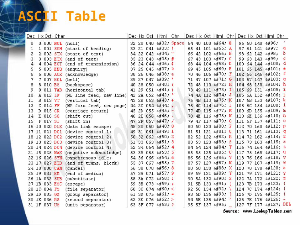
ASCII Table

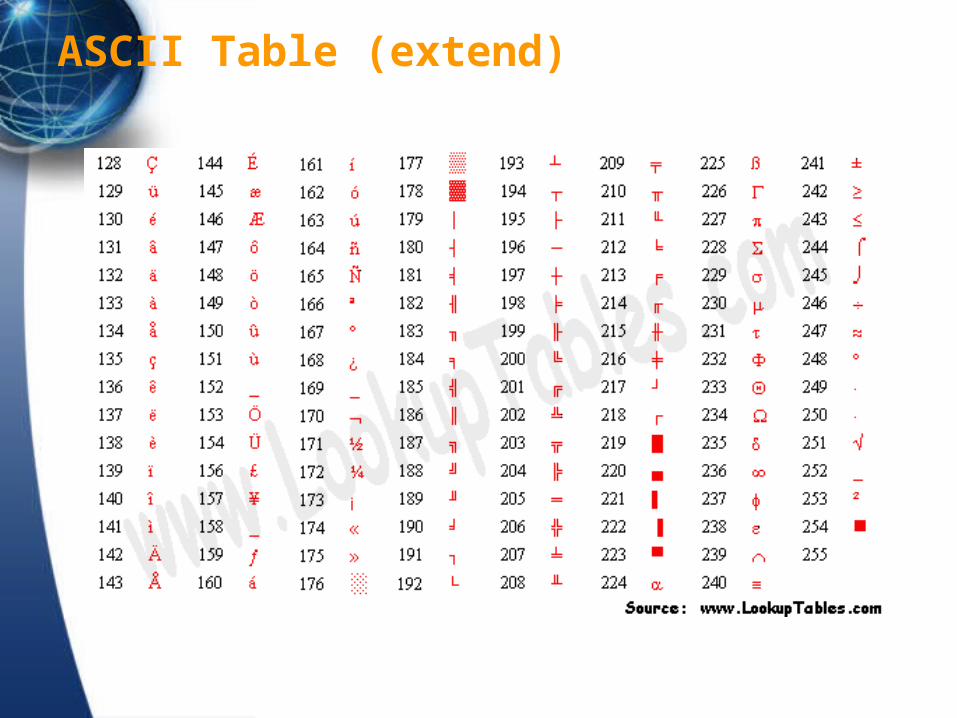
ASCII Table (extend)

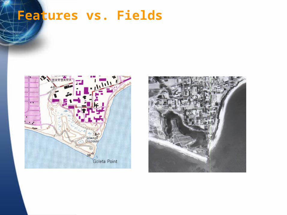
Features vs. Fields

The Data Model

A logical data model is how data are organized for use by the GIS.

GISs have traditionally used either vector or raster for maps.

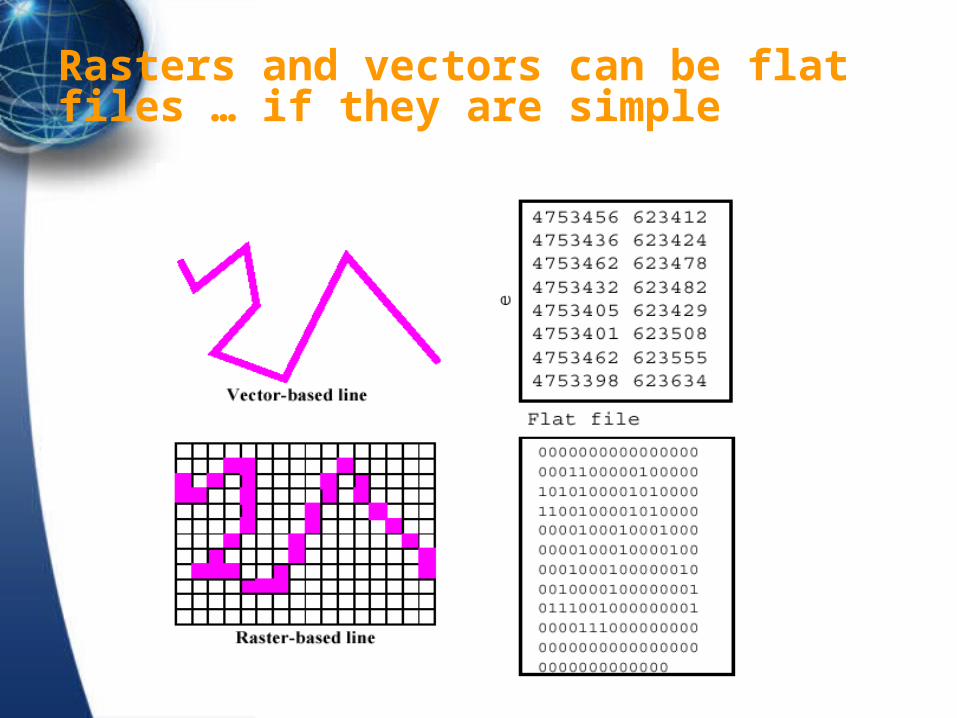
Rasters and vectors can be flat files … if they are simple

Features and Maps

A GIS map is a scaled-down digital representation of point, line, area, and volume features.

While most GIS systems can handle raster and vector, only one is used for the internal organization of spatial data.

Attribute data

Attribute data are stored logically in flat files.

A flat file is a matrix of numbers and values stored in rows and columns, like a spreadsheet.

Both logical and physical data models have evolved over time.

DBMSs use many different methods to store and manage flat files in physical files.

A raster data model uses a grid.

One grid cell is one unit or holds one attribute.

Every cell has a value, even if it is “missing.”

A cell can hold a number or an index value standing for an attribute.

A cell has a resolution, given as the cell size in ground units.

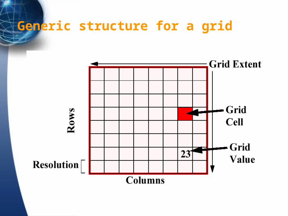
Generic structure for a grid

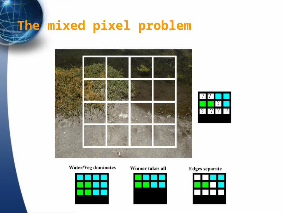
The mixed pixel problem

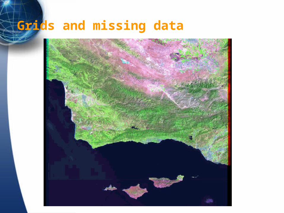
Grids and missing data

Rasters are faster...

Points and lines in raster format have to move to a cell center.

Lines can become fat. Areas may need separately coded edges.

Each cell can be owned by only one feature.

As data, all cells must be able to hold the maximum cell value.

Rasters are easy to understand, easy to read and write, and easy to draw on the screen.

RASTER

A grid or raster maps directly onto a programming computer memory structure called an array.

Grids are poor at representing points, lines and areas, but good at surfaces.

Grids are good only at very localized topology, and weak otherwise.

Grids are a natural for scanned or remotely sensed data.

Grids suffer from the mixed pixel problem.

Grids must often include redundant or missing data.

Grid compression techniques used in GIS are run-length encoding and quad trees.

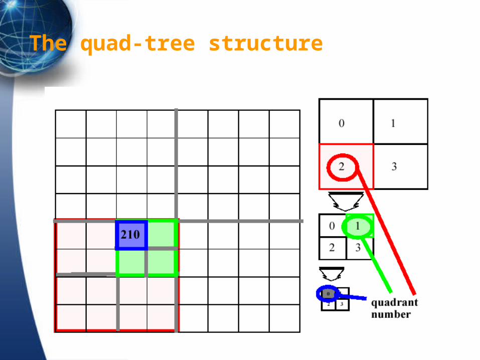
The quad-tree structure

The Vector Model

A vector data model uses points stored by their real (earth) coordinates.

Lines and areas are built from sequences of points in order.

Lines have a direction to the ordering of the points.

Polygons can be built from points or lines.

Vectors can store information about topology.

VECTOR

At first, GISs used vector data and cartographic spaghetti structures.

Vector data evolved the arc/node model in the 1960s.

In the arc/node model, an area consist of lines and a line consists of points.

Points, lines, and areas can each be stored in their own files, with links between them.

The topological vector model uses the line (arc) as a basic unit. Areas (polygons) are built up from arcs.

The endpoint of a line (arc) is called a node. Arc junctions are only at nodes.

Stored with the arc is the topology (i.e. the connecting arcs and left and right polygons).

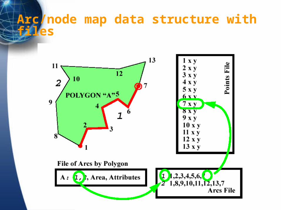
Arc/node map data structure with files

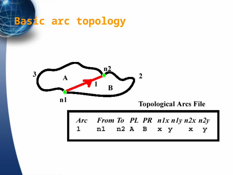
Basic arc topology

Vectors just seemed more correcter.

Vector can represent point, line, and area features very accurately.

Vectors are far more efficient than grids.

Vectors work well with pen and light-plotting devices and tablet digitizers.

Vectors are not good at continuous coverages or plotters that fill areas.

TOPOLOGY

Topological data structures dominate GIS software.

Topology allows automated error detection and elimination.

Rarely are maps topologically clean when digitized or imported.

A GIS has to be able to build topology from unconnected arcs.

Nodes that are close together are snapped.

Slivers due to double digitizing and overlay are eliminated.

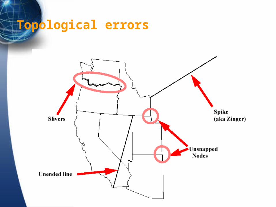
Topological errors

Topology Matters

The tolerances controlling snapping, elimination, and merging must be considered carefully, because they can move features.

Complete topology makes map overlay feasible.

Topology allows many GIS operations to be done without accessing the point files.

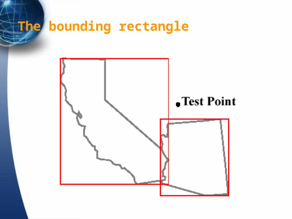
The bounding rectangle

Vectors and 3D

Volumes (surfaces) are structured with the TIN model, including edge or triangle topology.

TINs use an optimal Delaunay triangulation of a set of irregularly distributed points.

TINs are popular in CAD and surveying packages.

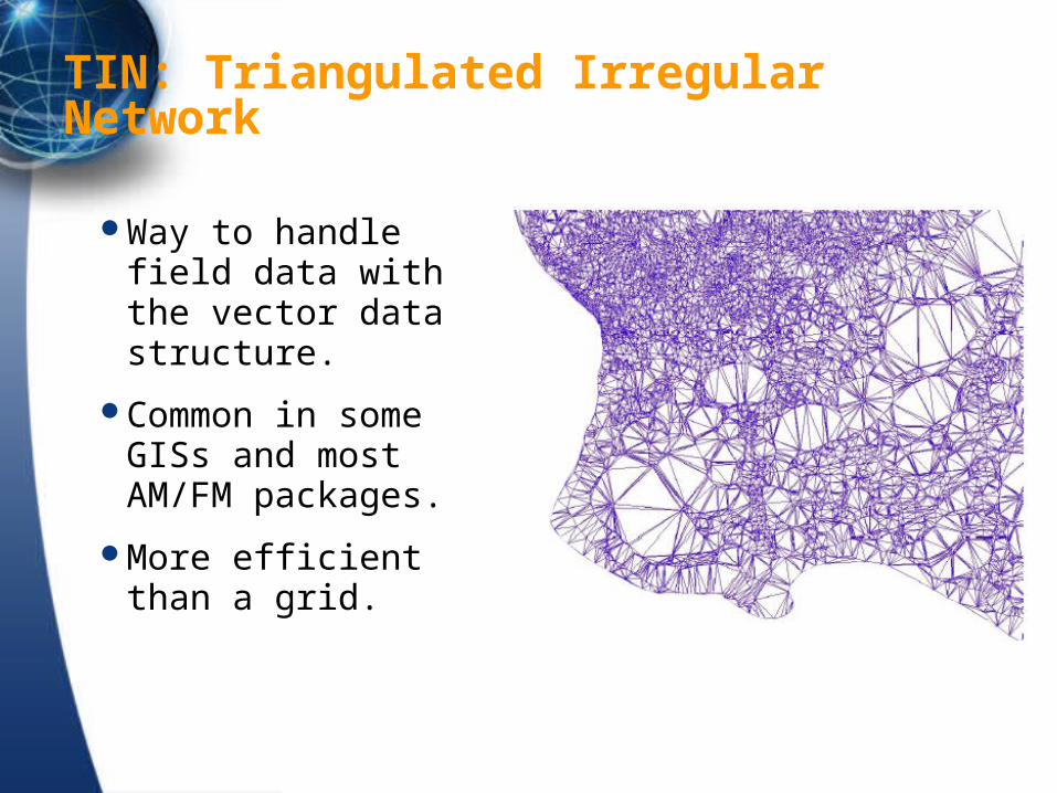
TIN: Triangulated Irregular Network

Way to handle field data with the vector data structure.

Common in some GISs and most AM/FM packages.

More efficient than a grid.

FORMATS

Most GIS systems can import different data formats, or use utility programs to convert them.

Data formats can be industry standard, commonly accepted or standard.

Vector Data Formats

Vector formats are either page definition languages or preserve ground coordinates.

Page languages are HPGL, PostScript, and Autocad DXF.

True vector GIS data formats are DLG and TIGER, which has topology.

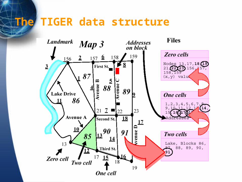
The TIGER data structure

Raster Data Formats

Most raster formats are digital image formats.

Most GISs accept TIF, GIF, JPEG or encapsulated PostScript, which are not georeferenced.

DEMs are true raster data formats.

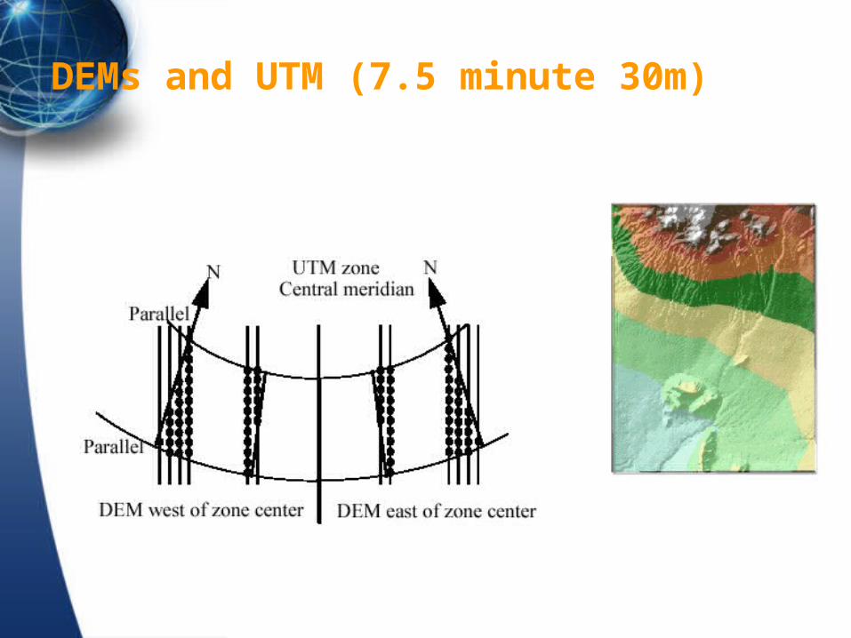
DEMs and UTM (7.5 minute 30m)

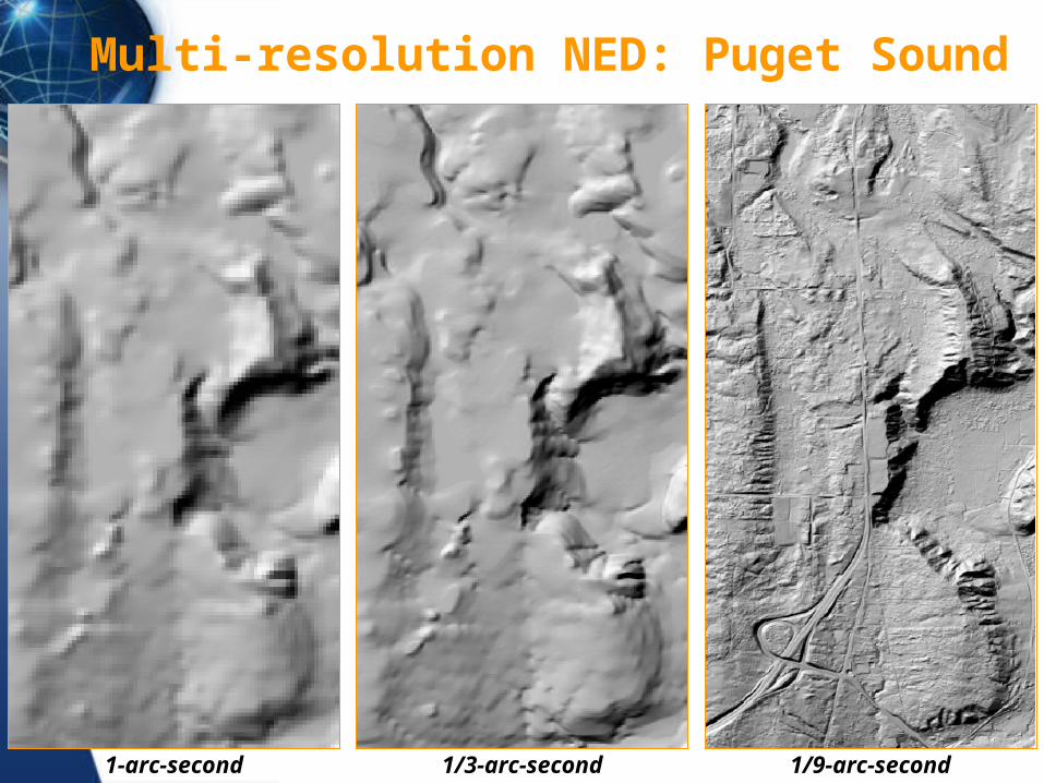
Multi-resolution NED: Puget Sound

1-arc-second 1/3-arc-second 1/9-arc-second

EXCHANGE

Most GISs use many formats and one data structure.

If a GIS supports many data structures, changing structures becomes the user’s responsibility.

Changing vector to raster is easy; raster to vector is hard.

Data also are often exchanged or transferred between different GIS packages and computer systems.

The history of GIS data exchange is chaotic and has been wasteful.

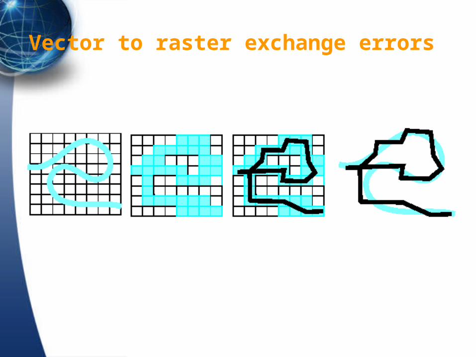
Vector to raster exchange errors

GIS Data Exchange

Data exchange by translation (export and import) can lead to significant errors in attributes and in geometry.

In the United States, the SDTS was evolved to facilitate data transfer.

SDTS became a federal standard (FIPS 173) in 1992.

SDTS contains a terminology, a set of references, a list of features, a transfer mechanism, and an accuracy standard.

Both DLG and TIGER data are available in SDTS format.

Other standards efforts are OpenGIS, DIGEST, DX-90, the Tri-Service Spatial Data Standards, and many other international standards.

Efficient data exchange is important for the future of GIS - Interoperability.

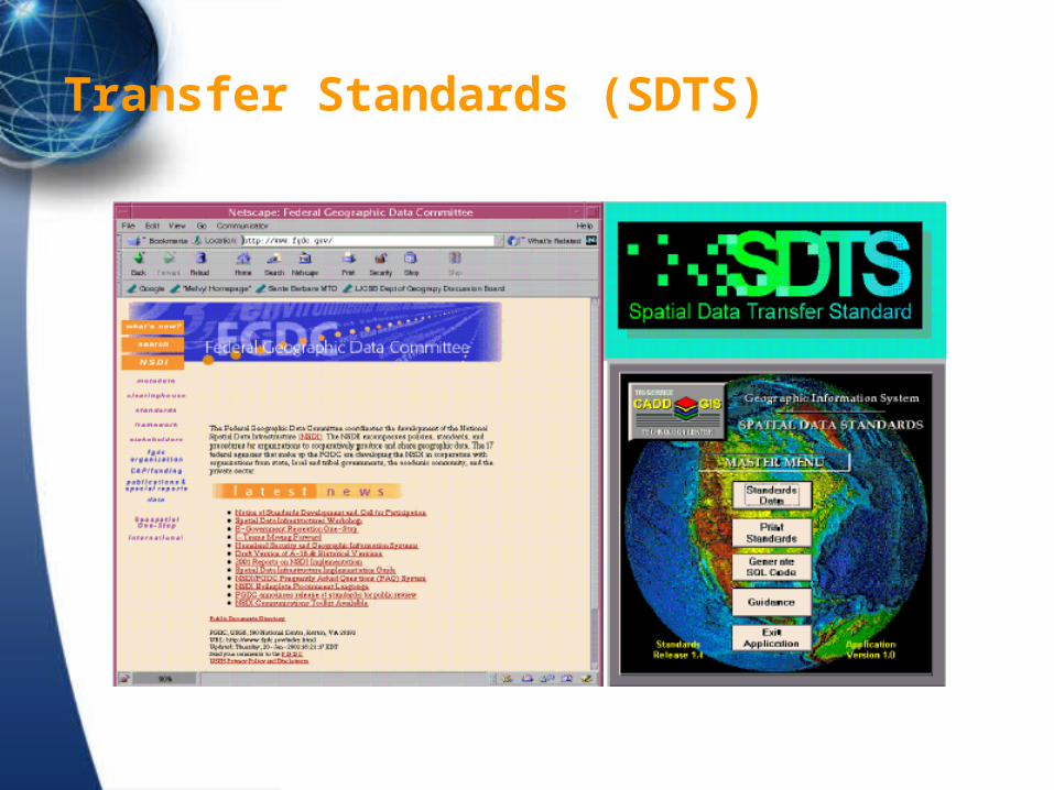
Transfer Standards (SDTS)

Transfer Standards (OpenGIS)

Next Topic:

Getting the Map Into the Computer