Illinois Journal of Mathematics Volume 49, Number 4, Winter 2005, Pages 1039–1060 S 0019-2082 MAPPINGS WITH CONVEX POTENTIALS AND THE QUASICONFORMAL JACOBIAN PROBLEM LEONID V. KOVALEV AND DIEGO MALDONADO Abstract. This paper concerns convex functions that arise as poten- tials of quasiconformal mappings. Several equivalent definitions for such functions are given. We use them to construct quasiconformal mappings whose Jacobian determinants are singular on a prescribed set of Haus- dorff dimension less than 1. 1. Introduction Throughout the paper Ω denotes a convex domain in R n . We use D 2 u(x) to denote the Hessian matrix of a function u :Ω → R at a point x ∈ Ω. The operator norm of a matrix A is denoted by kAk; the Euclidean norm of a vector v is denoted by |v| = hv,vi 1/2 . As usually, W k,p loc stands for local Sobolev spaces of real-valued functions. Definition 1.1. Let Ω ⊂ R n , n ≥ 2. A convex function u :Ω → R is called quasiuniformly convex if u is not affine, u ∈ W 2,n loc (Ω), and there is a constant K ∈ [1, ∞) such that (1.1) kD 2 u(x)k n ≤ K det D 2 u(x), a.e. x ∈ Ω. When we want to specify the value of K, we call u a K-quasiuniformly convex function, usually using the abbreviation “q.u.” Condition (1.1) is equivalent to saying that the ratio of the maximal and minimal eigenvalues of D 2 u is essentially bounded on Ω. This should be compared to a related definition of uniformly convex functions [38, p. 59], which imposes a bound on the Hessian eigenvalues themselves rather than on their ratio. Recall that a function u :Ω → R is λ-uniformly convex if u(x) - λ|x| 2 /2 is convex. One can easily see that if u ∈ C 2 (Ω) is uniformly convex, then u is q.u. convex on every domain Ω 0 that is compactly contained in Ω. However, Example 2.4 below shows that in general q.u. convex functions are not uniformly convex, even locally. Received January 19, 2005; received in final form December 6, 2005. 2000 Mathematics Subject Classification. Primary 30C65. Secondary 26B25, 31B15. c 2005 University of Illinois 1039

Welcome message from author
This document is posted to help you gain knowledge. Please leave a comment to let me know what you think about it! Share it to your friends and learn new things together.
Transcript
Illinois Journal of MathematicsVolume 49, Number 4, Winter 2005, Pages 1039–1060S 0019-2082
MAPPINGS WITH CONVEX POTENTIALS AND THEQUASICONFORMAL JACOBIAN PROBLEM
LEONID V. KOVALEV AND DIEGO MALDONADO
Abstract. This paper concerns convex functions that arise as poten-tials of quasiconformal mappings. Several equivalent definitions for such
functions are given. We use them to construct quasiconformal mappingswhose Jacobian determinants are singular on a prescribed set of Haus-dorff dimension less than 1.
1. Introduction
Throughout the paper Ω denotes a convex domain in Rn. We use D2u(x)to denote the Hessian matrix of a function u : Ω → R at a point x ∈ Ω.The operator norm of a matrix A is denoted by ‖A‖; the Euclidean norm ofa vector v is denoted by |v| = 〈v, v〉1/2. As usually, W k,p
loc stands for localSobolev spaces of real-valued functions.
Definition 1.1. Let Ω ⊂ Rn, n ≥ 2. A convex function u : Ω → R iscalled quasiuniformly convex if u is not affine, u ∈ W 2,n
loc (Ω), and there is aconstant K ∈ [1,∞) such that
(1.1) ‖D2u(x)‖n ≤ K detD2u(x), a.e. x ∈ Ω.
When we want to specify the value of K, we call u a K-quasiuniformlyconvex function, usually using the abbreviation “q.u.” Condition (1.1) isequivalent to saying that the ratio of the maximal and minimal eigenvaluesof D2u is essentially bounded on Ω. This should be compared to a relateddefinition of uniformly convex functions [38, p. 59], which imposes a boundon the Hessian eigenvalues themselves rather than on their ratio. Recall thata function u : Ω → R is λ-uniformly convex if u(x) − λ|x|2/2 is convex. Onecan easily see that if u ∈ C2(Ω) is uniformly convex, then u is q.u. convexon every domain Ω′ that is compactly contained in Ω. However, Example 2.4below shows that in general q.u. convex functions are not uniformly convex,even locally.
Received January 19, 2005; received in final form December 6, 2005.
2000 Mathematics Subject Classification. Primary 30C65. Secondary 26B25, 31B15.
c©2005 University of Illinois
1039
1040 LEONID V. KOVALEV AND DIEGO MALDONADO
Our motivation for introducing quasiuniformly convex functions comesfrom their connection with quasiconformal mappings [24], [37], [39]. In the fol-lowing definition Df stands for the first-order derivative matrix of a mappingf .
Definition 1.2. Let Ω ⊂ Rn, n ≥ 2. An injective mapping f : Ω→ Rn is
called quasiconformal if f ∈ W 1,nloc (Ω;Rn) and there is a constant K ∈ [1,∞)
such that
(1.2) ‖Df(x)‖n ≤ K detDf(x), a.e. x ∈ Ω.
A mapping is called K-quasiregular if it verifies all of the above conditionsexcept for injectivity.
If u is a K-q.u. convex function, then its gradient
f(x) := ∇u(x) =(∂u
∂x1, . . . ,
∂u
∂xn
)is locally in W 1,n and (1.2) holds. This means that f is K-quasiregularand therefore continuous. Suppose that f(x) = f(y) for some distinct pointsx, y ∈ Ω. Since the graph of u admits only one supporting plane at every point,it follows that f(z) = f(x) for all points z between x and y. This contradictsReshetnyak’s theorem [29], [30], which says that nonconstant quasiregularmappings are open and discrete. Therefore, f is injective, which implies thatu is strictly convex (see Corollary 26.3.1 in [31]). To summarize the above, uis K-q.u. convex if and only if f is K-quasiconformal.
In addition to being quasiconformal, f is a monotone mapping [1] in thesense that
〈f(x)− f(y), x− y〉 ≥ 0, x, y ∈ Ω.The interplay between monotonicity and quasiconformality is one of the mainunderlying themes of this paper. While mappings with convex potentials havebeen a subject of recent research (see [8], [9], [10]), our setup is somewhatdifferent since condition (1.1) is not invariant under affine transformations ofRn. However, the family of all quasiuniformly convex functions is invariant
under affine changes of variables.David and Semmes [12] asked for a characterization of nonnegative func-
tions w such that C−1w ≤ detDf ≤ Cw a.e. in Rn for some quasiconformalmapping f : Rn → R
n and some constant C > 0. This question becameknown as the quasiconformal Jacobian problem and drew much interest [4],[5], [21], [26], [32], [33], in part because of its connection to the problem ofcharacterizing bi-Lipschitz images of Rn [5], [6].
Despite all the efforts, “currently there seems to be no good guess as towhat analytic conditions would characterize quasiconformal Jacobians” [5].One can try to gain a better understanding of this problem by studying thesets on which quasiconformal Jacobians assume the values 0 or ∞. Indeed,
MAPPINGS WITH CONVEX POTENTIALS 1041
the function w from the previous paragraph must be equal to 0 or ∞ on thesame set. In order to make these remarks more precise, we introduce somemore notation. Let Ln stand for the n-dimensional Lebesgue measure on Rn,and let dimE denote the Hausdorff dimension of a set E ⊂ Rn. When ϕ is afunction defined on a subset of Rn, we write ess lim
y→xϕ(y) = a if there is a set
Z ⊂ Rn such that Ln(Z) = 0 and limy→x, y/∈Z
ϕ(y) = a.
Definition 1.3. A set E ⊂ Rn is a quasiconformal 0-set if there is a
quasiconformal mapping f : Rn → Rn such that
ess limy→x
detDf(y) = 0, x ∈ E.
A quasiconformal ∞-set is defined in the same way, except that the essentiallimit is required to be ∞ instead of 0.
Definition 1.3 admits an equivalent formulation in terms of the preciserepresentative of detDf . Given a locally integrable function ϕ, its preciserepresentative ϕ is defined by
ϕ(x) =
limr→0
1Ln(B(x, r))
∫B(x,r)
ϕ(y) dLn(y) if the limit exists;
0 otherwise.
According to Definition 1.3, E is a quasiconformal 0-set if and only if
limy→x
detDf(y) = 0, x ∈ E.
The same is true with 0 replaced by ∞.Bonk, Heinonen and Saksman [5] proved that if a set E ⊂ R2 has variational
2-capacity zero, then E is both a quasiconformal 0-set and a quasiconformal∞-set. Note that a set of 2-capacity zero must have Hausdorff dimension zero.In Sections 4 and 5 we combine the tools of convex analysis and potentialtheory to prove that if E ⊂ R
n has Hausdorff dimension strictly smallerthan 1, then E is both a quasiconformal 0-set and a quasiconformal∞-set. Itis known that some sets of dimension 1 are not quasiconformal 0-sets (see §5).
Tyson [36] conjectured that for every compact set E ⊂ Rn of Hausdorffdimension less than 1 and for every ε > 0 there is a quasiconformal mappingf : Rn → R
n such that dim f(E) < ε. Theorem 5.6 suggests that such an fmight arise as the gradient of a convex function. This idea eventually led tothe proof of Tyson’s conjecture [25].
2. Definitions and preliminary results
Let u : Ω→ R be a convex function. For z ∈ Ω, the subdifferential of u atz is the set
∂u(z) = p ∈ Rn : u(x) ≥ u(z) + 〈p, x− z〉 ∀x ∈ Ω.
1042 LEONID V. KOVALEV AND DIEGO MALDONADO
If u is differentiable at z, then ∂u(z) consists of only one vector, namely∇u(z).For z ∈ Ω and p ∈ ∂u(z) let
uz,p(x) = u(x)− u(z)− 〈p, x− z〉, x ∈ Ω.
If u is differentiable at z, then we write uz instead of uz,∇u(z). To avoidpossible confusion, we do not use subscripts to denote derivatives in thispaper. Following Caffarelli [7], we define the section of u with the centerz ∈ Ω, direction p ∈ ∂u(z), and height t > 0 by
Su(z, p, t) = x ∈ Ω : uz,p(x) < t.
If u is differentiable at z, then we write Su(z, t) for Su(z,∇u(z), t). The convexfunctions whose sections are similar in shape to Euclidean balls B(z, r) = x ∈Rn : |x− z| < r shall be of primary interest to us.
Definition 2.1. We say that u : Rn → R has round sections if thereexists a constant τ ∈ (0, 1) with the following property. For every z ∈ Rn,p ∈ ∂u(z) and t > 0 there is R > 0 such that
(2.1) B(z, τR) ⊂ Su(z, p, t) ⊂ B(z,R).
In other words, the boundary of every section of u is pinched between twoconcentric spheres of comparable size.
Definition 2.2. The sections of a convex function u : Rn → R verify theengulfing property with constant C if for every y ∈ Su(x, p, t)
(2.2) Su(x, p, t) ⊂ Su(y, q, Ct), ∀q ∈ ∂u(y).
The Monge-Ampere measure associated with a convex function u : Rn → R
is a Borel measure µu defined by µu(E) = Ln(∂u(E)) for every Borel setE ⊂ Rn [18]. Note that µu does not change if u is replaced with uz,p for anyz ∈ Rn, p ∈ ∂u(z). Given a set E ⊂ Rn such that Ln(E) < ∞, let x∗ be itscenter of mass and define λE = x∗ + λ(x − x∗) : x ∈ E, λ > 0. In otherwords, λE is the dilation of E with respect to its center of mass. The Monge-Ampere measure µu is called doubling if there exist C > 0 and α ∈ (0, 1) suchthat
(2.3) µu(Su(z, p, t)) ≤ Cµu(αSu(z, p, t)), z ∈ Rn, p ∈ ∂u(p), t > 0.
If the sections of u are bounded sets, then the doubling condition on µu canbe proved to be equivalent to the engulfing property of the sections of u(Theorem 2.2 [19] and Theorem 8 [14]). In §3 we will prove that q.u. convexfunctions have round sections and verify the engulfing property.
Definition 2.3. A homeomorphism f : Rn → Rn is called quasisymmet-
ric, or η-quasisymmetric, if there is a homeomorphism η : [0,∞) → [0,∞)
MAPPINGS WITH CONVEX POTENTIALS 1043
such that
(2.4)|f(x)− f(z)||f(y)− f(z)|
≤ η(|x− z||y − z|
), z ∈ Ω, x, y ∈ Ω \ z.
Note that Definition 2.3 makes sense for all n ≥ 1, whereas the abovedefinition of quasiconformal mappings is vacuous when n = 1. In dimensions2 or higher, a mapping f : Rn → R
n is K-quasiconformal if and only ifit is η-quasisymmetric. Moreover, K and η depend only on each other andthe dimension n (see Theorem 11.14 [20] and [37]). The relation betweenconvex functions and quasisymmetric mappings in one dimension is rathersimple: a convex function on a line has a quasisymmetric gradient if andonly if its Monge-Ampere measure is doubling [15], [20]. In §3 we exploresuch connections in higher dimensions. The rest of this section is devoted toseveral basic facts about q.u. convex functions.
We write In for the n × n identity matrix. When A and B are squarematrices, the inequality A ≤ B means that B − A is positive semidefinite.See [23] for basic properties of the positive semidefinite ordering.
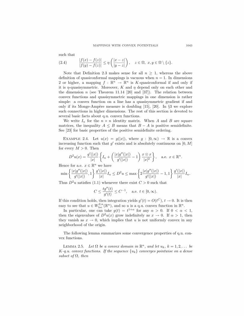
Example 2.4. Let u(x) = g(|x|), where g : [0,∞) → R is a convexincreasing function such that g′ exists and is absolutely continuous on [0,M ]for every M > 0. Then
D2u(x) =g′(|x|)|x|
In +
(|x|g′′(|x|)g′(|x|)
− 1)x⊗ x|x|2
, a.e. x ∈ Rn.
Hence for a.e. x ∈ Rn we have
min|x|g′′(|x|)g′(|x|)
, 1g′(|x|)|x|
In ≤ D2u ≤ max
2|x|g′′(|x|)g′(|x|)
− 1, 1g′(|x|)|x|
In.
Thus D2u satisfies (1.1) whenever there exist C > 0 such that
C ≤ tg′′(t)g′(t)
≤ C−1, a.e. t ∈ [0,∞).
If this condition holds, then integration yields g′(t) = O(tC), t→ 0. It is theneasy to see that u ∈W 2,n
loc (Rn), and so u is a q.u. convex function in Rn.In particular, one can take g(t) = t1+α for any α > 0. If 0 < α < 1,
then the eigenvalues of D2u(x) grow indefinitely as x → 0. If α > 1, thenthey vanish as x → 0, which implies that u is not uniformly convex in anyneighborhood of the origin.
The following lemma summarizes some convergence properties of q.u. con-vex functions.
Lemma 2.5. Let Ω be a convex domain in Rn, and let uk, k = 1, 2, . . . beK-q.u. convex functions. If the sequence uk converges pointwise on a densesubset of Ω, then
1044 LEONID V. KOVALEV AND DIEGO MALDONADO
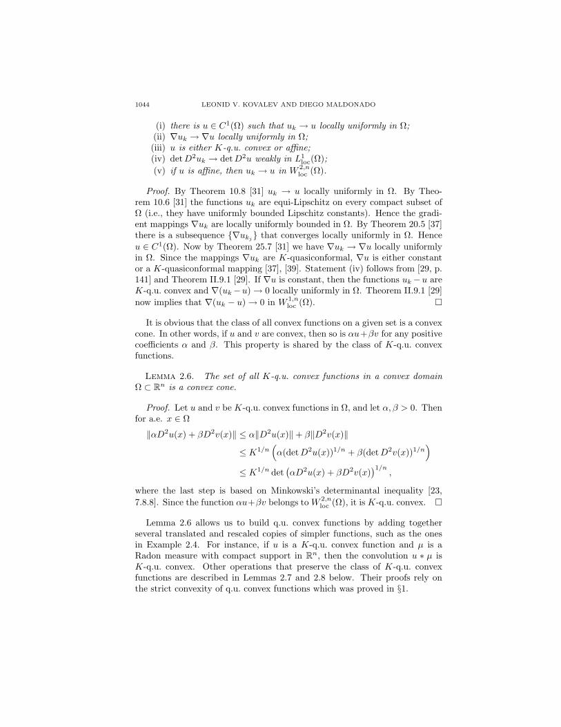
(i) there is u ∈ C1(Ω) such that uk → u locally uniformly in Ω;(ii) ∇uk → ∇u locally uniformly in Ω;(iii) u is either K-q.u. convex or affine;(iv) detD2uk → detD2u weakly in L1
loc(Ω);(v) if u is affine, then uk → u in W 2,n
loc (Ω).
Proof. By Theorem 10.8 [31] uk → u locally uniformly in Ω. By Theo-rem 10.6 [31] the functions uk are equi-Lipschitz on every compact subset ofΩ (i.e., they have uniformly bounded Lipschitz constants). Hence the gradi-ent mappings ∇uk are locally uniformly bounded in Ω. By Theorem 20.5 [37]there is a subsequence ∇ukj that converges locally uniformly in Ω. Henceu ∈ C1(Ω). Now by Theorem 25.7 [31] we have ∇uk → ∇u locally uniformlyin Ω. Since the mappings ∇uk are K-quasiconformal, ∇u is either constantor a K-quasiconformal mapping [37], [39]. Statement (iv) follows from [29, p.141] and Theorem II.9.1 [29]. If ∇u is constant, then the functions uk−u areK-q.u. convex and ∇(uk−u)→ 0 locally uniformly in Ω. Theorem II.9.1 [29]now implies that ∇(uk − u)→ 0 in W 1,n
loc (Ω).
It is obvious that the class of all convex functions on a given set is a convexcone. In other words, if u and v are convex, then so is αu+βv for any positivecoefficients α and β. This property is shared by the class of K-q.u. convexfunctions.
Lemma 2.6. The set of all K-q.u. convex functions in a convex domainΩ ⊂ Rn is a convex cone.
Proof. Let u and v be K-q.u. convex functions in Ω, and let α, β > 0. Thenfor a.e. x ∈ Ω
‖αD2u(x) + βD2v(x)‖ ≤ α‖D2u(x)‖+ β‖D2v(x)‖
≤ K1/n(α(detD2u(x))1/n + β(detD2v(x))1/n
)≤ K1/n det
(αD2u(x) + βD2v(x)
)1/n,
where the last step is based on Minkowski’s determinantal inequality [23,7.8.8]. Since the function αu+βv belongs to W 2,n
loc (Ω), it is K-q.u. convex.
Lemma 2.6 allows us to build q.u. convex functions by adding togetherseveral translated and rescaled copies of simpler functions, such as the onesin Example 2.4. For instance, if u is a K-q.u. convex function and µ is aRadon measure with compact support in Rn, then the convolution u ∗ µ isK-q.u. convex. Other operations that preserve the class of K-q.u. convexfunctions are described in Lemmas 2.7 and 2.8 below. Their proofs rely onthe strict convexity of q.u. convex functions which was proved in §1.
MAPPINGS WITH CONVEX POTENTIALS 1045
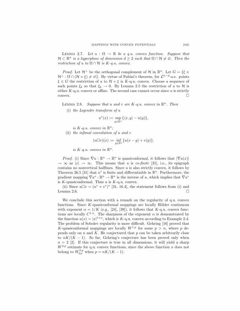
Lemma 2.7. Let u : Ω → R be a q.u. convex function. Suppose thatH ⊂ Rn is a hyperplane of dimension d ≥ 2 such that Ω ∩ H 6= ∅. Then therestriction of u to Ω ∩H is K-q.u. convex.
Proof. Let H⊥ be the orthogonal complement of H in Rn. Let G = ξ ∈H⊥ : Ω ∩ (H + ξ) 6= ∅. By virtue of Fubini’s theorem, for Ln−d-a.e. pointsξ ∈ G the restriction of u to H + ξ is K-q.u. convex. Choose a sequence ofsuch points ξk so that ξk → 0. By Lemma 2.5 the restriction of u to H iseither K-q.u. convex or affine. The second case cannot occur since u is strictlyconvex.
Lemma 2.8. Suppose that u and v are K-q.u. convex in Rn. Then
(i) the Legendre transform of u
u∗(x) := supy∈Rn〈x, y〉 − u(y),
is K-q.u. convex in Rn;(ii) the infimal convolution of u and v
(uv)(x) := infy∈Rnu(x− y) + v(y),
is K-q.u. convex in Rn.
Proof. (i) Since ∇u : Rn → Rn is quasiconformal, it follows that |∇u(x)|
→ ∞ as |x| → ∞. This means that u is co-finite [31], i.e., its epigraphcontains no nonvertical halflines. Since u is also strictly convex, it follows byTheorem 26.5 [31] that u∗ is finite and differentiable in Rn. Furthermore, thegradient mapping ∇u∗ : Rn → R
n is the inverse of u, which implies that ∇u∗is K-quasiconformal. Thus u is K-q.u. convex.
(ii) Since uv = (u∗ + v∗)∗ [31, 16.4], the statement follows from (i) andLemma 2.6.
We conclude this section with a remark on the regularity of q.u. convexfunctions. Since K-quasiconformal mappings are locally Holder continuouswith exponent α = 1/K (e.g., [24], [39]), it follows that K-q.u. convex func-tions are locally C1,α. The sharpness of the exponent α is demonstrated bythe function u(x) = |x|1+α, which is K-q.u. convex according to Example 2.4.The problem of Sobolev regularity is more difficult. Gehring [16] proved thatK-quasiconformal mappings are locally W 1,p for some p > n, where p de-pends only on n and K. He conjectured that p can be taken arbitrarily closeto nK/(K − 1). So far, Gehring’s conjecture has been proved only whenn = 2 [2]. If this conjecture is true in all dimensions, it will yield a sharpW 2,p estimate for q.u. convex functions, since the above function u does notbelong to W 2,p
loc when p = nK/(K − 1).
1046 LEONID V. KOVALEV AND DIEGO MALDONADO
3. Definitions of quasiuniform convexity
The following theorem provides several equivalent definitions of q.u. convexfunctions.
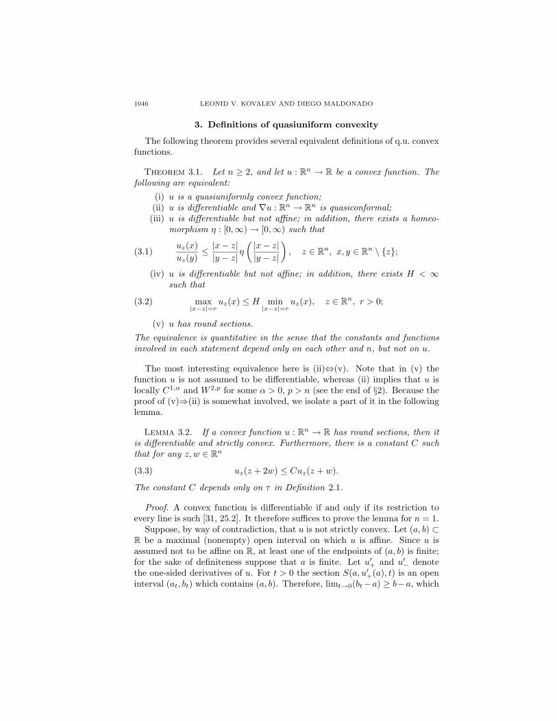
Theorem 3.1. Let n ≥ 2, and let u : Rn → R be a convex function. Thefollowing are equivalent:
(i) u is a quasiuniformly convex function;(ii) u is differentiable and ∇u : Rn → R
n is quasiconformal;(iii) u is differentiable but not affine; in addition, there exists a homeo-
morphism η : [0,∞)→ [0,∞) such that
(3.1)uz(x)uz(y)
≤ |x− z||y − z|
η
(|x− z||y − z|
), z ∈ Rn, x, y ∈ Rn \ z;
(iv) u is differentiable but not affine; in addition, there exists H < ∞such that
(3.2) max|x−z|=r
uz(x) ≤ H min|x−z|=r
uz(x), z ∈ Rn, r > 0;
(v) u has round sections.
The equivalence is quantitative in the sense that the constants and functionsinvolved in each statement depend only on each other and n, but not on u.
The most interesting equivalence here is (ii)⇔(v). Note that in (v) thefunction u is not assumed to be differentiable, whereas (ii) implies that u islocally C1,α and W 2,p for some α > 0, p > n (see the end of §2). Because theproof of (v)⇒(ii) is somewhat involved, we isolate a part of it in the followinglemma.
Lemma 3.2. If a convex function u : Rn → R has round sections, then itis differentiable and strictly convex. Furthermore, there is a constant C suchthat for any z, w ∈ Rn
(3.3) uz(z + 2w) ≤ Cuz(z + w).
The constant C depends only on τ in Definition 2.1.
Proof. A convex function is differentiable if and only if its restriction toevery line is such [31, 25.2]. It therefore suffices to prove the lemma for n = 1.
Suppose, by way of contradiction, that u is not strictly convex. Let (a, b) ⊂R be a maximal (nonempty) open interval on which u is affine. Since u isassumed not to be affine on R, at least one of the endpoints of (a, b) is finite;for the sake of definiteness suppose that a is finite. Let u′+ and u′− denotethe one-sided derivatives of u. For t > 0 the section S(a, u′+(a), t) is an openinterval (at, bt) which contains (a, b). Therefore, limt→0(bt−a) ≥ b−a, which
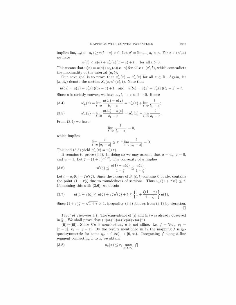
MAPPINGS WITH CONVEX POTENTIALS 1047
implies limt→0(a− at) ≥ τ(b− a) > 0. Let a′ = limt→0 at < a. For x ∈ (a′, a)we have
u(x) < u(a) + u′+(a)(x− a) + t, for all t > 0.This means that u(x) = u(a)+u′+(a)(x−a) for all x ∈ (a′, b), which contradictsthe maximality of the interval (a, b).
Our next goal is to prove that u′−(z) = u′+(z) for all z ∈ R. Again, let(at, bt) denote the section Su(z, u′+(z), t). Note that
u(at) = u(z) + u′+(z)(at − z) + t and u(bt) = u(z) + u′+(z)(bt − z) + t.
Since u is strictly convex, we have at, bt → z as t→ 0. Hence
u′+(z) = limt→0
u(bt)− u(z)bt − z
= u′+(z) + limt→0
t
bt − z;(3.4)
u′−(z) = limt→0
u(at)− u(z)at − z
= u′+(z) + limt→0
t
at − z.(3.5)
From (3.4) we have
limt→0
t
|bt − z|= 0,
which implies
limt→0
t
|at − z|≤ τ−1 lim
t→0
t
|bt − z|= 0.
This and (3.5) yield u′−(z) = u′+(z).It remains to prove (3.3). In doing so we may assume that u = uz, z = 0,
and w = 1. Let ζ = (1 + τ)−1/2. The convexity of u implies
(3.6) u′(ζ) ≤ u(1)− u(ζ)1− ζ
≤ u(1)1− ζ
.
Let t = uζ(0) = ζu′(ζ). Since the closure of Su(ζ, t) contains 0, it also containsthe point (1 + τ)ζ due to roundedness of sections. Thus uζ((1 + τ)ζ) ≤ t.Combining this with (3.6), we obtain
(3.7) u((1 + τ)ζ) ≤ u(ζ) + τζu′(ζ) + t ≤
1 +ζ(1 + τ)
1− ζ
u(1).
Since (1 + τ)ζ =√
1 + τ > 1, inequality (3.3) follows from (3.7) by iteration.
Proof of Theorem 3.1. The equivalence of (i) and (ii) was already observedin §1. We shall prove that (ii)⇒(iii)⇒(iv)⇒(v)⇒(ii).
(ii)⇒(iii). Since ∇u is nonconstant, u is not affine. Let f = ∇uz, r1 =|x − z|, r2 = |y − z|. By the results mentioned in §2 the mapping f is η0-quasisymmetric for some η0 : [0,∞) → [0,∞). Integrating f along a linesegment connecting x to z, we obtain
(3.8) uz(x) ≤ r1 maxB(z,r1)
|f |
1048 LEONID V. KOVALEV AND DIEGO MALDONADO
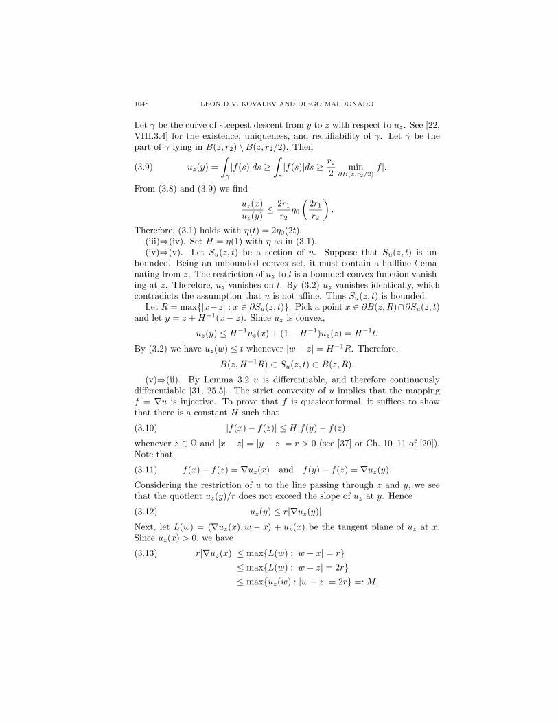
Let γ be the curve of steepest descent from y to z with respect to uz. See [22,VIII.3.4] for the existence, uniqueness, and rectifiability of γ. Let γ be thepart of γ lying in B(z, r2) \B(z, r2/2). Then
(3.9) uz(y) =∫γ
|f(s)|ds ≥∫γ
|f(s)|ds ≥ r2
2min
∂B(z,r2/2)|f |.
From (3.8) and (3.9) we find
uz(x)uz(y)
≤ 2r1
r2η0
(2r1
r2
).
Therefore, (3.1) holds with η(t) = 2η0(2t).(iii)⇒(iv). Set H = η(1) with η as in (3.1).(iv)⇒(v). Let Su(z, t) be a section of u. Suppose that Su(z, t) is un-
bounded. Being an unbounded convex set, it must contain a halfline l ema-nating from z. The restriction of uz to l is a bounded convex function vanish-ing at z. Therefore, uz vanishes on l. By (3.2) uz vanishes identically, whichcontradicts the assumption that u is not affine. Thus Su(z, t) is bounded.
Let R = max|x−z| : x ∈ ∂Su(z, t). Pick a point x ∈ ∂B(z,R)∩∂Su(z, t)and let y = z +H−1(x− z). Since uz is convex,
uz(y) ≤ H−1uz(x) + (1−H−1)uz(z) = H−1t.
By (3.2) we have uz(w) ≤ t whenever |w − z| = H−1R. Therefore,
B(z,H−1R) ⊂ Su(z, t) ⊂ B(z,R).
(v)⇒(ii). By Lemma 3.2 u is differentiable, and therefore continuouslydifferentiable [31, 25.5]. The strict convexity of u implies that the mappingf = ∇u is injective. To prove that f is quasiconformal, it suffices to showthat there is a constant H such that
(3.10) |f(x)− f(z)| ≤ H|f(y)− f(z)|whenever z ∈ Ω and |x− z| = |y − z| = r > 0 (see [37] or Ch. 10–11 of [20]).Note that
(3.11) f(x)− f(z) = ∇uz(x) and f(y)− f(z) = ∇uz(y).
Considering the restriction of u to the line passing through z and y, we seethat the quotient uz(y)/r does not exceed the slope of uz at y. Hence
(3.12) uz(y) ≤ r|∇uz(y)|.Next, let L(w) = 〈∇uz(x), w − x〉 + uz(x) be the tangent plane of uz at x.Since uz(x) > 0, we have
r|∇uz(x)| ≤ maxL(w) : |w − x| = r(3.13)
≤ maxL(w) : |w − z| = 2r≤ maxuz(w) : |w − z| = 2r =: M.
MAPPINGS WITH CONVEX POTENTIALS 1049
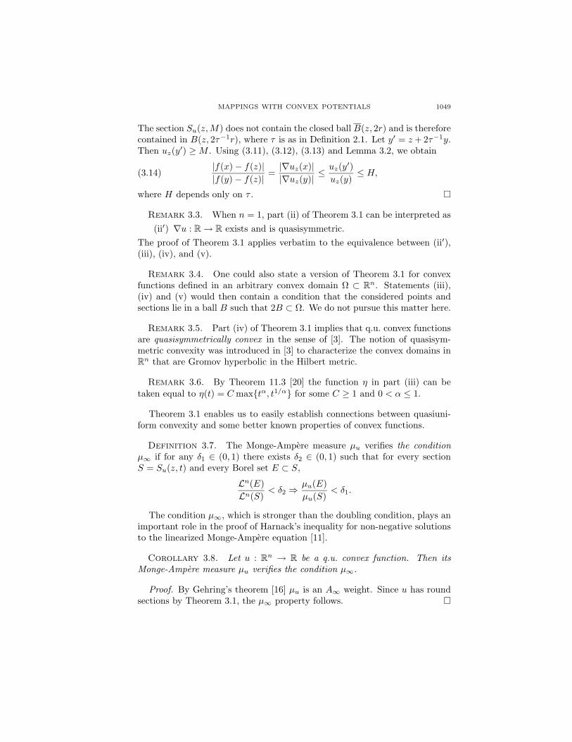
The section Su(z,M) does not contain the closed ball B(z, 2r) and is thereforecontained in B(z, 2τ−1r), where τ is as in Definition 2.1. Let y′ = z+ 2τ−1y.Then uz(y′) ≥M . Using (3.11), (3.12), (3.13) and Lemma 3.2, we obtain
(3.14)|f(x)− f(z)||f(y)− f(z)|
=|∇uz(x)||∇uz(y)|
≤ uz(y′)uz(y)
≤ H,
where H depends only on τ .
Remark 3.3. When n = 1, part (ii) of Theorem 3.1 can be interpreted as(ii′) ∇u : R→ R exists and is quasisymmetric.
The proof of Theorem 3.1 applies verbatim to the equivalence between (ii′),(iii), (iv), and (v).
Remark 3.4. One could also state a version of Theorem 3.1 for convexfunctions defined in an arbitrary convex domain Ω ⊂ Rn. Statements (iii),(iv) and (v) would then contain a condition that the considered points andsections lie in a ball B such that 2B ⊂ Ω. We do not pursue this matter here.
Remark 3.5. Part (iv) of Theorem 3.1 implies that q.u. convex functionsare quasisymmetrically convex in the sense of [3]. The notion of quasisym-metric convexity was introduced in [3] to characterize the convex domains inRn that are Gromov hyperbolic in the Hilbert metric.
Remark 3.6. By Theorem 11.3 [20] the function η in part (iii) can betaken equal to η(t) = C maxtα, t1/α for some C ≥ 1 and 0 < α ≤ 1.
Theorem 3.1 enables us to easily establish connections between quasiuni-form convexity and some better known properties of convex functions.
Definition 3.7. The Monge-Ampere measure µu verifies the conditionµ∞ if for any δ1 ∈ (0, 1) there exists δ2 ∈ (0, 1) such that for every sectionS = Su(z, t) and every Borel set E ⊂ S,
Ln(E)Ln(S)
< δ2 ⇒µu(E)µu(S)
< δ1.
The condition µ∞, which is stronger than the doubling condition, plays animportant role in the proof of Harnack’s inequality for non-negative solutionsto the linearized Monge-Ampere equation [11].
Corollary 3.8. Let u : Rn → R be a q.u. convex function. Then itsMonge-Ampere measure µu verifies the condition µ∞.
Proof. By Gehring’s theorem [16] µu is an A∞ weight. Since u has roundsections by Theorem 3.1, the µ∞ property follows.
1050 LEONID V. KOVALEV AND DIEGO MALDONADO
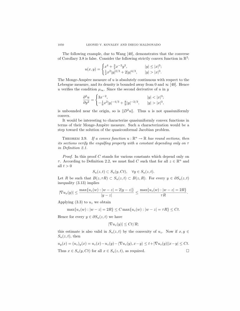
The following example, due to Wang [40], demonstrates that the converseof Corollary 3.8 is false. Consider the following strictly convex function in R2:
u(x, y) =
x4 + 3
2x−2y2, |y| ≤ |x|3;
12x
2|y|2/3 + 2|y|4/3, |y| > |x|3.
The Monge-Ampere measure of u is absolutely continuous with respect to theLebesgue measure, and its density is bounded away from 0 and∞ [40]. Henceu verifies the condition µ∞. Since the second derivative of u in y
∂2u
∂y2=
3x−2, |y| < |x|3;− 1
9x2|y|−4/3 + 8
9 |y|−2/3, |y| > |x|3,
is unbounded near the origin, so is ‖D2u‖. Thus u is not quasiuniformlyconvex.
It would be interesting to characterize quasiuniformly convex functions interms of their Monge-Ampere measure. Such a characterization would be astep toward the solution of the quasiconformal Jacobian problem.
Theorem 3.9. If a convex function u : Rn → R has round sections, thenits sections verify the engulfing property with a constant depending only on τin Definition 2.1.
Proof. In this proof C stands for various constants which depend only onτ . According to Definition 2.2, we must find C such that for all z ∈ Rn andall t > 0
Su(z, t) ⊂ Su(y, Ct), ∀y ∈ Su(z, t).
Let R be such that B(z, τR) ⊂ Su(z, t) ⊂ B(z,R). For every y ∈ ∂Su(z, t)inequality (3.13) implies
|∇ux(y)| ≤ maxuz(w) : |w − z| = 2|y − z||y − z|
≤ maxuz(w) : |w − z| = 2RτR
.
Applying (3.3) to uz we obtain
maxuz(w) : |w − z| = 2R ≤ C maxuz(w) : |w − z| = τR ≤ Ct.
Hence for every y ∈ ∂Su(z, t) we have
|∇uz(y)| ≤ Ct/R;
this estimate is also valid in Su(z, t) by the convexity of uz. Now if x, y ∈Su(z, t), then
uy(x) = (uz)y(x) = uz(x)−uz(y)−〈∇uz(y), x−y〉 ≤ t+ |∇uz(y)||x−y| ≤ Ct.
Thus x ∈ Su(y, Ct) for all x ∈ Su(z, t), as required.
MAPPINGS WITH CONVEX POTENTIALS 1051
4. Quasiconformal ∞-sets
For p ∈ R letMp denote the space of all Radon measures on Rn such that∫(1 + |x|)pdµ(x) < ∞. In other words, M0 is the space of all finite Radon
measures, and Mp is the image of M0 under multiplication by the weight(1 + |x|)−p. The space M0 is naturally equipped with the weak∗ topologysince M0 ⊂ C0(Rn)∗. For p 6= 0 the topology on Mp is induced from M0
by the above multiplication map. The spaces Mp are ordered by inclusion:Mp ⊂ Mq if p > q. In this section we are mainly concerned with the casep < 0, while in §5 we shall consider Mp with p > 0.
For every measure µ ∈Mp its Riesz potential
Iβµ(x) =∫|x− y|β−ndµ(y)
is finite a.e. in Rn as long as 0 < β ≤ n+ p [27, p. 61].
Lemma 4.1. Suppose that µ ∈ Mα−1, 0 < α < 1, and µ(Rn) > 0. Thenthere exists a q.u. convex function u : Rn → R such that
(4.1) αn(In+α−1µ)n ≤ detD2u ≤ (In+α−1µ)n
a.e. in Rn.
Proof. We shall obtain u by convolving µ with the kernel
Kα(x, y) =|x− y|α+1 − |y|α+1
α+ 1+ 〈x, y〉|y|α−1, x, y ∈ Rn,
which is q.u. convex in x by Example 2.4. Using the asymptotic expansion
|x− y|α+1 = |y|α+1
∣∣∣∣ x|y| − y
|y|
∣∣∣∣α+1
= |y|α+1
1− (α+ 1)
〈x, y〉|y|2
+O
(|x|2
|y|2
)= |y|α+1 − (α+ 1)〈x, y〉|y|α−1 +O(|x|2|y|α−1), |y| → ∞,
we obtain
(4.2) Kα(x, y) = O(|y|α−1), |y| → ∞,
locally uniformly in x. Similarly,
(4.3) ∇xKα(x, y) = (x− y)|x− y|α−1 + y|y|α−1 = O(|y|α−1), |y| → ∞,
locally uniformly in x. Let
(4.4) u(x) =∫Kα(x, y)dµ(y), x ∈ Rn.
Since the integral converges locally uniformly in x, it follows from Lemma 2.5that u is a q.u. convex function. Differentiating (4.4) yields
(4.5) ∇u(x) =∫∇xKα(x, y)dµ(y), x ∈ Rn,
1052 LEONID V. KOVALEV AND DIEGO MALDONADO
and
(4.6) D2u(x) =∫|x− y|α−1
(In + (α− 1)
(x− y)⊗ (x− y)|x− y|2
)dµ(y),
for a.e. x ∈ Rn. For any z ∈ Rn we have
αIn ≤ In + (α− 1)z ⊗ z|z|2
≤ In
in the sense of the positive semidefinite ordering. This and (4.6) readilyimply (4.1).
Theorem 4.2. For every set E ⊂ Rn of Hausdorff dimension less than 1there is a q.u. convex function u : Rn → R such that
(4.7) ess limy→x
detD2u(y) =∞, x ∈ E.
Furthermore, there is a set of Hausdorff dimension 1 for which no such uexists.
Proof. Since Hausdorff measures are Borel regular [28, 4.5], we can replaceE with a Borel superset of the same dimension. Thus we may assume that Eis Borel and therefore capacitable [27, 2.8]. Choose γ so that dimE < γ < 1.By Theorem 3.14 [27] the set E has (n − γ)-capacity zero. This means thatthere exists a sequence of open sets
G1 ⊃ G2 ⊃ · · · ⊃ E
such that their (n−γ)-capacity tends to 0. Let E′ =⋂kGk; this is a Gδ-set of
zero (n−γ)-capacity. Let Ej = E′∩B(0, j), j = 1, 2, . . . . By Theorem 3.1 [27]for each j there exists a finite measure µj with compact support on Rn suchthat its Riesz potential In−γµj is infinite at every point of Ej . Since Rieszpotentials are lower semicontinuous, it follows that
(4.8) limy→xIn−γµj(y) =∞, x ∈ Ej .
Let µ =∑j cjµj , where the coefficients cj > 0 are sufficiently small so that
µ ∈ M−γ . (In fact, we can achieve µ ∈ Mp for any p ∈ R by making cj verysmall.) Applying Lemma 4.1 to µ with α = 1− γ, we obtain the first part ofthe theorem.
It remains to show that the condition dimE < 1 cannot be replaced withdimE ≤ 1. Let E be the line segment te1 : 0 ≤ t ≤ 1, where e1 =(1, 0, . . . , 0) ∈ Rn. Suppose that u : Rn → R is a K-q.u. convex functionsuch that (4.7) holds. Then for any given M > 0 there exists ε > 0 suchthat detD2u ≥M a.e. in the ε-neighborhood of E. Since u ∈ W 2,n
loc (Rn), fora.e. x ∈ Rn the function ϕx(t) = u(x + te1), t ∈ R, has locally absolutely
MAPPINGS WITH CONVEX POTENTIALS 1053
continuous derivative ϕ′x. Hence
ϕ′x(1)− ϕ′x(0) =∫ 1
0
ϕ′′x(t)dt, a.e. x ∈ Rn.
If D2u exists at the point x + te1, then ϕ′′x(t) is bounded from below bythe minimal eigenvalue of D2u, which is in turn bounded from below byK−1(detD2u)1/n. Therefore,
(4.9) |∇u(x+ e1)−∇u(x)| ≥ K−1M1/n, a.e. x ∈ B(0, ε).
In fact, the latter inequality holds for all x ∈ B(0, ε) because ∇u is con-tinuous. On the other hand, the continuity of ∇u implies that it is locallybounded. Since the constant M in (4.9) can be arbitrarily large, we arrive ata contradiction.
Corollary 4.3. Every set E ⊂ Rn of Hausdorff dimension less than 1is a quasiconformal ∞-set.
It seems likely that the condition dimE < 1 in Corollary 4.3 can be con-siderably weakened. In fact, it is possible that every set of n-dimensionalmeasure zero is a quasiconformal ∞-set. See [5], [21].
5. Quasiconformal 0-sets
By an argument similar to the second part of the proof of Theorem 4.2, aquasiconformal 0-set cannot contain a line segment [5], [12]. In this sectionwe prove that every set of Hausdorff dimension less than 1 is a quasiconfor-mal 0-set. The idea of the proof is to apply the Legendre transform to theconvex functions constructed in the previous section. The main difficulty liesin finding a q.u. convex function whose Legendre transform has a vanishingHessian matrix on a prescribed set.
Let Mp, p ∈ R, be as in §4. Recall that µk → µ in Mp if and only ifwpµk
w∗−−→ wpµ, where w(x) = (1 + |x|). Given 0 < α < 1 and µ ∈ Mα, wedefine
ρα,µ(x) =|x|2
2+∫|x− y|α+1 − |y|α+1
α+ 1dµ(y), x ∈ Rn;
Fα,µ(x) = ∇ρα,µ(x) = x+∫
(x− y)|x− y|α−1 dµ(y), x ∈ Rn.
Since the integrands are majorized by |y|α locally uniformly in x, both inte-grals converge. Consequently, ρα,µ is q.u. convex. The reader might wonderwhy we did not use the kernel Kα from §4, which would allow for measuresfrom a larger space Mα−1. The reason is that for the proof of Lemma 5.5to work, we need a kernel K(x, y) such that its gradient F = ∇xK is anti-symmetric, i.e., F (x, y) = −F (y, x). Unfortunately, Kα does not possess thisproperty.
1054 LEONID V. KOVALEV AND DIEGO MALDONADO
Lemma 5.1. Let µ ∈Mα, 0 < α < 1. Then
(5.1) |Fα,µ(x)− Fα,µ(y)| ≥ |x− y|, x, y ∈ Rn,
and
(5.2) |x| − C1 ≤ |Fα,µ(x)| ≤ C2|x|+ C3, x ∈ Rn,
where the constants C1, C2 and C3 are positive and depend only on α and∫wαdµ.
Proof. The mapping x 7→ Fα,µ(x)− x is monotone, being the gradient of aconvex function. Since
〈Fα,µ(x)− Fα,µ(y)− (x− y), x− y〉 ≥ 0,
it follows that 〈Fα,µ(x)−Fα,µ(y), x−y〉 ≥ |x−y|2, which implies (5.1). Usingthe elementary inequality |x− y|α ≤ |x|α + |y|α, we obtain
|Fα,µ(x)| ≤ |x|+∫
(|x|α + |y|α) dµ(y).
On the other hand, (5.1) implies
|Fα,µ(x)| ≥ |x| − |Fα,µ(0)| ≥ |x| −∫wα dµ.
This proves (5.2).
Lemma 5.2. Suppose that µk → µ in Mα, 0 < α < 1, and∫wα dµk →∫
wα dµ. Then Fα,µk → Fα,µ and F−1α,µk
→ F−1α,µ locally uniformly in Rn.
Proof. Let µk = wαµk and µ = wαµ. For any bounded continuous functionϕ : Rn → R we have
∫ϕdµk →
∫ϕdµ [13, p. 225]. For any fixed x ∈ Rn
ρα,µk(x) =|x|2
2+∫|x− y|α+1 − |y|α+1
(α+ 1)w(y)αdµk(y),
where the integrand is bounded and continuous on Rn. Hence ρα,µk → ρα,µpointwise in Rn. Since the pointwise convergence of differentiable convexfunctions implies locally uniform convergence of their gradients [31, 25.7],Fα,µk → Fα,µ locally uniformly in Rn. Since F−1
α,µ is a contraction by (i), itfollows that F−1
α,µ Fα,µk → id locally uniformly. Let M = supk|Fα,µk(0)|.Since F−1
α,µkis a contraction,
|F−1α,µk
(x)| ≤ |x− Fα,µk(0)| ≤ |x|+M, x ∈ Rn.
It remains to observe that for every R > 0
sup|x|≤R
|F−1α,µk
(x)− F−1α,µ(x)| ≤ sup
|y|≤R+M
|y − F−1α,µ(Fα,µk(y))| → 0
as k →∞.
MAPPINGS WITH CONVEX POTENTIALS 1055
Consider the pushforward of µ under Fα,µ:
Fα(µ) := (Fα,µ)#µ.
By (5.2) Fα maps Mp into itself for all p ≥ α.
Lemma 5.3. Let 0 < α < 1 and let p ≥ α. If µk → µ in Mp and∫wp dµk →
∫wp dµ, then Fα(µk)→ Fα(µ) in Mp.
Proof. Let µk = wpµk and µ = wpµ. Pick a test function ϕ ∈ C0(Rn). Wemust prove that ∫
ϕwp dFα(µk)→∫ϕwp dFα(µ),
which is equivalent to
(5.3)∫
(ϕ Fα,µk)(w Fα,µk)p
wpdµk →
∫(ϕ Fα,µ)
(w Fα,µ)p
wpdµ.
Since µkw∗−−→ µ and µk(Rn)→ µ(Rn), it suffices to prove that the integrands
in (5.3) converge uniformly in Rn. For this we use Lemma 5.2, whose assump-tions are satisfied because p ≥ α. Since the functions ϕ and w are uniformlycontinuous on Rn, Lemma 5.2 implies
ϕ Fα,µk → ϕ Fα,µ
and
(w Fα,µk)p
wp→ (w Fα,µ)p
wp
locally uniformly. Using (5.2), we find that
lim|x|→∞
supk
(ϕ Fα,µk)(x) = 0
and
supx∈Rn
supk
(w Fα,µk)(x)w(x)
<∞,
hence
lim|x|→∞
supk
(ϕ Fα,µk)(x)(w Fα,µk)p(x)
wp(x)→ 0.
Locally uniform convergence together with uniform vanishing at infinity implyuniform convergence of the integrands in (5.3).
Remark 5.4. The assumptions of Lemma 5.3 are satisfied whenever µk →µ in Mq for some q > p.
Lemma 5.5. Let 0 < α < 1. The mapping Fα : Mp → Mp is surjectivefor all p ≥ 2.
1056 LEONID V. KOVALEV AND DIEGO MALDONADO
Proof. Let us introduce the spaces of finite atomic measures
Mc,m =
cm∑k=1
δak : ak ∈ Rn,
where c > 0 and m ≥ 1. To avoid double indices, write δA =∑mk=1 δak where
A = (a1, . . . , am) ∈ Rmn. Let µ = cδA for some A ∈ Rmn. Then Fα(µ) = cδB ,where
(5.4) bk = ak + c∑l 6=k
(ak − al)|ak − al|α−1, k = 1, . . . ,m.
Define Φ : Rmn → R by
Φ(A) =12
m∑k=1
|ak|2 +c
α+ 1
∑1≤k<l≤m
|ak − al|α+1.
It is easy to see that Φ is a co-finite, strictly convex function and therefore∇Φ : Rmn → R
mn is a bijection. Furthermore, ∇Φ(A) = B, where A and Bare related by (5.4). This shows that Fα :Mc,m →Mc,m is a bijection.
By the same argument as in the first part of Lemma 5.1 we have
|∇Φ(A)−∇Φ(A′)| ≥ |A−A′|, A,A′ ∈ Rmn.
Since ∇Φ(0) = 0, it follows that |∇Φ(A)| ≥ |A| for all A ∈ Rmn. To put itanother way, ∫
|x|2 dFα(µ)(x) ≥∫|x|2 dµ(x), µ ∈Mc,m.
This and µ(Rn) = cm = Fα(µ)(Rn) imply
(5.5)∫
(1 + |x|2) dFα(µ)(x) ≥∫
(1 + |x|2) dµ(x), µ ∈Mc,m.
Given ν ∈ Mp, let ν = wpν and find a sequence νk ⊂⋃c,mMc,m such
that νkw∗−−→ ν and νk(Rn) → ν(Rn). It follows that the family of measures
νk is tight in the sense that
(5.6) limR→∞
supkνk(Rn \B(0, R)) = 0.
For each k let νk = w−pνk and let µk ∈⋃c,mMc,m be such that Fα(µk) = νk.
By virtue of (5.5)
supk
∫w2(x) dµk(x) ≤ 2 sup
k
∫(1 + |x|2) dνk(x)(5.7)
≤ 2 supk
∫wpdνk <∞.
MAPPINGS WITH CONVEX POTENTIALS 1057
Let Fk = Fα,µk . By (5.2) and (5.7) there is a constant C such that Fk(x) ≥|x| − C for all k. Since νk = (Fk)#µk, it follows that∫
|x|>R(1 + |x|)pdµk(x) =
∫|F−1k (x)|>R
(1 + |F−1k (x)|)pdνk(x)
≤∫|x|>R−C
(1 + |x| − C)pdνk(x)
≤ νk(Rn \B(0, R− C)), R > C.
Combining this with (5.6), we conclude that the measures µk = wpµk forma tight family. It follows (see, e.g., [34, p. 133]) that there exists a weak∗-convergent subsequence µkj with a limit µ such that µkj (R
n) → µ(Rn).The measure µ = w−pµ evidently belongs to Mp. By Lemma 5.3 we haveFα(µ) = ν.
Theorem 5.6. Let E ⊂ Rn be a set of Hausdorff dimension less than 1.Then there exists a q.u. convex function u : Rn → R such that
(5.8) ess limy→x
detD2u(y) = 0, x ∈ E.
Proof. As in the proof of Theorem 4.2, we can find α ∈ (0, 1) and ν ∈M2
such that In+α−1ν =∞ on E. Let µ ∈M2 be such that Fα(µ) = ν. By (5.1)the mapping T = F−1
α,µ is a contraction. Since µ = T#ν, for every x ∈ E wehave∫|T (x)− y|α−1 dµ(y) =
∫|T (x)− T (y)|α−1 dν(y) ≥
∫|x− y|α−1 dν(y) =∞.
In other words, the Riesz potential In+α−1µ is infinite on T (E). As in theproof of Theorem 4.2, we obtain
ess limy→x
detD2ρα,µ(y) =∞, x ∈ T (E).
Since ρα,µ is q.u. convex, so is ρ∗α,µ, by virtue of Lemma 2.8. Finally, usingthe fact that ∇ρ∗α,µ = T is the inverse of ∇ρα,µ, we obtain
ess limy→x
detD2ρ∗α,µ(y) = 0, x ∈ E.
This completes the proof.
Corollary 5.7. Every set E ⊂ Rn of Hausdorff dimension less than 1is a quasiconformal 0-set.
Corollary 5.7 is a more satisfactory result than Corollary 4.3, because theformer is sharp as far as the dimension of E is concerned. However, thereexist quasiconformal 0-sets of Hausdorff dimension greater than 1 [17], [35],which means that quasiconformal 0-sets cannot be characterized by their sizealone.
1058 LEONID V. KOVALEV AND DIEGO MALDONADO
Acknowledgements. We would like to thank Albert Baernstein II, LuisA. Caffarelli, Juha Heinonen and Richard Rochberg for helpful discussions,and Tadeusz Iwaniec for his observation that led to Lemma 2.6. Commentsof the referee helped to improve the presentation of the paper.
References
[1] G. Alberti and L. Ambrosio, A geometrical approach to monotone functions in Rn,Math. Z. 230 (1999), 259–316. MR 1676726 (2000d:49033)
[2] K. Astala, Area distortion of quasiconformal mappings, Acta Math. 173 (1994), 37–60.MR 1294669 (95m:30028b)
[3] Y. Benoist, Convexes hyperboliques et fonctions quasisymetriques, Publ. Math. Inst.
Hautes Etudes Sci. (2003), 181–237. MR 2010741 (2005g:53066)
[4] M. Bonk, J. Heinonen, and S. Rohde, Doubling conformal densities, J. Reine Angew.
Math. 541 (2001), 117–141. MR 1876287 (2002k:30036)[5] M. Bonk, J. Heinonen, and E. Saksman, The quasiconformal Jacobian problem, In
the tradition of Ahlfors and Bers, III, Contemp. Math., vol. 355, Amer. Math. Soc.,Providence, RI, 2004, pp. 77–96. MR 2145057
[6] M. Bonk and B. Kleiner, Quasisymmetric parametrizations of two-dimensional metricspheres, Invent. Math. 150 (2002), 127–183. MR 1930885 (2004k:53057)
[7] L. A. Caffarelli, Interior W 2,p estimates for solutions of the Monge-Ampere equation,Ann. of Math. (2) 131 (1990), 135–150. MR 1038360 (91f:35059)
[8] , The regularity of mappings with a convex potential, J. Amer. Math. Soc. 5(1992), 99–104. MR 1124980 (92j:35018)
[9] , Boundary regularity of maps with convex potentials, Comm. Pure Appl. Math.45 (1992), 1141–1151. MR 1177479 (93k:35054)
[10] , Boundary regularity of maps with convex potentials. II, Ann. of Math. (2)
144 (1996), 453–496. MR 1426885 (97m:35027)[11] L. A. Caffarelli and C. E. Gutierrez, Properties of the solutions of the linearized Monge-
Ampere equation, Amer. J. Math. 119 (1997), 423–465. MR 1439555 (98e:35060)[12] G. David and S. Semmes, Strong A∞ weights, Sobolev inequalities and quasiconformal
mappings, Analysis and partial differential equations, Lecture Notes in Pure and Appl.
Math., vol. 122, Dekker, New York, 1990, pp. 101–111. MR 1044784 (91c:30037)[13] G. B. Folland, Real analysis, Pure and Applied Mathematics (New York), John Wiley
& Sons Inc., New York, 1999. MR 1681462 (2000c:00001)[14] L. Forzani and D. Maldonado, On geometric characterizations for Monge-Ampere dou-
bling measures, J. Math. Anal. Appl. 275 (2002), 721–732. MR 1943775 (2003k:35066)
[15] , Doubling weights, quasi-symmetric mappings, and a class of convex functionson the real line, preprint.
[16] F. W. Gehring, The Lp-integrability of the partial derivatives of a quasiconformalmapping, Acta Math. 130 (1973), 265–277. MR 0402038 (53 #5861)
[17] F. W. Gehring and J. Vaisala, Hausdorff dimension and quasiconformal mappings, J.
London Math. Soc. (2) 6 (1973), 504–512. MR 0324028 (48 #2380)[18] C. E. Gutierrez, The Monge-Ampere equation, Progress in Nonlinear Differential
Equations and their Applications, 44, Birkhauser Boston Inc., Boston, MA, 2001.MR 1829162 (2002e:35075)
[19] C. E. Gutierrez and Q. Huang, Geometric properties of the sections of solutions
to the Monge-Ampere equation, Trans. Amer. Math. Soc. 352 (2000), 4381–4396.MR 1665332 (2000m:35060)
[20] J. Heinonen, Lectures on analysis on metric spaces, Universitext, Springer-Verlag, NewYork, 2001. MR 1800917 (2002c:30028)
MAPPINGS WITH CONVEX POTENTIALS 1059
[21] J. Heinonen and S. Semmes, Thirty-three yes or no questions about mappings, mea-sures, and metrics, Conform. Geom. Dyn. 1 (1997), 1–12. MR 1452413 (99h:28012)
[22] J.-B. Hiriart-Urruty and C. Lemarechal, Convex analysis and minimization algorithms.I, Grundlehren der Mathematischen Wissenschaften, vol. 305, Springer-Verlag, Berlin,
1993. MR 1261420 (95m:90001)
[23] R. A. Horn and C. R. Johnson, Matrix analysis, Cambridge University Press, Cam-bridge, 1990. MR 1084815 (91i:15001)
[24] T. Iwaniec and G. Martin, Geometric function theory and nonlinear analysis, OxfordUniv. Press, New York, 2001. MR 1859913 (2003c:30001)
[25] L. V. Kovalev, Conformal dimension does not assume values between 0 and 1, Duke
Math. J., to appear.[26] T. J. Laakso, Plane with A∞-weighted metric not bi-Lipschitz embeddable to RN , Bull.
London Math. Soc. 34 (2002), 667–676. MR 1924353 (2003h:30029)[27] N. S. Landkof, Foundations of modern potential theory, Springer-Verlag, New York,
1972. MR 0350027 (50 #2520)[28] P. Mattila, Geometry of sets and measures in Euclidean spaces, Cambridge Studies
in Advanced Mathematics, vol. 44, Cambridge University Press, Cambridge, 1995.MR 1333890 (96h:28006)
[29] Y. G. Reshetnyak, Space mappings with bounded distortion, Translations of Mathe-
matical Monographs, vol. 73, American Mathematical Society, Providence, RI, 1989.MR 994644 (90d:30067)
[30] S. Rickman, Quasiregular mappings, Ergebnisse der Mathematik und ihrer Grenzgebi-
ete (3), vol. 26, Springer-Verlag, Berlin, 1993. MR 1238941 (95g:30026)[31] R. T. Rockafellar, Convex analysis, Princeton Mathematical Series, No. 28, Princeton
University Press, Princeton, N.J., 1970. MR 0274683 (43 #445)
[32] S. Semmes, Bi-Lipschitz mappings and strong A∞ weights, Ann. Acad. Sci. Fenn. Ser.A I Math. 18 (1993), 211–248. MR 1234732 (95g:30032)
[33] , On the nonexistence of bi-Lipschitz parameterizations and geometric prob-
lems about A∞-weights, Rev. Mat. Iberoamericana 12 (1996), 337–410. MR 1402671(97e:30040)
[34] D. W. Stroock, Probability theory, an analytic view, Cambridge University Press, Cam-bridge, 1993. MR 1267569 (95f:60003)
[35] P. Tukia, A quasiconformal group not isomorphic to a Mobius group, Ann. Acad. Sci.
Fenn. Ser. A I Math. 6 (1981), 149–160. MR 639972 (83b:30019)[36] J. T. Tyson, Sets of minimal Hausdorff dimension for quasiconformal maps, Proc.
Amer. Math. Soc. 128 (2000), 3361–3367. MR 1676353 (2001b:30033)[37] J. Vaisala, Lectures on n-dimensional quasiconformal mappings, Springer-Verlag,
Berlin, 1971. MR 0454009 (56 #12260)
[38] C. Villani, Topics in optimal transportation, Graduate Studies in Mathematics, vol. 58,American Mathematical Society, Providence, RI, 2003. MR 1964483 (2004e:90003)
[39] M. Vuorinen, Conformal geometry and quasiregular mappings, Lecture Notes in Math-ematics, vol. 1319, Springer-Verlag, Berlin, 1988. MR 950174 (89k:30021)
[40] X. J. Wang, Some counterexamples to the regularity of Monge-Ampere equations, Proc.Amer. Math. Soc. 123 (1995), 841–845. MR 1223269 (95d:35025)
1060 LEONID V. KOVALEV AND DIEGO MALDONADO
Leonid V. Kovalev, Department of Mathematics, Washington University, St.
Louis, MO 63130, USA
Current address: Department of Mathematics, Mailstop 3368, Texas A&M University,College Station, TX 77843-3368, USA
E-mail address: [email protected]
Diego Maldonado, Department of Mathematics, University of Kansas, Law-
rence, KS 66045, USA
Current address: Department of Mathematics, University of Maryland, College Park,MD 20742, USA
E-mail address: [email protected]
Related Documents

![GavenJ.Martin arXiv:1311.0899v1 [math.CV] 4 Nov 2013 · The Theory of Quasiconformal Mappings in Higher Dimensions, I 3 1 Introduction Geometric Function Theory in higher dimensions](https://static.cupdf.com/doc/110x72/5f651f339a3ed71b3a104b54/arxiv13110899v1-mathcv-4-nov-2013-the-theory-of-quasiconformal-mappings-in.jpg)


