Mapping temperature using kriging with external …cg.ensmp.fr/bibliotheque/public/HUDSON_Publication_02316.pdf · MAPPING TEMPERATURE USING KRIGING WITH EXTERNAL DRIFT: THEORY AND

INTERNATIONAL JOURNAL OF CLIMATOLOGY, VOL. 14, 77-91 (1994) 551.524.2:551.588.2:528.9(410.5)

MAPPING TEMPERATURE USING KRIGING WITH EXTERNAL DRIFT: THEORY AND AN EXAMPLE FROM SCOTLAND

GORDON HUDSON

Macaulay Land Use Research Institute Craigiehuckler. Aherdeen AB9 2QJ. Scotland

AND

HANS WACKERNAGEL

Centre de GPostatistiyue. Ecole des Mines de Paris, 35 rue Saint Honor;. 77305 Fontainehleau, France

Received I September 1992 Accepted 4 March 1993

ABSTRACT

Land suitability mapping requires information about climate, topography, and soils in relation to crop performance. Climatic data are available from recording stations which present point samples and so interpolation is needed to generate estimates for non-sampled points. The annual temperature cycle must be interpolated differently for different land suitability projects. A common theme, however, is spatial interpolation and here we investigate the application of kriging with external drift to mapping January mean temperatures in Scotland. The spatial structure of the mean temperature is analysed using variograms computed in different directions. From these we see that January temperature is second-order stationary in the north-south direction. Hence the variogram exists in that direction and is taken to represent the underlying variogram. This variogram is modelled and used in universal kriging to produce point-kriged estimates on a 5-km square grid. These estimates d o not adequately show the variation in temperature between stations and so the correlation with elevation was exploited in universal kriging with elevation as external drift. This method gives a kriged estimate for temperature that reproduces the correlation with elevation at the climate stations.

KEY WORDS January temperatures Underlying variogram Non-stationary geostatistics External drift Scotland

INTRODUCTION

Land evaluation systems use information about the soil, topography, and climate to make predictions about the potential of different areas of land for specified uses (Bibby ef al., 1982). The principal information sources comprise climate-station data, topographic maps, and soil maps, augmented with field measurements. The usual way of classifying an area of land is to make spatial interpolations of each variable separately in order to produce maps at the same scale as the existing maps. Once all the data sources are at the same scale on a common grid, they are integrated according to the rules of a classification convention to produce land classification maps. The evaluations are mapped by expert assessment in a GIs. This work needs information about the space and time variability of soil and climatic properties in order to be effective. Temperature is one of the variables used in these assessments and there are crop-specific temperature limits that must be interpolated in both space and time.

The air temperature close to the ground is a factor in plant growth and is an important land characteristic used in determining land qualities in land suitability for agricultural and forest crops. The potential production of a crop, assuming adequate water and nutrient supplies, is controlled by solar radiation and the efficiency with which that radiation is used by t& plants (Cooper, 1969). For a grass crop, canopy structure and duration are known to be temperature dependent (Peacock, 1975), because the crop canopy structure at different stages of the growing cycle affects energy interception and utilization. Plant growth in relation to

0899-841 8/94/010077-15$12.50 0 1994 by the Royal Meteorological Society

78 G. HUDSON AND H. WACKERNAGEL

temperature has been described by Monteith (1977), and in a temperate climate temperature is most important during leaf growth for a wide range of crops, but the yield of wheat is negatively correlated with temperature in summer when the stand is mature. Many studies of how temperatures affect growth and yield are site-specific and to use temperatures in simulation modelling of land suitability over farms or countries we require spatial and temporal interpolation of temperatures from a sparse network of meteorological recording stations.

A spatial analysis of the data utilizing variograms and their multivariate analogues, cross-variograms, seems ideally suited to tackling such assessments. Non-stationary kriging incorporates the trend in the kriging system and co-kriging utilizes the cross-variogram for co-kriging with correlated variables. Several geostatistical approaches to mapping components of the spatial variation and regionalized principal components are discussed in Wackernagel(1988). As a first step towards such analysis we need information about the spatial and temporal autocorrelation of the individual variables. Rainfall has been mapped using kriging (Bigg, 1991) over small regions where stationarity can be assumed. Here we want to estimate over a large region where stationarity cannot be assumed, so we use non-stationary methods to krige temperature. In particular, we focus on January mean air temperatures in Scotland and make use of the dependence of the temperature above the ground on the elevation.

Scotland is situated in the temperate climate zone with a strong maritime influence. The climate varies both in space and time, but here we investigate the use of exhaustive elevation data to help in mapping January mean temperatures for the period 1961-1980 in Scotland. The spatial variation of temperature is strongly controlled by topography, longitude, and latitude, although the distance from the coast also has an effect. The lapse rate of temperature with altitude in Britain has been stated as 0.6"C for 100m altitude (Meteorological Ofice, 1952) and there is further evidence in support of this statement from the North Pennine hills in England, close to the Scottish border (MAFF, 1976). Also the temperature gradient in the troposphere, which occurs below 10000 m, is linear (Lamb, 1972). Knowledge of the relationship between temperature and topography has guided the choice of elevation as an external drift variable in this study, although the use of elevation alone is a first step to exploring the possibilities of using more than one auxiliary variable for kriging or co-kriging temperatures.

TEMPERATURE AND ELEVATION DATA USED IN THE STUDY IN SCOTLAND

Temperatures are measured daily at 149 meteorological stations in Scotland, and we are using January values averaged over a period of 30 years (1951-1980). The stations are all located below 400 m altitude and mainly in agricultural areas. This preferential sampling means that we have no samples from land above 400 m, which covers 21 Yo of Scotland, and the linear relationship we find below 400 m is assumed to apply at the higher elevations.

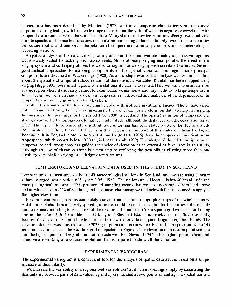
Elevation can be regarded as completely known from accurate topographic maps of the whole country. A data base of elevation at closely spaced grid-nodes could be constructed, but for the purpose of this study and to reduce computing time a subset of the elevation at points on a 5-km square grid was used for kriging and as the external drift variable. The Orkney and Shetland Islands are excluded from this case study, because they have only four climate stations; too few to provide adequate kriging neighbourhoods. The elevation data set was thus reduced to 3035 grid points and is shown on Figure 1. The position of the 145 remaining stations inside the elevation grid is depicted on Figure 2. The elevation data is from point samples and the highest point on the grid does not coincide with Ben Nevis, at 1344 m the highest point in Scotland. Thus we are working at a coarser resolution than is required to show all the variation.

EXPERIMENTAL VARIOGRAM

The experimental variogram is a convenient tool for the analysis of spatial data as it is based on a simple measure of dissimilarity.

We measure the variability of a regionalized variable z(x) at different spacings simply by calculating the dissimilarity between pairs of data values, z1 and z2 say, located at two points x1 and x2 in a spatial domain

JANUARY TEMPERATURES IN SCOTLAND BY KRlGlNG 79

Figure 1. The elevation in Scotland at 3035 nodes of a 5 x 5 kmz grid

D. The measure for the dissimilarity of two values, labelled y*, is

i.e. half of the square of the difference between the two values.

described by a vector h = x2 -xl We let the dissimilarity y* depend on the spacing and on the orientation of the point pair, which is

Y * (h) = 1 CZ(Xl+ h) - z(x 111 By forming the average of the dissimilarities y*(h) for all N h point pairs that can be linked by a vector

h (with, in the case of an irregularly mekhed sampling grid, a given tolerance on the length and the orientation of the vector) we obtain the experimental variogram

1 Nh Y*(h) = __ c CZ(Xa + h) - z(x,)12

2Nh a= 1

Usually we can observe that the dissimilarity between values increases on average when the spacing between the pairs of sample points is increased at low separation distance.

80

900.

800.

700.

600.

G. HUDSON AND H. WACKERNAGEL

100. 200. 300. 400. km

Stations Figure 2. The location in Scotland of the 145 climate stations on the grid

The behaviour at very small scales, near the origin of the variogram, is critical as it indicates the type of continuity of the regionalized variable: differentiable, continuous but not differentiable, or discontinuous. In this last case, when the variogram is discontinuous at the origin, this is a symptom of a ‘nugget-effect’, which means that the values of the variable change abruptly at a very small scale, like gold grades when a few gold nuggets are contained in the samples.

MODEL OF THE EXPERIMENTAL VARIOGRAM

The regionalized variable z(x) is viewed as a realization of a random function Z(x) composed of a mean function m(x) and of a second-order stationary random function Y(x) with a mean equal to zero,

Z(x) = m(x) + Y(x)

The random function Y(x), called the ‘residual’, has a stationary covariance function Cy (h) that describes the covariance between any pair of random variables { Y(x), Y(x + h)} independently of the position of the point x in the domain,

Cy(h)= E [ Y(x) x Y(x + h)]

The theoretical variogram yz(h) of the random function Z(x) is defined as half of the variance of the squared differences at a lag h,

Yz(h) = 4 varC(Z(x + h) - z(x))zl

JANUARY TEMPERATURES IN SCOTLAND BY KRIGING 81

As Y(x) is second-order stationary, a variogram yy(h) can be constructed on the basis of the covariance function Cy(h) using the relation

Y Y (h) = fEC( Y(X + h) - y(x))21 = CY (0) - CY (h)

THE DRIFT

The mean function m(x) is called the ‘drift’. We assume that the drift is a smooth function of the coordinate vector x and that it can be represented by a polynomial of order k with coefficients al,

L

m ( x ) = c alfi(X) l = O

where the L + 1 basis functionsf(x) span a vector space which is translation invariant. Polynomials of order one and two were tested by cross-validation and the order one gave the lowest mean squared error. So we assume for this study that the drift in temperature is a linear function of the components of the coordinate vector,

m(x) = m ( x l , x2) = a. + alxl + a2x2

where x1 is the National Grid easting and x2 is the northing.

then the variogram of Z(x) along this coordinate is obviously equal to the variogram of Y(x): Further we shall use the fact that when the drift is constant in a direction parallel to one coordinate, x1 say,

yz(h)=rv(M9 if m(x1)=ao.

Building on an assumption of isotropy of yy(h), it will be possible to infer the theoretical variogram of the residual Y(x) from the experimental variogram of Z(x), computed in a direction where the drift is constant (Armstrong, 1984).

In general, however, the drift is not likely to be constant in any direction of space. Hence a more sophisticated approach is necessary, based on intrinsic random functions of order k and involving generalized covariances instead of variograms (Matheron, 1973; Chauvet and Galli, 1982).

MODELLING THE VARIOGRAM OF JANUARY MEAN TEMPERATURE

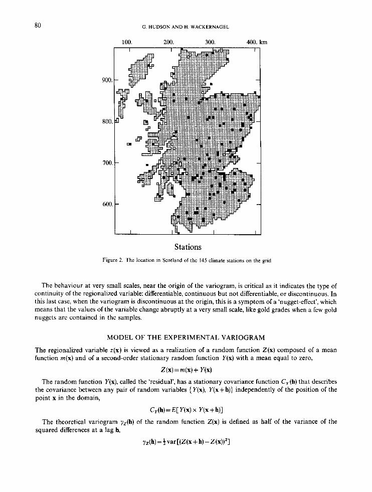
In January, mean temperature is well correlated with longitude (-0.55) but not correlated with latitude (0.07), as can be seen on Figures 3 and 4. Variograms calculated along longitude and latitude are shown on Figure 5. The experimental variogram in the E-W direction is strongly influenced by the drift in the longitudes and grows without bounds, while the N-S variogram has an upper asymptote (the ‘sill’) as there is no drift in temperature with latitudes. The variogram in the N-S direction is taken as the underlying variogram in the other directions. The structure of the spatial variation observed for July mean temperature was different to that of January, the drift was absent in the longitudes and strong along the latitudes (Hudson, 1991), and the direction of the drift changes in spring and autumn. We assume that mean monthly temperatures are highly spatially continuous and hence suppose that the variogram has zero nugget effect. A theoretical variogram composed of three nested spherical models was fitted to the N-S variogram and this model is used in kriging. A simpler model of the experimental variogram, comprising two nested models would produce similar kriged estimates provided the shape of the function was similar at the origin. The spherical model is not differentiable at the origin and so is robust for kriging (Armstrong and Wackernagel, 1988). A spherical covariance model is derived by calculating the volume of the intersection of two spheres of radius r whose centres are separated by a vector h. The radius r can be thought of as half the correlation length (range) around a point x of the domain. The model derived in three dimensions is also valid in two dimensions, though a model derived in two dimensions could have been used. In this study three spherical models with radii 20, 70, and 150 km were used. The significance of the ranges is not clear because many factors influence the spatial variability, and hence the variogram, of mean temperatures in Scotland.

82 G. HUDSON A N D H. WACKERNAGEL

3.0

2.0

1 .o I

.*

M i I 100.0 200.0 300.0 400.0 km

Longitude

Figure 3. Correlation diagram of January mean temperature with longitude

3.0

2.0

x * * It x It

x x x 1 %

x x

Y x x It*

1 .o

600.0 700.0 800.0 900.0 km

Latitude

Figure 4. Correlation diagram of January mean temperature with latitude

UNIVERSAL KRIGING THEORY AND APPLICATION TO JANUARY TEMPERATURE

The kriging operation is usually repeated at each node of a regular grid (here we shall use the grid-nodes defined by the elevation grid). Around each grid node xo the n nearest samples at locations x, are selected and this is called the 'kriging neighbourhood'. An estimator Z*(xo) is sought using a weighted average of the


1 S O

1 .oo

0.50

0. h 0. 50.0 100.0 150.0 km

Figure 5. Variogram of January mean temperature

selected samples with weights ,la,

The estimation error Z(xo)-Z*(xo), i.e. the difference between the unknown true value at xo and the estimated value should be nil on average,

n

ECZ(x0) - Z*(xo) l= m(x0) - 1 Aam(xa) = 0 a = l

This condition can be fulfilled by constraining the sum of weights Aa to filter each coefficient of the drift polynomial. In this case study, the filtering of the three coefficients ao, u l , and u2 of a linear drift in two spatial dimensions produces the three constraints:

n n n

Next, the variance of the estimation error is to be minimized, and the three constraints give rise to three Lagrange parameters po, pl, and p 2 . Solving the ‘universal kriging’ system,

, n

\ n n n


Figure 6 . Kriged map of January mean temperature using climate station data

yields the optimal weights Am as well as the minimal estimation variance &, called the ‘kriging variance’, n

d= C ~ a ~ ~ ( ~ a - ~ o ) + ~ ~ + ~ l ~ o , ~ + ~ z x O , z u = l

The map of January mean temperature in Scotland on Figure 6 is obtained by using the temperature data at 145 meteorological stations. The kriging neighbourhood consists of the 20 nearest stations around each node. The minimum of the kriging estimates is 064°C and is within the range of the data (minimum, 0.6”C; maximum, 52°C). The map is thus unsatisfactory in the mountainous areas of Scotland, which rise far above 400 m where temperatures are expected to be significantly cooler than at the meteorological stations in the valleys and on the plains. This leads us to choose a geostatistical technique that integrates explicitly the elevation data measured everywhere in Scotland. .

THE EXTERNAL DRIFT METHOD

In certain applications a regionalized variable s(x) can be measured exhaustively in the domain D. If s(x) happens to be equivalent to E[Z(x) ] up to a linear transformation with coefficients bo and b l ,

E[Z(x)] =bo + bl S ( X )


the map of s(x) reflects in a way the average shape of Z(x)-just the scaling is different. When such a shape function is available, it is worthwhile to insert it as an additional constraint into the universal kriging system. Starting from the relation,

n n n

EIZ*(xo)] = 1 1, E [Z(x,)] = bo + bl c Aas(x4)= bo + bls(xo) with A, = 1 a = 1 a = l a= 1

we obtain the condition n c 1&4) = S ( X 0 )

a = 1

and bo and bl are filtered by weights 1, constrained in this way. This is an ‘external drift’ condition because it is incorporated into the universal kriging system on the basis

of considerations that are not connected with the computation and the inference of the variogram (or generalized covariance) of Z(x). In the present case study the mean function m(x) depends both on the internal drift with the coordinates and on the external drift with elevation

m(x)= b o + a l x l +azxz +bls(x)

The external drift method originated in petroleum and gas exploration where a few accurately measured (expensive) borehole data z(x) needed to be combined with many fairly imprecise (but easily obtainable) seismic data s(x) in order to map the top of a reservoir (Delhomme, 1979; Galli and Meunier, 1987). More recently the method has been applied in hydrogeology to map the log of transmissivity z(x) using the log of specific capacity s(x) as an external drift variable (Ahmed and de Marsily, 1987). Another application in the same field consists in mapping piezometric measurements in a given year by combining the few available data z(x) from that year with a great many data s(x) gathered in a former year (Chiles, 1991). The possibility of including several shape functions as external drift has been tested by Renard and Nai-Hsien (1988).

We wish to stress that auxiliary variables should be incorporated in the form of an external drift only if they are highly linearly correlated with the variable of interest. Otherwise it is preferable to use the method of co-kriging, which requires the fitting of a model for the cross-variograms between the different variables.

With data from Northern Italy of the same type as in this case study, but with stations at all altitudes Liberta and Girolamo (1991) were able to fit a variogram in three-dimensional space (latitude, longitude, and altitude) and thus used elevation as an internal drift.

THE CORRELATION OF TEMPERATURE WITH ELEVATION

Average temperatures are controlled by factors that are strongly correlated with spatial location and topography. Incoming solar radiation declines with increasing distance from the Equator and the amount received by the land varies according to the aspect. Locally, in temperate maritime countries, cool air from polar regions exert a more random cooling influence correlated with elevation, latitude, longitude, and distance from the sea. Thus we have a set of conditions influencing temperatures which suggest using either co-kriging, non-stationary kriging, or the external drift method for spatial estimation of temperature. For each of the 12 months, the average tevperature is negatively correlated with elevation more strongly than with latitude or longitude and there are iJistinctly seasonal changes in this correlation. The seasonal effects are due to the deterministic periodic variation in solar radiation, overlaid in winter by random air movements. Cold polar air streams arrive in eastern Scotland and warmer westerlies from the Atlantic, often in close succession, and when frontal weather systems arrive the temperatures are cold and warm on opposing sides of the ‘cold front’. The correlations with elevation change with time and space. The weakest correlation is between July temperatures and elevation because of the stronger correlations with latitude in summer. The correlations of temperature with longitude, latitude, and elevation in January, March, July, and September are shown in Table I.

86 G . HUDSON AND H. WACKERNAGEL

Table I . Correlation coefficients between mean temperatures in January, April, July, and October versus longitude, latitude, and elevation

Month January April July October

Longitude -0.55 -0.43 0.0 1 - 0.42 Latitude + 0.07 -0.19 -038 - 0.07 Elevation -0.80 - 0.85 -0.61 - 0.85

USING ELEVATION AS EXTERNAL DRIFT FOR KRIGING JANUARY MEAN TEMPERATURE

The correlation diagram between January mean temperature and elevation (Figure 7) shows that temperatures are much scattered at low elevations (up to 50m) and are an approximatively linear function of elevation above 100 m. We shall implicitly make the assumption that this linear behaviour extends also to temperatures above 400m, although we do not possess data to confirm this hypothesis. If a non-linear function were given, describing the average relationship between temperature and elevation in Scotland, this function could be used to transform the elevation data. The transformed data could then be used as an external drift to the temperature data from stations and this would certainly lead to improved results.

The hypothesis of a linear relation between temperature and elevation obviously plays an important role in the estimation of temperature by the external drift method. It should be emphasized, though, that this relationship is made use of locally, as each estimation at a grid-node was done taking the nearest stations to the estimation node.

Kriging with external drift was performed three times with neighbourhoods consisting of the 16,20, and 32 nearest stations to the grid-node to be estimated. These neighbourhood sizes were selected after cross-

4.0 U 5 $ U 3 a

3.0 E k

g 2.0

cb s c,

x

n X x x l l x

', 1.0

0. 100.0 200.0 300.0 m Elevation

Figure 7. Correlation diagram of January mean temperature with elevation


validation tests, which are not reported here. The kriged estimates using elevation as an external drift variable yielded much more detail than universal kriging using only the temperature data. However, a few unrealistic extrapolations occurred in north-west Scotland with a 16-station neighbourhood.

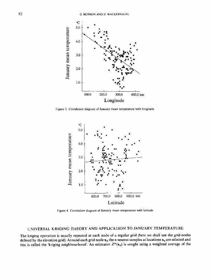
The Scottish mainland has three principal mountain ranges: the Northern and Western Highlands, the Grampian Highlands, and the Southern Uplands. The Grampians and the Southern Uplands have a reason- able network of temperature recording stations at a range of altitudes. The kriged estimates are more accurate in this area, where climate stations covering a wide range of elevations exist within the kriging neighbourhood, so that the local (implicit) regression is a good estimate of the trend. In the Northern and Western Highlands there is a sparser coverage. There are low-elevation stations in two quite different thermal regimes. Firstly on the islands in a maritime climate and secondly in highland glens with sheltered 'continental' conditions and temperature inversion effects causing lowering of temperatures. Two stations that may have contributed to a steep local regression are Benbecula, with an average January temperature of 4.5"C at an elevation of 5 m, and Strathconon, with an average January temperature of 1.9"C at an elevation of 107 m. The effect of these stations on estimates with a 16 station neighbourhood is clearly demonstrated in Figure 8, where a steeper regression line is apparent. The five values below -5°C have been marked by circles and are located near the highest points of the Northern and Western Highlands. Increasing the kriging neighbourhood to 20 stations gave the more closely packed scatter on Figure 9. The lowest temperature estimated using a 20-station neighbourhood is - 4.9"C.

The warm stations at sea-level and the cool stations at higher elevations together confuse the implicit local regression calculated in the kriging system. Setting up new recording stations in the Northern and Western Highlands would improve the estimation of the implicit regression and give more accurately estimated temperatures in this area, as would incorporation of distance from the sea and topographic situation in the variogram analysis and kriging system as second and third external drift variables. The effects of oceanicity on temperatures could also be used in the estimation process by the inclusion of distance from the sea, but further work is necessary to identify the appropriate points around the coastline at which to divide between 'sea' and 'land'.

The parameters of the linear regression functions of the estimated values against elevation on Figures 8 and 9 are very similar to those of linear regression of the station data, although with a less steep slope (see Table 11). The correlation is stronger for the estimated values and rises (in absolute value) when the kriging

h

-10.0 0

0

0. 500.0 1000.0 m

Elevation Figure 8. Correlation diagram of estimated January mean temperature with elevation data (16-station neighbourhood). The values

below - 5°C are shown as circles


5.0

0.

-5.0 c 0. 500.0 1000.0 m

Elevation

Figure 9. Correlation diagram of estimated January mean temperature with elevation data (20 stations neighbourhood)

Figure 10. Kriged map of January mean temperature with external drift using a 20-station kriging neighbourhood


Table 11. Intercepts and slopes of linear regression with elevation for January mean temperature at stations and after kriging with external drift

Data Minimum Maximum Intercept Slope Correlation

At Stations 0.6 5.2 3.6 1 - 0.009 - 0.80 Ext. Drift Method (16 points) - 1 1 . 1 5.4 3.60 - 0’007 -0.89 Ext. Drift Method (20 points) - 4.9 5.3 3.59 - 0.007 - 0.9 1 Ext. Drift Method (32 points) - 4.6 5.2 3.57 - 0.007 - 0.92

neighbourhood is larger. The selection of neighbourhood is critical and with such irregularly scattered data it may be the case that the neighbourhood should vary depending on the data density.

The kriged estimates of January mean temperatures obtained using a 20-station neighbourhood and with elevation as an external drift variable are shown on Figure 10.

KRIGING THE EXTERNAL DRIFT COEFFICIENT b, As the implicit local regression between the temperature and the external variable, elevation, is based on a few samples only, it is useful to display the slope coefficients, especially when extrapolation effects are

Figure 11. Map of external drift coefficients hf


0.150

0.100

0.050

0.

Min = -.OM Max = ,0002 Mean = -.006

External drift coefficient bl Figure 12. Histogram of external drift coefficients b:

observed. The slope coefficients depend only on the neighbourhood used, and not on the position of a particular grid-node within it, and can be evaluated with the linear combination,

n

bT= c n u z k ) u = 1

Deriving the corresponding equations gives a universal kriging system in which all the right-hand sides of the equations are zero, except for the equation relative to the external drift:

I n

I n n n

The estimated external drift coefficients b: for a 20-station neighbourhood are shown on Figure 11 and the histogram of these coefficients is found on Figure 12. The steepest regression slopes occur in the west, on the Outer Hebrides and on Skye.

CONCLUSION

The method of integrating the information about elevation into the mapping of temperature by kriging improves the map of January mean temperatures in Scotland, as compared with kriging based on temperature data alone. However, some exaggerated extrapolation effects are observed for a region in the Highlands, where stations are scarce and located at low altitudes. Increasing the kriging neighbourhood from

JANUARY TEMPERATURES IN SCOTLAND BY KRlGlNG 91

16 to 20 nearest neighbouring stations reduces the influence of Benbecula and Strathconon on the slope of the regression. Mapping the external drift coefficient gives an indication about the slope of the local regression with elevation for each neighbourhood.

The use of elevation as an external drift implies a linear relationship between temperature and elevation. If a non-linear function, describing more precisely the average relationship between temperature and elevation, were available for Scotland, the results could be further improved using elevation data transformed on the basis of this function as external drift.

The distance from the sea influences temperatures and further study is required to reveal how it can be integrated into the estimation procedure. The effects of topographic position are also important and the degree of ‘shelter’ might be quantified by analysis of digital terrain data.

Eventually the external drift method could readily be used to map rainfall data as well. Following Bigg (1991), there seems to exist a ‘dominant linear relation between altitude and rainfall on the temporal scales from a day to a year’.

REFERENCES Ahmed, S. and de Marsily, G. 1987. ‘Comparison of geostatistical methods for estimating transmissivity using data on transmissivity and

Armstrong, M. 1984. ‘Problems with universal kriging’, Math. Geol., 16, 101-108. Armstrong, M. and Wackernagel, H. 1988. ’The influence of the covariance function on the kriged estimator’, Sci. Terre, Ski-. In$, 27,

Bibby, J. S., Douglas, H. A,, Thomasson, A. J . and Robertson, J. S. 1982. Land Capability Classificationfor Agriculture. The Macdulay

Bigg, G . R. 1991. ‘Kriging and intraregional rainfall variability in England, In t . J . Climatol., 11, 663475. Chauvet, P. and Galfi, A. 1982. Universal Kriging. Publication C-96, Centre de Mines de GCostatistique, Ecole des Mines de Paris,

Chilis, J. P. 1991. ‘Application du krigeage avec derive exrerne a I’implantation d’un reseau de mesures piezometriques’, Sci. Terre, Sir.

Cooper, J.P. 1969. ‘Potential forage production’, Occas, Symp. Br. Grassland Soc., 5, 5-13. Delhomme, J. P. 1979. Rejexions sur ia prise en compte simultanie des donnies de forayes et des donnies sismiques, Report

Galli, A. and Meunier, G. 1987. ‘Study of a gas reservoir using the external drift method’, in Matheron, G. and Armstrong M. (eds)

Hudson, G. 1991. Kriging the temperatures in Scotland using the External Drift Method (Interpolation of Climutefor Land Evaluation),

Lamb, H. H. 1972. Climate: Present, Past and Future, Volume 1, Fundamentals and Climate Now, Methuen, London, p. 9. Liberti, A. and Girolamo, A. 1991. ‘Geostatistical analysis of the average temperature fields in North Italy in the period 1961 to 1985’.

MAFF 1976. The Agricultural Climate of’ England and Wales: Areal Aueruges 1941-70, Technical Bulletin, 35, Ministry of Agriculture,

Matheron, G. 1973. ‘The intrinsic random functions and their applications’, Adu. Appl. Probability, 5, 439468. Meteorological Office 1952. Climatological Atlas of the British Isles. HMSO, London, p. 28. Monteith, J. L. 1977. ‘Climate and the efficiency of crop production in Britain’, Philos. Trans. R. Soc. London, Ser. B, 281, 277-294. Peacock, J. M. 1975. ‘Temperature and leaf growth in Lolium perenne. 1. The thermal microclimate: its measurement and relation to crop

Renard, D. and Nai-Hsien, M. 1988. ‘Utilisation de derives externes multiples’, Sci. Terre, Sir. Inf , 28, 281-301. Wackernagel, H. 1988. ‘Geostatistical techniques for interpreting multivariate spatial information’, in: Chung, C. F. et a/. (eds),

specific capacity’, Water Resour. Res., 23, 1717-1737.

245-262.

Institute for Soil Research, Aberdeen.

Fontainebleau, 94 pp.

In f , 30, 131-147.

LHM/RC/79/41, Centre d’hformatique Gtologique, Ecole des Mines de Paris, Fontainebleau, 16 pp.

Geostatistical Case Studies, Reidel, Dordrecht, 105-1 19 pp.

Report S-275, Centre de Geostatistique, Ecole des Mines de Paris, Fontainebleau, 42 pp.

Sci. Terre, Ser. In$, 30, 1-36.

Fisheries and Food, HMSO, London.

growth’, J . Appl. Ecol., 12, 99-114.

Quantitative Analysis of Mineral and Energy Resources, NATO AS1 Series, C 223, Reidel. Dordrecht, pp. 393409.

Mapping temperature using kriging with external …cg.ensmp.fr/bibliotheque/public/HUDSON_Publication_02316.pdf · MAPPING TEMPERATURE USING KRIGING WITH EXTERNAL DRIFT: THEORY AND

Documents