Mapping sub-pixel fluvial grain sizes with hyperspatial imagery

Mapping sub-pixel fluvial grain sizes with hyperspatialimagery

MARTIN BLACK*† , PATRICE CARBONNEAU*, MICHAEL CHURCH‡ andJEFF WARBURTON**Department of Geography, Durham University, Lower Mountjoy South Road, Durham, DH1 3LE, UK(E-mail: [email protected])†British Antarctic Survey, High Cross Madingley Road, Cambridge, Cambridgeshire, CB3 0ET, UK‡Faculty of Arts, Department of Geography, The University of British Columbia, 1984 West Mall,Vancouver, BC V6T 1Z2, Canada

ABSTRACT

This study presents an investigation of image texture approaches for mapping

sub-pixel fluvial grain-size features from airborne imagery, allowing for the

rapid acquisition of surface sand and coarse fraction (>1�41 mm) grain-size

information. Imagery at 30 mm resolution was acquired over four gravel bars

from the Fraser River (British Columbia, Canada). Combined first-order and

second-order image texture approaches (windowed standard deviation filter

and the grey level co-occurrence matrix) were used. First-order image texture,

through the application of a standard deviation filter and subsequent thres-

holding was used to detect the presence of surface sand, with optimal accuracy

achieved at 91 � 1�9%. A wide-ranging parameter space investigation was

used to derive optimum parameters for the grey-level co-occurrence matrix.

Subsequently first-order and second-order image textures were used in multi-

ple linear regression to achieve good calibrations with several sub-pixel grain-

size percentiles; relative error at 1�44%, 3�18%, 6�80% and 10�6% for D5, D16,

D35 and D50, respectively. The larger percentiles of D84 and D95 had relative

errors of 24�7% and 29�7%, respectively. The breakdown of calibration preci-

sion for larger percentiles is attributed to a ‘pixel averaging effect’. It is con-

cluded that multispectral imagery is not required, because sufficient image

texture information can be derived from standard colour imagery. Recommen-

dations are suggested for the application of this method to other localities and

data sets, thus reducing exhaustive parameter searches in future studies.

Keywords Airborne remote sensing, digital image processing, fluvial grainsize, grey-level co-occurrence matrix, hyperspatial imagery, image texture,sub-pixel features.

INTRODUCTION

Research into fluvial systems is often basedon field studies that are inevitably limited interms of spatial coverage and resolution (Fauschet al., 2002). However, technological advancesare changing the way in which river scientistsmap, manage and analyze rivers (Marcus & Fon-stad, 2008). Among these new technologies, theincreasing acquisition and processing of hyper-spatial imagery (<100 mm spatial resolution;

Rango et al., 2009; Carbonneau & Piegay, 2012)are revealing great potential for catchment scalemapping at unprecedented resolutions (Carbon-neau et al., 2012).Grain-size information for gravel bed rivers is

important in a wide variety of contexts, provid-ing information to guide the development offlood defences and maintaining navigability, bio-diversity and ecological integrity within largerivers (Klingeman, 1998). Within the remotesensing literature, two main categories of

© 2013 The Authors. Journal compilation © 2013 International Association of Sedimentologists 691

Sedimentology (2014) 61, 691–711 doi: 10.1111/sed.12072

techniques are discussed for extracting grain-sizeinformation from digital imagery, close range‘photosieving’ techniques and reach-scale assess-ments using image texture analysis. Photosievingtechniques are based on the images of sedimentcollected at ground level where each grain isimaged by several pixels; images are rapidlyacquired in the field and grains manually mea-sured from the image at a later date (Ibbeken &Schleyer, 1986). Thus, photosieving reduces theneed for surface gravel sampling and increasesthe amount of collected data. More recently,automated procedures to extract grain-size infor-mation from digital images have been developed.These procedures use image segmentation andboundary detection approaches to emulate theway a human user would delineate grains (Mc-Ewan et al., 2000; Butler et al., 2001; Grahamet al., 2005a,b; Chang & Chung, 2012). Alterna-tively, statistical methods such as mathematicalmorphological operators (Pina et al., 2011), spa-tial autocorrelation (Rubin, 2004) or spectralautocorrelation (Buscombe, 2008; Buscombeet al., 2010; Buscombe & Rubin, 2012a,b) can beused. Given the requirement for pixel sizes muchsmaller than grain sizes, photosieving uses ter-restrial imagery.In the case of airborne, reach scale studies,

image texture applied to hyperspatial imageryhas been used to extract grain-size information(Carbonneau et al., 2004; Verdu et al., 2005).Image texture analysis involves quantifying thedifferences in pixel intensity values within aregion of neighbouring pixels. These operationscan be split into two types; first-order methodswhich are simple statistical measures, wherepixel neighbour relations are not considered, andsecond-order methods which consider the spatialrelation and spatial structure of the pixels. Somecommon measures of first-order image textureinclude mean, variance and range of pixel inten-sity values within a local neighbourhood. Forsecond-order methods, the grey-level co-occurrencematrix (GLCM) (Haralick et al., 1973; Haralick,1979) is perhaps the best-known texture measure.Early applications of airborne grain-size map-

ping were limited to gravels, cobbles and boul-ders. Sand particles, being much smaller thanthe pixel size, remained undetectable (Carbon-neau, 2005). However, preliminary resultspresented by Chandler et al. (2004) suggest thatsimple first-order texture measures are sufficientfor detecting the presence of surface sand,whilst the work of Carbonneau et al. (2004) andVerdu et al. (2005) showed that second-order

texture approaches can be used to extract multi-ple grain-size percentiles. However, measuressuch as the GLCM require several input parame-ters (for example, directional offset, grey levelsand window size); an extensive parameterinvestigation also increases data processingtime. Carbonneau et al. (2004) and Verdu et al.(2005) investigated only a small sub-set ofGLCM parameters and did not address the appli-cability of these methods for detecting sub-pixelgrains.In this study, a detailed investigation into

first-order and second-order image textureapproaches is presented, expanding the para-meter space investigated by Carbonneau et al.(2004) and Verdu et al. (2005), with the mainaim of extracting sub-pixel fluvial grain-size fea-tures from hyperspatial imagery. The prelimin-ary investigations of Chandler et al. (2004) werelimited; hence, first-order image texture methodsare re-examined in more detail. Second-orderimage texture methods (through the GLCM andits expansive parameter space) were applied tothe coarser (>1�41 mm) fluvial sediment sizefraction. These tasks were formulated into tworesearch objectives:

1 To investigate first-order image texturemethods for producing maps of surface sandareas.2 To investigate first-order and second-orderimage texture methods (through the GLCM) forderiving grain-size distributions for the coarse(>1�41 mm) size fraction.

METHODS

Study area

The Fraser River (British Columbia, Canada) isone of the large rivers in North America, drain-ing an area of ca 233 000 km2. The river rises inthe high plateaux and mountains in the centralpart of the province and descends a series ofcanyons to enter the distal Fraser Valley whereit receives its final major tributary, HarrisonRiver. Mean annual flow at Mission, down-stream of Harrison River is 3410 m3sec�1 andmean annual flood is 9710 m3sec�1. Gravel isthe predominant bed sediment type in the100 km ‘gravel reach’ of the lower Fraser,between Hope and Mission (Fig. 1); however,there are also significant quantities of sand. Thesediments show both downstream and vertical

© 2013 The Authors. Journal compilation © 2013 International Association of Sedimentologists, Sedimentology, 61, 691–711

692 M. Black et al.

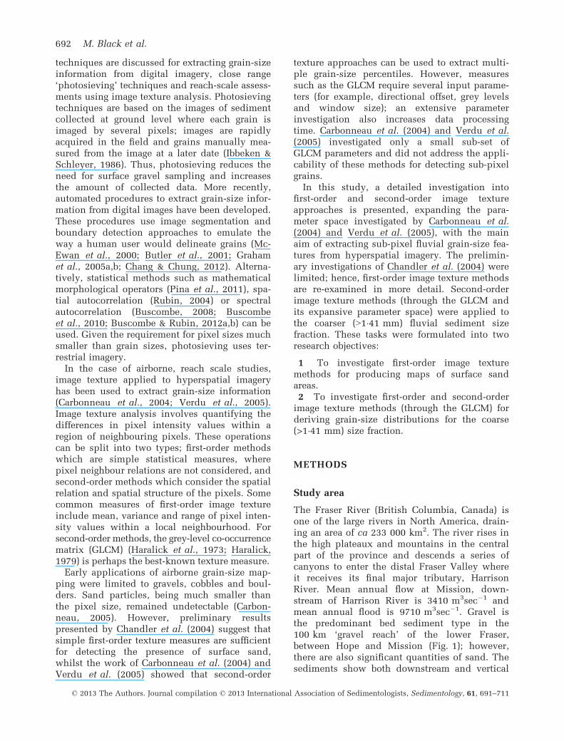
patterns of sorting within the channel system(Rice & Church, 2010), becoming finer and moresand-rich downstream. Four gravel bars withinthe ‘gravel reach’ were selected for data acquisi-tion: Queens Bar, N Bar, Calamity Bar and Harri-son Bar (Fig. 1). These bars are located between110 km and 120 km upstream of Sand Heads(mouth of the Fraser River).

Airborne hyperspatial image acquisition

In March 2012, hyperspatial imagery wasacquired over Queens Bar, N Bar, Calamity Barand Harrison Bar by the DTM Mapping Corpora-tion (http://www.dtm-global.com). Eight-bitimagery was collected using a Vexel ImagingUltraCamX (Vexcel Imaging GmbH, Graz, Austria)at a spatial resolution of 30 mm. Imagery wasacquired in Near Infrared, Red, Green and Bluebands. Following the collection of raw imagery,image enhancement was performed during theorthorectification stage, through the applicationof an image dodger. The image dodger performedhistogram matching on the overlapping region ofthe neighbouring images to normalize the inten-sity values between individual images. Due to the

consistent (cloudy bright) lighting conditions,during acquisition, the effects of the image dodgeron pixel intensities were minimal. Images wereautomatically mosaicked and rectified, producingca 230 image tiles covering the areas shown inFig. 1.

Ground truth grain-size data

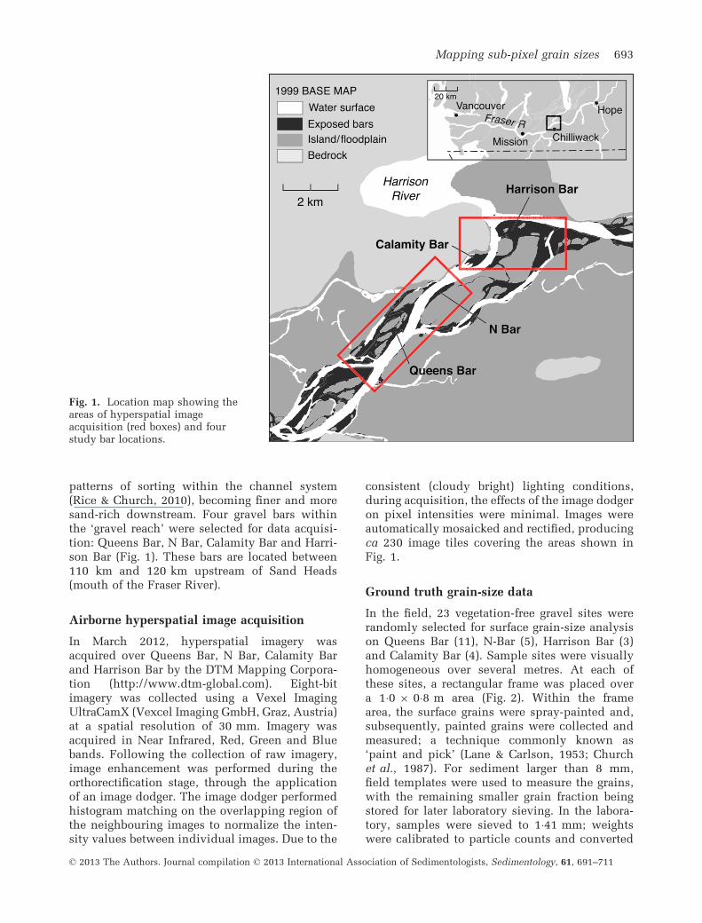
In the field, 23 vegetation-free gravel sites wererandomly selected for surface grain-size analysison Queens Bar (11), N-Bar (5), Harrison Bar (3)and Calamity Bar (4). Sample sites were visuallyhomogeneous over several metres. At each ofthese sites, a rectangular frame was placed overa 1�0 9 0�8 m area (Fig. 2). Within the framearea, the surface grains were spray-painted and,subsequently, painted grains were collected andmeasured; a technique commonly known as‘paint and pick’ (Lane & Carlson, 1953; Churchet al., 1987). For sediment larger than 8 mm,field templates were used to measure the grains,with the remaining smaller grain fraction beingstored for later laboratory sieving. In the labora-tory, samples were sieved to 1�41 mm; weightswere calibrated to particle counts and converted

Fig. 1. Location map showing theareas of hyperspatial imageacquisition (red boxes) and fourstudy bar locations.

© 2013 The Authors. Journal compilation © 2013 International Association of Sedimentologists, Sedimentology, 61, 691–711

Mapping sub-pixel grain sizes 693

to a full distribution. Geolocation of the fieldsites was carried out using a Trimble 5700differential Global Positioning System (GPS;Trimble Navigation Limited, Sunnyvale, CA,USA). Post-processing of the GPS data wascarried out using the Canadian Spatial Referenc-ing System (CSRS) online GPS Processing service(http://www.geod.nrcan.gc.ca/products-produits/ppp_e.php). With an integrated base stationtime of around seven hours, the GPS points havean estimated precision in X, Y and Z of� 20 mm.

Image texture and grain-size features

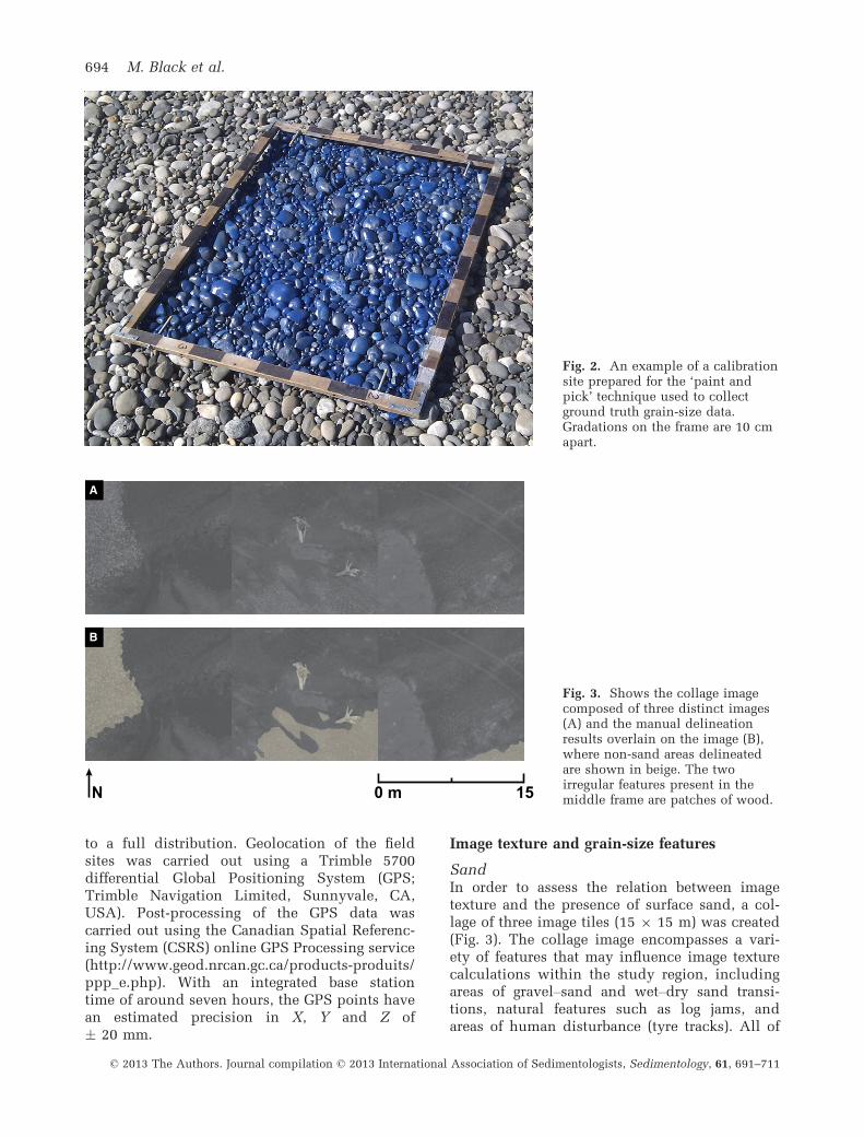
SandIn order to assess the relation between imagetexture and the presence of surface sand, a col-lage of three image tiles (15 9 15 m) was created(Fig. 3). The collage image encompasses a vari-ety of features that may influence image texturecalculations within the study region, includingareas of gravel–sand and wet–dry sand transi-tions, natural features such as log jams, andareas of human disturbance (tyre tracks). All of

Fig. 2. An example of a calibrationsite prepared for the ‘paint andpick’ technique used to collectground truth grain-size data.Gradations on the frame are 10 cmapart.

0 m 15N

A

B

Fig. 3. Shows the collage imagecomposed of three distinct images(A) and the manual delineationresults overlain on the image (B),where non-sand areas delineatedare shown in beige. The twoirregular features present in themiddle frame are patches of wood.

© 2013 The Authors. Journal compilation © 2013 International Association of Sedimentologists, Sedimentology, 61, 691–711

694 M. Black et al.

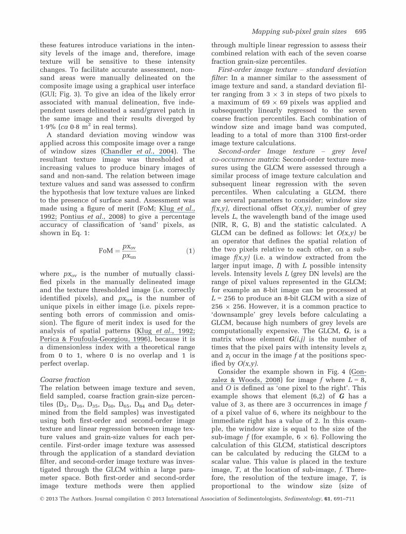
these features introduce variations in the inten-sity levels of the image and, therefore, imagetexture will be sensitive to these intensitychanges. To facilitate accurate assessment, non-sand areas were manually delineated on thecomposite image using a graphical user interface(GUI; Fig. 3). To give an idea of the likely errorassociated with manual delineation, five inde-pendent users delineated a sand/gravel patch inthe same image and their results diverged by1�9% (ca 0�8 m2 in real terms).A standard deviation moving window was

applied across this composite image over a rangeof window sizes (Chandler et al., 2004). Theresultant texture image was thresholded atincreasing values to produce binary images ofsand and non-sand. The relation between imagetexture values and sand was assessed to confirmthe hypothesis that low texture values are linkedto the presence of surface sand. Assessment wasmade using a figure of merit (FoM; Klug et al.,1992; Pontius et al., 2008) to give a percentageaccuracy of classification of ‘sand’ pixels, asshown in Eq. 1:

FoM ¼ pxovpxun

ð1Þ

where pxov is the number of mutually classi-fied pixels in the manually delineated imageand the texture thresholded image (i.e. correctlyidentified pixels), and pxun is the number ofunique pixels in either image (i.e. pixels repre-senting both errors of commission and omis-sion). The figure of merit index is used for theanalysis of spatial patterns (Klug et al., 1992;Perica & Foufoula-Georgiou, 1996), because it isa dimensionless index with a theoretical rangefrom 0 to 1, where 0 is no overlap and 1 isperfect overlap.

Coarse fractionThe relation between image texture and seven,field sampled, coarse fraction grain-size percen-tiles (D5, D16, D35, D50, D65, D84 and D95 deter-mined from the field samples) was investigatedusing both first-order and second-order imagetexture and linear regression between image tex-ture values and grain-size values for each per-centile. First-order image texture was assessedthrough the application of a standard deviationfilter, and second-order image texture was inves-tigated through the GLCM within a large para-meter space. Both first-order and second-orderimage texture methods were then applied

through multiple linear regression to assess theircombined relation with each of the seven coarsefraction grain-size percentiles.First-order image texture – standard deviation

filter: In a manner similar to the assessment ofimage texture and sand, a standard deviation fil-ter ranging from 3 9 3 in steps of two pixels toa maximum of 69 9 69 pixels was applied andsubsequently linearly regressed to the sevencoarse fraction percentiles. Each combination ofwindow size and image band was computed,leading to a total of more than 3100 first-orderimage texture calculations.Second-order Image texture – grey level

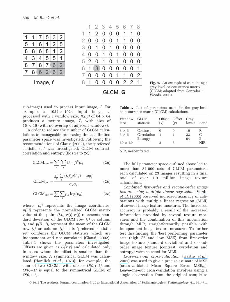
co-occurrence matrix: Second-order texture mea-sures using the GLCM were assessed through asimilar process of image texture calculation andsubsequent linear regression with the sevenpercentiles. When calculating a GLCM, thereare several parameters to consider; window sizef(x,y), directional offset O(x,y), number of greylevels L, the wavelength band of the image used(NIR, R, G, B) and the statistic calculated. AGLCM can be defined as follows: let O(x,y) bean operator that defines the spatial relation ofthe two pixels relative to each other, on a sub-image f(x,y) (i.e. a window extracted from thelarger input image, I) with L possible intensitylevels. Intensity levels L (grey DN levels) are therange of pixel values represented in the GLCM;for example an 8-bit image can be processed atL = 256 to produce an 8-bit GLCM with a size of256 9 256. However, it is a common practice to‘downsample’ grey levels before calculating aGLCM, because high numbers of grey levels arecomputationally expensive. The GLCM, G, is amatrix whose element G(i,j) is the number oftimes that the pixel pairs with intensity levels ziand zj occur in the image f at the positions spec-ified by O(x,y).Consider the example shown in Fig. 4 (Gon-

zalez & Woods, 2008) for image f where L = 8,and O is defined as ‘one pixel to the right’. Thisexample shows that element (6,2) of G has avalue of 3, as there are 3 occurrences in image fof a pixel value of 6, where its neighbour to theimmediate right has a value of 2. In this exam-ple, the window size is equal to the size of thesub-image f (for example, 6 9 6). Following thecalculation of this GLCM, statistical descriptorscan be calculated by reducing the GLCM to ascalar value. This value is placed in the textureimage, T, at the location of sub-image, f. There-fore, the resolution of the texture image, T, isproportional to the window size (size of

© 2013 The Authors. Journal compilation © 2013 International Association of Sedimentologists, Sedimentology, 61, 691–711

Mapping sub-pixel grain sizes 695

sub-image) used to process input image, I. Forexample, a 1024 9 1024 input image, I,processed with a window size, f(x,y) of 64 9 64produces a texture image, T, with size of16 9 16 (with no overlap of adjacent windows).In order to reduce the number of GLCM calcu-

lations to manageable processing times, a limitedparameter space was investigated. Following therecommendations of Clausi (2002), the ‘preferredstatistic set’ was investigated; GLCM contrast,correlation and entropy (Eqs 2a to 2c):

GLCMcon ¼X

i

X

j

ði � jÞ2pij ð2aÞ

GLCMcor ¼

Pi

Pj

ði; jÞpði; jÞ � lilj

rxryð2bÞ

GLCMent ¼X

i

X

j

pij logðpijÞ ð2cÞ

where (i,j) represents the image coordinates,p(i,j) represents the normalized GLCM matrixvalue at the point (i,j), r(i) r(j) represents stan-dard deviation of the GLCM row (i) or column(j) and l(i) l(j) represent the mean of the GLCMrow (i) or column (j). This ‘preferred statisticset’ combines the GLCM statistics which areindependent and not correlated (Clausi, 2002).Table 1 shows the parameters investigated.Offsets are given as O(x,y) and calculated onlyin cases where the offset is smaller than thewindow size. A symmetrical GLCM was calcu-lated (Haralick et al., 1973); for example, thesum of two GLCMs with offsets O(0,+ 1) andO(0,�1) is equal to the symmetrical GLCM ofO(0,+ 1).

The full parameter space outlined above led tomore than 84 000 sets of GLCM parameters,each calculated on 23 images resulting in a finaltotal of over 1�9 million image texturecalculations.Combined first-order and second-order image

texture using multiple linear regression: Verduet al. (2005) observed increased accuracy of cali-brations with multiple linear regression (MLR)of several image texture measures. The increasedaccuracy is probably a result of the increasedinformation provided by several texture mea-sures and the combination of this informationthrough MLR, straightforwardly possible withindependent image texture measures. To furthertest this finding, the ‘best performing’ parametersets (high R2 and low MSE) from first-orderimage texture (standard deviation) and second-order image texture (contrast, correlation andentropy) were selected for MLR.Leave-one-out cross-validation (Hastie et al.,

2001) was used to give a precise estimate of MSE(cross-validated Mean Square Error: MSEcv).Leave-one-out cross-validation involves using asingle observation from the original sample as

158487

118378

766486

518572

321566

252122

10002101

12345678

1 2 3 4 5 6 7 820100300

00011000

00100000

01011010

11000012

10000002

00000121Image, f

GLCM, G

6 26 26 2

3

Fig. 4. An example of calculating agrey level co-occurrence matrix(GLCM; adapted from Gonzalez &Woods, 2008).

Table 1. List of parameters used for the grey-levelco-occurrence matrix (GLCM) calculations.

Windowsize

GLCMstatistic

Offset(x)

Offset(y)

Greylevels Band

3 9 3 Contrast 0 0 16 R5 9 5 Correlation 1 1 32 G– Entropy – – 64 B69 9 69 8 8 NIR

NIR, near-infrared.

© 2013 The Authors. Journal compilation © 2013 International Association of Sedimentologists, Sedimentology, 61, 691–711

696 M. Black et al.

validation data, and the remaining observations astraining data. The process is iterated until eachobservation in the sample is used once for valida-tion.

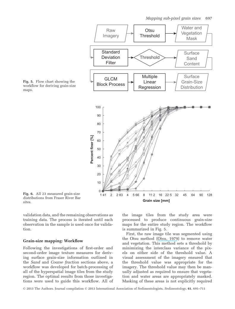
Grain-size mapping: Workflow

Following the investigations of first-order andsecond-order image texture measures for deriv-ing surface grain-size information outlined inthe Sand and Coarse fraction sections above, aworkflow was developed for batch-processing ofall of the hyperspatial image tiles from the studyregion. The optimal results from those investiga-tions were used to guide this workflow. All of

the image tiles from the study area wereprocessed to produce continuous grain-sizemaps for the entire study region. The workflowis summarized in Fig. 5.First, the raw image tile was segmented using

the Otsu method (Otsu, 1979) to remove waterand vegetation. This method sets a threshold byminimizing the interclass variance of the pix-els on either side of the threshold value. Avisual assessment of the imagery ensured thatthe threshold value was appropriate for theimagery. The threshold value may then be man-ually adjusted as required to ensure that vegeta-tion and water areas are appropriately masked.Masking of these areas is not explicitly required

GLCMBlock Process

MultipleLinear

Regression

OtsuThreshold

StandardDeviation

Filter

SurfaceSand

Content

SurfaceGrain-SizeDistribution

RawImagery

Water andVegetation

Mask

Threshold

Fig. 5. Flow chart showing theworkflow for deriving grain-sizemaps.

1·41 2 2·83 4 5·66 8 11·2 16 22·5 32 45 64 90 1280

10

20

30

40

50

60

70

80

90

100

Grain size [mm]

Perc

ent f

iner

[%]

Fig. 6. All 23 measured grain-sizedistributions from Fraser River Barsites.

© 2013 The Authors. Journal compilation © 2013 International Association of Sedimentologists, Sedimentology, 61, 691–711

Mapping sub-pixel grain sizes 697

to calculate surface sand and grain-size maps,because vegetated and water surfaces can bemasked at any stage. However, masking earlierin the workflow avoids unnecessary computa-tion in the latter stages.A standard deviation filter was then applied

and thresholded to produce surface sand con-tent. Remaining pixels (i.e. those not classifiedas water and vegetation or sand), were then pro-cessed through the GLCM and MLR to producea surface grain-size distribution.

RESULTS

Ground truth grain-size data

Figure 6 shows the full grain-size distributionfor all 23 coarse fraction sites, truncated at

1�41 mm. Table 2 shows summary statistics,with percentile data being linearly interpolatedbetween sieve data points shown in Fig. 6. Thesamples represent a good range for the investiga-tion of texture detection methods.

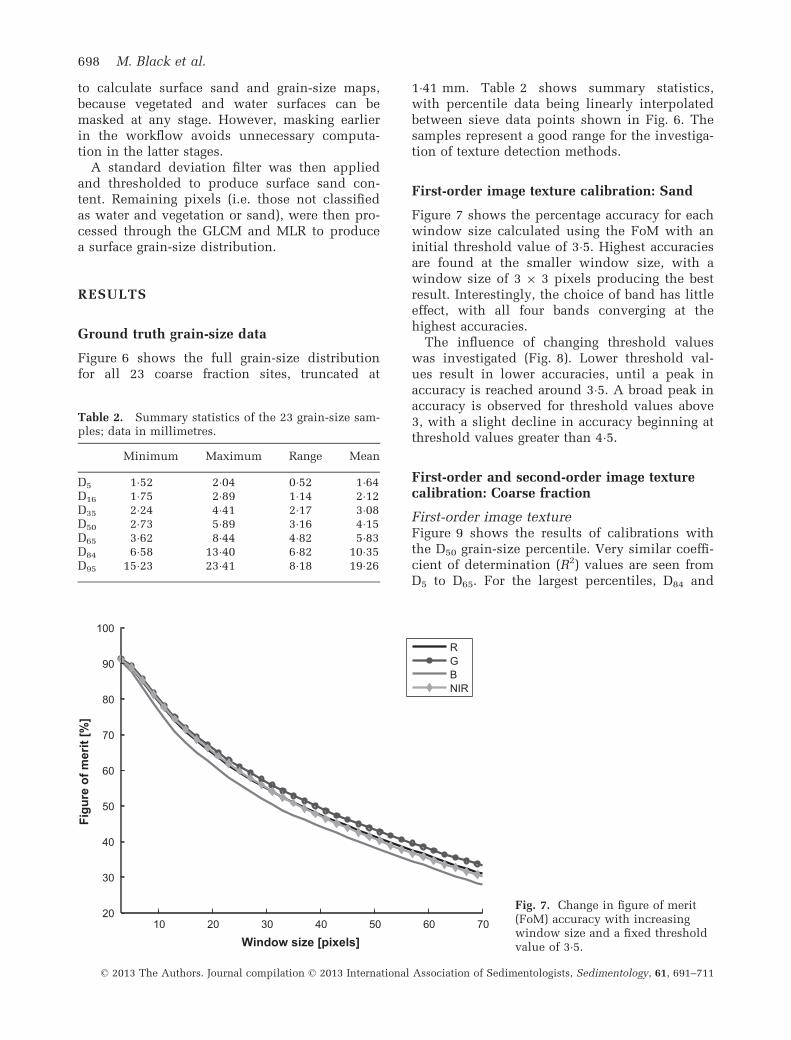
First-order image texture calibration: Sand

Figure 7 shows the percentage accuracy for eachwindow size calculated using the FoM with aninitial threshold value of 3�5. Highest accuraciesare found at the smaller window size, with awindow size of 3 9 3 pixels producing the bestresult. Interestingly, the choice of band has littleeffect, with all four bands converging at thehighest accuracies.The influence of changing threshold values

was investigated (Fig. 8). Lower threshold val-ues result in lower accuracies, until a peak inaccuracy is reached around 3�5. A broad peak inaccuracy is observed for threshold values above3, with a slight decline in accuracy beginning atthreshold values greater than 4�5.

First-order and second-order image texturecalibration: Coarse fraction

First-order image textureFigure 9 shows the results of calibrations withthe D50 grain-size percentile. Very similar coeffi-cient of determination (R2) values are seen fromD5 to D65. For the largest percentiles, D84 and

Table 2. Summary statistics of the 23 grain-size sam-ples; data in millimetres.

Minimum Maximum Range Mean

D5 1�52 2�04 0�52 1�64D16 1�75 2�89 1�14 2�12D35 2�24 4�41 2�17 3�08D50 2�73 5�89 3�16 4�15D65 3�62 8�44 4�82 5�83D84 6�58 13�40 6�82 10�35D95 15�23 23�41 8�18 19�26

10 20 30 40 50 60 7020

30

40

50

60

70

80

90

100

Window size [pixels]

Figu

re o

f mer

it [%

]

RGBNIR

Fig. 7. Change in figure of merit(FoM) accuracy with increasingwindow size and a fixed thresholdvalue of 3�5.

© 2013 The Authors. Journal compilation © 2013 International Association of Sedimentologists, Sedimentology, 61, 691–711

698 M. Black et al.

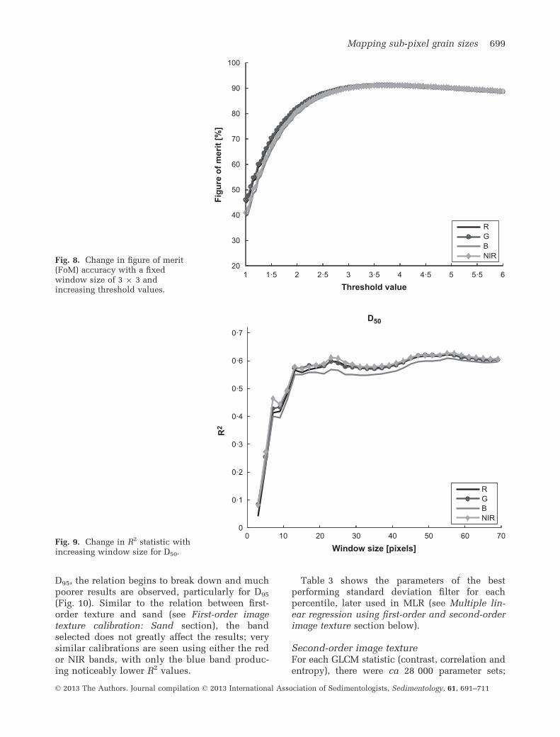
D95, the relation begins to break down and muchpoorer results are observed, particularly for D95

(Fig. 10). Similar to the relation between first-order texture and sand (see First-order imagetexture calibration: Sand section), the bandselected does not greatly affect the results; verysimilar calibrations are seen using either the redor NIR bands, with only the blue band produc-ing noticeably lower R2 values.

Table 3 shows the parameters of the bestperforming standard deviation filter for eachpercentile, later used in MLR (see Multiple lin-ear regression using first-order and second-orderimage texture section below).

Second-order image textureFor each GLCM statistic (contrast, correlation andentropy), there were ca 28 000 parameter sets;

1 1·5 2 2·5 3 3·5 4 4·5 5 5·5 620

30

40

50

60

70

80

90

100

Threshold value

Figu

re o

f mer

it [%

]RGBNIR

Fig. 8. Change in figure of merit(FoM) accuracy with a fixedwindow size of 3 9 3 andincreasing threshold values.

0 10 20 30 40 50 60 700

0·1

0·2

0·3

0·4

0·5

0·6

0·7

Window size [pixels]

R2

D50

RGBNIR

Fig. 9. Change in R2 statistic withincreasing window size for D50.

© 2013 The Authors. Journal compilation © 2013 International Association of Sedimentologists, Sedimentology, 61, 691–711

Mapping sub-pixel grain sizes 699

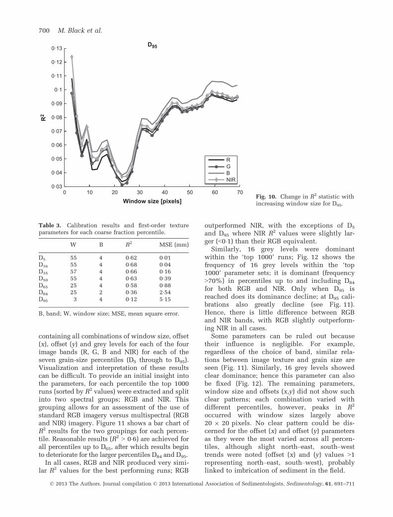
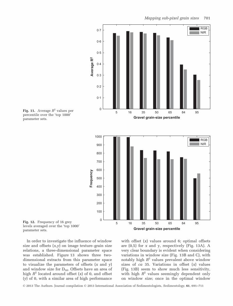
containing all combinations of window size, offset(x), offset (y) and grey levels for each of the fourimage bands (R, G, B and NIR) for each of theseven grain-size percentiles (D5 through to D95).Visualization and interpretation of these resultscan be difficult. To provide an initial insight intothe parameters, for each percentile the top 1000runs (sorted by R2 values) were extracted and splitinto two spectral groups; RGB and NIR. Thisgrouping allows for an assessment of the use ofstandard RGB imagery versus multispectral (RGBand NIR) imagery. Figure 11 shows a bar chart ofR2 results for the two groupings for each percen-tile. Reasonable results (R2 > 0�6) are achieved forall percentiles up to D65, after which results beginto deteriorate for the larger percentiles D84 and D95.In all cases, RGB and NIR produced very simi-

lar R2 values for the best performing runs; RGB

outperformed NIR, with the exceptions of D5

and D95 where NIR R2 values were slightly lar-ger (<0�1) than their RGB equivalent.Similarly, 16 grey levels were dominant

within the ‘top 1000’ runs; Fig. 12 shows thefrequency of 16 grey levels within the ‘top1000’ parameter sets; it is dominant (frequency>70%) in percentiles up to and including D84

for both RGB and NIR. Only when D95 isreached does its dominance decline; at D95 cali-brations also greatly decline (see Fig. 11).Hence, there is little difference between RGBand NIR bands, with RGB slightly outperform-ing NIR in all cases.Some parameters can be ruled out because

their influence is negligible. For example,regardless of the choice of band, similar rela-tions between image texture and grain size areseen (Fig. 11). Similarly, 16 grey levels showedclear dominance; hence this parameter can alsobe fixed (Fig. 12). The remaining parameters,window size and offsets (x,y) did not show suchclear patterns; each combination varied withdifferent percentiles, however, peaks in R2

occurred with window sizes largely above20 9 20 pixels. No clear pattern could be dis-cerned for the offset (x) and offset (y) parametersas they were the most varied across all percen-tiles, although slight north–east, south–westtrends were noted (offset (x) and (y) values >1representing north–east, south–west), probablylinked to imbrication of sediment in the field.

0 10 20 30 40 50 60 700·03

0·04

0·05

0·06

0·07

0·08

0·09

0·1

0·11

0·12

0·13

Window size [pixels]

R2

D95

RGBNIR

Fig. 10. Change in R2 statistic withincreasing window size for D95.

Table 3. Calibration results and first-order textureparameters for each coarse fraction percentile.

W B R2 MSE (mm)

D5 55 4 0�62 0�01D16 55 4 0�68 0�04D35 57 4 0�66 0�16D50 55 4 0�63 0�39D65 25 4 0�58 0�88D84 25 2 0�36 2�54D95 3 4 0�12 5�15

B, band; W, window size; MSE, mean square error.

© 2013 The Authors. Journal compilation © 2013 International Association of Sedimentologists, Sedimentology, 61, 691–711

700 M. Black et al.

In order to investigate the influence of windowsize and offsets (x,y) on image texture–grain sizerelations, a three-dimensional parameter spacewas established. Figure 13 shows three two-dimensional extracts from this parameter spaceto visualize the parameters of offsets (x and y)and window size for D50. Offsets have an area ofhigh R2 located around offset (x) of 0, and offset(y) of 0, with a similar area of high performance

with offset (x) values around 6; optimal offsetsare (0,5) for x and y, respectively (Fig. 13A). Avery clear boundary is evident when consideringvariations in window size (Fig. 13B and C), withnotably high R2 values prevalent above windowsizes of ca 35. Variations in offset (x) values(Fig. 13B) seem to show much less sensitivity,with high R2 values seemingly dependent onlyon window size; once in the optimal window

5 16 35 50 65 84 950

0·1

0·2

0·3

0·4

0·5

0·6

0·7

Ave

rage

R2

Gravel grain-size percentile

RGBNIR

Fig. 11. Average R2 values perpercentile over the ‘top 1000’parameter sets.

5 16 35 50 65 84 950

100

200

300

400

500

600

700

800

900

1000

Freq

uenc

y

Gravel grain-size percentile

RGBNIR

Fig. 12. Frequency of 16 greylevels averaged over the ‘top 1000’parameter sets.

© 2013 The Authors. Journal compilation © 2013 International Association of Sedimentologists, Sedimentology, 61, 691–711

Mapping sub-pixel grain sizes 701

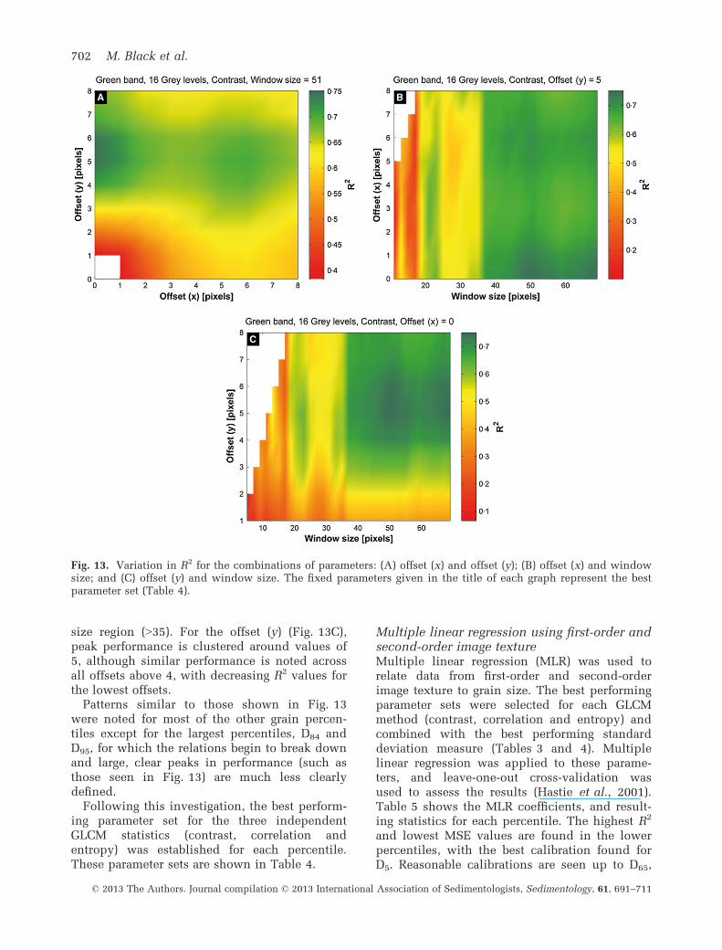
size region (>35). For the offset (y) (Fig. 13C),peak performance is clustered around values of5, although similar performance is noted acrossall offsets above 4, with decreasing R2 values forthe lowest offsets.Patterns similar to those shown in Fig. 13

were noted for most of the other grain percen-tiles except for the largest percentiles, D84 andD95, for which the relations begin to break downand large, clear peaks in performance (such asthose seen in Fig. 13) are much less clearlydefined.Following this investigation, the best perform-

ing parameter set for the three independentGLCM statistics (contrast, correlation andentropy) was established for each percentile.These parameter sets are shown in Table 4.

Multiple linear regression using first-order andsecond-order image textureMultiple linear regression (MLR) was used torelate data from first-order and second-orderimage texture to grain size. The best performingparameter sets were selected for each GLCMmethod (contrast, correlation and entropy) andcombined with the best performing standarddeviation measure (Tables 3 and 4). Multiplelinear regression was applied to these parame-ters, and leave-one-out cross-validation wasused to assess the results (Hastie et al., 2001).Table 5 shows the MLR coefficients, and result-ing statistics for each percentile. The highest R2

and lowest MSE values are found in the lowerpercentiles, with the best calibration found forD5. Reasonable calibrations are seen up to D65,

BA

C

Fig. 13. Variation in R2 for the combinations of parameters: (A) offset (x) and offset (y); (B) offset (x) and windowsize; and (C) offset (y) and window size. The fixed parameters given in the title of each graph represent the bestparameter set (Table 4).

© 2013 The Authors. Journal compilation © 2013 International Association of Sedimentologists, Sedimentology, 61, 691–711

702 M. Black et al.

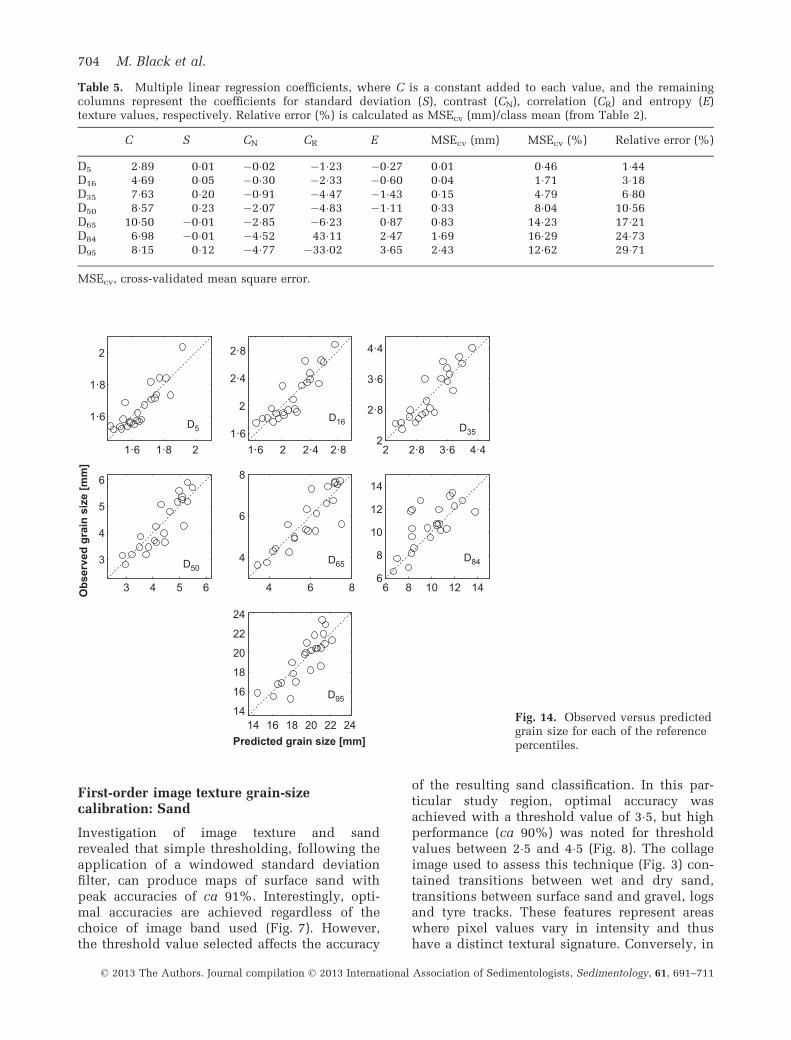
with MSE at 17�2%. Calibrations are poorest forD95 with MSE at 29�7%. For each percentile, thegrain size was calculated and compared toobserved grain size (Fig. 14).

Grain-size maps: Sand and coarse fraction

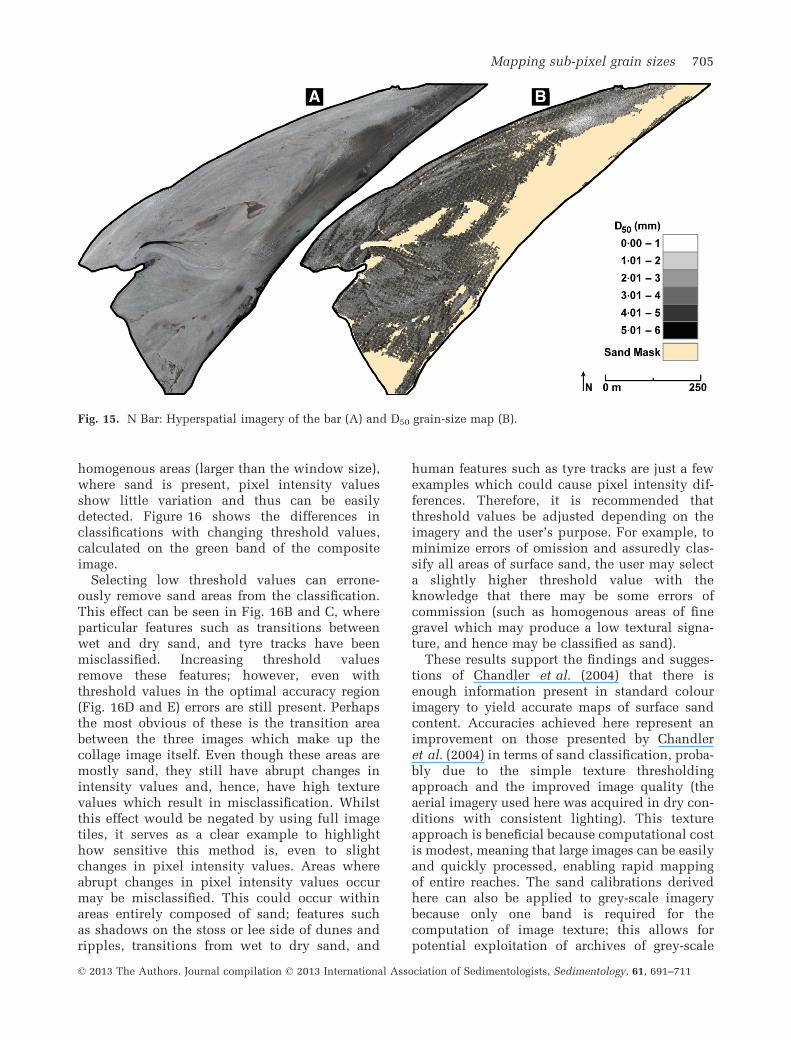
Figure 15 shows a sample D50 map producedfollowing the workflow outlined in the Grain-size mapping: Workflow section. These imagesare gridded at variable spatial resolutions. Sandclassification maps are resolved at 81 cm2 (win-dow size of 3 9 3 pixels), whilst coarse fractionpercentiles have varying resolution. The spatialresolution is a product of the largest windowsize used; the coarsest resolution was that of D5,

at ca 4�3 m2 (largest window of 69 9 69 pixels).

DISCUSSION

Results show that first-order and second-orderimage texture approaches are suitable for the

detection of surface sand and the extraction ofsurface grain-size percentiles from hyperspatialimagery. Unlike previous approaches usingimage texture, the applicability of these tech-niques for extracting both surface sand contentand a grain-size distribution has been shown.The preliminary findings of Chandler et al.(2004) are confirmed; a simple first-order texturemeasure proved adequate for the detectionof surface sand features. Similarly, following awide-ranging parameter space investigation andmultiple linear regression using first-order andsecond-order image texture, a technique suitablefor extracting the finer scale grain-size percen-tiles (D5 through to D65) was also achieved. Bothof these techniques improve on current methodsby explicitly extracting sub-pixel grain-size dis-tributions; however, an important constraint isnoted as the pixel resolution is approached (seeFirst-order and second-order image texturegrain-size calibration: Coarse fraction sectionbelow).

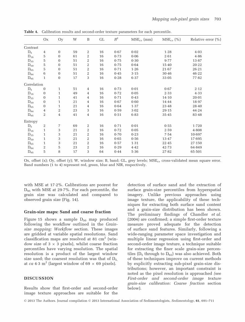
Table 4. Calibration results and second-order texture parameters for each percentile.

Ox Oy W B GL R2 MSEcv (mm) MSEcv (%) Relative error (%)

ContrastD5 4 0 59 2 16 0�67 0�02 1�28 4�03D16 5 0 61 2 16 0�73 0�06 2�61 4�86D35 5 0 51 2 16 0�75 0�30 9�77 13�87D50 5 0 51 2 16 0�75 0�64 15�40 20�22D65 5 0 51 2 16 0�71 1�26 21�67 26�21D84 6 0 51 2 16 0�45 3�15 30�46 46�22D95 1 0 17 3 16 0�28 6�37 33�05 77�82

CorrelationD5 0 1 51 4 16 0�73 0�01 0�67 2�12D16 0 1 49 4 16 0�72 0�05 2�33 4�33D35 0 1 41 4 16 0�71 0�43 14�10 20�01D50 0 1 21 4 16 0�67 0�60 14�44 18�97D65 0 1 21 4 16 0�64 1�37 23�48 28�40D84 4 2 23 3 16 0�59 3�02 29�15 44�24D95 2 4 41 4 16 0�51 6�83 35�45 83�48

EntropyD5 2 7 69 2 16 0�71 0�01 0�55 1�720D16 1 3 21 2 16 0�72 0�05 2�59 4�808D35 1 3 21 2 16 0�70 0�23 7�54 10�697D50 1 3 21 2 16 0�65 0�56 13�47 17�695D65 1 3 21 2 16 0�57 1�31 22�45 27�150D84 2 5 23 2 16 0�29 4�42 42�73 64�849D95 5 8 17 3 64 0�44 5�36 27�82 65�501

Ox, offset (x); Oy, offset (y); W, window size; B, band; GL, grey levels; MSEcv cross-validated mean square error.Band numbers (1 to 4) represent red, green, blue and NIR, respectively.

© 2013 The Authors. Journal compilation © 2013 International Association of Sedimentologists, Sedimentology, 61, 691–711

Mapping sub-pixel grain sizes 703

First-order image texture grain-sizecalibration: Sand

Investigation of image texture and sandrevealed that simple thresholding, following theapplication of a windowed standard deviationfilter, can produce maps of surface sand withpeak accuracies of ca 91%. Interestingly, opti-mal accuracies are achieved regardless of thechoice of image band used (Fig. 7). However,the threshold value selected affects the accuracy

of the resulting sand classification. In this par-ticular study region, optimal accuracy wasachieved with a threshold value of 3�5, but highperformance (ca 90%) was noted for thresholdvalues between 2�5 and 4�5 (Fig. 8). The collageimage used to assess this technique (Fig. 3) con-tained transitions between wet and dry sand,transitions between surface sand and gravel, logsand tyre tracks. These features represent areaswhere pixel values vary in intensity and thushave a distinct textural signature. Conversely, in

1·6 1·8 2

1·6

1·8

2

D5

1·6 2 2·4 2·81·6

2

2·4

2·8

2 2·8 3·6 4·42

2·8

3·6

4·4

3 4 5 6

3

4

5

6

4 6 8

4

6

8

6 8 10 12 146

8

10

12

14

14 16 18 20 22 2414

16

18

20

22

24

Obs

erve

d gr

ain

size

[mm

]

Predicted grain size [mm]

D16 D35

D84D65D50

D95

Fig. 14. Observed versus predictedgrain size for each of the referencepercentiles.

Table 5. Multiple linear regression coefficients, where C is a constant added to each value, and the remainingcolumns represent the coefficients for standard deviation (S), contrast (CN), correlation (CR) and entropy (E)texture values, respectively. Relative error (%) is calculated as MSEcv (mm)/class mean (from Table 2).

C S CN CR E MSEcv (mm) MSEcv (%) Relative error (%)

D5 2�89 0�01 �0�02 �1�23 �0�27 0�01 0�46 1�44D16 4�69 0�05 �0�30 �2�33 �0�60 0�04 1�71 3�18D35 7�63 0�20 �0�91 �4�47 �1�43 0�15 4�79 6�80D50 8�57 0�23 �2�07 �4�83 �1�11 0�33 8�04 10�56D65 10�50 �0�01 �2�85 �6�23 0�87 0�83 14�23 17�21D84 6�98 �0�01 �4�52 43�11 2�47 1�69 16�29 24�73D95 8�15 0�12 �4�77 �33�02 3�65 2�43 12�62 29�71

MSEcv, cross-validated mean square error.

© 2013 The Authors. Journal compilation © 2013 International Association of Sedimentologists, Sedimentology, 61, 691–711

704 M. Black et al.

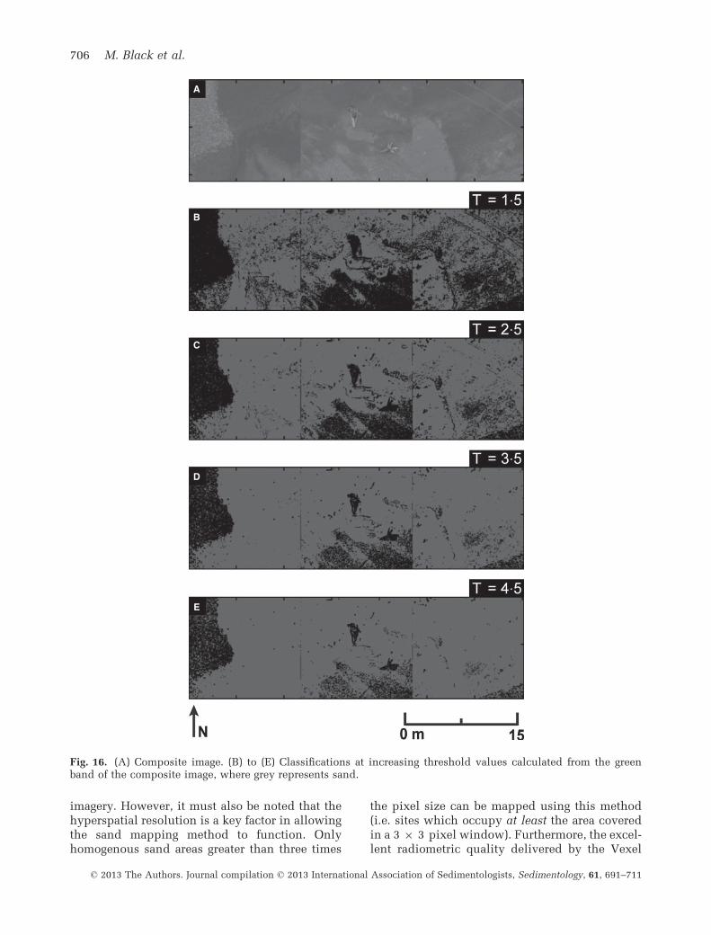
homogenous areas (larger than the window size),where sand is present, pixel intensity valuesshow little variation and thus can be easilydetected. Figure 16 shows the differences inclassifications with changing threshold values,calculated on the green band of the compositeimage.Selecting low threshold values can errone-

ously remove sand areas from the classification.This effect can be seen in Fig. 16B and C, whereparticular features such as transitions betweenwet and dry sand, and tyre tracks have beenmisclassified. Increasing threshold valuesremove these features; however, even withthreshold values in the optimal accuracy region(Fig. 16D and E) errors are still present. Perhapsthe most obvious of these is the transition areabetween the three images which make up thecollage image itself. Even though these areas aremostly sand, they still have abrupt changes inintensity values and, hence, have high texturevalues which result in misclassification. Whilstthis effect would be negated by using full imagetiles, it serves as a clear example to highlighthow sensitive this method is, even to slightchanges in pixel intensity values. Areas whereabrupt changes in pixel intensity values occurmay be misclassified. This could occur withinareas entirely composed of sand; features suchas shadows on the stoss or lee side of dunes andripples, transitions from wet to dry sand, and

human features such as tyre tracks are just a fewexamples which could cause pixel intensity dif-ferences. Therefore, it is recommended thatthreshold values be adjusted depending on theimagery and the user’s purpose. For example, tominimize errors of omission and assuredly clas-sify all areas of surface sand, the user may selecta slightly higher threshold value with theknowledge that there may be some errors ofcommission (such as homogenous areas of finegravel which may produce a low textural signa-ture, and hence may be classified as sand).These results support the findings and sugges-

tions of Chandler et al. (2004) that there isenough information present in standard colourimagery to yield accurate maps of surface sandcontent. Accuracies achieved here represent animprovement on those presented by Chandleret al. (2004) in terms of sand classification, proba-bly due to the simple texture thresholdingapproach and the improved image quality (theaerial imagery used here was acquired in dry con-ditions with consistent lighting). This textureapproach is beneficial because computational costis modest, meaning that large images can be easilyand quickly processed, enabling rapid mappingof entire reaches. The sand calibrations derivedhere can also be applied to grey-scale imagerybecause only one band is required for thecomputation of image texture; this allows forpotential exploitation of archives of grey-scale

A B

Fig. 15. N Bar: Hyperspatial imagery of the bar (A) and D50 grain-size map (B).

© 2013 The Authors. Journal compilation © 2013 International Association of Sedimentologists, Sedimentology, 61, 691–711

Mapping sub-pixel grain sizes 705

imagery. However, it must also be noted that thehyperspatial resolution is a key factor in allowingthe sand mapping method to function. Onlyhomogenous sand areas greater than three times

the pixel size can be mapped using this method(i.e. sites which occupy at least the area coveredin a 3 9 3 pixel window). Furthermore, the excel-lent radiometric quality delivered by the Vexel

A

B

C

D

E

Fig. 16. (A) Composite image. (B) to (E) Classifications at increasing threshold values calculated from the greenband of the composite image, where grey represents sand.

© 2013 The Authors. Journal compilation © 2013 International Association of Sedimentologists, Sedimentology, 61, 691–711

706 M. Black et al.

UltraCamX (Vexcel Imaging GmbH; MicrosoftPhotogrammetry, Graz, Austria) was undoubtedlyanother key factor in the success of the method.

First-order and second-order image texturegrain-size calibration: Coarse fraction

A combined MLR approach encompassing alltexture measures provides the best calibrations,a finding similar to that of Verdu et al. (2005).All of the derived grain-size percentiles in thisstudy are smaller than the image resolution of30 mm. Interestingly, relations become muchweaker as the pixel resolution is approached,with the strongest relations found for the finerpercentiles (D5 through to D65).

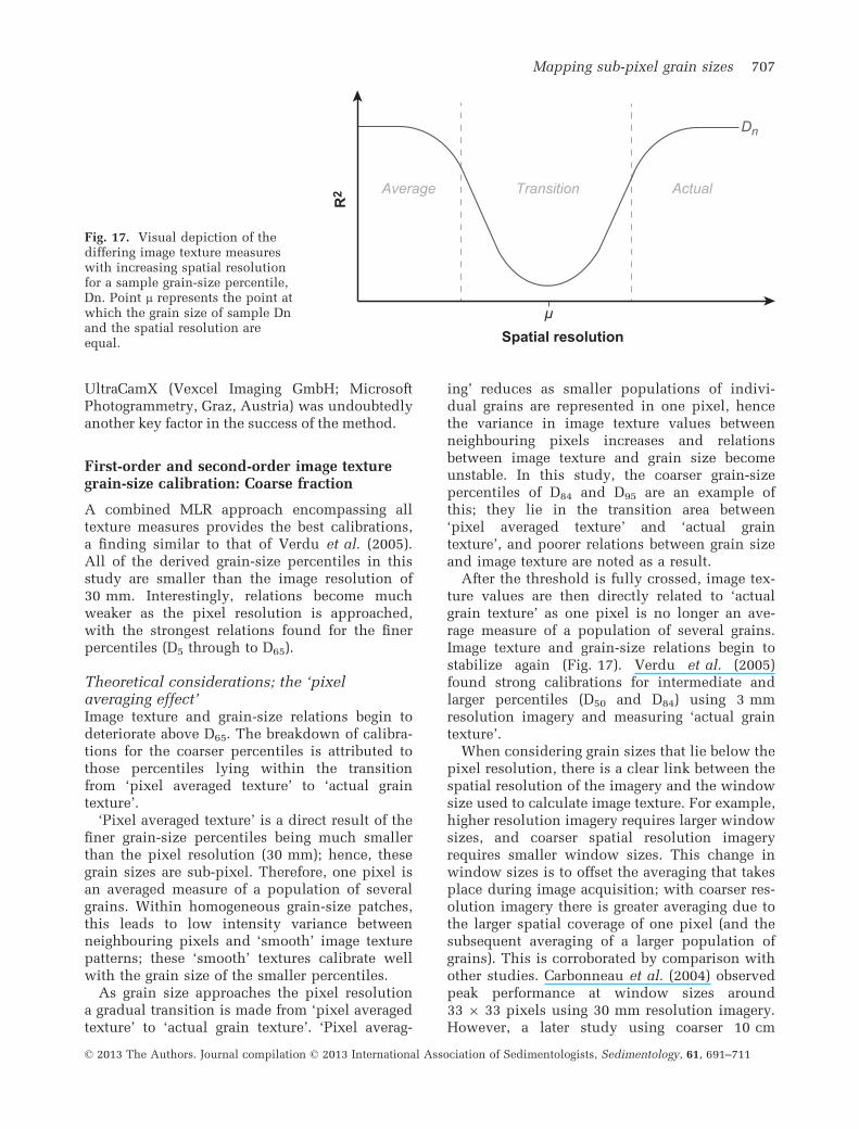
Theoretical considerations; the ‘pixelaveraging effect’Image texture and grain-size relations begin todeteriorate above D65. The breakdown of calibra-tions for the coarser percentiles is attributed tothose percentiles lying within the transitionfrom ‘pixel averaged texture’ to ‘actual graintexture’.‘Pixel averaged texture’ is a direct result of the

finer grain-size percentiles being much smallerthan the pixel resolution (30 mm); hence, thesegrain sizes are sub-pixel. Therefore, one pixel isan averaged measure of a population of severalgrains. Within homogeneous grain-size patches,this leads to low intensity variance betweenneighbouring pixels and ‘smooth’ image texturepatterns; these ‘smooth’ textures calibrate wellwith the grain size of the smaller percentiles.As grain size approaches the pixel resolution

a gradual transition is made from ‘pixel averagedtexture’ to ‘actual grain texture’. ‘Pixel averag-

ing’ reduces as smaller populations of indivi-dual grains are represented in one pixel, hencethe variance in image texture values betweenneighbouring pixels increases and relationsbetween image texture and grain size becomeunstable. In this study, the coarser grain-sizepercentiles of D84 and D95 are an example ofthis; they lie in the transition area between‘pixel averaged texture’ and ‘actual graintexture’, and poorer relations between grain sizeand image texture are noted as a result.After the threshold is fully crossed, image tex-

ture values are then directly related to ‘actualgrain texture’ as one pixel is no longer an ave-rage measure of a population of several grains.Image texture and grain-size relations begin tostabilize again (Fig. 17). Verdu et al. (2005)found strong calibrations for intermediate andlarger percentiles (D50 and D84) using 3 mmresolution imagery and measuring ‘actual graintexture’.When considering grain sizes that lie below the

pixel resolution, there is a clear link between thespatial resolution of the imagery and the windowsize used to calculate image texture. For example,higher resolution imagery requires larger windowsizes, and coarser spatial resolution imageryrequires smaller window sizes. This change inwindow sizes is to offset the averaging that takesplace during image acquisition; with coarser res-olution imagery there is greater averaging due tothe larger spatial coverage of one pixel (and thesubsequent averaging of a larger population ofgrains). This is corroborated by comparison withother studies. Carbonneau et al. (2004) observedpeak performance at window sizes around33 9 33 pixels using 30 mm resolution imagery.However, a later study using coarser 10 cm

R2

Spatial resolutionµ

Average Transition Actual

Dn

Fig. 17. Visual depiction of thediffering image texture measureswith increasing spatial resolutionfor a sample grain-size percentile,Dn. Point l represents the point atwhich the grain size of sample Dnand the spatial resolution areequal.

© 2013 The Authors. Journal compilation © 2013 International Association of Sedimentologists, Sedimentology, 61, 691–711

Mapping sub-pixel grain sizes 707

resolution imagery noted peak performance witha smaller 20 9 20 pixel window (Carbonneau,2005).

Parameter space investigation; whichparameters are important?First-order image texture measures present thesimple situation in which the user has only toconsider which combination of band and win-dow size to adopt. Figure 9 shows an investiga-tion of these parameters. Interestingly, there isa high degree of similarity in the resultsirrespective of the band used; namely, red,green, blue and NIR bands produce very similarresults. This is probably due to the high degreeof correlation amongst the RGB–NIR bands inthe imagery and the spectral similarity ofsediment in these bands; hence image texturecalculations produce very similar results irre-spective of the band used. Similarly, second-order image texture also showed that there islittle additional benefit gained from having anNIR band.For the second-order GLCM parameter of grey

levels, a clear pattern could be discerned.Within the percentiles that produced robustrelations (D5 to D65), over 70% of the ‘top 1000’parameter sets had 16 grey levels (Fig. 12). Simi-larly, Table 4 shows this pattern with a distinctdominance of 16 grey levels. The resampling ofgrey levels to this smaller value may have intro-duced some stability into the texture calcula-tions and reduced grey level noise; converselythe expansion of grey levels, up to 64 (andbeyond, such as 128 or 256) increases theamount of information captured in the GLCM,because there is less resampling. However, thedownside is that there is much greater variancein the GLCM itself, as well as within the GLCMstatistics. Subsequent image texture and calibra-tions begin to break down as a result. This sug-gests that the downsampling of grey levels is anacceptable practice (in line with the findings ofCarbonneau, 2005), and is even beneficial.Patterns could also be discerned for window

sizes and offsets for the reliably estimated per-centiles (D5 to D65). An illustrative example ofthis is shown in Fig. 13. Distinct areas of higherperformance were evident, most clearly articu-lated for window sizes. A clear threshold wasobserved; performance greatly deteriorated withwindow sizes smaller than ca 35 9 35 pixels.The optimal window size is reached whenenough pixels are present to produce stable cali-brations; in this instance, this occurs with win-

dow sizes above 35 9 35 pixels (cf. ‘pixelaveraging effect’; Theoretical considerations; the‘pixel averaging effect’ section).Offset directions (x and y) had their own high

performance areas; however, patterns are moredifficult to interpret. Predominantly north–south,and slight north-east/south-west GLCM orienta-tions (using a symmetrical GLCM; Table 4) werenoted (in GLCM coordinate space, where north–south represents offsets in the y direction, andeast–west represents the x direction). A poten-tial reason for the trend in GLCM orientationcould be the imbrication of sediment in thefield; GLCM orientations are the same as thedownstream flow direction of the river.Each of the independent GLCM statistics

(contrast, correlation and entropy) was calcu-lated with the premise that they would be laterused in MLR; but reasonable results (R2 > 0�65)were achieved for percentiles up to and includ-ing D65 without the use of MLR. Performancewas similar irrespective of the method used,however, both correlation and entropy rapidlydeteriorated for the larger percentiles (D84 andD95), suggesting that contrast may produce themost stable relations when considering the fullseven point coarse fraction grain-size distribu-tion. In assessing the applicability of these tech-niques at other study localities and withdiffering scales of imagery, a reduced parameterspace is recommended. Multispectral imagery isnot required, because similar relations are foundusing only standard colour imagery. Futurestudies need to consider only the parameters ofwindow size (where the minimum window sizeis set according to the image resolution) and off-sets. Offsets should be investigated with priorknowledge of sediment imbrication in the field,because it is likely that the optimal GLCM ori-entation will be coincident with any imbrica-tion. Remaining parameters can be set asdesired; if MLR is used, the independent statis-tic set (contrast, correlation and entropy) isadvised, and contrast is recommended if noMLR is used. Grey levels can be fixed at 16 (orperhaps even reduced).

Grain-size mapping considerations

Figure 15 shows a D50 grain-size map calculatedfor N bar, at a spatial resolution of 2�34 m2 (win-dow size of 51 9 51 pixels). Coarser resolutionis noted compared to Carbonneau et al. (2004)and Verdu et al. (2005) as a result of block pro-cessing at larger window sizes. This D50 map

© 2013 The Authors. Journal compilation © 2013 International Association of Sedimentologists, Sedimentology, 61, 691–711

708 M. Black et al.

was produced following the workflow outlinedin the Grain-size mapping: Workflow section.The final outputs from this processing chain areeight images; a surface sand classification, andan image for each of the seven grain-sizepercentiles.Consideration must be given to the MSE

values achieved for each percentile, and errorsmust be accounted for when using calculatedgrain sizes for other applications, such as mod-elling. Significant uncertainty exists for the lar-ger percentiles, particularly D84 and D95;however, the finer grain size fractions providefairly precise estimates compared to field sieveddata, and are much improved compared to pre-vious remote sensing methods.The direct applicability of the actual para-

meters and MLR coefficients presented here forderiving similar results at other field sites is dif-ficult to assess due to the lack of a similar data-set in a different location. It is expected thatgrain morphology, a consequence of grain litho-logy, may introduce variability in the parame-ters of the calibration equations. However, thesame methodology and workflow (Grain-sizemapping: Workflow section) are directly trans-ferable to other sites, although local calibrationmay be required. Parameter investigations neednot be as exhaustive as those presented here,and can follow the general recommendationsoutlined at the end of the Parameter spaceinvestigation; which parameters are important?section.Consideration must be given to the computa-

tional power required to process expansiveparameter spaces. Of all the parameters, thedominant control on CPU time is window size;smaller windows require the processing ofmore blocks, therefore more time is spent cal-culating GLCMs. The CPU time (seconds) isinversely proportional to window size, w, withan approximate relation of 45(w�2) where w isthe window size. This should then be multi-plied by the total number of blocks to gain theapproximate CPU time to process an entireimage.

Limitations

Several limitations and areas of uncertainty existin this study. An increased number of groundsampling sites would provide a better indicationof calibrations and other methods of measuringgrain size (for example, Wolman sampling)could have been employed to aid in validation

of results, particularly for the sand sites. Anincreased number of sites would also allow forthe retention of some data for grain-size valida-tion, rather than using cross-validation. Usingthe paint and pick technique, paint may havepenetrated the interstitial space between surfaceand buried grains; hence some sub-surfacegrains may have been incorrectly collected andsampled, introducing some uncertainty into theresults. Paint may have adhered smaller, parti-cularly sand and silt, grains to larger particles,thereby introducing a bias into the finer grainedfraction of the distribution (or in some cases itmay have acted to remove finer grained materialfrom the sample). Conversion of the finergrained material from weights to grain countsmay have also introduced slight error within thedata.The field sampling might introduce an addi-

tional difficulty for unbiased representation ofthe largest sizes. Large clasts are least commonin a single sample, so a large number of samplesmust be recovered in order to assure that per-centiles at the upper limit of the size distribu-tion are correctly assigned (Church et al., 1987).However, in the present case, the largest grains(of order 22 mm) each occupy about 0�04% ofthe field sample area and the problem shouldnot be significant.A particular area of uncertainty exists in refe-

rence to the aerial imagery itself. The georefe-renced image tiles supplied by the DTMMapping Corporation had undergone some ele-ment of pre-processing, the summary effect ofwhich has not been investigated. Raw, unpro-cessed image tiles were also supplied; however,the influence of significant georeferencing issuesand lack of perspective correction meant thatthe raw imagery introduced a much greatersource of positional error; and thus could not becalibrated due to uncertainty in georeferencing.

CONCLUSIONS

This study has investigated the relation betweenimage texture and surface grain size usinghyperspatial imagery. Detailed investigation offirst-order and second-order image textureapproaches for extracting sub-pixel grain-sizeinformation has shown convincingly that simplefirst-order measures are suitable for delineatingsurface sand features, whilst a combinedapproach of first-order and second-order image

© 2013 The Authors. Journal compilation © 2013 International Association of Sedimentologists, Sedimentology, 61, 691–711

Mapping sub-pixel grain sizes 709

texture can extract sub-pixel grain-size percen-tiles for the coarse fraction. This study repre-sents a significant step forward in terms of theapplicability of image texture approaches forderiving sub-pixel grain-size features fromhyperspatial imagery. The main conclusions areas follows:

1 The sand fraction can be automaticallydelineated with a peak classification accuracy ofca 90% using simple image texture thresholding.2 Coarse fraction (>1�41 mm) grain-size per-

centiles can be extracted using combinedfirst-order and second-order image texture andmultiple linear regression; relative error in thisstudy was 1�5%, 3�2%, 6�8% and 11% for D5,D16, D35 and D50, respectively. The largestpercentiles of D84 and D95 had relative errors of25% and 30%, respectively.3 Multispectral imagery (i.e. the additional of

a near-infrared band) is not required, as stan-dard colour imagery is sufficient.

The final workflow presented in the Grain-sizemapping: Workflow section allowed for theproduction of surface sand classification and aseven point coarse fraction grain-size distributioncovering the major sand and gravel bars ofQueens Bar, N Bar, Calamity Bar and HarrisonBar located within the gravel reach of FraserRiver. The limited number of field sites for cali-bration and validation (14 for sand and 23 for thecoarse fraction) is noted as a point for expansionin future studies. This method allows for a rapidacquisition of a seven point grain-size distribu-tion and map of surface sand content for large,vegetation-free sediment areas at a much higherspatial resolution than can be obtained throughstandard field techniques.

ACKNOWLEDGEMENTS

MB was supported by a Durham UniversityResearch Bursary. Acquisition of the hyperspa-tial imagery and field operations on Fraser Riverwere supported by a Discovery Grant from theNatural Sciences and Engineering ResearchCouncil of Canada and a contract from the Cana-dian Department of Fisheries and Oceans(awarded to MC). The cooperation of membersof DTM Mapping Corporation is gratefullyacknowledged. Dave Reid and Matt Chernos aregratefully thanked for their support in the field.Reviewers are thanked for their detailed com-ments on earlier versions of this manuscript.

REFERENCES

Buscombe, D. (2008) Estimation of grain-size distributions

and associated parameters from digital images of

sediment. Sed. Geol., 210, 1–10.Buscombe, D. and Rubin, D. (2012a) Advances in the

simulation and automated measurement of well-sorted

granular material. Part 1: simulation. J. Geophys. Res., 117,F02001. doi:10.1029/2011JF001974.

Buscombe, D. and Rubin, D. (2012b) Advances in the

simulation and automated measurement of well-sorted

granular material. Part 2: direct measures of particle

properties. J. Geophys. Res., 117, F02001. doi:10.1029/

2011JF001975.

Buscombe, D., Rubin, D.M. and Warrick, J.A. (2010) A

universal approximation of grain size from images of

noncohesive sediment. J. Geophys. Res., 115, F02015.

doi:10.1029/2009JF001477.

Butler, J., Lane, S. and Chandler, J. (2001) Automated

extraction of grain-size data from gravel surfaces using

digital image processing. J. Hydraul. Res., 39, 519–529.Carbonneau, P. (2005) The threshold effect of image

resolution on image-based automated grain size mapping in

fluvial environments. Earth Surf. Proc. Land., 30, 1687–1693.

Carbonneau, P. and Piegay, H. (2012) Fluvial Remote

Sensing for Science and Management. John Wiley and

Sons, Chichester.

Carbonneau, P., Lane, S. and Bergeron, N. E. (2004).

Catchment-scale mapping of surface grain size in gravel

bed rivers using airborne digital imagery. Water Resour.

Res., 40, W07202.

Carbonneau, P., Fonstad, M.A., Marcus, W.A. and Dugdale,S.J. (2012) Making riverscapes real. Geomorphology, 137,74–86. doi:10.1016/j.geomorph.2010.09.030.

Chandler, J. H., Rice, S. and Church, M. (2004). Colour

aerial photography for riverbed classification, The

International Archives of the Photogrammetry. Remote

Sens. Spatial Inform. Sci., 34, Commission 7, Istanbul,

1079–1085. Available at: http://www.isprs.org/proceedings

/XXXV/congress/comm7/papers/206.pdf.

Chang, F. and Chung, C. (2012) Estimation of riverbed

grain-size distribution using image-processing techniques.

J. Hydrol., 440–441, 102–112.Church, M., McLean, D. and Wolcott, J. (1987). River bed

gravels: sampling and analysis. In: Sediment Transport in

Gravel-Bed Rivers (Eds C. Thorne, J. Bathurst and R. Hey),

pp. 43–79. John Wiley and Sons (Wiley-Interscience),

Chichester.

Clausi, D.A. (2002) An analysis of co-occurrence texture

statistics as a function of grey level quantization. Can. J.Remote Sens., 28, 45–62.

Fausch, K.D., Torgersen, C.E., Baxter, C.V. and Li, H.W.(2002) Landscapes to Riverscapes: bridging the gap

between research and conservation of stream fishes: a

continuous view of the river is needed to understand how

process interacting among scales set the context for stream

fishes and their habitat. Bioscience, 52, 483–498.Gonzalez, R. and Woods, R. (2008). Digital Image

Processing. Pearson/Prentice Hall, New Jersey.

Graham, D., Reid, I. and Rice, S. (2005a) Automated sizing

of coarse-grained sediments: image-processing procedures.

Math. Geol., 37, 1–28.Graham, D., Reid, I. and Rice, S. (2005b) A transferable

method for the automated grain sizing of river gravels.

© 2013 The Authors. Journal compilation © 2013 International Association of Sedimentologists, Sedimentology, 61, 691–711

710 M. Black et al.

Water Resour. Res., 41, W07020. doi:10.1029/2004WR0038

68.

Haralick, R.M. (1979) Statistical and structural approaches

to texture. Proc. Inst. Electr. Electron. Eng., 67, 786–804.Haralick, R.M., Shanmugam, K. and Dinstein, I. (1973)

Textural features for image classification. Syst. ManCybernetics. IEEE Trans., 3, 610–621.

Hastie, T.J., Tibshirani, R.G. and Friedman, J.H. (2001) Theelements of statistical learning: data mining, inference,

and prediction. Springer Series in Statistics, Springer,

New York.

Ibbeken, H. and Schleyer, R. (1986) Photo-sieving: a method

for grain-size analysis of coarse-grained, unconsolidated

bedding surfaces. Earth Surf. Proc. Land., 11, 59–77.Klingeman, P. C. (1998). Gravel Bed Rivers in the

Environment. Water Resources Publication, Colorado, 832

pp.

Klug, W., Graziani, G., Grippa, G., Pierce, D. and Tassone,C (eds) (1992). Evaluation of Long Range Atmospheric

Transport Models Using Environmental Radioactivity Data

from the Chernobyl Accident: The ATMES Report.Elsevier, London, 366 pp.

Lane, E. and Carlson, E. (1953). Some factors affecting the

stability of canals constructed in coarse granular materials.

Proceedings of International Association of HydraulicResearch. 5th Congress, Minneapolis, 37–48.

Marcus, W.A. and Fonstad, M.A. (2008) Optical remote

mapping of rivers at sub-meter resolutions and watershed

extents. Earth Surf. Proc. Land., 33, 4–24.McEwan, I., Sheen, T., Cunningham, G. and Allen, A. (2000)

Estimating the size composition of sediment surfaces

through image analysis. Proc. Inst. Civil Eng. Water, Marit.Energy, 142, 189–195.

Otsu, N. (1979) A threshold selection method from gray-level

histograms. IEEE Trans. Syst. Man. Cybernetics, 9, 62–66.

Perica, S. and Foufoula-Georgiou, E. (1996) Model for

multiscale disaggregation of spatial rainfall based on coupling

meteorological and scaling descriptions. J. Geophys. Res.Atmos 101, 26347–26361. doi: 10.1029/96JD01870.

Pina, P., Lira, C. and Lousda, M. (2011) In-situ computation of

granulometries of sedimentary grains - some preliminary

results. J. Coastal Res., Special Edition, 64, 1727–1730.Pontius, R., Boersma, W., Castella, J., Clarke, K., de Nijs, T.,

Dietzel, C., Duan, Z., Fotsing, E., Goldstein, N., Kok, K.,Koomen, E., Lippitt, C.D., McConnell, B., Mohd Sood, A.,Pijanowski, B., Pithadia, S., Sweeney, S., Trung, T.N.,Veldkamp, A.T. and Verburg, P.H. (2008) Comparing the

input, output, and validation maps for several models of

land change. Ann. Regional Sci., 42, 11–37.Rango, A., Laliberte, A., Herrick, J. E., Winters, C., Havstad,

K., Steele, C. and Browning, D. (2009). Unmanned aerial

vehicle-based remote sensing for rangeland assessment,

monitoring, and management. J. Appl. Remote Sens., 3,033542. doi:10.1117/1.3216822

Rice, S.P. and Church, M. (2010) Grain size sorting within

river bars in relation to downstream fining along a

wandering channel. Sedimentology, 57, 232–251.Rubin, D.M. (2004) A simple autocorrelation algorithm for

determining grain size from digital images of sediment.

J. Sed. Res., 74, 160–165.Verdu, J.M., Batalla, R.J. and Martinez-Casasnovas, J.A.

(2005) High-resolution grain-size characterisation of

gravel bars using imagery analysis and geo-statistics.

Geomorphology, 72, 73–93.

Manuscript received 13 November 2012; revisionaccepted 18 July 2013

© 2013 The Authors. Journal compilation © 2013 International Association of Sedimentologists, Sedimentology, 61, 691–711

Mapping sub-pixel grain sizes 711