Mapping multiple insect outbreaks across large regions ...

remote sensing

Article

Mapping Multiple Insect Outbreaks across LargeRegions Annually Using Landsat Time Series Data

Benjamin C. Bright 1,* , Andrew T. Hudak 1 , Arjan J.H. Meddens 2, Joel M. Egan 3 andCarl L. Jorgensen 4

1 Rocky Mountain Research Station, United States Forest Service, 1221 South Main Street,Moscow, ID 83843, USA; [email protected]

2 School of the Environment, Washington State University, PO Box 642812, Pullman, WA 99164, USA;[email protected]

3 Northern Region, Forest Health Protection, United States Forest Service, 26 Fort Missoula Road,Missoula, MT 59804, USA; [email protected]

4 Intermountain Regions, Forest Health Protection, United States Forest Service, 1249 Vinnell Way, Suite 200,Boise, ID 83709, USA; [email protected]

* Correspondence: [email protected]; Tel.: +1-208-883-2311

Received: 27 April 2020; Accepted: 19 May 2020; Published: 21 May 2020�����������������

Abstract: Forest insect outbreaks have caused and will continue to cause extensive tree mortalityworldwide, affecting ecosystem services provided by forests. Remote sensing is an effective toolfor detecting and mapping tree mortality caused by forest insect outbreaks. In this study, we mapinsect-caused tree mortality across three coniferous forests in the Western United States for theyears 1984 to 2018. First, we mapped mortality at the tree level using field observations andhigh-resolution multispectral imagery collected in 2010, 2011, and 2018. Using these high-resolutionmaps of tree mortality as reference images, we then classified moderate-resolution Landsat imageryas disturbed or undisturbed and for disturbed pixels, predicted percent tree mortality with randomforest (RF) models. The classification approach and RF models were then applied to time series ofLandsat imagery generated with Google Earth Engine (GEE) to create annual maps of percent treemortality. We separated disturbed from undisturbed forest with overall accuracies of 74% to 80%.Cross-validated RF models explained 61% to 68% of the variation in percent tree mortality withindisturbed 30-m pixels. Landsat-derived maps of tree mortality were comparable to vector aerialsurvey data for a variety of insect agents, in terms of spatial patterns of mortality and annual estimatesof total mortality area. However, low-level tree mortality was not always detected. We conclude thatour methodology has the potential to generate reasonable estimates of annual tree mortality acrosslarge extents.

Keywords: forest; insects; bark beetles; defoliators; tree mortality; Landsat; time series; mapping

1. Introduction

Forest insect outbreaks have caused widespread tree mortality worldwide in recent years [1].Although insect-caused tree mortality has been ongoing for millennia [2], recent climate conditionshave facilitated insect outbreaks by increasing tree vulnerability and altering insect populationdynamics [1,3–5]. Extensive tree mortality caused by insect outbreaks affects crucial ecosystemservices provided by forests such as water supply [6,7], carbon storage [8], wildlife habitat [9], and theavailability of forest products [10]. Accurate estimates of the extent and severity of insect-caused treemortality are important for determining to what degree ecosystem services have been affected [11–13].In this study, we demonstrate a methodology for mapping insect-caused tree mortality annually acrosslarge extents using Landsat time series analysis.

Remote Sens. 2020, 12, 1655; doi:10.3390/rs12101655 www.mdpi.com/journal/remotesensing

Remote Sens. 2020, 12, 1655 2 of 20

The United States Department of Agriculture (USDA) Forest Service and partner agenciesconduct annual insect and disease surveys (IDS) to monitor insect activity across the nation’s forests.Surveyors aboard fixed-wing aircraft estimate the spatial extent, insect mortality agent, tree species host,and severity of insect-caused tree damage. IDS data are not only useful for monitoring and anticipatingfuture insect-caused tree mortality [14,15], but are also valuable for research applications investigatingthe causes and effects of forest insect outbreaks e.g., [8,16,17]. However, IDS data accuracy is limited;surveyors only have a short time to estimate often extensive tree damage; surveying conditions can beless than ideal; surveyor experience can influence accuracy; and some areas such as wilderness aresurveyed only infrequently, leading to data gaps [18]. In addition, IDS data coverage might become lessextensive in the future than recent years as costs increase and budgets decrease; therefore, the USDAForest Health Protection program responsible for overseeing IDS is making efforts to incorporatesatellite remote sensing in future forest health monitoring [19].

Satellite imagery is becoming a logical alternative to aerial surveys for monitoring and mappinginsect-caused tree mortality. Landsat satellites, with moderate spatial resolutions of 30 m and temporalrevisit times of 16 days, are particularly well-suited for this task. Furthermore, the Landsat TM missionof satellites has been in operation since 1984, making it possible to perform long-term time seriesanalyses. Several algorithms have been developed for detecting general forest change through timewith Landsat time series analysis [20]; these algorithms include Vegetation Change Tracker (VCT) [21],Landsat-based detection of Trends in Disturbance and Recovery (LandTrendr) [22], Breaks for AdditiveSeasonal and Trend (BFAST) [23], and Continuous Change Detection and Classification (CCDC) [24].Google Earth Engine (GEE) has recently made the application of such algorithms more accessible tousers [25]; for instance, the LandTrendr algorithm and associated Landsat preprocessing tasks havebeen implemented in GEE [26].

Previous work has shown how Landsat time series analysis can be used to estimate continuouslevels (i.e., percent of a 30-m pixel) of severe insect-related forest disturbances (see Senf et al. [27] fora review). Meigs et al. [28] showed that LandTrendr was sensitive to continuous levels of defoliatorand bark beetle damage in Oregon, USA. Townsend et al. [29] developed models predicting canopydefoliation severity in broadleaf deciduous forests in the eastern USA. Meddens et al. [30] and Meddensand Hicke [31] demonstrated a methodology for predicting continuous mountain pine beetle damagethrough time in Colorado, USA; in this methodology, tree mortality is mapped using high-resolutionsatellite imagery, which is then used to 1) classify forested Landsat pixels as disturbed or undisturbed,and 2) predict the continuous percent tree mortality of disturbed pixels. Assal et al. [32] and Long andLawrence [33] followed a similar approach to Meddens and Hicke [31] to estimate continuous mountainpine beetle-caused tree mortality in Montana, USA. Meigs et al. [34] predicted and mapped bark beetleand defoliator damage in terms of basal area across Oregon and Washington, USA. Woodward et al. [35]used a time series of Landsat data to map tree mortality severity caused by spruce beetles in Colorado,USA. Most previous studies have demonstrated the use of Landsat imagery for predicting mountainpine beetle-caused tree mortality; more studies are needed that demonstrate the use of Landsat imagetime series for predicting continuous tree mortality caused by other mortality agents.

To extend the work of Meddens et al. [30] and Meddens and Hicke [31], we investigated howtheir methodology performed in three additional study areas in the Western United States that haveexperienced tree mortality caused by a variety of mortality agents. Our approach differed from thatof Meddens et al. [30] and Meddens and Hicke [31] in that we (1) used GEE [25] to generate Landsatimage time series and implement the algorithm of Meddens and Hicke [31]; and (2) we used RandomForest (RF) modeling rather than linear modeling to predict continuous tree mortality. We concludethat the methodology of Meddens et al. [30] and Meddens and Hicke [31], implemented withinGEE, provides an effective means for mapping insect-caused tree mortality annually across largespatial extents.

Remote Sens. 2020, 12, 1655 3 of 20

2. Materials and Methods

2.1. Study Areas

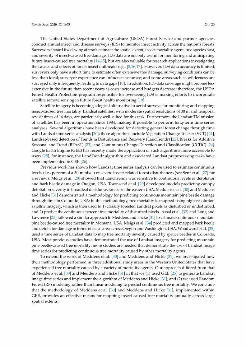
We chose three areas in the Western United States where insect activity has been elevated in recentyears, and where classified high-resolution multispectral imagery was available. Study areas includedthe 1) Stanley, Idaho vicinity, 2) Chimney Park, Wyoming vicinity, and 3) Elk City, Idaho vicinity(Figure 1). The forest around both Stanley and Chimney Park is dominated by lodgepole pine(Pinus contorta Douglas ex Loudon), with Douglas-fir (Pseudotsuga menziesii (Mirb.) Franco) andponderosa pine (Pinus ponderosa Lawson and C. Lawson) occurring at lower elevations, and Engelmannspruce (Picea engelmannii Parry ex Engelm.), subalpine fir (Abies lasiocarpa (Hook.) Nutt.), limber pine(Pinus flexilis James), and whitebark pine (Pinus albicaulis Engelm.) occurring at higher elevations.The forest around Elk City is mixed-conifer consisting of grand fir (Abies grandis (Douglas ex D. Don)Lindl.), Douglas-fir, ponderosa pine, lodgepole pine, Western white pine (Pinus monticola (Douglas exD. Don)), Western larch (Larix occidentalis Nutt.), Engelmann spruce, and subalpine fir.

Mountain pine beetle (Dendroctonus ponderosae Hopkins) outbreaks began in 2000 and 2005 in theStanley and Chimney Park study areas, respectively. Other prominent mortality agents in the Stanleyand Chimney Park study areas include Western spruce budworms (Choristoneura occidentalis Freeman)in Douglas-fir and subalpine fir, Douglas-fir beetles (Dendroctonus pseudotsugae Hopkins) in Douglas-fir,and spruce beetles (Dendroctonus rufipennis Kirby) in Engelmann spruce. In the Elk City study area,insect activity has been elevated for many years and includes several mortality agents: mountain pinebeetles in lodgepole pine, Douglas-fir beetles in Douglas-fir, fir engravers (Scolytus ventralis LeConte) ingrand fir, spruce beetles in Engelmann spruce, Western pine beetles (Dendroctonus brevicomis LeConte)in ponderosa pine, Western balsam bark beetles (Dryocoetes confuses Swaine) in subalpine fir, and balsamwoolly adelgids (Adelges piceae (Ratzeburg)) in grand and subalpine fir.

Terrain is generally mountainous in all study areas with elevations that range from 1080 to 3270,2000 to 4140, and 370 to 2710 m above sea level for the Stanley, Chimney Park, and Elk City study areas,respectively. Temperature averages 2.0, 2.7, and 3.8 ◦C, and annual precipitation averages 654, 381,and 800 mm for the Stanley, Chimney Park, and Elk City study areas, respectively (1961 to 1990) [36].

2.2. Field Observations

Field observations of live and beetle-killed trees in the Stanley and Elk City study areas weregathered in the summers of 2010 and 2018, respectively. Field observations were not gathered in theChimney Park study area. As part of a previous project [37], we stratified the Stanley study area bybiomass using pre-outbreak NDVI to sample in a variety of forest conditions. The Elk City study areawas stratified by mortality severity and agent using 2017 to 2018 IDS data, to ensure sampling across arange of mortality conditions and agents [38]. In both study areas, we located plot centers followingstratified random sampling designs, and navigated to plot centers with professional-grade TrimbleGNSS receivers in the field.

At plot centers, we established circular 400 m2 fixed-radius plots (radii of 11.3 m) and measuredall trees within plot extents with a diameter at breast height (DBH) >7 cm and >10 cm in Stanleyand Elk City, respectively. In addition to DBH, we measured tree condition (live or dead), species,canopy dominance, mortality agent, estimated time since death (based on needle, branch, and bolecondition, see Bright et al. [38], Table A1) or how many needles were remaining on dead trees,and distance and bearing from plot center. We logged several hundred positions at plot centers usingthe GNSS receivers, and differentially corrected plot center locations so that estimated plot centeraccuracies were <1 m. Plot center locations along with distance and bearing measurements were usedto calculate individual tree locations, which were then used to select pixels for image classification.

Remote Sens. 2020, 12, 1655 4 of 20Remote Sens. 2020, 11, x FOR PEER REVIEW 4 of 21

Figure 1. Study areas near Elk City and Stanley, Idaho, and Chimney Park, Wyoming, United States. Models predicting percent tree mortality were developed in areas of high-resolution multispectral imagery. Models were then applied to time series of Landsat imagery within 1 × 1 degree extents.

2.2. Field Observations

Field observations of live and beetle-killed trees in the Stanley and Elk City study areas were gathered in the summers of 2010 and 2018, respectively. Field observations were not gathered in the Chimney Park study area. As part of a previous project [37], we stratified the Stanley study area by biomass using pre-outbreak NDVI to sample in a variety of forest conditions. The Elk City study area was stratified by mortality severity and agent using 2017 to 2018 IDS data, to ensure sampling across a range of mortality conditions and agents [38]. In both study areas, we located plot centers following stratified random sampling designs, and navigated to plot centers with professional-grade Trimble GNSS receivers in the field.

Figure 1. Study areas near Elk City and Stanley, Idaho, and Chimney Park, Wyoming, United States.Models predicting percent tree mortality were developed in areas of high-resolution multispectralimagery. Models were then applied to time series of Landsat imagery within 1 × 1 degree extents.

2.3. High-Resolution and Landsat Imagery

High-resolution multispectral imagery was acquired over the Stanley, Chimney Park, and Elk Citystudy areas in 2010, 2011, and 2018, respectively (Figure 1). High-resolution imagery characteristicsvaried by study area (Table 1). Imagery of the Stanley study area consisted of digital aerialorthophotography, whereas Chimney Park and Elk City imagery came from the QuickBird andWorldView-2 satellites. Landsat imagery was processed in and acquired from the LandTrendrimplementation in GEE, which uses USGS Landsat Surface Reflectance Tier 1 imagery data sets.

Remote Sens. 2020, 12, 1655 5 of 20

Table 1. Characteristics of high-resolution multispectral imagery for each area.

Study Area Platform Date SpatialResolution (m)

Number ofBands Area (ha)

Stanley Fixed-wing aircraft Aug. 2010 0.2 4 6432Chimney Park QuickBird Aug. 2011 2.4 4 13,600

Elk City WorldView-2 Sept. 2018 2 8 104,896

2.4. Imagery Processing

In each of the three study areas, high-resolution imagery was used to create maps of tree mortality,which were then aggregated to a spatial resolution of 30-m, and used as reference data to (1) classifyLandsat imagery as non-forest, disturbed forest and undisturbed forest, and (2) predict percent treemortality of disturbed pixels (Figure 2). Models predicting percent tree mortality were then appliedto Landsat time series spanning the years 1984 to 2018. Each of these steps are described in moredetail below.Remote Sens. 2020, 11, x FOR PEER REVIEW 6 of 21

Figure 2. Overview of how field observations, high-resolution imagery, and Landsat imagery were used to create maps of percent tree mortality. This process was repeated for each of the three study areas.

2.4.1. High-Resolution Multispectral Imagery Processing

Image classification routines for each study area resulted in the separation of beetle-killed trees from live trees. The routines all used maximum likelihood classification and similar classification variables, including the Normalized Difference Vegetation Index (NDVI) and Red-Green Index (RGI), which are defined as:

NDVI = (NIR – RED) / (NIR + RED), (1)

RGI = RED / GREEN, (2)

where NIR is the near-infrared band, RED is the red band, and GREEN is the green band. Classification accuracy was evaluated using confusion matrices and visual comparison with true-color imagery.

For details on the classification of the Stanley aerial orthoimagery, see Bright et al. [37]. Briefly here, digital aerial orthoimagery was aggregated by averaging 0.2-m pixels to a spatial resolution of 2.4 m, the approximate average crown area of canopy trees in the imagery extent; aggregating imagery to 2.4 m pixels increased classification accuracy by reducing confusion between sunlit and shadowed tree crowns [39]. Sixteen-bit digital numbers (DN) were divided by 65,535 so that pixel values ranged from 0 to 1. Field observations were used to identify live and beetle-killed tree pixels on aggregated imagery. Two-thirds of the identified pixels were used for classification training; the remaining third were used for classification evaluation. Classification consisted of several steps: 1) water was classified using the NIR band (NIR <0.15 indicated water); 2) shadows were separated

Figure 2. Overview of how field observations, high-resolution imagery, and Landsat imagery were usedto create maps of percent tree mortality. This process was repeated for each of the three study areas.

2.4.1. High-Resolution Multispectral Imagery Processing

Image classification routines for each study area resulted in the separation of beetle-killed treesfrom live trees. The routines all used maximum likelihood classification and similar classificationvariables, including the Normalized Difference Vegetation Index (NDVI) and Red-Green Index (RGI),which are defined as:

NDVI = (NIR − RED) / (NIR + RED), (1)

Remote Sens. 2020, 12, 1655 6 of 20

RGI = RED / GREEN, (2)

where NIR is the near-infrared band, RED is the red band, and GREEN is the green band.Classification accuracy was evaluated using confusion matrices and visual comparison withtrue-color imagery.

For details on the classification of the Stanley aerial orthoimagery, see Bright et al. [37]. Briefly here,digital aerial orthoimagery was aggregated by averaging 0.2-m pixels to a spatial resolution of 2.4 m,the approximate average crown area of canopy trees in the imagery extent; aggregating imagery to2.4 m pixels increased classification accuracy by reducing confusion between sunlit and shadowedtree crowns [39]. Sixteen-bit digital numbers (DN) were divided by 65,535 so that pixel values rangedfrom 0 to 1. Field observations were used to identify live and beetle-killed tree pixels on aggregatedimagery. Two-thirds of the identified pixels were used for classification training; the remaining thirdwere used for classification evaluation. Classification consisted of several steps: (1) water was classifiedusing the NIR band (NIR < 0.15 indicated water); (2) shadows were separated from non-shadowpixels using the RED band (RED < 0.15 indicated shadow); (3) a canopy height model (CHM) derivedfrom coincident light detection and ranging data (lidar) was used separate forest and non-forest(CHM < 0.5 m indicated non-forest); (4) pixels with a RGI > 1.08 were classified as newly-killed redtrees, and the remaining pixels were classified as either green or gray trees using NIR, NDVI, and RGIin a maximum likelihood classifier. Water, shadow, and red tree thresholds were determined fromvisual inspection of true- and false-color imagery [37,39]. Overall lifeform classification accuracy was87%.

The Chimney Park QuickBird satellite imagery was classified similarly to the Stanley imagery,except no field observations were available for calibration/evaluation. DNs in 11 bits were dividedby 2048 to convert pixels to values between 0 and 1. The topography of the Chimney Park studyarea is relatively flat; healthy trees and red and gray beetle-killed tree pixels were easily identifiedon true- and false-color QuickBird imagery (Figure 1). Pixels of green and brown herbaceous coverand non-vegetated surfaces such as bare soil and road were also identified on imagery. Six hundredpixels of each class were identified across the image; half were used for classification training andhalf for evaluation. Water and shadow pixels were classified with threshold values of NIR < 0.07and RED < 0.04, respectively, and the remainder of classes were classified in a maximum likelihoodclassifier using GREEN, NDVI, and RGI as classification variables. Overall lifeform classificationaccuracy was 97%.

Elk City WorldView-2 imagery was delivered as a standard (2A) product, which had beenorthocorrected using a coarse digital elevation model (DEM). Imagery appeared to be well-correctedfor terrain when compared with high-resolution orthoimagery. Imagery was converted from DNs totop-of-atmosphere (TOA) reflectance using equations recommended by DigitalGlobe [40]. TOA reflectanceimagery was then converted to surface reflectance using empirical line calibration [41,42]. We selectedlive and dead tree pixels on imagery using field-measured tree locations. Visual inspection of imagerywas used to select pixels of green and brown herbaceous cover, as well as non-vegetated surfaces. Half ofthe pixels were used for classification training; the remainder were used for classification evaluation.Imagery was classified using the GREEN, red-edge (WV2 band 6), NIR (WV2 band 8), NDVI, and RGI asclassification variables in a maximum likelihood classifier. Shadows were masked with the RED band(RED < 4.1% indicated shadow). Overall lifeform classification accuracy was 96%.

High-resolution classifications for each study area were then aggregated to 30-m grids to beused for comparison with Landsat imagery. We created a mode aggregation grid for each study area,where aggregated 30-m pixels took the value of the modal class, as well as grids of percent area byclass, including percent dead tree grids to be used as response variables in predictive models.

2.4.2. Landsat Imagery Processing

Annual Landsat image time series for the years 1984 to 2018 coincident with high-resolutionimagery were created using functions from the LandTrendr implementation in GEE [25,26].

Remote Sens. 2020, 12, 1655 7 of 20

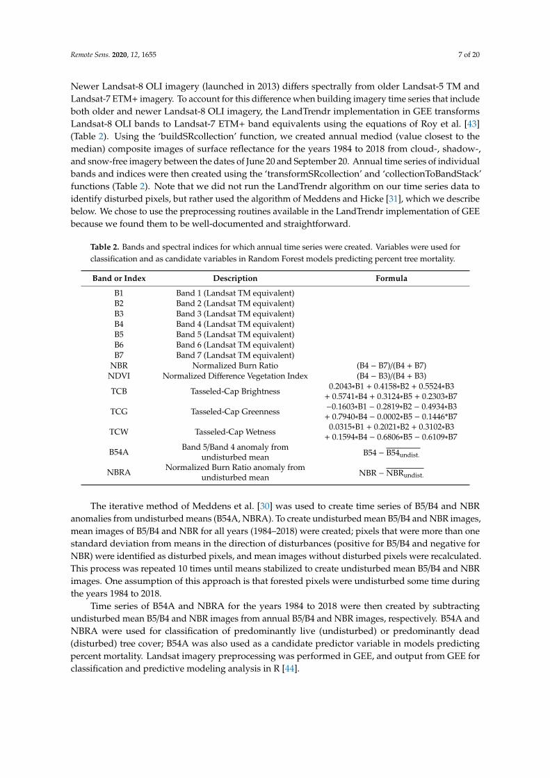
Newer Landsat-8 OLI imagery (launched in 2013) differs spectrally from older Landsat-5 TM andLandsat-7 ETM+ imagery. To account for this difference when building imagery time series that includeboth older and newer Landsat-8 OLI imagery, the LandTrendr implementation in GEE transformsLandsat-8 OLI bands to Landsat-7 ETM+ band equivalents using the equations of Roy et al. [43](Table 2). Using the ‘buildSRcollection’ function, we created annual mediod (value closest to themedian) composite images of surface reflectance for the years 1984 to 2018 from cloud-, shadow-,and snow-free imagery between the dates of June 20 and September 20. Annual time series of individualbands and indices were then created using the ‘transformSRcollection’ and ‘collectionToBandStack’functions (Table 2). Note that we did not run the LandTrendr algorithm on our time series data toidentify disturbed pixels, but rather used the algorithm of Meddens and Hicke [31], which we describebelow. We chose to use the preprocessing routines available in the LandTrendr implementation of GEEbecause we found them to be well-documented and straightforward.

Table 2. Bands and spectral indices for which annual time series were created. Variables were used forclassification and as candidate variables in Random Forest models predicting percent tree mortality.

Band or Index Description Formula

B1 Band 1 (Landsat TM equivalent)B2 Band 2 (Landsat TM equivalent)B3 Band 3 (Landsat TM equivalent)B4 Band 4 (Landsat TM equivalent)B5 Band 5 (Landsat TM equivalent)B6 Band 6 (Landsat TM equivalent)B7 Band 7 (Landsat TM equivalent)

NBR Normalized Burn Ratio (B4 − B7)/(B4 + B7)NDVI Normalized Difference Vegetation Index (B4 − B3)/(B4 + B3)

TCB Tasseled-Cap Brightness 0.2043∗B1 + 0.4158∗B2 + 0.5524∗B3+ 0.5741∗B4 + 0.3124∗B5 + 0.2303∗B7

TCG Tasseled-Cap Greenness −0.1603∗B1 − 0.2819∗B2 − 0.4934∗B3+ 0.7940∗B4 − 0.0002∗B5 − 0.1446*B7

TCW Tasseled-Cap Wetness 0.0315∗B1 + 0.2021∗B2 + 0.3102∗B3+ 0.1594∗B4 − 0.6806∗B5 − 0.6109∗B7

B54A Band 5/Band 4 anomaly fromundisturbed mean B54 − B54undist.

NBRA Normalized Burn Ratio anomaly fromundisturbed mean NBR − NBRundist.

The iterative method of Meddens et al. [30] was used to create time series of B5/B4 and NBRanomalies from undisturbed means (B54A, NBRA). To create undisturbed mean B5/B4 and NBR images,mean images of B5/B4 and NBR for all years (1984–2018) were created; pixels that were more than onestandard deviation from means in the direction of disturbances (positive for B5/B4 and negative forNBR) were identified as disturbed pixels, and mean images without disturbed pixels were recalculated.This process was repeated 10 times until means stabilized to create undisturbed mean B5/B4 and NBRimages. One assumption of this approach is that forested pixels were undisturbed some time duringthe years 1984 to 2018.

Time series of B54A and NBRA for the years 1984 to 2018 were then created by subtractingundisturbed mean B5/B4 and NBR images from annual B5/B4 and NBR images, respectively. B54A andNBRA were used for classification of predominantly live (undisturbed) or predominantly dead(disturbed) tree cover; B54A was also used as a candidate predictor variable in models predictingpercent mortality. Landsat imagery preprocessing was performed in GEE, and output from GEE forclassification and predictive modeling analysis in R [44].

Remote Sens. 2020, 12, 1655 8 of 20

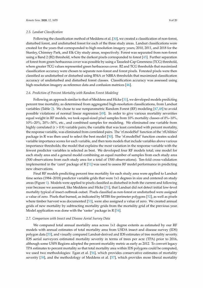
2.5. Landsat Classification

Following the classification method of Meddens et al. [30], we created a classification of non-forest,disturbed forest, and undisturbed forest for each of the three study areas. Landsat classifications werecreated for the years that corresponded to high-resolution imagery years; 2010, 2011, and 2018 for theStanley, Chimney Park, and Elk City study areas, respectively. Forest was separated from non-forestusing a Band 2 (B2) threshold, where the darkest pixels corresponded to forest [45]. Further separationof forest from green herbaceous cover was possible by using a Tasseled-Cap Greenness (TCG) threshold,where greater TCG values represented green herbaceous cover. B2 and TCG thresholds that maximizedclassification accuracy were chosen to separate non-forest and forest pixels. Forested pixels were thenclassified as undisturbed or disturbed using B54A or NBRA thresholds that maximized classificationaccuracy of undisturbed and disturbed forest classes. Classification accuracy was assessed usinghigh-resolution imagery as reference data and confusion matrices [46].

2.6. Prediction of Percent Mortality with Random Forest Modeling

Following an approach similar to that of Meddens and Hicke [31], we developed models predictingpercent tree mortality, as determined from aggregated high-resolution classifications, from Landsatvariables (Table 2). We chose to use nonparametric Random Forest (RF) modeling [47,48] to avoidpossible violations of normal linear regression [49]. In order to give various mortality severitiesequal weight in RF models, we took equal-sized pixel samples from 10% mortality classes of 0%–10%,10%–20%, 20%–30%, etc., and combined samples for modeling. We eliminated one variable fromhighly correlated (r > 0.9) variable pairs; the variable that was least correlated with percent mortality,the response variable, was eliminated from correlated pairs. The ‘rf.modelSel’ function of the ‘rfUtilities’package in R was then used to select the best model [50]. The ‘rf.modelSel’ function creates scaledvariable importance scores for each variable, and then tests models that include variables above variousimportance thresholds; the model that explains the most variation in the response variable with thefewest predictor variables is selected as best. We developed four RF models total; one model foreach study area and a general model combining an equal number of samples from each study area(500 observations from each study area for a total of 1500 observations). Ten-fold cross-validationimplemented in the ‘caret’ package of R [51] was used to assess RF model performance in predictingnew observations.

Final RF models predicting percent tree mortality for each study area were applied to Landsattime series (1984–2018) predictor variable grids that were 1x1 degrees in size and centered on studyareas (Figure 1). Models were applied to pixels classified as disturbed in both the current and followingyear because we assumed, like Meddens and Hicke [31], that Landsat did not detect initial low-levelmortality typical of insect outbreak outset. Pixels classified as non-forest or undisturbed were assigneda value of zero. Pixels that burned, as indicated by MTBS fire perimeter polygons [52], as well as pixelswhere timber harvest was documented [53], were also assigned a value of zero. We created annualgrids of new mortality by subtracting mortality grids from the mortality grid of the previous year.Model application was done with the ‘raster’ package in R [54].

2.7. Comparison with Insect and Disease Aerial Survey Data

We compared total annual mortality area across 1x1 degree extents as estimated by our RFmodels with annual estimates of total mortality area from USDA insect and disease survey (IDS)polygon data [55], and visually compared Landsat-derived and IDS estimates of tree mortality severity.IDS aerial surveyors estimated mortality severity in terms of trees per acre (TPA) prior to 2016,although some USFS Regions adopted the percent mortality metric as early as 2012. To convert legacyTPA estimates to percent mortality so that total mortality area within IDS polygons could be computed,we used two methodologies: Egan et al. [56], which provides conservative estimates of mortalityseverity [38], and the methodology of Meddens et al. [57], which provides more liberal mortality

Remote Sens. 2020, 12, 1655 9 of 20

severity estimates. The methodology of Egan et al. [56], which utilizes the relationship betweensurveyed field TPA and percent mortality plot data to adjust IDS TPA estimates, assigns percentmortality values of 5%, 20%, and 65% to IDS polygons having TPA estimates from 0 to 9.9, 10 to 30,and >30, respectively. The methodology of Meddens et al. [57], which is based on a comparison ofhigh-resolution remote sensing data and IDS TPA, estimates percent mortality with the following:

PM = TPA × CA × 100 × 13.6, (3)

where PM is percent mortality, TPA is the legacy trees per acre (TPA) attribute of the polygon andCA is the species-specific average crown area, in acres, of the recorded tree host [57] (Appendix A);the 13.6 multiplier compensates for IDS underestimation bias for most tree species/damage agentcombinations [57,58]. IDS polygons of abiotic (0.6% of polygons) or insect-caused tree mortalitywithout TPA measurements were assigned a TPA value of 2, the median for all IDS polygons. Our aimwas to predict and map tree mortality. However, initial comparison of our tree mortality mapswith IDS polygons showed that our approach also detected biotic defoliation or mortality caused bydefoliation, hence we included IDS polygons representing defoliation damage when validating ourLandsat-derived maps with independent IDS polygon data. IDS polygons of defoliator damage wereassigned a percent mortality value of 10% [59–61], the median for all IDS polygons after conversionfrom TPA.

3. Results

3.1. Landsat Classification into Non-Forest, Undisturbed Forest, and Disturbed Forest

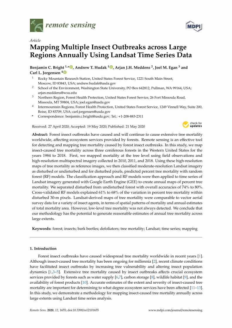
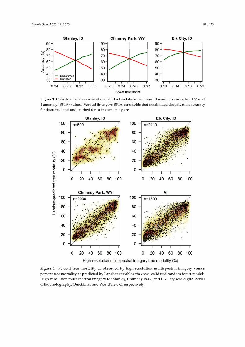
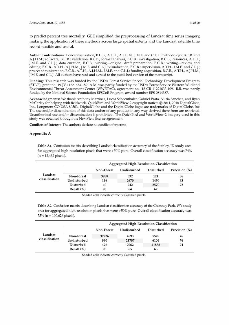
Overall classification accuracies ranged from 74% to 80% for pixels that contained > 50% of agiven class (Tables 3 and A1–A3). We found that using the B2 mean or the B2 mean plus one standarddeviation worked well for separating forest from non-forest. TCG thresholds of the mean TCG plus oneor two standard deviations further separated forest from green herbaceous cover. B54A consistentlyseparated disturbed from non-disturbed forest with greater accuracy than NBRA, so we used B54Afor final classifications. B54A thresholds that maximized class accuracies ranged from 0.165 to 0.307(Table 3, Figure 3).

Table 3. Band 2 (B2), tasseled-cap greenness (TCG), and band 5/band 4 anomaly (B54A) thresholds usedto classify non-, disturbed, and undisturbed forest for each study area. B2 and TGC thresholds wereused to separate forest from non-forest (values < thresholds corresponded to forest). B54A thresholdswere used to separate disturbed from undisturbed forest (values > B54A thresholds indicate disturbedforest). sd = standard deviation.

Study Area B2 Threshold TCG Threshold B54A Threshold Overall Accuracy (%)

Stanley, ID 0.57 (mean) 1.0 (mean + 1 sd) 0.307 74Chimney Park, WY 0.50 (mean) 1.1 (mean + 1 sd) 0.265 75

Elk City, ID 0.51 (mean + 1 sd) 1.8 (mean + 2 sd) 0.165 80

3.2. Prediction of Percent Tree Mortality with Random Forest Modeling

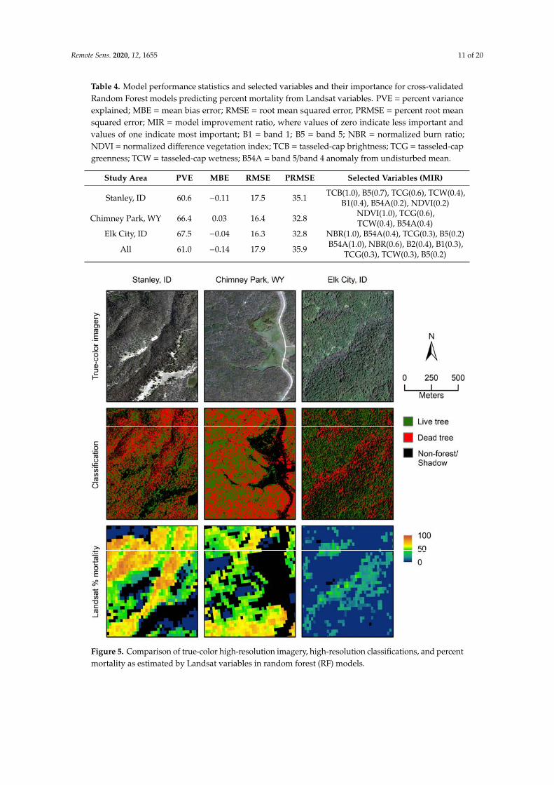
Ten-fold cross-validated RF models explained 61% to 68% of the variation in percent mortality(Table 4, Figure 4). TCB, NDVI, and NBR were the most important variables in RF models for theStanley, Chimney Park, and Elk City study areas, respectively. TCG and B54A were selected aspredictor variables in all study areas. B5, NBR, and TCW were selected as predictor variables in twostudy areas. B54A and NBR were the most important variables in the general model. Spatial patternsof tree mortality severity as predicted by Landsat variables matched those of high-resolution imagery(Figure 5).

Remote Sens. 2020, 12, 1655 10 of 20

Remote Sens. 2020, 11, x FOR PEER REVIEW 10 of 21

defoliation, hence we included IDS polygons representing defoliation damage when validating our Landsat-derived maps with independent IDS polygon data. IDS polygons of defoliator damage were assigned a percent mortality value of 10% [59–61], the median for all IDS polygons after conversion from TPA.

3. Results

3.1. Landsat Classification into Non-Forest, Undisturbed Forest, and Disturbed Forest

Overall classification accuracies ranged from 74% to 80% for pixels that contained > 50% of a given class (Table 3, Tables A1–A3). We found that using the B2 mean or the B2 mean plus one standard deviation worked well for separating forest from non-forest. TCG thresholds of the mean TCG plus one or two standard deviations further separated forest from green herbaceous cover. B54A consistently separated disturbed from non-disturbed forest with greater accuracy than NBRA, so we used B54A for final classifications. B54A thresholds that maximized class accuracies ranged from 0.165 to 0.307 (Table 3, Figure 3).

Table 3. Band 2 (B2), tasseled-cap greenness (TCG), and band 5/band 4 anomaly (B54A) thresholds used to classify non-, disturbed, and undisturbed forest for each study area. B2 and TGC thresholds were used to separate forest from non-forest (values < thresholds corresponded to forest). B54A thresholds were used to separate disturbed from undisturbed forest (values > B54A thresholds indicate disturbed forest). sd = standard deviation.

Study area B2 threshold TCG threshold B54A threshold Overall accuracy (%) Stanley, ID 0.57 (mean) 1.0 (mean + 1 sd) 0.307 74

Chimney Park, WY 0.50 (mean) 1.1 (mean + 1 sd) 0.265 75 Elk City, ID 0.51 (mean + 1 sd) 1.8 (mean + 2 sd) 0.165 80

Figure 3. Classification accuracies of undisturbed and disturbed forest classes for various band 5/band 4 anomaly (B54A) values. Vertical lines give B54A thresholds that maximized classification accuracy for disturbed and undisturbed forest in each study area.

3.2. Prediction of Percent Tree Mortality with Random Forest Modeling

Ten-fold cross-validated RF models explained 61% to 68% of the variation in percent mortality (Table 4, Figure 4). TCB, NDVI, and NBR were the most important variables in RF models for the Stanley, Chimney Park, and Elk City study areas, respectively. TCG and B54A were selected as predictor variables in all study areas. B5, NBR, and TCW were selected as predictor variables in two study areas. B54A and NBR were the most important variables in the general model. Spatial patterns of tree mortality severity as predicted by Landsat variables matched those of high-resolution imagery (Figure 5).

Figure 3. Classification accuracies of undisturbed and disturbed forest classes for various band 5/band4 anomaly (B54A) values. Vertical lines give B54A thresholds that maximized classification accuracyfor disturbed and undisturbed forest in each study area.

Remote Sens. 2020, 11, x FOR PEER REVIEW 11 of 21

Table 4. Model performance statistics and selected variables and their importance for cross-validated Random Forest models predicting percent mortality from Landsat variables. PVE = percent variance explained; MBE = mean bias error; RMSE = root mean squared error, PRMSE = percent root mean squared error; MIR = model improvement ratio, where values of zero indicate less important and values of one indicate most important; B1 = band 1; B5 = band 5; NBR = normalized burn ratio; NDVI = normalized difference vegetation index; TCB = tasseled-cap brightness; TCG = tasseled-cap greenness; TCW = tasseled-cap wetness; B54A = band 5/band 4 anomaly from undisturbed mean.

Study area PVE MBE RMSE PRMSE Selected variables (MIR)

Stanley, ID 60.6 -0.11 17.5 35.1 TCB(1.0), B5(0.7), TCG(0.6), TCW(0.4),

B1(0.4), B54A(0.2), NDVI(0.2) Chimney Park, WY 66.4 0.03 16.4 32.8 NDVI(1.0), TCG(0.6), TCW(0.4), B54A(0.4)

Elk City, ID 67.5 -0.04 16.3 32.8 NBR(1.0), B54A(0.4), TCG(0.3), B5(0.2)

All 61.0 -0.14 17.9 35.9 B54A(1.0), NBR(0.6), B2(0.4), B1(0.3),

TCG(0.3), TCW(0.3), B5(0.2)

Figure 4. Percent tree mortality as observed by high-resolution multispectral imagery versus percent tree mortality as predicted by Landsat variables via cross-validated random forest models. High-resolution multispectral imagery for Stanley, Chimney Park, and Elk City was digital aerial orthophotography, QuickBird, and WorldView-2, respectively.

Figure 4. Percent tree mortality as observed by high-resolution multispectral imagery versuspercent tree mortality as predicted by Landsat variables via cross-validated random forest models.High-resolution multispectral imagery for Stanley, Chimney Park, and Elk City was digital aerialorthophotography, QuickBird, and WorldView-2, respectively.

Remote Sens. 2020, 12, 1655 11 of 20

Table 4. Model performance statistics and selected variables and their importance for cross-validatedRandom Forest models predicting percent mortality from Landsat variables. PVE = percent varianceexplained; MBE = mean bias error; RMSE = root mean squared error, PRMSE = percent root meansquared error; MIR = model improvement ratio, where values of zero indicate less important andvalues of one indicate most important; B1 = band 1; B5 = band 5; NBR = normalized burn ratio;NDVI = normalized difference vegetation index; TCB = tasseled-cap brightness; TCG = tasseled-capgreenness; TCW = tasseled-cap wetness; B54A = band 5/band 4 anomaly from undisturbed mean.

Study Area PVE MBE RMSE PRMSE Selected Variables (MIR)

Stanley, ID 60.6 −0.11 17.5 35.1 TCB(1.0), B5(0.7), TCG(0.6), TCW(0.4),B1(0.4), B54A(0.2), NDVI(0.2)

Chimney Park, WY 66.4 0.03 16.4 32.8 NDVI(1.0), TCG(0.6),TCW(0.4), B54A(0.4)

Elk City, ID 67.5 −0.04 16.3 32.8 NBR(1.0), B54A(0.4), TCG(0.3), B5(0.2)

All 61.0 −0.14 17.9 35.9 B54A(1.0), NBR(0.6), B2(0.4), B1(0.3),TCG(0.3), TCW(0.3), B5(0.2)Remote Sens. 2020, 11, x FOR PEER REVIEW 12 of 21

Figure 5. Comparison of true-color high-resolution imagery, high-resolution classifications, and percent mortality as estimated by Landsat variables in random forest (RF) models.

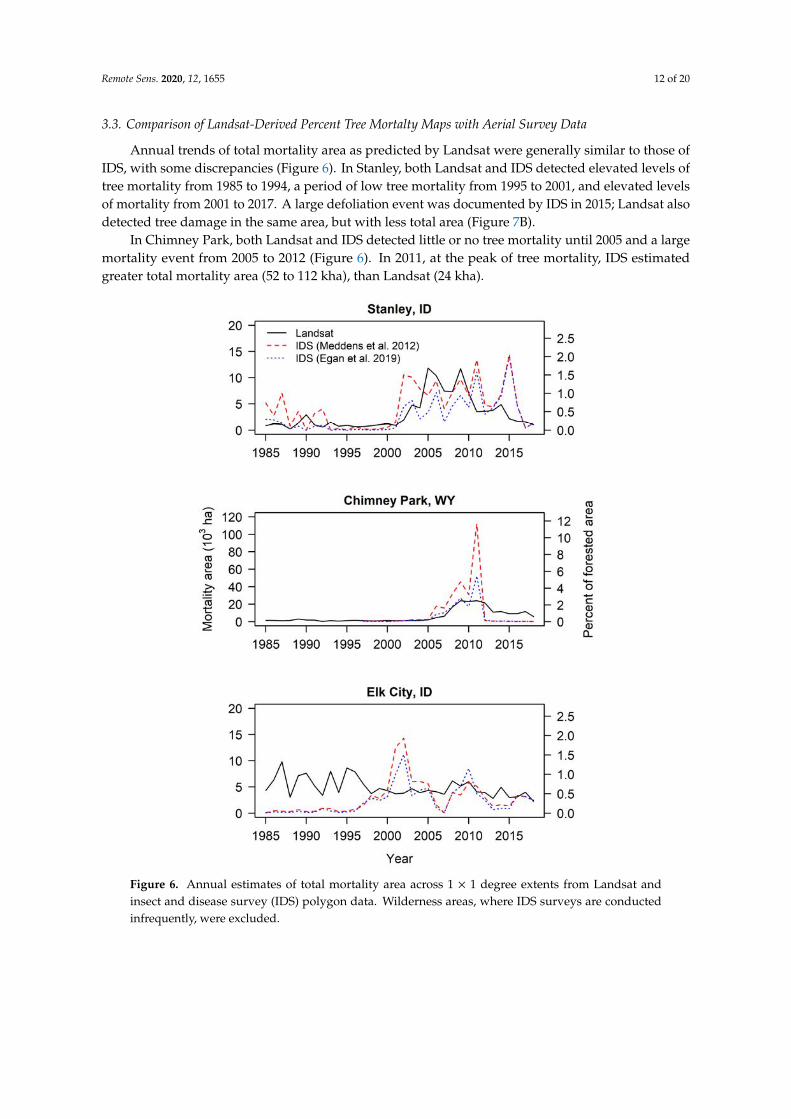
3.3. Comparison of Landsat-Derived Percent Tree Mortalty Maps with Aerial Survey Data

Annual trends of total mortality area as predicted by Landsat were generally similar to those of IDS, with some discrepancies (Figure 6). In Stanley, both Landsat and IDS detected elevated levels of tree mortality from 1985 to 1994, a period of low tree mortality from 1995 to 2001, and elevated levels of mortality from 2001 to 2017. A large defoliation event was documented by IDS in 2015; Landsat also detected tree damage in the same area, but with less total area (Figure 7B).

In Chimney Park, both Landsat and IDS detected little or no tree mortality until 2005 and a large mortality event from 2005 to 2012 (Figure 6). In 2011, at the peak of tree mortality, IDS estimated greater total mortality area (52 to 112 kha), than Landsat (24 kha).

Annual trends of total mortality area were most dissimilar between Landsat and IDS in Elk City (Figure 6); Landsat detected continuous mortality levels of 2-10 kha yr-1 throughout the entire time series (1984 to 2018), whereas IDS did not show elevated tree mortality levels >1 kha yr-1 until 1997. IDS showed a peak in mortality of 7-14 kha yr-1 in 2001 and 2002; Landsat detected mortality in the same vicinity, but at lower levels of 4-5 kha yr-1. Although annual trends differed, overall mortality levels ranged from 0.1-14 kha yr-1 for both Landsat and IDS throughout the time series, and Landsat and IDS trends post-2002 tracked each other (Figure 6).

Figure 5. Comparison of true-color high-resolution imagery, high-resolution classifications, and percentmortality as estimated by Landsat variables in random forest (RF) models.

Remote Sens. 2020, 12, 1655 12 of 20

3.3. Comparison of Landsat-Derived Percent Tree Mortalty Maps with Aerial Survey Data

Annual trends of total mortality area as predicted by Landsat were generally similar to those ofIDS, with some discrepancies (Figure 6). In Stanley, both Landsat and IDS detected elevated levels oftree mortality from 1985 to 1994, a period of low tree mortality from 1995 to 2001, and elevated levelsof mortality from 2001 to 2017. A large defoliation event was documented by IDS in 2015; Landsat alsodetected tree damage in the same area, but with less total area (Figure 7B).

In Chimney Park, both Landsat and IDS detected little or no tree mortality until 2005 and a largemortality event from 2005 to 2012 (Figure 6). In 2011, at the peak of tree mortality, IDS estimatedgreater total mortality area (52 to 112 kha), than Landsat (24 kha).

Remote Sens. 2020, 11, x FOR PEER REVIEW 13 of 21

Visual comparison of Landsat-derived maps of tree mortality with IDS polygons generally showed good agreement for a variety of insect agents, especially for moderate and severe forest mortality (Figure 7). Agreement was less apparent for low forest mortality; Landsat often detected forest disturbance in and around the vicinity of low severity IDS polygons, but not always (Figure 7B,E,F). Although tree mortality caused by fires and harvest, as well as non-forest, were masked, Landsat maps also showed mortality outside IDS polygons (Figure 7E,F). Both the Stanley and Elk City 1x1 degree study areas contained large portions of wilderness areas in which Landsat maps revealed substantial unsurveyed tree mortality.

Figure 6. Annual estimates of total mortality area across 1 × 1 degree extents from Landsat and insect and disease survey (IDS) polygon data. Wilderness areas, where IDS surveys are conducted infrequently, were excluded.

Figure 6. Annual estimates of total mortality area across 1 × 1 degree extents from Landsat andinsect and disease survey (IDS) polygon data. Wilderness areas, where IDS surveys are conductedinfrequently, were excluded.

Remote Sens. 2020, 12, 1655 13 of 20Remote Sens. 2020, 11, x FOR PEER REVIEW 14 of 21

Figure 7. Comparison of annual maps of Landsat-derived percent tree mortality and insect and disease survey (IDS) polygon data from various insect agents. Panels show: (A) moderate forest mortality caused by mountain pine beetles in the Stanley study area in 2008; (B) low forest mortality caused by Western spruce budworms in the Stanley study area in 2015; (C) severe forest mortality caused by mountain pine beetles and Western spruce budworms in the Chimney Park study area in 2008; (D) moderate forest mortality caused by spruce and mountain pine beetles in the Chimney Park study area in 2011; (E) low forest mortality caused by Western balsam bark and mountain pine beetles in the Elk City study area in 2001; and (F) low forest mortality caused by Douglas-fir and fir engraver beetles in the Elk City study area in 2017.

4. Discussion

We estimated insect-caused tree mortality caused by a variety of mortality agents across three large areas for the years 1984 to 2018 using Landsat time series analysis. We separated non-forest, undisturbed, and disturbed forest with overall accuracies of 74% to 80% and explained 61% to 68% of the variation in percent tree mortality using Landsat variables. Similar to others, we found the Landsat shortwave-infrared to near-infrared ratio (B54) index to be a good indicator of change in coniferous forest [31,62,63]. The B54 index was likely sensitive to changes in forest structure caused by forest mortality, rather than directly sensing changes to vegetation physiology. For our

Figure 7. Comparison of annual maps of Landsat-derived percent tree mortality and insect and diseasesurvey (IDS) polygon data from various insect agents. Panels show: (A) moderate forest mortalitycaused by mountain pine beetles in the Stanley study area in 2008; (B) low forest mortality causedby Western spruce budworms in the Stanley study area in 2015; (C) severe forest mortality causedby mountain pine beetles and Western spruce budworms in the Chimney Park study area in 2008;(D) moderate forest mortality caused by spruce and mountain pine beetles in the Chimney Park studyarea in 2011; (E) low forest mortality caused by Western balsam bark and mountain pine beetles in theElk City study area in 2001; and (F) low forest mortality caused by Douglas-fir and fir engraver beetlesin the Elk City study area in 2017.

Annual trends of total mortality area were most dissimilar between Landsat and IDS in Elk City(Figure 6); Landsat detected continuous mortality levels of 2–10 kha yr−1 throughout the entire timeseries (1984 to 2018), whereas IDS did not show elevated tree mortality levels >1 kha yr−1 until 1997.IDS showed a peak in mortality of 7–14 kha yr−1 in 2001 and 2002; Landsat detected mortality in thesame vicinity, but at lower levels of 4–5 kha yr−1. Although annual trends differed, overall mortalitylevels ranged from 0.1–4 kha yr−1 for both Landsat and IDS throughout the time series, and Landsatand IDS trends post-2002 tracked each other (Figure 6).

Visual comparison of Landsat-derived maps of tree mortality with IDS polygons generally showedgood agreement for a variety of insect agents, especially for moderate and severe forest mortality(Figure 7). Agreement was less apparent for low forest mortality; Landsat often detected forest

Remote Sens. 2020, 12, 1655 14 of 20

disturbance in and around the vicinity of low severity IDS polygons, but not always (Figure 7B,E,F).Although tree mortality caused by fires and harvest, as well as non-forest, were masked, Landsat mapsalso showed mortality outside IDS polygons (Figure 7E,F). Both the Stanley and Elk City 1 × 1 degreestudy areas contained large portions of wilderness areas in which Landsat maps revealed substantialunsurveyed tree mortality.

4. Discussion

We estimated insect-caused tree mortality caused by a variety of mortality agents across threelarge areas for the years 1984 to 2018 using Landsat time series analysis. We separated non-forest,undisturbed, and disturbed forest with overall accuracies of 74% to 80% and explained 61% to 68%of the variation in percent tree mortality using Landsat variables. Similar to others, we found theLandsat shortwave-infrared to near-infrared ratio (B54) index to be a good indicator of change inconiferous forest [31,62,63]. The B54 index was likely sensitive to changes in forest structure caused byforest mortality, rather than directly sensing changes to vegetation physiology. For our application,the detection of insect-caused canopy disturbance, B54 outperformed NBR, another popular index fordocumenting forest change. However, NBR, as well as NDVI and Landsat Tasseled-Cap variables,were still found to be important predictors of the degree of insect-caused forest decline. Rates of forestdisturbance that we estimated within our study areas (0.1% to 3% of forest area yr−1) were similar tothe national estimates of Cohen et al. [64] (1.5% to 4.5% of forest area yr−1).

We found GEE [25] and the preprocessing functions of the LandTrendr implementation in GEE [26]to be powerful tools for simplifying the processing of Landsat time series data. Before GEE, the taskof preprocessing and managing Landsat time series data required significant resources and time.What required days or weeks of work can now be completed in hours with the functions availablein the LandTrendr implementation of GEE, which we found to be simple to understand and execute.The simplicity and efficiency of GEE makes the application of our method across large areas feasible.

RF modeling provided several benefits over linear modeling. First, RF allowed for nonlinearrelationships between response and predictor variables. Although many of the relationships betweenour response variable, percent tree mortality, and Landsat predictor variables were approximately linear,some, particularly B54A, were nonlinear. Second, RF modeling is better suited to modeling continuouspercent tree mortality, which can be zero-inflated, i.e., having many values near zero. Zero-inflated datacan result in heteroskedastic variance of errors, a violation of normal linear regression [49]. Third, the RFalgorithm partitions data into training and evaluation datasets internally. Although we performedten-fold cross-validation to rigorously evaluate our RF models, we found that model diagnostics ofcross-validated models were nearly identical to model diagnostics of non-cross-validated models,suggesting that cross-validation was not necessary and the out-of-bag estimate of error provided byRF was sufficient.

Our methodology has the potential to be applied across large spatial extents. The B2 and TCGthresholds that we used to separate forest from non-forest, as well as the B54A threshold values thatwe used to separate undisturbed from disturbed forest were comparable across our three study areas(Table 3). In addition, our general RF model combining observations from all study areas performedsimilarly to RF models of individual study areas (Table 4, Figure 4). This suggests that we could applythis methodology across a large region, such as an entire wilderness area, national forest, state, or ForestService Region. However, caution should be used when applying algorithms and models outsideareas where those models were calibrated, as accuracy might decrease in new areas [63,65]. The use ofseveral calibration sites distributed across the larger area of interest, as well as applying algorithms andmodels only within similar forest types, would help to minimize inappropriate extrapolation outsidecalibration areas. Few previous studies have applied Landsat time series analysis for the detection ofinsect-caused tree mortality across large study areas [27,31,34].

Detection of lower-severity forest disturbance with Landsat remains a challenge. Insect-caused treemortality usually occurs gradually and at lower levels relative to fire or harvest, making it more challenging

Remote Sens. 2020, 12, 1655 15 of 20

to detect with moderate-resolution satellites. Numerous previous studies have shown that Landsat timeseries analysis can be used to detect high-severity forest disturbance, where most trees within a 30-mpixel are disturbed, with high accuracy [30,32,49,66]. However, lower-severity disturbance, where fewertrees are disturbed within a 30-m pixel, is detected with less accuracy [30,63,66]. Although we did notspecifically examine classification accuracy by disturbance severity, comparison of our Landsat-derivedmaps with IDS polygons showed that low-severity disturbance as detected by IDS surveyors was notalways detected with our Landsat time series analysis, as expected.

Comparison of our Landsat-derived mortality maps with IDS showed some discrepancies,especially in areas of low tree mortality (Figures 6 and 7). However, IDS data are a fundamentallydifferent, vector-based representation of disturbance, so differences are expected. For example,IDS showed a large amount of defoliator-caused tree damage in our Stanley study area in 2015,while Landsat showed much less total area affected (Figure 6). Examination of IDS polygons within ageographic information system (GIS) showed that IDS polygons were large and highly generalized(Figure 7B). Our Landsat-derived maps detected damage in the same areas, but perhaps more precisely.Meigs et al. [34] made a similar observation that IDS polygons are a generalization of damage areathat can exaggerate overall area affected, whereas Landsat methods can give more resolved damageestimates at 30-m resolution. So, while our estimates of low-level damage did not always agree withIDS polygons, Landsat representations of low-level tree damage, when detected, are likely moreaccurate representations of diffuse tree damage than large generalized IDS polygons.

Another notable difference between our Landsat-derived maps and IDS was in the Elk City studyarea for the years before 1997, where Landsat detected considerable disturbance and IDS showedlittle. This discrepancy could be caused by limited IDS survey coverage in the 1980s and 1990s,when IDS flights often targeted specific insect agents and some areas were missed on a regular basis.We could not verify this because no information on survey extent was available for IDS data priorto 1997. Our Landsat methodology could have also detected non-insect-related forest disturbance,such as undocumented forest harvest, small fires, or forest decline such as that caused by drought [64].Indeed, Landsat identified considerable mortality in 1987, the driest year of the years 1980 to 2018in the Elk City vicinity. Although we masked areas of documented forest harvest, many of the areasidentified as being disturbed in the Elk City area prior to 1997 occurred adjacent to areas of timberharvest, particularly along the edges of harvested areas. This highlights one limitation of our approach,that beyond masking large burns and documented harvest with ancillary data, disturbance is notseparated by type.

Attributing causes of forest change with satellite time series analysis is a topic of currentresearch [27], where others have made some progress. Senf et al. [67] successfully distinguishedbetween mountain pine beetle mortality and Western spruce budworm damage in British Columbia,Canada using LandTrendr-derived spectral trajectories. Meigs et al. [34] used IDS polygons asancillary information for distinguishing between forest damage caused by mountain pine beetles andWestern spruce budworms. Cohen et al. [64] used TimeSync [68] and ancillary datasets to distinguishharvest and fire from forest decline across the United States. Oeser et al. [69] distinguished betweenwindthrow, bark beetles, and harvest in central Europe with intra-annual Landsat time series analysis.Vogeler et al. [70] distinguished various types of forest disturbance in Minnesota, USA using Landsattime series analysis. Future work could implement similar approaches that use spectral trajectorydifferences or incorporate ancillary data to further distinguish tree mortality by type.

5. Conclusions

We estimated continuous insect-caused tree mortality in three study areas in the Western UnitedStates that have experienced recent forest insect outbreaks, and generated maps of continuous treemortality estimates across large extents for the years 1984 to 2018 for a variety of insect mortalityagents. We adapted the previously developed methods of Meddens et al. by using Google EarthEngine (GEE) to pre-process Landsat imagery, and developing nonparametric Random Forest models

Remote Sens. 2020, 12, 1655 16 of 20

to predict percent tree mortality. GEE simplified the preprocessing of Landsat time series imagery,making the application of these methods across large spatial extents and the Landsat satellite timerecord feasible and useful.

Author Contributions: Conceptualization, B.C.B., A.T.H., A.J.H.M., J.M.E. and C.L.J.; methodology, B.C.B. andA.J.H.M.; software, B.C.B.; validation, B.C.B.; formal analysis, B.C.B.; investigation, B.C.B.; resources, A.T.H.,J.M.E. and C.L.J.; data curation, B.C.B.; writing—original draft preparation, B.C.B.; writing—review andediting, B.C.B., A.T.H., A.J.H.M., J.M.E. and C.L.J.; visualization, B.C.B.; supervision, A.T.H., J.M.E. and C.L.J.;project administration, B.C.B., A.T.H., A.J.H.M., J.M.E. and C.L.J.; funding acquisition, B.C.B., A.T.H., A.J.H.M.,J.M.E. and C.L.J. All authors have read and agreed to the published version of the manuscript.

Funding: This research was funded by the USDA Forest Service Special Technology Development Program(STDP), grant no. 19-JV-11221633-189. A.M. was partly funded by the USDA Forest Service Western WildlandEnvironmental Threat Assessment Center (WWETAC), agreement no. 18-CR-11221633-109. B.B. was partlyfunded by the National Science Foundation EPSCoR Program, award number EPS-0814387.

Acknowledgments: We thank Anthony Martinez, Lucca Schoenthaler, Gabriel Prata, Nuria Sanchez, and RyanMcCarley for helping with fieldwork. QuickBird and WorldView-2 copyright notice: © 2011, 2018 DigitalGlobe,Inc., Longmont CO USA 80503. DigitalGlobe and the DigitalGlobe logos are trademarks of DigitalGlobe, Inc.The use and/or dissemination of this data and/or of any product in any way derived there from are restricted.Unauthorized use and/or dissemination is prohibited. The QuickBird and WorldView-2 imagery used in thisstudy was obtained through the NextView license agreement.

Conflicts of Interest: The authors declare no conflict of interest.

Appendix A

Table A1. Confusion matrix describing Landsat classification accuracy of the Stanley, ID study areafor aggregated high-resolution pixels that were >50% pure. Overall classification accuracy was 74%(n = 12,432 pixels).

Landsatclassification

Aggregated High-Resolution Classification

Non-Forest Undisturbed Disturbed Precision (%)

Non-forest 3988 532 124 86Undisturbed 116 2670 1450 63

Disturbed 40 942 2570 72Recall (%) 96 64 62

Shaded cells indicate correctly classified pixels.

Table A2. Confusion matrix describing Landsat classification accuracy of the Chimney Park, WY studyarea for aggregated high-resolution pixels that were >50% pure. Overall classification accuracy was75% (n = 100,626 pixels).

Landsatclassification

Aggregated High-Resolution Classification

Non-Forest Undisturbed Disturbed Precision (%)

Non-forest 32226 4693 5578 76Undisturbed 890 21787 6106 76

Disturbed 426 7062 21858 74Recall (%) 96 65 65

Shaded cells indicate correctly classified pixels.

Remote Sens. 2020, 12, 1655 17 of 20

Table A3. Confusion matrix describing Landsat classification accuracy of the Elk City, ID study areafor aggregated high-resolution pixels that were >50% pure. Overall classification accuracy was 80%(n = 16,116 pixels).

Landsatclassification

Aggregated High-Resolution Classification

Non-Forest Undisturbed Disturbed Precision (%)

Non-forest 4814 1028 843 72Undisturbed 418 4061 472 82

Disturbed 140 283 4057 91Recall (%) 90 76 76

References

1. Allen, C.D.; Macalady, A.K.; Chenchouni, H.; Bachelet, M.; McDowell, N.; Vennetier, M.; Kitzberger, T.;Rigling, A.; Breshears, D.D.; Hogg, T.; et al. A global overview of drought and heat-induced tree mortalityreveals emerging climate change risks for forests. For. Ecol. Manag. 2010, 259, 660–684. [CrossRef]

2. Brunelle, A.; Rehfeldt, G.E.; Bentz, B.; Munson, A.S. Holocene records of Dendroctonus bark beetles in highelevation pine forests of Idaho and Montana, USA. For. Ecol. Manag. 2008, 255, 836–846. [CrossRef]

3. Raffa, K.F.; Aukema, B.H.; Bentz, B.J.; Carroll, A.L.; Hicke, J.; Turner, M.G.; Romme, W.H. Cross-scale Driversof Natural Disturbances Prone to Anthropogenic Amplification: The Dynamics of Bark Beetle Eruptions.Bioscience 2008, 58, 501–517. [CrossRef]

4. Bentz, B.J.; Régnière, J.; Fettig, C.J.; Hansen, E.M.; Hayes, J.L.; Hicke, J.A.; Kelsey, R.G.; Negrón, J.F.;Seybold, S.J. Climate Change and Bark Beetles of the Western United States and Canada: Direct and IndirectEffects. Bioscience 2010, 60, 602–613. [CrossRef]

5. Seidl, R.; Thom, D.; Kautz, M.; Martin-Benito, D.; Peltoniemi, M.; Vacchiano, G.; Wild, J.; Ascoli, D.; Petr, M.;Honkaniemi, J.; et al. Forest disturbances under climate change. Nat. Clim. Chang. 2017, 7, 395–402.[CrossRef] [PubMed]

6. Pugh, E.; Small, E. The impact of pine beetle infestation on snow accumulation and melt in the headwatersof the Colorado River. Ecohydrology 2011, 5, 467–477. [CrossRef]

7. Mikkelson, K.M.; Bearup, L.; Maxwell, R.M.; Stednick, J.D.; McCray, J.E.; Sharp, J.O. Bark beetle infestationimpacts on nutrient cycling, water quality and interdependent hydrological effects. Biogeochemistry 2013, 115,1–21. [CrossRef]

8. Hicke, J.; Meddens, A.J.H.; Allen, C.D.; Kolden, C.A. Carbon stocks of trees killed by bark beetles and wildfirein the western United States. Environ. Res. Lett. 2013, 8, 035032. [CrossRef]

9. Saab, V.A.; Latif, Q.S.; Rowland, M.M.; Johnson, T.N.; Chalfoun, A.D.; Buskirk, S.; Heyward, J.E.; Dresser, M.A.Ecological Consequences of Mountain Pine Beetle Outbreaks for Wildlife in Western North American Forests.For. Sci. 2014, 60, 539–559. [CrossRef]

10. Dhar, A.; Parrott, L.; Heckbert, S. Consequences of mountain pine beetle outbreak on forest ecosystemservices in western Canada. Can. J. For. Res. 2016, 46, 987–999. [CrossRef]

11. Edburg, S.L.; Hicke, J.A.; Lawrence, D.; Thornton, P.E. Simulating coupled carbon and nitrogen dynamicsfollowing mountain pine beetle outbreaks in the western United States. J. Geophys. Res. Space Phys. 2011, 116.[CrossRef]

12. Bright, B.C.; Hicke, J.; Meddens, A.J.H. Effects of bark beetle-caused tree mortality on biogeochemical andbiogeophysical MODIS products. J. Geophys. Res. Biogeosci. 2013, 118, 974–982. [CrossRef]

13. Dietze, M.C.; Matthes, J.H. A general ecophysiological framework for modelling the impact of pests andpathogens on forest ecosystems. Ecol. Lett. 2014, 17, 1418–1426. [CrossRef] [PubMed]

14. Krist, F.J., Jr.; Ellenwood, J.R.; Woods, M.E.; McMahan, A.J.; Cowardin, J.P.; Ryerson, D.E.; Sapio, F.J.;Zweifler, M.O.; Romero, S.A. 2013–2027 National Insect and Disease Forest Risk Assessment; FHTET-14-01; U.S.Department of Agriculture Forest Service, Forest Health Technology Enterprise Team: Fort Collins, CO, USA,2014; 199p.

15. USDA Forest Service. Major Forest Insect and Disease Conditions in the United States: 2015; FS-1093; Forest HealthProtection: Washington, DC, USA, 2017; 56p.

Remote Sens. 2020, 12, 1655 18 of 20

16. Hart, S.J.; Schoennagel, T.; Veblen, T.T.; Chapman, T.B. Area burned in the western United States is unaffectedby recent mountain pine beetle outbreaks. Proc. Natl. Acad. Sci. USA 2015, 112, 4375–4380. [CrossRef][PubMed]

17. Buotte, P.C.; Hicke, J.; Preisler, H.K.; Abatzoglou, J.T.; Raffa, K.F.; Logan, J.A. Climate influences on whitebarkpine mortality from mountain pine beetle in the Greater Yellowstone Ecosystem. Ecol. Appl. 2016, 26,2507–2524. [CrossRef]

18. Coleman, T.W.; Graves, A.D.; Heath, Z.; Flowers, R.W.; Hanavan, R.P.; Cluck, D.R.; Ryerson, D. Accuracy ofaerial detection surveys for mapping insect and disease disturbances in the United States. For. Ecol. Manag.2018, 430, 321–336. [CrossRef]

19. Housman, I.W.; Chastain, R.A.; Finco, M.V. An Evaluation of Forest Health Insect and Disease Survey Dataand Satellite-Based Remote Sensing Forest Change Detection Methods: Case Studies in the United States.Remote Sens. 2018, 10, 1184. [CrossRef]

20. Banskota, A.; Kayastha, N.; Falkowski, M.J.; Wulder, M.A.; Froese, R.E.; White, J.C. Forest Monitoring UsingLandsat Time Series Data: A Review. Can. J. Remote Sens. 2014, 40, 362–384. [CrossRef]

21. Huang, C.; Goward, S.N.; Masek, J.G.; Thomas, N.; Zhu, Z.; Vogelmann, J. An automated approach forreconstructing recent forest disturbance history using dense Landsat time series stacks. Remote Sens. Environ.2010, 114, 183–198. [CrossRef]

22. Kennedy, R.E.; Yang, Z.; Cohen, W. Detecting trends in forest disturbance and recovery using yearly Landsattime series: 1. LandTrendr—Temporal segmentation algorithms. Remote Sens. Environ. 2010, 114, 2897–2910.[CrossRef]

23. Verbesselt, J.; Hyndman, R.J.; Newnham, G.; Culvenor, D. Detecting trend and seasonal changes in satelliteimage time series. Remote Sens. Environ. 2010, 114, 106–115. [CrossRef]

24. Zhu, Z.; Woodcock, C.E. Continuous change detection and classification of land cover using all availableLandsat data. Remote Sens. Environ. 2014, 144, 152–171. [CrossRef]

25. Gorelick, N.; Hancher, M.; Dixon, M.; Ilyushchenko, S.; Thau, D.; Moore, R. Google Earth Engine:Planetary-scale geospatial analysis for everyone. Remote Sens. Environ. 2017, 202, 18–27. [CrossRef]

26. Kennedy, R.; Yang, Z.; Gorelick, N.; Braaten, J.; Cavalcante, L.; Cohen, W.B.; Healey, S.P. Implementation ofthe LandTrendr Algorithm on Google Earth Engine. Remote Sens. 2018, 10, 691. [CrossRef]

27. Senf, C.; Seidl, R.; Hostert, P. Remote sensing of forest insect disturbances: Current state and future directions.Int. J. Appl. Earth Obs. Geoinf. 2017, 60, 49–60. [CrossRef] [PubMed]

28. Meigs, G.W.; Kennedy, R.E.; Cohen, W. A Landsat time series approach to characterize bark beetle anddefoliator impacts on tree mortality and surface fuels in conifer forests. Remote Sens. Environ. 2011, 115,3707–3718. [CrossRef]

29. Townsend, P.A.; Singh, A.; Foster, J.; Rehberg, N.J.; Kingdon, C.C.; Eshleman, K.; Seagle, S.W. A generalLandsat model to predict canopy defoliation in broadleaf deciduous forests. Remote Sens. Environ. 2012, 119,255–265. [CrossRef]

30. Meddens, A.J.H.; Hicke, J.; Vierling, L.A.; Hudak, A.T. Evaluating methods to detect bark beetle-causedtree mortality using single-date and multi-date Landsat imagery. Remote Sens. Environ. 2013, 132, 49–58.[CrossRef]

31. Meddens, A.J.H.; Hicke, J. Spatial and temporal patterns of Landsat-based detection of tree mortality causedby a mountain pine beetle outbreak in Colorado, USA. For. Ecol. Manag. 2014, 322, 78–88. [CrossRef]

32. Assal, T.; Sibold, J.; Reich, R. Modeling a Historical Mountain Pine Beetle Outbreak Using Landsat MSS andMultiple Lines of Evidence. Remote Sens. Environ. 2014, 155, 275–288. [CrossRef]

33. Long, J.; Lawrence, R.L. Mapping Percent Tree Mortality Due to Mountain Pine Beetle Damage. For. Sci.2016, 62, 392–402. [CrossRef]

34. Meigs, G.W.; Kennedy, R.E.; Gray, A.N.; Gregory, M.J. Spatiotemporal dynamics of recent mountain pinebeetle and western spruce budworm outbreaks across the Pacific Northwest Region, USA. For. Ecol. Manag.2015, 339, 71–86. [CrossRef]

35. Woodward, B.D.; Evangelista, P.H.; Vorster, A. Mapping Progression and Severity of a Southern ColoradoSpruce Beetle Outbreak Using Calibrated Image Composites. Forests 2018, 9, 336. [CrossRef]

36. Research on Forest Climate Change: Potential Effects of Global Warming on Forests and Plant ClimateRelationships in Western North America and Mexico. Available online: http://charcoal.cnre.vt.edu/climate/

(accessed on 6 April 2020).

Remote Sens. 2020, 12, 1655 19 of 20

37. Bright, B.C.; Hicke, J.A.; Hudak, A.T. Estimating aboveground carbon stocks of a forest affected by mountainpine beetle in Idaho using lidar and multispectral imagery. Remote Sens. Environ. 2012, 124, 270–281.[CrossRef]

38. Bright, B.C.; Hudak, A.; Egan, J.; Jorgensen, C.; Rex, F.; Hicke, J.A.; Meddens, A. Using Satellite Imageryto Evaluate Bark Beetle-Caused Tree Mortality Reported in Aerial Surveys in a Mixed Conifer Forest inNorthern Idaho, USA. Forests 2020, 11, 529. [CrossRef]

39. Meddens, A.J.H.; Hicke, J.; Vierling, L.A. Evaluating the potential of multispectral imagery to map multiplestages of tree mortality. Remote Sens. Environ. 2011, 115, 1632–1642. [CrossRef]

40. DigitalGlobe. Absolute Radiometric Calibration: 2016v0, Prepared by Michele, A. Kuester. DigitalGlobe Inc.Headquarters: Westminster, Colorado, USA, 2017, 8p. Available online: https://dg-cms-uploads-production.s3.amazonaws.com/uploads/document/file/209/ABSRADCAL_FLEET_2016v0_Rel20170606.pdf (accessed on9 March 2020).

41. Smith, G.M.; Milton, E.J. The use of the empirical line method to calibrate remotely sensed data to reflectance.Int. J. Remote Sens. 1999, 20, 2653–2662. [CrossRef]

42. Jensen, J.R.; Lulla, K. Introductory digital image processing: A remote sensing perspective. Geocarto Int.1987, 2, 65. [CrossRef]

43. Roy, D.; Kovalskyy, V.; Zhang, H.; Vermote, E.; Yan, L.; Kumar, S.S.; Egorov, A. Characterization of Landsat-7 toLandsat-8 reflective wavelength and normalized difference vegetation index continuity. Remote Sens. Environ.2016, 185, 57–70. [CrossRef]

44. Anonymous. The R Project for Statistical Computing. Available online: http://www.r-project.org/ (accessed on13 February 2012).

45. Huang, C.; Song, K.; Kim, S.; Townshend, J.R.; Davis, P.; Masek, J.; Goward, S.N. Use of a dark object conceptand support vector machines to automate forest cover change analysis. Remote Sens. Environ. 2008, 112,970–985. [CrossRef]

46. Congalton, R.G. A review of assessing the accuracy of classifications of remotely sensed data. Remote Sens. Environ.1991, 37, 35–46. [CrossRef]

47. Breiman, L. Random Forests. Mach. Learn. 2001, 45, 5–32. [CrossRef]48. Liaw, A.; Wiener, M. Classification and regression by randomforest. R News 2002, 2, 18–22.49. Schwantes, A.M.; Swenson, J.J.; Jackson, R.B. Quantifying drought-induced tree mortality in the open canopy

woodlands of central Texas. Remote Sens. Environ. 2016, 181, 54–64. [CrossRef]50. Murphy, M.; Evans, J.; Storfer, A. Quantifying Bufo boreas connectivity in Yellowstone National Park with

landscape genetics. Ecology 2010, 91, 252–261. [CrossRef]51. Kuhn, M. Caret: Classification and Regression Training. R Package Version 6.0-86. 2020. Available online:

https://CRAN.R-project.org/package=caret (accessed on 6 April 2020).52. Eidenshink, J.; Schwind, B.; Brewer, K.; Zhu, Z.; Quayle, B.; Howard, S. A Project for Monitoring Trends in

Burn Severity. Fire Ecol. 2007, 3, 3–21. [CrossRef]53. FSGeodata Clearinghouse, Download National Datasets, Timber Harvest. Available online: https://data.fs.

usda.gov/geodata/edw/datasets.php (accessed on 31 January 2020).54. Hijmans, R.J. Raster: Geographic Data Analysis and Modeling. R Package Version 3.0-12. 2020. Available online:

https://CRAN.R-project.org/package=raster (accessed on 6 April 2020).55. Insect & Disease Detection Survey (IDS) Data Downloads. Available online: https://www.fs.fed.us/

foresthealth/applied-sciences/mapping-reporting/detection-surveys.shtml (accessed on 5 December 2019).56. Egan, J.M.; Kaiden, J.; Lestina, J.; Stasey, A.; Jenne, J.L. Techniques to Enhance Assessment and Reporting of

Pest Damage Estimated with Aerial Detection Surveys; R1-19-09; US Department of Agriculture, Forest Service,Northern Region, Forest Health Protection: Missoula, MT, USA, 2019; 33p.

57. Meddens, A.J.H.; Hicke, J.; Ferguson, C.A. Spatiotemporal patterns of observed bark beetle-caused treemortality in British Columbia and the western United States. Ecol. Appl. 2012, 22, 1876–1891. [CrossRef]

58. Hicke, J.; Meddens, A.J.H.; Kolden, C.A. Recent Tree Mortality in the Western United States from Bark Beetlesand Forest Fires. For. Sci. 2016, 62, 141–153. [CrossRef]

59. Collis, D.G.; van Sickle, G.A. Damage Appraisal Cruises in Spruce Budworm Defoliated Stands of Douglas-firin 1977, Information Report BC-P-19. Fisheries and Environment Canada, Canadian Forest Service,Pacific Forest Research Centre, Victoria, British Columbia, 1978. 8p. Available online: https://cfs.nrcan.gc.ca/

publications?id=1853 (accessed on 6 April 2020).

Remote Sens. 2020, 12, 1655 20 of 20

60. Alfaro, R.I.; Van Sickle, G.A.; Thomson, A.J.; Wegwitz, E. Tree mortality and radial growth losses caused bythe western spruce budworm in a Douglas-fir stand in British Columbia. Can. J. For. Res. 1982, 12, 780–787.[CrossRef]

61. Powell, D. Effects of the 1980s Western Spruce Budworm Outbreak on the Malheur National Forest in NortheasternOregon; Technical Publication R6-FI&D-TP-12-94; USDA Forest Service, Pacific Northwest Region: Portland,OR, USA, 1994; 176p.

62. Vogelmann, J.; Xian, G.; Homer, C.; Tolk, B. Monitoring gradual ecosystem change using Landsat time seriesanalyses: Case studies in selected forest and rangeland ecosystems. Remote Sens. Environ. 2012, 122, 92–105.[CrossRef]

63. Cohen, W.; Yang, Z.; Healey, S.P.; Kennedy, R.E.; Gorelick, N. A LandTrendr multispectral ensemble for forestdisturbance detection. Remote Sens. Environ. 2018, 205, 131–140. [CrossRef]

64. Cohen, W.B.; Yang, Z.; Stehman, S.V.; Schroeder, T.A.; Bell, D.M.; Masek, J.G.; Huang, C.; Meigs, G.W.Forest disturbance across the conterminous United States from 1985–2012: The emerging dominance offorest decline. For. Ecol. Manag. 2016, 360, 242–252. [CrossRef]

65. Cohen, W.B.; Healey, S.P.; Yang, Z.; Stehman, S.V.; Brewer, C.K.; Brooks, E.B.; Gorelick, N.; Huang, C.;Hughes, M.J.; Kennedy, R.E.; et al. How Similar Are Forest Disturbance Maps Derived from Different LandsatTime Series Algorithms? Forests 2017, 8, 98. [CrossRef]

66. Goodwin, N.R.; Coops, N.C.; Wulder, M.A.; Gillanders, S.; Schroeder, T.A.; Nelson, T. Estimation of insectinfestation dynamics using a temporal sequence of Landsat data. Remote Sens. Environ. 2008, 112, 3680–3689.[CrossRef]

67. Senf, C.; Pflugmacher, D.; Wulder, M.A.; Hostert, P. Characterizing spectral–temporal patterns of defoliatorand bark beetle disturbances using Landsat time series. Remote Sens. Environ. 2015, 170, 166–177. [CrossRef]

68. Cohen, W.; Yang, Z.; Kennedy, R. Detecting trends in forest disturbance and recovery using yearly Landsattime series: 2. TimeSync—Tools for calibration and validation. Remote Sens. Environ. 2010, 114, 2911–2924.[CrossRef]

69. Oeser, J.; Pflugmacher, D.; Senf, C.; Heurich, M.; Hostert, P. Using Intra-Annual Landsat Time Series forAttributing Forest Disturbance Agents in Central Europe. Forests 2017, 8, 251. [CrossRef]

70. Vogeler, J.C.; Slesak, R.A.; Fekety, P.A.; Falkowski, M.J. Characterizing over Four Decades of Forest Disturbancein Minnesota, USA. Forests 2020, 11, 362. [CrossRef]

© 2020 by the authors. Licensee MDPI, Basel, Switzerland. This article is an open accessarticle distributed under the terms and conditions of the Creative Commons Attribution(CC BY) license (http://creativecommons.org/licenses/by/4.0/).