Mapping maximum urban air temperature on hot summer days

Remote Sensing of Environment 154 (2014) 38–45

Contents lists available at ScienceDirect

Remote Sensing of Environment

j ourna l homepage: www.e lsev ie r .com/ locate / rse

Mapping maximum urban air temperature on hot summer days

Hung Chak Ho a,⁎, Anders Knudby a, Paul Sirovyak a, Yongming Xu b, Matus Hodul a, Sarah B. Henderson c,d

a Department of Geography, Simon Fraser University, Burnaby, BC, Canadab School of Remote Sensing, Nanjing University of Information Science & Technology, Nanjing, Chinac School of Population and Public Health, University of British Columbia, Vancouver, BC, Canadad BC Centre for Disease Control, Vancouver, BC, Canada

⁎ Corresponding author.E-mail address: [email protected] (H.C. Ho).

http://dx.doi.org/10.1016/j.rse.2014.08.0120034-4257/© 2014 Elsevier Inc. All rights reserved.

a b s t r a c t

Article history:Received 4 April 2014Received in revised form 4 July 2014Accepted 6 August 2014Available online xxxx

Keywords:LandsatAir temperatureUrbanSpatial modelingRemote sensing applicationRandom forestStatistical modelUrban heat island

Air temperature is an essential component in microclimate and environmental health research, but difficult tomap inurbanenvironments because of strong temperature gradients.We introduce a spatial regression approachto map the peak daytime air temperature relative to a reference station on typical hot summer days usingVancouver, Canada as a case study. Three regression models, ordinary least squares regression, support vectormachine, and random forest, were all calibrated using Landsat TM/ETM+ data and field observations fromtwo sources: Environment Canada and the Weather Underground. Results based on cross-validation indicatethat the random forest model produced the lowest prediction errors (RMSE = 2.31 °C). Some weather stationswere consistently cooler/hotter than the reference station and were predicted well, while other stations, partic-ularly those close to the ocean, showed greater temperature variability andwere predictedwith greater errors. Afew stations, most of which were from the Weather Underground data set, were very poorly predicted and pos-sibly unrepresentative of air temperature in the area. The random forest model generally produced a sensiblemap of temperature distribution in the area. The spatial regression approach appears useful for mapping intra-urban air temperature variability and can easily be applied to other cities.

© 2014 Elsevier Inc. All rights reserved.

1 . Introduction

Near-surface air temperature, defined as the temperature 2 mabove the land surface, is a key variable in studies of meteorology,climate, and environmental health (Garske, Ferguson, & Ghani, 2013;Harvell et al., 2002; Katsouyanni et al., 1993; Koken et al., 2003; Kuhn,Campbell-Lendrum, &Davies, 2002;Maria & Renganathan, 2008;Nichol,Fung, Lam, & Wong, 2009; Oke & Maxwell, 1975; Saaroni & Baruch,2010). Previous studies have widely used air temperature to estimatethe intensity of urban heat islands (Kolokotroni & Giridharan, 2008;Unger, Sümeghya, & Zobokib, 2001), to study the relationship air tem-perature and air pollution (Koken et al., 2003), and to predict risks ofheat-related mortality (Laaidi et al., 2012). Air temperature is tradition-ally monitored by stationary meteorological instruments (weather sta-tions), which provide point data with high temporal frequency,typically recorded on an hourly basis. However, such observations areoften unable to adequately describe spatial heterogeneity over smallgeographic extents (Benali, Carvalho, Nunes, Carvalhais, & Santos,2012). This is particularly important in thermally complex environ-ments such as urban settings, where local microclimatic variability isinfluenced by factors such as land cover (Saaroni & Baruch, 2010), expo-sure to wind and sun, soil and vegetation moisture, and the thermal

properties of upwind areas (Oke & Maxwell, 1975). Spatial patterns inthese variables exist at very fine scales (101–102 m) compared withthe sampling density typically provided by weather station networks(104–105 m), suggesting that spatial interpolation between station ob-servations is not an optimal solution for mapping air temperature inthe urban environment (Vogt, Viau, & Paquet, 1997). Remote sensingprovides an additional source of data that can provide high-resolutionspatially explicit information on many of the factors that influence airtemperature and thus assist with mapping it in spatially heterogeneousenvironments. Three principal approaches have been used to map airtemperature from remote sensing data: 1) the Temperature–VegetationIndex (TVX), 2) energy balance models, and 3) statistical analyses(Benali et al., 2012; Zakšek & Schroedter-Homscheidt, 2009).

The TVXmethod is basedon the hypothesis thatwhile an unvegetatedsurface can be substantially warmer than the surrounding air, the sur-face temperature of an infinitely thick vegetation canopy will approxi-mate the air temperature because the canopy consists primarily of air,with branches and leaves volumetrically a minor component. On thatbasis, Prihodko and Goward (1997) used the observed negative correla-tion between the Normalized Difference Vegetation Index (NDVI) andLand Surface Temperature (LST), as well as an estimate of the NDVIvalue for an infinitely thick canopy, to estimate air temperature. To em-ploy the TVX method, a sample window with varying vegetation coveris needed for the establishment of local NDVI–LST correlations. In addi-tion to requiring local variations in vegetation cover, the use of a sample

39H.C. Ho et al. / Remote Sensing of Environment 154 (2014) 38–45

window effectively reduces the spatial resolution of the predicted airtemperatures and makes the TVXmethod best suited for large regionswith gradual temperature changes (e.g. Sandholt, Rasmussen, &Andersen, 2002; Stisen, Sandholt, Norgaard, Fensholt, & Eklundh,2007; Vancutsem, Ceccato, Dinku, & Connor, 2010; Zhu, Lu, & Jia,2013) but unsuitable for urban areas.

The energy balance approach considers air temperature to becontrolled by Earth system energy dynamics, including the radiationbalance as well as soil, sensible, and latent heat fluxes (Meteotest,2010; Oke, 1988; Sun et al., 2005). It is thus directly grounded in ther-modynamics, but it relies on comprehensive parameterization forwhich spatially distributed data are rarely available, specifically at theresolution necessary for application to urban studies (Mostovoy, King,Reddy, Kakani, & Filippova, 2006).

Statistical analyses are mostly based on empirical regressionmodel-ing, which can take the form of linear (Nichol et al., 2009) ormore com-plex statistical models like neural networks, genetic algorithms andregression trees (Emamifar, Rahimikhoob, & Noroozi, 2013; Jang, Viau,&Anctil, 2004; Singh, Joshi, & Kishtawal, 2006). Predictors of air temper-ature can be limited to land surface temperature (LST) (Mostovoy et al.,2006), or also include one or more additional environmental variables(Benali et al., 2012) such as NDVI, elevation, and land cover. Regressionmodels can be suitable for areaswith complex landscape characteristics,such as urban areas, although applicationwill generally be limited to theenvironment for which they were developed.

Remote sensing-based air temperature mapping has typicallyfocused on relatively large (N100,000 km2) and homogeneous geo-graphic regions (Benali et al., 2012; Mostovoy et al., 2006; Stisen et al.,2007; Vogt et al., 1997; Xu, Qin, & Shen, 2012). Few existing studieshave attempted to map air temperature distributions at the city scale;the only notable example is provided by Nichol and To (2012) studyingthe distribution of air temperature in Kowloon, Hong Kong. The devel-opment and validation of approaches optimized tomap air temperaturedistributions in urban environments is of particular importance in thecontext of extreme heat events and their impacts on human health,which are expected to increase in severity in the future. Specifically,development of a method to map peak daytime air temperature(Tmax) is of importance because this variable is commonly used toquantify the relationship between extreme heat and mortality (Kunst,Looman, & Mackenback, 1993; Medina-Ramon, Zanobetti, Cavanagh, &Schwartz, 2006), and recent studies indicate that maps of temperatureduring extreme heat events can help explain the spatial pattern ofheat-related risk (Anderson & Bell, 2011; Buscail, Upegui, & Viel,2012; Hondula et al., 2012; Laaidi et al., 2012; Tomlinson,Chapman, Thornes, & Baker, 2011). However, to be useful for heatemergency planning purposes, Tmax maps must be valid for typical(as opposed to specific) hot summer days, which precludes mappingof absolute temperature values that vary depending on the severityof the heat wave.

In this study, we assess the ability of three remote sensing-basedregression models to map Tmax for the Greater Vancouver region ofBritish Columbia, Canada, using Landsat data and point observationsfrom weather stations in the area. The methods are ordinary leastsquares regression, support vector machine, and random forest. Wequantify Tmax relative to Vancouver International Airport (YVR), asforecasted and observed temperatures at this weather station formthe basis for heat health emergency definitions for the area.

2 . Study Area

Our study area is Greater Vancouver, British Columbia, Canada(Fig. 1), a coastal metropolitan area with N2 million people (StatisticsCanada, 2007). Greater Vancouver is bordered to the north by foldmountain ridges, to the west by the Pacific Ocean, and to the east bythe semi-arid Fraser Valley, a geographic context that generates a com-plex microclimate in the area (Oke, 1976; Oke & Hay, 1994; Runnalls &

Oke, 2000). During the summer, ocean breezes and winds from themountain ridges can cool down the coastal regions, while the FraserValley can trap air masses and create a relatively hot zone (Oke & Hay,1994). Temperature in the urban area is heavily influenced by cloudcover in the summer period, while evaporative cooling is of little influ-ence due to limited vegetation cover. On a hot summer day GreaterVancouver is typically cloudless with lightwinds from the Fraser Valley,a weather situation that can generate a strong urban heat island effectand substantially higher temperatures in the urban areas comparedwith their surroundings (Oke & Hay, 1994).

3 . Data and methods

3.1 . Satellite data

The satellite data used in this study consist of all (n = 6) cloud-freeLandsat 5 TM and Landsat 7 ETM+ images available from 2001 to 2010for hot summer days in the study area, here defined as days withTmax N 25 °C at YVR (Table 1). 25 m Canadian Digital Elevation Data(CDED, http://www.geobase.ca) were used to provide elevation infor-mation for the study area. Landsat 5 TM images and the DEM wereresampled to 60m tomatch the spatial resolution of the ETM+ thermalband, and all data were projected to UTM zone 10 N.

3.2 . Satellite-derived predictors

Several spatial data layers were derived from the Landsat and eleva-tion data for use as predictors in regression models to map Tmax: LST,Normalized Difference Water Index (NDWI), elevation, skyview factor(SVF), and solar radiation. All layers except elevation were derivedseparately for each Landsat image.

LSTwas estimated from Landsat band 6. Top of atmosphere radiancevalues were atmospherically corrected using NASA's Atmospheric Cor-rection Parameter Calculator to obtain at-surface radiance (Barsi,Barker, & Schott, 2003), and kinetic surface temperature was thenderived by inversion of Planck's Law, applying emissivity values fromthe North American ASTER Land Surface Emissivity Database (Hulley& Hook, 2009).

LST ¼ K2= ln εK1Lλ þ 1ð Þ

where K1 and K2 are the coefficients, ε is the emissivity and Lλ is theradiance.

NDWI is an index designed to quantify vegetation water content(Gao, 1996), which strongly influences surface cooling through evapo-transpiration. NDWI is defined as:

NDWI ¼ ρNIR−ρMIRð Þ= ρNIR þ ρMIRð Þ

In this study, Landsat bands 4 and 5were used to calculate NDWI forland areas. NDWI values are notmeaningful overwater and, as both ρNIRand ρMIR are very small over water, tend to be noisy. To allow the NDWIlayer to function as a proxy for cooling by evapotranspiration, we foundthe maximum NDWI value on land and applied it to all water surfaces,replacing the results from the original NDWI calculation for water.

SVF can be defined as the portion of unobscured sky,which is relatedto the radiation received or emitted in an area (Chen et al., 2012; Su,Brauer, & Buzzelli, 2008) and is influenced by both topography andbuilding structure. SVF was mapped for each pixel using an empiricallycalibrated relationship with shadow proportion, which was derivedusingpartial spectral unmixing. Full details of themethod used to derivethe SVF data layer will be forthcoming in a separate paper; validationusing independent lidar data for Vancouver shows the method to per-form well (SVF root mean square error = 0.056).

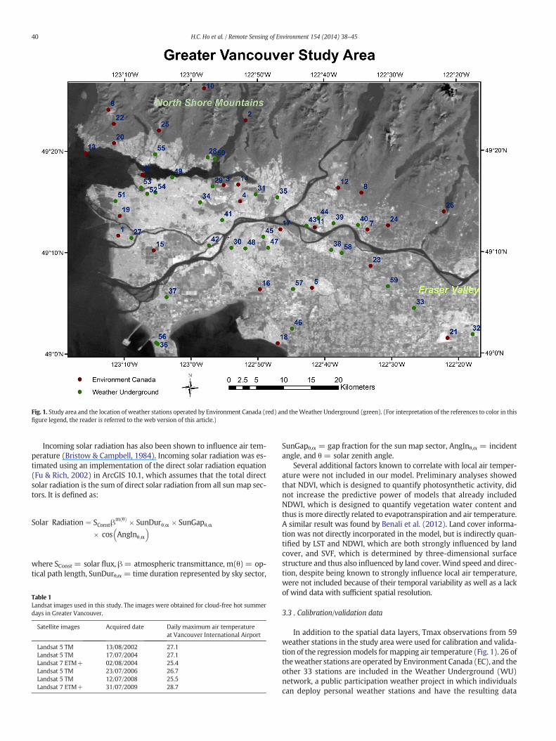
Fig. 1. Study area and the location of weather stations operated by Environment Canada (red) and theWeather Underground (green). (For interpretation of the references to color in thisfigure legend, the reader is referred to the web version of this article.)

40 H.C. Ho et al. / Remote Sensing of Environment 154 (2014) 38–45

Incoming solar radiation has also been shown to influence air tem-perature (Bristow & Campbell, 1984). Incoming solar radiation was es-timated using an implementation of the direct solar radiation equation(Fu & Rich, 2002) in ArcGIS 10.1, which assumes that the total directsolar radiation is the sum of direct solar radiation from all sun map sec-tors. It is defined as:

Solar Radiation ¼ SConstβm θð Þ � SunDurθ;α � SunGapθ;α

� cos AngInθ;α

� �

where SConst = solar flux, β= atmospheric transmittance, m(θ) = op-tical path length, SunDurθ,α = time duration represented by sky sector,

Table 1Landsat images used in this study. The images were obtained for cloud-free hot summerdays in Greater Vancouver.

Satellite images Acquired date Daily maximum air temperatureat Vancouver International Airport

Landsat 5 TM 13/08/2002 27.1Landsat 5 TM 17/07/2004 27.1Landsat 7 ETM+ 02/08/2004 25.4Landsat 5 TM 23/07/2006 26.7Landsat 5 TM 12/07/2008 25.5Landsat 7 ETM+ 31/07/2009 28.7

SunGapθ,α = gap fraction for the sun map sector, AngInθ,α = incidentangle, and θ = solar zenith angle.

Several additional factors known to correlate with local air temper-ature were not included in our model. Preliminary analyses showedthat NDVI, which is designed to quantify photosynthetic activity, didnot increase the predictive power of models that already includedNDWI, which is designed to quantify vegetation water content andthus is more directly related to evapotranspiration and air temperature.A similar result was found by Benali et al. (2012). Land cover informa-tion was not directly incorporated in the model, but is indirectly quan-tified by LST and NDWI, which are both strongly influenced by landcover, and SVF, which is determined by three-dimensional surfacestructure and thus also influenced by land cover.Wind speed and direc-tion, despite being known to strongly influence local air temperature,were not included because of their temporal variability as well as a lackof wind data with sufficient spatial resolution.

3.3 . Calibration/validation data

In addition to the spatial data layers, Tmax observations from 59weather stations in the study area were used for calibration and valida-tion of the regressionmodels formapping air temperature (Fig. 1). 26 oftheweather stations are operated by Environment Canada (EC), and theother 33 stations are included in the Weather Underground (WU)network, a public participation weather project in which individualscan deploy personal weather stations and have the resulting data

Table 2Maximum air temperature (Tmax) error estimates based on cross-validation, for eachmodel type.

Model MAE RMSE

Random forest 1.82 °C 2.31 °CSupport vector machine 1.91 °C 2.46 °COrdinary least squares regression 1.93 °C 2.46 °C

41H.C. Ho et al. / Remote Sensing of Environment 154 (2014) 38–45

uploaded to a publicly accessible geodatabase (Goodchild, 2007; Sieber,2006). Not all weather stations were operational for all of the six daysused in our study, including several of the WU stations for which datawere only available for one or two of the latest dates.

3.4 . Regression models

Regression models, using predictors derived from satellite and ele-vation data, were first used to predict the absolute Tmax observed atweather stations for each of the six days for which Landsat data wereavailable, and Tmax values were then normalized relative to the corre-sponding Tmax value at YVR. Ultimately the six maps of relative Tmaxwere averaged to describe Tmax, relative to YVR, for a typical hot sum-mer day in the study area. Per-pixel predictions of absolute temperaturewere based on the pixel values of elevation, SVF and solar radiation, aswell as spatially averaged values of LST and NDWI, calculated for circu-lar areas with radii of 100, 200, 400, 600, 800, and 1000 m surroundingeach pixel. The spatial averaging was used to account for the influenceof temperature and moisture surface conditions in the areas surround-ing each station (Liu &Moore, 1998; Zakšek & Oštir, 2012), and the spe-cific radii were selected to cover the range from the smallestmeaningfulradius, given the 60m spatial resolution of the data, to the largest radiuswithin which the predictors were expected to influence Tmax. Addi-tional research on the spatial dependence of interaction between sur-face properties and air temperature could inform better selection ofthese radii in future studies.

Three types of statistical modelswere used to predict Tmax from the15 predictors: 1) Ordinary least squares multiple linear regression, 2)support vector machine (SVM), and 3) random forest. Ordinary leastsquares regression uses the observed data to estimate the parametersof a linear regression function (Kutner, Nachtsheim, & Neter, 2004).SVM is a machine learning based regression model initially developedfor classification problems. It determines the location of decisionboundaries and uses the boundaries to predict optimal separation ofclasses (Cortes & Vapnik, 1995; Mountrakis, Im, & Ogole, 2011; Pal &Mather, 2005). Previous remote sensing studies have primarily usedthis method for classification (Huang, Davis, & Townshend, 2002;Melgani & Bruzzone, 2004; Ocak & Seker, 2013; Oommen et al.,2008; Pal & Mather, 2005) but Bruzzone and Melgani (2005) devel-oped an SVM-based conceptual multiple estimator system for bio-physical parameter prediction. This system successfully develops aregression-based SVM and is widely applied to predict continuousoutput in environmental studies (Camps-Valls, Bruzzone, Rojo-Alvarez,&Melgani, 2006; Camps-Valls et al., 2006; Das, Samui, Sabat, & Sitharam,2010; Durbha, King, & Younan, 2007; Knudby, Brenning, & LeDrew,2010; Knudby, LeDrew, & Brenning, 2010; Mountrakis et al., 2011;Sun, Li, &Wang, 2009). Random forest is a nonlinear ensemble machinelearning model using multiple regression trees, where each tree istrained on a random subset of the training data and each split ineach tree is determined using a random subsample of the availablepredictors (Breiman, 2001; Stumpf & Kerle, 2011; Timm & McGraigal,2012). R and its contributed packages (raster, e1071, andrandomForest) were used to develop and apply the statistical modelsusing default model parameter settings (Hijmans & van Etten, 2009;Liaw & Wiener, 2012; Meyer, Dimitriadou, Hornik, Weingessel, &Leisch, 2012; R Core Development Team, 2008).

3.5 . Accuracy assessment

To quantify the prediction error expected for an unsampled area,each regression model was calibrated using observations from allweather stations except one, and predictions for that station werethen compared to the observations to determine prediction error. Thisleave-one-out process was repeated using observations from each sta-tion for validation once. Using all data from a given weather station ineither the calibration or validation data set ensured that this cross-

validation procedure provided a good estimate of typical predictionerrors for an unsampled location. Cross-validation is awidely recognizederror assessment method frequently used to validate machine learningmodels such as random forest and SVM (Gislason, Benediktsson, &Sveinsson, 2006). Themean absolute error (MAE) and rootmean squareerror (RMSE)were used to quantify errors (Willmott &Matsuura, 2005),and themodelwith the lowest error valueswas ultimately used to createa relative Tmax map for Greater Vancouver.

3.6 . Variance importance analysis

A model-independent permutation-based analysis was used toassess the influence of the individual predictors in the most accuratemodel (Genuer, Poggi, & Tuleau-Malot, 2010; Knudby, LeDrew, et al.,2010; Strobl, Malley, & Tutz, 2009). During this analysis, a model wascalibrated using a subset (63.2%) of all observations and validated byquantifying the prediction error for the remaining observations. Thevalues of one predictor were then randomly permuted in the valida-tion data, new predictions produced, and the percentage increase inmean squared error (%IncMSE) caused by the permutation was calcu-lated. This permutation was repeated for each predictor to quantifythe relative increase in prediction error caused by permutation of theindividual predictors.

4 . Results

4.1 . Model performance

The MAE and RMSE values were similar for all models (Table 2),ranging from 1.82 to 1.93 °C and from 2.31 to 2.46 °C respectively,which is comparable with previous remote sensing-based air tem-perature mapping studies (Benali et al., 2012; Czajkowski, Goward,Stadler, & Walz, 2000; Prihodko & Goward, 1997; Vancutsem et al.,2010; Zakšek & Schroedter-Homscheidt, 2009; Zhu et al., 2013).The random forest model outperformed the other model types slightly,and was therefore retained for further analysis and mapping.

Observations with very high Tmax values were consistently under-estimated by the model, and observations with very low Tmax valueswere consistently underestimated (Fig. 2). This is partly an inevitableresult of themodel specification, where the air temperature predictionsfor a typical hot summer day are comparedwith observations for all hotsummer days, some typical and some extreme. It may also result fromthe fact that several environmental variables with known influence onair temperature were not included as predictors in the model, such aswind speed and direction, turbulence, and anthropogenic heat, all ofwhich may influence air temperature at very small spatial scales.

4.2 . Spatial distribution of relative maximum air temperature

The map of Tmax distribution in the study area (Fig. 3) was pro-duced by application of the random forest model to each of the fourLandsat 5 images and calculation of the average per-pixel Tmax predic-tion from each image. The two Landsat 7 images were excluded fromthis map production as their Scan-Line Corrector errors produced sub-stantial local artifacts. The map presents a sensible description of thespatial distribution of air temperature in the study area. Low

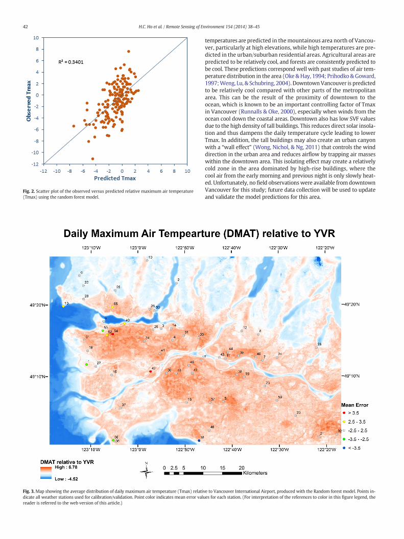
Fig. 2. Scatter plot of the observed versus predicted relative maximum air temperature(Tmax) using the random forest model.

Fig. 3.Map showing the average distribution of daily maximum air temperature (Tmax) relativdicate all weather stations used for calibration/validation. Point color indicates mean error valureader is referred to the web version of this article.)

42 H.C. Ho et al. / Remote Sensing of Environment 154 (2014) 38–45

temperatures are predicted in themountainous area north of Vancou-ver, particularly at high elevations, while high temperatures are pre-dicted in the urban/suburban residential areas. Agricultural areas arepredicted to be relatively cool, and forests are consistently predicted tobe cool. These predictions correspondwell with past studies of air tem-perature distribution in the area (Oke &Hay, 1994; Prihodko & Goward,1997;Weng, Lu, & Schubring, 2004). DowntownVancouver is predictedto be relatively cool compared with other parts of the metropolitanarea. This can be the result of the proximity of downtown to theocean, which is known to be an important controlling factor of Tmaxin Vancouver (Runnalls & Oke, 2000), especially when winds from theocean cool down the coastal areas. Downtown also has low SVF valuesdue to the high density of tall buildings. This reduces direct solar insola-tion and thus dampens the daily temperature cycle leading to lowerTmax. In addition, the tall buildings may also create an urban canyonwith a “wall effect” (Wong, Nichol, & Ng, 2011) that controls the winddirection in the urban area and reduces airflow by trapping air masseswithin the downtown area. This isolating effect may create a relativelycold zone in the area dominated by high-rise buildings, where thecool air from the early morning and previous night is only slowly heat-ed. Unfortunately, no field observationswere available from downtownVancouver for this study; future data collection will be used to updateand validate the model predictions for this area.

e to Vancouver International Airport, produced with the Random forest model. Points in-es for each station. (For interpretation of the references to color in this figure legend, the

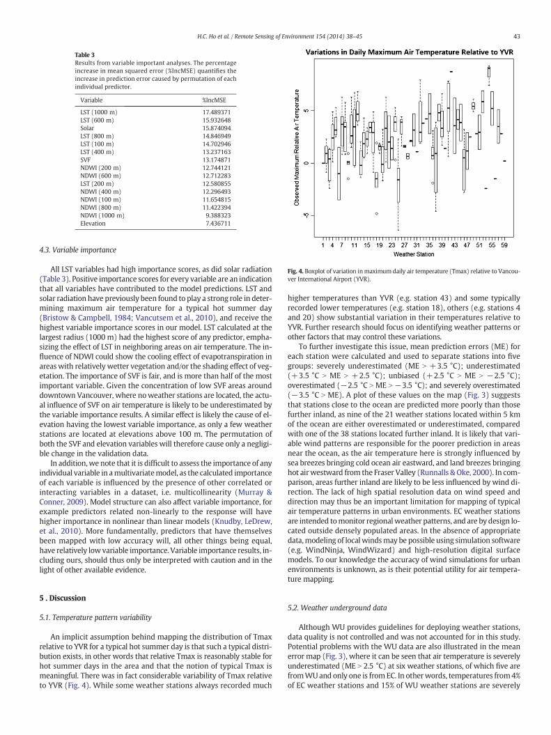
Table 3Results from variable important analyses. The percentageincrease in mean squared error (%IncMSE) quantifies theincrease in prediction error caused by permutation of eachindividual predictor.

Variable %IncMSE

LST (1000 m) 17.489371LST (600 m) 15.932648Solar 15.874094LST (800 m) 14.846949LST (100 m) 14.702946LST (400 m) 13.237163SVF 13.174871NDWI (200 m) 12.744121NDWI (600 m) 12.712283LST (200 m) 12.580855NDWI (400 m) 12.296493NDWI (100 m) 11.654815NDWI (800 m) 11.422394NDWI (1000 m) 9.388323Elevation 7.436711

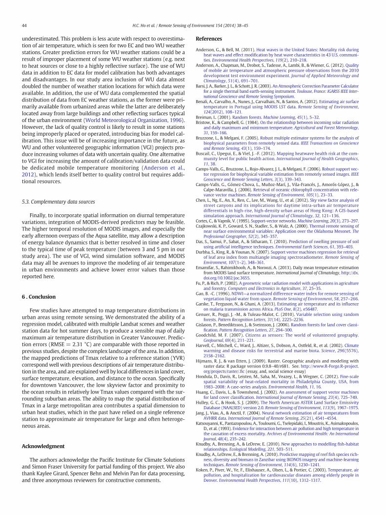
Fig. 4. Boxplot of variation inmaximum daily air temperature (Tmax) relative to Vancou-ver International Airport (YVR).

43H.C. Ho et al. / Remote Sensing of Environment 154 (2014) 38–45

4.3. Variable importance

All LST variables had high importance scores, as did solar radiation(Table 3). Positive importance scores for every variable are an indicationthat all variables have contributed to the model predictions. LST andsolar radiation have previously been found to play a strong role in deter-mining maximum air temperature for a typical hot summer day(Bristow & Campbell, 1984; Vancutsem et al., 2010), and receive thehighest variable importance scores in our model. LST calculated at thelargest radius (1000 m) had the highest score of any predictor, empha-sizing the effect of LST in neighboring areas on air temperature. The in-fluence of NDWI could show the cooling effect of evapotranspiration inareaswith relatively wetter vegetation and/or the shading effect of veg-etation. The importance of SVF is fair, and is more than half of the mostimportant variable. Given the concentration of low SVF areas arounddowntown Vancouver, where noweather stations are located, the actu-al influence of SVF on air temperature is likely to be underestimated bythe variable importance results. A similar effect is likely the cause of el-evation having the lowest variable importance, as only a few weatherstations are located at elevations above 100 m. The permutation ofboth the SVF and elevation variables will therefore cause only a negligi-ble change in the validation data.

In addition,we note that it is difficult to assess the importance of anyindividual variable in amultivariatemodel, as the calculated importanceof each variable is influenced by the presence of other correlated orinteracting variables in a dataset, i.e. multicollinearity (Murray &Conner, 2009). Model structure can also affect variable importance, forexample predictors related non-linearly to the response will havehigher importance in nonlinear than linear models (Knudby, LeDrew,et al., 2010). More fundamentally, predictors that have themselvesbeen mapped with low accuracy will, all other things being equal,have relatively lowvariable importance. Variable importance results, in-cluding ours, should thus only be interpreted with caution and in thelight of other available evidence.

5 . Discussion

5.1. Temperature pattern variability

An implicit assumption behind mapping the distribution of Tmaxrelative to YVR for a typical hot summer day is that such a typical distri-bution exists, in other words that relative Tmax is reasonably stable forhot summer days in the area and that the notion of typical Tmax ismeaningful. There was in fact considerable variability of Tmax relativeto YVR (Fig. 4). While some weather stations always recorded much

higher temperatures than YVR (e.g. station 43) and some typicallyrecorded lower temperatures (e.g. station 18), others (e.g. stations 4and 20) show substantial variation in their temperatures relative toYVR. Further research should focus on identifying weather patterns orother factors that may control these variations.

To further investigate this issue, mean prediction errors (ME) foreach station were calculated and used to separate stations into fivegroups: severely underestimated (ME N +3.5 °C); underestimated(+3.5 °C N ME N +2.5 °C); unbiased (+2.5 °C N ME N −2.5 °C);overestimated (−2.5 °C N ME N −3.5 °C); and severely overestimated(−3.5 °C N ME). A plot of these values on the map (Fig. 3) suggeststhat stations close to the ocean are predicted more poorly than thosefurther inland, as nine of the 21 weather stations located within 5 kmof the ocean are either overestimated or underestimated, comparedwith one of the 38 stations located further inland. It is likely that vari-able wind patterns are responsible for the poorer prediction in areasnear the ocean, as the air temperature here is strongly influenced bysea breezes bringing cold ocean air eastward, and land breezes bringinghot airwestward from the Fraser Valley (Runnalls & Oke, 2000). In com-parison, areas further inland are likely to be less influenced by wind di-rection. The lack of high spatial resolution data on wind speed anddirection may thus be an important limitation for mapping of typicalair temperature patterns in urban environments. EC weather stationsare intended tomonitor regionalweather patterns, and are by design lo-cated outside densely populated areas. In the absence of appropriatedata,modeling of localwindsmay be possible using simulation software(e.g. WindNinja, WindWizard) and high-resolution digital surfacemodels. To our knowledge the accuracy of wind simulations for urbanenvironments is unknown, as is their potential utility for air tempera-ture mapping.

5.2. Weather underground data

Although WU provides guidelines for deploying weather stations,data quality is not controlled and was not accounted for in this study.Potential problems with the WU data are also illustrated in the meanerror map (Fig. 3), where it can be seen that air temperature is severelyunderestimated (ME N 2.5 °C) at six weather stations, of which five arefromWUand only one is fromEC. In otherwords, temperatures from4%of EC weather stations and 15% of WU weather stations are severely

44 H.C. Ho et al. / Remote Sensing of Environment 154 (2014) 38–45

underestimated. This problem is less acute with respect to overestima-tion of air temperature, which is seen for two EC and two WU weatherstations. Greater prediction errors for WU weather stations could be aresult of improper placement of some WU weather stations (e.g. nextto heat sources or close to a highly reflective surface). The use of WUdata in addition to EC data for model calibration has both advantagesand disadvantages. In our study area inclusion of WU data almostdoubled the number of weather station locations for which data wereavailable. In addition, the use of WU data complemented the spatialdistribution of data from EC weather stations, as the former were pri-marily available from urbanized areas while the latter are deliberatelylocated away from large buildings and other reflecting surfaces typicalof the urban environment (World Meteorological Organization, 1996).However, the lack of quality control is likely to result in some stationsbeing improperly placed or operated, introducing bias for model cal-ibration. This issue will be of increasing importance in the future, asWU and other volunteered geographic information (VGI) projects pro-duce increasing volumes of data with uncertain quality. One alternativeto VGI for increasing the amount of calibration/validation data couldbe dedicated mobile temperature monitoring (Anderson et al.,2012), which lends itself better to quality control but requires addi-tional resources.

5.3. Complementary data sources

Finally, to incorporate spatial information on diurnal temperaturevariations, integration of MODIS-derived predictors may be feasible.The higher temporal resolution of MODIS images, and especially theearly afternoon overpass of the Aqua satellite, may allow a descriptionof energy balance dynamics that is better resolved in time and closerto the typical time of peak temperature (between 3 and 5 pm in ourstudy area). The use of VGI, wind simulation software, and MODISdata may all be avenues to improve the modeling of air temperaturein urban environments and achieve lower error values than thosereported here.

6 . Conclusion

Few studies have attempted to map temperature distributions inurban areas using remote sensing. We demonstrated the ability of aregression model, calibrated with multiple Landsat scenes and weatherstation data for hot summer days, to produce a sensible map of dailymaximum air temperature distribution in Greater Vancouver. Predic-tion errors (RMSE = 2.31 °C) are comparable with those reported inprevious studies, despite the complex landscape of the area. In addition,the mapped predictions of Tmax relative to a reference station (YVR)correspondwell with previous descriptions of air temperature distribu-tion in the area, and are explainedwell by local differences in land cover,surface temperature, elevation, and distance to the ocean. Specificallyfor downtown Vancouver, the low skyview factor and proximity tothe ocean results in relatively low Tmax values compared with the sur-rounding suburban areas. The ability to map the spatial distribution ofTmax in a large metropolitan area contributes a spatial dimension tourban heat studies, which in the past have relied on a single referencestation to approximate air temperature for large and often heteroge-neous areas.

Acknowledgment

The authors acknowledge the Pacific Institute for Climate Solutionsand Simon Fraser University for partial funding of this project. We alsothank Kaylee Girard, Spencer Behn and Melvin Pan for data processing,and three anonymous reviewers for constructive comments.

References

Anderson, G., & Bell, M. (2011). Heat waves in the United States: Mortality risk duringheat waves and effect modification by heat wave characteristics in 43 U.S. communi-ties. Environmental Health Perspectives, 119(2), 210–218.

Anderson, A., Chapman, M., Drobot, S., Tadesse, A., Lambi, B., & Wiener, G. (2012). Qualityof mobile air temperature and atmospheric pressure observations from the 2010development test environment experiment. Journal of Applied Meteorology andClimatology, 51(4), 691–701.

Barsi, J. A., Barker, J. L., & Schott, J. R. (2003). An Atmospheric Correction Parameter Calculatorfor a single thermal band earth-sensing instrument. Toulouse, France: IGARSS IEEE Inter-national Geoscience and Remote Sensing Symposium.

Benali, A., Carvalho, A., Nunes, J., Carvalhais, N., & Santos, A. (2012). Estimating air surfacetemperature in Portugal using MODIS LST data. Remote Sensing of Environment,124(2012), 108–121.

Breiman, L. (2001). Random forests. Machine Learning, 45(1), 5–32.Bristow, K., & Campbell, G. (1984). On the relationship between incoming solar radiation

and daily maximum and minimum temperature. Agricultural and Forest Meteorology,31, 159–166.

Bruzzone, L., & Melgani, F. (2005). Robust multiple estimator systems for the analysis ofbiophysical parameters from remotely sensed data. IEEE Transactions on Geoscienceand Remote Sensing, 43(1), 159–174.

Buscail, C., Upegui, E., & Viel, J. -F. (2012). Mapping heatwave health risk at the com-munity level for public health action. International Journal of Health Geographics,11, 38.

Camps-Valls, G., Bruzzone, L., Rojo-Alvarez, J. L., & Melgani, F. (2006). Robust support vec-tor regression for biophysical variable estimation from remotely sensed images. IEEEGeoscience and Remote Sensing Letters, 3(3), 339–343.

Camps-Valls, G., Gómez-Chova, L., Muñoz-Marí, J., Vila-Francés, J., Amorós-López, J., &Calpe-Maravilla, J. (2006). Retrieval of oceanic chlorophyll concentration with rele-vance vector machines. Remote Sensing of Environment, 105(1), 23–33.

Chen, L., Ng, E., An, X., Ren, C., Lee, M., Wang, U., et al. (2012). Sky view factor analysis ofstreet canyons and its implications for daytime intra-urban air temperaturedifferentials in high-rise, high-density urban areas of Hong Kong: A GIS-basedsimulation approach. International Journal of Climatology, 32, 121–136.

Cortes, C., & Vapnik, V. (1995). Support-vector networks.Machine Learning, 20(3), 273–297.Czajkowski, K. P., Goward, S. N., Stadler, S., & Walz, A. (2000). Thermal remote sensing of

near surface environmental variables: Application over the Oklahoma Mesonet. TheProfessional Geographer, 52(2), 345–357.

Das, S., Samui, P., Sabat, A., & Sitharam, T. (2010). Prediction of swelling pressure of soilusing artificial intelligence techniques. Environmental Earth Sciences, 61, 393–403.

Durbha, S., King, R., & Younan, N. (2007). Support vector machines regression for retrievalof leaf area index from multiangle imaging spectroradiometer. Remote Sensing ofEnvironment, 107(1–2), 348–361.

Emamifar, S., Rahimikhoob, A., & Noroozi, A. (2013). Daily mean temperature estimationfrom MODIS land surface temperature. International Journal of Climatology, http://dx.doi.org/10.1002/joc.3655.

Fu, P., & Rich, P. (2002). A geometric solar radiationmodel with applications in agricultureand forestry. Computers and Electronics in Agriculture, 37, 25–35.

Gao, B. -C. (1996). NDWI—a normalized difference water index for remote sensing ofvegetation liquid water from space. Remote Sensing of Environment, 58, 257–266.

Garske, T., Ferguson, N., & Ghani, A. (2013). Estimating air temperature and its influenceon malaria transmission across Africa. PLoS One, 8(2), e56487.

Genuer, R., Poggi, J. -M., & Tuleau-Malot, C. (2010). Variable selection using randomforests. Pattern Recognition Letters, 31(14), 2225–2236.

Gislason, P., Benediktsson, J., & Sveinsson, J. (2006). Random forests for land cover classi-fication. Pattern Recognition Letters, 27, 294–300.

Goodchild, M. F. (2007). Citizens as sensors: The world of volunteered geography.GeoJournal, 69(4), 211–221.

Harvell, C., Mitchell, C., Ward, J., Altizer, S., Dobson, A., Ostfeld, R., et al. (2002). Climatewarming and disease risks for terrestrial and marine biota. Science, 296(5576),2158–2162.

Hijmans, R. J., & van Etten, J. (2009). Raster. Geographic analysis and modeling withraster data: R package version 0.9.8–40/r681. See. http://www.R-Forge.R-project.org/projects/raster/.fic (essay, and, social science essay)

Hondula, D., Davis, R., Leisten, M., Saha, M., Veazey, L., & Wegner, C. (2012). Fine-scalespatial variability of heat-related mortality in Philadelphia County, USA, from1983–2008: A case-series analysis. Environmental Health, 11, 16.

Huang, C., Davis, L., & Townshend, J. (2002). An assessment of support vector machinesfor land cover classification. International Journal of Remote Sensing, 23(4), 725–749.

Hulley, G. C., & Hook, S. J. (2009). The North American ASTER Land Surface EmissivityDatabase (NAALSED) version 2.0. Remote Sensing of Environment, 113(9), 1967–1975.

Jang, J., Viau, A., & Anctil, F. (2004). Neural network estimation of air temperatures fromAVHRR data. International Journal of Remote Sensing, 25(21), 4541–4554.

Katsouyanni, K., Pantazopoulou, A., Touloumi, G., Tselepidaki, I., Moustris, K., Asimakopoulos,D., et al. (1993). Evidence for interaction between air pollution and high temperature inthe causation of excess mortality. Archives of Environmental Health: An InternationalJournal, 48(4), 235–242.

Knudby, A., Brenning, A., & LeDrew, E. (2010). New approaches to modelling fish-habitatrelationships. Ecological Modelling, 221, 503–511.

Knudby, A., LeDrew, E., & Brenning, A. (2010). Predictivemapping of reef fish species rich-ness, diversity and biomass in Zanzibar using IKONOS imagery and machine-learningtechniques. Remote Sensing of Environment, 114(6), 1230–1241.

Koken, P., Piver, W., Ye, F., Elixhauser, A., Olsen, L., & Portier, C. (2003). Temperature, airpollution, and hospitalization for cardiovascular diseases among elderly people inDenver. Environmental Health Perspectives, 111(10), 1312–1317.

45H.C. Ho et al. / Remote Sensing of Environment 154 (2014) 38–45

Kolokotroni, M., & Giridharan, R. (2008). Urban heat island intensity in London: An inves-tigation of the impact of physical characteristics on changes in outdoor air tempera-ture during summer. Solar Energy, 82(11), 986–998.

Kuhn, K., Campbell-Lendrum, D., & Davies, C. (2002). A continental risk map for malariamosquito (Diptera: Culicidae) vectors in Europe. Journal of Medical Entomology,39(4), 621–630.

Kunst, A., Looman, C., & Mackenback, J. (1993). Outdoor air temperature and mortality inthe Netherlands: A time-series analysis. American Journal of Epidemiology, 137(3),331–341.

Kutner, M., Nachtsheim, C., & Neter, J. (2004). Applied linear regression models (4th ed.).McGraw Hill.

Laaidi, K., Zeghnoun, A., Dousset, B., Bretin, P., Vandentorren, S., Giraudet, E., et al. (2012).The impact of heat islands on mortality in Paris during the August 2003 heat wave.Environmental Health Perspectives, 120(2), 254–259.

Liaw, A., & Wiener, M. (2012). Breiman and Cutler's random forests for classification andregression, R package.

Liu, J. G., & Moore, J. M. (1998). Pixel block intensity modulation: Adding spatial detail toTM band 6 thermal imagery. International Journal of Remote Sensing, 19, 2477–2491.

Maria, K., & Renganathan, G. (2008). Urban heat island intensity in London: An investiga-tion of the impact of physical characteristics on changes in outdoor air temperatureduring summer. Solar Energy, 82(11), 986–998.

Medina-Ramon, M., Zanobetti, A., Cavanagh, D., & Schwartz, J. (2006). Extreme tempera-tures and mortality: Assessing effect modification by personal characteristics andspecific cause of death in a multi-city case-only analysis. Environmental HealthPerspectives, 114(9), 1131–1136.

Melgani, F., & Bruzzone, L. (2004). Classification of hyperspectral remote sensing imageswith support vector machines. IEEE Transactions on Geoscience and Remote Sensing,42(8), 1778–1790.

Meteotest (2010). Meteonorm handbook, Part III: Theory part 2. Accessed online inFebruary 9 (2011). http://www.meteonorm.com/media/pdf/mn6_software.pdf

Meyer, D., Dimitriadou, E., Hornik, K., Weingessel, A., & Leisch, F. (2012).Misc functions ofthe department of statistics (e1071), TU Wien, R package.

Mostovoy, G. V., King, R. L., Reddy, K. R., Kakani, V. G., & Filippova, M. G. (2006). Statisticalestimation of daily maximum and minimum air temperatures from MODIS LST dataover the state of Mississippi. GIScience and Remote Sensing, 43(1), 78–110.

Mountrakis, G., Im, J., & Ogole, C. (2011). Support vector machines in remote sensing: Areview. ISPRS Journal of Photogrammetry and Remote Sensing, 66(2011), 247–259.

Murray, K., & Conner, M. M. (2009). Methods to quantify variable importance: Implica-tions for the analysis of noisy ecological data. Ecology, 90, 348–355.

Nichol, J. E., Fung, W. Y., Lam, K. -S., & Wong, M. S. (2009). Urban heat island diagnosisusing ASTER satellite images and ‘in situ’ air temperature. Atmospheric Research,276–284.

Nichol, J. E., & To, P. H. (2012). Temporal characteristics of thermal satellite images forurban heat stress and heat island mapping. ISPRS Journal of Photogrammetry andRemote Sensing, 74, 153–162.

Ocak, I., & Seker, S. (2013). Calculation of surface settlements caused by EPBM tunnelingusing artificial neural network, SVM, and Gaussian processes. Environmental EarthSciences, http://dx.doi.org/10.1007/s12665-012-2214-x.

Oke, T. (1976). The distinction between canopy and boundary-layer urban heat islands.Atmosphere, 14(4), 268–277.

Oke, T. (1988). The urban energy balance. Progress in Physical Geography, 12, 471–508.Oke, T., & Hay, J. (1994). The climate of Vancouver (2nd ed.). B.C. Geographical Series, 50,

Vancouver, British Columbia: Tantalus Press.Oke, T. R., & Maxwell, G. B. (1975). Urban heat island dynamics in Montreal and Vancou-

ver. Atmospheric Environment, 9(2), 191–200.Oommen, T., Misra, D., Twarakavi, N., Prakash, A., Sahoo, B., & Bandopadhyay, S. (2008).

An objective analysis of support vector machine based classification for remotesensing. Mathematical Geosciences, 40(4), 409–424.

Pal, M., & Mather, P.M. (2005). Support vector machines for classification in remotesensing. International Journal of Remote Sensing, 26(5), 1007–1011.

Prihodko, L., & Goward, S. N. (1997). Estimation of air temperature from remotely sensedsurface observations. Remote Sensing of Environment, 60(3), 335–346.

R Core Development Team (2008). R: A language and environment for statisticalcomputing. http://www.R-project.org/

Runnalls, K., & Oke, T. (2000). Dynamics and controls of the near-surface heat island ofVancouver, British Columbia. Physical Geography, 21(4), 283–304.

Saaroni, H., & Baruch, Z. (2010). Estimating the urban heat island contribution to urbanand rural air temperature differences over complex terrain: Application to an aridcity. Journal of Applied Meteorology and Climatology, 49, 2159–2166.

Sandholt, I., Rasmussen, K., & Andersen, J. (2002). A simple interpretation of the surfacetemperature/vegetation index space for assessment of surface moisture status.Remote Sensing of Environment, 79(2–3), 213–224.

Sieber, R. (2006). Public participation geographic information systems: A literaturereview and framework. Annals of the Association of American Geographers, 96(3),491–507.

Singh, R., Joshi, P., & Kishtawal, C. (2006). A new method to determine near surface airtemperature from satellite observations. International Journal of Remote Sensing,27(14), 2831–2846.

Statistics Canada (2007). Greater Vancouver, British Columbia (Code5915) (table). 2006Community Profiles. 2006 Census. Statistics Canada Catalogue no. 92-591-XWE(Ottawa. Released March 13, 2007).

Stisen, S., Sandholt, I., Norgaard, A., Fensholt, R., & Eklundh, L. (2007). Estimation of diur-nal air temperature using MSG SEVIRI data in West Africa. Remote Sensing ofEnvironment, 110(2), 262–274.

Strobl, C., Malley, J., & Tutz, G. (2009). An introduction to recursive partitioning: Rational,application, and characteristics of classification and regression trees, bagging, andrandom forests. Psychological Methods, 14(4), 323–348.

Stumpf, A., & Kerle, N. (2011). Object-oriented mapping of landslides using randomforests. Remote Sensing of Environment, 115, 2564–2577.

Su, J., Brauer, M., & Buzzelli, M. (2008). Estimating urban morphometry at the neighbor-hood scale for improvement in modeling long-term average air pollution concentra-tions. Atmospheric Environment, 42, 7884–7893.

Sun, D., Li, Y., &Wang, Q. (2009). A unifiedmodel for remotely estimating chlorophyll a inLake Taihu, China, based on SVM and in situ hyperspectral data. IEEE Transactions onGeoscience and Remote Sensing, 47(8), 2957–2965.

Sun, Y. J., Wang, J. F., Zhang, R. H., Gillies, R. R., Xue, Y., & Bo, Y. C. (2005). Air temperatureretrieval from remote sensing data based on thermodynamics. Theoretical and AppliedClimatology, 80(1), 37–48.

Timm, B., & McGraigal, K. (2012). Fine-scale remotely-sensed cover mapping of coastaldune and salt marsh ecosystems at Cape Cod National Seashore using RandomForests. Remote Sensing of Environment, 127, 106–117.

Tomlinson, C., Chapman, L., Thornes, J., & Baker, C. (2011). Including the urban heat islandin spatial heat health risk assessment strategies: A case study for Birmingham, UK.International Journal of Health Geographics, 10, 42.

Unger, J., Sümeghya, Z., & Zobokib, J. (2001). Temperature cross-section features in anurban area. Atmospheric Research, 58(2), 117–127.

Vancutsem, C., Ceccato, P., Dinku, T., & Connor, S. J. (2010). Evaluation of MODIS land sur-face temperature data to estimate air temperature in different ecosystems overAfrica. Remote Sensing of Environment, 114(2), 449–465.

Vogt, J., Viau, A. A., & Paquet, F. (1997). Mapping regional air temperature fields usingsatellite derived surface skin temperatures. International Journal of Climatology, 17,1559–1579.

Weng, Q., Lu, D., & Schubring, J. (2004). Estimation of land surface temperature–vegetation abundance relationship for urban heat island studies. Remote Sensing ofEnvironment, 89, 467–483.

Willmott, C. J., & Matsuura, K. (2005). Advantages of the mean absolute error (MAE) overthe root mean square error (RMSE) in assessing average model performance. ClimateResearch, 30, 79–82.

Wong, M., Nichol, J., & Ng, E. (2011). A study of the “wall effect” caused by proliferation ofhigh-rise buildings using GIS techniques. Landscape and Urban Planning, 102,245–253.

World Meteorological Organization (1996). Guide to meteorological instruments andmethods of observation WMO-No. 8 (6th ed.) (Geneva).

Xu, Y., Qin, Z., & Shen, Y. (2012). Study on the estimation of nearsurface air temperaturefrom MODIS data by statistical methods. International Journal of Remote Sensing,33(24), 7629–7643.

Zakšek, K., & Oštir, K. (2012). Downscaling land surface temperature for urban heat islanddiurnal cycle analysis. Remote Sensing of Environment, 117, 114–124.

Zakšek, K., & Schroedter-Homscheidt, M. (2009). Parameterization of air temperaturein high temporal and spatial resolution from a combination of the SEVIRI andMODIS instruments. ISPRS Journal of Photogrammetry and Remote Sensing, 64(4),414–421.

Zhu, W., Lu, A., & Jia, S. (2013). Estimation of daily maximum and minimum air temper-ature using MODIS land surface temperature products. Remote Sensing ofEnvironment, 130(2013), 62–73.