Mapping image processing operations onto a linear systolic ... · r,i.suul c,oritrol of ... Mapping image processing operations onto a linear systolic machine ... (200 ns) instruction

Distributed Computing (1986) 1 : 246-257

( Springer-Verhg 1986

Mapping image processing operations onto a linear systolic machine* H.T. Kung and Jon A. Webb Departmcnt of Computer Science. Carnegie Mellon University, Pittsburgh. PA 1521 3. USA

H.T. K u n g joinrd t l ie,fucult j . o f ' C 'urn egic. M~~lloti Uti iwr.c.itj in 1974 ufter rewiring his P1i.D. c i i y c v thcw. Appointed to Pro- fP.sor in 1982. he is curreti(1j holding Shell Distingui.vlied C'liuir in Coniputer SciiJnce ut C'urtic~gic Mellori. He )t'us Gug-

(I /iill tinic Arc,liitci,ture C70nsu/- t i i t i t to ESL, fnc . , (I .suh.sidiurj, of T R W, in I Y H I . Dr. Kung 's current research in- tcrc.si.s ure in high-performunce computer urchitectures and their upplicutions. He has .served on

rrials and proRram conimittees of rind computer science.

getiheitil Fc~Io\v it1 1983-84. Ntld

Jon A. Webb rcwivcd the P1i.D. c lq rw in c~oniputt"r science .from The L1tiir~~rsit>~ qf Tc>.uus ut Aus- tin iri 1980. From 1981 he has worked on the j u c u l t ~ ~ q f the Departrnerit of C'otnputer Science ut Carnegie- Mellorr b'nirersitj,, where he is currmtlj, a Rc~seurch C'oniputrr Scicwtist. His reseurch interests inc~lucli~ the tlieorj. qf rision mid purullc~l urchirectures ,f(ir vision. He has puhlished papers on the rrcorwj. q/ .s[ructure f rom mo- tion. the . s h i p of subjective con- t~ i i r s . rhr design unci use of a

purullcl urc~liiti~c~tirrc~ f o r k t ~ c ~ - k ~ r ~ c l i,i.sioii. mid rzprrinrcwts in the r,i.suul c,oritrol of (I robot r.c4iclc~. Dr. Wchh i.s o nicvtihcr i t / ' thc IEEE C'oniputcv Socictj. arid the A,ssociutioti f iir ('onipiitiri~q Miic~hini~rj~.

Abstract. A high-performance systolic machine, called Warp. is operational at Carnegie Mellon. The machinc has a programmable systolic array of linearly connected cells, each capable of per-

forming 10 million floating-point operations per second. Many image processing operations have been programmed on the machine. This programming experience has yielded new insights in the mapping of image processing operations onto a parallel computer. This paper identifies three major mapping methods that are particularly suited to a Warp-like parallel machinc using a linear array of processing elements. These mapping methods correspond to partitioning of input dataset, partitioning of output dataset, and partitioning of computation along the timc domain (pipelining). Parallel implementations of several important image processing operations are presented to illustrate the mapping methods. These operations include the Fast Fourier transform (FFT), connected component labelling, Hough transform. image warping and relaxation. . -

Key words: Image processing - Systolic arrays - Parallel processing - Connected component labelling - Hough transform - Imagc warping - Rclaxa- tion

1 Introduction Warp is a programmable systolic array machine designed at Carnegie Mellon [ l ] and built together with its industrial partners - GE and Honeywell. The first large scale version of the machine with

* The research was supported in part by Defcnsc Advanccd Research Projects Agency (DOD). monitored by thc Air Force Avionics Laboratory under Contract F'33615-X4-K- t 520. and Naval Electronic Systems Command undcr Con- tract N00039-85-C-0134. in part under ARPA Order number 5147, monitored by the US Army Engineer Topographic Laboratories under contract DACA76-X5-C-0002. and in part by the Office of Naval Research undcr Contracts N00014-80-C-0236. N R 048-659, and N00014-X5-1(-0152. NR SDRJ-007

247 H.T. Kung and Jon A. Webb: Mapping image processing operations onto a linear systolic machine

r -. I I I

an array of 10 linearly connected cells is operational at Carnegie Mellon. Each cell in the array is capable of performing 10 million 32-bit floating- point Operations per second (IO MFLOPS). The 10-cell array can achieve performance of SO- 100 MFLOPS for a large variety of signal and low- level vision operations.

Warp’s first applications are low-level vision for robots, laboratory processing of images [4] and analysis of large images (IO K x 10 K). It has therefore been important for us to understand how to map typical image processing operations onto the Warp array so that work can be partitioned evently between all the cells.

We have identified three major mapping schemes. They include two methods of space divi- sion (that is, the assignment of part of the data to each cell): one is input partitioning, or the assignment of part of the input to each cell, and the other is oiitpitt pcirtitioning. The third method is pipdining: each cell does one stage of a multi-stage computation. All the mapping schemes that we have used on Warp for image processing operations are covered by these three mapping methods.

We begin with a brief review of the Warp machine and architectural features of its linear processor array that have allowed efficient mapping of many image processing operations onto the machine. Then we consider each mapping method, describe how it is done, and list its advantages and disadvantages and other characteristics. More precisely, in Sect. 3 we consider the input partitioning method, and present a new parallel implementation for the connected component labelling computation. Section 4 deals with the output partitioning method, illustrated by Hough transform and image warping. Section 5 discusses the pipelining method using the FFT and relaxation as examples.

I N T E R F A C E (-

U N I T

1 I

C E L L nt.)y I

-

3 4 . . . X I . . . A-

Y W C E L L I t . ) C f L L P c) . . .

2 The Warp machine

> + 3 I

In this section we first give an overview of the Warp system, and then describe the linear processor array used by the system.

I

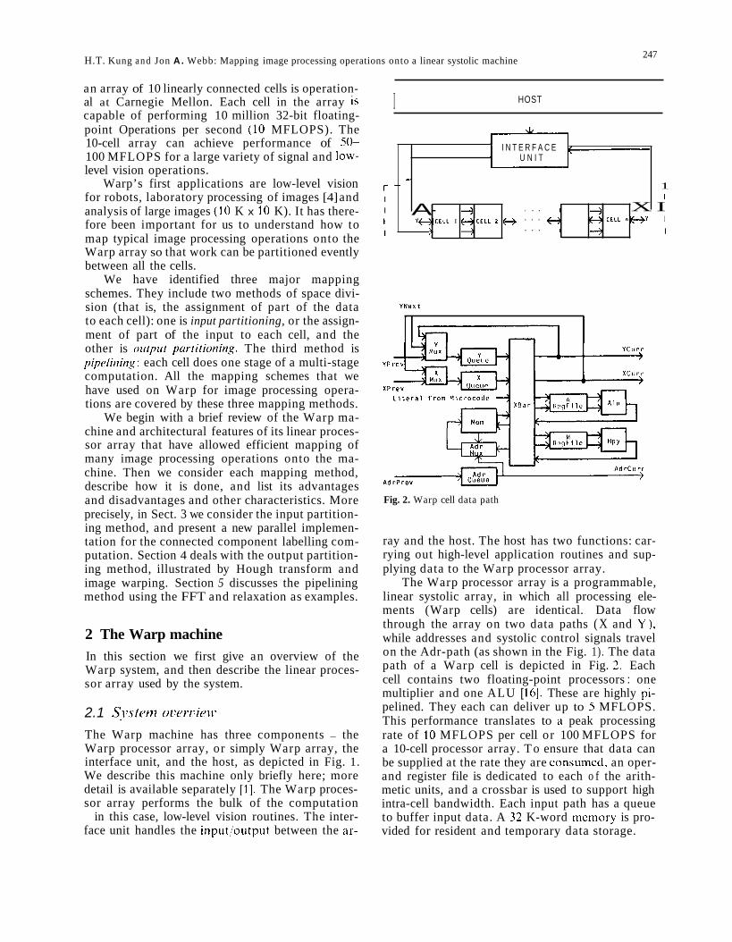
2.1 Sj~stc~rn orersieit~ The Warp machine has three components - the Warp processor array, or simply Warp array, the interface unit, and the host, as depicted in Fig. 1. We describe this machine only briefly here; more detail is available separately [1]. The Warp processor array performs the bulk of the computation - in this case, low-level vision routines. The interface unit handles the input/output between the ar-

HOST I

YNex t

Fig. 2. Warp cell data path

ray and the host. The host has two functions: car- rying out high-level application routines and sup- plying data to the Warp processor array.

The Warp processor array is a programmable, linear systolic array, in which all processing elements (Warp cells) are identical. Data flow through the array on two data paths ( X and Y) , while addresses and systolic control signals travel on the Adr-path (as shown in the Fig. 1). The data path of a Warp cell is depicted in Fig. 2. Each cell contains two floating-point processors : one multiplier and one ALU [ 161. These are highly pi- pelined. They each can deliver up to S MFLOPS. This performance translates to ;I peak processing rate of 10 MFLOPS per cell or 100 MFLOPS for a 10-cell processor array. T o ensure that data can be supplied at the rate they are consumed. an oper- and register file is dedicated to each o f the arith- metic units, and a crossbar is used to support high intra-cell bandwidth. Each input path has a queue to buffer input data. A 32 K-word mcmory is provided for resident and temporary data storage.

248 H.T. Kung and Jon A. Webb: Mapping image processing operations onto ;I linear systolic. machinc

As address patterns are typically data-independent and common to all the cells, full address generation capability is factored out from the cell architecture and provided in the interface unit. Ad- dresses are generated by the interface unit and pro- pagated from cell to cell (together with the control signals). In addition to generating addresses, the interface unit passes data and results between the host and the Warp array, possibly performing some data conversion in the process. For new Warp systems in 1987, each cell has its own address generation unit.

The host is a general purpose computer (cur- rently a Sun workstation, with added MC68020 stand alone processors for I,’O and control of the Warp array). I t is responsible for executing high- level application routines as well as coordinating all the peripherals, which might include other de- vices such a s the digitizer and graphics displays. The host has a large memory in which images are stored. These images are fed through the Warp array by the host, and results from the Warp array are stored back into memory by the host. This arrangement is flexible. I t allows the host to d o tasks not suited to the Warp array, including low- level tasks, such as initializing an array to zero, as well as tasks that involve a lot of decision making but little computation, such as processing a histogram (computed by the Warp array) to determine a threshold.

The Warp array is a linear array of identical cells. The linear configuration was chosen for several reasons. First, i t is easy to implement. Second, it is easy to extend the number of cells in the array. Third, a linear array has modest IjO requirements since only the two end-cells communicate with the outside world.

The advantages of the linear interconnection are outweighed, however, if the constraints of interconnection render the machine too difficult to use for programmers. The concern is whether or not we can efficiently map applications on the linear array of cells. While many algorithms have been designed specifically for linear arrays [6], computations designed for other interconnection topologies can often be efficiently simulated on the linear array mainly because the Warp cell, the building-block of the array, is itself a powerful en- gine. In particular, a single Warp cell can be programmed to perform the function of a column of cells, and therefore the linear array can, for exam-

ple, implement a two-dimensional systolic array in an effective way.

A feature that distinguishes the Warp cell from many other processors of similar computation power is its high IjO bandwidth ~ an important characteristic for systolic arrays. Each Warp cell can transfer up to 20 million words (80 Mbytes) to and from its neighboring cells per second. (In addition, 10 million 16-bit addresses can flow from one cell to the next cell every second.) We have been able to implement this high bandwidth communication link with only modest engineering ef- forts, because of the simplicity of the linear interconnection structure and clocked synchronous communication between cells. This high inter-cell communication bandwidth makes i t possible to transfer large volumes of intermediate data between neighboring cells and thus supports fine grain problem decomposition.

For communication with the outside world, the Warp array can sustain a 80 Mbytcs/s peak transfer rate. In the current setup, the interface unit can communicate with the Warp array at a rate of 40 Mbytes/s. This assumes that the Warp array inputs and outputs a 32-bit word every (200 ns) instruction cycle. However the current host can only support up to 10 Mbytes/s transfer rates. The smaller transfer rate supported by the host is not expected to affect the effective use of the Warp array for our applications for the following reasons: first, the Warp array typically docs not perform an input and output more than every two or more cycles. Second, for most signal and image processing applications. the host deals with &bit integers rather than 32-bit floating-point numbers, and therefore the I/O bandwidth for the host needs only be a quarter of that for the Warp array (assuming the image can be sent in raster- order). This implies that 10 Mbytes/s transfer rate for the host is sufficient.

Each cell has a large local data memory that can hold 32 K words; this feature is seldom found in special-purpose, systolic array designs, and is another reason why Warp is powerful and flexible. It can be shown that by increasing the data menio- ry size, higher computation bandwidth can be SUS-

tained without imposing increased demand on the I /O bandwidth [7]. The large menlory size, together with the high IjO bandwidth. makes Warp capable of performing global operations in which each output depends on any or a large portion of the input [8]. Examples of global operations are FFT, component labelling, Hough transform. image warping, and matrix computations such as matrix multiplication. Systolic arrays are known t o be ef-

249 I1.T. K u n g and Jon A. Webb: Mapping image processing operations onto a linear systolic inachlnc

fcctive for local operations such as a 3 x 3 convolution [6]. The additional ability to perform global operations significantly broadens the applicability of the machine.

In summary, the simple linear processor array used in Warp is a powerful and flexible structure largely because the array is made of powerful, programmable processors with high IjO capabilities and large local memories.

Warp is being used intensively at Carnegie Mel- Ion for vision and signal processing and for scien- tific computing. At least eight printed circuit board versions of the machine will be built in 1987.

A major effort of developing a VLSI Warp chip that can implement the entire Warp cell except its local memory has started. The integrated Warp system will achieve an order of magnitude reduc- tion in cost, size, and power consumption, and a similar increase in computing power. It will consist of tens of cells with a total computing power of over a billion floating point operations per second. This VLSI Warp effort is being carried out jointly by Carnegie Mellon and an industrial partner.

3 Input partitioning

In this section, we describe the first mapping method ~ input partitioning. In input partitioning each cell receives part of the input data, and generates all of the output corresponding to its set of inputs. Each processor does the same operation on its portion of the input. The outputs are then combined. We will illustrate this mapping method by considering a rather elaborate example, that is, the labelling of connected components in an image.

3.1 I.s.sues in the input partitioning method Input partitioning is natural in low-level image processing. Image operations are often local and regular, or produce data structures that are fairly easy t o combine, as in histogram. Image sizes tend to be large (for example, 512 x 512) so that much parallelism is available even if the image is divided only along one dimension (for example, each cell gets one set of adjacent columns). In addition, this method lends itself naturally to raster-order processing; if the image is divided according to columns, the image can be sent in raster order, while each cell accepts its portion of the inputs as they are pumped through the array.

The overhead in computation time for input partitioning comes from three sources: first, the cost of dividing the image into its parts, second,

the cost of any additional bookkeeping on the Warp cell to allow outputs to be rccombincd later (see below); and third, the cost of recombining outputs.

For many computations, on a linear systolic array, these costs are negligible. Consider convolution-like operations with a small kernel, for example. In these computations, each output depends only on a local, corresponding area of the input image. The computation is partitioned so that each cell takes a set of adjacent columns from the image. The cost of partitioning the data is simply the cost of sending a row through the array while each cell picks off its part of the data, which is negligible since systolic arrays have sufficient internal bandwidth to allow the communication of the data through all cells at little cost. There is no additional bookkeeping, and the cost of recombining outputs is simply the cost of concatenating the outputs from the different columns of the image, which again is negligible.

The advantages of input partitioning arc its ease of programming and the good speedup i t usually gives to an algorithm. Using a simplified cost model, we can calculate the speedup from input partitioning as follows. Suppose computation of the output for the complete input set on one cell takes time n. Then computation of the input on k cells takes time n l k f k c , where c is the time required to combine two cell's outputs, assuming the outputs are combined in sequence over thc cells. If we are allowed to optimize this by adjusting the number of cells the optimimum point has k = fi. Computation is wasted if the number of cells is greater than this, and as the number of cells approaches this point adding more cells becomes less cost-effective. For 51 2 x 51 2 image processing, we have n=512x512xd , where tl is the cost of computing the operation on one input pixel. As- sume that each cell takes one operation to read in the previous cell's outputs, and another operation to insert its outputs and send them t o the next cell. Then c=2 . Hence the optimal number of cells is 362 x fi/, much more than the number of Warp cells in the Warp machine, so that no cells are wasted. For 8-bit histogram. c=356 (the cost adding two histograms). and t /= 3 (based on the current implementation of histogram on Warp) so the optimal number of cells is approximately 55, again much more than the number of Warp cells. The optimal number of cells will be even higher if input, computation and output are over- lapped.

There are, however, two potential disadvantages to the input partitioning method. First. inter-

250 H.T. Kung and Jon A. Webb: Mapping image processing operations o n t o ;I lincar hyslolic n l ~ l ~ h ~ n ~

mediate data structures may be duplicated at each cell, wasting memory. For example, consider labelled histogram: in this algorithm the input is a standard grayvalue image and a labelled image (produced by a connected components algorithm). The output is a set of histograms, with each histogram i counting the frequency of occurrence of pixel values in the standard image whose locations have the label i in the labelled image. If each cell computes the histogram for a portion of the input image, then the same table of histograms spanning all the labels (which may be in the hundreds) must be maintained at every cell. Second, it is not always possible to find a simple method to recombine outputs. In fact. devising an efficient way for output recombination can be quite a challenge.

Consider for example one important algorithm in image processing - the extraction of region features from a labelled image. In this algorithm, significant regions of the image have been labelled, so that the input is an image with each region identified by having its pixels all be the same label, and the task is to reduce this labelled image to a set of symbolically described regions and their properties. Once this is done, the region property set is processed, for example, to find a large region of a particular color that may correspond to a road. Many different properties may be required to do this, and the particular property set depends on the application : properties may include area, center of gravity, moment of inertia, grayvalue mean and variance, boundary properties such as number of concavities, and internal properties such as number of holes. Some of these properties (such as area) are quite easy to compute separately and recombine later, while others (such as number of holes) may require some careful thought to figure out how they can be fit into the input partitioning method.

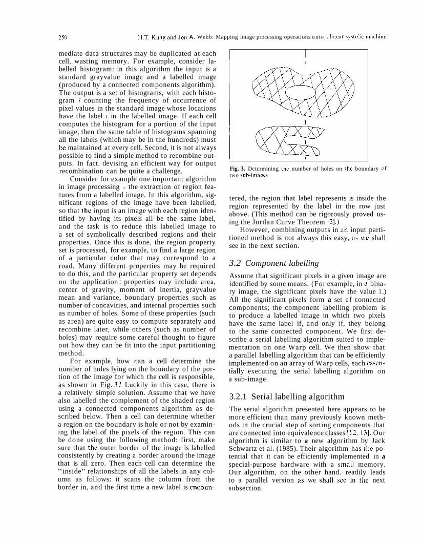
For example, how can a cell determine the number of holes lying on the boundary of the portion of the image for which the cell is responsible, as shown in Fig. 3? Luckily in this case, there is a relatively simple solution. Assume that we have also labelled the complement of the shaded region using a connected components algorithm as described below. Then a cell can determine whether a region on the boundary is hole or not by examin- ing the label of the pixels of the region. This can be done using the following method: first, make sure that the outer border of the image is labelled consistently by creating a border around the image that is all zero. Then each cell can determine the "inside" relationships of all the labels in any column as follows: it scans the column from the border in, and the first time a new label is encoun-

Fig. 3. Dctcrmining thc number of holes on thc boundary or two sub-imagcs

tered, the region that label represents is inside the region represented by the label in the row just above. (This method can be rigorously proved using the Jordan Curve Theorem [3] . )

However, combining outputs in ;in input partitioned method is not always this easy, ;is we shall see in the next section.

3.2 Component labelling Assume that significant pixels in a given image are identified by some means. (For example, in a binary image, the significant pixels have the value 1 .) All the significant pixels form a set o f connected components; the component labelling problem is to produce a labelled image in which two pixels have the same label if, and only if, they belong to the same connected component. We first describe a serial labelling algorithm suited to implementation on one Warp cell. We then show that a parallel labelling algorithm that can be efficiently implemented on an array of Warp cells, each cssen- tially executing the serial labelling algorithm on a sub-image.

3.2.1 Serial labelling algorithm The serial algorithm presented here appears to be more efficient than many previously known methods in the crucial step of sorting components that are connected into equivalence classes [12, 131. Our algorithm is similar to a new algorithm by Jack Schwartz et al. (1985). Their algorithm has thc potential that it can be efficiently implemented in a special-purpose hardware with a small memory. Our algorithm, on the other hand. readily leads to a parallel version CIS we shall sce in thc next subsection.

251 I1.T. Kung and Jon A. Webb: Mapping image processing operations onto a linear systolic machine

- ROW k

Our algorithm works in two passes. The first pass takes the image in raster-scan order and produces a partially labelled image and a label mapping table (LMT) for each row. The partially labelled image has the property that the labels for each row are correct (in the sense that two pixels have the same label if and only if they belong to the same Connected component) if only that row and all rows above are taken into account. The second pass takes the partially labelled image and LMT's in reverse order (that is, reverse raster-scan order) and produces a final labelled image. The LMT translates labels on one row into the labels on the previous row that correspond to the same Connected component.

In the first pass, we scan each row twice, in two phases. The first phase scans the row left to right and produces a partially labelled row, a (ten- tative) LMT, and a re-labelling table (RLT). The RLT is used to unify labels in a row that belong to the same connected component; RLT(a) = RLT(b) if a and b belong to the same connected component based on information from the current and previous rows. The second phase scans the row right to left and applies the RLT to produce the final labellings and LMT for that row.

For each row the first phase works as follows: scan the row from left to right, and for each significant pixel, label it using the following strategy:

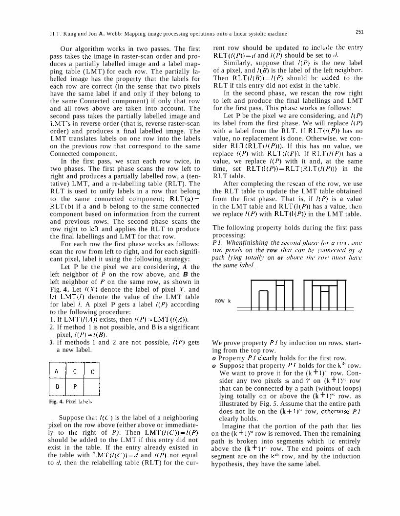
Let P be the pixel we are considering, A the left neighbor of P on the row above, and B the left neighbor of P on the same row, as shown in Fig. 4. Let / ( X ) denote the label of pixel X , and let LMT(/) denote the value of the LMT table for label 1. A pixel P gets a label /(P) according to the following procedure: 1 . If LMT(/(A)) exists, then / ( P ) = LMT(/(A)). 2. If method 1 is not possible, and B is a significant

3 . I f methods 1 and 2 are not possible, I (P) gets pixel, / ( P ) = / ( B ) .

a new label.

- - I

Fig. 4. Pixel label5

Suppose tha t / ( C ) is the label of a neighboring pixel on the row above (either above or immediate- ly to the right of P). Then LMT(/(C))=/(P) should be added to the LMT if this entry did not exist in the table. If the entry already existed in the table with LMT(/(C))=d and / ( P ) not equal to d, then the relabelling table (RLT) for the cur-

rent row should be updated to includc the cntry RLT(I(P))=d and / ( P ) should be set to ti.

Similarly, suppose that / ( P ) is the new label of a pixel, and / ( B ) is the label of the left ncighbor. Then RLT(/(B))=/(P) should bc added to the RLT if this entry did not exist in the table.

In the second phase, we rescan the row right to left and produce the final labellings and LMT for the first pass. This phasc works as follows:

Let P be the pixel we are considering, and / ( P ) its label from the first phase. We will replace /(P) with a label from the RLT. I f RLT(/(P)) has no value, no replacement is done. Otherwise. we consider RLT(RLT(/(P))). I f this has no value, we replace / ( P ) with RLT(/(P)). I f RLT(/(P)) has a value, we replace /(P) with it and, at the same time, set RLT(I(P))= RLT(RLT(/(P))) in the RLT table.

After completing the rescan of the row, we use the RLT table to update the LMT table obtained from the first phase. That is, if / ( P ) is a value in the LMT table and RLT(I(P)) has a value, then we replace / ( P ) with RLT(I(P)) in the LMT table.

The following property holds during the first pass processing: P 1. When finishing the scc .ont / p/ia.sc,fhr ( I ro\t.. on?- two pixels on the row thrit ('(in hc c~onnc~c~tctl h?. [ I

path lying total!,. on or ( ihow thc row iniist / i r r r c the same lahd.

We prove property P I by induction on rows. start- ing from the top row. 0

0

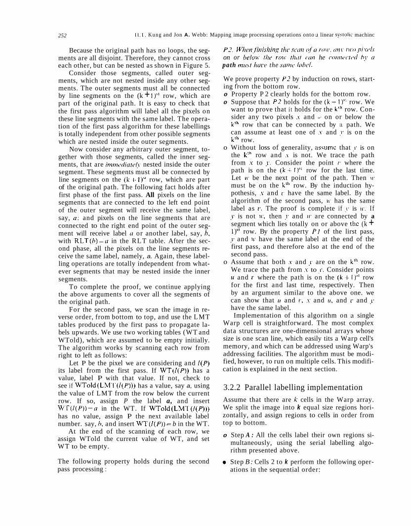
Property Plc lear ly holds for the first row. Suppose that property P I holds for the k'h row. We want to prove it for the ( k + I)" row. Con- sider any two pixels s and ?' on (k + 1)" row that can be connected by a path (without loops) lying totally on or above the (k + I)" row. as illustrated by Fig. 5. Assume that the entire path does not lie on the (k + 1)" row, othcrwisc P I clearly holds. Imagine that the portion of the path that lies

on the (k + I)" row is removed. Then the remaining path is broken into segments which lie entirely above the (k + 1)" row. The end points of each segment are on the k'h row, and by the induction hypothesis, they have the same label.

252 H.T. Kung and Jon A. Webb: Mapping image processing operations onto :I linear xyatolic machinc

Because the original path has no loops, the segments are all disjoint. Therefore, they cannot cross each other, but can be nested as shown in Figure 5.

Consider those segments, called outer segments, which are not nested inside any other segments. The outer segments must all be connected by line segments on the (k + l)', row, which are part of the original path. It is easy to check that the first pass algorithm will label all the pixels on these line segments with the same label. The operation of the first pass algorithm for these labellings is totally independent from other possible segments which are nested inside the outer segments.

Now consider any arbitrary outer segment, together with those segments, called the inner segments, that are itnnwdicite!,~ nested inside the outer segment. These segments must all be connected by line segments on the ( k + 1)" row, which are part of the original path. The following fact holds after first phase of the first pass. All pixels on the line segments that are connected to the left end point of the outer segment will receive the same label, say, ( I ; and pixels on the line segments that are connected to the right end point of the outer segment will receive label CI or another label, say, h, with RLT(h)=u in the RLT table. After the second phase, all the pixels on the line segments receive the same label, namely, a. Again, these labelling operations are totally independent from what- ever segments that may be nested inside the inner segments.

To complete the proof, we continue applying the above arguments to cover all the segments of the original path.

For the second pass, we scan the image in reverse order, from bottom to top, and use the LMT tables produced by the first pass to propagate labels upwards. We use two working tables (WT and WTold), which are assumed to be empty initially. The algorithm works by scanning each row from right to left as follows:

Let P be the pixel we are considering and / ( P ) its label from the first pass. If WT(I(P)) has a value, label P with that value. If not, check to see i f WTold(LMT(/(P))) has a value, say a, using the value of LMT from the row below the current row. If so, assign P the label a, and insert WT(I(P))=u in the WT. If WTold(LMT(I(P))) has no value, assign P the next available label number. say, h, and insert WT(/(P))= b in the WT.

At the end of the scanning of each row, we assign WTold the current value of WT, and set WT to be empty.

The following property holds during the second pass processing :

P2. When,finishirig t l ic s c m of ' r i r o i ~ ' ~ iiti.1, t i t 'o pi.vc1.Y on or helou- the roit' tlitrt cut1 he c o t i t i c ~ c t c i l hjs (I

path must lime the s m i c l rhcl .

We prove property P 2 by induction on rows, start- ing from the bottom row. 0 Property P 2 clearly holds for the bottom row. 0 Suppose that P 2 holds for the ( k + 1)'' row. We

want to prove that i t holds for the klh row. Con- sider any two pixels .Y and >' on or below the k'h row that can be connected by a path. We can assume at least one of .Y and is o n the klh row.

o Without loss of generality, assume that j' is on the kth row and .Y is not. We trace the path from .Y to >*. Consider the point I ' where the path is on the (k+ 1)'' row for the last time. Let )v be the next point of the path. Then i t '

must be on the klh row. By the induction hypothesis, .Y and I' have the same label. By the algorithm of the second pass, i t ' has the same label as r . The proof is complete if j' is 11'. I f 4' is not it', then 1- and 11 ' are connected by a segment which lies totally on or above the (k + l),' row. By the property P 1 of the lirst pass, y and it' have the same label at the end of the first pass, and therefore also at the end of the second pass.

o Assume that both .Y and j - are on the k'h row. We trace the path from .Y to j-. Consider points u and 1 1 where the path is on the ( k t 1)" row for the first and last time, respectively. Then by an argument similar to the above one. we can show that u and r , s and ( I . and I * and js have the same label. Implementation of this algorithm on ii single

Warp cell is straightforward. The most complex data structures are one-dimensional arrays whose size is one scan line, which easily tits a Warp cell's memory, and which can be addressed using Warp's addressing facilities. The algorithm must be modi- fied, however, to run on multiple cells. This modifi- cation is explained in the next section.

3.2.2 Parallel labelling implementation Assume that there are k cells in the Warp array. We split the image into k equal size regions hori- zontally, and assign regions to cells in order from top to bottom.

0 Step A : All the cells label their own regions simultaneously, using the serial labelling algorithm presented above.

0 Step B : Cells 2 to k perform the following operations in the sequential order:

f1.T. Kung and J o n A. Webb: Mapping image processing operations onto a lincar systolic machine 253

o Step B,: Cell 2 performs the following opera-

1 . Input from cell 1 the last row of region 1 and its labels. 2. Re-label the first row of region 2 (assuming that above it is the last row of region 1 input from cell 1 in the previous step), remember the re-labelling, and savc the resulting LMT table as LMT,. (This labelling is done by the same scheme as the one applied t o a typical row in the first pass of the serial labelling algorithm.) 3. Apply the same re-labelling (remembered from the previous step) to the last row of region 2. o Step B,: Cell 3 performs operations similar to

those of step B, on the first and last rows of region 3 , and saves the resulting LMT table as LMT,.

tions on the first and last rows of region 2.

0 . . . o Step B,: Cell k performs operations similar to

those of step B2 on the first and last rows of region k , and saves the resulting LMT table as LMT,.

0 Step C': Cells k to 1 perform the following oper-

o Step ck: Cell k performs the following opera-

1 . Initialize the working table WT to be empty. 2. For each pixel P on the last and first rows of region k , if WT(l(P)) has a value, assign it to the label of P. If not, assign P the next available label number, say, h, and insert WT(I(P))=h in the WT. 3 . S a v e W T a s WTk. 4. Form a new working table WTnew by inserting to it WTnew(rr)=WT(LMT,(a)) for each label ci

assigned to the last row of region k- 1. (Note that cell k input all the labels assigned to the last row of region k - 1 in the first step of step B, . ) o Step ck-, : Cell k - 1 sets WT,- to be the

WTnew input from cell k , performs operations similar to those in the second step of step Ck on the last and first row of region k - 1, and forms WTnew for cell k- 2 .

ations in the sequential order:

tions :

u . . . o Step C, : Cell 1 sets WT, to be the WTnew input

from cell 2, performs operations similar to those in the second step of step Ck on the last row of region 1.

0 Step D : All the cells re-label their own regions simultaneously, with different labels used for each region. More precisely, for each i = 1, . . ., k , cell i re-labels rows in region i in order from bottom to top. Consider the operations of cell I. For the bottom row, the cell assigns to WT,,, the value of WT, from step C, initializes WT

to be empty, and re-labels the row in the following manner: for each pixel P on the row, i f WT(I(P)) has a value. assign it to be the label of P. If not, check to see if WTold(/(P)) has a value, say N . If so, assign P the label (1, and insert WT(I(P))=[i in the WT. I f WTold(l(P)) has no value, assign P the next available label number, say, h, and insert W T ( / ( P ) = h in the WT. At the end of the scanning o f the row. cell i assigns WTold to the current value of WT, and sets WT to be empty. Cell i then performs similar operations on the row above. We see that steps B and C arc csscntially the

first and second passes, respectively, of the serial algorithm applied only to those rows which arc on the boundaries of adjacent regions. Since after step A pixels belonging to the same connected component in each region have the same label, the labels produced by steps B and C ' are the same as those produced by the first and second passes, respectively, of the serial algorithm applied to the whole image. Therefore after step C'. the bottom row of each region will have the final labels, and as a result all other rows of each region will receive the final labels during step D.

Note that sub-steps in steps B and C must be carried out sequentially, that is, by only one cell a t a time. However, the time taken by these steps is not significant with respect to the total time of the parallel algorithm, when the number of rows n in the given image is much larger than the number of cells k in the Warp machine. More precisely, suppose that the serial algorithm takes time T,. Then the time for the parallel algorithm is roughly :

Tk = (Tl/k) + (Tl kin),

where the first term is the time for steps A and D, and the second term is that for steps B and D. Therefore the speedup ratio is % = k p n Tk n + k 2 '

For n=512 and k = 10 (as in the case of the current Warp machine), the speedup ratio is more than 8.

4 Output partitioning In this section we consider image processing operations where the value of each output depends on the entire input dataset, or a subset that cannot be determined a priori. The input partitioning method described in the preceding section does not work well here, because any subset of the input dataset alone will not have all the information

254 F1.T. Kung and Jon A. Webb: Mapping image processing operations o n t o ;i lincar systolic m;ichinc

needed for generating any output. For these operations, i t is often natural to use the second mapping method ~ output partitioning. In output partitioning the output dataset is partitioned among the cells. Each cell sees the entire input dataset and generates part of the output set. Outputs from different cells are concatenated as they are fed out of the array. We will use the Hough transform and image warping to illustrate the output partitioning method.

4 , I Issuc..~ in the output partitioning method An advantage of this method is that i t does not require the duplication of intermediate data structures necessary in input partitioning, such as the LMT in component labelling. It is less wasteful of memory. Each cell must maintain only the data structures it needs to compute its outputs, which it would have to anyway (there is no cost to this unless output data structures overlap).

In this method, for maximum efficiency on a synchronous machine like Warp, each cell must be able to make use of each data item. The reason for this is that as the data are sent in, each datum must be either used or rejected; but because the decision to accept or reject a datum must be made at run-time, enough time must be left to process the datum even if it is rejected to maintain synchro- ny. As a result, no time is saved by rejecting data. Consider the labelled histogram computation. As we observed in the input partitioning section, it may not be possible to partition this algorithm by input because duplication of data structures may lead to too large memory requirements (since hundreds of histograms must be stored at each cell). I f output partitioning is used in this algorithm, and the histograms are split across cells (by, for example, storing a range of the histogram elements at each cell) then each datum is used by only one cell (the cell that holds the histogram elements for that data range) and so there is no speedup from parallelism. There appears to be no good method of implementing this algorithm on a synchronous distributed memory machine like Warp if the local memory of a cell is not large enough for the intermediate data structures needed for input partitioning. In this case either the algorithm must be output partitioned, without an increase in speed over one cell, or the algorithm must be implemented on Warp's standalone processors.

In output partitioning, the only overhead is duplication of effort when intermediate results for one output could contribute to the computation of another output, but these intermediate results

are on different cells and so must be recomputed. For example, in F F T the computation of any single output requires nearly the same effort as to calculate all outputs. There is no ovcrhcad associated with broadcasting the input data or combining the output data: on Warp. data can be broadcast at little cost. Since each cell has a l l the information it needs to compute each output, all that has to be done is to concatenate outputs, which can also be implemented at negligible cost on Warp.

In input partitioning there was an advantage if each cell took a set of adjacent columns of the input data; for local neighborhood operations, i t is necessary to have a set of adjacent columns that form the neighborhood. N o such input or output advantage exists for output partitioning; since each cell sees the entire dataset. i t can produce any set of outputs that is necessary.

As examples of output partitioned algorithms, we present the Hough transform and image warping.

4.2 Hough transform The Hough transform is a template matching algorithm originally invented to find lines in cloud chamber photographs [5] and later generalized to find arbitrary parameterized curves [3]. The algorithm works by mapping each significant pixel into a set of locations in a table representing different locations in the parameter space. The mapping takes each pixel in the image into all possible com- binations of parameters generating curves that pass through the image pixel.

For example, in line-finding, lines are paramc- terized by two values, H and p. The line described by a particular pair of values of these parameters is x cos8+j , s in8=p. Thus, for line finding, the Hough transform takes the (s, y ) location of each significant pixel and. over a range of N values, calculates the / I value for this (s, j x ) using the formula above. lt then in- crements a table at location (0, p) . Once the entire data set has been processed, the table is scanned and peaks are found. These peaks arc the most likely lines in the image.

This algorithm can be used to find any other curve by changing the mapping between the image space and the parameter space. For example, to find circles of a certain size one maps each signili- cant pixel into the (.Y,J,) locations of centers of circles that pass through this pixel (which is itself a circle in the parameter space).

H.T. Kung and Jon A. Webb: Mapping image processing operations onto a linear systolic machine 255

Thc time-consuming step in this algorithm is the mapping between the image and the parameter space. This can involve floating-point computation and must be done once for each significant pixel in the image, which can be a good portion of the image. Also. the parameter space searched can be quite large, depending on its dimensionality and the granularity of the parameter search.

The Warp implementation of the Hough transform works by dividing the parameter space into different segments to a ccll’s memory, then allocat- ing cach segment to one Warp cell. The host pre- processes the image by selecting significant pixels and sending their locations to Warp (alternatively, these pixel locations can be generated in a pass of the image through Warp). The location of each significant pixel is sent to every cell systolically. At cach cell, the segment of the Hough space that belongs to the cell is indexed by some set of paramctcrs p l , p z . . . ., p,,. The pixel location is fed into a formula with some particular value of the first 17- 1 paramctcrs and the dh parameter is generated. Table lookup can be used to simplify computation of thc dh parameter. The table element a t this location is then incremented. This process is repeated until the computation for the entire segment belonging to the cell is completed, and then the pixel location is sent on to the next cell. Thus in the steady state, all the Warp cells carry out computations simultaneously for different seg- mcnts.

After all the data has been sent through the Warp cell, each cell selects its significant peaks and sends thcm to the host where the maxima of all the peaks can be found.

4.3 Iniugc. uwr-ping In some applications, it is desirable to remap or “warp” an image according to some transformation. This may be done, for example, if the lens distortions introduced by a particular calibrated lens arc to be undone. A more interesting application of this technique [15] is in a robot vehicle which is following a road; the camera is mounted on the vehiclc, and of course sees an image dis- torted by pcrspectivc projection. I f we know the position of the ground plane relative to the camera, we can warp the image so that it appears as i t would from an aerial view. Once this is done, i t is relatively casy to find the road edges. For example, aftcr this transformation road edges appear as parallel lincs.

In a typical application of this technique a “fish-eye” lens is used (because this lens gives a

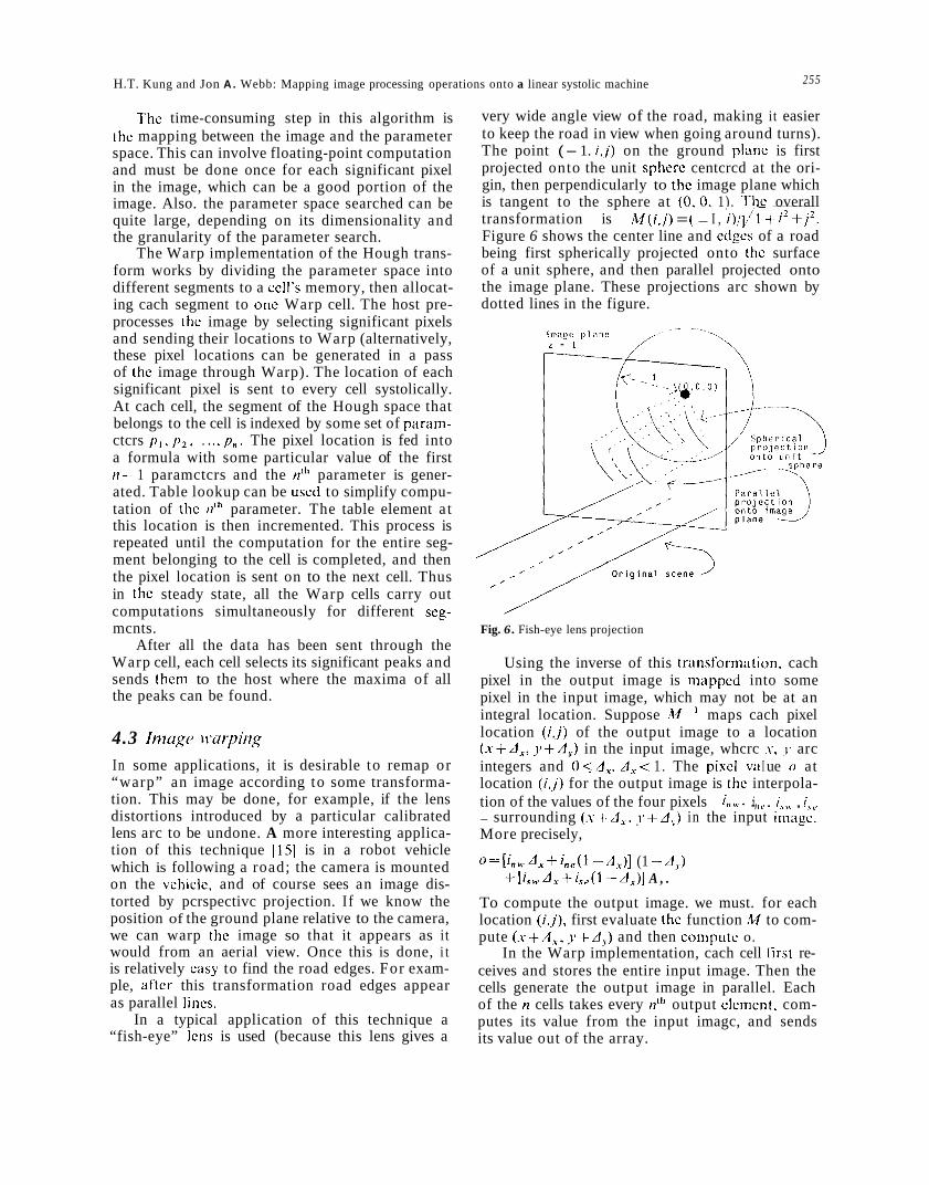
very wide angle view of the road, making it easier to keep the road in view when going around turns). The point (- 1. i , j ) on the ground plane is first projected onto the unit spherc centcrcd at the ori- gin, then perpendicularly to thc image plane which is tangent to the sphere at (0, 0, 1) . Thc overall transformation is M ( i , j > = ( - I , i ) / f i + i’ + j ’ . Figure 6 shows the center line and edgcs of a road being first spherically projected onto thc surface of a unit sphere, and then parallel projected onto the image plane. These projections arc shown by dotted lines in the figure.

Fig. 6. Fish-eye lens projection

Using the inverse of this transformation, cach pixel in the output image is mappcd into some pixel in the input image, which may not be at an integral location. Suppose M - maps cach pixel location (ij) of the output image to a location (x-td,, y+Ay) in the input image, whcrc .Y, J- arc integers and O I A , , A , < 1 . The pixcl v‘ ‘1 I ue 0 at location (iJ) for the output image is thc interpola- tion of the values of the four pixels ~ i, ,,,. i,,, , i,,, - surrounding ( s + A , , J ’ + A , ) in the input imagc. More precisely,

o=[ i , , , ,A ,+i , , ( l -A.v)] (1 -A,,.) +[i,,d,+i,,(l - A x ) ] A , .

To compute the output image. we must. for each location ( i , j ) , first evaluate the function M to compute (x- td , . j ’ td , ) and then computc o.

In the Warp implementation, cach cell first receives and stores the entire input image. Then the cells generate the output image in parallel. Each of the n cells takes every nth output clcnient, computes its value from the input imagc, and sends its value out of the array.

256 11.T. Kung and Jon A. Webb: Mapping image processing operations onto ;I linear systolic machinc

I f a cell's memory is not large enough to hold a complete image, the algorithm can be done in several passes, with each cell taking the same portion of the input and generating what outputs i t can from the given input portion. The partial output images can then be combined to create the complete output image. Note that this algorithm is memory limited; doubling the memory available to a cell leads to a doubling of the speed of the algorithm, up to the point that a cell can hold a complete image.

5 Pipelining

In pipelining. an algorithm is broken down into steps. and each cell does one step of the computation. Inputs flow into the first cell, are subjected to a series of operations, and eventually become outputs that flow out of the last cell. Intermediate results flow between cells. This mode of computation is what is usually thought of as "systolic processing. ' *

This method requires that the algorithm be regular, so that each cell can do nearly an identical operation. This is not often the case in image processing, so that this method has not been as widely used a s the space partitioning methods mentioned before.

This method has the advantage that there is no duplication of data structures between cells; each cell maintains only the data structures necessary for its stage of the computation. Also, the input and output sets are not divided, so that there is no extra cost associated with splitting them up or recombining them.

We illustrate this method with the FFT. Other image processing tasks suited to this mode of computation are one-dimensional convolution [6] and relaxation [12], which is discussed in the next section.

5.1 Fust Fouricr Tramform The problem of computing an n point Discrete Fourier Transform (DFT) is as follows:

Given so . s , . . . , s, ~ , compute .I'", , . . ., .I,, ~ defined by

where tr) is a primitive n-th root of unity. Assume that n is a power of two. The well

known Fast Fourier Transform (FFT) method solves an I I point D F T problem in O(n log n ) operations, while the straightforward method requires

- I 1 ' . == ,yo ([p ~ ' ) W i ( n - 2 ) + . . . +.T"-,

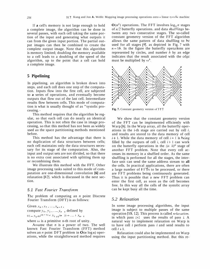
O(n2) operations. The FFT involves log2 I I stages of n/2 butterfly operations. and data shufllings between any two consecutive stages. The so-called constant geometry version of the FFT algorithm allows the same pattern of data shuffling to be used for all stages [9]. as depicted in Fig. 7 with n = 1 6 . In the figure the butterfly oper ;i t ' ions are represented by circles, and number / I by an edge indicates that the result associated with the edge must be multiplied by (oh.

Fig. 7. Constant geometry version of FFT

We show that the constant geometry version of the FFT can be implemented efficiently with Warp [6]. In the Warp array, all the butterfly operations in the i-th stage are carried out by cell i, and results are stored to the data memory of cell i+ 1. While the data memory of cell i t 1 is being filled by the outputs of cell i, cell i + 1 can work on the butterfly operations in the (i+ 1)" stage of another FFT problem. Note that every cell ac- cesses its memory in a shuffied order. As the same shuffling is performed for all the stages, the interface unit can send the same address stream to all the cells. In practical applications, there are often a large number of FFTs to be processed, or there are F F T problems being continuously generated. Thus i t is possible that a new FFT problem can enter the first cell, as soon as the cell becomes free. In this way all the cells of the systolic array can be kept busy all the time.

5.2 Relaxation In some image processing algorithms, the input image is subject to multiple passes of the same operation [lo, 121. This process is called rc/ri.\-ation, in which pass i + l uses the results of pass i. A natural way to implement relaxation on Warp is to have cell i perform pass i and send results to cell i + l .

Relaxation could also be implemented on Warp using the input partitioning method. But this re-

I1.T. Kung iiiid Jon A. Webb: Mapping image processing operations onto a linear systolic machine 257

quires more involved communication and control between cells. For example, as each cell completes a pass o f the relaxation method over its portion of the image, i t must communicate the results of its computation to its neighbors - both its prede- cessor, and its successor. This requires bidirec- tional communication on the Warp array and special handling of boundary conditions, which is physically possible. but difficult to schedule.

Therefore, it is better to implement relaxation by pipclining, with each cell performing one stage of the relaxation. In image processing, it is common for relaxation algorithms to require tens of passes over the image to stabilize (since images arc large. i t takes many passes for constraints to relax across the entire image). Thus, the ten-cell size of thc Warp array is suited to image processing re1 a x a t i o n in et h od s .

6 Conclusions

I t is somewhat surprising and convenient that only three algorithm partitioning methods seem to work for most image processing algorithms that can be implemented on Warp. In this section we analyze the reasons for this result.

First, we must note that image processing has several characteristics that help make these partitioning techniques, or variants of them, work on any parallel computer. Images are large, which is a ready source of parallelism, and a t the low level results from one part of the image d o not influence what computation is done in another part of the image. This makes i t easy to distribute computation among cells by splitting up the input or output images, since there is little communication among distant parts of the image.

Second. the short, linear structure of Warp and its high intcrnal bandwidth make it easy to divide algorithms up among cells. The algorithm must be divided only along one dimension, and only among ten cells, rather than two-dimensionally among hundreds or thousands of cells. This means there is a negligible cost associated with broadcasting. splitting. or combining the data among all cells.

Third, the host can prepare inputs for Warp, as in the Hough transform, where i t filters out non-significant pixels so only significant pixels will be processed by the Warp array. This makes load balancing in the array easier.

Fourth, each cell has a fairly large local memory. This memory can be used to store intermediate results for output after the entire data stream is

processed. This is used in the FFT, component labelling, image warping and the Hough transform. The relatively large local memory of each cell (and fast inter-cell communication) are necessary for many operations as shown in a recent analysis [7].

References

1 . Annaratone M. Arnould E. Gross T. Kung f I T . I.am M. Menzilcioglu 0. Sarocky K. Wcbb JA (19x6) Warp Arclii- tecture and Implcmentation. I n : C‘onfcrcncc Procccdings o f the 13th Annual Intcrnationol Symposium on Computcr Architecture. June 1986. pp 346 356

2. Apostol T (1974) Mathematical analysis. Addison-Wesley, Reading. Mass

3. Ballard DH. Brown DM (19x2) Computer bisioii. I’rcnticc- Hall, Englewood Cliffs. NJ. pp 123- 3 1

4. Gross T. Kung UT. Lam M. Wcbb J (19x5) Warp ;is ;I

machine for low-level vision. I n : Proc l V X 5 Il:L:l.. Interna- tional Conference on Robotics and Automation. pp 790 800

5. Hough PVC (1962) Method and means h r rccagntiing complex patterns. United States Patent Number 3.069.654

6. Kung HT (1984) Systolic algorithms f o r thc C‘MIJ harp processor. In: Proc of the Seventh International Conli.rence on Pattern Recognition. Internationsl Association for Pat- tern Recognition. pp 57G-577

7. Kung HT (1985) Memory requiremcnts for balirnccd c o n - puter architectures. Journal of Complexity l ( 1 ) : 147 157. (A revised version also appears in Confcrcncc Proceedings of the 13th Annual International Symposium on Computcr Architecture. Junc 1986. pp 49 54

8. Kung HT. Webb JA (1985) Global operations on the CMIJ warp machine. In: Proc 1985 AlAA Coniputcrs in Acrosp- ace V Conference. American Institute oi‘ Aeronautics and Astronautics, pp 209-218

9. Rabiner LR, Gold B (1975) Theory and application ofdigi- tal signal processing. Prcntice-I lall. Englcwood Clif1.s

10. Rosenfeld A (1977) Iterative methods i n iniage analysis. I n : Proc IEEE Computer Society Conference on l’attcrn Recognition and Image Processing. Internat~onal Associn- tion for Pattern Recognition. pp 14 18

11. Rosenfeld A. Kak A C (1982) Digital picture processing. 2nd edn. Academic Press. New York

12. Rosenfeld A, Hummer RA. Zucker SW (1976) Scene labelling by relaxation operations. I Trans 011 Syhtcnis, Man, and Cybernetics SMC-6.420-433

13. Schwartz J. Sharir M. Siege1 A (1985) An efficient algorithm for finding connected components in ;I binary irmgc. R o - botics Research Technical Report 38. New York University. Courant lnstititute of Mathematical Sciences

14. Electrotechnical laboratory (1983) S P l D t R (Subroutinc Package for Image Data Enhancement and Recognition). Joint System Development Corp.. Tokyo. Japarl

15. Wallace R, Matsuzaki K. Goto Y . Crisman .I. Wcbb 1. Kanade T (1986) Progress in robot road-following. In: f’roc 1986 IEEE International Conference on Robotics and Au- tomation

16. Woo B, Lin L, Ware F (1984) A high-speed 37 bit ll:t:l: floating-point chip set for digital signal processing. 111 : [’roc 1984 IEEE International Conference on Acoustics. Spcccll and Signal Processing. pp 16.6.1~ 16.6.4

Mapping image processing operations onto a linear systolic ... · r,i.suul c,oritrol of ... Mapping image processing operations onto a linear systolic machine ... (200 ns) instruction

Documents