Remote Sens. 2011, 3, 1088-1103; doi:10.3390/rs3061088 Remote Sensing ISSN 2072-4292 www.mdpi.com/journal/remotesensing Article Mapping Green Spaces in Bishkek—How Reliable can Spatial Analysis Be? Peter Hofmann 1,2, *, Josef Strobl 1,2,3 and Ainura Nazarkulova 3 1 Department of GIScience, Austrian Academy of Sciences, Schillerstr. 30, A-5020 Salzburg, Austria 2 Centre for Geoinformatics, University of Salzburg, Hellbrunnerstr. 34, A-5020 Salzburg, Austria; E-Mail: [email protected] 3 Austria-Central Asia Centre for GIScience, Maldybaeva Street 34 ―B‖, Bischkek 720020, Kyrgyzstan; E-Mail: [email protected] * Author to whom correspondence should be addressed; E-Mail: [email protected]; Tel.: +43-662-8044-7514; Fax: +43-662-8044-5260. Received: 19 April 2011; in revised form: 16 May 2011 / Accepted: 17 May 2011 / Published: 30 May 2011 Abstract: Within urban areas, green spaces play a critically important role in the quality of life. They have remarkable impact on the local microclimate and the regional climate of the city. Quantifying the ‗greenness‘ of urban areas allows comparing urban areas at several levels, as well as monitoring the evolution of green spaces in urban areas, thus serving as a tool for urban and developmental planning. Different categories of vegetation have different impacts on recreation potential and microclimate, as well as on the individual perception of green spaces. However, when quantifying the ‗greenness‘ of urban areas the reliability of the underlying information is important in order to qualify analysis results. The reliability of geo-information derived from remote sensing data is usually assessed by ground truth validation or by comparison with other reference data. When applying methods of object based image analysis (OBIA) and fuzzy classification, the degrees of fuzzy membership per object in general describe to what degree an object fits (prototypical) class descriptions. Thus, analyzing the fuzzy membership degrees can contribute to the estimation of reliability and stability of classification results, even when no reference data are available. This paper presents an object based method using fuzzy class assignments to outline and classify three different classes of vegetation from GeoEye imagery. The classification result, its reliability and stability are evaluated using the reference-free parameters Best Classification Result and Classification Stability as introduced by Benz et al. in 2004 and implemented in the software package eCognition OPEN ACCESS

Welcome message from author
This document is posted to help you gain knowledge. Please leave a comment to let me know what you think about it! Share it to your friends and learn new things together.
Transcript

Remote Sens. 2011, 3, 1088-1103; doi:10.3390/rs3061088
Remote Sensing ISSN 2072-4292
www.mdpi.com/journal/remotesensing
Article
Mapping Green Spaces in Bishkek—How Reliable can Spatial
Analysis Be?
Peter Hofmann 1,2,
*, Josef Strobl 1,2,3
and Ainura Nazarkulova 3
1 Department of GIScience, Austrian Academy of Sciences, Schillerstr. 30, A-5020 Salzburg, Austria
2 Centre for Geoinformatics, University of Salzburg, Hellbrunnerstr. 34, A-5020 Salzburg, Austria;
E-Mail: [email protected] 3 Austria-Central Asia Centre for GIScience, Maldybaeva Street 34 ―B‖, Bischkek 720020,
Kyrgyzstan; E-Mail: [email protected]
* Author to whom correspondence should be addressed; E-Mail: [email protected];
Tel.: +43-662-8044-7514; Fax: +43-662-8044-5260.
Received: 19 April 2011; in revised form: 16 May 2011 / Accepted: 17 May 2011 /
Published: 30 May 2011
Abstract: Within urban areas, green spaces play a critically important role in the quality of
life. They have remarkable impact on the local microclimate and the regional climate of the
city. Quantifying the ‗greenness‘ of urban areas allows comparing urban areas at several
levels, as well as monitoring the evolution of green spaces in urban areas, thus serving as a
tool for urban and developmental planning. Different categories of vegetation have
different impacts on recreation potential and microclimate, as well as on the individual
perception of green spaces. However, when quantifying the ‗greenness‘ of urban areas the
reliability of the underlying information is important in order to qualify analysis results.
The reliability of geo-information derived from remote sensing data is usually assessed by
ground truth validation or by comparison with other reference data. When applying
methods of object based image analysis (OBIA) and fuzzy classification, the degrees of
fuzzy membership per object in general describe to what degree an object fits
(prototypical) class descriptions. Thus, analyzing the fuzzy membership degrees can
contribute to the estimation of reliability and stability of classification results, even when
no reference data are available. This paper presents an object based method using fuzzy
class assignments to outline and classify three different classes of vegetation from GeoEye
imagery. The classification result, its reliability and stability are evaluated using the
reference-free parameters Best Classification Result and Classification Stability as
introduced by Benz et al. in 2004 and implemented in the software package eCognition
OPEN ACCESS
Remote Sens. 2011, 3
1089
(www.ecognition.com). To demonstrate the application potentials of results a scenario for
quantifying urban ‗greenness‘ is presented.
Keywords: Object Based Image Analysis; GeoEye; urban green; fuzzy classification;
classification reliability
1. The Role of Green Spaces in Bishkek
Although embedded in an area with semi-arid climate, the capital of Kyrgyzstan is widely
recognized and labeled as a ‗green city‘. Bishkek‘s mostly tree-lined streets, parks and other urban
green areas are maintained through hot summers by a network of open irrigation channels. This lush
vegetation essentially is the only ‗green‘ factor of the city and contributes substantially to the quality
of life of Bishkek‘s residents. As ascertained by [1] and [2], vegetation affects urban climate by
moderating temperature, increasing humidity, influencing wind speed and reducing noise. Further
desirables are reduction of solar radiation, view screening and visual amenity. Since green spaces are
not distributed evenly throughout the city, the spatial distribution and density of urban green spaces is
of interest for city planners as well as for real estate developers and of course for individuals looking
for attractive residential and business locations. The methodology outlined in this paper therefore can
provide decision support and planning assistance for these target groups, as well as create input data
for urban climate modeling as outlined in [3].
2. Methods and Objectives
In general, GIS acts as a key tool for the integration and leverage of geo-referenced information for
planning, decision making and assessment. In this context the objectives of this study are: (a) to
generate a transferable and flexibly applicable methodology for mapping urban green spaces based on
remote sensing data; (b) to define indices for rating recreational potential and other factors on a
regionalized basis; (c) to develop a framework for enabling the monitoring of green spaces
quantitatively and qualitatively on the basis of the Green Index as outlined in [4]; and (d) to offer
methods to assess the reliability of spatial analysis results based upon the underlying image analysis
results. Since vegetation is a relatively dynamic land cover class, methods of detecting its physical and
spatial conditions over a larger (urban) area and over longer periods (synoptically) are proposed
through the analysis of remote sensing data. With respect to the complex and fine-grained structures of
urban areas, remote sensing data with appropriate spatial and radiometric capabilities have to be used.
For a more differentiated determination of the Green Index, a rough categorization of vegetation
(e.g., grassy vs. wooded) is an asset. In the example presented here, different vegetation types detected
from remote sensing data act as weighted input for determining the ‗greenness‘ of a region. Since the
reliability and stability of the image classification directly affects the reliability of the calculated Green
Index, this is calculated and visualized respectively.

Remote Sens. 2011, 3
1090
3. Detecting Urban Green Spaces from GeoEye-1 Data
Throughout this investigation, we have used a subset of a GeoEye-1 image fulfilling the GeoTM
product standards of GeoEye (http://www.geoeye.com/CorpSite/products/), covering the southern part
of Bishkek. The image was acquired on 16 August 2009 with zero percent cloud coverage. During this
capture time in the region grassy vegetation is usually completely dry, while trees, bushes and areas
under irrigation can be observed as green. Consequently, the near infrared (NIR) signal of dry grassy
vegetation is reduced and similar to that of non-vegetation land cover classes. In addition, a quick
inspection shows several locations with extreme blooming effects resulting from intense reflections at
plane (roof) surfaces.
3.1. Pre-Processing
In order to fully benefit from the data‘s spatial and spectral capabilities we were pan-sharpening the
subset by applying the principal components method as suggested in [5] (Figure 1). Additionally, for
further analysis the NDVI (Normalized Difference Vegetation Index, [6]) has been calculated on the
pan-sharpened subset per pixel and used as an additional channel (Figure 2).
Figure 1. Subset of area under investigation from GeoEye-1 data. Original data
pan-sharpened (see text for details) with a vegetation-denoting color visualization
(red = red, green = (green + NIR)/2 and blue = blue).

Remote Sens. 2011, 3
1091
Figure 2. Calculated NDVI for subset area based on GeoEye-1 data.
3.2. Object Based Image Analysis
For detecting and further differentiating vegetation we followed the approach of object based image
analysis (OBIA) [7]. OBIA as a method for image analysis has evolved in the last decade, especially
for analyzing remote sensing data with high spatial resolution. In comparison to per-pixel-based
methods of image analysis, OBIA uses image objects instead of pixels as the building blocks for image
classification. These image objects are generated by arbitrary, knowledge-free image segmentation,
whereas the segmentation process is usually steered by one or more homogeneity criteria concerning
color and shape which have to be parameterized [8-10]. Recognized major advantages of OBIA are the
reduction of noise and the extension of the potential feature space [11-14]. That is, instead of
per-pixel-feature-values aligned in a layer-stack-like manner, objects can be analyzed and classified
based upon their statistical spectral features, their texture and their shape. Linking the generated
objects, topological relations between objects can be used for image analysis in a manner typical for
GIS. This way it is even possible to describe and use spatial context information, such as neighborhood
relations and distances. Some researchers [15,16] name the potential to use concepts of scale [17] and
mereology through a hierarchical network of image objects as a further advantage of OBIA. Because
of these GIS-like characteristics used in image analysis, OBIA is often considered as the bridging
element between remote sensing and GIS [18,19]. In order to assign the generated image objects to
classes of their corresponding real-world objects, in principle any sensible classification method can be
used. Without going into details about classification methods, widely used classification methods in
OBIA are: (a) rule-based methods which classify objects according to expert knowledge formulated in
rules [20-22]; and (b) sample-based methods which assign objects to classes according to their
similarity to samples, that is, their distance from samples in feature space [23,24]. Both principles can

Remote Sens. 2011, 3
1092
be applied using so-called hard or soft classifiers, that is, assigning objects to distinct classes (hard
classifiers, such as threshold-based assignment) or allow objects to be a gradual member of more than
one class (soft classifiers, such as fuzzy classifiers or neural networks [22,25]). The last case only
makes sense in conjunction with respective expressions for the gradual class assignment per object. In
the present case, we were using the software package eCognition 8 Developer
(http://www.ecognition.com) for OBIA. We first applied a multi resolution segmentation [10] which is
a global region growing method mainly controlled by the so-called ‗scale parameter‘ determining the
maximum allowed heterogeneity of the segments to be created. The scale parameter is constituted by
the weighted heterogeneity of color and shape, whereas the heterogeneity of shape is constituted by
weighting compactness vs. smoothness. Compactness is defined by the ratio of a segment‘s perimeter
PObj to its area AObj; smoothness is defined by the ratio of the object‘s perimeter to the perimeter of its
minimum bounding box parallel to the image grid PMBB. Both together form the shape homogeneity
hform by weighting them to the sum of 1:
Obj
Obj
MBB
Obj
formA
Pw
P
Pwh 1 (1)
with 𝑤 ∈ 𝑅+ and 0 ≤ w ≤ 1. The heterogeneity of color hcolor is defined by the weighted sum of the
segment‘s standard deviations per channel:
n
c
cccolor wh1
(2)
with 𝑤𝑐 ∈ 𝑅+ and 0 ≤ w ≤ 1 the weight of channel number c and σc the standard deviation of the
segment‘s pixels in channel c. Neighboring segments or pixels are merged if their weighted combined
color and shape heterogeneity h:
formcolor hwhwh 1 (3)
with 𝑤 ∈ 𝑅+ and 0 ≤ w ≤ 1 is a minimum and below the scale parameter (see [10] and [20] for details).
We applied the multi resolution segmentation on the four pan-sharpened channels with a scale
parameter of 100 and a weighting of 0.9 for color and 0.1 for shape. Compactness and smoothness were
weighted by 0.5 each and each channel was weighted equally (Figure 3).
In order to mask blooming effects, we classified all segments with an average brightness of more
than 1,500 respectively. For the next classification steps, we applied a fuzzy hierarchical classification
scheme [26]. Hierarchical means: classes are sorted into sub- and super-classes by their common
(super-class) and individual (sub-class) properties. This way, sub-classes inherit the properties of their
super-classes. That is, all sub-classes share the class-description of their super-class (Figure 4.).
Simultaneously, classes can also be sorted following a semantic hierarchy scheme. That is, classes with
similar meaning can be pooled and labeled by a common semantic super-class, although their physical
properties might be very different. These common semantic labels can be used for the description and
analysis of topological relationships.

Remote Sens. 2011, 3
1093
Figure 3. Segmentation result from multi resolution segmentation (see text for details)
zoomed into the red marked zone in the north-east.
Figure 4. Inheritance hierarchy of vegetation classes (left) and exemplary (‗meadow-like
vegetation‘) class description by fuzzy-membership functions and respective fuzzy
operators (right). The semantic hierarchy looks similar to the inheritance hierarchy.
Each class of this scheme can be described as a fuzzy set within feature space (see [20] and [27]).
That is, instead of crisp class assignment, each object obtains a degree of membership µ with 𝜇 ∈ 𝑅+
and 0 ≤ μ ≤ 1 to one or more classes. This way, µ expresses for each object its degree of fulfilling the
classification conditions for each individual class in a range between 0 and 1. When using more than
one feature to describe the class membership of an object, µ is the result of the fuzzy combinations of
the membership degrees concerning these features. That is, the object‘s individual degree of
membership is the result of a fuzzy combination of membership functions connected via the operators
fuzzy-AND (returning the minimum µ for all properties) and fuzzy-OR (returning the maximum µ for
all properties). Fuzzy membership functions can be of different shape depending on how to express µ
concerning the property used (see Figure 5).

Remote Sens. 2011, 3
1094
Figure 5. Rule set consisting of classes A and B described by fuzzy membership functions
concerning features a, b, c, d, e, f which are connected via fuzzy-and and fuzzy-or
operators.
The upper border of a membership function along the feature value axis is usually named β and the
lower border is usually named α. That is, for a fuzzy-greater-than function—as like the membership
functions concerning feature a and b in Figure 5—µ = 1.0 at a = β and b = β and µ = 0.0 at a = α and
b = α. Vice versa for a fuzzy-lower-than function (e.g., feature c, e and f in Figure 5). A fuzzy-range
function combines a fuzzy-lower-than and fuzzy-greater-than function in a single membership function
(feature d in Figure 5). Hence, µ is at maximum in the range of the upper bound of the greater-than part
and the lower bound of the lower-than part of the range function. Combinations with a single maximum
at α + ((β − α)/2) are possible, too. Although individual shapes of membership functions are possible in
principle, the shapes outlined here are most common, since they are easy to understand and therefore
make the interpretation of fuzzy classification results more comprehensive. For example, the class
descriptions depicted in Figure 5 can be interpreted as follows:
object i is the more a member of class A, the closer its value of feature a and b is to β and the
closer its value for feature c is to α.
the final degree of membership to class A is the minimum membership value of the membership
functions for feature a, b and c:
c
i
b
i
a
i
A
i µµµµ ,,min (4)
the lower the value of feature f or e for object i is and the closer its value of feature d lies in the
range between α and β, the more object i belongs to class B:
f
i
e
i
d
i
B
i µµµµ ,max,min (5)
Note: an individual object i can be a member of more than one class but with different degrees of
membership, describing the ambiguity of a fuzzy classification result. In practice, when de-fuzzyfying
the fuzzy classification result, object i is crisply assigned to the class with the maximum degree of
membership above a to-be-defined threshold. For Nn classes, the membership degree in the ‗best‘
class is defined as Best Classification Result 𝜇𝑖𝑏 for object i (see [20]):

Remote Sens. 2011, 3
1095
n
ii
b
i µµµ ,...,max 1 (6)
Within the class hierarchy, in the case presented, the class ‗vegetation‘ acts as the super-class for
‗wooded vegetation‘, ‗meadow-like vegetation‘ and ‗mixed vegetation‘ (Figure 4). Consequently, these
sub-classes inherit the NDVI-description of ‗vegetation‘. For each of the sub-classes the fuzzy
description concerning the mean NDVI is connected with its individual descriptions by a fuzzy-AND
operator (Figure 4). In our particular case, the classes were described as depicted in Table 1 producing
the classification result as displayed in (Figure 6).
Table 1. Fuzzy class descriptions of vegetation classes.
Class Property Membership Function Parameters of Membership Function
α β
vegetation Mean NDVI
0.45 0.60
wooded vegetation
Ratio NIR
0.40 0.50
Standard Dev.
NIR
35.00 50.00
meadow-like vegetation
Ratio NIR
0.40 0.70
Standard Dev.
NIR
45.00 65.00
mixed vegetation
Ratio NIR
0.45 0.75
Standard Dev.
NIR
30.00 50.00
Figure 6. Classification results superimposed on pan-sharpened image data, differentiating
three vegetation classes.

Remote Sens. 2011, 3
1096
Their spectral properties were described by the color fraction (ratio) of the NIR channel only.
According to [27] the ratio of a channel within an object is defined as follows: Let 𝑏𝑖𝑐 be the mean value
(DN) of an object with p pixels in channel c:
p
j
c
j
c
i DNp
b1
1 (7)
The overall brightness 𝑏𝑖 of an object is defined as the weighted mean over all channels of an object:
n
j
j
iji bwn
b1
1 (8)
with 𝑤𝑗 ∈ 𝑅+ and 0 ≤ wj ≤ 1 the weight of channel j. The ratio 𝑟𝑖𝑐 of channel c in object i is defined as:
i
c
ic
ib
br (9)
whereas 𝑟𝑖𝑐 = 0 if 𝑏𝑖 = 0 or 𝑤𝑐 = 0 respectively. The standard deviation per object in the NIR channel
describes the spectral homogeneity of an object concerning this particular feature. The lower the
standard deviation, the more spectrally homogeneous an object is considered and vice versa. Thus, the
standard deviation is rather a texture describing feature than a spectral characteristic.
A side effect of using a hierarchical classification approach is the handling of objects fulfilling the
criteria of super-classes but none of the respective sub-classes. If there is no explicit alternative
sub-class defined (which is expressed as the inverse of all other sub-classes), objects fulfilling the
criteria of a super-class but none of a sub-class remain unclassified. However, such an alternative
sub-class has the disadvantage of semantically being a rather diffuse class (usually named as ―others‖ or
―rest‖). Hence, we did not create such an alternative vegetation sub-class, which led to some
unclassified vegetation objects (Tables 2 and 3).
Table 2. Global Statistics for Best Classification Result (𝜇𝑖𝑏).
Class No. of Objects Mean Standard Deviation Min. Max.
vegetation 18,748 0.87 0.26 0.10 1.00
After classifying vegetation child classes
Class No. of Objects Mean Standard Deviation Min. Max.
wooded vegetation 9,232 0.65 0.30 0.10 1.00
meadow-like vegetation 644 0.84 0.22 0.10 1.00
mixed vegetation 8,003 0.86 0.21 0.11 0.99
Table 3. Global Statistics for Classification Stability (CSi).
Class No. of Objects Mean Standard Deviation Min. Max.
vegetation 18,748 0.87 0.26 0.10 1.00
After classifying vegetation child classes
Class No. of Objects Mean Standard Deviation Min. Max.
wooded vegetation 9,232 0.64 0.32 0.00 1.00
meadow-like vegetation 644 0.47 0.35 0.00 1.00
mixed vegetation 8,003 0.72 0.30 0.00 1.00

Remote Sens. 2011, 3
1097
As the class descriptions show, the sub-classes are hard to separate, due to some degree of overlap in
feature space. Thus, a clear and distinct assignment of vegetation objects to one of the three child
classes for some objects is hardly feasible. These objects then are member of more than one class, but to
different degrees of membership. This ambiguity is expressed by the Classification Stability (see [20]
and [26]) per object (CSi), taking into account the fuzzy membership of an object to multiple classes:
s
i
b
ii µµCS (10)
with 𝜇𝑖𝑏 as the Best Classification Result for object i to the class it was assigned and 𝜇𝑖
𝑠 the degree of
fuzzy membership in the class object i fulfills the classification criteria at second-best level, with
𝜇𝑖𝑏 ≥ 𝜇𝑖
𝑠 and 𝜇𝑖𝑏 , 𝜇𝑖
𝑠 ∈ [0,1]. That means, object i is a member of the second-best class, too, but to the
lower membership degree of 𝜇𝑖𝑠. The higher 𝜇𝑖
𝑏 , the better object i satisfies the classification criteria of
the class it was assigned to. The higher CSi, the less ambiguous an object i is classified and the less it
belongs to the second-best class respectively. Since 𝜇𝑖𝑏and CSi express how distinctly an object belongs
to the class it was assigned to, both values express the reliability of the crisp class assignment after
de-fuzzyfication (Figure 7).
Figure 7. Interrelationship between CSi (red indicates low, green indicates high value for
CSi), 𝜇𝑖𝑏 and 𝜇𝑖
𝑠.
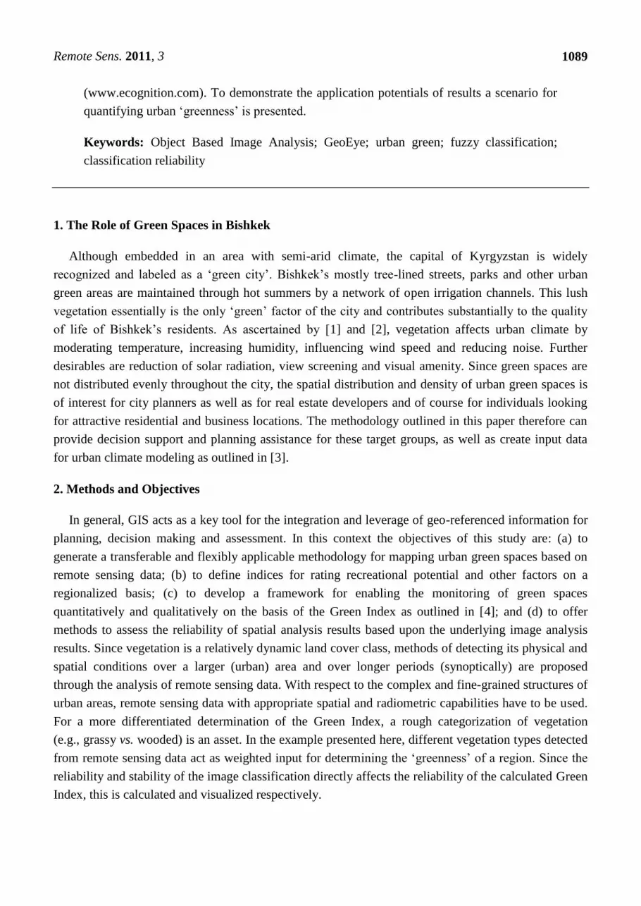
Analyzing statistical moments, such as mean and standard deviation of CSi and 𝜇𝑖𝑏 of the whole
scene can be helpful in terms of assessing global reliability and adequacy of class descriptions (Tables 2
and 3; see [26,27]).
Table 2 indicates that objects of the super-class ‗vegetation‘ fulfill the classification criteria on
average by 0.87. 869 ‗vegetation‘ objects (18748 − (9232 + 644 + 8003) = 869) could not further be
assigned to any of its sub-classes since they do not fulfill any of the respective classification conditions.
Objects of the class ‗mixed vegetation‘ were classified most distinctly, but there is no object of this
class being a full member of it (maximum 𝜇𝑖𝑏 = 0.99). ‗Meadow-like vegetation‘ obviously is least
separable from other classes (mean CSi = 0.47). A map-like display of CSi and 𝜇𝑖𝑏 per object shows the
spatial distribution of the values and can reveal spatial concentrations of (un)ambiguity (Figure 8).
Remote Sens. 2011, 3
1098
Figure 8. Reliability of classification results per object expressed by Best Classification
Result (𝜇𝑖𝑏 ) per object (top) and Classification Stability (CSi) per object bottom. Both
superimposed to GeoEye-1 pan-sharpened image.
4. Spatial Analysis and Mapping
While image analysis produces a high resolution map of the land cover features of interest, to
support longer-term monitoring as well as planning applications, a standardized geometry is desirable.
Options are location-specific structures like micro districts or city blocks, or regular ‗neutral‘ tilings
like a regular grid. The latter is well suited as a common framework for integration of data sets from
Remote Sens. 2011, 3
1099
different sources and lends itself easily to a broad range of analysis techniques as well as visualization
approaches. In the example present we have chosen a grid approach for further analysis of Bishkek‘s
green spaces. Subsequent steps are based on a 100-m resolution (hectare) grid aligned with UTM.
5. Developing an Urban Green Index
In order to determine the ‗Green Index‘ per cell following [4], first the vegetation polygons need to
be intersected with grid cells. In contrast to [4] for the determination of the ‗Green Index‘ per cell we
have weighted the various types of vegetation differently. The ‗Green Index‘ per cell GIj then is
calculated by summarizing the weighted area wcAc of the vegetation sub-classes C within cell j and
dividing it by the area Aj of the cell:
jCC
j
j AwA
GI1
(11)
With 0 ≤ GIj ≤ 1 and 0 ≤ wc ≤ 1. A ‗Green Index‘ of GIj = 0 indicates no vegetation at all within cell j
and GIj = 1 indicates a complete coverage of the vegetation sub-class(es) weighted by 1 within cell j. In
the example present we decided to weight the different sub-classes of vegetation as outlined in Table 4.
Table 4. Class weights for the calculation of the Green Index.
Vegetation type Weight
meadow-like vegetation 0.3
mixed vegetation 0.8
wooded vegetation 1.0
Of course, these weights can be adjusted depending on the application framework. Results for the
study area are presented in Figure 9.
6. Impact of Classification Reliability on Analysis Results
Having quantified information on the reliability of the input data, in principle allows assessing the
reliability of subsequent spatial analysis. Spatial analysis results generated based on doubtful
classification results can be highlighted or excluded from analysis. In order to evaluate the reliability of
analysis results synoptically a cartographic presentation can be useful. Without going into detail about
the visualization of uncertainty in maps [28] we decided to visualize the mean 𝜇𝑖𝑏 per cell as displayed
in Figure 10. Of course CSi can be visualized accordingly. Alternatively, in order to avoid doubtful
analysis results, unreliable or unstable objects can be excluded in advance from calculation of the
‗Green Index‘. For this purpose we decided to exclude objects (before intersecting with the grid cells)
with a Classification Stability of CSi ≤ 0.90 and a Best Classification Result of 𝜇𝑖𝑏 ≤ 0.75 for the
calculation of GIj. Only vegetation objects fulfilling these criteria (Figure 10) are considered for
calculating the weighted ‗Green Index‘. The difference between the GIj with and without reliable
vegetation objects is relatively low—in the present subset we have observed a mean difference of 0.026
for the overall ‗Green Index‘. However, when excluding doubtful objects in advance, the reliability of
the calculated GIj rises in many instances.

Remote Sens. 2011, 3
1100
Figure 9. Weighted Green Index superimposed to pan-sharpened GeoEye-1 image.
Figure 10. Weighted Green Index superimposed on pan-sharpened GeoEye-1 image, plus
mean Best Classification Result per cell as crosshairs. Size of crosshairs indicates the mean
value of Best Classification Result per cell. Weighted Green Index and Best Classification
Result are calculated based on vegetation objects with CSi > 0.90 and 𝜇𝑖𝑏 > 0.75. No
crosshair indicates a Best Classification Result of 𝜇𝑖𝑏 > 0.9.

Remote Sens. 2011, 3
1101
7. Results and Discussion
This paper introduces a workflow for mapping a modified ‗Green Index‘ as introduced by [4]. The
modification is based on different weightings for vegetation classes determining the ‗Green Index‘. The
weights presented here were chosen arbitrarily. Methodologically the paper focuses on estimating the
reliability of classification results derived from object based image analysis and fuzzy classification. We
demonstrate how primary classification reliability can be determined by the parameters Best
Classification Result (𝜇𝑖𝑏) and Classification Stability (CSi) as introduced by [20], and implemented in
the software package eCognition (see [26,27]). Both parameters are derived directly from fuzzy
classification results. We further demonstrate how this information can be passed to the evaluation of
reliability of subsequent spatial analysis (here: the calculation of a modified ‗Green Index‘). As outlined
in Section 6, 𝜇𝑖𝑏 and CSi can even be used to exclude obviously unreliably classified objects from
further spatial analysis processes.
Nevertheless, we are aware that the parameters Best Classification Result (𝜇𝑖𝑏) and Classification
Stability (CSi) are just comparing the classification results with their underlying class models. While 𝜇𝑖𝑏
shows how well a classified object fits a model, CSi expresses the ambiguity of the class assignment.
However, none of the parameters expresses the consistency with reality, which still needs to be assessed
by comparing classification results with on-site samples.
Acknowledgments
We gratefully acknowledge support by the GeoEye Foundation providing GeoEye-1 imagery for
the city of Bishkek, a research fellowship awarded to Nazarkulova by the Eurasia-Pacific Uninet
(http://www.eurasiapacific.net) and input from our fellow researchers at the Center for Geoinformatics,
University of Salzburg.
References
1. Zoulia, D.; Santamouris, M.; Dimoudi, A.; Monitoring the effect of urban green areas on the heat
island in Athens. Environ. Monit. Assess. 2009, 156, 275-292.
2. Alexandri, E.; Jones, P. Temperature decreases in an urban canyon due to green walls and green
roofs in diverse climates. Build. Environ. 2008, 42, 480-493.
3. Robitu, M.; Musy, M.; Inard, C.; Groleau, D.; Modeling the influence of vegetation and water
pond on urban microclimate. Solar Energy 2006, 80, 435-447.
4. Schöpfer, E.; Lang, S.; Blaschke, T. A ―Green Index‖ Incorporating Remote Sensing and
Citizen‘s Perception of Green Space. In Proceedings of the ISPRS Joint Conference on 3rd
International Symposium Remote Sensing and Data Fusion Over Urban Areas (URBAN 2005)
and 5th International Symposium Remote Sensing of Urban Areas (URS 2005), Tempe, AZ, USA,
14–16 March 2005; Volume 37, Part 5/W1, pp. 1-6.
5. Welch, R.; Ehlers, M.; Merging multiresolution SPOT HRV and Landsat TM Data. Photogramm.
Eng. Remote Sensing 1987, 53, 301-303.
6. Lillesand, T.M.; Kiefer, R.W.; Chipman, J.W. Remote Sensing and Image Interpretation, 6th ed.;
John Wiley & Sons: Hoboken, NJ, USA, 2008.

Remote Sens. 2011, 3
1102
7. Lang, S. Object-based image analysis for remote sensing applications: modelling reality—Dealing
with complexity. In Object Based Image Analysis; Blaschke, T., Lang, S., Hay, G.J., Eds.;
Springer: Heidelberg/Berlin, New York, 2008; pp. 1-25.
8. Haralick, R.M.; Shapiro, L. Survey: Image segmentation techniques. Comput. Vis. Graph. Image
Process. 1985, 29, 100-132.
9. Pal, N.R.; Pal, S.K. A review on image segmentation techniques. Patt. Recog. 1993, 26,
1277-1294.
10. Baatz, M.; Schäpe, A.; Multiresolution segmentation: An optimization approach for high quality
multi-scale image segmentation. In Angewandte Geographische Informations—Verarbeitung;
Strobl, J., Blaschke, T., Griesebner, G., Eds.; Wichmann Verlag: Karlsruhe, Germany, 2000;
Volume XII, pp. 12-23.
11. Neubert, M.; Meinel, G.; Evaluation of Segmentation Programs for High Resolution Remote
Sensing Applications. In Proceedings of the Joint ISPRS/EARSeL Workshop “High Resolution
Mapping from Space 2003”, Hannover, Germany, 6–8 October 2003.
12. Hay, G.J.; Blaschke, T.; Marceau, D.J.; Bouchard, A. A comparison of three image-object
methods for the multiscale analysis of landscape structure. ISPRS J. Photogramm. Remote Sens.
2003, 57, 327-345.
13. Neubert, M.; Herold, H.; Meinel, G. Assessing image segmentation quality—Concepts, methods
and application. In Object Based Image Analysis; Blaschke, T., Lang, S., Hay, G.J., Eds.;
Springer: Heidelberg/Berlin, Germany, 2008; pp. 760-784
14. Thiel, C.; Thiel, C.; Riedel, T.; Schmullius, C. Object-based classification of SAR data for the
delineation of forest cover maps and the detection of deforestation—A viable procedure and its
application in GSE forest monitoring. In Object Based Image Analysis; Blaschke, T., Lang, S.,
Hay, G.J., Eds.; Springer: Heidelberg/Berlin, Germany, 2008; pp. 327-343.
15. Lang, S.; Blaschke, T. Hierarchical Object Representation—Comparative Multiscale Mapping of
Anthropogenic and Natural Features. In Proceedings of ISPRS Workshop “Photogrammetric
Image Analysis”, Munich, Germany, 17–19 September 2003; Volume 34, pp. 181-186.
16. Hay, G.J.; Castilla, G.; Wulder, M.A.; Ruiz, J.R. An automated object-based approach for the
multiscale image segmentation of forest scenes. Int. J. Appl. Earth Obs. Geoinf. 2005, 7, 339-359.
17. Koestler, A. The Ghost in the Machine; Random House: New York, NY, USA, 1967.
18. Câmara, G.; Souza, R.C.M.; Freitas, U.M.; Garrido, J. SPRING: Integrating remote sensing and
GIS by object-oriented data modelling. Comput. Graph. 1996, 20, 395-403.
19. Lang, S.; Blaschke, T. Bridging Remote Sensing and GIS—What are the Main Supporting
Pillars? In Proceedings of 1st International Conference on Object-based Image Analysis (OBIA
2006), Salzburg, Austria, 4–5 July 2006.
20. Benz, U.; Hofmann, P.; Willhauck, G.; Lingenfelder I.; Heynen, M.; Multi-resolution
object-oriented fuzzy analysis of remote sensing data for GIS-ready information. ISPRS J.
Photogramm. Remote Sens. 2004, 58, 239-258.
21. Liedtke, C.-E.; Bückner J.; Grau, O.; Growe, S.; Tönjes, R. AIDA: A System for the Knowledge
Based Interpretation of Remote Sensing Data. In Proceedings of the Third International Airborne
Remote Sensing Conference and Exhibition, Copenhagen, Denmark, 7–10 July 1997.
Remote Sens. 2011, 3
1103
22. Siler, W.; Buckley, J.J. Fuzzy Expert Systems and Fuzzy Reasoning; John Wiley & Sons:
Hoboken, NJ, USA, 2005.
23. Richards, J.A.; Jia, X. Remote Sensing Digital Image Analysis, 4th ed.; Springer:
Berlin/Heidelberg, Germany, 2006.
24. Cristianini, N.; Shawe-Taylor, J. An Introduction to Support Vector Machines; Cambridge
University Press: Cambridge, UK, 2000.
25. Zell, A.; Mamier, G.; Vogt, M.; Mache, N.; Hübner, R.; Döring, S.; Herrmann, K.-U.; Soyez, T.;
Schmalzl, M.; Sommer, T.; et al. SNNS Stuttgart Neural Network Simulator, User Manual,
Version 4.2, Available online: http://www.ra.cs.uni-tuebingen.de/downloads/SNNS/
SNNSv4.2.Manual.pdf (accessed on 15 May 2011).
26. Trimble. eCognition Developer 8.64.0 User Guide; Trimble: Munich, Germany, 2010.
27. Trimble. eCognition Developer 8.64.0 Reference Book; Trimble: Munich, Germany, 2010.
28. MacEachren, A.M.; Robinson, A.; Hopper, S.; Gardner, S.; Murray, R.; Gahegan, M.; Hetzler, E.
Visualizing geospatial information uncertainty: What we know and what we need to know.
Cartogr. Geogr. Inform. Sci. 2005, 32, 139-160.
© 2011 by the authors; licensee MDPI, Basel, Switzerland. This article is an open access article
distributed under the terms and conditions of the Creative Commons Attribution license
(http://creativecommons.org/licenses/by/3.0/).
Related Documents