Mapping epibenthic assemblages and their relations to sedimentary features in shallow-water, high-energy environments

Continental Shelf Research 22 (2002) 565–583

Mapping epibenthic assemblages and their relationsto sedimentary features in shallow-water,

high-energy environments

John D. Sissona, Jeff Shimetab,*, Cheryl Ann Zimmera,1, Peter Traykovskia

aWoods Hole Oceanographic Institution, Woods Hole, MA 02543, USAbBiology Department, Franklin and Marshall College, P. O. Box 3003, Lancaster, PA 17604-3003, USA

Received 26 February 2001; accepted 1 June 2001

Abstract

Knowledge of spatial relationships among benthic biota and sedimentary features in shallow-water (o30m) high-energy environments has been severely limited by sampling technology. We describe and report tests of a SCUBA-

diving mapping method specifically for this region. Underwater acoustic location is used to achieve meter-scaleresolution over kilometer-scale regions of the sea floor. A triad of acoustic transponders is bottom-mounted at knownpositions, 300–500m apart. Transported by underwater personal vehicles, SCUBA-divers map the bed using hand-held

acoustic receivers that record ranges to the transponders. The mean error of acoustic fixes was 2.471.2m in a0.5 km� 1.0 km test area. Dense assemblages of epibenthic animals were mapped relative to sediment texture andbedforms off the exposed south coast of Martha’s Vineyard Island, Massachusetts, USA. Surveys one month apartwithin a 0.6 km� 0.6 km area (8–12m depth) revealed 100-m-scale patches of the tube worm Spiophanes bombyx

(p30,000m�2) in fine sand and of the sand dollar Echinarachnius parma (p55m�2) in coarse sand. Raised mud patchesthat, together with fine sand, occurred in two shore-perpendicular belts are likely exposed, ancient marsh deposits.Depth gradients of sand-ripple geometry indicated that ripples in deeper areas were not in equilibrium with wave

conditions monitored during surveys; i.e., they were relict ripples. Thus, sand dollars in some areas may have had >1month to rework surficial sands since their transformation by physical processes. Linear regressions of ripplecharacteristics against sand dollar or tube worm densities were not significant, although such relationships would be

highly dependent on temporal scale. The survey method described here can be used at more frequent intervals toexplore such interactions between epibenthic animals and sediment-transport dynamics. r 2002 Elsevier Science Ltd.All rights reserved.

Keywords: Mapping; Epibenthic; SCUBA; Acoustics; USA; Massachusetts; Martha’s Vineyard Island

1. Introduction

Mapping the distribution and abundance ofbenthic organisms frequently involves reconcilingconflicting requirements of small-scale spatialresolution and large-scale areal coverage. Most

*Corresponding author. Fax: +1-717-358-4548.

E-mail address: j [email protected] (J. Shimeta).1Formerly C.A. Butman Present address: Department of

Biology, University of California, 621 Charles E. Young

Dr. South, Los Angeles, CA 90095-1606, USA.

0278-4343/02/$ - see front matter r 2002 Elsevier Science Ltd. All rights reserved.

PII: S 0 2 7 8 - 4 3 4 3 ( 0 1 ) 0 0 0 7 4 - 7

survey methods involve compromises in onecriterion or the other. Thus, it is often difficult tointerpret small-scale spatial patterns in the contextof larger-scale processes.We mapped dense assemblages of epibenthic

(surface-visible) organisms and sedimentary fea-tures with meter-scale resolution over kilometer-scale expanses of the sandy, high-energy, innershelf. The purpose was to determine the spatialrelationships between biota and bedforms, and toassess whether the organisms influence sediment-transport processes. A critical part of this studywas the testing and application of a SCUBA-diving survey technique where the locations ofsurficial biological and sedimentary features weredetermined using underwater acoustics. Themethod can be applied easily to shallow-water,high-energy environments in which surveying thequantitative distributions of organisms have tra-ditionally been problematic.

1.1. Importance of benthic biological patchiness

Marine benthic macro-organisms can be dis-tributed in patches spanning length scales from0.01 to 1000m or more. Biological and physicalprocesses in and among these patches havenumerous ecological consequences. In intertidaland shallow subtidal sediments, aggregations ofmacrofauna such as tube-dwelling polychaetesoccur at centimeter to meter scales (e.g., Zettlerand Bick, 1996). These assemblages can influencesediment transport, larval settlement, and recruit-ment through processes such as flow alteration,accumulation of chemical signals, and other adult-larval interactions (Eckman and Nowell, 1984;Butman, 1987). Patches of subtidal macrophytesand megafauna extend from meters to kilometersor more (Aronson, 1989; Irlandi, 1996). Kelp andseagrass patches affect local flow, sedimentation,and the recruitment and growth of suspensionfeeders (Peterson et al., 1984; Eckman et al., 1989).Not surprisingly, small-scale processes are

known to determine or influence distributions oforganisms at small scales. Largely unknown,however, are whether small-scale distributionsare representative of patterns on the scale of akilometer or more, and whether large- and

small-scale distributions are shaped by similarprocesses. For example, the role of regional-scalelarval supply in determining local distributions ofrecruited juveniles has been debated for decades(Olafsson et al., 1994). Moreover, there is virtuallyno information on the influence of small-scalepatches of benthic organisms on net rates ofsediment transport or deposition at large scalesin estuaries or along exposed coastlines. To deter-mine such influences of benthic assemblages onphysical processes, and vice versa, organismaldistributions must be mapped with appropri-ately small-scale resolution over survey areas ofappropriately large scale.Benthic organisms can affect sediment charac-

teristics and sediment transport in a variety ofways. Biologists have observed these effects,largely qualitatively, for almost a century(Snelgrove and Butman, 1994), and potentialeffects of benthic biology on boundary-layer flowsand sediment transport have been acknowledgedin major reviews of the physical processes (Nowell,1983; Grant and Madsen, 1986; Cacchione andDrake, 1990). Organismal effects on sedimenttransport have been studied in the laboratory orin muddy, depositional intertidal and shallowsubtidal environments (e.g., Nowell et al., 1981;Grant et al., 1982; Wheatcroft and Butman, 1997).Studies in high-energy areas have been almostexclusively intertidal (Grant, 1983; Grant et al.,1986; Grant and Gust, 1987; Miller and Sternberg,1988).In sandy, shallow, high-energy shelf environ-

ments, sediment-transport events are intense andfrequent; thus, biological effects on sedimenttransport are typically presumed negligible. Thereis a dearth of information on even the identitiesand densities of the large, epibenthic organisms(e.g., sand dollars, tube worms and clams) that arelikely to affect the transport of sands, let alonedata on their quantitative effects. Sands generallyare difficult to sample using grabs and box cores,and, because large organisms are often patchilydistributed, diving surveys may not cover asufficiently large area to obtain accurate densitiesof these organisms. The high-energy nature ofthe environment has been a further obstacle tosampling.

J.D. Sisson et al. / Continental Shelf Research 22 (2002) 565–583566

1.2. Methods of mapping organisms on the sea floor

Most sampling and surveying methods provideeither fine-scale resolution over a small area orcoarse resolution over a large area. Organismalpatchiness and percent cover on the scale of1–100m remains the least characterized, particu-larly in the shallow subtidal. Box cores providethe best quantitative information on cm-scale dis-persion of sedimentary benthos (Jumars, 1975;Hughes, 1996). Box coring is limited, however,from low accuracy and precision of positioningmultiple cores on scales of 1–10m, and a boat atleast 15m in length is required to deploy a large(e.g., 0.25m2) box core. Benthic sleds and towedvideo cameras can cover large areas but withrelatively coarse spatial resolution (Christiansenand Nuppenau, 1997; Sotheran et al., 1997), andthey can be expensive or impractical for routineshallow-water work. Remote-sensing acousticsand photography can operate over 100–1000mareas with meter-scale resolution in some cases(Jumars et al., 1996; Mumby et al., 1997; Sotheranet al., 1997). Cost may be prohibitive, however,and it is generally difficult, if not impossible, toidentify organisms to species. SCUBA divers inthe shallow subtidal can manually sample organ-isms and map distributions by photography orquadrat sampling over small scales (Downing andAnderson, 1985; Benedetti-Cecchi et al., 1996).Over distances greater than about 50m, however,the extent and accuracy of mapping are limited byswimming distance, bottom time, and navigationby compass, particularly in strong currents.

1.3. Testing and application of a SCUBA-divingmapping method using acoustic location

We here describe an underwater acoustic loca-tion method that can be used by SCUBA-divers tomap surficial benthic assemblages and sedimentaryfeatures in the high-energy shallow subtidal.Organism and sediment distributions can beresolved with meter-scale accuracy over kilo-meter-scale regions of the sea floor. The simplestdesign for underwater acoustic location involvestriangulating a position from the ranges to threeunderwater transponders (Spindel et al., 1976).

The basic technique has been modified foroceanographic applications such as the positioningor tracking of surface ships, submersibles, free-falling instruments, and swimming animals, andacoustic tomography of oceanic hydrography(McCartney, 1981; Luyten et al., 1982; Mercer,1986). Some commercial positioning systems areavailable.We anchored three transponders on the sea floor

such that the baseline distances between transpon-ders were long relative to the ranges to the divers(i.e., a ‘‘long baseline’’ configuration; McCartney,1981). To determine the accuracy of the under-water acoustic fixes obtained with this method,a pilot study was done offshore of a high-energybeach where land surveyors provided fixes onbuoys located directly above the bottom-mountedtransponders. In the same region, exploratorySCUBA-diving transects of ca. 400m were run toevaluate the limitations of this technique forplotting features (biological and sedimentary)observed on the sea floor. A more extensive fieldsurvey was then conducted to map dense assem-blages of epibenthic organisms and their relationsto sedimentary features in a 600m� 600m,high-energy nearshore region off the south shoreof Martha’s Vineyard Island, Massachusetts(USA).

2. Methods

2.1. Overview of acoustic underwater locationtechnique

The acoustic underwater location technique usesa triad of moored, geopositioned, acoustic trans-ponders (Datasonics UAT series, minimum rangeof 750m) each replying at a different frequency(range 25–32 kHz). The ideal configuration is tobottom-mount the transponders on rigid poststo form an equilateral triangle. Differential globalpositioning system (dGPS) fixes are taken onthe transponders from a boat while cinching tautthe anchor lines to buoys directly above thetransponders. As divers conduct transect surveysof organisms and sedimentary features, theydetermine the range to each transponder using a

J.D. Sisson et al. / Continental Shelf Research 22 (2002) 565–583 567

hand-held acoustic interrogator (Datasonics DiveRanger DRI-267A). Transponder frequency,range, and time of interrogation, taken directlyfrom the interrogator at 0.5Hz, are stored in awaterproof data logger that straps to the back ofa SCUBA tank. This underwater data logger wasbuilt in-house at WHOI. Positional fixes are latercalculated by triangulation of the acoustic ranges(Spindel et al., 1976). With the aid of commercial,underwater personal vehicles (SCUBA-diving‘‘scooters’’), transect distances of up to 600m canbe covered during a single dive.

2.2. Evaluating fix error

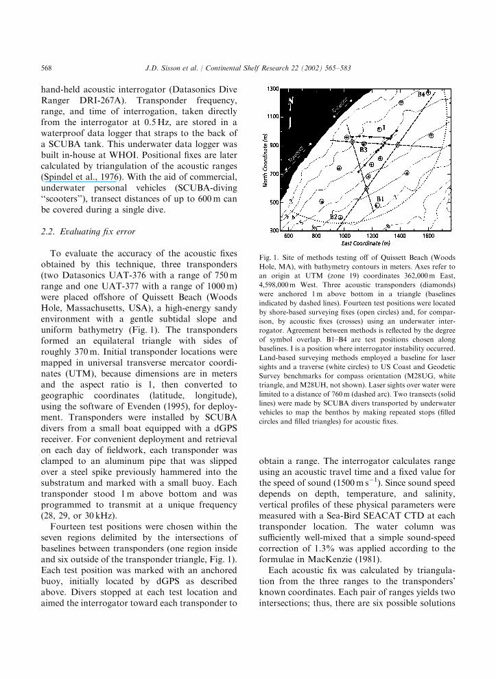
To evaluate the accuracy of the acoustic fixesobtained by this technique, three transponders(two Datasonics UAT-376 with a range of 750mrange and one UAT-377 with a range of 1000m)were placed offshore of Quissett Beach (WoodsHole, Massachusetts, USA), a high-energy sandyenvironment with a gentle subtidal slope anduniform bathymetry (Fig. 1). The transpondersformed an equilateral triangle with sides ofroughly 370m. Initial transponder locations weremapped in universal transverse mercator coordi-nates (UTM), because dimensions are in metersand the aspect ratio is 1, then converted togeographic coordinates (latitude, longitude),using the software of Evenden (1995), for deploy-ment. Transponders were installed by SCUBAdivers from a small boat equipped with a dGPSreceiver. For convenient deployment and retrievalon each day of fieldwork, each transponder wasclamped to an aluminum pipe that was slippedover a steel spike previously hammered into thesubstratum and marked with a small buoy. Eachtransponder stood 1m above bottom and wasprogrammed to transmit at a unique frequency(28, 29, or 30 kHz).Fourteen test positions were chosen within the

seven regions delimited by the intersections ofbaselines between transponders (one region insideand six outside of the transponder triangle, Fig. 1).Each test position was marked with an anchoredbuoy, initially located by dGPS as describedabove. Divers stopped at each test location andaimed the interrogator toward each transponder to

obtain a range. The interrogator calculates rangeusing an acoustic travel time and a fixed value forthe speed of sound (1500m s�1). Since sound speeddepends on depth, temperature, and salinity,vertical profiles of these physical parameters weremeasured with a Sea-Bird SEACAT CTD at eachtransponder location. The water column wassufficiently well-mixed that a simple sound-speedcorrection of 1.3% was applied according to theformulae in MacKenzie (1981).Each acoustic fix was calculated by triangula-

tion from the three ranges to the transponders’known coordinates. Each pair of ranges yields twointersections; thus, there are six possible solutions

Fig. 1. Site of methods testing off of Quissett Beach (Woods

Hole, MA), with bathymetry contours in meters. Axes refer to

an origin at UTM (zone 19) coordinates 362,000m East,

4,598,000m West. Three acoustic transponders (diamonds)

were anchored 1m above bottom in a triangle (baselines

indicated by dashed lines). Fourteen test positions were located

by shore-based surveying fixes (open circles) and, for compar-

ison, by acoustic fixes (crosses) using an underwater inter-

rogator. Agreement between methods is reflected by the degree

of symbol overlap. B1–B4 are test positions chosen along

baselines. I is a position where interrogator instability occurred.

Land-based surveying methods employed a baseline for laser

sights and a traverse (white circles) to US Coast and Geodetic

Survey benchmarks for compass orientation (M28UG, white

triangle, and M28UH, not shown). Laser sights over water were

limited to a distance of 760m (dashed arc). Two transects (solid

lines) were made by SCUBA divers transported by underwater

vehicles to map the benthos by making repeated stops (filled

circles and filled triangles) for acoustic fixes.

J.D. Sisson et al. / Continental Shelf Research 22 (2002) 565–583568

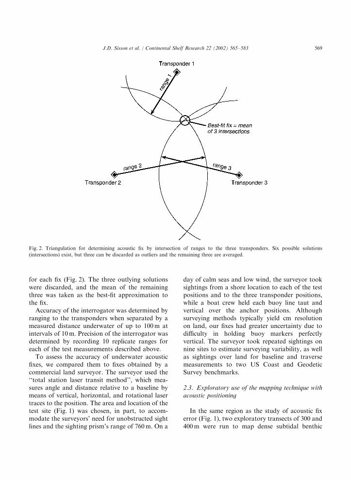
for each fix (Fig. 2). The three outlying solutionswere discarded, and the mean of the remainingthree was taken as the best-fit approximation tothe fix.Accuracy of the interrogator was determined by

ranging to the transponders when separated by ameasured distance underwater of up to 100m atintervals of 10m. Precision of the interrogator wasdetermined by recording 10 replicate ranges foreach of the test measurements described above.To assess the accuracy of underwater acoustic

fixes, we compared them to fixes obtained by acommercial land surveyor. The surveyor used the‘‘total station laser transit method’’, which mea-sures angle and distance relative to a baseline bymeans of vertical, horizontal, and rotational lasertraces to the position. The area and location of thetest site (Fig. 1) was chosen, in part, to accom-modate the surveyors’ need for unobstructed sightlines and the sighting prism’s range of 760m. On a

day of calm seas and low wind, the surveyor tooksightings from a shore location to each of the testpositions and to the three transponder positions,while a boat crew held each buoy line taut andvertical over the anchor positions. Althoughsurveying methods typically yield cm resolutionon land, our fixes had greater uncertainty due todifficulty in holding buoy markers perfectlyvertical. The surveyor took repeated sightings onnine sites to estimate surveying variability, as wellas sightings over land for baseline and traversemeasurements to two US Coast and GeodeticSurvey benchmarks.

2.3. Exploratory use of the mapping technique withacoustic positioning

In the same region as the study of acoustic fixerror (Fig. 1), two exploratory transects of 300 and400m were run to map dense subtidal benthic

Fig. 2. Triangulation for determining acoustic fix by intersection of ranges to the three transponders. Six possible solutions

(intersections) exist, but three can be discarded as outliers and the remaining three are averaged.

J.D. Sisson et al. / Continental Shelf Research 22 (2002) 565–583 569

assemblages using underwater photography andobservations. To maximize the area covered on asingle dive, divers used underwater scooters(Dacor Seasprint U/W Vehicle SV900) that weremodified by attaching a PVC-sheet ‘‘benchtop’’ formounting a compass, camera brackets, and a slateto record written observations. A 400-m transectthat was down current and along-isobath crossedthe center of the transponder triangle, and a 300-mcross-isobath transect ran parallel to a transpon-der baseline, 50m outside of the triangle (Fig. 1).The intent was to map transitions amongpatchy beds of the seagrass Zostera marina,epibenthic megafaunal assemblages, and changingsedimentary features. Two divers visually scanneda 10-m wide path while transported by scooters,and stopped at each transition to take transponderranges, enumerate densities of organisms in quad-rats, measure bedform geometries, and documentfeatures with underwater photographs (NikonosV camera and strobe). Acoustic fixes were laterdetermined from transponder ranges and used toreconstruct dive tracks.

2.4. The field study

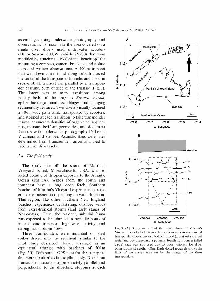
The study site off the shore of Martha’sVineyard Island, Massachusetts, USA, was se-lected because of its open exposure to the AtlanticOcean (Fig. 3A). Winds from the south andsoutheast have a long, open fetch. Southernbeaches of Martha’s Vineyard experience extremeerosion or accretion depending on wind direction.This region, like other southern New Englandbeaches, experiences devastating, onshore windsfrom extra-tropical storms (and early stages ofNor’easters). Thus, the resident, subtidal faunawas expected to be adapted to periodic bouts ofintense sand transport, high wave activity, andstrong near-bottom flows.Three transponders were mounted on steel

spikes driven into the sediment (similar to thepilot study described above), arranged in anequilateral triangle with baselines of 500m(Fig. 3B). Differential GPS fixes for the transpon-ders were obtained as in the pilot study. Divers rantransects on scooters approximately parallel andperpendicular to the shoreline, stopping at each

Fig. 3. (A) Study site off of the south shore of Martha’s

Vineyard Island. (B) Indicates the locations of bottom-mounted

transponders (open circles), bottom tripod (cross) with current

meter and tide gauge, and a potential fourth transponder (filled

circle) that was not used due to poor visibility for diver

observations at depths o8m. Dash-dotted rectangle shows the

limit of the survey area set by the ranges of the three

transponders.

J.D. Sisson et al. / Continental Shelf Research 22 (2002) 565–583570

interesting biological or sedimentary feature ortransition to record ranges on the data logger, toapproximate grain size by touch, to count organ-isms in quadrats, to measure bedform geometries,to take photographs, and to make written ob-servations. The wavelength, height, and compassbearing of up to three ripples were measured andaveraged at each stop. Low-visibility conditionslimited the inshore depth of the transects to 8 m;the offshore limit of 12m was set by the range ofthe transponders. The transect length of a singledive was up to 600m, depending on the frequencyand complexity of the bottom features surveyed.An approximately 600m� 600m region wassurveyed in early July and in early August, 1997,with each survey spanning a 10-day period.Transect paths were reconstructed from acousticfixes as described above, and contour mapsof animal densities were calculated from adistance-inverse method using Matlab v.4.2. Fol-lowing each month’s survey, divers took coresamples for quantitative sediment grain-size ana-lyses (method of Fuller and Butman, 1988) andfaunal identifications.From 23 June to 4 September, 1997, the near-

bottom flow and hydrographic regime weremonitored with an InterOcean S4 current meterand Seabird tide gauge on a tripod (instruments at1.13 and 0.45mab, respectively), in 12m of waterat the outer boundary of the survey area (Fig. 3B).The S4 sampled continuously, integrating mea-surements over 3-min intervals. The tide gaugerecorded water temperature, pressure andconductivity, integrating over 30-min intervals.Pressure was burst-sampled at 1Hz for 1024 severy 3 h.

3. Results

3.1. Acoustic fix error

Underwater acoustic fixes agreed well with thelaser-transit surveyed fixes (Fig. 1). Of the 14 testpositions, acoustic fixes at three positions wereeasily identified as erroneous and discarded (B1,B2, and I, as explained below), while the remaining11 fixes were accepted as valid. The mean

discrepancy (i.e. fix error) for these 11 acousticfixes compared to the corresponding laser-transitfixes was 2.4m (SD=1.2m, range=0.6–4.9m).One source of fix error is poor geometry of

range overlaps, which occurs in cases where thethree central intersections are widely spaced(contrasting with the closely spaced intersectionsin Fig. 2), reducing the accuracy of the meanposition for the fix. Fixes very near the baselinesbetween transponders are potentially the mostproblematic, because ranges between the trans-ponders have minimal overlap and the positionof the intersections is highly sensitive to smallinaccuracies in measurements. For example, atposition B1 (Fig. 1) the three ranges intersected ina highly distorted triangle that was clearlyerroneous and gave a fix error of 11.2m. In theextreme case of a ‘‘baseline anomaly,’’ (e.g.position B2), ranges from the two baselinetransponders failed to overlap and no solutionfor the fix was possible. Nonetheless, baselinepositions B3 and B4 gave good fixes (errors of 4.0and 1.7m, respectively).Two other potential sources of fix error, namely

inaccuracies of the acoustic interrogator and of theshore-based surveys, were relatively unimportantin our results. The mean error of interrogatorranges was only 0.73m (SD=0.47m, n ¼ 30), withthe larger errors occurring at the closer ranges.Precision of the interrogator was excellent, with amean coefficient of variation of 0.0026 from 42 setsof 10 replicate ranges. However, one test-positionfix (I, Fig. 1) was erroneous due to anomalousinstability of the interrogator reading (8m range ofvalues during 10 replicate readings, compared tothe typical 1–2m range). Finally, shore-basedlaser-transit fixes were highly precise, with anaverage SD=0.85m among repeated fixes at ninepositions.

3.2. Resolving patchiness in the benthos

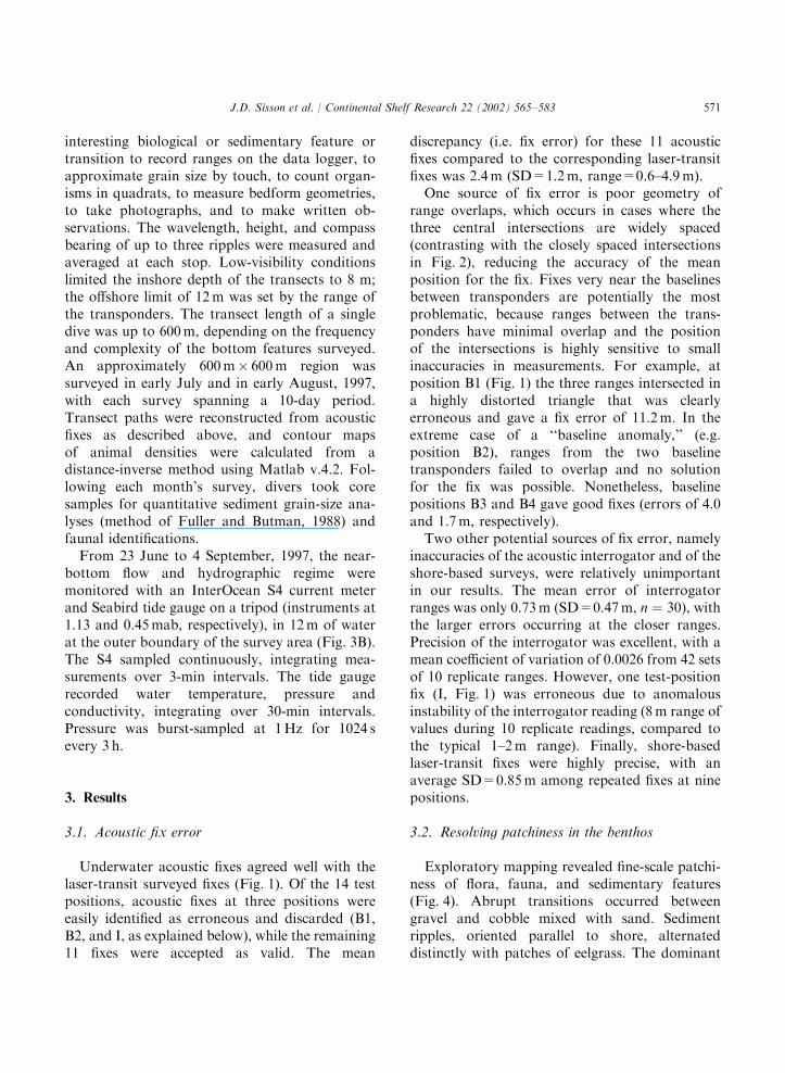
Exploratory mapping revealed fine-scale patchi-ness of flora, fauna, and sedimentary features(Fig. 4). Abrupt transitions occurred betweengravel and cobble mixed with sand. Sedimentripples, oriented parallel to shore, alternateddistinctly with patches of eelgrass. The dominant

J.D. Sisson et al. / Continental Shelf Research 22 (2002) 565–583 571

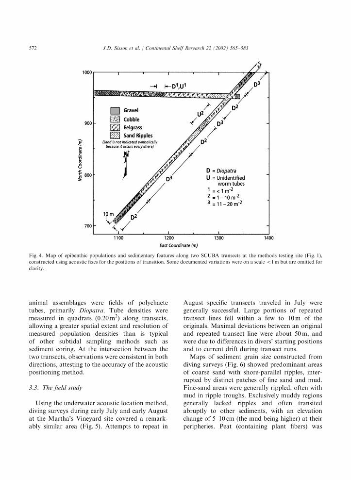
animal assemblages were fields of polychaetetubes, primarily Diopatra. Tube densities weremeasured in quadrats (0.20m2) along transects,allowing a greater spatial extent and resolution ofmeasured population densities than is typicalof other subtidal sampling methods such assediment coring. At the intersection between thetwo transects, observations were consistent in bothdirections, attesting to the accuracy of the acousticpositioning method.

3.3. The field study

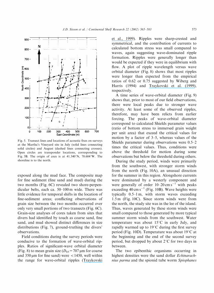
Using the underwater acoustic location method,diving surveys during early July and early Augustat the Martha’s Vineyard site covered a remark-ably similar area (Fig. 5). Attempts to repeat in

August specific transects traveled in July weregenerally successful. Large portions of repeatedtransect lines fell within a few to 10m of theoriginals. Maximal deviations between an originaland repeated transect line were about 50m, andwere due to differences in divers’ starting positionsand to current drift during transect runs.Maps of sediment grain size constructed from

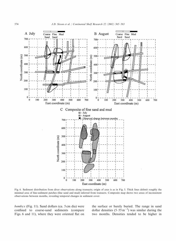
diving surveys (Fig. 6) showed predominant areasof coarse sand with shore-parallel ripples, inter-rupted by distinct patches of fine sand and mud.Fine-sand areas were generally rippled, often withmud in ripple troughs. Exclusively muddy regionsgenerally lacked ripples and often transitedabruptly to other sediments, with an elevationchange of 5–10 cm (the mud being higher) at theirperipheries. Peat (containing plant fibers) was

Fig. 4. Map of epibenthic populations and sedimentary features along two SCUBA transects at the methods testing site (Fig. 1),

constructed using acoustic fixes for the positions of transition. Some documented variations were on a scale o1m but are omitted for

clarity.

J.D. Sisson et al. / Continental Shelf Research 22 (2002) 565–583572

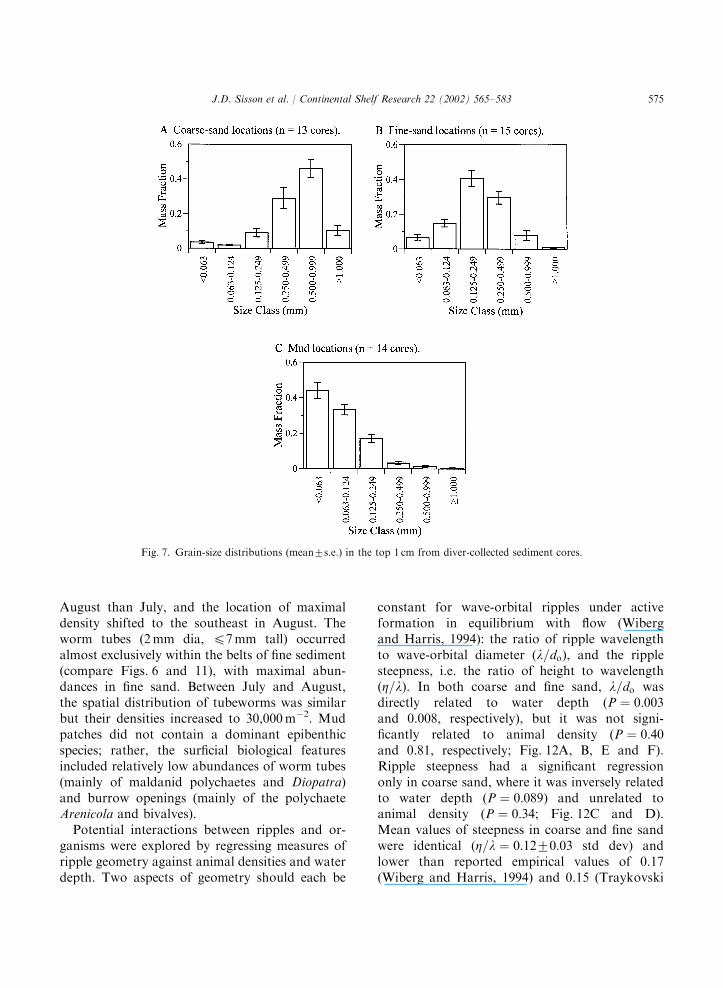
exposed along the mud face. The composite mapfor fine sediment (fine sand and mud) during thetwo months (Fig. 6C) revealed two shore-perpen-dicular belts, each ca. 50–100m wide. There waslittle evidence for temporal shifts in the location offine-sediment areas; conflicting observations ofgrain size between the two months occurred overonly very small portions of two transects (Fig. 6C).Grain-size analyses of cores taken from sites thatdivers had identified by touch as coarse sand, finesand, and mud showed distinct differences in sizedistributions (Fig. 7), ground-truthing the divers’observations.Field conditions during the survey periods were

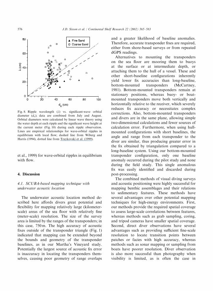
conducive to the formation of wave-orbital rip-ples. Ratios of significant-wave orbital diameter(Fig. 8) to mean grain size (D85=707 mm for coarseand 350 mm for fine sand) were o1450, well withinthe range for wave-orbital ripples (Traykovski

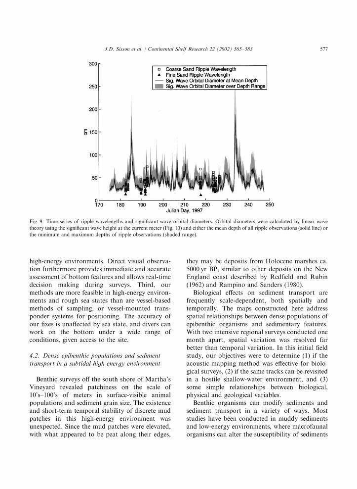
et al., 1999). Ripples were sharp-crested andsymmetrical, and the contribution of currents tocalculated bottom stress was small compared towaves, again suggesting wave-dominated rippleformation. Ripples were generally longer thanwould be expected if they were in equilibrium withflow. A plot of ripple wavelength versus waveorbital diameter (Fig. 8) shows that most rippleswere longer than expected from the empiricalratios of 0.62 or 0.75 suggested by Wiberg andHarris (1994) and Traykovski et al. (1999),respectively.A time series of wave-orbital diameter (Fig. 9)

shows that, prior to most of our field observations,there were local peaks due to stronger waveactivity. At least some of the observed ripples,therefore, may have been relicts from earlierforcing. The peaks of wave-orbital diametercorrespond to calculated Shields parameter values(ratio of bottom stress to immersed grain weightper unit area) that exceed the critical values formotion by a factor of 3–5, whereas values of theShields parameter during observations were 0.5–2times the critical values. Thus, conditions wereabove the threshold for motion during someobservations but below the threshold during others.During the study period, winds were primarily

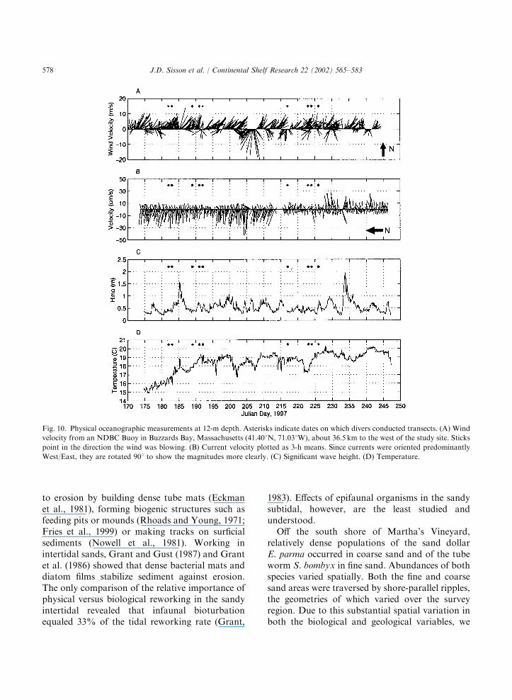
from the southwest, with stronger storm windsfrom the north (Fig. 10A), an unusual directionfor the summer in this region. Alongshore currentswere dominated by a westerly component andwere generally of order 10–20 cm s�1 with peaksexceeding 40 cm s�1 (Fig. 10B). Wave heights weretypically 0.5–1m, with storm waves exceeding1.5m (Fig. 10C). Since storm winds were fromthe north, the study site was in the lee of the island.Thus, waves generated by these storm winds weresmall compared to those generated by more typicalsummer storm winds from the southwest. Watertemperature was about 151C in early July, andrapidly warmed up to 191C during the first surveyperiod (Fig. 10D). Temperature was about 191C atthe beginning and the end of the second surveyperiod, but dropped by about 21C for two days inbetween.The two epibenthic organisms occurring in

highest densities were the sand dollar Echinarach-nius parma and the spionid tube worm Spiophanes

Fig. 5. Transect lines and locations of acoustic fixes on surveys

at the Martha’s Vineyard site in July (solid lines connecting

solid circles) and August (dashed lines connecting crosses).

Open circles are transponder locations, corresponding to

Fig. 3B. The origin of axes is at 41.3401N, 70.6041W. The

shoreline is to the north.

J.D. Sisson et al. / Continental Shelf Research 22 (2002) 565–583 573

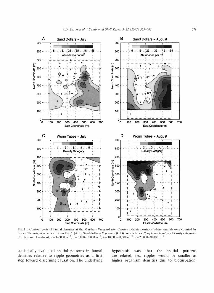
bombyx (Fig. 11). Sand dollars (ca. 5 cm dia) wereconfined to coarse-sand sediments (compareFigs. 6 and 11), where they were oriented flat on

the surface or barely buried. The range in sanddollar densities (5–55m�2) was similar during thetwo months. Densities tended to be higher in

Fig. 6. Sediment distribution from diver observations along transects; origin of axes is as in Fig. 5. Thick lines delimit roughly the

minimal area of fine-sediment patches (fine sand and mud) inferred from transects. Composite map shows two areas of inconsistent

observations between months, revealing temporal changes in sediment cover.

J.D. Sisson et al. / Continental Shelf Research 22 (2002) 565–583574

August than July, and the location of maximaldensity shifted to the southeast in August. Theworm tubes (2mm dia, p7mm tall) occurredalmost exclusively within the belts of fine sediment(compare Figs. 6 and 11), with maximal abun-dances in fine sand. Between July and August,the spatial distribution of tubeworms was similarbut their densities increased to 30,000m�2. Mudpatches did not contain a dominant epibenthicspecies; rather, the surficial biological featuresincluded relatively low abundances of worm tubes(mainly of maldanid polychaetes and Diopatra)and burrow openings (mainly of the polychaeteArenicola and bivalves).Potential interactions between ripples and or-

ganisms were explored by regressing measures ofripple geometry against animal densities and waterdepth. Two aspects of geometry should each be

constant for wave-orbital ripples under activeformation in equilibrium with flow (Wibergand Harris, 1994): the ratio of ripple wavelengthto wave-orbital diameter (l=do), and the ripplesteepness, i.e. the ratio of height to wavelength(Z=l). In both coarse and fine sand, l=do wasdirectly related to water depth (P ¼ 0:003and 0.008, respectively), but it was not signi-ficantly related to animal density (P ¼ 0:40and 0.81, respectively; Fig. 12A, B, E and F).Ripple steepness had a significant regressiononly in coarse sand, where it was inversely relatedto water depth (P ¼ 0:089) and unrelated toanimal density (P ¼ 0:34; Fig. 12C and D).Mean values of steepness in coarse and fine sandwere identical (Z=l ¼ 0:1270:03 std dev) andlower than reported empirical values of 0.17(Wiberg and Harris, 1994) and 0.15 (Traykovski

Fig. 7. Grain-size distributions (mean7s.e.) in the top 1 cm from diver-collected sediment cores.

J.D. Sisson et al. / Continental Shelf Research 22 (2002) 565–583 575

et al., 1999) for wave-orbital ripples in equilibriumwith flow.

4. Discussion

4.1. SCUBA-based mapping technique withunderwater acoustic location

The underwater acoustic location method de-scribed here affords divers great potential andflexibility for mapping relatively large (kilometer-scale) areas of the sea floor with relatively fine(meter-scale) resolution. The size of the surveyarea is limited by the ranges of the transponders; inthis case, 750m. The high accuracy of acousticfixes outside of the transponder triangle (Fig. 1)indicated that mapping can be extended beyondthe bounds and geometry of the transponderbaselines, as in our Martha’s Vineyard study.Potentially the largest source of acoustic fix erroris inaccuracy in locating the transponders them-selves, causing poor geometry of range overlaps

and a greater likelihood of baseline anomalies.Therefore, accurate transponder fixes are required,either from shore-based surveys or from repeateddGPS readings.Alternatives to mounting the transponders

on the sea floor are mooring them to buoysat the surface or at intermediate depth, orattaching them to the hull of a vessel. These andother short-baseline configurations inherentlyyield lower fix accuracies than long-baseline,bottom-mounted transponders (McCartney,1981). Bottom-mounted transponders remain atstationary positions, whereas buoy- or boat-mounted transponders move both vertically andhorizontally relative to the receiver, which severelyreduces fix accuracy or necessitates complexcorrections. Also, bottom-mounted transpondersand divers are in the same plane, allowing simpletwo-dimensional calculations and fewer sources ofcalculation error. Furthermore, when using hull-mounted configurations with short baselines, theangle and range from each transponder to thediver are similar, thus producing greater error inthe fix obtained by triangulation compared to along-baseline system. Using our bottom-mountedtransponder configuration, only one baselineanomaly occurred during the pilot study and noneduring the field study. This single anomalousfix was easily identified and discarded duringpost-processing.The combined methods of visual diving surveys

and acoustic positioning were highly successful formapping benthic assemblages and their relationsto sedimentary features. These methods haveseveral advantages over other potential mappingtechniques for high-energy environments. First,our methods provide the required spatial coverageto assess large-scale correlations between features,whereas methods such as grab sampling, coring,and tripod cameras have smaller spatial coverage.Second, direct diver observations have severaladvantages such as providing sufficient fine-scaleresolution to locate transition points betweenpatches or facies with high accuracy, whereasmethods such as sonar mapping or sampling fromboats have poorer resolution. Diver observationis also more successful than photography whenvisibility is limited, as is often the case in

Fig. 8. Ripple wavelength (l) vs. significant-wave orbital

diameter (do); data are combined from July and August.

Orbital diameters were calculated by linear wave theory using

the water depth at each ripple and the significant wave height at

the current meter (Fig. 10) during each ripple observation.

Lines are empirical relationships for wave-orbital ripples in

equilibrium with local flow; dashed line from Wiberg and

Harris (1994), dotted line from Traykovski et al. (1999).

J.D. Sisson et al. / Continental Shelf Research 22 (2002) 565–583576

high-energy environments. Direct visual observa-tion furthermore provides immediate and accurateassessment of bottom features and allows real-timedecision making during surveys. Third, ourmethods are more feasible in high-energy environ-ments and rough sea states than are vessel-basedmethods of sampling, or vessel-mounted trans-ponder systems for positioning. The accuracy ofour fixes is unaffected by sea state, and divers canwork on the bottom under a wide range ofconditions, given access to the site.

4.2. Dense epibenthic populations and sedimenttransport in a subtidal high-energy environment

Benthic surveys off the south shore of Martha’sVineyard revealed patchiness on the scale of10’s–100’s of meters in surface-visible animalpopulations and sediment grain size. The existenceand short-term temporal stability of discrete mudpatches in this high-energy environment wasunexpected. Since the mud patches were elevated,with what appeared to be peat along their edges,

they may be deposits from Holocene marshes ca.5000 yr BP, similar to other deposits on the NewEngland coast described by Redfield and Rubin(1962) and Rampino and Sanders (1980).Biological effects on sediment transport are

frequently scale-dependent, both spatially andtemporally. The maps constructed here addressspatial relationships between dense populations ofepibenthic organisms and sedimentary features.With two intensive regional surveys conducted onemonth apart, spatial variation was resolved farbetter than temporal variation. In this initial fieldstudy, our objectives were to determine (1) if theacoustic-mapping method was effective for biolo-gical surveys, (2) if the same tracks can be revisitedin a hostile shallow-water environment, and (3)some simple relationships between biological,physical and geological variables.Benthic organisms can modify sediments and

sediment transport in a variety of ways. Moststudies have been conducted in muddy sedimentsand low-energy environments, where macrofaunalorganisms can alter the susceptibility of sediments

Fig. 9. Time series of ripple wavelengths and significant-wave orbital diameters. Orbital diameters were calculated by linear wave

theory using the significant wave height at the current meter (Fig. 10) and either the mean depth of all ripple observations (solid line) or

the minimum and maximum depths of ripple observations (shaded range).

J.D. Sisson et al. / Continental Shelf Research 22 (2002) 565–583 577

to erosion by building dense tube mats (Eckmanet al., 1981), forming biogenic structures such asfeeding pits or mounds (Rhoads and Young, 1971;Fries et al., 1999) or making tracks on surficialsediments (Nowell et al., 1981). Working inintertidal sands, Grant and Gust (1987) and Grantet al. (1986) showed that dense bacterial mats anddiatom films stabilize sediment against erosion.The only comparison of the relative importance ofphysical versus biological reworking in the sandyintertidal revealed that infaunal bioturbationequaled 33% of the tidal reworking rate (Grant,

1983). Effects of epifaunal organisms in the sandysubtidal, however, are the least studied andunderstood.Off the south shore of Martha’s Vineyard,

relatively dense populations of the sand dollarE. parma occurred in coarse sand and of the tubeworm S. bombyx in fine sand. Abundances of bothspecies varied spatially. Both the fine and coarsesand areas were traversed by shore-parallel ripples,the geometries of which varied over the surveyregion. Due to this substantial spatial variation inboth the biological and geological variables, we

Fig. 10. Physical oceanographic measurements at 12-m depth. Asterisks indicate dates on which divers conducted transects. (A) Wind

velocity from an NDBC Buoy in Buzzards Bay, Massachusetts (41.401N, 71.031W), about 36.5 km to the west of the study site. Sticks

point in the direction the wind was blowing. (B) Current velocity plotted as 3-h means. Since currents were oriented predominantly

West/East, they are rotated 901 to show the magnitudes more clearly. (C) Significant wave height. (D) Temperature.

J.D. Sisson et al. / Continental Shelf Research 22 (2002) 565–583578

statistically evaluated spatial patterns in faunaldensities relative to ripple geometries as a firststep toward discerning causation. The underlying

hypothesis was that the spatial patternsare related; i.e., ripples would be smaller athigher organism densities due to bioturbation.

Fig. 11. Contour plots of faunal densities at the Martha’s Vineyard site. Crosses indicate positions where animals were counted by

divers. The origins of axes are as in Fig. 5. (A,B). Sand dollars (E. parma). (C,D). Worm tubes (Spiophanes bombyx). Density categories

of tubes are: 1=absent; 2=1–5000m�2; 3=5,000–10,000m�2; 4=10,000–20,000m�2; 5=20,000–30,000m�2.

J.D. Sisson et al. / Continental Shelf Research 22 (2002) 565–583 579

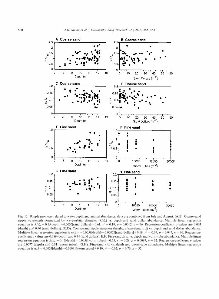
Fig. 12. Ripple geometry related to water depth and animal abundance; data are combined from July and August. (A,B). Coarse-sand

ripple wavelength normalized by wave-orbital diameter (l=do) vs. depth and sand dollar abundance. Multiple linear regression

equation is l=do ¼ 0:15[depth]+0.0035[sand dollars]F0.61, r2 ¼ 0:19; p ¼ 0:0012; n ¼ 66: Regression-coefficient p values are 0.003

(depth) and 0.40 (sand dollars). (C,D). Coarse-sand ripple steepness (height, Z=wavelength, l) vs. depth and sand dollar abundance.

Multiple linear regression equation is Z=l ¼ �0:0058[depth]F0.00027[sand dollars]+0.19, r2 ¼ 0:09; p ¼ 0:047; n ¼ 66: Regression-coefficient p values are 0.089 (depth) and 0.34 (sand dollars). E,F. Fine-sand l=do vs. depth and worm-tube abundance. Multiple linear

regression equation is l=do ¼ 0:13[depth]F0.0058[worm tubes]F0.65, r2 ¼ 0:28; p ¼ 0:0089; n ¼ 32: Regression-coefficient p valuesare 0.0077 (depth) and 0.81 (worm tubes). (G,H). Fine-sand Z=l vs. depth and worm-tube abundance. Multiple linear regression

equation is Z=l ¼ 0:0024[depth]F0.00091[worm tubes]+0.10, r2 ¼ 0:02; p ¼ 0:76; n ¼ 32:

J.D. Sisson et al. / Continental Shelf Research 22 (2002) 565–583580

Surface-dwelling animals rework ripples duringtheir feeding and burrowing activities, thuschanging ripple geometries over space and time.A large sediment-transport event would, however,interrupt this biological process, resetting thebioturbation clock.In the multiple-regression analysis, there was no

support for the hypothesis that spatial patterns inbedform geometry were related to animal (sanddollar or tubeworm) densities (Fig. 12). However,at least some of the ripplesFespecially in coarsesandFwere not in equilibrium with wave condi-tions at the time of the surveys. Their wavelengthswere longer and steepness smaller than calculatedfrom wave-orbital diameters (Figs. 8 and 12),indicating that they were not produced by thelocal wave field but from prior forcing. Further-more, the direct relationships between ripplewavelength and water depth (Fig. 12) are consis-tent with the presence of more relicts at depth, apattern rarely reported (e.g., Komar, 1974), buteasily explained. As depth increases, wave energydecreases and less wave stress impacts the bed.Relicts from strong storms thus can persist longerat greater depth, because subsequent events ofsmaller waves only rework ripples at shallowerdepth. Therefore, l=do increases with increasingdepth, reflecting forcing from an earlier maximumin wave energy. This direct relationship betweenl=do and depth is contrary to what one mightexpect from linear wave theory, which predictsdecreasing orbital diameter in deeper water. Thus,the increase of l=do at depth is most likelyexplained by relict ripples. Likewise, Z=l decreaseswith increasing depth, due to collapse of relictripple crests over time.Evidence for relict ripples suggests that sand

dollars could have had at least a month to reworkthe ripple fields since storm waves had physicallyaltered the bed. This species of sand dollar iscertainly capable of reworking surficial sands. Itburrows just below the sand surface and feeds onbenthic diatoms, using tube feet on its upper(aboral) surface to transport particles toward itsmouth underneath (Ghiold, 1983). Laboratoryflume studies indicate that the speed of sand dollarlocomotion through surficial sands is a function ofthe near-bed flow/sediment-transport-regime (J.D.

Sisson, C.A. Zimmer and R.K. Zimmer, unpubl.data), although the level of sand dollar activity atthe field site was not measured in this study.E. parma densities observed in this study were as

low as 1/8 of the maximal values (up to 400m�2)reported for sandy subtidal North Pacific andNorth Atlantic areas (Sokolova and Kuznetsov,1960; Harold and Telford, 1982). For an average5-cm-diameter sand dollar, this maximal densitywould cover about 80% of the sediment surface,whereas a density of 55m�2 (this study) wouldcover only about 10%. At this low areal coverage,bioturbation by E. parma evidently was notsufficient to affect ripple geometry in a patternthat could be detected by our statisticalanalyses. A significant bioturbation effect wouldnot be detected, for example, if sand dollarsmodify ripple geometry, but the effect is density-independent below some threshold value. Suchanalyses were outside the scope of this proof-of-concept study.Nonetheless, there is great potential for

E. parma to affect significantly bed topography.For example, on the Nova Scotian shelf, Stanleyand James (1971) determined that bioturbation byE. parma in densities reaching 185m�2 at 50-mdepth was the second most important factor, aftercurrents, in modifying surficial sediment cover. Inthe Gulf of Mexico, Salsman and Tolbert (1965)observed at 7-m depth that sand dollars of thespeciesMellita quinquiesperforata in densities of upto 821m�2 leveled a field of 6–10 cm high ripples ina single night. In this study, we surveyed but asmall fraction of the shallow subtidal off of thesouth shore of Martha’s Vineyard (Fig. 3A). Moreextensive surveys may reveal denser populations ofE. parma than reported here, and that can, in fact,alter sediment transport in a predictable andmeaningful way.Like for sand dollars, spatial patterns in bed-

form geometry and tubeworm density were notstatistically significant. Tube worms at highdensity, however, are known to stabilize the bedagainst erosion by facilitating microbial growth orinducing skimming flow (Eckman, 1985; Frie-drichs et al., 2000). Such stabilization would allowthe persistence of relict ripples under conditionsfor which they would otherwise breakdown, and

J.D. Sisson et al. / Continental Shelf Research 22 (2002) 565–583 581

require stronger waves to initiate new rippleformation. Densities of the tubeworm S. bombyxobserved here correspond to a maximal arealcoverage of 9.4%. Although the numerical densityof 30,000m�2 is not particularly high (cf. Daroand Polk, 1973; Friedrichs et al., 2000), bedstabilization due to skimming flow has beenreported for areal coverage as low as 8.8%in artificial tube arrays (Friedrichs et al,2000). Moreover, Featherstone and Risk (1977)found that an areal coverage of only0.3% prevented ripple formation in intertidalsands.Mapping benthic assemblages together with

sedimentary features provides comprehensive datasets for coastal benthic biologists and sedimentol-ogists. Such information on spatial pattern allowshypotheses to be developed regarding mechanismsresponsible for field observations, and thesehypotheses can be tested subsequently via labora-tory or field experiments. In the very energetic,shallow, subtidal sands of exposed open coasts,ecological research has been limited by the lack ofa survey technique with appropriate resolutionand areal coverage. Mapping by divers, usingacoustic positioning, can begin to fill this criticalvoid.

Acknowledgements

We thank A. Frese, V. Starczak, andN. Trowbridge for assistance in the field and lab,and an anonymous reviewer for helpful commentson the manuscript. This work was supported byONR contract N00014-96-0946 to C.A. Zimmerand a WHOI Postdoctoral Scholarship, NSF grantOCE-9711441, and a grant from F&M College toJ. Shimeta. This is WHOI contribution number9755.

References

Aronson, R.B., 1989. Brittlestar beds: low-predation anachron-

isms in the British Isles. Ecology 70, 856–865.

Benedetti-Cecchi, L., Airoldi, L., Abbiati, L., Cinelli, F., 1996.

Estimating the abundance of benthic invertebrates: a

comparison of procedures and variability between obser-

vers. Marine Ecology Progress Series 138, 93–101.

Butman, C.A., 1987. Larval settlement of soft-sediment

invertebrates: the spatial scales of pattern explained by

active habitat selection and the emerging role of hydro-

dynamical processes. Oceanography and Marine Biology:

an Annual Review 25, 113–165.

Cacchione, D.A., Drake, D.E., 1990. Shelf sediment transport:

an overview with applications to the northern california

continental shelf. In: Le M!ehaut!e, B., Hanes, D.M. (Eds.),

The Sea, Vol. 9, Part B. Wiley-Interscience, New York,

pp. 729–773.

Christiansen, B., Nuppenau, V., 1997. The IHF Fototrawl:

experiences with a television-controlled, deep-sea epibenthic

sledge. Deep-Sea Research 44, 533–540.

Daro, M.H., Polk, P., 1973. The autecology of Polydora ciliata

along the Belgian Coast. Netherlands Journal of Sea

Research 6, 130–140.

Downing, J.A., Anderson, M.R., 1985. Estimating the standing

biomass of aquatic macrophytes. Canadian Journal of

Fisheries and Aquatic Sciences 42, 1860–1869.

Eckman, J.E., 1985. Flow disruption by an animal-tube mimic

affects sediment bacterial colonization. Journal of Marine

Research 43, 419–435.

Eckman, J.E., Duggins, D.O., Sewell, A.T., 1989. Ecology of

understory kelp environments. I. Effects of kelps on flow

and particle transport near the bottom. Journal of Experi-

mental Marine Biology and Ecology 129, 173–187.

Eckman, J.E., Nowell, A.R.M., 1984. Boundary skin friction

and sediment transport about an animal-tube mimic.

Sedimentology 31, 851–862.

Eckman, J.E., Nowell, A.R.M., Jumars, P.A., 1981. Sediment

destabilization by animal tubes. Journal of Marine Research

39, 361–374.

Evenden, G.I., 1995. Cartographic projection procedures for

the UNIX environmentFa user’s manual. United States

Geological Survey Open-File Report 90-284.

Featherstone, R.P., Risk, M.J., 1977. Effect of tube-building

polychaetes on intertidal sediments of the Minas Basin, Bay

of Fundy. Journal of Sedimentary Petrology 47, 446–450.

Friedrichs, M., Graf, G., Springer, B., 2000. Skimming flow

induced over a simulated polychaete tube lawn at low

population densities. Marine Ecology Progress Series 192,

219–228.

Fries, J.S., Butman, C.A., Wheatcroft, R.A., 1999. Ripple

formation induced by biogenic mounds. Marine Geology

159, 287–302.

Fuller, C.M., Butman, C.A., 1988. A simple technique for fine-

scale, vertical sectioning of fresh sediment cores. Journal of

Sedimentary Petrology 58, 763–768.

Ghiold, J., 1983. The role of external appendages in the

distribution and life habits of the sand dollar Echinarachnius

parma (Echinodermata: Echinoidea). Journal of Zoology

(London) 200, 405–419.

Grant, J., 1983. The relative magnitude of biological and

physical sediment reworking in an intertidal community.

Journal of Marine Research 41, 673–689.

J.D. Sisson et al. / Continental Shelf Research 22 (2002) 565–583582

Grant, J., Bathmann, U.V., Mills, E.L., 1986. The interaction

between benthic diatom films and sediment transport.

Estuarine, Coastal, and Shelf Science 23, 225–238.

Grant, J., Gust, G., 1987. Prediction of coastal sediment

stability from photopigment content of mats of purple

sulphur bacteria. Nature 330, 244–246.

Grant, W.D., Boyer, L., Sanford, L.P., 1982. The effects of

bioturbation on the initiation of motion of intertidal sands.

Journal of Marine Research 40, 659–677.

Grant, W.D., Madsen, O.S., 1986. The continental-shelf

bottom boundary layer. Annual Review of Fluid Mechanics

18, 265–305.

Harold, A.S., Telford, M., 1982. Substrate preference and

distribution of the northern sand dollar, Echinarachnius

parma (Lamarck). In: Lawrence, J.M. (Ed.), International

Echinoderms Conference, Tampa Bay. A.A. Balkema,

Rotterdam, pp. 243–249.

Hughes, J.E., 1996. Size-dependent, small-scale dispersion of

the capitellid polychaete,Mediomastus ambiseta. Journal of

Marine Research 54, 915–937.

Irlandi, E.A., 1996. The effects of seagrass patch size and energy

regime on growth of a suspension-feeding bivalve. Journal

of Marine Research 54, 161–185.

Jumars, P.A., 1975. Environmental grain and polychaete

species’ diversity in a bathyal benthic community. Marine

Biology 30, 253–266.

Jumars, P.A., Jackson, D.R., Gross, T.F., Sherwood, C., 1996.

Acoustic remote sensing of benthic activity: a statistical

approach. Limnology and Oceanography 41, 220–1241.

Komar, P.D., 1974. Oscillatory ripple marks and the evaluation

of ancient wave conditions and environments. Journal of

Sedimentary Petrology 44, 169–180.

Luyten, J.R., Needell, G., Thomson, J., 1982. An acoustic

dropsondeFdesign, performance and evaluation. Deep-Sea

Research 29, 499–524.

MacKenzie, K.V., 1981. Nine-term equation for sound speed in

the ocean. Journal of the Acoustical Society of America 70,

807–812.

McCartney, B.S., 1981. Underwater acoustic positioning

systems: state of the art and applications in deep water.

International Hydrographic Review 58, 91–113.

Mercer, J.A., 1986. Acoustic tomography by remote sensing.

IEEE Journal of Oceanic Engineering 11, 51–57.

Miller, D.C., Sternberg, R.W., 1988. Field measurements of the

fluid and sediment-dynamic environment of a benthic

deposit feeder. Journal of Marine Research 46, 771–796.

Mumby, P.J., Green, E.P., Edwards, A.J., Clark, C.D., 1997.

Coral reef habitat-mapping: how much detail can remote

sensing provide? Marine Biology 130, 193–202.

Nowell, A.R.M., 1983. The benthic boundary layer and

sediment transport. Reviews of Geophysics and Space

Physics 21, 1181–1192.

Nowell, A.R.M., Jumars, P.A., Eckman, J.E., 1981. Effects of

biological activity on the entrainment of marine sediments.

Marine Geology 42, 133–153.

Olafsson, E.B., Peterson, C.H., Ambrose Jr., W.G., 1994. Does

recruitment limitation structure populations and commu-

nities of macroinvertebrates in marine soft sediments: the

relative significance of pre- and post-settlement processes.

Oceanography and Marine Biology Annual Review 32,

65–109.

Peterson, C.H., Summerson, H.C., Duncan, P.B., 1984. The

influence of seagrass cover on population structure and

individual growth rate of a suspension-feeding bivalve,

Mercenaria mercenaria. Journal of Marine Research 42,

123–138.

Rampino, M.R., Sanders, J.E., 1980. Holocene transgression in

south-central Long Island, New York. Journal of Sedimen-

tary Petrology 50, 1063–1080.

Redfield, A.C., Rubin, M., 1962. The age of salt marsh peat and

its relation to recent changes in sea level at barnstable,

massachusetts. Proceedings of the National Academy of

Sciences (USA) 48, 1728–1735.

Rhoads, D.C., Young, D.K., 1971. Animal-sediment relations

in cape cod bay, Massachusetts. II. Reworking byMolpadia

oolitica (Holothuroidea). Marine Biology 11, 255–261.

Salsman, G.G., Tolbert, W.H., 1965. Observations on the sand

dollar, Mellita quinquiesperforata. Limnology and Oceano-

graphy 10, 152–155.

Snelgrove, P.V.R., Butman, C.A., 1994. Animal–sediment

relationships revisited: cause versus effect. Oceanography

and Marine Biology Annual Review 32, 111–177.

Sokolova, M.N., Kuznetsov, A.P., 1960. On the feeding

character and on the role played by trophic factor in the

distribution of the hedgehog Echinarachnius parma lam.

Zoologicheskii Zhurnal 39, 1253–1256.

Sotheran, I.S., Foster-Smith, R.L., Davies, J., 1997. Mapping

of marine benthic habitats using image processing techni-

ques with a raster-based geographic information system.

Estuarine, Coastal, and Shelf Science 44 (Suppl A), 25–31.

Spindel, R.C., Porter, R.P., Marquet, W.M., Durham, J.L.,

1976. A high-resolution pulse-doppler underwater acoustic

navigation system. IEEE Journal of Oceanic Engineering 1,

6–13.

Stanley, D.J., James, N.P., 1971. Distribution of Echinarachnius

parma (Lamarck) and associated fauna on Sable Island

Bank, Southeast Canada. Smithsonian Contributions to

Earth Sciences 6, 1–24.

Traykovski, P., Hay, A.E., Irish, J.D., Lynch, J.F., 1999.

Geometry, migration, and evolution of wave orbital

ripples at LEO-15. Journal of Geophysical Research 104,

1505–1524.

Wheatcroft, R.A., Butman, C.A., 1997. Spatial and temporal

variability in aggregated grain-size distributions with

implications for sediment dynamics. Continental Shelf

Research 17, 367–390.

Wiberg, P.L., Harris, C.K., 1994. Ripple geometry in wave-

dominated environments. Journal of Geophysical Research

99, 775–789.

Zettler, M.L., Bick, A., 1996. The analysis of small- and

mesoscale dispersion patterns of Marenzelleria viridis

(Polychaeta: Spionidae) in a coastal water area of the

southern Baltic. Helgolander Meeresuntersuchungen 50,

265–286.

J.D. Sisson et al. / Continental Shelf Research 22 (2002) 565–583 583