Remote Sens. 2015, 7, 1048-1073; doi:10.3390/rs70101048 remote sensing ISSN 2072-4292 www.mdpi.com/journal/remotesensing Article Mapping Deciduous Rubber Plantation Areas and Stand Ages with PALSAR and Landsat Images Weili Kou 1,2,3 , Xiangming Xiao 3,4, *, Jinwei Dong 3 , Shu Gan 2 , Deli Zhai 5,6 , Geli Zhang 3 , Yuanwei Qin 3 and Li Li 7 1 School of Computer Science and Information, Southwest Forestry University, Kunming 650224, China; 2 Faculty of Land Resource Engineering, Kunming University of Science and Technology, Kunming 650093, China; E-Mail: [email protected] 3 Department of Microbiology and Plant Biology, and Center for Spatial Analysis, University of Oklahoma, Norman, OK 73019, USA; E-Mails: [email protected] (W.K.); [email protected] (J.D.); [email protected] (G.Z.); [email protected] (Y.Q.) 4 Institute of Biodiversity Science, Fudan University, Shanghai 200433, China 5 Centre for Mountain Ecosystem Studies (CMES), Kunming Institute of Botany (CAS), Lanhei Road132,Heilongtan, Kunming 650201, China; E-Mail: [email protected] 6 World Agroforestry Centre (ICRAF), Central and East Asia Office, Lanhei Road132, Heilongtan, Kunming 650201, China 7 College of Information & Electrical Engineering, China Agricultural University, Beijing 100083, China; E-Mail: [email protected] * Author to whom correspondence should be addressed; E-Mail: [email protected]; Tel.: +1-405-325-8941; Fax: +1-405-325-3442. Academic Editors: Nicolas Baghdadi and Prasad S. Thenkabail Received: 10 September 2014 / Accepted: 12 January 2015 / Published: 19 January 2015 Abstract: Accurate and updated finer resolution maps of rubber plantations and stand ages are needed to understand and assess the impacts of rubber plantations on regional ecosystem processes. This study presented a simple method for mapping rubber plantation areas and their stand ages by integration of PALSAR 50-m mosaic images and multi-temporal Landsat TM/ETM+ images. The L-band PALSAR 50-m mosaic images were used to map forests (including both natural forests and rubber trees) and non-forests. For those PALSAR-based forest pixels, we analyzed the multi-temporal Landsat TM/ETM+ images from 2000 to 2009. We first studied phenological signatures of deciduous rubber plantations (defoliation and foliation) and natural forests through analysis of surface reflectance, Normal Difference OPEN ACCESS

Welcome message from author
This document is posted to help you gain knowledge. Please leave a comment to let me know what you think about it! Share it to your friends and learn new things together.
Transcript
Remote Sens. 2015, 7, 1048-1073; doi:10.3390/rs70101048
remote sensing ISSN 2072-4292
www.mdpi.com/journal/remotesensing
Article
Mapping Deciduous Rubber Plantation Areas and Stand Ages with PALSAR and Landsat Images
Weili Kou 1,2,3, Xiangming Xiao 3,4,*, Jinwei Dong 3, Shu Gan 2, Deli Zhai 5,6, Geli Zhang 3,
Yuanwei Qin 3 and Li Li 7
1 School of Computer Science and Information, Southwest Forestry University, Kunming 650224, China; 2 Faculty of Land Resource Engineering, Kunming University of Science and Technology,
Kunming 650093, China; E-Mail: [email protected] 3 Department of Microbiology and Plant Biology, and Center for Spatial Analysis, University of
Oklahoma, Norman, OK 73019, USA; E-Mails: [email protected] (W.K.); [email protected] (J.D.);
[email protected] (G.Z.); [email protected] (Y.Q.) 4 Institute of Biodiversity Science, Fudan University, Shanghai 200433, China 5 Centre for Mountain Ecosystem Studies (CMES), Kunming Institute of Botany (CAS), Lanhei
Road132,Heilongtan, Kunming 650201, China; E-Mail: [email protected]
6 World Agroforestry Centre (ICRAF), Central and East Asia Office, Lanhei Road132, Heilongtan,
Kunming 650201, China 7 College of Information & Electrical Engineering, China Agricultural University, Beijing 100083, China;
E-Mail: [email protected]
* Author to whom correspondence should be addressed; E-Mail: [email protected];
Tel.: +1-405-325-8941; Fax: +1-405-325-3442.
Academic Editors: Nicolas Baghdadi and Prasad S. Thenkabail
Received: 10 September 2014 / Accepted: 12 January 2015 / Published: 19 January 2015
Abstract: Accurate and updated finer resolution maps of rubber plantations and stand ages
are needed to understand and assess the impacts of rubber plantations on regional ecosystem
processes. This study presented a simple method for mapping rubber plantation areas and
their stand ages by integration of PALSAR 50-m mosaic images and multi-temporal Landsat
TM/ETM+ images. The L-band PALSAR 50-m mosaic images were used to map forests
(including both natural forests and rubber trees) and non-forests. For those PALSAR-based
forest pixels, we analyzed the multi-temporal Landsat TM/ETM+ images from 2000 to 2009.
We first studied phenological signatures of deciduous rubber plantations (defoliation and
foliation) and natural forests through analysis of surface reflectance, Normal Difference
OPEN ACCESS
Remote Sens. 2015, 7 1049
Vegetation Index (NDVI), Enhanced Vegetation Index (EVI), and Land Surface Water Index
(LSWI) and generated a map of rubber plantations in 2009. We then analyzed phenological
signatures of rubber plantations with different stand ages and generated a map, in 2009, of
rubber plantation stand ages (≤5, 6–10, >10 years-old) based on multi-temporal Landsat
images. The resultant maps clearly illustrated how rubber plantations have expanded into the
mountains in the study area over the years. The results in this study demonstrate the potential
of integrating microwave (e.g., PALSAR) and optical remote sensing in the characterization
of rubber plantations and their expansion over time.
Keywords: stand age; rubber plantations; phenology; Xishuangbanna; Landsat; PALSAR
1. Introduction
As economies and industries develop, the need for natural rubber products has been increasing over
time, which has led to substantial and continuous expansions of rubber plantations around the world.
The Food and Agriculture Organization of the United Nations (FAO) reported a twenty percent
expansion of global rubber plantations in the past two decades, and 90% of the expansion is in Asia [1],
mainly distributed in Indonesia, Thailand, Malaysia, and China. Rubber trees were first successfully planted
in Southern China in the 1950s, and then expanded from their original planting places (10° N–10° S) to areas
as far north as 22° N, including Hainan and Yunnan provinces, China [2]. The expansion mainly occurred
at the expense of natural forests and shifting agriculture [3,4]. Now Southern China has been a hotspot
for northward-expansion of rubber plantations. The dramatic expansion may negatively impact forest
carbon stocks and biodiversity [3–6]. Accurate and updated maps of rubber plantation cover areas and
their stand ages are needed to quantify Land Use Land Cover Changes (LULCC) and assess its impacts
on biodiversity, carbon sinks, and water cycles in the tropical forest areas.
Satellite remote sensing technology has played a vital role to map rubber plantation cover at local and
regional scales [7–9]. Previous studies can be generally divided into three groups based on sensor types:
optical sensors, microwave or radar sensors, and integration of optical and radar sensors. A few studies
used images from optical sensors (MODIS, Landsat and ASTER) and calculated image statistics and
classified images to map rubber plantations in Southeast Asia [7,10,11]. As cloud cover occurs frequently
in the moist tropical areas, high temporal resolution image data (e.g., MODIS) make it possible to obtain
some cloud-free observations. Based on the temporal analysis of MODIS data, Senf et al. (2013) and
Liu et al. (2013) mapped the rubber plantations in Xishuangbanna, Yunnan Province, China. Because of
its coarse spatial resolutions (250–500 m), it is difficult to identify and map small patches of rubber
plantations using MODIS images. Tropical regions lack high-resolution, satellite-based maps of their forests
due to persistent cloud cover [12–14]. Clouds on optical images obscure the dense humid tropical forest over
70% of the time [15], hence optical images are constrained to use for monitoring forests [12–14,16].
Synthetic aperture radar (SAR) can penetrate clouds, haze and dust, and provide cloud-free images
for mapping forests in moist tropical regions, where frequent cloud cover makes it difficult to acquire
cloud-free optical images from those optical sensors with long revisit cycles (e.g., 16-day revisit cycle
from Landsat). Radar images from long wavelength sensors (e.g., L-band SAR) are also capable of

Remote Sens. 2015, 7 1050
penetrating tree canopies [17] and are sensitive to forest structure and the moisture content of the forest
canopy. The Phased Arrayed L-band Synthetic Aperture Radar (PALSAR) from Japan Aerospace
Exploration Agency (JAXA) provided multi-year cloud-free images (2006–2010) for the global land
surface, and several studies have used multiple polarization images (HH, HV, VH, VV) to map forests
at local scale in tropical regions [14,15,18,19]. Based on the backscatter coefficient values (HH, HV) of
PALSAR orthorectified mosaic data, forest cover maps at 50-m spatial resolution were developed at
regional and global scales [18,20,21]. However, these PALSAR-based forest cover maps do not
differentiate between evergreen forests and deciduous forests (e.g., rubber plantations). Rubber trees in
Southern China often have a defoliation phase (leaf-off) and foliation phase (leaf-on, new leaf
emergence) during the relatively cold and dry winters [22,23]. Combining these phenological features,
rubber plantations can be identified from natural forest based on a PALSAR-based forest map [23].
In an effort to take full advantage of both optical and radar data, several recent studies combined radar
and multi-temporal optical data to map tropical forests [24] and rubber plantations [25]. For example,
the PALSAR images in 2009 were first used to generate a forest cover map, and the resultant forest
cover map in 2009 was combined with the phenology information (defoliation and foliation phases) from
multi-temporal MODIS images [25] and Landsat images [23] to map rubber plantations in Hainan Island,
China, which has the largest area of rubber plantations in China. The multi-temporal MODIS and
Landsat images from 2009 provide information on whether a forest pixel experienced a defoliation
and/or foliation phase (timing and duration). The pilot study area in Hainan Island, China is located in
areas with relatively simple and flat topography. But in our study area, rubber plantations are cultivated
in mountains. The complex topography and climate in the mountainous regions pose challenges for the
characterization and mapping of rubber plantations.
When trying to compare mapping methods of rubber plantations, few references were found that
attempted to retrieve stand age by remote sensing technology [26]. It is well known that stand ages of
forests are important in many research fields such as monitoring and management of forest ecosystems,
carbon flux estimates, and biomass estimates [27–33]. At present, stand ages of plantation forests are
mainly retrieved from field surveys and historical planting records of local forestry bureaus [34,35].
Field surveys are always limited by transportation conditions and complex montane topography, as well
as human and financial resources [35]. Additionally, updated stand age map cannot be made available
regularly because field surveys are time-consuming work. Fortunately, long-term free Landsat data
provide an opportunity to trace rubber plantation planting stages and identify their stand ages. Until now,
there have been no efficient ways to identify rubber plantation stand ages in Xishuangbanna at fine
spatial resolutions. Therefore, there is a need to develop an algorithm that can establish stand ages of
rubber plantations in a rapid and repeatable way for dynamically monitoring rubber plantations.
This study aimed to address the above-mentioned challenges in mapping rubber plantation areas and
their stand ages in topographically complex settings. The specific objectives of this study are threefold:
(1) generate a forest cover map using PALSAR images from 2009 at 50-m spatial resolution; (2) generate a
map of rubber plantations in 2009 at 30-m spatial resolution, based on the PALSAR-forest map and
phenological analysis of Landsat images in 2009; and (3) to generate a stand age map of rubber
plantations with a 30-m spatial resolution (≤5, 6–10, and >10 years old). This pilot study will contribute
to evaluate the integrated approach used in Hainan Island [23] and use both PALSAR images from 2009
and time series Landsat data (2000–2012). The study area is located in Jinghong City of Xishuangbanna
Remote Sens. 2015, 7 1051
Dai Nationality Autonomous Prefecture, China, where there are good-quality Landsat images and
extensive rubber plantations.
2. Materials and Methods
2.1. Study Area
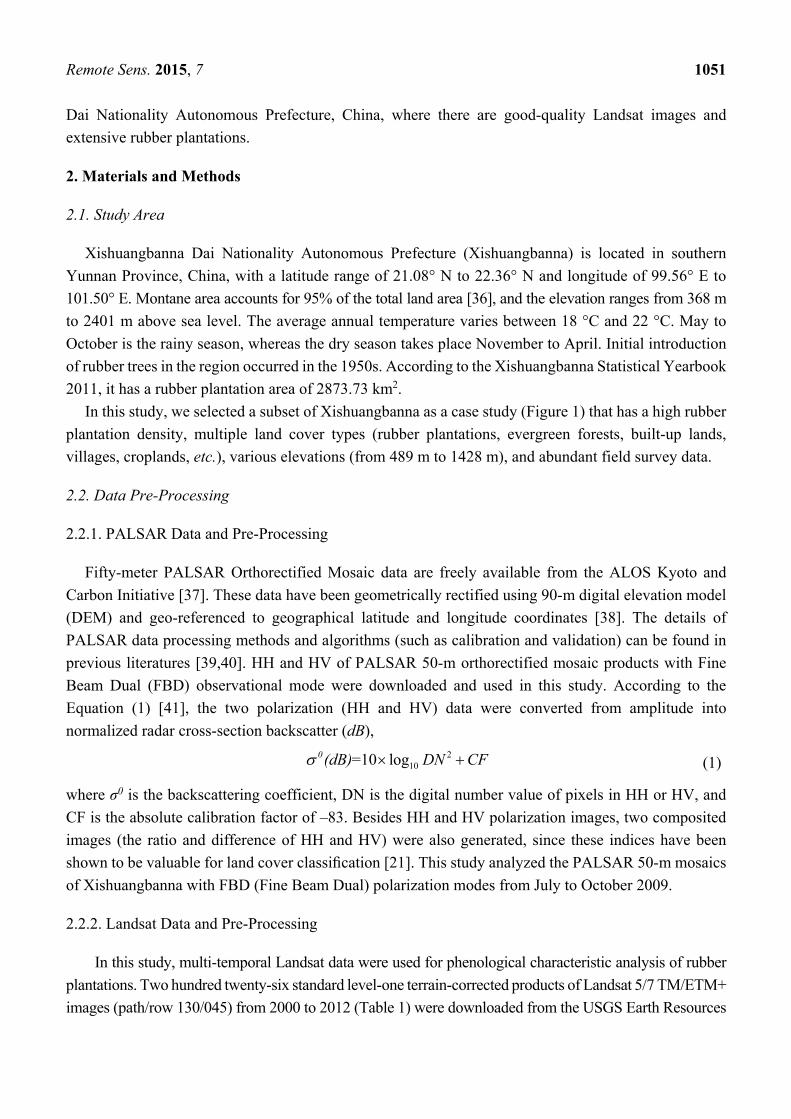
Xishuangbanna Dai Nationality Autonomous Prefecture (Xishuangbanna) is located in southern
Yunnan Province, China, with a latitude range of 21.08° N to 22.36° N and longitude of 99.56° E to
101.50° E. Montane area accounts for 95% of the total land area [36], and the elevation ranges from 368 m
to 2401 m above sea level. The average annual temperature varies between 18 °C and 22 °C. May to
October is the rainy season, whereas the dry season takes place November to April. Initial introduction
of rubber trees in the region occurred in the 1950s. According to the Xishuangbanna Statistical Yearbook
2011, it has a rubber plantation area of 2873.73 km2.
In this study, we selected a subset of Xishuangbanna as a case study (Figure 1) that has a high rubber
plantation density, multiple land cover types (rubber plantations, evergreen forests, built-up lands,
villages, croplands, etc.), various elevations (from 489 m to 1428 m), and abundant field survey data.
2.2. Data Pre-Processing
2.2.1. PALSAR Data and Pre-Processing
Fifty-meter PALSAR Orthorectified Mosaic data are freely available from the ALOS Kyoto and
Carbon Initiative [37]. These data have been geometrically rectified using 90-m digital elevation model
(DEM) and geo-referenced to geographical latitude and longitude coordinates [38]. The details of
PALSAR data processing methods and algorithms (such as calibration and validation) can be found in
previous literatures [39,40]. HH and HV of PALSAR 50-m orthorectified mosaic products with Fine
Beam Dual (FBD) observational mode were downloaded and used in this study. According to the
Equation (1) [41], the two polarization (HH and HV) data were converted from amplitude into
normalized radar cross-section backscatter (dB), 2
10=10 log0(dB) DN CF (1)
where σ0 is the backscattering coefficient, DN is the digital number value of pixels in HH or HV, and
CF is the absolute calibration factor of –83. Besides HH and HV polarization images, two composited
images (the ratio and difference of HH and HV) were also generated, since these indices have been
shown to be valuable for land cover classification [21]. This study analyzed the PALSAR 50-m mosaics
of Xishuangbanna with FBD (Fine Beam Dual) polarization modes from July to October 2009.
2.2.2. Landsat Data and Pre-Processing
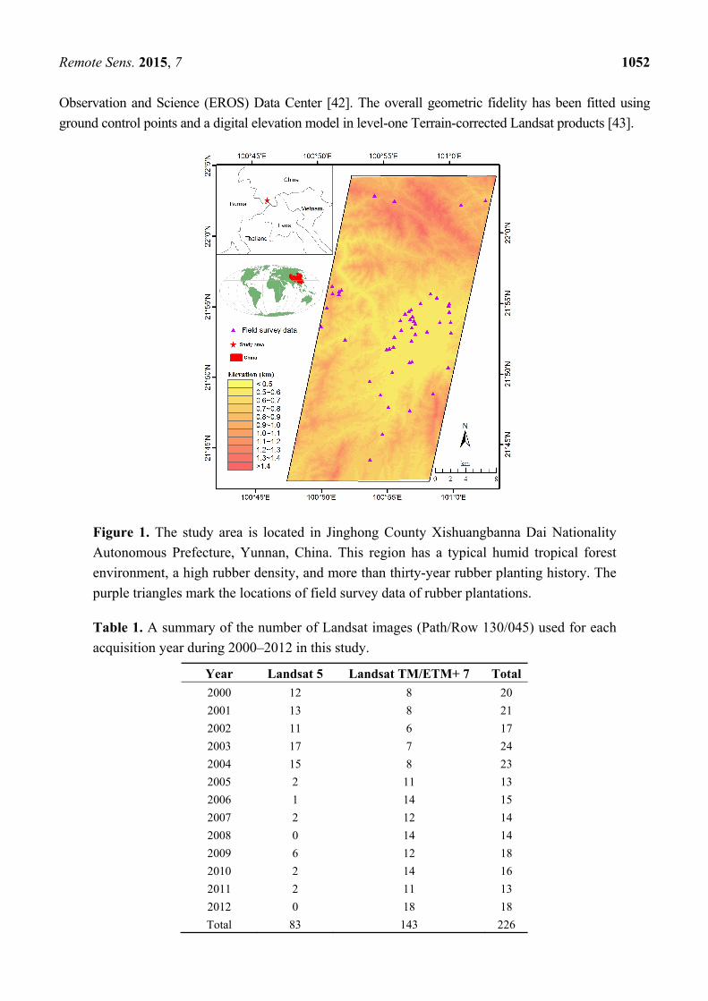
In this study, multi-temporal Landsat data were used for phenological characteristic analysis of rubber
plantations. Two hundred twenty-six standard level-one terrain-corrected products of Landsat 5/7 TM/ETM+
images (path/row 130/045) from 2000 to 2012 (Table 1) were downloaded from the USGS Earth Resources
Remote Sens. 2015, 7 1052
Observation and Science (EROS) Data Center [42]. The overall geometric fidelity has been fitted using
ground control points and a digital elevation model in level-one Terrain-corrected Landsat products [43].
Figure 1. The study area is located in Jinghong County Xishuangbanna Dai Nationality
Autonomous Prefecture, Yunnan, China. This region has a typical humid tropical forest
environment, a high rubber density, and more than thirty-year rubber planting history. The
purple triangles mark the locations of field survey data of rubber plantations.
Table 1. A summary of the number of Landsat images (Path/Row 130/045) used for each
acquisition year during 2000–2012 in this study.
Year Landsat 5 Landsat TM/ETM+ 7 Total
2000 12 8 20
2001 13 8 21
2002 11 6 17
2003 17 7 24
2004 15 8 23
2005 2 11 13
2006 1 14 15
2007 2 12 14
2008 0 14 14
2009 6 12 18
2010 2 14 16
2011 2 11 13
2012 0 18 18
Total 83 143 226
Remote Sens. 2015, 7 1053
(1) Atmospheric correction
The Landsat Ecosystem Disturbance Adaptive Processing System (LEDAPS) uses the 6S radiative
transfer approach to conduct atmospheric correction and retrieve surface reflectance of Landsat
images [44,45]. Following previous studies [23,46], here, we also employed LEDAPS to conduct
atmospheric correction and retrieve surface reflectance from 226 Landsat images.
(2) Clouds, cloud shadows, and SLC-Off gaps
In tropical and subtropical regions, clouds are major barriers for analysis of optical satellite data [16].
Fmask is a free software for automated processing of clouds, cloud shadows, and snow for Landsat 4, 5,
7 and 8 images [47]. We used Fmask to identify and map clouds and cloud shadows on Landsat
TM/ETM+ imagery.
Landsat 7 images acquired after 31 May 2003 have strips of missing data, as the Scan Line Corrector
(SLC), which compensates for the forward motion of Landsat 7, failed. There are no data for these SLC-off
gaps and blank margins. The gaps and blank margins of images were marked with flags. This study used
the minimum of all images in the defoliation phrase to generate a composite map, which almost have no
gap in observations. So gap-fill was not further conducted.
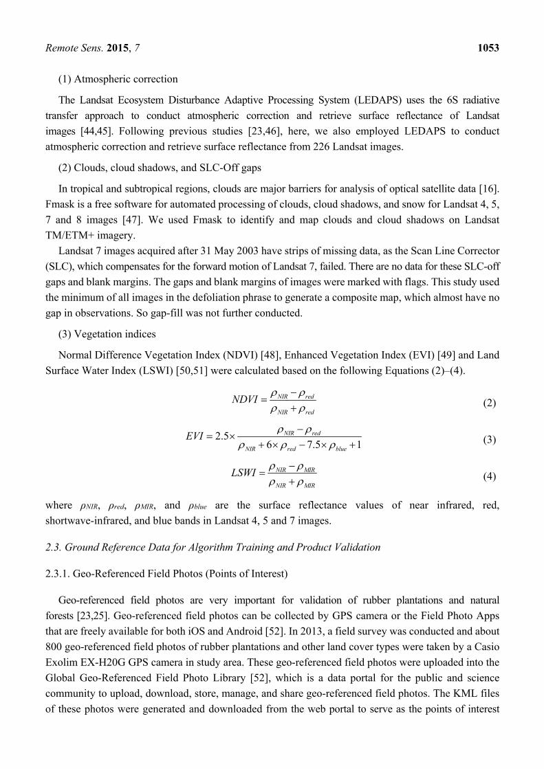
(3) Vegetation indices
Normal Difference Vegetation Index (NDVI) [48], Enhanced Vegetation Index (EVI) [49] and Land
Surface Water Index (LSWI) [50,51] were calculated based on the following Equations (2)–(4).
where ρNIR, ρred, ρMIR, and ρblue are the surface reflectance values of near infrared, red,
shortwave-infrared, and blue bands in Landsat 4, 5 and 7 images.
2.3. Ground Reference Data for Algorithm Training and Product Validation
2.3.1. Geo-Referenced Field Photos (Points of Interest)
Geo-referenced field photos are very important for validation of rubber plantations and natural
forests [23,25]. Geo-referenced field photos can be collected by GPS camera or the Field Photo Apps
that are freely available for both iOS and Android [52]. In 2013, a field survey was conducted and about
800 geo-referenced field photos of rubber plantations and other land cover types were taken by a Casio
Exolim EX-H20G GPS camera in study area. These geo-referenced field photos were uploaded into the
Global Geo-Referenced Field Photo Library [52], which is a data portal for the public and science
community to upload, download, store, manage, and share geo-referenced field photos. The KML files
of these photos were generated and downloaded from the web portal to serve as the points of interest
NIR red
NIR red
NDVI
(2)
2.56 7.5 1
NIR red
NIR red blue
EVI
(3)
NIR MIR
NIR MIR
LSWI
(4)
Remote Sens. 2015, 7 1054
(POIs) in this study. We also obtained stand age information from 49 rubber plantation sites through
interviews with workers in the plantation fields. Although this study used Landsat and PALSAR imagery
from 2009 for mapping rubber plantations, ground truth data from 2013 are suitable as rubber trees grow
for many years with consistent seasonal phenology.
2.3.2. Regions of Interest (ROIs) for Algorithm Training and Product Validation
Google Earth images with high-resolution have good geo-metric accuracy and finer spatial
resolution (e.g., 0.61-m QUCKBIRD images) and were used to validate the results of land cover
classifications [46,53–57] and maps of forests and rubber plantations [21,23,25]. In this study, ROIs
(Table 2) for result validating and algorithm training (Figure 2) are from two sources: Google Earth
high-resolution imagery and field survey data.
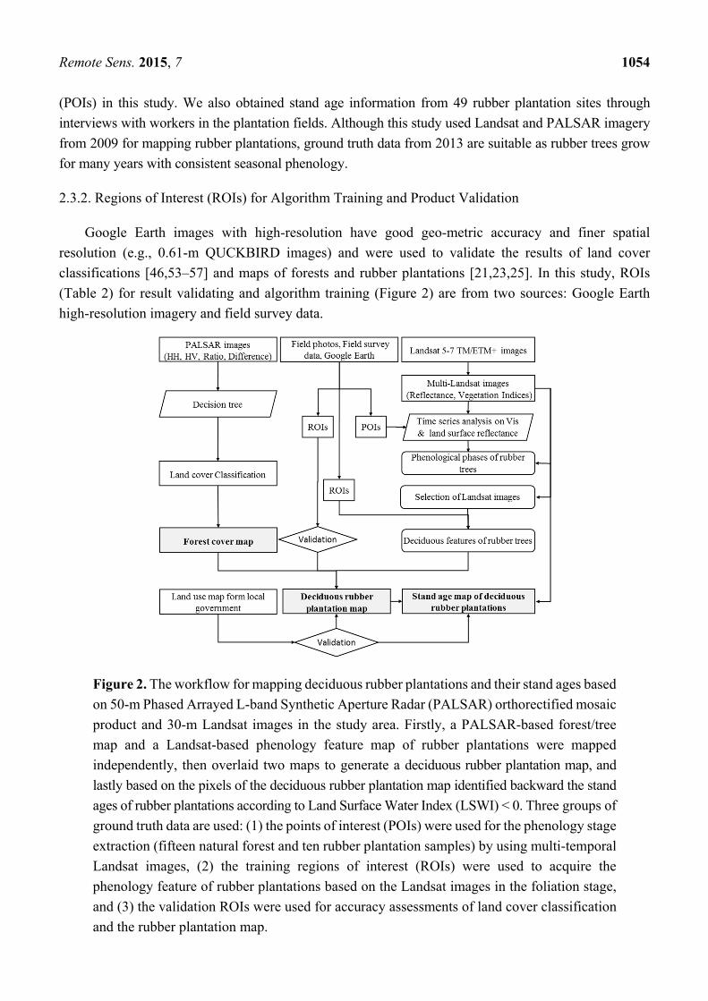
Figure 2. The workflow for mapping deciduous rubber plantations and their stand ages based
on 50-m Phased Arrayed L-band Synthetic Aperture Radar (PALSAR) orthorectified mosaic
product and 30-m Landsat images in the study area. Firstly, a PALSAR-based forest/tree
map and a Landsat-based phenology feature map of rubber plantations were mapped
independently, then overlaid two maps to generate a deciduous rubber plantation map, and
lastly based on the pixels of the deciduous rubber plantation map identified backward the stand
ages of rubber plantations according to Land Surface Water Index (LSWI) < 0. Three groups of
ground truth data are used: (1) the points of interest (POIs) were used for the phenology stage
extraction (fifteen natural forest and ten rubber plantation samples) by using multi-temporal
Landsat images, (2) the training regions of interest (ROIs) were used to acquire the
phenology feature of rubber plantations based on the Landsat images in the foliation stage,
and (3) the validation ROIs were used for accuracy assessments of land cover classification
and the rubber plantation map.
Remote Sens. 2015, 7 1055
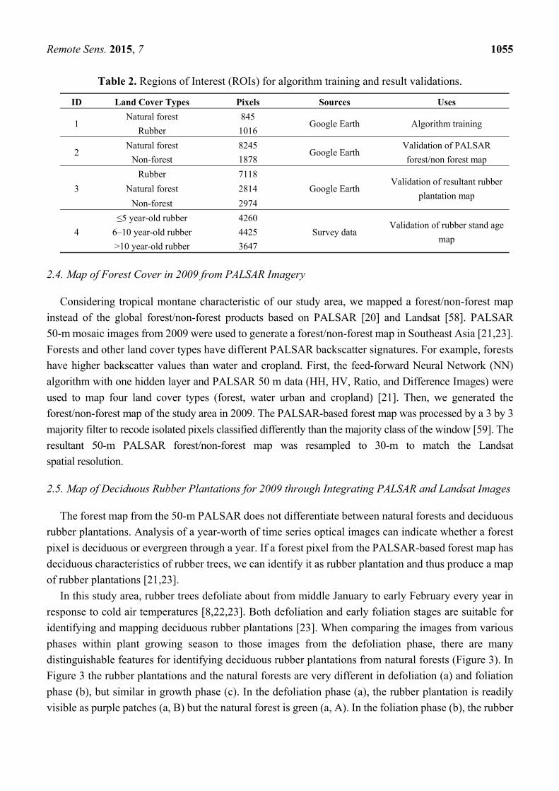
Table 2. Regions of Interest (ROIs) for algorithm training and result validations.
ID Land Cover Types Pixels Sources Uses
1 Natural forest 845
Google Earth Algorithm training Rubber 1016
2 Natural forest 8245
Google Earth Validation of PALSAR
forest/non forest map Non-forest 1878
3
Rubber 7118
Google Earth Validation of resultant rubber
plantation map Natural forest 2814
Non-forest 2974
4
≤5 year-old rubber 4260
Survey data Validation of rubber stand age
map 6–10 year-old rubber 4425
>10 year-old rubber 3647
2.4. Map of Forest Cover in 2009 from PALSAR Imagery
Considering tropical montane characteristic of our study area, we mapped a forest/non-forest map
instead of the global forest/non-forest products based on PALSAR [20] and Landsat [58]. PALSAR
50-m mosaic images from 2009 were used to generate a forest/non-forest map in Southeast Asia [21,23].
Forests and other land cover types have different PALSAR backscatter signatures. For example, forests
have higher backscatter values than water and cropland. First, the feed-forward Neural Network (NN)
algorithm with one hidden layer and PALSAR 50 m data (HH, HV, Ratio, and Difference Images) were
used to map four land cover types (forest, water urban and cropland) [21]. Then, we generated the
forest/non-forest map of the study area in 2009. The PALSAR-based forest map was processed by a 3 by 3
majority filter to recode isolated pixels classified differently than the majority class of the window [59]. The
resultant 50-m PALSAR forest/non-forest map was resampled to 30-m to match the Landsat
spatial resolution.
2.5. Map of Deciduous Rubber Plantations for 2009 through Integrating PALSAR and Landsat Images
The forest map from the 50-m PALSAR does not differentiate between natural forests and deciduous
rubber plantations. Analysis of a year-worth of time series optical images can indicate whether a forest
pixel is deciduous or evergreen through a year. If a forest pixel from the PALSAR-based forest map has
deciduous characteristics of rubber trees, we can identify it as rubber plantation and thus produce a map
of rubber plantations [21,23].
In this study area, rubber trees defoliate about from middle January to early February every year in
response to cold air temperatures [8,22,23]. Both defoliation and early foliation stages are suitable for
identifying and mapping deciduous rubber plantations [23]. When comparing the images from various
phases within plant growing season to those images from the defoliation phase, there are many
distinguishable features for identifying deciduous rubber plantations from natural forests (Figure 3). In
Figure 3 the rubber plantations and the natural forests are very different in defoliation (a) and foliation
phase (b), but similar in growth phase (c). In the defoliation phase (a), the rubber plantation is readily
visible as purple patches (a, B) but the natural forest is green (a, A). In the foliation phase (b), the rubber
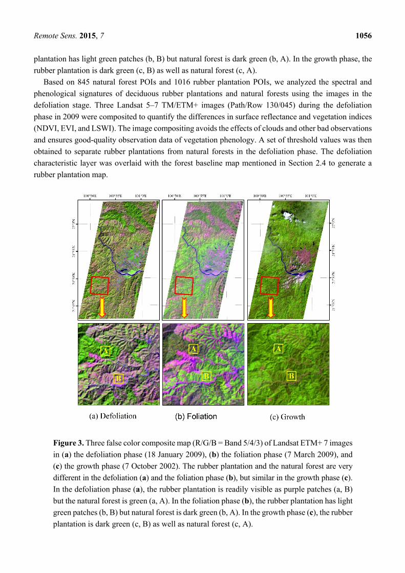
Remote Sens. 2015, 7 1056
plantation has light green patches (b, B) but natural forest is dark green (b, A). In the growth phase, the
rubber plantation is dark green (c, B) as well as natural forest (c, A).
Based on 845 natural forest POIs and 1016 rubber plantation POIs, we analyzed the spectral and
phenological signatures of deciduous rubber plantations and natural forests using the images in the
defoliation stage. Three Landsat 5–7 TM/ETM+ images (Path/Row 130/045) during the defoliation
phase in 2009 were composited to quantify the differences in surface reflectance and vegetation indices
(NDVI, EVI, and LSWI). The image compositing avoids the effects of clouds and other bad observations
and ensures good-quality observation data of vegetation phenology. A set of threshold values was then
obtained to separate rubber plantations from natural forests in the defoliation phase. The defoliation
characteristic layer was overlaid with the forest baseline map mentioned in Section 2.4 to generate a
rubber plantation map.
Figure 3. Three false color composite map (R/G/B = Band 5/4/3) of Landsat ETM+ 7 images
in (a) the defoliation phase (18 January 2009), (b) the foliation phase (7 March 2009), and
(c) the growth phase (7 October 2002). The rubber plantation and the natural forest are very
different in the defoliation (a) and the foliation phase (b), but similar in the growth phase (c).
In the defoliation phase (a), the rubber plantation is readily visible as purple patches (a, B)
but the natural forest is green (a, A). In the foliation phase (b), the rubber plantation has light
green patches (b, B) but natural forest is dark green (b, A). In the growth phase (c), the rubber
plantation is dark green (c, B) as well as natural forest (c, A).
Remote Sens. 2015, 7 1057
2.6. Map of Stand Age of Deciduous Rubber Plantations
2.6.1. Landsat-Based Signature Analysis of Rubber Plantations with Different Stand Ages
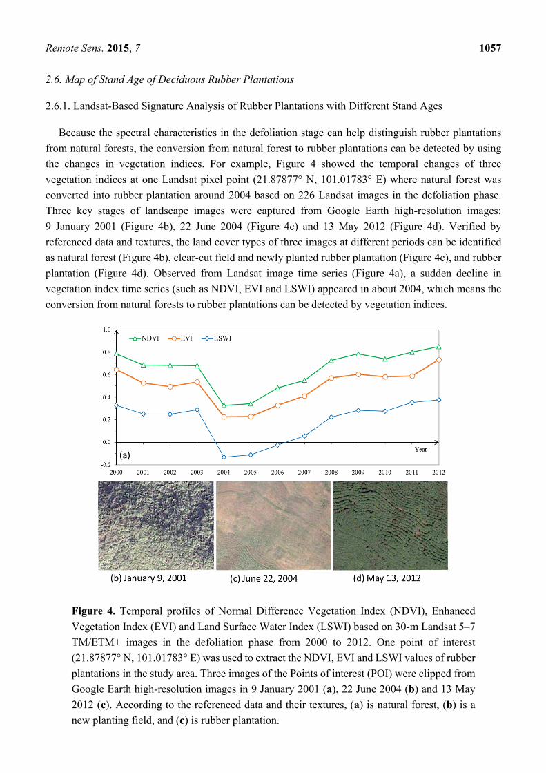
Because the spectral characteristics in the defoliation stage can help distinguish rubber plantations
from natural forests, the conversion from natural forest to rubber plantations can be detected by using
the changes in vegetation indices. For example, Figure 4 showed the temporal changes of three
vegetation indices at one Landsat pixel point (21.87877° N, 101.01783° E) where natural forest was
converted into rubber plantation around 2004 based on 226 Landsat images in the defoliation phase.
Three key stages of landscape images were captured from Google Earth high-resolution images:
9 January 2001 (Figure 4b), 22 June 2004 (Figure 4c) and 13 May 2012 (Figure 4d). Verified by
referenced data and textures, the land cover types of three images at different periods can be identified
as natural forest (Figure 4b), clear-cut field and newly planted rubber plantation (Figure 4c), and rubber
plantation (Figure 4d). Observed from Landsat image time series (Figure 4a), a sudden decline in
vegetation index time series (such as NDVI, EVI and LSWI) appeared in about 2004, which means the
conversion from natural forests to rubber plantations can be detected by vegetation indices.
Figure 4. Temporal profiles of Normal Difference Vegetation Index (NDVI), Enhanced
Vegetation Index (EVI) and Land Surface Water Index (LSWI) based on 30-m Landsat 5–7
TM/ETM+ images in the defoliation phase from 2000 to 2012. One point of interest
(21.87877° N, 101.01783° E) was used to extract the NDVI, EVI and LSWI values of rubber
plantations in the study area. Three images of the Points of interest (POI) were clipped from
Google Earth high-resolution images in 9 January 2001 (a), 22 June 2004 (b) and 13 May
2012 (c). According to the referenced data and their textures, (a) is natural forest, (b) is a
new planting field, and (c) is rubber plantation.

Remote Sens. 2015, 7 1058
Furthermore, rubber plantations with different stand ages may have various features (e.g., defoliation
intensity), which can help to identify their stand ages. To determine the signatures of different stand ages
of rubber plantations in the defoliation phase, we used 49 rubber plantation field survey POIs (Figure 1)
with stand ages and 10 natural forest POIs and then grouped the 49 POIs into five age groups (≤5, 6–10,
11–15, 16–20, and 21–25 years old), based on the field survey in 2011 (also assumed as the baseline
year). Time series NDVI, EVI, and LSWI from Landsat 5/7 TM/ETM+ images in the defoliation phase
during 2000–2011 were used for individual pixels and used to analyze the characteristics of deciduous
rubber plantations with different stand age groups (≤5, 6–10, 11–15, 16–20, and 21–25 years old). The
relationships between vegetation indices (NDVI, EVI and LSWI) and the stand ages from these 49 POIs
were quantified.
2.6.2. Map of Deciduous Rubber Plantations with Different Stand Ages
As shown in Figure 4, LSWI value was negative in clear-cut fields and newly cultivated rubber
plantations. We used LSWI to detect disturbance (negative LSWI value in a time series LSWI data over
2000–2009 for a rubber plantation pixel in 2009). The stand age of a rubber plantation pixel in 2009 was
determined using the following steps: first, we tracked and recorded the year when LSWIdefoliation < 0
occurred for the first time between 2000 and 2009 (10 years), which was considered to be the starting
year of rubber plantations; second, we grouped and reported the resultant stand ages into two age groups
(≤5 years, 6–10 years); third, those rubber plantation pixels that did not have any observations with
LSWIdefoliation < 0 during 2000–2009 were considered to be >10 years.
2.7. Validation and Comparison
Confusion matrices created from ROIs were used to validate the resampled 30-m PALSAR
forest/non-forest map, the 30-m resultant map of deciduous rubber plantations and their stand ages. Eight
thousand two hundred forty-five forest POIs and one thousand eight hundred seventy-eight
non-forest POIs created from Google Earth high-resolution images were used to verify the resampled
30-m PALSAR forest map. Seven thousand one hundred eighteen rubber plantation POIs, two thousand
eight hundred fourteen natural forest and two thousand nine hundred seventy-four non-forest POIs from
Google Earth high-resolution images were used to verify the 30-m resultant rubber plantation map. For
evaluating the stand age map of rubber plantations in 2009, 4260 five-year-old and younger, 4425
six-to-ten-year-old, and 3647 greater than ten-year-old rubber plantation POIs were created from a
survey map from the Jinghong Forestry Bureau.
3. Results
3.1. Map of Forest Cover from PALSAR Imagery in 2009
The resultant PALSAR-based forest map (Figure 5a) has a high accuracy based on the validation
ROIs. The overall accuracy was 95%, and the Kappa coefficient was 0.89. Both the user’s accuracy and
producer's accuracy of the forest cover were higher than 96% (Table 3). Therefore, the forest map can
serve as a reliable base map for rubber plantation delineation. The categories of cropland and other land
cover had lower accuracies than those of forest and water; for example, the other land cover category
Remote Sens. 2015, 7 1059
had a low user’s accuracy (71%) and producer’s accuracy (64%) due to the complex backscatter from
built-up land. However, this is not of any critical concern as the focus in this study is forest.
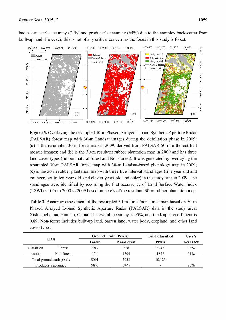
Figure 5. Overlaying the resampled 30-m Phased Arrayed L-band Synthetic Aperture Radar
(PALSAR) forest map with 30-m Landsat images during the defoliation phase in 2009:
(a) is the resampled 30-m forest map in 2009, derived from PALSAR 50-m orthorectified
mosaic images; and (b) is the 30-m resultant rubber plantation map in 2009 and has three
land cover types (rubber, natural forest and Non-forest). It was generated by overlaying the
resampled 30-m PALSAR forest map with 30-m Landsat-based phenology map in 2009;
(c) is the 30-m rubber plantation map with three five-interval stand ages (five year-old and
younger, six-to-ten-year-old, and eleven-years-old and older) in the study area in 2009. The
stand ages were identified by recording the first occurrence of Land Surface Water Index
(LSWI) < 0 from 2000 to 2009 based on pixels of the resultant 30-m rubber plantation map.
Table 3. Accuracy assessment of the resampled 30-m forest/non-forest map based on 50-m
Phased Arrayed L-band Synthetic Aperture Radar (PALSAR) data in the study area,
Xishuangbanna, Yunnan, China. The overall accuracy is 95%, and the Kappa coefficient is
0.89. Non-forest includes built-up land, barren land, water body, cropland, and other land
cover types.
Class Ground Truth (Pixels) Total Classified
Pixels
User’s
Accuracy Forest Non-Forest
Classified
results
Forest 7917 328 8245 96%
Non-forest 174 1704 1878 91%
Total ground truth pixels 8091 2032 10,123 -
Producer’s accuracy 98% 84% - 95%
Remote Sens. 2015, 7 1060
3.2. Map of Rubber Plantations in 2009
3.2.1. Seasonal Phenology of Deciduous Rubber Plantations in 2009 from Landsat
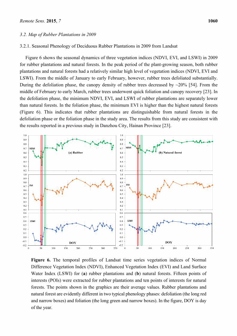
Figure 6 shows the seasonal dynamics of three vegetation indices (NDVI, EVI, and LSWI) in 2009
for rubber plantations and natural forests. In the peak period of the plant-growing season, both rubber
plantations and natural forests had a relatively similar high level of vegetation indices (NDVI, EVI and
LSWI). From the middle of January to early February, however, rubber trees defoliated substantially.
During the defoliation phase, the canopy density of rubber trees decreased by ~20% [54]. From the
middle of February to early March, rubber trees underwent quick foliation and canopy recovery [23]. In
the defoliation phase, the minimum NDVI, EVI, and LSWI of rubber plantations are separately lower
than natural forests. In the foliation phase, the minimum EVI is higher than the highest natural forests
(Figure 6). This indicates that rubber plantations are distinguishable from natural forests in the
defoliation phase or the foliation phase in the study area. The results from this study are consistent with
the results reported in a previous study in Danzhou City, Hainan Province [23].
Figure 6. The temporal profiles of Landsat time series vegetation indices of Normal
Difference Vegetation Index (NDVI), Enhanced Vegetation Index (EVI) and Land Surface
Water Index (LSWI) for (a) rubber plantations and (b) natural forests. Fifteen points of
interests (POIs) were extracted for rubber plantations and ten points of interests for natural
forests. The points shown in the graphics are their average values. Rubber plantations and
natural forest are evidently different in two typical phenology phases: defoliation (the long red
and narrow boxes) and foliation (the long green and narrow boxes). In the figure, DOY is day
of the year.
Remote Sens. 2015, 7 1061
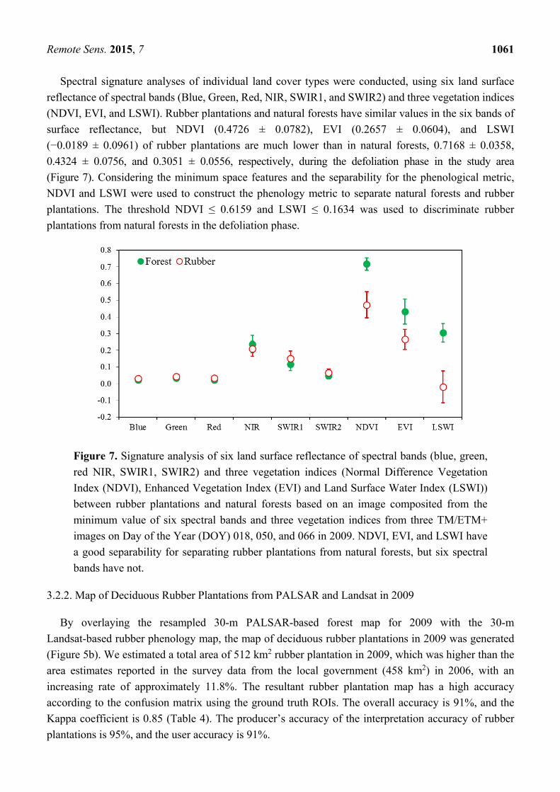
Spectral signature analyses of individual land cover types were conducted, using six land surface
reflectance of spectral bands (Blue, Green, Red, NIR, SWIR1, and SWIR2) and three vegetation indices
(NDVI, EVI, and LSWI). Rubber plantations and natural forests have similar values in the six bands of
surface reflectance, but NDVI (0.4726 ± 0.0782), EVI (0.2657 ± 0.0604), and LSWI
(−0.0189 ± 0.0961) of rubber plantations are much lower than in natural forests, 0.7168 ± 0.0358,
0.4324 ± 0.0756, and 0.3051 ± 0.0556, respectively, during the defoliation phase in the study area
(Figure 7). Considering the minimum space features and the separability for the phenological metric,
NDVI and LSWI were used to construct the phenology metric to separate natural forests and rubber
plantations. The threshold NDVI ≤ 0.6159 and LSWI ≤ 0.1634 was used to discriminate rubber
plantations from natural forests in the defoliation phase.
Figure 7. Signature analysis of six land surface reflectance of spectral bands (blue, green,
red NIR, SWIR1, SWIR2) and three vegetation indices (Normal Difference Vegetation
Index (NDVI), Enhanced Vegetation Index (EVI) and Land Surface Water Index (LSWI))
between rubber plantations and natural forests based on an image composited from the
minimum value of six spectral bands and three vegetation indices from three TM/ETM+
images on Day of the Year (DOY) 018, 050, and 066 in 2009. NDVI, EVI, and LSWI have
a good separability for separating rubber plantations from natural forests, but six spectral
bands have not.
3.2.2. Map of Deciduous Rubber Plantations from PALSAR and Landsat in 2009
By overlaying the resampled 30-m PALSAR-based forest map for 2009 with the 30-m
Landsat-based rubber phenology map, the map of deciduous rubber plantations in 2009 was generated
(Figure 5b). We estimated a total area of 512 km2 rubber plantation in 2009, which was higher than the
area estimates reported in the survey data from the local government (458 km2) in 2006, with an
increasing rate of approximately 11.8%. The resultant rubber plantation map has a high accuracy
according to the confusion matrix using the ground truth ROIs. The overall accuracy is 91%, and the
Kappa coefficient is 0.85 (Table 4). The producer’s accuracy of the interpretation accuracy of rubber
plantations is 95%, and the user accuracy is 91%.
Remote Sens. 2015, 7 1062
Table 4. Accuracy assessment of the land cover classification map based on 30-m Landsat 5/7
Themetic Mapper (TM)/Ehanced Thematic Mapper Plus (ETM+) images in the study area.
The overall accuracy is 92%, and the Kappa coefficient is 0.87. Non-forest includes built-up
land, barren land, water body, cropland, and other land cover types.
Class Ground Truth (Pixels)
Total Classified Pixels User’s
Accuracy Rubber Natural Forest Non-Forest
Classified
results
Rubber 6480 37 601 7118 91%
Natural Forest 21 2780 13 2814 99%
Non-forest 359 6 2609 2974 88%
Total ground truth pixels 6860 2823 3223 12906
Producer’s accuracy 94% 98% 81% - -
3.3. Map of Stand Ages of Rubber Plantations in 2009
3.3.1. Changes in Seasonal Phenology of Deciduous Rubber Plantations at Different Stand Ages from
Landsat iMages in 2000–2011
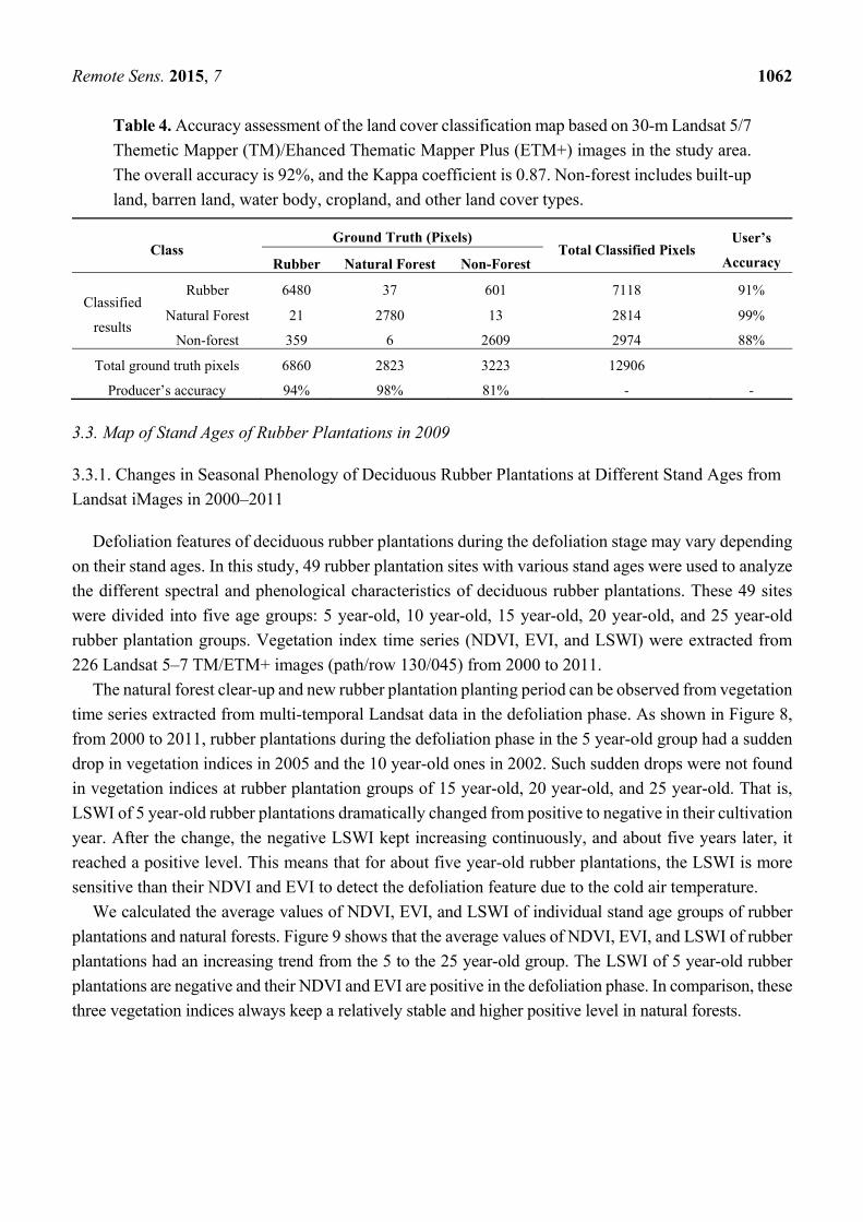
Defoliation features of deciduous rubber plantations during the defoliation stage may vary depending
on their stand ages. In this study, 49 rubber plantation sites with various stand ages were used to analyze
the different spectral and phenological characteristics of deciduous rubber plantations. These 49 sites
were divided into five age groups: 5 year-old, 10 year-old, 15 year-old, 20 year-old, and 25 year-old
rubber plantation groups. Vegetation index time series (NDVI, EVI, and LSWI) were extracted from
226 Landsat 5–7 TM/ETM+ images (path/row 130/045) from 2000 to 2011.
The natural forest clear-up and new rubber plantation planting period can be observed from vegetation
time series extracted from multi-temporal Landsat data in the defoliation phase. As shown in Figure 8,
from 2000 to 2011, rubber plantations during the defoliation phase in the 5 year-old group had a sudden
drop in vegetation indices in 2005 and the 10 year-old ones in 2002. Such sudden drops were not found
in vegetation indices at rubber plantation groups of 15 year-old, 20 year-old, and 25 year-old. That is,
LSWI of 5 year-old rubber plantations dramatically changed from positive to negative in their cultivation
year. After the change, the negative LSWI kept increasing continuously, and about five years later, it
reached a positive level. This means that for about five year-old rubber plantations, the LSWI is more
sensitive than their NDVI and EVI to detect the defoliation feature due to the cold air temperature.
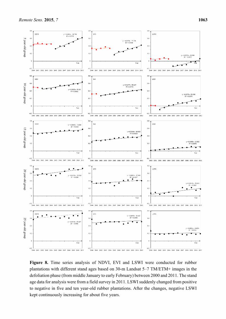
We calculated the average values of NDVI, EVI, and LSWI of individual stand age groups of rubber
plantations and natural forests. Figure 9 shows that the average values of NDVI, EVI, and LSWI of rubber
plantations had an increasing trend from the 5 to the 25 year-old group. The LSWI of 5 year-old rubber
plantations are negative and their NDVI and EVI are positive in the defoliation phase. In comparison, these
three vegetation indices always keep a relatively stable and higher positive level in natural forests.
Remote Sens. 2015, 7 1063
Figure 8. Time series analysis of NDVI, EVI and LSWI were conducted for rubber
plantations with different stand ages based on 30-m Landsat 5–7 TM/ETM+ images in the
defoliation phase (from middle January to early February) between 2000 and 2011. The stand
age data for analysis were from a field survey in 2011. LSWI suddenly changed from positive
to negative in five and ten year-old rubber plantations. After the changes, negative LSWI
kept continuously increasing for about five years.
Remote Sens. 2015, 7 1064
Figure 9. Comparing vegetation index (NDVI, EVI and LSWI) variations between rubber
plantations with different stand ages in the defoliation phase and natural forests. From the
youngest group (5 year-old) to the oldest (25 year-old) rubber plantation group, the NDVI,
EVI and LSWI were increasing toward to that of natural forests, but natural forests kept a
relative stable level. 49 POIs of rubber plantations with stand ages in the defoliation phase
in 2011 and 10 Points of interest (POIs) of natural forests were used in this analysis. The
points shown in the figures are the average NDVI, EVI and LSWI of these POIs.
3.3.2. Map of Stand Age of Deciduous Rubber Plantations in 2009
A stand age map of deciduous rubber plantations was generated based on 30-m Landsat 5/7 TM/ETM+
images (Figure 5c). To validate the stand age map, this study extracted ROIs from a reference map with age
information that was from local forestry bureau. Based on these ROIs, we built a confusion matrix (Table 5)
to validate the stand age map. According to the confusion matrix, the overall accuracy is 85%, and the Kappa
coefficient is 0.78. The individual user’s accuracies of ≤5, 6–10, and ≥11 year-old rubber plantations are
88%, 87%, and 80%, respectively, and the producer’s accuracies are 87%, 81%, and 90%, respectively.
Table 5. Accuracy assessment of the stand age map based on 30-m Landsat images in the
study area. Overall accuracy is 85%, and the Kappa coefficient is 0.78.
Class (year-old) Ground Truth (Pixels) Total Classified
Pixels
User’s
Accuracy <6 6–10 >10
Classified
results
<6 3763 388 109 4260 88%
6–10 373 3843 209 4425 87%
>10 180 540 2927 3647 80%
Total ground truth pixels 4316 4771 3245 12332
Producer’s accuracy 87% 81% 90%
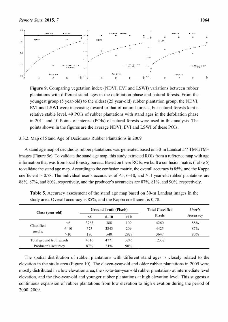
The spatial distribution of rubber plantations with different stand ages is closely related to the
elevation in the study area (Figure 10). The eleven-year-old and older rubber plantations in 2009 were
mostly distributed in a low elevation area, the six-to-ten-year-old rubber plantations at intermediate level
elevation, and the five-year-old and younger rubber plantations at high elevation level. This suggests a
continuous expansion of rubber plantations from low elevation to high elevation during the period of
2000–2009.
Remote Sens. 2015, 7 1065
Figure 10. The relationship between the distribution of rubber plantations and elevations.
(a) Area distribution of rubber plantations with different stand ages in different elevations.
(b) Area % of rubber plantations with different stand ages versus the surface of the
corresponding elevation category. (c) Area distribution of different elevation categories in
the study area.
4. Discussions
4.1. Major Findings and Potentials for Mapping Forest, Rubber Plantations, and Their Stand Ages
Synthetic aperture radar (SAR) data (e.g., PALSAR images) have a number of advantages in mapping
forests over optical sensors, particularly in moist and cloudy tropical regions, and have been used
recently to map (1) forest cover in Southeast Asia [8,21–23,25,60,61], the Amazon basin [24], and across
the globe [20], and (2) industrial forest plantations such as rubber, oil palm, coconut, and wattle
plantations [23,62]. In this study, we used L-band PALSAR 50-m orthorectified mosaic images to
generate a forest and non-forest map for 2009 at 50-m spatial resolution in the study area, using the same
algorithm reported in previous studies [21,23]. As L-band PALSAR images are sensitive to forest structure,
biomass and water content of the canopy, this study has demonstrated the potential of PALSAR 50-m
orthorectified mosaic images for mapping forests in the moist tropical areas. Several other studies have
also evaluated the potential of combing PALSAR and Landsat images to improve forest mapping [63–65],
future studies might be needed to evaluate the potential of combining Landsat 8 and PALSAR-2 images
in 2015.
Remote Sens. 2015, 7 1066
Rubber plantations in China are deciduous broadleaf forests. A number of studies have recognized
the defoliation phase in the relatively cold and dry winter season as a key phenological stage for
separating evergreen natural forests and deciduous rubber plantations in Xishuangbanna, China [9,35].
Satellite images including Landsat images [9,21,23,35] and HJ-1 images [8,22], within the defoliation
phase in one year were often selected for image-based classification to identify and map rubber
plantations. In addition to the defoliation phase, another study also recognized the foliation phase (new
leaf emergence) as a key phenological stage for separating evergreen natural forests and deciduous
rubber plantations in Hainan Island, which has the largest area of rubber plantations in China [23]. The
results from our study in Xishuangbanna also show that both the defoliation and foliation periods are
good for identifying and mapping rubber plantations, which is consistent with the findings in the
previous study in Hainan, China [23]. The longer time window from either defoliation or foliation stages
make it possible to have good quality satellite observations available for image analysis.
Several studies used NDVI time series data to characterize and map deciduous rubber plantations in
Xishuangbanna and Southeast Asia [7,9,35,46,61]. Liu et al. determined that mature rubber plantations
are different from other land cover types and that young rubber plantations (< 10 years old) were often
confused with fallow croplands and tea gardens. One recent study used MODIS-based EVI and
shortwave infrared band (SWIR) in 2010 to map rubber plantations in Xishuangbanna [46]. Similar to
the previous study in Hainan Island [21,23,25], in this study we evaluated NDVI, EVI, and LSWI data
to characterize phenological phases of deciduous rubber plantations and evergreen natural forests in the
mountainous areas. Our results show that NDVI and LSWI provide additional insight into the
characterization of vegetation phenology, and that it is beneficial to use all three vegetation indices in
phenological studies.
The algorithms and procedures used to map deciduous rubber plantations in previous studies can be
grouped into two approaches. The image-based approach first calculates image statistics in optical
image(s) for various land cover types and then applies a clustering method (e.g., maximum likelihood,
decision tree) to map rubber plantations [7,9,35,46,61]. The pixel-based approach first investigates time
series data (vegetation indices and spectral reflectance) for a forest pixel over year(s) and then applies
signal detection methods to determine whether a pixel is rubber plantation or not in that year(s) [21,23].
This study is a follow-on case study of the pixel-based approach for mapping rubber plantations in
complex mountainous areas, and it also uses a PALSAR-based forest map as the baseline for analysis of
deciduous and evergreen trees.
Stand ages of deciduous rubber plantations are critical information for management of rubber
plantations. This study mapped and reported stand ages for rubber plantations at 5-year intervals
(≤ 5 years old, 6–10 years old, and ≥11 years old), based on analysis of time series Landsat images from
2000 to 2009. It started with a signature analysis of rubber plantations at different stand ages, using time
series NDVI, EVI, and LSWI data from 2000 to 2009. When the stand ages of deciduous rubber
plantations are 5 years or less, their LSWI values are negative during the defoliation stage in the study
area. We used this unique feature to develop a simple method to determine stand ages of deciduous
rubber plantations at 5-year intervals, based on 30-m Landsat 5–7 TM/ETM+ imagery from 2000 to
2009 in the defoliation phase. Compared to the traditional field survey method, the new method can
estimate stand ages of deciduous rubber plantations over a large region without limitations like
transportation or weather conditions.
Remote Sens. 2015, 7 1067
4.2. Sources of Errors and Uncertainties in Mapping of Forest, Rubber Plantations, and Stand Ages
In this study, we generated a map of forests in 2009 at 50-m spatial resolution from analysis of PALSAR
images, a map of rubber plantations in 2009 at 30-m spatial resolution from analysis of multi-temporal
Landsat images in 2009 for all PALSAR-based forest pixels, and a map of stand ages of rubber
plantations in 2009. There are some uncertainties in each of resultant maps in the study due to data
quality and availability as well as algorithm design. First, the forest/non-forest map from the L-band
PALSAR data are likely to omit young (one- or two-year-old) rubber plantations due to their small and
sparse canopies and low height in the fields. In addition, 50-m PALSAR data may be too coarse to
identify sparse forests and woodlands in the classification (especially towards the lower cover threshold
of 10%), which may result in underestimating the total area [20]. Second, topographic factors (such as
slopes, aspects, and elevations) may affect backscatter coefficients of PALSAR images and spectral
properties of deciduous rubber plantations. Third, stand age factor may also affect backscatter
coefficients of PALSAR images and the spectral properties of rubber plantations, specifically during the
defoliation and foliation processes (timing, duration, and magnitude). These factors together suggest that
the time windows for selection of Landsat images and the threshold values in classification algorithms
may vary in different areas, and therefore, additional studies across the subtropical areas in China and
Southeast Asia are needed in the near future. In addition, the improvement in data quality, numbers, and
continuity of available satellite images may present further opportunities in mapping stand ages of rubber
plantations. An application of the approach used in this study clearly needs to carried out on the regional
scale and evaluated in the future studies.
4.3. Field Survey Data and High Resolution Images
Validation or accuracy assessment of land cover maps developed from analysis of satellite images is
important to all land cover mapping studies however, it is often restrained by insufficient data from the
field. Due to high costs of getting reliable field survey data and super high resolution imagery (≤1 m) in
land cover and use change research, insufficient accuracy assessment via field survey data may cause
considerable error and misinterpretation [23,66]. Sharing scientific field survey data among scientists is a
feasible way to mitigate the problem of insufficient ground data. The field survey data in this study are
based on the Global Geo-Referenced Field Photo Library [67], which has a large amount of geo-referenced
field photos (120,000+ as of July 2014) shared by scientists from all over the world and provides effective
support for many research fields, such as land cover and land use changes and biogeography [18,23].
Although these geo-referenced field photos can provide abundant spatial information, they still cannot
fully support needs for algorithm training and resultant map validation. We used the Google Earth high
spatial resolution images to extend the POIs from abundant field photos into ROIs. Some previous studies
also used these free high-resolution images on Google Earth for algorithm training or classification result
validation [10,17,21,23,25,54,55,57]. This study also used the multi-temporal high-resolution images on
Google Earth to validate the planting period of rubber plantations (Figure 4).
Additionally, disturbances from clouds, cloud shadows, and gaps affect the data quality of Landsat
data. In this study, they were taken into account to improve Landsat data quality, but in some of previous
studies [23,25,35,46] they were not; in previous studies, the cloud-free Landsat images were chosen and

Remote Sens. 2015, 7 1068
used, but in humid, tropical montane regions, cloud-free images are very limited. The clouds and their
shadows can be well detected by Fmask [47].
4.4. Implications for the Expansion of Rubber Plantations in Xishuangbanna
The spatial distribution and areas of rubber plantations in the Xishuangbanna received broad attention
from many researchers in China and the world and were reported in several studies [4,8,9,35,46,61,68].
These studies used either MODIS data (250-m spatial resolution) or Landsat images (30-m spatial
resolution) to generate maps of rubber plantations in Xishuangbanna, which is covered by three Landsat
path/row scenes. Our study did not cover the entire Xishuangbanna region, but did showcase a new
methodology of combining SAR and optical data to map rubber plantations and their stand ages in
complex mountainous areas. The defoliation stage of deciduous rubber plantations is a key phenological
stage for discriminating rubber plantations and evergreen natural forests. In this stage, based on the
PALSAR-derived forest cover map, a map of rubber plantations can be generated by using phenological
signals in the time series NDVI and LSWI data. We found that LSWI is a strong variable for estimating
stand ages of deciduous rubber plantations through analysis of LSWI data during the defoliation period.
Based on 30-m multi temporal Landsat imagery in defoliation phase, we can generate a map of stand
ages of deciduous rubber plantations by using the rule LSWI < 0.
5. Conclusions
In this study, we have developed a novel, simple and robust procedure that combines Phased Array
type L-band Synthetic Aperture Radar (PALSAR) 50-m orthorectified images and multi-temporal
Landsat images to map forest, deciduous rubber plantations, and stand ages of rubber plantations in
tropical regions. We applied the procedure to a small area (Jinghong city area) in Xishuangbanna, the
2nd largest natural production base in China, using PALSAR 50-m orthorectified images in 2009 and
Landsat images in 2000–2009. The resultant forest map in 2009 from 50-m PALSAR orthorectified
mosaic data has high producer and user accuracies, which clearly demonstrates the potential of PALSAR
images for forest mapping. The algorithm uses unique spectral properties during the defoliation stage of
deciduous rubber plantations, and then discriminates deciduous rubber plantations from evergreen
natural forests through analysis of time series Normalized Difference Vegetation Index (NDVI) and
Land Surface Water Index (LSWI) data derived from Landsat images. The resultant map of deciduous
rubber plantations also has high producer’s (94%) and user’s accuracies (91%), which highlights the
potential of combining PALSAR and Landsat images for mapping rubber plantations. We also found
that LSWI (LSWI < 0) is a good variable (the overall accuracies is 85%) for estimating stand ages of
deciduous rubber plantations through analysis of LSWI data during the defoliation period. The resultant
stand age map of deciduous rubber plantations clearly shows spatial-temporal patterns that rubber
plantations expanded from regions with low elevation level into mountains over years (2000–2009). To
our limited knowledge, this study was the first effort that maps forest, deciduous rubber plantation, and
stand age of rubber plantation through integration of PALSAR and Landsat images. The algorithms
developed in this study need to be applied and further evaluated when both PALSAR-2 (launched on
24 May 2014) and Landsat 8 (launched on 11 February 2013) images are freely available to map forest
cover, deciduous rubber plantation and stand age of rubber plantations. Additional studies are also needed
Remote Sens. 2015, 7 1069
to combine multi-year PALSAR (2006–2010), JERS-1 (1992–1993) and Landsat 5/7 (1985–2013) to track
expansion and stand age of rubber plantations at local, regional and continental scales over decades. The
resultant geospatial datasets from these proposed future studies are important inputs for us to better
understand the consequences of rubber plantation expansion in the region on biodiversity, carbon, water
and climate.
Acknowledgments
This study was supported by US NASA Land Use and Land Cover Change program (NNX09AC39G,
NNX11AJ35G), the US National Science Foundation (NSF) EPSCoR program (NSF-IIA-1301789), the
National Natural Science Foundation of China (31400493,41201340,31300403). Landsat imagery is
available from the U.S. Geological Survey (USGS) EROS Data Center. The original PALSAR data are
provided by JAXA as the ALOS products. We thank Sarah Xiao for her English editing and comments.
Author Contributions
Weili Kou, Xiangming Xiao, and Jinwei Dong designed the study and conducted the data processing
and manuscript writing. Shu Gan, Deli Zhai, Geli Zhang, Yuanwei Qin, and Li Li contributed to the
PALSAR and other related data processing and manuscript editing. All the authors worked on the
interpretation of results and manuscript revisions.
Conflicts of Interest
The authors declare no conflict of interest.
References
1. FAO. Global Forest Resources Assessment 2010. Available online: http://www.fao.org/docrep/
013/i1757e/i1757e.pdf (accessed on 10 September 2014).
2. Fox, J.; Castella, J.-C. Expansion of rubber (Hevea brasiliensis) in mainland Southeast Asia:
What are the prospects for smallholders? J. Peasant Stud. 2013, 40, 155–170.
3. Ziegler, A.D.; Fox, J.M.; Xu, J.C. The rubber juggernaut. Science 2009, 324, 1024–1025.
4. Li, H.; Aide, T.M.; Ma, Y.; Liu, W.; Cao, M. Demand for rubber is causing the loss of high diversity
rain forest in SW China. Biodivers. Conserv. 2007, 16, 1731–1745.
5. Qiu, J. Where the rubber meets the garden. Nature 2009, 457, 246–247.
6. Yi, Z.-F.; Cannon, C.H.; Chen, J.; Ye, C.-X.; Swetnam, R.D. Developing indicators of economic
value and biodiversity loss for rubber plantations in Xishuangbanna, Southwest China: A case study
from Menglun township. Ecol. Indic. 2014, 36, 788–797.
7. Li, Z.; Fox, J.M. Mapping rubber tree growth in mainland southeast Asia using time-series MODIS
250 m NDVI and statistical data. Appl. Geogr. 2012, 32, 420–432.
8. Li, Y.; Liu, G.; Huang, C. Analysis of distribution characteristics of Hevea brasiliensis in the
Xishuangbanna area based on HJ-1 satellite data. Sci. China Inform. Sci. 2011, 41, 166–176.
9. Liu, X.; Feng, Z.; Jiang, L.; Jiang, Y. Rubber plantations in Xishuangbanna: Remote sensing
identification and digital mapping. Resour. Sci. 2012, 34, 1769–1780.
Remote Sens. 2015, 7 1070
10. Li, Z.; Fox, J.M. Integrating Mahalanobis typicalities with a neural network for rubber distribution
mapping. Remote Sens. Lett. 2011, 2, 157–166.
11. Li, Z. Rubber tree distribution mapping in Northeast Thailand. Int. J. Geosci. 2011, 2, 573–584.
12. Santoro, M.; Fransson, J.E.S.; Eriksson, L.E.B.; Magnusson, M.; Ulander, L.M.H.; Olsson, H.
Signatures of ALOS PALSAR l-band backscatter in Swedish forest. IEEE Trans. Geosci. Remote Sens.
2009, 47, 4001–4019.
13. DeFries, R.; Achard, F.; Brown, S.; Herold, M.; Murdiyarso, D.; Schlamadinger, B.; de Souza, C., Jr.
Earth observations for estimating greenhouse gas emissions from deforestation in developing countries.
Environ. Sci. Policy 2007, 10, 385–394.
14. Hansen, M.C.; Roy, D.P.; Lindquist, E.; Adusei, B.; Justice, C.O.; Altstatt, A. A method for
integrating MODIS and Landsat data for systematic monitoring of forest cover and change in the
Congo basin. Remote Sens. Environ. 2008, 112, 2495–2513.
15. Walker, W.S.; Stickler, C.M.; Kellndorfer, J.M.; Kirsch, K.M.; Nepstad, D.C.
Large-area classification and mapping of forest and land cover in the Brazilian Amazon:
A comparative analysis of ALOS/PALSAR and Landsat data sources. IEEE J. Sel. Top. Appl. Earth
Obs. Remote Sens. 2010, 3, 594–604.
16. Asner, G.P. Cloud cover in Landsat observations of the Brazilian Amazon. Int. J. Remote Sens.
2001, 22, 3855–3862.
17. Baghdadi, N.; Boyer, N.; Todoroff, P.; Hajj, E.M.; Begue, A. Potential of SAR sensors TerraSAR-X,
ASAR/ENVISAT and PALSAR/ALOS for monitoring sugarcane crops on Reunion Island.
Remote Sens. Environ. 2009, 113, 1724–1738.
18. Dong, J.; Xiao, X.; Sheldon, S.; Biradar, C.; Zhang, G.; Duong, N.D.; Hazarika, M.; Wikantika, K.;
Takeuhci, W.; Moore, B, III. A 50-m forest cover map in Southeast Asia from ALOS/PALSAR and
its application on forest fragmentation assessment. PLoS One 2014, 9,
doi:10.1371/journal.pone.0085801.
19. Lucas, R.M.; Clewley, D.; Accad, A.; Butler, D.; Armston, J.; Bowen, M.; Bunting, P.; Carreiras, J.;
Dwyer, J.; Eyre, T.; et al. Mapping forest growth and degradation stage in the Brigalow Belt
Bioregion of Australia through integration of ALOS PALSAR and Landsat-derived foliage
projective cover data. Remote Sens. Environ. 2014, 155, 42–57.
20. Shimada, M.; Itoh, T.; Motooka, T.; Watanabe, M.; Shiraishi, T.; Thapa, R.; Lucas, R. New global
forest/non-forest maps from ALOS PALSAR data (2007–2010). Remote Sens. Environ. 2014, 155,
13–31.
21. Dong, J.; Xiao, X.; Sheldon, S.; Biradar, C.; Duong, N.D.; Hazarika, M. A comparison of forest cover
maps in mainland Southeast Asia from multiple sources: PALSAR, MERIS, MODIS and FRA.
Remote Sens. Environ. 2012, 127, 60–73.
22. Yu, L.; Zhu, Y.; Lu, W.; Li, X.; Zhao, Z.; Li, C. Rubber planting area extraction in Xishuangbanna
region based on HJ-1 CCD remote sensing image. Chin. J. Agrometeorol. 2013, 34, 493–497.
(In Chinese)
23. Dong, J.; Xiao, X.; Chen, B.; Torbick, N.; Jin, C.; Zhang, G.; Biradar, C. Mapping deciduous rubber
plantations through integration of PALSAR and multi-temporal Landsat imagery.
Remote Sens. Environ. 2013, 134, 392–402.
Remote Sens. 2015, 7 1071
24. Sheldon, S.; Xiao, X.; Biradar, C. Mapping evergreen forests in the Brazilian Amazon using MODIS
and PALSAR 500-m mosaic imagery. ISPRS J. Photogramm. Remote Sens. 2012, 74, 34–40.
25. Dong, J.; Xiao, X.; Sheldon, S.; Biradar, C.; Xie, G. Mapping tropical forests and rubber plantations
in complex landscapes by integrating PALSAR and MODIS imagery. ISPRS J. Photogramm.
Remote Sens. 2012, 74, 20–33.
26. Suratman, M.N.; Bull, G.Q.; Leckie, D.G.; Lemay, V.M.; Marshall, P.L.; Mispan, M.R.
Prediction models for estimating the area, volume, and age of rubber (Hevea brasiliensis)
plantations in Malaysia using Landsat TM data. Int. Forestry Rev. 2004, 6, 1–12.
27. Deng, F.; Chen, J.M.; Pan, Y.; Peters, W.; Birdsey, R.; McCullough, K.; Xiao, J. The use of forest
stand age information in an atmospheric CO2 inversion applied to North America. Biogeosciences
2013, 10, 5335–5348.
28. Deng, F.; Chen, J.M.; Pan, Y.; Peters, W.; Birdsey, R.; McCullough, K.; Xiao, J. Forest stand age
information improves an inverse North American carbon flux estimate. Biogeosci. Discuss. 2013,
10, 4781–4817.
29. Liu, Y.; Yu, G.; Wang, Q.; Zhang, Y. How temperature, precipitation and stand age control the
biomass carbon density of global mature forests. Glob. Ecol. Biogeogr. 2014, 23, 323–333.
30. Pretzsch, H.; Biber, P.; Schütze, G.; Bielak, K. Changes of forest stand dynamics in Europe:
Facts from long-term observational plots and their relevance for forest ecology and management.
Forest Ecol. Manag. 2014, 316, 65–77.
31. Yu, G.; Chen, Z.; Piao, S.; Peng, C.; Ciais, P.; Wang, Q.; Li, X.; Zhu, X. High carbon dioxide uptake
by subtropical forest ecosystems in the East Asian monsoon region. Proc. Natl. Acad. Sci. USA
2014, 111, 4910–4915.
32. Sivanpillai, R.; Smith, C.T.; Srinivasan, R.; Messina, M.G.; Wu, X.B. Estimation of managed loblolly
pine stand age and density with Landsat ETM+ data. Forest Ecol. Manag. 2006, 223, 247–254.
33. Chen, B.; Cao, J.; Wang, J.; Wu, Z.; Tao, Z.; Chen, J.; Yang, C.; Xie, G. Estimation of rubber stand
age in typhoon and chilling injury afflicted area with Landsat TM data: A case study in Hainan
Island, China. Forest Ecol. Manag. 2012, 274, 222–230.
34. Wu, Z.; Xie, G.; Tao, Z.; Zhou, Z.; Wang, X. Characteristics of soil carbon and total nitrogen
contents of rubber plantations at different age stages in Danzhou, Hainan Island. Ecol. Environ. Sci.
2009, 18, 1484–1491.
35. Liu, X.; Feng, Z.; Jiang, L.; Li, P.; Liao, C.; Yang, Y.; You, Z. Rubber plantation and its relationship
with topographical factors in the border region of China, Laos and Myanmar. J. Geogr. Sci. 2013,
23, 1019–1040.
36. Lu, H.; Liu, W.; Luo, Q. Ecohydrological effects of litter layer in a mountainous rubber plantation
in Xishuangbanna, Southwest China. Chin. J. Ecol. 2011, 30, 2129–2136 (In Chinese).
37. Japan Aerospace Exploration Agency (JAXA), K&C Mosaic Homepage—PALSAR 50 m
Orthorectified Mosaic Product. Available online: http://www.eorc.jaxa.jp/ALOS/
en/kc_mosaic/kc_map_50.htm (accessed on 10 September 2014).
38. Longepe, N.; Rakwatin, P.; Isoguchi, O.; Shimada, M.; Uryu, Y.; Yulianto, K. Assessment of ALOS
PALSAR 50 m orthorectied FBD data for regional land cover classification by support vector machines.
IEEE Trans. Geosci. Remote Sens. 2011, 49, 2135–2150.
Remote Sens. 2015, 7 1072
39. Shimada, M.; Isoguchi, O.; Rosenqvist, A. PALSAR calval and generation of the continent scale
mosaic products for Kyoto and Carbon projects. In Proceedings of Geoscience and remote sensing
Symposium, IEEE International, Boston, MA, USA, 7–11 July 2008.
40. Shimada, M.; Ohtaki, T. Generating large-scale high-quality SAR mosaic datasets: Application to
PALSAR data for global monitoring. IEEE J. Sel. Top. Appl. Earth Obs. Remote Sens. 2010, 3,
637–656.
41. Rosenqvist, A.; Shimada, M.; Ito, N.; Watanabe, M. ALOS PALSAR: A pathfinder mission for
global-scale monitoring of the environment. IEEE Trans. Geosci. Remote Sens. 2007, 45, 3307–3316.
42. The National Center for Earth Resource Observations and Science. Available online:
http://earthexplorer.usgs.gov (accessed on 10 September 2014).
43. The National Center for Earth Resource Observations and Science (EROS). Landsat 7 Science Data
Users Handbook. Available online: http://landsathandbook.Gsfc.Nasa.Gov/pdfs/landsat7_handbook.
Pdf. (accessed on 10 September 2014).
44. Masek, J.G.; Vermote, E.F.; Saleous, N.E.; Wolfe, R.; Hall, F.G.; Huemmrich, K.F.; Gao, F.; Kutler, J.;
Lim, T.K. A Landsat surface reflectance dataset for North America, 1990–2000. IEEE Geosci.
Remote Sens. 2006, 3, 68–72.
45. Vermote, E.F.; ElSaleous, N.; Justice, C.O.; Kaufman, Y.J.; Privette, J.L.; Remer, L.; Roger, J.C.;
Tanre, D. Atmospheric correction of visible to middle-infrared EOS-MODIS data over land
surfaces: Background, operational algorithm and validation. J. Geophys. Res.: Atmos 1997, 102,
17131–17141.
46. Senf, C.; Pflugmacher, D.; van der Linden, S.; Hostert, P. Mapping rubber plantations and natural
forests in Xishuangbanna (Southwest China) using multi-spectral phenological metrics from
MODIS time series. Remote Sens. 2013, 5, 2795–2812.
47. Zhu, Z.; Woodcock, C.E. Object-based cloud and cloud shadow detection in Landsat imagery.
Remote Sens. Environ. 2012, 118, 83–94.
48. Tucker, C.J. Red and photographic infrared linear combinations for monitoring vegetation.
Remote Sens. Environ. 1979, 8, 127–150.
49. Huete, A.; Didan, K.; Miura, T.; Rodriguez, E.P.; Gao, X.; Ferreira, L.G. Overview of the
radiometric and biophysical performance of the MODIS vegetation indices. Remote Sens. Environ.
2002, 83, 195–213.
50. Xiao, X.; Hollinger, D.; Aber, J.; Goltz, M.; Davidson, E.A.; Zhang, Q.; Moore, M., III.
Satellite-based modeling of gross primary production in an evergreen needleleaf forest.
Remote Sens. Environ. 2004, 89, 519–534.
51. Xiao, X.M.; Zhang, Q.Y.; Hollinger, D.; Aber, J.; Moore, B. Modeling gross primary production of
an evergreen needleleaf forest using MODIS and climate data. Ecol. Appl. 2004, 15, 954–969.
52. Xiao, X. Earth Observation and Modeling Facility (EOMF). Available online:
http://www.eomf.ou.edu (accessed on 10 September 2014).
53. Benedek, C.; Sziranyi, T. Change detection in optical aerial images by a multilayer conditional
mixed markov model. IEEE Trans. Geosci. Remote Sens. 2009, 47, 3416–3430.
54. Cohen, W.B.; Yang, Z.G.; Kennedy, R. Detecting trends in forest disturbance and recovery using
yearly Landsat time series: 2. Timesync–Tools for calibration and validation. Remote Sens. Environ.
2010, 114, 2911–2924.
Remote Sens. 2015, 7 1073
55. Huang, C.Q.; Coward, S.N.; Masek, J.G.; Thomas, N.; Zhu, Z.L.; Vogelmann, J.E. An automated
approach for reconstructing recent forest disturbance history using dense Landsat time series stacks.
Remote Sens. Environ. 2010, 114, 183–198.
56. Montesano, P.M.; Nelson, R.; Sun, G.; Margolis, H.; Kerber, A.; Ranson, K.J. MODIS tree cover
validation for the circumpolar taiga-tundra transition zone. Remote Sens. Environ. 2009, 113,
2130–2141.
57. Potere, D. Horizontal positional accuracy of google earth’s high-resolution imagery archive.
Sensors 2008, 8, 7973–7981.
58. Hansen, M.C.; Potapov, P.V.; Moore, R.; Hancher, M.; Turubanova, S.A.; Tyukavina, A.; Thau, D.;
Stehman, S.V.; Goetz, S.J.; Loveland, T.R.; et al. High-resolution global maps of 21st-century
forest cover change. Science 2013, 342, 850–853.
59. Yuan, F.; Sawaya, K.E.; Loeffelholz, B.C.; Bauer, M.E. Land cover classification and change analysis
of the Twin Cities (Minnesota) metropolitan area by multitemporal Landsat remote sensing.
Remote Sens. Environ. 2005, 98, 317–328.
60. Liu, X.; Feng, Z.; Jiang, L. Application of decision tree classification to rubber plantations
extraction with remote sensing. Trans. Chin. Soc. Agr. Eng. 2013, 29, 163–172.
61. Feng, Z.; Liu, X.; Jiang, L.; Li, P. Spatial-temporal analysis of rubber plantation and its relationship
with topographical factors in the border region of China, Laos and Myanmar. J. Geogr. Sci. 2013,
68, 1442–1446.
62. Miettinen, J.; Liew, S.C. Separability of insular Southeast Asian woody plantation species in the 50 m
resolution ALOS PALSAR mosaic product. Remote Sens. Lett. 2011, 2, 299–307.
63. Walker, W.S.; Stickler, C.M.; Kellndorfer, J.M.; Kirsch, K.M.; Nepstad, D.C. Large-area
classification and mapping of forest and land cover in the Brazilian Amazon: A comparative analysis
of ALOS/PALSAR and Landsat data sources. IEEE J. Sel. Top. Appl. Earth Obs. Remote Sens.
2010, 3, 594–604.
64. Lehmann, E.A.; Caccetta, P.A.; Zheng-Shu, Z.; McNeill, S.J.; Xiaoliang, W.; Mitchell, A.L.
Joint processing of Landsat and ALOS-PALSAR data for forest mapping and monitoring.
IEEE Trans. Geosci. Remote Sens. 2012, 50, 55–67.
65. Wijaya, A.; Gloaguen, R. In fusion of ALOS PALSAR and Landsat ETM data for land cover
classification and biomass modeling using non-linear methods, Geosci. Remote Sens. 2009, 3,
III-581–III-584.
66. Foody, G.M. Assessing the accuracy of land cover change with imperfect ground reference data.
Remote Sens. Environ. 2010, 114, 2271–2285.
67. Xiao, X.; Dorovskoy, P.; Biradar, C.; Bridge, E. A library of georeferenced photos from the field.
EOS Trans. Am. Geophys. Union 2011, 92, doi:10.1029/2011EO490002.
68. Zhang, M.; Schaefer, D.A.; Chan, O.C.; Zou, X. Decomposition differences of labile carbon from
litter to soil in a tropical rain forest and rubber plantation of Xishuangbanna, Southwest China.
Eur. J. Soil Biol. 2013, 55, 55–61.
© 2015 by the authors; licensee MDPI, Basel, Switzerland. This article is an open access article
distributed under the terms and conditions of the Creative Commons Attribution license
(http://creativecommons.org/licenses/by/4.0/).
Related Documents