Map Intersection Based Merging Schemes for Administrative Data Sources and an Application to Germany

Discussion Paper No. 05-20

Map Intersection Based Merging Schemesfor Administrative Data Sourcesand an Application to Germany

Melanie Arntz and Ralf. A. Wilke

Discussion Paper No. 05-20

Map Intersection Based Merging Schemesfor Administrative Data Sourcesand an Application to Germany

Melanie Arntz and Ralf. A. Wilke

Die Discussion Papers dienen einer möglichst schnellen Verbreitung von neueren Forschungsarbeiten des ZEW. Die Beiträge liegen in alleiniger Verantwortung

der Autoren und stellen nicht notwendigerweise die Meinung des ZEW dar.

Discussion Papers are intended to make results of ZEW research promptly available to other economists in order to encourage discussion and suggestions for revisions. The authors are solely

responsible for the contents which do not necessarily represent the opinion of the ZEW.

Download this ZEW Discussion Paper from our ftp server:

ftp://ftp.zew.de/pub/zew-docs/dp/dp0520.pdf

Non–technical Summary

There are many situations in which the applied researcher wants to combine two different

administrative data sources without knowing the exact link or merging rule. In particular,

researchers often want to append data coded at different regional entities. One naive solution

to this problem allocates a region coded at a particular regional classification to a region

coded at another regional classification if these regions possess the largest intersecting area.

However, such a naive merging rule based on simple visual inspection may be rather rough

and could induce serious measurement errors.

This paper considers alternative merging rules based on intersecting maps of the cor-

responding regional classifications. The paper presents a number of alternative merging

schemes based on the resulting intersection areas and some additional region-specific in-

formation (e.g. population density). However, typically, exact intersection areas are not

available to the researcher, but need to be estimated from intersecting two digital maps.

Depending on the properties of the underlying maps, i.e. the resolution and scale, such

estimates may come with non-systematic measurement errors. This paper develops a theo-

retical framework for the estimation of map intersections and derives properties under which

estimated intersection areas and weighting schemes that are based on these estimates are

unbiased. A simulation study confirms our theoretical findings. Moreover, we identify con-

ditions under which all merging schemes including the naive merging rule derive similar and

reliable results. Under a high degree of local homogeneity in the region-specific information

(e.g. population density) and under a high degree of similarity between the two regional clas-

sifications, all merging rules yield comparable results. A number of simulations demonstrates

that with increasing local heterogeneity differences between merging schemes disappear.

As an empirical application, we use a map intersection of German counties and German

labor office districts in order to investigate whether the theoretical results carry over to

the empirical case. We estimate intersection areas using the software package ArcView.

There is no systematic measurement error such that area estimates and merging schemes

are unbiased. Still, estimation results may be sensitive to the choice of merging scheme.

However, for an unemployment duration analysis based on the IAB employment sub-sample

1975-1997, we find that the effect of some merged regional characteristics are extremely

robust with respect to the merging scheme applied. We conclude that in our particular case,

a high degree of local homogeneity in the neighboring regions combined with a relatively

high degree of similarity between both entities and a positive spatial autocorrelation of the

regional characteristics even out any differences between the merging rules. The estimated

weighting matrices for the merger of data from the federal Employment Office and the from

federal Statistical Office is freely accessible to the research community and can be downloaded

from ftp : //ftp.zew.de/pub/zew − docs/div/arntz − wilke− weights.xls.

Map Intersection Based Merging Schemes

for Administrative Data Sources

and an Application to Germany∗

Melanie Arntz†, Ralf A. Wilke‡

March 2005

Abstract

In many situations the applied researcher wants to combine different data sources

without knowing the exact link and merging rule. This paper introduces a theoretical

framework how two different regional administrative data sources can be merged. It

presents different merging schemes based on the area size of intersections between

both regional entities. Estimates of intersection areas are derived from a digital map

intersection. The theoretical framework derives conditions for the unbiasedness of

estimated intersections and merging rules. The paper also presents conditions under

which the choice of merging rule does not matter and illustrates the theoretical results

with a simulation study. An application to German counties and federal employment

office districts illustrates the applicability of the approach. It delivers merging schemes

for regional data sources of the federal German statistical office and of the federal

German employment office.

Keywords: map intersection, administrative data, merging schemes, estimation

JEL: C49, C89, R10

∗We thank Ernst Heil and Rudiger Meng for the GIS and computer support. We thank Thiess Buttner

and Horst Entorf for helpful remarks, Elke Ludemann for her research assistance and Anette Haas for

providing us the map with the employment office districts. We are also thankful for useful comments at the

Interdisciplinary Spatial Statistics Workshop in Paris (JISS 2004) and at a seminar at Goethe-University

Frankfurt. All errors are our sole responsibility.†ZEW Mannheim, Zentrum fur Europaische Wirtschaftsforschung (ZEW), P.O. Box 10 34 43, 68034

Mannheim, Germany. E–mail: [email protected]. Financial support by the German Research Foundation

(DFG) through the research project “Potentials for more flexibility of regional labour markets by means of

interregional labour mobility” is gratefully acknowledged.‡ZEW Mannheim , Zentrum fur Europaische Wirtschaftsforschung (ZEW), P.O. Box 10 34 43, 68034

Mannheim, Germany. E–mail: [email protected]. Financial support by the German Research Foundation (DFG)

through the research project “Microeconometric modelling of unemployment durations under consideration

of the macroeconomic situation” is gratefully acknowledged.

1 Introduction

Applied research in economics often involves situations where we want to use region-specific

variables coming from different data sources. Appending one variable to the other is non-

trivial if the data sources are coded for different local entities for which no exact merging rule

is available, i.e. it is not possible to simply aggregate regions of one classification to match

the other classification. This is often the case if one wants to combine data coming from

different administrative data sources. In this case, appropriate merging schemes need to be

developed. Merging schemes require the availability of weighting matrices. These typically

depend on the intersections of the local entities.

An easy solution applied by many researchers based on simple visual inspection are

binary weights. This naive weighting scheme allocates a weight of one to a region’s largest

intersection area among all its intersection areas with the other regional classification and

a weight of zero to all other intersection areas. However, this approach may be rather

crude. As an alternative, this paper presents merging rules based on area size, population

density and other criteria. Such merging rules can be easily calculated if the area size of all

intersections between both regional classifications is known.

Typically, such intersection areas are not available from any administrative data source

but need to be estimated from intersecting two digital maps. Thus, this approach requires

maps of the corresponding regional classifications to be available. Depending on the proper-

ties of these maps, i.e. the resolution and scale, such estimates may come with non-systematic

measurement errors. Since this paper is meant to be a guideline to researchers who need

to tackle similar methodological issues, we develop a general framework for the estimation

of map intersections that can be easily adapted to a multiplicity of contexts. We use this

framework to derive at properties under which estimated intersection areas are unbiased.

We then propose several merging schemes based on these estimated intersection areas

and derive how the measurement error of the underlying intersection areas affects estimated

weighting schemes. We then discuss theoretical conditions under which estimated merging

schemes yield reliable results even in the presence of estimation biases. These are the same

conditions that ensure that even the naive merging rule derives at a reliable result. In

fact, under a high degree of local homogeneity and/or similarity, a misspecification of the

merging scheme is avoided and the choice of merging rule does not matter. Using a Monte

Carlo simulation, we demonstrate the effect of local homogeneity on the proposed merging

schemes.

In order to show that the theoretical results carry over to the empirical case, we conduct

2

an application to German counties and labor office districts. The weighting matrices are

determined based on estimates from a digital map intersection using the software package

ArcView. In this application, the underlying map of labor office districts comes with a

higher degree of generalization than the map of German communities. This introduces a

measurement error, but does not systematically affect the estimated weighting schemes. A

sensitivity analysis of the merging schemes shows that estimation results are not strongly

affected by the choice of merging scheme. This may be attributed to some special conditions

in the German context which tend to level out the differences.

The paper is structured as follows: section 2 presents the theoretical framework of the

estimation of map intersections and it suggests merging rules with appropriate weights.

Section 3 contains the application to German communities and labor office districts. Section

4 summarizes the main findings.

2 Theory

2.1 Estimation of map intersections

This subsection introduces the theoretical framework for the estimation of map intersections.

We have two maps R and D. Each map contains a different disjoint regional classification of

the same country. Denote {Dj}j=1,...,n and {Rj}j=1,...,m as two sequences of disjoint regions.

Let us denote µ as a measure of land area with the usual properties (Elstrodt, 1999,

definition 4.1): µ(∅) = 0, µ(A) ≤ µ(B) for A ⊂ B (monotonicity). For a sequence of

subregions Rj (or Dj) we have

µ(⋃j

Rj) ≤∑

j

µ(Rj) (σ-additivity).

The inequality holds with equality if Rj is a sequence of disjoint subregions. Then µ(R) =

µ(⋃

j Rj) = µ(⋃

j Dj) = µ(D). Our purpose is to determine µij = µ(Di∩Rj), the intersection

size of regions Di and Rj, for i = 1, . . . , n and j = 1, . . . , m.

In our application we face the following difficulty: we don’t know the true µ(Rj) and

µ(Dj) and therefore we have to estimate them from map data using a GIS software package.

The estimated areas may be affected by the properties of the underlying maps. In particular,

maps usually come with a certain degree of generalization. The corresponding smoothing

of the border lines generates a non-systematic error component whenever a part of region

i is allocated to region j on the map. Moreover, maps may come with different degrees

3

of generalization depending on the scale of the map. For the exposition of the theoretical

framework, we assume the border lines of map R to be exact whereas the border lines of

map D generate a non-systematic random error by smoothing the true border1. For this

reason some part of Dj is allocated to Di (i 6= j) and vice versa. Figure 1 shows the areas

that are falsely allocated to the neighboring region due to the smoothing of the border line.

Figure 1: Map generalization and the random measurement error

j

j

j

True border line

Smoothed border line

Dj

Di

j

We assume that in expectation over two randomly chosen regions these errors balance

out. Let us denote εj as the error set associated with region j, i.e. some subset of Dj that is

misleadingly allocated to Di, i 6= j, on the map. The error area µ(εj) is therefore a stochastic

measurement error. Also, note that µ(Dj ∩ εj) = 0 since by definition Dj and εj are disjoint

subsets. Moreover, εj is not necessarily a subset of D since at the outer border of the map

εj may lie outside the territory of map D. Denote DC as the complementary set of D, i.e.

the area surrounding D, and let us denote τ−j = Dj ∩ (⋃

i εi ∪ εDC) and τ+

j = (D ∪DC)∩ εj.

The intersections with DC and εDCare relevant at the outer border of D only. We make

three assumptions about the outer border line and the aggregated error area:

Assumption 1 The measurement error does not systematically in- or decrease the area of

any region, i.e. Eµ(τ+j ) = Eµ(τ−j ) ≥ 0.

Assumption 2 µ(DC ∩⋃j εj) = µ(D ∩ εDC

), i.e. the error area at the outer border of D

balances out.

In this paper, expectations are always taken over the regions and over the nonsystematic

smoothing error of the border lines.

Let us denote µ(A) as an estimate of µ(A).

Theorem 1 Suppose assumptions 1-2 hold, then µ(Rj) equals to µ(Rj) and µ(Dj) is an

unbiased estimator for µ(Dj).

1The theoretical framework carries over to the more complex case with both maps introducing a random

error due to the map generalization.

4

The first result is stable with respect to all unions of Rj and therefore also applies to⋃

j Rj.

The second result is due to the observation µ(Dj) = µ(Dj)−µ(τ−j )+µ(τ+j ) and assumption

1. We need an additional lemma before we come to µ(D).

Lemma 1 The error areas between the regions (εj) perfectly balance out, i.e.∑

j µ(τ−j ) =∑j µ(τ+

j )).

Proof.

∑j

µ(τ−j ) =∑

j

µ(Dj ∩⋃i

εi) +∑

j

µ(Dj ∩ εDC

)

= µ(D ∩⋃i

εi) + µ(D ∩ εDC

)

= µ(D ∩⋃j

εj) + µ(DC ∩⋃j

εj)

= µ(D ∪DC ∩⋃j

εj)

=∑

j

µ(D ∪DC ∩ εj)

=∑

j

µ(τ+j )

where we use the properties of µ and assumption 2. ¥

Theorem 2 Suppose assumption 2 holds, then µ(D) equals to µ(D).

Proof.

µ(D) = µ(⋃j

Dj)

=∑

j

µ(Dj)−∑

j

µ(τ−j ) +∑

j

(τ+j )

= µ(D),

where lemma 1 immediately applies. ¥An interesting quantity is the relative bias of the size of Dj. Rewrite the previous equation

for one particular area Dj as a fraction of its true area size µ(Dj):

µ(Dj)

µ(Dj)= 1 +

µ(τ+j )− µ(τ−j )

µ(Dj).

5

In expectation, the last term equals zero due to assumption 1. However in an application

the distribution of this error may depend on the perimeter-size ratio of Dj.

A similar line of argument applies to the area size of the intersection of regions Di and

Rj if we make an additional assumption that slightly extends assumption 1.

Assumption 3 The measurement error does not systematically in- or decrease the area of

any intersection between Rj and Di, i.e. Eµ(τ−i ∩Rj) = Eµ(τ+i ∩Rj) ≥ 0 for all i, j.

This is a non crucial assumption if one considers that the partitioning of the regions

into sub-regions as a result of the intersection between Di’s and Rj’s not to systematically

depend on the topology of the border lines. In the real world this is because administrative

considerations typically form the basis of establishing border lines between sub-regions.

Theorem 3 Suppose assumptions 2-3 hold, then µ(D∩R) equals to µ(D∩R) and µ(Di∩Rj)

is an unbiased estimator for µ(Di ∩Rj).

Proof. The first part is shown by

µ(D ∩R) =∑i,j

µ(Di ∩Rj)

=∑i,j

µ(Di ∩Rj)−∑i,j

µ(τ−i ∩Rj) +∑i,j

µ(τ+i ∩Rj)

=∑i,j

µ(Di ∩Rj)−∑

i

µ(τ−i ∩⋃j

Rj) +∑

i

µ(τ+i ∩

⋃j

Rj)

=∑i,j

µ(Di ∩Rj)−∑

i

µ(τ−i ) +∑

i

µ(τ+i )

= µ(D ∩R),

where lemma 1 immediately applies. The second part follows from an application of the

expectation operator to the second equality above together with assumption 3. ¥Again, rewrite the previous equation for one particular intersection area µ(Di ∩Rj) as a

fraction of its true area size µ(Di ∩Rj):

µ(Di ∩Rj)

µ(Di ∩Rj)= 1− µ(τ−i ∩Rj)

µ(Di ∩Rj)+

µ(τ+i ∩Rj)

µ(Di ∩Rj)

where the last two terms balance out in expectations due to assumption 3. As argued above,

these two terms may affect the estimated intersection area in an application and higher

moments of the error distribution may depend on the perimeter-area ratio of any Dj.

6

2.2 Weighting schemes for data merger

The purpose of this subsection is to present different merging schemes that merge information

coded at Dj to information coded at the regions Ri2 and to show how the required weighting

matrices may be constructed. Available estimates of area sizes of µ(Dj), µ(Ri) and µ(Ri∩Dj)

may be used to construct such weights. Information about the population density may also

be incorporated. This section discusses how the estimation error of the map intersection

affects such weighting matrices. We also consider a possible misspecification of the weighting

schemes themselves, i.e. of the construction of weights, and derive at conditions under which

such a misspecification does not affect the results.

Before discussing several possible merging schemes, note that there are two different

kinds of information which have to be treated differently, i.e. which need to use different

weighting matrices: frequencies (F) such as the number of job vacancies, participants in

certain employment policies etc. and proportions (P) such as an unemployment rate.

Merging Schemes Without loss of generality, we focus on the case where we convert

information from regions Dj to regions Ri. Let us denote fi,j and pi,j as weights with the

usual properties: fi,j and pi,j ≥ 0,∑

i fi,j = 1 and∑

j pi,j = 1 for all i, j. The general rule

for the merger of information for this case is

FRi=

∑j

FDjfi,j for i = 1, . . . , n

where fi,j is an appropriate weight for frequency FDj, j = 1, . . . , m and

PRi=

∑j

PDjpi,j for i = 1, . . . , n

where pi,j is an appropriate weight for proportion PDj, j = 1, . . . , m. These merging schemes

contain the special case of uniform weights fi,j = fi or pi,j = pi for all i. Uniform weights

imply that FRiand PRi

are simple averages over the FDjand PDj

.

Construction of weights In an application there are several ways how the weights fi,j

and pi,j can be constructed. We focus here on two approaches: naive binary weights and

continuous weights that use the intersection size of regions Ri and Dj and an additional

region-specific variable such as the population density.

2The vice versa case is not considered but our framework directly carries over.

7

First, consider naive binary weights. Region Dj is allocated to region Ri if they posses

the largest intersection. In other words, we allocate a weight of one to the region Dj that

shares the largest common area with Ri among all other intersecting regions. Obviously,

wi,j = fi,j = pi,j, where

wi,j =

1/]i,j (µ(Ri ∩Dj) = µ(Ri ∩Dl)) if µ(Ri ∩Dj) = supDlµ(Ri ∩Dl)

0 otherwise

for all i, j, where ]i,j (µ(Ri ∩Dj) = µ(Ri ∩Dl)) is the number of sets Dl for which the equality

holds. In an application we have typically ]i,j = 1 for all i, j and therefore we refer to these

weights as binary weights. They may be considered a rule of thumb and can be obtained by

simple visual inspection.

Secondly, we suggest continuous weights that use information about the area size and

intersection size of region Ri and Dj and another region-specific information, which is denoted

as SRiand SDj

in what follows3. For the merger of frequencies we suggest

fi,j =µ(Ri ∩Dj)SRi∑i µ(Ri ∩Dj)SRi

for all i, j

with an appropriately defined SRi. For the merger of proportions we suggest

pi,j =µ(Ri ∩Dj)SDj∑j µ(Ri ∩Dj)SDj

for all i, j

with an appropriately defined SDj. These weights include the special case in which the

region-specific variable does not contain any information, i.e. SRi= SR or SDj

= SD for all

i, j. In this case the information is uniformly distributed across area space4 and the weights

simplify to

fi,j =µ(Ri ∩Dj)

µ(Dj)for all i, j

in the case of frequencies and to

pi,j =µ(Ri ∩Dj)

µ(Ri)for all i, j

in the case of proportions. These weights use information on the intersection and area size

of Ri and Dj only.

3In an application one may use, for example, population densities, workplace densities or labor force

densities as the region-specific information. The choice of information depends on the research question at

hand. In the case of population densities, one may use SRi = pop(Ri)/µ(Ri), where pop(Ri) is the number

of individuals in Ri.4For a given region i this requirement could be relaxed since it is only necessary that SRi does not vary

in the neighborhood of i.

8

Estimation of weights The above weights can be estimated by replacing the true area

sizes µ with their empirical counterparts µ. Naive weights can be estimated by

wi,j =

1/]i,j (µ(Ri ∩Dj) = µ(Ri ∩Dl)) if µ(Ri ∩Dj) = supDlµ(Ri ∩Dl)

0 otherwise.(1)

for all i, j.

Theorem 4 Suppose assumptions 1-3 hold, then estimator (1) is unbiased, i.e. Ewi,j = wi,j.

The proof is straightforward by taking expectations over µ(Ri ∩Dj).

The estimator for the second continuous weight is given by

fi,j =µ(Ri ∩Dj)SRi∑i µ(Ri ∩Dj)SRi

, (2)

for all i, j and for pi,j analogously. Note that for simplicity we assume here that SRiand SDj

are known numbers. Furthermore we require:

Assumption 4 Assume that the measurement error of Dj intersected with any Ri is inde-

pendent of the total measurement error of Dj for all i, j.

From assumption 4 follows

E

[µ(τ+

j ∩Ri)− µ(τ−j ∩Ri)

µ(τ+j )− µ(τ−j )

]= 0

for all i, j.

Theorem 5 Suppose assumptions 1-4 hold, then estimator (2) is unbiased, i.e. Efi,j = fi,j.

The proof uses the results of the previous subsection and assumption 4. Note that SRi

and SDjare constants. In an application, however, fi,j may be affected by the random

measurement error of the map intersection.

We conclude that our proposed estimators have nice theoretical properties, i.e. they are

unbiased. The estimates in an application are more precise if the underlying maps are exact.

Note that the theorems directly carry over to the case of pi,j.

9

Misspecification of merging schemes Weights and thus merging schemes may not only

be affected by the random measurement error of the underlying map intersection. The con-

struction of weights, i.e. the merging schemes themselves, may be misspecified. Therefore,

the question arises under which conditions such misspecifications result in large differences

between the estimated frequencies FRiand proportions PRi

across merging schemes and un-

der which conditions the two merging schemes yield the same or very similar results. For

this purpose we introduce the concept of local homogeneity and global heterogeneity with

respect to information S.

Definition 1 Local homogeneity with respect to information contained in Si induces that

Si ≈ Sj for all i and all j in the direct neighborhood of i.

Definition 2 Global c−heterogeneity corresponds to

supi infj |Si − Sj| ≤ c

for all regions i and all regions j in the direct neighborhood of i and any c ≥ 0.

It is then evident that a small c implies local homogeneity for all regions i. Having this in

mind it is easy to show that local homogeneity implies that the continuous merging scheme

using the region-specific information S and the continuous merging scheme with a uniform

distribution of S yield very similar results.

Definition 3 Similarity of the regional entities Ri and Dj is defined by

supRi|µ(Ri)− supDj

µ(Ri ∩Dj)| < ε

for all i, j and any ε > 0.

Similarity of the regional entities suggests that weights are similar across all merging schemes.

Clearly, if for all intersections i, j there is one large intersection that almost completely covers

the reference region, differences between the two continuous and the naive weights tend to

be small.

In practice, a combination of local homogeneity and similarity of the two regional entities

may yield very similar weights for all merging schemes. On the other hand, it is clear that

the naive weights are not reliable estimates in case of non-similarity of the regional entities.

Moreover, all proposed merging schemes may be inappropriate if there is local heterogeneity

within the regions. This, however, is not modelled here and with increasing similarity of the

regional entities it becomes less relevant.

10

Monte Carlo Evidence It is interesting to investigate how the proposed weighting schemes

affect the results when the true value is known. For this reason we perform a series of simula-

tions for the prediction of frequency FR. In order to make the simulation results comparable

to our application in the following section we use here the same regional classification for R

and D. The number of sets Ri and Dj and the set of intersections is therefore identical to

the empirical framework. The remaining simulation framework is chosen as follows:

• maximum dissimilarity of regional entities conditional on the set of intersections. This

implies equal intersection areas for a given Ri, i.e. µ(Ri ∩ Dj) = µ(Ri ∩ Dl) for all l

s.t. µ(Ri ∩Dl) > 0.

• FD ∼ U(900, 1100) is discrete random variable, i.e. no autocorrelation in FDj.

• the error of the estimated intersection sizes follows a normal distribution: µ(Ri∩Dj)−µ(Ri ∩ Dj) = εi,j, where εi,j ∼ N(0, µ(Ri ∩ Dj)). This error is resampled in each

repetition of the 500 simulations.

• SR is drawn according to three different designs of spatial autocorrelation:

– i) SR = 1, no variation in the region-specific information.

– ii) SR is drawn element by element from N(5, 0.5). If there is already a SR as-

signed to the direct neighborhood of SRiwe compute SRi

= 0.2εRi+ SRi

, where

εR ∼ N(0, 0.5) and SRiis the average over all neighboring and already assigned

SRi. This simulation design induces a weak spatial autocorrelation which is con-

firmed by a Moran’s I statistic. Accordingly, there is significant clustering of

similar values of the region-specific information SRi5.

– iii) SR ∼ N(5, 0.5), random variation in the region-specific information,

Simulation designs i-iii allow us to evaluate the relevance of the information SR in an appli-

cation. Simulation results are presented in table 1, where we relate the resulting FR to their

values. The true values are computed with the exact µ(Ri ∩ Dj) and the correct merging

scheme, which is always the continuous weighting scheme that uses the region-specific infor-

mation. The bias and higher moments of the distribution are therefore due to the errors in

5We calculate Moran’s I using different weights for the spatially lagged vector. Using a weight of one for

regions within a 0.5 degree radius of the grid location of the county, we get a test statistic of 0.23 (z = 7.0).

Using a 1 degree radius the test statistic falls to 0.15 (z = 9.6) but again is highly significant. 0.1 degree

correspond to 11.1 km along the longitude and between 6.5 to 7.5 km along the latitude. Clearly, using the

grid position for the weighting scheme is a somewhat crude but justifiable approach.

11

the map or due to the misspecification of the weighting scheme. In particular, the continuous

weights that use the region-specific information deviate from the true weights only due to

the measurement error in the map, while the other weighting schemes may be affected by a

combination of measurement errors and misspecification. Table 1 clearly supports our theo-

retical framework that the measurement error in the maps does not bias estimation results if

the weighting scheme is correctly specified. As expected for our simulation design, the naive

estimator performs poorly in our simulation framework. We also observe that the continu-

ous weighting scheme always behaves better. However, ignoring region-specific information

biases results and the variance increases slightly. Only the third weighting scheme behaves

properly in all designs. However, in case of spatial autocorrelation in FD and similarity of

the regional entities, both continuous schemes as well as the naive estimator produce similar

results6.

Table 1: Monte Carlo Evidence for the distribution of (FR − FR)/FR

Mean Sd MSE‡ MSE‡in % of i

Simulation i

Naive weights −0.2417 1.5350 2.4146 100%

Cont. weights, SRi= 1 −0.0001 0.0436 0.0019 100%

Cont. weights −0.0001 0.0436 0.0019 100%

Simulation ii

Naive weights −0.2369 1.5166 2.3562 97.6%

Cont. weights, SRi= 1 0.0035 0.0682 0.0047 247.4%

Cont. weights −0.0000 0.0436 0.0019 100%

Simulation iii

Naive weights −0.2331 1.5337 2.4066 99.7%

Cont. weights, SRi= 1 0.0085 0.0965 0.0094 494.7%

Cont. weights −0.0000 0.0436 0.0019 100%

‡ Mean squared error

We conclude that without any precise information on the spatial distribution of the data

and the degree of similarity of the regional entities, there is no way to tell how strongly

research results are affected by the choice of merging scheme. In empirical applications, a

6These cases are not presented but results are available on request.

12

sensitivity analysis may be useful to investigate the robustness of research results based on

the chosen merging scheme. Our simulation results suggest that higher moments of the error

distribution are also affected by the choice of the weighting scheme.

3 Empirical application

The purpose of the empirical application is twofold. First of all, we want to show how

the above framework may be easily applied to any particular case. Secondly, we want to

perform a sensitivity analysis in order to test the robustness of estimation results with regard

to the choice of merging scheme and discuss the results in light of the above theoretical

considerations.

Figure 2: The German Communities (left) and the German federal employment office dis-

tricts (right)

As an empirical application we use two maps of distinct regional entities in Germany (see

figure 2), a map of German counties (Kreise) and a map of federal employment office districts

(Arbeitsamtsdienststellen). Both of these regional entities are important data sources for

researchers in labor economics, other fields of economics and social sciences alike. Typically,

13

microdata are coded at the level of the German counties while important labor market

characteristics are coded at the level of the federal employment office districts. Unfortunately,

counties and labor office districts intersect each other and there is no exact merging rule

available. Thus, we have a prime field of application for deriving a merging rule based on

intersecting two digital maps.

The theoretical framework that has been developed in the previous section can easily be

applied to the intersection of these two maps. Think of the German counties as the Ri regions

with i = 1, . . . , 440 disjoint entities. The federal employment office districts correspond to the

Dj regions with j = 1, . . . , 840. In order to develop merging rules based on this intersection,

we estimate the area size of the counties Ri, the districts Dj and their intersections µ(Ri∩Dj)

using the software package ArcView. Figure 3 to the right shows the resulting map from

intersecting counties and districts. This intersection results in more than 3, 600 subregions.

Figure 3: The intersection of German Communities and German federal employment office

districts (left) and stochastic measurement error at the Berlin border lines (right)

In line with the theoretical framework, the district map D comes with a larger scale than

the county map R7. However, both maps come with a scale that involves some smoothing

7In our particular case, map D was not available electronically such that we scanned the map in a raster

14

of the border lines. This slightly extends the theoretical framework with two instead of

one source of random noise, the border lines of Dj as well as the border lines of Ri. This

measurement error can be seen at the border line of the Berlin area (see figure 3 to the

right). Moreover, the stochastic measurement error now is also relevant at the outer bor-

der of Germany. Still, the spirit of our theoretical framework directly carries over to this

application.

In particular, we expect area estimates not to show any systematic biases, but to be very

close to the true area sizes on average. Thus, as a first step, we compare the total estimated

area of both maps R and D, i.e. µ(R) and map D µ(D), to the known exact area size of

Germany. On this aggregate level, estimates may deviate from the true area size due to

the stochastic measurement error at the outer border line of Germany. The following table

shows the exact area size of Germany, the area estimates and the corresponding percentage

deviations.

Table 2: True and estimated area size of Germany (in km2).

µ(G) µ(R) µ(D)

Area size in km2 357, 020.8 357, 382.0 357, 305.5

Percentage deviation +0.1 +0.1

Table 2 shows that estimates µ(R) and µ(D) overestimate the German area size. Ap-

parently, in our case, the error areas at the outer border of D and R do not balance out,

but slightly increase the estimated area size. However, at least on this aggregate level, the

estimated area is very close to the true area size of Germany. Estimates deviate by 0.1%

from this benchmark only. Yet, for any particular sub-region, this stochastic measurement

error need not be negligible. However, there should be no systematic measurement error

involved.

Thus, as a next step, we examine the measurement error involved in estimating regional

area sizes by comparing µ(Ri) to its exact area size µ(Ri). We use area sizes that are officially

released as the county areas by the federal German statistical office (Statistik Regional,

data format. Afterwards we the raster data have been converted to vector data. This conversion does not

produce any systematic errors so that consistent with the theoretical framework, the measurement error

along the border lines may be considered random.

15

1999) as a measure of µ(Ri). Table 3 shows the summary statistics of µ(Ri), µ(Ri) and their

percentage deviation.

Table 3: Comparing the estimated to the true area size of 440 German counties.

Mean Std. dev. 25th pct. 50th pct. 75th pct. Min Max

µ(Ri) 812.23 599.28 264.1 760.5 1186.5 35.7 3073.6

µ(Ri) 811.15 596.97 262.1 759.5 1188.7 35.6 3058.2µ(Ri)−µ(Ri)

µ(Ri)∗ 100 -0.075 2.180 -0.214 0.048 0.313 -19.764 10.275

Comparing the summary statistics for µ(Ri) and µ(Ri), suggests that, on average, the

estimated and true areas are remarkably similar again with a percentage deviation of less

than 0.1%. However, note that there are some rather extreme outliers in both directions.

In particular, we find that some Eastern urban areas such as Chemnitz, Zwickau, Gorlitz,

Stollberg, Wartburgkreis and Leipzig are among these outliers. Apparently, there is a prob-

lem with some Eastern areas stemming from the fact that there have been various reforms

during the last decade to spatially restructure the county. What we considered the exact

area sizes µ(Ri), may therefore not reflect the true area size for some Eastern regions since

the data source for the exact measure µ(Ri) (Statistik regional, 1999) does not correspond

to the same point in time as the map used for the map intersection which corresponds to

1996. Thus, excluding the Eastern areas should eliminate some of the major outliers. This

is indeed the case. The remaining outliers unsurprisingly tend to be coastal areas such as

Lubeck and Bremerhaven. For coastal areas which typically possess a natural border line,

the smoothing of the border lines may be expected to result in larger error components than

for other regions. Apart from this aspect, no systematic relationship between the measure-

ment error and any regional characteristic (e.g. perimeter-area ratio) can be found. Thus,

as predicted by the theoretical framework, area estimates seem to be unbiased.

We conclude that for some (coastal) sub-regions the smoothing of the border lines results

in pronounced under- or overestimation of the true area size due to the stochastic measure-

ment error involved. However, on average, this stochastic component is very small. Moreover,

no systematic influences could be detected. This suggests that, in line with the theoretical

predictions, area estimates and the corresponding weighting schemes are unbiased.

Sensitivity Analysis Due to the possibility of misspecifying merging schemes, even un-

biased weights may produce false results. Put differently, unbiasedness does not tell us

16

anything about the best choice among the various merging schemes. Ultimately, whether a

particular merging schemes is preferable compared to an alternative scheme depends on the

degree of similarity and local homogeneity in the underlying spatial context. As presented

in section 2.2, a high degree of similarity between two types of regions as well as a high

degree of local homogeneity render differences between merging schemes negligible. Under

such conditions, even a naive merging scheme may be an appropriate choice. Otherwise,

only a sensitivity analysis reveals whether estimation results are robust with respect to the

merging scheme used.

Therefore, this section conducts a sensitivity analysis of the effect of certain regional labor

market characteristics on the job-finding hazard of unemployed individuals in West Germany

(excluding the Berlin area) between 1981 and 1997. The micro data set used for the analysis

is the IAB Employment Subsample (IAB-Beschaftigtenstichprobe) 1975 to 1997. See Bender

et al. (2000) for a detailed discussion of the data. The data set contains daily register data

of about 500,000 individuals in West-Germany with information on their employment spells

as well as on spells during which they received unemployment insurance. The data set is a

representative sample of employment that is subject to social security taxation and excludes,

for example, civil servants and self-employed individuals. All individual information is coded

at the level of the so called micro-census regions. These regional sub-divisions lump together

up to four communities. There are 270 micro-census regions in West Germany. Regional

labor market related variables, however, are coded at the level of labor office regions. These

regions consist of labor office districts and typically lump together three to four labor office

districts to one labor office region. In order to merge the micro data set coded at the level

of the 270 microcensus regions with regional data coded at the level of the 141 labor office

regions, we can use the map intersection of German labor office districts and counties. This

is, we aggregate the estimated areas to the level of microcensus and labor office regions and

use the corresponding intersection estimates as the basis for the merging rules proposed in

section 2.2. Intersecting these two regional entities yields a total of 1.149 sub-regions.

There are two possible reasons why estimated weights might not differ substantially be-

tween alternative weighting schemes. First of all, there may be a high degree of local homo-

geneity in the region-specific information that is used for the continuous weighting scheme.

Here, we use regional labor force densities as the region-specific information S. Indeed, la-

bor force densities between counties, for example, do not tend to change abruptly. Using a

Moran’s I statistic8, we find evidence in favor of a clustering of similar values, i.e. areas with

8See footnote on page 11 for details on the test statistic. Using a weight of one for regions within a 0.4

17

high (low) labor force densities tend to be close to other regions with high (low) densities.

Apparently, there is a high degree of local homogeneity or a low level of c-heterogeneity in

the underlying region-specific information S (see section 2.1). As a consequence, differences

between weights that do or do not use this region-specific information should be rather small.

Secondly, we may also expect differences between the naive and the two continuous

merging schemes to be rather small. This is because the intersected regional maps do show a

high degree of similarity (see figure 2). In several cases, counties do not even intersect with a

labor office region or only have small intersections with one additional labor office region. As

a consequence, the naive merging scheme may be relatively close to the continuous weighting

schemes.

Indeed, we find that the resulting weights on average do not differ substantially. In fact,

weights based on the merging rule that uses region-specific information shows an extremely

similar distribution to the weights assuming a uniform distribution of the region-specific

information with an average value that differs only in the 10th decimal place. Standard

deviations, percentiles as well as minima and maxima are also quite similar. However,

while on average the merging rule does not appear to be very influential, weights differ

substantially between merging rules for some sub-regions for which there is a low degree of

local homogeneity within the neighboring area. Table 4 looks at an example to demonstrate

this point.

Table 4: Weighting schemes fi,j for the Bremen labor office region

Labor office region Micro census region SRi= 1 SRi

= lf(Ri)µRi

Naive

Bremen Bremen .31311 .83763 1

Bremen Diepholz .00189 .00039 0

Bremen Wesermarsch .01382 .00208 0

Bremen Osterholz .65232 .15748 1

Bremen Rotenburg .01576 .00169 0

Bremen Verden .00309 .00073 0

Bremen is a large city in the north of Germany with around 500,000 residents and a

relatively high labor force density compared to the surrounding rural areas (Diepholz, We-

degree radius of the grid location of the county, we get a test statistic of 0.21 (z = 5.3). Using a 0.8 degree

radius the test statistic falls to 0.16 (z = 8.9) but again is highly significant.

18

sermarsch, Osterholz, Rotenburg, Verden). Thus, while around 31 % of the area of the

Bremen labor office region intersects with the micro-census region of the same name, tak-

ing account of the fact that most of the labor force of the labor office region works in this

intersecting area results in a weight of almost 84 %.

We conclude at that point that, on average, the weighting factors do not differ substan-

tially at all. Apparently, in most cases, labor force densities in neighboring and intersecting

regions are relatively homogenous or the underlying regions are relatively similar so that all

schemes result in very similar weighting matrices. However, for some selective regions with

a high degree of heterogeneity in the region-specific information within the local neighbor-

hood, the choice of merging rule may have an important influence. We therefore decide to

look at two different samples for the sensitivity analysis, a full and a selective sample. The

full sample includes all 255,100 unemployment spells 9 produced by 126,189 individuals and

beginning between 1981 and 1997 in any West German micro-census region10. The selective

sample includes only unemployment spells from those micro-census regions whose estimated

weighting schemes differed substantially11. Given the above results, we expect the analysis

based on the full sample to be more sensitive with respect to the weighting scheme than for

the heterogeneous subsample. However, even for the selective sample, estimation results may

be quite robust if the regional data to be converted, FDjand PDJ

, does not vary significantly

between adjacent and nearby regions.

There are two regional labor market indicators that are coded at the labor office regions

and which need to be converted to micro-census regions: the unemployment rate (PDj) and

9Periods of registered unemployment cannot be identified easily given the data structure of the IAB

employment subsample. This is because we only observe periods of dependent employment and periods of

transfer payments from the labor office, but do not observe any information on the labor force status of the

individuals during these spells or during the gaps between spells. For a detailed discussion of these problems

see Fitzenberger and Wilke (2004). For our purpose, we define an unemployment spell as all episodes after

an employment spell during which an individual continuously receives transfer payments. There may be

interruptions of these transfer payments of up to four weeks - in the case of cut-off times up to six weeks.

Moreover, the gap between employment and the beginning of transfer payments may not exceed 10 weeks.

The gap between the end of transfer payments and the beginning of employment may not exceed 12 weeks.

Otherwise, the unemployment spell is treated as censored when transfer payments end. This is a reasonable

restriction because longer gaps may mean that individuals temporarily or permanently left the labor force

or that they became self-employed in which case we do not observe them any longer in our sample.10The sample has been restricted to individuals aged 18-52 at the beginning of the unemployment spell.11A micro-census region belongs to the selective sample if either the absolute deviation between fi,j(S =

const.) and fi,j(S 6= const.) or the absolute deviation between pi,j(S = const.) and pi,j(S 6= const.) is above

the 99th or below the 1st percentile.

19

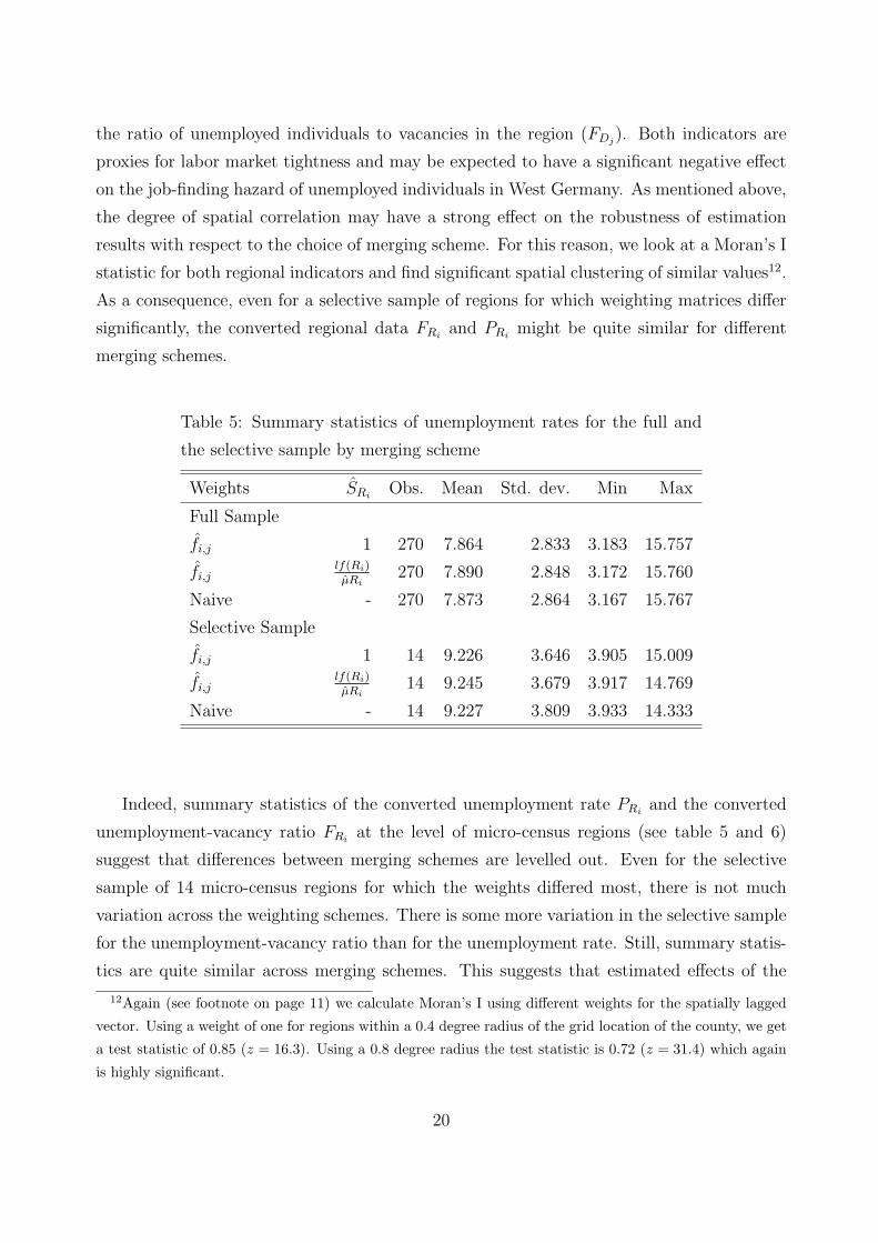
the ratio of unemployed individuals to vacancies in the region (FDj). Both indicators are

proxies for labor market tightness and may be expected to have a significant negative effect

on the job-finding hazard of unemployed individuals in West Germany. As mentioned above,

the degree of spatial correlation may have a strong effect on the robustness of estimation

results with respect to the choice of merging scheme. For this reason, we look at a Moran’s I

statistic for both regional indicators and find significant spatial clustering of similar values12.

As a consequence, even for a selective sample of regions for which weighting matrices differ

significantly, the converted regional data FRiand PRi

might be quite similar for different

merging schemes.

Table 5: Summary statistics of unemployment rates for the full and

the selective sample by merging scheme

Weights SRiObs. Mean Std. dev. Min Max

Full Sample

fi,j 1 270 7.864 2.833 3.183 15.757

fi,jlf(Ri)µRi

270 7.890 2.848 3.172 15.760

Naive - 270 7.873 2.864 3.167 15.767

Selective Sample

fi,j 1 14 9.226 3.646 3.905 15.009

fi,jlf(Ri)µRi

14 9.245 3.679 3.917 14.769

Naive - 14 9.227 3.809 3.933 14.333

Indeed, summary statistics of the converted unemployment rate PRiand the converted

unemployment-vacancy ratio FRiat the level of micro-census regions (see table 5 and 6)

suggest that differences between merging schemes are levelled out. Even for the selective

sample of 14 micro-census regions for which the weights differed most, there is not much

variation across the weighting schemes. There is some more variation in the selective sample

for the unemployment-vacancy ratio than for the unemployment rate. Still, summary statis-

tics are quite similar across merging schemes. This suggests that estimated effects of the

12Again (see footnote on page 11) we calculate Moran’s I using different weights for the spatially lagged

vector. Using a weight of one for regions within a 0.4 degree radius of the grid location of the county, we get

a test statistic of 0.85 (z = 16.3). Using a 0.8 degree radius the test statistic is 0.72 (z = 31.4) which again

is highly significant.

20

unemployment rate and the unemployment-vacancy ratio on the unemployment duration of

West German job seekers should be very robust across merging scheme, even for the selective

sample.

Table 6: Summary statistics of unemployment/vacancy ratio for the

full and the selective sample by merging scheme

Weights SDiObs. Mean Std. dev. Min Max

Full Sample

pi,j 1 270 8.371 5.121 1.723 30.803

pi,jlf(Dj)

µDj270 8.372 5.109 1.730 31.001

Naive - 270 8.544 5.484 1.720 31.494

Selective Sample

pi,j 1 14 9.833 6.788 1.727 25.023

pi,jlf(Dj)

µDj14 10.064 6.625 1.733 24.994

Naive - 14 11.549 8.178 1.720 25.278

For the sensitivity analysis, we estimate a proportional hazard model where the baseline

hazard includes a common fixed effects for individuals in the same labor market region13.

This may be estimated using Cox’s partial likelihood estimator (Cox, 1972). Including

location-fixed effects in this estimator removes a potential bias of individual and labor mar-

ket related variables that may result from omitting important regional labor market char-

acteristics (Kalbfleisch and Prentice, 1980; Ridder and Tunali, 1999). In addition to the

location-specific fixed effects we also take account of the fact that some individuals have

repeated unemployment spells. Thus, we use the modified sandwich variance estimator to

correct for dependence at the level of the individual (Lin and Wei, 1989).

Table 7 summarizes estimation results for the unemployment rate and the unemployment-

vacancy ratio for the full sample and the three merging schemes. We control for education,

sex, age, marital status, occupational status, economic sector, a set of year dummies as

well as some indicators of prior employment history including total previous unemployment

duration, tenure in the previous job and an indicator variable of whether there has ever been

13We use labor market regions instead of microcensus regions because labor market regions are likely to

be the relevant regional context in which individuals mainly seek employment. There are a total of 180

West-German labor market regions.

21

a recall from the previous employer. Summary statistics and estimation results using the

full and the selective sample can be found in the appendix14.

Table 7: Cox PH model estimates for regional indicators by merging scheme and sample

Full Sample Selective Sample

Merging Scheme Haz. Rat. Std. Err. Haz. Rat.Std. Err.

Unemployment-vacancy ratio

fi,j with SRi= 1 0.989∗∗ 0.000 0.986∗∗ 0.001

fi,j with SRi6= 1 0.989∗∗ 0.000 0.985∗∗ 0.001

Naive 0.989∗∗ 0.000 0.987∗∗ 0.001

Unemployment rate

fi,j with SDj= 1 0.967∗∗ 0.001 0.971∗∗ 0.005

fi,j with SDj6= 1 0.966∗∗ 0.001 0.973∗∗ 0.005

Naive 0.967∗∗ 0.001 0.976∗∗ 0.005

Significance levels : † : 10% ∗ : 5% ∗∗ : 1%

As expected from the above discussion, the effect of the unemployment rate and the

unemployment-vacancy ratio on the job finding hazard is extremely robust across the differ-

ent weighting schemes for the full and the selective sample. In our empirical application the

merging scheme applied has no impact on the estimated hazard ratios up to the 4th decimal

place for the full and up to the 3rd decimal place for the selective sample. This even holds

for the naive merging scheme.

We conclude that, at least in the case of a merging rule between German districts and

counties, the choice of merging rule does not substantially affect our estimation results.

In our specific application it even seems safe to take the simplest approach available to

the researcher: a merging rule based on simple binary weights. However, due to a high

degree of local homogeneity in S, a high degree of similarity of the regional entities and a

strong positive spatial autocorrelation of the data to be merged, this is likely to be a result

that is unique to this particular application. Other countries, for example, may be much

more heterogeneous across space with regard to labor-force densities. Also, other regional

14Since estimation results across the various specifications are very similar, the appendix only includes

detailed results for the Cox model using the unemployment rate as the regional labor market variable in

addition to the individual-specific characteristics. Moreover the estimation results only show the case of

merging the unemployment rate based on a uniform distribution of the region-specific information.

22

entities may be less similar. Thus, researchers applying the above approach to a different

set of regional entities should be aware that these factors have an important effect on the

robustness of their results. Also, they should check the degree of spatial autocorrelation of

the data that has to be merged. If there is spatial clustering of dissimilar values, estimation

results are likely to be much more sensitive to the choice of merging rule than in our particular

application. Therefore, researchers are advised to carefully apply the theoretical framework

to their context and examine the conditions of local homogeneity, similarity of regional

entities and positive or negative spatial autocorrelation in detail before choosing one of the

above merging schemes. Moreover, a sensitivity analysis is always advisable.

4 Conclusion

This paper introduces a theoretical framework for merging different regional data sources

for which no exact merging rule is available. It therefore tackles a substantial problem for

empirical work in labor economics, other fields of economics and social sciences alike. The

combination of data sources often allows the researcher to choose a broader econometric

modelling approach such as allowing for region-specific effects.

We introduce alternative merging rules based on estimates of intersections between both

regional classifications. Such estimates may be obtained from a digital map intersection.

Depending on the properties of the underlying maps, i.e. the resolution and scale, we show

that such estimates may come with non-systematic measurement errors. This paper develops

a theoretical framework for the estimation of map intersections and derives properties under

which estimated intersection areas and weighting schemes that are based on these estimates

are unbiased. Moreover, we identify conditions under which all merging schemes including

the naive merging rule derive comparable and reliable results. Under a high degree of local

homogeneity in the region-specific information (e.g. population density) and under a high

degree of similarity between the two regional classifications, differences between merging

schemes are levelled out. A Monte Carlo simulation demonstrates our theoretical findings.

Moreover it shows for different degrees of local homogeneity that estimation results can

substantially differ depending on the chosen merging scheme.

We apply our theoretical framework to the maps of German counties and employment

office districts and show that our theoretical results carry over to the empirical case. Per-

forming an unemployment duration analysis using the IAB employment subsample merged

with regional data from the federal statistical office shows that the chosen weighting scheme

23

does not significantly affect the estimation results (on average and for a specific subsample).

This result is well explained by our theoretical model.

The estimated weighting matrices for merging data from the federal Employment Office

and the from federal Statistical Office is freely accessible to the research community and can

be downloaded from ftp : //ftp.zew.de/pub/zew − docs/div/arntz − wilke− weights.xls

24

5 Appendix

Table 8: Summary statistics for the full and the selective sample of

unemployment spells, IAB employment subsample, 1981-1997

Full Sample Selective Sample

Mean Std. Err. Mean Std. Err.

Unemployment duration (in days) 293.24 443.86 285.55 407.46

Female 0.41 0.49 0.44 0.50

Married 0.46 0.50 0.44 0.50

Married female 0.21 0.41 0.21 0.41

Age < 21 0.08 0.28 0.07 0.26

Age 21-25 0.23 0.42 0.21 0.41

Age 31-35 0.14 0.35 0.14 0.35

Age 36-40 0.11 0.31 0.13 0.32

Age 41-45 0.10 0.30 0.11 0.31

Age 46-49 0.07 0.26 0.08 0.27

Age 50-53 0.08 0.27 0.08 0.27

Low education 0.38 0.49 0.36 0.48

Higher education 0.04 0.20 0.05 0.23

Low educ. x Sex 0.16 0.37 0.17 0.37

High. educ. x Sex 0.02 0.13 0.02 0.15

Apprenticeship 0.07 0.25 0.06 0.25

Low skilled worker 0.34 0.48 0.32 0.47

White collar worker 0.25 0.43 0.30 0.46

Parttime work 0.08 0.27 0.09 0.28

Agriculture 0.03 0.17 0.02 0.13

Inv. goods industry 0.20 0.40 0.17 0.38

Cons. goods industry 0.12 0.32 0.08 0.28

Construction 0.15 0.36 0.12 0.33

Services 0.31 0.46 0.38 0.49

Tenure in previous job (in months) 27.20 38.09 26.88 38.64

Previous recall 0.06 0.23 0.05 0.22

Total unemp. duration (in months) 8.43 15.03 8.29 14.70

1983-1987 0.32 0.47 0.32 0.47

1988-1991 0.19 0.39 0.19 0.39

1992-1997 0.34 0.47 0.34 0.47

Unemployment ratea 9.70 3.38 9.34 3.56

Number of spells 255,100 83,104

Number of individuals 126,189 24,674

Percentage right-censored 28.4 29.7

a Regional information has been merged using the uniform distribution of the

region-specific information SDj = 1.

25

Table 9: Cox PH model estimates using the full and the selective sample, IAB employment

subsample, 1981-1997

Full Sample Selective Sample

Variable Hazard Ratio (Std. Err.) Hazard Ratio (Std. Err.)

Female 1.112∗∗ (0.011) 1.127∗∗ (0.035)

Married 1.219∗∗ (0.008) 1.227∗∗ (0.031)

Married female 0.539∗∗ (0.013) 0.583∗∗ (0.022)

Age < 21 1.217∗∗ (0.010) 1.281∗∗ (0.045)

Age 21-25 1.103∗∗ (0.008) 1.141∗∗ (0.029)

Age 31-35 0.985† (0.009) 1.001† (0.029)

Age 36-40 1.000 (0.011) 1.002 (0.031)

Age 41-45 1.001 (0.011) 1.011 (0.035)

Age 46-49 0.968∗ (0.013) 0.930∗ (0.037)

Age 50-53 0.831∗∗ (0.015) 0.823∗∗ (0.037)

Low education 0.883∗∗ (0.009) 0.847∗∗ (0.023)

Higher education 0.792∗∗ (0.020) 0.779∗∗ (0.044)

Low educ. x Sex 0.968∗ (0.013) 1.035∗ (0.041)

High. educ. x Sex 1.149∗∗ (0.030) 1.120∗∗ (0.089)

Apprenticeship 1.082∗∗ (0.013) 1.136∗∗ (0.045)

Low skilled worker 0.798∗∗ (0.009) 0.845∗∗ (0.023)

White collar worker 0.752∗∗ (0.010) 0.805∗∗ (0.023)

Parttime work 0.806∗∗ (0.016) 0.829∗∗ (0.035)

Agriculture 1.317∗∗ (0.020) 1.333∗∗ (0.092)

Inv. goods industry 0.927∗∗ (0.010) 0.926∗∗ (0.027)

Cons. goods industry 0.925∗∗ (0.011) 1.029∗∗ (0.036)

Construction 1.221∗∗ (0.010) 1.347∗∗ (0.041)

Services 0.984† (0.009) 1.024† (0.025)

Tenure in previous job 0.995∗∗ (0.000) 0.994∗∗ (0.000)

Previous recall 0.781∗∗ (0.012) 0.756∗∗ (0.031)

Total unemp. duration 0.995∗∗ (0.000) 0.997∗∗ (0.001)

1983-1987 1.245∗∗ (0.008) 1.252∗∗ (0.033)

1988-1991 1.332∗∗ (0.009) 1.365∗∗ (0.039)

1992-1997 1.085∗∗ (0.009) 1.122∗∗ (0.032)

Unemployment rate 0.967∗∗ (0.001) 0.971∗∗ (0.005)

Log-likelihood -1,217,399.365 -121,004

χ2(30) 18,724.774 1,961.91

Significance levels : † : 10% ∗ : 5% ∗∗ : 1%

Using the merging scheme with SDj = 1.

26

References

[1] Bender, S., Haas, A., and Klose, C. (2000). The IAB Employment Subsample 1975–1995.

Schmollers Jahrbuch 120, 649–662.

[2] Elstrodt, J. (1999). Maß- und Integrationstheorie. 2nd ed., Springer, Berlin.

[3] Cox (1972). Regression Models and Life Tables. Journal of the Statistical Society B 34,

187–220.

[4] Fitzenberger, B. and Wilke, R. (2004). Unemployment Durations in West-Germany

Before and After the Reform of the Unemployment Compensation System during the

1980ties. ZEW Discussion Paper 04-24.

[5] Kalbfleisch, J.D. and Prentice, R.L. (1980). The Statistical Analysis of Failure Time

Data. Wiley, New York.

[6] Lin, D.Y. and Wei, L.J. (1989). The robust inference for the Cox proportional hazards

model. Journal of the American Statistical Association 84, 1074–1078.

[7] Ridder, G. and Tunali, I. (1999). Stratified partial likelihood estimation. Journal of

Econometrics 92, 193–232.

[8] Statistische Amter des Bundes und der Lander (1999). Statistik Regional. Daten fur die

Kreise und kreisfreien Stadte Deutschlands. Wiesbaden.

27