NNT : 2018SACLT009 THÈSE DE DOCTORAT de L’UNIVERSITÉ PARIS -S ACLAY École doctorale de mathématiques Hadamard (EDMH, ED 574) Établissement d’inscription : Télécom ParisTech Laboratoire d’accueil : Laboratoire traitement et communication de l’information (LTCI) Spécialité de doctorat : Mathématiques appliquées Anna Charlotte Korba Learning from Ranking Data: Theory and Methods Date de soutenance : 25 octobre 2018 Après avis des rapporteurs : SHIVANI AGARWAL (University of Pennsylvania) EYKE HÜLLERMEIER (Paderborn University) Jury de soutenance : STEPHAN CLÉMENÇON (Télécom ParisTech) Directeur de thèse SHIVANI AGARWAL (University of Pennsylvania) Rapporteure EYKE HÜLLERMEIER (University of Paderborn) Rapporteur J EAN-PHILIPPE VERT (Mines ParisTech) Président du jury NICOLAS VAYATIS (ENS Cachan) Examinateur FLORENCE D’ALCHÉ BUC (Télécom ParisTech) Examinatrice

Welcome message from author
This document is posted to help you gain knowledge. Please leave a comment to let me know what you think about it! Share it to your friends and learn new things together.
Transcript
NNT : 2018SACLT009
THÈSE DE DOCTORAT
de
L’UNIVERSITÉ PARIS-SACLAY
École doctorale de mathématiques Hadamard (EDMH, ED 574)
Établissement d’inscription : Télécom ParisTech
Laboratoire d’accueil : Laboratoire traitement et communication de l’information (LTCI)
Spécialité de doctorat : Mathématiques appliquées
Anna Charlotte Korba
Learning from Ranking Data: Theory and Methods
Date de soutenance : 25 octobre 2018
Après avis des rapporteurs :SHIVANI AGARWAL (University of Pennsylvania)
EYKE HÜLLERMEIER (Paderborn University)
Jury de soutenance :
STEPHAN CLÉMENÇON (Télécom ParisTech) Directeur de thèse
SHIVANI AGARWAL (University of Pennsylvania) Rapporteure
EYKE HÜLLERMEIER (University of Paderborn) Rapporteur
JEAN-PHILIPPE VERT (Mines ParisTech) Président du jury
NICOLAS VAYATIS (ENS Cachan) Examinateur
FLORENCE D’ALCHÉ BUC (Télécom ParisTech) Examinatrice


Remerciements
Mes premiers remerciements vont à mon directeur de thèse Stephan et mon encadrant Eric.
Stephan, merci pour ta présence et ton soutien, pendant toute la thèse et jusque dans la recherche
de postdoc. Je te remercie pour le savoir que tu m’as transmis, pour ta gentillesse quotidienne.
Tu m’as fait découvrir le monde de la recherche et j’ai beaucoup appris à tes côtés. Et merci
de m’avoir envoyée en conférence aux quatre coins du monde! Pour tout cela, je te suis très
reconnaissante. Eric, merci pour ton investissement, ton énergie incroyable, tu m’as grandement
mis le pied à l’étrier au début de la thèse. C’était un vrai challenge de passer après toi. J’adore
nos discussions mathématiques (et cinéma!) et j’espère que l’on en aura encore d’autres dans le
futur.
I also thank deeply Arthur Gretton, for giving me the opportunity to continue in postdoc in his
laboratory. I really look forward to working with you and the team on new machine learning
projects!
I sincerely thank Eyke Hüllermeier et Shivani Agarwal, whose contributions in ranking and
preference learning have inspired me for three years, for having reviewed this thesis. It was
an honour for me. Merci à Jean-Philippe Vert, Nicolas Vayatis, Florence d’Alché-Buc d’avoir
accepté de faire partie de mon jury, je vous en suis très reconnaissante.
Je veux bien évidemment remercier toutes les personnes que j’ai rencontré pendant ma thèse, à
commencer par mes collègues de l’équipe stats à Telecom, avec qui j’ai passé trois années fab-
uleuses. Merci à Florence d’Alché Buc pour nos discussions (scientifiques et autres), à François
Roueff pour son suivi pendant ma thèse, à Ons Jelassi pour sa gentillesse. Merci aux jeunes
chercheurs qui m’inspirent, Joseph, François, Maxime, pour leur bienveillance et leurs conseils
précieux. Je remercie bien évidemment mon premier bureau, composé de Nicolas qui tient la
baraque, Igor au Mexique, ce bon vieil Aurélien et Albert le thug (qui parle désormais le verlan
mieux que moi). Je n’arrive pas à compter le nombre de blagues cultes qui rythment notre amitié
et nos discussions, sur le bar à huîtres, la peau de phoque d’Igor, DAMEX, ou sur les apparitions
du rôdeur ou de la sentinelle. Merci pour tous les fous rires. Parmi les anciens de Dareau, je
remercie aussi ce cher Guillaume Papa pour son humour fin et épicé, nos discussions cinéma
et musique, et pour avoir toujours été disponible quand j’avais besoin d’un coup de main. Je
n’oublie évidemment pas nos partenaires de crime Ray Brault (prononcer "Bro") et Maël pour
leur zenitude et nos pauses cigarette. Un grand big up à ma génération de thésards à Télécom:
la mafia Black in AI composée d’Adil et Eugène, qui partagent avec moi le goût des belles
mathématiques et du rap de qualité, je ris encore de vos galères à New York (@Adil: pense à
vider ton téléphone, @Eugène: pense à charger le tien ou prendre les clés de l’appart) ; ainsi
iii

iv REMERCIEMENTS
que Moussab, qui j’en suis sûre va conquérir le monde. J’espère que l’on continuera à avoir des
discussions toujours aussi enrichissantes. Merci aux générations suivantes, avec los chicos de
Argentina Mastane (qui n’oublie jamais de mettre sa sacoche Lacoste pour donner un talk) et
Robin (qui se prépare pour les J.O.), the great Pierre A. le romantique, Alexandre l’avocat du
deep learning, la team de choc et police du style Pierre L. et Mathurin, jamais à court d’idées
pour des calembours ou de ressources pour shoes de chercheurs, les sapeurs et ambassadeurs du
swag Alex, Hamid, Kévin; la dernière génération avec Sholom et Anas. Je remercie en parti-
culier mes coauteurs Mastane et Alexandre, c’était vraiment un plaisir de travailler avec vous.
Thanks to my neighbor Umut for always being up for a beer. Merci à tous les autres collègues
de l’équipe que j’oublie. Merci aussi à mes autres amis thésards du domaine, tout d’abord mes
amis de master qui ont aussi poursuivi en thèse: Aude, Martin, Thibault, Antoine, Maryan. I
also thank my coauthor Yunlong, it was a pleasure to work with you and I hope our geographic
proximity for the postdoc will bring us to meet again very soon. Je remercie ma party squad à
MLSS: la deutsch mafia comprenant Alexander, Malte, Florian et Julius; la french mafia avec
Arthur aka blazman, Elvis, Thibaud; merci pour ces souvenirs incroyables. Nous avons cer-
tainement donné un nouveau sens à l’amitié franco-allemande. Merci aussi à Thomas et Cédric
de Cachan, pour nos discussions (souvent gossip), pauses cafés et bières en conférence. Avec
toutes ces personnes que j’ai eu le plaisir de connaître pendant ma thèse, je garde d’excellents
souvenirs de nos moments à la Butte aux cailles, ou bien en voyage à Lille, Montréal, New York,
Barcelone, Miami, Tübingen, Los Angeles, Stockholm et j’en passe. Merci à Laurence Zelmar
à qui j’ai donné beaucoup de boulot avec tous ces ordres de mission.
J’aimerais ensuite remercier toutes les personnes qui m’ont toujours soutenue. Un merci très
spécial à ma famille et en particulier mes parents. Je n’en serais pas là sans vous aujourd’hui,
vous m’avez donné toutes les chances de réussir. Votre force de travail et votre détermination
m’ont forgée et sont un exemple. Merci aussi à mon petit frère Julien qui en a aussi hérité, pour
son soutien. Merci à mes professeurs de lycée, de prépa et d’école qui m’ont mise sur la voie
des mathématiques et de la recherche et m’ont encouragé dans cette direction.
Je remercie aussi profondément mes amis, ma deuxième famille, toujours présents pour
m’écouter, décompresser autour d’un verre ou faire la fête. Merci aux amis d’enfance (Juli-
ette, Alix), aux Cegarra (Christine, Camille, Lila), aux amis du lycée (Mahalia, Jean S., Yaacov,
Cristina, Georgia, Sylvain, Raphaël, Hugo P., Hugo H., Julien, Larry, Bastien, Maryon, Alice),
de prépa (Bettina, Clément G., Anne, Yvanie, Louis P., Charles, Samar, Igor, Pibrac, Kévin),
de l’ENSAE (Pascal, Amine, Dona, Parviz, Gombert, Marie B., Jean P., Antoine, Théo, Louise,
Clément P.), aux amis d’amis qui sont devenus les miens (Marie V., Elsa, Léo S., le ghetto
bébère, Arnaud, Rémi), et pardon à tous ceux que j’oublie ici. Merci pour votre soutien, votre
franchise, vous êtes très importants pour moi. J’ai de la chance de vous avoir dans ma vie et
j’espère bien que vous me rendrez visite l’année prochaine!
Enfin je remercie Louis, qui partage ma vie, de me supporter et d’être présent pour moi depuis
tant d’années. Merci pour ta patience et ton affection.

Contents
List of Publications ix
List of Figures xi
List of Tables xiii
List of Symbols xv
1 Introduction 11.1 Background on Ranking Data . . . . . . . . . . . . . . . . . . . . . . . . . . . 21.2 Ranking Aggregation . . . . . . . . . . . . . . . . . . . . . . . . . . . . . . . 2
1.2.1 Definition and Context . . . . . . . . . . . . . . . . . . . . . . . . . . 31.2.2 A General Method to Bound the Distance to Kemeny Consensus . . . . 41.2.3 A Statistical Framework for Ranking Aggregation . . . . . . . . . . . 6
1.3 Beyond Ranking Aggregation: Dimensionality Reduction and Ranking Regression 71.3.1 Dimensionality Reduction for Ranking Data: a Mass Transportation Ap-
proach . . . . . . . . . . . . . . . . . . . . . . . . . . . . . . . . . . . 81.3.2 Ranking Median Regression: Learning to Order through Local Consensus 101.3.3 A Structured Prediction Approach for Label Ranking . . . . . . . . . . 12
1.4 Conclusion . . . . . . . . . . . . . . . . . . . . . . . . . . . . . . . . . . . . 131.5 Outline of the Thesis . . . . . . . . . . . . . . . . . . . . . . . . . . . . . . . 14
2 Background on Ranking Data 152.1 Introduction to Ranking Data . . . . . . . . . . . . . . . . . . . . . . . . . . . 15
2.1.1 Definitions and Notations . . . . . . . . . . . . . . . . . . . . . . . . 152.1.2 Ranking Problems . . . . . . . . . . . . . . . . . . . . . . . . . . . . 162.1.3 Applications . . . . . . . . . . . . . . . . . . . . . . . . . . . . . . . 18
2.2 Analysis of Full Rankings . . . . . . . . . . . . . . . . . . . . . . . . . . . . 202.2.1 Parametric Approaches . . . . . . . . . . . . . . . . . . . . . . . . . . 212.2.2 Non-parametric Approaches . . . . . . . . . . . . . . . . . . . . . . . 232.2.3 Distances on Rankings . . . . . . . . . . . . . . . . . . . . . . . . . . 26
2.3 Other Frameworks . . . . . . . . . . . . . . . . . . . . . . . . . . . . . . . . 28
I Ranking Aggregation 31
3 The Ranking Aggregation Problem 333.1 Ranking Aggregation . . . . . . . . . . . . . . . . . . . . . . . . . . . . . . . 33
3.1.1 Definition . . . . . . . . . . . . . . . . . . . . . . . . . . . . . . . . . 33
v
vi CONTENTS
3.1.2 Voting Rules Axioms . . . . . . . . . . . . . . . . . . . . . . . . . . . 343.2 Methods . . . . . . . . . . . . . . . . . . . . . . . . . . . . . . . . . . . . . . 35
3.2.1 Kemeny’s Consensus . . . . . . . . . . . . . . . . . . . . . . . . . . . 353.2.2 Scoring Methods . . . . . . . . . . . . . . . . . . . . . . . . . . . . . 363.2.3 Spectral Methods . . . . . . . . . . . . . . . . . . . . . . . . . . . . . 383.2.4 Other Ranking Aggregation Methods . . . . . . . . . . . . . . . . . . 39
4 A General Method to Bound the Distance to Kemeny Consensus 414.1 Introduction . . . . . . . . . . . . . . . . . . . . . . . . . . . . . . . . . . . . 414.2 Controlling the Distance to a Kemeny Consensus . . . . . . . . . . . . . . . . 424.3 Geometric Analysis of Kemeny Aggregation . . . . . . . . . . . . . . . . . . . 434.4 Main Result . . . . . . . . . . . . . . . . . . . . . . . . . . . . . . . . . . . . 454.5 Geometric Interpretation and Proof of Theorem 10.1 . . . . . . . . . . . . . . 47
4.5.1 Extended Cost Function . . . . . . . . . . . . . . . . . . . . . . . . . 474.5.2 Interpretation of the Condition in Theorem 10.1 . . . . . . . . . . . . . 484.5.3 Embedding of a Ball . . . . . . . . . . . . . . . . . . . . . . . . . . . 504.5.4 Proof of Theorem 10.1 . . . . . . . . . . . . . . . . . . . . . . . . . . 50
4.6 Numerical Experiments . . . . . . . . . . . . . . . . . . . . . . . . . . . . . . 514.6.1 Tightness of the Bound . . . . . . . . . . . . . . . . . . . . . . . . . . 514.6.2 Applicability of the Method . . . . . . . . . . . . . . . . . . . . . . . 54
4.7 Conclusion and Discussion . . . . . . . . . . . . . . . . . . . . . . . . . . . . 55
5 A Statistical Framework for Ranking Aggregation 575.1 Introduction . . . . . . . . . . . . . . . . . . . . . . . . . . . . . . . . . . . . 575.2 Background . . . . . . . . . . . . . . . . . . . . . . . . . . . . . . . . . . . . 58
5.2.1 Consensus Ranking . . . . . . . . . . . . . . . . . . . . . . . . . . . . 585.2.2 Statistical Framework . . . . . . . . . . . . . . . . . . . . . . . . . . 595.2.3 Connection to Voting Rules . . . . . . . . . . . . . . . . . . . . . . . 60
5.3 Optimality . . . . . . . . . . . . . . . . . . . . . . . . . . . . . . . . . . . . . 615.4 Empirical Consensus . . . . . . . . . . . . . . . . . . . . . . . . . . . . . . . 64
5.4.1 Universal Rates . . . . . . . . . . . . . . . . . . . . . . . . . . . . . . 645.4.2 Fast Rates in Low Noise . . . . . . . . . . . . . . . . . . . . . . . . . 665.4.3 Computational Issues . . . . . . . . . . . . . . . . . . . . . . . . . . . 67
5.5 Conclusion . . . . . . . . . . . . . . . . . . . . . . . . . . . . . . . . . . . . 685.6 Proofs . . . . . . . . . . . . . . . . . . . . . . . . . . . . . . . . . . . . . . . 68
II Beyond Ranking Aggregation: Dimensionality Reduction and Ranking Re-gression 77
6 Dimensionality Reduction and (Bucket) Ranking:A Mass Transportation Approach 796.1 Introduction . . . . . . . . . . . . . . . . . . . . . . . . . . . . . . . . . . . . 796.2 Preliminaries . . . . . . . . . . . . . . . . . . . . . . . . . . . . . . . . . . . 80
6.2.1 Background on Bucket Orders . . . . . . . . . . . . . . . . . . . . . . 806.2.2 A Mass Transportation Approach to Dimensionality Reduction on Sn . 816.2.3 Optimal Couplings and Minimal Distortion . . . . . . . . . . . . . . . 836.2.4 Related Work . . . . . . . . . . . . . . . . . . . . . . . . . . . . . . . 84

CONTENTS vii
6.3 Empirical Distortion Minimization - Rate Bounds and Model Selection . . . . . 856.4 Numerical Experiments on Real-world Datasets . . . . . . . . . . . . . . . . . 886.5 Conclusion . . . . . . . . . . . . . . . . . . . . . . . . . . . . . . . . . . . . 896.6 Appendix . . . . . . . . . . . . . . . . . . . . . . . . . . . . . . . . . . . . . 896.7 Proofs . . . . . . . . . . . . . . . . . . . . . . . . . . . . . . . . . . . . . . . 100
7 Ranking Median Regression: Learning to Order through Local Consensus 1057.1 Introduction . . . . . . . . . . . . . . . . . . . . . . . . . . . . . . . . . . . . 1057.2 Preliminaries . . . . . . . . . . . . . . . . . . . . . . . . . . . . . . . . . . . 107
7.2.1 Best Strictly Stochastically Transitive Approximation . . . . . . . . . . 1077.2.2 Predictive Ranking and Statistical Conditional Models . . . . . . . . . 108
7.3 Ranking Median Regression . . . . . . . . . . . . . . . . . . . . . . . . . . . 1097.4 Local Consensus Methods for Ranking Median Regression . . . . . . . . . . . 112
7.4.1 Piecewise Constant Predictive Ranking Rules and Local Consensus . . 1127.4.2 Nearest-Neighbor Rules for Ranking Median Regression . . . . . . . . 1167.4.3 Recursive Partitioning - The CRIT algorithm . . . . . . . . . . . . . . 118
7.5 Numerical Experiments . . . . . . . . . . . . . . . . . . . . . . . . . . . . . . 1217.6 Conclusion and Perspectives . . . . . . . . . . . . . . . . . . . . . . . . . . . 1237.7 Appendix - On Aggregation in Ranking Median Regression . . . . . . . . . . . 1237.8 Proofs . . . . . . . . . . . . . . . . . . . . . . . . . . . . . . . . . . . . . . . 126
8 A Structured Prediction Approach for Label Ranking 1378.1 Introduction . . . . . . . . . . . . . . . . . . . . . . . . . . . . . . . . . . . . 1378.2 Preliminaries . . . . . . . . . . . . . . . . . . . . . . . . . . . . . . . . . . . 138
8.2.1 Mathematical Background and Notations . . . . . . . . . . . . . . . . 1388.2.2 Related Work . . . . . . . . . . . . . . . . . . . . . . . . . . . . . . . 139
8.3 Structured Prediction for Label Ranking . . . . . . . . . . . . . . . . . . . . . 1408.3.1 Learning Problem . . . . . . . . . . . . . . . . . . . . . . . . . . . . . 1408.3.2 Losses for Ranking . . . . . . . . . . . . . . . . . . . . . . . . . . . . 141
8.4 Output Embeddings for Rankings . . . . . . . . . . . . . . . . . . . . . . . . 1428.4.1 The Kemeny Embedding . . . . . . . . . . . . . . . . . . . . . . . . . 1428.4.2 The Hamming Embedding . . . . . . . . . . . . . . . . . . . . . . . . 1438.4.3 Lehmer Code . . . . . . . . . . . . . . . . . . . . . . . . . . . . . . . 1448.4.4 Extension to Partial and Incomplete Rankings . . . . . . . . . . . . . . 145
8.5 Computational and Theoretical Analysis . . . . . . . . . . . . . . . . . . . . . 1468.5.1 Theoretical Guarantees . . . . . . . . . . . . . . . . . . . . . . . . . . 1468.5.2 Algorithmic Complexity . . . . . . . . . . . . . . . . . . . . . . . . . 148
8.6 Numerical Experiments . . . . . . . . . . . . . . . . . . . . . . . . . . . . . . 1488.7 Conclusion . . . . . . . . . . . . . . . . . . . . . . . . . . . . . . . . . . . . 1498.8 Proofs and Additional Experiments . . . . . . . . . . . . . . . . . . . . . . . . 150
8.8.1 Proof of Theorem 1 . . . . . . . . . . . . . . . . . . . . . . . . . . . . 1508.8.2 Lehmer Embedding for Partial Rankings . . . . . . . . . . . . . . . . 1528.8.3 Additional Experimental Results . . . . . . . . . . . . . . . . . . . . . 153
9 Conclusion, Limitations & Perspectives 155
10 Résumé en français 15710.1 Préliminaires sur les Données de Classements . . . . . . . . . . . . . . . . . . 158

viii CONTENTS
10.2 L’agrégation de Classements . . . . . . . . . . . . . . . . . . . . . . . . . . . 15910.2.1 Définition et Contexte . . . . . . . . . . . . . . . . . . . . . . . . . . 15910.2.2 Une Méthode Générale pour Borner la Distance au Consensus de Kemeny16110.2.3 Un Cadre Statistique pour l’Agrégation de Classements . . . . . . . . . 162
10.3 Au-delà de l’Agrégation de Classements : la Réduction de Dimension et la Ré-gression de Classements . . . . . . . . . . . . . . . . . . . . . . . . . . . . . 16410.3.1 Réduction de Dimension pour les Données de Classements : une Ap-
proche de Transport de Masse . . . . . . . . . . . . . . . . . . . . . . 16410.3.2 Régression Médiane de Classements: Apprendre à Classer à travers des
Consensus Locaux . . . . . . . . . . . . . . . . . . . . . . . . . . . . 16710.3.3 Une Approche de Prédiction Structurée pour la Régression de Classements169
10.4 Conclusion . . . . . . . . . . . . . . . . . . . . . . . . . . . . . . . . . . . . 17110.5 Plan de la Thèse . . . . . . . . . . . . . . . . . . . . . . . . . . . . . . . . . . 171
Bibliography 173

List of Publications
Publications
• Dimensionality Reduction and (Bucket) Ranking: A Mass Transportation Approach. (preprint)Authors: Mastane Achab*, Anna Korba*, Stephan Clémençon. (*: equal contribution).
• A Structured Prediction Approach for Label Ranking. (NIPS 2018)Authors: Anna Korba, Alexandre Garcia, Florence D’Alché Buc.
• On Aggregation in Ranking Median Regression. (ESANN 2018)Authors: Stephan Clémençon and Anna Korba.
• Ranking Median Regression: Learning to Order through Local Consensus. (ALT 2018)Authors: Stephan Clémençon, Anna Korba and Eric Sibony.
• A Learning Theory of Ranking Aggregation. (AISTATS 2017).Authors: Anna Korba, Stephan Clémençon and Eric Sibony.
• Controlling the distance to a Kemeny consensus without computing it. (ICML 2016).Authors: Yunlong Jiao, Anna Korba and Eric Sibony.
Workshops
• Ranking Median Regression: Learning to Order through Local Consensus. (NIPS 2017 Workshopon Discrete Structures in Machine Learning)Authors: Stephan Clémençon, Anna Korba and Eric Sibony.
ix


List of Figures
2.1 An illustration of a pairwise comparison graph for 4 items. . . . . . . . . . . . 252.2 Permutahedron of order 4. . . . . . . . . . . . . . . . . . . . . . . . . . . . . 28
3.1 An election where Borda count does not elect the Condorcet winner . . . . . . . 373.2 Hodge/Helmotz decomposition of the space of pairwise rankings. . . . . . . . 38
4.1 Kemeny aggregation for n = 3. . . . . . . . . . . . . . . . . . . . . . . . . . . 454.2 Level sets of CN over S. . . . . . . . . . . . . . . . . . . . . . . . . . . . . . . 484.3 Illustration of Lemma 4.7. . . . . . . . . . . . . . . . . . . . . . . . . . . . . 504.4 Boxplot of s (r,DN , n) over sampling collections of datasets shows the ef-
fect from different size of alternative set n with restricted sushi datasets (n =3; 4; 5, N = 5000). . . . . . . . . . . . . . . . . . . . . . . . . . . . . . . . . 52
4.5 Boxplot of s (r,DN , n) over sampling collections of datasets shows the effectfrom different voting rules r with 500 bootstrapped pseudo-samples of the APAdataset (n = 5, N = 5738). . . . . . . . . . . . . . . . . . . . . . . . . . . . . 53
4.6 Boxplot of s (r,DN , n) over sampling collections of datasets shows the effectfrom datasets DN . 100 Netflix datasets with the presence of Condorcet winnerand 100 datasets with no Condorcet winner (n = 4 and N varies for each sample). 53
4.7 Boxplot of kmin over 500 bootstrapped pseudo-samples of the sushi dataset(n = 10, N = 5000). . . . . . . . . . . . . . . . . . . . . . . . . . . . . . . . 54
6.1 Dimension-Distortion plot for different bucket sizes on real-world preferencedatasets. . . . . . . . . . . . . . . . . . . . . . . . . . . . . . . . . . . . . . . 88
6.2 Dimension-Distortion plot for different bucket sizes on simulated datasets. . . . 916.3 Dimension-Distortion plot for a true bucket distribution versus a uniform distri-
bution (n = 10 on top and n = 20 below). . . . . . . . . . . . . . . . . . . . . 92
7.1 Example of a distribution satisfying Assumptions 2-3 in R2 . . . . . . . . . . . 1147.2 Pseudo-code for the k-NN algorithm. . . . . . . . . . . . . . . . . . . . . . . 1167.3 Pseudo-code for the CRIT algorithm. . . . . . . . . . . . . . . . . . . . . . . 1187.4 Pseudo-code for the aggregation of RMR rules. . . . . . . . . . . . . . . . . . 124
xi


List of Tables
2.1 Possible rankings for n = 3. . . . . . . . . . . . . . . . . . . . . . . . . . . . 152.2 The dataset from Croon (1989) (p.111), which collected 2262 answers. After
the fall of the Berlin wall a survey of German citizens was conducted wherethey were asked to rank four political goals: (1) maintain order, (2) give peoplemore say in government, (3) fight rising prices, (4) protect freedom of speech. . 18
2.3 An overview of popular assumptions on the pairwise probabilities. . . . . . . . 25
4.1 Summary of a case-study on the validity of Method 1 with the sushi dataset(N = 5000, n = 10). Rows are ordered by increasing kmin (or decreasingcosine) value. . . . . . . . . . . . . . . . . . . . . . . . . . . . . . . . . . . . 47
7.1 Empirical risk averaged on 50 trials on simulated data for kNN, CRIT and para-metric baseline. . . . . . . . . . . . . . . . . . . . . . . . . . . . . . . . . . . 134
7.2 Empirical risk averaged on 50 trials on simulated data for aggregation of RMRrules. . . . . . . . . . . . . . . . . . . . . . . . . . . . . . . . . . . . . . . . . 135
8.1 Embeddings and regressors complexities. . . . . . . . . . . . . . . . . . . . . 1488.2 Mean Kendall’s τ coefficient on benchmark datasets . . . . . . . . . . . . . . . 1498.3 Rescaled Hamming distance on benchmark datasets . . . . . . . . . . . . . . . 1538.4 Mean Kendall’s τ coefficient on additional datasets . . . . . . . . . . . . . . . 154
xiii


List of Symbols
n Number of objects
JnK Set of n items 1, 2, . . . , nN Number of samples
Sn Symmetric group over n items
dτ Kendall’s τ distance
σ Any permutation in Sn
δσ Dirac mass at any point σ
Σ Any random permutation in Sn
P Any distribution on Sn
X A feature space
µ Any distribution on Xa ≺ b Item a is preferred to item b
C Any finite set
#C Cardinality of finite set C
‖.‖ L-2 norm
|.| L-1 norm
f Any function
f−1 Inverse of f
Im(f) Image of function f
R Set of real numbers
I. Indicator of an event
P. Probability of an event
E[.] Expectation of an event
xv


CHAPTER 1Introduction
Ranking data naturally appears in a wide variety of situations, especially when the data comes
from human activities: ballots in political elections, survey answers, competition results, cus-
tomer buying behaviors or user preferences. Handling preference data, in particular to perform
aggregation, refers to a long series of works in social choice theory initiated by Condorcet at
the 18th century, and modeling such distributions began to be studied in 1951 by Mallows. But
ordering objects is also a task that often arises in modern applications of data processing. For
instance, search engines aim at presenting to an user who has entered a given query, the list of
matching results ordered from most to least relevant. Similarly, recommendation systems (for
e-commerce, movie or music platforms...) aim at presenting objects that might interest an user,
in an order that sticks best to her preferences. However, ranking data is much less considered in
the statistics and machine learning literature than real-valued data, mainly because the space of
rankings is not provided with a vector-space structure and thus classical statistics and machine
learning methods cannot be applied in a direct manner. Indeed, even the basic notion of an
average or a median for ranking data, namely ranking aggregation or consensus ranking, raises
great mathematical and computational challenges. Hence, a vast majority of the literature rely
on parametric models.
In this thesis, we investigate the hardness of ranking data problems and introduce new non-
parametric statistical methods tailored to this data. In particular, we formulate the consensus
ranking problem in a rigorous statistical framework and derive theoretical results concerning the
statistical behavior of empirical solutions and the tractability of the problem. This framework
is actually a cornerstone since it can be extended to two closely related problems, supervised
and unsupervised: dimensionality reduction and ranking regression, or label ranking. Indeed,
while classical algebraic-based methods for dimensionality reduction cannot be applied in this
setting, we propose a mass transportation approach for ranking data. Then, we explore and
build consistent rules for ranking regression, firstly by highlighting the fact that this supervised
problem is an extension of ranking aggregation. In this chapter, we recall the main statistical
challenges in ranking data and outline the contributions of the thesis.
1
2 Chapter 1. Introduction
1.1 Background on Ranking Data
We start by introducing the notations and objects used along the manuscript. Consider a set of
items indexed by 1, . . . , n, that we will denote JnK. A ranking is an ordered list of items in
JnK. Rankings are heterogeneous objets: they can be complete (i.e., involving all the items) or
incomplete; and for both cases, they can be without-ties (total order) or with-ties (weak order).
A full ranking is a total order: i.e. complete, and without-ties ranking of the items in JnK. It
can be seen as a permutation, i.e. a bijection σ : JnK → JnK, mapping each item i to its rank
σ(i). The rank of item i is thus σ(i) and the item ranked at position j is σ−1(j). We say that
i is preferred over j (denoted by i ≺ j) according to σ if and only if i is ranked lower than j:
σ(i) < σ(j). The set of all permutations over n items, endowed with the composition operation,
is called the symmetric group and denoted by Sn. The analysis of full ranking data thus relies
on this group. Other types of rankings are particularly present in the literature, namely partial
and incomplete rankings. A partial ranking is a complete ranking (i.e. involving all the items)
with ties, and is also referred sometimes in the literature as a weak order or bucket order. It
includes in particular the case of top-k rankings, that is to say partial rankings dividing the items
in two groups: the first one being the k ≤ n most relevant (or preferred) items and the second
one including all the remaining items. These top-k rankings are given a lot of attention since
they are especially relevant for modern applications, such as search engines or recommendation
systems where the number of items to be ranked is very large and users pay more attention to the
items ranked first. Another type of ranking, also very relevant in such large-scale settings, is the
case of incomplete ranking; i.e., strict orders involving only a small subset of items. A particular
case of incomplete rankings is the case of pairwise comparisons, i.e. rankings involving only
two items. As any ranking, of any type, can be decomposed into pairwise comparisons, the
study of these rankings is exceptionally well-spread in the literature.
The heterogeneity of ranking data makes it arduous to cast in a general framework, and usually
the contributions in the literature focus on one specific class of rankings. The reader may refer
to Chapter 2 for a general background on this subject. In this thesis, we will focus on the case of
full rankings; i.e. complete, and without-ties ranking of the items in JnK. However, as we will
underline through the thesis, our analysis can be naturally extended to the setting of pairwise
comparisons through the extensive use we make of a specific distance, namely Kendall’s τ .
1.2 Ranking Aggregation
Ranking aggregation was the first problem to be considered on ranking data and was certainly
the most widely studied in the literature. Originally considered in social choice for elections, the
ranking aggregation problem appears nowadays in many modern applications implying machine
learning (e.g., meta-search engines, information retrieval, biology). It can be viewed as a unsu-
pervised problem, since the goal is to summarize a dataset or a distribution of rankings, as one
Chapter 1. Introduction 3
would compute an average or a median for real-valued data. An overview of the mathematical
challenges and state-of-the-art methods are given Chapter 3. We firstly give the formulation of
the problem and then present our contributions.
1.2.1 Definition and Context
Consider that besides the set of n items, one is given a population of N agents. Suppose that
each agent t ∈ 1, . . . , N expresses its preferences as a full ranking over the n items, which,
as said before, can be seen as a permutation σt ∈ Sn. Collecting preferences of the agents
over the set of items then results in dataset of permutations DN = (σ1, . . . , σN ) ∈ SNn , some-
times referred to as the profile in the social choice literature. The ranking aggregation problem
consists in finding a permutation σ∗ ∈ Sn, called consensus, that best summarizes the dataset.
This task was introduced in the study of election systems in social choice theory, and any proce-
dure mapping a dataset to a consensus is thus called a voting rule. Interestingly, Arrow (1951)
demonstrated his famous impossibility theorem which states that no voting rule can satisfy a
predefined set of axioms, each reflecting the fairness of the election (see Chapter 3). Hence,
there is no canonical procedure for ranking aggregation, and each one has its advantages and its
drawbacks.
This problem has thus been studied extensively and a lot of approaches have been developped,
in particular in two settings. The first possibility is to consider that the dataset is constituted
of noisy versions of a true ranking (e.g., realizations of a parameterized distribution centered
around the true ranking), and the goal is to reconstruct the true ranking thanks to the samples
(e.g., with MLE estimation). The second possibility is to formalize this problem as a discrete
optimization problem over the set of rankings, and to look for the ranking which is the closest
(with respect to some distance) to the rankings observed in the dataset, without any assumption
on the data. The former approach tackles the problem in a rigorous manner, but can lead to
heavy computational costs in practice. In particular, Kemeny ranking aggregation (Kemeny
(1959)) aims at solving:
minσ∈Sn
CN (σ), (1.1)
where CN (σ) =∑N
t=1 d(σ, σt) and d is the Kendall’s τ distance defined for σ, σ′ ∈ Sn as the
number of their pairwise disagreements:
dτ (σ, σ′) =∑
1≤i<j≤nI(σ(j)− σ(i))(σ′(j)− σ′(i)) < 0. (1.2)
For any σ ∈ Sn, we will refer to the quantity CN (σ) as its cost. A solution of (10.1) always
exists, since the cardinality of Sn is finite (however exploding with n, since #Sn = n!), but
can be multimodal. We will denote by KN the set of solutions of (10.1), namely the set of
Kemeny consensus(es). This aggregation method is attractive because it has both a social choice
justification (it is the unique rule satisfying some desirable properties), and a statistical one (it
outputs the maximum likelihood estimator under the Mallows model), see Chapter 2 and 3 for
4 Chapter 1. Introduction
more details. However, exact Kemeny aggregation is known to be NP-hard in the worst case
(see Dwork et al. (2001)), and cannot be solved efficiently with a general procedure. Therefore,
many other methods have been used in the literature, such as scoring rules or spectral methods
(see Chapter 3). The former are much more efficient in practice, but have fewer or no theoretical
support.
Many contributions from the literature have focused on a particular approach to apprehend some
part of the complexity of Kemeny aggregation and can be divided in three main categories.
• General guarantees for approximation procedures. These results provide a bound on
the cost of one voting rule, valid for any dataset (see Diaconis & Graham (1977); Cop-
persmith et al. (2006); Van Zuylen & Williamson (2007); Ailon et al. (2008); Freund &
Williamson (2015)).
• Bounds on the approximation cost computed from the dataset. These results provide a
bound, either on the cost of a consensus or on the cost of the outcome of a specific voting
rule, that depends on a quantity computed from the dataset (see Davenport & Kalagnanam
(2004); Conitzer et al. (2006); Sibony (2014)).
• Conditions for the exact Kemeny aggregation to become tractable. These results en-
sure the tractability of exact Kemeny aggregation if the dataset satisfies some condition or
if some quantity is known from the dataset (see Betzler et al. (2008, 2009); Cornaz et al.
(2013); Brandt et al. (2015)).
Our contributions on the ranking aggregation problem in this thesis are summarized in the two
next subsections. We firstly propose a dataset-dependent measure, which enables to upper bound
the Kendall’s τ distance between any candidate for the ranking aggregation problem (typically
the outcome of an efficient procedure), and an (intractable) Kemeny consensus. Then, we cast
the problem in a statistical setting, making the assumption that the dataset consists of realiza-
tions of a random variable drawn from a distribution P on the space of full rankings Sn. As
this approach may appear natural to a statistician, most contributions from the social choice or
computer science literature do not analyze this problem through the distribution; however the
analysis through the distribution properties is widely spread in the literature concerning pairwise
comparisons, see Chapter 2 and 3. In this view, we derive statistical results and give conditions
on P so that the Kemeny aggregation is tractable.
1.2.2 A General Method to Bound the Distance to Kemeny Consensus
Our first question was the following. Let σ ∈ Sn be any consensus candidate, typically output
by a computationally efficient aggregation procedure on DN = (σ1, . . . , σN ). Can we use com-
putationally tractable quantities to give an upper bound for the Kendall’s τ distance dτ (σ, σ∗)
between σ and a Kemeny consensus σ∗ ∈ KN? The answer to this problem is positive as we
will elaborate.

Chapter 1. Introduction 5
Our analysis is geometric and relies on the following embedding, named Kemeny embedding:
φ : Sn → R(n2), σ 7→ (sign(σ(j) − σ(i))1≤i<j≤n, where sign(x) = 1 if x ≥ 0 and −1
otherwise. It has the following interesting properties. Firstly, for all σ, σ′ ∈ Sn, ‖φ(σ) −φ(σ′)‖2 = 4dτ (σ, σ′), i.e., the square of the euclidean distance between the mappings of two
permutations recovers their Kendall’s τ distance up to a multiplicative constant, proving at the
same time that the embedding is injective. Then, Kemeny aggregation (10.1) is equivalent to the
minimization problem:
minσ∈Sn
C ′N (σ),
where C ′N (σ) = ‖φ(σ)− φ(DN )‖2 and
φ (DN ) :=1
N
N∑t=1
φ (σt) . (1.3)
is called the mean embedding of the dataset. The reader may refer to Chapter 4 for illustrations.
Such a quantity thus contains rich information about the localization of a Kemeny consensus,
and is the key to derive our result.
We first define for any permutation σ ∈ Sn, its angle θN (σ) between φ(σ) and φ(DN ) by:
cos(θN (σ)) =〈φ(σ), φ(DN )〉‖φ(σ)‖‖φ(DN )‖
, (1.4)
with 0 ≤ θN (σ) ≤ π by convention. Our main result, relying on a geometric analysis of
Kemeny aggregation in the Euclidean space R(n2) is the following.
Theorem 1.1. For any k ∈ 0, . . . ,(n2
)− 1, one has the following implication:
cos(θN (σ)) >
√1− k + 1(
n2
) ⇒ maxσ∗∈KN
dτ (σ, σ∗) ≤ k.
More specifically, the best bound is given by the minimal k ∈ 0, . . . ,(n2
)− 1 such that
cos(θN (σ)) >√
1− (k + 1)/(n2
). Denoting by kmin(σ;DN ) this integer, it is easy to see that
kmin(σ;DN ) =
⌊(n2
)sin2(θN (σ))
⌋if 0 ≤ θN (σ) ≤ π
2(n2
)if π2 ≤ θN (σ) ≤ π.
(1.5)
where bxc denotes the integer part of the real x. Thus, given a dataset DN and a candidate
σ for aggregation, after computing the mean embedding of the dataset and kmin(σ;DN ), one
obtains a bound on the distance between σ and a Kemeny consensus. The tightness of the bound
is demonstrated in the experiments Chapter 4. Our method has complexity of order O(Nn2),
whereN is the number of samples and n is the number of items to be ranked, and is very general
since it can be applied to any dataset and consensus candidate.
6 Chapter 1. Introduction
1.2.3 A Statistical Framework for Ranking Aggregation
Our next question was the following. Suppose that the dataset of rankings to be aggregated DNis composed of N ≥ 1 i.i.d. copies Σ1, . . . , ΣN of a generic random variable Σ, defined on
a probability space (Ω, F , P) and drawn from an unknown probability distribution P on Sn
(i.e. P (σ) = PΣ = σ for any σ ∈ Sn). Can we derive statistical rates of convergence for
the excess of risk of an empirical consensus (i.e. based on DN ) compared to a true one (with
respect to the underlying distribution)? Then, are there any conditions on P so that Kemeny
aggregation becomes tractable? Once again, the answer is positive as we will detail below.
We firstly define a (true) median of distribution P w.r.t. d (any metric on Sn) as any solution of
the minimization problem:
minσ∈Sn
LP (σ), (1.6)
where LP (σ) = EΣ∼P [d(Σ, σ)] denotes the expected distance between any permutation σ and
Σ and shall be referred to as the risk of the median candidate σ. Any solution of (10.6), denoted
σ∗, will be referred to as Kemeny medians throughout the thesis, and L∗P = LP (σ∗) as its risk.
Whereas problem (10.6) is NP-hard in general, in the Kendall’s τ case, exact solutions can
be explicited when the pairwise probabilities pi,j = PΣ(i) < Σ(j), 1 ≤ i 6= j ≤ n (so
pi,j + pj,i = 1), fulfill the following property, referred to as stochastic transitivity.
Definition 1.2. Let P be a probability distribution on Sn.
(i) Distribution P is said to be (weakly) stochastically transitive iff
∀(i, j, k) ∈ JnK3 : pi,j ≥ 1/2 and pj,k ≥ 1/2 ⇒ pi,k ≥ 1/2.
If, in addition, pi,j 6= 1/2 for all i < j, one says that P is strictly stochastically transitive.
(ii) Distribution P is said to be strongly stochastically transitive iff
∀(i, j, k) ∈ JnK3 : pi,j ≥ 1/2 and pj,k ≥ 1/2 ⇒ pi,k ≥ max(pi,j , pj,k).
which is equivalent to the following condition (see Davidson & Marschak (1959)):
∀(i, j) ∈ JnK2 : pi,j ≥ 1/2 ⇒ pi,k ≥ pj,k for all k ∈ JnK \ i, j.
These conditions were firstly introduced in the psychology literature (Fishburn (1973); Davidson
& Marschak (1959)) and were used recently for the estimation of pairwise probabilities and
ranking from pairwise comparisons (Shah et al. (2017); Shah & Wainwright (2017); Rajkumar
& Agarwal (2014)). Our main result on optimality for (10.6), which can be seen as a classical
topological sorting result on the graph of pairwise comparisons (see Figure 2.1 Chapter 2), is
the following.
Chapter 1. Introduction 7
Proposition 1.3. Suppose that P verifies strict (weak) stochastic transitivity. Then, the Kemeny
median σ∗ is unique and given by the Copeland method, i.e. the following mapping:
σ∗(i) = 1 +∑k 6=i
Ipi,k <1
2 for any i in JnK (1.7)
An interesting additional result is that when strong stochastic transitivity holds additionally, the
Kemeny median is also given by the Borda method, see Remark 5.6 in Chapter 5.
However, the functional LP (.) is unknown in practice, just like distribution P or its marginal
probabilities pi,j’s. Following the Empirical Risk Minimization (ERM) paradigm (see e.g. Vap-
nik, 2000), we were thus interested in assessing the performance of solutions σN , called empir-
ical Kemeny medians, of
minσ∈Sn
LN (σ), (1.8)
where LN (σ) = 1/N∑N
t=1 d(Σt, σ). Notice that LN = LPN
where PN = 1/N∑N
t=1 δΣt
is the empirical distribution. Precisely, we establish rate bounds of order OP(1/√N) for the
excess of risk LP (σN )−L∗P in probability/expectation and prove they are sharp in the minimax
sense, when d is the Kendall’s τ distance. We also establish fast rates when the distribution P
is strictly stochastically transitive and verifies a certain low-noise condition NA(h), defined for
h > 0 by:
mini<j|pi,j − 1/2| ≥ h. (1.9)
This condition may be considered as analogous to that introduced in Koltchinskii & Beznosova
(2005) in binary classification, and was used in Shah et al. (2017) to prove fast rates for the
estimation of the matrix of pairwise probabilities. Under these conditions (transitivity (10.2)
and low-noise (10.9), the empirical distribution PN is also strictly stochastically transitive with
overwhelming probability, and the excess of risk of empirical Kemeny medians decays at an
exponential rate. In this case, the optimal solution σ∗N of (10.8) is also a solution of (10.6) and
can be made explicit and straightforwardly computed using Eq. (10.7) based on the empirical
pairwise probabilities pi,j = 1N
∑Nt=1 IΣt(i) < Σt(j). This last result will be of the greatest
importance for practical applications described in the next section.
1.3 Beyond Ranking Aggregation: Dimensionality Reduction andRanking Regression
The results we obtained on statistical ranking aggregation enabled us to consider two closely
related problems. The first one is another unsupervised problem, namely dimensionality reduc-
tion; we propose to represent in a sparse manner any distribution P on full rankings by a bucket
order C and an approximate distribution PC relative to this bucket order. The second one is
a supervised problem closely related to ranking aggregation, namely ranking regression, often
called label ranking in the literature.
8 Chapter 1. Introduction
1.3.1 Dimensionality Reduction for Ranking Data: a Mass Transportation Ap-proach
Due to the absence of a vector space structure on Sn, applying traditional dimensionality re-
duction techniques for vectorial data (e.g. PCA) is not possible and summarizing ranking data
is challenging. We thus proposed a mass transportation framework for dimensionality reduc-
tion fully tailored to ranking data exhibiting a specific type of sparsity, extending somehow the
framework we proposed for ranking aggregation. We propose a way of describing a distribution
P on Sn, originally described by n!− 1 parameters, by finding a much simpler distribution that
approximates P in the sense of the Wasserstein metric introduced below.
Definition 1.4. Let d : S2n → R+ be a metric on Sn and q ≥ 1. The q-th Wasserstein metric
with d as cost function between two probability distributions P and P ′ on Sn is given by:
Wd,q
(P, P ′
)= inf
Σ∼P, Σ′∼P ′E[dq(Σ,Σ′)
], (1.10)
where the infimum is taken over all possible couplings (Σ,Σ′) of (P, P ′).
We recall that a coupling of two probability distributions Q and Q′ is a pair (U,U ′) of random
variables defined on the same probability space such that the marginal distributions of U and U ′
are Q and Q′.
Let K ≤ n and C = (C1, . . . , CK) be a bucket order of JnK with K buckets, meaning that
the collection Ck1≤k≤K is a partition of JnK (i.e. the Ck’s are each non empty, pairwise
disjoints and their union is equal to JnK), whose elements (referred to as buckets) are ordered
C1 ≺ . . . ≺ CK . For any bucket order C = (C1, . . . , CK), its number of buckets K is referred
to as its size, whereas the vector λ = (#C1, . . . ,#CK), i.e the sequence of sizes of buckets
in C (verifying∑K
k=1 #Ck = n), is referred to as its shape. Observe that, when K << n, a
distribution P ′ can be naturally said to be sparse if the relative order of two items belonging
to two different buckets is deterministic: for all 1 ≤ k < l ≤ K and all (i, j) ∈ JKK2,
(i, j) ∈ Ck × Cl =⇒ p′i,j = PΣ′∼P ′ [Σ′(i) < Σ′(j)] = 0. Throughout the thesis, such a
probability distribution is referred to as a bucket distribution associated to C. Since the variability
of a bucket distribution corresponds to the variability of its marginals within each bucket, the set
PC of all bucket distributions associated to C is of dimension dC =∏
1≤k≤K #Ck!−1 ≤ n!−1.
A best summary in PC of a distribution P on Sn, in the sense of the Wasserstein metric (10.10),
is then given by any solution P ∗C of the minimization problem:
minP ′∈PC
Wdτ ,1(P, P ′). (1.11)
For any bucket order C, the quantity ΛP (C) = minP ′∈PCWdτ ,1(P, P ′) measures the accuracy
of the approximation and will be referred as the distortion. In the case of Kendall’s τ distance,
this distortion can be written in closed-form as ΛP (C) =∑
i≺Cj pj,i (see Chapter 6 for the
investigation of other distances).
Chapter 1. Introduction 9
We denote by CK the set of all bucket orders C of JnK with K buckets. If P can be accurately
approximated by a probability distribution associated to a bucket order withK buckets, a natural
dimensionality reduction approach consists in finding a solution C∗(K) of
minC∈CK
ΛP (C), (1.12)
as well as a solution P ∗C∗(K) of (10.11) for C = C∗(K), and a coupling (Σ,ΣC∗(K)) such that
E[dτ (Σ,ΣC∗(K))] = ΛP (C∗(K)).
This approach is closely connected to the consensus ranking problem we investigated before,
see Chapter 6 for a deeper explanation. Indeed, observe that ∪C∈CnPC is the set of all Dirac
distributions δσ, σ ∈ Sn. Hence, in the case K = n, dimensionality reduction as formulated
above boils down to solve Kemeny consensus ranking: P ∗C∗(n) = δσ∗ and ΣC∗(n) = σ∗ being
solutions of the latter, for any Kemeny median σ∗ of P . In contrast, the other extreme case K =
1 corresponds to no dimensionality reduction at all: ΣC∗(1) = Σ. Then, we have the following
remarkable result stated below which shows that, under some conditions, P ’s dispersion can
be decomposed as the sum of the (reduced) dispersion of the simplified distribution PC and the
minimum distortion ΛP (C).
Corollary 1.5. Suppose that P is stochastically transitive. A bucket order C = (C1, . . . , CK)
is said to agree with a Kemeny consensus iff we have: ∀1 ≤ k < l ≤ K, ∀(i, j) ∈ Ck × Cl,pj,i ≤ 1/2. Then, for any bucket order C that agrees with Kemeny consensus, we have:
L∗P = L∗PC + ΛP (C). (1.13)
We obtain several results in this framework.
Fix the number of buckets K ∈ 1, . . . , n, as well as the bucket order shape λ =
(λ1, . . . , λK) ∈ 1, . . . , nK . Let CK,λ be the class of bucket orders C = (C1, . . . , CK)
of shape λ (i.e. s.t. λ = (#C1, . . . ,#CK)). We have the following result.
Theorem 1.6. Suppose that P is strongly/strictly stochastically transitive. Then, the minimizer
of the distortion ΛP (C) over CK,λ is unique and given by C∗(K,λ) = (C∗(K,λ)1 , . . . , C∗(K,λ)
K ),
where
C∗(K,λ)k =
i ∈ JnK :∑l<k
λl < σ∗P (i) ≤∑l≤k
λl
for k ∈ 1, . . . , K. (1.14)
In other words, C∗(K,λ) is the unique bucket in CK,λ that agrees with σ∗P , and corresponds to
one of the(n−1K−1
)possible segmentations of the ordered list (σ∗−1
P (1), . . . , σ∗−1P (n)) into K
segments.
10 Chapter 1. Introduction
Finally, we obtained results describing the generalization capacity of solutions of the minimiza-
tion problem
minC∈CK,λ
ΛN (C) =∑i≺Cj
pj,i = ΛPN
(C). (1.15)
Precisely, we obtained rate bounds the excess risk of solutions of 10.15 or orderOP(1/√N) and
OP(1/N) when P satisfies additionally the low-noise condition 10.9.
However, a crucial issue in dimensionality reduction is to determine the dimension of the simpler
representation of the distribution of interest, in our case, a number of buckets K and a size λ.
Suppose that a sequence (Km, λm)1≤m≤M of bucket order sizes/shapes is given (observe that
M ≤∑n
K=1
(n−1K−1
)= 2n−1). Technically, we proposed a complexity regularization method to
select the bucket order shape λ that uses a data-driven penalty based on Rademacher averages.
We demonstrate the relevance of our approach with experiments on real datasets, which show
that one can keep a low distortion while drastically reducing the dimension of the distribution.
1.3.2 Ranking Median Regression: Learning to Order through Local Consensus
Beyond full or partial ranking aggregation, we were interested in the following learning prob-
lem. We suppose now that, in addition to the ranking Σ, one observes a random vector X ,
defined on the same probability space (Ω, F , P), valued in a feature space X (of possibly high
dimension, typically a subset of Rd with d ≥ 1) and modelling some information hopefully
useful to predict Σ. Given such a dataset ((X1,Σ1), . . . , (XN ,ΣN )), whereas ranking aggrega-
tion methods applied to the Σi’s would ignore the information carried by the Xi’s for prediction
purpose, our goal is to learn a predictive function s that maps any point X in the input space to
a permutation s(X) in Sn. This problem, also called label ranking in the literature, can be seen
as an extension of multiclass and multilabel classification (see Dekel et al. (2004); Hüllermeier
et al. (2008); Zhou et al. (2014)).
We firstly showed that this problem can be seen as a natural extension of the ranking aggregation
problem. The joint distribution of the r.v. (Σ, X) is described by (µ, PX), where µ denotesX’s
marginal distribution and PX is the conditional probability distribution of Σ givenX: ∀σ ∈ Sn,
PX(σ) = PΣ = σ | X almost-surely. The marginal distribution of Σ is then P (σ) =∫X Px(σ)µ(x). Let d be a metric on Sn (e.g. Kendall’s τ ), assuming that the quantity d(Σ, σ)
reflects the cost of predicting a value σ for the ranking Σ, one can formulate the predictive
problem that consists in finding a measurable mapping s : X → Sn with minimum prediction
error:
R(s) = EX∼µ[EΣ∼PX [d (s(X),Σ)]] = EX∼µ [LPX (s(X))] . (1.16)
where LP (σ) is the risk of ranking aggregation that we defined Section 10.2.3 for any P and
σ ∈ Sn. We denote by S the collection of all measurable mappings s : X → Sn, its elements
will be referred to as predictive ranking rules. The minimum of the quantity inside the expec-
tation is thus attained as soon as s(X) is a median σ∗PX for PX (see (10.6)), and the minimum
Chapter 1. Introduction 11
prediction error can be written as R∗ = EX∼µ[L∗PX ]. For this reason, the predictive problem
formulated above is referred to as ranking median regression and its solutions as conditional
median rankings.
This motivated us to develop local learning approaches: conditional Kemeny medians of Σ at a
given point X = x are relaxed to Kemeny medians within a region C of the input space contain-
ing x (i.e. local consensus), which can be computed by applying locally any ranking aggregation
technique (in practice, Copeland or Borda based on theoretical insights, see Chapter 7). Beyond
computational tractability, it is motivated by the fact that the optimal ranking median regression
rule can be well approximated by piecewise constants under the hypothesis that the pairwise
conditional probabilities pi,j(x) = PΣ(i) < Σ(j) | X = x, with 1 ≤ i < j ≤ n, are
Lipschitz, i.e. there exists M <∞ such that:
∀(x, x′) ∈ X 2,∑i<j
|pi,j(x)− pi,j(x′)| ≤M · ||x− x′||. (1.17)
Indeed, let P be a partition of the feature space X composed of K ≥ 1 cells C1, . . . , CK(i.e. the Ck’s are pairwise disjoint and their union is the whole feature space X ). Any piecewise
constant ranking rule s, i.e. that is constant on each subset Ck, can be written as
sP,σ(x) =K∑k=1
σk · Ix ∈ Ck, (1.18)
where σ = (σ1, . . . , σK) is a collection of K permutations. Let SP be the space of piecewise
constant ranking rules. Under specific assumptions, the optimal prediction rule σ∗PX can be
accurately approximated by an element of SP , provided that the regions Ck are ’small’ enough.
Theorem 1.7. Suppose that Px verifies strict stochastic transitivity and verifies (10.17) for all
x ∈ X . Then, we have: ∀sP ∈ arg mins∈SP R(s),
R(sP)−R∗ ≤M · δP , (1.19)
where δP = maxC∈P sup(x,x′)∈C2 ||x − x′|| is the maximal diameter of P’s cells. Hence, if
(Pm)m≥1 is a sequence of partitions of X such that δPm → 0 as m tends to infinity, then
R(sPm)→ R∗ as m→∞.
Additional results under a low-noise assumption on the conditional distributions of rankings are
also demonstrated. We also provide rates of convergence for the solutions of:
mins∈S0RN (s), (1.20)
where S0 is a subset of S, ideally rich enough for containing approximate versions of elements of
S∗, and appropriate for continuous or greedy optimization (typically, SP ). Precisely, the excess
of risk of solutions of (10.20) is of order OP(1/√N) under a finite VC-dimension assumption
on S0, and of orderOP(1/N) when the conditional distributions of rankings verify the low-noise
12 Chapter 1. Introduction
assumption. Finally, two data-dependent partition methods, based on the notion of local Kemeny
consensus are investigated. The first technique is a version of the popular nearest neighbor
method and the second of CART (Classification and Regression Trees), both tailored to ranking
median regression. It is shown that such predictive methods based on the concept of local
Kemeny consensus, are well-suited for this learning task. This is justified by approximation
theoretic arguments and algorithmic simplicity/efficiency both at the same time and illustrated
by numerical experiments. We point out that extensions of other data-dependent partitioning
methods, such as those investigated in Chapter 21 of Devroye et al. (1996) for instance could be
of interest as well.
1.3.3 A Structured Prediction Approach for Label Ranking
Ranking regression can also be seen as a structured prediction problem, on which a vast liter-
ature exists. In particular, we adopted the surrogate least square loss approach introduced in
the context of output kernels (Cortes et al., 2005; Kadri et al., 2013; Brouard et al., 2016) and
recently theoretically studied by (Ciliberto et al., 2016; Osokin et al., 2017) using Calibration
theory (Steinwart & Christmann, 2008). This approach divides the learning task in two steps: the
first one is a vector regression step in a Hilbert space where the outputs objects are represented,
and the second one solves a pre-image problem to retrieve an output object in the (structured)
output space, here Sn. In this framework, the algorithmic performances of the learning and pre-
diction tasks and the generalization properties of the resulting predictor crucially rely on some
properties of the output objects representation.
We propose to study how to solve this problem for a family of loss functions d over the space of
rankings Sn based on some embedding φ : Sn → F that maps the permutations σ ∈ Sn into a
Hilbert space F :
d(σ, σ′) = ‖φ(σ)− φ(σ′)‖2F . (1.21)
Our main motivation is that the widely used Kendall’s τ distance and Hamming distance can be
written in this form. Then, this choice benefits from the theoretical results on Surrogate Least
Square problems for Structured Prediction using Calibration theory Ciliberto et al. (2016). These
works approach Structured Output Prediction along a common angle by introducing a surrogate
problem involving a function g : X → F (with values in F) and a surrogate loss L(g(x), σ) to
be minimized instead of (10.16). In the context of true risk minimization, the surrogate problem
for our case writes as:
minimize g:X→FL(g), with L(g) =
∫X×Sn
L(g(x), φ(σ))dQ(x, σ). (1.22)
where Q is the joint distribution of (X,Σ) and L is the following surrogate loss:
L(g(x), φ(σ)) = ‖g(x)− φ(σ)‖2F . (1.23)
Chapter 1. Introduction 13
Problem (1.22) is in general easier to optimize since g has values in F instead of the set of
structured objects, here Sn. The solution of (1.22), denoted as g∗, can be written for any x ∈ X :
g∗(x) = E[φ(σ)|x]. Eventually, a candidate s(x) pre-image for g∗(x) can then be obtained by
solving:
s(x) = arg minσ∈Sn
L(g∗(x), φ(σ)) (1.24)
In the context of Empirical Risk Minimization, we consider an available training sample
(Xi,Σi), i = 1, . . . N, with N i.i.d. copies of the random variable (X,Σ). The Surrogate
Least Square approach for Label Ranking Prediction decomposes into two steps:
• Step 1: minimize a regularized empirical risk to provide an estimator of the minimizer of
the regression problem in Eq. (1.22):
minimize g∈H LS(g), with LS(g) =1
N
N∑i=1
L(g(Xi), φ(Σi)) + Ω(g). (1.25)
with an appropriate choice of hypothesis space H and complexity term Ω(g). We denote
by g a solution of (10.25).
• Step 2: solve, for any x in X , the pre-image problem that provides a prediction in the
original space Sn:
s(x) = arg minσ∈Sn
‖φ(σ)− g(x)‖2F (1.26)
The pre-image operation can be written as s(x) = d g(x) with d the decoding function:
d(h) = arg minσ∈Sn
‖φ(σ)− h‖2F for all h ∈ F (1.27)
applied on g for any x ∈ X .
We studied how to leverage the choice of the embedding φ to obtain a good compromise be-
tween computational complexity and theoretical guarantees. We investigate the choice of three
embeddings, namely the Kemeny, Hamming and Lehmer embedding. The two first ones benefit
from the consistency results of Ciliberto et al. (2016), but have still a heavy computational cost
because of the pre-image step (10.26). The last one has the lowest complexity because of its
trivial solving of the pre-image step, at the cost of weaker theoretical guarantees. Our method
finds to be very competitive on the benchmark datasets.
1.4 Conclusion
Ranking data arise in a diverse variety of machine learning applications but due to the absence of
any vectorial structure of the space of rankings, most of the classical methods from statistics and

14 Chapter 1. Introduction
multivariate analysis cannot be applied. The existing literature thus heavily relies on parametric
models, but in this thesis we propose a non-parametric analysis and methods for ranking data.
Three different problems have been adressed: deriving guarantees and statistical rates of conver-
gence about the NP-hard Kemeny aggregation problem and related approximation procedures,
reducing the dimension of a ranking distribution by performing partial ranking aggregation, and
predicting full rankings with features. Our analysis heavily relies on two main tricks. The first
one is the use of the Kendall’s tau distance, decomposing rankings over pairs. This enables us to
analyze distribution over rankings through their pairwise marginals and through the transitivity
assumption. The second one is the extensive use of embeddings tailored to rankings.
1.5 Outline of the Thesis
This dissertation is organized as follows.
• Chapter 2 provides a concise survey on ranking data and the relevant background to this
thesis.
Part I focuses on the ranking aggregation problem.
• Chapter 3 describes the ranking aggregation problem, the challenges and the state-of-the-
art approaches.
• Chapter 4 presents a general method to bound the distance of any candidate solution for
the ranking aggregation problem to a Kemeny consensus.
• Chapter 5 is certainly the cornerstone of this thesis; it introduces our new framework for
the ranking aggregation problem and characterize the statistical behavior of its solutions.
Part II deals with problems closely connected to ranking aggregation: in particular dimension-
ality reduction with partial rank raggregation and ranking regression.
• Chapter 6 suggests an optimal transport approach for dimensionality reduction for ranking
data; more precisely how to approximate a distribution on full rankings by a distribution
respecting a (central) bucket order.
• Chapter 7 tackles the supervised problem of learning a mapping from a general feature
space to the space of full rankings. We provide a statistical analysis of this problem and
adapt well-known partition methods.
• Chapter 8 considers the same learning problem in the framework of structured output
prediction. We propose additional algorithms relying on well-tailored embeddings for
permutations.

CHAPTER 2Background on Ranking Data
Chapter abstract This chapter provides a general background and overview on ranking data.Such data appears in a variety of applications, as input data, or output data, or both. We thus in-troduce the main definitions and exhibit common machine learning problems and applicationsinvolving ranking data. Rankings can be defined as ordered lists of items, and in particu-lar, full rankings can be seen as permutations and their analysis thus relies on the symmetricgroup. The existing approaches in the literature to analyze ranking data can be divided in twogroups, where the first one is an analysis relying on parametric models, and the other one is"non-parametric" and exploits the structure of the space of rankings.
2.1 Introduction to Ranking Data
We first introduce the main definitions and notations we will use through the thesis.
2.1.1 Definitions and Notations
Consider n ≥ 1, and a set of n indexed items JnK = 1, . . . , n. We will use the following
convention: a ≺ b means that element a is preferred to, or ranked higher than element b.
Definition 2.1. A ranking is a strict partial order ≺ on JnK, i.e. a binary relation satisfying the
following properties:
• Irreflexivity: For all a ∈ JnK, a 6≺ a.
• Transitivity: For all a, b, c ∈ JnK, if a ≺ b and b ≺ c then a ≺ c.
• Assymetry: For all a, b ∈ JnK, if a ≺ b then b 6≺ a.
Full rankings 1 ≺ 2 ≺ 3 1 ≺ 3 ≺ 2 2 ≺ 1 ≺ 3 2 ≺ 3 ≺ 1 3 ≺ 1 ≺ 2 3 ≺ 2 ≺ 1
Partial rankings 1 ≺ 2, 3 2 ≺ 1, 3 3 ≺ 1, 2 2, 3 ≺ 1 1, 3 ≺ 2 1, 2 ≺ 3
Incomplete rankings 1 ≺ 2 2 ≺ 1 1 ≺ 3 3 ≺ 1 2 ≺ 3 3 ≺ 2
TABLE 2.1: Possible rankings for n = 3.
15
16 Chapter 2. Background on Ranking Data
Rankings can be complete (i.e, involving all the items) or incomplete and for both cases, they
can be without-ties (total order) or with-ties (weak order). Common types of rankings which
can be found in the literature are the following:
Full rankings: orders of the form a1 ≺ a2 ≺ . . . an where a1 and an are respectively the
items ranked first and last. A full ranking is thus a total order: a complete, and without-
ties ranking of the items in JnK.
Partial rankings/Bucket orders: orders of the form a1,1, . . . , a1,µ1 ≺ · · · ≺ ar,1, . . . , ar,µr ,
with r ≥ 1 and∑r
i=1 µi = n. They correspond to full/complete rankings with ties:
all the items are involved in the ranking, but within a group (bucket), their order is not
specified. Bucket orders include the particular case of top-k rankings, i.e. orders of the
form a1 . . . ak ≺ the rest, which divide items in two groups (or more if a1 . . . ak are
ranked), the first one being the k ≤ n most relevant items and the second one including
all the remaining items.
Incomplete rankings: orders of the form a1 ≺ · · · ≺ ak with 2 ≤ k < n. The fundamental
difference with full or partial rankings is that an incomplete ranking only involves a small
subset of items, that can vary a lot in observations. They include the specific case of
pairwise comparisons (k = 2).
Rankings are thus heterogenous objects (see Table 2.1 for an example when n=3) and the con-
tributions in the literature generally focus on studying one of the preceding classes.
2.1.2 Ranking Problems
Many computational or machine learning problems involve ranking data analysis. They differ
in several aspects: whether they take as input and/or as output ranking data, whether they take
into account additionally features or context, whether they are supervised or unsupervised. We
now briefly describe common ranking problems one can find in the machine learning literature.
Ranking Aggregation. This task has been widely studied in the literature. It will be described
at length Chapter 3 and our contributions on this problem Chapter 4 and 5. The goal of rank-
ing aggregation is to find a full ranking that best summarizes a collection of rankings. A first
approach is to consider that the dataset consists of noisy realizations of a true central ranking
that should be reconstructed. The estimation of the central ranking can be done for instance
by assuming a parametric distribution over the rankings and performing Maximum Likelihood
Estimation (see Meila et al. (2007); Soufiani et al. (2013)). Another approach, which is the one
we focus on in this thesis, formalizes the ranking aggregation as an optimization problem over
the space of rankings. Many procedures have been proposed to solve it in the literature, see
Chapter 3 for an overview.
Chapter 2. Background on Ranking Data 17
Partial Rank Aggregation. In some cases, aggregating a collection of rankings in a full rank-
ing may be not necessary; and one may desire a bucket order instead in order to summarize the
dataset. For example, an e-commerce platform may be interested in finding the top-k (k most
preferred) items of its catalog, given the observed preferences of its visitors. Numerous algo-
rithms have been proposed, inspired from Quicksort (see Gionis et al. (2006); Ailon et al. (2008);
Ukkonen et al. (2009)), or other heuristics (see Feng et al. (2008); Kenkre et al. (2011); Xia &
Conitzer (2011)), to aggregate full or partial rankings (see Fagin et al. (2004); Ailon (2010)).
Our contribution on this problem is described Chapter 6. A particular case of Partial aggregation
is the Top-1 recovery, i.e. find the most preferred item given a dataset of rankings/preferences,
whose historical application is elections (see Condorcet (1785)). Nowadays several voting sys-
tems collect the preferences of the voters over the set of candidates as rankings (see Lundell
(2007)).
Clustering. Clustering is a natural problem in the machine learning literature, where the goal is
divide the dataset into clusters. It has been naturally applied to ranking data, where the dataset
can represent for instance users preferences. Numerous contributions in the literature tackle
this problem via the estimation of a mixture of ranking models (see Section 2.2.1 for a detailed
description), e.g. Bradley-Terry-Luce model (see Croon (1989)) or distance-based models (see
Murphy & Martin (2003); Gormley & Murphy (2008); Meila & Chen (2010); Lee & Yu (2012)).
Other contributions propose non-parametric approaches for this problem, e.g. loss-function
based approaches (see Heiser & D’Ambrosio (2013)) or clustering based on representations of
ranking data (see Clémençon et al. (2011)).
Collaborative Ranking. Here the problem is, given an user feedback (e.g. ratings or rankings)
on some items, to predict her preferences as a ranking on a subset of (unseen) items, for example
in a recommendation setting. Collaborative Ranking is very close in spirit to the well-known
Collaborative Filtering (CF, see Su & Khoshgoftaar (2009)), a technique widely used for rec-
ommender systems, which recommend items to a user based on the tastes of similar users. A
common approach, as in CF is to use matrix factorization methods to optimize pairwise ranking
losses (see Park et al. (2015); Wu et al. (2017)).
Label ranking/Ranking Regression. This supervised problem consists in learning a mapping
from some feature space X to the space of (full) rankings. The goal, for example, is to predict
the preferences of an user as a ranking on the set of items, given some characteristics of the
user; or to predict a ranking (by relevance) of a set of labels, given features on the instance
to be labelled. An overview of existing methods in the literature can be found in Vembu &
Gärtner (2010); Zhou et al. (2014). They rely for instance on pairwise decomposition (Fürnkranz
& Hüllermeier (2003)); partitioning methods such as k-nearest neighbors (see Zhang & Zhou
(2007), Chiang et al. (2012)) or tree-based methods, in a parametric (Cheng et al. (2010), Cheng
et al. (2009), Aledo et al. (2017a)) or non-parametric way (see Cheng & Hüllermeier (2013),
Yu et al. (2010), Zhou & Qiu (2016), Clémençon et al. (2017), Sá et al. (2017)); or rule-based
approaches (see Gurrieri et al. (2012); Sá et al. (2018)); or based on the surrogate least square
18 Chapter 2. Background on Ranking Data
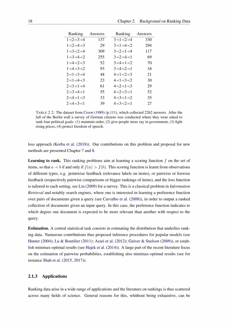
Ranking Answers Ranking Answers1≺2≺3≺4 137 3≺1≺2≺4 3301≺2≺4≺3 29 3≺1≺4≺2 2941≺3≺2≺4 309 3≺2≺1≺4 1171≺3≺4≺2 255 3≺2≺4≺1 691≺4≺2≺3 52 3≺4≺1≺2 701≺4≺3≺2 93 3≺4≺2≺1 342≺1≺3≺4 48 4≺1≺2≺3 212≺1≺4≺3 23 4≺1≺3≺2 302≺3≺1≺4 61 4≺2≺1≺3 292≺3≺4≺1 55 4≺2≺3≺1 522≺4≺1≺3 33 4≺3≺1≺2 352≺4≺3≺1 39 4≺3≺2≺1 27
TABLE 2.2: The dataset from Croon (1989) (p.111), which collected 2262 answers. After thefall of the Berlin wall a survey of German citizens was conducted where they were asked torank four political goals: (1) maintain order, (2) give people more say in government, (3) fightrising prices, (4) protect freedom of speech.
loss approach (Korba et al. (2018)). Our contributions on this problem and proposal for new
methods are presented Chapter 7 and 8.
Learning to rank. This ranking problems aim at learning a scoring function f on the set of
items, so that a ≺ b if and only if f(a) > f(b). This scoring function is learnt from observations
of different types, e.g. pointwise feedback (relevance labels on items), or pairwise or listwise
feedback (respectively pairwise comparisons or bigger rankings of items), and the loss function
is tailored to each setting, see Liu (2009) for a survey. This is a classical problem in Information
Retrieval and notably search engines, where one is interested in learning a preference function
over pairs of documents given a query (see Carvalho et al. (2008)), in order to output a ranked
collection of documents given an input query. In this case, the preference function indicates to
which degree one document is expected to be more relevant than another with respect to the
query.
Estimation. A central statistical task consists in estimating the distribution that underlies rank-
ing data. Numerous contributions thus proposed inference procedures for popular models (see
Hunter (2004); Lu & Boutilier (2011); Azari et al. (2012); Guiver & Snelson (2009)), or estab-
lish minimax-optimal results (see Hajek et al. (2014)). A large part of the recent literature focus
on the estimation of pairwise probabilities, establishing also minimax-optimal results (see for
instance Shah et al. (2015, 2017)).
2.1.3 Applications
Ranking data arise in a wide range of applications and the literature on rankings is thus scattered
across many fields of science. General reasons for this, whithout being exhaustive, can be
Chapter 2. Background on Ranking Data 19
grouped as follows.
Modelling human preferences. First, ranking data can naturally represent preferences of an
agent over a set of items. The mathematical analysis of ranking data began in the 18th century
with the study of an election system for the French Académie des Sciences. In this voting sys-
tem, a voter could express its preferences as a ranking of the candidates, and the goal was to elect
a winner. There was a great debate between Borda and Condorcet (see Borda (1781); Condorcet
(1785); Risse (2005)) to develop the best voting rule, and this started the study of elections
systems in social choice theory. Such voting systems are still used nowadays, for instance for
presidential elections in Ireland (see Gormley & Murphy (2008)). Moreover, it has been shown
by psychologists (see Alwin & Krosnick (1985)) and computer scientists (see Carterette et al.
(2008)) that is it easier for an individual to express her preferences as relative judgements, i.e.
by producing a ranking, rather than absolute judgements, for instance by giving ratings. As
noted by Carterette et al. (2008), “by collecting preferences directly, some of the noise asso-
ciated with difficulty in distinguishing between different levels of relevance may be reduced”.
This motivated the explicit collection of preferences in this form, from classical opinion surveys
(see the Berlin dataset from Croon (1989), given Table 2.2 or the "Song" dataset from Critchlow
et al. (1991)), to more modern applications such as crowdsourcing (e.g., annotators are asked to
compare pair of labels or items, see Gomes et al. (2011); Lee et al. (2011); Chen et al. (2013); Yi
et al. (2013); Dong et al. (2017)) and peer grading (see Shah et al. (2013); Raman & Joachims
(2014)). Similarly, in recommender systems, the central problem is to recommend items to an
user based on some feedback about her preferences. This feedback can be explicitly expressed
by the user, e.g. in the form of ratings, such as in the classical Netflix challenge which boosted
the use of matrix completion methods (see Bell & Koren (2007)). More recently, a vast literature
was developed to deal with implicit feedback (e.g. clicks, view times, purchases) which is more
realistic in some scenarios, in particular to cast it in the framework of pairwise comparisons
(see Rendle et al. (2009) or Radlinski & Joachims (2005); Joachims et al. (2005) in the context
of search engines) and to tackle it with methods and models from ranking data. For all these
reasons, the analysis of ranking data is often seen as a subfield of Preference Learning (see
Fürnkranz & Hüllermeier (2011)).
Competitions. Ranking data also naturally appears in the domain of sports and competitions :
match results between teams or players can be recorded as pairwise comparisons and one may
want to aggregate them into a full ranking. A common approach is to consider these pairwise
outcomes as realizations of a probabilistic model on pairs, and this has been applied to sports
and racing (see Plackett (1975); Keener (1993)), or chess and gaming (see Elo (1978); Herbrich
et al. (2006); Glickman (1999)).
Computer systems. Whereas social choice and sports constitute the historical applications of
ranking data, the latter has also arised in modern machine learning applications. In the domain
of Information Retrieval, search engines aims at presenting to a user a list of documents, ranked
by relevance, given some query. Whereas in the original formulation of this problem, such
as in the Yahoo Learning to Rank challenge (see Chapelle & Chang (2011)), the documents
20 Chapter 2. Background on Ranking Data
relevance was labeled on a predefined scale (called absolute relevant judgement method), a vast
number of contributions dealt with rankings and comparisons between documents (see Radlinski
& Joachims (2007); Xia et al. (2008); Wu et al. (2016)) and sometimes use a labelling strategy to
convert ranking data into scores (see Niu et al. (2012); Bashir et al. (2013); Niu et al. (2015)) in
the training phase. Another modern problem, called metasearch, consists in combining outputs
of different search engines, and can be formalized as a ranking aggregation problem. This
motivated the application of classical voting rules and the development of more efficient ones
(see Dwork et al. (2001); Aslam & Montague (2001); Renda & Straccia (2003); Lam & Leung
(2004); Liu et al. (2007); Akritidis et al. (2011); Desarkar et al. (2016); Bhowmik & Ghosh
(2017)). Another application where ranking data arises is recommender systems, where the
feedback from users can be implicit as explained at the beginning of the section and thus can be
modeled as ranking data, and the learner may want to recommend items as a ranked list. A vast
literature focused about this problem, especially Collaborative ranking (see Section 2.1.2).
Biological data. Ranking methods have also interesting applications in bioinformatics or life
sciences. For instance, powerful techniques such as microarrays can measure the level of expres-
sions of enormous genes but these measures can vary a lot in experiments; a common approach
is then to order the genes by their expression profiles in each experiment and then aggregate
the results through rank aggregation for instance (see Sese & Morishita (2001); Breitling et al.
(2004); Brancotte et al. (2015); Jiao & Vert (2017)). Other applications include nanotoxicology
(see Patel et al. (2013)) or neuro-imaging analysis Gunasekar et al. (2016).
2.2 Analysis of Full Rankings
We now turn to the specific case of full rankings, which will be at the core of this thesis. A full
ranking a1 ≺ a2 ≺ . . . an is usually described as the permutation σ on JnK that maps an item
to its rank, i.e. such that σ(ai) = i, ∀ i ∈ JnK. Item i is thus preferred over item j (denoted by
i ≺ j) according to σ if and only if i is ranked lower than j: σ(i) < σ(j). A permutation can be
seen as a bijection on the set JnK onto itself:
JnK→ JnK
i 7→ σ(i)
For each i ∈ JnK, σ(i) represents the rank of the i-th element, whereas σ−1(i) represents the
i-th ranked element. We denote by Sn the set of all permutations over n items. Endowed with
the composition operation σ σ′(i) = σ(σ′(i)) for all σ, σ′ ∈ Sn, Sn is a group, called the
symmetric group and we denote e its identity element which maps each item j to position j.
Statistical analysis of full rankings thus relies on this group, and the variability of observations
Chapter 2. Background on Ranking Data 21
is represented by a discrete probability distribution P on the set Sn:
Sn → [0, 1]
σ 7→ P (σ)
Though empirical estimation of P may appear as a simple problem at first glance, it is actu-
ally a great statistical challenge since the number of possible rankings (i.e. Sn’s cardinality)
explodes as n! with the number of instances to be ranked. Moreover, applying techniques from
multivariate analysis is arduous for two reasons. First, for a given random permutation Σ ∈ Sn,
the random variables (Σ(1), . . . ,Σ(n)) are highly dependent: each of them takes its values in
JnK and their values must be different. Then, the sum of two random permutations vectors
Σ = (Σ(1), . . . ,Σ(n)) and Σ′ = (Σ′(1), . . . ,Σ′(n)) does not correspond to another permuta-
tion vector. Hence, to represent probability distributions over permutations, several approaches
exist but we can divide them between parametric versus "non-parametric" ones. The term "non-
parametric" is not correct since Sn is finite. What we call a “parametric” approach consists
in fitting a predefined generative model on the data, analyzing the data through that model and
inferring knowledge with respect to that model. In contrast, what we call “non-parametric” ap-
proach consists in choosing a structure on the symmetric group, analyzing the data with respect
to that structure, and inferring knowledge through a “regularity” assumption.
2.2.1 Parametric Approaches
Most-known statistical models can be categorized into five classes:
• distance-based models: the probability of a ranking decreases as the distance from a
central ranking increases. Example: the Mallows model (see Mallows (1957)).
• order statistics or random utility models: the ranking reflects the ordering of latent
scores given to each object. Example: the Thurstone model (see Thurstone (1927)).
• multistage ranking models: the ranking is modeled as a sequential process of selecting
the next most preferred object. Example: the Plackett model (see Plackett (1975)).
• paired-comparison models: the probability expression of a ranking σ considers every
pair of items i, j such that i is preferred to j (Pσ ∝∏
(i,j)|σ(i)<σ(j) pij). Example: the
Bradley-Terry model (see Bradley & Terry (1952)).
These models are now described at length, since through this thesis they will often be used for
baselines in the experiments.
Mallows model. This model can be seen as analoguous to a Gaussian distribution for per-
mutations. The Mallows ψ-model is parametrized by a modal or reference ranking σ∗ and a
dispersion parameter ψ ∈ (0, 1]. Let σ be a ranking, then the Mallows model specifies:
22 Chapter 2. Background on Ranking Data
P (σ) = Pσ|σ∗, ψ =1
Zψ−d(σ,σ∗)
where d is a distance for permutations (see Diaconis (1988) for several distances choices which
give rise to the family of distance-based models), and Z =∑
σ∈Sn ψd(σ,σ∗) is the normalization
constant. When ψ is equal to 1, one obtains the uniform distribution over permutations, whereas
when ψ tends towards 0 one obtains a distribution that concentrates all mass on the central rank-
ing σ∗. Sometimes the model is written as Pσ|σ∗, λ = 1Z e−λd(σ,σ∗), where λ = −ln(ψ) ≥ 0.
Most of the time in the literature, the chosen distance is the Kendall’s τ distance (see Sec-
tion 2.2.3). This choice is motivated by a range of properties. Firstly, it has an intuitive and
plausible interpretation as a number of pairwise choices: Mallows (1957) argues that it pro-
vides the best possible description of the process of ranking items as performed by a human and
for this reason this distance is widely used. Then, it has a number of appealing mathematical
properties: it is decomposable into a sum, and its standardized distribution has a normal limit
(see Diaconis (1988)). Still, this model has several inconvenients or rigidities. Firstly, permu-
tations at the same distance from σ∗ have the same probability. This assumption is relaxed in
the Generalized Mallows Model, which uses n spread parameters each affecting a position in
the permutation, enabling to stress the consensus on some positions (see Fligner & Verducci
(1986)). Then, the computation of the normalization constant is generally expensive (see Lu &
Boutilier (2014); Irurozki et al. (2017) for a closed-form when d is the Kendall’s τ distance and
Hamming distance respectively).
Thurstone model. In the Thurstone model, each item is associated with a true continuous
value: a judge assesses values to the items and classify them. Errors are thus a consequence
of the lack of exactness of the judge. Formally, the Thurstone model is defined as follows:
given X1, X2, . . . , Xn random variables with a continuous joint distribution F (X1, . . . , Xn),
we can define a random ranking σ in such a way that σ(i) is the rank that Xi occupied in
X1, X2, . . . , Xn and its probability is:
P (σ) = PXσ−1(1) < Xσ−1(2) < · · · < Xσ−1(n)
This model makes one assumption: all the Xi’s are independent. The most common models for
F are Gaussian or Gumbel distributions.
Bradley-Terry and Plackett-Luce models. Bradley and Terry suggested the following pairwise
comparison model, defined by a vector of weights w = (w1, . . . , wn), each one associated with
an item. This model specifies the probability that item i is preferred to item j as:
Pi ≺ j =wi
wi + wj
The Plackett-Luce model generalizes the Bradley-Terry model for full rankings and is still
parametrized by a support parameter w = (w1, w2, . . . , wn) where 0 ≤ wj ≤ 1 and∑n
j=1wj =
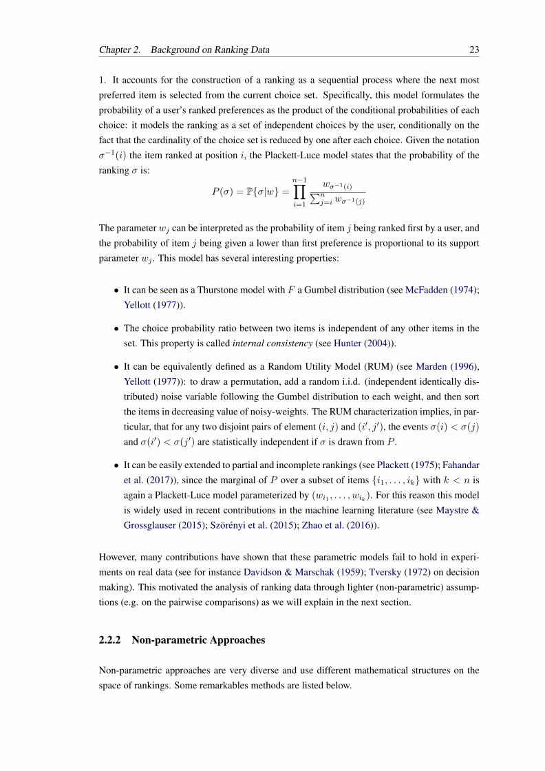
Chapter 2. Background on Ranking Data 23
1. It accounts for the construction of a ranking as a sequential process where the next most
preferred item is selected from the current choice set. Specifically, this model formulates the
probability of a user’s ranked preferences as the product of the conditional probabilities of each
choice: it models the ranking as a set of independent choices by the user, conditionally on the
fact that the cardinality of the choice set is reduced by one after each choice. Given the notation
σ−1(i) the item ranked at position i, the Plackett-Luce model states that the probability of the
ranking σ is:
P (σ) = Pσ|w =
n−1∏i=1
wσ−1(i)∑nj=iwσ−1(j)
The parameter wj can be interpreted as the probability of item j being ranked first by a user, and
the probability of item j being given a lower than first preference is proportional to its support
parameter wj . This model has several interesting properties:
• It can be seen as a Thurstone model with F a Gumbel distribution (see McFadden (1974);
Yellott (1977)).
• The choice probability ratio between two items is independent of any other items in the
set. This property is called internal consistency (see Hunter (2004)).
• It can be equivalently defined as a Random Utility Model (RUM) (see Marden (1996),
Yellott (1977)): to draw a permutation, add a random i.i.d. (independent identically dis-
tributed) noise variable following the Gumbel distribution to each weight, and then sort
the items in decreasing value of noisy-weights. The RUM characterization implies, in par-
ticular, that for any two disjoint pairs of element (i, j) and (i′, j′), the events σ(i) < σ(j)
and σ(i′) < σ(j′) are statistically independent if σ is drawn from P .
• It can be easily extended to partial and incomplete rankings (see Plackett (1975); Fahandar
et al. (2017)), since the marginal of P over a subset of items i1, . . . , ik with k < n is
again a Plackett-Luce model parameterized by (wi1 , . . . , wik). For this reason this model
is widely used in recent contributions in the machine learning literature (see Maystre &
Grossglauser (2015); Szörényi et al. (2015); Zhao et al. (2016)).
However, many contributions have shown that these parametric models fail to hold in experi-
ments on real data (see for instance Davidson & Marschak (1959); Tversky (1972) on decision
making). This motivated the analysis of ranking data through lighter (non-parametric) assump-
tions (e.g. on the pairwise comparisons) as we will explain in the next section.
2.2.2 Non-parametric Approaches
Non-parametric approaches are very diverse and use different mathematical structures on the
space of rankings. Some remarkables methods are listed below.
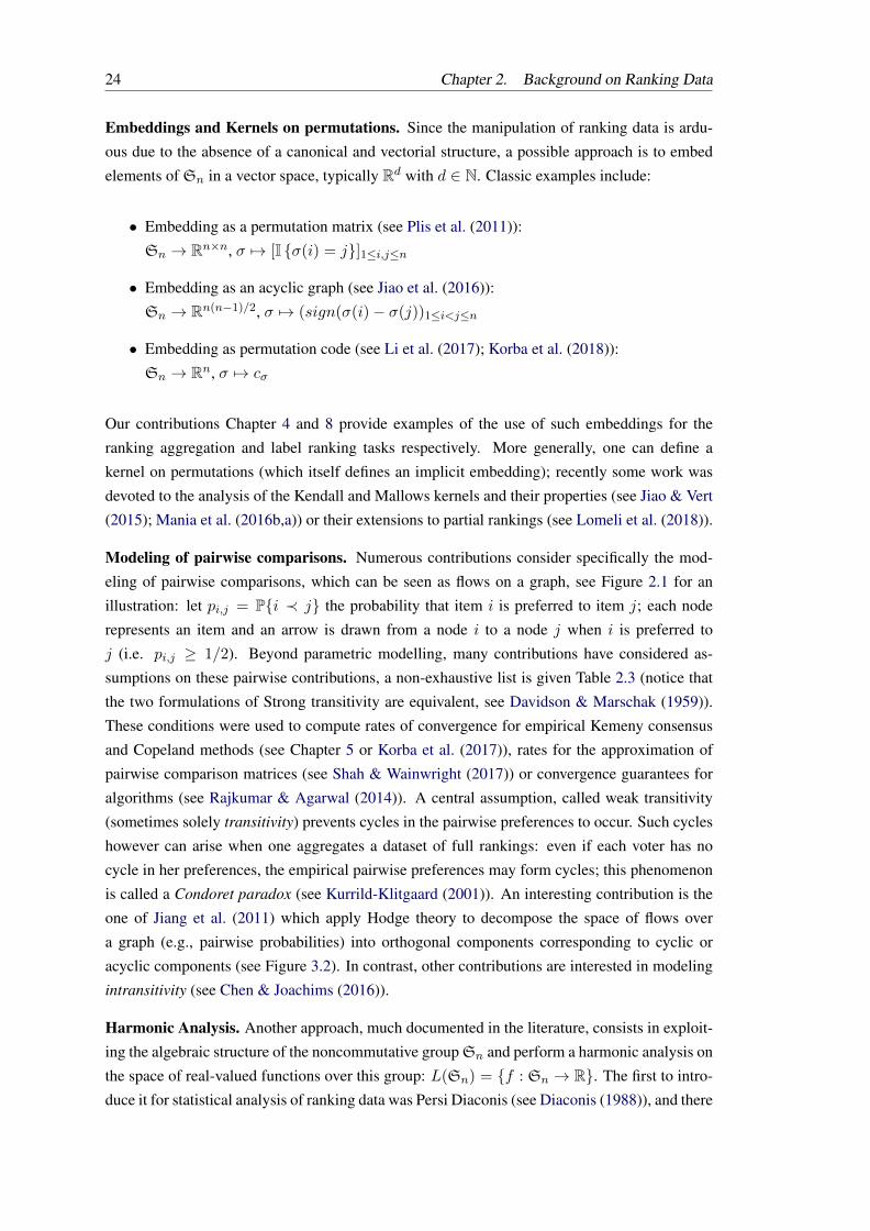
24 Chapter 2. Background on Ranking Data
Embeddings and Kernels on permutations. Since the manipulation of ranking data is ardu-
ous due to the absence of a canonical and vectorial structure, a possible approach is to embed
elements of Sn in a vector space, typically Rd with d ∈ N. Classic examples include:
• Embedding as a permutation matrix (see Plis et al. (2011)):
Sn → Rn×n, σ 7→ [I σ(i) = j]1≤i,j≤n
• Embedding as an acyclic graph (see Jiao et al. (2016)):
Sn → Rn(n−1)/2, σ 7→ (sign(σ(i)− σ(j))1≤i<j≤n
• Embedding as permutation code (see Li et al. (2017); Korba et al. (2018)):
Sn → Rn, σ 7→ cσ
Our contributions Chapter 4 and 8 provide examples of the use of such embeddings for the
ranking aggregation and label ranking tasks respectively. More generally, one can define a
kernel on permutations (which itself defines an implicit embedding); recently some work was
devoted to the analysis of the Kendall and Mallows kernels and their properties (see Jiao & Vert
(2015); Mania et al. (2016b,a)) or their extensions to partial rankings (see Lomeli et al. (2018)).
Modeling of pairwise comparisons. Numerous contributions consider specifically the mod-
eling of pairwise comparisons, which can be seen as flows on a graph, see Figure 2.1 for an
illustration: let pi,j = Pi ≺ j the probability that item i is preferred to item j; each node
represents an item and an arrow is drawn from a node i to a node j when i is preferred to
j (i.e. pi,j ≥ 1/2). Beyond parametric modelling, many contributions have considered as-
sumptions on these pairwise contributions, a non-exhaustive list is given Table 2.3 (notice that
the two formulations of Strong transitivity are equivalent, see Davidson & Marschak (1959)).
These conditions were used to compute rates of convergence for empirical Kemeny consensus
and Copeland methods (see Chapter 5 or Korba et al. (2017)), rates for the approximation of
pairwise comparison matrices (see Shah & Wainwright (2017)) or convergence guarantees for
algorithms (see Rajkumar & Agarwal (2014)). A central assumption, called weak transitivity
(sometimes solely transitivity) prevents cycles in the pairwise preferences to occur. Such cycles
however can arise when one aggregates a dataset of full rankings: even if each voter has no
cycle in her preferences, the empirical pairwise preferences may form cycles; this phenomenon
is called a Condoret paradox (see Kurrild-Klitgaard (2001)). An interesting contribution is the
one of Jiang et al. (2011) which apply Hodge theory to decompose the space of flows over
a graph (e.g., pairwise probabilities) into orthogonal components corresponding to cyclic or
acyclic components (see Figure 3.2). In contrast, other contributions are interested in modeling
intransitivity (see Chen & Joachims (2016)).
Harmonic Analysis. Another approach, much documented in the literature, consists in exploit-
ing the algebraic structure of the noncommutative group Sn and perform a harmonic analysis on
the space of real-valued functions over this group: L(Sn) = f : Sn → R. The first to intro-
duce it for statistical analysis of ranking data was Persi Diaconis (see Diaconis (1988)), and there
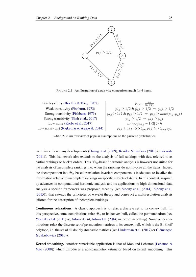
Chapter 2. Background on Ranking Data 25
1
2
3
4
p 1,2≥
1/2
p1,3 ≥ 1/2
p1,4 ≥
1/2p
3,2 ≥1/2
p 4,3≥
1/2
FIGURE 2.1: An illustration of a pairwise comparison graph for 4 items.
Bradley-Terry (Bradley & Terry, 1952) pi,j = wiwi+wj
Weak transitivity (Fishburn, 1973) pi,j ≥ 1/2 & pj,k ≥ 1/2 ⇒ pi,k ≥ 1/2
Strong transitivity (Fishburn, 1973) pi,j ≥ 1/2 & pj,k ≥ 1/2 ⇒ pi,k ≥ max(pi,j , pj,k)
Strong transitivity (Shah et al., 2017) pi,j ≥ 1/2 ⇒ pi,k ≥ pj,kLow noise (Korba et al., 2017) mini<j |pi,j − 1/2| > h
Low noise (bis) (Rajkumar & Agarwal, 2014) pi,j ≥ 1/2⇒∑
k 6=i pi,k ≥∑
k 6=j pj,k
TABLE 2.3: An overview of popular assumptions on the pairwise probabilities.
were since then many developments (Huang et al. (2009), Kondor & Barbosa (2010)), Kakarala
(2011)). This framework also extends to the analysis of full rankings with ties, referred to as
partial rankings or bucket orders. This "Sn-based" harmonic analysis is however not suited for
the analysis of incomplete rankings, i.e. when the rankings do not involve all the items. Indeed
the decomposition into Sn-based translation-invariant components is inadequate to localize the
information relative to incomplete rankings on specific subsets of items. In this context, inspired
by advances in computational harmonic analysis and its applications to high-dimensional data
analysis a specific framework was proposed recently (see Sibony et al. (2014), Sibony et al.
(2015)), that extends the principles of wavelet theory and construct a multiresolution analysis
tailored for the description of incomplete rankings.
Continuous relaxations. A classic approach is to relax a discrete set to its convex hull. In
this perspective, some contributions relax Sn to its convex hull, called the permutahedron (see
Yasutake et al. (2011) or, Ailon (2014), Ailon et al. (2014) in the online setting). Some other con-
tributions relax the discrete set of permutation matrices to its convex hull, which is the Birkhoff
polytope, i.e. the set of all doubly stochastic matrices (see Linderman et al. (2017) or Clémençon
& Jakubowicz (2010)).
Kernel smoothing. Another remarkable application is that of Mao and Lebanon (Lebanon &
Mao (2008)) which introduces a non-parametric estimator based on kernel smoothing. This

26 Chapter 2. Background on Ranking Data
approach has been extended to incomplete rankings (Sun et al. (2012)).
2.2.3 Distances on Rankings
To perform a statistical analysis on ranking data, one needs a distance d(σ, σ′) to compare two
elements σ, σ′ ∈ S2n. Several distance measures have been proposed for ranking data. To be a
valid distance measure, it needs to satisfy the following properties:
• Reflexivity: d(σ, σ′) = 0,
• Positivity: d(σ, σ′) ≥ 0,
• Symmetry: d(σ, σ′) = d(σ′, σ).
These properties are called axioms by Kemeny (1972). Furthermore, a distance measure is said
to be metric when it satisfies the triangle inequality for any triplet of rankings σ, σ′ and π:
d(σ, σ′) ≤ d(σ, π) + d(π, σ′)
A label-invariant distance guarantees that the distance between two rankings remains the same
even if the labels of the objects are permuted, which is a standard assumption when dealing with
ranking data:
d is label-invariant if : ∀ π ∈ Sn, d(σπ, σ′π) = d(σ, σ′)
In particular in this case, taking π = σ′−1, since we have σ′σ′−1 = e, we can write d(σ, σ′) =
d(σσ′−1, e) i.e., we can always take the identity permutation as the reference one. Some label-
invariant metrics are particularly known and useful. For σ, σ′ ∈ Sn, we can consider:
• The Kendall’s τ distance, which counts the pairwise disagreements:
dτ (σ, σ′) =∑
1≤i<j≤n1
(σ(j)− σ(i))(σ′(j)− σ′(i)) < 0
It can also be defined as the minimal number of adjacent swaps to convert σ into σ′. The
maximum value of the Kendall’s tau distance between two permutations is n(n − 1)/2
(when σ′ is the reverse of σ and thus σ(i) + σ′(i) = n+ 1 for each i).
• The Hamming distance, which counts the number of entries on which σ and σ′ disagree
and thus corresponds to the l0 metric:
dH(σ, σ′) =
n∑i=1
1σ(i) 6= σ′(i)
The maximum value of the Hamming distance between two permutations is thus n.
Chapter 2. Background on Ranking Data 27
• The Spearman’s footrule metric, which corresponds to the l1 metric:
d1(σ, σ′) =n∑i=1
|σ(i)− σ′(i)|
• The Spearman rho’s metric, which corresponds to the l2 metric:
d2(σ, σ′) = (
n∑i=1
(σ(i)− σ′(i))2)12
The Kendall’s τ distance is a natural discrepancy measure when permutations are interpreted as
rankings and is thus the most widely used in the preference learning literature. In contrast, the
Hamming distance is particularly used when permutations represent matching of bipartite graphs
and is thus also very popular. Many others metrics could have been considered and are also well-
spread in the literature, for example: the Cayley metric (minimum number of transpositions,
not necessariry adjacent as in Kendall’s tau distance, to map σ to σ′), the Ulam metric, the
maximum rank difference. The reader may refer to Diaconis (1988); Marden (1996); Deza &
Deza (2009) for detailed examples. Some of these metrics are linked by nice inequalities. For
instance, Kendall’s τ distance and Spearman’s footrule verify that for σ, σ′ ∈ Sn, dτ (σ, σ′) ≤d1(σ, σ′) ≤ 2dτ (σ, σ′) (see Diaconis & Graham (1977), see also the Durbin-Stuart inequality
in Kamishima et al. (2010) for these two metrics). Similarly, for dC and dH respectively the
Cayley and Hamming distance, one has: dC(σ, σ′) ≤ dH(σ, σ′) ≤ 2dC(σ, σ′) (see Farnoud
et al. (2012b)).
Many extensions of these metrics exist. For instance, Kumar & Vassilvitskii (2010) propose an
extension of Spearman’s footrule and Kendall’s τ distance to take into account position and ele-
ment weights. Several distances have also been proposed for partial rankings, such as modified
version of the Kendall’s τ distance (parameterized by a penalty p when an item in a pair belongs
to a bucket) or Haussdorff metrics Fagin et al. (2003, 2004), or cosine distance after vectorizing
the partial rankings (see Ukkonen (2011)). Another well-known distance for partial rankings
is the Kemeny distance (see Kemeny (1959, 1972). Concerning incomplete rankings, Kidwell
et al. (2008) propose to represent an incomplete ranking, possibly with ties, as the mean on the
set of the consistent rankings (i.e. the full rankings extending the given incomplete ranking).
These distances can thus be used as performance metrics in machine learning tasks involving
ranking data. Other measures of performance are widely used in the Learning to Rank problem
(see Section 2.1.2), such as NDCG and MAP (Liu (2009)). However they are tailored to abso-
lute judgements, and not to ranking as feedback. Some contributions have proposed to extend
these metrics (see Carterette & Bennett (2008)) for relative judgements or labeling strategies
(see Niu et al. (2012)) to convert rankings to ratings.
In this thesis, we will use in particular the Kendall’s τ distance, which has the nice property of
decomposing rankings over pairs and is the most widely used in the literature. A nice visual-
ization of the symmetric group provided with this distance is the permutation polytope, called
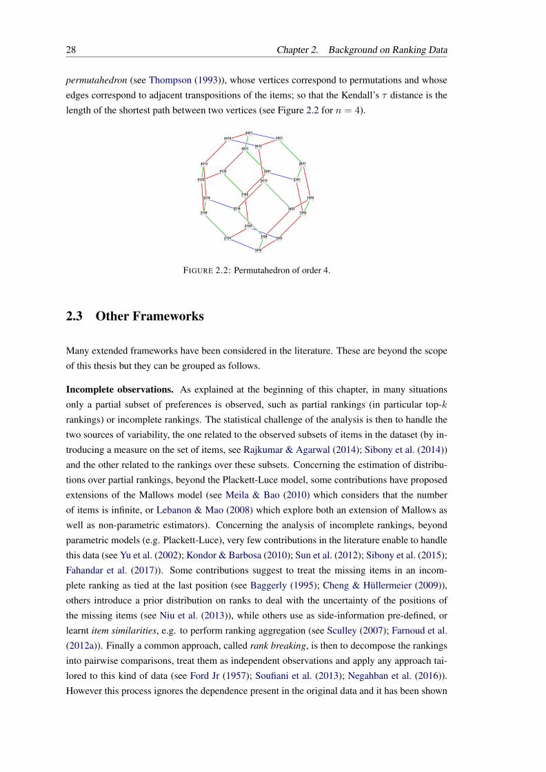
28 Chapter 2. Background on Ranking Data
permutahedron (see Thompson (1993)), whose vertices correspond to permutations and whose
edges correspond to adjacent transpositions of the items; so that the Kendall’s τ distance is the
length of the shortest path between two vertices (see Figure 2.2 for n = 4).
FIGURE 2.2: Permutahedron of order 4.
2.3 Other Frameworks
Many extended frameworks have been considered in the literature. These are beyond the scope
of this thesis but they can be grouped as follows.
Incomplete observations. As explained at the beginning of this chapter, in many situations
only a partial subset of preferences is observed, such as partial rankings (in particular top-k
rankings) or incomplete rankings. The statistical challenge of the analysis is then to handle the
two sources of variability, the one related to the observed subsets of items in the dataset (by in-
troducing a measure on the set of items, see Rajkumar & Agarwal (2014); Sibony et al. (2014))
and the other related to the rankings over these subsets. Concerning the estimation of distribu-
tions over partial rankings, beyond the Plackett-Luce model, some contributions have proposed
extensions of the Mallows model (see Meila & Bao (2010) which considers that the number
of items is infinite, or Lebanon & Mao (2008) which explore both an extension of Mallows as
well as non-parametric estimators). Concerning the analysis of incomplete rankings, beyond
parametric models (e.g. Plackett-Luce), very few contributions in the literature enable to handle
this data (see Yu et al. (2002); Kondor & Barbosa (2010); Sun et al. (2012); Sibony et al. (2015);
Fahandar et al. (2017)). Some contributions suggest to treat the missing items in an incom-
plete ranking as tied at the last position (see Baggerly (1995); Cheng & Hüllermeier (2009)),
others introduce a prior distribution on ranks to deal with the uncertainty of the positions of
the missing items (see Niu et al. (2013)), while others use as side-information pre-defined, or
learnt item similarities, e.g. to perform ranking aggregation (see Sculley (2007); Farnoud et al.
(2012a)). Finally a common approach, called rank breaking, is then to decompose the rankings
into pairwise comparisons, treat them as independent observations and apply any approach tai-
lored to this kind of data (see Ford Jr (1957); Soufiani et al. (2013); Negahban et al. (2016)).
However this process ignores the dependence present in the original data and it has been shown

Chapter 2. Background on Ranking Data 29
that it introduces inconsistency (see Soufiani et al. (2014a)). Some contributions thus propose
to weight the pairs in a data-dependent manner (see Khetan & Oh (2016)). Our work in this the-
sis, through the extensive use of the Kendall’s τ distance which decomposes the rankings over
pairs (see Chapter 5 and Chapter 7), offers a natural framework to handle the case of pairwise
comparisons.
Online Setting. Many contributions consider the setting where the preferences (in particular,
pairwise comparisons) are measured actively; in this case the performance is measured in terms
of sample complexity, i.e. the number of queries needed to recover the target (exactly or with a
high probability in the Probably Approximately Correct, or PAC setting). The learner is allowed
to sample pairs of items in an adaptive manner, e.g. in active ranking to recover a true underlying
central ranking (see Jamieson & Nowak (2011), Ailon (2012)), under transitivity assumptions
(see Qian et al. (2015); Falahatgar et al. (2017, 2018)) or noise assumptions (i.e., the observa-
tions correspond to true pairwise comparisons corrupted up to some noise, see Braverman &
Mossel (2008, 2009)). Some contributions focused on recovering a top-k ranking (see Chen &
Suh (2015); Mohajer et al. (2017)) or more generally in the preference elicitation context, to
estimate the parameters of the model underlying the data, e.g. Plackett-Luce (see Szörényi et al.
(2015)) or Bradley-Terry (see Maystre & Grossglauser (2017); Negahban et al. (2012)) or Mal-
lows (see Busa-Fekete et al. (2014)). However this scenario is sometimes viewed as unrealistic
in many applications and some contributions consider the passive setting (see Wauthier et al.
(2013); Rajkumar & Agarwal (2016)) or intermediate regimes (see Agarwal et al. (2017)). A re-
lated literature in online learning, called dueling bandits (see Yue et al. (2012); Sui et al. (2018))
generalizes the classical multi-armed bandits problem (see Lai & Robbins (1985); Kuleshov &
Precup (2014)) to the setting where the learner can pull two arms at each round and observe
a random pairwise comparison, in a minimum number of queries, or to optimize an error rate
(probability of playing a suboptimal arm) or a cumulative regret (the cost suffered by playing
an unoptimal arm). The goal is, at the end, to identify the best arm (i.e. an arm which beats any
other arm, namely a Condorcet winner when it exists), or a subset of good arms (e.g. winners
of the Copeland set, see Rajkumar et al. (2015); Ramamohan et al. (2016)). Several extensions
exist where the learner observe a winner or a ranking over a bigger subset of arms (see Sui et al.
(2017); Saha & Gopalan (2018)). The reader may refer to Busa-Fekete et al. (2018); Agarwal
(2016) for an exhaustive review. Finally, some contributions casts online ranking as the problem
of online permutation learning (see Yasutake et al. (2011); Ailon (2014)), where at each round,
the learner predicts a permutation, suffers some related loss and is revealed some feedback;
the goal being to identify as soon as possible in the learning process the best permutation (i.e.
minimizing a cumulative regret).
The following Part I focuses on the ranking aggregation problem, which was certainly the most
widely studied in the literature. In particular, we introduce at length the problem Chapter 3 and
present our contributions Chapter 4 and 5.


PART I
Ranking Aggregation
31

CHAPTER 3The Ranking Aggregation Problem
Chapter abstract In this chapter, we describe the ranking aggregation problem: given adataset of (full) rankings, what is the most representative ranking summarizing this dataset?Originally considered in social choice for elections, the ranking aggregation problem appearsnowadays in many modern applications implying machine learning (e.g., meta-search engines,information retrieval, biology). This problem has been studied extensively, in particular in twosettings. The first possibility is to consider that the dataset is constituted of noisy versions of atrue ranking (e.g., realizations of a parameterized distribution centered around some ranking),and the goal is to reconstruct the true ranking thanks to the samples (e.g., with MLE estima-tion). The second possibility is to formalize this problem as a discrete optimization problemover the set of rankings, and to look for the ranking which is the closest (with respect to somedistance) to the rankings observed in the dataset, without stochastic assumptions. These formerapproaches tackle the problem in a rigorous manner, but can lead to heavy computational costsin practice. Therefore, many other methods have been used in the litterature, such as scoringmethods or spectral methods, but with fewer or no theoretical support. In this chapter, we thusexplain in detail the ranking aggregation problem, the mathematical challenges it raises andgive an overview of the ranking aggregation methods in the litterature.
3.1 Ranking Aggregation
3.1.1 Definition
Consider a set JnK = 1, . . . , n of n indexed items and N agents. Suppose that each agent t
expresses her preferences as a full ranking over the n items, which, as described Chapter 2, can
be seen as a permutation σt ∈ Sn. Collecting preferences of the agents over the set of items
then results in dataset of permutations DN = (σ1, . . . , σN ) ∈ SNn . The ranking aggregation
problem consists in finding a permutation σ∗, called consensus, that best summarizes the dataset
(sometimes referred to as the profile) DN = (σ1, . . . , σN ). This problem has been studied ex-
tensively and a lot of approaches have been developped, in particular in two settings. The first
possibility is to consider that the dataset is constituted of noisy versions of a true ranking (e.g.,
realizations of a parameterized distribution centered around some ranking), and the goal is to
reconstruct the true ranking thanks to the samples (e.g., with MLE estimation). The second pos-
sibility is to formalize this problem as a discrete optimization problem over the set of rankings,
33

34 Chapter 3. The Ranking Aggregation Problem
and to look for the ranking which is the closest (with respect to some distance) to the rankings
observed in the dataset, without stochastic assumptions. These former approaches tackle the
problem in a rigorous manner, but can lead to heavy computational costs in practice. Therefore,
many other methods have been used in the literature, such as scoring methods or spectral meth-
ods, but with fewer or no theoretical support. In this chapter, we thus give an overview of the
ranking aggregation problem, the challenges it raises and the main methods in the literature.
3.1.2 Voting Rules Axioms
The ranking aggregation problem arised in the context of elections (see Section 2.1.3). Hence,
many axioms for the consensus have been considered in the social choice litterature, reflecting
some aspects of a fair election.
• Independance to irrelevant alternatives: the relative order of i and j in σ∗ should only
depend on the relative order of i and j in σ1, . . . σN .
• Neutrality : no item should be favored to others. If two items switch positions in σ1, . . . σN ,
they should switch positions also in σ∗.
• Monotonicity: if the ranking of an item is improved by a voter, its ranking in σ∗ can only
improve.
• Consistency: if voters are split into two disjoint sets, and both the aggregation of voters in
the first and second set prefer i to j, then i should be ranked above j in σ∗.
• Non-dictatorship: there is no single voter t with the individual preference order σt such
that σt = σ∗, unless all votes are identical to σt.
• Unanimity (or Pareto efficiency): if all voters prefer item i to item j, then also σ∗ should
prefer i to j.
• Condorcet criterion: any item which wins every other in pairwise simple majority voting
should be ranked first (see Condorcet (1785)). If there is a Condorcet winner in the profile,
the latter is called a Condorcet profile.
Other criterions exist in the literature and can extend the ones listed previously. A famous
example is the extended Condorcet criterion, due to Truchon (see Truchon (1998)) which states
that if there exists a partition (A,B) of JnK, such that for any i ∈ A and any j ∈ B, the majority
prefers i to j, then i should be ranked above j in σ∗. However, the following theorem (see Arrow
(1951)) states the limits of the properties that any election procedure can satisfy.
Theorem 3.1. (Arrow’s impossibility theorem). No voting system can satisfy simultaneously
unanimity, non-dictatorship and independance to irrelevant alternatives.
Chapter 3. The Ranking Aggregation Problem 35
Arrow’s theorem states that there exists no universally fair voting rule, implying that there ex-
ists no canonical solution to the ranking aggregation problem. One will thus choose a given
procedure with respect to the axioms one wants to be satisfied by the output. This problem is
thus fondamentally challenging, and very diverse methods were developed in the literature to
produce a consensus. These are presented in the next section.
3.2 Methods
3.2.1 Kemeny’s Consensus
One of the most popular formulation of the ranking aggregation problem is the Kemeny defini-
tion of a consensus (see Kemeny (1959)). Kemeny defines the consensus ranking σ∗ as the one
that minimizes the sum of the distances to the rankings in DN = (σ1, . . . , σN ), i.e. a solution
to the minimization problem:
minσ∈Sn
CN (σ) (3.1)
where CN (σ) = minσ∈Sn∑N
t=1 d(σ, σt) and d is a given metric on Sn (see section 2.2.3).
Such an element always exists, as Sn is finite, but is not necessarily unique, and the solution(s)
depend on the choice of the distance d.
Kemeny’s rule computes the exact consensus(es) for the Kendall’s τ distance dτ , which counts
the number of pairwise disagreements between two permutations (see section 2.2.3). Kemeny’s
rule thus consists in solving:
maxσ∈Sn
∑1≤i 6=j≤n
Ni,jI σ(i) < σ(j) (3.2)
where for i 6= j, Ni,j = 1/N∑N
t=1 Iσt(i) < σt(j) is the number of times i is preferred over
j in the collection (σ1, . . . , σN ). This aggregation method has several justifications. Firstly, it
has a social choice justification since its solution satisfies many voting properties, such as the
Condorcet Criterion. In fact, the Kemeny’s rule is the unique rule that meets all three of follow-
ing axioms: it satisfies the Condorcet criterion, consistency under elimination, and neutrality
(see Young & Levenglick (1978)). Then, it has a statistical justification since it outputs the max-
imum likelihood estimator under the Mallows model defined section 2.2.1 with the Kendall’s τ
distance dτ (see Young (1988)):
arg maxσ∈Sn
N∏t=1
φ−dτ (σt,σ)
Z= arg min
σ∈Sn
N∑t=1
dτ (σt, σ)
The main drawback of this method is that it is NP-hard in the number of votes N in the worst
case (see Bartholdi et al. (1989)), even for N = 4 votes (see Dwork et al. (2001)). Kemeny
ranking aggregation is actually closely related to the (weighted) Feedback Arc Set Tournament
36 Chapter 3. The Ranking Aggregation Problem
(FAST) problem, also known to be NP-hard (see Alon (2006), Ailon et al. (2008)). It can be
solved by exact algorithms (Integer Linear Programming or Branch and Bound) given enough
time, depending on the agreement of the ranking in the dataset DN . In Meila et al. (2007) it is
shown that with strong agreements inDN , the Branch and Bound will have a running time com-
plexity of O(n2), whereas in Ali & Meila (2012), the authors identify several regimes (strong,
weak or no consensus) and compute data-dependent lower and upper bounds for the running
time of these algorithms and when the Kemeny ranking seems (empirically) to be given by other
procedures, see Remark 3.2. On the other hand, some contributions developed PTAS (Polyno-
mial Time Approximation Scheme, see Coppersmith et al. (2006), Kenyon-Mathieu & Schudy
(2007), Karpinski & Schudy (2010)). A relaxation of Kemeny’s rule, named Local Kemeny
Aggregation, satisfying the extended Condorcet criterion and computable in timeO(Nn log n),
has also been proposed in Dwork et al. (2001).
Footrule aggregation computes the exact consensus(es) for the Spearman’s footrule distance
d1. The footrule consensus can actually be computed in polynomial time since can be solved
by the Hungarian algorithm in O(n3) (see Ali & Meila (2012)). Moreover, it provides a 2-
approximation to Kemeny’s rule (see Dwork et al. (2001)), i.e: CN (σ1) ≤ 5CN (σ∗) where CNis the cost defined in (5.1) with d the Kendall’s τ distance, σ∗ is a Kemeny consensus and σ1 is
a solution of (5.1) with d the Spearman’s footrule distance.
3.2.2 Scoring Methods
Scoring methods consists in computing a score for each item, and then rank the items according
to these scores (by decreasing order). Ties can occur in the scores, and then one is allowed to
break them arbitrarily to output a full ranking in Sn. The most popular scoring methods are
Copeland method and Positional scoring rules, including the famous Borda method.
Copeland method. The Copeland score (see Copeland (1951)) of each individual item i corre-
sponds to the number of its pairwise victories against the other items:
sC,N (i) =∑j 6=i
INi,j >1
2 (3.3)
where for i 6= j,Ni,j = 1/N∑N
t=1 Iσt(i) < σt(j) is the number of times i is preferred over j
in the collection (σ1, . . . , σN ). For example, the Copeland winner is the alternative that wins the
most pairwise elections. The output of Copeland method then naturally verifies the Condorcet
criterion.
Positional Scoring rules. Positional scoring rules rely on the absolute position of items in
the ranked lists rather than their relative rankings, and compute scores for items as follows.
Given a scoring vector w = (w1, . . . , wn) ∈ Rn of weights respectively for each position in
JnK, the ith alternative in a vote scores wi. A full ranking is given by sorting the averaged
scores over all votes, so that the winner is the alternative with the highest total score over all the
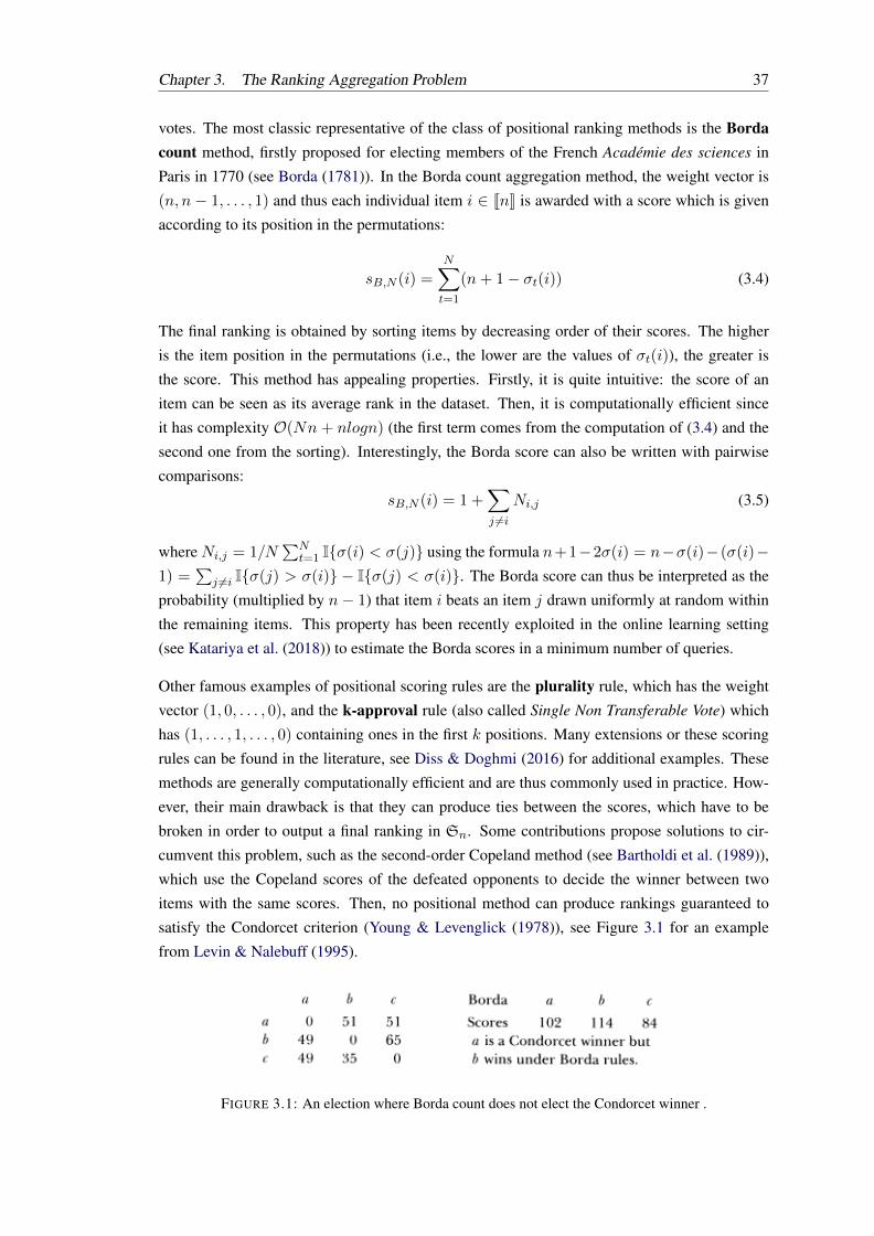
Chapter 3. The Ranking Aggregation Problem 37
votes. The most classic representative of the class of positional ranking methods is the Bordacount method, firstly proposed for electing members of the French Académie des sciences in
Paris in 1770 (see Borda (1781)). In the Borda count aggregation method, the weight vector is
(n, n − 1, . . . , 1) and thus each individual item i ∈ JnK is awarded with a score which is given
according to its position in the permutations:
sB,N (i) =
N∑t=1
(n+ 1− σt(i)) (3.4)
The final ranking is obtained by sorting items by decreasing order of their scores. The higher
is the item position in the permutations (i.e., the lower are the values of σt(i)), the greater is
the score. This method has appealing properties. Firstly, it is quite intuitive: the score of an
item can be seen as its average rank in the dataset. Then, it is computationally efficient since
it has complexity O(Nn + nlogn) (the first term comes from the computation of (3.4) and the
second one from the sorting). Interestingly, the Borda score can also be written with pairwise
comparisons:
sB,N (i) = 1 +∑j 6=i
Ni,j (3.5)
whereNi,j = 1/N∑N
t=1 Iσ(i) < σ(j) using the formula n+1−2σ(i) = n−σ(i)− (σ(i)−1) =
∑j 6=i Iσ(j) > σ(i) − Iσ(j) < σ(i). The Borda score can thus be interpreted as the
probability (multiplied by n− 1) that item i beats an item j drawn uniformly at random within
the remaining items. This property has been recently exploited in the online learning setting
(see Katariya et al. (2018)) to estimate the Borda scores in a minimum number of queries.
Other famous examples of positional scoring rules are the plurality rule, which has the weight
vector (1, 0, . . . , 0), and the k-approval rule (also called Single Non Transferable Vote) which
has (1, . . . , 1, . . . , 0) containing ones in the first k positions. Many extensions or these scoring
rules can be found in the literature, see Diss & Doghmi (2016) for additional examples. These
methods are generally computationally efficient and are thus commonly used in practice. How-
ever, their main drawback is that they can produce ties between the scores, which have to be
broken in order to output a final ranking in Sn. Some contributions propose solutions to cir-
cumvent this problem, such as the second-order Copeland method (see Bartholdi et al. (1989)),
which use the Copeland scores of the defeated opponents to decide the winner between two
items with the same scores. Then, no positional method can produce rankings guaranteed to
satisfy the Condorcet criterion (Young & Levenglick (1978)), see Figure 3.1 for an example
from Levin & Nalebuff (1995).
FIGURE 3.1: An election where Borda count does not elect the Condorcet winner .
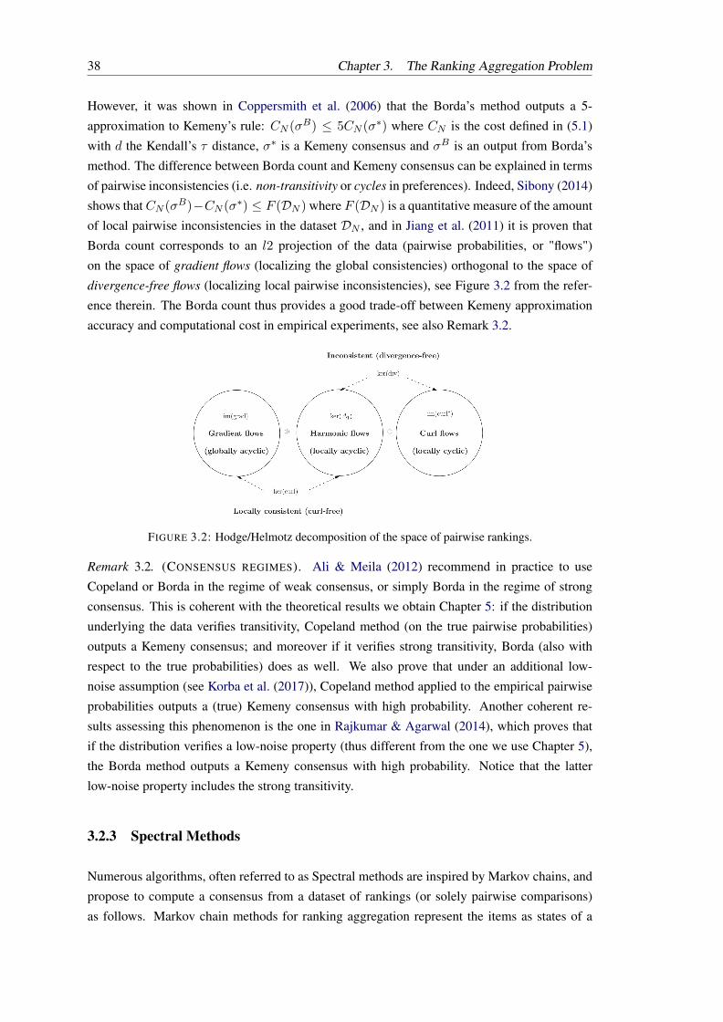
38 Chapter 3. The Ranking Aggregation Problem
However, it was shown in Coppersmith et al. (2006) that the Borda’s method outputs a 5-
approximation to Kemeny’s rule: CN (σB) ≤ 5CN (σ∗) where CN is the cost defined in (5.1)
with d the Kendall’s τ distance, σ∗ is a Kemeny consensus and σB is an output from Borda’s
method. The difference between Borda count and Kemeny consensus can be explained in terms
of pairwise inconsistencies (i.e. non-transitivity or cycles in preferences). Indeed, Sibony (2014)
shows thatCN (σB)−CN (σ∗) ≤ F (DN ) where F (DN ) is a quantitative measure of the amount
of local pairwise inconsistencies in the dataset DN , and in Jiang et al. (2011) it is proven that
Borda count corresponds to an l2 projection of the data (pairwise probabilities, or "flows")
on the space of gradient flows (localizing the global consistencies) orthogonal to the space of
divergence-free flows (localizing local pairwise inconsistencies), see Figure 3.2 from the refer-
ence therein. The Borda count thus provides a good trade-off between Kemeny approximation
accuracy and computational cost in empirical experiments, see also Remark 3.2.
FIGURE 3.2: Hodge/Helmotz decomposition of the space of pairwise rankings.
Remark 3.2. (CONSENSUS REGIMES). Ali & Meila (2012) recommend in practice to use
Copeland or Borda in the regime of weak consensus, or simply Borda in the regime of strong
consensus. This is coherent with the theoretical results we obtain Chapter 5: if the distribution
underlying the data verifies transitivity, Copeland method (on the true pairwise probabilities)
outputs a Kemeny consensus; and moreover if it verifies strong transitivity, Borda (also with
respect to the true probabilities) does as well. We also prove that under an additional low-
noise assumption (see Korba et al. (2017)), Copeland method applied to the empirical pairwise
probabilities outputs a (true) Kemeny consensus with high probability. Another coherent re-
sults assessing this phenomenon is the one in Rajkumar & Agarwal (2014), which proves that
if the distribution verifies a low-noise property (thus different from the one we use Chapter 5),
the Borda method outputs a Kemeny consensus with high probability. Notice that the latter
low-noise property includes the strong transitivity.
3.2.3 Spectral Methods
Numerous algorithms, often referred to as Spectral methods are inspired by Markov chains, and
propose to compute a consensus from a dataset of rankings (or solely pairwise comparisons)
as follows. Markov chain methods for ranking aggregation represent the items as states of a
Chapter 3. The Ranking Aggregation Problem 39
Markov chain, which can be seen as nodes in a graph. The transition probability of going
from node i to node j is based on the relative orders of these items in the rankings in the
dataset, and decreases as i is more preferred to j. The consensus of the dataset is obtained by
computing, or approximating, the stationary distribution of the Markov chain and then sort the
nodes by decreasing probability in the stationary distribution. The position of an item in the
final consensus can thus be interpreted as the probability to be visited by a random walk on this
graph. Markov chain methods thus propose a general algorithm for rank aggregation, composed
of three steps:
• map the set of ranked lists to a single Markov chain M , with one node per item in
1, . . . , n,
• compute (or approximate) the stationary distribution π on M ,
• rank the items in 1, . . . , n based on π.
The key in this method is to define the appropriate mapping in the first step, from the set of
ranked lists to a Markov Chain M . Dwork et al. (2001) proposed, analyzed, and tested four
mapping schemes, called MC1, MC2, MC3 and MC4. The second step boils down to do power
iteration on the transition probability matrix, which can lead to computationally efficient and
iterative algorithms (see the RankCentrality algorithm from Negahban et al. (2012)). Many al-
gorithms modeling preferences as random walks on a graph were considered in the literature,
such as the famous random surfer model on the webpage graph named PageRank (see Brin &
Page (1998)). These methods have been proven to be effective in practice. For instance, Rank
Centrality outputs with high probability a Kemeny consensus under the assumption that the ob-
served comparisons are generated by a Bradley-Terry model (see Rajkumar & Agarwal (2014)).
Recently, extensions to incomplete rankings have been proposed in Maystre & Grossglauser
(2015); Agarwal et al. (2018) which are consistent under the Plackett-Luce model assumption.
3.2.4 Other Ranking Aggregation Methods
Many other methods have been proposed in the literature, that we do not list exhaustively here.
However, many of them will be used as baselines in the experiments of Chapter 4.
MLE and Bayesian approaches. A common approach is to consider that the observed rank-
ings, for examples pairwise comparisons, are generated according to a given model centered
around a true underlying order. The outcomes of the pairwise comparisons are then noisy ver-
sions of the true relative orders under some model, and one can perform MLE (Maximum Like-
lihood Estimation) to recover the underlying central ranking. Several models and settings have
been considered. This idea actually originally arised in the work of Condorcet (see Condorcet
(1785)) under a particular noise model (equivalent to Mallows, see Lu & Boutilier (2011)): a
voter ranks correctly two candidates with probability p > 1/2. Numerous contributions thus
40 Chapter 3. The Ranking Aggregation Problem
consider a Mallows model (see Fligner & Verducci (1990); Meila et al. (2007); Braverman &
Mossel (2008)), a γ-noise model (Pi ≺ j = 1/2 + γ for all i < j, see Braverman & Mos-
sel (2008)), Bradley-Terry model (see BTL-ML algorithm in Rajkumar & Agarwal (2014)), or
more original ones such as the coset-permutation distance based stagewise (CPS) model (see Qin
et al. (2010)). Some come with statistical guarantees, for instance BTL-ML outputs a Kemeny
consensus with high probability under the assumption that the pairwise probabilities verifies the
low-noise (bis) assumption (see Section 2.2.2). An interesting work is also the one of Conitzer
& Sandholm (2012) which states for which voting rules (e.g. scoring rules), there exists (or
not) a noise model such that the voting rule is an MLE estimator under this model. Another ap-
proach, especially in the domain of chess gaming, use Bayesian statistics to estimate a ranking,
assuming some priors on the items preferences (see Glickman (1995); Herbrich et al. (2006);
Coulom (2008)). The obvious limitations of these approaches is that it depends on the unknown
underlying noise model.
Other popular methods. Many other heuristics can be found in the literature. For instance,
QuickSort recursively divides the unsorted list of items into two lists: one list comprising alter-
natives that are preferred to a chosen item (called the pivot), and another comprising alternatives
that are less preferred, and then sorts each of the two lists. The pivot is always chosen as the
first alternative. This method has been proved to be a 2-approximation for Kemeny consen-
sus Ailon et al. (2008), and several variants have been proposed (see Ali & Meila (2012)). In
Schalekamp & Van Zuylen (2009), the authors propose Pick-a-Perm: a full ranking is picked
randomly from Sn according to the empirical distribution of the dataset DN . Another remark-
ably simple method, namely Median Rank Aggregation, aggregates a set of complete rankings
by using the median rank for each item in the dataset DN , and is actually a practical heuristic
for footrule aggregation. Indeed, if the median ranks form a permutation, then it is a footrule
consensus (see Dwork et al. (2001)).
CHAPTER 4A General Method to Bound the Distance to Kemeny
Consensus
Chapter abstract Due to its numerous applications, rank aggregation has become a problemof major interest across many fields of the computer science literature. In the vast majorityof situations, Kemeny consensus(es) are considered as the ideal solutions. It is however wellknown that their computation is NP-hard. Many contributions have thus established variousresults to apprehend this complexity. In this chapter we introduce a practical method to predict,for a ranking and a dataset, how close this ranking is to the Kemeny consensus(es) of thedataset. A major strength of this method is its generality: it does not require any assumptionon the dataset nor the ranking. Furthermore, it relies on a new geometric interpretation ofKemeny aggregation that we believe could lead to many other results.
4.1 Introduction
Given a collection of rankings on a set of alternatives, how to aggregate them into one ranking?
This rank aggregation problem has gained a major interest across many fields of the scientific
literature. Starting from elections in social choice theory (see Borda (1781); Condorcet (1785);
Arrow (1950); Xia (2015)), it has been applied to meta-search engines (see Dwork et al. (2001);
Renda & Straccia (2003); Desarkar et al. (2016)), competitions ranking (see Davenport & Lovell
(2005); Deng et al. (2014)), analysis of biological data (see Kolde et al. (2012); Patel et al.
(2013)) or natural language processing (see Li (2014); Zamani et al. (2014)) among others.
Among the many ways to state the rank aggregation problem stands out Kemeny aggregation
Kemeny (1959). Defined as the problem of minimizing a cost function over the symmetric group
(see Section 4.2 for the definition), its solutions, called Kemeny consensus(es), have been shown
to satisfy desirable properties from many points of view, see Young (1988).
Computing a Kemeny consensus is however NP-hard, even for only four rankings (see Bartholdi
et al. (1989); Cohen et al. (1999); Dwork et al. (2001)). This fact has motivated the scientific
community to introduce many approximation procedures and to evaluate them on datasets (see
Schalekamp & Van Zuylen (2009); Ali & Meila (2012) for examples of procedures and exper-
iments). It has also triggered a tremendous amount of work to obtain theoretical guarantees
41
42 Chapter 4. A General Method to Bound the Distance to Kemeny Consensus
on these procedures and more generally to tackle the complexity of Kemeny aggregation from
various perspectives. Some contributions have proven bounds on the approximation cost of pro-
cedures (see Diaconis & Graham (1977); Coppersmith et al. (2006); Van Zuylen & Williamson
(2007); Ailon et al. (2008); Freund & Williamson (2015)) while some have established recovery
properties (see for instanceSaari & Merlin (2000); Procaccia et al. (2012)). Some other contri-
butions have shown that exact Kemeny aggregation is tractable if some quantity is known on the
dataset (see for instance Betzler et al. (2008, 2009); Cornaz et al. (2013)) or if the dataset satisfies
some conditions (see Brandt et al. (2015)). At last, some contributions have established approx-
imation bounds that can be computed on the dataset (see Davenport & Kalagnanam (2004);
Conitzer et al. (2006); Sibony (2014)).
In this chapter we introduce a novel approach to apprehend the complexity of Kemeny aggrega-
tion. We consider the following question: Given a dataset and a ranking, can we predict how
close the ranking is to a Kemeny consensus without computing the latter? We exhibit a tractable
quantity that allows to give a positive answer to this question. The main practical application
of our results is a simple method to obtain such a guarantee for the outcome of an aggregation
procedure on any dataset. A major strength of our approach is its generality: it applies to all
aggregation procedures, for any dataset.
Our results are based on a certain geometric structure of Kemeny aggregation (see Section 4.3)
that has been barely exploited in the literature yet but constitutes a powerful tool. We thus take
efforts to explain it in details. We believe that it could lead to many other results on Kemeny
aggregation.
The chapter is structured as follows. Section 4.2 introduces the general notations and states the
problem. The geometric structure is detailed in Section 4.3 and further studied in Section 4.5
while our main result is presented in Section 4.4. At last, numerical experiments are described
in details in Section 4.6 to address the efficiency and usefulness of our method on real datasets.
4.2 Controlling the Distance to a Kemeny Consensus
Let JnK = 1, . . . , n be a set of alternatives to be ranked. A full ranking a1 · · · an on JnKis seen as the permutation σ of JnK that maps an item to its rank: σ(ai) = i for i ∈ JnK. The set
of all permutations of JnK is called the symmetric group and denoted by Sn. Given a collection
of N permutations DN = (σ1, . . . , σN ) ∈ SNn , Kemeny aggregation aims at solving
minσ∈Sn
CN (σ), (4.1)
where CN (σ) =∑N
t=1 d(σ, σt) and d is the Kendall’s tau distance defined for σ, σ′ ∈ Sn as the
number of their pairwise disagreements: d(σ, σ′) =∑
1≤i<j≤n I(σ(j)−σ(i))(σ′(j)−σ′(i)) <0. The function CN denotes the cost, and a permutation σ∗ solving (4.1) is called a Kemeny
Chapter 4. A General Method to Bound the Distance to Kemeny Consensus 43
consensus. We denote by KN the set of Kemeny consensuses on the dataset DN . We consider
the following problem.
The Problem. Let σ ∈ Sn be a permutation, typically output by a computationally efficient
aggregation procedure on DN . Can we use computationally tractable quantities to give an
upper bound for the distance d(σ, σ∗) between σ and a Kemeny consensus σ∗ on DN?
The answer to this problem is positive as we will elaborate. It is well known that the Kendall’s
tau distance takes its values in 0, . . . ,(n2
) (see for instance Stanley (1986)). Our main result,
Theorem 10.1, thus naturally takes the form: given σ and DN , if the proposed condition is
satisfied for some k ∈ 0, . . . ,(n2
)− 1, then d(σ, σ∗) ≤ k for all consensuses σ∗ ∈ Kn.
Its application in practice is then straightforward (see Section 4.4 for an illustration). A major
strength of our method is its generality: it can be applied to any dataset DN , any permutation
σ. This is because it exploits a powerful geometric framework for the analysis of Kemeny
aggregation.
4.3 Geometric Analysis of Kemeny Aggregation
Because of its rich mathematical structure, Kemeny aggregation can be analyzed from many
different point of views. While some contributions deal directly with the combinatorics of the
symmetric group (see Diaconis & Graham (1977); Blin et al. (2011)), some work for instance
on the pairwise comparison graph (see for instance ?Conitzer et al. (2006); Jiang et al. (2011)),
and others exploit the geometry of the Permutahedron (see Saari & Merlin (2000)). Here, we
analyze it via the Kemeny embedding (see Jiao & Vert (2015)).
Definition 4.1 (Kemeny embedding). The Kemeny embedding is the mapping φ : Sn → R(n2)
defined by
φ : σ 7→
...
sign(σ(j)− σ(i))...
1≤i<j≤n
,
where sign(x) = 1 if x ≥ 0 and −1 otherwise.
The Kemeny embedding φ maps a permutation to a vector in R(n2) where each coordinate is
indexed by an (unordered) pair i, j ⊂ JnK (we choose i < j by convention). Though this
vector representation is equivalent to representing a permutation as a flow on the complete graph
on JnK, it allows us to perform a geometric analysis of Kemeny aggregation in the Euclidean
space R(n2). Denoting by 〈·, ·〉 the canonical inner product and ‖ · ‖ the Euclidean norm, the
starting point of our analysis is the following result, already proven in Barthelemy & Monjardet
(1981).
44 Chapter 4. A General Method to Bound the Distance to Kemeny Consensus
Proposition 4.2 (Background results). For all σ, σ′ ∈ Sn,
‖φ(σ)‖ =
√n(n− 1)
2and ‖φ(σ)− φ(σ′)‖2 = 4d(σ, σ′),
and for any dataset DN = (σ1, . . . σN ) ∈ SNn , Kemeny aggregation (4.1) is equivalent to the
minimization problem
minσ∈Sn
C ′N (σ), (4.2)
where C ′N (σ) = ‖φ(σ)− φ(DN )‖2 and
φ (DN ) :=1
N
N∑t=1
φ (σt) . (4.3)
Remark 4.3. Proposition 4.2 says that Kemeny rule is a “Mean Proximity Rule”, a family of
voting rules introduced in Zwicker (2008) and further studied in Lahaie & Shah (2014). Our
approach actually applies more generally to other voting rules from this class but we limit our-
selves to Kemeny rule in the chapter for sake of clarity.
Proposition 4.2 leads to the following geometric interpretation of Kemeny aggregation, illus-
trated by Figure 4.1. First, as ‖φ(σ)‖ =√n(n− 1)/2 for all σ ∈ Sn, the embeddings of all
the permutations in Sn lie on the sphere S of center 0 and radius R :=√n(n− 1)/2. No-
tice that ‖φ(σ) − φ(σ′)‖2 = 4d(σ, σ′) for all σ, σ′ ∈ Sn implies that φ is injective, in other
words that it maps two different permutations to two different points on the sphere. A dataset
DN = (σ1, . . . , σN ) ∈ SNn is thus mapped to a weighted point cloud on this sphere, where for
any σ ∈ Sn, the weight of φ(σ) is the number of times σ appears in DN . The vector φ(DN ),
defined by Equation (4.3), is then equal to the barycenter of this weighted point cloud. We call it
the mean embedding of DN . Now, the reformulation of Kemeny aggregation given by Equation
(4.2) means that a Kemeny consensus is a permutation σ∗ whose embedding φ(σ∗) is closest to
φ(DN ), with respect to the Euclidean norm in R(n2).
From an algorithmic point of view, Proposition 4.2 naturally decomposes problem (4.1) of Ke-
meny aggregation in two steps: first compute the mean embedding φ(DN ) in the space R(n2),
and then find a consensus σ∗ as a solution of problem (4.2). The first step is naturally performed
in O(Nn2) operations. The NP-hardness of Kemeny aggregation thus stems from the second
step. In this regard, one may argue that having φ(DN ) does not reduce much of the complex-
ity in identifying an exact Kemeny consensus. However, a closer look at the problem leads
us to asserting that φ(DN ) greatly contains rich information about the localization of the Ke-
meny consensus(es). More specifically, we show in Theorem 10.1 that the knowledge of φ(DN )
helps to provide an upper bound for the distance between a given permutation σ ∈ Sn and any
Kemeny consensus σ∗.

Chapter 4. A General Method to Bound the Distance to Kemeny Consensus 45
FIGURE 4.1: Kemeny aggregation for n = 3.
4.4 Main Result
We now state our main result. For a permutation σ ∈ Sn, we define the angle θN (σ) between
φ(σ) and φ(DN ) by
cos(θN (σ)) =〈φ(σ), φ(DN )〉‖φ(σ)‖‖φ(DN )‖
, (4.4)
with 0 ≤ θN (σ) ≤ π by convention.
Theorem 4.4. Let DN ∈ SNn be a dataset and σ ∈ Sn a permutation. For any k ∈
0, . . . ,(n2
)− 1, one has the following implication:
cos(θN (σ)) >
√1− k + 1(
n2
) ⇒ maxσ∗∈KN
d(σ, σ∗) ≤ k.
The proof of Theorem 10.1 along with its geometric interpretation are postponed to Section
4.5. Here we focus on its application. Broadly speaking, Theorem 10.1 ensures that if the
angle θN (σ) between the embedding φ(σ) of a permutation σ ∈ Sn and the mean embedding
φ(DN ) is small, then the Kemeny consensus(es) cannot be too far from σ. Its application in
practice is straightforward. Assume that one applies an aggregation procedure on DN (say the
Borda count for instance) with an output σ. A natural question is then: how far is it from the
Kemeny consensus(es)? Of course, it is at most equal to maxσ′,σ′′∈Sn d(σ′, σ′′) =(n2
). But if
one computes the quantity cos(θN (σ)), it can happen that Theorem 10.1 allows to give a better
bound. More specifically, the best bound is given by the minimal k ∈ 0, . . . ,(n2
)−1 such that
cos(θN (σ)) >√
1− (k + 1)/(n2
). Denoting by kmin(σ;DN ) this integer, it is easy to see that
kmin(σ;DN ) =
⌊(n2
)sin2(θN (σ))
⌋if 0 ≤ θN (σ) ≤ π
2(n2
)if π2 ≤ θN (σ) ≤ π.
(4.5)
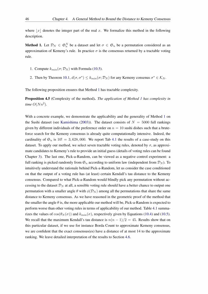
46 Chapter 4. A General Method to Bound the Distance to Kemeny Consensus
where bxc denotes the integer part of the real x. We formalize this method in the following
description.
Method 1. Let DN ∈ SNn be a dataset and let σ ∈ Sn be a permutation considered as an
approximation of Kemeny’s rule. In practice σ is the consensus returned by a tractable voting
rule.
1. Compute kmin(σ;DN ) with Formula (10.5).
2. Then by Theorem 10.1, d(σ, σ∗) ≤ kmin(σ;DN ) for any Kemeny consenus σ∗ ∈ KN .
The following proposition ensures that Method 1 has tractable complexity.
Proposition 4.5 (Complexity of the method). The application of Method 1 has complexity in
time O(Nn2).
With a concrete example, we demonstrate the applicability and the generality of Method 1 on
the Sushi dataset (see Kamishima (2003)). The dataset consists of N = 5000 full rankings
given by different individuals of the preference order on n = 10 sushi dishes such that a brute-
force search for the Kemeny consensus is already quite computationally intensive. Indeed, the
cardinality of Sn is 10! = 3, 628, 000. We report Tab 4.1 the results of a case-study on this
dataset. To apply our method, we select seven tractable voting rules, denoted by σ, as approxi-
mate candidates to Kemeny’s rule to provide an initial guess (details of voting rules can be found
Chapter 3). The last one, Pick-a-Random, can be viewed as a negative control experiment: a
full ranking is picked randomly from Sn according to uniform law (independent from DN ). To
intuitively understand the rationale behind Pick-a-Random, let us consider the case conditioned
on that the output of a voting rule has (at least) certain Kendall’s tau distance to the Kemeny
consensus. Compared to what Pick-a-Random would blindly pick any permutation without ac-
cessing to the dataset DN at all, a sensible voting rule should have a better chance to output one
permutation with a smaller angle θ with φ(DN ) among all the permutations that share the same
distance to Kemeny consensus. As we have reasoned in the geometric proof of the method that
the smaller the angle θ is, the more applicable our method will be, Pick-a-Random is expected to
perform worse than other voting rules in terms of applicability of our method. Table 4.1 summa-
rizes the values of cos(θN (σ)) and kmin(σ), respectively given by Equations (10.4) and (10.5).
We recall that the maximum Kendall’s tau distance is n(n − 1)/2 = 45. Results show that on
this particular dataset, if we use for instance Borda Count to approximate Kemeny consensus,
we are confident that the exact consensus(es) have a distance of at most 14 to the approximate
ranking. We leave detailed interpretation of the results to Section 4.6.

Chapter 4. A General Method to Bound the Distance to Kemeny Consensus 47
TABLE 4.1: Summary of a case-study on the validity of Method 1 with the sushi dataset (N =5000, n = 10). Rows are ordered by increasing kmin (or decreasing cosine) value.
Voting rule cos(θN (σ)) kmin(σ)
Borda 0.820 14Copeland 0.822 14QuickSort 0.822 14
Plackett-Luce 0.80 152-approval 0.745 201-approval 0.710 22
Pick-a-Perm 0.383† 34.85†
Pick-a-Random 0.377† 35.09†
†For randomized methods such as Pick-a-Perm and Pick-a-Random, results are averaged over 10 000 computations.
4.5 Geometric Interpretation and Proof of Theorem 10.1
This section details the proof of Theorem 10.1 and its geometric interpretation. We deem that
our proof has indeed a standalone interest, and that it could lead to other profound results on
Kemeny aggregation.
4.5.1 Extended Cost Function
We recall that the Kemeny consensuses of a dataset DN are the solutions of Problem (4.2):
minσ∈Sn
C ′N (σ) = ‖φ(σ)− φ(DN )‖2.
This is an optimization problem on the discrete set Sn, naturally hard to analyze. In particular
the shape of the cost function C ′N is not easy to understand. However, since all the vectors φ(σ)
for σ ∈ Sn lie on the sphere S = x ∈ R(n2)| ‖x‖ = R with R =√n(n− 1)/2, it is natural
to consider the relaxed problem on S
minx∈SCN (x) := ‖x− φ(DN )‖2. (4.6)
We call CN the extended cost function with domain S. The advantage of CN is that it has a very
simple shape. We denote by θN (x) the angle between a vector x ∈ S and φ(DN ) (with the slight
abuse of notations that θN (φ(σ)) ≡ θN (σ)). For any x ∈ S, one has
CN (x) = R2 + ‖φ(DN )‖2 − 2R‖φ(DN )‖ cos(θN (x)).
This means that the extended cost CN (x) of a vector x ∈ S only depends on the angle θN (x).
The level sets of CN are thus of the form x ∈ S | θN (x) = α, for 0 ≤ α ≤ π. If n = 3, these

48 Chapter 4. A General Method to Bound the Distance to Kemeny Consensus
level sets are circles in planes orthogonal to φ(DN ), each centered around the projection of the
latter on the plane (Figure 4.2). This property implies the following result.
Lemma 4.6. A Kemeny consensus of a dataset DN is a permutation σ∗ such that:
θN (σ∗) ≤ θN (σ) for all σ ∈ Sn.
Lemma 4.6 means that the problem of Kemeny aggregation translates into finding permutations
σ∗ that have minimal angle θN (σ∗). This reformulation is crucial to our approach.
FIGURE 4.2: Level sets of CN over S.
4.5.2 Interpretation of the Condition in Theorem 10.1
The second element of our approach is motivated by the following observation. Let x ∈ S be a
point on the sphere and let r ≥ 0. If r is large enough, then all the points x′ ∈ S on the sphere
that have distance ‖x′−x‖ greater than r will have a greater angle θN (x′). Formally, we denote
by B(x, r) = x′ ∈ R(n2) | ‖x′ − x‖ < r the (open) ball of center x and radius r. Then one
has the following result.
Lemma 4.7. For x ∈ S and r ≥ 0, one has the following implication:
cos(θN (x)) >
√1− r2
4R2⇒ min
x′∈S\B(x,r)θN (x′) > θN (x).
Proof. Let φ(DN ) = φ(DN )‖φ(DN )‖ . We discuss over two cases.
Case I:∥∥φ(DN )− x
∥∥ ≥ r. By laws of cosines, this case is equivalent to:
2R2(1− cos(θN (x))) =∥∥φ(DN )− x
∥∥2 ≥ r2
⇔ cos(θN (x)) ≤ 1− r2
2R2≤ 1− r2
4R2.

Chapter 4. A General Method to Bound the Distance to Kemeny Consensus 49
Note also that in this case, we have φ(DN ) ∈ S \ B(x, r) and hence minx′∈S\B(x,r) θN (x′) =
minx′∈S θN (x′) = 0 ≤ θN (x) always holds, where the minimum is attained at x′ = φ(DN ).
Case II: ‖φ(DN ) − x‖ < r, that is φ(DN ) ∈ B(x, r). As the function x′ 7→ θN (x′) is convex
with global minimum in B(x, r), its minimum over S \ B(x, r) is attained at the boundary
S ∩ ∂B(x, r) = x′ ∈ R(n2) | ‖x′‖ = R and ‖x′ − x‖ = r, which is formed by cutting S with
the((n2
)− 1)-dimensional hyperplane written as
L :=x′ ∈ R(n2)
∣∣∣ 〈x′, x〉 =2R2 − r2
2
Straightforwardly one can verify that S ∩ ∂B(x, r) is in fact a
((n2
)− 1)-dimensional sphere
lying in L, centered at c = 2R2−r22R2 x with radius γ = r
√1− r2
4R2 . Now we take effort to
identify:
x∗ = arg minx′∈S∩∂B(x,r)
θN (x′) = arg minx′∈S∩∂B(x,r)
CN (x′) .
Note that φ(DN ) projected onto L is the vector (φ(DN ))L := φ(DN ) − 〈φ(DN ),x〉R2 x. One can
easily verify by Pythagoras rule that, for any set K ⊆ L,
arg minx′∈K
∥∥x′ − φ(DN )∥∥ = arg min
x′∈K
∥∥x′ − (φ(DN ))L∥∥ .
Therefore we have:
x∗ = arg minx′∈S∩∂B(x,r)
∥∥x′ − (φ(DN ))L∥∥ = c+ γ
(φ(DN ))L‖(φ(DN ))L‖
=2R2 − r2
2R2x+ r
√1− r2
4R2
φ(DN )− 〈φ(DN ),x〉R2 x√
‖φ(DN )‖2 − 〈φ(DN ),x〉2R2
.
Tedious but essentially undemanding calculation leads to
θN (x∗) > θN (x)⇔ 〈x∗, φ(DN )〉 > 〈x, φ(DN )〉
⇔ cos(θN (x)) >
√1− r2
4R2.
It is interesting to look at the geometric interpretation of Lemma 4.7. In fact, it is clear from
the proof that x∗ should lie in the 2-dimensional subspace spanned by φ(DN ) and x. We
are thus able to properly define multiples of an angle by summation of angles on such linear
space 2θN (x) := θN (x) + θN (x). Figure 4.3 provides an illustration of Lemma 4.7 in this
2-dimensional subspace from the geometric point of view, with r taking integer values (repre-
senting possible Kendall’s tau distance). In this illustration, the smallest integer value for r such
that these inequalities hold is r = 2.
50 Chapter 4. A General Method to Bound the Distance to Kemeny Consensus
In words, provided that θN (x) ≤ π/2, x∗ has a smaller angle than x is equivalently written
using laws of cosines as
r2 = ‖x− x∗‖2 > 2R2(1− cos(2θN (x))
)⇔ cos(2θN (x)) > 1− r2
2R2⇔ cos(θN (x)) >
√1− r2
4R2.
This recovers exactly the condition stated in Lemma 4.7.
FIGURE 4.3: Illustration of Lemma 4.7.
4.5.3 Embedding of a Ball
For σ ∈ Sn and k ∈ 0, . . . ,(n2
) we denote by B(σ, k) the (closed) ball for the Kendall’s tau
distance of center σ and radius k, i.e. B(σ, k) = σ′ ∈ Sn | d(σ, σ′) ≤ k. The following is a
direct consequence of Proposition 4.2.
Lemma 4.8. For σ ∈ Sn and k ∈ 0, . . . ,(n2
),
φ (Sn \B(σ, k)) ⊂ S \ B(φ(σ), 2√k + 1)
4.5.4 Proof of Theorem 10.1
We can now prove Theorem 10.1 by combining the previous results and observations.
Proof of Theorem 10.1. Let DN ∈ SNn be a dataset and σ ∈ Sn a permutation. By Lemma 4.7,
one has for any r > 0,
cos(θN (σ)) >
√1− r2
4R2⇒ min
x∈S\B(φ(σ),r)θN (x) > θN (σ).
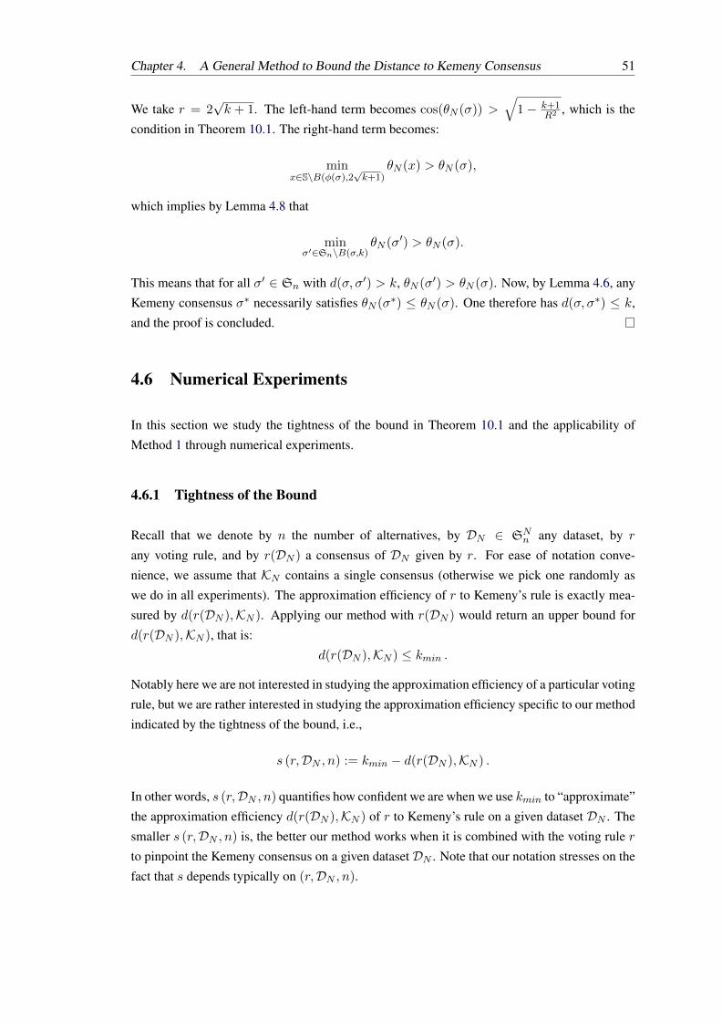
Chapter 4. A General Method to Bound the Distance to Kemeny Consensus 51
We take r = 2√k + 1. The left-hand term becomes cos(θN (σ)) >
√1− k+1
R2 , which is the
condition in Theorem 10.1. The right-hand term becomes:
minx∈S\B(φ(σ),2
√k+1)
θN (x) > θN (σ),
which implies by Lemma 4.8 that
minσ′∈Sn\B(σ,k)
θN (σ′) > θN (σ).
This means that for all σ′ ∈ Sn with d(σ, σ′) > k, θN (σ′) > θN (σ). Now, by Lemma 4.6, any
Kemeny consensus σ∗ necessarily satisfies θN (σ∗) ≤ θN (σ). One therefore has d(σ, σ∗) ≤ k,
and the proof is concluded.
4.6 Numerical Experiments
In this section we study the tightness of the bound in Theorem 10.1 and the applicability of
Method 1 through numerical experiments.
4.6.1 Tightness of the Bound
Recall that we denote by n the number of alternatives, by DN ∈ SNn any dataset, by r
any voting rule, and by r(DN ) a consensus of DN given by r. For ease of notation conve-
nience, we assume that KN contains a single consensus (otherwise we pick one randomly as
we do in all experiments). The approximation efficiency of r to Kemeny’s rule is exactly mea-
sured by d(r(DN ),KN ). Applying our method with r(DN ) would return an upper bound for
d(r(DN ),KN ), that is:
d(r(DN ),KN ) ≤ kmin .
Notably here we are not interested in studying the approximation efficiency of a particular voting
rule, but we are rather interested in studying the approximation efficiency specific to our method
indicated by the tightness of the bound, i.e.,
s (r,DN , n) := kmin − d(r(DN ),KN ) .
In other words, s (r,DN , n) quantifies how confident we are when we use kmin to “approximate”
the approximation efficiency d(r(DN ),KN ) of r to Kemeny’s rule on a given dataset DN . The
smaller s (r,DN , n) is, the better our method works when it is combined with the voting rule r
to pinpoint the Kemeny consensus on a given dataset DN . Note that our notation stresses on the
fact that s depends typically on (r,DN , n).
52 Chapter 4. A General Method to Bound the Distance to Kemeny Consensus
Bord
a
Cop
elan
d
1-Ap
prov
al2-
Appr
oval
Plac
kett-
Luce
Qui
ckso
rtPi
ck-a
-Per
mPi
ck-a
-Ran
dom
0
1
2
3
4s
(Tig
htne
ss o
f the
bou
nd)
sushi 3 items
Bord
a
Cop
elan
d
1-Ap
prov
al2-
Appr
oval
Plac
kett-
Luce
Qui
ckso
rtPi
ck-a
-Per
mPi
ck-a
-Ran
dom
0
1
2
3
4
5
6
s (T
ight
ness
of t
he b
ound
)
sushi 4 items
Bord
a
Cop
elan
d
1-Ap
prov
al2-
Appr
oval
Plac
kett-
Luce
Qui
ckso
rtPi
ck-a
-Per
mPi
ck-a
-Ran
dom
0
1
2
3
4
5
6
7
s (T
ight
ness
of t
he b
ound
)
sushi 5 items
FIGURE 4.4: Boxplot of s (r,DN , n) over sampling collections of datasets shows the effectfrom different size of alternative set n with restricted sushi datasets (n = 3; 4; 5, N = 5000).
We empirically investigate the efficiency of our proposed method by experimenting s (r,DN , n)
with various voting rules r, on different datasetsDN , implicitly involving n as well. For that pur-
pose, in each experiment we test six prevalent voting rules plus one negative-control method as
approximate candidates to Kemeny’s rule: three scoring rules that are Borda Count, k-approval,
Copeland; two algorithmic approaches that are QuickSort and Pick-a-Perm; one statistical ap-
proach based on Plackett-Luce ranking model; one baseline method serving a negative control
that is Pick-a-Random where a random permutation is picked from Sn according to uniform
law (independent from the dataset DN ). Details of the voting rules may be found Chapter 3.
We first look at the the effect of different voting rules r on s (r;DN , n) with the APA dataset.
In the 1980 American Psychological Association (APA) presidential election, voters were asked
to rank n = 5 candidates in order of preference and a total of N = 5738 complete ballots were
reported. With the original collection of ballots introduced by Diaconis (1989), We created 500
bootstrapped pseudo-samples following Popova (2012). As shown in Figure 4.5, s (r;DN , n)
varies across different voting rules and our method works typically well combined with Borda
Count or Plackett-Luce, a phenomenon that constantly occurs in many experiments. For ex-
ample for Borda Count the median tightness being 3 means that our method provides a bound
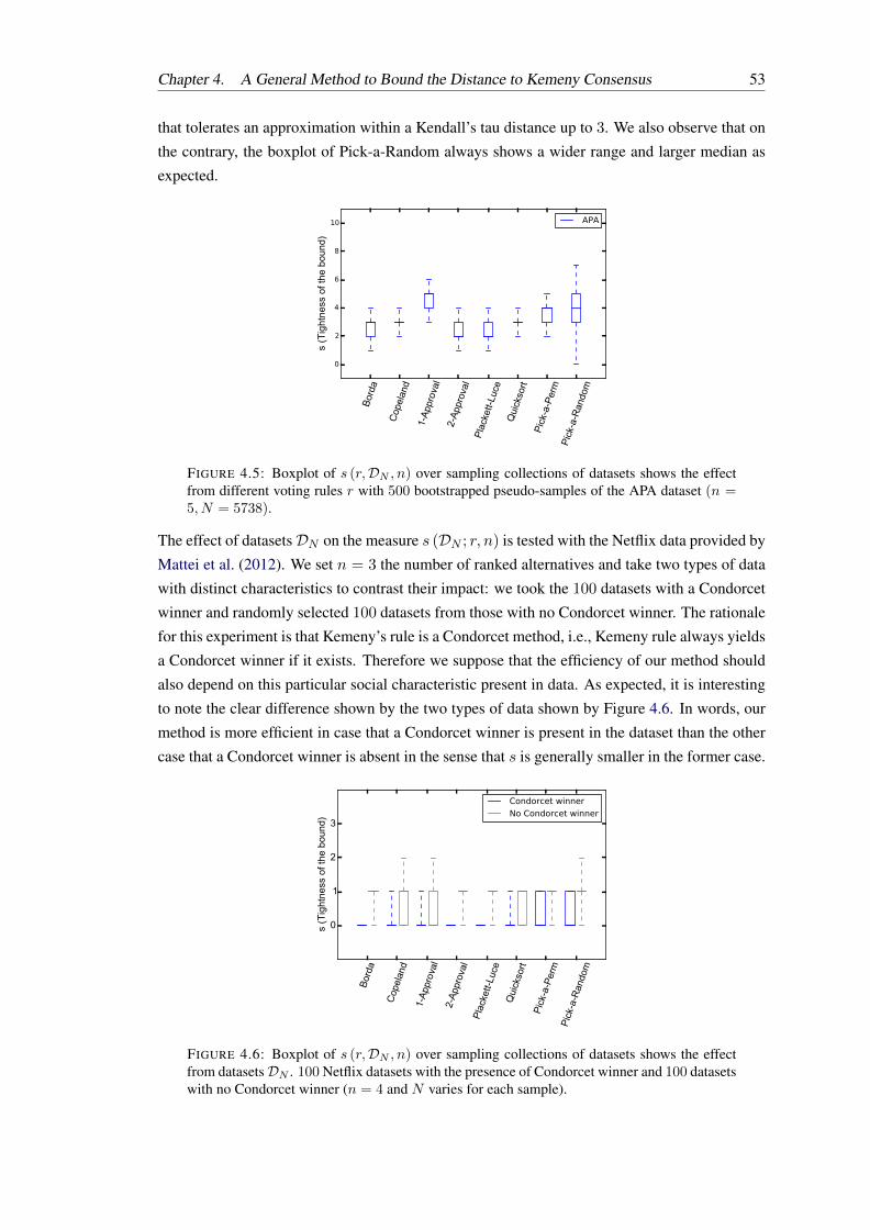
Chapter 4. A General Method to Bound the Distance to Kemeny Consensus 53
that tolerates an approximation within a Kendall’s tau distance up to 3. We also observe that on
the contrary, the boxplot of Pick-a-Random always shows a wider range and larger median as
expected.
Bord
a
Cop
elan
d1-
Appr
oval
2-Ap
prov
alPl
acke
tt-Lu
ceQ
uick
sort
Pick
-a-P
erm
Pick
-a-R
ando
m
0
2
4
6
8
10
s (T
ight
ness
of t
he b
ound
)
APA
FIGURE 4.5: Boxplot of s (r,DN , n) over sampling collections of datasets shows the effectfrom different voting rules r with 500 bootstrapped pseudo-samples of the APA dataset (n =5, N = 5738).
The effect of datasetsDN on the measure s (DN ; r, n) is tested with the Netflix data provided by
Mattei et al. (2012). We set n = 3 the number of ranked alternatives and take two types of data
with distinct characteristics to contrast their impact: we took the 100 datasets with a Condorcet
winner and randomly selected 100 datasets from those with no Condorcet winner. The rationale
for this experiment is that Kemeny’s rule is a Condorcet method, i.e., Kemeny rule always yields
a Condorcet winner if it exists. Therefore we suppose that the efficiency of our method should
also depend on this particular social characteristic present in data. As expected, it is interesting
to note the clear difference shown by the two types of data shown by Figure 4.6. In words, our
method is more efficient in case that a Condorcet winner is present in the dataset than the other
case that a Condorcet winner is absent in the sense that s is generally smaller in the former case.
Bord
a
Cop
elan
d1-
Appr
oval
2-Ap
prov
alPl
acke
tt-Lu
ceQ
uick
sort
Pick
-a-P
erm
Pick
-a-R
ando
m
0
1
2
3
s (T
ight
ness
of t
he b
ound
)
Condorcet winner
No Condorcet winner
FIGURE 4.6: Boxplot of s (r,DN , n) over sampling collections of datasets shows the effectfrom datasetsDN . 100 Netflix datasets with the presence of Condorcet winner and 100 datasetswith no Condorcet winner (n = 4 and N varies for each sample).
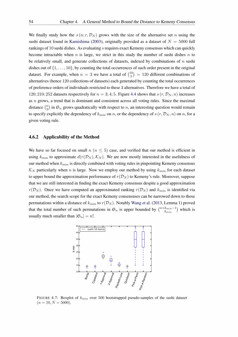
54 Chapter 4. A General Method to Bound the Distance to Kemeny Consensus
We finally study how the s (n; r,DN ) grows with the size of the alternative set n using the
sushi dataset found in Kamishima (2003), originally provided as a dataset of N = 5000 full
rankings of 10 sushi dishes. As evaluating s requires exact Kemeny consensus which can quickly
become intractable when n is large, we strict in this study the number of sushi dishes n to
be relatively small, and generate collections of datasets, indexed by combinations of n sushi
dishes out of 1, . . . , 10, by counting the total occurrences of such order present in the original
dataset. For example, when n = 3 we have a total of(
103
)= 120 different combinations of
alternatives (hence 120 collections of datasets) each generated by counting the total occurrences
of preference orders of individuals restricted to these 3 alternatives. Therefore we have a total of
120; 210; 252 datasets respectively for n = 3; 4; 5. Figure 4.4 shows that s (r,DN , n) increases
as n grows, a trend that is dominant and consistent across all voting rules. Since the maximal
distance(n2
)in Sn grows quadratically with respect to n, an interesting question would remain
to specify explicitly the dependency of kmin on n, or the dependency of s (r,DN , n) on n, for a
given voting rule.
4.6.2 Applicability of the Method
We have so far focused on small n (n ≤ 5) case, and verified that our method is efficient in
using kmin to approximate d(r(DN ),KN ). We are now mostly interested in the usefulness of
our method when kmin is directly combined with voting rules in pinpointing Kemeny consensus
KN particularly when n is large. Now we employ our method by using kmin for each dataset
to upper bound the approximation performance of r(DN ) to Kemeny’s rule. Moreover, suppose
that we are still interested in finding the exact Kemeny consensus despite a good approximation
r(DN ). Once we have computed an approximated ranking r(DN ) and kmin is identified via
our method, the search scope for the exact Kemeny consensuses can be narrowed down to those
permutations within a distance of kmin to r(DN ). Notably Wang et al. (2013, Lemma 1) proved
that the total number of such permutations in Sn is upper bounded by(n+kmin−1
kmin
)which is
usually much smaller than |Sn| = n!.
Bord
a
Cop
elan
d1-
Appr
oval
2-Ap
prov
alPl
acke
tt-Lu
ceQ
uick
sort
Pick
-a-P
erm
Pick
-a-R
ando
m
10
15
20
25
30
35
40
45
k m
in
sushi 10 items
FIGURE 4.7: Boxplot of kmin over 500 bootstrapped pseudo-samples of the sushi dataset(n = 10, N = 5000).
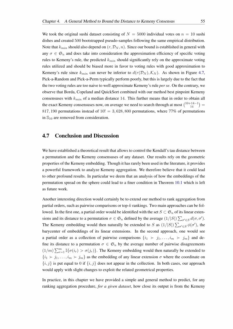
Chapter 4. A General Method to Bound the Distance to Kemeny Consensus 55
We took the original sushi dataset consisting of N = 5000 individual votes on n = 10 sushi
dishes and created 500 bootstrapped pseudo-samples following the same empirical distribution.
Note that kmin should also depend on (r,DN , n). Since our bound is established in general with
any σ ∈ Sn and does take into consideration the approximation efficiency of specific voting
rules to Kemeny’s rule, the predicted kmin should significantly rely on the approximate voting
rules utilized and should be biased more in favor to voting rules with good approximation to
Kemeny’s rule since kmin can never be inferior to d(r(DN ),KN ). As shown in Figure 4.7,
Pick-a-Random and Pick-a-Perm typically perform poorly, but this is largely due to the fact that
the two voting rules are too naive to well approximate Kemeny’s rule per se. On the contrary, we
observe that Borda, Copeland and QuickSort combined with our method best pinpoint Kemeny
consensuses with kmin of a median distance 14. This further means that in order to obtain all
the exact Kemeny consensuses now, on average we need to search through at most(
10+14−114
)=
817, 190 permutations instead of 10! = 3, 628, 800 permutations, where 77% of permutations
in S10 are removed from consideration.
4.7 Conclusion and Discussion
We have established a theoretical result that allows to control the Kendall’s tau distance between
a permutation and the Kemeny consensuses of any dataset. Our results rely on the geometric
properties of the Kemeny embedding. Though it has rarely been used in the literature, it provides
a powerful framework to analyze Kemeny aggregation. We therefore believe that it could lead
to other profound results. In particular we deem that an analysis of how the embeddings of the
permutation spread on the sphere could lead to a finer condition in Theorem 10.1 which is left
as future work.
Another interesting direction would certainly be to extend our method to rank aggregation from
partial orders, such as pairwise comparisons or top-k rankings. Two main approaches can be fol-
lowed. In the first one, a partial order would be identified with the set S ⊂ Sn of its linear exten-
sions and its distance to a permutation σ ∈ Sn defined by the average (1/|S|)∑
σ′∈S d(σ, σ′).
The Kemeny embedding would then naturally be extended to S as (1/|S|)∑
σ′∈S φ(σ′), the
barycenter of embeddings of its linear extensions. In the second approach, one would see
a partial order as a collection of pairwise comparisons i1 j1, . . . , im jm and de-
fine its distance to a permutation σ ∈ Sn by the average number of pairwise disagreements
(1/m)∑m
r=1 Iσ(ir) > σ(jr). The Kemeny embedding would then naturally be extended to
i1 j1, . . . , im jm as the embedding of any linear extension σ where the coordinate on
i, j is put equal to 0 if i, j does not appear in the collection. In both cases, our approach
would apply with slight changes to exploit the related geometrical properties.
In practice, in this chapter we have provided a simple and general method to predict, for any
ranking aggregation procedure, for a given dataset, how close its output is from the Kemeny

56 Chapter 4. A General Method to Bound the Distance to Kemeny Consensus
consensuses. However, our analysis is valid for a fixed dataset; and it is then natural to in-
vestigate the behavior of ranking aggregation rules when the number of samples in the dataset
increases. In the next chapter, we investigate the generalization abilities of such rules in a formal
probabilistic setup.
CHAPTER 5A Statistical Framework for Ranking Aggregation
Chapter abstract This chapter develops a statistical learning theory for ranking aggregationin a general probabilistic setting (avoiding any rigid ranking model assumptions) which is at thecore of this thesis. We assess the generalization ability of empirical ranking medians: universalrate bounds are established and the situations where convergence occurs at an exponential rateare fully characterized. Minimax lower bounds are also proved, showing that the rate boundswe obtain are optimal.
5.1 Introduction
In ranking aggregation, the goal is to summarize a collection of rankings over a set of alterna-
tives by a single (consensus) ranking. Two main approaches have emerged in the literature to
state the rank aggregation problem. The first one, originating from the seminal work of Con-
dorcet in the 18th century (Condorcet, 1785), considers a generative probabilistic model on the
rankings and the problem then consists in maximizing the likelihood of a candidate aggregate
ranking. This MLE approach has been widely used in machine-learning and computational
social choice, see e.g. Conitzer & Sandholm (2005); Truchon (2008); Conitzer et al. (2009).
Alternatively, the metric approach consists in choosing a (pseudo-) distance on the set of rank-
ings and then finding a barycentric/median ranking, i.e. a ranking at minimum distance from
the observed ones. It encompasses numerous methods, including the popular Kemeny aggre-
gation, which the present chapter focuses on. These two approaches can be related in certain
situations however. Indeed, Kemeny aggregation can be given a statistical interpretation: it is
equivalent to the MLE approach under the noise model intuited by Condorcet (see Young, 1988)
then formalized as the Mallows model (see definition in Remark 5.7).
Concerning the metric approach, much effort has been devoted to developing efficient algo-
rithms for the computation of a median permutation related to a given collection of rankings,
whereas statistical issues about the generalization properties of such empirical medians have
been largely ignored as far as we know. The sole statistical analyses of ranking aggregation
have been carried out in the restrictive setting of parametric models. Hence, in spite of this un-
interrupted research activity, the generalization ability of ranking aggregation rules has not been
investigated in a formal probabilistic setup, with the notable exception of Soufiani et al. (2014b),
57
58 Chapter 5. A Statistical Framework for Ranking Aggregation
where a decision-theoretic framework is introduced and the properties of Bayesian estimators
for parametric models are discussed (as popular axioms in social choice). In this chapter, we
develop a general statistical framework for Kemeny aggregation, on the model of the probabilis-
tic results developed for pattern recognition (see Devroye et al., 1996), the flagship problem in
statistical learning theory. Precisely, conditions under which optimal elements can be character-
ized are exhibited, universal rate bounds for empirical Kemeny medians are stated and shown
to be minimax. A low noise property is also introduced that allows to establish exponentially
fast rates of convergence, following in the footsteps of the results obtained in Koltchinskii &
Beznosova (2005) for binary classification.
The chapter is organized as follows. In section 5.2, key notions of consensus ranking are briefly
recalled and the statistical framework considered through the chapter is introduced at length,
together with the main notations. Section 5.3 is devoted to the characterization of optimal so-
lutions for the Kemeny aggregation problem, while section 5.4 provides statistical guarantees
for the generalization capacity of empirically barycentric rankings in the form of rate bounds in
expectation/probability. The proofs are deferred to section 5.6.
5.2 Background
We start with a rigorous formulation of (the metric approach of) consensus ranking and describe
next the probabilistic framework for ranking aggregation we consider in this chapter. Here and
throughout, the indicator function of any event E is denoted by IE, the Dirac mass at any point
a by δa, and we set sgn(x) = 2Ix ≥ 0 − 1 for all x ∈ R. At last, the set of permutations of
the ensemble JnK = 1, . . . , n, n ≥ 1 is denoted by Sn.
5.2.1 Consensus Ranking
In the simplest formulation, a (full) ranking on a set of items JnK is seen as the permutation
σ ∈ Sn that maps an item i to its rank σ(i). Given a collection of N ≥ 1 permutations
σ1, . . . , σN , the goal of ranking aggregation is to find σ∗ ∈ Sn that best summarizes it. A
popular approach consists in solving the following optimization problem:
minσ∈Sn
N∑i=1
d(σ, σi), (5.1)
where d(., .) is a given metric on Sn. Such a barycentric permutation, referred to as a consen-
sus/median ranking sometimes, always exists, since Sn is finite, but is not necessarily unique.
In the most studied version of this problem, termed Kemeny ranking aggregation, the metric
considered is equal to the Kendall’s τ distance (see Kemeny, 1959): ∀(σ, σ′) ∈ S2n,
dτ (σ, σ′) =∑i<j
I(σ(i)− σ(j))(σ′(i)− σ′(j)) < 0,
Chapter 5. A Statistical Framework for Ranking Aggregation 59
i.e. the number of pairwise disagreements between σ and σ′. Such a consensus has many in-
teresting properties, but is NP-hard to compute. Various algorithms have been proposed in the
literature to compute acceptably good solutions in a reasonable amount of time, their descrip-
tion is beyond the scope of the chapter, see for example Ali & Meila (2012) or Chapter 3 for
references.
5.2.2 Statistical Framework
In the probabilistic setting we consider here, the collection of rankings to be aggregated is sup-
posed to be composed of N ≥ 1 i.i.d. copies Σ1, . . . , ΣN of a generic random variable Σ
defined on a probability space (Ω, F , P) drawn from an unknown probability distribution P
on Sn (i.e. P (σ) = PΣ = σ for any σ ∈ Sn). With respect to a certain metric d(., .) on
Sn (e.g. the Kendall τ distance), a (true) median of distribution P w.r.t. d is any solution of the
minimization problem:
minσ∈Sn
LP (σ), (5.2)
where LP (σ) = EΣ∼P [d(Σ, σ)] denotes the expected distance between any permutation σ and
Σ and shall be referred to as the risk of the median candidate σ throughout the thesis. The
objective pursued is to recover approximately a solution σ∗ of this minimization problem, plus
an estimate of this minimum L∗P = LP (σ∗), as accurate as possible, based on the observations
Σ1, . . . , ΣN . The minimization problem (5.2) always has a solution since the cardinality
of Sn is finite (however exploding with n) but can be multimodal, see Section 5.3. A median
permutation σ∗ can be interpreted as a central value for P , a crucial location parameter, whereas
the quantity L∗P can be viewed as a dispersion measure. However, the functional LP (.) is
unknown in practice, just like distribution P . When there is no ambiguity on the distribution
considered, we write L(.) for LP (.), and L∗ for L∗P in this chapter. We only have access to
the dataset Σ1, . . . , ΣN to find a reasonable approximant of a median and would like to
avoid rigid assumptions on P such as those stipulated by the Mallows model, see Mallows
(1957) and Remark 5.7. Following the Empirical Risk Minimization (ERM) paradigm (see e.g.
Vapnik, 2000), one replaces the quantity L(σ) by a statistical version based on the sampling
data, typically the unbiased estimator
LN (σ) =1
N
N∑i=1
d(Σi, σ). (5.3)
Notice that LN = LPN
where PN = 1/N∑N
t=1 δΣt is the empirical distribution. It is the goal
of the subsequent analysis to assess the performance of solutions σN of
minσ∈Sn
LN (σ), (5.4)
60 Chapter 5. A Statistical Framework for Ranking Aggregation
by establishing (minimax) bounds for the excess of risk L(σN )−L∗ in probability/expectation,
when d is the Kendall’s τ distance. In this case, any solution of problem (5.2) (resp., of problem
(5.4)) is called a Kemeny median (resp., an empirical Kemeny median) throughout the thesis.
Remark 5.1. (ALTERNATIVE DISPERSION MEASURE) An alternative measure of dispersion
which can be more easily estimated than L∗ = L(σ∗) is given by
γ(P ) =1
2E[d(Σ,Σ′)], (5.5)
where Σ′ is an independent copy of Σ. One may easily show that γ(P ) ≤ L∗ ≤ 2γ(P ).
The estimator of (5.5) with minimum variance among all unbiased estimators is given by the
U -statistic
γN =2
N(N − 1)
∑i<j
d(Σi,Σj). (5.6)
In addition, we point out that confidence intervals for the parameter γ(P ) can be constructed by
means of Hoeffding/Bernstein type deviation inequalities forU -statistics and a direct (smoothed)
bootstrap procedure can be applied for this purpose, see Lahiri (1993). In contrast, a bootstrap
technique for building CI’s for L∗ would require to solve several times an empirical version of
(5.2) based on bootstrap samples.
Remark 5.2. (ALTERNATIVE FRAMEWORK) Since the computation of Kendall’s τ distance in-
volves pairwise comparisons only, one could compute empirical versions of the risk functionalL
in a statistical framework stipulating that the observations are less complete than Σ1, . . . , ΣNand formed by i.i.d. pairs (ek, εk), k = 1, . . . , N, where the ek = (ik, jk)’s are indepen-
dent from the Σk’s and drawn from an unknown distribution ν on the set En such that ν(e) > 0
for all e ∈ En and εk = sgn(Σk(jk) − Σk(ik)) with ek = (ik, jk) for 1 ≤ k ≤ N . Based on
these observations, an estimate of the risk EνEΣ∼P [Ie = (i, j), ε(σ(j) − σ(i)) < 0] of any
median candidate σ ∈ Sn is given by:
∑i<j
1
Ni,j
N∑k=1
Iek = (i, j), εk(σ(j)− σ(i)) < 0,
where Ni,j =∑N
k=1 Iek = (i, j), see for instance Lu & Boutilier (2014) or Rajkumar &
Agarwal (2014) for ranking aggregation results in this setting.
5.2.3 Connection to Voting Rules
In Social Choice, we have a collection of votes under the form of rankingsDN = (σ1, . . . , σN ).
Such a collection of votes DN ∈ SNn is called a profile and a voting rule, which outputs a
consensus ranking on this profile, is classically defined as follows:
σPN = arg minσ∈Sn
g(σ,DN )
Chapter 5. A Statistical Framework for Ranking Aggregation 61
where g : Sn×⋃∞t=1 S
tn → R. This definition can be easily translated in order to be applied to
any given distribution P instead of a profile. Indeed, the authors of Prasad et al. (2015) define a
distributional rank aggregation procedure as follows:
σP = arg minσ∈Sn
g(σ, P )
where g : Sn×Pn → R wherePn is the set of all distributions on Sn. Many classic aggregation
procedures are naturally extended through this definition and thus to our statistical framework, as
we have seen for Kemeny ranking aggregation previously. To detail some examples, we denote
by pi,j = PΣ(i) < Σ(j) = 1 − pj,i for 1 ≤ i 6= j ≤ n and define the associated empirical
estimator by pi,j = (1/N)∑N
m=1 IΣm(i) < Σm(j). The Copeland method (Copeland, 1951)
consists on DN in ranking the items by decreasing order of their Copeland score, calculated
for each one as the number of items it beats in pairwise duels minus the number of items it
looses against: sN (i) =∑
k 6=i Ipi,k ≤ 1/2 − Ipi,k > 1/2. It thus naturally applies to
a distribution P using the scores s(i) =∑
k 6=i Ipi,k ≤ 1/2 − Ipi,k > 1/2. Similarly,
Borda aggregation (Borda, 1781) which consists in ranking items in increasing order of their
score sN (i) =∑N
m=1 Σm(i) when applied on PN , naturally extends to P using the scores
s(i) = EP [Σ(i)].
5.3 Optimality
As recalled above, the discrete optimization problem (5.2) always has a solution, whatever the
metric d chosen. In the case of the Kendall’s τ distance however, the optimal elements can be
explicitly characterized in certain situations. It is the goal of this section to describe the set of
Kemeny medians under specific conditions. As a first go, observe that the risk of a permutation
candidate σ ∈ Sn can be then written as
L(σ) =∑i<j
pi,jIσ(i) > σ(j)+∑i<j
(1− pi,j)Iσ(i) < σ(j). (5.7)
Remark 5.3. (CONNECTION TO BINARY CLASSIFICATION) Let (i, j) be a random pair defined
on (Ω,F , P), uniformly distributed on the set (i, j) : 1 ≤ i < j ≤ n and independent from
Σ. Up to the factor n(n−1)/2, the risk (5.7) can be rewritten as the expectation of the error made
when predicting the sign variable sgn(Σ(j)−Σ(i)) by the specific classifier sgn(σ(j)− σ(i)):
L(σ) =n(n− 1)
2E [li,j(Σ, σ)] , (5.8)
where we set li,j(σ, σ′) = I(σ(i) − σ(j)) · (σ′(i) − σ′(j)) < 0 for all i < j, (σ, σ′) ∈ S2n.
The r.v. pi,j can be viewed as the posterior related to this classification problem.

62 Chapter 5. A Statistical Framework for Ranking Aggregation
We deduce from (5.7) that L∗ ≥∑
i<j minpi,j , 1− pi,j. In addition, if there exists a permu-
tation σ with the property that ∀i < j s.t. pi,j 6= 1/2,
(σ(j)− σ(i)) · (pi,j − 1/2) > 0, (5.9)
it would be necessarily a median for P (notice incidentally that L∗ =∑
i<j minpi,j , 1− pi,jin this case).
Definition 5.4. The probability distribution P on Sn is said to be stochastically transitive if it
fulfills the condition: ∀(i, j, k) ∈ JnK3,
pi,j ≥ 1/2 and pj,k ≥ 1/2⇒ pi,k ≥ 1/2
In addition, if pi,j 6= 1/2 for all i < j, P is said to be strictly stochastically transitive.
Let s∗ : JnK→ JnK be the mapping defined by:
s∗(i) = 1 +∑k 6=i
Ipi,k <1
2 (5.10)
for all i ∈ JnK, which induces the same ordering as the Copeland method (see Subsection 5.2.3).
Observe that, if the stochastic transitivity is fulfilled, then: pi,j < 1/2 ⇔ s∗(i) < s∗(j).
Equipped with this notation, property (5.9) can be also formulated as follows: ∀i < j s.t.
s∗(i) 6= s∗(j),
(σ(j)− σ(i)) · (s∗(j)− s∗(i)) > 0. (5.11)
The result stated below describes the set of Kemeny median rankings under the conditions intro-
duced above, and states the equivalence between the Copeland method and Kemeny aggregation
in this setting.
Theorem 5.5. If the distribution P is stochastically transitive, there exists σ∗ ∈ Sn such that
(5.9) holds true. In this case, we have
L∗ =∑i<j
minpi,j , 1− pi,j (5.12)
=∑i<j
1
2−∣∣∣∣pi,j − 1
2
∣∣∣∣ ,the excess of risk of any σ ∈ Sn is given by
L(σ)− L∗ = 2∑i<j
|pi,j − 1/2| · I(σ(j)− σ(i))(pi,j − 1/2) < 0
and the set of medians of P is the class of equivalence of σ∗ w.r.t. the equivalence relationship:
σRPσ′ ⇔ (σ(j)− σ(i))(σ′(j)− σ′(i)) > 0, for all i < j such that pi,j 6= 1/2. (5.13)
Chapter 5. A Statistical Framework for Ranking Aggregation 63
In addition, the mapping s∗ belongs to Sn iff P is strictly stochastically positive. In this case,
s∗ is the unique median of P .
The proof is detailed in section 5.6. Before investigating the accuracy of empirical Kemeny
medians, a few remarks are in order.
Remark 5.6. (BORDA CONSENSUS) We say that the distribution P is strongly stochastically
transitive if ∀(i, j, k) ∈ JnK3:
pi,j ≥ 1/2 and pj,k ≥ 1/2⇒ pi,k ≥ max(pi,j , pj,k).
Then under this condition, and for i < j, pi,j 6= 12 , there exists a unique σ∗ ∈ Sn such that (5.9)
holds true, corresponding to the Kemeny and Borda consensus both at the same time (see the
section 5.6 for the proof).
Remark 5.7. (MALLOWS MODEL) The Mallows model introduced in the seminal contribution
Mallows (1957) is a probability distribution Pθ on Sn parametrized by θ = (σ0, ψ) ∈ Sn ×[0, 1]: ∀σ ∈ Sn,
Pθ0(σ) =1
Zψdτ (σ0,σ), (5.14)
where Z =∑
σ∈Sn ψdτ (σ0,σ) is a normalization constant. One may easily show that Z is inde-
pendent from σ and that Z =∏n−1i=1
∑ij=0 ψ
j . Observe firstly that the smallest the parameter
ψ, the spikiest the distribution Pθ (equal to a Dirac distribution for ψ = 0). In contrast, Pθ is
the uniform distribution on Sn when ψ = 1. Observe in addition that, as soon as ψ < 1, the
Mallows model Pθ fulfills the strict stochastic transitivity property. Indeed, it follows in this
case from Corollary 3 in Busa-Fekete et al. (2014) that for any i < j, we have:
(i) σ0(i) < σ0(j)⇐ pi,j ≥ 11+ψ >
12 with equality holding iff σ0(i) = σ0(j)− 1,
(ii) σ0(i) > σ0(j)⇐ pi,j ≤ ψ1+ψ <
12 with equality holding iff σ0(i) = σ0(j) + 1,
(iii) pi,j > 12 iff σ0(i) < σ0(j) and pi,j < 1
2 iff σ0(i) > σ0(j).
This directly implies that for any i < j:
|pi,j −1
2| ≥ |ψ − 1|
2(1 + ψ)
Therefore, according to (5.12), we have in this setting:
L∗Pθ ≤n(n− 1)
2
ψ
1 + ψ. (5.15)
The permutation σ0 of reference is then the unique mode of distribution Pθ, as well as its unique
median.
Remark 5.8. (BRADLEY-TERRY-LUCE-PLACKETT MODEL) The Bradley-Terry-Luce-Plackett
model (Bradley & Terry, 1952; Luce, 1959; Plackett, 1975) assumes the existence of some

64 Chapter 5. A Statistical Framework for Ranking Aggregation
hidden preference vector w = [wi]1≤i≤n, where wi represents the underlying preference score
of item i. For all i < j, pij = wiwi+wj
. If w1 ≤ · · · ≤ wn, we have in this case L∗Pθ =∑i<j wi/(wi + wj). Observe in addition that as soon as for all i < j, wi 6= wj , the model
fulfills the strict stochastic transitivity property. The permutation σ0 of reference is then the one
which sorts the vector w in decreasing order.
5.4 Empirical Consensus
Here, our goal is to establish sharp bounds for the excess of risk of empirical Kemeny medians,
of solutions σN of (5.4) in the Kendall’s τ distance case namely. Beyond the study of univer-
sal rates for the convergence of the expected distance L(σN ) to L∗, we prove that, under the
stochastic transitivity condition, exponentially fast convergence occurs, if the pi,j’s are bounded
away from 1/2, similarly to the phenomenon exhibited in Koltchinskii & Beznosova (2005) for
binary classification under extremely low noise assumption.
5.4.1 Universal Rates
Such rate bounds are classically based on the fact that any minimizer σn of (5.4) fulfills
L(σN )− L∗ ≤ 2 maxσ∈Sn
|LN (σ)− L(σ)|. (5.16)
As the cardinality of the set Sn of median candidates is finite, they can be directly derived from
bounds (tail probabilities or expectations) for the absolute deviations of i.i.d. sample means
LN (σ) from their expectations, |LN (σ)− L(σ)|. Let pi,j = (1/N)∑N
m=1 IΣm(i) < Σm(j)and pi,j the r.v. defined in Remark 5.3. First notice that same as in (5.7) one has for any σ ∈ Sn:
LN (σ) =n(n− 1)
2E [pi,jIσ(i) > σ(j) + (1− pi,j)Iσ(i) < σ(j)] (5.17)
which, combined with (5.16), gives
|LN (σ)−L(σ)| =(n
2
)|E [(pi,j − pi,j)Iσ(i) > σ(j) − (pi,j − pi,j)Iσ(i) < σ(j)] | (5.18)
and finally:
|LN (σ)− L(σ)| ≤ n(n− 1)
2Ei,j [|pi,j − pi,j|] . (5.19)
This leads to the bounds in expectation and probability for ERM in the context of Kemeny
ranking aggregation stated below, unsurprisingly of order O(1/√N).
Proposition 5.9. Let N ≥ 1 and σN be any Kemeny empirical median based on i.i.d. training
data Σ1, . . . , ΣN , i.e. a minimizer of (5.3) over Sn with d = dτ . The excess risk of σN is
upper bounded:
Chapter 5. A Statistical Framework for Ranking Aggregation 65
(i) In expectation by
E [L(σN )− L∗] ≤ n(n− 1)
2√N
(ii) With probability higher than 1− δ for any δ ∈ (0, 1) by
L(σN )− L∗ ≤ n(n− 1)
2
√2 log(n(n− 1)/δ)
N.
The proof is given in section 5.6.
Remark 5.10. As the problem (5.4) is NP-hard in general, one uses in practice an optimization
algorithm to produce an approximate solution σN of the original minimization problem, with
a control of the form: LN (σN ) ≤ minσ∈Sn LN (σ) + ρ, where ρ > 0 is a tolerance fixed in
advance, see e.g. Jiao et al. (2016) or Chapter 4. As pointed out in Bottou & Bousquet (2008),
a bound for the expected excess of risk of σN is then obtained by adding the quantity ρ to the
estimation error given in Proposition 5.9.
We now establish the tightness of the upper bound for empirical Kemeny aggregation stated in
Proposition 5.9. Precisely, the next theorem provides a lower bound of order O(1√N) for the
quantity below, referred to as the minimax risk,
RNdef= inf
σNsupP
EP [LP (σN )− L∗P ] , (5.20)
where the supremum is taken over all probability distributions on Sn and the infimum is taken
over all mappings σN that maps a dataset (Σ1, . . . , ΣN ) composed of N independent realiza-
tions of P to an empirical median candidate .
Proposition 5.11. The minimax risk for Kemeny aggregation is lower bounded as follows:
RN ≥1
16e√N.
The proof of Proposition 5.11 relies on the classical Le Cam’s method, it is detailed in sec-
tion 5.6. The result shows that no matter the method used for picking a median candidate from
Sn based on the training data, one may find a distribution such that the expected excess of risk
is larger than 1/(16e√N). If the upper bound from Proposition 5.9 depends on n, it is also of
order O(1/√N) when N goes to infinity. Empirical Kemeny aggregation is thus optimal in this
sense.
Remark 5.12. (DISPERSION ESTIMATES) In the stochastically transitive case, one may get an
estimator of L∗ by plugging the empirical estimates pi,j into Formula (5.12):
L∗ =∑i<j
minpi,j , 1− pi,j (5.21)
=∑i<j
1
2−∣∣∣∣pi,j − 1
2
∣∣∣∣ .

66 Chapter 5. A Statistical Framework for Ranking Aggregation
One may easily show that the related MSE is of order O(1/N): E[(L∗ − L∗)2] ≤ n2(n −1)2/(16N), see section 5.6. Notice also that, in the Kendall’s τ case, the alternative dispersion
measure (5.5) can be expressed as γ(P ) =∑
i<j pi,j(1 − pi,j) and that the plugin estimator of
γ(P ) based on the pi,j’s coincides with (5.6).
While Proposition 5.9 makes no assumption about the underlying distribution P , it is also desir-
able to understand the circumstances under which the excess risk of empirical Kemeny medians
is small. Following in the footsteps of results obtained in binary classification, it is the purpose
of the subsequent analysis to exhibit conditions guaranteeing exponential convergence rates in
Kemeny aggregation.
5.4.2 Fast Rates in Low Noise
The result proved in this subsection shows that the bound stated in Proposition 5.9 can be sig-
nificantly improved under specific conditions. In binary classification, it is now well-known that
(super) fast rate bounds can be obtained for empirical risk minimizers, see Massart & Nédélec
(2006), Tsybakov (2004), and for certain plug-in rules, see Audibert & Tsybakov (2007). As
shown below, under the stochastic transitivity hypothesis and the following low noise assump-
tion (then implying strict stochastic transitivity), the risk of empirical minimizers in Kemeny
aggregation converges exponentially fast to L∗ and remarkably, with overwhelming probability,
empirical Kemeny aggregation has a unique solution that coincides with a natural plug-in esti-
mator of the true median (namely s∗ in this situation, see Theorem 5.5). For h > 0, we define
condition:
NA(h): mini<j |pi,j − 1/2| ≥ h.
Remark 5.13. (LOW NOISE FOR PARAMETRIC MODELS ) Condition NA(h) is fulfilled by many
parametric models. For example, the Mallows model (5.14) parametrized by θ = (σ0, φ) ∈Sn × [0, 1] satisfies NA(h) iff φ ≤ (1 − 2h)/(1 + 2h). For the Bradley-Terry-Luce-Plackett
model with preference vector w = [wi]1≤i≤n, condition NA(h) is satisfied iff min1≤i≤n |wi −wi+1| ≥ (4h)/(1 − 2h), see Chen & Suh (2015) where minimax bounds are obtained for the
problem of identifying top-K items.
This condition may be considered as analogous to that introduced in Koltchinskii & Beznosova
(2005) in binary classification, and was used in Shah et al. (2017) to prove fast rates for the
estimation of the matrix of pairwise probabilities.
Proposition 5.14. Assume that P is stochastically transitive and fulfills condition NA(h) for
some h > 0. The following assertions hold true.
(i) For any empirical Kemeny median σN , we have: ∀N ≥ 1,
E [L(σN )− L∗] ≤ n2(n− 1)2
8e−N
2log(
11−4h2
).
Chapter 5. A Statistical Framework for Ranking Aggregation 67
(ii) With probability at least 1− (n(n− 1)/4)e−N
2log(
11−4h2
), the mapping
sN (i) = 1 +∑k 6=i
Ipi,k <1
2
for 1 ≤ i ≤ n belongs to Sn and is the unique solution of the empirical Kemeny aggre-
gation problem (5.4). It is then referred to as the plug-in Kemeny median.
The technical proof is given in section 5.6. The main argument consists in showing that, un-
der the hypotheses stipulated, with very large probability, the empirical distribution PN =
(1/N)∑N
i=1 δΣi is strictly stochastically transitive and Theorem 5.5 applies to it. Proposition
5.14 gives a rate in O(e−αhN ) with αh = 12 log
(1/(1− 4h2)
). Notice that αh → +∞ as
h → 1/2, which corresponds to the situation where the distribution converges to a Dirac δσsince P is supposed to be stochastically transitive. Therefore the greatest h is, the easiest is the
problem and the strongest is the rate. On the other hand, the rate decreases when h gets smaller.
The next result proves that, in the low noise setting, the rate of Proposition 5.14 is almost sharp
in the minimax sense.
Proposition 5.15. Let h > 0 and define
RN (h) = infσN
supP
EP [LP (σN )− L∗P ] ,
where the supremum is taken over all stochastically transitive probability distributions P on Sn
satisfying NA(h). We have: ∀N ≥ 1,
RN (h) ≥ h
4e−N2h log( 1+2h
1−2h). (5.22)
The proof of Proposition 5.15 is provided section 5.6. It shows that the minimax rate is lower
bounded by a rate in O(e−βhN ) with βh = 2h log((1 + 2h)/(1− 2h)). Notice that αh ∼ βh/2when h→ 1/2. The rate obtained for empirical Kemeny aggregation in Proposition 5.14 is thus
almost optimal in this case. The bound from Proposition 5.15 is however too small when h→ 0
as it goes to 0. Improving the minimax lower bound in this situation is left for future work.
5.4.3 Computational Issues
As mentioned previously, the computation of an empirical Kemeny consensus is NP-hard and
therefore usually not tractable in practice. Proposition 5.9 and 5.14 can therefore be seen as
providing theoretical guarantees for the ideal estimator σN . Under the low noise assump-
tion however, Proposition 5.14 also has a practical interest. Part (ii) says indeed that in this
case, the Copeland method (ordering items by decreasing score sN ), which has complexity
in O(N(n2
)), outputs the exact Kemeny consensus with high probability. Furthermore, part
(i) actually applies to any empirical median σN that is equal to σN with probability at least
68 Chapter 5. A Statistical Framework for Ranking Aggregation
1− (n(n− 1)/4)e−(N/2) log(1/(1−4h2)) thus in particular to the Copeland method. In summary,
under assumption NA(h) with h > 0, the tractable Copeland method outputs the exact Kemeny
consensus with high probability and has almost optimal excess risk convergence rate.
5.5 Conclusion
Whereas the issue of computing (approximately) ranking medians has received much attention
in the literature, just like statistical modelling of the variability of ranking data, the generaliza-
tion ability of practical ranking aggregation methods has not been studied in a general (non-
parametric) probabilistic setup. By describing optimal elements and establishing learning rate
bounds for empirical Kemeny ranking medians, our analysis provides a first statistical explana-
tion for the success of these techniques, and highlights regimes where Kemeny aggregation is
tractable.
This chapter closes Part I where we investigated the full ranking aggregation problem. The
results we obtained on statistical ranking aggregation, especially in this chapter, enabled us to
consider two closely related problems that we will investigate Part II. The first one is another
unsupervised problem, namely dimensionality reduction; we propose to represent in a sparse
manner any distribution P on full rankings by a partial ranking C and an approximate distribu-
tion PC relative to this partial ranking. The second one is a supervised problem closely related
to ranking aggregation, namely ranking regression, often called label ranking in the literature.
5.6 Proofs
Proof of Remark 5.6
Suppose P satisfies the strongly stochastically transitive condition. According to Theorem 5,
there exists σ∗ ∈ Sn satisfying (5.9) and (5.11). We already know that σ∗ is a Kemeny con-
sensus since it minimizes the loss with respect to the Kendall’s τ distance. Then, Copeland’s
method order the items by the number of their pairwise victories, which corresponds to sort them
according to the mapping s∗ and thus σ∗ is a Copeland consensus. Finally, the Borda score for
an item is: s(i) =∑
σ∈Sn σ(i)P (σ). Firstly observe that for any σ ∈ Sn,∑k 6=i
Iσ(k) < σ(i)−∑k 6=i
Iσ(k) > σ(i) = σ(i)−1− (n−σ(i)) = 2σ(i)− (n+1). (5.23)
Chapter 5. A Statistical Framework for Ranking Aggregation 69
According to (5.23), we have the following calculations:
s(i) =∑σ∈Sn
1
2
n+ 1 +∑k 6=i
(2Iσ(k) < σ(i) − 1)
P (σ)
=n+ 1
2+
1
2
∑σ∈Sn
∑k 6=i
2Iσ(k) < σ(i) − (n− 1)
P (σ)
=n+ 1
2− n− 1
2+∑k 6=i
∑σ∈Sn
Iσ(k) < σ(i)P (σ)
= 1 +∑k 6=i
pk,i.
Let i, j such that pi,j > 1/2 (⇔ s∗(i) < s∗(j) under stochastic transitivity).
s(j)− s(i) =∑k 6=j
pk,j −∑k 6=i
pk,i
=∑k 6=i,j
pk,j −∑k 6=i,j
pk,i + pi,j − pj,i
=∑k 6=i,j
pk,j − pk,i + (2pi,j − 1)
With (2pi,j − 1) > 0. Now we focus on the first term, and consider k 6= i, j.
(i) First case: pj,k ≥ 1/2. The strong stochastic transitivity condition implies that :
pi,k ≥ max(pi,j , pj,k)
1− pk,i ≥ max(pi,j , pj,k)
pk,j − pk,i ≥ pk,j − 1 + max(pi,j , pj,k)
pk,j − pk,i ≥ −pj,k + max(pi,j , pj,k)
pk,j − pk,i ≥ max(pi,j − pj,k, 0)
pk,j − pk,i ≥ 0.
(ii) Second case: pk,j > 1/2. If pk,i ≤ 1/2, pk,j − pk,i > 0. Now if pk,i > 1/2, having
pi,j > 1/2, the strong stochastic transitivity condition implies that pk,j ≥ max(pk,i, pi,j).
Therefore in any case, ∀k 6= i, j, pk,j − pk,i ≥ 0 and s(j)− s(i) > 0.

70 Chapter 5. A Statistical Framework for Ranking Aggregation
Proof of Proposition 5.9
(i) By the Cauchy-Schwartz inequality,
Ei,j [|pi,j − pi,j|] ≤√Ei,j [(pi,j − pi,j)2] =
√V ar(pi,j).
Since Ei,j [pi,j − pi,j] = 0. Then, for i < j, Npi,j ∼ B(N, pi,j)) so V ar(pi,j) =pi,j(1−pi,j)
N ≤ 14N . Finally, we can upper bound the expectation of the excess of risk
as follows:
E [L(σN )− L∗] ≤ 2E[
maxσ∈Sn
|LN (σ)− L(σ)|]≤ 2
(n
2
)1√4N
=n(n− 1)
2√N
.
(ii) By (5.16) one has for any t > 0
PL(σN )− L∗ > t
≤ P
2
(n
2
)Ei,j [|pi,j − pi,j|] > t
= P
∑1≤i<j≤n
|pi,j − pi,j | >t
2
, (5.24)
and the other hand, it holds that
P ∑
1≤i<j≤n|pi,j − pi,j | >
t
2
≤ P
⋃1≤i<j≤n
|pi,j − pi,j | >
t
2(n2
)≤
∑1≤i<j≤n
P|pi,j − pi,j | >
t
2(n2
). (5.25)
Now, Hoeffding’s inequality to pi,j = (1/N)∑N
t=1 IΣt(i) < Σt(j) gives
P|pi,j − pi,j | >
t
2(n2
) ≤ 2e−2N(t/2(n2))2 . (5.26)
Therefore, combining (5.24), (5.25) and (5.26) we get
PL(σN )− L∗ > t
≤ 2
(n
2
)e− Nt2
2(n2)2
.
Setting δ = 2(n2
)e− Nt2
2(n2)2
one obtains that with probability greater than 1− δ,
L(σN )− L∗ ≤(n
2
)√2 log(n(n− 1)/δ)
N.

Chapter 5. A Statistical Framework for Ranking Aggregation 71
Proof of Proposition 5.11
In the following proof, we follow Le Cam’s method, see section 2.3 in Tsybakov (2009).
Consider two Mallows models Pθ0 and Pθ1 where θk = (σ∗k, φ) ∈ Sn × (0, 1) and σ∗0 6= σ∗1 .
We clearly have:
RN ≥ infσN
maxk=0, 1
EPθk[LPθk (σN )− L∗Pθk
]= infσN
maxk=0, 1
∑i<j
EPθk
[2|pi,j −
1
2| × I(σN (i)− σN (j)(σ∗k(i)− σ∗k(j)) < 0
]≥ infσN
|φ− 1|(1 + φ)
maxk=0, 1
∑i<j
EPθk [I(σN (i)− σN (j)(σ∗k(i)− σ∗k(j)) < 0]
≥|φ− 1|2
infσN
maxk=0, 1
EPθk [dτ (σN , σ∗k)] ,
using the fact that |pi,j − 12 | ≥
|φ−1|2(1+φ) (based on Corollary 3 from Busa-Fekete et al. (2014), see
Remark 5.7). Set ∆ = dτ (σ∗0, σ∗1) ≥ 1, and consider the test statistic related to σN :
ψ(Σ1, . . . , ΣN ) = Idτ (σN , σ∗1) ≤ dτ (σN , σ
∗0) .
If ψ = 1, by triangular inequality, we have:
∆ ≤ dτ (σN , σ∗0) + dτ (σN , σ
∗1) ≤ 2dτ (σN , σ
∗0).
Hence, we have
EPθ0 [dτ (σN , σ∗0)] ≥ EPθ0 [dτ (σN , σ
∗0)Iψ = +1] ≥ ∆
2Pθ0ψ = +1
and similarly
EPθ1 [dτ (σN , σ∗1)] ≥ EPθ1 [dτ (σN , σ
∗1)Iψ = 0] ≥ ∆
2Pθ1ψ = 0.
Bounding by below the maximum by the average, we have:
infσN
maxk=0, 1
EPθk [dτ (σN , σ∗k)] ≥ inf
σN
∆
2
1
2Pθ1ψ = 0+ Pθ0ψ = 1
≥ ∆
4mink=0, 1
Pθ1ψ∗ = 0+ Pθ0ψ∗ = 1 ,
where the last inequality follows from a standard Neyman-Pearson argument, denoting by
ψ∗(Σ1, . . . , ΣN ) = I
N∏i=1
Pθ1(Σi)
Pθ0(Σi)≥ 1

72 Chapter 5. A Statistical Framework for Ranking Aggregation
the likelihood ratio test statistic. We deduce that
RN ≥∆|φ−1|
8
∑σi∈SN , 1≤i≤N
min
N∏i=1
Pθ0(σi),N∏i=1
Pθ1(σi)
,
and with Le Cam’s inequality that:
RN ≥∆|φ−1|
16e−NK(Pθ0 ||Pθ1 ),
where K(Pθ0 ||Pθ1) =∑
σ∈SN Pθ0(σ) log(Pθ0(σ)/Pθ1(σ)) denotes the Kullback-Leibler di-
vergence. In order to establish a minimax lower bound of order 1/√N , one should choose
θ0 = (φ0, σ0) and θ1 = (φ1, σ1) so that, for k ∈ 0, 1, φk → 1 and K(Pθ0 ||Pθ1) → 0 as
N → +∞ at appropriate rates.
We consider the special case where φ0 = φ1 = φ, which results in Z0 = Z1 = Z for the
normalization constant, and we fix σ0 ∈ Sn. Let i < j such that σ0(i) + 1 = σ0(j). We
consider σ1 = (i, j)σ0 the permutation where the adjacent pair (i, j) has been transposed, so
that σ1(i) = σ1(j) + 1 and ∆ = 1. For any σ ∈ Sn, notice that
dτ (σ0, σ)− dτ (σ1, σ) = I(σ(i) > σ(j) − I(σ(i) < σ(j) (5.27)
According to (5.14), the Kullback-Leibler divergence is given by
K(Pθ0 ||Pθ1) =∑σ∈Sn
Pθ0(σ) log(φdτ (σ0,σ)−dτ (σ1,σ)
)And combining it with (5.27) yields
K(Pθ0 ||Pθ1) = log(φ)∑σ∈Sn
Pθ0(σ) (I(σ(i) > σ(j) − I(σ(i) < σ(j))
By denoting p0j,i = Pθ0 [Σ(i) < Σ(j)], this gives us
K(Pθ0 ||Pθ1) = log(φ)(p0j,i − p0
i,j
)= log(
1
φ)(2p0i,j − 1
)= log(
1
φ)1− φ1 + φ
(5.28)
Where the last equality comes from Busa-Fekete et al. (2014) (Corollary 3 for adjacent items in
the central permutation, see also Remark 5.7).
By taking φ = 1− 1/√N , we firstly have |φ− 1| = 1/
√N and
K(Pθ0 ||Pθ1) = − log(1− 1/√N)
1/√N
2− 1/√N.
Chapter 5. A Statistical Framework for Ranking Aggregation 73
Then, since for all x < 1, x 6= 0, −log(1 − x) > x and for all N ≥ 1, 2 − 1√N≥ 1, the
Kullback-Leibler divergence can be upper bounded as follows:
K(Pθ0 ||Pθ1) ≤ 1√N.
1√N
=1
N
and thus the exponential term e−NK(Pθ0 ||Pθ1 ) is lower bounded by e−1. Finally:
RN ≥∆
32mink=0, 1
|φk − 1|e−NK(Pθ0 ||Pθ1 ) ≥ 1
16e√N
Proof of Proposition 5.14
Let AN =⋂i<j(pi,j −
12)(pi,j − 1
2) > 0. On the event AN , p and p satisfy the strongly
stochastic transitivity property, and agree on each pair, therefore σN = σ∗ and L(σN )−L∗ = 0.
We can suppose without loss of generality that for any i < j, 12 + h ≤ pi,j ≤ 1, and we have
Npi,j ∼ B(N, pi,j). We thus have:
Ppi,j ≤
1
2
= P
Npi,j ≤
N
2
=
bN2c∑
k=0
(N
k
)pki,j(1− pi,j)N−k (5.29)
As k 7→ pki,j(1− pi,j)N−k is an increasing function of k since pi,j > 12 , we have
bN2c∑
k=0
(N
k
)pki,j(1− pi,j)N−k ≤
bN2c∑
k=0
(N
k
).pN2i,j(1− pi,j)
N2 (5.30)
Then, since∑bN
2c
k=0
(Nk
)+∑N
k=bN2c(Nk
)=∑N
k=0
(Nk
)= 2N and pi,j ≥ 1
2 + h, we obtain
N2∑
k=0
(N
k
).pN2i,j(1− pi,j)
N2 ≤ 2N−1.
(1
4− h2
)N2
=1
2
(1− 4h2
)N2 =
1
2e−N
2log(
11−4h2
),
(5.31)
Combining (5.29), (5.30) and (5.31), yields
Ppi,j ≤
1
2
≤ 1
2e−N
2log(
11−4h2
)(5.32)
Since the probability of the complementary of AN is
PAcN
= P⋃i<j
(pi,j −1
2)(pi,j −
1
2) < 0
= P
⋃i<j
pi,j ≤1
2, (5.33)

74 Chapter 5. A Statistical Framework for Ranking Aggregation
combining (5.32) and Boole’s inequality on (5.33) yields
PAcN≤∑i<j
Ppi,j ≤
1
2
≤ n(n− 1)
4e−N
2log(
11−4h2
). (5.34)
As the expectation of the excess of risk can be written
EL(σN )− L∗
= E
(L(σN )− L∗)IAN+ (L(σN )− L∗)IAcN
,
using successively the fact that L(σN )− L∗ = 0 on AN and (5.34) we obtain finally
EL(σN )− L∗
≤ n(n− 1)
2PAcN≤ n2(n− 1)2
8e−N
2log(
11−4h2
).
Proof of Remark 12
According to (5.12) and (5.21) we have
E[(L∗ − L∗)2] = E
∑i<j
1
2−∣∣∣∣pi,j − 1
2
∣∣∣∣−∑i<j
1
2−∣∣∣∣pi,j − 1
2
∣∣∣∣2 ,
and pushing further the calculus gives
E[(L∗ − L∗)2] = E
∑i<j
∣∣∣∣pi,j − 1
2
∣∣∣∣− ∣∣∣∣pi,j − 1
2
∣∣∣∣2 = E
∑i<j
|pi,j − pi,j |
2 .Firstly, with the bias-variance decomposition we obtain
E[(L∗ − L∗)2] = V ar
∑i<j
|pi,j − pi,j |
+
E
∑i<j
|pi,j − pi,j |
2
. (5.35)
The bias in (5.35) can be written as
E
∑i<j
|pi,j − pi,j |
=∑i<j
pi,j>pi,j
E [pi,j − pi,j ] +∑i<j
pi,j<pi,j
E [pi,j − pi,j ] = 0 (5.36)
And the variance in (5.35) is
V ar
∑i<j
|pi,j − pi,j |
=∑i<j
∑i′<j′
Cov(|pi,j − pi,j | ,
∣∣pi′,j′ − pi′,j′∣∣) (5.37)
≤∑i<j
∑i′<j′
√V ar(|pi,j − pi,j |)V ar(
∣∣pi′,j′ − pi′,j′∣∣). (5.38)

Chapter 5. A Statistical Framework for Ranking Aggregation 75
Since for i < j, pi,j ∼ B(N, pi,j), we have
V ar(|pi,j − pi,j |)V ar(∣∣pi′,j′ − pi′,j′∣∣) =
pi,j(1− pi,j)pi′,j′(1− pi′,j′)N2
≤ 1
16N2. (5.39)
Therefore combining (5.39) with (5.37) gives
V ar
∑i<j
|pi,j − pi,j |
≤ (n(n− 1)
2
)2 1
4N. (5.40)
Finally according to (5.35), (5.36) and (5.40) we obtain: E[(L∗ − L∗)2] ≤ n2(n−1)2
16N .
Proof of Proposition 5.15
Similarly to Proposition 5.11, we use Le Cam’s method and consider two Mallows models Pθ0and Pθ1 where θk = (σ∗k, φ) ∈ Sn× (0, 1) and σ∗0 6= σ∗1 . We can lower bound the minimax risk
as follows
RN ≥ infσN
maxk=0, 1
EPθk[LPθk (σN )− L∗Pθk
]= infσN
maxk=0, 1
∑i<j
EPθk
[2|pi,j −
1
2| × I(σN (i)− σN (j)(σ∗(i)− σ∗k(j)) < 0
]≥ infσN
maxk=0, 1
hEPθk [dτ (σN , σ∗)]
≥h∆
4e−NK(Pθ0||θ1 )
WithK(Pθ0||θ1) = log( 1φ)1−φ
1+φ accordig to (5.28) and ∆ = 1, choosing σ0 and σ1 as in the proof
of Proposition 5.11. Now we take φ = 1−2h1+2h so that both Pθ0 and Pθ1 satisfy NA(h), and we
have K(Pθ0||θ1) = 2h log(1+2h1−2h), which gives us finally:
RN ≥h
4e−N2h log( 1+2h
1−2h)

PART II
Beyond Ranking Aggregation:Dimensionality Reduction and
Ranking Regression
77

CHAPTER 6Dimensionality Reduction and (Bucket) Ranking:
A Mass Transportation Approach
Chapter abstract Whereas most dimensionality reduction techniques (e.g. PCA) for mul-tivariate data essentially rely on linear algebra to a certain extent, summarizing ranking data,viewed as realizations of a random permutation Σ on a set of items indexed by i ∈ 1, . . . , n,is a great statistical challenge, due to the absence of vector space structure for the set of per-mutations Sn. It is the goal of this chapter to develop an original framework for possiblyreducing the number of parameters required to describe the distribution of a statistical popu-lation composed of rankings/permutations, on the premise that the collection of items understudy can be partitioned into subsets/buckets, such that, with high probability, items in a certainbucket are either all ranked higher or else all ranked lower than items in another bucket. In thiscontext, Σ’s distribution can be hopefully represented in a sparse manner by a bucket distribu-tion, i.e. a bucket ordering plus the ranking distributions within each bucket. More precisely,we introduce a dedicated distortion measure, based on a mass transportation metric, in orderto quantify the accuracy of such representations. The performance of buckets minimizing anempirical version of the distortion is investigated through a rate bound analysis. Complexitypenalization techniques are also considered to select the shape of a bucket order with mini-mum expected distortion. Beyond theoretical concepts and results, numerical experiments onreal ranking data are displayed in order to provide empirical evidence of the relevance of theapproach promoted.
6.1 Introduction
Recommendation systems and search engines are becoming ubiquitous in modern technological
tools. Operating continuously on still more content, use of such tools generate or take as input
more and more data. The design of machine-learning algorithms, tailored for these data, is cru-
cial in order to optimize the performance of such systems (e.g. rank documents by degree of
relevance for a specific request in information retrieval, propose a sorted list of items/products
to a prospect she/he is most liable to buy in e-commerce). The scientific challenge relies on the
nature of the data feeding or being produced by such algorithms: input or/and output informa-
tion generally consists of rankings/orderings, expressing preferences. Because the number of
possible rankings explodes with the number of instances, it is of crucial importance to elabo-
rate dedicated dimensionality reduction methods in order to represent ranking data efficiently.
79
80Chapter 6. Dimensionality Reduction and (Bucket) Ranking:
A Mass Transportation Approach
Whatever the type of task considered (supervised, unsupervised), machine-learning algorithms
generally rest upon the computation of statistical quantities such as averages or linear combina-
tions of the observed features, representing efficiently the data. However, summarizing ranking
variability is far from straightforward and extending simple concepts such as that of an average
or median in the context of preference data, i.e. ranking aggregation, raises a certain number
of deep mathematical and computational problems, on which we focused on Part I. Regarding
dimensionality reduction, it is far from straightforward to adapt traditional techniques such as
Principal Component Analysis and its numerous variants to the ranking setup, the main barrier
being the absence of a vector space structure on the set of permutations. In this chapter, we
develop a novel framework for representing the distribution of ranking data in a simple manner,
that is shown to extend, in some sense, consensus ranking. The rationale behind the approach
we promote is that, in many situations encountered in practice, the set of instances may be
partitioned into subsets/buckets, such that, with high probability, objects belonging to a certain
bucket are either all ranked higher or else all ranked lower than objects lying in another bucket.
In such a case, the ranking distribution can be described in a sparse fashion by: 1) a partial
ranking structure (related to the buckets) and 2) the marginal ranking distributions associated to
each bucket. Precisely, optimal representations are defined here as those associated to a bucket
order minimizing a certain distortion measure we introduce, the latter being based on a mass
transportation metric on the set of ranking distributions. In this chapter, we also establish rate
bounds describing the generalization capacity of bucket order representations obtained by min-
imizing an empirical version of the distortion and address model selection issues related to the
choice of the bucket order size/shape. Numerical results are also displayed, providing in partic-
ular strong empirical evidence of the relevance of the notion of sparsity considered, which the
dimensionality reduction technique introduced is based on.
The chapter is organized as follows. In section 7.2, a few concepts and results pertaining to
(Kemeny) consensus ranking are briefly recalled and the extended framework we consider for
dimensionality reduction in the ranking context is described at length. Statistical results guar-
anteeing that optimal representations of reduced dimension can be learnt from ranking observa-
tions are established in section 6.3, while numerical experiments are presented in section 6.4 for
illustration purpose. Some concluding remarks are collected in section 6.5. Technical details
are deferred to section 6.7.
6.2 Preliminaries
6.2.1 Background on Bucket Orders
It is the purpose of this section to introduce the main concepts and definitions that shall be used
in the subsequent analysis. The indicator function of any event E is denoted by IE, the Dirac
mass as any point a by δa, the cardinality of any finite subset A by #A. For any non empty
subset A ⊂ JnK, any ranking σ on JnK naturally defines a ranking on A, denoted by ΠA(σ) (i.e.
Chapter 6. Dimensionality Reduction and (Bucket) Ranking:A Mass Transportation Approach 81
∀i ∈ I, ΠA(σ)(i) = 1 +∑
j∈A\i Iσ(j) < σ(i)). If Σ is a random permutation on Sn with
distribution P , the distribution of ΠA(Σ) will be referred to as the marginal of P related to the
subset A. A bucket order C (also referred as a partial ranking in the literature) is a strict partial
order defined by an ordered partition of JnK, i.e a sequence (C1, . . . , CK) of K ≥ 1 pairwise
disjoint non empty subsets (buckets) of JnK such that: (1) ∪Kk=1Ck = JnK, (2) ∀(i, j) ∈ JnK2, we
have: i ≺C j (i is ranked lower than j in C) iff ∃k < l s.t. (i, j) ∈ Ck × Cl. The items in C1
thus have the lowest ranks whereas the items in CK have the highest ones; and the items within
each bucket are incomparable. For any bucket order C = (C1, . . . , CK), its number of buckets
K is referred to as its size, whereas the vector λ = (#C1, . . . ,#CK), i.e the sequence of sizes
of buckets in C (verifying∑K
k=1 #Ck = n), is referred to as its shape. Hence, any bucket order
C of size n corresponds to a full ranking/permutation σ ∈ Sn, whereas the set of all items JnKis the unique bucket order of size 1.
6.2.2 A Mass Transportation Approach to Dimensionality Reduction on Sn
We now develop a framework, that is shown to extend consensus ranking, for dimensionality
reduction fully tailored to ranking data exhibiting a specific type of sparsity. For this purpose, we
consider the so-termed mass transportation approach to defining metrics on the set of probability
distributions on Sn as follows, see Rachev (1991) (incidentally, this approach is also used in
Clémençon & Jakubowicz (2010) to introduce a specific relaxation of the consensus ranking
problem).
Definition 6.1. Let d : S2n → R+ be a metric on Sn and q ≥ 1. The q-th Wasserstein metric
with d as cost function between two probability distributions P and P ′ on Sn is given by:
Wd,q
(P, P ′
)= inf
Σ∼P, Σ′∼P ′E[dq(Σ,Σ′)
], (6.1)
where the infimum is taken over all possible couplings1 (Σ,Σ′) of (P, P ′).
As revealed by the following result, when the cost function d is equal to the Kendall’s τ distance,
which case the subsequent analysis focuses on, the Wasserstein metric is bounded by below by
the l1 distance between the pairwise probabilities.
Lemma 6.2. For any probability distributions P and P ′ on Sn:
Wdτ ,1
(P, P ′
)≥∑i<j
|pi,j − p′i,j |. (6.2)
The equality holds true when the distribution P ′ is deterministic (i.e. when ∃σ ∈ Sn s.t. P ′ =
δσ).1Recall that a coupling of two probability distributions Q and Q′ is a pair (U,U ′) of random variables defined on
the same probability space such that the marginal distributions of U and U ′ are Q and Q′.
82Chapter 6. Dimensionality Reduction and (Bucket) Ranking:
A Mass Transportation Approach
The proof of Lemma 6.2 as well as discussions on alternative cost functions (the Spearman
ρ distance) are deferred to section 6.7. As shown below, (6.2) is actually an equality for var-
ious distributions P ′ built from P that are of special interest regarding dimensionality reduction.
Sparsity and Bucket Orders. Here, we propose a way of describing a distribution P on Sn,
originally described by n! − 1 parameters, by finding a much simpler distribution that approx-
imates P in the sense of the Wasserstein metric introduced above under specific assumptions,
extending somehow the consensus ranking concept. Let 2 ≤ K ≤ n and C = (C1, . . . , CK)
be a bucket order of JnK with K buckets. In order to gain insight into the rationale behind the
approach we promote, observe that a distribution P ′ can be naturally said to be sparse if, for all
1 ≤ k < l ≤ K and all (i, j) ∈ Ck × Cl (i.e. i ≺C j), we have p′j,i = 0, which means that
with probability one Σ′(i) < Σ′(j), when Σ′ ∼ P ′. In other words, the relative order of two
items belonging to two different buckets is deterministic. Throughout the paper, such a proba-
bility distribution is referred to as a bucket distribution associated to C. Since the variability of a
bucket distribution corresponds to the variability of its marginals within the buckets Ck’s, the set
PC of all bucket distributions associated to C is of dimension dC =∏k≤K #Ck! − 1 ≤ n! − 1.
A best summary in PC of a distribution P on Sn, in the sense of the Wasserstein metric (6.1),
is then given by any solution P ∗C of the minimization problem
minP ′∈PC
Wdτ ,1(P, P ′). (6.3)
Set ΛP (C) = minP ′∈PCWdτ ,1(P, P ′) for any bucket order C.
Dimensionality Reduction. Let K ≤ n. We denote by CK the set of all bucket orders C of JnKwith K buckets. If P can be accurately approximated by a probability distribution associated to
a bucket order with K buckets, a natural dimensionality reduction approach consists in finding
a solution C∗(K) of
minC∈CK
ΛP (C), (6.4)
as well as a solution P ∗C∗(K) of (6.3) for C = C∗(K) and a coupling (Σ,ΣC∗(K)) s.t.
E[dτ (Σ,ΣC∗(K))] = ΛP (C∗(K)).
Connection with Consensus Ranking. Observe that ∪C∈CnPC is the set of all Dirac distribu-
tions δσ, σ ∈ Sn. Hence, in the caseK = n, dimensionality reduction as formulated above boils
down to solve Kemeny consensus ranking. Indeed, we have: ∀σ ∈ Sn, Wdτ ,1 (P, δσ) = LP (σ).
Hence, medians σ∗ of a probability distribution P (i.e. solutions of (5.2)) correspond to the
Dirac distributions δσ∗ closest to P in the sense of the Wasserstein metric (6.1): P ∗C∗(n) = δσ∗
and ΣC∗(n) = σ∗. Whereas the space of probability measures on Sn is of explosive dimension
Chapter 6. Dimensionality Reduction and (Bucket) Ranking:A Mass Transportation Approach 83
n! − 1, consensus ranking can be thus somehow viewed as a radical dimension reduction tech-
nique, where the original distribution is summarized by a median permutation σ∗. In constrast,
the other extreme caseK = 1 corresponds to no dimensionality reduction at all, i.e. ΣC∗(1) = Σ.
6.2.3 Optimal Couplings and Minimal Distortion
Fix a bucket order C = (C1, . . . , CK). A simple way of building a distribution in PC based
on P consists in considering the random ranking ΣC coupled with Σ, that ranks the elements of
any bucket Ck in the same order as Σ and whose distribution PC belongs to PC :
∀k ∈ 1, . . . , K, ∀i ∈ Ck, ΣC(i) = 1 +∑l<k
#Cl +∑j∈Ck
IΣ(j) < Σ(i), (6.5)
which defines a permutation. Distributions P and PC share the same marginals within the Ck’s
and thus have the same intra-bucket pairwise probabilities (pi,j)(i,j)∈C2k, for all k ∈ 1, . . . ,K.
Observe that the expected Kendall τ distance between Σ and ΣC is given by:
E [dτ (Σ,ΣC)] =∑i≺Cj
pj,i =∑
1≤k<l≤K
∑(i,j)∈Ck×Cl
pj,i, (6.6)
which can be interpreted as the expected number of pairs for which Σ violates the (partial) strict
order defined by the bucket order C. The result stated below shows that (Σ,ΣC) is optimal
among all couplings between P and distributions in PC in the sense where (6.6) is equal to the
minimum of (6.3), namely ΛP (C).
Proposition 6.3. Let P be any distribution on Sn. For any bucket order C = (C1, . . . , CK),
we have:
ΛP (C) =∑i≺Cj
pj,i. (6.7)
The proof, given in section 6.7, reveals that (6.2) in Lemma 6.2 is actually an equality when
P ′ = PC and that Wdτ ,1 (P, PC) = E [dτ (Σ,ΣC)]. Attention must be paid that it is quite re-
markable that, when the Kendall τ distance is chosen as cost function, the distortion measure
introduced admits a simple closed-analytical form, depending on elementary marginals solely,
the pairwise probabilities namely. Hence, the distortion of any bucket order can be straightfor-
wardly estimated from independent copies of Σ, opening up to the design of practical dimen-
sionality reduction techniques based on empirical distortion minimization, as investigated in the
next section. The case where the cost is the Spearman ρ distance is also discussed in section 6.7:
it is worth noticing that, in this situation as well, the distortion can be expressed in a simple
manner, as a function of triplet-wise probabilities namely.
Property 1. Let P be stochastically transitive. A bucket order C = (C1, . . . , CK) is said to
agree with Kemeny consensus iff we have: i ≺C j (i.e. ∃k < l, (i, j) ∈ Ck × Cl)⇒ pj,i ≤ 1/2.
84Chapter 6. Dimensionality Reduction and (Bucket) Ranking:
A Mass Transportation Approach
As recalled in the previous subsection, the quantity L∗P can be viewed as a natural dispersion
measure of distribution P and can be expressed as a function of the pi,j’s as soon as P is
stochastically transitive. The remarkable result stated below shows that, in this case and for
any bucket order C satisfying Property 1, P ’s dispersion can be decomposed as the sum of the
(reduced) dispersion of the simplified distribution PC and the minimum distortion ΛP (C).
Corollary 6.4. Suppose that P is stochastically transitive. Then, for any bucket order C that
agrees with Kemeny consensus, we have:
L∗P = L∗PC + ΛP (C). (6.8)
In the case where P is strictly stochastically transitive, the Kemeny median σ∗P of P is unique
(see Korba et al. (2017)). If C fulfills Property 1, it is also obviously the Kemeny median of the
bucket distribution PC . As shall be seen in the next section, when P fulfills a strong version
of the stochastic transitivity property, optimal bucket orders C∗(K) necessarily agree with the
Kemeny consensus, which may greatly facilitates their statistical recovery.
6.2.4 Related Work
The dimensionality reduction approach developed in this paper is connected with the optimal
bucket order (OBO) problem considered in the literature, see e.g. Aledo et al. (2017b), Aledo
et al. (2018), Feng et al. (2008), Gionis et al. (2006), Ukkonen et al. (2009). Given the pairwise
probabilities (pi,j)1≤i 6=j≤n of a distribution P over Sn, solving the OBO problem consists in
finding a bucket order C = (C1, . . . , CK) that minimizes the following cost:
ΛP (C) =∑i 6=j|pi,j − pi,j |, (6.9)
where pi,j = 1 if i ≺C j, pi,j = 0 if j ≺C i and pi,j = 1/2 if i ∼C j. In other words, the
pi,j’s are the pairwise marginals of the bucket distribution PC related to C with independent and
uniformly distributed partial rankings ΠCk(ΣC)’s for ΣC ∼ PC . Moreover, this cost verifies:
ΛP (C) = 2ΛP (C) +
K∑k=1
∑(i,j)∈C2k
|pi,j − 1/2|. (6.10)
Observe that solving the OBO problem is much more restrictive than the framework we devel-
oped, insofar as no constraint is set about the intra-bucket marginals of the summary distributions
solutions of (6.4). Another related work is documented in Shah et al. (2016); Pananjady et al.
(2017) and develops the concept of indifference sets. Formally, a family of pairwise probabilities
(pi,j) is said to satisfy the indifference set partition (or bucket order) C when:
pi,j = pi′,j′ for all quadruples (i, j, i′, j′) such that i ∼C i′ and j ∼C j′, (6.11)

Chapter 6. Dimensionality Reduction and (Bucket) Ranking:A Mass Transportation Approach 85
which condition also implies that the intra-bucket marginals are s.t. pi,j = 1/2 for i ∼C j (take
i′ = j and j′ = i in (6.11)). Though related, our approach significantly differs from these
works, since it avoids stipulating arbitrary distributional assumptions. For instance, it permits in
contrast to test a posteriori, once the best bucket order C∗(K) is determined for a fixed K, statis-
tical hypotheses such as the independence of the bucket marginal components (i.e. ΠC∗(K)k
(Σ)’s
) or the uniformity of certain bucket marginal distributions. A summary distribution, often very
informative and of small dimension both at the same time, is the marginal of the first bucket
C∗(K)1 (the top-m rankings where m = |C∗(K)
1 |).
6.3 Empirical Distortion Minimization - Rate Bounds and ModelSelection
In order to recover optimal bucket orders, based on the observation of a training sample
Σ1, . . . , ΣN of independent copies of Σ, Empirical Risk Minimization, the major paradigm of
statistical learning, naturally suggests to consider bucket orders C = (C1, . . . , CK) minimizing
the empirical version of the distortion (6.7)
ΛN (C) =∑i≺Cj
pj,i = ΛPN
(C), (6.12)
where the pi,j’s are the pairwise probabilities of the empirical distribution. For a given shape λ,
we define the Rademacher average
RN (λ) = Eε1,...,εN
maxC∈CK,λ
1
N
∣∣∣∣∣∣N∑s=1
εs∑i≺Cj
IΣs(j) < Σs(i)
∣∣∣∣∣∣ ,
where ε1, . . . , εN are i.i.d. Rademacher r.v.’s (i.e. symmetric sign random variables), in-
dependent from the Σs’s. Fix the number of buckets K ∈ 1, . . . , n, as well as the
bucket order shape λ = (λ1, . . . , λK) ∈ N∗K such that∑K
k=1 λk = n. We recall that
CK = ∪λ′=(λ′1,...,λ′K)∈N∗K s.t.
∑Kk=1 λ
′k=nCK,λ′ . The result stated below describes the general-
ization capacity of solutions of the minimization problem
minC∈CK,λ
ΛN (C), (6.13)
over the class CK,λ of bucket orders C = (C1, . . . , CK) of shape λ (i.e. s.t. λ =
(#C1, . . . ,#CK)), through a rate bound for their excess of distortion. Its proof is given in
section 6.7.
86Chapter 6. Dimensionality Reduction and (Bucket) Ranking:
A Mass Transportation Approach
Theorem 6.5. Let CK,λ be any empirical distortion minimizer over CK,λ, i.e solution of (6.13).
Then, for all δ ∈ (0, 1), we have with probability at least 1− δ:
ΛP (CK,λ)− infC∈CK
ΛP (C) ≤ 4E [RN (λ)]+κ(λ)
√2 log(1
δ )
N+
inf
C∈CK,λΛP (C)− inf
C∈CKΛP (C)
,
where κ(λ) =∑K−1
k=1 λk × (n− λ1 − . . .− λk).
We point out that the Rademacher average is of order O(1/√N): RN (λ) ≤
κ(λ)√
2 log((nλ
))/N with
(nλ
)= n!/(#C1! × · · · × #CK !) = #CK,λ, where κ(λ) is the
number of terms involved in (6.7)-(6.12) and(nλ
)is the multinomial coefficient, i.e. the number
of bucket orders of shape λ. Putting aside the approximation error, the rate of decay of the
distortion excess is classically of order OP(1/√N).
Remark 6.6. (EMPIRICAL DISTORTION MINIMIZATION OVER CK ) We point out that rate
bounds describing the generalization ability of minimizers of (6.12) over the whole class
CK can be obtained using a similar argument. A slight modification of Theorem 6.5’s
proof shows that, with probability larger than 1 − δ, their excess of distortion is less than
n2(K − 1)/K√
log(n2(K − 1)#CK/(Kδ))/(2N). Indeed, denoting by λC the shape of
any bucket order C in CK , maxC∈CK κ(λC) ≤ n2(K − 1)/(2K), the upper bound being
attained when K divides n for λ1 = · · · = λK = n/K. In addition, we have: #CK =∑Kk=0(−1)K−k
(Kk
)kn.
Remark 6.7. (ALTERNATIVE STATISTICAL FRAMEWORK) Since the distortion (6.7) in-
volves pairwise comparisons solely, an empirical version could be computed in a sta-
tistical framework stipulating that the observations are of pairwise nature, (IΣ1(i1) <
Σ1(j1), . . . , IΣN (iN ) < ΣN (jN )), where (is, js), s = 1, . . . , N, are i.i.d. pairs,
independent from the Σs’s, drawn from an unknown distribution ν on the set (i, j) : 1 ≤ i <
j ≤ n such that ν((i, j)) > 0 for all i < j. Based on these observations, more easily avail-
able in most practical applications (see e.g. Chen et al. (2013), Park et al. (2015)), the pairwise
probability pi,j , i < j, can be estimated by:
1
Ni,j
N∑s=1
I(is, js) = (i, j), Σs(is) < Σs(js),
with Ni,j =∑N
s=1 I(is, js) = (i, j) and the convention 0/0 = 0.
Selecting the shape of the bucket order. A crucial issue in dimensionality reduction is to
determine the dimension of the simpler representation of the distribution of interest. Here we
consider a complexity regularization method to select the bucket order shape λ that uses a data-
driven penalty based on Rademacher averages. Suppose that a sequence (Km, λm)1≤m≤M of
bucket order sizes/shapes is given (observe that M ≤∑n
K=1
(n−1K−1
)= 2n−1). In order to avoid
overfitting, consider the complexity penalty given by
pen(λm, N) = 2RN (λm) (6.14)

Chapter 6. Dimensionality Reduction and (Bucket) Ranking:A Mass Transportation Approach 87
and the minimizer CKm,λm of the penalized empirical distortion, with
m = arg min1≤m≤M
ΛN (CKm,λm) + pen(λm, N)
and ΛN (CK,λ) = min
C∈CK,λΛN (C). (6.15)
The next result shows that the bucket order thus selected nearly achieves the performance that
would be obtained with the help of an oracle, revealing the value of the index m ruling the
bucket order size/shape that minimizes E[ΛP (CKm,λm)].
Theorem 6.8. (AN ORACLE INEQUALITY) Let CKm,λm be any penalized empirical distortion
minimizer over CKm,λm , i.e solution of (6.15). Then, for all δ ∈ (0, 1), we have with probability
at least 1− δ:
E[ΛP (CKm,λm)
]≤ min
1≤m≤M
min
C∈CKm,λmΛP (C) + 2E [RN (λm)]
+ 5M
(n
2
)√π
2N.
The Strong Stochastic Transitive Case. The theorem below shows that, when strong/strict
stochastic transitivity properties hold for the considered distribution P , optimal buckets are those
which agree with the Kemeny median.
Theorem 6.9. Suppose that P is strongly/strictly stochastically transitive. LetK ∈ 1, . . . , nand λ = (λ1, . . . , λK) be a given bucket size and shape. Then, the minimizer of the distortion
ΛP (C) over CK,λ is unique and given by C∗(K,λ) = (C∗(K,λ)1 , . . . , C∗(K,λ)
K ), where
C∗(K,λ)k =
i ∈ JnK :∑l<k
λl < σ∗P (i) ≤∑l≤k
λl
for k ∈ 1, . . . , K. (6.16)
In addition, for any C ∈ CK,λ, we have:
ΛP (C)− ΛP (C∗(K,λ)) ≥ 2∑j≺Ci
(1/2− pi,j) · Ipi,j < 1/2. (6.17)
In other words, C∗(K,λ) is the unique bucket in CK,λ that agrees with σ∗P (cf Property 1).
Hence, still under the hypotheses of Theorem 6.9, the minimizer C∗(K) of (6.4) also agrees
with σ∗P and corresponds to one of the(n−1K−1
)possible segmentations of the ordered list
(σ∗−1P (1), . . . , σ∗−1
P (n)) into K segments. This property paves the way to design efficient al-
gorithms for recovering bucket order representations with a fixed distortion rate of minimal
dimension, avoiding to specify the size/shape in advance, see section 6.6 for further details. If,
in addition, a low-noise condition for h > 0:
mini<j|pi,j − 1/2| ≥ h (6.18)
is verified by P , then PN is strictly stochastically transitive (which then happens with over-
whelming probability (see Proposition 5.14 in Chapter 5), the computation of the empirical
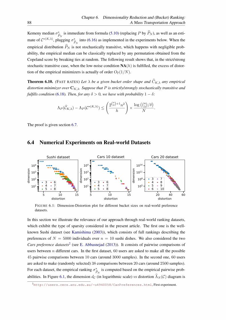
88Chapter 6. Dimensionality Reduction and (Bucket) Ranking:
A Mass Transportation Approach
Kemeny median σ∗PN
is immediate from formula (5.10) (replacing P by PN ), as well as an esti-
mate of C∗(K,λ), plugging σ∗PN
into (6.16) as implemented in the experiments below. When the
empirical distribution PN is not stochastically transitive, which happens with negligible prob-
ability, the empirical median can be classically replaced by any permutation obtained from the
Copeland score by breaking ties at random. The following result shows that, in the strict/strong
stochastic transitive case, when the low-noise condition NA(h) is fulfilled, the excess of distor-
tion of the empirical minimizers is actually of order OP(1/N).
Theorem 6.10. (FAST RATES) Let λ be a given bucket order shape and CK,λ any empirical
distortion minimizer over CK,λ. Suppose that P is strictly/strongly stochastically transitive and
fulfills condition (6.18). Then, for any δ > 0, we have with probability 1− δ:
ΛP (CK,λ)− ΛP (C∗(K,λ)) ≤
(2(n2)+1n2
h
)×
log((nλ
)/δ)
N.
The proof is given section 6.7.
6.4 Numerical Experiments on Real-world Datasets
5 10 15distortion
101
102
103
104
dim
ensio
n
Sushi dataset
345
678
5 10 15distortion
101
102
103
104
dim
ensio
n
Cars 10 dataset
345
678
20 40 60distortion
105
108
1011
1014
dim
ensio
n
Cars 20 dataset
3456
78910
FIGURE 6.1: Dimension-Distortion plot for different bucket sizes on real-world preferencedatasets.
In this section we illustrate the relevance of our approach through real-world ranking datasets,
which exhibit the type of sparsity considered in the present article. The first one is the well-
known Sushi dataset (see Kamishima (2003)), which consists of full rankings describing the
preferences of N = 5000 individuals over n = 10 sushi dishes. We also considered the two
Cars preference datasets2 (see E. Abbasnejad (2013)). It consists of pairwise comparisons of
users between n different cars. In the first dataset, 60 users are asked to make all the possible
45 pairwise comparisons between 10 cars (around 3000 samples). In the second one, 60 users
are asked to make (randomly selected) 38 comparisons between 20 cars (around 2500 samples).
For each dataset, the empirical ranking σ∗PN
is computed based on the empirical pairwise prob-
abilities. In Figure 6.1, the dimension dC (in logarithmic scale) vs distortion ΛN (C) diagram is
2http://users.cecs.anu.edu.au/~u4940058/CarPreferences.html, First experiment.
Chapter 6. Dimensionality Reduction and (Bucket) Ranking:A Mass Transportation Approach 89
plotted for each dataset, for several bucket sizes (K) and shapes (λ). These buckets are obtained
by segmenting σ∗PN
with respect to λ as explained at the end of the previous section. Each color
on a plot corresponds to a specific sizeK, and each point in a given color thus represents a bucket
order of size K. As expected, on each plot the lowest distortion is attained for high-dimensional
buckets (i.e., of smaller size K). These numerical results shed light on the sparse character of
these empirical ranking distributions. Indeed, the dimension dC can be drastically reduced, by
choosing the size K and shape λ in an appropriate manner, while keeping a low distortion for
the representation. The reader may refer to section 6.6 for additional dimension/distortion plots
for different distributions which underline the sparsity observed here: specifically, these empir-
ical distributions show intermediate behaviors between a true bucket distribution and a uniform
distribution (i.e., without exhibiting bucket sparsity).
6.5 Conclusion
In this chapter, we have developed theoretical concepts to represent efficiently sparse ranking
data distributions. We have introduced a distortion measure, based on a mass transportation
metric on the set of probability distributions on the set of rankings (with Kendall’s τ as trans-
portation cost) in order to evaluate the accuracy of (bucket) distribution representations. This
distortion measure can be related to the dispersion measure we introduced for ranking aggrega-
tion Chapter 5. We investigated the performance of empirical distortion minimizers and have
also provided empirical evidence that the notion of sparsity, on which the dimensionality re-
duction method proposed relies, is encountered in various real-world situations. Such sparse
representations could be exploited to improve the completion of certain statistical learning tasks
based on ranking data (e.g. clustering, ranking prediction), by circumventing this way the curse
of dimensionality. In the next chapter, we investigate another problem closely related to ranking
aggregation, namely ranking regression.
6.6 Appendix
A - Hierarchical Recovery of a Bucket Distribution
Motivated by Theorem 6.9, we propose a hierarchical ’bottom-up’ procedure to recover, from
ranking data, a bucket order representation (agreeing with Kemeny consensus) of smallest di-
mension for a fixed level of distortion, that does not requires to specify in advance the bucket
size K and thus avoids computing the optimum (6.16) for all possible shape/size.
Suppose for simplicity that P is strictly/strongly stochastically transitive. One starts with the
bucket order of size n defined by its Kemeny median σ∗P :
C(0) = (σ∗−1P (1), . . . , σ∗−1
P (n)).

90Chapter 6. Dimensionality Reduction and (Bucket) Ranking:
A Mass Transportation Approach
The initial representation has minimum dimension, i.e. dC(0) = 0, and maximal distortion
among all bucket order representations agreeing with σ∗P , i.e. ΛP (C(0)) = L∗P , see Corollary
6.4. The binary agglomeration strategy we propose consists in recursively merging two adjacent
buckets Ck(j) and Ck+1(j) of the current bucket order C(j) = (C1(j), . . . , CK(j) into a single
bucket, yielding the ’coarser’ bucket order
C(j + 1) = (C1(j), . . . , Ck−1(j), Ck(j) ∪ Ck+1(j), Ck+2(j), . . . , CK(j)). (6.19)
The pair (Ck(j), Ck+1(j)) chosen corresponds to that maximizing the quantity
∆(k)P (C(j)) =
∑i∈Ck(j),j∈Ck+1(j)
pj,i. (6.20)
The agglomerative stage C(j)→ C(j + 1) increases the dimension of the representation,
dC(j+1) = (dC(j) + 1)×(
#Ck(j) + #Ck+1(j)
#Ck(j)
)− 1, (6.21)
while reducing the distortion by ΛP (C(j))− ΛP (C(j + 1)) = ∆(k)P (C(j)).
AGGLOMERATIVE ALGORITHM
1. Input. Training data ΣiNi=1, maximum dimension dmax ≥ 0, distortion tolerance ε ≥ 0.
2. Initialization. Compute empirical Kemeny median σ∗PN
and C(0) =
(σ∗−1
PN(1), . . . , σ∗−1
PN(n). Set K ← n.
3. Iterations. While K ≥ 3 and ΛN (C(n−K)) > ε,
(a) Compute k ∈ arg max1≤l≤K−1 ∆(l)
PN(C(n−K)) and C(n−K + 1).
(b) If dC(n−K+1) > dmax: go to 4. Else: set K ← K − 1.
4. Output. Bucket order C(n−K).
This algorithm is specifically designed for finding the bucket order C of minimal dimension dC(i.e. of maximal size K) such that a bucket distribution in PC approximates well the original
distribution P (i.e. with small distortion ΛP (C)). The next result formally supports this idea in
the limit case of P being a bucket distribution.
Theorem 6.11. Let P be a strongly/strictly stochastically transitive bucket distribution and
denote K∗ = maxK ∈ 2, . . . , n,∃ bucket order C of size K s.t. P ∈ PC.(i) There exists a unique K∗-shape λ∗ such that ΛP (C∗(K∗,λ∗)) = 0.
(ii) For any bucket order C such that P ∈ PC: C 6= C∗(K∗,λ∗) ⇒ dC > dC∗(K∗,λ∗) .
(iii) The agglomerative algorithm, runned with dmax = n!− 1, ε = 0 and theoretical quantities
(σ∗P , ∆(k)P ’s and ΛP ) instead of estimates, outputs C∗(K∗,λ∗).
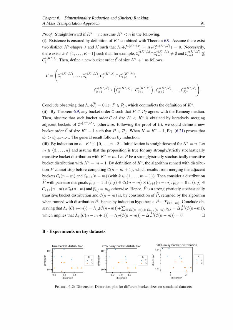
Chapter 6. Dimensionality Reduction and (Bucket) Ranking:A Mass Transportation Approach 91
Proof. Straightforward if K∗ = n: assume K∗ < n in the following.
(i). Existence is ensured by definition of K∗ combined with Theorem 6.9. Assume there exist
two distinct K∗-shapes λ and λ′ such that ΛP (C∗(K∗,λ)) = ΛP (C∗(K∗,λ′)) = 0. Necessarily,
there exists k ∈ 1, . . . ,K−1 such that, for example, C∗(K∗,λ)
k ∩C∗(K∗,λ′)
k+1 6= ∅ and C∗(K∗,λ′)
k+1 *C∗(K
∗,λ)k . Then, define a new bucket order C of size K∗ + 1 as follows:
C =
(C∗(K
∗,λ′)1 , . . . , C∗(K
∗,λ′)k , C∗(K
∗,λ)k ∩ C∗(K
∗,λ′)k+1 ,
C∗(K∗,λ′)
k+1 \(C∗(K
∗,λ)k ∩ C∗(K
∗,λ′)k+1
), C∗(K
∗,λ′)k+2 , . . . , C∗(K
∗,λ′)K∗
).
Conclude observing that ΛP (C) = 0 i.e. P ∈ PC , which contradicts the definition of K∗.
(ii). By Theorem 6.9, any bucket order C such that P ∈ PC agrees with the Kemeny median.
Then, observe that such bucket order C of size K < K∗ is obtained by iteratively merging
adjacent buckets of C∗(K∗,λ∗): otherwise, following the proof of (i), we could define a new
bucket order C of size K∗ + 1 such that P ∈ PC . When K = K∗ − 1, Eq. (6.21) proves that
dC > dC∗(K∗,λ∗) . The general result follows by induction.
(iii). By induction on n−K∗ ∈ 0, . . . , n−2. Initialization is straightforward forK∗ = n. Let
m ∈ 3, . . . , n and assume that the proposition is true for any strongly/strictly stochastically
transitive bucket distribution with K∗ = m. Let P be a strongly/strictly stochastically transitive
bucket distribution with K∗ = m− 1. By definition of K∗, the algorithm runned with distribu-
tion P cannot stop before computing C(n −m + 1), which results from merging the adjacent
buckets Ck(n−m) and Ck+1(n−m) (with k ∈ 1, . . . ,m− 1). Then consider a distribution
P with pairwise marginals pi,j = 1 if (i, j) ∈ Ck(n −m) × Ck+1(n −m), pi,j = 0 if (i, j) ∈Ck+1(n−m)×Ck(n−m) and pi,j = pi,j otherwise. Hence, P is a strongly/strictly stochastically
transitive bucket distribution and C(n −m) is, by construction of P , returned by the algorithm
when runned with distribution P . Hence by induction hypothesis: P ∈ PC(n−m). Conclude ob-
serving that ΛP (C(n−m)) = ΛP
(C(n−m))+∑
i∈Ck(n−m),j∈Ck+1(n−m) pj,i = ∆(k)P (C(n−m)),
which implies that ΛP (C(n−m+ 1)) = ΛP (C(n−m))−∆(k)P (C(n−m)) = 0.
B - Experiments on toy datasets
0.0 0.2 0.4distortion
101
102
dim
ensio
n
true bucket distribution
K23
0.5 1.0 1.5distortion
101
102
dim
ensio
n
20% noisy bucket distribution
K23
1 2distortion
101
102
dim
ensio
n
50% noisy bucket distribution
K23
FIGURE 6.2: Dimension-Distortion plot for different bucket sizes on simulated datasets.
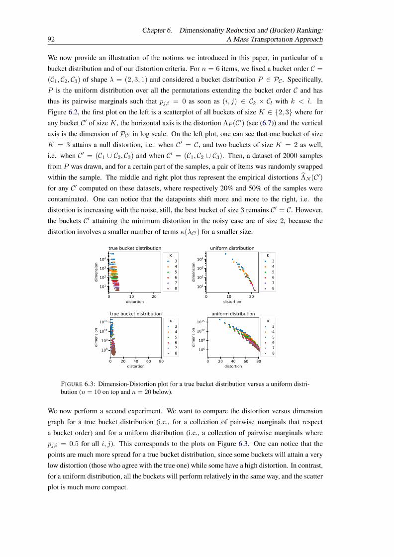
92Chapter 6. Dimensionality Reduction and (Bucket) Ranking:
A Mass Transportation Approach
We now provide an illustration of the notions we introduced in this paper, in particular of a
bucket distribution and of our distortion criteria. For n = 6 items, we fixed a bucket order C =
(C1, C2, C3) of shape λ = (2, 3, 1) and considered a bucket distribution P ∈ PC . Specifically,
P is the uniform distribution over all the permutations extending the bucket order C and has
thus its pairwise marginals such that pj,i = 0 as soon as (i, j) ∈ Ck × Cl with k < l. In
Figure 6.2, the first plot on the left is a scatterplot of all buckets of size K ∈ 2, 3 where for
any bucket C′ of size K, the horizontal axis is the distortion ΛP (C′) (see (6.7)) and the vertical
axis is the dimension of PC′ in log scale. On the left plot, one can see that one bucket of size
K = 3 attains a null distortion, i.e. when C′ = C, and two buckets of size K = 2 as well,
i.e. when C′ = (C1 ∪ C2, C3) and when C′ = (C1, C2 ∪ C3). Then, a dataset of 2000 samples
from P was drawn, and for a certain part of the samples, a pair of items was randomly swapped
within the sample. The middle and right plot thus represent the empirical distortions ΛN (C′)for any C′ computed on these datasets, where respectively 20% and 50% of the samples were
contaminated. One can notice that the datapoints shift more and more to the right, i.e. the
distortion is increasing with the noise, still, the best bucket of size 3 remains C′ = C. However,
the buckets C′ attaining the minimum distortion in the noisy case are of size 2, because the
distortion involves a smaller number of terms κ(λC′) for a smaller size.
0 10 20distortion
101
102
103
104
dim
ensio
n
true bucket distributionK
345678
0 10 20distortion
101
102
103
104
dim
ensio
n
uniform distributionK
345678
0 20 40 60 80distortion
106
109
1012
1015
dim
ensio
n
true bucket distributionK
345678
0 20 40 60 80distortion
106
109
1012
1015
dim
ensio
n
uniform distributionK
345678
FIGURE 6.3: Dimension-Distortion plot for a true bucket distribution versus a uniform distri-bution (n = 10 on top and n = 20 below).
We now perform a second experiment. We want to compare the distortion versus dimension
graph for a true bucket distribution (i.e., for a collection of pairwise marginals that respect
a bucket order) and for a uniform distribution (i.e., a collection of pairwise marginals where
pj,i = 0.5 for all i, j). This corresponds to the plots on Figure 6.3. One can notice that the
points are much more spread for a true bucket distribution, since some buckets will attain a very
low distortion (those who agree with the true one) while some have a high distortion. In contrast,
for a uniform distribution, all the buckets will perform relatively in the same way, and the scatter
plot is much more compact.
Chapter 6. Dimensionality Reduction and (Bucket) Ranking:A Mass Transportation Approach 93
C - Mass Transportation for Other Distances
The approach developed in the chapter mainly relies on the choice of the Kendall’s τ distance as
cost function involved in the Wasserstein metric. We now investigate two other well-known dis-
tances for permutations, the Spearman ρ distance and the Hamming distance (see section 2.2.3
Chapter 2).
The Spearman ρ case. The following result shows that the alternative study based on the
2-nd Wasserstein metric with the Spearman ρ distance d2 as cost function would lead to a dif-
ferent distortion measure: Λ′P (C) = minP ′∈PCWd2,2(P, P ′), whose explicit formula, given
by the right hand side of Eq. (6.22), writes in terms of the triplet-wise probabilities pi,j,k =
PΣ∼P Σ(i) < Σ(j) < Σ(k). Moreover, the coupling (Σ,ΣC) is also optimal in this case as
the distortion verifies Λ′P (C) = E[d2
2 (Σ,ΣC)].
Lemma 6.12. Let n ≥ 3 and P be a probability distribution on Sn.
(i). For any probability distribution P ′ on Sn:
Wd2,2
(P, P ′
)≥ 2
n− 2
∑a<b<c
∑(i,j,k)∈σ(a,b,c)
max(pi,j,k, p′i,j,k)− 1
,
where σ(a, b, c) is the set of permutations of triplet (a, b, c).
(ii). If P ′ ∈ PC with C a bucket order of JnK with K buckets:
Wd2,2
(P, P ′
)≥
2
n− 2
∑1≤k<l<m≤K
∑(a,b,c)∈Ck×Cl×Cm
(n+ 1)pc,b,a + n(pb,c,a + pc,a,b) + pb,a,c + pa,c,b
+2
n− 2
∑1≤k<l≤K
∑(a,b,c)∈Ck×Cl×Cl
n(pb,c,a + pc,b,a) + pb,a,c + pc,a,b
+∑
(a,b,c)∈Ck×Ck×Cl
n(pc,a,b + pc,b,a) + pa,c,b + pb,c,a
,
(6.22)
with equality when P ′ = PC is the distribution of ΣC .
Proof. (i). Consider a coupling (Σ,Σ′) of two probability distributions P and P ′ on Sn. Define
the triplet-wise probabilities pi,j,k = PΣ∼P Σ(i) < Σ(j) < Σ(k) and p′i,j,k = PΣ′∼P ′Σ′(i) <Σ′(j) < Σ′(k). For clarity’s sake, we will assume that pi,j,k = min(pi,j,k, p
′i,j,k) > 0 for
all triplets (i, j, k), the extension to the general case being straightforward. We also denote
pi,j,k = max(pi,j,k, p′i,j,k). Given two pairs of three distinct elements of JnK, (i, j, k) and

94Chapter 6. Dimensionality Reduction and (Bucket) Ranking:
A Mass Transportation Approach
(a, b, c), we define the following quantities:
πa,b,c|i,j,k = P
Σ′(a) < Σ′(b) < Σ′(c) | Σ(i) < Σ(j) < Σ(k),
π′a,b,c|i,j,k = P
Σ(a) < Σ(b) < Σ(c) | Σ′(i) < Σ′(j) < Σ′(k),
πa,b,c|i,j,k = πa,b,c|i,j,kIpi,j,k ≤ p′i,j,k+ π′a,b,c|i,j,kIpi,j,k > p′i,j,k,
πa,b,c|i,j,k = πa,b,c|i,j,kIpi,j,k > p′i,j,k+ π′a,b,c|i,j,kIpi,j,k ≤ p′i,j,k.
The interest of defining the πa,b,c|i,j,k’s is that it will allow us to choose πi,j,k|i,j,k = 1 at the end
of the proof, which implies πi,j,k|i,j,k =pi,j,kpi,j,k
. Throughout the proof, the triplets (a, b, c) will
always be permutations of (i, j, k). Now write
E[d2
(Σ,Σ′
)2]=
n∑i=1
E[Σ(i)2] + E[Σ′(i)2]− 2E[Σ(i)Σ′(i)],
where
E[Σ(i)2] = E[(1 +∑j 6=i
IΣ(j) < Σ(i))2] = 1 +∑j 6=i
(n+ 1)pj,i −∑k 6=i,j
pj,i,k
and
E[Σ(i)Σ′(i)] = 1 +∑j 6=i
pj,i + p′j,i + PΣ(j) < Σ(i),Σ′(j) < Σ′(i)
+∑k 6=i,j
PΣ(j) < Σ(i),Σ′(k) < Σ′(i).
Hence,
E[d2
(Σ,Σ′
)2]=∑a<b<c
∑(i,j,k)∈σ(a,b,c)
1
n− 2
(n− 1)(pj,i + p′j,i)− 2PΣ(j) < Σ(i),Σ′(j) < Σ′(i)
− pj,i,k − p′j,i,k − 2PΣ(j) < Σ(i),Σ′(k) < Σ′(i),
(6.23)
where σ(a, b, c) is the set of the 6 permutations of triplet (a, b, c). Some terms simplify in Eq.
(6.23) when summing over σ(a, b, c), namely:
∑(i,j,k)∈σ(a,b,c)
n− 1
n− 2(pj,i + p′j,i)− pj,i,k − p′j,i,k =
4n− 2
n− 2.

Chapter 6. Dimensionality Reduction and (Bucket) Ranking:A Mass Transportation Approach 95
We now simply have:
E[d2
(Σ,Σ′
)2]=∑a<b<c
4n− 2
n− 2− 2
∑(i,j,k)∈σ(a,b,c)
1
n− 2PΣ(j) < Σ(i),Σ′(j) < Σ′(i)
+ PΣ(j) < Σ(i),Σ′(k) < Σ′(i).(6.24)
Observe that for all triplets (a, b, c) and (i, j, k),
P(Σ′(a) < Σ′(b) < Σ′(c),Σ(i) < Σ(j) < Σ(k)) + P(Σ′(i) < Σ′(j) < Σ′(k),Σ(a) < Σ(b) < Σ(c))
= πa,b,c|i,j,kpi,j,k + π′a,b,c|i,j,kp′i,j,k.
Then, by the law of total probability, we have for all distinct i, j, k,
PΣ(j) < Σ(i),Σ′(j) < Σ′(i)
=1
2πj,k,i|j,k,ipj,k,i + π′j,k,i|j,k,ip
′j,k,i
+1
2πk,j,i|k,j,ipk,j,i + π′k,j,i|k,j,ip
′k,j,i
+1
2πj,i,k|j,i,kpj,i,k + π′j,i,k|j,i,kp
′j,i,k
+1
2πj,i,k|j,k,ipj,k,i + π′j,i,k|j,k,ip
′j,k,i + πj,k,i|j,i,kpj,i,k + π′j,k,i|j,i,kp
′j,i,k
+1
2πk,j,i|j,k,ipj,k,i + π′k,j,i|j,k,ip
′j,k,i + πj,k,i|k,j,ipk,j,i + π′j,k,i|k,j,ip
′k,j,i
+1
2πj,i,k|k,j,ipk,j,i + π′j,i,k|k,j,ip
′k,j,i + πk,j,i|j,i,kpj,i,k + π′k,j,i|j,i,kp
′j,i,k,
and
PΣ(j) < Σ(i),Σ′(k) < Σ′(i)
=1
2πj,k,i|j,k,ipj,k,i + π′j,k,i|j,k,ip
′j,k,i
+1
2πk,j,i|k,j,ipk,j,i + π′k,j,i|k,j,ip
′k,j,i
+1
2πk,j,i|j,k,ipj,k,i + π′k,j,i|j,k,ip
′j,k,i + πj,k,i|k,j,ipk,j,i + π′j,k,i|k,j,ip
′k,j,i
+ P(Σ′(j) < Σ′(k) < Σ′(i),Σ(j) < Σ(i) < Σ(k))
+ P(Σ′(k) < Σ′(i) < Σ′(j),Σ(j) < Σ(k) < Σ(i))
+ P(Σ′(k) < Σ′(j) < Σ′(i),Σ(j) < Σ(i) < Σ(k))
+ P(Σ′(k) < Σ′(i) < Σ′(j),Σ(k) < Σ(j) < Σ(i))
+ P(Σ′(k) < Σ′(i) < Σ′(j),Σ(j) < Σ(i) < Σ(k)),

96Chapter 6. Dimensionality Reduction and (Bucket) Ranking:
A Mass Transportation Approach
which implies:
PΣ(j) < Σ(i),Σ′(k) < Σ′(i)+ PΣ(k) < Σ(i),Σ′(j) < Σ′(i)
= πj,k,i|j,k,ipj,k,i + π′j,k,i|j,k,ip′j,k,i
+ πk,j,i|k,j,ipk,j,i + π′k,j,i|k,j,ip′k,j,i
+ πk,j,i|j,k,ipj,k,i + π′k,j,i|j,k,ip′j,k,i + πj,k,i|k,j,ipk,j,i + π′j,k,i|k,j,ip
′k,j,i
+1
2
πj,k,i|j,i,kpj,i,k + π′j,k,i|j,i,kp
′j,i,k + πj,i,k|j,k,ipj,k,i + π′j,i,k|j,k,ip
′j,k,i
+
1
2
πk,i,j|j,k,ipj,k,i + π′k,i,j|j,k,ip
′j,k,i + πj,k,i|k,i,jpk,i,j + π′j,k,i|k,i,jp
′k,i,j
+
1
2
πk,j,i|j,i,kpj,i,k + π′k,j,i|j,i,kp
′j,i,k + πj,i,k|k,j,ipk,j,i + π′j,i,k|k,j,ip
′k,j,i
+
1
2
πk,i,j|k,j,ipk,j,i + π′k,i,j|k,j,ip
′k,j,i + πk,j,i|k,i,jpk,i,j + π′k,j,i|k,i,jp
′k,i,j
+
1
2
πk,i,j|j,i,kpj,i,k + π′k,i,j|j,i,kp
′j,i,k + πj,i,k|k,i,jpk,i,j + π′j,i,k|k,i,jp
′k,i,j
,
which is symmetric by permuting indices j and k. Hence,
H(a, b, c) =∑
(i,j,k)∈σ(a,b,c)
1
n− 2PΣ(j) < Σ(i),Σ′(j) < Σ′(i)+ PΣ(j) < Σ(i),Σ′(k) < Σ′(i)
=∑
(i,j,k)∈σ(a,b,c)
2n− 1
2(n− 2)πj,k,i|j,k,i +
n− 1
n− 2(πk,j,i|j,k,i + πj,i,k|j,k,i)
+n− 1
2(n− 2)(πk,i,j|j,k,i + πi,j,k|j,k,i) +
1
2πi,k,j|j,k,i
pj,k,i
+
2n− 1
2(n− 2)πj,k,i|j,k,i +
n− 1
n− 2(πk,j,i|j,k,i + πj,i,k|j,k,i)
+n− 1
2(n− 2)(πk,i,j|j,k,i + πi,j,k|j,k,i) +
1
2πi,k,j|j,k,i
pj,k,i,
(6.25)
which is maximized when πj,k,i|j,k,i = 1 (which implies πj,k,i|j,k,i =pj,k,ipj,k,i
) and πk,j,i|j,k,i +
πj,i,k|j,k,i = 1− pj,k,ipj,k,i
for all (i, j, k) ∈ σ(a, b, c) and then verifies:
H(a, b, c) ≤∑
(i,j,k)∈σ(a,b,c)
n
n− 2pi,j,k +
n− 1
n− 2pi,j,k =
1
n− 2
∑(i,j,k)∈σ(a,b,c)
n(pi,j,k + p′i,j,k)− pi,j,k
=1
n− 2
2n−∑
(i,j,k)∈σ(a,b,c)
pi,j,k
,
(6.26)
which concludes the first part of the proof.
(ii). Now we consider the particular case of P ′ ∈ PC , with C a bucket order of JnK with
Chapter 6. Dimensionality Reduction and (Bucket) Ranking:A Mass Transportation Approach 97
K buckets. We propose to prove that minP ′∈PCWd2,2(P, P ′) = Wd2,2(P, PC) = E[d22(Σ,ΣC)]
and to obtain an explicit expression. Given three distinct indices 1 ≤ a < b < c ≤ n, we analyze
the following four possible situations to reveal what are the optimal values of the conditional
probabilities in Eq. (6.25):
• (a, b, c) ∈ Ck are in the same bucket: the maximizing conditions are πj,k,i|j,k,i = 1 and
πk,j,i|j,k,i + πj,i,k|j,k,i = 1 − pj,k,ipj,k,i
. Both are verified when P ′ = PC and Σ′ = ΣC as
Σ(j) < Σ(k) < Σ(i) iff ΣC(j) < ΣC(k) < ΣC(i). Hence, using Eq. (6.26):
H(a, b, c) ≤ 1
n− 2
2n−∑
(i,j,k)∈σ(a,b,c)
pi,j,k
≤ 2n− 1
n− 2.
Moreover, this upper bound is attained when Σ′ = ΣC : H(a, b, c) = 2n−1n−2 .
• (a, b, c) ∈ Ck × Cl × Cm are in three different buckets (k < l < m): this situation is fully
characterized by the bucket structure and is hence independent of the coupling (Σ,Σ′).
For all (j, k, i) ∈ σ(a, b, c)\(a, b, c), p′j,k,i = pj,k,i = 0 so Eq. (6.25) is not completely
defined but H(a, b, c) rewrites more simply without the terms corresponding to the five
impossible events Σ′(j) < Σ′(k) < Σ′(i). If (j, k, i) 6= (a, b, c), pj,k,i = pj,k,i and
πa,b,c|j,k,i = 1 so the sum of these contributions in H(a, b, c) is:
n− 1
n− 2(pb,a,c + pa,c,b) +
n− 1
2(n− 2)(pb,c,a + pc,a,b) +
1
2pc,b,a. (6.27)
We have pa,b,c ≤ p′a,b,c = 1 so the condition πa,b,c|a,b,c = 1 is realized and for all
(i, j, k) ∈ σ(a, b, c), πi,j,k|a,b,c = pi,j,k. The sum of the corresponding contributions
in H(a, b, c) is:
2n− 1
n− 2pa,b,c +
n− 1
n− 2(pb,a,c + pa,c,b) +
n− 1
2(n− 2)(pb,c,a + pc,a,b) +
1
2pc,b,a. (6.28)
Finally, by combining equations 6.27 and 6.28,
H(a, b, c) =2n− 1
n− 2pa,b,c +
2(n− 1)
n− 2(pb,a,c + pa,c,b) +
n− 1
n− 2(pb,c,a + pc,a,b) + pc,b,a.
• (a, b, c) ∈ Ck × Cl × Cl are in two different buckets (k < l) such that a is ranked first
among the triplet. For all (j, k, i) ∈ σ(a, b, c) \ (a, b, c), (a, c, b), p′j,k,i = pj,k,i = 0 so
Eq. (6.25) is not completely defined butH(a, b, c) rewrites more simply without the terms
corresponding to the four impossible events Σ′(j) < Σ′(k) < Σ′(i). For all (j, k, i) ∈

98Chapter 6. Dimensionality Reduction and (Bucket) Ranking:
A Mass Transportation Approach
σ(a, b, c), πa,b,c|j,k,i + πa,c,b|j,k,i = 1, and the sum of their contributions in H(a, b, c) is:(2n− 1
2(n− 2)πa,b,c|a,b,c +
n− 1
n− 2πa,c,b|a,b,c
)pa,b,c +
(2n− 1
2(n− 2)πa,c,b|a,c,b +
n− 1
n− 2πa,b,c|a,c,b
)pa,c,b
+
(n− 1
2(n− 2)πa,b,c|b,c,a +
1
2πa,c,b|b,c,a
)pb,c,a +
(n− 1
n− 2πa,b,c|b,a,c +
n− 1
2(n− 2)πa,c,b|b,a,c
)pb,a,c
+
(n− 1
2(n− 2)πa,c,b|c,b,a +
1
2πa,b,c|c,b,a
)pc,b,a +
(n− 1
n− 2πa,c,b|c,a,b +
n− 1
2(n− 2)πa,b,c|c,a,b
)pc,a,b.
(6.29)
Observe that the expression above is maximized when πa,b,c|a,b,c = πa,c,b|a,c,b = πa,b,c|b,c,a =
πa,b,c|b,a,c = πa,c,b|c,b,a = πa,c,b|c,a,b = 1, which is verified by Σ′ = ΣC . In this case, Eq.
(6.30) becomes:
2n− 1
2(n− 2)(pa,b,c + pa,c,b) +
n− 1
n− 2(pb,a,c + pc,a,b) +
n− 1
2(n− 2)(pb,c,a + pc,b,a) (6.30)
Now consider (j, k, i) ∈ (a, b, c), (a, c, b): p′a,b,c + p′a,c,b = 1 and the corresponding
contributions to H(a, b, c) sum as follows:2n− 1
2(n− 2)π′a,b,c|a,b,c +
n− 1
n− 2(π′b,a,c|a,b,c + π′a,c,b|a,b,c)
+n− 1
2(n− 2)(π′b,c,a|a,b,c + π′c,a,b|a,b,c) +
1
2π′c,b,a|a,b,c
p′a,b,c
+
2n− 1
2(n− 2)π′a,c,b|a,c,b +
n− 1
n− 2(π′c,a,b|a,c,b + π′a,b,c|a,c,b)
+n− 1
2(n− 2)(π′c,b,a|a,c,b + π′b,a,c|a,c,b) +
1
2π′b,c,a|a,c,b
p′a,c,b,
which is maximized when π′a,c,b|a,b,c = π′c,a,b|a,b,c = π′c,b,a|a,b,c = 0 and π′a,b,c|a,c,b =
π′b,a,c|a,c,b = π′b,c,a|a,c,b = 0: both conditions are true for Σ′ = ΣC . Then, the expression
above is upper bounded by:
2n− 1
2(n− 2)(pa,b,c + pa,c,b) +
n− 1
n− 2(pb,a,c + pc,a,b) +
n− 1
2(n− 2)(pb,c,a + pc,b,a) (6.31)
with equality when Σ′ = ΣC . Finally, by summing the terms in 6.30 and 6.31,
H(a, b, c) ≤ 2n− 1
n− 2(pa,b,c + pa,c,b) +
2(n− 1)
n− 2(pb,a,c + pc,a,b) +
n− 1
n− 2(pb,c,a + pc,b,a),
where the equality holds for Σ′ = ΣC .
Chapter 6. Dimensionality Reduction and (Bucket) Ranking:A Mass Transportation Approach 99
• (a, b, c) ∈ Ck × Ck × Cl are in two different buckets (k < l) such that c is ranked last
among the triplet. Similarly as in the previous situation, we obtain:
H(a, b, c) ≤ 2n− 1
n− 2(pa,b,c + pb,a,c) +
2(n− 1)
n− 2(pa,c,b + pb,c,a) +
n− 1
n− 2(pc,a,b + pc,b,a),
where the equality holds for Σ′ = ΣC .
As a conclusion, we proved that: minP ′∈PCWd2,2(P, P ′) = Wd2,2(P, PC) = E[d22(Σ,ΣC)].
The Hamming case. We also provide a lower bound on the 1-st Wasserstein metric with the
Hamming distance dH as cost function.
Lemma 6.13. For any probability distributions P and P ′ on Sn:
WdH ,1(P, P ′) ≥n∑i=1
1−n∑j=1
min(qi,j , q′i,j)
,
where qi,j = PΣ∼P Σ(i) = j and q′i,j = PΣ′∼P ′Σ′(i) = j.
Proof. Consider a coupling (Σ,Σ′) of two probability distributions P and P ′ on Sn. For all
i, j, k, set
ρi,j,k = P
Σ′(i) = k | Σ(i) = j
and ρ′i,j,k = P
Σ(i) = k | Σ′(i) = j.
For simplicity, we assume throughout the proof that min(qi,j , q′i,j) > 0 for all (i, j) ∈ JnK2, the
generalization being straightforward. We may write
E[dH(Σ,Σ′
)]=
n∑i=1
P
Σ(i) 6= Σ′(i)
=
n∑i=1
n∑j=1
∑k 6=j
P
Σ(i) = j,Σ′(i) = k
=n∑i=1
n∑j=1
∑k 6=j
ρi,j,kqi,j =
n∑i=1
n∑j=1
qi,j (1− ρi,j,j) = n−n∑
i,j=1
ρi,j,jqi,j .
(6.32)
For (i, j) ∈ JnK2, the quantity ρi,j,jqi,j is maximized when ρi,j,j = 1, which requires that
qi,j ≤ q′i,j . If qi,j > q′i,j , rather write in a similar fashion:
E[dH(Σ,Σ′
)]= n−
n∑i,j=1
ρ′i,j,jq′i,j ,

100Chapter 6. Dimensionality Reduction and (Bucket) Ranking:
A Mass Transportation Approach
and set ρ′i,j,j = 1. We thus have from Eq. (6.32):
WdH ,1(P, P ′) ≥n∑i=1
inf(Σ,Σ′) s.t. PΣ(i)=j=qi,j and PΣ′(i)=j=q′i,j
1−n∑j=1
P
Σ(i) = Σ′(i) = j
=n∑i=1
1−n∑j=1
min(qi,j , q′i,j)
.
6.7 Proofs
Proof of Lemma 6.2
Consider two probability distributions P and P ′ on Sn. Fix i 6= j and let (Σ,Σ′) be a
pair of random variables defined on a same probability space, valued in Sn and such that
pi,j = PΣ∼P Σ(i) < Σ(j) and p′i,j = PΣ′∼P ′Σ′(i) < Σ′(j). Set
πi,j = P
Σ′(i) < Σ′(j) | Σ(i) < Σ(j).
Equipped with this notation, by the law of total probability, we have:
p′i,j = pi,jπi,j + (1− pi,j)(1− πj,i). (6.33)
In addition, we may write
E[dτ (Σ,Σ′)
]=∑i<j
E[I(Σ(i)− Σ(j))(Σ′(i)− Σ′(j)) < 0
]=∑i<j
E[IΣ(i) < Σ(j)IΣ′(i) > Σ′(j)+ IΣ(i) > Σ(j)IΣ′(i) < Σ′(j)
]=∑i<j
pi,j(1− πi,j) + (1− pi,j)(1− πj,i).
Suppose that pi,j < p′i,j . Using (6.33), we have pi,j(1−πi,j)+(1−pi,j)(1−πj,i) = p′i,j +(1−2πi,j)pi,j , which quantity is minimum when πi,j = 1 (and in this case πj,i = (1 − p′i,j)/(1 −pi,j)), and then equal to |pi,j − p′i,j |. We recall that we can only set πi,j = 1 if the initial
assumption pi,j < p′i,j holds. In a similar fashion, if pi,j > p′i,j , we have pi,j(1 − πi,j) + (1 −pi,j)(1 − πj,i) = 2(1 − pi,j)(1 − πj,i) + pi,j − p′i,j , which is minimum for πj,i = 1 (we have
Chapter 6. Dimensionality Reduction and (Bucket) Ranking:A Mass Transportation Approach 101
incidentally πi,j = p′i,j/pi,j in this case) and then equal to |pi,j − p′i,j |. Since we clearly have
Wdτ ,1
(P, P ′
)≥∑
i<j
inf(Σ,Σ′) s.t. PΣ(i)<Σ(j)=pi,j and PΣ′(i)<Σ′(j)=p′i,j
P[(Σ(i)− Σ(j))(Σ′(i)− Σ′(j)) < 0
],
this proves that
Wdτ ,1
(P, P ′
)≥∑i<j
|p′i,j − pi,j |.
As a remark, given a distribution P on Sn, when P ′ = PC with C a bucket order of JnK with
K buckets, the optimality conditions on the πi,j’s are fulfilled by the coupling (Σ,ΣC), which
implies that:
Wdτ ,1 (P, PC) =∑i<j
|p′i,j − pi,j | =∑
1≤k<l≤K
∑(i,j)∈Ck×Cl
pj,i, (6.34)
where p′i,j = PΣC∼PC [ΣC(i) < ΣC(j)] = pi,jIk = l + Ik < l, with (k, l) ∈ 1, . . . ,K2
such that (i, j) ∈ Ck × Cl.
Proof of Proposition 6.3
Let C be a bucket order of JnK with K buckets. Then, for P ′ ∈ PC , Lemma 6.2 implies that:
Wdτ ,1
(P, P ′
)≥∑i<j
|p′i,j − pi,j | =K∑k=1
∑i<j,(i,j)∈C2k
|p′i,j − pi,j |+∑
1≤k<l≤K
∑(i,j)∈Ck×Cl
pj,i,
where the last equality results from the fact that p′i,j = 1 when (i, j) ∈ Ck × Cl with k < l.
When P ′ = PC , the intra-bucket terms are all equal to zero. Hence, it results from (6.34) that :
Wdτ ,1 (P, PC) =∑
1≤k<l≤K
∑(i,j)∈Ck×Cl
pj,i = ΛP (C).
Proof of Theorem 6.5
Observe first that the excess of distortion can be bounded as follows:
ΛP (CK,λ)− infC∈CK
ΛP (C) ≤ 2 maxC∈CK,λ
∣∣∣ΛN (C)− ΛP (C)∣∣∣+ inf
C∈CK,λΛP (C)− inf
C∈CKΛP (C)
.
By a classical symmetrization device (see e.g. Van Der Vaart & Wellner (1996)), we have:
E[
maxC∈CK,λ
∣∣∣ΛN (C)− ΛP (C)∣∣∣] ≤ 2E [RN (λ)] . (6.35)

102Chapter 6. Dimensionality Reduction and (Bucket) Ranking:
A Mass Transportation Approach
Hence, using McDiarmid’s inequality, for all δ ∈ (0, 1) it holds with probability at least 1− δ:
maxC∈CK,λ
∣∣∣ΛN (C)− ΛP (C)∣∣∣ ≤ 2E [RN (λ)] + κ(λ)
√log(1
δ )
2N.
Proof of Theorem 6.8
Following the proof of Theorem 8.1 in Boucheron et al. (2005), we have for allm ∈ 1, . . . ,M,
E[ΛP (CKm,λm)
]≤ minC∈CKm,λm
ΛP (C) + E [pen(λm, N)]
+M∑
m′=1
E
[(max
C∈CKm′ ,λm′ΛP (C)− ΛN (C)− pen(λm′ , N)
)+
],
where x+ = max(x, 0) denotes the positive part of x. In adition, for any δ > 0, we have:
P
maxC∈CKm,λm
ΛP (C)− ΛN (C) ≥ pen(λm, N) + δ
≤ P
max
C∈CKm,λmΛP (C)− ΛN (C) ≥ E
[max
C∈CKm,λmΛP (C)− ΛN (C)
]+δ
5
+ P
RN (λm) ≤ E [RN (λm)]− 2
5δ
≤ 2 exp
(− 2Nδ2
25κ(λm)2
),
using (6.35) for the first term, and both McDiarmid’s inequality and Lemma 8.2 in Boucheron
et al. (2005) for the second term. Observing that κ(λ) ≤(n2
), integration by parts concludes the
proof.
Proof of Theorem 6.9
Consider a bucket order C = (C1, . . . , CK) of shape λ, different from (6.16). Hence, there
exists at least a pair i, j such that j ≺C i and σ∗P (j) < σ∗P (i) (or equivalently pi,j < 1/2).
Consider such a pair i, j. Hence, there exist 1 ≤ k < l ≤ K s.t. (i, j) ∈ Ck × Cl. Define
the bucket order C′ which is the same as C except that the buckets of i and j are swapped:
C′k = j ∪ Ck \ i, C′l = i ∪ Cl \ j and C′m = Cm if m ∈ 1, . . . ,K \ k, l. Observe
that
ΛP (C′)− ΛP (C) = pi,j − pj,i +∑
a∈Ck\i
pi,a − pj,a +∑
a∈Cl\j
pa,j − pa,i
+l−1∑
m=k+1
∑a∈Cm
pa,j − pa,i + pi,a − pj,a ≤ 2(pi,j − 1/2) < 0.

Chapter 6. Dimensionality Reduction and (Bucket) Ranking:A Mass Transportation Approach 103
Considering now all the pairs i, j such that j ≺C i and pi,j < 1/2, it follows by induction that
ΛP (C)− ΛP (C∗(K,λ)) ≥ 2∑j≺Ci
(1/2− pi,j) · Ipi,j < 1/2. (6.36)
Proof of Theorem 6.10
The fast rate analysis essentially relies on the following lemma providing a control of the vari-
ance of the empirical excess of distortion
ΛN (C)− ΛN (C∗(K,λ)) =1
N
N∑s=1
∑i 6=j
IΣs(j) < Σs(i) · (I i ≺C j − Ii <C∗(K,λ) j) .
Set D(C) =∑
i 6=j IΣ(j) < Σ(i) · (I i ≺C j − Ii <C∗(K,λ) j). Observe that E[D(C)] =
ΛP (C)− ΛP (C∗(K,λ)).
Lemma 6.14. Let λ be a given bucket order shape. We have:
var (D(C)) ≤ 2(n2)(n2/h) · E[D(C)].
Proof. As in the proof of Theorem 6.9, consider a bucket order C = (C1, . . . , CK) of shape λ,
different from (6.16), a pair i, j such that there exist 1 ≤ k < l ≤ K s.t. (i, j) ∈ Ck ×Cl and
σ∗P (j) < σ∗P (i) and the bucket order C′ which is the same as C except that the buckets of i and
j are swapped. We have:
D(C′)−D(C) = IΣ(i) < Σ(j)−IΣ(j) < Σ(i)+∑
a∈Ck\i
IΣ(i) < Σ(a)−IΣ(j) < Σ(a)
+∑
a∈Cl\j
IΣ(a) < Σ(j) − IΣ(a) < Σ(i)
+l−1∑
m=k+1
∑a∈Cm
IΣ(a) < Σ(j) − IΣ(a) < Σ(i)+ IΣ(i) < Σ(a) − IΣ(j) < Σ(a).
Hence, we have: var(D(C′)−D(C)) ≤ 4n2. By induction, we then obtain that:
var (D(C)) ≤ 2(n2)−1(4n2)# (i, j) : i ≺C j and pj,i > 1/2
≤ 2(n2)−1(4n2/h)∑j≺Ci
(1/2− pi,j) · Ipi,j < 1/2 ≤ 2(n2)(n2/h)E[D(C)],
by combining (6.17) with condition (6.18).
Applying Bernstein’s inequality to the i.i.d. average (1/N)∑N
s=1Ds(C), where
Ds(C) =∑i 6=j
IΣs(j) < Σs(i) · (I i ≺C j − Ii <C∗(K,λ) j) ,

104Chapter 6. Dimensionality Reduction and (Bucket) Ranking:
A Mass Transportation Approach
for 1 ≤ s ≤ N and the union bound over the bucket orders C in CK,λ (recall that #CK,λ =(nλ
)),
we obtain that, for all δ ∈ (0, 1), we have with probability larger than 1− δ: ∀C ∈ CK,λ,
E[D(C)] = ΛP (C)− ΛP (C∗(K,λ)) ≤ ΛN (C)− ΛN (C∗(K,λ)) +
√2var(D(C)) log
((nλ
)/δ)
N
+4κ(λ) log(
(nλ
)/δ)
3N.
Since ΛN (CK,λ)− ΛN (C∗(K,λ)) ≤ 0 by assumption and using the variance control provided by
Lemma 7.14 above, we obtain that, with probability at least 1− δ, we have:
ΛP (CK,λ)− ΛP (C∗(K,λ)) ≤
√√√√2(n2)+1n2(
ΛP (CK,λ)− ΛP (C∗(K,λ)))/h× log(
(nλ
)/δ)
N
+4κ(λ) log(
(nλ
)/δ)
3N.
Finally, solving this inequality in ΛP (CK,λ)− ΛP (C∗(K,λ)) yields the desired result.
CHAPTER 7Ranking Median Regression: Learning to Order through
Local Consensus
Chapter abstract This chapter is devoted to the problem of predicting the value taken bya random permutation Σ, describing the preferences of an individual over a set of num-bered items 1, . . . , n say, based on the observation of an input/explanatory r.v. X (e.g.characteristics of the individual), when error is measured by the Kendall τ distance. In theprobabilistic formulation of the ’Learning to Order’ problem we propose, which extends theframework for statistical Kemeny ranking aggregation developped in Chapter 5, this boilsdown to recovering conditional Kemeny medians of Σ given X from i.i.d. training examples(X1,Σ1), . . . , (XN ,ΣN ). For this reason, this statistical learning problem is referred to asranking median regression here. Our contribution is twofold. We first propose a probabilistictheory of ranking median regression: the set of optimal elements is characterized, the perfor-mance of empirical risk minimizers is investigated in this context and situations where fastlearning rates can be achieved are also exhibited. Next we introduce the concept of local con-sensus/median, in order to derive efficient methods for ranking median regression. The majoradvantage of this local learning approach lies in its close connection with the Kemeny aggre-gation problem we studied Chapter 5. From an algorithmic perspective, this permits to buildpredictive rules for ranking median regression by implementing efficient techniques for (ap-proximate) Kemeny median computations at a local level in a tractable manner. In particular,versions of k-nearest neighbor and tree-based methods, tailored to ranking median regression,are investigated. Accuracy of piecewise constant ranking median regression rules is studiedunder a specific smoothness assumption for Σ’s conditional distribution given X . The resultsof various numerical experiments are also displayed for illustration purpose.
7.1 Introduction
The machine-learning problem considered in this chapter is easy to state. Given a vector X of
attributes describing the characteristics of an individual, the goal is to predict her preferences
over a set of n ≥ 1 numbered items, indexed by 1, . . . , n say, modelled as a random permu-
tation Σ in Sn. Based on the observation of independent copies of the random pair (X,Σ), the
task consists in building a predictive function s that maps any point X in the input space to a
permutation s(X), the accuracy of the prediction being measured by means of a certain distance
between Σ and s(X), the Kendall τ distance typically. This problem is of growing importance
105
106 Chapter 7. Ranking Median Regression: Learning to Order through Local Consensus
these days, since users with declared characteristics express their preferences through more and
more devices/interfaces (e.g. social surveys, web activities...). This chapter proposes a proba-
bilistic analysis of this statistical learning problem: optimal predictive rules are exhibited and
(fast) learning rate bounds for empirical risk minimizers are established in particular. However,
truth should be said, this problem is more difficult to solve in practice than other supervised
learning problems such as classification or regression, due to the structured nature of the output
space. The symmetric group is not a vector space and its elements cannot be defined by means of
simple operations, such as thresholding some real valued function, like in classification. Hence,
it is far from straightforward in general to find analogues of methods for distribution-free re-
gression or classification consisting in expanding the decision function using basis functions in
a flexible dictionary (e.g. splines, wavelets) and fitting its coefficients from training data, with
the remarkable exception of techniques building piecewise constant predictive functions, such
as the popular nearest-neighbor method or the celebrated CART algorithm, see Breiman et al.
(1984). Indeed, observing that, when X and Σ are independent, the best predictions for Σ are
its Kemeny medians (i.e. any permutation that is closest to Σ in expectation, see the probabilis-
tic formulation of ranking aggregation in Chapter 5), we consider local learning approaches in
this chapter. Conditional Kemeny medians of Σ at a given point X = x are relaxed to Ke-
meny medians within a region C of the input space containing x (i.e. local consensus), which
can be computed by applying locally any ranking aggregation technique (in practice, Copeland
method or Borda count). Beyond computational tractability, it is motivated by the fact that, as
shall be proved in this chapter, the optimal ranking median regression rule can be well approx-
imated by piecewise constants under the hypothesis that the pairwise conditional probabilities
PΣ(i) < Σ(j) | X = x, with 1 ≤ i < j ≤ n, are Lipschitz. Two methods based on
the notion of local Kemeny consensus are investigated here. The first technique is a version of
the popular nearest neighbor method tailored to ranking median regression, while the second
one, refered to as the CRIT algorithm (standing for ’Consensus RankIng Tree’), produces, by
successive data-driven refinements, an adaptive partitioning of the input space X formed of re-
gions, where the Σi’s exhibit low variability. Like CART, the recursive learning process CRIT
can be described by a binary tree, whose terminal leafs are associated with the final regions. It
can be seen as a variant of the methodology introduced in Yu et al. (2010): we show here that
the node impurity measure they originally propose can be related to the local ranking median
regression risk, the sole major difference being the specific computationally effective method
we consider for computing local predictions, i.e. for assigning permutations to terminal nodes.
Beyond approximation theoretic arguments, its computational feasability and the advantages of
the predictive rules it produces regarding interpretability or aggregation are also discussed to
support the use of piecewise constants. The results of various numerical experiments are also
displayed in order to illustrate the approach we propose.
The chapter is organized as follows. In section 7.2, concepts related to stochastic transitivity
and Kemeny aggregation are investigated, the ranking predictive problem being next formulated
as an extension of the latter and studied from a theoretical perspective. A probabilistic theory of
ranking median regression is developed in section 7.3. In section 7.4, approximation of optimal

Chapter 7. Ranking Median Regression: Learning to Order through Local Consensus 107
predictive rules by piecewise constants is investigated as well as two local learning methods
for solving ranking median regression. The results of illustrative numerical experiments are
presented in section 7.5. Technical proofs and further details can be found section 7.8.
7.2 Preliminaries
As a first go, we start with investigating further (empirical) stochastic transitivity, and introduce
the ranking median regression problem.
7.2.1 Best Strictly Stochastically Transitive Approximation
Let T be the set of strictly stochastically transitive distributions on Sn, and consider P ∈ T . It
was proven Chapter 5 that under the additional low-noise condition on the pairwise marginals
of P , the empirical distribution PN ∈ T as well with overwhelming probability, and that the
expectation of the excess of risk of empirical Kemeny medians decays at an exponential rate. In
this case, the nearly optimal solution σ∗PN
can be made explicit and straightforwardly computed
using Eq. (5.10), namely Copeland method, based on the empirical pairwise probabilities
pi,j =1
N
N∑k=1
IΣk(i) < Σk(j), i < j.
If the empirical estimation PN of P does not belong to T , solving the NP-hard problem
minσ∈Sn LPN (σ) requires to get an empirical Kemeny median. A natural strategy would consist
in approximating it by a strictly stochastically transitive probability distribution P as accurately
as possible (in a sense that is specified below) and consider the (unique) Kemeny median of
the latter as an approximate median for PN (for P , respectively). It is legitimated by the result
below, whose proof is given in the section 7.8.
Lemma 7.1. Let P ′ and P′′
be two probability distributions on Sn.
(i) Let σP ′′ be any Kemeny median of distribution P′′. Then, we have:
L∗P ′ ≤ LP ′(σP ′′) ≤ L∗P ′ + 2∑i<j
|p′i,j − p′′i,j |, (7.1)
where p′i,j = PΣ∼P ′Σ(i) < Σ(j) and p′′i,j = PΣ∼P ′′Σ(i) < Σ(j) for any i < j.
(ii) Suppose that (P ′, P′′) ∈ T 2 and set h = mini<j |p′′i,j − 1/2|. Then, we have:
dτ (σ∗P ′ , σ∗P ′′) ≤ (1/h)
∑i<j
|p′i,j − p′′i,j |. (7.2)

108 Chapter 7. Ranking Median Regression: Learning to Order through Local Consensus
We go back to the approximate Kemeny aggregation problem and suppose that it is known
a priori that the underlying probability P belongs to a certain subset T ′ of T , on which the
quadratic minimization problem
minP ′∈T ′
∑i<j
(p′i,j − pi,j)2 (7.3)
can be solved efficiently (by orthogonal projection typically, when T ′ is a vector space or a
convex set, up to an appropriate reparametrization). Denoting by P the solution of (7.3), we
deduce from Lemma 7.1 combined with Cauchy-Schwarz inequality that
L∗PN≤ L
PN(σ∗P
) ≤ L∗PN
+√
2n(n− 1)
∑i<j
(pi,j − pi,j)2
1/2
≤ L∗PN
+√
2n(n− 1)
∑i<j
(pi,j − pi,j)2
1/2
,
where the final upper bound can be easily shown to be of order OP(1/√N).
In Jiang et al. (2011), the case
T ′ = P ′ : (pi,j − 1/2) + (pj,k − 1/2) + (pk,i − 1/2) = 0 for all 3-tuple (i, j, k) ⊂ T
has been investigated at length in particular. Indeed, it is shown there that the Borda count
corresponds to the least squares projection of the pairwise probabilities onto this space, namely
the space of gradient flows. In practice, when PN does not belong to T , we thus propose
to consider as a pseudo-empirical median any permutation σ∗PN
that ranks the objects as the
empirical Borda count:(N∑k=1
Σk(i)−N∑k=1
Σk(j)
)·(σ∗PN
(i)− σ∗PN
(j))> 0 for all i < j s.t.
N∑k=1
Σk(i) 6=N∑k=1
Σk(j),
breaking possible ties in an arbitrary fashion.
7.2.2 Predictive Ranking and Statistical Conditional Models
We suppose now that, in addition to the ranking Σ, one observes a random vector X , defined on
the same probability space (Ω, F , P), valued in a feature space X (of possibly high dimension,
typically a subset of Rd with d ≥ 1) and modelling some information hopefully useful to predict
Σ (or at least to recover some of its characteristics). The joint distribution of the r.v. (Σ, X)
is described by (µ, PX), where µ denotes X’s marginal distribution and PX means the condi-
tional probability distribution of Σ given X: ∀σ ∈ Sn, PX(σ) = PΣ = σ | X almost-surely.
The marginal distribution of Σ is then P (σ) =∫X Px(σ)µ(x). Whereas ranking aggregation
Chapter 7. Ranking Median Regression: Learning to Order through Local Consensus 109
methods applied to the Σi’s would ignore the information carried by the Xi’s for prediction pur-
pose, our goal is to learn a predictive function s that maps any point X in the input space to a
permutation s(X) in Sn. This problem can be seen as a generalization of multiclass classifica-
tion and has been referred to as label ranking in Tsoumakas et al. (2009) and Vembu & Gärtner
(2010) for instance. Some approaches are rule-based (see Gurrieri et al. (2012)), while certain
others adapt classic algorithms such as those investigated in section 7.4 to this problem (see Yu
et al. (2010)), but most of the methods documented in the literature rely on parametric modeling
(see Cheng & Hüllermeier (2009), Cheng et al. (2009), Cheng et al. (2010)). In parallel, several
authors proposed to model explicitly the dependence of the parameter θ w.r.t. the covariate X
and rely next on MLE or Bayesian techniques to compute a predictive rule. One may refer to
Rendle et al. (2009) or Lu & Negahban (2015). In contrast, the approach we develop in the next
section aims at formulating the ranking regression problem, free of any parametric assumptions,
in a general statistical framework. In particular, we show that it can be viewed as an extension
of statistical ranking aggregation.
7.3 Ranking Median Regression
Let d be a metric on Sn, assuming that the quantity d(Σ, σ) reflects the cost of predicting a
value σ for the ranking Σ, one can formulate the predictive problem that consists in finding a
measurable mapping s : X → Sn with minimum prediction error:
R(s) = EX∼µ[EΣ∼PX [d (s(X),Σ)]] = EX∼µ [LPX (s(X))] . (7.4)
where LP (σ) is the risk of ranking aggregation that we defined Chapter 5 for any P and σ ∈ Sn.
We denote by S the collection of all measurable mappings s : X → Sn, its elements will be
referred to as predictive ranking rules. As the minimum of the quantity inside the expectation
is attained as soon as s(X) is a median for PX , the set of optimal predictive rules can be easily
made explicit, as shown by the proposition below.
Proposition 7.2. (OPTIMAL ELEMENTS) The set S∗ of minimizers of the risk (7.4) is composed
of all measurable mappings s∗ : X → Sn such that s∗(X) ∈ MX with probability one,
denoting byMx the set of median rankings related to distribution Px, x ∈ X .
For this reason, the predictive problem formulated above is referred to as ranking median re-
gression and its solutions as conditional median rankings. It extends the ranking aggregation
problem in the sense that S∗ coincides with the set of medians of the marginal distribution P
when Σ is independent from X . Equipped with the notations above, notice incidentally that the
minimum prediction error can be written as R∗ = EX∼µ[L∗PX ] and that the risk excess of any
s ∈ S can be controlled as follows:
R(s)−R∗ ≤ E [d (s(X), s∗(X))] ,

110 Chapter 7. Ranking Median Regression: Learning to Order through Local Consensus
for any s∗ ∈ S∗. We assume from now on that d = dτ . If PX ∈ T with probability one, we
almost-surely have s∗(X) = σ∗PX and
R∗ =∑i<j
1/2−
∫x∈X|pi,j(x)− 1/2|µ(dx)
,
where pi,j(x) = PΣ(i) < Σ(j) | X = x for all i < j, x ∈ X . Observe also that in this case,
the excess of risk is given by: ∀s ∈ S,
R(s)−R∗ =∑i<j
∫x∈X|pi,j(x)− 1/2|I(s(x)(j)− s(x)(i)) (pi,j(x)− 1/2) < 0µ(dx).
(7.5)
The equation above shall play a crucial role in the subsequent fast rate analysis, see Proposition
7.5’s proof section 7.8.
Statistical setting. We assume that we observe (X1, Σ1) . . . , (X1, ΣN ), N ≥ 1 i.i.d. copies
of the pair (X, Σ) and, based on these training data, the objective is to build a predictive ranking
rule s that nearly minimizes R(s) over the class S of measurable mappings s : X → Sn. Of
course, the Empirical Risk Minimization (ERM) paradigm encourages to consider solutions of
the empirical minimization problem:
mins∈S0RN (s), (7.6)
where S0 is a subset of S, supposed to be rich enough for containing approximate versions of
elements of S∗ (i.e. so that infs∈S0 R(s)−R∗ is ’small’) and ideally appropriate for continuous
or greedy optimization, and
RN (s) =1
N
N∑i=1
dτ (s(Xi), Σi) (7.7)
is a statistical version of (7.4) based on the (Xi,Σi)’s. Extending those established Chapter 5
in the context of ranking aggregation, statistical results describing the generalization capacity of
minimizers of (7.7) can be established under classic complexity assumptions for the class S0,
such as the following one (observe incidentally that it is fulfilled by the class of ranking rules
output by the algorithm described in subsection 7.4.3).
Assumption 1. For all i < j, the collection of sets
x ∈ X : s(x)(i)− s(x)(j) > 0 : s ∈ S0∪x ∈ X : s(x)(i)− s(x)(j) < 0 : s ∈ S0
is of finite VC dimension V <∞.
Proposition 7.3. Suppose that the class S0 fulfills Assumption 1. Let sN be any minimizer of
the empirical risk (7.7) over S0. For any δ ∈ (0, 1), we have with probability at least 1 − δ:
Chapter 7. Ranking Median Regression: Learning to Order through Local Consensus 111
∀N ≥ 1,
R(sN )−R∗ ≤ C√V log(n(n− 1)/(2δ))
N+
R∗ − inf
s∈S0R(s)
, (7.8)
where C < +∞ is a universal constant.
Refer to section 7.8 for the technical proof. It is also established that the rate bound OP(1/√N)
is sharp in the minimax sense, see Remark 7.4.
Remark 7.4. (ON MINIMAXITY) Observing that, when X and Σ are independent, the best pre-
dictions are P ’s Kemeny medians, it follows from Proposition 5.20 in Chapter 5 that the mini-
max risk can be bounded by below as follows:
infsN
supQ
EQ[RQ(sN )−R∗Q
]≥ 1
16e√N,
where the supremum is taken over all possible probability distributions Q = µ(dx) ⊗ Px(dσ)
for (X,Σ) (including the independent case) and the minimum is taken over all mappings that
map a dataset (X1,Σ1), . . . , (XN ,ΣN ) made of independent copies of (X,Σ) to a ranking
rule in S.
Faster learning rates. As recalled in Section 7.2, it is proved that rates of convergence for
the excess of risk of empirical Kemeny medians can be much faster than OP(1/√N) under
transitivity and a certain noise condition, see Proposition 5.14 in Chapter 5. We now introduce
the following hypothesis, involved in the subsequent analysis.
Assumption 2. For all x ∈ X , Px ∈ T and H = infx∈X mini<j |pi,j(x)− 1/2| > 0.
This condition generalizes the noise condition introduced Chapter 5, which corresponds to As-
sumption 2 when X and Σ are independent. The result stated below reveals that a similar fast
rate phenomenon occurs for minimizers of the empirical risk (7.7) if Assumption 2 is satisfied.
Refer to the section 7.8 for the technical proof. Since the goal is to give the main ideas, it is as-
sumed for simplicity that the class S0 is of finite cardinality and that the optimal ranking median
regression rule σ∗Px belongs to it.
Proposition 7.5. Suppose that Assumption 2 is fulfilled, that the cardinality of class S0 is equal
to C < +∞ and that the unique true risk minimizer s∗(x) = σ∗Px belongs to S0. Let sN be any
minimizer of the empirical risk (7.7) over S0. For any δ ∈ (0, 1), we have with probability at
least 1− δ:
R(sN )−R∗ ≤(n(n− 1)
2H
)× log(C/δ)
N. (7.9)
Regarding the minimization problem (10.20), attention should be paid to the fact that, in contrast
to usual (median/quantile) regression, the set S of predictive ranking rules is not a vector space,
which makes the design of practical optimization strategies challenging and the implementation
of certain methods, based on (forward stagewise) additive modelling for instance, unfeasible
112 Chapter 7. Ranking Median Regression: Learning to Order through Local Consensus
(unless the constraint that predictive rules take their values in Sn is relaxed, see Clémençon &
Jakubowicz (2010) or Fogel et al. (2013)). If µ is continuous (the Xi’s are pairwise distinct), it
is always possible to find s ∈ S such that RN (s) = 0 and model selection/regularization issues
(i.e. choosing an appropriate class S0) are crucial. In contrast, if X takes discrete values only
(corresponding to possible requests in a search engine for instance, like in the usual ’learning to
order’ setting), in the set 1, . . . , K with K ≥ 1 say, the problem (10.20) boils down to solv-
ing independently K empirical ranking median problems. However, K may be large and it may
be relevant to use some regularization procedure accounting for the possible amount of similar-
ity shared by certain requests/tasks, adding some penalization term to (7.7). The approach to
ranking median regression we develop in this chapter, close in spirit to adaptive approximation
methods, relies on the concept of local learning and permits to derive practical procedures for
building piecewise constant ranking rules (the complexity of the related classes S0 can be natu-
rally described by the number of constant pieces involved in the predictive rules) from efficient
(approximate) Kemeny aggregation (such as that investigated in Chapter 5), when implemented
at a local level. The first method is a version of the popular nearest-neighbor technique, tailored
to the ranking median regression setup, while the second algorithm is inspired by the CART
algorithm and extends that introduced in Yu et al. (2010), see also Chapter 10 in Alvo & Yu
(2014).
7.4 Local Consensus Methods for Ranking Median Regression
We start here with introducing notations to describe the class of piecewise constant ranking rules
and explore next approximation of a given ranking rule s(x) by elements of this class, based on
a local version of the concept of ranking median recalled in the previous section. Two strategies
are next investigated in order to generate adaptively a partition tailored to the training data and
yielding a ranking rule with nearly minimum predictive error. Throughout this section, for any
measurable set C ⊂ X weighted by µ(x), the conditional distribution of Σ given X ∈ C is
denoted by PC . When it belongs to T , the unique median of distribution PC is denoted by σ∗Cand referred to as the local median on region C.
7.4.1 Piecewise Constant Predictive Ranking Rules and Local Consensus
Let P be a partition of X composed of K ≥ 1 cells C1, . . . , CK (i.e. the Ck’s are pairwise
disjoint and their union is the whole feature space X ). Suppose in addition that µ(Ck) > 0 for
k = 1, . . . , K. Any ranking rule s ∈ S that is constant on each subset Ck can be written as
sP,σ(x) =K∑k=1
σk · Ix ∈ Ck, (7.10)
where σ = (σ1, . . . , σK) is a collection of K permutations. We denote by SP the collection of
all ranking rules that are constant on each cell of P . Notice that #SP = K × n!.

Chapter 7. Ranking Median Regression: Learning to Order through Local Consensus 113
Local Ranking Medians. The following result describes the most accurate ranking median
regression function in this class. The values it takes correspond to local Kemeny medians, i.e.
medians of the PCk ’s. The proof is straightforward and postponed to section 7.8.
Proposition 7.6. The set S∗P of solutions of the risk minimization problem mins∈SP R(s) is
composed of all scoring functions sP,σ(x) such that, for all k ∈ 1, . . . , K, the permutation
σk is a Kemeny median of distribution PCk and
mins∈SP
R(s) =
K∑k=1
µ(Ck)L∗PCk .
If PCk ∈ T for 1 ≤ k ≤ K, there exists a unique risk minimizer over class SP given by:
∀x ∈ X ,
s∗P(x) =K∑k=1
σ∗PCk· Ix ∈ Ck. (7.11)
Attention should be paid to the fact that the bound
mins∈SP
R(s)−R∗ ≤ infs∈SP
EX [dτ (s∗(X), s(X))] (7.12)
is valid for all s∗ ∈ S∗, shows in particular that the bias of ERM over the class SP can be
controlled by the approximation rate of optimal ranking rules by elements of SP when error is
measured by the integrated Kendall τ distance and X’s marginal distribution, µ(x) namely, is
the integration measure.
Approximation. We now investigate to what extent ranking median regression functions s∗(x)
can be well approximated by predictive rules of the form (10.18). We assume that X ⊂ Rd with
d ≥ 1 and denote by ||.|| any norm on Rd. The following hypothesis is a classic smoothness
assumption on the conditional pairwise probabilities.
Assumption 3. For all 1 ≤ i < j ≤ n, the mapping x ∈ X 7→ pi,j(x) is Lipschitz, i.e. there
exists M <∞ such that:
∀(x, x′) ∈ X 2,∑i<j
|pi,j(x)− pi,j(x′)| ≤M · ||x− x′||. (7.13)
The following result shows that, under the assumptions above, the optimal prediction rule σ∗PXcan be accurately approximated by (7.11), provided that the regions Ck are ’small’ enough.
Theorem 7.7. Suppose that Px ∈ T for all x ∈ X and that Assumption 3 is fulfilled. Then, we
have: ∀sP ∈ S∗P .
R(sP)−R∗ ≤M · δP , (7.14)
where δP = maxC∈P sup(x,x′)∈C2 ||x − x′|| is the maximal diameter of P’s cells. Hence, if
(Pm)m≥1 is a sequence of partitions of X such that δPm → 0 as m tends to infinity, then
R(sPm)→ R∗ as m→∞.

114 Chapter 7. Ranking Median Regression: Learning to Order through Local Consensus
x
y
M1 M2
M3M4
FIGURE 7.1: Example of a distribution satisfying Assumptions 2-3 in R2 .
Suppose in addition that Assumption 2 is fulfilled and that PC ∈ T for all C ∈ P . Then, we
have:
E[dτ(σ∗PX , s
∗P(X)
)]≤ sup
x∈Xdτ(σ∗Px , s
∗P(x)
)≤ (M/H) · δP . (7.15)
The upper bounds above reflect the fact that the the smaller the Lipschitz constant M , the easier
the ranking median regression problem and that the larger the quantityH , the easier the recovery
of the optimal RMR rule. In the following example and Figure 7.1, examples of distributions
(µ(dx), Px) satisfying Assumptions 2-3 both at the same time are given.
Example 7.1. We will give an example in dimension 2. Let P a partition of R2 represented
Figure 7.1. Suppose that for x ∈ X , µ(x) is null outside the colored areas (Mk)k=1,...,4, and
that on eachMk for k = 1, . . . , 4, PX is constant and equals toPMk, the conditional distribution
of Σ given X ∈Mk. Suppose then that PMkis a Mallows distribution with parameters (πk, φk)
for k = 1, . . . , 4. Firstly, if for each k = 1, . . . , 4, φk ≤ (1 − 2H)/(1 + 2H), Assumption
2 is verified. Secondly, Assumption 3 is satisfied given that the Mk’s cells are far from each
other enough. Indeed, for any pair (x, x′), it is trivial if x and x′ are in the same cell. Then
the M -Lipschitz condition is always satisfied, as soon as the partition P is such that d(x, x′) ≥n(n− 1)/2M for any (x, x′) not in the same cell.
Remark 7.8. (ON LEARNING RATES) For simplicity, assume that X = [0, 1]d and that Pm is a
partition with md cells with diameter less than C × 1/m each, where C is a constant. Provided
the assumptions it stipulates are fulfilled, Theorem 10.7 shows that the bias of the ERM method
over the class SPm is of order 1/m. Combined with Proposition 7.3, choosing m ∼√N gives
a nearly optimal learning rate, of order OP((logN)/N) namely.
Remark 7.9. (ON SMOOTHNESS ASSUMPTIONS) We point out that the analysis above could be
naturally refined, insofar as the accuracy of a piecewise constant median ranking regression rule
is actually controlled by its capacity to approximate an optimal rule s∗(x) in the µ-integrated
Kendall τ sense, as shown by Eq. (7.12). Like in Binev et al. (2005) for distribution-free regres-
sion, learning rates for ranking median regression could be investigated under the assumption
Chapter 7. Ranking Median Regression: Learning to Order through Local Consensus 115
that s∗ belongs to a certain smoothness class defined in terms of approximation rate, specifying
the decay rate of infs∈Sm E[dτ (s∗(X), s(X))] for a certain sequence (Sm)m≥1 of classes of
piecewise constant ranking rules. This is beyond the scope of the present chapter.
The next result, proved in section 7.8, states a very general consistency theorem for a wide
class of RMR rules based on data-based partitioning, in the spirit of Lugosi & Nobel (1996)
for classification. For simplicity’s sake, we assume that X is compact, equal to [0, 1]d say.
Let N ≥ 1, a N -sample partitioning rule πN maps any possible training sample DN =
((x1, σ1), . . . , (xN , σN )) ∈ (X ×Sn)N to a partition πN (DN ) of [0, 1]d composed of bore-
lian cells. The associated collection of partitions is denoted by FN = πN (DN ) : DN ∈(X ×Sn)N. As in Lugosi & Nobel (1996), the complexity of FN is measured by the N -order
shatter coefficient of the class of sets that can be obtained as unions of cells of a partition in FN ,
denoted by ∆N (FN ). An estimate of this quantity can be found in e.g. Chapter 21 of Devroye
et al. (1996) for various data-dependent partitioning rules (including the recursive partitioning
scheme described in subsection 7.4.3, when implemented with axis-parallel splits). When πN is
applied to a training sample DN , it produces a partition PN = πN (DN ) (that is random in the
sense that it depends on DN ) associated with a RMR prediction rule: ∀x ∈ X ,
sN (x) =∑C∈PN
σ∗PC· Ix ∈ C (7.16)
where σ∗PC
denotes a Kemeny median of the empirical version of Σ’s distribution given X ∈ C,
PC = (1/NC)∑
i: Xi∈C δΣi with NC =∑
i IXi ∈ C and the convention 0/0 = 0, for any
measurable set C s.t. µ(C) > 0. Notice that, although σ∗PC
is given by Copeland method if
PC ∈ T , the rule 7.16 is somehow theoretical, since the way the Kemeny medians σC are
obtained is not specified in general. Alternatively, using the notations of Chapter 5, one may
consider the RMR rule
sN (x) =∑C∈PN
σ∗PC· Ix ∈ C, (7.17)
which takes values that are not necessarily local empirical Kemeny medians but can always be
easily computed. Observe incidentally that, for any C ∈ PN s.t. PC ∈ T , we have sN (x) =
sN (x) for all x ∈ C. The theorem below establishes the consistency of these RMR rules in
situations where the diameter of the cells of the data-dependent partition and their µ-measure
decay to zero but not too fast, with respect to the rate at which the quantity√N/ log(∆n(FN ))
increases.
Theorem 7.10. Let (π1, π2, . . .) be a fixed sequence of partitioning rules and for each N let
FN be the collection of partitions associated with theN−sample partitioning rule πN . Suppose
that Px ∈ T for all x ∈ X and that Assumption 3 is satisfied. Assume also that the conditions
below are fulfilled:
(i) limn→∞ log(∆N (FN ))/N = 0,

116 Chapter 7. Ranking Median Regression: Learning to Order through Local Consensus
(ii) we have δPN → 0 in probability as N →∞ and
1/κN = oP(√N/ log ∆N (FN )) as N →∞,
where κN = infµ(C) : C ∈ PN.
Then any RMR rule sN of the form (7.16) is consistent, i.e. R(sN ) → R∗ in probability as
N →∞.
Suppose in addition that Assumption 2 is satisfied. Then, the RMR rule sN (x) given by (7.17) is
also consistent.
The next section presents two approaches for building a partition P of the predictor variable
space in a data-driven fashion. The first method is a version of the nearest neighbor methods
tailored to ranking median regression, whereas the second algorithm constructs P recursively,
depending on the local variability of the Σi’s, and scales with the dimension of the input space.
7.4.2 Nearest-Neighbor Rules for Ranking Median Regression
THE k-NN ALGORITHM
Inputs. Training dataset DN = (X1,Σ1), . . . , (XN ,ΣN ). Norm ||.|| on the inputspace X ⊂ Rd. Number k ∈ 1, . . . , N of neighbours. Query point x ∈ X .
1. (SORT.) Sort the training points by increasing order of distance to x:
‖X(1,N) − x‖ ≤ . . . ≤ ‖X(N,N) − x‖.
2. (ESTIMATION/APPROXIMATION.) Compute the marginal empirical distribution basedon the k-nearest neighbors in the input space:
P (x) =1
k
k∑l=1
δΣ(k,N)
Output. Compute the local consensus in order to get the prediction at x:
sk,N (x) = σ∗P (x)
.
FIGURE 7.2: Pseudo-code for the k-NN algorithm.
Fix k ∈ 1, . . . , N and a query point x ∈ X . The k-nearest neighbor RMR rule prediction
sk,N (x) is obtained as follows. Sort the training data (X1,Σ1), . . . , (Xn,Σn) by increasing
order of the distance to x, measured, for simplicity, by ‖Xi − x‖ for a certain norm chosen on
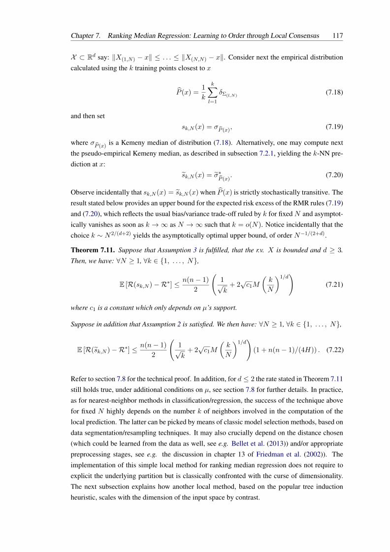
Chapter 7. Ranking Median Regression: Learning to Order through Local Consensus 117
X ⊂ Rd say: ‖X(1,N) − x‖ ≤ . . . ≤ ‖X(N,N) − x‖. Consider next the empirical distribution
calculated using the k training points closest to x
P (x) =1
k
k∑l=1
δΣ(l,N)(7.18)
and then set
sk,N (x) = σP (x)
, (7.19)
where σP (x)
is a Kemeny median of distribution (7.18). Alternatively, one may compute next
the pseudo-empirical Kemeny median, as described in subsection 7.2.1, yielding the k-NN pre-
diction at x:
sk,N (x) = σ∗P (x)
. (7.20)
Observe incidentally that sk,N (x) = sk,N (x) when P (x) is strictly stochastically transitive. The
result stated below provides an upper bound for the expected risk excess of the RMR rules (7.19)
and (7.20), which reflects the usual bias/variance trade-off ruled by k for fixed N and asymptot-
ically vanishes as soon as k →∞ as N →∞ such that k = o(N). Notice incidentally that the
choice k ∼ N2/(d+2) yields the asymptotically optimal upper bound, of order N−1/(2+d).
Theorem 7.11. Suppose that Assumption 3 is fulfilled, that the r.v. X is bounded and d ≥ 3.
Then, we have: ∀N ≥ 1, ∀k ∈ 1, . . . , N,
E [R(sk,N )−R∗] ≤ n(n− 1)
2
(1√k
+ 2√c1M
(k
N
)1/d)
(7.21)
where c1 is a constant which only depends on µ’s support.
Suppose in addition that Assumption 2 is satisfied. We then have: ∀N ≥ 1, ∀k ∈ 1, . . . , N,
E [R(sk,N )−R∗] ≤ n(n− 1)
2
(1√k
+ 2√c1M
(k
N
)1/d)
(1 + n(n− 1)/(4H)) . (7.22)
Refer to section 7.8 for the technical proof. In addition, for d ≤ 2 the rate stated in Theorem 7.11
still holds true, under additional conditions on µ, see section 7.8 for further details. In practice,
as for nearest-neighbor methods in classification/regression, the success of the technique above
for fixed N highly depends on the number k of neighbors involved in the computation of the
local prediction. The latter can be picked by means of classic model selection methods, based on
data segmentation/resampling techniques. It may also crucially depend on the distance chosen
(which could be learned from the data as well, see e.g. Bellet et al. (2013)) and/or appropriate
preprocessing stages, see e.g. the discussion in chapter 13 of Friedman et al. (2002)). The
implementation of this simple local method for ranking median regression does not require to
explicit the underlying partition but is classically confronted with the curse of dimensionality.
The next subsection explains how another local method, based on the popular tree induction
heuristic, scales with the dimension of the input space by contrast.
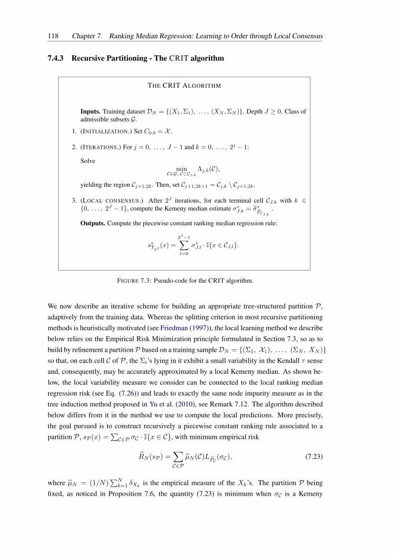
118 Chapter 7. Ranking Median Regression: Learning to Order through Local Consensus
7.4.3 Recursive Partitioning - The CRIT algorithm
THE CRIT ALGORITHM
Inputs. Training dataset DN = (X1,Σ1), . . . , (XN ,ΣN ). Depth J ≥ 0. Class ofadmissible subsets G.
1. (INITIALIZATION.) Set C0,0 = X .
2. (ITERATIONS.) For j = 0, . . . , J − 1 and k = 0, . . . , 2j − 1:
Solvemin
C∈G, C⊂Cj,kΛj,k(C),
yielding the region Cj+1,2k. Then, set Cj+1,2k+1 = Cj,k \ Cj+1,2k.
3. (LOCAL CONSENSUS.) After 2J iterations, for each terminal cell CJ,k with k ∈0, . . . , 2J − 1, compute the Kemeny median estimate σ∗J,k = σ∗
PCJ,k
.
Outputs. Compute the piecewise constant ranking median regression rule:
s∗T2J(x) =
2J−1∑l=0
σ∗J,l · Ix ∈ CJ,l.
FIGURE 7.3: Pseudo-code for the CRIT algorithm.
We now describe an iterative scheme for building an appropriate tree-structured partition P ,
adaptively from the training data. Whereas the splitting criterion in most recursive partitioning
methods is heuristically motivated (see Friedman (1997)), the local learning method we describe
below relies on the Empirical Risk Minimization principle formulated in Section 7.3, so as to
build by refinement a partitionP based on a training sampleDN = (Σ1, X1), . . . , (ΣN , XN )so that, on each cell C of P , the Σi’s lying in it exhibit a small variability in the Kendall τ sense
and, consequently, may be accurately approximated by a local Kemeny median. As shown be-
low, the local variability measure we consider can be connected to the local ranking median
regression risk (see Eq. (7.26)) and leads to exactly the same node impurity measure as in the
tree induction method proposed in Yu et al. (2010), see Remark 7.12. The algorithm described
below differs from it in the method we use to compute the local predictions. More precisely,
the goal pursued is to construct recursively a piecewise constant ranking rule associated to a
partition P , sP(x) =∑C∈P σC · Ix ∈ C, with minimum empirical risk
RN (sP) =∑C∈P
µN (C)LPC
(σC), (7.23)
where µN = (1/N)∑N
k=1 δXk is the empirical measure of the Xk’s. The partition P being
fixed, as noticed in Proposition 7.6, the quantity (7.23) is minimum when σC is a Kemeny

Chapter 7. Ranking Median Regression: Learning to Order through Local Consensus 119
median of PC for all C ∈ P . It is then equal to
mins∈SP
RN (s) =∑C∈P
µN (C)L∗PC. (7.24)
Except in the case where the intra-cell empirical distributions PC’s are all stochastically transi-
tive (each L∗PC
can be then computed using formula (5.12)), computing (7.24) at each recursion
of the algorithm can be very expensive, since it involves the computation of a Kemeny median
within each cell C. We propose to measure instead the accuracy of the current partition by the
quantity
γP =∑C∈P
µN (C)γPC, (7.25)
which satisfies the double inequality (see Remark 5.1)
γP ≤ mins∈SP
RN (s) ≤ 2γP , (7.26)
and whose computation is straightforward: ∀C ∈ P ,
γPC
=1
2
∑i<j
pi,j(C) (1− pi,j(C)) , (7.27)
where pi,j(C) = (1/NC)∑
k: Xk∈C IΣk(i) < Σk(j), i < j, denote the local pairwise empiri-
cal probabilities, with NC =∑N
k=1 IXk ∈ C. A ranking median regression tree of maximal
depth J ≥ 0 is grown as follows. One starts from the root node C0,0 = X . At depth level
0 ≤ j < J , any cell Cj,k, 0 ≤ k < 2j shall be split into two (disjoint) subsets Cj+1,2k and
Cj+1,2k+1, respectively identified as the left and right children of the interior leaf (j, k) of the
ranking median regression tree, according to the following splitting rule.
Splitting rule. For any candidate left child C ⊂ Cj,k, picked in a class G of ’admissible’ subsets
(see the paragraph on the choice of the class at the end of the section), the relevance of the split
Cj,k = C ∪ (Cj,k \ C) is naturally evaluated through the quantity:
Λj,k(C)def= µN (C)γ
PC+ µN (Cj,k \ C)γPCj,k\C
. (7.28)
The determination of the splitting thus consists in computing a solution Cj+1,2k of the optimiza-
tion problem
minC∈G, C⊂Cj,k
Λj,k(C) (7.29)
As explained in section 7.8, an appropriate choice for class G permits to solve exactly the opti-
mization problem very efficiently, in a greedy fashion.
Local medians. The consensus ranking regression tree is grown until depth J and on each
terminal leave CJ,l, 0 ≤ l < 2J , one computes the local Kemeny median estimate by means of

120 Chapter 7. Ranking Median Regression: Learning to Order through Local Consensus
the best strictly stochastically transitive approximation method investigated in subsection 7.2.1
σ∗J,ldef= σ∗
PCJ,l. (7.30)
If PCJ,l ∈ T , σ∗J,l is straightforwardly obtained from formula (5.10) and otherwise, one uses the
pseudo-empirical Kemeny median described in subsection 7.2.1. The ranking median regression
rule related to the binary tree T2J thus constructed is given by:
s∗T2J
(x) =2J−1∑l=0
σ∗J,lIx ∈ CJ,l. (7.31)
Its training prediction error is equal to LN (s∗T2J
), while the training accuracy measure of the
final partition is given by
γT2J
=
2J−1∑l=0
µN (CJ,l)γPCJ,l . (7.32)
Remark 7.12. We point out that the impurity measure (7.25) corresponds (up to a constant
factor) to that considered in Yu et al. (2010), where it is referred to as the pairwise Gini criterion.
Borrowing their notation, one may indeed write: for any measurable C ⊂ X , i(2)w (C) = 8/(n(n−
1))× γPC
.
Now that we have summarized the tree growing stage, we present possible procedures avoiding
overfitting as well as additional comments on the advantages of this method regarding inter-
pretability and computational feasibility.
Pruning. From the original tree T2J , one recursively merges children of a same parent node
until the root T1 is reached in a bottom up fashion. Precisely, the weakest link pruning consists
here in sequentially merging the children Cj+1,2l and Cj+1,2l+1 producing the smallest dispersion
increase:
µN (Cj,l)γPCj,l − Λj,l(Cj+1,2l).
One thus obtains a sequence of ranking median regression trees T2J ⊃ T2J−1 ⊃ · · · ⊃ T1, the
subtree Tm corresponding to a partition with #Tm = m cells. The final subtree T is selected by
minimizing the complexity penalized intra-cell dispersion:
γT = γT + λ×#T, (7.33)
where λ ≥ 0 is a parameter that rules the trade-off between the complexity of the ranking median
regression tree, as measured by #T , and intra-cell dispersion. In practice, model selection can
be performed by means of common resampling techniques.
Early stopping. One stops the splitting process if no improvement can be achieved by splitting
the current node Cj,l, i.e. if minC∈G Λ(C) =∑
1≤k<l≤N I(Xk, Xl) ∈ C2j,l · dτ (Σk,Σl) (one
then set Cj+1,2l = Cj,l by convention), or if a minimum node size, specified in advance, is
attained.
Chapter 7. Ranking Median Regression: Learning to Order through Local Consensus 121
On class G. The choice of class G involves a trade-off between computational cost and flexibil-
ity: a rich class (of controlled complexity though) may permit to capture the conditional vari-
ability of Σ given X appropriately but might significantly increase the cost of solving (7.29).
Typically, as proposed in Breiman et al. (1984), subsets can be built by means of axis parallel
splits, leading to partitions whose cells are finite union of hyperrectangles. This corresponds to
the case where G is stable by intersection, i.e. ∀(C, C′) ∈ G2, C ∩C′ ∈ G, and admissible subsets
of any C ∈ G are of the form C ∩ X(m) ≥ s or C ∩ X(m) ≤ s, where X(m) can be any
component of X and s ∈ R any threshold value. In this case, the minimization problem can be
efficiently solved by means of a double loop (over the d coordinates of the input vector X and
over the data lying in the current parent node), see e.g. Breiman et al. (1984).
Interpretability and computational feasability. The fact that the computation of (local) Ke-
meny medians takes place at the level of terminal nodes of the ranking median regression tree
T only makes the CRIT algorithm very attractive from a practical perspective. In addition, it
produces predictive rules that can be easily interpreted by means of a binary tree graphic repre-
sentation and, when implemented with axis parallel splits, provides, as a by-product, indicators
quantifying the impact of each input variable. The relative importance of a variable can be mea-
sured by summing the decreases of empirical γ-dispersion induced by all splits involving it as
splitting variable. More generally, the CRIT algorithm inherits the appealing properties of tree
induction methods: it easily adapts to categorical predictor variables, training and prediction are
fast and it is not affected by monotone transformations of the predictor variables.
Aggregation. Just like other tree-based methods, the CRIT algorithm may suffer from instabil-
ity, meaning that, due to its hierarchical structure, the rules it produces can be much affected by
a small change in the training dataset. As proposed in Breiman (1996), boostrap aggregatingtechniques may remedy to instability of ranking median regression trees. Applied to the CRIT
method, bagging consists in generating B ≥ 1 bootstrap samples by drawing with replacement
in the original data sample and running next the learning algorithm from each of these training
datasets, yielding B predictive rules s1, . . . , sB . For any prediction point x, the ensemble of
predictions s1(x), . . . , sB(x) are combined in the sense of Kemeny ranking aggregation, so as
to produce a consensus sB(x) in Sn. Observe that a crucial advantage of dealing with piece-
wise constant ranking rules is that computing a Kemeny median for each new prediction point
can be avoided: one may aggregate the ranking rules rather than the rankings in this case. We
finally point out that a certain amount of randomization can be incorporated in each bootstrap
tree growing procedure, following in the footsteps of the random forest procedure proposed in
Breiman (2001), so as to increase flexibility and hopefully improve accuracy. The reader may
refer to Appendix 7.7 for further details and experiments.
7.5 Numerical Experiments
For illustration purpose, experimental results based on simulated/real data are displayed.
122 Chapter 7. Ranking Median Regression: Learning to Order through Local Consensus
Results on Simulated Data. Here, datasets of full rankings on n items are generated according
to two explanatory variables. We carried out several experiments by varying the number of
items (n = 3, 5, 8) and the nature of the features. In Setting 1, both features are numerical; in
Setting 2, one is numerical and the other categorical, while, in Setting 3, both are categorical.
For a fixed setting, a partition P of X composed of K cells C1, . . . , CK is fixed. In each trial, K
permutations σ1, . . . , σK (which can be arbitrarily close) are generated, as well as three datasets
of N samples, where on each cell Ck: the first one is constant (all samples are equal to σk),
and the two others are noisy versions of the first one, where the samples follow a Mallows
distribution (see Mallows (1957)) centered on σk with dispersion parameter φ. We recall that
the greater the dispersion parameter φ, the spikiest the distribution (and closest to piecewise
constant). We choose K=6 and N=1000. In each trial, the dataset is divided into a training
set (70%) and a test set (30%). Concerning the CRIT algorithm, since the true partition is
known and is of depth 3, the maximum depth is set to 3 and the minimum size in a leaf is set
to the number of samples in the training set divided by 10. For the k-NN algorithm, the number
of neighbors k is fixed to 5. The baseline model to which we compare our algorithms is the
following: on the train set, we fit a K-means (with K=6), train a Plackett-Luce model on each
cluster and assign the mode of this learnt distribution as the center ranking of the cluster. For
each configuration (number of items, characteristics of feature and distribution of the dataset),
the empirical risk (see 7.3, denoted as RN (s)) is averaged on 50 repetitions of the experiment.
Results of the k-NN algorithm (indicated with a star *), of the CRIT algorithm (indicated with
two stars **) and of the baseline model (between parenthesis) on the various configurations are
provided in Table 7.2. They show that the methods we develop recover the true partition of the
data, insofar as the underlying distribution can be well approximated by a piecewise constant
function (φ ≥ 2 for instance in our simulations).
Analysis of GSS Data on Job Value Preferences. We test our algorithm on the full rankings
dataset which was obtained by the US General Social Survey (GSS) and which is already used
in Alvo & Yu (2014). This multidimensional survey collects across years socio-demographic
attributes and answers of respondents to numerous questions, including societal opinions. In
particular, participants were asked to rank in order of preference five aspects about a job: "high
income", "no danger of being fired", "short working hours", "chances for advancement", and
"work important and gives a feeling of accomplishment". The dataset we consider contains
answers collected between 1973 and 2014. As in Alvo & Yu (2014), for each individual, we
consider eight individual attributes (sex, race, birth cohort, highest educational degree attained,
family income, marital status, number of children that the respondent ever had, and household
size) and three properties of work conditions (working status, employment status, and occupa-
tion). After preprocessing, the full dataset contains 18544 samples. We average the results of
our algorithms over 10 experiments: each time, a bootstrap sample of size 1000 is drawn, then
randomly divided in a training set (70%) and a test set (30%), and the model is trained on the
training set and evaluated on the test set. The results are stable among the experiments. Con-
cerning the k-NN algorithm, we obtain an average empirical risk of 2.842 (for the best k = 22).
For the CRIT algorithm, we obtain an average empirical risk of 2.763 (recall that the maximum
Chapter 7. Ranking Median Regression: Learning to Order through Local Consensus 123
Kendall distance is 10) and splits coherent with the analysis in Alvo & Yu (2014): the first
splitting variable is occupation (managerial, professional, sales workers and related vs services,
natural resources, production, construction and transportation occupations), then at the second
level the race is the most important factor in both groups (black respondents vs others in the first
group, white respondents vs others in the second group). At the lower level the degree obtained
seems to play an important role (higher than high school, or higher than bachelor’s for example
in some groups); then other discriminating variables among lower levels are birth cohort, family
income or working status.
7.6 Conclusion and Perspectives
The contribution of this chapter is twofold. The problem of learning to predict preferences, ex-
pressed in the form of a permutation, in a supervised setting is formulated and investigated in
a rigorous probabilistic framework (optimal elements, learning rate bounds, bias analysis), ex-
tending that recently developped for statistical Kemeny ranking aggregation Chapter 5. Based on
this formulation, it is also shown that predictive methods based on the concept of local Kemeny
consensus, variants of nearest-neighbor and tree-induction methods namely, are well-suited for
this learning task. This is justified by approximation theoretic arguments and algorithmic sim-
plicity/efficiency both at the same time and illustrated by numerical experiments. We point out
that extensions of other data-dependent partitioning methods, such as those investigated in Chap-
ter 21 of Devroye et al. (1996) for instance could be of interest as well. In the next chapter, we
tackle the ranking regression problem in a structured prediction problem, for a specific family
of loss functions, including Kendall’s τ distance as well as well-spread distances for rankings.
7.7 Appendix - On Aggregation in Ranking Median Regression
Aggregation of Ranking Median Regression Rules. We now investigate RMR rules that
compute their predictions by aggregating those of randomized RMR rules. Let Z be a r.v.
defined on the same probability space as (X,Σ), valued in a measurable space Z say, de-
scribing the randomization mechanism. A randomized RMR algorithm is then any function
S :⋃N≥1(X ×Sn)N ×Z → S that maps any pair (z,DN ) to a RMR rule S(., z,DN ). Given
the training sample DN , its risk isR(S(., .,DN )) = E(X,Σ,Z)[dτ (Σ, S(X,Z,DN ))]. Given any
RMR algorithm and any training set DN , one may compute an aggregated rule as follows.
The result stated below shows that, provided that PX fulfills the strict stochastic transitivity
property and that the pi,j(X)’s satisfy the noise condition NA(h) for some h > 0 with probabil-
ity one (we recall that fast learning rates are attained by empirical risk minimizers in this case),
consistency is preserved by Kemeny aggregation, as well as the learning rate.
Theorem 7.13. Let h > 0. Assume that the sequence of RMR rules (S(., Z,DN ))N≥1 is consis-
tent for a certain distribution of (X,Σ). Suppose also that PX is strictly stochastically transitive
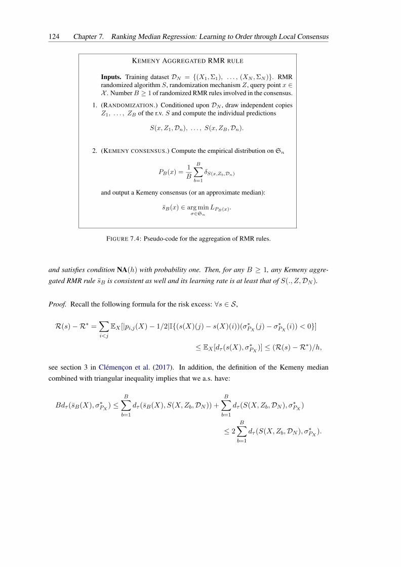
124 Chapter 7. Ranking Median Regression: Learning to Order through Local Consensus
KEMENY AGGREGATED RMR RULE
Inputs. Training dataset DN = (X1,Σ1), . . . , (XN ,ΣN ). RMRrandomized algorithm S, randomization mechanism Z, query point x ∈X . NumberB ≥ 1 of randomized RMR rules involved in the consensus.
1. (RANDOMIZATION.) Conditioned upon DN , draw independent copiesZ1, . . . , ZB of the r.v. S and compute the individual predictions
S(x, Z1,Dn), . . . , S(x, ZB ,Dn).
2. (KEMENY CONSENSUS.) Compute the empirical distribution on Sn
PB(x) =1
B
B∑b=1
δS(x,Zb,Dn)
and output a Kemeny consensus (or an approximate median):
sB(x) ∈ arg minσ∈Sn
LPB(x).
FIGURE 7.4: Pseudo-code for the aggregation of RMR rules.
and satisfies condition NA(h) with probability one. Then, for any B ≥ 1, any Kemeny aggre-
gated RMR rule sB is consistent as well and its learning rate is at least that of S(., Z,DN ).
Proof. Recall the following formula for the risk excess: ∀s ∈ S,
R(s)−R∗ =∑i<j
EX [|pi,j(X)− 1/2|I(s(X)(j)− s(X)(i))(σ∗PX (j)− σ∗PX (i)) < 0]
≤ EX [dτ (s(X), σ∗PX )] ≤ (R(s)−R∗)/h,
see section 3 in Clémençon et al. (2017). In addition, the definition of the Kemeny median
combined with triangular inequality implies that we a.s. have:
Bdτ (sB(X), σ∗PX ) ≤B∑b=1
dτ (sB(X), S(X,Zb,DN )) +B∑b=1
dτ (S(X,Zb,DN ), σ∗PX )
≤ 2
B∑b=1
dτ (S(X,Zb,DN ), σ∗PX ).
Chapter 7. Ranking Median Regression: Learning to Order through Local Consensus 125
Combined with the formula/bound above, we obtain that
R(sB)−R∗ ≤ E[dτ (sB, σ∗PX
)] ≤ 2
B
B∑b=1
EX [dτ (S(X,Zb,DN ), σ∗PX )]
≤ (2/h)1
B
B∑b=1
(R(S(., Zb,DN ))−R∗).
The proof is then immediate.
Experimental Results. For illustration purpose, experimental results based on simulated data
are displayed. Datasets of full rankings on n items are generated according to p=2 explanatory
variables. We carried out several experiments by varying the number of items (n = 3, 5, 8) and
the "level of noise" of the distribution of permutations. For a given setting, one considers a fixed
partition on the feature space, so that on each cell, the rankings/preferences are drawn from a
certain Mallows distribution centered around a permutation with a fixed dispersion parameter φ.
We recall that the greater φ, the spikiest the distribution (so closest to piecewise constant and
less noisy in this sense). In each trial, the dataset ofN = 1000 samples is divided into a training
set (70%) and a test set (30%). We compare the results of (a randomized variant of) the CRIT
algorithm vs the aggregated version: in our case, the randomization is a boostrap procedure.
Concerning the CRIT algorithm, since the true partition is known and can be recovered by
means of a tree-structured recursive partitioning of depth 3, the maximum depth is set to 3
and the minimum size in a leaf is set to the number of samples in the training set divided by
10. For each configuration (number of items n and distribution of the dataset parameterized by
Φ), the empirical risk, denoted as RN (s), is averaged over 50 replications of the experiment.
Results of the aggregated version of the (randomized) CRIT algorithm (one star * indicates the
aggregate over 10 models, two stars over 30 models **) and of the CRIT algorithm (without
stars) in the various configurations are provided in Table 7.2. In practice, for n = 8, the outputs
of the randomized algorithms are aggregated with the Copeland procedure so that the running
time remains reasonable. The results show notably that the noisier the data (smaller φ) and the
larger the number of items n to be ranked, the more difficult the problem and the higher the risk.
In a nutshell, and as confirmed by additional experiments, the results show that aggregating the
randomized rules globally improves the average performance and reduces the standard deviation
of the risk.

126 Chapter 7. Ranking Median Regression: Learning to Order through Local Consensus
7.8 Proofs
Proof of Lemma 7.1
Observe first that: ∀σ ∈ Sn,
LP ′(σ) =∑i<j
p′i,jIσ(i) > σ(j)+∑i<j
(1− p′i,j)Iσ(i) < σ(j). (7.34)
We deduce from the equality above, applied twice, that: ∀σ ∈ Sn,
|LP ′(σ))− LP ′′(σ)| ≤∑i<j
∣∣p′i,j − p′′i,j∣∣ . (7.35)
Hence, we may write:
L∗P ′ = infσ∈Sn
LP ′(σ) ≤ LP ′(σP ′′) = LP ′′(σP ′′) + (LP ′(σP ′′)− LP ′′(σP ′′))
≤ L∗P ′′ +∑i<j
∣∣p′i,j − p′′i,j∣∣ .In a similar fashion, we have L∗P ′′ ≤ L∗P ′ +
∑i<j |p′i,j − p′′i,j |, which yields assertion (i) when
combined with the inequality above.
We turn to (ii) and assume now that both P ′ and P ′′ belong to T . Let i < j. Suppose that
σ∗P ′(i) < σ∗P ′(j) and σ∗P ′′(i) > σ∗P ′′(j). In this case, we have p′i,j > 1/2 and p′′i,j < 1/2, so that
|p′i,j − p′′i,j |/h =(p′i,j − 1/2
)/h+
(1/2− p′′i,j
)/h ≥ 1.
More generally, we have
I (σ∗P ′(i)− σ∗P ′(j)) (σ∗P ′(i)− σ∗P ′(j)) < 0 ≤ |p′i,j − p′′i,j |/h
for all i < j. Summing over the pairs (i, j) establishes assertion (ii).

Chapter 7. Ranking Median Regression: Learning to Order through Local Consensus 127
Proof of Proposition 7.3
First, observe that, using the definition of empirical risk minimizers and the union bound, we
have with probability one: ∀N ≥ 1,
R(sN )−R∗ ≤ 2 sups∈S0
∣∣∣RN (s)−R(s)∣∣∣+
infs∈S0R(s)−R∗
≤ 2∑i<j
sups∈S0
∣∣∣∣∣ 1
N
N∑k=1
I (Σk(i)− Σk(j)) (s(Xk)(i)− s(Xk)(j)) < 0 −Ri,j(s)
∣∣∣∣∣+
infs∈S0R(s)−R∗
,
where Ri,j(s) = P(Σ(i) − Σ(j))(s(X)(i) − s(X)(j)) < 0 for i < j and s ∈ S . Since
Assumption 1 is satisfied, by virtue of Vapnik-Chervonenkis inequality (see e.g. Devroye et al.
(1996)), for all i < j and any δ ∈ (0, 1), we have with probability at least 1− δ:
sups∈S0
∣∣∣∣∣ 1
N
N∑k=1
I (Σk(i)− Σk(j)) (s(Xk)(i)− s(Xk)(j)) < 0 −Ri,j(s)
∣∣∣∣∣ ≤ c√V log(1/δ)/N,
(7.36)
where c < +∞ is a universal constant. The desired bound then results from the combination of
the bound above and the union bound.
Proof of Proposition 7.5
The subsequent fast rate analysis mainly relies on the lemma below.
Lemma 7.14. Suppose that Assumption 2 is fulfilled. Let s ∈ S and set
Z(s) =∑i<j
I (Σ(i)− Σ(j)) (s(X)(i)− s(X)(j)) < 0−
∑i<j
I
(Σ(i)− Σ(j))(σ∗PX (i)− σ∗PX (j)
)< 0
.
Then, we have:
V ar (Z(s)) ≤(n(n− 1)
2H
)× (R(s)−R∗) .
Proof. Recall first that it follows from (5.11) that, for all i < j,
(σ∗PX (j)− σ∗PX (i)
)(pi,j(X)− 1/2) > 0.

128 Chapter 7. Ranking Median Regression: Learning to Order through Local Consensus
Hence, we have:
V ar (Z(s)) ≤ n(n− 1)
2×∑i<j
V ar (I (pi,j(X)− 1/2) (s(X)(j)− s(X)(i)) < 0)
≤ n(n− 1)
2×∑i<j
E [I (pi,j(X)− 1/2) (s(X)(j)− s(X)(i)) < 0] .
In addition, it follows from formula (7.5) for the risk excess that:
R(s)−R∗ ≥ H ×∑i<j
E [I (pi,j(X)− 1/2) (s(X)(j)− s(X)(i)) < 0] .
Combined with the previous inequality, this establishes the lemma.
Since the goal is to give the main ideas, we assume for simplicity that the S0 is of finite cardi-
nality and that the optimal ranking median regression rule s∗(x) = σ∗Px belongs to it. Applying
Bernstein’s inequality to the i.i.d. average (1/N)∑N
k=1 Zk(s), where
Zk(s) =∑i<j
I (Σk(i)− Σk(j)) (s(Xk)(i)− s(Xk)(j)) < 0−
∑i<j
I
(Σk(i)− Σk(j))(σ∗PXk
(i)− σ∗PXk (j))< 0
,
for 1 ≤ k ≤ N and the union bound over the ranking rules s in S0, we obtain that, for all
δ ∈ (0, 1), we have with probability larger than 1− δ: ∀s ∈ S0,
E[Z(s)] = R(s)−R∗ ≤ RN (s)− RN (s∗) +
√2V ar(Z(s)) log(C/δ)
N+
4 log(C/δ)
3N.
Since RN (sN )−RN (s∗) ≤ 0 by assumption and using the variance control provided by Lemma
7.14 above, we obtain that, with probability at least 1− δ, we have:
R(sN )−R∗ ≤
√n(n−1)H (R(sN )−R∗) /H × log(C/δ)
N+
4 log(C/δ)
3N.
Finally, solving this inequality inR(sN )−R∗ yields the desired result.
Proof of Proposition 7.6
Let s(x) =∑K
k=1 σkIx ∈ Ck in SP . It suffices to observe that we have
R(s) =K∑k=1
E [IX ∈ Ckdτ (σk,Σ)] =K∑k=1
µ(Ck)E [dτ (σk,Σ) | X ∈ Ck] , (7.37)

Chapter 7. Ranking Median Regression: Learning to Order through Local Consensus 129
and that each term involved in the summation above is minimum for σk ∈MPCk, 1 ≤ k ≤ K.
Proof of Theorem 10.7
Consider sP(x) =∑C∈P σPC · Ix ∈ C in S∗P , i.e. σPC ∈MPC for all C ∈ P .
R(sN )−R∗ =
∫x∈X
LPx(sN (x))− L∗Px
µ(dx) =
∑C∈P
∫x∈C
LPx(σPC)− L
∗Px
µ(dx).
Now, by virtue of assertion (i) of Lemma 7.1, we have
R(sP)−R∗ ≤ 2∑i<j
∑C∈P
∫x∈C|pi,j(C)− pi,j(x)|µ(dx).
Now, observe that, for any C ∈ P , all x ∈ C and i < j, it results from Jensen’s inequality and
Assumption 3 that
|pi,j(C)− pi,j(x)| ≤∫x∈C
∣∣pi,j(x′)− pi,j(x)∣∣µ(dx′)/µ(C) ≤MδP ,
which establishes (10.19).
We now prove the second assertion. For any measurable set C ⊂ X such that µ(C) > 0, we set
pi,j(C) = PΣ(i) < Σ(j) | X ∈ C for i < j. Suppose that x ∈ Ck, k ∈ 1, . . . , K. It
follows from assertion (ii) in Lemma 7.1 combined with Jensen’s inequality and Assumption 3
that:
dτ(σ∗Px , s
∗P(x)
)= dτ
(σ∗Px , σ
∗PCk
)≤ (1/H)
∑i<j
|pi,j(x)− pi,j(Ck)|
≤ (1/H)∑i<j
E [|pi,j(x)− pi,j(X)| | X ∈ Ck] ≤ (M/H) supx′∈Ck
||x− x′|| ≤ (M/H) · δP .
Proof of Theorem 7.10
We start with proving the first assertion and consider a RMR rule sN of the form (7.16). With
the notations of Theorem 10.7, we have the following decomposition:
R(sN )−R∗ = (R(sN )−R(sPN )) + (R(sPN )−R∗) . (7.38)
Consider first the second term on the right hand side of the equation above. It results from the
argument of Theorem 10.7’s that:
R(sPN )−R∗ ≤MδPN → 0 in probability as N →∞. (7.39)

130 Chapter 7. Ranking Median Regression: Learning to Order through Local Consensus
We now turn to the first term. Notice that, by virtue of Lemma 7.1,
R(sN )−R(sPN ) =∑C∈PN
LPC(σC)− L
∗PC
µ(C) ≤ 2
∑i<j
∑C∈PN
|pi,j(C)− pi,j(C)|µ(C),
(7.40)
where, for any i < j and all measurable C ⊂ X , we set
pi,j(C) = (1/(NµN (C)))N∑k=1
IXk ∈ C, Σk(i) < Σk(j)
and µN (C) = (1/N)∑N
k=1 IXk ∈ C = NC/N , with the convention that pi,j(C) = 0 when
µN (C) = 0. We incidentally point out that the pi,j(C)’s are the pairwise probabilities related to
the distribution PC = (1/(NµN (C)))∑
k: Xk∈C δΣk . Observe that for all i < j and C ∈ PN , we
have:
µ(C) (pi,j(C)− pi,j(C)) =
1
N
N∑k=1
IXk ∈ C, Σk(i) < Σk(j) − E [IX ∈ C, Σ(i) < Σ(j)]
+
(µ(C)
−µN (C) + µ(C)− 1
)−1
× 1
N
N∑k=1
IXk ∈ C, Σk(i) < Σk(j)
.
Combining this equality with the previous bound yields
R(sN )−R(sPN ) ≤ 2∑i<j
AN (i, j) +BN/κN , (7.41)
where we set
AN (i, j) = supP∈FN
∑C∈P
∣∣∣∣∣ 1
N
N∑k=1
IXk ∈ C, Σk(i) < Σk(j) − E [IX ∈ C, Σ(i) < Σ(j)]
∣∣∣∣∣ ,BN = sup
P∈FN
∑C∈P|µN (C)− µ(C)|
The following result is a straightforward application of the VC inequality for data-dependent
partitions stated in Theorem 21.1 of Devroye et al. (1996).
Lemma 7.15. Under the hypotheses of Theorem 7.10, the following bounds hold true: ∀ε > 0,
∀N ≥ 1,
P AN (i, j) > ε ≤ 8 log(∆N (FN ))e−Nε2/512 + e−Nε
2/2,
P BN > ε ≤ 8 log(∆N (FN ))e−Nε2/512 + e−Nε
2/2.
The terms AN (i, j) and BN are both of order OP(√
log(∆N (FN ))/N)), as shown by the
lemma above. Hence, using Eq. (7.41) and the assumption that κN → 0 in probability as
N → ∞, so that 1/κN = oP(√N/ log ∆N (FN )), we obtain that R(sN ) − R(sPN ) → 0 in
Chapter 7. Ranking Median Regression: Learning to Order through Local Consensus 131
probability as N →∞, which concludes the proof of the first assertion of the theorem.
We now consider the RMR rule (7.17). Observe that
R(sN )−R(sPN ) =∑C∈PN
LPC(σ
∗PC
)− L∗PCµ(C)
=∑C∈PN
IPC ∈ T LPC(σ
∗PC
)− L∗PCµ(C) +
∑C∈PN
IPC /∈ T LPC(σ
∗PC
)− L∗PCµ(C)
≤ R(sN )−R(sPN ) +n(n− 1)
2
∑C∈PN
IPC /∈ T µ(C). (7.42)
Recall that it has been proved previously thatR(sN )−R(sPN )→ 0 in probability as N →∞.
Observe in addition that
IPC /∈ T ≤ IPC /∈ T + IPC /∈ T and PC ∈ T
and, under Assumption 2,
PC /∈ T ⊂ δPN ≥M/H,
PC /∈ T and PC ∈ T ⊂ ∪i<j|pi,j(C)− pi,j(C)| ≥ H,
so that∑C∈PN IPC /∈ T µ(C) is bounded by
IδPN ≥M/H+∑i<j
∑C∈PN
I|pi,j(C)− pi,j(C)| ≥ Hµ(C)
≤ IδPN ≥M/H+∑i<j
∑C∈PN
|pi,j(C)− pi,j(C)|µ(C)/H
≤ IδPN ≥M/H+1
H
∑i<j
AN (i, j) +BN/κN ,
re-using the argument that previously lead to (7.41). This bound clearly converges to zero in
probability, which implies that R(sN ) − R(sPN ) → 0 in probability when combined with
(7.42) and concludes the proof of the second assertion of the theorem.

132 Chapter 7. Ranking Median Regression: Learning to Order through Local Consensus
Proof of Theorem 7.11
Denote by pi,j(x)’s the pairwise probabilities related to distribution P (x). It follows from
Lemma 7.1 combined with Jensen’s inequality, that
E [R(sk,N )−R∗] = E[∫
x∈X(LPx(sk,N (x))− L∗Px)µ(dx)
]≤ 2
∑i<j
∫x∈X
E [|pi,j(x)− pi,j(x)|]
≤ 2∑i<j
∫x∈X
(E[(pi,j(x)− pi,j(x))2
])1/2
Following the argument of Theorem 6.2’s proof in Györfi et al. (2006), write:
E[(pi,j(x)− pi,j(x))2
]= E
[(pi,j(x)− E [pi,j(x)|X1, . . . , XN ])2
]+ E
[(E [pi,j(x)|X1, . . . , XN ]− pi,j(x))2
]= I1(x) + I2(x).
The first term can be upper bounded as follows:
I1(x) = E
(1
k
k∑l=1
(I
Σ(l,N)(i) < Σ(l,N)(j)− pi,j(X(l,N))
))2
= E
[1
k2
k∑l=1
V ar(I Σ(i) < Σ(j) |X = X(l,N))
]≤ 1
4k.
For the second term, we use the following result.
Lemma 7.16. (Lemma 6.4, Györfi et al. (2006)) Assume that the r.v. X is bounded. If d ≥ 3,
then:
E[‖X(1,N)(x)− x‖2
]≤ c1
N2/d,
where c1 is a constant that depends on µ’s support only.
Observe first that, following line by line the argument of Theorem 6.2’s proof in Györfi et al.
(2006) (see p.95 therein), we have:
I2(x) = E
1
k
(k∑l=1
(pi,j(X(l,N))− pi,j(x)
))2 ≤ E
(1
k
k∑l=1
M‖X(l,N) − x‖
)2
≤M2E[‖X(1,bN/kc)(x)− x‖2
].
Next, by virtue of Lemma 7.16, we have:
1
M2bN/kc2/d
∫x∈X
I2(x)µ(dx) ≤ c1.

Chapter 7. Ranking Median Regression: Learning to Order through Local Consensus 133
Finally, we have:
E [R(sk,N )−R∗] ≤ 2∑i<j
∫x∈X
√I1(x) + I2(x)µ(dx)
≤ n(n− 1)
2
(1√k
+ 2√c1M
(k
N
)1/d).
We now consider the problem of bounding the expectation of the excess of risk of the RMR rule
sk,N . Observing that sk,N (x) = sk,N (x) when P (x) ∈ T , we have:
E [R(sk,N )−R∗] = E[∫
x∈XIP (x) ∈ T (LPx(sk,N (x))− L∗Px)µ(dx)
]+
E[∫
x∈XIP (x) /∈ T (LPx(sk,N (x))− L∗Px)µ(dx)
]≤ E [R(sk,N )−R∗] +
n(n− 1)
2E[∫
x∈XIP (x) /∈ T µ(dx)
].
Notice in addition that, under Assumption 2, we have, for all x ∈ X ,
P (x) /∈ T ⊂ ∪i<j |pi,j(x)− pi,j(x) ≥ H| , (7.43)
so that
IP (x) /∈ T ≤∑i<j
|pi,j(x)− pi,j(x)|H
. (7.44)
Hence, the second assertion finally results directly from the bounds established to prove the first
one.
Let Sx,ε denote the closed ball centered at x of radius ε > 0. For d ≤ 2, the rates of convergence
hold under the following additional conditions on µ (see Györfi et al. (2006)): there exists
ε0 > 0, a non negative g such that for all x ∈ Rd and 0 < ε ≤ ε0, µ(Sx,ε) > g(x)εd and∫1/g(x)2/dµ(dx) <∞.

134 Chapter 7. Ranking Median Regression: Learning to Order through Local Consensus
Datasetdistribution
Setting1
Setting2
Setting3
n=3n=5
n=8n=3
n=5n=8
n=3n=5
n=8
Piecewise
constant0.0698*
0.1290*0.2670*
0.0173*0.0405*
0.110*0.0112*
0.0372*0.0862*
0.0473**0.136**
0.324**0.0568**
0.145**0.2695**
0.099**0.1331**
0.2188**(0.578)
(1.147)(2.347)
(0.596)(1.475)
(3.223)(0.5012)
(1.104)(2.332)
Mallow
sw
ithφ=2
0.3475*
0.569*0.9405
*0.306*
0.494*0.784*
0.289*0.457*
0.668*0.307**
0.529**0.921**
0.308**0.536**
0.862**0.3374**
0.5714**0.8544**
(0.719)(1.349)
(2.606)(0.727)
(1.634)(3.424)
(0.5254)(1.138)
(2.287)
Mallow
sw
ithφ=1
0.8656*1.522*
2.503*0.8305
*1.447
*2.359*
0.8105*1.437*
2.189*0.7228**
1.322**2.226**
0.723**1.3305**
2.163**0.7312**
1.3237**2.252**
(0.981)(1.865)
(3.443)(1.014)
(2.0945)(4.086)
(0.8504)(1.709)
(3.005)
TA
BL
E7.1:
Em
piricalriskaveraged
on50
trialson
simulated
dataforkN
N,C
RIT
andparam
etricbaseline.

Chapter 7. Ranking Median Regression: Learning to Order through Local Consensus 135
Level ofNoise
Number of itemsn=3 n=5 n=8
φ = 2
0.534 +/ - 0.167 1.454 +/ - 0.427 3.349 +/ - 0.9520.385 +/ - 0.085* 1.001 +/ - 0.232* 2.678 +/ - 0.615*0.379 +/ - 0.057** 0.961 +/ - 0.218** 2.281 +/ - 0.589**
φ = 1
0.875 +/ - 0.108 2.346 +/ - 0.269 5.638+/ - 1.6880.807+/ - 0.061* 2.064 +/ - 0.130 * 4.499 +/ - 0.574*
0.756 +/ - 0.063** 2.011 +/ - 0.110** 4.061 +/ - 0.259**
TABLE 7.2: Empirical risk averaged on 50 trials on simulated data for aggregation of RMRrules.

CHAPTER 8A Structured Prediction Approach for Label Ranking
Chapter abstract In this chapter, we propose to solve the ranking regression problem, some-times referred to in the literature as label ranking, as a structured output regression task. Weadopt a least square surrogate loss approach that solves a supervised learning problem in twosteps: the regression step in a well-chosen feature space and the pre-image step. We use spe-cific feature maps/embeddings for ranking data, which convert any ranking/permutation intoa vector representation. These embeddings are all well-tailored for our approach, either byresulting in consistent estimators, or by solving trivially the pre-image problem which is oftenthe bottleneck in structured prediction. We also propose their natural extension the case ofpartial rankings and prove their efficiency on real-world datasets.
8.1 Introduction
Label ranking is a prediction task which aims at mapping input instances to a (total) order over a
given set of labels indexed by 1, . . . , n. This problem is motivated by applications where the
output reflects some preferences, or order of relevance, among a set of objects. Hence there is an
increasing number of practical applications of this problem in the machine learning litterature.
In pattern recognition for instance (Geng & Luo, 2014), label ranking can be used to predict the
different objects which are the more likely to appear in an image among a predefined set. Simi-
larly, in sentiment analysis, (Wang et al., 2011) where the prediction of the emotions expressed
in a document is cast as a label ranking problem over a set of possible affective expressions. In
ad targeting, the prediction of preferences of a web user over ad categories (Djuric et al., 2014)
can be also formalized as a label ranking problem, and the prediction as a ranking guarantees
that each user is qualified into several categories, eliminating overexposure. Another application
is metalearning, where the goal is to rank a set of algorithms according to their suitability based
on the characteristics of a target dataset and learning problem (see Brazdil et al. (2003); Aiguzhi-
nov et al. (2010)). Interestingly, the label ranking problem can also be seen as an extension of
several supervised tasks, such as multiclass classification or multi-label ranking (see Dekel et al.
(2004); Fürnkranz & Hüllermeier (2003)). Indeed for these tasks, a prediction can be obtained
by postprocessing the output of a label ranking model in a suitable way. However, label ranking
differs from other ranking problems, such as in information retrieval or recommender systems,
137
138 Chapter 8. A Structured Prediction Approach for Label Ranking
where the goal is (generally) to predict a target variable under the form of a rating or a relevance
score (Cao et al., 2007).
More formally, the goal of label ranking is to map a vector x lying in some feature space X to
a ranking y lying in the space of rankings Y . A ranking is an ordered list of items of the set
1, . . . , n. These relations linking the components of the y objects induce a structure on the
output space Y . The label ranking task thus naturally enters the framework of structured output
prediction for which an abundant litterature is available (Nowozin & Lampert, 2011). In this
paper, we adopt the Surrogate Least Square Loss approach introduced in the context of output
kernels (Cortes et al., 2005; Kadri et al., 2013; Brouard et al., 2016) and recently theoretically
studied by Ciliberto et al. (2016) and Osokin et al. (2017) using Calibration theory (Steinwart
& Christmann, 2008). This approach divides the learning task in two steps: the first one is a
vector regression step in a Hilbert space where the outputs objects are represented through an
embedding, and the second one solves a pre-image problem to retrieve an output object in the
Y space. In this framework, the algorithmic complexity of the learning and prediction tasks as
well as the generalization properties of the resulting predictor crucially rely on some properties
of the embedding. In this work we study and discuss some embeddings dedicated to ranking
data.
Our contribution is three folds: (1) we cast the label ranking problem into the structured pre-
diction framework and propose embeddings dedicated to ranking representation, (2) for each
embedding we propose a solution to the pre-image problem and study its algorithmic complex-
ity and (3) we provide theoretical and empirical evidence for the relevance of our method.
The paper is organized as follows. In section 8.2, definitions and notations of objects consid-
ered through the paper are introduced, and section 8.3 is devoted to the statistical setting of the
learning problem. section 8.4 describes at length the embeddings we propose and section 8.5 de-
tails the theoretical and computational advantages of our approach. Finally section 8.6 contains
empirical results on benchmark datasets.
8.2 Preliminaries
8.2.1 Mathematical Background and Notations
Consider a set of items indexed by 1, . . . , n, that we will denote JnK. Rankings, i.e. ordered
lists of items of JnK, can be complete (i.e, involving all the items) or incomplete and for both
cases, they can be without-ties (total order) or with-ties (weak order). A full ranking is a com-
plete, and without-ties ranking of the items in JnK. It can be seen as a permutation, i.e a bijection
σ : JnK→ JnK, mapping each item i to its rank σ(i). The rank of item i is thus σ(i) and the item
ranked at position j is σ−1(j). We say that i is preferred over j (denoted by i j) according
to σ if and only if i is ranked lower than j: σ(i) < σ(j). The set of all permutations over n
items is the symmetric group which we denote by Sn. A partial ranking is a complete ranking
Chapter 8. A Structured Prediction Approach for Label Ranking 139
including ties, and is also referred as a weak order or bucket order in the litterature (see Kenkre
et al. (2011)). This includes in particular the top-k rankings, that is to say partial rankings di-
viding items in two groups, the first one being the k ≤ n most relevant items and the second
one including all the rest. These top-k rankings are given a lot of attention because of their
relevance for modern applications, especially search engines or recommendation systems (see
Ailon (2010)). An incomplete ranking is a strict order involving only a small subset of items,
and includes as a particular case pairwise comparisons, another kind of ranking which is very
relevant in large-scale settings when the number of items to be ranked is very large. We now
introduce the main notations used through the paper. For any function f , Im(f) denotes the
image of f , and f−1 its inverse. The indicator function of any event E is denoted by IE. We
will denote by sign the function such that for any x ∈ R, sign(x) = Ix > 0 − Ix < 0.The notations ‖.‖ and |.| denote respectively the usual l2 and l1 norm in an Euclidean space.
Finally, for any integers a ≤ b, Ja, bK denotes the set a, a+ 1, . . . , b, and for any finite set C,
#C denotes its cardinality.
8.2.2 Related Work
An overview of label ranking algorithms can be found in Vembu & Gärtner (2010), Zhou
et al. (2014)), but we recall here the main contributions. One of the first proposed approaches,
called pairwise classification (see Fürnkranz & Hüllermeier (2003)) transforms the label rank-
ing problem into n(n − 1)/2 binary classification problems. For each possible pair of labels
1 ≤ i < j ≤ n, the authors learn a model mij that decides for any given example whether
i j or j i holds. The model is trained with all examples for which either i j or j i
is known (all examples for which nothing is known about this pair are ignored). At prediction
time, an example is submitted to all n(n − 1)/2 classifiers, and each prediction is interpreted
as a vote for a label: if the classifier mij predicts i j, this counts as a vote for label i. The
labels are then ranked according to the number of votes. Another approach (see ?) consists in
learning for each label a linear utility function from which the ranking is deduced. Then, a large
part of the dedicated literature was devoted to adapting classical partitioning methods such as
k-nearest neighbors (see Zhang & Zhou (2007), Chiang et al. (2012)) or tree-based methods, in
a parametric (Cheng et al. (2010), Cheng et al. (2009), Aledo et al. (2017a)) or a non-parametric
way (see Cheng & Hüllermeier (2013), Yu et al. (2010), Zhou & Qiu (2016), Clémençon et al.
(2017), Sá et al. (2017)). Finally, some approaches are rule-based (see Gurrieri et al. (2012), Sá
et al. (2018)). We will compare our numerical results with the best performances attained by
these methods on a set of benchmark datasets of the label ranking problem in section 8.6.
140 Chapter 8. A Structured Prediction Approach for Label Ranking
8.3 Structured Prediction for Label Ranking
8.3.1 Learning Problem
Our goal is to learn a function s : X → Y between a feature space X and a structured output
space Y , that we set to be Sn the space of full rankings over the set of items JnK. The quality
of a prediction s(x) is measured using a loss function ∆ : Sn × Sn → R, where ∆(s(x), σ)
is the cost suffered by predicting s(x) for the true output σ. We suppose that the input/output
pairs (x, σ) come from some fixed distribution P on X ×Sn. The label ranking problem is then
defined as:
minimizes:X→SnR(s), with R(s) =
∫X×Sn
∆(s(x), σ)dP (x, σ). (8.1)
In this paper, we propose to study how to solve this problem and its empirical counterpart for
a family of loss functions based on some ranking embedding φ : Sn → F that maps the
permutations σ ∈ Sn into a Hilbert space F :
∆(σ, σ′) = ‖φ(σ)− φ(σ′)‖2F . (8.2)
This loss presents two main advantages: first, there exists popular losses for ranking data that
can take this form within a finite dimensional Hilbert Space F , second, this choice benefits
from the theoretical results on Surrogate Least Square problems for structured prediction using
Calibration Theory of Ciliberto et al. (2016) and of works of Brouard et al. (2016) on Struc-
tured Output Prediction within vector-valued Reproducing Kernel Hilbert Spaces. These works
approach Structured Output Prediction along a common angle by introducing a surrogate prob-
lem involving a function g : X → F (with values in F) and a surrogate loss L(g(x), σ) to be
minimized instead of Eq. 8.1. The surrogate loss is said to be calibrated if a minimizer for the
surrogate loss is always optimal for the true loss (Calauzenes et al., 2012). In the context of true
risk minimization, the surrogate problem for our case writes as:
minimize g:X→FL(g), with L(g) =
∫X×Sn
L(g(x), φ(σ))dP (x, σ). (8.3)
with the following surrogate loss:
L(g(x), φ(σ)) = ‖g(x)− φ(σ)‖2F . (8.4)
Problem of Eq. (8.3) is in general easier to optimize since g has values in F instead of the set
of structured objects Y , here Sn. The solution of (8.3), denoted as g∗, can be written for any
x ∈ X : g∗(x) = R[φ(σ)|x]. Eventually, a candidate s(x) pre-image for g∗(x) can then be
obtained by solving:
s(x) = arg minσ∈Sn
L(g∗(x), φ(σ)). (8.5)
Chapter 8. A Structured Prediction Approach for Label Ranking 141
In the context of Empirical Risk Minimization, a training sample S = (xi, σi), i = 1, . . . , N,with N i.i.d. copies of the random variable (x, σ) is available. The Surrogate Least Square
approach for Label Ranking Prediction decomposes into two steps:
• Step 1: minimize a regularized empirical risk to provide an estimator of the minimizer of
the regression problem in Eq. (8.3):
minimize g∈H LS(g), with LS(g) =1
N
N∑i=1
L(g(xi), φ(σi)) + Ω(g). (8.6)
with an appropriate choice of hypothesis space H and complexity term Ω(g). We denote
by g a solution of (8.6).
• Step 2: solve, for any x in X , the pre-image problem that provides a prediction in the
original space Sn:
s(x) = arg minσ∈Sn
‖φ(σ)− g(x)‖2F . (8.7)
The pre-image operation can be written as s(x) = d g(x) with d the decoding function:
d(h) = arg minσ∈Sn
‖φ(σ)− h‖2F for all h ∈ F , (8.8)
applied on g for any x ∈ X .
This paper studies how to leverage the choice of the embedding φ to obtain a good compromise
between computational complexity and theoretical guarantees. Typically, the pre-image problem
on the discrete set Sn (of cardinality n!) can be eased for appropriate choices of φ as we show
in section 4, leading to efficient solutions. In the same time, one would like to benefit from
theoretical guarantees and control the excess risk of the proposed predictor s.
In the following subsection we exhibit popular losses for ranking data that we will use for the
label ranking problem.
8.3.2 Losses for Ranking
We now present losses ∆ on Sn that we will consider for the label ranking task. A natural
loss for full rankings, i.e. permutations in Sn, is a distance between permutations. Several
distances on Sn are widely used in the literature (Deza & Deza, 2009), one of the most popular
being the Kendall’s τ distance, which counts the number of pairwise disagreements between
two permutations σ, σ′ ∈ Sn:
∆τ (σ, σ′) =∑i<j
I[(σ(i)− σ(j))(σ′(i)− σ′(j)) < 0]. (8.9)
142 Chapter 8. A Structured Prediction Approach for Label Ranking
The maximal Kendall’s τ distance is thus n(n− 1)/2, the total number of pairs. Another well-
spread distance between permutations is the Hamming distance, which counts the number of
entries on which two permutations σ, σ′ ∈ Sn disagree:
∆H(σ, σ′) =
n∑i=1
I[σ(i) 6= σ′(i)]. (8.10)
The maximal Hamming distance is thus n, the number of labels or items.
The Kendall’s τ distance is a natural discrepancy measure when permutations are interpreted
as rankings and is thus the most widely used in the preference learning literature. In contrast,
the Hamming distance is particularly used when permutations represent matching of bipartite
graphs and is thus also very popular (see Fathony et al. (2018)). In the next section we show
how these distances can be written as Eq. (10.21) for a well chosen embedding φ.
8.4 Output Embeddings for Rankings
In what follows, we study three embeddings tailored to represent full rankings/permutations in
Sn and discuss their properties in terms of link with the ranking distances ∆τ and ∆H , and in
terms of algorithmic complexity for the pre-image problem (8.5) induced.
8.4.1 The Kemeny Embedding
Motivated by the minimization of the Kendall’s τ distance ∆τ , we study the Kemeny embed-
ding, previously introduced for the ranking aggregation problem (see Jiao et al. (2016)):
φτ : Sn → Rn(n−1)/2
σ 7→ (sign(σ(j)− σ(i)))1≤i<j≤n .
which maps any permutation σ ∈ Sn into Im(φτ ) ( −1, 1n(n−1)/2 (that we have embedded
into the Hilbert space (Rn(n−1)/2, 〈., .〉)). One can show that the square of the euclidean distance
between the mappings of two permutations σ, σ′ ∈ Sn recovers their Kendall’s τ distance
(proving at the same time that φτ is injective) up to a constant: ‖φτ (σ)−φτ (σ′)‖2 = 4∆τ (σ, σ′).
The Kemeny embedding then naturally appears to be a good candidate to build a surrogate loss
related to ∆τ . By noticing that φτ has a constant norm (∀σ ∈ Sn, ‖φτ (σ)‖ =√n(n− 1)/2),
we can rewrite the pre-image problem (8.7) under the form:
s(x) = arg minσ∈Sn
−〈φτ (σ), g(x)〉. (8.11)
To compute (8.11), one can first solve an Integer Linear Program (ILP) to find φσ =
arg minφσ∈Im(φτ )−〈φσ, g(x)〉, and then find the output object σ = φ−1τ (φσ). The latter step,
Chapter 8. A Structured Prediction Approach for Label Ranking 143
i.e. inverting φτ , can be performed in O(n2) by means of the Copeland method (see Mer-
lin & Saari (1997)), which ranks the items by their number of pairwise victories1. In con-
trast, the ILP problem is harder to solve since it involves a minimization over Im(φτ ), a set
of structured vectors since their coordinates are strongly correlated by the transitivity prop-
erty of rankings. Indeed, consider a vector v ∈ Im(φτ ), so ∃σ ∈ Sn such that v = φτ (σ).
Then, for any 1 ≤ i < j < k ≤ n, if its coordinates corresponding to the pairs (i, j) and
(j, k) are equal to one (meaning that σ(i) < σ(j) and σ(j) < σ(k)), then the coordinate
corresponding to the pair (i, k) cannot contradict the others and must be set to one as well.
Since φσ = (φσ)i,j ∈ Im(φτ ) is only defined for 1 ≤ i < j ≤ n, one cannot directly
encode the transitivity constraints that take into account the components (φσ)i,j with j > i.
Thus to encode the transitivity constraint we introduce φ′σ = (φ′σ)i,j ∈ Rn(n−1) defined by
(φ′σ)i,j = (φσ)i,j if 1 ≤ i < j ≤ n and (φ′σ)i,j = −(φσ)i,j else, and write the ILP problem as
follows:
φσ = arg minφ′σ
∑1≤i,j≤n
g(x)i,j(φ′σ)i,j ,
s.c.
(φ′σ)i,j ∈ −1, 1 ∀ i, j
(φ′σ)i,j + (φ′σ)j,i = 0 ∀ i, j
−1 ≤ (φ′σ)i,j + (φ′σ)j,k + (φ′σ)k,i ≤ 1 ∀ i, j, k s.t. i 6= j 6= k.
(8.12)
Such a problem is NP-Hard. In previous works (see Calauzenes et al. (2012); Ramaswamy et al.
(2013)), the complexity of designing calibrated surrogate losses for the Kendall’s τ distance
had already been investigated. In particular, Calauzenes et al. (2012) proved that there exists
no convex n-dimensional calibrated surrogate loss for Kendall’s τ distance. As a consequence,
optimizing this type of loss has an inherent computational cost. However, in practice, branch and
bound based ILP solvers find the solution of (8.12) in a reasonable time for a reduced number
of labels n. We discuss the computational implications of choosing the Kemeny embedding
section 8.5.2. We now turn to the study of an embedding devoted to build a surrogate loss for
the Hamming distance.
8.4.2 The Hamming Embedding
Another well-spread embedding for permutations, that we will call the Hamming embedding,
consists in mapping σ to its permutation matrix φH(σ):
φH : Sn → Rn×n
σ 7→ (Iσ(i) = j)1≤i,j≤n ,
where we have embedded the set of permutation matrices Im(φH) ( 0, 1n×n into the Hilbert
space (Rn×n, 〈., .〉) with 〈., .〉 the Froebenius inner product. This embedding shares similar1Copeland method firstly affects a score si for item i as: si =
∑j 6=i Iσ(i) < σ(j) and then ranks the items
by decreasing score.

144 Chapter 8. A Structured Prediction Approach for Label Ranking
properties with the Kemeny embedding: first, it is also of constant (Froebenius) norm, since
∀σ ∈ Sn, ‖φH(σ)‖ =√n. Then, the squared euclidean distance between the mappings of two
permutations σ, σ′ ∈ Sn recovers their Hamming distance (proving that φH is also injective):
‖φH(σ) − φH(σ′)‖2 = ∆H(σ, σ′). Once again, the pre-image problem consists in solving the
linear program:
s(x) = arg minσ∈Sn
−〈φH(σ), g(x)〉, (8.13)
which is, as for the Kemeny embedding previously, divided in a minimization step, i.e. find
φσ = arg minφσ∈Im(φH)−〈φσ, g(x)〉, and an inversion step, i.e. compute σ = φ−1H (φσ). The
inversion step is of complexity O(n2) since it involves scrolling through all the rows (items i)
of the matrix φσ and all the columns (to find their positions σ(i)). The minimization step itself
writes as the following problem:
φσ = arg maxφσ
∑1≤i,j≤n
g(x)i,j(φσ)i,j ,
s.c
(φσ)i,j ∈ 0, 1 ∀ i, j∑i(φσ)i,j =
∑j(φσ)i,j = 1 ∀ i, j ,
(8.14)
which can be solved with the Hungarian algorithm (see Kuhn (1955)) in O(n3) time. Now we
turn to the study of an embedding which presents efficient algorithmic properties.
8.4.3 Lehmer Code
A permutation σ = (σ(1), . . . , σ(n)) ∈ Sn may be uniquely represented via its Lehmer code
(also called the inversion vector), i.e. a word of the form cσ ∈ Cn =∆ 0 × J0, 1K × J0, 2K ×· · · × J0, n− 1K, where for j = 1, . . . , n:
cσ(j) = #i ∈ JnK : i < j, σ(i) > σ(j). (8.15)
The coordinate cσ(j) is thus the number of elements i with index smaller than j that are ranked
higher than j in the permutation σ. By default, cσ(1) = 0 and is typically omitted. For instance,
we have:
e 1 2 3 4 5 6 7 8 9
σ 2 1 4 5 7 3 6 9 8
cσ 0 1 0 0 0 3 1 0 1
It is well known that the Lehmer code is bijective, and that the encoding and decoding algorithms
have linear complexity O(n) (see Mareš & Straka (2007), Myrvold & Ruskey (2001)). This
embedding has been recently used for ranking aggregation of full or partial rankings (see Li
Chapter 8. A Structured Prediction Approach for Label Ranking 145
et al. (2017)). Our idea is thus to consider the following Lehmer mapping for label ranking;
φL : Sn → Rn
σ 7→ (cσ(i)))i=1,...,n ,
which maps any permutation σ ∈ Sn into the space Cn (that we have embedded into the Hilbert
space (Rn, 〈., .〉)). The loss function in the case of the Lehmer embedding is thus the following:
∆L(σ, σ′) = ‖φL(σ)− φL(σ′)‖2, (8.16)
which does not correspond to a known distance over permutations (Deza & Deza, 2009). Notice
that |φL(σ)| = dτ (σ, e) where e is the identity permutation, a quantity which is also called
the number of inversions of σ. Therefore, in contrast to the previous mappings, the norm
‖φL(σ)‖ is not constant for any σ ∈ Sn. Hence it is not possible to write the loss ∆L(σ, σ′)
as −〈φL(σ), φL(σ′)〉2.Moreover, this mapping is not distance preserving and it can be proven
that 1n−1∆τ (σ, σ′) ≤ |φL(σ) − φL(σ′)| ≤ ∆τ (σ, σ′) (see Wang et al. (2015)). However, the
Lehmer embedding still enjoys great advantages. Firstly, its coordinates are decoupled, which
will enable a trivial solving of the inverse image step (8.7). Indeed we can write explicitly its
solution as:
s(x) = φ−1L dL︸ ︷︷ ︸
d
g(x) withdL : Rn → Cn
(hi)i=1,...,n 7→ (arg minj∈J0,i−1K
(hi − j))i=1,...,n,(8.17)
where d is the decoding function defined in (8.8). Then, there may be repetitions in the coordi-
nates of the Lehmer embedding, allowing for a compact representation of the vectors.
8.4.4 Extension to Partial and Incomplete Rankings
In many real-world applications, one does not observe full rankings but only partial or incom-
plete rankings (see the definitions section 8.2.1). We now discuss to what extent the embeddings
we propose for permutations can be adapted to this kind of rankings as input data. Firstly,
the Kemeny embedding can be naturally extended to partial and incomplete rankings since it
encodes relative information about the positions of the items. Indeed, we propose to map any
partial ranking σ to the vector:
φ(σ) = (sign(σ(i)− σ(j))1≤i<j≤n, (8.18)
where each coordinate can now take its value in −1, 0, 1 (instead of −1, 1 for full rankings).
For any incomplete ranking σ, we also propose to fill the missing entries (missing comparisons)
in the embedding with zeros. This can be interpreted as setting the probability that i j to 1/2
for a missing comparison between (i, j). In contrast, the Hamming embedding, since it encodes
2The scalar product of two embeddings of two permutations φL(σ), φL(σ′) is not maximized for σ = σ′.
146 Chapter 8. A Structured Prediction Approach for Label Ranking
the absolute positions of the items, is tricky to extend to map partial or incomplete rankings
where this information is missing. Finally, the Lehmer embedding falls between the two latter
embeddings. It also relies on an encoding of relative rankings and thus may be adapted to take
into account the partial ranking information. Indeed, in Li et al. (2017), the authors propose a
generalization of the Lehmer code for partial rankings. We recall that a tie in a ranking happens
when #i 6= j, σ(i) = σ(j) > 0. The generalized representation c′ takes into account ties, so
that for any partial ranking σ:
c′σ(j) = #i ∈ JnK : i < j, σ(i) ≥ σ(j). (8.19)
Clearly, c′σ(j) ≥ cσ(j) for all j ∈ JnK. Given a partial ranking σ, it is possible to break its ties
to convert it in a permutation σ as follows: for i, j ∈ JnK2, if σ(i) = σ(j) then σ(i) = σ(j) iff
i < j. The entries j = 1, . . . , n of the Lehmer codes of σ (see (8.20)) and σ (see (8.15)) then
verify:
c′σ(j) = cσ(j) + INj − 1 , cσ(j) = cσ(j), (8.20)
where INj = #i ≤ j, σ(i) = σ(j). An example illustrating the extension of the Lehmer code
to partial rankings is given section 8.8.2. However, computing each coordinate of the Lehmer
code cσ(j) for any j ∈ JnK requires to sum over the JnK items. As an incomplete ranking do
not involve the whole set of items, it is also tricky to extend the Lehmer code to map incomplete
rankings.
Taking as input partial or incomplete rankings only modifies Step 1 of our method since it cor-
responds to the mapping step of the training data, and in Step 2 we still predict a full ranking.
Extending our method to the task of predicting as output a partial or incomplete ranking raises
several mathematical questions that we did not develop at length here because of space limita-
tions. For instance, to predict partial rankings, a naive approach would consist in predicting a
full ranking and then converting it to a partial ranking according to some threshold (i.e, keep
the top-k items of the full ranking). A more formal extension of our method to make it able to
predict directly partial rankings as outputs would require to optimize a metric tailored for this
data and which could be written as in Eq. (10.21). A possibility for future work could be to
consider the extension of the Kendall’s τ distance with penalty parameter p for partial rankings
proposed in Fagin et al. (2004).
8.5 Computational and Theoretical Analysis
8.5.1 Theoretical Guarantees
In this section, we give some statistical guarantees for the estimators obtained by following
the steps described in section 8.3. To this end, we build upon recent results in the framework
of Surrogate Least Square by Ciliberto et al. (2016). Consider one of the embeddings φ on
permutations presented in the previous section, which defines a loss ∆ as in Eq. (10.21). Let
Chapter 8. A Structured Prediction Approach for Label Ranking 147
cφ = maxσ∈Sn ‖φ(σ)‖. We will denote by s∗ a minimizer of the true risk (8.1), g∗ a minimizer
of the surrogate risk (8.3), and d a decoding function as (8.8)3. Given an estimator g of g∗ from
Step 1, i.e. a minimizer of the empirical surrogate risk (8.6) we can then consider in Step 2 an
estimator s = d g. The following theorem reveals how the performance of the estimator s we
propose can be related to a solution s∗ of (8.1) for the considered embeddings.
Theorem 8.1. The excess risks of the proposed predictors are linked to the excess surrogate
risks as:
(i) For the loss (10.21) defined by the Kemeny and Hamming embedding φτ and φH respec-
tively:
R(d g)−R(s∗) ≤ cφ√L(g)− L(g∗)
with cφτ =
√n(n−1)
2 and cφH =√n.
(ii) For the loss (10.21) defined by the Lehmer embedding φL:
R(d g)−R(s∗) ≤√n(n− 1)
2
√L(g)− L(g∗) +R(d g∗)−R(s∗) +O(n
√n)
The full proof is given section 8.8.1. Assertion (i) is a direct application of Theorem 2 in
Ciliberto et al. (2016). In particular, it comes from a preliminary consistency result which shows
that R(d g∗) = R(s∗) for both embeddings. Concerning the Lehmer embedding, it is not
possible to apply their consistency results immediately; however a large part of the arguments
of their proof is used to bound the estimation error for the surrogate risk, and we remain with an
approximation errorR(d g∗)−R(s∗) +O(n√n) resulting in Assertion (ii). In Remark 8.4 in
section 8.8.1, we give several insights about this approximation error. Firstly we show that it can
be upper bounded by 2√
2√n(n− 1)R(s∗)+O(n
√n). Then, we explain how this term results
from using φL in the learning procedure. The Lehmer embedding thus have weaker statistical
guarantees, but has the advantage of being more computationnally efficient, as we explain in the
next subsection.
Notice that for Step 1, one can choose a consistent regressor with vector values g, i.e such
that L(g) → L(g∗) when the number of training points tends to infinity. Examples of such
methods that we use in our experiments to learn g, are the k-nearest neighbors (kNN) or kernel
ridge regression (Micchelli & Pontil, 2005) methods whose consistency have been proved (see
Chapter 5 in Devroye et al. (1996) and Caponnetto & De Vito (2007)). In this case the control
of the excess of the surrogate risk L(g) − L(g∗) implies the control of R(s) − R(s∗) where
s = d g by Theorem 8.1.
Remark 8.2. We clarify that the consistency results of Theorem 1 are established for the task
of predicting full rankings which is adressed in this paper. In the case of predicting partial or
incomplete rankings, these results are not guaranteed to hold. Providing theoretical guarantees
for this task is left for future work.3Note that d = φ−1
L dL for φL and is obtained as the composition of two steps for φτ and φH : solving anoptimization problem and compute the inverse of the embedding.
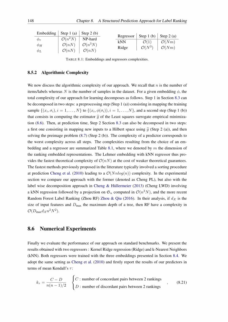
148 Chapter 8. A Structured Prediction Approach for Label Ranking
Embedding Step 1 (a) Step 2 (b)φτ O(n2N) NP-hardφH O(nN) O(n3N)
φL O(nN) O(nN)
Regressor Step 1 (b) Step 2 (a)kNN O(1) O(Nm)
Ridge O(N3) O(Nm)
TABLE 8.1: Embeddings and regressors complexities.
8.5.2 Algorithmic Complexity
We now discuss the algorithmic complexity of our approach. We recall that n is the number of
items/labels whereas N is the number of samples in the dataset. For a given embedding φ, the
total complexity of our approach for learning decomposes as follows. Step 1 in Section 8.3 can
be decomposed in two steps: a preprocessing step (Step 1 (a)) consisting in mapping the training
sample (xi, σi), i = 1, . . . , N to (xi, φ(σi)), i = 1, . . . , N, and a second step (Step 1 (b))
that consists in computing the estimator g of the Least squares surrogate empirical minimiza-
tion (8.6). Then, at prediction time, Step 2 Section 8.3 can also be decomposed in two steps:
a first one consisting in mapping new inputs to a Hilbert space using g (Step 2 (a)), and then
solving the preimage problem (8.7) (Step 2 (b)). The complexity of a predictor corresponds to
the worst complexity across all steps. The complexities resulting from the choice of an em-
bedding and a regressor are summarized Table 8.1, where we denoted by m the dimension of
the ranking embedded representations. The Lehmer embedding with kNN regressor thus pro-
vides the fastest theoretical complexity of O(nN) at the cost of weaker theoretical guarantees.
The fastest methods previously proposed in the litterature typically involved a sorting procedure
at prediction Cheng et al. (2010) leading to a O(Nnlog(n)) complexity. In the experimental
section we compare our approach with the former (denoted as Cheng PL), but also with the
label wise decomposition approach in Cheng & Hüllermeier (2013) (Cheng LWD) involving
a kNN regression followed by a projection on Sn computed in O(n3N), and the more recent
Random Forest Label Ranking (Zhou RF) Zhou & Qiu (2016). In their analysis, if dX is the
size of input features and Dmax the maximum depth of a tree, then RF have a complexity in
O(DmaxdXn2N2).
8.6 Numerical Experiments
Finally we evaluate the performance of our approach on standard benchmarks. We present the
results obtained with two regressors : Kernel Ridge regression (Ridge) and k-Nearest Neighbors
(kNN). Both regressors were trained with the three embeddings presented in Section 8.4. We
adopt the same setting as Cheng et al. (2010) and firstly report the results of our predictors in
terms of mean Kendall’s τ :
kτ =C −D
n(n− 1)/2
C : number of concordant pairs between 2 rankings
D : number of discordant pairs between 2 rankings, (8.21)
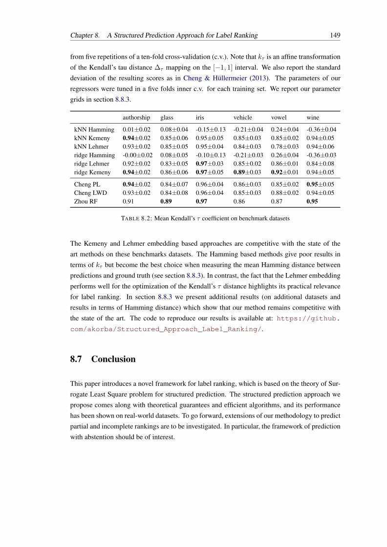
Chapter 8. A Structured Prediction Approach for Label Ranking 149
from five repetitions of a ten-fold cross-validation (c.v.). Note that kτ is an affine transformation
of the Kendall’s tau distance ∆τ mapping on the [−1, 1] interval. We also report the standard
deviation of the resulting scores as in Cheng & Hüllermeier (2013). The parameters of our
regressors were tuned in a five folds inner c.v. for each training set. We report our parameter
grids in section 8.8.3.
authorship glass iris vehicle vowel wine
kNN Hamming 0.01±0.02 0.08±0.04 -0.15±0.13 -0.21±0.04 0.24±0.04 -0.36±0.04kNN Kemeny 0.94±0.02 0.85±0.06 0.95±0.05 0.85±0.03 0.85±0.02 0.94±0.05kNN Lehmer 0.93±0.02 0.85±0.05 0.95±0.04 0.84±0.03 0.78±0.03 0.94±0.06ridge Hamming -0.00±0.02 0.08±0.05 -0.10±0.13 -0.21±0.03 0.26±0.04 -0.36±0.03ridge Lehmer 0.92±0.02 0.83±0.05 0.97±0.03 0.85±0.02 0.86±0.01 0.84±0.08ridge Kemeny 0.94±0.02 0.86±0.06 0.97±0.05 0.89±0.03 0.92±0.01 0.94±0.05
Cheng PL 0.94±0.02 0.84±0.07 0.96±0.04 0.86±0.03 0.85±0.02 0.95±0.05Cheng LWD 0.93±0.02 0.84±0.08 0.96±0.04 0.85±0.03 0.88±0.02 0.94±0.05Zhou RF 0.91 0.89 0.97 0.86 0.87 0.95
TABLE 8.2: Mean Kendall’s τ coefficient on benchmark datasets
The Kemeny and Lehmer embedding based approaches are competitive with the state of the
art methods on these benchmarks datasets. The Hamming based methods give poor results in
terms of kτ but become the best choice when measuring the mean Hamming distance between
predictions and ground truth (see section 8.8.3). In contrast, the fact that the Lehmer embedding
performs well for the optimization of the Kendall’s τ distance highlights its practical relevance
for label ranking. In section 8.8.3 we present additional results (on additional datasets and
results in terms of Hamming distance) which show that our method remains competitive with
the state of the art. The code to reproduce our results is available at: https://github.
com/akorba/Structured_Approach_Label_Ranking/.
8.7 Conclusion
This paper introduces a novel framework for label ranking, which is based on the theory of Sur-
rogate Least Square problem for structured prediction. The structured prediction approach we
propose comes along with theoretical guarantees and efficient algorithms, and its performance
has been shown on real-world datasets. To go forward, extensions of our methodology to predict
partial and incomplete rankings are to be investigated. In particular, the framework of prediction
with abstention should be of interest.

150 Chapter 8. A Structured Prediction Approach for Label Ranking
8.8 Proofs and Additional Experiments
8.8.1 Proof of Theorem 1
We borrow the notations of Ciliberto et al. (2016) and recall their main result Theorem 8.3. They
firstly exhibit the following assumption for a given loss ∆, see Assumption 1 therein:
Assumption 1. There exists a separable Hilbert space F with inner product 〈., .〉F , a continuous
embedding ψ : Y → F and a bounded linear operator V : F → F , such that:
∆(y, y′) = 〈ψ(y), V ψ(y′)〉F ∀y, y′ ∈ Y (8.22)
Theorem 8.3. Let ∆ : Y → Y satisfying Assumption 1 with Y a compact set. Then, for every
measurable g : X → F and d : F → Y such that ∀h ∈ F , d(h) = arg miny∈Y〈φ(y), h〉F , the
following holds:
(i) Fisher Consistency: E(d g∗) = E(s∗)
(ii) Comparison Inequality: E(d g)− E(s∗) ≤ 2c∆
√R(g)−R(g∗)
with c∆ = ‖V ‖maxy∈Y ‖φ(y)‖.
Notice that any discrete set Y is compact and φ : Y → F is continuous. We now prove the two
assertions of Theorem 8.1.
Proof of Assertion(i) in Theorem 8.1. Firstly, Y = Sn is finite. Then, for the Kemeny and
Hamming embeddings, ∆ satisfies Assumption 1 with V = −id (where id denotes the identity
operator) , and ψ = φK and ψ = φH respectively. Theorem 8.3 thus applies directly.
Proof of Assertion(ii) in Theorem 8.1. In the following proof, Y denotes Sn, φ denotes φL and
d = φ−1L dL with dL as defined in (8.17). Our goal is to control the excess risk E(s)− E(s∗).
E(s)− E(s∗) = E(d g)− E(s∗)
= E(d g)− E(d g∗)︸ ︷︷ ︸(A)
+ E(d g∗)− E(s∗)︸ ︷︷ ︸(B)
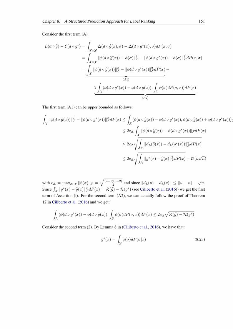
Chapter 8. A Structured Prediction Approach for Label Ranking 151
Consider the first term (A).
E(d g)− E(d g∗) =
∫X×Y
∆(d g(x), σ)−∆(d g∗(x), σ)dP (x, σ)
=
∫X×Y
‖φ(d g(x))− φ(σ)‖2F − ‖φ(d g∗(x))− φ(σ)‖2FdP (x, σ)
=
∫X‖φ(d g(x))‖2F − ‖φ(d g∗(x))‖2FdP (x)︸ ︷︷ ︸
(A1)
+
2
∫X〈φ(d g∗(x))− φ(d g(x)),
∫Yφ(σ)dP (σ, x)〉dP (x)︸ ︷︷ ︸
(A2)
The first term (A1) can be upper bounded as follows:∫X‖φ(d g(x))‖2F − ‖φ(d g∗(x))‖2FdP (x) ≤
∫X〈φ(d g(x))− φ(d g∗(x)), φ(d g(x)) + φ(d g∗(x))〉FdP (x)
≤ 2c∆
∫X‖φ(d g(x))− φ(d g∗(x))‖FdP (x)
≤ 2c∆
√∫X‖dL(g(x))− dL(g∗(x))‖2FdP (x)
≤ 2c∆
√∫X‖g∗(x)− g(x)‖2FdP (x) +O(n
√n)
with c∆ = maxσ∈Y ‖φ(σ)‖F =
√(n−1)(n−2)
2 and since ‖dL(u) − dL(v)‖ ≤ ‖u − v‖ +√n.
Since∫X ‖g
∗(x)− g(x)‖2FdP (x) = R(g)−R(g∗) (see Ciliberto et al. (2016)) we get the first
term of Assertion (i). For the second term (A2), we can actually follow the proof of Theorem
12 in Ciliberto et al. (2016) and we get:∫X〈φ(d g∗(x))− φ(d g(x)),
∫Yφ(σ)dP (σ, x)〉dP (x) ≤ 2c∆
√R(g)−R(g∗)
Consider the second term (2). By Lemma 8 in (Ciliberto et al., 2016), we have that:
g∗(x) =
∫Yφ(σ)dP (σ|x) (8.23)

152 Chapter 8. A Structured Prediction Approach for Label Ranking
and then:
E(d g∗)− E(s∗) =
∫X×Y
‖φ(d g∗(x))− φ(σ)‖2F − ‖φ(s∗(x))− φ(σ)‖2FdP (x, σ)
≤∫X×Y〈φ(d g(x))− φ(s∗(x)), φ(d g(x)) + φ(s∗(x))− 2φ(σ)〉FdP (x, σ)
≤ 4c∆
∫X‖φ(d g∗(x))− φ(s∗(x))‖FdP (x)
≤ 4c∆
∫X‖dL g∗(x))− dL φ(s∗(x))‖FdP (x)
≤ 4c∆
∫X‖g∗(x))− φ(s∗(x))‖FdP (x) +O(n
√n)
where we used that φ(s∗(x)) ∈ Cn so dL φ(s∗(x)) = φ(s∗(x)). Then we can plug (8.23) in
the right term:
E(d g∗)− E(s∗) ≤ 4c∆
∫X‖∫Yφ(σ)dP (σ|x)− φ(s∗(x))‖FdP (x) +O(n
√n)
≤ 4c∆
∫X×Y
‖φ(σ)− φ(s∗(x))‖FdP (x) +O(n√n)
≤ 4c∆E(s∗) +O(n√n)
Remark 8.4. As proved in Theorem 19 in (Ciliberto et al., 2016), since the space of rankings
Y is finite, ∆L necessarily satisfies Assumption 1 with some continuous embedding ψ. If the
approach we developped was relying on this ψ, we would have consistency for the minimizer g∗
of the Lehmer loss (8.16). However, the choice of φL is relevant because it yields a pre-image
problem with low computational complexity.
8.8.2 Lehmer Embedding for Partial Rankings
An example, borrowed from (Li et al., 2017) illustrating the extension of the Lehmer code for
partial rankings is the following:
e 1 2 3 4 5 6 7 8 9
σ 1 1 2 2 3 1 2 3 3
σ 1 2 4 5 7 3 6 8 9
cσ 0 0 0 0 0 3 1 0 0
IN 1 2 1 2 1 3 3 2 3
cσ 0 0 0 0 0 3 1 0 0
c′σ 0 1 0 1 0 5 3 1 2
where each row represents a step to encode a partial ranking.
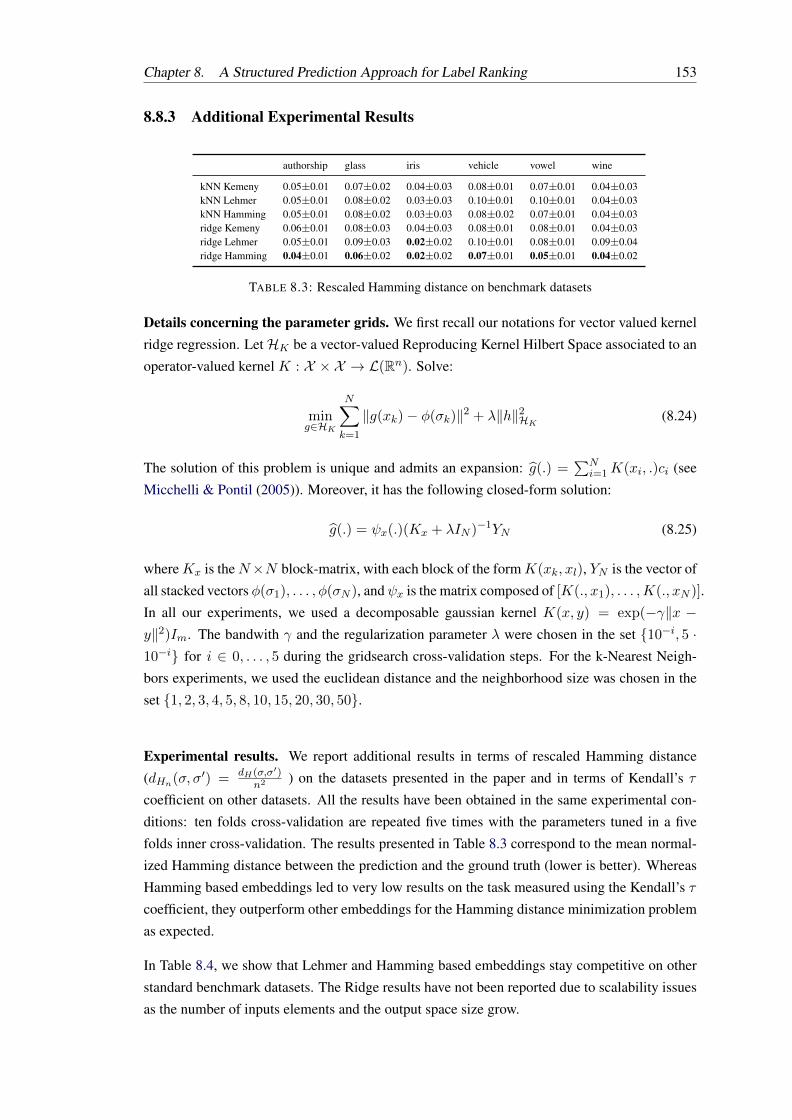
Chapter 8. A Structured Prediction Approach for Label Ranking 153
8.8.3 Additional Experimental Results
authorship glass iris vehicle vowel wine
kNN Kemeny 0.05±0.01 0.07±0.02 0.04±0.03 0.08±0.01 0.07±0.01 0.04±0.03kNN Lehmer 0.05±0.01 0.08±0.02 0.03±0.03 0.10±0.01 0.10±0.01 0.04±0.03kNN Hamming 0.05±0.01 0.08±0.02 0.03±0.03 0.08±0.02 0.07±0.01 0.04±0.03ridge Kemeny 0.06±0.01 0.08±0.03 0.04±0.03 0.08±0.01 0.08±0.01 0.04±0.03ridge Lehmer 0.05±0.01 0.09±0.03 0.02±0.02 0.10±0.01 0.08±0.01 0.09±0.04ridge Hamming 0.04±0.01 0.06±0.02 0.02±0.02 0.07±0.01 0.05±0.01 0.04±0.02
TABLE 8.3: Rescaled Hamming distance on benchmark datasets
Details concerning the parameter grids. We first recall our notations for vector valued kernel
ridge regression. LetHK be a vector-valued Reproducing Kernel Hilbert Space associated to an
operator-valued kernel K : X × X → L(Rn). Solve:
ming∈HK
N∑k=1
‖g(xk)− φ(σk)‖2 + λ‖h‖2HK (8.24)
The solution of this problem is unique and admits an expansion: g(.) =∑N
i=1K(xi, .)ci (see
Micchelli & Pontil (2005)). Moreover, it has the following closed-form solution:
g(.) = ψx(.)(Kx + λIN )−1YN (8.25)
whereKx is theN×N block-matrix, with each block of the formK(xk, xl), YN is the vector of
all stacked vectors φ(σ1), . . . , φ(σN ), andψx is the matrix composed of [K(., x1), . . . ,K(., xN )].
In all our experiments, we used a decomposable gaussian kernel K(x, y) = exp(−γ‖x −y‖2)Im. The bandwith γ and the regularization parameter λ were chosen in the set 10−i, 5 ·10−i for i ∈ 0, . . . , 5 during the gridsearch cross-validation steps. For the k-Nearest Neigh-
bors experiments, we used the euclidean distance and the neighborhood size was chosen in the
set 1, 2, 3, 4, 5, 8, 10, 15, 20, 30, 50.
Experimental results. We report additional results in terms of rescaled Hamming distance
(dHn(σ, σ′) = dH(σ,σ′)n2 ) on the datasets presented in the paper and in terms of Kendall’s τ
coefficient on other datasets. All the results have been obtained in the same experimental con-
ditions: ten folds cross-validation are repeated five times with the parameters tuned in a five
folds inner cross-validation. The results presented in Table 8.3 correspond to the mean normal-
ized Hamming distance between the prediction and the ground truth (lower is better). Whereas
Hamming based embeddings led to very low results on the task measured using the Kendall’s τ
coefficient, they outperform other embeddings for the Hamming distance minimization problem
as expected.
In Table 8.4, we show that Lehmer and Hamming based embeddings stay competitive on other
standard benchmark datasets. The Ridge results have not been reported due to scalability issues
as the number of inputs elements and the output space size grow.

154 Chapter 8. A Structured Prediction Approach for Label Ranking
bodyfat calhousing cpu-small pendigits segment wisconsin fried sushi
kNN Lehmer 0.23±0.01 0.22±0.01 0.40±0.01 0.94±0.00 0.95±0.01 0.49±0.00 0.85±0.02 0.17±0.01kNN Kemeny 0.23±0.06 0.33±0.01 0.51±0.00 0.94±0.00 0.95±0.01 0.49±0.04 0.89±0.00 0.31±0.01
Cheng PL 0.23 0.33 0.50 0.94 0.95 0.48 0.89 0.32Zhou RF 0.185 0.37 0.51 0.94 0.96 0.48 0.93 –
TABLE 8.4: Mean Kendall’s τ coefficient on additional datasets
On the sushi dataset Kamishima et al. (2010), we additionally tested our approach Ridge Ke-
meny which obtained the same results as Cheng PL (0.32 Kendall’s τ ).
CHAPTER 9Conclusion, Limitations & Perspectives
Ranking data arise in a diverse variety of machine learning applications but due to the absence of
any vectorial structure of the space of rankings, most of the classical methods from statistics and
multivariate analysis cannot be applied. The existing literature thus heavily relies on parametric
models, but in this thesis we propose a non-parametric analysis and methods for ranking data. In
particular, three different problems have been adressed: deriving guarantees and statistical guar-
antees about the NP-hard Kemeny aggregation problem and related approximation procedures,
reducing the dimension of a ranking distribution by performing partial ranking aggregation, and
predicting full rankings with features.
Concerning the ranking aggregation problem, we have firstly proposed a dataset-dependent mea-
sure, based on a specific embedding for rankings, enabling to upper bound the Kendall’s τ dis-
tance between the output of any ranking aggregation procedure, and a Kemeny consensus. This
measure relies on a mean embedding of the rankings in the dataset, for a well-chosen embed-
ding which preserves Kendall’s tau distance in a vectorial space. We thus provided a practical
procedure to evaluate the accuracy of any aggregegation procedure, on any dataset, with a rea-
sonable complexity in the number of items and samples. Then, we have casted the ranking
aggregation problem in a rigorous statistical framework, reformulating it in terms of ranking
distributions. The expected distance between a consensus candidate and realizations of a given
distribution appears to be written as a risk, and can be viewed as a dispersion measure. In this
framework, we demonstrated rates of convergence for the excess of risk of empirical solutions
of the Kemeny aggregation problem; in particular, we exhibited classical rates of convergence
for any distribution, and (exponential) fast rates when the distribution satisfies the transitivity
and low-noise conditions. In the latter case, the solution of the NP-hard Kemeny aggregation is
given by the Copeland ranking with high probability.
Then, we extended the statistical framework we proposed to two related machine learning tasks,
unsupervised and supervised respectively. The first one is a proposal for dimensionality reduc-
tion for ranking data. This is a classical machine learning task, which is especially relevant in
our context since modern machine-learning applications typically involve a very large number
of items to be ranked. Since popular methods (e.g. PCA) cannot be applied for the non-vectorial
data we consider, we propose a mass transportation approach to approximate any distribution
over rankings by a distribution involving a much smaller number of parameters, namely a bucket
distribution. This bucket distribution, parametrized by a partial ranking/bucket order, is sparse in
155

156 Chapter 9. Conclusion, Limitations & Perspectives
the sense that the relative order of two items belonging to two different buckets is deterministic.
This approximate distribution minimizes a distortion measure, that is closely related to the risk
of a consensus, extending thus the framework we proposed for ranking aggregation. Then, we
considered the supervised problem of ranking regression/label ranking, and exhibited that it is
also a direct extension of the ranking aggregation problem. Our first proposal is thus to compute
piecewise constant methods, partitioning the feature space into regions and locally computing
consensus to assign a final label (in this case, a ranking) to each region. We provided theoretical
results assessing that solutions of this problem can be well approximated by such local learning
approaches, and investigated in particular a k-nearest neighbor algorithm and a decision-tree
algorithm tailored for this data. Finally, this ranking regression problem can be also casted in
the structured prediction framework which benefits from an abundant literature. In this view, we
proposed a structured prediction approach for this problem, relying on embedding maps enjoy-
ing theoretical and computational advantages. One of these embeddings being at the core of our
first contribution for ranking aggregation, this final work closed this thesis.
Rankings are heterogenous objects, and the literature generally focus on studying of their classes:
full rankings, partial rankings or incomplete rankings. The main limitation of this thesis is that
we derive our results for the case of full rankings, i.e. on the space of permutations named the
symmetric group. In future work, one could investigate the case of distributions over incomplete
and partial rankings. Since we make an extensive use of the Kendall’s tau distance, decompos-
ing rankings over pairs, our work could be extended to this setting by introducing a distribution
over the subsets of items to be observed, such as in Rajkumar & Agarwal (2014); Sibony et al.
(2014).

CHAPTER 10Résumé en français
Les données de classement apparaissent naturellement dans une grande variété de situations,
en particulier lorsque les données proviennent d’activités humaines: bulletins de vote aux
élections, enquêtes d’opinion, résultats de compétitions, comportements d’achat de clients ou
préférences d’utilisateurs. Le traitement des données de préférences, en particulier pour en
effectuer l’agrégation, fait référence à une longue série de travaux sur la théorie du choix so-
cial initiés par Condorcet au 18e siècle, et la modélisation des distributions sur les données de
préférences a commencé à être étudiée en 1951 par Mallows. Mais ordonner des objets est aussi
une tâche qui se pose souvent dans les applications modernes de traitement des données. Par
exemple, les moteurs de recherche visent à présenter à un utilisateur qui a saisi une certaine
requête, la liste des résultats classés du plus pertinent au moins pertinent. De même, les sys-
tèmes de recommandation (pour le e-commerce, plateformes de contenus cinéma et musique...)
visent à présenter des objets susceptibles d’intéresser un utilisateur, dans l’ordre qui correspond
le mieux à ses préférences. Cependant, les données de classement sont beaucoup moins prises
en compte dans la littérature sur les statistiques et l’apprentissage machine que les données à
valeur réelle, principalement parce que l’espace des classements n’est pas doté d’une structure
vectorielle et que les statistiques classiques et les méthodes d’apprentissage machine ne peuvent
être appliquées de manière directe. En effet, même la notion de moyenne ou de médiane pour les
données de classement, à savoir l’ agrégation de classement ou classement par consensus, pose
de grands défis mathématiques et computationnels. Par conséquent, la plupart des contributions
dans la littérature s’appuient sur des modèles paramétriques.
Dans cette thèse, nous étudions la difficulté des problèmes impliquant des données de classement
et introduisons de nouvelles méthodes statistiques non paramétriques adaptées à ces données.
En particulier, nous formulons le problème de l’agrégation de classements dans un cadre statis-
tique rigoureux et en tirons des résultats théoriques concernant le comportement statistique des
solutions empiriques et la tractabilité du problème. Ce cadre est en fait une pierre angulaire
de cette thèse puisqu’il peut être étendu à deux problèmes étroitement liés, respectivement su-
pervisé et non supervisé : la réduction de dimension et la régression de classement. En effet,
bien que les méthodes classiques de réduction de dimension ne puissent être appliquées dans ce
contexte, puisque souvent basées sur de l’algèbre et une structure vectorielle, nous proposons
une approche de transport de masse pour l’appliquer à des données de classement. Ensuite, nous
explorons et construisons des règles consistantes pour la régression de classements, d’abord en
157

158 Chapter 10. Résumé en français
soulignant le fait que ce problème supervisé est une extension de l’agrégation de classements.
Dans ce chapitre, nous rappelons les principaux défis statistiques liés au traitement des données
de classements et soulignons les contributions de cette thèse.
10.1 Préliminaires sur les Données de Classements
Nous commençons par présenter les notations et les objets utilisés tout le long de ce manuscrit.
Considérons un ensemble d’éléments indexés par 1, . . . , n, que nous désignerons par JnK.
Un classement est une liste ordonnée d’éléments de JnK. Les classements sont des objets
hétérogènes: ils peuvent être complets (c’est-à-dire qu’ils impliquent tous les éléments) ou in-
complets; dans les deux cas, ils peuvent être sans liens entre les éléments ou avec liens, où ici
un lien désigne le fait que deux éléments soient incomparables. Un classement complet est un
ordre total: c’est-à-dire complet, et sans liens entre les éléments. Il peut être vu comme une
permutation, c’est-à-dire une bijection σ : JnK → JnK, faisant correspondre chaque élément i à
son rang σ(i). Le rang de l’élément i est donc σ(i) et l’élément classé à la position j est σ−1(j).
Nous dirons que i est préféré à j (indiqué par i ≺ j) selon σ si et seulement si i a un classement
inférieur à j : σ(i) < σ(j). L’ensemble de toutes les permutations sur n, doté de l’opération
de composition, est appelé le groupe symétrique et noté Sn. L’analyse des données de classe-
ments complets repose donc sur ce groupe. D’autres types de classements sont particulièrement
présents dans la littérature, notamment les classements partiels et incomplets. Un classement
partiel est un classement complet (c’est-à-dire impliquant tous les éléments) avec des liens, et
est aussi parfois désigné dans la littérature comme un ordre partiel ou un classements en paquets.
Il comprend notamment le cas des classements top-k, c’est-à-dire des classements partiels di-
visant les élements de JnK en deux groupes: le premier comprenant les k ≤ n élements les plus
pertinents (ou préférés) et le second comprenant tous les éléments restants. Ces classements
top-k reçoivent beaucoup d’attention dans la littérature car ils sont particulièrement pertinents
pour les applications modernes, comme les moteurs de recherche ou les systèmes de recom-
mandation où le nombre d’éléments à classer est très important et où les utilisateurs accordent
plus d’attention aux éléments classés en premier. Un autre type de classements, également très
pertinent dans de tels contextes à grande échelle, est le cas du classement incomplet ; c’est-à-
dire un ordres strict ne concernant qu’un petit sous-ensemble d’éléments. Un cas particulier
de classements incomplets est celui des comparaisons par paires, c’est-à-dire des classements
ne comportant que deux élements. Comme tout classement, de tout type, peut être décomposé
en comparaisons par paires, l’étude de ces classements est aussi largement répandue dans la
littérature.
L’hétérogénéité des données de classement rend difficile l’établissement d’un cadre général, et
les contributions de la littérature portent habituellement sur une catégorie particulière de classe-
ments. Le lecteur peut se référer au chapitre 2 pour un historique général sur ce sujet. Dans cette
thèse, nous nous concentrerons sur le cas des classements complets, c’est-à-dire impliquant tous
les éléments de JnK, et sans liens. Cependant, comme nous le soulignerons dans la thèse, notre

Chapter 10. Résumé en français 159
analyse peut naturellement s’étendre à l’analyse des comparaisons par paires grâce à l’utilisation
extensive que nous faisons d’une distance spécifique, à savoir la distance du τ de Kendall.
10.2 L’agrégation de Classements
L’agrégation de classements a été le premier problème à être considéré sur les données de classe-
ment et a certainement été le plus étudié dans la littérature. Considéré à l’origine en choix social
pour les élections, le problème de l’agrégation de classements apparaît aujourd’hui dans de nom-
breuses applications modernes impliquant l’apprentissage automatique (par exemple, les méta-
moteurs de recherche, la recherche d’informations, la biologie). Il peut être considéré comme
un problème non supervisé, puisque l’objectif est de résumer un ensemble de données ou une
distribution sur les classements, comme on calculerait une moyenne ou une médiane pour des
données à valeur réelle. Un aperçu des défis mathématiques et des méthodes de l’état de l’art
est donné chapitre 3. Nous donnons d’abord la formulation du problème, puis nous présentons
nos contributions.
10.2.1 Définition et Contexte
Supposons maintenant qu’en plus de l’ensemble des éléments n, nous disposons d’une popula-
tion de N agents. Supposons que chaque agent t ∈ 1, . . . , N exprime ses préférences sous
forme de classement complet sur n, ce qui, comme dit précédemment, peut être vu comme une
permutation σt ∈ Sn. La collecte des préférences des agents par rapport à l’ensemble des élé-
ments de JnK résulte alors en un ensemble de données de permutations DN = (σ1, . . . , σN ) ∈SNn , parfois appelé le profil dans la littérature du choix social. Le problème d’agrégation de
classements consiste alors à trouver une permutation σ∗ ∈ Sn, appelé consensus, qui résume le
mieux l’ensemble de données. Cette tâche a été introduite dans l’étude des systèmes électoraux
dans la théorie du choix social, et toute procédure de mise en correspondance d’un ensemble de
données avec un consensus s’appelle donc une règle de vote. Fait intéressant, Arrow (1951) a
démontré son célèbre théorème d’impossibilité qui affirme qu’aucune règle de vote ne peut sat-
isfaire un ensemble prédéfini d’axiomes, chacun reflétant l’équité de l’élection (voir Chapitre 3).
Il n’existe donc pas de procédure canonique d’agrégation de classements, et chacune a ses avan-
tages et ses inconvénients.
Ce problème a donc été largement étudié et de nombreuses approches ont été développées,
en particulier dans deux contextes. La première possibilité est de considérer que l’ensemble
de données est constitué de versions bruitées d’un vrai classement (par exemple, la réalisation
d’une distribution paramétrique centrée autour d’un vrai classement), et l’objectif alors est de
reconstruire le vrai classement grâce aux échantillons (par exemple, avec une estimation du
maximum de vraisemblance). La deuxième possibilité est de formaliser ce problème comme un
problème d’optimisation discret sur l’ensemble des classements, et de rechercher le classement

160 Chapter 10. Résumé en français
qui est le plus proche (au sens d’une certaine distance) des classements observés dans l’ensemble
de données, sans faire aucune hypothèse sur les données. Cette dernière approche aborde le
problème de manière rigoureuse, mais peut entraîner des coûts de calcul élevés en pratique. En
particulier, l’agrégation de Kemeny (Kemeny (1959)) vise à résoudre :
minσ∈Sn
CN (σ), (10.1)
où CN (σ) =∑N
t=1 d(σ, σt) et d est la distance du τ de Kendall définie pour σ, σ′ ∈ Sn comme
le nombre de leurs désaccords par paires :
dτ (σ, σ′) =∑
1≤i<j≤nI(σ(j)− σ(i))(σ′(j)− σ′(i) < 0. (10.2)
Pour tout σ ∈ Sn, nous ferons référence à la quantité CN (σ) comme son coût. Une solu-
tion de (10.1) existe toujours, puisque la cardinalité de Sn est finie (même si explosant avec
n, puisque #Sn = n!), mais peut être multimodale. Nous noterons KN l’ensemble des solu-
tions de (10.1), à savoir l’ensemble des consensus de Kemeny. Cette méthode d’agrégation est
attrayante parce qu’elle a à la fois une justification en choix social (c’est l’unique règle qui satis-
fait certaines propriétés désirables) et une justification statistique (elle correspond à l’estimateur
du maximum de vraisemblance sous le modèle de Mallows), voir Chapitre 2 et 3 pour plus de
détails. Cependant, l’agrégation de Kemeny est connue pour être NP-difficile dans le pire des
cas (voir Dwork et al. (2001)), et ne peut être résolue efficacement par une procédure générale.
Par conséquent, de nombreuses autres méthodes ont été utilisées dans la littérature, comme les
méthodes de vote pondérés ou les méthodes spectrales (voir Chapitre 3). Les premières sont
beaucoup plus efficaces en pratique, mais n’ont que peu ou pas de support théorique.
De nombreuses contributions de la littérature se sont concentrées sur une approche particulière
pour appréhender une partie de la complexité de l’agrégation de Kemeny, et peuvent être divisées
en trois grandes catégories.
• Garanties générales pour les procédures d’approximation. Ces résultats fournissent
une borne sur le coût d’une règle de vote, valable pour tout ensemble de données (voir
Diaconis & Graham (1977); Coppersmith et al. (2006); Van Zuylen & Williamson (2007);
Ailon et al. (2008); Freund & Williamson (2015)).
• Borne sur le coût d’approximation calculée à partir de l’ensemble de données. Ces
résultats fournissent une borne, soit sur le coût d’un consensus, soit sur le coût du résul-
tat d’une règle de vote spécifique, qui dépend d’une quantité calculée à partir du jeu de
données (voir Davenport & Kalagnanam (2004); Conitzer et al. (2006); Sibony (2014)).
• Conditions pour que l’agrégation exacte de Kemeny devienne tractable. Ces résultats
assurent la tractabilité de l’agrégation exacte de Kemeny si l’ensemble de données satis-
fait certaines conditions ou si une certaine quantité est connue à partir de l’ensemble de
données (voir Betzler et al. (2008, 2009); Cornaz et al. (2013); Brandt et al. (2015)).
Chapter 10. Résumé en français 161
Nos contributions sur le problème de l’agrégation de classements dans cette thèse sont résumées
dans les deux sous-sections suivantes. Nous proposons tout d’abord une quantité dépendant de
l’ensemble de données, qui permet de borner supèrieurement la distance du τ de Kendall en-
tre tout candidat pour le problème d’agrégation de classement (généralement le résultat d’une
procédure efficace), et un consensus de Kemeny (intractable). Ensuite, nous formalisons le
problème dans un cadre statistique, en supposant que l’ensemble de données est constitué de
réalisations d’une variable aléatoire suivant une distribution P sur l’espace des classements
complets/permutations Sn. Bien que cette approche puisse sembler naturelle pour un statisti-
cien, la plupart des contributions de la littérature en choix social ou en informatique n’analysent
pas ce problème à travers la distribution des données; cependant, l’analyse à travers les pro-
priétés de distribution est largement répandue dans la littérature concernant les comparaisons
par paires, voir chapitre 2 et 3. Dans cette optique, nous dérivons des résultats statistiques et
donnons des conditions sur P pour que l’agrégation de Kemeny soit tractable.
10.2.2 Une Méthode Générale pour Borner la Distance au Consensus de Kemeny
Notre première question était la suivante. Soit σ ∈ Sn un candidat pour le consensus, générale-
ment produit par une procédure d’agrégation efficace sur DN = (σ1, . . . , σN ). Peut-on utiliser
une quantité tractable pour donner une borne supérieure à la distance du τ de Kendall dτ (σ, σ∗)
entre σ et un consensus de Kemeny σ∗ ∈ KN ? La réponse à ce problème est positive, comme
nous allons le développer.
Notre analyse est géométrique et repose sur la fonction de réprésentation suivante, nommée
représentation de Kemeny : φ : Sn → R(n2), σ 7→ [sign(σ(j)− σ(i)]1≤i<j<j≤n, où sign(x) =
1 si x ≥ 0 et −1 sinon. Elle a les propriétés suivantes. Premièrement, pour tous σ, σ′ ∈Sn, ‖φ(σ) − φ(σ′)‖2 = 4dτ (σ, σ′), c’est-à-dire, le carré de la distance euclidienne entre les
représentations de deux permutations correspond à leur distance du τ de leur Kendall à une
constante multiplicative près, prouvant en même temps que la fonction de représentation est
injective. Ensuite, l’agrégation de Kemeny (10.1) est équivalente au problème de minimisation
suivant:
minσ∈Sn
C ′N (σ),
où C ′N (σ) = ‖φ(σ)− φ(DN )‖2 et
φ (DN ) :=1
N
N∑t=1
φ (σt) . (10.3)
est appelé la représentation moyenne de l’ensemble de données. Le lecteur peut se référer au
chapitre 4 pour des illustrations. Une telle quantité contient donc une information riche sur la
localisation d’un consensus Kemeny, qui sera la clef pour en déduire notre résultat.

162 Chapter 10. Résumé en français
Nous définissons premièrement pour toute permutation σ ∈ Sn, son angle θN (σ) entre φ(σ) et
φ(DN ) par:
cos(θN (σ)) =〈φ(σ), φ(DN )〉‖φ(σ)‖‖φ(DN )‖
, (10.4)
avec 0 ≤ θN (σ) ≤ π par convention. Notre résultat principal, basé sur une analyse géométrique
de l’agrégation de Kemeny dans l’espace euclidien R(n2), est le suivant.
Theorem 10.1. Pour tout k ∈ 0, . . . ,(n2
)− 1, nous avons l’implication suivante:
cos(θN (σ)) >
√1− k + 1(
n2
) ⇒ maxσ∗∈KN
dτ (σ, σ∗) ≤ k.
Plus précisément, la meilleure borne est donnée par le plus petit k ∈ 0, . . . ,(n2
)− 1 tel que
cos(θN (σ)) >√
1− (k + 1)/(n2
).En notant par kmin(σ;DN ) cet entier, il est facile de montrer
que:
kmin(σ;DN ) =
⌊(n2
)sin2(θN (σ))
⌋if 0 ≤ θN (σ) ≤ π
2(n2
)if π2 ≤ θN (σ) ≤ π.
(10.5)
où bxc est la partie entière du réel x. Ainsi, étant donné un ensemble de donnéesDN et un candi-
dat σ pour l’agrégation, après avoir calculé la représentation moyenne de l’ensemble de données
et kmin(σ;DN ), on obtient une borne sur la distance entre σ et un consensus de Kemeny. La
finesse de la borne est mise en évidence dans les expériences Chapitre 4. Notre méthode a une
complexité d’ordre O(Nn2), où N est le nombre de classements (taille de l’ensemble de don-
nées) et n est le nombre d’objets à classer, et est très générale puisqu’elle peut être appliquée à
tout jeu de données et tout candidat pour le consensus.
10.2.3 Un Cadre Statistique pour l’Agrégation de Classements
Notre deuxième question était la suivante. Supposons que l’ensemble de des classements à
agréger DN est composé de N ≥ 1 copies i.i.d. Σ1, ; . . . , ; ΣN d’une variable aléatoire
générique Σ, définie sur un espace de probabilité (Ω, ;F , ;P) et suivant une distribution de
probabilité inconnue P sur Sn (i.e. P (σ) = PΣ = σ pour tout σ ∈ Sn). Pouvons-nous
calculer la vitesse de convergence pour l’excès de risque d’un consensus empirique (c.-à-d. basé
sur DN ) par rapport à un vrai consensus (par rapport à la distribution sous-jacente) ? Ensuite,
y a-t-il des conditions sur P pour que l’agrégation de Kemeny devienne tractable ? Encore une
fois, la réponse est positive, comme nous le détaillons ci-dessous.
Nous définissons d’abord une (vraie) médiane de la distribution P par rapport d (n’importe
quelle métrique sur Sn) comme une solution du problème de minimisation :
minσ∈Sn
LP (σ), (10.6)

Chapter 10. Résumé en français 163
où LP (σ) = EΣ∼P [d(Σ, σ)] correspond à la distance en espérance entre toute permutation σ
et Σ et sera appelé risque du candidat médian σ. Toute solution de (10.6), dénotée σ∗, sera
appelée médiane Kemeny tout au long de cette thèse, et L∗P = LP (σ∗) son risque, aussi appelé
dispersion de P .
Alors que le problème (10.6) est NP-difficile en général, dans le cas de la distance du τ de
Kendall, les solutions exactes peuvent être explicitées lorsque les probabilités par paires pi,j =
PΣ(i) < Σ(i) < Σ(j), 1 ≤ i 6= j ≤ n (donc pi,j + pj,i = 1), vérifient la propriété suivante,
appelée transitivité stochastique.
Definition 10.2. Soit P une distribution de probabilité sur Sn.
(i) La distribution P est dite (faiblement) transitive stochastiquement ssi
∀(i, j, k) ∈ JnK3 : pi,j ≥ 1/2 and pj,k ≥ 1/2 ⇒ pi,k ≥ 1/2.
Si, en plus, pi,j 6= 1/2 pour tous les i < j, on dit que P est strictement transitive stochas-
tiquement.
(ii) la distribution P est dite fortement transitive stochastiquement ssi
∀(i, j, k) ∈ JnK3 : pi,j ≥ 1/2 and pj,k ≥ 1/2 ⇒ pi,k ≥ max(pi,j , pj,k).
ce qui est équivalent à la condition suivante (voir Davidson & Marschak (1959)):
∀(i, j) ∈ JnK2 : pi,j ≥ 1/2 ⇒ pi,k ≥ pj,k for all k ∈ JnK \ i, j.
Ces conditions ont d’abord été introduites dans la littérature en psychologie (Fishburn (1973);
Davidson & Marschak (1959)) et ont été utilisées récemment pour l’estimation des probabil-
ités par paires et le classement à partir de comparaisons par paires (Shah et al. (2017); Shah
& Wainwright (2017); Rajkumar & Agarwal (2014)). Notre résultat principal sur l’optimalité
pour (10.6), qui peut être considéré comme un résultat de tri topologique classique sur le graphe
des comparaisons par paires (voir Figure 2.1. Chapitre 2), est le suivant.
Proposition 10.3. Supposons que P est strictement (et faiblement) transitive stochastiquement.
Alors, la médiane de Kemeny σ∗ est unique et donnée par la méthode de Copeland, c.-à-d. la
règle suivante:
σ∗(i) = 1 +∑k 6=i
Ipi,k <1
2 for any i in JnK (10.7)
Un autre résultat intéressant est que lorsque la transitivité stochastique est forte, la médiane de
Kemeny est également donnée par la méthode de Borda, voir Remarque 5.6 au chapitre 5.
Cependant, la quantitéLP (.) est inconnue en pratique, tout comme la distribution P ou ses prob-
abilités marginales pi,j . Suivant le paradigme de la minimisation du risque empirique (MRE)

164 Chapter 10. Résumé en français
(voir Vapnik, 2000), nous nous sommes donc intéressés à l’évaluation de la performance des
solutions σN , appelées médiane de Kemeny empiriques, du problème
minσ∈Sn
LN (σ), (10.8)
où LN (σ) = 1/N∑N
t=1 d(Σt, σ). Remarquez que LN = LPN
où PN = 1/N∑N
t=1 δΣt est
la distribution empirique. Précisément, nous établissons des vitesses de l’ordre de OP(1/√N)
pour l’excès de risque LP (σN ) − L∗P en probabilité/en espérance et prouvons qu’elles sont
minimax, lorsque d est la distance τ de Kendall. Nous établissons également des vitesses rapi-
des lorsque la distribution P est strictement transitive stochastiquement et vérifie une certaine
condition de bruit faible NA(h), définie pour h > 0 par :
mini<j|pi,j − 1/2| ≥ h. (10.9)
Cette condition peut être considérée comme analogue à celle introduite dans Koltchinskii &
Beznosova (2005) pour la classification binaire, et a été utilisée dans Shah et al. (2017) pour
prouver des vitesses rapides pour l’estimation de la matrice des probabilités par paires. Dans
ces conditions (transitivité (10.2) et bruit faible (10.9)), la distribution empirique PN est aussi
strictement transitive stochastiquement avec très grande probabilité, et l’excès de risque d’une
médiane empirique de Kemeny décroît à vitesse exponentielle. Dans ce cas, la solution op-
timale σ∗N de (10.8) est aussi une solution de (10.6) et peut être rendue explicite et très sim-
plement calculée avec Eq. (10.7), à partir des probabilités empiriques par paires empiriques
pi,j = 1N
∑Nt=1 IΣt(i) < Σt(j). Ce dernier résultat sera de la plus haute importance pour les
applications pratiques décrites dans la section suivante.
10.3 Au-delà de l’Agrégation de Classements : la Réduction de Di-mension et la Régression de Classements
Les résultats que nous avons obtenus sur l’agrégation de classements statistique nous ont permis
de considérer deux problèmes étroitement liés. Le premier est un autre problème non supervisé,
à savoir la réduction de dimension; nous proposons de représenter de manière parcimonieuse
toute distribution P sur les classements complets par un ordre partiel C et une distribution ap-
proximative PC relative à cet ordre partiel. Le second est un problème supervisé étroitement lié
à l’agrégation de classements, à savoir la régression de classements.
10.3.1 Réduction de Dimension pour les Données de Classements : une Approchede Transport de Masse
En raison de l’absence d’une structure d’espace vectoriel sur Sn, il n’est pas possible d’appliquer
de manière directe les techniques traditionnelles de réduction de dimension pour les données
Chapter 10. Résumé en français 165
vectorielles (ex: l’ACP), et la synthèse des données de classements est difficile. Nous avons
donc proposé un cadre de transport de masse pour la réduction de dimension adapté aux don-
nées de classements présentant un type spécifique de parcimonie, prolongeant en quelque sorte
le cadre statistique que nous avons proposé pour l’agrégation de classement. Nous proposons
une manière de décrire une distribution P sur Sn, initialement caractérisée par n!−1 paramètres,
en trouvant une distribution beaucoup plus simple proche de P au sens de la distance de Wasser-
stein introduite ci-dessous.
Definition 10.4. Soit d : S2n → R+ une métrique sur Sn et q ≥ 1. La distance de Wasserstein
d’ordre q avec d comme fonction de coût entre deux distributions de probabilité P et P ′ sur Sn
est donnée par :
Wd,q
(P, P ′
)= inf
Σ∼P, Σ′∼P ′E[dq(Σ,Σ′)
], (10.10)
où l’infimum est pris sur tous les couplages possibles (Σ,Σ′) de (P, P ′).
Rappelons qu’un couplage de deux distributions de probabilités Q et Q′ est une paire (U,U ′)
de variables aléatoires définies sur le même espace de probabilité de sorte que les distributions
marginales de U et U ′ sont Q et Q′.
Soit K ≤ n et C = (C1, ; . . . , ; CK) un ordre partiel ou ordre par paquets sur JnK avec K
paquets, ce qui signifie que la collection Ck1≤k≤K est une partition de JnK (c.-à-d. les Ck sont
chacun non vides, disjoints par paires et leur union est JnK), dont les éléments (appelés paquets)
sont classés C1 ≺ . . . ≺ CK . Pour tout ordre par paquets C = (C1, . . . , CK), son nombre de
paquets K est appelé sa taille, tandis que le vecteur λ = (#C1, . . . ,#CK), c.-à-d. la séquence
des tailles des paquets de C (vérifiant∑K
k=1 #Ck = n), est appelée sa forme. Remarquez
que, lorsque K << n, une distribution P ′ peut naturellement être dite parcimonieuse lorsque
l’ordre relatif de deux éléments appartenant à deux paquets différents est déterministe : pour
tout 1 ≤ k < l ≤ K et tout (i, j) ∈ JKK2, (i, j) ∈ Ck×Cl =⇒ p′i,j = PΣ′∼P ′ [Σ′(i) < Σ′(j)] =
0. Tout au long de cette thèse, une telle distribution de probabilité est appelée distribution
en paquets associée à C. Puisque la variabilité d’une distribution en paquets correspond à la
variabilité de ses probabilités marginales par paires dans chaque paquet, l’ensemble PC de toutes
les distributions par paquets associées à C est de dimension dC =∏
1≤k≤K #Ck!− 1 ≤ n!− 1.
Un meilleur résumé en PC d’une distribution P sur Sn, au sens de la distance de Wasserstein
(10.10), est alors donné par toute solution P ∗C du problème de minimisation:
minP ′∈PC
Wdτ ,1(P, P ′). (10.11)
Pour tout ordre par paquets C, la quantité ΛP (C) = minP ′∈PCWdτ ,1(P, P ′) mesure la précision
de l’approximation et sera appelée distorsion. Dans le cas de la distance du τ de Kendall, cette
distorsion peut être écrite sous forme close comme ΛP (C) =∑
i≺Cj pj,i (voir Chapitre 6 pour
d’autres distances).
Nous désignons par CK l’ensemble des ordres par paquets C de JnK avec K paquets. Si P
peut être approchée avec précision par une distribution de probabilité associée à un ordre par

166 Chapter 10. Résumé en français
paquets de taille K, une approche naturelle pour la réduction de dimension consiste à trouver
une solution C∗(K) de
minC∈CK
ΛP (C), (10.12)
ainsi qu’une solution P ∗C∗(K) de (10.11) pour C = C∗(K), et un couplage (Σ,ΣC∗(K)) tel que
E[dτ (Σ,ΣC∗(K))] = ΛP (C∗(K)).
Cette approche est étroitement liée au problème d’agrégation de classements que nous avons
étudié précédemment, voir Chapitre 6 pour une explication plus approfondie. En effet, remar-
quez que ∪C∈CnPC est l’ensemble des distributions Dirac δσ, σ ∈ Sn. Ainsi, dans le cas
K = n, la réduction de dimension telle que formulée ci-dessus se résume à résoudre l’agrégation
de Kemeny : P ∗C∗(n) = δσ∗ et ΣC∗(n) = σ∗ étant les solutions du second, pour toute médiane de
Kemeny σ∗ de P . En revanche, l’autre cas extrême K = 1 correspond à aucune réduction de
dimension: ΣC∗(1) = Σ. Ensuite, nous avons le résultat remarquable suivant énoncé ci-dessous
qui montre que, dans certaines conditions, la dispersion de P peut être décomposée comme la
somme de la dispersion (réduite) de la distribution simplifiée PC et de la distorsion minimale
ΛP (C).
Corollary 10.5. Supposons que P soit transitive stochastiquement. Une ordre par paquets
C = (C1, . . . , CK) s’accorde avec un consensus Kemeny si nous avons: ∀1 ≤ k < l ≤ K,
∀(i, j) ∈ Ck × Cl, pj,i ≤ 1/2. Ensuite, pour tout ordre par paquets C qui s’accorde avec le
consensus de Kemeny, nous avons:
L∗P = L∗PC + ΛP (C). (10.13)
Nous obtenons plusieurs résultats dans ce cadre.
Fixons le nombre de paquets K ∈ 1, . . . , n, ainsi que la forme de l’ordre par paquets λ =
(λ1, . . . , λK) ∈ 1, . . . , nK . Soit CK,λ l’ensemble des ordres par paquets C = (C1, . . . , CK)
de forme λ (c.-à-d. tel que λ = (#C1, . . . ,#CK)). Nous avons le résultat suivant.
Theorem 10.6. Supposons que P est fortement/strictement transitive stochastiquement. Alors,
le minimiseur de la distorsion ΛP (C) sur CK,λ est unique et donné par C∗(K,λ) =
(C∗(K,λ)1 , . . . , C∗(K,λ)
K ), où
C∗(K,λ)k =
i ∈ JnK :∑l<k
λl < σ∗P (i) ≤∑l≤k
λl
for k ∈ 1, . . . , K. (10.14)
En d’autres termes, C∗(K,λ) est l’unique ordre par paquets de CK,λ qui s’accorde avec
σ∗P , et correspond donc à l’une des(n−1K−1
)segmentations possibles de la liste ordonnée
(σ∗−1P (1), . . . , σ∗−1
P (n)) en K segments.
Chapter 10. Résumé en français 167
Enfin, nous avons obtenu des résultats décrivant la capacité de généralisation des solutions du
problème de minimisation
minC∈CK,λ
ΛN (C) =∑i≺Cj
pj,i = ΛPN
(C). (10.15)
Précisément, nous avons calculé des bornes sur l’excès de risque des solutions de (10.15)
d’ordre OP(1/√N), et OP(1/N) lorsque P satisfait additionnellement la condition de bruit
faible (10.9).
Cependant, une question cruciale pour la réduction de dimension est de déterminer la dimension
de la représentation approximative de la distribution d’intérêt; dans notre cas, un nombre de
paquets K et une forme λ. Supposons qu’une séquence (Km, λm)1≤m≤M de formes soit
donnée (observez que M ≤∑n
K=1
(n−1K−1
)= 2n−1). Théoriquement, nous avons proposé une
méthode de régularisation de la complexité pour sélectionner la forme de l’ordre par paquets λ,
qui utilise des complexités de Rademacher (pénalités basées sur l’ensemble de données). Nous
démontrons la pertinence de notre approche par des expériences sur des ensembles de données
simulées et réelles, qui mettent en évidence que l’on peut maintenir une faible distorsion tout en
réduisant drastiquement la dimension de la distribution.
10.3.2 Régression Médiane de Classements: Apprendre à Classer à travers desConsensus Locaux
Au-delà de l’agrégation de classements en un classement complet ou partiel, nous nous sommes
intéressés au problème d’apprentissage suivant. Nous supposons maintenant que, en plus du
classement Σ, on observe un vecteur aléatoire X , défini sur le même espace de probabilité
(Ω,F ,P), à valeurs dans un espace objet X (possiblement de grande dimension, généralement
un sous ensemble de Rd avec d ≥ 1) et contenant peut-être quelques informations utiles pour
prédire Σ. Étant donné un tel ensemble de données ((X1,Σ1), . . . , (XN ,ΣN )), alors que les
méthodes d’agrégation de classements appliquées aux Σi’s ignoreraient les informations portées
par les Xi pour la prédiction, notre objectif est d’apprendre une règle prédictive s qui met
en correspondance tout point X de l’espace d’entrée avec une permutation s(X) de Sn. Ce
problème, appelé régression de classements, peut être considéré comme une extension de la
classification multiclasse et multilabel (voir Dekel et al. (2004); Hüllermeier et al. (2008); Zhou
et al. (2014)).
Nous avons d’abord montré que ce problème peut être considéré comme une extension naturelle
du problème d’agrégation de classements. La distribution jointe de la v.a. (Σ, X) est décrite
par (µ, PX), où µ désigne la distribution marginale de X et PX est la distribution de probabilité
conditionnelle de Σ sachant X : ∀σ ∈ Sn, PX(σ) = PΣ = σ | X presque sûrement.
La distribution marginale de Σ est alors P (σ) =∫X Px(σ)µ(x). Soit d une métrique sur Sn
(par ex. la distance du τ de Kendall), en supposant que la quantité d(Σ, σ) reflète le coût de
prédiction de la valeur σ pour le classement Σ, on peut formuler le problème qui consiste à

168 Chapter 10. Résumé en français
apprendre une règle s : X → Sn avec erreur de prédiction minimale:
R(s) = EX∼µ[EΣ∼PX [d (s(X),Σ)]] = EX∼µ [LPX (s(X))] . (10.16)
où LP (σ) est le risque d’agrégation de classements que nous avons défini Section 10.2.3 pour
tout P et σ ∈ Sn. Nous désignons par S la collection de toutes les règles mesurables s : X →Sn, ses éléments seront appelés règles prédictives de classements. Le minimum de la quantité
à l’intérieur de l’espérance est donc atteint dès que s(X) est une médiane σ∗PX pour PX (voir
(10.6)), et l’erreur de prévision minimale peut être écrite commeR∗ = EX∼µ[L∗PX ]. Pour cette
raison, le problème prédictif formulé ci-dessus est appelé régréssion médiane de classements et
ses solutions comme classements médians conditionnels.
Cela nous a incité à développer des approches d’apprentissage local : le calcul d’une médiane
conditionnelle de Kemeny de Σ à un point donné X = x est relaxé au calcul d’une médiane
de Kemeny d’une cellule C de l’espace objet contenant x (c.-à-d. le consensus local), qui peut
être calculé en appliquant localement toute technique d’agrégation de classements (en pratique,
Copeland ou Borda sur la base de nos connaissances théoriques, voir chapitre 7). Au-delà
de la tractabilité, cette approche est motivée par le fait que la règle de régression médiane de
classements optimale peut être bien approchée par des règles constantes par morceaux sous
l’hypothèse que les probabilités conditionnelles par paires pi,j(x) = PΣ(i) < Σ(j) | X = x,avec 1 ≤ i < j ≤ n, sont Lipschitz, c.-à-d. il existe M <∞ tel que:
∀(x, x′) ∈ X 2,∑i<j
|pi,j(x)− pi,j(x′)| ≤M · ||x− x′||. (10.17)
En effet, supposons que P soit une partition de l’espace objet X composé de K ≥ 1 cellules
C1, . . . , CK (c.-à-d. les Ck’s sont disjoints par paires et leur union est l’espace objet X ). Toute
règle de classement constante par morceaux s, c’est-à-dire constante sur chaque cellule Ck, peut
être écrite comme suit:
sP,σ(x) =K∑k=1
σk · Ix ∈ Ck, (10.18)
où σ = (σ1, . . . , σK) est une collection de K permutations. Soit SP l’espace des règles de
classement constantes par morceaux. Sous des hypothèses spécifiques, la règle de prédiction
optimale σ∗PX peut être approchée avec précision par un élément de SP , à condition que les
régions Ck soient suffisamment petites.
Theorem 10.7. Supposons que Px vérifie la transitivité stochastique stricte et vérifie (10.17)
pour tout x ∈ X . Alors, nous avons: ∀sP ∈ arg mins∈SP R(s),
R(sP)−R∗ ≤M · δP , (10.19)
où δP = maxC∈P sup(x,x′)∈C2 ||x − x′|| est le diamètre maximal des cellules de P . Par con-
séquent, si (Pm)m≥1 est une séquence de partitions de X telle que δPm → 0 quand m tend vers
l’infini, alorsR(sPm)→ R∗ quand m→∞.

Chapter 10. Résumé en français 169
D’autres résultats sont aussi démontrés sous une hypothèse de bruit faible sur les distributions
conditionnelles des classements. Nous calculons également des vitesses de convergence pour
les solutions de :
mins∈S0RN (s), (10.20)
où S0 est un sous-ensemble de S, idéalement assez riche pour contenir des versions approxima-
tives d’éléments de S∗, et appropriées pour une optimisation continue ou gourmande (générale-
ment, SP ). Précisément, l’excès de risque des solutions de (10.20) est d’ordre OP(1/√N)
sous une hypothèse de dimension VC finie sur S0, et d’ordre OP(1/N) lorsque les distributions
conditionnelles des classements vérifient l’hypothèse de bruit faible. Enfin, deux méthodes de
partitionnement dépendant des données, basées sur la notion de consensus de Kemeny local sont
étudiées. La première technique est une version de la méthode des k plus proches voisins et la
seconde de CART (Classification and Regression Trees), toutes deux adaptées à la régression
médiane de classements. Nous démontrons que de telles méthodes prédictives basées sur le con-
cept de consensus de Kemeny local sont bien adaptées à cette tâche d’apprentissage. Ceci est
justifié par des arguments théoriques d’approximation ainsi que de simplicité/efficacité algorith-
mique, et illustré par des expériences numériques. Nous soulignons que les extensions d’autres
méthodes de partitionnement dépendantes des données, telles que celles étudiées au chapitre 21
de Devroye et al. (1996) par exemple, pourraient également être d’intérêt pour ce problème.
10.3.3 Une Approche de Prédiction Structurée pour la Régression de Classe-ments
La régression de classement peut aussi être considérée comme un problème de prédiction struc-
turée, sur laquelle une vaste littérature existe. En particulier, nous avons adopté l’approche
de substitution pour la perte des moindres carrés introduite dans le contexte des noyaux de
sortie (Cortes et al., 2005; Kadri et al., 2013; Brouard et al., 2016) et récemment étudiée par
(Ciliberto et al., 2016; Osokin et al., 2017) en utilisant la théorie de la calibration (Steinwart &
Christmann, 2008). Cette approche divise la tâche d’apprentissage en deux étapes: la première
est une étape de régression vectorielle dans un espace de Hilbert où les objets de sortie sont
représentés, et la seconde résout un problème de pré-image pour récupérer un objet de sortie
dans l’espace de sortie (structuré), ici Sn. Dans ce cadre, les performances algorithmiques des
tâches d’apprentissage et de prédiction et les propriétés de généralisation du prédicteur résultant
reposent essentiellement sur certaines propriétés de la représentation des objets de sortie.
Nous proposons d’étudier comment résoudre ce problème pour une famille de fonctions de perte
∆ sur l’espace des classements Sn basé sur une fonction de réprésentation φ : Sn → F qui
envoie les permutations σ ∈ Sn dans un espace Hilbert F :
∆(σ, σ′) = ‖φ(σ)− φ(σ′)‖2F . (10.21)

170 Chapter 10. Résumé en français
Notre motivation principale est que la distance τ de Kendall et la distance de Hamming, large-
ment utilisées dans la littérature sur les permutations et les préférences, peuvent être écrites sous
cette forme avec une fonction de représentation explicite. Ensuite, ce choix bénéficie des résul-
tats théoriques sur l’approche de substitution pour la perte des moindres carrés pour la prédiction
structurée utilisant la théorie de la calibration Ciliberto et al. (2016). Ces travaux abordent la
prédiction d’objets structurée sous un angle commun en introduisant un problème de substitution
impliquant une fonction g : X → F (à valeurs dans F) et une perte de substitution L(g(x), σ)
à minimiser plutôt que (10.16). Dans le contexte de minimisation du vrai risque, le problème de
substitution pour notre cas est le suivant :
minimiser g:X→FL(g), avec L(g) =
∫X×Sn
L(g(x), φ(σ))dQ(x, σ). (10.22)
où Q est la distribution jointe de (X,Σ) et L est la perte de substitution suivante :
L(g(x), φ(σ)) = ‖g(x)− φ(σ)‖2F . (10.23)
Le problème (10.22) est en général plus facile à optimiser puisque g est à valeurs dans F au lieu
d’être à valeurs dans l’ensemble des objets structurés, ici Sn. La solution de (10.22), désignée
par g∗, peut être écrite pour tout x ∈ X : g∗(x) = E[φ(σ)|x]. Éventuellement, une pré-image
s(x) pour g∗(x) peut alors être obtenue en résolvant :
s(x) = arg minσ∈Sn
L(g∗(x), φ(σ))) (10.24)
Dans le contexte de la minimisation du risque empirique, nous considérons un échantillon
d’entraînement disponible (Xi,Σi), i = 1, . . . N, avec N copies i.i.d. de la v.a. (X,Σ).
L’approche de substitution pour les moindres carrés pour la régression de classement se décom-
pose en deux étapes :
• Étape 1 : minimiser un risque empirique régularisé pour fournir un estimateur du min-
imiseur du problème de régression dans Eq. (1.22) :
minimiser g∈H LS(g), avec LS(g) =1
N
N∑i=1
L(g(Xi), φ(Σi)) + Ω(g). (10.25)
avec un choix approprié de l’espace d’hypothèse H et du terme de régularisation Ω(g).
Nous dénotons par g une solution de (10.25).
• Étape 2 : résoudre, pour tout x de X , le problème de pré-image qui fournit une prédiction
dans l’espace original Sn :
s(x) = arg minσ∈Sn
‖φ(σ)− g(x)‖2F (10.26)

Chapter 10. Résumé en français 171
L’opération de pré-image peut s’écrire s(x) = d g(x) avec d la fonction de décodage :
d(h) = arg minσ∈Sn
‖φ(σ)− h‖2F for all h ∈ F (10.27)
appliquée sur g pour tout x ∈ X .
Nous avons étudié comment tirer parti du choix de la fonction de représentation φ pour obtenir
un bon compromis entre complexité de calcul et garanties théoriques. Nous étudions le choix de
trois représentations, à savoir la représentation de Kemeny, d’Hamming et de Lehmer. Les deux
premières bénéficient des résultats de consistance de Ciliberto et al. (2016), mais ont encore
un coût de calcul élevé en raison de l’étape de pré-image (10.26). La dernière a la complexité
la plus faible en raison de sa résolution triviale de l’étape de pré-image, au prix de garanties
théoriques plus faibles. Notre méthode s’avère compétitive (en termes de résultats numériques
et complexité) sur les ensembles de données de référence pour ce problème.
10.4 Conclusion
Les données de classement apparaissent dans une grande variété d’applications d’apprentissage
automatique, mais en raison de l’absence de structure vectorielle de l’espace des classements,
la plupart des méthodes classiques de statistiques et d’analyse multivariée ne peuvent être ap-
pliquées. La littérature existante s’appuie donc largement sur des modèles paramétriques, mais
dans cette thèse, nous proposons une analyse non paramétrique et des méthodes d’apprentissage
adaptées aux données de classements. Trois problèmes différents ont été abordés: la démonstra-
tion de garanties et des vitesses de convergence pour le problème de l’agrégation de Kemeny et
les procédures d’approximation associées, la réduction de dimension d’une distribution sur les
classements en effectuant une agrégation de classements partielle, et la prédiction de classements
complets avec caractéristiques. Notre analyse s’appuie largement sur deux astuces principales.
La première est l’utilisation de la distance du τ de Kendall, qui décompose les classements
en comparaisons par paires. Cela nous permet d’analyser la distribution sur les classements à
travers ses marginales par paires et l’hypothèse de transitivité stochastique. La deuxième est
l’utilisation extensive de fonction de représentation adaptées aux classements.
10.5 Plan de la Thèse
Cette thèse est organisée comme suit.
• Le chapitre 2 fournit un aperçu concis sur les données de classements et les préliminaires
nécessaires pour cette thèse.
La Partie I se concentre sur le problème d’agrégation de classements.

172 Chapter 10. Résumé en français
• Le chapitre 3 décrit le problème d’agrégation de classements, les défis mathématiques et
computationnels ainsi les différentes approches dans la littérature pour ce problème.
• Le chapitre 4 présente une méthode générale pour borner la distance de toute solution
candidate au problème d’agrégation de classements à un consensus de Kemeny.
• Le chapitre 5 est certainement la pierre angulaire de cette thèse; il présente notre nouveau
cadre statistique pour le problème d’agrégation de classements et caractérise le comporte-
ment statistique de ses solutions.
La partie II traite de problèmes étroitement liés à l’agrégation de classements : en particulier
la réduction de dimension avec l’agrégation partielle de classements et la régression de classe-
ments.
• Le chapitre 6 suggère une approche de transport optimal pour la réduction de dimension
pour les données de classements; plus précisément comment approximer une distribution
sur les classement complets par une distribution respectant un ordre partiel des objets.
• Le chapitre 7 aborde le problème supervisé de l’apprentissage d’une règle de prédiction
de classements, d’un espace objet (espace de caractéristiques) à l’espace des classements
complets. Nous fournissons une analyse statistique de ce problème et adaptons des méth-
odes de partition bien connues pour la prédiction de classements.
• Le chapitre 8 considère le même problème d’apprentissage dans le cadre de la prédiction
de sorties structurées. Nous y proposons d’autres algorithmes reposant sur des fonctions
de représentation bien choisies.

Bibliography
A. Agarwal, S. Agarwal, S. Assadi, and S. Khanna. Learning with limited rounds of adaptivity: Cointossing, multi-armed bandits, and ranking from pairwise comparisons. In The 30th Conference onLearning Theory (COLT), pages 39–75, 2017.
A. Agarwal, P. Patil, and S. Agarwal. Accelerated spectral ranking. In Proceedings of the 35th Interna-tional Conference on Machine Learning (ICML), pages 70–79, 2018.
S. Agarwal. On ranking and choice models. In Proceedings of the 25th International Joint Conferenceon Artificial Intelligence (IJCAI), pages 4050–4053, 2016.
A. Aiguzhinov, C. Soares, and A. P. Serra. A similarity-based adaptation of naive bayes for label ranking:Application to the metalearning problem of algorithm recommendation. In International Conferenceon Discovery Science, pages 16–26. Springer, 2010.
N. Ailon. Aggregation of partial rankings, p-ratings and top-m lists. Algorithmica, 57(2):284–300, 2010.
N. Ailon. An active learning algorithm for ranking from pairwise preferences with an almost optimalquery complexity. Journal of Machine Learning Research, 13(Jan):137–164, 2012.
N. Ailon. Improved bounds for online learning over the permutahedron and other ranking polytopes.In Proceedings of the Seventeenth International Conference on Artificial Intelligence and Statistics(AISTATS), pages 29–37, 2014.
N. Ailon, M. Charikar, and A. Newman. Aggregating inconsistent information: Ranking and clustering.Journal of the ACM (JACM), 55(5):23:1–23:27, 2008.
N. Ailon, K. Hatano, and E. Takimoto. Bandit online optimization over the permutahedron. In Interna-tional Conference on Algorithmic Learning Theory (ALT), pages 215–229. Springer, 2014.
L. Akritidis, D. Katsaros, and P. Bozanis. Effective rank aggregation for metasearching. Journal ofSystems and Software, 84(1):130–143, 2011.
J. A Aledo, J. A. Gámez, and D. Molina. Tackling the supervised label ranking problem by bagging weaklearners. Information Fusion, 35:38–50, 2017a.
J.A. Aledo, J.A. Gámez, and A. Rosete. Utopia in the solution of the bucket order problem. DecisionSupport Systems, 97:69–80, 2017b.
J.A. Aledo, J.A. Gámez, and A. Rosete. Approaching rank aggregation problems by using evolutionstrategies: the case of the optimal bucket order problem. European Journal of Operational Research,2018.
173

174 BIBLIOGRAPHY
A. Ali and M. Meila. Experiments with kemeny ranking: What works when? Mathematical SocialSciences, 64(1):28–40, 2012.
N. Alon. Ranking tournaments. SIAM Journal on Discrete Mathematics, 20(1):137–142, 2006.
M. Alvo and P. L. H. Yu. Statistical Methods for Ranking Data. Springer, 2014.
D. F. Alwin and J. A. Krosnick. The measurement of values in surveys: A comparison of ratings andrankings. Public Opinion Quarterly, 49(4):535–552, 1985.
K. J. Arrow. A difficulty in the concept of social welfare. The Journal of Political Economy, pages328–346, 1950.
K. J. Arrow. Social choice and individual values. 1951.
J. A. Aslam and M. Montague. Models for metasearch. In Proceedings of the 24th annual internationalACM SIGIR conference on Research and development in information retrieval, pages 276–284. ACM,2001.
J. Y. Audibert and A. Tsybakov. Fast learning rates for plug-in classifiers. Annals of statistics, 35(2):608–633, 2007.
H. Azari, D. Parks, and L. Xia. Random utility theory for social choice. In Advances in Neural Informa-tion Processing Systems (NIPS), pages 126–134, 2012.
K. A. Baggerly. Visual estimation of structure in ranked data. PhD thesis, Rice University, 1995.
J. P. Barthelemy and B. Monjardet. The median procedure in cluster analysis and social choice theory.Mathematical Social Sciences, 1:235–267, 1981.
J. J. Bartholdi, C. A. Tovey, and M. A. Trick. The computational difficulty of manipulating an election.Social Choice and Welfare, 6:227–241, 1989.
M. Bashir, J. Anderton, J. Wu, P. B. Golbus, V. Pavlu, and J. A. Aslam. A document rating system forpreference judgements. In Proceedings of the 36th international ACM SIGIR conference on Researchand development in information retrieval, pages 909–912. ACM, 2013.
R. M. Bell and Y. Koren. Lessons from the netflix prize challenge. Acm Sigkdd Explorations Newsletter,9(2):75–79, 2007.
A. Bellet, A. Habrard, and M. Sebban. A Survey on Metric Learning for Feature Vectors and StructuredData. ArXiv e-prints, June 2013.
N. Betzler, M. R. Fellows, J. Guo, R. Niedermeier, and F. A. Rosamond. How similarity helps to effi-ciently compute kemeny rankings. In Proceedings of The 8th International Conference on AutonomousAgents and Multiagent Systems-Volume 1, pages 657–664. International Foundation for AutonomousAgents and Multiagent Systems, 2009.
N. Betzler, M.R. Fellows, J. Guo, R. Niedermeier, and F.A. Rosamond. Computing kemeny rankings,parameterized by the average kt-distance. In Proceedings of the 2nd International Workshop on Com-putational Social Choice, 2008.

BIBLIOGRAPHY 175
A. Bhowmik and J. Ghosh. Letor methods for unsupervised rank aggregation. In Proceedings of the26th International Conference on World Wide Web, pages 1331–1340. International World Wide WebConferences Steering Committee, 2017.
P. Binev, A. Cohen, W. Dahmen, R. DeVore, and V. Temlyakov. Universal algorithms for learning theorypart i: piecewise constant functions. Journal of Machine Learning Research, pages 1297–1321, 2005.
G. Blin, M. Crochemore, S. Hamel, and S. Vialette. Median of an odd number of permutations. PureMathematics and Applications, 21(2):161–175, 2011.
J. C. Borda. Mémoire sur les élections au scrutin. 1781.
L. Bottou and O. Bousquet. The trade-offs of large-scale learning. In J.C. Platt, D. Koller, Y. Singer,and S.T. Roweis, editors, Advances in Neural Information Processing Systems (NIPS), pages 161–168,2008.
S. Boucheron, O. Bousquet, and G. Lugosi. Theory of classification: A survey of some recent advances.ESAIM: probability and statistics, 9:323–375, 2005.
R. A. Bradley and M. E. Terry. Rank analysis of incomplete block designs: I. the method of pairedcomparisons. Biometrika, 39(3/4):324–345, 1952.
B. Brancotte, B. Yang, G. Blin, S. Cohen-Boulakia, A. Denise, and S. Hamel. Rank aggregation withties: Experiments and analysis. Proceedings of the VLDB Endowment, 8(11):1202–1213, 2015.
F. Brandt, M. Brill, E. Hemaspaandra, and L. A. Hemaspaandra. Bypassing combinatorial protections:Polynomial-time algorithms for single-peaked electorates. Journal of Artificial Intelligence Research,pages 439–496, 2015.
M. Braverman and E. Mossel. Noisy sorting without resampling. In Proceedings of the NineteenthAnnual ACM-SIAM Symposium on Discrete Algorithms, SODA ’08, pages 268–276, 2008.
M. Braverman and E. Mossel. Sorting from noisy information. arXiv preprint arXiv:0910.1191, 2009.
P. B. Brazdil, C. Soares, and J. P. Da Costa. Ranking learning algorithms: Using ibl and meta-learningon accuracy and time results. Machine Learning, 50(3):251–277, 2003.
L. Breiman. Bagging predictors. Machine Learning, 26:123–140, 1996.
L. Breiman. Random forests. Machine Learning, 45(1):5–32, 2001.
L. Breiman, J. Friedman, R. Olshen, and C. Stone. Classification and Regression Trees. Wadsworth andBrooks, 1984.
R. Breitling, P. Armengaud, A. Amtmann, and P. Herzyk. Rank products: a simple, yet powerful, newmethod to detect differentially regulated genes in replicated microarray experiments. FEBS letters,573(1):83–92, 2004.
S. Brin and L. Page. The anatomy of a large-scale hypertextual web search engine. Computer networksand ISDN systems, 30(1-7):107–117, 1998.
C. Brouard, M. Szafranski, and F. d’Alché Buc. Input output kernel regression: supervised and semi-supervised structured output prediction with operator-valued kernels. Journal of Machine LearningResearch, 17(176):1–48, 2016.

176 BIBLIOGRAPHY
R. Busa-Fekete, E. Hüllermeier, and A. E. Mesaoudi-Paul. Preference-based online learning with duelingbandits: A survey. arXiv preprint arXiv:1807.11398, 2018.
R. Busa-Fekete, E. Hüllermeier, and B. Szörényi. Preference-based rank elicitation using statistical mod-els: The case of mallows. In Proceedings of the 31st International Conference on Machine Learning(ICML), pages 1071–1079, 2014.
C. Calauzenes, N. Usunier, and P. Gallinari. On the (non-) existence of convex, calibrated surrogate lossesfor ranking. In Advances in Neural Information Processing Systems (NIPS), pages 197–205, 2012.
Z. Cao, T. Qin, T-Y. Liu, M.-F. Tsai, and H. Li. Learning to rank: from pairwise approach to listwiseapproach. In Proceedings of the 24th Annual International Conference on Machine learning (ICML),pages 129–136. ACM, 2007.
A. Caponnetto and E. De Vito. Optimal rates for the regularized least-squares algorithm. Foundations ofComputational Mathematics, 7(3):331–368, 2007.
B. Carterette and P. N. Bennett. Evaluation measures for preference judgments. In Proceedings of the 31stannual international ACM SIGIR conference on Research and development in information retrieval,pages 685–686. ACM, 2008.
B. Carterette, P. N. Bennett, D. M. Chickering, and S. T. Dumais. Here or there. In European Conferenceon Information Retrieval, pages 16–27. Springer, 2008.
V. R. Carvalho, J. L. Elsas, W. W. Cohen, and J. G. Carbonell. A meta-learning approach for robust ranklearning. In SIGIR 2008 workshop on learning to rank for information retrieval, volume 1, 2008.
O. Chapelle and Y. Chang. Yahoo! learning to rank challenge overview. In Yahoo! Learning to RankChallenge, pages 1–24, 2011.
S. Chen and T. Joachims. Modeling intransitivity in matchup and comparison data. In Proceedings of the9th ACM international conference on web search and data mining, pages 227–236. ACM, 2016.
X. Chen, P.N. Bennett, K. Collins-Thompson, and E. Horvitz. Pairwise ranking aggregation in a crowd-sourced setting. In Proceedings of the sixth ACM international conference on Web search and datamining, pages 193–202. ACM, 2013.
Y. Chen and C. Suh. Spectral mle: Top-k rank aggregation from pairwise comparisons. In Proceedingsof the 32nd International Conference on Machine Learning (ICML), pages 371–380, 2015.
W. Cheng, J. Hühn, and E. Hüllermeier. Decision tree and instance-based learning for label ranking.In Proceedings of the 26th International Conference on Machine Learning (ICML), pages 161–168,2009.
W. Cheng and E. Hüllermeier. A new instance-based label ranking approach using the mallows model.Advances in Neural Networks–ISNN 2009, pages 707–716, 2009.
W. Cheng and E. Hüllermeier. A nearest neighbor approach to label ranking based on generalized label-wise loss minimization, 2013.
W. Cheng, E. Hüllermeier, and K. J Dembczynski. Label ranking methods based on the plackett-lucemodel. In Proceedings of the 27th International Conference on Machine Learning (ICML), pages215–222, 2010.

BIBLIOGRAPHY 177
T. H. Chiang, H. Y. Lo, and S. D. Lin. A ranking-based knn approach for multi-label classification. InAsian Conference on Machine Learning, pages 81–96, 2012.
C. Ciliberto, L. Rosasco, and A. Rudi. A consistent regularization approach for structured prediction. InAdvances in Neural Information Processing Systems (NIPS), pages 4412–4420, 2016.
S. Clémençon, R. Gaudel, and J. Jakubowicz. Clustering rankings in the fourier domain. In MachineLearning and Knowledge Discovery in Databases, pages 343–358. Springer, 2011.
S. Clémençon and J. Jakubowicz. Kantorovich distances between rankings with applications to rankaggregation. In Machine Learning and Knowledge Discovery in Databases, pages 248–263. Springer,2010.
S. Clémençon, A. Korba, and E. Sibony. Ranking median regression: Learning to order through localconsensus. International Conference on Algorithmic Learning Theory (ALT), 2017.
W. W. Cohen, R. E. Schapire, and Y. Singer. Learning to order things. Journal of Artificial IntelligenceResearch, 10(1):243–270, may 1999.
N. Condorcet. Essai sur l’application de l’analyse à la probabilité des décisions rendues à la pluralitédes voix. L’imprimerie royale, 1785.
V. Conitzer, A. Davenport, and J. Kalagnanam. Improved bounds for computing kemeny rankings. InProceedings, The 21st National Conference on Artificial Intelligence and the 18th Innovative Applica-tions of Artificial Intelligence Conference (AAAI), volume 6, pages 620–626, 2006.
V. Conitzer, M. Rognlie, and L. Xia. Preference functions that score rankings and maximum likelihoodestimation. In Proceedings of the 21st International Joint Conference on Artificial Intelligence (IJCAI),volume 9, pages 109–115, 2009.
V. Conitzer and T. Sandholm. Common voting rules as maximum likelihood estimators. In Proceedings ofthe 21st Conference in Uncertainty in Artificial Intelligence (UAI), pages 145–152, Arlington, Virginia,2005. AUAI Press.
V. Conitzer and T. Sandholm. Common voting rules as maximum likelihood estimators. arXiv preprintarXiv:1207.1368, 2012.
A. H. Copeland. A reasonable social welfare function. In Seminar on applications of mathematics tosocial sciences, University of Michigan, 1951.
D. Coppersmith, L. Fleischer, and A. Rudra. Ordering by weighted number of wins gives a good rankingfor weighted tournaments. In Proceedings of the 17th Annual ACM-SIAM Symposium on DiscreteAlgorithm, SODA ’06, pages 776–782, 2006.
D. Cornaz, L. Galand, and O. Spanjaard. Kemeny elections with bounded single-peaked or single-crossing width. In Proceedings of the 23rd International Joint Conference on Artificial Intelligence(IJCAI), volume 13, pages 76–82. Citeseer, 2013.
C. Cortes, M. Mohri, and J. Weston. A general regression technique for learning transductions. InProceedings of the 22nd International Conference on Machine Learning (ICML), pages 153–160,2005.
178 BIBLIOGRAPHY
R. Coulom. Whole-history rating: A bayesian rating system for players of time-varying strength. InInternational Conference on Computers and Games, pages 113–124. Springer, 2008.
D. E. Critchlow, M. A. Fligner, and J. S. Verducci. Probability models on rankings. Journal of Mathe-matical Psychology, 35(3):294 – 318, 1991.
M. A. Croon. Latent class models for the analysis of rankings. In Hubert Feger Geert de Soete andKarl C. Klauer, editors, New Developments in Psychological Choice Modeling, volume 60 of Advancesin Psychology, pages 99 – 121. North-Holland, 1989.
A. Davenport and J. Kalagnanam. A computational study of the kemeny rule for preference aggregation.In AAAI, volume 4, pages 697–702, 2004.
A. Davenport and D. Lovell. Ranking pilots in aerobatic flight competitions. Technical report, IBMResearch Report RC23631 (W0506-079), TJ Watson Research Center, NY, 2005.
D. Davidson and J. Marschak. Experimental tests of a stochastic decision theory. Measurement: Defini-tions and theories, 17:274, 1959.
O. Dekel, Y. Singer, and C. D. Manning. Log-linear models for label ranking. In Advances in NeuralInformation Processing Systems (NIPS), pages 497–504, 2004.
K. Deng, S. Han, K. J. Li, and J. S. Liu. Bayesian aggregation of order-based rank data. Journal of theAmerican Statistical Association, 109(507):1023–1039, 2014.
M. S. Desarkar, S. Sarkar, and P. Mitra. Preference relations based unsupervised rank aggregation formetasearch. Expert Systems with Applications, 49:86–98, 2016.
L. Devroye, L. Györfi, and G. Lugosi. A probabilistic theory of pattern recognition. Springer, 1996.
M.M. Deza and E. Deza. Encyclopedia of Distances. Springer, 2009.
P. Diaconis. Group representations in probability and statistics. Institute of Mathematical StatisticsLecture Notes - Monograph Series. Institute of Mathematical Statistics, Hayward, CA, 1988. ISBN0-940600-14-5.
P. Diaconis. A generalization of spectral analysis with application to ranked data. The Annals of Statistics,pages 949–979, 1989.
P. Diaconis and R. L. Graham. Spearman’s footrule as a measure of disarray. Journal of the RoyalStatistical Society. Series B (Methodological), pages 262–268, 1977.
M. Diss and A. Doghmi. Multi-winner scoring election methods: Condorcet consistency and paradoxes.Public Choice, 169(1-2):97–116, 2016.
N. Djuric, M. Grbovic, V. Radosavljevic, N. Bhamidipati, and S. Vucetic. Non-linear label ranking forlarge-scale prediction of long-term user interests. In AAAI, pages 1788–1794, 2014.
J. Dong, K. Yang, and Y. Shi. Ranking from crowdsourced pairwise comparisons via smoothed matrixmanifold optimization. In Data Mining Workshops (ICDMW), 2017 IEEE International Conferenceon, pages 949–956. IEEE, 2017.
C. Dwork, R. Kumar, M. Naor, and D. Sivakumar. Rank aggregation methods for the web. In Proceedingsof the 10th International Conference on World Wide Web, pages 613–622. ACM, 2001.
BIBLIOGRAPHY 179
E. V. Bonilla P. Poupart E. Abbasnejad, S. Sanner. Learning community-based preferences via dirichletprocess mixtures of gaussian processes. In Proceedings of the 23rd International Joint Conference onArtificial Intelligence (IJCAI), 2013.
A. E Elo. The rating of chessplayers, past and present. Arco Pub., 1978.
R. Fagin, R. Kumar, M. Mahdian, D. Sivakumar, and E. Vee. Comparing and aggregating rankingswith ties. In Proceedings of the 23rd ACM SIGMOD-SIGACT-SIGART symposium on Principles ofdatabase systems, pages 47–58. ACM, 2004.
R. Fagin, R. Kumar, and D. Sivakumar. Comparing top k lists. SIAM Journal on discrete mathematics,17(1):134–160, 2003.
M. A. Fahandar, E. Hüllermeier, and I Couso. Statistical inference for incomplete ranking data: Thecase of rank-dependent coarsening. In Proceedings of the 34th International Conference on MachineLearning (ICML), pages 1078–1087, 2017.
M. Falahatgar, Y. Hao, A. Orlitsky, V. Pichapati, and V. Ravindrakumar. Maxing and ranking with fewassumptions. In Advances in Neural Information Processing Systems (NIPS), pages 7060–7070, 2017.
M. Falahatgar, A. Jain, A. Orlitsky, V. Pichapati, and V. Ravindrakumar. The limits of maxing, ranking,and preference learning. In Proceedings of the 35th International Conference on Machine Learning(ICML), pages 1426–1435, 2018.
F. Farnoud, O. Milenkovic, and B. Touri. A novel distance-based approach to constrained rank aggrega-tion. arXiv preprint arXiv:1212.1471, 2012a.
F. Farnoud, V. Skachek, and O. Milenkovic. Rank modulation for translocation error correction. InInformation Theory Proceedings (ISIT), 2012 IEEE International Symposium on, pages 2988–2992.IEEE, 2012b.
R. Fathony, S. Behpour, X. Zhang, and B. Ziebart. Efficient and consistent adversarial bipartite matching.In Proceedings of the 35th International Conference on Machine Learning (ICML), pages 1456–1465,2018.
J. Feng, Q. Fang, and W. Ng. Discovering bucket orders from full rankings. In Proceedings of the 2008ACM SIGMOD international conference on Management of data, pages 55–66. ACM, 2008.
P. C. Fishburn. Binary choice probabilities: on the varieties of stochastic transitivity. Journal of Mathe-matical psychology, 10(4):327–352, 1973.
M. A. Fligner and J. S. Verducci. Distance based ranking models. JRSS Series B (Methodological), 48(3):359–369, 1986.
M. A. Fligner and J. S. Verducci. Posterior probabilities for a consensus ordering. Psychometrika, 55(1):53–63, 1990.
F. Fogel, R. Jenatton, F. Bach, and A. d’Aspremont. Convex relaxations for permutation problems. InAdvances in Neural Information Processing Systems (NIPS), pages 1016–1024, 2013.
Lester R. Ford Jr. Solution of a ranking problem from binary comparisons. The American MathematicalMonthly, 64(8P2):28–33, 1957.

180 BIBLIOGRAPHY
D. Freund and D. P. Williamson. Rank aggregation: New bounds for mcx. CoRR, abs/1510.00738, 2015.
J. Friedman. Local learning based on recursive covering. Computing Science and Statistics, pages 123–140, 1997.
J. Friedman, T. Hastie, and R. Tibshirani. The elements of statistical learning. Springer, 2002.
J. Fürnkranz and E. Hüllermeier. Pairwise preference learning and ranking. In European Conference onMachine Learning, pages 145–156. Springer, 2003.
J. Fürnkranz and E. Hüllermeier. Preference learning. Springer, 2011.
X. Geng and L. Luo. Multilabel ranking with inconsistent rankers. In Computer Vision and PatternRecognition (CVPR), 2014 IEEE Conference on, pages 3742–3747. IEEE, 2014.
A. Gionis, H. Mannila, K. Puolamäki, and A. Ukkonen. Algorithms for discovering bucket orders fromdata. In Proceedings of the 12th ACM SIGKDD international conference on Knowledge discovery anddata mining, pages 561–566. ACM, 2006.
M. E. Glickman. The glicko system. Boston University, 1995.
M. E. Glickman. Parameter estimation in large dynamic paired comparison experiments. Journal of theRoyal Statistical Society: Series C (Applied Statistics), 48(3):377–394, 1999.
R. G. Gomes, P. Welinder, A. Krause, and P. Perona. Crowdclustering. In Advances in neural informationprocessing systems, pages 558–566, 2011.
I. C. Gormley and T. B. Murphy. A mixture of experts model for rank data with applications in electionstudies. The Annals of Applied Statistics, 2(4):1452–1477, 12 2008.
J. Guiver and E. Snelson. Bayesian inference for plackett-luce ranking models. In Proceedings of the26th International Conference on Machine Learning (ICML), 2009.
S. Gunasekar, O. O. Koyejo, and J. Ghosh. Preference completion from partial rankings. In Advances inNeural Information Processing Systems (NIPS), pages 1370–1378, 2016.
M. Gurrieri, X. Siebert, P. Fortemps, S. Greco, and R. Słowinski. Label ranking: A new rule-basedlabel ranking method. In International Conference on Information Processing and Management ofUncertainty in Knowledge-Based Systems, pages 613–623. Springer, 2012.
L. Györfi, M. Kohler, A. Krzyzak, and H. Walk. A distribution-free theory of nonparametric regression.Springer Science & Business Media, 2006.
B. Hajek, S. Oh, and J. Xu. Minimax-optimal inference from partial rankings. In Advances in NeuralInformation Processing Systems (NIPS), pages 1475–1483, 2014.
W. J. Heiser and A. D’Ambrosio. Clustering and prediction of rankings within a kemeny distance frame-work. In Algorithms from and for Nature and Life, pages 19–31. Springer, 2013.
R. Herbrich, T. Minka, and T. Graepel. TrueskillTM: A bayesian skill rating system. In Advances inNeural Information Processing Systems (NIPS), pages 569–576, 2006.
J. Huang, C. Guestrin, and L. Guibas. Fourier theoretic probabilistic inference over permutations. Journalof Machine Learning Research, 10:997–1070, 2009.

BIBLIOGRAPHY 181
E. Hüllermeier, J. Fürnkranz, W. Cheng, and K. Brinker. Label ranking by learning pairwise preferences.Artificial Intelligence, 172(16):1897–1916, 2008.
D. R. Hunter. MM algorithms for generalized bradley-terry models. Annals of Statistics, pages 384–406,2004.
E. Irurozki, B. Calvo, and J. Lozano. Mallows and generalized mallows model for matchings. 2017.
K. G. Jamieson and R. Nowak. Active ranking using pairwise comparisons. In Advances in NeuralInformation Processing Systems (NIPS), pages 2240–2248, 2011.
X. Jiang, L. H. Lim, Y. Yao, and Y. Ye. Statistical ranking and combinatorial Hodge theory. MathematicalProgramming, 127(1):203–244, 2011.
Y. Jiao, A. Korba, and E. Sibony. Controlling the distance to a kemeny consensus without computing it.In Proceedings of the 33rd International Conference on Machine Learning (ICML), 2016.
Y. Jiao and J. P. Vert. The kendall and mallows kernels for permutations. IEEE transactions on patternanalysis and machine intelligence, 2017.
Y. Jiao and J.P. Vert. The kendall and mallows kernels for permutations. In D. Blei and F. Bach, editors,Proceedings of the 32nd International Conference on Machine Learning (ICML), pages 1935–1944,2015.
T. Joachims, L. Granka, B. Pan, H. Hembrooke, and G. Gay. Accurately interpreting clickthrough dataas implicit feedback. In ACM SIGIR Forum, volume 51, pages 4–11. Acm, 2005.
H. Kadri, M. Ghavamzadeh, and P. Preux. A generalized kernel approach to structured output learning.In Proceedings of the 30th International Conference on Machine Learning (ICML), pages 471–479,2013.
R. Kakarala. A signal processing approach to Fourier analysis of ranking data: the importance of phase.IEEE Transactions on Signal Processing, pages 1–10, 2011.
T. Kamishima. Nantonac collaborative filtering: recommendation based on order responses. In Proceed-ings of the ninth ACM SIGKDD international conference on Knowledge discovery and data mining,pages 583–588. ACM, 2003.
T. Kamishima, H. Kazawa, and S. Akaho. A survey and empirical comparison of object ranking methods.In Preference learning, pages 181–201. Springer, 2010.
M. Karpinski and W. Schudy. Faster algorithms for feedback arc set tournament, kemeny rank aggrega-tion and betweenness tournament. Algorithms and Computation, pages 3–14, 2010.
S. Katariya, L. Jain, N. Sengupta, J. Evans, and R. Nowak. Adaptive sampling for coarse ranking.Proceedings of the 21st International Conference on Artificial Intelligence and Statistics (AISTATS),2018.
J. P. Keener. The perron-frobenius theorem and the ranking of football teams. SIAM review, 35(1):80–93,1993.
J. G. Kemeny. Mathematics without numbers. Daedalus, 88:571–591, 1959.
J. G Kemeny. Mathematical models in the social sciences. Technical report, 1972.

182 BIBLIOGRAPHY
S. Kenkre, A. Khan, and V. Pandit. On discovering bucket orders from preference data. In Societyfor Industrial and Applied Mathematics. Proceedings of the SIAM International Conference on DataMining, page 872. SIAM, 2011.
C. Kenyon-Mathieu and W. Schudy. How to rank with few errors. In Proceedings of the thirty-ninthannual ACM symposium on Theory of computing, pages 95–103. ACM, 2007.
A. Khetan and S. Oh. Data-driven rank breaking for efficient rank aggregation. arxiv preprint, 2016.
P. Kidwell, G. Lebanon, and W. S. Cleveland. Visualizing incomplete and partially ranked data. IEEEtransactions on visualization and computer graphics, 14(6):1356–63, 2008.
R. Kolde, S. Laur, P. Adler, and J. Vilo. Robust rank aggregation for gene list integration and meta-analysis. Bioinformatics, 28(4):573–580, 2012.
V. Koltchinskii and O. Beznosova. Exponential convergence rates in classification. In The 18th Confer-ence on Learning Theory (COLT), 2005.
R. Kondor and M. S. Barbosa. Ranking with kernels in Fourier space. In The 23rd Conference onLearning Theory (COLT), pages 451–463, 2010.
A. Korba, S. Clémençon, and E. Sibony. A learning theory of ranking aggregation. In Proceedings of the20th International Conference on Artificial Intelligence and Statistics (AISTATS), 2017.
A. Korba, A. Garcia, and F. Buc d’Alché. A structured prediction approach for label ranking. arXivpreprint arXiv:1807.02374, 2018.
H. W. Kuhn. The hungarian method for the assignment problem. Naval Research Logistics (NRL), 2(1-2):83–97, 1955.
V. Kuleshov and D. Precup. Algorithms for multi-armed bandit problems. arXiv preprintarXiv:1402.6028, 2014.
R. Kumar and S. Vassilvitskii. Generalized distances between rankings. In Proceedings of the 19thinternational conference on World wide web, pages 571–580. ACM, 2010.
P. Kurrild-Klitgaard. An empirical example of the condorcet paradox of voting in a large electorate.Public Choice, 107(1-2):135–145, 2001.
S. Lahaie and N. Shah. Neutrality and geometry of mean voting. In Proceedings of the fifteenth ACMconference on Economics and computation, pages 333–350. ACM, 2014.
M. Lahiri. Bootstrapping the studentized sample mean of lattice variables. Journal of MultivariateAnalysis., 45:247–256, 1993.
T. L. Lai and H. Robbins. Asymptotically efficient adaptive allocation rules. Advances in applied math-ematics, 6(1):4–22, 1985.
K. W. Lam and C. H. Leung. Rank aggregation for meta-search engines. In Proceedings of the 13thinternational World Wide Web conference on Alternate track papers & posters, pages 384–385. ACM,2004.
G. Lebanon and Y. Mao. Non-parametric modeling of partially ranked data. Journal of Machine LearningResearch, 9:2401–2429, 2008.

BIBLIOGRAPHY 183
M. Lee, M. Steyvers, M. DeYoung, and B. Miller. A model-based approach to measuring expertise inranking tasks. In Proceedings of the Annual Meeting of the Cognitive Science Society, volume 33,2011.
P. H. Lee and P. L. H. Yu. Mixtures of weighted distance-based models for ranking data with applicationsin political studies. Computational Statistics & Data Analysis, 56(8):2486 – 2500, 2012.
J. Levin and B. Nalebuff. An introduction to vote-counting schemes. Journal of Economic Perspectives,9(1):3–26, 1995.
H. Li. Learning to rank for information retrieval and natural language processing. Synthesis Lectures onHuman Language Technologies, 7(3):1–121, 2014.
P. Li, A. Mazumdar, and O. Milenkovic. Efficient rank aggregation via lehmer codes. arXiv preprintarXiv:1701.09083, 2017.
S. W. Linderman, G. E. Mena, H. Cooper, L. Paninski, and J. P. Cunningham. Reparameterizing thebirkhoff polytope for variational permutation inference. arXiv preprint arXiv:1710.09508, 2017.
T. Y. Liu. Learning to rank for information retrieval. Foundations and Trends in Information Retrieval, 3(3):225–331, 2009.
Y. T. Liu, T. Y. Liu, T. Qin, Z. M. Ma, and H. Li. Supervised rank aggregation. In Proceedings of the16th international conference on World Wide Web, pages 481–490. ACM, 2007.
M. Lomeli, M. Rowland, A. Gretton, and Z. Ghahramani. Antithetic and monte carlo kernel estimatorsfor partial rankings. arXiv preprint arXiv:1807.00400, 2018.
T. Lu and C. Boutilier. Learning mallows models with pairwise preferences. In Proceedings of the 28thInternational Conference on Machine Learning (ICML), pages 145–152, 2011.
T. Lu and C. Boutilier. Effective sampling and learning for mallows models with pairwise-preferencedata. volume 15, pages 3963–4009, 2014.
Y. Lu and S. N. Negahban. Individualized rank aggregation using nuclear norm regularization. In Com-munication, Control, and Computing (Allerton), 2015 53rd Annual Allerton Conference on, pages1473–1479. IEEE, 2015.
R. D. Luce. Individual Choice Behavior. Wiley, 1959.
G. Lugosi and A. Nobel. Consistency of data-driven histogram methods for density estimation andclassification. Ann. Statist., 24(2):687–706, 1996.
J. Lundell. Second report of the irish commission on electronic voting. Voting matters, 23:13–17, 2007.
C. L. Mallows. Non-null ranking models. Biometrika, 44(1-2):114–130, 1957.
H. Mania, A. Ramdas, M. J. Wainwright, M. I. Jordan, and B. Recht. On kernel methods for covariatesthat are rankings. arXiv preprint arXiv:1603.08035, 2016a.
H. Mania, A. Ramdas, M. J. Wainwright, M. I. Jordan, and B. Recht. Universality of mallows’ anddegeneracy of kendall’s kernels for rankings. stat, 1050:25, 2016b.
J. I. Marden. Analyzing and Modeling Rank Data. CRC Press, London, 1996.

184 BIBLIOGRAPHY
M. Mareš and M. Straka. Linear-time ranking of permutations. In European Symposium on Algorithms,pages 187–193. Springer, 2007.
P. Massart and E. Nédélec. Risk bounds for statistical learning. Annals of Statistics, 34(5), 2006.
N. Mattei, J. Forshee, and J. Goldsmith. An empirical study of voting rules and manipulation with largedatasets. In Proceedings of COMSOC. Citeseer, 2012.
L. Maystre and M. Grossglauser. Fast and accurate inference of plackett–luce models. In Advances inNeural Information Processing Systems (NIPS), pages 172–180, 2015.
L. Maystre and M. Grossglauser. Just sort it! a simple and effective approach to active preferencelearning. Proceedings of the 34th International Conference on Machine Learning (ICML), 2017.
D. McFadden. Conditional logit analysis of qualitative choice behavior. Frontiers in Econometrics, pages105–142, 1974.
M. Meila and L. Bao. An exponential model for infinite rankings. Journal of Macine Learning Research,11:3481–3518, dec 2010.
M. Meila and H. Chen. Dirichlet process mixtures of generalized mallows models. In Proceedings of the26th Conference on Uncertainty in Artificial Intelligence (UAI), pages 358–367, 2010.
M. Meila, K. Phadnis, A. Patterson, and J. Bilmes. Consensus ranking under the exponential model. InProceedings of UAI’07, pages 729–734, 2007.
V. R. Merlin and D. G. Saari. Copeland method ii: Manipulation, monotonicity, and paradoxes. Journalof Economic Theory, 72(1):148–172, 1997.
C. A. Micchelli and M. Pontil. Learning the kernel function via regularization. Journal of machinelearning research, 6(Jul):1099–1125, 2005.
S. Mohajer, C. Suh, and A. Elmahdy. Active learning for top-k rank aggregation from noisy comparisons.In Proceedings of the 34th International Conference on Machine Learning (ICML), pages 2488–2497,2017.
T. B. Murphy and D. Martin. Mixtures of distance-based models for ranking data. Computationalstatistics & data analysis, 41(3):645–655, 2003.
W. Myrvold and F. Ruskey. Ranking and unranking permutations in linear time. Information ProcessingLetters, 79(6):281–284, 2001.
S. Negahban, S. Oh, and D. Shah. Iterative ranking from pair-wise comparisons. In Advances in NeuralInformation Processing Systems (NIPS), pages 2474–2482, 2012.
S. Negahban, S. Oh, and D. Shah. Rank centrality: Ranking from pairwise comparisons. OperationsResearch, 65(1):266–287, 2016.
S. Niu, J. Guo, Y. Lan, and X. Cheng. Top-k learning to rank: labeling, ranking and evaluation. InProceedings of the 35th international ACM SIGIR conference on Research and development in infor-mation retrieval, pages 751–760. ACM, 2012.
S. Niu, Y. Lan, J. Guo, and X. Cheng. Stochastic rank aggregation. In Proceedings of the 31st Conferenceon Uncertainty in Artificial Intelligence (UAI), pages 478–487. AUAI Press, 2013.

BIBLIOGRAPHY 185
S. Niu, Y. Lan, J. Guo, S. Wan, and X. Cheng. Which noise affects algorithm robustness for learning torank. Information Retrieval Journal, 18(3):215–245, 2015.
S. Nowozin and C. H. Lampert. Structured learning and prediction in computer vision. Foundations andTrends in Computer Graphics and Vision, 6(3–4):185–365, 2011.
A. Osokin, F.R. Bach, and S. Lacoste-Julien. On structured prediction theory with calibrated convexsurrogate losses. In Advances in Neural Information Processing Systems (NIPS), pages 301–312,2017.
A. Pananjady, C. Mao, V. Muthukumar, M. J. Wainwright, and T. A. Courtade. Worst-case vs average-case design for estimation from fixed pairwise comparisons. arXiv preprint arXiv:1707.06217, 2017.
D. Park, J. Neeman, J. Zhang, S. Sanghavi, and I. Dhillon. Preference completion: Large-scale collab-orative ranking from pairwise comparisons. In Proceedings of the 32nd International Conference onMachine Learning (ICML), pages 1907–1916, 2015.
T. Patel, D. Telesca, R. Rallo, S. George, T. Xia, and A. E. Nel. Hierarchical rank aggregation withapplications to nanotoxicology. Journal of Agricultural, Biological, and Environmental Statistics, 18(2):159–177, 2013.
R. L. Plackett. The analysis of permutations. Applied Statistics, 2(24):193–202, 1975.
S. Plis, S. McCracken, T. Lane, and V. Calhoun. Directional statistics on permutations. In Proceedings ofthe 14th International Conference on Artificial Intelligence and Statistics (AISTATS), pages 600–608,2011.
A. Popova. The robust beauty of apa presidential elections: an empty-handed hunt for the social choiceconundrum. Master’s thesis, University of Illinois at Urbana-Champaign, 2012.
A. Prasad, H. Pareek, and P. Ravikumar. Distributional rank aggregation, and an axiomatic analysis. InDavid Blei and Francis Bach, editors, Proceedings of the 32nd International Conference on MachineLearning (ICML), pages 2104–2112. JMLR Workshop and Conference Proceedings, 2015.
A. D. Procaccia, S. J. Reddi, and N. Shah. A maximum likelihood approach for selecting sets of alterna-tives. CoRR, 2012.
L. Qian, J. Gao, and H. Jagadish. Learning user preferences by adaptive pairwise comparison. Proceed-ings of the VLDB Endowment, 8(11):1322–1333, 2015.
T. Qin, X. Geng, and T. Y. Liu. A new probabilistic model for rank aggregation. In Advances in NeuralInformation Processing Systems (NIPS), pages 1948–1956, 2010.
S.T. Rachev. Probability Metrics and the Stability of Stochastic Models. Wiley, 1991.
F. Radlinski and T. Joachims. Query chains: learning to rank from implicit feedback. In Proceedings ofthe eleventh ACM SIGKDD international conference on Knowledge discovery in data mining, pages239–248. ACM, 2005.
F. Radlinski and T. Joachims. Active exploration for learning rankings from clickthrough data. In Pro-ceedings of the 13th ACM SIGKDD international conference on Knowledge discovery and data min-ing, pages 570–579. ACM, 2007.

186 BIBLIOGRAPHY
A. Rajkumar and S. Agarwal. A statistical convergence perspective of algorithms for rank aggregationfrom pairwise data. In Proceedings of the 31st International Conference on Machine Learning (ICML),pages 118–126, 2014.
A. Rajkumar and S. Agarwal. When can we rank well from comparisons of o(nlog(n)) non-activelychosen pairs? In The 29th Conference on Learning Theory (COLT), pages 1376–1401, 2016.
A. Rajkumar, S. Ghoshal, L. H. Lim, and S. Agarwal. Ranking from stochastic pairwise preferences:Recovering condorcet winners and tournament solution sets at the top. In Proceedings of the 32ndInternational Conference on Machine Learning (ICML), pages 665–673, 2015.
S. Y. Ramamohan, A. Rajkumar, and S. Agarwal. Dueling bandits: Beyond condorcet winners to generaltournament solutions. In Advances in Neural Information Processing Systems (NIPS), pages 1253–1261, 2016.
K. Raman and T. Joachims. Methods for ordinal peer grading. In Proceedings of the 20th ACM SIGKDDinternational conference on Knowledge discovery and data mining, pages 1037–1046. ACM, 2014.
H. G. Ramaswamy, S. Agarwal, and A. Tewari. Convex calibrated surrogates for low-rank loss matriceswith applications to subset ranking losses. In Advances in Neural Information Processing Systems(NIPS), pages 1475–1483, 2013.
M. E. Renda and U. Straccia. Web metasearch: rank vs. score based rank aggregation methods. InProceedings of the 2003 ACM symposium on Applied computing, pages 841–846. ACM, 2003.
S. Rendle, C. Freudenthaler, Z. Gantner, and L. Schmidt-Thieme. Bpr: Bayesian personalized rankingfrom implicit feedback. In Proceedings of the 25th conference on uncertainty in artificial intelligence,pages 452–461. AUAI Press, 2009.
M. Risse. Why the count de borda cannot beat the marquis de condorcet. Social Choice and Welfare, 25(1):95–113, 2005.
C. R. Sá, P. Azevedo, C. Soares, A. M. Jorge, and A. Knobbe. Preference rules for label ranking: Miningpatterns in multi-target relations. Information Fusion, 40:112–125, 2018.
C. R. Sá, C. M. Soares, A. Knobbe, and P. Cortez. Label ranking forests. Expert Systems - The Journalof Knowledge Engineering, 2017.
D. G. Saari and V. R. Merlin. A geometric examination of kemeny’s rule. Social Choice and Welfare, 17(3):403–438, 2000.
A. Saha and A. Gopalan. Battle of bandits. 2018.
F. Schalekamp and A. Van Zuylen. Rank aggregation: Together we’re strong. In Proceedings of theMeeting on Algorithm Engineering & Expermiments, pages 38–51. Society for Industrial and AppliedMathematics, 2009.
D. Sculley. Rank aggregation for similar items. In Proceedings of the 2007 SIAM international conferenceon data mining, pages 587–592. SIAM, 2007.
J. Sese and S. Morishita. Rank aggregation method for biological databases. Genome Informatics, 12:506–507, 2001.

BIBLIOGRAPHY 187
N. B. Shah, S. Balakrishnan, A. Guntuboyina, and M. J. Wainright. Stochastically transitive modelsfor pairwise comparisons: Statistical and computational issues. IEEE Transactions on InformationTheory, 2017.
N. B. Shah, S. Balakrishnan, and M. J. Wainwright. Feeling the bern: Adaptive estimators for bernoulliprobabilities of pairwise comparisons. In Information Theory (ISIT), 2016 IEEE International Sympo-sium on, pages 1153–1157. IEEE, 2016.
N. B. Shah, J. K. Bradley, A. Parekh, M. Wainwright, and K. Ramchandran. A case for ordinal peer-evaluation in moocs. In NIPS Workshop on Data Driven Education, pages 1–8, 2013.
N. B. Shah, A. Parekh, S. Balakrishnan, K. Ramchandran, J. Bradley, and M. Wainwright. Estimationfrom pairwise comparisons: Sharp minimax bounds with topology dependence. In Proceedings ofthe 18th International Conference on Artificial Intelligence and Statistics (AISTATS), pages 856–865,2015.
N. B. Shah and M. J. Wainwright. Simple, robust and optimal ranking from pairwise comparisons.Journal of Machine Learning Research, 2017.
E. Sibony. Borda count approximation of kemeny’s rule and pairwise voting inconsistencies. In NIPS-2014 Workshop on Analysis of Rank Data: Confluence of Social Choice, Operations Research, andMachine Learning. Curran Associates, Inc., 2014.
E. Sibony, S. Clemencon, and J. Jakubowicz. Multiresolution analysis of incomplete rankings withapplications to prediction. In Big Data (Big Data), 2014 IEEE International Conference on, pages88–95. IEEE, 2014.
E. Sibony, S. Clemençon, and J. Jakubowicz. Mra-based statistical learning from incomplete rankings. InProceedings of the 32nd International Conference on Machine Learning (ICML), pages 1432–1441,2015.
H. A. Soufiani, W. Chen, D. C. Parkes, and L. Xia. Generalized method-of-moments for rank aggregation.In Advances in Neural Information Processing Systems (NIPS), pages 2706–2714, 2013.
H. A. Soufiani, D. C. Parkes, and L. Xia. Computing parametric ranking models via rank-breaking. InProceedings of The 31st International Conference on Machine Learning (ICML). International Con-ference on Machine Learning, 2014a.
H. A. Soufiani, D. C. Parkes, and L. Xia. A statistical decision-theoretic framework for social choice. InAdvances in Neural Information Processing Systems (NIPS), pages 3185–3193, 2014b.
R. P. Stanley. Enumerative Combinatorics. Wadsworth Publishing Company, Belmont, CA, USA, 1986.ISBN 0-534-06546-5.
I. Steinwart and A. Christmann. Support Vector Machines. Springer, 2008.
X. Su and T. M. Khoshgoftaar. A survey of collaborative filtering techniques. Advances in artificialintelligence, 2009, 2009.
Y. Sui, V. Zhuang, J. W. Burdick, and Y. Yue. Multi-dueling bandits with dependent arms. arXiv preprintarXiv:1705.00253, 2017.

188 BIBLIOGRAPHY
Y. Sui, M. Zoghi, K. Hofmann, and Y. Yue. Advancements in dueling bandits. In Proceedings of the 27thInternational Joint Conference on Artificial Intelligence (IJCAI), pages 5502–5510, 2018.
M. Sun, G. Lebanon, and P. Kidwell. Estimating probabilities in recommendation systems. Journal ofthe Royal Statistical Society: Series C (Applied Statistics), 61(3):471–492, 2012.
B. Szörényi, R. Busa-Fekete, A. Paul, and E. Hüllermeier. Online rank elicitation for plackett-luce:A dueling bandits approach. In Advances in Neural Information Processing Systems (NIPS), pages604–612, 2015.
G. L. Thompson. Generalized permutation polytopes and exploratory graphical methods for ranked data.The Annals of Statistics, pages 1401–1430, 1993.
L. L. Thurstone. A law of comparative judgment. Psychological Review, 34(4):273–286, July 1927.
M. Truchon. An extension of the condorcet criterion and kemeny orders. Cahier, 9813, 1998.
M. Truchon. Borda and the maximum likelihood approach to vote aggregation. Mathematical SocialSciences, 55(1):96–102, 2008.
G. Tsoumakas, I. Katakis, and I. Vlahavas. Mining multi-label data. In Data mining and knowledgediscovery handbook, pages 667–685. Springer, 2009.
A. B. Tsybakov. Optimal aggregation of classifiers in statistical learning. Annals of Statistics, 32(1):135–166, 2004.
A. B. Tsybakov. Introduction to nonparametric estimation. revised and extended from the 2004 frenchoriginal. translated by vladimir zaiats, 2009.
A. Tversky. Elimination by aspects: A theory of choice. Psychological review, 79(4):281, 1972.
A. Ukkonen. Clustering algorithms for chains. Journal of Machine Learning Research, 12(Apr):1389–1423, 2011.
A. Ukkonen, K. Puolamäki, A. Gionis, and H. Mannila. A randomized approximation algorithm forcomputing bucket orders. Information Processing Letters, 109(7):356–359, 2009.
A. W. Van Der Vaart and J. A. Wellner. Weak convergence. In Weak convergence and empirical processes,pages 16–28. Springer, 1996.
A. Van Zuylen and D. P. Williamson. Deterministic algorithms for rank aggregation and other rankingand clustering problems. In Approximation and Online Algorithms, pages 260–273. Springer, 2007.
V. N. Vapnik. The Nature of Statistical Learning Theory. Lecture Notes in Statistics. Springer, 2000.
S. Vembu and T. Gärtner. Label ranking algorithms: A survey. In Preference learning, pages 45–64.Springer, 2010.
D. Wang, A. Mazumdar, and G. W. Wornell. A rate-distortion theory for permutation spaces. In Infor-mation Theory Proceedings (ISIT), 2013 IEEE International Symposium on, pages 2562–2566. IEEE,2013.
D. Wang, A. Mazumdar, and G. W. Wornell. Compression in the space of permutations. IEEE Transac-tions on Information Theory, 61(12):6417–6431, 2015.

BIBLIOGRAPHY 189
Q. Wang, O. Wu, W. Hu, J. Yang, and W. Li. Ranking social emotions by learning listwise preference.In Pattern Recognition (ACPR), 2011 First Asian Conference on, pages 164–168. IEEE, 2011.
F. Wauthier, M. Jordan, and N. Jojic. Efficient ranking from pairwise comparisons. In Proceedings of the30th International Conference on Machine Learning (ICML), pages 109–117, 2013.
L. Wu, C. J. Hsieh, and J. Sharpnack. Large-scale collaborative ranking in near-linear time. In Proceed-ings of the 23rd ACM SIGKDD International Conference on Knowledge Discovery and Data Mining,pages 515–524. ACM, 2017.
O. Wu, Q. You, X. Mao, F. Xia, F. Yuan, and W. Hu. Listwise learning to rank by exploring structure ofobjects. IEEE Trans. Knowl. Data Eng., 28(7):1934–1939, 2016.
F. Xia, T. Y. Liu, J. Wang, W. Zhang, and H. Li. Listwise approach to learning to rank: theory andalgorithm. In Proceedings of the 25th international conference on Machine learning, pages 1192–1199. ACM, 2008.
L. Xia. Generalized decision scoring rules: Statistical, computational, and axiomatic properties. InProceedings of the Sixteenth ACM Conference on Economics and Computation, EC ’15, pages 661–678, New York, NY, USA, 2015. ACM.
L. Xia and V. Conitzer. A maximum likelihood approach towards aggregating partial orders. In Proceed-ings of the 22nd International Joint Conference on Artificial Intelligence (IJCAI), volume 22, page446, 2011.
S. Yasutake, K. Hatano, S. Kijima, E. Takimoto, and M. Takeda. Online linear optimization over per-mutations. In International Symposium on Algorithms and Computation, pages 534–543. Springer,2011.
J. I. Yellott. The relationship between luce’s choice axiom, thurstone’s theory of comparative judgment,and the double exponential distribution. Journal of Mathematical Psychology, 15(2):109–144, 1977.
J. Yi, R. Jin, S. Jain, and A. Jain. Inferring users’ preferences from crowdsourced pairwise comparisons:A matrix completion approach. In First AAAI Conference on Human Computation and Crowdsourcing,2013.
H. P. Young. Condorcet’s theory of voting. American Political Science Review, 82(4):1231–1244, 1988.
H. P. Young and A. Levenglick. A consistent extension of condorcet’s election principle. SIAM Journalon applied Mathematics, 35(2):285–300, 1978.
P. L. H. Yu, K. F. Lam, and M. Alvo. Nonparametric rank test for independence in opinion surveys.Australian Journal of Statistics, 31:279–290, 2002.
P. L. H. Yu, W. M. Wan, and P. H. Lee. Preference Learning, chapter Decision tree modelling for rankingdata, pages 83–106. Springer, New York, 2010.
Y. Yue, J. Broder, R. Kleinberg, and T. Joachims. The k-armed dueling bandits problem. Journal ofComputer and System Sciences, 78(5):1538–1556, 2012.
H. Zamani, A. Shakery, and P. Moradi. Regression and learning to rank aggregation for user engagementevaluation. In Proceedings of the 2014 Recommender Systems Challenge, page 29. ACM, 2014.

190 BIBLIOGRAPHY
M. L. Zhang and Z. H. Zhou. Ml-knn: A lazy learning approach to multi-label learning. Pattern recog-nition, 40(7):2038–2048, 2007.
Z. Zhao, P. Piech, and L. Xia. Learning mixtures of plackett-luce models. In Proceedings of the 33ndInternational Conference on Machine Learning (ICML), pages 2906–2914, 2016.
Y. Zhou, Y. Liu, J. Yang, X. He, and L. Liu. A taxonomy of label ranking algorithms. JCP, 9(3):557–565,2014.
Y. Zhou and G. Qiu. Random forest for label ranking. arXiv preprint arXiv:1608.07710, 2016.
W. S. Zwicker. Consistency without neutrality in voting rules: When is a vote an average? Mathematicaland Computer Modelling, 48(9):1357–1373, 2008.


192 BIBLIOGRAPHY
Titre : Apprendre des Données de Classement: Théorie et Méthodes
Mots Clefs : Statistiques, Apprentissage automatique, Classements, Agrégation, Permutations,
Comparaisons par paires.
Résumé : Les données de classement, c.à.d. des listes ordonnées d’objets, apparaissent na-
turellement dans une grande variété de situations, notamment lorsque les données proviennent
d’activités humaines (bulletins de vote d’élections, enquêtes d’opinion, résultats de compéti-
tions) ou dans des applications modernes du traitement de données (moteurs de recherche, sys-
tèmes de recommendation). La conception d’algorithmes d’apprentissage automatique, adaptés
à ces données, est donc cruciale. Cependant, en raison de l’absence de structure vectorielle de
l’espace des classements et de sa cardinalité explosive lorsque le nombre d’objets augmente,
la plupart des méthodes classiques issues des statistiques et de l’analyse multivariée ne peu-
vent être appliquées directement. Par conséquent, la grande majorité de la littérature repose
sur des modèles paramétriques. Dans cette thèse, nous proposons une théorie et des méthodes
non paramétriques pour traiter les données de classement. Notre analyse repose fortement sur
deux astuces principales. La première est l’utilisation poussée de la distance du tau de Kendall,
qui décompose les classements en comparaisons par paires. Cela nous permet d’analyser les
distributions sur les classements à travers leurs marginales par paires et à travers une hypothèse
spécifique appelée transitivité, qui empêche les cycles dans les préférences de se produire. La
seconde est l’utilisation des fonctions de représentation adaptées aux données de classements,
envoyant ces dernières dans un espace vectoriel. Trois problèmes différents, non supervisés et
supervisés, ont été abordés dans ce contexte: l’agrégation de classement, la réduction de dimen-
sionnalité et la prévision de classements avec variables explicatives.
La première partie de cette thèse se concentre sur le problème de l’agrégation de classements,
dont l’objectif est de résumer un ensemble de données de classement par un classement con-
sensus. Parmi les méthodes existantes pour ce problème, la méthode d’agrégation de Kemeny
se démarque. Ses solutions vérifient de nombreuses propriétés souhaitables, mais peuvent être
NP-difficiles à calculer. Dans cette thèse, nous avons étudié la complexité de ce problème de
deux manières. Premièrement, nous avons proposé une méthode pour borner la distance du tau
de Kendall entre tout candidat pour le consensus (généralement le résultat d’une procédure ef-
ficace) et un consensus de Kemeny, sur tout ensemble de données. Nous avons ensuite inscrit
le problème d’agrégation de classements dans un cadre statistique rigoureux en le reformulant
en termes de distributions sur les classements, et en évaluant la capacité de généralisation de
consensus de Kemeny empiriques.
La deuxième partie de cette thèse est consacrée à des problèmes d’apprentissage automatique,
qui se révèlent être étroitement liés à l’agrégation de classement. Le premier est la réduction de
la dimensionnalité pour les données de classement, pour lequel nous proposons une approche
de transport optimal, pour approximer une distribution sur les classements par une distribution
montrant un certain type de parcimonie. Le second est le problème de la prévision des classe-
ments avec variables explicatives, pour lesquelles nous avons étudié plusieurs méthodes. Notre
première proposition est d’adapter des méthodes constantes par morceaux à ce problème, qui
partitionnent l’espace des variables explicatives en régions et assignent à chaque région un label
(un consensus). Notre deuxième proposition est une approche de prédiction structurée, reposant
sur des fonctions de représentations, aux avantages théoriques et computationnels, pour les don-
nées de classements.

Title : Learning from Ranking Data: Theory and Methods
Keywords : Statistics, Machine learning, Ranking, Aggregation, Permutations, Pairwise com-
parisons.
Abstract : Ranking data, i.e., ordered list of items, naturally appears in a wide variety of sit-
uations, especially when the data comes from human activities (ballots in political elections,
survey answers, competition results) or in modern applications of data processing (search en-
gines, recommendation systems). The design of machine-learning algorithms, tailored for these
data, is thus crucial. However, due to the absence of any vectorial structure of the space of
rankings, and its explosive cardinality when the number of items increases, most of the classical
methods from statistics and multivariate analysis cannot be applied in a direct manner. Hence,
a vast majority of the literature rely on parametric models. In this thesis, we propose a non-
parametric theory and methods for ranking data. Our analysis heavily relies on two main tricks.
The first one is the extensive use of the Kendall’s tau distance, which decomposes rankings into
pairwise comparisons. This enables us to analyze distributions over rankings through their pair-
wise marginals and through a specific assumption called transitivity, which prevents cycles in
the preferences from happening. The second one is the extensive use of embeddings tailored to
ranking data, mapping rankings to a vector space. Three different problems, unsupervised and
supervised, have been addressed in this context: ranking aggregation, dimensionality reduction
and predicting rankings with features.
The first part of this thesis focuses on the ranking aggregation problem, where the goal is to
summarize a dataset of rankings by a consensus ranking. Among the many ways to state this
problem stands out the Kemeny aggregation method, whose solutions have been shown to satisfy
many desirable properties, but can be NP-hard to compute. In this work, we have investigated
the hardness of this problem in two ways. Firstly, we proposed a method to upper bound the
Kendall’s tau distance between any consensus candidate (typically the output of a tractable pro-
cedure) and a Kemeny consensus, on any dataset. Then, we have casted the ranking aggregation
problem in a rigorous statistical framework, reformulating it in terms of ranking distributions,
and assessed the generalization ability of empirical Kemeny consensus.
The second part of this thesis is dedicated to machine learning problems which are shown to
be closely related to ranking aggregation. The first one is dimensionality reduction for ranking
data, for which we propose a mass-transportation approach to approximate any distribution on
rankings by a distribution exhibiting a specific type of sparsity. The second one is the prob-
lem of predicting rankings with features, for which we investigated several methods. Our first
proposal is to adapt piecewise constant methods to this problem, partitioning the feature space
into regions and locally assigning as final label (a consensus ranking) to each region. Our sec-
ond proposal is a structured prediction approach, relying on embedding maps for ranking data
enjoying theoretical and computational advantages.
Related Documents