Manuscript for ECSS - dspace.stir.ac.uk et al 2015 manuscript... · 22 the macroalgae Ulva sp. is described. The three growth models interact with each other and 23 with their surrounding

Accepted refereed manuscript of:

Lamprianidou F, Telfer T & Ross L (2015) A model for optimization of the productivity and bioremediation efficiency of marine integrated multitrophic aquaculture, Estuarine, Coastal and Shelf Science, 164, pp. 253-264. DOI: 10.1016/j.ecss.2015.07.045

© 2015, Elsevier. Licensed under the Creative Commons Attribution-

NonCommercial-NoDerivatives 4.0 International

http://creativecommons.org/licenses/by-nc-nd/4.0/

Page | 1

A MODEL FOR OPTIMIZATION OF THE PRODUCTIVITY AND BIOREMEDIATION 1

EFFICIENCY OF MARINE INTEGRATED MULTITROPHIC AQUACULTURE 2

3

Fani Lamprianidou*, Trevor Telfer and Lindsay G. Ross 4

5

Institute of Aquaculture, University of Stirling, Stirling FK9 4LA, UK 6

*Corresponding author. E-mail address: [email protected] 7

8

Keywords: IMTA, Ulva, Paracentrotus lividus, Dynamic energy budget, Nitrogen, modelling 9

10

Abstract 11

Integrated multitrophic aquaculture (IMTA) has been proposed as a solution to 12

nutrient enrichment generated by intensive fish mariculture. In order to evaluate the potential 13

of IMTA as a nutrient bioremediation method it is essential to know the ratio of fed to 14

extractive organisms required for the removal of a given proportion of the waste nutrients. 15

This ratio depends on the species that compose the IMTA system, on the environmental 16

conditions and on production practices at a target site. Due to the complexity of IMTA the 17

development of a model is essential for designing efficient IMTA systems. In this study, a 18

generic nutrient flux model for IMTA was developed and used to assess the potential of 19

IMTA as a method for nutrient bioremediation. A baseline simulation consisting of three 20

growth models for Atlantic salmon Salmo salar, the sea urchin Paracentrotus lividus and for 21

the macroalgae Ulva sp. is described. The three growth models interact with each other and 22

with their surrounding environment and they are all linked via processes that affect the release 23

and assimilation of particulate organic nitrogen (PON) and dissolved inorganic nitrogen 24

(DIN). The model’s forcing functions are environmental parameters with temporal variations, 25

which enables investigation of the understanding of interactions among IMTA components 26

and of the effect of environmental parameters. The baseline simulation has been developed 27

for marine species in a virtually closed system in which hydrodynamic influences on the 28

system are not considered. The model can be used as a predictive tool for comparing the 29

nitrogen bioremediation efficiency of IMTA systems under different environmental 30

conditions (temperature, irradiance and ambient nutrient concentration) and production 31

practices, for example seaweed harvesting frequency, seaweed culture depth, nitrogen content 32

of feed and others, or of IMTA systems with varying combinations of cultured species 33

(salmon, seaweed, sea urchins) and can be extended to open water IMTA once coupled with 34

waste distribution models. 35

36

Page | 2

1. Introduction 37

The constantly increasing demand for seafood, during a period of overexploitation of the 38

fisheries sector can only be met by sustainable growth of aquaculture. This growth is limited 39

by the environmental impacts and economic requirements of intensive monoculture of fed 40

species. Moreover, rapid and uncontrolled expansion of the aquaculture sector challenges the 41

realization of an Ecosystem Approach to Aquaculture (Soto, 2008). If industry expansion is 42

not regulated and developed appropriately, it has the potential to cause further damage to the 43

environment. It has been proposed that expansion of marine aquaculture in parallel with 44

environmental protection can be achieved using Integrated Multi-Trophic Aquaculture 45

systems (IMTA) (Chopin et al. 2001; Neori et al. 2004). IMTA has the potential to be an 46

economically viable solution to the problems of dissolved and particulate nutrient enrichment, 47

since the waste from fed species aquaculture is exploited as a food source by extractive 48

organisms of lower trophic levels giving added value to the investment in feed by producing a 49

low input protein source as well as increasing the farm income. For example, in order to 50

promote more resilient growth of the aquaculture industry in Scotland, a draft Seaweed Policy 51

Statement that examines the cultivation of seaweed in general, and as part of IMTA systems 52

was introduced in 2013 (Marine Scotland, 2013). Large-scale seaweed cultivation has been 53

suggested as a means to mitigate the nutrient enrichment environmental impact of marine fish 54

farms (Abreu et al. 2009; Fei et al. 1998; Wang et al. 2013). As a very large area is required 55

for the cultivation of sufficient seaweed biomass for complete nutrient bioremediation, doubt 56

remains as to whether complete bioremediation by seaweed cultivation is practically feasible 57

(Broch and Slagstad, 2012). However, there is a general agreement that cultivation of 58

seaweed as part of an IMTA is a promising way for partial removal of dissolved fish farm 59

effluent (Broch et al. 2013; Jiang et al. 2010; Reid 2013; Wang et al. 2013). The amount of 60

excess nutrients released from sea cages depends on the fish species and on farm practises. In 61

salmon monoculture, approximately 62% of the nitrogen (N) and 70% of the phosphorus (P) 62

input from feed is lost to the environment as feed wastage (non-consumed food) and fish 63

excretory waste products (Wang et al. 2012). Particulate waste derived from intensive fed 64

aquaculture is deposited in the proximity of sea cages and can lead to changes in sediment 65

chemistry, oxygen availability and in the number and diversity of benthic species (Corner et 66

al. 2006). 67

68

From a biological point of view, the choice of extractive species in an IMTA system is crucial 69

because their physiology and their ecological attributes determine the rate of particle or 70

nutrient consumption and assimilation, their growth rate and in capabilities in terms of 71

biofiltration. Species are chosen based on specific culture performance traits, for which 72

Page | 3

quantitative information needs to be available, with respect to nutrient uptake efficiency and 73

secondary considerations (e.g. yield and protein content). The marketability of the extractive 74

species is largely dependent on the location, with the Western world showing less demand for 75

food species that are low in the trophic chain. Nevertheless, dried seaweed products can 76

always be exported and seaweeds can be processed to produce cosmetics, fertilizers, animal 77

feed, biogas and others. 78

79

The environmental benefits, matter and energy flux within an IMTA farm as well as between 80

the environment and the IMTA system, need to be qualified and quantified prior to the 81

establishment of a marine IMTA system. The aim of this study was to provide a tool for 82

designing IMTA farms at any site by creating a modelling tool that can be used to fine-tune 83

IMTA designs for maximising yields and nutrient removal. 84

85

Without a thorough understanding of the system’s dynamic, the environmental and 86

economical benefits of IMTA cannot be achieved. However, field measurements of nutrient 87

and Particulate Organic Matter (POM) concentrations in open-water systems are challenging 88

due to the highly diluting, dynamic nature of open-water systems, presenting high spatial and 89

temporal variation both diurnally and seasonally. The model described in this study 90

determines the temporal availability of nutrients and POM released by the different IMTA 91

components and thus the amount available for uptake by different groups of extractive 92

organisms. Because of the site specificity of waste distribution, this model focuses on 93

simulation of a virtually closed system, within which the nitrogen is homogenously 94

distributed. The species used in this study are Atlantic salmon (Salmon salar), a sea urchin 95

(Paracentrotus lividus) and the sea lettuce (Ulva lactuca), though it will be possible to re-96

parameterise for a range of different species. 97

98

2. Model development 99

100

The model was implemented using the visual simulation package Powersim™ Constructor 101

Studio 8 (Powersim Software AS, Bergen), which supports structural construction, equation 102

deduction and computer implementation of a conceptual model. The time horizon used was 103

an 18-month period, to simulate the at-sea phase of salmon production cycle, which can last 104

between 14 and 24 months (Marine Harvest, 2012). The model is typically operated with a 105

one day time step and the model's differential equations were solved using a third order 106

Runge-Kutta integration method. The selected time-step can reflect accurately all the 107

Page | 4

important time dependent environmental changes (accurate integration) with low computing 108

effort. 109

110

An extensive literature review was carried out for model parameterization for Ulva (see Table 111

1) and for Paracentrotus lividus (Add_my_pet, 2014), while the model for Salmo salar was 112

parameterized using data acquired from commercial Scottish salmon farms. For some 113

parameters, a range of values was available in the literature in which case the most 114

representative value was used. It is evident that the inclusion of many proxy variables from 115

the literature propagates uncertainties through the model, which affects the overall model 116

accuracy. Since the model presented in this study is deterministic, its output is entirely 117

determined by the input parameters and structure of the model. Due to the high structural 118

complexity of the model and high degree of uncertainty in estimating the values of many 119

input parameters, a detailed sensitivity analysis was performed by varying each input 120

parameter by ± 10% and quantifying the effect on eight output variables (Tables 3-6). The 121

selected output variables reflect the objectives of the research with respect to nitrogen 122

bioremediation and yield productivity. Within the sensitivity analysis all model parameters 123

and initial values of state variables (50 input variables) were varied in order to determine the 124

response of the following eight effect variables: harvested biomass of seaweed, salmon and 125

sea urchin, nitrogen accumulated by the seaweed, salmon and sea urchin, DIN and PON 126

available at the IMTA site at the end of the simulation. The sensitivity analysis results are 127

presented as a normalized sensitivity coefficient (NS) (Fasham et al. 1990): 128

129

𝑁𝑆 =!"

!!!"

!! (1) 130

131

where, DV = (Vb– V) is the change of a response variable, Vb is the value of a response 132

variable for the base run, V is the value of a response variable for the sensitivity analysis run, 133

DP = (Pb– P) is the change in a model parameter, Pb is the baseline value of a model 134

parameter and P is the value of a model parameter for the sensitivity analysis run. 135

136

When the value of NS for a parameter +10% is negative then there is a negative correlation 137

between parameter and effect. When it is negative for a parameter -10% then there is a 138

positive correlation between parameter and effect. 139

140

2.1 Model  outline  141

 142

Page | 5

The model determines the nutrient recovery efficiency and biomass production of IMTA 143

systems based on a baseline simulation so that components of the model can be altered or 144

removed for the simulation of particular scenarios. Following re-parameterization, the model 145

can simulate IMTA systems consisting of different finfish, sea urchin (or other grazing 146

invertebrate) or seaweed combinations of species. The present model is for an IMTA system 147

comprising of Atlantic salmon (Salmo salar), seaweed (Ulva sp.) and sea urchins 148

(Paracentrotus lividus). It incorporates an ecosystem model consisting of three submodels 149

that interact with each other and with their surrounding environment via nutrient cycling (Fig. 150

1). The submodels consist of growth models for salmon, seaweed and sea urchin that include 151

nitrogen uptake and release via feed intake and excretion, and interact with each other through 152

modelled nitrogen release and subsequent assimilation (Fig. 1). 153

154

Insert fig. 1 here 155

156

Salmon growth was modelled using the Thermal-unit Growth Coefficient (TGC) (Iwama and 157

Tautz, 1981), the seaweed growth model is based on Droop's model for nutrient-limited algal 158

growth (Droop, 1968) and sea urchin growth was modeled using the Dynamic Energy Budget 159

(DEB) theory (Kooijman 1986). In principle, all three models are DEB models because the 160

TGC is a special case of the Von Bertalanffy equation (Dumas et al. 2010) which, along with 161

Droop's model for nutrient-limited algal growth (Kooijman, 2008), is a special case of the 162

DEB approach. 163

164

The TGC is a simple model widely used in aquaculture, based on three basic assumptions, 165

which may be violated under certain conditions (Jobling, 2003). Firstly, growth rate increases 166

linearly with temperature, secondly the length (L) and weight (W) relationship is W α L3, and 167

thirdly the growth in length for any given temperature is constant over time (Jobling, 2003). 168

The TGC can present errors when the temperature deviates far from the optimum for growth 169

(Jobling 2003), but this is not a setback given the temperature range used in the present 170

simulations. For the organic extractive organisms a bioenergetic model was used in order to 171

link the environmental variables, mainly food availability and temperature, with feed intake, 172

growth, excretion and faeces production. For the simulation of salmon growth and nutrient 173

uptake and release, the TGC was preferred to a bioenergetic model because under intensive 174

aquaculture conditions feed is not limiting growth. Furthermore, salmon is well studied and 175

daily time series data for the TGC and food conversion ratio (FCR) as well as sources of data 176

for excretions and faeces production were available in the literature. Finally, as salmon are 177

Page | 6

grown at sea for only for a part of their production, data are not required for the full life cycle, 178

which is the strength of the DEB approach. 179

180

The model includes daily time steps for better understanding of the process affecting the 181

IMTA productivity and nutrient removal efficiency. Due to the dynamic design of the model 182

the bioremediation potential of different production scenarios can be estimated by altering 183

various production parameters of the baseline simulation. These include site-specific 184

environmental conditions (temperature, irradiance and ambient nutrient concentration) and 185

production practices (seaweed harvesting frequency, seaweed culture depth, nitrogen content 186

of feed, initial stocking biomass of extractive organisms etc.). The maximum seaweed and sea 187

urchin biomass that can be sustained at any given time can also be estimated based on the 188

daily amount of nitrogen within the IMTA system that is available for uptake. 189

190

The complete model is used to determine the overall ability of the IMTA system to reduce the 191

nutrient and POM waste of fed-species monoculture taking into account the quantity of 192

nutrients and POM that are released and the quantity that could be potentially 193

absorbed/consumed by the extractive organisms if all the waste remained within the virtually 194

closed system. The only nitrogenous input to the seaweed and sea urchin submodels is the 195

daily waste released to the sea from the salmon submodel. This is used to calculate the 196

amount of particulate (suspended) and dissolved nitrogen released from the salmon farm for a 197

given fish production over 18 months, as well as the potential for decreasing the nutrient 198

released by converting salmon monocultures into IMTA systems. The model takes into 199

account fish growth and consequent feed input and waste release, and the uptake and release 200

of DIN and PON by the different IMTA components. The growth models are combined with 201

nutrient transfer/cycling and this way the virtually closed system bioremediation efficiency is 202

estimated (Fig. 1). 203

204

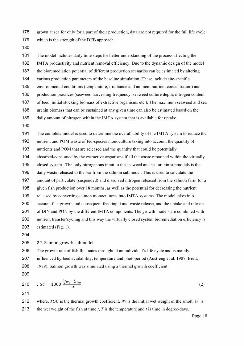
2.2 Salmon  growth  submodel    205

The growth rate of fish fluctuates throughout an individual’s life cycle and is mainly 206

influenced by feed availability, temperature and photoperiod (Austreng et al. 1987; Brett, 207

1979). Salmon growth was simulated using a thermal growth coefficient: 208

209

𝑇𝐺𝐶 = 1000   !!! !   !!

!

!∗!   (2) 210

211

where, TGC is the thermal growth coefficient, W0 is the initial wet weight of the smolt, Wt is 212

the wet weight of the fish at time t, T is the temperature and t is time in degree-days. 213

Page | 7

Solving for Wt we obtain: 214

215

 𝑊! = 𝑊!! +  !"#∗!∗!

!"""

! (3) 216

217

The total salmon biomass was calculated as individual weight multiplied by the number of 218

individuals. The model also accounted for natural mortality, modeled as a time series variable 219

since mortality decreases with fish size, using empirical data from Scottish salmon farms. 220

221

The amount of waste released from the salmon farm in the form of excretion, faeces 222

production and feed loss was assumed to be as calculated by Wang et al (2012) for 223

Norwegian salmon farms. In detail, we assume that every day of the simulation 2% of the 224

feed nitrogen is released in the environment in the form of feed loss, 45% in the form of 225

dissolved excretions and 15% in the form of faeces, while the remaining 38% is assimilated 226

into the salmon biomass and removed from the ecosystem when the fish are harvested. The 227

nitrogen content of the feed was set to be 7.2% of the feed weight (Gillibrand et al. 2002). 228

229

2.3 Seaweed growth and nitrogen uptake 230

231

Seaweed biomass (B) increases with a varying growth rate and decreases due to both natural 232

causes and periodic harvesting. The basic processes affecting seaweed biomass form the 233

differential equation 4: 234

235 !"!"=   𝜇  –  𝛺 ∗  𝛣  – (𝐷 + 𝐻)  ∗  𝐵 (4) 236

where, µ is the specific growth rate, Ω the specific decomposition rate, D the loss rate due to 237

environmental disturbance and H the harvesting rate. Biomass is calculated as wet biomass, 238

for the conversion of seaweed wet to dry weight an 8.43 to 1 ratio was used (Angell et al. 239

2012; Neori et al. 1991). At the baseline simulation due to lack of data in the literature for the 240

specific decomposition rate and the loss due to environmental disturbance for Ulva sp. the 241

term mortality (M) is used, where M = 𝛺 + D and 𝛺 = D (Table 1). 242

243

The gross growth rate was defined as a function of water temperature, availability of 244

Photosynthetic Active Radiation (PAR) and nutrient concentration in the water column and in 245

the plant tissues. The joint dependence of growth on environmental variables is defined by 246

separate growth limiting factors, which can range between 0 and 1. A value of 1 means the 247

factor does not inhibit growth (i.e. light is at optimum intensity, temperature is optimum and 248

Page | 8

nutrients are available in excess). The limiting factors are then combined with the maximum 249

gross growth rate at a reference temperature as in equation 5 (Solidoro et al. 1997): 250

251

𝜇   = 𝜇  !"#(!!"#)  ∗  𝑓(𝑇  )  ∗ 𝑓(𝐼)  ∗  𝑚𝑖𝑛(𝑓(𝑁), 𝑓(𝑃)) (5) 252

253

where, µmax(Tref) is the maximum growth rate at a particular reference temperature (Tref) under 254

conditions of saturated light intensity and excess nutrients, f(T), f(I), f(N, P) are the growth 255

limiting functions for temperature, light and nutrients (nitrogen and phosphorus). 256

257

The major nutrients required for growth are nitrogen and phosphorus, while carbon is often 258

available in excess and micronutrients such as iron and manganese are only limiting in 259

oligotrophic environments. Typically, in marine ecosystems, nitrogen is the element limiting 260

algal growth (Lobban and Harrison, 1994). Thus in the baseline simulation it is assumed that 261

phosphorus is not limiting, so Eq. 5 becomes: 262

263

𝜇 = 𝜇  !"#(!!"#) ∗ 𝑓 𝑇 ∗ 𝑓 𝐼 ∗ 𝑓 𝑁 (6) 264

265

The Photosynthetic response to light is based on Steele’s photoinhibition law (Steele, 1962): 266

267 !

!!"#= !

!!"#𝑒𝑥𝑝   !!!

!!"# (7) 268

269

where, P is the photosynthetic response at a given light intensity I (W m−2) for an organism 270

that has a maximum photosynthetic rate Pmax at the optimal (saturating) light intensity Iopt and 271

I is the light intensity at a given depth (z). Light intensity at a given depth is an exponential 272

function of depth, seaweed and phytoplankton standing biomass and is given by: 273

𝐼(𝑧) =   𝐼!  𝑒!!" (8) 274

275

After mathematical integration of the light limitation factor Eq. 8 we obtain: 276

277

𝐹 𝐼 = !!!"#

𝑑𝑧!! = !(!)

!!"#𝑒𝑥𝑝   !!!(!)

!!"#𝑑𝑥!

!    =     !!!!!"

!!"#

!! exp !!  !!  !

!!"

!!"#  𝑑𝑥 =   !

!∗ exp  ( !

!!"#) ∗278

exp − !!!!"#

∗ exp −𝑧 ∗ 𝑘 − exp − !!!!"#

(9) 279

where, k is the light extinction coefficient (m-1), z is the culture depth (m), Iopt is the optimal 280

light intensity and P is the photosynthetic rate at a given light intensity I (W m−2). 281

282

Page | 9

The temperature, like the light, limitation factor follows an inhibition law. 283

284

𝐹 𝑇 = 𝑞!"!.! !!!!"# (10) 285

286

where, q10 is a temperature coefficient, T is the water temperature and 𝑇!"#  is the reference 287

temperature at which the seaweed growth rate was measured. The q10 temperature coefficient 288

is a measure of the rate of change of a biological or chemical system as a consequence of 289

increasing the temperature by 10°C (Raven and Geider, 1988). 290

291

The nitrogen limitation factor Eq. 11 is given by the range of internal nitrogen concentration, 292

with a feedback effect on the uptake function (Aveytua-Alcázar et al. 2008; Coffaro and 293

Sfriso, 1997; Solidoro et al. 1997; Trancoso et al. 2005; Zaldívar et al. 2009). It can range 294

between 1, when N = Nmax and uptake is saturated and 0 when N = Nmin and maximum uptake 295

rate is possible, all measured in mg N per g dry seaweed. Internal nitrogen 296

quota/concentration (N) refers to the concentrations in the algal cells as opposed to external 297

concentrations that refers to the concentration amount in the water column. 298

299

𝐹 𝑁 = 1 − !!"#  !!!!"#!!!"#

(11) 300

301

where, Nmax is the maximum internal quota of nitrogen and Nmin the minimum. 302

303

For calculation of the nitrogen quota (N), a quota-based model was used developed from 304

Droop’s original formula (Droop, 1968): 305

306 !"!"= 𝑉 ∗ 𝐹 𝑁 − 𝜇 ∗ 𝑁 (12) 307

308

where, V is the nitrogen uptake rate (mg g-1dw h-1) and 𝜇 is the specific growth rate. 309

310

Nutrient uptake rates (V) are proportional to nutrient concentration in the water column 311

according to Michaelis–Menten kinetics: 312

313

𝑉 = !!"#!!!!!

(13) 314

315

Page | 10

where, Vmax is the maximum nitrogen uptake rate under the prevailing conditions at the site 316

(mg g-1dw h-1), S is the total DIN concentration in the seawater (mg l-1) and 𝐾! is the half-317

saturation coefficient for the uptake of nitrogen (mg l-1). 318

319

By combining Eqs. 11, 12 and 13 we obtain: 320

321 !"!"= !!"#  !

!!!!   !!"#  !!!!"#!!!"#

− (𝜇 ∗ 𝑁) (14) 322

323

The bioremediation effect of IMTA is closely dependent on the biomass of extractive 324

organisms harvested. However, the maximum biomass is restricted by culture practicalities 325

such as the potential alteration of water currents and by the availability of nutrients. The 326

maximum biomass is site and species dependent, and for the baseline simulation presented in 327

this study the maximum seaweed biomass permitted to be on site at any given time was set at 328

35 tonnes wet weight. The area required for the culture of 35 t of Ulva, with stocking density 329

of 1.6 kg/m2 and two layers of seaweed one at the sea surface and one 3 m deep would be 330

10,937 m2. This stocking density was selected because the maximum density permitted to 331

guarantee the greatest uptake of nutrients in U. lactuca is 1.9 kg m-2 (Neori et al. 1991). The 332

area required for the seaweed culture is used for the estimation of the virtually closed IMTA 333

site’s water volume, which is estimated using the following formula: 334

335

'IMTA site volume' = 'Average depth' * 'Number of salmon cages' * 'Sea cage area' + 'raft 336

area' * 'number of rafts' * 'Average depth'. 337

338

Seaweed is lost due to mortality, harvesting and natural biomass loss (seedling mortality, 339

grazing, epiphytism, sediment abrasion and smothering and removal by wave action). 340

Managing the harvesting rate is of paramount importance for achieving high productivity 341

rates. For optimal results, in the present model, when the seaweed biomass reaches a 342

predefined level (35 t in the baseline simulation) the seaweed is harvested at regular time 343

intervals. The biomass harvested depends on the forecasted growth and natural mortality rate 344

of the forthcoming days. A discrete flow in the model controls the loss of seaweed biomass 345

due to harvesting; the rate of the flow (harvest rate) is regulated by the following instruction: 346

347

IF (start harvesting = 0, 0 ton, IF (current time step * timestep = stoptime - starttime, 348

seaweed biomass, IF (accrued part of 10 days = 1, seaweed biomass – maximum seaweed 349

biomass, IF (accrued part of 10 days = 0, seaweed biomass – maximum seaweed biomass, 0 350

ton)))) 351

Page | 11

352

where, ‘start harvesting’ is a level that allows harvesting to start only when the seaweed 353

biomass has surpassed the value of a constant that defined as maximum biomass that can be 354

on site (maximum seaweed biomass). The level ‘start harvesting’ changes from 0 to 1 when 355

the level ‘seaweed biomass’ is equal to or larger than the constant ‘maximum seaweed 356

biomass’. ‘Current time step’ is a level that counts the time steps, starting from zero. Timestep 357

is a Powersim built-in function that returns the time step of the simulation, starttime and 358

stoptime are Powersim built-in functions that return the start-time and stop-time of the 359

simulation, respectively. In the final time step all the seaweed in the level ‘seaweed biomass’ 360

is transferred to the level ‘harvested seaweed’. ‘Seaweed biomass’ is a level that shows the 361

seaweed biomass. ‘Accrued part of 10 days’ is a level used for the calculation of 10-day 362

periods. When the value of this level is one, all the seaweed is harvested apart from 363

‘maximum seaweed biomass’. 364

365

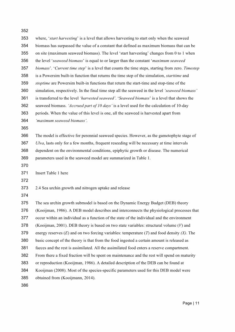
The model is effective for perennial seaweed species. However, as the gametophyte stage of 366

Ulva, lasts only for a few months, frequent reseeding will be necessary at time intervals 367

dependent on the environmental conditions, epiphytic growth or disease. The numerical 368

parameters used in the seaweed model are summarized in Table 1. 369

370

Insert Table 1 here 371

372

2.4 Sea urchin growth and nitrogen uptake and release 373

374

The sea urchin growth submodel is based on the Dynamic Energy Budget (DEB) theory 375

(Kooijman, 1986). A DEB model describes and interconnects the physiological processes that 376

occur within an individual as a function of the state of the individual and the environment 377

(Kooijman, 2001). DEB theory is based on two state variables: structural volume (V) and 378

energy reserves (E) and on two forcing variables: temperature (T) and food density (X). The 379

basic concept of the theory is that from the food ingested a certain amount is released as 380

faeces and the rest is assimilated. All the assimilated food enters a reserve compartment. 381

From there a fixed fraction will be spent on maintenance and the rest will spend on maturity 382

or reproduction (Kooijman, 1986). A detailed description of the DEB can be found at 383

Kooijman (2008). Most of the species-specific parameters used for this DEB model were 384

obtained from (Kooijmann, 2014). 385

386

Page | 12

The initial structural length/diameter of the sea urchin juveniles was set to 10 mm, because at 387

this size hatchery reared sea urchins can be transferred to sea successfully (Kelly et al. 1998). 388

At this length P. lividus individuals are characterized as sub adults (Grosjean et al. 1998), so 389

in the baseline simulation the DEB model simulates the growth from late juveniles to mature 390

adults. The physical length (Lw) was converted to volumetric length (L): 391

392

Lw = L/ 𝛿! (15) 393

394

where, δM is the shape coefficient. 395

396

For this simulation the notation from Kooijman (2000) was used. All rate variables are dotted 397

above, all variables that are expressed per unit volume and per unit surface area are given 398

between square brackets and braces, respectively. Additionally, the expression (x)+ is defined 399

as: [x]+ = x for x > 0, [x]+ = 0. 400

Most of the processes described by the DEB model are influenced by the effect of 401

temperature on the metabolic rate (K(T)) according to Eq. 16: 402

403

𝐾(𝑇) = 𝐾!  𝑒!!!!!!!! ∗ 1 +  𝑒

!!"! !!!"!! +  𝑒

!!"!!

!!!"!!!

(16) 404

405

where, Ko is the reference reaction rate at 288 K, TA is the Arhenius temperature, To is the 406

Reference temperature, TAL and TAH are the Arrhenius temperature at lower and upper 407

boundary, respectively, TL and TH are the lower and upper boundary tolerance, respectively 408

and T is the water temperature (simulated as a time series variable). 409

410

The DEB model starts with the ingestion of PON (mgN d-1) by the sea urchins. This is based 411

on ingestion rate (𝐽!) (𝑚𝑔𝐶  𝑑!!)  divided by the C/N ratio of the aquaculture waste (Eq. 17). 412

Ingestion rate is proportional to the surface area of the structural volume and follows type-II 413

function response depending on the density of PON. 414

415

𝐽! = 𝐾(𝑇) ∗  𝑓 ∗ {𝐽!} ∗ 𝑉!/! (17) 416

417

where, 𝐾(𝑇) is a temperature dependent rate, {𝐽!} is the maximum surface area-specific 418

ingestion, V is the structural volume and f is the functional response that can range between 0 419

and 1 and is given by: 420

421

Page | 13

𝑓 = !!!!!

(18) 422

423

The saturation coefficient (XK), is analogous to a Michaelis-Menten constant, in this case 424

being the food density at which the ingestion rate is half the maximum. For the calculation of 425

the food density in the environment (X), the concentration of PON is converted to organic 426

carbon concentration. 427

428

DEB models assume that the assimilation rate,  (𝑃!), is independent of the ingestion rate: 429

430

𝑃! = 𝐾(𝑇) ∗  𝑓 ∗ 𝑃!" ∗ 𝑉!/! (19) 431

432

where, 𝐾(𝑇) is a temperature dependent rate, f is the functional response, 𝑃!"  is the 433

maximum surface area specific assimilation and V is the structural volume. 434

435

The food that is ingested but not assimilated as biomass will be released to the environment as 436

faeces or as excretion by diffusion. The DEB model enables estimation of the potential 437

amounts of faeces released by the sea urchins by estimating the hourly production of faeces 438

released into the surroundings using Eq. 20 for the faeces production in (𝑚𝑔𝐶  𝑑!!) and Eq. 439

21 for the excretion rate in (𝑚𝑔𝑁  𝑑!!). Eq. 20 is then divided by the C/N ratio in order to 440

calculate the amount of PON that is in the sea urchin faeces, which is assumed to be 441

immediately added to the PON and DIN pools and is thus available for consumption by the 442

sea urchins and seaweed, respectively. 443

444

𝐹 = 𝐽! − 𝑃!/𝜇!" (20) 445

446

where, 𝐽! is the consumption rate, 𝑃! is the assimilation rate and µcj is the ratio of carbon to 447

energy content. 448

449

𝐷!"#$ = 𝑃! − 1 − 𝑘! ∗ !"!!"

− 𝜇! ∗ 𝜌 ∗!"!"

∗ 𝑄 + 𝑃! ∗ (𝑄𝑠 − 𝑄)! /𝜇!" (21) 450

451

where, 𝑃! is the catabolic rate, kR are the reproductive reserves fixed in the eggs, ER are the 452

reproductive reserves, µV is the structural energy quota, ρ is the biovolume density, V is the 453

structural volume, Q is the sea urchin N quota, 𝑃! is the assimilation rate, µcj is the ratio of 454

carbon to energy content and Qs is the sediment N quota (calculated as the ratio of organic 455

nitrogen to organic carbon in the sediment). The P. lividus N quota (Q) was set to 456

Page | 14

127  𝑚𝑔𝑁  𝑚𝑔𝐶!!  (Tomas et al. 2005) and sediment N quota (Qs) is site specific it was set to 457

7, which is a representative value for an average Scottish salmon farm site. 458

459

The assimilated energy from the food enters the reserve pool. The energy density [E] in an 460

organism may vary between 0 and the maximum energy density [Em] depending on the food 461

density in the environment. 462 ![!]!"

=  𝑃! − 𝑃! (22) 463

464

where, 𝑃! is the assimilation and 𝑃! the catabolic rate. 465

466

The sea urchin catabolic rate)  (𝑃!) denotes the energy utilised by the structural body and is 467

given by: 468

469

𝑃! = 𝐾(𝑇) ∗ !!! !!∗ !

∗ !! ∗ !!" ∗!!/!

!!+ 𝑃! ∗ 𝑉 (23) 470

471

where, 𝐾(𝑇) is a temperature dependent rate, 𝐸 is the reserves, 𝐸! the volume specific 472

cost of growth, 𝐾 the catabolic flux to growth and maintenance, 𝑃!"  the maximum surface 473

area specific assimilation, 𝑉 the structural volume, 𝐸! the maximum reserve density and 474

𝑃! the volume specific maintenance rate. 475

476

The rate of maintenance cost of the animals (𝑃!) is proportional to the body volume and 477

calculated with Eq. 24. Since the sea urchins will be mature the maturity maintenance Pj is 478

also used Eq. 25: 479

480

𝑃! = 𝐾(𝑇) ∗ 𝑃!  ∗ 𝑉 (24) 481

482

𝑃! = min 𝑉,𝑉! ∗   𝑃! ∗ !!!!

(25) 483

484

where, 𝐾(𝑇) is a temperature dependent rate, 𝑃! is the volume specific maintenance rate, 𝑉 485

is the structural volume, 𝑉! is the structural volume at puberty and 𝐾 is the catabolic flux to 486

growth and maintenance. 487

488

The sea urchin structural volume growth (V) is given by: 489

490

Page | 15

!"!"= !∗!!!!! !

!! (26) 491

492

where, 𝐾 is the catabolic flux to growth and maintenance, 𝑃! is catabolic rate, 𝑃! is the 493

maintenance rate and 𝐸! is the volume specific cost of growth. 494

495

In this model we are also interested in the body mass (W) of the sea urchins, in order to 496

calculate the total biomass of the stock. To convert volume to dry weight Eq. 27 is used: 497

498

𝑊 = V   ∗  𝜌 + (!!!!∗!!)!!

(27) 499

500

where, V is the structural volume, ρ is the biovolume density, E and ER are reserves and 501

reproductive reserves, respectively, kR are the reproductive reserves fixed in the eggs and µE is 502

the reserve energy content. 503

504

The total biomass was calculated as individual weight multiplied by the number of 505

individuals. Once an individual has reached the volume (Vp) at sexual maturity, a portion of 506

the total energy reserve is stored in the sea urchin reproductive reserves (ER): 507

508 !!!!"

= 1 − 𝑘 ∗ 𝑃! − 𝑃! (28) 509

510

where, K is the catabolic flux to growth and maintenance, 𝑃!  is the catabolic rate and 𝑃!  is the 511

maturity maintenance 512

513

The DEB model simulates the process within individuals. However for this model it is 514

necessary to know how a non-reproducing stock (N) will decrease in size with time, due to 515

mortality. The decrease of the sea urchin stock size is calculated in Eq. 29 where due to the 516

planktonic nature of sea urchin larvae, it is assumed they will be dispersed from the IMTA 517

site and thus reproduction will represent a net energy loss and restocking of the sea urchins 518

will be necessary. However, the release of the larvae will contribute to restocking the native 519

sea urchin population. 520

521 !"!"=  −𝛿! ∗ 𝑁 − 𝛿!* N (29) 522

523

Page | 16

where, δr and δh are the natural and harvest mortality of sea urchins, respectively. The harvest 524

mortality (𝛿!) was zero and at the last time step of the simulation all sea urchins were 525

harvested, same as in the salmon and seaweed submodels. The natural mortality (𝛿!) was set 526

to 0.00102 individuals d-1 for sea urchins with test diameter smaller than 2 cm and 0.00056 527

individuals d-1 for sea urchins with test diameter larger than 2 cm (Turon et al. 1995). 528

529

During the grow-out stage of P. lividus juveniles, the stocking density is approximately 400 530

individuals m-2 (Carboni, 2013). Space is not an issue for the organic extractive component of 531

the IMTA, since for the production of 560,525 individuals only 1,401 m2 would be required 532

and this area would be directly underneath the fish cages and the seaweed rafts. 533

534

535

2.5 Assumptions  and  simplifications  536

The overall model’s key assumption is that all nitrogen released by the various IMTA 537

components is dispersed homogenously within a quantified water volume defined as the 538

IMTA site water volume (see section 2.3). It is also assumed that all the nitrogen available in 539

the IMTA site volume is in a form suitable for uptake; thus the model does not distinguish 540

between nitrate and ammonium. Correspondingly, the model does not take into account the 541

interactions between nitrate and ammonium within the environment and organisms, such as 542

the role of sediment and water in the nutrient dynamics or denitrification. The increase of 543

light limitation due to increased self-shading as the seaweed grows was not considered, 544

neither was the shading caused by phytoplankton. Data from Broch and Slagstad (2012) could 545

be used to derive a seaweed self -shading formula from which an add-on model could be used 546

to simulate the changes in k. In this study the light extinction coefficient (k) was a constant 547

(k=1). In the seaweed growth submodel the small biomass loss due to mechanical damage 548

caused by harvesting was not included. It is also assumed that nitrogen is the only nutrient 549

limiting seaweed growth. Additionally, the seaweed biomass used as initial biomass is 550

assumed to have an average (𝑁!"# + 𝑁!"#) 2 N quota (this can be regulated by using 551

nitrogen deprived seedlings). When seaweed is harvested it is assumed that the N quota of the 552

harvested seaweed is equal to the maximum N quota due to the high availability of DIN in the 553

virtually closed system. The assumption that the seaweed harvested has this high nitrogen 554

quota might lead to overestimation of the bioremediation efficiency and the effect of lower N 555

quota at harvest was examined in the sensitivity analysis (Tables 5 and 10). From a farm 556

practice perspective it is assumed, that the relative position of the extractive organisms in 557

relation to the fish cages is such that it ensures high O2 availability for the fish. For the 558

Page | 17

salmon growth model, excretion, faeces production and feed loss were assumed to be steady 559

during the 18 month production period while in reality they change as the fish grow. 560

561

2.6 Production specifications of the baseline simulation 562 The results presented are from the IMTA baseline simulation, which was parameterized using 563

data acquired from the literature and from commercial salmon farm sites. The environmental 564

data such as monthly variations in seawater temperature and irradiance were acquired from 565

empirical databases for the West coast of Scotland and the production-specific input data 566

from Scottish commercial salmon farm sites (Figs. 2 and 3). Typically, S1 smolts are 567

transferred to sea in spring (April-May), so April is set as simulation time 0 and the model 568

then runs for 18 months. The test scenario farm consists of nine 90 m circular salmon cages 569

with the extractive organisms placed in immediate proximity to those cages. The model 570

simulates a farm that produces 1,000 t of Atlantic salmon in 18 months on-growing, a farm 571

size representative of the Scottish industry (FAO, Scottish Fish Farm Production Survey 572

2011). 573

574

Insert Fig 2 and Fig 3 575

576

3 Results 577

3.1 Growth performance of IMTA components at the baseline simulation 578

The baseline simulation run estimated that the mean individual fish biomass after 540 days 579

(18 months) was 3.78 kg (Fig. 4a) and the salmon stock decreased by 16,525 individuals 580

from 280,883 to 264,358 individuals (Fig. 4b). 581

582

Insert fig. 4 here 583

584

During the 18-month production period, 348 t of seaweed and 50 t of sea urchins were 585

produced and harvested as well as the targeted 1000t of salmon (Table 2). The seaweed 586

achieved high growth rates, especially during the summer months (Fig. 5). The effect of the 587

growth limitation factors on the seaweed growth rate is presented in Fig. 6. The lower 588

seaweed growth rate during the first 300 days (10 months) of the simulation (Fig. 5) can be 589

mainly attributed to low levels of nitrogen available for uptake (Figs. 6 and 10). It is clear that 590

in the hypothetical baseline model scenario, during the first 300 days of the simulation 591

seaweed growth is mainly limited by the availability of nitrogen. Temperature limits growth 592

more during the colder months (October – April) while, the effect of light intensity is rather 593

Page | 18

stable throughout the year (Fig. 6). It should be emphasized here that site specific shading 594

caused by phytoplankton or seaweed self shading does not contribute to light limitation in the 595

baseline simulation (see section 2.5 for more details). 596

597

Insert Fig. 5 and fig. 6 here 598

599

The aim of the IMTA model developed was to achieve high bioremediation efficiency. 600

Sustaining the seaweed biomass at a high density at all times, using the harvesting instruction 601

(described at section 2.3), played an important role in achieving this (Fig. 7). The first 602

seaweed harvesting occurred 330 days after the simulation start, following which there was 603

enough nitrogen available due to the large size of the fish and the environmental conditions 604

were also favorable for the remaining seven months of the simulation (April – October) (Figs. 605

3 and 6) thus ensuring constant high growth rate and harvesting at 10-day intervals (Fig. 7). 606

607

Insert Fig.7 here 608

609

At the beginning of the IMTA simulation the site was stocked with 827,900 sea urchins. 610

During the 18-month production period 50 t (wet weight) of sea urchins of the species P. 611

lividus were produced with average test diameter 4.47 cm (Table 2, Fig. 8). As a result 1.01 t 612

of nitrogen were assimilated in the sea urchin biomass and removed from the ecosystem via 613

the process of harvesting. 614

615

Insert fig. 8 and fig. 9 here 616

617

3.2 Test scenario bioremediation potential 618

For the production of 1,000 t of salmon with average feed conversion ratio (FCR) of 1.02 and 619

feed nitrogen content 7.2%; the model shows that 80 t of nitrogen are introduced into the 620

system over the 540 day simulated production period. From this 80 t, only 38% will be 621

accumulated by the fish and incorporated into their biomass. The remaining 62%, which 622

under the production scenario described above (production of 1000t of salmon) is 49.6 t, will 623

be released into the environment as dissolved and particulate nitrogen. Under the 624

environmental conditions and production method of the test scenario the total nitrogen 625

released to the environment from the IMTA site would be 36% less (31.8 t instead of 49.6 t) 626

than what would have been released from a salmon monocutlure farm of the same capacity. In 627

detail, the amount of nitrogen released from salmon monoculture would be 62% of the 628

exogenous nitrogen input but only 39% in the IMTA system since a large proportion of the 629

Page | 19

nitrogenous waste will be assimilated by the extractive organisms and removed from the 630

ecosystem via harvesting (Figs. 9 and 10). Fig. 10 shows the gradual increase in nitrogen 631

within the IMTA system over the simulated production period. 632

633

3.3 Sensitivity analysis 634

All biological, environmental and production parameters were analysed in terms of 635

uncertainty and their relative importance in the model. Due to the large number of input and 636

response variables used in the sensitivity analysis, the results for only those that were shown 637

to be the most sensitive parameters (absolute values) to operation of the model are 638

summarized in Tables 3 to 6. Those parameters were therefore classified as potential critical 639

assumptions and thus require accurate estimation and/or calibration. 640

641

In the salmon submodel, the growth and nutrient uptake is most sensitive to change in the 642

TGC and secondarily on variation in the FCR (Table 3). 643

644

Insert Table 3 here 645

646

In the seaweed submodel, all output variables were most sensitive to parameters affecting 647

growth and nutrient uptake either indirectly through nitrogen uptake and nitrogen content of 648

the seaweed tissues, wet/dry ratio and the culture depth or directly through maximum growth 649

rate, temperature and nitrogen input from salmon excretion. These results show the overall 650

importance of temperature and nitrogen uptake for seaweed growth (Table 4). All parameters, 651

apart from culture depth that was negatively correlated with seaweed biomass harvested, were 652

positively correlated with the output variables. Also, increasing parameter values mirrored the 653

effect on the model output of decreasing parameter values, which indicates that most 654

parameters affected growth linearly. 655

656

Insert Table 4 here 657

658

In the sea urchin submodel the output variables were most sensitive to parameters related to 659

temperature. Other sensitive parameters included the maximum surface-specific feeding rate 660

(Table 5), the volume specific cost of growth and the ratio of carbon to energy content. An 661

increase in the value of TL had a strong negative effect on the output variable ‘harvested sea 662

urchin biomass’ (sensitivity -9.96), while a reduction caused a weak positive effect 663

(sensitivity 0.08). Overall, this analysis revealed that the DEB model was most sensitive to 664

increases in TL. The model also showed a high sensitivity to increases or decreases in other 665

Page | 20

parameters (Table 5) while changes in the remaining DEB input variables had little effect on 666

growth (sensitivity < 1). 667

668

Insert Table 5 here 669

670

Table 6 summarizes tables 3 to 5 in the context of the overall model. The most sensitive 671

parameters within the salmon and seaweed sub-models are also the most sensitive to 672

outcomes of the overall model. The most sensitive parameters of the DEB sub-model do not 673

play such an important role within the overall model performance due to the sea urchin 674

biomass being very small in comparison to that of salmon and seaweed (Table 6). 675

676

Insert Table 6 here 677

678

4. Discussion 679

The aim of this study was the development of a dynamic tool for relative comparison of 680

different IMTA scenarios at a given production site, rather than the generation of absolute 681

bioremediation and production estimates. The model results presented are derived from a 682

baseline simulation, which can be re-parameterised to simulate different scenarios. 683

684

Results from IMTA studies similar to the one presented here, have shown bioremediation 685

potential of a similar scale to the output generated by the present model. Broch and Slagstad 686

(2012) estimated that 0.8 km2 of Saccharina latissima biomass would be needed to sequester 687

all the waste released from a salmon farm producing 1,000 tonnes a year and Abreu et al. 688

(2009) estimated that a 1 km2 Gracilaria chilensis farm would be needed to fully sequester 689

the dissolved nutrients released from a salmon farm producing 1,000 tonnes a year. Sanderson 690

et al. (2012) estimated that 0.01 km2 of S. latissima could remove 5.3-10% of the dissolved 691

nitrogen released from a salmon farm producing 500 t of salmon in two years. However, the 692

results presented, as the results from any other IMTA model or trial, cannot be directly 693

compared with output from similar studies due to the fact that the productivity of an IMTA 694

farm depends on local environmental characteristics, the species combination used, the 695

duration of the grow out seasons and other factors. Moreover, linear interpolation of results 696

from studies with shorter durations can lead to misestimating results. Thus a large variance in 697

production and bioremediation results is natural. The results of this study are in the same 698

order of magnitude as the results acquired from the studies mentioned above; however they 699

suggest higher bioremediation potential, possibly largely due to the harvesting method 700

applied. Specifically, it was estimated that 35% of the total nitrogen released from a salmon 701

Page | 21

farm, with the specifications of the simulated scenario, will be accumulated by the 0.01 km2 702

of Ulva sp suggesting a very high bioremediation efficiency. Aiming to achieve 100% 703

bioremediation (i.e. no available nitrogen above the ambient concentration occurs at any 704

given time), especially without the addition of external feed sources for the extractive 705

organisms and while sustaining the quality of the extractive organisms, is unrealistic and 706

might only be possible in a fully closed system such as a Recirculating Aquaculture System 707

(RAS). Nonetheless, even at lower bioremediation efficiencies, the model already 708

demonstrates the environmental benefits of IMTA. 709

710

The simulated growth for juvenile and adult sea urchins showed good correspondence with 711

empirical data, although the reference temperature for which all the DEB constants were 712

calculated was 20°C (Table 2) which is significantly higher than the average temperature (11°713

C) at the modelled IMTA site during the 18 month grow out period. The sea urchin growth 714

model output is comparable to the results of Cook and Kelly (2007) who concluded that P. 715

lividus, with an initial test diameter of 1 cm, deployed adjacent to fish cages need 716

approximately 3 years to reach market size (> 5.5 cm test diameter). The sea urchins will be 717

around 1 year old when they are deployed and 2.5 years old at the end of the grow out phase 718

at which point their test diameter will be 4.47 cm. At the end of the 18-month grow-out phase 719

of the salmon, the sea urchins will have reached the lower limit of their target market size. 720

The growth rate achieved in this study was similar to that achieved directly adjacent to the sea 721

cages (Cook and Kelly, 2007) and higher than that achieved by Fernandez and Clatagirone 722

(1994) (1.41 mm per month) where the sea urchins were fed with artificial feed containing 723

fish meal and fish oil at higher water temperature than this study (5-33°C). After the sea 724

urchins have reached market size a two to three month period of market conditioning at 725

controlled environment is required (Carboni, 2013; Grosjean et al. 1998). 726

727

In the first eight to ten months of the IMTA baseline scenario, seaweed and sea urchin growth 728

is limited by nitrogen (Figs. 6 and 8b), since the fish are still small and thus require a 729

relatively low feed input. From the eleventh month onwards mainly light and to a lower 730

extend temperature are limiting the seaweed growth. From that point onwards the seaweed 731

growth rate is high as can be seen in Fig. 5. For successful high bioremediation efficiency, at 732

an IMTA farm seaweed growth should not be limited by light or temperature but only by 733

nutrient availability. For this reason IMTA systems could be more efficient in sites further 734

south than the one used for the baseline simulation. It can be seen clearly in Fig. 10 that there 735

is a constant increase of the residual DIN and PON remaining at the IMTA site. This high 736

waste output particularly during the last months of the salmon production is a challenge for 737

Page | 22

achieving very high bioremediation efficiency. The ratio of salmon to extractive organisms 738

(especially for sea urchins) used at the test scenario is very low (Table 2). From the 739

perspective of space requirement there is the potential for increase of the amount of sea 740

urchins produced, however the quantity of waste available for consumption by the sea urchins 741

decreases with distance from the sea cages and thus increasing the production would mean 742

that some sea urchins would be potentially too far from the food source. Furthermore, limited 743

market demand for marine invertebrates might also pose limitations. 744

745

The results of the sensitivity analysis indicate that the model is robust, since variation of key 746

model parameters by ±10% does not cause unexpected changes in the effect parameters. The 747

various model parameters have a different relative influence on the model’s output, both in 748

terms of harvestable biomass and in terms of nitrogen bioremediation. Thus, depending on 749

users’ specific study objectives, one should consider the precision with which certain 750

parameter values are determined, and whether further tuning is required. This model 751

sensitivity analysis is a useful means for assessing which are the key parameters that increase 752

model uncertainty. Those parameters with high sensitivity have a big impact on the output of 753

the model (e.g. thermal sensitivity parameters TL in the sea urchin DEB submodel, T in all the 754

submodels and µmax in the seaweed submodel), and therefore future efforts should focus on 755

methods for improving their estimation. In contrast, because parameters with low sensitivity 756

have little influence on the output of the model, their estimation could be simplified. 757

Consequently, despite the large variability observed in some of the parameters, their relative 758

importance may be minor if their sensitivity is low. 759

760

The model presented here is highly adaptable as all the submodels can function 761

independently. By altering model variables the submodels can simulate growth and nutrient 762

assimilation under different environmental conditions or for different species. Altering the 763

values of constants can also help assess their effect on the IMTA system and in some cases 764

these values can be optimised. For example, all the values related with production practices at 765

the IMTA site, such as seaweed harvesting frequency, maximum seaweed biomass allowed, 766

initial biomass of seaweed or sea urchins, seaweed culture depth and seaweed density, can be 767

optimised for the achievement of higher bioremediation efficiency and/or higher extractive 768

organism production. 769

770

Apart from achieving the major objectives described the model can be used for the 771

accomplishment of more general objectives such as: optimization of IMTA culture practices 772

(e.g. timing and sizes for seeding and harvesting, in terms of total production), assessment of 773

Page | 23

the role of IMTA in nutrient waste control and used as input for the evaluation of economic 774

efficiency of various system designs. The present model can be used as a decision support 775

tool for open-water IMTA only after being coupled with waste distribution modelling and 776

environmental sampling for model parameterization. Future versions of the model can link the 777

virtually closed IMTA system to hydrodynamic models for spatial analysis of the waste 778

dispersion and nutrient dilution. Such a model could help develop a balance among the 779

components of the IMTA system and assist in developing an IMTA design for maximum 780

waste uptake in “open environment systems”, as water exchange rate is the key factor 781

influencing the assimilative performance, thus enabling prediction of the effectiveness and 782

productivity of open water IMTA systems. 783

784

Acknowledgements 785

786

This PhD study was funded by the Marine Alliance of Science and Technology, by the 787

Institute of Aquaculture, University of Stirling and by IKY State Scholarships Foundation of 788

Greece. 789

790

791

References 792

793

Abreu, H., Varela, D.A., HenriÅLquez, L., Villaroel, A., Yarish, C., Sousa-Pinto, I., 794

Buschmann, A.H., 2009. Traditional vs. integrated multi-trophic aquaculture of 795

Gracilaria chilensis C. J. Bird, J. McLachlan & E. C. Oliveira: productivity and 796

physiological performance. Aquaculture. 293 (3-4), 211−220. 797

Angell, A.R., Pirozzi, I., de Nys, R., Paul, N.A., 2012. Feeding preferences and the nutritional 798

value of tropical algae for the abalone Haliotis asinine. PLoS ONE, 7 (6), art. No. 799

e38857. 800

Austreng, E., Storebakken, T., Åsgård, T., 1987. Growth rate estimates for cultured Atlantic 801

salmon and rainbow trout. Aquaculture. 60, 157–160. 802

Aveytua-Alcázara, L., Camacho-Ibara, V.F., Souzab, A.J., Allenc, J.I., Torres, R., 2008. 803

Modelling Zostera marina and Ulva sp. in a coastal lagoon. Ecol. Model. 218, 354–804

366.. 805

Bjornsater, B.R., Wheeler, P.A., 1990. Effect of nitrogen and phosphorus supply on growth 806

and tissue composition of Ulva fenestrata and Enteromorpha intestinalis (Ulvales 807

Chlorophyta). J. Phycol. 26, 603-611. 808

Page | 24

Brett, J.R., 1979. Environmental Factors and Growth, in: Hoar, W.S., Randall, D.J., Brett, 809

J.R. (Eds.), Fish Physiology VIII. Academic Press, New York, pp. 599–675. 810

Broch, O., Slagstad, D., 2012. Modelling seasonal growth and composition of the kelp 811

Saccharina latissima. J. Appl. Phyc. 24, 759–776. 812

Broch, O.J., Ellingsen, I.H., Forbord, S., Wang, X., Volent, Z., Alver, M.O., Handå, A., 813

Andresen, K., Slagstad, D., Reitan, K.I., Olsen, Y., Skjermo, J., 2013. Modelling the 814

cultivation and bioremediation potential of the kelp Saccharina latissima in close 815

proximity to an exposed salmon farm in Norway. Aquaculture Environmental 816

Interactions 4, 186–206. 817

Carboni, S., 2013. Research and development of hatchery techniques to opimize juvenile 818

production of the edible Sea Urchin, Paracentrotus lividus. PhD. Thesis. University of 819

Stirling, UK. 820

Chopin, T., Buschmann, A. H., Halling, C., Troell, M., Kautsky, N., Neori, A., Kraemer, G. 821

P., Zertuche-González, J. A., Yarish, C. and Neefus, C., 2001. Integrating seaweeds 822

into marine aquaculture systems: a key toward sustainability. J. Phycol. 37, 975–986. 823

Coffaro, G., Sfriso, A., 1997. Simulation model of Ulva rigida growth in shallow water of the 824

Lagoon of Venice. Ecol. Model. 102, 55-66. 825

Cohen, I., Neori, A., 1991. Ulva lactuca biofilters for marine fishpond effluents. Bot. Mar. 34, 826

475-482. 827

Cook, E.J., Kelly, M.S., 2007. Enhanced production of the sea urchin Paracentrotus lividus in 828

integrated open-water cultivation with Atlantic salmon Salmo salar. Aquaculture. 273 829

(4), 573-585. 830

Corner, R., Brooker, A., Telfer, T., Ross, L.G., 2006. A fully integrated GIS-based model of 831

particulate waste distribution from marine fish-cage sites. Aquaculture. 258, 299−311. 832

Droop, M., 1968. Vitamin B12 and marine ecology. IV. The kinetics of uptake, growth and 833

inhibition in Monochrysis Lutheri. J. Mar. Biol. 48, 689–733. 834

Dumas, A., France, J., Bureau, D., 2010. Modelling growth and body composition in fish 835

nutrition: where have we been and where are we going?. Aquaculture Research. 41-2, 836

161–181. 837

FAO, 2011. Scottish Fish Farm Production Survey 2011. 838

http://www.scotland.gov.uk/Resource/0040/ 00401446.pdf [21 May 2014] 839

Fei, X.G., Lu, S., Bao, Y., Wilkes, R., Yarish, C., 1998. Seaweed cultivation in China. World 840

Aquaculture 29, 22–24. 841

Fernandez, C.M., Caltagirone, A., 1994. Growth rate of adult Paracentrotus lividus in a 842

lagoon environment: the effect of different diet types, in: David, B., Guille, A., Feral, 843

Page | 25

J.P., Roux, M. (Eds.), Echinoderms Through Time. Balkema, Rotterdam, pp. 655–844

660. 845

Fujita, R.M., 1985. The role of nitrogen status in regulating transient ammonium uptake and 846

nitrogen storage by macroalgae. J. Exp. Mar. Biol. Ecol. 92, 283-301. 847

Gillibrand, P.A., Gubbins, M.J., Greathead, C., Davies, I.M., 2002. Scottish Executive 848

locational guidelines for fish farming: predicted levels of nutrient enhancement and 849

benthic impact. Scottish Fisheries Research Report Number 63 / 2002 Fisheries 850

Research Services, Marine Laboratory, Aberdeen. 851

Grosjean, P., 2001. Growth model of the reared sea urchin Paracentrotus lividus (Lamarck, 852

1816). PhD thesis. Universite Libre de Bruxelles, Belgium. 853

Iwama, G.K., and Tautz A.F., 1981. A Simple Growth Model for Salmonids in Hatcheries. 854

Can. J. Fish. Aquat. Sci. 38(6), 649-656. 855

Jiang, Z.J., Fang, J.G., Mao, Y.Z., Wang, W., 2010. Eutrophication assessment and 856

bioremediation strategy in a marine fish cage culture area in Nansha Bay. J. Appl. 857

Phyc. 22, 421–426. 858

Jobling, M., 2003. The thermal growth coefficient (TGC) model of fish growth: a cautionary 859

note. Aquaculture Research. 34, 581-584. 860

Kelly, M.S., Brodie, C.C., McKenzie, J.D., 1998. Somatic and gonadal growth of the sea 861

urchin Psammechinus miliaris (Gmelin) maintained in polyculture with the Atlantic 862

salmon. J. Shellfish Res. 17, 1557–1562. 863

Kooijman, S.A.L.M., 1986. Energy budgets can explain body size relations. J. Theor. Biol. 864

121, 269–282. 865

Kooijman, S.A.L.M., 2000. Dynamic Energy and Mass Budgets in Biological Systems. CUP, 866

Cambridge. 867

Kooijman, S.A.L.M., 2001. Quantitative aspects of metabolic organization: a discussion of 868

concepts. Phil. Trans. Royal Soc. London B: Biol. Sci. 356, 331–349. 869

Kooijman, S.A.L.M., 2008. Dynamic Energy Budget theory for metabolic organization. Third 870

Edition CUP, Cambridge. 871

Kooijman, S.A.L.M., 2014. Add_my_pet: Paracentrotus lividus. URL: 872

http://www.bio.vu.nl/thb/deb/deblab/add_my_pet/html/Paracentrotus_lividus.html 873

[21 May 2014] 874

Lapointe, B.E., Tenore, K.R., 1981. Experimental outdoor studies with Ulva fasciata Delile I. 875

Interaction of light and nitrogen on nutrient uptake, growth and biochemical 876

composition. J. Exp. Mar. Biol. Ecol. 92, 135 152. 877

Lobban, C.S., Harrison P.J., 1994. Seaweed Ecology and Physiology. CUP, Cambridge. 878

Page | 26

Luo, M.B., Liu, F., Xu, Z.L., 2012. Growth and nutrient uptake capacity of two co-occurring 879

species, Ulva prolifera and Ulva linza. Aquat. Bot. 100, 18-24. 880

Marine Harvest, 2012. Salmon farming industry handbook. 881

http://www.marineharvest.com/PageFiles/1296/2012%20Salmon%20Handbook%201882

8.juli_h%C3%B8y%20tl.pdf [30 April 2014] 883

Marine Scotland, 2013. Draft Seaweed Policy Statement Consultation Paper. 884

http://www.scotland.gov.uk/Publications/2013/08/6786 [1 June 2014] 885

Neori, A., Chopin, T., Troell, M., Buschmann, A.H., Kraemer, G.P., Halling, C., Shipgel, M., 886

Yarish C., 2004. Integrated aquaculture: rationale, evolution and state of the art 887

emphasizing seaweed biofiltration in modern mariculture. Aquaculture. 231, 361–888

391. 889

Neori, A., Cohen, I., Gordin, H., 1991. Ulva lactuca biofilters for marine fishpond effluents. 890

II. Growth rate, yield and C:N ratio. Bot. Marina. 34, 483-489. 891

Perrot, T., Rossi, N., Ménesguen, A., Dumas, F., 2014. Modelling green macroalgal blooms 892

on the coasts of Brittany, France to enhance water quality management. J. Mar. 893

Syst.132, 38-53. 894

Raven, J.A., Geider, R.J., 1988. Temperature and algal growth. New Phytol. 110, 441-461. 895

Reid, G.K., Chopin, T., Robinson, S.M.C., Azevedo, P., Quinton, M., Belyea, E., 2013. 896

Weight ratios of the kelps, Alaria esculenta and Saccharina latissima, required to 897

sequester dissolved inorganic nutrients and supply oxygen for Atlantic salmon, Salmo 898

salar, in Integrated Multi-Trophic Aquaculture systems. Aquaculture. 408/409, 34-46. 899

Sanderson, J.C., Dring, M.J., Davidson, K., Kelly, M.S., 2012. Culture, yield and 900

bioremediation potential of Palmaria palmata (Linnaeus) Weber & Mohr and 901

Saccharina latissima (Linnaeus) C. E. Lane, C. Mayes, Druehl & G. W. Saunders 902

adjacent to fish farm cages in northwest Scotland. Aquaculture. 354/355, 128−135. 903

Solidoro, C., Pecenik G., Pastres, R., Franco D., Dejak, C., 1997. Modelling macroalgae 904

(Ulva rigida) in the Venice lagoon: Model structure identification and first 905

parameters estimation, Ecol. Model. 94 (2–3), 191-206. 906

Soto, D., Aguilar-Manjarrez, J., Hishamunda, N., 2008. Building an ecosystem approach to 907

aquaculture. FAO/Universitat de les Illes Balears Expert Workshop. 7–11 May 2007, 908

Palma de Mallorca, Spain. FAO Fisheries and Aquaculture Proceedings. No. 14. 909

Rome, FAO. 910

Steele, J.H., 1962. Environmental control of photosynthesis in the sea. Limnol. Oceanogr., 7, 911

137–150 912

Page | 27

Tomas, F., Romero, X., Turon, X., 2005. Experimental evidence that intra-specific 913

competition in seagrass meadows reduces reproductive potential in the sea urchin 914

Paracentrotus lividus (Lamarck). Sci Mar. 69, 475–484. 915

Trancoso, A.R., Saraira, S., Fernandes, L., Pina, P., Leitao, P., Neves, R., 2005. Modelling 916

macroalgae using a 3D hydrodynamic-ecological model in a shallow, temperate 917

estuary. Ecol. Model. 187, 232-246. 918

Turon, X., Giribet, G., López, S., Palacín, C., 1995. Growth and population structure of 919

Paracentrotus lividus (Echinodermata: Echinoidea) in two contrasting habitats. Mar. 920

Ecol. Prog. Ser. 122, 193-204. 921

Wang, X., Broch, O.J., Forbord, S., Handå, A., Skjermo, J., Reitan, K.I., Vadstein, O., Olsen, 922

Y., 2013. Assimilation of inorganic nutrients from salmon (Salmo salar) farming by 923

the macroalgae (Saccharina latissima) in an exposed coastal environment: 924

implications for integrated multi-trophic aquaculture. J. Appl. Phyc. DOI 925

10.1007/s10811-013-0230-1 926

Wang, X., Olsen, L.M., Reitan, K.I., Olsen, Y., 2012. Discharge of nutrient wastes from 927

salmon farms: environmental effects, and potential for integrated multi-trophic 928

aquaculture. Aquaculture Environmental Interactions. 2, 267-283. 929

Zaldívara, J.M., Bacelarb, F.S., Dueria, S., Marinova, D., Viaroli, P., Hernández-García E., 930

2009. Modeling approach to regime shifts of primary production in shallow coastal 931

ecosystems. Ecol. Model. 220, 3100-3110. 932

933

Page | 28

934 Fig. 1: Conceptual diagram of the model showing the major state variables (squares) and 935

forcing functions (circles) of each submodel as well as the interactions among the submodels. 936

The dashed lines represent nitrogen assimilation and the solid lines nitrogen release. T, I and 937

N represent temperature, irradiance and nitrogen, respectively. 938

939

940

941

942 943

Fig. 2: Production scenario values of the time series variables, TGC, FCR and salmon 944

mortality. 945

946

947

948

0.0%

0.2%

0.4%

0.6%

0.8%

0

1

2

3

4

0 60 120 180 240 300 360 420 480 540

Mor

talit

y

TGC

, FC

R

Time (days)

TGC FCR Mortality

DIN PON

Biomass Biomass

Biomass

Submodel 1: Seaweed growth Submodel 2: Salmon growth

Submodel 3: Sea cucumber growth

T

N

I T

T

Page | 29

949

950

the sea surface of the IMTA site. 951

952

953

954

955

956

957

958

Fig. 3: Production scenario values of the time series variables, water temperature and light 959

intensity. 960

961

962

A

B

Fig. 4: Simulated output of the salmon: a) individual average biomass, b) stock size, during 963

the 540 days of culture at sea. 964

965

0

30

60

90

120

150

180

210

0

3

6

9

12

15

18

0 60 120 180 240 300 360 420 480 540

Ligh

t int

ensi

ty (W

m-2

)

Tem

pera

ture

(°C

)

Time (days)

Temperature Light intensity

Page | 30

966 967

Fig. 5: Seaweed specific growth rate for Ulva sp. during the test scenario production 968

conditions. 969

970

971

972

973 974

Fig. 6: Seaweed growth limitation factors, under the test scenario production conditions. The 975

limitation factors can vary between 0 and 1; where a value of 1 means that the factor does not 976

inhibit growth. 977

978

0 40 80 120 160 200 240 280 320 360 400 440 480 5200.0

0.2

0.4

0.6

0.8

1.0

Temperature limitation factorLight limitation factorN limitation factor

Time (days)

Gro

wth

lim

itatio

nfa

ctro

s

Non-commercial use only!

January1st

0 30 60 90 120 150 180 210 240 270 300 330 360 390 420 450 480 510 5400.0

0.2

0.4

0.6

0.8

1.0

Temperature limitation factorLight limitation factorN limitation factor

Time (days)

Gro

wth

lim

itat

ion

fact

ros

Non-commercial use only!

Page | 31

979 Fig. 7: Seaweed submodel simulation output for Ulva sp. produced under the test scenario 980

conditions. It illustrates the biomass change over time, the cumulative amount of seaweed 981

biomass lost due to natural causes and the cumulative amount of seaweed biomass harvested. 982

983

984

A

B

985

Fig. 8: Sea urchin submodel simulation output for: a) the length - dry weight relationship of 986

P. lividus b) P. lividus dry weight 987

0 60 120 180 240 300 360 420 480 5400

100

200

300

tons

Seaweed biomassHarvested SeaweedSeaweed biomass lost

Time (days)Non-commercial use only!

1 2 3 40

10

20

30

Test diameter (cm)

Dry

wei

ght

(g)

Non-commercial use only!

0 60 120 180 240 300 360 420 480 5400

100

200

300

tons

Seaweed biomassHarvested SeaweedSeaweed biomass lost

Time (days)Non-commercial use only!

Page | 32

988

989 Fig. 9: Modelled output of nitrogen assimilated (in harvested biomass) in the different IMTA 990

components and the amount of DIN or PON remaining at the virtually closed IMTA site area 991

(above the ambient seawater nutrient concentration) over a 540 day simulated production 992

period. 993

994 995

Fig. 10: Modelled output of cumulative amount of nitrogen assimilated by the different IMTA 996

components and the amount of DIN or PON remaining at the IMTA site area at each time 997

step. 998

999

30.82  

1.01  

17.4  19.5  

12.32  

0  5  

10  15  20  25  30  35  

Salmo  salar   Paracentrotus  lividus  

Ulva  sp.   DIN  remaining  at  sea  

PON  remaining  at  sea  

Nitr

ogen

ass

imila

ted

(tonn

es)

0 30 60 90 120 150 180 210 240 270 300 330 360 390 420 450 480 510 5400

10

20

30tons

N accumulated in fish biomassDIN availableDIN accumulated in harvested seaweedPON accumulated in sea urchin biomassDIN accumulated in harvested seaweedPON available

Time ( days)Non-commercial use only!

Page | 33

Table 1: Parameterization of constants and time series variables used at the seaweed growth submodel. 1000

Variable Description

Value

range in

literature

Value

used Units Reference

µmax Maximum

growth rate 0.8-18 10 % Day-1

Neori et al., 1991; Luo et al.,

2012; Perrot et al., 2014

Nmax

Maximum

intracelular

quota for N

36-54 50 mg-1N g dw-1

Fujita, 1985; Bjornsater and

Wheeler, 1990; Cohen and

Neori 1991; Perrot et al.,

2014

Nmin

Minimum

intracelular

quota for N

10 to 13 10 mg-1 N g dw-1

Fujita, 1985; Bjornsater and

Wheeler, 1990; Cohen and

Neori 1991; Perrot et al.,

2014

T Water

Temperature

Site

specific

6.8-

13.7* °C n/a

q10

Seaweed

temperature

coefficient

2 2 n/a Aveytua-Alcázara et al.,

2008

I0 Water surface

light intensity

Site

specific

50-

190* W m-2 n/a

Iopt

Optimum light

intensity for

macroalagae

50 50 W m-2 Perrot et al., 2014

k Light extinction

coefficient

Site

specific 1 m-1 n/a

z Culture depth Farm

practice 2 m n/a

Vmax Maximum N

uptake rate 0.44-2.2 1.32 mgN g-1 dw h-1

Lapointe and Tenore 1981;

Perrot et al., 2014

KN N half

saturation 0.06-0.55 0.31 mg L-1 Perrot et al., 2014

Wet/Dry Wet to dry

weight ratio 6.7-10.15 8.43 n/a

Neori et al., 1991; Angell et

al., 2012

M Mortality 0.009-

0.02 0.015 d-1

Aveytua-Alcázara et al.,

2008; Perrot et al., 2014

Tref

Reference

temperature for

seaweed growth

n/a 15 °C Neori et al., 1991; Luo et al.,

2012; Perrot et al., 2014

Page | 34

Ω

Decomposition

rate and natural

biomass loss

n/a M / 2 d-1 n/a

D

Loss rate due to

environmental

disturbance

n/a M / 2 d-1 n/a

S

DIN

concentration in

sea water

Site

specific 0.594 mg m-3 n/a

* Time series variable 1001

1002

1003

Table 2: Test scenario output illustrating the initial and final wet biomass of each IMTA 1004

component, as well as the salmon to extractive organism weight ratios required for achieving 1005

the bioremediation effect described above. 1006

1007

Biomass (wet) Initial (tonnes)

Final (tonnes)

Ulva sp. 2 348 P. lividus 0.09 50 Salmo salar 22.47 1000 Ratio Salmo salar / Ulva sp. 11.24 2.87 Salmo salar / P. lividus 249.67 20

1008

1009

Page | 35

1010

Table 3: Most sensitive parameters (with NS ≥ 1) for the effect variables N accumulated in 1011

harvested salmon and Harvested salmon biomass, by descending absolute normalized 1012

sensitivity coefficient (NS) for either + or – 10% of the effect parameter’s value. The baseline 1013

values of the effect variables N accumulated in harvested salmon and Harvested salmon 1014

biomass were 30.82 and 1000 tonnes, respectively. 1015

1016

Parameter symbol Parameter name

Parameter baseline

value

Effect for parameter

+ 10%

NS for parameter

+10%

Effect for parameter

-10%

NS for parameter

-10%

N accumulated in harvested salmon: effect baseline value is 30.82 tonnes

TGC Thermal-unit growth coefficient* 2.33 38.24 2.41 24.42 2.08

FCR Feed conversion ratio* 1.04 33.91 1 27.74 1

Harvested salmon biomass: effect baseline value is 1000 tonnes.

TGC Thermal-unit growth coefficient* 2.33 1233 2.33 798 2.02

1017

1018

Page | 36

Table 4: Most sensitive parameters (with NS ≥ 1) for the effect variables DIN accumulated in 1019

harvested seaweed and harvested seaweed biomass, by descending absolute NS value for 1020

either + or – 10% of the effect parameter’s value. The baseline values of the effect variables 1021

DIN accumulated in harvested seaweed and Harvested seaweed biomass were 17.55 and 1022

347.97 tonnes, respectively. 1023

Parameter symbol Parameter name

Parameter baseline

value

Effect for parameter

+ 10%

NS for parameter

+10%

Effect for parameter

- 10%

NS for parameter

-10%

DIN accumulated in harvested seaweed: effect baseline value is 17.55 tonnes

Nstate Nutrient state of

seaweed at harvest** 10 3.63 -7.93 10.59 3.97

µmax Max seaweed growth

rate 0.13 21.38 2.18 13.96 2.05

T Water Temperature* 10.89 21 1.97 14.83 1.55

Vmax Maximum N uptake rate 1.32 19.98 1.38 14.59 1.69

W/D Wet / dry ratio 8.43 20 1.40 14.68 1.64

z Culture depth 2 20 1.40 15.41 1.22

Nexcr Nitrogen lost via

excretion 0.45 18.25 0.40 15.64 1.09

Harvested seaweed biomass: effect baseline value is 347.97 tonnes

µmax Max seaweed growth rate 0.13 424.57 2.20 293.53 1.56

T Water Temperature* 10.89 416.95 1.98 293.60 1.56

Vmax Maximum N uptake rate 1.32 396.47 1.39 288.71 1.70

W/D Wet / dry ratio 8.43 397.21 1.42 290.29 1.66

z Culture depth 2 296.91 -1.47 305.13 1.23

Nmin Min intracellular quota for

N 10 320.95 -0.78 387.64 -1.14

Nmax Max intracellular quota for

N 50 327.78 -0.58 387.43 -1.13

1024

Page | 37

Table 5: Most sensitive parameters (with NS ≥ 1) for the effect variables Nitrogen 1025

accumulated in harvested sea urchin biomass and Harvested sea urchin biomass, by 1026

descending absolute NS value for either + or – 10% of the effect parameter’s value. The 1027

baseline values of the effect variables Nitrogen accumulated in harvested sea urchin biomass 1028

and Harvested sea urchin biomass were 1.01 and 20.86 tonnes, respectively. 1029

1030

1031

1032

Parameter symbol Parameter name

Parameter baseline

value

Effect for parameter

+10%

NS for parameter

+10%

Effect for parameter -

10%

NS for parameter -

10%

Nitrogen accumulated in harvested sea urchin biomass: effect baseline value is 1.01 tonnes

T Water Temperature* 10.89 11.98 3.46 9.8 2.58

𝑃𝑥 Maximum surface-specific feeding rate 578.55 1.21 2.9 0.71 2.44

𝐾! Reference reaction rate at 288 K 1 1.19 2.72 0.72 2.33

𝑇! P. lividus Arhenius temperature 8000 0.77 -1.74 1.14 -2.13

𝐸! Volume specific cost of P. lividus growth 2748 0.82 -1.23 0.94 -0.01

𝜇!" Ratio of carbon to

energy content 83.30 0.85 -0.91 1.04 -1.10

Harvested sea urchin biomass: effect baseline value is 20.86 tonnes

𝑇! P. lividus lower boundary tolerance 273 0.09 -9.96 21.02 -0.08

T Water Temperature* 10.89 27.77 3.31 15.65 2.50

𝑃𝑥 Maximum surface-specific feeding rate 578.55 26.95 2.92 15.76 2.44

𝐾! Reference reaction rate at 288 K 1 26.30 2.61 16.16 2.25

𝑇! P. lividus Arhenius temperature 8000 17.36 -1.68 25.14 -2.05

𝐸! Volume specific cost of P. lividus growth 2748 17.96 -1.39 21.48 -0.30

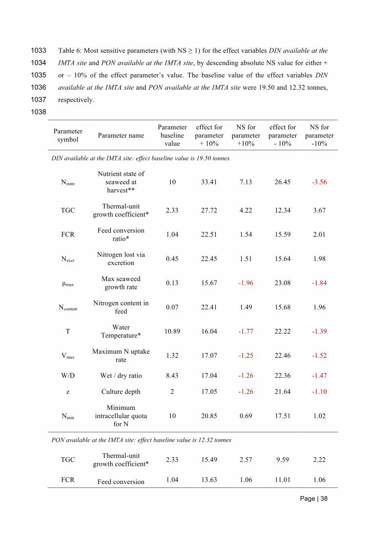
Page | 38

Table 6: Most sensitive parameters (with NS ≥ 1) for the effect variables DIN available at the 1033

IMTA site and PON available at the IMTA site, by descending absolute NS value for either + 1034

or – 10% of the effect parameter’s value. The baseline value of the effect variables DIN 1035

available at the IMTA site and PON available at the IMTA site were 19.50 and 12.32 tonnes, 1036

respectively. 1037

1038

Parameter symbol Parameter name

Parameter baseline

value

effect for parameter

+ 10%

NS for parameter

+10%

effect for parameter

- 10%

NS for parameter

-10%

DIN available at the IMTA site: effect baseline value is 19.50 tonnes.

Nstate Nutrient state of

seaweed at harvest**

10 33.41 7.13 26.45 -3.56

TGC Thermal-unit growth coefficient* 2.33 27.72 4.22 12.34 3.67

FCR Feed conversion ratio* 1.04 22.51 1.54 15.59 2.01

Nexcr Nitrogen lost via

excretion 0.45 22.45 1.51 15.64 1.98

µmax Max seaweed growth rate 0.13 15.67 -1.96 23.08 -1.84

Ncontent Nitrogen content in

feed 0.07 22.41 1.49 15.68 1.96

T Water Temperature* 10.89 16.04 -1.77 22.22 -1.39

Vmax Maximum N uptake

rate 1.32 17.07 -1.25 22.46 -1.52

W/D Wet / dry ratio 8.43 17.04 -1.26 22.36 -1.47

z Culture depth 2 17.05 -1.26 21.64 -1.10

Nmin Minimum

intracellular quota for N

10 20.85 0.69 17.51 1.02

PON available at the IMTA site: effect baseline value is 12.32 tonnes

TGC Thermal-unit growth coefficient*

2.33 15.49 2.57 9.59 2.22

FCR Feed conversion 1.04 13.63 1.06 11.01 1.06

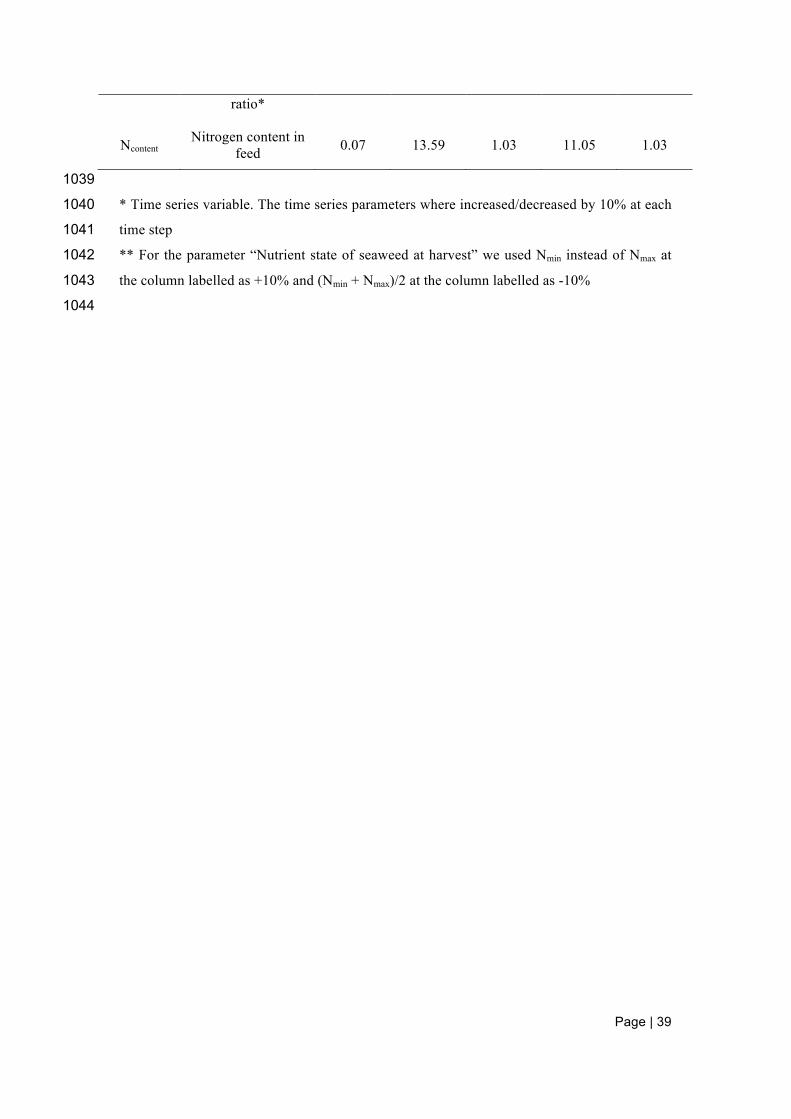
Page | 39

ratio*

Ncontent Nitrogen content in

feed 0.07 13.59 1.03 11.05 1.03

1039

* Time series variable. The time series parameters where increased/decreased by 10% at each 1040

time step 1041

** For the parameter “Nutrient state of seaweed at harvest” we used Nmin instead of Nmax at 1042

the column labelled as +10% and (Nmin + Nmax)/2 at the column labelled as -10%  1043

1044