Manufacturing Processes - II · Module 2 Mechanics of Machining Version 2 ME IIT, Kharagpur . Lesson 4 Conversion of tool angles from one system to another Version 2 ME IIT, Kharagpur

Module 2

Mechanics of Machining

Version 2 ME IIT, Kharagpur

Lesson 4

Conversion of tool angles from one system

to another


Instructional objectives At the end of this lesson the students should be able to (i) State the purposes of conversion of tool angles (ii) Identify the four different methods of conversion of tool angles (iii) Employ the graphical method for conversion of

• Rake angles • clearance angles • Cutting angles

From ASA to ORS and ORS to ASA systems (iv) Convert rake angle and clearance angle from ORS to NRS (v) Demonstrate tool angle’s relationship in some critical conditions.

(i) Purposes of conversion of tool angles from one system to another

• To understand the actual tool geometry in any system of choice or convenience from the geometry of a tool expressed in any other systems

• To derive the benefits of the various systems of tool designation as and when required

• Communication of the same tool geometry between people following different tool designation systems.

(ii) Methods of conversion of tool angles from one system to another

• Analytical (geometrical) method: simple but tedious • Graphical method – Master line principle: simple, quick and popular • Transformation matrix method: suitable for complex tool geometry • Vector method: very easy and quick but needs concept of vectors

(iii) Conversion of tool angles by Graphical method – Master Line principle. This convenient and popular method of conversion of tool angles from ASA to ORS and vice-versa is based on use of Master lines (ML) for the rake surface and the clearance surfaces.

• Conversion of rake angles The concept and construction of ML for the tool rake surface is shown in Fig. 4.1.


A

B

C

D

A' B'

C'

D'O'

O' O'

Zm

Xm

Ym

Xm

Xo

O' Zm

Ym

λ

γx

γo

γy

Master line for rake surface

πR

πX

πY

πC

T

T

T

φ

Zo Yo

Zo

Yo

O

πR

πo

πR

T

Xo

Fig. 4.1 Master line for rake surface (with all rake angles: positive) In Fig. 4.1, the rake surface, when extended along πX plane, meets the tool’s bottom surface (which is parallel to πR) at point D’ i.e. D in the plan view. Similarly when the same tool rake surface is extended along πY, it meets the tool’s bottom surface at point B’ i.e., at B in plan view. Therefore, the straight line obtained by joining B and D is nothing but the line of intersection of the rake surface with the tool’s bottom surface which is also parallel to πR. Hence, if the rake surface is extended in any direction, its meeting point with the tool’s bottom plane must be situated on the line of intersection, i.e., BD. Thus the points C and A (in Fig. 4.1) obtained by extending the rake surface along πo and πC respectively upto the tool’s bottom surface, will be situated on that line of intersection, BD. This line of intersection, BD between the rake surface and a plane parallel to πR is called the “Master line of the rake surface”. From the diagram in Fig. 4.1, OD = TcotγX

OB = TcotγY

OC = Tcotγo

OA = Tcotλ


Where, T = thickness of the tool shank. The diagram in Fig. 4.1 is redrawn in simpler form in Fig. 4.2 for conversion of tool angles.

A

B

C M

E

F

φ φγ

Ym

Xm

Xo Yo

D

Masterline of Rake surface

OD = cotγxOB = cotγyOC = cotγoOA = cotλ

for T=unity]

O G

Fig. 4.2 Use of Master line for conversion of rake angles.

• Conversion of tool rake angles from ASA to ORS γo and λ (in ORS) = f (γx and γy of ASA system) cosφtanγsinφtanγtanγ yxo += (4.1) and sinφtanγcosφtanγtanλ yx +−= (4.2) Proof of Equation 4.1: With respect to Fig. 4.2, Consider, ΔOBD = Δ OBC + Δ OCD Or, ½ OB.OD = ½ OB.CE + ½ OD.CF Or, ½ OB.OD = ½ OB.OCsinφ + ½ OD.OCcosφ Dividing both sides by ½ OB.OD.OC,

cosφOB1sinφ

OD1

OC1

+=

i.e. ⎯ Proved. cosφtanγsinφtanγtanγ yxo +=


Similarly Equation 4.2 can be proved considering; Δ OAD = Δ OAB + Δ OBD i.e., ½ OD.AG = ½ OB.OG + ½ OB.OD where, AG = OAsinφ and OG = OAcosφ Now dividing both sides by ½ OA.OB.OD,

OA1cosφ

OD1sinφ

OB1

+=

⎯ Proved. sinφtanγcosφtanγtanλ yx +−=The conversion equations 4.1 and 4.2 can be combined in a matrix form,

(4.3) ⎥⎦

⎤⎢⎣

⎡⎥⎦

⎤⎢⎣

⎡−

=⎥⎦

⎤⎢⎣

⎡

y

xo

γγ

φφφφ

λγ

tantan

sincoscossin

tantan

(ORS) (ASA)

where, is the transformation matrix. ⎥⎦

⎤⎢⎣

⎡− φφ

φφsincoscossin

• Conversion of rake angles from ORS to ASA system γx and γy (in ASA) = f(γo and λof ORS) cosφtansinφtanγtanγ ox λ−= (4.4) and sinφtancosφtanγtanγ oy λ+= (4.5) The relations (4.4) and (4.5) can be arrived at indirectly using Equation 4.3. By inversion, Equation 4.3 becomes,

(4.6) ⎥⎦

⎤⎢⎣

⎡⎥⎦

⎤⎢⎣

⎡ −=⎥

⎦

⎤⎢⎣

⎡λγ

φφφφ

γγ

tantan

sincoscossin

tantan o

y

x

from which equation 4.4 and 4.5 are obtained. The conversion equations 4.4 and 4.5 can also be proved directly from the diagram in Fig. 4.2 Hints To prove equation 4.4, proceed by taking (from Fig. 4.2) Δ OAD = Δ OAC + Δ OCD, [involving the concerned angles γo, λ and γx i.e., OC, OA and OD] And to prove Equation 4.5, proceed by taking Δ OAC = Δ OAB + Δ OBC [involving the concerned angles γo, λ and γy i.e., OC, OA and OB] • Maximum rake angle (γmax or γm) The magnitude of maximum rake angle (γm) and the direction of the maximum slope of the rake surface of any single point tool can be easily derived from its geometry specified in both ASA or ORS by using the diagram of Fig. 4.2. The smallest intercept OM normal to the Master line (Fig. 4.2) represents γmax or γm as


OM = cot γmSingle point cutting tools like HSS tools after their wearing out are often resharpened by grinding their rake surface and the two flank surfaces. The rake face can be easily and correctly ground by using the values of γm and the orientation angle, φγ (visualized in Fig. 4.2) of the Master line. • Determination of γm and φγ from tool geometry specified in ASA system. In Fig. 4.2, Δ OBD = ½ OB.OD = ½ BD.OM or, ½ OB.OD = ½ OMODOB .22 + Dividing both sides by ½ OB.OD.OM

22 OB1

OD1

OM1

+=

or y2

x2

m γtanγtantanγ += (4.7)

Again from Δ OBD

ODOBtanφγ =

or ⎟⎟⎠

⎞⎜⎜⎝

⎛= −

y

x

γγ

φγ tantan

tan (4.8)

• γm and φγ from tool geometry specified in ORS Similarly from the diagram in Fig. 4.2, and taking Δ OAC, one can prove λ2

o2

m tanγtantanγ += (4.9)

⎟⎟⎠

⎞⎜⎜⎝

⎛−= −

oγλφφγ tan

tantan (4.10)

• Conversion of clearance angles from ASA system to ORS and vice

versa by Graphical method. Like rake angles, the conversion of clearance angles also make use of corresponding Master lines. The Master lines of the two flank surfaces are nothing but the dotted lines that appear in the plan view of the tool (Fig. 4.3). The dotted line are the lines of intersection of the flank surfaces concerned with the tool’s bottom surface which is parallel to the Reference plane πR. Thus according to the definition those two lines represent the Master lines of the flank surfaces. Fig. 4.4 shows the geometrical features of the Master line of the principal flank of a single point cutting tool. From Fig. 4.4,

OD = Ttanαx

OB = Ttanαy

OC = Ttanαo


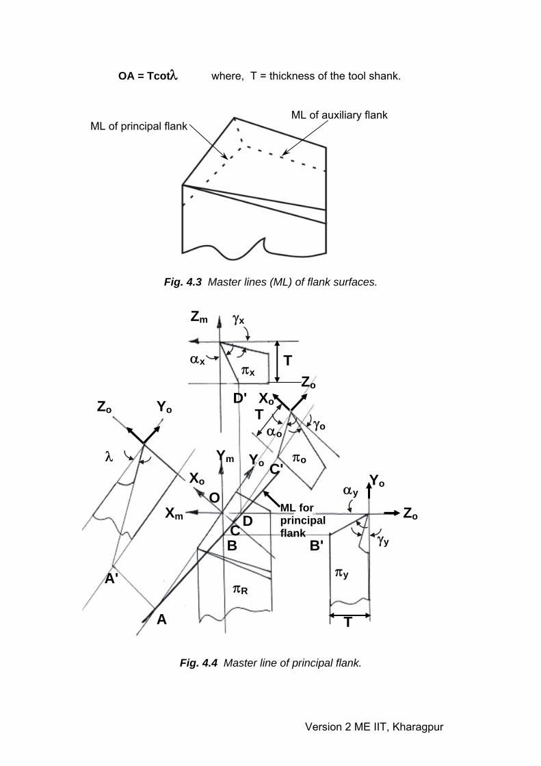
OA = Tcotλ where, T = thickness of the tool shank.

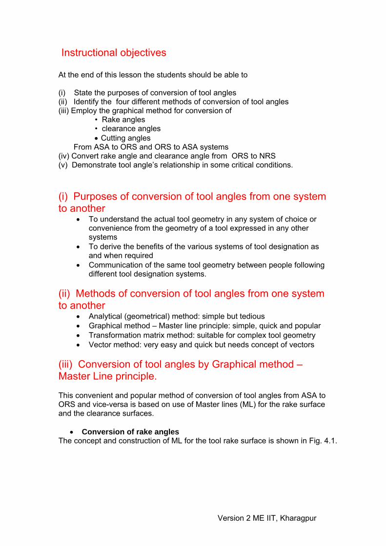
ML of principal flank ML of auxiliary flank

Fig. 4.3 Master lines (ML) of flank surfaces.

λ

αx

αy

γx

γy

αo

πx

πo

πyπR

O

Ym

Xm

Xo

Yo

Yo

Zo

Zo Xo

Zm

Zo Yo

A'

D'

C'

B' B

C D

A

ML for principal flank

T

T

T

γo

Fig. 4.4 Master line of principal flank.


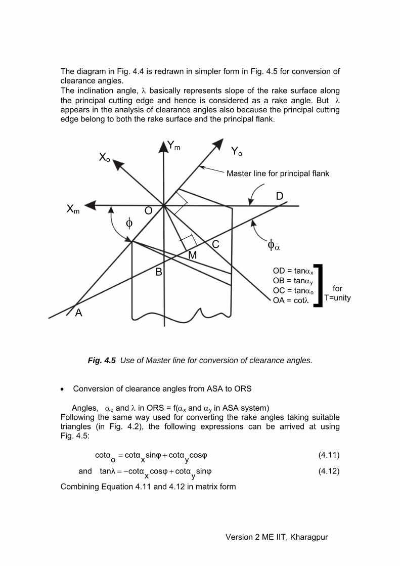
The diagram in Fig. 4.4 is redrawn in simpler form in Fig. 4.5 for conversion of clearance angles. The inclination angle, λ basically represents slope of the rake surface along the principal cutting edge and hence is considered as a rake angle. But λ appears in the analysis of clearance angles also because the principal cutting edge belong to both the rake surface and the principal flank.

φα

φ

A

B

M

C

O

Ym YoXo

Xm

Master line for principal flank

OD = tanαxOB = tanαyOC = tanαoOA = cotλ ] for

T=unity

D

Fig. 4.5 Use of Master line for conversion of clearance angles. • Conversion of clearance angles from ASA to ORS Angles, αo and λ in ORS = f(αx and αy in ASA system) Following the same way used for converting the rake angles taking suitable triangles (in Fig. 4.2), the following expressions can be arrived at using Fig. 4.5: cosφycotαsinφxcotαocotα += (4.11)

and sinφycotαcosφxcotαtanλ +−= (4.12)

Combining Equation 4.11 and 4.12 in matrix form


(4.13) ⎥⎦

⎤⎢⎣

⎡⎥⎦

⎤⎢⎣

⎡−

=⎥⎦

⎤⎢⎣

⎡

y

xo

αα

φφφφ

λα

cotcot

sincoscossin

tancot

• Conversion of clearance angles from ORS to ASA system

αx and αy (in ASA) = f(αo and λ in ORS) Proceeding in the same way using Fig. 4.5, the following expressions are derived cosφsinφocotαxcotα λtan−= (4.14)

and sinφcosφocotαycotα λtan+= (4.15)

The relations (4.14) and (4.15) are also possible to be attained from inversions of Equation 4.13 as indicated in case of rake angles.

• Minimum clearance, αmin or αm The magnitude and direction of minimum clearance of a single point tool may be evaluated from the line segment OM taken normal to the Master line (Fig. 4.5) as OM = tanαmThe values of αm and the orientation angle, φα (Fig. 4.5) of the principal flank are useful for conveniently grinding the principal flank surface to sharpen the principal cutting edge. Proceeding in the same way and using Fig. 4.5, the following expressions could be developed to evaluate the values of αm and φα

o From tool geometry specified in ASA system

yxm ααα 22 cotcotcot += (4.16)

and ⎟⎟⎠

⎞⎜⎜⎝

⎛= −

y

x

αα

φγ cotcottan 1

(4.17)

o From tool geometry specified in ORS

λαα 20

2 tancotcot +=x (4.18)

and ⎟⎟⎠

⎞⎜⎜⎝

⎛−= −

oαλφφα cot

tantan 1 (4.19)

Similarly the clearance angles and the grinding angles of the auxiliary flank surface can also be derived and evaluated. o Interrelationship amongst the cutting angles used in ASA and ORS The relations are very simple as follows: φ (in ORS) = 90o - φs (in ASA) (4.20)

and φ1(in ORS) = φe (in ASA) (4.21)


(iv) Conversion of tool angles from ORS to NRS The geometry of any single point tool is designated in ORS and NRS respectively as,

λ, γo, αo, αo’, φ1, φ, r (mm) – ORS λ, γn, αn, αn’, φ1, φ, r (mm) – NRS

The two methods are almost same, the only difference lies in the fact that γo, αo and αo’ of ORS are replaced by γn, αn and αn’ in NRS. The corresponding rake and clearance angles of ORS and NRS are related as , tanγn = tanγocosλ (4.22) cotαn = cotαocosλ (4.23) and cotαn'= cotαo'cosλ' (4.24) The equation 4.22 can be easily proved with the help of Fig. 4.6.

λ λ

γo

γn

γo

γn

λ

πn

πc

ZoZn Yn

Yo

A

B

C A

B A

C

Xo, Xn

λ

Fig. 4.6 Relation between normal rake (γn) and orthogonal rake (γo) The planes πo and πn are normal to Yo and Yn (principal cutting edge) respectively and their included angle is λ when πo and πn are extended below OA (i.e. πR) they intersect the rake surface along OB and OC respectively. Therefore, ∠AOB = γo ∠AOC = γnwhere, ∠BAC = λ


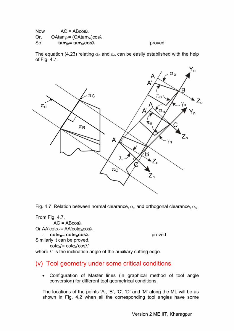
Now AC = ABcosλ Or, OAtanγn= (OAtanγo)cosλ So, tanγn= tanγocosλ proved The equation (4.23) relating αn and αo can be easily established with the help of Fig. 4.7.

Fig. 4.7 Relation between normal clearance, αn and orthogonal clearance, αo From Fig. 4.7, AC = ABcosλ Or AA’cotαn= AA’cotαocosλ ∴ cotαn= cotαocosλ proved Similarly it can be proved, cotαn’= cotαo’cosλ’ where λ’ is the inclination angle of the auxiliary cutting edge. (v) Tool geometry under some critical conditions

• Configuration of Master lines (in graphical method of tool angle conversion) for different tool geometrical conditions.

The locations of the points ‘A’, ‘B’, ‘C’, ‘D’ and ‘M’ along the ML will be as shown in Fig. 4.2 when all the corresponding tool angles have some

λ

αn

αo

γo

γn

πn

πo

πC

πR

A

B

C

A

C

A

B A'

A'

Zn

Zo

Zn

Yn

Zo

Yo

πC

πo


positive values. When any rake angle will be negative, the location of the corresponding point will be on the other side of the tool. Some typical configurations of the Master line for rake surface and the corresponding geometrical significance are indicated in Fig. 4.8.

Configuration of ML Tool geometry

f

or ML parallel to πC

γx = positive γy = positive

γo = positive λ = 0 γm = γo for ML parallel to πY γx = positive γy = 0

γo = positive λ = negative

γm = γx for ML parallel to πX γx = 0 γy = negative γo = negative λ = negative ⏐γm⏐ = ⏐γy⏐

(c)

(b)

(a)

O

ML

ML

C B A

O

B at infinity

C

D

A

ML

A at infinity

O

D C

B


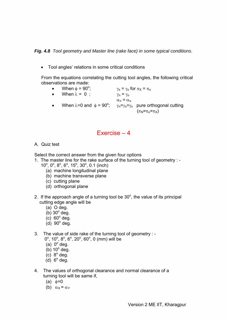
Fig. 4.8 Tool geometry and Master line (rake face) in some typical conditions.

• Tool angles’ relations in some critical conditions From the equations correlating the cutting tool angles, the following critical observations are made:

• When φ = 90o; γx = γo for πX = πo • When λ = 0 ; γn = γo

αn = αo• When λ=0 and φ = 90o; γn=γo=γx pure orthogonal cutting

(πN=πo=πX)

Exercise – 4 A. Quiz test Select the correct answer from the given four options 1. The master line for the rake surface of the turning tool of geometry : - 10o, 0o, 8o, 6o, 15o, 30o, 0.1 (inch) (a) machine longitudinal plane (b) machine transverse plane (c) cutting plane (d) orthogonal plane 2. If the approach angle of a turning tool be 30o, the value of its principal cutting edge angle will be (a) O deg. (b) 30o deg. (c) 60o deg. (d) 90o deg. 3. The value of side rake of the turning tool of geometry : - 0o, 10o, 8o, 6o, 20o, 60o, 0 (mm) will be (a) 0o deg. (b) 10o deg. (c) 8o deg.

(d) 6o deg.

4. The values of orthogonal clearance and normal clearance of a turning tool will be same if, (a) φ=0 (b) αX = αY


(c) λ = 0 (d) none of the above 5. The angle between orthogonal plane and normal plane of a turning tool is (a) γo (b) φ (c) γn (d) λ B. Problem 1. Determine the values of normal rake of the turning tool whose geometry is designated as : 10o, - 10o, 8o, 6o, 15o, 30o, 0 (inch)? 2. Determine the value of side clearance of the turning tool whose geometry is specified as 0o, - 10o, 8o, 6o, 20o, 60o, 0 (mm) ? Solutions of Exercise – 4 A. Quiz test 1 – (a) 2 – (c) 3 – (b) 4 – (c) 5 – (d) B. Problems Ans. 1 Tool geometry given : 10o, - 10o, 8o, 6o, 15o, 30o, 0 (inch) γy, γx, αy, αx, φe, φs, r – ASA tanγn = tanγocosλ where, tanγo = tanγxsinφ + tanγycosφ = tan(-10o)sin(90o- 30o) + tan(10o)cos(90o- 30o) = - 0.065 So, γo = - 3.7o

And tanλ = - tanγxcosφ + tanγysinφ = - tan(-10o)cos(90o- 30o) + tan(10o)sin(90o- 30o) = 0.2408 So, λ = 13.54o

tanγn = tanγocosλ = tan (-3.7)cos(13.54) = - 0.063 So, γn = - 3.6o Ans.


Ans. 2 Tool geometry given : 0o, - 10o, 8o, 6o, 20o, 60o, 0 (mm) λ, γo, αo, αo', φ1, φ , r (mm) cotαx = cotαosinφ- tanλcosφ = cot 8.sin60 – tan0.cos60 = cot8.sin60 = 6.16 So, αx = 9.217o Ans.


Manufacturing Processes - II · Module 2 Mechanics of Machining Version 2 ME IIT, Kharagpur . Lesson 4 Conversion of tool angles from one system to another Version 2 ME IIT, Kharagpur

Documents