Federal Reserve Bank of Chicago Manufacturing Plants’ Use of Temporary Workers: An Analysis Using Census Micro Data Yukako Ono and Daniel Sullivan REVISED February 2010 WP 2006-24

Welcome message from author
This document is posted to help you gain knowledge. Please leave a comment to let me know what you think about it! Share it to your friends and learn new things together.
Transcript

Fe
dera
l Res
erve
Ban
k of
Chi
cago
Manufacturing Plants’ Use of Temporary Workers: An Analysis Using Census Micro Data Yukako Ono and Daniel Sullivan
REVISED February 2010
WP 2006-24

1
Manufacturing Plants’ Use of Temporary Workers: An Analysis Using Census Micro Data
Yukako Ono and Daniel Sullivan, Federal Reserve Bank of Chicago1
February, 2010
Abstract
How is the nature of firms’ output fluctuations associated with the firms’ preferences
between permanent (indefinite term) and temporary (definite term) labor contract? Using
plant-level data from the Plant Capacity Utilization (PCU) survey, we explore how
manufacturing plants’ use of temporary workers is associated with the nature of their output
fluctuations and other plant characteristics. We find that plants tend to use temporary workers
when their output is expected to fall; this may indicate that firms use temporary workers to
reduce costs associated with dismissing permanent employees. In addition, we find that
plants whose future output levels are subject to greater uncertainty tend to use more
temporary workers. We also examine the effects of wage and benefit levels for permanent
workers, unionization rates, turnover rates, seasonal factors, and plant size and age on the use
of temporary workers; based on our results, we discuss various views of why firms use
temporary workers.
Key words: temporary workers, output fluctuations
JEL codes: J2, J3
1 The research in this paper was conducted while the authors were Special Sworn Status researchers of the U.S. Census Bureau at the Chicago Census Research Data Center. Views, research results, and conclusions expressed are those of the authors and do not necessarily reflect the views of the Census Bureau, the Federal Reserve Bank of Chicago, or the Federal Reserve System. This paper has been screened to insure that no confidential data are revealed. Support for this research at the Chicago RDC from NSF (awards no. SES-0004335 and ITR-0427889) is also gratefully acknowledged.

2
1. Introduction
The temporary help industry (THS) has grown rapidly over the last quarter century. The
industry’s rapid growth has attracted substantial attention from researchers (ex. Autor (2003),
Erickcek, Houseman, and Kelleberg (2002), Golden (1996), Houseman (2001), Polivka
(1996), and Segal and Sullivan (1995, 1997)) who, along with industry analysts, have
identified a number of reasons why temporary workers may be attractive to client firms
beyond their traditional role of filling in when permanent employees are absent for short
periods.
In this paper, we investigate to what extent temporary workers are used by firms to
accommodate fluctuations in production level. While various papers (Houseman (2001),
Segal and Sullivan (1995, 1997), Golden (1996), Autor (2003)) seem to view this role as one
of primary reasons why firms use temporary workers, few papers examine how a firm’s use
of these workers is associated with the nature of its output fluctuation.2
As many papers (ex. Hamermesh (1989), Bentolila and Bertola (1990),
Aguirregabiria and Alonso-Borrego (1999), and Campbell and Fisher (2004)) have
considered, adjusting the level of permanent employees can involve hiring and firing costs.
This contrasts with adjusting the level of temporary workers; a firm can reduce the number of
temporary workers when the short-term contract ends without additional costs, and less
training is typically required for the type of jobs filled by temporary workers. The use of
temporary workers may, however, incur higher unit costs of labor; because the short-term
contracts impose more job insecurities (Houseman and Polivka, 2000), and, given the skill of
2 Houseman (2001) surveyed firms about their use of temporary workers and found that a substantial fraction of firms reported meeting fluctuations in demand as a reason. Campbell and Fisher (2004) developed a theoretical model describing a firm’s decision to adjust employment of two groups of workers with some of the characteristics of temporary and permanent workers and compare their calibration with aggregate level data. However, there are no empirical studies that examine the relationship between a firm’s use of temporary workers and its own output fluctuations.
3
a worker, the worker may demand higher wages for a temporary job than a permanent job.
The temporary help agencies also charge a margin. Productivity may also be lower for those
under the temporal employment contract, which increase the costs for an efficient unit of
labor.
Focusing on such differences in the nature of costs associated with using permanent
and temporary workers, our stylized model suggests that the firm that experiences higher
output volatility maintains a higher temporary worker share when firing costs are high. Our
stylized model also suggests that the firm that expects its output to fall maintains higher
temporary worker share. When the firm expects its output to fall, it can justify the use of
temporary workers in the current period, even when the unit labor costs are higher than those
of permanent employees. This is because the firm can avoid the potential costs associated
with dismissing permanent employees. In the empirical section of this paper, we test the
above implications by examining a manufacturing plant’s use of temporary workers.
Few empirical papers document the characteristics of firms that use temporary
workers, while the literature has focused on documenting the difference in demographic
characteristics between temporary and permanent workers (Polivka (1996), Cohany (1998)).
One reason might have been limited data that provide the detailed characteristics of firms
using temporary workers. The data is limited because the temporary workers are not on the
payroll of firms that they engage in production activities. Thus, they are not in the
employment data collected in the major economic surveys or census, such as the ASM and
the CM.3 Abowd, Corbel, and Kramarz (1999) use the French data4 that allows them to
distinguish contract type (short-term or permanent) of employment and report that short-term
3 This has also caused issues in labor productivity measure based on payroll data as Houseman (2007) points out. Understanding what kind of firms use temporary workers helps us to infer whose labor productivity measure might have been influenced.

4
contracts represents high share in hiring and separations.5 However, the number of firm
characteristics that are incorporated in their study is limited.
We use the plant-level data from the Plant Capacity Utilization (PCU) survey
conducted by the U.S. Census Bureau.6 The PCU survey began collecting information on the
number of temporary workers used at manufacturing plants in 1998. The data for 1998, 1999,
2000, and 2001 are available for our study. We also link the plant-level PCU data to the
plant-level Annual Survey of Manufactures (ASM) and the Census of Manufactures (CM),
which provides us with a unique opportunity to observe a plant’s output fluctuations over
time. We fit an autoregressive form to a plant’s output trajectories to create a measure of
output fluctuations and expected output growth.
While our focus is on testing to what extent firms use temporary workers to
accommodate output fluctuation, we also discuss other motives. In particular, the use of
temporary workers has been considered attractive to firms as a means to screen potential
permanent employees. Autor (2003) points out that THS agency plays a role of facilitating
worker screening. Given the sometimes significant costs of dismissing poorly performing
employees, a client firm may want to first observe their performance as temporary workers.
If that performance is judged inadequate, they can simply request a new worker from the
THS agency. Such a trial period as a temporary worker may be preferable to a formal
probationary period as a permanent employee.
Depending on the primary motive to use temporary workers, higher expected output
growth could be associated with greater or lesser use of temporary workers. If the primary
4 Their data come from four surveys conducted by the Institut National de la Statistique et des Etudes Economiques. 5 They found that two-thirds of all hiring and more than half of all separations are involved with short-term contracts. 6 These data are used by the Federal Reserve Board to estimate capacity utilization rates for the manufacturing and publishing industries.

5
motive to use temporary workers is to reduce the potential costs of dismissing permanent
workers due to the lower expected output, the expectations of higher output growth would be
associated with lesser use of temporary workers. In addition, as our stylized model shows, if
firing costs are sufficiently high, greater uncertainty about future output leads the firm to cap
the number of permanent workers at a lower level, and thus hire more temporary workers. In
contrast, if the primary motive to use temporary workers is to screen future permanent
workers, then higher expected output growth is likely to be associated with greater use of
temporary workers, because, by doing so, the firm can secure enough qualified workers for
next period. In the empirical section, we also discuss which stories seem to dominate in our
findings.
The different motives to use temporary workers are considered to have different labor
market outcomes for temporary workers. As Houseman and Polivka (2000) and Houseman
(2001) point out, while the growth of temporary work arrangements or other non-standard
arrangements is considered to reduce job stability, if firms use these arrangements primarily
to screen workers for regular jobs, then job stability for these workers may increase by
facilitating better matches between workers and firms. Few empirical papers, however,
compare the motivations for firms to use temporary workers.7
In addition to testing plant’s use of temporary workers in relation to its output
fluctuation, we also examine how a plant’s temporary worker share depends on a number of
other characteristics, such as its size, age, and the product that a plant produces. There are
number of reasons why plant size may matter for a plant’s use of temporary workers. One
might imagine that the use of temporary workers to buffer fluctuations in the labor
7 In Houseman and Polivka (2000), only weak evidence is found for a firm’s use of temporary workers for screening purpose, while there was clear evidence that temporary workers face much more job insecurities than regular full or pert-time workers. Houseman (2001) also reports many employers report the use of temporary workers as accommodating fluctuations in their work load rather than screening.

6
requirement may require a level of sophistication likely to be found in a large plant. Its larger
size may also increase a plant’s ability to negotiate a lower margin from a THS firm. In
addition, a larger plant, with its deeper pockets, may face higher costs in the event of an
unjust dismissal lawsuit. On the other hand, the larger scale of such a plant may allow the
plant to be flexible without relying on temporary workers, by redistributing its permanent
workers across different production processes. Plant age and industry may also matter for the
use of temporary workers because of their effect on the level of uncertainty and other factors.
Moreover, we investigate the relationship between the use of temporary workers and
a plant’s wage and benefit levels. It has been suggested that the use of temporary workers
may allow client firms to circumvent nondiscrimination requirements in the provision of
benefits (Houseman, 2001). Under normal circumstances, in order to secure the tax
advantages associated with providing certain benefits, firms need to provide those benefits to
all their employees. If the firm would not otherwise want to provide a certain benefit to a
particular segment of its workforce, one strategy might be to staff that segment with
employees of a THS agency. Having such a dual work force may allow it to provide benefits
to the remainder of its workforce without jeopardizing their tax status.8 It is possible that a
plant whose permanent workers earn high wage rates is more motivated to use temporary
workers. However, what should matter for the choice of temporary worker share is the ratio
of temporary worker to permanent worker wage rates. Industry observers indicate that THS
agencies charge client firms a higher markup over wages in the case of higher skilled workers
(Kilcoyne, 2004). Thus, it is possible that a firm with a high wage rate for permanent workers
8 The legal issues surrounding the employment status of temporary workers are complex. A temporary worker can under some circumstances be considered an employee of the client firm. In particular, in the Microsoft case, the U.S. Supreme Court ruled that temporary workers who provided services to Microsoft for a period of several years were entitled to benefits, including stock options, which Microsoft provided to all its permanent employees. The Microsoft decision has limited firms’ ability to implement such a strategy of using the same temporary workers for long periods.

7
might use temporary workers less. A similar argument may apply to a firm that provides
generous benefit packages, although it is also possible that a firm that provides expensive
benefits packages may have greater incentive to employ temporary workers to keep benefit
costs low.
Finally, we analyze how the temporary worker share at the three-digit NAICS
industry level is dependent upon several additional variables. These variables include
unionization, labor turnover rates, and seasonality. We expect unions to resist the use of
temporary workers and thus would expect a lesser use of temporary help in an industry with a
higher unionization rate. When voluntary turnover is high, the likelihood of a firm needing
to fire workers due to insufficient demand would be lower. So, greater turnover could be
associated with less use of temporary workers. At the same time, higher voluntary turnover
rates would likely increase the value of screening potential employees and thus could lead to
greater use of temporary workers. A stronger seasonal component would also be positively
correlated with the higher use of temporary workers, ceteris paribus.
One can view our study as similar in intent to a number of micro-level studies of
other forms of firm adjustment to demand shocks. For example, using plant-level data,
Copeland and Hall (2005) examine how automakers accommodate shocks to demand by
adjusting price, inventories, and labor inputs through temporary layoffs and overtime work.
Such considerations are closely linked to a firm’s decision to adjust temporary worker share.
We intend to examine such interactions in future work.
In Section 2, we provide a stylized model that motivates our empirical specification.
In Section 3, we describe our data in more detail and discuss empirical implementation. In
Section 4, we present our empirical results. Section 5 concludes.

8
2. Motivational Model
In this section, we present a stylized model of a plant’s choice on the number of permanent
and temporary workers. The model is intended to help motivate and guide our empirical work,
emphasizing the role of temporary workers in accommodating output fluctuations.
We assume that labor is the only factor of production and that, in each period, the
plant manager must hire an appropriate quantity of labor, te , to meet an exogenously
determined level of output, ( )t ty f e= , where f is a standard, strictly increasing production
function. The required labor input come from a combination of “permanent employees,” tp ,
and “agency temporary workers,” ta , with the total quantity of labor given by t t te p aθ= + ,
where θ is a positive constant representing the productivity of a temporary worker relative to
that of a permanent worker. The wage rates for permanent and temporary workers are pw
and aw , respectively. The plant incurs costs, δ , to fire each permanent worker. Thus, the
plant’s total costs in a period are 1max( ,0)p t a t t tw p w a p pδ −+ + − . We assume that future
levels of output are uncertain and that the firm minimizes the expected present value of total
costs given a discount factor, 1/(1 )rβ = + , where γ is a real interest rate.
Let the unit labor costs for permanent workers be p pu w≡ and that for temporary
workers /a au w θ≡ . We assume that 0a pu u uΔ = − > ; absent firing costs, temporary workers
are more expensive, either because their wage rate is higher ( a pw w> ), they are less
productive ( 1θ < ), or both.9 We further assume that the cost of firing a permanent worker is
9 Kilcoyne shows that, for a given low-skilled occupation, temporary workers are paid lower hourly wages. This may reflect their lower productivity; for low-skilled jobs where experience or reputation is not important for future employment, it may be difficult to motivate temporary workers to achieve a high level of performance because their efforts would not, typically, be rewarded by promotion or future wage increases. The legal limit of a temporary employment contract duration would also imply that temporary employment would not increase a worker’s firm-specific skills and knowledge. In high-skilled occupations,

9
greater than the (discounted) difference in unit labor costs, but less than a full period’s wage;
i.e., / pu wβ δΔ < < . If u βδΔ > , the plant never hires any temporary workers; it is cheaper
to use permanent workers even if it is certain that they will be fired in the next period. The
condition that pwδ < is a convenient simplification implying that the firm does not keep any
idle workers on the payroll; keeping an idle worker on the payroll costs more than firing the
worker in the current period and may also increase firing costs in the future. With this
configuration of costs, the plant faces a tradeoff between using more permanent workers,
which lowers current wage costs, versus using more temporary workers, which may lower
future firing costs.
The Two-Period Case
It is easiest to see the logic of the model when there are only two periods. In this case, the
plant is unconcerned about firing costs in the second period. Let 2y represent a required
output level in the second period. The plant meets its entire labor need with permanent
workers, 12 2( )p f y−= , incurring costs 1 1
2 2 1 2( ) max(0, ( ))pC w f y p f yδ− −= + − .
In the first period, given 1y and knowledge of the distribution of 2y , the firm chooses
1p and 1a to minimize total expected discounted costs, TC , which is written as
1 11 1 2 1 2[ ( ) max(0, ( ))]p a pTC w p w a E w f y p f yβ δ− −= + + + − . The quantity of labor that
meets the required level of production is 11 1 1( )f y p aθ− = + . Thus, we can rewrite TC as a
temporary workers are often paid higher hourly wages than permanent workers (Kilcoyne,2005). For example, on average, registered nurses sent by THS agencies earn an hourly wage that is $4.93 more than the national average for this occupation in 2004. Computer programmers sent by THS agencies earn $7.85 more per hour than those hired as permanent employees. For occupations in which past experience or licenses help firms identify workers’ skills, firms would be able to select temporary workers who are qualified to meet a given performance level. Among workers with the same qualifications, however, they

10
function of 1p alone:
1 1 11 1 1 2 1 2( ( ) ) [ ( ) max(0, ( ))]p a pTC u p u f y p E w f y p f yβ δ− − −= + − + + − .
Thus, the derivative of costs with respect to (w.r.t.) permanent labor in the first period is
11 1 2
1 1
( ) [max(0, ( )]dTC dp u E p f ydp dp
βδ −= −Δ + − . (1)
Assume that 2y follows a continuous distribution with density 2( )g y that is strictly
positive over the relevant interval; distribution function is 2( )G y . Then, the expected
number of permanent workers fired in the second period given 1p is
1( )1 11 1 2 1 2 2 20
( ) [max(0, ( )] ( ( )) ( )f p
L p E p f y p f y g y dy− −= − = −∫ . Thus the derivative of the
number of permanent workers fired w.r.t. permanent labor in period 1 is
1( )11 1 1 1 2 2 10
( ) ( ( ( )) ( ( )) ( ) ( ( ))f p
L p p f f p g f p g y dy G f p−′ = − + =∫ . (2)
From (2), we can rewrite (1) as
1 11
( ) ( ( ))dTC p u G f pdp
βδ= −Δ + . (3)
Increasing permanent workers by one (and thus lowering the number of temporary workers
by 1/θ ) in period 1 reduces current costs by the difference in unit costs between temporary
and permanent workers ( uΔ ), but raises expected firing costs in the second period by the
product of the cost of firing a worker (δ ) and the probability that the marginal worker is
fired ( ( ( ))G f p ).
would not take temporary positions unless compensation for job insecurity is provided. Employers may also be willing to pay a premium to quickly meet, say, a sudden increase in demand.

11
Because ( )G y and ( )f p are increasing functions, 11
( )dTC pdp
is increasing in 1p .
Moreover, 1
(0) 0dTC udp
= −Δ < and 1
11
lim ( ) 0p
dTC p udp
βδ→∞
= −Δ + > . Thus, there exists a
unique level of permanent employment, p , such that
1
( ) ( ( )) 0dTC p u G f pdp
βδ= −Δ + = . (4)
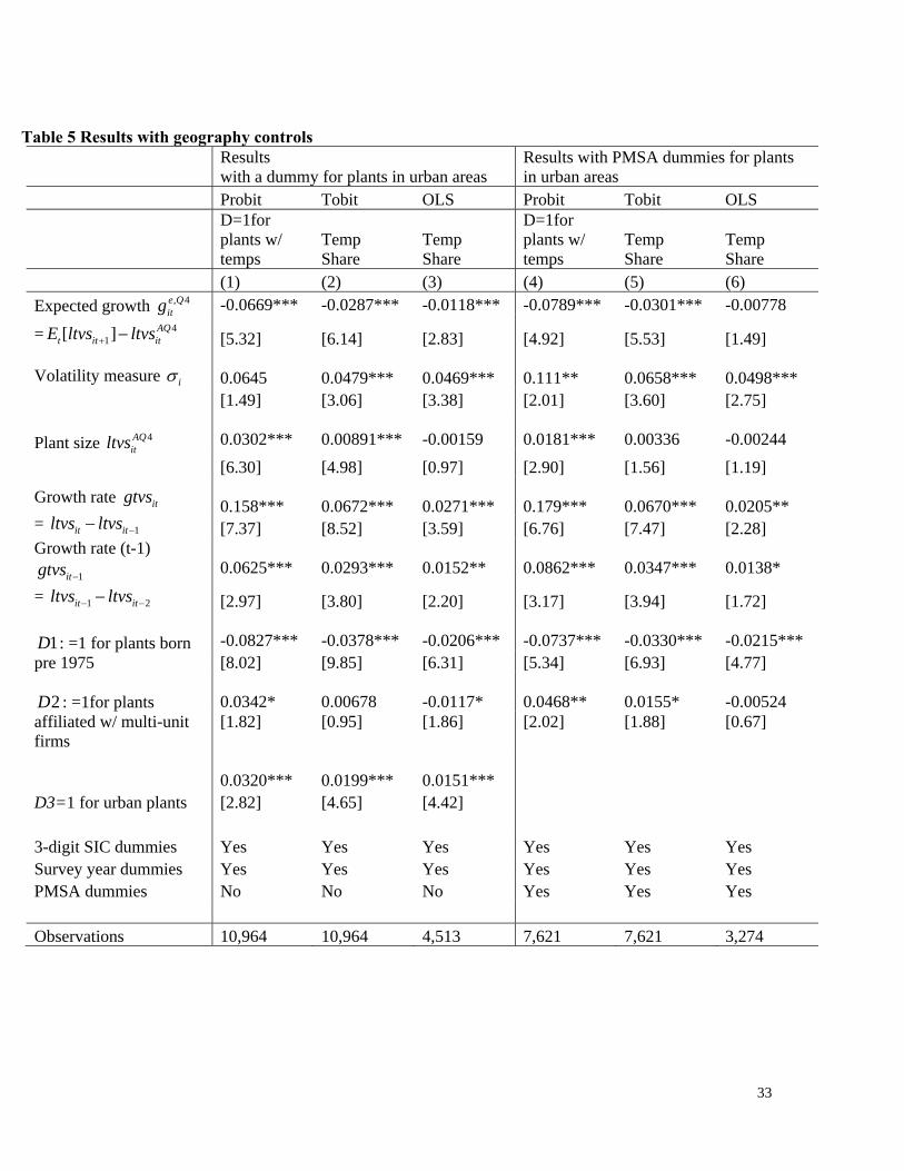
See Figure 1 for an illustration of the case in which 2y is uniformly distributed in the interval
from lowy to highy and ( )f e is linear. If 11( )f y p− < , as permanent employment increases,
TC decreases until permanent employment reaches the level that satisfies the plant’s labor
requirements given 1y . Thus, the optimal number of permanent workers is 11( )f y− , and that
of temporary workers is zero. On the other hand, if 11( )f y p− > , TC falls with 1p until
1p p= , and then begins to rise. Thus the optimal number of permanent workers is p , and
that of temporary workers is 11( ( ) ) /f y p θ− − , the level necessary to meet the rest of the
labor requirement. We can summarize the solution by writing the optimal numbers of the
first period permanent workers, *1p , and temporary workers, *
1a , as
* 11 1min( ( ), )p f y p−= (5)
* 1 *1 1 1( ( ) ) /a f y p θ−= − , (6)
where p satisfies ( ( ))G f p uβδ = Δ . The plant hires permanent workers up to a maximum
level at which the expected discounted costs of firing an additional permanent worker are
equal to the extra current unit labor costs of substituting temporary workers. In Appendix A,
we show that in the case of an infinite horizon with independently and identically distributed

12
(i.i.d.) random output levels; the plant’s optimal policy is essentially identical to the solution
of the first period of the two-period model.
Lognormal Output Levels and Power Production Function
Suppose that the distribution of 2y is lognormal, 2log y ~ 22( , )N μ σ and that the production
function takes the power form,
( )f e Aeα= . (7)
Then, based on (4), p is such that (s.t.) 2log log( )A pu α μβδσ
+ −Δ = Φ , where ( )xΦ is the
standard normal distribution function. Alternatively, we can write
1 12log [ log ( )]up Aα μ σ
βδ− − Δ
= − + Φ . (8)
The impact of σ on p depends on uΔ and firing costs δ .10 If firing costs are sufficiently
high so that 12
u βδΔ < , then 1( ) 0uβδ
− ΔΦ < , and the probability of needing to fire the
marginal worker is less than one half. In this case, greater uncertainty increases the
probability, moving it toward one half. The increased probability of firing causes the plant to
use fewer permanent workers and more temporary workers to produce the given output.11
10 Becauseα and δ are positive constants and 1 ( )−Φ ⋅ is an increasing function, a higher value of uΔ is associated with a greater level for p , leading to the use of fewer temporary workers. On the other hand, a higher value of the firing cost, δ , is associated with a lower level of p , leading to the use of more temporary workers. 11 Note that the opposite is true if firing costs are low so that (1/ 2)u βδΔ > . It is somewhat counterintuitive that an increase in uncertainty could lead to the use of fewer temporary workers. When firing costs are low, the plant worries little about firing and thus hires so many permanent workers that the probability of firing a marginal permanent worker in the second period exceeds one half. In such a situation, an increase in the uncertainty in the second period labor requirements lowers the probability of firing to the level closer to

13
Implications for Empirical Analysis
The simple model sketched above suggests that expected output growth, 2 1logeg yμ≡ − , is
an important determinant of a plant’s use of temporary workers. When eg is lower, the model
suggests that firms tend to use more temporary workers in order to avoid future firing costs.
The model also says that if firing costs are high enough, higher uncertainty, σ , increases the
use of temporary workers. These are two key hypotheses we test in the empirical section. As
noted above, if screening is the primary reason why firms use temporary workers, then in
contrast to the above model, higher expected output growth would be associated with greater
use of temporary workers.
3. Empirical Implementation and Construction of Variables
Empirical Specification
Using (7) and (8) and assuming for simplicity that α and A are one, the condition that a plant
hires temporary workers is
11( )f y p− > ⇔ 1( ) 0e uZ g σ
βδ− Δ
= − − Φ > . (9)
Introducing heterogeneity across plants through a normally distributed random components
in log output, iν , and assuming (9) can be well approximated by a linear function, we can
rewrite the condition that a plant uses temporary workers as [ , , ] 0ei i i i iZ g σ ν= + >X β ,
where iX contains other control variables. The plant uses no temporary workers when iZ is
negative; once iZ is positive, the plant begins using temporary workers, and its temporary
one half. This reduces the marginal expected firing costs and gives the plant the incentive to hire more permanent workers.

14
worker share increases as iZ continues to increase. Both a plant’s likelihood to use
temporary workers and its temporary worker share increases with eig and iσ .
To examine a plant’s discrete choice to use any temporary workers, we estimate the
Probit model. We also estimate Tobit models to examine how the temporary worker share is
associated with our key variables. The Tobit model is consistent with our framework in that
plants start using temporary workers once iZ becomes positive and continue to increase their
use of temporary workers as iZ increases further. Using the observations on plants with
positive numbers of temporary workers, we also fit linear regression models relating the
continuous part of temporary worker share to our key variables, thus relaxing a restriction
imposed by Tobit analysis. iX includes industry dummies as well as other plant
characteristics such as plant size and age that may proxy for variation in the level of firing
costs and wage differentials between temporary and permanent workers, which the model
says should also influence the use of temporary workers.
Data
The main data set for this study is the Plant Capacity Utilization (PCU) survey from 1998,
1999, 2000, and 2001.12 The surveys collect information only for the fourth quarter of each
year. The key variable for our study is the number of temporary production workers. In the
PCU questionnaires, temporary production workers are defined as “production workers not
on the payroll (hired through temporary help agencies or as their own agent)”.13
12 The PCU survey is used by the Federal Reserve Board to estimate capacity utilization rates of manufacturing and publishing plants http://www.census.gov/econ/overview/ma0500.html (August 2006) 13 In the PCU questionnaires, “production workers” are defined as workers (up through the line-supervisor level) engaged in fabricating, processing, assembling, inspecting, receiving, packing, warehousing, shipping (but not delivering), maintenance, repair, janitorial, guard services, product development, auxiliary production for plant’s own use (e.g., power plant), record keeping, and other closely associated services. They also include truck drivers delivering ready-mixed concrete (U.S Census Bureau, 2000). Note

15
In our empirical work, we include manufacturing plants that are in operation and that
provide valid answers to the key employment questions. We further select those for which we
can calculate measures of the expected level and volatility of production; (we describe in
detail below.) We also limited our sample to plants that appear in the ASM for enough
consecutive years prior to being in the PCU to allow us to use lagged variables in the
regressions. Appendix B provides more details about which plants are included in our sample.
Combining both years of available PCUs leaves us with about 11,000 plants.
Measure for eig
As our stylized model shows, expected output growth is a key variable in determining a
plant’s use of temporary workers. In order to create an empirical measure of this variable, we
have to make three choices. We have to specify the current period, the future period, and
how the expectation of the future period’s output is estimated. Because information on
temporary worker employment from the PCU is that of the fourth quarter, we take the current
period to be the fourth quarter of the survey year. We use the annualized fourth quarter total
value of shipments (TVS) reported in the PCU survey as the current output; the ASM and the
CM, which we use to estimate time series process for TVS, report annual TVS. As a future
period, one could view the length of the horizon considered by the plant for employment
decisions as an empirical question to be investigated thoroughly. However, given that no
monthly or quarterly output series at plant-level are available, we take the entire year
following the survey to be the future period.
that while the PCU provides employment and hours data for each shift, examining the allocation of permanent and temporary workers between different shifts is beyond the scope of this paper. We focus on a plant’s overall use of temporary workers for all shifts in total.

16
Let us define the annualized fourth quarter output for plant i in year t as
4 4ln(4 )AQ Qit itltvs tvs≡ × , where 4Q
ittvs is the TVS of plant i ’s fourth quarter in year t . We
define , 4 41[ ]e Q AQ
it t it itg E ltvs ltvs+≡ − , where 1[ ]t itE ltvs + is plant i ’s expected TVS in year 1t + .
, 4e Qitg reflects the difference between the current quarter’s output and the expected average
quarterly output over the next year.
Specification for the Expected Output Level and the Uncertainty Level
To measure expected future output, 1[ ]t itE ltvs + , as well as the uncertainty, σ , for each plant,
we use the time series data of the plant’s TVS from the ASM and the CM. The combination
of ASM and CM, often called the Longitudinal Research Database (LRD), provides us
annual time series data for the U.S. manufacturing plants. While the CM is a population
survey and is conducted every five years, the ASM is a sample survey in off-census years.
Thus, we observe the TVS of all manufacturing plants in a census year as long as they exist,
but in off-census years, we observe only for plants sampled in the ASM. Using a plant
identification number, which is given based on the physical location of the plant, we match
these data to PCU by plant identification number to learn the nature of each plant’s output
fluctuation. To use a consistent plant identifier, we limit ourselves to the ASM and CM
observations from 1976 and after;14 the final year we use is 2001. We focus on real TVS by
employing the TVS deflator for each of 4-digit SIC calculated by Bartelsman, Becker, and
14 As a plant identifier, we use the Longitudinal Business Database (LBD) number, which is a revised version of the Permanent Plant Number (PPN) used for manufacturing plants in the Longitudinal Research Data. Similar to the PPN, the LBD number does not change in the event of merger and acquisition and is specific to a plant’s physical location. The LBD number is created as a part of the effort by Census to create the LBD data set, which reviews and updates the longitudinal linkage as well as the operation status of the establishments/plants in the Standard Statistical Establishment List. While the Census of Manufactures goes back to 1963, the LBD begins in 1976.

17
Gray.15 As we previously noted, monthly and quarterly series on plant level TVS are not
available in the ASM, CM, or any other sources that can be matched to PCU. Thus we
analyze output fluctuations at the annual frequency.
Note that, to measure the fluctuation that the plant faces in its demand or output, one
might also consider using a plant’s employment given by the Longitudinal Business Database
(LBD), which provide annual employment data for virtually all U.S. business establishments
(that have employees). However, like most other data sources, the employment reported in
the LBD includes only workers on a plant’s payroll and thus excludes temporary workers. To
the extent that a plant uses temporary workers to accommodate output fluctuations,
permanent employment fluctuations should be smoother than the fluctuation of all workers
including temporary workers. Thus, any unobserved or uncontrolled factors that increase a
plant’s use of temporary workers may be translated into a smaller fluctuation in permanent
employment, which biases our estimation. Thus, in this paper, we use TVS from the ASM-
CM data to capture output fluctuations.16
We assume that output growth follows a first order autoregressive process. In
particular, denoting the growth rate of TVS by gtvs , we estimate:
1 1it i i it i t itgtvs gtvs dnβ ρ γ υ− −= + + +% , (12)
where 1t t tdn n n −≡ − ; tn is a macroeconomic variable that captures the business cycle. Any
linear plant-specific time trend is captured by iβ% . The uncertainty measure iσ is the standard
deviation of the residuals of the model, which is written as
1 1[ ] [ ]it t it it t it itgtvs E gtvs ltvs E ltvs υ− −− = − = and represents unforeseeable events after a plant
15 http://www.nber.org/nberces/ We thank Randy Becker for letting us use the preliminary version of the TVS deflators for the later period. 16 Note that labor hours reported in ASM and CM suffer the same problem, as they include only the hours worked by permanent employees. The LBD does not provide any data on labor hours.

18
observes the output or growth rate from the previous year. For tn , we use the deviation of log
real gross domestic products (GDP) from log potential GDP provided by the Congressional
Budget Office.
Summary Statistics of Key Variables
Table 1 shows the summary statistics of the variables we use in the analyses. On average,
, 4e Qitg varies widely across plants. iσ is on average 0.19. Large heterogeneity in iσ across
plants is also observed. A plant with iσ that is one standard deviation (s.d.) larger than the
mean experiences annual output levels that typically deviate from the expected output by
over 30%.
In our sample, the fraction of plants employing a positive number of temporary
workers in a particular year is 41%. The remaining 59% of plants operate without using any
temporary workers. Of plants with temporary workers, on average, the temporary worker
share of total production workers is about 12%.
Other Control Variables in Analyses
We also include a number of additional control variables. The most important of these is a
variable that controls for the previous level of permanent employees. As we mentioned above,
our two-period model does not address how the previous level of permanent workers
influences a plant’s current use of temporary workers. However, in reality, if a plant’s
permanent employment in the previous period is greater than the level required to produce
the current output, then to respond to any positive shock to the current output, a plant would
be more likely to rely on already hired permanent workers and less likely to rely on
temporary workers. Indeed, in a version of our model with more realistic time series

19
processes for output, the number of permanent workers from the previous period is a state
variable. As a remedy, one might consider controlling for the level of permanent employment,
1tp − , in the previous period. However, in the cross-section, such a variable may capture other
factors. While the model assumed a homogenous production function, plants are, in fact,
heterogeneous. A high level of 1tp − may simply mean that the plant is unproductive, rather
than that it has a binding level of permanent workers on its payroll.
As an alternative way to control for variation in the previous number of permanent
workers relative to current output levels, we include plants’ recent output growth rates.17 If a
plant’s output has been growing, it is unlikely that the number of permanent workers in the
last period is binding. However, if output has been falling, the number of permanent workers
inherited from the previous period may constrain the plant; in this case, even when a plant’s
current output is greater for a given future expected level, the plant would be unlikely to use
temporary workers.
In addition to the control for the previous level of permanent employees, we control
for several other variables that may influence a plant’s use of temporary workers. Such
variables include plant size age, and whether a plant is a part of a multi-plant firm or not. For
plant size, we use 4AQitltvs . Age is measured based on the first year that a plant’s identifier for
its physical location appeared in the LBD.
As we discussed earlier, we also include various other variables. We control for the
wage rate of permanent workers and the ratio of benefit payments to wages at plant-level. To
calculate the permanent production worker wage rate, Pitw , for each plant, we use the ASM; the
PCU does not provide any wage information. Note that we cannot distinguish overtime hours
from total production hours in the ASM. Thus the calculation for Pitw is influenced by wage

20
premium for overtime; Pitw would be greater for plants that use more overtime. If a plant’s use of
overtime is motivated by a reason similar to why they use temporary workers, it would induce the
positive correlation between Pitw and temporary worker share. Thus, we calculate the straight rate
permanent worker wage, (1 .5 )SP P overit it itw w s≡ + , using the overtime share, over
its ,18 from the PCU,
and use this measure in our regressions. We also use the ASM to calculate supplemental labor
costs for each dollar of wage payments.19
We further add the unionization rate, turnover rate, and the seasonal factor for the
fourth quarter at 3-digit SIC industry level. The unionization rate, turnover rate, and seasonal
component are all calculated at the three-digit SIC level, as plant-level information is not
available. The data on the unionization rate among production workers are derived from the
monthly outgoing rotation files of the Current Population Survey (CPS). We pooled data
from 1996 through 2000 to estimate the rate of unionization for each three-digit SIC industry.
As a proxy for voluntary turnover, we use job-to-job transition rates based on the non-
outgoing rotation groups of CPS.20 The job-to-job transition rate would be more associated
with the tendency of voluntary quit than the overall turnover rate. 21 Again, we pool all data
17 A dummy variable for a survey year is also included. 18 The PCU data provide information on hours for all production workers (including temporary workers), hours worked by temporary workers (including overtime if any), and total overtime. Assuming that overtime is performed only by permanent workers, we use the ratio of the overtime to the hours worked by permanent workers. We also used the ratio of overtime to hours worked by all workers, which did not qualitatively change our results. 19 Supplemental labor costs are not provided separately for production and non-production workers in the ASM/CM. We divide such a total number by wage payments to all employees. Note that some years in the micro data provide the decomposition of supplemental labor costs into voluntary and non-voluntary parts. Such data are not available for the years relevant to this study. 20 The Bureau of Labor Statistics (BLS) produces a voluntary quit rate, but only at the level of broad industry category, which does not provide us enough detail for our study. 21 Specifically, we matched each observation in the non-outgoing rotations to the corresponding observation in the following month using the household ID and line numbers. In addition, we required that the sex of respondents match and that the reported ages be within one year of each other. We then determined which workers remained employed at the same firm as in the previous month using the employment status variable and the indicator for whether an employed worker remained at his previous employer. This latter variable is available starting in 1996 and makes possible the identification of job-to-job transitions. See Fallick and Flieshman (2004).

21
since 1996 for each detailed CPS industry. We also calculate seasonal components for each
3-digit SIC based on the industrial production (IP) quarterly series (not seasonally adjusted)
for the period between 1987 and 2005 from the Federal Reserve Board of Governors.
Denoting IP of industry j in q th quarter in year y by using qjtIP , we specify the seasonal
component of q th quarter for industry j , qjf , as {ln(4 ) ln( )}q q
j jt jtt
f IP IP≡ × −∑ . When we
include the above 3-digit SIC level variables in our models, we report standard errors that
account for clustering at the 3-digit SIC level.
Table 1 includes the summary statistics of the above variables. Plants in our sample
are much bigger and older than that of average manufacturing plants in the CM for 1997.
Plant TVS is on average 54 million based on the 1987 dollar. Sixty-one percent of the plants
in our sample exist in 1975 or before.
4. Results
In Table 2, we report results with our base specification with and without industry dummies.
The net effects of , 4e Qitg is negative and significant, and iσ is positive and significant. The
data seem to support the view that higher expected growth decreases both a plant’s likelihood
of using temporary workers and, for a plant that uses temporary workers, decreases its
temporary worker share. The model in section 2 illustrated that the expectation of growth
reduces the probability for a marginal permanent worker to be fired, which in turn reduces
the expected future firing costs and motivates a plant to use more permanent workers. Our
results are consistent with such a view. Note that, as we discussed, it is still possible that a
higher expectation of growth might necessitate more screening of future permanent workers
and thus more current temporary workers, but in our analysis, such effects seem to be
dominated by the former effect. It is also possible that screening matters for short-run growth

22
prospects, while our data do not allow us to capture plant-level growth rates at the monthly or
quarterly levels.
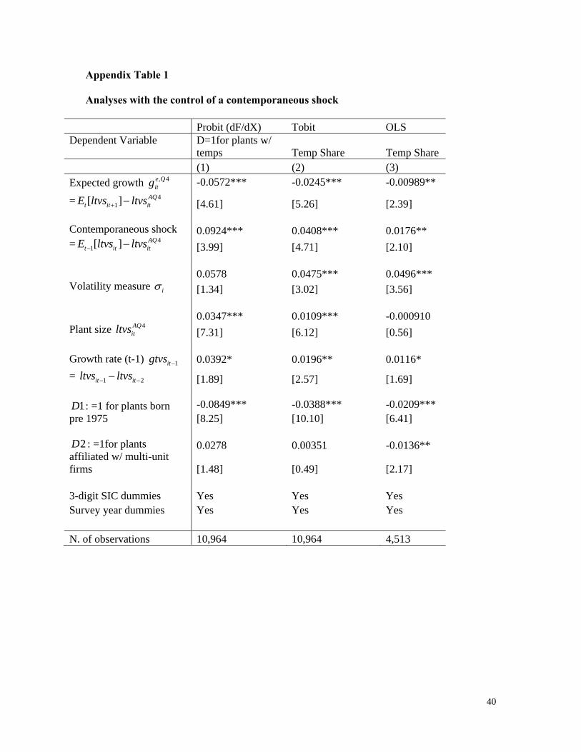
We also perform the analysis, controlling for a variable representing a current year
shock, 1[ ]it t itltvs E ltvs−− , to see if our data identify any effect of current shock separate from
that of , 4e Qitg . The results are in Appendix C. We find that, even after controlling for a current
year shock, the coefficient for the expected growth rate remains negative and significant. The
measure of current shock obtains a positive and significant coefficient. The size of the effect
of , 4e Qitg remains almost the same. Note that, in this regression, we exclude itgtvs as it is
highly correlated with the current year shock measure.
Based on the Probit result with industry dummies, if , 4e Qitg increases by a one s.d.
from its average, moving from 0.12 to 0.56, the probability to use temporary workers
decreases from 0.42 to 0.39. Based on the Tobit results with industry dummies, for plants
using temporary workers, a one s.d. increase in , 4e Qitg decreases the temporary worker share
by 1.2 percentage points, which is 10% of the average temporary worker share.
Plants that face more uncertainty appear to use more temporary workers. As we also
discussed, when firing costs are large enough, it is possible that greater uncertainty increases
the probability of marginal permanent worker to be fired, discouraging plants to use
permanent employees. For plants using temporary workers, the uncertainty level that is one
s.d. greater than average is associated with temporary worker share that that is 0.6 percentage
points lower than average, based on the Tobit and OLS results with industry dummies.22
22 We also performed Probit and Tobit analyses replacing expected annual output level in 1t + with its realized value. For this exercise, out of 4,909 plants used in Table 3, we used the data of 4,617 plants, which appear in ASM sample in the year following their PCU survey. The results remain qualitatively the same.

23
We also performed quantile regression analysis using the data of plants with
temporary workers to see whether the magnitude of effects vary between plants in different
quartiles of the distribution of the temporary worker share. The quantile regressions showed
that, among plants with temporary workers, the magnitudes of the effects of our key variables
are much greater for plants with higher temporary worker shares. Once we replace our
dependent variable with log of the temporary worker share, however, the quantile regressions
obtain almost the same coefficients across all quantiles. It seems that the effects of our key
variables are constant in terms of the percentage by which they increase the share.
Let us now look at the coefficients of other variables. The results generally suggest
that bigger plants are more likely to use temporary workers, and if they do, the temporary
worker share is greater than smaller plants. It is possible that fixed costs are involved in using
temporary workers for, perhaps, negotiating with temporary help agencies. The results may
also be reflecting that larger plants are more likely to face greater penalty in the event of an
unjust dismissal lawsuit. Such effect seems to offset possible negative effect, if any, from the
larger plants’ ability to redistribute workers within itself. A one s.d. increase in 4AQitltvs raises
a plant’s likelihood to use temporary workers by 4.1 percentage points. Note that the ability
to negotiate or allocate workers should be better captured at firm level rather than plant level.
Our analysis also control for a dummy indicating whether the plant is affiliated with multi-
plant firm.23 The dummy obtains a positive coefficient for Probit and a negative coefficient
for OLS. It is possible that the plants in a multi-plant firm can share the fixed costs, which
justify each plant to use temporary worker even by a small amount.
We found that older plants tend to use temporary workers less. The likelihood for
plants built pre-1975 to use temporary workers is 8.2 percentage points smaller than newer
23 Firm output size is not available.

24
plants. For plants using temporary workers, the temporary worker share for older plants is 3.7
percentage points lower than the young plants. Plant age may reflect the degree of
uncertainty that is not captured by σ . While σ is an average measure of uncertainty over the
lifecycle of a plant, the degree of uncertainty may change over time.
While we treated firms’ output level to be exogenous, in reality, a firm’s use of
flexible labor can influence a firm’s output adjustment. To the degree that such adjustments
are not predicted by equation (12), it may decrease or increase our measure of uncertainty
level. For example, with the easy access to temporary workers, under negative labor
productivity shocks, a firm may be able to keep the firm’s output stable using temporary
workers rather than decreasing the firm’s output; this may lower our measure of uncertainty
level. On the other hand, the firm may adjust outputs more flexibly having the access to
temporary workers; this may increase our measure of uncertainty level. Such effects are
screened out to some extend by industry dummies and other controls. As we show later, we
also control for geographical area fixed effects and the key results remain the same.
However, as a robustness analysis, we also create a variable for a plant’s output
volatility using only the data before 1985. The THS industry grew rapidly starting late 1980s.
Before 1985, the use of THS by manufacturing plants was not common.24 The growth of THS
industry might have reduced the costs to deal with temporary employment assignments, and
enhanced the manufacturing plants’ use of temporary workers in general. Thus by using the
output data before 1985, we can capture a manufacturing plant’s output volatility minimizing
the influence by its use of temporary workers. We denote the new measure by 1985preσ −% . The
results are presented in Table 3. As you can see, the coefficients for 1985preσ −% are positive, and
for the Probit analysis, the coefficient turns more significant than we saw in Table 2.

25
Next we explore the effect of other variables, including wage, unionization rate, job-
to-job transition rates, and seasonality. The results are summarized in Table 4. First, let us
look at the effect of two variables that summarize the compensation paid to permanent
workers. As discussed earlier, one might expect that plants that pay high wages or high
benefits would have an incentive to use temporary workers to reduce labor costs. In contrast,
industry analysts report that the markup that staffing agencies charge over wages for
temporary workers tends to be higher for high wage occupations. Thus, higher wage plants
may use fewer temporary workers. In our analysis, the latter story seems dominate. The
straight rate wage for permanent production workers and the supplemental labor costs per
dollar of permanent worker wages are both negatively correlated with plants’ use of
temporary workers. Note that when we control for these two variables, the positive
coefficient obtained for plant size becomes bigger. Since larger plants tend to pay higher
wages, once we separate the negative effect of wage, the scale effect seems to be more
pronounced.
Next we add the unionization rate, the turnover rate, and the fourth-quarter seasonal
component, which we measure at the three-digit SIC level. Columns 4, 5, 6 in Table 4 show
the results where we replace three-digit SIC dummies with these three continuous variables.
The results seem to suggest that the unionization rate is negatively correlated with a plant’s
use of temporary workers. This is counter to the idea that unions might increase the use of
temporary workers through their effect in increasing wages as well as firing costs relative to
productivity. Similar results are found in the study by Houseman (2001). Analogous to what
she argues, it is possible that our results reflect the fact that unions oppose the use of non-
standard employment relationships to secure regular employment positions. Note that the
24 Based on the BLS’s Occupational Employment Statistics data, the workers defined as “production workers” in that survey represents only 4.4% of THS workers in 1990, where in 2007, it is 19.2%.

26
coefficient for unionization rate is not significant in the OLS result. The unionization rate
may not influence the temporary worker share once plants decide to use temporary workers.
Note that we also examined whether the unionization rate has any interaction effect
with , 4e Qitg , which seems to suggest that greater union pressures against the use of temporary
work arrangements also enhance the negative effect of , 4e Qitg on a plants’ likelihood to use
temporary workers.
Coefficients for the job-to-job transition rate are not significant in any specification.
This is different from our original conjecture that higher voluntary turnover reduces the
probability of needing to fire permanent workers in the future and thus increases the
permanent worker share. As we discussed, it is possible that greater voluntary turnover
increases the on-going need to screen workers through temporary employment, and this
might have offset the effect of the decreased probability of needing to fire permanent workers.
The coefficients for the fourth-quarter seasonal component are positive and significant; the
higher seasonal component for output increases the use of temporary workers.
Note that in the specifications with the above additional controls, the coefficients for
our key variables, , 4e Qitg and σ , are still consistent with our conjectures. It would be, however,
instructive to note that the variations of our control variables such as wage, benefit, and
unionization rate seem to have relatively large contribution to the overall variation of the
plants’ use of temporary workers. Based on the Probit analysis in Column 4 in Table 4, one
s.d. increase in wage, benefit, unionization rate, and fourth-quarter seasonal factor decrease
the probability for a plant to use some temporary workers by 6.9, 2.8, 3.8, and 2.7 percentage
points, respectively. In terms of the variation of temporary worker shares across plants, based
on the Tobit analysis in Column 5 in Table 4, one s.d. increase in wage, benefit, unionization

27
rate, and fourth-quarter seasonal factor decrease the share by 2.6, 1.1, 1.2, and 1.1 percentage
points, respectively.
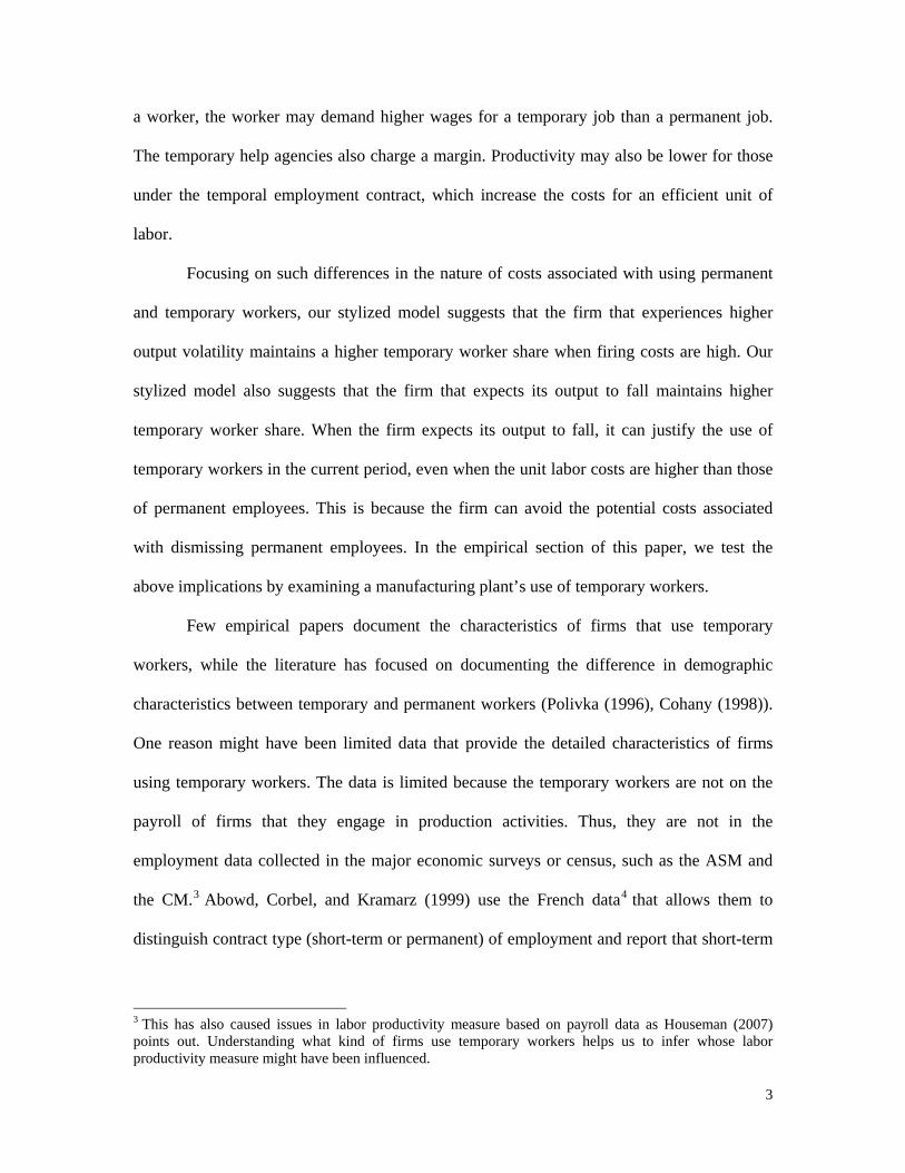
Finally, we examine whether our key results hold when we control for the effects of
geographical variables. In Columns 1, 2, 3 in Table 5, we show the results based on our base
specification, adding a dummy indicating urban plants (plants in metropolitan areas). We
then limit our sample to urban plants and control for Metropolitan statistical area fixed effects
in addition to three-digit industry effects. We find that in both cases, the effect of our key
variables stay qualitatively the same. We also found that plants in urban area are more likely
to use temporary workers. To the extent that markets for temporary worker are local, there
are many geographic variables such as the unemployment rate and the degree of local
concentration of temporary agencies, which would be associated with a plant’s use of
temporary workers. Examining the effect of these variables requires a thorough consideration
of local labor markets. We leave it to our future research to explore the influence of local
demand and supply of the temporary workers on a plant’s use of temporary workers.
5. Conclusion
We have provided some evidence in support of the proposition that temporary work
arrangements facilitate flexibility in a firm’s use of labor and allow it to accommodate output
fluctuations at lower cost. Our stylized model identifies the expected output growth rate and
the uncertainty in that expectation as two key variables in a firm’s decision to use temporary
workers. We approximated both of these variables using the ASM and the CM. We used
Probit, Tobit, and OLS analyses to examine the relationship between these two variables and
plants’ use of temporary workers.
First, we find that plants make greater use of temporary workers when their expected
output growth is lower. This suggests that a plant chooses temporary workers over permanent

28
workers when it expects its output to fall and thus wants to avoid costs associated with
dismissing permanent employees. This effect remains identified after netting out the effect of
a seasonal factor in a plant’s output, which itself had a positive relationship with a plant’s use
of temporary workers, as well as other variables.
Second, we find that a plant with greater uncertainty over its future output level uses
more temporary workers. Firing costs appear to be large enough to induce a more volatile
plant to make greater attempts to minimize the costs of firing permanent workers; this might
have made the plant rely more on temporary workers even though the current unit costs of
using temporary workers is greater than those for permanent workers.
In addition to output fluctuations, we also examine the effect of several other
motivations that are thought to play an important role in a plant’s decision to use temps. First,
we found evidence that a plant’s that requires high-skill workers are less likely to use
temporary workers, likely because the wage premium or the margin paid to agencies for
high-skill temporary workers may be higher than that for low-skill temporary workers.
Second, a plant in an industry that is highly unionized seems to use fewer temporary workers,
possibly because unions are successful in resisting the use of nonmembers’ labor.

29
Table 1. Summary Statistics
Plant characteristics (10,964 observations) Mean (S.d.)
, 4e Qitg .120 .420 iσ .195 .121
4AQitltvs 10.9 1.34
itgtvs : growth rate of annual real output in survey years -0.0164 0.247 1itgtvs − : growth rate of annual real output in previous
years 0.0179 0.245 Percentage of plants that existed from 1975 or before: 60.5% Percentage of plants belonging to a multi-unit firms 91.3% Percentage of plants in urban areas 71.4%
Three-digit SIC level variables included in the study (8,142 observations)†
ln. straight wage of perm production worker† 2.67 0.355 Benefit per $1 perm wage† 0.274 0.105 Unionization rates 0.234 0.116 Job-to-job transition rates 0.0200 0.00568 Fourth quarter seasonal factor 0.00793 0.0415 †: The sample is restricted due to the missing observations of overtime used to calculate straight wage. It is used in Table 3.

30
Table 2. Base specification
Without 3-digit SIC dummies With 3-digit SIC dummies
Probit (dF/dX) Tobit OLS
Probit (dF/dX) Tobit OLS
D=1for plants w/ temps
Temp Share
Temp Share
D=1for plants w/ temps
Temp Share
Temp Share
(1) (2) (3) (4) (5) (6) Expected growth , 4e Q
itg
= 41[ ] AQ
t it itE ltvs ltvs+ −
-0.0556*** -0.0248*** -0.00872** -0.0665*** -0.0285*** -0.0116***
[4.62] [5.21] [2.04] [5.29] [6.08] [2.79] Volatility measure iσ 0.0271 0.0424*** 0.0602*** 0.0667 0.0497*** 0.0494*** [0.68] [2.72] [4.50] [1.54] [3.17] [3.55] Plant size 4AQ
itltvs 0.0411*** 0.0167*** 0.00362** 0.0304*** 0.00900*** -0.0017 [10.60] [10.82] [2.55] [6.35] [5.02] [1.04] Growth rate itgtvs = 1it itltvs ltvs −−
0.162*** 0.0721*** 0.0261*** 0.157*** 0.0673*** 0.0273***
[7.79] [8.83] [3.29] [7.35] [8.51] [3.59] Growth rate (t-1) 1itgtvs − = 1 2it itltvs ltvs− −−
0.0670*** 0.0302*** 0.0122* 0.0622*** 0.0293*** 0.0155**
[3.29] [3.79] [1.74] [2.95] [3.79] [2.24]
1D : =1 for plants born pre 1975
-0.0902*** -0.0429*** -0.0199*** -0.0821*** -0.0374*** -0.0203*** [9.21] [11.01] [6.21] [7.96] [9.74] [6.20]
2D : =1for plants affiliated
w/ multi-unit firms
0.0347* 0.00421 -0.0188*** 0.0314* 0.00510 -0.0129** [1.94] [0.58] [2.91] [1.67] [0.71] [2.05]
3-digit SIC dummies No No No Yes Yes Yes Survey year dummies Yes Yes Yes Yes Yes Yes N. of observations 10,964 10,964 4,513 10,964 10,964 4,513

31
Table 3. Robustness Check with a volatility measure calculated using pre-1985 data Probit (dF/dX) Tobit OLS
D=1for plants w/ temps Temp Share Temp Share
(1) (2) (3)
Expected growth , 4e Qitg
= 41[ ] AQ
t it itE ltvs ltvs+ −
-0.0415** -0.0187*** -0.0130** [2.24] [2.85] [2.02]
Volatility measure based on pre-1985 data
1985preiσ
−
0.140** 0.0514** 0.0206
[2.18]
[2.29]
[1.12]
Plant size 4AQitltvs
0.0335*** 0.0106*** -0.000240 [4.59] [4.13] [0.09]
Growth rate itgtvs = 1it itltvs ltvs −−
0.139*** 0.0562*** 0.0251** [4.52] [5.16] [2.21]
Growth rate (t-1) 1itgtvs − = 1 2it itltvs ltvs− −−
0.0703** 0.0244** 0.00628 [2.25] [2.26] [0.60]
1D : =1 for plants born
pre 1975
-0.0831*** -0.0351*** -0.0170** [3.02] [3.87] [2.07]
2D : =1for plants
affiliated w/ multi-unit firms
0.0896** 0.0390** 0.0258*
[1.96] [2.31] [1.72] 3-digit SIC dummies Yes Yes Yes Survey year dummies Yes Yes Yes Observations 5,545 5,545 2,117

32
Table 4 Effect of other variables Effects of wage variables (plant level) Effect of other 3-digit SIC level variables Probit Tobit OLS Probit Tobit OLS
D=1for plants w/ temps
Temp Share
Temp Share
D=1for plants w/ temps
Temp Share
Temp Share
(1) (2) (3) (4) (5) (6)
Expected growth , 4e Qitg
= 41[ ] AQ
t it itE ltvs ltvs+ −
-0.0566*** -0.0219*** -0.00953** -0.0454** -0.0184*** -0.00642 [3.70] [4.27] [2.05] [2.07] [3.56] [1.06]
Volatility measure iσ
0.0631 0.0464*** 0.0497*** 0.000193 0.0334** 0.0605*** [1.24] [2.73] [3.23] [0.00] [1.99] [3.50]
Plant size 4AQ
itltvs
0.0567*** 0.0172*** 0.00127 0.0713*** 0.0249*** 0.00492*
[9.21] [8.42] [0.67] [6.91] [13.99] [1.81]
Growth rate itgtvs = 1it itltvs ltvs −−
0.1627*** 0.0637*** 0.0271*** 0.161*** 0.0666*** 0.0271*** [6.16] [7.34] [3.18] [5.37] [7.45] [3.23]
Growth rate (t-1) 1itgtvs − = 1 2it itltvs ltvs− −−
0.0372 0.0207** 0.0148* 0.0396 0.0209** 0.0142* [1.46] [2.45] [1.93] [1.36] [2.39] [1.74]
1D : =1 for plants born pre 1975
-0.0705*** -0.0310*** -0.0180*** -0.0718*** -0.0330*** -0.0182*** [5.74] [7.45] [5.03] [3.65] [7.88] [4.46]
2D : =1for plants affiliated w/ multi-unit firms
0.0493** 0.0115 -0.00577 0.0542* 0.0125 -0.0106 [2.14] [1.44] [0.80] [1.88] [1.56] [1.10]
ln. straight rate wage rate for perm workers
-0.210*** -0.0856*** -0.0398*** -0.191*** -0.0745*** -0.0249*** [10.51] [12.78] [6.41] [4.93] [11.78] [3.11]
Supplemental labor costs per $1 perm wage
-0.259*** -0.0994*** -0.0471** -0.265*** -0.108*** -0.0474** [4.37] [4.80] [2.46] [2.61] [5.20] [2.07]
Unionization rate -0.328** -0.105*** -0.0184
[2.18] [5.41] [0.62]
Job-to-job transition rate -3.53 -0.429 1.14*
[1.35] [1.12] [1.81]
Fourth-quarter seasonal factor 0.644** 0.266*** 0.118*
[2.47] [5.33] [1.86] 3-digit SIC dummies Yes Yes Yes No No No Survey year dummies Yes Yes Yes Yes Yes Yes Observations 8,142 8,142 3,793 8,142 8,142 3,793 [ ]: Robust z-statistics for Probit, t-statistics for Tobit, and robust t-statistics for OLS (errors are clustered for plants in the same three-digit SIC for Columns 4 and 6); * significant at 10%; ** significant at 5%; *** significant at 1%
33
Table 5 Results with geography controls
Results with a dummy for plants in urban areas
Results with PMSA dummies for plants in urban areas
Probit Tobit OLS Probit Tobit OLS
D=1for plants w/ temps
Temp Share
Temp Share
D=1for plants w/ temps
Temp Share
Temp Share
(1) (2) (3) (4) (5) (6) Expected growth , 4e Q
itg
= 41[ ] AQ
t it itE ltvs ltvs+ −
-0.0669*** -0.0287*** -0.0118*** -0.0789*** -0.0301*** -0.00778
[5.32] [6.14] [2.83] [4.92] [5.53] [1.49]
Volatility measure iσ
0.0645 0.0479*** 0.0469*** 0.111** 0.0658*** 0.0498*** [1.49] [3.06] [3.38] [2.01] [3.60] [2.75]
Plant size 4AQ
itltvs
0.0302*** 0.00891*** -0.00159 0.0181*** 0.00336 -0.00244
[6.30] [4.98] [0.97] [2.90] [1.56] [1.19]
Growth rate itgtvs = 1it itltvs ltvs −−
0.158*** 0.0672*** 0.0271*** 0.179*** 0.0670*** 0.0205** [7.37] [8.52] [3.59] [6.76] [7.47] [2.28]
Growth rate (t-1) 1itgtvs −
= 1 2it itltvs ltvs− −−
0.0625*** 0.0293*** 0.0152** 0.0862*** 0.0347*** 0.0138*
[2.97] [3.80] [2.20] [3.17] [3.94] [1.72]
1D : =1 for plants born pre 1975
-0.0827*** -0.0378*** -0.0206*** -0.0737*** -0.0330*** -0.0215*** [8.02] [9.85] [6.31] [5.34] [6.93] [4.77]
2D : =1for plants
affiliated w/ multi-unit firms
0.0342* 0.00678 -0.0117* 0.0468** 0.0155* -0.00524 [1.82]
[0.95]
[1.86]
[2.02]
[1.88]
[0.67]
D3=1 for urban plants
0.0320*** 0.0199*** 0.0151*** [2.82] [4.65] [4.42]
3-digit SIC dummies Yes Yes Yes Yes Yes Yes Survey year dummies Yes Yes Yes Yes Yes Yes PMSA dummies No No No Yes Yes Yes Observations 10,964 10,964 4,513 7,621 7,621 3,274
34
Figure 1. The determination of the cap on permanent workers: Two-period model
p
0
u−Δ
u βδ−Δ +
11
( )dTC pdp
1p1( )lowf y− 1( )highf y−
35
References Aaronson, Daniel, Ellen Rissman, and Daniel Sullivan. “Can sectoral reallocation explain the jobless recovery?,” Economic Perspectives, Vol. 28, No. 2, pp. 36-49, 2004 Autor, David. “Outsourcing at Will: Unjust Dismissal Doctrine and the Growth of Temporary Help Employment,” Journal of Labor Economics. January 2003. Autor, David. “Why Do Temporary Help Firms Provide Free General Skills Training?,” Quarterly Journal of Economics, 116 (4), 2003. Campbell, Jeffery and Jonas Fisher. “Idiosyncratic Risk and Aggregate Employment Fluctuations,” Review of Economic Dynamics, April 2004, Vol. 7, Issue. 2, pp. 331-353. Cohany, Sharon R. “Workers in alternative employment arrangements: a second look”, Monthly Labor Review, November 1998. Dixit, Avinash K. and Robert S. Pindyck. Investment under Uncertainty, Princeton University Press, 1993 Estevao, Marcello and Saul Lach. “Measuring temporary labor outsourcing in U.S. manufacturing”, Board of Governors of the Federal Reserve System, Working paper, October 1999. Golden, Marcello. “The expansion of temporary help employment in the US, 1982-1992: A test of alternative economic explanations”, Applied Economics, 1996, Vol. 28, pp. 1127-1141. Grosben Erica L. and Simon Potter. “Has structural change contributed to a jobless recovery?”, Current Issues, Federal Reserve Bank of New York, Vol. 9, No. 8, 2003. Houseman, Susan N. and Anna E. Polivka, “The implication of flexible staffing arrangements for job security,” in On the Job: Is Long-Term Employment A Thing of the Past?, David Neumark ed., (pp. 427-462). New York: Russell Sage Foundation, 2000. Houseman, Susan N. “Why employers use flexible staffing arrangements: evidence from an establishment survey,” Industrial and Labor Relations Review, Vol. 55, No. 1, October 2001, pp. 149-170. Houseman, Susan N. “the benefits implication on recent trends in flexible staffing arrangements,” in Benefits for the Workplace of the Future. Mithcell, Olivia S., David S. Blitzstein, Michael Gordon, and Judith F. Mazo, eds. Philadelphia: University of Pennsylvania Press, 2003. Houseman, Susan N. Arne L. Kalleberg, and George A. Erickcek, “The role of temporary help employment in tight labor markets”, Industrial and Labor Relations Review, Vol. 57, No. 1, pp. 105-127. 2003.

36
Houseman, Susan N. “Outsourcing, Offshoring, and Productivity Measurement in U.S. Manufacturing,” International Labour Review 146(1-2): 61-80, 2007. Katz, Lawrence and Alan Krueger, “The high-pressure U.S. labor market of the 1990s,” Brookings Papers on Economic Activity, 1999, Issue 1, pp.1-65. Kilcoyne, Patrick, http://www.bls.gov/oes/2004/may/temp.pdf (downloaded April, 2006), U.S. Bureau of Labor Statistics, 2004. Ono, Yukako and Alexei Zelenev, “Temporary workers and volatility of industry output”, Economic Perspectives, Federal Reserve Bank of Chicago, May 2003. Polivka, Anne E. “A profile of contingent workers”, Monthly Labor Review, October 1996. Segal, Lewis M. and Daniel G. Sullivan, “The growth of temporary services work”, Journal of Economic Perspectives, Spring 1997, pp. 117-136. Segal, Lewis M. and Daniel G. Sullivan, “The temporary labor force”, Economic Perspectives, Federal Reserve Bank of Chicago, April 1995, pp. 2-19. Segal, Lewis M. and Daniel G. Sullivan, “Wage differentials for temporary service work: Evidence from administrative data”, Federal Reserve Bank of Chicago, working paper, No. 98-23, 1998.
U.S. Census Bureau, Form MQ-C1; Survey of Plant Capacity Utilization, Current Industrial
Reports
37
Appendix
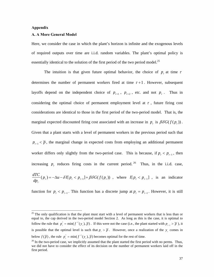
A. A More General Model
Here, we consider the case in which the plant’s horizon is infinite and the exogenous levels
of required outputs over time are i.i.d. random variables. The plant’s optimal policy is
essentially identical to the solution of the first period of the two period model.25
The intuition is that given future optimal behavior, the choice of pτ at time τ
determines the number of permanent workers fired at time 1τ + . However, subsequent
layoffs depend on the independent choice of 1pτ + , 2pτ + , etc. and not pτ . Thus in
considering the optimal choice of permanent employment level at τ , future firing cost
considerations are identical to those in the first period of the two-period model. That is, the
marginal expected discounted firing cost associated with an increase in pτ is ( ( ))G f pτβδ .
Given that a plant starts with a level of permanent workers in the previous period such that
1p pτ − < , the marginal change in expected costs from employing an additional permanent
worker differs only slightly from the two-period case. This is because, if 1p pτ τ −< , then
increasing pτ reduces firing costs in the current period. 26 Thus, in the i.i.d. case,
1( ) [ ] ( ( ))dTC p u I p p G f pdp τ τ τ τ
τ
δ βδ−= −Δ − < + , where 1[ ]I p pτ τ −< , is an indicator
function for 1p pτ τ −< . This function has a discrete jump at 1p pτ τ −= . However, it is still
25 The only qualification is that the plant must start with a level of permanent workers that is less than or equal to, the cap derived in the two-period model Section 2. As long as this is the case, it is optimal to follow the rule that * 1min( ( ), )p f y pτ τ
−= . If this were not the case (i.e., the plant started with 1p pτ − > ), it
is possible that the optimal level is such that p pτ > . However, once a realization of the yτ comes in
below ( )f p , the rule * 1min( ( ), )p f y pτ τ
−= becomes optimal for the rest of time. 26 In the two-period case, we implicitly assumed that the plant started the first period with no perms. Thus, we did not have to consider the effect of its decision on the number of permanent workers laid off in the first period.

38
strictly increasing and given that 1p pτ − < , it still is equal to zero at p pτ = (See Appendix
Figure 1).
Appendix Figure 1: Determination of the Cap on Permanent Workers: Infinite Horizon i.i.d.
B. Our sample based on the PCU data
In the questionnaire, plants are asked to report, for each shift, the total number of production
workers, temporary production workers, total hours worked by production workers, hours
worked by temporary workers, and overtime hours. We consider that a plant operates a given
shift if it reports positive total production workers for the shift, who are defined to include
temporary workers in the instructions for the questionnaire given to the plant. Among plants
operating a particular shift, however, many left the information for temporary production
workers unfilled, and often, such plants do not provide a temporary worker number for any
shift. In such a case, it is not clear whether the plant did not use temporary workers or did not
p
0
u−Δ
u βδ−Δ +
( )dTC pdp τ
τ
pτ 1( )lowf y− 1( )highf y−
u δ−Δ −
1pτ −

39
fill out the item. We consider that they did not fill out the item, since the instructions for the
PCU survey explicitly instructs them both in words and with visual examples of the tables to
write zero when plants operate a given shift but do not use temporary workers. We exclude
such plants with missing temporary employment data for any of their active shifts (i.e., shifts
for which the plant reports positive total number of production workers).
In addition, by the definition given in the instructions, when a given shift exists, the
total number of production workers should be greater than or equal to the number of
temporary workers. We exclude plants with any inconsistency regarding these figures. We
also exclude a few plants reporting the same number for both total and temporary workers for
some shifts. It is possible that these shifts are actually supported by only temporary workers.
However, such incidents are rare and we cannot tell whether these are miss data entry.
Once we clean the PCU data, we limit the sample to those for which we can estimate
our key variables based on the ASM and the CM as discussed in the main text. Based on the
method discussed in Section 3, for a plant to be included in estimation, the plant has to
appear in consecutive three years more than once in ASM-CM panel. We limit our sample to
plants that appear in three years consecutively at least three times to avoid outliers. Some
further outliers based on other variables are excluded.
40
Appendix Table 1
Analyses with the control of a contemporaneous shock
Probit (dF/dX) Tobit OLS Dependent Variable
D=1for plants w/ temps Temp Share Temp Share
(1) (2) (3) Expected growth , 4e Q
itg
= 41[ ] AQ
t it itE ltvs ltvs+ −
-0.0572*** -0.0245*** -0.00989**
[4.61] [5.26] [2.39] Contemporaneous shock = 4
1[ ] AQt it itE ltvs ltvs− −
0.0924*** 0.0408*** 0.0176** [3.99] [4.71] [2.10]
Volatility measure iσ
0.0578 0.0475*** 0.0496*** [1.34] [3.02] [3.56]
Plant size 4AQ
itltvs 0.0347*** 0.0109*** -0.000910 [7.31] [6.12] [0.56]
Growth rate (t-1) 1itgtvs − = 1 2it itltvs ltvs− −−
0.0392* 0.0196** 0.0116*
[1.89] [2.57] [1.69]
1D : =1 for plants born pre 1975
-0.0849*** -0.0388*** -0.0209*** [8.25] [10.10] [6.41]
2D : =1for plants
affiliated w/ multi-unit firms
0.0278 0.00351 -0.0136**
[1.48] [0.49] [2.17] 3-digit SIC dummies Yes Yes Yes Survey year dummies Yes Yes Yes N. of observations 10,964 10,964 4,513

1
Working Paper Series
A series of research studies on regional economic issues relating to the Seventh Federal Reserve District, and on financial and economic topics.
A Proposal for Efficiently Resolving Out-of-the-Money Swap Positions WP-03-01 at Large Insolvent Banks George G. Kaufman Depositor Liquidity and Loss-Sharing in Bank Failure Resolutions WP-03-02 George G. Kaufman Subordinated Debt and Prompt Corrective Regulatory Action WP-03-03 Douglas D. Evanoff and Larry D. Wall When is Inter-Transaction Time Informative? WP-03-04 Craig Furfine Tenure Choice with Location Selection: The Case of Hispanic Neighborhoods WP-03-05 in Chicago Maude Toussaint-Comeau and Sherrie L.W. Rhine Distinguishing Limited Commitment from Moral Hazard in Models of WP-03-06 Growth with Inequality* Anna L. Paulson and Robert Townsend Resolving Large Complex Financial Organizations WP-03-07 Robert R. Bliss The Case of the Missing Productivity Growth: WP-03-08 Or, Does information technology explain why productivity accelerated in the United States but not the United Kingdom? Susanto Basu, John G. Fernald, Nicholas Oulton and Sylaja Srinivasan Inside-Outside Money Competition WP-03-09 Ramon Marimon, Juan Pablo Nicolini and Pedro Teles The Importance of Check-Cashing Businesses to the Unbanked: Racial/Ethnic Differences WP-03-10 William H. Greene, Sherrie L.W. Rhine and Maude Toussaint-Comeau A Firm’s First Year WP-03-11 Jaap H. Abbring and Jeffrey R. Campbell Market Size Matters WP-03-12 Jeffrey R. Campbell and Hugo A. Hopenhayn The Cost of Business Cycles under Endogenous Growth WP-03-13 Gadi Barlevy The Past, Present, and Probable Future for Community Banks WP-03-14 Robert DeYoung, William C. Hunter and Gregory F. Udell

2
Working Paper Series (continued) Measuring Productivity Growth in Asia: Do Market Imperfections Matter? WP-03-15 John Fernald and Brent Neiman Revised Estimates of Intergenerational Income Mobility in the United States WP-03-16 Bhashkar Mazumder Product Market Evidence on the Employment Effects of the Minimum Wage WP-03-17 Daniel Aaronson and Eric French Estimating Models of On-the-Job Search using Record Statistics WP-03-18 Gadi Barlevy Banking Market Conditions and Deposit Interest Rates WP-03-19 Richard J. Rosen Creating a National State Rainy Day Fund: A Modest Proposal to Improve Future WP-03-20 State Fiscal Performance Richard Mattoon Managerial Incentive and Financial Contagion WP-03-21 Sujit Chakravorti and Subir Lall Women and the Phillips Curve: Do Women’s and Men’s Labor Market Outcomes WP-03-22 Differentially Affect Real Wage Growth and Inflation? Katharine Anderson, Lisa Barrow and Kristin F. Butcher Evaluating the Calvo Model of Sticky Prices WP-03-23 Martin Eichenbaum and Jonas D.M. Fisher The Growing Importance of Family and Community: An Analysis of Changes in the WP-03-24 Sibling Correlation in Earnings Bhashkar Mazumder and David I. Levine Should We Teach Old Dogs New Tricks? The Impact of Community College Retraining WP-03-25 on Older Displaced Workers Louis Jacobson, Robert J. LaLonde and Daniel Sullivan Trade Deflection and Trade Depression WP-03-26 Chad P. Brown and Meredith A. Crowley China and Emerging Asia: Comrades or Competitors? WP-03-27 Alan G. Ahearne, John G. Fernald, Prakash Loungani and John W. Schindler International Business Cycles Under Fixed and Flexible Exchange Rate Regimes WP-03-28 Michael A. Kouparitsas Firing Costs and Business Cycle Fluctuations WP-03-29 Marcelo Veracierto Spatial Organization of Firms WP-03-30 Yukako Ono Government Equity and Money: John Law’s System in 1720 France WP-03-31 François R. Velde

3
Working Paper Series (continued) Deregulation and the Relationship Between Bank CEO WP-03-32 Compensation and Risk-Taking Elijah Brewer III, William Curt Hunter and William E. Jackson III Compatibility and Pricing with Indirect Network Effects: Evidence from ATMs WP-03-33 Christopher R. Knittel and Victor Stango Self-Employment as an Alternative to Unemployment WP-03-34 Ellen R. Rissman Where the Headquarters are – Evidence from Large Public Companies 1990-2000 WP-03-35 Tyler Diacon and Thomas H. Klier Standing Facilities and Interbank Borrowing: Evidence from the Federal Reserve’s WP-04-01 New Discount Window Craig Furfine Netting, Financial Contracts, and Banks: The Economic Implications WP-04-02 William J. Bergman, Robert R. Bliss, Christian A. Johnson and George G. Kaufman Real Effects of Bank Competition WP-04-03 Nicola Cetorelli Finance as a Barrier To Entry: Bank Competition and Industry Structure in WP-04-04 Local U.S. Markets? Nicola Cetorelli and Philip E. Strahan The Dynamics of Work and Debt WP-04-05 Jeffrey R. Campbell and Zvi Hercowitz Fiscal Policy in the Aftermath of 9/11 WP-04-06 Jonas Fisher and Martin Eichenbaum Merger Momentum and Investor Sentiment: The Stock Market Reaction To Merger Announcements WP-04-07 Richard J. Rosen Earnings Inequality and the Business Cycle WP-04-08 Gadi Barlevy and Daniel Tsiddon Platform Competition in Two-Sided Markets: The Case of Payment Networks WP-04-09 Sujit Chakravorti and Roberto Roson Nominal Debt as a Burden on Monetary Policy WP-04-10 Javier Díaz-Giménez, Giorgia Giovannetti, Ramon Marimon, and Pedro Teles On the Timing of Innovation in Stochastic Schumpeterian Growth Models WP-04-11 Gadi Barlevy Policy Externalities: How US Antidumping Affects Japanese Exports to the EU WP-04-12 Chad P. Bown and Meredith A. Crowley Sibling Similarities, Differences and Economic Inequality WP-04-13 Bhashkar Mazumder

4
Working Paper Series (continued) Determinants of Business Cycle Comovement: A Robust Analysis WP-04-14 Marianne Baxter and Michael A. Kouparitsas The Occupational Assimilation of Hispanics in the U.S.: Evidence from Panel Data WP-04-15 Maude Toussaint-Comeau Reading, Writing, and Raisinets1: Are School Finances Contributing to Children’s Obesity? WP-04-16 Patricia M. Anderson and Kristin F. Butcher Learning by Observing: Information Spillovers in the Execution and Valuation WP-04-17 of Commercial Bank M&As Gayle DeLong and Robert DeYoung Prospects for Immigrant-Native Wealth Assimilation: WP-04-18 Evidence from Financial Market Participation Una Okonkwo Osili and Anna Paulson Individuals and Institutions: Evidence from International Migrants in the U.S. WP-04-19 Una Okonkwo Osili and Anna Paulson Are Technology Improvements Contractionary? WP-04-20 Susanto Basu, John Fernald and Miles Kimball The Minimum Wage, Restaurant Prices and Labor Market Structure WP-04-21 Daniel Aaronson, Eric French and James MacDonald Betcha can’t acquire just one: merger programs and compensation WP-04-22 Richard J. Rosen Not Working: Demographic Changes, Policy Changes, WP-04-23 and the Distribution of Weeks (Not) Worked Lisa Barrow and Kristin F. Butcher The Role of Collateralized Household Debt in Macroeconomic Stabilization WP-04-24 Jeffrey R. Campbell and Zvi Hercowitz Advertising and Pricing at Multiple-Output Firms: Evidence from U.S. Thrift Institutions WP-04-25 Robert DeYoung and Evren Örs Monetary Policy with State Contingent Interest Rates WP-04-26 Bernardino Adão, Isabel Correia and Pedro Teles Comparing location decisions of domestic and foreign auto supplier plants WP-04-27 Thomas Klier, Paul Ma and Daniel P. McMillen China’s export growth and US trade policy WP-04-28 Chad P. Bown and Meredith A. Crowley Where do manufacturing firms locate their Headquarters? WP-04-29 J. Vernon Henderson and Yukako Ono Monetary Policy with Single Instrument Feedback Rules WP-04-30 Bernardino Adão, Isabel Correia and Pedro Teles

5
Working Paper Series (continued) Firm-Specific Capital, Nominal Rigidities and the Business Cycle WP-05-01 David Altig, Lawrence J. Christiano, Martin Eichenbaum and Jesper Linde Do Returns to Schooling Differ by Race and Ethnicity? WP-05-02 Lisa Barrow and Cecilia Elena Rouse Derivatives and Systemic Risk: Netting, Collateral, and Closeout WP-05-03 Robert R. Bliss and George G. Kaufman Risk Overhang and Loan Portfolio Decisions WP-05-04 Robert DeYoung, Anne Gron and Andrew Winton Characterizations in a random record model with a non-identically distributed initial record WP-05-05 Gadi Barlevy and H. N. Nagaraja Price discovery in a market under stress: the U.S. Treasury market in fall 1998 WP-05-06 Craig H. Furfine and Eli M. Remolona Politics and Efficiency of Separating Capital and Ordinary Government Budgets WP-05-07 Marco Bassetto with Thomas J. Sargent Rigid Prices: Evidence from U.S. Scanner Data WP-05-08 Jeffrey R. Campbell and Benjamin Eden Entrepreneurship, Frictions, and Wealth WP-05-09 Marco Cagetti and Mariacristina De Nardi Wealth inequality: data and models WP-05-10 Marco Cagetti and Mariacristina De Nardi What Determines Bilateral Trade Flows? WP-05-11 Marianne Baxter and Michael A. Kouparitsas Intergenerational Economic Mobility in the U.S., 1940 to 2000 WP-05-12 Daniel Aaronson and Bhashkar Mazumder Differential Mortality, Uncertain Medical Expenses, and the Saving of Elderly Singles WP-05-13 Mariacristina De Nardi, Eric French, and John Bailey Jones Fixed Term Employment Contracts in an Equilibrium Search Model WP-05-14 Fernando Alvarez and Marcelo Veracierto Causality, Causality, Causality: The View of Education Inputs and Outputs from Economics WP-05-15 Lisa Barrow and Cecilia Elena Rouse

6
Working Paper Series (continued) Competition in Large Markets WP-05-16 Jeffrey R. Campbell Why Do Firms Go Public? Evidence from the Banking Industry WP-05-17 Richard J. Rosen, Scott B. Smart and Chad J. Zutter Clustering of Auto Supplier Plants in the U.S.: GMM Spatial Logit for Large Samples WP-05-18 Thomas Klier and Daniel P. McMillen Why are Immigrants’ Incarceration Rates So Low? Evidence on Selective Immigration, Deterrence, and Deportation WP-05-19 Kristin F. Butcher and Anne Morrison Piehl Constructing the Chicago Fed Income Based Economic Index – Consumer Price Index: Inflation Experiences by Demographic Group: 1983-2005 WP-05-20 Leslie McGranahan and Anna Paulson Universal Access, Cost Recovery, and Payment Services WP-05-21 Sujit Chakravorti, Jeffery W. Gunther, and Robert R. Moore Supplier Switching and Outsourcing WP-05-22 Yukako Ono and Victor Stango Do Enclaves Matter in Immigrants’ Self-Employment Decision? WP-05-23 Maude Toussaint-Comeau The Changing Pattern of Wage Growth for Low Skilled Workers WP-05-24 Eric French, Bhashkar Mazumder and Christopher Taber U.S. Corporate and Bank Insolvency Regimes: An Economic Comparison and Evaluation WP-06-01 Robert R. Bliss and George G. Kaufman Redistribution, Taxes, and the Median Voter WP-06-02 Marco Bassetto and Jess Benhabib Identification of Search Models with Initial Condition Problems WP-06-03 Gadi Barlevy and H. N. Nagaraja Tax Riots WP-06-04 Marco Bassetto and Christopher Phelan The Tradeoff between Mortgage Prepayments and Tax-Deferred Retirement Savings WP-06-05 Gene Amromin, Jennifer Huang,and Clemens Sialm Why are safeguards needed in a trade agreement? WP-06-06 Meredith A. Crowley

7
Working Paper Series (continued) Taxation, Entrepreneurship, and Wealth WP-06-07 Marco Cagetti and Mariacristina De Nardi A New Social Compact: How University Engagement Can Fuel Innovation WP-06-08 Laura Melle, Larry Isaak, and Richard Mattoon Mergers and Risk WP-06-09 Craig H. Furfine and Richard J. Rosen Two Flaws in Business Cycle Accounting WP-06-10 Lawrence J. Christiano and Joshua M. Davis Do Consumers Choose the Right Credit Contracts? WP-06-11 Sumit Agarwal, Souphala Chomsisengphet, Chunlin Liu, and Nicholas S. Souleles Chronicles of a Deflation Unforetold WP-06-12 François R. Velde Female Offenders Use of Social Welfare Programs Before and After Jail and Prison: Does Prison Cause Welfare Dependency? WP-06-13 Kristin F. Butcher and Robert J. LaLonde Eat or Be Eaten: A Theory of Mergers and Firm Size WP-06-14 Gary Gorton, Matthias Kahl, and Richard Rosen Do Bonds Span Volatility Risk in the U.S. Treasury Market? A Specification Test for Affine Term Structure Models WP-06-15 Torben G. Andersen and Luca Benzoni Transforming Payment Choices by Doubling Fees on the Illinois Tollway WP-06-16 Gene Amromin, Carrie Jankowski, and Richard D. Porter How Did the 2003 Dividend Tax Cut Affect Stock Prices? WP-06-17 Gene Amromin, Paul Harrison, and Steven Sharpe Will Writing and Bequest Motives: Early 20th Century Irish Evidence WP-06-18 Leslie McGranahan How Professional Forecasters View Shocks to GDP WP-06-19 Spencer D. Krane Evolving Agglomeration in the U.S. auto supplier industry WP-06-20 Thomas Klier and Daniel P. McMillen Mortality, Mass-Layoffs, and Career Outcomes: An Analysis using Administrative Data WP-06-21 Daniel Sullivan and Till von Wachter

8
Working Paper Series (continued) The Agreement on Subsidies and Countervailing Measures: Tying One’s Hand through the WTO. WP-06-22 Meredith A. Crowley How Did Schooling Laws Improve Long-Term Health and Lower Mortality? WP-06-23 Bhashkar Mazumder Manufacturing Plants’ Use of Temporary Workers: An Analysis Using Census Micro Data WP-06-24 Yukako Ono and Daniel Sullivan
Related Documents