MITgcm User Manual Alistair Adcroft Jean-Michel Campin Stephanie Dutkiewicz Constantinos Evangelinos David Ferreira Gael Forget Baylor Fox-Kemper Patrick Heimbach Chris Hill Ed Hill Helen Hill Oliver Jahn Martin Losch John Marshall Guillaume Maze Dimitris Menemenlis Andrea Molod MIT Department of EAPS 77 Massachusetts Ave. Cambridge, MA 02139-4307 January 23, 2018

Welcome message from author
This document is posted to help you gain knowledge. Please leave a comment to let me know what you think about it! Share it to your friends and learn new things together.
Transcript
MITgcm User Manual
Alistair Adcroft Jean-Michel Campin Stephanie Dutkiewicz
Constantinos Evangelinos David Ferreira Gael Forget Baylor Fox-Kemper
Patrick Heimbach Chris Hill Ed Hill Helen Hill Oliver Jahn
Martin Losch John Marshall Guillaume Maze Dimitris Menemenlis
Andrea Molod
MIT Department of EAPS
77 Massachusetts Ave.
Cambridge, MA 02139-4307
January 23, 2018

2
Contents
1 Overview of MITgcm 91.1 Introduction . . . . . . . . . . . . . . . . . . . . . . . . . . . . . . . . . . . . . . . . . . . . 91.2 Illustrations of the model in action . . . . . . . . . . . . . . . . . . . . . . . . . . . . . . . 13
1.2.1 Global atmosphere: ‘Held-Suarez’ benchmark . . . . . . . . . . . . . . . . . . . . . 131.2.2 Ocean gyres . . . . . . . . . . . . . . . . . . . . . . . . . . . . . . . . . . . . . . . . 141.2.3 Global ocean circulation . . . . . . . . . . . . . . . . . . . . . . . . . . . . . . . . . 141.2.4 Convection and mixing over topography . . . . . . . . . . . . . . . . . . . . . . . . 141.2.5 Boundary forced internal waves . . . . . . . . . . . . . . . . . . . . . . . . . . . . . 141.2.6 Parameter sensitivity using the adjoint of MITgcm . . . . . . . . . . . . . . . . . . 141.2.7 Global state estimation of the ocean . . . . . . . . . . . . . . . . . . . . . . . . . . 201.2.8 Ocean biogeochemical cycles . . . . . . . . . . . . . . . . . . . . . . . . . . . . . . 201.2.9 Simulations of laboratory experiments . . . . . . . . . . . . . . . . . . . . . . . . . 20
1.3 Continuous equations in ‘r’ coordinates . . . . . . . . . . . . . . . . . . . . . . . . . . . . . 231.3.1 Kinematic Boundary conditions . . . . . . . . . . . . . . . . . . . . . . . . . . . . . 261.3.2 Atmosphere . . . . . . . . . . . . . . . . . . . . . . . . . . . . . . . . . . . . . . . . 261.3.3 Ocean . . . . . . . . . . . . . . . . . . . . . . . . . . . . . . . . . . . . . . . . . . . 271.3.4 Hydrostatic, Quasi-hydrostatic, Quasi-nonhydrostatic and Non-hydrostatic forms . 271.3.5 Solution strategy . . . . . . . . . . . . . . . . . . . . . . . . . . . . . . . . . . . . . 301.3.6 Finding the pressure field . . . . . . . . . . . . . . . . . . . . . . . . . . . . . . . . 311.3.7 Forcing/dissipation . . . . . . . . . . . . . . . . . . . . . . . . . . . . . . . . . . . . 331.3.8 Vector invariant form . . . . . . . . . . . . . . . . . . . . . . . . . . . . . . . . . . 331.3.9 Adjoint . . . . . . . . . . . . . . . . . . . . . . . . . . . . . . . . . . . . . . . . . . 33
1.4 Appendix ATMOSPHERE . . . . . . . . . . . . . . . . . . . . . . . . . . . . . . . . . . . . 341.4.1 Hydrostatic Primitive Equations for the Atmosphere in pressure coordinates . . . . 34
1.5 Appendix OCEAN . . . . . . . . . . . . . . . . . . . . . . . . . . . . . . . . . . . . . . . . 361.5.1 Equations of motion for the ocean . . . . . . . . . . . . . . . . . . . . . . . . . . . 36
1.6 Appendix:OPERATORS . . . . . . . . . . . . . . . . . . . . . . . . . . . . . . . . . . . . . 391.6.1 Coordinate systems . . . . . . . . . . . . . . . . . . . . . . . . . . . . . . . . . . . 39
2 Discretization and Algorithm 412.1 Notation . . . . . . . . . . . . . . . . . . . . . . . . . . . . . . . . . . . . . . . . . . . . . . 412.2 Time-stepping . . . . . . . . . . . . . . . . . . . . . . . . . . . . . . . . . . . . . . . . . . . 412.3 Pressure method with rigid-lid . . . . . . . . . . . . . . . . . . . . . . . . . . . . . . . . . 422.4 Pressure method with implicit linear free-surface . . . . . . . . . . . . . . . . . . . . . . . 442.5 Explicit time-stepping: Adams-Bashforth . . . . . . . . . . . . . . . . . . . . . . . . . . . 442.6 Implicit time-stepping: backward method . . . . . . . . . . . . . . . . . . . . . . . . . . . 452.7 Synchronous time-stepping: variables co-located in time . . . . . . . . . . . . . . . . . . . 472.8 Staggered baroclinic time-stepping . . . . . . . . . . . . . . . . . . . . . . . . . . . . . . . 492.9 Non-hydrostatic formulation . . . . . . . . . . . . . . . . . . . . . . . . . . . . . . . . . . . 512.10 Variants on the Free Surface . . . . . . . . . . . . . . . . . . . . . . . . . . . . . . . . . . . 53
2.10.1 Crank-Nicolson barotropic time stepping . . . . . . . . . . . . . . . . . . . . . . . . 542.10.2 Non-linear free-surface . . . . . . . . . . . . . . . . . . . . . . . . . . . . . . . . . . 55
2.11 Spatial discretization of the dynamical equations . . . . . . . . . . . . . . . . . . . . . . . 592.11.1 The finite volume method: finite volumes versus finite difference . . . . . . . . . . 59
3
4 CONTENTS
2.11.2 C grid staggering of variables . . . . . . . . . . . . . . . . . . . . . . . . . . . . . . 602.11.3 Grid initialization and data . . . . . . . . . . . . . . . . . . . . . . . . . . . . . . . 602.11.4 Horizontal grid . . . . . . . . . . . . . . . . . . . . . . . . . . . . . . . . . . . . . . 612.11.5 Vertical grid . . . . . . . . . . . . . . . . . . . . . . . . . . . . . . . . . . . . . . . 632.11.6 Topography: partially filled cells . . . . . . . . . . . . . . . . . . . . . . . . . . . . 64
2.12 Continuity and horizontal pressure gradient terms . . . . . . . . . . . . . . . . . . . . . . 652.13 Hydrostatic balance . . . . . . . . . . . . . . . . . . . . . . . . . . . . . . . . . . . . . . . 652.14 Flux-form momentum equations . . . . . . . . . . . . . . . . . . . . . . . . . . . . . . . . 66
2.14.1 Advection of momentum . . . . . . . . . . . . . . . . . . . . . . . . . . . . . . . . . 662.14.2 Coriolis terms . . . . . . . . . . . . . . . . . . . . . . . . . . . . . . . . . . . . . . . 672.14.3 Curvature metric terms . . . . . . . . . . . . . . . . . . . . . . . . . . . . . . . . . 672.14.4 Non-hydrostatic metric terms . . . . . . . . . . . . . . . . . . . . . . . . . . . . . . 682.14.5 Lateral dissipation . . . . . . . . . . . . . . . . . . . . . . . . . . . . . . . . . . . . 682.14.6 Vertical dissipation . . . . . . . . . . . . . . . . . . . . . . . . . . . . . . . . . . . . 692.14.7 Derivation of discrete energy conservation . . . . . . . . . . . . . . . . . . . . . . . 702.14.8 Mom Diagnostics . . . . . . . . . . . . . . . . . . . . . . . . . . . . . . . . . . . . . 70
2.15 Vector invariant momentum equations . . . . . . . . . . . . . . . . . . . . . . . . . . . . . 722.15.1 Relative vorticity . . . . . . . . . . . . . . . . . . . . . . . . . . . . . . . . . . . . . 722.15.2 Kinetic energy . . . . . . . . . . . . . . . . . . . . . . . . . . . . . . . . . . . . . . 722.15.3 Coriolis terms . . . . . . . . . . . . . . . . . . . . . . . . . . . . . . . . . . . . . . . 732.15.4 Shear terms . . . . . . . . . . . . . . . . . . . . . . . . . . . . . . . . . . . . . . . . 732.15.5 Gradient of Bernoulli function . . . . . . . . . . . . . . . . . . . . . . . . . . . . . 732.15.6 Horizontal divergence . . . . . . . . . . . . . . . . . . . . . . . . . . . . . . . . . . 742.15.7 Horizontal dissipation . . . . . . . . . . . . . . . . . . . . . . . . . . . . . . . . . . 742.15.8 Vertical dissipation . . . . . . . . . . . . . . . . . . . . . . . . . . . . . . . . . . . . 74
2.16 Tracer equations . . . . . . . . . . . . . . . . . . . . . . . . . . . . . . . . . . . . . . . . . 752.16.1 Time-stepping of tracers: ABII . . . . . . . . . . . . . . . . . . . . . . . . . . . . . 75
2.17 Linear advection schemes . . . . . . . . . . . . . . . . . . . . . . . . . . . . . . . . . . . . 762.17.1 Centered second order advection-diffusion . . . . . . . . . . . . . . . . . . . . . . . 782.17.2 Third order upwind bias advection . . . . . . . . . . . . . . . . . . . . . . . . . . . 782.17.3 Centered fourth order advection . . . . . . . . . . . . . . . . . . . . . . . . . . . . 792.17.4 First order upwind advection . . . . . . . . . . . . . . . . . . . . . . . . . . . . . . 79
2.18 Non-linear advection schemes . . . . . . . . . . . . . . . . . . . . . . . . . . . . . . . . . . 802.18.1 Second order flux limiters . . . . . . . . . . . . . . . . . . . . . . . . . . . . . . . . 802.18.2 Third order direct space time . . . . . . . . . . . . . . . . . . . . . . . . . . . . . . 802.18.3 Third order direct space time with flux limiting . . . . . . . . . . . . . . . . . . . . 812.18.4 Multi-dimensional advection . . . . . . . . . . . . . . . . . . . . . . . . . . . . . . . 85
2.19 Comparison of advection schemes . . . . . . . . . . . . . . . . . . . . . . . . . . . . . . . . 852.20 Shapiro Filter . . . . . . . . . . . . . . . . . . . . . . . . . . . . . . . . . . . . . . . . . . . 87
2.20.1 SHAP Diagnostics . . . . . . . . . . . . . . . . . . . . . . . . . . . . . . . . . . . . 882.21 Nonlinear Viscosities for Large Eddy Simulation . . . . . . . . . . . . . . . . . . . . . . . 88
2.21.1 Eddy Viscosity . . . . . . . . . . . . . . . . . . . . . . . . . . . . . . . . . . . . . . 892.21.2 Mercator, Nondimensional Equations . . . . . . . . . . . . . . . . . . . . . . . . . . 92
3 Getting Started with MITgcm 953.1 Where to find information . . . . . . . . . . . . . . . . . . . . . . . . . . . . . . . . . . . . 953.2 Obtaining the code . . . . . . . . . . . . . . . . . . . . . . . . . . . . . . . . . . . . . . . . 95
3.2.1 Method 1 - Checkout from CVS . . . . . . . . . . . . . . . . . . . . . . . . . . . . 953.2.2 Method 2 - Tar file download . . . . . . . . . . . . . . . . . . . . . . . . . . . . . . 97
3.3 Model and directory structure . . . . . . . . . . . . . . . . . . . . . . . . . . . . . . . . . . 983.4 Building MITgcm . . . . . . . . . . . . . . . . . . . . . . . . . . . . . . . . . . . . . . . . . 98
3.4.1 Building/compiling the code elsewhere . . . . . . . . . . . . . . . . . . . . . . . . . 993.4.2 Using genmake2 . . . . . . . . . . . . . . . . . . . . . . . . . . . . . . . . . . . . . 1013.4.3 Building with MPI . . . . . . . . . . . . . . . . . . . . . . . . . . . . . . . . . . . . 103
3.5 Running MITgcm . . . . . . . . . . . . . . . . . . . . . . . . . . . . . . . . . . . . . . . . . 1043.5.1 Output files . . . . . . . . . . . . . . . . . . . . . . . . . . . . . . . . . . . . . . . . 104
CONTENTS 5
3.5.2 Looking at the output . . . . . . . . . . . . . . . . . . . . . . . . . . . . . . . . . . 1053.6 Customizing MITgcm . . . . . . . . . . . . . . . . . . . . . . . . . . . . . . . . . . . . . . 107
3.6.1 Parameters: Computational domain, geometry and time-discretization . . . . . . . 1083.6.2 Parameters: Equation of state . . . . . . . . . . . . . . . . . . . . . . . . . . . . . 1133.6.3 Parameters: Momentum equations . . . . . . . . . . . . . . . . . . . . . . . . . . . 1143.6.4 Parameters: Tracer equations . . . . . . . . . . . . . . . . . . . . . . . . . . . . . . 1153.6.5 Parameters: Simulation controls . . . . . . . . . . . . . . . . . . . . . . . . . . . . 116
3.7 Testing . . . . . . . . . . . . . . . . . . . . . . . . . . . . . . . . . . . . . . . . . . . . . . 1173.7.1 Using testreport . . . . . . . . . . . . . . . . . . . . . . . . . . . . . . . . . . . . 1173.7.2 Automated testing . . . . . . . . . . . . . . . . . . . . . . . . . . . . . . . . . . . . 117
3.8 MITgcm Example Experiments . . . . . . . . . . . . . . . . . . . . . . . . . . . . . . . . . 1183.8.1 Full list of model examples . . . . . . . . . . . . . . . . . . . . . . . . . . . . . . . 1183.8.2 Directory structure of model examples . . . . . . . . . . . . . . . . . . . . . . . . . 122
3.9 Barotropic Gyre MITgcm Example . . . . . . . . . . . . . . . . . . . . . . . . . . . . . . . 1243.9.1 Equations Solved . . . . . . . . . . . . . . . . . . . . . . . . . . . . . . . . . . . . . 1243.9.2 Discrete Numerical Configuration . . . . . . . . . . . . . . . . . . . . . . . . . . . . 1243.9.3 Code Configuration . . . . . . . . . . . . . . . . . . . . . . . . . . . . . . . . . . . 126
3.10 Baroclinic Gyre MITgcm Example . . . . . . . . . . . . . . . . . . . . . . . . . . . . . . . 1313.10.1 Overview . . . . . . . . . . . . . . . . . . . . . . . . . . . . . . . . . . . . . . . . . 1313.10.2 Equations solved . . . . . . . . . . . . . . . . . . . . . . . . . . . . . . . . . . . . . 1313.10.3 Discrete Numerical Configuration . . . . . . . . . . . . . . . . . . . . . . . . . . . . 1333.10.4 Code Configuration . . . . . . . . . . . . . . . . . . . . . . . . . . . . . . . . . . . 1353.10.5 Running The Example . . . . . . . . . . . . . . . . . . . . . . . . . . . . . . . . . . 140
3.11 Gyre Advection Example . . . . . . . . . . . . . . . . . . . . . . . . . . . . . . . . . . . . 1413.11.1 Advection and tracer transport . . . . . . . . . . . . . . . . . . . . . . . . . . . . . 1413.11.2 Introducing a tracer into the flow . . . . . . . . . . . . . . . . . . . . . . . . . . . . 1413.11.3 Selecting an advection scheme . . . . . . . . . . . . . . . . . . . . . . . . . . . . . . 1423.11.4 Comparison of different advection schemes . . . . . . . . . . . . . . . . . . . . . . . 1423.11.5 Code and Parameters files for this tutorial . . . . . . . . . . . . . . . . . . . . . . . 142
3.12 Global Ocean MITgcm Example . . . . . . . . . . . . . . . . . . . . . . . . . . . . . . . . 1433.12.1 Overview . . . . . . . . . . . . . . . . . . . . . . . . . . . . . . . . . . . . . . . . . 1433.12.2 Discrete Numerical Configuration . . . . . . . . . . . . . . . . . . . . . . . . . . . . 1443.12.3 Experiment Configuration . . . . . . . . . . . . . . . . . . . . . . . . . . . . . . . . 145
3.13 P coordinate Global Ocean MITgcm Example . . . . . . . . . . . . . . . . . . . . . . . . . 1533.13.1 Overview . . . . . . . . . . . . . . . . . . . . . . . . . . . . . . . . . . . . . . . . . 1533.13.2 Discrete Numerical Configuration . . . . . . . . . . . . . . . . . . . . . . . . . . . . 1533.13.3 Experiment Configuration . . . . . . . . . . . . . . . . . . . . . . . . . . . . . . . . 155
3.14 Held-Suarez Atmosphere MITgcm Example . . . . . . . . . . . . . . . . . . . . . . . . . . 1693.14.1 Overview . . . . . . . . . . . . . . . . . . . . . . . . . . . . . . . . . . . . . . . . . 1693.14.2 Forcing . . . . . . . . . . . . . . . . . . . . . . . . . . . . . . . . . . . . . . . . . . 1693.14.3 Set-up description . . . . . . . . . . . . . . . . . . . . . . . . . . . . . . . . . . . . 1703.14.4 Experiment Configuration . . . . . . . . . . . . . . . . . . . . . . . . . . . . . . . . 171
3.15 Surface Driven Convection . . . . . . . . . . . . . . . . . . . . . . . . . . . . . . . . . . . . 1803.15.1 Overview . . . . . . . . . . . . . . . . . . . . . . . . . . . . . . . . . . . . . . . . . 1803.15.2 Equations solved . . . . . . . . . . . . . . . . . . . . . . . . . . . . . . . . . . . . . 1823.15.3 Discrete numerical configuration . . . . . . . . . . . . . . . . . . . . . . . . . . . . 1823.15.4 Numerical stability criteria and other considerations . . . . . . . . . . . . . . . . . 1823.15.5 Experiment configuration . . . . . . . . . . . . . . . . . . . . . . . . . . . . . . . . 1833.15.6 Running the example . . . . . . . . . . . . . . . . . . . . . . . . . . . . . . . . . . 190
3.16 Gravity Plume On a Continental Slope . . . . . . . . . . . . . . . . . . . . . . . . . . . . . 1913.16.1 Configuration . . . . . . . . . . . . . . . . . . . . . . . . . . . . . . . . . . . . . . . 1923.16.2 Binary input data . . . . . . . . . . . . . . . . . . . . . . . . . . . . . . . . . . . . 1923.16.3 Code configuration . . . . . . . . . . . . . . . . . . . . . . . . . . . . . . . . . . . . 1943.16.4 Model parameters . . . . . . . . . . . . . . . . . . . . . . . . . . . . . . . . . . . . 1953.16.5 Build and run the model . . . . . . . . . . . . . . . . . . . . . . . . . . . . . . . . . 195
3.17 Biogeochemistry Tutorial . . . . . . . . . . . . . . . . . . . . . . . . . . . . . . . . . . . . 196
6 CONTENTS
3.17.1 Overview . . . . . . . . . . . . . . . . . . . . . . . . . . . . . . . . . . . . . . . . . 1963.17.2 Equations Solved . . . . . . . . . . . . . . . . . . . . . . . . . . . . . . . . . . . . . 1973.17.3 Code configuration . . . . . . . . . . . . . . . . . . . . . . . . . . . . . . . . . . . . 1973.17.4 Running the example . . . . . . . . . . . . . . . . . . . . . . . . . . . . . . . . . . 199
3.18 Global Ocean State Estimation Example . . . . . . . . . . . . . . . . . . . . . . . . . . . . 2003.18.1 Overview . . . . . . . . . . . . . . . . . . . . . . . . . . . . . . . . . . . . . . . . . 2003.18.2 Implementation of the control variable and the cost function . . . . . . . . . . . . 2013.18.3 Code Configuration . . . . . . . . . . . . . . . . . . . . . . . . . . . . . . . . . . . 2023.18.4 Compiling . . . . . . . . . . . . . . . . . . . . . . . . . . . . . . . . . . . . . . . . . 2033.18.5 Running the estimation . . . . . . . . . . . . . . . . . . . . . . . . . . . . . . . . . 204
3.19 Sensitivity of Air-Sea Exchange to Tracer Injection Site . . . . . . . . . . . . . . . . . . . 2053.19.1 Overview of the experiment . . . . . . . . . . . . . . . . . . . . . . . . . . . . . . . 2053.19.2 Code configuration . . . . . . . . . . . . . . . . . . . . . . . . . . . . . . . . . . . . 2053.19.3 Compiling the model and its adjoint . . . . . . . . . . . . . . . . . . . . . . . . . . 210
3.20 Offline Example . . . . . . . . . . . . . . . . . . . . . . . . . . . . . . . . . . . . . . . . . . 2123.20.1 Overview . . . . . . . . . . . . . . . . . . . . . . . . . . . . . . . . . . . . . . . . . 2123.20.2 Time-stepping of tracers . . . . . . . . . . . . . . . . . . . . . . . . . . . . . . . . . 2123.20.3 Code Configuration . . . . . . . . . . . . . . . . . . . . . . . . . . . . . . . . . . . 2123.20.4 Running The Example . . . . . . . . . . . . . . . . . . . . . . . . . . . . . . . . . . 2193.20.5 A more complicated example . . . . . . . . . . . . . . . . . . . . . . . . . . . . . . 220
3.21 A Rotating Tank in Cylindrical Coordinates . . . . . . . . . . . . . . . . . . . . . . . . . . 2253.21.1 Overview . . . . . . . . . . . . . . . . . . . . . . . . . . . . . . . . . . . . . . . . . 2253.21.2 Equations Solved . . . . . . . . . . . . . . . . . . . . . . . . . . . . . . . . . . . . . 2253.21.3 Discrete Numerical Configuration . . . . . . . . . . . . . . . . . . . . . . . . . . . . 2253.21.4 Code Configuration . . . . . . . . . . . . . . . . . . . . . . . . . . . . . . . . . . . 225
4 Software Architecture 2314.1 Overall architectural goals . . . . . . . . . . . . . . . . . . . . . . . . . . . . . . . . . . . . 2314.2 WRAPPER . . . . . . . . . . . . . . . . . . . . . . . . . . . . . . . . . . . . . . . . . . . . 232
4.2.1 Target hardware . . . . . . . . . . . . . . . . . . . . . . . . . . . . . . . . . . . . . 2324.2.2 Supporting hardware neutrality . . . . . . . . . . . . . . . . . . . . . . . . . . . . . 2324.2.3 WRAPPER machine model . . . . . . . . . . . . . . . . . . . . . . . . . . . . . . . 2344.2.4 Machine model parallelism . . . . . . . . . . . . . . . . . . . . . . . . . . . . . . . 2344.2.5 Communication mechanisms . . . . . . . . . . . . . . . . . . . . . . . . . . . . . . 2344.2.6 Shared memory communication . . . . . . . . . . . . . . . . . . . . . . . . . . . . . 2364.2.7 Distributed memory communication . . . . . . . . . . . . . . . . . . . . . . . . . . 2374.2.8 Communication primitives . . . . . . . . . . . . . . . . . . . . . . . . . . . . . . . . 2384.2.9 Memory architecture . . . . . . . . . . . . . . . . . . . . . . . . . . . . . . . . . . . 2394.2.10 Summary . . . . . . . . . . . . . . . . . . . . . . . . . . . . . . . . . . . . . . . . . 240
4.3 Using the WRAPPER . . . . . . . . . . . . . . . . . . . . . . . . . . . . . . . . . . . . . . 2404.3.1 Specifying a domain decomposition . . . . . . . . . . . . . . . . . . . . . . . . . . . 2404.3.2 Starting the code . . . . . . . . . . . . . . . . . . . . . . . . . . . . . . . . . . . . . 2454.3.3 Controlling communication . . . . . . . . . . . . . . . . . . . . . . . . . . . . . . . 248
4.4 MITgcm execution under WRAPPER . . . . . . . . . . . . . . . . . . . . . . . . . . . . . 2524.4.1 Annotated call tree for MITgcm and WRAPPER . . . . . . . . . . . . . . . . . . . 2524.4.2 Measuring and Characterizing Performance . . . . . . . . . . . . . . . . . . . . . . 2574.4.3 Estimating Resource Requirements . . . . . . . . . . . . . . . . . . . . . . . . . . . 257
5 Automatic Differentiation 2595.1 Some basic algebra . . . . . . . . . . . . . . . . . . . . . . . . . . . . . . . . . . . . . . . . 259
5.1.1 Forward or direct sensitivity . . . . . . . . . . . . . . . . . . . . . . . . . . . . . . . 2605.1.2 Reverse or adjoint sensitivity . . . . . . . . . . . . . . . . . . . . . . . . . . . . . . 2605.1.3 Storing vs. recomputation in reverse mode . . . . . . . . . . . . . . . . . . . . . . 263
5.2 TLM and ADM generation in general . . . . . . . . . . . . . . . . . . . . . . . . . . . . . 2645.2.1 General setup . . . . . . . . . . . . . . . . . . . . . . . . . . . . . . . . . . . . . . 2645.2.2 Building the AD code using TAF . . . . . . . . . . . . . . . . . . . . . . . . . . . 265
CONTENTS 7
5.2.3 The AD build process in detail . . . . . . . . . . . . . . . . . . . . . . . . . . . . . 2665.2.4 The cost function (dependent variable) . . . . . . . . . . . . . . . . . . . . . . . . 2685.2.5 The control variables (independent variables) . . . . . . . . . . . . . . . . . . . . . 269
5.3 The gradient check package . . . . . . . . . . . . . . . . . . . . . . . . . . . . . . . . . . . 2755.3.1 Code description . . . . . . . . . . . . . . . . . . . . . . . . . . . . . . . . . . . . . 2755.3.2 Code configuration . . . . . . . . . . . . . . . . . . . . . . . . . . . . . . . . . . . . 275
5.4 Adjoint dump & restart – divided adjoint (DIVA) . . . . . . . . . . . . . . . . . . . . . . 2765.4.1 Introduction . . . . . . . . . . . . . . . . . . . . . . . . . . . . . . . . . . . . . . . 2765.4.2 Recipe 1: single processor . . . . . . . . . . . . . . . . . . . . . . . . . . . . . . . . 2775.4.3 Recipe 2: multi processor (MPI) . . . . . . . . . . . . . . . . . . . . . . . . . . . . 278
5.5 Adjoint code generation using OpenAD . . . . . . . . . . . . . . . . . . . . . . . . . . . . 2795.5.1 Introduction . . . . . . . . . . . . . . . . . . . . . . . . . . . . . . . . . . . . . . . 2795.5.2 Downloading and installing OpenAD . . . . . . . . . . . . . . . . . . . . . . . . . . 2795.5.3 Building MITgcm adjoint with OpenAD . . . . . . . . . . . . . . . . . . . . . . . . 279
6 Physical Parameterizations - Packages I 2816.1 Using MITgcm Packages . . . . . . . . . . . . . . . . . . . . . . . . . . . . . . . . . . . . . 283
6.1.1 Package Inclusion/Exclusion . . . . . . . . . . . . . . . . . . . . . . . . . . . . . . 2836.1.2 Package Activation . . . . . . . . . . . . . . . . . . . . . . . . . . . . . . . . . . . . 2836.1.3 Package Coding Standards . . . . . . . . . . . . . . . . . . . . . . . . . . . . . . . 283
6.2 Packages Related to Hydrodynamical Kernel . . . . . . . . . . . . . . . . . . . . . . . . . 2876.2.1 Generic Advection/Diffusion . . . . . . . . . . . . . . . . . . . . . . . . . . . . . . 2876.2.2 Shapiro Filter . . . . . . . . . . . . . . . . . . . . . . . . . . . . . . . . . . . . . . . 2886.2.3 FFT Filtering Code . . . . . . . . . . . . . . . . . . . . . . . . . . . . . . . . . . . 2896.2.4 exch2: Extended Cubed Sphere Topology . . . . . . . . . . . . . . . . . . . . . . . 2906.2.5 Gridalt - Alternate Grid Package . . . . . . . . . . . . . . . . . . . . . . . . . . . . 297
6.3 General purpose numerical infrastructure packages . . . . . . . . . . . . . . . . . . . . . . 3016.3.1 OBCS: Open boundary conditions for regional modeling . . . . . . . . . . . . . . . 3016.3.2 RBCS Package . . . . . . . . . . . . . . . . . . . . . . . . . . . . . . . . . . . . . . 3076.3.3 PTRACERS Package . . . . . . . . . . . . . . . . . . . . . . . . . . . . . . . . . . 309
6.4 Ocean Packages . . . . . . . . . . . . . . . . . . . . . . . . . . . . . . . . . . . . . . . . . . 3126.4.1 GMREDI: Gent-McWilliams/Redi SGS Eddy Parameterization . . . . . . . . . . . 3126.4.2 KPP: Nonlocal K-Profile Parameterization for Vertical Mixing . . . . . . . . . . . 3186.4.3 GGL90: a TKE vertical mixing scheme . . . . . . . . . . . . . . . . . . . . . . . . 3236.4.4 OPPS: Ocean Penetrative Plume Scheme . . . . . . . . . . . . . . . . . . . . . . . 3246.4.5 KL10: Vertical Mixing Due to Breaking Internal Waves . . . . . . . . . . . . . . . 3256.4.6 BULK FORCE: Bulk Formula Package . . . . . . . . . . . . . . . . . . . . . . . . 3286.4.7 EXF: The external forcing package . . . . . . . . . . . . . . . . . . . . . . . . . . 3326.4.8 CAL: The calendar package . . . . . . . . . . . . . . . . . . . . . . . . . . . . . . 338
6.5 Atmosphere Packages . . . . . . . . . . . . . . . . . . . . . . . . . . . . . . . . . . . . . . 3426.5.1 Atmospheric Intermediate Physics: AIM . . . . . . . . . . . . . . . . . . . . . . . . 3426.5.2 Land package . . . . . . . . . . . . . . . . . . . . . . . . . . . . . . . . . . . . . . . 3436.5.3 Fizhi: High-end Atmospheric Physics . . . . . . . . . . . . . . . . . . . . . . . . . . 345
6.6 Sea Ice Packages . . . . . . . . . . . . . . . . . . . . . . . . . . . . . . . . . . . . . . . . . 3806.6.1 THSICE: The Thermodynamic Sea Ice Package . . . . . . . . . . . . . . . . . . . . 3806.6.2 SEAICE Package . . . . . . . . . . . . . . . . . . . . . . . . . . . . . . . . . . . . . 3856.6.3 SHELFICE Package . . . . . . . . . . . . . . . . . . . . . . . . . . . . . . . . . . . 3976.6.4 STREAMICE Package . . . . . . . . . . . . . . . . . . . . . . . . . . . . . . . . . . 402
6.7 Packages Related to Coupled Model . . . . . . . . . . . . . . . . . . . . . . . . . . . . . . 4086.7.1 Coupling interface for Atmospheric Intermediate code . . . . . . . . . . . . . . . . 4086.7.2 Coupler for mapping between Atmosphere and ocean . . . . . . . . . . . . . . . . 4096.7.3 Toolkit for building couplers . . . . . . . . . . . . . . . . . . . . . . . . . . . . . . 410
6.8 Biogeochemistry Packages . . . . . . . . . . . . . . . . . . . . . . . . . . . . . . . . . . . . 4116.8.1 GCHEM Package . . . . . . . . . . . . . . . . . . . . . . . . . . . . . . . . . . . . . 4116.8.2 DIC Package . . . . . . . . . . . . . . . . . . . . . . . . . . . . . . . . . . . . . . . 413
8 CONTENTS
7 Diagnostics and I/O - Packages II, and Post–Processing Utilities 4177.1 Diagnostics–A Flexible Infrastructure . . . . . . . . . . . . . . . . . . . . . . . . . . . . . 417
7.1.1 Introduction . . . . . . . . . . . . . . . . . . . . . . . . . . . . . . . . . . . . . . . 4177.1.2 Equations . . . . . . . . . . . . . . . . . . . . . . . . . . . . . . . . . . . . . . . . . 4177.1.3 Key Subroutines and Parameters . . . . . . . . . . . . . . . . . . . . . . . . . . . . 4177.1.4 Usage Notes . . . . . . . . . . . . . . . . . . . . . . . . . . . . . . . . . . . . . . . . 4217.1.5 Dos and Donts . . . . . . . . . . . . . . . . . . . . . . . . . . . . . . . . . . . . . . 4287.1.6 Diagnostics Reference . . . . . . . . . . . . . . . . . . . . . . . . . . . . . . . . . . 428
7.2 NetCDF I/O: MNC . . . . . . . . . . . . . . . . . . . . . . . . . . . . . . . . . . . . . . . 4297.2.1 Using MNC . . . . . . . . . . . . . . . . . . . . . . . . . . . . . . . . . . . . . . . . 4297.2.2 MNC Troubleshooting . . . . . . . . . . . . . . . . . . . . . . . . . . . . . . . . . . 4327.2.3 MNC Internals . . . . . . . . . . . . . . . . . . . . . . . . . . . . . . . . . . . . . . 432
7.3 Fortran Native I/O: MDSIO and RW . . . . . . . . . . . . . . . . . . . . . . . . . . . . . . 4357.3.1 MDSIO . . . . . . . . . . . . . . . . . . . . . . . . . . . . . . . . . . . . . . . . . . 4357.3.2 RW Basic binary I/O utilities . . . . . . . . . . . . . . . . . . . . . . . . . . . . . . 437
7.4 Monitor: Simulation state monitoring toolkit . . . . . . . . . . . . . . . . . . . . . . . . . 4387.4.1 Introduction . . . . . . . . . . . . . . . . . . . . . . . . . . . . . . . . . . . . . . . 4387.4.2 Using Monitor . . . . . . . . . . . . . . . . . . . . . . . . . . . . . . . . . . . . . . 438
7.5 Grid Generation . . . . . . . . . . . . . . . . . . . . . . . . . . . . . . . . . . . . . . . . . 4397.5.1 Using SPGrid . . . . . . . . . . . . . . . . . . . . . . . . . . . . . . . . . . . . . . . 4397.5.2 Example Grids . . . . . . . . . . . . . . . . . . . . . . . . . . . . . . . . . . . . . . 440
7.6 Pre– and Post–Processing Scripts and Utilities . . . . . . . . . . . . . . . . . . . . . . . . 4417.6.1 Utilities supplied with the model . . . . . . . . . . . . . . . . . . . . . . . . . . . . 4417.6.2 Pre-processing software . . . . . . . . . . . . . . . . . . . . . . . . . . . . . . . . . 441
7.7 Potential vorticity Matlab Toolbox . . . . . . . . . . . . . . . . . . . . . . . . . . . . . . . 4427.7.1 Introduction . . . . . . . . . . . . . . . . . . . . . . . . . . . . . . . . . . . . . . . 4427.7.2 Equations . . . . . . . . . . . . . . . . . . . . . . . . . . . . . . . . . . . . . . . . . 4427.7.3 Key routines . . . . . . . . . . . . . . . . . . . . . . . . . . . . . . . . . . . . . . . 4437.7.4 Technical details . . . . . . . . . . . . . . . . . . . . . . . . . . . . . . . . . . . . . 4447.7.5 Notes on the flux form of the PV equation and vertical PV fluxes . . . . . . . . . . 445
8 Ocean State Estimation Packages 4498.1 ECCO: model-data comparisons using gridded data sets . . . . . . . . . . . . . . . . . . . 449
8.1.1 Generic Cost Function . . . . . . . . . . . . . . . . . . . . . . . . . . . . . . . . . . 4498.1.2 Generic Integral Function . . . . . . . . . . . . . . . . . . . . . . . . . . . . . . . . 4538.1.3 Custom Cost Functions . . . . . . . . . . . . . . . . . . . . . . . . . . . . . . . . . 4538.1.4 Key Routines . . . . . . . . . . . . . . . . . . . . . . . . . . . . . . . . . . . . . . . 4538.1.5 Compile Options . . . . . . . . . . . . . . . . . . . . . . . . . . . . . . . . . . . . . 453
8.2 PROFILES: model-data comparisons at observed locations . . . . . . . . . . . . . . . . . 4548.3 CTRL: Model Parameter Adjustment Capability . . . . . . . . . . . . . . . . . . . . . . . 4578.4 SMOOTH: Smoothing And Covariance Model . . . . . . . . . . . . . . . . . . . . . . . . . 4598.5 The line search optimisation algorithm . . . . . . . . . . . . . . . . . . . . . . . . . . . . 460
8.5.1 General features . . . . . . . . . . . . . . . . . . . . . . . . . . . . . . . . . . . . . 4608.5.2 The online vs. offline version . . . . . . . . . . . . . . . . . . . . . . . . . . . . . . 4608.5.3 Number of iterations vs. number of simulations . . . . . . . . . . . . . . . . . . . . 460
9 Under development 4659.1 Other Time-stepping Options . . . . . . . . . . . . . . . . . . . . . . . . . . . . . . . . . . 465
9.1.1 Adams-Bashforth III . . . . . . . . . . . . . . . . . . . . . . . . . . . . . . . . . . . 4659.1.2 Time-extrapolation of tracer (rather than tendency) . . . . . . . . . . . . . . . . . 467
10 Previous Applications of MITgcm 469
BIBLIOGRAPHY 471
Chapter 1
Overview of MITgcm
This document provides the reader with the information necessary to carry out numerical experimentsusing MITgcm. It gives a comprehensive description of the continuous equations on which the model isbased, the numerical algorithms the model employs and a description of the associated program code.Along with the hydrodynamical kernel, physical and biogeochemical parameterizations of key atmosphericand oceanic processes are available. A number of examples illustrating the use of the model in both processand general circulation studies of the atmosphere and ocean are also presented.
1.1 Introduction
MITgcm has a number of novel aspects:
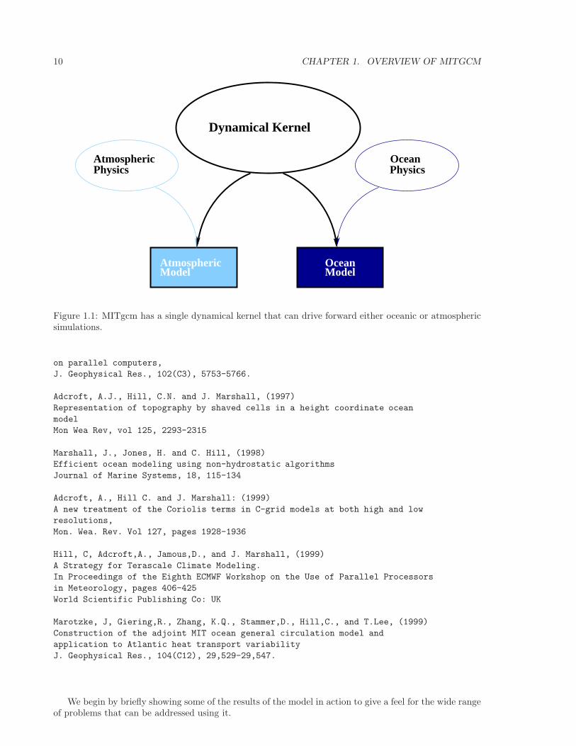
• it can be used to study both atmospheric and oceanic phenomena; one hydrodynamical kernel isused to drive forward both atmospheric and oceanic models - see fig 1.1
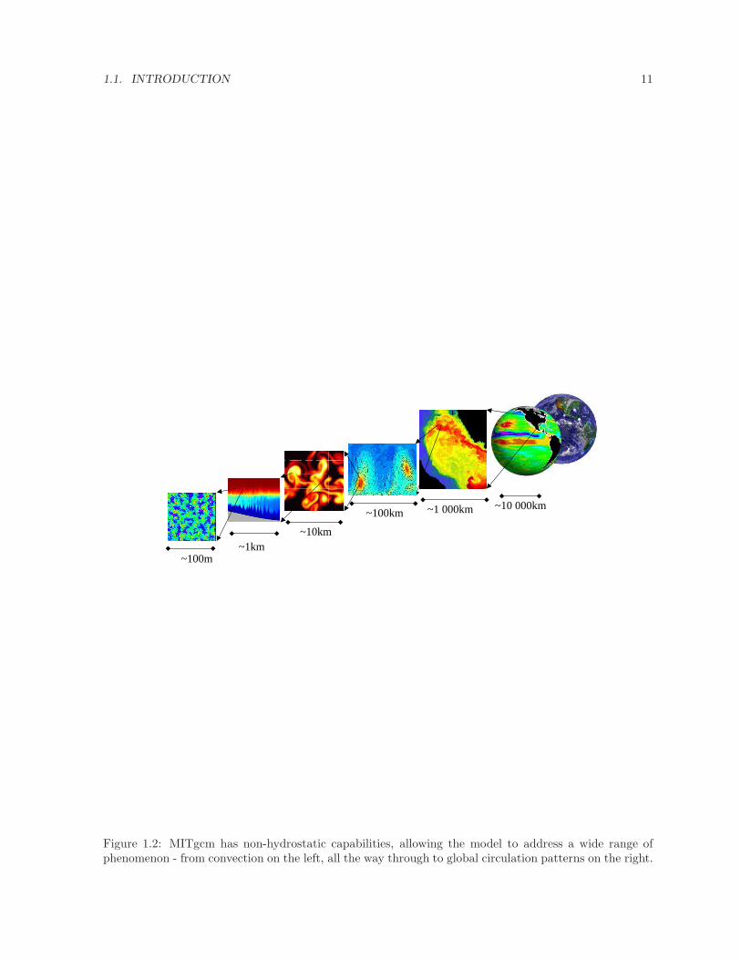
• it has a non-hydrostatic capability and so can be used to study both small-scale and large scaleprocesses - see fig 1.2
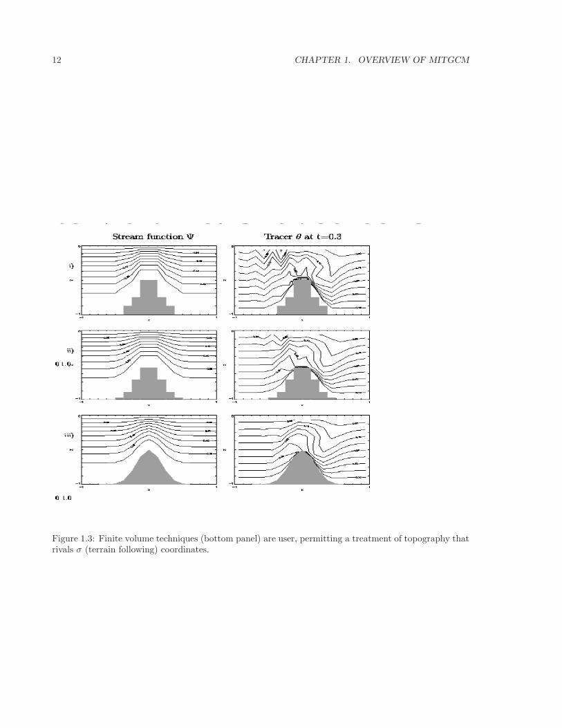
• finite volume techniques are employed yielding an intuitive discretization and support for the treat-ment of irregular geometries using orthogonal curvilinear grids and shaved cells - see fig 1.3
• tangent linear and adjoint counterparts are automatically maintained along with the forward model,permitting sensitivity and optimization studies.
• the model is developed to perform efficiently on a wide variety of computational platforms.
Key publications reporting on and charting the development of the model are Hill and Marshall[1995]; Marshall et al. [1997b,a]; Adcroft et al. [1997]; Marshall et al. [1998]; Adcroft and Marshall [1999];Chris Hill and Marshall [1999]; Marotzke et al. [1999]; Adcroft and Campin [2004]; Adcroft et al. [2004a];Marshall et al. [2004] (an overview on the model formulation can also be found in Adcroft et al. [2004b]):
Hill, C. and J. Marshall, (1995)
Application of a Parallel Navier-Stokes Model to Ocean Circulation in
Parallel Computational Fluid Dynamics
In Proceedings of Parallel Computational Fluid Dynamics: Implementations
and Results Using Parallel Computers, 545-552.
Elsevier Science B.V.: New York
Marshall, J., C. Hill, L. Perelman, and A. Adcroft, (1997)
Hydrostatic, quasi-hydrostatic, and nonhydrostatic ocean modeling
J. Geophysical Res., 102(C3), 5733-5752.
Marshall, J., A. Adcroft, C. Hill, L. Perelman, and C. Heisey, (1997)
A finite-volume, incompressible Navier Stokes model for studies of the ocean
9
10 CHAPTER 1. OVERVIEW OF MITGCM
Atmospheric Ocean
Dynamical Kernel
AtmosphericPhysics
ModelModel
OceanPhysics
Figure 1.1: MITgcm has a single dynamical kernel that can drive forward either oceanic or atmosphericsimulations.
on parallel computers,
J. Geophysical Res., 102(C3), 5753-5766.
Adcroft, A.J., Hill, C.N. and J. Marshall, (1997)
Representation of topography by shaved cells in a height coordinate ocean
model
Mon Wea Rev, vol 125, 2293-2315
Marshall, J., Jones, H. and C. Hill, (1998)
Efficient ocean modeling using non-hydrostatic algorithms
Journal of Marine Systems, 18, 115-134
Adcroft, A., Hill C. and J. Marshall: (1999)
A new treatment of the Coriolis terms in C-grid models at both high and low
resolutions,
Mon. Wea. Rev. Vol 127, pages 1928-1936
Hill, C, Adcroft,A., Jamous,D., and J. Marshall, (1999)
A Strategy for Terascale Climate Modeling.
In Proceedings of the Eighth ECMWF Workshop on the Use of Parallel Processors
in Meteorology, pages 406-425
World Scientific Publishing Co: UK
Marotzke, J, Giering,R., Zhang, K.Q., Stammer,D., Hill,C., and T.Lee, (1999)
Construction of the adjoint MIT ocean general circulation model and
application to Atlantic heat transport variability
J. Geophysical Res., 104(C12), 29,529-29,547.
We begin by briefly showing some of the results of the model in action to give a feel for the wide rangeof problems that can be addressed using it.
1.1. INTRODUCTION 11
~10 000km~1 000km~100km
~1km~10km
~100m
Figure 1.2: MITgcm has non-hydrostatic capabilities, allowing the model to address a wide range ofphenomenon - from convection on the left, all the way through to global circulation patterns on the right.
12 CHAPTER 1. OVERVIEW OF MITGCM
nite Volume: Shaved cells
Figure 1.3: Finite volume techniques (bottom panel) are user, permitting a treatment of topography thatrivals σ (terrain following) coordinates.
1.2. ILLUSTRATIONS OF THE MODEL IN ACTION 13
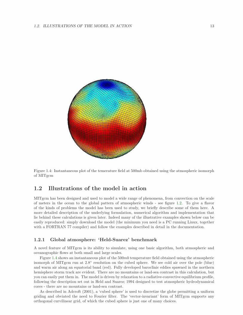
Figure 1.4: Instantaneous plot of the temerature field at 500mb obtained using the atmospheric isomorphof MITgcm
1.2 Illustrations of the model in action
MITgcm has been designed and used to model a wide range of phenomena, from convection on the scaleof meters in the ocean to the global pattern of atmospheric winds - see figure 1.2. To give a flavorof the kinds of problems the model has been used to study, we briefly describe some of them here. Amore detailed description of the underlying formulation, numerical algorithm and implementation thatlie behind these calculations is given later. Indeed many of the illustrative examples shown below can beeasily reproduced: simply download the model (the minimum you need is a PC running Linux, togetherwith a FORTRAN 77 compiler) and follow the examples described in detail in the documentation.
1.2.1 Global atmosphere: ‘Held-Suarez’ benchmark
A novel feature of MITgcm is its ability to simulate, using one basic algorithm, both atmospheric andoceanographic flows at both small and large scales.
Figure 1.4 shows an instantaneous plot of the 500mb temperature field obtained using the atmosphericisomorph of MITgcm run at 2.8 resolution on the cubed sphere. We see cold air over the pole (blue)and warm air along an equatorial band (red). Fully developed baroclinic eddies spawned in the northernhemisphere storm track are evident. There are no mountains or land-sea contrast in this calculation, butyou can easily put them in. The model is driven by relaxation to a radiative-convective equilibrium profile,following the description set out in Held and Suarez; 1994 designed to test atmospheric hydrodynamicalcores - there are no mountains or land-sea contrast.
As described in Adcroft (2001), a ‘cubed sphere’ is used to discretize the globe permitting a uniformgriding and obviated the need to Fourier filter. The ‘vector-invariant’ form of MITgcm supports anyorthogonal curvilinear grid, of which the cubed sphere is just one of many choices.
14 CHAPTER 1. OVERVIEW OF MITGCM
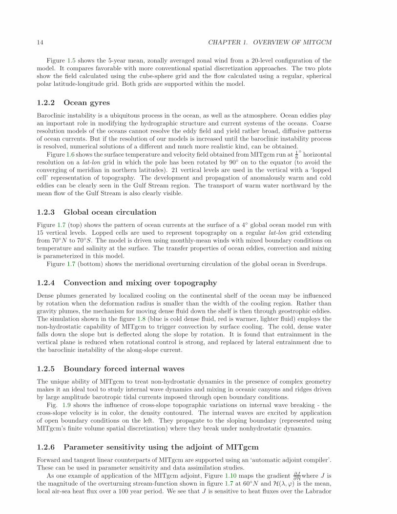
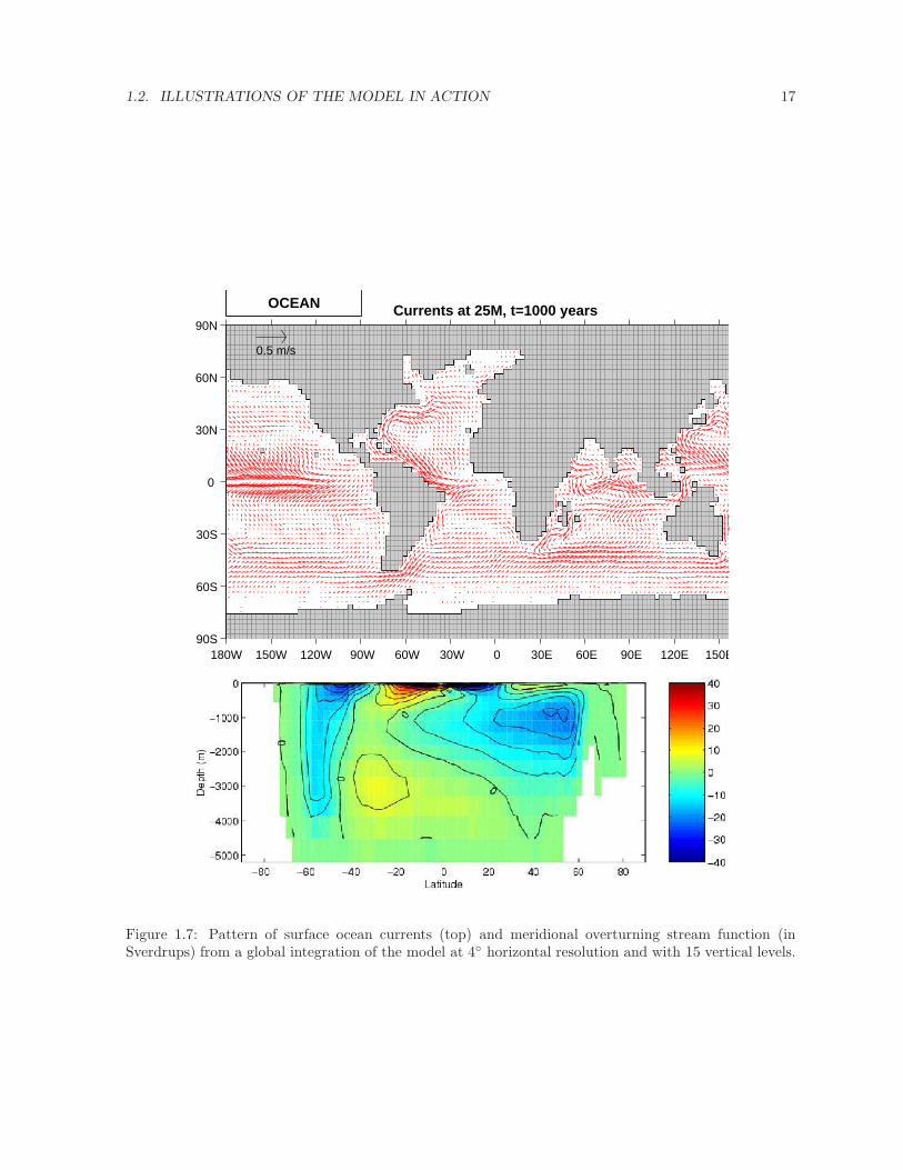
Figure 1.5 shows the 5-year mean, zonally averaged zonal wind from a 20-level configuration of themodel. It compares favorable with more conventional spatial discretization approaches. The two plotsshow the field calculated using the cube-sphere grid and the flow calculated using a regular, sphericalpolar latitude-longitude grid. Both grids are supported within the model.
1.2.2 Ocean gyres
Baroclinic instability is a ubiquitous process in the ocean, as well as the atmosphere. Ocean eddies playan important role in modifying the hydrographic structure and current systems of the oceans. Coarseresolution models of the oceans cannot resolve the eddy field and yield rather broad, diffusive patternsof ocean currents. But if the resolution of our models is increased until the baroclinic instability processis resolved, numerical solutions of a different and much more realistic kind, can be obtained.
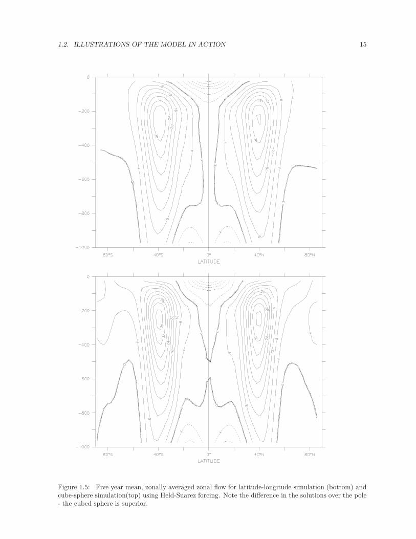
Figure 1.6 shows the surface temperature and velocity field obtained from MITgcm run at 16
horizontal
resolution on a lat-lon grid in which the pole has been rotated by 90 on to the equator (to avoid theconverging of meridian in northern latitudes). 21 vertical levels are used in the vertical with a ‘loppedcell’ representation of topography. The development and propagation of anomalously warm and coldeddies can be clearly seen in the Gulf Stream region. The transport of warm water northward by themean flow of the Gulf Stream is also clearly visible.
1.2.3 Global ocean circulation
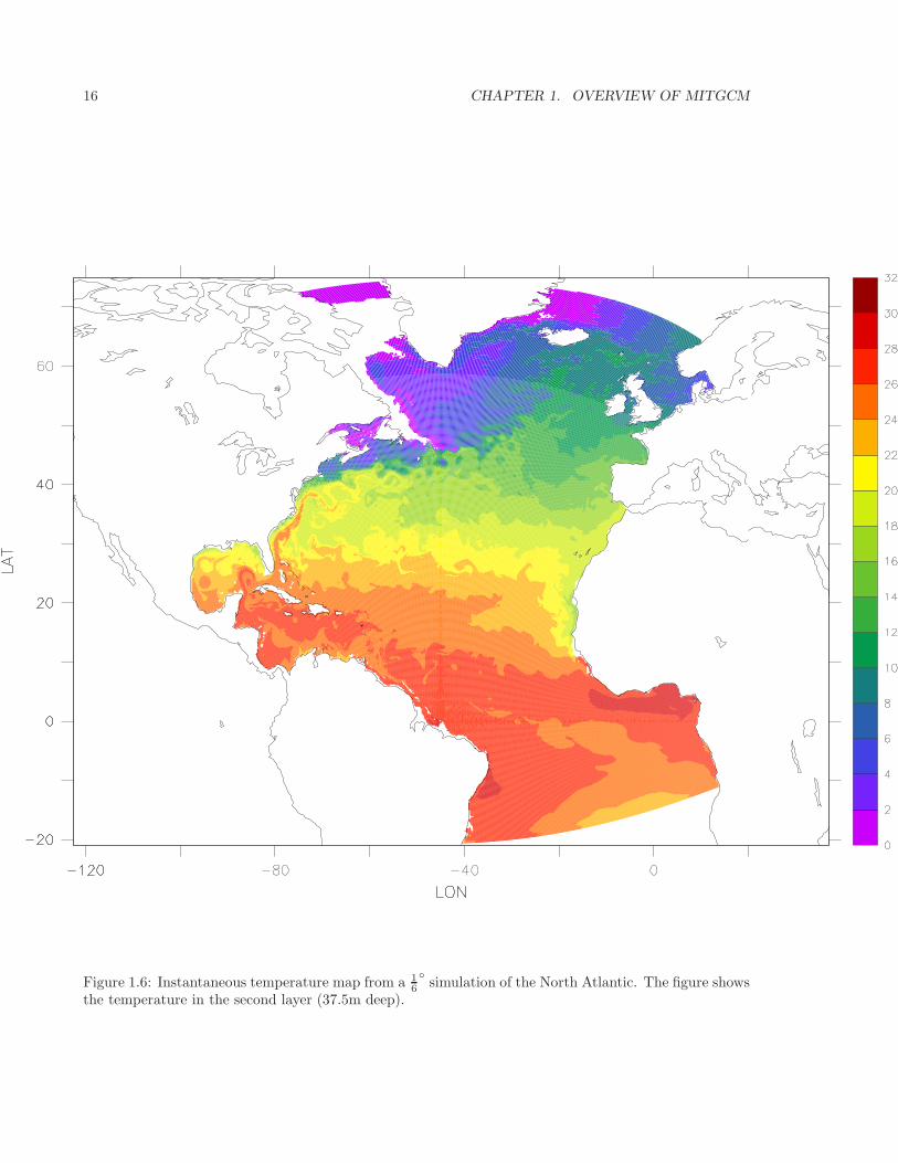
Figure 1.7 (top) shows the pattern of ocean currents at the surface of a 4 global ocean model run with15 vertical levels. Lopped cells are used to represent topography on a regular lat-lon grid extendingfrom 70N to 70S. The model is driven using monthly-mean winds with mixed boundary conditions ontemperature and salinity at the surface. The transfer properties of ocean eddies, convection and mixingis parameterized in this model.
Figure 1.7 (bottom) shows the meridional overturning circulation of the global ocean in Sverdrups.
1.2.4 Convection and mixing over topography
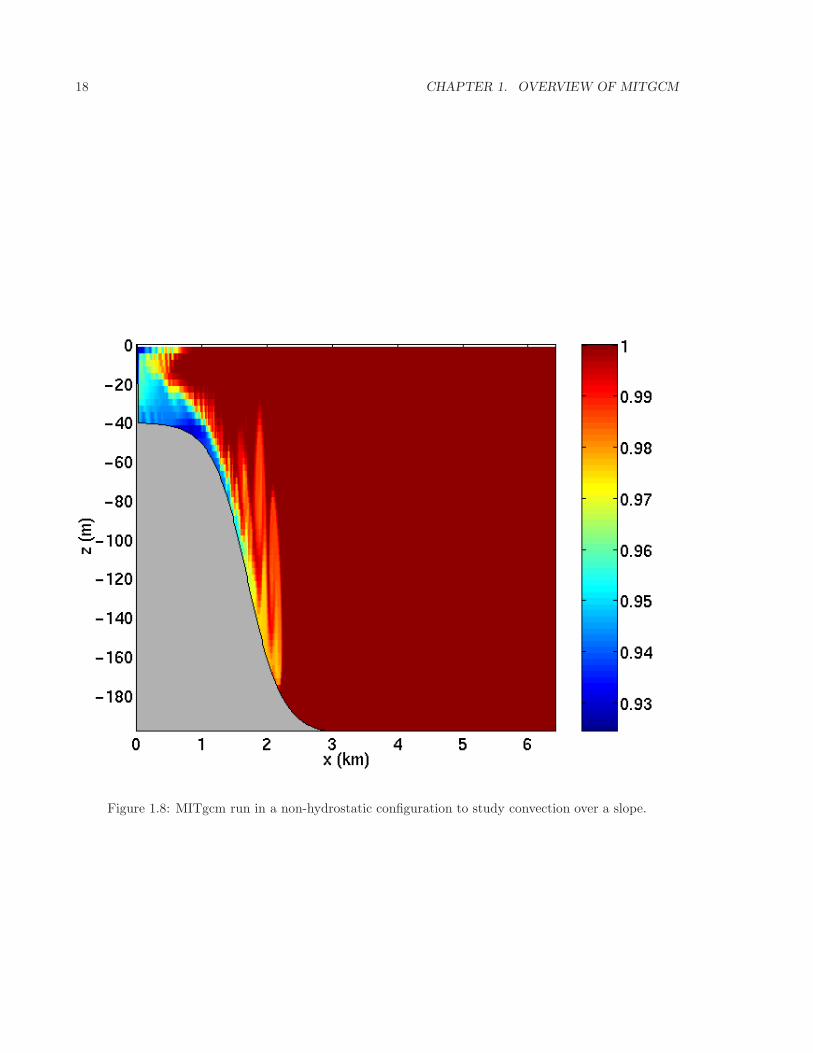
Dense plumes generated by localized cooling on the continental shelf of the ocean may be influencedby rotation when the deformation radius is smaller than the width of the cooling region. Rather thangravity plumes, the mechanism for moving dense fluid down the shelf is then through geostrophic eddies.The simulation shown in the figure 1.8 (blue is cold dense fluid, red is warmer, lighter fluid) employs thenon-hydrostatic capability of MITgcm to trigger convection by surface cooling. The cold, dense waterfalls down the slope but is deflected along the slope by rotation. It is found that entrainment in thevertical plane is reduced when rotational control is strong, and replaced by lateral entrainment due tothe baroclinic instability of the along-slope current.
1.2.5 Boundary forced internal waves
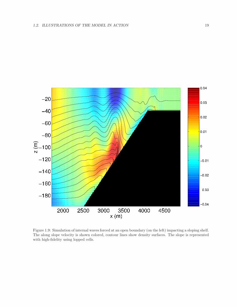
The unique ability of MITgcm to treat non-hydrostatic dynamics in the presence of complex geometrymakes it an ideal tool to study internal wave dynamics and mixing in oceanic canyons and ridges drivenby large amplitude barotropic tidal currents imposed through open boundary conditions.
Fig. 1.9 shows the influence of cross-slope topographic variations on internal wave breaking - thecross-slope velocity is in color, the density contoured. The internal waves are excited by applicationof open boundary conditions on the left. They propagate to the sloping boundary (represented usingMITgcm’s finite volume spatial discretization) where they break under nonhydrostatic dynamics.
1.2.6 Parameter sensitivity using the adjoint of MITgcm
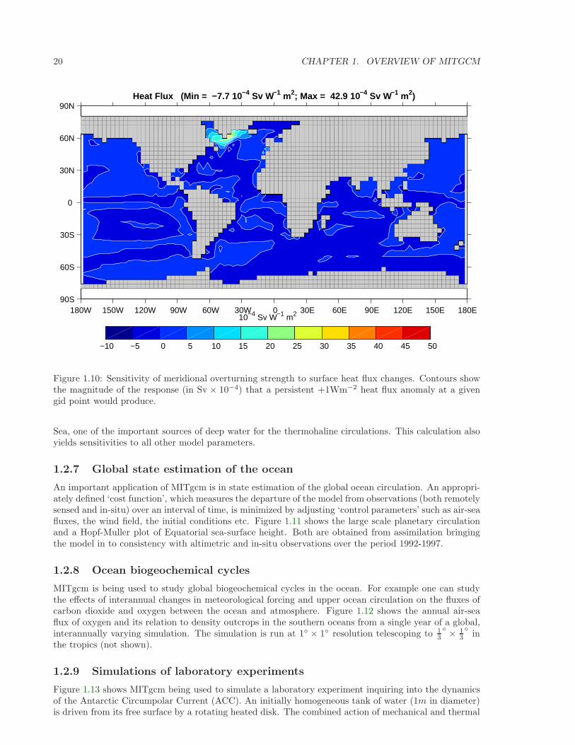
Forward and tangent linear counterparts of MITgcm are supported using an ‘automatic adjoint compiler’.These can be used in parameter sensitivity and data assimilation studies.
As one example of application of the MITgcm adjoint, Figure 1.10 maps the gradient ∂J∂Hwhere J is
the magnitude of the overturning stream-function shown in figure 1.7 at 60N and H(λ, ϕ) is the mean,local air-sea heat flux over a 100 year period. We see that J is sensitive to heat fluxes over the Labrador
1.2. ILLUSTRATIONS OF THE MODEL IN ACTION 15
Figure 1.5: Five year mean, zonally averaged zonal flow for latitude-longitude simulation (bottom) andcube-sphere simulation(top) using Held-Suarez forcing. Note the difference in the solutions over the pole- the cubed sphere is superior.
16 CHAPTER 1. OVERVIEW OF MITGCM
Figure 1.6: Instantaneous temperature map from a 16
simulation of the North Atlantic. The figure shows
the temperature in the second layer (37.5m deep).
1.2. ILLUSTRATIONS OF THE MODEL IN ACTION 17
180W 150W 120W 90W 60W 30W 0 30E 60E 90E 120E 150E 90S
60S
30S
0
30N
60N
90NCurrents at 25M, t=1000 years
0.5 m/s
OCEAN
Figure 1.7: Pattern of surface ocean currents (top) and meridional overturning stream function (inSverdrups) from a global integration of the model at 4 horizontal resolution and with 15 vertical levels.
18 CHAPTER 1. OVERVIEW OF MITGCM
Figure 1.8: MITgcm run in a non-hydrostatic configuration to study convection over a slope.
1.2. ILLUSTRATIONS OF THE MODEL IN ACTION 19
Figure 1.9: Simulation of internal waves forced at an open boundary (on the left) impacting a sloping shelf.The along slope velocity is shown colored, contour lines show density surfaces. The slope is representedwith high-fidelity using lopped cells.
20 CHAPTER 1. OVERVIEW OF MITGCM
180W 150W 120W 90W 60W 30W 0 30E 60E 90E 120E 150E 180E 90S
60S
30S
0
30N
60N
90NHeat Flux (Min = −7.7 10 −4 Sv W−1 m2; Max = 42.9 10−4 Sv W−1 m2)
−10 −5 0 5 10 15 20 25 30 35 40 45 50
10−4 Sv W−1 m2
Figure 1.10: Sensitivity of meridional overturning strength to surface heat flux changes. Contours showthe magnitude of the response (in Sv × 10−4) that a persistent +1Wm−2 heat flux anomaly at a givengid point would produce.
Sea, one of the important sources of deep water for the thermohaline circulations. This calculation alsoyields sensitivities to all other model parameters.
1.2.7 Global state estimation of the ocean
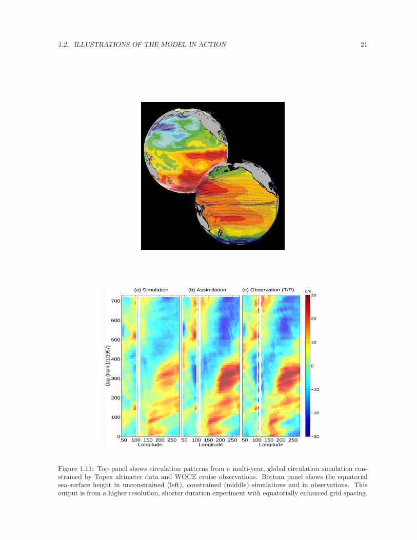
An important application of MITgcm is in state estimation of the global ocean circulation. An appropri-ately defined ‘cost function’, which measures the departure of the model from observations (both remotelysensed and in-situ) over an interval of time, is minimized by adjusting ‘control parameters’ such as air-seafluxes, the wind field, the initial conditions etc. Figure 1.11 shows the large scale planetary circulationand a Hopf-Muller plot of Equatorial sea-surface height. Both are obtained from assimilation bringingthe model in to consistency with altimetric and in-situ observations over the period 1992-1997.
1.2.8 Ocean biogeochemical cycles
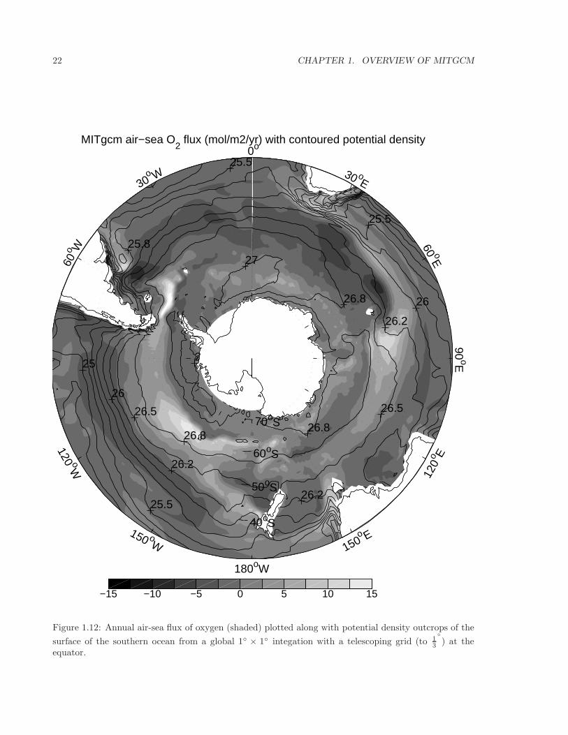
MITgcm is being used to study global biogeochemical cycles in the ocean. For example one can studythe effects of interannual changes in meteorological forcing and upper ocean circulation on the fluxes ofcarbon dioxide and oxygen between the ocean and atmosphere. Figure 1.12 shows the annual air-seaflux of oxygen and its relation to density outcrops in the southern oceans from a single year of a global,interannually varying simulation. The simulation is run at 1 × 1 resolution telescoping to 1
3
× 13
in
the tropics (not shown).
1.2.9 Simulations of laboratory experiments
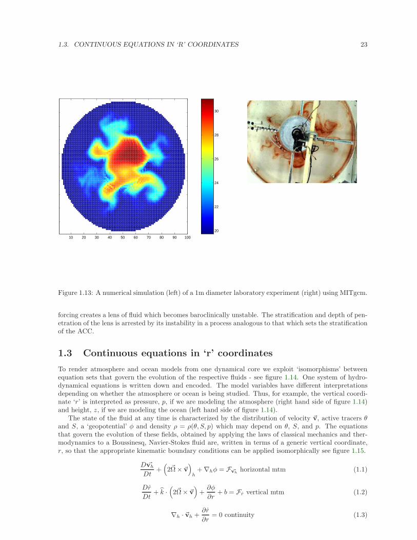
Figure 1.13 shows MITgcm being used to simulate a laboratory experiment inquiring into the dynamicsof the Antarctic Circumpolar Current (ACC). An initially homogeneous tank of water (1m in diameter)is driven from its free surface by a rotating heated disk. The combined action of mechanical and thermal
1.2. ILLUSTRATIONS OF THE MODEL IN ACTION 21
50 100 150 200 2500
100
200
300
400
500
600
700
(a) Simulation
Longitude
Day
(fro
m 1
/1/1
997)
50 100 150 200 250
(b) Assimilation
Longitude
−30
−20
−10
0
10
20
30
50 100 150 200 250Longitude
(c) Observation (T/P) cm
Figure 1.11: Top panel shows circulation patterns from a multi-year, global circulation simulation con-strained by Topex altimeter data and WOCE cruise observations. Bottom panel shows the equatorialsea-surface height in unconstrained (left), constrained (middle) simulations and in observations. Thisoutput is from a higher resolution, shorter duration experiment with equatorially enhanced grid spacing.
22 CHAPTER 1. OVERVIEW OF MITGCM
26.8
26.2
25.5
26.5
27
26.8
26.2
26
25.5
25.5
25.8
25
26
26.5
26.2
26.8
26.5
MITgcm air−sea O2 flux (mol/m2/yr) with contoured potential density
150 oW
120 oW
60
o W
30o W
0o
30 oE
60 oE
90oE
120
o E
150o E
180oW
70oS
60oS
50oS
40oS
−15 −10 −5 0 5 10 15
Figure 1.12: Annual air-sea flux of oxygen (shaded) plotted along with potential density outcrops of the
surface of the southern ocean from a global 1 × 1 integation with a telescoping grid (to 13
) at theequator.
1.3. CONTINUOUS EQUATIONS IN ‘R’ COORDINATES 23
20
22
24
26
28
30
10 20 30 40 50 60 70 80 90 100
10
20
30
40
50
60
70
80
90
100
Figure 1.13: A numerical simulation (left) of a 1m diameter laboratory experiment (right) using MITgcm.
forcing creates a lens of fluid which becomes baroclinically unstable. The stratification and depth of pen-etration of the lens is arrested by its instability in a process analogous to that which sets the stratificationof the ACC.
1.3 Continuous equations in ‘r’ coordinates
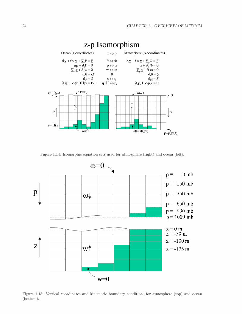
To render atmosphere and ocean models from one dynamical core we exploit ‘isomorphisms’ betweenequation sets that govern the evolution of the respective fluids - see figure 1.14. One system of hydro-dynamical equations is written down and encoded. The model variables have different interpretationsdepending on whether the atmosphere or ocean is being studied. Thus, for example, the vertical coordi-nate ‘r’ is interpreted as pressure, p, if we are modeling the atmosphere (right hand side of figure 1.14)and height, z, if we are modeling the ocean (left hand side of figure 1.14).
The state of the fluid at any time is characterized by the distribution of velocity ~v, active tracers θand S, a ‘geopotential’ φ and density ρ = ρ(θ, S, p) which may depend on θ, S, and p. The equationsthat govern the evolution of these fields, obtained by applying the laws of classical mechanics and ther-modynamics to a Boussinesq, Navier-Stokes fluid are, written in terms of a generic vertical coordinate,r, so that the appropriate kinematic boundary conditions can be applied isomorphically see figure 1.15.
D ~vh
Dt+(2~Ω × ~v
)h
+ ∇hφ = F ~vhhorizontal mtm (1.1)
Dr
Dt+ k ·
(2~Ω × ~v
)+∂φ
∂r+ b = Fr vertical mtm (1.2)
∇h · ~vh +∂r
∂r= 0 continuity (1.3)
24 CHAPTER 1. OVERVIEW OF MITGCM
Figure 1.14: Isomorphic equation sets used for atmosphere (right) and ocean (left).
MIT Climate Modeling Initiative
Z-P Isomorphism
z
p
ω=0
ω
w
Figure 1.15: Vertical coordinates and kinematic boundary conditions for atmosphere (top) and ocean(bottom).
1.3. CONTINUOUS EQUATIONS IN ‘R’ COORDINATES 25
b = b(θ, S, r) equation of state (1.4)
Dθ
Dt= Qθ potential temperature (1.5)
DS
Dt= QS humidity/salinity (1.6)
Here:
r is the vertical coordinate
D
Dt=
∂
∂t+ ~v · ∇ is the total derivative
∇ = ∇h + k∂
∂ris the ‘grad’ operator
with ∇h operating in the horizontal and k ∂∂r operating in the vertical, where k is a unit vector in the
vertical
t is time
~v = (u, v, r) = (~vh, r) is the velocity
φ is the ‘pressure’/‘geopotential’
~Ω is the Earth’s rotation
b is the ‘buoyancy’
θ is potential temperature
S is specific humidity in the atmosphere; salinity in the ocean
F~v are forcing and dissipation of ~v
Qθ are forcing and dissipation of θ
QS are forcing and dissipation of S
The F ′s and Q′s are provided by ‘physics’ and forcing packages for atmosphere and ocean. These aredescribed in later chapters.
26 CHAPTER 1. OVERVIEW OF MITGCM
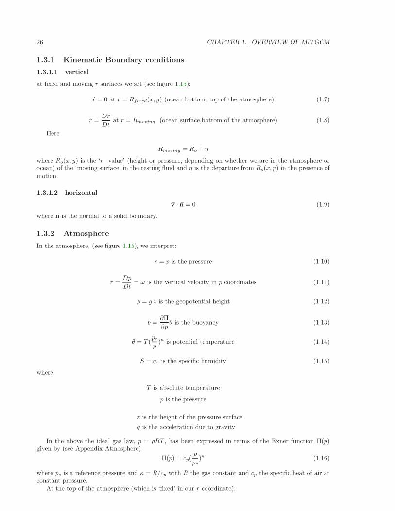
1.3.1 Kinematic Boundary conditions
1.3.1.1 vertical
at fixed and moving r surfaces we set (see figure 1.15):
r = 0 at r = Rfixed(x, y) (ocean bottom, top of the atmosphere) (1.7)
r =Dr
Dtat r = Rmoving (ocean surface,bottom of the atmosphere) (1.8)
Here
Rmoving = Ro + η
where Ro(x, y) is the ‘r−value’ (height or pressure, depending on whether we are in the atmosphere orocean) of the ‘moving surface’ in the resting fluid and η is the departure from Ro(x, y) in the presence ofmotion.
1.3.1.2 horizontal
~v · ~n = 0 (1.9)
where ~n is the normal to a solid boundary.
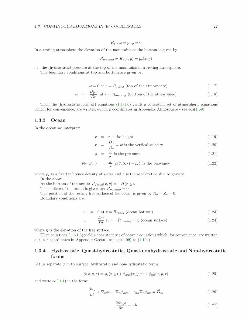
1.3.2 Atmosphere
In the atmosphere, (see figure 1.15), we interpret:
r = p is the pressure (1.10)
r =Dp
Dt= ω is the vertical velocity in p coordinates (1.11)
φ = g z is the geopotential height (1.12)
b =∂Π
∂pθ is the buoyancy (1.13)
θ = T (pc
p)κ is potential temperature (1.14)
S = q, is the specific humidity (1.15)
where
T is absolute temperature
p is the pressure
z is the height of the pressure surface
g is the acceleration due to gravity
In the above the ideal gas law, p = ρRT , has been expressed in terms of the Exner function Π(p)given by (see Appendix Atmosphere)
Π(p) = cp(p
pc)κ (1.16)
where pc is a reference pressure and κ = R/cp with R the gas constant and cp the specific heat of air atconstant pressure.
At the top of the atmosphere (which is ‘fixed’ in our r coordinate):
1.3. CONTINUOUS EQUATIONS IN ‘R’ COORDINATES 27
Rfixed = ptop = 0
In a resting atmosphere the elevation of the mountains at the bottom is given by
Rmoving = Ro(x, y) = po(x, y)
i.e. the (hydrostatic) pressure at the top of the mountains in a resting atmosphere.The boundary conditions at top and bottom are given by:
ω = 0 at r = Rfixed (top of the atmosphere) (1.17)
ω =Dps
Dt; at r = Rmoving (bottom of the atmosphere) (1.18)
Then the (hydrostatic form of) equations (1.1-1.6) yields a consistent set of atmospheric equationswhich, for convenience, are written out in p coordinates in Appendix Atmosphere - see eqs(1.59).
1.3.3 Ocean
In the ocean we interpret:
r = z is the height (1.19)
r =Dz
Dt= w is the vertical velocity (1.20)
φ =p
ρcis the pressure (1.21)
b(θ, S, r) =g
ρc(ρ(θ, S, r) − ρc) is the buoyancy (1.22)
where ρc is a fixed reference density of water and g is the acceleration due to gravity.In the aboveAt the bottom of the ocean: Rfixed(x, y) = −H(x, y).The surface of the ocean is given by: Rmoving = ηThe position of the resting free surface of the ocean is given by Ro = Zo = 0.Boundary conditions are:
w = 0 at r = Rfixed (ocean bottom) (1.23)
w =Dη
Dtat r = Rmoving = η (ocean surface) (1.24)
where η is the elevation of the free surface.Then equations (1.1-1.6) yield a consistent set of oceanic equations which, for convenience, are written
out in z coordinates in Appendix Ocean - see eqs(1.99) to (1.104).
1.3.4 Hydrostatic, Quasi-hydrostatic, Quasi-nonhydrostatic and Non-hydrostaticforms
Let us separate φ in to surface, hydrostatic and non-hydrostatic terms:
φ(x, y, r) = φs(x, y) + φhyd(x, y, r) + φnh(x, y, r) (1.25)
and write eq( 1.1) in the form:
∂ ~vh
∂t+ ∇hφs + ∇hφhyd + ǫnh∇hφnh = ~G~vh
(1.26)
∂φhyd
∂r= −b (1.27)
28 CHAPTER 1. OVERVIEW OF MITGCM
ǫnh∂r
∂t+∂φnh
∂r= Gr (1.28)
Here ǫnh is a non-hydrostatic parameter.
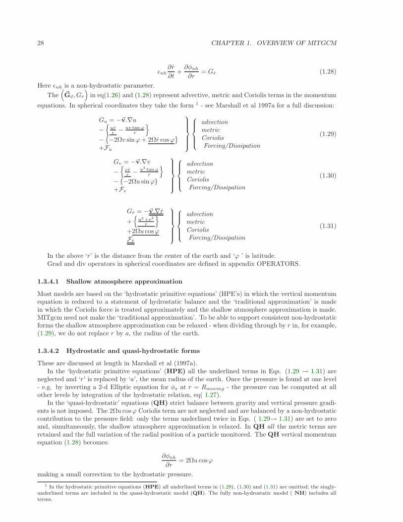
The(~G~v, Gr
)in eq(1.26) and (1.28) represent advective, metric and Coriolis terms in the momentum
equations. In spherical coordinates they take the form 1 - see Marshall et al 1997a for a full discussion:
Gu = −~v.∇u−
urr − uv tan ϕ
r
−−2Ωv sinϕ+ 2Ωr cosϕ
+Fu
advectionmetricCoriolisForcing/Dissipation
(1.29)
Gv = −~v.∇v−
vrr − u2 tan ϕ
r
−−2Ωu sinϕ+Fv
advectionmetricCoriolisForcing/Dissipation
(1.30)
Gr = −~v.∇r+
u2 +v2
r
+2Ωu cosϕFr
advectionmetricCoriolisForcing/Dissipation
(1.31)
In the above ‘r’ is the distance from the center of the earth and ‘ϕ ’ is latitude.Grad and div operators in spherical coordinates are defined in appendix OPERATORS.
1.3.4.1 Shallow atmosphere approximation
Most models are based on the ‘hydrostatic primitive equations’ (HPE’s) in which the vertical momentumequation is reduced to a statement of hydrostatic balance and the ‘traditional approximation’ is madein which the Coriolis force is treated approximately and the shallow atmosphere approximation is made.MITgcm need not make the ‘traditional approximation’. To be able to support consistent non-hydrostaticforms the shallow atmosphere approximation can be relaxed - when dividing through by r in, for example,(1.29), we do not replace r by a, the radius of the earth.
1.3.4.2 Hydrostatic and quasi-hydrostatic forms
These are discussed at length in Marshall et al (1997a).In the ‘hydrostatic primitive equations’ (HPE) all the underlined terms in Eqs. (1.29 → 1.31) are
neglected and ‘r’ is replaced by ‘a’, the mean radius of the earth. Once the pressure is found at one level- e.g. by inverting a 2-d Elliptic equation for φs at r = Rmoving - the pressure can be computed at allother levels by integration of the hydrostatic relation, eq( 1.27).
In the ‘quasi-hydrostatic’ equations (QH) strict balance between gravity and vertical pressure gradi-ents is not imposed. The 2Ωu cosϕ Coriolis term are not neglected and are balanced by a non-hydrostaticcontribution to the pressure field: only the terms underlined twice in Eqs. ( 1.29→ 1.31) are set to zeroand, simultaneously, the shallow atmosphere approximation is relaxed. In QH all the metric terms areretained and the full variation of the radial position of a particle monitored. The QH vertical momentumequation (1.28) becomes:
∂φnh
∂r= 2Ωu cosϕ
making a small correction to the hydrostatic pressure.
1 In the hydrostatic primitive equations (HPE) all underlined terms in (1.29), (1.30) and (1.31) are omitted; the singly-underlined terms are included in the quasi-hydrostatic model (QH). The fully non-hydrostatic model ( NH) includes allterms.
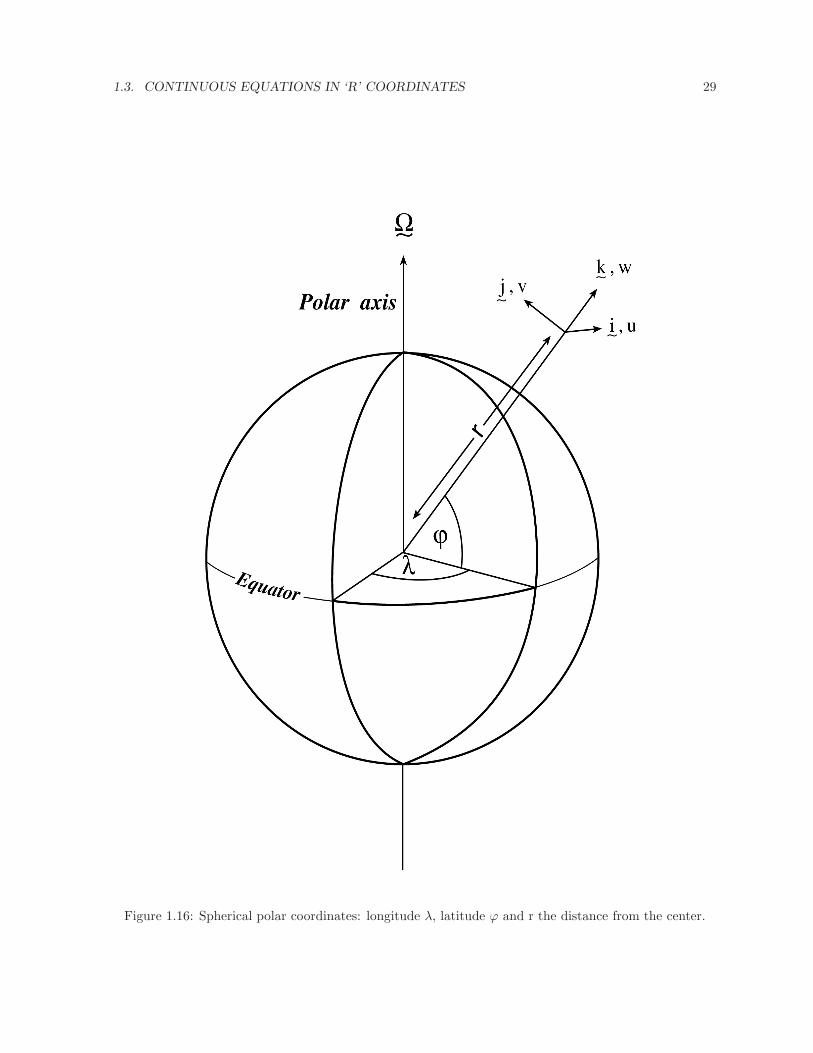
1.3. CONTINUOUS EQUATIONS IN ‘R’ COORDINATES 29
Figure 1.16: Spherical polar coordinates: longitude λ, latitude ϕ and r the distance from the center.
30 CHAPTER 1. OVERVIEW OF MITGCM
QH has good energetic credentials - they are the same as for HPE. Importantly, however, it has thesame angular momentum principle as the full non-hydrostatic model (NH) - see Marshall et.al., 1997a.As in HPE only a 2-d elliptic problem need be solved.
1.3.4.3 Non-hydrostatic and quasi-nonhydrostatic forms
MITgcm presently supports a full non-hydrostatic ocean isomorph, but only a quasi-non-hydrostaticatmospheric isomorph.
Non-hydrostatic Ocean In the non-hydrostatic ocean model all terms in equations Eqs.(1.29 →1.31) are retained. A three dimensional elliptic equation must be solved subject to Neumann boundaryconditions (see below). It is important to note that use of the full NH does not admit any new ‘fast’waves in to the system - the incompressible condition eq(1.3) has already filtered out acoustic modes. Itdoes, however, ensure that the gravity waves are treated accurately with an exact dispersion relation. TheNH set has a complete angular momentum principle and consistent energetics - see White and Bromley,1995; Marshall et.al. 1997a.
Quasi-nonhydrostatic Atmosphere In the non-hydrostatic version of our atmospheric model weapproximate r in the vertical momentum eqs(1.28) and (1.30) (but only here) by:
r =Dp
Dt=
1
g
Dφ
Dt(1.32)
where phy is the hydrostatic pressure.
1.3.4.4 Summary of equation sets supported by model
Atmosphere Hydrostatic, and quasi-hydrostatic and quasi non-hydrostatic forms of the compressiblenon-Boussinesq equations in p−coordinates are supported.
Hydrostatic and quasi-hydrostatic The hydrostatic set is written out in p−coordinates in ap-pendix Atmosphere - see eq(1.59).
Quasi-nonhydrostatic A quasi-nonhydrostatic form is also supported.
Ocean
Hydrostatic and quasi-hydrostatic Hydrostatic, and quasi-hydrostatic forms of the incompress-ible Boussinesq equations in z−coordinates are supported.
Non-hydrostatic Non-hydrostatic forms of the incompressible Boussinesq equations in z− coordi-nates are supported - see eqs(1.99) to (1.104).
1.3.5 Solution strategy
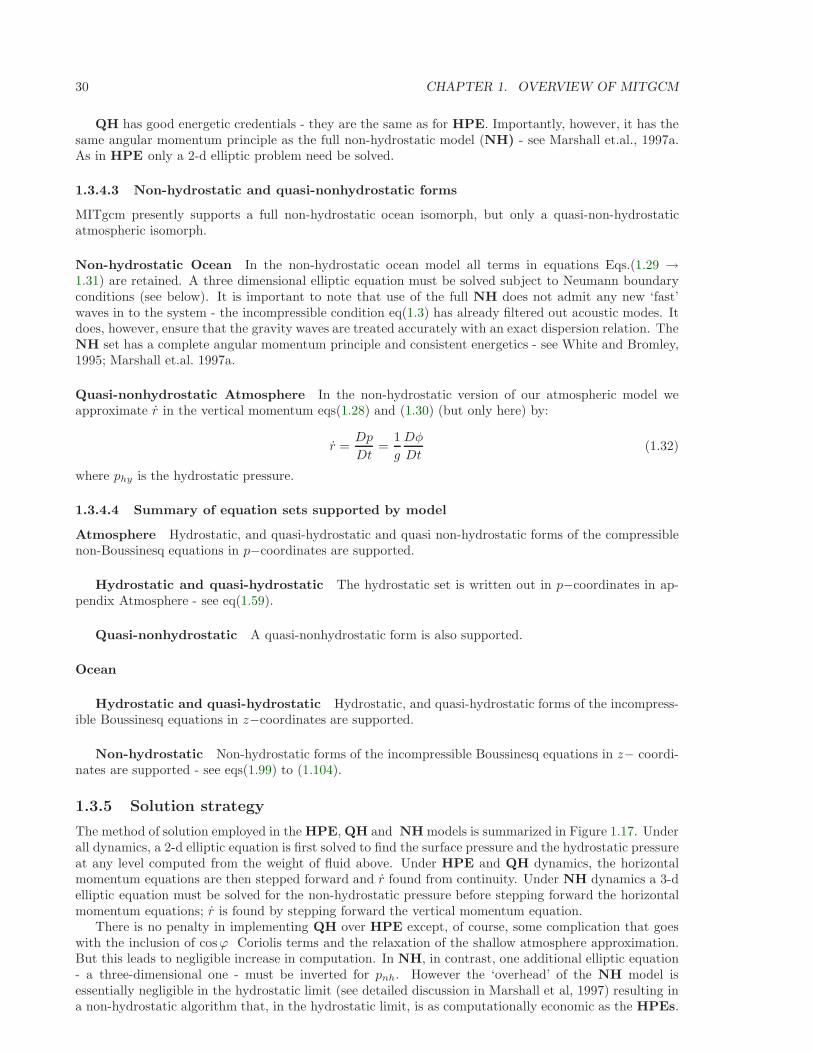
The method of solution employed in the HPE, QH and NH models is summarized in Figure 1.17. Underall dynamics, a 2-d elliptic equation is first solved to find the surface pressure and the hydrostatic pressureat any level computed from the weight of fluid above. Under HPE and QH dynamics, the horizontalmomentum equations are then stepped forward and r found from continuity. Under NH dynamics a 3-delliptic equation must be solved for the non-hydrostatic pressure before stepping forward the horizontalmomentum equations; r is found by stepping forward the vertical momentum equation.
There is no penalty in implementing QH over HPE except, of course, some complication that goeswith the inclusion of cosϕ Coriolis terms and the relaxation of the shallow atmosphere approximation.But this leads to negligible increase in computation. In NH, in contrast, one additional elliptic equation- a three-dimensional one - must be inverted for pnh. However the ‘overhead’ of the NH model isessentially negligible in the hydrostatic limit (see detailed discussion in Marshall et al, 1997) resulting ina non-hydrostatic algorithm that, in the hydrostatic limit, is as computationally economic as the HPEs.
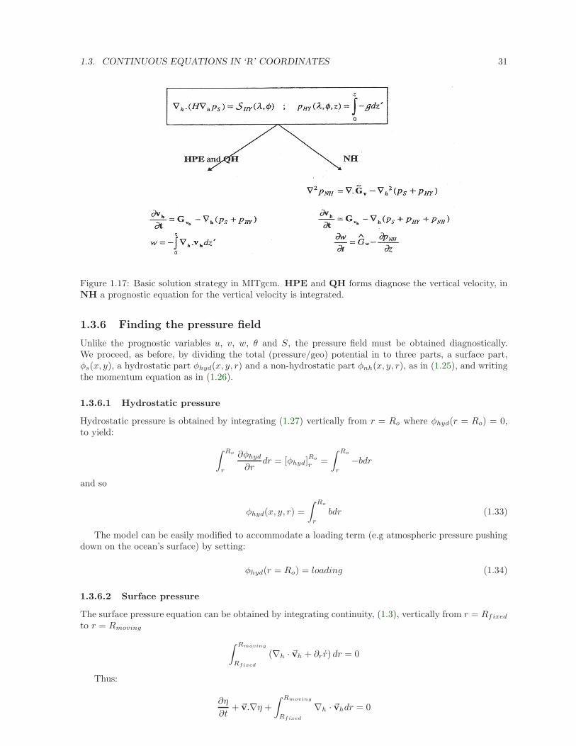
1.3. CONTINUOUS EQUATIONS IN ‘R’ COORDINATES 31
Figure 1.17: Basic solution strategy in MITgcm. HPE and QH forms diagnose the vertical velocity, inNH a prognostic equation for the vertical velocity is integrated.
1.3.6 Finding the pressure field
Unlike the prognostic variables u, v, w, θ and S, the pressure field must be obtained diagnostically.We proceed, as before, by dividing the total (pressure/geo) potential in to three parts, a surface part,φs(x, y), a hydrostatic part φhyd(x, y, r) and a non-hydrostatic part φnh(x, y, r), as in (1.25), and writingthe momentum equation as in (1.26).
1.3.6.1 Hydrostatic pressure
Hydrostatic pressure is obtained by integrating (1.27) vertically from r = Ro where φhyd(r = Ro) = 0,to yield:
∫ Ro
r
∂φhyd
∂rdr = [φhyd]
Ro
r =
∫ Ro
r
−bdr
and so
φhyd(x, y, r) =
∫ Ro
r
bdr (1.33)
The model can be easily modified to accommodate a loading term (e.g atmospheric pressure pushingdown on the ocean’s surface) by setting:
φhyd(r = Ro) = loading (1.34)
1.3.6.2 Surface pressure
The surface pressure equation can be obtained by integrating continuity, (1.3), vertically from r = Rfixed
to r = Rmoving
∫ Rmoving
Rfixed
(∇h · ~vh + ∂r r) dr = 0
Thus:
∂η
∂t+ ~v.∇η +
∫ Rmoving
Rfixed
∇h · ~vhdr = 0
32 CHAPTER 1. OVERVIEW OF MITGCM
where η = Rmoving − Ro is the free-surface r-anomaly in units of r. The above can be rearranged toyield, using Leibnitz’s theorem:
∂η
∂t+ ∇h ·
∫ Rmoving
Rfixed
~vhdr = source (1.35)
where we have incorporated a source term.Whether φ is pressure (ocean model, p/ρc) or geopotential (atmospheric model), in (1.26), the hori-
zontal gradient term can be written
∇hφs = ∇h (bsη) (1.36)
where bs is the buoyancy at the surface.In the hydrostatic limit (ǫnh = 0), equations (1.26), (1.35) and (1.36) can be solved by inverting a
2-d elliptic equation for φs as described in Chapter 2. Both ‘free surface’ and ‘rigid lid’ approaches areavailable.
1.3.6.3 Non-hydrostatic pressure
Taking the horizontal divergence of (1.26) and adding ∂∂r of (1.28), invoking the continuity equation (1.3),
we deduce that:
∇23φnh = ∇. ~G~v −
(∇2
hφs + ∇2φhyd
)= ∇.~F (1.37)
For a given rhs this 3-d elliptic equation must be inverted for φnh subject to appropriate choice ofboundary conditions. This method is usually called The Pressure Method [Harlow and Welch, 1965;Williams, 1969; Potter, 1976]. In the hydrostatic primitive equations case (HPE), the 3-d problem doesnot need to be solved.
Boundary Conditions We apply the condition of no normal flow through all solid boundaries - thecoasts (in the ocean) and the bottom:
~v.n = 0 (1.38)
where n is a vector of unit length normal to the boundary. The kinematic condition (1.38) is also appliedto the vertical velocity at r = Rmoving. No-slip (vT = 0) or slip (∂vT /∂n = 0) conditions are employedon the tangential component of velocity, vT , at all solid boundaries, depending on the form chosen forthe dissipative terms in the momentum equations - see below.
Eq.(1.38) implies, making use of (1.26), that:
n.∇φnh = n.~F (1.39)
where
~F = ~G~v − (∇hφs + ∇φhyd)
presenting inhomogeneous Neumann boundary conditions to the Elliptic problem (1.37). As shown,for example, by Williams (1969), one can exploit classical 3D potential theory and, by introducing anappropriately chosen δ-function sheet of ‘source-charge’, replace the inhomogeneous boundary conditionon pressure by a homogeneous one. The source term rhs in (1.37) is the divergence of the vector ~F.By simultaneously setting n.~F = 0 and n.∇φnh = 0 on the boundary the following self-consistent butsimpler homogenized Elliptic problem is obtained:
∇2φnh = ∇.~F
where ~F is a modified ~F such that ~F.n = 0. As is implied by (1.39) the modified boundary conditionbecomes:
n.∇φnh = 0 (1.40)
1.3. CONTINUOUS EQUATIONS IN ‘R’ COORDINATES 33
If the flow is ‘close’ to hydrostatic balance then the 3-d inversion converges rapidly because φnh isthen only a small correction to the hydrostatic pressure field (see the discussion in Marshall et al, a,b).
The solution φnh to (1.37) and (1.39) does not vanish at r = Rmoving, and so refines the pressurethere.
1.3.7 Forcing/dissipation
1.3.7.1 Forcing
The forcing terms F on the rhs of the equations are provided by ‘physics packages’ and forcing packages.These are described later on.
1.3.7.2 Dissipation
Momentum Many forms of momentum dissipation are available in the model. Laplacian and bihar-monic frictions are commonly used:
DV = Ah∇2hv +Av
∂2v
∂z2+A4∇4
hv (1.41)
where Ah and Av are (constant) horizontal and vertical viscosity coefficients and A4 is the horizontalcoefficient for biharmonic friction. These coefficients are the same for all velocity components.
Tracers The mixing terms for the temperature and salinity equations have a similar form to that ofmomentum except that the diffusion tensor can be non-diagonal and have varying coefficients.
DT,S = ∇.[K∇(T, S)] +K4∇4h(T, S) (1.42)
where K is the diffusion tensor and the K4 horizontal coefficient for biharmonic diffusion. In thesimplest case where the subgrid-scale fluxes of heat and salt are parameterized with constant horizontaland vertical diffusion coefficients, K, reduces to a diagonal matrix with constant coefficients:
K =
Kh 0 00 Kh 00 0 Kv
(1.43)
where Kh and Kv are the horizontal and vertical diffusion coefficients. These coefficients are the samefor all tracers (temperature, salinity ... ).
1.3.8 Vector invariant form
For some purposes it is advantageous to write momentum advection in eq(1.1) and (1.2) in the (so-called)‘vector invariant’ form:
D~v
Dt=∂~v
∂t+ (∇× ~v) × ~v + ∇
[1
2(~v · ~v)
](1.44)
This permits alternative numerical treatments of the non-linear terms based on their representation asa vorticity flux. Because gradients of coordinate vectors no longer appear on the rhs of (1.44), explicitrepresentation of the metric terms in (1.29), (1.30) and (1.31), can be avoided: information about thegeometry is contained in the areas and lengths of the volumes used to discretize the model.
1.3.9 Adjoint
Tangent linear and adjoint counterparts of the forward model are described in Chapter 5.
34 CHAPTER 1. OVERVIEW OF MITGCM
1.4 Appendix ATMOSPHERE
1.4.1 Hydrostatic Primitive Equations for the Atmosphere in pressure coor-dinates
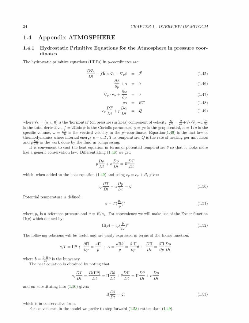
The hydrostatic primitive equations (HPEs) in p-coordinates are:
D~vh
Dt+ f k × ~vh + ∇pφ = ~F (1.45)
∂φ
∂p+ α = 0 (1.46)
∇p · ~vh +∂ω
∂p= 0 (1.47)
pα = RT (1.48)
cvDT
Dt+ p
Dα
Dt= Q (1.49)
where ~vh = (u, v, 0) is the ‘horizontal’ (on pressure surfaces) component of velocity, DDt = ∂
∂t +~vh·∇p+ω ∂∂p
is the total derivative, f = 2Ω sinϕ is the Coriolis parameter, φ = gz is the geopotential, α = 1/ρ is thespecific volume, ω = Dp
Dt is the vertical velocity in the p−coordinate. Equation(1.49) is the first law ofthermodynamics where internal energy e = cvT , T is temperature, Q is the rate of heating per unit massand pDα
Dt is the work done by the fluid in compressing.
It is convenient to cast the heat equation in terms of potential temperature θ so that it looks morelike a generic conservation law. Differentiating (1.48) we get:
pDα
Dt+ α
Dp
Dt= R
DT
Dt
which, when added to the heat equation (1.49) and using cp = cv +R, gives:
cpDT
Dt− α
Dp
Dt= Q (1.50)
Potential temperature is defined:
θ = T (pc
p)κ (1.51)
where pc is a reference pressure and κ = R/cp. For convenience we will make use of the Exner functionΠ(p) which defined by:
Π(p) = cp(p
pc)κ (1.52)
The following relations will be useful and are easily expressed in terms of the Exner function:
cpT = Πθ ;∂Π
∂p=κΠ
p; α =
κΠθ
p=∂ Π
∂pθ ;
DΠ
Dt=∂Π
∂p
Dp
Dt
where b = ∂ Π∂p θ is the buoyancy.
The heat equation is obtained by noting that
cpDT
Dt=D(Πθ)
Dt= Π
Dθ
Dt+ θ
DΠ
Dt= Π
Dθ
Dt+ α
Dp
Dt
and on substituting into (1.50) gives:
ΠDθ
Dt= Q (1.53)
which is in conservative form.
For convenience in the model we prefer to step forward (1.53) rather than (1.49).
1.4. APPENDIX ATMOSPHERE 35
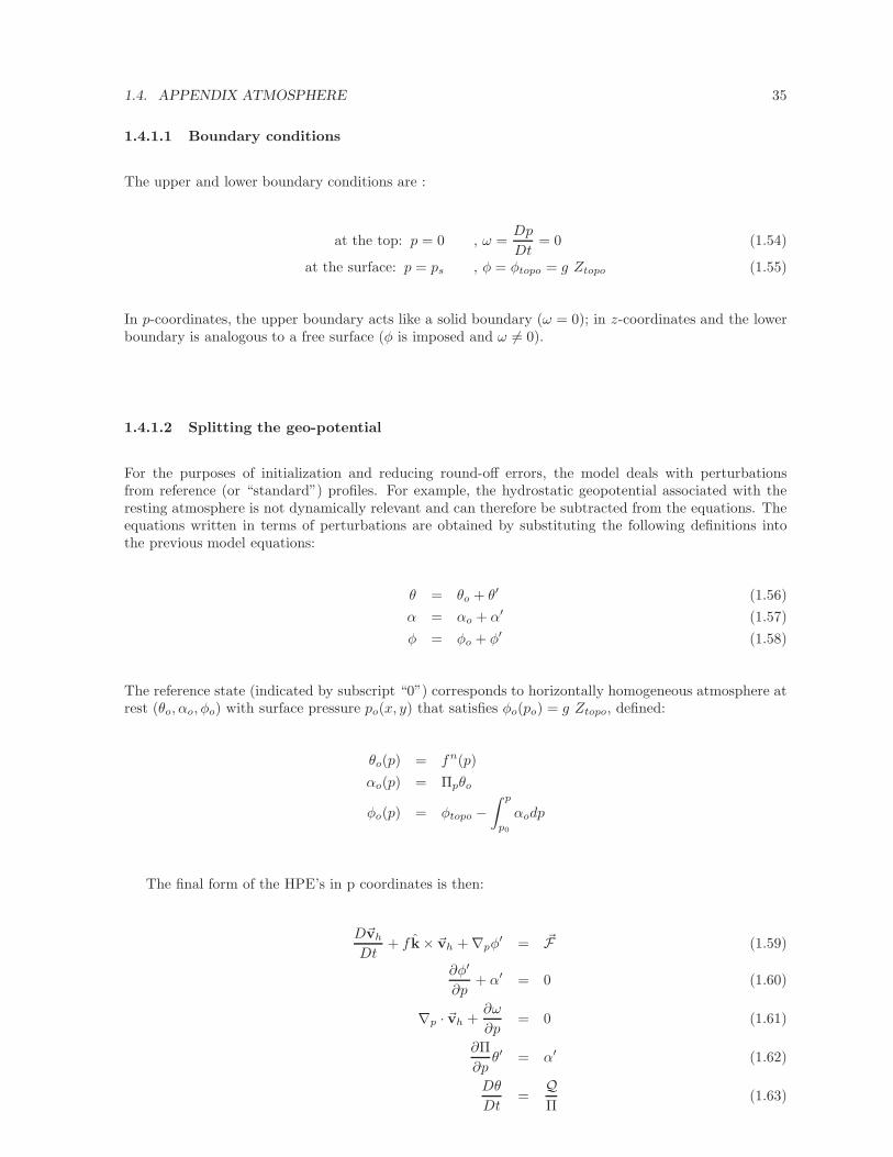
1.4.1.1 Boundary conditions
The upper and lower boundary conditions are :
at the top: p = 0 , ω =Dp
Dt= 0 (1.54)
at the surface: p = ps , φ = φtopo = g Ztopo (1.55)
In p-coordinates, the upper boundary acts like a solid boundary (ω = 0); in z-coordinates and the lowerboundary is analogous to a free surface (φ is imposed and ω 6= 0).
1.4.1.2 Splitting the geo-potential
For the purposes of initialization and reducing round-off errors, the model deals with perturbationsfrom reference (or “standard”) profiles. For example, the hydrostatic geopotential associated with theresting atmosphere is not dynamically relevant and can therefore be subtracted from the equations. Theequations written in terms of perturbations are obtained by substituting the following definitions intothe previous model equations:
θ = θo + θ′ (1.56)
α = αo + α′ (1.57)
φ = φo + φ′ (1.58)
The reference state (indicated by subscript “0”) corresponds to horizontally homogeneous atmosphere atrest (θo, αo, φo) with surface pressure po(x, y) that satisfies φo(po) = g Ztopo, defined:
θo(p) = fn(p)
αo(p) = Πpθo
φo(p) = φtopo −∫ p
p0
αodp
The final form of the HPE’s in p coordinates is then:
D~vh
Dt+ f k× ~vh + ∇pφ
′ = ~F (1.59)
∂φ′
∂p+ α′ = 0 (1.60)
∇p · ~vh +∂ω
∂p= 0 (1.61)
∂Π
∂pθ′ = α′ (1.62)
Dθ
Dt=
QΠ
(1.63)
36 CHAPTER 1. OVERVIEW OF MITGCM
1.5 Appendix OCEAN
1.5.1 Equations of motion for the ocean
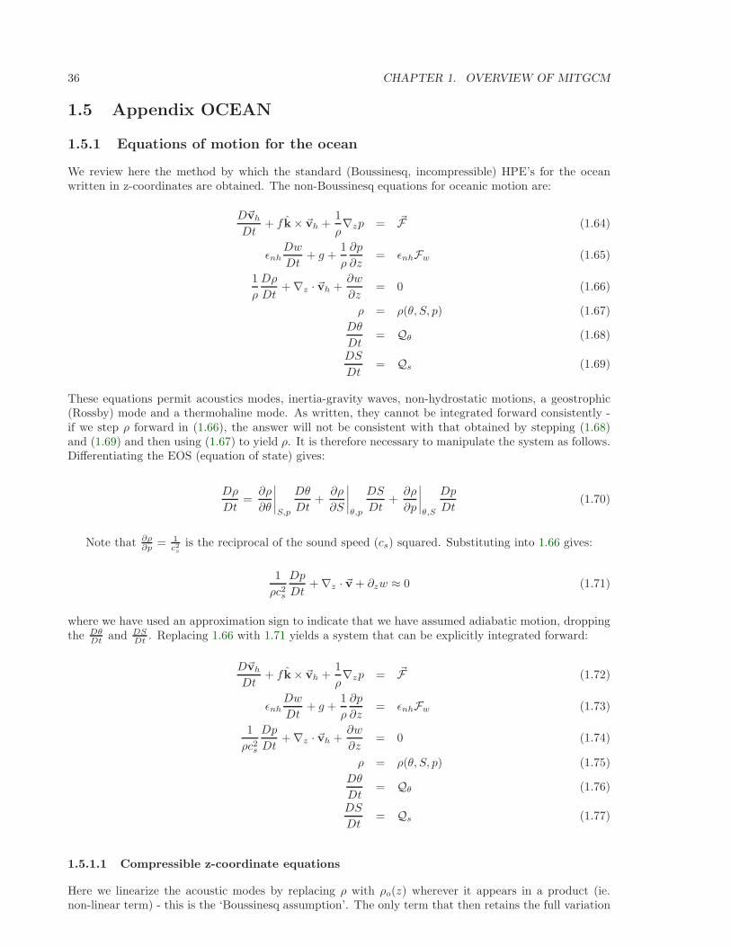
We review here the method by which the standard (Boussinesq, incompressible) HPE’s for the oceanwritten in z-coordinates are obtained. The non-Boussinesq equations for oceanic motion are:
D~vh
Dt+ f k× ~vh +
1
ρ∇zp = ~F (1.64)
ǫnhDw
Dt+ g +
1
ρ
∂p
∂z= ǫnhFw (1.65)
1
ρ
Dρ
Dt+ ∇z · ~vh +
∂w
∂z= 0 (1.66)
ρ = ρ(θ, S, p) (1.67)
Dθ
Dt= Qθ (1.68)
DS
Dt= Qs (1.69)
These equations permit acoustics modes, inertia-gravity waves, non-hydrostatic motions, a geostrophic(Rossby) mode and a thermohaline mode. As written, they cannot be integrated forward consistently -if we step ρ forward in (1.66), the answer will not be consistent with that obtained by stepping (1.68)and (1.69) and then using (1.67) to yield ρ. It is therefore necessary to manipulate the system as follows.Differentiating the EOS (equation of state) gives:
Dρ
Dt=∂ρ
∂θ
∣∣∣∣S,p
Dθ
Dt+
∂ρ
∂S
∣∣∣∣θ,p
DS
Dt+∂ρ
∂p
∣∣∣∣θ,S
Dp
Dt(1.70)
Note that ∂ρ∂p = 1
c2s
is the reciprocal of the sound speed (cs) squared. Substituting into 1.66 gives:
1
ρc2s
Dp
Dt+ ∇z · ~v + ∂zw ≈ 0 (1.71)
where we have used an approximation sign to indicate that we have assumed adiabatic motion, droppingthe Dθ
Dt and DSDt . Replacing 1.66 with 1.71 yields a system that can be explicitly integrated forward:
D~vh
Dt+ f k× ~vh +
1
ρ∇zp = ~F (1.72)
ǫnhDw
Dt+ g +
1
ρ
∂p
∂z= ǫnhFw (1.73)
1
ρc2s
Dp
Dt+ ∇z · ~vh +
∂w
∂z= 0 (1.74)
ρ = ρ(θ, S, p) (1.75)
Dθ
Dt= Qθ (1.76)
DS
Dt= Qs (1.77)
1.5.1.1 Compressible z-coordinate equations
Here we linearize the acoustic modes by replacing ρ with ρo(z) wherever it appears in a product (ie.non-linear term) - this is the ‘Boussinesq assumption’. The only term that then retains the full variation
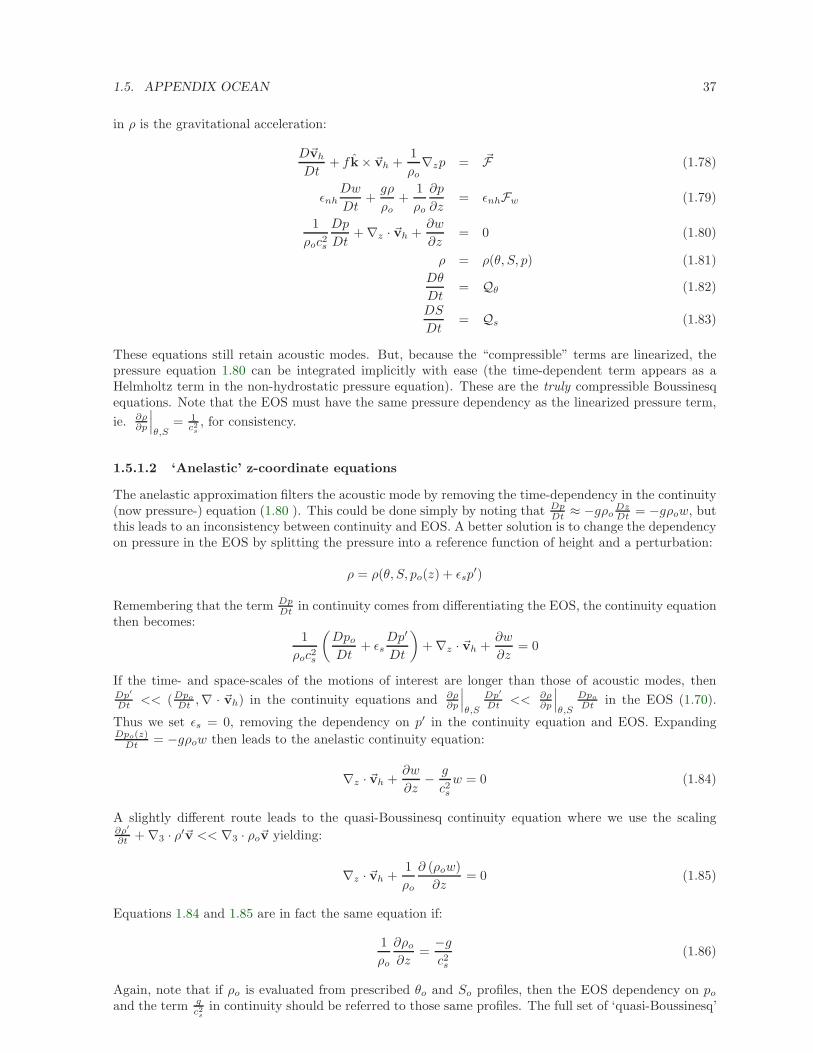
1.5. APPENDIX OCEAN 37
in ρ is the gravitational acceleration:
D~vh
Dt+ f k× ~vh +
1
ρo∇zp = ~F (1.78)
ǫnhDw
Dt+gρ
ρo+
1
ρo
∂p
∂z= ǫnhFw (1.79)
1
ρoc2s
Dp
Dt+ ∇z · ~vh +
∂w
∂z= 0 (1.80)
ρ = ρ(θ, S, p) (1.81)
Dθ
Dt= Qθ (1.82)
DS
Dt= Qs (1.83)
These equations still retain acoustic modes. But, because the “compressible” terms are linearized, thepressure equation 1.80 can be integrated implicitly with ease (the time-dependent term appears as aHelmholtz term in the non-hydrostatic pressure equation). These are the truly compressible Boussinesqequations. Note that the EOS must have the same pressure dependency as the linearized pressure term,
ie. ∂ρ∂p
∣∣∣θ,S
= 1c2
s, for consistency.
1.5.1.2 ‘Anelastic’ z-coordinate equations
The anelastic approximation filters the acoustic mode by removing the time-dependency in the continuity(now pressure-) equation (1.80 ). This could be done simply by noting that Dp
Dt ≈ −gρoDzDt = −gρow, but
this leads to an inconsistency between continuity and EOS. A better solution is to change the dependencyon pressure in the EOS by splitting the pressure into a reference function of height and a perturbation:
ρ = ρ(θ, S, po(z) + ǫsp′)
Remembering that the term DpDt in continuity comes from differentiating the EOS, the continuity equation
then becomes:1
ρoc2s
(Dpo
Dt+ ǫs
Dp′
Dt
)+ ∇z · ~vh +
∂w
∂z= 0
If the time- and space-scales of the motions of interest are longer than those of acoustic modes, thenDp′
Dt << (Dpo
Dt ,∇ · ~vh) in the continuity equations and ∂ρ∂p
∣∣∣θ,S
Dp′
Dt << ∂ρ∂p
∣∣∣θ,S
Dpo
Dt in the EOS (1.70).
Thus we set ǫs = 0, removing the dependency on p′ in the continuity equation and EOS. ExpandingDpo(z)
Dt = −gρow then leads to the anelastic continuity equation:
∇z · ~vh +∂w
∂z− g
c2sw = 0 (1.84)
A slightly different route leads to the quasi-Boussinesq continuity equation where we use the scaling∂ρ′
∂t + ∇3 · ρ′~v << ∇3 · ρo~v yielding:
∇z · ~vh +1
ρo
∂ (ρow)
∂z= 0 (1.85)
Equations 1.84 and 1.85 are in fact the same equation if:
1
ρo
∂ρo
∂z=
−gc2s
(1.86)
Again, note that if ρo is evaluated from prescribed θo and So profiles, then the EOS dependency on po
and the term gc2
sin continuity should be referred to those same profiles. The full set of ‘quasi-Boussinesq’
38 CHAPTER 1. OVERVIEW OF MITGCM
or ‘anelastic’ equations for the ocean are then:
D~vh
Dt+ f k× ~vh +
1
ρo∇zp = ~F (1.87)
ǫnhDw
Dt+gρ
ρo+
1
ρo
∂p
∂z= ǫnhFw (1.88)
∇z · ~vh +1
ρo
∂ (ρow)
∂z= 0 (1.89)
ρ = ρ(θ, S, po(z)) (1.90)
Dθ
Dt= Qθ (1.91)
DS
Dt= Qs (1.92)
1.5.1.3 Incompressible z-coordinate equations
Here, the objective is to drop the depth dependence of ρo and so, technically, to also remove the depen-dence of ρ on po. This would yield the “truly” incompressible Boussinesq equations:
D~vh
Dt+ f k× ~vh +
1
ρc∇zp = ~F (1.93)
ǫnhDw
Dt+gρ
ρc+
1
ρc
∂p
∂z= ǫnhFw (1.94)
∇z · ~vh +∂w
∂z= 0 (1.95)
ρ = ρ(θ, S) (1.96)
Dθ
Dt= Qθ (1.97)
DS
Dt= Qs (1.98)
where ρc is a constant reference density of water.
1.5.1.4 Compressible non-divergent equations
The above “incompressible” equations are incompressible in both the flow and the density. In manyoceanic applications, however, it is important to retain compressibility effects in the density. To do thiswe must split the density thus:
ρ = ρo + ρ′
We then assert that variations with depth of ρo are unimportant while the compressible effects in ρ′ are:
ρo = ρc
ρ′ = ρ(θ, S, po(z)) − ρo
This then yields what we can call the semi-compressible Boussinesq equations:
D~vh
Dt+ f k × ~vh +
1
ρc∇zp
′ = ~F (1.99)
ǫnhDw
Dt+gρ′
ρc+
1
ρc
∂p′
∂z= ǫnhFw (1.100)
∇z · ~vh +∂w
∂z= 0 (1.101)
ρ′ = ρ(θ, S, po(z)) − ρc (1.102)
Dθ
Dt= Qθ (1.103)
DS
Dt= Qs (1.104)
1.6. APPENDIX:OPERATORS 39
Note that the hydrostatic pressure of the resting fluid, including that associated with ρc, is subtractedout since it has no effect on the dynamics.
Though necessary, the assumptions that go into these equations are messy since we essentially assumea different EOS for the reference density and the perturbation density. Nevertheless, it is the hydrostatic(ǫnh = 0 form of these equations that are used throughout the ocean modeling community and referredto as the primitive equations (HPE).
1.6 Appendix:OPERATORS
1.6.1 Coordinate systems
1.6.1.1 Spherical coordinates
In spherical coordinates, the velocity components in the zonal, meridional and vertical direction respec-tively, are given by (see Fig.2) :
u = r cosϕDλ
Dt
v = rDϕ
Dt
r =Dr
Dt
Here ϕ is the latitude, λ the longitude, r the radial distance of the particle from the center of theearth, Ω is the angular speed of rotation of the Earth and D/Dt is the total derivative.
The ‘grad’ (∇) and ‘div’ (∇·) operators are defined by, in spherical coordinates:
∇ ≡(
1
r cosϕ
∂
∂λ,1
r
∂
∂ϕ,∂
∂r
)
∇ · v ≡ 1
r cosϕ
∂u
∂λ+
∂
∂ϕ(v cosϕ)
+
1
r2∂(r2r)
∂r

40 CHAPTER 1. OVERVIEW OF MITGCM
Chapter 2
Discretization and Algorithm
This chapter lays out the numerical schemes that are employed in the core MITgcm algorithm. Wheneverpossible links are made to actual program code in the MITgcm implementation. The chapter begins witha discussion of the temporal discretization used in MITgcm. This discussion is followed by sectionsthat describe the spatial discretization. The schemes employed for momentum terms are described first,afterwards the schemes that apply to passive and dynamically active tracers are described.
2.1 Notation
Because of the particularity of the vertical direction in stratified fluid context, in this chapter, the vectornotations are mostly used for the horizontal component: the horizontal part of a vector is simply written~v (instead of vh or ~vh in chaper 1) and a 3.D vector is simply written ~v (instead of ~v in chapter 1).
The notations we use to describe the discrete formulation of the model are summarized hereafter:general notation:∆x,∆y,∆r grid spacing in X,Y,R directions.Ac, Aw, As, Aζ : horizontal area of a grid cell surrounding θ, u, v, ζ point.Vu,Vv,Vw,Vθ : Volume of the grid box surrounding u, v, w, θ point;i, j, k : current index relative to X,Y,R directions;basic operator:δi : δiΦ = Φi+1/2 − Φi−1/2
−i : Φi= (Φi+1/2 + Φi−1/2)/2
δx : δxΦ = 1∆xδiΦ
∇ = horizontal gradient operator : ∇Φ = δxΦ, δyΦ∇· = horizontal divergence operator : ∇ ·~f = 1
Aδi∆y fx + δj∆x fy∇2
= horizontal Laplacian operator : ∇2Φ = ∇ · ∇Φ
2.2 Time-stepping
The equations of motion integrated by the model involve four prognostic equations for flow, u and v, tem-perature, θ, and salt/moisture, S, and three diagnostic equations for vertical flow, w, density/buoyancy,ρ/b, and pressure/geo-potential, φhyd. In addition, the surface pressure or height may by described byeither a prognostic or diagnostic equation and if non-hydrostatics terms are included then a diagnosticequation for non-hydrostatic pressure is also solved. The combination of prognostic and diagnostic equa-tions requires a model algorithm that can march forward prognostic variables while satisfying constraintsimposed by diagnostic equations.
Since the model comes in several flavors and formulation, it would be confusing to present the modelalgorithm exactly as written into code along with all the switches and optional terms. Instead, we presentthe algorithm for each of the basic formulations which are:
41
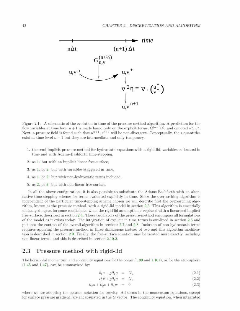
42 CHAPTER 2. DISCRETIZATION AND ALGORITHM
( )
u,vG(n+½)
u,vn+1
∆2η = ∆. uv
**
∆(n+1) t∆time
n t
n *u,v u,v
Figure 2.1: A schematic of the evolution in time of the pressure method algorithm. A prediction for theflow variables at time level n+ 1 is made based only on the explicit terms, G(n+1/2), and denoted u∗, v∗.Next, a pressure field is found such that un+1, vn+1 will be non-divergent. Conceptually, the ∗ quantitiesexist at time level n+ 1 but they are intermediate and only temporary.
1. the semi-implicit pressure method for hydrostatic equations with a rigid-lid, variables co-located intime and with Adams-Bashforth time-stepping,
2. as 1. but with an implicit linear free-surface,
3. as 1. or 2. but with variables staggered in time,
4. as 1. or 2. but with non-hydrostatic terms included,
5. as 2. or 3. but with non-linear free-surface.
In all the above configurations it is also possible to substitute the Adams-Bashforth with an alter-native time-stepping scheme for terms evaluated explicitly in time. Since the over-arching algorithm isindependent of the particular time-stepping scheme chosen we will describe first the over-arching algo-rithm, known as the pressure method, with a rigid-lid model in section 2.3. This algorithm is essentiallyunchanged, apart for some coefficients, when the rigid lid assumption is replaced with a linearized implicitfree-surface, described in section 2.4. These two flavors of the pressure-method encompass all formulationsof the model as it exists today. The integration of explicit in time terms is out-lined in section 2.5 andput into the context of the overall algorithm in sections 2.7 and 2.8. Inclusion of non-hydrostatic termsrequires applying the pressure method in three dimensions instead of two and this algorithm modifica-tion is described in section 2.9. Finally, the free-surface equation may be treated more exactly, includingnon-linear terms, and this is described in section 2.10.2.
2.3 Pressure method with rigid-lid
The horizontal momentum and continuity equations for the ocean (1.99 and 1.101), or for the atmosphere(1.45 and 1.47), can be summarized by:
∂tu+ g∂xη = Gu (2.1)
∂tv + g∂yη = Gv (2.2)
∂xu+ ∂yv + ∂zw = 0 (2.3)
where we are adopting the oceanic notation for brevity. All terms in the momentum equations, exceptfor surface pressure gradient, are encapsulated in the G vector. The continuity equation, when integrated
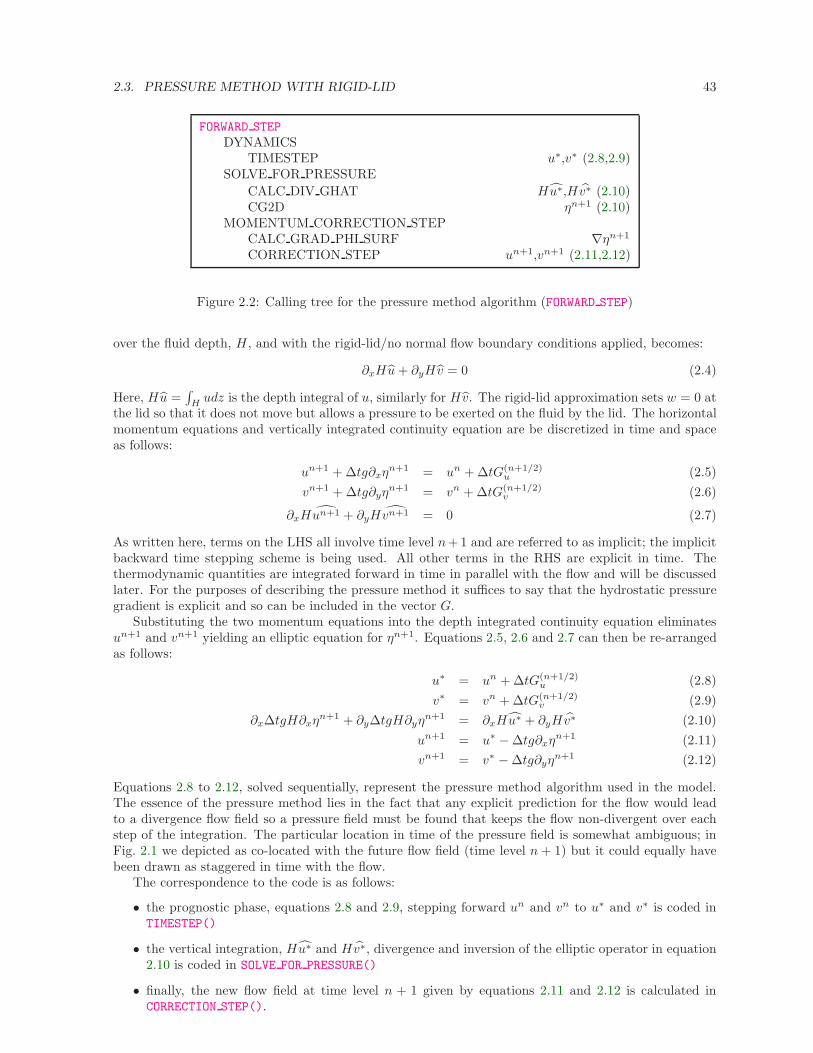
2.3. PRESSURE METHOD WITH RIGID-LID 43
FORWARD STEP
DYNAMICSTIMESTEP u∗,v∗ (2.8,2.9)
SOLVE FOR PRESSURE
CALC DIV GHAT Hu∗,Hv∗ (2.10)CG2D ηn+1 (2.10)
MOMENTUM CORRECTION STEPCALC GRAD PHI SURF ∇ηn+1
CORRECTION STEP un+1,vn+1 (2.11,2.12)
Figure 2.2: Calling tree for the pressure method algorithm (FORWARD STEP)
over the fluid depth, H , and with the rigid-lid/no normal flow boundary conditions applied, becomes:
∂xHu+ ∂yHv = 0 (2.4)
Here, Hu =∫
H udz is the depth integral of u, similarly for Hv. The rigid-lid approximation sets w = 0 atthe lid so that it does not move but allows a pressure to be exerted on the fluid by the lid. The horizontalmomentum equations and vertically integrated continuity equation are be discretized in time and spaceas follows:
un+1 + ∆tg∂xηn+1 = un + ∆tG(n+1/2)
u (2.5)
vn+1 + ∆tg∂yηn+1 = vn + ∆tG(n+1/2)
v (2.6)
∂xHun+1 + ∂yHvn+1 = 0 (2.7)
As written here, terms on the LHS all involve time level n+1 and are referred to as implicit; the implicitbackward time stepping scheme is being used. All other terms in the RHS are explicit in time. Thethermodynamic quantities are integrated forward in time in parallel with the flow and will be discussedlater. For the purposes of describing the pressure method it suffices to say that the hydrostatic pressuregradient is explicit and so can be included in the vector G.
Substituting the two momentum equations into the depth integrated continuity equation eliminatesun+1 and vn+1 yielding an elliptic equation for ηn+1. Equations 2.5, 2.6 and 2.7 can then be re-arrangedas follows:
u∗ = un + ∆tG(n+1/2)u (2.8)
v∗ = vn + ∆tG(n+1/2)v (2.9)
∂x∆tgH∂xηn+1 + ∂y∆tgH∂yη
n+1 = ∂xHu∗ + ∂yHv∗ (2.10)
un+1 = u∗ − ∆tg∂xηn+1 (2.11)
vn+1 = v∗ − ∆tg∂yηn+1 (2.12)
Equations 2.8 to 2.12, solved sequentially, represent the pressure method algorithm used in the model.The essence of the pressure method lies in the fact that any explicit prediction for the flow would leadto a divergence flow field so a pressure field must be found that keeps the flow non-divergent over eachstep of the integration. The particular location in time of the pressure field is somewhat ambiguous; inFig. 2.1 we depicted as co-located with the future flow field (time level n+ 1) but it could equally havebeen drawn as staggered in time with the flow.
The correspondence to the code is as follows:
• the prognostic phase, equations 2.8 and 2.9, stepping forward un and vn to u∗ and v∗ is coded inTIMESTEP()
• the vertical integration, Hu∗ and Hv∗, divergence and inversion of the elliptic operator in equation2.10 is coded in SOLVE FOR PRESSURE()
• finally, the new flow field at time level n + 1 given by equations 2.11 and 2.12 is calculated inCORRECTION STEP().
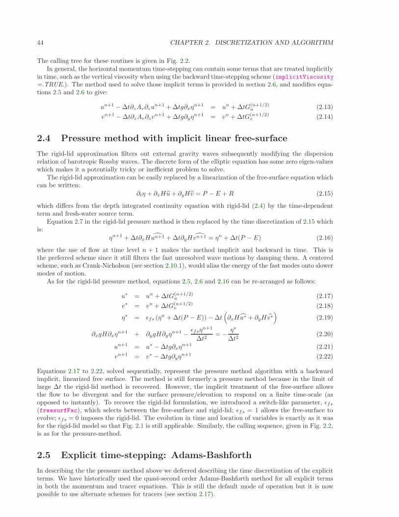
44 CHAPTER 2. DISCRETIZATION AND ALGORITHM
The calling tree for these routines is given in Fig. 2.2.In general, the horizontal momentum time-stepping can contain some terms that are treated implicitly
in time, such as the vertical viscosity when using the backward time-stepping scheme (implicitViscosity=.TRUE.). The method used to solve those implicit terms is provided in section 2.6, and modifies equa-tions 2.5 and 2.6 to give:
un+1 − ∆t∂zAv∂zun+1 + ∆tg∂xη
n+1 = un + ∆tG(n+1/2)u (2.13)
vn+1 − ∆t∂zAv∂zvn+1 + ∆tg∂yη
n+1 = vn + ∆tG(n+1/2)v (2.14)
2.4 Pressure method with implicit linear free-surface
The rigid-lid approximation filters out external gravity waves subsequently modifying the dispersionrelation of barotropic Rossby waves. The discrete form of the elliptic equation has some zero eigen-valueswhich makes it a potentially tricky or inefficient problem to solve.
The rigid-lid approximation can be easily replaced by a linearization of the free-surface equation whichcan be written:
∂tη + ∂xHu+ ∂yHv = P − E +R (2.15)
which differs from the depth integrated continuity equation with rigid-lid (2.4) by the time-dependentterm and fresh-water source term.
Equation 2.7 in the rigid-lid pressure method is then replaced by the time discretization of 2.15 whichis:
ηn+1 + ∆t∂xHun+1 + ∆t∂yHvn+1 = ηn + ∆t(P − E) (2.16)
where the use of flow at time level n + 1 makes the method implicit and backward in time. This isthe preferred scheme since it still filters the fast unresolved wave motions by damping them. A centeredscheme, such as Crank-Nicholson (see section 2.10.1), would alias the energy of the fast modes onto slowermodes of motion.
As for the rigid-lid pressure method, equations 2.5, 2.6 and 2.16 can be re-arranged as follows:
u∗ = un + ∆tG(n+1/2)u (2.17)
v∗ = vn + ∆tG(n+1/2)v (2.18)
η∗ = ǫfs (ηn + ∆t(P − E)) − ∆t(∂xHu∗ + ∂yHv∗
)(2.19)
∂xgH∂xηn+1 + ∂ygH∂yη
n+1 − ǫfsηn+1
∆t2= − η∗
∆t2(2.20)
un+1 = u∗ − ∆tg∂xηn+1 (2.21)
vn+1 = v∗ − ∆tg∂yηn+1 (2.22)
Equations 2.17 to 2.22, solved sequentially, represent the pressure method algorithm with a backwardimplicit, linearized free surface. The method is still formerly a pressure method because in the limit oflarge ∆t the rigid-lid method is recovered. However, the implicit treatment of the free-surface allowsthe flow to be divergent and for the surface pressure/elevation to respond on a finite time-scale (asopposed to instantly). To recover the rigid-lid formulation, we introduced a switch-like parameter, ǫfs
(freesurfFac), which selects between the free-surface and rigid-lid; ǫfs = 1 allows the free-surface toevolve; ǫfs = 0 imposes the rigid-lid. The evolution in time and location of variables is exactly as it wasfor the rigid-lid model so that Fig. 2.1 is still applicable. Similarly, the calling sequence, given in Fig. 2.2,is as for the pressure-method.
2.5 Explicit time-stepping: Adams-Bashforth
In describing the the pressure method above we deferred describing the time discretization of the explicitterms. We have historically used the quasi-second order Adams-Bashforth method for all explicit termsin both the momentum and tracer equations. This is still the default mode of operation but it is nowpossible to use alternate schemes for tracers (see section 2.17).
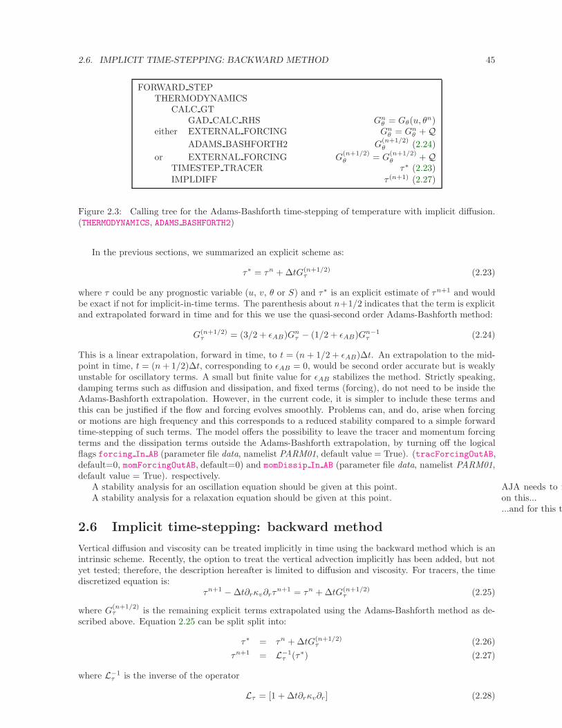
2.6. IMPLICIT TIME-STEPPING: BACKWARD METHOD 45
FORWARD STEPTHERMODYNAMICS
CALC GTGAD CALC RHS Gn
θ = Gθ(u, θn)
either EXTERNAL FORCING Gnθ = Gn
θ + QADAMS BASHFORTH2 G
(n+1/2)θ (2.24)
or EXTERNAL FORCING G(n+1/2)θ = G
(n+1/2)θ + Q
TIMESTEP TRACER τ∗ (2.23)
IMPLDIFF τ (n+1) (2.27)
Figure 2.3: Calling tree for the Adams-Bashforth time-stepping of temperature with implicit diffusion.(THERMODYNAMICS, ADAMS BASHFORTH2)
In the previous sections, we summarized an explicit scheme as:
τ∗ = τn + ∆tG(n+1/2)τ (2.23)
where τ could be any prognostic variable (u, v, θ or S) and τ∗ is an explicit estimate of τn+1 and wouldbe exact if not for implicit-in-time terms. The parenthesis about n+1/2 indicates that the term is explicitand extrapolated forward in time and for this we use the quasi-second order Adams-Bashforth method:
G(n+1/2)τ = (3/2 + ǫAB)Gn
τ − (1/2 + ǫAB)Gn−1τ (2.24)
This is a linear extrapolation, forward in time, to t = (n+ 1/2 + ǫAB)∆t. An extrapolation to the mid-point in time, t = (n+ 1/2)∆t, corresponding to ǫAB = 0, would be second order accurate but is weaklyunstable for oscillatory terms. A small but finite value for ǫAB stabilizes the method. Strictly speaking,damping terms such as diffusion and dissipation, and fixed terms (forcing), do not need to be inside theAdams-Bashforth extrapolation. However, in the current code, it is simpler to include these terms andthis can be justified if the flow and forcing evolves smoothly. Problems can, and do, arise when forcingor motions are high frequency and this corresponds to a reduced stability compared to a simple forwardtime-stepping of such terms. The model offers the possibility to leave the tracer and momentum forcingterms and the dissipation terms outside the Adams-Bashforth extrapolation, by turning off the logicalflags forcing In AB (parameter file data, namelist PARM01, default value = True). (tracForcingOutAB,default=0, momForcingOutAB, default=0) and momDissip In AB (parameter file data, namelist PARM01,default value = True). respectively.
A stability analysis for an oscillation equation should be given at this point. AJA needs to findon this...A stability analysis for a relaxation equation should be given at this point....and for this to
2.6 Implicit time-stepping: backward method
Vertical diffusion and viscosity can be treated implicitly in time using the backward method which is anintrinsic scheme. Recently, the option to treat the vertical advection implicitly has been added, but notyet tested; therefore, the description hereafter is limited to diffusion and viscosity. For tracers, the timediscretized equation is:
τn+1 − ∆t∂rκv∂rτn+1 = τn + ∆tG(n+1/2)
τ (2.25)
where G(n+1/2)τ is the remaining explicit terms extrapolated using the Adams-Bashforth method as de-
scribed above. Equation 2.25 can be split split into:
τ∗ = τn + ∆tG(n+1/2)τ (2.26)
τn+1 = L−1τ (τ∗) (2.27)
where L−1τ is the inverse of the operator
Lτ = [1 + ∆t∂rκv∂r] (2.28)
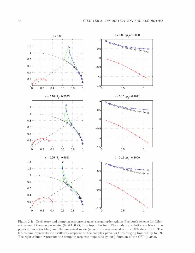
46 CHAPTER 2. DISCRETIZATION AND ALGORITHM
0 0.2 0.4 0.6 0.8 10
0.2
0.4
0.6
0.8
1
1.2
3
6
9
ε = 0.00
0 0.2 0.4 0.6 0.8 10
0.2
0.4
0.6
0.8
1
1.2
3
6
9
ε = 0.10 ; fc= 0.5025
0 0.2 0.4 0.6 0.8 10
0.2
0.4
0.6
0.8
1
1.2
1.4
3
6
9
ε = 0.25 ; fc= 0.5963
0 0.5 1−1.5
−1
−0.5
0
0.5
1
ε = 0.00 ; µc= 1.0000
0 0.5 1−1.5
−1
−0.5
0
0.5
1
ε = 0.10 ; µc= 0.9091
0 0.5 1−1.5
−1
−0.5
0
0.5
1
ε = 0.25 ; µc= 0.8000
Figure 2.4: Oscillatory and damping response of quasi-second order Adams-Bashforth scheme for differ-ent values of the ǫAB parameter (0., 0.1, 0.25, from top to bottom) The analytical solution (in black), thephysical mode (in blue) and the numerical mode (in red) are represented with a CFL step of 0.1. Theleft column represents the oscillatory response on the complex plane for CFL ranging from 0.1 up to 0.9.The right column represents the damping response amplitude (y-axis) function of the CFL (x-axis).
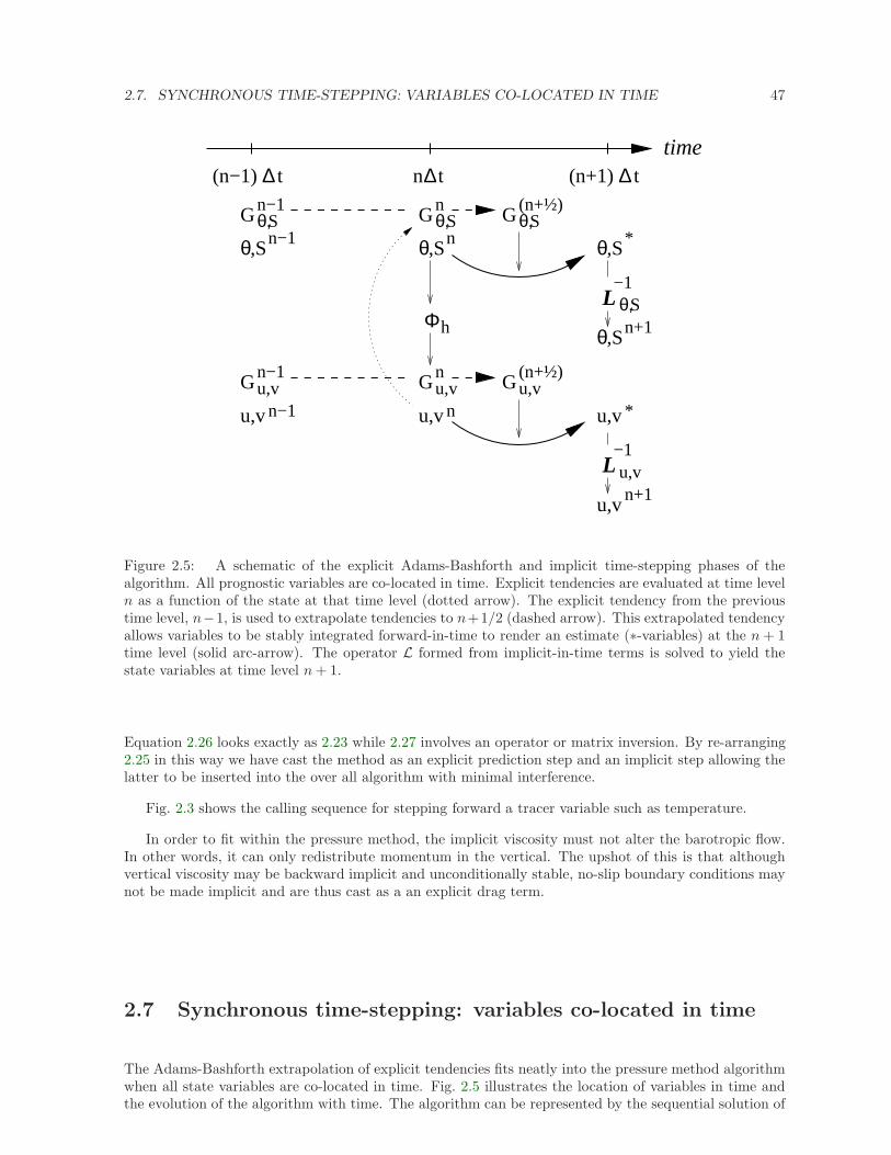
2.7. SYNCHRONOUS TIME-STEPPING: VARIABLES CO-LOCATED IN TIME 47
∆(n+1) t∆(n−1) t ∆time
n t
,Sθ ,Sθ ,Sθ
,Sθ n+1
L−1
θ,S θ,S θ,S
θ,SΦh
L−1
u,vn+1
n−1 n *Gn−1 GGn (n+½)
n−1 n *u,v u,v u,vu,vGn−1
u,v
u,v u,vG(n+½)Gn
Figure 2.5: A schematic of the explicit Adams-Bashforth and implicit time-stepping phases of thealgorithm. All prognostic variables are co-located in time. Explicit tendencies are evaluated at time leveln as a function of the state at that time level (dotted arrow). The explicit tendency from the previoustime level, n−1, is used to extrapolate tendencies to n+1/2 (dashed arrow). This extrapolated tendencyallows variables to be stably integrated forward-in-time to render an estimate (∗-variables) at the n+ 1time level (solid arc-arrow). The operator L formed from implicit-in-time terms is solved to yield thestate variables at time level n+ 1.
Equation 2.26 looks exactly as 2.23 while 2.27 involves an operator or matrix inversion. By re-arranging2.25 in this way we have cast the method as an explicit prediction step and an implicit step allowing thelatter to be inserted into the over all algorithm with minimal interference.
Fig. 2.3 shows the calling sequence for stepping forward a tracer variable such as temperature.
In order to fit within the pressure method, the implicit viscosity must not alter the barotropic flow.In other words, it can only redistribute momentum in the vertical. The upshot of this is that althoughvertical viscosity may be backward implicit and unconditionally stable, no-slip boundary conditions maynot be made implicit and are thus cast as a an explicit drag term.
2.7 Synchronous time-stepping: variables co-located in time
The Adams-Bashforth extrapolation of explicit tendencies fits neatly into the pressure method algorithmwhen all state variables are co-located in time. Fig. 2.5 illustrates the location of variables in time andthe evolution of the algorithm with time. The algorithm can be represented by the sequential solution of
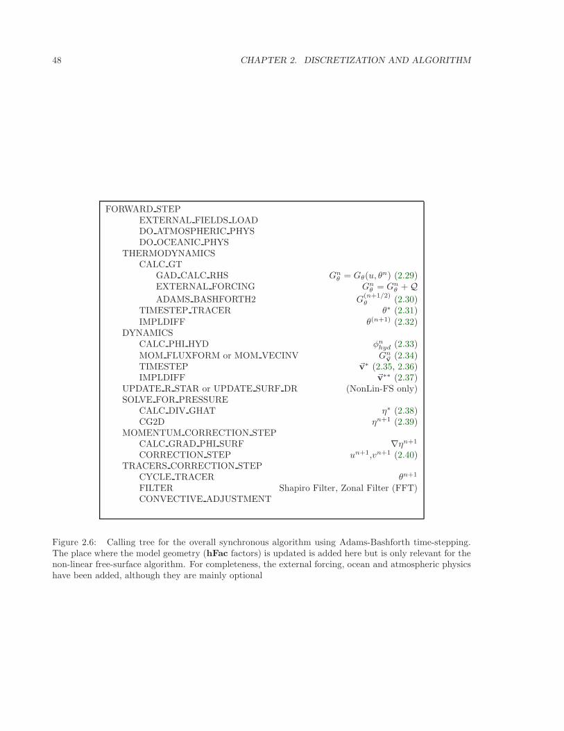
48 CHAPTER 2. DISCRETIZATION AND ALGORITHM
FORWARD STEPEXTERNAL FIELDS LOADDO ATMOSPHERIC PHYSDO OCEANIC PHYS
THERMODYNAMICSCALC GT
GAD CALC RHS Gnθ = Gθ(u, θ
n) (2.29)EXTERNAL FORCING Gn
θ = Gnθ + Q
ADAMS BASHFORTH2 G(n+1/2)θ (2.30)
TIMESTEP TRACER θ∗ (2.31)IMPLDIFF θ(n+1) (2.32)
DYNAMICSCALC PHI HYD φn
hyd (2.33)
MOM FLUXFORM or MOM VECINV Gn~v (2.34)
TIMESTEP ~v∗ (2.35, 2.36)IMPLDIFF ~v∗∗ (2.37)
UPDATE R STAR or UPDATE SURF DR (NonLin-FS only)SOLVE FOR PRESSURE
CALC DIV GHAT η∗ (2.38)CG2D ηn+1 (2.39)
MOMENTUM CORRECTION STEPCALC GRAD PHI SURF ∇ηn+1
CORRECTION STEP un+1,vn+1 (2.40)TRACERS CORRECTION STEP
CYCLE TRACER θn+1
FILTER Shapiro Filter, Zonal Filter (FFT)CONVECTIVE ADJUSTMENT
Figure 2.6: Calling tree for the overall synchronous algorithm using Adams-Bashforth time-stepping.The place where the model geometry (hFac factors) is updated is added here but is only relevant for thenon-linear free-surface algorithm. For completeness, the external forcing, ocean and atmospheric physicshave been added, although they are mainly optional
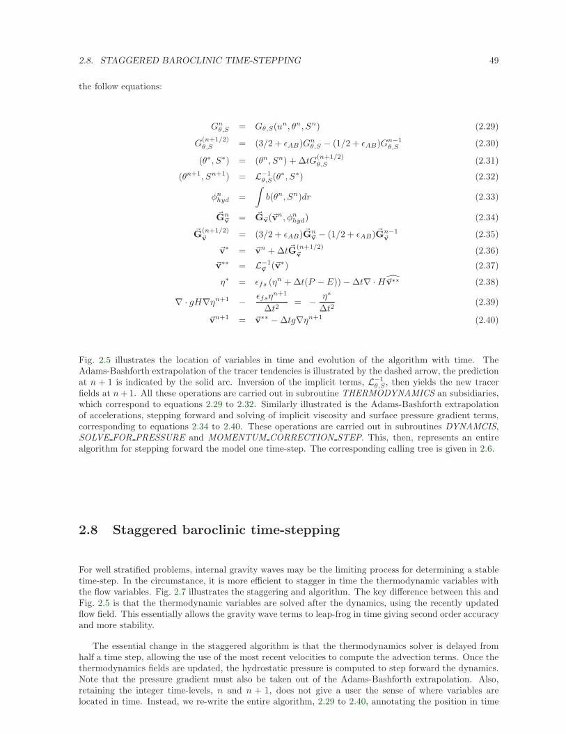
2.8. STAGGERED BAROCLINIC TIME-STEPPING 49
the follow equations:
Gnθ,S = Gθ,S(un, θn, Sn) (2.29)
G(n+1/2)θ,S = (3/2 + ǫAB)Gn
θ,S − (1/2 + ǫAB)Gn−1θ,S (2.30)
(θ∗, S∗) = (θn, Sn) + ∆tG(n+1/2)θ,S (2.31)
(θn+1, Sn+1) = L−1θ,S(θ∗, S∗) (2.32)
φnhyd =
∫b(θn, Sn)dr (2.33)
~Gn~v = ~G~v(~vn, φn
hyd) (2.34)
~G(n+1/2)~v = (3/2 + ǫAB)~Gn
~v − (1/2 + ǫAB)~Gn−1~v (2.35)
~v∗ = ~vn + ∆t~G(n+1/2)~v (2.36)
~v∗∗ = L−1~v (~v∗) (2.37)
η∗ = ǫfs (ηn + ∆t(P − E)) − ∆t∇ ·H~v∗∗ (2.38)
∇ · gH∇ηn+1 − ǫfsηn+1
∆t2= − η∗
∆t2(2.39)
~vn+1 = ~v∗∗ − ∆tg∇ηn+1 (2.40)
Fig. 2.5 illustrates the location of variables in time and evolution of the algorithm with time. TheAdams-Bashforth extrapolation of the tracer tendencies is illustrated by the dashed arrow, the predictionat n + 1 is indicated by the solid arc. Inversion of the implicit terms, L−1
θ,S, then yields the new tracerfields at n+ 1. All these operations are carried out in subroutine THERMODYNAMICS an subsidiaries,which correspond to equations 2.29 to 2.32. Similarly illustrated is the Adams-Bashforth extrapolationof accelerations, stepping forward and solving of implicit viscosity and surface pressure gradient terms,corresponding to equations 2.34 to 2.40. These operations are carried out in subroutines DYNAMCIS,SOLVE FOR PRESSURE and MOMENTUM CORRECTION STEP. This, then, represents an entirealgorithm for stepping forward the model one time-step. The corresponding calling tree is given in 2.6.
2.8 Staggered baroclinic time-stepping
For well stratified problems, internal gravity waves may be the limiting process for determining a stabletime-step. In the circumstance, it is more efficient to stagger in time the thermodynamic variables withthe flow variables. Fig. 2.7 illustrates the staggering and algorithm. The key difference between this andFig. 2.5 is that the thermodynamic variables are solved after the dynamics, using the recently updatedflow field. This essentially allows the gravity wave terms to leap-frog in time giving second order accuracyand more stability.
The essential change in the staggered algorithm is that the thermodynamics solver is delayed fromhalf a time step, allowing the use of the most recent velocities to compute the advection terms. Once thethermodynamics fields are updated, the hydrostatic pressure is computed to step forward the dynamics.Note that the pressure gradient must also be taken out of the Adams-Bashforth extrapolation. Also,retaining the integer time-levels, n and n + 1, does not give a user the sense of where variables arelocated in time. Instead, we re-write the entire algorithm, 2.29 to 2.40, annotating the position in time
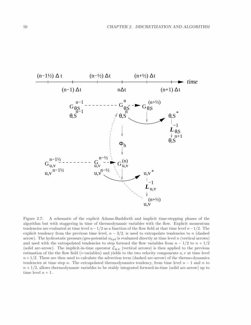
50 CHAPTER 2. DISCRETIZATION AND ALGORITHM
L−1
,Sθ ,Sθ ,Sθ
L−1
θ,S θ,S
θ,S
,SθΦh
θ,S
∆ (n+½) t∆(n−½) t
∆(n+1) t∆(n−1) t ∆time
n t
(n−1½) t∆
*u,v u,v u,vu,vG u,vGu,v
G
*G GG
(n)
(n+½)
n−½
n
n−1½
n−1
n−1½ n−½
u,v
u,v(n+½)
n+1
n−1 n
Figure 2.7: A schematic of the explicit Adams-Bashforth and implicit time-stepping phases of thealgorithm but with staggering in time of thermodynamic variables with the flow. Explicit momentumtendencies are evaluated at time level n−1/2 as a function of the flow field at that time level n−1/2. Theexplicit tendency from the previous time level, n − 3/2, is used to extrapolate tendencies to n (dashedarrow). The hydrostatic pressure/geo-potential φhyd is evaluated directly at time level n (vertical arrows)and used with the extrapolated tendencies to step forward the flow variables from n − 1/2 to n + 1/2(solid arc-arrow). The implicit-in-time operator Lu,v (vertical arrows) is then applied to the previousestimation of the the flow field (∗-variables) and yields to the two velocity components u, v at time leveln+1/2. These are then used to calculate the advection term (dashed arc-arrow) of the thermo-dynamicstendencies at time step n. The extrapolated thermodynamics tendency, from time level n − 1 and n ton+ 1/2, allows thermodynamic variables to be stably integrated forward-in-time (solid arc-arrow) up totime level n+ 1.
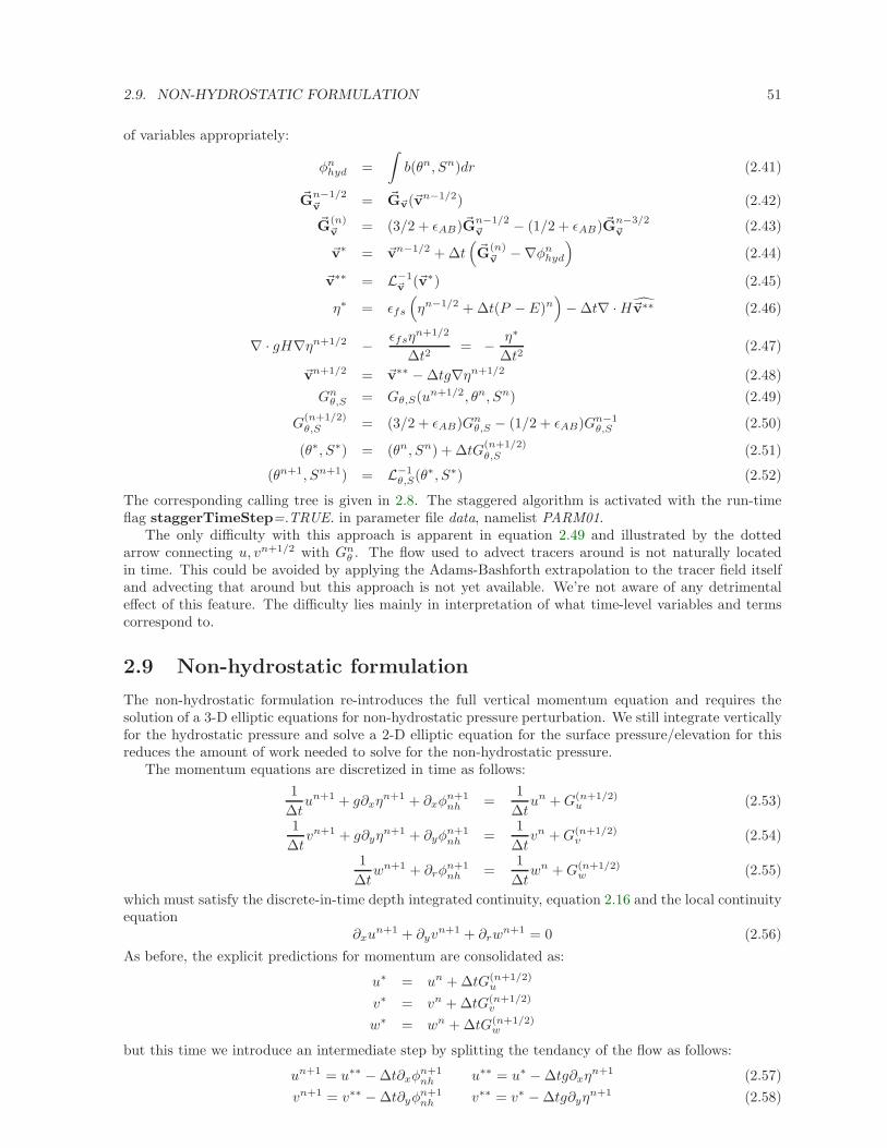
2.9. NON-HYDROSTATIC FORMULATION 51
of variables appropriately:
φnhyd =
∫b(θn, Sn)dr (2.41)
~Gn−1/2~v = ~G~v(~vn−1/2) (2.42)
~G(n)~v = (3/2 + ǫAB)~G
n−1/2~v − (1/2 + ǫAB)~G
n−3/2~v (2.43)
~v∗ = ~vn−1/2 + ∆t(~G
(n)~v −∇φn
hyd
)(2.44)
~v∗∗ = L−1~v (~v∗) (2.45)
η∗ = ǫfs
(ηn−1/2 + ∆t(P − E)n
)− ∆t∇ ·H~v∗∗ (2.46)
∇ · gH∇ηn+1/2 − ǫfsηn+1/2
∆t2= − η∗
∆t2(2.47)
~vn+1/2 = ~v∗∗ − ∆tg∇ηn+1/2 (2.48)
Gnθ,S = Gθ,S(un+1/2, θn, Sn) (2.49)
G(n+1/2)θ,S = (3/2 + ǫAB)Gn
θ,S − (1/2 + ǫAB)Gn−1θ,S (2.50)
(θ∗, S∗) = (θn, Sn) + ∆tG(n+1/2)θ,S (2.51)
(θn+1, Sn+1) = L−1θ,S(θ∗, S∗) (2.52)
The corresponding calling tree is given in 2.8. The staggered algorithm is activated with the run-timeflag staggerTimeStep=.TRUE. in parameter file data, namelist PARM01.
The only difficulty with this approach is apparent in equation 2.49 and illustrated by the dottedarrow connecting u, vn+1/2 with Gn
θ . The flow used to advect tracers around is not naturally locatedin time. This could be avoided by applying the Adams-Bashforth extrapolation to the tracer field itselfand advecting that around but this approach is not yet available. We’re not aware of any detrimentaleffect of this feature. The difficulty lies mainly in interpretation of what time-level variables and termscorrespond to.
2.9 Non-hydrostatic formulation
The non-hydrostatic formulation re-introduces the full vertical momentum equation and requires thesolution of a 3-D elliptic equations for non-hydrostatic pressure perturbation. We still integrate verticallyfor the hydrostatic pressure and solve a 2-D elliptic equation for the surface pressure/elevation for thisreduces the amount of work needed to solve for the non-hydrostatic pressure.
The momentum equations are discretized in time as follows:
1
∆tun+1 + g∂xη
n+1 + ∂xφn+1nh =
1
∆tun +G(n+1/2)
u (2.53)
1
∆tvn+1 + g∂yη
n+1 + ∂yφn+1nh =
1
∆tvn +G(n+1/2)
v (2.54)
1
∆twn+1 + ∂rφ
n+1nh =
1
∆twn +G(n+1/2)
w (2.55)
which must satisfy the discrete-in-time depth integrated continuity, equation 2.16 and the local continuityequation
∂xun+1 + ∂yv
n+1 + ∂rwn+1 = 0 (2.56)
As before, the explicit predictions for momentum are consolidated as:
u∗ = un + ∆tG(n+1/2)u
v∗ = vn + ∆tG(n+1/2)v
w∗ = wn + ∆tG(n+1/2)w
but this time we introduce an intermediate step by splitting the tendancy of the flow as follows:
un+1 = u∗∗ − ∆t∂xφn+1nh u∗∗ = u∗ − ∆tg∂xη
n+1 (2.57)
vn+1 = v∗∗ − ∆t∂yφn+1nh v∗∗ = v∗ − ∆tg∂yη
n+1 (2.58)
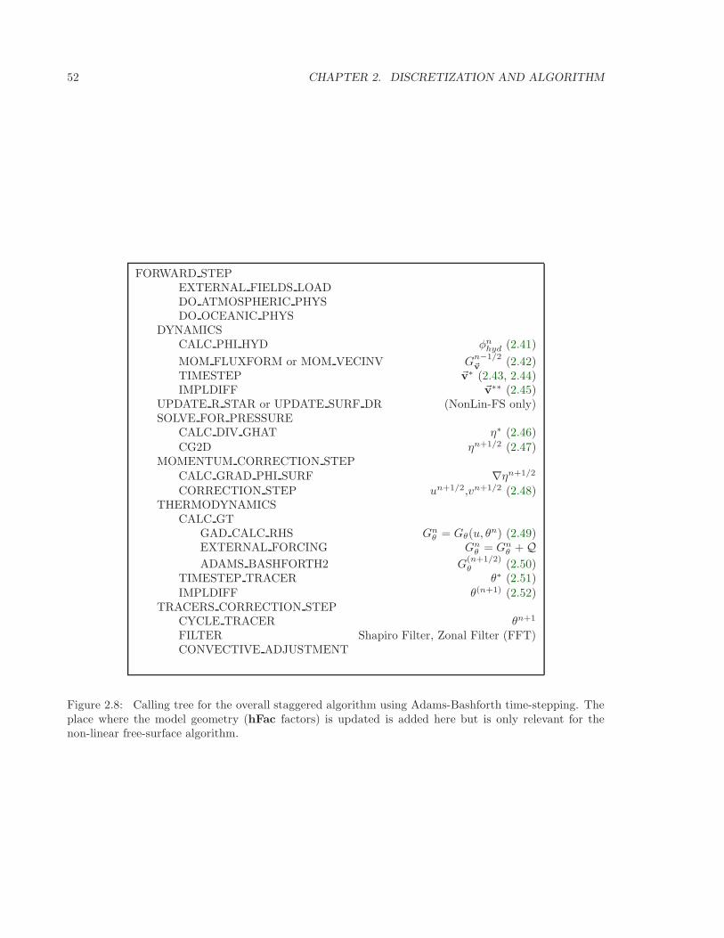
52 CHAPTER 2. DISCRETIZATION AND ALGORITHM
FORWARD STEPEXTERNAL FIELDS LOADDO ATMOSPHERIC PHYSDO OCEANIC PHYS
DYNAMICSCALC PHI HYD φn
hyd (2.41)
MOM FLUXFORM or MOM VECINV Gn−1/2~v (2.42)
TIMESTEP ~v∗ (2.43, 2.44)IMPLDIFF ~v∗∗ (2.45)
UPDATE R STAR or UPDATE SURF DR (NonLin-FS only)SOLVE FOR PRESSURE
CALC DIV GHAT η∗ (2.46)
CG2D ηn+1/2 (2.47)MOMENTUM CORRECTION STEP
CALC GRAD PHI SURF ∇ηn+1/2
CORRECTION STEP un+1/2,vn+1/2 (2.48)THERMODYNAMICS
CALC GTGAD CALC RHS Gn
θ = Gθ(u, θn) (2.49)
EXTERNAL FORCING Gnθ = Gn
θ + QADAMS BASHFORTH2 G
(n+1/2)θ (2.50)
TIMESTEP TRACER θ∗ (2.51)IMPLDIFF θ(n+1) (2.52)
TRACERS CORRECTION STEPCYCLE TRACER θn+1
FILTER Shapiro Filter, Zonal Filter (FFT)CONVECTIVE ADJUSTMENT
Figure 2.8: Calling tree for the overall staggered algorithm using Adams-Bashforth time-stepping. Theplace where the model geometry (hFac factors) is updated is added here but is only relevant for thenon-linear free-surface algorithm.
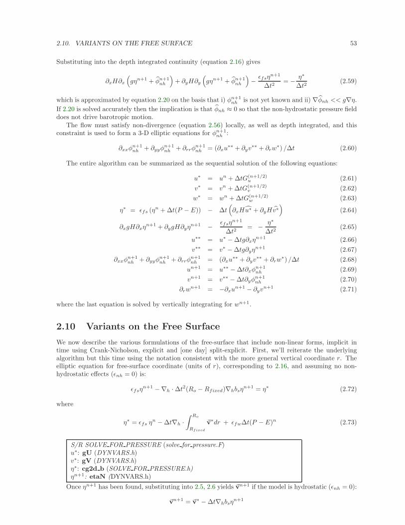
2.10. VARIANTS ON THE FREE SURFACE 53
Substituting into the depth integrated continuity (equation 2.16) gives
∂xH∂x
(gηn+1 + φn+1
nh
)+ ∂yH∂y
(gηn+1 + φn+1
nh
)− ǫfsη
n+1
∆t2= − η∗
∆t2(2.59)
which is approximated by equation 2.20 on the basis that i) φn+1nh is not yet known and ii) ∇φnh << g∇η.
If 2.20 is solved accurately then the implication is that φnh ≈ 0 so that the non-hydrostatic pressure fielddoes not drive barotropic motion.
The flow must satisfy non-divergence (equation 2.56) locally, as well as depth integrated, and thisconstraint is used to form a 3-D elliptic equations for φn+1
nh :
∂xxφn+1nh + ∂yyφ
n+1nh + ∂rrφ
n+1nh = (∂xu
∗∗ + ∂yv∗∗ + ∂rw
∗) /∆t (2.60)
The entire algorithm can be summarized as the sequential solution of the following equations:
u∗ = un + ∆tG(n+1/2)u (2.61)
v∗ = vn + ∆tG(n+1/2)v (2.62)
w∗ = wn + ∆tG(n+1/2)w (2.63)
η∗ = ǫfs (ηn + ∆t(P − E)) − ∆t(∂xHu∗ + ∂yHv∗
)(2.64)
∂xgH∂xηn+1 + ∂ygH∂yη
n+1 − ǫfsηn+1
∆t2= − η∗
∆t2(2.65)
u∗∗ = u∗ − ∆tg∂xηn+1 (2.66)
v∗∗ = v∗ − ∆tg∂yηn+1 (2.67)
∂xxφn+1nh + ∂yyφ
n+1nh + ∂rrφ
n+1nh = (∂xu
∗∗ + ∂yv∗∗ + ∂rw
∗) /∆t (2.68)
un+1 = u∗∗ − ∆t∂xφn+1nh (2.69)
vn+1 = v∗∗ − ∆t∂yφn+1nh (2.70)
∂rwn+1 = −∂xu
n+1 − ∂yvn+1 (2.71)
where the last equation is solved by vertically integrating for wn+1.
2.10 Variants on the Free Surface
We now describe the various formulations of the free-surface that include non-linear forms, implicit intime using Crank-Nicholson, explicit and [one day] split-explicit. First, we’ll reiterate the underlyingalgorithm but this time using the notation consistent with the more general vertical coordinate r. Theelliptic equation for free-surface coordinate (units of r), corresponding to 2.16, and assuming no non-hydrostatic effects (ǫnh = 0) is:
ǫfsηn+1 −∇h · ∆t2(Ro −Rfixed)∇hbsη
n+1 = η∗ (2.72)
where
η∗ = ǫfs ηn − ∆t∇h ·
∫ Ro
Rfixed
~v∗dr + ǫfw∆t(P − E)n (2.73)
S/R SOLVE FOR PRESSURE (solve for pressure.F)u∗: gU (DYNVARS.h)v∗: gV (DYNVARS.h)η∗: cg2d b (SOLVE FOR PRESSURE.h)ηn+1: etaN (DYNVARS.h)
Once ηn+1 has been found, substituting into 2.5, 2.6 yields ~vn+1 if the model is hydrostatic (ǫnh = 0):
~vn+1 = ~v∗ − ∆t∇hbsηn+1
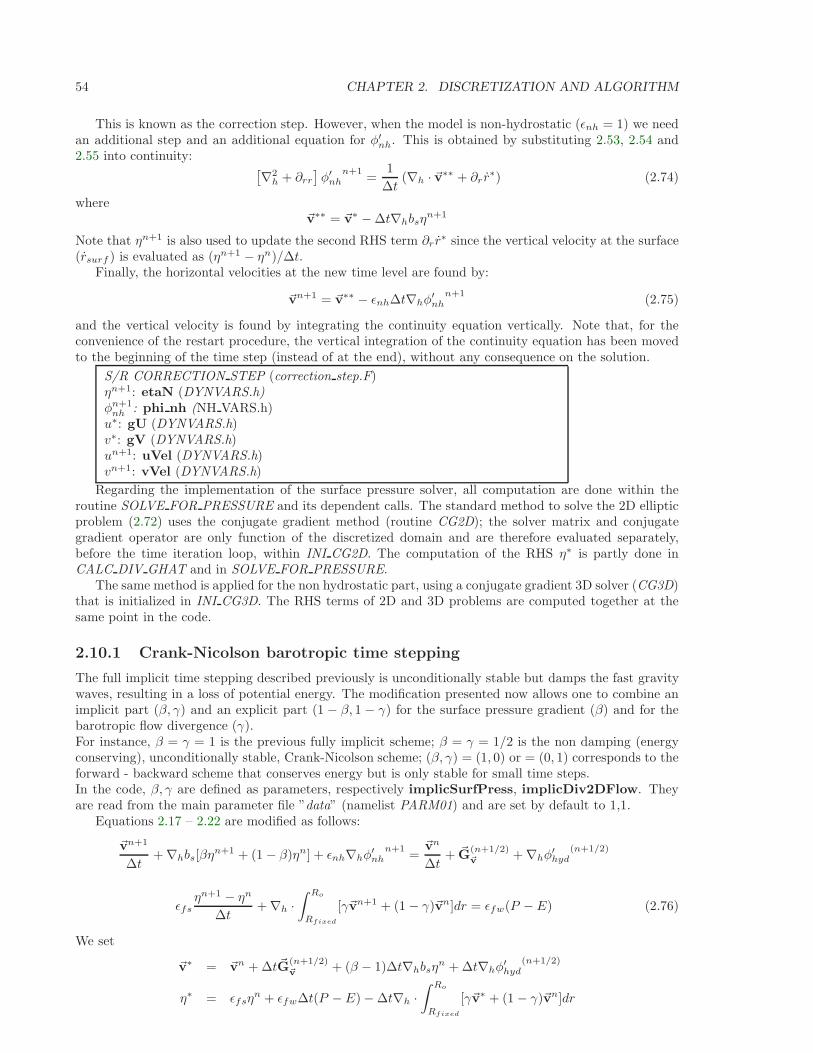
54 CHAPTER 2. DISCRETIZATION AND ALGORITHM
This is known as the correction step. However, when the model is non-hydrostatic (ǫnh = 1) we needan additional step and an additional equation for φ′nh. This is obtained by substituting 2.53, 2.54 and2.55 into continuity:
[∇2
h + ∂rr
]φ′nh
n+1=
1
∆t(∇h · ~v∗∗ + ∂r r
∗) (2.74)
where~v∗∗ = ~v∗ − ∆t∇hbsη
n+1
Note that ηn+1 is also used to update the second RHS term ∂r r∗ since the vertical velocity at the surface
(rsurf ) is evaluated as (ηn+1 − ηn)/∆t.Finally, the horizontal velocities at the new time level are found by:
~vn+1 = ~v∗∗ − ǫnh∆t∇hφ′nh
n+1(2.75)
and the vertical velocity is found by integrating the continuity equation vertically. Note that, for theconvenience of the restart procedure, the vertical integration of the continuity equation has been movedto the beginning of the time step (instead of at the end), without any consequence on the solution.
S/R CORRECTION STEP (correction step.F)ηn+1: etaN (DYNVARS.h)φn+1
nh : phi nh (NH VARS.h)u∗: gU (DYNVARS.h)v∗: gV (DYNVARS.h)un+1: uVel (DYNVARS.h)vn+1: vVel (DYNVARS.h)
Regarding the implementation of the surface pressure solver, all computation are done within theroutine SOLVE FOR PRESSURE and its dependent calls. The standard method to solve the 2D ellipticproblem (2.72) uses the conjugate gradient method (routine CG2D); the solver matrix and conjugategradient operator are only function of the discretized domain and are therefore evaluated separately,before the time iteration loop, within INI CG2D. The computation of the RHS η∗ is partly done inCALC DIV GHAT and in SOLVE FOR PRESSURE.
The same method is applied for the non hydrostatic part, using a conjugate gradient 3D solver (CG3D)that is initialized in INI CG3D. The RHS terms of 2D and 3D problems are computed together at thesame point in the code.
2.10.1 Crank-Nicolson barotropic time stepping
The full implicit time stepping described previously is unconditionally stable but damps the fast gravitywaves, resulting in a loss of potential energy. The modification presented now allows one to combine animplicit part (β, γ) and an explicit part (1 − β, 1 − γ) for the surface pressure gradient (β) and for thebarotropic flow divergence (γ).For instance, β = γ = 1 is the previous fully implicit scheme; β = γ = 1/2 is the non damping (energyconserving), unconditionally stable, Crank-Nicolson scheme; (β, γ) = (1, 0) or = (0, 1) corresponds to theforward - backward scheme that conserves energy but is only stable for small time steps.In the code, β, γ are defined as parameters, respectively implicSurfPress, implicDiv2DFlow. Theyare read from the main parameter file ”data” (namelist PARM01) and are set by default to 1,1.
Equations 2.17 – 2.22 are modified as follows:
~vn+1
∆t+ ∇hbs[βη
n+1 + (1 − β)ηn] + ǫnh∇hφ′nh
n+1=~vn
∆t+ ~G
(n+1/2)~v + ∇hφ
′hyd
(n+1/2)
ǫfsηn+1 − ηn
∆t+ ∇h ·
∫ Ro
Rfixed
[γ~vn+1 + (1 − γ)~vn]dr = ǫfw(P − E) (2.76)
We set
~v∗ = ~vn + ∆t~G(n+1/2)~v + (β − 1)∆t∇hbsη
n + ∆t∇hφ′hyd
(n+1/2)
η∗ = ǫfsηn + ǫfw∆t(P − E) − ∆t∇h ·
∫ Ro
Rfixed
[γ~v∗ + (1 − γ)~vn]dr
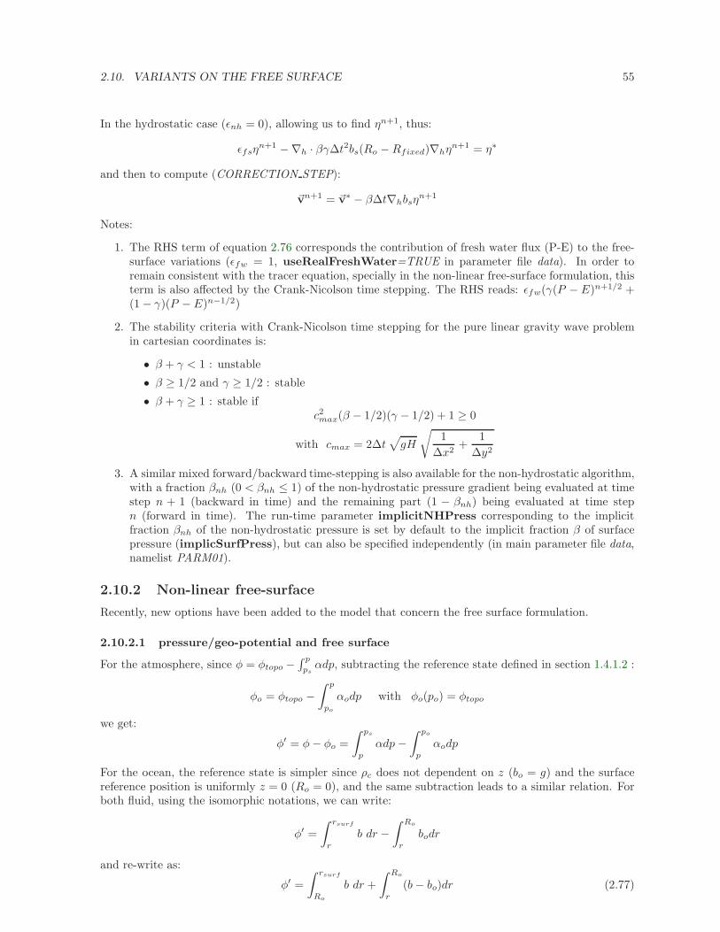
2.10. VARIANTS ON THE FREE SURFACE 55
In the hydrostatic case (ǫnh = 0), allowing us to find ηn+1, thus:
ǫfsηn+1 −∇h · βγ∆t2bs(Ro −Rfixed)∇hη
n+1 = η∗
and then to compute (CORRECTION STEP):
~vn+1 = ~v∗ − β∆t∇hbsηn+1
Notes:
1. The RHS term of equation 2.76 corresponds the contribution of fresh water flux (P-E) to the free-surface variations (ǫfw = 1, useRealFreshWater=TRUE in parameter file data). In order toremain consistent with the tracer equation, specially in the non-linear free-surface formulation, thisterm is also affected by the Crank-Nicolson time stepping. The RHS reads: ǫfw(γ(P − E)n+1/2 +(1 − γ)(P − E)n−1/2)
2. The stability criteria with Crank-Nicolson time stepping for the pure linear gravity wave problemin cartesian coordinates is:
• β + γ < 1 : unstable
• β ≥ 1/2 and γ ≥ 1/2 : stable
• β + γ ≥ 1 : stable ifc2max(β − 1/2)(γ − 1/2) + 1 ≥ 0
with cmax = 2∆t√gH
√1
∆x2+
1
∆y2
3. A similar mixed forward/backward time-stepping is also available for the non-hydrostatic algorithm,with a fraction βnh (0 < βnh ≤ 1) of the non-hydrostatic pressure gradient being evaluated at timestep n + 1 (backward in time) and the remaining part (1 − βnh) being evaluated at time stepn (forward in time). The run-time parameter implicitNHPress corresponding to the implicitfraction βnh of the non-hydrostatic pressure is set by default to the implicit fraction β of surfacepressure (implicSurfPress), but can also be specified independently (in main parameter file data,namelist PARM01).
2.10.2 Non-linear free-surface
Recently, new options have been added to the model that concern the free surface formulation.
2.10.2.1 pressure/geo-potential and free surface
For the atmosphere, since φ = φtopo −∫ p
psαdp, subtracting the reference state defined in section 1.4.1.2 :
φo = φtopo −∫ p
po
αodp with φo(po) = φtopo
we get:
φ′ = φ− φo =
∫ ps
p
αdp−∫ po
p
αodp
For the ocean, the reference state is simpler since ρc does not dependent on z (bo = g) and the surfacereference position is uniformly z = 0 (Ro = 0), and the same subtraction leads to a similar relation. Forboth fluid, using the isomorphic notations, we can write:
φ′ =
∫ rsurf
r
b dr −∫ Ro
r
bodr
and re-write as:
φ′ =
∫ rsurf
Ro
b dr +
∫ Ro
r
(b − bo)dr (2.77)
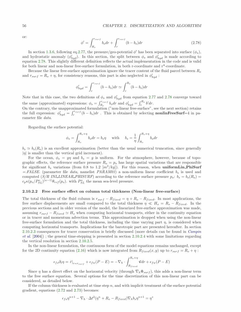
56 CHAPTER 2. DISCRETIZATION AND ALGORITHM
or:
φ′ =
∫ rsurf
Ro
bodr +
∫ rsurf
r
(b − bo)dr (2.78)
In section 1.3.6, following eq.2.77, the pressure/geo-potential φ′ has been separated into surface (φs),and hydrostatic anomaly (φ′hyd). In this section, the split between φs and φ′hyd is made according toequation 2.78. This slightly different definition reflects the actual implementation in the code and is validfor both linear and non-linear free-surface formulation, in both r-coordinate and r*-coordinate.
Because the linear free-surface approximation ignore the tracer content of the fluid parcel between Ro
and rsurf = Ro + η, for consistency reasons, this part is also neglected in φ′hyd :
φ′hyd =
∫ rsurf
r
(b− bo)dr ≃∫ Ro
r
(b − bo)dr
Note that in this case, the two definitions of φs and φ′hyd from equation 2.77 and 2.78 converge toward
the same (approximated) expressions: φs =∫ rsurf
Robodr and φ′hyd =
∫ Ro
r b′dr.
On the contrary, the unapproximated formulation (”non-linear free-surface”, see the next section) retainsthe full expression: φ′hyd =
∫ rsurf
r (b − bo)dr . This is obtained by selecting nonlinFreeSurf=4 in pa-rameter file data.
Regarding the surface potential:
φs =
∫ Ro+η
Ro
bodr = bsη with bs =1
η
∫ Ro+η
Ro
bodr
bs ≃ bo(Ro) is an excellent approximation (better than the usual numerical truncation, since generally|η| is smaller than the vertical grid increment).
For the ocean, φs = gη and bs = g is uniform. For the atmosphere, however, because of topo-graphic effects, the reference surface pressure Ro = po has large spatial variations that are responsiblefor significant bs variations (from 0.8 to 1.2 [m3/kg]). For this reason, when uniformLin PhiSurf=.FALSE. (parameter file data, namelist PARAM01) a non-uniform linear coefficient bs is used andcomputed (S/R INI LINEAR PHISURF) according to the reference surface pressure po: bs = bo(Ro) =cpκ(po/P
oSL)(κ−1)θref (po). with P o
SL the mean sea-level pressure.
2.10.2.2 Free surface effect on column total thickness (Non-linear free-surface)
The total thickness of the fluid column is rsurf − Rfixed = η + Ro − Rfixed. In most applications, thefree surface displacements are small compared to the total thickness η ≪ Ho = Ro − Rfixed. In theprevious sections and in older version of the model, the linearized free-surface approximation was made,assuming rsurf − Rfixed ≃ Ho when computing horizontal transports, either in the continuity equationor in tracer and momentum advection terms. This approximation is dropped when using the non-linearfree-surface formulation and the total thickness, including the time varying part η, is considered whencomputing horizontal transports. Implications for the barotropic part are presented hereafter. In section2.10.2.3 consequences for tracer conservation is briefly discussed (more details can be found in Campinet al. [2004]) ; the general time-stepping is presented in section 2.10.2.4 with some limitations regardingthe vertical resolution in section 2.10.2.5.
In the non-linear formulation, the continuous form of the model equations remains unchanged, exceptfor the 2D continuity equation (2.16) which is now integrated from Rfixed(x, y) up to rsurf = Ro + η :
ǫfs∂tη = r|r=rsurf+ ǫfw(P − E) = −∇h ·
∫ Ro+η
Rfixed
~vdr + ǫfw(P − E)
Since η has a direct effect on the horizontal velocity (through ∇hΦsurf ), this adds a non-linear termto the free surface equation. Several options for the time discretization of this non-linear part can beconsidered, as detailed below.
If the column thickness is evaluated at time step n, and with implicit treatment of the surface potentialgradient, equations (2.72 and 2.73) becomes:
ǫfsηn+1 −∇h · ∆t2(ηn +Ro −Rfixed)∇hbsη
n+1 = η∗
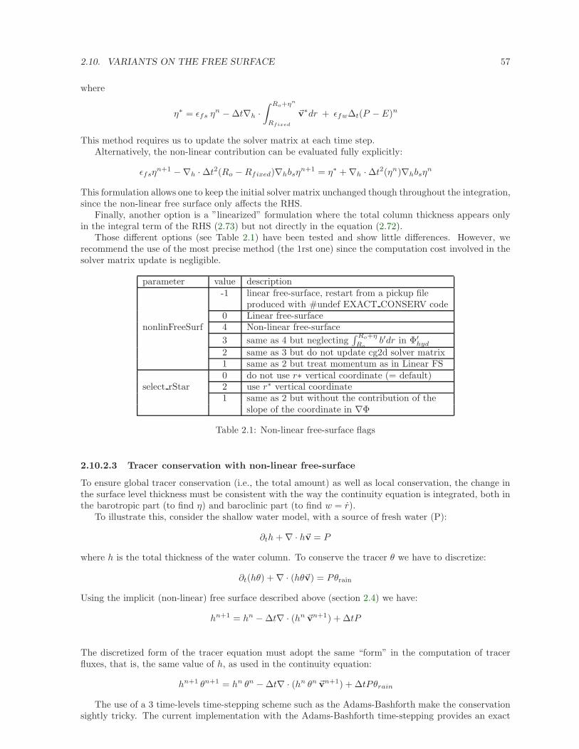
2.10. VARIANTS ON THE FREE SURFACE 57
where
η∗ = ǫfs ηn − ∆t∇h ·
∫ Ro+ηn
Rfixed
~v∗dr + ǫfw∆t(P − E)n
This method requires us to update the solver matrix at each time step.Alternatively, the non-linear contribution can be evaluated fully explicitly:
ǫfsηn+1 −∇h · ∆t2(Ro −Rfixed)∇hbsη
n+1 = η∗ + ∇h · ∆t2(ηn)∇hbsηn
This formulation allows one to keep the initial solver matrix unchanged though throughout the integration,since the non-linear free surface only affects the RHS.
Finally, another option is a ”linearized” formulation where the total column thickness appears onlyin the integral term of the RHS (2.73) but not directly in the equation (2.72).
Those different options (see Table 2.1) have been tested and show little differences. However, werecommend the use of the most precise method (the 1rst one) since the computation cost involved in thesolver matrix update is negligible.
parameter value description-1 linear free-surface, restart from a pickup file
produced with #undef EXACT CONSERV code0 Linear free-surface
nonlinFreeSurf 4 Non-linear free-surface
3 same as 4 but neglecting∫ Ro+η
Rob′dr in Φ′hyd
2 same as 3 but do not update cg2d solver matrix1 same as 2 but treat momentum as in Linear FS0 do not use r∗ vertical coordinate (= default)
select rStar 2 use r∗ vertical coordinate1 same as 2 but without the contribution of the
slope of the coordinate in ∇Φ
Table 2.1: Non-linear free-surface flags
2.10.2.3 Tracer conservation with non-linear free-surface
To ensure global tracer conservation (i.e., the total amount) as well as local conservation, the change inthe surface level thickness must be consistent with the way the continuity equation is integrated, both inthe barotropic part (to find η) and baroclinic part (to find w = r).
To illustrate this, consider the shallow water model, with a source of fresh water (P):
∂th+ ∇ · h~v = P
where h is the total thickness of the water column. To conserve the tracer θ we have to discretize:
∂t(hθ) + ∇ · (hθ~v) = Pθrain
Using the implicit (non-linear) free surface described above (section 2.4) we have:
hn+1 = hn − ∆t∇ · (hn ~vn+1) + ∆tP
The discretized form of the tracer equation must adopt the same “form” in the computation of tracerfluxes, that is, the same value of h, as used in the continuity equation:
hn+1 θn+1 = hn θn − ∆t∇ · (hn θn ~vn+1) + ∆tPθrain
The use of a 3 time-levels time-stepping scheme such as the Adams-Bashforth make the conservationsightly tricky. The current implementation with the Adams-Bashforth time-stepping provides an exact
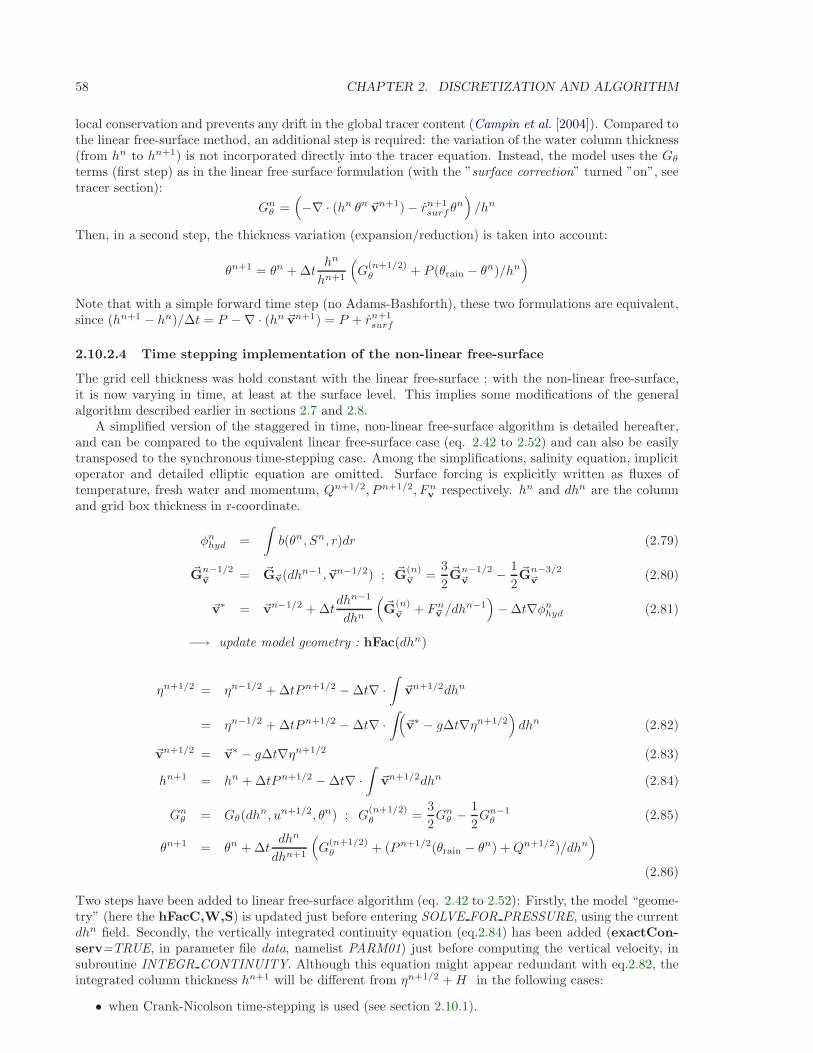
58 CHAPTER 2. DISCRETIZATION AND ALGORITHM
local conservation and prevents any drift in the global tracer content (Campin et al. [2004]). Compared tothe linear free-surface method, an additional step is required: the variation of the water column thickness(from hn to hn+1) is not incorporated directly into the tracer equation. Instead, the model uses the Gθ
terms (first step) as in the linear free surface formulation (with the ”surface correction” turned ”on”, seetracer section):
Gnθ =
(−∇ · (hn θn ~vn+1) − rn+1
surf θn)/hn
Then, in a second step, the thickness variation (expansion/reduction) is taken into account:
θn+1 = θn + ∆thn
hn+1
(G
(n+1/2)θ + P (θrain − θn)/hn
)
Note that with a simple forward time step (no Adams-Bashforth), these two formulations are equivalent,since (hn+1 − hn)/∆t = P −∇ · (hn ~vn+1) = P + rn+1
surf
2.10.2.4 Time stepping implementation of the non-linear free-surface
The grid cell thickness was hold constant with the linear free-surface ; with the non-linear free-surface,it is now varying in time, at least at the surface level. This implies some modifications of the generalalgorithm described earlier in sections 2.7 and 2.8.
A simplified version of the staggered in time, non-linear free-surface algorithm is detailed hereafter,and can be compared to the equivalent linear free-surface case (eq. 2.42 to 2.52) and can also be easilytransposed to the synchronous time-stepping case. Among the simplifications, salinity equation, implicitoperator and detailed elliptic equation are omitted. Surface forcing is explicitly written as fluxes oftemperature, fresh water and momentum, Qn+1/2, Pn+1/2, Fn
v respectively. hn and dhn are the columnand grid box thickness in r-coordinate.
φnhyd =
∫b(θn, Sn, r)dr (2.79)
~Gn−1/2~v = ~G~v(dhn−1, ~vn−1/2) ; ~G
(n)~v =
3
2~G
n−1/2~v − 1
2~G
n−3/2~v (2.80)
~v∗ = ~vn−1/2 + ∆tdhn−1
dhn
(~G
(n)~v + Fn
~v /dhn−1)− ∆t∇φn
hyd (2.81)
−→ update model geometry : hFac(dhn)
ηn+1/2 = ηn−1/2 + ∆tPn+1/2 − ∆t∇ ·∫~vn+1/2dhn
= ηn−1/2 + ∆tPn+1/2 − ∆t∇ ·∫(~v∗ − g∆t∇ηn+1/2
)dhn (2.82)
~vn+1/2 = ~v∗ − g∆t∇ηn+1/2 (2.83)
hn+1 = hn + ∆tPn+1/2 − ∆t∇ ·∫~vn+1/2dhn (2.84)
Gnθ = Gθ(dh
n, un+1/2, θn) ; G(n+1/2)θ =
3
2Gn
θ − 1
2Gn−1
θ (2.85)
θn+1 = θn + ∆tdhn
dhn+1
(G
(n+1/2)θ + (Pn+1/2(θrain − θn) +Qn+1/2)/dhn
)
(2.86)
Two steps have been added to linear free-surface algorithm (eq. 2.42 to 2.52): Firstly, the model “geome-try” (here the hFacC,W,S) is updated just before entering SOLVE FOR PRESSURE, using the currentdhn field. Secondly, the vertically integrated continuity equation (eq.2.84) has been added (exactCon-serv=TRUE, in parameter file data, namelist PARM01) just before computing the vertical velocity, insubroutine INTEGR CONTINUITY. Although this equation might appear redundant with eq.2.82, theintegrated column thickness hn+1 will be different from ηn+1/2 +H in the following cases:
• when Crank-Nicolson time-stepping is used (see section 2.10.1).
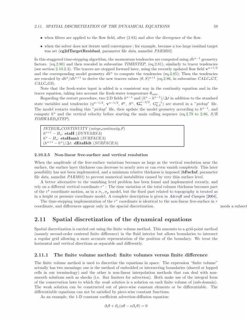
2.11. SPATIAL DISCRETIZATION OF THE DYNAMICAL EQUATIONS 59
• when filters are applied to the flow field, after (2.83) and alter the divergence of the flow.
• when the solver does not iterate until convergence ; for example, because a too large residual targetwas set (cg2dTargetResidual, parameter file data, namelist PARM02).
In this staggered time-stepping algorithm, the momentum tendencies are computed using dhn−1 geometryfactors. (eq.2.80) and then rescaled in subroutine TIMESTEP, (eq.2.81), similarly to tracer tendencies(see section 2.10.2.3). The tracers are stepped forward later, using the recently updated flow field vn+1/2
and the corresponding model geometry dhn to compute the tendencies (eq.2.85); Then the tendenciesare rescaled by dhn/dhn+1 to derive the new tracers values (θ, S)n+1 (eq.2.86, in subroutine CALC GT,CALC GS).
Note that the fresh-water input is added in a consistent way in the continuity equation and in thetracer equation, taking into account the fresh-water temperature θrain.
Regarding the restart procedure, two 2.D fields hn−1 and (hn −hn−1)/∆t in addition to the standard
state variables and tendencies (ηn−1/2, vn−1/2, θn, Sn, Gn−3/2v , Gn−1
θ,S ) are stored in a ”pickup” file.
The model restarts reading this ”pickup” file, then update the model geometry according to hn−1, andcompute hn and the vertical velocity before starting the main calling sequence (eq.2.79 to 2.86, S/RFORWARD STEP).
INTEGR CONTINUITY (integr continuity.F)hn+1 −Ho: etaH (DYNVARS.h)hn −Ho: etaHnm1 (SURFACE.h)(hn+1 − hn)/∆t: dEtaHdt (SURFACE.h)
2.10.2.5 Non-linear free-surface and vertical resolution
When the amplitude of the free-surface variations becomes as large as the vertical resolution near thesurface, the surface layer thickness can decrease to nearly zero or can even vanish completely. This laterpossibility has not been implemented, and a minimum relative thickness is imposed (hFacInf, parameterfile data, namelist PARM01) to prevent numerical instabilities caused by very thin surface level.
A better alternative to the vanishing level problem has been found and implemented recently, andrely on a different vertical coordinate r∗ : The time variation ot the total column thickness becomes partof the r* coordinate motion, as in a σz , σp model, but the fixed part related to topography is treated asin a height or pressure coordinate model. A complete description is given in Adcroft and Campin [2004].
The time-stepping implementation of the r∗ coordinate is identical to the non-linear free-surface in rcoordinate, and differences appear only in the spacial discretization. needs a subsection
2.11 Spatial discretization of the dynamical equations
Spatial discretization is carried out using the finite volume method. This amounts to a grid-point method(namely second-order centered finite difference) in the fluid interior but allows boundaries to intersecta regular grid allowing a more accurate representation of the position of the boundary. We treat thehorizontal and vertical directions as separable and differently.
2.11.1 The finite volume method: finite volumes versus finite difference
The finite volume method is used to discretize the equations in space. The expression “finite volume”actually has two meanings; one is the method of embedded or intersecting boundaries (shaved or loppedcells in our terminology) and the other is non-linear interpolation methods that can deal with non-smooth solutions such as shocks (i.e. flux limiters for advection). Both make use of the integral formof the conservation laws to which the weak solution is a solution on each finite volume of (sub-domain).The weak solution can be constructed out of piece-wise constant elements or be differentiable. Thedifferentiable equations can not be satisfied by piece-wise constant functions.
As an example, the 1-D constant coefficient advection-diffusion equation:
∂tθ + ∂x(uθ − κ∂xθ) = 0
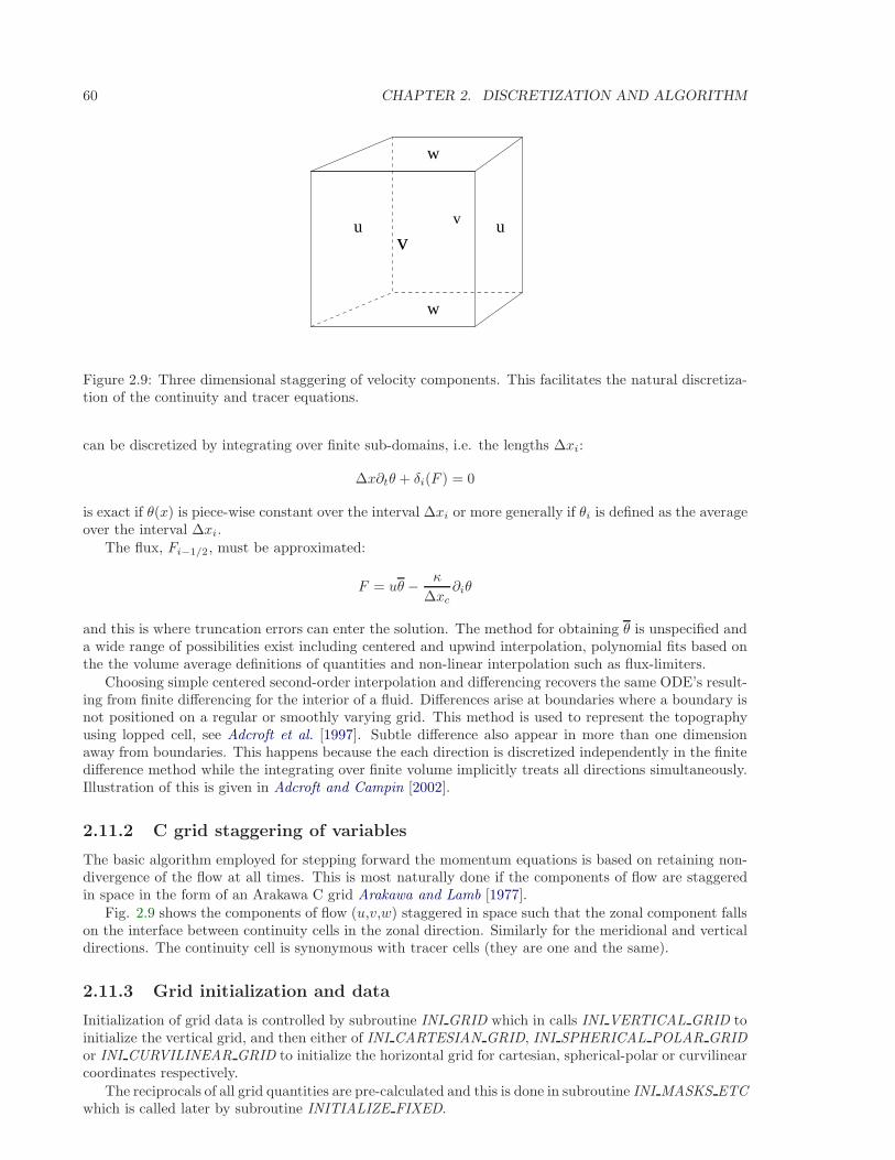
60 CHAPTER 2. DISCRETIZATION AND ALGORITHM
uv
v u
w
w
Figure 2.9: Three dimensional staggering of velocity components. This facilitates the natural discretiza-tion of the continuity and tracer equations.
can be discretized by integrating over finite sub-domains, i.e. the lengths ∆xi:
∆x∂tθ + δi(F ) = 0
is exact if θ(x) is piece-wise constant over the interval ∆xi or more generally if θi is defined as the averageover the interval ∆xi.
The flux, Fi−1/2, must be approximated:
F = uθ − κ
∆xc∂iθ
and this is where truncation errors can enter the solution. The method for obtaining θ is unspecified anda wide range of possibilities exist including centered and upwind interpolation, polynomial fits based onthe the volume average definitions of quantities and non-linear interpolation such as flux-limiters.
Choosing simple centered second-order interpolation and differencing recovers the same ODE’s result-ing from finite differencing for the interior of a fluid. Differences arise at boundaries where a boundary isnot positioned on a regular or smoothly varying grid. This method is used to represent the topographyusing lopped cell, see Adcroft et al. [1997]. Subtle difference also appear in more than one dimensionaway from boundaries. This happens because the each direction is discretized independently in the finitedifference method while the integrating over finite volume implicitly treats all directions simultaneously.Illustration of this is given in Adcroft and Campin [2002].
2.11.2 C grid staggering of variables
The basic algorithm employed for stepping forward the momentum equations is based on retaining non-divergence of the flow at all times. This is most naturally done if the components of flow are staggeredin space in the form of an Arakawa C grid Arakawa and Lamb [1977].
Fig. 2.9 shows the components of flow (u,v,w) staggered in space such that the zonal component fallson the interface between continuity cells in the zonal direction. Similarly for the meridional and verticaldirections. The continuity cell is synonymous with tracer cells (they are one and the same).
2.11.3 Grid initialization and data
Initialization of grid data is controlled by subroutine INI GRID which in calls INI VERTICAL GRID toinitialize the vertical grid, and then either of INI CARTESIAN GRID, INI SPHERICAL POLAR GRIDor INI CURVILINEAR GRID to initialize the horizontal grid for cartesian, spherical-polar or curvilinearcoordinates respectively.
The reciprocals of all grid quantities are pre-calculated and this is done in subroutine INI MASKS ETCwhich is called later by subroutine INITIALIZE FIXED.
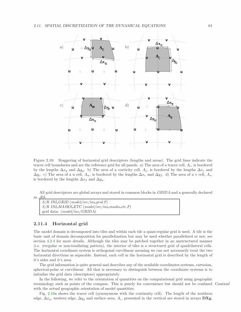
2.11. SPATIAL DISCRETIZATION OF THE DYNAMICAL EQUATIONS 61
a)
x∆
∆y
G
G C
u
v v
u
v
u u
v
u
v
u
v
A b)
y∆
x∆
C
C
u
u u
uu
v v
v
vv
v
u
Aζ
c) y∆
x∆
WF
V
v v
v v
uu
u u u
v v
A d)
y∆
x∆
U
F
S
v
u u u
u u u
v
v
v v
A
Figure 2.10: Staggering of horizontal grid descriptors (lengths and areas). The grid lines indicate thetracer cell boundaries and are the reference grid for all panels. a) The area of a tracer cell, Ac, is borderedby the lengths ∆xg and ∆yg. b) The area of a vorticity cell, Aζ , is bordered by the lengths ∆xc and∆yc. c) The area of a u cell, Aw, is bordered by the lengths ∆xv and ∆yf . d) The area of a v cell, As,is bordered by the lengths ∆xf and ∆yu.
All grid descriptors are global arrays and stored in common blocks in GRID.h and a generally declaredas RS.
S/R INI GRID (model/src/ini grid.F)S/R INI MASKS ETC (model/src/ini masks etc.F)grid data: (model/inc/GRID.h)
2.11.4 Horizontal grid
The model domain is decomposed into tiles and within each tile a quasi-regular grid is used. A tile is thebasic unit of domain decomposition for parallelization but may be used whether parallelized or not; seesection 4.2.4 for more details. Although the tiles may be patched together in an unstructured manner(i.e. irregular or non-tessilating pattern), the interior of tiles is a structured grid of quadrilateral cells.The horizontal coordinate system is orthogonal curvilinear meaning we can not necessarily treat the twohorizontal directions as separable. Instead, each cell in the horizontal grid is described by the length ofit’s sides and it’s area.
The grid information is quite general and describes any of the available coordinates systems, cartesian,spherical-polar or curvilinear. All that is necessary to distinguish between the coordinate systems is toinitialize the grid data (descriptors) appropriately.
In the following, we refer to the orientation of quantities on the computational grid using geographicterminology such as points of the compass. This is purely for convenience but should not be confused Caution!with the actual geographic orientation of model quantities.
Fig. 2.10a shows the tracer cell (synonymous with the continuity cell). The length of the southernedge, ∆xg , western edge, ∆yg and surface area, Ac, presented in the vertical are stored in arrays DXg,
62 CHAPTER 2. DISCRETIZATION AND ALGORITHM
DYg and rAc. The “g” suffix indicates that the lengths are along the defining grid boundaries. The“c” suffix associates the quantity with the cell centers. The quantities are staggered in space and theindexing is such that DXg(i,j) is positioned to the south of rAc(i,j) and DYg(i,j) positioned to thewest.
Fig. 2.10b shows the vorticity cell. The length of the southern edge, ∆xc, western edge, ∆yc andsurface area, Aζ , presented in the vertical are stored in arrays DXc, DYc and rAz. The “z” suffixindicates that the lengths are measured between the cell centers and the “ζ” suffix associates points withthe vorticity points. The quantities are staggered in space and the indexing is such that DXc(i,j) ispositioned to the north of rAz(i,j) and DYc(i,j) positioned to the east.
Fig. 2.10c shows the “u” or western (w) cell. The length of the southern edge, ∆xv, eastern edge,∆yf and surface area, Aw, presented in the vertical are stored in arrays DXv, DYf and rAw. The“v” suffix indicates that the length is measured between the v-points, the “f” suffix indicates that thelength is measured between the (tracer) cell faces and the “w” suffix associates points with the u-points(w stands for west). The quantities are staggered in space and the indexing is such that DXv(i,j) ispositioned to the south of rAw(i,j) and DYf(i,j) positioned to the east.
Fig. 2.10d shows the “v” or southern (s) cell. The length of the northern edge, ∆xf , western edge,∆yu and surface area, As, presented in the vertical are stored in arrays DXf, DYu and rAs. The “u”suffix indicates that the length is measured between the u-points, the “f” suffix indicates that the lengthis measured between the (tracer) cell faces and the “s” suffix associates points with the v-points (s standsfor south). The quantities are staggered in space and the indexing is such that DXf(i,j) is positioned tothe north of rAs(i,j) and DYu(i,j) positioned to the west.
S/R INI CARTESIAN GRID (model/src/ini cartesian grid.F)S/R INI SPHERICAL POLAR GRID (model/src/ini spherical polar grid.F)S/R INI CURVILINEAR GRID (model/src/ini curvilinear grid.F)Ac, Aζ , Aw, As: rAc, rAz, rAw, rAs (GRID.h)∆xg, ∆yg: DXg, DYg (GRID.h)∆xc, ∆yc: DXc, DYc (GRID.h)∆xf , ∆yf : DXf, DYf (GRID.h)∆xv, ∆yu: DXv, DYu (GRID.h)
2.11.4.1 Reciprocals of horizontal grid descriptors
Lengths and areas appear in the denominator of expressions as much as in the numerator. For efficiencyand portability, we pre-calculate the reciprocal of the horizontal grid quantities so that in-line divisionscan be avoided.
For each grid descriptor (array) there is a reciprocal named using the prefix RECIP . This doublesthe amount of storage in GRID.h but they are all only 2-D descriptors.
S/R INI MASKS ETC (model/src/ini masks etc.F)A−1
c : RECIP Ac (GRID.h)A−1
ζ : RECIP Az (GRID.h)
A−1w : RECIP Aw (GRID.h)
A−1s : RECIP As (GRID.h)
∆x−1g , ∆y−1
g : RECIP DXg, RECIP DYg (GRID.h)∆x−1
c , ∆y−1c : RECIP DXc, RECIP DYc (GRID.h)
∆x−1f , ∆y−1
f : RECIP DXf, RECIP DYf (GRID.h)
∆x−1v , ∆y−1
u : RECIP DXv, RECIP DYu (GRID.h)
2.11.4.2 Cartesian coordinates
Cartesian coordinates are selected when the logical flag usingCartesianGrid in namelist PARM04 isset to true. The grid spacing can be set to uniform via scalars dXspacing and dYspacing in namelistPARM04 or to variable resolution by the vectors DELX and DELY. Units are normally meters. Non-dimensional coordinates can be used by interpreting the gravitational constant as the Rayleigh number.
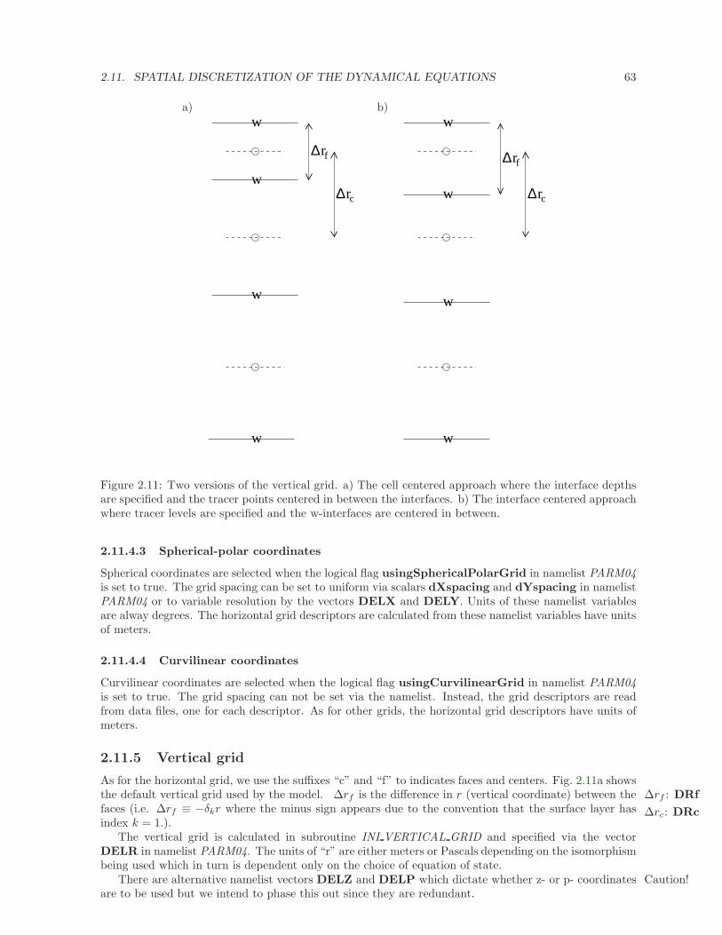
2.11. SPATIAL DISCRETIZATION OF THE DYNAMICAL EQUATIONS 63
a)
∆rf
∆rc
w
w
w
w
b)
∆rc
∆rf
w
w
w
w
Figure 2.11: Two versions of the vertical grid. a) The cell centered approach where the interface depthsare specified and the tracer points centered in between the interfaces. b) The interface centered approachwhere tracer levels are specified and the w-interfaces are centered in between.
2.11.4.3 Spherical-polar coordinates
Spherical coordinates are selected when the logical flag usingSphericalPolarGrid in namelist PARM04is set to true. The grid spacing can be set to uniform via scalars dXspacing and dYspacing in namelistPARM04 or to variable resolution by the vectors DELX and DELY. Units of these namelist variablesare alway degrees. The horizontal grid descriptors are calculated from these namelist variables have unitsof meters.
2.11.4.4 Curvilinear coordinates
Curvilinear coordinates are selected when the logical flag usingCurvilinearGrid in namelist PARM04is set to true. The grid spacing can not be set via the namelist. Instead, the grid descriptors are readfrom data files, one for each descriptor. As for other grids, the horizontal grid descriptors have units ofmeters.
2.11.5 Vertical grid
As for the horizontal grid, we use the suffixes “c” and “f” to indicates faces and centers. Fig. 2.11a showsthe default vertical grid used by the model. ∆rf is the difference in r (vertical coordinate) between the ∆rf : DRf
∆rc: DRcfaces (i.e. ∆rf ≡ −δkr where the minus sign appears due to the convention that the surface layer hasindex k = 1.).
The vertical grid is calculated in subroutine INI VERTICAL GRID and specified via the vectorDELR in namelist PARM04. The units of “r” are either meters or Pascals depending on the isomorphismbeing used which in turn is dependent only on the choice of equation of state.
There are alternative namelist vectors DELZ and DELP which dictate whether z- or p- coordinates Caution!are to be used but we intend to phase this out since they are redundant.
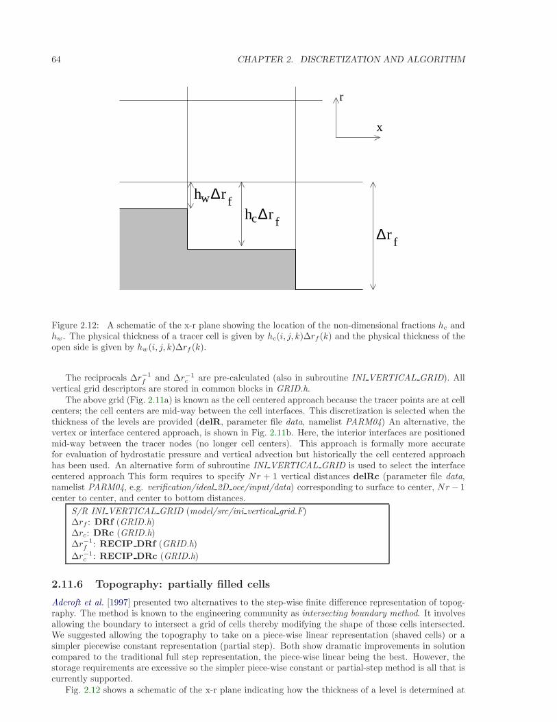
64 CHAPTER 2. DISCRETIZATION AND ALGORITHM
hwhc
∆r f
∆r f
∆r f
x
r
Figure 2.12: A schematic of the x-r plane showing the location of the non-dimensional fractions hc andhw. The physical thickness of a tracer cell is given by hc(i, j, k)∆rf (k) and the physical thickness of theopen side is given by hw(i, j, k)∆rf (k).
The reciprocals ∆r−1f and ∆r−1
c are pre-calculated (also in subroutine INI VERTICAL GRID). Allvertical grid descriptors are stored in common blocks in GRID.h.
The above grid (Fig. 2.11a) is known as the cell centered approach because the tracer points are at cellcenters; the cell centers are mid-way between the cell interfaces. This discretization is selected when thethickness of the levels are provided (delR, parameter file data, namelist PARM04) An alternative, thevertex or interface centered approach, is shown in Fig. 2.11b. Here, the interior interfaces are positionedmid-way between the tracer nodes (no longer cell centers). This approach is formally more accuratefor evaluation of hydrostatic pressure and vertical advection but historically the cell centered approachhas been used. An alternative form of subroutine INI VERTICAL GRID is used to select the interfacecentered approach This form requires to specify Nr + 1 vertical distances delRc (parameter file data,namelist PARM04, e.g. verification/ideal 2D oce/input/data) corresponding to surface to center, Nr− 1center to center, and center to bottom distances.
S/R INI VERTICAL GRID (model/src/ini vertical grid.F)∆rf : DRf (GRID.h)∆rc: DRc (GRID.h)∆r−1
f : RECIP DRf (GRID.h)
∆r−1c : RECIP DRc (GRID.h)
2.11.6 Topography: partially filled cells
Adcroft et al. [1997] presented two alternatives to the step-wise finite difference representation of topog-raphy. The method is known to the engineering community as intersecting boundary method. It involvesallowing the boundary to intersect a grid of cells thereby modifying the shape of those cells intersected.We suggested allowing the topography to take on a piece-wise linear representation (shaved cells) or asimpler piecewise constant representation (partial step). Both show dramatic improvements in solutioncompared to the traditional full step representation, the piece-wise linear being the best. However, thestorage requirements are excessive so the simpler piece-wise constant or partial-step method is all that iscurrently supported.
Fig. 2.12 shows a schematic of the x-r plane indicating how the thickness of a level is determined at
2.12. CONTINUITY AND HORIZONTAL PRESSURE GRADIENT TERMS 65
tracer and u points. The physical thickness of a tracer cell is given by hc(i, j, k)∆rf (k) and the physical hc: hFacC
hw: hFacW
hs: hFacS
thickness of the open side is given by hw(i, j, k)∆rf (k). Three 3-D descriptors hc, hw and hs are usedto describe the geometry: hFacC, hFacW and hFacS respectively. These are calculated in subroutineINI MASKS ETC along with there reciprocals RECIP hFacC, RECIP hFacW and RECIP hFacS.
The non-dimensional fractions (or h-facs as we call them) are calculated from the model depth arrayand then processed to avoid tiny volumes. The rule is that if a fraction is less than hFacMin then itis rounded to the nearer of 0 or hFacMin or if the physical thickness is less than hFacMinDr thenit is similarly rounded. The larger of the two methods is used when there is a conflict. By settinghFacMinDr equal to or larger than the thinnest nominal layers, min (∆zf ), but setting hFacMin tosome small fraction then the model will only lop thick layers but retain stability based on the thinnestunlopped thickness; min (∆zf ,hFacMinDr).
S/R INI MASKS ETC (model/src/ini masks etc.F)hc: hFacC (GRID.h)hw: hFacW (GRID.h)hs: hFacS (GRID.h)h−1
c : RECIP hFacC (GRID.h)h−1
w : RECIP hFacW (GRID.h)h−1
s : RECIP hFacS (GRID.h)
2.12 Continuity and horizontal pressure gradient terms
The core algorithm is based on the “C grid” discretization of the continuity equation which can besummarized as:
∂tu+1
∆xcδi∂Φ
∂r
∣∣∣∣s
η +ǫnh
∆xcδiΦ′nh = Gu − 1
∆xcδiΦ′h (2.87)
∂tv +1
∆ycδj∂Φ
∂r
∣∣∣∣s
η +ǫnh
∆ycδjΦ′nh = Gv − 1
∆ycδjΦ′h (2.88)
ǫnh
(∂tw +
1
∆rcδkΦ′nh
)= ǫnhGw + b
k − 1
∆rcδkΦ′h (2.89)
δi∆yg∆rfhwu+ δj∆xg∆rfhsv + δkAcw = Acδk(P − E)r=0 (2.90)
where the continuity equation has been most naturally discretized by staggering the three componentsof velocity as shown in Fig. 2.9. The grid lengths ∆xc and ∆yc are the lengths between tracer points(cell centers). The grid lengths ∆xg, ∆yg are the grid lengths between cell corners. ∆rf and ∆rc are thedistance (in units of r) between level interfaces (w-level) and level centers (tracer level). The surface areapresented in the vertical is denoted Ac. The factors hw and hs are non-dimensional fractions (between 0and 1) that represent the fraction cell depth that is “open” for fluid flow. hw: hFacW
hs: hFacSThe last equation, the discrete continuity equation, can be summed in the vertical to yield the free-surface equation:
Ac∂tη + δi∑
k
∆yg∆rfhwu+ δj∑
k
∆xg∆rfhsv = Ac(P − E)r=0 (2.91)
The source term P − E on the rhs of continuity accounts for the local addition of volume due to excessprecipitation and run-off over evaporation and only enters the top-level of the ocean model.
2.13 Hydrostatic balance
The vertical momentum equation has the hydrostatic or quasi-hydrostatic balance on the right handside. This discretization guarantees that the conversion of potential to kinetic energy as derived from thebuoyancy equation exactly matches the form derived from the pressure gradient terms when forming thekinetic energy equation.
In the ocean, using z-coordinates, the hydrostatic balance terms are discretized:
ǫnh∂tw + gρ′k
+1
∆zδkΦ′h = . . . (2.92)
66 CHAPTER 2. DISCRETIZATION AND ALGORITHM
In the atmosphere, using p-coordinates, hydrostatic balance is discretized:
θ′k
+1
∆ΠδkΦ′h = 0 (2.93)
where ∆Π is the difference in Exner function between the pressure points. The non-hydrostatic equationsare not available in the atmosphere.
The difference in approach between ocean and atmosphere occurs because of the direct use of theideal gas equation in forming the potential energy conversion term αω. The form of these conversionterms is discussed at length in Adcroft [2002].
Because of the different representation of hydrostatic balance between ocean and atmosphere there isno elegant way to represent both systems using an arbitrary coordinate.
The integration for hydrostatic pressure is made in the positive r direction (increasing k-index). Forthe ocean, this is from the free-surface down and for the atmosphere this is from the ground up.
The calculations are made in the subroutine CALC PHI HYD. Inside this routine, one of other of theatmospheric/oceanic form is selected based on the string variable buoyancyRelation.
2.14 Flux-form momentum equations
The original finite volume model was based on the Eulerian flux form momentum equations. This is thedefault though the vector invariant form is optionally available (and recommended in some cases).
The “G’s” (our colloquial name for all terms on rhs!) are broken into the various advective, Coriolis,horizontal dissipation, vertical dissipation and metric forces:
Gu = Gadvu +Gcor
u +Gh−dissu +Gv−diss
u +Gmetricu +Gnh−metric
u (2.94)
Gv = Gadvv +Gcor
v +Gh−dissv +Gv−diss
v +Gmetricv +Gnh−metric
v (2.95)
Gw = Gadvw +Gcor
w +Gh−dissw +Gv−diss
w +Gmetricw +Gnh−metric
w (2.96)
In the hydrostatic limit, Gw = 0 and ǫnh = 0, reducing the vertical momentum to hydrostatic balance.
These terms are calculated in routines called from subroutine MOM FLUXFORM a collected into theglobal arrays Gu, Gv, and Gw.
S/R MOM FLUXFORM (pkg/mom fluxform/mom fluxform.F)Gu: Gu (DYNVARS.h)Gv: Gv (DYNVARS.h)Gw: Gw (DYNVARS.h)
2.14.1 Advection of momentum
The advective operator is second order accurate in space:
Aw∆rfhwGadvu = δiU
iui + δjV
iuj + δkW
iuk (2.97)
As∆rfhsGadvv = δiU
jvi + δjV
jvj + δkW
jvk (2.98)
Ac∆rcGadvw = δiU
kwi + δjV
kwj + δkW
kwk (2.99)
and because of the flux form does not contribute to the global budget of linear momentum. The quantitiesU , V and W are volume fluxes defined:
U = ∆yg∆rfhwu (2.100)
V = ∆xg∆rfhsv (2.101)
W = Acw (2.102)
The advection of momentum takes the same form as the advection of tracers but by a translated advectiveflow. Consequently, the conservation of second moments, derived for tracers later, applies to u2 and v2
and w2 so that advection of momentum correctly conserves kinetic energy.
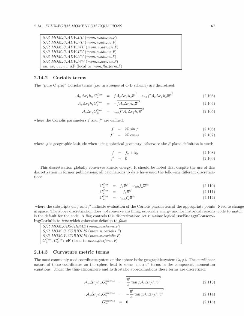
2.14. FLUX-FORM MOMENTUM EQUATIONS 67
S/R MOM U ADV UU (mom u adv uu.F)S/R MOM U ADV VU (mom u adv vu.F)S/R MOM U ADV WU (mom u adv wu.F)S/R MOM U ADV UV (mom u adv uv.F)S/R MOM U ADV VV (mom u adv vv.F)S/R MOM U ADV WV (mom u adv wv.F)uu, uv, vu, vv: aF (local to mom fluxform.F)
2.14.2 Coriolis terms
The “pure C grid” Coriolis terms (i.e. in absence of C-D scheme) are discretized:
Aw∆rfhwGCoru = fAc∆rfhcv
ji− ǫnhf ′Ac∆rfhcw
ki
(2.103)
As∆rfhsGCorv = −fAc∆rfhcu
ij
(2.104)
Ac∆rcGCorw = ǫnhf ′Ac∆rfhcu
ik
(2.105)
where the Coriolis parameters f and f ′ are defined:
f = 2Ω sinϕ (2.106)
f ′ = 2Ω cosϕ (2.107)
where ϕ is geographic latitude when using spherical geometry, otherwise the β-plane definition is used:
f = fo + βy (2.108)
f ′ = 0 (2.109)
This discretization globally conserves kinetic energy. It should be noted that despite the use of thisdiscretization in former publications, all calculations to date have used the following different discretiza-tion:
GCoru = fuv
ji − ǫnhf′uw
ik (2.110)
GCorv = −fvu
ij (2.111)
GCorw = ǫnhf
′wu
ik (2.112)
where the subscripts on f and f ′ indicate evaluation of the Coriolis parameters at the appropriate points Need to change thecode to match thisin space. The above discretization does not conserve anything, especially energy and for historical reasons
is the default for the code. A flag controls this discretization: set run-time logical useEnergyConserv-ingCoriolis to true which otherwise defaults to false.
S/R MOM CDSCHEME (mom cdscheme.F)S/R MOM U CORIOLIS (mom u coriolis.F)S/R MOM V CORIOLIS (mom v coriolis.F)GCor
u , GCorv : cF (local to mom fluxform.F)
2.14.3 Curvature metric terms
The most commonly used coordinate system on the sphere is the geographic system (λ, ϕ). The curvilinearnature of these coordinates on the sphere lead to some “metric” terms in the component momentumequations. Under the thin-atmosphere and hydrostatic approximations these terms are discretized:
Aw∆rfhwGmetricu =
ui
atanϕAc∆rfhcv
j
i
(2.113)
As∆rfhsGmetricv = −u
i
atanϕAc∆rfhcu
i
j
(2.114)
Gmetricw = 0 (2.115)
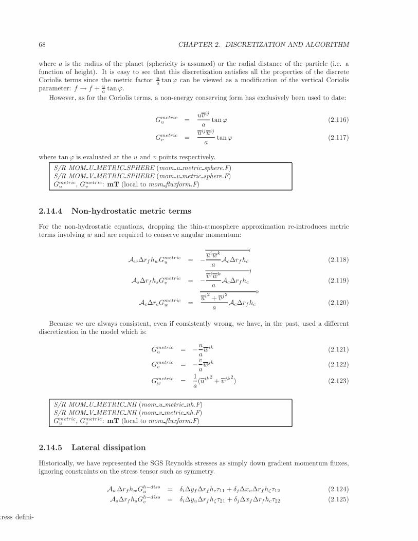
68 CHAPTER 2. DISCRETIZATION AND ALGORITHM
where a is the radius of the planet (sphericity is assumed) or the radial distance of the particle (i.e. afunction of height). It is easy to see that this discretization satisfies all the properties of the discreteCoriolis terms since the metric factor u
a tanϕ can be viewed as a modification of the vertical Coriolisparameter: f → f + u
a tanϕ.
However, as for the Coriolis terms, a non-energy conserving form has exclusively been used to date:
Gmetricu =
uvij
atanϕ (2.116)
Gmetricv =
uijuij
atanϕ (2.117)
where tanϕ is evaluated at the u and v points respectively.
S/R MOM U METRIC SPHERE (mom u metric sphere.F)S/R MOM V METRIC SPHERE (mom v metric sphere.F)Gmetric
u , Gmetricv : mT (local to mom fluxform.F)
2.14.4 Non-hydrostatic metric terms
For the non-hydrostatic equations, dropping the thin-atmosphere approximation re-introduces metricterms involving w and are required to conserve angular momentum:
Aw∆rfhwGmetricu = −u
iwk
aAc∆rfhc
i
(2.118)
As∆rfhsGmetricv = −v
jwk
aAc∆rfhc
j
(2.119)
Ac∆rcGmetricw =
ui2 + vj2
aAc∆rfhc
k
(2.120)
Because we are always consistent, even if consistently wrong, we have, in the past, used a differentdiscretization in the model which is:
Gmetricu = −u
awik (2.121)
Gmetricv = −v
awjk (2.122)
Gmetricw =
1
a(uik2
+ vjk2) (2.123)
S/R MOM U METRIC NH (mom u metric nh.F)S/R MOM V METRIC NH (mom v metric nh.F)Gmetric
u , Gmetricv : mT (local to mom fluxform.F)
2.14.5 Lateral dissipation
Historically, we have represented the SGS Reynolds stresses as simply down gradient momentum fluxes,ignoring constraints on the stress tensor such as symmetry.
Aw∆rfhwGh−dissu = δi∆yf∆rfhcτ11 + δj∆xv∆rfhζτ12 (2.124)
As∆rfhsGh−dissv = δi∆yu∆rfhζτ21 + δj∆xf∆rfhcτ22 (2.125)
stress defini-
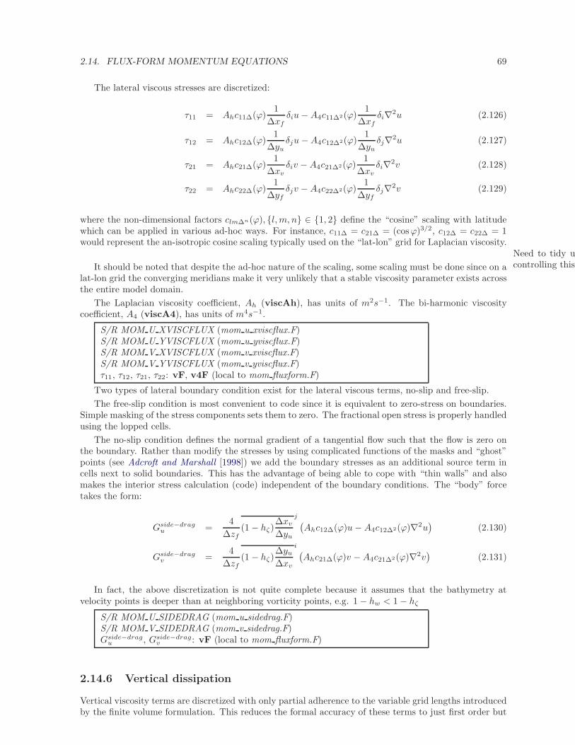
2.14. FLUX-FORM MOMENTUM EQUATIONS 69
The lateral viscous stresses are discretized:
τ11 = Ahc11∆(ϕ)1
∆xfδiu−A4c11∆2(ϕ)
1
∆xfδi∇2u (2.126)
τ12 = Ahc12∆(ϕ)1
∆yuδju−A4c12∆2(ϕ)
1
∆yuδj∇2u (2.127)
τ21 = Ahc21∆(ϕ)1
∆xvδiv −A4c21∆2(ϕ)
1
∆xvδi∇2v (2.128)
τ22 = Ahc22∆(ϕ)1
∆yfδjv −A4c22∆2(ϕ)
1
∆yfδj∇2v (2.129)
where the non-dimensional factors clm∆n(ϕ), l,m, n ∈ 1, 2 define the “cosine” scaling with latitudewhich can be applied in various ad-hoc ways. For instance, c11∆ = c21∆ = (cosϕ)3/2, c12∆ = c22∆ = 1would represent the an-isotropic cosine scaling typically used on the “lat-lon” grid for Laplacian viscosity.
Need to tidy upcontrolling thisIt should be noted that despite the ad-hoc nature of the scaling, some scaling must be done since on a
lat-lon grid the converging meridians make it very unlikely that a stable viscosity parameter exists acrossthe entire model domain.
The Laplacian viscosity coefficient, Ah (viscAh), has units of m2s−1. The bi-harmonic viscositycoefficient, A4 (viscA4), has units of m4s−1.
S/R MOM U XVISCFLUX (mom u xviscflux.F)S/R MOM U YVISCFLUX (mom u yviscflux.F)S/R MOM V XVISCFLUX (mom v xviscflux.F)S/R MOM V YVISCFLUX (mom v yviscflux.F)τ11, τ12, τ21, τ22: vF, v4F (local to mom fluxform.F)
Two types of lateral boundary condition exist for the lateral viscous terms, no-slip and free-slip.
The free-slip condition is most convenient to code since it is equivalent to zero-stress on boundaries.Simple masking of the stress components sets them to zero. The fractional open stress is properly handledusing the lopped cells.
The no-slip condition defines the normal gradient of a tangential flow such that the flow is zero onthe boundary. Rather than modify the stresses by using complicated functions of the masks and “ghost”points (see Adcroft and Marshall [1998]) we add the boundary stresses as an additional source term incells next to solid boundaries. This has the advantage of being able to cope with “thin walls” and alsomakes the interior stress calculation (code) independent of the boundary conditions. The “body” forcetakes the form:
Gside−dragu =
4
∆zf(1 − hζ)
∆xv
∆yu
j (Ahc12∆(ϕ)u− A4c12∆2(ϕ)∇2u
)(2.130)
Gside−dragv =
4
∆zf(1 − hζ)
∆yu
∆xv
i (Ahc21∆(ϕ)v −A4c21∆2(ϕ)∇2v
)(2.131)
In fact, the above discretization is not quite complete because it assumes that the bathymetry atvelocity points is deeper than at neighboring vorticity points, e.g. 1 − hw < 1 − hζ
S/R MOM U SIDEDRAG (mom u sidedrag.F)S/R MOM V SIDEDRAG (mom v sidedrag.F)Gside−drag
u , Gside−dragv : vF (local to mom fluxform.F)
2.14.6 Vertical dissipation
Vertical viscosity terms are discretized with only partial adherence to the variable grid lengths introducedby the finite volume formulation. This reduces the formal accuracy of these terms to just first order but
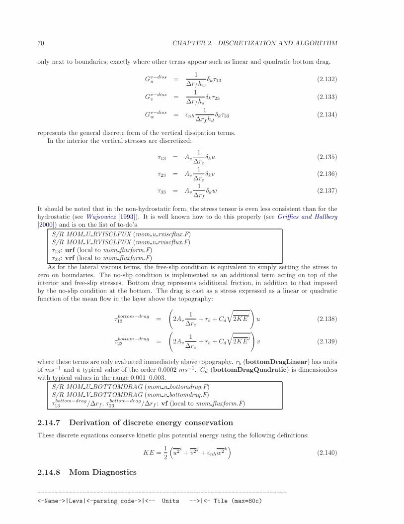
70 CHAPTER 2. DISCRETIZATION AND ALGORITHM
only next to boundaries; exactly where other terms appear such as linear and quadratic bottom drag.
Gv−dissu =
1
∆rfhwδkτ13 (2.132)
Gv−dissv =
1
∆rfhsδkτ23 (2.133)
Gv−dissw = ǫnh
1
∆rfhdδkτ33 (2.134)
represents the general discrete form of the vertical dissipation terms.In the interior the vertical stresses are discretized:
τ13 = Av1
∆rcδku (2.135)
τ23 = Av1
∆rcδkv (2.136)
τ33 = Av1
∆rfδkw (2.137)
It should be noted that in the non-hydrostatic form, the stress tensor is even less consistent than for thehydrostatic (see Wajsowicz [1993]). It is well known how to do this properly (see Griffies and Hallberg[2000]) and is on the list of to-do’s.
S/R MOM U RVISCLFUX (mom u rviscflux.F)S/R MOM V RVISCLFUX (mom v rviscflux.F)τ13: urf (local to mom fluxform.F)τ23: vrf (local to mom fluxform.F)
As for the lateral viscous terms, the free-slip condition is equivalent to simply setting the stress tozero on boundaries. The no-slip condition is implemented as an additional term acting on top of theinterior and free-slip stresses. Bottom drag represents additional friction, in addition to that imposedby the no-slip condition at the bottom. The drag is cast as a stress expressed as a linear or quadraticfunction of the mean flow in the layer above the topography:
τbottom−drag13 =
(2Av
1
∆rc+ rb + Cd
√2KE
i
)u (2.138)
τbottom−drag23 =
(2Av
1
∆rc+ rb + Cd
√2KE
j
)v (2.139)
where these terms are only evaluated immediately above topography. rb (bottomDragLinear) has unitsof ms−1 and a typical value of the order 0.0002 ms−1. Cd (bottomDragQuadratic) is dimensionlesswith typical values in the range 0.001–0.003.
S/R MOM U BOTTOMDRAG (mom u bottomdrag.F)S/R MOM V BOTTOMDRAG (mom v bottomdrag.F)
τbottom−drag13 /∆rf , τbottom−drag
23 /∆rf : vf (local to mom fluxform.F)
2.14.7 Derivation of discrete energy conservation
These discrete equations conserve kinetic plus potential energy using the following definitions:
KE =1
2
(u2
i+ v2
j+ ǫnhw2
k)
(2.140)
2.14.8 Mom Diagnostics
------------------------------------------------------------------------
<-Name->|Levs|<-parsing code->|<-- Units -->|<- Tile (max=80c)
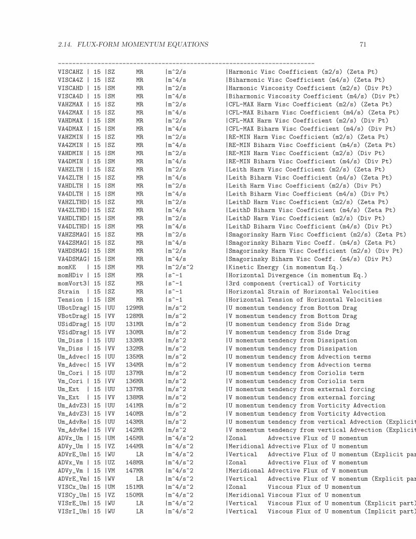
2.14. FLUX-FORM MOMENTUM EQUATIONS 71
------------------------------------------------------------------------
VISCAHZ | 15 |SZ MR |m^2/s |Harmonic Visc Coefficient (m2/s) (Zeta Pt)
VISCA4Z | 15 |SZ MR |m^4/s |Biharmonic Visc Coefficient (m4/s) (Zeta Pt)
VISCAHD | 15 |SM MR |m^2/s |Harmonic Viscosity Coefficient (m2/s) (Div Pt)
VISCA4D | 15 |SM MR |m^4/s |Biharmonic Viscosity Coefficient (m4/s) (Div Pt)
VAHZMAX | 15 |SZ MR |m^2/s |CFL-MAX Harm Visc Coefficient (m2/s) (Zeta Pt)
VA4ZMAX | 15 |SZ MR |m^4/s |CFL-MAX Biharm Visc Coefficient (m4/s) (Zeta Pt)
VAHDMAX | 15 |SM MR |m^2/s |CFL-MAX Harm Visc Coefficient (m2/s) (Div Pt)
VA4DMAX | 15 |SM MR |m^4/s |CFL-MAX Biharm Visc Coefficient (m4/s) (Div Pt)
VAHZMIN | 15 |SZ MR |m^2/s |RE-MIN Harm Visc Coefficient (m2/s) (Zeta Pt)
VA4ZMIN | 15 |SZ MR |m^4/s |RE-MIN Biharm Visc Coefficient (m4/s) (Zeta Pt)
VAHDMIN | 15 |SM MR |m^2/s |RE-MIN Harm Visc Coefficient (m2/s) (Div Pt)
VA4DMIN | 15 |SM MR |m^4/s |RE-MIN Biharm Visc Coefficient (m4/s) (Div Pt)
VAHZLTH | 15 |SZ MR |m^2/s |Leith Harm Visc Coefficient (m2/s) (Zeta Pt)
VA4ZLTH | 15 |SZ MR |m^4/s |Leith Biharm Visc Coefficient (m4/s) (Zeta Pt)
VAHDLTH | 15 |SM MR |m^2/s |Leith Harm Visc Coefficient (m2/s) (Div Pt)
VA4DLTH | 15 |SM MR |m^4/s |Leith Biharm Visc Coefficient (m4/s) (Div Pt)
VAHZLTHD| 15 |SZ MR |m^2/s |LeithD Harm Visc Coefficient (m2/s) (Zeta Pt)
VA4ZLTHD| 15 |SZ MR |m^4/s |LeithD Biharm Visc Coefficient (m4/s) (Zeta Pt)
VAHDLTHD| 15 |SM MR |m^2/s |LeithD Harm Visc Coefficient (m2/s) (Div Pt)
VA4DLTHD| 15 |SM MR |m^4/s |LeithD Biharm Visc Coefficient (m4/s) (Div Pt)
VAHZSMAG| 15 |SZ MR |m^2/s |Smagorinsky Harm Visc Coefficient (m2/s) (Zeta Pt)
VA4ZSMAG| 15 |SZ MR |m^4/s |Smagorinsky Biharm Visc Coeff. (m4/s) (Zeta Pt)
VAHDSMAG| 15 |SM MR |m^2/s |Smagorinsky Harm Visc Coefficient (m2/s) (Div Pt)
VA4DSMAG| 15 |SM MR |m^4/s |Smagorinsky Biharm Visc Coeff. (m4/s) (Div Pt)
momKE | 15 |SM MR |m^2/s^2 |Kinetic Energy (in momentum Eq.)
momHDiv | 15 |SM MR |s^-1 |Horizontal Divergence (in momentum Eq.)
momVort3| 15 |SZ MR |s^-1 |3rd component (vertical) of Vorticity
Strain | 15 |SZ MR |s^-1 |Horizontal Strain of Horizontal Velocities
Tension | 15 |SM MR |s^-1 |Horizontal Tension of Horizontal Velocities
UBotDrag| 15 |UU 129MR |m/s^2 |U momentum tendency from Bottom Drag
VBotDrag| 15 |VV 128MR |m/s^2 |V momentum tendency from Bottom Drag
USidDrag| 15 |UU 131MR |m/s^2 |U momentum tendency from Side Drag
VSidDrag| 15 |VV 130MR |m/s^2 |V momentum tendency from Side Drag
Um_Diss | 15 |UU 133MR |m/s^2 |U momentum tendency from Dissipation
Vm_Diss | 15 |VV 132MR |m/s^2 |V momentum tendency from Dissipation
Um_Advec| 15 |UU 135MR |m/s^2 |U momentum tendency from Advection terms
Vm_Advec| 15 |VV 134MR |m/s^2 |V momentum tendency from Advection terms
Um_Cori | 15 |UU 137MR |m/s^2 |U momentum tendency from Coriolis term
Vm_Cori | 15 |VV 136MR |m/s^2 |V momentum tendency from Coriolis term
Um_Ext | 15 |UU 137MR |m/s^2 |U momentum tendency from external forcing
Vm_Ext | 15 |VV 138MR |m/s^2 |V momentum tendency from external forcing
Um_AdvZ3| 15 |UU 141MR |m/s^2 |U momentum tendency from Vorticity Advection
Vm_AdvZ3| 15 |VV 140MR |m/s^2 |V momentum tendency from Vorticity Advection
Um_AdvRe| 15 |UU 143MR |m/s^2 |U momentum tendency from vertical Advection (Explicit
Vm_AdvRe| 15 |VV 142MR |m/s^2 |V momentum tendency from vertical Advection (Explicit
ADVx_Um | 15 |UM 145MR |m^4/s^2 |Zonal Advective Flux of U momentum
ADVy_Um | 15 |VZ 144MR |m^4/s^2 |Meridional Advective Flux of U momentum
ADVrE_Um| 15 |WU LR |m^4/s^2 |Vertical Advective Flux of U momentum (Explicit part)
ADVx_Vm | 15 |UZ 148MR |m^4/s^2 |Zonal Advective Flux of V momentum
ADVy_Vm | 15 |VM 147MR |m^4/s^2 |Meridional Advective Flux of V momentum
ADVrE_Vm| 15 |WV LR |m^4/s^2 |Vertical Advective Flux of V momentum (Explicit part)
VISCx_Um| 15 |UM 151MR |m^4/s^2 |Zonal Viscous Flux of U momentum
VISCy_Um| 15 |VZ 150MR |m^4/s^2 |Meridional Viscous Flux of U momentum
VISrE_Um| 15 |WU LR |m^4/s^2 |Vertical Viscous Flux of U momentum (Explicit part)
VISrI_Um| 15 |WU LR |m^4/s^2 |Vertical Viscous Flux of U momentum (Implicit part)
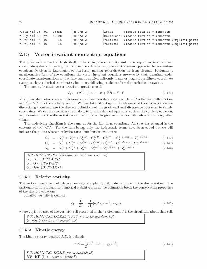
72 CHAPTER 2. DISCRETIZATION AND ALGORITHM
VISCx_Vm| 15 |UZ 155MR |m^4/s^2 |Zonal Viscous Flux of V momentum
VISCy_Vm| 15 |VM 154MR |m^4/s^2 |Meridional Viscous Flux of V momentum
VISrE_Vm| 15 |WV LR |m^4/s^2 |Vertical Viscous Flux of V momentum (Explicit part)
VISrI_Vm| 15 |WV LR |m^4/s^2 |Vertical Viscous Flux of V momentum (Implicit part)
2.15 Vector invariant momentum equations
The finite volume method lends itself to describing the continuity and tracer equations in curvilinearcoordinate systems. However, in curvilinear coordinates many new metric terms appear in the momentumequations (written in Lagrangian or flux-form) making generalization far from elegant. Fortunately,an alternative form of the equations, the vector invariant equations are exactly that; invariant undercoordinate transformations so that they can be applied uniformly in any orthogonal curvilinear coordinatesystem such as spherical coordinates, boundary following or the conformal spherical cube system.
The non-hydrostatic vector invariant equations read:
∂t~v + (2~Ω + ~ζ) ∧ ~v − br + ~∇B = ~∇ · ~τ (2.141)
which describe motions in any orthogonal curvilinear coordinate system. Here, B is the Bernoulli functionand ~ζ = ∇ ∧ ~v is the vorticity vector. We can take advantage of the elegance of these equations whendiscretizing them and use the discrete definitions of the grad, curl and divergence operators to satisfyconstraints. We can also consider the analogy to forming derived equations, such as the vorticity equation,and examine how the discretization can be adjusted to give suitable vorticity advection among otherthings.
The underlying algorithm is the same as for the flux form equations. All that has changed is thecontents of the “G’s”. For the time-being, only the hydrostatic terms have been coded but we willindicate the points where non-hydrostatic contributions will enter:
Gu = Gfvu +Gζ3v
u +Gζ2wu +G∂xB
u +G∂zτx
u +Gh−dissipu +Gv−dissip
u (2.142)
Gv = Gfuv +Gζ3u
v +Gζ1wv +G∂yB
v +G∂zτy
v +Gh−dissipv +Gv−dissip
v (2.143)
Gw = Gfuw +Gζ1v
w +Gζ2uw +G∂zB
w +Gh−dissipw +Gv−dissip
w (2.144)
S/R MOM VECINV (pkg/mom vecinv/mom vecinv.F)Gu: Gu (DYNVARS.h)Gv: Gv (DYNVARS.h)Gw: Gw (DYNVARS.h)
2.15.1 Relative vorticity
The vertical component of relative vorticity is explicitly calculated and use in the discretization. Theparticular form is crucial for numerical stability; alternative definitions break the conservation propertiesof the discrete equations.
Relative vorticity is defined:
ζ3 =Γ
Aζ=
1
Aζ(δi∆ycv − δj∆xcu) (2.145)
where Aζ is the area of the vorticity cell presented in the vertical and Γ is the circulation about that cell.
S/R MOM VI CALC RELVORT3 (mom vi calc relvort3.F)ζ3: vort3 (local to mom vecinv.F)
2.15.2 Kinetic energy
The kinetic energy, denoted KE, is defined:
KE =1
2(u2
i+ v2
j+ ǫnhw2
k) (2.146)
S/R MOM VI CALC KE (mom vi calc ke.F)KE: KE (local to mom vecinv.F)
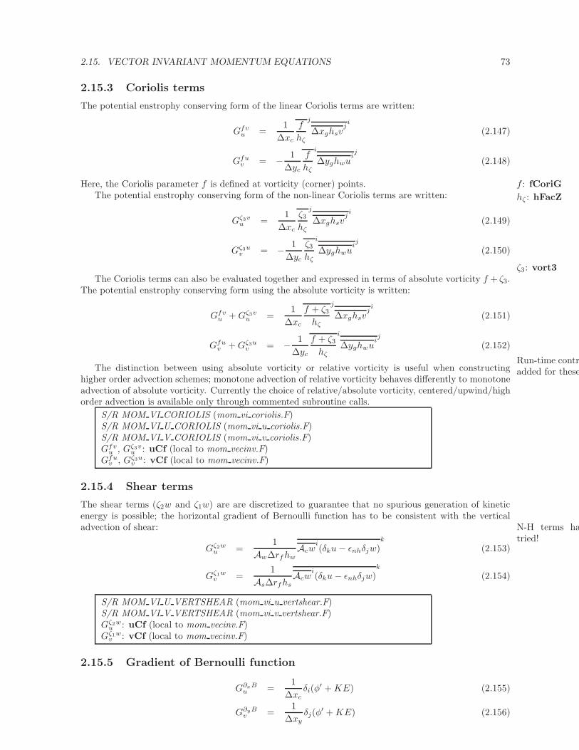
2.15. VECTOR INVARIANT MOMENTUM EQUATIONS 73
2.15.3 Coriolis terms
The potential enstrophy conserving form of the linear Coriolis terms are written:
Gfvu =
1
∆xc
f
hζ
j
∆xghsvji
(2.147)
Gfuv = − 1
∆yc
f
hζ
i
∆yghwuij
(2.148)
Here, the Coriolis parameter f is defined at vorticity (corner) points. f : fCoriG
hζ : hFacZThe potential enstrophy conserving form of the non-linear Coriolis terms are written:
Gζ3vu =
1
∆xc
ζ3hζ
j
∆xghsvji
(2.149)
Gζ3uv = − 1
∆yc
ζ3hζ
i
∆yghwuij
(2.150)
ζ3: vort3The Coriolis terms can also be evaluated together and expressed in terms of absolute vorticity f + ζ3.
The potential enstrophy conserving form using the absolute vorticity is written:
Gfvu +Gζ3v
u =1
∆xc
f + ζ3hζ
j
∆xghsvji
(2.151)
Gfuv +Gζ3u
v = − 1
∆yc
f + ζ3hζ
i
∆yghwuij
(2.152)
Run-time controladded for theseThe distinction between using absolute vorticity or relative vorticity is useful when constructing
higher order advection schemes; monotone advection of relative vorticity behaves differently to monotoneadvection of absolute vorticity. Currently the choice of relative/absolute vorticity, centered/upwind/highorder advection is available only through commented subroutine calls.
S/R MOM VI CORIOLIS (mom vi coriolis.F)S/R MOM VI U CORIOLIS (mom vi u coriolis.F)S/R MOM VI V CORIOLIS (mom vi v coriolis.F)Gfv
u , Gζ3vu : uCf (local to mom vecinv.F)
Gfuv , Gζ3u
v : vCf (local to mom vecinv.F)
2.15.4 Shear terms
The shear terms (ζ2w and ζ1w) are are discretized to guarantee that no spurious generation of kineticenergy is possible; the horizontal gradient of Bernoulli function has to be consistent with the verticaladvection of shear: N-H terms hav
tried!Gζ2w
u =1
Aw∆rfhwAcw
i(δku− ǫnhδjw)
k
(2.153)
Gζ1wv =
1
As∆rfhsAcw
i(δku− ǫnhδjw)
k
(2.154)
S/R MOM VI U VERTSHEAR (mom vi u vertshear.F)S/R MOM VI V VERTSHEAR (mom vi v vertshear.F)Gζ2w
u : uCf (local to mom vecinv.F)Gζ1w
v : vCf (local to mom vecinv.F)
2.15.5 Gradient of Bernoulli function
G∂xBu =
1
∆xcδi(φ
′ +KE) (2.155)
G∂yBv =
1
∆xyδj(φ
′ +KE) (2.156)
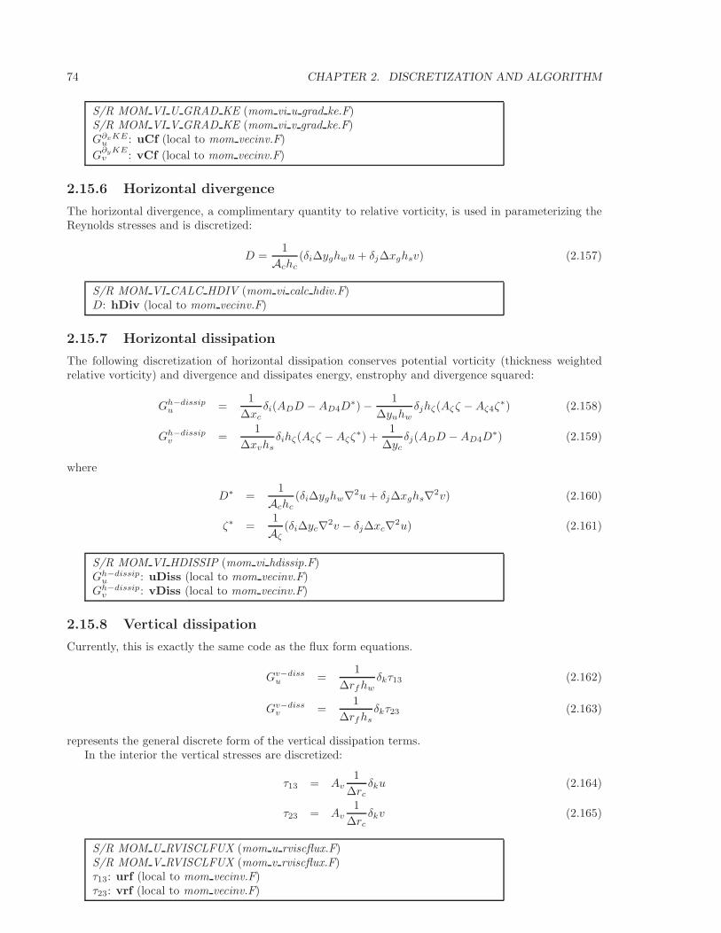
74 CHAPTER 2. DISCRETIZATION AND ALGORITHM
S/R MOM VI U GRAD KE (mom vi u grad ke.F)S/R MOM VI V GRAD KE (mom vi v grad ke.F)G∂xKE
u : uCf (local to mom vecinv.F)
G∂yKEv : vCf (local to mom vecinv.F)
2.15.6 Horizontal divergence
The horizontal divergence, a complimentary quantity to relative vorticity, is used in parameterizing theReynolds stresses and is discretized:
D =1
Achc(δi∆yghwu+ δj∆xghsv) (2.157)
S/R MOM VI CALC HDIV (mom vi calc hdiv.F)D: hDiv (local to mom vecinv.F)
2.15.7 Horizontal dissipation
The following discretization of horizontal dissipation conserves potential vorticity (thickness weightedrelative vorticity) and divergence and dissipates energy, enstrophy and divergence squared:
Gh−dissipu =
1
∆xcδi(ADD −AD4D
∗) − 1
∆yuhwδjhζ(Aζζ −Aζ4ζ
∗) (2.158)
Gh−dissipv =
1
∆xvhsδihζ(Aζζ −Aζζ
∗) +1
∆ycδj(ADD −AD4D
∗) (2.159)
where
D∗ =1
Achc(δi∆yghw∇2u+ δj∆xghs∇2v) (2.160)
ζ∗ =1
Aζ(δi∆yc∇2v − δj∆xc∇2u) (2.161)
S/R MOM VI HDISSIP (mom vi hdissip.F)Gh−dissip
u : uDiss (local to mom vecinv.F)Gh−dissip
v : vDiss (local to mom vecinv.F)
2.15.8 Vertical dissipation
Currently, this is exactly the same code as the flux form equations.
Gv−dissu =
1
∆rfhwδkτ13 (2.162)
Gv−dissv =
1
∆rfhsδkτ23 (2.163)
represents the general discrete form of the vertical dissipation terms.In the interior the vertical stresses are discretized:
τ13 = Av1
∆rcδku (2.164)
τ23 = Av1
∆rcδkv (2.165)
S/R MOM U RVISCLFUX (mom u rviscflux.F)S/R MOM V RVISCLFUX (mom v rviscflux.F)τ13: urf (local to mom vecinv.F)τ23: vrf (local to mom vecinv.F)
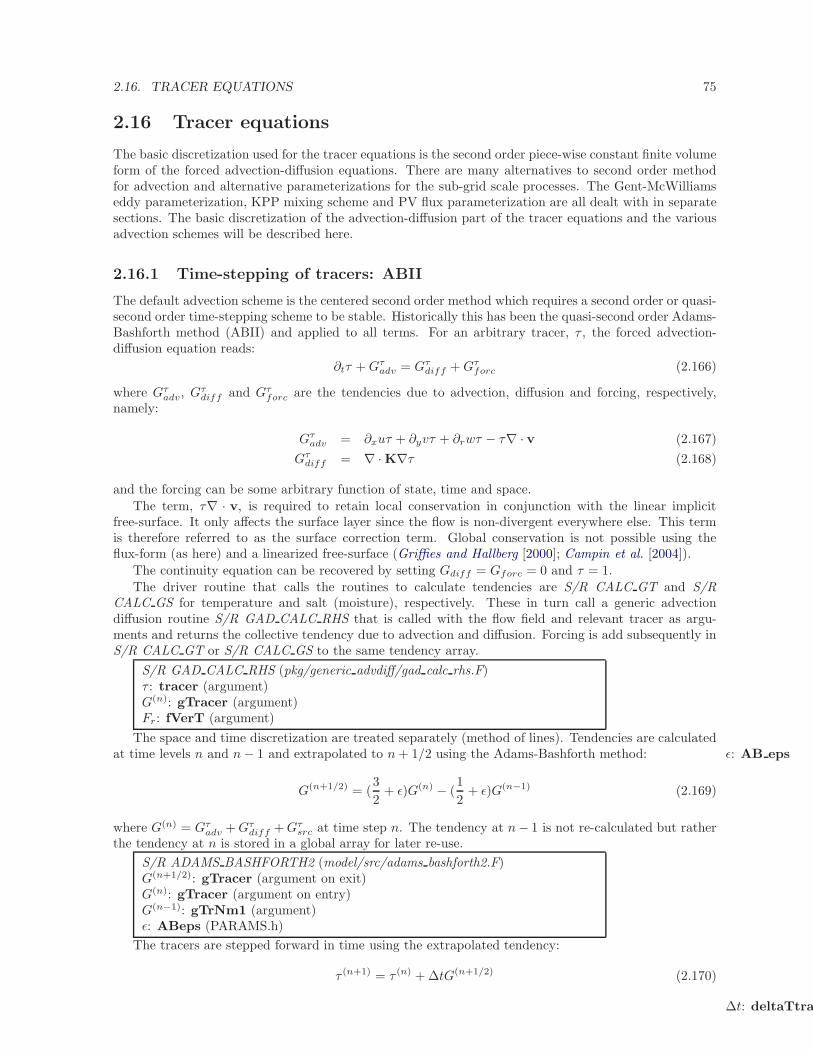
2.16. TRACER EQUATIONS 75
2.16 Tracer equations
The basic discretization used for the tracer equations is the second order piece-wise constant finite volumeform of the forced advection-diffusion equations. There are many alternatives to second order methodfor advection and alternative parameterizations for the sub-grid scale processes. The Gent-McWilliamseddy parameterization, KPP mixing scheme and PV flux parameterization are all dealt with in separatesections. The basic discretization of the advection-diffusion part of the tracer equations and the variousadvection schemes will be described here.
2.16.1 Time-stepping of tracers: ABII
The default advection scheme is the centered second order method which requires a second order or quasi-second order time-stepping scheme to be stable. Historically this has been the quasi-second order Adams-Bashforth method (ABII) and applied to all terms. For an arbitrary tracer, τ , the forced advection-diffusion equation reads:
∂tτ +Gτadv = Gτ
diff +Gτforc (2.166)
where Gτadv, G
τdiff and Gτ
forc are the tendencies due to advection, diffusion and forcing, respectively,namely:
Gτadv = ∂xuτ + ∂yvτ + ∂rwτ − τ∇ · v (2.167)
Gτdiff = ∇ · K∇τ (2.168)
and the forcing can be some arbitrary function of state, time and space.
The term, τ∇ · v, is required to retain local conservation in conjunction with the linear implicitfree-surface. It only affects the surface layer since the flow is non-divergent everywhere else. This termis therefore referred to as the surface correction term. Global conservation is not possible using theflux-form (as here) and a linearized free-surface (Griffies and Hallberg [2000]; Campin et al. [2004]).
The continuity equation can be recovered by setting Gdiff = Gforc = 0 and τ = 1.
The driver routine that calls the routines to calculate tendencies are S/R CALC GT and S/RCALC GS for temperature and salt (moisture), respectively. These in turn call a generic advectiondiffusion routine S/R GAD CALC RHS that is called with the flow field and relevant tracer as argu-ments and returns the collective tendency due to advection and diffusion. Forcing is add subsequently inS/R CALC GT or S/R CALC GS to the same tendency array.
S/R GAD CALC RHS (pkg/generic advdiff/gad calc rhs.F)τ : tracer (argument)G(n): gTracer (argument)Fr: fVerT (argument)
The space and time discretization are treated separately (method of lines). Tendencies are calculatedat time levels n and n− 1 and extrapolated to n+ 1/2 using the Adams-Bashforth method: ǫ: AB eps
G(n+1/2) = (3
2+ ǫ)G(n) − (
1
2+ ǫ)G(n−1) (2.169)
where G(n) = Gτadv +Gτ
diff +Gτsrc at time step n. The tendency at n− 1 is not re-calculated but rather
the tendency at n is stored in a global array for later re-use.
S/R ADAMS BASHFORTH2 (model/src/adams bashforth2.F)G(n+1/2): gTracer (argument on exit)G(n): gTracer (argument on entry)G(n−1): gTrNm1 (argument)ǫ: ABeps (PARAMS.h)
The tracers are stepped forward in time using the extrapolated tendency:
τ (n+1) = τ (n) + ∆tG(n+1/2) (2.170)
∆t: deltaTtracer
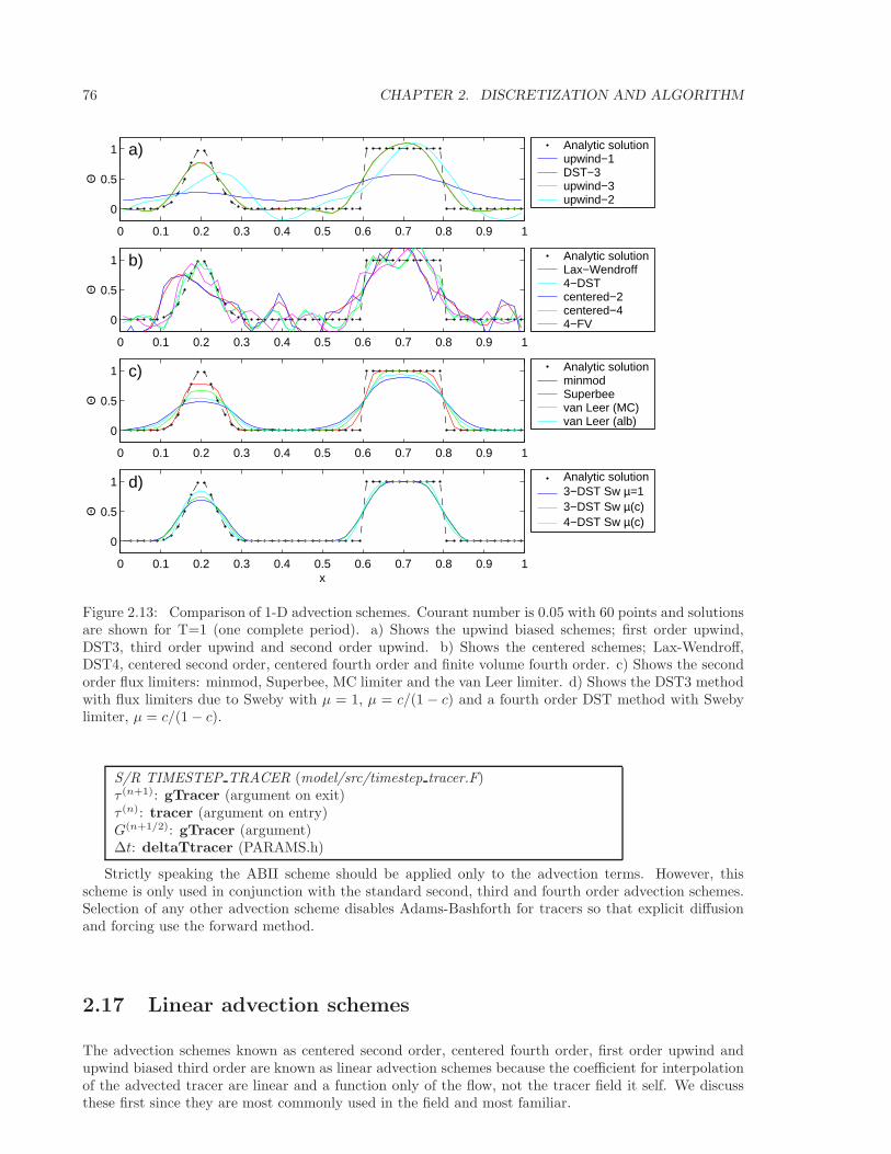
76 CHAPTER 2. DISCRETIZATION AND ALGORITHM
0 0.1 0.2 0.3 0.4 0.5 0.6 0.7 0.8 0.9 1
0
0.5
1
Θ
a) Analytic solutionupwind−1 DST−3 upwind−3 upwind−2
0 0.1 0.2 0.3 0.4 0.5 0.6 0.7 0.8 0.9 1
0
0.5
1
Θ
b) Analytic solutionLax−Wendroff 4−DST centered−2 centered−4 4−FV
0 0.1 0.2 0.3 0.4 0.5 0.6 0.7 0.8 0.9 1
0
0.5
1
Θ
c) Analytic solutionminmod Superbee van Leer (MC) van Leer (alb)
0 0.1 0.2 0.3 0.4 0.5 0.6 0.7 0.8 0.9 1
0
0.5
1
x
Θ
d) Analytic solution3−DST Sw µ=1 3−DST Sw µ(c) 4−DST Sw µ(c)
Figure 2.13: Comparison of 1-D advection schemes. Courant number is 0.05 with 60 points and solutionsare shown for T=1 (one complete period). a) Shows the upwind biased schemes; first order upwind,DST3, third order upwind and second order upwind. b) Shows the centered schemes; Lax-Wendroff,DST4, centered second order, centered fourth order and finite volume fourth order. c) Shows the secondorder flux limiters: minmod, Superbee, MC limiter and the van Leer limiter. d) Shows the DST3 methodwith flux limiters due to Sweby with µ = 1, µ = c/(1 − c) and a fourth order DST method with Swebylimiter, µ = c/(1 − c).
S/R TIMESTEP TRACER (model/src/timestep tracer.F)τ (n+1): gTracer (argument on exit)τ (n): tracer (argument on entry)G(n+1/2): gTracer (argument)∆t: deltaTtracer (PARAMS.h)
Strictly speaking the ABII scheme should be applied only to the advection terms. However, thisscheme is only used in conjunction with the standard second, third and fourth order advection schemes.Selection of any other advection scheme disables Adams-Bashforth for tracers so that explicit diffusionand forcing use the forward method.
2.17 Linear advection schemes
The advection schemes known as centered second order, centered fourth order, first order upwind andupwind biased third order are known as linear advection schemes because the coefficient for interpolationof the advected tracer are linear and a function only of the flow, not the tracer field it self. We discussthese first since they are most commonly used in the field and most familiar.
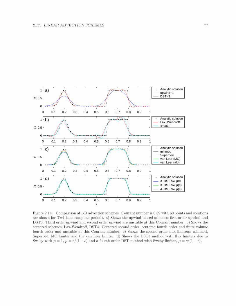
2.17. LINEAR ADVECTION SCHEMES 77
0 0.1 0.2 0.3 0.4 0.5 0.6 0.7 0.8 0.9 1
0
0.5
1
Θ
a) Analytic solutionupwind−1 DST−3
0 0.1 0.2 0.3 0.4 0.5 0.6 0.7 0.8 0.9 1
0
0.5
1
Θ
b) Analytic solutionLax−Wendroff 4−DST
0 0.1 0.2 0.3 0.4 0.5 0.6 0.7 0.8 0.9 1
0
0.5
1
Θ
c) Analytic solutionminmod Superbee van Leer (MC) van Leer (alb)
0 0.1 0.2 0.3 0.4 0.5 0.6 0.7 0.8 0.9 1
0
0.5
1
x
Θ
d) Analytic solution3−DST Sw µ=1 3−DST Sw µ(c) 4−DST Sw µ(c)
Figure 2.14: Comparison of 1-D advection schemes. Courant number is 0.89 with 60 points and solutionsare shown for T=1 (one complete period). a) Shows the upwind biased schemes; first order upwind andDST3. Third order upwind and second order upwind are unstable at this Courant number. b) Shows thecentered schemes; Lax-Wendroff, DST4. Centered second order, centered fourth order and finite volumefourth order and unstable at this Courant number. c) Shows the second order flux limiters: minmod,Superbee, MC limiter and the van Leer limiter. d) Shows the DST3 method with flux limiters due toSweby with µ = 1, µ = c/(1 − c) and a fourth order DST method with Sweby limiter, µ = c/(1 − c).
78 CHAPTER 2. DISCRETIZATION AND ALGORITHM
2.17.1 Centered second order advection-diffusion
The basic discretization, centered second order, is the default. It is designed to be consistent with thecontinuity equation to facilitate conservation properties analogous to the continuum. However, centeredsecond order advection is notoriously noisy and must be used in conjunction with some finite amount ofdiffusion to produce a sensible solution.
The advection operator is discretized:
Ac∆rfhcGτadv = δiFx + δjFy + δkFr (2.171)
where the area integrated fluxes are given by:
Fx = Uτ i (2.172)
Fy = V τ j (2.173)
Fr = Wτk (2.174)
The quantities U , V and W are volume fluxes defined:
U = ∆yg∆rfhwu (2.175)
V = ∆xg∆rfhsv (2.176)
W = Acw (2.177)
For non-divergent flow, this discretization can be shown to conserve the tracer both locally and globallyand to globally conserve tracer variance, τ2. The proof is given in Adcroft [1995]; Adcroft et al. [1997].
S/R GAD C2 ADV X (gad c2 adv x.F)Fx: uT (argument)U : uTrans (argument)τ : tracer (argument)S/R GAD C2 ADV Y (gad c2 adv y.F)Fy: vT (argument)V : vTrans (argument)τ : tracer (argument)S/R GAD C2 ADV R (gad c2 adv r.F)Fr: wT (argument)W : rTrans (argument)τ : tracer (argument)
2.17.2 Third order upwind bias advection
Upwind biased third order advection offers a relatively good compromise between accuracy and smooth-ness. It is not a “positive” scheme meaning false extrema are permitted but the amplitude of such aresignificantly reduced over the centered second order method.
The third order upwind fluxes are discretized:
Fx = Uτ − 1
6δiiτ
i
+1
2|U |δi
1
6δiiτ (2.178)
Fy = V τ − 1
6δiiτ
j
+1
2|V |δj
1
6δjjτ (2.179)
Fr = Wτ − 1
6δiiτ
k
+1
2|W |δk
1
6δkkτ (2.180)
At boundaries, δnτ is set to zero allowing δnn to be evaluated. We are currently examine the accuracyof this boundary condition and the effect on the solution.
2.17. LINEAR ADVECTION SCHEMES 79
S/R GAD U3 ADV X (gad u3 adv x.F)Fx: uT (argument)U : uTrans (argument)τ : tracer (argument)S/R GAD U3 ADV Y (gad u3 adv y.F)Fy: vT (argument)V : vTrans (argument)τ : tracer (argument)S/R GAD U3 ADV R (gad u3 adv r.F)Fr: wT (argument)W : rTrans (argument)τ : tracer (argument)
2.17.3 Centered fourth order advection
Centered fourth order advection is formally the most accurate scheme we have implemented and can beused to great effect in high resolution simulation where dynamical scales are well resolved. However, thescheme is noisy like the centered second order method and so must be used with some finite amount ofdiffusion. Bi-harmonic is recommended since it is more scale selective and less likely to diffuse away thewell resolved gradient the fourth order scheme worked so hard to create.
The centered fourth order fluxes are discretized:
Fx = Uτ − 1
6δiiτ
i
(2.181)
Fy = V τ − 1
6δiiτ
j
(2.182)
Fr = Wτ − 1
6δiiτ
k
(2.183)
As for the third order scheme, the best discretization near boundaries is under investigation butcurrently δiτ = 0 on a boundary.
S/R GAD C4 ADV X (gad c4 adv x.F)Fx: uT (argument)U : uTrans (argument)τ : tracer (argument)S/R GAD C4 ADV Y (gad c4 adv y.F)Fy: vT (argument)V : vTrans (argument)τ : tracer (argument)S/R GAD C4 ADV R (gad c4 adv r.F)Fr: wT (argument)W : rTrans (argument)τ : tracer (argument)
2.17.4 First order upwind advection
Although the upwind scheme is the underlying scheme for the robust or non-linear methods given later,we haven’t actually supplied this method for general use. It would be very diffusive and it is unlikelythat it could ever produce more useful results than the positive higher order schemes.
Upwind bias is introduced into many schemes using the abs function and is allows the first orderupwind flux to be written:
Fx = Uτ i − 1
2|U |δiτ (2.184)
Fy = V τ j − 1
2|V |δjτ (2.185)
Fr = Wτk − 1
2|W |δkτ (2.186)
80 CHAPTER 2. DISCRETIZATION AND ALGORITHM
If for some reason, the above method is required, then the second order flux limiter scheme describedlater reduces to the above scheme if the limiter is set to zero.
2.18 Non-linear advection schemes
Non-linear advection schemes invoke non-linear interpolation and are widely used in computational fluiddynamics (non-linear does not refer to the non-linearity of the advection operator). The flux limitedadvection schemes belong to the class of finite volume methods which neatly ties into the spatial dis-cretization of the model.
When employing the flux limited schemes, first order upwind or direct-space-time method the time-stepping is switched to forward in time.
2.18.1 Second order flux limiters
The second order flux limiter method can be cast in several ways but is generally expressed in termsof other flux approximations. For example, in terms of a first order upwind flux and second order Lax-Wendroff flux, the limited flux is given as:
F = F1 + ψ(r)FLW (2.187)
where ψ(r) is the limiter function,
F1 = uτ i − 1
2|u|δiτ (2.188)
is the upwind flux,
FLW = F1 +|u|2
(1 − c)δiτ (2.189)
is the Lax-Wendroff flux and c = u∆t∆x is the Courant (CFL) number.
The limiter function, ψ(r), takes the slope ratio
r =τi−1 − τi−2
τi − τi−1∀ u > 0 (2.190)
r =τi+1 − τiτi − τi−1
∀ u < 0 (2.191)
as it’s argument. There are many choices of limiter function but we only provide the Superbee limiterRoe [1985]:
ψ(r) = max[0,min[1, 2r],min[2, r]] (2.192)
S/R GAD FLUXLIMIT ADV X (gad fluxlimit adv x.F)Fx: uT (argument)U : uTrans (argument)τ : tracer (argument)S/R GAD FLUXLIMIT ADV Y (gad fluxlimit adv y.F)Fy: vT (argument)V : vTrans (argument)τ : tracer (argument)S/R GAD FLUXLIMIT ADV R (gad fluxlimit adv r.F)Fr: wT (argument)W : rTrans (argument)τ : tracer (argument)
2.18.2 Third order direct space time
The direct-space-time method deals with space and time discretization together (other methods thattreat space and time separately are known collectively as the “Method of Lines”). The Lax-Wendroff
2.18. NON-LINEAR ADVECTION SCHEMES 81
scheme falls into this category; it adds sufficient diffusion to a second order flux that the forward-in-timemethod is stable. The upwind biased third order DST scheme is:
F = u (τi−1 + d0(τi − τi−1) + d1(τi−1 − τi−2)) ∀ u > 0 (2.193)
F = u (τi − d0(τi − τi−1) − d1(τi+1 − τi)) ∀ u < 0 (2.194)
where
d1 =1
6(2 − |c|)(1 − |c|) (2.195)
d2 =1
6(1 − |c|)(1 + |c|) (2.196)
The coefficients d0 and d1 approach 1/3 and 1/6 respectively as the Courant number, c, vanishes. In thislimit, the conventional third order upwind method is recovered. For finite Courant number, the deviationsfrom the linear method are analogous to the diffusion added to centered second order advection in theLax-Wendroff scheme.
The DST3 method described above must be used in a forward-in-time manner and is stable for0 ≤ |c| ≤ 1. Although the scheme appears to be forward-in-time, it is in fact third order in time andthe accuracy increases with the Courant number! For low Courant number, DST3 produces very similarresults (indistinguishable in Fig. 2.13) to the linear third order method but for large Courant number,where the linear upwind third order method is unstable, the scheme is extremely accurate (Fig. 2.14)with only minor overshoots.
S/R GAD DST3 ADV X (gad dst3 adv x.F)Fx: uT (argument)U : uTrans (argument)τ : tracer (argument)S/R GAD DST3 ADV Y (gad dst3 adv y.F)Fy: vT (argument)V : vTrans (argument)τ : tracer (argument)S/R GAD DST3 ADV R (gad dst3 adv r.F)Fr: wT (argument)W : rTrans (argument)τ : tracer (argument)
2.18.3 Third order direct space time with flux limiting
The overshoots in the DST3 method can be controlled with a flux limiter. The limited flux is written:
F =1
2(u + |u|)
(τi−1 + ψ(r+)(τi − τi−1)
)+
1
2(u− |u|)
(τi−1 + ψ(r−)(τi − τi−1)
)(2.197)
where
r+ =τi−1 − τi−2
τi − τi−1(2.198)
r− =τi+1 − τiτi − τi−1
(2.199)
and the limiter is the Sweby limiter:
ψ(r) = max[0,min[min(1, d0 + d1r],1 − c
cr]] (2.200)
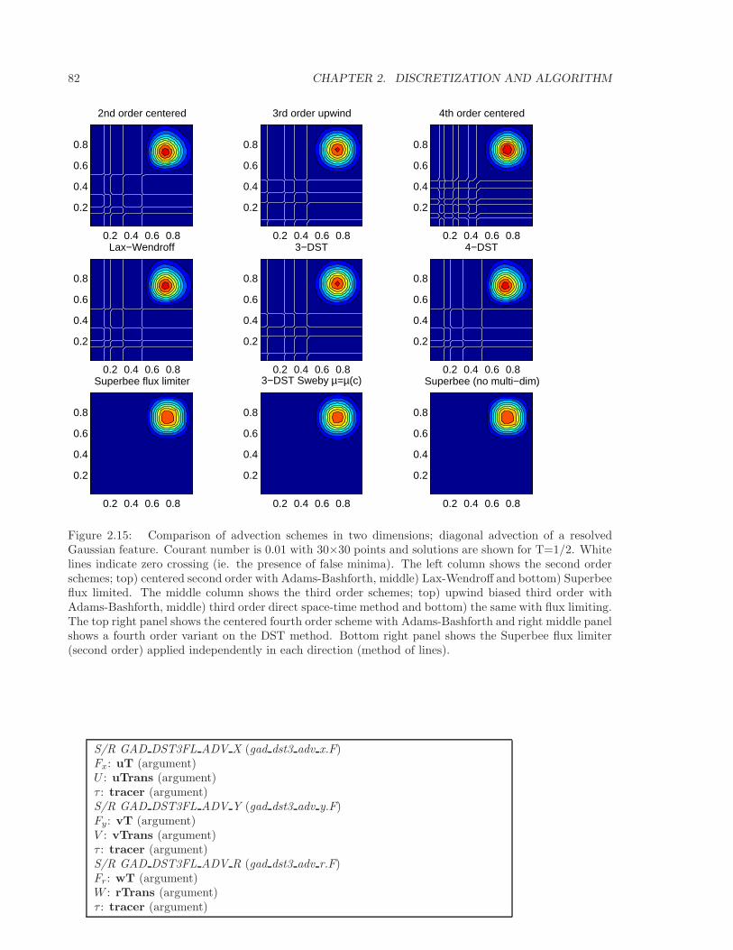
82 CHAPTER 2. DISCRETIZATION AND ALGORITHM
0.2 0.4 0.6 0.8
0.2
0.4
0.6
0.8
2nd order centered
0.2 0.4 0.6 0.8
0.2
0.4
0.6
0.8
3rd order upwind
0.2 0.4 0.6 0.8
0.2
0.4
0.6
0.8
4th order centered
0.2 0.4 0.6 0.8
0.2
0.4
0.6
0.8
Lax−Wendroff
0.2 0.4 0.6 0.8
0.2
0.4
0.6
0.8
3−DST
0.2 0.4 0.6 0.8
0.2
0.4
0.6
0.8
4−DST
0.2 0.4 0.6 0.8
0.2
0.4
0.6
0.8
Superbee flux limiter
0.2 0.4 0.6 0.8
0.2
0.4
0.6
0.8
3−DST Sweby µ=µ(c)
0.2 0.4 0.6 0.8
0.2
0.4
0.6
0.8
Superbee (no multi−dim)
Figure 2.15: Comparison of advection schemes in two dimensions; diagonal advection of a resolvedGaussian feature. Courant number is 0.01 with 30×30 points and solutions are shown for T=1/2. Whitelines indicate zero crossing (ie. the presence of false minima). The left column shows the second orderschemes; top) centered second order with Adams-Bashforth, middle) Lax-Wendroff and bottom) Superbeeflux limited. The middle column shows the third order schemes; top) upwind biased third order withAdams-Bashforth, middle) third order direct space-time method and bottom) the same with flux limiting.The top right panel shows the centered fourth order scheme with Adams-Bashforth and right middle panelshows a fourth order variant on the DST method. Bottom right panel shows the Superbee flux limiter(second order) applied independently in each direction (method of lines).
S/R GAD DST3FL ADV X (gad dst3 adv x.F)Fx: uT (argument)U : uTrans (argument)τ : tracer (argument)S/R GAD DST3FL ADV Y (gad dst3 adv y.F)Fy: vT (argument)V : vTrans (argument)τ : tracer (argument)S/R GAD DST3FL ADV R (gad dst3 adv r.F)Fr: wT (argument)W : rTrans (argument)τ : tracer (argument)
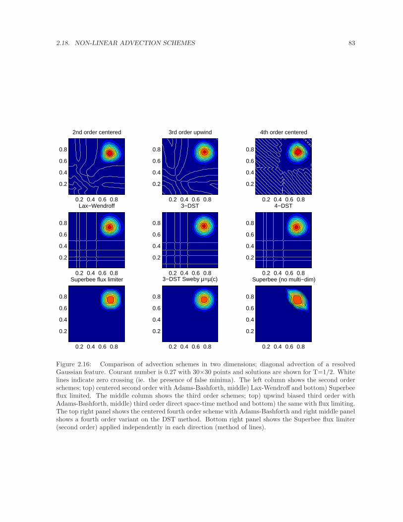
2.18. NON-LINEAR ADVECTION SCHEMES 83
0.2 0.4 0.6 0.8
0.2
0.4
0.6
0.8
2nd order centered
0.2 0.4 0.6 0.8
0.2
0.4
0.6
0.8
3rd order upwind
0.2 0.4 0.6 0.8
0.2
0.4
0.6
0.8
4th order centered
0.2 0.4 0.6 0.8
0.2
0.4
0.6
0.8
Lax−Wendroff
0.2 0.4 0.6 0.8
0.2
0.4
0.6
0.8
3−DST
0.2 0.4 0.6 0.8
0.2
0.4
0.6
0.8
4−DST
0.2 0.4 0.6 0.8
0.2
0.4
0.6
0.8
Superbee flux limiter
0.2 0.4 0.6 0.8
0.2
0.4
0.6
0.8
3−DST Sweby µ=µ(c)
0.2 0.4 0.6 0.8
0.2
0.4
0.6
0.8
Superbee (no multi−dim)
Figure 2.16: Comparison of advection schemes in two dimensions; diagonal advection of a resolvedGaussian feature. Courant number is 0.27 with 30×30 points and solutions are shown for T=1/2. Whitelines indicate zero crossing (ie. the presence of false minima). The left column shows the second orderschemes; top) centered second order with Adams-Bashforth, middle) Lax-Wendroff and bottom) Superbeeflux limited. The middle column shows the third order schemes; top) upwind biased third order withAdams-Bashforth, middle) third order direct space-time method and bottom) the same with flux limiting.The top right panel shows the centered fourth order scheme with Adams-Bashforth and right middle panelshows a fourth order variant on the DST method. Bottom right panel shows the Superbee flux limiter(second order) applied independently in each direction (method of lines).
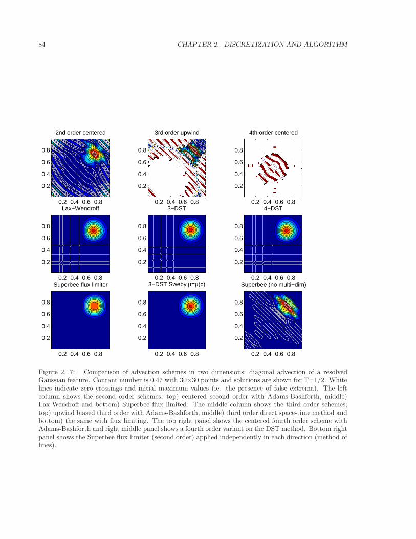
84 CHAPTER 2. DISCRETIZATION AND ALGORITHM
0.2 0.4 0.6 0.8
0.2
0.4
0.6
0.8
2nd order centered
0.2 0.4 0.6 0.8
0.2
0.4
0.6
0.8
3rd order upwind
0.2 0.4 0.6 0.8
0.2
0.4
0.6
0.8
4th order centered
0.2 0.4 0.6 0.8
0.2
0.4
0.6
0.8
Lax−Wendroff
0.2 0.4 0.6 0.8
0.2
0.4
0.6
0.8
3−DST
0.2 0.4 0.6 0.8
0.2
0.4
0.6
0.8
4−DST
0.2 0.4 0.6 0.8
0.2
0.4
0.6
0.8
Superbee flux limiter
0.2 0.4 0.6 0.8
0.2
0.4
0.6
0.8
3−DST Sweby µ=µ(c)
0.2 0.4 0.6 0.8
0.2
0.4
0.6
0.8
Superbee (no multi−dim)
Figure 2.17: Comparison of advection schemes in two dimensions; diagonal advection of a resolvedGaussian feature. Courant number is 0.47 with 30×30 points and solutions are shown for T=1/2. Whitelines indicate zero crossings and initial maximum values (ie. the presence of false extrema). The leftcolumn shows the second order schemes; top) centered second order with Adams-Bashforth, middle)Lax-Wendroff and bottom) Superbee flux limited. The middle column shows the third order schemes;top) upwind biased third order with Adams-Bashforth, middle) third order direct space-time method andbottom) the same with flux limiting. The top right panel shows the centered fourth order scheme withAdams-Bashforth and right middle panel shows a fourth order variant on the DST method. Bottom rightpanel shows the Superbee flux limiter (second order) applied independently in each direction (method oflines).
2.19. COMPARISON OF ADVECTION SCHEMES 85
2.18.4 Multi-dimensional advection
In many of the aforementioned advection schemes the behavior in multiple dimensions is not necessarilyas good as the one dimensional behavior. For instance, a shape preserving monotonic scheme in onedimension can have severe shape distortion in two dimensions if the two components of horizontal fluxesare treated independently. There is a large body of literature on the subject dealing with this problemand among the fixes are operator and flux splitting methods, corner flux methods and more. We haveadopted a variant on the standard splitting methods that allows the flux calculations to be implementedas if in one dimension:
τn+1/3 = τn − ∆t
(1
∆xδiF
x(τn) + τn 1
∆xδiu
)(2.201)
τn+2/3 = τn+1/3 − ∆t
(1
∆yδjF
y(τn+1/3) + τn 1
∆yδiv
)(2.202)
τn+3/3 = τn+2/3 − ∆t
(1
∆rδkF
x(τn+2/3) + τn 1
∆rδiw
)(2.203)
In order to incorporate this method into the general model algorithm, we compute the effectivetendency rather than update the tracer so that other terms such as diffusion are using the n time-leveland not the updated n+ 3/3 quantities:
Gn+1/2adv =
1
∆t(τn+3/3 − τn) (2.204)
So that the over all time-stepping looks likes:
τn+1 = τn + ∆t(G
n+1/2adv +Gdiff (τn) +Gn
forcing
)(2.205)
S/R GAD ADVECTION (gad advection.F)τ : Tracer (argument)
Gn+1/2adv : Gtracer (argument)
Fx, Fy, Fr : af (local)U : uTrans (local)V : vTrans (local)W : rTrans (local)
2.19 Comparison of advection schemes
Figs. 2.15, 2.16 and 2.17 show solutions to a simple diagonal advection problem using a selection ofschemes for low, moderate and high Courant numbers, respectively. The top row shows the linearschemes, integrated with the Adams-Bashforth method. Theses schemes are clearly unstable for the highCourant number and weakly unstable for the moderate Courant number. The presence of false extremais very apparent for all Courant numbers. The middle row shows solutions obtained with the unlimitedbut multi-dimensional schemes. These solutions also exhibit false extrema though the pattern now showssymmetry due to the multi-dimensional scheme. Also, the schemes are stable at high Courant numberwhere the linear schemes weren’t. The bottom row (left and middle) shows the limited schemes and mostobvious is the absence of false extrema. The accuracy and stability of the unlimited non-linear schemes isretained at high Courant number but at low Courant number the tendency is to loose amplitude in sharppeaks due to diffusion. The one dimensional tests shown in Figs. 2.13 and 2.14 showed this phenomenon.
Finally, the bottom left and right panels use the same advection scheme but the right does not use themulti-dimensional method. At low Courant number this appears to not matter but for moderate Courantnumber severe distortion of the feature is apparent. Moreover, the stability of the multi-dimensionalscheme is determined by the maximum Courant number applied of each dimension while the stability ofthe method of lines is determined by the sum. Hence, in the high Courant number plot, the scheme isunstable.
With many advection schemes implemented in the code two questions arise: “Which scheme is best?”and “Why don’t you just offer the best advection scheme?”. Unfortunately, no one advection scheme is
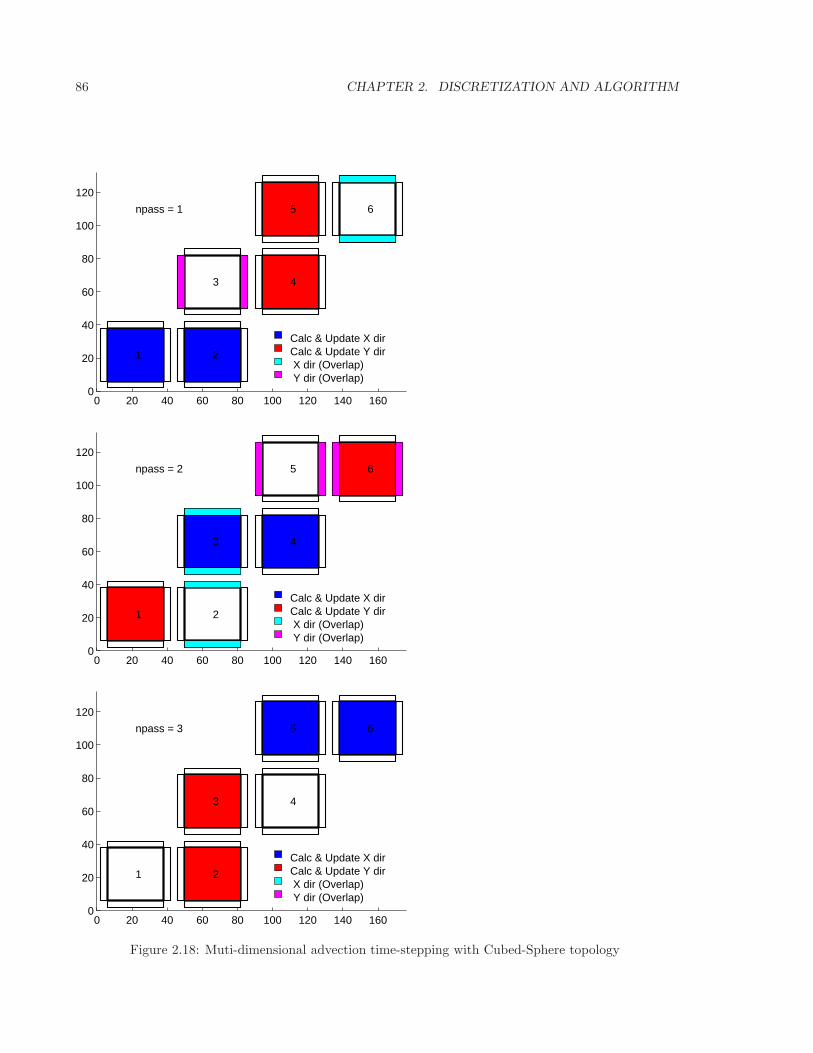
86 CHAPTER 2. DISCRETIZATION AND ALGORITHM
0 20 40 60 80 100 120 140 1600
20
40
60
80
100
120
1 2
3 4
5 6npass = 1
Calc & Update X dirCalc & Update Y dir X dir (Overlap) Y dir (Overlap)
0 20 40 60 80 100 120 140 1600
20
40
60
80
100
120
1 2
3 4
5 6npass = 2
Calc & Update X dirCalc & Update Y dir X dir (Overlap) Y dir (Overlap)
0 20 40 60 80 100 120 140 1600
20
40
60
80
100
120
1 2
3 4
5 6npass = 3
Calc & Update X dirCalc & Update Y dir X dir (Overlap) Y dir (Overlap)
Figure 2.18: Muti-dimensional advection time-stepping with Cubed-Sphere topology
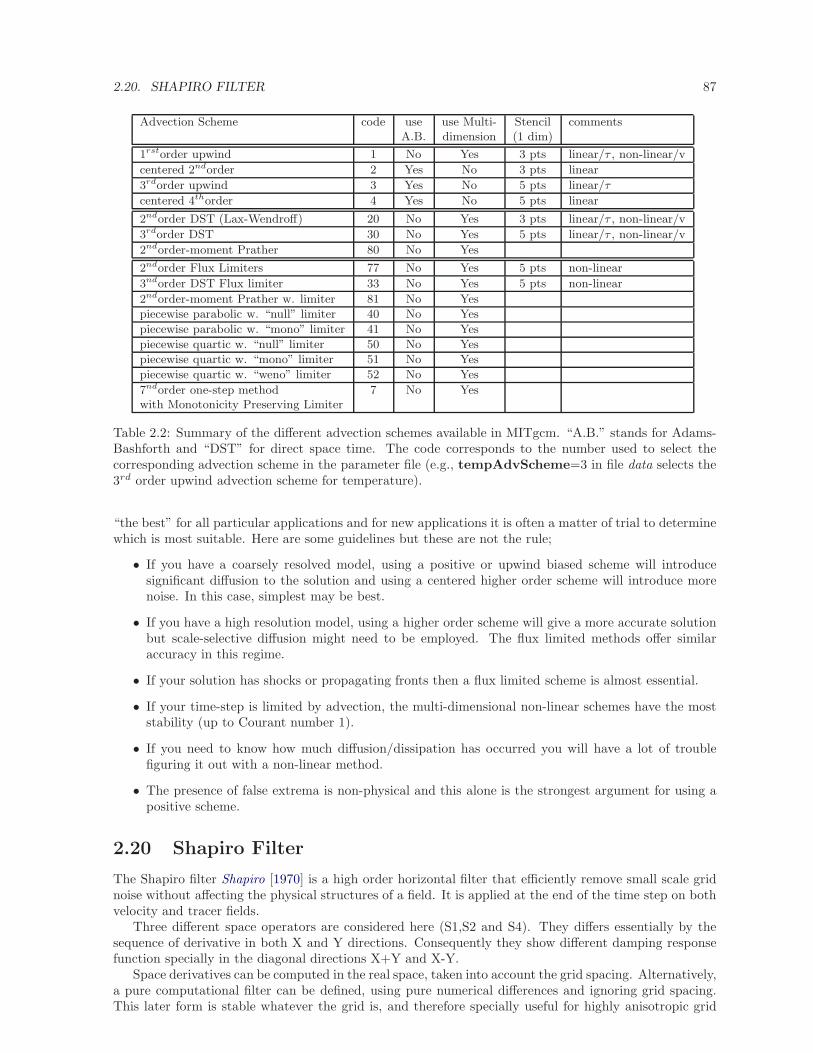
2.20. SHAPIRO FILTER 87
Advection Scheme code use use Multi- Stencil commentsA.B. dimension (1 dim)
1rstorder upwind 1 No Yes 3 pts linear/τ , non-linear/v
centered 2ndorder 2 Yes No 3 pts linear
3rdorder upwind 3 Yes No 5 pts linear/τ
centered 4thorder 4 Yes No 5 pts linear
2ndorder DST (Lax-Wendroff) 20 No Yes 3 pts linear/τ , non-linear/v
3rdorder DST 30 No Yes 5 pts linear/τ , non-linear/v
2ndorder-moment Prather 80 No Yes
2ndorder Flux Limiters 77 No Yes 5 pts non-linear
3ndorder DST Flux limiter 33 No Yes 5 pts non-linear
2ndorder-moment Prather w. limiter 81 No Yes
piecewise parabolic w. “null” limiter 40 No Yes
piecewise parabolic w. “mono” limiter 41 No Yes
piecewise quartic w. “null” limiter 50 No Yes
piecewise quartic w. “mono” limiter 51 No Yes
piecewise quartic w. “weno” limiter 52 No Yes
7ndorder one-step method 7 No Yeswith Monotonicity Preserving Limiter
Table 2.2: Summary of the different advection schemes available in MITgcm. “A.B.” stands for Adams-Bashforth and “DST” for direct space time. The code corresponds to the number used to select thecorresponding advection scheme in the parameter file (e.g., tempAdvScheme=3 in file data selects the3rd order upwind advection scheme for temperature).
“the best” for all particular applications and for new applications it is often a matter of trial to determinewhich is most suitable. Here are some guidelines but these are not the rule;
• If you have a coarsely resolved model, using a positive or upwind biased scheme will introducesignificant diffusion to the solution and using a centered higher order scheme will introduce morenoise. In this case, simplest may be best.
• If you have a high resolution model, using a higher order scheme will give a more accurate solutionbut scale-selective diffusion might need to be employed. The flux limited methods offer similaraccuracy in this regime.
• If your solution has shocks or propagating fronts then a flux limited scheme is almost essential.
• If your time-step is limited by advection, the multi-dimensional non-linear schemes have the moststability (up to Courant number 1).
• If you need to know how much diffusion/dissipation has occurred you will have a lot of troublefiguring it out with a non-linear method.
• The presence of false extrema is non-physical and this alone is the strongest argument for using apositive scheme.
2.20 Shapiro Filter
The Shapiro filter Shapiro [1970] is a high order horizontal filter that efficiently remove small scale gridnoise without affecting the physical structures of a field. It is applied at the end of the time step on bothvelocity and tracer fields.
Three different space operators are considered here (S1,S2 and S4). They differs essentially by thesequence of derivative in both X and Y directions. Consequently they show different damping responsefunction specially in the diagonal directions X+Y and X-Y.
Space derivatives can be computed in the real space, taken into account the grid spacing. Alternatively,a pure computational filter can be defined, using pure numerical differences and ignoring grid spacing.This later form is stable whatever the grid is, and therefore specially useful for highly anisotropic grid
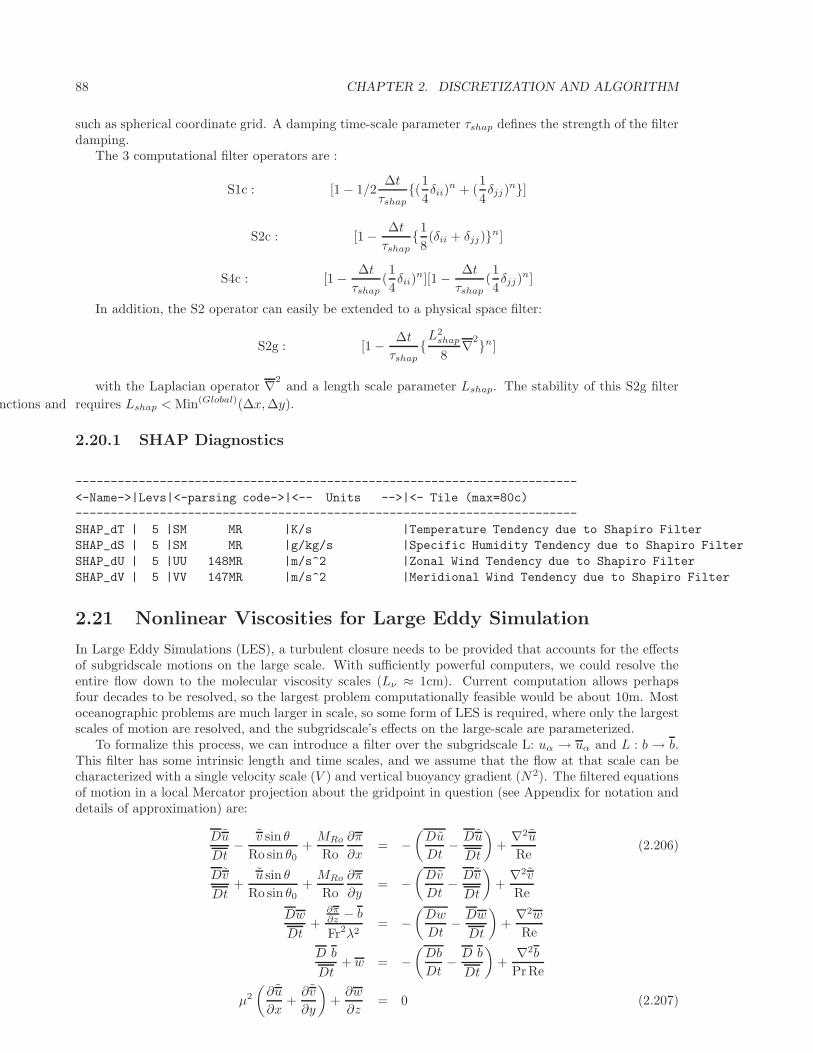
88 CHAPTER 2. DISCRETIZATION AND ALGORITHM
such as spherical coordinate grid. A damping time-scale parameter τshap defines the strength of the filterdamping.
The 3 computational filter operators are :
S1c : [1 − 1/2∆t
τshap(1
4δii)
n + (1
4δjj)
n]
S2c : [1 − ∆t
τshap1
8(δii + δjj)n]
S4c : [1 − ∆t
τshap(1
4δii)
n][1 − ∆t
τshap(1
4δjj)
n]
In addition, the S2 operator can easily be extended to a physical space filter:
S2g : [1 − ∆t
τshapL2
shap
8∇2n]
with the Laplacian operator ∇2and a length scale parameter Lshap. The stability of this S2g filter
requires Lshap < Min(Global)(∆x,∆y).functions and
2.20.1 SHAP Diagnostics
------------------------------------------------------------------------
<-Name->|Levs|<-parsing code->|<-- Units -->|<- Tile (max=80c)
------------------------------------------------------------------------
SHAP_dT | 5 |SM MR |K/s |Temperature Tendency due to Shapiro Filter
SHAP_dS | 5 |SM MR |g/kg/s |Specific Humidity Tendency due to Shapiro Filter
SHAP_dU | 5 |UU 148MR |m/s^2 |Zonal Wind Tendency due to Shapiro Filter
SHAP_dV | 5 |VV 147MR |m/s^2 |Meridional Wind Tendency due to Shapiro Filter
2.21 Nonlinear Viscosities for Large Eddy Simulation
In Large Eddy Simulations (LES), a turbulent closure needs to be provided that accounts for the effectsof subgridscale motions on the large scale. With sufficiently powerful computers, we could resolve theentire flow down to the molecular viscosity scales (Lν ≈ 1cm). Current computation allows perhapsfour decades to be resolved, so the largest problem computationally feasible would be about 10m. Mostoceanographic problems are much larger in scale, so some form of LES is required, where only the largestscales of motion are resolved, and the subgridscale’s effects on the large-scale are parameterized.
To formalize this process, we can introduce a filter over the subgridscale L: uα → uα and L : b → b.This filter has some intrinsic length and time scales, and we assume that the flow at that scale can becharacterized with a single velocity scale (V ) and vertical buoyancy gradient (N2). The filtered equationsof motion in a local Mercator projection about the gridpoint in question (see Appendix for notation anddetails of approximation) are:
Du
Dt− v sin θ
Ro sin θ0+MRo
Ro
∂π
∂x= −
(Du
Dt− Du
Dt
)+
∇2u
Re(2.206)
Dv
Dt+
u sin θ
Ro sin θ0+MRo
Ro
∂π
∂y= −
(Dv
Dt− Dv
Dt
)+
∇2v
Re
Dw
Dt+
∂π∂z − b
Fr2λ2= −
(Dw
Dt− Dw
Dt
)+
∇2w
Re
D b
Dt+ w = −
(Db
Dt− D b
Dt
)+
∇2b
PrRe
µ2
(∂u
∂x+∂v
∂y
)+∂w
∂z= 0 (2.207)
2.21. NONLINEAR VISCOSITIES FOR LARGE EDDY SIMULATION 89
Tildes denote multiplication by cos θ/ cos θ0 to account for converging meridians.The ocean is usually turbulent, and an operational definition of turbulence is that the terms in
parentheses (the ’eddy’ terms) on the right of (2.206) are of comparable magnitude to the terms onthe left-hand side. The terms proportional to the inverse of Re, instead, are many orders of magnitudesmaller than all of the other terms in virtually every oceanic application.
2.21.1 Eddy Viscosity
A turbulent closure provides an approximation to the ’eddy’ terms on the right of the preceding equations.The simplest form of LES is just to increase the viscosity and diffusivity until the viscous and diffusivescales are resolved. That is, we approximate:
(Du
Dt− Du
Dt
)≈ ∇2
hu
Reh+
∂2u∂z2
Rev,
(Dv
Dt− Dv
Dt
)≈ ∇2
hv
Reh+
∂2v∂z2
Rev
(Dw
Dt− Dw
Dt
)≈ ∇2
hw
Reh+
∂2w∂z2
Rev,
(Db
Dt− D b
Dt
)≈ ∇2
hb
PrReh+
∂2b∂z2
PrRev
2.21.1.1 Reynolds-Number Limited Eddy Viscosity
One way of ensuring that the gridscale is sufficiently viscous (ie. resolved) is to choose the eddy viscosityAh so that the gridscale horizontal Reynolds number based on this eddy viscosity, Reh, to is O(1). Thatis, if the gridscale is to be viscous, then the viscosity should be chosen to make the viscous terms as largeas the advective ones. Bryan et al Bryan et al. [1975] notes that a computational mode is squelched byusing Reh <2.
MITgcm users can select horizontal eddy viscosities based on Reh using two methods. 1) The usermay estimate the velocity scale expected from the calculation and grid spacing and set the viscAh tosatisfy Reh < 2. 2) The user may use viscAhReMax, which ensures that the viscosity is always chosenso that Reh < viscAhReMax. This last option should be used with caution, however, since it effectivelyimplies that viscous terms are fixed in magnitude relative to advective terms. While it may be a usefulmethod for specifying a minimum viscosity with little effort, tests Bryan et al. [1975] have shown thatsetting viscAhReMax=2 often tends to increase the viscosity substantially over other more ’physical’parameterizations below, especially in regions where gradients of velocity are small (and thus turbulencemay be weak), so perhaps a more liberal value should be used, eg. viscAhReMax=10.
While it is certainly necessary that viscosity be active at the gridscale, the wavelength where dissipa-tion of energy or enstrophy occurs is not necessarily L = Ah/U . In fact, it is by ensuring that the eitherthe dissipation of energy in a 3-d turbulent cascade (Smagorinsky) or dissipation of enstrophy in a 2-dturbulent cascade (Leith) is resolved that these parameterizations derive their physical meaning.
2.21.1.2 Vertical Eddy Viscosities
Vertical eddy viscosities are often chosen in a more subjective way, as model stability is not usually assensitive to vertical viscosity. Usually the ’observed’ value from finescale measurements, etc., is used(eg. viscAr≈ 1 × 10⁻⁴m2/s). However, Smagorinsky Smagorinsky [1993] notes that the Smagorinskyparameterization of isotropic turbulence implies a value of the vertical viscosity as well as the horizontalviscosity (see below).
2.21.1.3 Smagorinsky Viscosity
Some Smagorinsky [1963, 1993] suggest choosing a viscosity that depends on the resolved motions. Thus,the overall viscous operator has a nonlinear dependence on velocity. Smagorinsky chose his form ofviscosity by considering Kolmogorov’s ideas about the energy spectrum of 3-d isotropic turbulence.
Kolmogorov suppposed that is that energy is injected into the flow at large scales (small k) and is’cascaded’ or transferred conservatively by nonlinear processes to smaller and smaller scales until it isdissipated near the viscous scale. By setting the energy flux through a particular wavenumber k, ǫ, to bea constant in k, there is only one combination of viscosity and energy flux that has the units of length,the Kolmogorov wavelength. It is Lǫ(ν) ∝ πǫ−1/4ν3/4 (the π stems from conversion from wavenumberto wavelength). To ensure that this viscous scale is resolved in a numerical model, the gridscale should
90 CHAPTER 2. DISCRETIZATION AND ALGORITHM
be decreased until Lǫ(ν) > L (so-called Direct Numerical Simulation, or DNS). Alternatively, an eddyviscosity can be used and the corresponding Kolmogorov length can be made larger than the gridscale,
Lǫ(Ah) ∝ πǫ−1/4A3/4h (for Large Eddy Simulation or LES).
There are two methods of ensuring that the Kolmogorov length is resolved in MITgcm. 1) The usercan estimate the flux of energy through spectral space for a given simulation and adjust grid spacing orviscAh to ensure that Lǫ(Ah) > L. 2) The user may use the approach of Smagorinsky with viscC2Smag,which estimates the energy flux at every grid point, and adjusts the viscosity accordingly.
Smagorinsky formed the energy equation from the momentum equations by dotting them with velocity.There are some complications when using the hydrostatic approximation as described by SmagorinskySmagorinsky [1993]. The positive definite energy dissipation by horizontal viscosity in a hydrostatic flowis νD2, where D is the deformation rate at the viscous scale. According to Kolmogorov’s theory, thisshould be a good approximation to the energy flux at any wavenumber ǫ ≈ νD2. Kolmogorov andSmagorinsky noted that using an eddy viscosity that exceeds the molecular value ν should ensure thatthe energy flux through viscous scale set by the eddy viscosity is the same as it would have been had we
resolved all the way to the true viscous scale. That is, ǫ ≈ AhSmagD2. If we use this approximation to
estimate the Kolmogorov viscous length, then
Lǫ(AhSmag) ∝ πǫ−1/4A3/4hSmag ≈ π(AhSmagD
2)−1/4A
3/4hSmag = πA
1/2hSmagD
−1/2(2.208)
To make Lǫ(AhSmag) scale with the gridscale, then
AhSmag =
(viscC2Smag
π
)2
L2|D| (2.209)
Where the deformation rate appropriate for hydrostatic flows with shallow-water scaling is
|D| =
√(∂u
∂x− ∂v
∂y
)2
+
(∂u
∂y+∂v
∂x
)2
(2.210)
The coefficient viscC2Smag is what an MITgcm user sets, and it replaces the proportionality in theKolmogorov length with an equality. Others Griffies and Hallberg [2000] suggest values of viscC2Smagfrom 2.2 to 4 for oceanic problems. Smagorinsky Smagorinsky [1993] shows that values from 0.2 to 0.9have been used in atmospheric modeling.
Smagorinsky Smagorinsky [1993] shows that a corresponding vertical viscosity should be used:
AvSmag =
(viscC2Smag
π
)2
H2
√(∂u
∂z
)2
+
(∂v
∂z
)2
(2.211)
This vertical viscosity is currently not implemented in MITgcm (although it may be soon).
2.21.1.4 Leith Viscosity
Leith Leith [1968, 1996] notes that 2-d turbulence is quite different from 3-d. In two-dimensional tur-bulence, energy cascades to larger scales, so there is no concern about resolving the scales of energydissipation. Instead, another quantity, enstrophy, (which is the vertical component of vorticity squared)is conserved in 2-d turbulence, and it cascades to smaller scales where it is dissipated.
Following a similar argument to that above about energy flux, the enstrophy flux is estimated to beequal to the positive-definite gridscale dissipation rate of enstrophy η ≈ AhLeith|∇ω3|2. By dimensional
analysis, the enstrophy-dissipation scale is Lη(AhLeith) ∝ πA1/2hLeithη
−1/6. Thus, the Leith-estimatedlength scale of enstrophy-dissipation and the resulting eddy viscosity are
Lη(AhLeith) ∝ πA1/2hLeithη
−1/6 = πA1/3hLeith|∇ω3|−1/3 (2.212)
AhLeith =
(viscC2Leith
π
)3
L3|∇ω3| (2.213)
|∇ω3| ≡
√[∂
∂x
(∂v
∂x− ∂u
∂y
)]2+
[∂
∂y
(∂v
∂x− ∂u
∂y
)]2(2.214)
2.21. NONLINEAR VISCOSITIES FOR LARGE EDDY SIMULATION 91
2.21.1.5 Modified Leith Viscosity
The argument above for the Leith viscosity parameterization uses concepts from purely 2-dimensionalturbulence, where the horizontal flow field is assumed to be divergenceless. However, oceanic flows areonly quasi-two dimensional. While the barotropic flow, or the flow within isopycnal layers may behavenearly as two-dimensional turbulence, there is a possibility that these flows will be divergent. In a high-resolution numerical model, these flows may be substantially divergent near the grid scale, and in fact,numerical instabilities exist which are only horizontally divergent and have little vertical vorticity. Thiscauses a difficulty with the Leith viscosity, which can only responds to buildup of vorticity at the gridscale.
MITgcm offers two options for dealing with this problem. 1) The Smagorinsky viscosity can beused instead of Leith, or in conjunction with Leith–a purely divergent flow does cause an increase inSmagorinsky viscosity. 2) The viscC2LeithD parameter can be set. This is a damping specifically targetingpurely divergent instabilities near the gridscale. The combined viscosity has the form:
AhLeith = L3
√(viscC2Leith
π
)6
|∇ω3|2 +
(viscC2LeithD
π
)6
|∇∇ · uh|2 (2.215)
|∇∇ · uh| ≡
√[∂
∂x
(∂u
∂x+∂v
∂y
)]2+
[∂
∂y
(∂u
∂x+∂v
∂y
)]2(2.216)
Whether there is any physical rationale for this correction is unclear at the moment, but the numericalconsequences are good. The divergence in flows with the grid scale larger or comparable to the Rossbyradius is typically much smaller than the vorticity, so this adjustment only rarely adjusts the viscosityif viscC2LeithD = viscC2Leith. However, the rare regions where this viscosity acts are often the locationsfor the largest vales of vertical velocity in the domain. Since the CFL condition on vertical velocity isoften what sets the maximum timestep, this viscosity may substantially increase the allowable timestepwithout severely compromising the verity of the simulation. Tests have shown that in some calculations,a timestep three times larger was allowed when viscC2LeithD = viscC2Leith.
2.21.1.6 Courant–Freidrichs–Lewy Constraint on Viscosity
Whatever viscosities are used in the model, the choice is constrained by gridscale and timestep by theCourant–Freidrichs–Lewy (CFL) constraint on stability:
Ah <L2
4∆t(2.217)
A4 ≤ L4
32∆t(2.218)
The viscosities may be automatically limited to be no greater than these values in MITgcm by specifyingviscAhGridMax< 1 and viscA4GridMax< 1. Similarly-scaled minimum values of viscosities are provided byviscAhGridMin and viscA4GridMin, which if used, should be set to values ≪ 1. L is roughly the gridscale(see below).
Following Griffies and Hallberg [2000], we note that there is a factor of ∆x2/8 difference betweenthe harmonic and biharmonic viscosities. Thus, whenever a non-dimensional harmonic coefficient isused in the MITgcm (eg. viscAhGridMax< 1), the biharmonic equivalent is scaled so that the samenon-dimensional value can be used (eg. viscA4GridMax< 1).
2.21.1.7 Biharmonic Viscosity
Holland [1978] suggested that eddy viscosities ought to be focuses on the dynamics at the grid scale, aslarger motions would be ’resolved’. To enhance the scale selectivity of the viscous operator, he suggesteda biharmonic eddy viscosity instead of a harmonic (or Laplacian) viscosity:
(Du
Dt− Du
Dt
)≈ −∇4
hu
Re4+
∂2u∂z2
Rev,
(Dv
Dt− Dv
Dt
)≈ −∇4
hv
Re4+
∂2v∂z2
Rev
(Dw
Dt− Dw
Dt
)≈ −∇4
hw
Re4+
∂2w∂z2
Rev,
(Db
Dt− D b
Dt
)≈ −∇4
hb
PrRe4+
∂2b∂z2
PrRev
92 CHAPTER 2. DISCRETIZATION AND ALGORITHM
Griffies and Hallberg [2000] propose that if one scales the biharmonic viscosity by stability considerations,then the biharmonic viscous terms will be similarly active to harmonic viscous terms at the gridscale ofthe model, but much less active on larger scale motions. Similarly, a biharmonic diffusivity can be usedfor less diffusive flows.
In practice, biharmonic viscosity and diffusivity allow a less viscous, yet numerically stable, simulationthan harmonic viscosity and diffusivity. However, there is no physical rationale for such operators beingof leading order, and more boundary conditions must be specified than for the harmonic operators.If one considers the approximations of 2.208 and 2.219 to be terms in the Taylor series expansions ofthe eddy terms as functions of the large-scale gradient, then one can argue that both harmonic andbiharmonic terms would occur in the series, and the only question is the choice of coefficients. Usingbiharmonic viscosity alone implies that one zeros the first non-vanishing term in the Taylor series, whichis unsupported by any fluid theory or observation.
Nonetheless, MITgcm supports a plethora of biharmonic viscosities and diffusivities, which are con-trolled with parameters named similarly to the harmonic viscosities and diffusivities with the substitutionh→ 4. MITgcm also supports a biharmonic Leith and Smagorinsky viscosities:
A4Smag =
(viscC4Smag
π
)2L4
8|D| (2.219)
A4Leith =L5
8
√(viscC4Leith
π
)6
|∇ω3|2 +
(viscC4LeithD
π
)6
|∇∇ · uh|2 (2.220)
However, it should be noted that unlike the harmonic forms, the biharmonic scaling does not easily relateto whether energy-dissipation or enstrophy-dissipation scales are resolved. If similar arguments are usedto estimate these scales and scale them to the gridscale, the resulting biharmonic viscosities should be:
A4Smag =
(viscC4Smag
π
)5
L5|∇2uh| (2.221)
A4Leith = L6
√(viscC4Leith
π
)12
|∇2ω3|2 +
(viscC4LeithD
π
)12
|∇2∇ · uh|2 (2.222)
Thus, the biharmonic scaling suggested by Griffies and Hallberg [2000] implies:
|D| ∝ L|∇2uh| (2.223)
|∇ω3| ∝ L|∇2ω3| (2.224)
It is not at all clear that these assumptions ought to hold. Only the Griffies and Hallberg [2000] formsare currently implemented in MITgcm.
2.21.1.8 Selection of Length Scale
Above, the length scale of the grid has been denoted L. However, in strongly anisotropic grids, Lx
and Ly will be quite different in some locations. In that case, the CFL condition suggests that theminimum of Lx and Ly be used. On the other hand, other viscosities which involve whether a particularwavelength is ’resolved’ might be better suited to use the maximum of Lx and Ly. Currently, MITgcmuses useAreaViscLength to select between two options. If false, the geometric mean of L2
x and L2y is
used for all viscosities, which is closer to the minimum and occurs naturally in the CFL constraint. IfuseAreaViscLength is true, then the square root of the area of the grid cell is used.
2.21.2 Mercator, Nondimensional Equations
The rotating, incompressible, Boussinesq equations of motion Gill [1982] on a sphere can be written inMercator projection about a latitude θ0 and geopotential height z = r− r0. The nondimensional form ofthese equations is:
RoDu
Dt− v sin θ
sin θ0+MRo
∂π
∂x+λFr2MRo cos θ
µ sin θ0w = −Fr2MRouw
r/H+
Rox · ∇2u
Re(2.225)
2.21. NONLINEAR VISCOSITIES FOR LARGE EDDY SIMULATION 93
RoDv
Dt+u sin θ
sin θ0+MRo
∂π
∂y= −µRo tan θ(u2 + v2)
r/L− Fr2MRovw
r/H+
Roy · ∇2u
Re(2.226)
Fr2λ2Dw
Dt− b+
∂π
∂z− λ cot θ0u
MRo=
λµ2(u2 + v2)
MRo(r/L)+
Fr2λ2z · ∇2u
Re(2.227)
Db
Dt+ w =
∇2b
PrRe
µ2
(∂u
∂x+∂v
∂y
)+∂w
∂z= 0 (2.228)
Where
µ ≡ cos θ0cos θ
, u =u∗
V µ, v =
v∗
V µ(2.229)
f0 ≡ 2Ω sin θ0,D
Dt≡ µ2
(u∂
∂x+ v
∂
∂y
)+
Fr2MRo
Row∂
∂z(2.230)
x ≡ r
Lφ cos θ0, y ≡ r
L
∫ θ
θ0
cos θ0 dθ′
cos θ′, z ≡ λ
r − r0L
(2.231)
t∗ = tL
V, b∗ = b
V f0MRo
λ(2.232)
π∗ = πV f0LMRo, w∗ = wVFr2λMRo
Ro(2.233)
Ro ≡ V
f0L, MRo ≡ max[1,Ro] (2.234)
Fr ≡ V
NλL, Re ≡ V L
ν, Pr ≡ ν
κ(2.235)
Dimensional variables are denoted by an asterisk where necessary. If we filter over a grid scale typicalfor ocean models (1m < L < 100km, 0.0001 < λ < 1, 0.001m/s < V < 1m/s, f0 < 0.0001s−1,0.01s−1 < N < 0.0001s−1), these equations are very well approximated by
RoDu
Dt− v sin θ
sin θ0+MRo
∂π
∂x= −λFr2MRo cos θ
µ sin θ0w +
Ro∇2u
Re(2.236)
RoDv
Dt+u sin θ
sin θ0+MRo
∂π
∂y=
Ro∇2v
Re(2.237)
Fr2λ2Dw
Dt− b+
∂π
∂z=
λ cot θ0u
MRo+
Fr2λ2∇2w
Re(2.238)
Db
Dt+ w =
∇2b
PrRe(2.239)
µ2
(∂u
∂x+∂v
∂y
)+∂w
∂z= 0 (2.240)
∇2 ≈(∂2
∂x2+
∂2
∂y2+
∂2
λ2∂z2
)(2.241)
Neglecting the non-frictional terms on the right-hand side is usually called the ’traditional’ approximation.It is appropriate, with either large aspect ratio or far from the tropics. This approximation is used here,as it does not affect the form of the eddy stresses which is the main topic. The frictional terms arepreserved in this approximate form for later comparison with eddy stresses.

94 CHAPTER 2. DISCRETIZATION AND ALGORITHM
Chapter 3
Getting started with MITgcm
This chapter is divided into two main parts. The first part, which is covered in sections 3.1 through 3.7,contains information about how to run experiments using MITgcm. The second part, covered in sections3.9 through 3.20, contains a set of step-by-step tutorials for running specific pre-configured atmosphericand oceanic experiments.
We believe the best way to familiarize yourself with the model is to run the case study examplesprovided with the base version. Information on how to obtain, compile, and run the code is found here aswell as a brief description of the model structure directory and the case study examples. Information isalso provided here on how to customize the code when you are ready to try implementing the configurationyou have in mind. The code and algorithm are described more fully in chapters 2 and 4.
3.1 Where to find information
There is a web-archived support mailing list for the model that you can email at [email protected] subscribing to:
http://mailman.mitgcm.org/mailman/listinfo/mitgcm-support/
or browse at:
http://mailman.mitgcm.org/pipermail/mitgcm-support/
3.2 Obtaining the code
MITgcm can be downloaded from our system by following the instructions below. As a courtesy we askthat you send e-mail to us at [email protected] to enable us to keep track of who’s usingthe model and in what application. You can download the model two ways:
1. Using CVS software. CVS is a freely available source code management tool. To use CVS you needto have the software installed. Many systems come with CVS pre-installed, otherwise good placesto look for the software for a particular platform are cvshome.org and wincvs.org .
2. Using a tar file. This method is simple and does not require any special software. However, thismethod does not provide easy support for maintenance updates.
3.2.1 Method 1 - Checkout from CVS
If CVS is available on your system, we strongly encourage you to use it. CVS provides an efficient andelegant way of organizing your code and keeping track of your changes. If CVS is not available on yourmachine, you can also download a tar file.
Before you can use CVS, the following environment variable(s) should be set within your shell. For acsh or tcsh shell, put the following
% setenv CVSROOT :pserver:[email protected]:/u/gcmpack
95
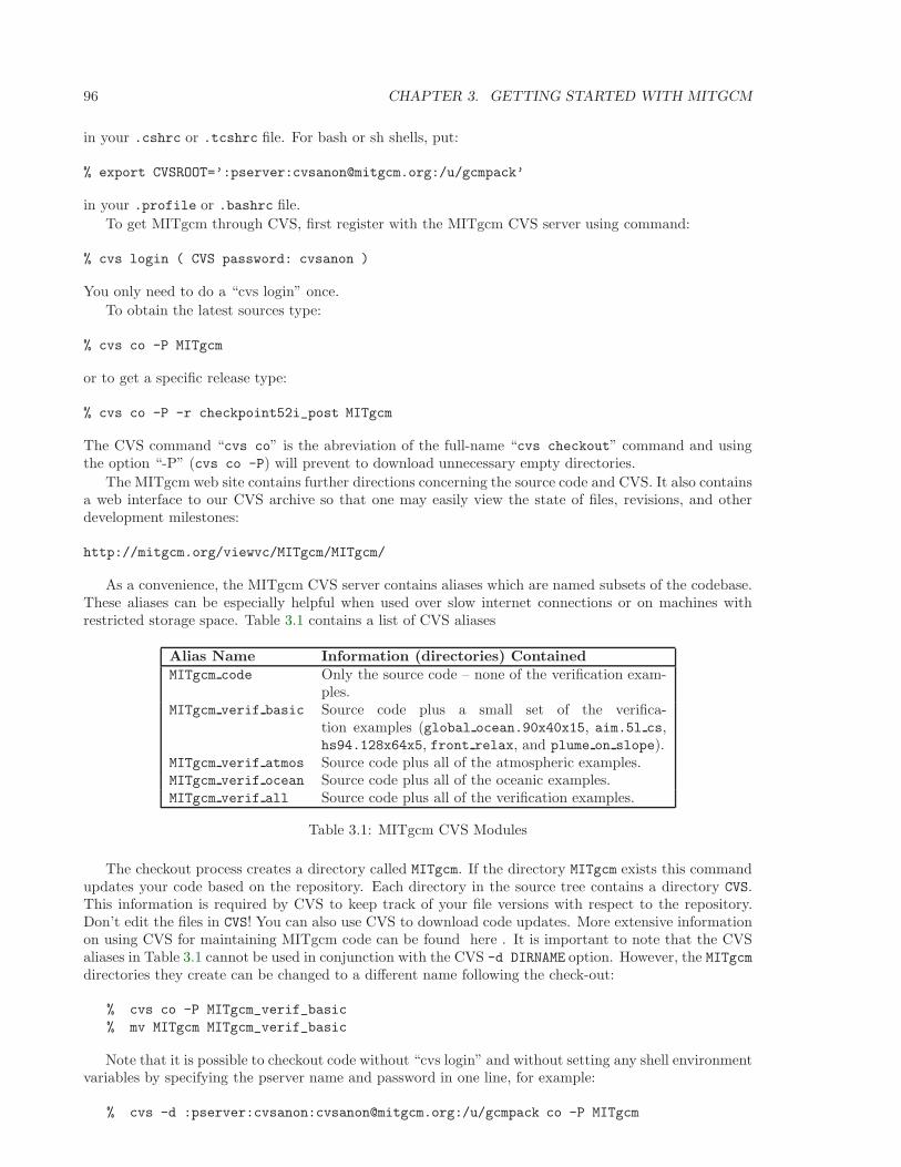
96 CHAPTER 3. GETTING STARTED WITH MITGCM
in your .cshrc or .tcshrc file. For bash or sh shells, put:
% export CVSROOT=’:pserver:[email protected]:/u/gcmpack’
in your .profile or .bashrc file.
To get MITgcm through CVS, first register with the MITgcm CVS server using command:
% cvs login ( CVS password: cvsanon )
You only need to do a “cvs login” once.
To obtain the latest sources type:
% cvs co -P MITgcm
or to get a specific release type:
% cvs co -P -r checkpoint52i_post MITgcm
The CVS command “cvs co” is the abreviation of the full-name “cvs checkout” command and usingthe option “-P” (cvs co -P) will prevent to download unnecessary empty directories.
The MITgcm web site contains further directions concerning the source code and CVS. It also containsa web interface to our CVS archive so that one may easily view the state of files, revisions, and otherdevelopment milestones:
http://mitgcm.org/viewvc/MITgcm/MITgcm/
As a convenience, the MITgcm CVS server contains aliases which are named subsets of the codebase.These aliases can be especially helpful when used over slow internet connections or on machines withrestricted storage space. Table 3.1 contains a list of CVS aliases
Alias Name Information (directories) ContainedMITgcm code Only the source code – none of the verification exam-
ples.MITgcm verif basic Source code plus a small set of the verifica-
tion examples (global ocean.90x40x15, aim.5l cs,hs94.128x64x5, front relax, and plume on slope).
MITgcm verif atmos Source code plus all of the atmospheric examples.MITgcm verif ocean Source code plus all of the oceanic examples.MITgcm verif all Source code plus all of the verification examples.
Table 3.1: MITgcm CVS Modules
The checkout process creates a directory called MITgcm. If the directory MITgcm exists this commandupdates your code based on the repository. Each directory in the source tree contains a directory CVS.This information is required by CVS to keep track of your file versions with respect to the repository.Don’t edit the files in CVS! You can also use CVS to download code updates. More extensive informationon using CVS for maintaining MITgcm code can be found here . It is important to note that the CVSaliases in Table 3.1 cannot be used in conjunction with the CVS -d DIRNAME option. However, the MITgcmdirectories they create can be changed to a different name following the check-out:
% cvs co -P MITgcm_verif_basic
% mv MITgcm MITgcm_verif_basic
Note that it is possible to checkout code without “cvs login” and without setting any shell environmentvariables by specifying the pserver name and password in one line, for example:
% cvs -d :pserver:cvsanon:[email protected]:/u/gcmpack co -P MITgcm
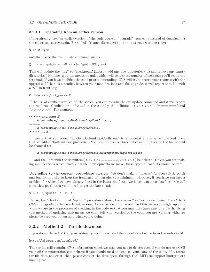
3.2. OBTAINING THE CODE 97
3.2.1.1 Upgrading from an earlier version
If you already have an earlier version of the code you can “upgrade” your copy instead of downloadingthe entire repository again. First, “cd” (change directory) to the top of your working copy:
% cd MITgcm
and then issue the cvs update command such as:
% cvs -q update -d -P -r checkpoint52i_post
This will update the “tag” to “checkpoint52i post”, add any new directories (-d) and remove any emptydirectories (-P). The -q option means be quiet which will reduce the number of messages you’ll see in theterminal. If you have modified the code prior to upgrading, CVS will try to merge your changes with theupgrades. If there is a conflict between your modifications and the upgrade, it will report that file witha “C” in front, e.g.:
C model/src/ini_parms.F
If the list of conflicts scrolled off the screen, you can re-issue the cvs update command and it will reportthe conflicts. Conflicts are indicated in the code by the delimites “<<<<<<<”, “=======” and“>>>>>>>”. For example,
<<<<<<< ini_parms.F
& bottomDragLinear,myOwnBottomDragCoefficient,
=======
& bottomDragLinear,bottomDragQuadratic,
>>>>>>> 1.18
means that you added “myOwnBottomDragCoefficient” to a namelist at the same time and placethat we added “bottomDragQuadratic”. You need to resolve this conflict and in this case the line shouldbe changed to:
& bottomDragLinear,bottomDragQuadratic,myOwnBottomDragCoefficient,
and the lines with the delimiters (<<<<<<,======,>>>>>>) be deleted. Unless you are mak-ing modifications which exactly parallel developments we make, these types of conflicts should be rare.
Upgrading to the current pre-release version We don’t make a “release” for every little patchand bug fix in order to keep the frequency of upgrades to a minimum. However, if you have run into aproblem for which “we have already fixed in the latest code” and we haven’t made a “tag” or “release”since that patch then you’ll need to get the latest code:
% cvs -q update -d -P -A
Unlike, the “check-out” and “update” procedures above, there is no “tag” or release name. The -A tellsCVS to upgrade to the very latest version. As a rule, we don’t recommend this since you might upgradewhile we are in the processes of checking in the code so that you may only have part of a patch. Usingthis method of updating also means we can’t tell what version of the code you are working with. Soplease be sure you understand what you’re doing.
3.2.2 Method 2 - Tar file download
If you do not have CVS on your system, you can download the model as a tar file from the web site at:
http://mitgcm.org/download/
The tar file still contains CVS information which we urge you not to delete; even if you do not use CVSyourself the information can help us if you should need to send us your copy of the code. If a recenttar file does not exist, then please contact the developers through the [email protected] list.
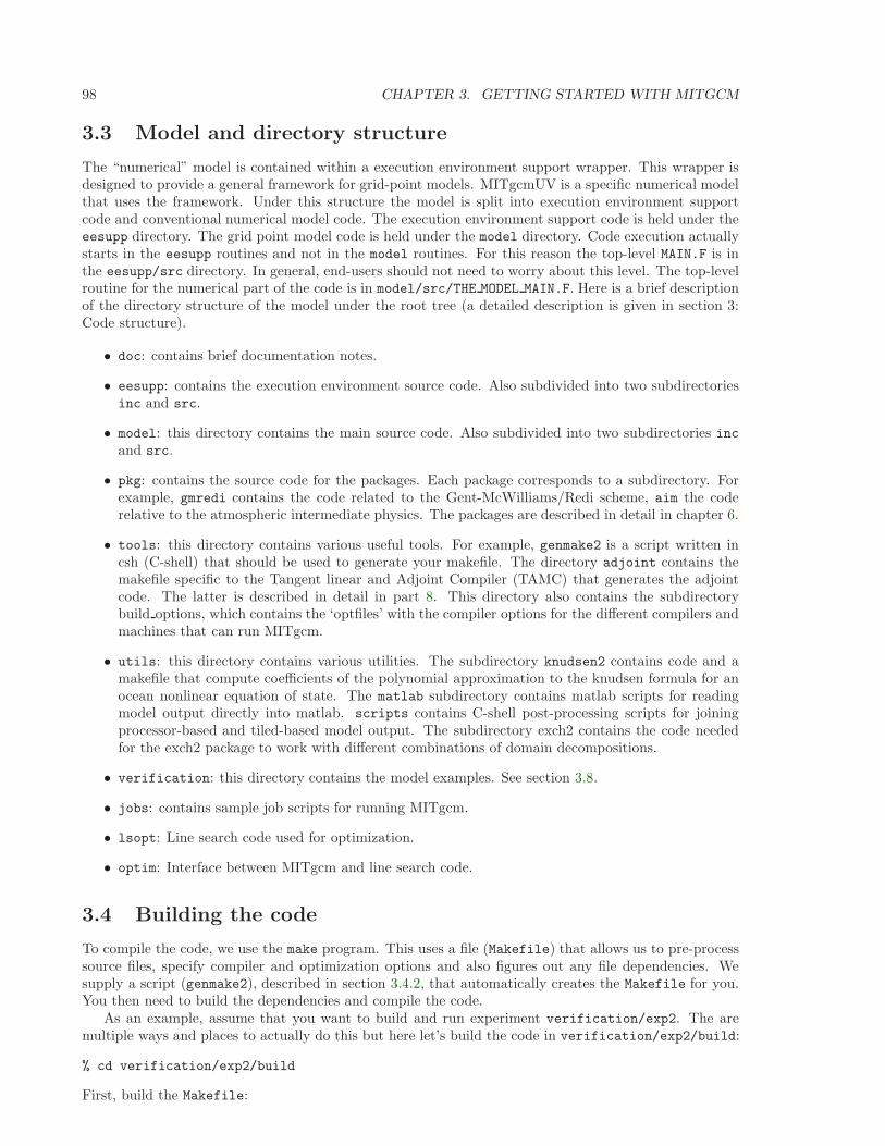
98 CHAPTER 3. GETTING STARTED WITH MITGCM
3.3 Model and directory structure
The “numerical” model is contained within a execution environment support wrapper. This wrapper isdesigned to provide a general framework for grid-point models. MITgcmUV is a specific numerical modelthat uses the framework. Under this structure the model is split into execution environment supportcode and conventional numerical model code. The execution environment support code is held under theeesupp directory. The grid point model code is held under the model directory. Code execution actuallystarts in the eesupp routines and not in the model routines. For this reason the top-level MAIN.F is inthe eesupp/src directory. In general, end-users should not need to worry about this level. The top-levelroutine for the numerical part of the code is in model/src/THE MODEL MAIN.F. Here is a brief descriptionof the directory structure of the model under the root tree (a detailed description is given in section 3:Code structure).
• doc: contains brief documentation notes.
• eesupp: contains the execution environment source code. Also subdivided into two subdirectoriesinc and src.
• model: this directory contains the main source code. Also subdivided into two subdirectories incand src.
• pkg: contains the source code for the packages. Each package corresponds to a subdirectory. Forexample, gmredi contains the code related to the Gent-McWilliams/Redi scheme, aim the coderelative to the atmospheric intermediate physics. The packages are described in detail in chapter 6.
• tools: this directory contains various useful tools. For example, genmake2 is a script written incsh (C-shell) that should be used to generate your makefile. The directory adjoint contains themakefile specific to the Tangent linear and Adjoint Compiler (TAMC) that generates the adjointcode. The latter is described in detail in part 8. This directory also contains the subdirectorybuild options, which contains the ‘optfiles’ with the compiler options for the different compilers andmachines that can run MITgcm.
• utils: this directory contains various utilities. The subdirectory knudsen2 contains code and amakefile that compute coefficients of the polynomial approximation to the knudsen formula for anocean nonlinear equation of state. The matlab subdirectory contains matlab scripts for readingmodel output directly into matlab. scripts contains C-shell post-processing scripts for joiningprocessor-based and tiled-based model output. The subdirectory exch2 contains the code neededfor the exch2 package to work with different combinations of domain decompositions.
• verification: this directory contains the model examples. See section 3.8.
• jobs: contains sample job scripts for running MITgcm.
• lsopt: Line search code used for optimization.
• optim: Interface between MITgcm and line search code.
3.4 Building the code
To compile the code, we use the make program. This uses a file (Makefile) that allows us to pre-processsource files, specify compiler and optimization options and also figures out any file dependencies. Wesupply a script (genmake2), described in section 3.4.2, that automatically creates the Makefile for you.You then need to build the dependencies and compile the code.
As an example, assume that you want to build and run experiment verification/exp2. The aremultiple ways and places to actually do this but here let’s build the code in verification/exp2/build:
% cd verification/exp2/build
First, build the Makefile:
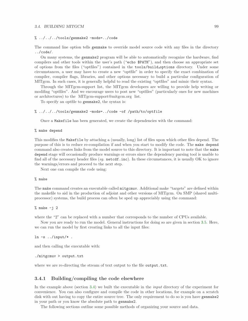
3.4. BUILDING MITGCM 99
% ../../../tools/genmake2 -mods=../code
The command line option tells genmake to override model source code with any files in the directory../code/.
On many systems, the genmake2 program will be able to automatically recognize the hardware, findcompilers and other tools within the user’s path (“echo $PATH”), and then choose an appropriate setof options from the files (“optfiles”) contained in the tools/build options directory. Under somecircumstances, a user may have to create a new “optfile” in order to specify the exact combination ofcompiler, compiler flags, libraries, and other options necessary to build a particular configuration ofMITgcm. In such cases, it is generally helpful to read the existing “optfiles” and mimic their syntax.
Through the MITgcm-support list, the MITgcm developers are willing to provide help writing ormodifing “optfiles”. And we encourage users to post new “optfiles” (particularly ones for new machinesor architectures) to the [email protected] list.
To specify an optfile to genmake2, the syntax is:
% ../../../tools/genmake2 -mods=../code -of /path/to/optfile
Once a Makefile has been generated, we create the dependencies with the command:
% make depend
This modifies the Makefile by attaching a (usually, long) list of files upon which other files depend. Thepurpose of this is to reduce re-compilation if and when you start to modify the code. The make depend
command also creates links from the model source to this directory. It is important to note that the makedepend stage will occasionally produce warnings or errors since the dependency parsing tool is unable tofind all of the necessary header files (eg. netcdf.inc). In these circumstances, it is usually OK to ignorethe warnings/errors and proceed to the next step.
Next one can compile the code using:
% make
The make command creates an executable called mitgcmuv. Additional make “targets” are defined withinthe makefile to aid in the production of adjoint and other versions of MITgcm. On SMP (shared multi-processor) systems, the build process can often be sped up appreciably using the command:
% make -j 2
where the “2” can be replaced with a number that corresponds to the number of CPUs available.
Now you are ready to run the model. General instructions for doing so are given in section 3.5. Here,we can run the model by first creating links to all the input files:
ln -s ../input/* .
and then calling the executable with:
./mitgcmuv > output.txt
where we are re-directing the stream of text output to the file output.txt.
3.4.1 Building/compiling the code elsewhere
In the example above (section 3.4) we built the executable in the input directory of the experiment forconvenience. You can also configure and compile the code in other locations, for example on a scratchdisk with out having to copy the entire source tree. The only requirement to do so is you have genmake2in your path or you know the absolute path to genmake2.
The following sections outline some possible methods of organizing your source and data.
100 CHAPTER 3. GETTING STARTED WITH MITGCM
3.4.1.1 Building from the ../code directory
This is just as simple as building in the input/ directory:
% cd verification/exp2/code
% ../../../tools/genmake2
% make depend
% make
However, to run the model the executable (mitgcmuv) and input files must be in the same place. If youonly have one calculation to make:
% cd ../input
% cp ../code/mitgcmuv ./
% ./mitgcmuv > output.txt
or if you will be making multiple runs with the same executable:
% cd ../
% cp -r input run1
% cp code/mitgcmuv run1
% cd run1
% ./mitgcmuv > output.txt
3.4.1.2 Building from a new directory
Since the input directory contains input files it is often more useful to keep input pristine and build in anew directory within verification/exp2/:
% cd verification/exp2
% mkdir build
% cd build
% ../../../tools/genmake2 -mods=../code
% make depend
% make
This builds the code exactly as before but this time you need to copy either the executable or the inputfiles or both in order to run the model. For example,
% cp ../input/* ./
% ./mitgcmuv > output.txt
or if you tend to make multiple runs with the same executable then running in a new directory each timemight be more appropriate:
% cd ../
% mkdir run1
% cp build/mitgcmuv run1/
% cp input/* run1/
% cd run1
% ./mitgcmuv > output.txt
3.4.1.3 Building on a scratch disk
Model object files and output data can use up large amounts of disk space so it is often the case that youwill be operating on a large scratch disk. Assuming the model source is in /MITgcm then the followingcommands will build the model in /scratch/exp2-run1:
% cd /scratch/exp2-run1
% ~/MITgcm/tools/genmake2 -rootdir=~/MITgcm \
-mods=~/MITgcm/verification/exp2/code
% make depend
% make
3.4. BUILDING MITGCM 101
To run the model here, you’ll need the input files:
% cp ~/MITgcm/verification/exp2/input/* ./
% ./mitgcmuv > output.txt
As before, you could build in one directory and make multiple runs of the one experiment:
% cd /scratch/exp2
% mkdir build
% cd build
% ~/MITgcm/tools/genmake2 -rootdir=~/MITgcm \
-mods=~/MITgcm/verification/exp2/code
% make depend
% make
% cd ../
% cp -r ~/MITgcm/verification/exp2/input run2
% cd run2
% ./mitgcmuv > output.txt
3.4.2 Using genmake2
To compile the code, first use the program genmake2 (located in the tools directory) to generate aMakefile. genmake2 is a shell script written to work with all “sh”–compatible shells including bash v1,bash v2, and Bourne. genmake2 parses information from the following sources:
- a gemake local file if one is found in the current directory
- command-line options
- an ”options file” as specified by the command-line option --optfile=/PATH/FILENAME
- a packages.conf file (if one is found) with the specific list of packages to compile. The search path forfile packages.conf is, first, the current directory and then each of the ”MODS” directories in thegiven order (see below).
3.4.2.1 Optfiles in tools/build options directory:
The purpose of the optfiles is to provide all the compilation options for particular “platforms” (where“platform” roughly means the combination of the hardware and the compiler) and code configurations.Given the combinations of possible compilers and library dependencies (eg. MPI and NetCDF) there maybe numerous optfiles available for a single machine. The naming scheme for the majority of the optfilesshipped with the code is
OS HARDWARE COMPILER
where
OS is the name of the operating system (generally the lower-case output of the ’uname’ command)
HARDWARE is a string that describes the CPU type and corresponds to output from the ’uname
-m’ command:
ia32 is for “x86” machines such as i386, i486, i586, i686, and athlon
ia64 is for Intel IA64 systems (eg. Itanium, Itanium2)
amd64 is AMD x86 64 systems
ppc is for Mac PowerPC systems
COMPILER is the compiler name (generally, the name of the FORTRAN executable)
102 CHAPTER 3. GETTING STARTED WITH MITGCM
In many cases, the default optfiles are sufficient and will result in usable Makefiles. However, for somemachines or code configurations, new “optfiles” must be written. To create a new optfile, it is generallybest to start with one of the defaults and modify it to suit your needs. Like genmake2, the optfiles areall written using a simple “sh”–compatible syntax. While nearly all variables used within genmake2 maybe specified in the optfiles, the critical ones that should be defined are:
FC the FORTRAN compiler (executable) to use
DEFINES the command-line DEFINE options passed to the compiler
CPP the C pre-processor to use
NOOPTFLAGS options flags for special files that should not be optimized
For example, the optfile for a typical Red Hat Linux machine (“ia32” architecture) using the GCC(g77) compiler is
FC=g77
DEFINES=’-D_BYTESWAPIO -DWORDLENGTH=4’
CPP=’cpp -traditional -P’
NOOPTFLAGS=’-O0’
# For IEEE, use the "-ffloat-store" option
if test "x$IEEE" = x ; then
FFLAGS=’-Wimplicit -Wunused -Wuninitialized’
FOPTIM=’-O3 -malign-double -funroll-loops’
else
FFLAGS=’-Wimplicit -Wunused -ffloat-store’
FOPTIM=’-O0 -malign-double’
fi
If you write an optfile for an unrepresented machine or compiler, you are strongly encouraged tosubmit the optfile to the MITgcm project for inclusion. Please send the file to the
mailing list.
3.4.2.2 Command-line options:
In addition to the optfiles, genmake2 supports a number of helpful command-line options. A completelist of these options can be obtained from:
% genmake2 -h
The most important command-line options are:
--optfile=/PATH/FILENAME specifies the optfile that should be used for a particular build.
If no ”optfile” is specified (either through the command line or the MITGCM OPTFILE en-vironment variable), genmake2 will try to make a reasonable guess from the list provided intools/build options. The method used for making this guess is to first determine the combina-tion of operating system and hardware (eg. ”linux ia32”) and then find a working FORTRANcompiler within the user’s path. When these three items have been identified, genmake2 will try tofind an optfile that has a matching name.
--mods=’DIR1 DIR2 DIR3 ...’ specifies a list of directories containing “modifications”. These directo-ries contain files with names that may (or may not) exist in the main MITgcm source tree but willbe overridden by any identically-named sources within the “MODS” directories.
The order of precedence for this ”name-hiding” is as follows:
• “MODS” directories (in the order given)
3.4. BUILDING MITGCM 103
• Packages either explicitly specified or provided by default (in the order given)
• Packages included due to package dependencies (in the order that that package dependenciesare parsed)
• The ”standard dirs” (which may have been specified by the “-standarddirs” option)
--pgroups=/PATH/FILENAME specifies the file where package groups are defined. If not set, the package-groups definition will be read from pkg/pkg groups. It also contains the default list of packages(defined as the group “default pkg list” which is used when no specific package list (packages.conf)is found in current directory or in any ”MODS” directory.
--pdepend=/PATH/FILENAME specifies the dependency file used for packages.
If not specified, the default dependency file pkg/pkg depend is used. The syntax for this file is parsedon a line-by-line basis where each line containes either a comment (”#”) or a simple ”PKGNAME1(+—-)PKGNAME2” pairwise rule where the ”+” or ”-” symbol specifies a ”must be used with” ora ”must not be used with” relationship, respectively. If no rule is specified, then it is assumed thatthe two packages are compatible and will function either with or without each other.
--adof=/path/to/file specifies the ”adjoint” or automatic differentiation options file to be used. Thefile is analogous to the “optfile” defined above but it specifies information for the AD build process.
The default file is located in tools/adjoint options/adjoint default and it defines the ”TAF” and”TAMC” compilers. An alternate version is also available at tools/adjoint options/adjoint staf thatselects the newer ”STAF” compiler. As with any compilers, it is helpful to have their directorieslisted in your $PATH environment variable.
--mpi This option enables certain MPI features (using CPP #defines) within the code and is necessaryfor MPI builds (see Section 3.4.3).
--make=/path/to/gmake Due to the poor handling of soft-links and other bugs common with the make
versions provided by commercial Unix vendors, GNU make (sometimes called gmake) should bepreferred. This option provides a means for specifying the make executable to be used.
--bash=/path/to/sh On some (usually older UNIX) machines, the “bash” shell is unavailable. To runon these systems, genmake2 can be invoked using an “sh” (that is, a Bourne, POSIX, or compatible)shell. The syntax in these circumstances is:
% /bin/sh genmake2 -bash=/bin/sh [...options...]
where /bin/sh can be replaced with the full path and name of the desired shell.
3.4.3 Building with MPI
Building MITgcm to use MPI libraries can be complicated due to the variety of different MPI imple-mentations available, their dependencies or interactions with different compilers, and their often ad-hoclocations within file systems. For these reasons, its generally a good idea to start by finding and readingthe documentation for your machine(s) and, if necessary, seeking help from your local systems adminis-trator.
The steps for building MITgcm with MPI support are:
1. Determine the locations of your MPI-enabled compiler and/or MPI libraries and put them into anoptions file as described in Section 3.4.2. One can start with one of the examples in:
MITgcm/tools/build options/
such as linux ia32 g77+mpi cg01 or linux ia64 efc+mpi and then edit it to suit the machine athand. You may need help from your user guide or local systems administrator to determine theexact location of the MPI libraries. If libraries are not installed, MPI implementations and relatedtools are available including:
104 CHAPTER 3. GETTING STARTED WITH MITGCM
• MPICH
• LAM/MPI
• MPIexec
2. Build the code with the genmake2 -mpi option (see Section 3.4.2) using commands such as:
% ../../../tools/genmake2 -mods=../code -mpi -of=YOUR_OPTFILE
% make depend
% make
3. Run the code with the appropriate MPI “run” or “exec” program provided with your particularimplementation of MPI. Typical MPI packages such as MPICH will use something like:
% mpirun -np 4 -machinefile mf ./mitgcmuv
Sightly more complicated scripts may be needed for many machines since execution of the codemay be controlled by both the MPI library and a job scheduling and queueing system such as PBS,LoadLeveller, Condor, or any of a number of similar tools. A few example scripts (those used for ourregular verification runs) are available at: http://mitgcm.org/viewvc/MITgcm/MITgcm/tools/example scripts/
or at: http://mitgcm.org/viewvc/MITgcm/MITgcm contrib/test scripts/
An example of the above process on the MITgcm cluster (“cg01”) using the GNU g77 compiler andthe mpich MPI library is:
% cd MITgcm/verification/exp5
% mkdir build
% cd build
% ../../../tools/genmake2 -mpi -mods=../code \
-of=../../../tools/build_options/linux_ia32_g77+mpi_cg01
% make depend
% make
% cd ../input
% /usr/local/pkg/mpi/mpi-1.2.4..8a-gm-1.5/g77/bin/mpirun.ch_gm \
-machinefile mf --gm-kill 5 -v -np 2 ../build/mitgcmuv
3.5 Running the model in prognostic mode
If compilation finished succesfully (section 3.4) then an executable called mitgcmuv will now exist in thelocal directory.
To run the model as a single process (ie. not in parallel) simply type:
% ./mitgcmuv
The “./” is a safe-guard to make sure you use the local executable in case you have others that existin your path (surely odd if you do!). The above command will spew out many lines of text output toyour screen. This output contains details such as parameter values as well as diagnostics such as meanKinetic energy, largest CFL number, etc. It is worth keeping this text output with the binary output sowe normally re-direct the stdout stream as follows:
% ./mitgcmuv > output.txt
In the event that the model encounters an error and stops, it is very helpful to include the last few lineof this output.txt file along with the (stderr) error message within any bug reports.
For the example experiments in verification, an example of the output is kept in results/output.txt
for comparison. You can compare your output.txt with the corresponding one for that experiment tocheck that the set-up works.
3.5.1 Output files
The model produces various output files and, when using mnc, sometimes even directories. Depend-ing upon the I/O package(s) selected at compile time (either mdsio or mnc or both as determined bycode/packages.conf) and the run-time flags set (in input/data.pkg), the following output may ap-pear.
3.5. RUNNING MITGCM 105
3.5.1.1 MDSIO output files
The “traditional” output files are generated by the mdsio package. At a minimum, the instantaneous“state” of the model is written out, which is made of the following files:
• U.00000nIter - zonal component of velocity field (m/s and positive eastward).
• V.00000nIter - meridional component of velocity field (m/s and positive northward).
• W.00000nIter - vertical component of velocity field (ocean: m/s and positive upward, atmosphere:Pa/s and positive towards increasing pressure i.e. downward).
• T.00000nIter - potential temperature (ocean: C, atmosphere: K).
• S.00000nIter - ocean: salinity (psu), atmosphere: water vapor (g/kg).
• Eta.00000nIter - ocean: surface elevation (m), atmosphere: surface pressure anomaly (Pa).
The chain 00000nIter consists of ten figures that specify the iteration number at which the outputis written out. For example, U.0000000300 is the zonal velocity at iteration 300.
In addition, a “pickup” or “checkpoint” file called:
• pickup.00000nIter
is written out. This file represents the state of the model in a condensed form and is used for restartingthe integration. If the C-D scheme is used, there is an additional “pickup” file:
• pickup cd.00000nIter
containing the D-grid velocity data and that has to be written out as well in order to restart theintegration. Rolling checkpoint files are the same as the pickup files but are named differently. Theirname contain the chain ckptA or ckptB instead of 00000nIter. They can be used to restart the modelbut are overwritten every other time they are output to save disk space during long integrations.
3.5.1.2 MNC output files
Unlike the mdsio output, the mnc–generated output is usually (though not necessarily) placed within asubdirectory with a name such as mnc test $DATE $SEQ.
3.5.2 Looking at the output
The “traditional” or mdsio model data are written according to a “meta/data” file format. Each variableis associated with two files with suffix names .data and .meta. The .data file contains the data writtenin binary form (big endian by default). The .meta file is a “header” file that contains information aboutthe size and the structure of the .data file. This way of organizing the output is particularly useful whenrunning multi-processors calculations. The base version of the model includes a few matlab utilities toread output files written in this format. The matlab scripts are located in the directory utils/matlab
under the root tree. The script rdmds.m reads the data. Look at the comments inside the script to seehow to use it.
Some examples of reading and visualizing some output in Matlab:
% matlab
>> H=rdmds(’Depth’);
>> contourf(H’);colorbar;
>> title(’Depth of fluid as used by model’);
>> eta=rdmds(’Eta’,10);
>> imagesc(eta’);axis ij;colorbar;
>> title(’Surface height at iter=10’);
>> eta=rdmds(’Eta’,[0:10:100]);
>> for n=1:11; imagesc(eta(:,:,n)’);axis ij;colorbar;pause(.5);end
106 CHAPTER 3. GETTING STARTED WITH MITGCM
Similar scripts for netCDF output (rdmnc.m) are available and they are described in Section 7.2.The MNC output files are all in the “self-describing” netCDF format and can thus be browsed and/or
plotted using tools such as:
• ncdump is a utility which is typically included with every netCDF install:
http://www.unidata.ucar.edu/packages/netcdf/
and it converts the netCDF binaries into formatted ASCII text files.
• ncview utility is a very convenient and quick way to plot netCDF data and it runs on most OSes:
http://meteora.ucsd.edu/~pierce/ncview_home_page.html
• MatLAB(c) and other common post-processing environments provide various netCDF interfacesincluding:
http://mexcdf.sourceforge.net/
http://woodshole.er.usgs.gov/staffpages/cdenham/public_html/MexCDF/nc4ml5.html
3.6. CUSTOMIZING MITGCM 107
3.6 Doing it yourself: customizing the model configuration
When you are ready to run the model in the configuration you want, the easiest thing is to use and adaptthe setup of the case studies experiment (described previously) that is the closest to your configuration.Then, the amount of setup will be minimized. In this section, we focus on the setup relative to the“numerical model” part of the code (the setup relative to the “execution environment” part is covered inthe parallel implementation section) and on the variables and parameters that you are likely to change.
The CPP keys relative to the “numerical model” part of the code are all defined and set in the fileCPP OPTIONS.h in the directory model/inc or in one of the code directories of the case study experi-ments under verification. The model parameters are defined and declared in the file model/inc/PARAMS.hand their default values are set in the routine model/src/set defaults.F. The default values can be mod-ified in the namelist file data which needs to be located in the directory where you will run the model.The parameters are initialized in the routine model/src/ini parms.F. Look at this routine to see in whatpart of the namelist the parameters are located. Here is a complete list of the model parameters relatedto the main model (namelist parameters for the packages are located in the package descriptions), theirmeaning, and their default values:
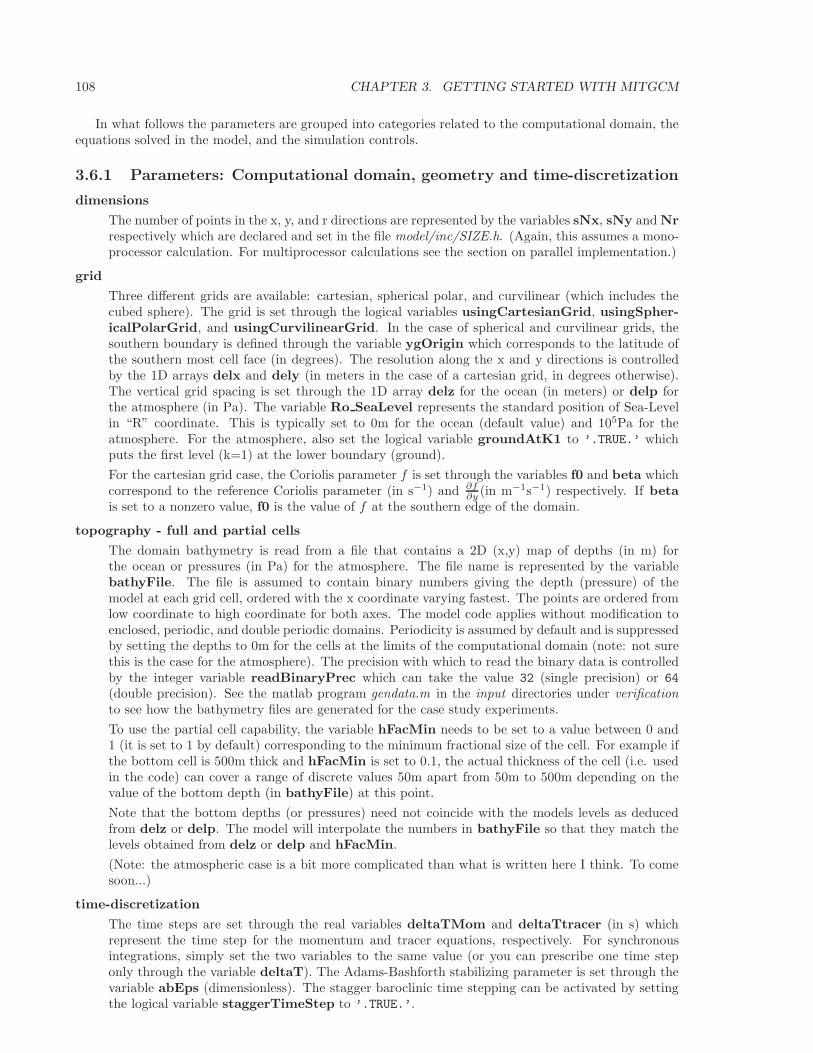
108 CHAPTER 3. GETTING STARTED WITH MITGCM
In what follows the parameters are grouped into categories related to the computational domain, theequations solved in the model, and the simulation controls.
3.6.1 Parameters: Computational domain, geometry and time-discretization
dimensions
The number of points in the x, y, and r directions are represented by the variables sNx, sNy and Nrrespectively which are declared and set in the file model/inc/SIZE.h. (Again, this assumes a mono-processor calculation. For multiprocessor calculations see the section on parallel implementation.)
grid
Three different grids are available: cartesian, spherical polar, and curvilinear (which includes thecubed sphere). The grid is set through the logical variables usingCartesianGrid, usingSpher-icalPolarGrid, and usingCurvilinearGrid. In the case of spherical and curvilinear grids, thesouthern boundary is defined through the variable ygOrigin which corresponds to the latitude ofthe southern most cell face (in degrees). The resolution along the x and y directions is controlledby the 1D arrays delx and dely (in meters in the case of a cartesian grid, in degrees otherwise).The vertical grid spacing is set through the 1D array delz for the ocean (in meters) or delp forthe atmosphere (in Pa). The variable Ro SeaLevel represents the standard position of Sea-Levelin “R” coordinate. This is typically set to 0m for the ocean (default value) and 105Pa for theatmosphere. For the atmosphere, also set the logical variable groundAtK1 to ’.TRUE.’ whichputs the first level (k=1) at the lower boundary (ground).
For the cartesian grid case, the Coriolis parameter f is set through the variables f0 and beta whichcorrespond to the reference Coriolis parameter (in s−1) and ∂f
∂y (in m−1s−1) respectively. If betais set to a nonzero value, f0 is the value of f at the southern edge of the domain.
topography - full and partial cells
The domain bathymetry is read from a file that contains a 2D (x,y) map of depths (in m) forthe ocean or pressures (in Pa) for the atmosphere. The file name is represented by the variablebathyFile. The file is assumed to contain binary numbers giving the depth (pressure) of themodel at each grid cell, ordered with the x coordinate varying fastest. The points are ordered fromlow coordinate to high coordinate for both axes. The model code applies without modification toenclosed, periodic, and double periodic domains. Periodicity is assumed by default and is suppressedby setting the depths to 0m for the cells at the limits of the computational domain (note: not surethis is the case for the atmosphere). The precision with which to read the binary data is controlledby the integer variable readBinaryPrec which can take the value 32 (single precision) or 64
(double precision). See the matlab program gendata.m in the input directories under verificationto see how the bathymetry files are generated for the case study experiments.
To use the partial cell capability, the variable hFacMin needs to be set to a value between 0 and1 (it is set to 1 by default) corresponding to the minimum fractional size of the cell. For example ifthe bottom cell is 500m thick and hFacMin is set to 0.1, the actual thickness of the cell (i.e. usedin the code) can cover a range of discrete values 50m apart from 50m to 500m depending on thevalue of the bottom depth (in bathyFile) at this point.
Note that the bottom depths (or pressures) need not coincide with the models levels as deducedfrom delz or delp. The model will interpolate the numbers in bathyFile so that they match thelevels obtained from delz or delp and hFacMin.
(Note: the atmospheric case is a bit more complicated than what is written here I think. To comesoon...)
time-discretization
The time steps are set through the real variables deltaTMom and deltaTtracer (in s) whichrepresent the time step for the momentum and tracer equations, respectively. For synchronousintegrations, simply set the two variables to the same value (or you can prescribe one time steponly through the variable deltaT). The Adams-Bashforth stabilizing parameter is set through thevariable abEps (dimensionless). The stagger baroclinic time stepping can be activated by settingthe logical variable staggerTimeStep to ’.TRUE.’.
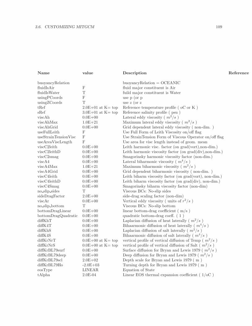
3.6. CUSTOMIZING MITGCM 109
Name value Description Reference
buoyancyRelation buoyancyRelation = OCEANICfluidIsAir F fluid major constituent is AirfluidIsWater T fuild major constituent is WaterusingPCoords F use p (or pusingZCoords T use z (or ztRef 2.0E+01 at K= top Reference temperature profile ( oC or K )sRef 3.0E+01 at K= top Reference salinity profile ( psu )viscAh 0.0E+00 Lateral eddy viscosity ( m2/s )viscAhMax 1.0E+21 Maximum lateral eddy viscosity ( m2/s )viscAhGrid 0.0E+00 Grid dependent lateral eddy viscosity ( non-dim. )useFullLeith F Use Full Form of Leith Viscosity on/off flaguseStrainTensionVisc F Use StrainTension Form of Viscous Operator on/off flaguseAreaViscLength F Use area for visc length instead of geom. meanviscC2leith 0.0E+00 Leith harmonic visc. factor (on grad(vort),non-dim.)viscC2leithD 0.0E+00 Leith harmonic viscosity factor (on grad(div),non-dim.)viscC2smag 0.0E+00 Smagorinsky harmonic viscosity factor (non-dim.)viscA4 0.0E+00 Lateral biharmonic viscosity ( m4/s )viscA4Max 1.0E+21 Maximum biharmonic viscosity ( m2/s )viscA4Grid 0.0E+00 Grid dependent biharmonic viscosity ( non-dim. )viscC4leith 0.0E+00 Leith biharm viscosity factor (on grad(vort), non-dim.)viscC4leithD 0.0E+00 Leith biharm viscosity factor (on grad(div), non-dim.)viscC4Smag 0.0E+00 Smagorinsky biharm viscosity factor (non-dim)no slip sides T Viscous BCs: No-slip sidessideDragFactor 2.0E+00 side-drag scaling factor (non-dim)viscAr 0.0E+00 Vertical eddy viscosity ( units of r2/s )no slip bottom T Viscous BCs: No-slip bottombottomDragLinear 0.0E+00 linear bottom-drag coefficient ( m/s )bottomDragQuadratic 0.0E+00 quadratic bottom-drag coeff. ( 1 )diffKhT 0.0E+00 Laplacian diffusion of heat laterally ( m2/s )diffK4T 0.0E+00 Bihaarmonic diffusion of heat laterally ( m4/s )diffKhS 0.0E+00 Laplacian diffusion of salt laterally ( m2/s )diffK4S 0.0E+00 Bihaarmonic diffusion of salt laterally ( m4/s )diffKrNrT 0.0E+00 at K= top vertical profile of vertical diffusion of Temp ( m2/s )diffKrNrS 0.0E+00 at K= top vertical profile of vertical diffusion of Salt ( m2/s )diffKrBL79surf 0.0E+00 Surface diffusion for Bryan and Lewis 1979 ( m2/s )diffKrBL79deep 0.0E+00 Deep diffusion for Bryan and Lewis 1979 ( m2/s )diffKrBL79scl 2.0E+02 Depth scale for Bryan and Lewis 1979 ( m )diffKrBL79Ho -2.0E+03 Turning depth for Bryan and Lewis 1979 ( m )eosType LINEAR Equation of StatetAlpha 2.0E-04 Linear EOS thermal expansion coefficient ( 1/oC )
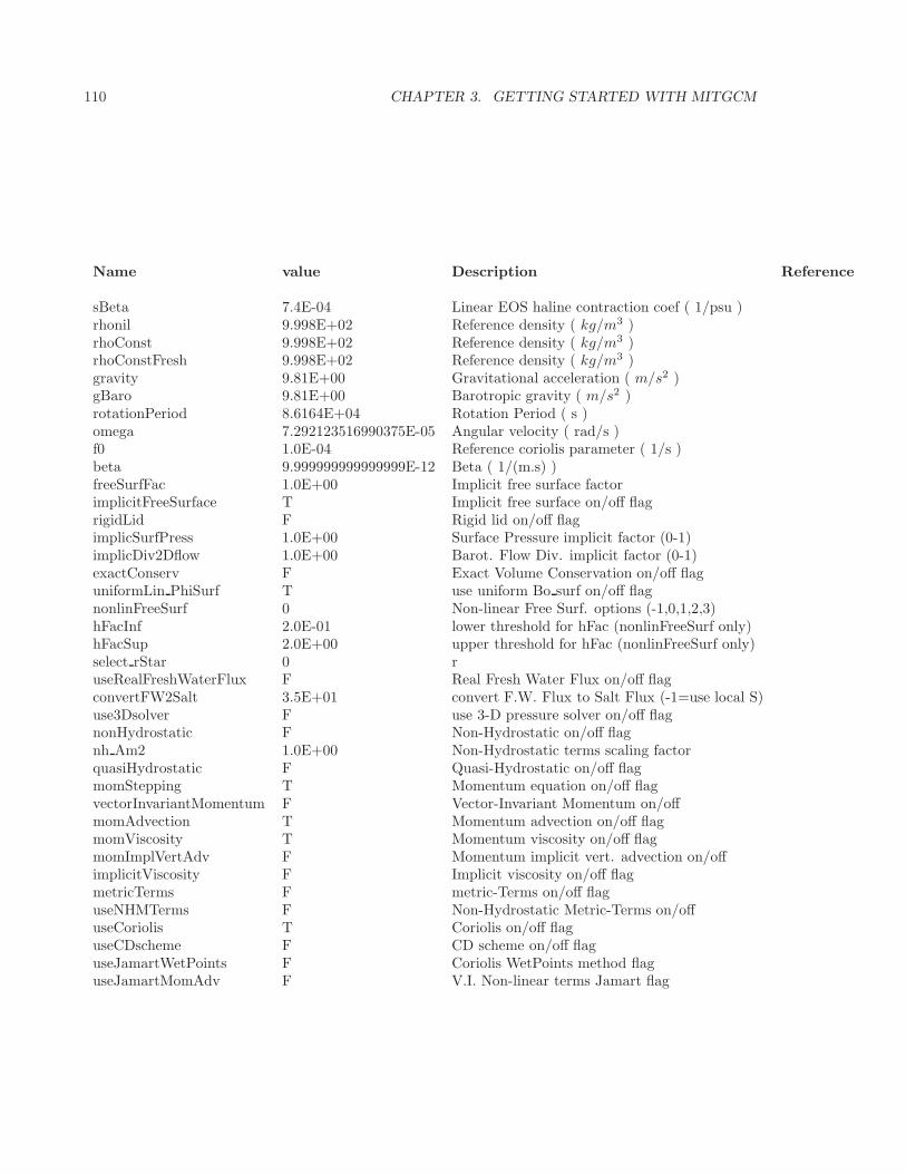
110 CHAPTER 3. GETTING STARTED WITH MITGCM
Name value Description Reference
sBeta 7.4E-04 Linear EOS haline contraction coef ( 1/psu )rhonil 9.998E+02 Reference density ( kg/m3 )rhoConst 9.998E+02 Reference density ( kg/m3 )rhoConstFresh 9.998E+02 Reference density ( kg/m3 )gravity 9.81E+00 Gravitational acceleration ( m/s2 )gBaro 9.81E+00 Barotropic gravity ( m/s2 )rotationPeriod 8.6164E+04 Rotation Period ( s )omega 7.292123516990375E-05 Angular velocity ( rad/s )f0 1.0E-04 Reference coriolis parameter ( 1/s )beta 9.999999999999999E-12 Beta ( 1/(m.s) )freeSurfFac 1.0E+00 Implicit free surface factorimplicitFreeSurface T Implicit free surface on/off flagrigidLid F Rigid lid on/off flagimplicSurfPress 1.0E+00 Surface Pressure implicit factor (0-1)implicDiv2Dflow 1.0E+00 Barot. Flow Div. implicit factor (0-1)exactConserv F Exact Volume Conservation on/off flaguniformLin PhiSurf T use uniform Bo surf on/off flagnonlinFreeSurf 0 Non-linear Free Surf. options (-1,0,1,2,3)hFacInf 2.0E-01 lower threshold for hFac (nonlinFreeSurf only)hFacSup 2.0E+00 upper threshold for hFac (nonlinFreeSurf only)select rStar 0 ruseRealFreshWaterFlux F Real Fresh Water Flux on/off flagconvertFW2Salt 3.5E+01 convert F.W. Flux to Salt Flux (-1=use local S)use3Dsolver F use 3-D pressure solver on/off flagnonHydrostatic F Non-Hydrostatic on/off flagnh Am2 1.0E+00 Non-Hydrostatic terms scaling factorquasiHydrostatic F Quasi-Hydrostatic on/off flagmomStepping T Momentum equation on/off flagvectorInvariantMomentum F Vector-Invariant Momentum on/offmomAdvection T Momentum advection on/off flagmomViscosity T Momentum viscosity on/off flagmomImplVertAdv F Momentum implicit vert. advection on/offimplicitViscosity F Implicit viscosity on/off flagmetricTerms F metric-Terms on/off flaguseNHMTerms F Non-Hydrostatic Metric-Terms on/offuseCoriolis T Coriolis on/off flaguseCDscheme F CD scheme on/off flaguseJamartWetPoints F Coriolis WetPoints method flaguseJamartMomAdv F V.I. Non-linear terms Jamart flag
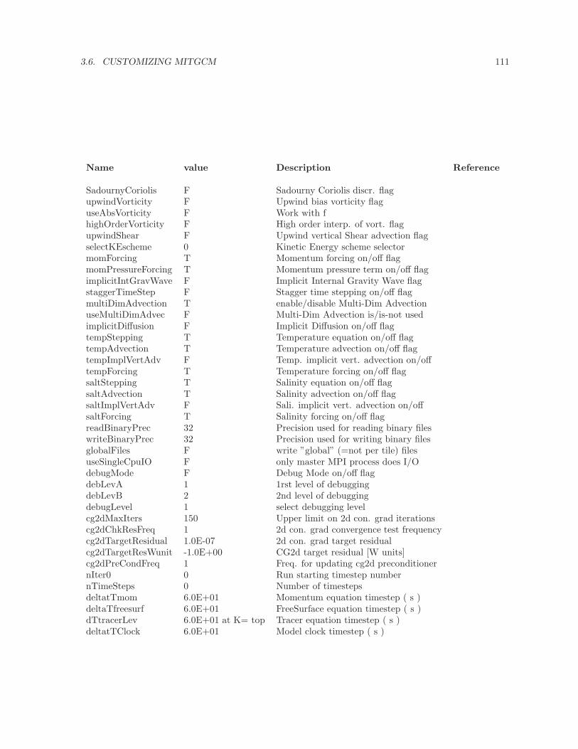
3.6. CUSTOMIZING MITGCM 111
Name value Description Reference
SadournyCoriolis F Sadourny Coriolis discr. flagupwindVorticity F Upwind bias vorticity flaguseAbsVorticity F Work with fhighOrderVorticity F High order interp. of vort. flagupwindShear F Upwind vertical Shear advection flagselectKEscheme 0 Kinetic Energy scheme selectormomForcing T Momentum forcing on/off flagmomPressureForcing T Momentum pressure term on/off flagimplicitIntGravWave F Implicit Internal Gravity Wave flagstaggerTimeStep F Stagger time stepping on/off flagmultiDimAdvection T enable/disable Multi-Dim AdvectionuseMultiDimAdvec F Multi-Dim Advection is/is-not usedimplicitDiffusion F Implicit Diffusion on/off flagtempStepping T Temperature equation on/off flagtempAdvection T Temperature advection on/off flagtempImplVertAdv F Temp. implicit vert. advection on/offtempForcing T Temperature forcing on/off flagsaltStepping T Salinity equation on/off flagsaltAdvection T Salinity advection on/off flagsaltImplVertAdv F Sali. implicit vert. advection on/offsaltForcing T Salinity forcing on/off flagreadBinaryPrec 32 Precision used for reading binary fileswriteBinaryPrec 32 Precision used for writing binary filesglobalFiles F write ”global” (=not per tile) filesuseSingleCpuIO F only master MPI process does I/OdebugMode F Debug Mode on/off flagdebLevA 1 1rst level of debuggingdebLevB 2 2nd level of debuggingdebugLevel 1 select debugging levelcg2dMaxIters 150 Upper limit on 2d con. grad iterationscg2dChkResFreq 1 2d con. grad convergence test frequencycg2dTargetResidual 1.0E-07 2d con. grad target residualcg2dTargetResWunit -1.0E+00 CG2d target residual [W units]cg2dPreCondFreq 1 Freq. for updating cg2d preconditionernIter0 0 Run starting timestep numbernTimeSteps 0 Number of timestepsdeltatTmom 6.0E+01 Momentum equation timestep ( s )deltaTfreesurf 6.0E+01 FreeSurface equation timestep ( s )dTtracerLev 6.0E+01 at K= top Tracer equation timestep ( s )deltatTClock 6.0E+01 Model clock timestep ( s )
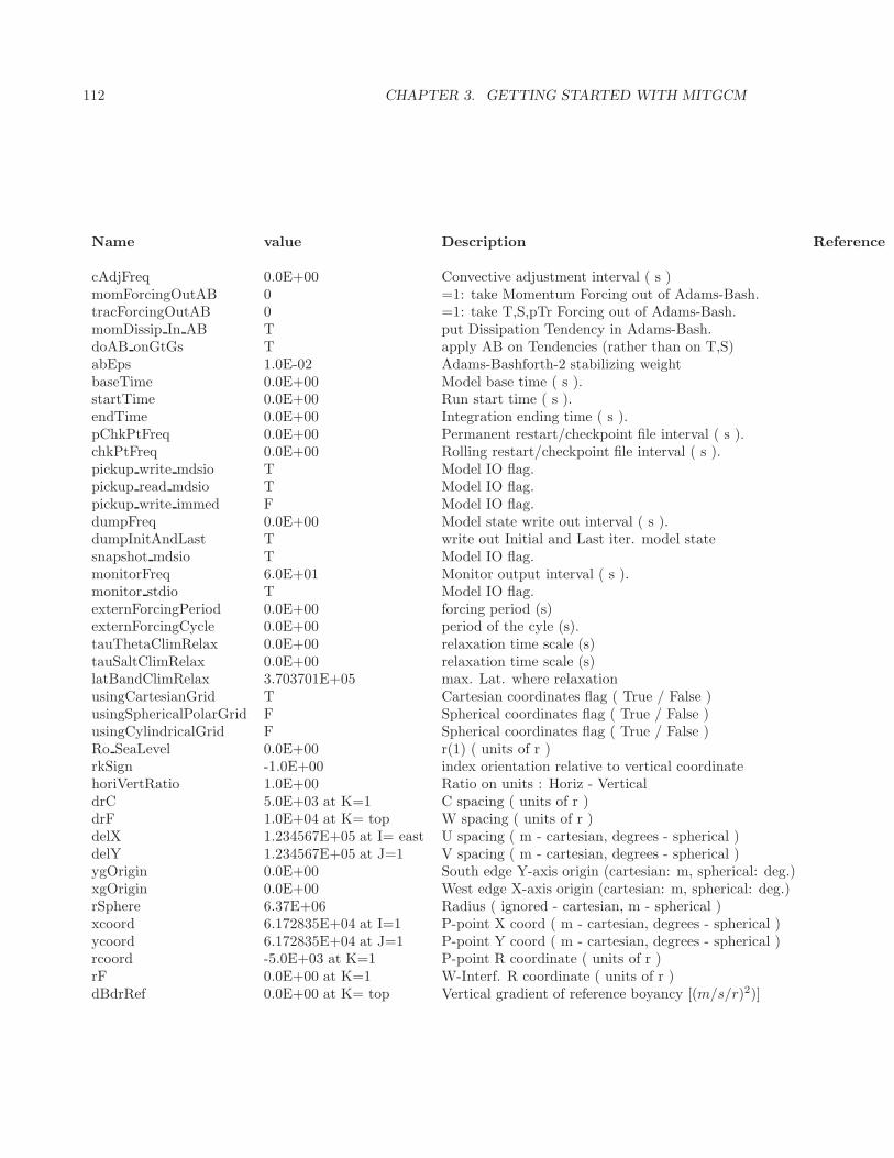
112 CHAPTER 3. GETTING STARTED WITH MITGCM
Name value Description Reference
cAdjFreq 0.0E+00 Convective adjustment interval ( s )momForcingOutAB 0 =1: take Momentum Forcing out of Adams-Bash.tracForcingOutAB 0 =1: take T,S,pTr Forcing out of Adams-Bash.momDissip In AB T put Dissipation Tendency in Adams-Bash.doAB onGtGs T apply AB on Tendencies (rather than on T,S)abEps 1.0E-02 Adams-Bashforth-2 stabilizing weightbaseTime 0.0E+00 Model base time ( s ).startTime 0.0E+00 Run start time ( s ).endTime 0.0E+00 Integration ending time ( s ).pChkPtFreq 0.0E+00 Permanent restart/checkpoint file interval ( s ).chkPtFreq 0.0E+00 Rolling restart/checkpoint file interval ( s ).pickup write mdsio T Model IO flag.pickup read mdsio T Model IO flag.pickup write immed F Model IO flag.dumpFreq 0.0E+00 Model state write out interval ( s ).dumpInitAndLast T write out Initial and Last iter. model statesnapshot mdsio T Model IO flag.monitorFreq 6.0E+01 Monitor output interval ( s ).monitor stdio T Model IO flag.externForcingPeriod 0.0E+00 forcing period (s)externForcingCycle 0.0E+00 period of the cyle (s).tauThetaClimRelax 0.0E+00 relaxation time scale (s)tauSaltClimRelax 0.0E+00 relaxation time scale (s)latBandClimRelax 3.703701E+05 max. Lat. where relaxationusingCartesianGrid T Cartesian coordinates flag ( True / False )usingSphericalPolarGrid F Spherical coordinates flag ( True / False )usingCylindricalGrid F Spherical coordinates flag ( True / False )Ro SeaLevel 0.0E+00 r(1) ( units of r )rkSign -1.0E+00 index orientation relative to vertical coordinatehoriVertRatio 1.0E+00 Ratio on units : Horiz - VerticaldrC 5.0E+03 at K=1 C spacing ( units of r )drF 1.0E+04 at K= top W spacing ( units of r )delX 1.234567E+05 at I= east U spacing ( m - cartesian, degrees - spherical )delY 1.234567E+05 at J=1 V spacing ( m - cartesian, degrees - spherical )ygOrigin 0.0E+00 South edge Y-axis origin (cartesian: m, spherical: deg.)xgOrigin 0.0E+00 West edge X-axis origin (cartesian: m, spherical: deg.)rSphere 6.37E+06 Radius ( ignored - cartesian, m - spherical )xcoord 6.172835E+04 at I=1 P-point X coord ( m - cartesian, degrees - spherical )ycoord 6.172835E+04 at J=1 P-point Y coord ( m - cartesian, degrees - spherical )rcoord -5.0E+03 at K=1 P-point R coordinate ( units of r )rF 0.0E+00 at K=1 W-Interf. R coordinate ( units of r )dBdrRef 0.0E+00 at K= top Vertical gradient of reference boyancy [(m/s/r)2)]
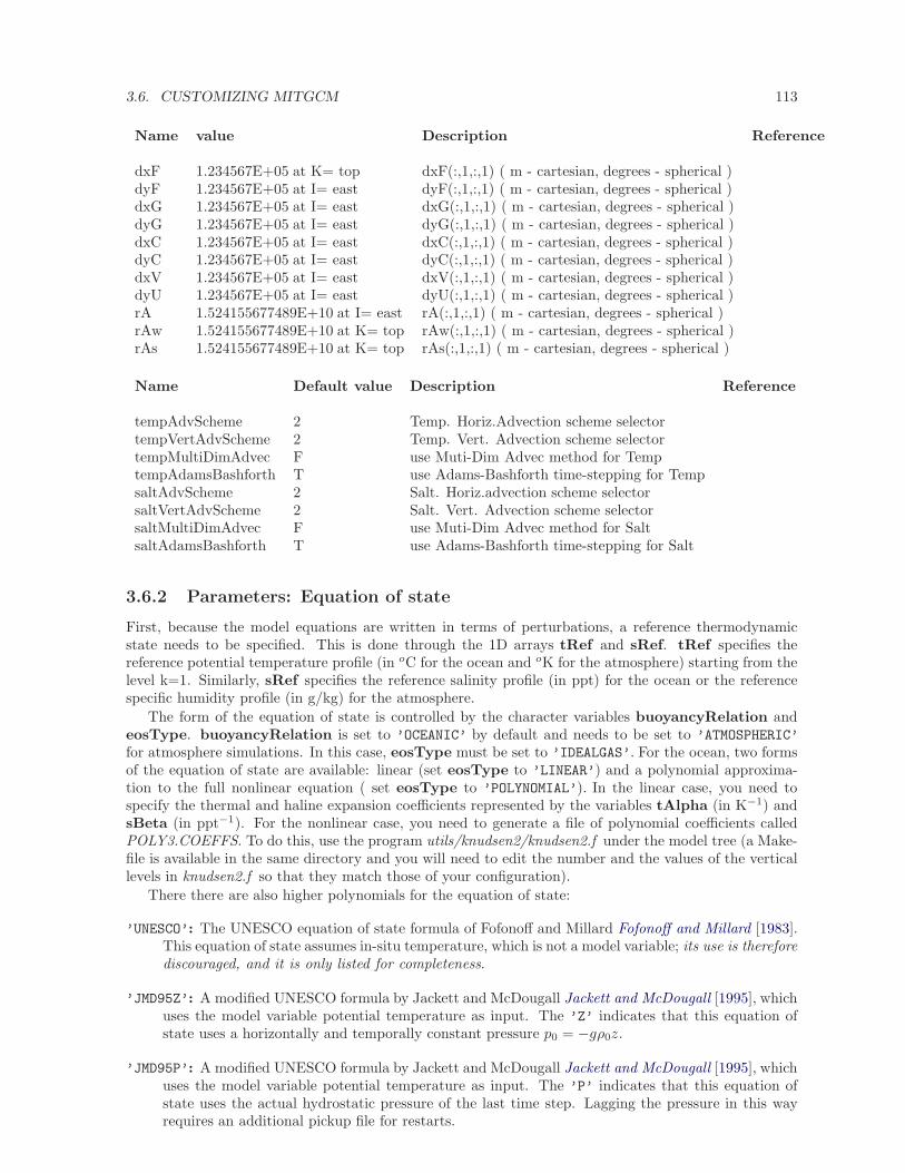
3.6. CUSTOMIZING MITGCM 113
Name value Description Reference
dxF 1.234567E+05 at K= top dxF(:,1,:,1) ( m - cartesian, degrees - spherical )dyF 1.234567E+05 at I= east dyF(:,1,:,1) ( m - cartesian, degrees - spherical )dxG 1.234567E+05 at I= east dxG(:,1,:,1) ( m - cartesian, degrees - spherical )dyG 1.234567E+05 at I= east dyG(:,1,:,1) ( m - cartesian, degrees - spherical )dxC 1.234567E+05 at I= east dxC(:,1,:,1) ( m - cartesian, degrees - spherical )dyC 1.234567E+05 at I= east dyC(:,1,:,1) ( m - cartesian, degrees - spherical )dxV 1.234567E+05 at I= east dxV(:,1,:,1) ( m - cartesian, degrees - spherical )dyU 1.234567E+05 at I= east dyU(:,1,:,1) ( m - cartesian, degrees - spherical )rA 1.524155677489E+10 at I= east rA(:,1,:,1) ( m - cartesian, degrees - spherical )rAw 1.524155677489E+10 at K= top rAw(:,1,:,1) ( m - cartesian, degrees - spherical )rAs 1.524155677489E+10 at K= top rAs(:,1,:,1) ( m - cartesian, degrees - spherical )
Name Default value Description Reference
tempAdvScheme 2 Temp. Horiz.Advection scheme selectortempVertAdvScheme 2 Temp. Vert. Advection scheme selectortempMultiDimAdvec F use Muti-Dim Advec method for TemptempAdamsBashforth T use Adams-Bashforth time-stepping for TempsaltAdvScheme 2 Salt. Horiz.advection scheme selectorsaltVertAdvScheme 2 Salt. Vert. Advection scheme selectorsaltMultiDimAdvec F use Muti-Dim Advec method for SaltsaltAdamsBashforth T use Adams-Bashforth time-stepping for Salt
3.6.2 Parameters: Equation of state
First, because the model equations are written in terms of perturbations, a reference thermodynamicstate needs to be specified. This is done through the 1D arrays tRef and sRef. tRef specifies thereference potential temperature profile (in oC for the ocean and oK for the atmosphere) starting from thelevel k=1. Similarly, sRef specifies the reference salinity profile (in ppt) for the ocean or the referencespecific humidity profile (in g/kg) for the atmosphere.
The form of the equation of state is controlled by the character variables buoyancyRelation andeosType. buoyancyRelation is set to ’OCEANIC’ by default and needs to be set to ’ATMOSPHERIC’
for atmosphere simulations. In this case, eosType must be set to ’IDEALGAS’. For the ocean, two formsof the equation of state are available: linear (set eosType to ’LINEAR’) and a polynomial approxima-tion to the full nonlinear equation ( set eosType to ’POLYNOMIAL’). In the linear case, you need tospecify the thermal and haline expansion coefficients represented by the variables tAlpha (in K−1) andsBeta (in ppt−1). For the nonlinear case, you need to generate a file of polynomial coefficients calledPOLY3.COEFFS. To do this, use the program utils/knudsen2/knudsen2.f under the model tree (a Make-file is available in the same directory and you will need to edit the number and the values of the verticallevels in knudsen2.f so that they match those of your configuration).
There there are also higher polynomials for the equation of state:
’UNESCO’: The UNESCO equation of state formula of Fofonoff and Millard Fofonoff and Millard [1983].This equation of state assumes in-situ temperature, which is not a model variable; its use is thereforediscouraged, and it is only listed for completeness.
’JMD95Z’: A modified UNESCO formula by Jackett and McDougall Jackett and McDougall [1995], whichuses the model variable potential temperature as input. The ’Z’ indicates that this equation ofstate uses a horizontally and temporally constant pressure p0 = −gρ0z.
’JMD95P’: A modified UNESCO formula by Jackett and McDougall Jackett and McDougall [1995], whichuses the model variable potential temperature as input. The ’P’ indicates that this equation ofstate uses the actual hydrostatic pressure of the last time step. Lagging the pressure in this wayrequires an additional pickup file for restarts.
114 CHAPTER 3. GETTING STARTED WITH MITGCM
’MDJWF’: The new, more accurate and less expensive equation of state by McDougall et al. McDougallet al. [2003]. It also requires lagging the pressure and therefore an additional pickup file for restarts.
For none of these options an reference profile of temperature or salinity is required.
3.6.3 Parameters: Momentum equations
In this section, we only focus for now on the parameters that you are likely to change, i.e. the onesrelative to forcing and dissipation for example. The details relevant to the vector-invariant form of theequations and the various advection schemes are not covered for the moment. We assume that you usethe standard form of the momentum equations (i.e. the flux-form) with the default advection scheme.Also, there are a few logical variables that allow you to turn on/off various terms in the momentumequation. These variables are called momViscosity, momAdvection, momForcing, useCoriolis,momPressureForcing, momStepping and metricTerms and are assumed to be set to ’.TRUE.’
here. Look at the file model/inc/PARAMS.h for a precise definition of these variables.
initialization
The initial horizontal velocity components can be specified from binary files uVelInitFile andvVelInitFile. These files should contain 3D data ordered in an (x,y,r) fashion with k=1 as the firstvertical level (surface level). If no file names are provided, the velocity is initialised to zero. Theinitial vertical velocity is always derived from the horizontal velocity using the continuity equation,even in the case of non-hydrostatic simulation (see, e.g.: tutorial deep convection/input/data).
In the case of a restart (from the end of a previous simulation), the velocity field is read from apickup file (see section on simulation control parameters) and the initial velocity files are ignored.
forcing
This section only applies to the ocean. You need to generate wind-stress data into two files zonal-WindFile and meridWindFile corresponding to the zonal and meridional components of the windstress, respectively (if you want the stress to be along the direction of only one of the model hori-zontal axes, you only need to generate one file). The format of the files is similar to the bathymetryfile. The zonal (meridional) stress data are assumed to be in Pa and located at U-points (V-points).As for the bathymetry, the precision with which to read the binary data is controlled by the variablereadBinaryPrec. See the matlab program gendata.m in the input directories under verificationto see how simple analytical wind forcing data are generated for the case study experiments.
There is also the possibility of prescribing time-dependent periodic forcing. To do this, concatenatethe successive time records into a single file (for each stress component) ordered in a (x,y,t) fashionand set the following variables: periodicExternalForcing to ’.TRUE.’, externForcingPeriodto the period (in s) of which the forcing varies (typically 1 month), and externForcingCycle tothe repeat time (in s) of the forcing (typically 1 year – note: externForcingCycle must be amultiple of externForcingPeriod). With these variables set up, the model will interpolate theforcing linearly at each iteration.
dissipation
The lateral eddy viscosity coefficient is specified through the variable viscAh (in m2s−1). Thevertical eddy viscosity coefficient is specified through the variable viscAz (in m2s−1) for the oceanand viscAp (in Pa2s−1) for the atmosphere. The vertical diffusive fluxes can be computed implicitlyby setting the logical variable implicitViscosity to ’.TRUE.’. In addition, biharmonic mixing canbe added as well through the variable viscA4 (in m4s−1). On a spherical polar grid, you mightalso need to set the variable cosPower which is set to 0 by default and which represents thepower of cosine of latitude to multiply viscosity. Slip or no-slip conditions at lateral and bottomboundaries are specified through the logical variables no slip sides and no slip bottom. If setto ’.FALSE.’, free-slip boundary conditions are applied. If no-slip boundary conditions are appliedat the bottom, a bottom drag can be applied as well. Two forms are available: linear (set thevariable bottomDragLinear in m/s) and quadratic (set the variable bottomDragQuadratic,dimensionless).
The Fourier and Shapiro filters are described elsewhere.
3.6. CUSTOMIZING MITGCM 115
C-D scheme
If you run at a sufficiently coarse resolution, you will need the C-D scheme for the computation ofthe Coriolis terms. The variable tauCD, which represents the C-D scheme coupling timescale (ins) needs to be set.
calculation of pressure/geopotential
First, to run a non-hydrostatic ocean simulation, set the logical variable nonHydrostatic to’.TRUE.’. The pressure field is then inverted through a 3D elliptic equation. (Note: this ca-pability is not available for the atmosphere yet.) By default, a hydrostatic simulation is assumedand a 2D elliptic equation is used to invert the pressure field. The parameters controlling the be-haviour of the elliptic solvers are the variables cg2dMaxIters and cg2dTargetResidual for the2D case and cg3dMaxIters and cg3dTargetResidual for the 3D case. You probably won’t needto alter the default values (are we sure of this?).
For the calculation of the surface pressure (for the ocean) or surface geopotential (for the at-mosphere) you need to set the logical variables rigidLid and implicitFreeSurface (set one to’.TRUE.’ and the other to ’.FALSE.’ depending on how you want to deal with the ocean upperor atmosphere lower boundary).
3.6.4 Parameters: Tracer equations
This section covers the tracer equations i.e. the potential temperature equation and the salinity (for theocean) or specific humidity (for the atmosphere) equation. As for the momentum equations, we onlydescribe for now the parameters that you are likely to change. The logical variables tempDiffusiontempAdvection tempForcing, and tempStepping allow you to turn on/off terms in the temperatureequation (same thing for salinity or specific humidity with variables saltDiffusion, saltAdvection etc.).These variables are all assumed here to be set to ’.TRUE.’. Look at file model/inc/PARAMS.h for aprecise definition.
initialization
The initial tracer data can be contained in the binary files hydrogThetaFile and hydrogSaltFile.These files should contain 3D data ordered in an (x,y,r) fashion with k=1 as the first vertical level.If no file names are provided, the tracers are then initialized with the values of tRef and sRefmentioned above (in the equation of state section). In this case, the initial tracer data are uniformin x and y for each depth level.
forcing
This part is more relevant for the ocean, the procedure for the atmosphere not being completelystabilized at the moment.
A combination of fluxes data and relaxation terms can be used for driving the tracer equations.For potential temperature, heat flux data (in W/m2) can be stored in the 2D binary file surfQfile.Alternatively or in addition, the forcing can be specified through a relaxation term. The SST datato which the model surface temperatures are restored to are supposed to be stored in the 2D binaryfile thetaClimFile. The corresponding relaxation time scale coefficient is set through the variabletauThetaClimRelax (in s). The same procedure applies for salinity with the variable namesEmPmRfile, saltClimFile, and tauSaltClimRelax for freshwater flux (in m/s) and surfacesalinity (in ppt) data files and relaxation time scale coefficient (in s), respectively. Also for salinity,if the CPP key USE NATURAL BCS is turned on, natural boundary conditions are appliedi.e. when computing the surface salinity tendency, the freshwater flux is multiplied by the modelsurface salinity instead of a constant salinity value.
As for the other input files, the precision with which to read the data is controlled by the variablereadBinaryPrec. Time-dependent, periodic forcing can be applied as well following the sameprocedure used for the wind forcing data (see above).
dissipation
116 CHAPTER 3. GETTING STARTED WITH MITGCM
Lateral eddy diffusivities for temperature and salinity/specific humidity are specified through thevariables diffKhT and diffKhS (in m2/s). Vertical eddy diffusivities are specified through thevariables diffKzT and diffKzS (in m2/s) for the ocean and diffKpT and diffKpS (in Pa2/s)for the atmosphere. The vertical diffusive fluxes can be computed implicitly by setting the logicalvariable implicitDiffusion to ’.TRUE.’. In addition, biharmonic diffusivities can be specifiedas well through the coefficients diffK4T and diffK4S (in m4/s). Note that the cosine powerscaling (specified through cosPower—see the momentum equations section) is applied to the tracerdiffusivities (Laplacian and biharmonic) as well. The Gent and McWilliams parameterization foroceanic tracers is described in the package section. Finally, note that tracers can be also subject toFourier and Shapiro filtering (see the corresponding section on these filters).
ocean convection
Two options are available to parameterize ocean convection: one is to use the convective adjustmentscheme. In this case, you need to set the variable cadjFreq, which represents the frequency (ins) with which the adjustment algorithm is called, to a non-zero value (if set to a negative valueby the user, the model will set it to the tracer time step). The other option is to parameterizeconvection with implicit vertical diffusion. To do this, set the logical variable implicitDiffusionto ’.TRUE.’ and the real variable ivdc kappa to a value (in m2/s) you wish the tracer verticaldiffusivities to have when mixing tracers vertically due to static instabilities. Note that cadjFreqand ivdc kappacan not both have non-zero value.
3.6.5 Parameters: Simulation controls
The model ”clock” is defined by the variable deltaTClock (in s) which determines the IO frequenciesand is used in tagging output. Typically, you will set it to the tracer time step for accelerated runs(otherwise it is simply set to the default time step deltaT). Frequency of checkpointing and dumping ofthe model state are referenced to this clock (see below).
run duration
The beginning of a simulation is set by specifying a start time (in s) through the real variablestartTime or by specifying an initial iteration number through the integer variable nIter0. Ifthese variables are set to nonzero values, the model will look for a ”pickup” file pickup.0000nIter0to restart the integration. The end of a simulation is set through the real variable endTime (ins). Alternatively, you can specify instead the number of time steps to execute through the integervariable nTimeSteps.
frequency of output
Real variables defining frequencies (in s) with which output files are written on disk need to be setup. dumpFreq controls the frequency with which the instantaneous state of the model is saved.chkPtFreq and pchkPtFreq control the output frequency of rolling and permanent checkpointfiles, respectively. See section 1.5.1 Output files for the definition of model state and checkpoint files.In addition, time-averaged fields can be written out by setting the variable taveFreq (in s). Theprecision with which to write the binary data is controlled by the integer variable writeBinaryPrec(set it to 32 or 64).
3.7. TESTING 117
3.7 Testing
A script (testreport) for automated testing is included in the model within the verification directory.While intended mostly for advanced users, the script can be helpful for beginners.
3.7.1 Using testreport
On many systems, the program can be run with the command:
% cd verification
% ./testreport
which will do the following:
1. Locate all “valid” test directories. Here, valid tests are defined to be those directories within thecurrent directory (which is generally verification) that contain a subdirectory and file with thenames results/output.txt.
2. Then within each valid test:
(a) run genmake2 to produce a Makefile
(b) build an executable
(c) run the executable
(d) compare and the output of the executable with the contents of certain variables within TEST-NAME/results/output.txt
(e) print and, if requested (with the -addr=EMAIL ADDRESS option), send a MIME-encoded emailwith the testing results
For further details, please see the MITgcm Developers’ HOWTO at:
http://mitgcm.org/public/docs.html
3.7.2 Automated testing
Automated testing results are produced on a regular basis and they can be viewed at:
http://mitgcm.org/public/testing.html
which also includes links to various scripts for batch job submission on a variety of different machines.
118 CHAPTER 3. GETTING STARTED WITH MITGCM
3.8 Example experiments
The full MITgcm distribution comes with a set of pre-configured numerical experiments. Some of theseexample experiments are tests of individual parts of the model code, but many are fully fledged numericalsimulations. Full tutorials exist for a few of the examples, and are documented in sections 3.9 - 3.21. Theother examples follow the same general structure as the tutorial examples. However, they only includebrief instructions in a text file called README. The examples are located in subdirectories under thedirectory verification. Each example is briefly described below.
3.8.1 Full list of model examples
1. tutorial advection in gyre - Test of various advection schemes in a single-layer double-gyreexperiment. This experiment is described in detail in section 3.11.
2. tutorial baroclinic gyre - Four layer, ocean double gyre. This experiment is described in detailin section 3.10.
3. tutorial barotropic gyre - Single layer, ocean double gyre (barotropic with free-surface). Thisexperiment is described in detail in section 3.9.
4. tutorial cfc offline - Offline form of the MITgcm to study advection of a passive tracer andCFCs. This experiment is described in detail in section 3.20.5.
5. tutorial deep convection - Non-uniformly forced ocean convection in a doubly periodic box.This experiment is described in detail in section 3.15.
6. tutorial dic adoffline - Offline form of MITgcm dynamics coupled to the dissolved inorganiccarbon biogeochemistry model; adjoint set-up.
7. tutorial global oce biogeo - Ocean model coupled to the dissolved inorganic carbon biogeo-chemistry model. This experiment is described in detail in section 3.17.
8. tutorial global oce in p - Global ocean simulation in pressure coordinate (non-Boussinesq oceanmodel). Described in detail in section 3.13.
9. tutorial global oce latlon - 4x4 degree global ocean simulation with steady climatological forc-ing. This experiment is described in detail in section 3.12.
10. tutorial global oce optim - Global ocean state estimation at 4 resolution. This experiment isdescribed in detail in section 3.18.
11. tutorial held suarez cs - 3D atmosphere dynamics using Held and Suarez (1994) forcing oncubed sphere grid. This experiment is described in detail in section 3.14.
12. tutorial offline - Offline form of the MITgcm to study advection of a passive tracer. Thisexperiment is described in detail in section 3.20.
13. tutorial plume on slope - Gravity Plume on a continental slope. This experiment is describedin detail in section 3.16.
14. tutorial tracer adjsens - Simple passive tracer experiment. Includes derivative calculation.This experiment is described in detail in section 3.19.Also contains an additional set-up using Secon Order Moment (SOM) advection scheme (input ad.som81/).
15. 1D ocean ice column - Oceanic column with seaice on top.
16. adjustment.128x64x1 - Barotropic adjustment problem on latitude longitude grid with 128x64grid points (2.8 resolution).
17. adjustment.cs-32x32x1 - Barotropic adjustment problem on cube sphere grid with 32x32 pointsper face (roughly 2.8 resolution).Also contains a non-linear free-surface adjustment version (input.nlfs/).
3.8. MITGCM EXAMPLE EXPERIMENTS 119
18. advect cs - Two-dimensional passive advection test on cube sphere grid (32x32 grid points perface, roughly 2.8 resolution)
19. advect xy - Two-dimensional (horizontal plane) passive advection test on Cartesian grid.Also contains an additional set-up using Adams-Bashforth 3 (input.ab3 c4/).
20. advect xz - Two-dimensional (vertical plane) passive advection test on Cartesian grid.Also contains an additional set-up using non-linear free-surface with divergent barotropic flow andimplicit vertical advection (input.nlfs/).
21. aim.5l Equatorial Channel - 5-levels Intermediate Atmospheric physics, 3D Equatorial Channelconfiguration.
22. aim.5l LatLon - 5-levels Intermediate Atmospheric physics, Global configuration, on latitude lon-gitude grid with 128x64x5 grid points (2.8 resolution).
23. aim.5l cs - 5-levels Intermediate Atmospheric physics, Global configuration on cube sphere grid(32x32 grid points per face, roughly 2.8).Also contains an additional set-up with a slab-ocean and thermodynamic sea-ice (input.thSI/).
24. bottom ctrl 5x5 - Adjoint test using the bottom topography as the control parameter.
25. cfc example - Global ocean with online computation and advection of CFC11 and CFC12.
26. cheapAML box - Example using cheap atmospheric mixed layer (cheapAML) package.
27. cpl aim+ocn - Coupled Ocean - Atmosphere realistic configuration on cubed-sphere cs32 horizontalgrid, using Intermediate Atmospheric physics (pkg/aim v23) thermodynamic seaice (pkg/thsice) andland packages. on cubed-sphere cs32 in a realistic configuration.
28. cpl atm2d+ocn - Coupled Ocean - Atmosphere realistic configuration using 2-D Atmospheric Model(pkg/atm2d).
29. deep anelastic - Convection simulation on a giant planet: relax both the Boussinesq approxima-tion (anelastic) and the thin atmosphere approximation (deep atmosphere).
30. dome - Idealized 3D test of a density-driven bottom current.
31. exp2 - Old version of the global ocean experiment (no GM, no partial-cells).Also contains an additional set-up with rigid-lid (input.rigidLid/).
32. exp4 - Flow over a Gaussian bump in open-water or channel with open boundaries.Also contains an additional set-up using non-linear free-surface (input.nlfs/).
33. fizhi-cs-32x32x40 - Global atmospheric simulation with realistic topography, 40 vertical levels,a cubed sphere grid and the full atmospheric physics package.
34. fizhi-cs-aqualev20 - Global atmospheric simulation on an aqua planet with full atmosphericphysics. Run is perpetual march with an analytical SST distribution. This is the configuration forthe APE (Aqua Planet Experiment) participation experiment.
35. fizhi-gridalt-hs - Global atmospheric simulation Held-Suarez (1994) forcing, with the physicalforcing and the dynamical forcing running on different vertical grids.
36. flt example - Example of using float package.
37. front relax - Relaxation of an ocean thermal front (test for Gent/McWilliams scheme). 2D (y-z).Also contains additional set-ups:
(a) using the Boundary-Value Problem method (Ferrari et al., 2010) (input.bvp/).
(b) with Mixed-Layer Eddy parameterization (Ferrari & McWilliams, 2007) (input.mxl/).
120 CHAPTER 3. GETTING STARTED WITH MITGCM
38. global ocean.90x40x15 - Global ocean simulation at 4x4 degree resolution. Similar to tuto-rial global oce latlon, but using z∗ coordinates with quasi-non-hydrostatic and non-hydrostaticmetric terms. This experiment also illustrate the use of SBO package. Also contains additionalset-ups:
(a) using down-slope package (pkg/down slope) (input.dwnslp/)
(b) an Open-AD adjoint set-up (code oad/, input oad/).
(c) four TAF adjoint set-ups (code ad/):
i. standard experiment (input ad/).
ii. with bottom drag as a control (input ad.bottomdrag/).
iii. with kappa GM as a control (input ad.kapgm/).
iv. with kappa Redi as a control (input ad.kapredi/).
39. global ocean.cs32x15 - Global ocean experiment on the cubed sphere grid.Also contains additional forward set-ups:
(a) non-hydrostatic with biharmonic viscosity (input.viscA4/)
(b) using thermodynamic sea ice and bulk force (input.thsice/)
(c) using thermodynamic (pkg/thsice) dynamic (pkg/seaice) sea-ice and exf package (input.icedyn/)
(d) using thermodynamic - dynamic (pkg/seaice) sea-ice with exf package (input.seaice/)
and few additional adjoint set-ups (code ad/):
(a) standard experiment without sea-ice (input ad/).
(b) using thermodynamic - dynamic sea-ice (input ad.seaice/)
(c) same as above without adjoint sea-ice dynamics (input ad.seaice dynmix/)
(d) using thermodynamic sea-ice from thsice package (input ad.thsice/)
40. global ocean ebm - Global ocean experiment on a lat-lon grid coupled to an atmospheric energybalance model. Similar to global ocean.90x40x15 experiment.Also contains an adjoint set-up (code ad/, input ad/).
41. global with exf - Global ocean experiment on a lat-lon grid using the exf package. Similar totutorial global oce latlon experiment.Also contains a secondary set-up with yearly exf fields (input ad.yearly/).
42. halfpipe streamice - Example using package ”streamice”.Also contains adjoint set-ups using TAF (code ad/, input ad/) and using Open-AD (code oad/,input oad/).
43. hs94.128x64x5 - 3D atmosphere dynamics on lat-lon grid, using Held and Suarez ’94 forcing.
44. hs94.1x64x5 - Zonal averaged atmosphere dynamics using Held and Suarez ’94 forcing.Also contains adjoint set-ups using TAF (code ad/, input ad/) and using Open-AD (code oad/,input oad/).
45. hs94.cs-32x32x5 - 3D atmosphere dynamics using Held and Suarez (1994) forcing on the cubedsphere, similar to tutorial held suarez cs experiment but using linear free-surface and only 5 levels.Also contains an additional set-up with Implicit Internal gravity waves treatment and Adams-Bashforth 3 (input.impIGW/).
46. ideal 2D oce - Idealized 2D global ocean simulation on an aqua planet.
47. internal wave - Ocean internal wave forced by open boundary conditions.Also contains an additional set-up using pkg/kl10 (see section 6.4.5, Klymak and Legg, 2010) (in-put.kl10/).
48. inverted barometer - Simple test of ocean response to atmospheric pressure loading.
3.8. MITGCM EXAMPLE EXPERIMENTS 121
49. isomip - ISOMIP like set-up including ice-shelf cavities (pkg/shelfice).Also contains additional set-ups:
(a) with ”htd” (input.htd/) but only Martin knows what ”htd” stands for.
(b) using package icefront (input.icefront)
and also adjoint set-ups using TAF (code ad/, input ad/, input ad.htd/) or using Open-AD (code oad/,input oad/).
50. lab sea - Regional Labrador Sea simulation on a lat-lon grid using the sea ice package.Also contains additional set-ups:
(a) using the simple ”free-drift” assumption for seaice (input.fd/)
(b) using EVP dynamics (instead of LSR solver) and Hibler & Bryan (1987) sea-ice ocean stress(input.hb87/)
(c) using package salt plume (input.salt plume/)
and also 3 adjoint set-ups (code ad/, input ad/, input ad.noseaicedyn/, input ad.noseaice/).
51. matrix example - Test of experimental method to accelerated convergence towards equilibrium.
52. MLAdjust - Simple tests for different viscosity formulations.Also contains additional set-ups (see: verification/MLAdjust/README):
(a) (input.A4FlxF/)
(b) (input.AhFlxF/)
(c) (input.AhVrDv/)
(d) (input.AhStTn/)
53. natl box - Eastern subtropical North Atlantic with KPP scheme; 1 month integration
54. obcs ctrl - Adjoint test using Open-Boundary conditions as control parameters.
55. offline exf seaice - Seaice on top of oceanic surface layer in an idealized channel. Forcing iscomputed by bulk-formulae (pkg/exf) with temperature relaxation to prescribed SST (offline ocean).Also contains additional set-ups:
(a) sea-ice dynamics-only using JFNK solver and pkg/thsice advection (input.dyn jfnk/)
(b) sea-ice dynamics-only using LSR solver and pkg/seaice advection (input.dyn lsr/)
(c) sea-ice thermodynamics-only using pkg/seaice (input.thermo/)
(d) sea-ice thermodynamics-only using pkg/thsice (input.thsice/)
and also 2 adjoint set-ups (code ad/, input ad/, input ad.thsice/).
56. OpenAD - Simple Adjoint experiment (used also to test Open-AD compiler)
57. rotating tank - Rotating tank simulation in cylindrical coordinates. This experiment is describedin detail in section 3.21.
58. seaice itd - Seaice example using Ice Thickness Distribution (ITD).Also contains additional set-ups:
(a) (input.thermo/)
(b) (input.lipscomb07/)
59. seaice obcs - Similar to ”lab sea” (input.salt plume/) experiment with only a fraction of thedomain and open-boundary conditions derived from ”lab sea” experiment.Also contains additional set-ups:
(a) (input.seaiceSponge/)
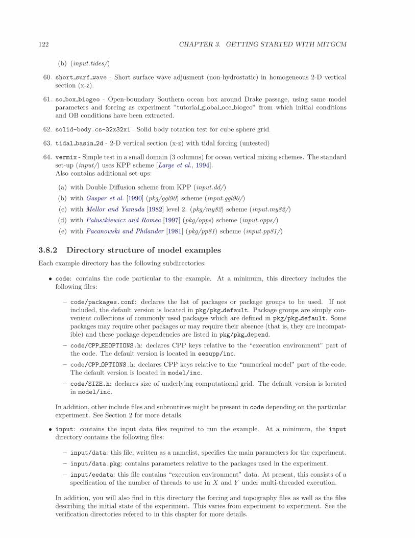
122 CHAPTER 3. GETTING STARTED WITH MITGCM
(b) (input.tides/)
60. short surf wave - Short surface wave adjusment (non-hydrostatic) in homogeneous 2-D verticalsection (x-z).
61. so box biogeo - Open-boundary Southern ocean box around Drake passage, using same modelparameters and forcing as experiment ”tutorial global oce biogeo” from which initial conditionsand OB conditions have been extracted.
62. solid-body.cs-32x32x1 - Solid body rotation test for cube sphere grid.
63. tidal basin 2d - 2-D vertical section (x-z) with tidal forcing (untested)
64. vermix - Simple test in a small domain (3 columns) for ocean vertical mixing schemes. The standardset-up (input/) uses KPP scheme [Large et al., 1994].Also contains additional set-ups:
(a) with Double Diffusion scheme from KPP (input.dd/)
(b) with Gaspar et al. [1990] (pkg/ggl90) scheme (input.ggl90/)
(c) with Mellor and Yamada [1982] level 2. (pkg/my82) scheme (input.my82/)
(d) with Paluszkiewicz and Romea [1997] (pkg/opps) scheme (input.opps/)
(e) with Pacanowski and Philander [1981] (pkg/pp81) scheme (input.pp81/)
3.8.2 Directory structure of model examples
Each example directory has the following subdirectories:
• code: contains the code particular to the example. At a minimum, this directory includes thefollowing files:
– code/packages.conf: declares the list of packages or package groups to be used. If notincluded, the default version is located in pkg/pkg default. Package groups are simply con-venient collections of commonly used packages which are defined in pkg/pkg default. Somepackages may require other packages or may require their absence (that is, they are incompat-ible) and these package dependencies are listed in pkg/pkg depend.
– code/CPP EEOPTIONS.h: declares CPP keys relative to the “execution environment” part ofthe code. The default version is located in eesupp/inc.
– code/CPP OPTIONS.h: declares CPP keys relative to the “numerical model” part of the code.The default version is located in model/inc.
– code/SIZE.h: declares size of underlying computational grid. The default version is locatedin model/inc.
In addition, other include files and subroutines might be present in code depending on the particularexperiment. See Section 2 for more details.
• input: contains the input data files required to run the example. At a minimum, the input
directory contains the following files:
– input/data: this file, written as a namelist, specifies the main parameters for the experiment.
– input/data.pkg: contains parameters relative to the packages used in the experiment.
– input/eedata: this file contains “execution environment” data. At present, this consists of aspecification of the number of threads to use in X and Y under multi-threaded execution.
In addition, you will also find in this directory the forcing and topography files as well as the filesdescribing the initial state of the experiment. This varies from experiment to experiment. See theverification directories refered to in this chapter for more details.
3.8. MITGCM EXAMPLE EXPERIMENTS 123
• results: this directory contains the output file output.txt produced by the simulation example.This file is useful for comparison with your own output when you run the experiment.
• build: this directory is initially empty and is used to compile and load the model, and to generatethe executable.
• run: this directory is initially empty and is used to run the executable.
Once you have chosen the example you want to run, you are ready to compile the code.
124 CHAPTER 3. GETTING STARTED WITH MITGCM
3.9 Barotropic Ocean Gyre In Cartesian Coordinates
(in directory: verification/tutorial barotropic gyre/)
This example experiment demonstrates using the MITgcm to simulate a Barotropic, wind-forced,ocean gyre circulation. The files for this experiment can be found in the verification directory tuto-rial barotropic gyre. The experiment is a numerical rendition of the gyre circulation problem similar tothe problems described analytically by Stommel in 1966 Stommel [1948] and numerically in Holland et.al Holland and Lin [975a].
In this experiment the model is configured to represent a rectangular enclosed box of fluid, 1200 ×1200 km in lateral extent. The fluid is 5 km deep and is forced by a constant in time zonal wind stress,τx, that varies sinusoidally in the “north-south” direction. Topologically the grid is Cartesian and thecoriolis parameter f is defined according to a mid-latitude beta-plane equation
f(y) = f0 + βy (3.1)
where y is the distance along the “north-south” axis of the simulated domain. For this experiment f0 isset to 10−4s−1 in (3.1) and β = 10−11s−1m−1.
The sinusoidal wind-stress variations are defined according to
τx(y) = τ0 sin(πy
Ly) (3.2)
where Ly is the lateral domain extent (1200 km) and τ0 is set to 0.1Nm−2.
Figure 3.1 summarizes the configuration simulated.
3.9.1 Equations Solved
The model is configured in hydrostatic form. The implicit free surface form of the pressure equationdescribed in Marshall et. al Marshall et al. [1997b] is employed. A horizontal Laplacian operator ∇2
h
provides viscous dissipation. The wind-stress momentum input is added to the momentum equation forthe “zonal flow”, u. Other terms in the model are explicitly switched off for this experiment configuration(see section 3.9.3 ), yielding an active set of equations solved in this configuration as follows
Du
Dt− fv + g
∂η
∂x−Ah∇2
hu =τx
ρ0∆z(3.3)
Dv
Dt+ fu+ g
∂η
∂y−Ah∇2
hv = 0 (3.4)
∂η
∂t+ ∇h · ~u = 0 (3.5)
where u and v and the x and y components of the flow vector ~u.
3.9.2 Discrete Numerical Configuration
The domain is discretised with a uniform grid spacing in the horizontal set to ∆x = ∆y = 20 km, so thatthere are sixty grid cells in the x and y directions. Vertically the model is configured with a single layerwith depth, ∆z, of 5000 m.
3.9.2.1 Numerical Stability Criteria
The Laplacian dissipation coefficient, Ah, is set to 400ms−1. This value is chosen to yield a Munk layerwidth Adcroft [1995],
Mw = π(Ah
β)
13 (3.6)
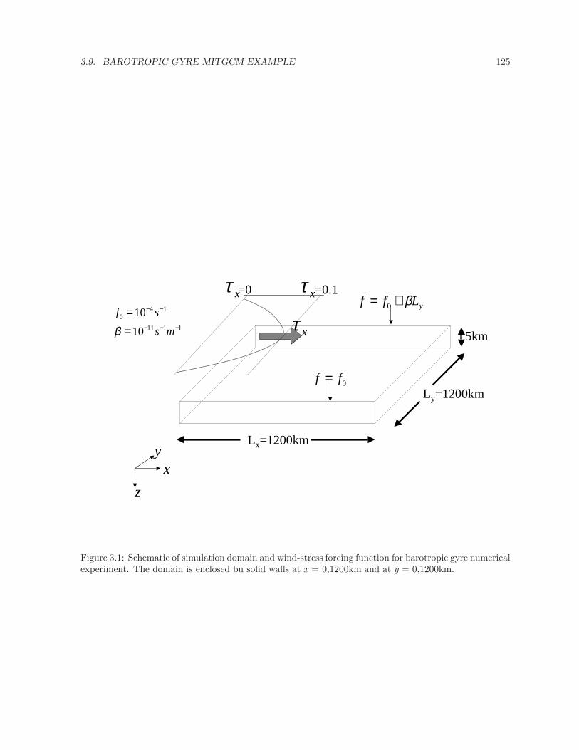
3.9. BAROTROPIC GYRE MITGCM EXAMPLE 125
5km
Ly=1200km
Lx=1200km
xτ
=0.1=0 xτxτ
1111
140
10
10−−−
−−
=
=
ms
sf
β
0ff =
yLff β+= 0
xy
z
Figure 3.1: Schematic of simulation domain and wind-stress forcing function for barotropic gyre numericalexperiment. The domain is enclosed bu solid walls at x = 0,1200km and at y = 0,1200km.
126 CHAPTER 3. GETTING STARTED WITH MITGCM
of ≈ 100km. This is greater than the model resolution ∆x, ensuring that the frictional boundary layer iswell resolved.
The model is stepped forward with a time step δt = 1200secs. With this time step the stability parameterto the horizontal Laplacian friction Adcroft [1995]
Sl = 4Ahδt
∆x2 (3.7)
evaluates to 0.012, which is well below the 0.3 upper limit for stability.
The numerical stability for inertial oscillations Adcroft [1995]
Si = f2δt2 (3.8)
evaluates to 0.0144, which is well below the 0.5 upper limit for stability.
The advective CFL Adcroft [1995] for an extreme maximum horizontal flow speed of |~u| = 2ms−1
Sa =|~u|δt∆x
(3.9)
evaluates to 0.12. This is approaching the stability limit of 0.5 and limits δt to 1200s.
3.9.3 Code Configuration
The model configuration for this experiment resides under the directory verification/tutorial barotropic gyre/.The experiment files
• input/data
• input/data.pkg
• input/eedata,
• input/windx.sin y,
• input/topog.box,
• code/CPP EEOPTIONS.h
• code/CPP OPTIONS.h,
• code/SIZE.h.
contain the code customizations and parameter settings for this experiments. Below we describe thecustomizations to these files associated with this experiment.
3.9.3.1 File input/data
This file, reproduced completely below, specifies the main parameters for the experiment. The parametersthat are significant for this configuration are
• Line 7,
viscAh=4.E2,
this line sets the Laplacian friction coefficient to 400m2s−1
• Line 10,
3.9. BAROTROPIC GYRE MITGCM EXAMPLE 127
beta=1.E-11,
this line sets β (the gradient of the coriolis parameter, f) to 10−11s−1m−1
• Lines 15 and 16
rigidLid=.FALSE.,
implicitFreeSurface=.TRUE.,
these lines suppress the rigid lid formulation of the surface pressure inverter and activate the implicitfree surface form of the pressure inverter.
• Line 27,
startTime=0,
this line indicates that the experiment should start from t = 0 and implicitly suppresses searchingfor checkpoint files associated with restarting an numerical integration from a previously savedstate.
• Line 29,
endTime=12000,
this line indicates that the experiment should start finish at t = 12000s. A restart file will bewritten at this time that will enable the simulation to be continued from this point.
• Line 30,
deltaTmom=1200,
This line sets the momentum equation timestep to 1200s.
• Line 39,
usingCartesianGrid=.TRUE.,
This line requests that the simulation be performed in a Cartesian coordinate system.
• Line 41,
delX=60*20E3,
This line sets the horizontal grid spacing between each x-coordinate line in the discrete grid. Thesyntax indicates that the discrete grid should be comprise of 60 grid lines each separated by 20×103m(20 km).
• Line 42,
delY=60*20E3,
This line sets the horizontal grid spacing between each y-coordinate line in the discrete grid to20 × 103m (20 km).
• Line 43,
delZ=5000,
This line sets the vertical grid spacing between each z-coordinate line in the discrete grid to 5000m(5 km).
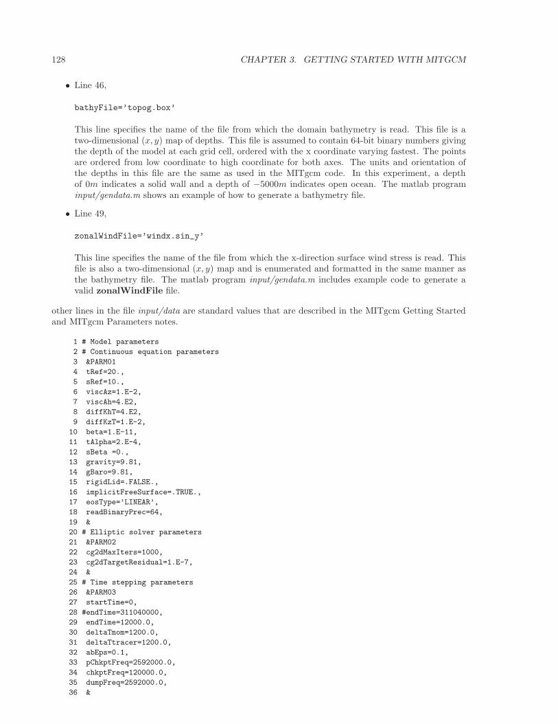
128 CHAPTER 3. GETTING STARTED WITH MITGCM
• Line 46,
bathyFile=’topog.box’
This line specifies the name of the file from which the domain bathymetry is read. This file is atwo-dimensional (x, y) map of depths. This file is assumed to contain 64-bit binary numbers givingthe depth of the model at each grid cell, ordered with the x coordinate varying fastest. The pointsare ordered from low coordinate to high coordinate for both axes. The units and orientation ofthe depths in this file are the same as used in the MITgcm code. In this experiment, a depthof 0m indicates a solid wall and a depth of −5000m indicates open ocean. The matlab programinput/gendata.m shows an example of how to generate a bathymetry file.
• Line 49,
zonalWindFile=’windx.sin_y’
This line specifies the name of the file from which the x-direction surface wind stress is read. Thisfile is also a two-dimensional (x, y) map and is enumerated and formatted in the same manner asthe bathymetry file. The matlab program input/gendata.m includes example code to generate avalid zonalWindFile file.
other lines in the file input/data are standard values that are described in the MITgcm Getting Startedand MITgcm Parameters notes.
1 # Model parameters
2 # Continuous equation parameters
3 &PARM01
4 tRef=20.,
5 sRef=10.,
6 viscAz=1.E-2,
7 viscAh=4.E2,
8 diffKhT=4.E2,
9 diffKzT=1.E-2,
10 beta=1.E-11,
11 tAlpha=2.E-4,
12 sBeta =0.,
13 gravity=9.81,
14 gBaro=9.81,
15 rigidLid=.FALSE.,
16 implicitFreeSurface=.TRUE.,
17 eosType=’LINEAR’,
18 readBinaryPrec=64,
19 &
20 # Elliptic solver parameters
21 &PARM02
22 cg2dMaxIters=1000,
23 cg2dTargetResidual=1.E-7,
24 &
25 # Time stepping parameters
26 &PARM03
27 startTime=0,
28 #endTime=311040000,
29 endTime=12000.0,
30 deltaTmom=1200.0,
31 deltaTtracer=1200.0,
32 abEps=0.1,
33 pChkptFreq=2592000.0,
34 chkptFreq=120000.0,
35 dumpFreq=2592000.0,
36 &
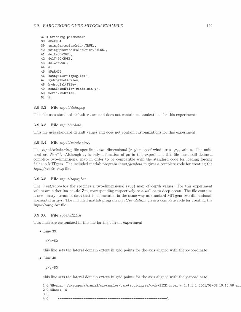
3.9. BAROTROPIC GYRE MITGCM EXAMPLE 129
37 # Gridding parameters
38 &PARM04
39 usingCartesianGrid=.TRUE.,
40 usingSphericalPolarGrid=.FALSE.,
41 delX=60*20E3,
42 delY=60*20E3,
43 delZ=5000.,
44 &
45 &PARM05
46 bathyFile=’topog.box’,
47 hydrogThetaFile=,
48 hydrogSaltFile=,
49 zonalWindFile=’windx.sin_y’,
50 meridWindFile=,
51 &
3.9.3.2 File input/data.pkg
This file uses standard default values and does not contain customizations for this experiment.
3.9.3.3 File input/eedata
This file uses standard default values and does not contain customizations for this experiment.
3.9.3.4 File input/windx.sin y
The input/windx.sin y file specifies a two-dimensional (x, y) map of wind stress ,τx, values. The unitsused are Nm−2. Although τx is only a function of yn in this experiment this file must still define acomplete two-dimensional map in order to be compatible with the standard code for loading forcingfields in MITgcm. The included matlab program input/gendata.m gives a complete code for creating theinput/windx.sin y file.
3.9.3.5 File input/topog.box
The input/topog.box file specifies a two-dimensional (x, y) map of depth values. For this experimentvalues are either 0m or -delZm, corresponding respectively to a wall or to deep ocean. The file containsa raw binary stream of data that is enumerated in the same way as standard MITgcm two-dimensional,horizontal arrays. The included matlab program input/gendata.m gives a complete code for creating theinput/topog.box file.
3.9.3.6 File code/SIZE.h
Two lines are customized in this file for the current experiment
• Line 39,
sNx=60,
this line sets the lateral domain extent in grid points for the axis aligned with the x-coordinate.
• Line 40,
sNy=60,
this line sets the lateral domain extent in grid points for the axis aligned with the y-coordinate.
1 C $Header: /u/gcmpack/manual/s_examples/barotropic_gyre/code/SIZE.h.tex,v 1.1.1.1 2001/08/08 16:15:58 adcroft
2 C $Name: $
3 C
4 C /==========================================================\
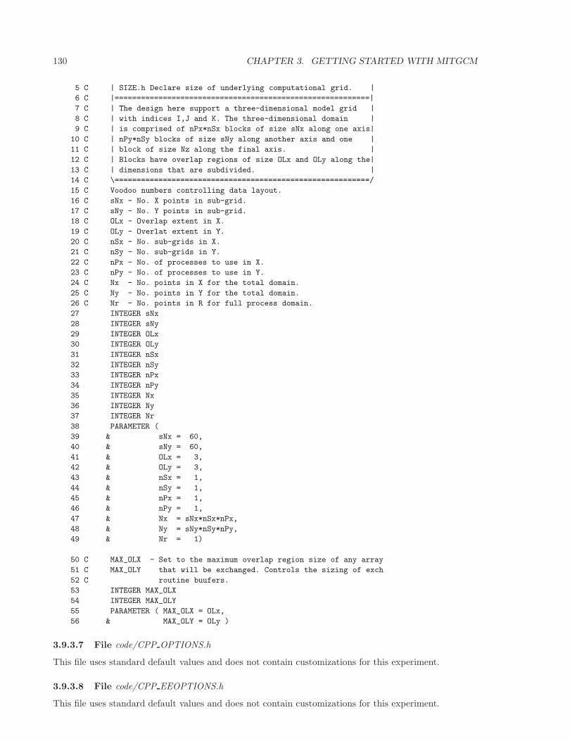
130 CHAPTER 3. GETTING STARTED WITH MITGCM
5 C | SIZE.h Declare size of underlying computational grid. |
6 C |==========================================================|
7 C | The design here support a three-dimensional model grid |
8 C | with indices I,J and K. The three-dimensional domain |
9 C | is comprised of nPx*nSx blocks of size sNx along one axis|
10 C | nPy*nSy blocks of size sNy along another axis and one |
11 C | block of size Nz along the final axis. |
12 C | Blocks have overlap regions of size OLx and OLy along the|
13 C | dimensions that are subdivided. |
14 C \==========================================================/
15 C Voodoo numbers controlling data layout.
16 C sNx - No. X points in sub-grid.
17 C sNy - No. Y points in sub-grid.
18 C OLx - Overlap extent in X.
19 C OLy - Overlat extent in Y.
20 C nSx - No. sub-grids in X.
21 C nSy - No. sub-grids in Y.
22 C nPx - No. of processes to use in X.
23 C nPy - No. of processes to use in Y.
24 C Nx - No. points in X for the total domain.
25 C Ny - No. points in Y for the total domain.
26 C Nr - No. points in R for full process domain.
27 INTEGER sNx
28 INTEGER sNy
29 INTEGER OLx
30 INTEGER OLy
31 INTEGER nSx
32 INTEGER nSy
33 INTEGER nPx
34 INTEGER nPy
35 INTEGER Nx
36 INTEGER Ny
37 INTEGER Nr
38 PARAMETER (
39 & sNx = 60,
40 & sNy = 60,
41 & OLx = 3,
42 & OLy = 3,
43 & nSx = 1,
44 & nSy = 1,
45 & nPx = 1,
46 & nPy = 1,
47 & Nx = sNx*nSx*nPx,
48 & Ny = sNy*nSy*nPy,
49 & Nr = 1)
50 C MAX_OLX - Set to the maximum overlap region size of any array
51 C MAX_OLY that will be exchanged. Controls the sizing of exch
52 C routine buufers.
53 INTEGER MAX_OLX
54 INTEGER MAX_OLY
55 PARAMETER ( MAX_OLX = OLx,
56 & MAX_OLY = OLy )
3.9.3.7 File code/CPP OPTIONS.h
This file uses standard default values and does not contain customizations for this experiment.
3.9.3.8 File code/CPP EEOPTIONS.h
This file uses standard default values and does not contain customizations for this experiment.
3.10. BAROCLINIC GYRE MITGCM EXAMPLE 131
3.10 Four Layer Baroclinic Ocean Gyre In Spherical Coordi-
nates
(in directory: verification/tutorial baroclinic gyre/)
This document describes an example experiment using MITgcm to simulate a baroclinic ocean gyrefor four layers in spherical polar coordinates. The files for this experiment can be found in the verificationdirectory under tutorial baroclinic gyre.
3.10.1 Overview
This example experiment demonstrates using the MITgcm to simulate a baroclinic, wind-forced, oceangyre circulation. The experiment is a numerical rendition of the gyre circulation problem similar to theproblems described analytically by Stommel in 1966 Stommel [1948] and numerically in Holland et. alHolland and Lin [975a].
In this experiment the model is configured to represent a mid-latitude enclosed sector of fluid on asphere, 60× 60 in lateral extent. The fluid is 2 km deep and is forced by a constant in time zonal windstress, τλ, that varies sinusoidally in the north-south direction. Topologically the simulated domain is asector on a sphere and the coriolis parameter, f , is defined according to latitude, ϕ
f(ϕ) = 2Ω sin(ϕ) (3.10)
with the rotation rate, Ω set to 2π86400s .
The sinusoidal wind-stress variations are defined according to
τλ(ϕ) = τ0 sin(πϕ
Lϕ) (3.11)
where Lϕ is the lateral domain extent (60) and τ0 is set to 0.1Nm−2.
Figure 3.2 summarizes the configuration simulated. In contrast to the example in section 3.9, thecurrent experiment simulates a spherical polar domain. As indicated by the axes in the lower left of thefigure the model code works internally in a locally orthogonal coordinate (x, y, z). For this experimentdescription the local orthogonal model coordinate (x, y, z) is synonymous with the coordinates (λ, ϕ, r)shown in figure 1.16
The experiment has four levels in the vertical, each of equal thickness, ∆z = 500 m. Initially the fluidis stratified with a reference potential temperature profile, θ250 = 20 C, θ750 = 10 C, θ1250 = 8 C,θ1750 = 6 C. The equation of state used in this experiment is linear
ρ = ρ0(1 − αθθ′
) (3.12)
which is implemented in the model as a density anomaly equation
ρ′
= −ρ0αθθ′
(3.13)
with ρ0 = 999.8 kgm−3 and αθ = 2 × 10⁻⁴ degrees−1. Integrated forward in this configuration themodel state variable theta is equivalent to either in-situ temperature, T , or potential temperature, θ.For consistency with later examples, in which the equation of state is non-linear, we use θ to representtemperature here. This is the quantity that is carried in the model core equations.
3.10.2 Equations solved
For this problem the implicit free surface, HPE (see section 1.3.4.2) form of the equations described inMarshall et. al Marshall et al. [1997b] are employed. The flow is three-dimensional with just temperature,θ, as an active tracer. The equation of state is linear. A horizontal Laplacian operator ∇2
h provides viscousdissipation and provides a diffusive sub-grid scale closure for the temperature equation. A wind-stress
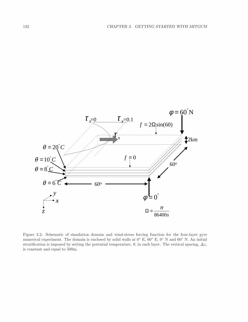
132 CHAPTER 3. GETTING STARTED WITH MITGCM
2km
60o
60o
xτ
=0.1=0 xτxτ
0=f
)60sin(2Ω=f
xy
z
C°= 6θ
°= 0φ
°= 60φ N
C°= 8θC°=10θ
C°= 20θ
s86400
π=Ω
Figure 3.2: Schematic of simulation domain and wind-stress forcing function for the four-layer gyrenumerical experiment. The domain is enclosed by solid walls at 0 E, 60 E, 0 N and 60 N. An initialstratification is imposed by setting the potential temperature, θ, in each layer. The vertical spacing, ∆z,is constant and equal to 500m.
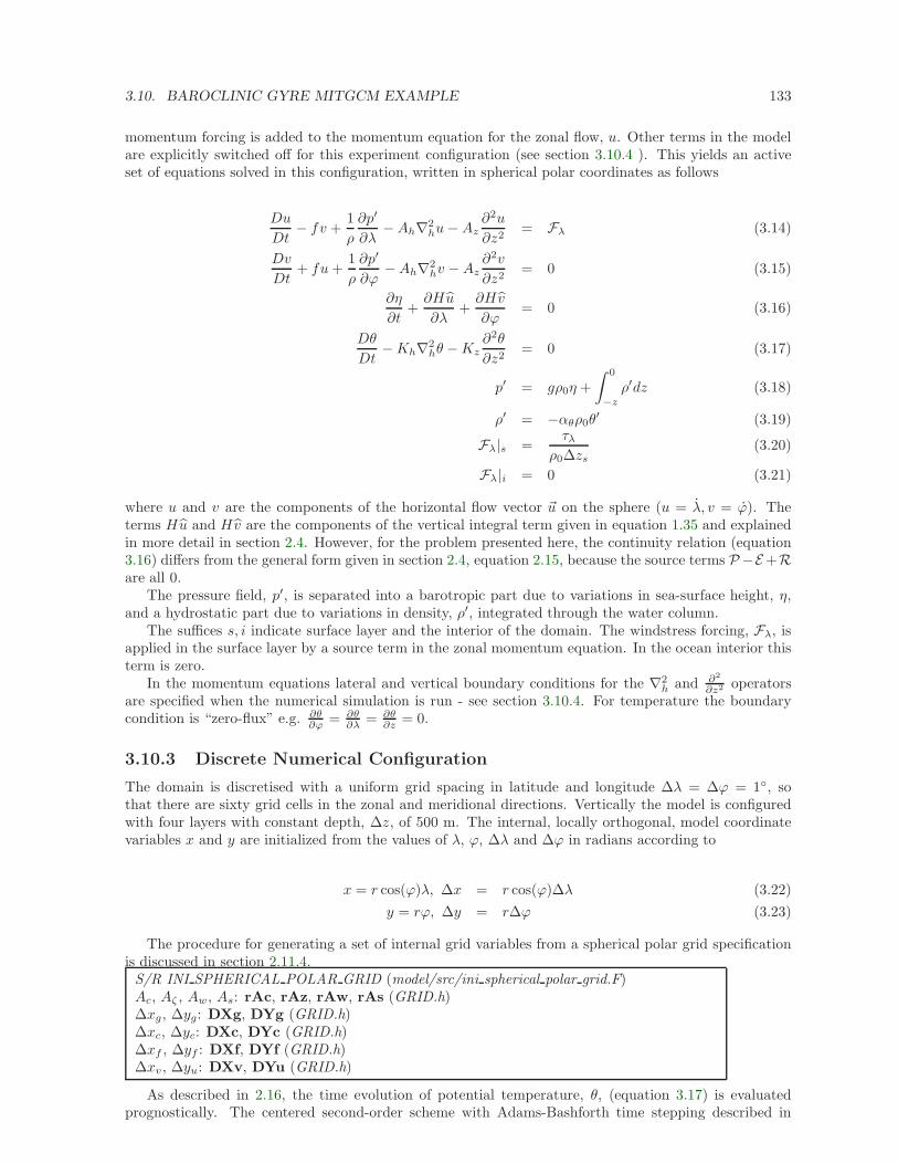
3.10. BAROCLINIC GYRE MITGCM EXAMPLE 133
momentum forcing is added to the momentum equation for the zonal flow, u. Other terms in the modelare explicitly switched off for this experiment configuration (see section 3.10.4 ). This yields an activeset of equations solved in this configuration, written in spherical polar coordinates as follows
Du
Dt− fv +
1
ρ
∂p′
∂λ−Ah∇2
hu−Az∂2u
∂z2= Fλ (3.14)
Dv
Dt+ fu+
1
ρ
∂p′
∂ϕ−Ah∇2
hv −Az∂2v
∂z2= 0 (3.15)
∂η
∂t+∂Hu
∂λ+∂Hv
∂ϕ= 0 (3.16)
Dθ
Dt−Kh∇2
hθ −Kz∂2θ
∂z2= 0 (3.17)
p′ = gρ0η +
∫ 0
−z
ρ′dz (3.18)
ρ′ = −αθρ0θ′ (3.19)
Fλ|s =τλ
ρ0∆zs(3.20)
Fλ|i = 0 (3.21)
where u and v are the components of the horizontal flow vector ~u on the sphere (u = λ, v = ϕ). Theterms Hu and Hv are the components of the vertical integral term given in equation 1.35 and explainedin more detail in section 2.4. However, for the problem presented here, the continuity relation (equation3.16) differs from the general form given in section 2.4, equation 2.15, because the source terms P−E+Rare all 0.
The pressure field, p′, is separated into a barotropic part due to variations in sea-surface height, η,and a hydrostatic part due to variations in density, ρ′, integrated through the water column.
The suffices s, i indicate surface layer and the interior of the domain. The windstress forcing, Fλ, isapplied in the surface layer by a source term in the zonal momentum equation. In the ocean interior thisterm is zero.
In the momentum equations lateral and vertical boundary conditions for the ∇2h and ∂2
∂z2 operatorsare specified when the numerical simulation is run - see section 3.10.4. For temperature the boundarycondition is “zero-flux” e.g. ∂θ
∂ϕ = ∂θ∂λ = ∂θ
∂z = 0.
3.10.3 Discrete Numerical Configuration
The domain is discretised with a uniform grid spacing in latitude and longitude ∆λ = ∆ϕ = 1, sothat there are sixty grid cells in the zonal and meridional directions. Vertically the model is configuredwith four layers with constant depth, ∆z, of 500 m. The internal, locally orthogonal, model coordinatevariables x and y are initialized from the values of λ, ϕ, ∆λ and ∆ϕ in radians according to
x = r cos(ϕ)λ, ∆x = r cos(ϕ)∆λ (3.22)
y = rϕ, ∆y = r∆ϕ (3.23)
The procedure for generating a set of internal grid variables from a spherical polar grid specificationis discussed in section 2.11.4.S/R INI SPHERICAL POLAR GRID (model/src/ini spherical polar grid.F)Ac, Aζ , Aw, As: rAc, rAz, rAw, rAs (GRID.h)∆xg, ∆yg: DXg, DYg (GRID.h)∆xc, ∆yc: DXc, DYc (GRID.h)∆xf , ∆yf : DXf, DYf (GRID.h)∆xv, ∆yu: DXv, DYu (GRID.h)
As described in 2.16, the time evolution of potential temperature, θ, (equation 3.17) is evaluatedprognostically. The centered second-order scheme with Adams-Bashforth time stepping described in
134 CHAPTER 3. GETTING STARTED WITH MITGCM
section 2.16.1 is used to step forward the temperature equation. Prognostic terms in the momentumequations are solved using flux form as described in section 2.14. The pressure forces that drive the fluid
motions, ( ∂p′
∂λ and ∂p′
∂ϕ ), are found by summing pressure due to surface elevation η and the hydrostaticpressure. The hydrostatic part of the pressure is diagnosed explicitly by integrating density. The sea-surface height, η, is diagnosed using an implicit scheme. The pressure field solution method is describedin sections 2.4 and 1.3.6.
3.10.3.1 Numerical Stability Criteria
The Laplacian viscosity coefficient, Ah, is set to 400ms−1. This value is chosen to yield a Munk layerwidth,
Mw = π(Ah
β)
13 (3.24)
of ≈ 100km. This is greater than the model resolution in mid-latitudes ∆x = r cos(ϕ)∆λ ≈ 80 km atϕ = 45, ensuring that the frictional boundary layer is well resolved.
The model is stepped forward with a time step δt = 1200secs. With this time step the stability parameterto the horizontal Laplacian friction
Sl = 4Ahδt
∆x2 (3.25)
evaluates to 0.012, which is well below the 0.3 upper limit for stability for this term under ABII time-stepping.
The vertical dissipation coefficient, Az , is set to 1 × 10⁻²m2s−1. The associated stability limit
Sl = 4Azδt
∆z2 (3.26)
evaluates to 4.8× 10⁻⁵ which is again well below the upper limit. The values of Ah and Az are also usedfor the horizontal (Kh) and vertical (Kz) diffusion coefficients for temperature respectively.
The numerical stability for inertial oscillations
Si = f2δt2 (3.27)
evaluates to 0.0144, which is well below the 0.5 upper limit for stability.
The advective CFL for a extreme maximum horizontal flow speed of |~u| = 2ms−1
Ca =|~u|δt∆x
(3.28)
evaluates to 5 × 10⁻². This is well below the stability limit of 0.5.
The stability parameter for internal gravity waves propagating at 2 m s−1
Sc =cgδt
∆x(3.29)
evaluates to ≈ 5 × 10⁻². This is well below the linear stability limit of 0.25.
3.10. BAROCLINIC GYRE MITGCM EXAMPLE 135
3.10.4 Code Configuration
The model configuration for this experiment resides under the directory verification/tutorial barotropic gyre/.The experiment files
• input/data
• input/data.pkg
• input/eedata,
• input/windx.sin y,
• input/topog.box,
• code/CPP EEOPTIONS.h
• code/CPP OPTIONS.h,
• code/SIZE.h.
contain the code customisations and parameter settings for this experiment. Below we describe thecustomisations to these files associated with this experiment.
3.10.4.1 File input/data
This file, reproduced completely below, specifies the main parameters for the experiment. The parametersthat are significant for this configuration are
• Line 4,
tRef=20.,10.,8.,6.,
this line sets the initial and reference values of potential temperature at each model level in unitsof C. The entries are ordered from surface to depth. For each depth level the initial and referenceprofiles will be uniform in x and y. The values specified here are read into the variable tRef in themodel code, by procedure INI PARMS
S/R INI THETA(ini theta.F) ini theta.F
• Line 6,
viscAz=1.E-2,
this line sets the vertical Laplacian dissipation coefficient to 1 × 10⁻²m2s−1. Boundary conditionsfor this operator are specified later. The variable viscAz is read in the routine ini parms.F and iscopied into model general vertical coordinate variable viscAr At each time step, the viscous termcontribution to the momentum equations is calculated in routine CALC DIFFUSIVITY
S/R CALC DIFFUSIVITY(calc diffusivity.F)
• Line 7,
viscAh=4.E2,
this line sets the horizontal laplacian frictional dissipation coefficient to 1 × 10⁻²m2s−1. Boundaryconditions for this operator are specified later. The variable viscAh is read in the routine INI PARMS
and applied in routine MOM FLUXFORM.
S/R MOM FLUXFORM(mom fluxform.F)
• Line 8,
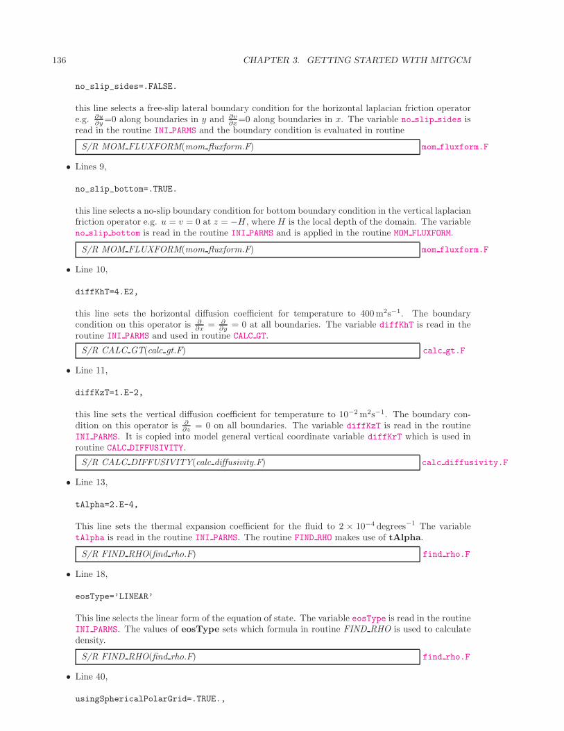
136 CHAPTER 3. GETTING STARTED WITH MITGCM
no_slip_sides=.FALSE.
this line selects a free-slip lateral boundary condition for the horizontal laplacian friction operatore.g. ∂u
∂y =0 along boundaries in y and ∂v∂x=0 along boundaries in x. The variable no slip sides is
read in the routine INI PARMS and the boundary condition is evaluated in routine
S/R MOM FLUXFORM(mom fluxform.F) mom fluxform.F
• Lines 9,
no_slip_bottom=.TRUE.
this line selects a no-slip boundary condition for bottom boundary condition in the vertical laplacianfriction operator e.g. u = v = 0 at z = −H , where H is the local depth of the domain. The variableno slip bottom is read in the routine INI PARMS and is applied in the routine MOM FLUXFORM.
S/R MOM FLUXFORM(mom fluxform.F) mom fluxform.F
• Line 10,
diffKhT=4.E2,
this line sets the horizontal diffusion coefficient for temperature to 400 m2s−1. The boundarycondition on this operator is ∂
∂x = ∂∂y = 0 at all boundaries. The variable diffKhT is read in the
routine INI PARMS and used in routine CALC GT.
S/R CALC GT(calc gt.F) calc gt.F
• Line 11,
diffKzT=1.E-2,
this line sets the vertical diffusion coefficient for temperature to 10−2 m2s−1. The boundary con-dition on this operator is ∂
∂z = 0 on all boundaries. The variable diffKzT is read in the routineINI PARMS. It is copied into model general vertical coordinate variable diffKrT which is used inroutine CALC DIFFUSIVITY.
S/R CALC DIFFUSIVITY(calc diffusivity.F) calc diffusivity.F
• Line 13,
tAlpha=2.E-4,
This line sets the thermal expansion coefficient for the fluid to 2 × 10⁻⁴ degrees−1 The variabletAlpha is read in the routine INI PARMS. The routine FIND RHO makes use of tAlpha.
S/R FIND RHO(find rho.F) find rho.F
• Line 18,
eosType=’LINEAR’
This line selects the linear form of the equation of state. The variable eosType is read in the routineINI PARMS. The values of eosType sets which formula in routine FIND RHO is used to calculatedensity.
S/R FIND RHO(find rho.F) find rho.F
• Line 40,
usingSphericalPolarGrid=.TRUE.,
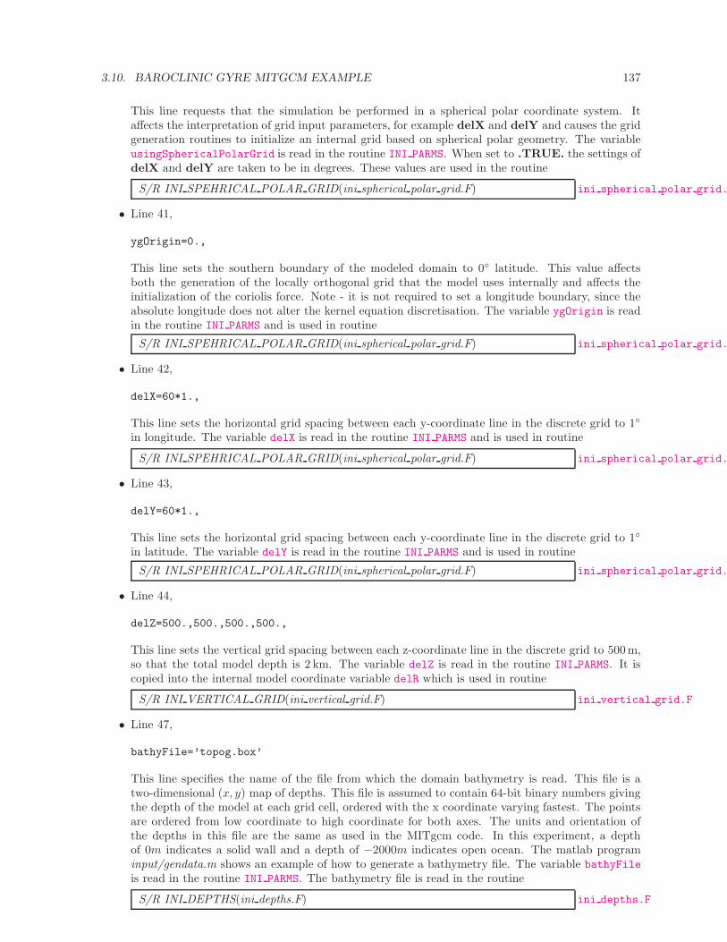
3.10. BAROCLINIC GYRE MITGCM EXAMPLE 137
This line requests that the simulation be performed in a spherical polar coordinate system. Itaffects the interpretation of grid input parameters, for example delX and delY and causes the gridgeneration routines to initialize an internal grid based on spherical polar geometry. The variableusingSphericalPolarGrid is read in the routine INI PARMS. When set to .TRUE. the settings ofdelX and delY are taken to be in degrees. These values are used in the routine
S/R INI SPEHRICAL POLAR GRID(ini spherical polar grid.F) ini spherical polar grid.F
• Line 41,
ygOrigin=0.,
This line sets the southern boundary of the modeled domain to 0 latitude. This value affectsboth the generation of the locally orthogonal grid that the model uses internally and affects theinitialization of the coriolis force. Note - it is not required to set a longitude boundary, since theabsolute longitude does not alter the kernel equation discretisation. The variable ygOrigin is readin the routine INI PARMS and is used in routine
S/R INI SPEHRICAL POLAR GRID(ini spherical polar grid.F) ini spherical polar grid.F
• Line 42,
delX=60*1.,
This line sets the horizontal grid spacing between each y-coordinate line in the discrete grid to 1
in longitude. The variable delX is read in the routine INI PARMS and is used in routine
S/R INI SPEHRICAL POLAR GRID(ini spherical polar grid.F) ini spherical polar grid.F
• Line 43,
delY=60*1.,
This line sets the horizontal grid spacing between each y-coordinate line in the discrete grid to 1
in latitude. The variable delY is read in the routine INI PARMS and is used in routine
S/R INI SPEHRICAL POLAR GRID(ini spherical polar grid.F) ini spherical polar grid.F
• Line 44,
delZ=500.,500.,500.,500.,
This line sets the vertical grid spacing between each z-coordinate line in the discrete grid to 500 m,so that the total model depth is 2 km. The variable delZ is read in the routine INI PARMS. It iscopied into the internal model coordinate variable delR which is used in routine
S/R INI VERTICAL GRID(ini vertical grid.F) ini vertical grid.F
• Line 47,
bathyFile=’topog.box’
This line specifies the name of the file from which the domain bathymetry is read. This file is atwo-dimensional (x, y) map of depths. This file is assumed to contain 64-bit binary numbers givingthe depth of the model at each grid cell, ordered with the x coordinate varying fastest. The pointsare ordered from low coordinate to high coordinate for both axes. The units and orientation ofthe depths in this file are the same as used in the MITgcm code. In this experiment, a depthof 0m indicates a solid wall and a depth of −2000m indicates open ocean. The matlab programinput/gendata.m shows an example of how to generate a bathymetry file. The variable bathyFile
is read in the routine INI PARMS. The bathymetry file is read in the routine
S/R INI DEPTHS(ini depths.F) ini depths.F
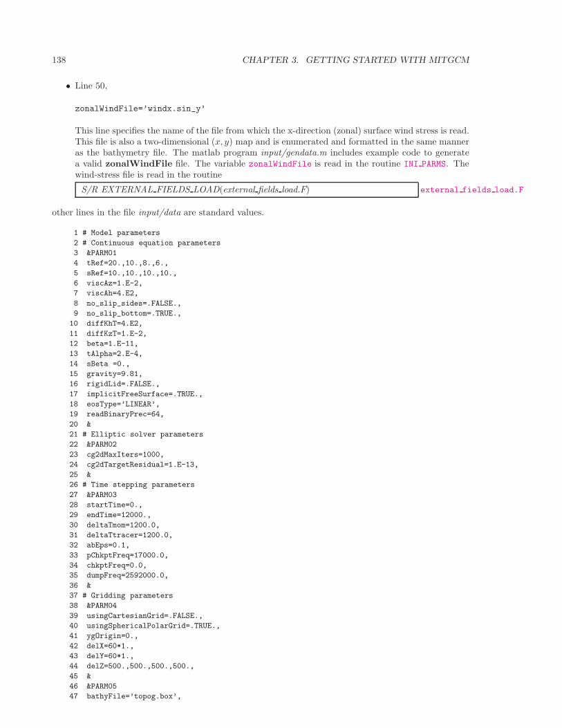
138 CHAPTER 3. GETTING STARTED WITH MITGCM
• Line 50,
zonalWindFile=’windx.sin_y’
This line specifies the name of the file from which the x-direction (zonal) surface wind stress is read.This file is also a two-dimensional (x, y) map and is enumerated and formatted in the same manneras the bathymetry file. The matlab program input/gendata.m includes example code to generatea valid zonalWindFile file. The variable zonalWindFile is read in the routine INI PARMS. Thewind-stress file is read in the routine
S/R EXTERNAL FIELDS LOAD(external fields load.F) external fields load.F
other lines in the file input/data are standard values.
1 # Model parameters
2 # Continuous equation parameters
3 &PARM01
4 tRef=20.,10.,8.,6.,
5 sRef=10.,10.,10.,10.,
6 viscAz=1.E-2,
7 viscAh=4.E2,
8 no_slip_sides=.FALSE.,
9 no_slip_bottom=.TRUE.,
10 diffKhT=4.E2,
11 diffKzT=1.E-2,
12 beta=1.E-11,
13 tAlpha=2.E-4,
14 sBeta =0.,
15 gravity=9.81,
16 rigidLid=.FALSE.,
17 implicitFreeSurface=.TRUE.,
18 eosType=’LINEAR’,
19 readBinaryPrec=64,
20 &
21 # Elliptic solver parameters
22 &PARM02
23 cg2dMaxIters=1000,
24 cg2dTargetResidual=1.E-13,
25 &
26 # Time stepping parameters
27 &PARM03
28 startTime=0.,
29 endTime=12000.,
30 deltaTmom=1200.0,
31 deltaTtracer=1200.0,
32 abEps=0.1,
33 pChkptFreq=17000.0,
34 chkptFreq=0.0,
35 dumpFreq=2592000.0,
36 &
37 # Gridding parameters
38 &PARM04
39 usingCartesianGrid=.FALSE.,
40 usingSphericalPolarGrid=.TRUE.,
41 ygOrigin=0.,
42 delX=60*1.,
43 delY=60*1.,
44 delZ=500.,500.,500.,500.,
45 &
46 &PARM05
47 bathyFile=’topog.box’,
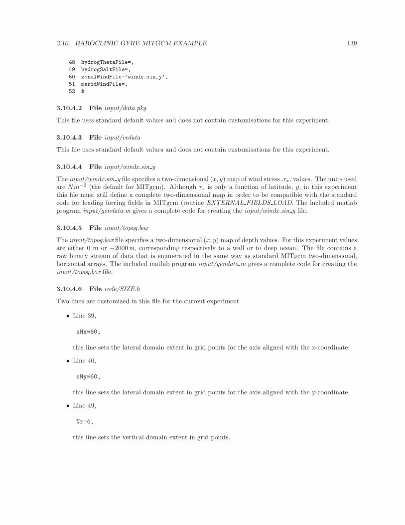
3.10. BAROCLINIC GYRE MITGCM EXAMPLE 139
48 hydrogThetaFile=,
49 hydrogSaltFile=,
50 zonalWindFile=’windx.sin_y’,
51 meridWindFile=,
52 &
3.10.4.2 File input/data.pkg
This file uses standard default values and does not contain customisations for this experiment.
3.10.4.3 File input/eedata
This file uses standard default values and does not contain customisations for this experiment.
3.10.4.4 File input/windx.sin y
The input/windx.sin y file specifies a two-dimensional (x, y) map of wind stress ,τx, values. The units usedare Nm−2 (the default for MITgcm). Although τx is only a function of latitude, y, in this experimentthis file must still define a complete two-dimensional map in order to be compatible with the standardcode for loading forcing fields in MITgcm (routine EXTERNAL FIELDS LOAD. The included matlabprogram input/gendata.m gives a complete code for creating the input/windx.sin y file.
3.10.4.5 File input/topog.box
The input/topog.box file specifies a two-dimensional (x, y) map of depth values. For this experiment valuesare either 0 m or −2000 m, corresponding respectively to a wall or to deep ocean. The file contains araw binary stream of data that is enumerated in the same way as standard MITgcm two-dimensional,horizontal arrays. The included matlab program input/gendata.m gives a complete code for creating theinput/topog.box file.
3.10.4.6 File code/SIZE.h
Two lines are customized in this file for the current experiment
• Line 39,
sNx=60,
this line sets the lateral domain extent in grid points for the axis aligned with the x-coordinate.
• Line 40,
sNy=60,
this line sets the lateral domain extent in grid points for the axis aligned with the y-coordinate.
• Line 49,
Nr=4,
this line sets the vertical domain extent in grid points.
140 CHAPTER 3. GETTING STARTED WITH MITGCM
3.10.4.7 File code/CPP OPTIONS.h
This file uses standard default values and does not contain customisations for this experiment.
3.10.4.8 File code/CPP EEOPTIONS.h
This file uses standard default values and does not contain customisations for this experiment.
3.10.4.9 Other Files
Other files relevant to this experiment are
• model/src/ini cori.F. This file initializes the model coriolis variables fCorU and fCorV.
• model/src/ini spherical polar grid.F This file initializes the model grid discretisation variables dxF,dyF, dxG, dyG, dxC, dyC.
• model/src/ini parms.F.
3.10.5 Running The Example
3.10.5.1 Code Download
In order to run the examples you must first download the code distribution. Instructions for downloadingthe code can be found in section 3.2.
3.10.5.2 Experiment Location
This example experiments is located under the release sub-directory
verification/exp2/
3.10.5.3 Running the Experiment
To run the experiment
1. Set the current directory to input/
% cd input
2. Verify that current directory is now correct
% pwd
You should see a response on the screen ending in
verification/exp2/input
3. Run the genmake script to create the experiment Makefile
% ../../../tools/genmake -mods=../code
4. Create a list of header file dependencies in Makefile
% make depend
5. Build the executable file.
% make
6. Run the mitgcmuv executable
% ./mitgcmuv
3.11. GYRE ADVECTION EXAMPLE 141
3.11 Ocean Gyre Advection Schemes
(in directory: verification/tutorial advection in gyre/)
Author: Oliver Jahn and Chris Hill
This set of examples is based on the barotropic and baroclinic gyre MITgcm configurations, that aredescribed in the tutorial sections 3.9 and 3.10. The examples in this section explain how to introducea passive tracer into the flow field of the barotropic and baroclinic gyre setups and looks at how thetime evolution of the passive tracer depends on the advection or transport scheme that is selected for thetracer.
Passive tracers are useful in many numerical experiments. In some cases tracers are used to trackflow pathways, for example in Dutay et al. [2002] a passive tracer is used to track pathways of CFC-11in 13 global ocean models, using a numerical configuration similar to the example described in section3.20.5). In other cases tracers are used as a way to infer bulk mixing coefficients for a turbulent flow field,for example in Marshall et al. [2006] a tracer is used to infer eddy mixing coefficients in the AntarcticCircumpolar Current region. In biogeochemical and ecological simulations large numbers of tracers areused that carry the concentrations of biological nutrients and concentrations of biological species, forexample in .... When using tracers for these and other purposes it is useful to have a feel for therole that the advection scheme employed plays in determining properties of the tracer distribution. Inparticular, in a discrete numerical model tracer advection only approximates the continuum behavior inspace and time and different advection schemes introduce diferent approximations so that the resultingtracer distributions vary. In the following text we illustrate how to use the different advection schemesavailable in MITgcm here, and discuss which properties are well represented by each one. The advectionschemes selections also apply to active tracers (e.g. T and S) and the character of the schemes also affecttheir distributions and behavior.
3.11.1 Advection and tracer transport
In general, the tracer problem we want to solve can be written
∂C
∂t= −U · ∇C + S (3.30)
where C is the tracer concentration in a model cell, U is the model three-dimensional flow field ( U =(u, v, w) ). In (3.30) S represents source, sink and tendency terms not associated with advective transport.Example of terms in S include (i) air-sea fluxes for a dissolved gas, (ii) biological grazing and growthterms (for a biogeochemical problem) or (iii) convective mixing and other sub-grid parameterizations ofmixing. In this section we are primarily concerned with
1. how to introduce the tracer term, C, into an integration
2. the different discretized forms of the −U · ∇C term that are available
3.11.2 Introducing a tracer into the flow
The MITgcm ptracers package (see section 6.3.3 for a more complete discussion of the ptracers packageand section 6.1 for a general introduction to MITgcm packages) provides pre-coded support for a simplepassive tracer with an initial distribution at simulation time t = 0 of C0(x, y, z). The steps required touse this capability are
1. Activating the ptracers package. This simply requires adding the line ptracers to thepackages.conf file in the code/ directory for the experiment.
2. Setting an initial tracer distribution.
Once the two steps above are complete we can proceed to examine how the tracer we have createdis carried by the flow field and what properties of the tracer distribution are preserved under differentadvection schemes.
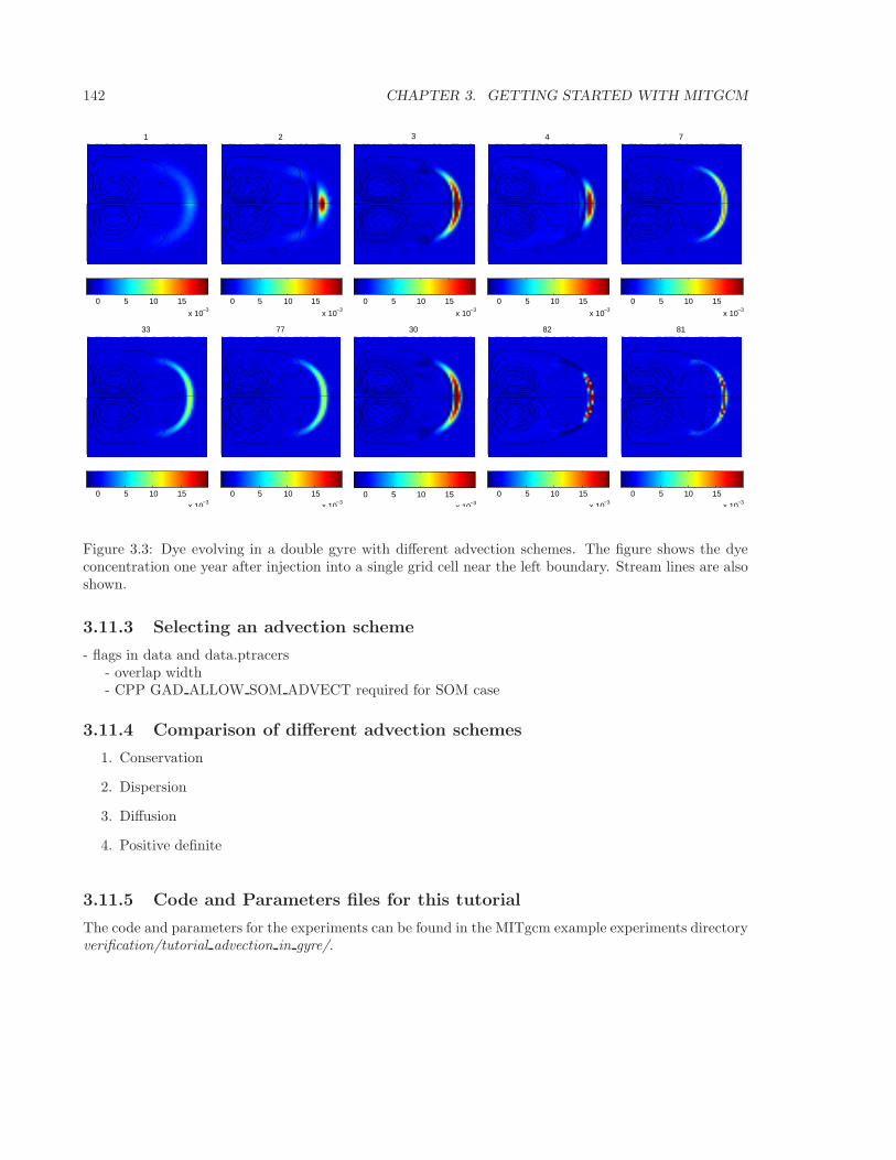
142 CHAPTER 3. GETTING STARTED WITH MITGCM
1
0 5 10 15
x 10−3
2
0 5 10 15
x 10−3
3
0 5 10 15
x 10−3
4
0 5 10 15
x 10−3
7
0 5 10 15
x 10−3
33
0 5 10 15
x 10−3
77
0 5 10 15
x 10−3
30
0 5 10 15
x 10−3
82
0 5 10 15
x 10−3
81
0 5 10 15
x 10−3
Figure 3.3: Dye evolving in a double gyre with different advection schemes. The figure shows the dyeconcentration one year after injection into a single grid cell near the left boundary. Stream lines are alsoshown.
3.11.3 Selecting an advection scheme
- flags in data and data.ptracers- overlap width- CPP GAD ALLOW SOM ADVECT required for SOM case
3.11.4 Comparison of different advection schemes
1. Conservation
2. Dispersion
3. Diffusion
4. Positive definite
3.11.5 Code and Parameters files for this tutorial
The code and parameters for the experiments can be found in the MITgcm example experiments directoryverification/tutorial advection in gyre/.
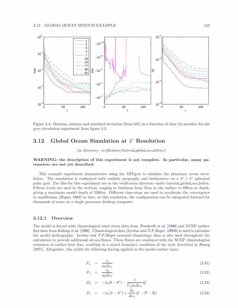
3.12. GLOBAL OCEAN MITGCM EXAMPLE 143
0 50 10010
−4
10−3
10−2
10−1
100
t
max
1 2 3 4 73033778081
0 50 100
−10−2
−10−4
−10−6
−10−8
−10−10
t
min
0 50 10010
−5
10−4
10−3
10−2
t
sd
Figure 3.4: Maxima, minima and standard deviation (from left) as a function of time (in months) for thegyre circulation experiment from figure 3.3.
3.12 Global Ocean Simulation at 4 Resolution
(in directory: verification/tutorial global oce latlon/)
WARNING: the description of this experiment is not complete. In particular, many pa-rameters are not yet described.
This example experiment demonstrates using the MITgcm to simulate the planetary ocean circu-lation. The simulation is configured with realistic geography and bathymetry on a 4 × 4 sphericalpolar grid. The files for this experiment are in the verification directory under tutorial global oce latlon.Fifteen levels are used in the vertical, ranging in thickness from 50 m at the surface to 690 m at depth,giving a maximum model depth of 5200 m. Different time-steps are used to accelerate the convergenceto equilibrium [Bryan, 1984] so that, at this resolution, the configuration can be integrated forward forthousands of years on a single processor desktop computer.
3.12.1 Overview
The model is forced with climatological wind stress data from Trenberth et al. [1990] and NCEP surfaceflux data from Kalnay et al. [1996]. Climatological data [Levitus and T.P.Boyer, 1994b] is used to initializethe model hydrography. Levitus and T.P.Boyer seasonal climatology data is also used throughout thecalculation to provide additional air-sea fluxes. These fluxes are combined with the NCEP climatologicalestimates of surface heat flux, resulting in a mixed boundary condition of the style described in Haney[1971]. Altogether, this yields the following forcing applied in the model surface layer.
Fu =τx
ρ0∆zs(3.31)
Fv =τy
ρ0∆zs(3.32)
Fθ = −λθ(θ − θ∗) − 1
Cpρ0∆zsQ (3.33)
Fs = −λs(S − S∗) +S0
∆zs(E − P −R) (3.34)
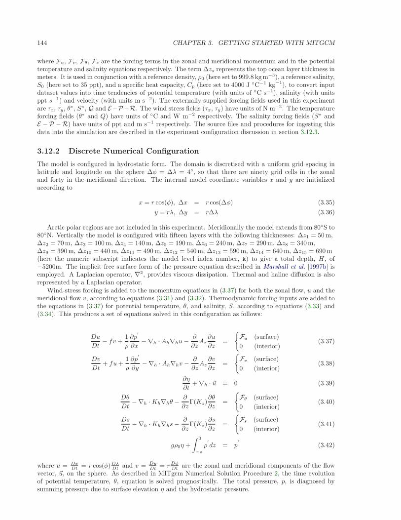
144 CHAPTER 3. GETTING STARTED WITH MITGCM
where Fu, Fv, Fθ, Fs are the forcing terms in the zonal and meridional momentum and in the potentialtemperature and salinity equations respectively. The term ∆zs represents the top ocean layer thickness inmeters. It is used in conjunction with a reference density, ρ0 (here set to 999.8 kgm−3), a reference salinity,S0 (here set to 35 ppt), and a specific heat capacity, Cp (here set to 4000 J C−1 kg−1), to convert inputdataset values into time tendencies of potential temperature (with units of C s−1), salinity (with unitsppt s−1) and velocity (with units m s−2). The externally supplied forcing fields used in this experimentare τx, τy, θ∗, S∗, Q and E−P−R. The wind stress fields (τx, τy) have units of N m−2. The temperatureforcing fields (θ∗ and Q) have units of C and W m−2 respectively. The salinity forcing fields (S∗ andE − P −R) have units of ppt and m s−1 respectively. The source files and procedures for ingesting thisdata into the simulation are described in the experiment configuration discussion in section 3.12.3.
3.12.2 Discrete Numerical Configuration
The model is configured in hydrostatic form. The domain is discretised with a uniform grid spacing inlatitude and longitude on the sphere ∆φ = ∆λ = 4, so that there are ninety grid cells in the zonaland forty in the meridional direction. The internal model coordinate variables x and y are initializedaccording to
x = r cos(φ), ∆x = r cos(∆φ) (3.35)
y = rλ, ∆y = r∆λ (3.36)
Arctic polar regions are not included in this experiment. Meridionally the model extends from 80S to80N. Vertically the model is configured with fifteen layers with the following thicknesses: ∆z1 = 50 m,∆z2 = 70 m, ∆z3 = 100 m, ∆z4 = 140 m, ∆z5 = 190 m, ∆z6 = 240 m, ∆z7 = 290 m, ∆z8 = 340 m,∆z9 = 390 m, ∆z10 = 440 m, ∆z11 = 490 m, ∆z12 = 540 m, ∆z13 = 590 m, ∆z14 = 640 m, ∆z15 = 690 m(here the numeric subscript indicates the model level index number, k) to give a total depth, H , of−5200m. The implicit free surface form of the pressure equation described in Marshall et al. [1997b] isemployed. A Laplacian operator, ∇2, provides viscous dissipation. Thermal and haline diffusion is alsorepresented by a Laplacian operator.
Wind-stress forcing is added to the momentum equations in (3.37) for both the zonal flow, u and themeridional flow v, according to equations (3.31) and (3.32). Thermodynamic forcing inputs are added tothe equations in (3.37) for potential temperature, θ, and salinity, S, according to equations (3.33) and(3.34). This produces a set of equations solved in this configuration as follows:
Du
Dt− fv +
1
ρ
∂p′
∂x−∇h ·Ah∇hu− ∂
∂zAz
∂u
∂z=
Fu (surface)
0 (interior)(3.37)
Dv
Dt+ fu+
1
ρ
∂p′
∂y−∇h · Ah∇hv −
∂
∂zAz
∂v
∂z=
Fv (surface)
0 (interior)(3.38)
∂η
∂t+ ∇h · ~u = 0 (3.39)
Dθ
Dt−∇h ·Kh∇hθ −
∂
∂zΓ(Kz)
∂θ
∂z=
Fθ (surface)
0 (interior)(3.40)
Ds
Dt−∇h ·Kh∇hs−
∂
∂zΓ(Kz)
∂s
∂z=
Fs (surface)
0 (interior)(3.41)
gρ0η +
∫ 0
−z
ρ′
dz = p′
(3.42)
where u = DxDt = r cos(φ)Dλ
Dt and v = DyDt = rDφ
Dt are the zonal and meridional components of the flowvector, ~u, on the sphere. As described in MITgcm Numerical Solution Procedure 2, the time evolutionof potential temperature, θ, equation is solved prognostically. The total pressure, p, is diagnosed bysumming pressure due to surface elevation η and the hydrostatic pressure.
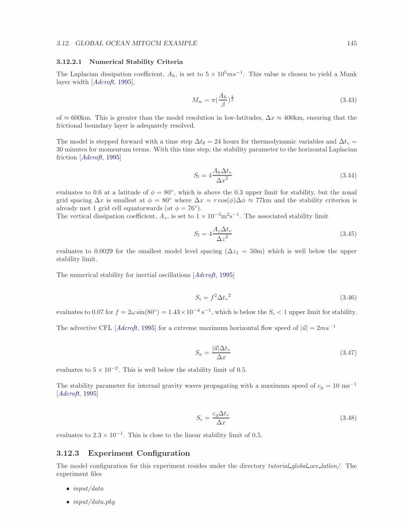
3.12. GLOBAL OCEAN MITGCM EXAMPLE 145
3.12.2.1 Numerical Stability Criteria
The Laplacian dissipation coefficient, Ah, is set to 5 × 10⁵ms−1. This value is chosen to yield a Munklayer width [Adcroft, 1995],
Mw = π(Ah
β)
13 (3.43)
of ≈ 600km. This is greater than the model resolution in low-latitudes, ∆x ≈ 400km, ensuring that thefrictional boundary layer is adequately resolved.
The model is stepped forward with a time step ∆tθ = 24 hours for thermodynamic variables and ∆tv =30 minutes for momentum terms. With this time step, the stability parameter to the horizontal Laplacianfriction [Adcroft, 1995]
Sl = 4Ah∆tv
∆x2 (3.44)
evaluates to 0.6 at a latitude of φ = 80, which is above the 0.3 upper limit for stability, but the zonalgrid spacing ∆x is smallest at φ = 80 where ∆x = r cos(φ)∆φ ≈ 77km and the stability criterion isalready met 1 grid cell equatorwards (at φ = 76).The vertical dissipation coefficient, Az , is set to 1 × 10⁻³m2s−1. The associated stability limit
Sl = 4Az∆tv
∆z2 (3.45)
evaluates to 0.0029 for the smallest model level spacing (∆z1 = 50m) which is well below the upperstability limit.
The numerical stability for inertial oscillations [Adcroft, 1995]
Si = f2∆tv2 (3.46)
evaluates to 0.07 for f = 2ω sin(80) = 1.43×10⁻⁴ s−1, which is below the Si < 1 upper limit for stability.
The advective CFL [Adcroft, 1995] for a extreme maximum horizontal flow speed of |~u| = 2ms−1
Sa =|~u|∆tv
∆x(3.47)
evaluates to 5 × 10⁻². This is well below the stability limit of 0.5.
The stability parameter for internal gravity waves propagating with a maximum speed of cg = 10 ms−1
[Adcroft, 1995]
Sc =cg∆tv∆x
(3.48)
evaluates to 2.3 × 10⁻¹. This is close to the linear stability limit of 0.5.
3.12.3 Experiment Configuration
The model configuration for this experiment resides under the directory tutorial global oce latlon/. Theexperiment files
• input/data
• input/data.pkg
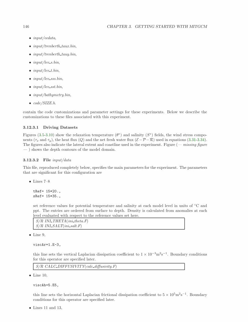
146 CHAPTER 3. GETTING STARTED WITH MITGCM
• input/eedata,
• input/trenberth taux.bin,
• input/trenberth tauy.bin,
• input/lev s.bin,
• input/lev t.bin,
• input/lev sss.bin,
• input/lev sst.bin,
• input/bathymetry.bin,
• code/SIZE.h.
contain the code customizations and parameter settings for these experiments. Below we describe thecustomizations to these files associated with this experiment.
3.12.3.1 Driving Datasets
Figures (3.5-3.10) show the relaxation temperature (θ∗) and salinity (S∗) fields, the wind stress compo-nents (τx and τy), the heat flux (Q) and the net fresh water flux (E−P−R) used in equations (3.31-3.34).The figures also indicate the lateral extent and coastline used in the experiment. Figure (— missing figure— ) shows the depth contours of the model domain.
3.12.3.2 File input/data
This file, reproduced completely below, specifies the main parameters for the experiment. The parametersthat are significant for this configuration are
• Lines 7–8
tRef= 15*20.,
sRef= 15*35.,
set reference values for potential temperature and salinity at each model level in units of C andppt. The entries are ordered from surface to depth. Density is calculated from anomalies at eachlevel evaluated with respect to the reference values set here.
S/R INI THETA(ini theta.F)S/R INI SALT(ini salt.F)
• Line 9,
viscAr=1.E-3,
this line sets the vertical Laplacian dissipation coefficient to 1 × 10⁻³m2s−1. Boundary conditionsfor this operator are specified later.
S/R CALC DIFFUSIVITY(calc diffusivity.F)
• Line 10,
viscAh=5.E5,
this line sets the horizontal Laplacian frictional dissipation coefficient to 5 × 10⁵m2s−1. Boundaryconditions for this operator are specified later.
• Lines 11 and 13,
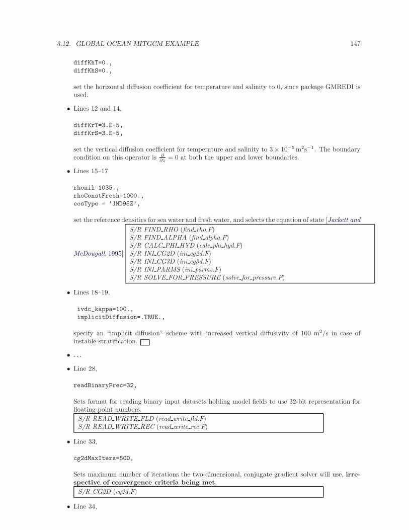
3.12. GLOBAL OCEAN MITGCM EXAMPLE 147
diffKhT=0.,
diffKhS=0.,
set the horizontal diffusion coefficient for temperature and salinity to 0, since package GMREDI isused.
• Lines 12 and 14,
diffKrT=3.E-5,
diffKrS=3.E-5,
set the vertical diffusion coefficient for temperature and salinity to 3 × 10⁻⁵ m2s−1. The boundarycondition on this operator is ∂
∂z = 0 at both the upper and lower boundaries.
• Lines 15–17
rhonil=1035.,
rhoConstFresh=1000.,
eosType = ’JMD95Z’,
set the reference densities for sea water and fresh water, and selects the equation of state [Jackett and
McDougall, 1995]
S/R FIND RHO (find rho.F)S/R FIND ALPHA (find alpha.F)S/R CALC PHI HYD (calc phi hyd.F)S/R INI CG2D (ini cg2d.F)S/R INI CG3D (ini cg3d.F)S/R INI PARMS (ini parms.F)S/R SOLVE FOR PRESSURE (solve for pressure.F)
• Lines 18–19,
ivdc_kappa=100.,
implicitDiffusion=.TRUE.,
specify an “implicit diffusion” scheme with increased vertical diffusivity of 100 m2/s in case ofinstable stratification.
• . . .
• Line 28,
readBinaryPrec=32,
Sets format for reading binary input datasets holding model fields to use 32-bit representation forfloating-point numbers.
S/R READ WRITE FLD (read write fld.F)S/R READ WRITE REC (read write rec.F)
• Line 33,
cg2dMaxIters=500,
Sets maximum number of iterations the two-dimensional, conjugate gradient solver will use, irre-spective of convergence criteria being met.
S/R CG2D (cg2d.F)
• Line 34,
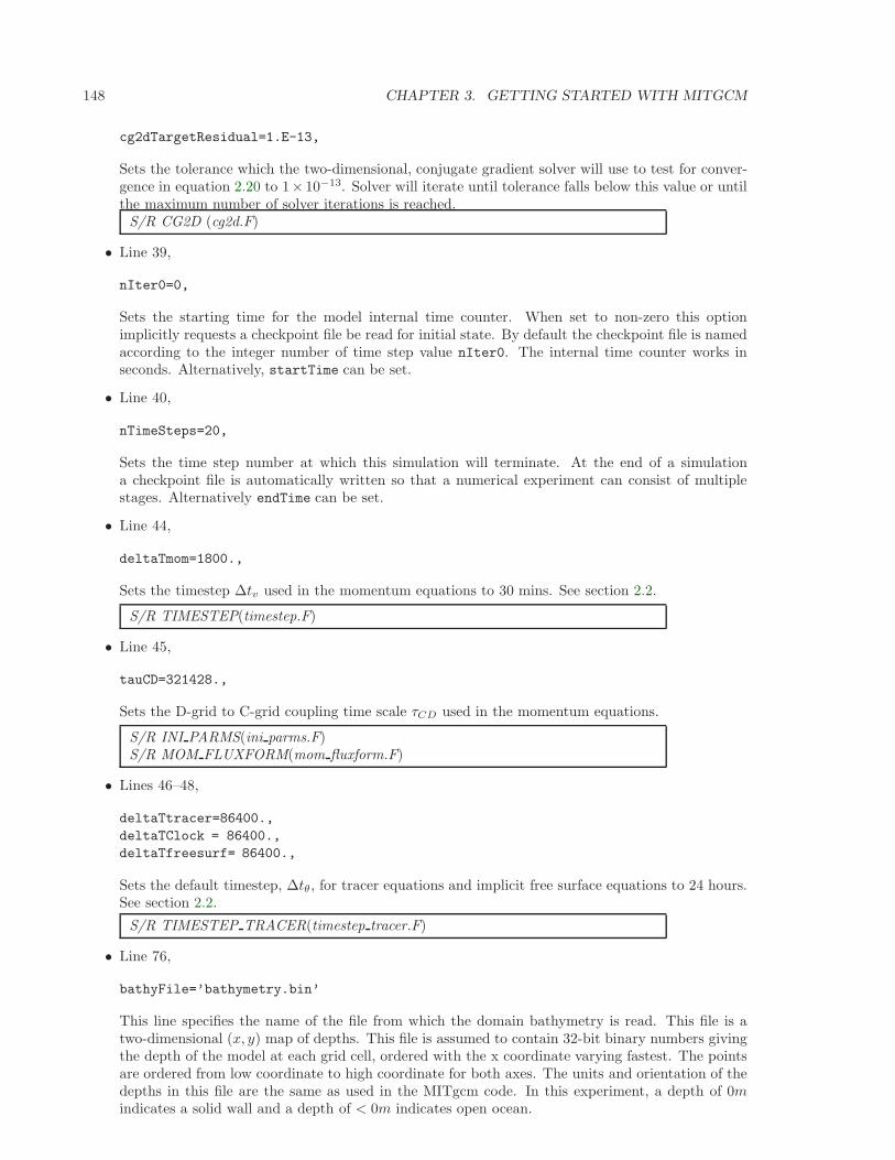
148 CHAPTER 3. GETTING STARTED WITH MITGCM
cg2dTargetResidual=1.E-13,
Sets the tolerance which the two-dimensional, conjugate gradient solver will use to test for conver-gence in equation 2.20 to 1× 10⁻¹³. Solver will iterate until tolerance falls below this value or untilthe maximum number of solver iterations is reached.S/R CG2D (cg2d.F)
• Line 39,
nIter0=0,
Sets the starting time for the model internal time counter. When set to non-zero this optionimplicitly requests a checkpoint file be read for initial state. By default the checkpoint file is namedaccording to the integer number of time step value nIter0. The internal time counter works inseconds. Alternatively, startTime can be set.
• Line 40,
nTimeSteps=20,
Sets the time step number at which this simulation will terminate. At the end of a simulationa checkpoint file is automatically written so that a numerical experiment can consist of multiplestages. Alternatively endTime can be set.
• Line 44,
deltaTmom=1800.,
Sets the timestep ∆tv used in the momentum equations to 30 mins. See section 2.2.
S/R TIMESTEP(timestep.F)
• Line 45,
tauCD=321428.,
Sets the D-grid to C-grid coupling time scale τCD used in the momentum equations.
S/R INI PARMS(ini parms.F)S/R MOM FLUXFORM(mom fluxform.F)
• Lines 46–48,
deltaTtracer=86400.,
deltaTClock = 86400.,
deltaTfreesurf= 86400.,
Sets the default timestep, ∆tθ, for tracer equations and implicit free surface equations to 24 hours.See section 2.2.
S/R TIMESTEP TRACER(timestep tracer.F)
• Line 76,
bathyFile=’bathymetry.bin’
This line specifies the name of the file from which the domain bathymetry is read. This file is atwo-dimensional (x, y) map of depths. This file is assumed to contain 32-bit binary numbers givingthe depth of the model at each grid cell, ordered with the x coordinate varying fastest. The pointsare ordered from low coordinate to high coordinate for both axes. The units and orientation of thedepths in this file are the same as used in the MITgcm code. In this experiment, a depth of 0mindicates a solid wall and a depth of < 0m indicates open ocean.
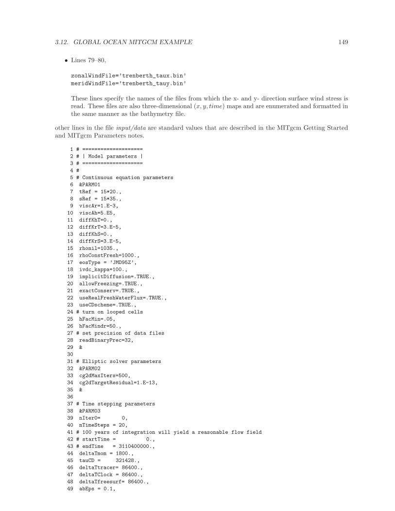
3.12. GLOBAL OCEAN MITGCM EXAMPLE 149
• Lines 79–80,
zonalWindFile=’trenberth_taux.bin’
meridWindFile=’trenberth_tauy.bin’
These lines specify the names of the files from which the x- and y- direction surface wind stress isread. These files are also three-dimensional (x, y, time) maps and are enumerated and formatted inthe same manner as the bathymetry file.
other lines in the file input/data are standard values that are described in the MITgcm Getting Startedand MITgcm Parameters notes.
1 # ====================
2 # | Model parameters |
3 # ====================
4 #
5 # Continuous equation parameters
6 &PARM01
7 tRef = 15*20.,
8 sRef = 15*35.,
9 viscAr=1.E-3,
10 viscAh=5.E5,
11 diffKhT=0.,
12 diffKrT=3.E-5,
13 diffKhS=0.,
14 diffKrS=3.E-5,
15 rhonil=1035.,
16 rhoConstFresh=1000.,
17 eosType = ’JMD95Z’,
18 ivdc_kappa=100.,
19 implicitDiffusion=.TRUE.,
20 allowFreezing=.TRUE.,
21 exactConserv=.TRUE.,
22 useRealFreshWaterFlux=.TRUE.,
23 useCDscheme=.TRUE.,
24 # turn on looped cells
25 hFacMin=.05,
26 hFacMindr=50.,
27 # set precision of data files
28 readBinaryPrec=32,
29 &
30
31 # Elliptic solver parameters
32 &PARM02
33 cg2dMaxIters=500,
34 cg2dTargetResidual=1.E-13,
35 &
36
37 # Time stepping parameters
38 &PARM03
39 nIter0= 0,
40 nTimeSteps = 20,
41 # 100 years of integration will yield a reasonable flow field
42 # startTime = 0.,
43 # endTime = 3110400000.,
44 deltaTmom = 1800.,
45 tauCD = 321428.,
46 deltaTtracer= 86400.,
47 deltaTClock = 86400.,
48 deltaTfreesurf= 86400.,
49 abEps = 0.1,
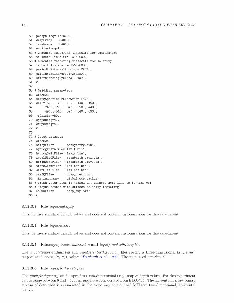
150 CHAPTER 3. GETTING STARTED WITH MITGCM
50 pChkptFreq= 1728000.,
51 dumpFreq= 864000.,
52 taveFreq= 864000.,
53 monitorFreq=1.,
54 # 2 months restoring timescale for temperature
55 tauThetaClimRelax= 5184000.,
56 # 6 months restoring timescale for salinity
57 tauSaltClimRelax = 15552000.,
58 periodicExternalForcing=.TRUE.,
59 externForcingPeriod=2592000.,
60 externForcingCycle=31104000.,
61 &
62
63 # Gridding parameters
64 &PARM04
65 usingSphericalPolarGrid=.TRUE.,
66 delR= 50., 70., 100., 140., 190.,
67 240., 290., 340., 390., 440.,
68 490., 540., 590., 640., 690.,
69 ygOrigin=-80.,
70 dySpacing=4.,
71 dxSpacing=4.,
72 &
73
74 # Input datasets
75 &PARM05
76 bathyFile= ’bathymetry.bin’,
77 hydrogThetaFile=’lev_t.bin’,
78 hydrogSaltFile= ’lev_s.bin’,
79 zonalWindFile= ’trenberth_taux.bin’,
80 meridWindFile= ’trenberth_tauy.bin’,
81 thetaClimFile= ’lev_sst.bin’,
82 saltClimFile= ’lev_sss.bin’,
83 surfQFile= ’ncep_qnet.bin’,
84 the_run_name= ’global_oce_latlon’,
85 # fresh water flux is turned on, comment next line to it turn off
86 # (maybe better with surface salinity restoring)
87 EmPmRFile= ’ncep_emp.bin’,
88 &
3.12.3.3 File input/data.pkg
This file uses standard default values and does not contain customisations for this experiment.
3.12.3.4 File input/eedata
This file uses standard default values and does not contain customisations for this experiment.
3.12.3.5 Filesinput/trenberth taux.bin and input/trenberth tauy.bin
The input/trenberth taux.bin and input/trenberth tauy.bin files specify a three-dimensional (x, y, time)map of wind stress, (τx, τy), values [Trenberth et al., 1990]. The units used are Nm−2.
3.12.3.6 File input/bathymetry.bin
The input/bathymetry.bin file specifies a two-dimensional (x, y) map of depth values. For this experimentvalues range between 0 and −5200 m, and have been derived from ETOPO5. The file contains a raw binarystream of data that is enumerated in the same way as standard MITgcm two-dimensional, horizontalarrays.
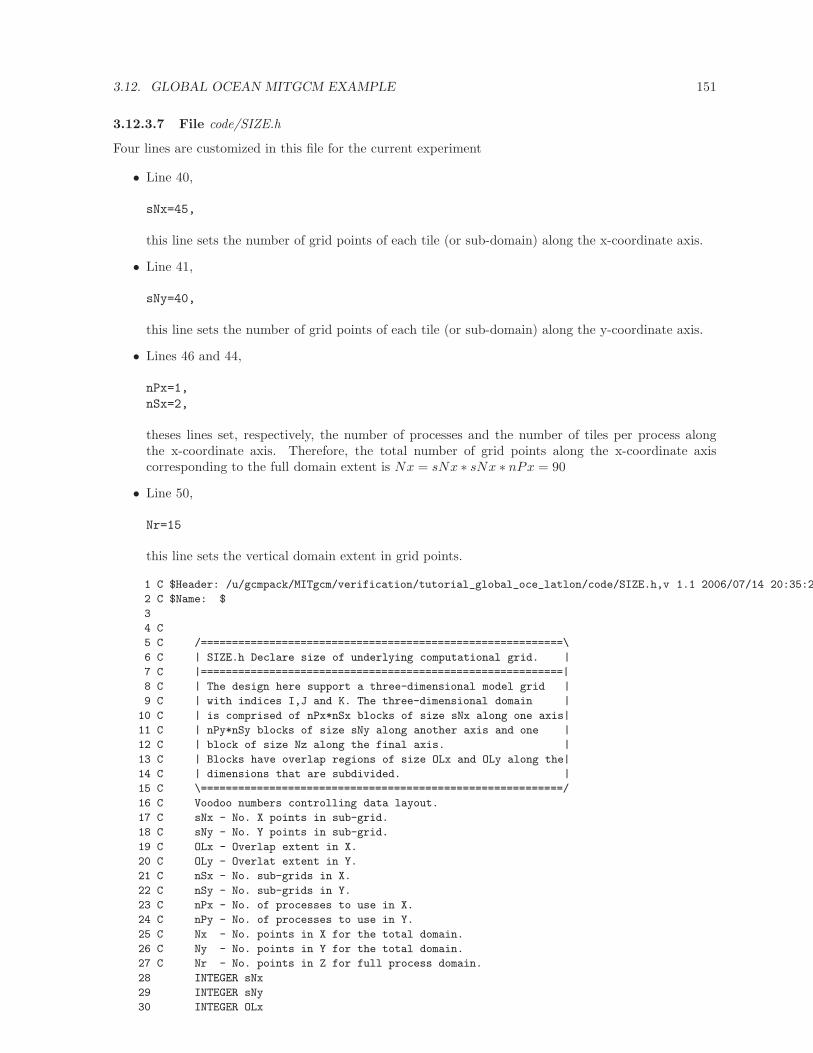
3.12. GLOBAL OCEAN MITGCM EXAMPLE 151
3.12.3.7 File code/SIZE.h
Four lines are customized in this file for the current experiment
• Line 40,
sNx=45,
this line sets the number of grid points of each tile (or sub-domain) along the x-coordinate axis.
• Line 41,
sNy=40,
this line sets the number of grid points of each tile (or sub-domain) along the y-coordinate axis.
• Lines 46 and 44,
nPx=1,
nSx=2,
theses lines set, respectively, the number of processes and the number of tiles per process alongthe x-coordinate axis. Therefore, the total number of grid points along the x-coordinate axiscorresponding to the full domain extent is Nx = sNx ∗ sNx ∗ nPx = 90
• Line 50,
Nr=15
this line sets the vertical domain extent in grid points.
1 C $Header: /u/gcmpack/MITgcm/verification/tutorial_global_oce_latlon/code/SIZE.h,v 1.1 2006/07/14 20:35:22
2 C $Name: $
3
4 C
5 C /==========================================================\
6 C | SIZE.h Declare size of underlying computational grid. |
7 C |==========================================================|
8 C | The design here support a three-dimensional model grid |
9 C | with indices I,J and K. The three-dimensional domain |
10 C | is comprised of nPx*nSx blocks of size sNx along one axis|
11 C | nPy*nSy blocks of size sNy along another axis and one |
12 C | block of size Nz along the final axis. |
13 C | Blocks have overlap regions of size OLx and OLy along the|
14 C | dimensions that are subdivided. |
15 C \==========================================================/
16 C Voodoo numbers controlling data layout.
17 C sNx - No. X points in sub-grid.
18 C sNy - No. Y points in sub-grid.
19 C OLx - Overlap extent in X.
20 C OLy - Overlat extent in Y.
21 C nSx - No. sub-grids in X.
22 C nSy - No. sub-grids in Y.
23 C nPx - No. of processes to use in X.
24 C nPy - No. of processes to use in Y.
25 C Nx - No. points in X for the total domain.
26 C Ny - No. points in Y for the total domain.
27 C Nr - No. points in Z for full process domain.
28 INTEGER sNx
29 INTEGER sNy
30 INTEGER OLx
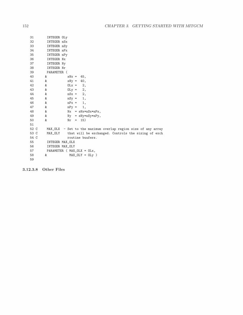
152 CHAPTER 3. GETTING STARTED WITH MITGCM
31 INTEGER OLy
32 INTEGER nSx
33 INTEGER nSy
34 INTEGER nPx
35 INTEGER nPy
36 INTEGER Nx
37 INTEGER Ny
38 INTEGER Nr
39 PARAMETER (
40 & sNx = 45,
41 & sNy = 40,
42 & OLx = 2,
43 & OLy = 2,
44 & nSx = 2,
45 & nSy = 1,
46 & nPx = 1,
47 & nPy = 1,
48 & Nx = sNx*nSx*nPx,
49 & Ny = sNy*nSy*nPy,
50 & Nr = 15)
51
52 C MAX_OLX - Set to the maximum overlap region size of any array
53 C MAX_OLY that will be exchanged. Controls the sizing of exch
54 C routine buufers.
55 INTEGER MAX_OLX
56 INTEGER MAX_OLY
57 PARAMETER ( MAX_OLX = OLx,
58 & MAX_OLY = OLy )
59
3.12.3.8 Other Files
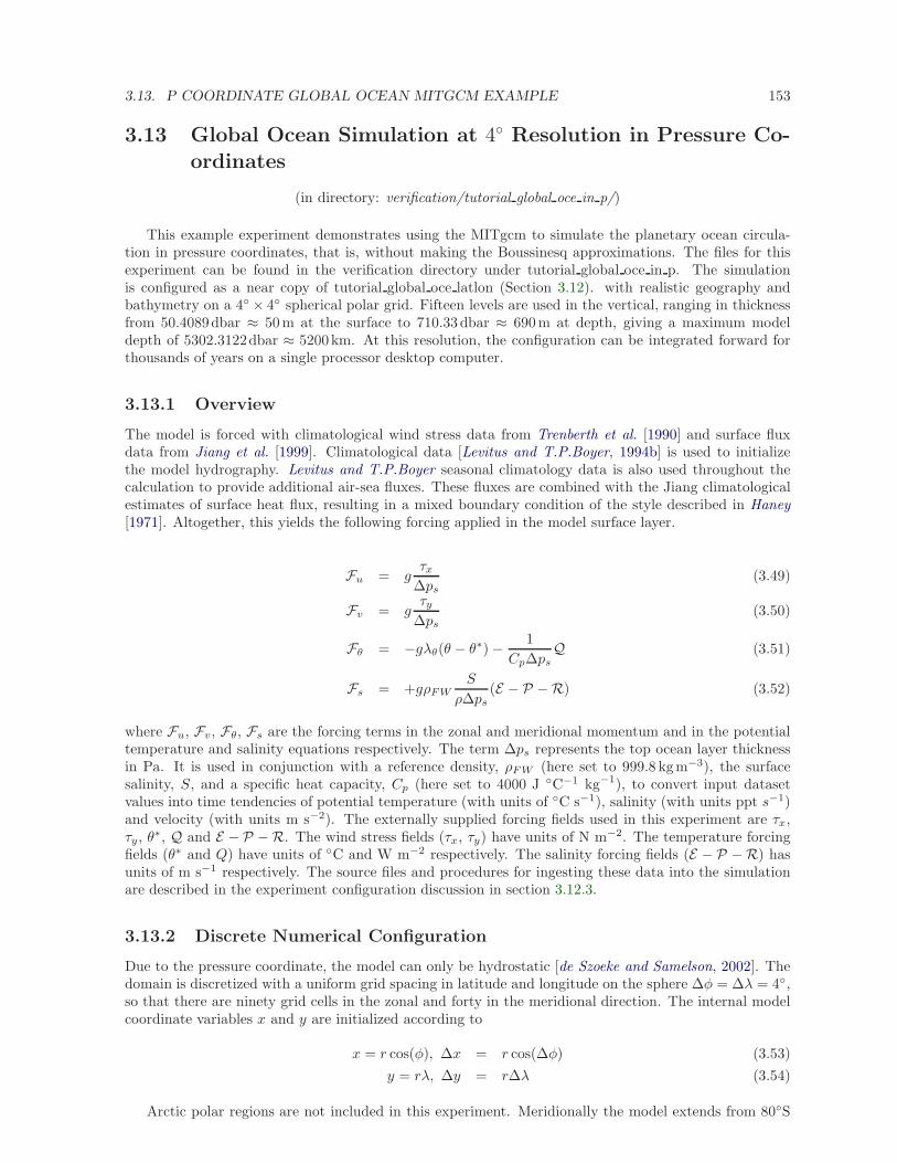
3.13. P COORDINATE GLOBAL OCEAN MITGCM EXAMPLE 153
3.13 Global Ocean Simulation at 4 Resolution in Pressure Co-
ordinates
(in directory: verification/tutorial global oce in p/)
This example experiment demonstrates using the MITgcm to simulate the planetary ocean circula-tion in pressure coordinates, that is, without making the Boussinesq approximations. The files for thisexperiment can be found in the verification directory under tutorial global oce in p. The simulationis configured as a near copy of tutorial global oce latlon (Section 3.12). with realistic geography andbathymetry on a 4 × 4 spherical polar grid. Fifteen levels are used in the vertical, ranging in thicknessfrom 50.4089dbar ≈ 50m at the surface to 710.33dbar ≈ 690m at depth, giving a maximum modeldepth of 5302.3122dbar ≈ 5200km. At this resolution, the configuration can be integrated forward forthousands of years on a single processor desktop computer.
3.13.1 Overview
The model is forced with climatological wind stress data from Trenberth et al. [1990] and surface fluxdata from Jiang et al. [1999]. Climatological data [Levitus and T.P.Boyer, 1994b] is used to initializethe model hydrography. Levitus and T.P.Boyer seasonal climatology data is also used throughout thecalculation to provide additional air-sea fluxes. These fluxes are combined with the Jiang climatologicalestimates of surface heat flux, resulting in a mixed boundary condition of the style described in Haney[1971]. Altogether, this yields the following forcing applied in the model surface layer.
Fu = gτx
∆ps(3.49)
Fv = gτy
∆ps(3.50)
Fθ = −gλθ(θ − θ∗) − 1
Cp∆psQ (3.51)
Fs = +gρFWS
ρ∆ps(E − P −R) (3.52)
where Fu, Fv, Fθ, Fs are the forcing terms in the zonal and meridional momentum and in the potentialtemperature and salinity equations respectively. The term ∆ps represents the top ocean layer thicknessin Pa. It is used in conjunction with a reference density, ρFW (here set to 999.8 kgm−3), the surfacesalinity, S, and a specific heat capacity, Cp (here set to 4000 J C−1 kg−1), to convert input datasetvalues into time tendencies of potential temperature (with units of C s−1), salinity (with units ppt s−1)and velocity (with units m s−2). The externally supplied forcing fields used in this experiment are τx,τy, θ∗, Q and E − P −R. The wind stress fields (τx, τy) have units of N m−2. The temperature forcingfields (θ∗ and Q) have units of C and W m−2 respectively. The salinity forcing fields (E − P −R) hasunits of m s−1 respectively. The source files and procedures for ingesting these data into the simulationare described in the experiment configuration discussion in section 3.12.3.
3.13.2 Discrete Numerical Configuration
Due to the pressure coordinate, the model can only be hydrostatic [de Szoeke and Samelson, 2002]. Thedomain is discretized with a uniform grid spacing in latitude and longitude on the sphere ∆φ = ∆λ = 4,so that there are ninety grid cells in the zonal and forty in the meridional direction. The internal modelcoordinate variables x and y are initialized according to
x = r cos(φ), ∆x = r cos(∆φ) (3.53)
y = rλ, ∆y = r∆λ (3.54)
Arctic polar regions are not included in this experiment. Meridionally the model extends from 80S
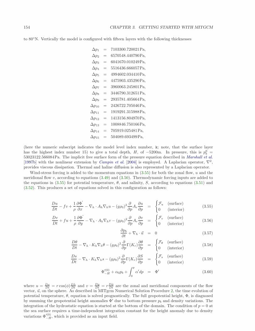
154 CHAPTER 3. GETTING STARTED WITH MITGCM
to 80N. Vertically the model is configured with fifteen layers with the following thicknesses
∆p1 = 7103300.720021Pa,
∆p2 = 6570548.440790Pa,
∆p3 = 6041670.010249Pa,
∆p4 = 5516436.666057Pa,
∆p5 = 4994602.034410Pa,
∆p6 = 4475903.435290Pa,
∆p7 = 3960063.245801Pa,
∆p8 = 3446790.312651Pa,
∆p9 = 2935781.405664Pa,
∆p10 = 2426722.705046Pa,
∆p11 = 1919291.315988Pa,
∆p12 = 1413156.804970Pa,
∆p13 = 1008846.750166Pa,
∆p14 = 705919.025481Pa,
∆p15 = 504089.693499Pa,
(here the numeric subscript indicates the model level index number, k; note, that the surface layerhas the highest index number 15) to give a total depth, H , of −5200m. In pressure, this is p0
b =53023122.566084Pa. The implicit free surface form of the pressure equation described in Marshall et al.[1997b] with the nonlinear extension by Campin et al. [2004] is employed. A Laplacian operator, ∇2,provides viscous dissipation. Thermal and haline diffusion is also represented by a Laplacian operator.
Wind-stress forcing is added to the momentum equations in (3.55) for both the zonal flow, u and themeridional flow v, according to equations (3.49) and (3.50). Thermodynamic forcing inputs are added tothe equations in (3.55) for potential temperature, θ, and salinity, S, according to equations (3.51) and(3.52). This produces a set of equations solved in this configuration as follows:
Du
Dt− fv +
1
ρ
∂Φ′
∂x−∇h ·Ah∇hu− (gρ0)
2 ∂
∂pAr
∂u
∂p=
Fu (surface)
0 (interior)(3.55)
Dv
Dt+ fu+
1
ρ
∂Φ′
∂y−∇h · Ah∇hv − (gρ0)
2 ∂
∂pAr
∂v
∂p=
Fv (surface)
0 (interior)(3.56)
∂pb
∂t+ ∇h · ~u = 0 (3.57)
Dθ
Dt−∇h ·Kh∇hθ − (gρ0)
2 ∂
∂pΓ(Kr)
∂θ
∂p=
Fθ (surface)
0 (interior)(3.58)
Ds
Dt−∇h ·Kh∇hs− (gρ0)
2 ∂
∂pΓ(Kr)
∂S
∂p=
Fs (surface)
0 (interior)(3.59)
Φ′(0)−H + α0pb +
∫ p
0
α′dp = Φ′ (3.60)
where u = DxDt = r cos(φ)Dλ
Dt and v = DyDt = rDφ
Dt are the zonal and meridional components of the flowvector, ~u, on the sphere. As described in MITgcm Numerical Solution Procedure 2, the time evolution ofpotential temperature, θ, equation is solved prognostically. The full geopotential height, Φ, is diagnosedby summing the geopotential height anomalies Φ′ due to bottom pressure pb and density variations. Theintegration of the hydrostatic equation is started at the bottom of the domain. The condition of p = 0 atthe sea surface requires a time-independent integration constant for the height anomaly due to density
variations Φ′(0)−H , which is provided as an input field.
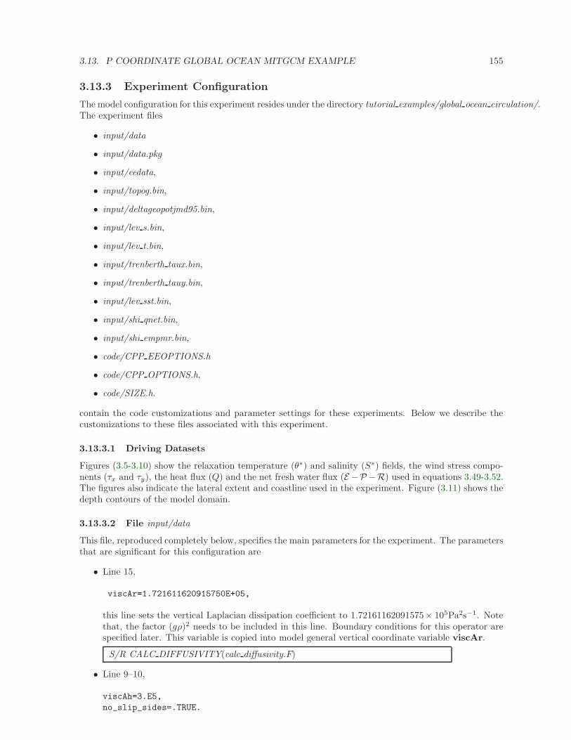
3.13. P COORDINATE GLOBAL OCEAN MITGCM EXAMPLE 155
3.13.3 Experiment Configuration
The model configuration for this experiment resides under the directory tutorial examples/global ocean circulation/.The experiment files
• input/data
• input/data.pkg
• input/eedata,
• input/topog.bin,
• input/deltageopotjmd95.bin,
• input/lev s.bin,
• input/lev t.bin,
• input/trenberth taux.bin,
• input/trenberth tauy.bin,
• input/lev sst.bin,
• input/shi qnet.bin,
• input/shi empmr.bin,
• code/CPP EEOPTIONS.h
• code/CPP OPTIONS.h,
• code/SIZE.h.
contain the code customizations and parameter settings for these experiments. Below we describe thecustomizations to these files associated with this experiment.
3.13.3.1 Driving Datasets
Figures (3.5-3.10) show the relaxation temperature (θ∗) and salinity (S∗) fields, the wind stress compo-nents (τx and τy), the heat flux (Q) and the net fresh water flux (E −P −R) used in equations 3.49-3.52.The figures also indicate the lateral extent and coastline used in the experiment. Figure (3.11) shows thedepth contours of the model domain.
3.13.3.2 File input/data
This file, reproduced completely below, specifies the main parameters for the experiment. The parametersthat are significant for this configuration are
• Line 15,
viscAr=1.721611620915750E+05,
this line sets the vertical Laplacian dissipation coefficient to 1.72161162091575× 10⁵Pa2s−1. Notethat, the factor (gρ)2 needs to be included in this line. Boundary conditions for this operator arespecified later. This variable is copied into model general vertical coordinate variable viscAr.
S/R CALC DIFFUSIVITY(calc diffusivity.F)
• Line 9–10,
viscAh=3.E5,
no_slip_sides=.TRUE.
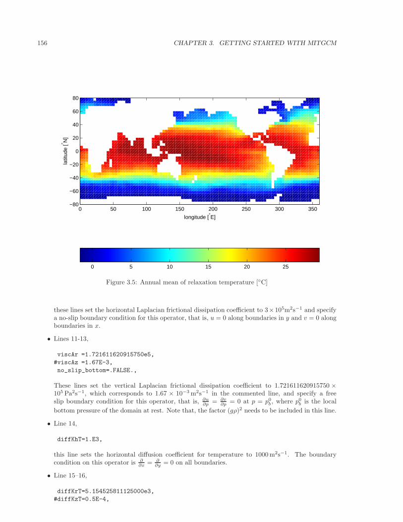
156 CHAPTER 3. GETTING STARTED WITH MITGCM
0 5 10 15 20 25
longitude [°E]
latit
ude
[° N]
0 50 100 150 200 250 300 350−80
−60
−40
−20
0
20
40
60
80
Figure 3.5: Annual mean of relaxation temperature [C]
these lines set the horizontal Laplacian frictional dissipation coefficient to 3×10⁵m2s−1 and specifya no-slip boundary condition for this operator, that is, u = 0 along boundaries in y and v = 0 alongboundaries in x.
• Lines 11-13,
viscAr =1.721611620915750e5,
#viscAz =1.67E-3,
no_slip_bottom=.FALSE.,
These lines set the vertical Laplacian frictional dissipation coefficient to 1.721611620915750 ×10⁵ Pa2s−1, which corresponds to 1.67 × 10⁻³ m2s−1 in the commented line, and specify a freeslip boundary condition for this operator, that is, ∂u
∂p = ∂v∂p = 0 at p = p0
b , where p0b is the local
bottom pressure of the domain at rest. Note that, the factor (gρ)2 needs to be included in this line.
• Line 14,
diffKhT=1.E3,
this line sets the horizontal diffusion coefficient for temperature to 1000 m2s−1. The boundarycondition on this operator is ∂
∂x = ∂∂y = 0 on all boundaries.
• Line 15–16,
diffKrT=5.154525811125000e3,
#diffKzT=0.5E-4,
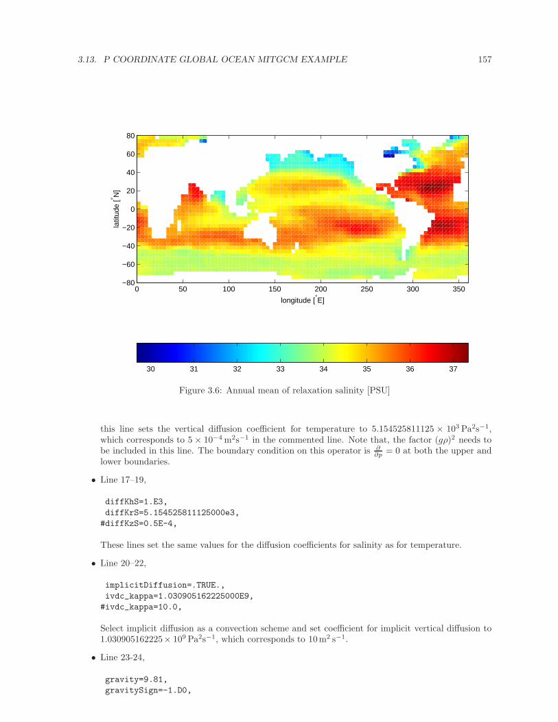
3.13. P COORDINATE GLOBAL OCEAN MITGCM EXAMPLE 157
30 31 32 33 34 35 36 37
longitude [°E]
latit
ude
[° N]
0 50 100 150 200 250 300 350−80
−60
−40
−20
0
20
40
60
80
Figure 3.6: Annual mean of relaxation salinity [PSU]
this line sets the vertical diffusion coefficient for temperature to 5.154525811125 × 10³ Pa2s−1,which corresponds to 5 × 10⁻⁴ m2s−1 in the commented line. Note that, the factor (gρ)2 needs tobe included in this line. The boundary condition on this operator is ∂
∂p = 0 at both the upper andlower boundaries.
• Line 17–19,
diffKhS=1.E3,
diffKrS=5.154525811125000e3,
#diffKzS=0.5E-4,
These lines set the same values for the diffusion coefficients for salinity as for temperature.
• Line 20–22,
implicitDiffusion=.TRUE.,
ivdc_kappa=1.030905162225000E9,
#ivdc_kappa=10.0,
Select implicit diffusion as a convection scheme and set coefficient for implicit vertical diffusion to1.030905162225× 109 Pa2s−1, which corresponds to 10m2 s−1.
• Line 23-24,
gravity=9.81,
gravitySign=-1.D0,
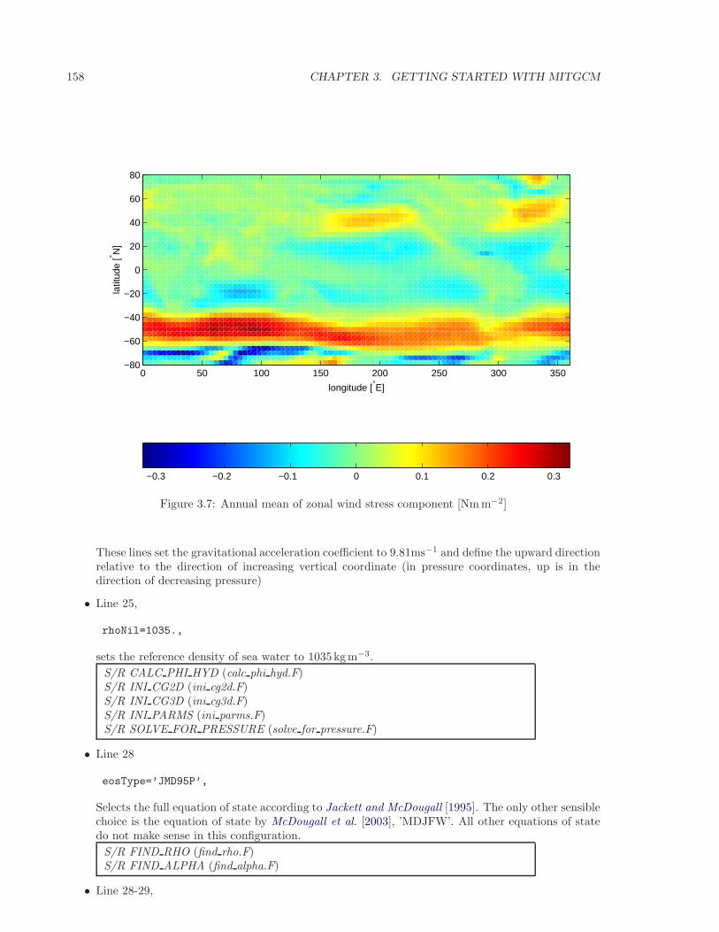
158 CHAPTER 3. GETTING STARTED WITH MITGCM
−0.3 −0.2 −0.1 0 0.1 0.2 0.3
longitude [°E]
latit
ude
[° N]
0 50 100 150 200 250 300 350−80
−60
−40
−20
0
20
40
60
80
Figure 3.7: Annual mean of zonal wind stress component [Nm m−2]
These lines set the gravitational acceleration coefficient to 9.81ms−1 and define the upward directionrelative to the direction of increasing vertical coordinate (in pressure coordinates, up is in thedirection of decreasing pressure)
• Line 25,
rhoNil=1035.,
sets the reference density of sea water to 1035kgm−3.
S/R CALC PHI HYD (calc phi hyd.F)S/R INI CG2D (ini cg2d.F)S/R INI CG3D (ini cg3d.F)S/R INI PARMS (ini parms.F)S/R SOLVE FOR PRESSURE (solve for pressure.F)
• Line 28
eosType=’JMD95P’,
Selects the full equation of state according to Jackett and McDougall [1995]. The only other sensiblechoice is the equation of state by McDougall et al. [2003], ’MDJFW’. All other equations of statedo not make sense in this configuration.
S/R FIND RHO (find rho.F)S/R FIND ALPHA (find alpha.F)
• Line 28-29,
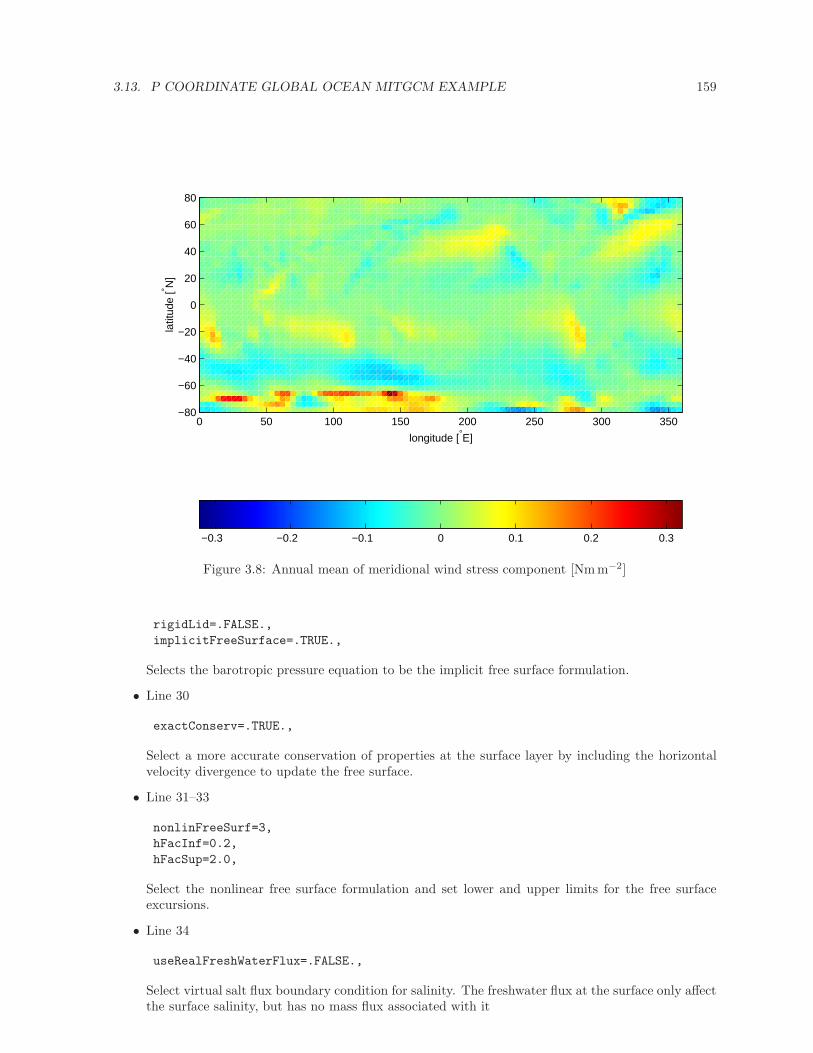
3.13. P COORDINATE GLOBAL OCEAN MITGCM EXAMPLE 159
−0.3 −0.2 −0.1 0 0.1 0.2 0.3
longitude [°E]
latit
ude
[° N]
0 50 100 150 200 250 300 350−80
−60
−40
−20
0
20
40
60
80
Figure 3.8: Annual mean of meridional wind stress component [Nmm−2]
rigidLid=.FALSE.,
implicitFreeSurface=.TRUE.,
Selects the barotropic pressure equation to be the implicit free surface formulation.
• Line 30
exactConserv=.TRUE.,
Select a more accurate conservation of properties at the surface layer by including the horizontalvelocity divergence to update the free surface.
• Line 31–33
nonlinFreeSurf=3,
hFacInf=0.2,
hFacSup=2.0,
Select the nonlinear free surface formulation and set lower and upper limits for the free surfaceexcursions.
• Line 34
useRealFreshWaterFlux=.FALSE.,
Select virtual salt flux boundary condition for salinity. The freshwater flux at the surface only affectthe surface salinity, but has no mass flux associated with it
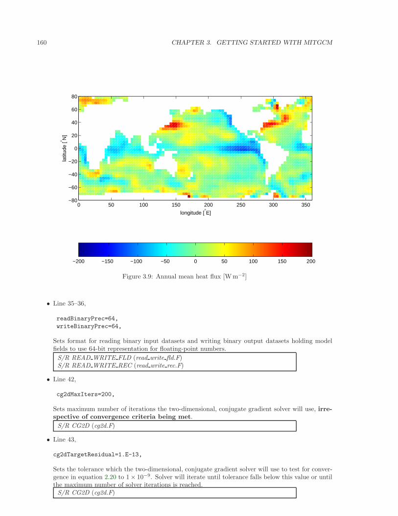
160 CHAPTER 3. GETTING STARTED WITH MITGCM
−200 −150 −100 −50 0 50 100 150 200
longitude [°E]
latit
ude
[° N]
0 50 100 150 200 250 300 350−80
−60
−40
−20
0
20
40
60
80
Figure 3.9: Annual mean heat flux [Wm−2]
• Line 35–36,
readBinaryPrec=64,
writeBinaryPrec=64,
Sets format for reading binary input datasets and writing binary output datasets holding modelfields to use 64-bit representation for floating-point numbers.
S/R READ WRITE FLD (read write fld.F)S/R READ WRITE REC (read write rec.F)
• Line 42,
cg2dMaxIters=200,
Sets maximum number of iterations the two-dimensional, conjugate gradient solver will use, irre-spective of convergence criteria being met.
S/R CG2D (cg2d.F)
• Line 43,
cg2dTargetResidual=1.E-13,
Sets the tolerance which the two-dimensional, conjugate gradient solver will use to test for conver-gence in equation 2.20 to 1× 10⁻⁹. Solver will iterate until tolerance falls below this value or untilthe maximum number of solver iterations is reached.S/R CG2D (cg2d.F)
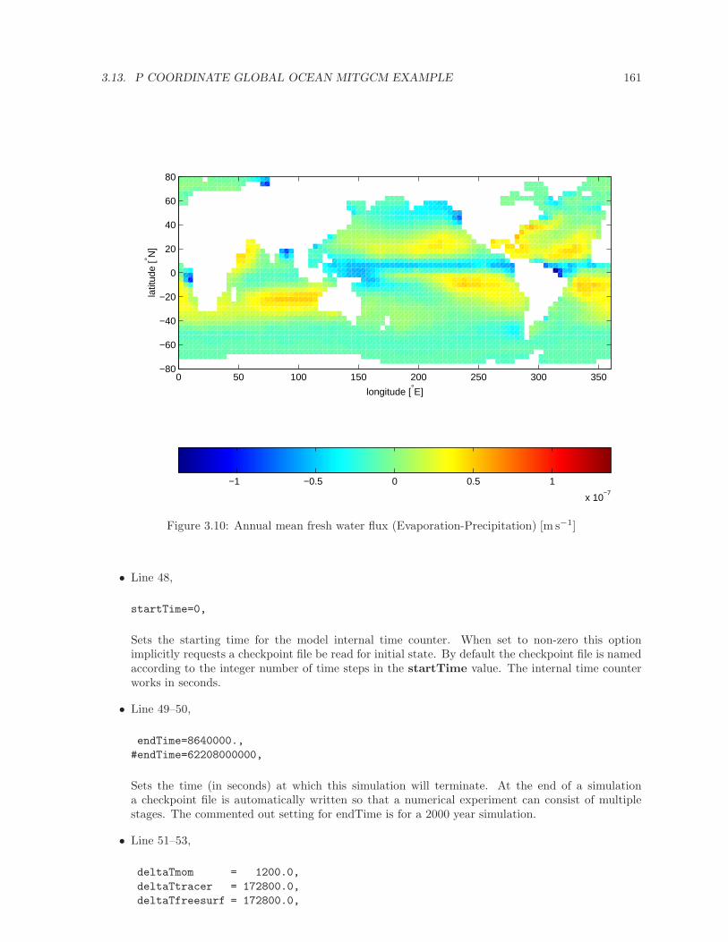
3.13. P COORDINATE GLOBAL OCEAN MITGCM EXAMPLE 161
−1 −0.5 0 0.5 1
x 10−7
longitude [°E]
latit
ude
[° N]
0 50 100 150 200 250 300 350−80
−60
−40
−20
0
20
40
60
80
Figure 3.10: Annual mean fresh water flux (Evaporation-Precipitation) [m s−1]
• Line 48,
startTime=0,
Sets the starting time for the model internal time counter. When set to non-zero this optionimplicitly requests a checkpoint file be read for initial state. By default the checkpoint file is namedaccording to the integer number of time steps in the startTime value. The internal time counterworks in seconds.
• Line 49–50,
endTime=8640000.,
#endTime=62208000000,
Sets the time (in seconds) at which this simulation will terminate. At the end of a simulationa checkpoint file is automatically written so that a numerical experiment can consist of multiplestages. The commented out setting for endTime is for a 2000 year simulation.
• Line 51–53,
deltaTmom = 1200.0,
deltaTtracer = 172800.0,
deltaTfreesurf = 172800.0,
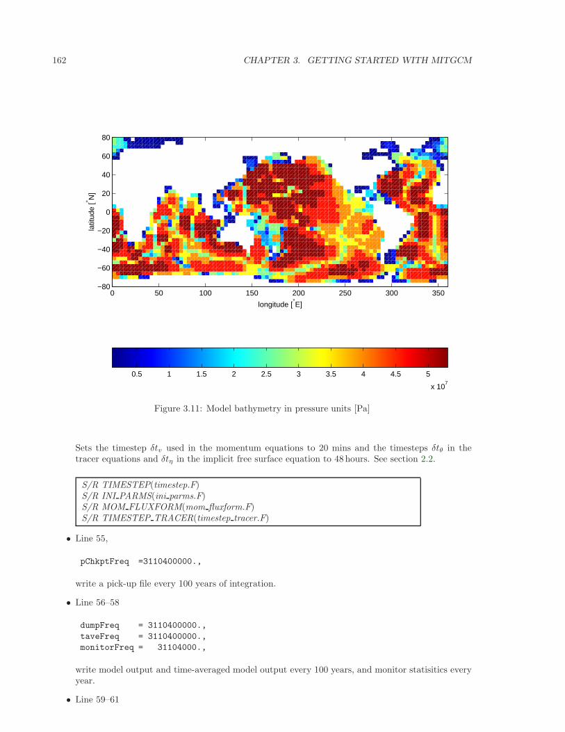
162 CHAPTER 3. GETTING STARTED WITH MITGCM
0.5 1 1.5 2 2.5 3 3.5 4 4.5 5
x 107
longitude [°E]
latit
ude
[° N]
0 50 100 150 200 250 300 350−80
−60
−40
−20
0
20
40
60
80
Figure 3.11: Model bathymetry in pressure units [Pa]
Sets the timestep δtv used in the momentum equations to 20 mins and the timesteps δtθ in thetracer equations and δtη in the implicit free surface equation to 48 hours. See section 2.2.
S/R TIMESTEP(timestep.F)S/R INI PARMS(ini parms.F)S/R MOM FLUXFORM(mom fluxform.F)S/R TIMESTEP TRACER(timestep tracer.F)
• Line 55,
pChkptFreq =3110400000.,
write a pick-up file every 100 years of integration.
• Line 56–58
dumpFreq = 3110400000.,
taveFreq = 3110400000.,
monitorFreq = 31104000.,
write model output and time-averaged model output every 100 years, and monitor statisitics everyyear.
• Line 59–61
3.13. P COORDINATE GLOBAL OCEAN MITGCM EXAMPLE 163
periodicExternalForcing=.TRUE.,
externForcingPeriod=2592000.,
externForcingCycle=31104000.,
Allow periodic external forcing, set forcing period, during which one set of data is valid, to 1 monthand the repeat cycle to 1 year.
S/R EXTERNAL FORCING SURF(external forcing surf.F)
• Line 62
tauThetaClimRelax=5184000.0,
Set the restoring timescale to 2 months.
S/R EXTERNAL FORCING SURF(external forcing surf.F)
• Line 63
abEps=0.1,
Adams-Bashford factor (see section 2.5)
• Line 68–69
usingCartesianGrid=.FALSE.,
usingSphericalPolarGrid=.TRUE.,
Select spherical grid.
• Line 70–71
dXspacing=4.,
dYspacing=4.,
Set the horizontal grid spacing in degrees spherical distance.
• Line 72
Ro_SeaLevel=53023122.566084,
specifies the total height (in r-units, i.e., pressure units) of the sea surface at rest. This is a referencevalue.
• Line 73
groundAtK1=.TRUE.,
specifies the reversal of the vertical indexing. The vertical index is 1 at the bottom of the domanand maximal (i.e., 15) at the surface.
• Line 74–78
delR=7103300.720021, \ldots
set the layer thickness in pressure units, starting with the bottom layer.
• Line 84–93,
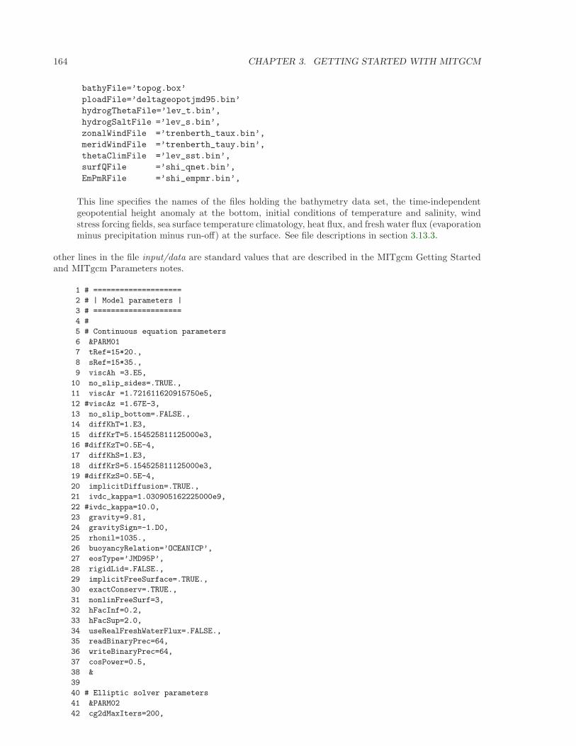
164 CHAPTER 3. GETTING STARTED WITH MITGCM
bathyFile=’topog.box’
ploadFile=’deltageopotjmd95.bin’
hydrogThetaFile=’lev_t.bin’,
hydrogSaltFile =’lev_s.bin’,
zonalWindFile =’trenberth_taux.bin’,
meridWindFile =’trenberth_tauy.bin’,
thetaClimFile =’lev_sst.bin’,
surfQFile =’shi_qnet.bin’,
EmPmRFile =’shi_empmr.bin’,
This line specifies the names of the files holding the bathymetry data set, the time-independentgeopotential height anomaly at the bottom, initial conditions of temperature and salinity, windstress forcing fields, sea surface temperature climatology, heat flux, and fresh water flux (evaporationminus precipitation minus run-off) at the surface. See file descriptions in section 3.13.3.
other lines in the file input/data are standard values that are described in the MITgcm Getting Startedand MITgcm Parameters notes.
1 # ====================
2 # | Model parameters |
3 # ====================
4 #
5 # Continuous equation parameters
6 &PARM01
7 tRef=15*20.,
8 sRef=15*35.,
9 viscAh =3.E5,
10 no_slip_sides=.TRUE.,
11 viscAr =1.721611620915750e5,
12 #viscAz =1.67E-3,
13 no_slip_bottom=.FALSE.,
14 diffKhT=1.E3,
15 diffKrT=5.154525811125000e3,
16 #diffKzT=0.5E-4,
17 diffKhS=1.E3,
18 diffKrS=5.154525811125000e3,
19 #diffKzS=0.5E-4,
20 implicitDiffusion=.TRUE.,
21 ivdc_kappa=1.030905162225000e9,
22 #ivdc_kappa=10.0,
23 gravity=9.81,
24 gravitySign=-1.D0,
25 rhonil=1035.,
26 buoyancyRelation=’OCEANICP’,
27 eosType=’JMD95P’,
28 rigidLid=.FALSE.,
29 implicitFreeSurface=.TRUE.,
30 exactConserv=.TRUE.,
31 nonlinFreeSurf=3,
32 hFacInf=0.2,
33 hFacSup=2.0,
34 useRealFreshWaterFlux=.FALSE.,
35 readBinaryPrec=64,
36 writeBinaryPrec=64,
37 cosPower=0.5,
38 &
39
40 # Elliptic solver parameters
41 &PARM02
42 cg2dMaxIters=200,
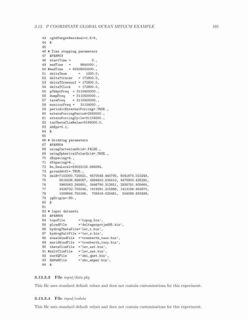
3.13. P COORDINATE GLOBAL OCEAN MITGCM EXAMPLE 165
43 cg2dTargetResidual=1.E-9,
44 &
45
46 # Time stepping parameters
47 &PARM03
48 startTime = 0.,
49 endTime = 8640000.,
50 #endTime = 62208000000.,
51 deltaTmom = 1200.0,
52 deltaTtracer = 172800.0,
53 deltaTfreesurf = 172800.0,
54 deltaTClock = 172800.0,
55 pChkptFreq = 3110400000.,
56 dumpFreq = 3110400000.,
57 taveFreq = 3110400000.,
58 monitorFreq = 31104000.,
59 periodicExternalForcing=.TRUE.,
60 externForcingPeriod=2592000.,
61 externForcingCycle=31104000.,
62 tauThetaClimRelax=5184000.0,
63 abEps=0.1,
64 &
65
66 # Gridding parameters
67 &PARM04
68 usingCartesianGrid=.FALSE.,
69 usingSphericalPolarGrid=.TRUE.,
70 dXspacing=4.,
71 dYspacing=4.,
72 Ro_SeaLevel=53023122.566084,
73 groundAtK1=.TRUE.,
74 delR=7103300.720021, 6570548.440790, 6041670.010249,
75 5516436.666057, 4994602.034410, 4475903.435290,
76 3960063.245801, 3446790.312651, 2935781.405664,
77 2426722.705046, 1919291.315988, 1413156.804970,
78 1008846.750166, 705919.025481, 504089.693499,
79 ygOrigin=-80.,
80 &
81
82 # Input datasets
83 &PARM05
84 topoFile =’topog.bin’,
85 pLoadFile =’deltageopotjmd95.bin’,
86 hydrogThetaFile=’lev_t.bin’,
87 hydrogSaltFile =’lev_s.bin’,
88 zonalWindFile =’trenberth_taux.bin’,
89 meridWindFile =’trenberth_tauy.bin’,
90 thetaClimFile =’lev_sst.bin’,
91 #saltClimFile =’lev_sss.bin’,
92 surfQFile =’shi_qnet.bin’,
93 EmPmRFile =’shi_empmr.bin’,
94 &
3.13.3.3 File input/data.pkg
This file uses standard default values and does not contain customisations for this experiment.
3.13.3.4 File input/eedata
This file uses standard default values and does not contain customisations for this experiment.
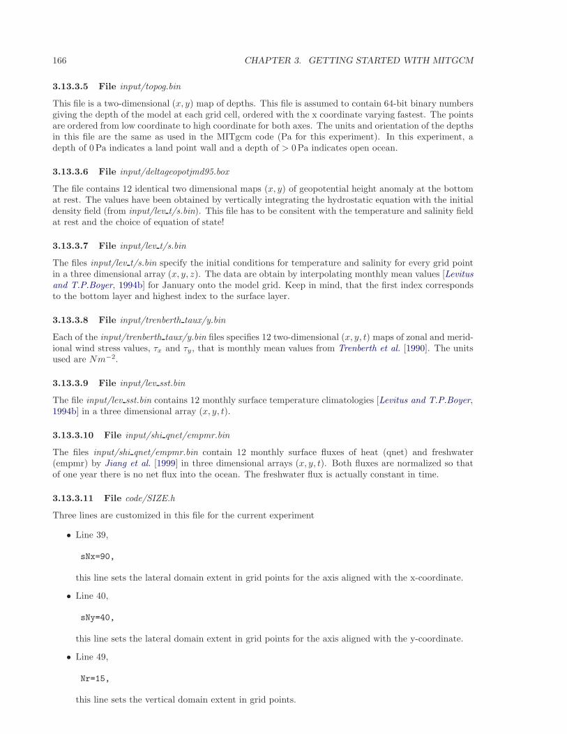
166 CHAPTER 3. GETTING STARTED WITH MITGCM
3.13.3.5 File input/topog.bin
This file is a two-dimensional (x, y) map of depths. This file is assumed to contain 64-bit binary numbersgiving the depth of the model at each grid cell, ordered with the x coordinate varying fastest. The pointsare ordered from low coordinate to high coordinate for both axes. The units and orientation of the depthsin this file are the same as used in the MITgcm code (Pa for this experiment). In this experiment, adepth of 0 Pa indicates a land point wall and a depth of > 0Pa indicates open ocean.
3.13.3.6 File input/deltageopotjmd95.box
The file contains 12 identical two dimensional maps (x, y) of geopotential height anomaly at the bottomat rest. The values have been obtained by vertically integrating the hydrostatic equation with the initialdensity field (from input/lev t/s.bin). This file has to be consitent with the temperature and salinity fieldat rest and the choice of equation of state!
3.13.3.7 File input/lev t/s.bin
The files input/lev t/s.bin specify the initial conditions for temperature and salinity for every grid pointin a three dimensional array (x, y, z). The data are obtain by interpolating monthly mean values [Levitusand T.P.Boyer, 1994b] for January onto the model grid. Keep in mind, that the first index correspondsto the bottom layer and highest index to the surface layer.
3.13.3.8 File input/trenberth taux/y.bin
Each of the input/trenberth taux/y.bin files specifies 12 two-dimensional (x, y, t) maps of zonal and merid-ional wind stress values, τx and τy, that is monthly mean values from Trenberth et al. [1990]. The unitsused are Nm−2.
3.13.3.9 File input/lev sst.bin
The file input/lev sst.bin contains 12 monthly surface temperature climatologies [Levitus and T.P.Boyer,1994b] in a three dimensional array (x, y, t).
3.13.3.10 File input/shi qnet/empmr.bin
The files input/shi qnet/empmr.bin contain 12 monthly surface fluxes of heat (qnet) and freshwater(empmr) by Jiang et al. [1999] in three dimensional arrays (x, y, t). Both fluxes are normalized so thatof one year there is no net flux into the ocean. The freshwater flux is actually constant in time.
3.13.3.11 File code/SIZE.h
Three lines are customized in this file for the current experiment
• Line 39,
sNx=90,
this line sets the lateral domain extent in grid points for the axis aligned with the x-coordinate.
• Line 40,
sNy=40,
this line sets the lateral domain extent in grid points for the axis aligned with the y-coordinate.
• Line 49,
Nr=15,
this line sets the vertical domain extent in grid points.
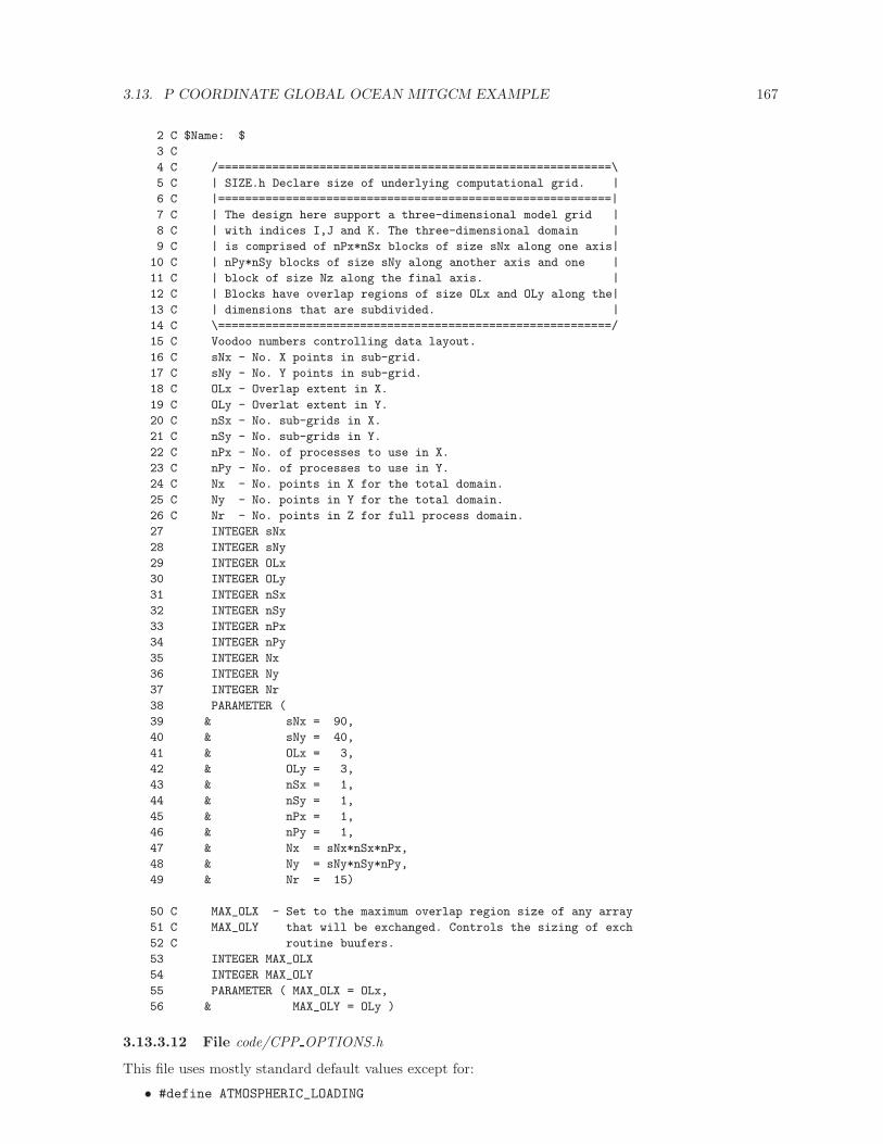
3.13. P COORDINATE GLOBAL OCEAN MITGCM EXAMPLE 167
2 C $Name: $
3 C
4 C /==========================================================\
5 C | SIZE.h Declare size of underlying computational grid. |
6 C |==========================================================|
7 C | The design here support a three-dimensional model grid |
8 C | with indices I,J and K. The three-dimensional domain |
9 C | is comprised of nPx*nSx blocks of size sNx along one axis|
10 C | nPy*nSy blocks of size sNy along another axis and one |
11 C | block of size Nz along the final axis. |
12 C | Blocks have overlap regions of size OLx and OLy along the|
13 C | dimensions that are subdivided. |
14 C \==========================================================/
15 C Voodoo numbers controlling data layout.
16 C sNx - No. X points in sub-grid.
17 C sNy - No. Y points in sub-grid.
18 C OLx - Overlap extent in X.
19 C OLy - Overlat extent in Y.
20 C nSx - No. sub-grids in X.
21 C nSy - No. sub-grids in Y.
22 C nPx - No. of processes to use in X.
23 C nPy - No. of processes to use in Y.
24 C Nx - No. points in X for the total domain.
25 C Ny - No. points in Y for the total domain.
26 C Nr - No. points in Z for full process domain.
27 INTEGER sNx
28 INTEGER sNy
29 INTEGER OLx
30 INTEGER OLy
31 INTEGER nSx
32 INTEGER nSy
33 INTEGER nPx
34 INTEGER nPy
35 INTEGER Nx
36 INTEGER Ny
37 INTEGER Nr
38 PARAMETER (
39 & sNx = 90,
40 & sNy = 40,
41 & OLx = 3,
42 & OLy = 3,
43 & nSx = 1,
44 & nSy = 1,
45 & nPx = 1,
46 & nPy = 1,
47 & Nx = sNx*nSx*nPx,
48 & Ny = sNy*nSy*nPy,
49 & Nr = 15)
50 C MAX_OLX - Set to the maximum overlap region size of any array
51 C MAX_OLY that will be exchanged. Controls the sizing of exch
52 C routine buufers.
53 INTEGER MAX_OLX
54 INTEGER MAX_OLY
55 PARAMETER ( MAX_OLX = OLx,
56 & MAX_OLY = OLy )
3.13.3.12 File code/CPP OPTIONS.h
This file uses mostly standard default values except for:
• #define ATMOSPHERIC_LOADING

168 CHAPTER 3. GETTING STARTED WITH MITGCM
enable pressure loading which is abused to include the initial geopotential height anomaly
• #define EXACT_CONSERV
enable more accurate conservation properties to include the horizontal mass divergence in the freesurface
• #define NONLIN_FRSURF
enable the nonlinear free surface
3.13.3.13 File code/CPP EEOPTIONS.h
This file uses standard default values and does not contain customisations for this experiment.
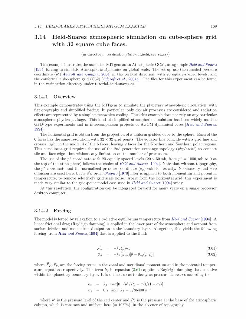
3.14. HELD-SUAREZ ATMOSPHERE MITGCM EXAMPLE 169
3.14 Held-Suarez atmospheric simulation on cube-sphere grid
with 32 square cube faces.
(in directory: verification/tutorial held suarez cs/)
This example illustrates the use of the MITgcm as an Atmospheric GCM, using simple Held and Suarez[1994] forcing to simulate Atmospheric Dynamics on global scale. The set-up use the rescaled pressurecoordinate (p∗)[Adcroft and Campin, 2004] in the vertical direction, with 20 equaly-spaced levels, andthe conformal cube-sphere grid (C32) [Adcroft et al., 2004a]. The files for this experiment can be foundin the verification directory under tutorial held suarez cs.
3.14.1 Overview
This example demonstrates using the MITgcm to simulate the planetary atmospheric circulation, withflat orography and simplified forcing. In particular, only dry air processes are considered and radiationeffects are represented by a simple newtownien cooling, Thus this example does not rely on any particularatmospheric physics package. This kind of simplified atmospheric simulation has been widely used inGFD-type experiments and in intercomparison projects of AGCM dynamical cores [Held and Suarez,1994].
The horizontal grid is obtain from the projection of a uniform gridded cube to the sphere. Each of the6 faces has the same resolution, with 32 × 32 grid points. The equator line coincide with a grid line andcrosses, right in the midle, 4 of the 6 faces, leaving 2 faces for the Northern and Southern polar regions.This curvilinear grid requires the use of the 2nd generation exchange topology (pkg/exch2) to connecttile and face edges, but without any limitation on the number of processors.
The use of the p∗ coordinate with 20 equally spaced levels (20 × 50 mb, from p∗ = 1000,mb to 0 atthe top of the atmosphere) follows the choice of Held and Suarez [1994]. Note that without topography,the p∗ coordinate and the normalized pressure coordinate (σp) coincide exactly. No viscosity and zerodiffusion are used here, but a 8th order Shapiro [1970] filter is applied to both momentum and potentialtemperature, to remove selectively grid scale noise. Apart from the horizontal grid, this experiment ismade very similar to the grid-point model case used in Held and Suarez [1994] study.
At this resolution, the configuration can be integrated forward for many years on a single processordesktop computer.
3.14.2 Forcing
The model is forced by relaxation to a radiative equilibrium temperature from Held and Suarez [1994]. Alinear frictional drag (Rayleigh damping) is applied in the lower part of the atmosphere and account fromsurface friction and momentum dissipation in the boundary layer. Altogether, this yields the followingforcing [from Held and Suarez, 1994] that is applied to the fluid:
~Fv = −kv(p)~vh (3.61)
Fθ = −kθ(ϕ, p)[θ − θeq(ϕ, p)] (3.62)
where ~Fv, Fθ, are the forcing terms in the zonal and meridional momentum and in the potential temper-ature equations respectively. The term kv in equation (3.61) applies a Rayleigh damping that is activewithin the planetary boundary layer. It is defined so as to decay as pressure decreases according to
kv = kf max[0, (p∗/P 0s − σb)/(1 − σb)]
σb = 0.7 and kf = 1/86400 s−1
where p∗ is the pressure level of the cell center and P 0s is the pressure at the base of the atmospheric
column, which is constant and uniform here (= 105Pa), in the absence of topography.
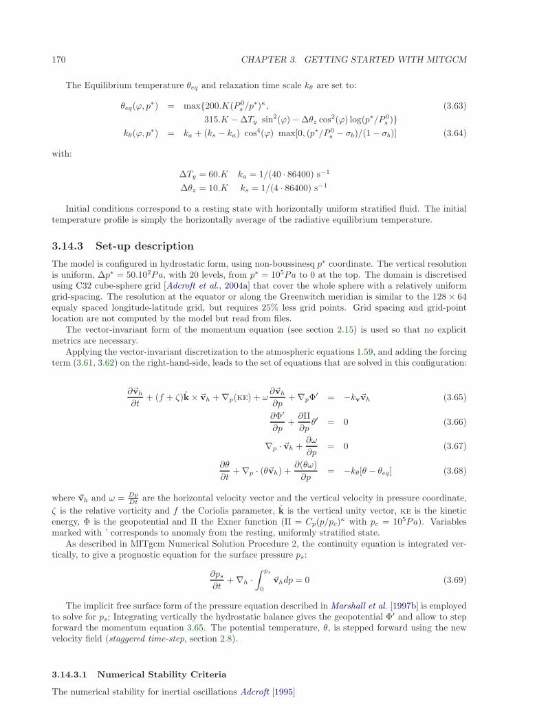
170 CHAPTER 3. GETTING STARTED WITH MITGCM
The Equilibrium temperature θeq and relaxation time scale kθ are set to:
θeq(ϕ, p∗) = max200.K(P 0
s /p∗)κ, (3.63)
315.K − ∆Ty sin2(ϕ) − ∆θz cos2(ϕ) log(p∗/P 0s )
kθ(ϕ, p∗) = ka + (ks − ka) cos4(ϕ) max[0, (p∗/P 0
s − σb)/(1 − σb)] (3.64)
with:
∆Ty = 60.K ka = 1/(40 · 86400) s−1
∆θz = 10.K ks = 1/(4 · 86400) s−1
Initial conditions correspond to a resting state with horizontally uniform stratified fluid. The initialtemperature profile is simply the horizontally average of the radiative equilibrium temperature.
3.14.3 Set-up description
The model is configured in hydrostatic form, using non-boussinesq p∗ coordinate. The vertical resolutionis uniform, ∆p∗ = 50.102Pa, with 20 levels, from p∗ = 105Pa to 0 at the top. The domain is discretisedusing C32 cube-sphere grid [Adcroft et al., 2004a] that cover the whole sphere with a relatively uniformgrid-spacing. The resolution at the equator or along the Greenwitch meridian is similar to the 128 × 64equaly spaced longitude-latitude grid, but requires 25% less grid points. Grid spacing and grid-pointlocation are not computed by the model but read from files.
The vector-invariant form of the momentum equation (see section 2.15) is used so that no explicitmetrics are necessary.
Applying the vector-invariant discretization to the atmospheric equations 1.59, and adding the forcingterm (3.61, 3.62) on the right-hand-side, leads to the set of equations that are solved in this configuration:
∂~vh
∂t+ (f + ζ)k × ~vh + ∇p(ke) + ω
∂~vh
∂p+ ∇pΦ
′ = −kv~vh (3.65)
∂Φ′
∂p+∂Π
∂pθ′ = 0 (3.66)
∇p · ~vh +∂ω
∂p= 0 (3.67)
∂θ
∂t+ ∇p · (θ~vh) +
∂(θω)
∂p= −kθ[θ − θeq] (3.68)
where ~vh and ω = DpDt are the horizontal velocity vector and the vertical velocity in pressure coordinate,
ζ is the relative vorticity and f the Coriolis parameter, k is the vertical unity vector, ke is the kineticenergy, Φ is the geopotential and Π the Exner function (Π = Cp(p/pc)
κ with pc = 105Pa). Variablesmarked with ’ corresponds to anomaly from the resting, uniformly stratified state.
As described in MITgcm Numerical Solution Procedure 2, the continuity equation is integrated ver-tically, to give a prognostic equation for the surface pressure ps:
∂ps
∂t+ ∇h ·
∫ ps
0
~vhdp = 0 (3.69)
The implicit free surface form of the pressure equation described in Marshall et al. [1997b] is employedto solve for ps; Integrating vertically the hydrostatic balance gives the geopotential Φ′ and allow to stepforward the momentum equation 3.65. The potential temperature, θ, is stepped forward using the newvelocity field (staggered time-step, section 2.8).
3.14.3.1 Numerical Stability Criteria
The numerical stability for inertial oscillations Adcroft [1995]
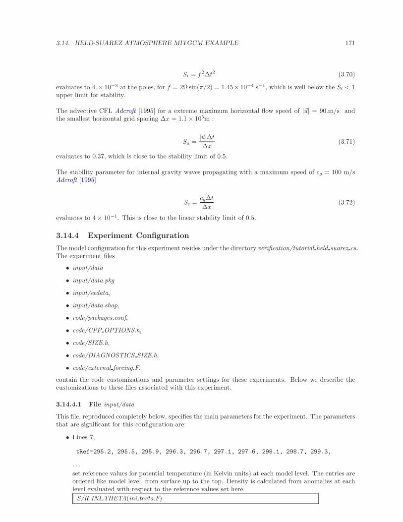
3.14. HELD-SUAREZ ATMOSPHERE MITGCM EXAMPLE 171
Si = f2∆t2 (3.70)
evaluates to 4.× 10−3 at the poles, for f = 2Ω sin(π/2) = 1.45× 10⁻⁴ s−1, which is well below the Si < 1upper limit for stability.
The advective CFL Adcroft [1995] for a extreme maximum horizontal flow speed of |~u| = 90.m/s andthe smallest horizontal grid spacing ∆x = 1.1 × 10⁵m :
Sa =|~u|∆t∆x
(3.71)
evaluates to 0.37, which is close to the stability limit of 0.5.
The stability parameter for internal gravity waves propagating with a maximum speed of cg = 100 m/sAdcroft [1995]
Sc =cg∆t
∆x(3.72)
evaluates to 4 × 10⁻¹. This is close to the linear stability limit of 0.5.
3.14.4 Experiment Configuration
The model configuration for this experiment resides under the directory verification/tutorial held suarez cs.The experiment files
• input/data
• input/data.pkg
• input/eedata,
• input/data.shap,
• code/packages.conf,
• code/CPP OPTIONS.h,
• code/SIZE.h,
• code/DIAGNOSTICS SIZE.h,
• code/external forcing.F,
contain the code customizations and parameter settings for these experiments. Below we describe thecustomizations to these files associated with this experiment.
3.14.4.1 File input/data
This file, reproduced completely below, specifies the main parameters for the experiment. The parametersthat are significant for this configuration are:
• Lines 7,
tRef=295.2, 295.5, 295.9, 296.3, 296.7, 297.1, 297.6, 298.1, 298.7, 299.3,
· · ·set reference values for potential temperature (in Kelvin units) at each model level. The entries areordered like model level, from surface up to the top. Density is calculated from anomalies at eachlevel evaluated with respect to the reference values set here.
S/R INI THETA(ini theta.F)
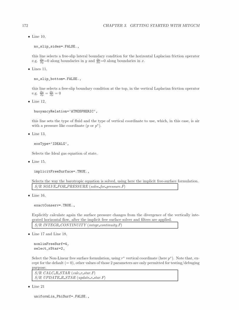
172 CHAPTER 3. GETTING STARTED WITH MITGCM
• Line 10,
no_slip_sides=.FALSE.,
this line selects a free-slip lateral boundary condition for the horizontal Laplacian friction operatore.g. ∂u
∂y =0 along boundaries in y and ∂v∂x=0 along boundaries in x.
• Lines 11,
no_slip_bottom=.FALSE.,
this line selects a free-slip boundary condition at the top, in the vertical Laplacian friction operatore.g. ∂u
∂p = ∂v∂p = 0
• Line 12,
buoyancyRelation=’ATMOSPHERIC’,
this line sets the type of fluid and the type of vertical coordinate to use, which, in this case, is airwith a pressure like coordinate (p or p∗).
• Line 13,
eosType=’IDEALG’,
Selects the Ideal gas equation of state.
• Line 15,
implicitFreeSurface=.TRUE.,
Selects the way the barotropic equation is solved, using here the implicit free-surface formulation.
S/R SOLVE FOR PRESSURE (solve for pressure.F)
• Line 16,
exactConserv=.TRUE.,
Explicitly calculate again the surface pressure changes from the divergence of the vertically inte-grated horizontal flow, after the implicit free surface solver and filters are applied.
S/R INTEGR CONTINUITY (integr continuity.F)
• Line 17 and Line 18,
nonlinFreeSurf=4,
select_rStar=2,
Select the Non-Linear free surface formulation, using r∗ vertical coordinate (here p∗). Note that, ex-cept for the default (= 0), other values of those 2 parameters are only permitted for testing/debugingpurpose.
S/R CALC R STAR (calc r star.F)S/R UPDATE R STAR (update r star.F)
• Line 21
uniformLin_PhiSurf=.FALSE.,
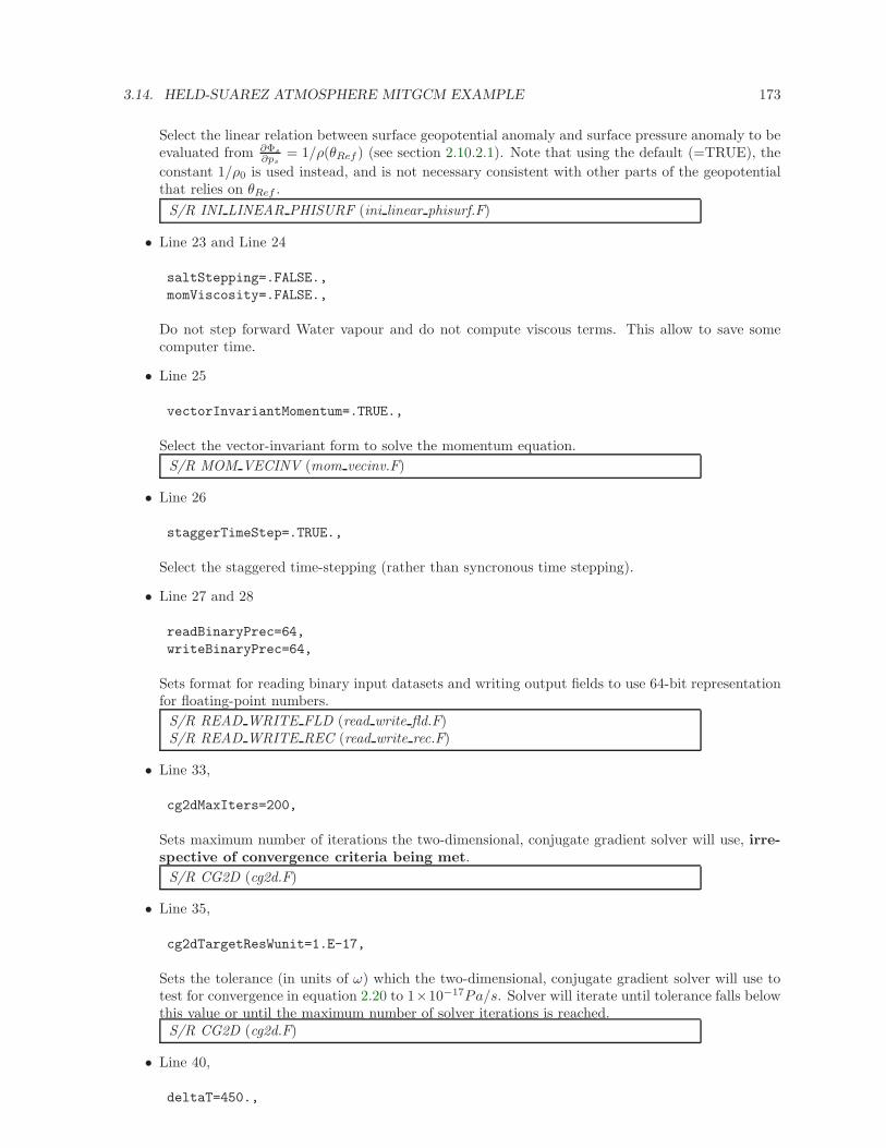
3.14. HELD-SUAREZ ATMOSPHERE MITGCM EXAMPLE 173
Select the linear relation between surface geopotential anomaly and surface pressure anomaly to beevaluated from ∂Φs
∂ps= 1/ρ(θRef ) (see section 2.10.2.1). Note that using the default (=TRUE), the
constant 1/ρ0 is used instead, and is not necessary consistent with other parts of the geopotentialthat relies on θRef .
S/R INI LINEAR PHISURF (ini linear phisurf.F)
• Line 23 and Line 24
saltStepping=.FALSE.,
momViscosity=.FALSE.,
Do not step forward Water vapour and do not compute viscous terms. This allow to save somecomputer time.
• Line 25
vectorInvariantMomentum=.TRUE.,
Select the vector-invariant form to solve the momentum equation.
S/R MOM VECINV (mom vecinv.F)
• Line 26
staggerTimeStep=.TRUE.,
Select the staggered time-stepping (rather than syncronous time stepping).
• Line 27 and 28
readBinaryPrec=64,
writeBinaryPrec=64,
Sets format for reading binary input datasets and writing output fields to use 64-bit representationfor floating-point numbers.
S/R READ WRITE FLD (read write fld.F)S/R READ WRITE REC (read write rec.F)
• Line 33,
cg2dMaxIters=200,
Sets maximum number of iterations the two-dimensional, conjugate gradient solver will use, irre-spective of convergence criteria being met.
S/R CG2D (cg2d.F)
• Line 35,
cg2dTargetResWunit=1.E-17,
Sets the tolerance (in units of ω) which the two-dimensional, conjugate gradient solver will use totest for convergence in equation 2.20 to 1×10⁻¹⁷Pa/s. Solver will iterate until tolerance falls belowthis value or until the maximum number of solver iterations is reached.S/R CG2D (cg2d.F)
• Line 40,
deltaT=450.,
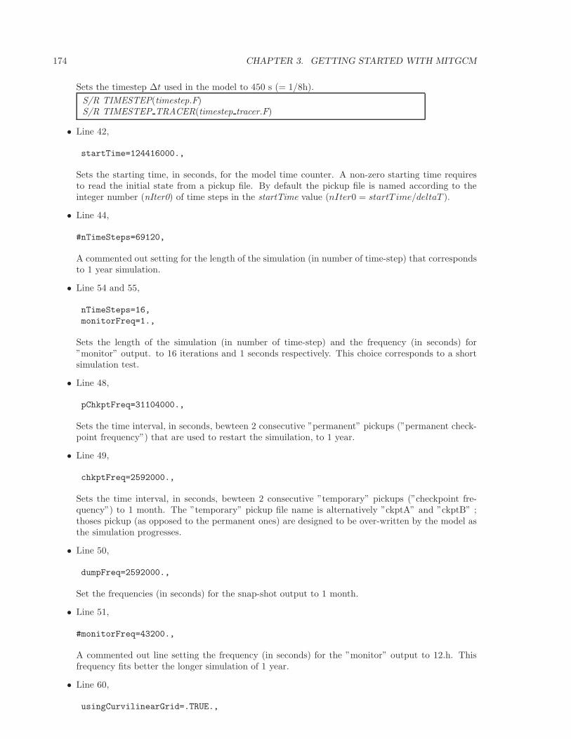
174 CHAPTER 3. GETTING STARTED WITH MITGCM
Sets the timestep ∆t used in the model to 450 s (= 1/8h).
S/R TIMESTEP(timestep.F)S/R TIMESTEP TRACER(timestep tracer.F)
• Line 42,
startTime=124416000.,
Sets the starting time, in seconds, for the model time counter. A non-zero starting time requiresto read the initial state from a pickup file. By default the pickup file is named according to theinteger number (nIter0) of time steps in the startTime value (nIter0 = startT ime/deltaT ).
• Line 44,
#nTimeSteps=69120,
A commented out setting for the length of the simulation (in number of time-step) that correspondsto 1 year simulation.
• Line 54 and 55,
nTimeSteps=16,
monitorFreq=1.,
Sets the length of the simulation (in number of time-step) and the frequency (in seconds) for”monitor” output. to 16 iterations and 1 seconds respectively. This choice corresponds to a shortsimulation test.
• Line 48,
pChkptFreq=31104000.,
Sets the time interval, in seconds, bewteen 2 consecutive ”permanent” pickups (”permanent check-point frequency”) that are used to restart the simuilation, to 1 year.
• Line 49,
chkptFreq=2592000.,
Sets the time interval, in seconds, bewteen 2 consecutive ”temporary” pickups (”checkpoint fre-quency”) to 1 month. The ”temporary” pickup file name is alternatively ”ckptA” and ”ckptB” ;thoses pickup (as opposed to the permanent ones) are designed to be over-written by the model asthe simulation progresses.
• Line 50,
dumpFreq=2592000.,
Set the frequencies (in seconds) for the snap-shot output to 1 month.
• Line 51,
#monitorFreq=43200.,
A commented out line setting the frequency (in seconds) for the ”monitor” output to 12.h. Thisfrequency fits better the longer simulation of 1 year.
• Line 60,
usingCurvilinearGrid=.TRUE.,
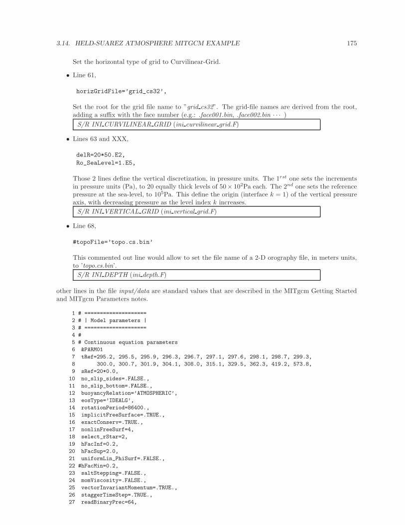
3.14. HELD-SUAREZ ATMOSPHERE MITGCM EXAMPLE 175
Set the horizontal type of grid to Curvilinear-Grid.
• Line 61,
horizGridFile=’grid_cs32’,
Set the root for the grid file name to ”grid cs32”. The grid-file names are derived from the root,adding a suffix with the face number (e.g.: .face001.bin, .face002.bin · · · )
S/R INI CURVILINEAR GRID (ini curvilinear grid.F)
• Lines 63 and XXX,
delR=20*50.E2,
Ro_SeaLevel=1.E5,
Those 2 lines define the vertical discretization, in pressure units. The 1rst one sets the incrementsin pressure units (Pa), to 20 equally thick levels of 50× 102Pa each. The 2nd one sets the referencepressure at the sea-level, to 105Pa. This define the origin (interface k = 1) of the vertical pressureaxis, with decreasing pressure as the level index k increases.
S/R INI VERTICAL GRID (ini vertical grid.F)
• Line 68,
#topoFile=’topo.cs.bin’
This commented out line would allow to set the file name of a 2-D orography file, in meters units,to ’topo.cs.bin’.
S/R INI DEPTH (ini depth.F)
other lines in the file input/data are standard values that are described in the MITgcm Getting Startedand MITgcm Parameters notes.
1 # ====================
2 # | Model parameters |
3 # ====================
4 #
5 # Continuous equation parameters
6 &PARM01
7 tRef=295.2, 295.5, 295.9, 296.3, 296.7, 297.1, 297.6, 298.1, 298.7, 299.3,
8 300.0, 300.7, 301.9, 304.1, 308.0, 315.1, 329.5, 362.3, 419.2, 573.8,
9 sRef=20*0.0,
10 no_slip_sides=.FALSE.,
11 no_slip_bottom=.FALSE.,
12 buoyancyRelation=’ATMOSPHERIC’,
13 eosType=’IDEALG’,
14 rotationPeriod=86400.,
15 implicitFreeSurface=.TRUE.,
16 exactConserv=.TRUE.,
17 nonlinFreeSurf=4,
18 select_rStar=2,
19 hFacInf=0.2,
20 hFacSup=2.0,
21 uniformLin_PhiSurf=.FALSE.,
22 #hFacMin=0.2,
23 saltStepping=.FALSE.,
24 momViscosity=.FALSE.,
25 vectorInvariantMomentum=.TRUE.,
26 staggerTimeStep=.TRUE.,
27 readBinaryPrec=64,
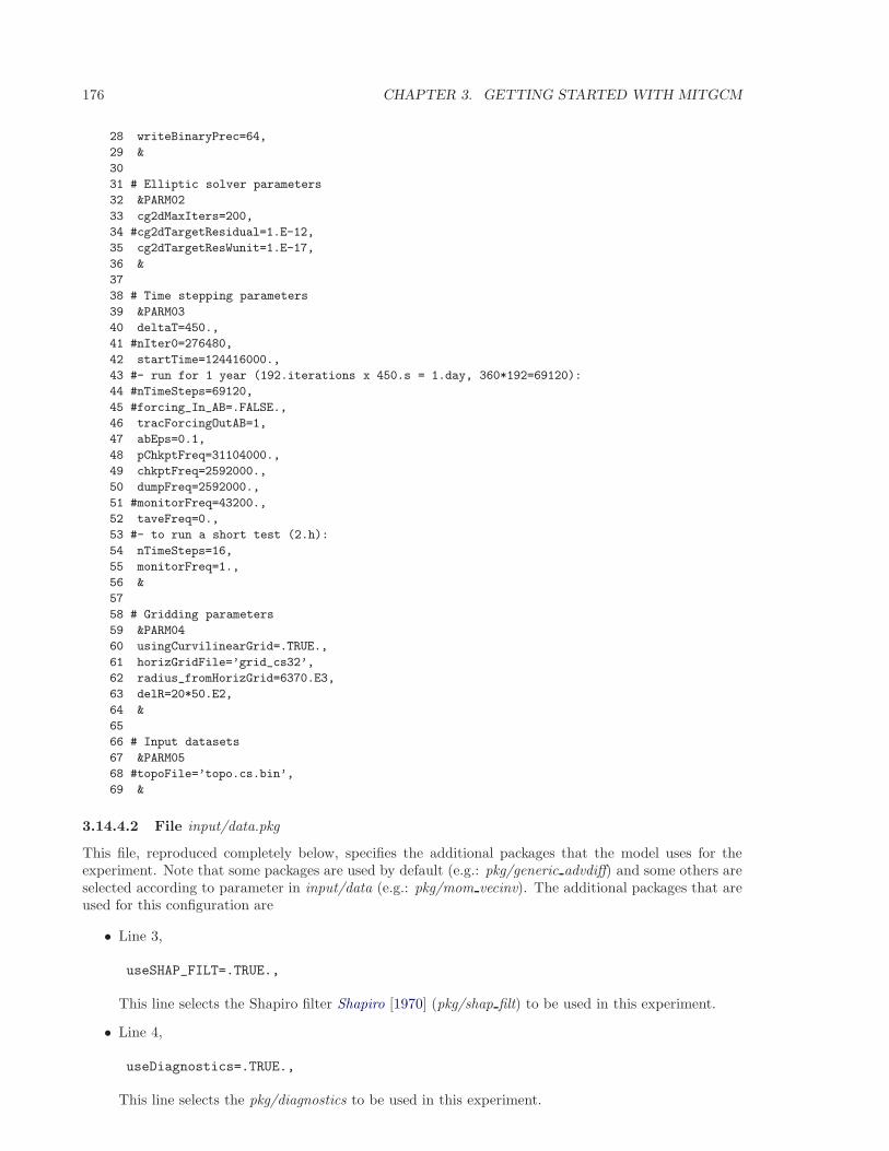
176 CHAPTER 3. GETTING STARTED WITH MITGCM
28 writeBinaryPrec=64,
29 &
30
31 # Elliptic solver parameters
32 &PARM02
33 cg2dMaxIters=200,
34 #cg2dTargetResidual=1.E-12,
35 cg2dTargetResWunit=1.E-17,
36 &
37
38 # Time stepping parameters
39 &PARM03
40 deltaT=450.,
41 #nIter0=276480,
42 startTime=124416000.,
43 #- run for 1 year (192.iterations x 450.s = 1.day, 360*192=69120):
44 #nTimeSteps=69120,
45 #forcing_In_AB=.FALSE.,
46 tracForcingOutAB=1,
47 abEps=0.1,
48 pChkptFreq=31104000.,
49 chkptFreq=2592000.,
50 dumpFreq=2592000.,
51 #monitorFreq=43200.,
52 taveFreq=0.,
53 #- to run a short test (2.h):
54 nTimeSteps=16,
55 monitorFreq=1.,
56 &
57
58 # Gridding parameters
59 &PARM04
60 usingCurvilinearGrid=.TRUE.,
61 horizGridFile=’grid_cs32’,
62 radius_fromHorizGrid=6370.E3,
63 delR=20*50.E2,
64 &
65
66 # Input datasets
67 &PARM05
68 #topoFile=’topo.cs.bin’,
69 &
3.14.4.2 File input/data.pkg
This file, reproduced completely below, specifies the additional packages that the model uses for theexperiment. Note that some packages are used by default (e.g.: pkg/generic advdiff) and some others areselected according to parameter in input/data (e.g.: pkg/mom vecinv). The additional packages that areused for this configuration are
• Line 3,
useSHAP_FILT=.TRUE.,
This line selects the Shapiro filter Shapiro [1970] (pkg/shap filt) to be used in this experiment.
• Line 4,
useDiagnostics=.TRUE.,
This line selects the pkg/diagnostics to be used in this experiment.
3.14. HELD-SUAREZ ATMOSPHERE MITGCM EXAMPLE 177
• Line 5,
#useMNC=.TRUE.,
This line that would selects the pkg/mnc for I/O is commented out.
The entire file input/data.pkg is reproduced here below:
1 # Packages
2 &PACKAGES
3 useSHAP_FILT=.TRUE.,
4 useDiagnostics=.TRUE.,
5 #useMNC=.TRUE.,
6 &
3.14.4.3 File input/eedata
This file uses standard default values except line 6:
useCubedSphereExchange=.TRUE.,
This line selects the cubed-sphere specific exchanges to to connect tiles and faces edges.
3.14.4.4 File input/data.shap
This file, reproduced completely below, specifies the parameters that the model uses for the Shapiro filterpackage (Shapiro [1970], section 2.20). The parameters that are significant for this configuration are:
• Line 5,
Shap_funct=2,
This line selects the shapiro filter function to use, here S2 in this experiment (see section 2.20).
• Lines 6 and 7,
nShapT=0,
nShapUV=4,
Those lines select the order of the shapiro filter for active tracer (θ and q) and momentum (u, v)respectively. In this case, no filter is applied to active tracers. Regarding the momentum, this setsthe integer parameter n to 4, in the equations of section 2.20, which corresponds to a 8th orderfilter.
• Line 9,
nShapUVPhys=4,
This line selects the order of the physical space filter (filter function S2g, in section 2.20) that appliesto u, v. The difference nShapUV - nShapUVPhys corresponds to the order of the computationalfilter (filter function S2c, in section 2.20).
• Lines 12 and 13,
#Shap_Trtau=5400.,
#Shap_uvtau=1800.,
Those commented lines would have set the time scale of the filter (in seconds), for θ and q and for uand v respectively, to 5400 s (90 min) and 1800 s (30 min) respectively. Without explicitly settingthose timescales, the default is used which corresponds to the model time-step.
178 CHAPTER 3. GETTING STARTED WITH MITGCM
The entire file input/data.shap is reproduced here below:
1 # Shapiro Filter parameters
2 &SHAP_PARM01
3 shap_filt_uvStar=.FALSE.,
4 shap_filt_TrStagg=.TRUE.,
5 Shap_funct=2,
6 nShapT=0,
7 nShapUV=4,
8 #nShapTrPhys=0,
9 nShapUVPhys=4,
10 #Shap_TrLength=140000.,
11 #Shap_uvLength=110000.,
12 #Shap_Trtau=5400.,
13 #Shap_uvtau=1800.,
14 #Shap_diagFreq=2592000.,
15 &
3.14.4.5 File code/SIZE.h
Four lines are customized in this file for the current experiment
• Line 39,
sNx=32,
sets the lateral domain extent in grid points along the x-direction, for 1 face.
• Line 40,
sNy=32,
sets the lateral domain extent in grid points along the y-direction, for 1 face.
• Line 43,
nSx=6,
sets the number of tiles in the x-direction, for the model domain decomposition. In this simple case(one processor and 1 tile per face), this number corresponds to the total number of faces.
• Line 49,
Nr=20,
sets the vertical domain extent in grid points.
3.14.4.6 File code/packages.conf
This file, reproduced completely below, specifies the packages that are compiled and made available forthis experiment. The additional packages that are used for this configuration are
• Line 4,
gfd
This line selects the standard set of packages that are used by default.
• Line 5,
shap_filt
3.14. HELD-SUAREZ ATMOSPHERE MITGCM EXAMPLE 179
This line makes the Shapiro filter package available for this experiment.
• Line 6,
exch2
This line selects the exch2 pacakge to be compiled and used in this experiment. Note that, withthe present structure of the model, the parameter useEXCH2 does not exists and therefore, thispackage is always used when it is compiled.
• Line 7,
diagnostics
This line selects the pkg/diagnostics to be compiled, and makes it available for this experiment.
• Line 8,
mnc
This line selects the pkg/mnc to be compiled, and makes it available for this experiment.
The entire file code/packages.conf is reproduced here below:
1 # $Header: /u/gcmpack/MITgcm/verification/tutorial_held_suarez_cs/code/packages.conf,v 1.2 2014/08/20 20:24:09
2 # $Name: $
3
4 gfd
5 shap_filt
6 exch2
7 diagnostics
8 mnc
3.14.4.7 File code/CPP OPTIONS.h
This file uses standard default except for Line 40(diff CPP OPTIONS.h ../../../model/inc):
#define NONLIN_FRSURF
This line allow to use the non-linear free-surface part of the code, which is required for the p∗ coordinateformulation.
3.14.4.8 Other Files
Other files relevant to this experiment are
• code/external forcing.F
• input/grid cs32.face00[n].bin, with n = 1, 2, 3, 4, 5, 6
contain the code customisations and binary input files for this experiments. Below we describe the cus-tomisations to these files associated with this experiment.
The file code/external forcing.F contains 4 subroutines that calculate the forcing terms (Right-Handside term) in the momentum equation (3.61, S/R EXTERNAL FORCING U and EXTERNAL FORCING V)and in the potential temperature equation (3.62, S/R EXTERNAL FORCING T). The water-vapourforcing subroutine (S/R EXTERNAL FORCING S) is left empty for this experiment.
The grid-files input/grid cs32.face00[n].bin, with n = 1, 2, 3, 4, 5, 6, are binary files (direct-access, big-endian 64.bits real) that contains all the cubed-sphere grid lengths, areas and grid-point positions, withone file per face. Each file contains 18 2-D arrays (dimension 33 × 33) that correspond to the modelvariables: XC YC DXF DYF RA XG YG DXV DYU RAZ DXC DYC RAW RAS DXG DYG AngleCSAngleSN (see GRID.h file)
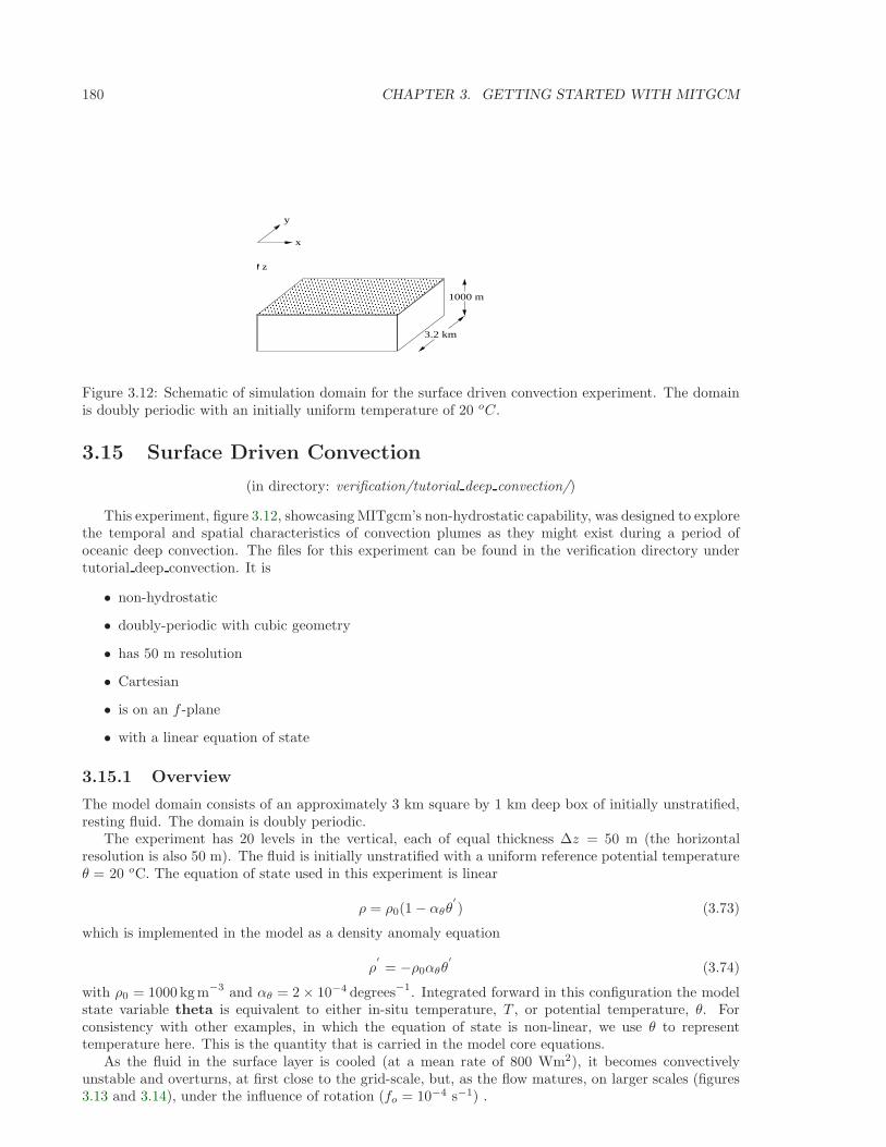
180 CHAPTER 3. GETTING STARTED WITH MITGCM
3.2 km
1000 m
z
x
y
Figure 3.12: Schematic of simulation domain for the surface driven convection experiment. The domainis doubly periodic with an initially uniform temperature of 20 oC.
3.15 Surface Driven Convection
(in directory: verification/tutorial deep convection/)
This experiment, figure 3.12, showcasing MITgcm’s non-hydrostatic capability, was designed to explorethe temporal and spatial characteristics of convection plumes as they might exist during a period ofoceanic deep convection. The files for this experiment can be found in the verification directory undertutorial deep convection. It is
• non-hydrostatic
• doubly-periodic with cubic geometry
• has 50 m resolution
• Cartesian
• is on an f -plane
• with a linear equation of state
3.15.1 Overview
The model domain consists of an approximately 3 km square by 1 km deep box of initially unstratified,resting fluid. The domain is doubly periodic.
The experiment has 20 levels in the vertical, each of equal thickness ∆z = 50 m (the horizontalresolution is also 50 m). The fluid is initially unstratified with a uniform reference potential temperatureθ = 20 oC. The equation of state used in this experiment is linear
ρ = ρ0(1 − αθθ′
) (3.73)
which is implemented in the model as a density anomaly equation
ρ′
= −ρ0αθθ′
(3.74)
with ρ0 = 1000 kgm−3 and αθ = 2 × 10⁻⁴ degrees−1. Integrated forward in this configuration the modelstate variable theta is equivalent to either in-situ temperature, T , or potential temperature, θ. Forconsistency with other examples, in which the equation of state is non-linear, we use θ to representtemperature here. This is the quantity that is carried in the model core equations.
As the fluid in the surface layer is cooled (at a mean rate of 800 Wm2), it becomes convectivelyunstable and overturns, at first close to the grid-scale, but, as the flow matures, on larger scales (figures3.13 and 3.14), under the influence of rotation (fo = 10−4 s−1) .
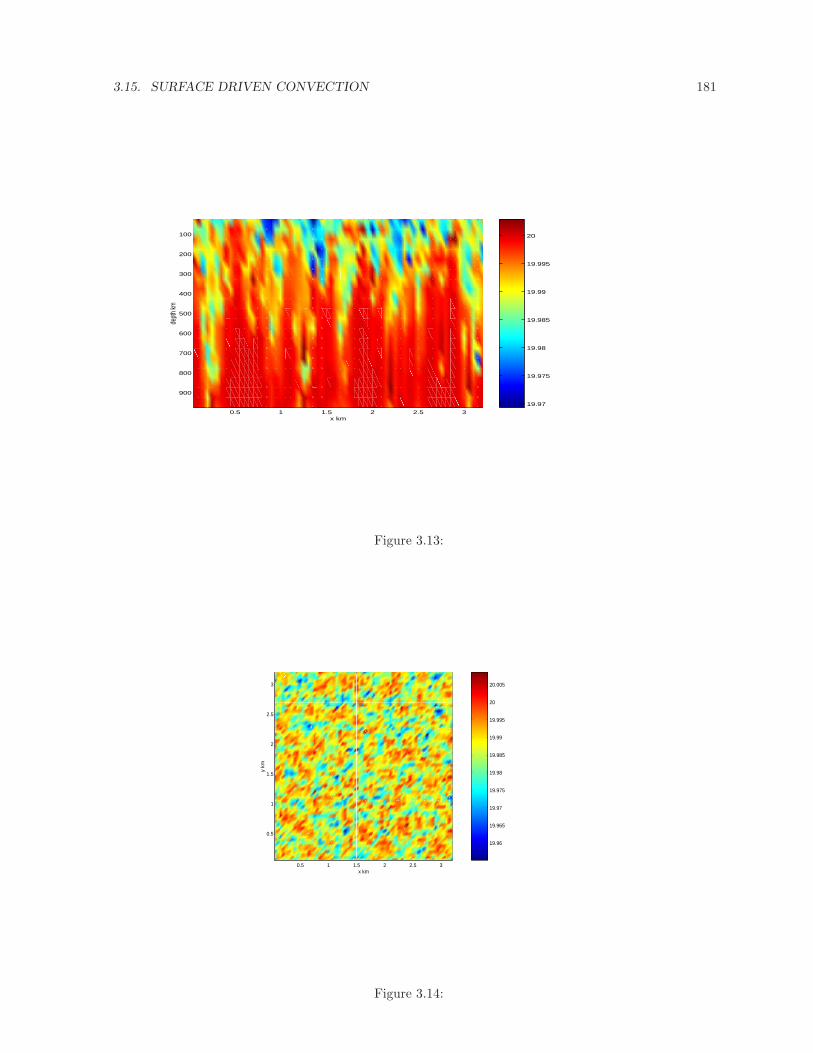
3.15. SURFACE DRIVEN CONVECTION 181
19.97
19.975
19.98
19.985
19.99
19.995
20
0.5 1 1.5 2 2.5 3
100
200
300
400
500
600
700
800
900
x km
dept
h km
Figure 3.13:
19.96
19.965
19.97
19.975
19.98
19.985
19.99
19.995
20
20.005
0.5 1 1.5 2 2.5 3
0.5
1
1.5
2
2.5
3
x km
y km
Figure 3.14:
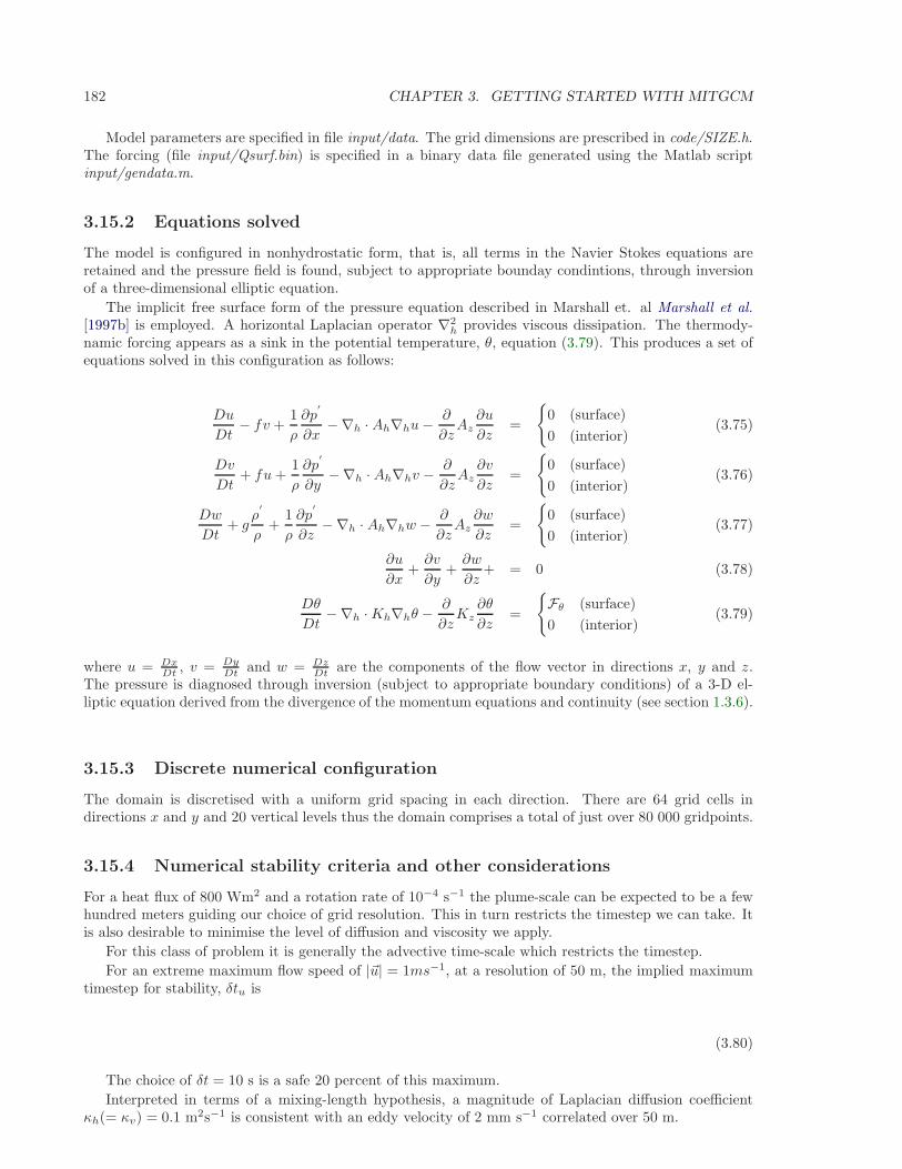
182 CHAPTER 3. GETTING STARTED WITH MITGCM
Model parameters are specified in file input/data. The grid dimensions are prescribed in code/SIZE.h.The forcing (file input/Qsurf.bin) is specified in a binary data file generated using the Matlab scriptinput/gendata.m.
3.15.2 Equations solved
The model is configured in nonhydrostatic form, that is, all terms in the Navier Stokes equations areretained and the pressure field is found, subject to appropriate bounday condintions, through inversionof a three-dimensional elliptic equation.
The implicit free surface form of the pressure equation described in Marshall et. al Marshall et al.[1997b] is employed. A horizontal Laplacian operator ∇2
h provides viscous dissipation. The thermody-namic forcing appears as a sink in the potential temperature, θ, equation (3.79). This produces a set ofequations solved in this configuration as follows:
Du
Dt− fv +
1
ρ
∂p′
∂x−∇h · Ah∇hu− ∂
∂zAz
∂u
∂z=
0 (surface)
0 (interior)(3.75)
Dv
Dt+ fu+
1
ρ
∂p′
∂y−∇h · Ah∇hv −
∂
∂zAz
∂v
∂z=
0 (surface)
0 (interior)(3.76)
Dw
Dt+ g
ρ′
ρ+
1
ρ
∂p′
∂z−∇h · Ah∇hw − ∂
∂zAz
∂w
∂z=
0 (surface)
0 (interior)(3.77)
∂u
∂x+∂v
∂y+∂w
∂z+ = 0 (3.78)
Dθ
Dt−∇h ·Kh∇hθ −
∂
∂zKz
∂θ
∂z=
Fθ (surface)
0 (interior)(3.79)
where u = DxDt , v = Dy
Dt and w = DzDt are the components of the flow vector in directions x, y and z.
The pressure is diagnosed through inversion (subject to appropriate boundary conditions) of a 3-D el-liptic equation derived from the divergence of the momentum equations and continuity (see section 1.3.6).
3.15.3 Discrete numerical configuration
The domain is discretised with a uniform grid spacing in each direction. There are 64 grid cells indirections x and y and 20 vertical levels thus the domain comprises a total of just over 80 000 gridpoints.
3.15.4 Numerical stability criteria and other considerations
For a heat flux of 800 Wm2 and a rotation rate of 10−4 s−1 the plume-scale can be expected to be a fewhundred meters guiding our choice of grid resolution. This in turn restricts the timestep we can take. Itis also desirable to minimise the level of diffusion and viscosity we apply.
For this class of problem it is generally the advective time-scale which restricts the timestep.
For an extreme maximum flow speed of |~u| = 1ms−1, at a resolution of 50 m, the implied maximumtimestep for stability, δtu is
(3.80)
The choice of δt = 10 s is a safe 20 percent of this maximum.
Interpreted in terms of a mixing-length hypothesis, a magnitude of Laplacian diffusion coefficientκh(= κv) = 0.1 m2s−1 is consistent with an eddy velocity of 2 mm s−1 correlated over 50 m.
3.15. SURFACE DRIVEN CONVECTION 183
3.15.5 Experiment configuration
The model configuration for this experiment resides under the directory verification/convection/. Theexperiment files
• code/CPP EEOPTIONS.h
• code/CPP OPTIONS.h,
• code/SIZE.h.
• input/data
• input/data.pkg
• input/eedata,
• input/Qsurf.bin,
contain the code customisations and parameter settings for this experiment. Below we describe theseexperiment-specific customisations.
3.15.5.1 File code/CPP EEOPTIONS.h
This file uses standard default values and does not contain customisations for this experiment.
3.15.5.2 File code/CPP OPTIONS.h
This file uses standard default values and does not contain customisations for this experiment.
3.15.5.3 File code/SIZE.h
Three lines are customized in this file. These prescribe the domain grid dimensions.
• Line 36,
sNx=64,
this line sets the lateral domain extent in grid points for the axis aligned with the x-coordinate.
• Line 37,
sNy=64,
this line sets the lateral domain extent in grid points for the axis aligned with the y-coordinate.
• Line 46,
Nr=20,
this line sets the vertical domain extent in grid points.
1 C /==========================================================\
2 C | SIZE.h Declare size of underlying computational grid. |
3 C |==========================================================|
4 C | The design here support a three-dimensional model grid |
5 C | with indices I,J and K. The three-dimensional domain |
6 C | is comprised of nPx*nSx blocks of size sNx along one axis|
7 C | nPy*nSy blocks of size sNy along another axis and one |
8 C | block of size Nz along the final axis. |
9 C | Blocks have overlap regions of size OLx and OLy along the|
10 C | dimensions that are subdivided. |
11 C \==========================================================/
184 CHAPTER 3. GETTING STARTED WITH MITGCM
12 C Voodoo numbers controlling data layout.
13 C sNx - No. X points in sub-grid.
14 C sNy - No. Y points in sub-grid.
15 C OLx - Overlap extent in X.
16 C OLy - Overlat extent in Y.
17 C nSx - No. sub-grids in X.
18 C nSy - No. sub-grids in Y.
19 C nPx - No. of processes to use in X.
20 C nPy - No. of processes to use in Y.
21 C Nx - No. points in X for the total domain.
22 C Ny - No. points in Y for the total domain.
23 C Nr - No. points in Z for full process domain.
24 INTEGER sNx
25 INTEGER sNy
26 INTEGER OLx
27 INTEGER OLy
28 INTEGER nSx
29 INTEGER nSy
30 INTEGER nPx
31 INTEGER nPy
32 INTEGER Nx
33 INTEGER Ny
34 INTEGER Nr
35 PARAMETER (
36 & sNx = 64,
37 & sNy = 64,
38 & OLx = 3,
39 & OLy = 3,
40 & nSx = 1,
41 & nSy = 1,
42 & nPx = 1,
43 & nPy = 1,
44 & Nx = sNx*nSx*nPx,
45 & Ny = sNy*nSy*nPy,
46 & Nr = 20)
47 C MAX_OLX - Set to the maximum overlap region size of any array
48 C MAX_OLY that will be exchanged. Controls the sizing of exch
49 C routine buufers.
50 INTEGER MAX_OLX
51 INTEGER MAX_OLY
52 PARAMETER ( MAX_OLX = OLx,
53 & MAX_OLY = OLy )
3.15.5.4 File input/data
This file, reproduced completely below, specifies the main parameters for the experiment. The parametersthat are significant for this configuration are
• Line 4,
4 tRef=20*20.0,
this line sets the initial and reference values of potential temperature at each model level in unitsof C. Here the value is arbitrary since, in this case, the flow evolves independently of the absolutemagnitude of the reference temperature. For each depth level the initial and reference profiles willbe uniform in x and y. The values specified are read into the variable tRef in the model code,by procedure S/R INI PARMS (ini parms.F) . The temperature field is initialised, by procedureS/R INI THETA (ini theta.F) .
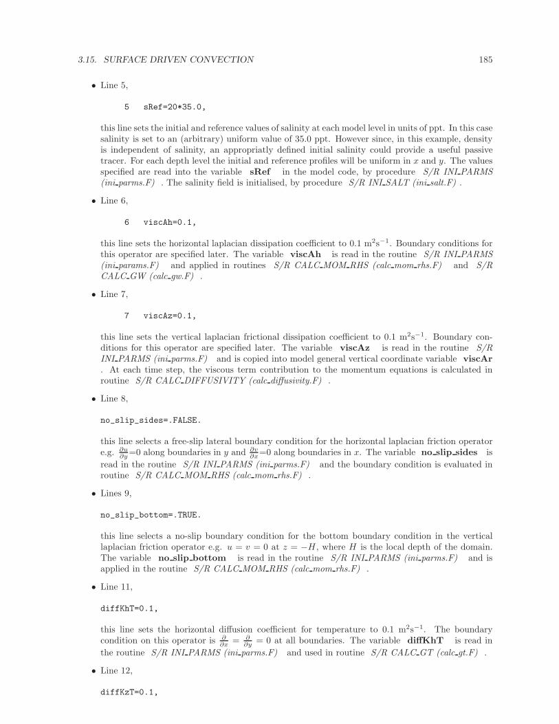
3.15. SURFACE DRIVEN CONVECTION 185
• Line 5,
5 sRef=20*35.0,
this line sets the initial and reference values of salinity at each model level in units of ppt. In this casesalinity is set to an (arbitrary) uniform value of 35.0 ppt. However since, in this example, densityis independent of salinity, an appropriatly defined initial salinity could provide a useful passivetracer. For each depth level the initial and reference profiles will be uniform in x and y. The valuesspecified are read into the variable sRef in the model code, by procedure S/R INI PARMS(ini parms.F) . The salinity field is initialised, by procedure S/R INI SALT (ini salt.F) .
• Line 6,
6 viscAh=0.1,
this line sets the horizontal laplacian dissipation coefficient to 0.1 m2s−1. Boundary conditions forthis operator are specified later. The variable viscAh is read in the routine S/R INI PARMS(ini params.F) and applied in routines S/R CALC MOM RHS (calc mom rhs.F) and S/RCALC GW (calc gw.F) .
• Line 7,
7 viscAz=0.1,
this line sets the vertical laplacian frictional dissipation coefficient to 0.1 m2s−1. Boundary con-ditions for this operator are specified later. The variable viscAz is read in the routine S/RINI PARMS (ini parms.F) and is copied into model general vertical coordinate variable viscAr. At each time step, the viscous term contribution to the momentum equations is calculated inroutine S/R CALC DIFFUSIVITY (calc diffusivity.F) .
• Line 8,
no_slip_sides=.FALSE.
this line selects a free-slip lateral boundary condition for the horizontal laplacian friction operatore.g. ∂u
∂y =0 along boundaries in y and ∂v∂x=0 along boundaries in x. The variable no slip sides is
read in the routine S/R INI PARMS (ini parms.F) and the boundary condition is evaluated inroutine S/R CALC MOM RHS (calc mom rhs.F) .
• Lines 9,
no_slip_bottom=.TRUE.
this line selects a no-slip boundary condition for the bottom boundary condition in the verticallaplacian friction operator e.g. u = v = 0 at z = −H , where H is the local depth of the domain.The variable no slip bottom is read in the routine S/R INI PARMS (ini parms.F) and isapplied in the routine S/R CALC MOM RHS (calc mom rhs.F) .
• Line 11,
diffKhT=0.1,
this line sets the horizontal diffusion coefficient for temperature to 0.1 m2s−1. The boundarycondition on this operator is ∂
∂x = ∂∂y = 0 at all boundaries. The variable diffKhT is read in
the routine S/R INI PARMS (ini parms.F) and used in routine S/R CALC GT (calc gt.F) .
• Line 12,
diffKzT=0.1,
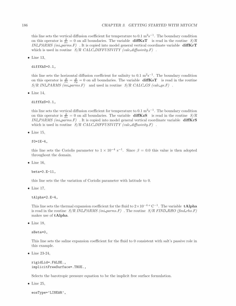
186 CHAPTER 3. GETTING STARTED WITH MITGCM
this line sets the vertical diffusion coefficient for temperature to 0.1 m2s−1. The boundary conditionon this operator is ∂
∂z = 0 on all boundaries. The variable diffKzT is read in the routine S/RINI PARMS (ini parms.F) . It is copied into model general vertical coordinate variable diffKrTwhich is used in routine S/R CALC DIFFUSIVITY (calc diffusivity.F) .
• Line 13,
diffKhS=0.1,
this line sets the horizontal diffusion coefficient for salinity to 0.1 m2s−1. The boundary conditionon this operator is ∂
∂x = ∂∂y = 0 on all boundaries. The variable diffKsT is read in the routine
S/R INI PARMS (ini parms.F) and used in routine S/R CALC GS (calc gs.F) .
• Line 14,
diffKzS=0.1,
this line sets the vertical diffusion coefficient for temperature to 0.1 m2s−1. The boundary conditionon this operator is ∂
∂z = 0 on all boundaries. The variable diffKzS is read in the routine S/RINI PARMS (ini parms.F) . It is copied into model general vertical coordinate variable diffKrSwhich is used in routine S/R CALC DIFFUSIVITY (calc diffusivity.F) .
• Line 15,
f0=1E-4,
this line sets the Coriolis parameter to 1 × 10⁻⁴ s−1. Since β = 0.0 this value is then adoptedthroughout the domain.
• Line 16,
beta=0.E-11,
this line sets the the variation of Coriolis parameter with latitude to 0.
• Line 17,
tAlpha=2.E-4,
This line sets the thermal expansion coefficient for the fluid to 2×10⁻⁴ o C−1. The variable tAlphais read in the routine S/R INI PARMS (ini parms.F) . The routine S/R FIND RHO (find rho.F)makes use of tAlpha.
• Line 18,
sBeta=0,
This line sets the saline expansion coefficient for the fluid to 0 consistent with salt’s passive role inthis example.
• Line 23-24,
rigidLid=.FALSE.,
implicitFreeSurface=.TRUE.,
Selects the barotropic pressure equation to be the implicit free surface formulation.
• Line 25,
eosType=’LINEAR’,
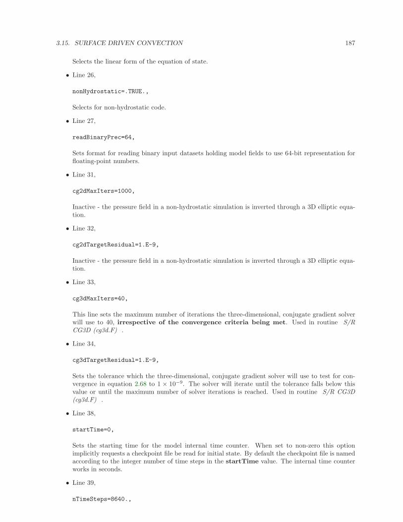
3.15. SURFACE DRIVEN CONVECTION 187
Selects the linear form of the equation of state.
• Line 26,
nonHydrostatic=.TRUE.,
Selects for non-hydrostatic code.
• Line 27,
readBinaryPrec=64,
Sets format for reading binary input datasets holding model fields to use 64-bit representation forfloating-point numbers.
• Line 31,
cg2dMaxIters=1000,
Inactive - the pressure field in a non-hydrostatic simulation is inverted through a 3D elliptic equa-tion.
• Line 32,
cg2dTargetResidual=1.E-9,
Inactive - the pressure field in a non-hydrostatic simulation is inverted through a 3D elliptic equa-tion.
• Line 33,
cg3dMaxIters=40,
This line sets the maximum number of iterations the three-dimensional, conjugate gradient solverwill use to 40, irrespective of the convergence criteria being met. Used in routine S/RCG3D (cg3d.F) .
• Line 34,
cg3dTargetResidual=1.E-9,
Sets the tolerance which the three-dimensional, conjugate gradient solver will use to test for con-vergence in equation 2.68 to 1 × 10⁻⁹. The solver will iterate until the tolerance falls below thisvalue or until the maximum number of solver iterations is reached. Used in routine S/R CG3D(cg3d.F) .
• Line 38,
startTime=0,
Sets the starting time for the model internal time counter. When set to non-zero this optionimplicitly requests a checkpoint file be read for initial state. By default the checkpoint file is namedaccording to the integer number of time steps in the startTime value. The internal time counterworks in seconds.
• Line 39,
nTimeSteps=8640.,
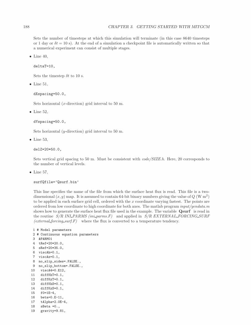
188 CHAPTER 3. GETTING STARTED WITH MITGCM
Sets the number of timesteps at which this simulation will terminate (in this case 8640 timestepsor 1 day or δt = 10 s). At the end of a simulation a checkpoint file is automatically written so thata numerical experiment can consist of multiple stages.
• Line 40,
deltaT=10,
Sets the timestep δt to 10 s.
• Line 51,
dXspacing=50.0,
Sets horizontal (x-direction) grid interval to 50 m.
• Line 52,
dYspacing=50.0,
Sets horizontal (y-direction) grid interval to 50 m.
• Line 53,
delZ=20*50.0,
Sets vertical grid spacing to 50 m. Must be consistent with code/SIZE.h. Here, 20 corresponds tothe number of vertical levels.
• Line 57,
surfQfile=’Qsurf.bin’
This line specifies the name of the file from which the surface heat flux is read. This file is a two-dimensional (x, y) map. It is assumed to contain 64-bit binary numbers giving the value ofQ (W m2)to be applied in each surface grid cell, ordered with the x coordinate varying fastest. The points areordered from low coordinate to high coordinate for both axes. The matlab program input/gendata.mshows how to generate the surface heat flux file used in the example. The variable Qsurf is read inthe routine S/R INI PARMS (ini parms.F) and applied in S/R EXTERNAL FORCING SURF(external forcing surf.F) where the flux is converted to a temperature tendency.
1 # Model parameters
2 # Continuous equation parameters
3 &PARM01
4 tRef=20*20.0,
5 sRef=20*35.0,
6 viscAh=0.1,
7 viscAz=0.1,
8 no_slip_sides=.FALSE.,
9 no_slip_bottom=.FALSE.,
10 viscA4=0.E12,
11 diffKhT=0.1,
12 diffKzT=0.1,
13 diffKhS=0.1,
14 diffKzS=0.1,
15 f0=1E-4,
16 beta=0.E-11,
17 tAlpha=2.0E-4,
18 sBeta =0.,
19 gravity=9.81,
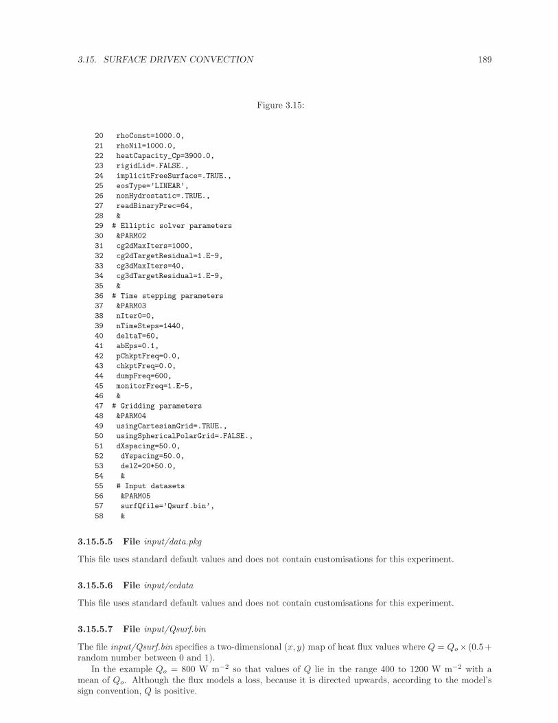
3.15. SURFACE DRIVEN CONVECTION 189
Figure 3.15:
20 rhoConst=1000.0,
21 rhoNil=1000.0,
22 heatCapacity_Cp=3900.0,
23 rigidLid=.FALSE.,
24 implicitFreeSurface=.TRUE.,
25 eosType=’LINEAR’,
26 nonHydrostatic=.TRUE.,
27 readBinaryPrec=64,
28 &
29 # Elliptic solver parameters
30 &PARM02
31 cg2dMaxIters=1000,
32 cg2dTargetResidual=1.E-9,
33 cg3dMaxIters=40,
34 cg3dTargetResidual=1.E-9,
35 &
36 # Time stepping parameters
37 &PARM03
38 nIter0=0,
39 nTimeSteps=1440,
40 deltaT=60,
41 abEps=0.1,
42 pChkptFreq=0.0,
43 chkptFreq=0.0,
44 dumpFreq=600,
45 monitorFreq=1.E-5,
46 &
47 # Gridding parameters
48 &PARM04
49 usingCartesianGrid=.TRUE.,
50 usingSphericalPolarGrid=.FALSE.,
51 dXspacing=50.0,
52 dYspacing=50.0,
53 delZ=20*50.0,
54 &
55 # Input datasets
56 &PARM05
57 surfQfile=’Qsurf.bin’,
58 &
3.15.5.5 File input/data.pkg
This file uses standard default values and does not contain customisations for this experiment.
3.15.5.6 File input/eedata
This file uses standard default values and does not contain customisations for this experiment.
3.15.5.7 File input/Qsurf.bin
The file input/Qsurf.bin specifies a two-dimensional (x, y) map of heat flux values where Q = Qo × (0.5+random number between 0 and 1).
In the example Qo = 800 W m−2 so that values of Q lie in the range 400 to 1200 W m−2 with amean of Qo. Although the flux models a loss, because it is directed upwards, according to the model’ssign convention, Q is positive.
190 CHAPTER 3. GETTING STARTED WITH MITGCM
3.15.6 Running the example
3.15.6.1 Code download
In order to run the examples you must first download the code distribution. Instructions for downloadingthe code can be found in 3.2.
3.15.6.2 Experiment Location
This example experiments is located under the release sub-directory
verification/convection/
3.15.6.3 Running the Experiment
To run the experiment
1. Set the current directory to input/
% cd input
2. Verify that current directory is now correct
% pwd
You should see a response on the screen ending in
verification/convection/input
3. Run the genmake script to create the experiment Makefile
% ../../../tools/genmake -mods=../code
4. Create a list of header file dependencies in Makefile
% make depend
5. Build the executable file.
% make
6. Run the mitgcmuv executable
% ./mitgcmuv
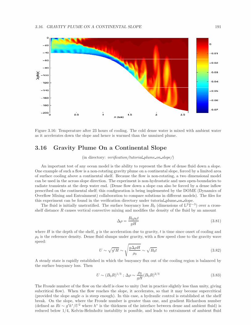
3.16. GRAVITY PLUME ON A CONTINENTAL SLOPE 191
Figure 3.16: Temperature after 23 hours of cooling. The cold dense water is mixed with ambient wateras it accelerates down the slope and hence is warmed than the unmixed plume.
3.16 Gravity Plume On a Continental Slope
(in directory: verification/tutorial plume on slope/)
An important test of any ocean model is the ability to represent the flow of dense fluid down a slope.One example of such a flow is a non-rotating gravity plume on a continental slope, forced by a limited areaof surface cooling above a continental shelf. Because the flow is non-rotating, a two dimensional modelcan be used in the across slope direction. The experiment is non-hydrostatic and uses open-boundaries toradiate transients at the deep water end. (Dense flow down a slope can also be forced by a dense inflowprescribed on the continental shelf; this configuration is being implemented by the DOME (Dynamics ofOverflow Mixing and Entrainment) collaboration to compare solutions in different models). The files forthis experiment can be found in the verification directory under tutorial plume on slope.
The fluid is initially unstratified. The surface buoyancy loss B0 (dimensions of L2T−3) over a cross-shelf distance R causes vertical convective mixing and modifies the density of the fluid by an amount
∆ρ =B0ρ0t
gH(3.81)
where H is the depth of the shelf, g is the acceleration due to gravity, t is time since onset of cooling andρ0 is the reference density. Dense fluid slumps under gravity, with a flow speed close to the gravity wavespeed:
U ∼√g′H ∼
√g∆ρH
ρ0∼√B0t (3.82)
A steady state is rapidly established in which the buoyancy flux out of the cooling region is balanced bythe surface buoyancy loss. Then
U ∼ (B0R)1/3 ; ∆ρ ∼ ρ0
gH(B0R)2/3 (3.83)
The Froude number of the flow on the shelf is close to unity (but in practice slightly less than unity, givingsubcritical flow). When the flow reaches the slope, it accelerates, so that it may become supercritical(provided the slope angle α is steep enough). In this case, a hydraulic control is established at the shelfbreak. On the slope, where the Froude number is greater than one, and gradient Richardson number(defined as Ri ∼ g′h∗/U2 where h∗ is the thickness of the interface between dense and ambient fluid) isreduced below 1/4, Kelvin-Helmholtz instability is possible, and leads to entrainment of ambient fluid
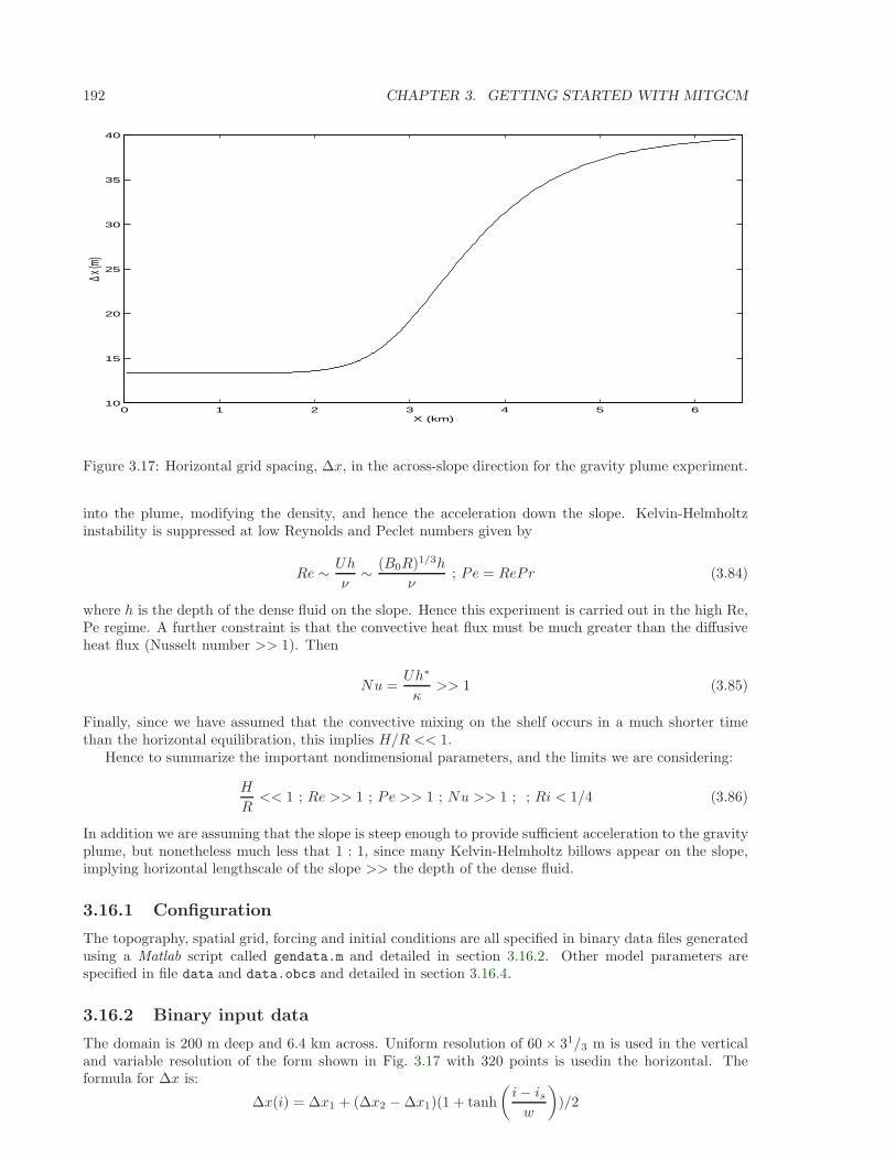
192 CHAPTER 3. GETTING STARTED WITH MITGCM
0 1 2 3 4 5 610
15
20
25
30
35
40
X (km)
∆ x (m
)
Figure 3.17: Horizontal grid spacing, ∆x, in the across-slope direction for the gravity plume experiment.
into the plume, modifying the density, and hence the acceleration down the slope. Kelvin-Helmholtzinstability is suppressed at low Reynolds and Peclet numbers given by
Re ∼ Uh
ν∼ (B0R)1/3h
ν; Pe = RePr (3.84)
where h is the depth of the dense fluid on the slope. Hence this experiment is carried out in the high Re,Pe regime. A further constraint is that the convective heat flux must be much greater than the diffusiveheat flux (Nusselt number >> 1). Then
Nu =Uh∗
κ>> 1 (3.85)
Finally, since we have assumed that the convective mixing on the shelf occurs in a much shorter timethan the horizontal equilibration, this implies H/R << 1.
Hence to summarize the important nondimensional parameters, and the limits we are considering:
H
R<< 1 ; Re >> 1 ; Pe >> 1 ; Nu >> 1 ; ; Ri < 1/4 (3.86)
In addition we are assuming that the slope is steep enough to provide sufficient acceleration to the gravityplume, but nonetheless much less that 1 : 1, since many Kelvin-Helmholtz billows appear on the slope,implying horizontal lengthscale of the slope >> the depth of the dense fluid.
3.16.1 Configuration
The topography, spatial grid, forcing and initial conditions are all specified in binary data files generatedusing a Matlab script called gendata.m and detailed in section 3.16.2. Other model parameters arespecified in file data and data.obcs and detailed in section 3.16.4.
3.16.2 Binary input data
The domain is 200 m deep and 6.4 km across. Uniform resolution of 60 × 31/3 m is used in the verticaland variable resolution of the form shown in Fig. 3.17 with 320 points is usedin the horizontal. Theformula for ∆x is:
∆x(i) = ∆x1 + (∆x2 − ∆x1)(1 + tanh
(i− isw
))/2
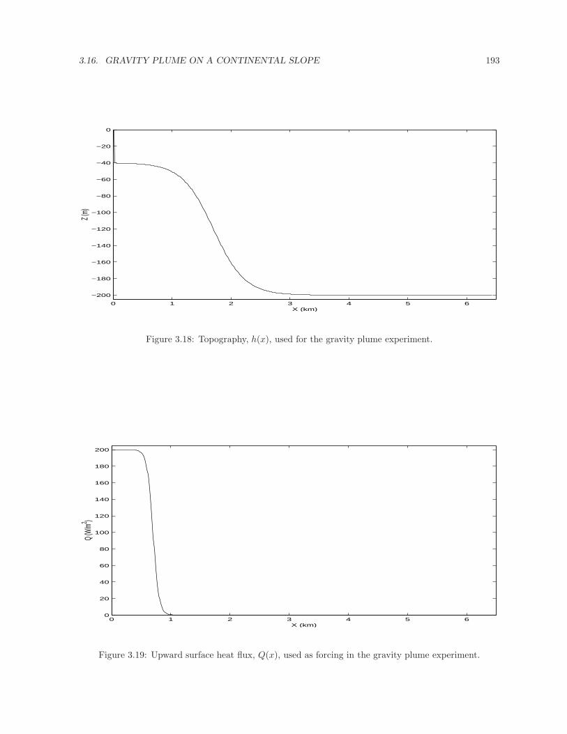
3.16. GRAVITY PLUME ON A CONTINENTAL SLOPE 193
0 1 2 3 4 5 6
−200
−180
−160
−140
−120
−100
−80
−60
−40
−20
0
X (km)
Z (m)
Figure 3.18: Topography, h(x), used for the gravity plume experiment.
0 1 2 3 4 5 60
20
40
60
80
100
120
140
160
180
200
X (km)
Q (W
/m2 )
Figure 3.19: Upward surface heat flux, Q(x), used as forcing in the gravity plume experiment.
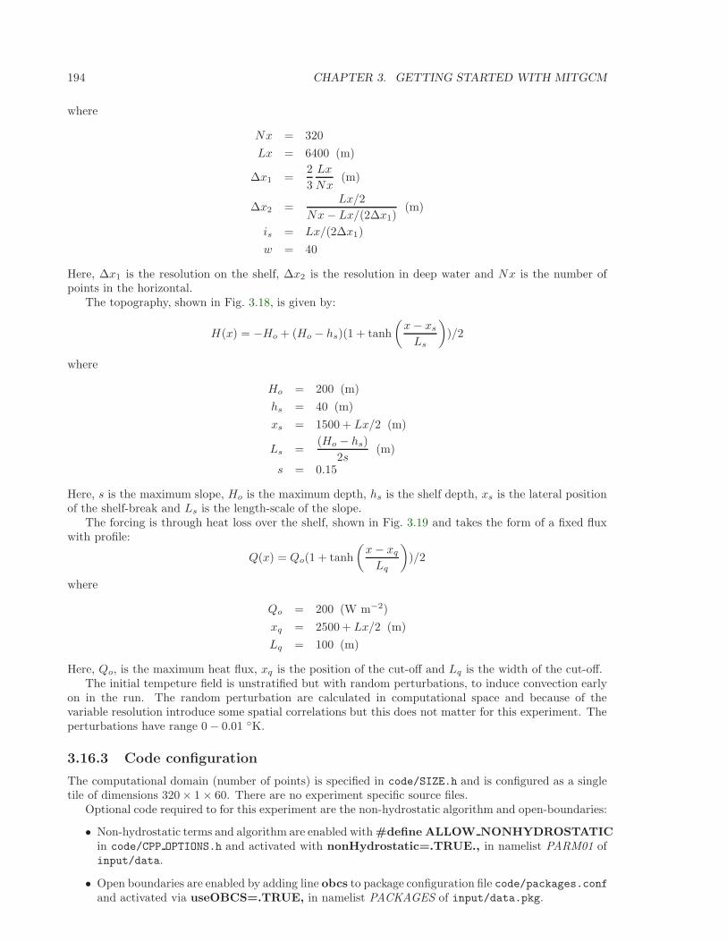
194 CHAPTER 3. GETTING STARTED WITH MITGCM
where
Nx = 320
Lx = 6400 (m)
∆x1 =2
3
Lx
Nx(m)
∆x2 =Lx/2
Nx− Lx/(2∆x1)(m)
is = Lx/(2∆x1)
w = 40
Here, ∆x1 is the resolution on the shelf, ∆x2 is the resolution in deep water and Nx is the number ofpoints in the horizontal.
The topography, shown in Fig. 3.18, is given by:
H(x) = −Ho + (Ho − hs)(1 + tanh
(x− xs
Ls
))/2
where
Ho = 200 (m)
hs = 40 (m)
xs = 1500 + Lx/2 (m)
Ls =(Ho − hs)
2s(m)
s = 0.15
Here, s is the maximum slope, Ho is the maximum depth, hs is the shelf depth, xs is the lateral positionof the shelf-break and Ls is the length-scale of the slope.
The forcing is through heat loss over the shelf, shown in Fig. 3.19 and takes the form of a fixed fluxwith profile:
Q(x) = Qo(1 + tanh
(x− xq
Lq
))/2
where
Qo = 200 (W m−2)
xq = 2500 + Lx/2 (m)
Lq = 100 (m)
Here, Qo, is the maximum heat flux, xq is the position of the cut-off and Lq is the width of the cut-off.The initial tempeture field is unstratified but with random perturbations, to induce convection early
on in the run. The random perturbation are calculated in computational space and because of thevariable resolution introduce some spatial correlations but this does not matter for this experiment. Theperturbations have range 0 − 0.01 K.
3.16.3 Code configuration
The computational domain (number of points) is specified in code/SIZE.h and is configured as a singletile of dimensions 320 × 1 × 60. There are no experiment specific source files.
Optional code required to for this experiment are the non-hydrostatic algorithm and open-boundaries:
• Non-hydrostatic terms and algorithm are enabled with #define ALLOW NONHYDROSTATICin code/CPP OPTIONS.h and activated with nonHydrostatic=.TRUE., in namelist PARM01 ofinput/data.
• Open boundaries are enabled by adding line obcs to package configuration file code/packages.confand activated via useOBCS=.TRUE, in namelist PACKAGES of input/data.pkg.
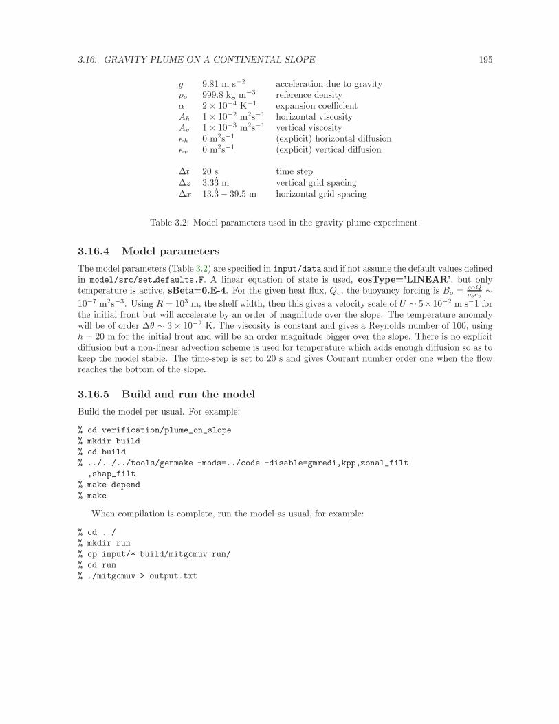
3.16. GRAVITY PLUME ON A CONTINENTAL SLOPE 195
g 9.81 m s−2 acceleration due to gravityρo 999.8 kg m−3 reference densityα 2 × 10⁻⁴ K−1 expansion coefficientAh 1 × 10⁻² m2s−1 horizontal viscosityAv 1 × 10⁻³ m2s−1 vertical viscosityκh 0 m2s−1 (explicit) horizontal diffusionκv 0 m2s−1 (explicit) vertical diffusion
∆t 20 s time step∆z 3.33 m vertical grid spacing∆x 13.3 − 39.5 m horizontal grid spacing
Table 3.2: Model parameters used in the gravity plume experiment.
3.16.4 Model parameters
The model parameters (Table 3.2) are specified in input/data and if not assume the default values definedin model/src/set defaults.F. A linear equation of state is used, eosType=’LINEAR’, but onlytemperature is active, sBeta=0.E-4. For the given heat flux, Qo, the buoyancy forcing is Bo = gαQ
ρocp∼
10−7 m2s−3. Using R = 103 m, the shelf width, then this gives a velocity scale of U ∼ 5×10⁻² m s−1 forthe initial front but will accelerate by an order of magnitude over the slope. The temperature anomalywill be of order ∆θ ∼ 3 × 10⁻² K. The viscosity is constant and gives a Reynolds number of 100, usingh = 20 m for the initial front and will be an order magnitude bigger over the slope. There is no explicitdiffusion but a non-linear advection scheme is used for temperature which adds enough diffusion so as tokeep the model stable. The time-step is set to 20 s and gives Courant number order one when the flowreaches the bottom of the slope.
3.16.5 Build and run the model
Build the model per usual. For example:
% cd verification/plume_on_slope
% mkdir build
% cd build
% ../../../tools/genmake -mods=../code -disable=gmredi,kpp,zonal_filt
,shap_filt
% make depend
% make
When compilation is complete, run the model as usual, for example:
% cd ../
% mkdir run
% cp input/* build/mitgcmuv run/
% cd run
% ./mitgcmuv > output.txt
196 CHAPTER 3. GETTING STARTED WITH MITGCM
−6
−4
−2
0
2
4
6
50 100 150 200 250 300 350
−80
−60
−40
−20
0
20
40
60
80
longitude
latitud
e
(a)
Figure 3.20: Modelled annual mean air-sea CO2 flux (mol C m−2 y−1) for pre-industrial steady-state.Positive indicates flux of CO2 from ocean to the atmosphere (out-gassing), contour interval is 1 mol Cm−2 y−1.
3.17 Biogeochemistry Tutorial
(in directory: verification/tutorial global oce biogeo/)
3.17.1 Overview
This model overlays the dissolved inorganic carbon biogeochemistry model (the “dic” package) over a 2.8o
global physical model. The physical model has 15 levels, and is forced with a climatological annual cycleof surface wind stresses Trenberth et al. [1989], surface heat and freshwater fluxes Jiang et al. [1999] withadditional relaxation toward climatological sea surface temperature and salinity Levitus and T.P.Boyer[1994a,b]. It uses the Gent and and McWilliams Gent and McWilliams [1990] eddy parameterizationscheme, has an implicit free-surface, implicit vertical diffusion and uses the convective adjustment scheme.The files for this experiment can be found in the verification directory under tutorial global oce biogeo.
The biogeochemical model considers the coupled cycles of carbon, oxygen, phosphorus and alkalinity.A simplified parameterization of biological production is used, limited by the availability of light andphosphate. A fraction of this productivity enters the dissolved organic pool pool, which has an e-foldingtimescale for remineralization of 6 months [following Yamanaka and Tajika, 1997]. The remaining fractionof this productivity is instantaneously exported as particulate to depth [Yamanaka and Tajika, 1997]where it is remineralized according to the empirical power law relationship determined by Martin et al[1987]. The fate of carbon is linked to that of phosphorus by the Redfield ratio. Carbonate chemistryis explicitly solved Follows et al. [ress] and the air-sea exchange of CO2 is parameterized with a uniformgas transfer coefficient following Wanninkhof [1992]. Oxygen is also linked to phosphorus by the Redfieldratio, and oxygen air-sea exchange also follows Wanninkhof [1992]. For more details see Dutkiewicz et al.[2005].
The example setup described here shows the physical model after 5900 years of spin-up and thebiogeochemistry after 2900 years of spin-up. The biogeochemistry is at a pre-industrial steady-state(atmospheric ppmv is kept at 278). Five tracers are resolved: dissolved inorganic carbon (DIC), alkalinity(ALK), phosphate (PO4), dissolved organic phosphorus (DOP ) and dissolved oxygen (O2).
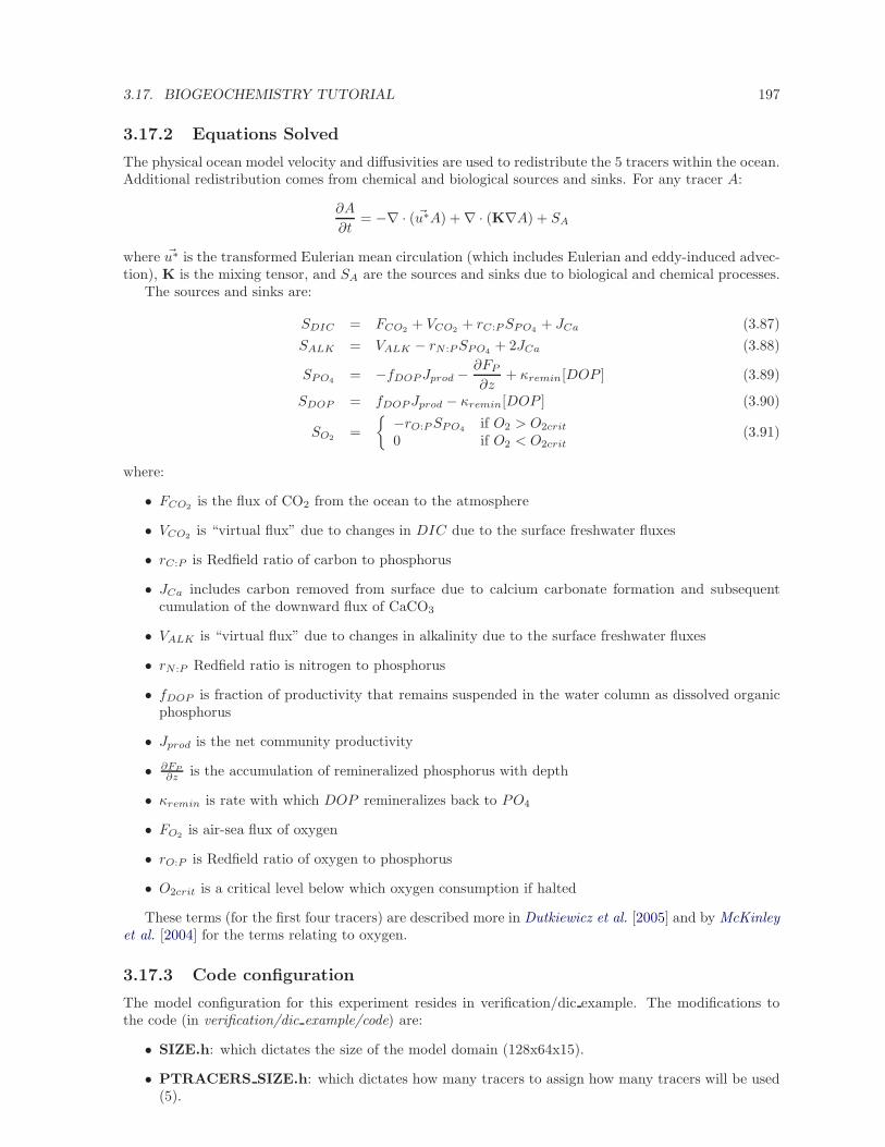
3.17. BIOGEOCHEMISTRY TUTORIAL 197
3.17.2 Equations Solved
The physical ocean model velocity and diffusivities are used to redistribute the 5 tracers within the ocean.Additional redistribution comes from chemical and biological sources and sinks. For any tracer A:
∂A
∂t= −∇ · ( ~u∗A) + ∇ · (K∇A) + SA
where ~u∗ is the transformed Eulerian mean circulation (which includes Eulerian and eddy-induced advec-tion), K is the mixing tensor, and SA are the sources and sinks due to biological and chemical processes.
The sources and sinks are:
SDIC = FCO2 + VCO2 + rC:PSPO4 + JCa (3.87)
SALK = VALK − rN :PSPO4 + 2JCa (3.88)
SPO4 = −fDOPJprod −∂FP
∂z+ κremin[DOP ] (3.89)
SDOP = fDOPJprod − κremin[DOP ] (3.90)
SO2 =
−rO:PSPO4 if O2 > O2crit
0 if O2 < O2crit(3.91)
where:
• FCO2 is the flux of CO2 from the ocean to the atmosphere
• VCO2 is “virtual flux” due to changes in DIC due to the surface freshwater fluxes
• rC:P is Redfield ratio of carbon to phosphorus
• JCa includes carbon removed from surface due to calcium carbonate formation and subsequentcumulation of the downward flux of CaCO3
• VALK is “virtual flux” due to changes in alkalinity due to the surface freshwater fluxes
• rN :P Redfield ratio is nitrogen to phosphorus
• fDOP is fraction of productivity that remains suspended in the water column as dissolved organicphosphorus
• Jprod is the net community productivity
• ∂FP
∂z is the accumulation of remineralized phosphorus with depth
• κremin is rate with which DOP remineralizes back to PO4
• FO2 is air-sea flux of oxygen
• rO:P is Redfield ratio of oxygen to phosphorus
• O2crit is a critical level below which oxygen consumption if halted
These terms (for the first four tracers) are described more in Dutkiewicz et al. [2005] and by McKinleyet al. [2004] for the terms relating to oxygen.
3.17.3 Code configuration
The model configuration for this experiment resides in verification/dic example. The modifications tothe code (in verification/dic example/code) are:
• SIZE.h: which dictates the size of the model domain (128x64x15).
• PTRACERS SIZE.h: which dictates how many tracers to assign how many tracers will be used(5).
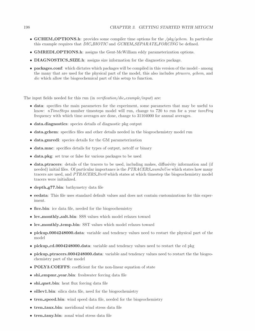
198 CHAPTER 3. GETTING STARTED WITH MITGCM
• GCHEM OPTIONS.h: provides some compiler time options for the /pkg/gchem. In particularthis example requires that DIC BIOTIC and GCHEM SEPARATE FORCING be defined.
• GMREDI OPTIONS.h: assigns the Gent-McWilliam eddy parameterization options.
• DIAGNOSTICS SIZE.h: assigns size information for the diagnostics package.
• packages.conf: which dictates which packages will be compiled in this version of the model - amongthe many that are used for the physical part of the model, this also includes ptracers, gchem, anddic which allow the biogeochemical part of this setup to function.
The input fields needed for this run (in verification/dic example/input) are:
• data: specifies the main parameters for the experiment, some parameters that may be useful toknow: nTimeSteps number timesteps model will run, change to 720 to run for a year taveFreqfrequency with which time averages are done, change to 31104000 for annual averages.
• data.diagnostics: species details of diagnostic pkg output
• data.gchem: specifics files and other details needed in the biogeochemistry model run
• data.gmredi: species details for the GM parameterization
• data.mnc: specifies details for types of output, netcdf or binary
• data.pkg: set true or false for various packages to be used
• data.ptracers: details of the tracers to be used, including makes, diffusivity information and (ifneeded) initial files. Of particular importance is the PTRACERS numInUse which states how manytracers are used, and PTRACERS Iter0 which states at which timestep the biogeochemistry modeltracers were initialized.
• depth g77.bin: bathymetry data file
• eedata: This file uses standard default values and does not contain customizations for this exper-iment.
• fice.bin: ice data file, needed for the biogeochemistry
• lev monthly salt.bin: SSS values which model relaxes toward
• lev monthly temp.bin: SST values which model relaxes toward
• pickup.0004248000.data: variable and tendency values need to restart the physical part of themodel
• pickup cd.0004248000.data: variable and tendency values need to restart the cd pkg
• pickup ptracers.0004248000.data: variable and tendency values need to restart the the biogeo-chemistry part of the model
• POLY3.COEFFS: coefficient for the non-linear equation of state
• shi empmr year.bin: freshwater forcing data file
• shi qnet.bin: heat flux forcing data file
• sillev1.bin: silica data file, need for the biogeochemistry
• tren speed.bin: wind speed data file, needed for the biogeochemistry
• tren taux.bin: meridional wind stress data file
• tren tauy.bin: zonal wind stress data file
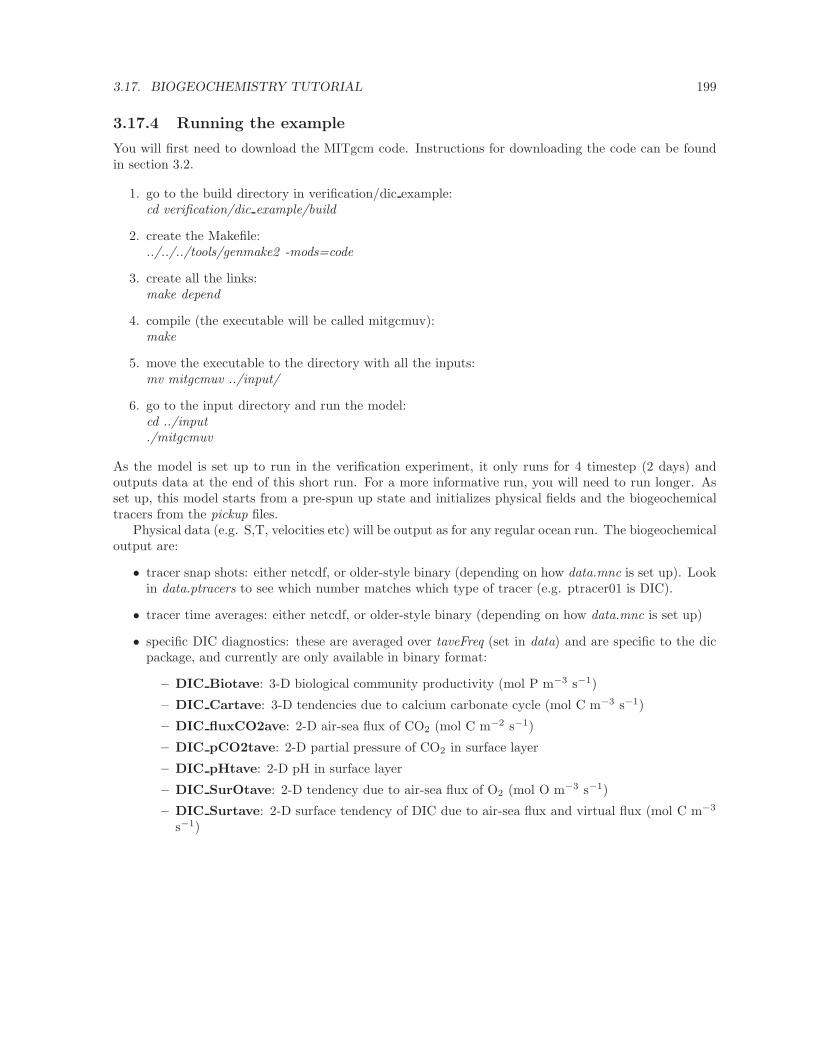
3.17. BIOGEOCHEMISTRY TUTORIAL 199
3.17.4 Running the example
You will first need to download the MITgcm code. Instructions for downloading the code can be foundin section 3.2.
1. go to the build directory in verification/dic example:cd verification/dic example/build
2. create the Makefile:../../../tools/genmake2 -mods=code
3. create all the links:make depend
4. compile (the executable will be called mitgcmuv):make
5. move the executable to the directory with all the inputs:mv mitgcmuv ../input/
6. go to the input directory and run the model:cd ../input./mitgcmuv
As the model is set up to run in the verification experiment, it only runs for 4 timestep (2 days) andoutputs data at the end of this short run. For a more informative run, you will need to run longer. Asset up, this model starts from a pre-spun up state and initializes physical fields and the biogeochemicaltracers from the pickup files.
Physical data (e.g. S,T, velocities etc) will be output as for any regular ocean run. The biogeochemicaloutput are:
• tracer snap shots: either netcdf, or older-style binary (depending on how data.mnc is set up). Lookin data.ptracers to see which number matches which type of tracer (e.g. ptracer01 is DIC).
• tracer time averages: either netcdf, or older-style binary (depending on how data.mnc is set up)
• specific DIC diagnostics: these are averaged over taveFreq (set in data) and are specific to the dicpackage, and currently are only available in binary format:
– DIC Biotave: 3-D biological community productivity (mol P m−3 s−1)
– DIC Cartave: 3-D tendencies due to calcium carbonate cycle (mol C m−3 s−1)
– DIC fluxCO2ave: 2-D air-sea flux of CO2 (mol C m−2 s−1)
– DIC pCO2tave: 2-D partial pressure of CO2 in surface layer
– DIC pHtave: 2-D pH in surface layer
– DIC SurOtave: 2-D tendency due to air-sea flux of O2 (mol O m−3 s−1)
– DIC Surtave: 2-D surface tendency of DIC due to air-sea flux and virtual flux (mol C m−3
s−1)
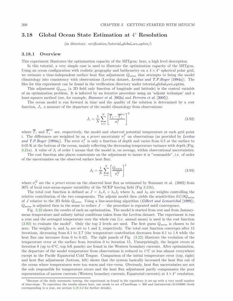
200 CHAPTER 3. GETTING STARTED WITH MITGCM
3.18 Global Ocean State Estimation at 4 Resolution
(in directory: verification/tutorial global oce optim/)
3.18.1 Overview
This experiment illustrates the optimization capacity of the MITgcm: here, a high level description.In this tutorial, a very simple case is used to illustrate the optimization capacity of the MITgcm.
Using an ocean configuration with realistic geography and bathymetry on a 4 × 4 spherical polar grid,we estimate a time-independent surface heat flux adjustment Qnetm that attempts to bring the modelclimatology into consistency with observations (Levitus dataset, Levitus and T.P.Boyer [1994a]). Thefiles for this experiment can be found in the verification directory under tutorial global oce optim.
This adjustment Qnetm (a 2D field only function of longitude and latitude) is the control variableof an optimization problem. It is inferred by an iterative procedure using an ‘adjoint technique’ and aleast-squares method (see, for example, Stammer et al. [002a] and Ferreira et al. [2005]).
The ocean model is run forward in time and the quality of the solution is determined by a costfunction, J1, a measure of the departure of the model climatology from observations:
J1 =1
N
N∑
i=1
[T i − T
lev
i
σTi
]2
(3.92)
where T i and Tlev
i are, respectively, the model and observed potential temperature at each grid pointi. The differences are weighted by an a priori uncertainty σT
i on observations (as provided by Levitusand T.P.Boyer [1994a]). The error σT
i is only a function of depth and varies from 0.5 at the surface to0.05 K at the bottom of the ocean, mainly reflecting the decreasing temperature variance with depth (Fig.3.21a). A value of J1 of order 1 means that the model is, on average, within observational uncertainties.
The cost function also places constraints on the adjustment to insure it is ”reasonable”, i.e. of orderof the uncertainties on the observed surface heat flux:
J2 =1
N
N∑
i=1
[Qnetm
σQi
]2
(3.93)
where σQi are the a priori errors on the observed heat flux as estimated by Stammer et al. (2002) from
30% of local root-mean-square variability of the NCEP forcing field (Fig 3.21b).The total cost function is defined as J = λ1J1 + λ2J2 where λ1 and λ2 are weights controlling the
relative contribution of the two components. The adjoint model then yields the sensitivities ∂J/∂Qnetm
of J relative to the 2D fields Qnetm. Using a line-searching algorithm (Gilbert and Lemarechal [1989]),Qnetm is adjusted then in the sense to reduce J — the procedure is repeated until convergence.
Fig. 3.22 shows the results of such an optimization. The model is started from rest and from January-mean temperature and salinity initial conditions taken from the Levitus dataset. The experiment is runa year and the averaged temperature over the whole run (i.e. annual mean) is used in the cost function(3.92) to evaluate the model1. Only the top 2 levels are used. The first guess Qnetm is chosen to bezero. The weights λ1 and λ2 are set to 1 and 2, respectively. The total cost function converges after 15iterations, decreasing from 6.1 to 2.7 (the temperature contribution decreases from 6.1 to 1.8 while theheat flux one increases from 0 to 0.42). The right panels of Fig. (3.22) illustrate the evolution of thetemperature error at the surface from iteration 0 to iteration 15. Unsurprisingly, the largest errors atiteration 0 (up to 6C, top left panels) are found in the Western boundary currents. After optimization,the departure of the model temperature from observations is reduced to 1C or less almost everywhereexcept in the Pacific Equatorial Cold Tongue. Comparison of the initial temperature error (top, right)and heat flux adjustment (bottom, left) shows that the system basically increased the heat flux out ofthe ocean where temperatures were too warm and vice-versa. Obviously, heat flux uncertainties are notthe sole responsible for temperature errors and the heat flux adjustment partly compensates the poorrepresentation of narrow currents (Western boundary currents, Equatorial currents) at 4× 4 resolution.
1Because of the daily automatic testing, the experiment as found in the repository is set-up with a very small numberof time-steps. To reproduce the results shown here, one needs to set nTimeSteps = 360 and lastinterval=31104000 (bothcorresponding to a year, see section 3.18.3.2 for further details).
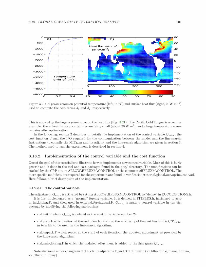
3.18. GLOBAL OCEAN STATE ESTIMATION EXAMPLE 201
0 0.2 0.4−5000
−4500
−4000
−3500
−3000
−2500
−2000
−1500
−1000
−500
0a)
Temperatureerror σT (in K)
b)
Heat flux error σQ
(in W.m−2)
0 100 200 300−80
−60
−40
−20
0
20
40
60
80
20 30 40 50 60 70 80 90
Figure 3.21: A priori errors on potential temperature (left, in C) and surface heat flux (right, in W m−2)used to compute the cost terms J1 and J2, respectively.
This is allowed by the large a priori error on the heat flux (Fig. 3.21). The Pacific Cold Tongue is a counterexample: there, heat fluxes uncertainties are fairly small (about 20 W.m2), and a large temperature errorsremains after optimization.
In the following, section 2 describes in details the implementation of the control variable Qnetm, thecost function J and the I/O required for the communication between the model and the line-search.Instructions to compile the MITgcm and its adjoint and the line-search algorithm are given in section 3.The method used to run the experiment is described in section 4.
3.18.2 Implementation of the control variable and the cost function
One of the goal of this tutorial is to illustrate how to implement a new control variable. Most of this is fairlygeneric and is done in the ctrl and cost packages found in the pkg/ directory. The modifications can betracked by the CPP option ALLOW HFLUXM CONTROL or the comment cHFLUXM CONTROL. Themore specific modifications required for the experiment are found in verification/tutorial global oce optim/code ad.Here follows a brief description of the implementation.
3.18.2.1 The control variable
The adjustmentQnetm is activated by setting ALLOW HFLUXM CONTROL to ”define” in ECCO OPTIONS.h.It is first implemented as a “normal” forcing variable. It is defined in FFIELDS.h, initialized to zero
in ini forcing.F, and then used in external forcing surf.F. Qnetm is made a control variable in the ctrlpackage by modifying the following subroutines:
• ctrl init.F where Qnetm is defined as the control variable number 24,
• ctrl pack.F which writes, at the end of each iteration, the sensitivity of the cost function ∂J/∂Qnetm
in to a file to be used by the line-search algorithm,
• ctrl unpack.F which reads, at the start of each iteration, the updated adjustment as provided bythe line-search algorithm,
• ctrl map forcing.F in which the updated adjustment is added to the first guess Qnetm.
Note also some minor changes in ctrl.h, ctrl readparams.F, and ctrl dummy.h (xx hfluxm file, fname hfluxm,xx hfluxm dummy).
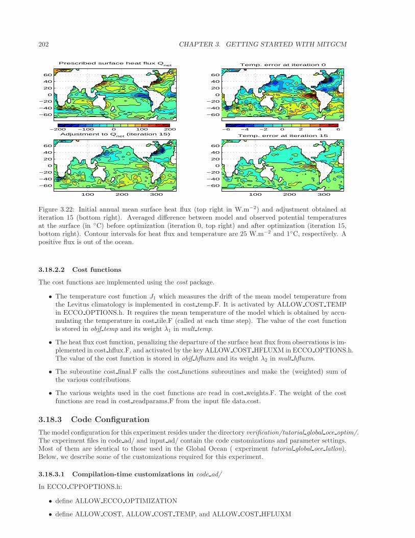
202 CHAPTER 3. GETTING STARTED WITH MITGCM
−60
−40
−20
0
20
40
60
Prescribed surface heat flux Qnet
100 200 300
−60
−40
−20
0
20
40
60
Adjustment to Qnet
(iteration 15)
−60
−40
−20
0
20
40
60
Temp. error at iteration 0
100 200 300
−60
−40
−20
0
20
40
60
Temp. error at iteration 15
−6 −4 −2 0 2 4 6−200 −100 0 100 200
Figure 3.22: Initial annual mean surface heat flux (top right in W.m−2) and adjustment obtained atiteration 15 (bottom right). Averaged difference between model and observed potential temperaturesat the surface (in C) before optimization (iteration 0, top right) and after optimization (iteration 15,bottom right). Contour intervals for heat flux and temperature are 25 W.m−2 and 1C, respectively. Apositive flux is out of the ocean.
3.18.2.2 Cost functions
The cost functions are implemented using the cost package.
• The temperature cost function J1 which measures the drift of the mean model temperature fromthe Levitus climatology is implemented in cost temp.F. It is activated by ALLOW COST TEMPin ECCO OPTIONS.h. It requires the mean temperature of the model which is obtained by accu-mulating the temperature in cost tile.F (called at each time step). The value of the cost functionis stored in objf temp and its weight λ1 in mult temp.
• The heat flux cost function, penalizing the departure of the surface heat flux from observations is im-plemented in cost hflux.F, and activated by the key ALLOW COST HFLUXM in ECCO OPTIONS.h.The value of the cost function is stored in objf hfluxm and its weight λ2 in mult hfluxm.
• The subroutine cost final.F calls the cost functions subroutines and make the (weighted) sum ofthe various contributions.
• The various weights used in the cost functions are read in cost weights.F. The weight of the costfunctions are read in cost readparams.F from the input file data.cost.
3.18.3 Code Configuration
The model configuration for this experiment resides under the directory verification/tutorial global oce optim/.The experiment files in code ad/ and input ad/ contain the code customizations and parameter settings.Most of them are identical to those used in the Global Ocean ( experiment tutorial global oce latlon).Below, we describe some of the customizations required for this experiment.
3.18.3.1 Compilation-time customizations in code ad/
In ECCO CPPOPTIONS.h:
• define ALLOW ECCO OPTIMIZATION
• define ALLOW COST, ALLOW COST TEMP, and ALLOW COST HFLUXM
3.18. GLOBAL OCEAN STATE ESTIMATION EXAMPLE 203
• define ALLOW HFLUXM CONTROL
3.18.3.2 Running-time customizations in input ad/
• data: note the smaller cg2dTargetResidual than in the forward-only experiment,
• data.optim specifies the iteration number,
• data.ctrl is used, in particular, to specify the name of the sensitivity and adjustment files associatedto a control variable,
• data.cost: parameters of the cost functions, in particular lastinterval specifies the length of time-averaging for the model temperature to be used in the cost function (3.92),
• data.pkg: note that the Gradient Check package is turned on by default (useGrdchk=.TRUE.),
• Err hflux.bin and Err levitus 15layer.bin are the files containing the heat flux and potential tem-perature uncertainties, respectively.
3.18.4 Compiling
The optimization experiment requires two executables: 1) the MITgcm and its adjoint (mitgcmuv ad)and 2) the line-search algorithm (optim.x).
3.18.4.1 Compilation of MITgcm and its adjoint: mitcgmuv ad
Before compiling, first note that, in the directory code ad/, two files must be updated:
• code ad diff.list which lists new subroutines to be compiled by the TAF software (cost temp.F andcost hflux.F here),
• the adjoint hfluxm files which provides a list of the control variables and the name of cost functionto the TAF software.
Then, in the directory build ad/, type:
% ../../../tools/genmake2 -mods=../code\_ad -adof=../code\_ad/adjoint\_hfluxm
% make depend
% make adall
to generate the MITgcm executable mitgcmuv ad.
3.18.4.2 Compilation of the line-search algorithm: optim.x
This is done from the directories lsopt/ and optim/ (under MITgcm/). In lsopt/, unzip the blash1 libraryadapted to your platform, and change the Makefile accordingly. Compile with:
% make all
(more details in lsopt doc.txt)In optim/, the path of the directory where mitgcm ad was compiled must be specified in the Makefile
in the variable INCLUDEDIRS. The file name of the control variable (xx hfluxm file here) must be addedto the name list read by optim num.F. Then use
% make depend
and
% make
to generate the line-search executable optim.x.
204 CHAPTER 3. GETTING STARTED WITH MITGCM
3.18.5 Running the estimation
Copy the mitgcmuv ad executable to input ad/ and optim.x to the subdirectory input ad/OPTIM/. Moveinto input ad/. The first iteration is somewhat particular and is best done ”by hand” while the followingiterations can be run automatically (see below). Check that the iteration number is set to 0 in data.optimand run the MITgcm:
% ./mitgcmuv_ad
The output files adxx hfluxm.0000000000.* and xx hfluxm.0000000000.* contain the sensitivity of thecost function to Qnetm and the adjustment to Qnetm (zero at the first iteration), respectively. Two otherfiles called costhflux tut MITgcm.opt0000 and ctrlhflux tut MITgcm.opt0000 are also generated. Theyessentially contain the same information as the adxx .hfluxm* and xx hfluxm* files, but in a compressedformat. These two files are the only ones involved in the communication between the adjoint modelmitgcmuv ad and the line-search algorithm optim.x. Only at the first iteration, are they both generated bymitgcmuv ad. Subsenquently, costhflux tut MITgcm.optn is an output of the adjoint model at iteration nand an input of the line-search. The latter returns an updated adjustment in ctrlhflux tut MITgcm.optn+1 to be used as an input of the adjoint model at iteration n+1.
At the first iteration, move costhflux tut MITgcm.opt0000 and ctrlhflux tut MITgcm.opt0000 to OP-TIM/, move into this directory and link data.optim and data.ctrl locally:
% cd OPTIM/
% ln -s ../data.optim .
% ln -s ../data.ctrl .
The target cost function fmin needs to be specified too: as a rule of thumb, it should be about 0.95-0.90times the value of the cost function at the first iteration. This value is only used at the first iterationand does not need to be updated afterward. However, it implicitly specifies the “pace” at which the costfunction is going down (if you are lucky and it does indeed diminish!). More in the ECCO section maybe?
Once this is done, run the line-search algorithm:
% ./optim.x
which computes the updated adjustment for iteration 1, ctrlhflux tut MITgcm.opt0001.The following iterations can be executed automatically using the shell script cycsh found in input ad/.
This script will take care of changing the iteration numbers in the data.optim, launch the adjoint model,clean and store the outputs, move the costhflux* and ctrlhflux* files, and run the line-search algorithm.Edit cycsh to specify the prefix of the directories used to store the outputs and the maximum number ofiteration.
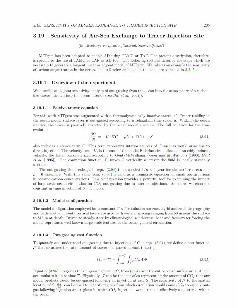
3.19. SENSITIVITY OF AIR-SEA EXCHANGE TO TRACER INJECTION SITE 205
3.19 Sensitivity of Air-Sea Exchange to Tracer Injection Site
(in directory: verification/tutorial tracer adjsens/)
MITgcm has been adapted to enable AD using TAMC or TAF. The present description, therefore,is specific to the use of TAMC or TAF as AD tool. The following sections describe the steps which arenecessary to generate a tangent linear or adjoint model of MITgcm. We take as an example the sensitivityof carbon sequestration in the ocean. The AD-relevant hooks in the code are sketched in 5.2, 5.4.
3.19.1 Overview of the experiment
We describe an adjoint sensitivity analysis of out-gassing from the ocean into the atmosphere of a carbon-like tracer injected into the ocean interior (see Hill et al. [2002]).
3.19.1.1 Passive tracer equation
For this work MITgcm was augmented with a thermodynamically inactive tracer, C. Tracer residing inthe ocean model surface layer is out-gassed according to a relaxation time scale, µ. Within the oceaninterior, the tracer is passively advected by the ocean model currents. The full equation for the timeevolution
∂C
∂t= −U · ∇C − µC + Γ(C) + S (3.94)
also includes a source term S. This term represents interior sources of C such as would arise due todirect injection. The velocity term, U , is the sum of the model Eulerian circulation and an eddy-inducedvelocity, the latter parameterized according to Gent/McWilliams (Gent and McWilliams [1990]; Gentet al. [1995]). The convection function, Γ, mixes C vertically wherever the fluid is locally staticallyunstable.
The out-gassing time scale, µ, in eqn. (3.94) is set so that 1/µ ∼ 1 year for the surface ocean andµ = 0 elsewhere. With this value, eqn. (3.94) is valid as a prognostic equation for small perturbationsin oceanic carbon concentrations. This configuration provides a powerful tool for examining the impactof large-scale ocean circulation on CO2 out-gassing due to interior injections. As source we choose aconstant in time injection of S = 1 mol/s.
3.19.1.2 Model configuration
The model configuration employed has a constant 4×4 resolution horizontal grid and realistic geographyand bathymetry. Twenty vertical layers are used with vertical spacing ranging from 50 m near the surfaceto 815 m at depth. Driven to steady-state by climatological wind-stress, heat and fresh-water forcing themodel reproduces well known large-scale features of the ocean general circulation.
3.19.1.3 Out-gassing cost function
To quantify and understand out-gassing due to injections of C in eqn. (3.94), we define a cost functionJ that measures the total amount of tracer out-gassed at each timestep:
J (t = T ) =
∫ t=T
t=0
∫
A
µC dAdt (3.95)
Equation(3.95) integrates the out-gassing term, µC, from (3.94) over the entire ocean surface area, A, andaccumulates it up to time T . Physically, J can be thought of as representing the amount of CO2 that ourmodel predicts would be out-gassed following an injection at rate S. The sensitivity of J to the spatiallocation of S, ∂J
∂S , can be used to identify regions from which circulation would cause CO2 to rapidly out-gas following injection and regions in which CO2 injections would remain effectively sequestered withinthe ocean.
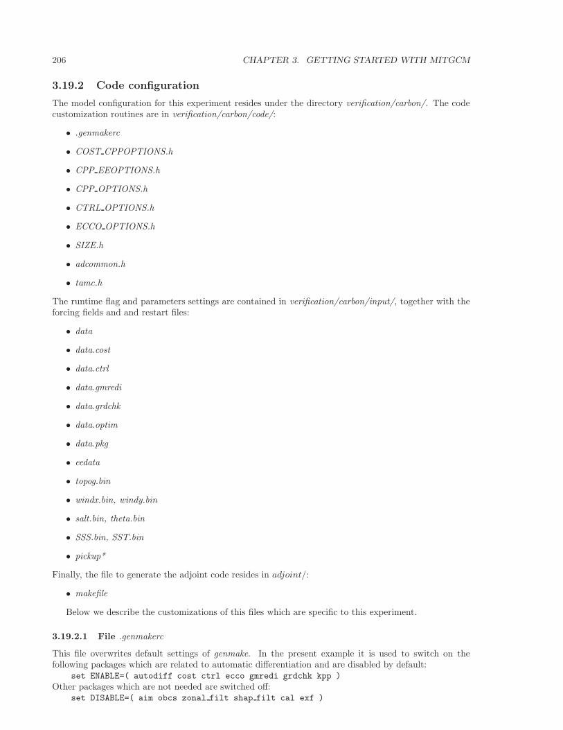
206 CHAPTER 3. GETTING STARTED WITH MITGCM
3.19.2 Code configuration
The model configuration for this experiment resides under the directory verification/carbon/. The codecustomization routines are in verification/carbon/code/:
• .genmakerc
• COST CPPOPTIONS.h
• CPP EEOPTIONS.h
• CPP OPTIONS.h
• CTRL OPTIONS.h
• ECCO OPTIONS.h
• SIZE.h
• adcommon.h
• tamc.h
The runtime flag and parameters settings are contained in verification/carbon/input/, together with theforcing fields and and restart files:
• data
• data.cost
• data.ctrl
• data.gmredi
• data.grdchk
• data.optim
• data.pkg
• eedata
• topog.bin
• windx.bin, windy.bin
• salt.bin, theta.bin
• SSS.bin, SST.bin
• pickup*
Finally, the file to generate the adjoint code resides in adjoint/:
• makefile
Below we describe the customizations of this files which are specific to this experiment.
3.19.2.1 File .genmakerc
This file overwrites default settings of genmake. In the present example it is used to switch on thefollowing packages which are related to automatic differentiation and are disabled by default:
set ENABLE=( autodiff cost ctrl ecco gmredi grdchk kpp )
Other packages which are not needed are switched off:set DISABLE=( aim obcs zonal filt shap filt cal exf )
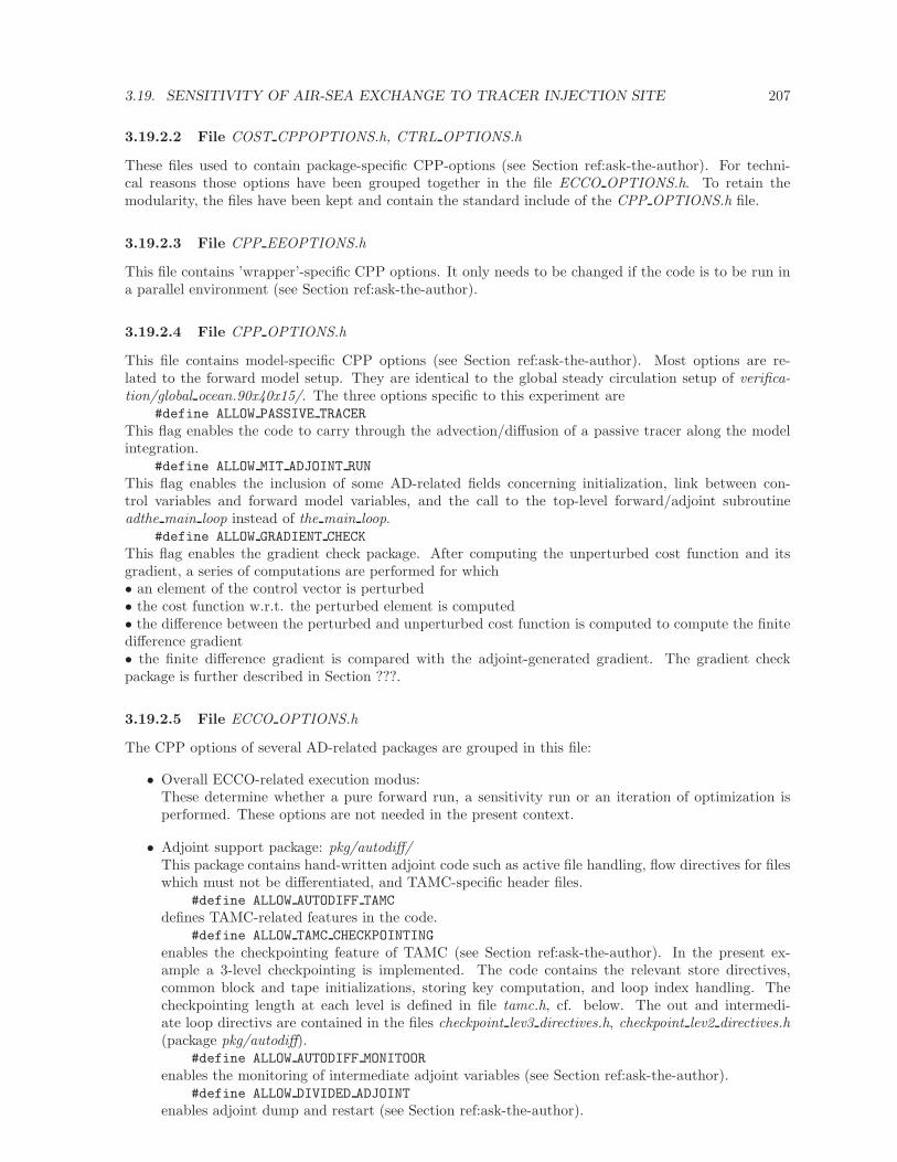
3.19. SENSITIVITY OF AIR-SEA EXCHANGE TO TRACER INJECTION SITE 207
3.19.2.2 File COST CPPOPTIONS.h, CTRL OPTIONS.h
These files used to contain package-specific CPP-options (see Section ref:ask-the-author). For techni-cal reasons those options have been grouped together in the file ECCO OPTIONS.h. To retain themodularity, the files have been kept and contain the standard include of the CPP OPTIONS.h file.
3.19.2.3 File CPP EEOPTIONS.h
This file contains ’wrapper’-specific CPP options. It only needs to be changed if the code is to be run ina parallel environment (see Section ref:ask-the-author).
3.19.2.4 File CPP OPTIONS.h
This file contains model-specific CPP options (see Section ref:ask-the-author). Most options are re-lated to the forward model setup. They are identical to the global steady circulation setup of verifica-tion/global ocean.90x40x15/. The three options specific to this experiment are
#define ALLOW PASSIVE TRACER
This flag enables the code to carry through the advection/diffusion of a passive tracer along the modelintegration.
#define ALLOW MIT ADJOINT RUN
This flag enables the inclusion of some AD-related fields concerning initialization, link between con-trol variables and forward model variables, and the call to the top-level forward/adjoint subroutineadthe main loop instead of the main loop.
#define ALLOW GRADIENT CHECK
This flag enables the gradient check package. After computing the unperturbed cost function and itsgradient, a series of computations are performed for which• an element of the control vector is perturbed• the cost function w.r.t. the perturbed element is computed• the difference between the perturbed and unperturbed cost function is computed to compute the finitedifference gradient• the finite difference gradient is compared with the adjoint-generated gradient. The gradient checkpackage is further described in Section ???.
3.19.2.5 File ECCO OPTIONS.h
The CPP options of several AD-related packages are grouped in this file:
• Overall ECCO-related execution modus:These determine whether a pure forward run, a sensitivity run or an iteration of optimization isperformed. These options are not needed in the present context.
• Adjoint support package: pkg/autodiff/This package contains hand-written adjoint code such as active file handling, flow directives for fileswhich must not be differentiated, and TAMC-specific header files.
#define ALLOW AUTODIFF TAMC
defines TAMC-related features in the code.#define ALLOW TAMC CHECKPOINTING
enables the checkpointing feature of TAMC (see Section ref:ask-the-author). In the present ex-ample a 3-level checkpointing is implemented. The code contains the relevant store directives,common block and tape initializations, storing key computation, and loop index handling. Thecheckpointing length at each level is defined in file tamc.h, cf. below. The out and intermedi-ate loop directivs are contained in the files checkpoint lev3 directives.h, checkpoint lev2 directives.h(package pkg/autodiff).
#define ALLOW AUTODIFF MONITOOR
enables the monitoring of intermediate adjoint variables (see Section ref:ask-the-author).#define ALLOW DIVIDED ADJOINT
enables adjoint dump and restart (see Section ref:ask-the-author).
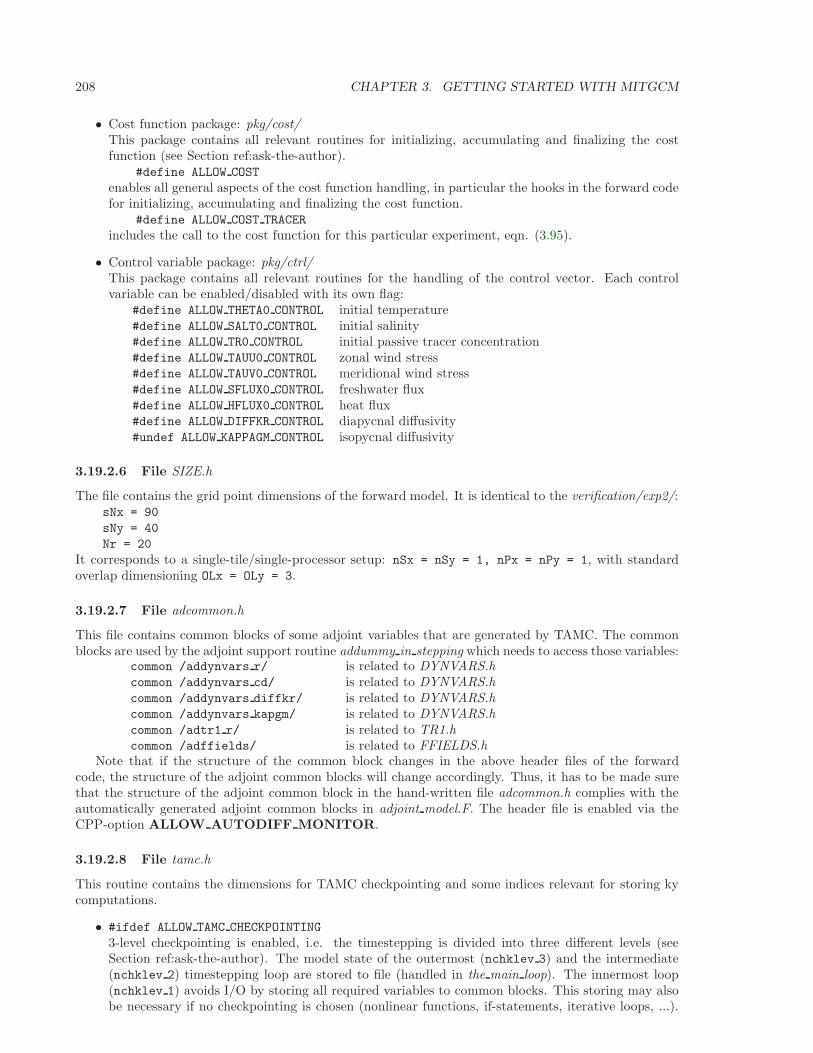
208 CHAPTER 3. GETTING STARTED WITH MITGCM
• Cost function package: pkg/cost/This package contains all relevant routines for initializing, accumulating and finalizing the costfunction (see Section ref:ask-the-author).
#define ALLOW COST
enables all general aspects of the cost function handling, in particular the hooks in the forward codefor initializing, accumulating and finalizing the cost function.
#define ALLOW COST TRACER
includes the call to the cost function for this particular experiment, eqn. (3.95).
• Control variable package: pkg/ctrl/This package contains all relevant routines for the handling of the control vector. Each controlvariable can be enabled/disabled with its own flag:
#define ALLOW THETA0 CONTROL initial temperature#define ALLOW SALT0 CONTROL initial salinity#define ALLOW TR0 CONTROL initial passive tracer concentration#define ALLOW TAUU0 CONTROL zonal wind stress#define ALLOW TAUV0 CONTROL meridional wind stress#define ALLOW SFLUX0 CONTROL freshwater flux#define ALLOW HFLUX0 CONTROL heat flux#define ALLOW DIFFKR CONTROL diapycnal diffusivity#undef ALLOW KAPPAGM CONTROL isopycnal diffusivity
3.19.2.6 File SIZE.h
The file contains the grid point dimensions of the forward model. It is identical to the verification/exp2/:sNx = 90
sNy = 40
Nr = 20
It corresponds to a single-tile/single-processor setup: nSx = nSy = 1, nPx = nPy = 1, with standardoverlap dimensioning OLx = OLy = 3.
3.19.2.7 File adcommon.h
This file contains common blocks of some adjoint variables that are generated by TAMC. The commonblocks are used by the adjoint support routine addummy in stepping which needs to access those variables:
common /addynvars r/ is related to DYNVARS.hcommon /addynvars cd/ is related to DYNVARS.hcommon /addynvars diffkr/ is related to DYNVARS.hcommon /addynvars kapgm/ is related to DYNVARS.hcommon /adtr1 r/ is related to TR1.hcommon /adffields/ is related to FFIELDS.h
Note that if the structure of the common block changes in the above header files of the forwardcode, the structure of the adjoint common blocks will change accordingly. Thus, it has to be made surethat the structure of the adjoint common block in the hand-written file adcommon.h complies with theautomatically generated adjoint common blocks in adjoint model.F. The header file is enabled via theCPP-option ALLOW AUTODIFF MONITOR.
3.19.2.8 File tamc.h
This routine contains the dimensions for TAMC checkpointing and some indices relevant for storing kycomputations.
• #ifdef ALLOW TAMC CHECKPOINTING
3-level checkpointing is enabled, i.e. the timestepping is divided into three different levels (seeSection ref:ask-the-author). The model state of the outermost (nchklev 3) and the intermediate(nchklev 2) timestepping loop are stored to file (handled in the main loop). The innermost loop(nchklev 1) avoids I/O by storing all required variables to common blocks. This storing may alsobe necessary if no checkpointing is chosen (nonlinear functions, if-statements, iterative loops, ...).
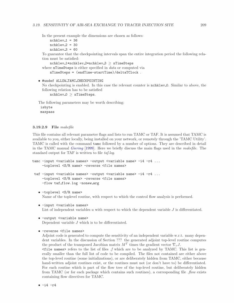
3.19. SENSITIVITY OF AIR-SEA EXCHANGE TO TRACER INJECTION SITE 209
In the present example the dimensions are chosen as follows:nchklev 1 = 36
nchklev 2 = 30
nchklev 3 = 60
To guarantee that the checkpointing intervals span the entire integration period the following rela-tion must be satisfied:
nchklev 1*nchklev 2*nchklev 3 ≥ nTimeSteps
where nTimeSteps is either specified in data or computed vianTimeSteps = (endTime-startTime)/deltaTClock .
• #undef ALLOW TAMC CHECKPOINTING
No checkpointing is enabled. In this case the relevant counter is nchklev 0. Similar to above, thefollowing relation has to be satisfied
nchklev 0 ≥ nTimeSteps.
The following parameters may be worth describing:isbyte
maxpass
3.19.2.9 File makefile
This file contains all relevant parameter flags and lists to run TAMC or TAF. It is assumed that TAMC isavailable to you, either locally, being installed on your network, or remotely through the ’TAMC Utility’.TAMC is called with the command tamc followed by a number of options. They are described in detailin the TAMC manual Giering [1999]. Here we briefly discuss the main flags used in the makefile. Thestandard output for TAF is written to file taf.log.
tamc -input <variable names> -output <variable name> -i4 -r4 ...
-toplevel <S/R name> -reverse <file names>
taf -input <variable names> -output <variable name> -i4 -r4 ...
-toplevel <S/R name> -reverse <file names>
-flow taf flow.log -nonew arg
• -toplevel <S/R name>
Name of the toplevel routine, with respect to which the control flow analysis is performed.
• -input <variable names>
List of independent variables u with respect to which the dependent variable J is differentiated.
• -output <variable name>
Dependent variable J which is to be differentiated.
• -reverse <file names>
Adjoint code is generated to compute the sensitivity of an independent variable w.r.t. many depen-dent variables. In the discussion of Section ??? the generated adjoint top-level routine computesthe product of the transposed Jacobian matrix MT times the gradient vector ∇vJ .<file names> refers to the list of files .f which are to be analyzed by TAMC. This list is gen-erally smaller than the full list of code to be compiled. The files not contained are either abovethe top-level routine (some initializations), or are deliberately hidden from TAMC, either becausehand-written adjoint routines exist, or the routines must not (or don’t have to) be differentiated.For each routine which is part of the flow tree of the top-level routine, but deliberately hiddenfrom TAMC (or for each package which contains such routines), a corresponding file .flow existscontaining flow directives for TAMC.
• -i4 -r4
210 CHAPTER 3. GETTING STARTED WITH MITGCM
• -flow taf flow.log
Will cause TAF to produce a flow listing file named taf flow.log in which the set of active andpassive variables are identified for each subroutine.
• -nonew arg
The default in the order of the parameter list of adjoint routines has changed. Before TAF 1.3 thedefault was compatible with the TAMC-generated list. As of TAF 1.3 the order of adjoint routineparameter lists is no longer copatible with TAMC. To restore compatibility when using TAF 1.3and higher, this argument is needed. It is currently crucial to use since all hand-written adjointroutines refer to the TAMC default.
3.19.2.10 The input parameter files
File data
File data.cost
File data.ctrl
File data.gmredi
File data.grdchk
File data.optim
File data.pkg
File eedata
File topog.binContains two-dimendional bathymetry information
File windx.bin, windy.bin, salt.bin, theta.bin, SSS.bin, SST.binThese contain the initial values (salinity, temperature, salt.bin, theta.bin), surface boundary values (sur-face wind stresses, (windx.bin, windy.bin), and surface restoring fields (SSS.bin, SST.bin).
File pickup*Contains model state after model spinup.
3.19.3 Compiling the model and its adjoint
The built process of the adjoint model is slightly more complex than that of compiling the forward code.The main reason is that the adjoint code generation requires a specific list of routines that are to bedifferentiated (as opposed to the automatic generation of a list of files to be compiled by genmake). Thislist excludes routines that don’t have to be or must not be differentiated. For some of the latter routinesflow directives may be necessary, a list of which has to be given as well. For this reason, a separatemakefile is currently maintained in the directory adjoint/. This makefile is responsible for the adjointcode generation.
In the following we describe the build process step by step, assuming you are in the directory bin/.A summary of steps to follow is given at the end.
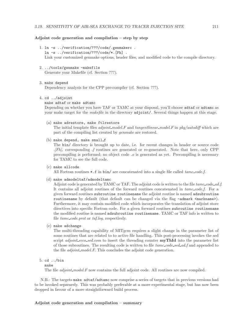
3.19. SENSITIVITY OF AIR-SEA EXCHANGE TO TRACER INJECTION SITE 211
Adjoint code generation and compilation – step by step
1. ln -s ../verification/???/code/.genmakerc .
ln -s ../verification/???/code/*.[Fh] .
Link your customized genmake options, header files, and modified code to the compile directory.
2. ../tools/genmake -makefile
Generate your Makefile (cf. Section ???).
3. make depend
Dependency analysis for the CPP pre-compiler (cf. Section ???).
4. cd ../adjoint
make adtaf or make adtamc
Depending on whether you have TAF or TAMC at your disposal, you’ll choose adtaf or adtamc asyour make target for the makefile in the directory adjoint/. Several things happen at this stage.
(a) make adrestore, make ftlrestore
The initial template files adjoint model.F and tangentlinear model.F in pkg/autodiff which arepart of the compiling list created by genmake are restored.
(b) make depend, make small f
The bin/ directory is brought up to date, i.e. for recent changes in header or source code.[Fh], corresponding .f routines are generated or re-generated. Note that here, only CPPprecompiling is performed; no object code .o is generated as yet. Precompiling is necessaryfor TAMC to see the full code.
(c) make allcode
All Fortran routines *.f in bin/ are concatenated into a single file called tamc code.f.
(d) make admodeltaf/admodeltamc
Adjoint code is generated by TAMC or TAF. The adjoint code is written to the file tamc code ad.f.It contains all adjoint routines of the forward routines concatenated in tamc code.f. For agiven forward routines subroutine routinename the adjoint routine is named adsubroutine
routinename by default (that default can be changed via the flag -admark <markname>).Furthermore, it may contain modified code which incorporates the translation of adjoint storedirectives into specific Fortran code. For a given forward routines subroutine routinename
the modified routine is named mdsubroutine routinename. TAMC or TAF info is written tofile tamc code.prot or taf.log, respectively.
(e) make adchange
The multi-threading capability of MITgcm requires a slight change in the parameter list ofsome routines that are related to to active file handling. This post-processing invokes the sedscript adjoint ecco sed.com to insert the threading counter myThId into the parameter listof those subroutines. The resulting code is written to file tamc code sed ad.f and appended tothe file adjoint model.F. This concludes the adjoint code generation.
5. cd ../bin
make
The file adjoint model.F now contains the full adjoint code. All routines are now compiled.
N.B.: The targets make adtaf/adtamc now comprise a series of targets that in previous versions hadto be invoked separarely. This was probably preferable at a more experimental stage, but has now beendropped in favour of a more straightforward build process.
Adjoint code generation and compilation – summary
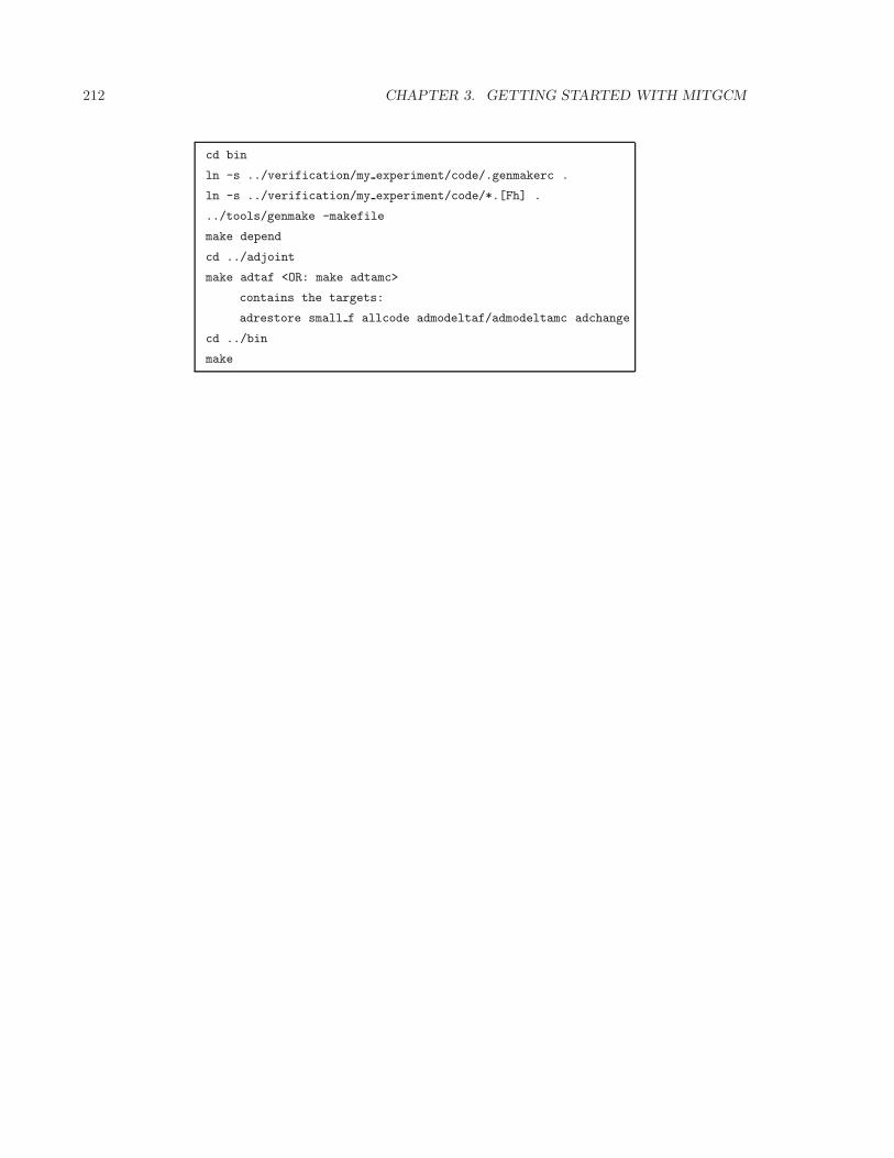
212 CHAPTER 3. GETTING STARTED WITH MITGCM
cd bin
ln -s ../verification/my experiment/code/.genmakerc .
ln -s ../verification/my experiment/code/*.[Fh] .
../tools/genmake -makefile
make depend
cd ../adjoint
make adtaf <OR: make adtamc>
contains the targets:
adrestore small f allcode admodeltaf/admodeltamc adchange
cd ../bin
make
3.20. OFFLINE EXAMPLE 213
3.20 Offline Experiments
(in directory: verification/tutorial offline/)
This document describes a simple experiment using the offline form of the MITgcm.
3.20.1 Overview
This experiment demonstrates use of the offline form of the MITgcm to study advection of a passivetracer. Time-averaged flow-fields and mixing coefficients, deriving from a prior online run, are re-usedleaving only the tracer equation to be integrated.
Figure — missing figure — shows a movie of tracer being advected using the offline package of theMITgcm. In the top panel the frames of the movie show the monthly surface evolution of an initiallylocal source of passive tracer. In the lower panel, the frames of the movie show the changing monthlysurface evolution where the initial tracer field had a global distribution.
3.20.2 Time-stepping of tracers
see section 2.15 through 2.18 for details of available tracer time-stepping schemes and their characteristics.
3.20.3 Code Configuration
The model configuration for this experiment resides under the directory verification/tutorial offline. Theexperiment files
• input/data
• input/data.off
• input/data.pkg
• input/data.ptracers
• input/eedata
• input/packages.conf
• code/PTRACERS SIZE.h
• code/SIZE.h.
contain the code customisations and parameter settings required to run the example. In addition thefollowing binary data files are required:
• input/depth g77.bin
• input/tracer1 .bin
• input/tracer2 .bin
• input/input off/uVeltave.0000000001-12.data
• input/input off/vVeltave.0000000001-12.data
• input/input off/wVeltave.0000000001-12.data
• input/input off/Convtave.0000000001-12.data
214 CHAPTER 3. GETTING STARTED WITH MITGCM
3.20.3.1 File input/data
This file, reproduced completely below, specifies the main parameters for the experiment.
• Line 18, 19
nIter0 = 0,
nTimeSteps = 720,
nIter0 and nTimesteps control the start time and the length of the run (in timesteps). If nIter0 is non-zero the model will require appropriate pickup files to be present in the run directory. Where nIter0 iszero, as here, the model makes a fresh start. In this case the model has been prescribed to run for 720timesteps or 1 year.
• Line 20
deltaTtracer= 43200.0,
deltaTtracer is the tracer timestep in seconds, in this case, 12 hours (43200s = 12 hours). Note thatdeltatTracer must be specified in input/data as well as specifying deltaToffline in input/data.off.
• Line 21
deltaTClock= 43200.0,
When using the MITgcm in offline mode deltaTClock (an internal model counter) should be made equalto the value assigned to deltatTtracer.
• Line 27
periodicExternalForcing=.TRUE.,
periodicExternalForcing is a flag telling the model whether to cyclically re-use forcing data where thereis external forcing (see ‘A More Complcated Example’, below). Where there is no external forcing, ashere, but where there is to be cyclic re-use of the offline flow and mixing fields, periodicExternalForcingmust be assigned the value .TRUE.
• Line 28
externForcingPeriod=2592000.,
externForcingPeriod specifies the period of the external forcing data in seconds. In the absence of externalforcing, as in this example, it must be made equal to the value of externForcingPeriod in input/data.off,in this case, monthly (2592000s = 1 month).
• Line 29
externForcingCycle=31104000.,
externForcingCycle specifies the duration of the external forcing data cycle in seconds. In the absenceof external forcing, as in this example, it must be made equal to the value of externForcingCycle ininput/data.off, in this case, the cycle is one year(31104000s = 1 year).
• Line 35
usingSphericalPolarGrid=.TRUE.,
This line requests that the simulation be performed in a spherical polar coordinate system. It affects theinterpretation of grid input parameters and causes the grid generation routines to initialize an internalgrid based on spherical polar geometry.
3.20. OFFLINE EXAMPLE 215
• Line 36
delR= 50., 70., 100., 140., 190.,
240., 290., 340., 390., 440.,
490., 540., 590., 640., 690.,
This line sets the vertical grid spacing between each z-coordinate line in the discrete grid. Here the totalmodel depth is 5200 m.
• Line 39
ygOrigin=-90.,
This line sets the southern boundary of the modeled domain to −90 latitude N (90 S). This valueaffects both the generation of the locally orthogonal grid that the model uses internally and affects theinitialization of the coriolis force. Note - it is not required to set a longitude boundary, since the absolutelongitude does not alter the kernel equation discretisation.
• Line 40
dxSpacing=2.8125,
This line sets the horizontal grid spacing between each y-coordinate line in the discrete grid to 2.8125
in longitude.
• Line 41
dySpacing=2.8125,
This line sets the vertical grid spacing between each x-coordinate line in the discrete grid to 2.8125 inlatitude.
• Line 46
bathyFile=’depth_g77.bin’,
This line specifies the name of the file, in this case depth g77.bin, from which the domain bathymetryis read. This file contains a two-dimensional (x, y) map of (assumed 64-bit) binary numbers giving thedepth of the model at each grid cell, ordered with the x coordinate varying fastest. The points are orderedfrom low coordinate to high coordinate for both axes. The units and orientation of the depths in this fileare the same as used in the MITgcm code. In this experiment, a depth of 0m indicates land.
1 # ====================
2 # | Model parameters |
3 # ====================
4 #
5 # Continuous equation parameters
6 &PARM01
7 &
8 #
9 # Elliptic solver parameters
10 &PARM02
11 cg2dMaxIters=1000,
12 cg2dTargetResidual=1.E-13,
13 &
14 #
15
16 # Time stepping parameters
216 CHAPTER 3. GETTING STARTED WITH MITGCM
17 &PARM03
18 nIter0 = 0,
19 nTimeSteps = 720,
20 deltaTtracer= 43200.0,
21 deltaTClock = 43200.0,
22 pChkptFreq=31104000.,
23 chkptFreq= 31104000.,
24 dumpFreq= 2592000.,
25 taveFreq= 311040000.,
26 monitorFreq= 1.,
27 periodicExternalForcing=.TRUE.,
28 externForcingPeriod=2592000.,
29 externForcingCycle=31104000.,
30 &
31 #
32 # Gridding parameters
33 &PARM04
34 usingCartesianGrid=.FALSE.,
35 usingSphericalPolarGrid=.TRUE.,
36 delR= 50., 70., 100., 140., 190.,
37 240., 290., 340., 390., 440.,
38 490., 540., 590., 640., 690.,
39 ygOrigin=-90.,
40 dxSpacing=2.8125,
41 dySpacing=2.8125,
42 &
43 #
44 # Input datasets
45 &PARM05
46 bathyFile= ’depth_g77.bin’,
47 &
3.20.3.2 File input/data.off
input/data.off provides the MITgcm offline package with package specific parameters. input/data.offspecifies the location (relative to the run directory) and prefix of files describing the flow field (UvelFile,VvelFile, WvelFile) and the corresponding convective mixing coefficients (ConvFile) which together pre-scribe the three dimensional, time varying dynamic system within which the offline model will advect thetracer.
• Lines 2 to 5
UvelFile= ’../input/input_off/uVeltave’,
VvelFile= ’../input/input_off/vVeltave’,
WvelFile= ’../input/input_off/wVeltave’,
ConvFile= ’../input/input_off/Convtave’,
In the example the offline data is located in the sub-directory input/input off. In this directory are fieldsdescribing the velocity and convective mixing histories of a prior forward integration of the MITgcmrequired for the offline package and identified in input/data off. Based on the values of deltatToffline,offlineForcingPeriod and offlineForcingCycle specified in input/data.off, since offlineForcingCycle cor-responds to 12 forcing periods offlineForcingPeriod and since offlineIter0 is zero, there needs to be 12uVeltave, 12 vVeltave, 12 wVeltave and 12 Convtave files each having a 10 digit sequence identifierbetween 0000000001 to 0000000012, that is, a total of 48 files.
• Line 9
offlineIter0=0,
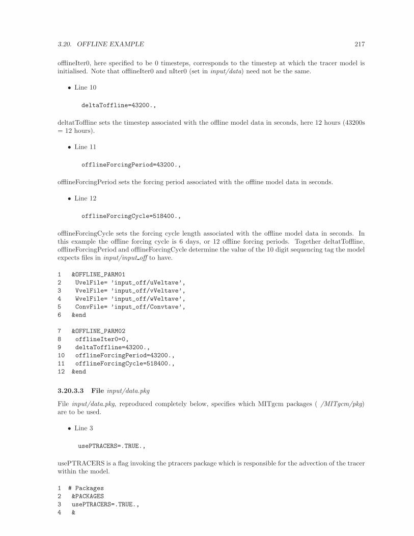
3.20. OFFLINE EXAMPLE 217
offlineIter0, here specified to be 0 timesteps, corresponds to the timestep at which the tracer model isinitialised. Note that offlineIter0 and nIter0 (set in input/data) need not be the same.
• Line 10
deltaToffline=43200.,
deltatToffline sets the timestep associated with the offline model data in seconds, here 12 hours (43200s= 12 hours).
• Line 11
offlineForcingPeriod=43200.,
offlineForcingPeriod sets the forcing period associated with the offline model data in seconds.
• Line 12
offlineForcingCycle=518400.,
offlineForcingCycle sets the forcing cycle length associated with the offline model data in seconds. Inthis example the offline forcing cycle is 6 days, or 12 offline forcing periods. Together deltatToffline,offlineForcingPeriod and offlineForcingCycle determine the value of the 10 digit sequencing tag the modelexpects files in input/input off to have.
1 &OFFLINE_PARM01
2 UvelFile= ’input_off/uVeltave’,
3 VvelFile= ’input_off/vVeltave’,
4 WvelFile= ’input_off/wVeltave’,
5 ConvFile= ’input_off/Convtave’,
6 &end
7 &OFFLINE_PARM02
8 offlineIter0=0,
9 deltaToffline=43200.,
10 offlineForcingPeriod=43200.,
11 offlineForcingCycle=518400.,
12 &end
3.20.3.3 File input/data.pkg
File input/data.pkg, reproduced completely below, specifies which MITgcm packages ( /MITgcm/pkg)are to be used.
• Line 3
usePTRACERS=.TRUE.,
usePTRACERS is a flag invoking the ptracers package which is responsible for the advection of the tracerwithin the model.
1 # Packages
2 &PACKAGES
3 usePTRACERS=.TRUE.,
4 &
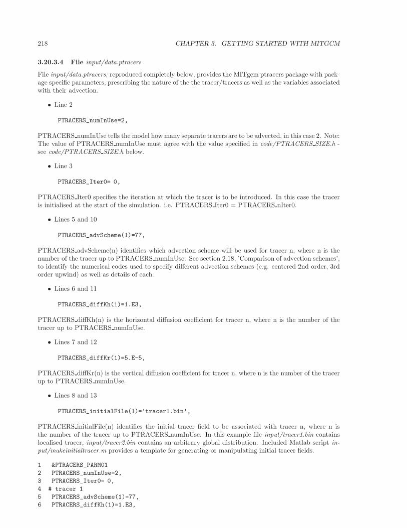
218 CHAPTER 3. GETTING STARTED WITH MITGCM
3.20.3.4 File input/data.ptracers
File input/data.ptracers, reproduced completely below, provides the MITgcm ptracers package with pack-age specific parameters, prescribing the nature of the the tracer/tracers as well as the variables associatedwith their advection.
• Line 2
PTRACERS_numInUse=2,
PTRACERS numInUse tells the model how many separate tracers are to be advected, in this case 2. Note:The value of PTRACERS numInUse must agree with the value specified in code/PTRACERS SIZE.h -see code/PTRACERS SIZE.h below.
• Line 3
PTRACERS_Iter0= 0,
PTRACERS Iter0 specifies the iteration at which the tracer is to be introduced. In this case the traceris initialised at the start of the simulation. i.e. PTRACERS Iter0 = PTRACERS nIter0.
• Lines 5 and 10
PTRACERS_advScheme(1)=77,
PTRACERS advScheme(n) identifies which advection scheme will be used for tracer n, where n is thenumber of the tracer up to PTRACERS numInUse. See section 2.18, ’Comparison of advection schemes’,to identify the numerical codes used to specify different advection schemes (e.g. centered 2nd order, 3rdorder upwind) as well as details of each.
• Lines 6 and 11
PTRACERS_diffKh(1)=1.E3,
PTRACERS diffKh(n) is the horizontal diffusion coefficient for tracer n, where n is the number of thetracer up to PTRACERS numInUse.
• Lines 7 and 12
PTRACERS_diffKr(1)=5.E-5,
PTRACERS diffKr(n) is the vertical diffusion coefficient for tracer n, where n is the number of the tracerup to PTRACERS numInUse.
• Lines 8 and 13
PTRACERS_initialFile(1)=’tracer1.bin’,
PTRACERS initialFile(n) identifies the initial tracer field to be associated with tracer n, where n isthe number of the tracer up to PTRACERS numInUse. In this example file input/tracer1.bin containslocalised tracer, input/tracer2.bin contains an arbitrary global distribution. Included Matlab script in-put/makeinitialtracer.m provides a template for generating or manipulating initial tracer fields.
1 &PTRACERS_PARM01
2 PTRACERS_numInUse=2,
3 PTRACERS_Iter0= 0,
4 # tracer 1
5 PTRACERS_advScheme(1)=77,
6 PTRACERS_diffKh(1)=1.E3,
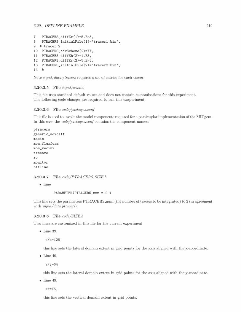
3.20. OFFLINE EXAMPLE 219
7 PTRACERS_diffKr(1)=5.E-5,
8 PTRACERS_initialFile(1)=’tracer1.bin’,
9 # tracer 2
10 PTRACERS_advScheme(2)=77,
11 PTRACERS_diffKh(2)=1.E3,
12 PTRACERS_diffKr(2)=5.E-5,
13 PTRACERS_initialFile(2)=’tracer2.bin’,
14 &
Note input/data.ptracers requires a set of entries for each tracer.
3.20.3.5 File input/eedata
This file uses standard default values and does not contain customisations for this experiment.The following code changes are required to run this exaperiment.
3.20.3.6 File code/packages.conf
This file is used to invoke the model components required for a particuylar implementation of the MITgcm.In this case the code/packages.conf contains the component names:
ptracers
generic_advdiff
mdsio
mom_fluxform
mom_vecinv
timeave
rw
monitor
offline
3.20.3.7 File code/PTRACERS SIZE.h
• Line
PARAMETER(PTRACERS_num = 2 )
This line sets the parameters PTRACERS num (the number of tracers to be integrated) to 2 (in agreementwith input/data.ptracers).
3.20.3.8 File code/SIZE.h
Two lines are customized in this file for the current experiment
• Line 39,
sNx=128,
this line sets the lateral domain extent in grid points for the axis aligned with the x-coordinate.
• Line 40,
sNy=64,
this line sets the lateral domain extent in grid points for the axis aligned with the y-coordinate.
• Line 49,
Nr=15,
this line sets the vertical domain extent in grid points.

220 CHAPTER 3. GETTING STARTED WITH MITGCM
3.20.4 Running The Example
3.20.4.1 Code Download
In order to run the examples you must first download the code distribution. Instructions for downloadingthe code can be found in section 3.2.
3.20.4.2 Experiment Location
This example experiment is located under the release sub-directory
verification/offline/
3.20.4.3 Running the Experiment
To run the experiment
1. Set the current directory to input/
% cd input
2. Verify that current directory is now correct
% pwd
You should see a response on the screen ending in verification/offline/input
3. Copy the contents of input/ including subdirectory input/input off/ to a new directory called run/
4. Listing directory run/ you should see:
data data.pkg depth_g77.bin input_off tracer2.bin
data.off data.ptracers eedata tracer1.bin
5. Set the current directory to run/
6. Run the genmake script to create the experiment Makefile
% ../../../tools/genmake2 -mods=../code
7. Create a list of header file dependencies in Makefile
% make depend
8. Build the executable file.
% make
9. Run the mitgcmuv executable
% ./mitgcmuv
Besides the input files and the files the model generates describing the grid (prefixed Depth, DXC,DXG, hFacC, hFacS and hFacW, you should now have 26 single precision binary files PTRACER01.0000000000-0000000720.001.001.data and PTRACER02.0000000000-0000000720.001.001.data and their 26 correspond-ing meta files as well as a single pickup file, pickup ptracers.0000000720.001.001.data and its correspond-ing meta file pickup ptracers.0000000720.001.001.meta. To run on simply change nIter0 in file run/datato 720...
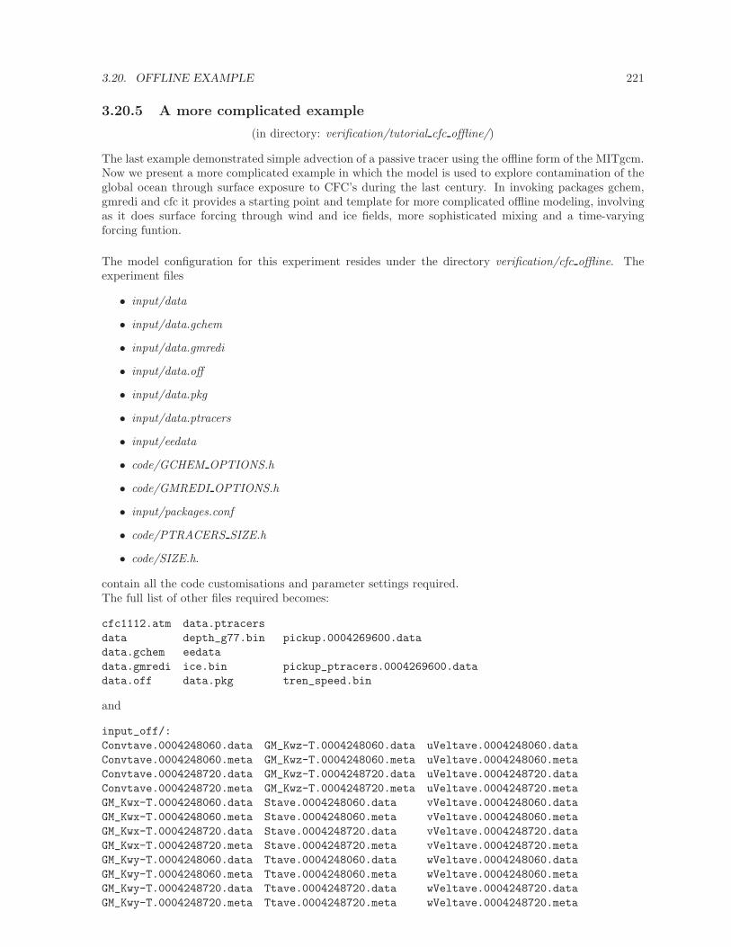
3.20. OFFLINE EXAMPLE 221
3.20.5 A more complicated example
(in directory: verification/tutorial cfc offline/)
The last example demonstrated simple advection of a passive tracer using the offline form of the MITgcm.Now we present a more complicated example in which the model is used to explore contamination of theglobal ocean through surface exposure to CFC’s during the last century. In invoking packages gchem,gmredi and cfc it provides a starting point and template for more complicated offline modeling, involvingas it does surface forcing through wind and ice fields, more sophisticated mixing and a time-varyingforcing funtion.
The model configuration for this experiment resides under the directory verification/cfc offline. Theexperiment files
• input/data
• input/data.gchem
• input/data.gmredi
• input/data.off
• input/data.pkg
• input/data.ptracers
• input/eedata
• code/GCHEM OPTIONS.h
• code/GMREDI OPTIONS.h
• input/packages.conf
• code/PTRACERS SIZE.h
• code/SIZE.h.
contain all the code customisations and parameter settings required.The full list of other files required becomes:
cfc1112.atm data.ptracers
data depth_g77.bin pickup.0004269600.data
data.gchem eedata
data.gmredi ice.bin pickup_ptracers.0004269600.data
data.off data.pkg tren_speed.bin
and
input_off/:
Convtave.0004248060.data GM_Kwz-T.0004248060.data uVeltave.0004248060.data
Convtave.0004248060.meta GM_Kwz-T.0004248060.meta uVeltave.0004248060.meta
Convtave.0004248720.data GM_Kwz-T.0004248720.data uVeltave.0004248720.data
Convtave.0004248720.meta GM_Kwz-T.0004248720.meta uVeltave.0004248720.meta
GM_Kwx-T.0004248060.data Stave.0004248060.data vVeltave.0004248060.data
GM_Kwx-T.0004248060.meta Stave.0004248060.meta vVeltave.0004248060.meta
GM_Kwx-T.0004248720.data Stave.0004248720.data vVeltave.0004248720.data
GM_Kwx-T.0004248720.meta Stave.0004248720.meta vVeltave.0004248720.meta
GM_Kwy-T.0004248060.data Ttave.0004248060.data wVeltave.0004248060.data
GM_Kwy-T.0004248060.meta Ttave.0004248060.meta wVeltave.0004248060.meta
GM_Kwy-T.0004248720.data Ttave.0004248720.data wVeltave.0004248720.data
GM_Kwy-T.0004248720.meta Ttave.0004248720.meta wVeltave.0004248720.meta
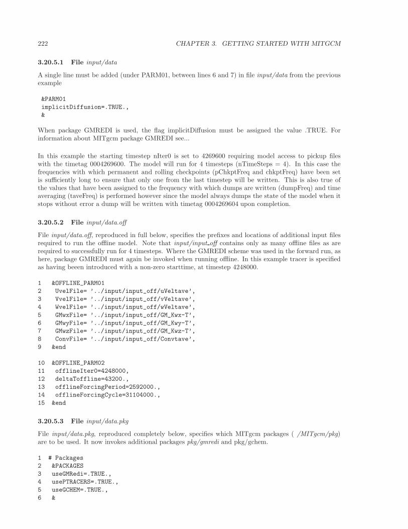
222 CHAPTER 3. GETTING STARTED WITH MITGCM
3.20.5.1 File input/data
A single line must be added (under PARM01, between lines 6 and 7) in file input/data from the previousexample
&PARM01
implicitDiffusion=.TRUE.,
&
When package GMREDI is used, the flag implicitDiffusion must be assigned the value .TRUE. Forinformation about MITgcm package GMREDI see...
In this example the starting timestep nIter0 is set to 4269600 requiring model access to pickup fileswith the timetag 0004269600. The model will run for 4 timesteps (nTimeSteps = 4). In this case thefrequencies with which permanent and rolling checkpoints (pChkptFreq and chkptFreq) have been setis sufficiently long to ensure that only one from the last timestep will be written. This is also true ofthe values that have been assigned to the frequency with which dumps are written (dumpFreq) and timeaveraging (taveFreq) is performed however since the model always dumps the state of the model when itstops without error a dump will be written with timetag 0004269604 upon completion.
3.20.5.2 File input/data.off
File input/data.off, reproduced in full below, specifies the prefixes and locations of additional input filesrequired to run the offline model. Note that input/input off contains only as many offline files as arerequired to successfully run for 4 timesteps. Where the GMREDI scheme was used in the forward run, ashere, package GMREDI must again be invoked when running offline. In this example tracer is specifiedas having beeen introduced with a non-zero starttime, at timestep 4248000.
1 &OFFLINE_PARM01
2 UvelFile= ’../input/input_off/uVeltave’,
3 VvelFile= ’../input/input_off/vVeltave’,
4 WvelFile= ’../input/input_off/wVeltave’,
5 GMwxFile= ’../input/input_off/GM_Kwx-T’,
6 GMwyFile= ’../input/input_off/GM_Kwy-T’,
7 GMwzFile= ’../input/input_off/GM_Kwz-T’,
8 ConvFile= ’../input/input_off/Convtave’,
9 &end
10 &OFFLINE_PARM02
11 offlineIter0=4248000,
12 deltaToffline=43200.,
13 offlineForcingPeriod=2592000.,
14 offlineForcingCycle=31104000.,
15 &end
3.20.5.3 File input/data.pkg
File input/data.pkg, reproduced completely below, specifies which MITgcm packages ( /MITgcm/pkg)are to be used. It now invokes additional packages pkg/gmredi and pkg/gchem.
1 # Packages
2 &PACKAGES
3 useGMRedi=.TRUE.,
4 usePTRACERS=.TRUE.,
5 useGCHEM=.TRUE.,
6 &
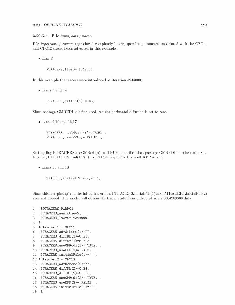
3.20. OFFLINE EXAMPLE 223
3.20.5.4 File input/data.ptracers
File input/data.ptracers, reproduced completely below, specifies parameters associated with the CFC11and CFC12 tracer fields advected in this example.
• Line 3
PTRACERS_Iter0= 4248000,
In this example the tracers were introduced at iteration 4248000.
• Lines 7 and 14
PTRACERS_diffKh(n)=0.E3,
Since package GMREDI is being used, regular horizontal diffusion is set to zero.
• Lines 9,10 and 16,17
PTRACERS_useGMRedi(n)=.TRUE. ,
PTRACERS_useKPP(n)=.FALSE. ,
Setting flag PTRACERS useGMRedi(n) to .TRUE. identifies that package GMREDI is to be used. Set-ting flag PTRACERS useKPP(n) to .FALSE. explicitly turns off KPP mixing.
• Lines 11 and 18
PTRACERS_initialFile(n)=’ ’,
Since this is a ‘pickup’ run the initial tracer files PTRACERS initialFile(1) and PTRACERS initialFile(2)aree not needed. The model will obtain the tracer state from pickup ptracers.0004269600.data
1 &PTRACERS_PARM01
2 PTRACERS_numInUse=2,
3 PTRACERS_Iter0= 4248000,
4 #
5 # tracer 1 - CFC11
6 PTRACERS_advScheme(1)=77,
7 PTRACERS_diffKh(1)=0.E3,
8 PTRACERS_diffKr(1)=5.E-5,
9 PTRACERS_useGMRedi(1)=.TRUE. ,
10 PTRACERS_useKPP(1)=.FALSE. ,
11 PTRACERS_initialFile(1)=’ ’,
12 # tracer 2 - CFC12
13 PTRACERS_advScheme(2)=77,
14 PTRACERS_diffKh(2)=0.E3,
15 PTRACERS_diffKr(2)=5.E-5,
16 PTRACERS_useGMRedi(2)=.TRUE. ,
17 PTRACERS_useKPP(2)=.FALSE. ,
18 PTRACERS_initialFile(2)=’ ’,
19 &
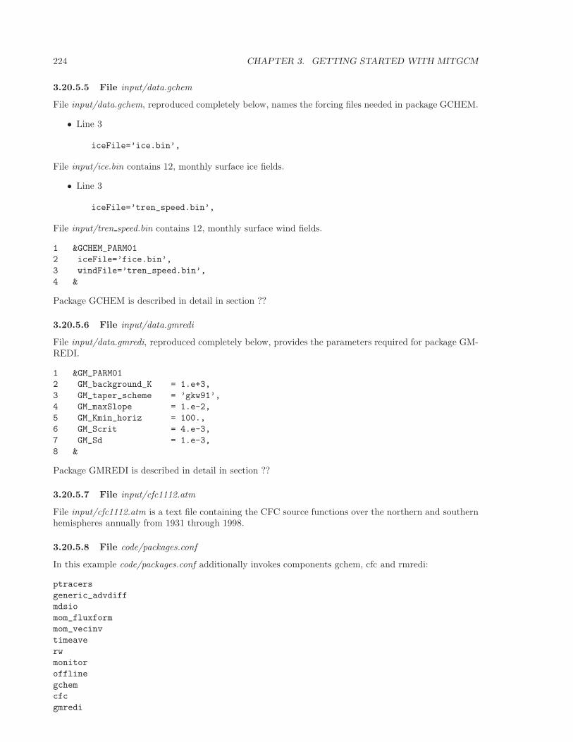
224 CHAPTER 3. GETTING STARTED WITH MITGCM
3.20.5.5 File input/data.gchem
File input/data.gchem, reproduced completely below, names the forcing files needed in package GCHEM.
• Line 3
iceFile=’ice.bin’,
File input/ice.bin contains 12, monthly surface ice fields.
• Line 3
iceFile=’tren_speed.bin’,
File input/tren speed.bin contains 12, monthly surface wind fields.
1 &GCHEM_PARM01
2 iceFile=’fice.bin’,
3 windFile=’tren_speed.bin’,
4 &
Package GCHEM is described in detail in section ??
3.20.5.6 File input/data.gmredi
File input/data.gmredi, reproduced completely below, provides the parameters required for package GM-REDI.
1 &GM_PARM01
2 GM_background_K = 1.e+3,
3 GM_taper_scheme = ’gkw91’,
4 GM_maxSlope = 1.e-2,
5 GM_Kmin_horiz = 100.,
6 GM_Scrit = 4.e-3,
7 GM_Sd = 1.e-3,
8 &
Package GMREDI is described in detail in section ??
3.20.5.7 File input/cfc1112.atm
File input/cfc1112.atm is a text file containing the CFC source functions over the northern and southernhemispheres annually from 1931 through 1998.
3.20.5.8 File code/packages.conf
In this example code/packages.conf additionally invokes components gchem, cfc and rmredi:
ptracers
generic_advdiff
mdsio
mom_fluxform
mom_vecinv
timeave
rw
monitor
offline
gchem
cfc
gmredi
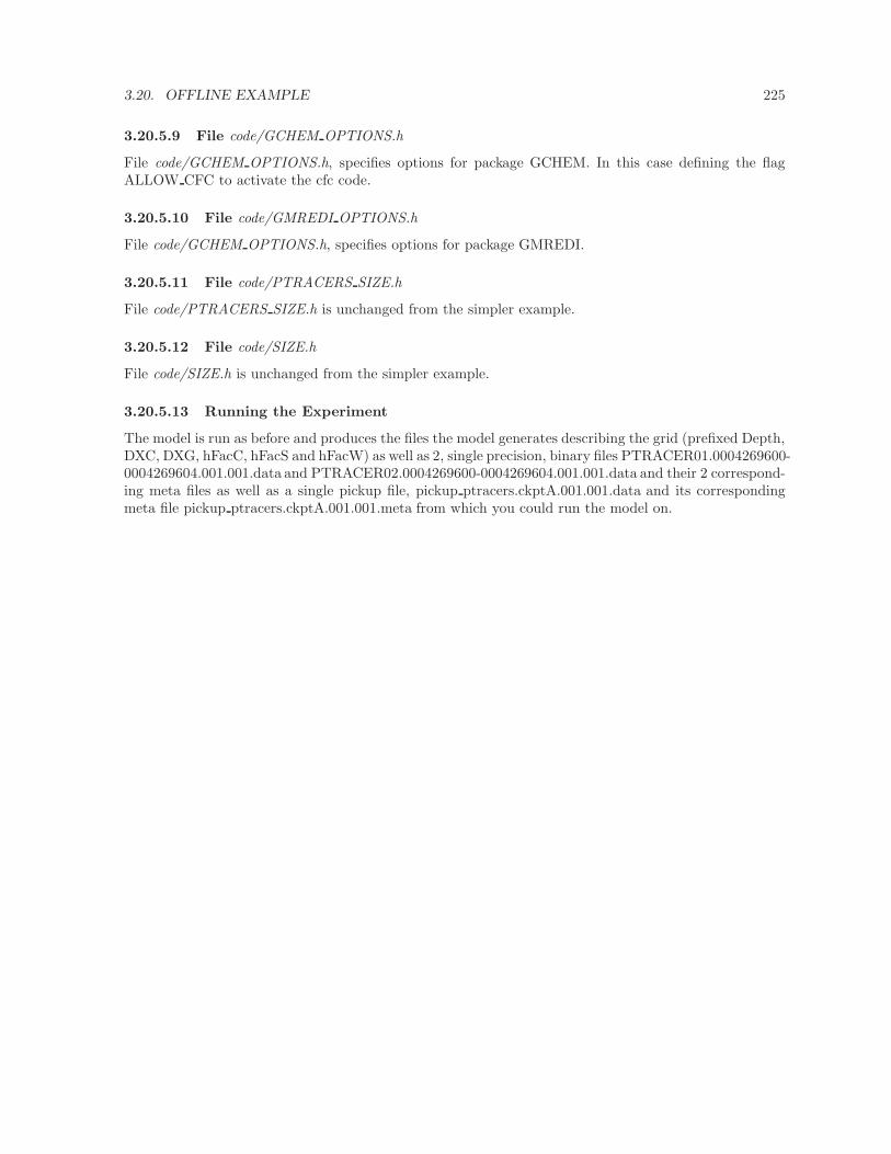
3.20. OFFLINE EXAMPLE 225
3.20.5.9 File code/GCHEM OPTIONS.h
File code/GCHEM OPTIONS.h, specifies options for package GCHEM. In this case defining the flagALLOW CFC to activate the cfc code.
3.20.5.10 File code/GMREDI OPTIONS.h
File code/GCHEM OPTIONS.h, specifies options for package GMREDI.
3.20.5.11 File code/PTRACERS SIZE.h
File code/PTRACERS SIZE.h is unchanged from the simpler example.
3.20.5.12 File code/SIZE.h
File code/SIZE.h is unchanged from the simpler example.
3.20.5.13 Running the Experiment
The model is run as before and produces the files the model generates describing the grid (prefixed Depth,DXC, DXG, hFacC, hFacS and hFacW) as well as 2, single precision, binary files PTRACER01.0004269600-0004269604.001.001.data and PTRACER02.0004269600-0004269604.001.001.data and their 2 correspond-ing meta files as well as a single pickup file, pickup ptracers.ckptA.001.001.data and its correspondingmeta file pickup ptracers.ckptA.001.001.meta from which you could run the model on.
226 CHAPTER 3. GETTING STARTED WITH MITGCM
3.21 A Rotating Tank in Cylindrical Coordinates
(in directory: verification/rotating tank/)
3.21.1 Overview
This example configuration demonstrates using the MITgcm to simulate a laboratory demonstration us-ing a differentially heated rotating annulus of water. The simulation is configured for a laboratory scaleon a 3×1cm cyclindrical grid with twenty-nine vertical levels of 0.5cm each. This is a typical laboratorysetup for illustration principles of GFD, as well as for a laboratory data assimilation project. The filesfor this experiment can be found in the verification directory under rotating tank.
example illustration from GFD lab here
3.21.2 Equations Solved
3.21.3 Discrete Numerical Configuration
The domain is discretised with a uniform cylindrical grid spacing in the horizontal set to ∆a = 1 cm and∆φ = 3, so that there are 120 grid cells in the azimuthal direction and thirty-one grid cells in the radial,representing a tank 62cm in diameter. The bathymetry file sets the depth=0 in the nine lowest radialrows to represent the central of the annulus. Vertically the model is configured with twenty-nine layersof uniform 0.5cm thickness.something about heat flux
3.21.4 Code Configuration
The model configuration for this experiment resides under the directory verification/rotatingi tank/. Theexperiment files
• input/data
• input/data.pkg
• input/eedata,
• input/bathyPol.bin,
• input/thetaPol.bin,
• code/CPP EEOPTIONS.h
• code/CPP OPTIONS.h,
• code/SIZE.h.
contain the code customizations and parameter settings for this experiments. Below we describe thecustomizations to these files associated with this experiment.
3.21.4.1 File input/data
This file, reproduced completely below, specifies the main parameters for the experiment. The parametersthat are significant for this configuration are
• Lines 9-10,
viscAh=5.0E-6,
viscAz=5.0E-6,
3.21. A ROTATING TANK IN CYLINDRICAL COORDINATES 227
These lines set the Laplacian friction coefficient in the horizontal and vertical, respectively. Notethat they are several orders of magnitude smaller than the other examples due to the small scaleof this example.
• Lines 13-16,
diffKhT=2.5E-6,
diffKzT=2.5E-6,
diffKhS=1.0E-6,
diffKzS=1.0E-6,
These lines set horizontal and vertical diffusion coefficients for temperature and salinity. Similarly tothe friction coefficients, the values are a couple of orders of magnitude less than most configurations.
• Line 17,
f0=0.5 ,
this line sets the coriolis term, and represents a tank spinning at about 2.4 rpm.
• Lines 23 and 24
rigidLid=.TRUE.,
implicitFreeSurface=.FALSE.,
These lines activate the rigid lid formulation of the surface pressure inverter and suppress theimplicit free surface form of the pressure inverter.
• Line 40,
nIter=0,
This line indicates that the experiment should start from t = 0 and implicitly suppresses searchingfor checkpoint files associated with restarting an numerical integration from a previously savedstate. Instead, the file thetaPol.bin will be loaded to initialized the temperature fields as indicatedbelow, and other variables will be initialized to their defaults.
• Line 43,
deltaT=0.1,
This line sets the integration timestep to 0.1s. This is an unsually small value among the examplesdue to the small physical scale of the experiment. Using the ensemble Kalman filter to produceinput fields can necessitate even shorter timesteps.
• Line 56,
usingCylindricalGrid=.TRUE.,
This line requests that the simulation be performed in a cylindrical coordinate system.
• Line 57,
dXspacing=3,
This line sets the azimuthal grid spacing between each x-coordinate line in the discrete grid. Thesyntax indicates that the discrete grid should be comprised of 120 grid lines each separated by 3.
• Line 58,
228 CHAPTER 3. GETTING STARTED WITH MITGCM
dYspacing=0.01,
This line sets the radial cylindrical grid spacing between each a-coordinate line in the discrete gridto 1cm.
• Line 59,
delZ=29*0.005,
This line sets the vertical grid spacing between each of 29 z-coordinate lines in the discrete grid to0.005m (5 mm).
• Line 64,
bathyFile=’bathyPol.bin’,
This line specifies the name of the file from which the domain “bathymetry” (tank depth) is read.This file is a two-dimensional (a, φ) map of depths. This file is assumed to contain 64-bit binarynumbers giving the depth of the model at each grid cell, ordered with the φ coordinate varyingfastest. The points are ordered from low coordinate to high coordinate for both axes. The units andorientation of the depths in this file are the same as used in the MITgcm code. In this experiment,a depth of 0m indicates an area outside of the tank and a depth f −0.145m indicates the tank itself.
• Line 65,
hydrogThetaFile=’thetaPol.bin’,
This line specifies the name of the file from which the initial values of temperature are read. Thisfile is a three-dimensional (x, y, z) map and is enumerated and formatted in the same manner asthe bathymetry file.
• Lines 66 and 67
tCylIn = 0
tCylOut = 20
These line specify the temperatures in degrees Celsius of the interior and exterior walls of the tank– typically taken to be icewater on the inside and room temperature on the outside.
Other lines in the file input/data are standard values that are described in the MITgcm Getting Startedand MITgcm Parameters notes.
# ====================
# | Model parameters |
# ====================
#
# Continuous equation parameters
&PARM01
tRef=29*20.0,
sRef=29*35.0,
viscAh=5.0E-6,
viscAz=5.0E-6,
no_slip_sides=.FALSE.,
no_slip_bottom=.FALSE.,
diffKhT=2.5E-6,
diffKzT=2.5E-6,
diffKhS=1.0E-6,
diffKzS=1.0E-6,
f0=0.5,
sBeta =0.,
3.21. A ROTATING TANK IN CYLINDRICAL COORDINATES 229
gravity=9.81,
rhoConst=1000.0,
rhoNil=1000.0,
# heatCapacity_Cp=3900.0,
rigidLid=.TRUE.,
implicitFreeSurface=.FALSE.,
eosType=’LINEAR’,
nonHydrostatic=.TRUE.,
readBinaryPrec=32,
&
# Elliptic solver parameters
&PARM02
cg2dMaxIters=1000,
cg2dTargetResidual=1.E-7,
cg3dMaxIters=10,
cg3dTargetResidual=1.E-9,
&
# Time stepping parameters
&PARM03
nIter0=0,
nTimeSteps=20,
# nTimeSteps=36000000,
deltaT=0.1,
abEps=0.1,
pChkptFreq=1.0,
chkptFreq=1.0,
dumpFreq=1.0,
monitorFreq=0.1,
outputTypesInclusive=.TRUE.,
&
# Gridding parameters
&PARM04
usingCartesianGrid=.FALSE.,
usingCylindricalGrid=.TRUE.,
usingCurvilinearGrid=.FALSE.,
dXspacing=3,
dYspacing=0.01,
delZ=29*0.005,
&
# Input datasets
&PARM05
hydrogThetaFile=’thetaPol.bin’,
bathyFile=’bathyPol.bin’,
tCylIn = 0
tCylOut = 20
&
3.21.4.2 File input/data.pkg
This file uses standard default values and does not contain customizations for this experiment.
3.21.4.3 File input/eedata
This file uses standard default values and does not contain customizations for this experiment.
230 CHAPTER 3. GETTING STARTED WITH MITGCM
3.21.4.4 File input/thetaPol.bin
The input/thetaPol.bin file specifies a three-dimensional (x, y, z) map of initial values of θ in degreesCelsius. This particular experiment is set to random values x around 20C to provide initial perturbations.
3.21.4.5 File input/bathyPol.bin
The input/bathyPol.bin file specifies a two-dimensional (x, y) map of depth values. For this experimentvalues are either 0m or -delZm, corresponding respectively to outside or inside of the tank. The filecontains a raw binary stream of data that is enumerated in the same way as standard MITgcm two-dimensional, horizontal arrays.
3.21.4.6 File code/SIZE.h
Two lines are customized in this file for the current experiment
• Line 39,
sNx=120,
this line sets the lateral domain extent in grid points for the axis aligned with the x-coordinate.
• Line 40,
sNy=31,
this line sets the lateral domain extent in grid points for the axis aligned with the y-coordinate.
C $Header: /u/gcmpack/manual/s_examples/rotating_tank/code/SIZE.h,v 1.1 2004/07/26 21:09:47 afe Exp $
C $Name: $
C
C /==========================================================\
C | SIZE.h Declare size of underlying computational grid. |
C |==========================================================|
C | The design here support a three-dimensional model grid |
C | with indices I,J and K. The three-dimensional domain |
C | is comprised of nPx*nSx blocks of size sNx along one axis|
C | nPy*nSy blocks of size sNy along another axis and one |
C | block of size Nz along the final axis. |
C | Blocks have overlap regions of size OLx and OLy along the|
C | dimensions that are subdivided. |
C \==========================================================/
C Voodoo numbers controlling data layout.
C sNx - No. X points in sub-grid.
C sNy - No. Y points in sub-grid.
C OLx - Overlap extent in X.
C OLy - Overlat extent in Y.
C nSx - No. sub-grids in X.
C nSy - No. sub-grids in Y.
C nPx - No. of processes to use in X.
C nPy - No. of processes to use in Y.
C Nx - No. points in X for the total domain.
C Ny - No. points in Y for the total domain.
C Nr - No. points in Z for full process domain.
INTEGER sNx
INTEGER sNy
INTEGER OLx
INTEGER OLy
INTEGER nSx
INTEGER nSy
INTEGER nPx
3.21. A ROTATING TANK IN CYLINDRICAL COORDINATES 231
INTEGER nPy
INTEGER Nx
INTEGER Ny
INTEGER Nr
PARAMETER (
& sNx = 120,
& sNy = 31,
& OLx = 3,
& OLy = 3,
& nSx = 1,
& nSy = 1,
& nPx = 1,
& nPy = 1,
& Nx = sNx*nSx*nPx,
& Ny = sNy*nSy*nPy,
& Nr = 29)
C MAX_OLX - Set to the maximum overlap region size of any array
C MAX_OLY that will be exchanged. Controls the sizing of exch
C routine buufers.
INTEGER MAX_OLX
INTEGER MAX_OLY
PARAMETER ( MAX_OLX = OLx,
& MAX_OLY = OLy )
3.21.4.7 File code/CPP OPTIONS.h
This file uses standard default values and does not contain customizations for this experiment.
3.21.4.8 File code/CPP EEOPTIONS.h
This file uses standard default values and does not contain customizations for this experiment.

232 CHAPTER 3. GETTING STARTED WITH MITGCM
Chapter 4
Software Architecture
This chapter focuses on describing the WRAPPER environment within which both the core numericsand the pluggable packages operate. The description presented here is intended to be a detailed expositionand contains significant background material, as well as advanced details on working with the WRAPPER.The tutorial sections of this manual (see sections 3.8 and 3.19) contain more succinct, step-by-stepinstructions on running basic numerical experiments, of varous types, both sequentially and in parallel.For many projects simply starting from an example code and adapting it to suit a particular situation willbe all that is required. The first part of this chapter discusses the MITgcm architecture at an abstractlevel. In the second part of the chapter we described practical details of the MITgcm implementationand of current tools and operating system features that are employed.
4.1 Overall architectural goals
Broadly, the goals of the software architecture employed in MITgcm are three-fold
• We wish to be able to study a very broad range of interesting and challenging rotating fluidsproblems.
• We wish the model code to be readily targeted to a wide range of platforms
• On any given platform we would like to be able to achieve performance comparable to an imple-mentation developed and specialized specifically for that platform.
These points are summarized in figure 4.1 which conveys the goals of the MITgcm design. The goalslead to a software architecture which at the high-level can be viewed as consisting of
1. A core set of numerical and support code. This is discussed in detail in section 2.
2. A scheme for supporting optional “pluggable” packages (containing for example mixed-layer schemes,biogeochemical schemes, atmospheric physics). These packages are used both to overlay alternatedynamics and to introduce specialized physical content onto the core numerical code. An overviewof the package scheme is given at the start of part 6.
3. A support framework called WRAPPER (Wrappable Application Parallel Programming Environ-ment Resource), within which the core numerics and pluggable packages operate.
This chapter focuses on describing the WRAPPER environment under which both the core numer-ics and the pluggable packages function. The description presented here is intended to be a detailedexposition and contains significant background material, as well as advanced details on working with theWRAPPER. The examples section of this manual (part 3) contains more succinct, step-by-step instruc-tions on running basic numerical experiments both sequentially and in parallel. For many projects simplystarting from an example code and adapting it to suit a particular situation will be all that is required.
233
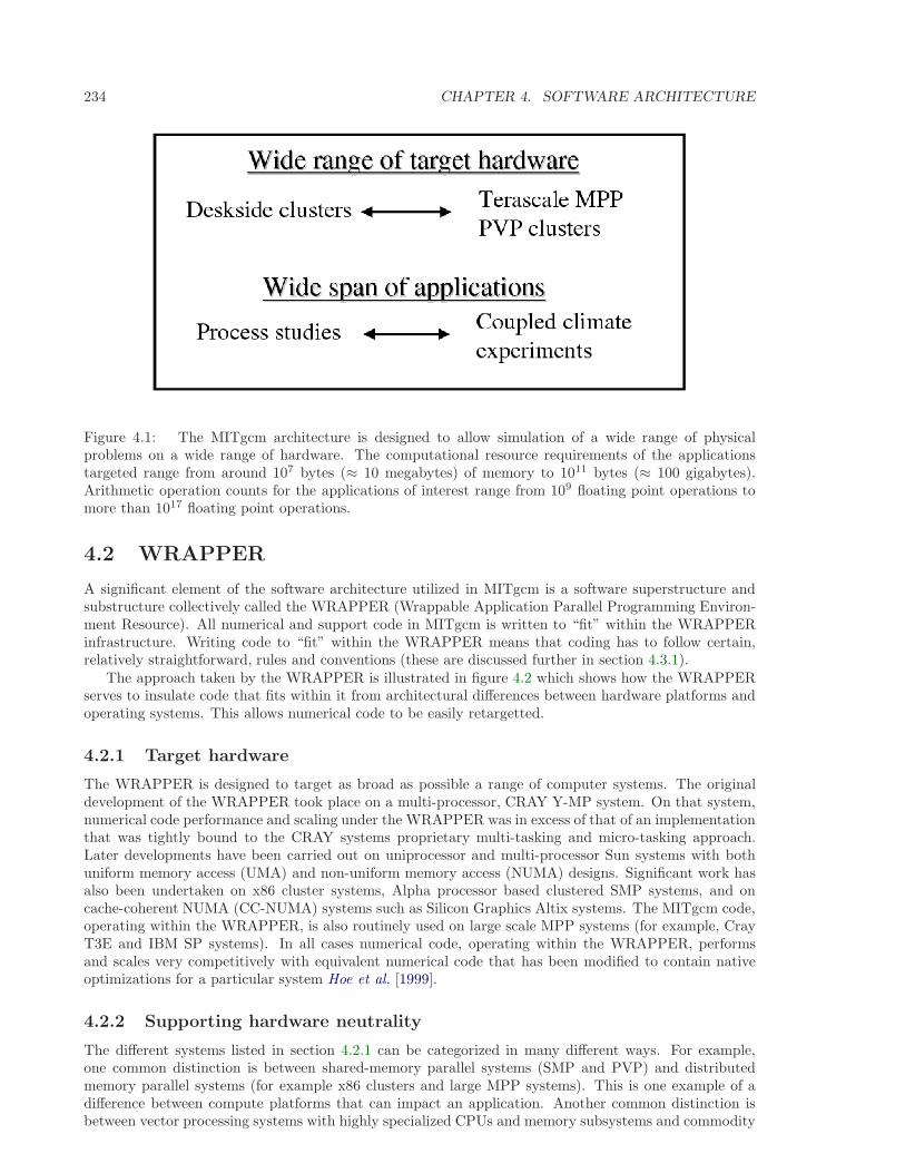
234 CHAPTER 4. SOFTWARE ARCHITECTURE
Figure 4.1: The MITgcm architecture is designed to allow simulation of a wide range of physicalproblems on a wide range of hardware. The computational resource requirements of the applicationstargeted range from around 107 bytes (≈ 10 megabytes) of memory to 1011 bytes (≈ 100 gigabytes).Arithmetic operation counts for the applications of interest range from 109 floating point operations tomore than 1017 floating point operations.
4.2 WRAPPER
A significant element of the software architecture utilized in MITgcm is a software superstructure andsubstructure collectively called the WRAPPER (Wrappable Application Parallel Programming Environ-ment Resource). All numerical and support code in MITgcm is written to “fit” within the WRAPPERinfrastructure. Writing code to “fit” within the WRAPPER means that coding has to follow certain,relatively straightforward, rules and conventions (these are discussed further in section 4.3.1).
The approach taken by the WRAPPER is illustrated in figure 4.2 which shows how the WRAPPERserves to insulate code that fits within it from architectural differences between hardware platforms andoperating systems. This allows numerical code to be easily retargetted.
4.2.1 Target hardware
The WRAPPER is designed to target as broad as possible a range of computer systems. The originaldevelopment of the WRAPPER took place on a multi-processor, CRAY Y-MP system. On that system,numerical code performance and scaling under the WRAPPER was in excess of that of an implementationthat was tightly bound to the CRAY systems proprietary multi-tasking and micro-tasking approach.Later developments have been carried out on uniprocessor and multi-processor Sun systems with bothuniform memory access (UMA) and non-uniform memory access (NUMA) designs. Significant work hasalso been undertaken on x86 cluster systems, Alpha processor based clustered SMP systems, and oncache-coherent NUMA (CC-NUMA) systems such as Silicon Graphics Altix systems. The MITgcm code,operating within the WRAPPER, is also routinely used on large scale MPP systems (for example, CrayT3E and IBM SP systems). In all cases numerical code, operating within the WRAPPER, performsand scales very competitively with equivalent numerical code that has been modified to contain nativeoptimizations for a particular system Hoe et al. [1999].
4.2.2 Supporting hardware neutrality
The different systems listed in section 4.2.1 can be categorized in many different ways. For example,one common distinction is between shared-memory parallel systems (SMP and PVP) and distributedmemory parallel systems (for example x86 clusters and large MPP systems). This is one example of adifference between compute platforms that can impact an application. Another common distinction isbetween vector processing systems with highly specialized CPUs and memory subsystems and commodity
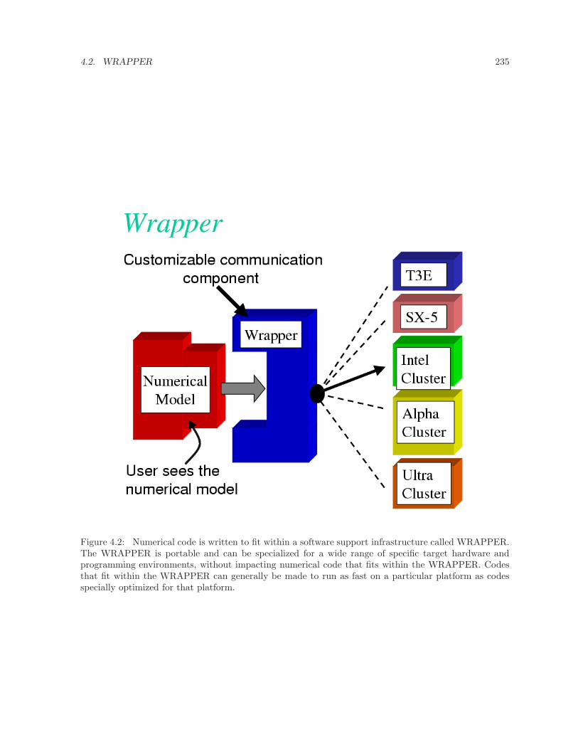
4.2. WRAPPER 235
Figure 4.2: Numerical code is written to fit within a software support infrastructure called WRAPPER.The WRAPPER is portable and can be specialized for a wide range of specific target hardware andprogramming environments, without impacting numerical code that fits within the WRAPPER. Codesthat fit within the WRAPPER can generally be made to run as fast on a particular platform as codesspecially optimized for that platform.
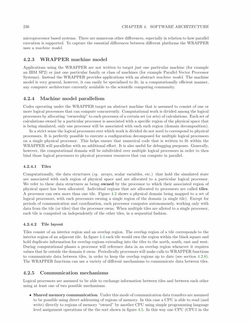
236 CHAPTER 4. SOFTWARE ARCHITECTURE
microprocessor based systems. There are numerous other differences, especially in relation to how parallelexecution is supported. To capture the essential differences between different platforms the WRAPPERuses a machine model.
4.2.3 WRAPPER machine model
Applications using the WRAPPER are not written to target just one particular machine (for examplean IBM SP2) or just one particular family or class of machines (for example Parallel Vector ProcessorSystems). Instead the WRAPPER provides applications with an abstract machine model. The machinemodel is very general, however, it can easily be specialized to fit, in a computationally efficient manner,any computer architecture currently available to the scientific computing community.
4.2.4 Machine model parallelism
Codes operating under the WRAPPER target an abstract machine that is assumed to consist of one ormore logical processors that can compute concurrently. Computational work is divided among the logicalprocessors by allocating “ownership” to each processor of a certain set (or sets) of calculations. Each set ofcalculations owned by a particular processor is associated with a specific region of the physical space thatis being simulated, only one processor will be associated with each such region (domain decomposition).
In a strict sense the logical processors over which work is divided do not need to correspond to physicalprocessors. It is perfectly possible to execute a configuration decomposed for multiple logical processorson a single physical processor. This helps ensure that numerical code that is written to fit within theWRAPPER will parallelize with no additional effort. It is also useful for debugging purposes. Generally,however, the computational domain will be subdivided over multiple logical processors in order to thenbind those logical processors to physical processor resources that can compute in parallel.
4.2.4.1 Tiles
Computationally, the data structures (eg. arrays, scalar variables, etc.) that hold the simulated stateare associated with each region of physical space and are allocated to a particular logical processor.We refer to these data structures as being owned by the processor to which their associated region ofphysical space has been allocated. Individual regions that are allocated to processors are called tiles.A processor can own more than one tile. Figure 4.3 shows a physical domain being mapped to a set oflogical processors, with each processors owning a single region of the domain (a single tile). Except forperiods of communication and coordination, each processor computes autonomously, working only withdata from the tile (or tiles) that the processor owns. When multiple tiles are alloted to a single processor,each tile is computed on independently of the other tiles, in a sequential fashion.
4.2.4.2 Tile layout
Tiles consist of an interior region and an overlap region. The overlap region of a tile corresponds to theinterior region of an adjacent tile. In figure 4.4 each tile would own the region within the black square andhold duplicate information for overlap regions extending into the tiles to the north, south, east and west.During computational phases a processor will reference data in an overlap region whenever it requiresvalues that lie outside the domain it owns. Periodically processors will make calls to WRAPPER functionsto communicate data between tiles, in order to keep the overlap regions up to date (see section 4.2.8).The WRAPPER functions can use a variety of different mechanisms to communicate data between tiles.
4.2.5 Communication mechanisms
Logical processors are assumed to be able to exchange information between tiles and between each otherusing at least one of two possible mechanisms.
• Shared memory communication. Under this mode of communication data transfers are assumedto be possible using direct addressing of regions of memory. In this case a CPU is able to read (andwrite) directly to regions of memory “owned” by another CPU using simple programming languagelevel assignment operations of the the sort shown in figure 4.5. In this way one CPU (CPU1 in the
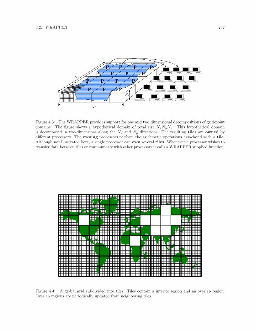
4.2. WRAPPER 237
Figure 4.3: The WRAPPER provides support for one and two dimensional decompositions of grid-pointdomains. The figure shows a hypothetical domain of total size NxNyNz. This hypothetical domainis decomposed in two-dimensions along the Nx and Ny directions. The resulting tiles are owned bydifferent processors. The owning processors perform the arithmetic operations associated with a tile.Although not illustrated here, a single processor can own several tiles. Whenever a processor wishes totransfer data between tiles or communicate with other processors it calls a WRAPPER supplied function.
Figure 4.4: A global grid subdivided into tiles. Tiles contain a interior region and an overlap region.Overlap regions are periodically updated from neighboring tiles.
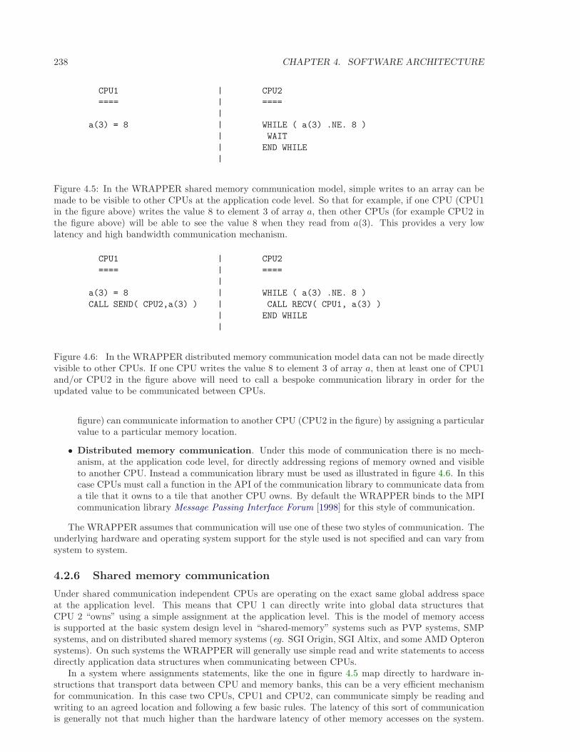
238 CHAPTER 4. SOFTWARE ARCHITECTURE
CPU1 | CPU2
==== | ====
|
a(3) = 8 | WHILE ( a(3) .NE. 8 )
| WAIT
| END WHILE
|
Figure 4.5: In the WRAPPER shared memory communication model, simple writes to an array can bemade to be visible to other CPUs at the application code level. So that for example, if one CPU (CPU1in the figure above) writes the value 8 to element 3 of array a, then other CPUs (for example CPU2 inthe figure above) will be able to see the value 8 when they read from a(3). This provides a very lowlatency and high bandwidth communication mechanism.
CPU1 | CPU2
==== | ====
|
a(3) = 8 | WHILE ( a(3) .NE. 8 )
CALL SEND( CPU2,a(3) ) | CALL RECV( CPU1, a(3) )
| END WHILE
|
Figure 4.6: In the WRAPPER distributed memory communication model data can not be made directlyvisible to other CPUs. If one CPU writes the value 8 to element 3 of array a, then at least one of CPU1and/or CPU2 in the figure above will need to call a bespoke communication library in order for theupdated value to be communicated between CPUs.
figure) can communicate information to another CPU (CPU2 in the figure) by assigning a particularvalue to a particular memory location.
• Distributed memory communication. Under this mode of communication there is no mech-anism, at the application code level, for directly addressing regions of memory owned and visibleto another CPU. Instead a communication library must be used as illustrated in figure 4.6. In thiscase CPUs must call a function in the API of the communication library to communicate data froma tile that it owns to a tile that another CPU owns. By default the WRAPPER binds to the MPIcommunication library Message Passing Interface Forum [1998] for this style of communication.
The WRAPPER assumes that communication will use one of these two styles of communication. Theunderlying hardware and operating system support for the style used is not specified and can vary fromsystem to system.
4.2.6 Shared memory communication
Under shared communication independent CPUs are operating on the exact same global address spaceat the application level. This means that CPU 1 can directly write into global data structures thatCPU 2 “owns” using a simple assignment at the application level. This is the model of memory accessis supported at the basic system design level in “shared-memory” systems such as PVP systems, SMPsystems, and on distributed shared memory systems (eg. SGI Origin, SGI Altix, and some AMD Opteronsystems). On such systems the WRAPPER will generally use simple read and write statements to accessdirectly application data structures when communicating between CPUs.
In a system where assignments statements, like the one in figure 4.5 map directly to hardware in-structions that transport data between CPU and memory banks, this can be a very efficient mechanismfor communication. In this case two CPUs, CPU1 and CPU2, can communicate simply be reading andwriting to an agreed location and following a few basic rules. The latency of this sort of communicationis generally not that much higher than the hardware latency of other memory accesses on the system.
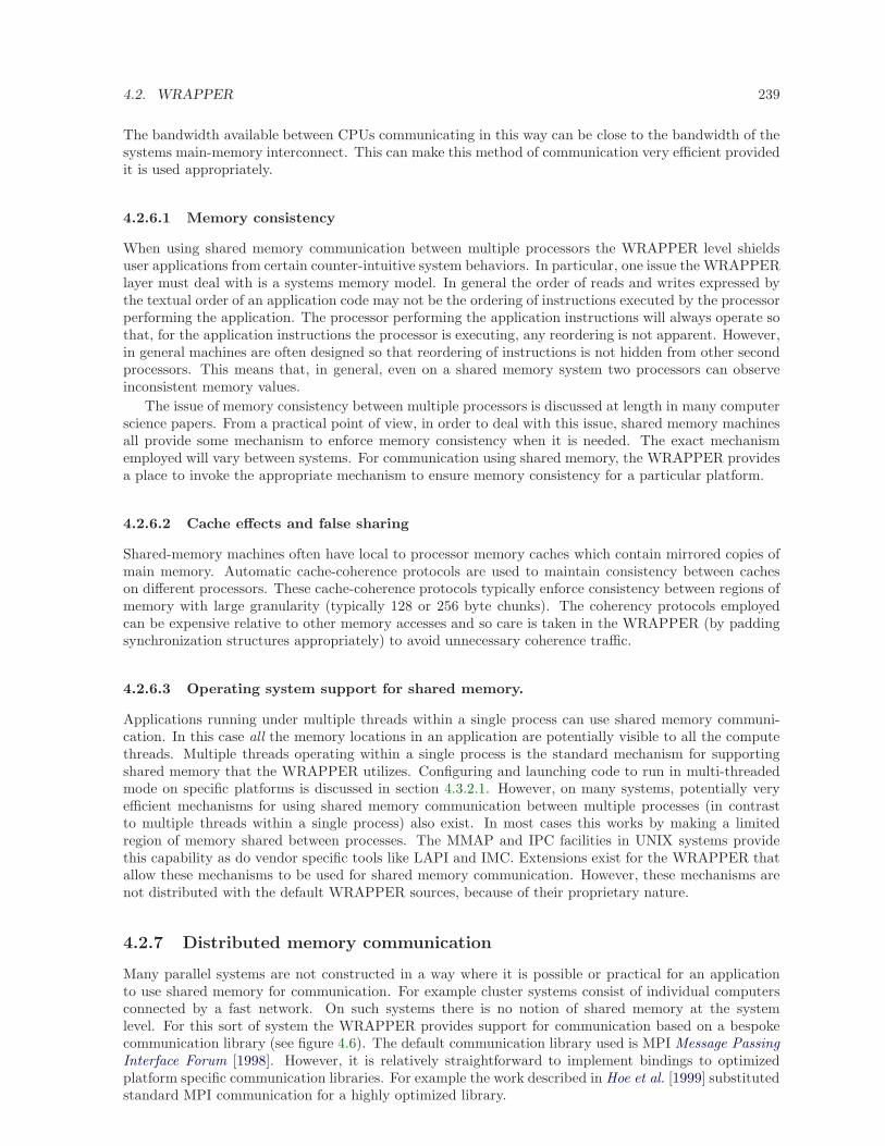
4.2. WRAPPER 239
The bandwidth available between CPUs communicating in this way can be close to the bandwidth of thesystems main-memory interconnect. This can make this method of communication very efficient providedit is used appropriately.
4.2.6.1 Memory consistency
When using shared memory communication between multiple processors the WRAPPER level shieldsuser applications from certain counter-intuitive system behaviors. In particular, one issue the WRAPPERlayer must deal with is a systems memory model. In general the order of reads and writes expressed bythe textual order of an application code may not be the ordering of instructions executed by the processorperforming the application. The processor performing the application instructions will always operate sothat, for the application instructions the processor is executing, any reordering is not apparent. However,in general machines are often designed so that reordering of instructions is not hidden from other secondprocessors. This means that, in general, even on a shared memory system two processors can observeinconsistent memory values.
The issue of memory consistency between multiple processors is discussed at length in many computerscience papers. From a practical point of view, in order to deal with this issue, shared memory machinesall provide some mechanism to enforce memory consistency when it is needed. The exact mechanismemployed will vary between systems. For communication using shared memory, the WRAPPER providesa place to invoke the appropriate mechanism to ensure memory consistency for a particular platform.
4.2.6.2 Cache effects and false sharing
Shared-memory machines often have local to processor memory caches which contain mirrored copies ofmain memory. Automatic cache-coherence protocols are used to maintain consistency between cacheson different processors. These cache-coherence protocols typically enforce consistency between regions ofmemory with large granularity (typically 128 or 256 byte chunks). The coherency protocols employedcan be expensive relative to other memory accesses and so care is taken in the WRAPPER (by paddingsynchronization structures appropriately) to avoid unnecessary coherence traffic.
4.2.6.3 Operating system support for shared memory.
Applications running under multiple threads within a single process can use shared memory communi-cation. In this case all the memory locations in an application are potentially visible to all the computethreads. Multiple threads operating within a single process is the standard mechanism for supportingshared memory that the WRAPPER utilizes. Configuring and launching code to run in multi-threadedmode on specific platforms is discussed in section 4.3.2.1. However, on many systems, potentially veryefficient mechanisms for using shared memory communication between multiple processes (in contrastto multiple threads within a single process) also exist. In most cases this works by making a limitedregion of memory shared between processes. The MMAP and IPC facilities in UNIX systems providethis capability as do vendor specific tools like LAPI and IMC. Extensions exist for the WRAPPER thatallow these mechanisms to be used for shared memory communication. However, these mechanisms arenot distributed with the default WRAPPER sources, because of their proprietary nature.
4.2.7 Distributed memory communication
Many parallel systems are not constructed in a way where it is possible or practical for an applicationto use shared memory for communication. For example cluster systems consist of individual computersconnected by a fast network. On such systems there is no notion of shared memory at the systemlevel. For this sort of system the WRAPPER provides support for communication based on a bespokecommunication library (see figure 4.6). The default communication library used is MPI Message PassingInterface Forum [1998]. However, it is relatively straightforward to implement bindings to optimizedplatform specific communication libraries. For example the work described in Hoe et al. [1999] substitutedstandard MPI communication for a highly optimized library.
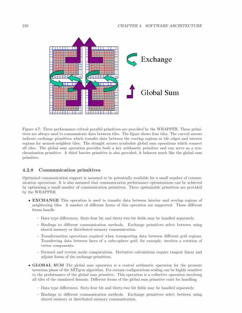
240 CHAPTER 4. SOFTWARE ARCHITECTURE
Figure 4.7: Three performance critical parallel primitives are provided by the WRAPPER. These primi-tives are always used to communicate data between tiles. The figure shows four tiles. The curved arrowsindicate exchange primitives which transfer data between the overlap regions at tile edges and interiorregions for nearest-neighbor tiles. The straight arrows symbolize global sum operations which connectall tiles. The global sum operation provides both a key arithmetic primitive and can serve as a syn-chronization primitive. A third barrier primitive is also provided, it behaves much like the global sumprimitive.
4.2.8 Communication primitives
Optimized communication support is assumed to be potentially available for a small number of commu-nication operations. It is also assumed that communication performance optimizations can be achievedby optimizing a small number of communication primitives. Three optimizable primitives are providedby the WRAPPER
• EXCHANGE This operation is used to transfer data between interior and overlap regions ofneighboring tiles. A number of different forms of this operation are supported. These differentforms handle
– Data type differences. Sixty-four bit and thirty-two bit fields may be handled separately.
– Bindings to different communication methods. Exchange primitives select between usingshared memory or distributed memory communication.
– Transformation operations required when transporting data between different grid regions.Transferring data between faces of a cube-sphere grid, for example, involves a rotation ofvector components.
– Forward and reverse mode computations. Derivative calculations require tangent linear andadjoint forms of the exchange primitives.
• GLOBAL SUM The global sum operation is a central arithmetic operation for the pressureinversion phase of the MITgcm algorithm. For certain configurations scaling can be highly sensitiveto the performance of the global sum primitive. This operation is a collective operation involvingall tiles of the simulated domain. Different forms of the global sum primitive exist for handling
– Data type differences. Sixty-four bit and thirty-two bit fields may be handled separately.
– Bindings to different communication methods. Exchange primitives select between usingshared memory or distributed memory communication.
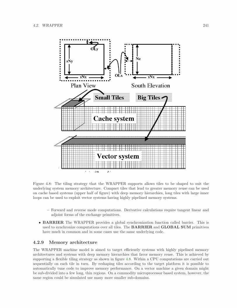
4.2. WRAPPER 241
Figure 4.8: The tiling strategy that the WRAPPER supports allows tiles to be shaped to suit theunderlying system memory architecture. Compact tiles that lead to greater memory reuse can be usedon cache based systems (upper half of figure) with deep memory hierarchies, long tiles with large innerloops can be used to exploit vector systems having highly pipelined memory systems.
– Forward and reverse mode computations. Derivative calculations require tangent linear andadjoint forms of the exchange primitives.
• BARRIER The WRAPPER provides a global synchronization function called barrier. This isused to synchronize computations over all tiles. The BARRIER and GLOBAL SUM primitiveshave much in common and in some cases use the same underlying code.
4.2.9 Memory architecture
The WRAPPER machine model is aimed to target efficiently systems with highly pipelined memoryarchitectures and systems with deep memory hierarchies that favor memory reuse. This is achieved bysupporting a flexible tiling strategy as shown in figure 4.8. Within a CPU computations are carried outsequentially on each tile in turn. By reshaping tiles according to the target platform it is possible toautomatically tune code to improve memory performance. On a vector machine a given domain mightbe sub-divided into a few long, thin regions. On a commodity microprocessor based system, however, thesame region could be simulated use many more smaller sub-domains.
242 CHAPTER 4. SOFTWARE ARCHITECTURE
4.2.10 Summary
Following the discussion above, the machine model that the WRAPPER presents to an application hasthe following characteristics
• The machine consists of one or more logical processors.
• Each processor operates on tiles that it owns.
• A processor may own more than one tile.
• Processors may compute concurrently.
• Exchange of information between tiles is handled by the machine (WRAPPER) not by the appli-cation.
Behind the scenes this allows the WRAPPER to adapt the machine model functions to exploit hardwareon which
• Processors may be able to communicate very efficiently with each other using shared memory.
• An alternative communication mechanism based on a relatively simple inter-process communicationAPI may be required.
• Shared memory may not necessarily obey sequential consistency, however some mechanism willexist for enforcing memory consistency.
• Memory consistency that is enforced at the hardware level may be expensive. Unnecessary triggeringof consistency protocols should be avoided.
• Memory access patterns may need to either repetitive or highly pipelined for optimum hardwareperformance.
This generic model captures the essential hardware ingredients of almost all successful scientific com-puter systems designed in the last 50 years.
4.3 Using the WRAPPER
In order to support maximum portability the WRAPPER is implemented primarily in sequential Fortran77. At a practical level the key steps provided by the WRAPPER are
1. specifying how a domain will be decomposed
2. starting a code in either sequential or parallel modes of operations
3. controlling communication between tiles and between concurrently computing CPUs.
This section describes the details of each of these operations. Section 4.3.1 explains how the way in whicha domain is decomposed (or composed) is expressed. Section 4.3.2 describes practical details of runningcodes in various different parallel modes on contemporary computer systems. Section 4.3.3 explains theinternal information that the WRAPPER uses to control how information is communicated between tiles.
4.3.1 Specifying a domain decomposition
At its heart much of the WRAPPER works only in terms of a collection of tiles which are interconnectedto each other. This is also true of application code operating within the WRAPPER. Application codeis written as a series of compute operations, each of which operates on a single tile. If application codeneeds to perform operations involving data associated with another tile, it uses a WRAPPER function toobtain that data. The specification of how a global domain is constructed from tiles or alternatively how aglobal domain is decomposed into tiles is made in the file SIZE.h. This file defines the following parameters
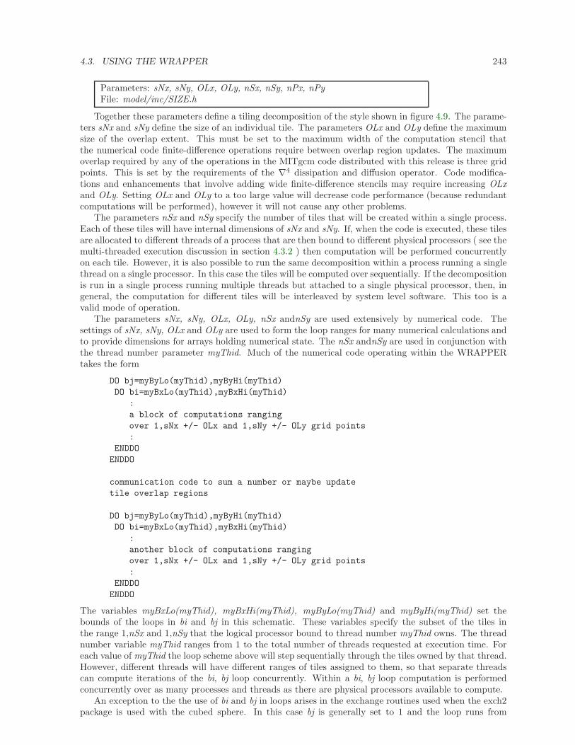
4.3. USING THE WRAPPER 243
Parameters: sNx, sNy, OLx, OLy, nSx, nSy, nPx, nPyFile: model/inc/SIZE.h
Together these parameters define a tiling decomposition of the style shown in figure 4.9. The parame-ters sNx and sNy define the size of an individual tile. The parameters OLx and OLy define the maximumsize of the overlap extent. This must be set to the maximum width of the computation stencil thatthe numerical code finite-difference operations require between overlap region updates. The maximumoverlap required by any of the operations in the MITgcm code distributed with this release is three gridpoints. This is set by the requirements of the ∇4 dissipation and diffusion operator. Code modifica-tions and enhancements that involve adding wide finite-difference stencils may require increasing OLxand OLy. Setting OLx and OLy to a too large value will decrease code performance (because redundantcomputations will be performed), however it will not cause any other problems.
The parameters nSx and nSy specify the number of tiles that will be created within a single process.Each of these tiles will have internal dimensions of sNx and sNy. If, when the code is executed, these tilesare allocated to different threads of a process that are then bound to different physical processors ( see themulti-threaded execution discussion in section 4.3.2 ) then computation will be performed concurrentlyon each tile. However, it is also possible to run the same decomposition within a process running a singlethread on a single processor. In this case the tiles will be computed over sequentially. If the decompositionis run in a single process running multiple threads but attached to a single physical processor, then, ingeneral, the computation for different tiles will be interleaved by system level software. This too is avalid mode of operation.
The parameters sNx, sNy, OLx, OLy, nSx andnSy are used extensively by numerical code. Thesettings of sNx, sNy, OLx and OLy are used to form the loop ranges for many numerical calculations andto provide dimensions for arrays holding numerical state. The nSx andnSy are used in conjunction withthe thread number parameter myThid. Much of the numerical code operating within the WRAPPERtakes the form
DO bj=myByLo(myThid),myByHi(myThid)
DO bi=myBxLo(myThid),myBxHi(myThid)
:
a block of computations ranging
over 1,sNx +/- OLx and 1,sNy +/- OLy grid points
:
ENDDO
ENDDO
communication code to sum a number or maybe update
tile overlap regions
DO bj=myByLo(myThid),myByHi(myThid)
DO bi=myBxLo(myThid),myBxHi(myThid)
:
another block of computations ranging
over 1,sNx +/- OLx and 1,sNy +/- OLy grid points
:
ENDDO
ENDDO
The variables myBxLo(myThid), myBxHi(myThid), myByLo(myThid) and myByHi(myThid) set thebounds of the loops in bi and bj in this schematic. These variables specify the subset of the tiles inthe range 1,nSx and 1,nSy that the logical processor bound to thread number myThid owns. The threadnumber variable myThid ranges from 1 to the total number of threads requested at execution time. Foreach value of myThid the loop scheme above will step sequentially through the tiles owned by that thread.However, different threads will have different ranges of tiles assigned to them, so that separate threadscan compute iterations of the bi, bj loop concurrently. Within a bi, bj loop computation is performedconcurrently over as many processes and threads as there are physical processors available to compute.
An exception to the the use of bi and bj in loops arises in the exchange routines used when the exch2package is used with the cubed sphere. In this case bj is generally set to 1 and the loop runs from
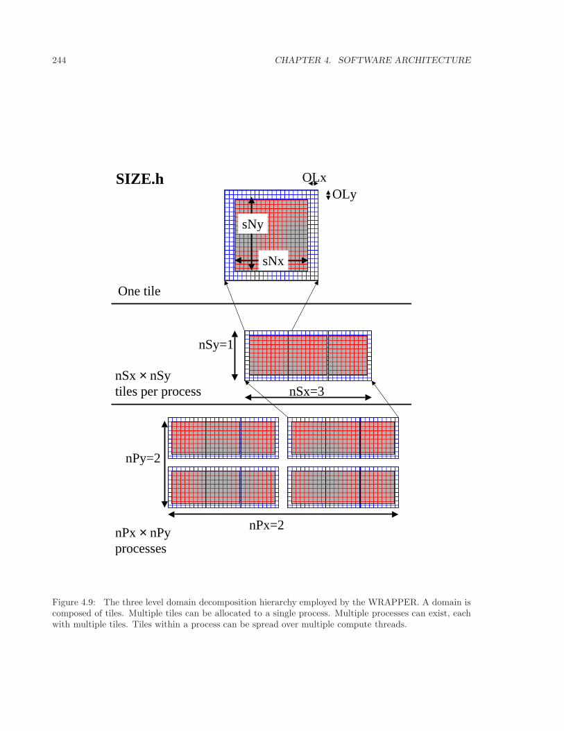
244 CHAPTER 4. SOFTWARE ARCHITECTURE
One tile
nSx × nSytiles per process
nPx × nPyprocesses
nPy=2
nPx=2
nSy=1
nSx=3
sNx
sNy
OLxOLy
SIZE.h
Figure 4.9: The three level domain decomposition hierarchy employed by the WRAPPER. A domain iscomposed of tiles. Multiple tiles can be allocated to a single process. Multiple processes can exist, eachwith multiple tiles. Tiles within a process can be spread over multiple compute threads.
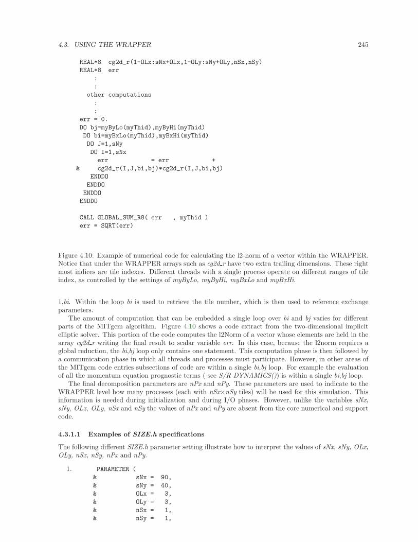
4.3. USING THE WRAPPER 245
REAL*8 cg2d_r(1-OLx:sNx+OLx,1-OLy:sNy+OLy,nSx,nSy)
REAL*8 err
:
:
other computations
:
:
err = 0.
DO bj=myByLo(myThid),myByHi(myThid)
DO bi=myBxLo(myThid),myBxHi(myThid)
DO J=1,sNy
DO I=1,sNx
err = err +
& cg2d_r(I,J,bi,bj)*cg2d_r(I,J,bi,bj)
ENDDO
ENDDO
ENDDO
ENDDO
CALL GLOBAL_SUM_R8( err , myThid )
err = SQRT(err)
Figure 4.10: Example of numerical code for calculating the l2-norm of a vector within the WRAPPER.Notice that under the WRAPPER arrays such as cg2d r have two extra trailing dimensions. These rightmost indices are tile indexes. Different threads with a single process operate on different ranges of tileindex, as controlled by the settings of myByLo, myByHi, myBxLo and myBxHi.
1,bi. Within the loop bi is used to retrieve the tile number, which is then used to reference exchangeparameters.
The amount of computation that can be embedded a single loop over bi and bj varies for differentparts of the MITgcm algorithm. Figure 4.10 shows a code extract from the two-dimensional implicitelliptic solver. This portion of the code computes the l2Norm of a vector whose elements are held in thearray cg2d r writing the final result to scalar variable err. In this case, because the l2norm requires aglobal reduction, the bi,bj loop only contains one statement. This computation phase is then followed bya communication phase in which all threads and processes must participate. However, in other areas ofthe MITgcm code entries subsections of code are within a single bi,bj loop. For example the evaluationof all the momentum equation prognostic terms ( see S/R DYNAMICS()) is within a single bi,bj loop.
The final decomposition parameters are nPx and nPy. These parameters are used to indicate to theWRAPPER level how many processes (each with nSx×nSy tiles) will be used for this simulation. Thisinformation is needed during initialization and during I/O phases. However, unlike the variables sNx,sNy, OLx, OLy, nSx and nSy the values of nPx and nPy are absent from the core numerical and supportcode.
4.3.1.1 Examples of SIZE.h specifications
The following different SIZE.h parameter setting illustrate how to interpret the values of sNx, sNy, OLx,OLy, nSx, nSy, nPx and nPy.
1. PARAMETER (
& sNx = 90,
& sNy = 40,
& OLx = 3,
& OLy = 3,
& nSx = 1,
& nSy = 1,
246 CHAPTER 4. SOFTWARE ARCHITECTURE
& nPx = 1,
& nPy = 1)
This sets up a single tile with x-dimension of ninety grid points, y-dimension of forty grid points,and x and y overlaps of three grid points each.
2. PARAMETER (
& sNx = 45,
& sNy = 20,
& OLx = 3,
& OLy = 3,
& nSx = 1,
& nSy = 1,
& nPx = 2,
& nPy = 2)
This sets up tiles with x-dimension of forty-five grid points, y-dimension of twenty grid points, andx and y overlaps of three grid points each. There are four tiles allocated to four separate processes(nPx=2,nPy=2) and arranged so that the global domain size is again ninety grid points in x andforty grid points in y. In general the formula for global grid size (held in model variables Nx andNy) is
Nx = sNx*nSx*nPx
Ny = sNy*nSy*nPy
3. PARAMETER (
& sNx = 90,
& sNy = 10,
& OLx = 3,
& OLy = 3,
& nSx = 1,
& nSy = 2,
& nPx = 1,
& nPy = 2)
This sets up tiles with x-dimension of ninety grid points, y-dimension of ten grid points, and xand y overlaps of three grid points each. There are four tiles allocated to two separate processes(nPy=2) each of which has two separate sub-domains nSy=2, The global domain size is again ninetygrid points in x and forty grid points in y. The two sub-domains in each process will be computedsequentially if they are given to a single thread within a single process. Alternatively if the code isinvoked with multiple threads per process the two domains in y may be computed concurrently.
4. PARAMETER (
& sNx = 32,
& sNy = 32,
& OLx = 3,
& OLy = 3,
& nSx = 6,
& nSy = 1,
& nPx = 1,
& nPy = 1)
This sets up tiles with x-dimension of thirty-two grid points, y-dimension of thirty-two grid points,and x and y overlaps of three grid points each. There are six tiles allocated to six separate logicalprocessors (nSx=6). This set of values can be used for a cube sphere calculation. Each tile of size32×32 represents a face of the cube. Initializing the tile connectivity correctly ( see section 4.3.3.3.allows the rotations associated with moving between the six cube faces to be embedded within thetile-tile communication code.
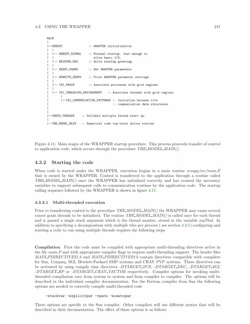
4.3. USING THE WRAPPER 247
MAIN
|
|--EEBOOT :: WRAPPER initialization
| |
| |-- EEBOOT_MINMAL :: Minimal startup. Just enough to
| | allow basic I/O.
| |-- EEINTRO_MSG :: Write startup greeting.
| |
| |-- EESET_PARMS :: Set WRAPPER parameters
| |
| |-- EEWRITE_EEENV :: Print WRAPPER parameter settings
| |
| |-- INI_PROCS :: Associate processes with grid regions.
| |
| |-- INI_THREADING_ENVIRONMENT :: Associate threads with grid regions.
| |
| |--INI_COMMUNICATION_PATTERNS :: Initialize between tile
| :: communication data structures
|
|
|--CHECK_THREADS :: Validate multiple thread start up.
|
|--THE_MODEL_MAIN :: Numerical code top-level driver routine
Figure 4.11: Main stages of the WRAPPER startup procedure. This process proceeds transfer of controlto application code, which occurs through the procedure THE MODEL MAIN().
4.3.2 Starting the code
When code is started under the WRAPPER, execution begins in a main routine eesupp/src/main.Fthat is owned by the WRAPPER. Control is transferred to the application through a routine calledTHE MODEL MAIN() once the WRAPPER has initialized correctly and has created the necessaryvariables to support subsequent calls to communication routines by the application code. The startupcalling sequence followed by the WRAPPER is shown in figure 4.11.
4.3.2.1 Multi-threaded execution
Prior to transferring control to the procedure THE MODEL MAIN() the WRAPPER may cause severalcoarse grain threads to be initialized. The routine THE MODEL MAIN() is called once for each threadand is passed a single stack argument which is the thread number, stored in the variable myThid. Inaddition to specifying a decomposition with multiple tiles per process ( see section 4.3.1) configuring andstarting a code to run using multiple threads requires the following steps.
Compilation First the code must be compiled with appropriate multi-threading directives active inthe file main.F and with appropriate compiler flags to request multi-threading support. The header filesMAIN PDIRECTIVES1.h and MAIN PDIRECTIVES2.h contain directives compatible with compilersfor Sun, Compaq, SGI, Hewlett-Packard SMP systems and CRAY PVP systems. These directives canbe activated by using compile time directives -DTARGET SUN, -DTARGET DEC, -DTARGET SGI,-DTARGET HP or -DTARGET CRAY VECTOR respectively. Compiler options for invoking multi-threaded compilation vary from system to system and from compiler to compiler. The options will bedescribed in the individual compiler documentation. For the Fortran compiler from Sun the followingoptions are needed to correctly compile multi-threaded code
-stackvar -explicitpar -vpara -noautopar
These options are specific to the Sun compiler. Other compilers will use different syntax that will bedescribed in their documentation. The effect of these options is as follows
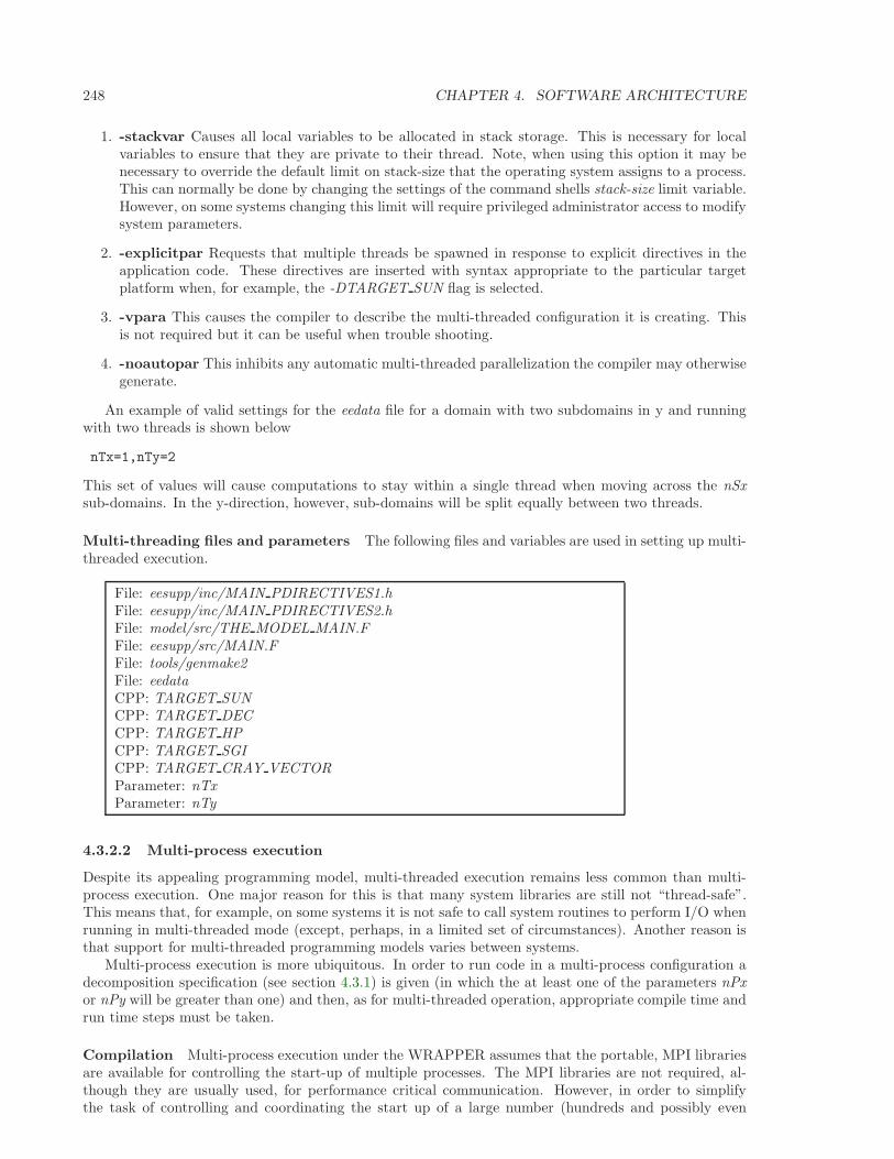
248 CHAPTER 4. SOFTWARE ARCHITECTURE
1. -stackvar Causes all local variables to be allocated in stack storage. This is necessary for localvariables to ensure that they are private to their thread. Note, when using this option it may benecessary to override the default limit on stack-size that the operating system assigns to a process.This can normally be done by changing the settings of the command shells stack-size limit variable.However, on some systems changing this limit will require privileged administrator access to modifysystem parameters.
2. -explicitpar Requests that multiple threads be spawned in response to explicit directives in theapplication code. These directives are inserted with syntax appropriate to the particular targetplatform when, for example, the -DTARGET SUN flag is selected.
3. -vpara This causes the compiler to describe the multi-threaded configuration it is creating. Thisis not required but it can be useful when trouble shooting.
4. -noautopar This inhibits any automatic multi-threaded parallelization the compiler may otherwisegenerate.
An example of valid settings for the eedata file for a domain with two subdomains in y and runningwith two threads is shown below
nTx=1,nTy=2
This set of values will cause computations to stay within a single thread when moving across the nSxsub-domains. In the y-direction, however, sub-domains will be split equally between two threads.
Multi-threading files and parameters The following files and variables are used in setting up multi-threaded execution.
File: eesupp/inc/MAIN PDIRECTIVES1.hFile: eesupp/inc/MAIN PDIRECTIVES2.hFile: model/src/THE MODEL MAIN.FFile: eesupp/src/MAIN.FFile: tools/genmake2File: eedataCPP: TARGET SUNCPP: TARGET DECCPP: TARGET HPCPP: TARGET SGICPP: TARGET CRAY VECTORParameter: nTxParameter: nTy
4.3.2.2 Multi-process execution
Despite its appealing programming model, multi-threaded execution remains less common than multi-process execution. One major reason for this is that many system libraries are still not “thread-safe”.This means that, for example, on some systems it is not safe to call system routines to perform I/O whenrunning in multi-threaded mode (except, perhaps, in a limited set of circumstances). Another reason isthat support for multi-threaded programming models varies between systems.
Multi-process execution is more ubiquitous. In order to run code in a multi-process configuration adecomposition specification (see section 4.3.1) is given (in which the at least one of the parameters nPxor nPy will be greater than one) and then, as for multi-threaded operation, appropriate compile time andrun time steps must be taken.
Compilation Multi-process execution under the WRAPPER assumes that the portable, MPI librariesare available for controlling the start-up of multiple processes. The MPI libraries are not required, al-though they are usually used, for performance critical communication. However, in order to simplifythe task of controlling and coordinating the start up of a large number (hundreds and possibly even
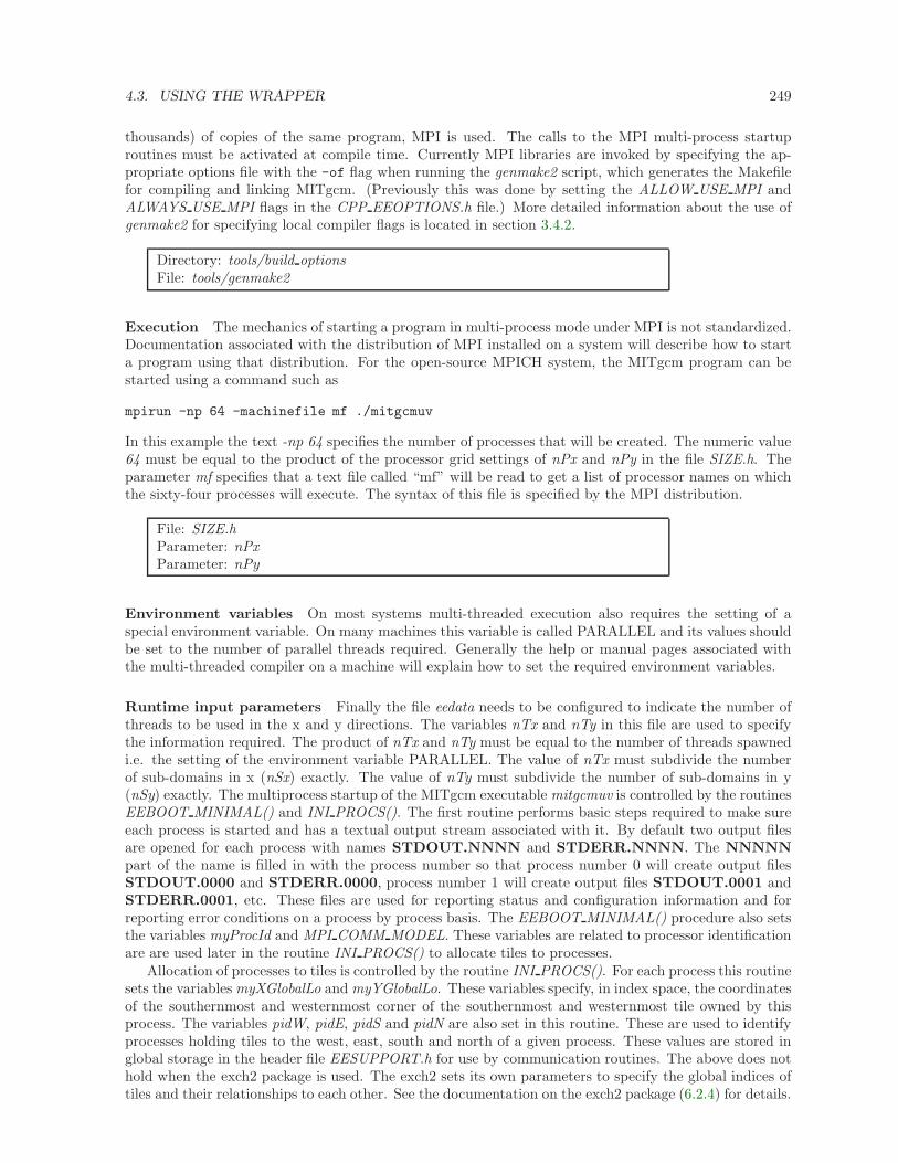
4.3. USING THE WRAPPER 249
thousands) of copies of the same program, MPI is used. The calls to the MPI multi-process startuproutines must be activated at compile time. Currently MPI libraries are invoked by specifying the ap-propriate options file with the -of flag when running the genmake2 script, which generates the Makefilefor compiling and linking MITgcm. (Previously this was done by setting the ALLOW USE MPI andALWAYS USE MPI flags in the CPP EEOPTIONS.h file.) More detailed information about the use ofgenmake2 for specifying local compiler flags is located in section 3.4.2.
Directory: tools/build optionsFile: tools/genmake2
Execution The mechanics of starting a program in multi-process mode under MPI is not standardized.Documentation associated with the distribution of MPI installed on a system will describe how to starta program using that distribution. For the open-source MPICH system, the MITgcm program can bestarted using a command such as
mpirun -np 64 -machinefile mf ./mitgcmuv
In this example the text -np 64 specifies the number of processes that will be created. The numeric value64 must be equal to the product of the processor grid settings of nPx and nPy in the file SIZE.h. Theparameter mf specifies that a text file called “mf” will be read to get a list of processor names on whichthe sixty-four processes will execute. The syntax of this file is specified by the MPI distribution.
File: SIZE.hParameter: nPxParameter: nPy
Environment variables On most systems multi-threaded execution also requires the setting of aspecial environment variable. On many machines this variable is called PARALLEL and its values shouldbe set to the number of parallel threads required. Generally the help or manual pages associated withthe multi-threaded compiler on a machine will explain how to set the required environment variables.
Runtime input parameters Finally the file eedata needs to be configured to indicate the number ofthreads to be used in the x and y directions. The variables nTx and nTy in this file are used to specifythe information required. The product of nTx and nTy must be equal to the number of threads spawnedi.e. the setting of the environment variable PARALLEL. The value of nTx must subdivide the numberof sub-domains in x (nSx) exactly. The value of nTy must subdivide the number of sub-domains in y(nSy) exactly. The multiprocess startup of the MITgcm executable mitgcmuv is controlled by the routinesEEBOOT MINIMAL() and INI PROCS(). The first routine performs basic steps required to make sureeach process is started and has a textual output stream associated with it. By default two output filesare opened for each process with names STDOUT.NNNN and STDERR.NNNN. The NNNNNpart of the name is filled in with the process number so that process number 0 will create output filesSTDOUT.0000 and STDERR.0000, process number 1 will create output files STDOUT.0001 andSTDERR.0001, etc. These files are used for reporting status and configuration information and forreporting error conditions on a process by process basis. The EEBOOT MINIMAL() procedure also setsthe variables myProcId and MPI COMM MODEL. These variables are related to processor identificationare are used later in the routine INI PROCS() to allocate tiles to processes.
Allocation of processes to tiles is controlled by the routine INI PROCS(). For each process this routinesets the variables myXGlobalLo and myYGlobalLo. These variables specify, in index space, the coordinatesof the southernmost and westernmost corner of the southernmost and westernmost tile owned by thisprocess. The variables pidW, pidE, pidS and pidN are also set in this routine. These are used to identifyprocesses holding tiles to the west, east, south and north of a given process. These values are stored inglobal storage in the header file EESUPPORT.h for use by communication routines. The above does nothold when the exch2 package is used. The exch2 sets its own parameters to specify the global indices oftiles and their relationships to each other. See the documentation on the exch2 package (6.2.4) for details.
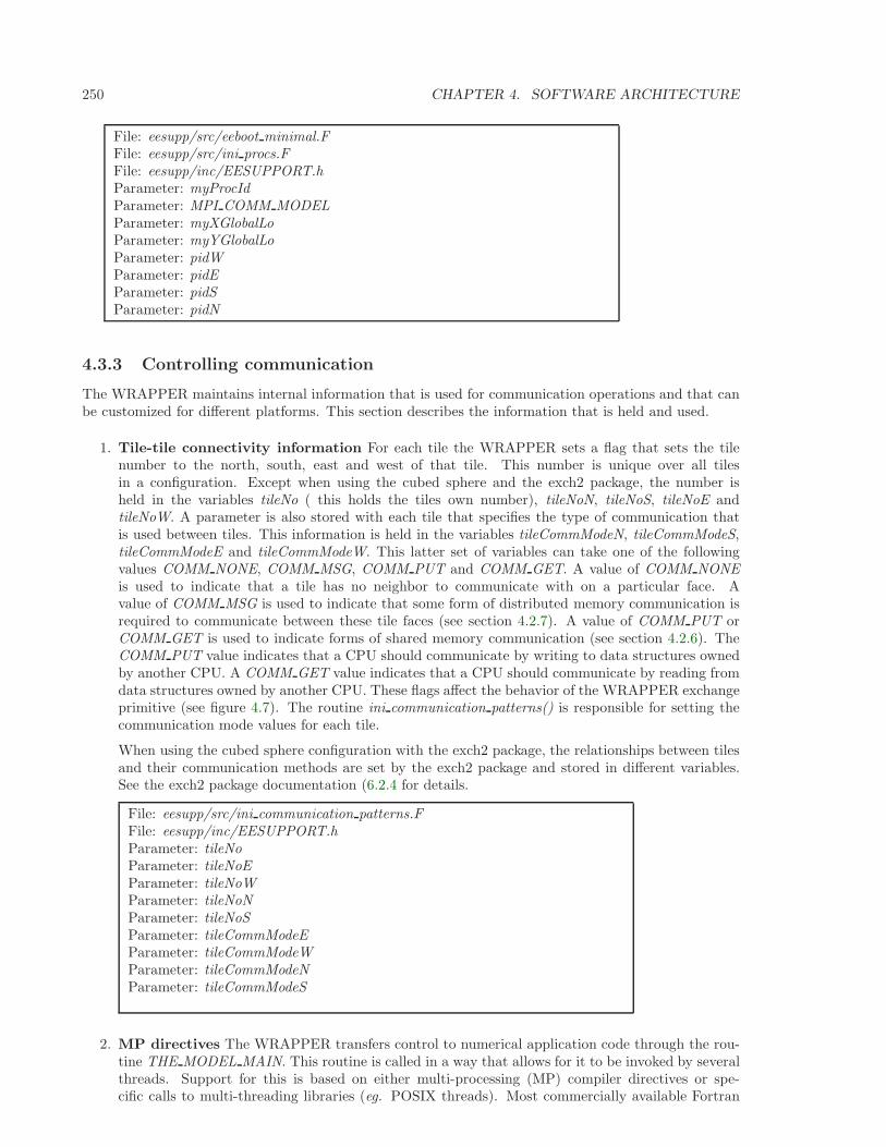
250 CHAPTER 4. SOFTWARE ARCHITECTURE
File: eesupp/src/eeboot minimal.FFile: eesupp/src/ini procs.FFile: eesupp/inc/EESUPPORT.hParameter: myProcIdParameter: MPI COMM MODELParameter: myXGlobalLoParameter: myYGlobalLoParameter: pidWParameter: pidEParameter: pidSParameter: pidN
4.3.3 Controlling communication
The WRAPPER maintains internal information that is used for communication operations and that canbe customized for different platforms. This section describes the information that is held and used.
1. Tile-tile connectivity information For each tile the WRAPPER sets a flag that sets the tilenumber to the north, south, east and west of that tile. This number is unique over all tilesin a configuration. Except when using the cubed sphere and the exch2 package, the number isheld in the variables tileNo ( this holds the tiles own number), tileNoN, tileNoS, tileNoE andtileNoW. A parameter is also stored with each tile that specifies the type of communication thatis used between tiles. This information is held in the variables tileCommModeN, tileCommModeS,tileCommModeE and tileCommModeW. This latter set of variables can take one of the followingvalues COMM NONE, COMM MSG, COMM PUT and COMM GET. A value of COMM NONEis used to indicate that a tile has no neighbor to communicate with on a particular face. Avalue of COMM MSG is used to indicate that some form of distributed memory communication isrequired to communicate between these tile faces (see section 4.2.7). A value of COMM PUT orCOMM GET is used to indicate forms of shared memory communication (see section 4.2.6). TheCOMM PUT value indicates that a CPU should communicate by writing to data structures ownedby another CPU. A COMM GET value indicates that a CPU should communicate by reading fromdata structures owned by another CPU. These flags affect the behavior of the WRAPPER exchangeprimitive (see figure 4.7). The routine ini communication patterns() is responsible for setting thecommunication mode values for each tile.
When using the cubed sphere configuration with the exch2 package, the relationships between tilesand their communication methods are set by the exch2 package and stored in different variables.See the exch2 package documentation (6.2.4 for details.
File: eesupp/src/ini communication patterns.FFile: eesupp/inc/EESUPPORT.hParameter: tileNoParameter: tileNoEParameter: tileNoWParameter: tileNoNParameter: tileNoSParameter: tileCommModeEParameter: tileCommModeWParameter: tileCommModeNParameter: tileCommModeS
2. MP directives The WRAPPER transfers control to numerical application code through the rou-tine THE MODEL MAIN. This routine is called in a way that allows for it to be invoked by severalthreads. Support for this is based on either multi-processing (MP) compiler directives or spe-cific calls to multi-threading libraries (eg. POSIX threads). Most commercially available Fortran
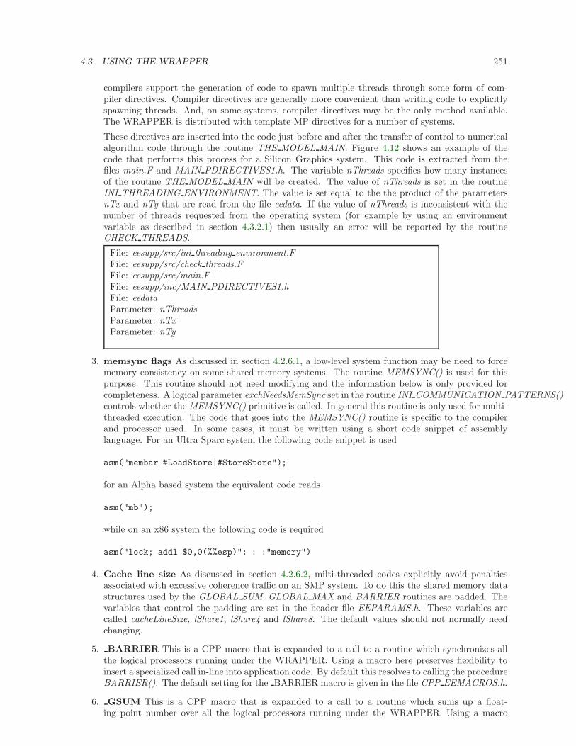
4.3. USING THE WRAPPER 251
compilers support the generation of code to spawn multiple threads through some form of com-piler directives. Compiler directives are generally more convenient than writing code to explicitlyspawning threads. And, on some systems, compiler directives may be the only method available.The WRAPPER is distributed with template MP directives for a number of systems.
These directives are inserted into the code just before and after the transfer of control to numericalalgorithm code through the routine THE MODEL MAIN. Figure 4.12 shows an example of thecode that performs this process for a Silicon Graphics system. This code is extracted from thefiles main.F and MAIN PDIRECTIVES1.h. The variable nThreads specifies how many instancesof the routine THE MODEL MAIN will be created. The value of nThreads is set in the routineINI THREADING ENVIRONMENT. The value is set equal to the the product of the parametersnTx and nTy that are read from the file eedata. If the value of nThreads is inconsistent with thenumber of threads requested from the operating system (for example by using an environmentvariable as described in section 4.3.2.1) then usually an error will be reported by the routineCHECK THREADS.
File: eesupp/src/ini threading environment.FFile: eesupp/src/check threads.FFile: eesupp/src/main.FFile: eesupp/inc/MAIN PDIRECTIVES1.hFile: eedataParameter: nThreadsParameter: nTxParameter: nTy
3. memsync flags As discussed in section 4.2.6.1, a low-level system function may be need to forcememory consistency on some shared memory systems. The routine MEMSYNC() is used for thispurpose. This routine should not need modifying and the information below is only provided forcompleteness. A logical parameter exchNeedsMemSync set in the routine INI COMMUNICATION PATTERNS()controls whether the MEMSYNC() primitive is called. In general this routine is only used for multi-threaded execution. The code that goes into the MEMSYNC() routine is specific to the compilerand processor used. In some cases, it must be written using a short code snippet of assemblylanguage. For an Ultra Sparc system the following code snippet is used
asm("membar #LoadStore|#StoreStore");
for an Alpha based system the equivalent code reads
asm("mb");
while on an x86 system the following code is required
asm("lock; addl $0,0(%%esp)": : :"memory")
4. Cache line size As discussed in section 4.2.6.2, milti-threaded codes explicitly avoid penaltiesassociated with excessive coherence traffic on an SMP system. To do this the shared memory datastructures used by the GLOBAL SUM, GLOBAL MAX and BARRIER routines are padded. Thevariables that control the padding are set in the header file EEPARAMS.h. These variables arecalled cacheLineSize, lShare1, lShare4 and lShare8. The default values should not normally needchanging.
5. BARRIER This is a CPP macro that is expanded to a call to a routine which synchronizes allthe logical processors running under the WRAPPER. Using a macro here preserves flexibility toinsert a specialized call in-line into application code. By default this resolves to calling the procedureBARRIER(). The default setting for the BARRIER macro is given in the file CPP EEMACROS.h.
6. GSUM This is a CPP macro that is expanded to a call to a routine which sums up a float-ing point number over all the logical processors running under the WRAPPER. Using a macro
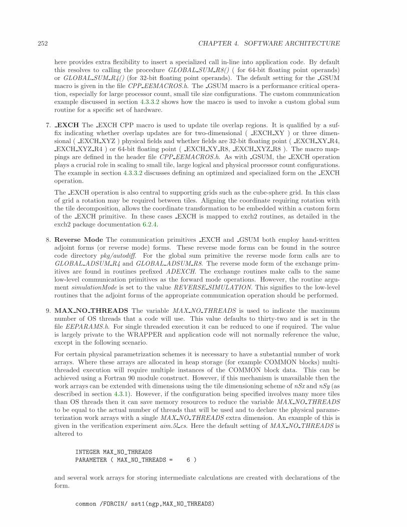
252 CHAPTER 4. SOFTWARE ARCHITECTURE
here provides extra flexibility to insert a specialized call in-line into application code. By defaultthis resolves to calling the procedure GLOBAL SUM R8() ( for 64-bit floating point operands)or GLOBAL SUM R4() (for 32-bit floating point operands). The default setting for the GSUMmacro is given in the file CPP EEMACROS.h. The GSUM macro is a performance critical opera-tion, especially for large processor count, small tile size configurations. The custom communicationexample discussed in section 4.3.3.2 shows how the macro is used to invoke a custom global sumroutine for a specific set of hardware.
7. EXCH The EXCH CPP macro is used to update tile overlap regions. It is qualified by a suf-fix indicating whether overlap updates are for two-dimensional ( EXCH XY ) or three dimen-sional ( EXCH XYZ ) physical fields and whether fields are 32-bit floating point ( EXCH XY R4,EXCH XYZ R4 ) or 64-bit floating point ( EXCH XY R8, EXCH XYZ R8 ). The macro map-pings are defined in the header file CPP EEMACROS.h. As with GSUM, the EXCH operationplays a crucial role in scaling to small tile, large logical and physical processor count configurations.The example in section 4.3.3.2 discusses defining an optimized and specialized form on the EXCHoperation.
The EXCH operation is also central to supporting grids such as the cube-sphere grid. In this classof grid a rotation may be required between tiles. Aligning the coordinate requiring rotation withthe tile decomposition, allows the coordinate transformation to be embedded within a custom formof the EXCH primitive. In these cases EXCH is mapped to exch2 routines, as detailed in theexch2 package documentation 6.2.4.
8. Reverse Mode The communication primitives EXCH and GSUM both employ hand-writtenadjoint forms (or reverse mode) forms. These reverse mode forms can be found in the sourcecode directory pkg/autodiff. For the global sum primitive the reverse mode form calls are toGLOBAL ADSUM R4 and GLOBAL ADSUM R8. The reverse mode form of the exchange prim-itives are found in routines prefixed ADEXCH. The exchange routines make calls to the samelow-level communication primitives as the forward mode operations. However, the routine argu-ment simulationMode is set to the value REVERSE SIMULATION. This signifies to the low-levelroutines that the adjoint forms of the appropriate communication operation should be performed.
9. MAX NO THREADS The variable MAX NO THREADS is used to indicate the maximumnumber of OS threads that a code will use. This value defaults to thirty-two and is set in thefile EEPARAMS.h. For single threaded execution it can be reduced to one if required. The valueis largely private to the WRAPPER and application code will not normally reference the value,except in the following scenario.
For certain physical parametrization schemes it is necessary to have a substantial number of workarrays. Where these arrays are allocated in heap storage (for example COMMON blocks) multi-threaded execution will require multiple instances of the COMMON block data. This can beachieved using a Fortran 90 module construct. However, if this mechanism is unavailable then thework arrays can be extended with dimensions using the tile dimensioning scheme of nSx and nSy (asdescribed in section 4.3.1). However, if the configuration being specified involves many more tilesthan OS threads then it can save memory resources to reduce the variable MAX NO THREADSto be equal to the actual number of threads that will be used and to declare the physical parame-terization work arrays with a single MAX NO THREADS extra dimension. An example of this isgiven in the verification experiment aim.5l cs. Here the default setting of MAX NO THREADS isaltered to
INTEGER MAX_NO_THREADS
PARAMETER ( MAX_NO_THREADS = 6 )
and several work arrays for storing intermediate calculations are created with declarations of theform.
common /FORCIN/ sst1(ngp,MAX_NO_THREADS)
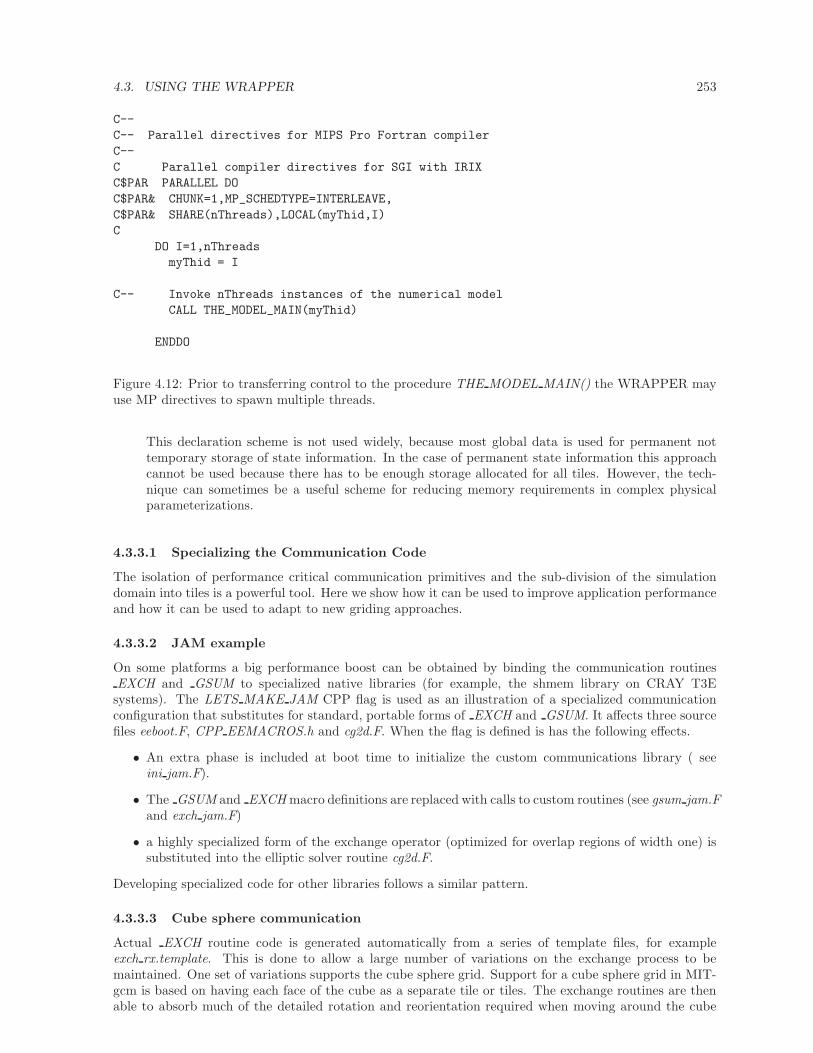
4.3. USING THE WRAPPER 253
C--
C-- Parallel directives for MIPS Pro Fortran compiler
C--
C Parallel compiler directives for SGI with IRIX
C$PAR PARALLEL DO
C$PAR& CHUNK=1,MP_SCHEDTYPE=INTERLEAVE,
C$PAR& SHARE(nThreads),LOCAL(myThid,I)
C
DO I=1,nThreads
myThid = I
C-- Invoke nThreads instances of the numerical model
CALL THE_MODEL_MAIN(myThid)
ENDDO
Figure 4.12: Prior to transferring control to the procedure THE MODEL MAIN() the WRAPPER mayuse MP directives to spawn multiple threads.
This declaration scheme is not used widely, because most global data is used for permanent nottemporary storage of state information. In the case of permanent state information this approachcannot be used because there has to be enough storage allocated for all tiles. However, the tech-nique can sometimes be a useful scheme for reducing memory requirements in complex physicalparameterizations.
4.3.3.1 Specializing the Communication Code
The isolation of performance critical communication primitives and the sub-division of the simulationdomain into tiles is a powerful tool. Here we show how it can be used to improve application performanceand how it can be used to adapt to new griding approaches.
4.3.3.2 JAM example
On some platforms a big performance boost can be obtained by binding the communication routinesEXCH and GSUM to specialized native libraries (for example, the shmem library on CRAY T3Esystems). The LETS MAKE JAM CPP flag is used as an illustration of a specialized communicationconfiguration that substitutes for standard, portable forms of EXCH and GSUM. It affects three sourcefiles eeboot.F, CPP EEMACROS.h and cg2d.F. When the flag is defined is has the following effects.
• An extra phase is included at boot time to initialize the custom communications library ( seeini jam.F).
• The GSUM and EXCH macro definitions are replaced with calls to custom routines (see gsum jam.Fand exch jam.F)
• a highly specialized form of the exchange operator (optimized for overlap regions of width one) issubstituted into the elliptic solver routine cg2d.F.
Developing specialized code for other libraries follows a similar pattern.
4.3.3.3 Cube sphere communication
Actual EXCH routine code is generated automatically from a series of template files, for exampleexch rx.template. This is done to allow a large number of variations on the exchange process to bemaintained. One set of variations supports the cube sphere grid. Support for a cube sphere grid in MIT-gcm is based on having each face of the cube as a separate tile or tiles. The exchange routines are thenable to absorb much of the detailed rotation and reorientation required when moving around the cube
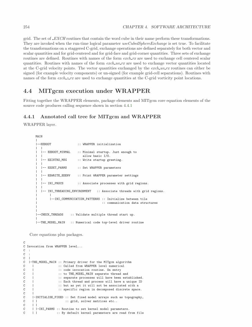
254 CHAPTER 4. SOFTWARE ARCHITECTURE
grid. The set of EXCH routines that contain the word cube in their name perform these transformations.They are invoked when the run-time logical parameter useCubedSphereExchange is set true. To facilitatethe transformations on a staggered C-grid, exchange operations are defined separately for both vector andscalar quantities and for grid-centered and for grid-face and grid-corner quantities. Three sets of exchangeroutines are defined. Routines with names of the form exch rx are used to exchange cell centered scalarquantities. Routines with names of the form exch uv rx are used to exchange vector quantities locatedat the C-grid velocity points. The vector quantities exchanged by the exch uv rx routines can either besigned (for example velocity components) or un-signed (for example grid-cell separations). Routines withnames of the form exch z rx are used to exchange quantities at the C-grid vorticity point locations.
4.4 MITgcm execution under WRAPPER
Fitting together the WRAPPER elements, package elements and MITgcm core equation elements of thesource code produces calling sequence shown in section 4.4.1
4.4.1 Annotated call tree for MITgcm and WRAPPER
WRAPPER layer.
MAIN
|
|--EEBOOT :: WRAPPER initialization
| |
| |-- EEBOOT_MINMAL :: Minimal startup. Just enough to
| | allow basic I/O.
| |-- EEINTRO_MSG :: Write startup greeting.
| |
| |-- EESET_PARMS :: Set WRAPPER parameters
| |
| |-- EEWRITE_EEENV :: Print WRAPPER parameter settings
| |
| |-- INI_PROCS :: Associate processes with grid regions.
| |
| |-- INI_THREADING_ENVIRONMENT :: Associate threads with grid regions.
| |
| |--INI_COMMUNICATION_PATTERNS :: Initialize between tile
| :: communication data structures
|
|
|--CHECK_THREADS :: Validate multiple thread start up.
|
|--THE_MODEL_MAIN :: Numerical code top-level driver routine
Core equations plus packages.
C
C Invocation from WRAPPER level...
C :
C :
C |
C |-THE_MODEL_MAIN :: Primary driver for the MITgcm algorithm
C | :: Called from WRAPPER level numerical
C | :: code invocation routine. On entry
C | :: to THE_MODEL_MAIN separate thread and
C | :: separate processes will have been established.
C | :: Each thread and process will have a unique ID
C | :: but as yet it will not be associated with a
C | :: specific region in decomposed discrete space.
C |
C |-INITIALISE_FIXED :: Set fixed model arrays such as topography,
C | | :: grid, solver matrices etc..
C | |
C | |-INI_PARMS :: Routine to set kernel model parameters.
C | | :: By default kernel parameters are read from file
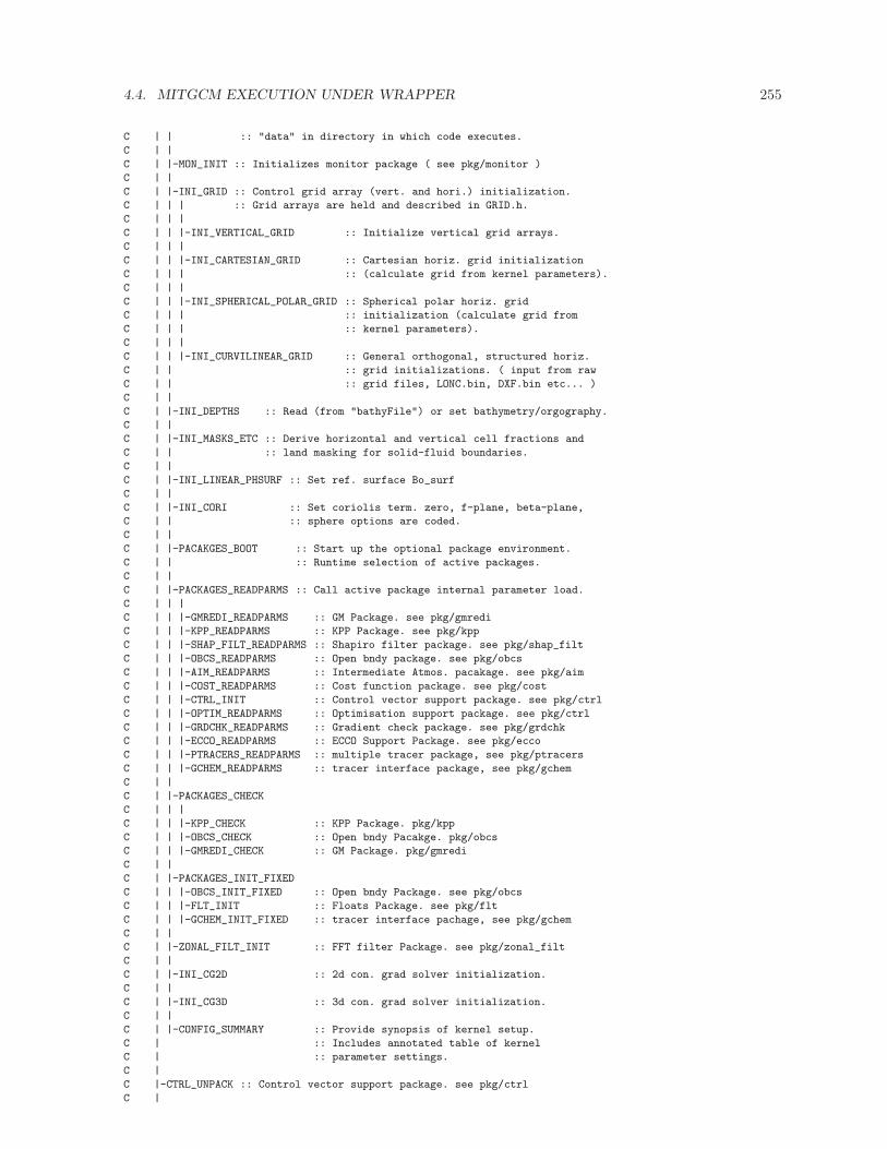
4.4. MITGCM EXECUTION UNDER WRAPPER 255
C | | :: "data" in directory in which code executes.
C | |
C | |-MON_INIT :: Initializes monitor package ( see pkg/monitor )
C | |
C | |-INI_GRID :: Control grid array (vert. and hori.) initialization.
C | | | :: Grid arrays are held and described in GRID.h.
C | | |
C | | |-INI_VERTICAL_GRID :: Initialize vertical grid arrays.
C | | |
C | | |-INI_CARTESIAN_GRID :: Cartesian horiz. grid initialization
C | | | :: (calculate grid from kernel parameters).
C | | |
C | | |-INI_SPHERICAL_POLAR_GRID :: Spherical polar horiz. grid
C | | | :: initialization (calculate grid from
C | | | :: kernel parameters).
C | | |
C | | |-INI_CURVILINEAR_GRID :: General orthogonal, structured horiz.
C | | :: grid initializations. ( input from raw
C | | :: grid files, LONC.bin, DXF.bin etc... )
C | |
C | |-INI_DEPTHS :: Read (from "bathyFile") or set bathymetry/orgography.
C | |
C | |-INI_MASKS_ETC :: Derive horizontal and vertical cell fractions and
C | | :: land masking for solid-fluid boundaries.
C | |
C | |-INI_LINEAR_PHSURF :: Set ref. surface Bo_surf
C | |
C | |-INI_CORI :: Set coriolis term. zero, f-plane, beta-plane,
C | | :: sphere options are coded.
C | |
C | |-PACAKGES_BOOT :: Start up the optional package environment.
C | | :: Runtime selection of active packages.
C | |
C | |-PACKAGES_READPARMS :: Call active package internal parameter load.
C | | |
C | | |-GMREDI_READPARMS :: GM Package. see pkg/gmredi
C | | |-KPP_READPARMS :: KPP Package. see pkg/kpp
C | | |-SHAP_FILT_READPARMS :: Shapiro filter package. see pkg/shap_filt
C | | |-OBCS_READPARMS :: Open bndy package. see pkg/obcs
C | | |-AIM_READPARMS :: Intermediate Atmos. pacakage. see pkg/aim
C | | |-COST_READPARMS :: Cost function package. see pkg/cost
C | | |-CTRL_INIT :: Control vector support package. see pkg/ctrl
C | | |-OPTIM_READPARMS :: Optimisation support package. see pkg/ctrl
C | | |-GRDCHK_READPARMS :: Gradient check package. see pkg/grdchk
C | | |-ECCO_READPARMS :: ECCO Support Package. see pkg/ecco
C | | |-PTRACERS_READPARMS :: multiple tracer package, see pkg/ptracers
C | | |-GCHEM_READPARMS :: tracer interface package, see pkg/gchem
C | |
C | |-PACKAGES_CHECK
C | | |
C | | |-KPP_CHECK :: KPP Package. pkg/kpp
C | | |-OBCS_CHECK :: Open bndy Pacakge. pkg/obcs
C | | |-GMREDI_CHECK :: GM Package. pkg/gmredi
C | |
C | |-PACKAGES_INIT_FIXED
C | | |-OBCS_INIT_FIXED :: Open bndy Package. see pkg/obcs
C | | |-FLT_INIT :: Floats Package. see pkg/flt
C | | |-GCHEM_INIT_FIXED :: tracer interface pachage, see pkg/gchem
C | |
C | |-ZONAL_FILT_INIT :: FFT filter Package. see pkg/zonal_filt
C | |
C | |-INI_CG2D :: 2d con. grad solver initialization.
C | |
C | |-INI_CG3D :: 3d con. grad solver initialization.
C | |
C | |-CONFIG_SUMMARY :: Provide synopsis of kernel setup.
C | :: Includes annotated table of kernel
C | :: parameter settings.
C |
C |-CTRL_UNPACK :: Control vector support package. see pkg/ctrl
C |
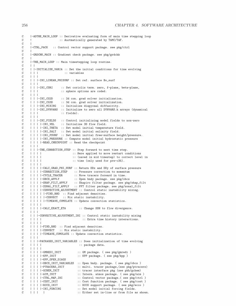
256 CHAPTER 4. SOFTWARE ARCHITECTURE
C |-ADTHE_MAIN_LOOP :: Derivative evaluating form of main time stepping loop
C ! :: Auotmatically generated by TAMC/TAF.
C |
C |-CTRL_PACK :: Control vector support package. see pkg/ctrl
C |
C |-GRDCHK_MAIN :: Gradient check package. see pkg/grdchk
C |
C |-THE_MAIN_LOOP :: Main timestepping loop routine.
C | |
C | |-INITIALISE_VARIA :: Set the initial conditions for time evolving
C | | | :: variables
C | | |
C | | |-INI_LINEAR_PHISURF :: Set ref. surface Bo_surf
C | | |
C | | |-INI_CORI :: Set coriolis term. zero, f-plane, beta-plane,
C | | | :: sphere options are coded.
C | | |
C | | |-INI_CG2D :: 2d con. grad solver initialization.
C | | |-INI_CG3D :: 3d con. grad solver initialization.
C | | |-INI_MIXING :: Initialize diapycnal diffusivity.
C | | |-INI_DYNVARS :: Initialize to zero all DYNVARS.h arrays (dynamical
C | | | :: fields).
C | | |
C | | |-INI_FIELDS :: Control initializing model fields to non-zero
C | | | |-INI_VEL :: Initialize 3D flow field.
C | | | |-INI_THETA :: Set model initial temperature field.
C | | | |-INI_SALT :: Set model initial salinity field.
C | | | |-INI_PSURF :: Set model initial free-surface height/pressure.
C | | | |-INI_PRESSURE :: Compute model initial hydrostatic pressure
C | | | |-READ_CHECKPOINT :: Read the checkpoint
C | | |
C | | |-THE_CORRECTION_STEP :: Step forward to next time step.
C | | | | :: Here applied to move restart conditions
C | | | | :: (saved in mid timestep) to correct level in
C | | | | :: time (only used for pre-c35).
C | | | |
C | | | |-CALC_GRAD_PHI_SURF :: Return DDx and DDy of surface pressure
C | | | |-CORRECTION_STEP :: Pressure correction to momentum
C | | | |-CYCLE_TRACER :: Move tracers forward in time.
C | | | |-OBCS_APPLY :: Open bndy package. see pkg/obcs
C | | | |-SHAP_FILT_APPLY :: Shapiro filter package. see pkg/shap_filt
C | | | |-ZONAL_FILT_APPLY :: FFT filter package. see pkg/zonal_filt
C | | | |-CONVECTIVE_ADJUSTMENT :: Control static instability mixing.
C | | | | |-FIND_RHO :: Find adjacent densities.
C | | | | |-CONVECT :: Mix static instability.
C | | | | |-TIMEAVE_CUMULATE :: Update convection statistics.
C | | | |
C | | | |-CALC_EXACT_ETA :: Change SSH to flow divergence.
C | | |
C | | |-CONVECTIVE_ADJUSTMENT_INI :: Control static instability mixing
C | | | | :: Extra time history interactions.
C | | | |
C | | | |-FIND_RHO :: Find adjacent densities.
C | | | |-CONVECT :: Mix static instability.
C | | | |-TIMEAVE_CUMULATE :: Update convection statistics.
C | | |
C | | |-PACKAGES_INIT_VARIABLES :: Does initialization of time evolving
C | | | | :: package data.
C | | | |
C | | | |-GMREDI_INIT :: GM package. ( see pkg/gmredi )
C | | | |-KPP_INIT :: KPP package. ( see pkg/kpp )
C | | | |-KPP_OPEN_DIAGS
C | | | |-OBCS_INIT_VARIABLES :: Open bndy. package. ( see pkg/obcs )
C | | | |-PTRACERS_INIT :: multi. tracer package,(see pkg/ptracers)
C | | | |-GCHEM_INIT :: tracer interface pkg (see pkh/gchem)
C | | | |-AIM_INIT :: Interm. atmos package. ( see pkg/aim )
C | | | |-CTRL_MAP_INI :: Control vector package.( see pkg/ctrl )
C | | | |-COST_INIT :: Cost function package. ( see pkg/cost )
C | | | |-ECCO_INIT :: ECCO support package. ( see pkg/ecco )
C | | | |-INI_FORCING :: Set model initial forcing fields.
C | | | | :: Either set in-line or from file as shown.
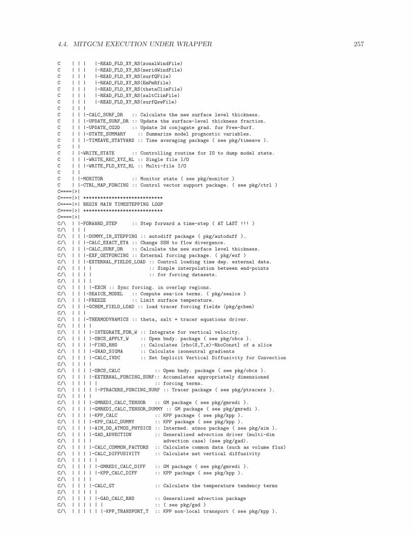
4.4. MITGCM EXECUTION UNDER WRAPPER 257
C | | | |-READ_FLD_XY_RS(zonalWindFile)
C | | | |-READ_FLD_XY_RS(meridWindFile)
C | | | |-READ_FLD_XY_RS(surfQFile)
C | | | |-READ_FLD_XY_RS(EmPmRfile)
C | | | |-READ_FLD_XY_RS(thetaClimFile)
C | | | |-READ_FLD_XY_RS(saltClimFile)
C | | | |-READ_FLD_XY_RS(surfQswFile)
C | | |
C | | |-CALC_SURF_DR :: Calculate the new surface level thickness.
C | | |-UPDATE_SURF_DR :: Update the surface-level thickness fraction.
C | | |-UPDATE_CG2D :: Update 2d conjugate grad. for Free-Surf.
C | | |-STATE_SUMMARY :: Summarize model prognostic variables.
C | | |-TIMEAVE_STATVARS :: Time averaging package ( see pkg/timeave ).
C | |
C | |-WRITE_STATE :: Controlling routine for IO to dump model state.
C | | |-WRITE_REC_XYZ_RL :: Single file I/O
C | | |-WRITE_FLD_XYZ_RL :: Multi-file I/O
C | |
C | |-MONITOR :: Monitor state ( see pkg/monitor )
C | |-CTRL_MAP_FORCING :: Control vector support package. ( see pkg/ctrl )
C====|>|
C====|>| ****************************
C====|>| BEGIN MAIN TIMESTEPPING LOOP
C====|>| ****************************
C====|>|
C/\ | |-FORWARD_STEP :: Step forward a time-step ( AT LAST !!! )
C/\ | | |
C/\ | | |-DUMMY_IN_STEPPING :: autodiff package ( pkg/autoduff ).
C/\ | | |-CALC_EXACT_ETA :: Change SSH to flow divergence.
C/\ | | |-CALC_SURF_DR :: Calculate the new surface level thickness.
C/\ | | |-EXF_GETFORCING :: External forcing package. ( pkg/exf )
C/\ | | |-EXTERNAL_FIELDS_LOAD :: Control loading time dep. external data.
C/\ | | | | :: Simple interpolation between end-points
C/\ | | | | :: for forcing datasets.
C/\ | | | |
C/\ | | | |-EXCH :: Sync forcing. in overlap regions.
C/\ | | |-SEAICE_MODEL :: Compute sea-ice terms. ( pkg/seaice )
C/\ | | |-FREEZE :: Limit surface temperature.
C/\ | | |-GCHEM_FIELD_LOAD :: load tracer forcing fields (pkg/gchem)
C/\ | | |
C/\ | | |-THERMODYNAMICS :: theta, salt + tracer equations driver.
C/\ | | | |
C/\ | | | |-INTEGRATE_FOR_W :: Integrate for vertical velocity.
C/\ | | | |-OBCS_APPLY_W :: Open bndy. package ( see pkg/obcs ).
C/\ | | | |-FIND_RHO :: Calculates [rho(S,T,z)-RhoConst] of a slice
C/\ | | | |-GRAD_SIGMA :: Calculate isoneutral gradients
C/\ | | | |-CALC_IVDC :: Set Implicit Vertical Diffusivity for Convection
C/\ | | | |
C/\ | | | |-OBCS_CALC :: Open bndy. package ( see pkg/obcs ).
C/\ | | | |-EXTERNAL_FORCING_SURF:: Accumulates appropriately dimensioned
C/\ | | | | | :: forcing terms.
C/\ | | | | |-PTRACERS_FORCING_SURF :: Tracer package ( see pkg/ptracers ).
C/\ | | | |
C/\ | | | |-GMREDI_CALC_TENSOR :: GM package ( see pkg/gmredi ).
C/\ | | | |-GMREDI_CALC_TENSOR_DUMMY :: GM package ( see pkg/gmredi ).
C/\ | | | |-KPP_CALC :: KPP package ( see pkg/kpp ).
C/\ | | | |-KPP_CALC_DUMMY :: KPP package ( see pkg/kpp ).
C/\ | | | |-AIM_DO_ATMOS_PHYSICS :: Intermed. atmos package ( see pkg/aim ).
C/\ | | | |-GAD_ADVECTION :: Generalised advection driver (multi-dim
C/\ | | | | advection case) (see pkg/gad).
C/\ | | | |-CALC_COMMON_FACTORS :: Calculate common data (such as volume flux)
C/\ | | | |-CALC_DIFFUSIVITY :: Calculate net vertical diffusivity
C/\ | | | | |
C/\ | | | | |-GMREDI_CALC_DIFF :: GM package ( see pkg/gmredi ).
C/\ | | | | |-KPP_CALC_DIFF :: KPP package ( see pkg/kpp ).
C/\ | | | |
C/\ | | | |-CALC_GT :: Calculate the temperature tendency terms
C/\ | | | | |
C/\ | | | | |-GAD_CALC_RHS :: Generalised advection package
C/\ | | | | | | :: ( see pkg/gad )
C/\ | | | | | |-KPP_TRANSPORT_T :: KPP non-local transport ( see pkg/kpp ).
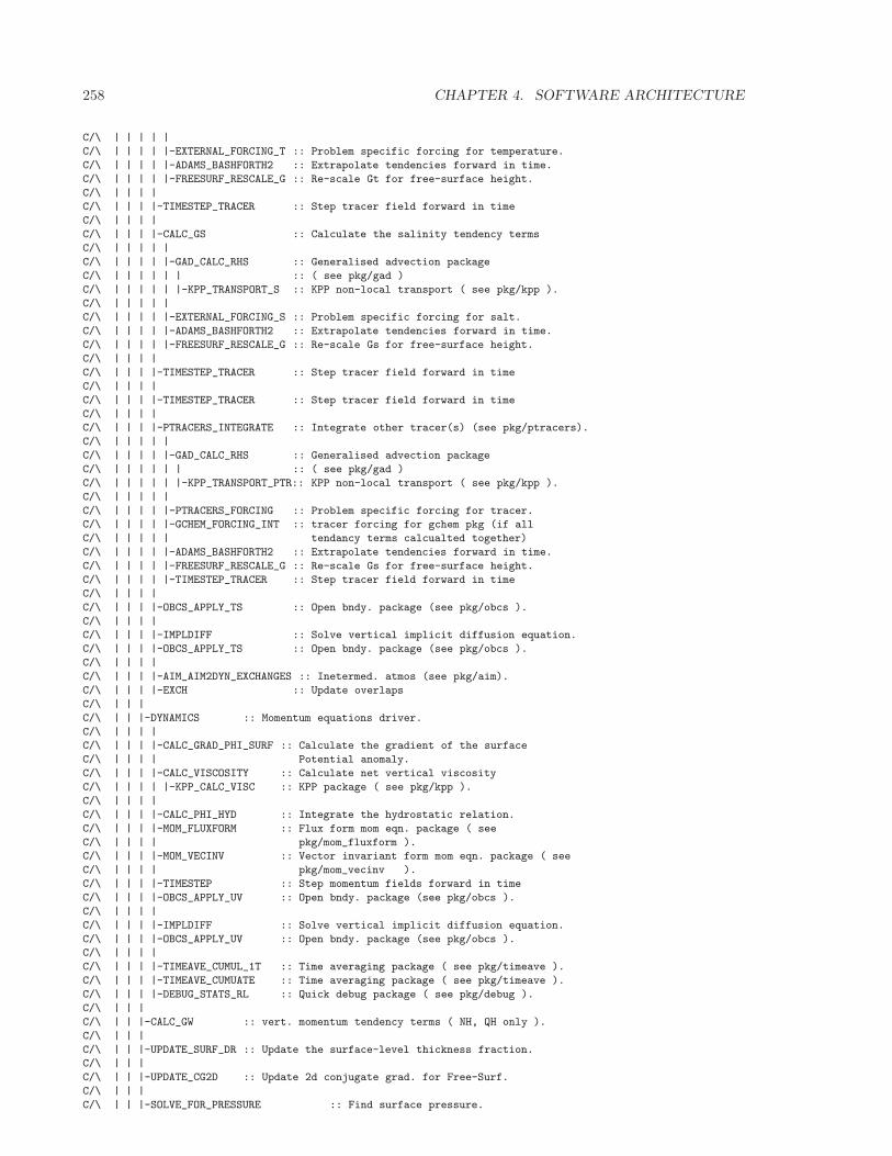
258 CHAPTER 4. SOFTWARE ARCHITECTURE
C/\ | | | | |
C/\ | | | | |-EXTERNAL_FORCING_T :: Problem specific forcing for temperature.
C/\ | | | | |-ADAMS_BASHFORTH2 :: Extrapolate tendencies forward in time.
C/\ | | | | |-FREESURF_RESCALE_G :: Re-scale Gt for free-surface height.
C/\ | | | |
C/\ | | | |-TIMESTEP_TRACER :: Step tracer field forward in time
C/\ | | | |
C/\ | | | |-CALC_GS :: Calculate the salinity tendency terms
C/\ | | | | |
C/\ | | | | |-GAD_CALC_RHS :: Generalised advection package
C/\ | | | | | | :: ( see pkg/gad )
C/\ | | | | | |-KPP_TRANSPORT_S :: KPP non-local transport ( see pkg/kpp ).
C/\ | | | | |
C/\ | | | | |-EXTERNAL_FORCING_S :: Problem specific forcing for salt.
C/\ | | | | |-ADAMS_BASHFORTH2 :: Extrapolate tendencies forward in time.
C/\ | | | | |-FREESURF_RESCALE_G :: Re-scale Gs for free-surface height.
C/\ | | | |
C/\ | | | |-TIMESTEP_TRACER :: Step tracer field forward in time
C/\ | | | |
C/\ | | | |-TIMESTEP_TRACER :: Step tracer field forward in time
C/\ | | | |
C/\ | | | |-PTRACERS_INTEGRATE :: Integrate other tracer(s) (see pkg/ptracers).
C/\ | | | | |
C/\ | | | | |-GAD_CALC_RHS :: Generalised advection package
C/\ | | | | | | :: ( see pkg/gad )
C/\ | | | | | |-KPP_TRANSPORT_PTR:: KPP non-local transport ( see pkg/kpp ).
C/\ | | | | |
C/\ | | | | |-PTRACERS_FORCING :: Problem specific forcing for tracer.
C/\ | | | | |-GCHEM_FORCING_INT :: tracer forcing for gchem pkg (if all
C/\ | | | | | tendancy terms calcualted together)
C/\ | | | | |-ADAMS_BASHFORTH2 :: Extrapolate tendencies forward in time.
C/\ | | | | |-FREESURF_RESCALE_G :: Re-scale Gs for free-surface height.
C/\ | | | | |-TIMESTEP_TRACER :: Step tracer field forward in time
C/\ | | | |
C/\ | | | |-OBCS_APPLY_TS :: Open bndy. package (see pkg/obcs ).
C/\ | | | |
C/\ | | | |-IMPLDIFF :: Solve vertical implicit diffusion equation.
C/\ | | | |-OBCS_APPLY_TS :: Open bndy. package (see pkg/obcs ).
C/\ | | | |
C/\ | | | |-AIM_AIM2DYN_EXCHANGES :: Inetermed. atmos (see pkg/aim).
C/\ | | | |-EXCH :: Update overlaps
C/\ | | |
C/\ | | |-DYNAMICS :: Momentum equations driver.
C/\ | | | |
C/\ | | | |-CALC_GRAD_PHI_SURF :: Calculate the gradient of the surface
C/\ | | | | Potential anomaly.
C/\ | | | |-CALC_VISCOSITY :: Calculate net vertical viscosity
C/\ | | | | |-KPP_CALC_VISC :: KPP package ( see pkg/kpp ).
C/\ | | | |
C/\ | | | |-CALC_PHI_HYD :: Integrate the hydrostatic relation.
C/\ | | | |-MOM_FLUXFORM :: Flux form mom eqn. package ( see
C/\ | | | | pkg/mom_fluxform ).
C/\ | | | |-MOM_VECINV :: Vector invariant form mom eqn. package ( see
C/\ | | | | pkg/mom_vecinv ).
C/\ | | | |-TIMESTEP :: Step momentum fields forward in time
C/\ | | | |-OBCS_APPLY_UV :: Open bndy. package (see pkg/obcs ).
C/\ | | | |
C/\ | | | |-IMPLDIFF :: Solve vertical implicit diffusion equation.
C/\ | | | |-OBCS_APPLY_UV :: Open bndy. package (see pkg/obcs ).
C/\ | | | |
C/\ | | | |-TIMEAVE_CUMUL_1T :: Time averaging package ( see pkg/timeave ).
C/\ | | | |-TIMEAVE_CUMUATE :: Time averaging package ( see pkg/timeave ).
C/\ | | | |-DEBUG_STATS_RL :: Quick debug package ( see pkg/debug ).
C/\ | | |
C/\ | | |-CALC_GW :: vert. momentum tendency terms ( NH, QH only ).
C/\ | | |
C/\ | | |-UPDATE_SURF_DR :: Update the surface-level thickness fraction.
C/\ | | |
C/\ | | |-UPDATE_CG2D :: Update 2d conjugate grad. for Free-Surf.
C/\ | | |
C/\ | | |-SOLVE_FOR_PRESSURE :: Find surface pressure.
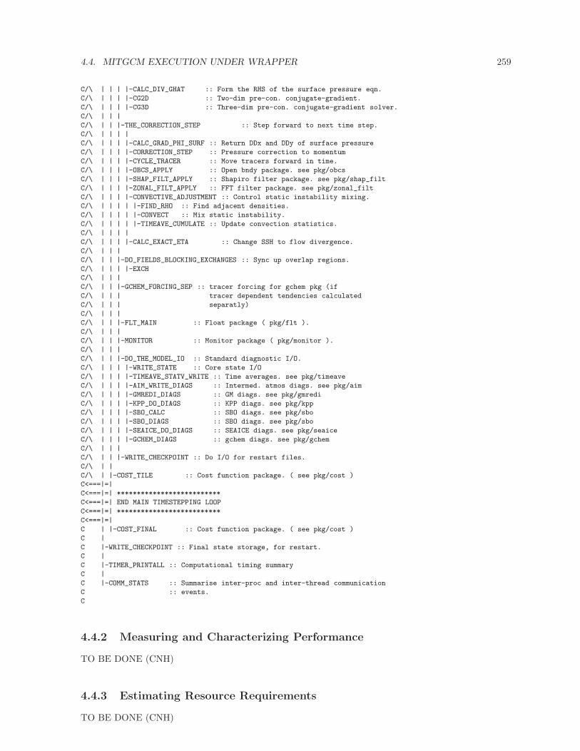
4.4. MITGCM EXECUTION UNDER WRAPPER 259
C/\ | | | |-CALC_DIV_GHAT :: Form the RHS of the surface pressure eqn.
C/\ | | | |-CG2D :: Two-dim pre-con. conjugate-gradient.
C/\ | | | |-CG3D :: Three-dim pre-con. conjugate-gradient solver.
C/\ | | |
C/\ | | |-THE_CORRECTION_STEP :: Step forward to next time step.
C/\ | | | |
C/\ | | | |-CALC_GRAD_PHI_SURF :: Return DDx and DDy of surface pressure
C/\ | | | |-CORRECTION_STEP :: Pressure correction to momentum
C/\ | | | |-CYCLE_TRACER :: Move tracers forward in time.
C/\ | | | |-OBCS_APPLY :: Open bndy package. see pkg/obcs
C/\ | | | |-SHAP_FILT_APPLY :: Shapiro filter package. see pkg/shap_filt
C/\ | | | |-ZONAL_FILT_APPLY :: FFT filter package. see pkg/zonal_filt
C/\ | | | |-CONVECTIVE_ADJUSTMENT :: Control static instability mixing.
C/\ | | | | |-FIND_RHO :: Find adjacent densities.
C/\ | | | | |-CONVECT :: Mix static instability.
C/\ | | | | |-TIMEAVE_CUMULATE :: Update convection statistics.
C/\ | | | |
C/\ | | | |-CALC_EXACT_ETA :: Change SSH to flow divergence.
C/\ | | |
C/\ | | |-DO_FIELDS_BLOCKING_EXCHANGES :: Sync up overlap regions.
C/\ | | | |-EXCH
C/\ | | |
C/\ | | |-GCHEM_FORCING_SEP :: tracer forcing for gchem pkg (if
C/\ | | | tracer dependent tendencies calculated
C/\ | | | separatly)
C/\ | | |
C/\ | | |-FLT_MAIN :: Float package ( pkg/flt ).
C/\ | | |
C/\ | | |-MONITOR :: Monitor package ( pkg/monitor ).
C/\ | | |
C/\ | | |-DO_THE_MODEL_IO :: Standard diagnostic I/O.
C/\ | | | |-WRITE_STATE :: Core state I/O
C/\ | | | |-TIMEAVE_STATV_WRITE :: Time averages. see pkg/timeave
C/\ | | | |-AIM_WRITE_DIAGS :: Intermed. atmos diags. see pkg/aim
C/\ | | | |-GMREDI_DIAGS :: GM diags. see pkg/gmredi
C/\ | | | |-KPP_DO_DIAGS :: KPP diags. see pkg/kpp
C/\ | | | |-SBO_CALC :: SBO diags. see pkg/sbo
C/\ | | | |-SBO_DIAGS :: SBO diags. see pkg/sbo
C/\ | | | |-SEAICE_DO_DIAGS :: SEAICE diags. see pkg/seaice
C/\ | | | |-GCHEM_DIAGS :: gchem diags. see pkg/gchem
C/\ | | |
C/\ | | |-WRITE_CHECKPOINT :: Do I/O for restart files.
C/\ | |
C/\ | |-COST_TILE :: Cost function package. ( see pkg/cost )
C<===|=|
C<===|=| **************************
C<===|=| END MAIN TIMESTEPPING LOOP
C<===|=| **************************
C<===|=|
C | |-COST_FINAL :: Cost function package. ( see pkg/cost )
C |
C |-WRITE_CHECKPOINT :: Final state storage, for restart.
C |
C |-TIMER_PRINTALL :: Computational timing summary
C |
C |-COMM_STATS :: Summarise inter-proc and inter-thread communication
C :: events.
C
4.4.2 Measuring and Characterizing Performance
TO BE DONE (CNH)
4.4.3 Estimating Resource Requirements
TO BE DONE (CNH)

260 CHAPTER 4. SOFTWARE ARCHITECTURE
4.4.3.1 Atlantic 1/6 degree example
4.4.3.2 Dry Run testing
4.4.3.3 Adjoint Resource Requirements
4.4.3.4 State Estimation Environment Resources
Chapter 5
Automatic Differentiation
Author: Patrick HeimbachAutomatic differentiation (AD), also referred to as algorithmic (or, more loosely, computational) dif-
ferentiation, involves automatically deriving code to calculate partial derivatives from an existing fullynon-linear prognostic code. (see Griewank [2000]). A software tool is used that parses and transformssource files according to a set of linguistic and mathematical rules. AD tools are like source-to-sourcetranslators in that they parse a program code as input and produce a new program code as output (werestrict our discussion to source-to-source tools, ignoring operator-overloading tools). However, unlike apure source-to-source translation, the output program represents a new algorithm, such as the evaluationof the Jacobian, the Hessian, or higher derivative operators. In principle, a variety of derived algorithmscan be generated automatically in this way.
MITgcm has been adapted for use with the Tangent linear and Adjoint Model Compiler (TAMC) andits successor TAF (Transformation of Algorithms in Fortran), developed by Ralf Giering (Giering andKaminski [1998], Giering [1999, 2000]). The first application of the adjoint of MITgcm for sensitivitystudies has been published by Marotzke et al. [1999]. Stammer et al. [1997, 002a] use MITgcm and its ad-joint for ocean state estimation studies. In the following we shall refer to TAMC and TAF synonymously,except were explicitly stated otherwise.
As of mid-2007 we are also able to generate fairly efficient adjoint code of the MITgcm using a new,open-source AD tool, called OpenAD (see Naumann et al. [2006]; Utke et al. [2008]. This enables us for thefirst time to compare adjoint models generated from different AD tools, providing an additional accuracycheck, complementary to finite-difference gradient checks. OpenAD and its application to MITgcm isdescribed in detail in section 5.5.
The AD tool exploits the chain rule for computing the first derivative of a function with respectto a set of input variables. Treating a given forward code as a composition of operations – each linerepresenting a compositional element, the chain rule is rigorously applied to the code, line by line. Theresulting tangent linear or adjoint code, then, may be thought of as the composition in forward or reverseorder, respectively, of the Jacobian matrices of the forward code’s compositional elements.
5.1 Some basic algebra
Let M be a general nonlinear, model, i.e. a mapping from the m-dimensional space U ⊂ IRm of inputvariables ~u = (u1, . . . , um) (model parameters, initial conditions, boundary conditions such as forcingfunctions) to the n-dimensional space V ⊂ IRn of model output variable ~v = (v1, . . . , vn) (model state,model diagnostics, objective function, ...) under consideration,
M :U −→ V
~u 7−→ ~v = M(~u)(5.1)
The vectors ~u ∈ U and v ∈ V may be represented w.r.t. some given basis vectors span(U) = ~eii=1,...,m
and span(V ) = ~fjj=1,...,n as
~u =
m∑
i=1
ui ~ei, ~v =
n∑
j=1
vj~fj
261
262 CHAPTER 5. AUTOMATIC DIFFERENTIATION
Two routes may be followed to determine the sensitivity of the output variable ~v to its input ~u.
5.1.1 Forward or direct sensitivity
Consider a perturbation to the input variables δ~u (typically a single component δ~u = δui ~ei). Their effecton the output may be obtained via the linear approximation of the model M in terms of its Jacobianmatrix M , evaluated in the point u(0) according to
δ~v = M |~u(0) δ~u (5.2)
with resulting output perturbation δ~v. In components Mji = ∂Mj/∂ui, it reads
δvj =∑
i
∂Mj
∂ui
∣∣∣∣u(0)
δui (5.3)
Eq. (5.2) is the tangent linear model (TLM). In contrast to the full nonlinear model M, the operator Mis just a matrix which can readily be used to find the forward sensitivity of ~v to perturbations in u, butif there are very many input variables (≫ O(106) for large-scale oceanographic application), it quicklybecomes prohibitive to proceed directly as in (5.2), if the impact of each component ei is to be assessed.
5.1.2 Reverse or adjoint sensitivity
Let us consider the special case of a scalar objective function J (~v) of the model output (e.g. the totalmeridional heat transport, the total uptake of CO2 in the Southern Ocean over a time interval, or ameasure of some model-to-data misfit)
J : U −→ V −→ IR~u 7−→ ~v = M(~u) 7−→ J (~u) = J (M(~u))
(5.4)
The perturbation of J around a fixed point J0,
J = J0 + δJ
can be expressed in both bases of ~u and ~v w.r.t. their corresponding inner product 〈 , 〉
J = J |~u(0) +⟨∇uJ T |~u(0) , δ~u
⟩+ O(δ~u2)
= J |~v(0) +⟨∇vJ T |~v(0) , δ~v
⟩+ O(δ~v2)
(5.5)
(note, that the gradient ∇f is a co-vector, therefore its transpose is required in the above inner product).Then, using the representation of δJ =
⟨∇vJ T , δ~v
⟩, the definition of an adjoint operator A∗ of a given
operator A,〈A∗~x , ~y 〉 = 〈 ~x , A~y 〉
which for finite-dimensional vector spaces is just the transpose of A,
A∗ = AT
and from eq. (5.2), (5.5), we note that (omitting |’s):
δJ =⟨∇vJ T , δ~v
⟩=⟨∇vJ T , M δ~u
⟩=⟨MT ∇vJ T , δ~u
⟩(5.6)
With the identity (5.5), we then find that the gradient ∇uJ can be readily inferred by invoking theadjoint M∗ of the tangent linear model M
∇uJ T |~u = MT |~u · ∇vJ T |~v= MT |~u · δ~v∗
= δ~u∗(5.7)
Eq. (5.7) is the adjoint model (ADM), in which MT is the adjoint (here, the transpose) of the tangentlinear operator M , δ~v∗ the adjoint variable of the model state ~v, and δ~u∗ the adjoint variable of thecontrol variable ~u.
5.1. SOME BASIC ALGEBRA 263
The reverse nature of the adjoint calculation can be readily seen as follows. Consider a model inte-gration which consists of Λ consecutive operations MΛ(MΛ−1(......(Mλ(......(M1(M0(~u))))), where theM’s could be the elementary steps, i.e. single lines in the code of the model, or successive time steps ofthe model integration, starting at step 0 and moving up to step Λ, with intermediate Mλ(~u) = ~v(λ+1)
and final MΛ(~u) = ~v(Λ+1) = ~v. Let J be a cost function which explicitly depends on the final state ~vonly (this restriction is for clarity reasons only). J (u) may be decomposed according to:
J (M(~u)) = J (MΛ(MΛ−1(......(Mλ(......(M1(M0(~u)))))) (5.8)
Then, according to the chain rule, the forward calculation reads, in terms of the Jacobi matrices (we’veomitted the |’s which, nevertheless are important to the aspect of tangent linearity; note also that bydefinition 〈∇vJ T , δ~v 〉 = ∇vJ · δ~v )
∇vJ (M(δ~u)) = ∇vJ ·MΛ · ...... ·Mλ · ...... ·M1 ·M0 · δ~u= ∇vJ · δ~v (5.9)
whereas in reverse mode we have
MT (∇vJ T ) = MT0 ·MT
1 · ...... ·MTλ · ...... ·MT
Λ · ∇vJ T
= MT0 ·MT
1 · ...... · ∇v(λ)J T
= ∇uJ T
(5.10)
clearly expressing the reverse nature of the calculation. Eq. (5.10) is at the heart of automatic adjointcompilers. If the intermediate steps λ in eqn. (5.8) – (5.10) represent the model state (forward oradjoint) at each intermediate time step as noted above, then correspondingly, MT (δ~v(λ) ∗) = δ~v(λ−1) ∗ forthe adjoint variables. It thus becomes evident that the adjoint calculation also yields the adjoint of eachmodel state component ~v(λ) at each intermediate step λ, namely
∇v(λ)J T |~v(λ) = MTλ |~v(λ) · ...... ·MT
Λ |~v(λ) · δ~v∗
= δ~v(λ) ∗(5.11)
in close analogy to eq. (5.7) We note in passing that that the δ~v(λ) ∗ are the Lagrange multipliers of themodel equations which determine ~v(λ).
In components, eq. (5.7) reads as follows. Let
δ~u = (δu1, . . . , δum)T, δ~u∗ = ∇uJ T =
(∂J∂u1
, . . . , ∂J∂um
)T
δ~v = (δv1, . . . , δun)T, δ~v∗ = ∇vJ T =
(∂J∂v1
, . . . , ∂J∂vn
)T
denote the perturbations in ~u and ~v, respectively, and their adjoint variables; further
M =
∂M1
∂u1. . . ∂M1
∂um
......
∂Mn
∂u1. . . ∂Mn
∂um
is the Jacobi matrix of M (an n×m matrix) such that δ~v = M · δ~u, or
δvj =m∑
i=1
Mji δui =m∑
i=1
∂Mj
∂uiδui
Then eq. (5.7) takes the form
δu∗i =
n∑
j=1
Mji δv∗j =
n∑
j=1
∂Mj
∂uiδv∗j
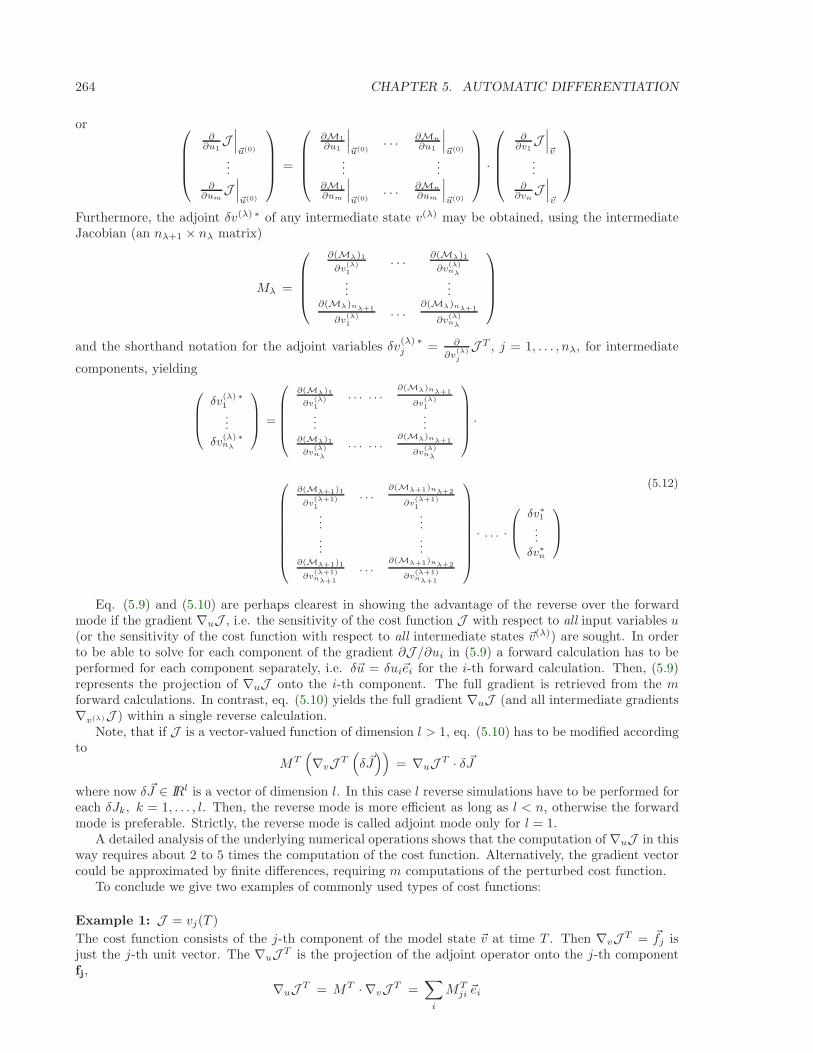
264 CHAPTER 5. AUTOMATIC DIFFERENTIATION
or
∂∂u1
J∣∣∣~u(0)
...∂
∂umJ∣∣∣~u(0)
=
∂M1
∂u1
∣∣∣~u(0)
. . . ∂Mn
∂u1
∣∣∣~u(0)
......
∂M1
∂um
∣∣∣~u(0)
. . . ∂Mn
∂um
∣∣∣~u(0)
·
∂∂v1
J∣∣∣~v
...∂
∂vnJ∣∣∣~v
Furthermore, the adjoint δv(λ) ∗ of any intermediate state v(λ) may be obtained, using the intermediateJacobian (an nλ+1 × nλ matrix)
Mλ =
∂(Mλ)1
∂v(λ)1
. . . ∂(Mλ)1
∂v(λ)nλ
......
∂(Mλ)nλ+1
∂v(λ)1
. . .∂(Mλ)nλ+1
∂v(λ)nλ
and the shorthand notation for the adjoint variables δv(λ) ∗j = ∂
∂v(λ)j
J T , j = 1, . . . , nλ, for intermediate
components, yielding
0
B
B
@
δv(λ) ∗1
...
δv(λ) ∗nλ
1
C
C
A
=
0
B
B
B
B
@
∂(Mλ)1
∂v(λ)1
. . . . . .∂(Mλ)nλ+1
∂v(λ)1
......
∂(Mλ)1
∂v(λ)nλ
. . . . . .∂(Mλ)nλ+1
∂v(λ)nλ
1
C
C
C
C
A
·
0
B
B
B
B
B
B
B
B
@
∂(Mλ+1)1
∂v(λ+1)1
. . .∂(Mλ+1)nλ+2
∂v(λ+1)1
......
......
∂(Mλ+1)1
∂v(λ+1)nλ+1
. . .∂(Mλ+1)nλ+2
∂v(λ+1)nλ+1
1
C
C
C
C
C
C
C
C
A
· . . . ·
0
B
@
δv∗1
...δv
∗n
1
C
A
(5.12)
Eq. (5.9) and (5.10) are perhaps clearest in showing the advantage of the reverse over the forwardmode if the gradient ∇uJ , i.e. the sensitivity of the cost function J with respect to all input variables u(or the sensitivity of the cost function with respect to all intermediate states ~v(λ)) are sought. In orderto be able to solve for each component of the gradient ∂J /∂ui in (5.9) a forward calculation has to beperformed for each component separately, i.e. δ~u = δui~ei for the i-th forward calculation. Then, (5.9)represents the projection of ∇uJ onto the i-th component. The full gradient is retrieved from the mforward calculations. In contrast, eq. (5.10) yields the full gradient ∇uJ (and all intermediate gradients∇v(λ)J ) within a single reverse calculation.
Note, that if J is a vector-valued function of dimension l > 1, eq. (5.10) has to be modified accordingto
MT(∇vJ T
(δ ~J))
= ∇uJ T · δ ~J
where now δ ~J ∈ IRl is a vector of dimension l. In this case l reverse simulations have to be performed foreach δJk, k = 1, . . . , l. Then, the reverse mode is more efficient as long as l < n, otherwise the forwardmode is preferable. Strictly, the reverse mode is called adjoint mode only for l = 1.
A detailed analysis of the underlying numerical operations shows that the computation of ∇uJ in thisway requires about 2 to 5 times the computation of the cost function. Alternatively, the gradient vectorcould be approximated by finite differences, requiring m computations of the perturbed cost function.
To conclude we give two examples of commonly used types of cost functions:
Example 1: J = vj(T )
The cost function consists of the j-th component of the model state ~v at time T . Then ∇vJ T = ~fj isjust the j-th unit vector. The ∇uJ T is the projection of the adjoint operator onto the j-th componentfj,
∇uJ T = MT · ∇vJ T =∑
i
MTji ~ei

5.1. SOME BASIC ALGEBRA 265
Example 2: J = 〈H(~v) − ~d , H(~v) − ~d 〉The cost function represents the quadratic model vs. data misfit. Here, ~d is the data vector and Hrepresents the operator which maps the model state space onto the data space. Then, ∇vJ takes theform
∇vJ T = 2 H ·(H(~v) − ~d
)
= 2∑
j
∑
k
∂Hk
∂vj(Hk(~v) − dk)
~fj
where Hkj = ∂Hk/∂vj is the Jacobi matrix of the data projection operator. Thus, the gradient ∇uJ isgiven by the adjoint operator, driven by the model vs. data misfit:
∇uJ T = 2MT ·H ·(H(~v) − ~d
)
5.1.3 Storing vs. recomputation in reverse mode
We note an important aspect of the forward vs. reverse mode calculation. Because of the local characterof the derivative (a derivative is defined w.r.t. a point along the trajectory), the intermediate results of themodel trajectory ~v(λ+1) = Mλ(v(λ)) may be required to evaluate the intermediate JacobianMλ|~v(λ) δ~v(λ).This is the case e.g. for nonlinear expressions (momentum advection, nonlinear equation of state), state-dependent conditional statements (parameterization schemes). In the forward mode, the intermediateresults are required in the same order as computed by the full forward model M, but in the reverse modethey are required in the reverse order. Thus, in the reverse mode the trajectory of the forward modelintegration M has to be stored to be available in the reverse calculation. Alternatively, the completemodel state up to the point of evaluation has to be recomputed whenever its value is required.
A method to balance the amount of recomputations vs. storage requirements is called checkpointing(e.g. Griewank [1992], Restrepo et al. [1998]). It is depicted in 5.1 for a 3-level checkpointing [as anexample, we give explicit numbers for a 3-day integration with a 1-hourly timestep in square brackets].
lev3 In a first step, the model trajectory is subdivided into nlev3 subsections [nlev3=3 1-day intervals],with the label lev3 for this outermost loop. The model is then integrated along the full trajectory,and the model state stored to disk only at every klev3
i -th timestep [i.e. 3 times, at i = 0, 1, 2corresponding to klev3
i = 0, 24, 48]. In addition, the cost function is computed, if needed.
lev2 In a second step each subsection itself is divided into nlev2 subsections [nlev2=4 6-hour intervalsper subsection]. The model picks up at the last outermost dumped state vklev3
nand is integrated
forward in time along the last subsection, with the label lev2 for this intermediate loop. The modelstate is now stored to disk at every klev2
i -th timestep [i.e. 4 times, at i = 0, 1, 2, 3 corresponding toklev2
i = 48, 54, 60, 66].
lev1 Finally, the model picks up at the last intermediate dump state vklev2n
and is integrated forwardin time along the last subsection, with the label lev1 for this intermediate loop. Within this sub-subsection only, parts of the model state is stored to memory at every timestep [i.e. every houri = 0, ..., 5 corresponding to klev1
i = 66, 67, . . . , 71]. The final state vn = vklev1n
is reached and themodel state of all preceding timesteps along the last innermost subsection are available, enablingintegration backwards in time along the last subsection. The adjoint can thus be computed alongthis last subsection klev2
n .
This procedure is repeated consecutively for each previous subsection klev2n−1, . . . , k
lev21 carrying the adjoint
computation to the initial time of the subsection klev3n . Then, the procedure is repeated for the previous
subsection klev3n−1 carrying the adjoint computation to the initial time klev3
1 .For the full model trajectory of nlev3 ·nlev2 ·nlev1 timesteps the required storing of the model state was
significantly reduced to nlev2 + nlev3 to disk and roughly nlev1 to memory [i.e. for the 3-day integrationwith a total oof 72 timesteps the model state was stored 7 times to disk and roughly 6 times to memory].This saving in memory comes at a cost of a required 3 full forward integrations of the model (onefor each checkpointing level). The optimal balance of storage vs. recomputation certainly dependson the computing resources available and may be adjusted by adjusting the partitioning among thenlev3, nlev2, nlev1.
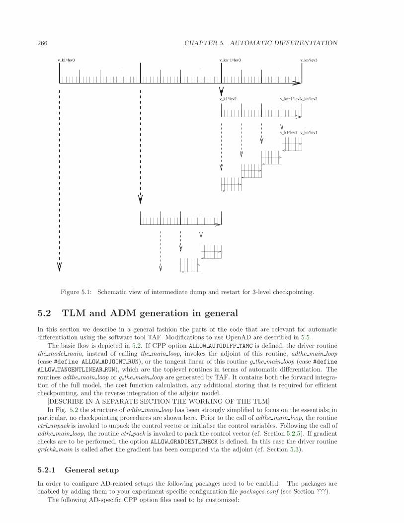
266 CHAPTER 5. AUTOMATIC DIFFERENTIATION
v_kn−1^lev2v_k1^lev2
v_kn^lev3v_kn−1^lev3v_k1^lev3
v_k1^lev1 v_kn^lev1
v_kn^lev2
Figure 5.1: Schematic view of intermediate dump and restart for 3-level checkpointing.
5.2 TLM and ADM generation in general
In this section we describe in a general fashion the parts of the code that are relevant for automaticdifferentiation using the software tool TAF. Modifications to use OpenAD are described in 5.5.
The basic flow is depicted in 5.2. If CPP option ALLOW AUTODIFF TAMC is defined, the driver routinethe model main, instead of calling the main loop, invokes the adjoint of this routine, adthe main loop(case #define ALLOW ADJOINT RUN), or the tangent linear of this routine g the main loop (case #define
ALLOW TANGENTLINEAR RUN), which are the toplevel routines in terms of automatic differentiation. Theroutines adthe main loop or g the main loop are generated by TAF. It contains both the forward integra-tion of the full model, the cost function calculation, any additional storing that is required for efficientcheckpointing, and the reverse integration of the adjoint model.
[DESCRIBE IN A SEPARATE SECTION THE WORKING OF THE TLM]
In Fig. 5.2 the structure of adthe main loop has been strongly simplified to focus on the essentials; inparticular, no checkpointing procedures are shown here. Prior to the call of adthe main loop, the routinectrl unpack is invoked to unpack the control vector or initialise the control variables. Following the call ofadthe main loop, the routine ctrl pack is invoked to pack the control vector (cf. Section 5.2.5). If gradientchecks are to be performed, the option ALLOW GRADIENT CHECK is defined. In this case the driver routinegrdchk main is called after the gradient has been computed via the adjoint (cf. Section 5.3).
5.2.1 General setup
In order to configure AD-related setups the following packages need to be enabled: The packages areenabled by adding them to your experiment-specific configuration file packages.conf (see Section ???).
The following AD-specific CPP option files need to be customized:
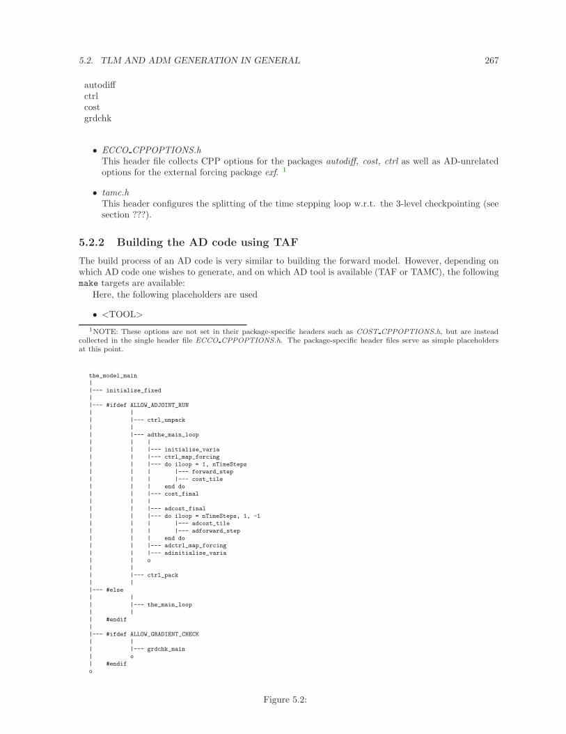
5.2. TLM AND ADM GENERATION IN GENERAL 267
autodiffctrlcostgrdchk
• ECCO CPPOPTIONS.hThis header file collects CPP options for the packages autodiff, cost, ctrl as well as AD-unrelatedoptions for the external forcing package exf. 1
• tamc.hThis header configures the splitting of the time stepping loop w.r.t. the 3-level checkpointing (seesection ???).
5.2.2 Building the AD code using TAF
The build process of an AD code is very similar to building the forward model. However, depending onwhich AD code one wishes to generate, and on which AD tool is available (TAF or TAMC), the followingmake targets are available:
Here, the following placeholders are used
• <TOOL>
1NOTE: These options are not set in their package-specific headers such as COST CPPOPTIONS.h, but are insteadcollected in the single header file ECCO CPPOPTIONS.h. The package-specific header files serve as simple placeholdersat this point.
the_model_main|
|--- initialise_fixed||--- #ifdef ALLOW_ADJOINT_RUN
| || |--- ctrl_unpack
| || |--- adthe_main_loop
| | || | |--- initialise_varia| | |--- ctrl_map_forcing
| | |--- do iloop = 1, nTimeSteps| | | |--- forward_step
| | | |--- cost_tile| | | end do| | |--- cost_final
| | || | |--- adcost_final
| | |--- do iloop = nTimeSteps, 1, -1| | | |--- adcost_tile
| | | |--- adforward_step| | | end do| | |--- adctrl_map_forcing
| | |--- adinitialise_varia| | o
| || |--- ctrl_pack| |
|--- #else| |
| |--- the_main_loop| |
| #endif||--- #ifdef ALLOW_GRADIENT_CHECK
| || |--- grdchk_main
| o| #endifo
Figure 5.2:
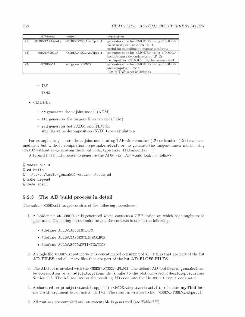
268 CHAPTER 5. AUTOMATIC DIFFERENTIATION
AD-target output description
(1) <MODE><TOOL>only <MODE> <TOOL> output.f generates code for <MODE> using <TOOL>no make dependencies on .F .h
useful for compiling on remote platforms(2) <MODE><TOOL> <MODE> <TOOL> output.f generates code for <MODE> using <TOOL>
includes make dependencies on .F .h
i.e. input for <TOOL> may be re-generated(3) <MODE>all mitgcmuv <MODE> generates code for <MODE> using <TOOL>
and compiles all code(use of TAF is set as default)
– TAF
– TAMC
• <MODE>
– ad generates the adjoint model (ADM)
– ftl generates the tangent linear model (TLM)
– svd generates both ADM and TLM forsingular value decomposition (SVD) type calculations
For example, to generate the adjoint model using TAF after routines (.F) or headers (.h) have beenmodified, but without compilation, type make adtaf; or, to generate the tangent linear model usingTAMC without re-generating the input code, type make ftltamconly.
A typical full build process to generate the ADM via TAF would look like follows:
% mkdir build
% cd build
% ../../../tools/genmake2 -mods=../code_ad
% make depend
% make adall
5.2.3 The AD build process in detail
The make <MODE>all target consists of the following procedures:
1. A header file AD CONFIG.h is generated which contains a CPP option on which code ought to begenerated. Depending on the make target, the contents is one of the following:
• #define ALLOW ADJOINT RUN
• #define ALLOW TANGENTLINEAR RUN
• #define ALLOW ECCO OPTIMIZATION
2. A single file <MODE> input code.f is concatenated consisting of all .f files that are part of the listAD FILES and all .flow files that are part of the list AD FLOW FILES.
3. The AD tool is invoked with the <MODE> <TOOL> FLAGS. The default AD tool flags in genmake2 canbe overrwritten by an adjoint options file (similar to the platform-specific build options, seeSection ???. The AD tool writes the resulting AD code into the file <MODE> input code ad.f
4. A short sed script adjoint sed is applied to <MODE> input code ad.f to reinstate myThid intothe CALL argument list of active file I/O. The result is written to file <MODE> <TOOL> output.f.
5. All routines are compiled and an executable is generated (see Table ???).
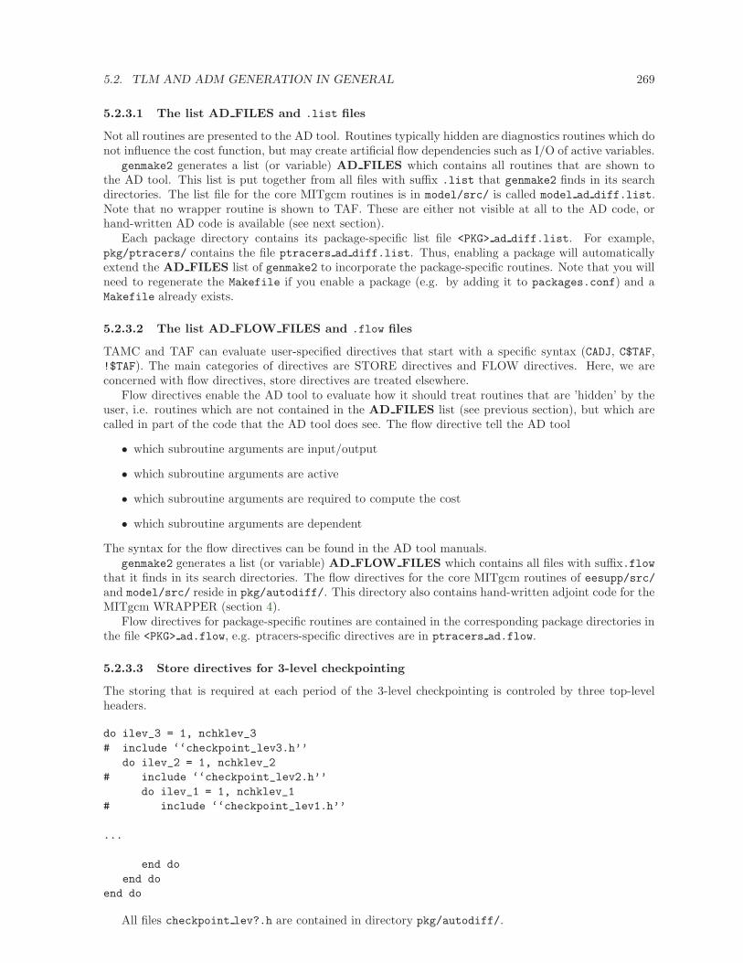
5.2. TLM AND ADM GENERATION IN GENERAL 269
5.2.3.1 The list AD FILES and .list files
Not all routines are presented to the AD tool. Routines typically hidden are diagnostics routines which donot influence the cost function, but may create artificial flow dependencies such as I/O of active variables.
genmake2 generates a list (or variable) AD FILES which contains all routines that are shown tothe AD tool. This list is put together from all files with suffix .list that genmake2 finds in its searchdirectories. The list file for the core MITgcm routines is in model/src/ is called model ad diff.list.Note that no wrapper routine is shown to TAF. These are either not visible at all to the AD code, orhand-written AD code is available (see next section).
Each package directory contains its package-specific list file <PKG> ad diff.list. For example,pkg/ptracers/ contains the file ptracers ad diff.list. Thus, enabling a package will automaticallyextend the AD FILES list of genmake2 to incorporate the package-specific routines. Note that you willneed to regenerate the Makefile if you enable a package (e.g. by adding it to packages.conf) and aMakefile already exists.
5.2.3.2 The list AD FLOW FILES and .flow files
TAMC and TAF can evaluate user-specified directives that start with a specific syntax (CADJ, C$TAF,!$TAF). The main categories of directives are STORE directives and FLOW directives. Here, we areconcerned with flow directives, store directives are treated elsewhere.
Flow directives enable the AD tool to evaluate how it should treat routines that are ’hidden’ by theuser, i.e. routines which are not contained in the AD FILES list (see previous section), but which arecalled in part of the code that the AD tool does see. The flow directive tell the AD tool
• which subroutine arguments are input/output
• which subroutine arguments are active
• which subroutine arguments are required to compute the cost
• which subroutine arguments are dependent
The syntax for the flow directives can be found in the AD tool manuals.genmake2 generates a list (or variable) AD FLOW FILES which contains all files with suffix.flow
that it finds in its search directories. The flow directives for the core MITgcm routines of eesupp/src/and model/src/ reside in pkg/autodiff/. This directory also contains hand-written adjoint code for theMITgcm WRAPPER (section 4).
Flow directives for package-specific routines are contained in the corresponding package directories inthe file <PKG> ad.flow, e.g. ptracers-specific directives are in ptracers ad.flow.
5.2.3.3 Store directives for 3-level checkpointing
The storing that is required at each period of the 3-level checkpointing is controled by three top-levelheaders.
do ilev_3 = 1, nchklev_3
# include ‘‘checkpoint_lev3.h’’
do ilev_2 = 1, nchklev_2
# include ‘‘checkpoint_lev2.h’’
do ilev_1 = 1, nchklev_1
# include ‘‘checkpoint_lev1.h’’
...
end do
end do
end do
All files checkpoint lev?.h are contained in directory pkg/autodiff/.
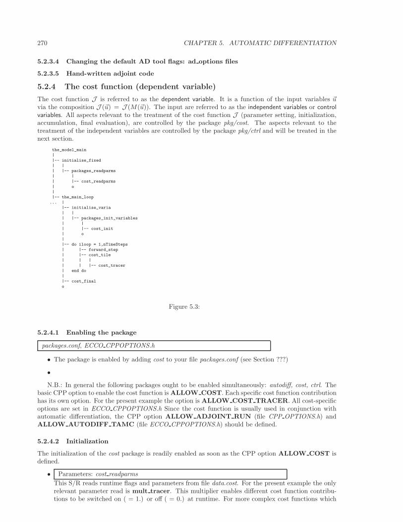
270 CHAPTER 5. AUTOMATIC DIFFERENTIATION
5.2.3.4 Changing the default AD tool flags: ad options files
5.2.3.5 Hand-written adjoint code
5.2.4 The cost function (dependent variable)
The cost function J is referred to as the dependent variable. It is a function of the input variables ~uvia the composition J (~u) = J (M(~u)). The input are referred to as the independent variables or controlvariables. All aspects relevant to the treatment of the cost function J (parameter setting, initialization,accumulation, final evaluation), are controlled by the package pkg/cost. The aspects relevant to thetreatment of the independent variables are controlled by the package pkg/ctrl and will be treated in thenext section.
the_model_main|
|-- initialise_fixed| || |-- packages_readparms
| || |-- cost_readparms
| o||-- the_main_loop
... ||-- initialise_varia
| || |-- packages_init_variables
| || |-- cost_init| o
||-- do iloop = 1,nTimeSteps
| |-- forward_step| |-- cost_tile| | |
| | |-- cost_tracer| end do
||-- cost_final
o
Figure 5.3:
5.2.4.1 Enabling the package
packages.conf, ECCO CPPOPTIONS.h
• The package is enabled by adding cost to your file packages.conf (see Section ???)
•
N.B.: In general the following packages ought to be enabled simultaneously: autodiff, cost, ctrl. Thebasic CPP option to enable the cost function is ALLOW COST. Each specific cost function contributionhas its own option. For the present example the option is ALLOW COST TRACER. All cost-specificoptions are set in ECCO CPPOPTIONS.h Since the cost function is usually used in conjunction withautomatic differentiation, the CPP option ALLOW ADJOINT RUN (file CPP OPTIONS.h) andALLOW AUTODIFF TAMC (file ECCO CPPOPTIONS.h) should be defined.
5.2.4.2 Initialization
The initialization of the cost package is readily enabled as soon as the CPP option ALLOW COST isdefined.
• Parameters: cost readparms
This S/R reads runtime flags and parameters from file data.cost. For the present example the onlyrelevant parameter read is mult tracer. This multiplier enables different cost function contribu-tions to be switched on ( = 1.) or off ( = 0.) at runtime. For more complex cost functions which
5.2. TLM AND ADM GENERATION IN GENERAL 271
involve model vs. data misfits, the corresponding data filenames and data specifications (start dateand time, period, ...) are read in this S/R.
• Variables: cost initThis S/R initializes the different cost function contributions. The contribution for the presentexample is objf tracer which is defined on each tile (bi,bj).
5.2.4.3 Accumulation
• cost tile, cost tracer
The ’driver’ routine cost tile is called at the end of each time step. Within this ’driver’ routine, S/R arecalled for each of the chosen cost function contributions. In the present example (ALLOW COST TRACER),S/R cost tracer is called. It accumulates objf tracer according to eqn. (ref:ask-the-author).
5.2.4.4 Finalize all contributions
• cost final
At the end of the forward integration S/R cost final is called. It accumulates the total cost function fcfrom each contribution and sums over all tiles:
J = fc = mult tracer∑
global sum
nSx, nSy∑
bi, bj
objf tracer(bi, bj) + ... (5.13)
The total cost function fc will be the ’dependent’ variable in the argument list for TAF, i.e.
taf -output ’fc’ ...
5.2.5 The control variables (independent variables)
The control variables are a subset of the model input (initial conditions, boundary conditions, modelparameters). Here we identify them with the variable ~u. All intermediate variables whose derivativew.r.t. control variables do not vanish are called active variables. All subroutines whose derivative w.r.t.the control variables don’t vanish are called active routines. Read and write operations from and to filecan be viewed as variable assignments. Therefore, files to which active variables are written and fromwhich active variables are read are called active files. All aspects relevant to the treatment of the controlvariables (parameter setting, initialization, perturbation) are controlled by the package pkg/ctrl.
5.2.5.1 genmake and CPP options
• genmake, CPP OPTIONS.h, ECCO CPPOPTIONS.h
To enable the directory to be included to the compile list, ctrl has to be added to the enable list in.genmakerc or in genmake itself (analogous to cost package, cf. previous section). Each control variableis enabled via its own CPP option in ECCO CPPOPTIONS.h.
5.2.5.2 Initialization
• Parameters: ctrl readparms
This S/R reads runtime flags and parameters from file data.ctrl. For the present example the filecontains the file names of each control variable that is used. In addition, the number of wet pointsfor each control variable and the net dimension of the space of control variables (counting wet pointsonly) nvarlength is determined. Masks for wet points for each tile (bi, bj) and vertical layer k aregenerated for the three relevant categories on the C-grid: nWetCtile for tracer fields, nWetWtilefor zonal velocity fields, nWetStile for meridional velocity fields.
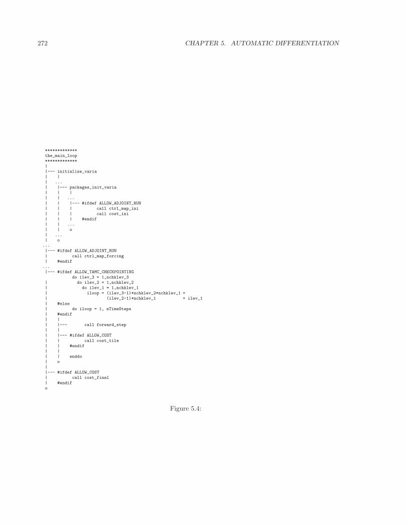
272 CHAPTER 5. AUTOMATIC DIFFERENTIATION
*************the_main_loop*************
||--- initialise_varia
| || ...| |--- packages_init_varia
| | || | ...
| | |--- #ifdef ALLOW_ADJOINT_RUN| | | call ctrl_map_ini
| | | call cost_ini| | | #endif| | ...
| | o| ...
| o...|--- #ifdef ALLOW_ADJOINT_RUN
| call ctrl_map_forcing| #endif
...|--- #ifdef ALLOW_TAMC_CHECKPOINTING
do ilev_3 = 1,nchklev_3| do ilev_2 = 1,nchklev_2| do ilev_1 = 1,nchklev_1
| iloop = (ilev_3-1)*nchklev_2*nchklev_1 +| (ilev_2-1)*nchklev_1 + ilev_1
| #else| do iloop = 1, nTimeSteps| #endif
| || |--- call forward_step
| || |--- #ifdef ALLOW_COST
| | call cost_tile| | #endif| |
| | enddo| o
||--- #ifdef ALLOW_COST| call cost_final
| #endifo
Figure 5.4:
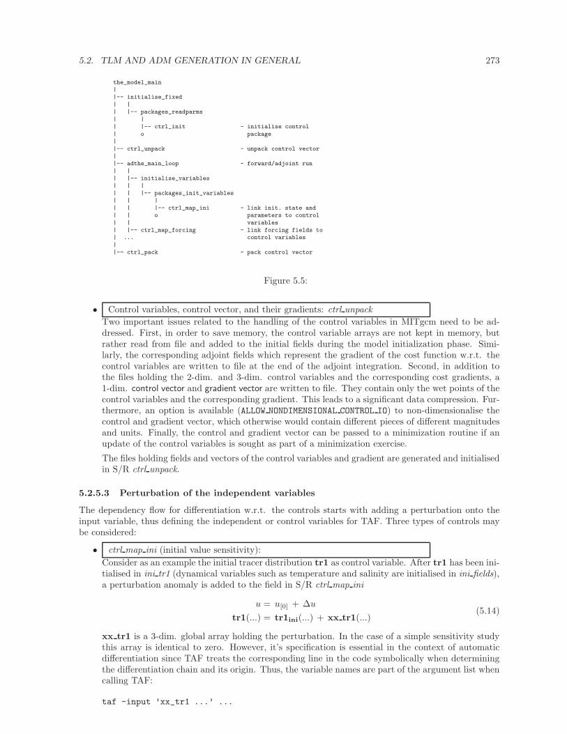
5.2. TLM AND ADM GENERATION IN GENERAL 273
the_model_main||-- initialise_fixed
| || |-- packages_readparms
| || |-- ctrl_init - initialise control
| o package||-- ctrl_unpack - unpack control vector
||-- adthe_main_loop - forward/adjoint run
| || |-- initialise_variables| | |
| | |-- packages_init_variables| | |
| | |-- ctrl_map_ini - link init. state and| | o parameters to control
| | variables| |-- ctrl_map_forcing - link forcing fields to| ... control variables
||-- ctrl_pack - pack control vector
Figure 5.5:
• Control variables, control vector, and their gradients: ctrl unpack
Two important issues related to the handling of the control variables in MITgcm need to be ad-dressed. First, in order to save memory, the control variable arrays are not kept in memory, butrather read from file and added to the initial fields during the model initialization phase. Simi-larly, the corresponding adjoint fields which represent the gradient of the cost function w.r.t. thecontrol variables are written to file at the end of the adjoint integration. Second, in addition tothe files holding the 2-dim. and 3-dim. control variables and the corresponding cost gradients, a1-dim. control vector and gradient vector are written to file. They contain only the wet points of thecontrol variables and the corresponding gradient. This leads to a significant data compression. Fur-thermore, an option is available (ALLOW NONDIMENSIONAL CONTROL IO) to non-dimensionalise thecontrol and gradient vector, which otherwise would contain different pieces of different magnitudesand units. Finally, the control and gradient vector can be passed to a minimization routine if anupdate of the control variables is sought as part of a minimization exercise.
The files holding fields and vectors of the control variables and gradient are generated and initialisedin S/R ctrl unpack.
5.2.5.3 Perturbation of the independent variables
The dependency flow for differentiation w.r.t. the controls starts with adding a perturbation onto theinput variable, thus defining the independent or control variables for TAF. Three types of controls maybe considered:
• ctrl map ini (initial value sensitivity):
Consider as an example the initial tracer distribution tr1 as control variable. After tr1 has been ini-tialised in ini tr1 (dynamical variables such as temperature and salinity are initialised in ini fields),a perturbation anomaly is added to the field in S/R ctrl map ini
u = u[0] + ∆u
tr1(...) = tr1ini(...) + xx tr1(...)(5.14)
xx tr1 is a 3-dim. global array holding the perturbation. In the case of a simple sensitivity studythis array is identical to zero. However, it’s specification is essential in the context of automaticdifferentiation since TAF treats the corresponding line in the code symbolically when determiningthe differentiation chain and its origin. Thus, the variable names are part of the argument list whencalling TAF:
taf -input ’xx_tr1 ...’ ...
274 CHAPTER 5. AUTOMATIC DIFFERENTIATION
Now, as mentioned above, MITgcm avoids maintaining an array for each control variable by readingthe perturbation to a temporary array from file. To ensure the symbolic link to be recognized byTAF, a scalar dummy variable xx tr1 dummy is introduced and an ’active read’ routine of theadjoint support package pkg/autodiff is invoked. The read-procedure is tagged with the variablexx tr1 dummy enabling TAF to recognize the initialization of the perturbation. The modifiedcall of TAF thus reads
taf -input ’xx_tr1_dummy ...’ ...
and the modified operation to (5.14) in the code takes on the form
call active_read_xyz(
& ..., tmpfld3d, ..., xx_tr1_dummy, ... )
tr1(...) = tr1(...) + tmpfld3d(...)
Note, that reading an active variable corresponds to a variable assignment. Its derivative corre-sponds to a write statement of the adjoint variable, followed by a reset. The ’active file’ routineshave been designed to support active read and corresponding adjoint active write operations (andvice versa).
• ctrl map forcing (boundary value sensitivity):
The handling of boundary values as control variables proceeds exactly analogous to the initial valueswith the symbolic perturbation taking place in S/R ctrl map forcing. Note however an importantdifference: Since the boundary values are time dependent with a new forcing field applied at eachtime steps, the general problem may be thought of as a new control variable at each time step (or,if the perturbation is averaged over a certain period, at each N timesteps), i.e.
uforcing = uforcing(tn) n =1,...,nTimeSteps
In the current example an equilibrium state is considered, and only an initial perturbation to surfaceforcing is applied with respect to the equilibrium state. A time dependent treatment of the surfaceforcing is implemented in the ECCO environment, involving the calendar (cal ) and external forcing(exf ) packages.
• ctrl map params (parameter sensitivity):
This routine is not yet implemented, but would proceed proceed along the same lines as the initialvalue sensitivity. The mixing parameters diffkr and kapgm are currently added as controls inctrl map ini.F.
5.2.5.4 Output of adjoint variables and gradient
Several ways exist to generate output of adjoint fields.
• ctrl map ini, ctrl map forcing:
– xx ...: the control variable fieldsBefore the forward integration, the control variables are read from file xx ... and added tothe model field.
– adxx ...: the adjoint variable fields, i.e. the gradient ∇uJ for each control variableAfter the adjoint integration the corresponding adjoint variables are written to adxx ....
• ctrl unpack, ctrl pack:
– vector ctrl: the control vectorAt the very beginning of the model initialization, the updated compressed control vector isread (or initialised) and distributed to 2-dim. and 3-dim. control variable fields.
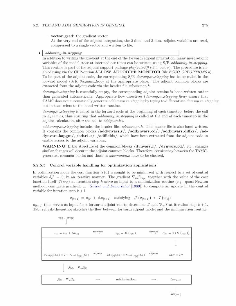
5.2. TLM AND ADM GENERATION IN GENERAL 275
– vector grad: the gradient vectorAt the very end of the adjoint integration, the 2-dim. and 3-dim. adjoint variables are read,compressed to a single vector and written to file.
• addummy in stepping:
In addition to writing the gradient at the end of the forward/adjoint integration, many more adjointvariables of the model state at intermediate times can be written using S/R addummy in stepping.This routine is part of the adjoint support package pkg/autodiff (cf.f. below). The procedure is en-abled using via the CPP-option ALLOW AUTODIFF MONITOR (file ECCO CPPOPTIONS.h).To be part of the adjoint code, the corresponding S/R dummy in stepping has to be called in theforward model (S/R the main loop) at the appropriate place. The adjoint common blocks areextracted from the adjoint code via the header file adcommon.h.
dummy in stepping is essentially empty, the corresponding adjoint routine is hand-written ratherthan generated automatically. Appropriate flow directives (dummy in stepping.flow) ensure thatTAMC does not automatically generate addummy in stepping by trying to differentiate dummy in stepping,but instead refers to the hand-written routine.
dummy in stepping is called in the forward code at the beginning of each timestep, before the callto dynamics, thus ensuring that addummy in stepping is called at the end of each timestep in theadjoint calculation, after the call to addynamics.
addummy in stepping includes the header files adcommon.h. This header file is also hand-written.It contains the common blocks /addynvars r/, /addynvars cd/, /addynvars diffkr/, /ad-dynvars kapgm/, /adtr1 r/, /adffields/, which have been extracted from the adjoint code toenable access to the adjoint variables.
WARNING: If the structure of the common blocks /dynvars r/, /dynvars cd/, etc., changessimilar changes will occur in the adjoint common blocks. Therefore, consistency between the TAMC-generated common blocks and those in adcommon.h have to be checked.
5.2.5.5 Control variable handling for optimization applications
In optimization mode the cost function J (u) is sought to be minimized with respect to a set of controlvariables δJ = 0, in an iterative manner. The gradient ∇uJ |u[k]
together with the value of the costfunction itself J (u[k]) at iteration step k serve as input to a minimization routine (e.g. quasi-Newtonmethod, conjugate gradient, ... Gilbert and Lemarechal [1989]) to compute an update in the controlvariable for iteration step k + 1
u[k+1] = u[0] + ∆u[k+1] satisfying J(u[k+1]
)< J
(u[k]
)
u[k+1] then serves as input for a forward/adjoint run to determine J and ∇uJ at iteration step k + 1.Tab. ref:ask-the-author sketches the flow between forward/adjoint model and the minimization routine.
u[0] , ∆u[k]?
?
y
u[k] = u[0] + ∆u[k]forward−→ v[k] = M
`
u[k]
´ forward−→ J[k] = J
`
M`
u[k]
´´
?
?
y
∇uJ[k](δJ ) = T∗ · ∇vJ |v[k](δJ )
adjoint←− ad v[k](δJ ) = ∇vJ |v[k]
(δJ )adjoint←− adJ = δJ
?
?
?
?
y
J[k], ∇uJ[k]
J[k] , ∇uJ[k] −→ minimisation −→ ∆u[k+1]
?
?
y
∆u[k+1]
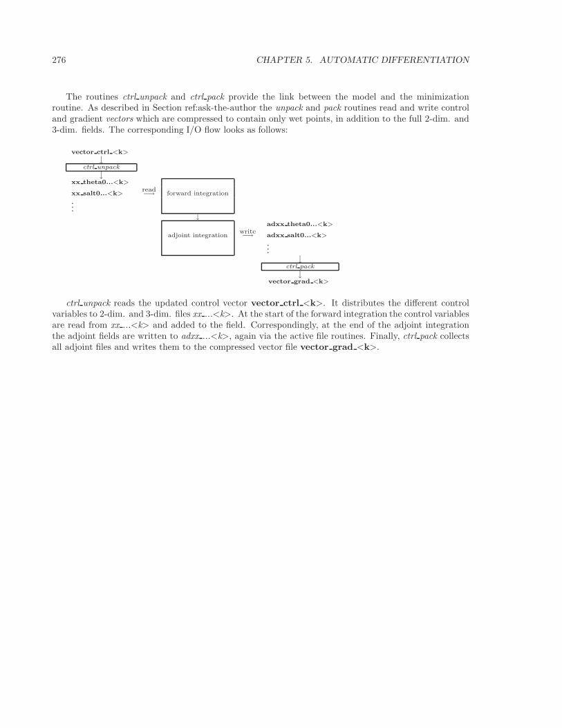
276 CHAPTER 5. AUTOMATIC DIFFERENTIATION
The routines ctrl unpack and ctrl pack provide the link between the model and the minimizationroutine. As described in Section ref:ask-the-author the unpack and pack routines read and write controland gradient vectors which are compressed to contain only wet points, in addition to the full 2-dim. and3-dim. fields. The corresponding I/O flow looks as follows:
vector ctrl <k>?
y
ctrl unpack?
y
xx theta0...<k>
xx salt0...<k>read−→ forward integration
.
.
.
↓adxx theta0...<k>
adjoint integrationwrite−→ adxx salt0...<k>
.
.
.?
y
ctrl pack?
y
vector grad <k>
ctrl unpack reads the updated control vector vector ctrl <k>. It distributes the different controlvariables to 2-dim. and 3-dim. files xx ...<k>. At the start of the forward integration the control variablesare read from xx ...<k> and added to the field. Correspondingly, at the end of the adjoint integrationthe adjoint fields are written to adxx ...<k>, again via the active file routines. Finally, ctrl pack collectsall adjoint files and writes them to the compressed vector file vector grad <k>.
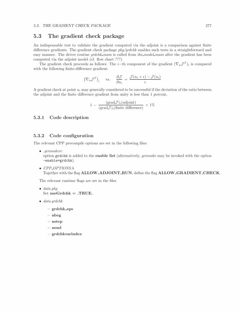
5.3. THE GRADIENT CHECK PACKAGE 277
5.3 The gradient check package
An indispensable test to validate the gradient computed via the adjoint is a comparison against finitedifference gradients. The gradient check package pkg/grdchk enables such tests in a straightforward andeasy manner. The driver routine grdchk main is called from the model main after the gradient has beencomputed via the adjoint model (cf. flow chart ???).
The gradient check proceeds as follows: The i−th component of the gradient (∇uJ T )i is comparedwith the following finite-difference gradient:
(∇uJ T
)i
vs.∂J∂ui
=J (ui + ǫ) − J (ui)
ǫ
A gradient check at point ui may generally considered to be successful if the deviation of the ratio betweenthe adjoint and the finite difference gradient from unity is less than 1 percent,
1 − (gradJ )i(adjoint)
(gradJ )i(finite difference)< 1%
5.3.1 Code description
5.3.2 Code configuration
The relevant CPP precompile options are set in the following files:
• .genmakercoption grdchk is added to the enable list (alternatively, genmake may be invoked with the option-enable=grdchk).
• CPP OPTIONS.hTogether with the flag ALLOW ADJOINT RUN, define the flag ALLOW GRADIENT CHECK.
The relevant runtime flags are set in the files
• data.pkgSet useGrdchk = .TRUE.
• data.grdchk
– grdchk eps
– nbeg
– nstep
– nend
– grdchkvarindex
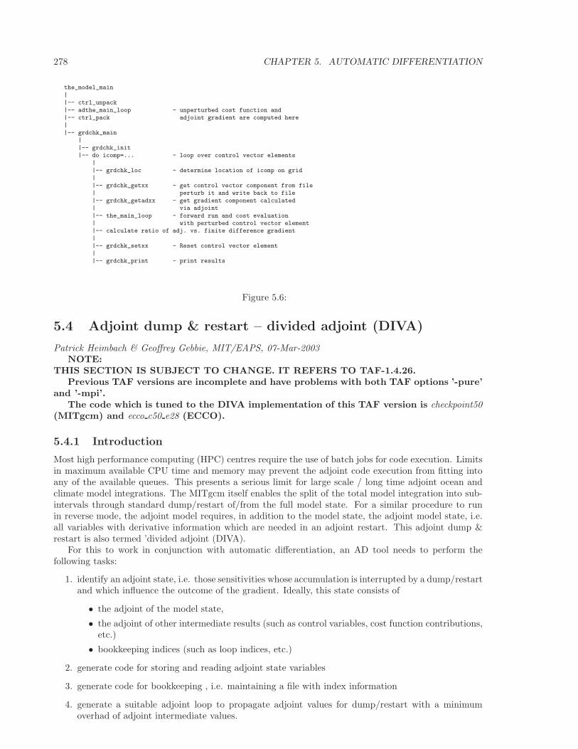
278 CHAPTER 5. AUTOMATIC DIFFERENTIATION
the_model_main
||-- ctrl_unpack
|-- adthe_main_loop - unperturbed cost function and|-- ctrl_pack adjoint gradient are computed here
||-- grdchk_main
|
|-- grdchk_init|-- do icomp=... - loop over control vector elements
||-- grdchk_loc - determine location of icomp on grid|
|-- grdchk_getxx - get control vector component from file| perturb it and write back to file
|-- grdchk_getadxx - get gradient component calculated| via adjoint
|-- the_main_loop - forward run and cost evaluation| with perturbed control vector element|-- calculate ratio of adj. vs. finite difference gradient
||-- grdchk_setxx - Reset control vector element
||-- grdchk_print - print results
Figure 5.6:
5.4 Adjoint dump & restart – divided adjoint (DIVA)
Patrick Heimbach & Geoffrey Gebbie, MIT/EAPS, 07-Mar-2003NOTE:
THIS SECTION IS SUBJECT TO CHANGE. IT REFERS TO TAF-1.4.26.Previous TAF versions are incomplete and have problems with both TAF options ’-pure’
and ’-mpi’.The code which is tuned to the DIVA implementation of this TAF version is checkpoint50
(MITgcm) and ecco c50 e28 (ECCO).
5.4.1 Introduction
Most high performance computing (HPC) centres require the use of batch jobs for code execution. Limitsin maximum available CPU time and memory may prevent the adjoint code execution from fitting intoany of the available queues. This presents a serious limit for large scale / long time adjoint ocean andclimate model integrations. The MITgcm itself enables the split of the total model integration into sub-intervals through standard dump/restart of/from the full model state. For a similar procedure to runin reverse mode, the adjoint model requires, in addition to the model state, the adjoint model state, i.e.all variables with derivative information which are needed in an adjoint restart. This adjoint dump &restart is also termed ’divided adjoint (DIVA).
For this to work in conjunction with automatic differentiation, an AD tool needs to perform thefollowing tasks:
1. identify an adjoint state, i.e. those sensitivities whose accumulation is interrupted by a dump/restartand which influence the outcome of the gradient. Ideally, this state consists of
• the adjoint of the model state,
• the adjoint of other intermediate results (such as control variables, cost function contributions,etc.)
• bookkeeping indices (such as loop indices, etc.)
2. generate code for storing and reading adjoint state variables
3. generate code for bookkeeping , i.e. maintaining a file with index information
4. generate a suitable adjoint loop to propagate adjoint values for dump/restart with a minimumoverhad of adjoint intermediate values.
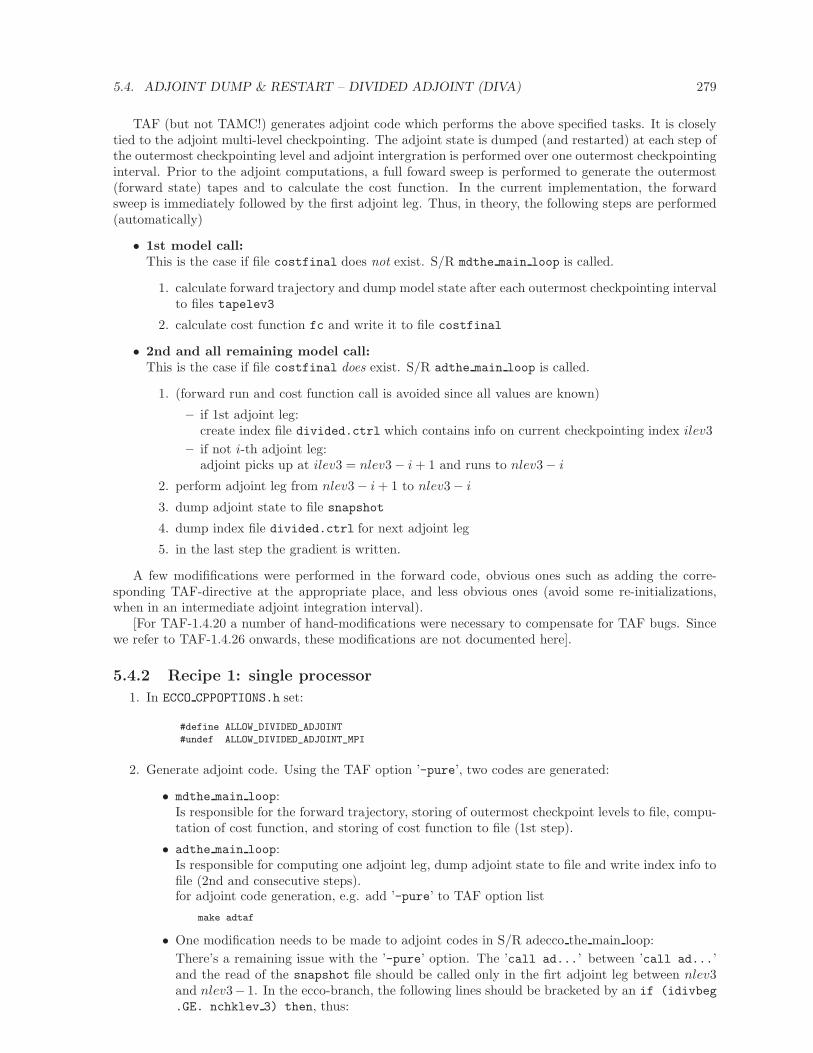
5.4. ADJOINT DUMP & RESTART – DIVIDED ADJOINT (DIVA) 279
TAF (but not TAMC!) generates adjoint code which performs the above specified tasks. It is closelytied to the adjoint multi-level checkpointing. The adjoint state is dumped (and restarted) at each step ofthe outermost checkpointing level and adjoint intergration is performed over one outermost checkpointinginterval. Prior to the adjoint computations, a full foward sweep is performed to generate the outermost(forward state) tapes and to calculate the cost function. In the current implementation, the forwardsweep is immediately followed by the first adjoint leg. Thus, in theory, the following steps are performed(automatically)
• 1st model call:This is the case if file costfinal does not exist. S/R mdthe main loop is called.
1. calculate forward trajectory and dump model state after each outermost checkpointing intervalto files tapelev3
2. calculate cost function fc and write it to file costfinal
• 2nd and all remaining model call:This is the case if file costfinal does exist. S/R adthe main loop is called.
1. (forward run and cost function call is avoided since all values are known)
– if 1st adjoint leg:create index file divided.ctrl which contains info on current checkpointing index ilev3
– if not i-th adjoint leg:adjoint picks up at ilev3 = nlev3 − i+ 1 and runs to nlev3 − i
2. perform adjoint leg from nlev3 − i+ 1 to nlev3 − i
3. dump adjoint state to file snapshot
4. dump index file divided.ctrl for next adjoint leg
5. in the last step the gradient is written.
A few modififications were performed in the forward code, obvious ones such as adding the corre-sponding TAF-directive at the appropriate place, and less obvious ones (avoid some re-initializations,when in an intermediate adjoint integration interval).
[For TAF-1.4.20 a number of hand-modifications were necessary to compensate for TAF bugs. Sincewe refer to TAF-1.4.26 onwards, these modifications are not documented here].
5.4.2 Recipe 1: single processor
1. In ECCO CPPOPTIONS.h set:
#define ALLOW_DIVIDED_ADJOINT
#undef ALLOW_DIVIDED_ADJOINT_MPI
2. Generate adjoint code. Using the TAF option ’-pure’, two codes are generated:
• mdthe main loop:Is responsible for the forward trajectory, storing of outermost checkpoint levels to file, compu-tation of cost function, and storing of cost function to file (1st step).
• adthe main loop:Is responsible for computing one adjoint leg, dump adjoint state to file and write index info tofile (2nd and consecutive steps).for adjoint code generation, e.g. add ’-pure’ to TAF option list
make adtaf
• One modification needs to be made to adjoint codes in S/R adecco the main loop:
There’s a remaining issue with the ’-pure’ option. The ’call ad...’ between ’call ad...’and the read of the snapshot file should be called only in the firt adjoint leg between nlev3and nlev3− 1. In the ecco-branch, the following lines should be bracketed by an if (idivbeg
.GE. nchklev 3) then, thus:
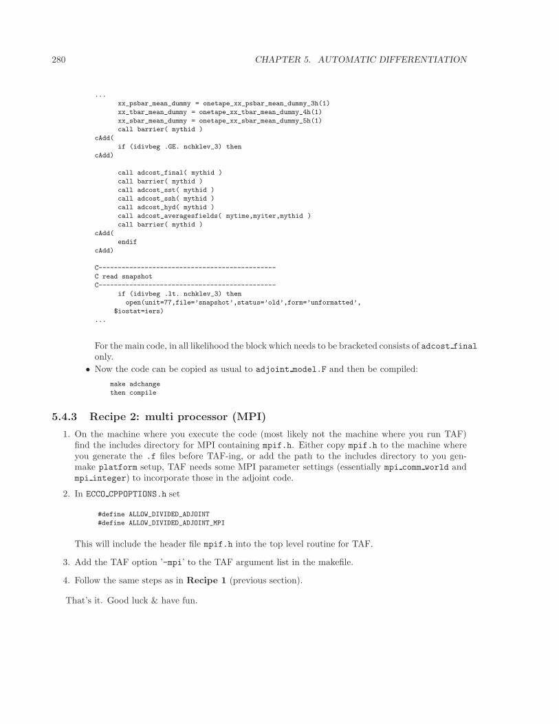
280 CHAPTER 5. AUTOMATIC DIFFERENTIATION
...
xx_psbar_mean_dummy = onetape_xx_psbar_mean_dummy_3h(1)
xx_tbar_mean_dummy = onetape_xx_tbar_mean_dummy_4h(1)
xx_sbar_mean_dummy = onetape_xx_sbar_mean_dummy_5h(1)
call barrier( mythid )
cAdd(
if (idivbeg .GE. nchklev_3) then
cAdd)
call adcost_final( mythid )
call barrier( mythid )
call adcost_sst( mythid )
call adcost_ssh( mythid )
call adcost_hyd( mythid )
call adcost_averagesfields( mytime,myiter,mythid )
call barrier( mythid )
cAdd(
endif
cAdd)
C----------------------------------------------
C read snapshot
C----------------------------------------------
if (idivbeg .lt. nchklev_3) then
open(unit=77,file=’snapshot’,status=’old’,form=’unformatted’,
$iostat=iers)
...
For the main code, in all likelihood the block which needs to be bracketed consists of adcost final
only.
• Now the code can be copied as usual to adjoint model.F and then be compiled:
make adchange
then compile
5.4.3 Recipe 2: multi processor (MPI)
1. On the machine where you execute the code (most likely not the machine where you run TAF)find the includes directory for MPI containing mpif.h. Either copy mpif.h to the machine whereyou generate the .f files before TAF-ing, or add the path to the includes directory to you gen-make platform setup, TAF needs some MPI parameter settings (essentially mpi comm world andmpi integer) to incorporate those in the adjoint code.
2. In ECCO CPPOPTIONS.h set
#define ALLOW_DIVIDED_ADJOINT
#define ALLOW_DIVIDED_ADJOINT_MPI
This will include the header file mpif.h into the top level routine for TAF.
3. Add the TAF option ’-mpi’ to the TAF argument list in the makefile.
4. Follow the same steps as in Recipe 1 (previous section).
That’s it. Good luck & have fun.
5.5. ADJOINT CODE GENERATION USING OPENAD 281
5.5 Adjoint code generation using OpenAD
Authors: Jean Utke, Patrick Heimbach and Chris Hill
5.5.1 Introduction
The development of OpenAD was initiated as part of the ACTS (Adjoint Compiler Technology & Stan-dards) project funded by the NSF Information Technology Research (ITR) program. The main goals forOpenAD initially defined for the ACTS project are:
1. develop a flexible, modular, open source tool that can ge‘nerate adjoint codes of numerical simulationprograms,
2. establish a platform for easy implementation and testing of source transformation algorithms via alanguage-independent abstract intermediate representation,
3. support for source code written in C and Fortan,
4. generate efficient tangent linear and adjoint for the MIT general circulation model.
OpenAD’s homepage is at http://www-unix.mcs.anl.gov/OpenAD/. A development WIKI is athttp://wiki.mcs.anl.gov/OpenAD/index.php/Main Page. From the WIKI’s main page, click on Handling
GCM for various aspects pertaining to differentiating the MITgcm with OpenAD.
5.5.2 Downloading and installing OpenAD
The OpenAD webpage has a detailed description on how to download and build OpenAD. From its home-page, please click on Download Test Binaries. You may either download pre-built binaries for quicktrial, or follow the detailed build process described at http://www-unix.mcs.anl.gov/OpenAD/access.html
5.5.3 Building MITgcm adjoint with OpenAD
17-January-2008OpenAD was successfully built on head node of itrda.acesgrid.org, for following system:
> uname -a
Linux itrda 2.6.22.2-42.fc6 #1 SMP Wed Aug 15 12:34:26 EDT 2007 i686 i686 i386 GNU/Linux
> cat /proc/version
Linux version 2.6.22.2-42.fc6 ([email protected])
(gcc version 4.1.2 20070626 (Red Hat 4.1.2-13)) #1 SMP Wed Aug 15 12:34:26 EDT 2007
> module load ifc/9.1.036 icc/9.1.042
Head of MITgcm branch (checkpoint59m with some modif.s) was used for building adjoint code.Following routing needed special care (revert to revision 1.1):MITgcm contrib/heimbach/OpenAD/OAD support/active module.f90

282 CHAPTER 5. AUTOMATIC DIFFERENTIATION
Chapter 6
Physical Parameterizations -Packages I
In this chapter and in the following chapter, the MITgcm “packages” are described. While you can carryout many experiments with MITgcm by starting from case studies in section 3.8, configuring a brand newexperiment or making major changes to an experimental configuration requires some knowledge of thepackages that make up the full MITgcm code. Packages are used in MITgcm to help organize and layervarious code building blocks that are assembled and selected to perform a specific experiment. Each of thespecific experiments described in section 3.8 uses a particular combination of packages. Figure 6.1 showsthe full set of packages that are available. As shown in the figure packages are classified into differentgroupings that layer on top of each other. The top layer packages are generally specialized to specificsimulation types. In this layer there are packages that deal with biogeochemical processes, ocean interiorand boundary layer processes, atmospheric processes, sea-ice, coupled simulations and state estimation.Below this layer are a set of general purpose numerical and computational packages. The general purposenumerical packages provide code for kernel numerical alogorithms that apply to many different simulationtypes. Similarly, the general purpose computational packages implement non-numerical alogorithms thatprovide parallelism, I/O and time-keeping functions that are used in many different scenarios.
The following sections describe the packages shown in figure 6.1. Section 6.1 describes the generalprocedure for using any package in MITgcm. Following that sections 6.2.1-7.4 layout the algorithmsimplemented in specific packages and describe how to use the individual packages. A brief synopsis ofthe function of each package is given in table 6.1. Organizationally package code is assigned a separatesubdirectory in the MITgcm code distribution (within the source code directory pkg). The name of thissubdirectory is used as the package name in table 6.1.
Table 6.1:.
283
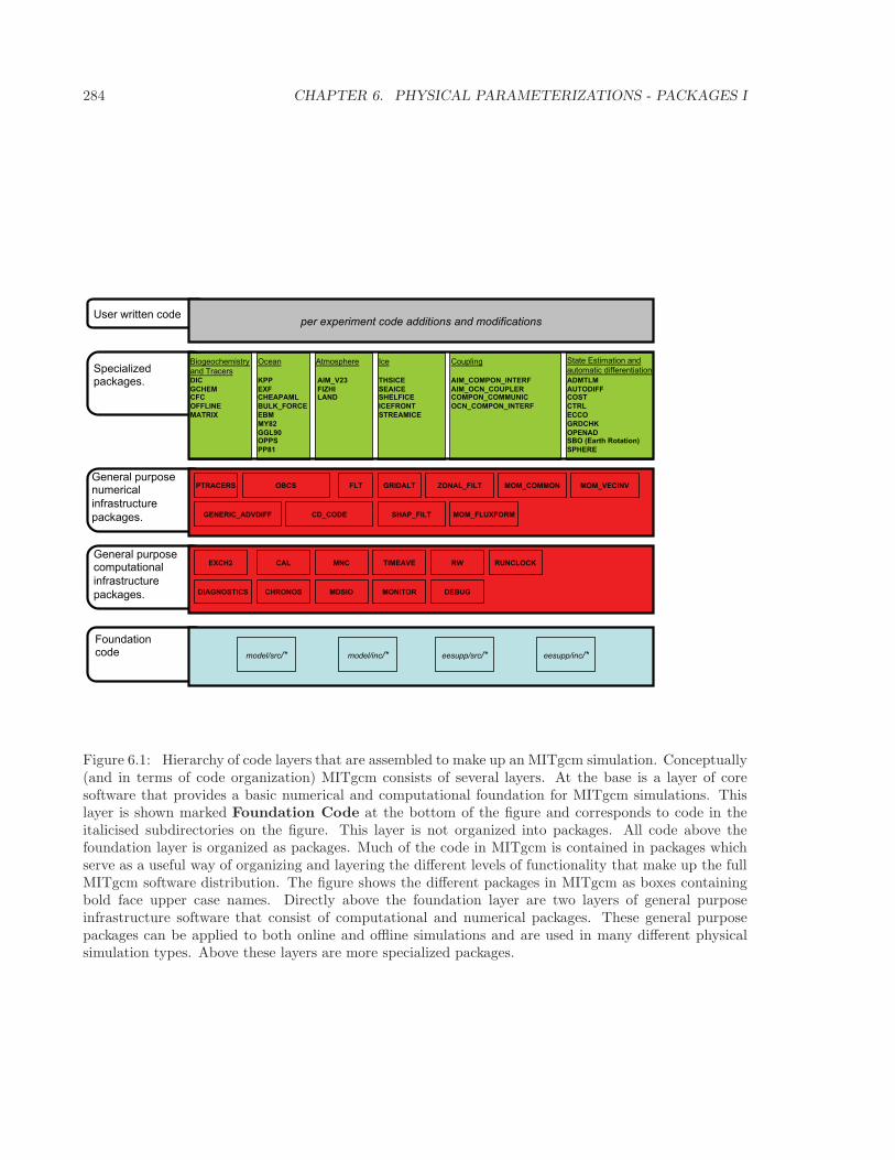
284 CHAPTER 6. PHYSICAL PARAMETERIZATIONS - PACKAGES I
!"#"$%&'()$(*+"',*-().%./*#%&'
/#0$%+.$),.)$"
(%,1%2"+3
4*)#5%./*#',*5"
6(",/%&/7"5'(%,1%2"+3
!"#$%&'()&* !"#$%&+,)&* $$'-..&'()&* $$'-..&+,)&*
8/*2"*,9"-/+.$:
%#5';$%,"$+!"#
$#%&'#(#
)((*"+&
',-."/
<,"%#
011
&/(#%&,1,'*
23*04().#&
&2'
'567
$$*89)11:
116;
&/#%7
=.-*+(9"$"
!",$+):-"#:
,"'4<7=
(">%"*,+!
>,"
!"#"$%&'()$(*+"'#)-"$/,%&'
/#0$%+.$),.)$"
(%,1%2"+3
1-.,#&.:
$&+&."#4,!<!"((
?*)(&/#2 6.%."'@+./-%./*#'%#5
%).*-%./,'5/00"$"#./%./*#
-%:"#&
:&,"#&:%&*("#&
"#&(.)+-
:-.&,'"#&
,"'4#)'1)+4"+-&.(
,"'4)#+4#)31*&.#)'1)+4#)''3+"#
)#+4#)'1)+4"+-&.(
,!'-*'
,3-)!"((#):-
#-.*
&##)
$.!#%0
)1&+,!:2)?@&ABCD?.ECACFEGH
:1%&.&
#,*
#%.)+):
)2#:
#!4#)!&
'+#
(*- $."!,*-
'!:")
-"'&,<&
')+"-).
>)+,*4("*-
:%,14("*-
.I
!&23$
')'4#)'')+
')'4(*3/().'
')'4<&#"+<
.3+#*)#0
.$(/$0.$(+!$,1/)"#$/2##+1+",'/2,#/!"#+3+)21+",'A+"$'B$/.."#',*5"
Figure 6.1: Hierarchy of code layers that are assembled to make up an MITgcm simulation. Conceptually(and in terms of code organization) MITgcm consists of several layers. At the base is a layer of coresoftware that provides a basic numerical and computational foundation for MITgcm simulations. Thislayer is shown marked Foundation Code at the bottom of the figure and corresponds to code in theitalicised subdirectories on the figure. This layer is not organized into packages. All code above thefoundation layer is organized as packages. Much of the code in MITgcm is contained in packages whichserve as a useful way of organizing and layering the different levels of functionality that make up the fullMITgcm software distribution. The figure shows the different packages in MITgcm as boxes containingbold face upper case names. Directly above the foundation layer are two layers of general purposeinfrastructure software that consist of computational and numerical packages. These general purposepackages can be applied to both online and offline simulations and are used in many different physicalsimulation types. Above these layers are more specialized packages.
6.1. USING MITGCM PACKAGES 285
6.1 Using MITgcm Packages
The set of packages that will be used within a partiucular model can be configured using a combinationof both “compile–time” and “run–time” options. Compile–time options are those used to select whichpackages will be “compiled in” or implemented within the program. Packages excluded at compile timeare completely absent from the executable program(s) and thus cannot be later activated by any set ofsubsequent run–time options.
6.1.1 Package Inclusion/Exclusion
There are numerous ways that one can specify compile–time package inclusion or exclusion and they areall implemented by the genmake2 program which was previously described in Section 3.4. The optionsare as follows:
1. Setting the genamake2 options --enable PKG and/or --disable PKG specifies inclusion or exclu-sion. This method is intended as a convenient way to perform a single (perhaps for a quick test)compilation.
2. By creating a text file with the name packages.conf in either the local build directory or the-mods=DIR directory, one can specify a list of packages (one package per line, with ’#’ as the commentcharacter) to be included. Since the packages.conf file can be saved, this is the preferred methodfor setting and recording (for future reference) the package configuration.
3. For convenience, a list of “standard” package groups is contained in the pkg/pkg groups file. Byselecting one of the package group names in the packages.conf file, one automatically obtains allpackages in that group.
4. By default (that is, if a packages.conf file is not found), the genmake2 program will use thepackage group default “default pkg list” as defined in pkg/pkg groups file.
5. To help prevent users from creating unusable package groups, the genmake2 program will parse thecontents of the pkg/pkg depend file to determine:
• whether any two requested packages cannot be simultaneously included (eg. seaice and thsiceare mutually exclusive),
• whether additional packages must be included in order to satisfy package dependencies (eg.rw depends upon functionality within the mdsio package), and
• whether the set of all requested packages is compatible with the dependencies (and producingan error if they aren’t).
Thus, as a result of the dependencies, additional packages may be added to those originally re-quested.
6.1.2 Package Activation
For run–time package control, MITgcm uses flags set through a data.pkg file. While some packages (eg.debug, mnc, exch2) may have their own usage conventions, most follow a simple flag naming conventionof the form:
usePackageName=.TRUE.
where the usePackageName variable can activate or disable the package at runtime. As mentioned previ-ously, packages must be included in order to be activated. Generally, such mistakes will be detected andreported as errors by the code. However, users should still be aware of the dependency.
6.1.3 Package Coding Standards
The following sections describe how to modify and/or create new MITgcm packages.
286 CHAPTER 6. PHYSICAL PARAMETERIZATIONS - PACKAGES I
6.1.3.1 Packages are Not Libraries
To a beginner, the MITgcm packages may resemble libraries as used in myriad software projects. Whilefuture versions are likely to implement packages as libraries (perhaps using FORTRAN90/95 syntax) thecurrent packages (FORTRAN77) are not based upon any concept of libraries.
6.1.3.2 File Inclusion Rules
Instead, packages should be viewed only as directories containing “sets of source files” that are built usingsome simple mechanisms provided by genmake2. Conceptually, the build process adds files as they arefound and proceeds according to the following rules:
1. genmake2 locates a “core” or main set of source files (the -standarddirs option sets these locationsand the default value contains the directories eesupp and model).
2. genmake2 then finds additional source files by inspecting the contents of each of the package direc-tories:
(a) As the new files are found, they are added to a list of source files.
(b) If there is a file name “collision” (that is, if one of the files in a package has the same name asone of the files previously encountered) then the file within the newer (more recently visited)package will superseed (or “hide”) any previous file(s) with the same name.
(c) Packages are visited (and thus files discovered) in the order that the packages are enabled withingenmake2. Thus, the files in PackB may superseed the files in PackA if PackA is enabled beforePackB. Thus, package ordering can be significant! For this reason, genmake2 honors the orderin which packages are specified.
These rules were adopted since they provide a relatively simple means for rapidly including (or “hid-ing”) existing files with modified versions.
6.1.3.3 Conditional Compilation and PACKAGES CONFIG.h
Given that packages are simply groups of files that may be added or removed to form a whole, one maywonder how linking (that is, FORTRAN symbol resolution) is handled. This is the second way thatgenmake2 supports the concept of packages. Basically, genmake2 creates a Makefile that, in turn, is ableto create a file called PACKAGES CONFIG.h that contains a set of C pre-processor (or “CPP”) directivessuch as:
#undef ALLOW_KPP
#undef ALLOW_LAND
...
#define ALLOW_GENERIC_ADVDIFF
#define ALLOW_MDSIO
...
These CPP symbols are then used throughout the code to conditionally isolate variable definitions,function calls, or any other code that depends upon the presence or absence of any particular package.
An example illustrating the use of these defines is:
#ifdef ALLOW_GMREDI
IF (useGMRedi) CALL GMREDI_CALC_DIFF(
I bi,bj,iMin,iMax,jMin,jMax,K,
I maskUp,
O KappaRT,KappaRS,
I myThid)
#endif
which is included from the file calc diffusivity.F and shows how both the compile–time ALLOW GMREDI
flag and the run–time useGMRedi are nested.
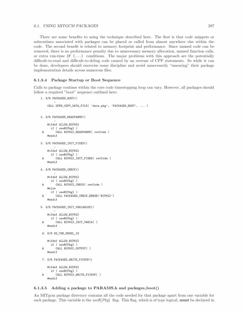
6.1. USING MITGCM PACKAGES 287
There are some benefits to using the technique described here. The first is that code snippets orsubroutines associated with packages can be placed or called from almost anywhere else within thecode. The second benefit is related to memory footprint and performance. Since unused code can beremoved, there is no performance penalty due to unnecessary memory allocation, unused function calls,or extra run-time IF (...) conditions. The major problems with this approach are the potentiallydifficult-to-read and difficult-to-debug code caused by an overuse of CPP statements. So while it canbe done, developers should exerecise some discipline and avoid unnecesarily “smearing” their packageimplementation details across numerous files.
6.1.3.4 Package Startup or Boot Sequence
Calls to package routines within the core code timestepping loop can vary. However, all packages shouldfollow a required ”boot” sequence outlined here:
1. S/R PACKAGES_BOOT()
:
CALL OPEN_COPY_DATA_FILE( ’data.pkg’, ’PACKAGES_BOOT’, ... )
2. S/R PACKAGES_READPARMS()
:
#ifdef ALLOW_$PKG
if ( use$Pkg )
& CALL $PKG_READPARMS( retCode )
#endif
3. S/R PACKAGES_INIT_FIXED()
:
#ifdef ALLOW_$PKG
if ( use$Pkg )
& CALL $PKG_INIT_FIXED( retCode )
#endif
4. S/R PACKAGES_CHECK()
:
#ifdef ALLOW_$PKG
if ( use$Pkg )
& CALL $PKG_CHECK( retCode )
#else
if ( use$Pkg )
& CALL PACKAGES_CHECK_ERROR(’$PKG’)
#endif
5. S/R PACKAGES_INIT_VARIABLES()
:
#ifdef ALLOW_$PKG
if ( use$Pkg )
& CALL $PKG_INIT_VARIA( )
#endif
6. S/R DO_THE_MODEL_IO
#ifdef ALLOW_$PKG
if ( use$Pkg )
& CALL $PKG_OUTPUT( )
#endif
7. S/R PACKAGES_WRITE_PICKUP()
#ifdef ALLOW_$PKG
if ( use$Pkg )
& CALL $PKG_WRITE_PICKUP( )
#endif
6.1.3.5 Adding a package to PARAMS.h and packages boot()
An MITgcm package directory contains all the code needed for that package apart from one variable foreach package. This variable is the use$Pkg flag. This flag, which is of type logical, must be declared in
288 CHAPTER 6. PHYSICAL PARAMETERIZATIONS - PACKAGES I
the shared header file PARAMS.h in the PARM PACKAGES block. This convention is used to supporta single runtime control file data.pkg which is read by the startup routine packages boot() and that sets aflag controlling the runtime use of a package. This routine needs to be able to read the flags for packagesthat were not built at compile time. Therefore when adding a new package, in addition to creating theper-package directory in the pkg/ subdirectory a developer should add a use$Pkg flag to PARAMS.hand a use$Pkg entry to the packages boot() PACKAGES namelist. The only other package specificcode that should appear outside the individual package directory are calls to the specific package API.
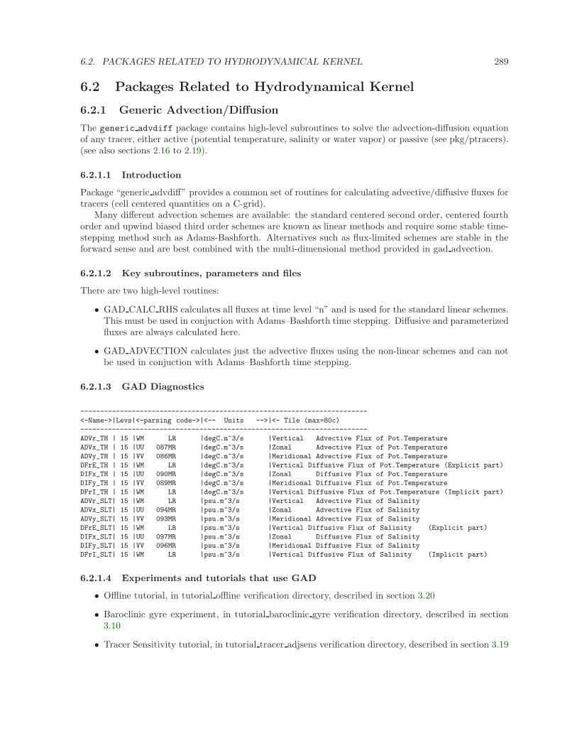
6.2. PACKAGES RELATED TO HYDRODYNAMICAL KERNEL 289
6.2 Packages Related to Hydrodynamical Kernel
6.2.1 Generic Advection/Diffusion
The generic advdiff package contains high-level subroutines to solve the advection-diffusion equationof any tracer, either active (potential temperature, salinity or water vapor) or passive (see pkg/ptracers).(see also sections 2.16 to 2.19).
6.2.1.1 Introduction
Package “generic advdiff” provides a common set of routines for calculating advective/diffusive fluxes fortracers (cell centered quantities on a C-grid).
Many different advection schemes are available: the standard centered second order, centered fourthorder and upwind biased third order schemes are known as linear methods and require some stable time-stepping method such as Adams-Bashforth. Alternatives such as flux-limited schemes are stable in theforward sense and are best combined with the multi-dimensional method provided in gad advection.
6.2.1.2 Key subroutines, parameters and files
There are two high-level routines:
• GAD CALC RHS calculates all fluxes at time level “n” and is used for the standard linear schemes.This must be used in conjuction with Adams–Bashforth time stepping. Diffusive and parameterizedfluxes are always calculated here.
• GAD ADVECTION calculates just the advective fluxes using the non-linear schemes and can notbe used in conjuction with Adams–Bashforth time stepping.
6.2.1.3 GAD Diagnostics
------------------------------------------------------------------------
<-Name->|Levs|<-parsing code->|<-- Units -->|<- Tile (max=80c)
------------------------------------------------------------------------
ADVr_TH | 15 |WM LR |degC.m^3/s |Vertical Advective Flux of Pot.Temperature
ADVx_TH | 15 |UU 087MR |degC.m^3/s |Zonal Advective Flux of Pot.Temperature
ADVy_TH | 15 |VV 086MR |degC.m^3/s |Meridional Advective Flux of Pot.Temperature
DFrE_TH | 15 |WM LR |degC.m^3/s |Vertical Diffusive Flux of Pot.Temperature (Explicit part)
DIFx_TH | 15 |UU 090MR |degC.m^3/s |Zonal Diffusive Flux of Pot.Temperature
DIFy_TH | 15 |VV 089MR |degC.m^3/s |Meridional Diffusive Flux of Pot.Temperature
DFrI_TH | 15 |WM LR |degC.m^3/s |Vertical Diffusive Flux of Pot.Temperature (Implicit part)
ADVr_SLT| 15 |WM LR |psu.m^3/s |Vertical Advective Flux of Salinity
ADVx_SLT| 15 |UU 094MR |psu.m^3/s |Zonal Advective Flux of Salinity
ADVy_SLT| 15 |VV 093MR |psu.m^3/s |Meridional Advective Flux of Salinity
DFrE_SLT| 15 |WM LR |psu.m^3/s |Vertical Diffusive Flux of Salinity (Explicit part)
DIFx_SLT| 15 |UU 097MR |psu.m^3/s |Zonal Diffusive Flux of Salinity
DIFy_SLT| 15 |VV 096MR |psu.m^3/s |Meridional Diffusive Flux of Salinity
DFrI_SLT| 15 |WM LR |psu.m^3/s |Vertical Diffusive Flux of Salinity (Implicit part)
6.2.1.4 Experiments and tutorials that use GAD
• Offline tutorial, in tutorial offline verification directory, described in section 3.20
• Baroclinic gyre experiment, in tutorial baroclinic gyre verification directory, described in section3.10
• Tracer Sensitivity tutorial, in tutorial tracer adjsens verification directory, described in section 3.19
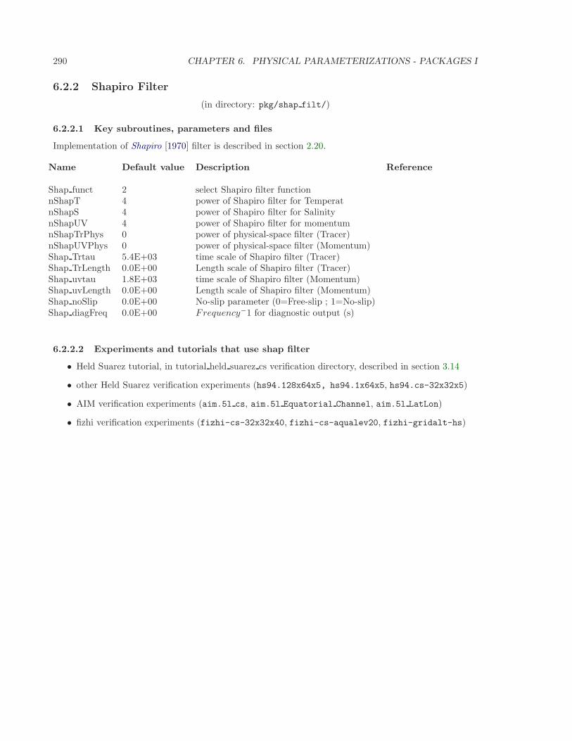
290 CHAPTER 6. PHYSICAL PARAMETERIZATIONS - PACKAGES I
6.2.2 Shapiro Filter
(in directory: pkg/shap filt/)
6.2.2.1 Key subroutines, parameters and files
Implementation of Shapiro [1970] filter is described in section 2.20.
Name Default value Description Reference
Shap funct 2 select Shapiro filter functionnShapT 4 power of Shapiro filter for TemperatnShapS 4 power of Shapiro filter for SalinitynShapUV 4 power of Shapiro filter for momentumnShapTrPhys 0 power of physical-space filter (Tracer)nShapUVPhys 0 power of physical-space filter (Momentum)Shap Trtau 5.4E+03 time scale of Shapiro filter (Tracer)Shap TrLength 0.0E+00 Length scale of Shapiro filter (Tracer)Shap uvtau 1.8E+03 time scale of Shapiro filter (Momentum)Shap uvLength 0.0E+00 Length scale of Shapiro filter (Momentum)Shap noSlip 0.0E+00 No-slip parameter (0=Free-slip ; 1=No-slip)Shap diagFreq 0.0E+00 Frequency−1 for diagnostic output (s)
6.2.2.2 Experiments and tutorials that use shap filter
• Held Suarez tutorial, in tutorial held suarez cs verification directory, described in section 3.14
• other Held Suarez verification experiments (hs94.128x64x5, hs94.1x64x5, hs94.cs-32x32x5)
• AIM verification experiments (aim.5l cs, aim.5l Equatorial Channel, aim.5l LatLon)
• fizhi verification experiments (fizhi-cs-32x32x40, fizhi-cs-aqualev20, fizhi-gridalt-hs)
6.2. PACKAGES RELATED TO HYDRODYNAMICAL KERNEL 291
6.2.3 FFT Filtering Code
(in directory: pkg/zonal filt/)
6.2.3.1 Key subroutines, parameters and files
6.2.3.2 Experiments and tutorials that use zonal filter
• Held Suarez verification experiment (hs94.128x64x5)
• AIM verification experiment (aim.5l LatLon)
292 CHAPTER 6. PHYSICAL PARAMETERIZATIONS - PACKAGES I
6.2.4 exch2: Extended Cubed Sphere Topology
6.2.4.1 Introduction
The exch2 package extends the original cubed sphere topology configuration to allow more flexible domaindecomposition and parallelization. Cube faces (also called subdomains) may be divided into any numberof tiles that divide evenly into the grid point dimensions of the subdomain. Furthermore, the tiles can runon separate processors individually or in groups, which provides for manual compile-time load balancingacross a relatively arbitrary number of processors.
The exchange parameters are declared in pkg/exch2/W2 EXCH2 TOPOLOGY.h and assigned in pkg/exch2/w2 e2setup.F.The validity of the cube topology depends on the SIZE.h file as detailed below. The default files pro-vided in the release configure a cubed sphere topology of six tiles, one per subdomain, each with 32×32grid points, with all tiles running on a single processor. Both files are generated by Matlab scripts inutils/exch2/matlab-topology-generator; see Section 6.2.4.3 Generating Topology Files for exch2 fordetails on creating alternate topologies. Pregenerated examples of these files with alternate topologiesare provided under utils/exch2/code-mods along with the appropriate SIZE.h file for single-processorexecution.
6.2.4.2 Invoking exch2
To use exch2 with the cubed sphere, the following conditions must be met:
• The exch2 package is included when genmake2 is run. The easiest way to do this is to add the lineexch2 to the packages.conf file – see Section 3.4 Building the code for general details.
• An example of W2 EXCH2 TOPOLOGY.h and w2 e2setup.F must reside in a directory containing filessymbolically linked by the genmake2 script. The safest place to put these is the directory indicatedin the -mods=DIR command line modifier (typically ../code), or the build directory. The defaultversions of these files reside in pkg/exch2 and are linked automatically if no other versions existelsewhere in the build path, but they should be left untouched to avoid breaking configurationsother than the one you intend to modify.
• Files containing grid parameters, named tile00n.mitgrid where n=(1:6) (one per subdomain),must be in the working directory when the MITgcm executable is run. These files are provided inthe example experiments for cubed sphere configurations with 32×32 cube sides – please contactMITgcm support if you want to generate files for other configurations.
• As always when compiling MITgcm, the file SIZE.h must be placed where genmake2 will find it.In particular for exch2, the domain decomposition specified in SIZE.h must correspond with theparticular configuration’s topology specified in W2 EXCH2 TOPOLOGY.h and w2 e2setup.F. Domaindecomposition issues particular to exch2 are addressed in Section 6.2.4.3 Generating Topology Filesfor exch2 and 6.2.4.4 exch2, SIZE.h, and Multiprocessing ; a more general background on the subjectrelevant to MITgcm is presented in Section 4.3.1 Specifying a decomposition.
At the time of this writing the following examples use exch2 and may be used for guidance:
verification/adjust_nlfs.cs-32x32x1
verification/adjustment.cs-32x32x1
verification/aim.5l_cs
verification/global_ocean.cs32x15
verification/hs94.cs-32x32x5
6.2.4.3 Generating Topology Files for exch2
Alternate cubed sphere topologies may be created using the Matlab scripts in utils/exch2/matlab-topology-generator.Running the m-file driver.m from the Matlab prompt (there are no parameters to pass) generates exch2topology files W2 EXCH2 TOPOLOGY.h and w2 e2setup.F in the working directory and displays a figure ofthe topology via Matlab – figures 6.4, 6.3, and 6.2 are examples of the generated diagrams. The otherm-files in the directory are subroutines called from driver.m and should not be run “bare” except for
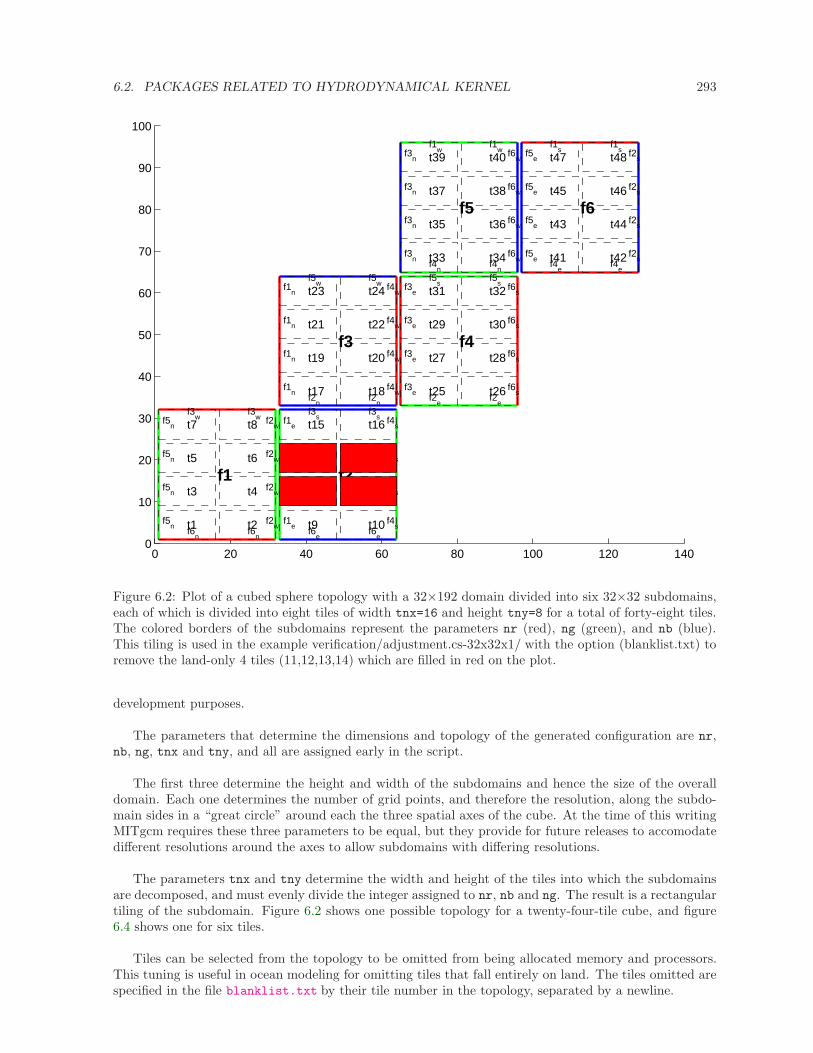
6.2. PACKAGES RELATED TO HYDRODYNAMICAL KERNEL 293
0 20 40 60 80 100 120 1400
10
20
30
40
50
60
70
80
90
100
f1
t1f5n
f6n
t2f6n
f2w
t3f5n t4 f2
w
t5f5n t6 f2
w
t7f5n
f3w
t8f3
w f2w
f2
t9f1e
f6e
t10f6e
f4s
t11f1e t12 f4
s
t13f1e t14 f4
s
t15f1e
f3s
t16f3
s f4s
f3
t17f1n
f2n
t18f2n
f4w
t19f1n t20 f4
w
t21f1n t22 f4
w
t23f1n
f5w
t24f5
w f4w
f4
t25f3e
f2e
t26f2e
f6s
t27f3e t28 f6
s
t29f3e t30 f6
s
t31f3e
f5s
t32f5
s f6s
f5
t33f3n
f4n
t34f4n
f6w
t35f3n t36 f6
w
t37f3n t38 f6
w
t39f3n
f1w
t40f1
w f6w
f6
t41f5e
f4e
t42f4e
f2s
t43f5e t44 f2
s
t45f5e t46 f2
s
t47f5e
f1s
t48f1
s f2s
Figure 6.2: Plot of a cubed sphere topology with a 32×192 domain divided into six 32×32 subdomains,each of which is divided into eight tiles of width tnx=16 and height tny=8 for a total of forty-eight tiles.The colored borders of the subdomains represent the parameters nr (red), ng (green), and nb (blue).This tiling is used in the example verification/adjustment.cs-32x32x1/ with the option (blanklist.txt) toremove the land-only 4 tiles (11,12,13,14) which are filled in red on the plot.
development purposes.
The parameters that determine the dimensions and topology of the generated configuration are nr,nb, ng, tnx and tny, and all are assigned early in the script.
The first three determine the height and width of the subdomains and hence the size of the overalldomain. Each one determines the number of grid points, and therefore the resolution, along the subdo-main sides in a “great circle” around each the three spatial axes of the cube. At the time of this writingMITgcm requires these three parameters to be equal, but they provide for future releases to accomodatedifferent resolutions around the axes to allow subdomains with differing resolutions.
The parameters tnx and tny determine the width and height of the tiles into which the subdomainsare decomposed, and must evenly divide the integer assigned to nr, nb and ng. The result is a rectangulartiling of the subdomain. Figure 6.2 shows one possible topology for a twenty-four-tile cube, and figure6.4 shows one for six tiles.
Tiles can be selected from the topology to be omitted from being allocated memory and processors.This tuning is useful in ocean modeling for omitting tiles that fall entirely on land. The tiles omitted arespecified in the file blanklist.txt by their tile number in the topology, separated by a newline.
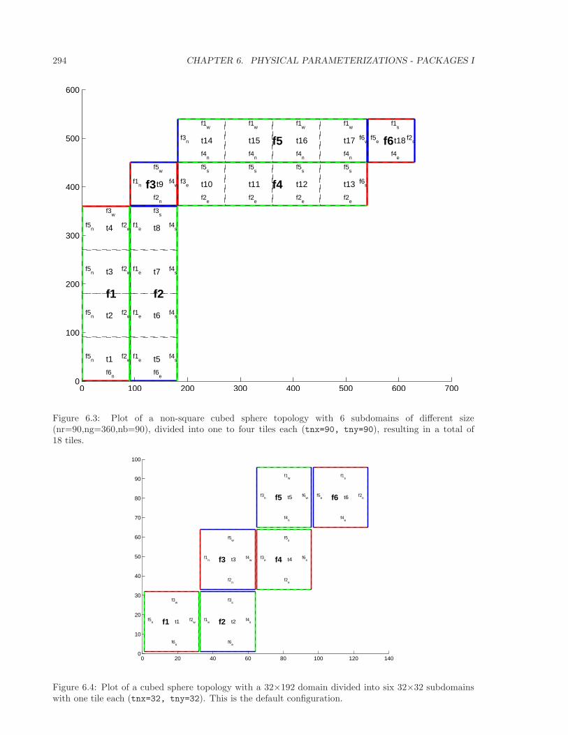
294 CHAPTER 6. PHYSICAL PARAMETERIZATIONS - PACKAGES I
0 100 200 300 400 500 600 7000
100
200
300
400
500
600
f1
t1f5n
f6n
f2w
t2f5n
f2w
t3f5n
f2w
t4f5n
f3w
f2w
f2
t5f1e
f6e
f4s
t6f1e
f4s
t7f1e
f4s
t8f1e
f3s
f4s
f3 t9f1n
f5w
f2n
f4w f4t10f3
e
f5s
f2e
t11
f5s
f2e
t12
f5s
f2e
t13
f5s
f2e
f6s
f5t14f3n
f1w
f4n
t15
f1w
f4n
t16
f1w
f4n
t17
f1w
f4n
f6w f6 t18f5
e
f1s
f4e
f2s
Figure 6.3: Plot of a non-square cubed sphere topology with 6 subdomains of different size(nr=90,ng=360,nb=90), divided into one to four tiles each (tnx=90, tny=90), resulting in a total of18 tiles.
0 20 40 60 80 100 120 1400
10
20
30
40
50
60
70
80
90
100
f1 t1f5n
f3w
f6n
f2w f2 t2f1
e
f3s
f6e
f4s
f3 t3f1n
f5w
f2n
f4w f4 t4f3
e
f5s
f2e
f6s
f5 t5f3n
f1w
f4n
f6w f6 t6f5
e
f1s
f4e
f2s
Figure 6.4: Plot of a cubed sphere topology with a 32×192 domain divided into six 32×32 subdomainswith one tile each (tnx=32, tny=32). This is the default configuration.
6.2. PACKAGES RELATED TO HYDRODYNAMICAL KERNEL 295
6.2.4.4 exch2, SIZE.h, and Multiprocessing
Once the topology configuration files are created, the Fortran PARAMETERs in SIZE.h must be configured tomatch. Section 4.3.1 Specifying a decomposition provides a general description of domain decompositionwithin MITgcm and its relation to SIZE.h. The current section specifies constraints that the exch2package imposes and describes how to enable parallel execution with MPI.
As in the general case, the parameters sNx and sNy define the size of the individual tiles, and so mustbe assigned the same respective values as tnx and tny in driver.m.
The halo width parameters OLx and OLy have no special bearing on exch2 and may be assigned as inthe general case. The same holds for Nr, the number of vertical levels in the model.
The parameters nSx, nSy, nPx, and nPy relate to the number of tiles and how they are distributed onprocessors. When using exch2, the tiles are stored in the x dimension, and so nSy=1 in all cases. Sincethe tiles as configured by exch2 cannot be split up accross processors without regenerating the topology,nPy=1 as well.
The number of tiles MITgcm allocates and how they are distributed between processors depends onnPx and nSx. nSx is the number of tiles per processor and nPx is the number of processors. The totalnumber of tiles in the topology minus those listed in blanklist.txt must equal nSx*nPx. Note that inorder to obtain maximum usage from a given number of processors in some cases, this restriction mightentail sharing a processor with a tile that would otherwise be excluded because it is topographicallyoutside of the domain and therefore in blanklist.txt. For example, suppose you have five processorsand a domain decomposition of thirty-six tiles that allows you to exclude seven tiles. To evenly distributethe remaining twenty-nine tiles among five processors, you would have to run one “dummy” tile to makean even six tiles per processor. Such dummy tiles are not listed in blanklist.txt.
The following is an example of SIZE.h for the six-tile configuration illustrated in figure 6.4 runningon one processor:
PARAMETER (
& sNx = 32,
& sNy = 32,
& OLx = 2,
& OLy = 2,
& nSx = 6,
& nSy = 1,
& nPx = 1,
& nPy = 1,
& Nx = sNx*nSx*nPx,
& Ny = sNy*nSy*nPy,
& Nr = 5)
The following is an example for the forty-eight-tile topology in figure 6.2 running on six processors:
PARAMETER (
& sNx = 16,
& sNy = 8,
& OLx = 2,
& OLy = 2,
& nSx = 8,
& nSy = 1,
& nPx = 6,
& nPy = 1,
& Nx = sNx*nSx*nPx,
& Ny = sNy*nSy*nPy,
& Nr = 5)
6.2.4.5 Key Variables
The descriptions of the variables are divided up into scalars, one-dimensional arrays indexed to the tilenumber, and two and three-dimensional arrays indexed to tile number and neighboring tile. This divi-sion reflects the functionality of these variables: The scalars are common to every part of the topology,
296 CHAPTER 6. PHYSICAL PARAMETERIZATIONS - PACKAGES I
the tile-indexed arrays to individual tiles, and the arrays indexed by tile and neighbor to relationshipsbetween tiles and their neighbors.
Scalars:The number of tiles in a particular topology is set with the parameter NTILES, and the maximum
number of neighbors of any tiles by MAX NEIGHBOURS. These parameters are used for defining the size ofthe various one and two dimensional arrays that store tile parameters indexed to the tile number and areassigned in the files generated by driver.m.
The scalar parameters exch2 domain nxt and exch2 domain nyt express the number of tiles in the xand y global indices. For example, the default setup of six tiles (Fig. 6.4) has exch2 domain nxt=6 andexch2 domain nyt=1. A topology of forty-eight tiles, eight per subdomain (as in figure 6.2), will haveexch2 domain nxt=12 and exch2 domain nyt=4. Note that these parameters express the tile layout inorder to allow global data files that are tile-layout-neutral. They have no bearing on the internal storageof the arrays. The tiles are stored internally in a range from bi=(1:NTILES) in the x axis, and the y axisvariable bj is assumed to equal 1 throughout the package.
Arrays indexed to tile number:The following arrays are of length NTILES and are indexed to the tile number, which is indicated in
the diagrams with the notation tn. The indices are omitted in the descriptions.
The arrays exch2 tnx and exch2 tny express the x and y dimensions of each tile. At present for eachtile exch2 tnx=sNx and exch2 tny=sNy, as assigned in SIZE.h and described in Section 6.2.4.4 exch2,SIZE.h, and Multiprocessing. Future releases of MITgcm may allow varying tile sizes.
The arrays exch2 tbasex and exch2 tbasey determine the tiles’ Cartesian origin within a subdo-main and locate the edges of different tiles relative to each other. As an example, in the default six-tiletopology (Fig. 6.4) each index in these arrays is set to 0 since a tile occupies its entire subdomain. Thetwenty-four-tile case discussed above will have values of 0 or 16, depending on the quadrant of the tilewithin the subdomain. The elements of the arrays exch2 txglobalo and exch2 txglobalo are similarto exch2 tbasex and exch2 tbasey, but locate the tile edges within the global address space, similar tothat used by global output and input files.
The array exch2 myFace contains the number of the subdomain of each tile, in a range (1:6) inthe case of the standard cube topology and indicated by fn in figures 6.4 and 6.2. exch2 nNeighbours
contains a count of the neighboring tiles each tile has, and sets the bounds for looping over neighboringtiles. exch2 tProc holds the process rank of each tile, and is used in interprocess communication.
The arrays exch2 isWedge, exch2 isEedge, exch2 isSedge, and exch2 isNedge are set to 1 if theindexed tile lies on the edge of its subdomain, 0 if not. The values are used within the topology generatorto determine the orientation of neighboring tiles, and to indicate whether a tile lies on the corner of asubdomain. The latter case requires special exchange and numerical handling for the singularities at theeight corners of the cube.
Arrays Indexed to Tile Number and Neighbor:The following arrays have vectors of length MAX NEIGHBOURS and NTILES and describe the orientations
between the the tiles.
The array exch2 neighbourId(a,T) holds the tile number Tn for each of the tile number T’s neigh-boring tiles a. The neighbor tiles are indexed (1:exch2 nNeighbours(T)) in the order right to left onthe north then south edges, and then top to bottom on the east then west edges.
The exch2 opposingSend record(a,T) array holds the index b of the element in exch2 neighbourId(b,Tn)
that holds the tile number T, given Tn=exch2 neighborId(a,T). In other words,
exch2_neighbourId( exch2_opposingSend_record(a,T),
exch2_neighbourId(a,T) ) = T
6.2. PACKAGES RELATED TO HYDRODYNAMICAL KERNEL 297
This provides a back-reference from the neighbor tiles.
The arrays exch2 pi and exch2 pj specify the transformations of indices in exchanges between theneighboring tiles. These transformations are necessary in exchanges between subdomains because a hor-izontal dimension in one subdomain may map to other horizonal dimension in an adjacent subdomain,and may also have its indexing reversed. This swapping arises from the “folding” of two-dimensionalarrays into a three-dimensional cube.
The dimensions of exch2 pi(t,N,T) and exch2 pj(t,N,T) are the neighbor ID N and the tile numberT as explained above, plus a vector of length 2 containing transformation factors t. The first element ofthe transformation vector holds the factor to multiply the index in the same dimension, and the secondelement holds the the same for the orthogonal dimension. To clarify, exch2 pi(1,N,T) holds the mappingof the x axis index of tile T to the x axis of tile T’s neighbor N, and exch2 pi(2,N,T) holds the mappingof T’s x index to the neighbor N’s y index.
One of the two elements of exch2 pi or exch2 pj for a given tile T and neighbor N will be 0, reflectingthe fact that the two axes are orthogonal. The other element will be 1 or -1, depending on whetherthe axes are indexed in the same or opposite directions. For example, the transform vector of the arraysfor all tile neighbors on the same subdomain will be (1,0), since all tiles on the same subdomain areoriented identically. An axis that corresponds to the orthogonal dimension with the same index directionin a particular tile-neighbor orientation will have (0,1). Those with the opposite index direction willhave (0,-1) in order to reverse the ordering.
The arrays exch2 oi, exch2 oj, exch2 oi f, and exch2 oj f are indexed to tile number and neigh-bor and specify the relative offset within the subdomain of the array index of a variable going from aneighboring tile N to a local tile T. Consider T=1 in the six-tile topology (Fig. 6.4), where
exch2_oi(1,1)=33
exch2_oi(2,1)=0
exch2_oi(3,1)=32
exch2_oi(4,1)=-32
The simplest case is exch2 oi(2,1), the southern neighbor, which is Tn=6. The axes of T and Tn
have the same orientation and their x axes have the same origin, and so an exchange between thetwo requires no changes to the x index. For the western neighbor (Tn=5), code oi(3,1)=32 since thex=0 vector on T corresponds to the y=32 vector on Tn. The eastern edge of T shows the reverse case(exch2 oi(4,1)=-32)), where x=32 on T exchanges with x=0 on Tn=2.
The most interesting case, where exch2 oi(1,1)=33 and Tn=3, involves a reversal of indices. As inevery case, the offset exch2 oi is added to the original x index of T multiplied by the transformationfactor exch2 pi(t,N,T). Here exch2 pi(1,1,1)=0 since the x axis of T is orthogonal to the x axis ofTn. exch2 pi(2,1,1)=-1 since the x axis of T corresponds to the y axis of Tn, but the index is reversed.The result is that the index of the northern edge of T, which runs (1:32), is transformed to (-1:-32).exch2 oi(1,1) is then added to this range to get back (32:1) – the index of the y axis of Tn relative toT. This transformation may seem overly convoluted for the six-tile case, but it is necessary to provide ageneral solution for various topologies.
Finally, exch2 itlo c, exch2 ithi c, exch2 jtlo c and exch2 jthi c hold the location and indexbounds of the edge segment of the neighbor tile N’s subdomain that gets exchanged with the local tile T.To take the example of tile T=2 in the forty-eight-tile topology (Fig. 6.2):
exch2_itlo_c(4,2)=17
exch2_ithi_c(4,2)=17
exch2_jtlo_c(4,2)=0
exch2_jthi_c(4,2)=33
298 CHAPTER 6. PHYSICAL PARAMETERIZATIONS - PACKAGES I
Here N=4, indicating the western neighbor, which is Tn=1. Tn resides on the same subdomain as T, sothe tiles have the same orientation and the same x and y axes. The x axis is orthogonal to the westernedge and the tile is 16 points wide, so exch2 itlo c and exch2 ithi c indicate the column beyond Tn’seastern edge, in that tile’s halo region. Since the border of the tiles extends through the entire height ofthe subdomain, the y axis bounds exch2 jtlo c to exch2 jthi c cover the height of (1:32), plus 1 ineither direction to cover part of the halo.
For the north edge of the same tile T=2 where N=1 and the neighbor tile is Tn=5:
exch2_itlo_c(1,2)=0
exch2_ithi_c(1,2)=0
exch2_jtlo_c(1,2)=0
exch2_jthi_c(1,2)=17
T’s northern edge is parallel to the x axis, but since Tn’s y axis corresponds to T’s x axis, T’s northernedge exchanges with Tn’s western edge. The western edge of the tiles corresponds to the lower boundof the x axis, so exch2 itlo c and exch2 ithi c are 0, in the western halo region of Tn. The range ofexch2 jtlo c and exch2 jthi c correspond to the width of T’s northern edge, expanded by one into thehalo.
6.2.4.6 Key Routines
Most of the subroutines particular to exch2 handle the exchanges themselves and are of the same formatas those described in 4.3.3.3 Cube sphere communication. Like the original routines, they are written astemplates which the local Makefile converts from RX into RL and RS forms.
The interfaces with the core model subroutines are EXCH UV XY RX, EXCH UV XYZ RX and EXCH XY RX.They override the standard exchange routines when genmake2 is run with exch2 option. They in turncall the local exch2 subroutines EXCH2 UV XY RX and EXCH2 UV XYZ RX for two and three-dimensionalvector quantities, and EXCH2 XY RX and EXCH2 XYZ RX for two and three-dimensional scalar quantities.These subroutines set the dimensions of the area to be exchanged, call EXCH2 RX1 CUBE for scalars andEXCH2 RX2 CUBE for vectors, and then handle the singularities at the cube corners.
The separate scalar and vector forms of EXCH2 RX1 CUBE and EXCH2 RX2 CUBE reflect that the vector-handling subroutine needs to pass both the u and v components of the physical vectors. This swappingarises from the topological folding discussed above, where the x and y axes get swapped in some cases,and is not an issue with the scalar case. These subroutines call EXCH2 SEND RX1 and EXCH2 SEND RX2,which do most of the work using the variables discussed above.
6.2.4.7 Experiments and tutorials that use exch2
• Held Suarez tutorial, in tutorial held suarez cs verification directory, described in section 3.14
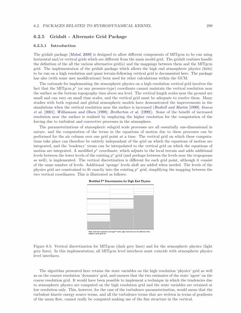
6.2. PACKAGES RELATED TO HYDRODYNAMICAL KERNEL 299
6.2.5 Gridalt - Alternate Grid Package
6.2.5.1 Introduction
The gridalt package [Molod, 2009] is designed to allow different components of MITgcm to be run usinghorizontal and/or vertical grids which are different from the main model grid. The gridalt routines handlethe definition of the all the various alternative grid(s) and the mappings between them and the MITgcmgrid. The implementation of the gridalt package which allows the high end atmospheric physics (fizhi)to be run on a high resolution and quasi terrain-following vertical grid is documented here. The packagehas also (with some user modifications) been used for other calculations within the GCM.
The rationale for implementing the atmospheric physics on a high resolution vertical grid involves thefact that the MITgcm p∗ (or any pressure-type) coordinate cannot maintain the vertical resolution nearthe surface as the bottom topography rises above sea level. The vertical length scales near the ground aresmall and can vary on small time scales, and the vertical grid must be adequate to resolve them. Manystudies with both regional and global atmospheric models have demonstrated the improvements in thesimulations when the vertical resolution near the surface is increased (Bushell and Martin [1999]; Innesset al. [2001]; Williamson and Olsen [1998]; Bretherton et al. [1999]). Some of the benefit of increasedresolution near the surface is realized by employing the higher resolution for the computation of theforcing due to turbulent and convective processes in the atmosphere.
The parameterizations of atmospheric subgrid scale processes are all essentially one-dimensional innature, and the computation of the terms in the equations of motion due to these processes can beperformed for the air column over one grid point at a time. The vertical grid on which these computa-tions take place can therefore be entirely independant of the grid on which the equations of motion areintegrated, and the ’tendency’ terms can be interpolated to the vertical grid on which the equations ofmotion are integrated. A modified p∗ coordinate, which adjusts to the local terrain and adds additionallevels between the lower levels of the existing p∗ grid (and perhaps between the levels near the tropopauseas well), is implemented. The vertical discretization is different for each grid point, although it consistof the same number of levels. Additional ’sponge’ levels aloft are added when needed. The levels of thephysics grid are constrained to fit exactly into the existing p∗ grid, simplifying the mapping between thetwo vertical coordinates. This is illustrated as follows:
Figure 6.5: Vertical discretization for MITgcm (dark grey lines) and for the atmospheric physics (lightgrey lines). In this implementation, all MITgcm level interfaces must coincide with atmospheric physicslevel interfaces.
The algorithm presented here retains the state variables on the high resolution ’physics’ grid as wellas on the coarser resolution ’dynamics‘ grid, and ensures that the two estimates of the state ’agree’ on thecoarse resolution grid. It would have been possible to implement a technique in which the tendencies dueto atmospheric physics are computed on the high resolution grid and the state variables are retained atlow resolution only. This, however, for the case of the turbulence parameterization, would mean that theturbulent kinetic energy source terms, and all the turbulence terms that are written in terms of gradientsof the mean flow, cannot really be computed making use of the fine structure in the vertical.
300 CHAPTER 6. PHYSICAL PARAMETERIZATIONS - PACKAGES I
6.2.5.2 Equations on Both Grids
In addition to computing the physical forcing terms of the momentum, thermodynamic and humidityequations on the modified (higher resolution) grid, the higher resolution structure of the atmosphere (theboundary layer) is retained between physics calculations. This neccessitates a second set of evolutionequations for the atmospheric state variables on the modified grid. If the equation for the evolution of Uon p∗ can be expressed as:
∂U
∂t
∣∣∣∣total
p∗
=∂U
∂t
∣∣∣∣dynamics
p∗
+∂U
∂t
∣∣∣∣physics
p∗
where the physics forcing terms on p∗ have been mapped from the modified grid, then an additionalequation to govern the evolution of U (for example) on the modified grid is written:
∂U
∂t
∣∣∣∣total
p∗m
=∂U
∂t
∣∣∣∣dynamics
p∗m
+∂U
∂t
∣∣∣∣physics
p∗m
+ γ(U |p∗ − U |p∗m)
where p∗m refers to the modified higher resolution grid, and the dynamics forcing terms have been mappedfrom p∗ space. The last term on the RHS is a relaxation term, meant to constrain the state variables onthe modified vertical grid to ‘track’ the state variables on the p∗ grid on some time scale, governed by γ.In the present implementation, γ = 1, requiring an immediate agreement between the two ’states’.
6.2.5.3 Time stepping Sequence
If we write Tphys as the temperature (or any other state variable) on the high resolution physics grid,and Tdyn as the temperature on the coarse vertical resolution dynamics grid, then:
1. Compute the tendency due to physics processes.
2. Advance the physics state: T n+1∗∗phys(l) = T n
phys(l) + δTphys.
3. Interpolate the physics tendency to the dynamics grid, and advance the dynamics state by physicsand dynamics tendencies: T n+1
dyn(L) = T ndyn(L) + δTdyn(L) + [δTphys(l)](L).
4. Interpolate the dynamics tendency to the physics grid, and update the physics grid due to dynamicstendencies: T n+1∗
phys(l) = T n+1∗∗phys(l) + δTdyn(L)(l).
5. Apply correction term to physics state to account for divergence from dynamics state: T n+1phys(l)
= T n+1∗phys(l) + γTdyn(L) − [Tphys(l)](L)(l).
Where γ = 1 here.
6.2.5.4 Interpolation
In order to minimize the correction terms for the state variables on the alternative, higher resolution grid,the vertical interpolation scheme must be constructed so that a dynamics-to-physics interpolation can beexactly reversed with a physics-to-dynamics mapping. The simple scheme employed to achieve this is:
Coarse to fine: For all physics layers l in dynamics layer L, Tphys(l) = Tdyn(L) = Tdyn(L).Fine to coarse: For all physics layers l in dynamics layer L, Tdyn(L) = [Tphys(l)] =
∫Tphysdp.
Where is defined as the dynamics-to-physics operator and [] is the physics-to-dynamics operator,T stands for any state variable, and the subscripts phys and dyn stand for variables on the physics anddynamics grids, respectively.
6.2.5.5 Key subroutines, parameters and files
One of the central elements of the gridalt package is the routine which is called from subroutine gri-dalt initialise to define the grid to be used for the high end physics calculations. Routine make phys gridpasses back the parameters which define the grid, ultimately stored in the common block gridalt mapping.
6.2. PACKAGES RELATED TO HYDRODYNAMICAL KERNEL 301
subroutine make_phys_grid(drF,hfacC,im1,im2,jm1,jm2,Nr,
. Nsx,Nsy,i1,i2,j1,j2,bi,bj,Nrphys,Lbot,dpphys,numlevphys,nlperdyn)
c***********************************************************************
c Purpose: Define the grid that the will be used to run the high-end
c atmospheric physics.
c
c Algorithm: Fit additional levels of some (~) known thickness in
c between existing levels of the grid used for the dynamics
c
c Need: Information about the dynamics grid vertical spacing
c
c Input: drF - delta r (p*) edge-to-edge
c hfacC - fraction of grid box above topography
c im1, im2 - beginning and ending i - dimensions
c jm1, jm2 - beginning and ending j - dimensions
c Nr - number of levels in dynamics grid
c Nsx,Nsy - number of processes in x and y direction
c i1, i2 - beginning and ending i - index to fill
c j1, j2 - beginning and ending j - index to fill
c bi, bj - x-dir and y-dir index of process
c Nrphys - number of levels in physics grid
c
c Output: dpphys - delta r (p*) edge-to-edge of physics grid
c numlevphys - number of levels used in the physics
c nlperdyn - physics level number atop each dynamics layer
c
c NOTES: 1) Pressure levs are built up from bottom, using p0, ps and dp:
c p(i,j,k)=p(i,j,k-1) + dp(k)*ps(i,j)/p0(i,j)
c 2) Output dp’s are aligned to fit EXACTLY between existing
c levels of the dynamics vertical grid
c 3) IMPORTANT! This routine assumes the levels are numbered
c from the bottom up, ie, level 1 is the surface.
c IT WILL NOT WORK OTHERWISE!!!
c 4) This routine does NOT work for surface pressures less
c (ie, above in the atmosphere) than about 350 mb
c***********************************************************************
In the case of the grid used to compute the atmospheric physical forcing (fizhi package), the locationsof the grid points move in time with the MITgcm p∗ coordinate, and subroutine gridalt update is calledduring the run to update the locations of the grid points:
subroutine gridalt_update(myThid)
c***********************************************************************
c Purpose: Update the pressure thicknesses of the layers of the
c alternative vertical grid (used now for atmospheric physics).
c
c Calculate: dpphys - new delta r (p*) edge-to-edge of physics grid
c using dpphys0 (initial value) and rstarfacC
c***********************************************************************
The gridalt package also supplies utility routines which perform the mappings from one grid to the other.These routines are called from the code which computes the fields on the alternative (fizhi) grid.
subroutine dyn2phys(qdyn,pedyn,im1,im2,jm1,jm2,lmdyn,Nsx,Nsy,
. idim1,idim2,jdim1,jdim2,bi,bj,windphy,pephy,Lbot,lmphy,nlperdyn,
. flg,qphy)
C***********************************************************************
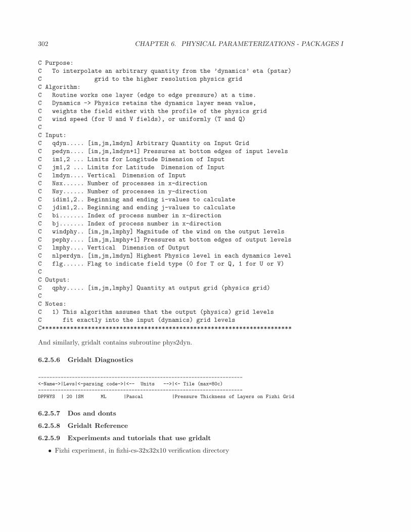
302 CHAPTER 6. PHYSICAL PARAMETERIZATIONS - PACKAGES I
C Purpose:
C To interpolate an arbitrary quantity from the ’dynamics’ eta (pstar)
C grid to the higher resolution physics grid
C Algorithm:
C Routine works one layer (edge to edge pressure) at a time.
C Dynamics -> Physics retains the dynamics layer mean value,
C weights the field either with the profile of the physics grid
C wind speed (for U and V fields), or uniformly (T and Q)
C
C Input:
C qdyn..... [im,jm,lmdyn] Arbitrary Quantity on Input Grid
C pedyn.... [im,jm,lmdyn+1] Pressures at bottom edges of input levels
C im1,2 ... Limits for Longitude Dimension of Input
C jm1,2 ... Limits for Latitude Dimension of Input
C lmdyn.... Vertical Dimension of Input
C Nsx...... Number of processes in x-direction
C Nsy...... Number of processes in y-direction
C idim1,2.. Beginning and ending i-values to calculate
C jdim1,2.. Beginning and ending j-values to calculate
C bi....... Index of process number in x-direction
C bj....... Index of process number in x-direction
C windphy.. [im,jm,lmphy] Magnitude of the wind on the output levels
C pephy.... [im,jm,lmphy+1] Pressures at bottom edges of output levels
C lmphy.... Vertical Dimension of Output
C nlperdyn. [im,jm,lmdyn] Highest Physics level in each dynamics level
C flg...... Flag to indicate field type (0 for T or Q, 1 for U or V)
C
C Output:
C qphy..... [im,jm,lmphy] Quantity at output grid (physics grid)
C
C Notes:
C 1) This algorithm assumes that the output (physics) grid levels
C fit exactly into the input (dynamics) grid levels
C***********************************************************************
And similarly, gridalt contains subroutine phys2dyn.
6.2.5.6 Gridalt Diagnostics
------------------------------------------------------------------------
<-Name->|Levs|<-parsing code->|<-- Units -->|<- Tile (max=80c)
------------------------------------------------------------------------
DPPHYS | 20 |SM ML |Pascal |Pressure Thickness of Layers on Fizhi Grid
6.2.5.7 Dos and donts
6.2.5.8 Gridalt Reference
6.2.5.9 Experiments and tutorials that use gridalt
• Fizhi experiment, in fizhi-cs-32x32x10 verification directory
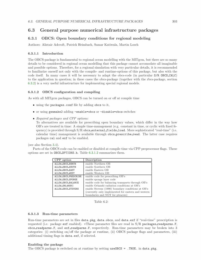
6.3. GENERAL PURPOSE NUMERICAL INFRASTRUCTURE PACKAGES 303
6.3 General purpose numerical infrastructure packages
6.3.1 OBCS: Open boundary conditions for regional modeling
Authors: Alistair Adcroft, Patrick Heimbach, Samar Katiwala, Martin Losch
6.3.1.1 Introduction
The OBCS-package is fundamental to regional ocean modelling with the MITgcm, but there are so manydetails to be considered in regional ocean modelling that this package cannot accomodate all imaginableand possible options. Therefore, for a regional simulation with very particular details, it is recommendedto familiarize oneself not only with the compile- and runtime-options of this package, but also with thecode itself. In many cases it will be necessary to adapt the obcs-code (in particular S/R OBCS CALC)to the application in question; in these cases the obcs-package (together with the rbcs-package, section6.3.2) is a very useful infrastructure for implementing special regional models.
6.3.1.2 OBCS configuration and compiling
As with all MITgcm packages, OBCS can be turned on or off at compile time
• using the packages.conf file by adding obcs to it,
• or using genmake2 adding -enable=obcs or -disable=obcs switches
• Required packages and CPP options:To alternatives are available for prescribing open boundary values, which differ in the way howOB’s are treated in time: A simple time-management (e.g. constant in time, or cyclic with fixed fe-quency) is provided through S/R obcs external fields load. More sophisticated “real-time” (i.e.calendar time) management is available through obcs prescribe read. The latter case requirespackages cal and exf to be enabled.
(see also Section 3.4).Parts of the OBCS code can be enabled or disabled at compile time via CPP preprocessor flags. These
options are set in OBCS OPTIONS.h. Table 6.3.1.2 summarizes them.
CPP option Description
ALLOW OBCS NORTH enable Northern OBALLOW OBCS SOUTH enable Southern OBALLOW OBCS EAST enable Eastern OBALLOW OBCS WEST enable Western OBALLOW OBCS PRESCRIBE enable code for prescribing OB’sALLOW OBCS SPONGE enable sponge layer codeALLOW OBCS BALANCE enable code for balancing transports through OB’sALLOW ORLANSKI enable Orlanski radiation conditions at OB’sALLOW OBCS STEVENS enable Stevens (1990) boundary conditions at OB’s
(currently only implemented for eastern and westernboundaries and NOT for ptracers)
Table 6.2:
6.3.1.3 Run-time parameters
Run-time parameters are set in files data.pkg, data.obcs, and data.exf if “real-time” prescription isrequested (i.e. package exf enabled). vThese parameter files are read in S/R packages readparms.F,obcs readparms.F, and exf readparms.F, respectively. Run-time parameters may be broken into 3categories: (i) switching on/off the package at runtime, (ii) OBCS package flags and parameters, (iii)additional timing flags in data.exf, if selected.
Enabling the packageThe OBCS package is switched on at runtime by setting useOBCS = .TRUE. in data.pkg.
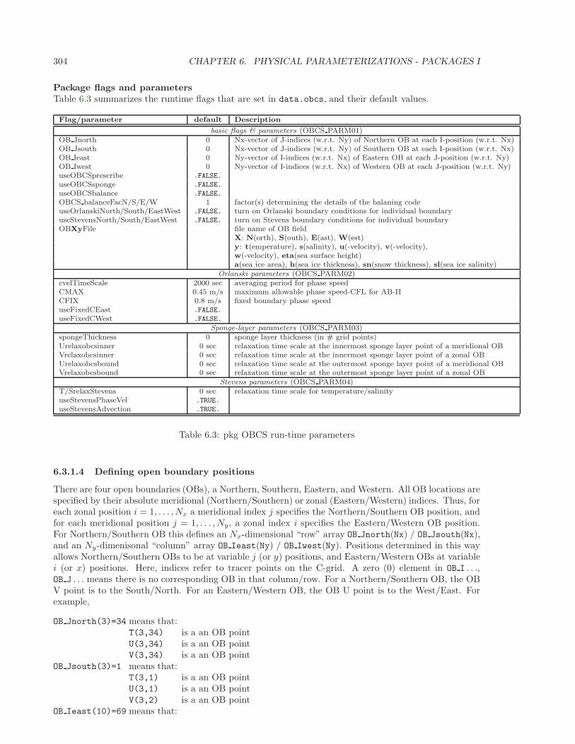
304 CHAPTER 6. PHYSICAL PARAMETERIZATIONS - PACKAGES I
Package flags and parametersTable 6.3 summarizes the runtime flags that are set in data.obcs, and their default values.
Flag/parameter default Description
basic flags & parameters (OBCS PARM01)OB Jnorth 0 Nx-vector of J-indices (w.r.t. Ny) of Northern OB at each I-position (w.r.t. Nx)OB Jsouth 0 Nx-vector of J-indices (w.r.t. Ny) of Southern OB at each I-position (w.r.t. Nx)OB Ieast 0 Ny-vector of I-indices (w.r.t. Nx) of Eastern OB at each J-position (w.r.t. Ny)OB Iwest 0 Ny-vector of I-indices (w.r.t. Nx) of Western OB at each J-position (w.r.t. Ny)useOBCSprescribe .FALSE.
useOBCSsponge .FALSE.
useOBCSbalance .FALSE.
OBCS balanceFacN/S/E/W 1 factor(s) determining the details of the balaning codeuseOrlanskiNorth/South/EastWest .FALSE. turn on Orlanski boundary conditions for individual boundaryuseStevensNorth/South/EastWest .FALSE. turn on Stevens boundary conditions for individual boundaryOBXyFile file name of OB field
X: N(orth), S(outh), E(ast), W(est)y: t(emperature), s(salinity), u(-velocity), v(-velocity),w(-velocity), eta(sea surface height)a(sea ice area), h(sea ice thickness), sn(snow thickness), sl(sea ice salinity)
Orlanski parameters (OBCS PARM02)cvelTimeScale 2000 sec averaging period for phase speedCMAX 0.45 m/s maximum allowable phase speed-CFL for AB-IICFIX 0.8 m/s fixed boundary phase speeduseFixedCEast .FALSE.
useFixedCWest .FALSE.
Sponge-layer parameters (OBCS PARM03)spongeThickness 0 sponge layer thickness (in # grid points)Urelaxobcsinner 0 sec relaxation time scale at the innermost sponge layer point of a meridional OBVrelaxobcsinner 0 sec relaxation time scale at the innermost sponge layer point of a zonal OBUrelaxobcsbound 0 sec relaxation time scale at the outermost sponge layer point of a meridional OBVrelaxobcsbound 0 sec relaxation time scale at the outermost sponge layer point of a zonal OB
Stevens parameters (OBCS PARM04)T/SrelaxStevens 0 sec relaxation time scale for temperature/salinityuseStevensPhaseVel .TRUE.
useStevensAdvection .TRUE.
Table 6.3: pkg OBCS run-time parameters
6.3.1.4 Defining open boundary positions
There are four open boundaries (OBs), a Northern, Southern, Eastern, and Western. All OB locations arespecified by their absolute meridional (Northern/Southern) or zonal (Eastern/Western) indices. Thus, foreach zonal position i = 1, . . . , Nx a meridional index j specifies the Northern/Southern OB position, andfor each meridional position j = 1, . . . , Ny, a zonal index i specifies the Eastern/Western OB position.For Northern/Southern OB this defines an Nx-dimensional “row” array OB Jnorth(Nx) / OB Jsouth(Nx),and an Ny-dimenisonal “column” array OB Ieast(Ny) / OB Iwest(Ny). Positions determined in this wayallows Northern/Southern OBs to be at variable j (or y) positions, and Eastern/Western OBs at variablei (or x) positions. Here, indices refer to tracer points on the C-grid. A zero (0) element in OB I . . .,OB J . . . means there is no corresponding OB in that column/row. For a Northern/Southern OB, the OBV point is to the South/North. For an Eastern/Western OB, the OB U point is to the West/East. Forexample,
OB Jnorth(3)=34 means that:T(3,34) is a an OB pointU(3,34) is a an OB pointV(3,34) is a an OB point
OB Jsouth(3)=1 means that:T(3,1) is a an OB pointU(3,1) is a an OB pointV(3,2) is a an OB point
OB Ieast(10)=69 means that:
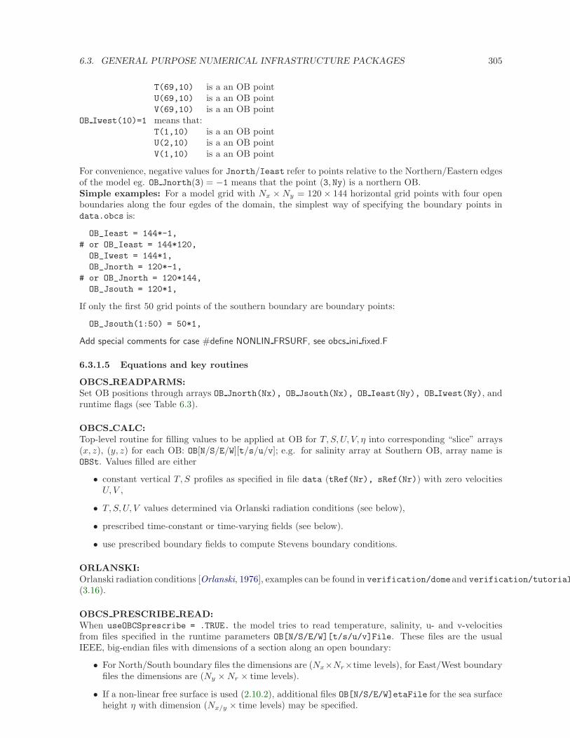
6.3. GENERAL PURPOSE NUMERICAL INFRASTRUCTURE PACKAGES 305
T(69,10) is a an OB pointU(69,10) is a an OB pointV(69,10) is a an OB point
OB Iwest(10)=1 means that:T(1,10) is a an OB pointU(2,10) is a an OB pointV(1,10) is a an OB point
For convenience, negative values for Jnorth/Ieast refer to points relative to the Northern/Eastern edgesof the model eg. OB Jnorth(3) = −1 means that the point (3, Ny) is a northern OB.Simple examples: For a model grid with Nx ×Ny = 120 × 144 horizontal grid points with four openboundaries along the four egdes of the domain, the simplest way of specifying the boundary points indata.obcs is:
OB_Ieast = 144*-1,
# or OB_Ieast = 144*120,
OB_Iwest = 144*1,
OB_Jnorth = 120*-1,
# or OB_Jnorth = 120*144,
OB_Jsouth = 120*1,
If only the first 50 grid points of the southern boundary are boundary points:
OB_Jsouth(1:50) = 50*1,
Add special comments for case #define NONLIN FRSURF, see obcs ini fixed.F
6.3.1.5 Equations and key routines
OBCS READPARMS:Set OB positions through arrays OB Jnorth(Nx), OB Jsouth(Nx), OB Ieast(Ny), OB Iwest(Ny), andruntime flags (see Table 6.3).
OBCS CALC:Top-level routine for filling values to be applied at OB for T, S, U, V, η into corresponding “slice” arrays(x, z), (y, z) for each OB: OB[N/S/E/W][t/s/u/v]; e.g. for salinity array at Southern OB, array name isOBSt. Values filled are either
• constant vertical T, S profiles as specified in file data (tRef(Nr), sRef(Nr)) with zero velocitiesU, V ,
• T, S, U, V values determined via Orlanski radiation conditions (see below),
• prescribed time-constant or time-varying fields (see below).
• use prescribed boundary fields to compute Stevens boundary conditions.
ORLANSKI:Orlanski radiation conditions [Orlanski, 1976], examples can be found in verification/domeand verification/tutorial
(3.16).
OBCS PRESCRIBE READ:When useOBCSprescribe = .TRUE. the model tries to read temperature, salinity, u- and v-velocitiesfrom files specified in the runtime parameters OB[N/S/E/W][t/s/u/v]File. These files are the usualIEEE, big-endian files with dimensions of a section along an open boundary:
• For North/South boundary files the dimensions are (Nx×Nr×time levels), for East/West boundaryfiles the dimensions are (Ny ×Nr × time levels).
• If a non-linear free surface is used (2.10.2), additional files OB[N/S/E/W]etaFile for the sea surfaceheight η with dimension (Nx/y × time levels) may be specified.
306 CHAPTER 6. PHYSICAL PARAMETERIZATIONS - PACKAGES I
• If non-hydrostatic dynamics are used (2.9), additional files OB[N/S/E/W]wFile for the verticalvelocity w with dimensions (Nx/y ×Nr × time levels) can be specified.
• If useSEAICE=.TRUE. then additional files OB[N/S/E/W][a,h,sl,sn,uice,vice] for sea ice area,thickness (HEFF), seaice salinity, snow and ice velocities (Nx/y × time levels) can be specified.
As in S/R external fields load or the exf-package, the code reads two time levels for each variable,e.g. OBNu0 and OBNu1, and interpolates linearly between these time levels to obtain the value OBNu
at the current model time (step). When the exf-package is used, the time levels are controlled foreach boundary separately in the same way as the exf-fields in data.exf, namelist EXF NML OBCS. Theruntime flags follow the above naming conventions, e.g. for the western boundary the correspondingflags are OBCWstartdate1/2 and OBCWperiod. Sea-ice boundary values are controlled separately withsiobWstartdate1/2 and siobWperiod. When the exf-package is not used, the time levels are controlledby the runtime flags externForcingPeriod and externForcingCycle in data, see verification/exp4
for an example.
OBCS CALC STEVENS:(THE IMPLEMENTATION OF THESE BOUNDARY CONDITIONS IS NOT COMPLETE. PASSIVETRACERS, SEA ICE AND NON-LINEAR FREE SURFACE ARE NOT SUPPORTED PROPERLY.)The boundary conditions following Stevens [1990] require the vertically averaged normal velocity (origi-nally specified as a stream function along the open boundary) uob and the tracer fields χob (note: passivetracers are currently not implemented and the code stops when package ptracers is used together withthis option). Currently, the code vertically averages the normal velocity as specified in OB[E,W]u orOB[N,S]v. From these prescribed values the code computes the boundary values for the next timestepn+ 1 as follows (as an example, we use the notation for an eastern or western boundary):
• un+1(y, z) = uob(y) + (u′)n(y, z), where (u′)n is the deviation from the vertically averaged velocityat timestep n on the boundary. (u′)n is computed in the previous time step n from the intermediatevelocity u∗ prior to the correction step (see section 2.2, e.g., eq. (2.17)). (This velocity is not availableat the beginning of the next time step n + 1, when S/R OBCS CALC/OBCS CALC STEVENSare called, therefore it needs to be saved in S/R DYNAMICS by calling S/R OBCS SAVE UV Nand also stored in a separate restart files pickup_stevens[N/S/E/W].$iteration.data)
• If un+1 is directed into the model domain, the boudary value for tracer χ is restored to the prescribedvalues:
χn+1 = χn +∆t
τχ(χob − χn),
where τχ is the relaxation time scale T/SrelaxStevens. The new χn+1 is then subject to theadvection by un+1.
• If un+1 is directed out of the model domain, the tracer χn+1 on the boundary at timestep n+ 1 isestimated from advection out of the domain with un+1 + c, where c is a phase velocity estimatedas 1
2∂χ∂t /
∂χ∂x . The numerical scheme is (as an example for an eastern boundary):
χn+1ib,j,k = χn
ib,j,k + ∆t(un+1 + c)ib,j,k
χnib,j,k − χn
ib−1,j,k
∆xCib,j
, if un+1ib,j,k > 0,
where ib is the boundary index.For test purposes, the phase velocity contribution or the entire advection can be turned off by settingthe corresponding parameters useStevensPhaseVel and useStevensAdvection to .FALSE..
See Stevens [1990] for details. With this boundary condition specifying the exact net transport acrossthe open boundary is simple, so that balancing the flow with (S/R OBCS BALANCE FLOW, see nextparagraph) is usually not necessary.
6.3. GENERAL PURPOSE NUMERICAL INFRASTRUCTURE PACKAGES 307
OBCS BALANCE FLOW:When turned on (ALLOW OBCS BALANCE defined in OBCS OPTIONS.h and useOBCSbalance=.true. indata.obcs/OBCS PARM01), this routine balances the net flow across the open boundaries. By default thenet flow across the boundaries is computed and all normal velocities on boundaries are adjusted to obtainzero net inflow.
This behavior can be controlled with the runtime flags OBCS balanceFacN/S/E/W. The values of theseflags determine how the net inflow is redistributed as small correction velocities between the individualsections. A value “-1” balances an individual boundary, values > 0 determine the relative size of thecorrection. For example, the values
OBCS balanceFacE = 1.,
OBCS balanceFacW = -1.,
OBCS balanceFacN = 2.,
OBCS balanceFacS = 0.,
make the model
• correct Western OBWu by substracting a uniform velocity to ensure zero net transport through theWestern open boundary;
• correct Eastern and Northern normal flow, with the Northern velocity correction two times largerthan the Eastern correction, but not the Southern normal flow, to ensure that the total inflowthrough East, Northern, and Southern open boundary is balanced.
The old method of balancing the net flow for all sections individually can be recovered by setting allflags to -1. Then the normal velocities across each of the four boundaries are modified separately, so thatthe net volume transport across each boundary is zero. For example, for the western boundary at i = ib,the modified velocity is:
u(y, z)−∫
western boundaryu dy dz ≈ OBNu(j, k) −
∑
j,k
OBNu(j, k)hw(ib, j, k)∆yG(ib, j)∆z(k).
This also ensures a net total inflow of zero through all boundaries, but this combination of flags is notuseful if you want to simulate, say, a sector of the Southern Ocean with a strong ACC entering throughthe western and leaving through the eastern boundary, because the value of “-1” for these flags will makesure that the strong inflow is removed. Clearly, gobal balancing with OBCS balanceFacE/W/N/S ≥ 0 isthe preferred method.
OBCS APPLY *:
OBCS SPONGE:The sponge layer code (turned on with ALLOW OBCS SPONGE and useOBCSsponge) adds a relaxation termto the right-hand-side of the momentum and tracer equations. The variables are relaxed towards theboundary values with a relaxation time scale that increases linearly with distance from the boundary
G(sponge)χ = −χ− [(L− δL)χBC + δLχ]/L
[(L− δL)τb + δLτi]/L= −χ− [(1 − l)χBC + lχ]
[(1 − l)τb + lτi]
where χ is the model variable (U/V/T/S) in the interior, χBC the boundary value, L the thickness of thesponge layer (runtime parameter spongeThickness in number of grid points), δL ∈ [0, L] ( δL
L = l ∈ [0, 1])the distance from the boundary (also in grid points), and τb (runtime parameters Urelaxobcsbound
and Vrelaxobcsbound) and τi (runtime parameters Urelaxobcsinner and Vrelaxobcsinner) the re-laxation time scales on the boundary and at the interior termination of the sponge layer. The param-eters Urelaxobcsbound/inner set the relaxation time scales for the Eastern and Western boundaries,Vrelaxobcsbound/inner for the Northern and Southern boundaries.
OB’s with nonlinear free surface
308 CHAPTER 6. PHYSICAL PARAMETERIZATIONS - PACKAGES I
6.3.1.6 Flow chart
C !CALLING SEQUENCE:
c ...
6.3.1.7 OBCS diagnostics
Diagnostics output is available via the diagnostics package (see Section 7.1). Available output fields aresummarized in Table 6.3.1.7.
------------------------------------------------------
<-Name->|Levs|grid|<-- Units -->|<- Tile (max=80c)
------------------------------------------------------
Table 6.4:
6.3.1.8 Reference experiments
In the directory verifcation, the following experiments use obcs:
• exp4: box with 4 open boundaries, simulating flow over a Gaussian bump based on Adcroft et al.[1997], also tests Stevens-boundary conditions;
• dome: based on the project “Dynamics of Overflow Mixing and Entrainment” (http://www.rsmas.miami.edu/personal/tauses Orlanski-BCs;
• internal wave: uses a heavily modified S/R OBCS CALC
• seaice obcs: simple example who to use the sea-ice related code, based on lab sea;
• tutorial plume on slope: uses Orlanski-BCs, see also section 3.16.
6.3.1.9 References
6.3.1.10 Experiments and tutorials that use obcs
• tutorial plume on slope (section 3.16)
6.3. GENERAL PURPOSE NUMERICAL INFRASTRUCTURE PACKAGES 309
6.3.2 RBCS Package
6.3.2.1 Introduction
A package which provides the flexibility to relax fields (temperature, salinity, ptracers) in any 3-D location:so could be used as a sponge layer, or as a ”source” anywhere in the domain.
For a tracer (T ) at every grid point the tendency is modified so that:
dT
dt=dT
dt− Mrbc
τT(T − Trbc)
where Mrbc is a 3-D mask (no time dependence) with values between 0 and 1. Where Mrbc is 1, relaxingtimescale is 1/τT . Where it is 0 there is no relaxing. The value relaxed to is a 3-D (potentially varyingin time) field given by Trbc.
A seperate mask can be used for T,S and ptracers and each of these can be relaxed or not and canhave its own timescale τT . These are set in data.rbcs (see below).
6.3.2.2 Key subroutines and parameters
The only compile-time parameter you are likely to have to change is in RBCS.h, the number of masks,PARAMETER(maskLEN = 3 ), see below.
The runtime parameters are set in data.rbcs:
Set in RBCS PARM01:• rbcsForcingPeriod: time interval between forcing fields (in seconds), zero means constant-in-timeforcing.• rbcsForcingCycle: repeat cycle of forcing fields (in seconds), zero means non-cyclic forcing.• rbcsForcingOffset: time offset of forcing fields (in seconds, default 0); this is relative to time averagesstarting at t = 0, i.e., the first forcing record/file is placed at rbcsForcingOffset + rbcsForcingPeriod/2;see below for examples.• rbcsSingleTimeFiles: true or false (default false), if true, forcing fields are given 1 file per rbcsForc-ingPeriod.• deltaTrbcs: time step used to compute the iteration numbers for rbcsSingleTimeFiles=T.• rbcsIter0: shift in iteration numbers used to label files if rbcsSingleTimeFiles=T (default 0, see belowfor examples).• useRBCtemp: true or false (default false)• useRBCsalt: true or false (default false)• useRBCptracers: true or false (default false), must be using ptracers to set true• tauRelaxT: timescale in seconds of relaxing in temperature (τT in equation above). Where mask is 1,relax rate will be 1/tauRelaxT. Default is 1.• tauRelaxS: same for salinity.• relaxMaskFile(irbc): filename of 3-D file with mask (Mrbc in equation above. Need a file for eachirbc. 1=temperature, 2=salinity, 3=ptracer01, 4=ptracer02 etc. If the mask numbers end (see maskLEN)are less than the number tracers, then relaxMaskFile(maskLEN) is used for all remaining ptracers.• relaxTFile: name of file where temperatures that need to be relaxed to (Trbc in equation above) arestored. The file must contain 3-D records to match the model domain. If rbcsSingleTimeFiles=F, it musthave one record for each forcing period. If T, there must be a separate file for each period and a 10-digititeration number is appended to the file name (see Table 6.5 and examples below).• relaxSFile: same for salinity.
Set in RBCS PARM02 for each of the ptracers (iTrc):• useRBCptrnum(iTrc): true or false (default is false).• tauRelaxPTR(iTrc): relax timescale.• relaxPtracerFile(iTrc): file with relax fields.
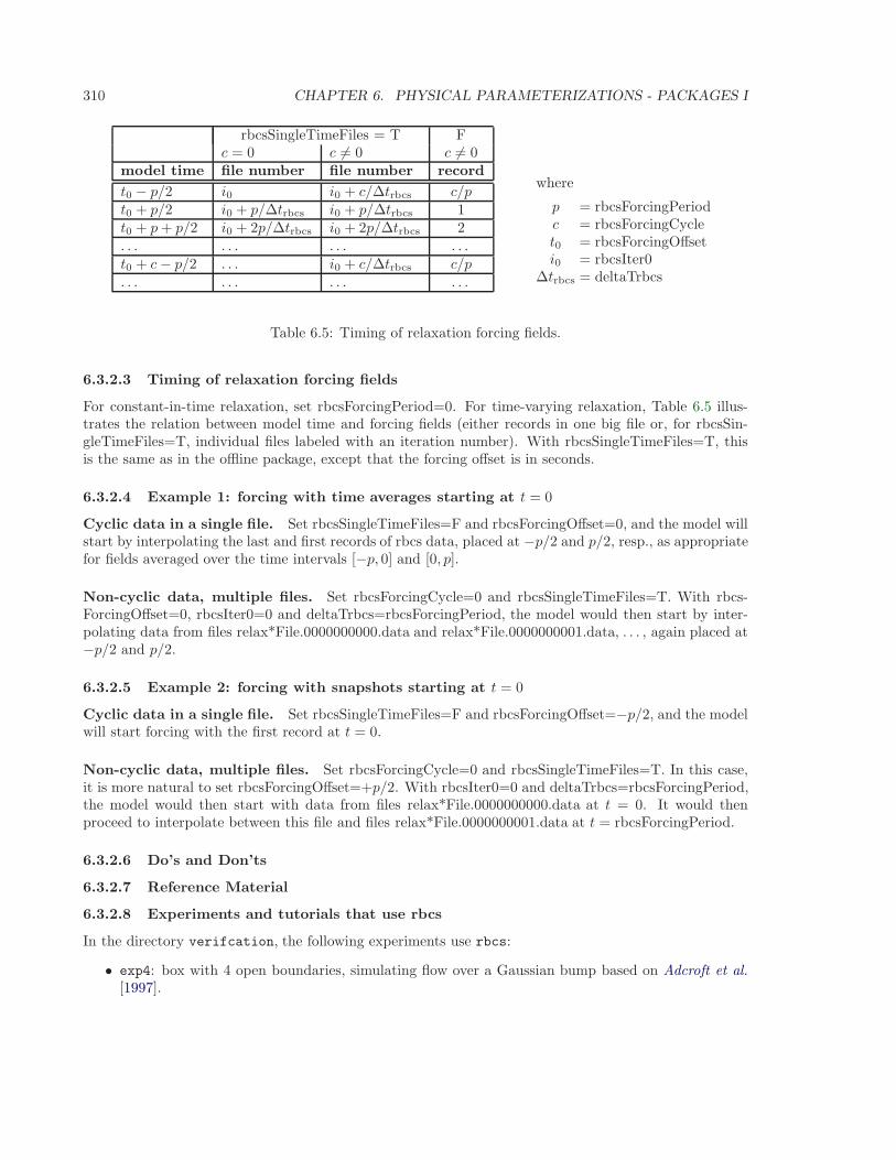
310 CHAPTER 6. PHYSICAL PARAMETERIZATIONS - PACKAGES I
rbcsSingleTimeFiles = T Fc = 0 c 6= 0 c 6= 0
model time file number file number record
t0 − p/2 i0 i0 + c/∆trbcs c/pt0 + p/2 i0 + p/∆trbcs i0 + p/∆trbcs 1t0 + p+ p/2 i0 + 2p/∆trbcs i0 + 2p/∆trbcs 2. . . . . . . . . . . .t0 + c− p/2 . . . i0 + c/∆trbcs c/p. . . . . . . . . . . .
where
p = rbcsForcingPeriodc = rbcsForcingCyclet0 = rbcsForcingOffseti0 = rbcsIter0
∆trbcs = deltaTrbcs
Table 6.5: Timing of relaxation forcing fields.
6.3.2.3 Timing of relaxation forcing fields
For constant-in-time relaxation, set rbcsForcingPeriod=0. For time-varying relaxation, Table 6.5 illus-trates the relation between model time and forcing fields (either records in one big file or, for rbcsSin-gleTimeFiles=T, individual files labeled with an iteration number). With rbcsSingleTimeFiles=T, thisis the same as in the offline package, except that the forcing offset is in seconds.
6.3.2.4 Example 1: forcing with time averages starting at t = 0
Cyclic data in a single file. Set rbcsSingleTimeFiles=F and rbcsForcingOffset=0, and the model willstart by interpolating the last and first records of rbcs data, placed at −p/2 and p/2, resp., as appropriatefor fields averaged over the time intervals [−p, 0] and [0, p].
Non-cyclic data, multiple files. Set rbcsForcingCycle=0 and rbcsSingleTimeFiles=T. With rbcs-ForcingOffset=0, rbcsIter0=0 and deltaTrbcs=rbcsForcingPeriod, the model would then start by inter-polating data from files relax*File.0000000000.data and relax*File.0000000001.data, . . . , again placed at−p/2 and p/2.
6.3.2.5 Example 2: forcing with snapshots starting at t = 0
Cyclic data in a single file. Set rbcsSingleTimeFiles=F and rbcsForcingOffset=−p/2, and the modelwill start forcing with the first record at t = 0.
Non-cyclic data, multiple files. Set rbcsForcingCycle=0 and rbcsSingleTimeFiles=T. In this case,it is more natural to set rbcsForcingOffset=+p/2. With rbcsIter0=0 and deltaTrbcs=rbcsForcingPeriod,the model would then start with data from files relax*File.0000000000.data at t = 0. It would thenproceed to interpolate between this file and files relax*File.0000000001.data at t = rbcsForcingPeriod.
6.3.2.6 Do’s and Don’ts
6.3.2.7 Reference Material
6.3.2.8 Experiments and tutorials that use rbcs
In the directory verifcation, the following experiments use rbcs:
• exp4: box with 4 open boundaries, simulating flow over a Gaussian bump based on Adcroft et al.[1997].
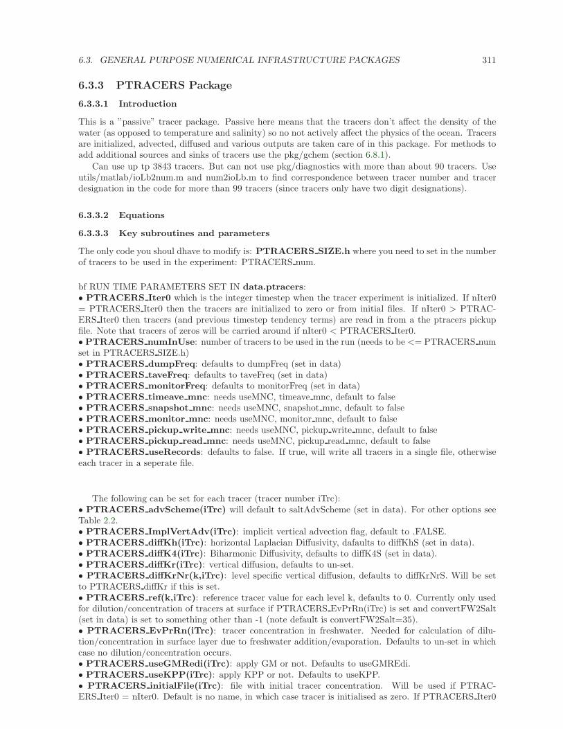
6.3. GENERAL PURPOSE NUMERICAL INFRASTRUCTURE PACKAGES 311
6.3.3 PTRACERS Package
6.3.3.1 Introduction
This is a ”passive” tracer package. Passive here means that the tracers don’t affect the density of thewater (as opposed to temperature and salinity) so no not actively affect the physics of the ocean. Tracersare initialized, advected, diffused and various outputs are taken care of in this package. For methods toadd additional sources and sinks of tracers use the pkg/gchem (section 6.8.1).
Can use up tp 3843 tracers. But can not use pkg/diagnostics with more than about 90 tracers. Useutils/matlab/ioLb2num.m and num2ioLb.m to find correspondence between tracer number and tracerdesignation in the code for more than 99 tracers (since tracers only have two digit designations).
6.3.3.2 Equations
6.3.3.3 Key subroutines and parameters
The only code you shoul dhave to modify is: PTRACERS SIZE.h where you need to set in the numberof tracers to be used in the experiment: PTRACERS num.
bf RUN TIME PARAMETERS SET IN data.ptracers:• PTRACERS Iter0 which is the integer timestep when the tracer experiment is initialized. If nIter0= PTRACERS Iter0 then the tracers are initialized to zero or from initial files. If nIter0 > PTRAC-ERS Iter0 then tracers (and previous timestep tendency terms) are read in from a the ptracers pickupfile. Note that tracers of zeros will be carried around if nIter0 < PTRACERS Iter0.• PTRACERS numInUse: number of tracers to be used in the run (needs to be <= PTRACERS numset in PTRACERS SIZE.h)• PTRACERS dumpFreq: defaults to dumpFreq (set in data)• PTRACERS taveFreq: defaults to taveFreq (set in data)• PTRACERS monitorFreq: defaults to monitorFreq (set in data)• PTRACERS timeave mnc: needs useMNC, timeave mnc, default to false• PTRACERS snapshot mnc: needs useMNC, snapshot mnc, default to false• PTRACERS monitor mnc: needs useMNC, monitor mnc, default to false• PTRACERS pickup write mnc: needs useMNC, pickup write mnc, default to false• PTRACERS pickup read mnc: needs useMNC, pickup read mnc, default to false• PTRACERS useRecords: defaults to false. If true, will write all tracers in a single file, otherwiseeach tracer in a seperate file.
The following can be set for each tracer (tracer number iTrc):• PTRACERS advScheme(iTrc) will default to saltAdvScheme (set in data). For other options seeTable 2.2.• PTRACERS ImplVertAdv(iTrc): implicit vertical advection flag, default to .FALSE.• PTRACERS diffKh(iTrc): horizontal Laplacian Diffusivity, dafaults to diffKhS (set in data).• PTRACERS diffK4(iTrc): Biharmonic Diffusivity, defaults to diffK4S (set in data).• PTRACERS diffKr(iTrc): vertical diffusion, defaults to un-set.• PTRACERS diffKrNr(k,iTrc): level specific vertical diffusion, defaults to diffKrNrS. Will be setto PTRACERS diffKr if this is set.• PTRACERS ref(k,iTrc): reference tracer value for each level k, defaults to 0. Currently only usedfor dilution/concentration of tracers at surface if PTRACERS EvPrRn(iTrc) is set and convertFW2Salt(set in data) is set to something other than -1 (note default is convertFW2Salt=35).• PTRACERS EvPrRn(iTrc): tracer concentration in freshwater. Needed for calculation of dilu-tion/concentration in surface layer due to freshwater addition/evaporation. Defaults to un-set in whichcase no dilution/concentration occurs.• PTRACERS useGMRedi(iTrc): apply GM or not. Defaults to useGMREdi.• PTRACERS useKPP(iTrc): apply KPP or not. Defaults to useKPP.• PTRACERS initialFile(iTrc): file with initial tracer concentration. Will be used if PTRAC-ERS Iter0 = nIter0. Default is no name, in which case tracer is initialised as zero. If PTRACERS Iter0
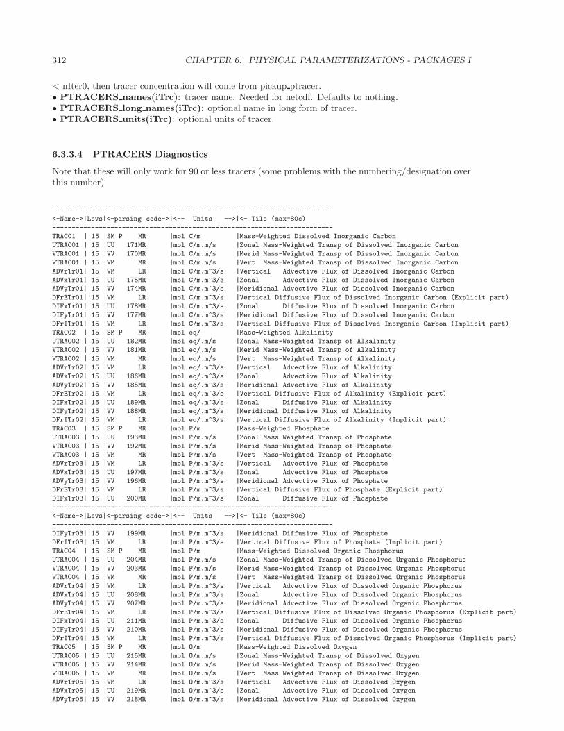
312 CHAPTER 6. PHYSICAL PARAMETERIZATIONS - PACKAGES I
< nIter0, then tracer concentration will come from pickup ptracer.• PTRACERS names(iTrc): tracer name. Needed for netcdf. Defaults to nothing.• PTRACERS long names(iTrc): optional name in long form of tracer.• PTRACERS units(iTrc): optional units of tracer.
6.3.3.4 PTRACERS Diagnostics
Note that these will only work for 90 or less tracers (some problems with the numbering/designation overthis number)
------------------------------------------------------------------------
<-Name->|Levs|<-parsing code->|<-- Units -->|<- Tile (max=80c)
------------------------------------------------------------------------
TRAC01 | 15 |SM P MR |mol C/m |Mass-Weighted Dissolved Inorganic Carbon
UTRAC01 | 15 |UU 171MR |mol C/m.m/s |Zonal Mass-Weighted Transp of Dissolved Inorganic Carbon
VTRAC01 | 15 |VV 170MR |mol C/m.m/s |Merid Mass-Weighted Transp of Dissolved Inorganic Carbon
WTRAC01 | 15 |WM MR |mol C/m.m/s |Vert Mass-Weighted Transp of Dissolved Inorganic Carbon
ADVrTr01| 15 |WM LR |mol C/m.m^3/s |Vertical Advective Flux of Dissolved Inorganic Carbon
ADVxTr01| 15 |UU 175MR |mol C/m.m^3/s |Zonal Advective Flux of Dissolved Inorganic Carbon
ADVyTr01| 15 |VV 174MR |mol C/m.m^3/s |Meridional Advective Flux of Dissolved Inorganic Carbon
DFrETr01| 15 |WM LR |mol C/m.m^3/s |Vertical Diffusive Flux of Dissolved Inorganic Carbon (Explicit part)
DIFxTr01| 15 |UU 178MR |mol C/m.m^3/s |Zonal Diffusive Flux of Dissolved Inorganic Carbon
DIFyTr01| 15 |VV 177MR |mol C/m.m^3/s |Meridional Diffusive Flux of Dissolved Inorganic Carbon
DFrITr01| 15 |WM LR |mol C/m.m^3/s |Vertical Diffusive Flux of Dissolved Inorganic Carbon (Implicit part)
TRAC02 | 15 |SM P MR |mol eq/ |Mass-Weighted Alkalinity
UTRAC02 | 15 |UU 182MR |mol eq/.m/s |Zonal Mass-Weighted Transp of Alkalinity
VTRAC02 | 15 |VV 181MR |mol eq/.m/s |Merid Mass-Weighted Transp of Alkalinity
WTRAC02 | 15 |WM MR |mol eq/.m/s |Vert Mass-Weighted Transp of Alkalinity
ADVrTr02| 15 |WM LR |mol eq/.m^3/s |Vertical Advective Flux of Alkalinity
ADVxTr02| 15 |UU 186MR |mol eq/.m^3/s |Zonal Advective Flux of Alkalinity
ADVyTr02| 15 |VV 185MR |mol eq/.m^3/s |Meridional Advective Flux of Alkalinity
DFrETr02| 15 |WM LR |mol eq/.m^3/s |Vertical Diffusive Flux of Alkalinity (Explicit part)
DIFxTr02| 15 |UU 189MR |mol eq/.m^3/s |Zonal Diffusive Flux of Alkalinity
DIFyTr02| 15 |VV 188MR |mol eq/.m^3/s |Meridional Diffusive Flux of Alkalinity
DFrITr02| 15 |WM LR |mol eq/.m^3/s |Vertical Diffusive Flux of Alkalinity (Implicit part)
TRAC03 | 15 |SM P MR |mol P/m |Mass-Weighted Phosphate
UTRAC03 | 15 |UU 193MR |mol P/m.m/s |Zonal Mass-Weighted Transp of Phosphate
VTRAC03 | 15 |VV 192MR |mol P/m.m/s |Merid Mass-Weighted Transp of Phosphate
WTRAC03 | 15 |WM MR |mol P/m.m/s |Vert Mass-Weighted Transp of Phosphate
ADVrTr03| 15 |WM LR |mol P/m.m^3/s |Vertical Advective Flux of Phosphate
ADVxTr03| 15 |UU 197MR |mol P/m.m^3/s |Zonal Advective Flux of Phosphate
ADVyTr03| 15 |VV 196MR |mol P/m.m^3/s |Meridional Advective Flux of Phosphate
DFrETr03| 15 |WM LR |mol P/m.m^3/s |Vertical Diffusive Flux of Phosphate (Explicit part)
DIFxTr03| 15 |UU 200MR |mol P/m.m^3/s |Zonal Diffusive Flux of Phosphate
------------------------------------------------------------------------
<-Name->|Levs|<-parsing code->|<-- Units -->|<- Tile (max=80c)
------------------------------------------------------------------------
DIFyTr03| 15 |VV 199MR |mol P/m.m^3/s |Meridional Diffusive Flux of Phosphate
DFrITr03| 15 |WM LR |mol P/m.m^3/s |Vertical Diffusive Flux of Phosphate (Implicit part)
TRAC04 | 15 |SM P MR |mol P/m |Mass-Weighted Dissolved Organic Phosphorus
UTRAC04 | 15 |UU 204MR |mol P/m.m/s |Zonal Mass-Weighted Transp of Dissolved Organic Phosphorus
VTRAC04 | 15 |VV 203MR |mol P/m.m/s |Merid Mass-Weighted Transp of Dissolved Organic Phosphorus
WTRAC04 | 15 |WM MR |mol P/m.m/s |Vert Mass-Weighted Transp of Dissolved Organic Phosphorus
ADVrTr04| 15 |WM LR |mol P/m.m^3/s |Vertical Advective Flux of Dissolved Organic Phosphorus
ADVxTr04| 15 |UU 208MR |mol P/m.m^3/s |Zonal Advective Flux of Dissolved Organic Phosphorus
ADVyTr04| 15 |VV 207MR |mol P/m.m^3/s |Meridional Advective Flux of Dissolved Organic Phosphorus
DFrETr04| 15 |WM LR |mol P/m.m^3/s |Vertical Diffusive Flux of Dissolved Organic Phosphorus (Explicit part)
DIFxTr04| 15 |UU 211MR |mol P/m.m^3/s |Zonal Diffusive Flux of Dissolved Organic Phosphorus
DIFyTr04| 15 |VV 210MR |mol P/m.m^3/s |Meridional Diffusive Flux of Dissolved Organic Phosphorus
DFrITr04| 15 |WM LR |mol P/m.m^3/s |Vertical Diffusive Flux of Dissolved Organic Phosphorus (Implicit part)
TRAC05 | 15 |SM P MR |mol O/m |Mass-Weighted Dissolved Oxygen
UTRAC05 | 15 |UU 215MR |mol O/m.m/s |Zonal Mass-Weighted Transp of Dissolved Oxygen
VTRAC05 | 15 |VV 214MR |mol O/m.m/s |Merid Mass-Weighted Transp of Dissolved Oxygen
WTRAC05 | 15 |WM MR |mol O/m.m/s |Vert Mass-Weighted Transp of Dissolved Oxygen
ADVrTr05| 15 |WM LR |mol O/m.m^3/s |Vertical Advective Flux of Dissolved Oxygen
ADVxTr05| 15 |UU 219MR |mol O/m.m^3/s |Zonal Advective Flux of Dissolved Oxygen
ADVyTr05| 15 |VV 218MR |mol O/m.m^3/s |Meridional Advective Flux of Dissolved Oxygen
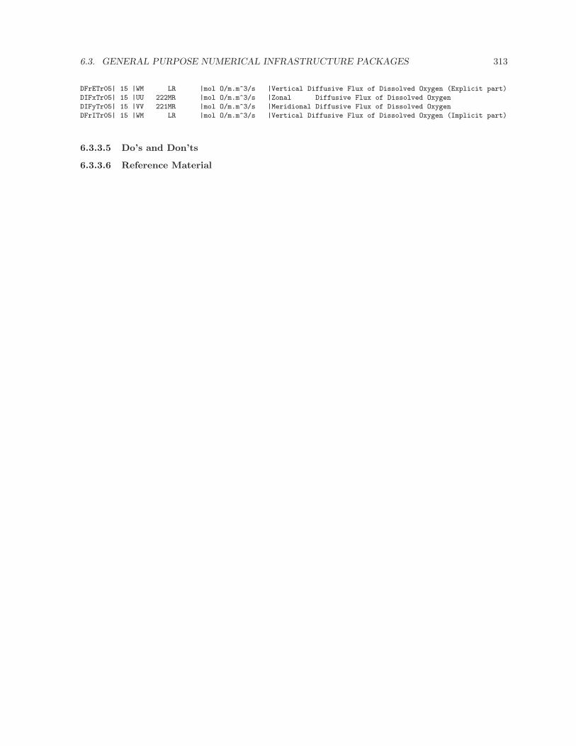
6.3. GENERAL PURPOSE NUMERICAL INFRASTRUCTURE PACKAGES 313
DFrETr05| 15 |WM LR |mol O/m.m^3/s |Vertical Diffusive Flux of Dissolved Oxygen (Explicit part)
DIFxTr05| 15 |UU 222MR |mol O/m.m^3/s |Zonal Diffusive Flux of Dissolved Oxygen
DIFyTr05| 15 |VV 221MR |mol O/m.m^3/s |Meridional Diffusive Flux of Dissolved Oxygen
DFrITr05| 15 |WM LR |mol O/m.m^3/s |Vertical Diffusive Flux of Dissolved Oxygen (Implicit part)
6.3.3.5 Do’s and Don’ts
6.3.3.6 Reference Material
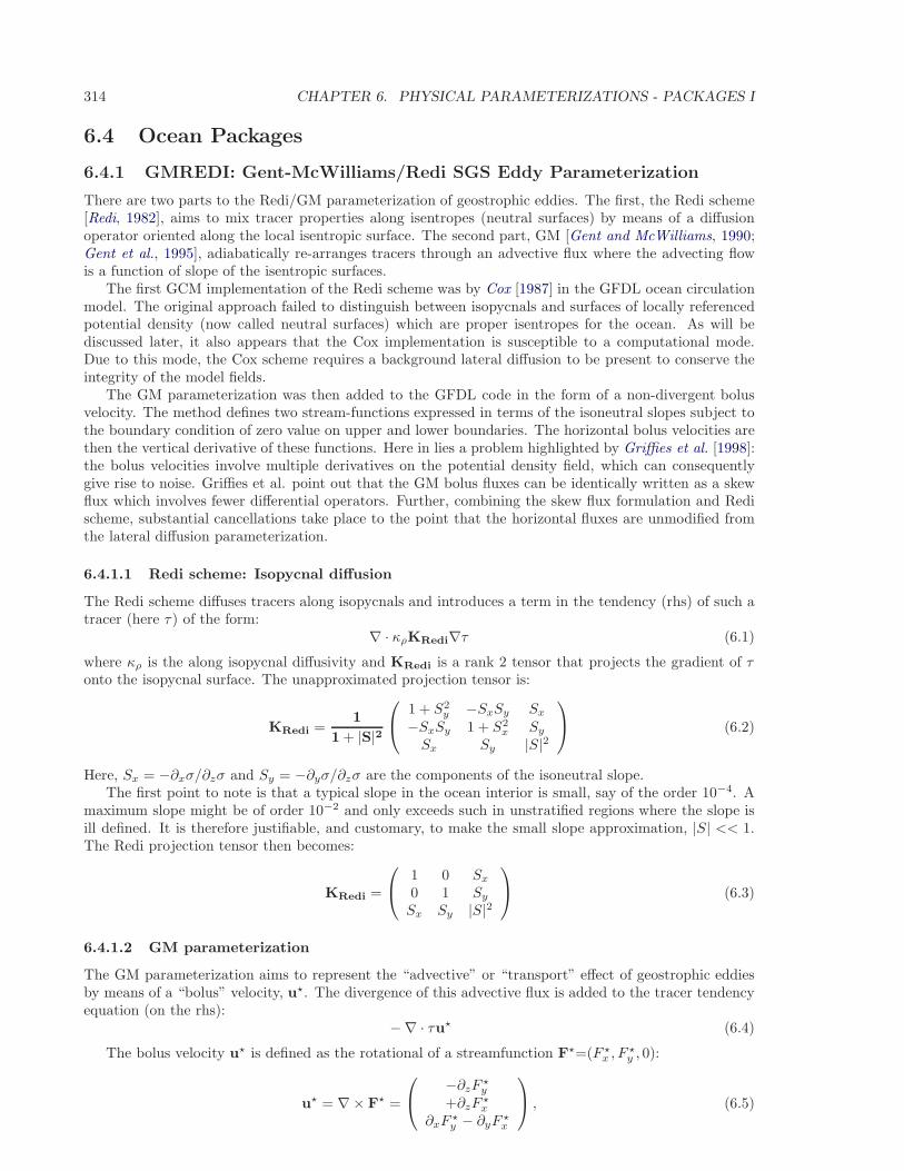
314 CHAPTER 6. PHYSICAL PARAMETERIZATIONS - PACKAGES I
6.4 Ocean Packages
6.4.1 GMREDI: Gent-McWilliams/Redi SGS Eddy Parameterization
There are two parts to the Redi/GM parameterization of geostrophic eddies. The first, the Redi scheme[Redi, 1982], aims to mix tracer properties along isentropes (neutral surfaces) by means of a diffusionoperator oriented along the local isentropic surface. The second part, GM [Gent and McWilliams, 1990;Gent et al., 1995], adiabatically re-arranges tracers through an advective flux where the advecting flowis a function of slope of the isentropic surfaces.
The first GCM implementation of the Redi scheme was by Cox [1987] in the GFDL ocean circulationmodel. The original approach failed to distinguish between isopycnals and surfaces of locally referencedpotential density (now called neutral surfaces) which are proper isentropes for the ocean. As will bediscussed later, it also appears that the Cox implementation is susceptible to a computational mode.Due to this mode, the Cox scheme requires a background lateral diffusion to be present to conserve theintegrity of the model fields.
The GM parameterization was then added to the GFDL code in the form of a non-divergent bolusvelocity. The method defines two stream-functions expressed in terms of the isoneutral slopes subject tothe boundary condition of zero value on upper and lower boundaries. The horizontal bolus velocities arethen the vertical derivative of these functions. Here in lies a problem highlighted by Griffies et al. [1998]:the bolus velocities involve multiple derivatives on the potential density field, which can consequentlygive rise to noise. Griffies et al. point out that the GM bolus fluxes can be identically written as a skewflux which involves fewer differential operators. Further, combining the skew flux formulation and Redischeme, substantial cancellations take place to the point that the horizontal fluxes are unmodified fromthe lateral diffusion parameterization.
6.4.1.1 Redi scheme: Isopycnal diffusion
The Redi scheme diffuses tracers along isopycnals and introduces a term in the tendency (rhs) of such atracer (here τ) of the form:
∇ · κρKRedi∇τ (6.1)
where κρ is the along isopycnal diffusivity and KRedi is a rank 2 tensor that projects the gradient of τonto the isopycnal surface. The unapproximated projection tensor is:
KRedi =1
1 + |S|2
1 + S2y −SxSy Sx
−SxSy 1 + S2x Sy
Sx Sy |S|2
(6.2)
Here, Sx = −∂xσ/∂zσ and Sy = −∂yσ/∂zσ are the components of the isoneutral slope.The first point to note is that a typical slope in the ocean interior is small, say of the order 10−4. A
maximum slope might be of order 10−2 and only exceeds such in unstratified regions where the slope isill defined. It is therefore justifiable, and customary, to make the small slope approximation, |S| << 1.The Redi projection tensor then becomes:
KRedi =
1 0 Sx
0 1 Sy
Sx Sy |S|2
(6.3)
6.4.1.2 GM parameterization
The GM parameterization aims to represent the “advective” or “transport” effect of geostrophic eddiesby means of a “bolus” velocity, u⋆. The divergence of this advective flux is added to the tracer tendencyequation (on the rhs):
−∇ · τu⋆ (6.4)
The bolus velocity u⋆ is defined as the rotational of a streamfunction F⋆=(F ⋆x , F
⋆y , 0):
u⋆ = ∇× F⋆ =
−∂zF⋆y
+∂zF⋆x
∂xF⋆y − ∂yF
⋆x
, (6.5)
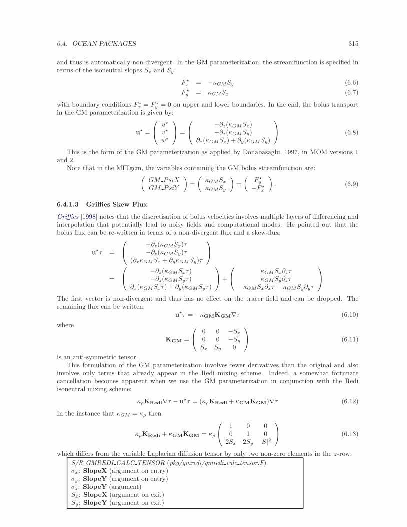
6.4. OCEAN PACKAGES 315
and thus is automatically non-divergent. In the GM parameterization, the streamfunction is specified interms of the isoneutral slopes Sx and Sy:
F ⋆x = −κGMSy (6.6)
F ⋆y = κGMSx (6.7)
with boundary conditions F ⋆x = F ⋆
y = 0 on upper and lower boundaries. In the end, the bolus transportin the GM parameterization is given by:
u⋆ =
u⋆
v⋆
w⋆
=
−∂z(κGMSx)−∂z(κGMSy)
∂x(κGMSx) + ∂y(κGMSy)
(6.8)
This is the form of the GM parameterization as applied by Donabasaglu, 1997, in MOM versions 1and 2.
Note that in the MITgcm, the variables containing the GM bolus streamfunction are:(GM PsiXGM PsiY
)=
(κGMSx
κGMSy
)=
(F ⋆
y
−F ⋆x
). (6.9)
6.4.1.3 Griffies Skew Flux
Griffies [1998] notes that the discretisation of bolus velocities involves multiple layers of differencing andinterpolation that potentially lead to noisy fields and computational modes. He pointed out that thebolus flux can be re-written in terms of a non-divergent flux and a skew-flux:
u⋆τ =
−∂z(κGMSx)τ−∂z(κGMSy)τ
(∂xκGMSx + ∂yκGMSy)τ
=
−∂z(κGMSxτ)−∂z(κGMSyτ)
∂x(κGMSxτ) + ∂y(κGMSyτ)
+
κGMSx∂zτκGMSy∂zτ
−κGMSx∂xτ − κGMSy∂yτ
The first vector is non-divergent and thus has no effect on the tracer field and can be dropped. Theremaining flux can be written:
u⋆τ = −κGMKGM∇τ (6.10)
where
KGM =
0 0 −Sx
0 0 −Sy
Sx Sy 0
(6.11)
is an anti-symmetric tensor.This formulation of the GM parameterization involves fewer derivatives than the original and also
involves only terms that already appear in the Redi mixing scheme. Indeed, a somewhat fortunatecancellation becomes apparent when we use the GM parameterization in conjunction with the Rediisoneutral mixing scheme:
κρKRedi∇τ − u⋆τ = (κρKRedi + κGMKGM)∇τ (6.12)
In the instance that κGM = κρ then
κρKRedi + κGMKGM = κρ
1 0 00 1 0
2Sx 2Sy |S|2
(6.13)
which differs from the variable Laplacian diffusion tensor by only two non-zero elements in the z-row.
S/R GMREDI CALC TENSOR (pkg/gmredi/gmredi calc tensor.F)σx: SlopeX (argument on entry)σy: SlopeY (argument on entry)σz : SlopeY (argument)Sx: SlopeX (argument on exit)Sy: SlopeY (argument on exit)
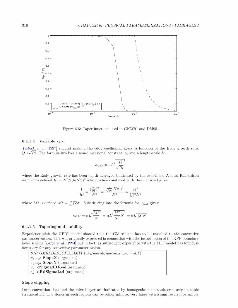
316 CHAPTER 6. PHYSICAL PARAMETERIZATIONS - PACKAGES I
10−4
10−3
10−2
10−1
0
0.1
0.2
0.3
0.4
0.5
0.6
0.7
0.8
0.9
1
Slope |S|
Tape
r fn f(
S)
DM95 1+tanh[ (Sc−|S|)/S
d ] /2
GKW91 (Smax
/|S|)2
Figure 6.6: Taper functions used in GKW91 and DM95.
6.4.1.4 Variable κGM
Visbeck et al. [1997] suggest making the eddy coefficient, κGM , a function of the Eady growth rate,|f |/
√Ri. The formula involves a non-dimensional constant, α, and a length-scale L:
κGM = αL2 |f |√Ri
z
where the Eady growth rate has been depth averaged (indicated by the over-line). A local Richardsonnumber is defined Ri = N2/(∂u/∂z)2 which, when combined with thermal wind gives:
1
Ri=
(∂u∂z )2
N2=
( gfρo
|∇σ|)2
N2=
M4
|f |2N2
where M2 is defined M2 = gρo|∇σ|. Substituting into the formula for κGM gives:
κGM = αL2M2
N
z
= αL2M2
N2N
z
= αL2|S|Nz
6.4.1.5 Tapering and stability
Experience with the GFDL model showed that the GM scheme has to be matched to the convectiveparameterization. This was originally expressed in connection with the introduction of the KPP boundarylayer scheme [Large et al., 1994] but in fact, as subsequent experience with the MIT model has found, isnecessary for any convective parameterization.
S/R GMREDI SLOPE LIMIT (pkg/gmredi/gmredi slope limit.F)σx, sx: SlopeX (argument)σy, sy: SlopeY (argument)σz : dSigmadRReal (argument)z∗σ: dRdSigmaLtd (argument)
Slope clipping
Deep convection sites and the mixed layer are indicated by homogenized, unstable or nearly unstablestratification. The slopes in such regions can be either infinite, very large with a sign reversal or simply
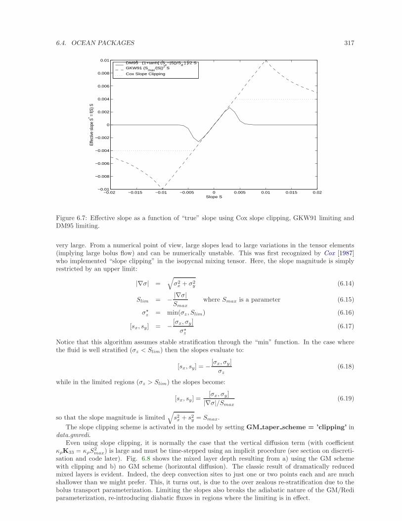
6.4. OCEAN PACKAGES 317
−0.02 −0.015 −0.01 −0.005 0 0.005 0.01 0.015 0.02−0.01
−0.008
−0.006
−0.004
−0.002
0
0.002
0.004
0.006
0.008
0.01
Slope S
Effe
ctive
slo
pe S
* = f(
S) S
DM95 1+tanh[ (Sc−|S|)/S
d ] /2 S
GKW91 (Smax
/|S|)2 S
Cox Slope Clipping
Figure 6.7: Effective slope as a function of “true” slope using Cox slope clipping, GKW91 limiting andDM95 limiting.
very large. From a numerical point of view, large slopes lead to large variations in the tensor elements(implying large bolus flow) and can be numerically unstable. This was first recognized by Cox [1987]who implemented “slope clipping” in the isopycnal mixing tensor. Here, the slope magnitude is simplyrestricted by an upper limit:
|∇σ| =√σ2
x + σ2y (6.14)
Slim = − |∇σ|Smax
where Smax is a parameter (6.15)
σ⋆z = min(σz , Slim) (6.16)
[sx, sy] = − [σx, σy]
σ⋆z
(6.17)
Notice that this algorithm assumes stable stratification through the “min” function. In the case wherethe fluid is well stratified (σz < Slim) then the slopes evaluate to:
[sx, sy] = − [σx, σy]
σz(6.18)
while in the limited regions (σz > Slim) the slopes become:
[sx, sy] =[σx, σy]
|∇σ|/Smax(6.19)
so that the slope magnitude is limited√s2x + s2y = Smax.
The slope clipping scheme is activated in the model by setting GM taper scheme = ’clipping’ indata.gmredi.
Even using slope clipping, it is normally the case that the vertical diffusion term (with coefficientκρK33 = κρS
2max) is large and must be time-stepped using an implicit procedure (see section on discreti-
sation and code later). Fig. 6.8 shows the mixed layer depth resulting from a) using the GM schemewith clipping and b) no GM scheme (horizontal diffusion). The classic result of dramatically reducedmixed layers is evident. Indeed, the deep convection sites to just one or two points each and are muchshallower than we might prefer. This, it turns out, is due to the over zealous re-stratification due to thebolus transport parameterization. Limiting the slopes also breaks the adiabatic nature of the GM/Rediparameterization, re-introducing diabatic fluxes in regions where the limiting is in effect.
318 CHAPTER 6. PHYSICAL PARAMETERIZATIONS - PACKAGES I
Figure missing.
Figure 6.8: Mixed layer depth using GM parameterization with a) Cox slope clipping and for comparisonb) using horizontal constant diffusion.
Tapering: Gerdes, Koberle and Willebrand, Clim. Dyn. 1991
The tapering scheme used in Gerdes et al. [1991] addressed two issues with the clipping method: theintroduction of large vertical fluxes in addition to convective adjustment fluxes is avoided by taperingthe GM/Redi slopes back to zero in low-stratification regions; the adjustment of slopes is replaced by atapering of the entire GM/Redi tensor. This means the direction of fluxes is unaffected as the amplitudeis scaled.
The scheme inserts a tapering function, f1(S), in front of the GM/Redi tensor:
f1(S) = min
[1,
(Smax
|S|
)2]
(6.20)
where Smax is the maximum slope you want allowed. Where the slopes, |S| < Smax then f1(S) = 1 andthe tensor is un-tapered but where |S| ≥ Smax then f1(S) scales down the tensor so that the effectivevertical diffusivity term κf1(S)|S|2 = κS2
max.The GKW91 tapering scheme is activated in the model by setting GM taper scheme = ’gkw91’
in data.gmredi.
Tapering: Danabasoglu and McWilliams, J. Clim. 1995
The tapering scheme used by Danabasoglu and McWilliams [1995] followed a similar procedure but useda different tapering function, f1(S):
f1(S) =1
2
(1 + tanh
[Sc − |S|Sd
])(6.21)
where Sc = 0.004 is a cut-off slope and Sd = 0.001 is a scale over which the slopes are smoothly tapered.Functionally, the operates in the same way as the GKW91 scheme but has a substantially lower cut-off,turning off the GM/Redi SGS parameterization for weaker slopes.
The DM95 tapering scheme is activated in the model by setting GM taper scheme = ’dm95’ indata.gmredi.
Tapering: Large, Danabasoglu and Doney, JPO 1997
The tapering used in Large et al. [1997] is based on the DM95 tapering scheme, but also tapers thescheme with an additional function of height, f2(z), so that the GM/Redi SGS fluxes are reduced nearthe surface:
f2(z) =1
2
(1 + sin(π
z
D− π
2))
(6.22)
where D = Lρ|S| is a depth-scale and Lρ = c/f with c = 2 m s−1. This tapering with height wasintroduced to fix some spurious interaction with the mixed-layer KPP parameterization.
The LDD97 tapering scheme is activated in the model by setting GM taper scheme = ’ldd97’ indata.gmredi.
6.4.1.6 Package Reference
------------------------------------------------------------------------
<-Name->|Levs|<-parsing code->|<-- Units -->|<- Tile (max=80c)
------------------------------------------------------------------------
GM_VisbK| 1 |SM P M1 |m^2/s |Mixing coefficient from Visbeck etal parameterization
GM_Kux | 15 |UU P 177MR |m^2/s |K_11 element (U.point, X.dir) of GM-Redi tensor
GM_Kvy | 15 |VV P 176MR |m^2/s |K_22 element (V.point, Y.dir) of GM-Redi tensor
GM_Kuz | 15 |UU 179MR |m^2/s |K_13 element (U.point, Z.dir) of GM-Redi tensor
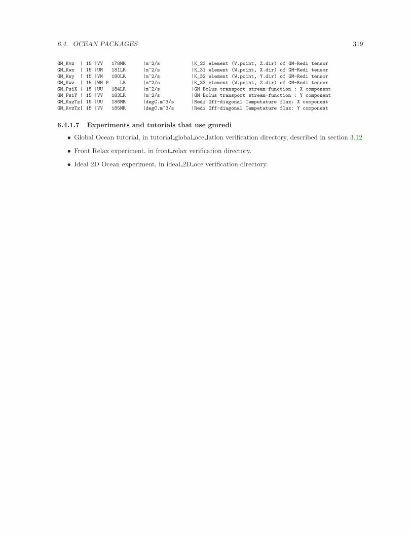
6.4. OCEAN PACKAGES 319
GM_Kvz | 15 |VV 178MR |m^2/s |K_23 element (V.point, Z.dir) of GM-Redi tensor
GM_Kwx | 15 |UM 181LR |m^2/s |K_31 element (W.point, X.dir) of GM-Redi tensor
GM_Kwy | 15 |VM 180LR |m^2/s |K_32 element (W.point, Y.dir) of GM-Redi tensor
GM_Kwz | 15 |WM P LR |m^2/s |K_33 element (W.point, Z.dir) of GM-Redi tensor
GM_PsiX | 15 |UU 184LR |m^2/s |GM Bolus transport stream-function : X component
GM_PsiY | 15 |VV 183LR |m^2/s |GM Bolus transport stream-function : Y component
GM_KuzTz| 15 |UU 186MR |degC.m^3/s |Redi Off-diagonal Tempetature flux: X component
GM_KvzTz| 15 |VV 185MR |degC.m^3/s |Redi Off-diagonal Tempetature flux: Y component
6.4.1.7 Experiments and tutorials that use gmredi
• Global Ocean tutorial, in tutorial global oce latlon verification directory, described in section 3.12
• Front Relax experiment, in front relax verification directory.
• Ideal 2D Ocean experiment, in ideal 2D oce verification directory.
320 CHAPTER 6. PHYSICAL PARAMETERIZATIONS - PACKAGES I
6.4.2 KPP: Nonlocal K-Profile Parameterization for Vertical Mixing
Authors: Dimitris Menemenlis and Patrick Heimbach
6.4.2.1 Introduction
The nonlocal K-Profile Parameterization (KPP) scheme of Large et al. [1994] unifies the treatment of avariety of unresolved processes involved in vertical mixing. To consider it as one mixing scheme is, in theview of the authors, somewhat misleading since it consists of several entities to deal with distinct mixingprocesses in the ocean’s surface boundary layer, and the interior:
1. mixing in the interior is goverened by shear instability (modeled as function of the local gradientRichardson number), internal wave activity (assumed constant), and double-diffusion (not imple-mented here).
2. a boundary layer depth h or hbl is determined at each grid point, based on a critical value ofturbulent processes parameterized by a bulk Richardson number;
3. mixing is strongly enhanced in the boundary layer under the stabilizing or destabilizing influenceof surface forcing (buoyancy and momentum) enabling boundary layer properties to penetrate wellinto the thermocline; mixing is represented through a polynomial profile whose coefficients aredetermined subject to several contraints;
4. the boundary-layer profile is made to agree with similarity theory of turbulence and is matched, inthe asymptotic sense (function and derivative agree at the boundary), to the interior thus fixing thepolynomial coefficients; matching allows for some fraction of the boundary layer mixing to affectthe interior, and vice versa;
5. a “non-local” term γ or ghat which is independent of the vertical property gradient further enhancesmixing where the water column is unstable
The scheme has been extensively compared to observations (see e.g. Large et al. [1997]) and is nowcoomon in many ocean models.
The current code originates in the NCAR NCOM 1-D code and was kindly provided by Bill Large andJan Morzel. It has been adapted first to the MITgcm vector code and subsequently to the current parallelcode. Adjustment were mainly in conjunction with WRAPPER requirements (domain decomposition andthreading capability), to enable automatic differentiation of tangent linear and adjoint code via TAMC.
The following sections will describe the KPP package configuration and compiling (6.4.2.2), the set-tings and choices of runtime parameters (6.4.2.3), more detailed description of equations to which theseparameters relate (6.4.2.4), and key subroutines where they are used (6.4.2.5), and diagnostics output ofKPP-derived diffusivities, viscosities and boundary-layer/mixed-layer depths (6.4.2.6).
6.4.2.2 KPP configuration and compiling
As with all MITgcm packages, KPP can be turned on or off at compile time
• using the packages.conf file by adding kpp to it,
• or using genmake2 adding -enable=kpp or -disable=kpp switches
• Required packages and CPP options:No additional packages are required, but the MITgcm kernel flag enabling the penetration of short-wave radiation below the surface layer needs to be set in CPP OPTIONS.h as follows:#define SHORTWAVE HEATING
(see Section 3.4).
Parts of the KPP code can be enabled or disabled at compile time via CPP preprocessor flags. Theseoptions are set in KPP OPTIONS.h. Table 6.4.2.2 summarizes them.
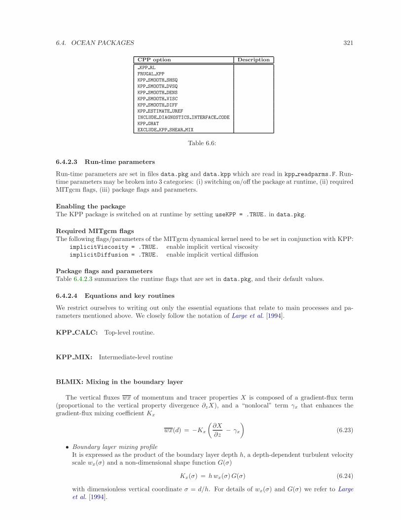
6.4. OCEAN PACKAGES 321
CPP option Description
KPP RL
FRUGAL KPP
KPP SMOOTH SHSQ
KPP SMOOTH DVSQ
KPP SMOOTH DENS
KPP SMOOTH VISC
KPP SMOOTH DIFF
KPP ESTIMATE UREF
INCLUDE DIAGNOSTICS INTERFACE CODE
KPP GHAT
EXCLUDE KPP SHEAR MIX
Table 6.6:
6.4.2.3 Run-time parameters
Run-time parameters are set in files data.pkg and data.kpp which are read in kpp readparms.F. Run-time parameters may be broken into 3 categories: (i) switching on/off the package at runtime, (ii) requiredMITgcm flags, (iii) package flags and parameters.
Enabling the packageThe KPP package is switched on at runtime by setting useKPP = .TRUE. in data.pkg.
Required MITgcm flagsThe following flags/parameters of the MITgcm dynamical kernel need to be set in conjunction with KPP:
implicitViscosity = .TRUE. enable implicit vertical viscosityimplicitDiffusion = .TRUE. enable implicit vertical diffusion
Package flags and parametersTable 6.4.2.3 summarizes the runtime flags that are set in data.pkg, and their default values.
6.4.2.4 Equations and key routines
We restrict ourselves to writing out only the essential equations that relate to main processes and pa-rameters mentioned above. We closely follow the notation of Large et al. [1994].
KPP CALC: Top-level routine.
KPP MIX: Intermediate-level routine
BLMIX: Mixing in the boundary layer
The vertical fluxes wx of momentum and tracer properties X is composed of a gradient-flux term(proportional to the vertical property divergence ∂zX), and a “nonlocal” term γx that enhances thegradient-flux mixing coefficient Kx
wx(d) = −Kx
(∂X
∂z− γx
)(6.23)
• Boundary layer mixing profileIt is expressed as the product of the boundary layer depth h, a depth-dependent turbulent velocityscale wx(σ) and a non-dimensional shape function G(σ)
Kx(σ) = hwx(σ)G(σ) (6.24)
with dimensionless vertical coordinate σ = d/h. For details of wx(σ) and G(σ) we refer to Largeet al. [1994].
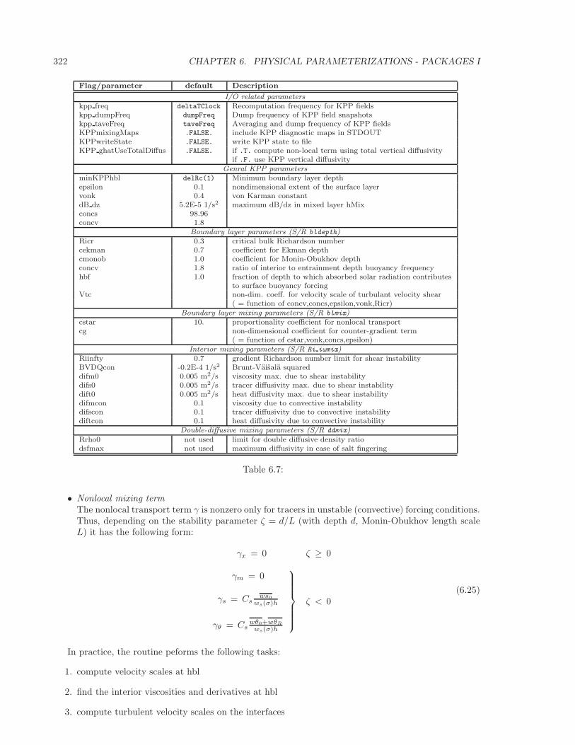
322 CHAPTER 6. PHYSICAL PARAMETERIZATIONS - PACKAGES I
Flag/parameter default Description
I/O related parameterskpp freq deltaTClock Recomputation frequency for KPP fieldskpp dumpFreq dumpFreq Dump frequency of KPP field snapshotskpp taveFreq taveFreq Averaging and dump frequency of KPP fieldsKPPmixingMaps .FALSE. include KPP diagnostic maps in STDOUTKPPwriteState .FALSE. write KPP state to fileKPP ghatUseTotalDiffus .FALSE. if .T. compute non-local term using total vertical diffusivity
if .F. use KPP vertical diffusivityGenral KPP parameters
minKPPhbl delRc(1) Minimum boundary layer depthepsilon 0.1 nondimensional extent of the surface layervonk 0.4 von Karman constantdB dz 5.2E-5 1/s2 maximum dB/dz in mixed layer hMixconcs 98.96concv 1.8
Boundary layer parameters (S/R bldepth)Ricr 0.3 critical bulk Richardson numbercekman 0.7 coefficient for Ekman depthcmonob 1.0 coefficient for Monin-Obukhov depthconcv 1.8 ratio of interior to entrainment depth buoyancy frequencyhbf 1.0 fraction of depth to which absorbed solar radiation contributes
to surface buoyancy forcingVtc non-dim. coeff. for velocity scale of turbulant velocity shear
( = function of concv,concs,epsilon,vonk,Ricr)Boundary layer mixing parameters (S/R blmix)
cstar 10. proportionality coefficient for nonlocal transportcg non-dimensional coefficient for counter-gradient term
( = function of cstar,vonk,concs,epsilon)Interior mixing parameters (S/R Ri iwmix)
Riinfty 0.7 gradient Richardson number limit for shear instabilityBVDQcon -0.2E-4 1/s2 Brunt-Vaisala squareddifm0 0.005 m2/s viscosity max. due to shear instabilitydifs0 0.005 m2/s tracer diffusivity max. due to shear instabilitydift0 0.005 m2/s heat diffusivity max. due to shear instabilitydifmcon 0.1 viscosity due to convective instabilitydifscon 0.1 tracer diffusivity due to convective instabilitydiftcon 0.1 heat diffusivity due to convective instability
Double-diffusive mixing parameters (S/R ddmix)Rrho0 not used limit for double diffusive density ratiodsfmax not used maximum diffusivity in case of salt fingering
Table 6.7:
• Nonlocal mixing termThe nonlocal transport term γ is nonzero only for tracers in unstable (convective) forcing conditions.Thus, depending on the stability parameter ζ = d/L (with depth d, Monin-Obukhov length scaleL) it has the following form:
γx = 0 ζ ≥ 0
γm = 0
γs = Csws0
ws(σ)h
γθ = Cswθ0+wθR
ws(σ)h
ζ < 0(6.25)
In practice, the routine peforms the following tasks:
1. compute velocity scales at hbl
2. find the interior viscosities and derivatives at hbl
3. compute turbulent velocity scales on the interfaces
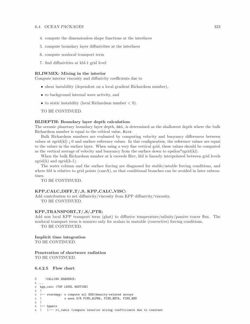
6.4. OCEAN PACKAGES 323
4. compute the dimensionless shape functions at the interfaces
5. compute boundary layer diffusivities at the interfaces
6. compute nonlocal transport term
7. find diffusivities at kbl-1 grid level
RI IWMIX: Mixing in the interiorCompute interior viscosity and diffusivity coefficients due to
• shear instability (dependent on a local gradient Richardson number),
• to background internal wave activity, and
• to static instability (local Richardson number < 0).
TO BE CONTINUED.
BLDEPTH: Boundary layer depth calculation:The oceanic planetary boundary layer depth, hbl, is determined as the shallowest depth where the bulkRichardson number is equal to the critical value, Ricr.
Bulk Richardson numbers are evaluated by computing velocity and buoyancy differences betweenvalues at zgrid(kl) ¡ 0 and surface reference values. In this configuration, the reference values are equalto the values in the surface layer. When using a very fine vertical grid, these values should be computedas the vertical average of velocity and buoyancy from the surface down to epsilon*zgrid(kl).
When the bulk Richardson number at k exceeds Ricr, hbl is linearly interpolated between grid levelszgrid(k) and zgrid(k-1).
The water column and the surface forcing are diagnosed for stable/ustable forcing conditions, andwhere hbl is relative to grid points (caseA), so that conditional branches can be avoided in later subrou-tines.
TO BE CONTINUED.
KPP CALC DIFF T/ S, KPP CALC VISC:Add contribution to net diffusivity/viscosity from KPP diffusivity/viscosity.
TO BE CONTINUED.
KPP TRANSPORT T/ S/ PTR:Add non local KPP transport term (ghat) to diffusive temperature/salinity/passive tracer flux. Thenonlocal transport term is nonzero only for scalars in unstable (convective) forcing conditions.
TO BE CONTINUED.
Implicit time integrationTO BE CONTINUED.
Penetration of shortwave radiationTO BE CONTINUED.
6.4.2.5 Flow chart
C !CALLING SEQUENCE:
c ...
c kpp_calc (TOP LEVEL ROUTINE)
c |
c |-- statekpp: o compute all EOS/density-related arrays
c | o uses S/R FIND_ALPHA, FIND_BETA, FIND_RHO
c |
c |-- kppmix
c | |--- ri_iwmix (compute interior mixing coefficients due to constant
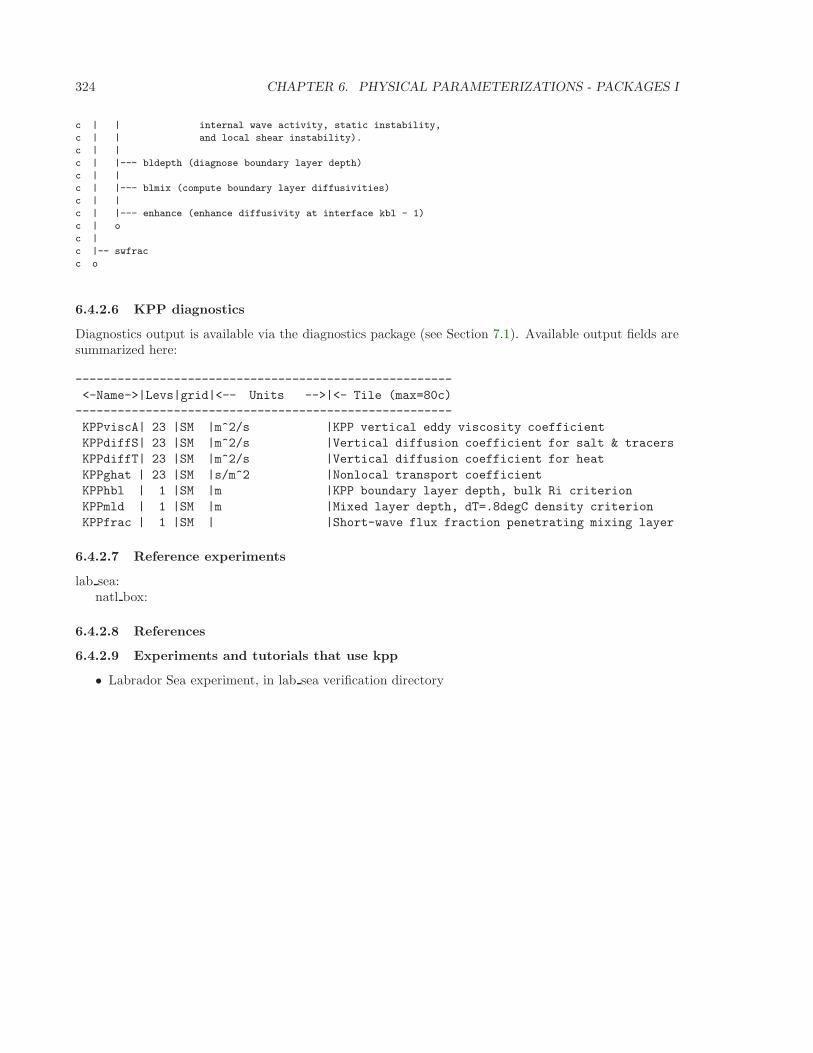
324 CHAPTER 6. PHYSICAL PARAMETERIZATIONS - PACKAGES I
c | | internal wave activity, static instability,
c | | and local shear instability).
c | |
c | |--- bldepth (diagnose boundary layer depth)
c | |
c | |--- blmix (compute boundary layer diffusivities)
c | |
c | |--- enhance (enhance diffusivity at interface kbl - 1)
c | o
c |
c |-- swfrac
c o
6.4.2.6 KPP diagnostics
Diagnostics output is available via the diagnostics package (see Section 7.1). Available output fields aresummarized here:
------------------------------------------------------
<-Name->|Levs|grid|<-- Units -->|<- Tile (max=80c)
------------------------------------------------------
KPPviscA| 23 |SM |m^2/s |KPP vertical eddy viscosity coefficient
KPPdiffS| 23 |SM |m^2/s |Vertical diffusion coefficient for salt & tracers
KPPdiffT| 23 |SM |m^2/s |Vertical diffusion coefficient for heat
KPPghat | 23 |SM |s/m^2 |Nonlocal transport coefficient
KPPhbl | 1 |SM |m |KPP boundary layer depth, bulk Ri criterion
KPPmld | 1 |SM |m |Mixed layer depth, dT=.8degC density criterion
KPPfrac | 1 |SM | |Short-wave flux fraction penetrating mixing layer
6.4.2.7 Reference experiments
lab sea:natl box:
6.4.2.8 References
6.4.2.9 Experiments and tutorials that use kpp
• Labrador Sea experiment, in lab sea verification directory
6.4. OCEAN PACKAGES 325
6.4.3 GGL90: a TKE vertical mixing scheme
(in directory: pkg/ggl90/)
6.4.3.1 Key subroutines, parameters and files
see Gaspar et al. [1990]
6.4.3.2 Experiments and tutorials that use zonal filter
• Vertical mixing verification experiment (vermix/input.ggl90)
326 CHAPTER 6. PHYSICAL PARAMETERIZATIONS - PACKAGES I
6.4.4 OPPS: Ocean Penetrative Plume Scheme
(in directory: pkg/opps/)
6.4.4.1 Key subroutines, parameters and files
see Paluszkiewicz and Romea [1997]
6.4.4.2 Experiments and tutorials that use zonal filter
• Vertical mixing verification experiment (vermix/input.opps)
6.4. OCEAN PACKAGES 327
6.4.5 KL10: Vertical Mixing Due to Breaking Internal Waves
(in directory: pkg/kl10/)
Authors: Jody M. Klymak
6.4.5.1 Introduction
The Klymak and Legg [2010, KL10] parameterization for breaking internal waves is meant to representmixing in the ocean “interior” due to convective instability. Many mixing schemes in the presence ofunstable stratification simply turn on an arbitrarily large diffusivity and viscosity in the overturningregion. This assumes the fluid completely mixes, which is probably not a terrible assumption, but it alsomakes estimating the turbulence dissipation rate in the overturning region meaningless.
The KL10 scheme overcomes this limitation by estimating the viscosity and diffusivity from a com-bination of the Ozmidov relation and the Osborn relation, assuming a turbulent Prandtl number of one.The Ozmidov relation says that outer scale of turbulence in an overturn will scale with the strength ofthe turbulence ǫ, and the stratification N , as
L2O ≈ ǫN−3. (6.26)
The Osborn relation relates the strength of the dissipation to the vertical diffusivity as
Kv = ΓǫN−2, (6.27)
where Γ ≈ 0.2 is the mixing ratio of buoyancy flux to thermal dissipation due to the turbulence. Com-bining the two gives us
Kv ≈ ΓL2ON. (6.28)
The ocean turbulence community often approximates the Ozmidov scale by the root-mean-square ofthe Thorpe displacement, δz, in an overturn [Thorpe, 1977]. The Thorpe displacement is the distanceone would have to move a water parcel for the water column to be stable, and is readily measured ina measured profile by sorting the profile and tracking how far each parcel moves during the sortingprocedure. This method gives an imperfect estimate of the turbulence, but it has been found to agree onaverage over a large range of overturns [Wesson and Gregg, 1994; Seim and Gregg, 1994; Moum, 1996].
The algorithm coded here is a slight simplification of the usual Thorpe method for estimating turbu-lence in overturning regions. Usually, overturns are identified and N is averaged over the overturn. Here,instead we estimate
Kv(z) ≈ Γδ2z Ns(z). (6.29)
where Ns(z) is the local sorted stratification. This saves complexity in the code and adds a slightinaccuracy, but we don’t believe is biased.
We assume a turbulent Prandtl number of 1, so Av = Kv.We also calculate and output a turbulent dissipation from this scheme. We do not simply evaluate
the overturns for ǫ using (6.26). Instead we compute the vertical shear terms that the viscosity is actingon:
ǫv = Av
((∂u
∂z
)2
+
(∂v
∂z
)2). (6.30)
There are straightforward caveats to this approach, covered in Klymak and Legg [2010].
• If your resolution is too low to resolve the breaking internal waves, you won’t have any turbulence.
• If the model resolution is too high, the estimates of ǫv will start to be exaggerated, particularly ifthe run in non-hydrostatic. That is because there will be significant shear at small scales that repre-sents the turbulence being parameterized in the scheme. At very high resolutions direct numericalsimulation or more sophisticated large-eddy schemes should be used.
• We find that grid cells of approximately 10 to 1 aspect ratio are a good rule of thumb for achievinggood results are usual oceanic scales. For a site like the Hawaiian Ridge, and Luzon Strait, thismeans 10-m vertical resolusion and approximately 100-m horizontal. The 10-m resolution can berelaxed if the stratification drops, and we often WKB-stretch the grid spacing with depth.
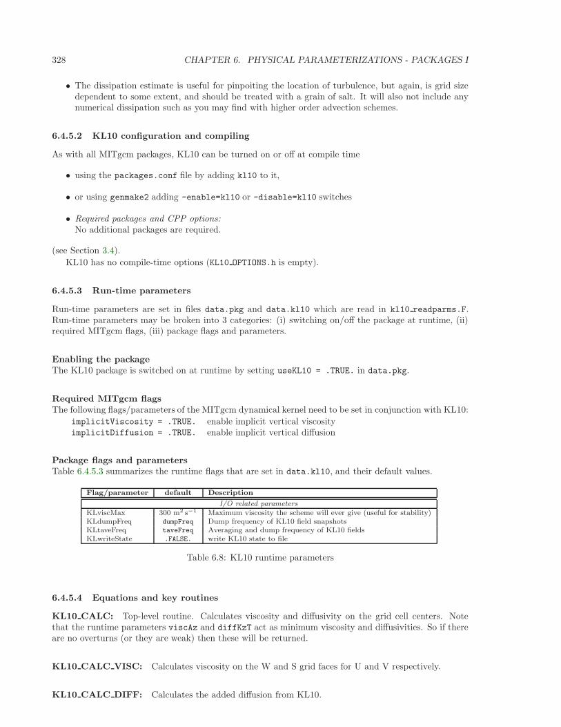
328 CHAPTER 6. PHYSICAL PARAMETERIZATIONS - PACKAGES I
• The dissipation estimate is useful for pinpoiting the location of turbulence, but again, is grid sizedependent to some extent, and should be treated with a grain of salt. It will also not include anynumerical dissipation such as you may find with higher order advection schemes.
6.4.5.2 KL10 configuration and compiling
As with all MITgcm packages, KL10 can be turned on or off at compile time
• using the packages.conf file by adding kl10 to it,
• or using genmake2 adding -enable=kl10 or -disable=kl10 switches
• Required packages and CPP options:No additional packages are required.
(see Section 3.4).
KL10 has no compile-time options (KL10 OPTIONS.h is empty).
6.4.5.3 Run-time parameters
Run-time parameters are set in files data.pkg and data.kl10 which are read in kl10 readparms.F.Run-time parameters may be broken into 3 categories: (i) switching on/off the package at runtime, (ii)required MITgcm flags, (iii) package flags and parameters.
Enabling the packageThe KL10 package is switched on at runtime by setting useKL10 = .TRUE. in data.pkg.
Required MITgcm flagsThe following flags/parameters of the MITgcm dynamical kernel need to be set in conjunction with KL10:
implicitViscosity = .TRUE. enable implicit vertical viscosityimplicitDiffusion = .TRUE. enable implicit vertical diffusion
Package flags and parametersTable 6.4.5.3 summarizes the runtime flags that are set in data.kl10, and their default values.
Flag/parameter default Description
I/O related parametersKLviscMax 300 m2 s−1 Maximum viscosity the scheme will ever give (useful for stability)KLdumpFreq dumpFreq Dump frequency of KL10 field snapshotsKLtaveFreq taveFreq Averaging and dump frequency of KL10 fieldsKLwriteState .FALSE. write KL10 state to file
Table 6.8: KL10 runtime parameters
6.4.5.4 Equations and key routines
KL10 CALC: Top-level routine. Calculates viscosity and diffusivity on the grid cell centers. Notethat the runtime parameters viscAz and diffKzT act as minimum viscosity and diffusivities. So if thereare no overturns (or they are weak) then these will be returned.
KL10 CALC VISC: Calculates viscosity on the W and S grid faces for U and V respectively.
KL10 CALC DIFF: Calculates the added diffusion from KL10.
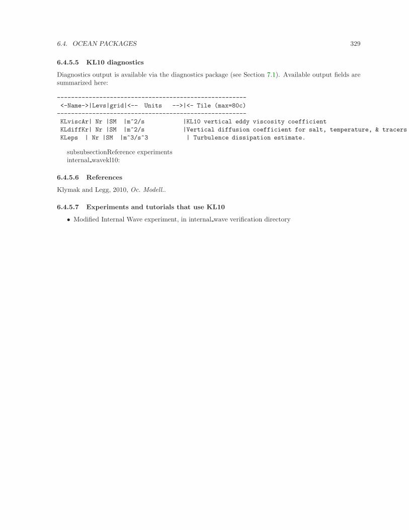
6.4. OCEAN PACKAGES 329
6.4.5.5 KL10 diagnostics
Diagnostics output is available via the diagnostics package (see Section 7.1). Available output fields aresummarized here:
------------------------------------------------------
<-Name->|Levs|grid|<-- Units -->|<- Tile (max=80c)
------------------------------------------------------
KLviscAr| Nr |SM |m^2/s |KL10 vertical eddy viscosity coefficient
KLdiffKr| Nr |SM |m^2/s |Vertical diffusion coefficient for salt, temperature, & tracers
KLeps | Nr |SM |m^3/s^3 | Turbulence dissipation estimate.
subsubsectionReference experimentsinternal wavekl10:
6.4.5.6 References
Klymak and Legg, 2010, Oc. Modell..
6.4.5.7 Experiments and tutorials that use KL10
• Modified Internal Wave experiment, in internal wave verification directory
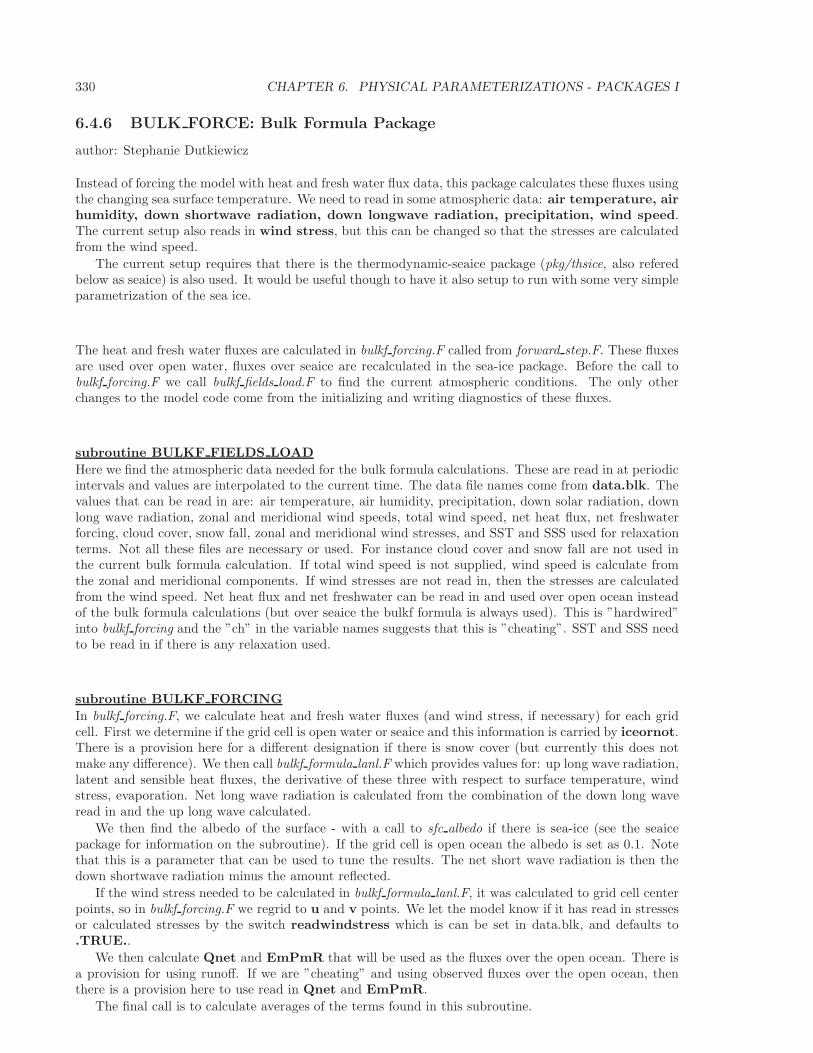
330 CHAPTER 6. PHYSICAL PARAMETERIZATIONS - PACKAGES I
6.4.6 BULK FORCE: Bulk Formula Package
author: Stephanie Dutkiewicz
Instead of forcing the model with heat and fresh water flux data, this package calculates these fluxes usingthe changing sea surface temperature. We need to read in some atmospheric data: air temperature, airhumidity, down shortwave radiation, down longwave radiation, precipitation, wind speed.The current setup also reads in wind stress, but this can be changed so that the stresses are calculatedfrom the wind speed.
The current setup requires that there is the thermodynamic-seaice package (pkg/thsice, also referedbelow as seaice) is also used. It would be useful though to have it also setup to run with some very simpleparametrization of the sea ice.
The heat and fresh water fluxes are calculated in bulkf forcing.F called from forward step.F. These fluxesare used over open water, fluxes over seaice are recalculated in the sea-ice package. Before the call tobulkf forcing.F we call bulkf fields load.F to find the current atmospheric conditions. The only otherchanges to the model code come from the initializing and writing diagnostics of these fluxes.
subroutine BULKF FIELDS LOAD
Here we find the atmospheric data needed for the bulk formula calculations. These are read in at periodicintervals and values are interpolated to the current time. The data file names come from data.blk. Thevalues that can be read in are: air temperature, air humidity, precipitation, down solar radiation, downlong wave radiation, zonal and meridional wind speeds, total wind speed, net heat flux, net freshwaterforcing, cloud cover, snow fall, zonal and meridional wind stresses, and SST and SSS used for relaxationterms. Not all these files are necessary or used. For instance cloud cover and snow fall are not used inthe current bulk formula calculation. If total wind speed is not supplied, wind speed is calculate fromthe zonal and meridional components. If wind stresses are not read in, then the stresses are calculatedfrom the wind speed. Net heat flux and net freshwater can be read in and used over open ocean insteadof the bulk formula calculations (but over seaice the bulkf formula is always used). This is ”hardwired”into bulkf forcing and the ”ch” in the variable names suggests that this is ”cheating”. SST and SSS needto be read in if there is any relaxation used.
subroutine BULKF FORCING
In bulkf forcing.F, we calculate heat and fresh water fluxes (and wind stress, if necessary) for each gridcell. First we determine if the grid cell is open water or seaice and this information is carried by iceornot.There is a provision here for a different designation if there is snow cover (but currently this does notmake any difference). We then call bulkf formula lanl.F which provides values for: up long wave radiation,latent and sensible heat fluxes, the derivative of these three with respect to surface temperature, windstress, evaporation. Net long wave radiation is calculated from the combination of the down long waveread in and the up long wave calculated.
We then find the albedo of the surface - with a call to sfc albedo if there is sea-ice (see the seaicepackage for information on the subroutine). If the grid cell is open ocean the albedo is set as 0.1. Notethat this is a parameter that can be used to tune the results. The net short wave radiation is then thedown shortwave radiation minus the amount reflected.
If the wind stress needed to be calculated in bulkf formula lanl.F, it was calculated to grid cell centerpoints, so in bulkf forcing.F we regrid to u and v points. We let the model know if it has read in stressesor calculated stresses by the switch readwindstress which is can be set in data.blk, and defaults to.TRUE..
We then calculate Qnet and EmPmR that will be used as the fluxes over the open ocean. There isa provision for using runoff. If we are ”cheating” and using observed fluxes over the open ocean, thenthere is a provision here to use read in Qnet and EmPmR.
The final call is to calculate averages of the terms found in this subroutine.
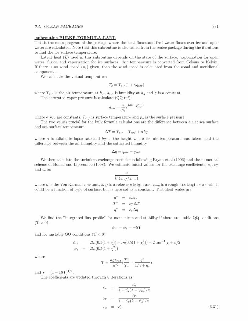
6.4. OCEAN PACKAGES 331
subroutine BULKF FORMULA LANLThis is the main program of the package where the heat fluxes and freshwater fluxes over ice and openwater are calculated. Note that this subroutine is also called from the seaice package during the iterationsto find the ice surface temperature.
Latent heat (L) used in this subroutine depends on the state of the surface: vaporization for openwater, fusion and vaporization for ice surfaces. Air temperature is converted from Celsius to Kelvin.If there is no wind speed (us) given, then the wind speed is calculated from the zonal and meridionalcomponents.
We calculate the virtual temperature:
To = Tair(1 + γqair)
where Tair is the air temperature at hT , qair is humidity at hq and γ is a constant.The saturated vapor pressure is calculate (QQ ref):
qsat =a
poe
L(b− cTsrf
)
where a, b, c are constants, Tsrf is surface temperature and po is the surface pressure.The two values crucial for the bulk formula calculations are the difference between air at sea surface
and sea surface temperature:∆T = Tair − Tsrf + αhT
where α is adiabatic lapse rate and hT is the height where the air temperature was taken; and thedifference between the air humidity and the saturated humidity
∆q = qair − qsat.
We then calculate the turbulent exchange coefficients following Bryan et al (1996) and the numericalscheme of Hunke and Lipscombe (1998). We estimate initial values for the exchange coefficients, cu, cTand cq as
κ
ln(zref/zrou)
where κ is the Von Karman constant, zref is a reference height and zrou is a roughness length scale whichcould be a function of type of surface, but is here set as a constant. Turbulent scales are:
u∗ = cuus
T ∗ = cT ∆T
q∗ = cq∆q
We find the ”integrated flux profile” for momentum and stability if there are stable QQ conditions(Υ > 0) :
ψm = ψs = −5Υ
and for unstable QQ conditions (Υ < 0):
ψm = 2ln(0.5(1 + χ)) + ln(0.5(1 + χ2)) − 2 tan−1 χ+ π/2
ψs = 2ln(0.5(1 + χ2))
where
Υ =κgzref
u∗2(T ∗
To+
q∗
1/γ + qa)
and χ = (1 − 16Υ)1/2.The coefficients are updated through 5 iterations as:
cu =cu
1 + cu(λ− ψm)/κ
cT =cT
1 + cT (λ − ψs)/κ
cq = c′T (6.31)
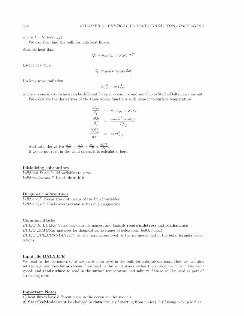
332 CHAPTER 6. PHYSICAL PARAMETERIZATIONS - PACKAGES I
where λ = ln(hT/zref ).
We can then find the bulk formula heat fluxes:
Sensible heat flux:
Qs = ρaircpairuscucT ∆T
Latent heat flux:
Ql = ρairLuscucq∆q
Up long wave radiation
Quplw = ǫσT 4
srf
where ǫ is emissivity (which can be different for open ocean, ice and snow), σ is Stefan-Boltzman constant.
We calculate the derivatives of the three above functions with respect to surface temperature
dQs
dT= ρaircpair
uscucT
dQl
dT=
ρairL2uscucqc
T 2srf
dQup]lw
dT= 4ǫσt3srf
And total derivative dQo
dT = dQs
dT + dQl
dT +dQup
lw
dT .
If we do not read in the wind stress, it is calculated here.
Initializing subroutines
bulkf init.F: Set bulkf variables to zero.
bulkf readparms.F: Reads data.blk
Diagnostic subroutines
bulkf ave.F: Keeps track of means of the bulkf variables
bulkf diags.F: Finds averages and writes out diagnostics
Common Blocks
BULKF.h: BULKF Variables, data file names, and logicals readwindstress and readsurface
BULKF DIAGS.h: matrices for diagnostics: averages of fields from bulkf diags.F
BULKF ICE CONSTANTS.h: all the parameters need by the ice model and in the bulkf formula calcu-lations.
Input file DATA.ICE
We read in the file names of atmospheric data used in the bulk formula calculations. Here we can alsoset the logicals: readwindstress if we read in the wind stress rather than calculate it from the windspeed; and readsurface to read in the surface temperature and salinity if these will be used as part ofa relaxing term.
Important Notes
1) heat fluxes have different signs in the ocean and ice models.
2) StartIceModel must be changed in data.ice: 1 (if starting from no ice), 0 (if using pickup.ic file).
6.4. OCEAN PACKAGES 333
References
Bryan F.O., B.G Kauffman, W.G. Large, P.R. Gent, 1996: The NCAR CSM flux coupler. Technical noteTN-425+STR, NCAR.
Hunke, E.C and W.H. Lipscomb, circa 2001: CICE: the Los Alamos Sea Ice Model Documentation andSoftware User’s Manual. LACC-98-16v.2.(note: this documentation is no longer available as CICE has progressed to a very different version 3)
6.4.6.1 Experiments and tutorials that use bulk force
• Global ocean experiment in global ocean.cs32x15 verification directory, input from input.thsicedirectory.
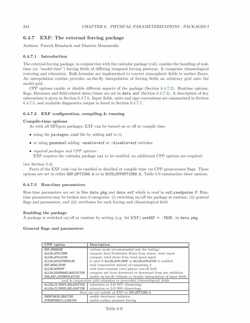
334 CHAPTER 6. PHYSICAL PARAMETERIZATIONS - PACKAGES I
6.4.7 EXF: The external forcing package
Authors: Patrick Heimbach and Dimitris Menemenlis
6.4.7.1 Introduction
The external forcing package, in conjunction with the calendar package (cal), enables the handling of real-time (or “model-time”) forcing fields of differing temporal forcing patterns. It comprises climatologicalrestoring and relaxation. Bulk formulae are implemented to convert atmospheric fields to surface fluxes.An interpolation routine provides on-the-fly interpolation of forcing fields an arbitrary grid onto themodel grid.
CPP options enable or disable different aspects of the package (Section 6.4.7.2). Runtime options,flags, filenames and field-related dates/times are set in data.exf (Section 6.4.7.3). A description of keysubroutines is given in Section 6.4.7.6. Input fields, units and sign conventions are summarized in Section6.4.7.5, and available diagnostics output is listed in Section 6.4.7.7.
6.4.7.2 EXF configuration, compiling & running
Compile-time optionsAs with all MITgcm packages, EXF can be turned on or off at compile time
• using the packages.conf file by adding exf to it,
• or using genmake2 adding -enable=exf or -disable=exf switches
• required packages and CPP options :EXF requires the calendar package cal to be enabled; no additional CPP options are required.
(see Section 3.4).Parts of the EXF code can be enabled or disabled at compile time via CPP preprocessor flags. These
options are set in either EXF OPTIONS.h or in ECCO CPPOPTIONS.h. Table 6.9 summarizes these options.
6.4.7.3 Run-time parameters
Run-time parameters are set in files data.pkg and data.exf which is read in exf readparms.F. Run-time parameters may be broken into 3 categories: (i) switching on/off the package at runtime, (ii) generalflags and parameters, and (iii) attributes for each forcing and climatological field.
Enabling the packageA package is switched on/off at runtime by setting (e.g. for EXF) useEXF = .TRUE. in data.pkg.
General flags and parameters
CPP option Description
EXF VERBOSE verbose mode (recommended only for testing)ALLOW ATM TEMP compute heat/freshwater fluxes from atmos. state inputALLOW ATM WIND compute wind stress from wind speed inputALLOW BULKFORMULAE is used if ALLOW ATM TEMP or ALLOW ATM WIND is enabledEXF READ EVAP read evaporation instead of computing itALLOW RUNOFF read time-constant river/glacier run-off fieldALLOW DOWNWARD RADIATION compute net from downward or downward from net radiationUSE EXF INTERPOLATION enable on-the-fly bilinear or bicubic interpolation of input fields
used in conjunction with relaxation to prescribed (climatological) fieldsALLOW CLIMSST RELAXATION relaxation to 2-D SST climatologyALLOW CLIMSSS RELAXATION relaxation to 2-D SSS climatology
these are set outside of EXF in CPP OPTIONS.h
SHORTWAVE HEATING enable shortwave radiationATMOSPHERIC LOADING enable surface pressure forcing
Table 6.9:
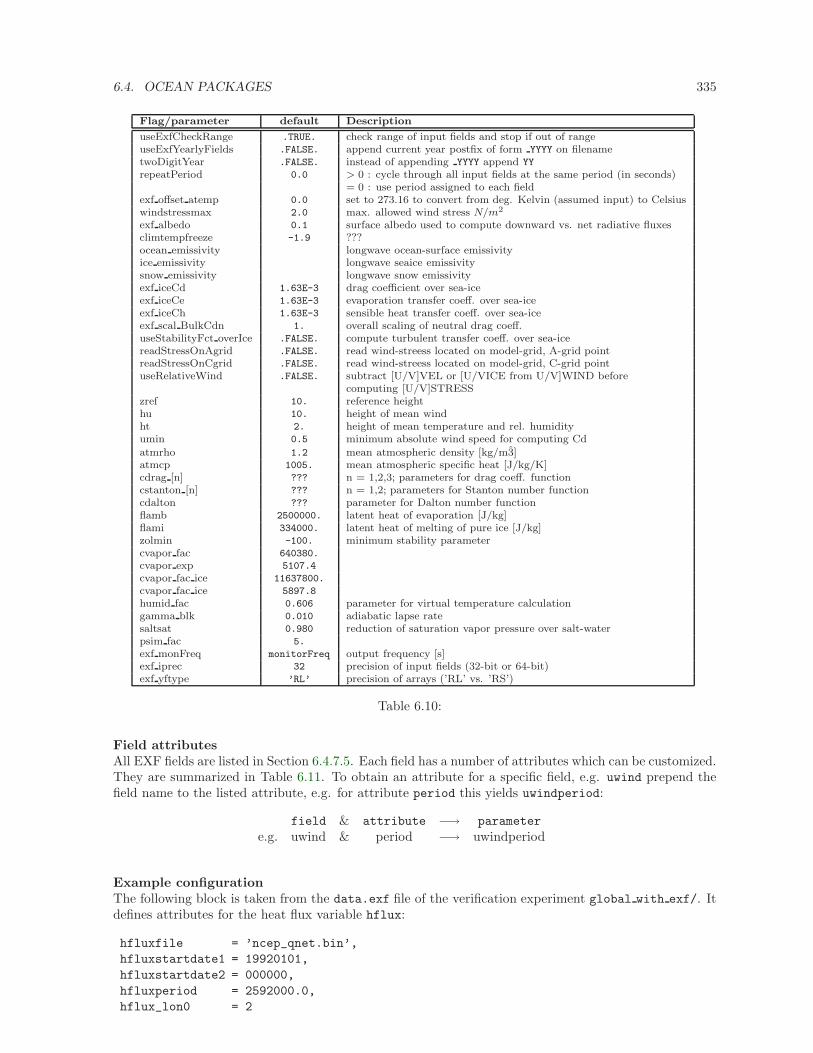
6.4. OCEAN PACKAGES 335
Flag/parameter default Description
useExfCheckRange .TRUE. check range of input fields and stop if out of rangeuseExfYearlyFields .FALSE. append current year postfix of form YYYY on filenametwoDigitYear .FALSE. instead of appending YYYY append YY
repeatPeriod 0.0 > 0 : cycle through all input fields at the same period (in seconds)= 0 : use period assigned to each field
exf offset atemp 0.0 set to 273.16 to convert from deg. Kelvin (assumed input) to Celsiuswindstressmax 2.0 max. allowed wind stress N/m2
exf albedo 0.1 surface albedo used to compute downward vs. net radiative fluxesclimtempfreeze -1.9 ???ocean emissivity longwave ocean-surface emissivityice emissivity longwave seaice emissivitysnow emissivity longwave snow emissivityexf iceCd 1.63E-3 drag coefficient over sea-iceexf iceCe 1.63E-3 evaporation transfer coeff. over sea-iceexf iceCh 1.63E-3 sensible heat transfer coeff. over sea-iceexf scal BulkCdn 1. overall scaling of neutral drag coeff.useStabilityFct overIce .FALSE. compute turbulent transfer coeff. over sea-icereadStressOnAgrid .FALSE. read wind-streess located on model-grid, A-grid pointreadStressOnCgrid .FALSE. read wind-streess located on model-grid, C-grid pointuseRelativeWind .FALSE. subtract [U/V]VEL or [U/VICE from U/V]WIND before
computing [U/V]STRESSzref 10. reference heighthu 10. height of mean windht 2. height of mean temperature and rel. humidityumin 0.5 minimum absolute wind speed for computing Cd
atmrho 1.2 mean atmospheric density [kg/m3]atmcp 1005. mean atmospheric specific heat [J/kg/K]cdrag [n] ??? n = 1,2,3; parameters for drag coeff. functioncstanton [n] ??? n = 1,2; parameters for Stanton number functioncdalton ??? parameter for Dalton number functionflamb 2500000. latent heat of evaporation [J/kg]flami 334000. latent heat of melting of pure ice [J/kg]zolmin -100. minimum stability parametercvapor fac 640380.
cvapor exp 5107.4
cvapor fac ice 11637800.
cvapor fac ice 5897.8
humid fac 0.606 parameter for virtual temperature calculationgamma blk 0.010 adiabatic lapse ratesaltsat 0.980 reduction of saturation vapor pressure over salt-waterpsim fac 5.
exf monFreq monitorFreq output frequency [s]exf iprec 32 precision of input fields (32-bit or 64-bit)exf yftype ’RL’ precision of arrays (’RL’ vs. ’RS’)
Table 6.10:
Field attributesAll EXF fields are listed in Section 6.4.7.5. Each field has a number of attributes which can be customized.They are summarized in Table 6.11. To obtain an attribute for a specific field, e.g. uwind prepend thefield name to the listed attribute, e.g. for attribute period this yields uwindperiod:
field & attribute −→ parameter
e.g. uwind & period −→ uwindperiod
Example configurationThe following block is taken from the data.exf file of the verification experiment global with exf/. Itdefines attributes for the heat flux variable hflux:
hfluxfile = ’ncep_qnet.bin’,
hfluxstartdate1 = 19920101,
hfluxstartdate2 = 000000,
hfluxperiod = 2592000.0,
hflux_lon0 = 2
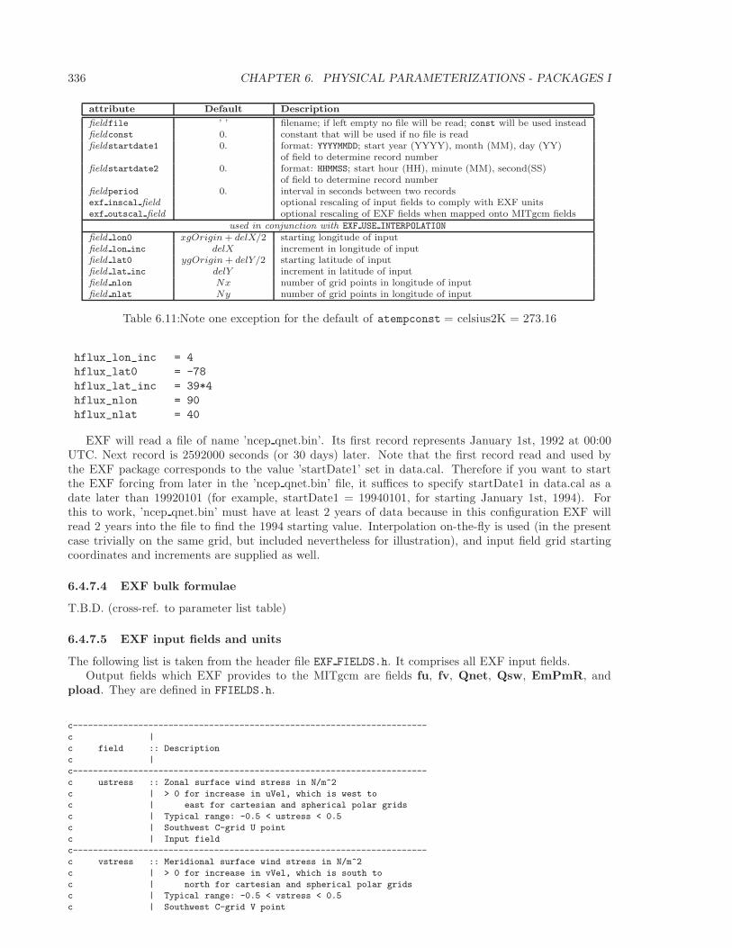
336 CHAPTER 6. PHYSICAL PARAMETERIZATIONS - PACKAGES I
attribute Default Description
fieldfile ’ ’ filename; if left empty no file will be read; const will be used insteadfieldconst 0. constant that will be used if no file is readfieldstartdate1 0. format: YYYYMMDD; start year (YYYY), month (MM), day (YY)
of field to determine record numberfieldstartdate2 0. format: HHMMSS; start hour (HH), minute (MM), second(SS)
of field to determine record numberfieldperiod 0. interval in seconds between two recordsexf inscal field optional rescaling of input fields to comply with EXF unitsexf outscal field optional rescaling of EXF fields when mapped onto MITgcm fields
used in conjunction with EXF USE INTERPOLATION
field lon0 xgOrigin + delX/2 starting longitude of inputfield lon inc delX increment in longitude of inputfield lat0 ygOrigin + delY/2 starting latitude of inputfield lat inc delY increment in latitude of inputfield nlon Nx number of grid points in longitude of inputfield nlat Ny number of grid points in longitude of input
Table 6.11:Note one exception for the default of atempconst = celsius2K = 273.16
hflux_lon_inc = 4
hflux_lat0 = -78
hflux_lat_inc = 39*4
hflux_nlon = 90
hflux_nlat = 40
EXF will read a file of name ’ncep qnet.bin’. Its first record represents January 1st, 1992 at 00:00UTC. Next record is 2592000 seconds (or 30 days) later. Note that the first record read and used bythe EXF package corresponds to the value ’startDate1’ set in data.cal. Therefore if you want to startthe EXF forcing from later in the ’ncep qnet.bin’ file, it suffices to specify startDate1 in data.cal as adate later than 19920101 (for example, startDate1 = 19940101, for starting January 1st, 1994). Forthis to work, ’ncep qnet.bin’ must have at least 2 years of data because in this configuration EXF willread 2 years into the file to find the 1994 starting value. Interpolation on-the-fly is used (in the presentcase trivially on the same grid, but included nevertheless for illustration), and input field grid startingcoordinates and increments are supplied as well.
6.4.7.4 EXF bulk formulae
T.B.D. (cross-ref. to parameter list table)
6.4.7.5 EXF input fields and units
The following list is taken from the header file EXF FIELDS.h. It comprises all EXF input fields.Output fields which EXF provides to the MITgcm are fields fu, fv, Qnet, Qsw, EmPmR, and
pload. They are defined in FFIELDS.h.
c----------------------------------------------------------------------
c |
c field :: Description
c |
c----------------------------------------------------------------------
c ustress :: Zonal surface wind stress in N/m^2
c | > 0 for increase in uVel, which is west to
c | east for cartesian and spherical polar grids
c | Typical range: -0.5 < ustress < 0.5
c | Southwest C-grid U point
c | Input field
c----------------------------------------------------------------------
c vstress :: Meridional surface wind stress in N/m^2
c | > 0 for increase in vVel, which is south to
c | north for cartesian and spherical polar grids
c | Typical range: -0.5 < vstress < 0.5
c | Southwest C-grid V point
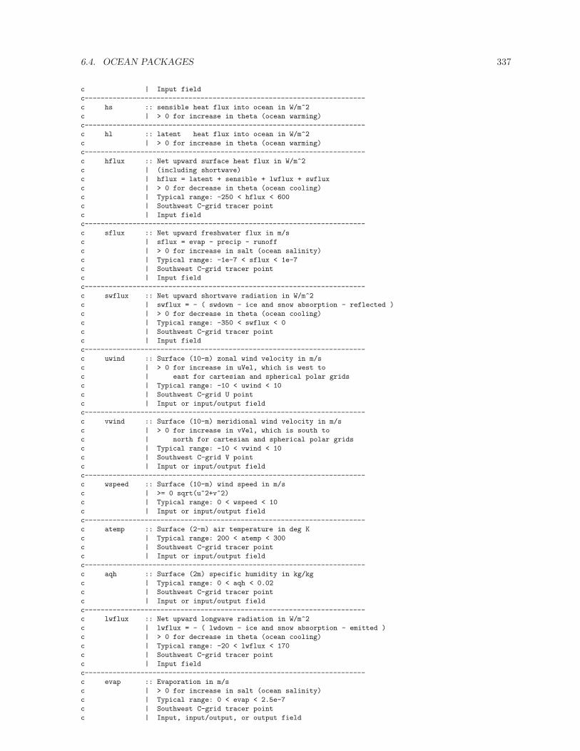
6.4. OCEAN PACKAGES 337
c | Input field
c----------------------------------------------------------------------
c hs :: sensible heat flux into ocean in W/m^2
c | > 0 for increase in theta (ocean warming)
c----------------------------------------------------------------------
c hl :: latent heat flux into ocean in W/m^2
c | > 0 for increase in theta (ocean warming)
c----------------------------------------------------------------------
c hflux :: Net upward surface heat flux in W/m^2
c | (including shortwave)
c | hflux = latent + sensible + lwflux + swflux
c | > 0 for decrease in theta (ocean cooling)
c | Typical range: -250 < hflux < 600
c | Southwest C-grid tracer point
c | Input field
c----------------------------------------------------------------------
c sflux :: Net upward freshwater flux in m/s
c | sflux = evap - precip - runoff
c | > 0 for increase in salt (ocean salinity)
c | Typical range: -1e-7 < sflux < 1e-7
c | Southwest C-grid tracer point
c | Input field
c----------------------------------------------------------------------
c swflux :: Net upward shortwave radiation in W/m^2
c | swflux = - ( swdown - ice and snow absorption - reflected )
c | > 0 for decrease in theta (ocean cooling)
c | Typical range: -350 < swflux < 0
c | Southwest C-grid tracer point
c | Input field
c----------------------------------------------------------------------
c uwind :: Surface (10-m) zonal wind velocity in m/s
c | > 0 for increase in uVel, which is west to
c | east for cartesian and spherical polar grids
c | Typical range: -10 < uwind < 10
c | Southwest C-grid U point
c | Input or input/output field
c----------------------------------------------------------------------
c vwind :: Surface (10-m) meridional wind velocity in m/s
c | > 0 for increase in vVel, which is south to
c | north for cartesian and spherical polar grids
c | Typical range: -10 < vwind < 10
c | Southwest C-grid V point
c | Input or input/output field
c----------------------------------------------------------------------
c wspeed :: Surface (10-m) wind speed in m/s
c | >= 0 sqrt(u^2+v^2)
c | Typical range: 0 < wspeed < 10
c | Input or input/output field
c----------------------------------------------------------------------
c atemp :: Surface (2-m) air temperature in deg K
c | Typical range: 200 < atemp < 300
c | Southwest C-grid tracer point
c | Input or input/output field
c----------------------------------------------------------------------
c aqh :: Surface (2m) specific humidity in kg/kg
c | Typical range: 0 < aqh < 0.02
c | Southwest C-grid tracer point
c | Input or input/output field
c----------------------------------------------------------------------
c lwflux :: Net upward longwave radiation in W/m^2
c | lwflux = - ( lwdown - ice and snow absorption - emitted )
c | > 0 for decrease in theta (ocean cooling)
c | Typical range: -20 < lwflux < 170
c | Southwest C-grid tracer point
c | Input field
c----------------------------------------------------------------------
c evap :: Evaporation in m/s
c | > 0 for increase in salt (ocean salinity)
c | Typical range: 0 < evap < 2.5e-7
c | Southwest C-grid tracer point
c | Input, input/output, or output field
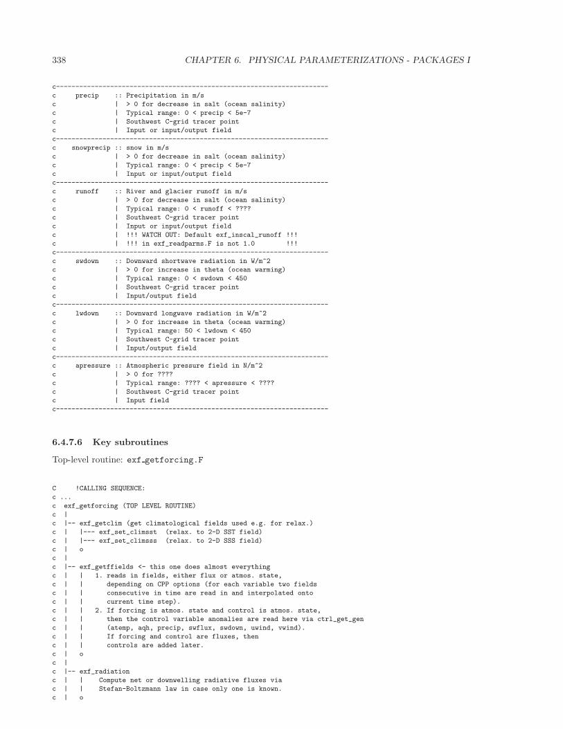
338 CHAPTER 6. PHYSICAL PARAMETERIZATIONS - PACKAGES I
c----------------------------------------------------------------------
c precip :: Precipitation in m/s
c | > 0 for decrease in salt (ocean salinity)
c | Typical range: 0 < precip < 5e-7
c | Southwest C-grid tracer point
c | Input or input/output field
c----------------------------------------------------------------------
c snowprecip :: snow in m/s
c | > 0 for decrease in salt (ocean salinity)
c | Typical range: 0 < precip < 5e-7
c | Input or input/output field
c----------------------------------------------------------------------
c runoff :: River and glacier runoff in m/s
c | > 0 for decrease in salt (ocean salinity)
c | Typical range: 0 < runoff < ????
c | Southwest C-grid tracer point
c | Input or input/output field
c | !!! WATCH OUT: Default exf_inscal_runoff !!!
c | !!! in exf_readparms.F is not 1.0 !!!
c----------------------------------------------------------------------
c swdown :: Downward shortwave radiation in W/m^2
c | > 0 for increase in theta (ocean warming)
c | Typical range: 0 < swdown < 450
c | Southwest C-grid tracer point
c | Input/output field
c----------------------------------------------------------------------
c lwdown :: Downward longwave radiation in W/m^2
c | > 0 for increase in theta (ocean warming)
c | Typical range: 50 < lwdown < 450
c | Southwest C-grid tracer point
c | Input/output field
c----------------------------------------------------------------------
c apressure :: Atmospheric pressure field in N/m^2
c | > 0 for ????
c | Typical range: ???? < apressure < ????
c | Southwest C-grid tracer point
c | Input field
c----------------------------------------------------------------------
6.4.7.6 Key subroutines
Top-level routine: exf getforcing.F
C !CALLING SEQUENCE:
c ...
c exf_getforcing (TOP LEVEL ROUTINE)
c |
c |-- exf_getclim (get climatological fields used e.g. for relax.)
c | |--- exf_set_climsst (relax. to 2-D SST field)
c | |--- exf_set_climsss (relax. to 2-D SSS field)
c | o
c |
c |-- exf_getffields <- this one does almost everything
c | | 1. reads in fields, either flux or atmos. state,
c | | depending on CPP options (for each variable two fields
c | | consecutive in time are read in and interpolated onto
c | | current time step).
c | | 2. If forcing is atmos. state and control is atmos. state,
c | | then the control variable anomalies are read here via ctrl_get_gen
c | | (atemp, aqh, precip, swflux, swdown, uwind, vwind).
c | | If forcing and control are fluxes, then
c | | controls are added later.
c | o
c |
c |-- exf_radiation
c | | Compute net or downwelling radiative fluxes via
c | | Stefan-Boltzmann law in case only one is known.
c | o
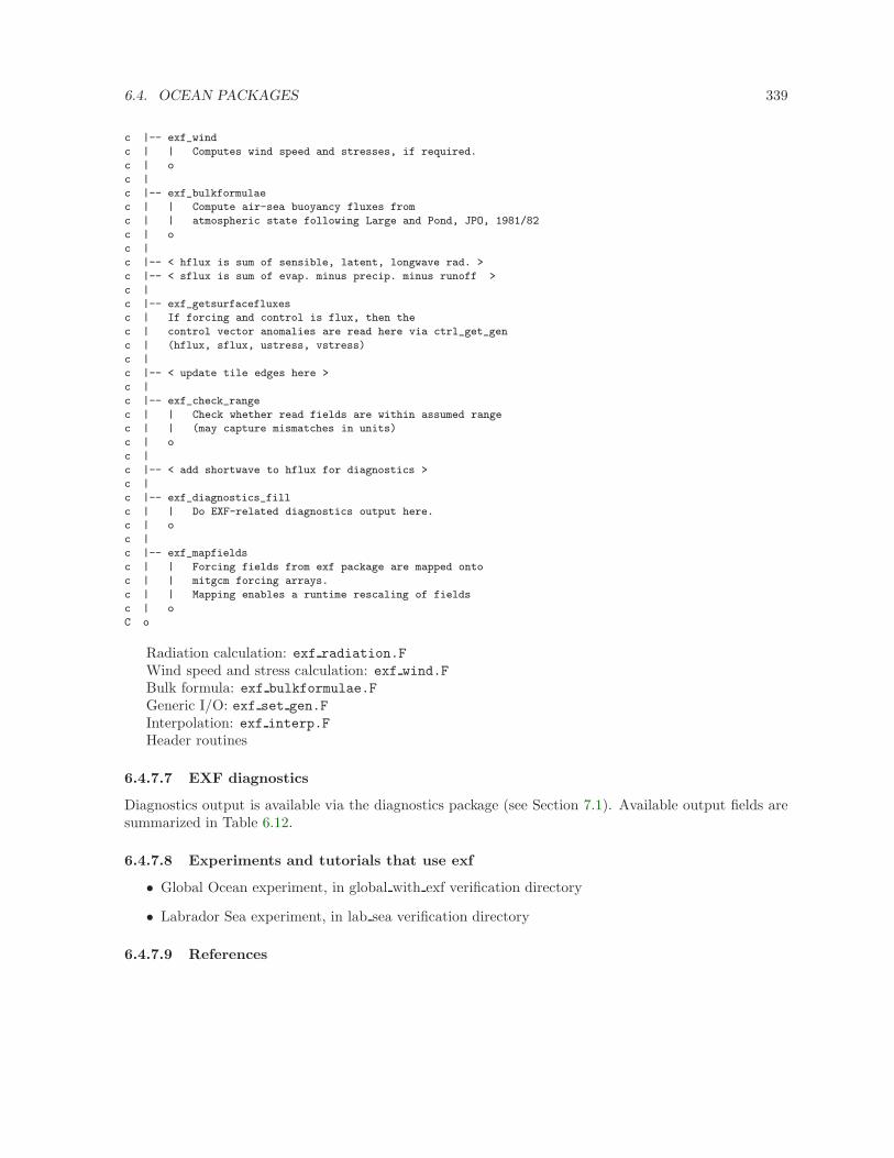
6.4. OCEAN PACKAGES 339
c |-- exf_wind
c | | Computes wind speed and stresses, if required.
c | o
c |
c |-- exf_bulkformulae
c | | Compute air-sea buoyancy fluxes from
c | | atmospheric state following Large and Pond, JPO, 1981/82
c | o
c |
c |-- < hflux is sum of sensible, latent, longwave rad. >
c |-- < sflux is sum of evap. minus precip. minus runoff >
c |
c |-- exf_getsurfacefluxes
c | If forcing and control is flux, then the
c | control vector anomalies are read here via ctrl_get_gen
c | (hflux, sflux, ustress, vstress)
c |
c |-- < update tile edges here >
c |
c |-- exf_check_range
c | | Check whether read fields are within assumed range
c | | (may capture mismatches in units)
c | o
c |
c |-- < add shortwave to hflux for diagnostics >
c |
c |-- exf_diagnostics_fill
c | | Do EXF-related diagnostics output here.
c | o
c |
c |-- exf_mapfields
c | | Forcing fields from exf package are mapped onto
c | | mitgcm forcing arrays.
c | | Mapping enables a runtime rescaling of fields
c | o
C o
Radiation calculation: exf radiation.F
Wind speed and stress calculation: exf wind.F
Bulk formula: exf bulkformulae.F
Generic I/O: exf set gen.F
Interpolation: exf interp.F
Header routines
6.4.7.7 EXF diagnostics
Diagnostics output is available via the diagnostics package (see Section 7.1). Available output fields aresummarized in Table 6.12.
6.4.7.8 Experiments and tutorials that use exf
• Global Ocean experiment, in global with exf verification directory
• Labrador Sea experiment, in lab sea verification directory
6.4.7.9 References
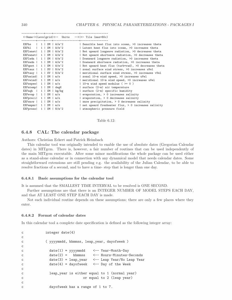
340 CHAPTER 6. PHYSICAL PARAMETERIZATIONS - PACKAGES I
---------+----+----+----------------+-----------------
<-Name->|Levs|grid|<-- Units -->|<- Tile (max=80c)
---------+----+----+----------------+-----------------
EXFhs | 1 | SM | W/m^2 | Sensible heat flux into ocean, >0 increases theta
EXFhl | 1 | SM | W/m^2 | Latent heat flux into ocean, >0 increases theta
EXFlwnet| 1 | SM | W/m^2 | Net upward longwave radiation, >0 decreases theta
EXFswnet| 1 | SM | W/m^2 | Net upward shortwave radiation, >0 decreases theta
EXFlwdn | 1 | SM | W/m^2 | Downward longwave radiation, >0 increases theta
EXFswdn | 1 | SM | W/m^2 | Downward shortwave radiation, >0 increases theta
EXFqnet | 1 | SM | W/m^2 | Net upward heat flux (turb+rad), >0 decreases theta
EXFtaux | 1 | SU | N/m^2 | zonal surface wind stress, >0 increases uVel
EXFtauy | 1 | SV | N/m^2 | meridional surface wind stress, >0 increases vVel
EXFuwind| 1 | SM | m/s | zonal 10-m wind speed, >0 increases uVel
EXFvwind| 1 | SM | m/s | meridional 10-m wind speed, >0 increases uVel
EXFwspee| 1 | SM | m/s | 10-m wind speed modulus ( >= 0 )
EXFatemp| 1 | SM | degK | surface (2-m) air temperature
EXFaqh | 1 | SM | kg/kg | surface (2-m) specific humidity
EXFevap | 1 | SM | m/s | evaporation, > 0 increases salinity
EXFpreci| 1 | SM | m/s | evaporation, > 0 decreases salinity
EXFsnow | 1 | SM | m/s | snow precipitation, > 0 decreases salinity
EXFempmr| 1 | SM | m/s | net upward freshwater flux, > 0 increases salinity
EXFpress| 1 | SM | N/m^2 | atmospheric pressure field
Table 6.12:
6.4.8 CAL: The calendar package
Authors: Christian Eckert and Patrick Heimbach
This calendar tool was originally intended to enable the use of absolute dates (Gregorian Calendardates) in MITgcm. There is, however, a fair number of routines that can be used independently ofthe main MITgcm executable. After some minor modifications the whole package can be used eitheras a stand-alone calendar or in connection with any dynamical model that needs calendar dates. Somestraightforward extensions are still pending e.g. the availability of the Julian Calendar, to be able toresolve fractions of a second, and to have a time- step that is longer than one day.
6.4.8.1 Basic assumptions for the calendar tool
It is assumed that the SMALLEST TIME INTERVAL to be resolved is ONE SECOND.
Further assumptions are that there is an INTEGER NUMBER OF MODEL STEPS EACH DAY,and that AT LEAST ONE STEP EACH DAY is made.
Not each individual routine depends on these assumptions; there are only a few places where theyenter.
6.4.8.2 Format of calendar dates
In this calendar tool a complete date specification is defined as the following integer array:
c integer date(4)
c
c ( yyyymmdd, hhmmss, leap_year, dayofweek )
c
c date(1) = yyyymmdd <-- Year-Month-Day
c date(2) = hhmmss <-- Hours-Minutes-Seconds
c date(3) = leap_year <-- Leap Year/No Leap Year
c date(4) = dayofweek <-- Day of the Week
c
c leap_year is either equal to 1 (normal year)
c or equal to 2 (leap year)
c
c dayofweek has a range of 1 to 7.
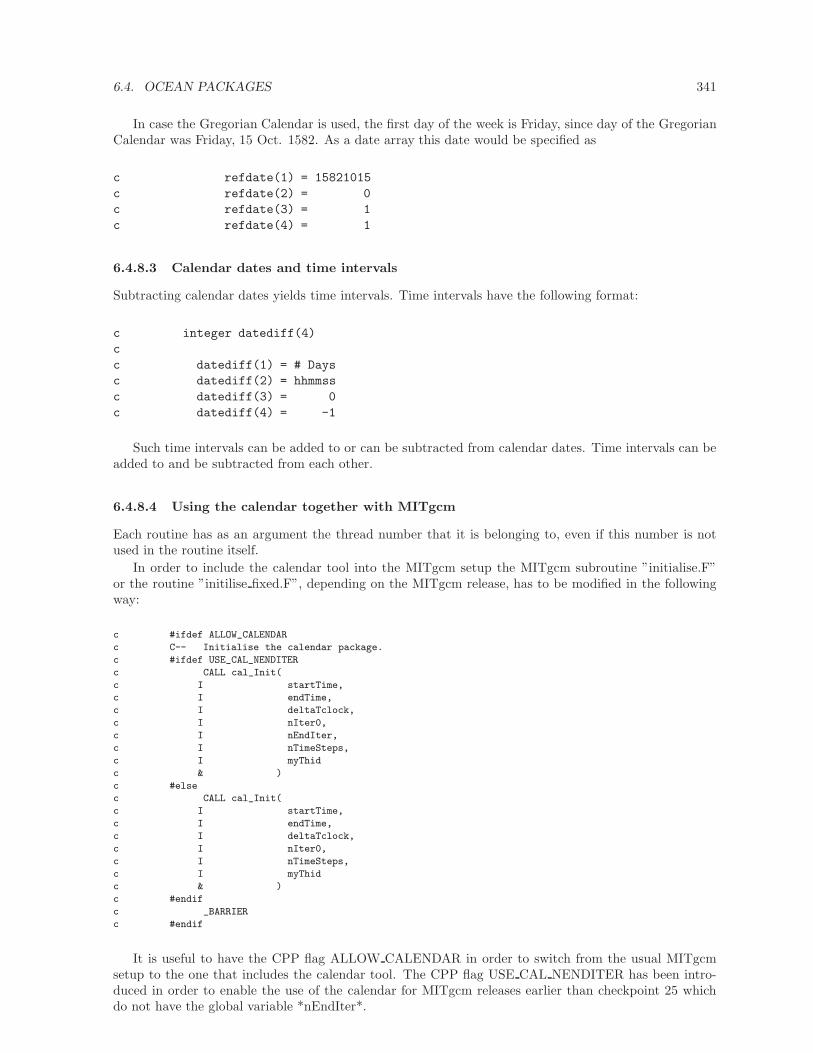
6.4. OCEAN PACKAGES 341
In case the Gregorian Calendar is used, the first day of the week is Friday, since day of the GregorianCalendar was Friday, 15 Oct. 1582. As a date array this date would be specified as
c refdate(1) = 15821015
c refdate(2) = 0
c refdate(3) = 1
c refdate(4) = 1
6.4.8.3 Calendar dates and time intervals
Subtracting calendar dates yields time intervals. Time intervals have the following format:
c integer datediff(4)
c
c datediff(1) = # Days
c datediff(2) = hhmmss
c datediff(3) = 0
c datediff(4) = -1
Such time intervals can be added to or can be subtracted from calendar dates. Time intervals can beadded to and be subtracted from each other.
6.4.8.4 Using the calendar together with MITgcm
Each routine has as an argument the thread number that it is belonging to, even if this number is notused in the routine itself.
In order to include the calendar tool into the MITgcm setup the MITgcm subroutine ”initialise.F”or the routine ”initilise fixed.F”, depending on the MITgcm release, has to be modified in the followingway:
c #ifdef ALLOW_CALENDAR
c C-- Initialise the calendar package.
c #ifdef USE_CAL_NENDITER
c CALL cal_Init(
c I startTime,
c I endTime,
c I deltaTclock,
c I nIter0,
c I nEndIter,
c I nTimeSteps,
c I myThid
c & )
c #else
c CALL cal_Init(
c I startTime,
c I endTime,
c I deltaTclock,
c I nIter0,
c I nTimeSteps,
c I myThid
c & )
c #endif
c _BARRIER
c #endif
It is useful to have the CPP flag ALLOW CALENDAR in order to switch from the usual MITgcmsetup to the one that includes the calendar tool. The CPP flag USE CAL NENDITER has been intro-duced in order to enable the use of the calendar for MITgcm releases earlier than checkpoint 25 whichdo not have the global variable *nEndIter*.
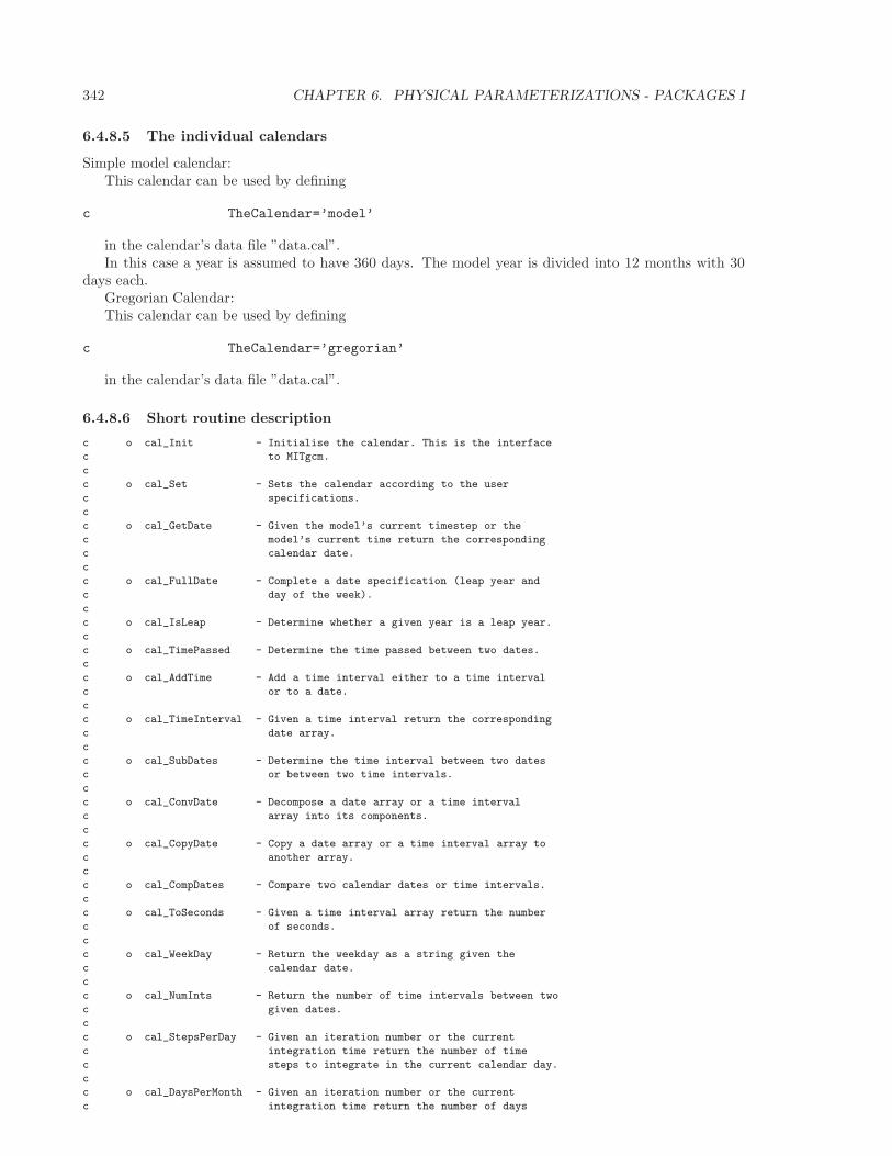
342 CHAPTER 6. PHYSICAL PARAMETERIZATIONS - PACKAGES I
6.4.8.5 The individual calendars
Simple model calendar:This calendar can be used by defining
c TheCalendar=’model’
in the calendar’s data file ”data.cal”.In this case a year is assumed to have 360 days. The model year is divided into 12 months with 30
days each.Gregorian Calendar:This calendar can be used by defining
c TheCalendar=’gregorian’
in the calendar’s data file ”data.cal”.
6.4.8.6 Short routine description
c o cal_Init - Initialise the calendar. This is the interface
c to MITgcm.
c
c o cal_Set - Sets the calendar according to the user
c specifications.
c
c o cal_GetDate - Given the model’s current timestep or the
c model’s current time return the corresponding
c calendar date.
c
c o cal_FullDate - Complete a date specification (leap year and
c day of the week).
c
c o cal_IsLeap - Determine whether a given year is a leap year.
c
c o cal_TimePassed - Determine the time passed between two dates.
c
c o cal_AddTime - Add a time interval either to a time interval
c or to a date.
c
c o cal_TimeInterval - Given a time interval return the corresponding
c date array.
c
c o cal_SubDates - Determine the time interval between two dates
c or between two time intervals.
c
c o cal_ConvDate - Decompose a date array or a time interval
c array into its components.
c
c o cal_CopyDate - Copy a date array or a time interval array to
c another array.
c
c o cal_CompDates - Compare two calendar dates or time intervals.
c
c o cal_ToSeconds - Given a time interval array return the number
c of seconds.
c
c o cal_WeekDay - Return the weekday as a string given the
c calendar date.
c
c o cal_NumInts - Return the number of time intervals between two
c given dates.
c
c o cal_StepsPerDay - Given an iteration number or the current
c integration time return the number of time
c steps to integrate in the current calendar day.
c
c o cal_DaysPerMonth - Given an iteration number or the current
c integration time return the number of days
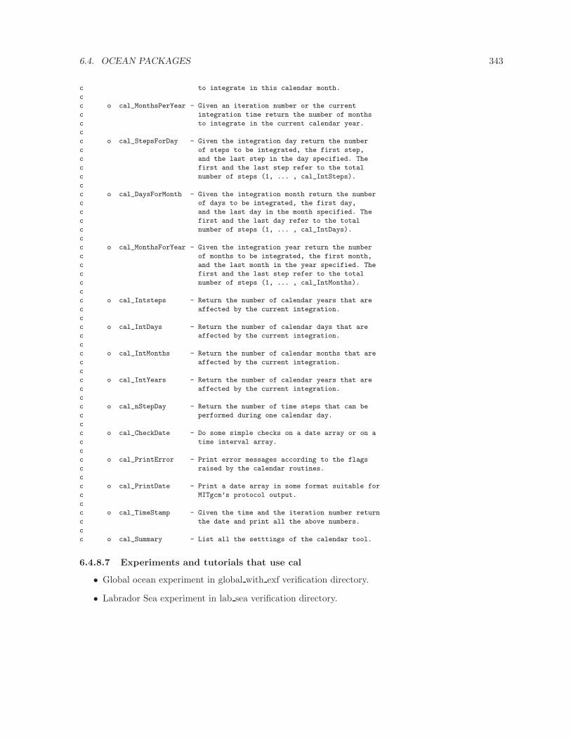
6.4. OCEAN PACKAGES 343
c to integrate in this calendar month.
c
c o cal_MonthsPerYear - Given an iteration number or the current
c integration time return the number of months
c to integrate in the current calendar year.
c
c o cal_StepsForDay - Given the integration day return the number
c of steps to be integrated, the first step,
c and the last step in the day specified. The
c first and the last step refer to the total
c number of steps (1, ... , cal_IntSteps).
c
c o cal_DaysForMonth - Given the integration month return the number
c of days to be integrated, the first day,
c and the last day in the month specified. The
c first and the last day refer to the total
c number of steps (1, ... , cal_IntDays).
c
c o cal_MonthsForYear - Given the integration year return the number
c of months to be integrated, the first month,
c and the last month in the year specified. The
c first and the last step refer to the total
c number of steps (1, ... , cal_IntMonths).
c
c o cal_Intsteps - Return the number of calendar years that are
c affected by the current integration.
c
c o cal_IntDays - Return the number of calendar days that are
c affected by the current integration.
c
c o cal_IntMonths - Return the number of calendar months that are
c affected by the current integration.
c
c o cal_IntYears - Return the number of calendar years that are
c affected by the current integration.
c
c o cal_nStepDay - Return the number of time steps that can be
c performed during one calendar day.
c
c o cal_CheckDate - Do some simple checks on a date array or on a
c time interval array.
c
c o cal_PrintError - Print error messages according to the flags
c raised by the calendar routines.
c
c o cal_PrintDate - Print a date array in some format suitable for
c MITgcm’s protocol output.
c
c o cal_TimeStamp - Given the time and the iteration number return
c the date and print all the above numbers.
c
c o cal_Summary - List all the setttings of the calendar tool.
6.4.8.7 Experiments and tutorials that use cal
• Global ocean experiment in global with exf verification directory.
• Labrador Sea experiment in lab sea verification directory.
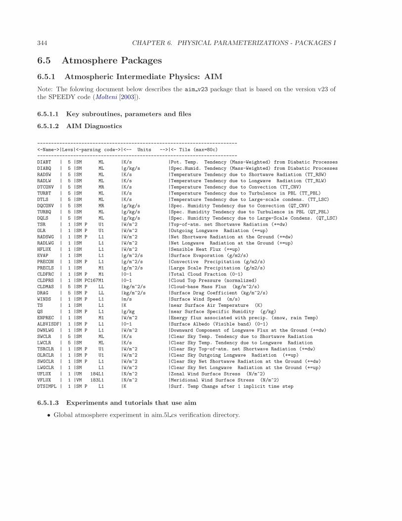
344 CHAPTER 6. PHYSICAL PARAMETERIZATIONS - PACKAGES I
6.5 Atmosphere Packages
6.5.1 Atmospheric Intermediate Physics: AIM
Note: The folowing document below describes the aim v23 package that is based on the version v23 ofthe SPEEDY code (Molteni [2003]).
6.5.1.1 Key subroutines, parameters and files
6.5.1.2 AIM Diagnostics
------------------------------------------------------------------------
<-Name->|Levs|<-parsing code->|<-- Units -->|<- Tile (max=80c)
------------------------------------------------------------------------
DIABT | 5 |SM ML |K/s |Pot. Temp. Tendency (Mass-Weighted) from Diabatic Processes
DIABQ | 5 |SM ML |g/kg/s |Spec.Humid. Tendency (Mass-Weighted) from Diabatic Processes
RADSW | 5 |SM ML |K/s |Temperature Tendency due to Shortwave Radiation (TT_RSW)
RADLW | 5 |SM ML |K/s |Temperature Tendency due to Longwave Radiation (TT_RLW)
DTCONV | 5 |SM MR |K/s |Temperature Tendency due to Convection (TT_CNV)
TURBT | 5 |SM ML |K/s |Temperature Tendency due to Turbulence in PBL (TT_PBL)
DTLS | 5 |SM ML |K/s |Temperature Tendency due to Large-scale condens. (TT_LSC)
DQCONV | 5 |SM MR |g/kg/s |Spec. Humidity Tendency due to Convection (QT_CNV)
TURBQ | 5 |SM ML |g/kg/s |Spec. Humidity Tendency due to Turbulence in PBL (QT_PBL)
DQLS | 5 |SM ML |g/kg/s |Spec. Humidity Tendency due to Large-Scale Condens. (QT_LSC)
TSR | 1 |SM P U1 |W/m^2 |Top-of-atm. net Shortwave Radiation (+=dw)
OLR | 1 |SM P U1 |W/m^2 |Outgoing Longwave Radiation (+=up)
RADSWG | 1 |SM P L1 |W/m^2 |Net Shortwave Radiation at the Ground (+=dw)
RADLWG | 1 |SM L1 |W/m^2 |Net Longwave Radiation at the Ground (+=up)
HFLUX | 1 |SM L1 |W/m^2 |Sensible Heat Flux (+=up)
EVAP | 1 |SM L1 |g/m^2/s |Surface Evaporation (g/m2/s)
PRECON | 1 |SM P L1 |g/m^2/s |Convective Precipitation (g/m2/s)
PRECLS | 1 |SM M1 |g/m^2/s |Large Scale Precipitation (g/m2/s)
CLDFRC | 1 |SM P M1 |0-1 |Total Cloud Fraction (0-1)
CLDPRS | 1 |SM PC167M1 |0-1 |Cloud Top Pressure (normalized)
CLDMAS | 5 |SM P LL |kg/m^2/s |Cloud-base Mass Flux (kg/m^2/s)
DRAG | 5 |SM P LL |kg/m^2/s |Surface Drag Coefficient (kg/m^2/s)
WINDS | 1 |SM P L1 |m/s |Surface Wind Speed (m/s)
TS | 1 |SM L1 |K |near Surface Air Temperature (K)
QS | 1 |SM P L1 |g/kg |near Surface Specific Humidity (g/kg)
ENPREC | 1 |SM M1 |W/m^2 |Energy flux associated with precip. (snow, rain Temp)
ALBVISDF| 1 |SM P L1 |0-1 |Surface Albedo (Visible band) (0-1)
DWNLWG | 1 |SM P L1 |W/m^2 |Downward Component of Longwave Flux at the Ground (+=dw)
SWCLR | 5 |SM ML |K/s |Clear Sky Temp. Tendency due to Shortwave Radiation
LWCLR | 5 |SM ML |K/s |Clear Sky Temp. Tendency due to Longwave Radiation
TSRCLR | 1 |SM P U1 |W/m^2 |Clear Sky Top-of-atm. net Shortwave Radiation (+=dw)
OLRCLR | 1 |SM P U1 |W/m^2 |Clear Sky Outgoing Longwave Radiation (+=up)
SWGCLR | 1 |SM P L1 |W/m^2 |Clear Sky Net Shortwave Radiation at the Ground (+=dw)
LWGCLR | 1 |SM L1 |W/m^2 |Clear Sky Net Longwave Radiation at the Ground (+=up)
UFLUX | 1 |UM 184L1 |N/m^2 |Zonal Wind Surface Stress (N/m^2)
VFLUX | 1 |VM 183L1 |N/m^2 |Meridional Wind Surface Stress (N/m^2)
DTSIMPL | 1 |SM P L1 |K |Surf. Temp Change after 1 implicit time step
6.5.1.3 Experiments and tutorials that use aim
• Global atmosphere experiment in aim.5l cs verification directory.
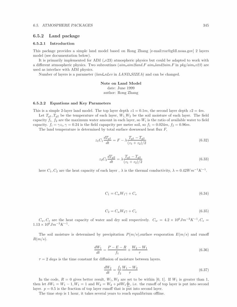
6.5. ATMOSPHERE PACKAGES 345
6.5.2 Land package
6.5.2.1 Introduction
This package provides a simple land model based on Rong Zhang [e-mail:[email protected]] 2 layersmodel (see documentation below).
It is primarily implemented for AIM ( v23) atmospheric physics but could be adapted to work witha different atmospheric physics. Two subroutines (aim aim2land.F aim land2aim.F in pkg/aim v23) areused as interface with AIM physics.
Number of layers is a parameter (land nLev in LAND SIZE.h) and can be changed.
Note on Land Modeldate: June 1999
author: Rong Zhang
6.5.2.2 Equations and Key Parameters
This is a simple 2-layer land model. The top layer depth z1 = 0.1m, the second layer depth z2 = 4m.Let Tg1, Tg2 be the temperature of each layer, W1,W2 be the soil moisture of each layer. The field
capacity f1, f2 are the maximum water amount in each layer, so Wi is the ratio of available water to fieldcapacity. fi = γzi, γ = 0.24 is the field capapcity per meter soil, so f1 = 0.024m, f2 = 0.96m.
The land temperature is determined by total surface downward heat flux F,
z1C1dTg1
dt= F − λ
Tg1 − Tg2
(z1 + z2)/2(6.32)
z2C2dTg2
dt= λ
Tg1 − Tg2
(z1 + z2)/2(6.33)
here C1, C2 are the heat capacity of each layer , λ is the thermal conductivity, λ = 0.42Wm−1K−1.
C1 = CwW1γ + Cs (6.34)
C2 = CwW2γ + Cs (6.35)
Cw, Cs are the heat capacity of water and dry soil respectively. Cw = 4.2 × 10⁶Jm−3K−1, Cs =1.13 × 10⁶Jm−3K−1.
The soil moisture is determined by precipitation P (m/s),surface evaporation E(m/s) and runoffR(m/s).
dW1
dt=P − E −R
f1+W2 −W1
τ(6.36)
τ = 2 days is the time constant for diffusion of moisture between layers.
dW2
dt=f1f2
W1 −W2
τ(6.37)
In the code, R = 0 gives better result, W1,W2 are set to be within [0, 1]. If W1 is greater than 1,then let δW1 = W1 − 1,W1 = 1 and W2 = W2 + pδW1
f1
f2, i.e. the runoff of top layer is put into second
layer. p = 0.5 is the fraction of top layer runoff that is put into second layer.The time step is 1 hour, it takes several years to reach equalibrium offline.
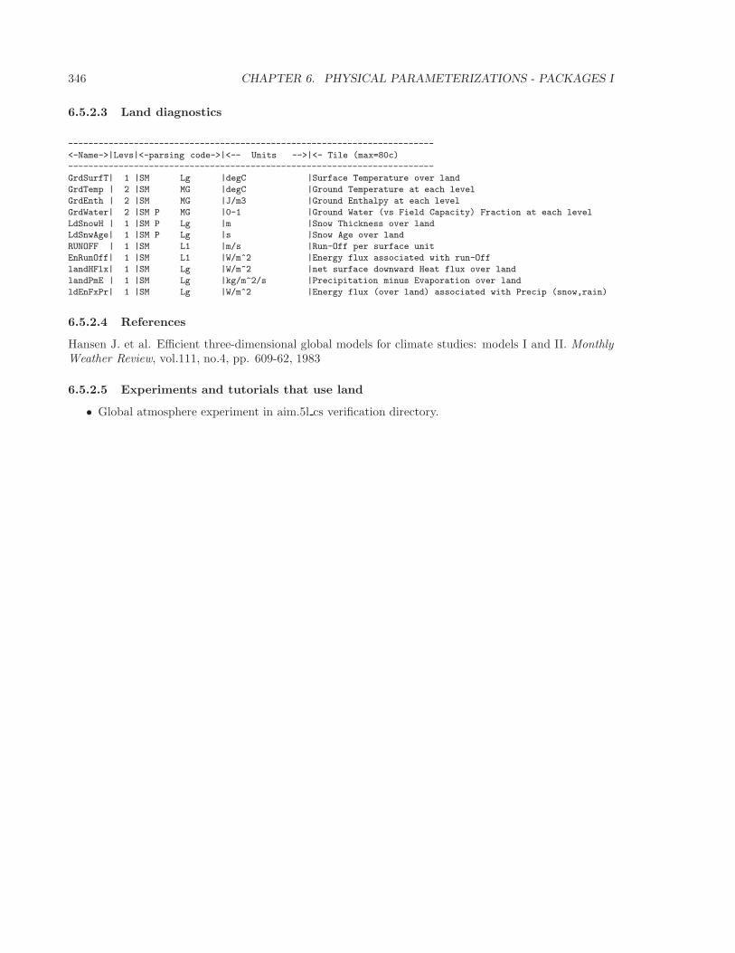
346 CHAPTER 6. PHYSICAL PARAMETERIZATIONS - PACKAGES I
6.5.2.3 Land diagnostics
------------------------------------------------------------------------
<-Name->|Levs|<-parsing code->|<-- Units -->|<- Tile (max=80c)
------------------------------------------------------------------------
GrdSurfT| 1 |SM Lg |degC |Surface Temperature over land
GrdTemp | 2 |SM MG |degC |Ground Temperature at each level
GrdEnth | 2 |SM MG |J/m3 |Ground Enthalpy at each level
GrdWater| 2 |SM P MG |0-1 |Ground Water (vs Field Capacity) Fraction at each level
LdSnowH | 1 |SM P Lg |m |Snow Thickness over land
LdSnwAge| 1 |SM P Lg |s |Snow Age over land
RUNOFF | 1 |SM L1 |m/s |Run-Off per surface unit
EnRunOff| 1 |SM L1 |W/m^2 |Energy flux associated with run-Off
landHFlx| 1 |SM Lg |W/m^2 |net surface downward Heat flux over land
landPmE | 1 |SM Lg |kg/m^2/s |Precipitation minus Evaporation over land
ldEnFxPr| 1 |SM Lg |W/m^2 |Energy flux (over land) associated with Precip (snow,rain)
6.5.2.4 References
Hansen J. et al. Efficient three-dimensional global models for climate studies: models I and II. MonthlyWeather Review, vol.111, no.4, pp. 609-62, 1983
6.5.2.5 Experiments and tutorials that use land
• Global atmosphere experiment in aim.5l cs verification directory.

6.5. ATMOSPHERE PACKAGES 347
6.5.3 Fizhi: High-end Atmospheric Physics
6.5.3.1 Introduction
The fizhi (high-end atmospheric physics) package includes a collection of state-of-the-art physical pa-rameterizations for atmospheric radiation, cumulus convection, atmospheric boundary layer turbulence,and land surface processes. The collection of atmospheric physics parameterizations were originallyused together as part of the GEOS-3 (Goddard Earth Observing System-3) GCM developed at theNASA/Goddard Global Modelling and Assimilation Office (GMAO).
6.5.3.2 Equations
Moist Convective Processes:
Sub-grid and Large-scale Convection Sub-grid scale cumulus convection is parameterized using theRelaxed Arakawa Schubert (RAS) scheme of Moorthi and Suarez [1992], which is a linearized ArakawaSchubert type scheme. RAS predicts the mass flux from an ensemble of clouds. Each subensemble isidentified by its entrainment rate and level of neutral bouyancy which are determined by the grid-scaleproperties.
The thermodynamic variables that are used in RAS to describe the grid scale vertical profile are thedry static energy, s = cpT + gz, and the moist static energy, h = cpT + gz + Lq. The conceptual modelbehind RAS depicts each subensemble as a rising plume cloud, entraining mass from the environmentduring ascent, and detraining all cloud air at the level of neutral buoyancy. RAS assumes that thenormalized cloud mass flux, η, normalized by the cloud base mass flux, is a linear function of height,expressed as:
∂η(z)
∂z= λ or
∂η(P κ)
∂P κ= −cp
gθλ
where we have used the hydrostatic equation written in the form:
∂z
∂P κ= −cp
gθ
The entrainment parameter, λ, characterizes a particular subensemble based on its detrainment level,and is obtained by assuming that the level of detrainment is the level of neutral buoyancy, ie., the levelat which the moist static energy of the cloud, hc, is equal to the saturation moist static energy of theenvironment, h∗. Following Moorthi and Suarez [1992], λ may be written as
λ =hB − h∗D
cp
g
∫ PB
PDθ(h∗D − h)dP κ
,
where the subscript B refers to cloud base, and the subscript D refers to the detrainment level.The convective instability is measured in terms of the cloud work function A, defined as the rate of
change of cumulus kinetic energy. The cloud work function is related to the buoyancy, or the differencebetween the moist static energy in the cloud and in the environment:
A =
∫ PB
PD
η
1 + γ
[hc − h∗
P κ
]dP κ
where γ is Lcp
∂q∗
∂T obtained from the Claussius Clapeyron equation, and the subscript c refers to the
value inside the cloud.To determine the cloud base mass flux, the rate of change of A in time due to dissipation by the clouds
is assumed to approximately balance the rate of change of A due to the generation by the large scale.This is the quasi-equilibrium assumption, and results in an expression for mB:
mB =− dA
dt
∣∣ls
K
where K is the cloud kernel, defined as the rate of change of the cloud work function per unit cloudbase mass flux, and is currently obtained by analytically differentiating the expression for A in time. The
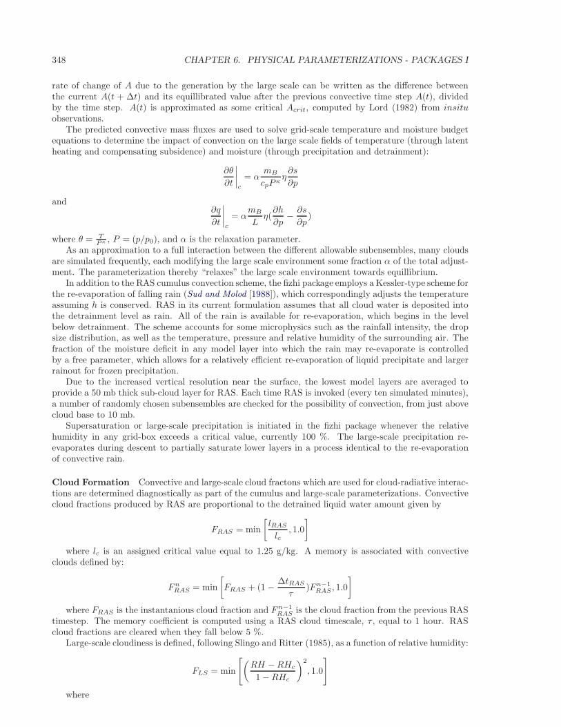
348 CHAPTER 6. PHYSICAL PARAMETERIZATIONS - PACKAGES I
rate of change of A due to the generation by the large scale can be written as the difference betweenthe current A(t + ∆t) and its equillibrated value after the previous convective time step A(t), dividedby the time step. A(t) is approximated as some critical Acrit, computed by Lord (1982) from insituobservations.
The predicted convective mass fluxes are used to solve grid-scale temperature and moisture budgetequations to determine the impact of convection on the large scale fields of temperature (through latentheating and compensating subsidence) and moisture (through precipitation and detrainment):
∂θ
∂t
∣∣∣∣c
= αmB
cpP κη∂s
∂p
and∂q
∂t
∣∣∣∣c
= αmB
Lη(∂h
∂p− ∂s
∂p)
where θ = TP κ , P = (p/p0), and α is the relaxation parameter.
As an approximation to a full interaction between the different allowable subensembles, many cloudsare simulated frequently, each modifying the large scale environment some fraction α of the total adjust-ment. The parameterization thereby “relaxes” the large scale environment towards equillibrium.
In addition to the RAS cumulus convection scheme, the fizhi package employs a Kessler-type scheme forthe re-evaporation of falling rain (Sud and Molod [1988]), which correspondingly adjusts the temperatureassuming h is conserved. RAS in its current formulation assumes that all cloud water is deposited intothe detrainment level as rain. All of the rain is available for re-evaporation, which begins in the levelbelow detrainment. The scheme accounts for some microphysics such as the rainfall intensity, the dropsize distribution, as well as the temperature, pressure and relative humidity of the surrounding air. Thefraction of the moisture deficit in any model layer into which the rain may re-evaporate is controlledby a free parameter, which allows for a relatively efficient re-evaporation of liquid precipitate and largerrainout for frozen precipitation.
Due to the increased vertical resolution near the surface, the lowest model layers are averaged toprovide a 50 mb thick sub-cloud layer for RAS. Each time RAS is invoked (every ten simulated minutes),a number of randomly chosen subensembles are checked for the possibility of convection, from just abovecloud base to 10 mb.
Supersaturation or large-scale precipitation is initiated in the fizhi package whenever the relativehumidity in any grid-box exceeds a critical value, currently 100 %. The large-scale precipitation re-evaporates during descent to partially saturate lower layers in a process identical to the re-evaporationof convective rain.
Cloud Formation Convective and large-scale cloud fractons which are used for cloud-radiative interac-tions are determined diagnostically as part of the cumulus and large-scale parameterizations. Convectivecloud fractions produced by RAS are proportional to the detrained liquid water amount given by
FRAS = min
[lRAS
lc, 1.0
]
where lc is an assigned critical value equal to 1.25 g/kg. A memory is associated with convectiveclouds defined by:
FnRAS = min
[FRAS + (1 − ∆tRAS
τ)Fn−1
RAS , 1.0
]
where FRAS is the instantanious cloud fraction and Fn−1RAS is the cloud fraction from the previous RAS
timestep. The memory coefficient is computed using a RAS cloud timescale, τ , equal to 1 hour. RAScloud fractions are cleared when they fall below 5 %.
Large-scale cloudiness is defined, following Slingo and Ritter (1985), as a function of relative humidity:
FLS = min
[(RH −RHc
1 −RHc
)2
, 1.0
]
where
6.5. ATMOSPHERE PACKAGES 349
RHc = 1 − s(1 − s)(2 −√
3 + 2√
3 s)r
s = p/psurf
r =
(1.0 −RHmin
α
)
RHmin = 0.75
α = 0.573285.
These cloud fractions are suppressed, however, in regions where the convective sub-cloud layer isconditionally unstable. The functional form of RHc is shown in Figure (6.9).
Figure 6.9: Critical Relative Humidity for Clouds.
The total cloud fraction in a grid box is determined by the larger of the two cloud fractions:
FCLD = max [FRAS , FLS ] .
Finally, cloud fractions are time-averaged between calls to the radiation packages.Radiation:The parameterization of radiative heating in the fizhi package includes effects from both shortwave
and longwave processes. Radiative fluxes are calculated at each model edge-level in both up and downdirections. The heating rates/cooling rates are then obtained from the vertical divergence of the netradiative fluxes.
The net flux is
F = F ↑ − F ↓
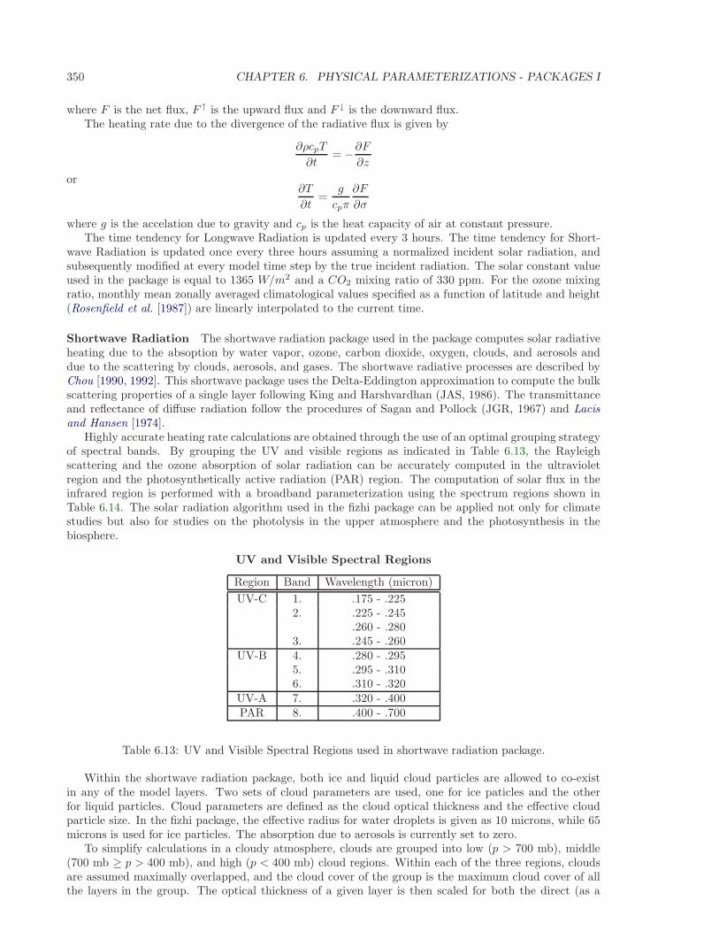
350 CHAPTER 6. PHYSICAL PARAMETERIZATIONS - PACKAGES I
where F is the net flux, F ↑ is the upward flux and F ↓ is the downward flux.The heating rate due to the divergence of the radiative flux is given by
∂ρcpT
∂t= −∂F
∂z
or∂T
∂t=
g
cpπ
∂F
∂σ
where g is the accelation due to gravity and cp is the heat capacity of air at constant pressure.The time tendency for Longwave Radiation is updated every 3 hours. The time tendency for Short-
wave Radiation is updated once every three hours assuming a normalized incident solar radiation, andsubsequently modified at every model time step by the true incident radiation. The solar constant valueused in the package is equal to 1365 W/m2 and a CO2 mixing ratio of 330 ppm. For the ozone mixingratio, monthly mean zonally averaged climatological values specified as a function of latitude and height(Rosenfield et al. [1987]) are linearly interpolated to the current time.
Shortwave Radiation The shortwave radiation package used in the package computes solar radiativeheating due to the absoption by water vapor, ozone, carbon dioxide, oxygen, clouds, and aerosols anddue to the scattering by clouds, aerosols, and gases. The shortwave radiative processes are described byChou [1990, 1992]. This shortwave package uses the Delta-Eddington approximation to compute the bulkscattering properties of a single layer following King and Harshvardhan (JAS, 1986). The transmittanceand reflectance of diffuse radiation follow the procedures of Sagan and Pollock (JGR, 1967) and Lacisand Hansen [1974].
Highly accurate heating rate calculations are obtained through the use of an optimal grouping strategyof spectral bands. By grouping the UV and visible regions as indicated in Table 6.13, the Rayleighscattering and the ozone absorption of solar radiation can be accurately computed in the ultravioletregion and the photosynthetically active radiation (PAR) region. The computation of solar flux in theinfrared region is performed with a broadband parameterization using the spectrum regions shown inTable 6.14. The solar radiation algorithm used in the fizhi package can be applied not only for climatestudies but also for studies on the photolysis in the upper atmosphere and the photosynthesis in thebiosphere.
UV and Visible Spectral Regions
Region Band Wavelength (micron)
UV-C 1. .175 - .2252. .225 - .245
.260 - .2803. .245 - .260
UV-B 4. .280 - .2955. .295 - .3106. .310 - .320
UV-A 7. .320 - .400PAR 8. .400 - .700
Table 6.13: UV and Visible Spectral Regions used in shortwave radiation package.
Within the shortwave radiation package, both ice and liquid cloud particles are allowed to co-existin any of the model layers. Two sets of cloud parameters are used, one for ice paticles and the otherfor liquid particles. Cloud parameters are defined as the cloud optical thickness and the effective cloudparticle size. In the fizhi package, the effective radius for water droplets is given as 10 microns, while 65microns is used for ice particles. The absorption due to aerosols is currently set to zero.
To simplify calculations in a cloudy atmosphere, clouds are grouped into low (p > 700 mb), middle(700 mb ≥ p > 400 mb), and high (p < 400 mb) cloud regions. Within each of the three regions, cloudsare assumed maximally overlapped, and the cloud cover of the group is the maximum cloud cover of allthe layers in the group. The optical thickness of a given layer is then scaled for both the direct (as a
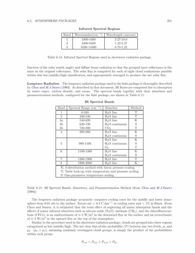
6.5. ATMOSPHERE PACKAGES 351
Infrared Spectral Regions
Band Wavenumber(cm−1) Wavelength (micron)
1 1000-4400 2.27-10.02 4400-8200 1.22-2.273 8200-14300 0.70-1.22
Table 6.14: Infrared Spectral Regions used in shortwave radiation package.
function of the solar zenith angle) and diffuse beam radiation so that the grouped layer reflectance is thesame as the original reflectance. The solar flux is computed for each of eight cloud realizations possiblewithin this low/middle/high classification, and appropriately averaged to produce the net solar flux.
Longwave Radiation The longwave radiation package used in the fizhi package is thoroughly describedby Chou and M.J.Suarez [1994]. As described in that document, IR fluxes are computed due to absorptionby water vapor, carbon dioxide, and ozone. The spectral bands together with their absorbers andparameterization methods, configured for the fizhi package, are shown in Table 6.15.
IR Spectral Bands
Band Spectral Range (cm−1) Absorber Method
1 0-340 H2O line T2 340-540 H2O line T3a 540-620 H2O line K3b 620-720 H2O continuum S3b 720-800 CO2 T4 800-980 H2O line K
H2O continuum SH2O line K
5 980-1100 H2O continuum SO3 T
6 1100-1380 H2O line KH2O continuum S
7 1380-1900 H2O line T8 1900-3000 H2O line K
K: k-distribution method with linear pressure scalingT: Table look-up with temperature and pressure scalingS: One-parameter temperature scaling
Table 6.15: IR Spectral Bands, Absorbers, and Parameterization Method (from Chou and M.J.Suarez[1994])
The longwave radiation package accurately computes cooling rates for the middle and lower atmo-sphere from 0.01 mb to the surface. Errors are < 0.4 C day−1 in cooling rates and < 1% in fluxes. FromChou and Suarez, it is estimated that the total effect of neglecting all minor absorption bands and theeffects of minor infrared absorbers such as nitrous oxide (N2O), methane (CH4), and the chlorofluorocar-bons (CFCs), is an underestimate of ≈ 5 W/m2 in the downward flux at the surface and an overestimateof ≈ 3 W/m2 in the upward flux at the top of the atmosphere.
Similar to the procedure used in the shortwave radiation package, clouds are grouped into three regionscatagorized as low/middle/high. The net clear line-of-site probability (P ) between any two levels, p1 andp2 (p2 > p1), assuming randomly overlapped cloud groups, is simply the product of the probabilitieswithin each group:
Pnet = Plow × Pmid × Phi.
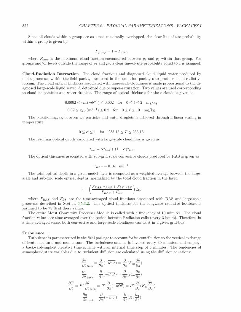
352 CHAPTER 6. PHYSICAL PARAMETERIZATIONS - PACKAGES I
Since all clouds within a group are assumed maximally overlapped, the clear line-of-site probabilitywithin a group is given by:
Pgroup = 1 − Fmax,
where Fmax is the maximum cloud fraction encountered between p1 and p2 within that group. Forgroups and/or levels outside the range of p1 and p2, a clear line-of-site probability equal to 1 is assigned.
Cloud-Radiation Interaction The cloud fractions and diagnosed cloud liquid water produced bymoist processes within the fizhi package are used in the radiation packages to produce cloud-radiativeforcing. The cloud optical thickness associated with large-scale cloudiness is made proportional to the di-agnosed large-scale liquid water, ℓ, detrained due to super-saturation. Two values are used correspondingto cloud ice particles and water droplets. The range of optical thickness for these clouds is given as
0.0002 ≤ τice(mb−1) ≤ 0.002 for 0 ≤ ℓ ≤ 2 mg/kg,
0.02 ≤ τh2o(mb−1) ≤ 0.2 for 0 ≤ ℓ ≤ 10 mg/kg.
The partitioning, α, between ice particles and water droplets is achieved through a linear scaling intemperature:
0 ≤ α ≤ 1 for 233.15 ≤ T ≤ 253.15.
The resulting optical depth associated with large-scale cloudiness is given as
τLS = ατh2o + (1 − α)τice.
The optical thickness associated with sub-grid scale convective clouds produced by RAS is given as
τRAS = 0.16 mb−1.
The total optical depth in a given model layer is computed as a weighted average between the large-scale and sub-grid scale optical depths, normalized by the total cloud fraction in the layer:
τ =
(FRAS τRAS + FLS τLS
FRAS + FLS
)∆p,
where FRAS and FLS are the time-averaged cloud fractions associated with RAS and large-scaleprocesses described in Section 6.5.3.2. The optical thickness for the longwave radiative feedback isassumed to be 75 % of these values.
The entire Moist Convective Processes Module is called with a frequency of 10 minutes. The cloudfraction values are time-averaged over the period between Radiation calls (every 3 hours). Therefore, ina time-averaged sense, both convective and large-scale cloudiness can exist in a given grid-box.
Turbulence :Turbulence is parameterized in the fizhi package to account for its contribution to the vertical exchange
of heat, moisture, and momentum. The turbulence scheme is invoked every 30 minutes, and employsa backward-implicit iterative time scheme with an internal time step of 5 minutes. The tendencies ofatmospheric state variables due to turbulent diffusion are calculated using the diffusion equations:
∂u
∂t turb=
∂
∂z(−u′w′) =
∂
∂z(Km
∂u
∂z)
∂v
∂t turb=
∂
∂z(−v′w′) =
∂
∂z(Km
∂v
∂z)
∂T
∂t= P κ∂θ
∂t turb= P κ ∂
∂z(−w′θ′) = P κ ∂
∂z(Kh
∂θv
∂z)
∂q
∂t turb=
∂
∂z(−w′q′) =
∂
∂z(Kh
∂q
∂z)
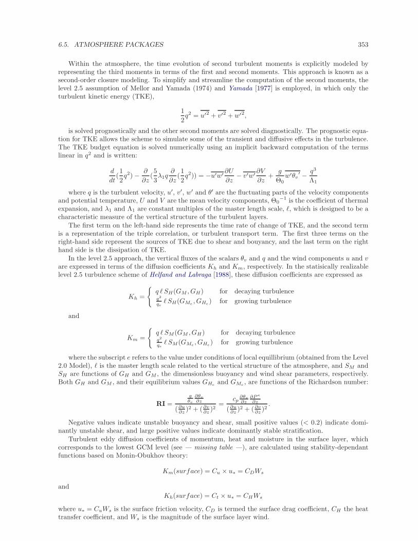
6.5. ATMOSPHERE PACKAGES 353
Within the atmosphere, the time evolution of second turbulent moments is explicitly modeled byrepresenting the third moments in terms of the first and second moments. This approach is known as asecond-order closure modeling. To simplify and streamline the computation of the second moments, thelevel 2.5 assumption of Mellor and Yamada (1974) and Yamada [1977] is employed, in which only theturbulent kinetic energy (TKE),
1
2q2 = u′2 + v′2 + w′2,
is solved prognostically and the other second moments are solved diagnostically. The prognostic equa-tion for TKE allows the scheme to simulate some of the transient and diffusive effects in the turbulence.The TKE budget equation is solved numerically using an implicit backward computation of the termslinear in q2 and is written:
d
dt(1
2q2) − ∂
∂z(5
3λ1q
∂
∂z(1
2q2)) = −u′w′ ∂U
∂z− v′w′
∂V
∂z+
g
Θ0w′θv
′ − q3
Λ1
where q is the turbulent velocity, u′, v′, w′ and θ′ are the fluctuating parts of the velocity componentsand potential temperature, U and V are the mean velocity components, Θ0
−1 is the coefficient of thermalexpansion, and λ1 and Λ1 are constant multiples of the master length scale, ℓ, which is designed to be acharacteristic measure of the vertical structure of the turbulent layers.
The first term on the left-hand side represents the time rate of change of TKE, and the second termis a representation of the triple correlation, or turbulent transport term. The first three terms on theright-hand side represent the sources of TKE due to shear and bouyancy, and the last term on the righthand side is the dissipation of TKE.
In the level 2.5 approach, the vertical fluxes of the scalars θv and q and the wind components u and vare expressed in terms of the diffusion coefficients Kh and Km, respectively. In the statisically realizablelevel 2.5 turbulence scheme of Helfand and Labraga [1988], these diffusion coefficients are expressed as
Kh =
q ℓ SH(GM , GH) for decaying turbulenceq2
qeℓ SH(GMe
, GHe) for growing turbulence
and
Km =
q ℓ SM (GM , GH) for decaying turbulenceq2
qeℓ SM (GMe
, GHe) for growing turbulence
where the subscript e refers to the value under conditions of local equillibrium (obtained from the Level2.0 Model), ℓ is the master length scale related to the vertical structure of the atmosphere, and SM andSH are functions of GH and GM , the dimensionless buoyancy and wind shear parameters, respectively.Both GH and GM , and their equilibrium values GHe
and GMe, are functions of the Richardson number:
RI =
gθv
∂θv
∂z
(∂u∂z )2 + (∂v
∂z )2=
cp∂θv
∂z∂P κ
∂z
(∂u∂z )2 + (∂v
∂z )2.
Negative values indicate unstable buoyancy and shear, small positive values (< 0.2) indicate domi-nantly unstable shear, and large positive values indicate dominantly stable stratification.
Turbulent eddy diffusion coefficients of momentum, heat and moisture in the surface layer, whichcorresponds to the lowest GCM level (see — missing table —), are calculated using stability-dependantfunctions based on Monin-Obukhov theory:
Km(surface) = Cu × u∗ = CDWs
and
Kh(surface) = Ct × u∗ = CHWs
where u∗ = CuWs is the surface friction velocity, CD is termed the surface drag coefficient, CH the heattransfer coefficient, and Ws is the magnitude of the surface layer wind.
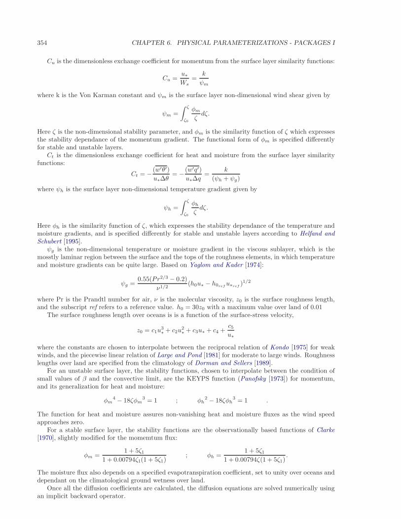
354 CHAPTER 6. PHYSICAL PARAMETERIZATIONS - PACKAGES I
Cu is the dimensionless exchange coefficient for momentum from the surface layer similarity functions:
Cu =u∗Ws
=k
ψm
where k is the Von Karman constant and ψm is the surface layer non-dimensional wind shear given by
ψm =
∫ ζ
ζ0
φm
ζdζ.
Here ζ is the non-dimensional stability parameter, and φm is the similarity function of ζ which expressesthe stability dependance of the momentum gradient. The functional form of φm is specified differentlyfor stable and unstable layers.
Ct is the dimensionless exchange coefficient for heat and moisture from the surface layer similarityfunctions:
Ct = − (w′θ′)
u∗∆θ= − (w′q′)
u∗∆q=
k
(ψh + ψg)
where ψh is the surface layer non-dimensional temperature gradient given by
ψh =
∫ ζ
ζ0
φh
ζdζ.
Here φh is the similarity function of ζ, which expresses the stability dependance of the temperature andmoisture gradients, and is specified differently for stable and unstable layers according to Helfand andSchubert [1995].
ψg is the non-dimensional temperature or moisture gradient in the viscous sublayer, which is themosstly laminar region between the surface and the tops of the roughness elements, in which temperatureand moisture gradients can be quite large. Based on Yaglom and Kader [1974]:
ψg =0.55(Pr2/3 − 0.2)
ν1/2(h0u∗ − h0ref
u∗ref)1/2
where Pr is the Prandtl number for air, ν is the molecular viscosity, z0 is the surface roughness length,and the subscript ref refers to a reference value. h0 = 30z0 with a maximum value over land of 0.01
The surface roughness length over oceans is is a function of the surface-stress velocity,
z0 = c1u3∗ + c2u
2∗ + c3u∗ + c4 +
c5u∗
where the constants are chosen to interpolate between the reciprocal relation of Kondo [1975] for weakwinds, and the piecewise linear relation of Large and Pond [1981] for moderate to large winds. Roughnesslengths over land are specified from the climatology of Dorman and Sellers [1989].
For an unstable surface layer, the stability functions, chosen to interpolate between the condition ofsmall values of β and the convective limit, are the KEYPS function (Panofsky [1973]) for momentum,and its generalization for heat and moisture:
φm4 − 18ζφm
3 = 1 ; φh2 − 18ζφh
3 = 1 .
The function for heat and moisture assures non-vanishing heat and moisture fluxes as the wind speedapproaches zero.
For a stable surface layer, the stability functions are the observationally based functions of Clarke[1970], slightly modified for the momemtum flux:
φm =1 + 5ζ1
1 + 0.00794ζ1(1 + 5ζ1); φh =
1 + 5ζ11 + 0.00794ζ(1 + 5ζ1)
.
The moisture flux also depends on a specified evapotranspiration coefficient, set to unity over oceans anddependant on the climatological ground wetness over land.
Once all the diffusion coefficients are calculated, the diffusion equations are solved numerically usingan implicit backward operator.
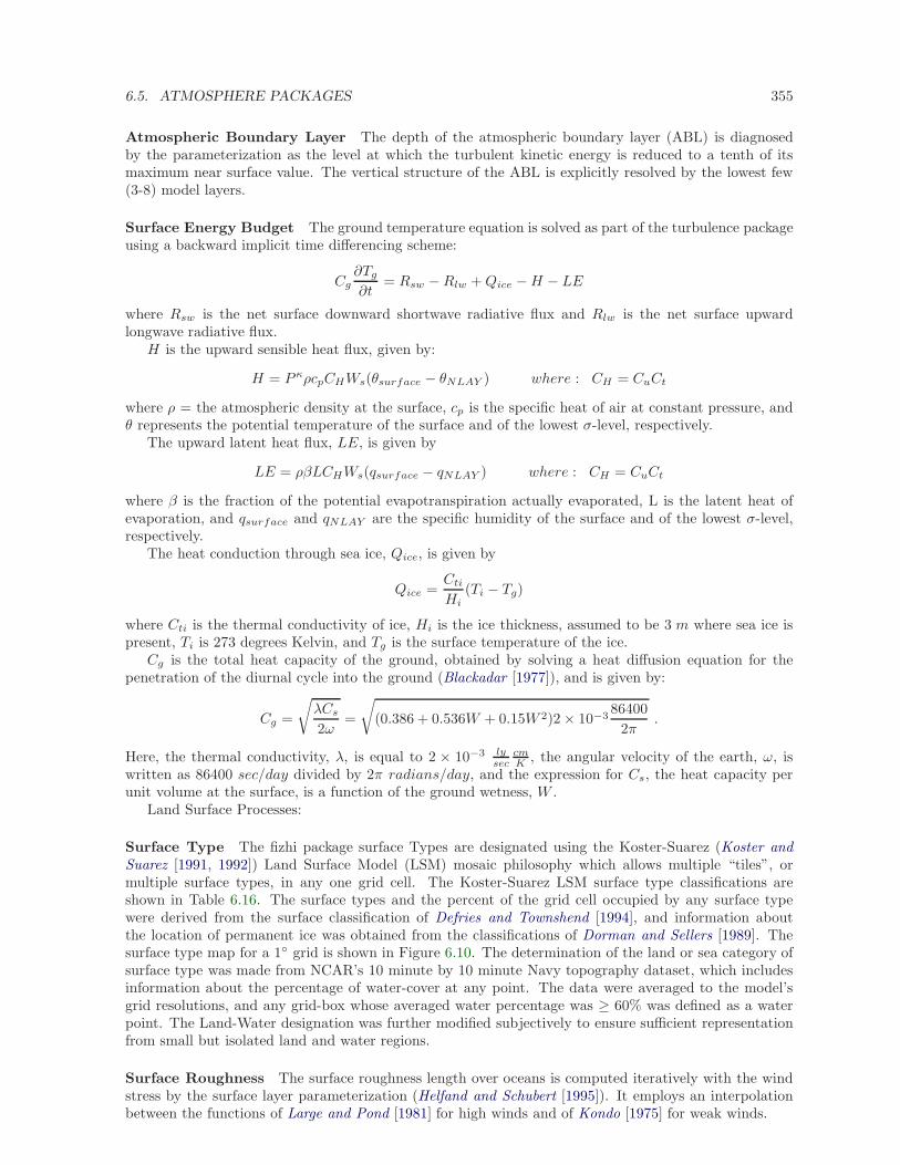
6.5. ATMOSPHERE PACKAGES 355
Atmospheric Boundary Layer The depth of the atmospheric boundary layer (ABL) is diagnosedby the parameterization as the level at which the turbulent kinetic energy is reduced to a tenth of itsmaximum near surface value. The vertical structure of the ABL is explicitly resolved by the lowest few(3-8) model layers.
Surface Energy Budget The ground temperature equation is solved as part of the turbulence packageusing a backward implicit time differencing scheme:
Cg∂Tg
∂t= Rsw −Rlw +Qice −H − LE
where Rsw is the net surface downward shortwave radiative flux and Rlw is the net surface upwardlongwave radiative flux.
H is the upward sensible heat flux, given by:
H = P κρcpCHWs(θsurface − θNLAY ) where : CH = CuCt
where ρ = the atmospheric density at the surface, cp is the specific heat of air at constant pressure, andθ represents the potential temperature of the surface and of the lowest σ-level, respectively.
The upward latent heat flux, LE, is given by
LE = ρβLCHWs(qsurface − qNLAY ) where : CH = CuCt
where β is the fraction of the potential evapotranspiration actually evaporated, L is the latent heat ofevaporation, and qsurface and qNLAY are the specific humidity of the surface and of the lowest σ-level,respectively.
The heat conduction through sea ice, Qice, is given by
Qice =Cti
Hi(Ti − Tg)
where Cti is the thermal conductivity of ice, Hi is the ice thickness, assumed to be 3 m where sea ice ispresent, Ti is 273 degrees Kelvin, and Tg is the surface temperature of the ice.
Cg is the total heat capacity of the ground, obtained by solving a heat diffusion equation for thepenetration of the diurnal cycle into the ground (Blackadar [1977]), and is given by:
Cg =
√λCs
2ω=
√(0.386 + 0.536W + 0.15W 2)2 × 10⁻³
86400
2π.
Here, the thermal conductivity, λ, is equal to 2 × 10⁻³ lysec
cmK , the angular velocity of the earth, ω, is
written as 86400 sec/day divided by 2π radians/day, and the expression for Cs, the heat capacity perunit volume at the surface, is a function of the ground wetness, W .
Land Surface Processes:
Surface Type The fizhi package surface Types are designated using the Koster-Suarez (Koster andSuarez [1991, 1992]) Land Surface Model (LSM) mosaic philosophy which allows multiple “tiles”, ormultiple surface types, in any one grid cell. The Koster-Suarez LSM surface type classifications areshown in Table 6.16. The surface types and the percent of the grid cell occupied by any surface typewere derived from the surface classification of Defries and Townshend [1994], and information aboutthe location of permanent ice was obtained from the classifications of Dorman and Sellers [1989]. Thesurface type map for a 1 grid is shown in Figure 6.10. The determination of the land or sea category ofsurface type was made from NCAR’s 10 minute by 10 minute Navy topography dataset, which includesinformation about the percentage of water-cover at any point. The data were averaged to the model’sgrid resolutions, and any grid-box whose averaged water percentage was ≥ 60% was defined as a waterpoint. The Land-Water designation was further modified subjectively to ensure sufficient representationfrom small but isolated land and water regions.
Surface Roughness The surface roughness length over oceans is computed iteratively with the windstress by the surface layer parameterization (Helfand and Schubert [1995]). It employs an interpolationbetween the functions of Large and Pond [1981] for high winds and of Kondo [1975] for weak winds.
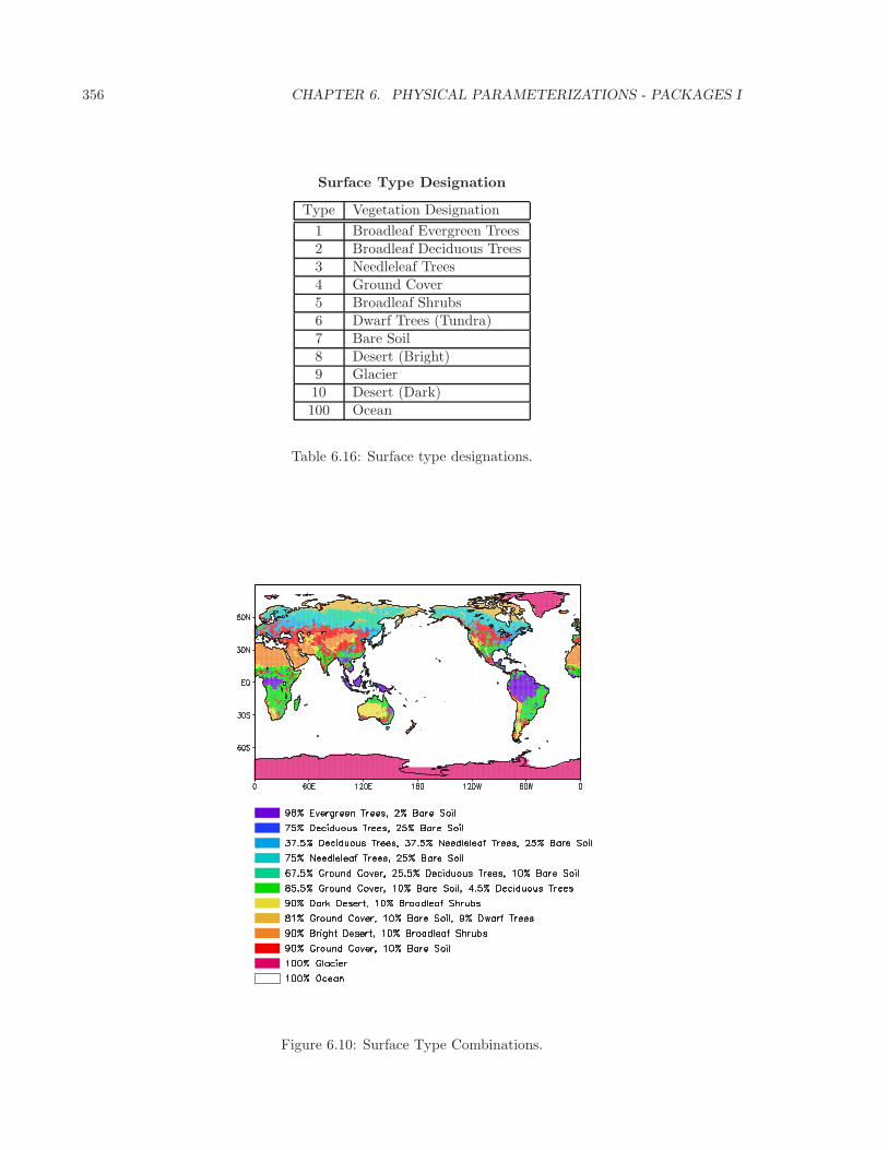
356 CHAPTER 6. PHYSICAL PARAMETERIZATIONS - PACKAGES I
Surface Type Designation
Type Vegetation Designation
1 Broadleaf Evergreen Trees2 Broadleaf Deciduous Trees3 Needleleaf Trees4 Ground Cover5 Broadleaf Shrubs6 Dwarf Trees (Tundra)7 Bare Soil8 Desert (Bright)9 Glacier10 Desert (Dark)100 Ocean
Table 6.16: Surface type designations.
Figure 6.10: Surface Type Combinations.
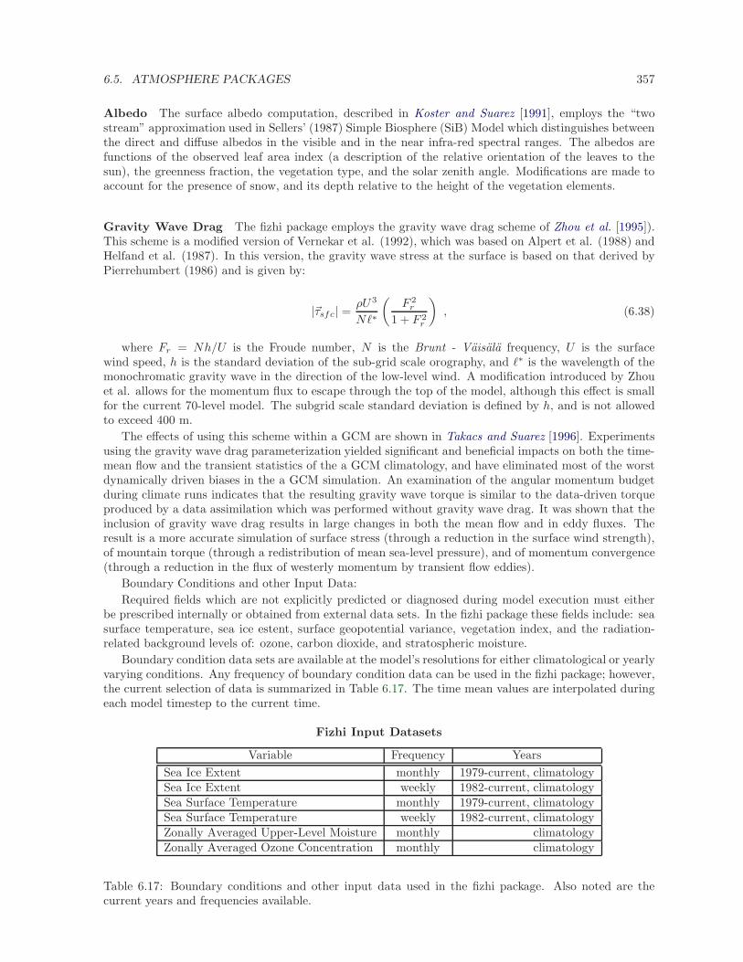
6.5. ATMOSPHERE PACKAGES 357
Albedo The surface albedo computation, described in Koster and Suarez [1991], employs the “twostream” approximation used in Sellers’ (1987) Simple Biosphere (SiB) Model which distinguishes betweenthe direct and diffuse albedos in the visible and in the near infra-red spectral ranges. The albedos arefunctions of the observed leaf area index (a description of the relative orientation of the leaves to thesun), the greenness fraction, the vegetation type, and the solar zenith angle. Modifications are made toaccount for the presence of snow, and its depth relative to the height of the vegetation elements.
Gravity Wave Drag The fizhi package employs the gravity wave drag scheme of Zhou et al. [1995]).This scheme is a modified version of Vernekar et al. (1992), which was based on Alpert et al. (1988) andHelfand et al. (1987). In this version, the gravity wave stress at the surface is based on that derived byPierrehumbert (1986) and is given by:
|~τsfc| =ρU3
Nℓ∗
(F 2
r
1 + F 2r
), (6.38)
where Fr = Nh/U is the Froude number, N is the Brunt - Vaisala frequency, U is the surfacewind speed, h is the standard deviation of the sub-grid scale orography, and ℓ∗ is the wavelength of themonochromatic gravity wave in the direction of the low-level wind. A modification introduced by Zhouet al. allows for the momentum flux to escape through the top of the model, although this effect is smallfor the current 70-level model. The subgrid scale standard deviation is defined by h, and is not allowedto exceed 400 m.
The effects of using this scheme within a GCM are shown in Takacs and Suarez [1996]. Experimentsusing the gravity wave drag parameterization yielded significant and beneficial impacts on both the time-mean flow and the transient statistics of the a GCM climatology, and have eliminated most of the worstdynamically driven biases in the a GCM simulation. An examination of the angular momentum budgetduring climate runs indicates that the resulting gravity wave torque is similar to the data-driven torqueproduced by a data assimilation which was performed without gravity wave drag. It was shown that theinclusion of gravity wave drag results in large changes in both the mean flow and in eddy fluxes. Theresult is a more accurate simulation of surface stress (through a reduction in the surface wind strength),of mountain torque (through a redistribution of mean sea-level pressure), and of momentum convergence(through a reduction in the flux of westerly momentum by transient flow eddies).
Boundary Conditions and other Input Data:
Required fields which are not explicitly predicted or diagnosed during model execution must eitherbe prescribed internally or obtained from external data sets. In the fizhi package these fields include: seasurface temperature, sea ice estent, surface geopotential variance, vegetation index, and the radiation-related background levels of: ozone, carbon dioxide, and stratospheric moisture.
Boundary condition data sets are available at the model’s resolutions for either climatological or yearlyvarying conditions. Any frequency of boundary condition data can be used in the fizhi package; however,the current selection of data is summarized in Table 6.17. The time mean values are interpolated duringeach model timestep to the current time.
Fizhi Input Datasets
Variable Frequency Years
Sea Ice Extent monthly 1979-current, climatologySea Ice Extent weekly 1982-current, climatologySea Surface Temperature monthly 1979-current, climatologySea Surface Temperature weekly 1982-current, climatologyZonally Averaged Upper-Level Moisture monthly climatologyZonally Averaged Ozone Concentration monthly climatology
Table 6.17: Boundary conditions and other input data used in the fizhi package. Also noted are thecurrent years and frequencies available.
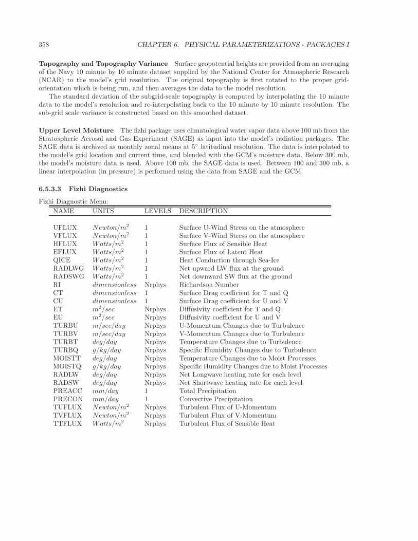
358 CHAPTER 6. PHYSICAL PARAMETERIZATIONS - PACKAGES I
Topography and Topography Variance Surface geopotential heights are provided from an averagingof the Navy 10 minute by 10 minute dataset supplied by the National Center for Atmospheric Research(NCAR) to the model’s grid resolution. The original topography is first rotated to the proper grid-orientation which is being run, and then averages the data to the model resolution.
The standard deviation of the subgrid-scale topography is computed by interpolating the 10 minutedata to the model’s resolution and re-interpolating back to the 10 minute by 10 minute resolution. Thesub-grid scale variance is constructed based on this smoothed dataset.
Upper Level Moisture The fizhi package uses climatological water vapor data above 100 mb from theStratospheric Aerosol and Gas Experiment (SAGE) as input into the model’s radiation packages. TheSAGE data is archived as monthly zonal means at 5 latitudinal resolution. The data is interpolated tothe model’s grid location and current time, and blended with the GCM’s moisture data. Below 300 mb,the model’s moisture data is used. Above 100 mb, the SAGE data is used. Between 100 and 300 mb, alinear interpolation (in pressure) is performed using the data from SAGE and the GCM.
6.5.3.3 Fizhi Diagnostics
Fizhi Diagnostic Menu:
NAME UNITS LEVELS DESCRIPTION
UFLUX Newton/m2 1 Surface U-Wind Stress on the atmosphereVFLUX Newton/m2 1 Surface V-Wind Stress on the atmosphereHFLUX Watts/m2 1 Surface Flux of Sensible HeatEFLUX Watts/m2 1 Surface Flux of Latent HeatQICE Watts/m2 1 Heat Conduction through Sea-IceRADLWG Watts/m2 1 Net upward LW flux at the groundRADSWG Watts/m2 1 Net downward SW flux at the groundRI dimensionless Nrphys Richardson NumberCT dimensionless 1 Surface Drag coefficient for T and QCU dimensionless 1 Surface Drag coefficient for U and VET m2/sec Nrphys Diffusivity coefficient for T and QEU m2/sec Nrphys Diffusivity coefficient for U and VTURBU m/sec/day Nrphys U-Momentum Changes due to TurbulenceTURBV m/sec/day Nrphys V-Momentum Changes due to TurbulenceTURBT deg/day Nrphys Temperature Changes due to TurbulenceTURBQ g/kg/day Nrphys Specific Humidity Changes due to TurbulenceMOISTT deg/day Nrphys Temperature Changes due to Moist ProcessesMOISTQ g/kg/day Nrphys Specific Humidity Changes due to Moist ProcessesRADLW deg/day Nrphys Net Longwave heating rate for each levelRADSW deg/day Nrphys Net Shortwave heating rate for each levelPREACC mm/day 1 Total PrecipitationPRECON mm/day 1 Convective PrecipitationTUFLUX Newton/m2 Nrphys Turbulent Flux of U-MomentumTVFLUX Newton/m2 Nrphys Turbulent Flux of V-MomentumTTFLUX Watts/m2 Nrphys Turbulent Flux of Sensible Heat
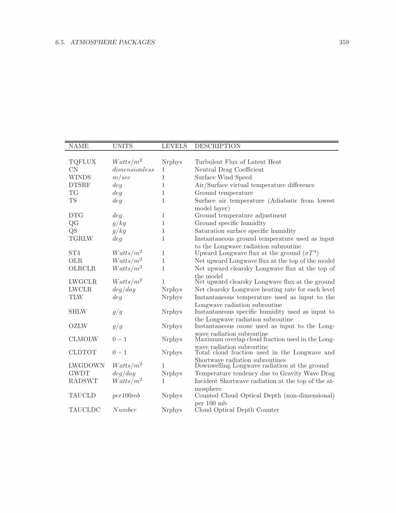
6.5. ATMOSPHERE PACKAGES 359
NAME UNITS LEVELS DESCRIPTION
TQFLUX Watts/m2 Nrphys Turbulent Flux of Latent HeatCN dimensionless 1 Neutral Drag CoefficientWINDS m/sec 1 Surface Wind SpeedDTSRF deg 1 Air/Surface virtual temperature differenceTG deg 1 Ground temperatureTS deg 1 Surface air temperature (Adiabatic from lowest
model layer)DTG deg 1 Ground temperature adjustmentQG g/kg 1 Ground specific humidityQS g/kg 1 Saturation surface specific humidityTGRLW deg 1 Instantaneous ground temperature used as input
to the Longwave radiation subroutineST4 Watts/m2 1 Upward Longwave flux at the ground (σT 4)OLR Watts/m2 1 Net upward Longwave flux at the top of the modelOLRCLR Watts/m2 1 Net upward clearsky Longwave flux at the top of
the modelLWGCLR Watts/m2 1 Net upward clearsky Longwave flux at the groundLWCLR deg/day Nrphys Net clearsky Longwave heating rate for each levelTLW deg Nrphys Instantaneous temperature used as input to the
Longwave radiation subroutineSHLW g/g Nrphys Instantaneous specific humidity used as input to
the Longwave radiation subroutineOZLW g/g Nrphys Instantaneous ozone used as input to the Long-
wave radiation subroutineCLMOLW 0 − 1 Nrphys Maximum overlap cloud fraction used in the Long-
wave radiation subroutineCLDTOT 0 − 1 Nrphys Total cloud fraction used in the Longwave and
Shortwave radiation subroutinesLWGDOWN Watts/m2 1 Downwelling Longwave radiation at the groundGWDT deg/day Nrphys Temperature tendency due to Gravity Wave DragRADSWT Watts/m2 1 Incident Shortwave radiation at the top of the at-
mosphereTAUCLD per100mb Nrphys Counted Cloud Optical Depth (non-dimensional)
per 100 mbTAUCLDC Number Nrphys Cloud Optical Depth Counter
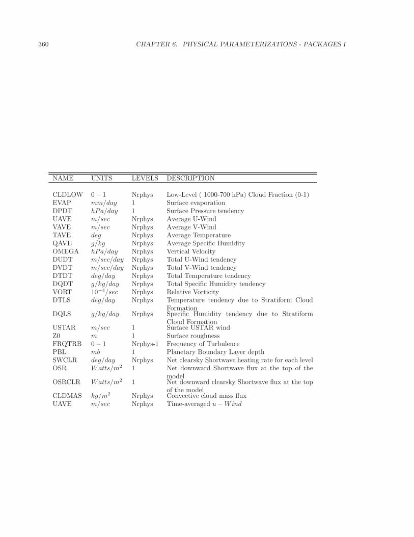
360 CHAPTER 6. PHYSICAL PARAMETERIZATIONS - PACKAGES I
NAME UNITS LEVELS DESCRIPTION
CLDLOW 0 − 1 Nrphys Low-Level ( 1000-700 hPa) Cloud Fraction (0-1)EVAP mm/day 1 Surface evaporationDPDT hPa/day 1 Surface Pressure tendencyUAVE m/sec Nrphys Average U-WindVAVE m/sec Nrphys Average V-WindTAVE deg Nrphys Average TemperatureQAVE g/kg Nrphys Average Specific HumidityOMEGA hPa/day Nrphys Vertical VelocityDUDT m/sec/day Nrphys Total U-Wind tendencyDVDT m/sec/day Nrphys Total V-Wind tendencyDTDT deg/day Nrphys Total Temperature tendencyDQDT g/kg/day Nrphys Total Specific Humidity tendencyVORT 10−4/sec Nrphys Relative VorticityDTLS deg/day Nrphys Temperature tendency due to Stratiform Cloud
FormationDQLS g/kg/day Nrphys Specific Humidity tendency due to Stratiform
Cloud FormationUSTAR m/sec 1 Surface USTAR windZ0 m 1 Surface roughnessFRQTRB 0 − 1 Nrphys-1 Frequency of TurbulencePBL mb 1 Planetary Boundary Layer depthSWCLR deg/day Nrphys Net clearsky Shortwave heating rate for each levelOSR Watts/m2 1 Net downward Shortwave flux at the top of the
modelOSRCLR Watts/m2 1 Net downward clearsky Shortwave flux at the top
of the modelCLDMAS kg/m2 Nrphys Convective cloud mass fluxUAVE m/sec Nrphys Time-averaged u−Wind
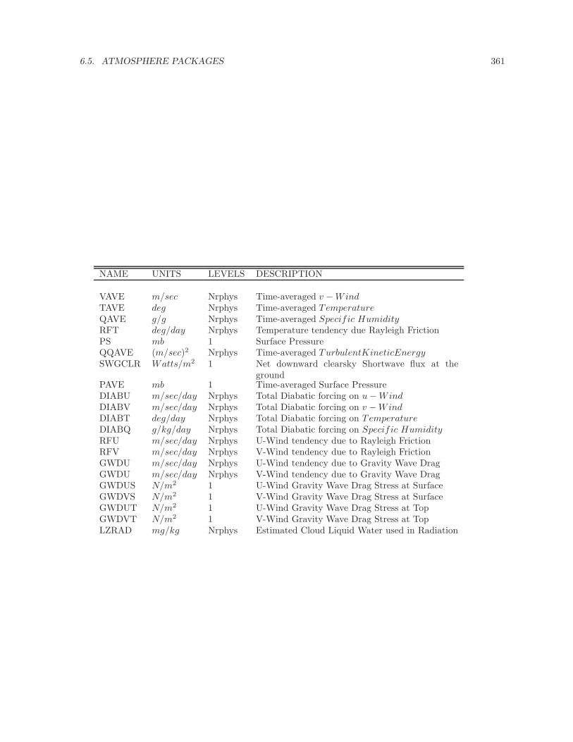
6.5. ATMOSPHERE PACKAGES 361
NAME UNITS LEVELS DESCRIPTION
VAVE m/sec Nrphys Time-averaged v −WindTAVE deg Nrphys Time-averaged TemperatureQAVE g/g Nrphys Time-averaged Specific HumidityRFT deg/day Nrphys Temperature tendency due Rayleigh FrictionPS mb 1 Surface PressureQQAVE (m/sec)2 Nrphys Time-averaged TurbulentKineticEnergySWGCLR Watts/m2 1 Net downward clearsky Shortwave flux at the
groundPAVE mb 1 Time-averaged Surface PressureDIABU m/sec/day Nrphys Total Diabatic forcing on u−WindDIABV m/sec/day Nrphys Total Diabatic forcing on v −WindDIABT deg/day Nrphys Total Diabatic forcing on TemperatureDIABQ g/kg/day Nrphys Total Diabatic forcing on Specific HumidityRFU m/sec/day Nrphys U-Wind tendency due to Rayleigh FrictionRFV m/sec/day Nrphys V-Wind tendency due to Rayleigh FrictionGWDU m/sec/day Nrphys U-Wind tendency due to Gravity Wave DragGWDU m/sec/day Nrphys V-Wind tendency due to Gravity Wave DragGWDUS N/m2 1 U-Wind Gravity Wave Drag Stress at SurfaceGWDVS N/m2 1 V-Wind Gravity Wave Drag Stress at SurfaceGWDUT N/m2 1 U-Wind Gravity Wave Drag Stress at TopGWDVT N/m2 1 V-Wind Gravity Wave Drag Stress at TopLZRAD mg/kg Nrphys Estimated Cloud Liquid Water used in Radiation
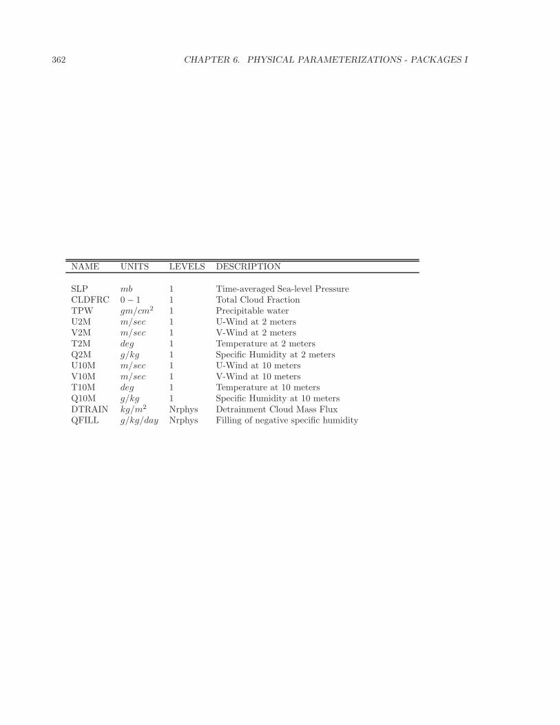
362 CHAPTER 6. PHYSICAL PARAMETERIZATIONS - PACKAGES I
NAME UNITS LEVELS DESCRIPTION
SLP mb 1 Time-averaged Sea-level PressureCLDFRC 0 − 1 1 Total Cloud FractionTPW gm/cm2 1 Precipitable waterU2M m/sec 1 U-Wind at 2 metersV2M m/sec 1 V-Wind at 2 metersT2M deg 1 Temperature at 2 metersQ2M g/kg 1 Specific Humidity at 2 metersU10M m/sec 1 U-Wind at 10 metersV10M m/sec 1 V-Wind at 10 metersT10M deg 1 Temperature at 10 metersQ10M g/kg 1 Specific Humidity at 10 metersDTRAIN kg/m2 Nrphys Detrainment Cloud Mass FluxQFILL g/kg/day Nrphys Filling of negative specific humidity
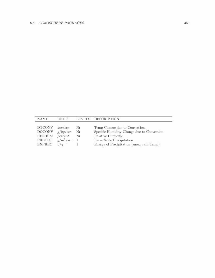
6.5. ATMOSPHERE PACKAGES 363
NAME UNITS LEVELS DESCRIPTION
DTCONV deg/sec Nr Temp Change due to ConvectionDQCONV g/kg/sec Nr Specific Humidity Change due to ConvectionRELHUM percent Nr Relative HumidityPRECLS g/m2/sec 1 Large Scale PrecipitationENPREC J/g 1 Energy of Precipitation (snow, rain Temp)
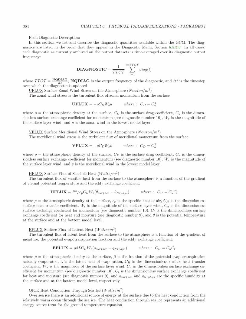
364 CHAPTER 6. PHYSICAL PARAMETERIZATIONS - PACKAGES I
Fizhi Diagnostic Description:In this section we list and describe the diagnostic quantities available within the GCM. The diag-
nostics are listed in the order that they appear in the Diagnostic Menu, Section 6.5.3.3. In all cases,each diagnostic as currently archived on the output datasets is time-averaged over its diagnostic outputfrequency:
DIAGNOSTIC =1
TTOT
t=TTOT∑
t=1
diag(t)
where TTOT = NQDIAG
∆t , NQDIAG is the output frequency of the diagnostic, and ∆t is the timestepover which the diagnostic is updated.
UFLUX Surface Zonal Wind Stress on the Atmosphere (Newton/m2)The zonal wind stress is the turbulent flux of zonal momentum from the surface.
UFLUX = −ρCDWsu where : CD = C2u
where ρ = the atmospheric density at the surface, CD is the surface drag coefficient, Cu is the dimen-sionless surface exchange coefficient for momentum (see diagnostic number 10), Ws is the magnitude ofthe surface layer wind, and u is the zonal wind in the lowest model layer.
VFLUX Surface Meridional Wind Stress on the Atmosphere (Newton/m2)The meridional wind stress is the turbulent flux of meridional momentum from the surface.
VFLUX = −ρCDWsv where : CD = C2u
where ρ = the atmospheric density at the surface, CD is the surface drag coefficient, Cu is the dimen-sionless surface exchange coefficient for momentum (see diagnostic number 10), Ws is the magnitude ofthe surface layer wind, and v is the meridional wind in the lowest model layer.
HFLUX Surface Flux of Sensible Heat (Watts/m2)The turbulent flux of sensible heat from the surface to the atmosphere is a function of the gradient
of virtual potential temperature and the eddy exchange coefficient:
HFLUX = P κρcpCHWs(θsurface − θNrphys) where : CH = CuCt
where ρ = the atmospheric density at the surface, cp is the specific heat of air, CH is the dimensionlesssurface heat transfer coefficient, Ws is the magnitude of the surface layer wind, Cu is the dimensionlesssurface exchange coefficient for momentum (see diagnostic number 10), Ct is the dimensionless surfaceexchange coefficient for heat and moisture (see diagnostic number 9), and θ is the potential temperatureat the surface and at the bottom model level.
EFLUX Surface Flux of Latent Heat (Watts/m2)The turbulent flux of latent heat from the surface to the atmosphere is a function of the gradient of
moisture, the potential evapotranspiration fraction and the eddy exchange coefficient:
EFLUX = ρβLCHWs(qsurface − qNrphys) where : CH = CuCt
where ρ = the atmospheric density at the surface, β is the fraction of the potential evapotranspirationactually evaporated, L is the latent heat of evaporation, CH is the dimensionless surface heat transfercoefficient, Ws is the magnitude of the surface layer wind, Cu is the dimensionless surface exchange co-efficient for momentum (see diagnostic number 10), Ct is the dimensionless surface exchange coefficientfor heat and moisture (see diagnostic number 9), and qsurface and qNrphys are the specific humidity atthe surface and at the bottom model level, respectively.
QICE Heat Conduction Through Sea Ice (Watts/m2)Over sea ice there is an additional source of energy at the surface due to the heat conduction from the
relatively warm ocean through the sea ice. The heat conduction through sea ice represents an additionalenergy source term for the ground temperature equation.
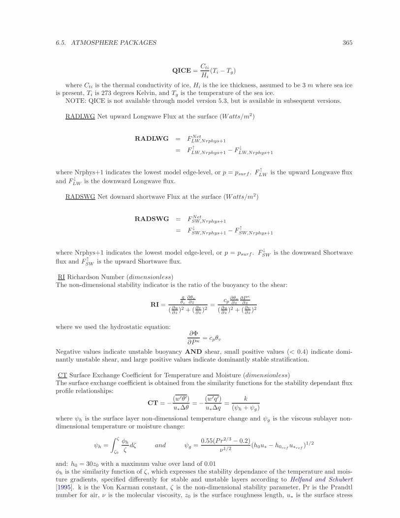
6.5. ATMOSPHERE PACKAGES 365
QICE =Cti
Hi(Ti − Tg)
where Cti is the thermal conductivity of ice, Hi is the ice thickness, assumed to be 3 m where sea iceis present, Ti is 273 degrees Kelvin, and Tg is the temperature of the sea ice.
NOTE: QICE is not available through model version 5.3, but is available in subsequent versions.
RADLWG Net upward Longwave Flux at the surface (Watts/m2)
RADLWG = FNetLW,Nrphys+1
= F ↑LW,Nrphys+1 − F ↓LW,Nrphys+1
where Nrphys+1 indicates the lowest model edge-level, or p = psurf . F ↑LW is the upward Longwave flux
and F ↓LW is the downward Longwave flux.
RADSWG Net downard shortwave Flux at the surface (Watts/m2)
RADSWG = FNetSW,Nrphys+1
= F ↓SW,Nrphys+1 − F ↑SW,Nrphys+1
where Nrphys+1 indicates the lowest model edge-level, or p = psurf . F ↓SW is the downward Shortwave
flux and F ↑SW is the upward Shortwave flux.
RI Richardson Number (dimensionless)The non-dimensional stability indicator is the ratio of the buoyancy to the shear:
RI =
gθv
∂θv
∂z
(∂u∂z )2 + (∂v
∂z )2=
cp∂θv
∂z∂P κ
∂z
(∂u∂z )2 + (∂v
∂z )2
where we used the hydrostatic equation:∂Φ
∂P κ= cpθv
Negative values indicate unstable buoyancy AND shear, small positive values (< 0.4) indicate domi-nantly unstable shear, and large positive values indicate dominantly stable stratification.
CT Surface Exchange Coefficient for Temperature and Moisture (dimensionless)The surface exchange coefficient is obtained from the similarity functions for the stability dependant fluxprofile relationships:
CT = − (w′θ′)
u∗∆θ= − (w′q′)
u∗∆q=
k
(ψh + ψg)
where ψh is the surface layer non-dimensional temperature change and ψg is the viscous sublayer non-dimensional temperature or moisture change:
ψh =
∫ ζ
ζ0
φh
ζdζ and ψg =
0.55(Pr2/3 − 0.2)
ν1/2(h0u∗ − h0ref
u∗ref)1/2
and: h0 = 30z0 with a maximum value over land of 0.01φh is the similarity function of ζ, which expresses the stability dependance of the temperature and mois-ture gradients, specified differently for stable and unstable layers according to Helfand and Schubert[1995]. k is the Von Karman constant, ζ is the non-dimensional stability parameter, Pr is the Prandtlnumber for air, ν is the molecular viscosity, z0 is the surface roughness length, u∗ is the surface stress
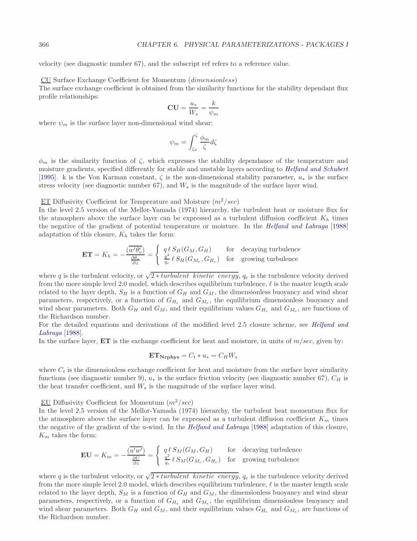
366 CHAPTER 6. PHYSICAL PARAMETERIZATIONS - PACKAGES I
velocity (see diagnostic number 67), and the subscript ref refers to a reference value.
CU Surface Exchange Coefficient for Momentum (dimensionless)The surface exchange coefficient is obtained from the similarity functions for the stability dependant fluxprofile relationships:
CU =u∗Ws
=k
ψm
where ψm is the surface layer non-dimensional wind shear:
ψm =
∫ ζ
ζ0
φm
ζdζ
φm is the similarity function of ζ, which expresses the stability dependance of the temperature andmoisture gradients, specified differently for stable and unstable layers according to Helfand and Schubert[1995]. k is the Von Karman constant, ζ is the non-dimensional stability parameter, u∗ is the surfacestress velocity (see diagnostic number 67), and Ws is the magnitude of the surface layer wind.
ET Diffusivity Coefficient for Temperature and Moisture (m2/sec)In the level 2.5 version of the Mellor-Yamada (1974) hierarchy, the turbulent heat or moisture flux forthe atmosphere above the surface layer can be expressed as a turbulent diffusion coefficient Kh timesthe negative of the gradient of potential temperature or moisture. In the Helfand and Labraga [1988]adaptation of this closure, Kh takes the form:
ET = Kh = − (w′θ′v)∂θv
∂z
=
q ℓ SH(GM , GH) for decaying turbulenceq2
qeℓ SH(GMe
, GHe) for growing turbulence
where q is the turbulent velocity, or√
2 ∗ turbulent kinetic energy, qe is the turbulence velocity derivedfrom the more simple level 2.0 model, which describes equilibrium turbulence, ℓ is the master length scalerelated to the layer depth, SH is a function of GH and GM , the dimensionless buoyancy and wind shearparameters, respectively, or a function of GHe
and GMe, the equilibrium dimensionless buoyancy and
wind shear parameters. Both GH and GM , and their equilibrium values GHeand GMe
, are functions ofthe Richardson number.For the detailed equations and derivations of the modified level 2.5 closure scheme, see Helfand andLabraga [1988].In the surface layer, ET is the exchange coefficient for heat and moisture, in units of m/sec, given by:
ETNrphys = Ct ∗ u∗ = CHWs
where Ct is the dimensionless exchange coefficient for heat and moisture from the surface layer similarityfunctions (see diagnostic number 9), u∗ is the surface friction velocity (see diagnostic number 67), CH isthe heat transfer coefficient, and Ws is the magnitude of the surface layer wind.
EU Diffusivity Coefficient for Momentum (m2/sec)In the level 2.5 version of the Mellor-Yamada (1974) hierarchy, the turbulent heat momentum flux forthe atmosphere above the surface layer can be expressed as a turbulent diffusion coefficient Km timesthe negative of the gradient of the u-wind. In the Helfand and Labraga [1988] adaptation of this closure,Km takes the form:
EU = Km = − (u′w′)∂U∂z
=
q ℓ SM (GM , GH) for decaying turbulenceq2
qeℓ SM (GMe
, GHe) for growing turbulence
where q is the turbulent velocity, or√
2 ∗ turbulent kinetic energy, qe is the turbulence velocity derivedfrom the more simple level 2.0 model, which describes equilibrium turbulence, ℓ is the master length scalerelated to the layer depth, SM is a function of GH and GM , the dimensionless buoyancy and wind shearparameters, respectively, or a function of GHe
and GMe, the equilibrium dimensionless buoyancy and
wind shear parameters. Both GH and GM , and their equilibrium values GHeand GMe
, are functions ofthe Richardson number.
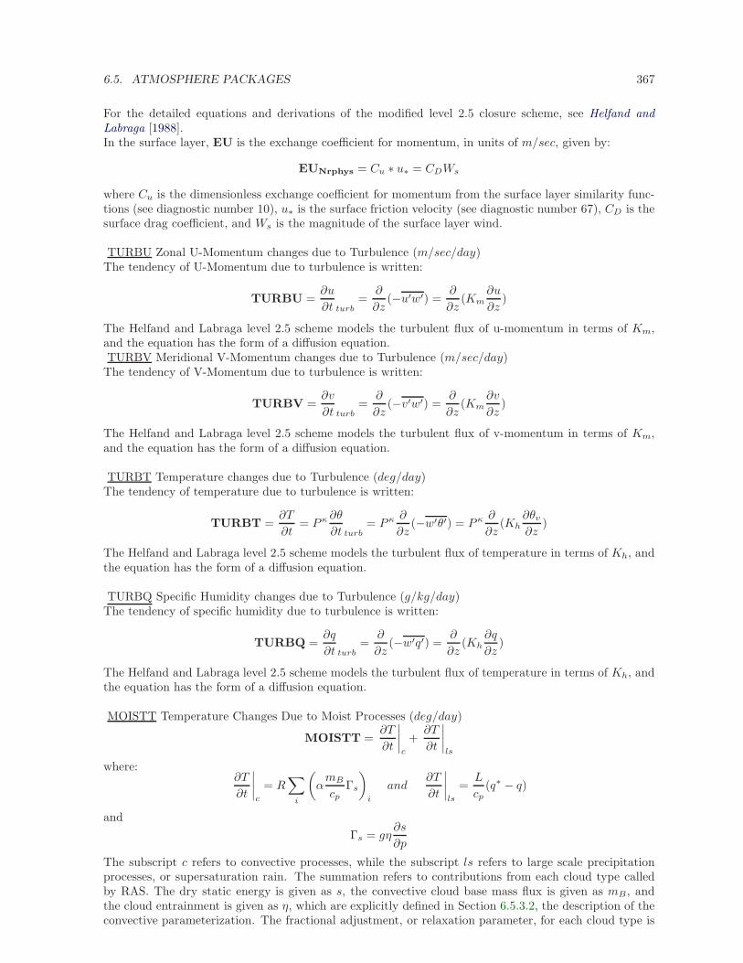
6.5. ATMOSPHERE PACKAGES 367
For the detailed equations and derivations of the modified level 2.5 closure scheme, see Helfand andLabraga [1988].In the surface layer, EU is the exchange coefficient for momentum, in units of m/sec, given by:
EUNrphys = Cu ∗ u∗ = CDWs
where Cu is the dimensionless exchange coefficient for momentum from the surface layer similarity func-tions (see diagnostic number 10), u∗ is the surface friction velocity (see diagnostic number 67), CD is thesurface drag coefficient, and Ws is the magnitude of the surface layer wind.
TURBU Zonal U-Momentum changes due to Turbulence (m/sec/day)The tendency of U-Momentum due to turbulence is written:
TURBU =∂u
∂t turb=
∂
∂z(−u′w′) =
∂
∂z(Km
∂u
∂z)
The Helfand and Labraga level 2.5 scheme models the turbulent flux of u-momentum in terms of Km,and the equation has the form of a diffusion equation.TURBV Meridional V-Momentum changes due to Turbulence (m/sec/day)The tendency of V-Momentum due to turbulence is written:
TURBV =∂v
∂t turb=
∂
∂z(−v′w′) =
∂
∂z(Km
∂v
∂z)
The Helfand and Labraga level 2.5 scheme models the turbulent flux of v-momentum in terms of Km,and the equation has the form of a diffusion equation.
TURBT Temperature changes due to Turbulence (deg/day)The tendency of temperature due to turbulence is written:
TURBT =∂T
∂t= P κ ∂θ
∂t turb= P κ ∂
∂z(−w′θ′) = P κ ∂
∂z(Kh
∂θv
∂z)
The Helfand and Labraga level 2.5 scheme models the turbulent flux of temperature in terms of Kh, andthe equation has the form of a diffusion equation.
TURBQ Specific Humidity changes due to Turbulence (g/kg/day)The tendency of specific humidity due to turbulence is written:
TURBQ =∂q
∂t turb=
∂
∂z(−w′q′) =
∂
∂z(Kh
∂q
∂z)
The Helfand and Labraga level 2.5 scheme models the turbulent flux of temperature in terms of Kh, andthe equation has the form of a diffusion equation.
MOISTT Temperature Changes Due to Moist Processes (deg/day)
MOISTT =∂T
∂t
∣∣∣∣c
+∂T
∂t
∣∣∣∣ls
where:∂T
∂t
∣∣∣∣c
= R∑
i
(αmB
cpΓs
)
i
and∂T
∂t
∣∣∣∣ls
=L
cp(q∗ − q)
and
Γs = gη∂s
∂p
The subscript c refers to convective processes, while the subscript ls refers to large scale precipitationprocesses, or supersaturation rain. The summation refers to contributions from each cloud type calledby RAS. The dry static energy is given as s, the convective cloud base mass flux is given as mB, andthe cloud entrainment is given as η, which are explicitly defined in Section 6.5.3.2, the description of theconvective parameterization. The fractional adjustment, or relaxation parameter, for each cloud type is
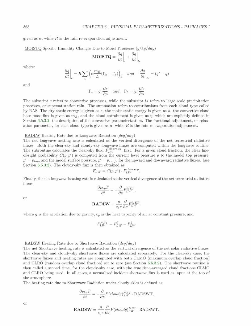
368 CHAPTER 6. PHYSICAL PARAMETERIZATIONS - PACKAGES I
given as α, while R is the rain re-evaporation adjustment.
MOISTQ Specific Humidity Changes Due to Moist Processes (g/kg/day)
MOISTQ =∂q
∂t
∣∣∣∣c
+∂q
∂t
∣∣∣∣ls
where:∂q
∂t
∣∣∣∣c
= R∑
i
(αmB
L(Γh − Γs)
)i
and∂q
∂t
∣∣∣∣ls
= (q∗ − q)
and
Γs = gη∂s
∂pand Γh = gη
∂h
∂p
The subscript c refers to convective processes, while the subscript ls refers to large scale precipitationprocesses, or supersaturation rain. The summation refers to contributions from each cloud type calledby RAS. The dry static energy is given as s, the moist static energy is given as h, the convective cloudbase mass flux is given as mB, and the cloud entrainment is given as η, which are explicitly defined inSection 6.5.3.2, the description of the convective parameterization. The fractional adjustment, or relax-ation parameter, for each cloud type is given as α, while R is the rain re-evaporation adjustment.
RADLW Heating Rate due to Longwave Radiation (deg/day)The net longwave heating rate is calculated as the vertical divergence of the net terrestrial radiativefluxes. Both the clear-sky and cloudy-sky longwave fluxes are computed within the longwave routine.The subroutine calculates the clear-sky flux, F clearsky
LW , first. For a given cloud fraction, the clear line-of-sight probability C(p, p′) is computed from the current level pressure p to the model top pressure,p′ = ptop, and the model surface pressure, p′ = psurf , for the upward and downward radiative fluxes. (seeSection 6.5.3.2). The cloudy-sky flux is then obtained as:
FLW = C(p, p′) · F clearskyLW ,
Finally, the net longwave heating rate is calculated as the vertical divergence of the net terrestrial radiativefluxes:
∂ρcpT
∂t= − ∂
∂zFNET
LW ,
or
RADLW =g
cpπ
∂
∂σFNET
LW .
where g is the accelation due to gravity, cp is the heat capacity of air at constant pressure, and
FNETLW = F ↑LW − F ↓LW
RADSW Heating Rate due to Shortwave Radiation (deg/day)The net Shortwave heating rate is calculated as the vertical divergence of the net solar radiative fluxes.The clear-sky and cloudy-sky shortwave fluxes are calculated separately. For the clear-sky case, theshortwave fluxes and heating rates are computed with both CLMO (maximum overlap cloud fraction)and CLRO (random overlap cloud fraction) set to zero (see Section 6.5.3.2). The shortwave routine isthen called a second time, for the cloudy-sky case, with the true time-averaged cloud fractions CLMOand CLRO being used. In all cases, a normalized incident shortwave flux is used as input at the top ofthe atmosphere.The heating rate due to Shortwave Radiation under cloudy skies is defined as:
∂ρcpT
∂t= − ∂
∂zF (cloudy)NET
SW · RADSWT,
or
RADSW =g
cpπ
∂
∂σF (cloudy)NET
SW · RADSWT.
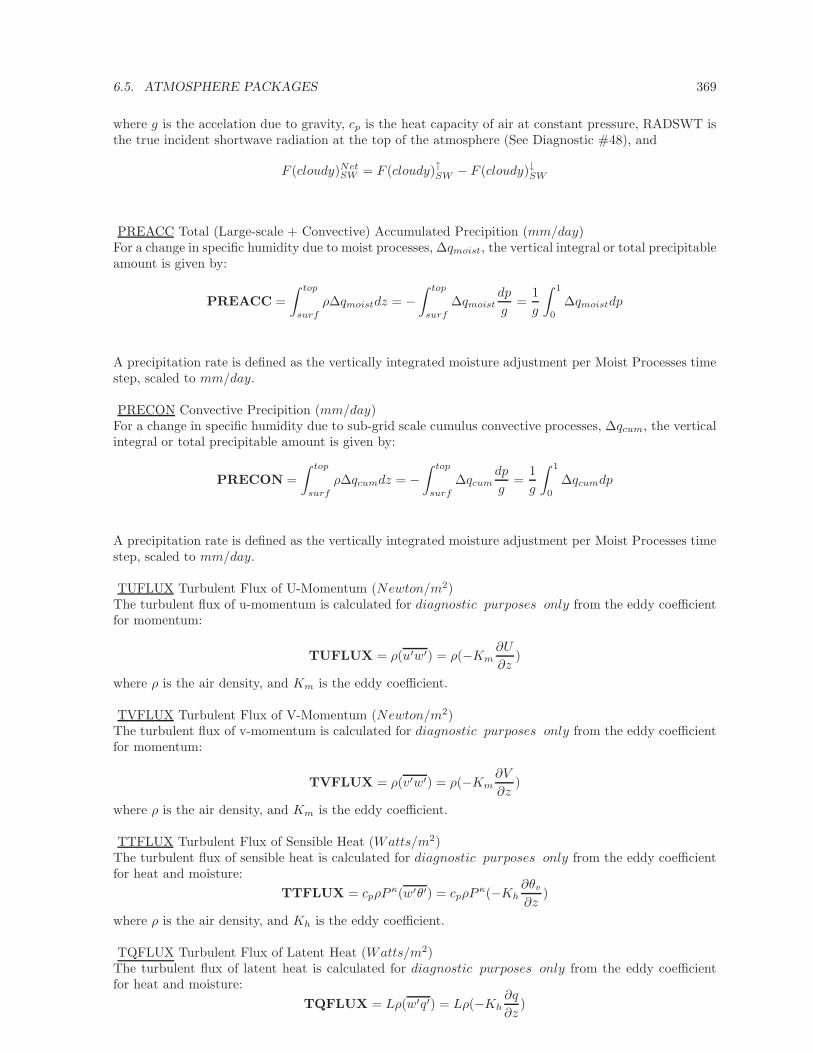
6.5. ATMOSPHERE PACKAGES 369
where g is the accelation due to gravity, cp is the heat capacity of air at constant pressure, RADSWT isthe true incident shortwave radiation at the top of the atmosphere (See Diagnostic #48), and
F (cloudy)NetSW = F (cloudy)↑SW − F (cloudy)↓SW
PREACC Total (Large-scale + Convective) Accumulated Precipition (mm/day)For a change in specific humidity due to moist processes, ∆qmoist, the vertical integral or total precipitableamount is given by:
PREACC =
∫ top
surf
ρ∆qmoistdz = −∫ top
surf
∆qmoistdp
g=
1
g
∫ 1
0
∆qmoistdp
A precipitation rate is defined as the vertically integrated moisture adjustment per Moist Processes timestep, scaled to mm/day.
PRECON Convective Precipition (mm/day)For a change in specific humidity due to sub-grid scale cumulus convective processes, ∆qcum, the verticalintegral or total precipitable amount is given by:
PRECON =
∫ top
surf
ρ∆qcumdz = −∫ top
surf
∆qcumdp
g=
1
g
∫ 1
0
∆qcumdp
A precipitation rate is defined as the vertically integrated moisture adjustment per Moist Processes timestep, scaled to mm/day.
TUFLUX Turbulent Flux of U-Momentum (Newton/m2)The turbulent flux of u-momentum is calculated for diagnostic purposes only from the eddy coefficientfor momentum:
TUFLUX = ρ(u′w′) = ρ(−Km∂U
∂z)
where ρ is the air density, and Km is the eddy coefficient.
TVFLUX Turbulent Flux of V-Momentum (Newton/m2)The turbulent flux of v-momentum is calculated for diagnostic purposes only from the eddy coefficientfor momentum:
TVFLUX = ρ(v′w′) = ρ(−Km∂V
∂z)
where ρ is the air density, and Km is the eddy coefficient.
TTFLUX Turbulent Flux of Sensible Heat (Watts/m2)The turbulent flux of sensible heat is calculated for diagnostic purposes only from the eddy coefficientfor heat and moisture:
TTFLUX = cpρPκ(w′θ′) = cpρP
κ(−Kh∂θv
∂z)
where ρ is the air density, and Kh is the eddy coefficient.
TQFLUX Turbulent Flux of Latent Heat (Watts/m2)The turbulent flux of latent heat is calculated for diagnostic purposes only from the eddy coefficientfor heat and moisture:
TQFLUX = Lρ(w′q′) = Lρ(−Kh∂q
∂z)
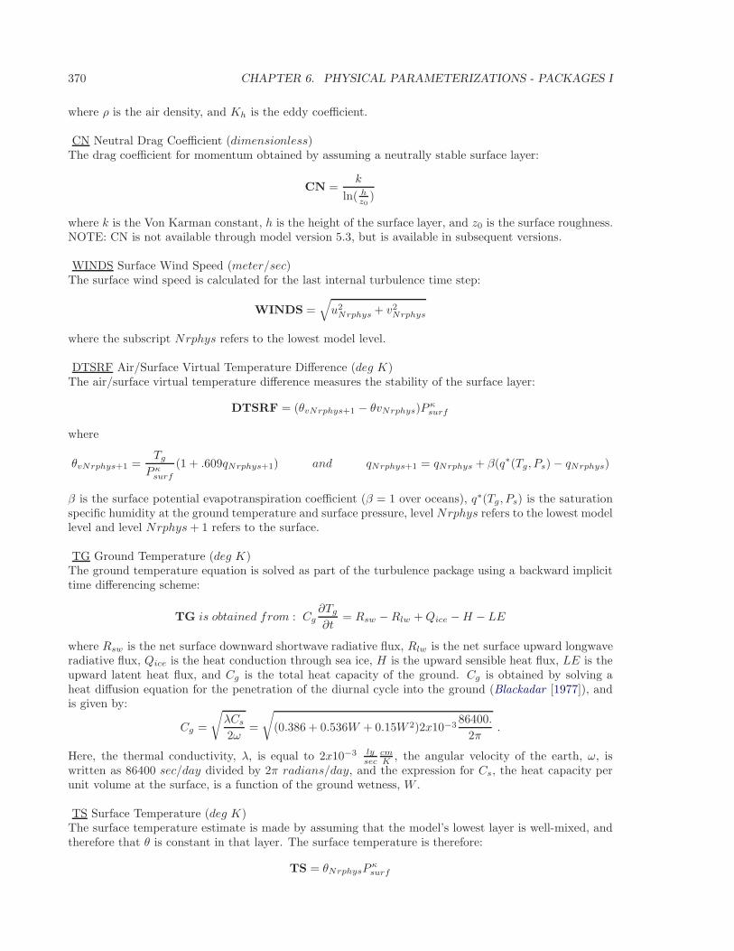
370 CHAPTER 6. PHYSICAL PARAMETERIZATIONS - PACKAGES I
where ρ is the air density, and Kh is the eddy coefficient.
CN Neutral Drag Coefficient (dimensionless)The drag coefficient for momentum obtained by assuming a neutrally stable surface layer:
CN =k
ln( hz0
)
where k is the Von Karman constant, h is the height of the surface layer, and z0 is the surface roughness.NOTE: CN is not available through model version 5.3, but is available in subsequent versions.
WINDS Surface Wind Speed (meter/sec)The surface wind speed is calculated for the last internal turbulence time step:
WINDS =√u2
Nrphys + v2Nrphys
where the subscript Nrphys refers to the lowest model level.
DTSRF Air/Surface Virtual Temperature Difference (deg K)The air/surface virtual temperature difference measures the stability of the surface layer:
DTSRF = (θvNrphys+1 − θvNrphys)Pκsurf
where
θvNrphys+1 =Tg
P κsurf
(1 + .609qNrphys+1) and qNrphys+1 = qNrphys + β(q∗(Tg, Ps) − qNrphys)
β is the surface potential evapotranspiration coefficient (β = 1 over oceans), q∗(Tg, Ps) is the saturationspecific humidity at the ground temperature and surface pressure, level Nrphys refers to the lowest modellevel and level Nrphys+ 1 refers to the surface.
TG Ground Temperature (deg K)The ground temperature equation is solved as part of the turbulence package using a backward implicittime differencing scheme:
TG is obtained from : Cg∂Tg
∂t= Rsw −Rlw +Qice −H − LE
where Rsw is the net surface downward shortwave radiative flux, Rlw is the net surface upward longwaveradiative flux, Qice is the heat conduction through sea ice, H is the upward sensible heat flux, LE is theupward latent heat flux, and Cg is the total heat capacity of the ground. Cg is obtained by solving aheat diffusion equation for the penetration of the diurnal cycle into the ground (Blackadar [1977]), andis given by:
Cg =
√λCs
2ω=
√(0.386 + 0.536W + 0.15W 2)2x10⁻³
86400.
2π.
Here, the thermal conductivity, λ, is equal to 2x10⁻³ lysec
cmK , the angular velocity of the earth, ω, is
written as 86400 sec/day divided by 2π radians/day, and the expression for Cs, the heat capacity perunit volume at the surface, is a function of the ground wetness, W .
TS Surface Temperature (deg K)The surface temperature estimate is made by assuming that the model’s lowest layer is well-mixed, andtherefore that θ is constant in that layer. The surface temperature is therefore:
TS = θNrphysPκsurf
6.5. ATMOSPHERE PACKAGES 371
DTG Surface Temperature Adjustment (deg K)The change in surface temperature from one turbulence time step to the next, solved using the GroundTemperature Equation (see diagnostic number 30) is calculated:
DTG = Tgn − Tg
n−1
where superscript n refers to the new, updated time level, and the superscript n− 1 refers to the valueat the previous turbulence time level.
QG Ground Specific Humidity (g/kg)The ground specific humidity is obtained by interpolating between the specific humidity at the lowestmodel level and the specific humidity of a saturated ground. The interpolation is performed using thepotential evapotranspiration function:
QG = qNrphys+1 = qNrphys + β(q∗(Tg, Ps) − qNrphys)
where β is the surface potential evapotranspiration coefficient (β = 1 over oceans), and q∗(Tg, Ps) is thesaturation specific humidity at the ground temperature and surface pressure.
QS Saturation Surface Specific Humidity (g/kg)The surface saturation specific humidity is the saturation specific humidity at the ground tempratureand surface pressure:
QS = q∗(Tg, Ps)
TGRLW Instantaneous ground temperature used as input to the Longwave radiation subroutine (deg)
TGRLW = Tg(λ, φ, n)
where Tg is the model ground temperature at the current time step n.
ST4 Upward Longwave flux at the surface (Watts/m2)
ST4 = σT 4
where σ is the Stefan-Boltzmann constant and T is the temperature.
OLR Net upward Longwave flux at p = ptop (Watts/m2)
OLR = FNETLW,top
where top indicates the top of the first model layer. In the GCM, ptop = 0.0 mb.
OLRCLR Net upward clearsky Longwave flux at p = ptop (Watts/m2)
OLRCLR = F (clearsky)NETLW,top
where top indicates the top of the first model layer. In the GCM, ptop = 0.0 mb.
LWGCLR Net upward clearsky Longwave flux at the surface (Watts/m2)
LWGCLR = F (clearsky)NetLW,Nrphys+1
= F (clearsky)↑LW,Nrphys+1 − F (clearsky)↓LW,Nrphys+1
where Nrphys+1 indicates the lowest model edge-level, or p = psurf . F (clearsky)↑LW is the upward
clearsky Longwave flux and the F (clearsky)↓LW is the downward clearsky Longwave flux.
LWCLR Heating Rate due to Clearsky Longwave Radiation (deg/day)
372 CHAPTER 6. PHYSICAL PARAMETERIZATIONS - PACKAGES I
The net longwave heating rate is calculated as the vertical divergence of the net terrestrial radiativefluxes. Both the clear-sky and cloudy-sky longwave fluxes are computed within the longwave routine.The subroutine calculates the clear-sky flux, F clearsky
LW , first. For a given cloud fraction, the clear line-of-sight probability C(p, p′) is computed from the current level pressure p to the model top pressure,p′ = ptop, and the model surface pressure, p′ = psurf , for the upward and downward radiative fluxes. (seeSection 6.5.3.2). The cloudy-sky flux is then obtained as:
FLW = C(p, p′) · F clearskyLW ,
Thus, LWCLR is defined as the net longwave heating rate due to the vertical divergence of the clear-skylongwave radiative flux:
∂ρcpT
∂t clearsky= − ∂
∂zF (clearsky)NET
LW ,
or
LWCLR =g
cpπ
∂
∂σF (clearsky)NET
LW .
where g is the accelation due to gravity, cp is the heat capacity of air at constant pressure, and
F (clearsky)NetLW = F (clearsky)↑LW − F (clearsky)↓LW
TLW Instantaneous temperature used as input to the Longwave radiation subroutine (deg)
TLW = T (λ, φ, level, n)
where T is the model temperature at the current time step n.
SHLW Instantaneous specific humidity used as input to the Longwave radiation subroutine (kg/kg)
SHLW = q(λ, φ, level, n)
where q is the model specific humidity at the current time step n.
OZLW Instantaneous ozone used as input to the Longwave radiation subroutine (kg/kg)
OZLW = OZ(λ, φ, level, n)
where OZ is the interpolated ozone data set from the climatological monthly mean zonally averaged ozonedata set.
CLMOLW Maximum Overlap cloud fraction used in LW Radiation (0 − 1)CLMOLW is the time-averaged maximum overlap cloud fraction that has been filled by the RelaxedArakawa/Schubert Convection scheme and will be used in the Longwave Radiation algorithm. Theseare convective clouds whose radiative characteristics are assumed to be correlated in the vertical. For acomplete description of cloud/radiative interactions, see Section 6.5.3.2.
CLMOLW = CLMORAS,LW (λ, φ, level)
CLDTOT Total cloud fraction used in LW and SW Radiation (0 − 1)CLDTOT is the time-averaged total cloud fraction that has been filled by the Relaxed Arakawa/Schubert
and Large-scale Convection schemes and will be used in the Longwave and Shortwave Radiation packages.For a complete description of cloud/radiative interactions, see Section 6.5.3.2.
CLDTOT = FRAS + FLS
where FRAS is the time-averaged cloud fraction due to sub-grid scale convection, and FLS is the time-averaged cloud fraction due to precipitating and non-precipitating large-scale moist processes.
6.5. ATMOSPHERE PACKAGES 373
CLMOSW Maximum Overlap cloud fraction used in SW Radiation (0 − 1)
CLMOSW is the time-averaged maximum overlap cloud fraction that has been filled by the RelaxedArakawa/Schubert Convection scheme and will be used in the Shortwave Radiation algorithm. Theseare convective clouds whose radiative characteristics are assumed to be correlated in the vertical. For acomplete description of cloud/radiative interactions, see Section 6.5.3.2.
CLMOSW = CLMORAS,SW (λ, φ, level)
CLROSW Random Overlap cloud fraction used in SW Radiation (0 − 1)
CLROSW is the time-averaged random overlap cloud fraction that has been filled by the RelaxedArakawa/Schubert and Large-scale Convection schemes and will be used in the Shortwave Radiationalgorithm. These are convective and large-scale clouds whose radiative characteristics are not assumedto be correlated in the vertical. For a complete description of cloud/radiative interactions, see Section6.5.3.2.
CLROSW = CLRORAS,LargeScale,SW (λ, φ, level)
RADSWT Incident Shortwave radiation at the top of the atmosphere (Watts/m2)
RADSWT =S0
R2a
· cosφz
where S0, is the extra-terrestial solar contant, Ra is the earth-sun distance in Astronomical Units, andcosφz is the cosine of the zenith angle. It should be noted that RADSWT, as well as OSR and OS-RCLR, are calculated at the top of the atmosphere (p=0 mb). However, the OLR and OLRCLRdiagnostics are currently calculated at p = ptop (0.0 mb for the GCM).
EVAP Surface Evaporation (mm/day)
The surface evaporation is a function of the gradient of moisture, the potential evapotranspiration fractionand the eddy exchange coefficient:
EVAP = ρβKh(qsurface − qNrphys)
where ρ = the atmospheric density at the surface, β is the fraction of the potential evapotranspirationactually evaporated (β = 1 over oceans), Kh is the turbulent eddy exchange coefficient for heat andmoisture at the surface in m/sec and qsurface and qNrphys are the specific humidity at the surface (seediagnostic number 34) and at the bottom model level, respectively.
DUDT Total Zonal U-Wind Tendency (m/sec/day)
DUDT is the total time-tendency of the Zonal U-Wind due to Hydrodynamic, Diabatic, and Analysisforcing.
DUDT =∂u
∂t Dynamics+∂u
∂tMoist+∂u
∂t Turbulence+∂u
∂t Analysis
DVDT Total Zonal V-Wind Tendency (m/sec/day)
DVDT is the total time-tendency of the Meridional V-Wind due to Hydrodynamic, Diabatic, and Anal-ysis forcing.
DVDT =∂v
∂tDynamics+∂v
∂tMoist+∂v
∂t Turbulence+∂v
∂t Analysis
DTDT Total Temperature Tendency (deg/day)
374 CHAPTER 6. PHYSICAL PARAMETERIZATIONS - PACKAGES I
DTDT is the total time-tendency of Temperature due to Hydrodynamic, Diabatic, and Analysis forcing.
DTDT =∂T
∂t Dynamics+∂T
∂t MoistProcesses+∂T
∂t ShortwaveRadiation
+∂T
∂t LongwaveRadiation+∂T
∂t Turbulence+∂T
∂t Analysis
DQDT Total Specific Humidity Tendency (g/kg/day)DQDT is the total time-tendency of Specific Humidity due to Hydrodynamic, Diabatic, and Analysisforcing.
DQDT =∂q
∂tDynamics+∂q
∂tMoistProcesses+∂q
∂t Turbulence+∂q
∂t Analysis
USTAR Surface-Stress Velocity (m/sec)The surface stress velocity, or the friction velocity, is the wind speed at the surface layer top impeded bythe surface drag:
USTAR = CuWs where : Cu =k
ψm
Cu is the non-dimensional surface drag coefficient (see diagnostic number 10), and Ws is the surface windspeed (see diagnostic number 28).Z0 Surface Roughness Length (m)
Over the land surface, the surface roughness length is interpolated to the local time from the monthlymean data of Dorman and Sellers [1989]. Over the ocean, the roughness length is a function of thesurface-stress velocity, u∗.
Z0 = c1u3∗ + c2u
2∗ + c3u∗ + c4 + c5u∗
where the constants are chosen to interpolate between the reciprocal relation of Kondo [1975] for weakwinds, and the piecewise linear relation of Large and Pond [1981] for moderate to large winds.
FRQTRB Frequency of Turbulence (0 − 1)The fraction of time when turbulence is present is defined as the fraction of time when the turbulentkinetic energy exceeds some minimum value, defined here to be 0.005 m2/sec2. When this criterion ismet, a counter is incremented. The fraction over the averaging interval is reported.
PBL Planetary Boundary Layer Depth (mb)The depth of the PBL is defined by the turbulence parameterization to be the depth at which theturbulent kinetic energy reduces to ten percent of its surface value.
PBL = PPBL − Psurface
where PPBL is the pressure in mb at which the turbulent kinetic energy reaches one tenth of its surfacevalue, and Ps is the surface pressure.
SWCLR Clear sky Heating Rate due to Shortwave Radiation (deg/day)The net Shortwave heating rate is calculated as the vertical divergence of the net solar radiative fluxes.The clear-sky and cloudy-sky shortwave fluxes are calculated separately. For the clear-sky case, theshortwave fluxes and heating rates are computed with both CLMO (maximum overlap cloud fraction)and CLRO (random overlap cloud fraction) set to zero (see Section 6.5.3.2). The shortwave routine isthen called a second time, for the cloudy-sky case, with the true time-averaged cloud fractions CLMOand CLRO being used. In all cases, a normalized incident shortwave flux is used as input at the top ofthe atmosphere.The heating rate due to Shortwave Radiation under clear skies is defined as:
∂ρcpT
∂t= − ∂
∂zF (clear)NET
SW · RADSWT,
6.5. ATMOSPHERE PACKAGES 375
or
SWCLR =g
cp
∂
∂pF (clear)NET
SW · RADSWT.
where g is the accelation due to gravity, cp is the heat capacity of air at constant pressure, RADSWT isthe true incident shortwave radiation at the top of the atmosphere (See Diagnostic #48), and
F (clear)NetSW = F (clear)↑SW − F (clear)↓SW
OSR Net upward Shortwave flux at the top of the model (Watts/m2)
OSR = FNETSW,top
where top indicates the top of the first model layer used in the shortwave radiation routine. In the GCM,pSWtop
= 0 mb.
OSRCLR Net upward clearsky Shortwave flux at the top of the model (Watts/m2)
OSRCLR = F (clearsky)NETSW,top
where top indicates the top of the first model layer used in the shortwave radiation routine. In the GCM,pSWtop
= 0 mb.
CLDMAS Convective Cloud Mass Flux (kg/m2)The amount of cloud mass moved per RAS timestep from all convective clouds is written:
CLDMAS = ηmB
where η is the entrainment, normalized by the cloud base mass flux, and mB is the cloud base mass flux.mB and η are defined explicitly in Section 6.5.3.2, the description of the convective parameterization.
UAVE Time-Averaged Zonal U-Wind (m/sec)The diagnostic UAVE is simply the time-averaged Zonal U-Wind over the NUAVE output frequency.This is contrasted to the instantaneous Zonal U-Wind which is archived on the Prognostic Output datastream.
UAVE = u(λ, φ, level, t)
Note, UAVE is computed and stored on the staggered C-grid.
VAVE Time-Averaged Meridional V-Wind (m/sec)The diagnostic VAVE is simply the time-averaged Meridional V-Wind over the NVAVE output fre-quency. This is contrasted to the instantaneous Meridional V-Wind which is archived on the PrognosticOutput data stream.
VAVE = v(λ, φ, level, t)
Note, VAVE is computed and stored on the staggered C-grid.
TAVE Time-Averaged Temperature (Kelvin)The diagnostic TAVE is simply the time-averaged Temperature over the NTAVE output frequency.This is contrasted to the instantaneous Temperature which is archived on the Prognostic Output datastream.
TAVE = T (λ, φ, level, t)
QAVE Time-Averaged Specific Humidity (g/kg)
376 CHAPTER 6. PHYSICAL PARAMETERIZATIONS - PACKAGES I
The diagnostic QAVE is simply the time-averaged Specific Humidity over the NQAVE output frequency.This is contrasted to the instantaneous Specific Humidity which is archived on the Prognostic Outputdata stream.
QAVE = q(λ, φ, level, t)
PAVE Time-Averaged Surface Pressure - PTOP (mb)The diagnostic PAVE is simply the time-averaged Surface Pressure - PTOP over the NPAVE outputfrequency. This is contrasted to the instantaneous Surface Pressure - PTOP which is archived on thePrognostic Output data stream.
PAVE = π(λ, φ, level, t)
= ps(λ, φ, level, t) − pT
QQAVE Time-Averaged Turbulent Kinetic Energy (m/sec)2
The diagnostic QQAVE is simply the time-averaged prognostic Turbulent Kinetic Energy produced bythe GCM Turbulence parameterization over the NQQAVE output frequency. This is contrasted to theinstantaneous Turbulent Kinetic Energy which is archived on the Prognostic Output data stream.
QQAVE = qq(λ, φ, level, t)
Note, QQAVE is computed and stored at the “mass-point” locations on the staggered C-grid.
SWGCLR Net downward clearsky Shortwave flux at the surface (Watts/m2)
SWGCLR = F (clearsky)NetSW,Nrphys+1
= F (clearsky)↓SW,Nrphys+1 − F (clearsky)↑SW,Nrphys+1
where Nrphys+1 indicates the lowest model edge-level, or p = psurf . F (clearsky)SW ↓ is the downward
clearsky Shortwave flux and F (clearsky)↑SW is the upward clearsky Shortwave flux.
DIABU Total Diabatic Zonal U-Wind Tendency (m/sec/day)DIABU is the total time-tendency of the Zonal U-Wind due to Diabatic processes and the Analysisforcing.
DIABU =∂u
∂tMoist+∂u
∂t Turbulence+∂u
∂t Analysis
DIABV Total Diabatic Meridional V-Wind Tendency (m/sec/day)DIABV is the total time-tendency of the Meridional V-Wind due to Diabatic processes and the Analysisforcing.
DIABV =∂v
∂tMoist+∂v
∂t Turbulence+∂v
∂t Analysis
DIABT Total Diabatic Temperature Tendency (deg/day)DIABT is the total time-tendency of Temperature due to Diabatic processes and the Analysis forcing.
DIABT =∂T
∂t MoistProcesses+∂T
∂t ShortwaveRadiation
+∂T
∂t LongwaveRadiation+∂T
∂t Turbulence+∂T
∂t Analysis
6.5. ATMOSPHERE PACKAGES 377
If we define the time-tendency of Temperature due to Diabatic processes as
∂T
∂t Diabatic=
∂T
∂t MoistProcesses+∂T
∂t ShortwaveRadiation
+∂T
∂t LongwaveRadiation+∂T
∂t Turbulence
then, since there are no surface pressure changes due to Diabatic processes, we may write
∂T
∂t Diabatic=pκ
π
∂πθ
∂t Diabatic
where θ = T/pκ. Thus, DIABT may be written as
DIABT =pκ
π
(∂πθ
∂t Diabatic+∂πθ
∂t Analysis
)
DIABQ Total Diabatic Specific Humidity Tendency (g/kg/day)DIABQ is the total time-tendency of Specific Humidity due to Diabatic processes and the Analysisforcing.
DIABQ =∂q
∂tMoistProcesses+∂q
∂t Turbulence+∂q
∂tAnalysis
If we define the time-tendency of Specific Humidity due to Diabatic processes as
∂q
∂tDiabatic=∂q
∂tMoistProcesses+∂q
∂t Turbulence
then, since there are no surface pressure changes due to Diabatic processes, we may write
∂q
∂tDiabatic=
1
π
∂πq
∂t Diabatic
Thus, DIABQ may be written as
DIABQ =1
π
(∂πq
∂t Diabatic+∂πq
∂t Analysis
)
VINTUQ Vertically Integrated Moisture Flux (m/sec · g/kg)The vertically integrated moisture flux due to the zonal u-wind is obtained by integrating uq over thedepth of the atmosphere at each model timestep, and dividing by the total mass of the column.
VINTUQ =
∫ top
surf uqρdz∫ top
surf ρdz
Using ρδz = − δpg = − 1
g δp, we have
VINTUQ =
∫ 1
0
uqdp
VINTVQ Vertically Integrated Moisture Flux (m/sec · g/kg)The vertically integrated moisture flux due to the meridional v-wind is obtained by integrating vq overthe depth of the atmosphere at each model timestep, and dividing by the total mass of the column.
VINTVQ =
∫ top
surf vqρdz∫ top
surfρdz
378 CHAPTER 6. PHYSICAL PARAMETERIZATIONS - PACKAGES I
Using ρδz = − δpg = − 1
g δp, we have
VINTVQ =
∫ 1
0
vqdp
VINTUT Vertically Integrated Heat Flux (m/sec · deg)The vertically integrated heat flux due to the zonal u-wind is obtained by integrating uT over the depthof the atmosphere at each model timestep, and dividing by the total mass of the column.
VINTUT =
∫ top
surf uTρdz∫ top
surf ρdz
Or,
VINTUT =
∫ 1
0
uTdp
VINTVT Vertically Integrated Heat Flux (m/sec · deg)The vertically integrated heat flux due to the meridional v-wind is obtained by integrating vT over thedepth of the atmosphere at each model timestep, and dividing by the total mass of the column.
VINTVT =
∫ top
surfvTρdz
∫ top
surfρdz
Using ρδz = − δpg , we have
VINTVT =
∫ 1
0
vTdp
CLDFRC Total 2-Dimensional Cloud Fracton (0 − 1)If we define the time-averaged random and maximum overlapped cloudiness as CLRO and CLMO
respectively, then the probability of clear sky associated with random overlapped clouds at any level is(1-CLRO) while the probability of clear sky associated with maximum overlapped clouds at any level is(1-CLMO). The total clear sky probability is given by (1-CLRO)*(1-CLMO), thus the total cloud fractionat each level may be obtained by 1-(1-CLRO)*(1-CLMO).
At any given level, we may define the clear line-of-site probability by appropriately accounting for themaximum and random overlap cloudiness. The clear line-of-site probability is defined to be equal to theproduct of the clear line-of-site probabilities associated with random and maximum overlap cloudiness.The clear line-of-site probability C(p, p′) associated with maximum overlap clouds, from the currentpressure p to the model top pressure, p′ = ptop, or the model surface pressure, p′ = psurf , is simply 1.0minus the largest maximum overlap cloud value along the line-of-site, ie.
1 −MAXp′
p (CLMOp)
Thus, even in the time-averaged sense it is assumed that the maximum overlap clouds are correlatedin the vertical. The clear line-of-site probability associated with random overlap clouds is defined to bethe product of the clear sky probabilities at each level along the line-of-site, ie.
p′∏
p
(1 − CLROp)
The total cloud fraction at a given level associated with a line- of-site calculation is given by
1 −(1 −MAXp′
p [CLMOp]) p′∏
p
(1 − CLROp)
6.5. ATMOSPHERE PACKAGES 379
The 2-dimensional net cloud fraction as seen from the top of the atmosphere is given by
CLDFRC = 1 −(1 −MAXNrphys
l=l1[CLMOl]
)Nrphys∏
l=l1
(1 − CLROl)
For a complete description of cloud/radiative interactions, see Section 6.5.3.2.QINT Total Precipitable Water (gm/cm2)The Total Precipitable Water is defined as the vertical integral of the specific humidity, given by:
QINT =
∫ top
surf
ρqdz
=π
g
∫ 1
0
qdp
where we have used the hydrostatic relation ρδz = − δpg .
U2M Zonal U-Wind at 2 Meter Depth (m/sec)The u-wind at the 2-meter depth is determined from the similarity theory:
U2M =u∗kψm2m
usl
Ws=ψm2m
ψmsl
usl
where ψm(2m) is the non-dimensional wind shear at two meters, and the subscript sl refers to the heightof the top of the surface layer. If the roughness height is above two meters, U2M is undefined.
V2M Meridional V-Wind at 2 Meter Depth (m/sec)The v-wind at the 2-meter depth is a determined from the similarity theory:
V2M =u∗kψm2m
vsl
Ws=ψm2m
ψmsl
vsl
where ψm(2m) is the non-dimensional wind shear at two meters, and the subscript sl refers to the heightof the top of the surface layer. If the roughness height is above two meters, V2M is undefined.
T2M Temperature at 2 Meter Depth (deg K)The temperature at the 2-meter depth is a determined from the similarity theory:
T2M = P κ(θ∗k
(ψh2m+ ψg) + θsurf ) = P κ(θsurf +
ψh2m+ ψg
ψhsl+ ψg
(θsl − θsurf ))
where:
θ∗ = − (w′θ′)
u∗
where ψh(2m) is the non-dimensional temperature gradient at two meters, ψg is the non-dimensionaltemperature gradient in the viscous sublayer, and the subscript sl refers to the height of the top of thesurface layer. If the roughness height is above two meters, T2M is undefined.
Q2M Specific Humidity at 2 Meter Depth (g/kg)The specific humidity at the 2-meter depth is determined from the similarity theory:
Q2M = P κ (
q∗k(ψh2m
+ ψg) + qsurf ) = P κ(qsurf +ψh2m
+ ψg
ψhsl+ ψg
(qsl − qsurf ))
where:
q∗ = − (w′q′)
u∗
where ψh(2m) is the non-dimensional temperature gradient at two meters, ψg is the non-dimensionaltemperature gradient in the viscous sublayer, and the subscript sl refers to the height of the top of the
380 CHAPTER 6. PHYSICAL PARAMETERIZATIONS - PACKAGES I
surface layer. If the roughness height is above two meters, Q2M is undefined.
U10M Zonal U-Wind at 10 Meter Depth (m/sec)The u-wind at the 10-meter depth is an interpolation between the surface wind and the model lowestlevel wind using the ratio of the non-dimensional wind shear at the two levels:
U10M =u∗kψm10m
usl
Ws=ψm10m
ψmsl
usl
where ψm(10m) is the non-dimensional wind shear at ten meters, and the subscript sl refers to the heightof the top of the surface layer.
V10M Meridional V-Wind at 10 Meter Depth (m/sec)The v-wind at the 10-meter depth is an interpolation between the surface wind and the model lowestlevel wind using the ratio of the non-dimensional wind shear at the two levels:
V10M =u∗kψm10m
vsl
Ws=ψm10m
ψmsl
vsl
where ψm(10m) is the non-dimensional wind shear at ten meters, and the subscript sl refers to the heightof the top of the surface layer.
T10M Temperature at 10 Meter Depth (deg K)The temperature at the 10-meter depth is an interpolation between the surface potential temperatureand the model lowest level potential temperature using the ratio of the non-dimensional temperaturegradient at the two levels:
T10M = P κ(θ∗k
(ψh10m+ ψg) + θsurf ) = P κ(θsurf +
ψh10m+ ψg
ψhsl+ ψg
(θsl − θsurf ))
where:
θ∗ = − (w′θ′)
u∗
where ψh(10m) is the non-dimensional temperature gradient at two meters, ψg is the non-dimensionaltemperature gradient in the viscous sublayer, and the subscript sl refers to the height of the top of thesurface layer.
Q10M Specific Humidity at 10 Meter Depth (g/kg)The specific humidity at the 10-meter depth is an interpolation between the surface specific humidityand the model lowest level specific humidity using the ratio of the non-dimensional temperature gradientat the two levels:
Q10M = P κ(q∗k
(ψh10m+ ψg) + qsurf ) = P κ(qsurf +
ψh10m+ ψg
ψhsl+ ψg
(qsl − qsurf ))
where:
q∗ = − (w′q′)
u∗
where ψh(10m) is the non-dimensional temperature gradient at two meters, ψg is the non-dimensionaltemperature gradient in the viscous sublayer, and the subscript sl refers to the height of the top of thesurface layer.
DTRAIN Cloud Detrainment Mass Flux (kg/m2)The amount of cloud mass moved per RAS timestep at the cloud detrainment level is written:
DTRAIN = ηrDmB
where rD is the detrainment level, mB is the cloud base mass flux, and η is the entrainment, defined inSection 6.5.3.2.
6.5. ATMOSPHERE PACKAGES 381
QFILL Filling of negative Specific Humidity (g/kg/day)Due to computational errors associated with the numerical scheme used for the advection of moisture,negative values of specific humidity may be generated. The specific humidity is checked for negativevalues after every dynamics timestep. If negative values have been produced, a filling algorithm isinvoked which redistributes moisture from below. Diagnostic QFILL is equal to the net filling needed toeliminate negative specific humidity, scaled to a per-day rate:
QFILL = qn+1final − qn+1
initial
whereqn+1 = (πq)n+1/πn+1
6.5.3.4 Key subroutines, parameters and files
6.5.3.5 Dos and donts
6.5.3.6 Fizhi Reference
6.5.3.7 Experiments and tutorials that use fizhi
• Global atmosphere experiment with realistic SST and topography in fizhi-cs-32x32x10 verificationdirectory.
• Global atmosphere aqua planet experiment in fizhi-cs-aqualev20 verification directory.
382 CHAPTER 6. PHYSICAL PARAMETERIZATIONS - PACKAGES I
6.6 Sea Ice Packages
6.6.1 THSICE: The Thermodynamic Sea Ice Package
Important note: This document has been written by Stephanie Dutkiewicz and describes an earlierimplementation of the sea-ice package. This needs to be updated to reflect the recent changes (JMC).This thermodynamic ice model is based on the 3-layer model by Winton (2000). and the energy-conservingLANL CICE model (Bitz and Lipscomb, 1999). The model considers two equally thick ice layers; theupper layer has a variable specific heat resulting from brine pockets, the lower layer has a fixed heatcapacity. A zero heat capacity snow layer lies above the ice. Heat fluxes at the top and bottom surfacesare used to calculate the change in ice and snow layer thickness. Grid cells of the ocean model are eitherfully covered in ice or are open water. There is a provision to parametrize ice fraction (and leads) in thispackage. Modifications are discussed in small font following the subroutine descriptions.
6.6.1.1 Key parameters and Routines
The ice model is called from thermodynamics.F, subroutine ice forcing.F is called in place of exter-nal forcing surf.F.
subroutine ICE FORCINGIn ice forcing.F, we calculate the freezing potential of the ocean model surface layer of water:
frzmlt = (Tf − SST )cswρsw∆z
∆t
where csw is seawater heat capacity, ρsw is the seawater density, ∆z is the ocean model upper layerthickness and ∆t is the model (tracer) timestep. The freezing temperature, Tf = µS is a function of thesalinity.
1) Provided there is no ice present and frzmlt is less than 0, the surface tendencies of wind, heat andfreshwater are calculated as usual (ie. as in external forcing surf.F).
2) If there is ice present in the grid cell we call the main ice model routine ice therm.F (see below).Output from this routine gives net heat and freshwater flux affecting the top of the ocean.
Subroutine ice forcing.F uses these values to find the sea surface tendencies in grid cells. When thereis ice present, the surface stress tendencies are set to zero; the ice model is purely thermodynamic andthe effect of ice motion on the sea-surface is not examined.
Relaxation of surface T and S is only allowed equatorward of relaxlat (see DATA.ICE below), andno relaxation is allowed under the ice at any latitude.(Note that there is provision for allowing grid cells to have both open water and seaice; if compact is between 0 and 1)
subroutine ICE FREEZEThis routine is called from thermodynamics.F after the new temperature calculation, calc gt.F, but
before calc gs.F. In ice freeze.F, any ocean upper layer grid cell with no ice cover, but with temperaturebelow freezing, Tf = µS has ice initialized. We calculate frzmlt from all the grid cells in the watercolumn that have a temperature less than freezing. In this routine, any water below the surface that isbelow freezing is set to Tf . A call to ice start.F is made if frzmlt > 0, and salinity tendancy is updatedfor brine release.(There is a provision for fractional ice: In the case where the grid cell has less ice coverage than icemaskmax we allow ice start.F to be called).
subroutine ICE STARTThe energy available from freezing the sea surface is brought into this routine as esurp. The enthalpyof the 2 layers of any new ice is calculated as:
q1 = −ci ∗ Tf + Li
q2 = −cfTmlt + ci(Tmlt − Tf) + Li(1 − Tmlt
Tf)
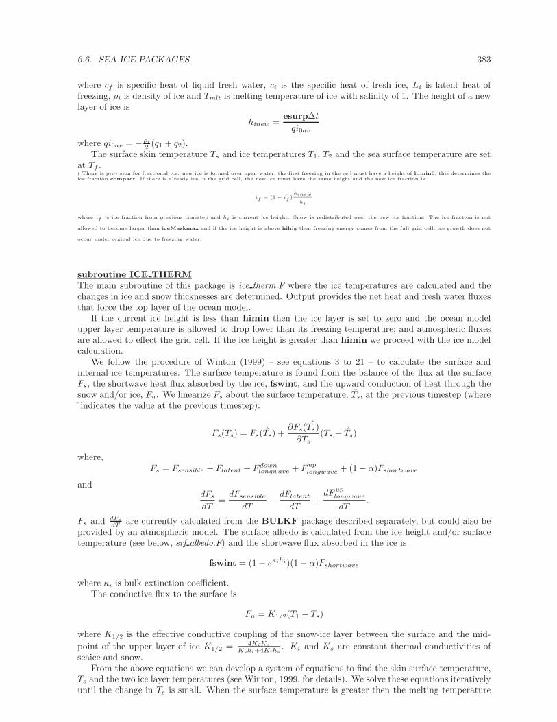
6.6. SEA ICE PACKAGES 383
where cf is specific heat of liquid fresh water, ci is the specific heat of fresh ice, Li is latent heat offreezing, ρi is density of ice and Tmlt is melting temperature of ice with salinity of 1. The height of a newlayer of ice is
hinew =esurp∆t
qi0av
where qi0av = − ρi
2 (q1 + q2).The surface skin temperature Ts and ice temperatures T1, T2 and the sea surface temperature are set
at Tf .( There is provision for fractional ice: new ice is formed over open water; the first freezing in the cell must have a height of himin0; this determines theice fraction compact. If there is already ice in the grid cell, the new ice must have the same height and the new ice fraction is
if = (1 − if )hinew
hi
where if is ice fraction from previous timestep and hi is current ice height. Snow is redistributed over the new ice fraction. The ice fraction is not
allowed to become larger than iceMaskmax and if the ice height is above hihig then freezing energy comes from the full grid cell, ice growth does not
occur under orginal ice due to freezing water.
subroutine ICE THERMThe main subroutine of this package is ice therm.F where the ice temperatures are calculated and thechanges in ice and snow thicknesses are determined. Output provides the net heat and fresh water fluxesthat force the top layer of the ocean model.
If the current ice height is less than himin then the ice layer is set to zero and the ocean modelupper layer temperature is allowed to drop lower than its freezing temperature; and atmospheric fluxesare allowed to effect the grid cell. If the ice height is greater than himin we proceed with the ice modelcalculation.
We follow the procedure of Winton (1999) – see equations 3 to 21 – to calculate the surface andinternal ice temperatures. The surface temperature is found from the balance of the flux at the surfaceFs, the shortwave heat flux absorbed by the ice, fswint, and the upward conduction of heat through thesnow and/or ice, Fu. We linearize Fs about the surface temperature, Ts, at the previous timestep (whereˆindicates the value at the previous timestep):
Fs(Ts) = Fs(Ts) +∂Fs(Ts)
∂Ts(Ts − Ts)
where,Fs = Fsensible + Flatent + F down
longwave + Fuplongwave + (1 − α)Fshortwave
anddFs
dT=dFsensible
dT+dFlatent
dT+dFup
longwave
dT.
Fs and dFs
dT are currently calculated from the BULKF package described separately, but could also beprovided by an atmospheric model. The surface albedo is calculated from the ice height and/or surfacetemperature (see below, srf albedo.F) and the shortwave flux absorbed in the ice is
fswint = (1 − eκihi)(1 − α)Fshortwave
where κi is bulk extinction coefficient.The conductive flux to the surface is
Fu = K1/2(T1 − Ts)
where K1/2 is the effective conductive coupling of the snow-ice layer between the surface and the mid-
point of the upper layer of ice K1/2 = 4KiKs
Kshi+4Kihs. Ki and Ks are constant thermal conductivities of
seaice and snow.From the above equations we can develop a system of equations to find the skin surface temperature,
Ts and the two ice layer temperatures (see Winton, 1999, for details). We solve these equations iterativelyuntil the change in Ts is small. When the surface temperature is greater then the melting temperature
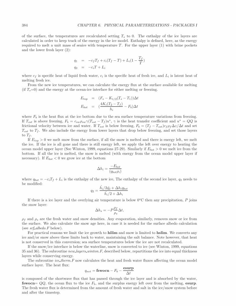
384 CHAPTER 6. PHYSICAL PARAMETERIZATIONS - PACKAGES I
of the surface, the temperatures are recalculated setting Ts to 0. The enthalpy of the ice layers arecalculated in order to keep track of the energy in the ice model. Enthalpy is defined, here, as the energyrequired to melt a unit mass of seaice with temperature T . For the upper layer (1) with brine pocketsand the lower fresh layer (2):
q1 = −cfTf + ci(Tf − T ) + Li(1 − Tf
T)
q2 = −ciT + Li
where cf is specific heat of liquid fresh water, ci is the specific heat of fresh ice, and Li is latent heat ofmelting fresh ice.
From the new ice temperatures, we can calculate the energy flux at the surface available for melting(if Ts=0) and the energy at the ocean-ice interface for either melting or freezing.
Etop = (Fs −K1/2(Ts − T1))∆t
Ebot = (4Ki(T2 − Tf )
hi− Fb)∆t
where Fb is the heat flux at the ice bottom due to the sea surface temperature variations from freezing.If Tsst is above freezing, Fb = cswρswγ(Tsst − Tf )u∗, γ is the heat transfer coefficient and u∗ = QQ isfrictional velocity between ice and water. If Tsst is below freezing, Fb = (Tf − Tsst)cfρf∆z/∆t and setTsst to Tf . We also include the energy from lower layers that drop below freezing, and set those layersto Tf .
If Etop > 0 we melt snow from the surface, if all the snow is melted and there is energy left, we meltthe ice. If the ice is all gone and there is still energy left, we apply the left over energy to heating theocean model upper layer (See Winton, 1999, equations 27-29). Similarly if Ebot > 0 we melt ice from thebottom. If all the ice is melted, the snow is melted (with energy from the ocean model upper layer ifnecessary). If Ebot < 0 we grow ice at the bottom
∆hi =−Ebot
(qbotρi)
where qbot = −ciTf +Li is the enthalpy of the new ice, The enthalpy of the second ice layer, q2 needs tobe modified:
q2 =hi/2q2 + ∆hiqbot
hi/2 + ∆hi
If there is a ice layer and the overlying air temperature is below 0oC then any precipitation, P joinsthe snow layer:
∆hs = −P ρf
ρs∆t,
ρf and ρs are the fresh water and snow densities. Any evaporation, similarly, removes snow or ice fromthe surface. We also calculate the snow age here, in case it is needed for the surface albedo calculation(see srf albedo.F below).
For practical reasons we limit the ice growth to hilim and snow is limited to hslim. We converts anyice and/or snow above these limits back to water, maintaining the salt balance. Note however, that heatis not conserved in this conversion; sea surface temperatures below the ice are not recalculated.
If the snow/ice interface is below the waterline, snow is converted to ice (see Winton, 1999, equations35 and 36). The subroutine new layers winton.F, described below, repartitions the ice into equal thicknesslayers while conserving energy.
The subroutine ice therm.F now calculates the heat and fresh water fluxes affecting the ocean modelsurface layer. The heat flux:
qnet = fswocn − Fb −esurp
∆t
is composed of the shortwave flux that has passed through the ice layer and is absorbed by the water,fswocn= QQ, the ocean flux to the ice Fb, and the surplus energy left over from the melting, esurp.The fresh water flux is determined from the amount of fresh water and salt in the ice/snow system beforeand after the timestep.
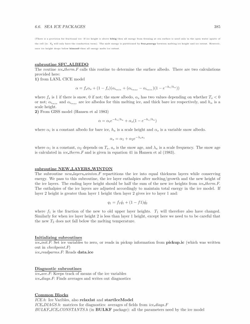
6.6. SEA ICE PACKAGES 385
(There is a provision for fractional ice: If ice height is above hihig then all energy from freezing at sea surface is used only in the open water aparts of
the cell (ie. Fb will only have the conduction term). The melt energy is partitioned by frac energy between melting ice height and ice extent. However,
once ice height drops below himon0 then all energy melts ice extent.
subroutine SFC ALBEDOThe routine ice therm.F calls this routine to determine the surface albedo. There are two calculationsprovided here:1) from LANL CICE model
α = fsαs + (1 − fs)(αimin+ (αimax
− αimin)(1 − e−hi/hα))
where fs is 1 if there is snow, 0 if not; the snow albedo, αs has two values depending on whether Ts < 0or not; αimin
and αimaxare ice albedos for thin melting ice, and thick bare ice respectively, and hα is a
scale height.2) From GISS model (Hansen et al 1983)
α = αie−hs/ha + αs(1 − e−hs/ha)
where αi is a constant albedo for bare ice, ha is a scale height and αs is a variable snow albedo.
αs = α1 + α2e−λaas
where α1 is a constant, α2 depends on Ts, as is the snow age, and λa is a scale frequency. The snow ageis calculated in ice therm.F and is given in equation 41 in Hansen et al (1983).
subroutine NEW LAYERS WINTONThe subroutine new layers winton.F repartitions the ice into equal thickness layers while conservingenergy. We pass to this subroutine, the ice layer enthalpies after melting/growth and the new height ofthe ice layers. The ending layer height should be half the sum of the new ice heights from ice therm.F.The enthalpies of the ice layers are adjusted accordingly to maintain total energy in the ice model. Iflayer 2 height is greater than layer 1 height then layer 2 gives ice to layer 1 and:
q1 = f1q1 + (1 − f1)q2
where f1 is the fraction of the new to old upper layer heights. T1 will therefore also have changed.Similarly for when ice layer height 2 is less than layer 1 height, except here we need to to be careful thatthe new T2 does not fall below the melting temperature.
Initializing subroutinesice init.F: Set ice variables to zero, or reads in pickup information from pickup.ic (which was writtenout in checkpoint.F)ice readparms.F: Reads data.ice
Diagnostic subroutinesice ave.F: Keeps track of means of the ice variablesice diags.F: Finds averages and writes out diagnostics
Common BlocksICE.h: Ice Varibles, also relaxlat and startIceModelICE DIAGS.h: matrices for diagnostics: averages of fields from ice diags.FBULKF ICE CONSTANTS.h (in BULKF package): all the parameters need by the ice model
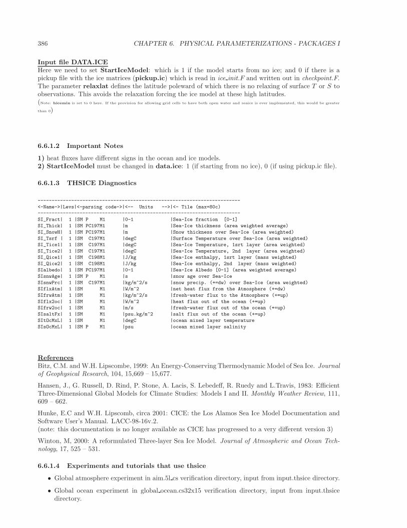
386 CHAPTER 6. PHYSICAL PARAMETERIZATIONS - PACKAGES I
Input file DATA.ICEHere we need to set StartIceModel: which is 1 if the model starts from no ice; and 0 if there is apickup file with the ice matrices (pickup.ic) which is read in ice init.F and written out in checkpoint.F.The parameter relaxlat defines the latitude poleward of which there is no relaxing of surface T or S toobservations. This avoids the relaxation forcing the ice model at these high latitudes.(Note: hicemin is set to 0 here. If the provision for allowing grid cells to have both open water and seaice is ever implemented, this would be greater
than 0)
6.6.1.2 Important Notes
1) heat fluxes have different signs in the ocean and ice models.2) StartIceModel must be changed in data.ice: 1 (if starting from no ice), 0 (if using pickup.ic file).
6.6.1.3 THSICE Diagnostics
------------------------------------------------------------------------
<-Name->|Levs|<-parsing code->|<-- Units -->|<- Tile (max=80c)
------------------------------------------------------------------------
SI_Fract| 1 |SM P M1 |0-1 |Sea-Ice fraction [0-1]
SI_Thick| 1 |SM PC197M1 |m |Sea-Ice thickness (area weighted average)
SI_SnowH| 1 |SM PC197M1 |m |Snow thickness over Sea-Ice (area weighted)
SI_Tsrf | 1 |SM C197M1 |degC |Surface Temperature over Sea-Ice (area weighted)
SI_Tice1| 1 |SM C197M1 |degC |Sea-Ice Temperature, 1srt layer (area weighted)
SI_Tice2| 1 |SM C197M1 |degC |Sea-Ice Temperature, 2nd layer (area weighted)
SI_Qice1| 1 |SM C198M1 |J/kg |Sea-Ice enthalpy, 1srt layer (mass weighted)
SI_Qice2| 1 |SM C198M1 |J/kg |Sea-Ice enthalpy, 2nd layer (mass weighted)
SIalbedo| 1 |SM PC197M1 |0-1 |Sea-Ice Albedo [0-1] (area weighted average)
SIsnwAge| 1 |SM P M1 |s |snow age over Sea-Ice
SIsnwPrc| 1 |SM C197M1 |kg/m^2/s |snow precip. (+=dw) over Sea-Ice (area weighted)
SIflxAtm| 1 |SM M1 |W/m^2 |net heat flux from the Atmosphere (+=dw)
SIfrwAtm| 1 |SM M1 |kg/m^2/s |fresh-water flux to the Atmosphere (+=up)
SIflx2oc| 1 |SM M1 |W/m^2 |heat flux out of the ocean (+=up)
SIfrw2oc| 1 |SM M1 |m/s |fresh-water flux out of the ocean (+=up)
SIsaltFx| 1 |SM M1 |psu.kg/m^2 |salt flux out of the ocean (+=up)
SItOcMxL| 1 |SM M1 |degC |ocean mixed layer temperature
SIsOcMxL| 1 |SM P M1 |psu |ocean mixed layer salinity
ReferencesBitz, C.M. and W.H. Lipscombe, 1999: An Energy-Conserving Thermodynamic Model of Sea Ice. Journalof Geophysical Research, 104, 15,669 – 15,677.
Hansen, J., G. Russell, D. Rind, P. Stone, A. Lacis, S. Lebedeff, R. Ruedy and L.Travis, 1983: EfficientThree-Dimensional Global Models for Climate Studies: Models I and II. Monthly Weather Review, 111,609 – 662.
Hunke, E.C and W.H. Lipscomb, circa 2001: CICE: the Los Alamos Sea Ice Model Documentation andSoftware User’s Manual. LACC-98-16v.2.(note: this documentation is no longer available as CICE has progressed to a very different version 3)
Winton, M, 2000: A reformulated Three-layer Sea Ice Model. Journal of Atmospheric and Ocean Tech-nology, 17, 525 – 531.
6.6.1.4 Experiments and tutorials that use thsice
• Global atmosphere experiment in aim.5l cs verification directory, input from input.thsice directory.
• Global ocean experiment in global ocean.cs32x15 verification directory, input from input.thsicedirectory.
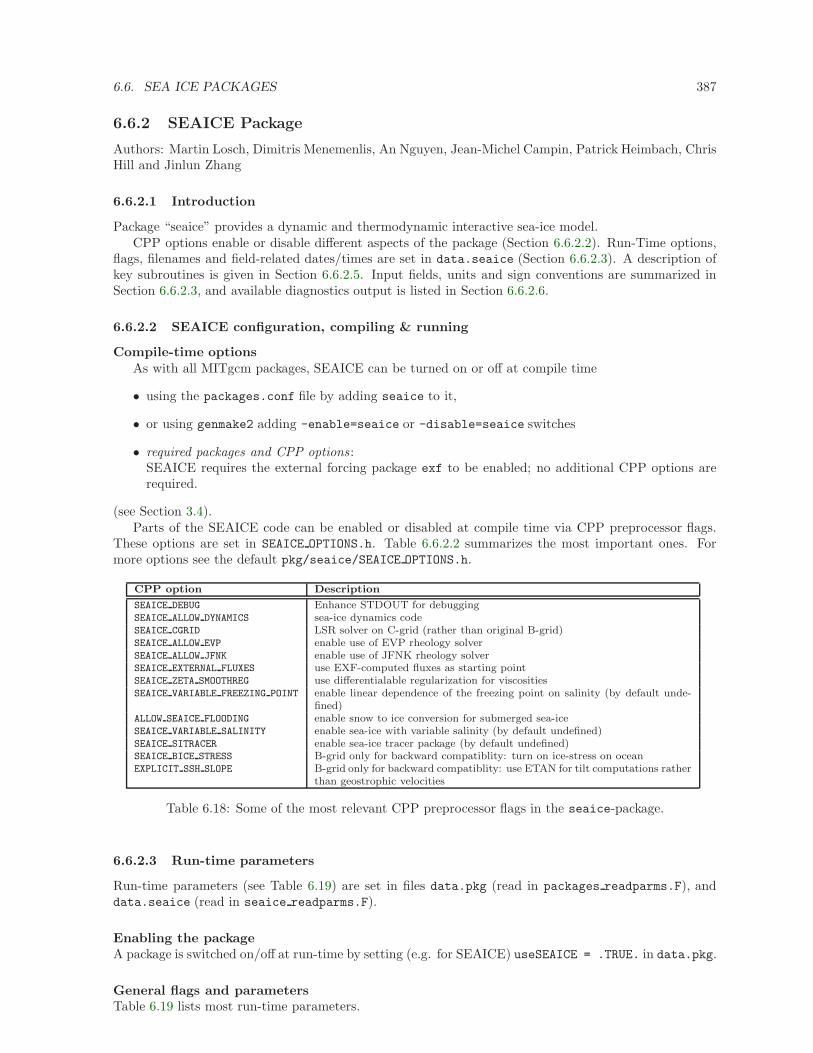
6.6. SEA ICE PACKAGES 387
6.6.2 SEAICE Package
Authors: Martin Losch, Dimitris Menemenlis, An Nguyen, Jean-Michel Campin, Patrick Heimbach, ChrisHill and Jinlun Zhang
6.6.2.1 Introduction
Package “seaice” provides a dynamic and thermodynamic interactive sea-ice model.CPP options enable or disable different aspects of the package (Section 6.6.2.2). Run-Time options,
flags, filenames and field-related dates/times are set in data.seaice (Section 6.6.2.3). A description ofkey subroutines is given in Section 6.6.2.5. Input fields, units and sign conventions are summarized inSection 6.6.2.3, and available diagnostics output is listed in Section 6.6.2.6.
6.6.2.2 SEAICE configuration, compiling & running
Compile-time optionsAs with all MITgcm packages, SEAICE can be turned on or off at compile time
• using the packages.conf file by adding seaice to it,
• or using genmake2 adding -enable=seaice or -disable=seaice switches
• required packages and CPP options :SEAICE requires the external forcing package exf to be enabled; no additional CPP options arerequired.
(see Section 3.4).Parts of the SEAICE code can be enabled or disabled at compile time via CPP preprocessor flags.
These options are set in SEAICE OPTIONS.h. Table 6.6.2.2 summarizes the most important ones. Formore options see the default pkg/seaice/SEAICE OPTIONS.h.
CPP option Description
SEAICE DEBUG Enhance STDOUT for debuggingSEAICE ALLOW DYNAMICS sea-ice dynamics codeSEAICE CGRID LSR solver on C-grid (rather than original B-grid)SEAICE ALLOW EVP enable use of EVP rheology solverSEAICE ALLOW JFNK enable use of JFNK rheology solverSEAICE EXTERNAL FLUXES use EXF-computed fluxes as starting pointSEAICE ZETA SMOOTHREG use differentialable regularization for viscositiesSEAICE VARIABLE FREEZING POINT enable linear dependence of the freezing point on salinity (by default unde-
fined)ALLOW SEAICE FLOODING enable snow to ice conversion for submerged sea-iceSEAICE VARIABLE SALINITY enable sea-ice with variable salinity (by default undefined)SEAICE SITRACER enable sea-ice tracer package (by default undefined)SEAICE BICE STRESS B-grid only for backward compatiblity: turn on ice-stress on oceanEXPLICIT SSH SLOPE B-grid only for backward compatiblity: use ETAN for tilt computations rather
than geostrophic velocities
Table 6.18: Some of the most relevant CPP preprocessor flags in the seaice-package.
6.6.2.3 Run-time parameters
Run-time parameters (see Table 6.19) are set in files data.pkg (read in packages readparms.F), anddata.seaice (read in seaice readparms.F).
Enabling the packageA package is switched on/off at run-time by setting (e.g. for SEAICE) useSEAICE = .TRUE. in data.pkg.
General flags and parametersTable 6.19 lists most run-time parameters.
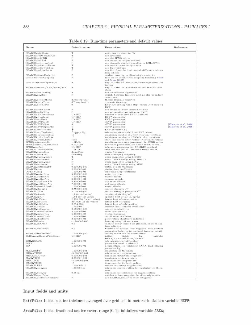
388 CHAPTER 6. PHYSICAL PARAMETERIZATIONS - PACKAGES I
Table 6.19: Run-time parameters and default values
Name Default value Description Reference
SEAICEwriteState T write sea ice state to fileSEAICEuseDYNAMICS T use dynamicsSEAICEuseJFNK F use the JFNK-solverSEAICEuseTEM F use truncated ellipse methodSEAICEuseStrImpCpl F use strength implicit coupling in LSR/JFNKSEAICEuseMetricTerms T use metric terms in dynamicsSEAICEuseEVPpickup T use EVP pickupsSEAICEuseFluxForm F use flux form for 2nd central difference advec-
tion schemeSEAICErestoreUnderIce F enable restoring to climatology under iceuseHB87stressCoupling F turn on ice-ocean stress coupling following Hibler
and Bryan [1987]usePW79thermodynamics T flag to turn off zero-layer-thermodynamics for
testingSEAICEadvHeff/Area/Snow/Salt T flag to turn off advection of scalar state vari-
ablesSEAICEuseFlooding T use flood-freeze algorithmSEAICE no slip F switch between free-slip and no-slip boundary
conditionsSEAICE deltaTtherm dTracerLev(1) thermodynamic timestepSEAICE deltaTdyn dTracerLev(1) dynamic timestepSEAICE deltaTevp 0 EVP sub-cycling time step, values > 0 turn on
EVPSEAICEuseEVPstar F use modified EVP* instead of EVPSEAICEuseEVPrev F use yet another variation on EVP*SEAICEnEVPstarSteps UNSET number of modified EVP* iterationSEAICE evpAlpha UNSET EVP* parameterSEAICE evpBeta UNSET EVP* parameterSEAICEaEVPcoeff UNSET aEVP parameterSEAICEaEVPcStar 4 aEVP parameter [Kimmritz et al., 2016]SEAICEaEVPalphaMin 5 aEVP parameter [Kimmritz et al., 2016]
SEAICE elasticParm 13
EVP paramter E0SEAICE evpTauRelax ∆tEV P E0 relaxation time scale T for EVP wavesSEAICEnewtonIterMax 10 maximum number of JFNK-Newton iterationsSEAICEkrylovIterMax 10 maximum number of JFNK-Krylov iterationsSEAICE JFNK lsIter (off) start line search after “lsIter” Newton iterationsJFNKgamma nonlin 1.0E-05 non-linear tolerance parameter for JFNK solverJFNKgamma lin min/max 0.10/0.99 tolerance parameters for linear JFNK solverJFNKres tFac UNSET tolerance parameter for FGMRES residualSEAICE JFNKepsilon 1.0E-06 step size for the FD-Jacobian-times-vectorSEAICE dumpFreq dumpFreq dump frequencySEAICE taveFreq taveFreq time-averaging frequencySEAICE dump mdsio T write snap-shot using MDSIOSEAICE tave mdsio T write TimeAverage using MDSIOSEAICE dump mnc F write snap-shot using MNCSEAICE tave mnc F write TimeAverage using MNCSEAICE initialHEFF 0.00000E+00 initial sea-ice thicknessSEAICE drag 2.00000E-03 air-ice drag coefficientOCEAN drag 1.00000E-03 air-ocean drag coefficientSEAICE waterDrag 5.50000E+00 water-ice dragSEAICE dryIceAlb 7.50000E-01 winter albedoSEAICE wetIceAlb 6.60000E-01 summer albedoSEAICE drySnowAlb 8.40000E-01 dry snow albedoSEAICE wetSnowAlb 7.00000E-01 wet snow albedoSEAICE waterAlbedo 1.00000E-01 water albedoSEAICE strength 2.75000E+04 sea-ice strength P∗
SEAICE cStar 20.0000E+00 sea-ice strength paramter C∗
SEAICE rhoAir 1.3 (or exf value) density of air (kg/m3)SEAICE cpAir 1004 (or exf value) specific heat of air (J/kg/K)SEAICE lhEvap 2,500,000 (or exf value) latent heat of evaporationSEAICE lhFusion 334,000 (or exf value) latent heat of fusionSEAICE lhSublim 2,834,000 latent heat of sublimationSEAICE dalton 1.75E-03 sensible heat transfer coefficientSEAICE iceConduct 2.16560E+00 sea-ice conductivitySEAICE snowConduct 3.10000E-01 snow conductivitySEAICE emissivity 5.50000E-08 Stefan-BoltzmanSEAICE snowThick 1.50000E-01 cutoff snow thicknessSEAICE shortwave 3.00000E-01 penetration shortwave radiationSEAICE freeze -1.96000E+00 freezing temp. of sea waterSEAICE saltFrac 0.0 salinity newly formed ice (fraction of ocean sur-
face salinity)SEAICE frazilFrac 0.0 Fraction of surface level negative heat content
anomalies (relative to the local freezing point)SEAICEstressFactor 1.00000E+00 scaling factor for ice-ocean stressHeff/Area/HsnowFile/Hsalt UNSET initial fields for variables
HEFF/AREA/HSNOW/HSALTLSR ERROR 1.00000E-04 sets accuracy of LSR solverDIFF1 0.0 parameter used in advect.FHO 5.00000E-01 demarcation ice thickness (AKA lead closing
paramter h0)MAX HEFF 1.00000E+01 maximum ice thicknessMIN ATEMP -5.00000E+01 minimum air temperatureMIN LWDOWN 6.00000E+01 minimum downward longwaveMAX TICE 3.00000E+01 maximum ice temperatureMIN TICE -5.00000E+01 minimum ice temperatureIMAX TICE 10 iterations for ice heat budgetSEAICE EPS 1.00000E-10 reduce derivative singularitiesSEAICE area reg 1.00000E-5 minimum concentration to regularize ice thick-
nessSEAICE hice reg 0.05 m minimum ice thickness for regularizationSEAICE multDim 1 number of ice categories for thermodynamicsSEAICE useMultDimSnow F use SEAICE multDim snow categories
Input fields and units
HeffFile: Initial sea ice thickness averaged over grid cell in meters; initializes variable HEFF;
AreaFile: Initial fractional sea ice cover, range [0, 1]; initializes variable AREA;
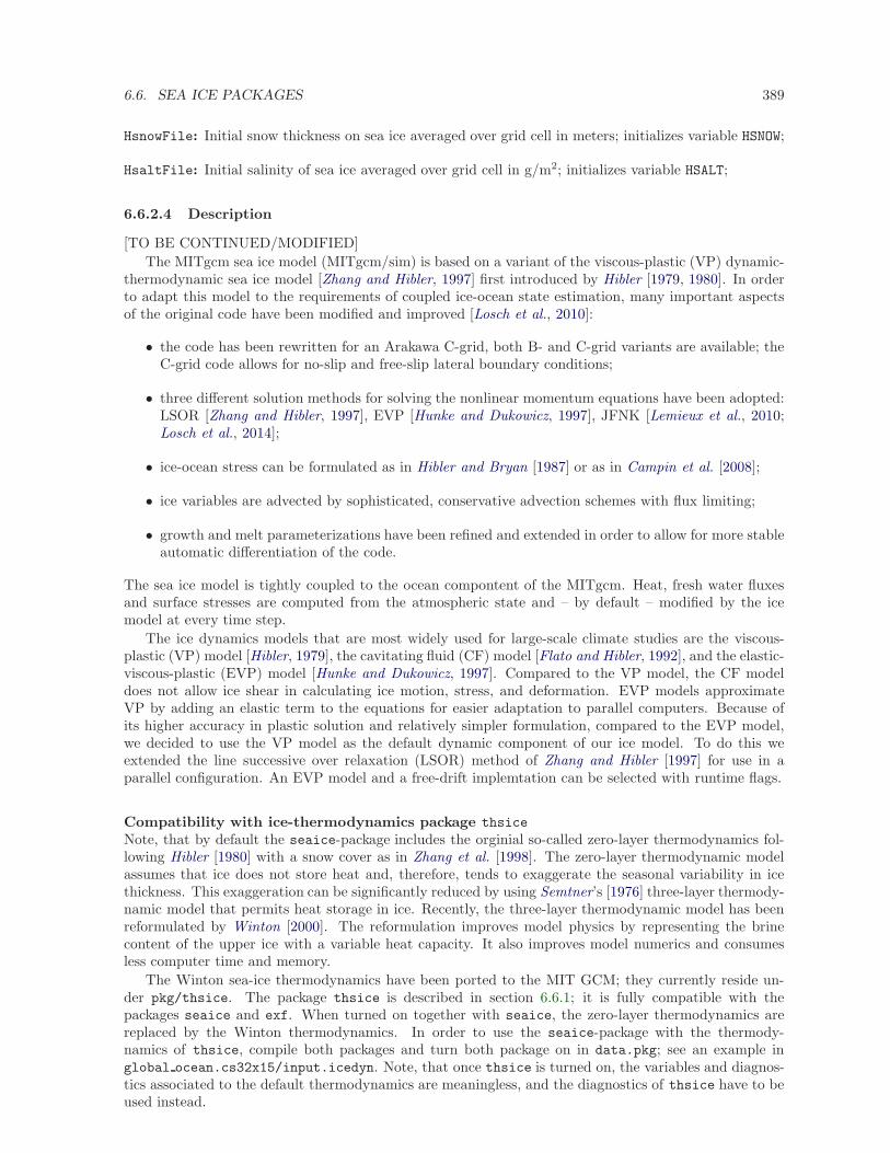
6.6. SEA ICE PACKAGES 389
HsnowFile: Initial snow thickness on sea ice averaged over grid cell in meters; initializes variable HSNOW;
HsaltFile: Initial salinity of sea ice averaged over grid cell in g/m2; initializes variable HSALT;
6.6.2.4 Description
[TO BE CONTINUED/MODIFIED]
The MITgcm sea ice model (MITgcm/sim) is based on a variant of the viscous-plastic (VP) dynamic-thermodynamic sea ice model [Zhang and Hibler, 1997] first introduced by Hibler [1979, 1980]. In orderto adapt this model to the requirements of coupled ice-ocean state estimation, many important aspectsof the original code have been modified and improved [Losch et al., 2010]:
• the code has been rewritten for an Arakawa C-grid, both B- and C-grid variants are available; theC-grid code allows for no-slip and free-slip lateral boundary conditions;
• three different solution methods for solving the nonlinear momentum equations have been adopted:LSOR [Zhang and Hibler, 1997], EVP [Hunke and Dukowicz, 1997], JFNK [Lemieux et al., 2010;Losch et al., 2014];
• ice-ocean stress can be formulated as in Hibler and Bryan [1987] or as in Campin et al. [2008];
• ice variables are advected by sophisticated, conservative advection schemes with flux limiting;
• growth and melt parameterizations have been refined and extended in order to allow for more stableautomatic differentiation of the code.
The sea ice model is tightly coupled to the ocean compontent of the MITgcm. Heat, fresh water fluxesand surface stresses are computed from the atmospheric state and – by default – modified by the icemodel at every time step.
The ice dynamics models that are most widely used for large-scale climate studies are the viscous-plastic (VP) model [Hibler, 1979], the cavitating fluid (CF) model [Flato and Hibler, 1992], and the elastic-viscous-plastic (EVP) model [Hunke and Dukowicz, 1997]. Compared to the VP model, the CF modeldoes not allow ice shear in calculating ice motion, stress, and deformation. EVP models approximateVP by adding an elastic term to the equations for easier adaptation to parallel computers. Because ofits higher accuracy in plastic solution and relatively simpler formulation, compared to the EVP model,we decided to use the VP model as the default dynamic component of our ice model. To do this weextended the line successive over relaxation (LSOR) method of Zhang and Hibler [1997] for use in aparallel configuration. An EVP model and a free-drift implemtation can be selected with runtime flags.
Compatibility with ice-thermodynamics package thsice
Note, that by default the seaice-package includes the orginial so-called zero-layer thermodynamics fol-lowing Hibler [1980] with a snow cover as in Zhang et al. [1998]. The zero-layer thermodynamic modelassumes that ice does not store heat and, therefore, tends to exaggerate the seasonal variability in icethickness. This exaggeration can be significantly reduced by using Semtner’s [1976] three-layer thermody-namic model that permits heat storage in ice. Recently, the three-layer thermodynamic model has beenreformulated by Winton [2000]. The reformulation improves model physics by representing the brinecontent of the upper ice with a variable heat capacity. It also improves model numerics and consumesless computer time and memory.
The Winton sea-ice thermodynamics have been ported to the MIT GCM; they currently reside un-der pkg/thsice. The package thsice is described in section 6.6.1; it is fully compatible with thepackages seaice and exf. When turned on together with seaice, the zero-layer thermodynamics arereplaced by the Winton thermodynamics. In order to use the seaice-package with the thermody-namics of thsice, compile both packages and turn both package on in data.pkg; see an example inglobal ocean.cs32x15/input.icedyn. Note, that once thsice is turned on, the variables and diagnos-tics associated to the default thermodynamics are meaningless, and the diagnostics of thsice have to beused instead.
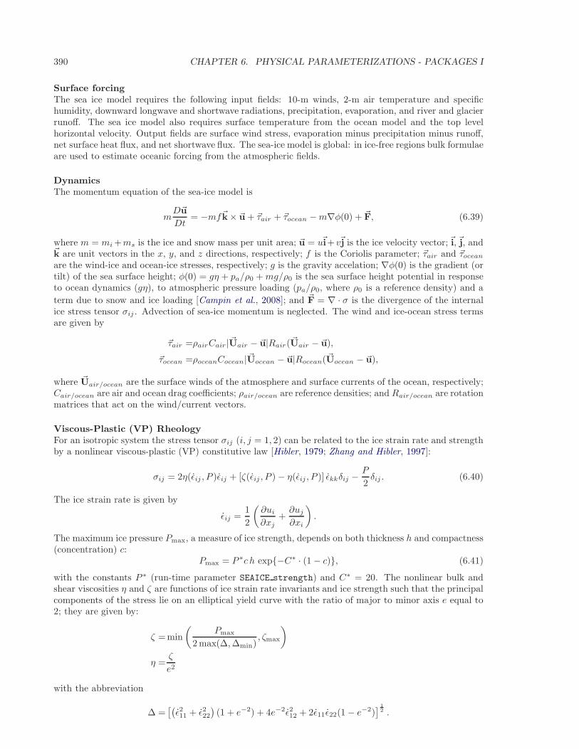
390 CHAPTER 6. PHYSICAL PARAMETERIZATIONS - PACKAGES I
Surface forcingThe sea ice model requires the following input fields: 10-m winds, 2-m air temperature and specifichumidity, downward longwave and shortwave radiations, precipitation, evaporation, and river and glacierrunoff. The sea ice model also requires surface temperature from the ocean model and the top levelhorizontal velocity. Output fields are surface wind stress, evaporation minus precipitation minus runoff,net surface heat flux, and net shortwave flux. The sea-ice model is global: in ice-free regions bulk formulaeare used to estimate oceanic forcing from the atmospheric fields.
DynamicsThe momentum equation of the sea-ice model is
mD~u
Dt= −mf~k× ~u + ~τair + ~τocean −m∇φ(0) + ~F, (6.39)
where m = mi +ms is the ice and snow mass per unit area; ~u = u~i+ v~j is the ice velocity vector;~i,~j, and~k are unit vectors in the x, y, and z directions, respectively; f is the Coriolis parameter; ~τair and ~τocean
are the wind-ice and ocean-ice stresses, respectively; g is the gravity accelation; ∇φ(0) is the gradient (ortilt) of the sea surface height; φ(0) = gη + pa/ρ0 +mg/ρ0 is the sea surface height potential in responseto ocean dynamics (gη), to atmospheric pressure loading (pa/ρ0, where ρ0 is a reference density) and a
term due to snow and ice loading [Campin et al., 2008]; and ~F = ∇ · σ is the divergence of the internalice stress tensor σij . Advection of sea-ice momentum is neglected. The wind and ice-ocean stress termsare given by
~τair =ρairCair|~Uair − ~u|Rair(~Uair − ~u),
~τocean =ρoceanCocean|~Uocean − ~u|Rocean(~Uocean − ~u),
where ~Uair/ocean are the surface winds of the atmosphere and surface currents of the ocean, respectively;Cair/ocean are air and ocean drag coefficients; ρair/ocean are reference densities; and Rair/ocean are rotationmatrices that act on the wind/current vectors.
Viscous-Plastic (VP) RheologyFor an isotropic system the stress tensor σij (i, j = 1, 2) can be related to the ice strain rate and strengthby a nonlinear viscous-plastic (VP) constitutive law [Hibler, 1979; Zhang and Hibler, 1997]:
σij = 2η(ǫij , P )ǫij + [ζ(ǫij , P ) − η(ǫij , P )] ǫkkδij −P
2δij . (6.40)
The ice strain rate is given by
ǫij =1
2
(∂ui
∂xj+∂uj
∂xi
).
The maximum ice pressure Pmax, a measure of ice strength, depends on both thickness h and compactness(concentration) c:
Pmax = P ∗c h exp−C∗ · (1 − c), (6.41)
with the constants P ∗ (run-time parameter SEAICE strength) and C∗ = 20. The nonlinear bulk andshear viscosities η and ζ are functions of ice strain rate invariants and ice strength such that the principalcomponents of the stress lie on an elliptical yield curve with the ratio of major to minor axis e equal to2; they are given by:
ζ =min
(Pmax
2 max(∆,∆min), ζmax
)
η =ζ
e2
with the abbreviation
∆ =[(ǫ211 + ǫ222
)(1 + e−2) + 4e−2ǫ212 + 2ǫ11ǫ22(1 − e−2)
] 12 .
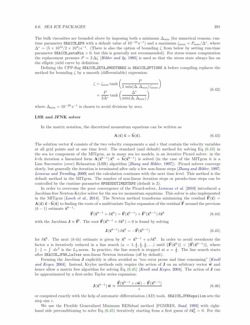
6.6. SEA ICE PACKAGES 391
The bulk viscosities are bounded above by imposing both a minimum ∆min (for numerical reasons, run-time parameter SEAICE EPS with a default value of 10−10 s−1) and a maximum ζmax = Pmax/∆
∗, where∆∗ = (5 × 10¹²/2 × 104) s−1. (There is also the option of bounding ζ from below by setting run-timeparameter SEAICE zetaMin > 0, but this is generally not recommended). For stress tensor computationthe replacement pressure P = 2 ∆ζ [Hibler and Ip, 1995] is used so that the stress state always lies onthe elliptic yield curve by definition.
Defining the CPP-flag SEAICE ZETA SMOOTHREG in SEAICE OPTIONS.h before compiling replaces themethod for bounding ζ by a smooth (differentiable) expression:
ζ = ζmax tanh
(P
2 min(∆,∆min) ζmax
)
=P
2∆∗tanh
(∆∗
min(∆,∆min)
) (6.42)
where ∆min = 10−20 s−1 is chosen to avoid divisions by zero.
LSR and JFNK solver
In the matrix notation, the discretized momentum equations can be written as
A(~x)~x = ~b(~x). (6.43)
The solution vector ~x consists of the two velocity components u and v that contain the velocity variablesat all grid points and at one time level. The standard (and default) method for solving Eq. (6.43) inthe sea ice component of the MITgcm, as in many sea ice models, is an iterative Picard solver: in thek-th iteration a linearized form A(~xk−1)~xk = ~b(~xk−1) is solved (in the case of the MITgcm it is aLine Successive (over) Relaxation (LSR) algorithm [Zhang and Hibler, 1997]). Picard solvers convergeslowly, but generally the iteration is terminated after only a few non-linear steps [Zhang and Hibler, 1997;Lemieux and Tremblay, 2009] and the calculation continues with the next time level. This method is thedefault method in the MITgcm. The number of non-linear iteration steps or pseudo-time steps can becontrolled by the runtime parameter NPSEUDOTIMESTEPS (default is 2).
In order to overcome the poor convergence of the Picard-solver, Lemieux et al. [2010] introduced aJacobian-free Newton-Krylov solver for the sea ice momentum equations. This solver is also implementedin the MITgcm [Losch et al., 2014]. The Newton method transforms minimizing the residual ~F(~x) =
A(~x)~x−~b(~x) to finding the roots of a multivariate Taylor expansion of the residual ~F around the previous(k − 1) estimate ~xk−1:
~F(~xk−1 + δ~xk) = ~F(~xk−1) + ~F′(~xk−1) δ~xk (6.44)
with the Jacobian J ≡ ~F′. The root ~F(~xk−1 + δ~xk) = 0 is found by solving
J(~xk−1) δ~xk = −~F(~xk−1) (6.45)
for δ~xk. The next (k-th) estimate is given by ~xk = ~xk−1 + a δ~xk. In order to avoid overshoots the
factor a is iteratively reduced in a line search (a = 1, 12 ,
14 ,
18 , . . .) until ‖~F(~xk)‖ < ‖~F(~xk−1)‖, where
‖ · ‖ =∫· dx2 is the L2-norm. In practice, the line search is stopped at a = 1
8 . The line search startsafter SEAICE JFNK lsIter non-linear Newton iterations (off by default).
Forming the Jacobian J explicitly is often avoided as “too error prone and time consuming” [Knolland Keyes, 2004]. Instead, Krylov methods only require the action of J on an arbitrary vector ~w andhence allow a matrix free algorithm for solving Eq. (6.45) [Knoll and Keyes, 2004]. The action of J canbe approximated by a first-order Taylor series expansion:
J(~xk−1) ~w ≈~F(~xk−1 + ǫ~w) − ~F(~xk−1)
ǫ(6.46)
or computed exactly with the help of automatic differentiation (AD) tools. SEAICE JFNKepsilon sets thestep size ǫ.
We use the Flexible Generalized Minimum RESidual method [FGMRES, Saad, 1993] with right-hand side preconditioning to solve Eq. (6.45) iteratively starting from a first guess of δ~xk
0 = 0. For the
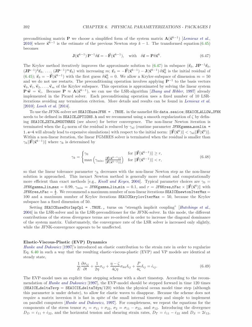
392 CHAPTER 6. PHYSICAL PARAMETERIZATIONS - PACKAGES I
preconditioning matrix P we choose a simplified form of the system matrix A(~xk−1) [Lemieux et al.,2010] where ~xk−1 is the estimate of the previous Newton step k − 1. The transformed equation (6.45)becomes
J(~xk−1)P−1δ~z = −~F(~xk−1), with δ~z = Pδ~xk. (6.47)
The Krylov method iteratively improves the approximate solution to (6.47) in subspace (~r0, JP−1~r0,
(JP−1)2~r0, . . . , (JP−1)m~r0) with increasing m; ~r0 = −~F(~xk−1) − J(~xk−1) δ~xk0 is the initial residual of
(6.45); ~r0 = −~F(~xk−1) with the first guess δ~xk0 = 0. We allow a Krylov-subspace of dimension m = 50
and we do not use restarts. The preconditioning operation involves applying P−1 to the basis vectors~v0, ~v1, ~v2, . . . , ~vm of the Krylov subspace. This operation is approximated by solving the linear systemP ~w = ~vi. Because P ≈ A(~xk−1), we can use the LSR-algorithm [Zhang and Hibler, 1997] alreadyimplemented in the Picard solver. Each preconditioning operation uses a fixed number of 10 LSR-iterations avoiding any termination criterion. More details and results can be found in Lemieux et al.[2010]; Losch et al. [2014].
To use the JFNK-solver set SEAICEuseJFNK = .TRUE. in the namelist file data.seaice; SEAICE ALLOW JFNK
needs to be defined in SEAICE OPTIONS.h and we recommend using a smooth regularization of ζ by defin-ing SEAICE ZETA SMOOTHREG (see above) for better convergence. The non-linear Newton iteration isterminated when the L2-norm of the residual is reduced by γnl (runtime parameter JFNKgamma nonlin =
1.e-4 will already lead to expensive simulations) with respect to the initial norm: ‖~F(~xk)‖ < γnl‖~F(~x0)‖.Within a non-linear iteration, the linear FGMRES solver is terminated when the residual is smaller thanγk‖~F(~xk−1)‖ where γk is determined by
γk =
γ0 for ‖~F(~xk−1)‖ ≥ r,
max(γmin,
‖~F(~xk−1)‖
‖~F(~xk−2)‖
)for ‖~F(~xk−1)‖ < r,
(6.48)
so that the linear tolerance parameter γk decreases with the non-linear Newton step as the non-linearsolution is approached. This inexact Newton method is generally more robust and computationallymore efficient than exact methods [e.g., Knoll and Keyes, 2004]. Typical parameter choices are γ0 =
JFNKgamma lin max = 0.99, γmin = JFNKgamma lin min = 0.1, and r = JFNKres tFac × ‖~F(~x0)‖ withJFNKres tFac = 1
2 . We recommend a maximum number of non-linear iterations SEAICEnewtonIterMax=100 and a maximum number of Krylov iterations SEAICEkrylovIterMax = 50, because the Krylovsubspace has a fixed dimension of 50.
Setting SEAICEuseStrImpCpl = .TRUE., turns on “strength implicit coupling” [Hutchings et al.,2004] in the LSR-solver and in the LSR-preconditioner for the JFNK-solver. In this mode, the differentcontributions of the stress divergence terms are re-ordered in order to increase the diagonal dominanceof the system matrix. Unfortunately, the convergence rate of the LSR solver is increased only slightly,while the JFNK-convergence appears to be unaffected.
Elastic-Viscous-Plastic (EVP) DynamicsHunke and Dukowicz [1997]’s introduced an elastic contribution to the strain rate in order to regularizeEq. 6.40 in such a way that the resulting elastic-viscous-plastic (EVP) and VP models are identical atsteady state,
1
E
∂σij
∂t+
1
2ησij +
η − ζ
4ζησkkδij +
P
4ζδij = ǫij . (6.49)
The EVP-model uses an explicit time stepping scheme with a short timestep. According to the recom-mendation of Hunke and Dukowicz [1997], the EVP-model should be stepped forward in time 120 times(SEAICE deltaTevp = SEAICIE deltaTdyn/120) within the physical ocean model time step (althoughthis parameter is under debate), to allow for elastic waves to disappear. Because the scheme does notrequire a matrix inversion it is fast in spite of the small internal timestep and simple to implementon parallel computers [Hunke and Dukowicz, 1997]. For completeness, we repeat the equations for thecomponents of the stress tensor σ1 = σ11 + σ22, σ2 = σ11 − σ22, and σ12. Introducing the divergenceDD = ǫ11 + ǫ22, and the horizontal tension and shearing strain rates, DT = ǫ11 − ǫ22 and DS = 2ǫ12,

6.6. SEA ICE PACKAGES 393
respectively, and using the above abbreviations, the equations 6.49 can be written as:
∂σ1
∂t+σ1
2T+
P
2T=
P
2T∆DD (6.50)
∂σ2
∂t+σ2e
2
2T=
P
2T∆DT (6.51)
∂σ12
∂t+σ12e
2
2T=
P
4T∆DS (6.52)
Here, the elastic parameter E is redefined in terms of a damping timescale T for elastic waves
E =ζ
T.
T = E0∆t with the tunable parameter E0 < 1 and the external (long) timestep ∆t. E0 = 13 is the default
value in the code and close to what Hunke and Dukowicz [1997] and Hunke [2001] recommend.To use the EVP solver, make sure that both SEAICE CGRID and SEAICE ALLOW EVP are defined in
SEAICE OPTIONS.h (default). The solver is turned on by setting the sub-cycling time step SEAICE deltaTevp
to a value larger than zero. The choice of this time step is under debate. Hunke and Dukowicz [1997]recommend order(120) time steps for the EVP solver within one model time step ∆t (deltaTmom).One can also choose order(120) time steps within the forcing time scale, but then we recommendadjusting the damping time scale T accordingly, by setting either SEAICE elasticParm (E0), so thatE0∆t = forcing time scale, or directly SEAICE evpTauRelax (T ) to the forcing time scale.
More stable variants of Elastic-Viscous-Plastic Dynamics: EVP* , mEVP, and aEVPThe genuine EVP schemes appears to give noisy solutions [Hunke, 2001; Lemieux et al., 2012; Bouillonet al., 2013]. This has lead to a modified EVP or EVP* [Lemieux et al., 2012; Bouillon et al., 2013;Kimmritz et al., 2015]; here, we refer to these variants by modified EVP (mEVP) and adaptive EVP(aEVP) [Kimmritz et al., 2016]. The main idea is to modify the “natural” time-discretization of themomentum equations:
mD~u
Dt≈ m
up+1 − un
∆t+ β∗
up+1 − up
∆tEVP(6.53)
where n is the previous time step index, and p is the previous sub-cycling index. The extra “intertial”term m (up+1 − un)/∆t) allows the definition of a residual |up+1 − up| that, as up+1 → un+1, convergesto 0. In this way EVP can be re-interpreted as a pure iterative solver where the sub-cycling has noassociation with time-relation (through ∆tEVP) [Bouillon et al., 2013; Kimmritz et al., 2015]. Using theterminology of Kimmritz et al. [2015], the evolution equations of stress σij and momentum ~u can bewritten as:
σp+1ij = σp
ij +1
α
(σij(~u
p) − σpij
), (6.54)
~up+1 = ~up +1
β
(∆t
m∇ · σp+1 +
∆t
m~Rp + ~un − ~up
). (6.55)
~R contains all terms in the momentum equations except for the rheology terms and the time derivative;α and β are free parameters (SEAICE evpAlpha, SEAICE evpBeta) that replace the time stepping pa-rameters SEAICE deltaTevp (∆TEVP), SEAICE elasticParm (E0), or SEAICE evpTauRelax (T ). α andβ determine the speed of convergence and the stability. Usually, it makes sense to use α = β, andSEAICEnEVPstarSteps≫ (α, β) [Kimmritz et al., 2015]. Currently, there is no termination criterion andthe number of mEVP iterations is fixed to SEAICEnEVPstarSteps.
In order to use mEVP in the MITgcm, set SEAICEuseEVPstar = .TRUE., in data.seaice. IfSEAICEuseEVPrev =.TRUE., the actual form of equations (6.54) and (6.55) is used with fewer implicitterms and the factor of e2 dropped in the stress equations (6.51) and (6.52). Although this modifies theoriginal EVP-equations, it turns out to improve convergence [Bouillon et al., 2013].
Another variant is the aEVP scheme [Kimmritz et al., 2016], where the value of α is set dynamicallybased on the stability criterion
α = β = max
(cπ
√cζ
Ac
∆t
max(m, 10−4 kg), αmin
)(6.56)
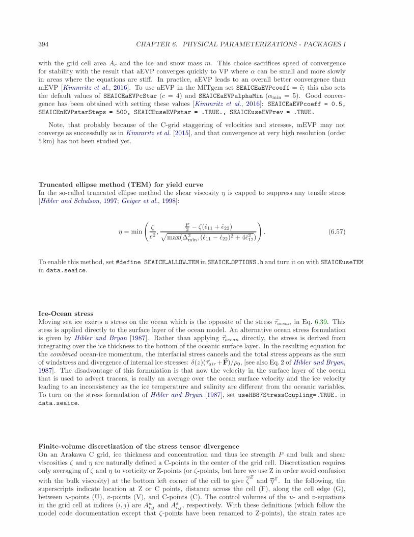
394 CHAPTER 6. PHYSICAL PARAMETERIZATIONS - PACKAGES I
with the grid cell area Ac and the ice and snow mass m. This choice sacrifices speed of convergencefor stability with the result that aEVP converges quickly to VP where α can be small and more slowlyin areas where the equations are stiff. In practice, aEVP leads to an overall better convergence thanmEVP [Kimmritz et al., 2016]. To use aEVP in the MITgcm set SEAICEaEVPcoeff = c; this also setsthe default values of SEAICEaEVPcStar (c = 4) and SEAICEaEVPalphaMin (αmin = 5). Good conver-gence has been obtained with setting these values [Kimmritz et al., 2016]: SEAICEaEVPcoeff = 0.5,
SEAICEnEVPstarSteps = 500, SEAICEuseEVPstar = .TRUE., SEAICEuseEVPrev = .TRUE.
Note, that probably because of the C-grid staggering of velocities and stresses, mEVP may notconverge as successfully as in Kimmritz et al. [2015], and that convergence at very high resolution (order5 km) has not been studied yet.
Truncated ellipse method (TEM) for yield curveIn the so-called truncated ellipse method the shear viscosity η is capped to suppress any tensile stress[Hibler and Schulson, 1997; Geiger et al., 1998]:
η = min
(ζ
e2,
P2 − ζ(ǫ11 + ǫ22)√
max(∆2min, (ǫ11 − ǫ22)2 + 4ǫ212)
). (6.57)
To enable this method, set #define SEAICE ALLOW TEM in SEAICE OPTIONS.h and turn it on with SEAICEuseTEM
in data.seaice.
Ice-Ocean stressMoving sea ice exerts a stress on the ocean which is the opposite of the stress ~τocean in Eq. 6.39. Thisstess is applied directly to the surface layer of the ocean model. An alternative ocean stress formulationis given by Hibler and Bryan [1987]. Rather than applying ~τocean directly, the stress is derived fromintegrating over the ice thickness to the bottom of the oceanic surface layer. In the resulting equation forthe combined ocean-ice momentum, the interfacial stress cancels and the total stress appears as the sumof windstress and divergence of internal ice stresses: δ(z)(~τair +~F)/ρ0, [see also Eq. 2 of Hibler and Bryan,1987]. The disadvantage of this formulation is that now the velocity in the surface layer of the oceanthat is used to advect tracers, is really an average over the ocean surface velocity and the ice velocityleading to an inconsistency as the ice temperature and salinity are different from the oceanic variables.To turn on the stress formulation of Hibler and Bryan [1987], set useHB87StressCoupling=.TRUE. indata.seaice.
Finite-volume discretization of the stress tensor divergenceOn an Arakawa C grid, ice thickness and concentration and thus ice strength P and bulk and shearviscosities ζ and η are naturally defined a C-points in the center of the grid cell. Discretization requiresonly averaging of ζ and η to vorticity or Z-points (or ζ-points, but here we use Z in order avoid confusion
with the bulk viscosity) at the bottom left corner of the cell to give ζZ
and ηZ . In the following, thesuperscripts indicate location at Z or C points, distance across the cell (F), along the cell edge (G),between u-points (U), v-points (V), and C-points (C). The control volumes of the u- and v-equationsin the grid cell at indices (i, j) are Aw
i,j and Asi,j , respectively. With these definitions (which follow the
model code documentation except that ζ-points have been renamed to Z-points), the strain rates are
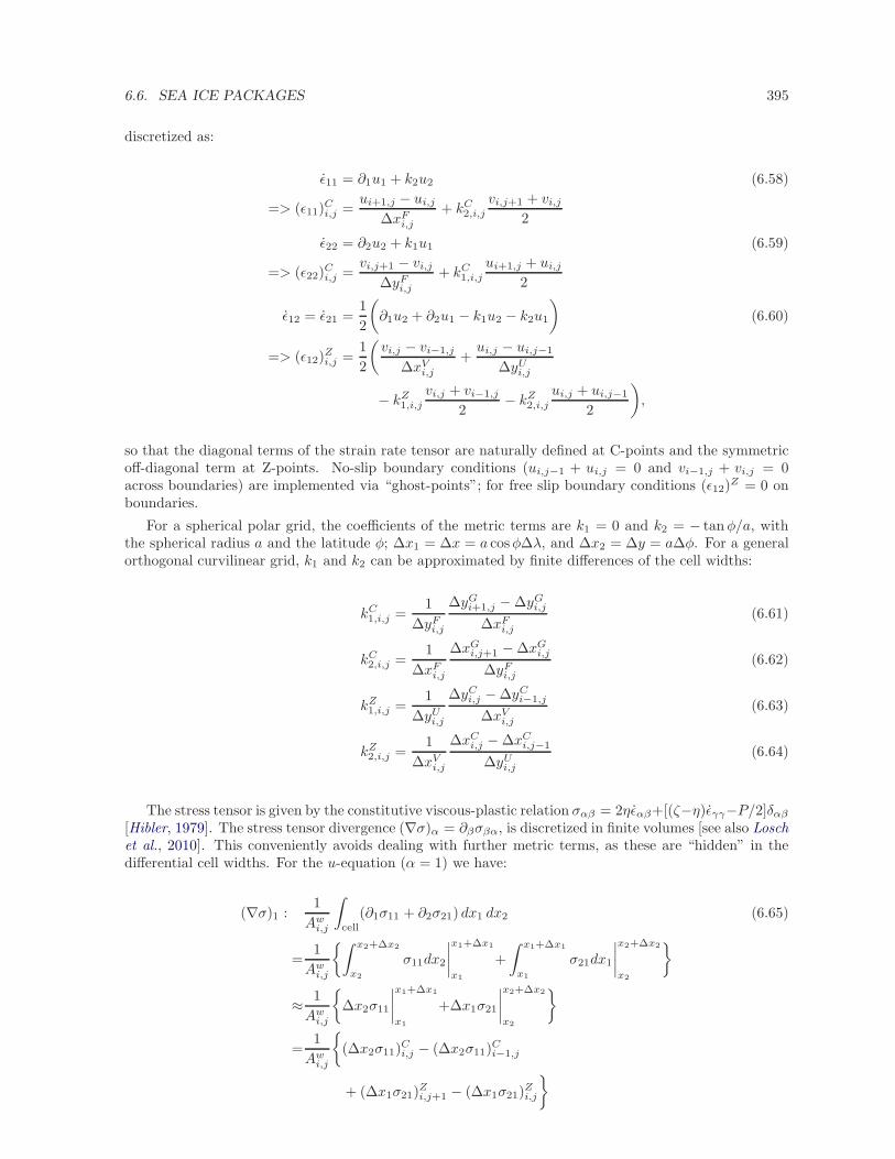
6.6. SEA ICE PACKAGES 395
discretized as:
ǫ11 = ∂1u1 + k2u2 (6.58)
=> (ǫ11)Ci,j =
ui+1,j − ui,j
∆xFi,j
+ kC2,i,j
vi,j+1 + vi,j
2
ǫ22 = ∂2u2 + k1u1 (6.59)
=> (ǫ22)Ci,j =
vi,j+1 − vi,j
∆yFi,j
+ kC1,i,j
ui+1,j + ui,j
2
ǫ12 = ǫ21 =1
2
(∂1u2 + ∂2u1 − k1u2 − k2u1
)(6.60)
=> (ǫ12)Zi,j =
1
2
(vi,j − vi−1,j
∆xVi,j
+ui,j − ui,j−1
∆yUi,j
− kZ1,i,j
vi,j + vi−1,j
2− kZ
2,i,j
ui,j + ui,j−1
2
),
so that the diagonal terms of the strain rate tensor are naturally defined at C-points and the symmetricoff-diagonal term at Z-points. No-slip boundary conditions (ui,j−1 + ui,j = 0 and vi−1,j + vi,j = 0across boundaries) are implemented via “ghost-points”; for free slip boundary conditions (ǫ12)
Z = 0 onboundaries.
For a spherical polar grid, the coefficients of the metric terms are k1 = 0 and k2 = − tanφ/a, withthe spherical radius a and the latitude φ; ∆x1 = ∆x = a cosφ∆λ, and ∆x2 = ∆y = a∆φ. For a generalorthogonal curvilinear grid, k1 and k2 can be approximated by finite differences of the cell widths:
kC1,i,j =
1
∆yFi,j
∆yGi+1,j − ∆yG
i,j
∆xFi,j
(6.61)
kC2,i,j =
1
∆xFi,j
∆xGi,j+1 − ∆xG
i,j
∆yFi,j
(6.62)
kZ1,i,j =
1
∆yUi,j
∆yCi,j − ∆yC
i−1,j
∆xVi,j
(6.63)
kZ2,i,j =
1
∆xVi,j
∆xCi,j − ∆xC
i,j−1
∆yUi,j
(6.64)
The stress tensor is given by the constitutive viscous-plastic relation σαβ = 2ηǫαβ+[(ζ−η)ǫγγ−P/2]δαβ
[Hibler, 1979]. The stress tensor divergence (∇σ)α = ∂βσβα, is discretized in finite volumes [see also Loschet al., 2010]. This conveniently avoids dealing with further metric terms, as these are “hidden” in thedifferential cell widths. For the u-equation (α = 1) we have:
(∇σ)1 :1
Awi,j
∫
cell
(∂1σ11 + ∂2σ21) dx1 dx2 (6.65)
=1
Awi,j
∫ x2+∆x2
x2
σ11dx2
∣∣∣∣x1+∆x1
x1
+
∫ x1+∆x1
x1
σ21dx1
∣∣∣∣x2+∆x2
x2
≈ 1
Awi,j
∆x2σ11
∣∣∣∣x1+∆x1
x1
+∆x1σ21
∣∣∣∣x2+∆x2
x2
=1
Awi,j
(∆x2σ11)
Ci,j − (∆x2σ11)
Ci−1,j
+ (∆x1σ21)Zi,j+1 − (∆x1σ21)
Zi,j
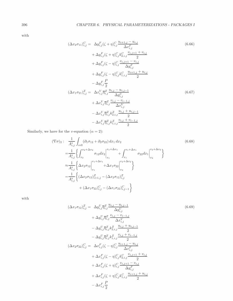
396 CHAPTER 6. PHYSICAL PARAMETERIZATIONS - PACKAGES I
with
(∆x2σ11)Ci,j = ∆yF
i,j(ζ + η)Ci,j
ui+1,j − ui,j
∆xFi,j
(6.66)
+ ∆yFi,j(ζ + η)C
i,jkC2,i,j
vi,j+1 + vi,j
2
+ ∆yFi,j(ζ − η)C
i,j
vi,j+1 − vi,j
∆yFi,j
+ ∆yFi,j(ζ − η)C
i,jkC1,i,j
ui+1,j + ui,j
2
− ∆yFi,j
P
2
(∆x1σ21)Zi,j = ∆xV
i,jηZi,j
ui,j − ui,j−1
∆yUi,j
(6.67)
+ ∆xVi,jη
Zi,j
vi,j − vi−1,j
∆xVi,j
− ∆xVi,jη
Zi,jk
Z2,i,j
ui,j + ui,j−1
2
− ∆xVi,jη
Zi,jk
Z1,i,j
vi,j + vi−1,j
2
Similarly, we have for the v-equation (α = 2):
(∇σ)2 :1
Asi,j
∫
cell
(∂1σ12 + ∂2σ22) dx1 dx2 (6.68)
=1
Asi,j
∫ x2+∆x2
x2
σ12dx2
∣∣∣∣x1+∆x1
x1
+
∫ x1+∆x1
x1
σ22dx1
∣∣∣∣x2+∆x2
x2
≈ 1
Asi,j
∆x2σ12
∣∣∣∣x1+∆x1
x1
+∆x1σ22
∣∣∣∣x2+∆x2
x2
=1
Asi,j
(∆x2σ12)
Zi+1,j − (∆x2σ12)
Zi,j
+ (∆x1σ22)Ci,j − (∆x1σ22)
Ci,j−1
with
(∆x1σ12)Zi,j = ∆yU
i,jηZi,j
ui,j − ui,j−1
∆yUi,j
(6.69)
+ ∆yUi,jη
Zi,j
vi,j − vi−1,j
∆xVi,j
− ∆yUi,jη
Zi,jk
Z2,i,j
ui,j + ui,j−1
2
− ∆yUi,jη
Zi,jk
Z1,i,j
vi,j + vi−1,j
2
(∆x2σ22)Ci,j = ∆xF
i,j(ζ − η)Ci,j
ui+1,j − ui,j
∆xFi,j
+ ∆xFi,j(ζ − η)C
i,jkC2,i,j
vi,j+1 + vi,j
2
+ ∆xFi,j(ζ + η)C
i,j
vi,j+1 − vi,j
∆yFi,j
+ ∆xFi,j(ζ + η)C
i,jkC1,i,j
ui+1,j + ui,j
2
− ∆xFi,j
P
2
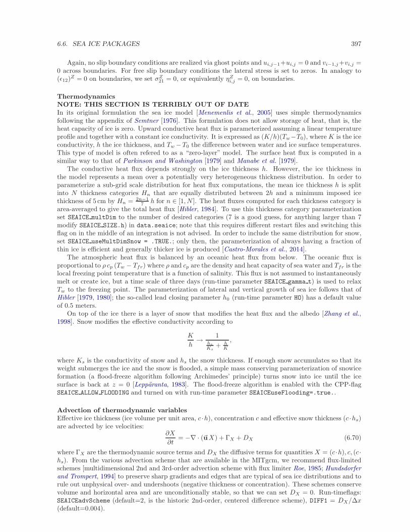
6.6. SEA ICE PACKAGES 397
Again, no slip boundary conditions are realized via ghost points and ui,j−1+ui,j = 0 and vi−1,j +vi,j =0 across boundaries. For free slip boundary conditions the lateral stress is set to zeros. In analogy to(ǫ12)
Z = 0 on boundaries, we set σZ21 = 0, or equivalently ηZ
i,j = 0, on boundaries.
ThermodynamicsNOTE: THIS SECTION IS TERRIBLY OUT OF DATEIn its original formulation the sea ice model [Menemenlis et al., 2005] uses simple thermodynamicsfollowing the appendix of Semtner [1976]. This formulation does not allow storage of heat, that is, theheat capacity of ice is zero. Upward conductive heat flux is parameterized assuming a linear temperatureprofile and together with a constant ice conductivity. It is expressed as (K/h)(Tw−T0), where K is the iceconductivity, h the ice thickness, and Tw −T0 the difference between water and ice surface temperatures.This type of model is often refered to as a “zero-layer” model. The surface heat flux is computed in asimilar way to that of Parkinson and Washington [1979] and Manabe et al. [1979].
The conductive heat flux depends strongly on the ice thickness h. However, the ice thickness inthe model represents a mean over a potentially very heterogeneous thickness distribution. In order toparameterize a sub-grid scale distribution for heat flux computations, the mean ice thickness h is splitinto N thickness categories Hn that are equally distributed between 2h and a minimum imposed icethickness of 5 cm by Hn = 2n−1
7 h for n ∈ [1, N ]. The heat fluxes computed for each thickness category isarea-averaged to give the total heat flux [Hibler, 1984]. To use this thickness category parameterizationset SEAICE multDim to the number of desired categories (7 is a good guess, for anything larger than 7modify SEAICE SIZE.h) in data.seaice; note that this requires different restart files and switching thisflag on in the middle of an integration is not advised. In order to include the same distribution for snow,set SEAICE useMultDimSnow = .TRUE.; only then, the parameterization of always having a fraction ofthin ice is efficient and generally thicker ice is produced [Castro-Morales et al., 2014].
The atmospheric heat flux is balanced by an oceanic heat flux from below. The oceanic flux isproportional to ρ cp (Tw − Tfr) where ρ and cp are the density and heat capacity of sea water and Tfr is thelocal freezing point temperature that is a function of salinity. This flux is not assumed to instantaneouslymelt or create ice, but a time scale of three days (run-time parameter SEAICE gamma t) is used to relaxTw to the freezing point. The parameterization of lateral and vertical growth of sea ice follows that ofHibler [1979, 1980]; the so-called lead closing parameter h0 (run-time parameter HO) has a default valueof 0.5 meters.
On top of the ice there is a layer of snow that modifies the heat flux and the albedo [Zhang et al.,1998]. Snow modifies the effective conductivity according to
K
h→ 1
hs
Ks+ h
K
,
where Ks is the conductivity of snow and hs the snow thickness. If enough snow accumulates so that itsweight submerges the ice and the snow is flooded, a simple mass conserving parameterization of snowiceformation (a flood-freeze algorithm following Archimedes’ principle) turns snow into ice until the icesurface is back at z = 0 [Lepparanta, 1983]. The flood-freeze algorithm is enabled with the CPP-flagSEAICE ALLOW FLOODING and turned on with run-time parameter SEAICEuseFlooding=.true..
Advection of thermodynamic variablesEffective ice thickness (ice volume per unit area, c ·h), concentration c and effective snow thickness (c ·hs)are advected by ice velocities:
∂X
∂t= −∇ · (~uX) + ΓX +DX (6.70)
where ΓX are the thermodynamic source terms and DX the diffusive terms for quantities X = (c ·h), c, (c ·hs). From the various advection scheme that are available in the MITgcm, we recommend flux-limitedschemes [multidimensional 2nd and 3rd-order advection scheme with flux limiter Roe, 1985; Hundsdorferand Trompert, 1994] to preserve sharp gradients and edges that are typical of sea ice distributions and torule out unphysical over- and undershoots (negative thickness or concentration). These schemes conservevolume and horizontal area and are unconditionally stable, so that we can set DX = 0. Run-timeflags:SEAICEadvScheme (default=2, is the historic 2nd-order, centered difference scheme), DIFF1 = DX/∆x(default=0.004).
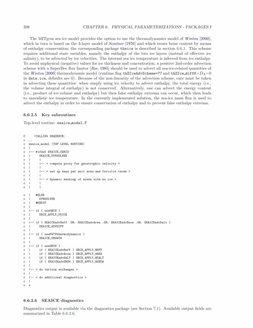
398 CHAPTER 6. PHYSICAL PARAMETERIZATIONS - PACKAGES I
The MITgcm sea ice model provides the option to use the thermodynamics model of Winton [2000],which in turn is based on the 3-layer model of Semtner [1976] and which treats brine content by meansof enthalpy conservation; the corresponding package thsice is described in section 6.6.1. This schemerequires additional state variables, namely the enthalpy of the two ice layers (instead of effective icesalinity), to be advected by ice velocities. The internal sea ice temperature is inferred from ice enthalpy.To avoid unphysical (negative) values for ice thickness and concentration, a positive 2nd-order advectionscheme with a SuperBee flux limiter [Roe, 1985] should be used to advect all sea-ice-related quantities ofthe Winton [2000] thermodynamic model (runtime flag thSIceAdvScheme=77 and thSIce diffK=DX=0in data.ice, defaults are 0). Because of the non-linearity of the advection scheme, care must be takenin advecting these quantities: when simply using ice velocity to advect enthalpy, the total energy (i.e.,the volume integral of enthalpy) is not conserved. Alternatively, one can advect the energy content(i.e., product of ice-volume and enthalpy) but then false enthalpy extrema can occur, which then leadsto unrealistic ice temperature. In the currently implemented solution, the sea-ice mass flux is used toadvect the enthalpy in order to ensure conservation of enthalpy and to prevent false enthalpy extrema.
6.6.2.5 Key subroutines
Top-level routine: seaice model.F
C !CALLING SEQUENCE:
c ...
c seaice_model (TOP LEVEL ROUTINE)
c |
c |-- #ifdef SEAICE_CGRID
c | SEAICE_DYNSOLVER
c | |
c | |-- < compute proxy for geostrophic velocity >
c | |
c | |-- < set up mass per unit area and Coriolis terms >
c | |
c | |-- < dynamic masking of areas with no ice >
c | |
c | |
c | #ELSE
c | DYNSOLVER
c | #ENDIF
c |
c |-- if ( useOBCS )
c | OBCS_APPLY_UVICE
c |
c |-- if ( SEAICEadvHeff .OR. SEAICEadvArea .OR. SEAICEadvSnow .OR. SEAICEadvSalt )
c | SEAICE_ADVDIFF
c |
c |-- if ( usePW79thermodynamics )
c | SEAICE_GROWTH
c |
c |-- if ( useOBCS )
c | if ( SEAICEadvHeff ) OBCS_APPLY_HEFF
c | if ( SEAICEadvArea ) OBCS_APPLY_AREA
c | if ( SEAICEadvSALT ) OBCS_APPLY_HSALT
c | if ( SEAICEadvSNOW ) OBCS_APPLY_HSNOW
c |
c |-- < do various exchanges >
c |
c |-- < do additional diagnostics >
c |
c o
6.6.2.6 SEAICE diagnostics
Diagnostics output is available via the diagnostics package (see Section 7.1). Available output fields aresummarized in Table 6.6.2.6.

6.6. SEA ICE PACKAGES 399
6.6.2.7 Experiments and tutorials that use seaice
• Labrador Sea experiment in lab sea verification directory.
• seaice obcs, based on lab sea
• offline exf seaice/input.seaicetd, based on lab sea
• global ocean.cs32x15/input.icedyn and global ocean.cs32x15/input.seaice, global cubed-sphere-experiment with combinations of seaice and thsice
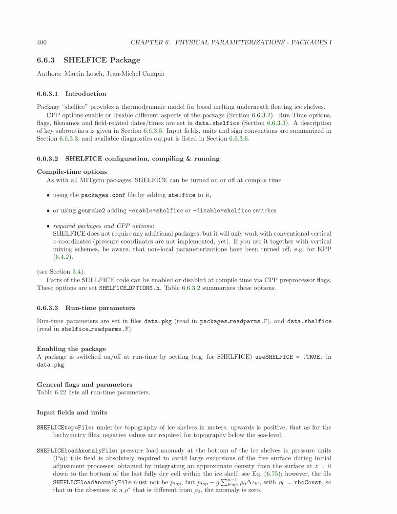
400 CHAPTER 6. PHYSICAL PARAMETERIZATIONS - PACKAGES I
6.6.3 SHELFICE Package
Authors: Martin Losch, Jean-Michel Campin
6.6.3.1 Introduction
Package “shelfice” provides a thermodynamic model for basal melting underneath floating ice shelves.
CPP options enable or disable different aspects of the package (Section 6.6.3.2). Run-Time options,flags, filenames and field-related dates/times are set in data.shelfice (Section 6.6.3.3). A descriptionof key subroutines is given in Section 6.6.3.5. Input fields, units and sign conventions are summarized inSection 6.6.3.3, and available diagnostics output is listed in Section 6.6.3.6.
6.6.3.2 SHELFICE configuration, compiling & running
Compile-time options
As with all MITgcm packages, SHELFICE can be turned on or off at compile time
• using the packages.conf file by adding shelfice to it,
• or using genmake2 adding -enable=shelfice or -disable=shelfice switches
• required packages and CPP options :SHELFICE does not require any additional packages, but it will only work with conventional verticalz-coordinates (pressure coordinates are not implemented, yet). If you use it together with verticalmixing schemes, be aware, that non-local parameterizations have been turned off, e.g. for KPP(6.4.2).
(see Section 3.4).
Parts of the SHELFICE code can be enabled or disabled at compile time via CPP preprocessor flags.These options are set SHELFICE OPTIONS.h. Table 6.6.3.2 summarizes these options.
6.6.3.3 Run-time parameters
Run-time parameters are set in files data.pkg (read in packages readparms.F), and data.shelfice
(read in shelfice readparms.F).
Enabling the packageA package is switched on/off at run-time by setting (e.g. for SHELFICE) useSHELFICE = .TRUE. indata.pkg.
General flags and parametersTable 6.22 lists all run-time parameters.
Input fields and units
SHEFLICEtopoFile: under-ice topography of ice shelves in meters; upwards is positive, that as for thebathymetry files, negative values are required for topography below the sea-level;
SHEFLICEloadAnomalyFile: pressure load anomaly at the bottom of the ice shelves in pressure units(Pa); this field is absolutely required to avoid large excursions of the free surface during initialadjustment processes; obtained by integrating an approximate density from the surface at z = 0down to the bottom of the last fully dry cell within the ice shelf, see Eq. (6.75); however, the file
SHEFLICEloadAnomalyFile must not be ptop, but ptop − g∑n−1
k′=1 ρ0∆zk′ , with ρ0 = rhoConst, sothat in the absenses of a ρ∗ that is different from ρ0, the anomaly is zero.
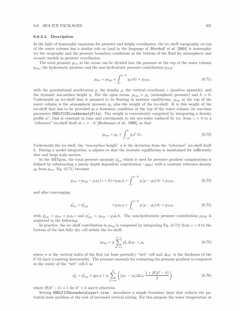
6.6. SEA ICE PACKAGES 401
6.6.3.4 Description
In the light of isomorphic equations for pressure and height coordinates, the ice shelf topography on topof the water column has a similar role as (and in the language of Marshall et al. [2004] is isomorphicto) the orography and the pressure boundary conditions at the bottom of the fluid for atmospheric andoceanic models in pressure coordinates.
The total pressure ptot in the ocean can be divided into the pressure at the top of the water columnptop, the hydrostatic pressure and the non-hydrostatic pressure contribution pNH :
ptot = ptop +
∫ η−h
z
g ρ dz + pNH , (6.71)
with the gravitational acceleration g, the density ρ, the vertical coordinate z (positive upwards), andthe dynamic sea-surface height η. For the open ocean, ptop = pa (atmospheric pressure) and h = 0.Underneath an ice-shelf that is assumed to be floating in isostatic equilibrium, ptop at the top of thewater column is the atmospheric pressure pa plus the weight of the ice-shelf. It is this weight of theice-shelf that has to be provided as a boundary condition at the top of the water column (in run-timeparameter SHELFICEloadAnomalyFile). The weight is conveniently computed by integrating a densityprofile ρ∗, that is constant in time and corresponds to the sea-water replaced by ice, from z = 0 to a“reference” ice-shelf draft at z = −h [Beckmann et al., 1999], so that
ptop = pa +
∫ 0
−h
g ρ∗ dz. (6.72)
Underneath the ice shelf, the “sea-surface height” η is the deviation from the “reference” ice-shelf drafth. During a model integration, η adjusts so that the isostatic equilibrium is maintained for sufficientlyslow and large scale motion.
In the MITgcm, the total pressure anomaly p′tot which is used for pressure gradient computations isdefined by substracting a purely depth dependent contribution −gρ0z with a constant reference densityρ0 from ptot. Eq. (6.71) becomes
ptot = ptop − g ρ0 (z + h)+g ρ0 η +
∫ η−h
z
g (ρ− ρ0) dz + pNH , (6.73)
and after rearranging
p′tot = p′top +g ρ0 η +
∫ η−h
z
g (ρ− ρ0) dz + pNH , (6.74)
with p′tot = ptot + g ρ0 z and p′top = ptop − g ρ0 h. The non-hydrostatic pressure contribution pNH isneglected in the following.
In practice, the ice shelf contribution to ptop is computed by integrating Eq. (6.72) from z = 0 to thebottom of the last fully dry cell within the ice shelf:
ptop = g
n−1∑
k′=1
ρ∗k′∆zk′ + pa (6.75)
where n is the vertical index of the first (at least partially) “wet” cell and ∆zk′ is the thickness of thek′-th layer (counting downwards). The pressure anomaly for evaluating the pressure gradient is computedin the center of the “wet” cell k as
p′k = p′top + gρnη + g
k∑
k′=n
((ρk′ − ρ0)∆zk′
1 +H(k′ − k)
2
)(6.76)
where H(k′ − k) = 1 for k′ < k and 0 otherwise.Setting SHELFICEboundaryLayer=.true. introduces a simple boundary layer that reduces the po-
tential noise problem at the cost of increased vertical mixing. For this purpose the water temperature at
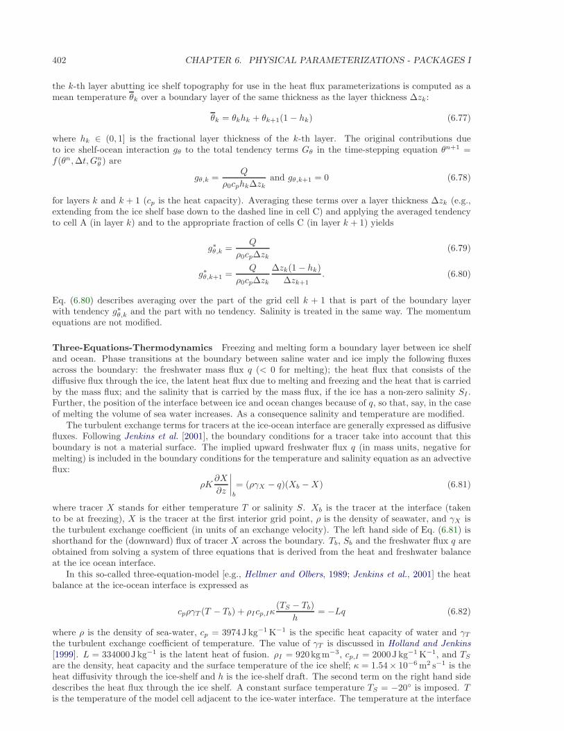
402 CHAPTER 6. PHYSICAL PARAMETERIZATIONS - PACKAGES I
the k-th layer abutting ice shelf topography for use in the heat flux parameterizations is computed as amean temperature θk over a boundary layer of the same thickness as the layer thickness ∆zk:
θk = θkhk + θk+1(1 − hk) (6.77)
where hk ∈ (0, 1] is the fractional layer thickness of the k-th layer. The original contributions dueto ice shelf-ocean interaction gθ to the total tendency terms Gθ in the time-stepping equation θn+1 =f(θn,∆t, Gn
θ ) are
gθ,k =Q
ρ0cphk∆zkand gθ,k+1 = 0 (6.78)
for layers k and k + 1 (cp is the heat capacity). Averaging these terms over a layer thickness ∆zk (e.g.,extending from the ice shelf base down to the dashed line in cell C) and applying the averaged tendencyto cell A (in layer k) and to the appropriate fraction of cells C (in layer k + 1) yields
g∗θ,k =Q
ρ0cp∆zk(6.79)
g∗θ,k+1 =Q
ρ0cp∆zk
∆zk(1 − hk)
∆zk+1. (6.80)
Eq. (6.80) describes averaging over the part of the grid cell k + 1 that is part of the boundary layerwith tendency g∗θ,k and the part with no tendency. Salinity is treated in the same way. The momentumequations are not modified.
Three-Equations-Thermodynamics Freezing and melting form a boundary layer between ice shelfand ocean. Phase transitions at the boundary between saline water and ice imply the following fluxesacross the boundary: the freshwater mass flux q (< 0 for melting); the heat flux that consists of thediffusive flux through the ice, the latent heat flux due to melting and freezing and the heat that is carriedby the mass flux; and the salinity that is carried by the mass flux, if the ice has a non-zero salinity SI .Further, the position of the interface between ice and ocean changes because of q, so that, say, in the caseof melting the volume of sea water increases. As a consequence salinity and temperature are modified.
The turbulent exchange terms for tracers at the ice-ocean interface are generally expressed as diffusivefluxes. Following Jenkins et al. [2001], the boundary conditions for a tracer take into account that thisboundary is not a material surface. The implied upward freshwater flux q (in mass units, negative formelting) is included in the boundary conditions for the temperature and salinity equation as an advectiveflux:
ρK∂X
∂z
∣∣∣∣b
= (ργX − q)(Xb −X) (6.81)
where tracer X stands for either temperature T or salinity S. Xb is the tracer at the interface (takento be at freezing), X is the tracer at the first interior grid point, ρ is the density of seawater, and γX isthe turbulent exchange coefficient (in units of an exchange velocity). The left hand side of Eq. (6.81) isshorthand for the (downward) flux of tracer X across the boundary. Tb, Sb and the freshwater flux q areobtained from solving a system of three equations that is derived from the heat and freshwater balanceat the ice ocean interface.
In this so-called three-equation-model [e.g., Hellmer and Olbers, 1989; Jenkins et al., 2001] the heatbalance at the ice-ocean interface is expressed as
cpργT (T − Tb) + ρIcp,Iκ(TS − Tb)
h= −Lq (6.82)
where ρ is the density of sea-water, cp = 3974J kg−1 K−1 is the specific heat capacity of water and γT
the turbulent exchange coefficient of temperature. The value of γT is discussed in Holland and Jenkins[1999]. L = 334000J kg−1 is the latent heat of fusion. ρI = 920kgm−3, cp,I = 2000J kg−1 K−1, and TS
are the density, heat capacity and the surface temperature of the ice shelf; κ = 1.54× 10⁻⁶ m2 s−1 is theheat diffusivity through the ice-shelf and h is the ice-shelf draft. The second term on the right hand sidedescribes the heat flux through the ice shelf. A constant surface temperature TS = −20 is imposed. Tis the temperature of the model cell adjacent to the ice-water interface. The temperature at the interface
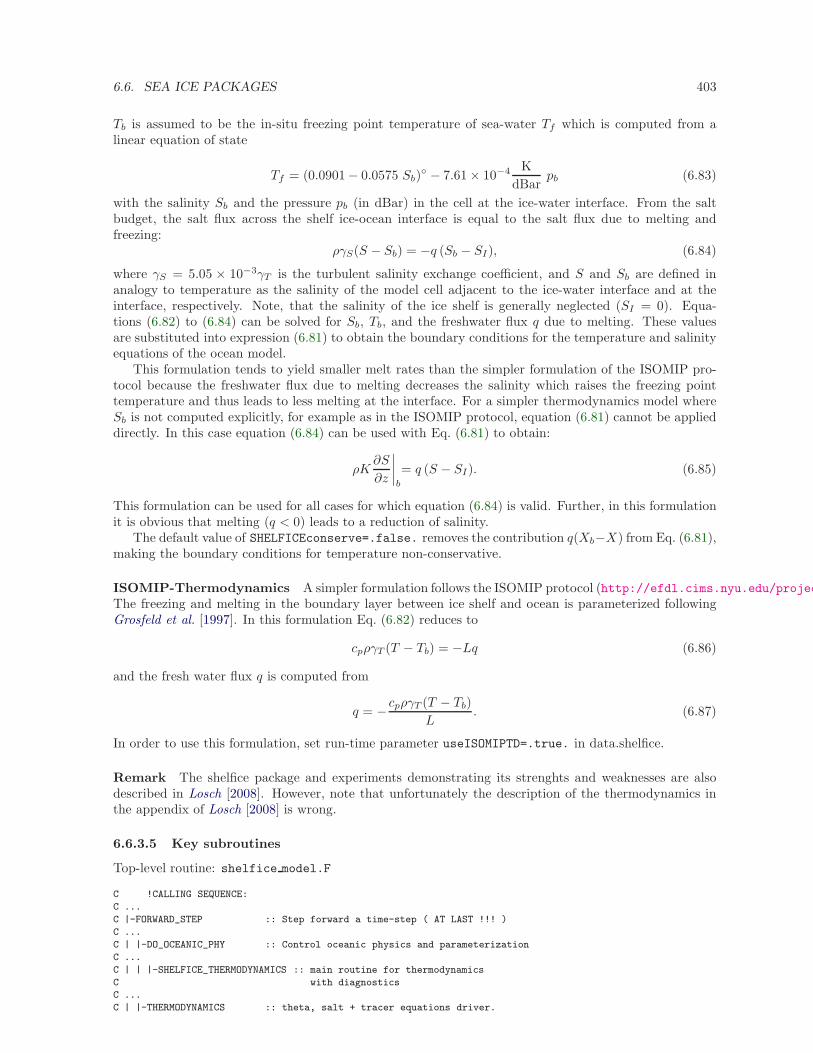
6.6. SEA ICE PACKAGES 403
Tb is assumed to be the in-situ freezing point temperature of sea-water Tf which is computed from alinear equation of state
Tf = (0.0901− 0.0575 Sb) − 7.61 × 10⁻⁴ K
dBarpb (6.83)
with the salinity Sb and the pressure pb (in dBar) in the cell at the ice-water interface. From the saltbudget, the salt flux across the shelf ice-ocean interface is equal to the salt flux due to melting andfreezing:
ργS(S − Sb) = −q (Sb − SI), (6.84)
where γS = 5.05 × 10⁻³γT is the turbulent salinity exchange coefficient, and S and Sb are defined inanalogy to temperature as the salinity of the model cell adjacent to the ice-water interface and at theinterface, respectively. Note, that the salinity of the ice shelf is generally neglected (SI = 0). Equa-tions (6.82) to (6.84) can be solved for Sb, Tb, and the freshwater flux q due to melting. These valuesare substituted into expression (6.81) to obtain the boundary conditions for the temperature and salinityequations of the ocean model.
This formulation tends to yield smaller melt rates than the simpler formulation of the ISOMIP pro-tocol because the freshwater flux due to melting decreases the salinity which raises the freezing pointtemperature and thus leads to less melting at the interface. For a simpler thermodynamics model whereSb is not computed explicitly, for example as in the ISOMIP protocol, equation (6.81) cannot be applieddirectly. In this case equation (6.84) can be used with Eq. (6.81) to obtain:
ρK∂S
∂z
∣∣∣∣b
= q (S − SI). (6.85)
This formulation can be used for all cases for which equation (6.84) is valid. Further, in this formulationit is obvious that melting (q < 0) leads to a reduction of salinity.
The default value of SHELFICEconserve=.false. removes the contribution q(Xb−X) from Eq. (6.81),making the boundary conditions for temperature non-conservative.
ISOMIP-Thermodynamics A simpler formulation follows the ISOMIP protocol (http://efdl.cims.nyu.edu/projectThe freezing and melting in the boundary layer between ice shelf and ocean is parameterized followingGrosfeld et al. [1997]. In this formulation Eq. (6.82) reduces to
cpργT (T − Tb) = −Lq (6.86)
and the fresh water flux q is computed from
q = −cpργT (T − Tb)
L. (6.87)
In order to use this formulation, set run-time parameter useISOMIPTD=.true. in data.shelfice.
Remark The shelfice package and experiments demonstrating its strenghts and weaknesses are alsodescribed in Losch [2008]. However, note that unfortunately the description of the thermodynamics inthe appendix of Losch [2008] is wrong.
6.6.3.5 Key subroutines
Top-level routine: shelfice model.F
C !CALLING SEQUENCE:
C ...
C |-FORWARD_STEP :: Step forward a time-step ( AT LAST !!! )
C ...
C | |-DO_OCEANIC_PHY :: Control oceanic physics and parameterization
C ...
C | | |-SHELFICE_THERMODYNAMICS :: main routine for thermodynamics
C with diagnostics
C ...
C | |-THERMODYNAMICS :: theta, salt + tracer equations driver.
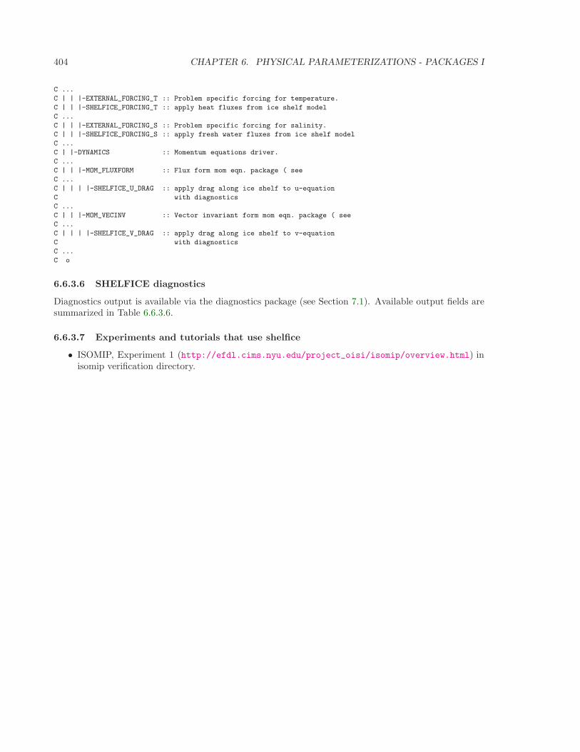
404 CHAPTER 6. PHYSICAL PARAMETERIZATIONS - PACKAGES I
C ...
C | | |-EXTERNAL_FORCING_T :: Problem specific forcing for temperature.
C | | |-SHELFICE_FORCING_T :: apply heat fluxes from ice shelf model
C ...
C | | |-EXTERNAL_FORCING_S :: Problem specific forcing for salinity.
C | | |-SHELFICE_FORCING_S :: apply fresh water fluxes from ice shelf model
C ...
C | |-DYNAMICS :: Momentum equations driver.
C ...
C | | |-MOM_FLUXFORM :: Flux form mom eqn. package ( see
C ...
C | | | |-SHELFICE_U_DRAG :: apply drag along ice shelf to u-equation
C with diagnostics
C ...
C | | |-MOM_VECINV :: Vector invariant form mom eqn. package ( see
C ...
C | | | |-SHELFICE_V_DRAG :: apply drag along ice shelf to v-equation
C with diagnostics
C ...
C o
6.6.3.6 SHELFICE diagnostics
Diagnostics output is available via the diagnostics package (see Section 7.1). Available output fields aresummarized in Table 6.6.3.6.
6.6.3.7 Experiments and tutorials that use shelfice
• ISOMIP, Experiment 1 (http://efdl.cims.nyu.edu/project_oisi/isomip/overview.html) inisomip verification directory.
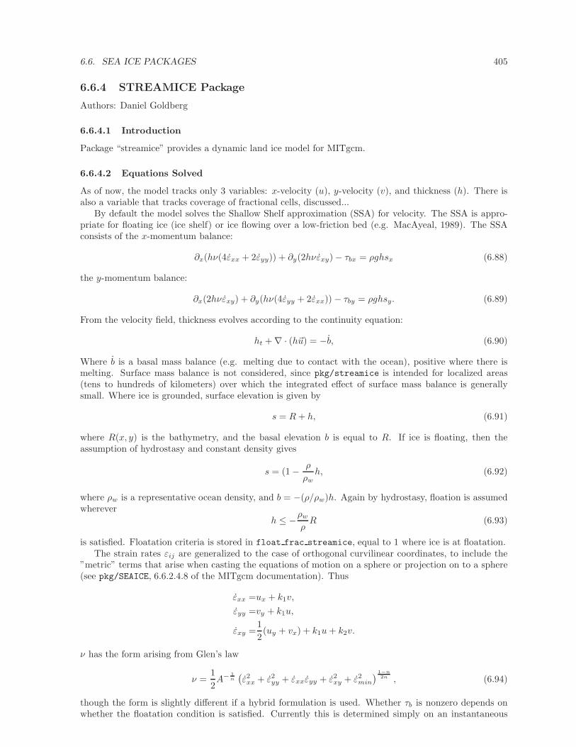
6.6. SEA ICE PACKAGES 405
6.6.4 STREAMICE Package
Authors: Daniel Goldberg
6.6.4.1 Introduction
Package “streamice” provides a dynamic land ice model for MITgcm.
6.6.4.2 Equations Solved
As of now, the model tracks only 3 variables: x-velocity (u), y-velocity (v), and thickness (h). There isalso a variable that tracks coverage of fractional cells, discussed...
By default the model solves the Shallow Shelf approximation (SSA) for velocity. The SSA is appro-priate for floating ice (ice shelf) or ice flowing over a low-friction bed (e.g. MacAyeal, 1989). The SSAconsists of the x-momentum balance:
∂x(hν(4εxx + 2εyy)) + ∂y(2hνεxy) − τbx = ρghsx (6.88)
the y-momentum balance:
∂x(2hνεxy) + ∂y(hν(4εyy + 2εxx)) − τby = ρghsy. (6.89)
From the velocity field, thickness evolves according to the continuity equation:
ht + ∇ · (h~u) = −b, (6.90)
Where b is a basal mass balance (e.g. melting due to contact with the ocean), positive where there ismelting. Surface mass balance is not considered, since pkg/streamice is intended for localized areas(tens to hundreds of kilometers) over which the integrated effect of surface mass balance is generallysmall. Where ice is grounded, surface elevation is given by
s = R+ h, (6.91)
where R(x, y) is the bathymetry, and the basal elevation b is equal to R. If ice is floating, then theassumption of hydrostasy and constant density gives
s = (1 − ρ
ρwh, (6.92)
where ρw is a representative ocean density, and b = −(ρ/ρw)h. Again by hydrostasy, floation is assumedwherever
h ≤ −ρw
ρR (6.93)
is satisfied. Floatation criteria is stored in float frac streamice, equal to 1 where ice is at floatation.The strain rates εij are generalized to the case of orthogonal curvilinear coordinates, to include the
”metric” terms that arise when casting the equations of motion on a sphere or projection on to a sphere(see pkg/SEAICE, 6.6.2.4.8 of the MITgcm documentation). Thus
εxx =ux + k1v,
εyy =vy + k1u,
εxy =1
2(uy + vx) + k1u+ k2v.
ν has the form arising from Glen’s law
ν =1
2A−
1n
(ε2xx + ε2yy + εxxεyy + ε2xy + ε2min
) 1−n2n , (6.94)
though the form is slightly different if a hybrid formulation is used. Whether τb is nonzero depends onwhether the floatation condition is satisfied. Currently this is determined simply on an instantaneous
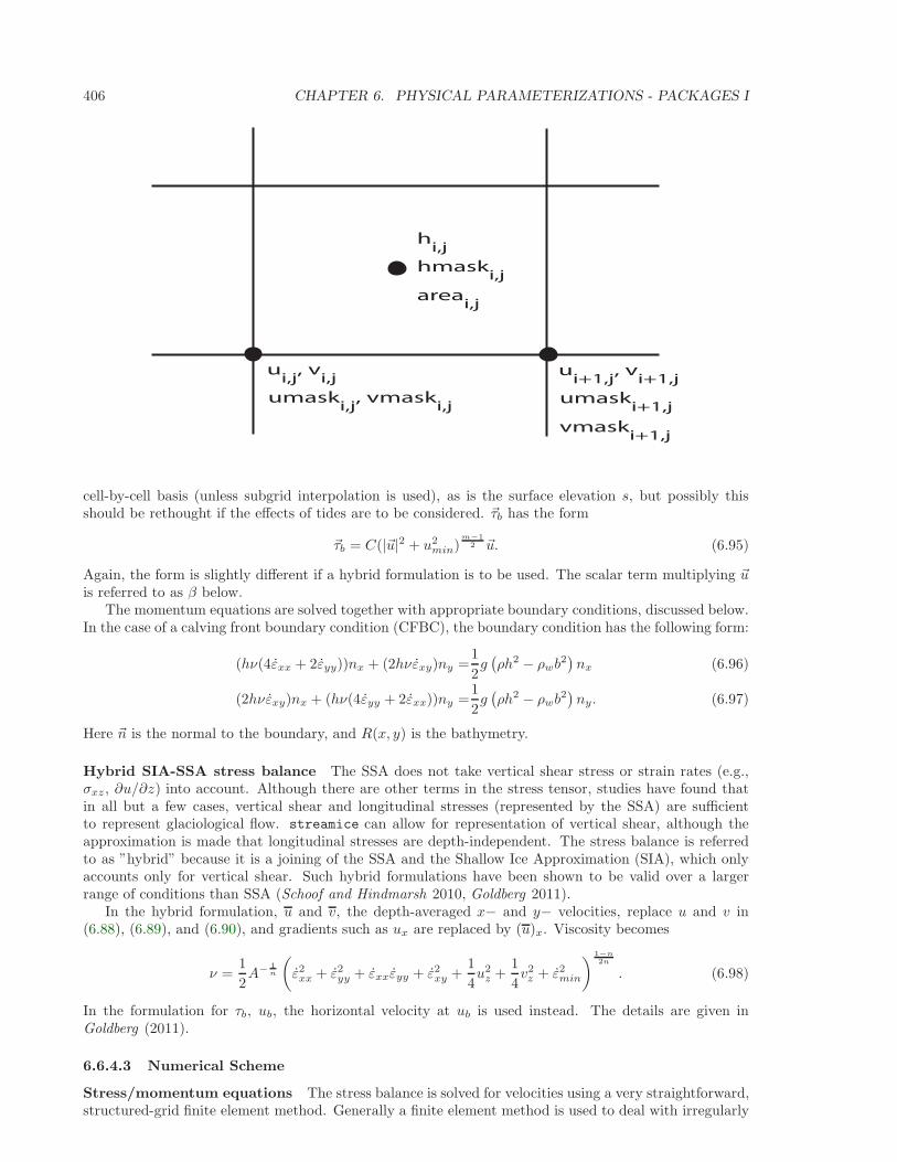
406 CHAPTER 6. PHYSICAL PARAMETERIZATIONS - PACKAGES I
hi,j
hmaski,j
areai,j
ui,j
, vi,j
umaski,j
, vmaski,j
ui+1,j
, vi+1,j
umaski+1,j
vmaski+1,j
cell-by-cell basis (unless subgrid interpolation is used), as is the surface elevation s, but possibly thisshould be rethought if the effects of tides are to be considered. ~τb has the form
~τb = C(|~u|2 + u2min)
m−12 ~u. (6.95)
Again, the form is slightly different if a hybrid formulation is to be used. The scalar term multiplying ~uis referred to as β below.
The momentum equations are solved together with appropriate boundary conditions, discussed below.In the case of a calving front boundary condition (CFBC), the boundary condition has the following form:
(hν(4εxx + 2εyy))nx + (2hνεxy)ny =1
2g(ρh2 − ρwb
2)nx (6.96)
(2hνεxy)nx + (hν(4εyy + 2εxx))ny =1
2g(ρh2 − ρwb
2)ny. (6.97)
Here ~n is the normal to the boundary, and R(x, y) is the bathymetry.
Hybrid SIA-SSA stress balance The SSA does not take vertical shear stress or strain rates (e.g.,σxz , ∂u/∂z) into account. Although there are other terms in the stress tensor, studies have found thatin all but a few cases, vertical shear and longitudinal stresses (represented by the SSA) are sufficientto represent glaciological flow. streamice can allow for representation of vertical shear, although theapproximation is made that longitudinal stresses are depth-independent. The stress balance is referredto as ”hybrid” because it is a joining of the SSA and the Shallow Ice Approximation (SIA), which onlyaccounts only for vertical shear. Such hybrid formulations have been shown to be valid over a largerrange of conditions than SSA (Schoof and Hindmarsh 2010, Goldberg 2011).
In the hybrid formulation, u and v, the depth-averaged x− and y− velocities, replace u and v in(6.88), (6.89), and (6.90), and gradients such as ux are replaced by (u)x. Viscosity becomes
ν =1
2A−
1n
(ε2xx + ε2yy + εxxεyy + ε2xy +
1
4u2
z +1
4v2
z + ε2min
) 1−n2n
. (6.98)
In the formulation for τb, ub, the horizontal velocity at ub is used instead. The details are given inGoldberg (2011).
6.6.4.3 Numerical Scheme
Stress/momentum equations The stress balance is solved for velocities using a very straightforward,structured-grid finite element method. Generally a finite element method is used to deal with irregularly
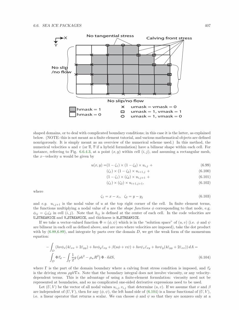
6.6. SEA ICE PACKAGES 407
No tangential stressCalving front stress
No slip/no !ow
No slip
/no !ow
X
Y
hmask = 1
hmask = 0
umask = vmask = 0
umask = 1, vmask = 1
umask = 1, vmask = 0
shaped domains, or to deal with complicated boundary conditions; in this case it is the latter, as explainedbelow. (NOTE: this is not meant as a finite element tutorial, and various mathematical objects are definednonrigorously. It is simply meant as an overview of the numerical scheme used.) In this method, thenumerical velocities u and v (or u, v if a hybrid formulation) have a bilinear shape within each cell. Forinstance, referring to Fig. 6.6.4.3, at a point (x, y) within cell (i, j), and assuming a rectangular mesh,the x−velocity u would be given by
u(x, y) =(1 − ζ1) × (1 − ζ2) × ui,j + (6.99)
(ζ1) × (1 − ζ2) × ui+1,j + (6.100)
(1 − ζ1) × (ζ2) × ui,j+1 + (6.101)
(ζ1) × (ζ2) × ui+1,j+1, (6.102)
where
ζ1 = x− xi, ζ2 = y − yj (6.103)
and e.g. ui,j+1 is the nodal value of u at the top right corner of the cell. In finite element terms,the functions multiplying a nodal value of u are the shape functions φ corresponding to that node, e.g.φij = ζ1ζ2 in cell (i, j). Note that hij is defined at the center of each cell. In the code velocities areU STREAMICE and V STREAMICE, and thickness is H STREAMICE.
If we take a vector-valued function Φ = (φ, ψ) which is in the “solution space” of (u, v) (i.e. φ and ψare bilinear in each cell as defined above, and are zero where velocities are imposed), take the dot productwith by (6.88,6.89), and integrate by parts over the domain D, we get the weak form of the momentumequation:
−∫
D
(hνφx(4εxx + 2εyy) + hνφy εxy + β(uφ+ vψ) + hνψxεxy + hνψy(4εyy + 2εxx)) dA =
∫
D
Φ~τd −∫
Γ
1
2g(ρh2 − ρwR
2)Φ · ~ndS, (6.104)
where Γ is the part of the domain boundary where a calving front stress condition is imposed, and ~τdis the driving stress ρgh∇s. Note that the boundary integral does not involve viscosity, or any velocity-dependent terms. This is the advantage of using a finite-element formulation: viscosity need not berepresented at boundaries, and so no complicated one-sided derivative expressions need to be used.
Let (U, V ) be the vector of all nodal values ui,j , vi,j that determine (u, v). If we assume that ν and βare independent of (U, V ), then for any (φ, ψ), the left hand side of (6.104) is a linear functional of (U, V ),i.e. a linear operator that returns a scalar. We can choose φ and ψ so that they are nonzero only at a
408 CHAPTER 6. PHYSICAL PARAMETERIZATIONS - PACKAGES I
single node; and we can evaluate (6.104) for each such φij and ψij , giving a linearly independent set ofequations for U and V . The left hand side of (6.104) for each φij and ψij is evaluated in the subroutineSTREAMICE CG ACTION() in the source file streamice cg functions.f. The right hand side is evaluatedin STREAMICE DRIVING STRESS(). The latter is not a straightforward calculation, since the thickness hand the surface s are not expressed by piecewise bilinear functions, and is discussed below.
STREAMICE CG ACTION() represents the action of a matrix on the vector represented by (U, V ) andSTREAMICE DRIVING STRESS() gives the right hand side of a linear system of equations. This informationis enough to solve the linear system, and this is done with the method of conjugate gradients, implemented(with simple Jacobi preconditioning) in STREAMICE CG SOLVE().
The full nonlinear system is solved in STREAMICE VEL SOLVE(). This subroutine evaluates drivingstress and then calls a loop in which a sequence of linear systems is solved. After each linear solve, theviscosity ν (the array visc streamice) and basal traction β (tau beta eff streamice) is updated fromthe new iterate of u and v. The iteration continues until a desired tolerance is reached or the maximumnumber of iterations is reached.
Rather than calling STREAMICE CG ACTION() each iteration of the conjugate gradient, the sparsematrix can be constructed explicitly. This is done if STREAMICE CONSTRUCT MATRIX is #defined inSTREAMICE OPTIONS.h. This speeds up the solution because STREAMICE CG ACTION() contains a numberof nested loops related to quadrature points and interactions between nodes of a cell.
The driving stress τd = ρg∇s is not as straightforward to deal with in the weak formulation, as h ands are considered constant in a cell. Furthermore, in the ice shelf the driving stress can be written as
~τd =1
2ρg(1 − ρ
ρw)∇(h2). (6.105)
Among other things, this (along with equations 6.96 and 6.97) implies that for an unconfined shelf(one for which the only boundaries are a calving front and a grounding line), the stress state along thegrounding line depends only on the location at depth of the grounding line. The numerical representationof velocities must respect this. Thus the driving stress contribution in the x− momentum equation atnode (i, j) is given as follows.
τd,x(i, j) =
14ρg(γijhij + γi−1,jhi−1,j)(γi−1,jsi−1,j − γijsij) case I14
rAi−1,j
∆xf,i−1,jg(ρh2
i−1,j − ρwb2i−1,j) case II
− 14
rAi,j
∆xf,ijg(ρh2
ij − ρwb2ij) case III.
(6.106)
where
γij =
√rAij
∆xf,ij, (6.107)
rAij is the area of cell (i, j) and ∆xf,ij is the width of the cell at its y−midpoint. Cases I, II, and IIIrefer to the situations when (I) both cells (i, j) and (i − 1, j) are in the domain, (II) only cell (i − 1, j)is in the domain, and (III) only cell (i, j) is in the domain. (The fact that τd,x(i, j) is being calculatedmeans that the implied boundary is a calving stress boundary, as explained below.) The above expressiongives the contribution from the cells above node (i, j) (in the y−direction). A similar expression givesthe contribution from cells (i−1, j−1) and (i, j−1), and corresponding expressions approximate drivingstress in the y− momentum equation. In the ice shelf, the case I expressions give approximations for(6.105) which are discretely integrable; in grounded ice the expression need not be integrable, so anyerrors associated with varying grid metrics can be subsumed into the discretization error.
Orthogonal curvilinear coordinates If the grid is not rectangular, but given in orthogonal curvi-linear coordinates, the evaluation of (6.104) is not exact, since the gradient of the basis functions areapproximated, as we do not have complete knowledge of the coordinate system, only the grid metrics.Still, we consider nodal basis functions that are equal to 1 at a single node, and zero elsewhere in a cell.
A cell (i, j) has separation ∆xi,j at the bottom and ∆xi,j+1 at the top (referred to as dxG(i,j) anddxG(i,j+1) in the code). So, for instance, for a cell given by [ξ1, ξ2] × [η1, η2], the ξ-derivative of thebasis function centered at (ξ1, η1) is approximated by
(1 − q
∆xi,j
)+
(q
∆xi,j+1
)(6.108)
6.6. SEA ICE PACKAGES 409
where q is the y-coordinate of the quadrature point being used. (The code currently uses 2-point gaussquadrature to evaluate the integrals in (6.104); with a rectangular grid and cellwise-constant β and ν,this is exact.)
Basis function derivatives and quadrature weights are stored in Dphi and grid jacq streamice. Bothare initialized in STREAMICE INIT PHI, called only once.
Boundary conditions and masks The computational domain (which may be smaller than the ar-ray/grid as defined by SIZE.h and GRID.h) is determined by a number of mask arrays within theSTREAMICE package. They are
• hmask (STREAMICE hmask): equal to 1 (ice-covered), 0 (open ocean), 2 (partly-covered), or -1 (outof domain)
• umask (STREAMICE umask): equal to 1 (an “active” velocity node), 3 (a Dirichlet node), or 0 (zerovelocity)
• vmask (STREAMICE vmask): similar to umask
• ufacemaskbdry (STREAMICE ufacemaskbdry): equal to -1 (interior face), 0 (no-slip), 1 (no-stress),2 (calving stress front), 3 (Dirichlet), or 4 (flux input boundary); when 4, then u flux bdry SI
must be initialized, through binary or parameter file
• vfacemaskbdry (STREAMICE vfacemaskbdry): similar to ufacemaskbdry
hmask is defined at cell centers, like h. umask and vmask are defined at cell nodes, like velocities.ufacemaskbdry and vfacemaskbdry are defined at cell faces, like velocities in a C-grid - but unlessSTREAMICE GEOM FILE SETUP is #defined in STREAMICE OPTIONS.h, the values are only relevant at theboundaries of the grid.
Essentially hmask controls the domain; it is specified at initialization and does not change unlesscalving front advance is allowed. ufacemaskbdry and vfacemaskbdry are defined at initialization aswell. Masks are either initialized through binary files or through the text file data.streamice (see thestreamice tutorial)
The values of umask and vmask determine which nodal values of u and v are involved in the solve forvelocities. Before each call to STREAMICE VEL SOLVE(), umask and vmask are re-initialized. Values areonly relevant if they border a cell where hmask = 1. Furthermore, if a cell face is a “no-slip” face, bothumask and vmask are set to zero at the face’s nodal endpoints. If the face is a Dirichlet boundary, bothnodal endpoints are set to 3. If ufacemaskbdry = 1 on the x−boundary of a cell, i.e. it is a no-stressboundary, then vmask is set to 1 at both endpoints while umask is set to zero (i.e. no normal flow).If the face is a flux boundary, velocities are set to zero (see ???). For a calving stress front, umask andvmask are 1: the nodes represent active degrees of freedom.
With umask and vmask appropriately initialized, STREAMICE VEL SOLVE can proceed rather generally.Contributions to (6.104) are only evaluated if hmask = 1 in a given cell, and a given nodal basis functionis only considered if umask = 1 or vmask = 1 at that node.
Thickness evolution (6.90) is solved in the subroutine STREAMICE ADVECT THICKNESS, similarly tothe advection routines in MITgcm. Mass fluxes are evaluated, first in the x-direction. This is done in thegeneric subroutine STREAMICE ADV FLUX FL X. Flux velocity in the x−direction at face (i, j) are generatedby averaging ui,j and ui,j+1. Assuming the flux velocity is positive, if hmaski−2,j , maski− 1, j andhmaski,j are equal to 1, then flux thickness, i.e. the interpolation of h at face (i, j), is through a minmodlimiter as in the generic advdiff package. If these values are not available, then a zero-order upwindflux is used. The exception is when STREAMICE ufacemask(i,j) is equal to 4; then u flux bdry SI(i,j)
is used for the flux. Fluxes are then differenced to update h in cells that are active (hmask = 1); a similarprocedure follows for the y−direction.
Ice front advance Flux out of the domain across Dirichlet boundaries is ignored, and flux at no-flow or no-stress boundaries is zero. However, fluxes that cross calving boundaries are stored, and ifSTREAMICE move front=.true., then STREAMICE ADV FRONT is called after all cells with hmask = 1 have
410 CHAPTER 6. PHYSICAL PARAMETERIZATIONS - PACKAGES I
their thickness updated. In this subroutine, cells with hmask = 0 or hmask = 2 with nonzero fluxesentering their boundaries are processed.
The algorithm is based on Albrecht (2011). In this scheme, if cell (i, j) fits the criteria, a referencethickness href (i, j) is found, defined as an average over the thickness of all neighboring cells with hmask =1 that are contributing mass to (i, j). The total mass input over the time step to (i, j) is calculated asVin(ij). This is added to the volume of ice already in the cell, which is nonzero only if hmaskij = 2 atthe beginning of the time step, and is equal to
Vcell(i, j) = areaijhij . (6.109)
(If hmaskij is not equal to 1, then hij has not yet been updated in the current time step.) areaij is storedin the array area shelf streamice. The total volume, Vtot(i, j), is then equal to Vcell(i, j) + Vin(i, j).Next an effective thickness
heff (i, j) =Vij
rAij(6.110)
is found. If heff (ij) < href (i, j) (but nonzero) then
• hmaskij is set to 2,
• hij is set to href (ij),
• areaij is set to Vtot(i,j)href (i,j) .
If, on the other hand, heff (ij) ≥ href (i, j),
• hmaskij is set to 1,
• hij is set to href (ij),
• areaij is set to rAij ,
• Excess flux qex(i, j) = Vtot(i, j) − heff (i, j)rAij is found.
If qex(i, j) is zero, nothing more needs to happen. If it is positive, then
• adjacent cells that are not completely covered (hmask = 0 or 1) are searched for.
• if there are no suitable cells, qex(i, j) is put back into cell (i, j) (hij is set to href (i, j) + qex(i,j)rAij
).
• if there are suitable cells, qex is divided uniformly among the corresponding faces of the receivingcells, and the algorithm begins again.
The last step is a recursive one; in theory the recursion could continue indefinitely, but in practice at mostone recursive call is done. The decision to spread the excess flux uniformly is not the most physicallymotivated choice, but with appropriate time steps the excess flux value is expected to be small, and ismore a matter of mass/volume conservation. This algorithm, while complicated, is necessary for realisticfront advance. If newly-covered cells were given full coverage instead of partial coverage and volume wereconserved, the front would quickly diffuse.
If calve to mask=.true., this sets a limit to how far the front can advance, even if advance is allowed.The front will not advance into cells where the array calve mask is not equal to 1. This mask must beset through a binary input file.
No calving parameterisation is implemented in STREAMICE. However, front advancement is a precursorfor such a development to be added.
Surface/basal mass balance After updating thickness in fully- and partially-covered cells, surfaceand basal mass balances are applied to nonempty cells. Currently surface mass balance is a uniformvalue, set through the parameter streamice adot uniform. Basal melt rates are stored in the arrayBDOT streamice, but are multiplied through by float frac streamice before being applied.

6.7. PACKAGES RELATED TO COUPLED MODEL 411
6.7 Packages Related to Coupled Model
6.7.1 Coupling interface for Atmospheric Intermediate code
6.7.1.1 Key subroutines, parameters and files
6.7.1.2 Experiments and tutorials that use aim compon interf
• Global coupled ocean atmosphere experiment in cpl aim+ocean verification directory.

412 CHAPTER 6. PHYSICAL PARAMETERIZATIONS - PACKAGES I
6.7.2 Coupler for mapping between Atmosphere and ocean
6.7.2.1 Key subroutines, parameters and files
6.7.2.2 Experiments and tutorials that use atm ocn coupler
• Global coupled ocean atmosphere experiment in cpl aim+ocean verification directory.

6.7. PACKAGES RELATED TO COUPLED MODEL 413
6.7.3 Toolkit for building couplers
6.7.3.1 Key subroutines, parameters and files
6.7.3.2 Experiments and tutorials that use component communications
• Global coupled ocean atmosphere experiment in cpl aim+ocean verification directory.
414 CHAPTER 6. PHYSICAL PARAMETERIZATIONS - PACKAGES I
6.8 Biogeochemistry Packages
6.8.1 GCHEM Package
6.8.1.1 Introduction
This package has been developed as interface to the PTRACERS package. The purpose is to providea structure where various (any) tracer experiments can be added to the code. For instance there areplaceholders for routines to read in parameters needed for any tracer experiments, a routine to readin extra fields required for the tracer code, routines for either external forcing or internal interactionsbetween tracers and routines for additional diagnostics relating to the tracers. Note that the gchempackage itself is only a means to call the subroutines used by specific biogeochemical experiments, anddoes not ”do” anything on its own.
There are two examples: cfc which looks at 2 tracers with a simple external forcing and dic with 4,5or 6 tracers whose tendency terms are related to one another. We will discuss these here only as howthey provide examples to use this package.
6.8.1.2 Key subroutines and parameters
FRAMEWORKThe different biogeochemistry frameworks (e.g. cfc of dic) are specified in the packages conf file. GCHEM OPTIONS.hincludes the compiler options to be used in any experiment. An important compiler option is #defineGCHEM SEPARATE FORCING which determined how and when the tracer forcing is applied (see dis-cussion on Forcing below). See section on dic for some additional flags that can be set for that experiment.
There are further runtime parameters set in data.gchem and kept in common block GCHEM.h. Theseruntime options include:• Parameters to set the timing for periodic forcing files to be loaded are: gchem ForcingPeriod, gchem ForcingCycle.The former is how often to load, the latter is how often to cycle through those fields (eg. period couplebe monthly and cycle one year). This is used in dic and cfc, with gchem ForcingPeriod=0 meaning noperiodic forcing.• nsubtime is the integer number of extra timesteps required by the tracer experiment. This will givea timestep of deltaTtracer/nsubtime for the dependencies between tracers. The default is one.• File names - these are several filenames than can be read in for external fields needed in the tracer forc-ing - for instance wind speed is needed in both DIC and CFC packages to calculate the air-sea exchangeof gases. Not all file names will be used for every tracer experiment.• gchem int * are variable names for run-time set integer numbers. (Currently 1 through 5).• gchem rl * are variable names for run-time set real numbers. (Currently 1 through 5).• Note that the old tIter0 has been replaced by PTRACERS Iter0 which is set in data.ptracersinstead.
INITIALIZATIONThe values set at runtime in data.gchem are read in using gchem readparms.F which is called frompackages readparms.F. This will include any external forcing files that will be needed by the tracerexperiment.
There are two routine used to initialize parameters and fields needed by the experiment packages.These are gchem init fixed.F which is called from packages init fixed.F, and gchem init vari.F called frompackages init variable.F. The first should be used to call a subroutine specific to the tracer experimentwhich sets fixed parameters, the second should call a subroutine specific to the tracer experiment whichsets (or initializes) time fields that will vary with time.
LOADING FIELDSExternal forcing fields used by the tracer experiment are read in by a subroutine (specific to the tracerexperiment) called from gchem fields load.F. This latter is called from forward step.F.
FORCINGTracer fields are advected-and-diffused by the ptracer package. Additional changes (e.g. surface forcing
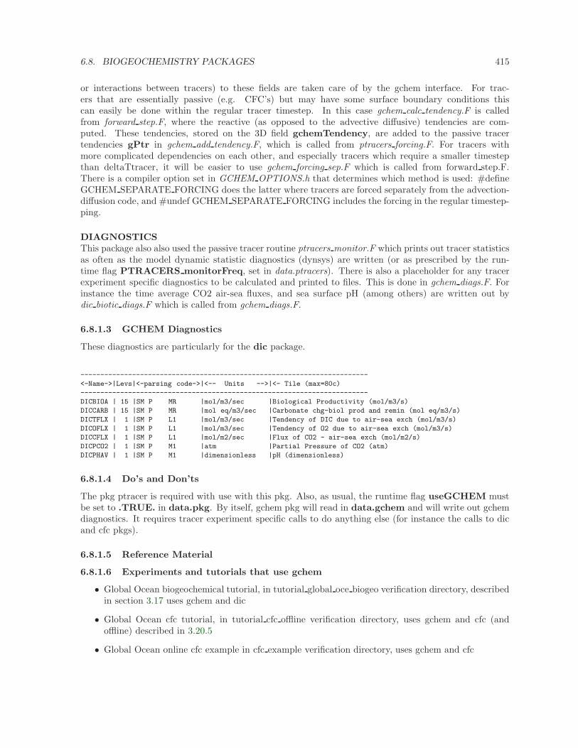
6.8. BIOGEOCHEMISTRY PACKAGES 415
or interactions between tracers) to these fields are taken care of by the gchem interface. For trac-ers that are essentially passive (e.g. CFC’s) but may have some surface boundary conditions thiscan easily be done within the regular tracer timestep. In this case gchem calc tendency.F is calledfrom forward step.F, where the reactive (as opposed to the advective diffusive) tendencies are com-puted. These tendencies, stored on the 3D field gchemTendency, are added to the passive tracertendencies gPtr in gchem add tendency.F, which is called from ptracers forcing.F. For tracers withmore complicated dependencies on each other, and especially tracers which require a smaller timestepthan deltaTtracer, it will be easier to use gchem forcing sep.F which is called from forward step.F.There is a compiler option set in GCHEM OPTIONS.h that determines which method is used: #defineGCHEM SEPARATE FORCING does the latter where tracers are forced separately from the advection-diffusion code, and #undef GCHEM SEPARATE FORCING includes the forcing in the regular timestep-ping.
DIAGNOSTICSThis package also also used the passive tracer routine ptracers monitor.F which prints out tracer statisticsas often as the model dynamic statistic diagnostics (dynsys) are written (or as prescribed by the run-time flag PTRACERS monitorFreq, set in data.ptracers). There is also a placeholder for any tracerexperiment specific diagnostics to be calculated and printed to files. This is done in gchem diags.F. Forinstance the time average CO2 air-sea fluxes, and sea surface pH (among others) are written out bydic biotic diags.F which is called from gchem diags.F.
6.8.1.3 GCHEM Diagnostics
These diagnostics are particularly for the dic package.
------------------------------------------------------------------------
<-Name->|Levs|<-parsing code->|<-- Units -->|<- Tile (max=80c)
------------------------------------------------------------------------
DICBIOA | 15 |SM P MR |mol/m3/sec |Biological Productivity (mol/m3/s)
DICCARB | 15 |SM P MR |mol eq/m3/sec |Carbonate chg-biol prod and remin (mol eq/m3/s)
DICTFLX | 1 |SM P L1 |mol/m3/sec |Tendency of DIC due to air-sea exch (mol/m3/s)
DICOFLX | 1 |SM P L1 |mol/m3/sec |Tendency of O2 due to air-sea exch (mol/m3/s)
DICCFLX | 1 |SM P L1 |mol/m2/sec |Flux of CO2 - air-sea exch (mol/m2/s)
DICPCO2 | 1 |SM P M1 |atm |Partial Pressure of CO2 (atm)
DICPHAV | 1 |SM P M1 |dimensionless |pH (dimensionless)
6.8.1.4 Do’s and Don’ts
The pkg ptracer is required with use with this pkg. Also, as usual, the runtime flag useGCHEM mustbe set to .TRUE. in data.pkg. By itself, gchem pkg will read in data.gchem and will write out gchemdiagnostics. It requires tracer experiment specific calls to do anything else (for instance the calls to dicand cfc pkgs).
6.8.1.5 Reference Material
6.8.1.6 Experiments and tutorials that use gchem
• Global Ocean biogeochemical tutorial, in tutorial global oce biogeo verification directory, describedin section 3.17 uses gchem and dic
• Global Ocean cfc tutorial, in tutorial cfc offline verification directory, uses gchem and cfc (andoffline) described in 3.20.5
• Global Ocean online cfc example in cfc example verification directory, uses gchem and cfc
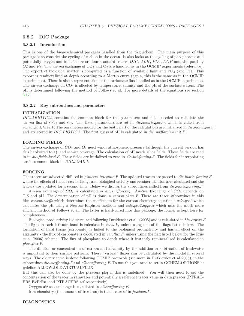
416 CHAPTER 6. PHYSICAL PARAMETERIZATIONS - PACKAGES I
6.8.2 DIC Package
6.8.2.1 Introduction
This is one of the biogeochemical packages handled from the pkg gchem. The main purpose of thispackage is to consider the cycling of carbon in the ocean. It also looks at the cycling of phosphorous andpotentially oxygen and iron. There are four standard tracers DIC, ALK, PO4, DOP and also possiblyO2 and Fe. The air-sea exchange of CO2 and O2 are handled as in the OCMIP experiments (reference).The export of biological matter is computed as a function of available light and PO4 (and Fe). Thisexport is remineralized at depth according to a Martin curve (again, this is the same as in the OCMIPexperiments). There is also a representation of the carbonate flux handled as in the OCMIP experiments.The air-sea exchange on CO2 is affected by temperature, salinity and the pH of the surface waters. ThepH is determined following the method of Follows et al. For more details of the equations see section3.17.
6.8.2.2 Key subroutines and parameters
INITIALIZATIONDIC ABIOTIC.h contains the common block for the parameters and fields needed to calculate theair-sea flux of CO2 and O2. The fixed parameters are set in dic abiotic param which is called fromgchem init fixed.F. The parameters needed for the biotic part of the calculations are initialized in dic biotic paramand are stored in DIC BIOTIC.h. The first guess of pH is calculated in dic surfforcing init.F.
LOADING FIELDSThe air-sea exchange of CO2 and O2 need wind, atmospheric pressure (although the current version hasthis hardwired to 1), and sea-ice coverage. The calculation of pH needs silica fields. These fields are readin in dic fields load.F. These fields are initialized to zero in dic ini forcing.F. The fields for interpolatingare in common block in DIC LOAD.h.
FORCINGThe tracers are advected-diffused in ptracers integrate.F. The updated tracers are passed to dic biotic forcing.Fwhere the effects of the air-sea exchange and biological activity and remineralization are calculated and thetracers are updated for a second time. Below we discuss the subroutines called from dic biotic forcing.F.
Air-sea exchange of CO2 is calculated in dic surfforcing. Air-Sea Exchange of CO2 depends onT,S and pH. The determination of pH is done in carbon chem.F. There are three subroutines in thisfile: carbon coeffs which determines the coefficients for the carbon chemistry equations; calc pco2 whichcalculates the pH using a Newton-Raphson method; and calc pco2 approx which uses the much moreefficient method of Follows et al. The latter is hard-wired into this package, the former is kept here forcompleteness.
Biological productivity is determined following Dutkiewicz et al. (2005) and is calculated in bio export.FThe light in each latitude band is calculate in insol.F, unless using one of the flags listed below. Theformation of hard tissue (carbonate) is linked to the biological productivity and has an effect on thealkalinity - the flux of carbonate is calculated in car flux.F, unless using the flag listed below for the Friiset al (2006) scheme. The flux of phosphate to depth where it instantly remineralized is calculated inphos flux.F.
The dilution or concentration of carbon and alkalinity by the addition or subtraction of freshwateris important to their surface patterns. These ”virtual” fluxes can be calculated by the model in severalways. The older scheme is done following OCMIP protocols (see more in Dutkiewicz et al 2005), in thesubroutines dic surfforcing.F and alk surfforcing.F. To use this you need to set in GCHEM OPTIONS.h:#define ALLOW OLD VIRTUALFLUXBut this can also be done by the ptracers pkg if this is undefined. You will then need to set theconcentration of the tracer in rainwater and potentially a reference tracer value in data.ptracer (PTRAC-ERS EvPrRn, and PTRACERS ref respectively).
Oxygen air-sea exchange is calculated in o2 surfforcing.F.Iron chemistry (the amount of free iron) is taken care of in fe chem.F.
DIAGNOSTICS
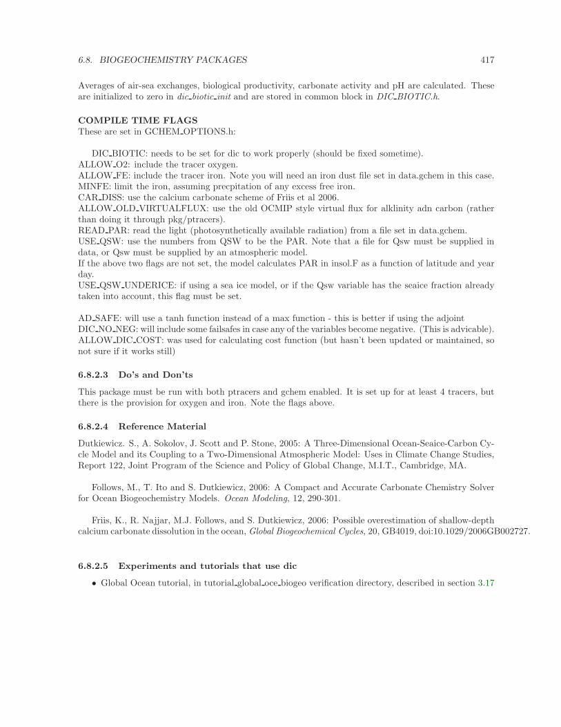
6.8. BIOGEOCHEMISTRY PACKAGES 417
Averages of air-sea exchanges, biological productivity, carbonate activity and pH are calculated. Theseare initialized to zero in dic biotic init and are stored in common block in DIC BIOTIC.h.
COMPILE TIME FLAGSThese are set in GCHEM OPTIONS.h:
DIC BIOTIC: needs to be set for dic to work properly (should be fixed sometime).ALLOW O2: include the tracer oxygen.ALLOW FE: include the tracer iron. Note you will need an iron dust file set in data.gchem in this case.MINFE: limit the iron, assuming precpitation of any excess free iron.CAR DISS: use the calcium carbonate scheme of Friis et al 2006.ALLOW OLD VIRTUALFLUX: use the old OCMIP style virtual flux for alklinity adn carbon (ratherthan doing it through pkg/ptracers).READ PAR: read the light (photosynthetically available radiation) from a file set in data.gchem.USE QSW: use the numbers from QSW to be the PAR. Note that a file for Qsw must be supplied indata, or Qsw must be supplied by an atmospheric model.If the above two flags are not set, the model calculates PAR in insol.F as a function of latitude and yearday.USE QSW UNDERICE: if using a sea ice model, or if the Qsw variable has the seaice fraction alreadytaken into account, this flag must be set.
AD SAFE: will use a tanh function instead of a max function - this is better if using the adjointDIC NO NEG: will include some failsafes in case any of the variables become negative. (This is advicable).ALLOW DIC COST: was used for calculating cost function (but hasn’t been updated or maintained, sonot sure if it works still)
6.8.2.3 Do’s and Don’ts
This package must be run with both ptracers and gchem enabled. It is set up for at least 4 tracers, butthere is the provision for oxygen and iron. Note the flags above.
6.8.2.4 Reference Material
Dutkiewicz. S., A. Sokolov, J. Scott and P. Stone, 2005: A Three-Dimensional Ocean-Seaice-Carbon Cy-cle Model and its Coupling to a Two-Dimensional Atmospheric Model: Uses in Climate Change Studies,Report 122, Joint Program of the Science and Policy of Global Change, M.I.T., Cambridge, MA.
Follows, M., T. Ito and S. Dutkiewicz, 2006: A Compact and Accurate Carbonate Chemistry Solverfor Ocean Biogeochemistry Models. Ocean Modeling, 12, 290-301.
Friis, K., R. Najjar, M.J. Follows, and S. Dutkiewicz, 2006: Possible overestimation of shallow-depthcalcium carbonate dissolution in the ocean, Global Biogeochemical Cycles, 20, GB4019, doi:10.1029/2006GB002727.
6.8.2.5 Experiments and tutorials that use dic
• Global Ocean tutorial, in tutorial global oce biogeo verification directory, described in section 3.17
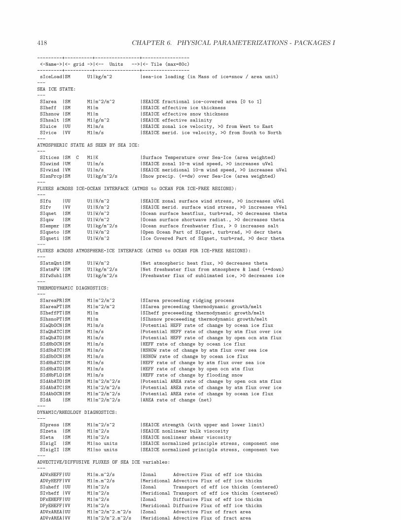
418 CHAPTER 6. PHYSICAL PARAMETERIZATIONS - PACKAGES I
---------+----------+----------------+-----------------
<-Name->|<- grid ->|<-- Units -->|<- Tile (max=80c)
---------+----------+----------------+-----------------
sIceLoad|SM U1|kg/m^2 |sea-ice loading (in Mass of ice+snow / area unit)
---
SEA ICE STATE:
---
SIarea |SM M1|m^2/m^2 |SEAICE fractional ice-covered area [0 to 1]
SIheff |SM M1|m |SEAICE effective ice thickness
SIhsnow |SM M1|m |SEAICE effective snow thickness
SIhsalt |SM M1|g/m^2 |SEAICE effective salinity
SIuice |UU M1|m/s |SEAICE zonal ice velocity, >0 from West to East
SIvice |VV M1|m/s |SEAICE merid. ice velocity, >0 from South to North
---
ATMOSPHERIC STATE AS SEEN BY SEA ICE:
---
SItices |SM C M1|K |Surface Temperature over Sea-Ice (area weighted)
SIuwind |UM U1|m/s |SEAICE zonal 10-m wind speed, >0 increases uVel
SIvwind |VM U1|m/s |SEAICE meridional 10-m wind speed, >0 increases uVel
SIsnPrcp|SM U1|kg/m^2/s |Snow precip. (+=dw) over Sea-Ice (area weighted)
---
FLUXES ACROSS ICE-OCEAN INTERFACE (ATMOS to OCEAN FOR ICE-FREE REGIONS):
---
SIfu |UU U1|N/m^2 |SEAICE zonal surface wind stress, >0 increases uVel
SIfv |VV U1|N/m^2 |SEAICE merid. surface wind stress, >0 increases vVel
SIqnet |SM U1|W/m^2 |Ocean surface heatflux, turb+rad, >0 decreases theta
SIqsw |SM U1|W/m^2 |Ocean surface shortwave radiat., >0 decreases theta
SIempmr |SM U1|kg/m^2/s |Ocean surface freshwater flux, > 0 increases salt
SIqneto |SM U1|W/m^2 |Open Ocean Part of SIqnet, turb+rad, >0 decr theta
SIqneti |SM U1|W/m^2 |Ice Covered Part of SIqnet, turb+rad, >0 decr theta
---
FLUXES ACROSS ATMOSPHERE-ICE INTERFACE (ATMOS to OCEAN FOR ICE-FREE REGIONS):
---
SIatmQnt|SM U1|W/m^2 |Net atmospheric heat flux, >0 decreases theta
SIatmFW |SM U1|kg/m^2/s |Net freshwater flux from atmosphere & land (+=down)
SIfwSubl|SM U1|kg/m^2/s |Freshwater flux of sublimated ice, >0 decreases ice
---
THERMODYNAMIC DIAGNOSTICS:
---
SIareaPR|SM M1|m^2/m^2 |SIarea preceeding ridging process
SIareaPT|SM M1|m^2/m^2 |SIarea preceeding thermodynamic growth/melt
SIheffPT|SM M1|m |SIheff preceeeding thermodynamic growth/melt
SIhsnoPT|SM M1|m |SIhsnow preceeeding thermodynamic growth/melt
SIaQbOCN|SM M1|m/s |Potential HEFF rate of change by ocean ice flux
SIaQbATC|SM M1|m/s |Potential HEFF rate of change by atm flux over ice
SIaQbATO|SM M1|m/s |Potential HEFF rate of change by open ocn atm flux
SIdHbOCN|SM M1|m/s |HEFF rate of change by ocean ice flux
SIdSbATC|SM M1|m/s |HSNOW rate of change by atm flux over sea ice
SIdSbOCN|SM M1|m/s |HSNOW rate of change by ocean ice flux
SIdHbATC|SM M1|m/s |HEFF rate of change by atm flux over sea ice
SIdHbATO|SM M1|m/s |HEFF rate of change by open ocn atm flux
SIdHbFLO|SM M1|m/s |HEFF rate of change by flooding snow
SIdAbATO|SM M1|m^2/m^2/s |Potential AREA rate of change by open ocn atm flux
SIdAbATC|SM M1|m^2/m^2/s |Potential AREA rate of change by atm flux over ice
SIdAbOCN|SM M1|m^2/m^2/s |Potential AREA rate of change by ocean ice flux
SIdA |SM M1|m^2/m^2/s |AREA rate of change (net)
---
DYNAMIC/RHEOLOGY DIAGNOSTICS:
---
SIpress |SM M1|m^2/s^2 |SEAICE strength (with upper and lower limit)
SIzeta |SM M1|m^2/s |SEAICE nonlinear bulk viscosity
SIeta |SM M1|m^2/s |SEAICE nonlinear shear viscosity
SIsigI |SM M1|no units |SEAICE normalized principle stress, component one
SIsigII |SM M1|no units |SEAICE normalized principle stress, component two
---
ADVECTIVE/DIFFUSIVE FLUXES OF SEA ICE variables:
---
ADVxHEFF|UU M1|m.m^2/s |Zonal Advective Flux of eff ice thickn
ADVyHEFF|VV M1|m.m^2/s |Meridional Advective Flux of eff ice thickn
SIuheff |UU M1|m^2/s |Zonal Transport of eff ice thickn (centered)
SIvheff |VV M1|m^2/s |Meridional Transport of eff ice thickn (centered)
DFxEHEFF|UU M1|m^2/s |Zonal Diffusive Flux of eff ice thickn
DFyEHEFF|VV M1|m^2/s |Meridional Diffusive Flux of eff ice thickn
ADVxAREA|UU M1|m^2/m^2.m^2/s |Zonal Advective Flux of fract area
ADVyAREA|VV M1|m^2/m^2.m^2/s |Meridional Advective Flux of fract area
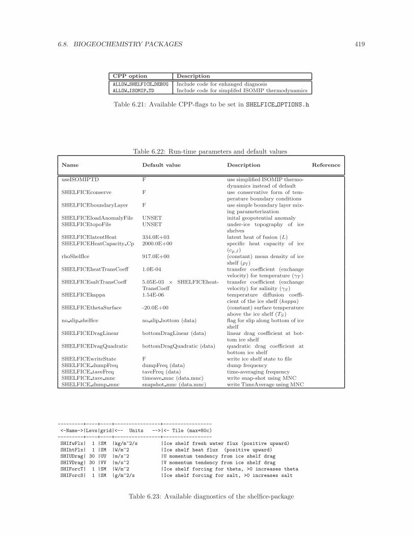
6.8. BIOGEOCHEMISTRY PACKAGES 419
CPP option Description
ALLOW SHELFICE DEBUG Include code for enhanged diagnosisALLOW ISOMIP TD Include code for simplifed ISOMIP thermodynamics
Table 6.21: Available CPP-flags to be set in SHELFICE OPTIONS.h
Table 6.22: Run-time parameters and default values
Name Default value Description Reference
useISOMIPTD F use simplified ISOMIP thermo-dynamics instead of default
SHELFICEconserve F use conservative form of tem-perature boundary conditions
SHELFICEboundaryLayer F use simple boundary layer mix-ing parameterization
SHELFICEloadAnomalyFile UNSET inital geopotential anomalySHELFICEtopoFile UNSET under-ice topography of ice
shelvesSHELFICElatentHeat 334.0E+03 latent heat of fusion (L)SHELFICEHeatCapacity Cp 2000.0E+00 specific heat capacity of ice
(cp,I)rhoShelfIce 917.0E+00 (constant) mean density of ice
shelf (ρI )SHELFICEheatTransCoeff 1.0E-04 transfer coefficient (exchange
velocity) for temperature (γT )SHELFICEsaltTransCoeff 5.05E-03 × SHELFICEheat-
TransCoefftransfer coefficient (exchangevelocity) for salinity (γS)
SHELFICEkappa 1.54E-06 temperature diffusion coeffi-cient of the ice shelf (kappa)
SHELFICEthetaSurface -20.0E+00 (constant) surface temperatureabove the ice shelf (TS)
no slip shelfice no slip bottom (data) flag for slip along bottom of iceshelf
SHELFICEDragLinear bottomDragLinear (data) linear drag coefficient at bot-tom ice shelf
SHELFICEDragQuadratic bottomDragQuadratic (data) quadratic drag coefficient atbottom ice shelf
SHELFICEwriteState F write ice shelf state to fileSHELFICE dumpFreq dumpFreq (data) dump frequencySHELFICE taveFreq taveFreq (data) time-averaging frequencySHELFICE tave mnc timeave mnc (data.mnc) write snap-shot using MNCSHELFICE dump mnc snapshot mnc (data.mnc) write TimeAverage using MNC
---------+----+----+----------------+-----------------
<-Name->|Levs|grid|<-- Units -->|<- Tile (max=80c)
---------+----+----+----------------+-----------------
SHIfwFlx| 1 |SM |kg/m^2/s |Ice shelf fresh water flux (positive upward)
SHIhtFlx| 1 |SM |W/m^2 |Ice shelf heat flux (positive upward)
SHIUDrag| 30 |UU |m/s^2 |U momentum tendency from ice shelf drag
SHIVDrag| 30 |VV |m/s^2 |V momentum tendency from ice shelf drag
SHIForcT| 1 |SM |W/m^2 |Ice shelf forcing for theta, >0 increases theta
SHIForcS| 1 |SM |g/m^2/s |Ice shelf forcing for salt, >0 increases salt
Table 6.23: Available diagnostics of the shelfice-package

420 CHAPTER 6. PHYSICAL PARAMETERIZATIONS - PACKAGES I
Chapter 7
Diagnostics and I/O - Packages II,and Post–Processing Utilities
MITgcm has several packages related to the input and output consumed and produced during a modelintegration. The packages used are related to the choice of input/output fields and the on-disk format ofthe model output.
7.1 Diagnostics–A Flexible Infrastructure
7.1.1 Introduction
This section of the documentation describes the Diagnostics package available within the GCM. A largeselection of model diagnostics is available for output. In addition to the diagnostic quantities pre-definedin the GCM, there exists the option, in any experiment, to define a new diagnostic quantity and includeit as part of the diagnostic output with the addition of a single subroutine call in the routine where thefield is computed. As a matter of philosophy, no diagnostic is enabled as default, thus each user mustspecify the exact diagnostic information required for an experiment. This is accomplished by enablingthe specific diagnostic of interest cataloged in the Diagnostic Menu (see Section 7.1.4.2). Instructionsfor enabling diagnostic output and defining new diagnostic quantities are found in Section 7.1.4 of thisdocument.
The Diagnostic Menu in this section of the manual is a listing of diagnostic quantities available within themain (dynamics) part of the GCM. Additional diagnostic quantities, defined within the different GCMpackages, are available and are listed in the diagnostic menu subsection of the manual section associatedwith each relevant package. Once a diagnostic is enabled, the GCM will continually increment an arrayspecifically allocated for that diagnostic whenever the appropriate quantity is computed. A counter isdefined which records how many times each diagnostic quantity has been incremented. Several specialdiagnostics are included in the menu. Quantities referred to as “Counter Diagnostics”, are defined forselected diagnostics which record the frequency at which a diagnostic is incremented separately for eachmodel grid location. Quantities referred to as “User Diagnostics” are included in the menu to facilitatedefining new diagnostics for a particular experiment.
7.1.2 Equations
Not relevant.
7.1.3 Key Subroutines and Parameters
There are several utilities within the GCM available to users to enable, disable, clear, write and retrievemodel diagnostics, and may be called from any routine. The available utilities and the CALL sequencesare listed below.
421
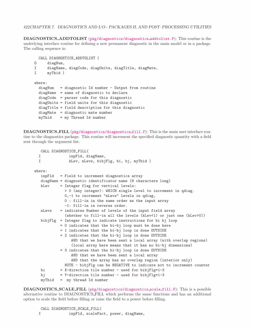
422CHAPTER 7. DIAGNOSTICS AND I/O - PACKAGES II, AND POST–PROCESSING UTILITIES
DIAGNOSTICS ADDTOLIST (pkg/diagnostics/diagnostics addtolist.F): This routine is theunderlying interface routine for defining a new permanent diagnostic in the main model or in a package.The calling sequence is:
CALL DIAGNOSTICS_ADDTOLIST (
O diagNum,
I diagName, diagCode, diagUnits, diagTitle, diagMate,
I myThid )
where:
diagNum = diagnostic Id number - Output from routine
diagName = name of diagnostic to declare
diagCode = parser code for this diagnostic
diagUnits = field units for this diagnostic
diagTitle = field description for this diagnostic
diagMate = diagnostic mate number
myThid = my Thread Id number
DIAGNOSTICS FILL (pkg/diagnostics/diagnostics fill.F): This is the main user interface rou-tine to the diagnostics package. This routine will increment the specified diagnostic quantity with a fieldsent through the argument list.
CALL DIAGNOSTICS_FILL(
I inpFld, diagName,
I kLev, nLevs, bibjFlg, bi, bj, myThid )
where:
inpFld = Field to increment diagnostics array
diagName = diagnostic identificator name (8 characters long)
kLev = Integer flag for vertical levels:
> 0 (any integer): WHICH single level to increment in qdiag.
0,-1 to increment "nLevs" levels in qdiag,
0 : fill-in in the same order as the input array
-1: fill-in in reverse order.
nLevs = indicates Number of levels of the input field array
(whether to fill-in all the levels (kLev<1) or just one (kLev>0))
bibjFlg = Integer flag to indicate instructions for bi bj loop
= 0 indicates that the bi-bj loop must be done here
= 1 indicates that the bi-bj loop is done OUTSIDE
= 2 indicates that the bi-bj loop is done OUTSIDE
AND that we have been sent a local array (with overlap regions)
(local array here means that it has no bi-bj dimensions)
= 3 indicates that the bi-bj loop is done OUTSIDE
AND that we have been sent a local array
AND that the array has no overlap region (interior only)
NOTE - bibjFlg can be NEGATIVE to indicate not to increment counter
bi = X-direction tile number - used for bibjFlg=1-3
bj = Y-direction tile number - used for bibjFlg=1-3
myThid = my thread Id number
DIAGNOSTICS SCALE FILL (pkg/diagnostics/diagnostics scale fill.F): This is a possiblealternative routine to DIAGNOSTICS FILL which performs the same functions and has an additionaloption to scale the field before filling or raise the field to a power before filling.
CALL DIAGNOSTICS_SCALE_FILL(
I inpFld, scaleFact, power, diagName,
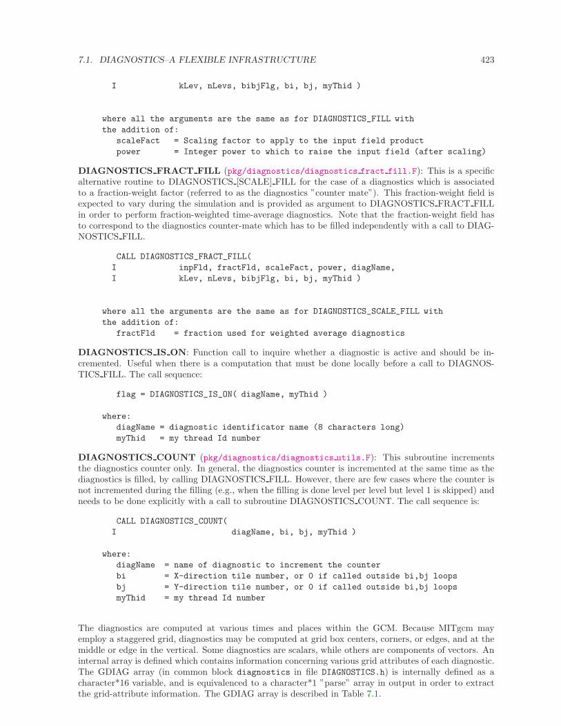
7.1. DIAGNOSTICS–A FLEXIBLE INFRASTRUCTURE 423
I kLev, nLevs, bibjFlg, bi, bj, myThid )
where all the arguments are the same as for DIAGNOSTICS_FILL with
the addition of:
scaleFact = Scaling factor to apply to the input field product
power = Integer power to which to raise the input field (after scaling)
DIAGNOSTICS FRACT FILL (pkg/diagnostics/diagnostics fract fill.F): This is a specificalternative routine to DIAGNOSTICS [SCALE] FILL for the case of a diagnostics which is associatedto a fraction-weight factor (referred to as the diagnostics ”counter mate”). This fraction-weight field isexpected to vary during the simulation and is provided as argument to DIAGNOSTICS FRACT FILLin order to perform fraction-weighted time-average diagnostics. Note that the fraction-weight field hasto correspond to the diagnostics counter-mate which has to be filled independently with a call to DIAG-NOSTICS FILL.
CALL DIAGNOSTICS_FRACT_FILL(
I inpFld, fractFld, scaleFact, power, diagName,
I kLev, nLevs, bibjFlg, bi, bj, myThid )
where all the arguments are the same as for DIAGNOSTICS_SCALE_FILL with
the addition of:
fractFld = fraction used for weighted average diagnostics
DIAGNOSTICS IS ON: Function call to inquire whether a diagnostic is active and should be in-cremented. Useful when there is a computation that must be done locally before a call to DIAGNOS-TICS FILL. The call sequence:
flag = DIAGNOSTICS_IS_ON( diagName, myThid )
where:
diagName = diagnostic identificator name (8 characters long)
myThid = my thread Id number
DIAGNOSTICS COUNT (pkg/diagnostics/diagnostics utils.F): This subroutine incrementsthe diagnostics counter only. In general, the diagnostics counter is incremented at the same time as thediagnostics is filled, by calling DIAGNOSTICS FILL. However, there are few cases where the counter isnot incremented during the filling (e.g., when the filling is done level per level but level 1 is skipped) andneeds to be done explicitly with a call to subroutine DIAGNOSTICS COUNT. The call sequence is:
CALL DIAGNOSTICS_COUNT(
I diagName, bi, bj, myThid )
where:
diagName = name of diagnostic to increment the counter
bi = X-direction tile number, or 0 if called outside bi,bj loops
bj = Y-direction tile number, or 0 if called outside bi,bj loops
myThid = my thread Id number
The diagnostics are computed at various times and places within the GCM. Because MITgcm mayemploy a staggered grid, diagnostics may be computed at grid box centers, corners, or edges, and at themiddle or edge in the vertical. Some diagnostics are scalars, while others are components of vectors. Aninternal array is defined which contains information concerning various grid attributes of each diagnostic.The GDIAG array (in common block diagnostics in file DIAGNOSTICS.h) is internally defined as acharacter*16 variable, and is equivalenced to a character*1 ”parse” array in output in order to extractthe grid-attribute information. The GDIAG array is described in Table 7.1.
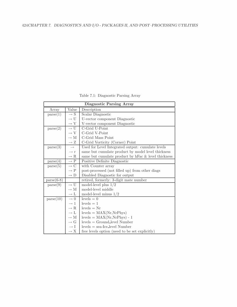
424CHAPTER 7. DIAGNOSTICS AND I/O - PACKAGES II, AND POST–PROCESSING UTILITIES
Table 7.1: Diagnostic Parsing Array
Diagnostic Parsing Array
Array Value Descriptionparse(1) → S Scalar Diagnostic
→ U U-vector component Diagnostic→ V V-vector component Diagnostic
parse(2) → U C-Grid U-Point→ V C-Grid V-Point→ M C-Grid Mass Point→ Z C-Grid Vorticity (Corner) Point
parse(3) → Used for Level Integrated output: cumulate levels→ r same but cumulate product by model level thickness→ R same but cumulate product by hFac & level thickness
parse(4) → P Positive Definite Diagnosticparse(5) → C with Counter array
→ P post-processed (not filled up) from other diags→ D Disabled Diagnostic for output
parse(6-8) retired, formerly: 3-digit mate numberparse(9) → U model-level plus 1/2
→ M model-level middle→ L model-level minus 1/2
parse(10) → 0 levels = 0→ 1 levels = 1→ R levels = Nr→ L levels = MAX(Nr,NrPhys)→ M levels = MAX(Nr,NrPhys) - 1→ G levels = Ground level Number→ I levels = sea-Ice level Number→ X free levels option (need to be set explicitly)
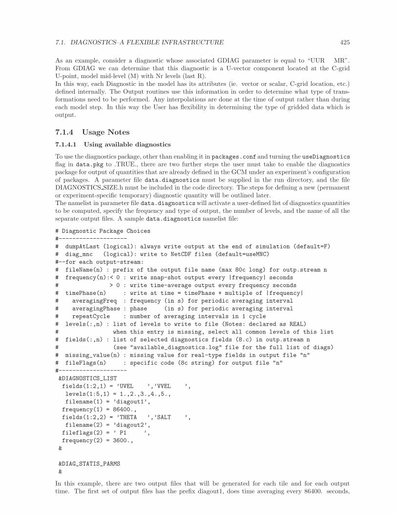
7.1. DIAGNOSTICS–A FLEXIBLE INFRASTRUCTURE 425
As an example, consider a diagnostic whose associated GDIAG parameter is equal to “UUR MR”.From GDIAG we can determine that this diagnostic is a U-vector component located at the C-gridU-point, model mid-level (M) with Nr levels (last R).In this way, each Diagnostic in the model has its attributes (ie. vector or scalar, C-grid location, etc.)defined internally. The Output routines use this information in order to determine what type of trans-formations need to be performed. Any interpolations are done at the time of output rather than duringeach model step. In this way the User has flexibility in determining the type of gridded data which isoutput.
7.1.4 Usage Notes
7.1.4.1 Using available diagnostics
To use the diagnostics package, other than enabling it in packages.conf and turning the useDiagnosticsflag in data.pkg to .TRUE., there are two further steps the user must take to enable the diagnosticspackage for output of quantities that are already defined in the GCM under an experiment’s configurationof packages. A parameter file data.diagnostics must be supplied in the run directory, and the fileDIAGNOSTICS SIZE.h must be included in the code directory. The steps for defining a new (permanentor experiment-specific temporary) diagnostic quantity will be outlined later.The namelist in parameter file data.diagnosticswill activate a user-defined list of diagnostics quantitiesto be computed, specify the frequency and type of output, the number of levels, and the name of all theseparate output files. A sample data.diagnostics namelist file:
# Diagnostic Package Choices
#--------------------
# dumpAtLast (logical): always write output at the end of simulation (default=F)
# diag_mnc (logical): write to NetCDF files (default=useMNC)
#--for each output-stream:
# fileName(n) : prefix of the output file name (max 80c long) for outp.stream n
# frequency(n):< 0 : write snap-shot output every |frequency| seconds
# > 0 : write time-average output every frequency seconds
# timePhase(n) : write at time = timePhase + multiple of |frequency|
# averagingFreq : frequency (in s) for periodic averaging interval
# averagingPhase : phase (in s) for periodic averaging interval
# repeatCycle : number of averaging intervals in 1 cycle
# levels(:,n) : list of levels to write to file (Notes: declared as REAL)
# when this entry is missing, select all common levels of this list
# fields(:,n) : list of selected diagnostics fields (8.c) in outp.stream n
# (see "available_diagnostics.log" file for the full list of diags)
# missing_value(n) : missing value for real-type fields in output file "n"
# fileFlags(n) : specific code (8c string) for output file "n"
#--------------------
&DIAGNOSTICS_LIST
fields(1:2,1) = ’UVEL ’,’VVEL ’,
levels(1:5,1) = 1.,2.,3.,4.,5.,
filename(1) = ’diagout1’,
frequency(1) = 86400.,
fields(1:2,2) = ’THETA ’,’SALT ’,
filename(2) = ’diagout2’,
fileflags(2) = ’ P1 ’,
frequency(2) = 3600.,
&
&DIAG_STATIS_PARMS
&
In this example, there are two output files that will be generated for each tile and for each outputtime. The first set of output files has the prefix diagout1, does time averaging every 86400. seconds,
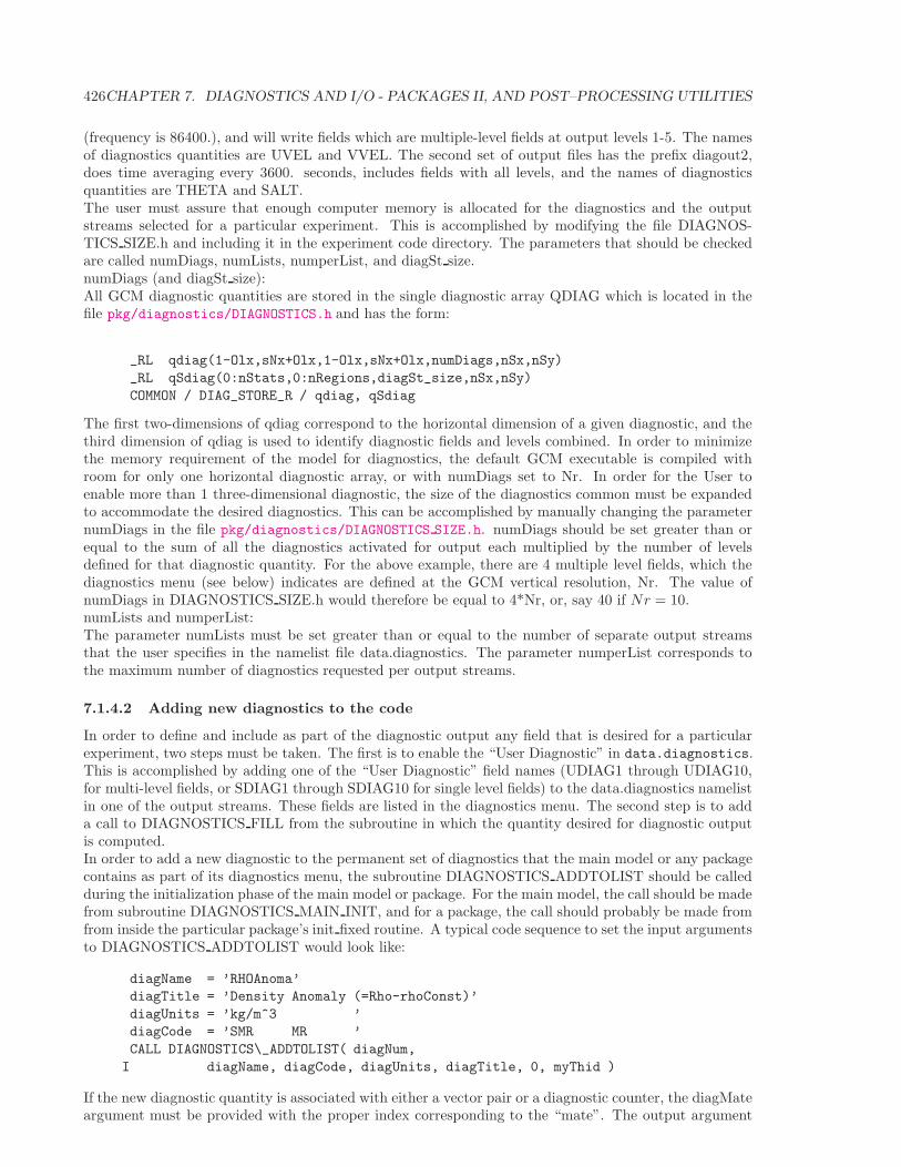
426CHAPTER 7. DIAGNOSTICS AND I/O - PACKAGES II, AND POST–PROCESSING UTILITIES
(frequency is 86400.), and will write fields which are multiple-level fields at output levels 1-5. The namesof diagnostics quantities are UVEL and VVEL. The second set of output files has the prefix diagout2,does time averaging every 3600. seconds, includes fields with all levels, and the names of diagnosticsquantities are THETA and SALT.The user must assure that enough computer memory is allocated for the diagnostics and the outputstreams selected for a particular experiment. This is accomplished by modifying the file DIAGNOS-TICS SIZE.h and including it in the experiment code directory. The parameters that should be checkedare called numDiags, numLists, numperList, and diagSt size.numDiags (and diagSt size):All GCM diagnostic quantities are stored in the single diagnostic array QDIAG which is located in thefile pkg/diagnostics/DIAGNOSTICS.h and has the form:
_RL qdiag(1-Olx,sNx+Olx,1-Olx,sNx+Olx,numDiags,nSx,nSy)
_RL qSdiag(0:nStats,0:nRegions,diagSt_size,nSx,nSy)
COMMON / DIAG_STORE_R / qdiag, qSdiag
The first two-dimensions of qdiag correspond to the horizontal dimension of a given diagnostic, and thethird dimension of qdiag is used to identify diagnostic fields and levels combined. In order to minimizethe memory requirement of the model for diagnostics, the default GCM executable is compiled withroom for only one horizontal diagnostic array, or with numDiags set to Nr. In order for the User toenable more than 1 three-dimensional diagnostic, the size of the diagnostics common must be expandedto accommodate the desired diagnostics. This can be accomplished by manually changing the parameternumDiags in the file pkg/diagnostics/DIAGNOSTICS SIZE.h. numDiags should be set greater than orequal to the sum of all the diagnostics activated for output each multiplied by the number of levelsdefined for that diagnostic quantity. For the above example, there are 4 multiple level fields, which thediagnostics menu (see below) indicates are defined at the GCM vertical resolution, Nr. The value ofnumDiags in DIAGNOSTICS SIZE.h would therefore be equal to 4*Nr, or, say 40 if Nr = 10.numLists and numperList:The parameter numLists must be set greater than or equal to the number of separate output streamsthat the user specifies in the namelist file data.diagnostics. The parameter numperList corresponds tothe maximum number of diagnostics requested per output streams.
7.1.4.2 Adding new diagnostics to the code
In order to define and include as part of the diagnostic output any field that is desired for a particularexperiment, two steps must be taken. The first is to enable the “User Diagnostic” in data.diagnostics.This is accomplished by adding one of the “User Diagnostic” field names (UDIAG1 through UDIAG10,for multi-level fields, or SDIAG1 through SDIAG10 for single level fields) to the data.diagnostics namelistin one of the output streams. These fields are listed in the diagnostics menu. The second step is to adda call to DIAGNOSTICS FILL from the subroutine in which the quantity desired for diagnostic outputis computed.In order to add a new diagnostic to the permanent set of diagnostics that the main model or any packagecontains as part of its diagnostics menu, the subroutine DIAGNOSTICS ADDTOLIST should be calledduring the initialization phase of the main model or package. For the main model, the call should be madefrom subroutine DIAGNOSTICS MAIN INIT, and for a package, the call should probably be made fromfrom inside the particular package’s init fixed routine. A typical code sequence to set the input argumentsto DIAGNOSTICS ADDTOLIST would look like:
diagName = ’RHOAnoma’
diagTitle = ’Density Anomaly (=Rho-rhoConst)’
diagUnits = ’kg/m^3 ’
diagCode = ’SMR MR ’
CALL DIAGNOSTICS\_ADDTOLIST( diagNum,
I diagName, diagCode, diagUnits, diagTitle, 0, myThid )
If the new diagnostic quantity is associated with either a vector pair or a diagnostic counter, the diagMateargument must be provided with the proper index corresponding to the “mate”. The output argument
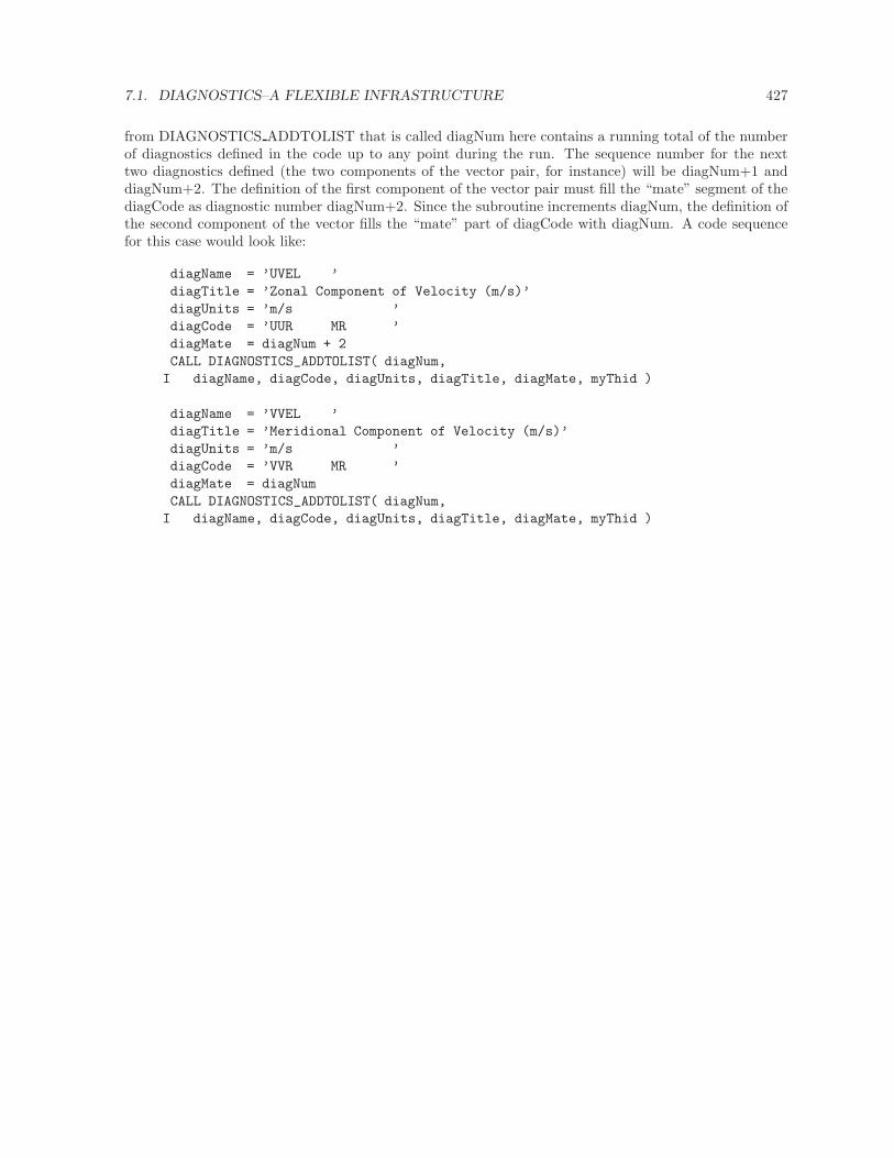
7.1. DIAGNOSTICS–A FLEXIBLE INFRASTRUCTURE 427
from DIAGNOSTICS ADDTOLIST that is called diagNum here contains a running total of the numberof diagnostics defined in the code up to any point during the run. The sequence number for the nexttwo diagnostics defined (the two components of the vector pair, for instance) will be diagNum+1 anddiagNum+2. The definition of the first component of the vector pair must fill the “mate” segment of thediagCode as diagnostic number diagNum+2. Since the subroutine increments diagNum, the definition ofthe second component of the vector fills the “mate” part of diagCode with diagNum. A code sequencefor this case would look like:
diagName = ’UVEL ’
diagTitle = ’Zonal Component of Velocity (m/s)’
diagUnits = ’m/s ’
diagCode = ’UUR MR ’
diagMate = diagNum + 2
CALL DIAGNOSTICS_ADDTOLIST( diagNum,
I diagName, diagCode, diagUnits, diagTitle, diagMate, myThid )
diagName = ’VVEL ’
diagTitle = ’Meridional Component of Velocity (m/s)’
diagUnits = ’m/s ’
diagCode = ’VVR MR ’
diagMate = diagNum
CALL DIAGNOSTICS_ADDTOLIST( diagNum,
I diagName, diagCode, diagUnits, diagTitle, diagMate, myThid )
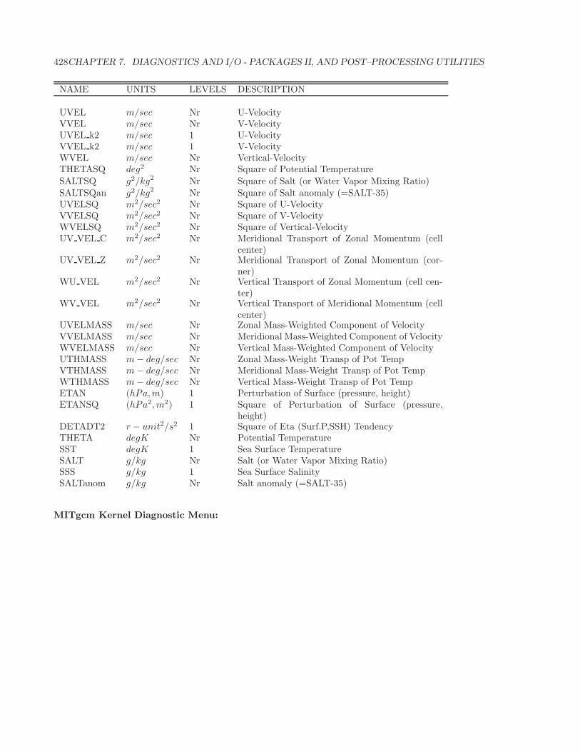
428CHAPTER 7. DIAGNOSTICS AND I/O - PACKAGES II, AND POST–PROCESSING UTILITIES
NAME UNITS LEVELS DESCRIPTION
UVEL m/sec Nr U-VelocityVVEL m/sec Nr V-VelocityUVEL k2 m/sec 1 U-VelocityVVEL k2 m/sec 1 V-VelocityWVEL m/sec Nr Vertical-VelocityTHETASQ deg2 Nr Square of Potential Temperature
SALTSQ g2/kg2 Nr Square of Salt (or Water Vapor Mixing Ratio)
SALTSQan g2/kg2 Nr Square of Salt anomaly (=SALT-35)UVELSQ m2/sec2 Nr Square of U-VelocityVVELSQ m2/sec2 Nr Square of V-VelocityWVELSQ m2/sec2 Nr Square of Vertical-VelocityUV VEL C m2/sec2 Nr Meridional Transport of Zonal Momentum (cell
center)UV VEL Z m2/sec2 Nr Meridional Transport of Zonal Momentum (cor-
ner)WU VEL m2/sec2 Nr Vertical Transport of Zonal Momentum (cell cen-
ter)WV VEL m2/sec2 Nr Vertical Transport of Meridional Momentum (cell
center)UVELMASS m/sec Nr Zonal Mass-Weighted Component of VelocityVVELMASS m/sec Nr Meridional Mass-Weighted Component of VelocityWVELMASS m/sec Nr Vertical Mass-Weighted Component of VelocityUTHMASS m− deg/sec Nr Zonal Mass-Weight Transp of Pot TempVTHMASS m− deg/sec Nr Meridional Mass-Weight Transp of Pot TempWTHMASS m− deg/sec Nr Vertical Mass-Weight Transp of Pot TempETAN (hPa,m) 1 Perturbation of Surface (pressure, height)ETANSQ (hPa2,m2) 1 Square of Perturbation of Surface (pressure,
height)DETADT2 r − unit2/s2 1 Square of Eta (Surf.P,SSH) TendencyTHETA degK Nr Potential TemperatureSST degK 1 Sea Surface TemperatureSALT g/kg Nr Salt (or Water Vapor Mixing Ratio)SSS g/kg 1 Sea Surface SalinitySALTanom g/kg Nr Salt anomaly (=SALT-35)
MITgcm Kernel Diagnostic Menu:
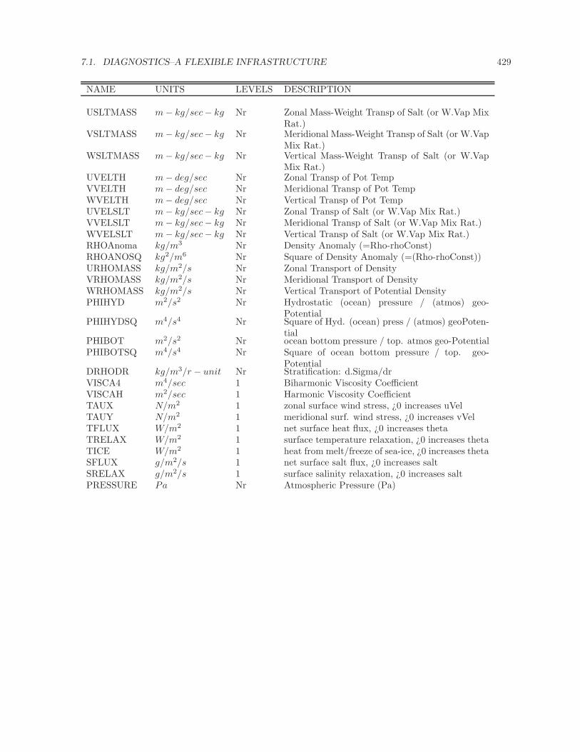
7.1. DIAGNOSTICS–A FLEXIBLE INFRASTRUCTURE 429
NAME UNITS LEVELS DESCRIPTION
USLTMASS m− kg/sec− kg Nr Zonal Mass-Weight Transp of Salt (or W.Vap MixRat.)
VSLTMASS m− kg/sec− kg Nr Meridional Mass-Weight Transp of Salt (or W.VapMix Rat.)
WSLTMASS m− kg/sec− kg Nr Vertical Mass-Weight Transp of Salt (or W.VapMix Rat.)
UVELTH m− deg/sec Nr Zonal Transp of Pot TempVVELTH m− deg/sec Nr Meridional Transp of Pot TempWVELTH m− deg/sec Nr Vertical Transp of Pot TempUVELSLT m− kg/sec− kg Nr Zonal Transp of Salt (or W.Vap Mix Rat.)VVELSLT m− kg/sec− kg Nr Meridional Transp of Salt (or W.Vap Mix Rat.)WVELSLT m− kg/sec− kg Nr Vertical Transp of Salt (or W.Vap Mix Rat.)RHOAnoma kg/m3 Nr Density Anomaly (=Rho-rhoConst)RHOANOSQ kg2/m6 Nr Square of Density Anomaly (=(Rho-rhoConst))URHOMASS kg/m2/s Nr Zonal Transport of DensityVRHOMASS kg/m2/s Nr Meridional Transport of DensityWRHOMASS kg/m2/s Nr Vertical Transport of Potential DensityPHIHYD m2/s2 Nr Hydrostatic (ocean) pressure / (atmos) geo-
PotentialPHIHYDSQ m4/s4 Nr Square of Hyd. (ocean) press / (atmos) geoPoten-
tialPHIBOT m2/s2 Nr ocean bottom pressure / top. atmos geo-PotentialPHIBOTSQ m4/s4 Nr Square of ocean bottom pressure / top. geo-
PotentialDRHODR kg/m3/r − unit Nr Stratification: d.Sigma/drVISCA4 m4/sec 1 Biharmonic Viscosity CoefficientVISCAH m2/sec 1 Harmonic Viscosity CoefficientTAUX N/m2 1 zonal surface wind stress, ¿0 increases uVelTAUY N/m2 1 meridional surf. wind stress, ¿0 increases vVelTFLUX W/m2 1 net surface heat flux, ¿0 increases thetaTRELAX W/m2 1 surface temperature relaxation, ¿0 increases thetaTICE W/m2 1 heat from melt/freeze of sea-ice, ¿0 increases thetaSFLUX g/m2/s 1 net surface salt flux, ¿0 increases saltSRELAX g/m2/s 1 surface salinity relaxation, ¿0 increases saltPRESSURE Pa Nr Atmospheric Pressure (Pa)
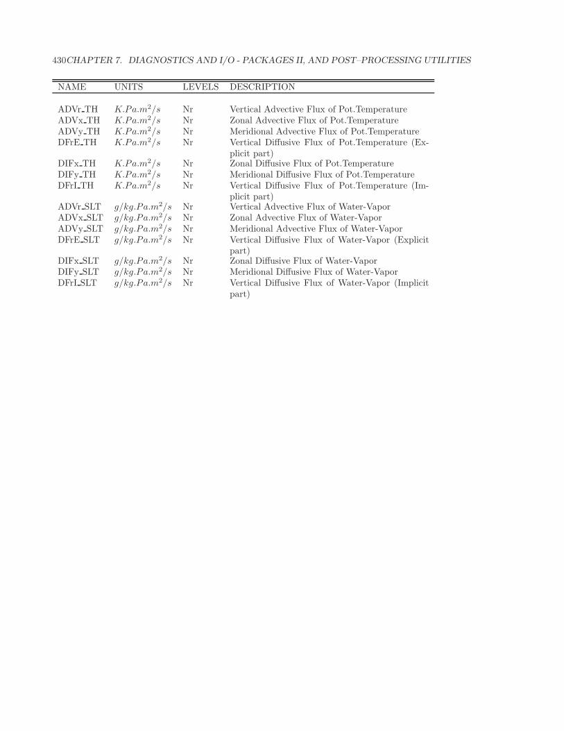
430CHAPTER 7. DIAGNOSTICS AND I/O - PACKAGES II, AND POST–PROCESSING UTILITIES
NAME UNITS LEVELS DESCRIPTION
ADVr TH K.Pa.m2/s Nr Vertical Advective Flux of Pot.TemperatureADVx TH K.Pa.m2/s Nr Zonal Advective Flux of Pot.TemperatureADVy TH K.Pa.m2/s Nr Meridional Advective Flux of Pot.TemperatureDFrE TH K.Pa.m2/s Nr Vertical Diffusive Flux of Pot.Temperature (Ex-
plicit part)DIFx TH K.Pa.m2/s Nr Zonal Diffusive Flux of Pot.TemperatureDIFy TH K.Pa.m2/s Nr Meridional Diffusive Flux of Pot.TemperatureDFrI TH K.Pa.m2/s Nr Vertical Diffusive Flux of Pot.Temperature (Im-
plicit part)ADVr SLT g/kg.Pa.m2/s Nr Vertical Advective Flux of Water-VaporADVx SLT g/kg.Pa.m2/s Nr Zonal Advective Flux of Water-VaporADVy SLT g/kg.Pa.m2/s Nr Meridional Advective Flux of Water-VaporDFrE SLT g/kg.Pa.m2/s Nr Vertical Diffusive Flux of Water-Vapor (Explicit
part)DIFx SLT g/kg.Pa.m2/s Nr Zonal Diffusive Flux of Water-VaporDIFy SLT g/kg.Pa.m2/s Nr Meridional Diffusive Flux of Water-VaporDFrI SLT g/kg.Pa.m2/s Nr Vertical Diffusive Flux of Water-Vapor (Implicit
part)
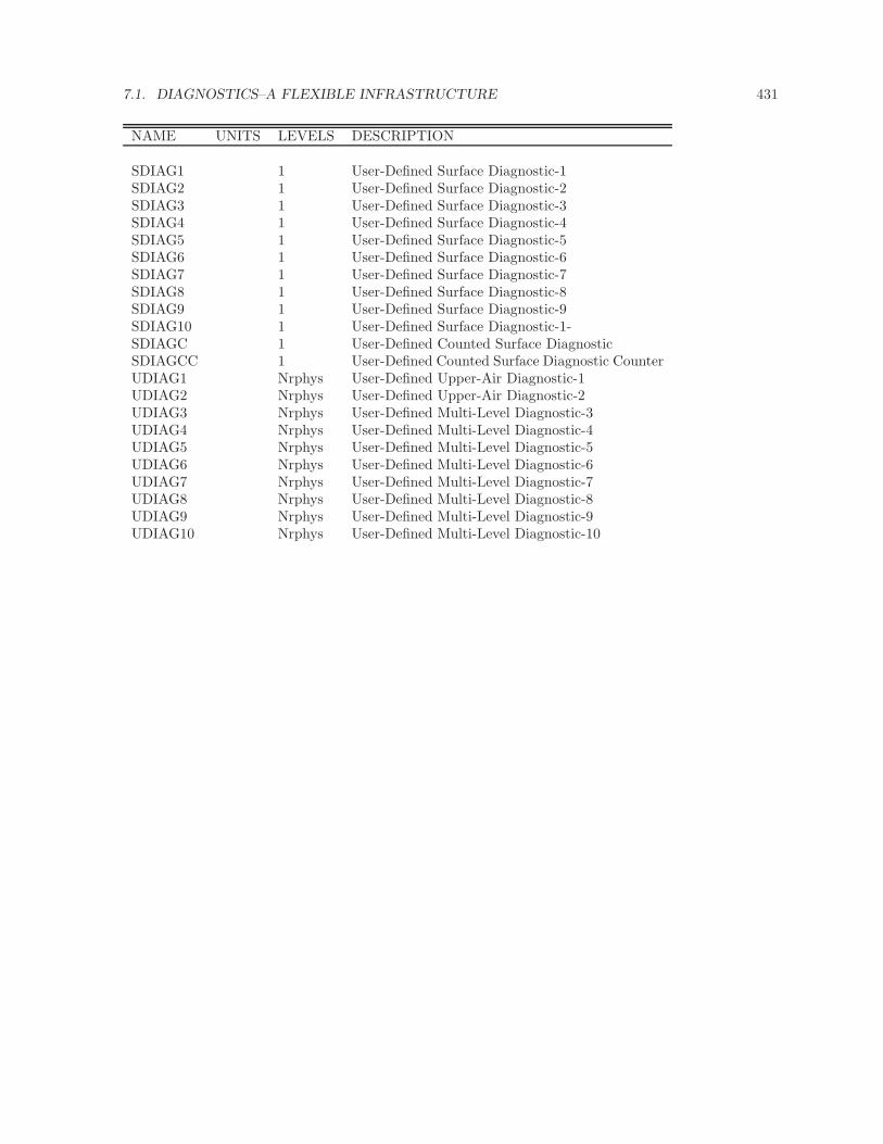
7.1. DIAGNOSTICS–A FLEXIBLE INFRASTRUCTURE 431
NAME UNITS LEVELS DESCRIPTION
SDIAG1 1 User-Defined Surface Diagnostic-1SDIAG2 1 User-Defined Surface Diagnostic-2SDIAG3 1 User-Defined Surface Diagnostic-3SDIAG4 1 User-Defined Surface Diagnostic-4SDIAG5 1 User-Defined Surface Diagnostic-5SDIAG6 1 User-Defined Surface Diagnostic-6SDIAG7 1 User-Defined Surface Diagnostic-7SDIAG8 1 User-Defined Surface Diagnostic-8SDIAG9 1 User-Defined Surface Diagnostic-9SDIAG10 1 User-Defined Surface Diagnostic-1-SDIAGC 1 User-Defined Counted Surface DiagnosticSDIAGCC 1 User-Defined Counted Surface Diagnostic CounterUDIAG1 Nrphys User-Defined Upper-Air Diagnostic-1UDIAG2 Nrphys User-Defined Upper-Air Diagnostic-2UDIAG3 Nrphys User-Defined Multi-Level Diagnostic-3UDIAG4 Nrphys User-Defined Multi-Level Diagnostic-4UDIAG5 Nrphys User-Defined Multi-Level Diagnostic-5UDIAG6 Nrphys User-Defined Multi-Level Diagnostic-6UDIAG7 Nrphys User-Defined Multi-Level Diagnostic-7UDIAG8 Nrphys User-Defined Multi-Level Diagnostic-8UDIAG9 Nrphys User-Defined Multi-Level Diagnostic-9UDIAG10 Nrphys User-Defined Multi-Level Diagnostic-10
432CHAPTER 7. DIAGNOSTICS AND I/O - PACKAGES II, AND POST–PROCESSING UTILITIES
For a list of the diagnostic fields available in the different MITgcm packages, follow the link to thediagnostics menu in the manual section describing the package:
• aim: 6.5.1.2
• exf: 6.4.7.7
• gchem: 6.8.1.3
• generic advdiff: 6.2.1.3
• gridalt: 6.2.5.6
• gmredi: 6.4.1.6
• fizhi: 6.5.3.3
• kpp: 6.4.2.6
• land: 6.5.2.3
• mom common: 2.14.8
• obcs: 6.3.1.7
• thsice: 6.6.1.3
• shap filt: 2.20.1
• ptracers: 6.3.3.4
7.1.5 Dos and Donts
7.1.6 Diagnostics Reference
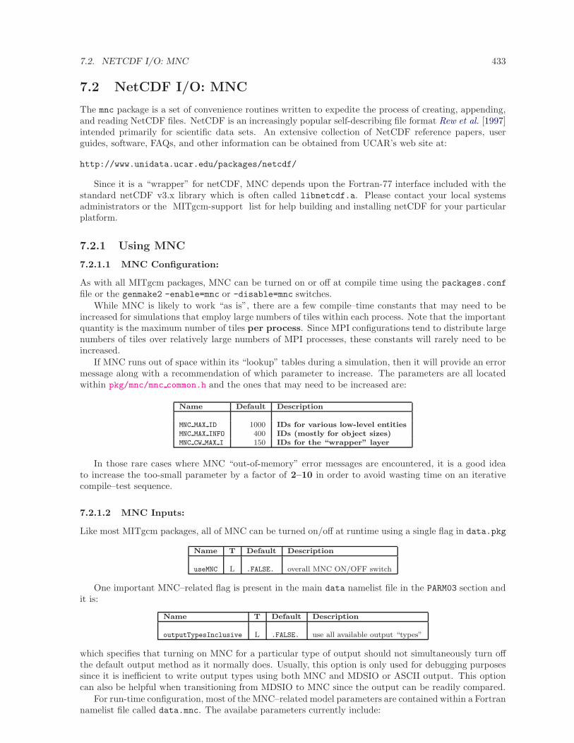
7.2. NETCDF I/O: MNC 433
7.2 NetCDF I/O: MNC
The mnc package is a set of convenience routines written to expedite the process of creating, appending,and reading NetCDF files. NetCDF is an increasingly popular self-describing file format Rew et al. [1997]intended primarily for scientific data sets. An extensive collection of NetCDF reference papers, userguides, software, FAQs, and other information can be obtained from UCAR’s web site at:
http://www.unidata.ucar.edu/packages/netcdf/
Since it is a “wrapper” for netCDF, MNC depends upon the Fortran-77 interface included with thestandard netCDF v3.x library which is often called libnetcdf.a. Please contact your local systemsadministrators or the MITgcm-support list for help building and installing netCDF for your particularplatform.
7.2.1 Using MNC
7.2.1.1 MNC Configuration:
As with all MITgcm packages, MNC can be turned on or off at compile time using the packages.conf
file or the genmake2 -enable=mnc or -disable=mnc switches.
While MNC is likely to work “as is”, there are a few compile–time constants that may need to beincreased for simulations that employ large numbers of tiles within each process. Note that the importantquantity is the maximum number of tiles per process. Since MPI configurations tend to distribute largenumbers of tiles over relatively large numbers of MPI processes, these constants will rarely need to beincreased.
If MNC runs out of space within its “lookup” tables during a simulation, then it will provide an errormessage along with a recommendation of which parameter to increase. The parameters are all locatedwithin pkg/mnc/mnc common.h and the ones that may need to be increased are:
Name Default Description
MNC MAX ID 1000 IDs for various low-level entitiesMNC MAX INFO 400 IDs (mostly for object sizes)MNC CW MAX I 150 IDs for the “wrapper” layer
In those rare cases where MNC “out-of-memory” error messages are encountered, it is a good ideato increase the too-small parameter by a factor of 2–10 in order to avoid wasting time on an iterativecompile–test sequence.
7.2.1.2 MNC Inputs:
Like most MITgcm packages, all of MNC can be turned on/off at runtime using a single flag in data.pkg
Name T Default Description
useMNC L .FALSE. overall MNC ON/OFF switch
One important MNC–related flag is present in the main data namelist file in the PARM03 section andit is:
Name T Default Description
outputTypesInclusive L .FALSE. use all available output “types”
which specifies that turning on MNC for a particular type of output should not simultaneously turn offthe default output method as it normally does. Usually, this option is only used for debugging purposessince it is inefficient to write output types using both MNC and MDSIO or ASCII output. This optioncan also be helpful when transitioning from MDSIO to MNC since the output can be readily compared.
For run-time configuration, most of the MNC–related model parameters are contained within a Fortrannamelist file called data.mnc. The availabe parameters currently include:
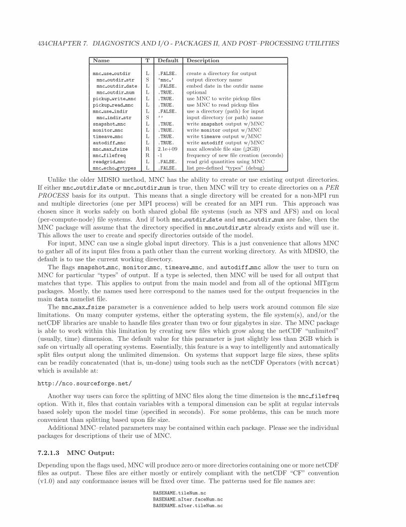
434CHAPTER 7. DIAGNOSTICS AND I/O - PACKAGES II, AND POST–PROCESSING UTILITIES
Name T Default Description
mnc use outdir L .FALSE. create a directory for outputmnc outdir str S ’mnc ’ output directory namemnc outdir date L .FALSE. embed date in the outdir namemnc outdir num L .TRUE. optional
pickup write mnc L .TRUE. use MNC to write pickup filespickup read mnc L .TRUE. use MNC to read pickup filesmnc use indir L .FALSE. use a directory (path) for inputmnc indir str S ’’ input directory (or path) name
snapshot mnc L .TRUE. write snapshot output w/MNCmonitor mnc L .TRUE. write monitor output w/MNCtimeave mnc L .TRUE. write timeave output w/MNCautodiff mnc L .TRUE. write autodiff output w/MNCmnc max fsize R 2.1e+09 max allowable file size (¡2GB)mnc filefreq R -1 frequency of new file creation (seconds)readgrid mnc L .FALSE. read grid quantities using MNCmnc echo gvtypes L .FALSE. list pre-defined “types” (debug)
Unlike the older MDSIO method, MNC has the ability to create or use existing output directories.If either mnc outdir date or mnc outdir num is true, then MNC will try to create directories on a PERPROCESS basis for its output. This means that a single directory will be created for a non-MPI runand multiple directories (one per MPI process) will be created for an MPI run. This approach waschosen since it works safely on both shared global file systems (such as NFS and AFS) and on local(per-compute-node) file systems. And if both mnc outdir date and mnc outdir num are false, then theMNC package will assume that the directory specified in mnc outdir str already exists and will use it.This allows the user to create and specify directories outside of the model.
For input, MNC can use a single global input directory. This is a just convenience that allows MNCto gather all of its input files from a path other than the current working directory. As with MDSIO, thedefault is to use the current working directory.
The flags snapshot mnc, monitor mnc, timeave mnc, and autodiff mnc allow the user to turn onMNC for particular “types” of output. If a type is selected, then MNC will be used for all output thatmatches that type. This applies to output from the main model and from all of the optional MITgcmpackages. Mostly, the names used here correspond to the names used for the output frequencies in themain data namelist file.
The mnc max fsize parameter is a convenience added to help users work around common file sizelimitations. On many computer systems, either the opterating system, the file system(s), and/or thenetCDF libraries are unable to handle files greater than two or four gigabytes in size. The MNC packageis able to work within this limitation by creating new files which grow along the netCDF “unlimited”(usually, time) dimension. The default value for this parameter is just slightly less than 2GB which issafe on virtually all operating systems. Essentially, this feature is a way to intelligently and automaticallysplit files output along the unlimited dimension. On systems that support large file sizes, these splitscan be readily concatenated (that is, un-done) using tools such as the netCDF Operators (with ncrcat)which is available at:
http://nco.sourceforge.net/
Another way users can force the splitting of MNC files along the time dimension is the mnc filefreq
option. With it, files that contain variables with a temporal dimension can be split at regular intervalsbased solely upon the model time (specified in seconds). For some problems, this can be much moreconvenient than splitting based upon file size.
Additional MNC–related parameters may be contained within each package. Please see the individualpackages for descriptions of their use of MNC.
7.2.1.3 MNC Output:
Depending upon the flags used, MNC will produce zero or more directories containing one or more netCDFfiles as output. These files are either mostly or entirely compliant with the netCDF “CF” convention(v1.0) and any conformance issues will be fixed over time. The patterns used for file names are:
BASENAME.tileNum.nc
BASENAME.nIter.faceNum.nc
BASENAME.nIter.tileNum.nc
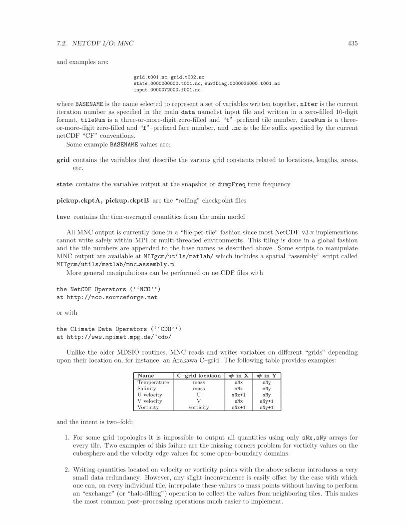
7.2. NETCDF I/O: MNC 435
and examples are:
grid.t001.nc, grid.t002.ncstate.0000000000.t001.nc, surfDiag.0000036000.t001.ncinput.0000072000.f001.nc
where BASENAME is the name selected to represent a set of variables written together, nIter is the currentiteration number as specified in the main data namelist input file and written in a zero-filled 10-digitformat, tileNum is a three-or-more-digit zero-filled and “t”–prefixed tile number, faceNum is a three-or-more-digit zero-filled and “f”–prefixed face number, and .nc is the file suffix specified by the currentnetCDF “CF” conventions.
Some example BASENAME values are:
grid contains the variables that describe the various grid constants related to locations, lengths, areas,etc.
state contains the variables output at the snapshot or dumpFreq time frequency
pickup.ckptA, pickup.ckptB are the “rolling” checkpoint files
tave contains the time-averaged quantities from the main model
All MNC output is currently done in a “file-per-tile” fashion since most NetCDF v3.x implementionscannot write safely within MPI or multi-threaded environments. This tiling is done in a global fashionand the tile numbers are appended to the base names as described above. Some scripts to manipulateMNC output are available at MITgcm/utils/matlab/ which includes a spatial “assembly” script calledMITgcm/utils/matlab/mnc assembly.m.
More general manipulations can be performed on netCDF files with
the NetCDF Operators (‘‘NCO’’)
at http://nco.sourceforge.net
or with
the Climate Data Operators (‘‘CDO’’)
at http://www.mpimet.mpg.de/~cdo/
Unlike the older MDSIO routines, MNC reads and writes variables on different “grids” dependingupon their location on, for instance, an Arakawa C–grid. The following table provides examples:
Name C–grid location # in X # in YTemperature mass sNx sNy
Salinity mass sNx sNy
U velocity U sNx+1 sNy
V velocity V sNx sNy+1
Vorticity vorticity sNx+1 sNy+1
and the intent is two–fold:
1. For some grid topologies it is impossible to output all quantities using only sNx,sNy arrays forevery tile. Two examples of this failure are the missing corners problem for vorticity values on thecubesphere and the velocity edge values for some open–boundary domains.
2. Writing quantities located on velocity or vorticity points with the above scheme introduces a verysmall data redundancy. However, any slight inconvenience is easily offset by the ease with whichone can, on every individual tile, interpolate these values to mass points without having to performan “exchange” (or “halo-filling”) operation to collect the values from neighboring tiles. This makesthe most common post–processing operations much easier to implement.
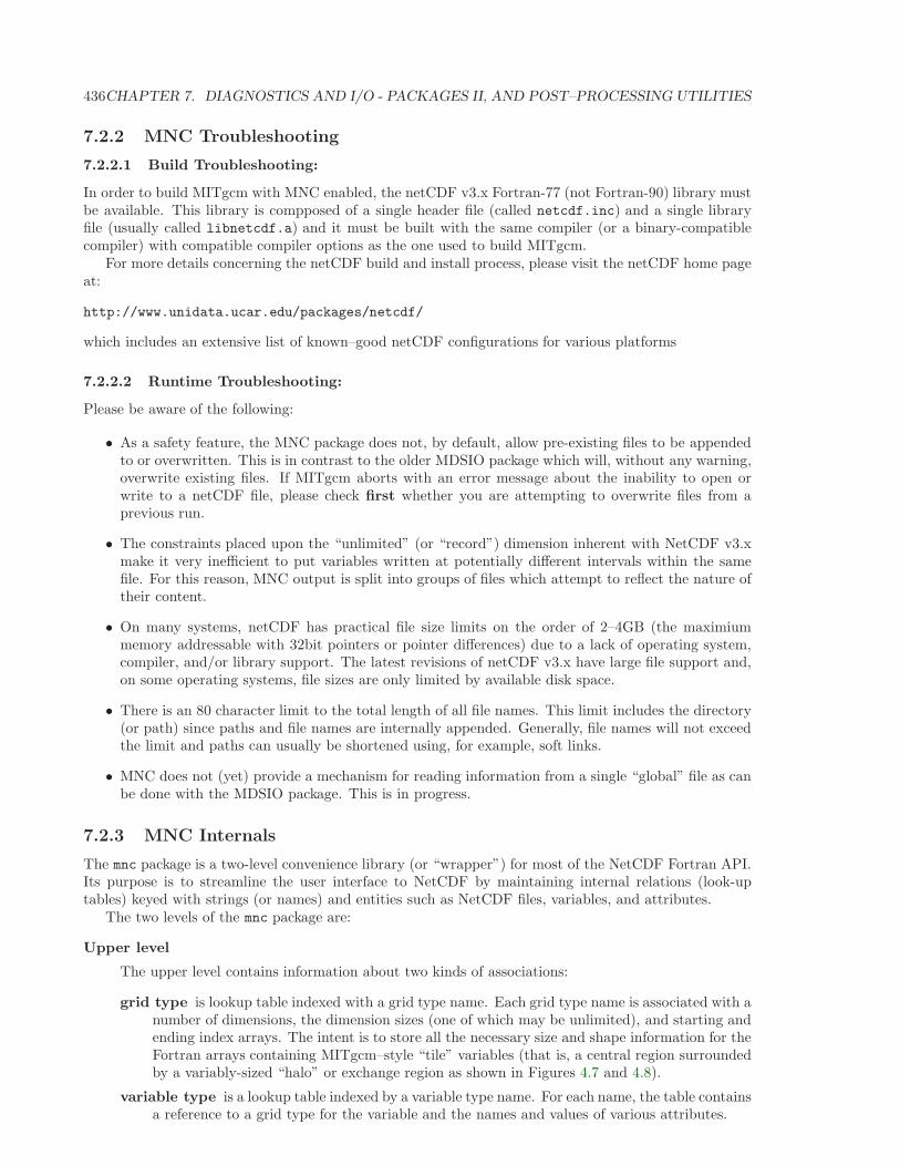
436CHAPTER 7. DIAGNOSTICS AND I/O - PACKAGES II, AND POST–PROCESSING UTILITIES
7.2.2 MNC Troubleshooting
7.2.2.1 Build Troubleshooting:
In order to build MITgcm with MNC enabled, the netCDF v3.x Fortran-77 (not Fortran-90) library mustbe available. This library is compposed of a single header file (called netcdf.inc) and a single libraryfile (usually called libnetcdf.a) and it must be built with the same compiler (or a binary-compatiblecompiler) with compatible compiler options as the one used to build MITgcm.
For more details concerning the netCDF build and install process, please visit the netCDF home pageat:
http://www.unidata.ucar.edu/packages/netcdf/
which includes an extensive list of known–good netCDF configurations for various platforms
7.2.2.2 Runtime Troubleshooting:
Please be aware of the following:
• As a safety feature, the MNC package does not, by default, allow pre-existing files to be appendedto or overwritten. This is in contrast to the older MDSIO package which will, without any warning,overwrite existing files. If MITgcm aborts with an error message about the inability to open orwrite to a netCDF file, please check first whether you are attempting to overwrite files from aprevious run.
• The constraints placed upon the “unlimited” (or “record”) dimension inherent with NetCDF v3.xmake it very inefficient to put variables written at potentially different intervals within the samefile. For this reason, MNC output is split into groups of files which attempt to reflect the nature oftheir content.
• On many systems, netCDF has practical file size limits on the order of 2–4GB (the maximiummemory addressable with 32bit pointers or pointer differences) due to a lack of operating system,compiler, and/or library support. The latest revisions of netCDF v3.x have large file support and,on some operating systems, file sizes are only limited by available disk space.
• There is an 80 character limit to the total length of all file names. This limit includes the directory(or path) since paths and file names are internally appended. Generally, file names will not exceedthe limit and paths can usually be shortened using, for example, soft links.
• MNC does not (yet) provide a mechanism for reading information from a single “global” file as canbe done with the MDSIO package. This is in progress.
7.2.3 MNC Internals
The mnc package is a two-level convenience library (or “wrapper”) for most of the NetCDF Fortran API.Its purpose is to streamline the user interface to NetCDF by maintaining internal relations (look-uptables) keyed with strings (or names) and entities such as NetCDF files, variables, and attributes.
The two levels of the mnc package are:
Upper level
The upper level contains information about two kinds of associations:
grid type is lookup table indexed with a grid type name. Each grid type name is associated with anumber of dimensions, the dimension sizes (one of which may be unlimited), and starting andending index arrays. The intent is to store all the necessary size and shape information for theFortran arrays containing MITgcm–style “tile” variables (that is, a central region surroundedby a variably-sized “halo” or exchange region as shown in Figures 4.7 and 4.8).
variable type is a lookup table indexed by a variable type name. For each name, the table containsa reference to a grid type for the variable and the names and values of various attributes.
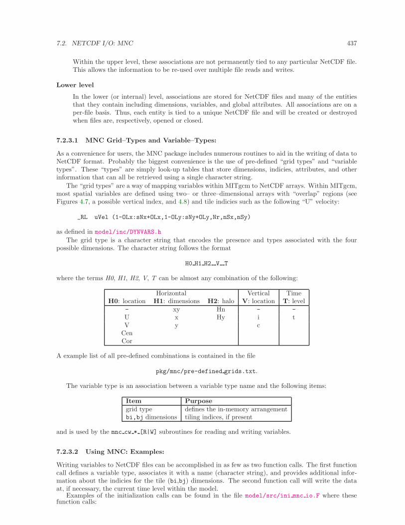
7.2. NETCDF I/O: MNC 437
Within the upper level, these associations are not permanently tied to any particular NetCDF file.This allows the information to be re-used over multiple file reads and writes.
Lower level
In the lower (or internal) level, associations are stored for NetCDF files and many of the entitiesthat they contain including dimensions, variables, and global attributes. All associations are on aper-file basis. Thus, each entity is tied to a unique NetCDF file and will be created or destroyedwhen files are, respectively, opened or closed.
7.2.3.1 MNC Grid–Types and Variable–Types:
As a convenience for users, the MNC package includes numerous routines to aid in the writing of data toNetCDF format. Probably the biggest convenience is the use of pre-defined “grid types” and “variabletypes”. These “types” are simply look-up tables that store dimensions, indicies, attributes, and otherinformation that can all be retrieved using a single character string.
The “grid types” are a way of mapping variables within MITgcm to NetCDF arrays. Within MITgcm,most spatial variables are defined using two– or three–dimensional arrays with “overlap” regions (seeFigures 4.7, a possible vertical index, and 4.8) and tile indicies such as the following “U” velocity:
_RL uVel (1-OLx:sNx+OLx,1-OLy:sNy+OLy,Nr,nSx,nSy)
as defined in model/inc/DYNVARS.h
The grid type is a character string that encodes the presence and types associated with the fourpossible dimensions. The character string follows the format
H0 H1 H2 V T
where the terms H0, H1, H2, V, T can be almost any combination of the following:
Horizontal Vertical TimeH0: location H1: dimensions H2: halo V: location T: level
- xy Hn - -
U x Hy i tV y c
CenCor
A example list of all pre-defined combinations is contained in the file
pkg/mnc/pre-defined grids.txt.
The variable type is an association between a variable type name and the following items:
Item Purposegrid type defines the in-memory arrangementbi,bj dimensions tiling indices, if present
and is used by the mnc cw * [R|W] subroutines for reading and writing variables.
7.2.3.2 Using MNC: Examples:
Writing variables to NetCDF files can be accomplished in as few as two function calls. The first functioncall defines a variable type, associates it with a name (character string), and provides additional infor-mation about the indicies for the tile (bi,bj) dimensions. The second function call will write the dataat, if necessary, the current time level within the model.
Examples of the initialization calls can be found in the file model/src/ini mnc io.F where thesefunction calls:
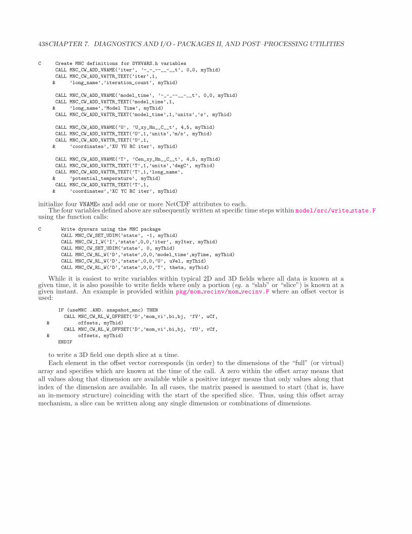
438CHAPTER 7. DIAGNOSTICS AND I/O - PACKAGES II, AND POST–PROCESSING UTILITIES
C Create MNC definitions for DYNVARS.h variables
CALL MNC_CW_ADD_VNAME(’iter’, ’-_-_--__-__t’, 0,0, myThid)
CALL MNC_CW_ADD_VATTR_TEXT(’iter’,1,
& ’long_name’,’iteration_count’, myThid)
CALL MNC_CW_ADD_VNAME(’model_time’, ’-_-_--__-__t’, 0,0, myThid)
CALL MNC_CW_ADD_VATTR_TEXT(’model_time’,1,
& ’long_name’,’Model Time’, myThid)
CALL MNC_CW_ADD_VATTR_TEXT(’model_time’,1,’units’,’s’, myThid)
CALL MNC_CW_ADD_VNAME(’U’, ’U_xy_Hn__C__t’, 4,5, myThid)
CALL MNC_CW_ADD_VATTR_TEXT(’U’,1,’units’,’m/s’, myThid)
CALL MNC_CW_ADD_VATTR_TEXT(’U’,1,
& ’coordinates’,’XU YU RC iter’, myThid)
CALL MNC_CW_ADD_VNAME(’T’, ’Cen_xy_Hn__C__t’, 4,5, myThid)
CALL MNC_CW_ADD_VATTR_TEXT(’T’,1,’units’,’degC’, myThid)
CALL MNC_CW_ADD_VATTR_TEXT(’T’,1,’long_name’,
& ’potential_temperature’, myThid)
CALL MNC_CW_ADD_VATTR_TEXT(’T’,1,
& ’coordinates’,’XC YC RC iter’, myThid)
initialize four VNAMEs and add one or more NetCDF attributes to each.The four variables defined above are subsequently written at specific time steps within model/src/write state.F
using the function calls:
C Write dynvars using the MNC package
CALL MNC_CW_SET_UDIM(’state’, -1, myThid)
CALL MNC_CW_I_W(’I’,’state’,0,0,’iter’, myIter, myThid)
CALL MNC_CW_SET_UDIM(’state’, 0, myThid)
CALL MNC_CW_RL_W(’D’,’state’,0,0,’model_time’,myTime, myThid)
CALL MNC_CW_RL_W(’D’,’state’,0,0,’U’, uVel, myThid)
CALL MNC_CW_RL_W(’D’,’state’,0,0,’T’, theta, myThid)
While it is easiest to write variables within typical 2D and 3D fields where all data is known at agiven time, it is also possible to write fields where only a portion (eg. a “slab” or “slice”) is known at agiven instant. An example is provided within pkg/mom vecinv/mom vecinv.F where an offset vector isused:
IF (useMNC .AND. snapshot_mnc) THEN
CALL MNC_CW_RL_W_OFFSET(’D’,’mom_vi’,bi,bj, ’fV’, uCf,
& offsets, myThid)
CALL MNC_CW_RL_W_OFFSET(’D’,’mom_vi’,bi,bj, ’fU’, vCf,
& offsets, myThid)
ENDIF
to write a 3D field one depth slice at a time.Each element in the offset vector corresponds (in order) to the dimensions of the “full” (or virtual)
array and specifies which are known at the time of the call. A zero within the offset array means thatall values along that dimension are available while a positive integer means that only values along thatindex of the dimension are available. In all cases, the matrix passed is assumed to start (that is, havean in-memory structure) coinciding with the start of the specified slice. Thus, using this offset arraymechanism, a slice can be written along any single dimension or combinations of dimensions.
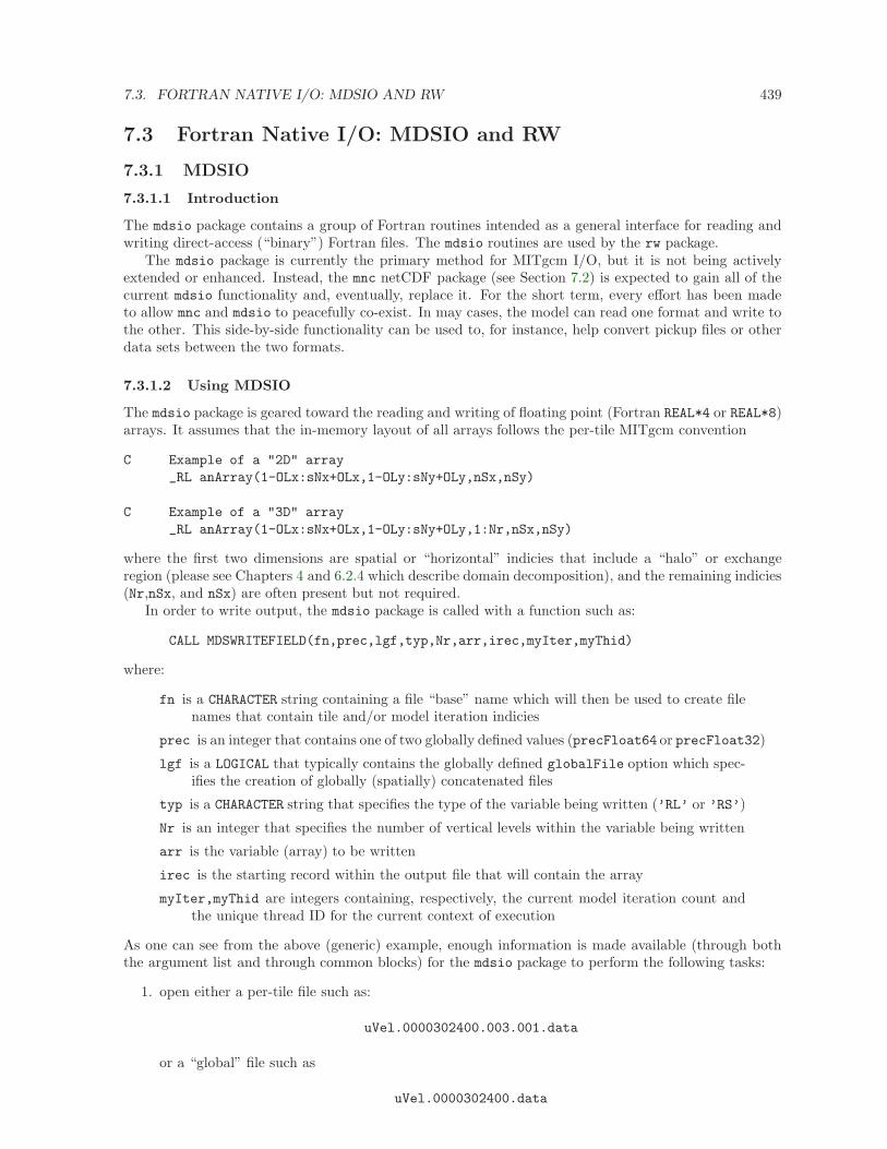
7.3. FORTRAN NATIVE I/O: MDSIO AND RW 439
7.3 Fortran Native I/O: MDSIO and RW
7.3.1 MDSIO
7.3.1.1 Introduction
The mdsio package contains a group of Fortran routines intended as a general interface for reading andwriting direct-access (“binary”) Fortran files. The mdsio routines are used by the rw package.
The mdsio package is currently the primary method for MITgcm I/O, but it is not being activelyextended or enhanced. Instead, the mnc netCDF package (see Section 7.2) is expected to gain all of thecurrent mdsio functionality and, eventually, replace it. For the short term, every effort has been madeto allow mnc and mdsio to peacefully co-exist. In may cases, the model can read one format and write tothe other. This side-by-side functionality can be used to, for instance, help convert pickup files or otherdata sets between the two formats.
7.3.1.2 Using MDSIO
The mdsio package is geared toward the reading and writing of floating point (Fortran REAL*4 or REAL*8)arrays. It assumes that the in-memory layout of all arrays follows the per-tile MITgcm convention
C Example of a "2D" array
_RL anArray(1-OLx:sNx+OLx,1-OLy:sNy+OLy,nSx,nSy)
C Example of a "3D" array
_RL anArray(1-OLx:sNx+OLx,1-OLy:sNy+OLy,1:Nr,nSx,nSy)
where the first two dimensions are spatial or “horizontal” indicies that include a “halo” or exchangeregion (please see Chapters 4 and 6.2.4 which describe domain decomposition), and the remaining indicies(Nr,nSx, and nSx) are often present but not required.
In order to write output, the mdsio package is called with a function such as:
CALL MDSWRITEFIELD(fn,prec,lgf,typ,Nr,arr,irec,myIter,myThid)
where:
fn is a CHARACTER string containing a file “base” name which will then be used to create filenames that contain tile and/or model iteration indicies
prec is an integer that contains one of two globally defined values (precFloat64 or precFloat32)
lgf is a LOGICAL that typically contains the globally defined globalFile option which spec-ifies the creation of globally (spatially) concatenated files
typ is a CHARACTER string that specifies the type of the variable being written (’RL’ or ’RS’)
Nr is an integer that specifies the number of vertical levels within the variable being written
arr is the variable (array) to be written
irec is the starting record within the output file that will contain the array
myIter,myThid are integers containing, respectively, the current model iteration count andthe unique thread ID for the current context of execution
As one can see from the above (generic) example, enough information is made available (through boththe argument list and through common blocks) for the mdsio package to perform the following tasks:
1. open either a per-tile file such as:
uVel.0000302400.003.001.data
or a “global” file such as
uVel.0000302400.data
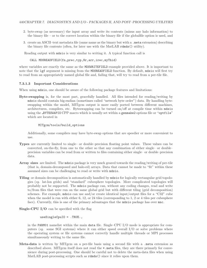
440CHAPTER 7. DIAGNOSTICS AND I/O - PACKAGES II, AND POST–PROCESSING UTILITIES
2. byte-swap (as necessary) the input array and write its contents (minus any halo information) tothe binary file – or to the correct location within the binary file if the globalfile option is used, and
3. create an ASCII–text metadata file (same name as the binary but with a .meta extension) describingthe binary file contents (often, for later use with the MatLAB rdmds() utility).
Reading output with mdsio is very similar to writing it. A typical function call is
CALL MDSREADFIELD(fn,prec,typ,Nr,arr,irec,myThid)
where variables are exactly the same as the MDSWRITEFIELD example provided above. It is important tonote that the lgf argument is missing from the MDSREADFIELD function. By default, mdsio will first tryto read from an appropriately named global file and, failing that, will try to read from a per-tile file.
7.3.1.3 Important Considerations
When using mdsio, one should be aware of the following package features and limitations:
Byte-swapping is, for the most part, gracefully handled. All files intended for reading/writing bymdsio should contain big-endian (sometimes called “network byte order”) data. By handling byte-swapping within the model, MITgcm output is more easily ported between different machines,architectures, compilers, etc. Byteswapping can be turned on/off at compile time within mdsio
using the BYTESWAPIO CPP macro which is usually set within a genmake2 options file or “optfile”which are located in
MITgcm/tools/build_options
Additionally, some compilers may have byte-swap options that are speedier or more convenient touse.
Types are currently limited to single– or double–precision floating point values. These values can beconverted, on-the-fly, from one to the other so that any combination of either single– or double–precision variables can be read from or written to files containing either single– or double–precisiondata.
Array sizes are limited. The mdsio package is very much geared towards the reading/writing of per-tile(that is, domain-decomposed and halo-ed) arrays. Data that cannot be made to “fit” within theseassumed sizes can be challenging to read or write with mdsio.
Tiling or domain decomposition is automatically handled by mdsio for logically rectangular grid topolo-gies (eg. lat-lon grids) and “standard” cubesphere topologies. More complicated topologies willprobably not be supported. The mdsio package can, without any coding changes, read and writeto/from files that were run on the same global grid but with different tiling (grid decomposition)schemes. For example, mdsio can use and/or create identical input/output files for a “C32” cubewhen the model is run with either 6, 12, or 24 tiles (corresponding to 1, 2 or 4 tiles per cubesphereface). Currently, this is one of the primary advantages that the mdsio package has over mnc.
Single-CPU I/O can be specified with the flag
useSingleCpuIO = .TRUE.,
in the PARM01 namelist within the main data file. Single–CPU I/O mode is appropriate for com-puters (eg. some SGI systems) where it can either speed overall I/O or solve problems wherethe operating system or file systems cannot correctly handle multiple threads or MPI processessimultaneously writing to the same file.
Meta-data is written by MITgcm on a per-file basis using a second file with a .meta extension asdescribed above. MITgcm itself does not read the *.meta files, they are there primarly for conve-nience during post-processing. One should be careful not to delete the meta-data files when usingMatLAB post-processing scripts such as rdmds() since it relies upon them.
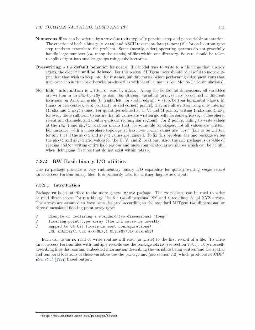
7.3. FORTRAN NATIVE I/O: MDSIO AND RW 441
Numerous files can be written by mdsio due to its typically per-time-step and per-variable orientation.The creation of both a binary (*.data) and ASCII text meta-data (*.meta) file for each output typestep tends to exacerbate the problem. Some (mostly, older) operating systems do not gracefullyhandle large numbers (eg. many thousands) of files within one directory. So care should be takento split output into smaller groups using subdirectories.
Overwriting is the default behavior for mdsio. If a model tries to write to a file name that alreadyexists, the older file will be deleted. For this reason, MITgcm users should be careful to move out-put that that wish to keep into, for instance, subdirectories before performing subsequent runs thatmay over–lap in time or otherwise produce files with identical names (eg. Monte-Carlo simulations).
No “halo” information is written or read by mdsio. Along the horizontal dimensions, all variablesare written in an sNx–by–sNy fashion. So, although variables (arrays) may be defined at differentlocations on Arakawa grids [U (right/left horizontal edges), V (top/bottom horizontal edges), M(mass or cell center), or Z (vorticity or cell corner) points], they are all written using only interior(1:sNx and 1:sNy) values. For quantities defined at U, V, and M points, writing 1:sNx and 1:sNy
for every tile is sufficient to ensure that all values are written globally for some grids (eg. cubesphere,re-entrant channels, and doubly-periodic rectangular regions). For Z points, failing to write valuesat the sNx+1 and sNy+1 locations means that, for some tile topologies, not all values are written.For instance, with a cubesphere topology at least two corner values are “lost” (fail to be writtenfor any tile) if the sNx+1 and sNy+1 values are ignored. To fix this problem, the mnc package writesthe sNx+1 and sNy+1 grid values for the U, V, and Z locations. Also, the mnc package is capable ofreading and/or writing entire halo regions and more complicated array shapes which can be helpfulwhen debugging–features that do not exist within mdsio.
7.3.2 RW Basic binary I/O utilities
The rw package provides a very rudimentary binary I/O capability for quickly writing single recorddirect-access Fortran binary files. It is primarily used for writing diagnostic output.
7.3.2.1 Introduction
Package rw is an interface to the more general mdsio package. The rw package can be used to writeor read direct-access Fortran binary files for two-dimensional XY and three-dimensional XYZ arrays.The arrays are assumed to have been declared according to the standard MITgcm two-dimensional orthree-dimensional floating point array type:
C Example of declaring a standard two dimensional "long"
C floating point type array (the _RL macro is usually
C mapped to 64-bit floats in most configurations)
_RL anArray(1-OLx:sNx+OLx,1-OLy:sNy+OLy,nSx,nSy)
Each call to an rw read or write routine will read (or write) to the first record of a file. To writedirect access Fortran files with multiple records use the package mdsio (see section 7.3.1). To write self-describing files that contain embedded information describing the variables being written and the spatialand temporal locations of those variables use the package mnc (see section 7.2) which produces netCDF1
Rew et al. [1997] based output.
1http://www.unidata.ucar.edu/packages/netcdf
442CHAPTER 7. DIAGNOSTICS AND I/O - PACKAGES II, AND POST–PROCESSING UTILITIES
7.4 Monitor: Simulation state monitoring toolkit
7.4.1 Introduction
The monitor package is primarily intended as a convenient method for calculating and writing thefollowing statistics:
minimum, maximum, mean, and standard deviation
for spatially distributed fields. By default, monitor output is sent to the “standard output” channelwhere it appears as ASCII text containing a %MON string such as this example:
(PID.TID 0000.0001) %MON time_tsnumber = 3
(PID.TID 0000.0001) %MON time_secondsf = 3.6000000000000E+03
(PID.TID 0000.0001) %MON dynstat_eta_max = 1.0025466645951E-03
(PID.TID 0000.0001) %MON dynstat_eta_min = -1.0008899950901E-03
(PID.TID 0000.0001) %MON dynstat_eta_mean = 2.1037438449350E-14
(PID.TID 0000.0001) %MON dynstat_eta_sd = 5.0985228723396E-04
(PID.TID 0000.0001) %MON dynstat_eta_del2 = 3.5216706549525E-07
(PID.TID 0000.0001) %MON dynstat_uvel_max = 3.7594045977254E-05
(PID.TID 0000.0001) %MON dynstat_uvel_min = -2.8264287531564E-05
(PID.TID 0000.0001) %MON dynstat_uvel_mean = 9.1369201945671E-06
(PID.TID 0000.0001) %MON dynstat_uvel_sd = 1.6868439193567E-05
(PID.TID 0000.0001) %MON dynstat_uvel_del2 = 8.4315445301916E-08
The monitor text can be readily parsed by the testreport script to determine, somewhat crudely butquickly, how similar the output from two experiments are when run on different platforms or before/aftercode changes.
The monitor output can also be useful for quickly diagnosing practical problems such as CFL limita-tions, model progress (through iteration counts), and behavior within some packages that use it.
7.4.2 Using Monitor
As with most packages, monitor can be turned on or off at compile and/or run times using the packages.confand data.pkg files.
The monitor output can be sent to the standard output channel, to an mnc–generated file, or to bothsimultaneously. For mnc output, the flag:
monitor_mnc=.TRUE.,
should be set within the data.mnc file. For output to both ASCII and mnc, the flag
outputTypesInclusive=.TRUE.,
should be set within the PARM03 section of the main data file. It should be noted that the outputTypesInclusiveflag will make ALL kinds of output (that is, everything written by mdsio, mnc, and monitor) simulta-neously active so it should be used only with caution–and perhaps only for debugging purposes.
7.5. GRID GENERATION 443
7.5 Grid Generation
The horizontal discretizations within MITgcm have been written to work with many different grid typesincluding:
• cartesian coordinates
• spherical polar (“latitude-longitude”) coordinates
• general curvilinear orthogonal coordinates
The last of these, especially when combined with the domain decomposition capabilities of MITgcm,allows a great degree of grid flexibility. To date, general curvilinear orthogonal coordinates have beenused primarily (in fact, almost exclusively) in conjunction with so-called “cube-sphere” grids. However,it is important to observe that cube-sphere arrangements are only one example of what is possiblewith domain-decomposed logically rectangular regions each containing curvilinear orthogonal coordinatesystems. Much more sophisticated domains can be imagined and constructed.
In order to explore the possibilities of domain-decomposed curvilinear orthogonal coordinate systems,a suite of grid generation software called “SPGrid” (for SPherical Gridding) has been developed. SPGridis a relatively new facility and papers detailing its algorithms are in preparation. Althogh SPGrid is newand rapidly developing, it has already demonstrated the ability to generate some useful and interestinggrids.
This section provides a very brief introduction to SPGrid and shows some early results. For furtherinformation, please contact the MITgcm support list at:
7.5.1 Using SPGrid
The SPGrid software is not a single program. Rather, it is a collection of C++ code and MatLAB scriptsthat can be used as a framework or library for grid generation and manipulation. Currently, grid creationis accomplished by either directly running matlab scripts or by writing a C++ “driver” program. Thematlab scripts are suitable for grids composed of a single “face” (that is, a single logically rectangularregion on the surface of a sphere). The C++ driver programs are appropriate for grids composed ofmultiple connected logically rectangular patches. Each driver is program is written to specify the shapeand connectivity of tiles and the preferred grid density (that is, the number of grid cells in each logicaldirection) and edge locations of the cells where they meet the edges of each face. The driver programspass this information to the SPGrid library which generates the actual grid and produces the output filesthat describe it.
Currently, driver programs are available for a few examples including cubes, “lat-lon caps” (cubetopologies that have conformal caps at the poles and are exactly lat-lon channels for the remainder ofthe domain), and some simple “embedded” regions that are meant to be used within typical cubes ortraditional lat-lon grids.
To create new grids, one may start with an existing driver program and modify it to describe a domainthat has a different arrangement. The number, location, size, and connectivity of grid “faces” (the nameused for the logically rectangular regions) can be readily changed. Further, the number of grid cellswithin faces and the location of the grid cells at the face edges can also be specified.
7.5.1.1 SPGrid Requirements
The following programs and libraries are required to build and/or run the SPGrid suite:
• MatLAB is a run-time requirement since many of the generation algorithms have been written asMatLAB scripts:http://www.mathworks.com
• the Wild Magic graphics engine (a C++ library) is needed for the main “driver” code:http://geometrictools.com/
444CHAPTER 7. DIAGNOSTICS AND I/O - PACKAGES II, AND POST–PROCESSING UTILITIES
• the NetCDF library is needed for file I/O:http://www.mathworks.com
• the BOOST Serialization library is used for I/O:http://www.boost.org
• a typical Linux/Unix build environment including the make utility (preferably Gnu Make) and aC++ compiler (SPGrid was developed with g++ v4.x).
7.5.1.2 Obtaining SPGrid
The latest version can be obtained from:
http://mitgcm.org/∼edhill/grids/spgrid releases/
7.5.1.3 Building SPGrid
The procedure for building is similar to many open source projects:
tar -xf spgrid-0.9.4.tar.gz
cd spgrid-0.9.4
export CPPFLAGS="-I/usr/include/netcdf-3"
export LDFLAGS="-L/usr/lib/netcdf-3"
./configure
make
where the CPPFLAGS and LDFLAGS environment variables can be edited to reflect the locations of all thenecessary dependencies. SPGrid is known to work on Fedora Core Linux (versions 4 and 5) and is likelyto work on most any Linux distribution that provides the needed dependencies.
7.5.1.4 Running SPGrid
Within the src sub-directory, various example driver programs exist. These examples describe small,simple domains and can generate the input files (formatted as either binary *.mitgrid or netCDF) usedby MITgcm.
One such example is called “SpF test cube cap” and it can be run with the following sequence ofcommands:
cd spgrid-0.9.4/src
make SpF_test_cube_cap
mkdir SpF_test_cube_cap.d
( cd SpF_test_cube_cap.d && ln -s ../../scripts/*.m . )
./SpF_test_cube_cap
which should create a series of output files:
SpF_test_cube_cap.d/grid_*.mitgrid
SpF_test_cube_cap.d/grid_*.nc
SpF_test_cube_cap.d/std_topology.nc
where the grid *.mitgrid and grid *.nc files contain the grid information in binary and netCDFformats and the std topology.nc file contains the information describing the connectivity (both edge–edge and corner–corner contacts) between all the faces.
7.5.2 Example Grids
The following grids are various examples created with SPGrid.
7.6. PRE– AND POST–PROCESSING SCRIPTS AND UTILITIES 445
7.6 Pre– and Post–Processing Scripts and Utilities
There are numerous tools for pre-processing data, converting model output and analysis written in Matlab,fortran (f77 and f90) and perl. As yet they remain undocumented although many are self-documenting(Matlab routines have ”help” written into them).
Here we’ll summarize what is available but this is an ever growing resource so this may not covereverything that is out there:
7.6.1 Utilities supplied with the model
We supply some basic scripts with the model to facilitate conversion or reading of data into analysissoftware.
7.6.1.1 utils/scripts
In the directory utils/scripts you will find joinds and joinmds: these are perl scripts used from joiningthe multi-part files created by MITgcm. Use joinmds always. You will only need joinds if you areworking with output older than two years (prior to c23).
7.6.1.2 utils/matlab
In the directory utils/matlab you will find several Matlab scripts (.m or dot-em files). The priniciplescript is rdmds.m used for reading the multi-part model output files in to matlab. Place the scripts inyour matlab path or change the path appropriately, then at the matlab prompt type:
>> help rdmds
to get help on how to use rdmds.Another useful script scans the terminal output file for ”monitor” information.Most other scripts are for working in the curvilinear coordinate systems which as yet are unpublished
and undocumented.
7.6.1.3 MNC Utils
The MITgcm netCDF integration is relatively new and the tools used to work on netCDF data sets aredeveloping. The following scripts and utilities have been written to help manipulate MNC (netCDF)files:
Tile Assembly: a matlab script utils/matlab/mnc assembly.m is available for spatially “assembling”MNC output. A convenience wrapper script called utils/matlab/gluemnc.m is also provided.Please use the matlab help facility for more information.
gmt: As MITgcm evolves to handle more complicated domains and topologies, a suite of matlab toolsis being written to more gracefully handle the model files. This suite is called “gmt” which refersto “generalized model topology” pre-/post-processing. Currently, this directory contains a matlabscript utils/matlab/gmt/rdnctiles.m that is able to read the MNC-created netCDF files for anydomain. Additional scripts are being created that will work with these fields on a per-tile basis.
7.6.2 Pre-processing software
There is a suite of pre-processing software for intepolating bathymetry and forcing data, written byAdcroft and Biastoch. At some point, these will be made available for download. If you are in need ofsuch software, contact one of them.
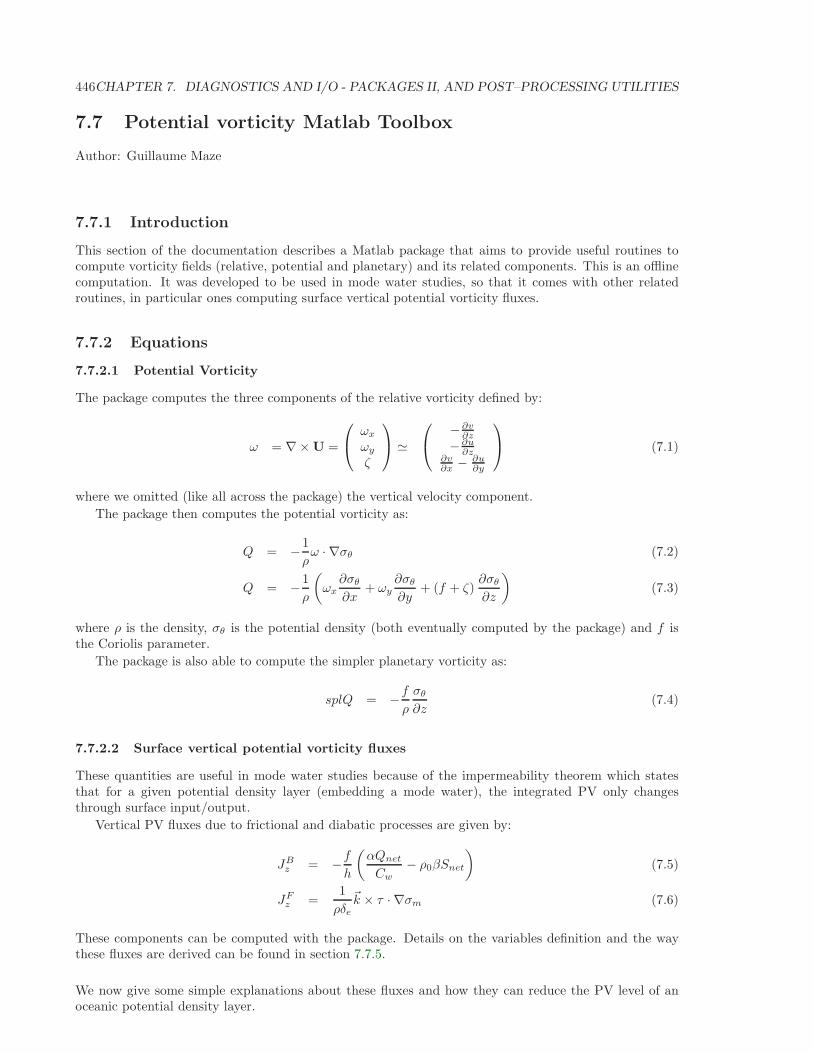
446CHAPTER 7. DIAGNOSTICS AND I/O - PACKAGES II, AND POST–PROCESSING UTILITIES
7.7 Potential vorticity Matlab Toolbox
Author: Guillaume Maze
7.7.1 Introduction
This section of the documentation describes a Matlab package that aims to provide useful routines tocompute vorticity fields (relative, potential and planetary) and its related components. This is an offlinecomputation. It was developed to be used in mode water studies, so that it comes with other relatedroutines, in particular ones computing surface vertical potential vorticity fluxes.
7.7.2 Equations
7.7.2.1 Potential Vorticity
The package computes the three components of the relative vorticity defined by:
ω = ∇× U =
ωx
ωy
ζ
≃
−∂v∂z
−∂u∂z
∂v∂x − ∂u
∂y
(7.1)
where we omitted (like all across the package) the vertical velocity component.
The package then computes the potential vorticity as:
Q = −1
ρω · ∇σθ (7.2)
Q = −1
ρ
(ωx∂σθ
∂x+ ωy
∂σθ
∂y+ (f + ζ)
∂σθ
∂z
)(7.3)
where ρ is the density, σθ is the potential density (both eventually computed by the package) and f isthe Coriolis parameter.
The package is also able to compute the simpler planetary vorticity as:
splQ = −fρ
σθ
∂z(7.4)
7.7.2.2 Surface vertical potential vorticity fluxes
These quantities are useful in mode water studies because of the impermeability theorem which statesthat for a given potential density layer (embedding a mode water), the integrated PV only changesthrough surface input/output.
Vertical PV fluxes due to frictional and diabatic processes are given by:
JBz = −f
h
(αQnet
Cw− ρ0βSnet
)(7.5)
JFz =
1
ρδe~k × τ · ∇σm (7.6)
These components can be computed with the package. Details on the variables definition and the waythese fluxes are derived can be found in section 7.7.5.
We now give some simple explanations about these fluxes and how they can reduce the PV level of anoceanic potential density layer.
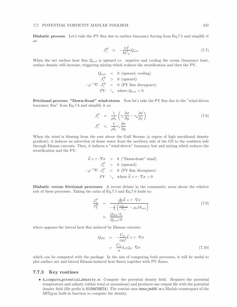
7.7. POTENTIAL VORTICITY MATLAB TOOLBOX 447
Diabatic process Let’s take the PV flux due to surface buoyancy forcing from Eq.7.5 and simplify itas:
JBz ≃ − αf
hCwQnet (7.7)
When the net surface heat flux Qnet is upward i.e. negative and cooling the ocean (buoyancy loss),surface density will increase, triggering mixing which reduces the stratification and then the PV.
Qnet < 0 (upward, cooling)
JBz > 0 (upward)
−ρ−1∇ · JBz < 0 (PV flux divergence)
PV ց where Qnet < 0
Frictional process: ”Down-front” wind-stress Now let’s take the PV flux due to the ”wind-drivenbuoyancy flux” from Eq.7.6 and simplify it as:
JFz =
1
ρδe
(τx∂σ
∂y− τy
∂σ
∂x
)(7.8)
JFz ≃ 1
ρδeτx∂σ
∂y
When the wind is blowing from the east above the Gulf Stream (a region of high meridional densitygradient), it induces an advection of dense water from the northern side of the GS to the southern sidethrough Ekman currents. Then, it induces a ”wind-driven” buoyancy lost and mixing which reduces thestratification and the PV.
~k × τ · ∇σ > 0 (”Down-front” wind)
JFz > 0 (upward)
−ρ−1∇ · JFz < 0 (PV flux divergence)
PV ց where ~k × τ · ∇σ > 0
Diabatic versus frictional processes A recent debate in the community arose about the relativerole of these processes. Taking the ratio of Eq.7.5 and Eq.7.6 leads to:
JFz
JBZ
=
1ρδe
~k × τ · ∇σ
− fh
(αQnet
Cw− ρ0βSnet
) (7.9)
≃ QEk/δeQnet/h
where appears the lateral heat flux induced by Ekman currents:
QEk = − Cw
αρf~k × τ · ∇σ
=Cw
αδe ~uEk · ∇σ (7.10)
which can be computed with the package. In the aim of comparing both processes, it will be useful toplot surface net and lateral Ekman-induced heat fluxes together with PV fluxes.
7.7.3 Key routines
• A compute potential density.m: Compute the potential density field. Requires the potentialtemperature and salinity (either total or anomalous) and produces one output file with the potentialdensity field (file prefix is SIGMATHETA). The routine uses densjmd95.m a Matlab counterpart of theMITgcm built-in function to compute the density.
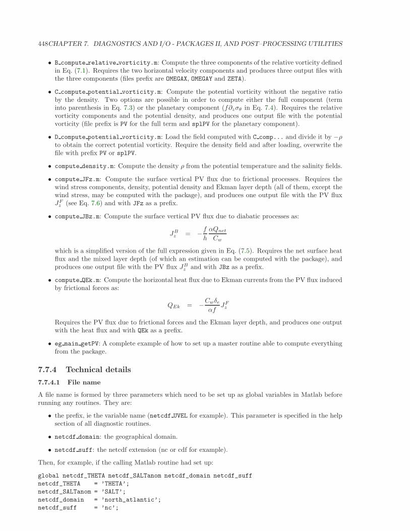
448CHAPTER 7. DIAGNOSTICS AND I/O - PACKAGES II, AND POST–PROCESSING UTILITIES
• B compute relative vorticity.m: Compute the three components of the relative vorticity definedin Eq. (7.1). Requires the two horizontal velocity components and produces three output files withthe three components (files prefix are OMEGAX, OMEGAY and ZETA).
• C compute potential vorticity.m: Compute the potential vorticity without the negative ratioby the density. Two options are possible in order to compute either the full component (terminto parenthesis in Eq. 7.3) or the planetary component (f∂zσθ in Eq. 7.4). Requires the relativevorticity components and the potential density, and produces one output file with the potentialvorticity (file prefix is PV for the full term and splPV for the planetary component).
• D compute potential vorticity.m: Load the field computed with C comp... and divide it by −ρto obtain the correct potential vorticity. Require the density field and after loading, overwrite thefile with prefix PV or splPV.
• compute density.m: Compute the density ρ from the potential temperature and the salinity fields.
• compute JFz.m: Compute the surface vertical PV flux due to frictional processes. Requires thewind stress components, density, potential density and Ekman layer depth (all of them, except thewind stress, may be computed with the package), and produces one output file with the PV fluxJF
z (see Eq. 7.6) and with JFz as a prefix.
• compute JBz.m: Compute the surface vertical PV flux due to diabatic processes as:
JBz = −f
h
αQnet
Cw
which is a simplified version of the full expression given in Eq. (7.5). Requires the net surface heatflux and the mixed layer depth (of which an estimation can be computed with the package), andproduces one output file with the PV flux JB
z and with JBz as a prefix.
• compute QEk.m: Compute the horizontal heat flux due to Ekman currents from the PV flux inducedby frictional forces as:
QEk = −Cwδeαf
JFz
Requires the PV flux due to frictional forces and the Ekman layer depth, and produces one outputwith the heat flux and with QEk as a prefix.
• eg main getPV: A complete example of how to set up a master routine able to compute everythingfrom the package.
7.7.4 Technical details
7.7.4.1 File name
A file name is formed by three parameters which need to be set up as global variables in Matlab beforerunning any routines. They are:
• the prefix, ie the variable name (netcdf UVEL for example). This parameter is specified in the helpsection of all diagnostic routines.
• netcdf domain: the geographical domain.
• netcdf suff: the netcdf extension (nc or cdf for example).
Then, for example, if the calling Matlab routine had set up:
global netcdf_THETA netcdf_SALTanom netcdf_domain netcdf_suff
netcdf_THETA = ’THETA’;
netcdf_SALTanom = ’SALT’;
netcdf_domain = ’north_atlantic’;
netcdf_suff = ’nc’;
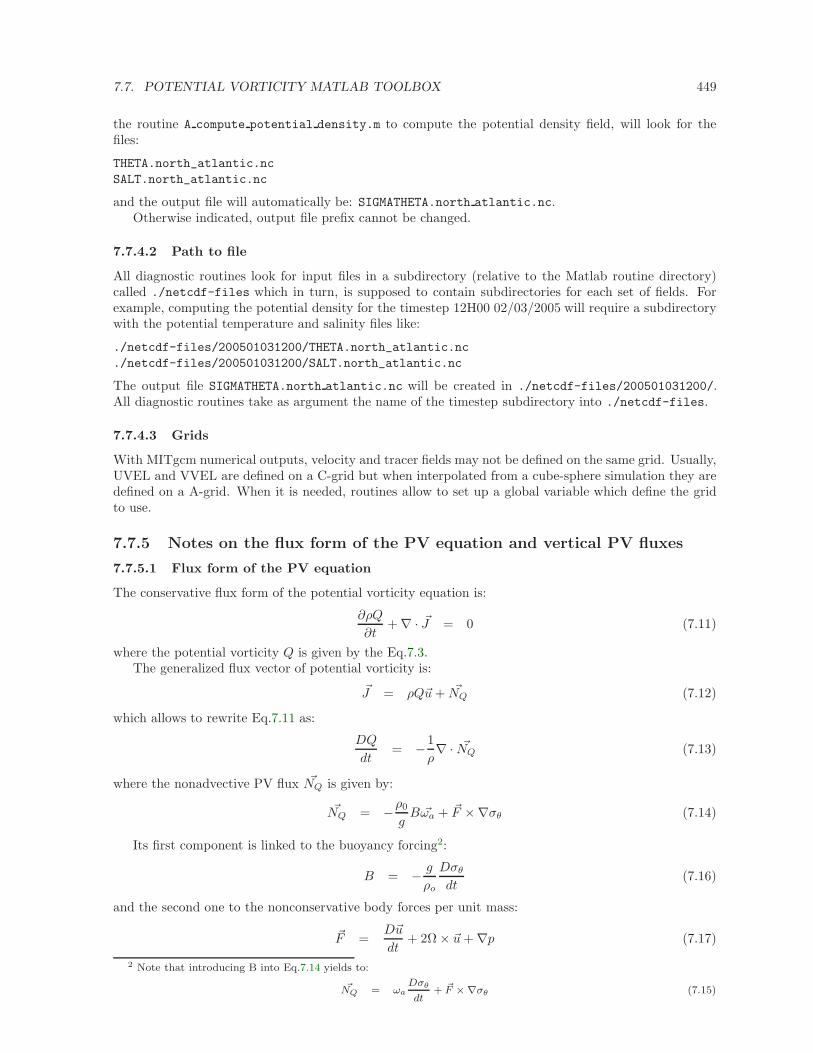
7.7. POTENTIAL VORTICITY MATLAB TOOLBOX 449
the routine A compute potential density.m to compute the potential density field, will look for thefiles:
THETA.north_atlantic.nc
SALT.north_atlantic.nc
and the output file will automatically be: SIGMATHETA.north atlantic.nc.Otherwise indicated, output file prefix cannot be changed.
7.7.4.2 Path to file
All diagnostic routines look for input files in a subdirectory (relative to the Matlab routine directory)called ./netcdf-files which in turn, is supposed to contain subdirectories for each set of fields. Forexample, computing the potential density for the timestep 12H00 02/03/2005 will require a subdirectorywith the potential temperature and salinity files like:
./netcdf-files/200501031200/THETA.north_atlantic.nc
./netcdf-files/200501031200/SALT.north_atlantic.nc
The output file SIGMATHETA.north atlantic.nc will be created in ./netcdf-files/200501031200/.All diagnostic routines take as argument the name of the timestep subdirectory into ./netcdf-files.
7.7.4.3 Grids
With MITgcm numerical outputs, velocity and tracer fields may not be defined on the same grid. Usually,UVEL and VVEL are defined on a C-grid but when interpolated from a cube-sphere simulation they aredefined on a A-grid. When it is needed, routines allow to set up a global variable which define the gridto use.
7.7.5 Notes on the flux form of the PV equation and vertical PV fluxes
7.7.5.1 Flux form of the PV equation
The conservative flux form of the potential vorticity equation is:
∂ρQ
∂t+ ∇ · ~J = 0 (7.11)
where the potential vorticity Q is given by the Eq.7.3.The generalized flux vector of potential vorticity is:
~J = ρQ~u+ ~NQ (7.12)
which allows to rewrite Eq.7.11 as:
DQ
dt= −1
ρ∇ · ~NQ (7.13)
where the nonadvective PV flux ~NQ is given by:
~NQ = −ρ0
gB ~ωa + ~F ×∇σθ (7.14)
Its first component is linked to the buoyancy forcing2:
B = − g
ρo
Dσθ
dt(7.16)
and the second one to the nonconservative body forces per unit mass:
~F =D~u
dt+ 2Ω × ~u+ ∇p (7.17)
2 Note that introducing B into Eq.7.14 yields to:
~NQ = ωaDσθ
dt+ ~F ×∇σθ (7.15)
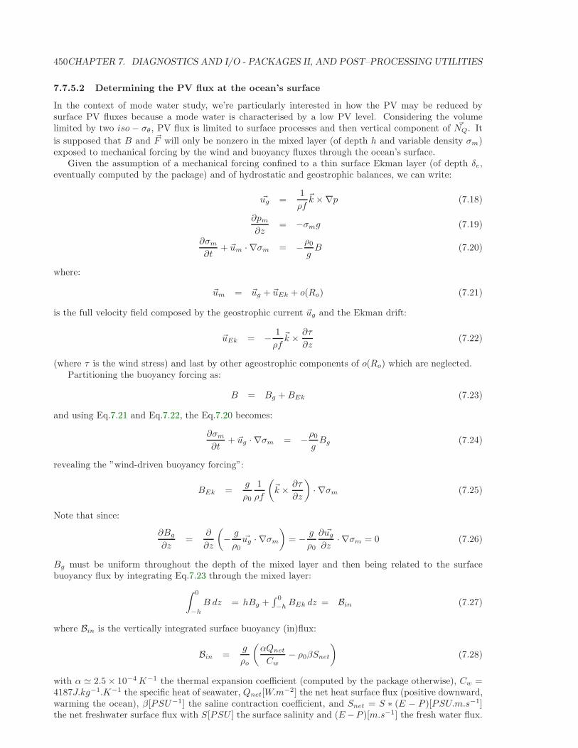
450CHAPTER 7. DIAGNOSTICS AND I/O - PACKAGES II, AND POST–PROCESSING UTILITIES
7.7.5.2 Determining the PV flux at the ocean’s surface
In the context of mode water study, we’re particularly interested in how the PV may be reduced bysurface PV fluxes because a mode water is characterised by a low PV level. Considering the volumelimited by two iso − σθ, PV flux is limited to surface processes and then vertical component of ~NQ. It
is supposed that B and ~F will only be nonzero in the mixed layer (of depth h and variable density σm)exposed to mechanical forcing by the wind and buoyancy fluxes through the ocean’s surface.
Given the assumption of a mechanical forcing confined to a thin surface Ekman layer (of depth δe,eventually computed by the package) and of hydrostatic and geostrophic balances, we can write:
~ug =1
ρf~k ×∇p (7.18)
∂pm
∂z= −σmg (7.19)
∂σm
∂t+ ~um · ∇σm = −ρ0
gB (7.20)
where:
~um = ~ug + ~uEk + o(Ro) (7.21)
is the full velocity field composed by the geostrophic current ~ug and the Ekman drift:
~uEk = − 1
ρf~k × ∂τ
∂z(7.22)
(where τ is the wind stress) and last by other ageostrophic components of o(Ro) which are neglected.Partitioning the buoyancy forcing as:
B = Bg +BEk (7.23)
and using Eq.7.21 and Eq.7.22, the Eq.7.20 becomes:
∂σm
∂t+ ~ug · ∇σm = −ρ0
gBg (7.24)
revealing the ”wind-driven buoyancy forcing”:
BEk =g
ρ0
1
ρf
(~k × ∂τ
∂z
)· ∇σm (7.25)
Note that since:
∂Bg
∂z=
∂
∂z
(− g
ρ0~ug · ∇σm
)= − g
ρ0
∂ ~ug
∂z· ∇σm = 0 (7.26)
Bg must be uniform throughout the depth of the mixed layer and then being related to the surfacebuoyancy flux by integrating Eq.7.23 through the mixed layer:
∫ 0
−h
B dz = hBg +∫ 0
−hBEk dz = Bin (7.27)
where Bin is the vertically integrated surface buoyancy (in)flux:
Bin =g
ρo
(αQnet
Cw− ρ0βSnet
)(7.28)
with α ≃ 2.5 × 10⁻⁴K−1 the thermal expansion coefficient (computed by the package otherwise), Cw =4187J.kg−1.K−1 the specific heat of seawater, Qnet[W.m
−2] the net heat surface flux (positive downward,warming the ocean), β[PSU−1] the saline contraction coefficient, and Snet = S ∗ (E − P )[PSU.m.s−1]the net freshwater surface flux with S[PSU ] the surface salinity and (E−P )[m.s−1] the fresh water flux.
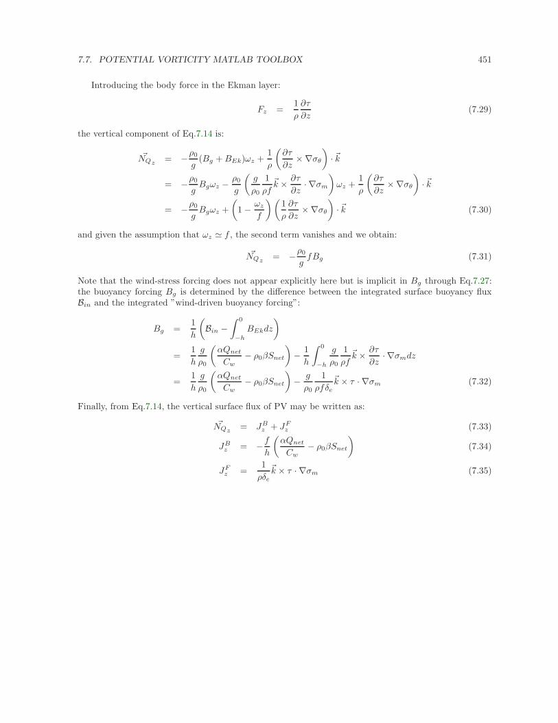
7.7. POTENTIAL VORTICITY MATLAB TOOLBOX 451
Introducing the body force in the Ekman layer:
Fz =1
ρ
∂τ
∂z(7.29)
the vertical component of Eq.7.14 is:
~NQz = −ρ0
g(Bg +BEk)ωz +
1
ρ
(∂τ
∂z×∇σθ
)· ~k
= −ρ0
gBgωz −
ρ0
g
(g
ρ0
1
ρf~k × ∂τ
∂z· ∇σm
)ωz +
1
ρ
(∂τ
∂z×∇σθ
)· ~k
= −ρ0
gBgωz +
(1 − ωz
f
)(1
ρ
∂τ
∂z×∇σθ
)· ~k (7.30)
and given the assumption that ωz ≃ f , the second term vanishes and we obtain:
~NQz = −ρ0
gfBg (7.31)
Note that the wind-stress forcing does not appear explicitly here but is implicit in Bg through Eq.7.27:the buoyancy forcing Bg is determined by the difference between the integrated surface buoyancy fluxBin and the integrated ”wind-driven buoyancy forcing”:
Bg =1
h
(Bin −
∫ 0
−h
BEkdz
)
=1
h
g
ρ0
(αQnet
Cw− ρ0βSnet
)− 1
h
∫ 0
−h
g
ρ0
1
ρf~k × ∂τ
∂z· ∇σmdz
=1
h
g
ρ0
(αQnet
Cw− ρ0βSnet
)− g
ρ0
1
ρfδe~k × τ · ∇σm (7.32)
Finally, from Eq.7.14, the vertical surface flux of PV may be written as:
~NQz = JBz + JF
z (7.33)
JBz = −f
h
(αQnet
Cw− ρ0βSnet
)(7.34)
JFz =
1
ρδe~k × τ · ∇σm (7.35)

452CHAPTER 7. DIAGNOSTICS AND I/O - PACKAGES II, AND POST–PROCESSING UTILITIES
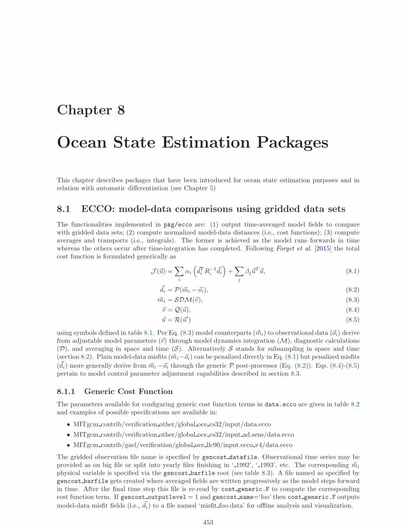
Chapter 8
Ocean State Estimation Packages
This chapter describes packages that have been introduced for ocean state estimation purposes and inrelation with automatic differentiation (see Chapter 5)
8.1 ECCO: model-data comparisons using gridded data sets
The functionalities implemented in pkg/ecco are: (1) output time-averaged model fields to comparewith gridded data sets; (2) compute normalized model-data distances (i.e., cost functions); (3) computeaverages and transports (i.e., integrals). The former is achieved as the model runs forwards in timewhereas the others occur after time-integration has completed. Following Forget et al. [2015] the totalcost function is formulated generically as
J (~u) =∑
i
αi
(~dTi R−1i~di
)+∑
j
βj~uT~u, (8.1)
~di = P(~mi − ~oi), (8.2)
~mi = SDM(~v), (8.3)
~v = Q(~u), (8.4)
~u = R(~u′) (8.5)
using symbols defined in table 8.1. Per Eq. (8.3) model counterparts (~mi) to observational data (~oi) derivefrom adjustable model parameters (~v) through model dynamics integration (M), diagnostic calculations(D), and averaging in space and time (S). Alternatively S stands for subsampling in space and time(section 8.2). Plain model-data misfits (~mi−~oi) can be penalized directly in Eq. (8.1) but penalized misfits
(~di) more generally derive from ~mi−~oi through the generic P post-processor (Eq. (8.2)). Eqs. (8.4)-(8.5)pertain to model control parameter adjustment capabilities described in section 8.3.
8.1.1 Generic Cost Function
The parameters available for configuring generic cost function terms in data.ecco are given in table 8.2and examples of possible specifications are available in:
• MITgcm contrib/verification other/global oce cs32/input/data.ecco
• MITgcm contrib/verification other/global oce cs32/input ad.sens/data.ecco
• MITgcm contrib/gael/verification/global oce llc90/input.ecco v4/data.ecco
The gridded observation file name is specified by gencost datafile. Observational time series may beprovided as on big file or split into yearly files finishing in ‘ 1992’, ‘ 1993’, etc. The corresponding ~mi
physical variable is specified via the gencost barfile root (see table 8.3). A file named as specified bygencost barfile gets created where averaged fields are written progressively as the model steps forwardin time. After the final time step this file is re-read by cost generic.F to compute the correspondingcost function term. If gencost outputlevel = 1 and gencost name=‘foo’ then cost generic.F outputs
model-data misfit fields (i.e., ~di) to a file named ‘misfit foo.data’ for offline analysis and visualization.
453
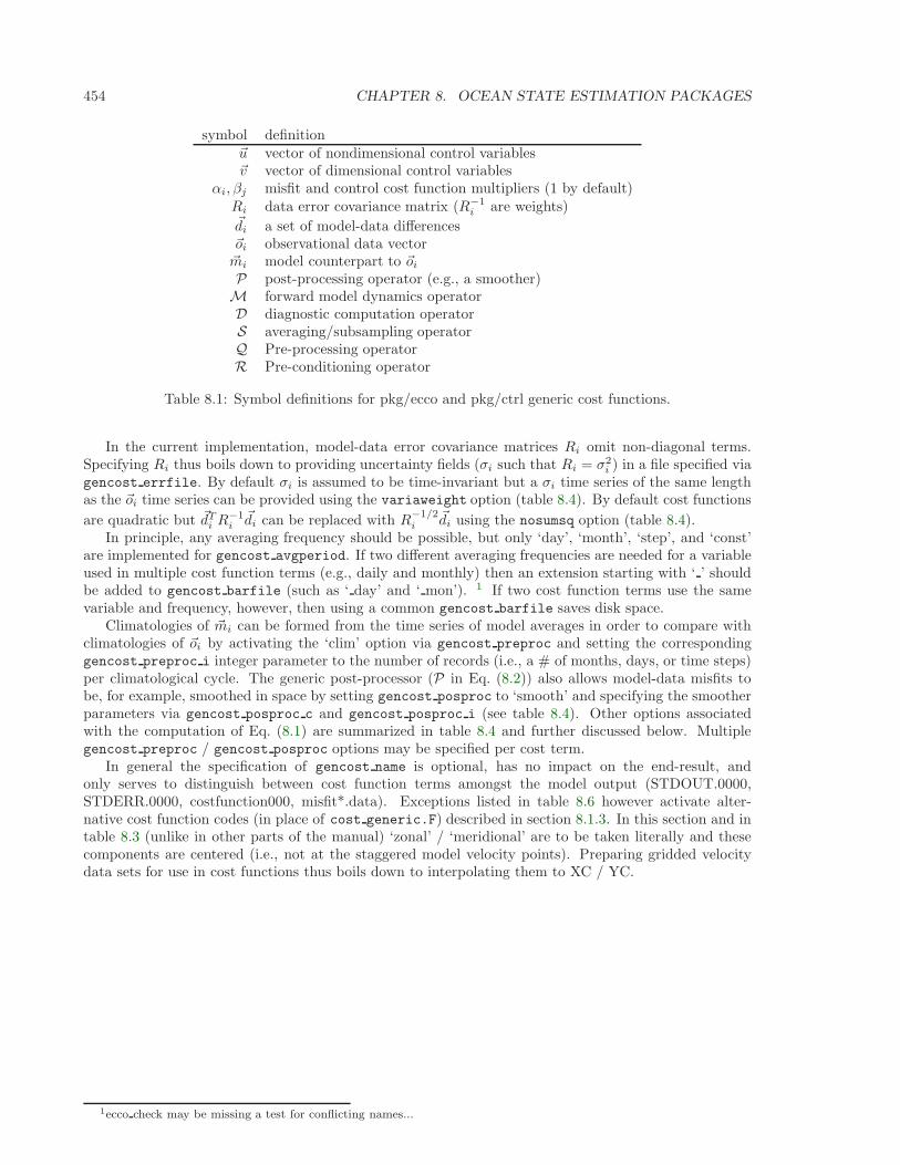
454 CHAPTER 8. OCEAN STATE ESTIMATION PACKAGES
symbol definition~u vector of nondimensional control variables~v vector of dimensional control variables
αi, βj misfit and control cost function multipliers (1 by default)Ri data error covariance matrix (R−1
i are weights)~di a set of model-data differences~oi observational data vector~mi model counterpart to ~oi
P post-processing operator (e.g., a smoother)M forward model dynamics operatorD diagnostic computation operatorS averaging/subsampling operatorQ Pre-processing operatorR Pre-conditioning operator
Table 8.1: Symbol definitions for pkg/ecco and pkg/ctrl generic cost functions.
In the current implementation, model-data error covariance matrices Ri omit non-diagonal terms.Specifying Ri thus boils down to providing uncertainty fields (σi such that Ri = σ2
i ) in a file specified viagencost errfile. By default σi is assumed to be time-invariant but a σi time series of the same lengthas the ~oi time series can be provided using the variaweight option (table 8.4). By default cost functions
are quadratic but ~dTi R−1i~di can be replaced with R
−1/2i
~di using the nosumsq option (table 8.4).In principle, any averaging frequency should be possible, but only ‘day’, ‘month’, ‘step’, and ‘const’
are implemented for gencost avgperiod. If two different averaging frequencies are needed for a variableused in multiple cost function terms (e.g., daily and monthly) then an extension starting with ‘ ’ shouldbe added to gencost barfile (such as ‘ day’ and ‘ mon’). 1 If two cost function terms use the samevariable and frequency, however, then using a common gencost barfile saves disk space.
Climatologies of ~mi can be formed from the time series of model averages in order to compare withclimatologies of ~oi by activating the ‘clim’ option via gencost preproc and setting the correspondinggencost preproc i integer parameter to the number of records (i.e., a # of months, days, or time steps)per climatological cycle. The generic post-processor (P in Eq. (8.2)) also allows model-data misfits tobe, for example, smoothed in space by setting gencost posproc to ‘smooth’ and specifying the smootherparameters via gencost posproc c and gencost posproc i (see table 8.4). Other options associatedwith the computation of Eq. (8.1) are summarized in table 8.4 and further discussed below. Multiplegencost preproc / gencost posproc options may be specified per cost term.
In general the specification of gencost name is optional, has no impact on the end-result, andonly serves to distinguish between cost function terms amongst the model output (STDOUT.0000,STDERR.0000, costfunction000, misfit*.data). Exceptions listed in table 8.6 however activate alter-native cost function codes (in place of cost generic.F) described in section 8.1.3. In this section and intable 8.3 (unlike in other parts of the manual) ‘zonal’ / ‘meridional’ are to be taken literally and thesecomponents are centered (i.e., not at the staggered model velocity points). Preparing gridded velocitydata sets for use in cost functions thus boils down to interpolating them to XC / YC.
1ecco check may be missing a test for conflicting names...
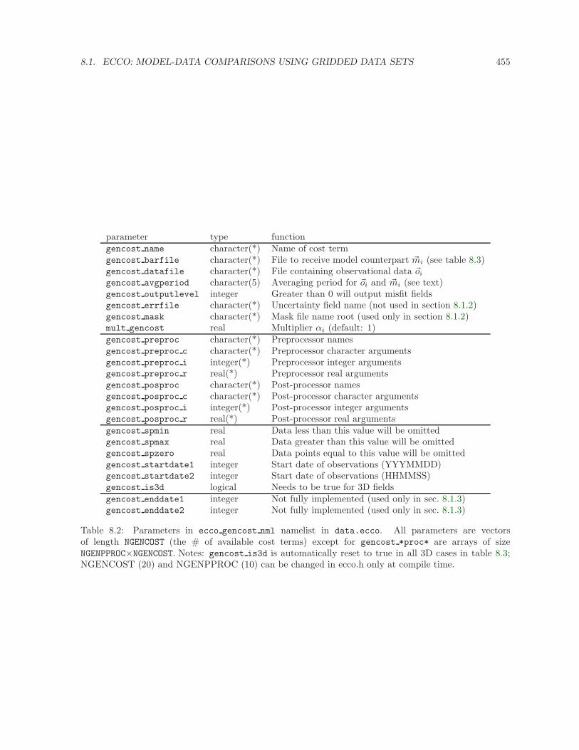
8.1. ECCO: MODEL-DATA COMPARISONS USING GRIDDED DATA SETS 455
parameter type functiongencost name character(*) Name of cost termgencost barfile character(*) File to receive model counterpart ~mi (see table 8.3)gencost datafile character(*) File containing observational data ~oi
gencost avgperiod character(5) Averaging period for ~oi and ~mi (see text)gencost outputlevel integer Greater than 0 will output misfit fieldsgencost errfile character(*) Uncertainty field name (not used in section 8.1.2)gencost mask character(*) Mask file name root (used only in section 8.1.2)mult gencost real Multiplier αi (default: 1)gencost preproc character(*) Preprocessor namesgencost preproc c character(*) Preprocessor character argumentsgencost preproc i integer(*) Preprocessor integer argumentsgencost preproc r real(*) Preprocessor real argumentsgencost posproc character(*) Post-processor namesgencost posproc c character(*) Post-processor character argumentsgencost posproc i integer(*) Post-processor integer argumentsgencost posproc r real(*) Post-processor real argumentsgencost spmin real Data less than this value will be omittedgencost spmax real Data greater than this value will be omittedgencost spzero real Data points equal to this value will be omittedgencost startdate1 integer Start date of observations (YYYMMDD)gencost startdate2 integer Start date of observations (HHMMSS)gencost is3d logical Needs to be true for 3D fieldsgencost enddate1 integer Not fully implemented (used only in sec. 8.1.3)gencost enddate2 integer Not fully implemented (used only in sec. 8.1.3)
Table 8.2: Parameters in ecco gencost nml namelist in data.ecco. All parameters are vectorsof length NGENCOST (the # of available cost terms) except for gencost *proc* are arrays of sizeNGENPPROC×NGENCOST. Notes: gencost is3d is automatically reset to true in all 3D cases in table 8.3;NGENCOST (20) and NGENPPROC (10) can be changed in ecco.h only at compile time.
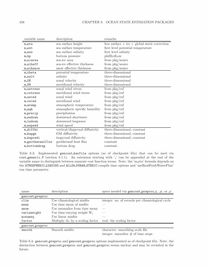
456 CHAPTER 8. OCEAN STATE ESTIMATION PACKAGES
variable name description remarks
m eta sea surface height free surface + ice + global steric correctionm sst sea surface temperature first level potential temperaturem sss sea surface salinity first level salinitym bp bottom pressure phiHydLowm siarea sea-ice area from pkg/seaicem siheff sea-ice effective thickness from pkg/seaicem sihsnow snow effective thickness from pkg/seaicem theta potential temperature three-dimensionalm salt salinity three-dimensionalm UE zonal velocity three-dimensionalm VN meridional velocity three-dimensionalm ustress zonal wind stress from pkg/exfm vstress meridional wind stress from pkg/exfm uwind zonal wind from pkg/exfm vwind meridional wind from pkg/exfm atemp atmospheric temperature from pkg/exfm aqh atmospheric specific humidity from pkg/exfm precip precipitation from pkg/exfm swdown downward shortwave from pkg/exfm lwdown downward longwave from pkg/exfm wspeed wind speed from pkg/exfm diffkr vertical/diapycnal diffusivity three-dimensional, constantm kapgm GM diffusivity three-dimensional, constantm kapredi isopycnal diffusivity three-dimensional, constantm geothermalflux geothermal heat flux constantm bottomdrag bottom drag constant
Table 8.3: Implemented gencost barfile options (as of checkpoint 65z) that can be used viacost generic.F (section 8.1.1). An extension starting with ‘ ’ can be appended at the end of thevariable name to distinguish between separate cost function terms. Note: the ‘m eta’ formula depends onthe ATMOSPHERIC LOADING and ALLOW PSBAR STERIC compile time options and ‘useRealFreshWaterFlux’run time parameter.
name description specs needed via gencost preproc i, r, or c
gencost preproc
clim Use climatological misfits integer: no. of records per climatological cyclemean Use time mean of misfits —anom Use anomalies from time mean —variaweight Use time-varying weight Wi —nosumsq Use linear misfits —factor Multiply ~mi by a scaling factor real: the scaling factor
gencost posproc
smooth Smooth misfits character: smoothing scale fileinteger: smoother # of time steps
Table 8.4: gencost preproc and gencost posproc options implemented as of checkpoint 65z. Note: thedistinction between gencost preproc and gencost posproc seems unclear and may be revisited in thefuture.
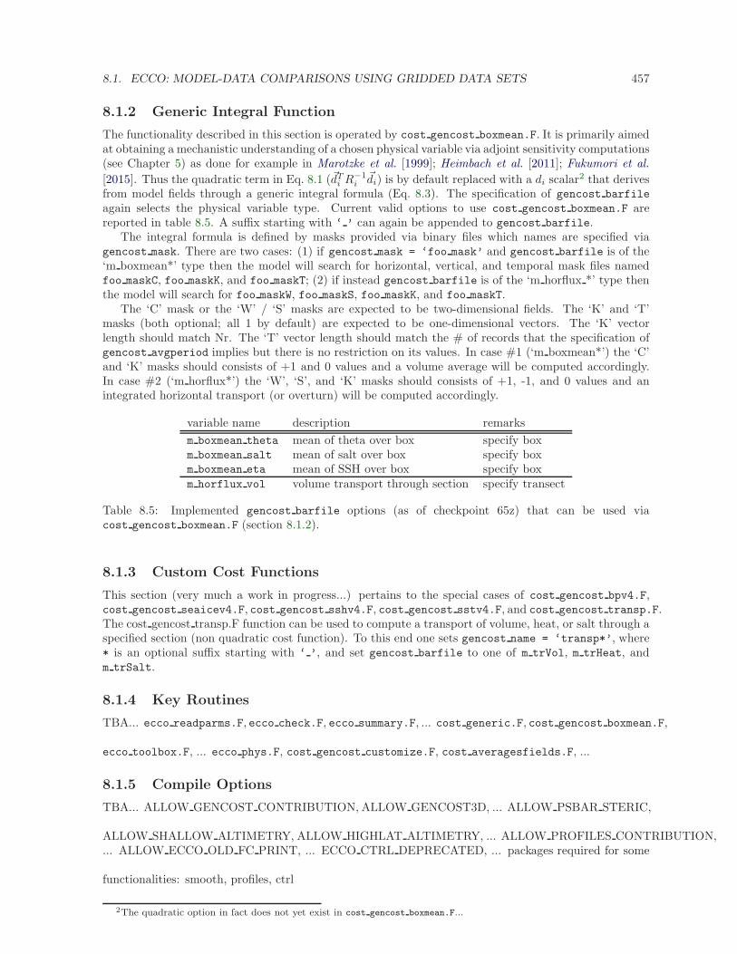
8.1. ECCO: MODEL-DATA COMPARISONS USING GRIDDED DATA SETS 457
8.1.2 Generic Integral Function
The functionality described in this section is operated by cost gencost boxmean.F. It is primarily aimedat obtaining a mechanistic understanding of a chosen physical variable via adjoint sensitivity computations(see Chapter 5) as done for example in Marotzke et al. [1999]; Heimbach et al. [2011]; Fukumori et al.
[2015]. Thus the quadratic term in Eq. 8.1 (~dTi R−1i~di) is by default replaced with a di scalar2 that derives
from model fields through a generic integral formula (Eq. 8.3). The specification of gencost barfile
again selects the physical variable type. Current valid options to use cost gencost boxmean.F arereported in table 8.5. A suffix starting with ‘ ’ can again be appended to gencost barfile.
The integral formula is defined by masks provided via binary files which names are specified viagencost mask. There are two cases: (1) if gencost mask = ‘foo mask’ and gencost barfile is of the‘m boxmean*’ type then the model will search for horizontal, vertical, and temporal mask files namedfoo maskC, foo maskK, and foo maskT; (2) if instead gencost barfile is of the ‘m horflux *’ type thenthe model will search for foo maskW, foo maskS, foo maskK, and foo maskT.
The ‘C’ mask or the ‘W’ / ‘S’ masks are expected to be two-dimensional fields. The ‘K’ and ‘T’masks (both optional; all 1 by default) are expected to be one-dimensional vectors. The ‘K’ vectorlength should match Nr. The ‘T’ vector length should match the # of records that the specification ofgencost avgperiod implies but there is no restriction on its values. In case #1 (‘m boxmean*’) the ‘C’and ‘K’ masks should consists of +1 and 0 values and a volume average will be computed accordingly.In case #2 (‘m horflux*’) the ‘W’, ‘S’, and ‘K’ masks should consists of +1, -1, and 0 values and anintegrated horizontal transport (or overturn) will be computed accordingly.
variable name description remarks
m boxmean theta mean of theta over box specify boxm boxmean salt mean of salt over box specify boxm boxmean eta mean of SSH over box specify boxm horflux vol volume transport through section specify transect
Table 8.5: Implemented gencost barfile options (as of checkpoint 65z) that can be used viacost gencost boxmean.F (section 8.1.2).
8.1.3 Custom Cost Functions
This section (very much a work in progress...) pertains to the special cases of cost gencost bpv4.F,cost gencost seaicev4.F, cost gencost sshv4.F, cost gencost sstv4.F, and cost gencost transp.F.The cost gencost transp.F function can be used to compute a transport of volume, heat, or salt through aspecified section (non quadratic cost function). To this end one sets gencost name = ‘transp*’, where* is an optional suffix starting with ‘ ’, and set gencost barfile to one of m trVol, m trHeat, andm trSalt.
8.1.4 Key Routines
TBA... ecco readparms.F, ecco check.F, ecco summary.F, ... cost generic.F, cost gencost boxmean.F,
ecco toolbox.F, ... ecco phys.F, cost gencost customize.F, cost averagesfields.F, ...
8.1.5 Compile Options
TBA... ALLOW GENCOST CONTRIBUTION, ALLOW GENCOST3D, ... ALLOW PSBAR STERIC,
ALLOW SHALLOW ALTIMETRY, ALLOW HIGHLAT ALTIMETRY, ... ALLOW PROFILES CONTRIBUTION,... ALLOW ECCO OLD FC PRINT, ... ECCO CTRL DEPRECATED, ... packages required for some
functionalities: smooth, profiles, ctrl
2The quadratic option in fact does not yet exist in cost gencost boxmean.F...
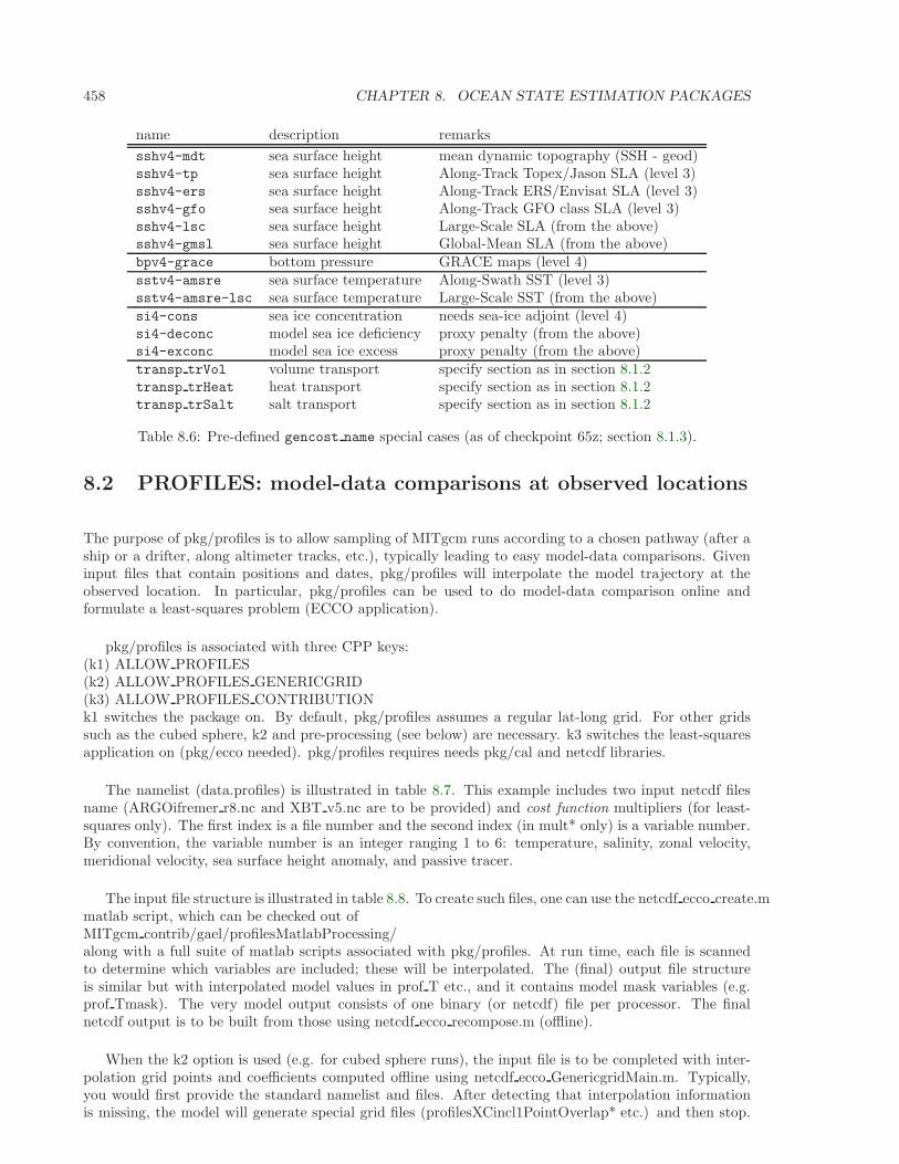
458 CHAPTER 8. OCEAN STATE ESTIMATION PACKAGES
name description remarks
sshv4-mdt sea surface height mean dynamic topography (SSH - geod)sshv4-tp sea surface height Along-Track Topex/Jason SLA (level 3)sshv4-ers sea surface height Along-Track ERS/Envisat SLA (level 3)sshv4-gfo sea surface height Along-Track GFO class SLA (level 3)sshv4-lsc sea surface height Large-Scale SLA (from the above)sshv4-gmsl sea surface height Global-Mean SLA (from the above)bpv4-grace bottom pressure GRACE maps (level 4)sstv4-amsre sea surface temperature Along-Swath SST (level 3)sstv4-amsre-lsc sea surface temperature Large-Scale SST (from the above)si4-cons sea ice concentration needs sea-ice adjoint (level 4)si4-deconc model sea ice deficiency proxy penalty (from the above)si4-exconc model sea ice excess proxy penalty (from the above)transp trVol volume transport specify section as in section 8.1.2transp trHeat heat transport specify section as in section 8.1.2transp trSalt salt transport specify section as in section 8.1.2
Table 8.6: Pre-defined gencost name special cases (as of checkpoint 65z; section 8.1.3).
8.2 PROFILES: model-data comparisons at observed locations
The purpose of pkg/profiles is to allow sampling of MITgcm runs according to a chosen pathway (after aship or a drifter, along altimeter tracks, etc.), typically leading to easy model-data comparisons. Giveninput files that contain positions and dates, pkg/profiles will interpolate the model trajectory at theobserved location. In particular, pkg/profiles can be used to do model-data comparison online andformulate a least-squares problem (ECCO application).
pkg/profiles is associated with three CPP keys:(k1) ALLOW PROFILES(k2) ALLOW PROFILES GENERICGRID(k3) ALLOW PROFILES CONTRIBUTIONk1 switches the package on. By default, pkg/profiles assumes a regular lat-long grid. For other gridssuch as the cubed sphere, k2 and pre-processing (see below) are necessary. k3 switches the least-squaresapplication on (pkg/ecco needed). pkg/profiles requires needs pkg/cal and netcdf libraries.
The namelist (data.profiles) is illustrated in table 8.7. This example includes two input netcdf filesname (ARGOifremer r8.nc and XBT v5.nc are to be provided) and cost function multipliers (for least-squares only). The first index is a file number and the second index (in mult* only) is a variable number.By convention, the variable number is an integer ranging 1 to 6: temperature, salinity, zonal velocity,meridional velocity, sea surface height anomaly, and passive tracer.
The input file structure is illustrated in table 8.8. To create such files, one can use the netcdf ecco create.mmatlab script, which can be checked out ofMITgcm contrib/gael/profilesMatlabProcessing/along with a full suite of matlab scripts associated with pkg/profiles. At run time, each file is scannedto determine which variables are included; these will be interpolated. The (final) output file structureis similar but with interpolated model values in prof T etc., and it contains model mask variables (e.g.prof Tmask). The very model output consists of one binary (or netcdf) file per processor. The finalnetcdf output is to be built from those using netcdf ecco recompose.m (offline).
When the k2 option is used (e.g. for cubed sphere runs), the input file is to be completed with inter-polation grid points and coefficients computed offline using netcdf ecco GenericgridMain.m. Typically,you would first provide the standard namelist and files. After detecting that interpolation informationis missing, the model will generate special grid files (profilesXCincl1PointOverlap* etc.) and then stop.
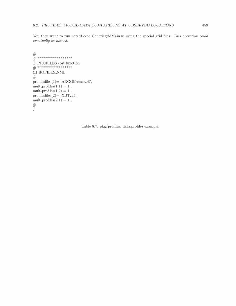
8.2. PROFILES: MODEL-DATA COMPARISONS AT OBSERVED LOCATIONS 459
You then want to run netcdf ecco GenericgridMain.m using the special grid files. This operation couldeventually be inlined.
## ******************# PROFILES cost function# ******************&PROFILES NML#profilesfiles(1)= ’ARGOifremer r8’,mult profiles(1,1) = 1.,mult profiles(1,2) = 1.,profilesfiles(2)= ’XBT v5’,mult profiles(2,1) = 1.,#/
Table 8.7: pkg/profiles: data.profiles example.
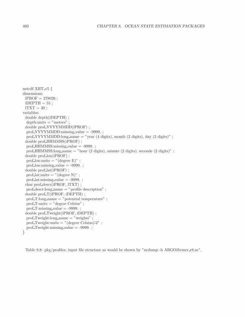
460 CHAPTER 8. OCEAN STATE ESTIMATION PACKAGES
netcdf XBT v5 dimensions:iPROF = 278026 ;iDEPTH = 55 ;lTXT = 30 ;
variables:double depth(iDEPTH) ;depth:units = ”meters” ;double prof YYYYMMDD(iPROF) ;prof YYYYMMDD:missing value = -9999. ;prof YYYYMMDD:long name = ”year (4 digits), month (2 digits), day (2 digits)” ;double prof HHMMSS(iPROF) ;prof HHMMSS:missing value = -9999. ;prof HHMMSS:long name = ”hour (2 digits), minute (2 digits), seconde (2 digits)” ;double prof lon(iPROF) ;prof lon:units = ”(degree E)” ;prof lon:missing value = -9999. ;double prof lat(iPROF) ;prof lat:units = ”(degree N)” ;prof lat:missing value = -9999. ;char prof descr(iPROF, lTXT) ;prof descr:long name = ”profile description” ;double prof T(iPROF, iDEPTH) ;prof T:long name = ”potential temperature” ;prof T:units = ”degree Celsius” ;prof T:missing value = -9999. ;double prof Tweight(iPROF, iDEPTH) ;prof Tweight:long name = ”weights” ;prof Tweight:units = ”(degree Celsius)-2” ;prof Tweight:missing value = -9999. ;
Table 8.8: pkg/profiles: input file structure as would be shown by ”ncdump -h ARGOifremer r8.nc”.
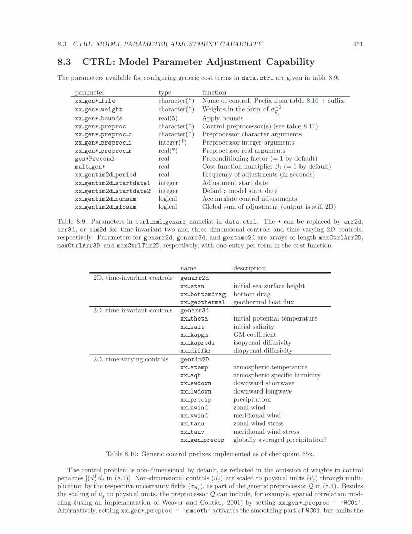
8.3. CTRL: MODEL PARAMETER ADJUSTMENT CAPABILITY 461
8.3 CTRL: Model Parameter Adjustment Capability
The parameters available for configuring generic cost terms in data.ctrl are given in table 8.9.
parameter type functionxx gen* file character(*) Name of control. Prefix from table 8.10 + suffix.xx gen* weight character(*) Weights in the form of σ−2
~uj
xx gen* bounds real(5) Apply boundsxx gen* preproc character(*) Control preprocessor(s) (see table 8.11)xx gen* preproc c character(*) Preprocessor character argumentsxx gen* preproc i integer(*) Preprocessor integer argumentsxx gen* preproc r real(*) Preprocessor real argumentsgen*Precond real Preconditioning factor (= 1 by default)mult gen* real Cost function multiplier βj (= 1 by default)xx gentim2d period real Frequency of adjustments (in seconds)xx gentim2d startdate1 integer Adjustment start datexx gentim2d startdate2 integer Default: model start datexx gentim2d cumsum logical Accumulate control adjustmentsxx gentim2d glosum logical Global sum of adjustment (output is still 2D)
Table 8.9: Parameters in ctrl nml genarr namelist in data.ctrl. The * can be replaced by arr2d,arr3d, or tim2d for time-invariant two and three dimensional controls and time-varying 2D controls,respectively. Parameters for genarr2d, genarr3d, and gentime2d are arrays of length maxCtrlArr2D,maxCtrlArr3D, and maxCtrlTim2D, respectively, with one entry per term in the cost function.
name description
2D, time-invariant controls genarr2d
xx etan initial sea surface heightxx bottomdrag bottom dragxx geothermal geothermal heat flux
3D, time-invariant controls genarr3d
xx theta initial potential temperaturexx salt initial salinityxx kapgm GM coefficientxx kapredi isopycnal diffusivityxx diffkr diapycnal diffusivity
2D, time-varying controls gentim2D
xx atemp atmospheric temperaturexx aqh atmospheric specific humidityxx swdown downward shortwavexx lwdown downward longwavexx precip precipitationxx uwind zonal windxx vwind meridional windxx tauu zonal wind stressxx tauv meridional wind stressxx gen precip globally averaged precipitation?
Table 8.10: Generic control prefixes implemented as of checkpoint 65x.
The control problem is non-dimensional by default, as reflected in the omission of weights in controlpenalties [(~uT
j ~uj in (8.1)]. Non-dimensional controls (~uj) are scaled to physical units (~vj) through multi-plication by the respective uncertainty fields (σ~uj
), as part of the generic preprocessor Q in (8.4). Besidesthe scaling of ~uj to physical units, the preprocessor Q can include, for example, spatial correlation mod-eling (using an implementation of Weaver and Coutier, 2001) by setting xx gen* preproc = ’WC01’.Alternatively, setting xx gen* preproc = ’smooth’ activates the smoothing part of WC01, but omits the
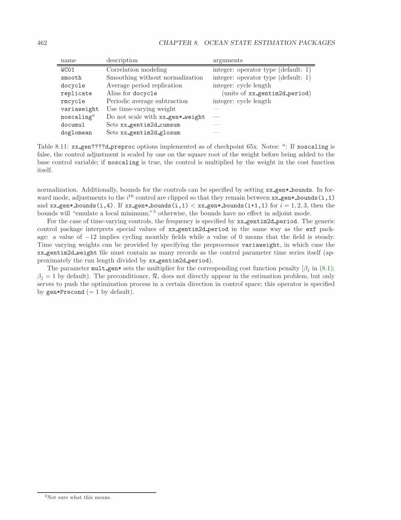
462 CHAPTER 8. OCEAN STATE ESTIMATION PACKAGES
name description arguments
WC01 Correlation modeling integer: operator type (default: 1)smooth Smoothing without normalization integer: operator type (default: 1)docycle Average period replication integer: cycle lengthreplicate Alias for docycle (units of xx gentim2d period)rmcycle Periodic average subtraction integer: cycle lengthvariaweight Use time-varying weight —noscalinga Do not scale with xx gen* weight —documul Sets xx gentim2d cumsum —doglomean Sets xx gentim2d glosum —
Table 8.11: xx gen????d preproc options implemented as of checkpoint 65x. Notes: a: If noscaling isfalse, the control adjustment is scaled by one on the square root of the weight before being added to thebase control variable; if noscaling is true, the control is multiplied by the weight in the cost functionitself.
normalization. Additionally, bounds for the controls can be specified by setting xx gen* bounds. In for-ward mode, adjustments to the ith control are clipped so that they remain between xx gen* bounds(i,1)
and xx gen* bounds(i,4). If xx gen* bounds(i,1) < xx gen* bounds(i+1,1) for i = 1, 2, 3, then thebounds will “emulate a local minimum;”3 otherwise, the bounds have no effect in adjoint mode.
For the case of time-varying controls, the frequency is specified by xx gentim2d period. The genericcontrol package interprets special values of xx gentim2d period in the same way as the exf pack-age: a value of −12 implies cycling monthly fields while a value of 0 means that the field is steady.Time varying weights can be provided by specifying the preprocessor variaweight, in which case thexx gentim2d weight file must contain as many records as the control parameter time series itself (ap-proximately the run length divided by xx gentim2d period).
The parameter mult gen* sets the multiplier for the corresponding cost function penalty [βj in (8.1);βj = 1 by default). The preconditioner, R, does not directly appear in the estimation problem, but onlyserves to push the optimization process in a certain direction in control space; this operator is specifiedby gen*Precond (= 1 by default).
3Not sure what this means.

8.4. SMOOTH: SMOOTHING AND COVARIANCE MODEL 463
8.4 SMOOTH: Smoothing And Covariance Model
TBA ...
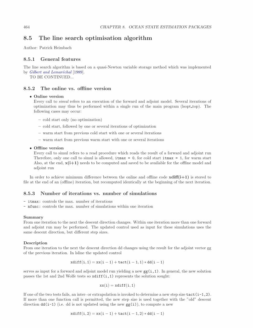
464 CHAPTER 8. OCEAN STATE ESTIMATION PACKAGES
8.5 The line search optimisation algorithm
Author: Patrick Heimbach
8.5.1 General features
The line search algorithm is based on a quasi-Newton variable storage method which was implementedby Gilbert and Lemarechal [1989].
TO BE CONTINUED...
8.5.2 The online vs. offline version
• Online versionEvery call to simul refers to an execution of the forward and adjoint model. Several iterations ofoptimization may thus be performed within a single run of the main program (lsopt top). Thefollowing cases may occur:
– cold start only (no optimization)
– cold start, followed by one or several iterations of optimization
– warm start from previous cold start with one or several iterations
– warm start from previous warm start with one or several iterations
• Offline versionEvery call to simul refers to a read procedure which reads the result of a forward and adjoint runTherefore, only one call to simul is allowed, itmax = 0, for cold start itmax = 1, for warm startAlso, at the end, x(i+1) needs to be computed and saved to be available for the offline model andadjoint run
In order to achieve minimum difference between the online and offline code xdiff(i+1) is stored tofile at the end of an (offline) iteration, but recomputed identically at the beginning of the next iteration.
8.5.3 Number of iterations vs. number of simulations
- itmax: controls the max. number of iterations- nfunc: controls the max. number of simulations within one iteration
SummaryFrom one iteration to the next the descent direction changes. Within one iteration more than one forwardand adjoint run may be performed. The updated control used as input for these simulations uses thesame descent direction, but different step sizes.
DescriptionFrom one iteration to the next the descent direction dd changes using the result for the adjoint vector ggof the previous iteration. In lsline the updated control
xdiff(i, 1) = xx(i− 1) + tact(i− 1, 1) ∗ dd(i− 1)
serves as input for a forward and adjoint model run yielding a new gg(i,1). In general, the new solutionpasses the 1st and 2nd Wolfe tests so xdiff(i,1) represents the solution sought:
xx(i) = xdiff(i, 1)
If one of the two tests fails, an inter- or extrapolation is invoked to determine a new step size tact(i-1,2).If more than one function call is permitted, the new step size is used together with the ”old” descentdirection dd(i-1) (i.e. dd is not updated using the new gg(i)), to compute a new
xdiff(i, 2) = xx(i− 1) + tact(i− 1, 2) ∗ dd(i− 1)
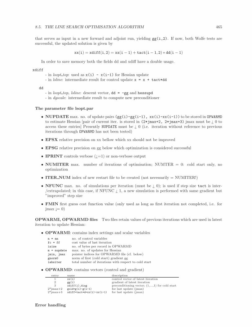
8.5. THE LINE SEARCH OPTIMISATION ALGORITHM 465
that serves as input in a new forward and adjoint run, yielding gg(i,2). If now, both Wolfe tests aresuccessful, the updated solution is given by
xx(i) = xdiff(i, 2) = xx(i− 1) + tact(i− 1, 2) ∗ dd(i− 1)
In order to save memory both the fields dd and xdiff have a double usage.
xdiff
- in lsopt top: used as x(i) - x(i-1) for Hessian update- in lsline: intermediate result for control update x = x + tact*dd
dd
- in lsopt top, lsline: descent vector, dd = -gg and hessupd
- in dgscale: intermediate result to compute new preconditioner
The parameter file lsopt.par
• NUPDATE max. no. of update pairs (gg(i)-gg(i-1), xx(i)-xx(i-1)) to be stored in OPWARMD
to estimate Hessian [pair of current iter. is stored in (2*jmax+2, 2*jmax+3) jmax must be ¿ 0 toaccess these entries] Presently NUPDATE must be ¿ 0 (i.e. iteration without reference to previousiterations through OPWARMD has not been tested)
• EPSX relative precision on xx bellow which xx should not be improved
• EPSG relative precision on gg below which optimization is considered successful
• IPRINT controls verbose (¿=1) or non-verbose output
• NUMITER max. number of iterations of optimisation; NUMTER = 0: cold start only, nooptimization
• ITER NUM index of new restart file to be created (not necessarily = NUMITER!)
• NFUNC max. no. of simulations per iteration (must be ¿ 0); is used if step size tact is inter-/extrapolated; in this case, if NFUNC ¿ 1, a new simulation is performed with same gradient but”improved” step size
• FMIN first guess cost function value (only used as long as first iteration not completed, i.e. forjmax ¡= 0)
OPWARMI, OPWARMD files Two files retain values of previous iterations which are used in latestiteration to update Hessian:
• OPWARMI: contains index settings and scalar variables
n = nn no. of control variablesfc = ff cost value of last iterationisize no. of bytes per record in OPWARMDm = nupdate max. no. of updates for Hessianjmin, jmax pointer indices for OPWARMD file (cf. below)gnorm0 norm of first (cold start) gradient ggiabsiter total number of iterations with respect to cold start
• OPWARMD: contains vectors (control and gradient)
entry name description1 xx(i) control vector of latest iteration2 gg(i) gradient of latest iteration3 xdiff(i),diag preconditioning vector; (1,...,1) for cold start
2*jmax+2 gold=g(i)-g(i-1) for last update (jmax)2*jmax+3 xdiff=tact*d=xx(i)-xx(i-1) for last update (jmax)
Error handling
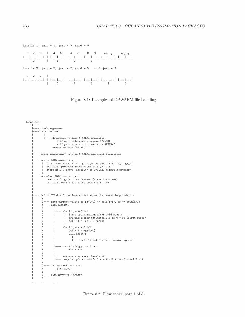
466 CHAPTER 8. OCEAN STATE ESTIMATION PACKAGES
Example 1: jmin = 1, jmax = 3, mupd = 5
1 2 3 | 4 5 6 7 8 9 empty empty
|___|___|___| | |___|___| |___|___| |___|___| |___|___| |___|___|
0 | 1 2 3
Example 2: jmin = 3, jmax = 7, mupd = 5 ---> jmax = 2
1 2 3 |
|___|___|___| | |___|___| |___|___| |___|___| |___|___| |___|___|
| 6 7 3 4 5
Figure 8.1: Examples of OPWARM file handling
lsopt_top||---- check arguments
|---- CALL INSTORE| |
| |---- determine whether OPWARMI available:| * if no: cold start: create OPWARMI| * if yes: warm start: read from OPWARMI
| create or open OPWARMD|
|---- check consistency between OPWARMI and model parameters|
|---- >>> if COLD start: <<<| | first simulation with f.g. xx_0; output: first ff_0, gg_0| | set first preconditioner value xdiff_0 to 1
| | store xx(0), gg(0), xdiff(0) to OPWARMD (first 3 entries)| |
| >>> else: WARM start: <<<| read xx(i), gg(i) from OPWARMD (first 2 entries)| for first warm start after cold start, i=0
||
||---- /// if ITMAX > 0: perform optimization (increment loop index i)
| (| )---- save current values of gg(i-1) -> gold(i-1), ff -> fold(i-1)| (---- CALL LSUPDXX
| ) || ( |---- >>> if jmax=0 <<<
| ) | | first optimization after cold start:| ( | | preconditioner estimated via ff_0 - ff_(first guess)
| ) | | dd(i-1) = -gg(i-1)*preco| ( | || ) | >>> if jmax > 0 <<<
| ( | dd(i-1) = -gg(i-1)| ) | CALL HESSUPD
| ( | || ) | |---- dd(i-1) modified via Hessian approx.| ( |
| ) |---- >>> if <dd,gg> >= 0 <<<| ( | ifail = 4
| ) || ( |---- compute step size: tact(i-1)
| ) |---- compute update: xdiff(i) = xx(i-1) + tact(i-1)*dd(i-1)| (| )---- >>> if ifail = 4 <<<
| ( goto 1000| )
| (---- CALL OPTLINE / LSLINE| ) |
... ... ...
Figure 8.2: Flow chart (part 1 of 3)
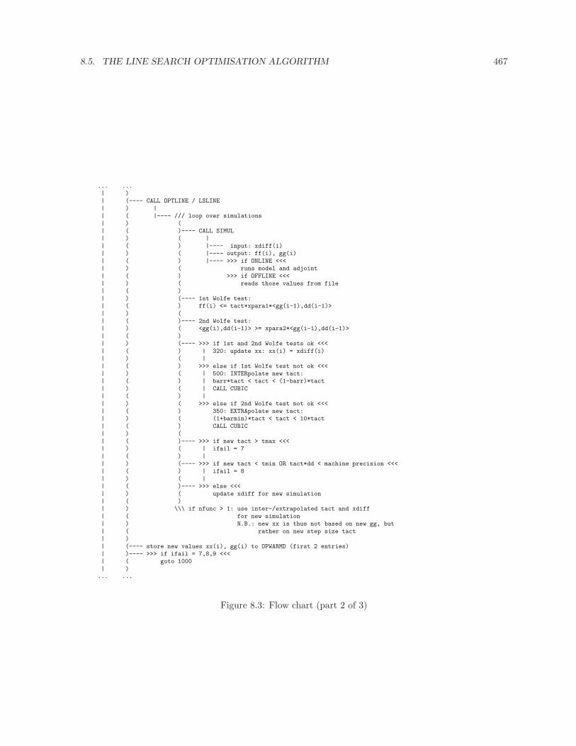
8.5. THE LINE SEARCH OPTIMISATION ALGORITHM 467
... ...| )| (---- CALL OPTLINE / LSLINE
| ) || ( |---- /// loop over simulations
| ) (| ( )---- CALL SIMUL| ) ( |
| ( ) |---- input: xdiff(i)| ) ( |---- output: ff(i), gg(i)
| ( ) |---- >>> if ONLINE <<<| ) ( runs model and adjoint
| ( ) >>> if OFFLINE <<<| ) ( reads those values from file| ( )
| ) (---- 1st Wolfe test:| ( ) ff(i) <= tact*xpara1*<gg(i-1),dd(i-1)>
| ) (| ( )---- 2nd Wolfe test:| ) ( <gg(i),dd(i-1)> >= xpara2*<gg(i-1),dd(i-1)>
| ( )| ) (---- >>> if 1st and 2nd Wolfe tests ok <<<
| ( ) | 320: update xx: xx(i) = xdiff(i)| ) ( |
| ( ) >>> else if 1st Wolfe test not ok <<<| ) ( | 500: INTERpolate new tact:| ( ) | barr*tact < tact < (1-barr)*tact
| ) ( | CALL CUBIC| ( ) |
| ) ( >>> else if 2nd Wolfe test not ok <<<| ( ) 350: EXTRApolate new tact:| ) ( (1+barmin)*tact < tact < 10*tact
| ( ) CALL CUBIC| ) (
| ( )---- >>> if new tact > tmax <<<| ) ( | ifail = 7
| ( ) || ) (---- >>> if new tact < tmin OR tact*dd < machine precision <<<| ( ) | ifail = 8
| ) ( || ( )---- >>> else <<<
| ) ( update xdiff for new simulation| ( )| ) \\\ if nfunc > 1: use inter-/extrapolated tact and xdiff
| ( for new simulation| ) N.B.: new xx is thus not based on new gg, but
| ( rather on new step size tact| )
| (---- store new values xx(i), gg(i) to OPWARMD (first 2 entries)| )---- >>> if ifail = 7,8,9 <<<| ( goto 1000
| )... ...
Figure 8.3: Flow chart (part 2 of 3)
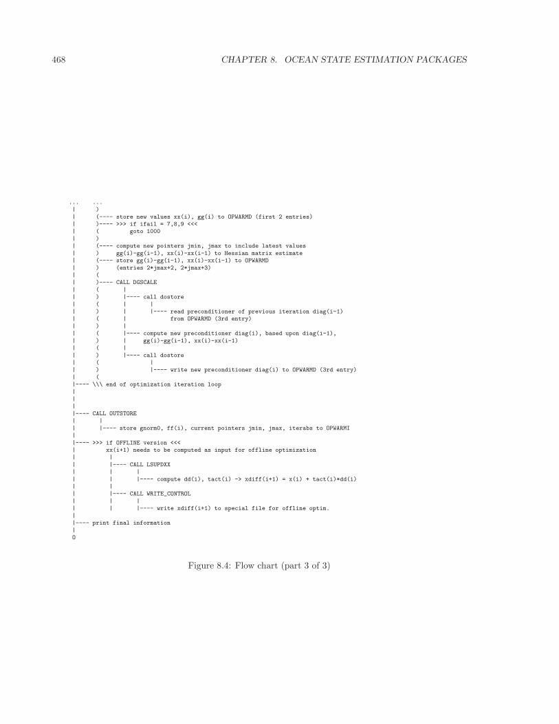
468 CHAPTER 8. OCEAN STATE ESTIMATION PACKAGES
... ...| )
| (---- store new values xx(i), gg(i) to OPWARMD (first 2 entries)| )---- >>> if ifail = 7,8,9 <<<| ( goto 1000
| )| (---- compute new pointers jmin, jmax to include latest values
| ) gg(i)-gg(i-1), xx(i)-xx(i-1) to Hessian matrix estimate| (---- store gg(i)-gg(i-1), xx(i)-xx(i-1) to OPWARMD
| ) (entries 2*jmax+2, 2*jmax+3)| (| )---- CALL DGSCALE
| ( || ) |---- call dostore
| ( | || ) | |---- read preconditioner of previous iteration diag(i-1)| ( | from OPWARMD (3rd entry)
| ) || ( |---- compute new preconditioner diag(i), based upon diag(i-1),
| ) | gg(i)-gg(i-1), xx(i)-xx(i-1)| ( |
| ) |---- call dostore| ( || ) |---- write new preconditioner diag(i) to OPWARMD (3rd entry)
| (|---- \\\ end of optimization iteration loop
|||
|---- CALL OUTSTORE| |
| |---- store gnorm0, ff(i), current pointers jmin, jmax, iterabs to OPWARMI|
|---- >>> if OFFLINE version <<<| xx(i+1) needs to be computed as input for offline optimization| |
| |---- CALL LSUPDXX| | |
| | |---- compute dd(i), tact(i) -> xdiff(i+1) = x(i) + tact(i)*dd(i)| || |---- CALL WRITE_CONTROL
| | || | |---- write xdiff(i+1) to special file for offline optim.
||---- print final information
|O
Figure 8.4: Flow chart (part 3 of 3)
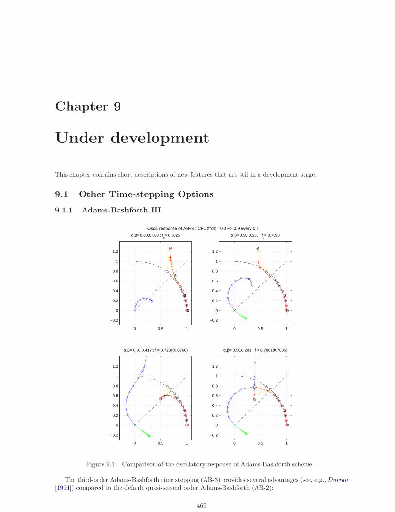
Chapter 9
Under development
This chapter contains short descriptions of new features that are stil in a development stage.
9.1 Other Time-stepping Options
9.1.1 Adams-Bashforth III
0 0.5 1
−0.2
0
0.2
0.4
0.6
0.8
1
1.2
0
3
6
9
α,β= 0.60,0.000 ; fc= 0.5025
0 0.5 1
−0.2
0
0.2
0.4
0.6
0.8
1
1.2
0
3
6
9
α,β= 0.50,0.250 ; fc= 0.7698
0 0.5 1
−0.2
0
0.2
0.4
0.6
0.8
1
1.2
0
3
69
α,β= 0.50,0.417 ; fc= 0.7236(0.6760)
0 0.5 1
−0.2
0
0.2
0.4
0.6
0.8
1
1.2
0
3
69
α,β= 0.50,0.281 ; fc= 0.7861(0.7686)
Oscil. response of AB−3 : CFL (f*dt)= 0.0 −> 0.9 every 0.1
Figure 9.1: Comparison of the oscillatory response of Adams-Bashforth scheme.
The third-order Adams-Bashforth time stepping (AB-3) provides several advantages (see, e.g., Durran[1991]) compared to the default quasi-second order Adams-Bashforth (AB-2):
469
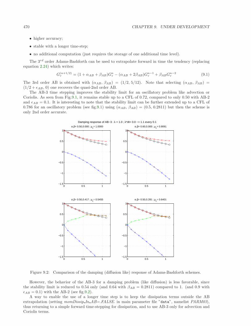
470 CHAPTER 9. UNDER DEVELOPMENT
• higher accuracy;
• stable with a longer time-step;
• no additional computation (just requires the storage of one additional time level).
The 3rd order Adams-Bashforth can be used to extrapolate forward in time the tendency (replacingequation 2.24) which writes:
G(n+1/2)τ = (1 + αAB + βAB)Gn
τ − (αAB + 2βAB)Gn−1τ + βABG
n−2τ (9.1)
The 3rd order AB is obtained with (αAB , βAB) = (1/2, 5/12). Note that selecting (αAB, βAB) =(1/2 + ǫAB, 0) one recovers the quasi-2nd order AB.
The AB-3 time stepping improves the stability limit for an oscillatory problem like advection orCoriolis. As seen from Fig.9.1, it remains stable up to a CFL of 0.72, compared to only 0.50 with AB-2and ǫAB = 0.1. It is interesting to note that the stability limit can be further extended up to a CFL of0.786 for an oscillatory problem (see fig.9.1) using (αAB , βAB) = (0.5, 0.2811) but then the scheme isonly 2nd order accurate.
0 0.5 1−1.5
−1
−0.5
0
0.5
1
α,β= 0.50,0.000 ; µc= 1.0000
0 0.5 1−1.5
−1
−0.5
0
0.5
1
α,β= 0.60,0.000 ; µc= 0.9091
0 0.5 1−1.5
−1
−0.5
0
0.5
1
α,β= 0.50,0.417 ; µc= 0.5455
0 0.5 1−1.5
−1
−0.5
0
0.5
1
α,β= 0.50,0.281 ; µc= 0.6401
Damping response of AB−3 : λ = 1.0 ; λ*dt= 0.0 −> 1.1 every 0.1
Figure 9.2: Comparison of the damping (diffusion like) response of Adams-Bashforth schemes.
However, the behavior of the AB-3 for a damping problem (like diffusion) is less favorable, sincethe stability limit is reduced to 0.54 only (and 0.64 with βAB = 0.2811) compared to 1. (and 0.9 withǫAB = 0.1) with the AB-2 (see fig.9.2).
A way to enable the use of a longer time step is to keep the dissipation terms outside the ABextrapolation (setting momDissip In AB=.FALSE. in main parameter file ”data”, namelist PARM03),thus returning to a simple forward time-stepping for dissipation, and to use AB-3 only for advection andCoriolis terms.
9.1. OTHER TIME-STEPPING OPTIONS 471
The AB-3 time stepping is activated by defining the option #define ALLOW ADAMSBASHFORTH 3in ”CPP OPTIONS.h”. The parameters αAB, βAB can be set from the main parameter file ”data” (namelistPARM03) and their default value corresponds to the 3rd order Adams-Bashforth. A simple example isprovided in ”verification/advect xy/input.ab3 c4”.
The AB-3 is not yet available for the vertical momentum equation (Non-Hydrostatic) neither forpassive tracers.
9.1.2 Time-extrapolation of tracer (rather than tendency)
(to be continued ...)

472 CHAPTER 9. UNDER DEVELOPMENT
Chapter 10
Previous Applications of MITgcm
To date, MITgcm has been used for number of purposes. The following papers are an incomplete yetfairly broad sample of MITgcm applications:
• R.S. Gross and I. Fukumori and D. Menemenlis (2003). Atmospheric and oceanic excitation of theEarth’s wobbles during 1980-2000. Journal of Geophysical Research-Solid Earth, vol.108.
• M.A. Spall and R.S. Pickart (2003). Wind-driven recirculations and exchange in the Labrador andIrminger Seas. Journal of Physical Oceanography, vol.33, pp.1829–1845.
• B. Ferron and J. Marotzke (2003). Impact of 4D-variational assimilation of WOCE hydrographyon the meridional circulation of the Indian Ocean. Deep-Sea Research Part II-Topical Studies inOceanography, vol.50, pp.2005–2021.
• G.A. McKinley and M.J. Follows and J. Marshall and S.M. Fan (2003). Interannual variability ofair-sea O-2 fluxes and the determination of CO2 sinks using atmospheric O-2/N-2. GeophysicalResearch Letters, vol.30.
• B.Y. Huang and P.H. Stone and A.P. Sokolov and I.V. Kamenkovich (2003). The deep-ocean heatuptake in transient climate change. Journal of Climate, vol.16, pp.1352–1363.
• G. de Coetlogon and C. Frankignoul (2003). The persistence of winter sea surface temperature inthe North Atlantic. Journal of Climate, vol.16, pp.1364–1377.
• K.H. Nisancioglu and M.E. Raymo and P.H. Stone (2003). Reorganization of Miocene deep watercirculation in response to the shoaling of the Central American Seaway. Paleoceanography, vol.18.
• T. Radko and J. Marshall (2003). Equilibration of a Warm Pumped Lens on a beta plane. Journalof Physical Oceanography, vol.33, pp.885–899.
• T. Stipa (2002). The dynamics of the N/P ratio and stratification in a large nitrogen-limitedestuary as a result of upwelling: a tendency for offshore Nodularia blooms. Hydrobiologia, vol.487,pp.219–227.
• D. Stammer and C. Wunsch and R. Giering and C. Eckert and P. Heimbach and J. Marotzkeand A. Adcroft and C.N. Hill and J. Marshall (2003). Volume, heat, and freshwater transportsof the global ocean circulation 1993-2000, estimated from a general circulation model constrainedby World Ocean Circulation Experiment (WOCE) data. Journal of Geophysical Research-Oceans,vol.108.
• P. Heimbach and C. Hill and R. Giering (2002). Automatic generation of efficient adjoint code fora parallel Navier-Stokes solver. Computational Science-ICCS 2002, PT II, Proceedings, vol.2330,pp.1019–1028.
• D. Stammer and C. Wunsch and R. Giering and C. Eckert and P. Heimbach and J. Marotzke and A.Adcroft and C.N. Hill and J. Marshall (2002). Global ocean circulation during 1992-1997, estimatedfrom ocean observations and a general circulation model. Journal of Geophysical Research-Oceans,vol.107.
473
474 CHAPTER 10. PREVIOUS APPLICATIONS OF MITGCM
• M. Solovev and P.H. Stone and P. Malanotte-Rizzoli (2002). Assessment of mesoscale eddy pa-rameterizations for a single-basin coarse-resolution ocean model. Journal of Geophysical Research-Oceans, vol.107.
• C. Herbaut and J. Sirven and S. Fevrier (2002). Response of a simplified oceanic general circulationmodel to idealized NAO-like stochastic forcing. Journal of Physical Oceanography, vol.32, pp.3182–3192.
• C. Wunsch (2002). Oceanic age and transient tracers: Analytical and numerical solutions. Journalof Geophysical Research-Oceans, vol.107.
• J. Sirven and C. Frankignoul and D. de Coetlogon and V. Taillandier (2002). Spectrum of wind-driven baroclinic fluctuations of the ocean in the midlatitudes. Journal of Physical Oceanography,vol.32, pp.2405–2417.
• R. Zhang and M. Follows and J. Marshall (2002). Mechanisms of thermohaline mode switchingwith application to warm equable climates. Journal of Climate, vol.15, pp.2056–2072.
• G. Brostrom (2002). On advection and diffusion of plankton in coarse resolution ocean models.Journal of Marine Systems, vol.35, pp.99–110.
• T. Lee and I. Fukumori and D. Menemenlis and Z.F. Xing and L.L. Fu (2002). Effects of theIndonesian Throughflow on the Pacific and Indian oceans. Journal of Physical Oceanography,vol.32, pp.1404–1429.
• C. Herbaut and J. Marshall (2002). Mechanisms of buoyancy transport through mixed layers andstatistical signatures from isobaric floats. Journal of Physical Oceanography, vol.32, pp.545–557.
• J. Marshall and H. Jones and R. Karsten and R. Wardle (2002). Can eddies set ocean stratification?,Journal of Physical Oceanography, vol.32, pp.26–38.
• C. Herbaut and J. Sirven and A. Czaja (2001). An idealized model study of the mass and heattransports between the subpolar and subtropical gyres. Journal of Physical Oceanography, vol.31,pp.2903–2916.
• R.H. Kase and A. Biastoch and D.B. Stammer (2001). On the Mid-Depth Circulation in theLabrador and Irminger Seas. Geophysical Research Letters, vol.28, pp.3433–3436.
• R. Zhang and M.J. Follows and J.P. Grotzinger and J. Marshall (2001). Could the Late Permiandeep ocean have been anoxic?. Paleoceanography, vol.16, pp.317–329.
• A. Adcroft and J.R. Scott and J. Marotzke (2001). Impact of geothermal heating on the globalocean circulation. Geophysical Research Letters, vol.28, pp.1735–1738.
• J. Marshall and D. Jamous and J. Nilsson (2001). Entry, flux, and exit of potential vorticity inocean circulation. Journal of Physical Oceanography, vol.31, pp.777–789.
• A. Mahadevan (2001). An analysis of bomb radiocarbon trends in the Pacific. Marine Chemistry,vol.73, pp.273–290.
• G. Brostrom (2000). The role of the annual cycles for the air-sea exchange of CO2. MarineChemistry, vol.72, pp.151–169.
• Y.H. Zhou and H.Q. Wu and N.H. Yu and D.W. Zheng (2000). Excitation of seasonal polar motionby atmospheric and oceanic angular momentums. Progress in Natural Science, vol.10, pp.931–936.
• R. Wardle and J. Marshall (2000). Representation of eddies in primitive equation models by a PVflux. Journal of Physical Oceanography, vol.30, pp.2481–2503.
• P.S. Polito and O.T. Sato and W.T. Liu (2000). Characterization and validation of the heat storagevariability from TOPEX/Poseidon at four oceanographic sites. Journal of Geophysical Research-Oceans, vol.105, pp.16911–16921.
475
• R.M. Ponte and D. Stammer (2000). Global and regional axial ocean angular momentum signals andlength-of-day variations (1985-1996). Journal of Geophysical Research-Oceans, vol.105, pp.17161–17171.
• J. Wunsch (2000). Oceanic influence on the annual polar motion. Journal of GEODYNAMICS,vol.30, pp.389–399.
• D. Menemenlis and M. Chechelnitsky (2000). Error estimates for an ocean general circulation modelfrom altimeter and acoustic tomography data. Monthly Weather Review, vol.128, pp.763–778.
• Y.H. Zhou and D.W. Zheng and N.H. Yu and H.Q. Wu (2000). Excitation of annual polar motionby atmosphere and ocean. Chinese Science Bulletin, vol.45, pp.139–142.
• J. Marotzke and R. Giering and K.Q. Zhang and D. Stammer and C. Hill and T. Lee (1999).Construction of the adjoint MIT ocean general circulation model and application to Atlantic heattransport sensitivity. Journal of Geophysical Research-Oceans, vol.104, pp.29529–29547.
• R.M. Ponte and D. Stammer (1999). Role of ocean currents and bottom pressure variability onseasonal polar motion. Journal of Geophysical Research-Oceans, vol.104, pp.23393–23409.
• J. Nastula and R.M. Ponte (1999). Further evidence for oceanic excitation of polar motion. Geo-physical Journal International, vol.139, pp.123–130.
• K.Q. Zhang and J. Marotzke (1999). The importance of open-boundary estimation for an IndianOcean GCM-data synthesis. Journal of Marine Research, vol.57, pp.305–334.
• J. Marshall and D. Jamous and J. Nilsson (1999). Reconciling thermodynamic and dynamic meth-ods of computation of water-mass transformation rates. Deep-Sea Research PART I-OceanographicResearch Papers, vol.46, pp.545–572.
• J. Marshall and F. Schott (1999). Open-ocean convection: Observations, theory, and models.Reviews of Geophysics, vol.37, pp.1–64.
• J. Marshall and H. Jones and C. Hill (1998). Efficient ocean modeling using non-hydrostatic algo-rithms. Journal of Marine Systems, vol.18, pp.115–134.
• A.B. Baggeroer and T.G. Birdsall and C. Clark and J.A. Colosi and B.D. Cornuelle and D. Costa andB.D. Dushaw and M. Dzieciuch and A.M.G. Forbes and C. Hill and B.M. Howe and J. Marshalland D. Menemenlis and J.A. Mercer and K. Metzger and W. Munk and R.C. Spindel and D.Stammer and P.F. Worcester and C. Wunsch (1998). Ocean climate change: Comparison of acoustictomography, satellite altimetry, and modeling. Science, vol.281, pp.1327–1332.
• C. Wunsch and D. Stammer (1998). Satellite altimetry, the marine geoid, and the oceanic generalcirculation. Annual Review of Earth and Planetary Sciences, vol.26, pp.219–253.
• A. Shaw and Arvind and K.C. Cho and C. Hill and R.P. Johnson and J. Marshall (1998). A com-parison of implicitly parallel multithreaded and data-parallel implementations of an ocean model.Journal of Parallel and Distributed Computing, vol.48, pp.1–51.
• T.W.N. Haine and J. Marshall (1998). Gravitational, symmetric, and baroclinic instability of theocean mixed layer. Journal of Physical Oceanography, vol.28, pp.634–658.
• R.M. Ponte and D. Stammer and J. Marshall (1998). Oceanic signals in observed motions of theEarth’s pole of rotation. Nature, vol.391, pp.476–479.
• D. Menemenlis and C. Wunsch (1997). Linearization of an oceanic general circulation model fordata assimilation and climate studies. Journal of Atmospheric and Oceanic Technology, vol.14,pp.1420–1443.
• H. Jones and J. Marshall (1997). Restratification after deep convection. Journal of PhysicalOceanography, vol.27, pp.2276–2287.
• S.R. Jayne and R. Tokmakian (1997). Forcing and sampling of ocean general circulation models:Impact of high-frequency motions. Journal of Physical Oceanography, vol.27, pp.1173–1179.

476 CHAPTER 10. PREVIOUS APPLICATIONS OF MITGCM
Bibliography
Adcroft, A., Numerical algorithms for use in a dynamical model of the ocean, Ph.D. thesis, ImperialCollege, London, 1995.
Adcroft, A., and J.-M. Campin, Comparison of finite volume schemes and direct-space-time methods forocean circulation models, Ocean Modelling, in preparation, 2002.
Adcroft, A., and J.-M. Campin, Re-scaled height coordinates for accurate representationof free-surface flows in ocean circulation models, Ocean Modelling, 7, 269–284, 2004.doi:10.1016/j.ocemod.2003.09.003.
Adcroft, A., and D. Marshall, How slippery are piecewise-constant coastlines in numerical ocean models?,Tellus, 50(1), 95–108, 1998.
Adcroft, A., C. Hill, and J. Marshall, Representation of topography byshaved cells in a height coordinate ocean model, Mon. Wea. Rev., 125,2293–2315, 1997. Available from: http://mitgcm.org/pdfs/mwr_1997.pdf,doi:10.1175/1520-0493%281997%29125¡2293:ROTBSC¿2.0.CO;2.
Adcroft, A., J.-M. Campin, C. Hill, and J. Marshall, Implementation of an atmosphere-ocean generalcirculation model on the expanded spherical cube, Mon. Wea. Rev., 132, 2845–2863, 2004a. Availablefrom: http://mitgcm.org/pdfs/mwr_2004.pdf, doi:10.1175/MWR2823.1.
Adcroft, A., C. Hill, J.-M. Campin, J. Marshall, and P. Heimbach, Overview of the formulation andnumerics of the MITgcm, in Proceedings of the ECMWF seminar series on Numerical Methods, Recentdevelopments in numerical methods for atmosphere and ocean modelling, pp. 139–149. ECMWF, 2004b.Available from: http://mitgcm.org/pdfs/ECMWF2004-Adcroft.pdf.
Adcroft, A., e. a., Energy conversion in discrete numerical models, Ocean Modelling, in preparation, 2002.
Adcroft, A., H. C., and J. Marshall, A new treatment of the coriolis termsin c-grid models at both high and low resolutions, Mon. Wea. Rev., 127,1928–1936, 1999. Available from: http://mitgcm.org/pdfs/mwr_1999.pdf,doi:10.1175/1520-0493%281999%29127¡1928:ANTOTC¿2.0.CO;2.
Arakawa, A., and V. Lamb, Computational design of the basic dynamical processes of the ucla generalcirculation model, in Methods in Computational Physics, vol. 17, pp. 174–267. Academic Press, 1977.
Beckmann, A., H. H. Hellmer, and R. Timmermann, A numerical model of the Weddell Sea: Large-scalecirculation and water mass distribution, J. Geophys. Res., 104(C10), 23,375–23,392, 1999.
Blackadar, A. K., High resolution models of the planetary boundary layer., in Advances in Environ-mental Science and Engineering, Vol 1, edited by Pfafflin, and Zeigler. Gordon and Breach, ScientificPublishers, 1977.
Bouillon, S., T. Fichefet, V. Legat, and G. Madec, The elastic-viscous-plastic methodrevisited, Ocean Modelling, 71(0), 2–12, Arctic Ocean, 2013. Available from:http://dx.doi.org/10.1016/j.ocemod.2013.05.013, doi:10.1016/j.ocemod.2013.05.013.
Bretherton, C. S., et al., An intercomparison of radiatively driven entrainment and turbulence in a smokecloud, as simulated by different numerical models., Q. J. R. Meteorol. Soc., 125, 391–423, 1999.
477
478 BIBLIOGRAPHY
Bryan, K., Accelerating the convergence to equilibrium of ocean-climate models, J. Phys. Oceanogr.,14(4), 666–673, 1984.
Bryan, K., S. Manabe, and R. C. Pacanowski, A global ocean-atmosphere climate model. Part II. Theoceanic circulation, Journal of Physical Oceanography, 5, 30–46, 1975.
Bushell, A. C., and G. Martin, The impact of vertical resolution upon gcm simulations of marine stra-tocumulus., Climate Dyn., 15, 293–318, 1999.
Campin, J.-M., A. Adcroft, C. Hill, and J. Marshall, Conservation of properties in a free-surface model,Ocean Modelling, 6, 221–244, 2004.
Campin, J.-M., J. Marshall, and D. Ferreira, Sea-ice ocean coupling using a rescaled vertical coordinatez∗, Ocean Modelling, 24(1–2), 1–14, 2008. doi:10.1016/j.ocemod.2008.05.005.
Castro-Morales, K., F. Kauker, M. Losch, S. Hendricks, K. Riemann-Campe, and R. Gerdes, Sensitivityof simulated Arctic sea ice to realistic ice thickness distributions and snow parameterizations, J. Geo-phys. Res., 119(1), 559–571, 2014. Available from: http://dx.doi.org/10.1002/2013JC009342,doi:10.1002/2013JC009342.
Chou, M.-D., Parameterizations for the absorption of solar radiation by o2 and co2 with applications toclimate studies., J. Clim., 3, 209–217, 1990.
Chou, M.-D., A solar radiation model for use in climate studies., J. Atmos. Sci., 49, 762–772, 1992.
Chou, M.-D., and M.J.Suarez, An efficient thermal infrared radiation parameterization for use ingeneral circulation models, NASA Technical Memorandum 104606-Vol 3, National Aeronauticsand Space Administration, NASA; Goddard Space Flight Center; Greenbelt (MD), 20771; USA,http://www.gmao.nasa.gov/, 1994.
Chris Hill, Alistair Adcroft, D. J., and J. Marshall, A strategy for terascale climate modeling, in InProceedings of the Eighth ECMWF Workshop on the Use of Parallel Processors in Meteorology, pp.406–425. World Scientific, 1999.
Clarke, R. H., Observational studies in the atmospheric boundary layer., Q. J. R. Meteorol. Soc., 96,91–114, 1970.
Cox, M. D., An isopycnal diffusion in a z-coordinate ocean model, Ocean modelling, 74, 1–5 (Unpublishedmanuscript), 1987.
Danabasoglu, G., and J. C. McWilliams, Sensitivity of the global ocean circulation to parameterizationsof mesoscale tracer transports, J. Clim., 8(12), 2967–2987, 1995.
de Szoeke, R. A., and R. M. Samelson, The duality between the Boussinesq and Non-Boussinesq hydro-static equations of motion, J. Phys. Oceanogr., 32(8), 2194–2203, 2002.
Defries, R. S., and J. R. G. Townshend, Ndvi-derived land cover classification at global scales., Int’l J.Rem. Sens., 15, 3567–3586, 1994.
Dorman, J. L., and P. J. Sellers, A global climatology of albedo, roughness length and stomatal resis-tance for atmospheric general circulation models as represented by the simple biosphere model (sib).,J. Appl. Meteor., 28, 833–855, 1989.
Durran, D. R., The third-order adams-bashforth method: An attractive alternative to leapfrog timedifferencing, Mon. Wea. Rev., 119, 702–720, 1991.
Dutay, J.-C., et al., Evaluation of ocean model ventilation with cfc-11: comparison of 13 global oceanmodels, Ocean Modelling, 4, 89–120, 2002.
Dutkiewicz, S., A. Sokolov, J. Scott, and P. Stone, A three-dimensional ocean-seaice-carbon cycle modeland its coupling to a two-dimensional atmospheric model: Uses in climate change studies, report122, Tech. rep., MIT Joint Program of the Science and Policy of Global Change, Cambridge, MA,http://web.mit.edu/globalchange/www/MITJPSPGC Rpt122.pdf, 2005.
BIBLIOGRAPHY 479
Ferreira, D., J. Marshall, and P. Heimbach, Estimating eddy stresses by fitting dynamics to observationsusing a residual-mean ocean circulation model and its adjoint, J. Phys. Oceanogr., 35, 1891–1910, 2005.
Flato, G. M., and W. D. Hibler, III, Modeling pack ice as a cavitating fluid, J. Phys. Oceanogr., 22,626–651, 1992.
Fofonoff, P., and R. Millard, Jr., Algorithms for computation of fundamental properties of seawater,Unesco Technical Papers in Marine Science 44, Unesco, 1983.
Follows, M., T. Ito, and S. Dutkiewicz, A compact and accurate carbonate chemistry solver for oceanbiogeochemistry models, Ocean Modeling, in press.
Forget, G., J.-M. Campin, P. Heimbach, C. N. Hill, R. M. Ponte, and C. Wunsch,ECCO version 4: an integrated framework for non-linear inverse modeling and global oceanstate estimation, Geoscientific Model Development, 8(10), 3071–3104, 2015. Available from:http://www.geosci-model-dev.net/8/3071/2015/, doi:10.5194/gmd-8-3071-2015.
Fukumori, I., O. Wang, W. Llovel, I. Fenty, and G. Forget, A near-uniform fluctua-tion of ocean bottom pressure and sea level across the deep ocean basins of the arcticocean and the nordic seas, Progress in Oceanography, 134(0), 152 – 172, 2015. Avail-able from: http://www.sciencedirect.com/science/article/pii/S0079661115000245,doi:http://dx.doi.org/10.1016/j.pocean.2015.01.013.
Gaspar, P., Y. Gregoris, and J.-M. Lefevre, A simple eddy kinetic energy model for simulations of theoceanic vertical mixing: Tests at station papa and long-term upper ocean study site, J. Geophys. Res.,95 (C9), 16,179–16,193, 1990.
Geiger, C. A., W. D. Hibler, III, and S. F. Ackley, Large-scale sea ice drift and deformation: Comparisonbetween models and observations in the western Weddell Sea during 1992, J. Geophys. Res., 103(C10),21893–21913, 1998.
Gent, P. R., and J. C. McWilliams, Isopycnal mixing in ocean circulation models, J. Phys. Oceanogr.,20, 150–155, 1990.
Gent, P. R., J. Willebrand, T. J. McDougall, and J. C. McWilliams, Parameterizing eddy-induced tracertransports in ocean circulation models, J. Phys. Oceanogr., 25, 463–474, 1995.
Gerdes, R., C. Koberle, and J. Willebrand, The influence of numerical advection schemes on the resultsof ocean general circulation models, Clim. Dynamics, 5(4), 211–226, 1991. doi:10.1007/BF00210006.
Giering, R., Tangent linear and adjoint model compiler. users manual 1.4 (tamc version 5.2), Report ,Massachusetts Institute of Technology, MIT/EAPS; 77 Massachusetts Ave.; Cambridge (MA) 02139;USA, http://puddle.mit.edu/∼ralf/tamc/tamc.html, 1999.
Giering, R., Tangent linear and adjoint biogeochemical models, in Inverse methods in global biogeochemicalcycles, edited by P. Kasibhatla, M. Heimann, P. Rayner, N. Mahowald, R. Prinn, and D. Hartley, vol.114 of Geophysical Monograph, pp. 33–48. American Geophysical Union, Washington, DC, 2000.
Giering, R., and T. Kaminski, Recipes for adjoint code construction, ACM Transactions on MathematicalSoftware, 24, 437–474, 1998.
Gilbert, J., and C. Lemarechal, Some numerical experiments with variable-storage quasi-newton algo-rithms, Math. Programming, 45, 407–435, 1989.
Gill, A. E., Atmosphere-Ocean Dynamics. Academic Press, New York, 662pp., 1982.
Griewank, A., Achieving logarithmic growth of temporal and spatial complexity in reverse AutomaticDifferentiation, Optimization Methods and Software, 1, 35–54, 1992.
Griewank, A., Evaluating Derivatives. Principles and Techniques of Algorithmic Differentiation, vol. 19of Frontiers in Applied Mathematics. SIAM, Philadelphia, 2000.
480 BIBLIOGRAPHY
Griffies, S., M., and W. Hallberg, R., Biharmonic friction with a Smagorinsky-like viscosity for use inlarge-scale eddy-permitting ocean models, Mon. Wea. Rev., 128(8), 2935–2946, 2000.
Griffies, S. M., The Gent-McWilliams skew flux, J. Phys. Oceanogr., 28, 831–841, 1998.
Griffies, S. M., A. Gnanadesikan, R. C. Pacanowski, V. Larichev, J. K. Dukowicz, and R. D. Smith,Isoneutral diffusion in a z-coordinate ocean model, J. Phys. Oceanogr., 28, 805–830, 1998.
Grosfeld, K., R. Gerdes, and J. Determann, Thermohaline circulation and interaction between ice shelfcavities and the adjacent open water, J. Geophys. Res., 102(C7), 15,595–15,610, 1997.
Haney, R., Surface thermal boundary conditions for ocean circulation models, J. Phys. Oceanogr., 1,241–248, 1971.
Heimbach, P., C. Wunsch, R. M. Ponte, G. Forget, C. Hill, and J. Utke, Timescales and regions of thesensitivity of Atlantic meridional volume and heat transport: Toward observing system design, DeepSea Research Part II: Topical Studies in Oceanography, 58(17), 1858–1879, 2011.
Held, I., and M. Suarez, A proposal for the intercomparison of the dynamical cores of atmospheric generalcirculation models, Bulletin of the American Meteorological Society, 75(10), 1825–1830, 1994.
Helfand, H. M., and J. C. Labraga, Design of a non-singular level 2.5 second-order closure model for theprediction of atmospheric turbulence., J. Atmos. Sci., 45, 113–132, 1988.
Helfand, H. M., and S. D. Schubert, Climatology of the simulated great plains low-level jet and itscontribution to the continental moisture budget of the united states., J. Clim., 8, 784–806, 1995.
Hellmer, H. H., and D. J. Olbers, A two-dimensional model of the thermohaline circulation under an iceshelf, Antarct. Sci., 1, 325–336, 1989.
Hibler, III, W. D., A dynamic thermodynamic sea ice model, J. Phys. Oceanogr., 9, 815–846, 1979.
Hibler, III, W. D., Modeling a variable thickness sea ice cover, Mon. Wea. Rev., 1, 1943–1973, 1980.
Hibler, III, W. D., The role of sea ice dynamics in modeling co2 increases, in Climate processes andclimate sensitivity, edited by J. E. Hansen, and T. Takahashi, vol. 29 of Geophysical Monograph, pp.238–253. AGU, Washington, D.C., 1984.
Hibler, III, W. D., and K. Bryan, A diagnostic ice-ocean model, J. Phys. Oceanogr., 17(7), 987–1015,1987.
Hibler, III, W. D., and C. F. Ip, The effect of sea ice rheology on Arcitc buoy drift, in Ice Mechanics,edited by J. P. Dempsey, and Y. D. S. Rajapakse, vol. 204 of AMD, pp. 255–264. Am. Soc. of Mech.Eng., New York, 1995.
Hibler, III, W. D., and E. M. Schulson, On modeling sea-ice fracture and flow in numerical investigationsof climate, Ann. Glaciol., 25, 26–32, 1997.
Hill, C., and J. Marshall, Application of a parallel navier-stokes model to ocean circulation in parallelcomputational fluid dynamics, in Implementations and Results Using Parallel Computers, edited byN. S. A. Ecer, J. Periaux, and S. Taylor, pp. 545–552. Elsevier Science B.V.: New York, 1995.
Hill, C., M. Follows, V. Bugnion, and J. Marshall, Spatial and temporal impacts of ocean general circu-lation on carbon sequestration, Global Biogeochemical Cycles, submitted, 2002.
Hoe, J. C., C. Hill, and A. Adcroft, A personal supercomputer for climate research, in In Proceedings ofthe ACM/IEEE Super-Computing Confrence, p. 10.1109/SC.1999. IEEE, 1999.
Holland, D. M., and A. Jenkins, Modeling thermodynamic ice-ocean interactions at the base of an iceshelf, J. Phys. Oceanogr., 29(8), 1787–1800, 1999.
Holland, W., and L. B. Lin, On the origin of mesoscale eddies and their contribution to the generalcirculation of the ocean. i. a preliminary numerical experiment, J. Phys. Oceanogr., 5, 642–657, 1975a.
BIBLIOGRAPHY 481
Holland, W. R., The role of mesoscale eddies in the general circulation of the ocean–numerical experimentsusing a wind-driven quasi-geostrophic model, Journal of Physical Oceanography, 8, 363–392, 1978.
Hundsdorfer, W., and R. A. Trompert, Method of lines and direct discretization: a comparison for linearadvection, Applied Numerical Mathematics, 13(6), 469–490, 1994. doi:10.1016/0168-9274(94)90009-4.
Hunke, E. C., Viscous-plastic sea ice dynamics with the EVP model: Linearization issues, J. Com-put. Phys., 170, 18–38, 2001. doi:10.1006/jcph.2001.6710.
Hunke, E. C., and J. K. Dukowicz, An elastic-viscous-plastic model for sea ice dynamics,J. Phys. Oceanogr., 27, 1849–1867, 1997.
Hutchings, J. K., H. Jasak, and S. W. Laxon, A strength implicit correction scheme for the viscous-plasticsea ice model, Ocean Modelling, 7(1–2), 111–133, 2004. doi:10.1016/S1463-5003(03)00040-4.
Inness, P. M., S. Slingo, R. Woolnough, B. Neale, and V. Pope, Organization of tropical convection in agcm with verying vertical resolution; implications for the simulation of the madden-julian oscillation.,Climate Dyn., 17, 777–794, 2001.
Jackett, D. R., and T. J. McDougall, Minimal adjustment of hydrographic profiles to achieve staticstability, J. Atmos. Ocean. Technol., 12(4), 381–389, 1995.
Jenkins, A., H. H. Hellmer, and D. M. Holland, The role of meltwater advection in the formulation ofconservative boundary conditions at an ice-ocean interface, J. Phys. Oceanogr., 31, 285–296, 2001.
Jiang, S., P. H. Stone, and P. Malanotte-Rizzoli, An assessment of the Geophysical Fluid DynamicsLaboratory ocean model with coarse resolution: Annual-mean climatology, J. Geophys. Res., 104(C11),25,623–25,645, 1999.
Kalnay, E., et al., The NMC/NCAR 40-year reanalysis project, Bull. Am. Met. Soc., 77, 437–471, 1996.
Kimmritz, M., S. Danilov, and M. Losch, On the convergence of the modified elastic-viscous-plastic method of solving for sea-ice dynamics, J. Comput. Phys., 296, 90–100, 2015.doi:10.1016/j.jcp.2015.04.051.
Kimmritz, M., S. Danilov, and M. Losch, The adaptive EVP method for solv-ing the sea ice momentum equation, Ocean Modelling, 2016. Available from:http://mitgcm.org/~mlosch/adaptiveEVP_accepted.pdf.
Klymak, J. M., and S. M. Legg, A simple mixing scheme for models that resolve breaking internal waves,Ocean Modelling, 33, 224–234, 2010. doi:10.1016/j.ocemod.2010.02.005.
Knoll, D., and D. Keyes, Jacobian-free Newton-Krylov methods: a survey of approaches and applications,J. Comput. Phys., 193, 357–397, 2004. doi:10.1016/j.jcp.2003.08.010.
Kondo, J., Air-sea bulk transfer coefficients in diabatic conditions., Bound. Layer Meteorol., 9, 91–112,1975.
Koster, R. D., and M. J. Suarez, A simplified treatment of sib’s land surface albedo parameterization.,NASA Technical Memorandum 104538, National Aeronautics and Space Administration, NASA; God-dard Space Flight Center; Greenbelt (MD), 20771; USA, http://www.gmao.nasa.gov/, 1991.
Koster, R. D., and M. J. Suarez, Modeling the land surface boundary in climate models as a compositeof independent vegetation stands., J. Geophys. Res., 97, 2697–2715, 1992.
Lacis, A. A., and J. E. Hansen, A parameterization for the absorption of solar radiation in the earth’satmosphere., J. Atmos. Sci., 31, 118–133, 1974.
Large, W., J. McWilliams, and S. Doney, Oceanic vertical mixing: A review and a model with nonlocalboundary layer parameterization, Rev. Geophys., 32, 363–403, 1994.
Large, W. G., and S. Pond, Open ocean momentum flux measurements in moderate to strong winds.,J. Phys. Oceanogr., 11, 324–336, 1981.
482 BIBLIOGRAPHY
Large, W. G., G. Danabasoglu, S. C. Doney, and J. C. McWilliams, Sensitivity to surface forcing andboundary layer mixing in a global ocean model: Annual-mean climatology, J. Phys. Oceanogr., 27(11),2418–2447, 1997.
Leith, C. E., Large eddy simulation of complex engineering and geophysical flows, Physics of Fluids, 10,1409–1416, 1968.
Leith, C. E., Stochastic models of chaotic systems, Physica D., 98, 481–491, 1996.
Lemieux, J.-F., and B. Tremblay, Numerical convergence of viscous-plastic sea ice models, J. Geo-phys. Res., 114(C05009), 2009. doi:10.1029/2008JC005017.
Lemieux, J.-F., B. Tremblay, J. Sedlacek, P. Tupper, S. Thomas, D. Huard, and J.-P. Auclair, Improvingthe numerical convergence of viscous-plastic sea ice models with the Jacobian-free Newton-Krylovmethod, J. Comput. Phys., 229, 2840–2852, 2010. doi:10.1016/j.jcp.2009.12.011c.
Lemieux, J.-F., D. Knoll, B. Tremblay, D. M. Holland, and M. Losch, A comparison of the Jacobian-free Newton-Krylov method and the EVP model for solving the sea ice momentum equation with aviscous-plastic formulation: a serial algorithm study, J. Comput. Phys., 231(17), 5926–5944, 2012.doi:10.1016/j.jcp.2012.05.024.
Lepparanta, M., A growth model for black ice, snow ican and snow thickness in subarctic basins, NordicHydrology, 14, 59–70, 1983.
Levitus, S., and T.P.Boyer, World Ocean Atlas 1994 Volume 3: Salinity, Tech. rep., NOAA Atlas NESDIS3, 1994a.
Levitus, S., and T.P.Boyer, World Ocean Atlas 1994 Volume 4: Temperature, Tech. rep., NOAA AtlasNESDIS 4, 1994b.
Losch, M., Modeling ice shelf cavities in a z-coordinate ocean general circulation model, J. Geophys. Res.,113(C08043), 2008. doi:10.1029/2007JC004368.
Losch, M., D. Menemenlis, J.-M. Campin, P. Heimbach, and C. Hill, On the formulation of sea-ice models.Part 1: Effects of different solver implementations and parameterizations, Ocean Modelling, 33(1–2),129–144, 2010. doi:10.1016/j.ocemod.2009.12.008.
Losch, M., A. Fuchs, J.-F. Lemieux, and A. Vanselow, A parallel Jacobian-free Newton-Krylov solver for acoupled sea ice-ocean model, J. Comput. Phys., 257(A), 901–910, 2014. doi:10.1016/j.jcp.2013.09.026.
Manabe, S., K. Bryan, and M. J. Spelman, A global ocean-atmosphere climate model with seasonalvariation for future studies of climate sensitivity, Dyn. Atmos. Oceans, 3(393–426), 1979.
Marotzke, J., R. Giering, K. Zhang, D. Stammer, C. Hill, and T. Lee, Construction of the adjoint mitocean general circulation model and application to atlantic heat transport variability, J. Geophys. Res.,104, C12, 29,529–29,547, 1999.
Marshall, J., A. Adcroft, C. Hill, L. Perelman, and C. Heisey, A finite-volume, incompressible navierstokes model for studies of the ocean on parallel computers, J. Geophys. Res., 102(C3), 5753–5766,1997a. Available from: http://mitgcm.org/pdfs/96JC02776.pdf.
Marshall, J., C. Hill, L. Perelman, and A. Adcroft, Hydrostatic, quasi-hydrostatic, and non-hydrostatic ocean modeling, J. Geophys. Res., 102(C3), 5733–5752, 1997b. Available from:http://mitgcm.org/pdfs/96JC02775.pdf.
Marshall, J., H. Jones, and C. Hill, Efficient ocean modeling using non-hydrostatic algorithms, J. Mar. Sys., 18, 115–134, 1998. Avail-able from: http://mitgcm.org/pdfs/journal_of_marine_systems_1998.pdf,doi:10.1016/S0924-7963%2898%2900008-6.
Marshall, J., A. Adcroft, J.-M. Campin, C. Hill, and A. White, Atmosphere-ocean model-ing exploiting fluid isomorphisms, Mon. Wea. Rev., 132, 2882–2894, 2004. Available from:http://mitgcm.org/pdfs/a_o_iso.pdf, doi:10.1175/MWR2835.1.
BIBLIOGRAPHY 483
Marshall, J., E. Shuckburgh, H. Jones, and C. Hill, Estimates and implications of surface eddy diffusivityin the southern ocean derived from tracer transport, J. Phys. Oceanogr., 36, 1806–1821, 2006.
McDougall, T. J., D. R. Jackett, D. G. Wright, and R. Feistel, Accurate and computationally efficientalgorithms for potential temperature and density of seawater, J. Atmos. Ocean. Technol., 2003.
McKinley, G., M. J. Follows, and J. C. Marshall, Mechanisms of air-sea co2 flux variability in the equa-torial pacific and the north atlantic, Global Biogeochemical Cycles, 18(doi:10.1029/2003GB002179),2004.
Mellor, G., and T. Yamada, Development of turbulence closure model for geophysical fluid problems.,Rev. Geophys. Space Phys., 20(4), 851–875, 1982.
Menemenlis, D., et al., NASA supercomputer improves prospects for ocean climate research, Eos Trans.AGU, 86(9), 89, 95–96, 2005.
Message Passing Interface Forum, MPI: A message-passing interface standard (version 2.0), Tech. rep.,mpi-forum.org, 1998.
Molod, A., Running GCM physics and dynamics on different grids: algorithm and tests, Tellus, 61A,381–393, 2009.
Molteni, F., Atmospheric simulations using a GCM with simplified physical parametrization, I: Modelclimatology and variability in multidecadal experiments, Clim. Dynamics, 20, 175–191, 2003.
Moorthi, S., and M. J. Suarez, Relaxed arakawa schubert: A parameterization of moist convection forgeneral circulation models., Mon. Wea. Rev., 120, 978–1002, 1992.
Moum, J., Energy-containing scales of turbulence in the ocean thermocline, J. Geophys. Res., 101 (C3),14095–14109, 1996.
Naumann, U., J. Utke, P. Heimbach, C. Hill, D. Ozyurt, C. Wunsch, M. Fagan, N. Tallent, and M. Strout,Adjoint code by source transformation with openad/f, in European Conference on Computational FluidDynamics ECCOMAS CFD 2006, edited by P. Wesseling, E. O nate and J. Periaux, p. . TU Delft,2006.
Orlanski, I., A simple boundary condition for unbounded hyperbolic flows, J. Comput. Phys., 21, 251–269,1976.
Pacanowski, R., and S. Philander, Parameterization of vertical mixing in numerical models of tropicaloceans, J. Phys. Ocean., 11, 1443–1451, 1981.
Paluszkiewicz, T., and R. Romea, A one-dimensional model for the parameterization of deep convectionin the ocean, Dyn. Atmos. Oceans, 26, 95–130, 1997.
Panofsky, H. A., Tower micrometeorology., in Workshop on Micrometeorology, edited by D. A. Haugen.American Meteorological Society, 1973.
Parkinson, C. L., and W. M. Washington, A Large-Scale Numerical Model of Sea Ice, J. Geophys. Res.,84(C1), 311–337, 1979.
Redi, M. H., Oceanic isopycnal mixing by coordinate rotation, Journal of Physical Oceanography, 12,1154–1158, 1982.
Restrepo, J., G. Leaf, and A. Griewank, Circumventing storage limitations in variational data assimilationstudies, SIAM J. Sci. Comput., 19, 1586–1605, 1998.
Rew, R. K., G. P. Davis, S. Emmerson, and H. Davies, NetCDF User’s Guide for C, FORTRAN 77,and FORTRAN 90, an interface for data access, version 3, Report, Unidata Program Center, Boulder,Colorado, http://www.unidata.ucar.edu/packages/netcdf/, 1997.
Roe, P., Some contributions to the modelling of discontinuous flows, in Large-Scale Computations inFluid Mechanics, edited by B. Engquist, S. Osher, and R. Somerville, vol. 22 of Lectures in AppliedMathematics, pp. 163–193. American Mathematical Society, Providence, RI, 1985.
484 BIBLIOGRAPHY
Rosenfield, J. E., M. R. Schoeberl, and M. A. Geller, A computation of the stratospheric diabatic circu-lation using an accurate radiative transfer model, J. Atmos. Sci., 44, 859–876, 1987.
Saad, Y., A flexible inner-outer preconditioned GMRES method, SIAM J. Sci. Comput., 14(2), 461–469,1993.
Seim, H. E., and M. C. Gregg, Detailed observations of a naturally occurring shear instability, J. Geo-phys. Res., 99 (C5), 10049–10073, 1994.
Semtner, Jr., A. J., A model for the thermodynamic growth of sea ice in numerical investigations ofclimate, J. Phys. Oceanogr., 6, 379–389, 1976.
Shapiro, R., Smoothing, filtering, and boundary effects, Reviews of Geophysics and Space Physics, 8(2),359–387, 1970.
Smagorinsky, J., General circulation experiments with the primitive equations I: The basic experiment,Monthly Weather Review, 91(3), 99–164, 1963.
Smagorinsky, J., Large eddy simulation of complex engineering and geophysical flows, in Evolution ofPhysical Oceanography, edited by B. Galperin, and S. A. Orszag, pp. 3–36. Cambridge University Press,1993.
Stammer, D., C. Wunsch, R. Giering, Q. Zhang, J. Marotzke, J. Marshall, and C. Hill, The globalocean circulation estimated from topex/poseidon altimetry and a general circulation model, TechnicalReport 49, Center for Global Change Science, Massachusetts Institute of Technology, Cambridge (MA),USA, 1997.
Stammer, D., C. Wunsch, R. Giering, C. Eckert, P. Heimbach, J. Marotzke, A. Adcroft, C. Hill,and J. Marshall, The global ocean circulation and transports during 1992 – 1997, estimated fromocean observations and a general circulation model., J. Geophys. Res., 107(C9), 3118, 2002a.doi:10.1029/2001JC000888.
Stevens, D. P., On open boundary conditions for three dimensional primitive equation ocean circulationmodels, Geophys. Astrophys. Fl. Dyn., 51, 103–133, 1990.
Stommel, H., The western intensification of wind-driven ocean currents, Trans. Am. Geophys. Union, 29,206, 1948.
Sud, Y. C., and A. Molod, The roles of dry convection, cloud-radiation feedback processes and theinfluence of recent improvements in the parameterization of convection in the gla gcm., Mon. Wea. Rev.,116, 2366–2387, 1988.
Takacs, L. L., and M. Suarez, Dynamical aspects of climate simulations using the geos general circulationmodel, NASA Technical Memorandum 104606 Volume 10, National Aeronautics and Space Administra-tion, NASA; Goddard Space Flight Center; Greenbelt (MD), 20771; USA, http://www.gmao.nasa.gov/,1996.
Thorpe, S., Turbulence and mixing in a scottish loch, Phil. Trans. R. Soc. Lond., 286, 125–181, 1977.
Trenberth, K., J. Olson, and W. Large, A global wind stress climatology based on ecmwf analyses, Tech.Rep. NCAR/TN-338+STR, NCAR, Boulder, CO, 1989.
Trenberth, K. M., J. Olson, and W. G. Large, The mean annual cycle in Global Ocean wind stress,J. Phys. Oceanogr., 20, 1742–1760, 1990.
Utke, J., U. Naumann, M. Fagan, N. Tallent, M. Strout, P. Heimbach, C. Hill, D. Ozyurt, and C. Wunsch,Openad/f: A modular open source tool for automatic differentiation of fortran codes, ACM Transac-tions on Mathematical Software, 34(4), , 2008.
Visbeck, M., J. Marshall, T. Haine, and M. Spall, Specification of eddy transfer coefficients in coarse-resolution ocean circulation models, J. Phys. Oceanogr., 27(3), 381–402, 1997.
BIBLIOGRAPHY 485
Wajsowicz, R., A consistent formulation of the anisotropic stress tensor for use in models of the large-scaleocean circulation, J. Comput. Phys., 105(2), 333–338, 1993.
Wanninkhof, R., Relationship between wind speed and gas exchange over the ocean, J. Geophys. Res.,97, 7373–7382, 1992.
Wesson, J. C., and M. C. Gregg, Mixing at camarinal sill in the strait of gibraltar, J. Geophys. Res., 99(C5), 9847–9878, 1994.
Williamson, D., and J. Olsen, A comparison of semi-langrangian and eulerian polar climate simulations.,Mon. Wea. Rev., 126, 991–1000, 1998.
Winton, M., A reformulated three-layer sea ice model, J. Atmos. Ocean. Technol., 17, 525–531, 2000.
Yaglom, A. M., and B. A. Kader, Heat and mass transfer between a rough wall and turbulent fluid flowat high reynolds and peclet numbers., J. Fluid Mech., 62, 601–623, 1974.
Yamada, T., A numerical experiment on pollutant dispersion in a horizontally-homogenious atmosphericboundary layer., Atmos. Environ., 11, 1015–1024, 1977.
Zhang, J., and W. D. Hibler, III, On an efficient numerical method for modeling sea ice dynamics,J. Geophys. Res., 102(C4), 8691–8702, 1997.
Zhang, J., W. D. Hibler, III, M. Steele, and D. A. Rothrock, Arctic ice-ocean modeling with and withoutclimate restoring, J. Phys. Oceanogr., 28, 191–217, 1998.
Zhou, J., Y. Sud, and K.-M. Lau, Impact of orographically induced gravity wave drag in the gla gcm,Q. J. R. Meteorol. Soc., 122, 903–927, 1995.
Related Documents


