LEP 3.2.01-01 Equation of state of ideal gases Students’ worksheet Tasks For a constant amount of gas (in our case air) investigate the correlation between 1. Volume and pressure at constant temperature (Boyle-Marriotte’s law) 2. Temperature and volume at constant pressure (Gay-Lussac’s law) 3. Temperature and pressure at constant volume (Charles’ (Amonton’s) law) From the correlations obtained calculate the universal gas constant as well as the coefficient of thermal expansion, the coefficient of thermal tension, and the coefficient of compressibility. Duration: approx. 1.5 hours Equipment Support base –PASS- 02005.55 1 Support rod, stainl. Steel, l = 1000 mm 02034.00 1 Right angle clamp 37697.00 2 Universal clamp 37715.00 2 Hose clip, d = 8-12 mm 40996.01 6 Rubber tubing, i.d. 6 mm 39282.00 3 Mercury, filtered, 1000 g 31776.70 1 Water, distilled, 5 l 31246.81 1 Gas laws apparatus 04362.00 1 Immersion thermostat TC10 08492.93 1 Accessory set for TC10 08492.01 1 Bath for thermostat, Makrolon 08487.02 1 Electronic weather station 87997.10 1 Lab thermometer, -10…+110 °C 38056.00 1 Mercury tray 02085.00 1 Pinchcock, width 15 mm 43631.15 1 Setup During the installation of the experiment, the mercury is filled into the gas laws apparatus . This has to be done only once! Fill the mercury reservoir of the demonstration device (right tube) carefully up to about one quarter of the graduated measuring range. It is very important to read the operating instructions for correct performance. The levels of the mercury in the mercury reservoir and in the leveling container must be the same. Set up the experiment according to the following instructions and pictures: - Fill the “bath for thermostat” with distilled or demineralised water - Put the thermostat into the “bath for thermostat” and fix it at the backside with the screw (Fig. 1) Fig. 1 - Connect one end of a rubber tubing to the upper part of the left tube (measuring tube) and the other end of the tubing to the left jacket pipe of the thermostat (Fig. 2 and 3). Use the hose clips for in- creasing the security of the connections. Laboratory Experiments Phywe Systeme GmbH & Co. KG © All rights reserved P23201-01 www.phywe.com 1

manual pvt
Dec 14, 2015
manual pvt
Welcome message from author
This document is posted to help you gain knowledge. Please leave a comment to let me know what you think about it! Share it to your friends and learn new things together.
Transcript
LEP
3.2.01-01Equation of state of ideal gases
Students’ worksheet
Tasks For a constant amount of gas (in our case air) investigate the correlation between
1. Volume and pressure at constant temperature (Boyle-Marriotte’s law) 2. Temperature and volume at constant pressure (Gay-Lussac’s law) 3. Temperature and pressure at constant volume (Charles’ (Amonton’s) law)
From the correlations obtained calculate the universal gas constant as well as the coefficient of thermal expansion, the coefficient of thermal tension, and the coefficient of compressibility. Duration: approx. 1.5 hours Equipment
Support base –PASS- 02005.55 1 Support rod, stainl. Steel, l = 1000 mm 02034.00 1 Right angle clamp 37697.00 2 Universal clamp 37715.00 2 Hose clip, d = 8-12 mm 40996.01 6 Rubber tubing, i.d. 6 mm 39282.00 3 Mercury, filtered, 1000 g 31776.70 1 Water, distilled, 5 l 31246.81 1
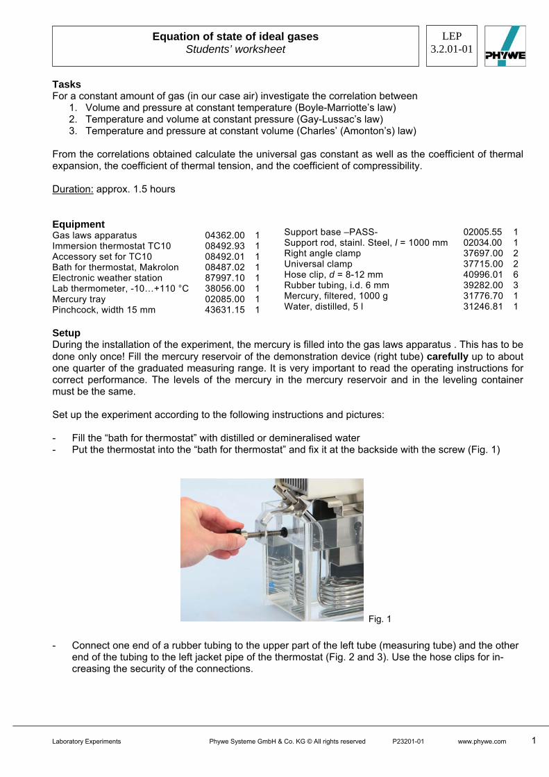
Gas laws apparatus 04362.00 1 Immersion thermostat TC10 08492.93 1 Accessory set for TC10 08492.01 1 Bath for thermostat, Makrolon 08487.02 1 Electronic weather station 87997.10 1 Lab thermometer, -10…+110 °C 38056.00 1 Mercury tray 02085.00 1 Pinchcock, width 15 mm 43631.15 1 Setup During the installation of the experiment, the mercury is filled into the gas laws apparatus . This has to be done only once! Fill the mercury reservoir of the demonstration device (right tube) carefully up to about one quarter of the graduated measuring range. It is very important to read the operating instructions for correct performance. The levels of the mercury in the mercury reservoir and in the leveling container must be the same. Set up the experiment according to the following instructions and pictures: - Fill the “bath for thermostat” with distilled or demineralised water - Put the thermostat into the “bath for thermostat” and fix it at the backside with the screw (Fig. 1)
Fig. 1 - Connect one end of a rubber tubing to the upper part of the left tube (measuring tube) and the other
end of the tubing to the left jacket pipe of the thermostat (Fig. 2 and 3). Use the hose clips for in-creasing the security of the connections.
Laboratory Experiments Phywe Systeme GmbH & Co. KG © All rights reserved P23201-01 www.phywe.com 1

LEP
3.2.01-01 Equation of state of ideal gases
Students’ worksheet
- Now connect one end of another rubber tubing to the lower part of the measuring tube and the other
end of it to the right jacket pipe of the thermostat (Fig. 4 and 5). Again make sure, that these con-nections are secure
- Connect the cooling coil of the thermostat to the water supply by using two rubber tubings (Fig. 6)
Fig. 6
Fig. 4 Fig. 5
Fig. 2 Fig. 3
2 www.phywe.com P23201-01 Phywe Systeme GmbH & Co. KG © All rights reserved Laboratory Experiments

LEP
3.2.01-01Equation of state of ideal gases
Students’ worksheet
- Now your setup should look like the following picture: Fig. 7 - Before beginning the measurements, remove the little rubber stopper from the mercury reservoir
(right tube) (Fig. 8) Fig. 8
Procedure Task 1: During this experiment, the temperature must be kept constant at 298.15 K (25 °C). This is achieved by pumping water, which has the desired temperature, through the rubber tubing with the aid of the thermo-stat. - Switch on the thermostat and set the temperature to 298.15 K (25 °C) - Wait until the temperature in the measuring tube remains constant (look at the thermometer above
the measuring tube) In order to investigate the correlation between the pressure p and the volume V, the pressure in the measuring tube is varied by raising or sinking the mercury reservoir. The length l of the column of air in the measuring tube and the height difference Δh between the mercury level in the mercury reservoir and the mercury level in the measuring tube can be read off the scale of the device.
Laboratory Experiments Phywe Systeme GmbH & Co. KG © All rights reserved P23201-01 www.phywe.com 3

LEP
3.2.01-01 Equation of state of ideal gases
Students’ worksheet
- Get the air pressure pa from the “Electronic weather station” and note the value above Table 1 (page 6)
- Move the mercury reservoir (Fig. 9) until the levels of the mercury in the mercury reservoir and in the measuring tube are at the same height ( 0=Δh )
- Read off the scale the length l of the column of air in the measuring tube (this is the distance be-tween the mercury level and the brown marked measuring tube segment at the top)
Fig. 9
- Perform at least 10 measurements by raising the mercury reservoir and reading off the scale the
length l of the column of air and the height difference Δh between the levels of the mercury in the mercury reservoir and in the measuring tube
- Note your results in Table 1 (page 6)
Task 2 and 3: - In order to determine the temperature dependency on pressure and volume, the two correlations are
investigated at the same time for each temperature step - The initial temperature is the same as in Task 1 ( 15.298=T K) - Move the mercury reservoir so, that the mercury levels in the mercury reservoir and in the measur-
ing tube are at the same height - Mark this position with a marker on the measuring tube or use a piece of adhesive tape to mark the
position on the scale (Fig. 10 and 11). This marking represents a constant volume of air ( ) in the measuring tube.
1VV =
Fig. 10
Fig. 11 - Measure the length l of the column of air in the measuring tube and note this value as well as the
value for the height difference Δh (in this initial case 0=Δh ) in Table 2 (page 7) - Now, increase the temperature to 303.15 K (30 °C) and wait until the temperature in the measuring
tube remains constant
4 www.phywe.com P23201-01 Phywe Systeme GmbH & Co. KG © All rights reserved Laboratory Experiments

LEP
3.2.01-01Equation of state of ideal gases
Students’ worksheet
- Task 2: To investigate the dependency of the temperature T on the volume V at constant pressure app = , move the mercury reservoir until the two mercury levels are equal
Fig. 12 - Read off the scale the “new” length l of the column of air in the measuring tube and note the value in
Table 2
- Task 3: In order to investigate the dependency of the temperature T on the pressure p at constant volume V, move the mercury reservoir until the mercury level in the measuring tube reaches the marking again (Fig. 13)
Fig. 13 - Measure the height difference Δh between the two mercury levels and note the value in Table 2 - Subsequently, increase the temperature in steps of 5 K up to 358.15 K (85 °C) and proceed in each
step the way described above - When you have finished your measurements, put the little rubber stopper back onto the mercury
reservoir
Laboratory Experiments Phywe Systeme GmbH & Co. KG © All rights reserved P23201-01 www.phywe.com 5

LEP
3.2.01-01 Equation of state of ideal gases
Students’ worksheet
Results Task 1:
External air pressure pa = Note your measuring results in the following table (first and second column).
Table 1
Determined length l [mm]
Height difference Δh [mm]
Volume V [ml]
Pressure p [kPa]
Now, calculate from your measuring results the Volume V and the pressure p. To do this, use the fol-lowing equations:
For the volume is valid:
2
2
1 2VldVVV R +×⎟
⎠⎞
⎜⎝⎛=+= π
ml 01.12mm 4.11 2
+×⎟⎠⎞
⎜⎝⎛= lπ (1)
and for the pressure: ppp a Δ+=
(2) -1mm kPa 1333.0 ××Δ+= hpa Use equation (1) to calculate the Volume V. 1.01 ml is approx. the volume of the brown marked measuring tube segment, which has to be added to the volume. Take into account that you have to convert the units since you have ml and mm3 in the same equation.
6 www.phywe.com P23201-01 Phywe Systeme GmbH & Co. KG © All rights reserved Laboratory Experiments

LEP
3.2.01-01Equation of state of ideal gases
Students’ worksheet
The correlation between them is: . Record your results in Table 1 (column 3). 3mm 1000ml 1 = Use equation (2) For the calculation of the pressure p in dependence of the height difference Δh. Note your results for the in Table 1, too (column 4). In our sample measurement we got the following results (Important: these are only sample results and your results may differ from them):
Sample results
Determined length l [mm]
Height difference Δh [mm]
Volume V [ml]
Pressure p [kPa]
183 0 19.96 100.00 180 16 19.38 102.12 175 33 18.87 104.40 170 56 18.36 107.46 160 102 17.34 113.60 150 158 16.32 121.06 140 213 15.30 128.39 134 251 14.69 133.46 130 282 14.28 137.59 124 328 13.67 143.72 120 366 13.26 148.79
Task 2 and 3: Note your measuring results in the table below (columns 1 – 3).
Table 2
Temperature T [K]
Determined lengthl [mm]
Height difference Δh [mm]
Volume V [ml]
Pressure p [kPa]
Again, calculate the Volume V and the pressure p using the equations (1) and (2) and note your re-sults in Table 2 (column 4 and 5). In our sample measurement we got the following results: Laboratory Experiments Phywe Systeme GmbH & Co. KG © All rights reserved P23201-01 www.phywe.com 7

LEP
3.2.01-01 Equation of state of ideal gases
Students’ worksheet
Sample results
Temperature
T [K] Determined length
l [mm] Height difference
Δh [mm] Volume V [ml]
Pressure p [kPa]
298.15 183 0 19.69 100.00 303.15 185 16 19.89 102.13 308.15 188 30 20.20 104.00 313.15 193 40 20.71 105.33 318.15 196 53 21.02 107.06 323.15 199 65 21.32 108.66 328.15 202 76 21.63 110.13 333.15 205 88 21.93 111.73 338.15 208 102 22.24 113.60 343.15 211 114 22.55 115.20 348.15 215 126 22.96 116.80 353.15 219 138 23.36 118.40 358.15 222 152 23.67 120.26
8 www.phywe.com P23201-01 Phywe Systeme GmbH & Co. KG © All rights reserved Laboratory Experiments

LEP
3.2.01-01Equation of state of ideal gases
Students’ worksheet
Evaluation 1. Correlation between volume and pressure at constant temperature (Boyle-Mariotte’s law) In order to explain the correlation between the volume V and the pressure p of a gas one must have a closer look at the results of Task 1. In this part of the experiment the temperature T was constant at 298.15 K whereas the pressure p and the volume V of the gas varied. This process is called isothermal expansion and compression. For the change in volume is valid: dpVdV 00χ−= (3)
where
nTpV
V ,00
1⎟⎟⎠
⎞⎜⎜⎝
⎛∂∂
−=χ
the coefficient of cubic compressibility. The indices T and n show that the temperature and the sub-stance quantity (n) of the gas are constant. From integration of equation (3) with .0 const=χ one gets VppV =00 (4)
p
constV 1.×=⇒ ,
where V0 and p0 the volume and the pressure of the gas at K 15.2730 =T . Therefore V0 and p0 are constant and so the product of both is constant, too. Boyle and Mariotte first investigated this correlation and so it is called Boyle-Mariotte’s law. To compare the theory with your measurements, convert your results for p into 1/p and note these values in the table below.
Reciprocal of the pressure 1/p [kPa]
Laboratory Experiments Phywe Systeme GmbH & Co. KG © All rights reserved P23201-01 www.phywe.com 9

LEP
3.2.01-01 Equation of state of ideal gases
Students’ worksheet
We got the following results for our measuring values:
Sample results
Reciprocal of the pressure 1/p [kPa] 0.01000 0.00979 0.00958 0.00931 0.00880 0.00826 0.00779 0.00749 0.00727 0.00696 0.00672
Now, design a graph where you draw the reciprocal pressure 1/p against the volume V (see Table 1). It is recommended to use the software “PHYWE measure” to do this. It is free for download on www.phywe.com (see appendix). You should get a graph similar to the following:
Fig. 14: Volume V as a function of the reciprocal pressure 1/p at constant temperature ( ) and at constant substance quantity n. K 15.298=T
- Note the value for the slope of the curve in the table on page 13 2. Correlation between temperature and volume at constant pressure (Gay-Lussac’s law)
To investigate the correlation between the temperature T and the volume V at constant pressure ( ) use your measuring results from Task 2. app =The process, in which the pressure p is constant and the temperature T as well as the volume V is variable, is called isobaric process.
10 www.phywe.com P23201-01 Phywe Systeme GmbH & Co. KG © All rights reserved Laboratory Experiments

LEP
3.2.01-01Equation of state of ideal gases
Students’ worksheet
For the change in volume is valid: dTVdV 00γ= (5) where
npTV
V ,00
1⎟⎠⎞
⎜⎝⎛∂∂
=γ
the coefficient of thermal expansion. After integration of (5) with .0 const=γ one gets
TV
TV
=0
0 (6)
TconstV ×=⇒ . Gay-Lussac first investigated this correlation and that is the reason why it is called Gay-Lussac’s law. Now, have a look at Table 2. Design a graph where you draw the values for the temperature T against the values for the volume V. If you measured accurately, you should be able to recognise the proportionality between V and T and your graph should look like the following. Again note the slope (page 13).
Fig. 15: Dependence of the volume V on the temperature T at constant pressure ( kPa 105== app ) and at constant substance quantity n.
3. Correlation between temperature and pressure at constant volume (Charles’ (Amonton’s) law) In order to determine the correlation between the temperature T and the pressure p you have to use Ta-ble 2 again.
Laboratory Experiments Phywe Systeme GmbH & Co. KG © All rights reserved P23201-01 www.phywe.com 11

LEP
3.2.01-01 Equation of state of ideal gases
Students’ worksheet
The process, in which the temperature and the pressure are variable while the volume of the gas is constant, is called isochoric process. For the change in pressure is therefore valid: dTpdp 00β= (7) where
nVTp
p ,00
1⎟⎠⎞
⎜⎝⎛∂∂
=β
the coefficient of thermal tension. After integration of (7) with .0 const=β one gets:
Tp
Tp
=0
0 (8)
Tconstp ×=⇒ . This correlation is called Charles’ (Amonton’s) law. Now, use your measuring results for the temperature T and the pressure p from Table 2 and design a graph where you draw p against T. If you measured accurately, you should be able to recognise the proportionality between p and T and thus your graph should look like the following. Note the slope (page 13).
Fig. 16: Correlation between the pressure p and the temperature T at constant volume V and constant substance quantity n.
12 www.phywe.com P23201-01 Phywe Systeme GmbH & Co. KG © All rights reserved Laboratory Experiments

LEP
3.2.01-01Equation of state of ideal gases
Students’ worksheet
In the next step, determine the universal gas constant R. This is done with the help of the following considerations: By combining the equation (6) or (8) with equation (4) one obtains
TpV
TVp
TVp
==1
11
0
00 (9)
and from that the general (or thermal) equation of state for ideal gases: nRTpV = (10) You can calculate the universal gas constant R with your measurement results and the following equations:
nRTpV
nT
=⎟⎟⎠
⎞⎜⎜⎝
⎛∂∂
−,
1 (10.1)
pnRV
TV
np
==⎟⎠⎞
⎜⎝⎛∂∂
00,
γ (10.2)
VnRp
Tp
nV
==⎟⎠⎞
⎜⎝⎛∂∂
00,
β (10.3)
The three terms in these equations that are on the left of the equality sign are equal to the slopes of the corresponding graphs. That means, (∂V/∂p-1)T,n corresponds to the slope of the graph showing the correlation between volume and pressure (Task 1), (∂V/∂T)p,n corresponds to the slope of the graph showing the correlation between volume and temperature (Task 2) and (∂p/∂T)V,n corresponds to the slope of the graph showing the correlation between pressure and temperature (Task 3). Look at the units of your measured slopes and convert the unit ml into m3. The correlation between them is:
33
33 m 100
1cm 1mm 1000ml 1 === ,
since . This has to be done for the slopes of Task 1 and 2. 333 cm 100m 1 =The unit of the slope of Task 2 should be . To do this, remember, that the following is valid:
Nmm Pa 3 =×
kPa 10kPa10
1 33 =− .
Measured slopes After converting
(∂V/∂p-1)T,n = =
(∂V/∂T)p,n = =
(∂p/∂T)V,n = = Laboratory Experiments Phywe Systeme GmbH & Co. KG © All rights reserved P23201-01 www.phywe.com 13

LEP
3.2.01-01 Equation of state of ideal gases
Students’ worksheet
In our measurement we got the following results:
Measured slopes After converting (∂V/∂p-1)T,n = kPa ml/10 989.1 -3 = Nm 989.1m Pa 989.1 3 =× (∂V/∂T)p,n = ml/K 067.0 = -138 K m 10686.6 ×× − (∂p/∂T)V,n = kPa/K 330.0 = -1K kPa 330.0 ×
The universal gas constant is calculated by using the equations (10.1), (10.2), (10.3). But first, you have to determine the value for n by the equation:
mVVn = (11)
where Vm the molar volume of the gas (air). Under standard conditions ( ,
) it is . In order to calculate n you have to reduce your measured volume V to these standard conditions. This is done by using equation (9). Insert one measured result each for V, p, T (have a look at Table 2) and the values for p
K 15.2730 =TkPa 325.1010 =p -13 mol m 022414.0 ×=mV
0 and T0 (see above) to calculate V0. Then insert this value in equation (11) to calculate n and note it below.
=n Now, you have all values to calculate the universal gas constant R according to the equations (10.1), (10.2) and (10.3). Note your results in the following table:
=R
=R
=R
and calculate the mean value:
=R
In our sample measurement we got the following results:
mol 0007943.0=n
-1-1 molKNm 399.8 ××=R -1-1 molKNm 418.8 ××=R -1-1 molKNm 181.8 ××=R
Mean value:
-1-1 molKNm 333.8 ××=R The literature value is . -1-1-1-1 molKJ 31441.8molKNm 31441.8 ××=××=R
14 www.phywe.com P23201-01 Phywe Systeme GmbH & Co. KG © All rights reserved Laboratory Experiments
LEP
3.2.01-01Equation of state of ideal gases
Students’ worksheet
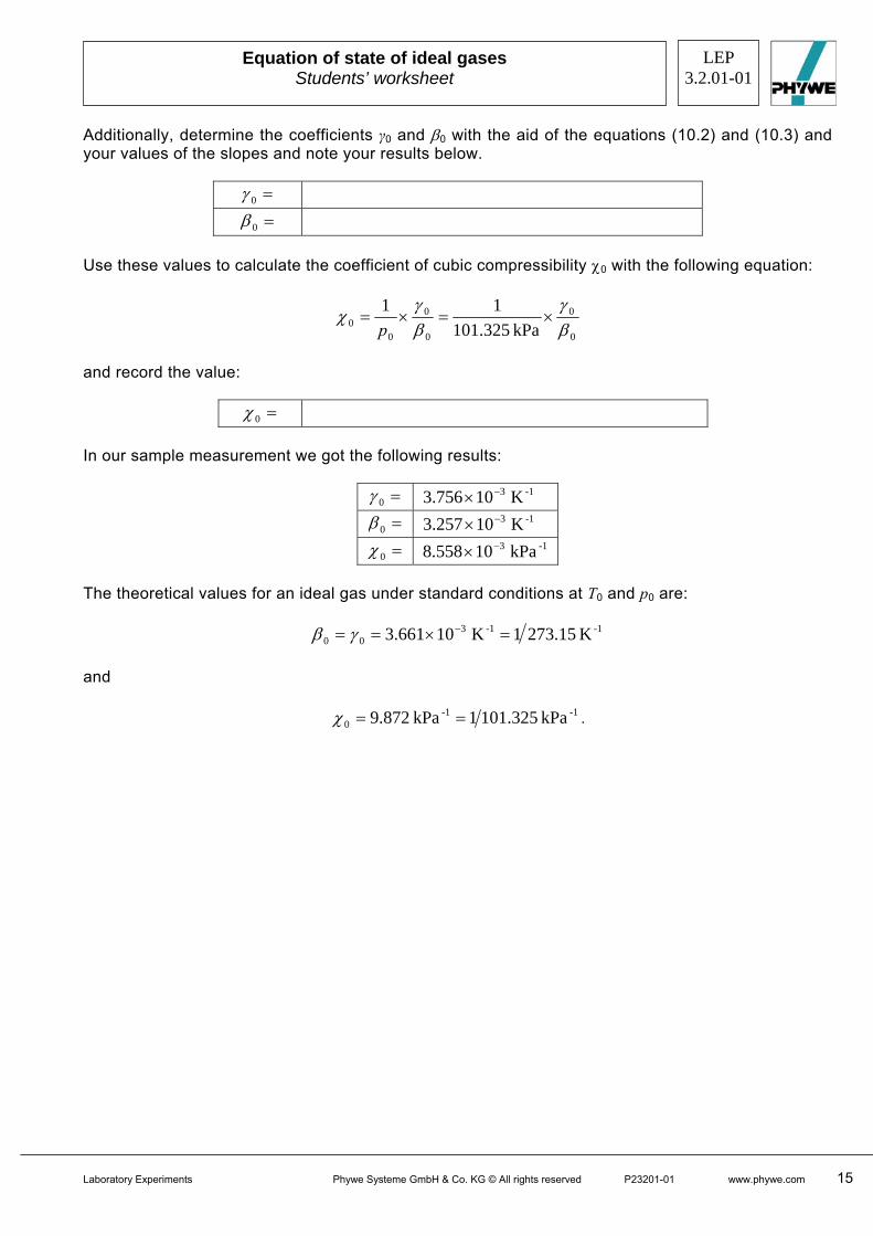
Additionally, determine the coefficients γ0 and β0 with the aid of the equations (10.2) and (10.3) and your values of the slopes and note your results below.
=0γ =0β
Use these values to calculate the coefficient of cubic compressibility χ0 with the following equation:
0
0
0
0
00 kPa 325.101
11βγ
βγ
χ ×=×=p
and record the value:
=0χ
In our sample measurement we got the following results:
=0γ -13 K 10756.3 −× =0β -13 K 10257.3 −× =0χ -13 kPa 10558.8 −×
The theoretical values for an ideal gas under standard conditions at T0 and p0 are:
-1-1300 K 15.2731K 10661.3 =×== −γβ
and
-1-10 kPa 325.1011kPa 872.9 ==χ .
Laboratory Experiments Phywe Systeme GmbH & Co. KG © All rights reserved P23201-01 www.phywe.com 15

LEP
3.2.01-01 Equation of state of ideal gases
Students’ worksheet
Appendix Using “measure” for creating the graphs and evaluation of the data - Once installed, start “measure”. - Click “Measurement” and choose “Enter data manually” - There select the parameters that are shown in the screenshot below
- Click “Continue” - Type in your values for V and 1/p (make sure to use commas instead of points for decimal num-
bers) - Click “OK” - Choose the first point “Sort x-data…” - Right-click on your graph and select “Display options” (Symbol: ) - Under “channels” select “interpolation” and “none” for displaying the points only. In this menu
you can also change the displayed area for the best display
- For fitting the graph click “Analysis” and then “Function fitting”, choose “straight” and click “Cal-culate”
- After clicking “Add new curve” the fitting curve will appear
16 www.phywe.com P23201-01 Phywe Systeme GmbH & Co. KG © All rights reserved Laboratory Experiments

LEP
3.2.01-01Equation of state of ideal gases
Students’ worksheet
- Click the button “Show slope” ( ) and note this value for the slope - This is how you can use “measure” for displaying the graphs for Tasks 2 and 3, too. For further
information about the program please go to the “Help”-menu.
Laboratory Experiments Phywe Systeme GmbH & Co. KG © All rights reserved P23201-01 www.phywe.com 17
Related Documents