Manual Calculation–Programs for Machine Design c KISSsoft AG, Frauwis 1, CH-8634 Hombrechtikon Fon +41 55 264 20 30; Fax +41 55 264 20 33 www.KISSsoft.ch [email protected] October 28, 2005

Welcome message from author
This document is posted to help you gain knowledge. Please leave a comment to let me know what you think about it! Share it to your friends and learn new things together.
Transcript

ManualCalculation–Programsfor Machine Design
c©KISSsoft AG, Frauwis 1, CH-8634 HombrechtikonFon +41 55 264 20 30; Fax +41 55 264 20 33
www.KISSsoft.ch [email protected]
October 28, 2005


Contents
I General 1-1
1 How to Use this Manual 1-3
1.1 Explanations to Font Formats and Symbols . . . . . . . . . . . . 1-3
1.2 Structure of Manual . . . . . . . . . . . . . . . . . . . . . . . . . 1-4
2 How to Work with KISSsoft 1-5
2.1 Control Panels . . . . . . . . . . . . . . . . . . . . . . . . . . . . 1-5
2.2 General Features of the User Interface . . . . . . . . . . . . . . . 1-6
2.2.1 Changing Units . . . . . . . . . . . . . . . . . . . . . . . . 1-6
2.2.2 Calculating an input value . . . . . . . . . . . . . . . . . . 1-6
2.3 KISSsoft Main Window . . . . . . . . . . . . . . . . . . . . . . . . 1-7
2.3.1 Calculation . . . . . . . . . . . . . . . . . . . . . . . . . . 1-7
2.3.2 Project . . . . . . . . . . . . . . . . . . . . . . . . . . . . . 1-8
2.3.3 Services . . . . . . . . . . . . . . . . . . . . . . . . . . . . 1-8
2.3.4 Help . . . . . . . . . . . . . . . . . . . . . . . . . . . . . . 1-12
3 The KISSsoft Help-System 1-13
3.1 The Menu Help . . . . . . . . . . . . . . . . . . . . . . . . . . . . 1-13
3.2 Contextual Help with F1 . . . . . . . . . . . . . . . . . . . . . . . 1-14
4 User Defined Settings - an Overview 1-15
1

2 CONTENTS
5 Installing KISSsoft 1-17
5.1 General Information . . . . . . . . . . . . . . . . . . . . . . . . . 1-17
5.2 Installing the Multi User Version . . . . . . . . . . . . . . . . . . 1-17
5.3 Read Only Directory . . . . . . . . . . . . . . . . . . . . . . . . . 1-19
5.3.1 Disconnecting Users . . . . . . . . . . . . . . . . . . . . . 1-20
6 Setting up KISSsoft 1-21
6.1 Defining Languages . . . . . . . . . . . . . . . . . . . . . . . . . . 1-21
6.2 Defining the Editor . . . . . . . . . . . . . . . . . . . . . . . . . . 1-22
6.3 Defining Individual Standard Files . . . . . . . . . . . . . . . . . 1-22
6.4 Project and User Administration . . . . . . . . . . . . . . . . . . 1-23
6.4.1 Saving Calculations . . . . . . . . . . . . . . . . . . . . . . 1-23
6.4.2 Saving Common Default Files . . . . . . . . . . . . . . . . 1-25
6.4.3 Typical Scenarios of Project and User Administration . . . 1-27
6.5 Command line parameters . . . . . . . . . . . . . . . . . . . . . . 1-27
7 KISSsoft Data Base Tool and Table Interface 1-29
7.1 Calculation Values in Data Bases and Tables . . . . . . . . . . . . 1-29
7.1.1 Data Base and Data Base Tool . . . . . . . . . . . . . . . 1-29
7.1.2 Opening a Table with Write Protection . . . . . . . . . . . 1-29
7.1.3 Interface Between KISSsoft and External Tables . . . . . . 1-30
7.2 Description of the Data Base . . . . . . . . . . . . . . . . . . . . . 1-30
7.2.1 Save, New, Copy . . . . . . . . . . . . . . . . . . . . . . . 1-30
7.2.2 Material Notation for Different Countries . . . . . . . . . . 1-31
7.2.3 Automatic Update Function . . . . . . . . . . . . . . . . . 1-31
7.2.4 Exporting and Importing Data Sets . . . . . . . . . . . . . 1-31
7.2.5 Navigating in the Data Base . . . . . . . . . . . . . . . . . 1-32
7.2.6 List . . . . . . . . . . . . . . . . . . . . . . . . . . . . . . 1-32
7.2.7 Input Fields of Data Bases . . . . . . . . . . . . . . . . . . 1-36
7.3 Description of the Look-up Table Interface . . . . . . . . . . . . . 1-52
CONTENTS 3
7.3.1 General . . . . . . . . . . . . . . . . . . . . . . . . . . . . 1-52
7.3.2 Treatment . . . . . . . . . . . . . . . . . . . . . . . . . . . 1-52
7.3.3 Structure of Tables . . . . . . . . . . . . . . . . . . . . . . 1-52
8 Reports 1-57
8.1 Calculation Report . . . . . . . . . . . . . . . . . . . . . . . . . . 1-57
8.2 Report Templates . . . . . . . . . . . . . . . . . . . . . . . . . . . 1-58
8.2.1 Name of Report templates . . . . . . . . . . . . . . . . . . 1-58
8.2.2 Length of Reports . . . . . . . . . . . . . . . . . . . . . . . 1-60
8.2.3 Format of Report Templates . . . . . . . . . . . . . . . . . 1-61
8.2.4 Formating Reports in RTF-Format . . . . . . . . . . . . . 1-67
8.3 The Report Editor KISSedit . . . . . . . . . . . . . . . . . . . . . 1-67
8.3.1 Saving reports . . . . . . . . . . . . . . . . . . . . . . . . . 1-68
8.3.2 Synchronised Scrolling . . . . . . . . . . . . . . . . . . . . 1-68
8.3.3 Quick Change from Portrait to Landscape . . . . . . . . . 1-69
8.3.4 Definition of Header and Footer . . . . . . . . . . . . . . . 1-69
9 Description of the Public Interface 1-71
9.1 Interfaces Between Calculation Programs and CAD – Overview . 1-71
9.1.1 Useful Interfaces . . . . . . . . . . . . . . . . . . . . . . . 1-71
9.1.2 Open-Interface-Concept in KISSsoft . . . . . . . . . . . . . 1-73
9.2 Defining Input and Output . . . . . . . . . . . . . . . . . . . . . . 1-74
9.2.1 Rough Remarks . . . . . . . . . . . . . . . . . . . . . . . . 1-74
9.2.2 Standard of External Programs . . . . . . . . . . . . . . . 1-75
9.2.3 Employed Files . . . . . . . . . . . . . . . . . . . . . . . . 1-76
9.2.4 Life Span of Files . . . . . . . . . . . . . . . . . . . . . . . 1-76
9.2.5 Explicitly Reading and Generating Data . . . . . . . . . . 1-77
9.3 Example: Interference Fit Calculation . . . . . . . . . . . . . . . . 1-77
9.4 Geometry data . . . . . . . . . . . . . . . . . . . . . . . . . . . . 1-78
9.4.1 Example on KISSsoft-Graphic-Format . . . . . . . . . . . 1-79

4 CONTENTS
9.5 3D-Interfaces . . . . . . . . . . . . . . . . . . . . . . . . . . . . . 1-80
9.5.1 IGES, SAT and STEP Interfaces . . . . . . . . . . . . . . 1-80
9.5.2 SolidWorks-Interface . . . . . . . . . . . . . . . . . . . . . 1-80
9.5.3 SolidEdge-Interface . . . . . . . . . . . . . . . . . . . . . . 1-81
9.5.4 Inventor-Interface . . . . . . . . . . . . . . . . . . . . . . 1-81
II Joints and Belts 2-1
10 Connecting Elements 2-3
10.1 KISSsoft Modules . . . . . . . . . . . . . . . . . . . . . . . . . . . 2-3
10.2 Shaft-Hub-Connections . . . . . . . . . . . . . . . . . . . . . . . . 2-4
10.2.1 Interference Fit . . . . . . . . . . . . . . . . . . . . . . . . 2-4
10.2.2 Feather-Key Connection . . . . . . . . . . . . . . . . . . . 2-8
10.2.3 Multi-Spline . . . . . . . . . . . . . . . . . . . . . . . . . . 2-14
10.2.4 Splines . . . . . . . . . . . . . . . . . . . . . . . . . . . . . 2-16
10.2.5 Polygon . . . . . . . . . . . . . . . . . . . . . . . . . . . . 2-18
10.2.6 Woodruff Key . . . . . . . . . . . . . . . . . . . . . . . . . 2-19
10.3 Dowels . . . . . . . . . . . . . . . . . . . . . . . . . . . . . . . . . 2-20
10.3.1 Determining factors . . . . . . . . . . . . . . . . . . . . . . 2-21
10.3.2 Specific module settings . . . . . . . . . . . . . . . . . . . 2-21
10.3.3 Sizing . . . . . . . . . . . . . . . . . . . . . . . . . . . . . 2-22
10.4 Bolted joints . . . . . . . . . . . . . . . . . . . . . . . . . . . . . . 2-22
10.5 Glued and Soldered Joints . . . . . . . . . . . . . . . . . . . . . . 2-22
10.5.1 Basic Materials . . . . . . . . . . . . . . . . . . . . . . . . 2-23
10.5.2 Sizing of Width for Basic Material . . . . . . . . . . . . . 2-23
10.5.3 Sizing of Width for Load . . . . . . . . . . . . . . . . . . . 2-23
10.5.4 Flat links . . . . . . . . . . . . . . . . . . . . . . . . . . . 2-23
10.5.5 Shaft Connections . . . . . . . . . . . . . . . . . . . . . . . 2-23
10.6 Welded Joints . . . . . . . . . . . . . . . . . . . . . . . . . . . . . 2-24
10.6.1 Seam Length . . . . . . . . . . . . . . . . . . . . . . . . . 2-24

CONTENTS 5
10.6.2 Part Safety Coefficient . . . . . . . . . . . . . . . . . . . . 2-24
10.6.3 Boundary Safety Coefficient . . . . . . . . . . . . . . . . . 2-24
11 Bolted Joints Calculation 2-25
11.1 Calculation-Basis and Abilities . . . . . . . . . . . . . . . . . . . . 2-25
11.1.1 General Remarks . . . . . . . . . . . . . . . . . . . . . . . 2-25
11.1.2 Calculating with KISSsoft . . . . . . . . . . . . . . . . . . 2-27
11.1.3 Special Features of KISSsoft . . . . . . . . . . . . . . . . . 2-28
11.1.4 Extent of Additional KISSsoft Modules . . . . . . . . . . . 2-29
11.2 Important Inputs . . . . . . . . . . . . . . . . . . . . . . . . . . . 2-29
11.2.1 Reference Diameter and Screw Type . . . . . . . . . . . . 2-29
11.2.2 Defining Individual Screw Geometry . . . . . . . . . . . . 2-30
11.2.3 Thread Types . . . . . . . . . . . . . . . . . . . . . . . . . 2-31
11.2.4 Restrained Parts . . . . . . . . . . . . . . . . . . . . . . . 2-32
11.2.5 Force Application Factor . . . . . . . . . . . . . . . . . . . 2-32
11.2.6 Eccentric Application of Force and Eccentric Restraint . . 2-35
11.2.7 Tightening Factor – Coefficient of Friction . . . . . . . . . 2-35
11.2.8 Configurations . . . . . . . . . . . . . . . . . . . . . . . . . 2-39
11.2.9 Bore Diameter . . . . . . . . . . . . . . . . . . . . . . . . 2-42
11.2.10Subsidence Value . . . . . . . . . . . . . . . . . . . . . . . 2-42
11.3 Display Screws . . . . . . . . . . . . . . . . . . . . . . . . . . . . 2-42
11.4 Possible Propositions . . . . . . . . . . . . . . . . . . . . . . . . . 2-43
11.5 Screws at High and Low Temperatures . . . . . . . . . . . . . . . 2-43
11.5.1 Technical Explanations . . . . . . . . . . . . . . . . . . . . 2-43
11.5.2 Inputs . . . . . . . . . . . . . . . . . . . . . . . . . . . . . 2-44
11.5.3 Outputs . . . . . . . . . . . . . . . . . . . . . . . . . . . . 2-45
11.6 Tension Diagram . . . . . . . . . . . . . . . . . . . . . . . . . . . 2-45
11.7 Stripping Strength . . . . . . . . . . . . . . . . . . . . . . . . . . 2-46
11.8 Special Settings . . . . . . . . . . . . . . . . . . . . . . . . . . . . 2-46
11.9 FAQ . . . . . . . . . . . . . . . . . . . . . . . . . . . . . . . . . . 2-48
11.9.1 Entering Additional Screws . . . . . . . . . . . . . . . . . 2-48

6 CONTENTS
12 Belts 2-53
12.1 Calculating V-belts . . . . . . . . . . . . . . . . . . . . . . . . . . 2-54
12.1.1 Standard . . . . . . . . . . . . . . . . . . . . . . . . . . . . 2-54
12.1.2 Configurating Tension Pulleys . . . . . . . . . . . . . . . . 2-55
12.1.3 Load Factor CB . . . . . . . . . . . . . . . . . . . . . . . . 2-55
12.1.4 Distance of Axes . . . . . . . . . . . . . . . . . . . . . . . 2-55
12.1.5 Belt Lenght . . . . . . . . . . . . . . . . . . . . . . . . . . 2-56
12.1.6 Number of V-Belts . . . . . . . . . . . . . . . . . . . . . . 2-56
12.1.7 Tension Pulley Diameter . . . . . . . . . . . . . . . . . . . 2-56
12.1.8 Position of Tension Pulley (x/y) . . . . . . . . . . . . . . . 2-56
12.1.9 Inspecting V-Belts . . . . . . . . . . . . . . . . . . . . . . 2-56
12.2 Calculating Toothed Belts . . . . . . . . . . . . . . . . . . . . . . 2-57
12.2.1 Technical Remarks (Toothed Belts) . . . . . . . . . . . . . 2-57
12.2.2 Standard Toothed Belts . . . . . . . . . . . . . . . . . . . 2-58
12.2.3 Possible Propositions . . . . . . . . . . . . . . . . . . . . . 2-59
12.2.4 Tension Pulley Configuration . . . . . . . . . . . . . . . . 2-59
12.2.5 Service Factor and Addendum for Operation . . . . . . . . 2-59
12.2.6 Distance of Axes . . . . . . . . . . . . . . . . . . . . . . . 2-60
12.2.7 Belt Length and Number of Teeth . . . . . . . . . . . . . . 2-60
12.2.8 Actual Belt Width . . . . . . . . . . . . . . . . . . . . . . 2-60
12.2.9 Tension Pulley Tooth Number . . . . . . . . . . . . . . . . 2-61
12.2.10Position of Tension Pulley x/y . . . . . . . . . . . . . . . . 2-62
12.3 Chain Drive Calculation . . . . . . . . . . . . . . . . . . . . . . . 2-62
12.3.1 Sizings: . . . . . . . . . . . . . . . . . . . . . . . . . . . . 2-62
12.3.2 Tension Pulleys . . . . . . . . . . . . . . . . . . . . . . . . 2-62
12.3.3 Standards . . . . . . . . . . . . . . . . . . . . . . . . . . . 2-62
12.3.4 Chain Type . . . . . . . . . . . . . . . . . . . . . . . . . . 2-63
12.3.5 Number of Lanes . . . . . . . . . . . . . . . . . . . . . . . 2-63
12.3.6 Service Factor . . . . . . . . . . . . . . . . . . . . . . . . . 2-63
12.3.7 Speed/Number of Teeth/Ratio . . . . . . . . . . . . . . . . 2-64

CONTENTS 7
12.3.8 Configuration . . . . . . . . . . . . . . . . . . . . . . . . . 2-64
12.3.9 Distance of Axes . . . . . . . . . . . . . . . . . . . . . . . 2-65
12.3.10Polygon effect . . . . . . . . . . . . . . . . . . . . . . . . . 2-65
12.3.11Number of Links . . . . . . . . . . . . . . . . . . . . . . . 2-65
12.3.12Graphical positioning of the Tension Pulley . . . . . . . . 2-65
13 Calculation of Springs 2-67
13.1 Garter Springs . . . . . . . . . . . . . . . . . . . . . . . . . . . . 2-67
13.1.1 Material Strength . . . . . . . . . . . . . . . . . . . . . . . 2-67
13.1.2 Support coefficient . . . . . . . . . . . . . . . . . . . . . . 2-68
13.1.3 Sizing . . . . . . . . . . . . . . . . . . . . . . . . . . . . . 2-68
13.2 Tension springs . . . . . . . . . . . . . . . . . . . . . . . . . . . . 2-68
13.2.1 Material Strength . . . . . . . . . . . . . . . . . . . . . . . 2-69
13.2.2 Production . . . . . . . . . . . . . . . . . . . . . . . . . . 2-70
13.2.3 Eyes . . . . . . . . . . . . . . . . . . . . . . . . . . . . . . 2-70
13.2.4 Sizing . . . . . . . . . . . . . . . . . . . . . . . . . . . . . 2-71
13.3 Leg Springs . . . . . . . . . . . . . . . . . . . . . . . . . . . . . . 2-71
13.3.1 Strength data . . . . . . . . . . . . . . . . . . . . . . . . . 2-72
13.3.2 Design of spring . . . . . . . . . . . . . . . . . . . . . . . . 2-72
13.3.3 Assumptions for analysis . . . . . . . . . . . . . . . . . . . 2-72
13.3.4 Sizing . . . . . . . . . . . . . . . . . . . . . . . . . . . . . 2-73
13.4 Disc springs . . . . . . . . . . . . . . . . . . . . . . . . . . . . . . 2-73
13.4.1 Geometry . . . . . . . . . . . . . . . . . . . . . . . . . . . 2-73
13.4.2 Strength . . . . . . . . . . . . . . . . . . . . . . . . . . . . 2-73
13.4.3 Calculate Number . . . . . . . . . . . . . . . . . . . . . . . 2-74
13.4.4 Limit Dimensions . . . . . . . . . . . . . . . . . . . . . . . 2-74
13.5 Torsion bar springs . . . . . . . . . . . . . . . . . . . . . . . . . . 2-74
13.5.1 Geometry . . . . . . . . . . . . . . . . . . . . . . . . . . . 2-74
13.5.2 Strength values . . . . . . . . . . . . . . . . . . . . . . . . 2-75
13.5.3 Determining Design . . . . . . . . . . . . . . . . . . . . . . 2-75
13.5.4 Limiting values . . . . . . . . . . . . . . . . . . . . . . . . 2-76

8 CONTENTS
III Shafts and Bearings 3-1
14 Input of Shafts 3-3
14.1 Shaft Calculation . . . . . . . . . . . . . . . . . . . . . . . . . . . 3-3
14.2 Main Input Menu . . . . . . . . . . . . . . . . . . . . . . . . . . . 3-7
14.2.1 Shaft Position . . . . . . . . . . . . . . . . . . . . . . . . . 3-7
14.2.2 Speed . . . . . . . . . . . . . . . . . . . . . . . . . . . . . 3-8
14.2.3 Sense of Rotation and Co-ordinate System . . . . . . . . . 3-8
14.2.4 Quality of Balance Grading . . . . . . . . . . . . . . . . . 3-9
14.2.5 Boundary Conditions at Shaft Ends and Bearings . . . . . 3-11
14.3 Module-Specific Settings . . . . . . . . . . . . . . . . . . . . . . . 3-12
14.3.1 General Module-Specific Settings . . . . . . . . . . . . . . 3-12
14.3.2 Module-Specific Settings Roller Bearing . . . . . . . . . . . 3-13
14.4 Graphical Input of Shaft Data . . . . . . . . . . . . . . . . . . . . 3-15
14.4.1 Input of Shaft or Support Elements . . . . . . . . . . . . . 3-15
14.4.2 Bearings . . . . . . . . . . . . . . . . . . . . . . . . . . . . 3-21
14.4.3 Roller Bearing . . . . . . . . . . . . . . . . . . . . . . . . . 3-21
14.4.4 External Forces and Masses . . . . . . . . . . . . . . . . . 3-22
14.4.5 Importing Shafts from Drawings (CAD) . . . . . . . . . . 3-26
14.4.6 Settings . . . . . . . . . . . . . . . . . . . . . . . . . . . . 3-27
14.4.7 End of Input . . . . . . . . . . . . . . . . . . . . . . . . . 3-28
14.5 Sizing of Shafts . . . . . . . . . . . . . . . . . . . . . . . . . . . . 3-29
14.6 Statically Undefined Bearings . . . . . . . . . . . . . . . . . . . . 3-30
15 Calculations 3-31
15.1 Bearing Forces and Line of Flex . . . . . . . . . . . . . . . . . . . 3-31
15.1.1 Considering Gears . . . . . . . . . . . . . . . . . . . . . . 3-34
15.1.2 Considering the load spectra . . . . . . . . . . . . . . . . . 3-34
15.1.3 Consider deformation due to shearing . . . . . . . . . . . . 3-34
15.1.4 Force calculation with bearings with pressure angle . . . . 3-35

CONTENTS 9
15.2 Bending Critical Speed . . . . . . . . . . . . . . . . . . . . . . . . 3-37
15.2.1 Considering Gear Wheels . . . . . . . . . . . . . . . . . . . 3-38
15.2.2 Eigen Frequency of Supports . . . . . . . . . . . . . . . . . 3-38
15.3 Calculating Rotational Natural Frequency for Shafts and Systems 3-39
15.4 Buckling . . . . . . . . . . . . . . . . . . . . . . . . . . . . . . . . 3-39
15.5 Shaft Strength . . . . . . . . . . . . . . . . . . . . . . . . . . . . . 3-40
15.5.1 Procedure Strength Calculation . . . . . . . . . . . . . . . 3-40
15.5.2 Sizing . . . . . . . . . . . . . . . . . . . . . . . . . . . . . 3-44
15.5.3 Kinds of Cross Sections . . . . . . . . . . . . . . . . . . . . 3-45
15.5.4 General Inputs . . . . . . . . . . . . . . . . . . . . . . . . 3-48
15.5.5 Calculation according to Hanchen + Decker . . . . . . . . 3-50
15.5.6 Calculation According to DIN 743 . . . . . . . . . . . . . . 3-55
15.5.7 Calculating According to FKM . . . . . . . . . . . . . . . 3-56
15.5.8 Materials . . . . . . . . . . . . . . . . . . . . . . . . . . . 3-59
15.5.9 Notch Factors . . . . . . . . . . . . . . . . . . . . . . . . . 3-61
15.5.10Surface-Factors . . . . . . . . . . . . . . . . . . . . . . . . 3-61
15.5.11Section Modulus . . . . . . . . . . . . . . . . . . . . . . . 3-61
15.6 Deformation of Shaft and Calculation of Gear Crowning . . . . . 3-62
15.7 Transfer of Data to Bearing Calculation . . . . . . . . . . . . . . 3-62
16 Calculating Bearings 3-65
16.1 Classification of Bearings . . . . . . . . . . . . . . . . . . . . . . . 3-65
16.1.1 Qualities . . . . . . . . . . . . . . . . . . . . . . . . . . . . 3-65
16.2 Calculating Roller Bearings . . . . . . . . . . . . . . . . . . . . . 3-66
16.2.1 Choosing Roller Bearing Type . . . . . . . . . . . . . . . . 3-67
16.2.2 Load Capacity and Calculation of Roller Bearings . . . . . 3-72
16.2.3 Thermal limit of operating speed . . . . . . . . . . . . . . 3-73
16.2.4 Friction Moment . . . . . . . . . . . . . . . . . . . . . . . 3-76
16.2.5 Maximal Speed . . . . . . . . . . . . . . . . . . . . . . . . 3-79
16.2.6 Service Life . . . . . . . . . . . . . . . . . . . . . . . . . . 3-79

10 CONTENTS
16.2.7 Failure Probability . . . . . . . . . . . . . . . . . . . . . . 3-81
16.2.8 Calculating Bearing Forces Considering the Pressure Angle 3-81
16.2.9 Bearings with Radial and/or Axial Force . . . . . . . . . . 3-82
16.2.10Calculating Axial Forces on Bearings in O- or X-Arrangement3-82
16.3 Calculating Journal Bearings . . . . . . . . . . . . . . . . . . . . . 3-83
16.3.1 Hydro Dynamic Radial Journal Bearings (W07) . . . . . . 3-83
16.3.2 Axial-Journal Bearings (W07C) . . . . . . . . . . . . . . . 3-89
17 Answers to most FAQs 3-93
17.1 Intersecting Notch Effects . . . . . . . . . . . . . . . . . . . . . . 3-93
17.2 Notch Effects on Hollow Shafts . . . . . . . . . . . . . . . . . . . 3-94
17.2.1 Notches on the Outer Contour . . . . . . . . . . . . . . . . 3-94
17.2.2 Notches on the Inner Contour . . . . . . . . . . . . . . . . 3-94
17.3 Fatigue Limits for New Materials . . . . . . . . . . . . . . . . . . 3-94
IV Gears 4-1
18 Gear Calculation in General 4-3
18.1 Handling . . . . . . . . . . . . . . . . . . . . . . . . . . . . . . . . 4-3
18.2 Overview on the Gear Wheel Part . . . . . . . . . . . . . . . . . . 4-3
19 Spur Gears 4-5
19.1 KISSsoft-Gear-Configuration . . . . . . . . . . . . . . . . . . . . . 4-5
19.2 Calculation-Basis . . . . . . . . . . . . . . . . . . . . . . . . . . . 4-6
19.3 Input Interfaces . . . . . . . . . . . . . . . . . . . . . . . . . . . . 4-7
19.3.1 Main Windows for Cylindrical Gear Calculation . . . . . . 4-7
19.3.2 Geometry-Manager . . . . . . . . . . . . . . . . . . . . . . 4-17
19.3.3 Tolerances . . . . . . . . . . . . . . . . . . . . . . . . . . . 4-18
19.3.4 Tolerance-Settings . . . . . . . . . . . . . . . . . . . . . . 4-18
19.3.5 Lubrication . . . . . . . . . . . . . . . . . . . . . . . . . . 4-19
19.3.6 Special Inputs . . . . . . . . . . . . . . . . . . . . . . . . . 4-20

CONTENTS 11
19.3.7 Gear-Specific Entries . . . . . . . . . . . . . . . . . . . . . 4-22
19.3.8 Pair-Specific Entries . . . . . . . . . . . . . . . . . . . . . 4-37
19.4 Settings . . . . . . . . . . . . . . . . . . . . . . . . . . . . . . . . 4-44
19.4.1 General Settings . . . . . . . . . . . . . . . . . . . . . . . 4-45
19.4.2 Entries for Calculations According to AGMA . . . . . . . 4-48
19.4.3 Settings for Plastics . . . . . . . . . . . . . . . . . . . . . . 4-50
19.4.4 Settings for Planetary gears . . . . . . . . . . . . . . . . . 4-51
19.4.5 Settings for Sizings . . . . . . . . . . . . . . . . . . . . . . 4-52
19.4.6 Settings for Calculations . . . . . . . . . . . . . . . . . . . 4-53
19.4.7 Nominal Safeties . . . . . . . . . . . . . . . . . . . . . . . 4-56
19.4.8 Rating . . . . . . . . . . . . . . . . . . . . . . . . . . . . . 4-56
19.5 Sizing . . . . . . . . . . . . . . . . . . . . . . . . . . . . . . . . . 4-57
19.5.1 Rough Sizing (Z03) . . . . . . . . . . . . . . . . . . . . . . 4-57
19.5.2 Spur Gear Fine Sizing (Z04) . . . . . . . . . . . . . . . . . 4-58
19.6 Tooth Form Calculations (Z05) . . . . . . . . . . . . . . . . . . . 4-66
19.6.1 Operations . . . . . . . . . . . . . . . . . . . . . . . . . . . 4-67
19.6.2 Tooth form display . . . . . . . . . . . . . . . . . . . . . . 4-80
19.7 Various Calculations in the Menu ’Calculations’ . . . . . . . . . . 4-82
19.7.1 Drawing (schematically) . . . . . . . . . . . . . . . . . . . 4-83
19.7.2 Calculating Contact Length to Verify the Involute and Sug-gestions for Optimal Profile Corrections) . . . . . . . . . . 4-83
19.7.3 Calculation of the tooth thickness for any diameter . . . . 4-89
19.7.4 Tolerances for Gear Manufacturing . . . . . . . . . . . . . 4-90
19.7.5 Crowning . . . . . . . . . . . . . . . . . . . . . . . . . . . 4-91
19.7.6 Calculating the Centre Points of Planets or Gear Wheels(Z19g) . . . . . . . . . . . . . . . . . . . . . . . . . . . . . 4-91
19.7.7 Specific Sliding(Z19e) . . . . . . . . . . . . . . . . . . . . . 4-92
19.7.8 Flashtemperature Course . . . . . . . . . . . . . . . . . . . 4-92
19.7.9 Hardness Depth (Z22) . . . . . . . . . . . . . . . . . . . . 4-92
19.7.10Rating . . . . . . . . . . . . . . . . . . . . . . . . . . . . . 4-92

12 CONTENTS
19.7.11Wohler Line Material . . . . . . . . . . . . . . . . . . . . . 4-93
19.7.12Course of Safety . . . . . . . . . . . . . . . . . . . . . . . . 4-93
19.7.13Calculation with path of contact under load . . . . . . . . 4-93
19.7.14Calculating Service Life (Z18) . . . . . . . . . . . . . . . . 4-94
19.7.15Sizing for Torque (Z16) . . . . . . . . . . . . . . . . . . . . 4-96
19.7.16Safety with load spectra . . . . . . . . . . . . . . . . . . . 4-96
19.7.17Operating Backlash (Z12) . . . . . . . . . . . . . . . . . . 4-96
19.7.18Lubricant gap EHD/Scoring (Z19k) . . . . . . . . . . . . . 4-98
19.7.19Deformation of Gear Rims (for Internal Gears) (Z23) . . . 4-99
19.7.20Master gear (Z29) . . . . . . . . . . . . . . . . . . . . . . . 4-99
19.7.21Gear pumps (Z26/Z26a) . . . . . . . . . . . . . . . . . . . 4-100
19.8 Calculation of Racks . . . . . . . . . . . . . . . . . . . . . . . . . 4-102
20 Bevel and Hypoid Gear Calculations 4-103
20.1 Calculation Basis . . . . . . . . . . . . . . . . . . . . . . . . . . . 4-103
20.1.1 Calculating Bevel Gears according to Klingelnberg, Glea-son and Oerlikon . . . . . . . . . . . . . . . . . . . . . . . 4-104
20.2 Input Interfaces . . . . . . . . . . . . . . . . . . . . . . . . . . . . 4-105
20.2.1 Main Window . . . . . . . . . . . . . . . . . . . . . . . . . 4-105
20.2.2 Gear Specific Inputs . . . . . . . . . . . . . . . . . . . . . 4-108
20.2.3 Pair Specific Input Window . . . . . . . . . . . . . . . . . 4-109
20.2.4 Interfaces: Additional Inputs . . . . . . . . . . . . . . . . . 4-110
20.3 Settings . . . . . . . . . . . . . . . . . . . . . . . . . . . . . . . . 4-112
20.4 Sizing of Bevel and Hypoid Gears . . . . . . . . . . . . . . . . . . 4-113
20.4.1 Ratio Reference Cone Length - Tooth Width Re/b . . . . 4-113
20.4.2 Ratio Tooth width - Normal Module b/mn . . . . . . . . . 4-113
20.5 The Menu-Item Calculations . . . . . . . . . . . . . . . . . . . . . 4-114
20.5.1 Conversion to the GLEASON-Geometry (Z7d) . . . . . . . 4-114
20.5.2 Tip and Root Circles(´Momentum´) and Tooth Thickness(Z7c) . . . . . . . . . . . . . . . . . . . . . . . . . . . . . . 4-114
20.6 Calculation of Bevel Gears According to Klingelnberg . . . . . . . 4-114

CONTENTS 13
20.6.1 Bevel Gears with Cyklo-Palloid-Toothing . . . . . . . . . . 4-114
20.6.2 Hypoid Gears with Cyklo-Palloid-Toothing . . . . . . . . . 4-116
20.6.3 General Information to Klingelnberg-Calculations . . . . . 4-118
20.7 Determining Toothing Data of Unknown Bevel Gear Teeth . . . . 4-119
21 Face Gears (Z6) 4-123
21.1 Additions/Notes . . . . . . . . . . . . . . . . . . . . . . . . . . . . 4-123
21.2 Design . . . . . . . . . . . . . . . . . . . . . . . . . . . . . . . . . 4-124
21.2.1 Important notes on how to design face gears . . . . . . . . 4-124
21.3 Input values . . . . . . . . . . . . . . . . . . . . . . . . . . . . . . 4-124
21.3.1 Width of the face gear b and shifting bv . . . . . . . . . . 4-124
21.3.2 Sizing of width of tooth . . . . . . . . . . . . . . . . . . . 4-125
21.3.3 Tooth height haFG, reduction of head height hak andmounting distance of the face gear aFG . . . . . . . . . . . 4-125
21.3.4 Definition of the sense of rotation and the hand of gear onthe face gear . . . . . . . . . . . . . . . . . . . . . . . . . . 4-125
21.4 Calculations . . . . . . . . . . . . . . . . . . . . . . . . . . . . . . 4-127
21.4.1 Calculation of the lines of contact . . . . . . . . . . . . . . 4-127
21.4.2 Hertzian pressure and tooth root stress . . . . . . . . . . . 4-127
21.4.3 Calculation of the scoring safety (and gliding speeds safety) 4-130
21.4.4 Calculation of the pressure angle, analysis of undercut . . 4-130
21.5 Problems in the production of the 3D shape . . . . . . . . . . . . 4-132
21.6 Selection of given tools from a list . . . . . . . . . . . . . . . . . . 4-132
22 Worm Gears (Z8) 4-135
22.1 Calculation Basis . . . . . . . . . . . . . . . . . . . . . . . . . . . 4-136
22.2 Input Interfaces . . . . . . . . . . . . . . . . . . . . . . . . . . . . 4-137
22.2.1 Main Window . . . . . . . . . . . . . . . . . . . . . . . . . 4-137
22.2.2 Inputs Worm Gear . . . . . . . . . . . . . . . . . . . . . . 4-137
22.2.3 Input of Pairs . . . . . . . . . . . . . . . . . . . . . . . . . 4-139
22.2.4 Special Inputs . . . . . . . . . . . . . . . . . . . . . . . . . 4-140

14 CONTENTS
22.2.5 Lubricant . . . . . . . . . . . . . . . . . . . . . . . . . . . 4-141
22.3 Settings . . . . . . . . . . . . . . . . . . . . . . . . . . . . . . . . 4-141
22.3.1 Nominal Safeties . . . . . . . . . . . . . . . . . . . . . . . 4-141
22.3.2 Axis Angle . . . . . . . . . . . . . . . . . . . . . . . . . . . 4-141
22.3.3 Standard Reference Gearbox . . . . . . . . . . . . . . . . . 4-142
22.3.4 Start-up Time . . . . . . . . . . . . . . . . . . . . . . . . . 4-142
22.3.5 Calculating Worms with Sizing over the Normal Module(Z19b) . . . . . . . . . . . . . . . . . . . . . . . . . . . . . 4-142
22.4 Calculations . . . . . . . . . . . . . . . . . . . . . . . . . . . . . . 4-142
22.4.1 Sizing of Torque (Z16) . . . . . . . . . . . . . . . . . . . . 4-142
23 Cross Helical Gears/Worms Precision Mechanics 4-145
23.1 Calculation Basis . . . . . . . . . . . . . . . . . . . . . . . . . . . 4-145
23.2 Input Interfaces . . . . . . . . . . . . . . . . . . . . . . . . . . . . 4-146
23.3 Settings . . . . . . . . . . . . . . . . . . . . . . . . . . . . . . . . 4-146
23.4 Sizing . . . . . . . . . . . . . . . . . . . . . . . . . . . . . . . . . 4-146
23.4.1 Helix Angle Gear Wheel 1 . . . . . . . . . . . . . . . . . . 4-146
23.4.2 Axis Distance . . . . . . . . . . . . . . . . . . . . . . . . . 4-146
23.5 Strength Calculation . . . . . . . . . . . . . . . . . . . . . . . . . 4-146
23.5.1 Strength of Worms according to Hochst . . . . . . . . . . . 4-147
23.5.2 Strength of Worms According to Hirn . . . . . . . . . . . . 4-147
23.5.3 Strength of Crossed Helical Gears accordingISO6336/Niemann . . . . . . . . . . . . . . . . . . . . . . 4-147
24 Splined Joints according to DIN 5480 4-149
24.1 Calculation Basis . . . . . . . . . . . . . . . . . . . . . . . . . . . 4-149
24.2 Input Interfaces . . . . . . . . . . . . . . . . . . . . . . . . . . . . 4-150
24.2.1 Calculation Method . . . . . . . . . . . . . . . . . . . . . . 4-150
24.2.2 Normal Module, Tooth Number, Addendum ModificationFactor . . . . . . . . . . . . . . . . . . . . . . . . . . . . . 4-150
24.2.3 Other Input Fields . . . . . . . . . . . . . . . . . . . . . . 4-150

CONTENTS 15
24.2.4 Pin Diameter for DIN 5480 . . . . . . . . . . . . . . . . . 4-151
24.3 Settings . . . . . . . . . . . . . . . . . . . . . . . . . . . . . . . . 4-151
24.4 Sizings . . . . . . . . . . . . . . . . . . . . . . . . . . . . . . . . . 4-151
24.5 Strength Calculation . . . . . . . . . . . . . . . . . . . . . . . . . 4-151
25 Answers to FAQs 4-153
25.1 Answers to Geometry Calculations . . . . . . . . . . . . . . . . . 4-153
25.1.1 Precision Mechanics . . . . . . . . . . . . . . . . . . . . . 4-153
25.1.2 Deep Tooth Form or Spur Gears with Large TransverseContact Ratio . . . . . . . . . . . . . . . . . . . . . . . . . 4-154
25.1.3 Pairing External Gear - Internal Gear Wheel with SmallDifferences in Tooth number . . . . . . . . . . . . . . . . . 4-154
25.1.4 Undercut or Insufficient Range of the Usable Involute . . . 4-155
25.1.5 Tooth Thickness at the Tip . . . . . . . . . . . . . . . . . 4-155
25.1.6 Special Toothings . . . . . . . . . . . . . . . . . . . . . . . 4-155
25.1.7 Calculating Spur Gears Manufactured according to DIN 39724-156
25.2 Answers to Strength Calculation . . . . . . . . . . . . . . . . . . . 4-156
25.2.1 Differences Between Different Gear Box Calculation Pro-grams . . . . . . . . . . . . . . . . . . . . . . . . . . . . . 4-156
25.2.2 Difference Between Spur Gear Calculations According toISO 6336 and According to DIN 3990 . . . . . . . . . . . . 4-157
25.2.3 Calculation According to Method B or C (DIN 3990, 3991,ISO 6336) . . . . . . . . . . . . . . . . . . . . . . . . . . . 4-158
25.2.4 Nominal Margins of Safety for Gear Calculations . . . . . 4-159
25.2.5 Insufficient Safety Against Scoring . . . . . . . . . . . . . . 4-160
25.2.6 Hardness Ratio Factor (Strengthening of a Non-HardenedGear) . . . . . . . . . . . . . . . . . . . . . . . . . . . . . 4-160
25.2.7 Determining the Scoring Load Level (Oilspecification) . . . 4-160
25.3 Abbreviations in the Gear Calculation . . . . . . . . . . . . . . . 4-161

16 CONTENTS
V Additional calculation modules 5-1
26 Strength Assessment with local stresses 5-3
26.1 General . . . . . . . . . . . . . . . . . . . . . . . . . . . . . . . . 5-3
26.1.1 Functionality of the software . . . . . . . . . . . . . . . . . 5-3
26.1.2 FKM Guideline’s Area of Application . . . . . . . . . . . . 5-4
26.1.3 Literature . . . . . . . . . . . . . . . . . . . . . . . . . . . 5-5
26.2 Background . . . . . . . . . . . . . . . . . . . . . . . . . . . . . . 5-5
26.2.1 The FKM-guidline: Strength Assessment Calculation forMachine Elements . . . . . . . . . . . . . . . . . . . . . . 5-5
26.2.2 Validity of lifetime calculation . . . . . . . . . . . . . . . . 5-6
26.3 Encoding in KISSsoft . . . . . . . . . . . . . . . . . . . . . . . . . 5-8
26.3.1 Main menue . . . . . . . . . . . . . . . . . . . . . . . . . . 5-8
26.3.2 Module specific settings . . . . . . . . . . . . . . . . . . . 5-10
26.3.3 General Data . . . . . . . . . . . . . . . . . . . . . . . . . 5-11
26.3.4 Stress ratio . . . . . . . . . . . . . . . . . . . . . . . . . . 5-16
26.3.5 Surface roughness . . . . . . . . . . . . . . . . . . . . . . . 5-18
26.3.6 Load collective . . . . . . . . . . . . . . . . . . . . . . . . 5-18
26.4 Menus . . . . . . . . . . . . . . . . . . . . . . . . . . . . . . . . . 5-21
26.4.1 File . . . . . . . . . . . . . . . . . . . . . . . . . . . . . . . 5-21
26.4.2 Project . . . . . . . . . . . . . . . . . . . . . . . . . . . . . 5-21
26.4.3 Protocol . . . . . . . . . . . . . . . . . . . . . . . . . . . . 5-21
26.4.4 Settings . . . . . . . . . . . . . . . . . . . . . . . . . . . . 5-21
26.4.5 Help . . . . . . . . . . . . . . . . . . . . . . . . . . . . . . 5-21
27 Hardness conversion 5-23
27.1 Description of the hardness conversion . . . . . . . . . . . . . . . 5-23
28 Tolerance Calculation 5-27
28.1 Description of the Tolerance Calculation . . . . . . . . . . . . . . 5-27

CONTENTS 17
29 Hertzian Stress 5-29
29.1 Calculation of the Hertzian Stress . . . . . . . . . . . . . . . . . . 5-29
VI KISSsys 6-1
30 KISSsys: Calculation Systems 6-3
30.1 General Information . . . . . . . . . . . . . . . . . . . . . . . . . 6-3
30.1.1 Structure . . . . . . . . . . . . . . . . . . . . . . . . . . . 6-3
30.1.2 KISSsys Implementation . . . . . . . . . . . . . . . . . . . 6-4
30.2 Graphical User Interface . . . . . . . . . . . . . . . . . . . . . . . 6-4
30.2.1 Tree Structure View . . . . . . . . . . . . . . . . . . . . . 6-5
30.2.2 Diagram View . . . . . . . . . . . . . . . . . . . . . . . . . 6-6
30.2.3 Table View . . . . . . . . . . . . . . . . . . . . . . . . . . 6-6
30.2.4 3D View . . . . . . . . . . . . . . . . . . . . . . . . . . . . 6-6
30.2.5 Message Output . . . . . . . . . . . . . . . . . . . . . . . . 6-7
30.3 Extended Functionality for Developers . . . . . . . . . . . . . . . 6-7
30.3.1 The Properties–dialogue . . . . . . . . . . . . . . . . . . . 6-7
30.3.2 Table View . . . . . . . . . . . . . . . . . . . . . . . . . . 6-9
30.4 Existing Elements . . . . . . . . . . . . . . . . . . . . . . . . . . . 6-9
30.4.1 Variables . . . . . . . . . . . . . . . . . . . . . . . . . . . . 6-9
30.4.2 Calculation Elements . . . . . . . . . . . . . . . . . . . . . 6-11
30.4.3 Shaft Elements . . . . . . . . . . . . . . . . . . . . . . . . 6-13
30.4.4 Connection Elements . . . . . . . . . . . . . . . . . . . . . 6-14
30.4.5 Display of Elements in 3D-View . . . . . . . . . . . . . . . 6-15
30.4.6 System settings . . . . . . . . . . . . . . . . . . . . . . . . 6-15
30.5 Programming in the Interpreter . . . . . . . . . . . . . . . . . . . 6-16
30.5.1 Expressions in Variables . . . . . . . . . . . . . . . . . . . 6-16
30.5.2 Functions . . . . . . . . . . . . . . . . . . . . . . . . . . . 6-17
30.5.3 Important Service Functions . . . . . . . . . . . . . . . . . 6-20
30.5.4 Variable Dialogues . . . . . . . . . . . . . . . . . . . . . . 6-20
30.5.5 Displaying and Formatting of 2D Plots . . . . . . . . . . . 6-28

18 CONTENTS
VII Appendix: Bibliography and Index 7-1

Part I
General
1-1

Chapter 1
How to Use this Manual
1.1 Explanations to Font Formats and Symbols
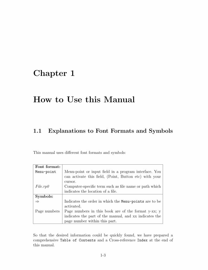
This manual uses different font formats and symbols:
Font format:Menu-point Menu-point or input field in a program interface. You
can activate this field, (Point, Button etc) with yourcursor.
File.rp0 Computer-specific term such as file name or path whichindicates the location of a file.
Symbols:⇒ Indicates the order in which the Menu-points are to be
activated.Page numbers Page numbers in this book are of the format y-xx; y
indicates the part of the manual, and xx indicates thepage number within this part.
So that the desired information could be quickly found, we have prepared acomprehensive Table of Contents and a Cross-reference Index at the end ofthis manual.
1-3

1-4 CHAPTER 1. HOW TO USE THIS MANUAL
1.2 Structure of Manual
Page Number Partxx Table of contents1-xx Diverse (Operating KISSsoft, Adjustments, etc)2-xx Connecting Elements, Screws, Belts3-xx Shafts and Bearings4-xx Gear Wheels5-xx Additional Calculation Modules6-xx KISSsys7-xx Appendix (Bibliography and Index)
Chapter 2
How to Work with KISSsoft
As a frequent Windows user, you will easily find your way through KISSsoft whichis designed in the commonly used Windows style. Elements on the interfaces areinput fields, buttons, control panels and popup-menus.
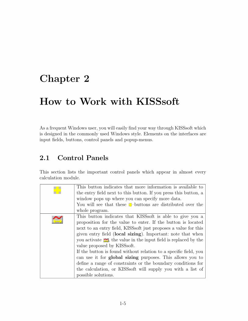
2.1 Control Panels
This section lists the important control panels which appear in almost everycalculation module.
This button indicates that more information is available tothe entry field next to this button. If you press this button, awindow pops up where you can specify more data.You will see that these –buttons are distributed over thewhole program.This button indicates that KISSsoft is able to give you aproposition for the value to enter. If the button is locatednext to an entry field, KISSsoft just proposes a value for thisgiven entry field (local sizing). Important: note that whenyou activate , the value in the input field is replaced by thevalue proposed by KISSsoft.If the button is found without relation to a specific field, youcan use it for global sizing purposes. This allows you todefine a range of constraints or the boundary conditions forthe calculation, or KISSsoft will supply you with a list ofpossible solutions.
1-5

1-6 CHAPTER 2. HOW TO WORK WITH KISSSOFT
This button opens a window with helpful dialog that can alsobe found in the handbook. The button permits faster accessto the appropriate help information.Some of the data the program requires are very difficult to de-termine. KISSsoft provides these data by default. Normally,the user should not change these data! These entry fields arelocked by default to minimise the possibility of errors or incor-rectly entered data. But it may be important to change thesedata for some special calculations. By setting the –flag, you can activate this field to enter your own data.
2.2 General Features of the User Interface
2.2.1 Changing Units
To change the unit of an input (or output) value, you can right click the associatedinput field. A pop up menue opens with all units available for this value. If youchoose a unit different from the currently used one KISSsoft converts the valuein the field to the new unit.
If you wish to change a unit permanently (i.e. the unit is allready set at start upof the calculation module) you can use the position save of the pop up menue.
For the general change from metrical to imperial units or vise versa you canuse the two different user interface languages (English (metrical) or English(imperial)). Or you can set the value UNITS in the file KISS.INI to an appro-priate value: 0 for metrical, 1 for imperial units. This is independent from theinterface language, the change, however, will not become active before you restartKISSsoft.
2.2.2 Calculating an input value
In some cases it is usefull to perform a simple calculation in order to obtain thevalue for an input field. In KISSsoft, you can right click the associated input fieldto open a pop up menue. This menue contains a position formula. If you choosethis position, a dialog opens where you can enter a formula. If you click on Ok,the formula is evaluated an the result is written to the input field. Please note,

2.3. KISSSOFT MAIN WINDOW 1-7
that the formula gets lost, i.e. if you return to the formula dialog you will seethe current input value listed in the input field, not the formula it was calculatedfrom.
The formula can consist of the four basic algebraic operators +, −, ∗ and /.Besides this all functions supported by the report generator are also possible forformula definition (see table 8.1 on page 1-64).
2.3 KISSsoft Main Window
The first window that is opened when you start KISSsoft is called the MainWindow. From here, you reach the different calculation modules via sub-menus.You find as well menus for important settings which are listed in the following.
Proceeding from the main window, you can choose between the following menus:
• Calculation
• Project
• Services
• Help
2.3.1 Calculation
When you open Calculation, you can choose between the following sub-menus:
• Calculation modules for Driving elements, Shafts and bearings
analysis, Connections and Springs, which are dealt with in detail inthe respective chapters.
• Diverse leads you to further sub-menus which are explained in chapter2.3.1.1.
• Quit KISSsoft with Quit.

1-8 CHAPTER 2. HOW TO WORK WITH KISSSOFT
2.3.1.1 Diverse
After choosing Calculation ⇒ Diverse you reach the following menu-points:
Safety elements (not available at the moment)Hardness-Conversion You can enter any value and the program calcu-
lates the other common hardness values. (see chap-ter 27)
Tolerance
calculation
After entering the nominal dimensions and the tol-erances, a dimension chain can be calculated. (seechapter 28)
Strength Assessment
with local Stresses
Additional program for the Life Expectancy Cal-culation with the help of FE Programs results. (seechapter 26)
LVR-Interface Interface to LVR-Calculation program (Calcula-tion of load distribution in a spur or helical gearstage).
Hertzian pressure Calculation the Hertzian pressure between twobodies. (See too chapter 29)
2.3.2 Project
When you open menu Project, you can choose between:
• New
• Open
These selections are only activated if Project Administration is activated (seechap. 6.4, page 1-23).
2.3.3 Services
When you open Services, you can choose between:
• Settings
• Data Base
2.3. KISSSOFT MAIN WINDOW 1-9
• Language
• Licence
You will find further explanation on these menue topics in the following sections.
2.3.3.1 Settings
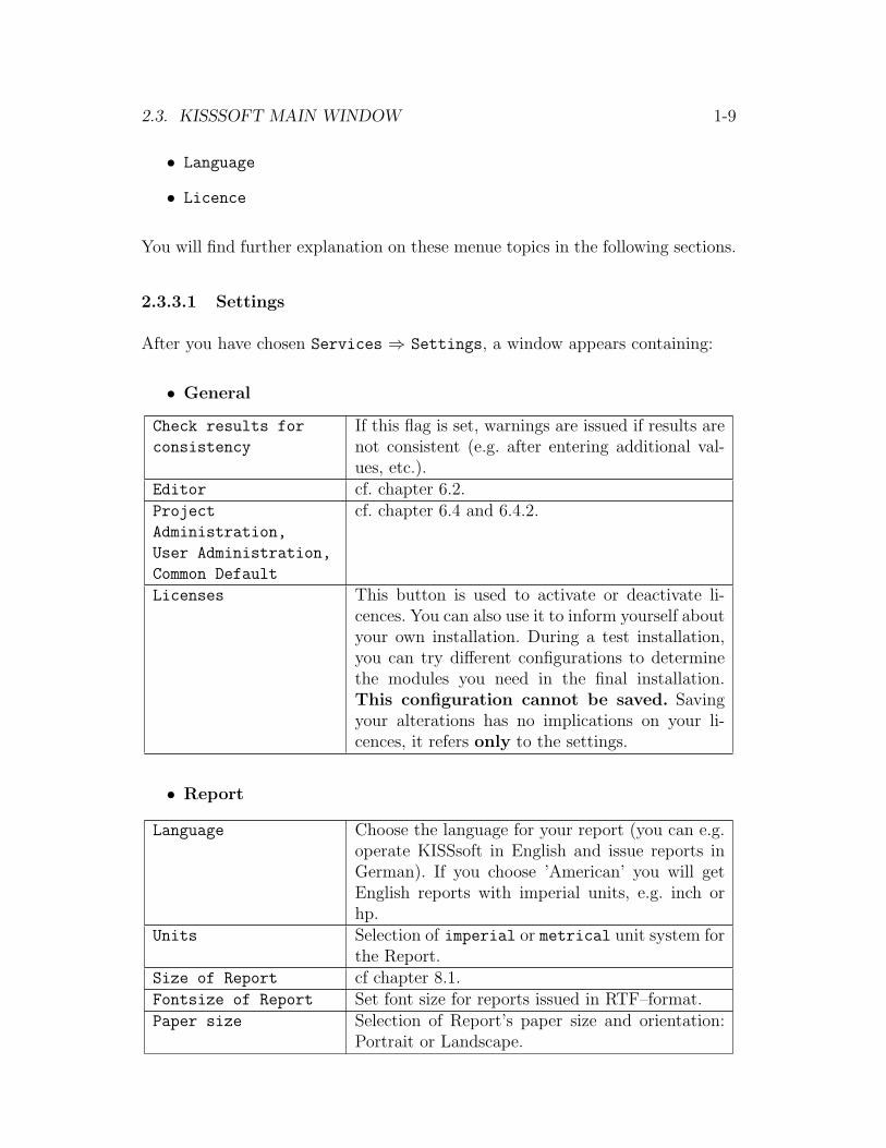
After you have chosen Services ⇒ Settings, a window appears containing:
• General
Check results for
consistency
If this flag is set, warnings are issued if results arenot consistent (e.g. after entering additional val-ues, etc.).
Editor cf. chapter 6.2.Project
Administration,
User Administration,
Common Default
cf. chapter 6.4 and 6.4.2.
Licenses This button is used to activate or deactivate li-cences. You can also use it to inform yourself aboutyour own installation. During a test installation,you can try different configurations to determinethe modules you need in the final installation.This configuration cannot be saved. Savingyour alterations has no implications on your li-cences, it refers only to the settings.
• Report
Language Choose the language for your report (you can e.g.operate KISSsoft in English and issue reports inGerman). If you choose ’American’ you will getEnglish reports with imperial units, e.g. inch orhp.
Units Selection of imperial or metrical unit system forthe Report.
Size of Report cf chapter 8.1.Fontsize of Report Set font size for reports issued in RTF–format.Paper size Selection of Report’s paper size and orientation:
Portrait or Landscape.
1-10 CHAPTER 2. HOW TO WORK WITH KISSSOFT
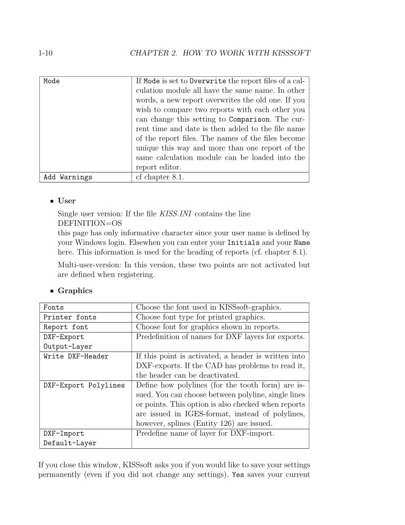
Mode If Mode is set to Overwrite the report files of a cal-culation module all have the same name. In otherwords, a new report overwrites the old one. If youwish to compare two reports with each other youcan change this setting to Comparison. The cur-rent time and date is then added to the file nameof the report files. The names of the files becomeunique this way and more than one report of thesame calculation module can be loaded into thereport editor.
Add Warnings cf chapter 8.1.
• User
Single user version: If the file KISS.INI contains the lineDEFINITION=OSthis page has only informative character since your user name is defined byyour Windows login. Elsewhen you can enter your Initials and your Namehere. This information is used for the heading of reports (cf. chapter 8.1).
Multi-user-version: In this version, these two points are not activated butare defined when registering.
• Graphics
Fonts Choose the font used in KISSsoft-graphics.Printer fonts Choose font type for printed graphics.Report font Choose font for graphics shown in reports.DXF-Export
Output-Layer
Predefinition of names for DXF layers for exports.
Write DXF-Header If this point is activated, a header is written intoDXF-exports. If the CAD has problems to read it,the header can be deactivated.
DXF-Export Polylines Define how polylines (for the tooth form) are is-sued. You can choose between polyline, single linesor points. This option is also checked when reportsare issued in IGES-format, instead of polylines,however, splines (Entity 126) are issued.
DXF-Import
Default-Layer
Predefine name of layer for DXF-import.
If you close this window, KISSsoft asks you if you would like to save your settingspermanently (even if you did not change any settings). Yes saves your current

2.3. KISSSOFT MAIN WINDOW 1-11
settings.
2.3.3.2 Data base
Opening Services ⇒ Data base opens the Data Base Tool, see chapter 7.
2.3.3.3 Language
This menu point allows the switching of the Program Windows’ dialog language.
See details in chapter ??.
2.3.3.4 License
After selecting Service ⇒ Licence, following Card masks will show on screen:
• General
User data number Displays the User number for the started version.Label ZDescription of the started version. The installation
type will be shown below (Test-, Student-, Singleuser-, Network- or Demo-version).
Licenses Button With this button, it is possible to deactivate theexisting KISSsoft licenses (released modules). Thisfunction may be used to see the details of the in-dividual installation. The most important use is dur-ing a KISSsoft test installation in which it is desir-able to activate some modules in order to adust andtest a desired configuration. The configuration set-tings cannot be saved. The KISSsoft question Save
Changes? applies to the settings mentioned aboveonly, and has no effect upon the licenses’ settings.
Remaining time In the Test version validity remaining time in d. h.m.
• Network version
This card is activated for the network version only.
Number of Licenses Displays available KISSsoft Licenses.License Directory Displays the Directory Name where the KISSsoft Li-
censes are saved.

1-12 CHAPTER 2. HOW TO WORK WITH KISSSOFT
List of active
Licenses and Users
This Table displays all used Licenses (Type, UserName and Entry Time). Click on the Separate Userbutton to free the used licenses (selected in the table).See use in Chapter ??
• Release
This card is only visible for a not yet released version or for a Demo version.
License Code Enter here the code received for a Test- or Network-version. Click on the Online Release button to re-lease the version.
Online Release For use, see License Code.Enter Release Code This release variant will only be used in computers
with no internet connection. Click on this button toobtain an 8-digit Code. Call us at (+41 55 264 20 30)and communicate this code; you will get then yourRelease Code to be entered below. Enter it and clickon OK to confirm the release.
2.3.4 Help
Manual Starts online help in HTML format.Product Information Product Information lists:
• Name of the release
• Name of the currently used module
• Version label
• Address of KISSsoft including the hotlinenumber.
See also chapter 3.

Chapter 3
The KISSsoft Help-System
In KISSsoft, you have two variants to get online-help.
3.1 The Menu Help
You can show the help file using the menue Help/Manual (cf. 2.3.4).The followingwindow is displayed:
The chapter corresponding to the current module is displayed. To get help, usethe Windows HTML Help menu. On the left corner, there are the following tabs:
Contents Handbook Table of Contents. A click on the desiredentry will display on the window at the right the cor-responding position in the handbook.
1-13

1-14 CHAPTER 3. THE KISSSOFT HELP-SYSTEM
Index Handbook complete Table of Contents. Introducingthe starting letter of the keyword will start the search.Clicking on the desired index entry, will display on thewindow at the right the corresponding position in thehandbook.
Search Enter a keyword and click on the List of Themesbutton to look for the word in the entire handbook.The corresponding Chapters will be displayed at thebottom part of the window. Click the desired Chapterto display its position in the handbook.
With the Print button, it is possible to choose between printing the selectedChapter only or all the corresponding sub-chapters as well.
3.2 Contextual Help with F1
If you want to get information about a certain input field, click with your mouseon the corresponding field and press the control button . KISSsoft displays ahelp window with explanations about the input field.
To receive information about a window element, just point the cursor on it. Aftera few seconds, a help text appears.

Chapter 4
User Defined Settings - anOverview
In order to provide a user-friendly and optimised system, KISSsoft can be adaptedto the specific needs of a user. The following overview contains the importantadaptable parts of programs and short explanations. Conciser information isfound in corresponding chapters.
• SetupHere, personal standardfiles of project- and user-administration are defined.This item is found in chapter 6 ’Arranging KISSsoft’, page 1-21.
• Definition of directoryIn file KISS.INI, paths and directories which are important for specificationsof the user are defined. Read about KISS.INI on pages 1-19, 1-21, 1-23, 1-25and 1-57.
• Printing and adapting reportsThe users’ calculations are recorded and displayed in the editor (usuallythe KISSsoft text editor KISSedit). The volume of a report can easily bechanged; read chapter 8.1 on page 1-58 for further information. It is possible,however, to define individual reports. Further details are provided in chapter8.2 on page 1-58.
• Adding/changing data in the KISSsoft data baseKISSsoft imports calculation parameters (as e.g. lubricants, reference pro-files or materials) from databases. Those can be modified or extended bythe user. Read about data bases in chapter 7 on page 1-29.
• How to complete or change data in the table interface file
1-15

1-16 CHAPTER 4. USER DEFINED SETTINGS - AN OVERVIEW
– deviation table (Tooth thickness deviation, Centre distance deviation)
– strength data verification of plastics
– pin diameter
c.f. chapter 7
• How to create individual interface files
– read: MMMMUSER.IN
– write: MMMMUSER.OUT
c.f. chapter 9

Chapter 5
Installing KISSsoft
5.1 General Information
KISSsoft operates with a standard installation program. Administrator -rightsare necessary for the installation; without Administrator -rights, certain standardentries in the Registry file cannot be filled in and with a safety key version, thekey drivers cannot be installed (If you don’t have administrator rights, pleasecontact your system administrator).
To install KISSsoft, insert the KISSsoft CD-ROM into your computer’s disk drive.Usually, you can choose the setup language as the setup program starts automat-ically, and the program guides you through the installation. If this mechanismis deactivated on your PC, you can start the setup program in the Explorer bydouble click on KSetup.exe in the main directory of the CD-ROM.
On an standard PC, it takes about five minutes to install KISSsoft. Youcan uninstall KISSsoft in about the same amount of time. In order to unin-stall, employ the uninstall option provided by Windows which you find inStart⇒Settings⇒Software.
During the installation, the installation program asks you to insert a floppy diskwith you personal customer particulars. Without these particulars, the programis not usable. If you do not have such a floppy disk or have received a filekund32.dllplease contact KISSsoft.
5.2 Installing the Multi User Version
The single user version of KISSsoft can also be installed on a file server and bestarted therefrom. On a stationary PC, however, a hard lock (dongle) is necessary.
1-17

1-18 CHAPTER 5. INSTALLING KISSSOFT
In order to use KISSsoft as multiuser version in a network, a special version isneeded that administers the licences.
The first KISSsoft installation must be released before you can use it. Proceedas follows:
1. Install KISSsoft using the userdata-disk, as described on the CD-cover.We recommend an installation from a work station (client) to a serverin order to get the correct entries for the directories in the file KISS.INIautomatically.
2. Start KISSsoft from any work station. KISSsoft will tell you that novalid license file for a multi user installation could be found and will offerto generate a new license file. Click on ’Yes’. A file dialogue opens. In thisdialogue, choose a directory on your network server. This directory laterrequires reading-, writing- and deleting-rights and has to be accessible fromall workstations operating with KISSsoft. By pressing on Save, the directoryis chosen. If the directory is not sufficient for the release, for instance if itis located on the local machine and not a redirected directory, an errormessage will appear.
3. If the workstation PC is connected to Internet, select Online Release; therelease code will then be electronically transmitted. Should no Internet con-nection be available, select Enter Release Code. This opens a file selectiondialog mask in which a directory in an available Network Server can beselected. Later on, this directory will need to have Read, Write and Deleterights assigned and must be visible on the workstation where KISSsoft issupposed to run.
4. If an adopt directory has been chosen, a new dialog will appear in whichyou can click on the button Release KISSsoft directly. A window con-taining an eight digit character code is displayed. Call KISSsoft and ask forthe corresponding release code (telephone number +41 (0)55 264 20 30).Important: Do not close the program before the release is completed, asthe program generates a different code every time it is started.
Important: Do not choose the KISSsoft installation directory or a subdi-rectory as a licence directory. If, after an update, the old KISSsoft version isdeleted, the release file might be cleared by mistake. Usually, later updatesdo not require new releases.
5. After successful release, the licence file can be converted into a read-onlyfile to prevent damage.

5.3. READ ONLY DIRECTORY 1-19
6. KISSsoft enters the licence directory into the file KISS.INI. If you workwith several KISS.INI files (e.g. with local installations), you have to enterthe directory manually in the other KISS.INI files (LICDIR=...).
Annotation: The directory for licence administration and the installation direc-tory of KISSsoft are independent from each other. According to this, the programcan, for example, also be installed on local work stations. We advise you not toplace the licence directories in the KISSsoft installation directory. If possible, thedesignation of the release should be included in the name of the installation di-rectory. In this way, the program is easier to update and there is no danger ofdeleting the licence release together with the outdated KISSsoft installation.
During an Update, there will be no initialization if there is already a valid releasefile in the License Administration Directory. It is absolutely necessary to transferan entry ’LICDIR=. . . ’ from the old KISS.INI -file into the new one. For moredetails, consult the Update Instructions delivered.
5.3 Read Only Directory
In the KISS.INI file, which is normally located in the installation directory, thedirectory structure of the KISSsoft installation is defined.
CADDIR and TEMPDIR are temporary directories and should be placed, in caseof multiuser access (with more than one licence), as local as possible on the workstations, e.g.:
CADDIR=C:\TEMPTEMPDIR=C:\TEMP
It is also possible to use the variable <TMPDIR> with which Windows willautomatically assign the temporary directory:CADDIR=<TMPDIR>TEMPDIR=<TMPDIR>
Usually, saved calculations are placed in USERDIR. Common data bases con-taining material data and other principal data are placed in KDBDIR.
Important: if the definition of KDBDIR is altered, all files ending on *.KDB mustbe copied into the new directory.
To operate KISSsoft in a read only directory, the following entries in file KISS.INIhave to be changed into a writeable directory:
[PATH]CADDIR=C:\Program Files\KISSsoft\CAD

1-20 CHAPTER 5. INSTALLING KISSSOFT
TEMPDIR=C:\Program Files\KISSsoft\TMPUSERDIR=C:\Program Files\KISSsoft\USR
Should the access to certain setting possibilities be assigned to some persons only,the following Network Settings are recommended:
Restrict access to.... . . through.... . .change database data write protecting all ∗.KDB files in KDBDIR.read database data restricting KISSdb.exe execution.change general set-tings (Report lan-guage, etc.)
Dwrite protecting the KISS.INI file.
change Report forms write protecting the installation directory.
5.3.1 Disconnecting Users
If, for any reasons, KISSsoft is not able to shut down properly, a user mightremain registered. This can cause you running out of licences, even if there arenot as many users operating KISSsoft as you possess licences. You can release theblocked licenses by deleting the cookie files (USR???.tmp) in the directory forlicense administration. You can disconnect the license from the Network selectingthe desired License (also shows the user and the entry time) in Service/Licenseunder the Tab Network; the corresponding Cookie file will be deleted (Licensewill be deactivated).
After some time a license which is no longer used is released automatically as soonas the next user tries to log in. The time until automatic relase can be defined inthe file KISS.INI by altering the lineTIMEOUT=The value is given in minutes, default is 120 minutes.
Note: once disconnected from KISSsoft, users cannot calculate anymore in thecurrent session. KISSsoft has to be started again. Data, however, can still besaved.

Chapter 6
Setting up KISSsoft
6.1 Defining Languages
KISSsoft is available with four languages: German (KISSsoft Modul K02), English(K02a), French (K02b), and Italian (K02c). You can also choose between metricaland imperial units when using English language.
Users can operate on the user interface in one language and simultanously displayor print reports in another. The following settings are necessary for this mode:
• Language of Report
The language of reports can be changed within the program, in activatingSettings ⇒ General ⇒ Report, if you are operating from the calculationwindow, or by means of Services ⇒ Settings ⇒ Report, if you are inthe starting window.
• Language of User Interface
In the main window (the very first dialog of the software) you can definethe language of the user interface with the menue Services ⇒ Language.When choosing a language you are asked whether you would like to changethe report language as well. Please note that you can redefine the reportlanguage any time you like in the general settings, see above.
• Messages
The error messages can either be displayed in the same language as thewhole interface, or in the language of the reports. Set this option in theKISS.ini -file, in paragraph [SETUP] in line MESSAGELANG=0. Thevalue behind the equivalent sign means:
1-21
1-22 CHAPTER 6. SETTING UP KISSSOFT
0 Language of messages = language of reports1 Languages of messages = language of interface
6.2 Defining the Editor
KISSsoft uses an editor to display reports and other text files. It does not matterwhich editor you use as long as it displays RTF files correctly (like wordpad forinstance). KISSsoft has a standard editor KISSedit. If you want to use anothereditor, choose Services ⇒ Settings and General.
Press on the browser button [...] behind the input field. A dialogue is openedwhere you can browse for the editor file. If you enter the filename manually pleasenote that the path of the file has to be entered and completely.
As usual, KISSsoft asks you whether you want to save your changes permanently.If you affirm, the changes are written in file KISS.ini.
You can also enter the desired editor directly in file KISS.ini. Remember to enterthe complete path.
6.3 Defining Individual Standard Files
Often, calculations that you make are the same, or at least similar. As it is quiteannoying to enter the same numbers over and over again, KISSsoft has provideda very simple but nevertheless effective solution:
For every software module there is a standard file. This standard file defineswhich constraints appear in the input fields of the user interface of the accordingmodule.
This file is loaded at start up of a calculation module or if File⇒New is chosen.
You can adapt the standard file to your individual needs:
• Open the desired module or choose menupoint New in menu File.
• Enter your standard numbers in the according fields (found in the subdialogs of the module as well).
• Choose menupoint Save as Standard.
• Affirm with OK and answer the checkback with Yes.

6.4. PROJECT AND USER ADMINISTRATION 1-23
The next time you enter the module interface, it displays your personal settings.
Where the standard files are saved, where they are loaded from and which in-fluence your personal settings have on other users depends on the mode you (oryour administrator) chose in file Services ⇒ Settings ⇒ General. Read thefollowing pages for further information, especially point 6.4.2. Settings that youhave to apply frequently in your standard files are dealt with separately in thechapters about the corresponding software modules.
6.4 Project and User Administration
Because of its project and user administration, KISSsoft is able to manage cal-culation and standard files very efficiently. By means of three flags, you or youradministrator can adjust the different modes. To find these flags, open Services
⇒ Settings in the KISSsoft main interface and choose General. The three flagsare named:
• Project Administration
• User Administration
• Common Default
The following paragraphs deal with the effects of the different flag-combinations.Read about flag-combinations in chapter 6.4.3.
6.4.1 Saving Calculations
In principle, your calculations are saved in the directory which has been definedby the variable USERDIR in file KISS.INI. Normally, this is the sub directoryUSR of the installation directory or shorter <USERDIR>1
Several subdirectories are connected to this directory, depending on the kind ofadministration you chose in dialogue field General (flag Common Default has noinfluence on the location where calculations are saved).
The program distinguishes between four different locations (PV = Project
Administration; BV = User Administration):
1<VARIABLE> means in this manual the path that is given by the variable; our example<USERDIR> means a path like \Program Files\KISSsoft\USR.

1-24 CHAPTER 6. SETTING UP KISSSOFT
PV BV Locationno no <USERDIR>yes no <USERDIR>\Projectno yes <USERDIR>\Useryes yes <USERDIR>\Project\User
1. Project Administration offUser Administration off
Your calculations are saved directly in <USERDIR>.
Example: You are operating with neither project- nor user administration,and at the time of the installation you chose the standard directory. All yourcalculations are saved in \Program Files \KISSsoft\USR.
2. Project Administration onUser Administration off
If only Project Administration is activated, all calculations aresaved in a directory named after the current project, and that name isadded to path <USERDIR>.
Example: The current project is called ’Trajan’, and the name has beenchosen while installing the standard directory; all calculations are saved in\Program Files\KISSsoft\USR\Trajan.
3. Project Administration offUser Administration on
If you activate only User Administration, all calculations are namedafter the user’s login name, added to path <USERDIR>.
Example: The current user’s name is ’hm’ and has been chosen at the timeof the installation of the standard directory. All calculations are saved in\Program Files\KISSsoft\USR\hm.
4. Project Administration onUser Administration on
If both Project Administration and User Admininstration are acti-vated, the name of the project as well as the user’s name are attached topath <USERDIR>.
Example: The user’s name is ’hm’ and the current projectis called ’Trajan’. All calculations are saved in \ProgramFiles\KISSsoft\USR\Trajan\hm.

6.4. PROJECT AND USER ADMINISTRATION 1-25
At start-up, the dialogues File ⇒ Open and File ⇒ Save automatically offerthe subdirectories that correspond to the settings of the kind of administration.
If you want to adopt calculations from a different project or user, choose [...]
(behind the entry field for file names) in dialogue File ⇒ Open. In the followingdialogue you choose the directory belonging to your desired project. Load thedesired calculation with Open. Choose File ⇒ Save as. Remove the diretorypart from the filename. In saving the calculation, it is sent under its ’old’ nameto your current subdirectory.
6.4.2 Saving Common Default Files
Button Common Default combined with Project Administration and User
Administration describes the location where standard files are available (formore information please read chapter 6.3).
With this setting, you can also define whether all users shall operate with thesame standard files or whether every user can operate with individual standardfiles for his project. In general standard files are only available after saving thestandard. Before this point KISSsoft uses the built in standard settings.
In principal, original standard files are available in directory TEMPLATE. Thisdirectory is located at the end of the path that is specified with the variableKISSDIR in file KISS.INI . The standard path is \Program Files\KISSsoft2.
If you wish, you can easily change these predetermined files and copy them intonew directories. The location of the directory depends, in this case, on the com-bination of the settings Common Default, Project Administration and User
Admininstration.
This table shows all possible locations (PA = Project Administration; UA =User administration; CD = Common Default):
PA UA CD Locationno no no <KISSDIR>\TEMPLATEno no yes <KISSDIR>\TEMPLATEno yes no <USERDIR>\Userno yes yes <KISSDIR>\TEMPLATEyes no no <USERDIR>\Projectyes no yes <KISSDIR>\TEMPLATEyes yes no <USERDIR>\Project\Useryes yes yes <USERDIR>\Project
2Short form: <KISSDIR>\TEMPLATE – compare to footnote 1.

1-26 CHAPTER 6. SETTING UP KISSSOFT
Annotation:At the beginning of a new project, standard files located in the TEMPLATEdirectory are copied into the new project directory. Hence, the program expectsstandard files to be present in the project directory.
6.4.2.1 Directories Checked for Standard Files
Depending on the defined mode, KISSsoft checks different directories for standardfiles:
• Project Administration onUser Administration onCommon Default on
With this combination, the program expects the standard file to be locatedin the project directory. If the standard file cannot be found in this directory,the file is loaded from directory TEMPLATE. If no standard file is foundthe built in standard settings are used.
• Project Administration on/offUser Administration onCommon Default off
With this combination, the user’s directory is first checked for a standardfile (which is located, in case of Project Administration being activated,below the project directory). If no suitable file is found, the program checksthe project directory in case of Project Administration activated. If thereis no standard file to be found in the project directory, or Project Adminis-tration is deactivated, the file is loaded from the TEMPLATE directory, asdescribed above. If no standard file is found the built in standard settingsare used.
• Project Administration offUser Administration offCommon Standard on/off
If User Administration and Project Administration are deactivated stan-dard files are loaded from the TEMPLATE directory and are saved thereas well. With this setting, standard files are neither filed in project nor inuser directories. If no standard file is found the built in standard settingsare used.
• Project Administration onUser Administration offCommon Standard on

6.5. COMMAND LINE PARAMETERS 1-27
If User Administration is deactivated and Common Standard is activated,standard files are loaded from directory TEMPLATE. With this combina-tion, always the same standard files are used. If no standard file is foundthe built in standard settings are used.
6.4.3 Typical Scenarios of Project and User Administra-tion
Single Work Station Version (Single user version), few usersProject Administration onUser Administration offCommon Default off
Single Work Station Version (Single user version), many usersProject Administration offUser Administration onCommon Standard on
Network Installation (Multi user version), occasionally using KISSsoftProject Administration offUser Administration onCommon Default on
Network Installation (Multi user version), frequently using KISSsoftProject Administration onUser Administration onCommon Default off
6.5 Command line parameters
Starting KISSsoft is possible with several command line parameters. Valid pa-rameters are:
Parameter BeschreibungINI=filename The file KISS.INI containing the general set-
tings is read from the location defined by theparameter. It is possible to define the wholefilename with full path of the directory only.
START=module The defined calculation module is started.The designation of the modules is for in-stance M040 for the calculation of boltedjoints or Z012 for helical gear pairs.

1-28 CHAPTER 6. SETTING UP KISSSOFT
LOAD=filename The defined file is loaded and the arbitrarycalculation module is started. If a filenamewith path is given, the file is loaded from thelocation defined. Elsewhen it is loaded fromthe directory defined by <USRDIR>.
LANGUAGE=digit KISSsoft starts with report and interface lan-guage defined by a digit. (0: German, 1: En-glish, 2: French, 3: Italian, 4: Spanish, 11:English with imperial units)
DEBUG=filename A file with debug informationen is writtenduring use. This file can be of great use whensearching for errors. It’s recommendable touse a filename with full and absolute path.This way it is much easier to lacate the debugfile.
filename The calculation module associated with thefile is started and the file is loaded. It’s pos-sible to link the filename extensions of KISS-soft calculation files with KISSsoft. This waya calculation file can be opened with KISS-soft by double clicking it in the Explorer.
Chapter 7
KISSsoft Data Base Tool andTable Interface
7.1 Calculation Values in Data Bases and Ta-
bles
7.1.1 Data Base and Data Base Tool
The data base tool can be used to modify the databases of KISSsoft.
The following data-bases can be edited:
Center distance tolerance; reference profiles; bore standard; thread type screw;production process of hypoid bevel gears; production process of bevel gears; v-belt standard; groove-toothing standard; chain type DIN 8154; chain type DIN8187; chain type DIN 8188; adhesives; equivalent design load; soldering materials;feather key standard; polygon standard; Woodruff key standard; lubricants; screwtype; washer standard; multi-spline standard; roller bearings; material glued andsoldered joints; materials; tooth thickness tolerance; toothed belt standard;
7.1.2 Opening a Table with Write Protection
The data contained in the data bases is highly sensitive. Wrongly entered oraltered data can cause fatal complications. Therefore when opening a table theuser is asked whether he wishes to open the data base with writing permissionsor not. If the user decides to open the data base without writing permissions hecan view all data in the table, but he can’t change the data. The prompt forwriting permissions is repeated every time when a table is opened until writing
1-29

1-30CHAPTER 7. KISSSOFT DATA BASE TOOL AND TABLE INTERFACE
permission are actually requested by the user. From then on for the rest of thesession every table is opened with writing permissions.
To be sure that the data base is not corrupted the files in < KDBDIR > (∗.kdb)can be set to ”read only”. In this case opening a data base with write permissionleads to an error message. The table will be opened without writing permissionsafterwards.
7.1.3 Interface Between KISSsoft and External Tables
Every data set is entered in one-dimensional tables. Complicated data sets (e.g.related data) are stored in a seperate table (using the so-called table interface).These tables are text files which can be edited with any text editor such asKISSedit, Notepad, Wordpad, Word. In the data sets of the data base only thefilename of the file containing the data is defined. Next to every data base fieldcontaining the file name is an Edit-button which loads the editor defined inKISSsoft (to choose an editor see 6.2).
The table interface is described in 7.3.
7.2 Description of the Data Base
7.2.1 Save, New, Copy
Use the Save button two accept changes. To save changes you must have writingpermissions, i.e. you have to open the table with writing permissions. Furtheractivities the user needs writing permissions for are copying data, enter newdata or rearange the data sets. It is important that you name the data setsunmistakably in order to choose the right data sets in KISSsoft.
Annotation:
• The data sets supplied by KISSsoft (recognisable by ID < 20000) cannotbe changed, but copied, and this copy can be changed. If you want torelease an original KISSsoft data set for another calculation module andenter module-specific data, you have to copy it.
• It is not possible to clear data sets since this can cause consistency problemswith saved calculations. If a data set created by yourself is no longer needed,however, you can overwrite it. Avoid entering unnecessary data sets.
7.2. DESCRIPTION OF THE DATA BASE 1-31
7.2.2 Material Notation for Different Countries
By default materials are displayed with German (DIN) notations; we recommendchoosing different standards if required. You can choose between material nota-tions according to:
• DIN (Default)
• British Standard (GB)
• AISI-Norm (USA)
• UNI-Norm (Italia)
• AFNOR-Norm (France)
• JIS-Norm (Japan)
To switch notation, select one from Extras ⇒ Material Notation for
different Countries. It is possible to freely switch between the various no-tations.
7.2.3 Automatic Update Function
As from release 10/2001, there is an automatic transfer of user-defined data fromprevious databases, as from Release 5/2001. This is possible calling the updatefunction in Extras⇒Update. This function asks for the Directory of the olddatabase. Once the directory selected, starts a search in all the database files(∗.kdb) for data entries with a Database-ID ≥ 20000 which will be transferred tothe new database. Important: It is strictly necessary to call the Update functionbefore making any new data entries in the new database. Otherwise, there willbe conflicts in the Database-IDs.
7.2.4 Exporting and Importing Data Sets
The data base tool can export single data sets in text files or import from textfiles. This function is primarily used to transfer data sets into a new release ifthese data sets have been modified by the user. To do so, open in the data basetool the table with the user-defined data set and write the data set into a text fileby activating Data set ⇒ Export. In the new installation, the table is openedand read by Data set ⇒ Import. The program issues a warning if the data setdoes not match to the current table.

1-32CHAPTER 7. KISSSOFT DATA BASE TOOL AND TABLE INTERFACE
If, however, a data set with the same data base ID exists which is also definedin a text file, the program asks whether the already existing data set shall beoverwritten. First, the data are only written into the interface. The content ofthe data set can be viewed. If the data are to be written permanently into thedata base, activate [Save]. If the data are not to be adopted, just change toanother data set and do not save the data. The original data set is not changed.
When exporting material data sets allways the whole information for the materialis written to the file, i.e. the general data section as well as the module specificsection. Export a data set to a file for every calculation module the material isreleased for.
When importing material data sets, load the right calculation module table (see7.2.6). If a material is to be imported for several calculation modules, importthe material for one calculation module first. Add afterwards the material tothe tables of the other calculation modules without module-specific imputs (see7.2.6). The remaining data sets can the be imported into the corresponding tables.
7.2.5 Navigating in the Data Base
After you’ve opened a table in the data base tool, you enter the following window(c.f. picture 7.1). This example shows the material data base:
A data set can be chosen using the four buttons [<<], [<], [>], [>>] or using theselection list.
7.2.6 List
The selection list appears automatically when a data base is opened. It can beused to
• select a data set directly by clicking on the name in the list
• delete data sets using the delete button (this function is deactivated)
• sort the data sets using buttons [⇑] and [⇓].
The list cannot be closed but minimised.
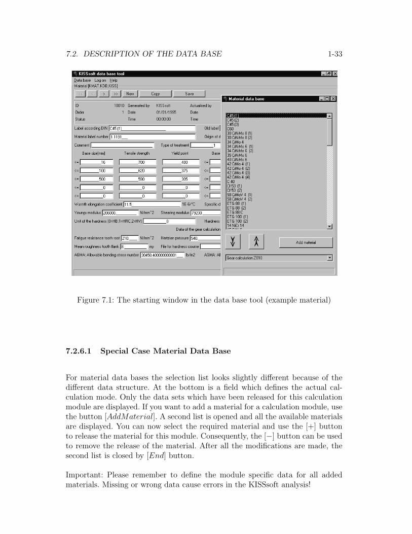
7.2. DESCRIPTION OF THE DATA BASE 1-33
Figure 7.1: The starting window in the data base tool (example material)
7.2.6.1 Special Case Material Data Base
For material data bases the selection list looks slightly different because of thedifferent data structure. At the bottom is a field which defines the actual cal-culation mode. Only the data sets which have been released for this calculationmodule are displayed. If you want to add a material for a calculation module, usethe button [AddMaterial]. A second list is opened and all the available materialsare displayed. You can now select the required material and use the [+] buttonto release the material for this module. Consequently, the [−] button can be usedto remove the release of the material. After all the modifications are made, thesecond list is closed by [End] button.
Important: Please remember to define the module specific data for all addedmaterials. Missing or wrong data cause errors in the KISSsoft analysis!

1-34CHAPTER 7. KISSSOFT DATA BASE TOOL AND TABLE INTERFACE
7.2.6.2 Example on Input of a New Material
Problem
A new material shall be entered in the data base, e.g. steel 25CrMoS4. The dataderives from the Thyssen material documentation. The material is needed forgear wheel and shaft calculation.
Procedure
First, the data base is checked for a similar material that has already been entered.In this case, the tool chooses 42CrMo4(1). (1) stands for ’alloyed, heat treated’,to distinguish between different heat treatments.
After having started the data base tool by double mouseclick on the correspondingicon, you can open the data base selection list by activating Data Base ⇒ Open.Choose Material Data Base and affirm with Ok. This opens a dialogue windowwhere you can register with your user name and password. After you have affirmedwith Ok, a message appears informing you that a safety copy of the data base isplaced in KMAT.BAK. Finally, two windows appear, one containing data of thefirst data set and one containing the data selection list. At the lower end of theselection list is a field indicating the calculation module which is activated whenyou open the material data base for gear wheel construction Z010.
Material 42CrMo4(1) is selected and the according data appears on the maininterface. If you press Copy, a new data set named 42CrMo4(1) new is writteninto the data base at the bottom of the selection list. First, you should change thematerial’s file name and enter the correct designation 25CrMoS4 in Designation
according to DIN. This data base field has to have an unmistakable designationsince KISSsoft selects the material by means of this designation.
In the next step you can enter common data in the corresponding input fields:Material Nr. 1.7213Data according to Thyssen product documentation:The data for 25CrMo4 are displayed but not for 25CrMoS4; however, the datafor 42CrMo4 can also be taken for 42CrMoS4.Dimension ≤ 16: yield point min 685, tensile strength 880-1080 N/mm2
Dimension > 16− 40: yield point min 590, tensile strength 780-930 N/mm2
Dimension > 40− 100: yield point min 460, tensile strengtht 690-840 N/mm2
Dimension > 100− 160: yield point min 410, tensile strength 640-790 N/mm2
Hardness HB 212Material-Type 2 (heat treatable steel; see materials)Type of treatment 2 (alloyed, heat treated; see materials)
• Gear Wheel Calculation:
7.2. DESCRIPTION OF THE DATA BASE 1-35
Afterwards you can enter the data specific for the calculation module. First,enter the data of the gear wheel calculation. For this purpose choose ’GearWheel Calculation’ below the material selection list if not already activated.
According to DIN 3990 part 5 for heat treatable steel HB 212 withoutsurface hardening (medium quality):SigHlim = 630 N/mm2
SigF lim = 275 N/mm2
Roughness (assume 16 µm for root and flank, since not grinded)Values for calculation according to AGMA (enter only if necessary, elseenter 0): enter 0.Data for plastics: do not fill in (for this example).
Important: to save data permanently in the data base use Save. All unsaveddata is lost if you change to a new data set!
• Calculating Shaft Strength:
To enter data for other calculation modules, the material has to be enteredfirst in the data base of the corresponding module. In order to do so choose’Calculating Shaft Strength’ located on the bottom of the material selectionlist. After the program has read the data base of the calculation module,you can open the comprehensive material selection list by Add Material. Inthis list (and not in the list titled Material Data Base) you find 25CrMoS4.Add it to the module specific data base by +. If you press quit, the programreminds you to enter data for the newly added material. You can closethe comprehensive material table by Ok. The new material is listed at thebottom of the module-specific list. To specify the new material with furtherdata, click on it and fill in the list appearing in the main window. Fill indata belonging to the gear wheel calculation in the lower part and save yourinputs with Save.
Material strength according to Hahnchen/Decker:Heat treatable steel, same for materials with same tensile strength:sig.bW = 440Material strength according to DIN 743:Material not mentioned, therefore:Sig.b, sig.s by Thyssen,sig.bW = sig.b ∗ 0.5 (DIN743, Part 3, Formula 1): = 880 ∗ 0.5 = 440sig.zdW = sig.b ∗ 0.4 (DIN743, Part 3, Formula 2): = 880 ∗ 0.4 = 352tau.tW = sig.b ∗ 0.3 (DIN743, Part 3, Formula 3): = 880 ∗ 0.3 = 264dB (Reference diameter) = 16 mm (same as other heat treatable steel)Material strength according to FKM-Guideline:Material is listed in table IV J3Sig.b = 900, sig.s = 700, sig.bN = 435, sig.zdN = 405, tau.tN = 260,tau.sN = 235

1-36CHAPTER 7. KISSSOFT DATA BASE TOOL AND TABLE INTERFACE
deffN (Reference diameter) = 16 mmA5 is dropped (only necessary for GG)FKM-material-group 2 (see materials)
• Bolt Calculation:
Same procedure as for shaft strength calculation.
Data:No specifications in VDI 2210.Procedure: similar material is 42CrMo4: permissible pressure 850, sig.B =1080; conclusion:permissible pressure = 850 ∗ 880/1080 = 693 N/mm2
7.2.7 Input Fields of Data Bases
The data bases vary in volume. In the following we list the input fields of allexisting data bases. The input field ”name” exists in every table and is thereforenot listed here. Please note, that all data sets have to have a unique in this fieldsince the user chooses the data sets according to this name.
7.2.7.1 Center Distance Tolerance
Data bases for center distance tolerances. The data base entries point to tables.The tables for center distance tolerances start with K10-???.DAT.
7.2.7.2 Reference Profiles
The reference profile types are entered directly in the data base. The values,however, depend on each other.
• Label according ISO:
• Comment:
• Data source:
• Cutter tip radius:
• Cutter root height:
• Protuberance height:
• Protuberance angle:

7.2. DESCRIPTION OF THE DATA BASE 1-37
• Buckling root flank height:
• Buckling root flank angle:
• Intersecting?:
• Cutter root radius:
7.2.7.3 Bore Standard
• File name:
7.2.7.4 Thread Type Screw
• Designation:
• File name:
• Flank angle:
• coefficient d2: to calculate the pitch diameter of the bolt thread (d2 =d− d2coefficient ∗ P )
• coefficient d3: to calculate the minor diameter of the bolt thread (d3 =d− d3coefficient ∗ P )
7.2.7.5 Production Process of Hypoid Bevel Gears
These values are only required for the analysis according to Klingelnberg. Theycorrespond to tables for machine types described in the Klingelnberg factorystandard. The data are valid for hypoid bevel gears.
• Machine type:
• Flight circle radius:
• Number of starts cutter:
• Max Machine distance:
• Min normal module:
• Max normal module:

1-38CHAPTER 7. KISSSOFT DATA BASE TOOL AND TABLE INTERFACE
7.2.7.6 Production Process of Bevel Gears
These values are only required for the analysis according to Klingelnberg. Theycorrespond to tables for machine types described in the Klingelnberg factorystandard. The data are valid for bevel gears.
• Machine type:
• Flight circle radius:
• Number of starts cutter:
• Max Machine distance:
• Min normal module:
• Max normal module:
7.2.7.7 V-belt Standard
• Filename:
• Calculation method [1|2]:
• Max belt speed:
• Elasticity:
• Weight per length:
• Coefficient of friction:
7.2.7.8 Groove-Toothing Standard
• Comment: textfield for individual use.
7.2.7.9 Chain Type DIN 8154
• Type:
• Power:
• Max Speed:
• Pitch:

7.2. DESCRIPTION OF THE DATA BASE 1-39
7.2.7.10 Chain Type DIN 8187
• Type:
• Power:
• Max Speed:
• Pitch:
7.2.7.11 Chain Type DIN 8188
• Type:
• Power:
• Max Speed:
• Pitch:
7.2.7.12 Adhesives
• Minimal shear strength:
• Maximal shear strength:
• Optimal shear strength:
7.2.7.13 Equivalent Design Load
The definitions of all inputs (frequency, power, speed) are factors. The sum offrequencies has to be 1. Power and speed are contained in factors of the nominalpower. In KISSsoft calculations the factor for torque (factor for power/factor forspeed) is used for forces and torque.
• Number of load cases: number of different load cases in equivalent designload
• Type: 0: factors for power are given, 1: factors for torque are given.
• Filename: If a filename is given the data is read from a file. The factors areread in the order frequency, power/torque and speed. All other input in thedatabase is ignored.
• Frequency: H0. . .H19, the sum of these frequencies has to be 1.

1-40CHAPTER 7. KISSSOFT DATA BASE TOOL AND TABLE INTERFACE
• Power factors (factors for torque if Type=1): P0. . .P19, 0 < Pn <∞.
• Speed factors: N0. . .N19, 0 < Nn <∞
7.2.7.14 Soldering Materials
• Minimal shear strength:
• Maximal shear strength:
7.2.7.15 Nut standard
• Name:
• File name: The data base entries refer to tables (see chapter 7.3)
7.2.7.16 Surface roughness
• Name:
• Comment:
• Rz:
• Ra:
7.2.7.17 Feather Key Standard
• Comment: textfield for individual use.
7.2.7.18 Polygon Standard
• Comment: textfield for individual use.
7.2.7.19 Woodruff Key Standard
• Comment: textfield for individual use.

7.2. DESCRIPTION OF THE DATA BASE 1-41
7.2.7.20 Lubricants
• Label according to ISO: this is a textfield.
• Comment: this is a textfield.
• Data source: this is a textfield.
• Kind: 0=oil, 1=grease
• Density oil: [kg/dm3]
• Kinematic viscosity at 40◦C: [mm2/s]
• Kinematic viscosity at 100◦C: [mm2/s]
• Lubricant basis:
0 Mineral-oil1 Synthetic oil based on polyglycol (EO :
PO = 1 : 1)2 Synthetic oil based on polyether3 Synthetic oil based on polyglykol (EO :
PO = 0 : 1)4 Synthetic oil based on polyalfaolefine5 Synthetic oil based on ester
Explanations:EO EthylenglykolPO PropylenglykolPolyalfaolefine similar to mineral oil, mixable with mineral
oil, agreable with food stuffs.Ester partly agreable with food stuffs, partly bio-
logically decomposable.
• FZG Test A/8.3/90: Input of the pitting level according to FZG-TestA/8.3/90. This data is required for the gear analysis.1=worst 12=best level.All good lubricants have level 12.
• Cone penetration at 25oC: [0.1mm] This input is required for the analysisof grease lubricated journal bearings.
• Soap content: [Complete %] This input is required for the analysis of greaselubricated journal bearings.
• Without additive for roller bearings [0=Yes, 1=No]:
1-42CHAPTER 7. KISSSOFT DATA BASE TOOL AND TABLE INTERFACE
– 0: Lubricant without additives, or if the effect was not tested for rollerbearings.
– 1: Lubricant with additives, if the effect was tested for roller bearings.
Input of lubricants for diverse modules. Some data is only used for the gearanalysis.
7.2.7.21 Screw Type
• Designation:
• File Name:
7.2.7.22 Washer Standard
• File Name:
7.2.7.23 Multi-Spline Standard
• Comment: textfield for individual use.
7.2.7.24 Roller Bearings
• Bearing label: the name of the data set is defined in this place. This namewill be used in KISSsoft to choose the required data set.
• Bearing series: The abbreviation of the bearing series are according to DIN623 part I.
• Inner diameter: input in mm.
• External diameter: input in mm.
• Bearing width: input in mm.
• Corner radius: input in mm.
• Dynamic load number: input in kN.
• Static load number: input in kN.
• Coefficient X1: *1) *5)

7.2. DESCRIPTION OF THE DATA BASE 1-43
• Coefficient Y 1: *1) *5)
• Coefficient X2: *2) *5)
• Coefficient Y 2: *2) *5)
• Coefficient E: *1) *5)
• Coefficient E0: *3)
• Coefficient X01: *3)
• Coefficient Y 01: *3)
• Coefficient X02: *4)
• Coefficient Y 02: *4)
• Speed limit grease lubricated: Input in rpm.
• Speed limit oil lubricated: Input in rpm.
• Weight: in kg.
• Pressure Angle: Pressure Angle (for angular contact-, tapered roller bear-ings etc). Input in degree.
• Permissible axial load: Input of the permissible axial load as a percentageof Fr. For Input 0.0 the axial-force is not checked.
• Maximal angular deviation: in minutes. For an input of 0.0 the amount ofangular deviation (effective value of shaft) is not checked.
• Thermal reference speed: input in rpm.
• Availability: Possibility to define whether bearing is available. 0: in stock,1: out of stock (not used by KISSsoft).
• Price: Price in user’s currency (not used by KISSsoft).
• Addition A - E: These fields are used to contain additional data for specialbearings, see table 2.
• Radial stiffness: in N/µm.
• Axial stiffness: N/µm.
• Angular (pitch) stiffness: Angular stiffness in Nm/degree.
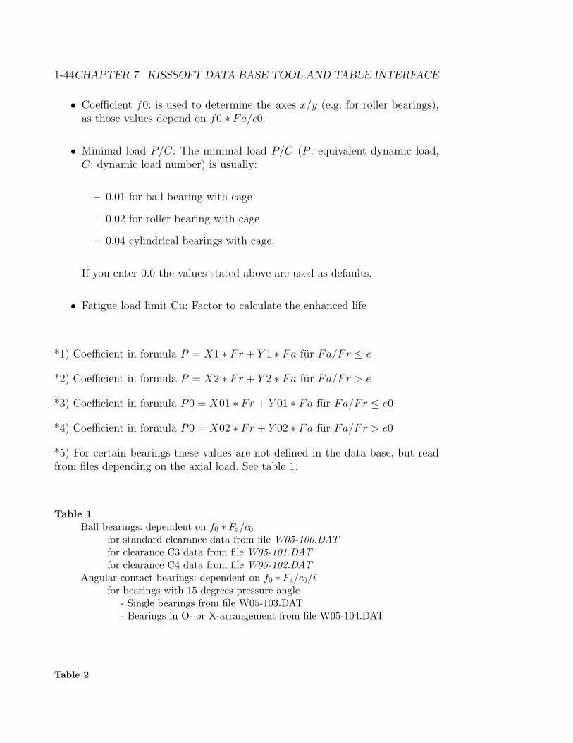
1-44CHAPTER 7. KISSSOFT DATA BASE TOOL AND TABLE INTERFACE
• Coefficient f0: is used to determine the axes x/y (e.g. for roller bearings),as those values depend on f0 ∗ Fa/c0.
• Minimal load P/C: The minimal load P/C (P : equivalent dynamic load,C: dynamic load number) is usually:
– 0.01 for ball bearing with cage
– 0.02 for roller bearing with cage
– 0.04 cylindrical bearings with cage.
If you enter 0.0 the values stated above are used as defaults.
• Fatigue load limit Cu: Factor to calculate the enhanced life
*1) Coefficient in formula P = X1 ∗ Fr + Y 1 ∗ Fa fur Fa/Fr ≤ e
*2) Coefficient in formula P = X2 ∗ Fr + Y 2 ∗ Fa fur Fa/Fr > e
*3) Coefficient in formula P0 = X01 ∗ Fr + Y 01 ∗ Fa fur Fa/Fr ≤ e0
*4) Coefficient in formula P0 = X02 ∗ Fr + Y 02 ∗ Fa fur Fa/Fr > e0
*5) For certain bearings these values are not defined in the data base, but readfrom files depending on the axial load. See table 1.
Table 1Ball bearings: dependent on f0 ∗ Fa/c0
for standard clearance data from file W05-100.DATfor clearance C3 data from file W05-101.DATfor clearance C4 data from file W05-102.DAT
Angular contact bearings: dependent on f0 ∗ Fa/c0/ifor bearings with 15 degrees pressure angle
- Single bearings from file W05-103.DAT- Bearings in O- or X-arrangement from file W05-104.DAT
Table 2
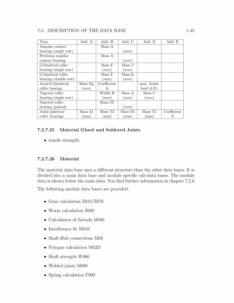
7.2. DESCRIPTION OF THE DATA BASE 1-45
Type Add. A Add. B Add. C Add. D Add. EAngular contact Mass Abearing (single row) (mm)Precision angular Mass Acontact bearing (mm)Cylindrical roller Mass F Mass Jbearing (single row) (mm) (mm)Cylindrical roller Mass F Mass Ebearing (double row) (mm) (mm)Axial-Cylindrical- Mass Dg Coefficient max. Axial-roller bearing (mm) A load (kN)Tapered roller Width B Mass A Mass Cbearing (single row) (mm) (mm) (mm)Tapered roller Mass 2Tbearing (paired) (mm)Axial spherical Mass d1 Mass T2 Mass D1 Mass T1 Coefficientroller bearings (mm) (mm) (mm) (mm) A
7.2.7.25 Material Glued and Soldered Joints
• tensile strength:
7.2.7.26 Material
The material data base uses a different structure than the other data bases. It isdivided into a main data base and module specific sub-data bases. The moduledata is shown below the main data. You find further information in chapter 7.2.6
The following module data bases are provided:
• Gear calculation Z010/Z070
• Worm calculation Z080
• Calculation of threads M040
• Interference fit M010
• Shaft-Hub connections M02
• Polygon calculation M02D
• Shaft strength W060
• Welded joints M080
• Spring calculation F000

1-46CHAPTER 7. KISSSOFT DATA BASE TOOL AND TABLE INTERFACE
• Disk spring calculation F040
• Plain bearings W070
The module data is displayed below the main data. You can change the moduledata base in the selection list.
Fields of the Main Data Base
• Designation according to DIN:
• Old designation:
• Material number:
• Source of data:
• Comment:
• Kind of treatment (indicated by a number):
0 untreated1 unalloyed, heat treated2 alloyed, heat treated3 flame/ind. hardened4 case-hardened5 nitrided6 gas-nitrided7 nitro-carburated
• Type of material is indicated by a figure:

7.2. DESCRIPTION OF THE DATA BASE 1-47
0 Neutral1 Structural steel2 Heat treatable steel3 Case-hardening steel4 Nitriding steel5 Stainless steel6 Cast iron spher. graphite7 Cast iron laminar graphite8 Bronze9 Aluminium alloyed10 Al knead. alloyed11 AL mould alloyed12 Free cutting steel13 Thermoplastic PA14 Thermoplastic POM15 Laminated fabric HGW16 Moulded laminated wood17 Steel casting GS18 Spring steel19 All-black malleable iron GT20 Dry powdered metal
• Base size [mm] 1..10:
• Tensile strength 1..10:
• Yield point 1..10:
• Thermal expansion coefficient:
• Specific density:
• Youngs modulus:
• Shearing modulus:
• Poissons ratio:
• Unit of the hardness (0=HB; 1=HRC; 2=HV):
• Hardness value: this value is only for information purpose and has hardlyany influence on the calculation.
Fields in the Module Data Base for Gear Wheel Calculation
These data are valid for spur wheel (Z010) and bevel gear calculations (Z070)

1-48CHAPTER 7. KISSSOFT DATA BASE TOOL AND TABLE INTERFACE
• Fatigue resistance tooth root: according to DIN 3990 or ISO 6336, part 5
• Hertzian stress: according to DIN 3990 or ISO 6336, part 5
• Mean roughness: roughness Rz in µm
• Mean roughness: roughness Rz in µm
• File for course of hardness: material hardness for graphical display in mod-ule Z22. Has no influence on calculation.
• Polymer data: the hardness of plastics depends on the temperature. Corre-sponding data are therefore placed in separate tables (see table interface).
Input Fields of the Module Data Base for Worm Calculation Z080
YW Material Coefficient (see DIN 3996, table 5)WML-Mineral Oil Material/Lubricant Coefficient for Mineral OilWML-Polyglykol EO : PO = 0 : 1 Material/Lubricant Coefficient for PolyglykolWML-Polyglykol EO : PO = 0 : 1 Material/Lubricant Coefficient for Polyglykol
EO : EthylenglykolPO : Propylenglykol
sig.Hlim (N/mm2) Pitting strengthtau.F limT (N/mm2) Shear fatigue stressCharacteristics Material Characteristics
0 : as GZ-CuSn12, GZ-CuSn12Ni1 : as GZ-CuAl10Ni2 : as GGG403 : as GG254 : as PA-12
Input Fields in the Module Data Base for Thread CalculationPermissible pressure: data should be indicated according to VDI 2230.
Input Fields in the Module Data Base for Interference FitNo calculation module specific data.
Input Fields in the Module Data Base for Shaft-Hub ConnectionsPermissable pressure: according to G. Niemann, Maschinenelemente I, SpringerVerlag [60]
Input Fields in the Module Data Base for Polygon CalculationPermissable pressure: according to G. Niemann, Maschinenelemente I, SpringerVerlag [60]
Input Fields in the Module Data Base for Shaft Strength calculation
strength calculation according to Hanchen/Decker:Hanchen sigbw N/mm2 limit of fatigue

7.2. DESCRIPTION OF THE DATA BASE 1-49
strength calculation according to DIN 743 (Data part 3):DIN Rm N/mm2 tensile strength with reference diameter dbDIN db mm reference diameterDIN Re N/mm2 tension limit with reference diameter dbDIN sigzdW N/mm2 limit of fatigue tension/pressureDIN sigbW N/mm2 bending fatigue limitDIN tautW N/mm2 torsion fatigue limit
strength calculation according to FKM:FKM Rm.N N/mm2 tensile strength with reference diameter deff.NFKM Re.N N/mm2 tension limit with reference diameter deff.NFKM sigW.zd.N N/mm2 limit of fatigue tension/pressureFKM sigW.b.N N/mm2 bending fatigue limitFKM sigW.s.N N/mm2 shear fatigue limitFKM sigW.t.N N/mm2 torsion fatigue limitFKM Group Group of material:
0: Rolled steel, Unalloyed structural steel1: Rolled steel, fine grain steel2: Rolled steel, heat treatable steel3: Rolled steel, case-hardening steel)4: Austenite steel5: Large piece of forged steel10: GS (steel casting)11: GGG (grey iron with spherical graphite))12: GT (all-black malleable iron)13: GG (grey iron with laminar graphite)20: Malleable aluminum alloy, age-hardening21: Malleable aluminum alloy, non age-hardening22: Aluminium casting alloy, hardenable23: Aluminium casting alloy, non hardenable
FKM A5 % Yield strain in % (only casting)FKM deff.N mm Standard diameter
Fields in the Module Data Base for Springs
The data apply to the garter (F010) and the tension spring calculation (F020).
• Usage (1=cold shaped; 2=thermo-formed)
• Temperature dependence of Youngs modulus
• Dmin minimal diameter
• Dmax maximal diameter
• permissible shear stress: File with the values for the permissible shear stressand the goodman diagram
Fields in the Module Data Base for Disk Springs F040
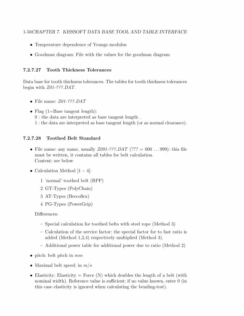
1-50CHAPTER 7. KISSSOFT DATA BASE TOOL AND TABLE INTERFACE
• Temperature dependence of Youngs modulus
• Goodman diagram: File with the values for the goodman diagram
7.2.7.27 Tooth Thickness Tolerances
Data base for tooth thickness tolerances. The tables for tooth thickness tolerancesbegin with Z01-???.DAT.
• File name: Z01-???.DAT
• Flag (1=Base tangent length):0 : the data are interpreted as base tangent length .1 : the data are interpreted as base tangent length (or as normal clearance).
7.2.7.28 Toothed Belt Standard
• File name: any name, usually Z091-???.DAT (??? = 000 . . . 999): this filemust be written, it contains all tables for belt calculation.Content: see below
• Calculation Method [1− 4]:
1 ’normal’ toothed belt (RPP)
2 GT-Types (PolyChain)
3 AT-Types (Brecoflex)
4 PG-Types (PowerGrip)
Differences:
– Special calculation for toothed belts with steel rope (Method 3)
– Calculation of the service factor: the special factor for to fast ratio isadded (Method 1,2,4) respectively multiplied (Method 3).
– Additional power table for additional power due to ratio (Method 2)
• pitch: belt pitch in mm
• Maximal belt speed: in m/s
• Elasticity: Elasticity = Force (N) which doubles the length of a belt (withnominal width). Reference value is sufficient; if no value known, enter 0 (inthis case elasticity is ignored when calculating the bending-test).

7.2. DESCRIPTION OF THE DATA BASE 1-51
• Weight per length: weight (kg) of a 1m belt per mm belt width.
• Addend for operation: no influence
• Nomimal-width for power table: belt width (mm) which corresponds to thepower data that are placed in the corresponding file (see file name).
• Calculation method for belt tension:
1 : in % of circumferential force
2 : in % of maximal permissable circumferential force
3 : in % of (operation factor*power (W)/circumferential force (m/s))(according to Dayco RPP Panther)(Method 3 only from Version 10/99 !)
• Factor for belt tension: 0.0 . . . 1.0 (%-Factor for calculation of belt tension)
Content of File:
File Z091-???.DAT (??? = 000 . . . 999) contains the following tables for beltcalculation purpose. Please look at an example file (e.g. Z091-006.dat).
List with proposed standard toothnumbers of toothed sheaves
:TABLE LIST z.RadZahne
List with proposed belt standard toothnumbers
:TABLE LIST z.NormZahne
Minimal tooth number depending onspeed (small sheave)
:TABLE FUNCTION z091k.ZahneZmin
Correction factor for inputs dependingon ratio (added to operation factor)
:TABLE FUNCTION z091k.factorINCR
Transmittable power depending onnumber of teeth (small sheave) andrpm (small sheave)
:TABLE FUNCTION z091k.powerNR
Correction factor for number of teethin contact (small sheave)
:TABLE FUNCTION z091k.factorCorrEZ
Correction factor for belt length :TABLE FUNCTION z091k.factorLengthCorrection factor for belt width :TABLE FUNCTION belt.bthCorrection factor for belt width (samevalues as in table shown beforehand!)
:TABLE FUNCTION belt.beff
Sheave width depending on belt width :TABLE FUNCTION z091k.ScheibenBreiteLay out of belt type: minimal transmit-table power (lower limit) depending onrpm (small sheave)
:TABLE FUNCTION z091k.kWlower
Lay out of belt type: Maximal trans-mittable power (upper limit) depend-ing on rpm (small sheave)
:TABLE FUNCTION z091k.kWupper
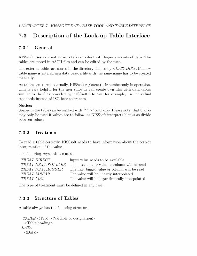
1-52CHAPTER 7. KISSSOFT DATA BASE TOOL AND TABLE INTERFACE
7.3 Description of the Look-up Table Interface
7.3.1 General
KISSsoft uses external look-up tables to deal with larger amounts of data. Thetables are stored in ASCII files and can be edited by the user.
The external tables are stored in the directory defined by <DATADIR>. If a newtable name is entered in a data base, a file with the same name has to be createdmanually.
As tables are stored externally, KISSsoft registers their number only in operation.This is very helpful for the user since he can create own files with data tablessimilar to the files provided by KISSsoft. He can, for example, use individualstandards instead of ISO base tolerances.
Notice:Spaces in the table can be marked with ’*’, ’-’ or blanks. Please note, that blanksmay only be used if values are to follow, as KISSsoft interprets blanks as dividebetween values.
7.3.2 Treatment
To read a table correctly, KISSsoft needs to have information about the correctinterpretation of the values.
The following keywords are used:
TREAT DIRECT Input value needs to be availableTREAT NEXT SMALLER The next smaller value or column will be readTREAT NEXT BIGGER The next bigger value or column will be readTREAT LINEAR The value will be linearly interpolatedTREAT LOG The value will be logarithmically interpolated
The type of treatment must be defined in any case.
7.3.3 Structure of Tables
A table always has the following structure:
:TABLE <Typ> <Variable or designation><Table heading>
DATA<Data>

7.3. DESCRIPTION OF THE LOOK-UP TABLE INTERFACE 1-53
END
Each table has its own table heading. The following examples show the threeemployed table types:
• Function Tables
– one dimensional
– two dimensional
• List Tables
• Range Tables
7.3.3.1 Function-Tables, One- and Two-Dimensional
Function tables are tables which require one or two input values (one- or two-dimensional) and return exactly one value.
Example of a one-dimensional function tableThe angle factor is determined by the given angle:
:TABLE FUNCTION factorINPUT X angle TREAT LINEAR
DATA0 30 60 90 . . .0.1 0.25 0.45 0.78 . . .
END
The variable factor is calculated by the value of the variable angle and is, in caseof intermediate results, linearly interpolated. The first line represents the inputvariable INPUT X and the second line the output value.
Example of a two-dimensional tableDetermining the nominal power, based on speed and disk diameter:
:TABLE FUNCTION powerINPUT X diameter TREAT LINEARINPUT Y speed TREAT LINEAR
DATA

1-54CHAPTER 7. KISSSOFT DATA BASE TOOL AND TABLE INTERFACE
50 100 200 300 . . .50 4 7 12 25 . . .75 12 25 30 35 . . .:: :: :: :: :: . . .3000 300 5005000 700
END
The variable power is computed by using the input variables INPUT X andINPUT Y. A linear interpolation will be carried out in (X) (Column) and (Y)(Line) if required. The first line represents the values of the input variable INPUTX and the the first column the values of INPUT Y. All other values are outputdata. Please note that you might define inverse tables. E.g. if your XY -beltcatalogue has the speed in the first line and the diameter in the first column,simply the allocation in the table head has to be changed and not the table itself.(just swap X and Y ).
7.3.3.2 List Tables
With at least one input value, several output values can be computed in list tables.If several input values are given, the hierarchy of those values is important. Theleftmost values are highest priority, this means, that the first value determinesthe range of the second and so on. All input values except the last one are treateddirectly (TREAT DIRECT is activated).
Example:
Before the table has been elevated, the relevant variables have the following val-ues:
g.d := 2.0; g.P := 0.8; s.l := 6;
:TABLE LIST s.normINPUT g.dINPUT g.PIN OUT s.l TREAT NEXT BIGGEROUTPUT s.k, s.dk
DATA1.4 0.3 01.4 0.3 2 1.4 2.61.4 0.3 3 1.4 2.61.4 0.3 5 1.4 2.6

7.3. DESCRIPTION OF THE LOOK-UP TABLE INTERFACE 1-55
2.0 0.4 02.0 0.4 3 2 3.82.0 0.4 4 2 3.82.0 0.4 5 2 3.82.0 0.8 02.0 0.8 5 3 4.52.0 0.8 7 3 4.5 ← Relevant Data Line2.0 0.8 10 3 4.8
END
:TABLE LIST screw.geometryINPUT typINPUT l TREAT NEXT SMALLEROUTPUT M, dw, (s), e, bez, vorrat
DATA::12x2.5 20 12 14.57 23.78 5.75 bez.1 112x2.5 25 12 15.78 24.88 5.75 bez.2 1::
END
The table is related to the variable screw.geometry, which is required for theidentification of the table. The order in the table head determines the order ofthe columns. First column for variable type, second for variable l and so on. Thevariables type and the variable l are used as inputs, the value for the variable typehas to be registered in the list. In case of an intermediate value for l, the line withthe next smaller value is interpreted as result. Empty spaces are not permitted,i.e. values always have to exist in this type of table. If a variable in the outputdefinition field is put into brackets, it is not read and the column ignored.
DANGER: This operation feature is not to be employed by the user!
7.3.3.3 Range Table
Range tables are used to check whether a given value is within a defined range.
Example: colon.
:TABLE RANGE ’A’INPUT X drehzahl TREAT LOGINPUT Y leistung

1-56CHAPTER 7. KISSSOFT DATA BASE TOOL AND TABLE INTERFACE
DATA200 300 500 1000 4000
LOWER 1.5 2.0 3.0 10 20UPPER 10 15 20 15 40END
The first line corresponds to the values of the variable speed. Intermediate valuesare interpolated logarithmically.
Further lines correspond to the values of the variable power where LOWER andUPPER represent lower and upper boundaries. The input value of power is com-pared with these boundaries, and the output defines whether the power is withinthe boundaries, too high or too low.

Chapter 8
Reports
8.1 Calculation Report
With KISSsoft you can generate reports listing the results of your calculations.In the module interface you find besides panel Calculate panel Report. You canactivate this function either by mouseclick or F6.
To assure that only records with valid content are saved, KISSsoft maintains amarking system. As soon as something is changed in the input field, the hooknamed Results consistent is removed. The hook is reset after successful cal-culation. If you activate Report while the hook is being removed, the programwarns you that the results of the record could possibly be invalid. Despite thiswarning, a report is made, which can be useful if you just want to print out yourinput data.
After the flag has been activated, a file named after the module designationis generated and the modification .rtf (e.g. M040.rtf for the calculation ofbolted joints); this file is placed in the tmp directory, that has been definedin file KISS.INI with the variable <TMPDIR>. Mostly, it is file \ProgramFiles\KISSsoft\tmp.
The standard editor displaying reports is KISSedit (see chapter 8.3); you canchoose a different editor (see 6.2). In the editor, you can process the report justas in any other word processing program.
Important: If you want to file reports for some time, you have to save them asself-defined files since new reports replace the old ones every time you generate areport. Moreover, KISSsoft frequently deletes all temporary files. Therefore youhave to choose a directory different from <TEMPDIR> to save the report files.
In Services ⇒ Settings ⇒ Reports ⇒ Size of Report, you can define thefine of the report (this partition does only make a sense for some modules). You
1-57

1-58 CHAPTER 8. REPORTS
can choose a number from 1 to 9, where 9 stands for a comprehensive report and1 for a very limitated one, in which only the most important facts are reported.
Similarly, you can define in Services ⇒ Settings ⇒ Report whether warningsshould be listed in reports or not. Errors are always recorded.
A report consists of the following:
• A heading with information on project, user and software. The headingenables you to identify reports and is specified in KISS.rpt (see chapter8.2).
• Errors or warnings having occured
• Specification of method of calculation
• in some large reports a summary
• Inputs
• Results
• Comments, e.g. module specific information on applicatable standards, de-viations therefrom, important comments on calculation methods of everykind or explanations of formulae.
• The foot of the report is defined in KISSF.rpt (see chapter 8.2).
8.2 Report Templates
KISSsoft provides report templates for every module which decide about formand content of a report (see picture at 8.1). You can adapt these templates in atext editor (e.g. KISSedit) to fit the report to your needs.
You cannot define your own variables, except numeral variables used for FOR-loops (see chapter 8.2.3.5).
8.2.1 Name of Report templates
Report templates are placed in directory <KISSDIR>. Their names have thestructure MMMMlsz.rpt and consist of:
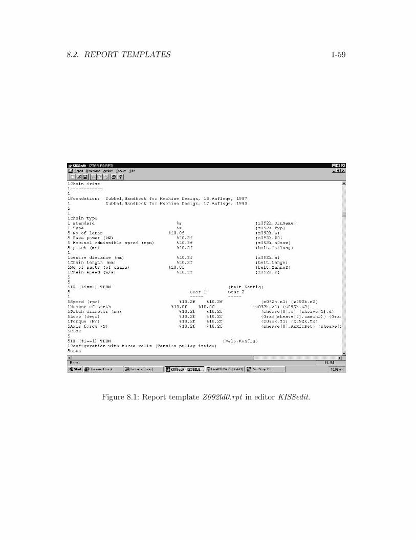
8.2. REPORT TEMPLATES 1-59
Figure 8.1: Report template Z092ld0.rpt in editor KISSedit.

1-60 CHAPTER 8. REPORTS
MMMM Designation of module e.g. M040l historical allways = ls Language of report s = d : german, e: english, f : french
i : italian, s :spanish, a: english(imperial)z historical always = 0.rpt Designation Reports of calculations
templates of reports end on .rtf.
Examples of Report Templates
Bolted joints calculation:M040LD0.RPT german issueM040USER.RPT standard issue over interface,
becomes file M040USER.OUT 1
Spur gear calculation:Z012LD0.RPT spur gear pair, german issueZ012USER.RPT standard issue over interface,
becomes file Z010USER.OUT 1
Z10GEAR1.RPT print out over interface, contains only dataof gear 1, becomes file Z010GEAR1.OUT 1
Z10GEAR2.RPT issued over interface, contains only dataof gear 2, becomes file Z010GEAR2.OUT 1
Z011LD0.RPT Single gear, german issueZ013LD0.RPT Rack, german issueZ014LD0.RPT Planetary gear, german issueZ015LD0.RPT 3 gears, german issueZ016LD0.RPT 4 gears, german issueEnglish issue:M040LE0.RPT Thread calculation, English issueAmerican issue:M040LA0.RPT Thread calculation, American issue
8.2.2 Length of Reports
The length of a report can be set on a scale from 1 to 9 (where 9 stands for thecomplete, 1 for a short report; c.f. Services ⇒ Settings ⇒ Report). In thereport template, there is at the beginning of each line a number between 1 and9. This number determines, depending on the above described setting, whetherthe line is read or not. Example: If you chose a 5 (nmedium) for the length ofthe report, all lines of the report template, which begin with 1, 2, 3, 4 or 5, areread. Lines beginning with 6, 7, 8 and 9 are ignored.
1compare chapter 9 on page 1-71
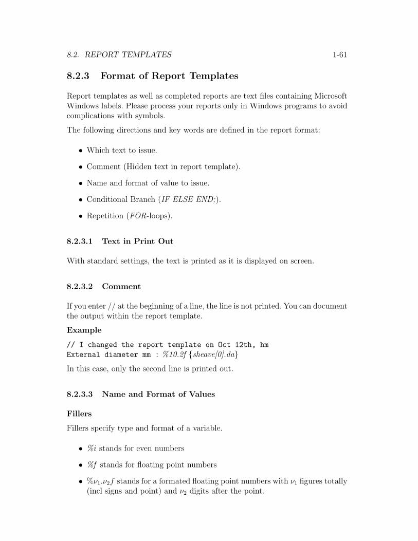
8.2. REPORT TEMPLATES 1-61
8.2.3 Format of Report Templates
Report templates as well as completed reports are text files containing MicrosoftWindows labels. Please process your reports only in Windows programs to avoidcomplications with symbols.
The following directions and key words are defined in the report format:
• Which text to issue.
• Comment (Hidden text in report template).
• Name and format of value to issue.
• Conditional Branch (IF ELSE END;).
• Repetition (FOR-loops).
8.2.3.1 Text in Print Out
With standard settings, the text is printed as it is displayed on screen.
8.2.3.2 Comment
If you enter // at the beginning of a line, the line is not printed. You can documentthe output within the report template.
Example
// I changed the report template on Oct 12th, hm
External diameter mm : %10.2f {sheave[0].da}
In this case, only the second line is printed out.
8.2.3.3 Name and Format of Values
Fillers
Fillers specify type and format of a variable.
• %i stands for even numbers
• %f stands for floating point numbers
• %ν1.ν2f stands for a formated floating point numbers with ν1 figures totally(incl signs and point) and ν2 digits after the point.

1-62 CHAPTER 8. REPORTS
• %s stands for a left-bound sequence of characters (text)
• %ns stands for a right-bound sequence of characters in a field containingn-characters (n is an even number)
Filler types have to be consistent with the definition of the associated variablesin the program. The value is stated exactly where the filler stands. The syntaxof the format corresponds to the C/C++-Standard.
Examples:
• %10.2f issues 10 digits with a precision of two digits right-bound of a float-ing point.
• %i issues an even number unformated exactly at this point.
• %30s stands for a right-bound sequence with a field containing 30 characters(If 30 is omitted, the characters are issued left-bound).
Counterexamples:
• %8.2i is an invalid format, as an even number has no decimals.
• %10f2 issues 10 digits of a floating point number right-bound, but the twofigures after the point are ignored and issued as text 2. Normally, floatingpoints are issued on 6 digits.
Variables
Which variable is issued has to be defined behind the filler of the same line. Thevariable is marked with braces. If these braces are omitted, the name of thevariable is issued as a normal text.
Important: There must be exactly as many fillers as {} brace pairs!
Example: %f {sheave[0].d} issues the value of the variable sheave[0].d in digit %fas floating point number with 6 digits after the point.
Basic Calculations – Output of Altered Variables
In the report, variables can be issued differently. They can be multiplied or dividedas well as factors can be added or subtracted. This function is also valid in thearguments of the IF - or FOR-conditions.
Value of the variable multiplied %3.2f {Var*2.0}Value of the variable divided %3.2f {Var/2.0}Value of the variable added %3.2f {Var+1.0}Value of the variable subtracted %3.2f {Var-2}

8.2. REPORT TEMPLATES 1-63
Similarly, the two functions grad and rad are availabele for conversion into degreeor radiant respectively.
angle %3.2f {grad(angle)}
Variables can be combined with each other, like {sheave[0].d-sheave[1].d}. Morethan two variables can be used also. Values with signs have to be put in brackets,e.g. {ZR[0].NL*(1e-6)}.
You can use the functions you find in table 8.1.
8.2.3.4 Interrogation of Condition IF ELSE END
The interrogation of condition enables you to issue certain values or text only ifa certain condition is fulfilled. The following conditions are supported:
Combination of Characters Meaning== equal>= larger or equal<= smaller or equal! = unequal< smaller> larger
This condition has to be written as follows:
IF (Condition) {Var}Case 1
ELSECase 2
END;
Example:
IF (%i==0) {Zst.kXmnFlag}Addendum modified no
ELSEAddendum modified yes
END;
If variable Zst.kXmnFlag is 0, the first text is issued, if it is not 0, the second. Anyamount of lines can stand between IF, ELSE and END. Every branch beginningon IF has to be closed by END; (Please note the semicolon after END !). Thekey word ELSE is optional, it reverses the condition. Branches can be interlacedup to level 9.
Example of a Simple Branch

1-64 CHAPTER 8. REPORTS
Function Meaningsin(angle) Sinus of angle in radianscos(angle) Cosinus of angle in radianstan(angle) Tangens of angle in radiansasin(val) Arcussinus of val, returns radiansacos(val) Arcuscosinus of val, returns radiansatan(val) Arcustangens of val, returns radiansabs(val) |val|exp(val) eval
log(val) returns x in ex = vallog10(val) returns x in 10x = valsqr(val) val2
sqrt(val) returns√
valpow(x;y) returns xy
sgn(val) returns
1 if val > 00 if val = 0−1 if val < 0
sgn2(val) returns
{1 if val ≥ 00 if val < 0
grad(angle) Conversion from radians to degreerad(angle) Conversion from degree to radiansmm in(val) returns val/25.4celsius f(val) returns 9
5val + 32
min(ν1; . . . , ν5) returns minimum of ν1, . . . , ν5
max(ν1; . . . , ν5) returns maximum of ν1, . . . , ν5
and(ν1; ν2) binary and functionor(ν1; ν2) binary or functionxor(ν1; ν2) binary exclusive or functionAND(ν1; . . . , ν5) logical and functionOR(ν1; . . . ; ν5) logical or function
NOT(val) returns
{0 if val 6= 01 if val = 0
LESS(ν1; ν2) returns
{1 if ν1 < ν2
0 if ν1 ≥ ν2
EQUAL(ν1; ν2) returns
{1 if ν1 = ν2
0 if ν1 6= ν2
GREATER(ν1; ν2) returns
{1 if ν1 > ν2
0 if ν1 ≤ ν2
Table 8.1: Possible functions in for calculations in the report.
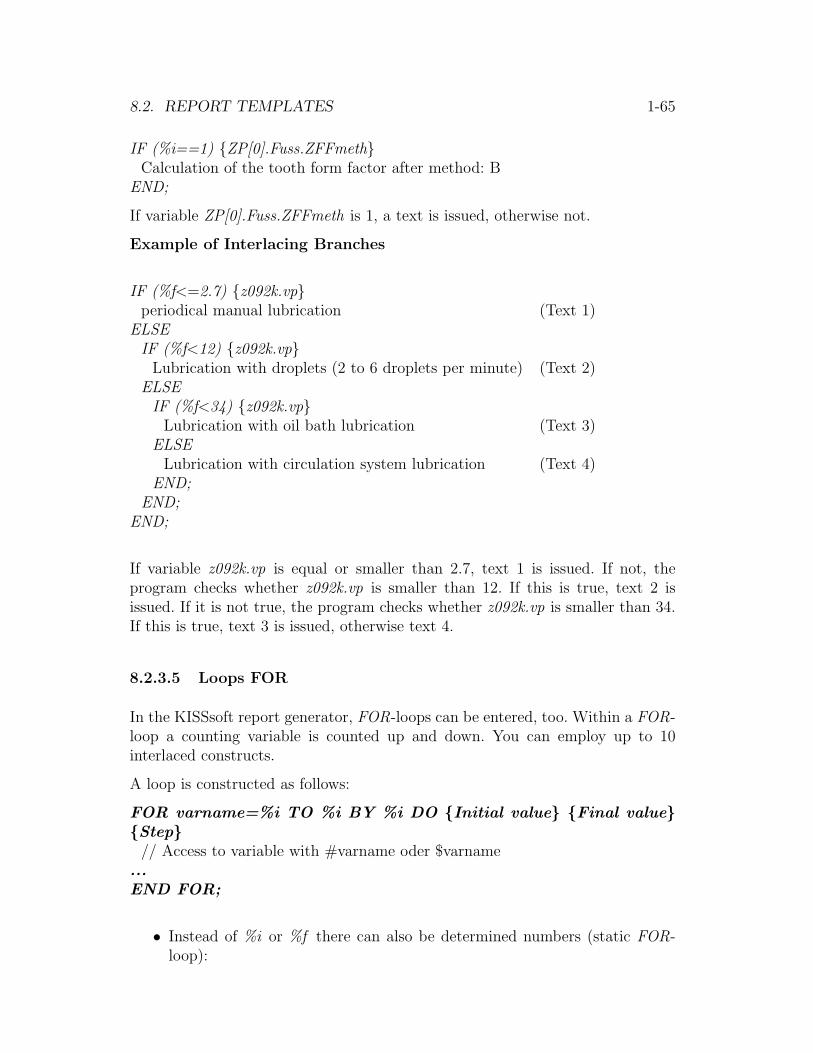
8.2. REPORT TEMPLATES 1-65
IF (%i==1) {ZP[0].Fuss.ZFFmeth}Calculation of the tooth form factor after method: B
END;
If variable ZP[0].Fuss.ZFFmeth is 1, a text is issued, otherwise not.
Example of Interlacing Branches
IF (%f<=2.7) {z092k.vp}periodical manual lubrication (Text 1)
ELSEIF (%f<12) {z092k.vp}
Lubrication with droplets (2 to 6 droplets per minute) (Text 2)ELSE
IF (%f<34) {z092k.vp}Lubrication with oil bath lubrication (Text 3)
ELSELubrication with circulation system lubrication (Text 4)
END;END;
END;
If variable z092k.vp is equal or smaller than 2.7, text 1 is issued. If not, theprogram checks whether z092k.vp is smaller than 12. If this is true, text 2 isissued. If it is not true, the program checks whether z092k.vp is smaller than 34.If this is true, text 3 is issued, otherwise text 4.
8.2.3.5 Loops FOR
In the KISSsoft report generator, FOR-loops can be entered, too. Within a FOR-loop a counting variable is counted up and down. You can employ up to 10interlaced constructs.
A loop is constructed as follows:
FOR varname=%i TO %i BY %i DO {Initial value} {Final value}{Step}
// Access to variable with #varname oder $varname...END FOR;
• Instead of %i or %f there can also be determined numbers (static FOR-loop):

1-66 CHAPTER 8. REPORTS
FOR varname=0 TO 10 BY 1 DO...END FOR;
• or intermingled:
FOR varname=5 TO %i BY -1 DO {Final value}...END FOR;
• Every FOR-loop has to be closed with condition END FOR; (inclsemikolon!). Every defined counter variable (varname) within a loop canbe called upon by #varname.
• You can choose negative steps (for example −1), but never can you choose0. The step width must always be defined.
• The #varname-condition can be used for the definition of a variable. Forexample:
Number of teeth: %3.2f {ZR[#varname].z}
• The $varname-condition can be used as a character for the issue of thevariable value. 0 is A, 1 is B etc. For example:
FOR quer=0 TO 3 BY 1 DOCross section $quer-$quer : %8.2f {Qu[#quer].sStatic}
END FOR;
Example of a Simple Loop
FOR i=0 TO 10 BY 1 DOphase number #i $i
END FOR;
This is issued as:
phase number 0 Aphase number 1 Bphase number 2 Cphase number 3 Dphase number 4 Ephase number 5 Fphase number 6 Gphase number 7 Hphase number 8 Iphase number 9 J
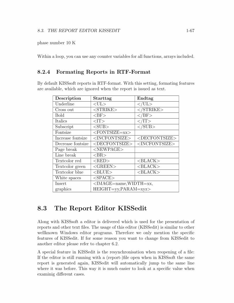
8.3. THE REPORT EDITOR KISSEDIT 1-67
phase number 10 K
Within a loop, you can use any counter variables for all functions, arrays included.
8.2.4 Formating Reports in RTF-Format
By default KISSsoft reports in RTF-format. With this setting, formating featuresare available, which are ignored when the report is issued as text.
Description Starttag EndtagUnderline <UL> </UL>Cross out <STRIKE> </STRIKE>Bold <BF> </BF>Italics <IT> </IT>Subscript <SUB> </SUB>Fontsize <FONTSIZE=xx>Increase fontsize <INCFONTSIZE> <DECFONTSIZE>Decrease fontsize <DECFONTSIZE> <INCFONTSIZE>Page break <NEWPAGE>Line break <BR>Textcolor red <RED> <BLACK>Textcolor green <GREEN> <BLACK>Textcolor blue <BLUE> <BLACK>White spaces <SPACE>Insert <IMAGE=name,WIDTH=xx,graphics HEIGHT=yy,PARAM=xyz>
8.3 The Report Editor KISSedit
Along with KISSsoft a editor is delivered which is used for the presentation ofreports and other text files. The usage of this editor (KISSedit) is similar to otherwellknown Windows editor programs. Therefore we only mention the specificfeatures of KISSedit. If for some reason you want to change from KISSedit toanother editor please refer to chapter 6.2.
A special feature in KISSedit is the resynchronisation when reopening of a file:If the editor is still running with a (report-)file open when in KISSsoft the samereport is generated again, KISSedit will automatically jump to the same linewhere it was before. This way it is much easier to look at a specific value whenexaminig different cases.

1-68 CHAPTER 8. REPORTS
8.3.1 Saving reports
The contents of reports is stored on temporary files first. Every call of the reportgenerator overwrites the current report file. If you want to keep a report file, youcan use the KISSedit menue File ⇒ Save as. Choose another directory thanthe temporary directory <TEMPDIR> because KISSsoft frequently deletes alltemporary files in this directory.
If you want to compare two reports of the same calculation module you do notnecessarily have to save them. You can also use the comparison mode of thereport generator, see chapter 2.4 on page 1-10.
As format for saving there are available:
rtf means ”rich text format” and is the format used by Microsoft to ensure filecompability among different Windows applications.
txt is pure ASCII format. All graphics and formatting are ommitted. This formatmay be of great use if the text should be transfered to a program whichdoesn’t read rtf nor doc files.
doc is the format of Microsoft - WinWord. Files saved in this format are directlyreadable in Word (you can, however, read rtf files direclty as well in mostcases).
htm,html hypertext format, this gives files which can be opened with a htmlbrowser or included into a web page.
rpt,rpu are the formats of the report templates provided along with KISSsoft(rpt) or generated by the user (rpu). See chapter 8.2 for details.
pdf is the ”portable document format”. Since this format can only be written,not read into KISSedit, this format is only available through the menu File
⇒ Export.
8.3.2 Synchronised Scrolling
Two compare two or more reports the scrolling of all open windows can be syn-chronised. For this the windows are arranged appropriate, for instance tiled verti-cally. Then, the reports are scrolled in a postion that the corresponding lines andcolumns are aligned. Now by activating the syncronised scrolling in the menuView (or by clicking on the button in the toolbar) whenever a window isscrolled, all others will follow. For deactivation of the synchronisation use themenu View (or the button in the toolbar) again.

8.3. THE REPORT EDITOR KISSEDIT 1-69
filler meaning%t next tabstop%dt(format) current date and time.
The date is formated according to the definition in ’format’.For the meaning of the parts of ’format’ refer to table 8.6.
%fd(format) date and time of report file.Usually this is the time when KISSsoft generated the report file.The meaning of ’format’ is like %dt.
%pn Number of current page.%pc Total number of pages.%logo Graphical logo.
Inserts the file Logo.bmp located in the directorywhere KISSedit is started.
Table 8.4: Meaning of the fillers in the definition of header and footer.
8.3.3 Quick Change from Portrait to Landscape
Some reports and result files are very wide. With A4 or legal format and the usualsize of the letters this may lead to line breaks and therefore to a text which is hardto read. A typical example for this are the results of the fine sizing function ofthe spur gears calculation. As a solution two buttons where added to the toolbar
( ). With this buttons you can quickly change from portrait to landscape andvers visa. The settings are automatically used for printing.
8.3.4 Definition of Header and Footer
By default KISSedit generates a header and a footer with some informationsabout the report file, such as number of pages, date of report file or date ofprinting. As well you can add a graphical logo. For changing the definition ofheader or footer a menue Format⇒ Definition Header/Footer is available. Inthe opening dialog you can define a format string or you can (de-)activate theheader or the footer. The format string consists of text and fillers. For the meaningof the fillers please refer to table 8.4. Two tabstops are defined, a centrical onein the middle of the page and a right bound one at the right limit of the text.The logo shown is taken from a file logo.bmp, which is located in the installationdirectory of KISSedit (i.e. the directory where the file KISSedit.exe is found). Ifyou wish to replace the original logo with your own one, you have to overwritethis file with your own.

1-70 CHAPTER 8. REPORTS
Format Meaning%a Abbreviated weekday name%A Full weekday name%b Abbreviated month name%B Full month name%c Date and time representation appropriate for locale%d Day of month as decimal number (01 – 31)%H Hour in 24-hour format (00 – 23)%I Hour in 12-hour format (01 – 12)%j Day of year as decimal number (001 – 366)%m Month as decimal number (01 – 12)%M Minute as decimal number (00 – 59)%p Current locale’s A.M./P.M. indicator for 12-hour clock%S Second as decimal number (00 – 59)%U Week of year as decimal number,
with Sunday as first day of week (00 – 53)%w Weekday as decimal number (0 – 6; Sunday is 0)%W Week of year as decimal number,
with Monday as first day of week (00 – 53)%x Date representation for current locale%X Time representation for current locale%y Year without century, as decimal number (00 – 99)%Y Year with century, as decimal number%z, %Z Time-zone name or abbreviation;
no characters if time zone is unknown%% Percent sign
Table 8.6: The meaning of formating symbols in date and time.

Chapter 9
Description of the PublicInterface
9.1 Interfaces Between Calculation Programs
and CAD – Overview
A calculation program within a CIM-concept is very closely connected to CAD-programs. KISSsoft has a free configurable public interface that is able to com-municate efficiently with external programs.
All input and output data can be exported in ASCII-format in any quantity andform. For this, every calculation module has a special editable report file. Externalprograms can even send input data (in ASCII-format as well) to calculationmodules. Such data is read automatically at start-up and displayed in the userinterface.
KISSsoft can exchange data over an interface via menu File ⇒ Interface ⇒Read Data and File ⇒ Interface ⇒ Output. Files MMMMUSER.RPT 1 serveas templates for this transfer. These files are empty by default. Before you issuedata over the interface, you have to create or enlarge the templates.
9.1.1 Useful Interfaces
You should only establish an automated data transfer between calculation andCAD program if you really need it frequently. An interface between a bolt calcula-tion program and CAD program for example is not very helpfull, as the amount of
1MMMM stands for a filler for the module to which the file refers. Example:M040USER.RPT
1-71
1-72 CHAPTER 9. DESCRIPTION OF THE PUBLIC INTERFACE
transferred information (e.g. that because of the calculation a bolt M10 is chosen)is too small and can be carried out much faster ”manually”. If, however, you haveaccess to a library of standard parts, a bidirectional relation of the three partscalculation program, library of standard parts and CAD can be highly efficient.
Efficient interfaces are (this list is not complete):
• Generally
The calculation programs should be started from the CAD directory (eg byF-button). In this way you can carry out short calculations while workingon a drawing, adopt the values and go on drawing.
• Calculation of shafts and bearings
– Output of a contour from CAD (e.g. a shaft in detail or assemblydrawing) and reading into the calculation program. (Problem: In manyCAD-programs, defining a contour for transfer is very tiring).
– Output of a shaft, optimised in a calculation program (incl. roller bear-ing etc.) and reading as drawing information into the CAD-program.
– Transfer of bending line and similar data to the CAD.
– Roller bearing and journal bearing are calculated in KISSsoft, thecontours are then transferred to the CAD. (Often, information on rollerbearings is already available in the CAD-program, so that only thebearing label is important.)
• Gear calculation
– Calculation of production data in the program and transfer of requiredvalues to the CAD. This is a very important function, as mistakes caneasily occur in copying this data manually, and implications of suchmistakes are fatal.
– Calculation of the exact tooth form in side view and transfer to theCAD. (Produces beautiful diagrams but is normally of no importance,unless the data is processed, e.g. with a wire cut machine.)
– Transfer of a schematic axis section or of the side view of gears to theCAD (although this can easily be made manually in the CAD)
• Other Machine elements
Transfer of contours of calculated machine elements (such as bolts, v-beltsheaves etc.) to the CAD-program. (Most CAD-stations already have suchinformation programmed, so that only the definitions of the parts are im-portant.)

9.1. INTERFACES BETWEEN CALCULATION PROGRAMS AND CAD – OVERVIEW 1-73
• Shaft-hub-connection
Lay out or references of connections should be implemented directly into theCAD, so that already known data can be adopted from the CAD-programand the calculation values can be given back to the CAD.
9.1.2 Open-Interface-Concept in KISSsoft
The interface concept of KISSsoft has a very simple and flexible structure.
Calculation programs should be able to integrate easily in CAD-systems. Theyalso have to run on different systems like MS-DOS, MS-Windows, UNIX, etc.
The interface mechanism between CAD and KISSsoft is based on a text dataset (ASCII-file), in which all transfer files get a designation and a number (seepicture in example 1-77). This data sets can have different length, but only knownvalues are transferred to the CAD. This depends on the CAD-system and on thecurrent drawing.
The data set transferred from the external program is tested by KISSsoft oncompletion and on what it consists of, and, if necessary, additional data can beentered into KISSsoft. Thereafter, the program carries out the calulation, writesoutput data that is important for the CAD-program into a text data set andsends it back to the CAD-program. By means of the reportgenerator you canchoose any format for your output file, i.e. KISSsoft adapts itself to the externalprogram. Now, the CAD can read the required information and work with itselectively.
This concept produces simple interface forms that even user not very experiencedin programming can easily write applications for.

1-74 CHAPTER 9. DESCRIPTION OF THE PUBLIC INTERFACE
9.2 Defining Input and Output
9.2.1 Rough Remarks
• For this description, KISSsoft is always taken as point of reference, i.e. a filethat is an input file for KISSsoft is an output file for the external programetc.
• For the automatic data exchange with other programs, files named MMM-MUSER.RPT are required. You can fit these files to your personal needs.However, if you have bought KISSsoft interfaces, you have to be careful, asthese files are needed by the interface.

9.2. DEFINING INPUT AND OUTPUT 1-75
File name Location DescriptionMMMMUSER.IN <CADDIR> ∗) Input file for KISSsoft (is written by the
external program)Temporary user file (= deleted byKISSsoft after reading)
MMMMUSER.OUT <CADDIR> Output file of KISSsoft (written byKISSsoft, read by the external program)Temporary user file (= should bedeleted by the CAD)
MMMMUSER.RPT <KISSDIR> Definition of output format (like report)Z10Gear1.RPT <KISSDIR> Template for output ofZ10Gear2.RPT spur/helical gear definition.Z10Gear3.RPT (see below). Analogue MMMMUSER.rptZ10Gear4.RPT for this special case.Z10Gear1.OUT <KISSDIR> Output file of definition
... for spur/helical gears.Z70Gear1.RPT <KISSDIR> Definition of ouput formatZ70Gear2.RPT ffor bevel gears.Z17Gear1.RPT <KISSDIR> Definition of ouput formatZ17Gear2.RPT for crossed helical gears.Z80Gear1.RPT <KISSDIR> Definition of ouput formatZ80Gear2.RPT for worm gears.Z9aGear1.RPT <KISSDIR> Definition of ouput formatZ9aGear2.RPT for splines.Z??Gear1.OUT <CADDIR> Contains definition analogZ??Gear2.OUT to template files.∗) If the filename contains the full path the files can also be read from an arbitrarylocation.
9.2.2 Standard of External Programs
An external program needs a minimal standard set to work successfully with KISSsoft.It has to
1. have a check mechanism (e.g. a macro system), to make information such asinput files available,
2. be able to read and write ASCII-files,
3. be able to tart a program.

1-76 CHAPTER 9. DESCRIPTION OF THE PUBLIC INTERFACE
9.2.3 Employed Files
9.2.3.1 Input File
The employed input file is called MMMMUSER.IN and has the same structure andthe same function - except of the temporary state - as saved calculations. The valuesare related by KISSsoft to the variable names with an equality sign =. Every variablegets an individual line.
Example:
VERSION=1.0;m02Aw.dWa=30;m02Aw.lW=20;m02An.lN=25;
The input file is read after the standard values have been defined, i.e. The valuesof the temporary input file overwrite the values set by default. Read aboutdefault files in chapter 6.3.
Annotation: Temporary input files replace frequently changing variables like geometryand/or power data which are different for every calculation. If you like, you can writethese data into the default files since they are just normal input variables. This means,though, that the program generating the files has to interprete already written data,i.e. to adopt permanent prescriptions, to define the standard entirely and reset it againat the end.
9.2.3.2 Output File
Immediately after the calculation, KISSsoft generates a specific output file MMM-MUSER.OUT to send relevant data back to the external program. The output file’sextent and format is defined in the report pattern MMMMUSER.RPT.
This means that KISSsoft can adapt itself to the syntax of an external program. Theextent of directions and the syntax of the report generator are described in chapter’Reports’ (see chapter. 8)
9.2.4 Life Span of Files
The input file MMMMUSER.IN is generated by the external program and is deleted byKISSsoft after having been read. The output file MMMMUSER.OUT is deleted whileKISSsoft is starting-up and written again after a calculation.
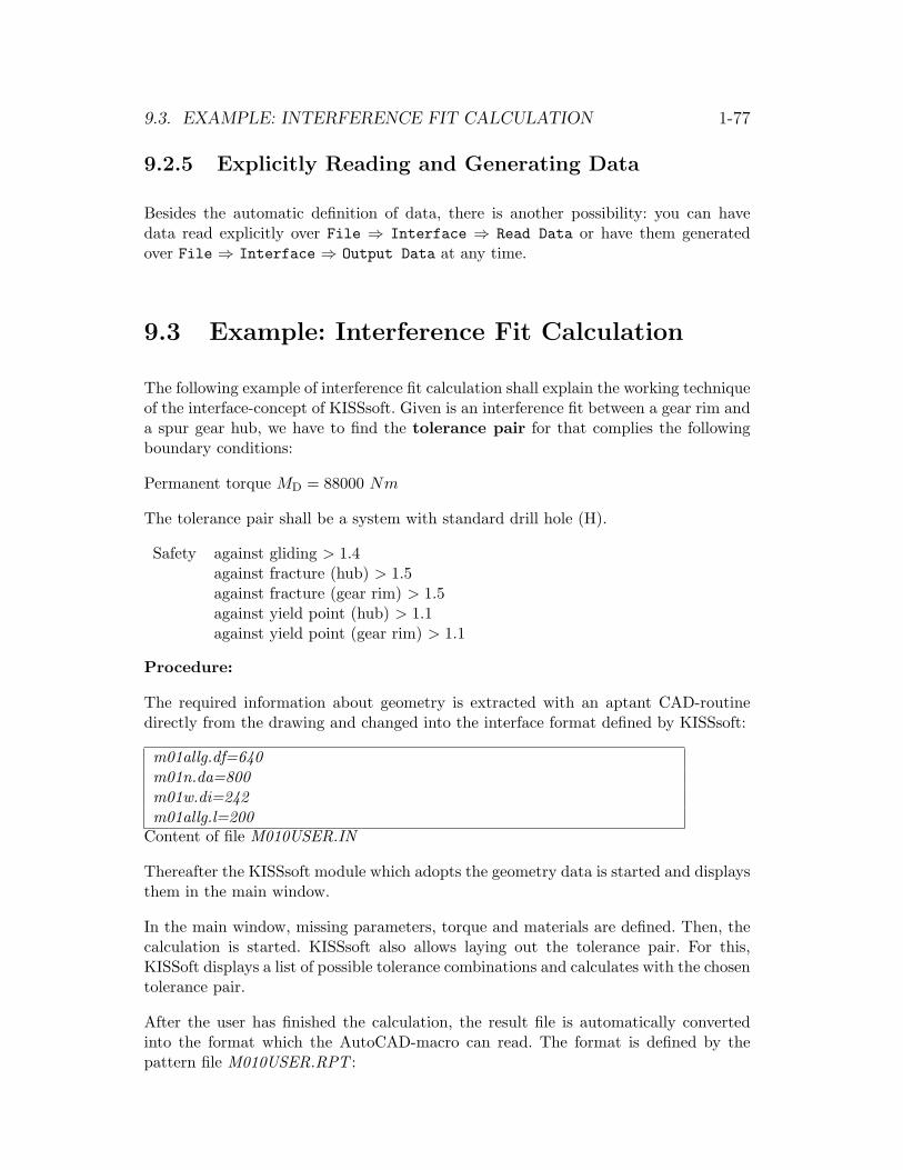
9.3. EXAMPLE: INTERFERENCE FIT CALCULATION 1-77
9.2.5 Explicitly Reading and Generating Data
Besides the automatic definition of data, there is another possibility: you can havedata read explicitly over File ⇒ Interface ⇒ Read Data or have them generatedover File ⇒ Interface ⇒ Output Data at any time.
9.3 Example: Interference Fit Calculation
The following example of interference fit calculation shall explain the working techniqueof the interface-concept of KISSsoft. Given is an interference fit between a gear rim anda spur gear hub, we have to find the tolerance pair for that complies the followingboundary conditions:
Permanent torque MD = 88000 Nm
The tolerance pair shall be a system with standard drill hole (H).
Safety against gliding > 1.4against fracture (hub) > 1.5against fracture (gear rim) > 1.5against yield point (hub) > 1.1against yield point (gear rim) > 1.1
Procedure:
The required information about geometry is extracted with an aptant CAD-routinedirectly from the drawing and changed into the interface format defined by KISSsoft:
m01allg.df=640m01n.da=800m01w.di=242m01allg.l=200
Content of file M010USER.IN
Thereafter the KISSsoft module which adopts the geometry data is started and displaysthem in the main window.
In the main window, missing parameters, torque and materials are defined. Then, thecalculation is started. KISSsoft also allows laying out the tolerance pair. For this,KISSoft displays a list of possible tolerance combinations and calculates with the chosentolerance pair.
After the user has finished the calculation, the result file is automatically convertedinto the format which the AutoCAD-macro can read. The format is defined by thepattern file M010USER.RPT :

1-78 CHAPTER 9. DESCRIPTION OF THE PUBLIC INTERFACE
[SHAFT]ntol max = %f{m01w.tol.max}ntol min = %f{m01w.tol.max}ntol bez = %s{m01w.tol.bez}
[HUB]ntol max = %f{m01n.tol.max}ntol min = %f{m01n.tol.max}ntol bez = %s{m01n.tol.bez}
Contents of template file M010USER.RPT
The results look like
[SHAFT]wtol max = 390.000000wtol min = 340.000000wtol bez = s6
[HUB]ntol max = 50.000000ntol min = 0.000000ntol bez = H6
content of file M010USER.OUT
The macro attaches these data directly to the corresponding calculation in the CAD.
Summary:The tasks are split between the sides of the interface; each interface-side does exactlythe task where its strenght lies. The CAD manages geometrical data and sends them tothe calculation program, which knows how to process them. The results are sent backto the CAD-program.
An efficient combination of CAD and calculation program is attainable through a de-fined interface.
9.4 Geometry data
KISSsoft has several interfaces for the transfer of geometry data (contours, drawings):
• DXF-Format (recommended for communication with most CAD-programs)
• IGES-Format (You can export tooth forms as splines in this format)
• BMP-Format (pixel picture)
• CDL-Format (specially for MegaCAD by JIT)

9.4. GEOMETRY DATA 1-79
• HPGL-Format (Drawing format for HP-Plotter)
• Text-Format (KISSsoft-Graphic-Format, see example)
• NC-Format (X-Y-Coordinates)
9.4.1 Example on KISSsoft-Graphic-Format
PICTURE0 -161.00
837 178.00LINE
3.50 28.703.50 22.80
LINE-3.20 22.503.20 22.50
ARC-3.20 22.801.00 0.303.14 4.71
ARC-3.20 28.701.00 0.301.57 3.14
DISPTEXTFAG 22236E
532.00 160.00
Linie:LINE
<A> <YA><XE> <YE>
arc:ARCUS
<XM> <YM><DREHS.> <RADIUS><ANF-WINKEL> <END-WINKEL>
text:DISPTEXT
<Text><XT> <YT>
Picture size: (not essential)PICTURE
<X0> <Y0><X1> <Y1>

1-80 CHAPTER 9. DESCRIPTION OF THE PUBLIC INTERFACE
XM, YM Co-ordinates circle centre pointDREHS. Sense of rotation (1 for ccw, -1 for cw)RADIUS circle diameterANF-WINKEL Initial angle of arc (in Radians)END-WINKEL Final angle of arc (in Radians)X0, Y0 Co-ordinates of lower left point of picture frameX1, Y1 Co-ordinates of upper right point of picture frameText TextXT, YT Co-ordinates of beginning of text
IMPORTANT: The data should refer to the centre point of the element. (Withgear wheels to the wheel centre point.)
9.5 3D-Interfaces
9.5.1 IGES, SAT and STEP Interfaces
This 3D-interface is called from the 3D-Viewer. With this interface from thecompany CADENAS 3D-data in IGES, STEP and SAT can be exported.
9.5.2 SolidWorks-Interface
The interface between Solid Works and KISSsoft represents a direct integrationto the 3D CAD system. It enables the direct start of all KISSsoft calculationroutines directly from Solid Works. Spur, helical, and bevel gear tooth formscalculated in KISSsoft can be used to generate 3D parts in Solid Works. Thetooth form calculation can be started from KISSsoft by pressing the Solid Worksbutton, after which a new part is initiated, and the corresponding component isproduced. External and internal toothed spur and helical gears, and non-helicalbevels according to DIN 3971 figure 1 are possible.There also exists the possibility to add tooth forms to existing shafts. This canbe done by selecting a reference surface on an existing shaft with a side surfaceto which the tooth form can be applied. The interface also offers the possibility(in 2D) to place gear manufacturing data directly on the drawing using textfields. The gear manufacturing data is associated with the corresponding Cutout(tooth space).

9.5. 3D-INTERFACES 1-81
9.5.3 SolidEdge-Interface
The interface between Solid Edge and KISSsoft represents a direct integrationto the 3D CAD system. It enables the direct start of all KISSsoft calculationroutines directly from Solid Edge. Spur, helical, and bevel gear tooth formscalculated in KISSsoft can be used to generate 3D parts in Solid Edge. Thetooth form calculation can be started from KISSsoft by pressing the Solid Edgebutton, after which a new part is initiated, and the corresponding component isproduced. External and internal toothed spur and helical gears, and non-helicalbevels according to DIN 3971 figure 1 are possible.There also exists the possibility to add tooth forms to existing shafts. This canbe done by selecting a reference surface on an existing shaft with a side surfaceto which the tooth form can be applied. The interface also offers the possibility(in 2D) to place gear manufacturing data directly on the drawing using textfields. The gear manufacturing data is associated with the corresponding Cutout(tooth space).
9.5.4 Inventor-Interface
The interface between Inventor and KISSsoft represents a direct integrationto the 3D CAD system. It enables the direct start of all KISSsoft calculationroutines directly from Inventor. Spur, helical, and bevel gear tooth formscalculated in KISSsoft can be used to generate 3D parts in Inventor. Thetooth form calculation can be started from KISSsoft by pressing the Inventorbutton, after which a new part is initiated, and the corresponding component isproduced. External and internal toothed spur and helical gears, and non-helicalbevels according to DIN 3971 figure 1 are possible.There also exists the possibility to add tooth forms to existing shafts. This canbe done by selecting a reference surface on an existing shaft with a side surfaceto which the tooth form can be applied. The interface also offers the possibility(in 2D) to place gear manufacturing data directly on the drawing using textfields. The gear manufacturing data is associated with the corresponding Cutout(tooth space).

1-82 CHAPTER 9. DESCRIPTION OF THE PUBLIC INTERFACE

Part II
Joints and Belts
2-1


Chapter 10
Connecting Elements
10.1 KISSsoft Modules
• Shaft-Hub-Connections
– M01a/M01x Interference fit: interference fits and rims influencedby centrifugal force; sizing of aptant tolerance pairing, influence of cen-trifugal force, influence of service temperature, varying outer diameter.(See 10.2.1)
– M01b Taper interference fit (See 10.2.1.2)
– M02a/M02ax Feather key: application factor, load factor, own in-puts, permissible pressure, sizing; feather key calculation according toDIN 6892, Method B. (See 10.2.2)
– M02b Multi-spline: multi-spline, application factor, load factor, owninputs, permissible pressure, sizing. (See 10.2.3)
– M02c Spline: spline profile, application factor, load factor, own in-puts, permissible pressure, sizing. (See 10.2.4)
– M02d Polygon: Polygon, application factor, own inputs, permissiblepressure, sizing. (See 10.2.5)
– M02e Disk springs: disk spring, application factor, load factor, owninputs, permissible pressure, sizing. (See 10.2.6)
• M03a Dowels: Application case, Determining factors, Specific module set-tings, Sizings (See 10.3)
• M04 Bolted joints: with M04a and M04b. see separate chapter 11.
• M09a/M09b Soldered and Glued joint (See 10.5)
• M10 Welded joint (See 10.6)
2-3
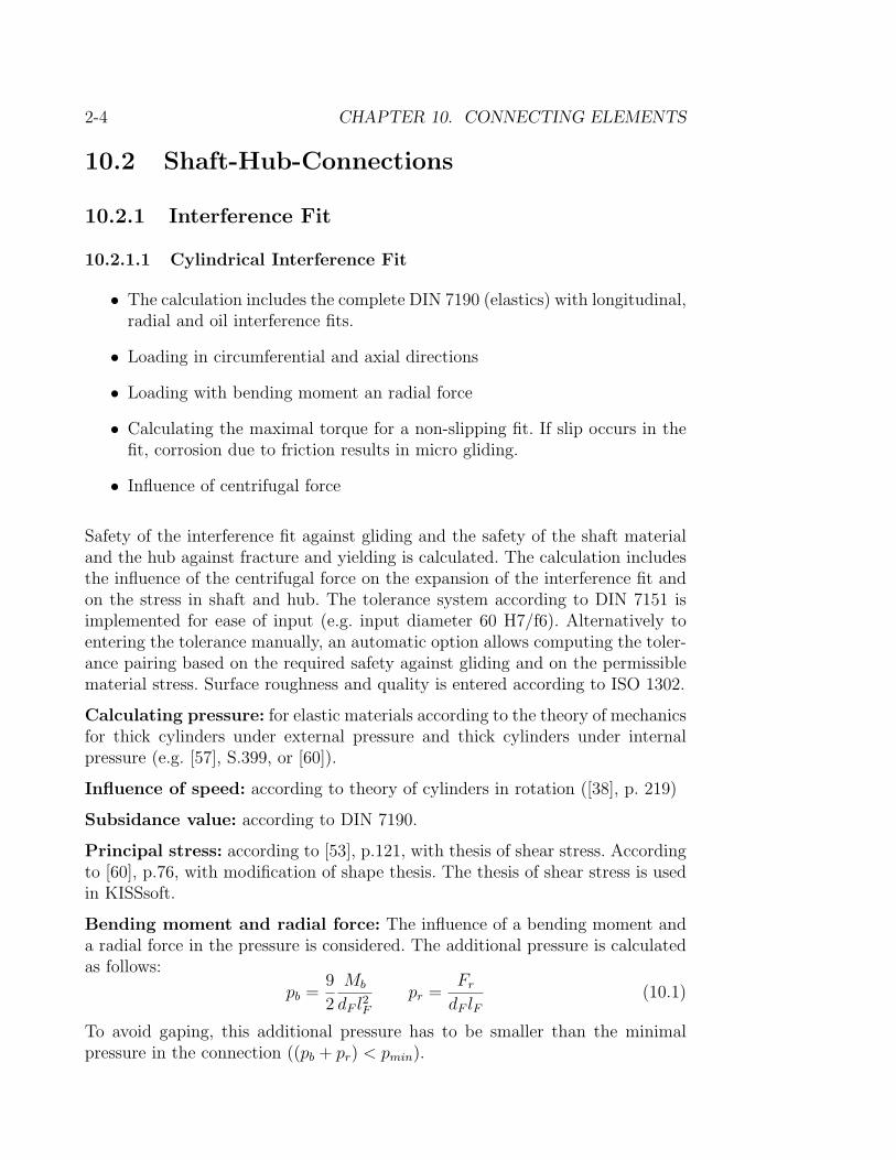
2-4 CHAPTER 10. CONNECTING ELEMENTS
10.2 Shaft-Hub-Connections
10.2.1 Interference Fit
10.2.1.1 Cylindrical Interference Fit
• The calculation includes the complete DIN 7190 (elastics) with longitudinal,radial and oil interference fits.
• Loading in circumferential and axial directions
• Loading with bending moment an radial force
• Calculating the maximal torque for a non-slipping fit. If slip occurs in thefit, corrosion due to friction results in micro gliding.
• Influence of centrifugal force
Safety of the interference fit against gliding and the safety of the shaft materialand the hub against fracture and yielding is calculated. The calculation includesthe influence of the centrifugal force on the expansion of the interference fit andon the stress in shaft and hub. The tolerance system according to DIN 7151 isimplemented for ease of input (e.g. input diameter 60 H7/f6). Alternatively toentering the tolerance manually, an automatic option allows computing the toler-ance pairing based on the required safety against gliding and on the permissiblematerial stress. Surface roughness and quality is entered according to ISO 1302.
Calculating pressure: for elastic materials according to the theory of mechanicsfor thick cylinders under external pressure and thick cylinders under internalpressure (e.g. [57], S.399, or [60]).
Influence of speed: according to theory of cylinders in rotation ([38], p. 219)
Subsidance value: according to DIN 7190.
Principal stress: according to [53], p.121, with thesis of shear stress. Accordingto [60], p.76, with modification of shape thesis. The thesis of shear stress is usedin KISSsoft.
Bending moment and radial force: The influence of a bending moment anda radial force in the pressure is considered. The additional pressure is calculatedas follows:
pb =9
2
Mb
dF l2Fpr =
Fr
dF lF(10.1)
To avoid gaping, this additional pressure has to be smaller than the minimalpressure in the connection ((pb + pr) < pmin).

10.2. SHAFT-HUB-CONNECTIONS 2-5
Further Values:
Dismounting pressure according to [60], p. 363Transmission without slip according to [53], equitations 2.93-2.110
Sizing: The maximal transmissible torque, the transmissible axial force, the re-quired length and the diameter can be sized by KISSsoft.
Possible tolerance inputs
• Tolerance according to ISO/DIN
To enter tolerances like 60 H7/f6, follow the following procedure:
– Insert 60 (mm) for joint diameter
– In the field ”Tolerances” insert H7 and f6. The first field refers to thehub and the second field refers to the shaft.
– The program examines independently whether the inserted tolerancesexist and also checks if everything is written correctly!
• Sizing tolerance according to ISO/DIN
KISSsoft offers a very comfortable sizing function for suitable tolerancepairs. Standardised tolerance pairs are stored in (M01-001.DAT). The sizingis started with the sizing button next to the tolerance field in the mainwindow.
Based on the nominal safety (which can be changed in Settings), all tol-erance pairs which fulfil the requirements (sufficient safety against sliding,safety against fracture and yield point) are determined, and these pairs aredisplayed in a list.
• User-defined tolerances
By activating the - button besides Tolerances, the user can edit themeasures on screen.
Friction factor during longitudinal gliding
Proposal according to Niemann:Inner part Steel Steel Steel Steel Steel SteelOuter part Steel Steel Grey Iron Grey Iron Mg-Al CuZnLubrication Oil dry Oil dry dry drya) b) 0.12 0.14 0.09 0.09 0.07c) 0.17 0.12 0.06
Proposal according to DIN 7190:

2-6 CHAPTER 10. CONNECTING ELEMENTS
Inner part Steel Steel Steel Steel Steel SteelOuter part Steel Steel Grey Iron Grey Iron Mg-Al CuZnLubrication Oil dry Oil dry dry drya) 0.14 0.20 0.10..0.15 0.17..0.25b) 0.12 0.18 0.10 0.16 0.10..0.15 0.17..0.25c) 0.08 0.11 0.06 0.12..0.14 0.10..0.15
Legend:a) Shrink fit (transverse press fit)b) Oil injection pressure fit (transverse press fit)c) Longitudinal press fit
Micro-gliding: If the torque of an interference fit is increased continuously andexceeds the micro-gliding limit in the place where torque is induced, local slipoccurs. As torque decreases continuously within the interference fit, the slip occursonly in a part of the fit, even if the torque still increases. This effect is calledmicro-gliding (shaft moving back and forth in the hub), which can cause frictionrust. Further explanations and details for the calculation is found in ”Welle-Nabe-Verbindungen (Shaft-Hub-Connections)”, F.G. Kollmann, Konstruktionsbucher(Construction books) [53].Note for calculation after Kollmann:Limiting torque for micro gliding after equation 2.110; with k after 2.107 andtau.r after 2.93.
Assembly: Informations on assembly is found in the reports. The temperaturedifference for the pressing is calculated in such a way that, even in case of maximaloversize (the worst case), still sufficient wing-play is reached. The oversize can bedetermined in Settings. Calculated are the parameters of assembly for ambienttemperature and for a cooled shaft (approximately -150 degree Celsius).
For this there is a tutorial ´Cylindrical Interference Fit´, in which the sizing ofcylindrical interference fit specially is described.
10.2.1.2 Taper Interference Fit
Calculating the service safety of a taper interference fit. Defining the mountingconditions. Method according to Kollman [53].
Angle of taper: The angle of taper is defined as the angle between the flankof the cone and its axis. The opening angle of the cone is two times the angle oftaper.
Calculating taper interference fits:

10.2. SHAFT-HUB-CONNECTIONS 2-7
• All known investigations focus on outer and inner parts consisting of ma-terials with the same E-module and inner parts without holes in the cone.
• Taper interference fits must have a stop at the upper end.
• Taper interference fits are normally joined axially with a screw, only inspecial cases by pressing them on. Proper joint is to be checked by measuringthe displacement of the cone. Measuring the torque only is not as accuratedue to variation of the coefficient of friction in the cone and thread.
Possible sizings: maximal transmittable torque, permissible cone angle and thelength of fit can be sized in KISSsoft.
Adhesive coefficient for axial sliding: friction coefficients (for axial sliding)according to Galle (see Kollmann [53], table 2.20):
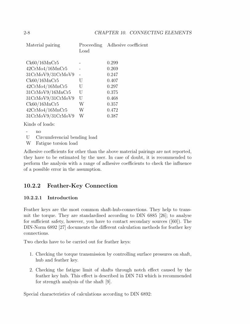
2-8 CHAPTER 10. CONNECTING ELEMENTS
Material pairing Proceeding Adhesive coefficientLoad
Ck60/16MnCr5 - 0.29942CrMo4/16MnCr5 - 0.26931CrMoV9/31CrMoV9 - 0.247Ck60/16MnCr5 U 0.40742CrMo4/16MnCr5 U 0.29731CrMoV9/16MnCr5 U 0.37531CrMoV9/31CrMoV9 U 0.468Ck60/16MnCr5 W 0.35742CrMo4/16MnCr5 W 0.47231CrMoV9/31CrMoV9 W 0.387
Kinds of loads:
- noU Circumferencial bending loadW Fatigue torsion load
Adhesive coefficients for other than the above material pairings are not reported,they have to be estimated by the user. In case of doubt, it is recommended toperform the analysis with a range of adhesive coefficients to check the influenceof a possible error in the assumption.
10.2.2 Feather-Key Connection
10.2.2.1 Introduction
Feather keys are the most common shaft-hub-connections. They help to trans-mit the torque. They are standardised according to DIN 6885 [26]; to analysefor sufficient safety, however, you have to contact secondary sources ([60]). TheDIN-Norm 6892 [27] documents the different calculation methods for feather keyconnections.
Two checks have to be carried out for feather keys:
1. Checking the torque transmission by controlling surface pressures on shaft,hub and feather key.
2. Checking the fatigue limit of shafts through notch effect caused by thefeather key hub. This effect is described in DIN 743 which is recommendedfor strength analysis of the shaft [9].
Special characteristics of calculations according to DIN 6892:

10.2. SHAFT-HUB-CONNECTIONS 2-9
• Feather key connections are mostly combined with light interference fits.The decreasing torque on the feather key is therefore taken into accountwhen calculating.
• The nominal torque as well as the pitch torque occurring in operation aredocumented. Calculating the fatigue strength also considers the amount ofload changes by which the feather key is worn.
• The kind of load application is very important for the service safety offeather keys. This effect is considered by a very distinguished load distri-bution coefficient.
• The values for permissible pressure are determined by the yield point; thesedata derive from the standards for common and uncommon materials. Thesurface treatment is considered by a hardness influence coefficient.
The calculation method B according to DIN 6892 prescribes a distinguished cal-culation to prove the service safety of feather key connections. Method C is toomuch simplified to achieve the safety standards.
10.2.2.2 Main Window
Loads on feather keys are calculated according to
• DIN 6885.1 (ISO/R 773, VSM 15161)
• DIN 6885.2
• DIN 6885.3
• User defined
for shaft and hub (surface pressure) and for feather keys (shearing), including themargin of safety. (Calculation method: DIN 6892 B/C [27]).
The calculation takes into account the tolerances of the keys’ radii and the direc-tion of force. The number of feather keys, the load factor and the service factorcan also be entered.
Explanations to picture 10.1:→ Application of torqueo Beginning of feather keyFu Centre of force application point on hub
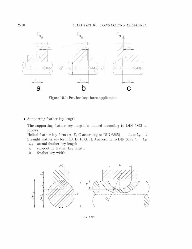
2-10 CHAPTER 10. CONNECTING ELEMENTS
Figure 10.1: Feather key: force application
• Supporting feather key length
The supporting feather key length is defined according to DIN 6892 asfollows:Helical feather key form (A, E, C according to DIN 6885) ltr = leff − bStraight feather key form (B, D, F, G, H, J according to DIN 6885)ltr = leffleff actual feather key lengthltr supporting feather key lengthb feather key width

10.2. SHAFT-HUB-CONNECTIONS 2-11
• Frictional torque
Feather key connections are mostly combined with a light interference fit.The calculation considers therefore the decrease of torque on the featherkey because of the interference fit. This effect has only an influence whencalculating according to DIN 6892.
• Frequency of load peak
To determine the safety regarding the maximal torque, the approximateamount of load peaks is needed. This has only an influence when calculatingaccording to DIN 6892.
10.2.2.3 Additional Inputs for DIN 6892 Method B
If you choose method DIN 6892 B, you can enter the following data in the sub-window:
• Chamfer on shaft
• Chamfer on hub
• Small outer diameter of hub D1
• Large outer diameter of hub D2
• Width c in relation to outer diameter D2
• Distance a0 (see picture 10.1)
• Torque-course: indicating whether changing or permanent torque.In case of changing torque, when the frictional torque is larger than thetorque applying in reverse, you can calculate with mode No torque.
• Frequency of loaddirection changeIn case of changing torque, the number of torque changes during the holeservice life has to be indicated.
10.2.2.4 Service Factor/Application Factor
The application factor is defined in the same way as in the spur gear calculation:
Suggestions for the application factor from other literatures:See tables 10.6 and 10.8.

2-12 CHAPTER 10. CONNECTING ELEMENTS
Procedure Procedure of driven machineof the driving conti- light moderate heavymachine nuous impacts impacts impactscontinuous 1.00 1.25 1.50 1.75light impacts 1.10 1.35 1.60 1.85moderate impacts 1.25 1.50 1.75 2.00heavy impacts 1.50 1.75 2.00 2.25
Table 10.4: Application factor for calculation according to DIN 6892; furtherdetails in DIN 3990, DIN 3991, ISO 6336.
Type of Characteristic Kind of Servicemachine working method impacts factorturbine, fan constant rota- light 1,0 . . . 1,1
ting movementsinternal-combustion reciprocating moderate 1,2 . . . 1,5engine movementspress, saw frame reciprocating, heavy 1,6 . . . 2,0
impacting movementshammer, stone striking very heavy 2 . . . 3crusher movements
Table 10.6: Application factor according to Roloff/Matek [58]
10.2.2.5 Load Factor
Load factor according to DIN 6892[15]
φ = 1 one springφ = 0.75 two springsMore than two springs are hardly ever used
The number of springs determines the amount of the load factor.
10.2.2.6 Own Inputs
In the option Own inputs, you can enter your own data for feather keys.

10.2. SHAFT-HUB-CONNECTIONS 2-13
Surfaces Surfaces Surfacespressed gliding glidinghead-on head-on head-on
without load under loadConstantload 1.0 2.0 6.0Pulsating loadmoderate impacts 1.5 3.0 9.0Alternating loadmoderate impacts 3.0 6.0 18.0Pulsating loadheavy impacts 2.0 4.0 12.0Alternating loadheavy impacts 6.0 8.0 36.0
Table 10.8: Application factor considering the load behaviour according to Pro-fessor Spinnler, [66].
NOTE:The mean value has to be entered for the chamfer and the two groove depths.
10.2.2.7 Permissible Pressure
The permissible values are calculated by the yield point (breaking point respec-tively).
10.2.2.8 Sizing
The sizing is calculated in such a way as to attain the desired nominal safetymargin. To view the results in the lower portion of the main window, the analysishast to be executed after the sizing.
Possible Sizings:
• transmittable torque
• required length of shaft and hub
For this there is a tutorial ´Feather key´, in which the validation of feather keysspecially is described.

2-14 CHAPTER 10. CONNECTING ELEMENTS
10.2.3 Multi-Spline
Multi-splines are often used for positive, axially adjustable shaft-hub connectionsMain application field of multi-splines: motor gear boxes, machine design. Theloading of shaft and hub (surface pressure) of multi-splines is calculated accordingto Niemann.
Multi-splines according to
• DIN 14, (light, for vehicles)
• DIN 14, (medium, for vehicles)
• DIN 5464, (heavy, for vehicles)
• DIN 5471, (for machine design)
• DIN 5472, (for machine desing)
• Own inputs
Additional norms can be added.
The load factor and the service factor can be changed. Loads on shaft and hub(surface pressure) are calculated (including determining the margins of safety)according to established literature ([60]). The calculation according to Niemannfollows the DIN 6892 (feather key calculation). The value for the load factor canbe found in the table 10.4. The special input value for the definition of the factorsare shown in the feather key calculation (see picture 10.1).
Own inputs: In option Own inputs, you can enter your own inputs for multisplines.
10.2.3.1 Service Factor/Application Factor
See in the feather key calculation table 10.4.

10.2. SHAFT-HUB-CONNECTIONS 2-15
10.2.3.2 Permissible Pressure
The permissible values are calculated by the yield point (breaking point respec-tively).
10.2.3.3 Sizing
The sizing is calculated in such a way as to attain the desired nominal safetymargin. To view the results in the lower portion of the main window, the analysishast to be executed after the sizing.
Possible Sizings:
• transmittable torque
• required length of shaft and hub

2-16 CHAPTER 10. CONNECTING ELEMENTS
10.2.4 Splines
Splines are spur gear toothings with shortened tooth height and a large appli-cation angle (normally 30◦). KISSsoft calculates the splines in two different cal-culation modules. Geometry, tolerances and strength are computed in moduleZ09 (see chapter 24), strength (without geometry/tolerances) in the shaft-hub-connections module.
For groove toothings according to
• DIN 5480
• DIN 5481
• Own input (tip circle diameter shaft/hub, module, tooth number)
the load on shaft and hub (surface pressure) is calculated. Further norms canbe added. The data is defined in the database, also special company standardsmay be used. The fabrication mass and tolerance can be calculated with moduleZ09 of the gear wheel calculation software. Load factor and safety factor can bechanged. The loading of shaft and hub (surface pressure), including determiningthe margins of safety, is calculated according to established literature (Niemann,Maschinenelemente I, 2001)([60]).
The standard data base contains the following values:

10.2. SHAFT-HUB-CONNECTIONS 2-17
daW Tip circle diameter of shaftdaN Tip circle diameter of hubm Modulez Tooth numberx ∗m Addendum modification
Own inputs: In option Own inputs, you can enter your own inputs for Splines.Essentially, the tip circle diameter of the shaft has to be larger than the tip circlediameter of the hub.
10.2.4.1 Calculation according to Niemann
The calculation according to Niemann follows the DIN 6892 (feather key calcula-tion). The value for the load factor can be found in the table 10.4 of the featherkey calculation. The special input value for the definition of the factors are shownin the feather key calculation (see picture 10.1).
10.2.4.2 Permissible Pressure
The permissible values are calculated by the yield point (breaking point respec-tively).
10.2.4.3 Sizing
The sizing is calculated in such a way as to attain the desired nominal safetymargin. To view the results in the lower portion of the main window, the analysishast to be executed after the sizing.
Possible Sizings:
• transmittable torque
• required wide on the shaft
10.2.4.4 Geometry Analysis
Basically according to DIN 5480, part 1.
Tip height hap = 0, 45m (10.2)
Root height hfp =da1 − df1
2− hap (10.3)
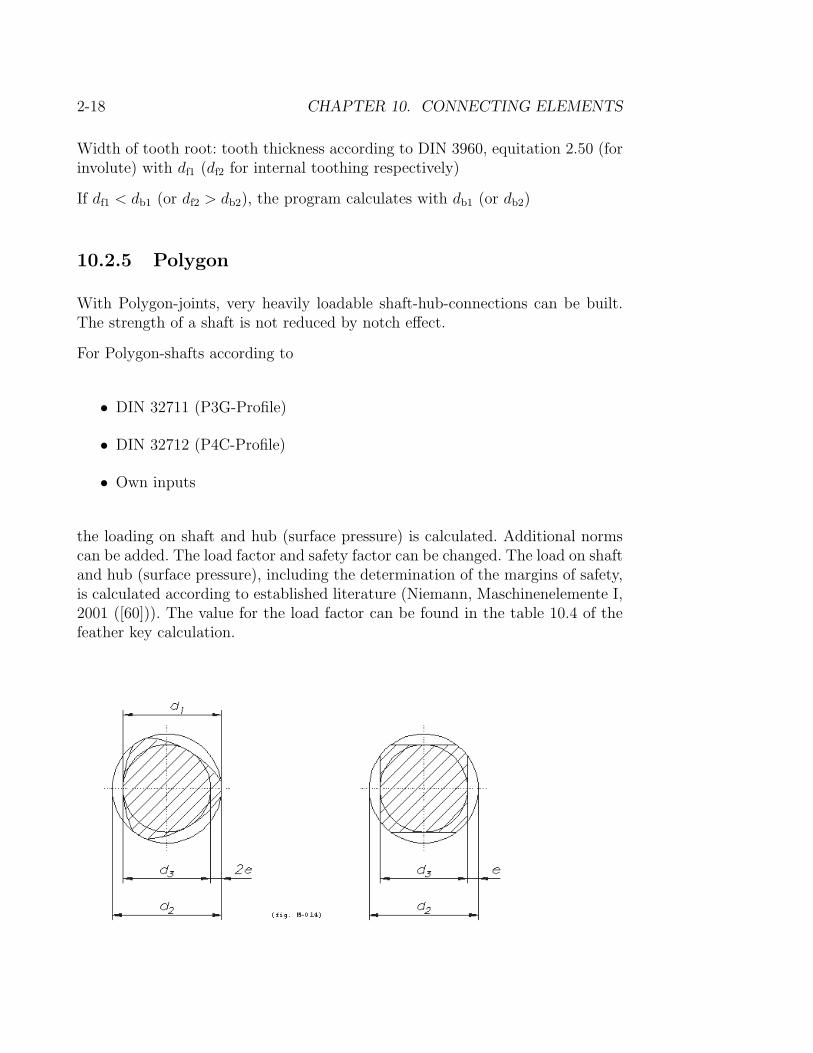
2-18 CHAPTER 10. CONNECTING ELEMENTS
Width of tooth root: tooth thickness according to DIN 3960, equitation 2.50 (forinvolute) with df1 (df2 for internal toothing respectively)
If df1 < db1 (or df2 > db2), the program calculates with db1 (or db2)
10.2.5 Polygon
With Polygon-joints, very heavily loadable shaft-hub-connections can be built.The strength of a shaft is not reduced by notch effect.
For Polygon-shafts according to
• DIN 32711 (P3G-Profile)
• DIN 32712 (P4C-Profile)
• Own inputs
the loading on shaft and hub (surface pressure) is calculated. Additional normscan be added. The load factor and safety factor can be changed. The load on shaftand hub (surface pressure), including the determination of the margins of safety,is calculated according to established literature (Niemann, Maschinenelemente I,2001 ([60])). The value for the load factor can be found in the table 10.4 of thefeather key calculation.

10.2. SHAFT-HUB-CONNECTIONS 2-19
Figure 10.2: Woodruff key with circular and normal forces for calculation accord-ing to Niemann
10.2.5.1 Permissible Pressure
The permissible values are calculated by the yield point (breaking point respec-tively).
10.2.5.2 Sizing
The sizing is calculated in such a way as to attain the desired nominal safetymargin. To view the results in the lower portion of the main window, the analysishast to be executed after the sizing.
Possible Sizings:
• transmittable torque
• required length of shaft and hub
10.2.6 Woodruff Key
A calculation of the load on shaft and hub (surface pressure) is carried out forWoodruff keys according to

2-20 CHAPTER 10. CONNECTING ELEMENTS
• DIN 6888, Row A (deep keyway in the hub)
• DIN 6888, Row B (shallow keyway in the hub)
• Own inputs
Additional norms can be added. The load on shaft and hub (surface pressure),including the determination of the margins of safety, is calculated according toestablished literature (Niemann, Maschinenelemente I, 2001 ([60])). The calcula-tion according to Niemann follows the DIN 6892 (feather key calculation). Thevalue for the load factor can be found in the table 10.4 of the feather key calcu-lation. The special input value for the definition of the factors are shown in thefeather key calculation (see picture 10.1).
Own inputs: In option Own inputs, you can enter your own inputs for Woodruffkeys.
10.2.6.1 Permissible Pressure
The permissible values are calculated by the yield point (breaking point respec-tively).
10.2.6.2 Sizing
The sizing is calculated in such a way as to attain the desired nominal safetymargin. To view the results in the lower portion of the main window, the analysishast to be executed after the sizing.
Possible Sizings:
• transmittable torque
10.3 Dowels
The bolt/pin connections are divided into four types of calculation according tothe case of application:
• Cross pin under torqueWith cross pin connections where large forces are in play the contact pres-sure of the shaft, the hub and shearing of the pin must be checked.

10.3. DOWELS 2-21
• Longitudinal bolt under torqueContact pressure in the shaft and the hub and the shering of the pin ischecked.
• Guide pin under bending forcesThe pin is subjected to bending stress by means of a moment and to shearstress by means of transverse forces. Shearing and bending stress of boltand contact pressure is calculated.
• Bolt under shearing action (in double shear)The pin is subject to bending and shear stress and to contact pressure inthis design. Different calculation methods are used depending on the fit ofthe bolt in the fork/rod. By experience the limiting factor in non slidingsurfaces is the bending stress and in sliding surfaces it is contact pressure.
Calculation of stress for bolts, shaft and hub (or part) and of safety factor isperformed according to standard engineering books (Niemann, Machine ElementsI, Edition 3, 2001[60]).
10.3.1 Determining factors
Certain determining factors are required in calculating individual connectionsdepending on the type of stress and of construction etc.:
• Application factor
• Dynamic factor:fixed load: Cd = 1; pulsating load: Cd = 0.7; alternating load: Cd = 0.5;
• Reduction factors for full/groove pinFull pin: Ck = 1; groove pin (bending, shear): Ck = 0.7; groove pin,contact pressure: Ckp = 0.8;
Since the permissible stress values in the literature are very low, other materialvalues have been added to obtain the values in the table.
10.3.2 Specific module settings
The above factors and safety factors of the individual calculations can be seenand modified in this window.
2-22 CHAPTER 10. CONNECTING ELEMENTS
10.3.3 Sizing
In addition to diameter and stress, approximate values based on nominal safetylimits can also be processed with the design buttons.
10.4 Bolted joints
see chapter 11
10.5 Glued and Soldered Joints
Calculation basis: [60]. For connections under shearing force, two different loadcases are provided:
• Shearing force: transmitting shearing force between two planes
• Torque: shaft-hub-connections under torque
The connection can be loaded statically or dynamically (normally dynamically).
Reference values for static strength of soldered joints are taken from [60], table8/8 (mean values for shearing and breaking strength), reference values for gluedjoints are taken from table 8/9. For soldered joints, the permissible dynamic loadscan be up to 50% of the static strength (soldered joints reduce the part strengthto ca 80%). The permissible dynamic load for glued joints is 30% of the staticstrength.
For glued joints, you can choose between the following materials:
• Hardened at room temperature
• Hardened at higher temperature
The program uses for the shearing strength value the mean of minimal and max-imal value in the data base. The maximum value achievable with optimal proce-dures as defined in Niemann is not used.
For soldered joints, you can choose between the following materials:
• Soft solder LSn40, LSn60, short time load
• Soft solder LSn40, continuous load

10.5. GLUED AND SOLDERED JOINTS 2-23
• Brass solder: steel non iron heavy metals
• German silver solder-copper: steel
• Silver solder: steel non iron heavy metals
Analysis of soldered joints with aluminum light alloys is not sensible, since thestrength of the base material is ususally lower than that of the connection. Theprogram uses for the shearing strength value the mean of minimal and maximalvalue in the data base.
10.5.1 Basic Materials
These materials are only used when the width is sized according to the strengthof the basic material.
Ck 45 N, Ck 60, CrNiMo, CrNi 4, CrNiMo, CrMo, St 37.3, St 52.3, St 60.2,Ganevasit, PA 12, PA 66, POM, laminated wood
The user has to decide by himself which material is sensible for the connection.
10.5.2 Sizing of Width for Basic Material
Sizing glued width and glued length for the strength of the material. The yieldpoint of the joint is sized in such a way as to correspond to the yield point of thebasic material (dynamic load of shaft).
10.5.3 Sizing of Width for Load
The yield point of the joint is designed in such a way as to transmit the actingforces considering the entered nominal safeties.
10.5.4 Flat links
Calculating glued or soldered joints of plates. Axial forces have to be entered aswell as glued length and plate thickness.
10.5.5 Shaft Connections
Calculating glued or soldered joints of Shaft-hub-connections. Transmittable forceas well as glued length and joint diameter have to be entered.

2-24 CHAPTER 10. CONNECTING ELEMENTS
10.6 Welded Joints
Calculation basis: DIN 18800, part 1, November 1990 edition, chapter 8.4 ”Con-nections with electrical welding”
10.6.1 Seam Length
See table 20 in DIN 18800
10.6.2 Part Safety Coefficient
Normally according to DIN 18800, chapter 7.3
10.6.3 Boundary Safety Coefficient
Weld seam type Seam quality Kind of St37-2 St52-3stress and similar and similar
1 - 4 all seamqualities pressure 1.0 1.0seam qualityproved tension 1.0 1.0seam qualitynotproved tension 0.95 0.85
5 - 15 all seam pressure,qualities tension 0.95 0.85
1 - 15 all seamqualities thrust 0.95 0.85

Chapter 11
Bolted Joints Calculation
11.1 Calculation-Basis and Abilities
11.1.1 General Remarks
A connection with screws is a connection which can be released, consisting oftwo or more parts with one or several threads. The screws have to be chosen insuch a way that the connected parts fulfil their purpose and also withstand theoccurring static and dynamic service forces.
The calculation of a screw connection aims to dimension the screws consideringthe following factors:
• Strength class of the screw
• Decreasing mounting-pretension force in the parting lines or parts of theparting lines by the service force
• Decreasing mounting-pretension force because of subsidence
• Scatter of the mounting-pretension force during tightening
• Fatigue life at alternating load
• Pressure load of the restrained parts by the screw head and/or nut
• Allowable surface pressure
• Change of the strength of the screw, nut and intermediate layers and theforces and tensions due to temperature changes
2-25
2-26 CHAPTER 11. BOLTED JOINTS CALCULATION
Rough RemarksIn VDI 2230 the ’mounting-pretension force’ plays a fundamental role. This iswith regard to the break-off pretension on assembly. Screws are usually mountedwith a tightening torque which can be looked up in tables, corresponding tomounting-pretension force of 90% of the elastic limit. The term ’mounting-pretension force’ is used in two contexts:
1. In the definition of mounting-pretension force necessary for connections sothat the transmission of shear forces is assured, and no openings appearon the join. The maximum and minimum mounting-pretension force areused for this in VDI 2230, which are called the maximum and minimummounting-pretension force in KISSsoft.
2. In the definition of the permissible mounting-pretension force for boltstrength which (depending upon the edition of the VDI guideline) are desig-nated FM or permissible mounting-pretension force FMzul. In KISSsoft thispretention force is designated maximum reached pretension force, and iscalculated as 90% of the elastic limit or is directly entered.
For a screw or bolt connection, the parts under tension are pressed together bythe stressed parts. In doing so, the pretension force FV in the screw and thetensioned parts are equal but in opposite directions. The required clamping forceFKerf is the clamping force between the tensioned parts which must remain aftercomposition of effects from external loads and temperatures.
The minimum pretensioning force necessary to transmit the operating forces cor-responds to the minimum required mounting pretension force FMmin. There is adistinct amount of uncertainty about the level of pretension produced becauseof the coefficient of friction and the distribution of the tightening torque. Thisregion of uncertainty is covered by the tightening factor. In order to be sure thatnecessary pretension force is reached, it is required that the tightening torque toraise such that the maximum required pretension FMmax is reached.
A minimum mounting-pretension force FMmax is required for the safe operation ofthe connection. The mounting-pretension force in screw connections is influencedby many factors, such as:
• Friction conditions of moving surfaces
• The geometrical form of the connection
• The tightening method
• The tightening tool

11.1. CALCULATION-BASIS AND ABILITIES 2-27
The mounting pretension force FM of the screw is a designing-criterion for thediameter. The resulting sizing formula is therefore:
FMmax = αAFMmin (11.1)
= αA (FKerf + (1− φ)FA + FZ + ∆FVth) (11.2)
The tightening factor αA takes into account that, depentent on the chosen mount-ing procedure, the mounting pretension force FM can scatter. FZ represents theloss of the pretension force which can occur due to an embedding process. Thefact that the mounting pretension force FM during service is reduced by (1−φ)FA
of the force acting in axial direction is taken into account, as well as that thermalexpansion results in a reduction of δFVth
. Finally, a minimal clamping force ofabout FKerf is necessary to guarantee the sealing function and to avoid one-sidedgaps at the interface or self-loosening of the connection.
Now either the maximum required mounting pretension force and the maximumreached mounting pretension force, or the minimum required mounting pretensionforce and the minimum reached mounting pretension forces can be compared.
FMmax
!< FM FMmin
!< FM/αA (11.3)
11.1.2 Calculating with KISSsoft
The KISSsoft modules M04, M04a and M04b allow calculations according to thelinear approach of the VDI norm 2230, part 1, February 2003 or corrected reprint,October 1990, and this norm includes all details, in particular it is possible touse it for cases with eccentric loadings and restraints.
For metric screws with a ISO thread (normal or fine) as well as for special threads,a complete strength re-calculation is carried out. This calculation includesthe following points:
• Calculating the required pretension force FV.
• Calculating the pretension force FMkat if the screw is tightened up to 90%of the yield point. (Exploiting the yield point to 90% is proposed in theVDI 2230; this value can be altered in Settings.)
• Calculating principal stress in the screw shank.
• Calculating occurring and maximal permissible surface pressure.
• Calculating dynamic load and the tightening moment.
2-28 CHAPTER 11. BOLTED JOINTS CALCULATION
To calculate pretension force of a screw and the resulting loads, three (four) inputvalues are required:
• Min pretension force FMmin (Calculation with the tightening factor = 1.0).
• Max pretension force FMmax (Calculation with the effective tightening fac-tor).
• Pretension force FMkat exploiting 90% of the yield point (this pretensionforce corresponds to the value which is given in the literature for the tight-ening moment).
• Pretension FM/αA (Pretension FM divided by tightening factor, to be acti-vated using Settings ⇒ Modul-spezifc, see 11.8)
Screws can be pre-dimensioned ; based on the service force, a reasonable sugges-tion for the reference diameter will be issued (according to Table 7 of the VDI2230). After having defined the clamping length, the program chooses the threadlength from a standard series.
The data for the screw geometries, nuts, washers and materials are filed in tableswhich were taken from the following norms: ISO 898, ISO 273, ISO 272 (DIN934), ISO 940 (DIN 125A,DIN 126), ISO 4014 (DIN 931), ISO 4016 (DIN 601),ISO 4017 (DIN 933), ISO 4018 (DIN 558), ISO 4762 (DIN 912), ISO 949 (DIN84, DIN 960, DIN 961), ISO 262 (DIN 13), gas threads, inch threads, ISO 898.These databases can be extended and adjusted to the needs of the user (cf. chap.Database). User-defined screws of any complexities can also be included (cf. chap.Own Screws). Moreover, hollow screws can also be calculated.
11.1.3 Special Features of KISSsoft
In the VDI 2230 are the values for the pretension force FMkat which exploits 90%of the yield point and the tightening torque taken from the Tables 1 to 4. Thesevalues are round-off figures (round-off errors ≤ 1%). KISSsoft however, calculatesthese values, based on the equations used for the tabulated figures. The resultsare therefore more general than these filed values and the former may differ fromthe latter.
An additional calculation of the minimum reached pretension force can be acti-vated under Settings ⇒ Module Specific. This force corresponds to FM/αA
and is reached with large friction values or small tightening torques. This pre-tension force always has to be larger than FMmin to guarantee that operation issafe.

11.2. IMPORTANT INPUTS 2-29
Calculating the Required Clamping ForceThe required clamping force is calculated according to the VDI 2230 (2003):
FKerf = max(FKerfA + FKerfD, FKerfN) (11.4)
FKerf Required clamping forceFKerfN Necessary clamping force (e.g. for friction contact closing)FKerfD Necessary clamping force for sealing function (with internal pressure)FKerfA Necessary clamping force to avoid gaps in case of eccentric load
11.1.4 Extent of Additional KISSsoft Modules
Option M04a Eccentric strain and loadScrew configurations with axial andshearing force and bending moment loadsshedding strength
Option M04b Screw calculation at high and low temperatures
11.2 Important Inputs
11.2.1 Reference Diameter and Screw Type
The screw geometry, which is based on reference diameter, thread type (normalor fine thread) and screw type, is taken from the database.
If in the window Details of screw a screw is chosen from the list Type thefollowing characteristic quantities are adopted:
• Screw length l
• Inner diameter of the screw head support da
• Outer diameter of the screw head support dw
• Addendum k
• Shank diameter d1 and length l1
• Reduced diameter d2 and length of the reduced diameter l2
• Thread diameter and length
• Width across flats

2-30 CHAPTER 11. BOLTED JOINTS CALCULATION
The data are stored in self-explaining files and are easy to expand. The name ofthe file can be found in the database (cf. chap. Database).
List of all screw types provided in the database:
EN ISO 4762/ Cylindric screw with hexagonal recessDIN 912 Standard thread M1.4 – M100
Fine thread M1.4 – M100EN ISO 4014/ Hexagonal cap screw with shank (former DIN 931
T1)DIN EN 24014 Standard thread M1.6 – M160EN ISO 4017/ Hexagonal cap screw with thread to the screw head
(former DIN 933)DIN EN 24017 Standard thread M1.6 – M48EN ISO 1207/ Cylinder screw with slotDIN 84 Standard thread M1.0 – M20EN ISO 8765 Hexagonal cap screw with shaft
Fine thread M8.0 – M64EN ISO 8676 Hexagonal cap screw without shank
Fine thread M8.0 – M64ISO 1662 Hexagonal cap screw with flange, light serie, form
FStandard thread M5.0 – M16
ISO 1662 Hexagonal cap screw with flange, light serie, formUStandard thread M5.0 – M16
ISO 1665 Hexagonal cap screw with flange, strong serie, formFStandard thread M5.0 – M20
ISO 1665 Hexagonal cap screw with flange, strong serie, formUStandard thread M5.0 – M20
11.2.2 Defining Individual Screw Geometry
A screw consists of several single elements which can be substituted as cylindricalbodies of different lengths and diameters (cf. figure 11.1).

11.2. IMPORTANT INPUTS 2-31
Figure 11.1: Screw geometry
When an own screw geometry is to be defined, following parameters have to beentered: Screw length, thread length and outer and inner diameter of the screwhead support. Furthermore, an area without a thread between screw head andthread (reduced shank diameter) can be defined. In order to define special screws,up to eight different diameters are possible. Optional data are insignificant. (cf.chapter 11.3 and 11.9
11.2.3 Thread Types
Data for the following thread types are stored in the files:
• Standard threads
• Fine threads
• Gas threads
• Inch threads
The data are stored in self-explaining files and are easy to expand. The name ofthe file can be found in the database (cf chap KISSDB).
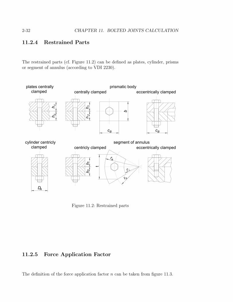
2-32 CHAPTER 11. BOLTED JOINTS CALCULATION
11.2.4 Restrained Parts
The restrained parts (cf. Figure 11.2) can be defined as plates, cylinder, prismsor segment of annulus (according to VDI 2230).
Figure 11.2: Restrained parts
11.2.5 Force Application Factor
The definition of the force application factor n can be taken from figure 11.3.

11.2. IMPORTANT INPUTS 2-33
Figure 11.3: Force application factor n; opper row: pocket hole; lower row: plug-in-link, according to VDI 2230 (edition 1990)
In the VDI–guideline (2003), equitations for force application factor calculationsare listed. Choose a configuration according to picture 11.4. The parting lineshould lie in the grey area. The distances h, ak and lA according to figure 11.5determine the position of the force application and, in this way, the force appli-cation factor.
For screw connections (ESV), the configurations SV1, SV2 and SV4 are available.Take the distance hESV to the parting line as height h.

2-34 CHAPTER 11. BOLTED JOINTS CALCULATION
����� ����� � � ����� ����� �����
Figure 11.4: Configuration to determine the force application factor according toVDI 2230 (2003)
Figure 11.5: Inputs to determine the force application factor according to VDI2230 (2003)

11.2. IMPORTANT INPUTS 2-35
11.2.6 Eccentric Application of Force and Eccentric Re-straint
Figure 11.6: Possible load cases for eccentric restraint
As Figure 11.6 shows, the axis of the centre of gravity 0 − 0 determines thebeginning of the x axis. The distance a must always included as positive value.The distance s is included as positive value if the screw axis S − S and the lineof action of force A − A are both on the same side of the axis of the centre ofgravity 0− 0, and negative if the line of action of force and the screw axis are onopposing sides.
11.2.7 Tightening Factor – Coefficient of Friction
• Tightening factorTable 11.1 lists the reference values for the tightening factor (cf. formula11.1). Some uncertainties – such as estimation errors of friction values, dif-ferent accurate tightening methods, errors of the instruments and handlingthereof and reading errors – can cause a scatter of the mounting pretensionforce. Hence the screw should be oversized, which is represented with thetightening factor αA. An increasing tightening factor αA means, that withthe same minimal pretension force FMmin, the screw has to be dimensionedfor larger – with resulting bigger scatter – maximal mounting pretensionforce FMmax.
• Coefficient of friction
KISSsoft can issue an interval for friction coefficients. The minimalvalue is used to calculate with FM, FMmax, the maximal value to calculate

2-36 CHAPTER 11. BOLTED JOINTS CALCULATION
Tightening Tightening procedure Setting procedurefactor αA
1.0 Yield point controlledtighteningmotor or manual
1.0 Angle of rotation controlled Experimental determina-tion of
tightening pre-tightening moment andangle of rotation
motor or manual1.2 to 1.6 Hydraulic Setting via length
tightening or pressure measurement1.4 to 1.6 Torque controlled Experimental determina-
tiontightening with of nominal tightening valuestorque wrench, on the original screwed part,signalling e.g. via length measurementkey or of the screwprecision torquescrew withdynamic torque measure-ment
1.6 to 1.8 dito Determination of nominaltightening value with guess-ing of thecoefficient of friction (sur-face andlubrication conditions)
1.7 to 2.5 Torque controlled Setting of torque screwtightening with torque with tightening up torque
whichscrew is formed of the nominal
tightening value (for esti-matedcoefficient of friction) andanaddition.
2.5 to 4 Pulse controlled Setting of torque screwtightening with via tightening up torquestroke torque screw – as above
Table 11.1: Standard values for tightening factor αA

11.2. IMPORTANT INPUTS 2-37
Figure 11.7: Coefficient of friction in the thread
with FMmin und FM/αA. You find the friction coefficients in the figures 11.7and 11.9
Figure 11.8: Static friction coefficient at the interface.

2-38 CHAPTER 11. BOLTED JOINTS CALCULATION
Figure 11.9: Coefficient of friction in tip and nut support
Influence of the Tightening Factor and Coefficient of FrictionPicture 11.10 shows the influence of several coefficients of friction and tighteningfactor son on the pretension-force and the tightening torque. The first line repre-sents the reference example. Underneath is one influence value at the time in thereference example changed and the corresponding change of the influence is shownwith arrows. Obviously, the coefficients of friction are involved in a different wayin the calculation: The coefficient of friction underneath the tip influences onlythe tightening torque, whereas the coefficient of friction in the thread influencesthe tightening torque and the standard pretension force FMkat (exploiting theyield point to 90%) as well.

11.2. IMPORTANT INPUTS 2-39
Figure 11.10: Example on influence of the coefficient of friction on the pretensionforces and the tightening torque.
11.2.8 Configurations
How a screwed joint is calculated depends on the geometry of the joint. KISSsoftenables the consideration of eccentric load and restraint, analyses the joint ongaps in the parting line and permits the input of screw configurations with axialand shearing force and bending moment loads.
External forces and momenti, which the screw connection has to transmit, haveto be converted into a axial force FA and a necessary clamping force FK. VDI2230 expects these values to be known. In KISSsoft, they can be entered asexternal forces or momenti when choosing a corresponding configuration (Threadin shearing force or Flange connection).
In a screwed connection, the shearing force is absorbed by the friction betweenscrewed parts. The friction results from friction coefficient and pre-tension force.
11.2.8.1 Shear or axial load of service force
Calculating the necessary clamping forces on a single screw with shear load:
FKerfN =1
µqF
(FQ +
2000 ·MT
d
)(11.5)
FKerf = max(FKerfA + FKerfD, FKerfN) (11.6)

2-40 CHAPTER 11. BOLTED JOINTS CALCULATION
qF Number of parting linesµ Coefficient of friction between screwed partsFQ Shearing forceMT Torqued Frictional diameterFKerf Required clamping forceFKerfN Required clamping force (e.g. against friction)FKerfD Required clamping force for sealing (with internal overpressure)FKerfA Required clamping force to avoid gapping under excentrical load
As already stated in chapters 11.1.3 or formula 11.4, KISSsoft adds anotherclamping force to the required clamping force, which is necessary for the seal-ing function. The service forces acting in axial direction FBo and FBu can beentered additionally.
11.2.8.2 Flange connections
Calculating the forces on single threads in flange connections (with loading torqueand/or shearing force and/or bending moment and/or axial force) according to[MATT], partly accordint to [MATE ex 8.4]:
FKerfN =1
nµ
(2000 ·MT
d+ F
)(11.7)
FKerfD =FD
n(11.8)
FKerf = max (FKerfA + FKerfD, FKerfN) (11.9)
FBo =1
n
(FAmax +
4000 ·MB
d
)(11.10)
FBu =1
n
(FAmin −
4000 ·MB
d
)(11.11)
(11.12)
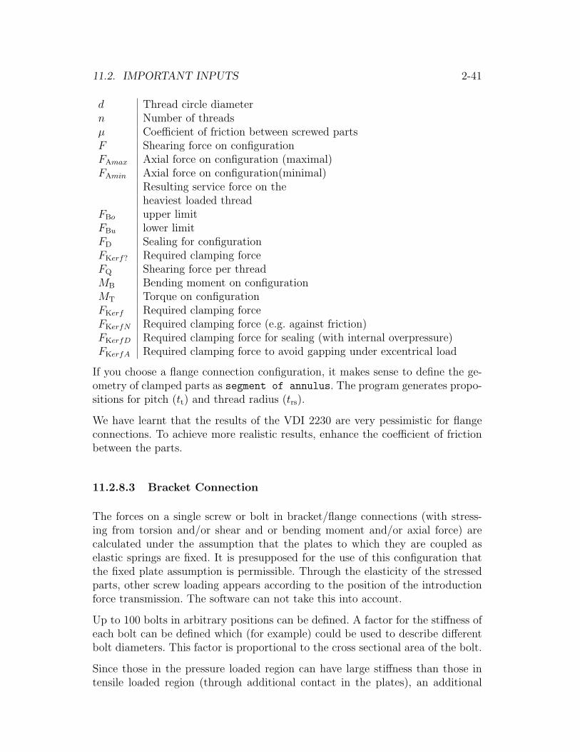
11.2. IMPORTANT INPUTS 2-41
d Thread circle diametern Number of threadsµ Coefficient of friction between screwed partsF Shearing force on configurationFAmax Axial force on configuration (maximal)FAmin Axial force on configuration(minimal)
Resulting service force on theheaviest loaded thread
FBo upper limitFBu lower limitFD Sealing for configurationFKerf? Required clamping forceFQ Shearing force per threadMB Bending moment on configurationMT Torque on configurationFKerf Required clamping forceFKerfN Required clamping force (e.g. against friction)FKerfD Required clamping force for sealing (with internal overpressure)FKerfA Required clamping force to avoid gapping under excentrical load
If you choose a flange connection configuration, it makes sense to define the ge-ometry of clamped parts as segment of annulus. The program generates propo-sitions for pitch (tt) and thread radius (trs).
We have learnt that the results of the VDI 2230 are very pessimistic for flangeconnections. To achieve more realistic results, enhance the coefficient of frictionbetween the parts.
11.2.8.3 Bracket Connection
The forces on a single screw or bolt in bracket/flange connections (with stress-ing from torsion and/or shear and or bending moment and/or axial force) arecalculated under the assumption that the plates to which they are coupled aselastic springs are fixed. It is presupposed for the use of this configuration thatthe fixed plate assumption is permissible. Through the elasticity of the stressedparts, other screw loading appears according to the position of the introductionforce transmission. The software can not take this into account.
Up to 100 bolts in arbitrary positions can be defined. A factor for the stiffness ofeach bolt can be defined which (for example) could be used to describe differentbolt diameters. This factor is proportional to the cross sectional area of the bolt.
Since those in the pressure loaded region can have large stiffness than those intensile loaded region (through additional contact in the plates), an additional

2-42 CHAPTER 11. BOLTED JOINTS CALCULATION
factor for pressure loaded bolts is required. The calculation of the screw forces isdone in one of three 3 ways :
• Without Load The position of the centre of balance is defined under noload, and the required clamping force used for the calculation.
• Minimum Load The centre of balance, the bending axis, as well as theresulting axial force of the bolt are calculated with the minimum load.
• Maximum Load The centre of balance, the bending axis, as well as theresulting axial force of the bolt are calculated with the minimum load.
An option exists to taken into consideration the direction of the shear forces dueto torsion and shear force. In cases where this option is not activated, the amountswill only be summed. The resulting shear force is used in the determination ofthe clamping force required. The highest loaded bolt is chosen for the calculation.
11.2.9 Bore Diameter
Further to the bore diameter, a chamfer on the bore can be defined. This cham-fer is taken into account for analysis of contact pressure and tightening torquebetween the clamped parts and the head/ nut. The inner diameter of the contactarea equals the bore diameter minus two times the chamfer width.
11.2.10 Subsidence Value
The subsidence value is calculated according to the analysis method selected.An additional subsidence value due to e.g. seals can be added. Furthermore, thesubsidence value calculated can be replaced by a value defined by the user, or theloss in pre-tension can be defined directly. When defining the loss of pre-tensiondirectly, the subsidence value does not influence the calculation any more.
11.3 Display Screws
The field Display screw displays a sketch of the screw, which can be printed ortransferred to a CAD. This function is very helpful to analyse the entered datawhen you have made own definitions of screws.
11.4. POSSIBLE PROPOSITIONS 2-43
11.4 Possible Propositions
KISSsoft offers for nominal diameter and screw length:
Variable Influencing/Required VariablesNominal Diameter Strength Class
LoadThread Length Nominal Diameter
Clamping LengthThread Norm
Material properties at service temperature see chap. 11.4
Please note that if you define your own threads NO standard value is offered forthe length of the thread!
Nominal diameter: according to VDI 2230, page 77, table 7, analysis of bolts isvalid only for 8.8, 10.9 and 12.9 qualities.
11.5 Screws at High and Low Temperatures
Threads are normally mounted at ambient temperature. The influence of theservice temperature on the state of the screw and therefore and on the safetyof the connection, is big. When screw joints of light metals are clamped withsteal screws, a service temperature of 70 degree higher than ambient temperatureaffects the connection prominently.
The extension of the KISSsoft screw calculation allows, with the application ofthe calculation instruction according to [VDI 2230], calculating screw joints forservice temperatures ranging from −200 to +1000◦C. Different temperatures canbe defined for screws and restrained parts. Also the temperature dependenceof the Young’s modulus, warmth elongation coefficient, the yield point and theallowable pressing of the material are taken into account.
The screw joint is checked for the mounting conditions at combined temperaturebut also for the stationary and instationary conditions at service temperaturefor all criteria (according to [VDI 2230], restrained force, screw force fatigueresistance and surface pressure.
11.5.1 Technical Explanations
The main effects of the temperature on the service condition of screws are:

2-44 CHAPTER 11. BOLTED JOINTS CALCULATION
• Change of the restrained forces due to heat expansion
• Change of the restrained forces due to relaxation (at high temperatures)
• Brittle fracture (at high and at low temperatures)
Because general data are not sufficiently available for materials ( material of thescrew and the restrained parts), the calculations have limited scope. The changeof the restrained forces due to heat expansion can easily be calculated, as the firstapproximation the warmth elongation number is linear to the temperature (for thetemperature range of −100 to +500◦C). The other effects (relaxation and brittlefailure) can be diminished through approximated measures (see correspondingliterature).
The pretension force derivation due to heat expansion is calculated accordingto H. Wiegand, Schraubenverbingungen (Screw connections), 4th edition 1988,chapter 7.1.3.1 (with temperature-dependent heat expansion number and Young’smodulus). All other calculations are based on the equations from the [VDI 2230]with the corresponding values at service temperature. For the coefficient of ex-pansion, for the calculation of the length expansion of screws and parts, the meanvalue for room and service temperature is taken.
We recommend calculating screwed connections for three cases:
1. At ambient temperature
2. At service temperature
3. At the largest temperature difference (of screw and restrained parts) duringstart and stop of the machine.
(1. and 2. are done simultaneously by KISSsoft)The minimum temperature difference between the parts and the bolts has to beat least 5◦ C, and that between the parts or the bolts and the room temeratureat least 30◦ C.
11.5.2 Inputs
For execution of above mentioned analysis, the following inputs are necessary:
• Ambient temperature (20◦C)
• Temperature of the screw
11.6. TENSION DIAGRAM 2-45
• Temperature of the restrained parts
• Young’s modulus for screws and parts at ambient temperature
• Young’s modulus for the screws and parts at service temperature
• Heat elongation factor for screws and parts at ambient temperature
• Heat elongation factor for the screws and parts at service temperature
• Yield point of the screw at ambient and service temperature
• Permissible fit of the parts at ambient and service temperature
For all input parameters (Young’s modulus, heat elongation number, yield pointat service temperature) KISSsoft offers sensible suggestions which are based onliterature (DIN-norms, literature from Bossard Inc, Zug). For calculating sugges-tions for the permissible fit at service temperature, KISSsoft assumes that the fitchanges proportionally to the changes of the yield point.
The suggestions have to be calculated for critical cases, as the temperature alsodepends on the kind of used material. This dependency is not considered inKISSsoft.
Using Settings ⇒ Modul-spezific (see 11.8) it can be selected whether thematerials data are calculated according to these formulas automatically.
11.5.3 Outputs
All important data (mounting pretension force, stress in thread shaft, surfacepressure, usage, etc.) are issued for both ambient and service temperature.
11.6 Tension Diagram
The tension diagram (see picture 11.11) can be displayed graphically, printed ortransferred to a CAD. Besides the tension diagram for FV , the tension diagramfor the pretension FM/α − Fz is shown. This is to show the influence of thetightening factor.
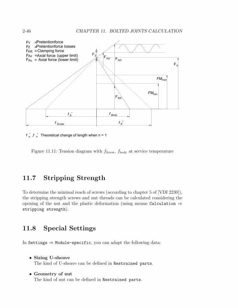
2-46 CHAPTER 11. BOLTED JOINTS CALCULATION
Figure 11.11: Tension diagram with fScrew, fbody at service temperature
11.7 Stripping Strength
To determine the minimal reach of screws (according to chapter 5 of [VDI 2230]),the stripping strength screws and nut threads can be calculated considering theopening of the nut and the plastic deformation (using menue Calculation ⇒stripping strength).
11.8 Special Settings
In Settings ⇒ Module-specific, you can adapt the following data:
• Sizing U-sheaveThe kind of U-sheave can be defined in Restrained parts.
• Geometry of nutThe kind of nut can be defined in Restrained parts.
11.8. SPECIAL SETTINGS 2-47
• Thread productionThe kind of thread production decides about the fatigue strength of a screw.In Threads, these values can be viewed and replaced if necessary.
• Exploitation of yield pointNormal screws are loaded up to 90% of the yield point for the pre-tensionforce calculation. The exploitation should be set to 100% if the screw is tobe tightened yield-point- or swing-angle-controlled.
• Swing-angle controlled tighteningIf a screw is to be tightened swing-angle-controlled, a pretension torque anda swing angle, divided into a number of steps, are issued in the report. Theamount of pretension torque and the number of steps can be entered in thisplace. The swing angle is calculated with FM.
• Calculate on in case of error messagesIf this flag is set, the program calculates on in case of error messages suchas exceeding the yield point or the permissible pressure.
• Service force only at service temperatureNormally, KISSsoft calculates the minimal pretension force basing on therequired clamp force and the loads at ambient and service temperature. Ifthe service force occurs only at service temperature, this flag can be set. Theminimal pretension force is then calculated only for service temperature.
• Calculate pretension force from the permissible loadIf this flag is set, the load case FM/alphaA is calculated additionally. Thepretension force FM/alphaA is the minimal force when a screw is tightenedwith the entered pretension force FM. alphaA is the tightening factor, itdescribes the scatter of the pretension force.
• Not increasing the required clamp force in case of eccentric re-straintKISSsoft increases the necessary clamp force to avoid gaps in case of ec-centrical restraint. You can switch this function off and enter the necessaryclamp force manually. Be careful when using this option, the program ex-pects no gaps in this case.
• Automatically calculating material data dependent on tempera-tureKISSsoft can automatically calculate material data at service temperaturewith approximate formulae. These formulae consider not the entered mate-rial, they use the mean dependence of common steel! If this flag is cleared,the material data at service temperature can be entered manually.
Only experts should change the listed data!

2-48 CHAPTER 11. BOLTED JOINTS CALCULATION
11.9 FAQ
11.9.1 Entering Additional Screws
The KISSsoft data base provides the following screw types:
• Cylindrical screw with socket head bolt EN ISO 4762
• Hexagon head screw with shank (AB) EN ISO 4014
• Hexagon head screw without shank (AB) EN ISO 4017
• Cylinder head stud with slot EN ISO 1207
• Hexagon cap screw with shaft, metric fine thread (AB) EN ISO 8765
• Hexagon cap screw with shaft, metric fine thread (AB) EN ISO 8676
• Hexagon cap screw with flange, light serie, form F EN 1662
• Hexagon cap screw with flange, light serie, form U EN 1662
• Hexagon cap screw with flange, strong serie, form F EN 1662
• Hexagon cap screw with flange, strong serie, form U EN 1662
• Own definition of screw geometry
For all of these types, different values are listed in tables (=Screw line). The nameof the file which contains the data of this screw line is located in the data base(see chapter ’Data Base Tool’).
You can add new screw types (see chapter 11.9.1.2) or change the values of alreadyentered types (see chapter 11.9.1.1).
11.9.1.1 Extending Screw Lines
Example: Entering the data of a M8 screw, 100 mm long in the line for ’Cylin-drical screw with socket head bolt EN ISO 4762’.
First, start the data base tool and open the table screw type M000.KDB,
M040type. Choose the data set Cylindrical screw with socket head bolt
EN ISO 4762. In the field File name, you find the name of the file where thetable containing data of the screw line is located. Open the file in the editor:

11.9. FAQ 2-49
If you want to enter a new screw, proceed accordingly:
• Look for a similiar screw (M8, 80mm).
• You find a line with all data about this screw.

2-50 CHAPTER 11. BOLTED JOINTS CALCULATION
• Copy this line; note the order of the lines!
• Change the data according to table 1 in EN ISO 4762 (length 100 insteadof 80, length l1 72 instead 52).
• Save the file
• Comment your alterations for other users (optional)
11.9.1.2 New Screw Type
To enter a new screw type, you have to know how the tables are built. You haveto know which column contains which value (you find the variable names in thelist in the supplies or in the explanations in the heading of the table).
Proceed accordingly:
• Open in the data base1 a data set similar to the new screw type.
• Copy this data set and save it under the name of the new screw type.
• Press Edit and a window is opened which still contains the ’old’ data.
1How to use the data base tool is explained in the chapters Data Base Tool and TableInterface.

11.9. FAQ 2-51
• Enter your new data. Note the structure of the variable (i.e. depending onthe place, a number gets a certain variable) and the order in the lines.
• Save the file under a new name and close the editor.
• Adopt the new file name in the data base (cross-connections).
• Save the new data set.
)

2-52 CHAPTER 11. BOLTED JOINTS CALCULATION
Chapter 12
Belts
• Calculating 14 different types of v-belts (Z90)
• Calculating 13 different types of toothed belts (Z91)
• Calculating chain drives (Z92)
Rough remarks:V-belt- and toothed belt drives are recalculated and laid out best according tothe manufacturer’s data. The most catalogues contain the comprehensive calcu-lation method. As belts improve because of better materials and flank shapes,manufacturer’s data are the only values which can be relied on.
Addresses of v-belt manufacturers:
• Angst+Pfister AG Thurgauerstr. 66, CH-8052 Zurich
• Ch. de Gaulle Cedex, F-95950 Roissy
• Arntz-Optibelt-KG Postfach 100364, D-3470 Hoxter 1
• Visurgis-Optibelt-France 26, Grand’Rue F-90170 Etueffont
Addresses of manufacturers of toothed belts:
• Angst+Pfister AG Thurgauerstr. 66, CH-8052 Zurich
• Ch. de Gaulle Cedex, F-95950 Roissy
• Breco Antriebstechnik, Postfach 1152, D-4952 Porta Westfalia
• Gates GmbH, Eisenbahnweg 50, Postfach 1428, D-5100 Aachen 1
2-53
2-54 CHAPTER 12. BELTS
12.1 Calculating V-belts
Calculating v-belts with information about standard v-belt lengths and standardefficiency diameter. Determining transmittable power per belt considering speed,efficiency diameter, transmission ratio and belt length. All data are read fromtables provided by the manufacturers. A belt stress calculation module calculatingwith data from belt-bending tests is integrated as well. It computes end of ropeforce and axis load in stand and in operation for optimal settings.
Another possibility is calculating a third roll (tension pulley). The position isdefined in the graphical interface. The pulley can either be positioned inside oroutside.
12.1.1 Standard
The following belt types are available:
• SPZ Narrow v-belt DIN 7753 (Fenner)
• SPA Narrow v-belt DIN 7753 (Fenner)
• SPB Narrow v-belt DIN 7753 (Fenner)
• SPC Narrow v-belt DIN 7753 (Fenner)
• XPZ Narrow v-belt DIN 7753-shaped
• XPA Narrow v-belt DIN 7753-shaped
• XPB Narrow v-belt DIN 7753-shaped
• XPC Narrow v-belt DIN 7753-shaped
• 3V/9J Force belts
• 5V/15J Force belts
• 8V/25J Force belts
• 3V/9N Narrow v-belt USA Standard
• 5V/15N Narrow v-belt USA Standard
• 8V/25N Narrow v-belt USA Standard
• XPA Narrow v-belt DIN 7753/ISO4184 (CONTI-FO-Z)
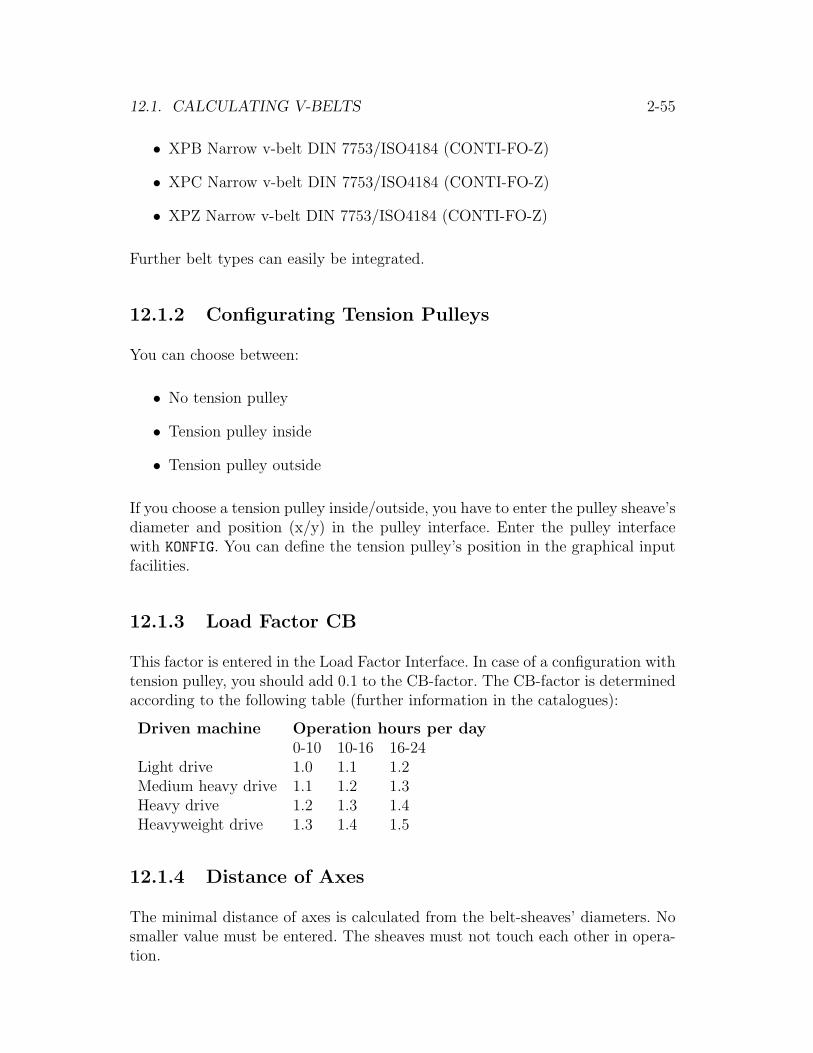
12.1. CALCULATING V-BELTS 2-55
• XPB Narrow v-belt DIN 7753/ISO4184 (CONTI-FO-Z)
• XPC Narrow v-belt DIN 7753/ISO4184 (CONTI-FO-Z)
• XPZ Narrow v-belt DIN 7753/ISO4184 (CONTI-FO-Z)
Further belt types can easily be integrated.
12.1.2 Configurating Tension Pulleys
You can choose between:
• No tension pulley
• Tension pulley inside
• Tension pulley outside
If you choose a tension pulley inside/outside, you have to enter the pulley sheave’sdiameter and position (x/y) in the pulley interface. Enter the pulley interfacewith KONFIG. You can define the tension pulley’s position in the graphical inputfacilities.
12.1.3 Load Factor CB
This factor is entered in the Load Factor Interface. In case of a configuration withtension pulley, you should add 0.1 to the CB-factor. The CB-factor is determinedaccording to the following table (further information in the catalogues):
Driven machine Operation hours per day0-10 10-16 16-24
Light drive 1.0 1.1 1.2Medium heavy drive 1.1 1.2 1.3Heavy drive 1.2 1.3 1.4Heavyweight drive 1.3 1.4 1.5
12.1.4 Distance of Axes
The minimal distance of axes is calculated from the belt-sheaves’ diameters. Nosmaller value must be entered. The sheaves must not touch each other in opera-tion.

2-56 CHAPTER 12. BELTS
12.1.5 Belt Lenght
The belt length is required for the v-belt calculation. If you have not entered anylength or if you change to a configuration with tension pulley, the program mustrecalculate the belt length.
12.1.6 Number of V-Belts
You should not use more than eight v-belts. However, if this is not enough, youhave to choose either a stronger belt profile or a larger sheave diameter.
Warning: If you use more than eight v-belts, the program issues a warning,but calculates still with your inputs on your account. Also if you enter fewerv-belts than calculated by the program, it computes with this amount on yourown account.
The actual number of v-belts is calculated from the theoretical number in round-ing this value to the next larger even number.
12.1.7 Tension Pulley Diameter
The tension pulley should be at least as big as the smallest belt sheave. Tensionpulleys and especially external tension pulleys should be avoided. If they arenecessary, however, the diameter should be at least 1.33 ∗ d for external position,1.0 ∗ d for internal position respectively (d: diameter of the smaller sheave).
Information about tension pulleys depends on the manufacturer.
12.1.8 Position of Tension Pulley (x/y)
The position of the tension pulley can be entered when configuring the tensionpulley (in x/y co-ordinates). The centre of the co-ordinate system represents theaxis of the small sheave. In the graphical input interface, the program checks ifthe entered position is possible or not.
12.1.9 Inspecting V-Belts
(Belt-bending test)
The actual axial stress of v-belt drives is calculated from data from the belt-bending test. This is important to avoid too heavy loads on bearings.
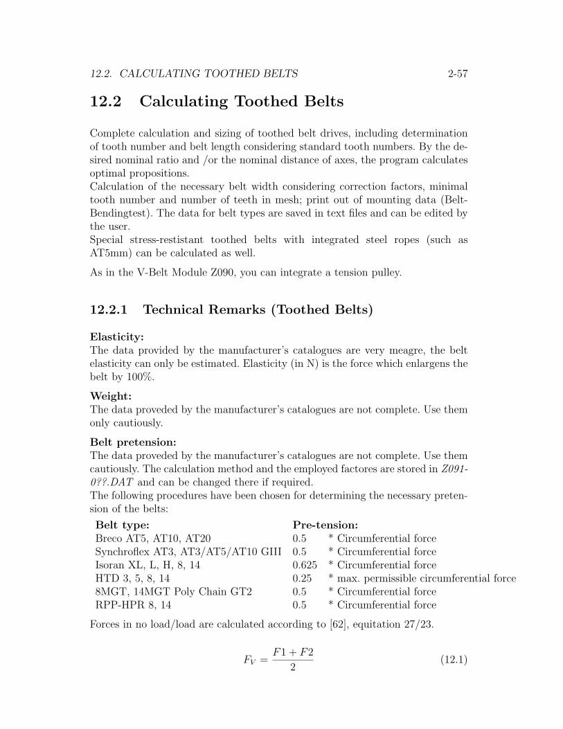
12.2. CALCULATING TOOTHED BELTS 2-57
12.2 Calculating Toothed Belts
Complete calculation and sizing of toothed belt drives, including determinationof tooth number and belt length considering standard tooth numbers. By the de-sired nominal ratio and /or the nominal distance of axes, the program calculatesoptimal propositions.Calculation of the necessary belt width considering correction factors, minimaltooth number and number of teeth in mesh; print out of mounting data (Belt-Bendingtest). The data for belt types are saved in text files and can be edited bythe user.Special stress-restistant toothed belts with integrated steel ropes (such asAT5mm) can be calculated as well.
As in the V-Belt Module Z090, you can integrate a tension pulley.
12.2.1 Technical Remarks (Toothed Belts)
Elasticity:The data provided by the manufacturer’s catalogues are very meagre, the beltelasticity can only be estimated. Elasticity (in N) is the force which enlargens thebelt by 100%.
Weight:The data proveded by the manufacturer’s catalogues are not complete. Use themonly cautiously.
Belt pretension:The data proveded by the manufacturer’s catalogues are not complete. Use themcautiously. The calculation method and the employed factores are stored in Z091-0??.DAT and can be changed there if required.The following procedures have been chosen for determining the necessary preten-sion of the belts:
Belt type: Pre-tension:Breco AT5, AT10, AT20 0.5 * Circumferential forceSynchroflex AT3, AT3/AT5/AT10 GIII 0.5 * Circumferential forceIsoran XL, L, H, 8, 14 0.625 * Circumferential forceHTD 3, 5, 8, 14 0.25 * max. permissible circumferential force8MGT, 14MGT Poly Chain GT2 0.5 * Circumferential forceRPP-HPR 8, 14 0.5 * Circumferential force
Forces in no load/load are calculated according to [62], equitation 27/23.
FV =F1 + F2
2(12.1)

2-58 CHAPTER 12. BELTS
F1 = FV +Ft
2(12.2)
F2 = FV −Ft
2(12.3)
12.2.2 Standard Toothed Belts
The following standards are available:
• XL-ISORAN RPP (FENNER)
• L-ISORAN RPP (FENNER)
• H-ISORAN RPP (FENNER)
• 8mm-ISORAN RPP (FENNER)
• 14mm-ISORAN RPP (FENNER)
• RP8mm-Pirelli RPP-HPR
• RP14mm-Pirelli RPP-HPR
• PG3mm-Power Grip-HTD
• PG5mm-Power Grip-HTD
• PG8mm-Power Grip-HTD
• PG14mm-Power Grip-HTD
• 8mmMGT-Poly Chain-GT2
• 14mmMGT-Poly Chain-GT2
• AT3mm-SYNCHROFLEX
• AT3mm GEN III-SYNCHROFLEX
• AT5mm GEN III-SYNCHROFLEX
• AT10mm GEN III-SYNCHROFLEX
• AT5mm-BRECOflex
• AT10mm-BRECOflex
• AT20mm-BRECOflex
Further norms upon request.

12.2. CALCULATING TOOTHED BELTS 2-59
12.2.3 Possible Propositions
Variable Influencing/necessary variablesBelt profile Power
Speed (small sheave)Service factor
Belt tooth number Distance of axesTooth number of sheave
Distance of axes Belt tooth numberTooth number of sheaves (all)
Ratio Distance of axesNominal ratioSpeed (small sheave)
Tooth number tension pulley Tooth number (small sheave)
12.2.4 Tension Pulley Configuration
You can choose between:
• No tension pulley
• Tension pulley inside
• Tension pulley outside
If you choose a tension pulley inside/outside, you have to enter the pulley sheave’sdiameter and position (x/y) in the pulley interface. Enter the pulley interfacewith KONFIG. You can define the tension pulley’s position in the graphical inputfacilities.
12.2.5 Service Factor and Addendum for Operation
The service factor can either be entered manually in the service factor interface,or the program can calculate the service parameters. If you choose a configura-tion with tension pulley, you should add 0.1 to the service factor. The factorcan be determined according to the following table (additional information incatalogues):

2-60 CHAPTER 12. BELTS
Driven Machine Service hours per day0-10 10-16 16-24
Light drive 1.2 1.3 1.4Medium ligth drive 1.4 1.5 1.6Medium heavy drive 1.5 1.6 1.7Heavy drive 1.7 1.8 1.9Heavyweight drive 1.8 1.9 2.0
Addendum for Operation(This addendum is added to the service factor in the calculation)
Type of operation: Addendumcontinuous, 0-10 hours/day 0continuous, 10-16 hours/day +0.1continuous, 16-24 hours/day +0.2intermittent or with changing load -0.1
12.2.6 Distance of Axes
The minimal distance of axes is calculated from both belt sheave diameters. Nosmaller value can be entered. The sheaves must not touch each other in operation.
12.2.7 Belt Length and Number of Teeth
The belt length for toothed wheel drives is calculated by the number of teeth. Itis necessary for the belt calculation. If you have not entered any tooth numberor if you change during the input phase to a configuration with tension pulley,the program must recalculate the tooth number.
12.2.8 Actual Belt Width
The theoretical belt width (required minimal width to transmit the torque) isstated in the manufacturer’s catalogue. The actual belt width is the next largerstandard belt width.
The belt should not be wider than 5*pitch. A warning is issued if you choosea too narrow or too wide belt. The calculation, however, is carried out on yourresponsibility.
Calculating the actual belt width / factor for belt width:
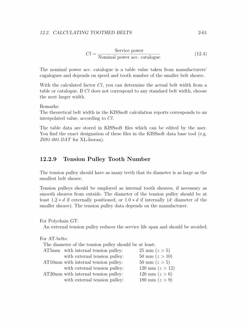
12.2. CALCULATING TOOTHED BELTS 2-61
Cl =Service power
Nominal power acc. catalogue(12.4)
The nominal power acc. catalogue is a table value taken from manufacturers’cagalogues and depends on speed and tooth number of the smaller belt sheave.
With the calculated factor Cl, you can determine the actual belt width from atable or catalogue. If Cl does not correspond to any standard belt width, choosethe next larger width.
Remarks:The theoretical belt width in the KISSsoft calculation reports corresponds to aninterpolated value, according to Cl.
The table data are stored in KISSsoft files which can be edited by the user.You find the exact designation of these files in the KISSsoft data base tool (e.g.Z091-001.DAT for XL-Isoran).
12.2.9 Tension Pulley Tooth Number
The tension pulley should have as many teeth that its diameter is as large as thesmallest belt sheave.
Tension pulleys should be employed as internal tooth sheaves, if necessary assmooth sheaves from outside. The diameter of the tension pulley should be atleast 1.2 ∗ d if externally positioned, or 1.0 ∗ d if internally (d: diameter of thesmaller sheave). The tension pulley data depends on the manufacturer.
For Polychain GT:An external tension pulley reduces the service life span and should be avoided.
For AT-belts:The diameter of the tension pulley should be at least:AT5mm with internal tension pulley: 25 mm (z > 5)
with external tension pulley: 50 mm (z > 10)AT10mm with internal tension pulley: 50 mm (z > 5)
with external tension pulley: 120 mm (z > 12)AT20mm with internal tension pulley: 120 mm (z > 6)
with external tension pulley: 180 mm (z > 9)

2-62 CHAPTER 12. BELTS
12.2.10 Position of Tension Pulley x/y
This value must be entered for a configuration with tension pulley. The co-ordinate system centre represents the axis of the small sheave. In the graphicalinput interface, the program analyses whether the inputs are possible.
12.3 Chain Drive Calculation
Calculating chain drives with roller chains according to DIN 8187 and DIN 8188(with standardised roller chains from a data base). For single or polychains, chaingeometry (distance of axes, number of chain links), transmittable power, axeforces, speed variations caused by Polygon effect, etc. is calculated. Calculationbasis: [38] and [60].
Analysing the permissible speed; proposition for required lubrication.
As in the v-belt module Z90, a third wheel (tension pulley) can be positionedgraphically on the screen and taken into account in the calculation.
12.3.1 Sizings:
• Basing in the drive data, a list with propositions for aptant chain drives isdisplayed.
• Calculating the distance of axes from the chain length.
• Calculating the chain length from the distance of axes.
12.3.2 Tension Pulleys
Tension pulleys are necessary if the chain deflection or the loop angle has to beminimised. Tension pulleys are arranged in no load and should drive the chainwith at least three teeth.
12.3.3 Standards
You can choose between the following standards:
• Roller chain DIN 8187

12.3. CHAIN DRIVE CALCULATION 2-63
• Roller chain DIN 8188
• Bush chain DIN 8154
Roller chains are the most frequently used chains, the lubricated rolls minimisenoise and wear. Chains according to DIN 8187 correspond to the European type,chains according to DIN 8188 to the American. Install bush chains according toDIN 8154 only with good lubrication in closed boxes!
Annotation: bush chain according to DIN 8154 is not yet installed in KISSsoft!
12.3.4 Chain Type
The following data depend on the chain type:
• Loop
• Maximal permissible speed of the small wheel
• Nominal power at maximal permissible speed
Table for DIN 8187 and DIN 8188 according to [38], Anhang G6, Tabelle 4 (17.Auflage).
12.3.5 Number of Lanes
High power is transmitted by multiple chains. Frequently, chains are laid out intwo or three lanes (Duplex, Triplex). In some cases, up to twelve lanes are used.
12.3.6 Service Factor
Reference values according to [38] G97, Tabelle 1:

2-64 CHAPTER 12. BELTS
Service conditions Examples Factorcontinuous operation, ventilators, gyroscopic 1.2small masses to pumps, generatorsaccelerate lathesintermittent operation pistons, turning piston 1.4without impacts, medium fans,masses to accelerate looms, stir machinesintermittent operation hobbing machines, 1.6with impacts, medium clams, stamps, gatemasses to accelerate saws, vibratorsstrong impact operation, stone breakers, gate saws, 2.0large masses to roller machines, single piston-accelerate and piston pumps with
small fly wheel
12.3.7 Speed/Number of Teeth/Ratio
Range of ratio:favourable i = 1. . . 5,optimal i = 1. . . 7,unfavourable i > 10.
Tooth number:Due to polygon effect, a minimal tooth number of 17 to 25 is recommended.Tooth numbers below 17 should only be employed for small power.
Employ at least three teeth for tension pulleys.
12.3.8 Configuration
The following configurations are possible:
• Without tension pulley
• Internal tension pulley
• External tension pulley
For configurations with tension pulleys, you have to enter tooth number andposition of the tension pulley (x/y). You can enter this data with you mouse. Usethe field Graphical Input.

12.3. CHAIN DRIVE CALCULATION 2-65
12.3.9 Distance of Axes
Recommended distance: a = 30 ∗ p. . . 50 ∗ p (p: pitch)Avoid: a < 20 ∗ p und a > 80 ∗ p
The distance of axes is calculated by the sizing button from the number of chainlinks.
12.3.10 Polygon effect
The polygon effect is considered when calculating pitch diameter as well as dis-tance of axes.
• Formula for pitch diameter:
d =pitch
sin(πz)
(12.5)
(see also [62], equitations 26/46)
• Formula for distance of axes:
The length of the loop on the chain wheel is altered as follows:
lUK = lUR ∗sin(π
z)
πz
(12.6)
lUK : length of loop chainlUR: length of loop v-belt
12.3.11 Number of Links
You should include an even number of links.
The link number is calculated by the sizing button from the distance of axes.
12.3.12 Graphical positioning of the Tension Pulley
Move the cursor on the tension pulley in the drawing, press the left mouse buttonand move the pulley with your mouse. Co-ordinates and chain length are displayedcontinuously.
You cannot position the pulley in an invalid position. When you are in yourdesired position, you can set the pulley by releasing the mouse button.

2-66 CHAPTER 12. BELTS
Chapter 13
Calculation of Springs
13.1 Garter Springs
The calculation of garter springs bases on the EN 13906-1 (2002)[30]. The wiretolerances are calculated according to DIN 2076 (1984), DIN 2077 (1979), EN10270-1 (2001), EN 10270-2 (2001), EN 10270-3 (2001) and the requirementsof quality are considered according to DIN 2095 (1973)[14] or DIN 2096 Teil 1(1981)[15].
13.1.1 Material Strength
Depending on diameter, the material strengths are stored in different files. Thetransverse strength is either saved in the tables, as in EN 13906-1 for ther-moformed springs, or it is calculated from the prescribed breaking strengthτczul
= 0.56 ·Rm.
To calculate the fatigue resistance, either the Goodman–Diagram according toEN 13906-1 or an approximation is used. The approximation assumes a dynamicstrength of 0.25 ·Rm and a gradient of the graph of the upper stress of 0.75. Forshot peened materials, the dynamic strength is increased by 20%. These valuesroughly correspond to the diagrams contained in the EN 13906-1, the safeties,however, have to be considered conservatively.
2-67

2-68 CHAPTER 13. CALCULATION OF SPRINGS
Figure 13.1: Types of supports with their respective support coefficients for axiallyloaded springs
13.1.2 Support coefficient
13.1.3 Sizing
When giving the loads, you can choose between entering them as forces or travel.Instead of prescribing springs without load L0, you can also prescribe springlengths in loaded state L1 or L2.
Based on the given spring rate R = ∆F/∆s and on given spring diameter, thenumber of turns n can be calculated. The number of turns is defined by this value,but strength and the geometric border conditions are not controlled. Additionally,the program issues a proposal for minimal wire diameter and the correspondingnumber of turns. The minimal wire diameter is determined by the strength of thematerial.
Also tables with geometry data can be loaded. The displayed data can be re-stricted by the entered data as e.g. coil diameter, spring length or spring forceF2.
13.2 Tension springs
Analysis of tension springs is defined and described in EN 13906-2 (2002)[31].The quality specifications for tensile springs are considered in DIN 2097[16] and

13.2. TENSION SPRINGS 2-69
Figure 13.2: Definitions on the tension springs
DIN 2096 Teil 1 (1981)[15]. Wire tolerances are according to DIN 2076 (1984),DIN 2077 (1979), EN 10270-1 (2001), EN 10270-2 (2001) or EN 10270-3 (2001).
13.2.1 Material Strength
Permissible shear stress is calculated from ultimate strength for cold formed ten-sile springs. The values for the ultimate strength depend on the wire diameterand are stored in a database. Shear stress is calculated as follows: τzul = 0.45 ·Rm.Hot formed tensile springs should have a permissible shear stress not higher thanτzul = 600N/mm2. These values are valid for the static and quasi-static case.For tensile springs according to DIN 2097, dynamic loading should be avoided.Distribution of shear stress over the cross section of the wire is very uneven, usingan intensity factor k, the highest stress can be estimated. At the transitions tothe eyes, additional stresses are present. They may be well above the permissibleshear stress, hence no general fatigue strength values can be given.

2-70 CHAPTER 13. CALCULATION OF SPRINGS
13.2.2 Production
Hot formed tensile springs can not be produced with internal pre-tension sincedue to the hot forming process, an air gap between the coils develops. For coldformed tensile springs, two types of productions are possible, winding on a coilingbench and winding on a spring winding automate. According to EN 13906-2, foreach production type a formula for the permissible shear stress τ0 is given.
13.2.3 Eyes
For tensile springs, 13 types of eyes exist according to DIN 2097. Depending onthe shape of the eye, different lengths of the eye are proposed. Furthermore, theposition of the eyes is defined in the above mentioned standard.
1/2 german loop 1/1 german loop
Double german loop German side loop
Double german side loop Hook
Extended side hook English loop

13.3. LEG SPRINGS 2-71
Coiled in hook Screwed plug
ScrewedScrewed-in shackle
1/1 German loop inclinedextension
13.2.4 Sizing
Using the sizing button next to the wire diameter, the number of coils n iscalculated using the spring rate according to R = ∆F/∆s. In addition, a minimalwire diameter and the corresponding coil number is proposed. The minimal wirediameter is defined by the strength of the material.
13.3 Leg Springs
Analysis of leg spring is documented in EN 13906-3 (2002)[32]. The quality spec-ifications for leg springs are given in DIN 2194 (2002)[17]. Wire tolerances areaccording to DIN 2076 (1984), DIN 2077 (1979), EN 10270-1 (2001), EN 10270-2(2001) or EN 10270-3 (2001).

2-72 CHAPTER 13. CALCULATION OF SPRINGS
Figure 13.3: Definitions on the leg springs
13.3.1 Strength data
Permissible bending stress are calculated from the ultimate strength for coldformed springs. Ultimate strength depends on the wire diameter and are definedin a database. Bending stress is calculated using the formula σzul = 0.7 · Rm.These values are valid for the static and quasi-static case.
Due to the curvature of the wire axis, an uneven bending stress distribution underload results. In order to estimate the theoretical stress level, a stress intensityfactor q is considered.
13.3.2 Design of spring
In order to avoid friction forces, the coils should not or only lightly touch eachother. The maximum free distance between two coils is:
amax = (0.24 · ω − 0.64) · d0.83
Generally, leg springs are wound. The design either uses bent ends (radius has tobe defined) or tangential ends.
13.3.3 Assumptions for analysis
The analysis is valid only for leg springs with fixed or circularily guided ends. Ifthe legs are not fixed, the spring has to guided by means of a pin or a sheath.

13.4. DISC SPRINGS 2-73
13.3.4 Sizing
The sizing button next to the wire diameter executes calculation of windingnumber n for the given wire diameter as a function of the spring rate RMR =∆M/∆α. Furthermore, the program proposes a minimal wire diameter and thecorresponding number of windings. The minimal wire diameter is defined throughthe ultimate strength of the material.
13.4 Disc springs
Analysis of disc springs is according to DIN 2092 (1992). Dimensions and qualityspecifications are according to DIN 2093.
13.4.1 Geometry
Disc springs are divided into 3 groups and 3 series according to DIN 2093. Groups1 and 2 are those springs without bearing surfce, group 3 those with bearingsurface. Disc thickness is smaller than 1.25 mm with group 1, smaller than 1.25- 6 mm for group 2 and 6 to 14mm for group 3. The series differ in terms ofstiffness of the spring. Series A is the stiffest, series C the least stiff series. If OwnInput is selected, the masks for definition of geometry are acitvated. This typeof analysis considers only spings without bearing surface, since the ratio of thethicknesses t’/t is not known but required for the analysis.
13.4.2 Strength
For statically or quasi-statically loaded springs (N ≤ 104), the maximum forceon the spring is analysed, the formula is given in DIN 2092. This force then iscompared to the effective force Fn of the spring (at s = 0.75h0) and an utilisationis calculated. Furthermore, stresses in the edge points 1 - 4 are calculated. Points2 and 3 are loaded in tension, points 1 and 4 in compression. Under dynamic load,using the maximum stress with the respective lower stress level, the stress range iscalculated. Permissible stress range is defined using a Goodman-diagram. Com-parison of permissible and maximum stress range yields the permissible cyclesnumber the spring should be able to withstand. Godman-diagrams are given inDIN 2093. They are valid only for the materials defined in DIN 17221 and 17222.When using other materials, data has to be obtained from the manufacturer ofthe springs.

2-74 CHAPTER 13. CALCULATION OF SPRINGS
Figure 13.4: Definitions on the torsion bar springs
13.4.3 Calculate Number
To estimate the number of discs necessary, use the sizing button next to thenumber of discs field. In this field, the maximum force and the maximum travelcan be defined. Then, the number of springs to be used is calculated based onthese values.
13.4.4 Limit Dimensions
For all disc springs, the outer diameter De has to be tolerated as h12 and theinner diameter Di as H12.
13.5 Torsion bar springs
The torsion bar spring calculation is described in DIN 2091 (1981)[11].
13.5.1 Geometry
The torsion bar spring can have three different head forms according to DIN2091: four-edge, six-edge, and toothed. The toothed heads are mostly machinedaccording to DIN 5481 Part 1 or SAE J 498 b, but can also have special toothforms. The body forms of the heads apply only to those bars that are loaded in thedirection of rotation. Oscillating loads require special measures in construction.

13.5. TORSION BAR SPRINGS 2-75
Figure 13.5: body forms of the heads (four-edge, six-edge, toothed)
13.5.2 Strength values
The DIN 2091 applies only for materials from DIN 17221.The permissible shear stresses:For non pre-loaded bars: τzul = 700 N/mm2
For pre-loaded bars: τzul = 1020 N/mm2
The heat-treated strength for these values amounts to around: Rm = 1600 - 1800N/mm2
For the shear modulus the value G = 78500 N/mm2 is taken as standard. Througha pre-load (above the yield point deformed in the direction of operation) afterthe heat treatment of torsion bar springs there will be a better distribution ofthe operating stress, and a relief in the boundary layer will be achieved.
13.5.3 Determining Design
In the design data interface, the torsional moment and the angle of rotation canbe input. From these the torsion ratio (torque per unit angle) is calculated, fromwhich the bar diameter d or the shaft length ls can be determined. In thedetermination of d and ls, first the d is calculated with the permissible shear stressvalue then from this diameter the length is calculated. So that a determinationof the dimensions is possible, various assumptions are made. (four-edge, toothed:

2-76 CHAPTER 13. CALCULATION OF SPRINGS
df = 1.35*d; six-edged: df = 1.3*d; da = df + df/7; Rh = (da-d)*1.2)These values are not conveyed to the main interface.
13.5.4 Limiting values
For the torsion bar spring the following limiting relationship applies to the heads:Four-edged, toothed: df/d > 1.3; Six-edged: df/d > 1.25The strength values from the DIN apply for bar diameters of 10-60 mm.As a guideline, the head length should be around 0.5-1.5*d.The ration Rh/d should be between 1-50.

Part III
Shafts and Bearings
3-1


Chapter 14
Input of Shafts
14.1 Shaft Calculation
The program is composed of individual modules controlled via the base module.Data that have been entered once (geometry, material, forces, etc.) can thereforebe used in all calculation modules and don’t have to be entered time and again.Following calculations are available:
• Deformation, force-, moment- and stress- course
• Bending critical speed
• Torsion critical speed
• Buckling load
• Static and fatigue resistance
• Bearing calculation
• Journal bearing calculation (hydrodynamic)
• Required drive pinion width correction
Shaft Base Module W01
Input and correction module for geometry and material data, shaft specification,drawing number, etc., type of bearing, boundary conditions, external forces andmoments (simplified input for couplings, spur and bevel gears, worms, wormgears, belt pulleys).
3-3

3-4 CHAPTER 14. INPUT OF SHAFTS
Shafts together with their machine elements (such as gears or bearings) will bedefined in the graphical shaft editor.The properties of the graphical input are:
• Any dimensions (cylindrical and conical), axial symmetric cross section,solid and hollow shafts, beams (H-, I-,L-profiles etc.)
• Integrated drawing tool that allows simple corrections on the shaft con-tour (diameter, lengths). All elements may be edited by mouse clicks orgraphically changed using grip-points.
• Definition of notch geometry for the automatic calculation of the notchfactor.Following notch geometries are available:
– Radius
– Chamfer
– Relief grooves
– Interference fit
– Longitudinal grooves
– Circumferential grooves
– Square grooves
– V-Notches
– Groove toothing
– Splined shafts
– Cross-holes
• Forces and moments can be entered arbitrarily in all spatial positions. Pre-programmed are the following:
– Spur gears
– Bevel pinion/gear
– Worm/worm gear
– Coupling
– Rope or belt pulley
– Individual radial and axial forces, bending and torsional moments
– Springs, torque-springs
– External masses with inertia

14.1. SHAFT CALCULATION 3-5
– Eccentric forces
– Dissipation loss
– Unbalanced forces
• Calculation of:
– Shaft weight
– Inertia
– Axial force
– Static torsion of the shaft
• Balance quality can be entered. This is used to determine the dynamicunbalance forces for the whole shaft. The unbalance value will be furtherused in the shaft deformation calculation.
• Clear display of the geometric data and of the calculated bearing andmarginal forces both on screen and on paper.

3-6 CHAPTER 14. INPUT OF SHAFTS
Figure 14.1: Flow-chart of the modules for shaft and bearing calculation in KISS-soft.
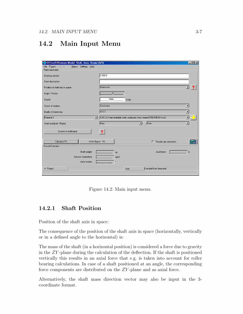
14.2. MAIN INPUT MENU 3-7
14.2 Main Input Menu
Figure 14.2: Main input menu.
14.2.1 Shaft Position
Position of the shaft axis in space:
The consequence of the position of the shaft axis in space (horizontally, verticallyor in a defined angle to the horizontal) is:
The mass of the shaft (in a horizontal position) is considered a force due to gravityin the ZY -plane during the calculation of the deflection. If the shaft is positionedvertically this results in an axial force that e.g. is taken into account for rollerbearing calculations. In case of a shaft positioned at an angle, the correspondingforce components are distributed on the ZY -plane and as axial force.
Alternatively, the shaft mass direction vector may also be input in the 3-coordinate format.

3-8 CHAPTER 14. INPUT OF SHAFTS
Figure 14.3: To define the shaft position and position of application.
14.2.2 Speed
The unit of speed is rpm. Important: If you change the speed of an already enteredshaft
• powers are not changed (torque, however, is changed because of differentpower and speed) in case of activated Input of power in Settings ⇒Module-Specific (see 14.3).
• torques are not changed (power, however, is changed because of differenttorques and speed) in case of activated Input of torque in Settings ⇒Module-Specific (see 14.3).
14.2.3 Sense of Rotation and Co-ordinate System
The shaft axis runs along the positive y–direction (left to right in the graphicalshaft editor). The z–axis points in the shaft editor to the top, the x–axis points

14.2. MAIN INPUT MENU 3-9
in the user’s direction. A right-way rotation of the shaft in the positive y axisdirection is entered as ’clockwise’.
You can look up the direction of co-ordinates and the positive direction of forcesand momenti in the following picture. Please note, that weight acts in negativez–direction if the shaft lies horizontally (see 14.2.1).
Figure 14.4: Figure W-002.
The directions of the moments is usually defined by the terms driving/driven.The input driving means that the shaft drives the following elements and hencethe moment acts in the direction against the direction of the rotation (i. e. theshaft loses power). The input driven means that the shaft will be driven fromoutside (e. g. through a motor) or that the torque acts in the sense of rotation(i. e. the shaft is supplied with power).
14.2.4 Quality of Balance Grading
The quality of balancing decides about the eccentricity of additional masses ifno eccentricity has been defined in advance. Unbalance is assumed in directionof the maximal deflection. Amount and direction of this force are displayed inresults (see 15).

3-10 CHAPTER 14. INPUT OF SHAFTS
Quality of Rotor type - General examplesbalance gradeG 4000 Rigidly set up crankshaft drives of low speed
Marine diesel engines with an uneven number of cylindersG 1600 Rigidly set up crankshaft drives of large two-stroke enginesG 630 Rigidly set up crankshaft drives of large four-stroke engines
Elastically set up crankshaft drives of marine diesel enginesG 250 Rigidly set up crankshaft drives of high speed
4-cylinder diesel enginesG 100 Crankshaft drives of high-speed diesel engines with six
and more cylinders, such as complete (Otto- or Diesel-)car, truck and locomotive engines
G 40 Car wheels, rims of wheels, wheel sets, universal-joint shafts;Elastically set up crankshaft drives of high speedfour-stroke engines (Otto or Diesel) with six andmore cylinders; Crankshaft drives of car, truck and locomotiveengines
G 16 Drive shafts (propeller shafts, Cardan shafts) withparticular requirements; Parts of agriculturalmachines; Components of car, truck andlocomotive engines (Otto or diesel); Crankshaft drivesof engines with six or more cylinders with particularrequirements
G 6,3 Parts of process engineering; Centrifugal drumsGearboxes for the main turbine in merchant vessels;Ventilators; Flywheels; Centrifugal pumps;Machine tool parts; Rolls of paper and printing machinery
G 2,5 Gas and steam turbines including the main turbines inmerchant vessels; Turbo-blowers, Stiff turbo-generator rotors;Machine tool drives; Turbine driven pumps
G 1 Tape recorder and record player drives; Grinding machinedrives;Armatures of small motors with particular requirements
G 0,4 Super-finish grinding machine rotors, shafts and discs; Gyro-scope
According to ISO 194 (former VDI 2006). Remark: The number following the Gindicates the maximum value for e ∗ ω in mm/sec.
e: Eccentricity (mm)ω: Frequency (2 * Pi * n / 60)n: Speed (rpm)

14.2. MAIN INPUT MENU 3-11
14.2.5 Boundary Conditions at Shaft Ends and Bearings
Normally, KISSsoft assumes free shaft ends, special cases can occur for supports(with fixed ends etc.).
Figure 14.5: Figure W-003: Boundary conditions at shaft ends and bearings.
0 Value = Zero# Value changes rapidly- No influence on valuefx, fz Deflection in XY -, respectively ZY -planeαxy, αzy Angle of bending line to Y -axisFx, Fz Shearing force in XY -, respectively ZY -planeMx, Mz Bending moment in XY -, respectively ZY -plane
Important: The kind of bearing ”Bearing/Support” according to figure W-003 isevaluated at the time of input, as the following table demonstrates:

3-12 CHAPTER 14. INPUT OF SHAFTS
KISSsoft Bearing- Kind of bearing Axial forceSelection list according to fig. W-003 AcceptanceRigid free bearing Bearing/Support –Rigid fixed bearing ↔ Bearing/Support in both directionsRigid fixed bearing → Bearing/Support only +y-directionRigid fixed bearing ← Bearing/Support only −y-directionElastic free bearing Spring –Elastic fixed bearing ↔ Spring in both directionsElastic fixed bearing → Spring only +y-directionElastic fixed bearing ← Spring only −y-direction
14.3 Module-Specific Settings
14.3.1 General Module-Specific Settings
Figure 14.6: General Module-Specific Settings/ Module-Specific Settings RollerBearings
• Adjustments of input of torque (Nm or Nmm) or power (kW or W). Notethat the value which has been defined will remain constant even if the speedis changed. For each element, either the power or the torque will be fixed.

14.3. MODULE-SPECIFIC SETTINGS 3-13
• Feather key grooves: set whether grooves are made with end milling cutteror side milling cutter or if a combination feather key tight fit will be used.This setting will influence the notch effect value in the strength calculation.These settings may be overwritten during the strength calculation.
• Gear wheels: rough settings, whethter the gear wheels are considered asmasses for stiffness when calculating bending or critical speed.
– Normal analysis: The gears are considered as having no mass.
– Regard gears as masses: The gears do not stiffen the shaft (e. g. onlywhen the gear is fixed to the shaft with a feather key).
– Regard gears as masses and stiffness: The gears are considered as hav-ing a mass (mass and inertia). It is assumed that the mass is equallydistributed over the width of the wheel.The gears stiffen the shaft (the gear and the shaft form a unit, e. g.pinion and shaft).
• Consider weight: set whether the shaft’s weight is respected as shearingforce corresponding to the position of the shaft.
• Centre of pressure taken into consideration : For roller bearings with in-clined pressure angle, the angle of the acting force will be taken into accountduring the calculation (see also 15.1.4).
• Shearing correction factor: The shearing correction factor is consideredwhen calculating bending with shearing deformation.
• Shaft made from several materials: An additional selection of materials ispossible at each shaft section. It is thus possible to define a shaft with upto three different materials (especially for the deformation calculation).
14.3.2 Module-Specific Settings Roller Bearing
The default values required for the bearing calculation are defined here. Theseare accessed and saved as part of the shaft calculation.
• Failure probability: This value will be used in the life expectancy calculationof roller bearings. The default value is 10% but it may be overwritten here.
• Choice of manufacturer: Only the bearings of the selected bearing manu-facturers will be considered in the possibilities of selection.

3-14 CHAPTER 14. INPUT OF SHAFTS
• Enhanced life calculation: At present, KISSsoft offers three methods for thelife expectancy calculation:Standard Lh10 Method (no enhanced life expectancy calculation), accord-ing to FAG and according to ISO 281, supplement 4.
• Nominal life: Default required life expectancy. This value does not go intothe roller bearing calculation. Should the calculated bearing life expectancybe smaller than this value, the program issues a warning.
• Clearance: Settings of the Clearence

14.4. GRAPHICAL INPUT OF SHAFT DATA 3-15
14.4 Graphical Input of Shaft Data
Directly in the main window, you can enter the important parameters like speedor material, all other data (geometry, forces, type of support) through Graphical
Shaft Input.
14.4.1 Input of Shaft or Support Elements
14.4.1.1 Definition of Outer Contour
The main elements that can be defined are (hollow) cylinders, (hollow) cones andsupports. In order to enter a new element activate the menu-item element andchoose the desired element. If no other element is activated (see chap. 14.4.1.4),the new element is positioned at the right end of the shaft. Otherwise, the newelement will be positioned in front of the activated element.
Important: An element of the same type is entered with the key combination Alt
+ r.
Possible elements for support are:
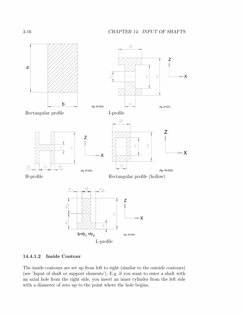
3-16 CHAPTER 14. INPUT OF SHAFTS
Rectangular profile I-profile
H-profile Rectangular profile (hollow)
L-profile
14.4.1.2 Inside Contour
The inside contours are set up from left to right (similar to the outside contours)(see ’Input of shaft or support elements’). E.g. if you want to enter a shaft withan axial hole from the right side, you insert an inner cylinder from the left sidewith a diameter of zero up to the point where the hole begins.
14.4. GRAPHICAL INPUT OF SHAFT DATA 3-17
14.4.1.3 Clearing Elements
An element has to be activated first to be deleted from an existing contour. Thenchoose Edit from the menu and Delete.
14.4.1.4 Activating Elements
An element is activated by positioning the cursor on one contour line and thenclicking the left mouse button. The activated element’s contour is then displayedwith dashed red lines. Alternative: Menu item Edit, then choose Select Next.Alternatively: Strike the shortcut key combination: Ctrl + N. If an element cannotbe activated using the mouse, the size of the grid point may be set to too low avalue. It can be changed as follows: Drawing, Settings.
14.4.1.5 Modifying the Characteristics of an Element
This is valid for shape elements, forces and bearings:
Activate one element (see Activating Elements). Then position the cursor ona contour line of that element and click the right mouse button. A window withthe data of that element pops up. Alternatively: Menu item Edit, then chooseEdit Element.
14.4.1.6 Adding Subelements to Mainelements
In order to define a subelement, the mainelement it referrs to has to be active. Thesubelement is shown in the sketch schematically, the appropriate notch factors arecalculated and used in the strength calculations. Subelements can be activatedin the same manner as main elements.
Defining subelements:
• Radius right/ leftInput:
– Radius: Size of the radius
– Surface roughness: Surface of the fillet
• Chamfer right/ leftInput:
– Length: Length of chamfer

3-18 CHAPTER 14. INPUT OF SHAFTS
– Angle: Angle of chamfer
• Relief groove right/ leftInput:
– Relief groove shape: Choice of relief groove shape according to DIN509 or FKM
– Series (DIN 509): (Choice: Series 1, radii according to DIN 250; Series2, special radii)
– Loading (DIN 509): (Choice: with standard loading; with raised fatiguelimit)
– Groove length: Length of undercut in direction of shaft
– Radius: Radius between undercut and following element
– Groove depth: Depth of undercut
– Surface roughness: Surface of the groove
• Interference-FitInput:
– Fit-Length: Length of press-fit
– Type of fit (Select from: light interference-fit, interference-fit and in-terference fit with holes)
– Reference Measure: Distance from left end of selected element to be-ginning of interference-fit
• Longitudinal GrooveInput:
– Groove length: Length of groove
– Surface roughness: Surface of the groove
– Reference measure: Distance from left end of selected element to centreof groove
• Circumferential grooveInput:
– Depth: Depth of groove
– Rounding at notch base: Radius in groove
– Surface roughness: Surface of the groove
– Reference measure: Distance from left end of selected element to centreof groove

14.4. GRAPHICAL INPUT OF SHAFT DATA 3-19
• Square grooveInput:
– Width: Width of groove
– Depth: Depth of groove
– Radius: Radius in groove
– Surface roughness: Surface of the groove
– Reference measure: Distance from left end of selected element to centreof groove
• V-notchInput:
– Depth: Depth of groove
– Surface roughness: Surface of the groove
– Reference measure: Distance from left end of selected element to centreof groove
• Groove-ToothingInput:
– Standard: Standards of groove-toothing (over the - button choosefrom list in sub-window)
– Tip circle: can be choosen from the list or entered directly
– Root circle: can be choosen from the list or entered directly
– Number of teeth: can be choosen from the list or entered directly
– Module: can be choosen from the list or entered directly
– Surface roughness: Surface roughness of the groove-toothing
– Length: length of groove-toothing
– Reference measure: Distance from left end of selected element to be-ginning of groove-toothing
• Splined shaftInput:
– Tip circle: Tip circle of splined shaft
– Root circle: Root circle of splined shaft
– Number of keys: Number of keys
– Splined shaft root radius: (Select from: Shape A, Shape B and ShapeC)

3-20 CHAPTER 14. INPUT OF SHAFTS
– Length: length of splined shaft
– Reference measure: Distance from left end of selected element to be-ginning of splined shaft
– Surface roughness: Surface roughness of the splined shaft
• Cross holeInput:
– Borehole diameter: Diameter of borehole
– Surface roughness: Surface roughness of the hole
– Reference measure: Distance from left end of selected element to theposition of the borehole
• ThreadInput:
– Label: Label of thread
– Thread depth: Depth of thread
– Rounding: Rounding in groove of thread
– Length: Length of thread
– Reference measure: Distance from left end of selected element to be-ginning of thread
– Surface roughness: Surface roughness of the thread
• General effect of notchInput:
– Width: Width of element
– Notch factor bending/ torsion/ tension-pressure/ shearing force: thenotch factors are entered manually
– Surface roughness: Surface of the groove
– Reference measure: Distance from left end of selected element to centreof groove
The Notch-type Taper shaft can be directly activated in the strength calcula-tion.(See chapter 15.5.3)

14.4. GRAPHICAL INPUT OF SHAFT DATA 3-21
14.4.1.7 Input of Lists
By activating Input of Lists below the input interface, a list appears contain-ing geometry data (outer diameter, length, etc). In this menu, it is mucheasier to make complex adjustments in the shaft geometry.
Centric and eccentric forces, bearings and additional masses can be exported andimported through tables held in text file format. This can be very helpful wherecomplex loading situations occur.
14.4.2 Bearings
All elements of a bearing (rigid or elastic) are considered as a bearing. The pointon the shaft at which the axial force is transmitted is determined when entering afixed bearing or an axial bearing. The point is determined by the input of a fixed,a right mounted (→), a left mounted (←), or an axial bearing. This informationwill also be transferred to the roller bearing calculation.
In case of taper roller bearings (or similar configurations) it is not always clearwhich bearing receives the axial force. In this case the mounting of the bearingsshould be entered. A radial offset in the bearing alignment can be defined. Thisenables the consideration of further factors e.g. simulation of assembly error.
See also chap. 14.2.5
14.4.3 Roller Bearing
Besides the general bearings, specific roller bearings may be selected. The bearingdata will be taken from the bearing database. In this case, the geometrical dataof the bearing is available and the bearing is drawn with the respective widthand outer-diameter. In addition, for a bearing with an inclined pressure angle thehelical direction of the force can be taken into consideration during the calcula-tion.(see 14.3). The stiffness of the bearing is read from the bearing database (ifavailable) or may be entered manually.
The type of roller bearing together with the loads are transferred to the bearinganalysis.

3-22 CHAPTER 14. INPUT OF SHAFTS
14.4.4 External Forces and Masses
14.4.4.1 Forces
Forces can be positioned arbitrarily on points on the shaft and even outside (!)the shaft. Different methods are available for defining force transmitting elements(such as gears) or even individual forces.
The direction of the torque is defined as driving/driven. With driving thetorque direction is opposed to the rotation direction.
Special elements are:
• Spur gearPosition of application: statement of position of point of application withthe counter wheel according to picture 14.3 in paragraph 14.2.1.
• Bevel gearPosition of application: cf. spur gear.An additional force component due to friction (µ = 0.05) is taken intoconsideration during the calculation of hypoid gears.
• Worm/worm gearIf the element is entered as a driving element then KISSsoft will interpretit as a worm; if entered as a driven element it will be interpreted as a wormgear.
• Rope sheaveDirection of rope pulley: statement of the direction of the resulting of therope force according to 14.3 in paragraph 14.2.1.
The direction of the helix angles and the positions of the elements are defined infigure 14.7.
Eccentrical Forces
Eccentrical Forces can be defined either in a cartesian or a polar co-ordinatessystem(siehe fig.14.8). The type of co-ordinates system to be selected in Drawing/
Settings.
Transfer of Data from Gear Calculation
By means of the file-Relation of a spur or bevel gear you can choose an existinggear wheel to set on a shaft from saved gear wheel data. After having chosenthe number of the wheel, the corresponding data is directly transferred. In doingthis, the data at the pitch point instead of the reference circle is used.
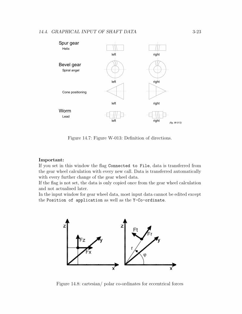
14.4. GRAPHICAL INPUT OF SHAFT DATA 3-23
Figure 14.7: Figure W-013: Definition of directions.
Important:If you set in this window the flag Connected to File, data is transferred fromthe gear wheel calculation with every new call. Data is transferred automaticallywith every further change of the gear wheel data.If the flag is not set, the data is only copied once from the gear wheel calculationand not actualised later.In the input window for gear wheel data, most input data cannot be edited exceptthe Position of application as well as the Y-Co-ordinate.
Figure 14.8: cartesian/ polar co-ordinates for eccentrical forces

3-24 CHAPTER 14. INPUT OF SHAFTS
14.4.4.2 Coupling
The coupling transmits torque but it can be strained additionally by radial andaxial forces. From the torque (respectively entered power and torque) results thecircumferential force to:
Ft =Mt · 2
d(14.1)
Ft = Circumferential forceMt = Torqued = Application diameter
Calculating Radial Forces on Couplings:
Fr = K2 · Ft (14.2)
Ft = Circumferential forceK2 = Radial force factor
The direction of the force is to be defined from the input window. Also theweight of the coupling has to be entered and this is included in the calculationas a gravitational force.
Calculating the Axial Forces on Couplings:
Fa = K3 · Ft (14.3)
Ft = Circumferential forceK3 = Axial force factor
The force acts along the centre line of the shaft.
14.4.4.3 Mass
Masses that are positioned on the shaft are used to determine the unbalanceforce by means of the quality of balance and are considered as a gravitationalforce resulting in bending in the negative Z-direction.
If the eccentricity is given, the force of unbalance is calculated therefrom; other-wise, this force is determined through the unbalance quality (see chap. 14.2.4).

14.4. GRAPHICAL INPUT OF SHAFT DATA 3-25
14.4.4.4 Magnetic Tension
Radial and axial forces that are produced by electromagnetic windings are con-sidered in the calculations.
Radial force calculation:
Fmr = K1 ·D · L · v · (f/del0) (14.4)
K1 = 0.1 for three-phase motors with the number of polesequal to 20.2 otherwise
D = (mm) Inner diameter of the stator of three-phase motorsor the outer diameter of the rotor of direct current mo-tors
L = (mm) Length of the active ”packet of plates” (excludingthe cooling slits)
v = Damping factor:Three phase current asynchronous motor: Squirrel cage:v = 0.25Three phase current asynchronous motor: with a woundrotor: v = 0.7Three-phase current synchronous motor v = 0.5Direct current motor with a wound shaft v = 1.3
f/del0 = Ratio of the mean eccentricity and the nominal air gap= 0.2 for three-phase current motors= 0.1 for direct current motors
Axial force calculation:
Fma = K3 · T (14.5)
K3 = 35 · α/DK3 = Axial force factorT = Torque (Nm)α = Axial groove helix angle (deg)D = (mm) Inner diameter of the stator of three-phase motors
or the outer diameter of the rotor of direct current motors
14.4.4.5 Power or Torque
With gear wheels and couplings, power or torque are required for inputs. InModule-specific Settings you can define whether it shall ask for power (W
3-26 CHAPTER 14. INPUT OF SHAFTS
or kW) or for torque (Nm or Nmm). See chapter 14.2.2 and 14.3 for furtherinformation.
14.4.5 Importing Shafts from Drawings (CAD)
The computer reads shaft geometry data in Drawing ⇒ Interface
The outer and inner contour (if available) of the shaft should be transferredfrom the CAD program individually if possible. For the name of the layer, thedefault value ALL may then be used. Alternatively the contours can be definedas different layers, as e.g. in AutoCAD, and when importing the file into KISSsoftthe program can selectively read the corresponding layer. The name of the layerthen has to be entered in the respective field.
If there are uncertainties about the exact name of the layer, an invalid name (e.g.XXXX) can be entered. When reading the data, an Error message is issued listingvalid layer names.
Outer and inner contours can be imported in any order.
Description of the Conversion-Algorithm
• Reading of a DXF-, VDA-, IGES-, CDL- or KISSgraphik-file and conver-sion of geometry data into KISSgrafik-format. This information is stored in<tmpdir> \DXForCDL.tmp.
• Sorting all lines in a list.
• Clearing all vertical lines. Determining the centre line (Axis of Symmetry)by means of the mean value of the biggest and smallest z-value.
• Clearing all horizontal lines which are too close to the centre line (esp anaccidentally entered axis of symmetry).
• Converting all remaining lines into cylindric or conical elements, dependingon position of lines. Phases are converted into special conical elements.
• Clearing of redundant elements (with entirely symmetric shafts, the upperand the lower edge of a shaft sections become individual elements).
• Solving conflicts caused by intersecting elements. The smallest diameter ischosen for outer contours, for inner the biggest.
• Entering radii in the shaft contour. The final points of the radii are com-pared to the corner points of a defined element. If no aptant radius is foundfor a gap between two elements, a warning appears and the left element isenlarged accordingly to maintain the actual length of the element.

14.4. GRAPHICAL INPUT OF SHAFT DATA 3-27
Figure 14.9: Settings in the shaft input
• Output of results in <tmpdir> \W01-H1.tmp. If you click buttonIntermediate results in the dialogue window, the defined editor openswith this file. This dialogue is closed by OK and the file is read by the shafteditor.
14.4.6 Settings
You find important rough conditions in Drawing ⇒ Settings.
• Maximal diameter: Indication for the Zoom factor in the z-direction (it iseasier to zoom)
• Maximal length: Indication for the Zoom factor in the y-direction
• Size of the grip-pointWhen activating an element, small squares - the grip-points - are shown.The size of these grip-points is defined in Pixels. The value of the gripp–point–size should be approximately 8. The grip–point–size determines thesize of the displayed forces and bearings. Using these grip-points, an elementcan be picked using the mouse and moved.

3-28 CHAPTER 14. INPUT OF SHAFTS
IMPORTANT: The size of the grip-point determines also the sensitivityduring the activation of an element with the right mousebutton. You canincrease the size of the grip-point for easier manipulation.
• Y co-ordinate origin: Indication for the display position on the screen (it iseasier to move the picture with the mouse)
• Show co-ordinate system: Display the shaft coordinates system
• Automatic measurement lines visible: Display the dimension lines
• Mouse round off in Y direction:0: Grip-point left/right resolution = 1 mm1: Grip-point left/right resolution = 0.1 mm
• Mouse round off in d direction:0: Grip-point up/down resolution = 1 mm1: Grip-point up/down resolution = 0.1 mm
• Move forcesThis adjustment defines whether the position of application (y-co-ordinate)should be kept at the same location (Shift forces = No) after deletingthe main elements, forces and supports, or if they shall be shifted with thecorresponding element (Shift forces = Yes).
• Absolute positions of imported forces/ bearings
• Eccentric load: see figure 14.10
• Principal stress (for sizing): see section 14.5
• Maximal deflection (sizing): see section 14.5
14.4.7 End of Input
When you have completed your inputs, you can leave the graphical shaft entrywindow by clicking Accept inputs.
You are again in the menu shafts, axes. As usual, you can save your inputs ortransfer e.g. a shaft contour as DXF-information to the CAD.
You can execute all calculations which are important for shafts. You find theselection list on possible calculations in Calculate F5.

14.5. SIZING OF SHAFTS 3-29
14.5 Sizing of Shafts
KISSsoft provides a shaft sizing pattern. You find this option in Graphical Shaft
Input. In the graphical input interface in Calculations you can choose betweenSizing (Stress) and Sizing (Deflection). If you choose one of these options,a green contour appears in the picture displaying an idealised curve of the outerdiameter. The green represented cross section at every point is computed in sucha way that the static principal stress always has the same given value (you canenter this value in Drawing and Settings), or that the deflection attains thepredetermined maximal value.
Condition for achieving an usable solution however is the correct definition of allexternal forces and bearings/ boundary conditions beforehand.
Due to the Green’s ideals, contour only allows the construction of the externalshaft contour already with the matching diameter, in order that, later on, duringthe actual strength- or deformation- calculation, fewer negative surprises pop up.
However, it should be taken into consideration that, during the layout of constantequivalent stress, the notches will not be considered. Thus, the layout function isless suitable for shafts that, primarily, have to be subject to fatigue calculation.
Figure 14.10: Representation of the input shaft

3-30 CHAPTER 14. INPUT OF SHAFTS
14.6 Statically Undefined Bearings
Shafts with more than two bearings can be calculated easily with KISSsoft (max.ten bearings).
However, the results of these calculations have to be checked more carefully thanin the normal case with two bearings, since numerical instabilities can occur withthis type of calculation.
This effect can be explained best with a simple example. A shaft is supported bythree roller bearings. At the left shaft end a single bearing is positioned and atthe right end two bearings are positioned closely together. In the case where theshaft is subject to a force (say 1000 N) at the centre, it is logical to say that theleft bearing experiences a 500 N reaction force while the two others together alsoexperience a reaction force of about 500 N. The calculation produces of course 500N for the first bearing, 9750 N for the second and 10250 for the third bearing,whereby the reaction forces for the second and third bearing act in oppositedirections and added up they result in exactly 500 N.
This problem occurs due to the assumption that bearings are infinitely stiff. In-troducing bearing stiffness eliminates this effect and the calculation issues correctresults.
Conclusion
• In case of statically undefined bearings you shouldn’t have problems if theindividual bearings are not spaced too closely together.
• In case of two bearings being positioned closely to each other then theyshould be defined as one support (in the centre of the two bearings). Theseare then treated as paired bearings in the roller bearing calculation.
• If you suspect that the calculation of the reaction forces is wrong you shouldintroduce a bearing stiffness.

Chapter 15
Calculations
By button Calculations F5 or by means of the main menu you can choosebetween the following calculations:
15.1 Bearing Forces and Line of Flex
The calculation basis is the general theory of mechanics. The solution of theline of flex and the reaction forces can be found either with the help of transfermatrices or by using simple finite element models.
The calculation in KISSsoft is also based on the segmented analytical solutionof differential equations according to [6] (transfer matrices). The program deter-mines the line of flex by automatically dividing the shaft into 50 to 100 sectionsand by using as many points for the line of flex. Boundary conditions and internalboundary conditions (bearing forces and forces at supports) are found by solvinga set of simultaneous equations with the same number of unknown variables.
Elastic bearings are computed by introducing springs.
3-31

3-32 CHAPTER 15. CALCULATIONS
Figure 15.1: Calculation Deflection
Abilities of the calculation module:
• Calculation of bending line, course of transverse force and course of flexuralmoment in the XY - and the ZY -plane (Shaft axes always along the Y -axis)with or without considering the total weight.
• Calculation of the axial force considering weight (depending on the lengthof the shaft)
• Graphical display of all essential dimensions on screen and printer: Courseof deflection, shearing force, bending moment in different planes, torsionalmoment and static comparative stress. (For the calculation the comparativestress module W06 is required in addition.)
• Calculation of the forces and torques in bearings (and ends of shafts) foran unlimited amount and any type of bearings.
• Calculation of the inclination of the bending line in bearings, e.g. whencalculating cylindrical roller bearings. The course of inclination can also bedisplayed on screen and printed.

15.1. BEARING FORCES AND LINE OF FLEX 3-33
Figure 15.2: Deflection ZY-plane
• The bending line can be calculated with or without considering the shearingdeflection.
• The display of the bending line allows the marking of points and examina-tion of the corresponding data.
• You can save your display and compare it to other results, provided thatthe length of the shafts are identical.
• The deflection output results and the section dimensions on any four se-lected locations in numerical values.
To calculate the deflection of a shaft, choose Deflection/Bearing forces. Ac-tivating Calculate is sufficient as no further information is needed. The bendingline is displayed in the ZY -plane if you choose ZY -plane in Bending.
Notice: The information about principal stress is not usable when calculatingthe fatigue resistance. The information is useful for supports, as they are mostlystressed staticly. If the section modulus is not defined for supports, the torsionstress is not considered with the principal stress, the calculation, however, canstill be carried out.
3-34 CHAPTER 15. CALCULATIONS
15.1.1 Considering Gears
The calculation of gear wheels set on a shaft can be modified by (see picture15.1):
• Normal (Not considering masses or stiffness)
• Considering Gear Wheel Mass: The gear wheel is considered a mass inthe bending calculation. The mass results from the difference between pitchdiameter and outer shaft diameter as well as gear wheel width (same specificweigth as shaft).
• Considering Gear Wheel Mass and Stiffness: The gear wheel is con-sidered in the shaft contour (pinion shaft).
Notice: Gear wheels set on shafts with firm interference fit always pose the prob-lem how much they stiffen the shaft. This problem cannot be solved with KISS-soft, but the program can estimate the influence of the interference fit; it is suf-ficient to calculate the cases Considering Gear Wheel Mass and Considering
Gear Wheel Mass and Stiffness and to consider the difference between thebending lines. If the difference is small, the interference fit has no influence, if itis large, you have to enter exacter information and integrate a part of the gearwheel in the shaft contour.
15.1.2 Considering the load spectra
Should the forces defined in the shaft editor include a Load spectra load level,the deformation calculation may be carried out either for the nominal load or forany Load spectra load level.In the second case, the flag With Load spectra (see Fig. 15.1) must be ser on.Furthermore, the desired Load spectra load level Step No. has to be defined inElement No. in the deformation calculation.
15.1.3 Consider deformation due to shearing
Normally, the bending line is calculated according to the model of the Euler–Bernoulli–bar. This means that shearing deformation are not considered. KISS-soft can consider shearing deformations through an extended bar model, if, inthe bending calculation, the corresponding option is activated (Flag Considerdeformation due to shearing activated). The calculation is carried out witha medium shearing stress τ = κFQ/A. The shearing correction factor κ ≥ 1
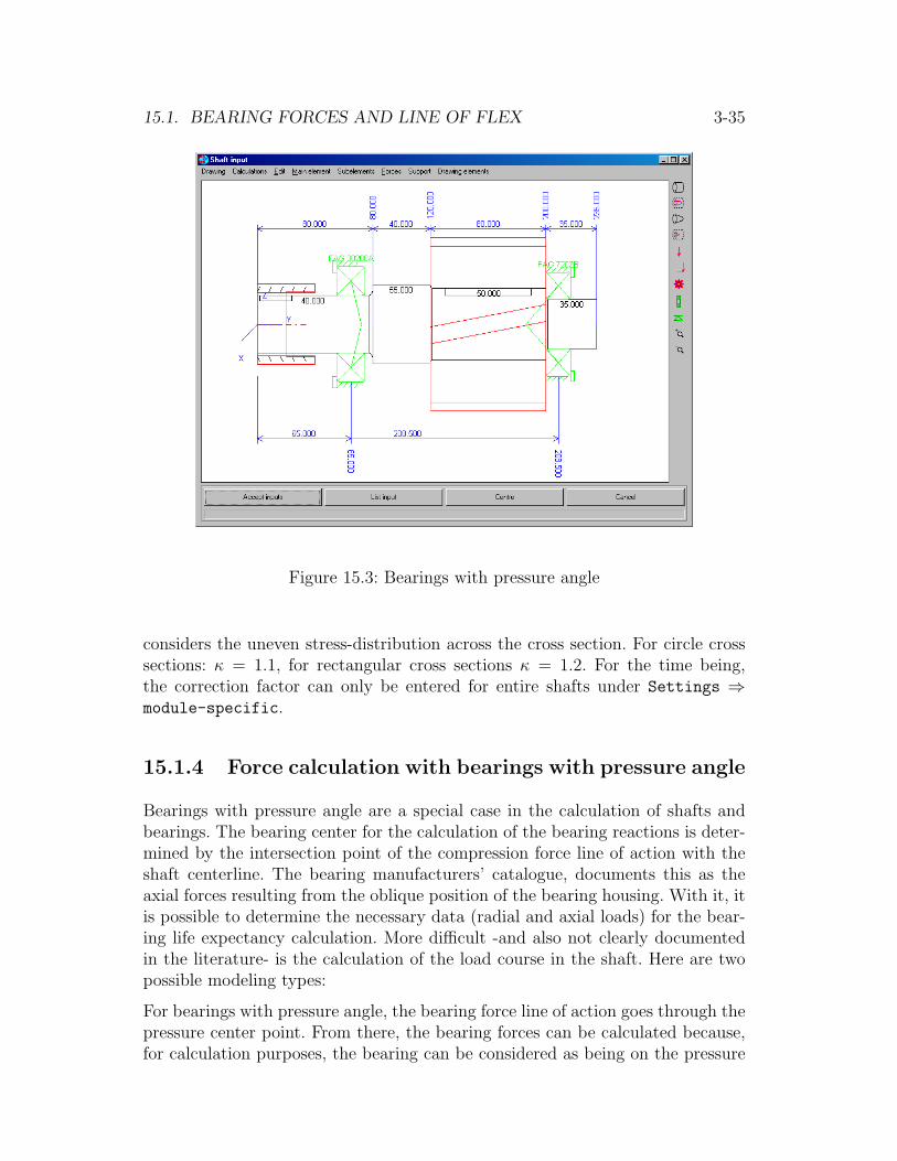
15.1. BEARING FORCES AND LINE OF FLEX 3-35
Figure 15.3: Bearings with pressure angle
considers the uneven stress-distribution across the cross section. For circle crosssections: κ = 1.1, for rectangular cross sections κ = 1.2. For the time being,the correction factor can only be entered for entire shafts under Settings ⇒module-specific.
15.1.4 Force calculation with bearings with pressure angle
Bearings with pressure angle are a special case in the calculation of shafts andbearings. The bearing center for the calculation of the bearing reactions is deter-mined by the intersection point of the compression force line of action with theshaft centerline. The bearing manufacturers’ catalogue, documents this as theaxial forces resulting from the oblique position of the bearing housing. With it, itis possible to determine the necessary data (radial and axial loads) for the bear-ing life expectancy calculation. More difficult -and also not clearly documentedin the literature- is the calculation of the load course in the shaft. Here are twopossible modeling types:
For bearings with pressure angle, the bearing force line of action goes through thepressure center point. From there, the bearing forces can be calculated because,for calculation purposes, the bearing can be considered as being on the pressure

3-36 CHAPTER 15. CALCULATIONS
center point. This is in accordance to the procedures for determining the bearingloading (Variant I).
However, the introduction of the bearing force on the shaft outside the shaftwidth is not possible. This is why KISSsoft places the bearing force in the centerof the bearing. At the same time, the eccentric application force creates an addi-tional flexural moment equals to the product of the distance of the bearing- andpressure- center points, times the radial force (Variant II).
Both variants give the same flexural moment course between the pressure centers.There is, however, a difference in the zone of the pressure/bearing centers. Theshouldered shaft part on the right of the picture, would be considered as notsubject to a force in Variant I (it could, thus, be dropped); in Variant II, ashearing force and a flexural moment will be considered.
Actually, the force does not act necessarily in the bearing center but in thewhole bearing zone. Therefore, the flexural moment can act precisely on theshaft shoulder. However, there is a problem in the strength calculation when theforce is acting directly on the proof point (i. e. when the proof point lies betweenthe bearing center and the shaft shoulder).
There is a difference in the calculation of the bending line, in that, in Variant I,the deflection is zero in the pressure center and, in Variant II, however, in thebearing position. Here, Variant II is for sure more precise, especially with largepressure angles where the pressure center lays outside the bearing width. OnlyVariant II allows the calculation to consider cases in which the pressure centerpoint lays outside the shaft.
In such cases, how frequently should reality lay between Variants I and II. Themost precise calculations are only possible to be carried out with costly FEM Cal-culations, taking into account the bearing housing. For shaft calculation, VariantII is more precise and comfortable (there is no problem for pressure center pointslaying outside the shaft), this is why this Variant was included in the KISSsoftshaft calculation from release 04-2004 on. In special cases, when the modeling inVariant II is questionable, it is possible to modify the loadings in the strengthproof according to more precise considerations when the proof point lays betweenthe bearing center and the pressure center points.
Another comment to the shaft strength calculation: any strength proof touchingthe nominal stress concept (DIN 743, FKM. . . ), has limited validity, in the forceapplication zone (e. g. internal bearing ring on the shaft shoulder) when the localstress distribution does not correspond to the nominal stress estimate. In practice,the calculated results on these points must be conservatively interpreted.
The additional internal force in bearings with pressure angle, is described inKISSsoft, as well as, in Die Walzlagerpraxis and in several bearing catalogues,as Fr ∗ 0.5/Y . [FAG as in here, NSK with a factor 0.6 instead of 0.5, SKF

15.2. BENDING CRITICAL SPEED 3-37
Figure 15.4: Bending Critical Speed
for taper roller bearings, as in here, and for contact angle ball bearings with afactor 1.14 (Catalog 2004 as a function of Fa/C)]. Should the factor Y be absentfrom the bearing database, no additional axial force will be considered. Thus, thecalculation step corresponds to the KISSsoft bearing calculation.
15.2 Bending Critical Speed
The calculation is carried out using the method of the transfer matrix accordingto [52] and [6] (solving analytically and in segments the differential equationdescribing the flexural vibrations). Boundary conditions are included by meansof ”conditions vectors”. Elastic bearings can be considered by introducing springs.
Abilities of the calculation:
• Calculating up to the 9th critical speed.
• Display the Eigen-forms.
• The gyroscopic effect of the momentum of mass is considered. The criticalspeed (bending mode) is calculated for the static case (natural frequency)

3-38 CHAPTER 15. CALCULATIONS
and for the forward and backward whirl. In synchronous parallel run, anunbalance increases the bending oscillations because the angular speeds ofthe rotating shaft and the of the shaft’s peripheral center point are equal.The synchronous counter run is, in most cases, technically unimportant.
• The critical speed (bending mode) is calculated in the two main planes forgirder profiles.
• For beam profiles, the bending critical natural frequencies will be deter-mined for both main surfaces.
• When calculating the critical speed (bending mode), masses that are posi-tioned on the shaft are considered. Acting forces have no influence on thecalculations and the additional masses must be entered as masses and notas gravitational forces!
• The second momentum of a shaft has a small influence on the result. If youchoose Consider second momentum of shaft, the second momentum ofall shaft elements is considered in the calculation.
Axial second momenti of additional masses and the stiffness of elastic bearings re-quire inputs in two planes.If Shaft with rotation-symmetric cross section
is selected, the mean value of the x– and of the z–component is used in thecalculation. Otherwise, the values of the corresponding level are used.
When calculating critical speeds, masses which are set on the shaft are considered.Acting forces, however, have no influence on the calculation. Additional massesmust therefore crucially be stated as masses and not as loading forces.
15.2.1 Considering Gear Wheels
See chapter 15.1.1.
15.2.2 Eigen Frequency of Supports
The critical speed of supports that have no rotational symmetric cross sectionhave to be listed seperately in the XY respectively ZY -plane. To do so set in thesub-window Resistance Momentum in XY -plane.

15.3. CALCULATING ROTATIONAL NATURAL FREQUENCY FOR SHAFTS AND SYSTEMS3-39
15.3 Calculating Rotational Natural Frequency
for Shafts and Systems
Prescriptions: for computing the rotational frequency, left and right ends of theshaft have to be defined either clamped or free.
• Calculating rotational natural frequency of shafts
• Calculating any rotational natural frequencies
• Determining natural frequencies in a definable interval
15.4 Buckling
The buckling load (1st to 5th order) of shafts and supports is calculated. Allboundary conditions, bearings and acting forces (point or line loads) are consid-ered in the calculations.
You can choose between two methods:
• A buckling load that is produced by two axial compressive loads at theshaft ends (with consideration of radially acting forces along the shaft).The necessary compressive force at the end of the shaft is calculated for thebuckling case.
• Buckling loads are only produced by the entered axial forces. The factorwith which all these forces have to be multiplied so that buckling occurs iscalculated. This factor therefore corresponds to the factor of safety againstbuckling.
Buckling according to Euler corresponds to the first methods.
For moments of inertia and spring stiffness of elastic bearings, two values for thetwo planes are present. If Shaft with rotation-symmetric cross section isselected the average of the x and y value is used for analysis. Otherwise therespective values for each plane is used.
The calculation of buckling is not possible if the shaft is made from severalmaterials. In addition, the influence of the bearing offset alignment can not betaken into consideration.
3-40 CHAPTER 15. CALCULATIONS
15.5 Shaft Strength
In KISSsoft, the shaft and axles strength calculation is carried out according tothe following methods:
• DIN 743
• FKM Guideline 183
• Hanchen + Decker
However, it is possible to introduce a static and fatigue proof. For the proofaccording to FKN and DIN, an operational strength proof is also available.
• DIN 743 ’Tragfahigkeit von Wellen und Achsen’ [9] (as well as the FVAsuggestion for extension concerning fatigue and rupture strength)
• FKM Guideline 183 [41]
• Hanchen + Decker [42]
15.5.1 Procedure Strength Calculation
If you chose in the main window Calculate F5 and Strength, the strengthcalculation is opened.
First, choose a calculation method, e.g. the method according to DIN 743. Thenlook at the prescriptions for calculation, which are displayed in the sub-windowsGeneral Data, Materials und Data for Calculation Method.

15.5. SHAFT STRENGTH 3-41
Figure 15.5: Main window strength calculation
• General Data:In this place, you decide how the loads (e.g. bending moment) are translated
3-42 CHAPTER 15. CALCULATIONS
into amplitude or means stress. The normal cases (changing, dynamic, staticload) can be chosen from a list, for special cases you can enter the relationR (R = σU/σO); you find further information in chapter 15.5.4.1. Rotatingshafts normally have a changing bending and a dynamic or static torsion.Furthermore, choose whether only a static proof or also a proof againstfatigue failure is to be performed. Choose from list Calculation Method.For the proof against fatigue failure, the following options are available:
– Fatigue resistance: Proof for infinite life (in the horizontal section ofthe SN curve, no load spectra used)
– Finite life fatigue strength: The safety against fatigue for a given num-ber of cycles is calculated. Here, a constant load is used (no load spec-tra).
– Miner elementar: Using a load spectra, the safety against fatigue iscalculated. Damage accumulation is according to method Miner ele-mentar.
– Miner extended: Using a load spectra, the safety against fatigue iscalculated. Damage accumulation is according to method Miner ex-tended.
– Miner consequent: Using a load spectra, the safety against fatigue iscalculated. Damage accumulation is according to method Miner con-sequent.
The required life expectancy in cycles will be displayed and calculated fromthe required life expectancy in hours (to be input).
• Materials:The material has already been defined in the main window; in this place,you enter only the raw diameter of the shaft. This value is important asmaterial data such as breaking strength depend on the material’s diameter.See chapters 15.5.8 and 15.5.4.3.
In case the shaft is constucted from several materials, the material canbe selected here for use in certification. Only a material which meets thedemands of all calculation procedures in all cross-sections can be used.
• Data for Calculation Method:In this place, additional information can be entered which are particularlyvalid for the chosen calculation method.
For the actual strength calculation you choose the cross sections you want tocompute:

15.5. SHAFT STRENGTH 3-43
First, activate the cross section (set flag in list next to Active where the first crosssection A−A is already entered. Enter the Y -co-ordinate for the position of thecross section. Normally, this value is not known exactly. For this case, KISSsoftprovides a help function in Graphical shaft input. You enter a window inwhich you can position the cross section with your mouse. The cross section youchose is red, all others are blue. To help you find the right position of the crosssection, the course of the static principal stress is displayed in green colour, whichmakes the critical boundaries of a shaft easily discernible.
To move points which are subject to notch effect, pull the red lines with yourmouse to the desired position. OK saves the position of the cross section. KISSsoftis context-sensible and can discern most features of a shaft.
Back in menu Calculating Strength of Shafts you have to enter additionaldata for the calculation:Kind of notch effect and surface quality in Details, special data such as fillet ra-dius in Details Notch Factor. Further data such as bending moment, shearingforce, etc, are determined by KiSSsoft by means of the Y co-ordinate and dis-played in the main window. These values should not be changed, as they resultfrom your earlier entered data.
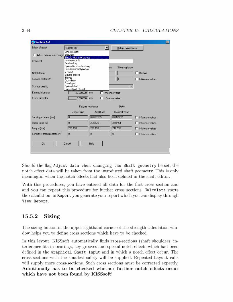
3-44 CHAPTER 15. CALCULATIONS
Should the flag Adjust data when changing the Shaft geometry be set, thenotch effect data will be taken from the introduced shaft geometry. This is onlymeaningful when the notch effects had also been defined in the shaft editor.
With this procedures, you have entered all data for the first cross section andand you can repeat this procedure for further cross sections. Calculate startsthe calculation, in Report you generate your report which you can display throughView Report.
15.5.2 Sizing
The sizing button in the upper righthand corner of the strength calculation win-dow helps you to define cross sections which have to be checked.
In this layout, KISSsoft automatically finds cross-sections (shaft shoulders, in-terference fits in bearings, key-grooves and special notch effects which had beendefined in the Graphical Shaft Input and in which a notch effect occur. Thecross-sections with the smallest safety will be supplied. Repeated Layout callswill supply more cross-sections. Such cross sections must be corrected expertly.Additionally has to be checked whether further notch effects occurwhich have not been found by KISSsoft!
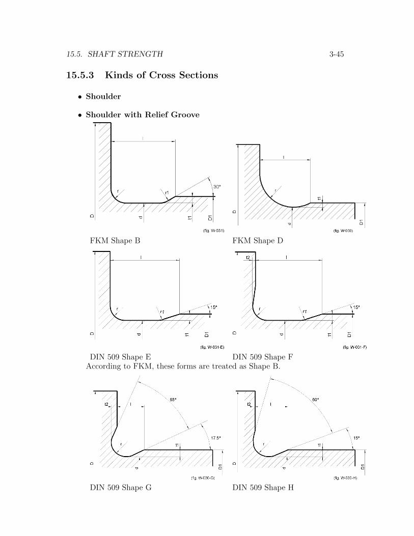
15.5. SHAFT STRENGTH 3-45
15.5.3 Kinds of Cross Sections
• Shoulder
• Shoulder with Relief Groove
FKM Shape B FKM Shape D
DIN 509 Shape E DIN 509 Shape FAccording to FKM, these forms are treated as Shape B.
DIN 509 Shape G DIN 509 Shape H

3-46 CHAPTER 15. CALCULATIONS
According to FKM, these forms are treated as Shape D.
• Shoulder with Conical Transition
• Shaft Recesses
• Thread
Notch factors for threads are treated like those for circumferential grooves.

15.5. SHAFT STRENGTH 3-47
• Interference Fit
(Firm interference fit, light interference fit, interference fit with reliefgrooves)
Figure 15.6: above: interference fit with relief grooves,below: interference fit with exceptions.
• Feather Key
All methods define the section modulus throught the shaft diameter d. Ac-cording to Hanchen, the section modulus is computed from the incorporatedcircle d− t, according to FKM and DIN from the outer shaft diameter.
Notch factors are documented in the different methods, but the methodaccording to Hanchen delivers only sparse information. Within the DINstandard and the FKM-Richtlinie, the respective values are well defined.
Spline tables for cross sections with feather key are included in the program.The data is read from a data file where the standards DIN 6885.1 (corre-sponds to ISO/R 773), DIN 6885.2, DIN 6885.3 are contained. Additionalstandards can be entered by the user.
• Groove-Toothing and splined shaft

3-48 CHAPTER 15. CALCULATIONS
Shapes of splined shafts
Computing groove-toothings or splined shafts requires data of tip and rootdiameter. All other data serve for documentation.
The section modulus is calculated as follows:
According to Hanchen+Decker: from the mean value (da/2 + df/2)According to FKM-guideline and DIN 743: from the root circle
Notch factors are documented in the different methods.
• Cross Hole
• Smooth Shaft
Smooth Shaft sets the notch factor 1. This setting makes sense for crosssections with maximal stress.
• Individually Entering Notch Factors
See chap. 15.5.9.
• Intersecting Notch Effects
See chap. 17.1.
15.5.4 General Inputs
15.5.4.1 Tension Conditions
The tension conditions must be entered, since KISSsoft requires them to split theload into mean load and load amplitude.

15.5. SHAFT STRENGTH 3-49
Greatest stress in a load cycle: σo
Smallest stress in a load cycle: σu
Tension conditions R = σu/σo
Mean stress: σm = (σo + σu)/2= (σo + R · σo)/2= σo · (1 + R)/2
Stress amplitude: σa = (σo − σu)/2= (σo −R · σo)/2= σo · (1−R)/2
For:
Pure alternating stress (σu = −σo) R = −1Dynamic stress (σu = 0) R = 0Static stress (σu = σo) R = 1
Normally valid for rotating shafts or axes:
Bending and shear force: R = −1Torsion and tension/pressure: R = 0 (ev. R = 0 . . . 1)
Limits in the strength calculation according to Hanchen
Contrary to the calculation according to DIN or FKM, which distinguish clearlybetween mean stress and stress amplitude, the strength calculation according toHanchen converts the entered loads into principal stress. These are compared tothe limit of fatigue, which limits the possible inputs. Only changing and staticbendings are possible. The tension conditions define the stress ratio factor (see15.5.5.1).
15.5.4.2 Maximal Load Factor
The static calculation normally uses the greatest possible load. The maximal loadfactor covers the difference between the entered load and the peak value.
Maximal stress: σmax = σo · fmax
For every kind of stress (bending, tension/pressure, etc), factors can be definedindividually.
Example:
Electric motor with a permanent torque 100 Nm, starting torque 180 Nm. Whenentering the shaft data enter 100 Nm and the maximal load factor 1.8.

3-50 CHAPTER 15. CALCULATIONS
15.5.4.3 Thickness Coefficient from Shaft Diameter
Material data depending on diameter result from the effective shaft diameter orfrom the thickness of the raw material. The shaft diameter delivers better safeties,but must only be used if the shaft has been heat treated in pre-turned state.
15.5.5 Calculation according to Hanchen + Decker
Combining methods of different authors is very difficult. To fill existing gaps,experiments or clarifications have to be conducted and, if possible, confirmed byan official office (e.g. the TUV).
KISSsoft computes the strength calculation according to [42].
• Material data
According to figures 52, 56, 60 in [42] for construction-, heat treated andcase hardened steels. Following Hanchen [42], page 37 the admitted alter-nating flexure stress σbw is approximatly σbw = 0.4*σb. The user can pro-gram the material data by implementing data on often used materials inthe database.
• Calculation of the comparative stress
In case of bending and torsion, KISSsoft calculates according to the hy-pothesis of the largest deformation energy in [42], chapter 3.2.5.
• Notch effect
– Thickness coefficient: according to [42], Figure 120
– Surface coefficient: according to [42], Figure 119, Definition of the as-sociated machining process in [42], Table 4.
The following graphs have been implemented into the program:
Coarsely cut out Graph with bo bo = 0, 50 bei 150kp/mm2
milled/finely turned Graph with bo bo = 0, 70 bei 150kp/mm2
ground Graph with bo bo = 0, 94 bei 150kp/mm2
polished Graph with bo bo = 0, 97 bei 150kp/mm2
– Shoulder notch effect coefficient during bending according to [42], Fig-ure 131
– Wheel seat with key: Proposed values after consulting TUV, Munich.Data according to [42], chapter 6.4 are sparse.
– Interference fit: Proposed values after consulting TUV, Munich. Dataaccording to [42], chapter 6.4.

15.5. SHAFT STRENGTH 3-51
– Bearings are treated as weak interference fits, data is sparse in [42],chapter 6.4.
– Splines (Multiple spline teeth): Stress concentration factor and sec-tion modulus according to [42], chapter 8.5 Conversion of the stressconcentration factor into the notch effect coefficient according to [42],chapter 5.6, Formula (36) and (37b) or (37c) with the radius for thesubstituting notch according to [42], Figure 112.
– Threads: Stress concentration factor according to [42], Figure 123.Conversion into notch effect coefficient as above.
• Calculation of safety against fatigue fracture
– Maximal load according to [42] Equation (4a); Service factor accordingto [42] Table 1 (page 24).
– Design fatigue strength under reversed bending according to [42] Equa-tion (42a)
– Safety margin for fatigue fracture according to [42] Equation (46)
– Required safety margin for fatigue fracture according to [42] Figure156 in ”Abhangigkeit der Haufigkeit der Hochstlast” [Depending onthe frequency of the maximum load]
– Result of the calculation is the ratio of the required safety margin andthe calculated safety margin in percent.
• Important formulae:
A) Calculation of the comparative stress (fatigue stress)
σv =√
σ2b + 3(α0τt)2 (15.1)
σb = Mb/Wb (15.2)
τt = Mt/Wt (15.3)
A1) Calculation of the comparative stress (Strength against force ruptureand deformation, but only if τt = 0):
σv =√
(σz + σb)2 + 3(α0(τt + τq))2 (15.4)
σz = Fz/A (15.5)
τq = Fq/A (15.6)

3-52 CHAPTER 15. CALCULATIONS
B) Calculation of the safety margin for fatigue fracture:
σbWG = σbW · bo · bd/bkb (15.7)
SD = σbWG/(σv · f) (15.8)

15.5. SHAFT STRENGTH 3-53
α0 a.0 Stress ratio factorA A Cross-section area (cm3)bd b.d Thickness coefficientbkb b.kb Notch factor (bending)bo b.o Surface coefficientf f Total load factorFq F.q Shearing force (N)Fz F.z Tension/pressure force (N)Mb M.b Bending moment (Nm)Mt M.t Torque (Nm)σb s.b Bending stress (N/mm2)σbW s.bW Fatigue strength under reversed bend-
ing stresses(N/mm2)
σbWG s.bWG Deformation strength under reversedbending stresses
(N/mm2)
σv s.v Comparative stress (N/mm2)SD S.D Margin of safety for fatigue fractureτq t.q Shear stress (shearing force) (N/mm2)τt t.t Torsional stress (N/mm2)Wb W.b Axial section modulus (cm3)Wt W.t Polar section modulus (cm3)
Notice: We recommend printing these explanations for the calculation basisand keeping them together with the actual calculation!
Inputs:
• Stress ratio factor
• Load factor for fatigue resistance calculations
• Load factor for static calculations
• Load frequency
• Nominal safety margin
15.5.5.1 Stress Ratio Factor
The stress ratio factor is used to calculate the principal stress. See also chapters15.5.5 and 15.5.5.

3-54 CHAPTER 15. CALCULATIONS
Suggestion for the stress ratio factor (Hahnchen, p.28 [42] or Niemann I, p.76[60]):
Bending: alternating alternating static static staticTorsion: dynamic alternating dynamic alternating staticStructure steel 0.7 0.88 1.45 1.6 1.0Case-hardened steel 0.77 0.96 1.14 1.6 1.0Heat treated steel 0.63 0.79 1.00 1.6 1.0
15.5.5.2 Load Factor for Fatigue Resistance Calculations
(Method by Haenchen + Decker)
Information on the (total-)load factor f (Hanchen [42], p.24)
f = fun · fbetr · fleb (15.9)
fun Uncertainity about maximal load (1.0 or 1.2...1.4)fbetr Conditions in service (impacts) (1.0 to 3.0)fleb Importance of part (1.0 or 1.2...1.5)
15.5.5.3 Load Factor for Static Calculations
See chap. 15.5.4.2.
15.5.5.4 Load Frequency
The statement refers to the previously entered load (such as torque). If the loadingoccurs during the whole life time of the shaft, the frequency is 100%, otherwiseaccordingly lower.
15.5.5.5 Nominal Safety Margin
The necessary safety margins against fatigue fracture and against forced ruptureor deformation depend both on the calculation method as well as on the type ofapplication.
• Method according to Haenchen/Decker:
The nominal margin of safety against fatigue fracture is calculated accord-ing to Haenchen from the frequency of the maximal load which occurs. Ifthe frequency is 100%, the specified margin of safety is 2.0, at 0% it is 1.0,
15.5. SHAFT STRENGTH 3-55
in between these two extremes the margin of safety does not follow a lineartrend.
The nominal margin of safety against forced rupture is 3.5 to 5.0, dependingon the type of application. The nominal margin of safety against deforma-tion (yield point) is usually 2.0 to 3.5.
15.5.6 Calculation According to DIN 743
The german standard DIN 743 [9] considers the latest knowledge for the calcula-tion of shafts and contains some impressive details which are not summarised inthe current literature and standards.
• Consistent distinction between the different types of loading (ten-sion/pressure, bending, torsion) and between mean stress and stress am-plitude.
• Surface hardening: The influence on the strength is documented when usingthermal methods (nitriding, case-hardening) and mechanical methods (shotpeening, rolling).
• Notch factor: Data for construction elements besides the usual notch factorsare mentioned in all specialised books. This data, such as relief grooves,interference fit with relief groove or square notches (recesses for a Seegerring) is widely used today, but until now it has been badly documented.All notch factors are documented for tension/pressure, for bending and fortorsion.
• Materials: An extensive list of materials, as well as an instruction for thededuction of estimated values for undocumented steels.
• Finite life calculation: based on a proposal for the extension of the DIN 743standard by the FVA, a finite life fatigue strenght calcualtion is available.It has already been included in KISSsoft although it is not yet officiallypart of the standard.
The most essential restraints of the DIN 743 are:
• Shear loading (shear forces) is not considered. This is not a disadvantageexcept for shafts with a very short distance between bearings.
• Only for steels and operating temperatures between −40◦C and +150◦C.

3-56 CHAPTER 15. CALCULATIONS
• Information about the minimum margins of safety is quite inadequate. Therequirements on the margins of safety of vital components should be quan-tified. DIN does not indicate any prescribed nominal margins of safety.
KISSsoft calculates strength exactly according to the latest issue of the DIN 743.Important annotations are printed in the report.
15.5.6.1 Nominal Safety Margin
Acoording to the standard, the prescribed safety margins against bending andfracture are 1.2. However, this safety factor covers only the inaccuracy of theanalysis method. Additional safety factors should be introduced if the damage incase of failure is high of if the load assumptions are not conservative.
15.5.7 Calculating According to FKM
The FKM-guideline (FKM: Forschungskuratorium Maschinenbau e.V., Frankfurt[Board of Research in Mechanical Engineering]) is based on the former GDR-norms and includes the latest knowledge on workshop theory. This guideline willprobably serve as a basis for a new VDI-guideline. The FKM-guideline is verycomplex (approx. 175 pages plus 400 pages annotations), but it allows not onlythe conventional strength calculations but also endurance strength calculationsand service life calculations, and it also includes the consideration of equivalentdesign load and other special problems (e.g. operating temperature above 100◦
C).
The calculation is carried out according to the FKM-guideline, FKM issue 183-2,1994 or FKM issue 183-3, 1998. The limitations are documented in the calculationreport. This calculation method corresponds to the method of Prof. Haibach usingnominal stresses.
Inputs:
• Safety factors according to the FKM-guideline (see chap. 15.5.7.1)
• Temperature (chap. 15.5.7.2)
• Frequency (chap. 15.5.7.3)
• Life limit (number of load changes, chapter 15.5.7.4)
• equivalent design load (chapter 15.5.7.5)

15.5. SHAFT STRENGTH 3-57
15.5.7.1 Safety Factors According to FKM-Guideline
The safety factors for the static strength calculation, jm and jp, are determinedaccording to Part IIG, the safety factor for fatigue resistance, jD, according toPart IIIG. Comprehensive comments are stated in the guideline.
Summary:
Steel jm = 2.0 jp = 1.5 jD = 1.5GS, GGG -not tested jm = 2.8 jp = 2.1 jD = 2.6
-non-destructively tested jm = 2.5 jp = 1.9 jD = 2.4GG, GT -not tested jm = 3.3 jp = 2.6 jD = 3.1
-non-destructively tested jm = 3.0 jp = 2.4 jD = 2.9
jm, jp: The values are valid for - large successive damage because of fracture- large probability of occurrence of load
If the successive damage because of fracture is only small, the safety factors canbe reduced by about 15%. Provided the probability of occurrence is low, thesafety factors can be reduced by about 10%.
jD: The values are valid for - large successive damage because of- irregular inspection
If the successive damage because of fracture is only small, the safety factors canbe reduced by about 15%. Provided inspections are carried out regularly, safetyfactors can be reduced by about 10%.
15.5.7.2 Temperature
The part temperatures are considered in a range from −40 to +500◦C accordingto the FKM-guideline.
For temperatures above 100◦C (for fine grain steels from 60◦C, the reduction ofstrength is considered by temperature factors.
15.5.7.3 Frequency
According to the guidelines, the loading frequency is considered in a range from0 to 100Hz. Below 1 Hz, the frequency factor KFr gets values between 0.9 (below0.1 Hz) and 1.0 (at 1.0 Hz). This considers the lower fatigue limit of steel withlower frequencies.
Important: from the 3rd edition of the FKM-guideline (1998), the frequency factoris no longer used.
3-58 CHAPTER 15. CALCULATIONS
15.5.7.4 Limited-Life
The service strength coefficient KBK,S is determined according to chapter 2.4 ofthe guideline. The cyclic buckling coefficient is ND for 106 load changes (5 ∗ 106
for welded parts).
KBK,S is mostly more than 1.0 if the number of load changes is smaller than ND.Above ND, KBK,S is mostly 1.0.
Normal calculations with a given load (without equivalent design load) is calcu-lated according to chapter 2.4. Three procedures are used to calculate equivalentdesign loads (c.f. the following chapter).
15.5.7.5 Equivalent Design Load
The service strength coefficient KBK,S of equi. design loads is determined as statedin chapter 2.4. You can choose between three calculation methods:
• Miner consequent
• Miner Eurocode (only second edition, 1994)
• Miner elementary
These methods calculate differently the pitch angle of the stress-cycle above thecyclic buckling coefficient.
Use for non-welded parts Miner consequent, for welded parts Miner Eurocode.Miner elementary can be used for all cases, it is more accurate than the othermethods.
Equi. design loads can be defined in the KISSsoft data base tool. In the calcula-tion, you only have to choose them from the list.
The KISSsoft 04/99 uses the percent number of the equi. design load element’sforce component in the same way for all four kinds of load (tension/pressure,bending moment, shearing force and torque). The same factor is used for meanstress and stress amplitude. All equi. design load elements have therefore thesame tension conditions. The simplified procedure can be applied for most cases,if all external forces depend proportionally on the power (e.g. gearbox shafts). Ifthis is not the case, the loads have to be modified by calculating the equivalenttension.

15.5. SHAFT STRENGTH 3-59
15.5.8 Materials
The data of the material which are used for calculating the shaft strength derivefrom the information in the data base as follows:
• Fatigue limit factors (for tension/pressure, bending, etc.) are read di-rectly from the material data base. The values are defined for every calcula-tion method. If data for materials is defined within the calculation method,the data is used.
• Breaking strength factors are stored in the data base depending ondiameter. Based on the raw diameter, the actual breaking strength is readfrom the data base and used for the calculation. This mode is very reliableand valid for all calculation methods. The same values are used for allcalculation methods.
When entering calculation methods, the material data base can be set onthe requirements of the corresponding standards. Then, the real rupturestrength will be determined with the thickness factor from the base rup-ture strength of the sample diameter (normally 10 mm), according to thestandards (FKM or DIN; with Hanchen there will be an error message)
• Yield point or strain limits are determined from the data base or thestandard.
15.5.8.1 Comments on the Term ’Thickness of Raw Material’
Can be selected from the list ’Status during Heat Treatment’, (to determinetechnological influence of size K1 (deff), and from it, the real melting point andbreaking strength):
• When preturned to the real diameter: the raw diameter has no influence;K1 (deff) will be calculated anew for each cross-section based on the actualdiameter
• For Raw diameter: K1 (deff) will be determined once from the raw diameterand used for all cross-sections.
Enter here that dimension of the raw material which is responsible for the finalmaterial characteristics at the last heat treatment.
Examples:
Solid shaft Outer diameter of the unworked partPipe Wall thicknessCast part Largest wall thickness

3-60 CHAPTER 15. CALCULATIONS
Furthermore, it can be defined how the yield strength and the ultimate strengthare defined, see list Choice Material Data
• Material value at reference diameter:Values are taken from database (at reference diameter) and multiplied withK1 (technological size coefficient
• Rm, Rp from data depending on size, sigW at reference diameter:Yield and ultimate strength are taken from database (for respective diame-ter, without adding K1), alternating strength is taken for reference diameterand multiplied with K1.
• Rm, Rp from data depending on size, sigW constant:As above, but alternating strength taken from databse for respective diam-eter, without adding K1
• Rm, Rp from data depending on size, sigW calculated with Rm:Alternating strength is calculated from ultimate strength (according to for-mulas given in DIN/FKM), ultimate strength is taken from database forrespective diameter.
The material is selected in the main window of the shaft calculation module.

15.5. SHAFT STRENGTH 3-61
15.5.8.2 Input data for the Wohler curve
Under Wohler line Data, should the flag Own Input be set, it is possible tointroduce an own Wohler curve. Furthermore, it is here possible to enter thetolerable damage value. With the flag Own Input set to off, the program willuse/define the Wohler curve according to DIN 743 or FKM. The Wohler curveown input, or the adjustment of the tolerable damage value is meaningful, forinstance, when it is necessary to adjust testing calculation results.
15.5.9 Notch Factors
All notch factors are calculated according to the corresponding prescriptions.Details have to be entered in this place. Depending on the calculation method,notch factors can be very different. Another reason for different notch factors isthat some prescriptions for section modulus calculation are different.
To modify notch factors, choose the kind of notch in Input and enter the factorsfor tension/pressure, bending, shearing force and torque.
Annotations:If the kind of notch is set on Own Input, the notch factors which were determinedin the last calculation are displayed in the input fields.
15.5.10 Surface-Factors
Input of surface roughness according to ISO 1302, the corresponding surfaceroughness RZ is displayed in the selection list. For the calculation, RZ is used.
In the calculation according to DIN or FKM, some notch cases have the surface-factors already included in the notch factor. For such cases, the surface factor isalways 1.0 and does not depend on the entered roughness.
15.5.11 Section Modulus
Section moduli are always calculated according to the corresponding procedure.This causes certain kinds of notch having having different section moduli, depend-ing on the procedure. This deviation is documented for feather keys in 15.5.3, forGroove-Toothing in 10.2.4.
Remark to shear stress:Calculation according to the known formula:Shear stress = 4/3∗ shearing force / cross section areafor neutral line.

3-62 CHAPTER 15. CALCULATIONS
15.6 Deformation of Shaft and Calculation of
Gear Crowning
For various purposes, e.g. for the grinding of crowning (in the MAAG manualthis is termed tooth alignment correction), it is important to know how much apoint on the shaft cross-section has moved in a certain direction due to elasticdeformation. This program calculates the displacement in specified intervals alongthe axis, prints the data and saves it on a special data file. Additionally, inmeshing cases the flank line deviation due to deformation is calculated. Thisis required for exact spur gear calculations. Graphical display of the deformingcomponents on screen.
15.7 Transfer of Data to Bearing Calculation
The crucial data for roller bearing calculations such as bearing forces, axial forceand speed, have normally already been entered and computed in the shaft cal-culation and can therefore be transferred without problems. Other values whichare crucial for cylindrical roller bearings are transferred as well.
The data is transferred as soon as in Calculations Roller Bearing or JournalBearing is chosen.

15.7. TRANSFER OF DATA TO BEARING CALCULATION 3-63
The shaft data can be read during the bearing calculation by choosing File ⇒Interface ⇒ Read Shaft Data.

3-64 CHAPTER 15. CALCULATIONS
Chapter 16
Calculating Bearings
16.1 Classification of Bearings
Bearings can be classified according to
• the type of motion in case of gliding bearings, where the gliding motiontakes place between the bearing and the supported part, and in case ofroller bearings where the rolling elements describe a rolling motion.
• the direction of the bearing forces in the cases of radial and axial bearings.
• the function in fixed bearings which can take up shearing forces and axialforces in both directions and in free bearings which allows movement in thelongitudinal direction.
16.1.1 Qualities
The most important characteristics for the operational performance and appli-cation of journal and roller bearings can often be identified by considering theiradvantages and disadvantages.
Rules like when to use journal bearings and when to use roller bearings canhardly be given. The choice of the bearing depends partly on the propertieswhich are determined from the advantages and disadvantages and partly fromthe operational requirements such as size and type of loading, maximum speed,demanded service life and practical experience.
3-65
3-66 CHAPTER 16. CALCULATING BEARINGS
16.1.1.1 Roller Bearings
Advantages: If used correctly, hardly any friction occurs in operation of rollerbearings, therefore the starting torque is only insignificantly larger than its op-erating torque (main advantage in driving units!); the lubricant consumption islow; they are easy to maintain and they do not require a running-in-time; a largedegree of standardisation allows an easy exchange and purchase of roller bearings.
Disadvantages: They are, especially in standstill and at small speeds, sensitiveto impacts and shocks; their service life and the maximum speed are limited; thesensitivity against pollution can require a high expense for sealing the bearing(wear, loss in efficiency!).
16.1.1.2 Journal Bearings
Advantages: Journal bearings are insensitive to impacts and shocks due totheir large, absorbing load and lubrication area; they permit unlimited largespeeds; in the case of fluid friction the service life can be practically unlimited;a split construction allows easy mounting and dismounting; adjustable bearingsyield supreme operational accuracy.
Disadvantages: Journal bearings require a larger starting torque (major dis-advantage!) because of the dry friction that occurs initially; they have a largelubricant consumption and require constant supervision; the efficiency is in gen-eral slightly lower than with roller bearings.
16.2 Calculating Roller Bearings
In the FAG or SKF catalogues one can find quite comprehensive methods for thecalculation of the service life and the static load number of roller bearings. Formore detailed problems specialised technical literature can be used [39].KISSsoft supplies certain data from well-known bearing manufacturers; the usermay extend these data.
Choose Roller Bearing in Calculations in in the starting window of KISSsoft.The crucial data for roller bearing calculation such as bearing forces, axial force,speed have normally already been entered and computed in the shaft calcula-tion and can therefore be transferred. Other values crucial for cylindrical rollerbearings are transferred as well.

16.2. CALCULATING ROLLER BEARINGS 3-67
There is not much to explain here, because the calculation offers many possi-bilities, such as extended service life calculation or equivalent loads; look at theentries under General Data.
Besides the field type in the main window you find, for every bearing, a sizingbutton. This function shows the service life of all bearings of the data base (withtype and diameter). You can choose the best bearing from this list.
16.2.1 Choosing Roller Bearing Type
16.2.1.1 Qualities of Important Bearings
Choosing the aptant roller bearing type is not always easy. The following tablepresents an overview on the important qualities of the important roller bearingtypes.
• Grooved ball bearing (DIN 625):The single row radial grooved roller bearing is the most common because ofits versatile characteristics and the lowest price. This bearing can withstandrelatively high radial and axial forces in both directions.

3-68 CHAPTER 16. CALCULATING BEARINGS
• Single row angular contact ball bearing and four point bearing(DIN 628):
Each ring of a self-holding single row angular contact ball bearing has gota lower and a higher shoulder. The grooves on the higher shoulder areorientated in such a way that the pressure angle totals normally α = 40◦.Due to the larger number of rollers this configuration can not only takeradial forces but also larger axial forces in one direction (towards the highershoulder) than grooved ball bearings. When loading the bearing radially,consider during the sizing that this results in axial reaction forces becauseof the angle of the groove. Because of its one-sided axial loading capacity,these types of bearings are usually installed in pairs where the second oneis mounted in the opposite direction (see also chap. 16.2.10.
• Double row angular contact ball bearing (DIN 628):
The double row angular contact ball bearing corresponds to a pair ofmirror image compounded single row angular contact ball bearings(O-arrangement) with α = 25o and 35o. Thus, this type of bearing can with-stand radial and high axial forces in both directions.
Application: Bearing of the shortest possible bending-resistant shaft withlarge radial and axial forces: worm shafts, shafts with angled spur gears andbevel gears.
• Self-aligning ball bearing (DIN 630):
The self-aligning ball bearing is a double row bearing with a cylindricalor conical bore. (bevel 1: 12), that can compensate shaft dislocation andmisalignment (up to approx. 4◦ angular deviation) because of its hollowsphere race in the outer ring. It can be loaded radially and axially in bothdirections.
Application: Bearings which inevitably are subject to mounting inaccu-racies and bending of the shaft, e.g. transmissions, conveying machinery,agricultural machinery, etc..
• Cylindrical roller bearing (DIN 5412):
Cylindrical roller bearings can support larger radial loads than equally sizedball bearings (point contact area!) as the contact between the roller and therace is made along a line. The dismountable cylindrical roller bearings canonly support small axial loads and require accurately aligned bearings.
16.2. CALCULATING ROLLER BEARINGS 3-69
Depending on the type of rim one distinguishes between the constructiontypes N and NU with an unconfined outer and inner ring, that can beused as free bearings, the construction type NJ as a step bearing and theconstruction types NUP and NJ, that can be used as a guide bearing foraxial shaft support in both directions.
Application: In gearboxes, electric motors, for axles of rail cars, for rollersin a rolling mill, in general for bearing with a large radial load.
• Needle roller bearing (DIN 617):
The needle roller bearing is a special type of the cylindrical roller bearingwhere a cage keeps the needle rollers parallel and separated. The bearing isdelivered with or without an inner ring and is only suitable for radial forces.It can be characterised by its small overall diameter, its large rigidity in theradial direction and by its relative insensitivity against intermittent loading.
Application: Predominantly used with small to medium speeds and oscil-latory motion, e.g. as connecting rod bearings, rocker-shaft bearings, swivelarm bearings, jointed cross-shaft axle bearings (vehicles), spindle bearings,etc.
• Taper roller bearing (DIN 720):
The races of the rings of taper roller bearings are cone-shaped shells whichhave to converge into one point due to the kinematics. The bearings withα = 15◦(30◦) can support high loads both in the radial and axial direction.The detachable outer ring enable easy mantling and dismantling. Taperroller bearings are installed in mirror image pairs and the bearing play canbe set and adjusted if necessary. Because of the angle of the race, a radialforce produces an axial reaction force.
Application: Hub bearings of vehicles, cable pulley bearings, spindle bear-ings of machine tools, shaft bearings of worm gears and of bevel gearings.
Calculation: the axial load which is to be entered when calculating dy-namic equivalent loads is designed exactly according to the theory (c.f. forexample FAG Walzlager Katalog WL 41520DE (1995) on p. 296). The axialload acting on the bearing is displayed in the mask. C.f. 16.2.10. The bearingforces considering the pressure angle can be calculated directly (16.2.8).
• Barrel-shaped and spherical roller bearing (DIN 635):
Spherical races in the outer ring and barrel-shaped rollers, as in self-aligningball bearings, enable barrel-shaped and spherical roller bearings with a
3-70 CHAPTER 16. CALCULATING BEARINGS
cylindrical and conical bore (1:12) to compensate for misalignment andfor the angular dislocation of the shaft (angle0, 5 ◦ to2◦). Barrel-shapedbearings are suitable for high radial but only small axial loads. Sphericalroller bearings (α = 10◦), on the other hand, can be used for the highestradial and axial loads.
Application: For heavy wheels and cable pulleys, propelling shafts, loomof an oar, crankshafts and other heavily loaded bearings.
• Angular contact ball bearings:
Angular contact ball bearings allow very high speeds and are used mostlyin machine engineering spindles.
Calculation: The axial load which has to be entered in the calculationof the equivalent load is calculated exactly according to the establishedtheories (C.f. for example FAG Walzlager Katalog WL 41520DE (1995) aufS. 182). The axial load acting on the bearing is displayed in the interface,c.f. 16.2.10.
16.2.1.2 Comparison of Different Bearings
Which bearing is chosen for given operating conditions is often already deter-mined through the described characteristics and features. For frequently occur-ring operating conditions and in specialised requirements the choice of bearingcan be performed as follows, whereby it is possible that overlapping results occurand then the cost may be decisive.
Guide lines for choosing the bearing design

16.2. CALCULATING ROLLER BEARINGS 3-71
Radial Bearing:
Requirement a b c d e f g h i j k l m nRadial load capability ⊕ ⊕ ⊕ � ⊕ + + + + + + + + +Axial load capability ⊗ ⊕ ⊕ ⊕ � - ⊗ ⊗ - ⊗ ⊗ + ⊗ ⊕Internal position adjustment - - - - - + � - + � - - - -Mounting position adjustment ⊗ ⊗ ⊗ - ⊗ - - ⊗ - ⊗ ⊗ ⊗ ⊗ ⊗Dismountable bearings - - ⊗ ⊗ - + + + + ⊗ - + - -Alignment error adjustment � - - - + � � � - � - � + +High precision ⊗ ⊗ ⊗ � - ⊕ ⊗ ⊗ + - - ⊕ - -High speed running + + ⊗ � ⊕ + ⊕ ⊕ + - - ⊗ ⊗ ⊗Quiet running + ⊕ � � � ⊗ � � ⊗ - - � � �Conical bore - - - - + ⊗ - - + - - - + +Seal on one/both sides ⊕ - ⊕ - ⊕ - - - - - ⊕ - - ⊗High stiffness ⊗ ⊕ ⊕ ⊗ � ⊕ ⊕ ⊕ + + + + ⊕ ⊕Low friction + ⊕ ⊗ ⊕ + ⊕ ⊕ ⊕ + - - ⊕ ⊗ ⊕Fixed bearing ⊕ + ⊕ ⊕ ⊗ - ⊗ ⊕ - ⊗ ⊗ + ⊕ ⊕Floating bearing ⊗ ⊗ ⊗ - ⊗ + ⊗ � + ⊗ ⊗ � ⊗ ⊗
+ very good ⊕ good ⊗ normally/ possible� with restrictions - not suitably
a Grooved ball bearingb Angular contact bearing (single row)c Angular contact bearing (double row)d Four-point bearinge Self-aligning ball bearingf Cylindrical roller bearings NU, Ng Cylindrical roller bearings NJh Cylindrical roller bearings NUP, NJ+HJi Cylindrical roller bearings NNj Cylindrical roller bearings NCF, NJ23VHk Cylindrical roller bearings NNC, NNFl Tapered roller bearingm Barrel Roller Bearingsn Spherical roller bearing
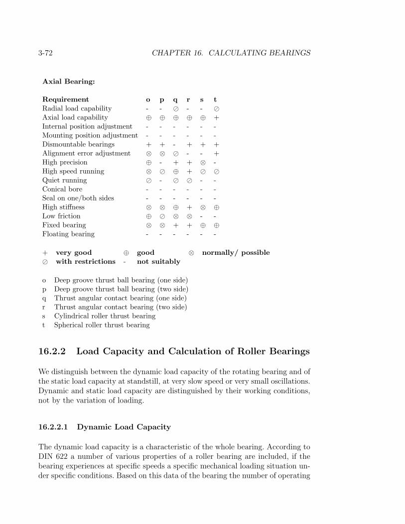
3-72 CHAPTER 16. CALCULATING BEARINGS
Axial Bearing:
Requirement o p q r s tRadial load capability - - � - - �Axial load capability ⊕ ⊕ ⊕ ⊕ ⊕ +Internal position adjustment - - - - - -Mounting position adjustment - - - - - -Dismountable bearings + + - + + +Alignment error adjustment ⊗ ⊗ � - - +High precision ⊕ - + + ⊗ -High speed running ⊗ � ⊕ + � �Quiet running � - � � - -Conical bore - - - - - -Seal on one/both sides - - - - - -High stiffness ⊗ ⊗ ⊕ + ⊗ ⊕Low friction ⊕ � ⊗ ⊗ - -Fixed bearing ⊗ ⊗ + + ⊕ ⊕Floating bearing - - - - - -
+ very good ⊕ good ⊗ normally/ possible� with restrictions - not suitably
o Deep groove thrust ball bearing (one side)p Deep groove thrust ball bearing (two side)q Thrust angular contact bearing (one side)r Thrust angular contact bearing (two side)s Cylindrical roller thrust bearingt Spherical roller thrust bearing
16.2.2 Load Capacity and Calculation of Roller Bearings
We distinguish between the dynamic load capacity of the rotating bearing and ofthe static load capacity at standstill, at very slow speed or very small oscillations.Dynamic and static load capacity are distinguished by their working conditions,not by the variation of loading.
16.2.2.1 Dynamic Load Capacity
The dynamic load capacity is a characteristic of the whole bearing. According toDIN 622 a number of various properties of a roller bearing are included, if thebearing experiences at specific speeds a specific mechanical loading situation un-der specific conditions. Based on this data of the bearing the number of operating

16.2. CALCULATING ROLLER BEARINGS 3-73
hours is calculated (normally this is based on a failure probability of 10%.)
16.2.2.2 Static Load Capacity
The static load capacity includes properties that a roller bearing must fulfill, asto withstand certain mechanical loading situations at standstill, during very slowspeeds (n < 20 min. rpm) or during oscillatory motion.
Plastic deformation (indentation) occurs between the rolling elements and theraces when the bearing is subjected to a moderate static load due to the weightof the shaft and the other elements. The magnitude of the deformation decreasesgradually with an increasing load. Notice that the plastic deformation must notbe as large, as to influence the operational properties of the bearing for its ro-tational movement. The static characteristic value, fs, is a safety factor againstdetrimental plastic deformation which is a measure of the sufficient static loadcapacity. The static load number, which is used to determine the bearing size,can be determined from considering the margin of safety which depends on theoperating conditions:
fs > 2 for shocks and impacts as well as exacting requirements on thesmooth operation and for self-aligning axial roller bearings
fs = 1 for normal operating conditions and requirements on low noisefs = 0, 5 . . . 0, 8 for smooth and non impact operation conditions with light re-
quirements (non-loaded bearing with adjusting or swivel mo-tion)
16.2.3 Thermal limit of operating speed
The definition of the thermal limit of operating speed is described in DIN 732-2(Draft) [8].The calculation of the thermal permissible number of revolutions is based upona heat balance at the bearing. The thermal operational number of revolutionswill be calculated from the thermal reference number of revolutions with the helpof the revolutions ratio. It will determine the number of revolutions that, in aconcrete application case, could be attained within the permissible bearing tem-perature. This limit can differ from other operating speed limits as the referenceconditions only apply to fully defined cases. In order to define the thermal op-erating limit, the reference thermal operating speed has to be defined for eachcase.
3-74 CHAPTER 16. CALCULATING BEARINGS
16.2.3.1 Reference Thermal Operating Speed
The definition of the reference thermal operating speed is defined in DIN 732-1 (Draft) [7]. It is the speed of rotation reached specific to a particular bear-ing arrangement and a given set of nominal operating conditions such that anequilibrium is achieved between heat development (friction) and heat dissipation(through bearing contact and lubrication). Mechanical or kinematic criteria arenot taken into account for this speed.The reference values (temperatures, loads, viscosity of the lubrication, datumface of the bearing,. . . ) are fixed so that the reference speed using oil or greaselubricated bearings will result in identical values.
16.2.3.2 Dissipated Heat Flows
The sum of the dissipated heat flows is calculated from the reference heat flow den-sity specific to a roller-bearing arrangement qSr (for heat flow dissipated throughbearing seat), and qLr (through heat dissipated by lubrication), as well as heatdissipation through the reference face, Asr.Qr = 10−6 ∗ (qSr + qLr) ∗ AsrqSr, qLr and Asr are defined in DIN 732-1.
16.2.3.3 Coefficients f0r and f1r
The coefficients f0r and f1r for the definition of the reference thermal operatingspeed are different dependent upon bearing type/series (also lubrication type forf0r). They are shown in Table 2 of the standard. Not all bearing variants areconsidered in the table (e.g. bearing construction).
16.2.3.4 Calculation of the reference thermal operating speed
So that the energy balance of the bearing is correct, the dissipating heat flowsand the friction are set as equal. The equation for energy conservation is:
NFr = 103 ∗Qr
The subsequent equation becomes:
(π∗nθr)/30∗(10−7∗f0r∗(νr∗nθr)2/3∗dm3 +f1r∗P1r∗dm) = (qSr+qLr)∗ASr
nθr: Reference thermal operating speed [1/min]f0r: Coefficient from Table 2, DIN 732-1 [-]r: Reference viscocity [mm2/s]dm: Average roller-bearing diameter [mm]
16.2. CALCULATING ROLLER BEARINGS 3-75
f1r: Coefficient from Table 2, DIN 732-1 [-]P1r: Reference load [N]qSr: bearing specific reference heat flow density (Bearing Seat) [kW/m2]qLr: Roller bearing specific reference heat flow density (Lubrication) [kW/m2]ASr: Reference surface area dissipating heat [mm2]
The value nθr can be determined from the equation.
16.2.3.5 Calculation procedure for the reference thermal limit of op-erating speed according to DIN 732-2
As in the calculation of the reference thermal operating speed, this calculation isbased on an equilibrium in the bearing. Dissipating Heat Flow:Q = QS + QL + QE
QS: Dissipating heat flow from the bearing seat surfaceQL: Dissipating heat flow from lubrication (only through circulation) (Density ρ= 0,91 kg/dm3 and specific heat capacity cL = 1,88 KJ/(kg∗K) of the lubricationare pre-defined.)QE: Additional heat flows (fort he calculation QE = 0 is assumed)
16.2.3.6 Friction Coefficients f0 and f1
The coefficient values f0 and f1 as well as the dynamic equivalent Load P1 are onlyrequired for the definition of the load and lubrication parameters, and are differ-ent dependent upon bearing type/model, lubrication, or load direction. They areshown in Table 3 of the standard. Not all bearing variants are considered in thetable (e.g. bearing construction). For ball-bearings or spherical roller-bearings,the finalised standard 732-2 will be further extended. However, in KISSsoft themissing data from the FAG Catalogue has been withdrawn. From the notes aboutf0 in Table 3 in the Standard, the following values have been defined (and incor-porated in KISSsoft) for various types of lubrication:
• Oil, splash lubrication, bearing in oil mist: f0 = 0,5 * f0 (Table Value)
• Oil, splash lubrication, oil level to the middle of the bearing: f0 = 2,0 * f0(Table Value)
• Oil, splash lubrication, oil level to the lowest rolling body: f0 = 1,0 * f0(Table Value)
• Oil, circulated lubrication: f0 = 2,0 * f0 (Table Value)

3-76 CHAPTER 16. CALCULATING BEARINGS
• Grease, run-in bearing: f0 = 1,0 * f0 (Table Value)
• Grease, newly greased: f0 = 2,0 * f0 (Table Value)
16.2.3.7 Calculation of the reference thermal limit of operating speed
The reference thermal limit of operating speed is calculated from the referencethermal operating speed with the help of the speed ratio, fn. nθ = fn ∗ nθr
So that the speed ratio can be iterated from the following equation, the load andlubrication parameters have to be calculated.
KL ∗ fn5/3 + KP ∗ fn = 1
Load Value KL:
KL = 10−6 ∗ (π/30) ∗ nθr∗10−7 ∗ (f0r ∗ ν2/3 ∗ nθr2/3 ∗ dm3)/Q
Lubrication Value KP:
KP = 10−6 ∗ (π/30) ∗ nθr∗(f1 ∗ P1 ∗ dm)/Q
nθr: Reference thermal operating speed [1/min]f0: Coefficient of friction from Table 3, DIN 732-2 [-]f1: Coefficient of friction from Table 3, DIN 732-2 [-]ν: Viscocity of the lubrication [mm2/s]dm: Average roller-bearing diameter [mm]P1: Reference load [N]Q: Sum of the dissipating heat flows [kW]
16.2.4 Friction Moment
The thermal development, and consequently the operating temperature, in aroller bearing comes from the friction between the individual components. Themoment of friction in the roller bearing is indicated by several distinct lossesthrough resistance during operation.
16.2.4.1 The calculation according to SKF Catalogue 2004
Because there are so many factors and influences taken into consideration forthis calculation, only those specific to the extended life time calculation will becovered. For any others, the moment of friction will be defined according to themethod of the 1994 SKF catalogue (see 16.2.4.2). The calculation of the totalmoment of friction according to the 2004 SKF catalogue is determined by a

16.2. CALCULATING ROLLER BEARINGS 3-77
combination of rolling and sliding friction in the roller contacts (between rollingelements and cage, the bearing surface, the lubricant, and the sliding frictionfrom grinding seals caused in sealed bearings). The calculation of the moment offriction depends upon various factors:
• Load
• Bearing type
• Size of bearing
• Operating speed
• Properties of the lubricant
• Amount of lubrication
• Sealing
The following operating conditions allow calculation:
• Grease or oil lubrication (oil bath, oil mist, or oil injection process)
• Load equal to or larger than the minumum load
• Load constant in size and direction
• Nominal clearance during operation
The formula for the total moment of friction is:
M = φish*φrs*Mrr + Msl + Mseal + Mdrag
φish: Lubricant film thickness factorThrough the formation of a lubricant flow the lubricant is exposed to shearingthrough the movement of the the rolling elements, and produces heat which as aconsequence reduces rolling moment of friction.
φrs: Lubricant displacement factorThe excess lubricant is pushed away from the contact zone of the rolling elementsthrough constant rolling action. This reduces the lubricant film thickness anddecreases the moment of friction.
Mrr: Rolling moment of frictionThe rolling moment of friction is dependent upon the type of bearing, the av-erage diameter, the radial and axial loading, the rotation speed, and viscosity

3-78 CHAPTER 16. CALCULATING BEARINGS
of the lubrication. The factors for the calculation are taken from the 2004 SKFcatalogue.
Msl: Sliding moment of frictionThe rolling moment of friction is dependent upon the type of bearing, the averagediameter, the radial and axial loading, and viscosity of the lubrication. The factorsfor the calculation are taken from the 2004 SKF catalogue.
Mseal: Moment of friction for grinding sealsThe rolling moment of friction is dependent upon the type of bearing, size ofbearing, the diameter of the seal-lip mating surface, and the layout of the seal.Because the type of seal, diameter of the seal-lip mating surface, and the layout ofthe seal are different according to each manufacturer, they are not yet definablein KISSsoft and consequently the moment of friction for grinding seals is set to0.
Mdrag: Moment of friction determined through lubrication lossesThis moment of friction is caused by flow, splash, or injection losses during oilbath lubrication. Because the lubrication type, as well as the condition of the oil,are not yet definable in KISSsoft, the value for the moment of friction determinedthrough lubrication losses will be set to 0.
16.2.4.2 The calculation according to SKF Catalogue 1994
In a bearing, the friction moment shows the losses due to the resistance to move-ment. Prerequisites for the calculation of the friction moment are that the bearingrotating surfaces be separate by a lubrication film. The total bearing friction mo-ment results from the sum:
M = M0 + M1 (16.1)
M0: load-independent friction moment
M0 is conditioned by the lubricant hydrodynamic loss. It is predominant in fastrunning bearings under light loads. The M0 value depends upon the lubricant’squantity and viscosity, as well as the rolling speed.
M1: load-dependent friction moment
M1 is conditioned by the elastic deformation and partial sliding between thecontact surfaces. It is mainly predominant in slow running bearings under load.The M1 value depends upon the bearing type (bearing-dependent exponents forthe calculation), the decisive load for the friction moment and the mean bearingdiameter.

16.2. CALCULATING ROLLER BEARINGS 3-79
For axially loaded cylindrical roller bearings, an additional axial load-dependentfriction moment M2 will be introduced in the formula:
M = M0 + M1 + M2 (16.2)
M2: axial load-dependent friction moment
M2 depends from a coefficient for cylindrical roller bearings, from the axial loadingand from the bearing mean diameter.
Independent from bearing type and loading, the factors f0, f1 and P1(valuesdepending from the bearing type and load) used for the calculations are takenfrom DIN 732-2 (see Chapter ??). The formulae, exponents and coefficients aretaken from the SKF Catalogue, issue 1994.
16.2.5 Maximal Speed
Roller bearings are safe and can be exspected to reach the calculated service lifeas long as a maximal speed (speed limit) is not exceeded. Service life also dependson construction, size and lubrication.
If the maximum permissible speed is exceeded, a warning is issued.
16.2.6 Service Life
16.2.6.1 Extended Service Life Calculation
• According to FAG Catalogue data (1999)
The extended life expectancy will be calculated according to the FAG Cat-alogue data, diagrams, etc..
Calculation of a23:
a23 = s · a23II (16.3)
s: Diagram to determine the purity coefficient sa23II: Diagram base values a23II (with K and κ)κ: = nu/nu1
nu1: Diagram reference viscositynu: V-T-Diagram of lubricantK: Diagram for K1 and for K2
Remarks:
3-80 CHAPTER 16. CALCULATING BEARINGS
– Factor K1: Needle and barrel shaped roller bearings are treated likeball bearings.
– Impurity characteristic quantity V depends on the cross section of thebearing, type of contact and purity class of the oil; see table p. 46 inFAG-catalogue WL41520DE, edition 1995.
• According to supplement to DIN ISO 281 (2003)
The supplement to DIN ISO 281 contains the regulations for the ’modi-fied life expectancy’ in order to consider the influence of loads, lubricantconditions, materials specifications, design, material internal stresses andenvironmental factors.
The life expectancy factor aDIN can be determined as follows:
aDIN = f(ec ∗ Cu/P, κ) (16.4)
aDIN : life expectancy factor from the diagram [-]ec : dirtiness characteristic value [-]Cu : fatigue load limit [N]P : dynamic equivalent load [W]κ: viscosity ratio = nu/nu1
nu1: reference viscosity diagram [mm2/2]nu: lubricant V-T diagram [mm2/2]
Bearing manufacturers supply the fatigue load limits Cu. Should no valuesbe know, calculate them with the approximate formula in the DIN ISO281.The dirtiness characteristic value ec (between 0 and 1), will be directlydetermined from the degree of cleanliness.Should these determining function values be known, the aDIN values mightbe read from the correspondent diagram.
16.2.6.2 Service Life Calculation with Equivalent Design Load
The equi. design load acting on the bearing has the following data:
k: Number of elements of the equivalent design loadqi: Frequency (equivalent design load element i) (%)ni: Speed (equivalent design load element i) (UpM)Fri: Radial force (equivalent design load element i) (N)Fai: Axial force (equivalent design load element i) (N)

16.2. CALCULATING ROLLER BEARINGS 3-81
Achievable service life for equal operating conditions:The service life is calculated via determining an equivalent design load and meanspeed. With these data the service life is determined with the usual formulae.
nm =n1 · q1
100+
n2 · q2
100+ . . . +
nk · qk
100(16.5)
Pm =p
√P p
1 · q1
100+
P p2 · q2
100+ . . . +
P pk · qk
100(16.6)
nm: Mean speedp: Exponent in the service life formula (3.0 and 3.333 respectively)Pi: Dynamic equivalent load (equivalent design load element i)Pm: Mean dynamic equivalent load
Achievable service life for variable operating conditions:When applying the Extended service life calculation, the service life iscalculated separately for every equivalent design load element and from this thetotal service life is determined:
Lhna =100
q1
Lhna1+ q2
Lhna2+ . . . + qk
Lhnak
(16.7)
Lhnai: Service life (equivalent design load element i) at the speed ni
and at load Fri, Fai
Lhna: Total service life
16.2.7 Failure Probability
Normally, the failure probability is assumed 10%. This means that the nominalservice life is reached with a probability of 90%. In this case the factor a1 is equalto 1.0; if the failure probability has to be lower, this factor is also lower (with1%, a1 is equal to 0.21).
The failure probability can be defined in Settings ⇒ module-specific.
16.2.8 Calculating Bearing Forces Considering the Pres-sure Angle
Roller bearings with angular runways (taper roller, angular contact ball and highprecision angular contact ball bearings) create an angular direction of pressurefrom the reaction forces. The actual point of support for the calculation of thebearing forces is therefore not in the middle of the bearing (like with normal roller

3-82 CHAPTER 16. CALCULATING BEARINGS
bearings); it is where the angular force through the middle of the bearing meetsthe shaft axis.
For the input of the supporting points in KISSsoft, the middle of the bearing hasto be given. After the input of a roller bearing with askew pressure direction, itis possible to carry out the calculation under consideration of the pressure angle.In that case, KISSsoft shifts the centre of the bearing by itself, calculates thereaction forces and then displays the modified results. The saved geometry datawith the centre of the bearings are not modified, therefore the type of the rollerbearing can be changed easily.
16.2.9 Bearings with Radial and/or Axial Force
For each bearing can be stated whether radial or axial forces are acting on it. Ifaxial force acts on the bearing, you have to state additionally whether the force isacting in both directions (<>), in direction of the y-axis (− >) or in the oppositedirection (> −).
16.2.10 Calculating Axial Forces on Bearings in O- or X-Arrangement
Because of the grading of shaft in the bearing, the radial load causes axial reactionforces in taper roller bearings, high precision angular contact ball bearings andangular contact ball bearings which have to be considered when analysing theequi. design load.
Axial reaction forces are computed according to SKF (roller bearing catalogue)which is more comprehensive than the FAG.
For bearings in 0-arrangment, left bearing A, right bearing B, outer axial forcein A-B direction:
Condition Formula
FrA
YA
≤ FrB
YB
FaA = Fa +FrB
2YB
FaB = Fa − FaA
FrA
YA
>FrB
YB
FaA = Fa +FrB
2YB
Fa >1
2(FrA
YA
− FrB
YB
) FaB = Fa − FaA

16.3. CALCULATING JOURNAL BEARINGS 3-83
FrA
YA
>FrB
YB
FaA = Fa − FaB
Fa ≤1
2(FrA
YA
− FrB
YB
) FaB =FrA
2YA
− Fa
FrA, FrB Radial force on bearing A, B
YA, YB Y -Factor of bearing A, B
Fa External axial force
FaA, FaB Axial force on bearing A, B
For all other cases, the reversed formula is valid.
These calculated pre-tension are shown in the main window. If the actual internalforces are higher, e.g. through using spring packages, the value can be changedmanually.
16.3 Calculating Journal Bearings
16.3.1 Hydro Dynamic Radial Journal Bearings (W07)
Niemann [60] provides a very accurate method for the calculation of radial journalbearings for fast operation. This method gives quite accurate approximations forother journal bearings.
DIN 31652 [33] is a good method for the calculation of stationary, hydro dynamicradial journal bearings for small and average speed.
16.3.1.1 Calculation methods
Calculating oil lubricated hydro dynamic radial journal bearings according to twodifferent methods:
a) According to G. Niemann, Machinery Elements I, 1984 This method is suit-able for fast rotating bearings. Also for special types of bearings, such aspatches, the results are quite good.The method calculates the power loss, amount of oil, oil temperature, min-imal lubricant gap thickness according to [60] and [54].

3-84 CHAPTER 16. CALCULATING BEARINGS
b) According to DIN 31652 [33], part 1 - 3, 1983This method is good for slow rotating bearings. It determines also the oilconsumption, mass flow and the complete heat balance.Calculation according to DIN 31652, part 1 to 3 (edition 1983) for pres-sureless and pressure lubricated bearings.
16.3.1.2 Calculating the Volume-Specific Heat of Lubricants
The volume-specific heat of lubricants can be calculated in two ways:
• Considering the temperature dependence
• Simplified assumption (DIN 31652): 1.8 · 106J/(m3K)
16.3.1.3 Coefficient of Expansion
To calculate the clearance, the coefficients of expansion fo shaft and hub arerequired.
Steal 11.5 · 10−6
Cast iron 11 · 10−6
White metal 18 · 10−6
Composite bronze 18 · 10−6
16.3.1.4 Mean Surface Pressure and Circumferential Speed
Specifications of permissible values in
• Niemann, Volume I, Table 15/1, [60]
• DIN 31652, Part 3, Table 2, [33]
Permissible maximal values for surface pressure
- White metal-bearing: 1...3 N/mm2
- Bronze : 1...8 N/mm2

16.3. CALCULATING JOURNAL BEARINGS 3-85
Figure 16.1:1: One lubrication hole, 180◦ C to load direction.2: One lubrication hole, 90◦ C to load direction.3: Two lubrication holes, 90◦ C to load direction.

3-86 CHAPTER 16. CALCULATING BEARINGS
Figure 16.2:4: Lubrication groove (circular groove).5: Lubrication groove (circumferencial groove).Remark: For lubrication with a circular groove, the calculation is done for eachbearing half with half of the load! (See also [33], part 1, paragraph 3.4).

16.3. CALCULATING JOURNAL BEARINGS 3-87
Figure 16.3:6: One lubrication pocket, 180◦ C to load direction.7: One lubrication pocket, 90◦ C to load direction.8: Two lubrication pockets, 90◦ C to load direction.

3-88 CHAPTER 16. CALCULATING BEARINGS
16.3.1.5 Lubrication Arrangement
(compare to DIN 31652, part 2, paragraph 2.5)
16.3.1.6 Sink Heat Surface
Suggestion: 10 · d · b . . . 20 · d · bd : Bearing diameterb : Bearing width
16.3.1.7 Heat Transfer Coefficient
Suggestion: 15 . . . 20 (W/m2K)
16.3.1.8 Oil Temperatures
Oil output temperature:
• Normal case approx. 60◦ C
• Upper limit for usual mineral oils: 70− 90◦ C
Oil input temperature:
• With the usual cooler: 10◦ C lower than the output temperature
• With very good cooler: 20◦ C lower
16.3.1.9 Sizing Bearing Clearance
Bearing clearance = D-boring – D-shaft
• Suggestion according to NiemannSuggestion for metal bearing in mechanical engineering according to Nie-mann, volume I, table 15/2.
For other materials following values should be applied:
Grey iron bearing : 0.001 · dLight metal bearing : 0.0013 · dSintered bearing : 0.0015 · dPlastic bearing : 0.003 · d
d : Bearing diameter

16.3. CALCULATING JOURNAL BEARINGS 3-89
• Suggestion according to DIN 31652Suggestion for metal bearing in mechanical engineering according to DIN31652, part 3, table 4 [33].In this sizing method either the proposal according to DIN 31652 can beadopted, or the backlash calculated from the given output temperature(only for sink heat through lubricant).
• Suggestion according to K.SpiegelSuggestion according to K.Spiegel: Goettner-EquationBacklash: (2.5+50.0/D)/1000.0*D
16.3.1.10 Sommerfeld Number
The Sommerfeld number is calculated. It is an important characteristic value.
Sommerfeld number > 1 occurs for bearings in the heavy load statelimit for b/d: 0 < b/d ≤ 2
Sommerfeld number < 1 occurs for bearings in the fast rotating statelimit for b/d: 0.5 < b/d ≤ 2
16.3.1.11 Bearing Width
Clue for the bearing width in Niemann, volume I, table 15/1Normal range: B/D = 1 . . . 2
Clue for the bearing width according to DIN 31652Normal range: B/D = .125 . . . 1
16.3.1.12 Permissible Lubricant Film Thickness
The suggestion stems from DIN 31652, part 3, table 1. This table contains empir-ical values and prescribes a mean roughness depth < 4µ, small shape derivationand sufficient filtering of the lubricant.
¨
16.3.2 Axial-Journal Bearings (W07C)
In the DIN standard there are two types of calculation depending upon the con-struction of sliding bearings.
3-90 CHAPTER 16. CALCULATING BEARINGS
• Calculation of pad thrust bearings according to DIN 31653 [34]: This stan-dard applies to bearings with defined sunken surfaces for lubrication (seeFigure 1), which are separated from the rotating disks by a lubrication film.
• Calculation of tilting-pad thrust bearings according to DIN 31654 [35]: Themoveable tilting pads to which this standard applies are also separated fromthe rotating disks by a lubrication film.
If an influence from the centre of pressure is anticipated on the tilting-pad thrustbearings, a similar calculation procedure is described in both standards, howeverthe calculation will only be described here once. Any significant deviations to befound in either standard will be mentioned.
16.3.2.1 Calculations
Essentially, both calculation procedures are based on the equation for thermalbalance in the bearing. Both convection and lubrication circulation can be se-lected for calculation:
• Non pressure lubricated bearings (self-lubricating) dissipate heat (by con-vection) to the environment. The thermal expansion coefficient factor kAaccording to the standard is between 15. . . 20 W/(m2*K). A nominal valueof 20 W/(m2*K) is used by the software, but this can become altered.
• Pressure lubricated bearings dissipate heat predominantly through the lu-brication. Here, a mixing factor has to be defined that lies in the range 0. . . 1.Through experience, values between 0,4 and 0,6 are found to be more appli-cable. The value of 0,5 is assumed by the software, but this can be changed.Formula with the mixing factor: ∆T1 = ∆T2 * (Q2 / (M*Q+(1-M)*Q3))
The results of the calculations are the friction, the smallest film thickness, andthe operating temperature. For circulated lubrication the lubrication flow rate isalso calculated.
The bearing force (in stand) is only, used for the sizing, of the thinnest admissiblelubricant film thickness. The value of the load coefficient, the friction coefficient,and the lubrication flow rates are calculated according to the formulas (not ac-cording to the diagram or table) in DIN 31653/ 31654 part 2. For tilting-padthrust bearings, the ratio hmin/Cwed from the support position of the tilting-pad aF* is calculated. The formula for which can be found in DIN 31654 part2.
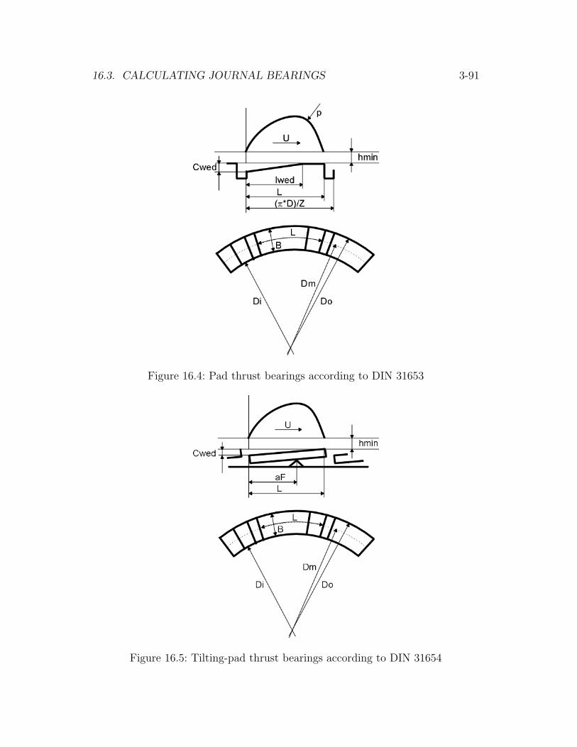
16.3. CALCULATING JOURNAL BEARINGS 3-91
Figure 16.4: Pad thrust bearings according to DIN 31653
Figure 16.5: Tilting-pad thrust bearings according to DIN 31654
3-92 CHAPTER 16. CALCULATING BEARINGS
16.3.2.2 Sizings
The bearing force (nominal load) can also be determined. For this all other inputparameters are required. The bearing force is then calculated using the givenvalue for the smallest possible lubrication film thickness, hlim.The smallest possible lubrication film thickness can be defined according to DIN31653 or 31654. The appropriate formula will be calculated depending on sliding-speed, average diameter, and the relative strength.
By convection:If the heat sink surface is not known, an formula for approximation is specifiedin the standard:A = (15...20) ∗B ∗ L ∗ ZThe sizing button next to the interface field calculates A = 15 ∗B ∗ L ∗ Z.
By circulation:The exit temperature through experience is ca. 10 to 30 K higher than the entrytemperature. For the sizing, an exit temperature of +10 K is used.
16.3.2.3 Calculation of the Volume-Specific Heat of the Lubrication
The volume-specific heat can be calculated under Setup/Module-Specific intwo ways :
• Consideration of temperature dependency
• Simplified assumption (as in DIN 31652): 1.8 ∗ 106J/(m3 ∗K)
16.3.2.4 Limiting Values in the Calculation
The standard is restricted to laminar flow for which a suitable Renold-number iscalculated in the program. For this the Renold-number must be lower than thecritical value of 600.Further, the results are checked for highest permissible bearing temperature,Tlim, the smallest possible film thickness, hlim, and the specific bearing load.These values are defined in the standards 31653/ 31654 part 3.

Chapter 17
Answers to most FAQs
Some FAQs are answered in this chapter.
17.1 Intersecting Notch Effects
Intersecting notch effects should be avoided when designing a shaft. If notcheffect occurs, however, the total notch effect coefficient Kf has to be calculated,according to FKM, from the partial notch effect coefficient Kf1 and Kf2:
Kf = 1 + (Kf1 − 1) + (Kf2 − 1) (17.1)
For this case, KISSsoft provides the possibility to set the notch effect to Own
Input.
For further information see chap. 15.5.3.
The calculation of the total notch effect factor Kf can take place as follows:
1. Define two cross-sections (e. g. A-A and B-B) with the same coordinates
2. Calculate Kf1 for the cross-section A-A selecting a notch type (e. g. Shoul-der). Then, under Details ⇒ Effect of notch select the notch type(Shoulder). To display the notch factors, set the Flag Display under Notchfactor on.
3. Repeat the procedure in 2. for cross-section B-B.
4. Take note of the notch factors for both individual notches and calculate Kfwith the above-mentioned formula.
3-93

3-94 CHAPTER 17. ANSWERS TO MOST FAQS
5. Now, deactivate both cross-sections A-A and B-B (set Flag Active off),and activate a third cross-section C-C with the same y-co-ordinates. UnderDetails select the notch form Own Input and enter the total notch effectfactor calculated in 4.
17.2 Notch Effects on Hollow Shafts
The notch factors stated in the norms were determined for solid shafts. For hollowshafts, no data is available. KISSsoft calculates the nominal stresses for hollowshafts with the section modulus, considering the inner diameter.
17.2.1 Notches on the Outer Contour
For ’small’ inner diameters, the error of the calculation with the notch effectvalues for solid shafts is relatively small, the results can serve as approximations.For ’large’ inner diameters, the notch effect values have to be corrected.
According to the FKM-Guidelines of 1998, the notch effect values of a round staffwith longitudinal hole for bending and tension/pressure cannot be calculatedcorrectly from the notch effect values of a round staff without. Use for torsionand round staffs with circumferential notch, shoulder or cone the notch effectvalue of a round staff without hole, but with nominal stress for a round staff withlongitudinal hole.
17.2.2 Notches on the Inner Contour
For notches on the inner contour, the notch factors of the calculation methodsare not suitable.
17.3 Fatigue Limits for New Materials
If a new material is to be entered in the data base, the permanent strengthis required besides the mostly already existing data for yield point and tensilestrength.
Approximation to the limit of fatigue (according to Hanchen):
σbW ≈ 0, 495 · σB

17.3. FATIGUE LIMITS FOR NEW MATERIALS 3-95
Hanchen also states approximations according to other methods. For tension-/pressure fatigue limit, he states:
σzdW ≈ 0, 45 · σB oder σzdW = 0, 5 . . . 0, 6 · σB
and for torsion fatigue limit:
τtW ≈ 0, 55 · σbW oder τtW = 0, 4 . . . 0, 5 · σbW
According to DIN 743, the following approximations are valid:
σbW ≈ 0, 5 · σB σzdW ≈ 0, 4 · σB τtW ≈ 0, 3 · σB
According to the FKM-Richtlinie, for heat-tretable steels (other values are givenfor other steels), the following values may be used:
σzdW ≈ 0, 45 · σB τtW ≈ 0, 26 · σB

3-96 CHAPTER 17. ANSWERS TO MOST FAQS

Part IV
Gears
4-1

Chapter 18
Gear Calculation in General
18.1 Handling
To be able to use the program effectively, the user must have a basic understand-ing of gear technology and related topics. The strength calculations are carriedout according to norms (DIN 3990, ISO 6336, etc.). Knowing these norms is use-ful, but not absolutely necessary to use the program correctly. In most cases, theprogram is protected against unreasonable input.
Furthermore, it is necessary to have some knowledge about gear technology, asyou have to interpret the results. In general, one can say that, according to DIN3990, part 11 (Industrial gear boxes), a safety factor for the root of 1.4 and asafety factor for Hertzian stress of 1 is sufficient. The definition of the individualvariables corresponds to the toothing- geometry-norm DIN 3960 and DIN 3971,3975 or 5480 respectively and have to be looked up in case of uncertainty.
Warning: The ease of use and the help system may lead to the conclusion that thesizing of gears has become unproblematic with this program and that the expertis dispensable. We must emphasise that this assumption is wrong. Expertise isessential when working with KISSsoft!
18.2 Overview on the Gear Wheel Part
In the manual you will find information about the following gear types:
• Spur Gears: chap. 19with configurations
– Pair gear wheel
4-3

4-4 CHAPTER 18. GEAR CALCULATION IN GENERAL
– Planetary set
– 3- or 4-gear wheels
– Rack with pinion
– Single gear wheel
• Bevel and hypoid gear calculations: chap. 20
• Face gears: chap. 21
• Worm gears: chap. 22
• Cross helical gears/worms precision mechanics: chap. 23
• Splinted joints DIN 5480: chap. 24
Chapter 25 lists FAQs / Answers as well as an index of abbreviations.

Chapter 19
Spur Gears
19.1 KISSsoft-Gear-Configuration
4-5
4-6 CHAPTER 19. SPUR GEARS
19.2 Calculation-Basis
Spur gears (spur and helical gears) are calculated according to DIN 3960. In mostbooks and standards, calculation methods for geometry calculation are quite sim-ilar. Additionally to the calculation of geometry, inspecting for defects (undercut,too short usable involute, etc) is very useful; information can be found in spe-cialised textbooks of tool- or tool-machine producers.The calculation of tooth thickness tolerances, allowances, and backlash is carriedout according to Standards such as ISO1328 (Edition 1970) or DIN 3967. Man-ufacturing tolerances are alternatively calculated according to ISO 1328, AGMA2015, DIN 3961 or DIN58405 (also see Section 19.7.4).Strength calculation with re-calculation of usual defects (tooth fracture, pitting,scoring) is carried out e.g. according to DIN 3990 or ISO 6336. This norm includesthe most comprehensive and detailed calculation method at present. To calculatethe safety against scoring, two methods can be used. The safety against scor-ing according to the integral-temperature method is employed mainly in vehiclemanufacturing, while the flash-temperature method is used for turbo gear-boxes.Which of these two methods proves to be more reliable is not clear yet.
The strength calculation according to AGMA 2001 is required in the USA. Thiscalculation method is very different from the calculation according to DIN 3990;the results are not comparable. Furthermore, for plastic gear wheels, several cal-culation methods are available.
The problem of DIN 3990 is its huge variety of calculation methods. BetweenMethod A (exact calculation combined with measurements) and Method D (roughsizing), there are about 10 different calculation variants. It is therefore not sur-prising that, with different re-calculations according to DIN 3990 or ISO 6336of the same gear, different results are can issued. For these calculation proce-dures, KISSsoft uses, if possible, the most detailed formulae for the pre-and post-calculation, which is Method B. The results of different calculation programs canshow huge differences. A detailed research, from where these differences comefrom is very complicated. It is therefore more elegant to use a reference program.Such a program could be, for instance, the spur gear program package ST+ ofFVA (Forschungsverein Antriebstechnik, Fed. Rep. of Germany) of the TechnicalUniversity of Munich. In KISSsoft, an option FVA-calculation is available. Withthis option, the results are the same as with the official FVA-program calcula-tions. The differences between the results in KISSsoft and the FVA-program arevery small; the reason are the minor derivations of the FVA-program from theregular version of DIN 3990. Several documents on this comparison are availableto our users upon demand.
Special Calculation: Calculation According to Niemann [61]

19.3. INPUT INTERFACES 4-7
• Tooth loss power with tooth loss degree HV according to (21.11/4)
• Mean coefficient of friction µm according to (21.11/6) with 1 ≤ vt ≤ 50m/s
• Tooth loss power PVZ according to (21.11/3)
19.3 Input Interfaces
The spur gear pair calculation has different main interfaces for the configuration’cylindrical gear pair’ and other configurations (planetary, three and four gears).There are also some subwindows for special inputs.
19.3.1 Main Windows for Cylindrical Gear Calculation
19.3.1.1 Windows for cylindrical gear pairs
Figure 19.1: Main Window for cylindrical gear pairs

4-8 CHAPTER 19. SPUR GEARS
The user may use KISSsoft mainly from the page Basis Data, even if the inputfacilities are on several tabulator pages of the cylindrical gear pair interface. Thegeometry--manager can help experienced users to achieve the results faster.(see19.3.2)
19.3.1.2 Windows for other configurations
Figure 19.2: Main window for cylindrical gear calculation (single wheel, 3/4 gearsor planetary trains)
The main window for all other spur gear configurations (single wheel, 3/4 gearsor planetary trains) corresponds to the uppermost tabulator of the pair window.There are several variants to enter wheel data for up to four wheels and up tothree wheel pairs. Depending on the configuration, only some of the input fieldsare activated.
The different tabulatorsides are missing in this place. Speed and torque havetherefore to be entered over a subwindow (19.3.1.12) and the tolerances for wheeldata can only be accessed by button T.
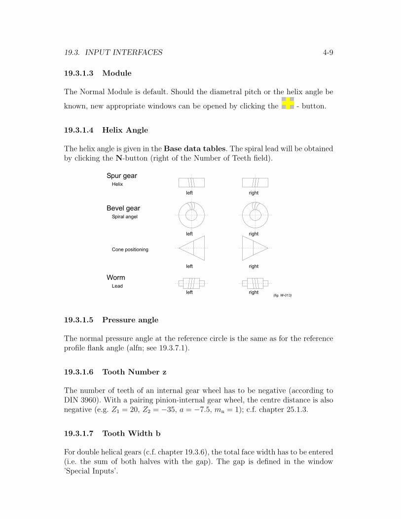
19.3. INPUT INTERFACES 4-9
19.3.1.3 Module
The Normal Module is default. Should the diametral pitch or the helix angle be
known, new appropriate windows can be opened by clicking the - button.
19.3.1.4 Helix Angle
The helix angle is given in the Base data tables. The spiral lead will be obtainedby clicking the N-button (right of the Number of Teeth field).
19.3.1.5 Pressure angle
The normal pressure angle at the reference circle is the same as for the referenceprofile flank angle (alfn; see 19.3.7.1).
19.3.1.6 Tooth Number z
The number of teeth of an internal gear wheel has to be negative (according toDIN 3960). With a pairing pinion-internal gear wheel, the centre distance is alsonegative (e.g. Z1 = 20, Z2 = −35, a = −7.5, mn = 1); c.f. chapter 25.1.3.
19.3.1.7 Tooth Width b
For double helical gears (c.f. chapter 19.3.6), the total face width has to be entered(i.e. the sum of both halves with the gap). The gap is defined in the window’Special Inputs’.
4-10 CHAPTER 19. SPUR GEARS
19.3.1.8 Addendum Modification Coefficient x
See chapter 19.3.7.1.
19.3.1.9 Material
The indicated materials are taken from the material database. If the desiredmaterial cannot be found there, Own Input can be chosen or the material can beentered in the database tool! (c.f. 7.)
Stress analysis with uncommon materials:
For the analysis of spur gear strength according to ISO 6336, DIN 3990 or AGMA2001, only certain (frequently used) materials and heat treatments are described:
• Heat treatable steel
• Case-hardening steel
• Nitriding steel
• Structural steel
• Cast iron with spherical graphite
• Cast iron with laminar graphite
Materials which are not described in the strength calculation standards:
• Stainless steel, alloys of aluminium and of bronze
These materials are treated like treatable steel. This has an influence on severalless important values which are used to calculate the permissible tooth root stressand flank strength, but the maximal possible error is very small.
Plastics
Plastic gear wheels are calculated according to Niemann. The permissible stressesand the Young’s modulus of plastics depend on the temperature and other factors.Determining the material data is therefore very difficult. For the time being, onlyfor the following materials exist reliable data:
• POM, PA12, PA66
• Laminated fabric

19.3. INPUT INTERFACES 4-11
• Moulded laminated wood
Further materials can easily be added, as all the specific data are contained indata-sets in the material data-base. For new plastics (e.g. fibre reinforced andothers), it is difficult to obtain the required data from the manufacturer. Tocalculate gears made of a material X not contained in the above list, a simplifiedprocedure can be used.
With the manufacturer, the following must be checked:
• Which material is the most similar to material X?
• If the strength of the material X for gear wheels (root, flank) is equal, higheror lower than the strength of the reference material.
Example:
• Used material: Delrin; Power 1.5 kW
• The manufacturer states that Delrin is similar to POM, but is stronger bya factor of 1.2.
• Calculate gears with KISSsoft and use POM as material. Reduce the nom-inal power by a factor of 1.2 (1.25 instead of 1.5 kW).
19.3.1.10 Centre distance
see 19.3.8.1
19.3.1.11 Application Factor
The application factor considers uncertainties in load and impacts. It is alwayslarger than or equal as 1. A hint for the factor can be found in the following tableand more comprehensive information is available in DIN 3990, DIN 3991 or ISO6336.
Working condition Working condition of the driven machineof the driving Uniform Moderate Medium Heavymachine Moderate Impact Impact ImpactUniform 1.00 1.25 1.50 1.75Moderate Impact 1.10 1.35 1.60 1.85Medium Impact 1.25 1.50 1.75 2.00Heavy Impact 1.50 1.75 2.00 2.25

4-12 CHAPTER 19. SPUR GEARS
DIN 3990, part 41 (motor gear boxes) distinguishes between an application factorfor flank strength (KAH) and root strength (KAF) (c.f. 19.3.1.13). All calculationsexcept flank strength calculations use the application factor KAF.
The application factor according to DIN 3990, part 41, can be smaller than 1to avoid calculations with equi. design load. DIN 3990, part 41, appendix A,proposes the following values for a 4–gear automobile gear box:
Gear R 1 2 3 4NL 105 2 · 106 1.5 · 107 3 · 107 2 · 108
KAH 0.65 0.65 0.65 0.65 –KAF 0.70 0.70 0.80 0.80 –
19.3.1.12 Lifetime
19.7.14
19.3.1.13 Power,Torque and Speed
The three values power, torque and speed which are to be entered depend on eachother. With the select-button, you can assign Lowest priority to a value; thisvalue is then calculated from the other two. In precision mechanics the power ismostly given in W instead of kW. If the given number of digits is to small for theinput the units can be changed with the right mouse button (see chap. 2.2.1).The input data refer to the selected reference wheel. For the cylindrical gearpair calculation all data can be directly input in the main window: for othercalculations (single wheel, chain wheels and planetary gear trains) a subwindowmust be called.
From the main window, this window (see 19.3) can either be opened by the field
behind Power or by the field N next to the wheel-specific inputs.
If the number of teeth is already defined, speed and torque of the inactive gearis calculated from the active one.

19.3. INPUT INTERFACES 4-13
Figure 19.3: The power-window in the cylindrical gear calculation
If tooth numbers have already been entered, speed and torque of the deactivatedwheel are calculated from the activated one.
Epicyclical Gearboxes
As epicyclical gearboxes have two degrees of freedom, an additional speed has tobe given. In conventional planetary gear trains with unmoving internal rim, thespeed of the rim is set to 0 rpm.
Figure 19.4: The power-window in the planetary gear calculation.

4-14 CHAPTER 19. SPUR GEARS
19.3.1.14 Strength Calculation Methods (Spur Gears)
The following methods are available:
1. Only Geometry
Should this method be selected, the strength calculation will not be per-formed. Thus, all the input data which are only required for the strengthcalculation (like power, application factor, etc.) will not apply.
2. Static strength calculation
In the static strength calculation, the occurring bending stresses are com-pared with the yield point and the breaking strength of the material.
There is no standard for this calculation; the method derives from DIN3990.
All factors (application factor, face load coefficient, transverse coefficient)are 1.0. The load on the tooth root is calculated with tooth form factor,helix angle factor and contact ratio factor according to method C (withoutstress correction factor).
Additionally, the stress resulting from multiplying the local foot root stressby the stress correction factor Ys, will also be calculated. This stress approx-imately corresponds to a normal stress as calculated with a FEM-Model.This stress will be shown in the protocol.
3. ISO 6336, 1996 edition, parts 1, 2, 3, 5
’Calculation of load capacity of spur and helical gears’All calculations are generally based on Method B, the tooth form factorcan be calculated according to Method B or C. (For internal gears MethodC, otherwise Method B is recommended.) See also chap 25.2.3.
4. DIN 3990, 1987 edition, parts 1, 2, 3, 4, 5, etc
’Calculating the permissible stress on spur gears’All calculations aregnerally according to Method B, the tooth form factorcan be calculated according to Method B or C. (For internal gears MethodC, otherwise Method B recommended). See also chap 25.2.3.
5. DIN 3990, 1987 edition, part 41
’Calculating the permissible stress for automobile gearboxes’Generally according to method B, but two application factors have to beentered for the display of equi. design loads. (c.f. 19.3.1.10)
6. US-standard AGMA 2001-B88, edition 1988
(see item AGMA 2001-C95)

19.3. INPUT INTERFACES 4-15
7. US-Standard AGMA 2001-C95, edition 1995
The latest edition of the US calculation standard AGMA 2001-C95 replacesthe former version AGMA 2001-B88. Since many companies still calculateaccording to the old version, it is still considered acceptable. The differencesbetween the new and old standard and are small, the calculation of theservice factor has been introduced in the new one.
The strength calculation for spur gears is calculated according to theUS-standard ANSI/AGMA 2001-B88. The standard is completely imple-mented. The proposal for the dynamic coefficient and the face load coeffi-cient are calculated according AGMA, but the proposal according DIN 3990can also be used. Geometry coefficients (for root and flank) are calculatedaccording ANSI/AGMA 908-B89.
The output includes, besides all the relevant intermediate results:Pitting Resistance Power Rating, Contact Load Factor, Bending StrengthPower Rating, Unit Load for Bending Strength, Service Factor.
The calculation can be used for all gear configurations (including planetarygear trains). Please notice that the AGMA instruction does not allow cal-culating the root strength of internal gears. In this case, use the graphicalmethod to calculate; c.f. chapter 19.4.2.
8. US-Standard AGMA 6004-F88
Special USA Norm for the stress of open gear rims. The calculation methodis fundamentally based on the AGMA 2001 one, with the difference that,for special applications, some individual coefficients are preestablished.
9. Plastics according Niemann
10. Plastics according to experimental formulae
(still in development)
11. VDI 2545, Edition 1981 ’Gear wheels made of thermoplastics’
Calculating plastic gears or plastic gears paired with steel gears. The toothform factor is calculated according to method C.
Calculating tooth root and the tooth flank safety margin for spur gearsmade of plastics according to methods in Niemann, [61].
The calculation method for plastics especially considers the extremetemperature-dependence of these materials. As lubricant, you can chooseoil, grease or dry running.
The material permissible load will be determined from data tables, basedupon the local temperature at the tooth flank and at the tooth root, as well

4-16 CHAPTER 19. SPUR GEARS
as the load cycle number. The local temperature can be calculated fromthe calculation method (for lubrication with grease or dry running; forlubrication with oil, the local temperature is equal to the oil temperature).Should this automatic temperature determination be undesirable, it canbe deactivated (deactivate (Settings ⇒ Module-specific ⇒ Calculate
contact temperature). In this case, le local temperature for grease andoil lubrication will be made equal to that of the lubricant; for dry running,that of the ambient.
The calculation can be carried out for pairing plastic/plastic as well as forsteel/plastic. The permissible deformation is also analysed. To the followingmaterials data are present in KISSsoft:
KISSsoft contains data for the following materials:
• Moulded laminated wood
• Laminated fabric
• Polyamide (PA12, PA66)
• Polyoxymethylen (POM)
All specific characteristics of the materials are stored in tables (text format);integrating own materials is very simple (c.f. chapter 7).
The strength of plastic gears can be calculated according to Niemann (Nie-mann und Winter, Maschinenelemente, Band III) or according to VDI2545(1981) (tooth form factor according method B or C). In addition, a mod-ified calculation method according to VDI 2545 is available. This methodcalculates the tooth root stress with the stress correction factor Ys. Themain differences between the several calculation methods are:
Root: accord. Niemann accord. VDI2545 accord. VDI2545-mod.YF method C method B or C method B or CYS (analog ISO6336) set to 1.0 (analog ISO6336)Yε set to 1.0 ∗4 = 1/εα
∗3 = 1/εα∗3
Yβ set to 1.0 (analog ISO6336) (analog ISO6336)σFE = 2 ∗ σFlim = σFlim = 2 ∗ σFlim
Flank: accord. Niemann accord. VDI2545 accord. VDI2545-mod.Zε set to 1.0 (analog ISO6336) (analog ISO6336)ZV (analog ISO6336)∗1 set to 1.0 set to 1.0ZR (analog ISO6336)∗2 set to 1.0 set to 1.0
deform. teeth: different calculation method!∗1: only laminated wood, else 1.0∗2: only pairs metal/plastics, else 1.0

19.3. INPUT INTERFACES 4-17
∗3: if tooth form factor YF according method B: 1.0∗4: The method sets 1.0 as contact ratio factor for the tooth root stress. Ac-cording to Niemann, this is done because material data are mostly uncertain. Ifthe material treatment is set to optimal (in Settings ⇒ Module-specific ⇒General), the contact ratio factor is calculated according to ISO 6336 MethodC.
12. Calculation in analogy to the FVA-spur-gear-calculation-program
Issues the same results as the reference program of the ’FVA’. Bases onDIN 3990, Method B, with small deviations.
13. ISO 9085 Industrial Gears
Calculation basically in accordance to ISO 6336, Method B and partially C;the suggested equations for industrial gears, in accordance with ISO 9085,are used.
19.3.2 Geometry-Manager
(only with gear pairs available)
Figure 19.5: Geometry-Manager.
Unlike classical machine engineering, where mostly a given standard referenceprofile is used, precision mechanics often changes the reference profile. In theGeometry-Manager, there are listed, besides the addendum modification, root-/tip circle, tooth width and the reference profile. Immediately after the entries

4-18 CHAPTER 19. SPUR GEARS
have been made, the program calculates. In this way, the tooth form can quicklybe optimised without having to open new subwindows.
Dark red marks highlight errors, fields which cause error-messages, however, arehighlighted light red. Error–messages and warnings are displayed if Calculate
is activated. To generate a report, execute Calculate as well. In the Geometry-Manager, only the theoretical toothing is calculated, the calculation of the toler-ance values is executed by Calculate.
19.3.3 Tolerances
(only with gear pairs available)
Figure 19.6: Entering tolerances in the Pair-Window.
In the tabulatorside Tolerances you can enter the tooth thickness deviationsand the axis distance deviations. Choose either a tolerance row from the lists orswitch to Own Input. Details to tolerance inputs in chapter 19.3.7.3.
19.3.4 Tolerance-Settings
(only with gear pairs available)
In the tabulatorside Tolerance--Settings you can enter the number of teeth tomeasure and the ball/rollerdiameter. C.f. chapter 19.3.7.3.

19.3. INPUT INTERFACES 4-19
19.3.5 Lubrication
The type of lubrication (except dry running) has hardly any influence on theresults of the calculation. Exceptions are:
• Plastic gear wheels
• Worm gears
• Appreciable influence on the safety against scoring
The characteristics of the lubricant (especially the viscosity) has a major influenceon the scoring and little influence on the margin of safety on the flank. The scoringimpact level is determined by using a special test according to FZA. The rangeis between 1 and 12. For gear lubricants, the level is usually above 12. The valuein the data base should be set to 12 for this case.
The displayed lubricants are listed in the data-base. If you cannot find a suitablelubricant in this place, enter it first in the data-base or choose Own Input.
Temperatures for the calculations
For oil or grease lubrication, the input of Lubricant Temperature defines the ba-sic temperature of the gear body. Ambient Temperature has no influence on thecalculation. The Lubricant Temperature is the needed input for the calclationof the effective oil viscosity. For dry running, the input of Ambient Temperature
defines the basic temperature of the gear body. Lubricant Temperature has noinfluence on the calculation.
Exceptions:
• Worm gears: The ambient temperature is an input for temperature safetycoefficient calculation.
• Plastic gears: As the resistance data of plastic gears depends strongly onthe gear body temperature, the introduction of the temperature (Lubri-cant Temp., respectively Ambient Temp.) is very important. See chapter19.3.1.14, subchapter VDI2545 calculation method: The VDI-norm pro-poses for palstic gears lubricated with grease or dry-running a specialmethod for the calculation of the actual gear body temperature.

4-20 CHAPTER 19. SPUR GEARS
19.3.6 Special Inputs
• Type of profile modification
You can make corrections on the theoretical involute (profile modification).Proposals for profile modifications (for spur gears) can be obtained usingKISSsoft module Z15 (c.f. 19.7.1). The type of profile modification has animpact on the calculation of the scoring safety. The Distribution factor (orForce Distribution factor) XGam is calculated differently depending on thetype of profile modification. There is a significant difference between caseswith ’no profile correction’ and with ’any profile correction’. The differencebetween profile correction ’for high power gears’ and ’for uniform mesh’however is not so important. The calculation procedure requires that theCa (of the profile correction) is sized according to the applied forces, butdoes not indicate an exact value. (With KISSsoft module Z1x a proposalfor Ca can be obtained.)
Distribution factor XGam (following DIN3990) depending upon theprofile modification, yields following results:
fig.1: for gears without profile fig.2: for gears with modificationmodification for high power gears -
if pinion is driving

19.3. INPUT INTERFACES 4-21
fig.3: for gears with fig.4: for gears with modificationmodification for high power for uniform mesh gearsgears - if gear is driving
• Load distribution coefficient
For gear configurations with load distribution, the distribution of the loadmay vary due to manufacturing tolerances. This is taken into account bythe load distribution coefficient.
Often, 1.0 is entered for this coefficient as ideal distribution is assumed.
More information can be found in Niemann [61], figure 22.5/2d. Niemannsuggests employing values between 1.05 and 1.3, depending on the qualityof toothing and mesh speed.
Remark:For gear wheel pairings or racks, the load distribution factor can be smallerthan 1.0 as only a part of the power is transmitted over the toothing.
• Number of lanes (or planets)
Load distribution over how many lanes (number of intermediate gears). Incase of planetary gear trains number of planetary gears.
• Permissible pitting
The building up of a small pitting on the flank may be permissible in certaincases. This can result in slightly higher margin of safety in the service lifefor the flank if case-hardened materials are employed.
• Double helical gearings
These are spiral gears consisting of two tooth halves, one with right-handand the other with left-hand helix.
For double helical gearings, the total face width has to be entered (i.e. thesum of both halves with the gap). The gap is the spacing distance betweenthe two halves forming the gear.
• Transmission accuracy level number
AGMA 2001-C95 includes a procedure to calculate the accuracy number(depending from the pitch accuracy). This procedure is included in theKISSsoft calculation also for the older version AGMA 2001-B88.
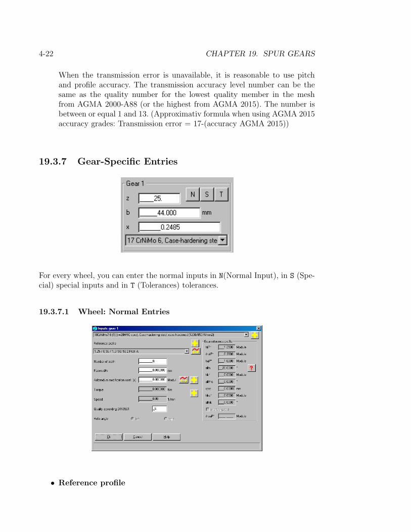
4-22 CHAPTER 19. SPUR GEARS
When the transmission error is unavailable, it is reasonable to use pitchand profile accuracy. The transmission accuracy level number can be thesame as the quality number for the lowest quality member in the meshfrom AGMA 2000-A88 (or the highest from AGMA 2015). The number isbetween or equal 1 and 13. (Approximativ formula when using AGMA 2015accuracy grades: Transmission error = 17-(accuracy AGMA 2015))
19.3.7 Gear-Specific Entries
For every wheel, you can enter the normal inputs in N(Normal Input), in S (Spe-cial) special inputs and in T (Tolerances) tolerances.
19.3.7.1 Wheel: Normal Entries
• Reference profile

19.3. INPUT INTERFACES 4-23
The displayed reference profiles are contained in the data base. If you requirea different reference profile, enter it in the data base - or in the list in Own
Inputs.
The data for the reference profile correspond to DIN 867 or DIN 58400. Thedata are referred to as tool proportion of the gear. The numbers represent(in the following order):
– Dedendum of gear (in module) (hfP: normal 1,25)
– Root radius (in module) (ρfP: normal 0,20)
– Addendum of gear (in module) (haP: normal 1,00)
– Pressure angle (αn (input in the main window)
– Protuberance height (in module) (hkP; no data: no protuberance)
– Protuberance angle (αnP; no data: no protuberance)
– Protuberance height spro (indicated as a check)
– Buckling root flank hight (in module) (hk0; no data: no buckling rootflank)
– Buckling root flank angle (αnP; no data: no buckling root flank)
– Tip radius ρaP (only with interfering tools)
The reference data in mm can be obtained by multiplication with the nor-mal module.
Important:
– For the tool reference profile, ha is changed to hf and ρa to ρf (accordingto chap 19.6.1.2).
– If the reference profile is set to Own Input, the modification of tipdiameter (chap. 19.3.7.2) will be set to zero.
– Important Note: To get the correct tip and root diameter, whenusing BS4582-1, Basic rack 2, you must introduce a correspondingtooth thickness allowance [As] of −0.1572∗Module! (Then the effectivetip and root diameters are according the formulas of BS4582-1(8)).
Thus, by change-over, the tip diameter can change.
The buckling root flank serves to generate useful profile corrections at thetooth tip. Sized correctly, (c.f. chap. 19.7.1), it does not diminish the trans-verse contact ratio in loaded state. Because of this, the influence of thebuckling root flank on the transverse contact ratio is mostly not consideredin the calculation. For large values it has to be considered, the treshold

4-24 CHAPTER 19. SPUR GEARS
value for consideration of protuberance or buckling root in the calculationof contact ratio can be adjusted under Settings ⇒ module-spezific ⇒calculations (see chap. 19.4.6.10).
If a prefabrication tool with protuberance is used, you can enter the ma-terial allowance for the prefabrication under Tolerances (c.f. 19.3.7.3). Inaddition, from the definition of reference profile it is possible to give thein-feed depth and radius of a griding wheel (see 19.8).
For profile corrections (difference of angle less treshold value, see chap.19.4.6.10) the height of buckling root hk0 will not be changed from prefab-rication to the resulting reference profile. For a buckling root with a greatdifference of angle (chamfer) the height hk0 will be changed with the finish-ing treatment. (See *4 at following figures: left flank with equal hk0, rightflank with buckling root only in prefabrication)
For better understanding some figures show:
– Reference profile of gear
– Measurement of tool for corresponding gearwheel
– Reference profile of gearwheel at prefabrication with a hob and finish-ing with grinding
Figure 19.7: Left figure: reference profile of gear; Right figure: Measurement ofhob (tool) with data of reference profile of the gearwheel
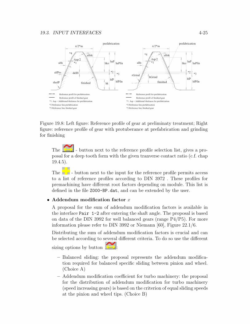
19.3. INPUT INTERFACES 4-25
Figure 19.8: Left figure: Reference profile of gear at preliminaty treatment; Rightfigure: reference profile of gear with protuberance at prefabrication and grindingfor finishing
The - button next to the reference profile selection list, gives a pro-posal for a deep tooth form with the given tranverse contact ratio (c.f. chap19.4.5).
The - button next to the input for the reference profile permits accessto a list of reference profiles according to DIN 3972 . These profiles forpremachining have different root factors depending on module. This list isdefined in the file Z000-BP.dat, and can be extended by the user.
• Addendum modification factor x
A proposal for the sum of addendum modification factors is available inthe interface Pair 1-2 after entering the shaft angle. The proposal is basedon data of the DIN 3992 for well balanced gears (range P4/P5). For moreinformation please refer to DIN 3992 or Niemann [60], Figure 22.1/6.
Distributing the sum of addendum modification factors is crucial and canbe selected according to several different criteria. To do so use the different
sizing options by button :
– Balanced sliding: the proposal represents the addendum modifica-tion required for balanced specific sliding between pinion and wheel.(Choice A)
– Addendum modification coefficient for turbo machinery: the proposalfor the distribution of addendum modification for turbo machinery(speed increasing gears) is based on the criterion of equal sliding speedsat the pinion and wheel tips. (Choice B)
4-26 CHAPTER 19. SPUR GEARS
– According DIN3992: this standard only sets a vague range for theaddendum modification and is therefore not recommended. (ChoiceC)
– Range of the permissible addendum modification according to MAAG[56]: in the MAAG-Gear book (2nd edition, 1985, Zuerich) a com-plicated procedure is described that leads to a range within which,according to MAAG, a sensible addendum modification is achieved.KISSsoft shows the proposed range (from . . . to) and issues addition-ally the mean value of this interval. (Choice D, E, F)
– The addendum modification for peak limit. The proposal refers onlyto the chosen wheel, the program does not check wether the resultingaddendum modification is also true for the counterwheel. The minimaltooth tip thickness can be entered at Settings ⇒ Module-Specific
⇒ General⇒ Minimal factor for tooth tip thickness(ChoiceG)
– The addendum modification for undercut limit. The proposal refersonly to the chosen wheel, the program does not check wether the result-ing addendum modification is also true for the counterwheel. (ChoiceH)
• Calculating the addendum modification from measured data
The - button starts the calculation of the addendum modification onthe basis of measured data or data from drawings.
The addendum modification can be calculated from the following:
– Base tangent lengthFor this, the face width and the number of teeth has to be entered.
– Ball measurement over two balls (or rollers)For this, the measurement and diameter of the body (ball or roller)have to be entered. The ball measurment differs from the roller mea-surement for helical gear forms and odd tooth numbers (see ThreeRoller Measurement).
– Three Roller MeasurementFor this, the measurement and the diameter of the rollers must begiven. For odd tooth numbers and helical tooth form this relates di-rectly to the measurment over two rollers.
– Tip diameterThis calculation is not very accurate as the tip diameter not onlydepends on the addendum modification.

19.3. INPUT INTERFACES 4-27
– Tooth thickness at pitch diameterFor this, tooth thickness and additionally, either entered as curvelength or chordal, transverse or normal section have to be entered.
Important: The entered data is used to calculate the production adden-dum modification. If a tooth thickness deviation is input, the programcalculates the theoretical addendum modification. For no deviation bothaddendum modifications are equal.
• Tooth quality according to ISO 1328
The tooth quality according to ISO 1328 is about the same quality as inDIN 3961 or BS 433/2.
The following qualities are achievable:
Manufacturing method QualityGrinding 2 . . . 7Chafing 5 . . . 7Planing (5)6 . . . 9Milling (5)6 . . . 9Ramming (5)6 . . . 9Slotting, Sintering 8 . . . 12
Converting qualities according to AGMA:
Quality according to ISO according to AGMA 390.031 152 143 134 125 116 107 98 89 710 611 5

4-28 CHAPTER 19. SPUR GEARS
19.3.7.2 Wheel: Specific Entries
• Drawing number
• Tip circle
The modification of the tip circle results in the tip diameter and vice-versa. Usually, KISSsoft conducts a sensible modification of tip diameteraccording to DIN 3960 (depending on the addendum modification). If youwish to change this value you can do so. KISSsoft warns you if your datais outside of the permissible boundaries.
Entering the tip circle sizes the reference profile. When changing the adden-dum modification, you can keep your tip circle by acivating option 19.4.1.8.
• Tip diameter deviations
• Modification of tip diameter
Modifications of tip diameter are made for a sum of addendum modifica-tions not equal zero to achieve sufficient tip clearance and to avoid contactinterference.
Normally, KISSsoft computes the tip diameter modification according toDIN 3960. You can enter values manually if you deactivate this automation.(Settings ⇒ Module-Specific ⇒ General; see too Kap. 19.4.1.3). For apair of external gears the modification of tip diameter is less that zero
19.3. INPUT INTERFACES 4-29
while for an internal gearing the modification of tip diameter is positivefor both gears, but KISSsoft won’t use a positive value for an internal gearautomatically, it will be set to zero instead.
If the reference profile is set to Own Input, the tip diameter modification isset to zero for the corresponding gear.
• Root circle
The root circle is usually determined by the reference profile. If you enterthe root circle, the tip height of the reference profile is changed accordingly.KISSsoft warns you if your data is outside of the permissible boundaries.You can enlargen these boundaries (c.f. 19.4.1.2).
Notice: If you change e.g. the addendum modification, the root circle ischanged as well. The reference profile remains the same. You can, however,keep your root circle by activating option 19.4.1.9.
• Root circle deviations
(Important: ) In normal production, the root circle deviations result fromthe tooth thickness deviations.
• Number of load cycles
KISSsoft calculates the number of load cycles by speed and demanded ser-vice life. If you wish to change this value manually, you can do so. Thereare four variants:
1. Automatic The number of load cycles is calculated automaticallyaccording lifetime, speed, and number of lanes/planets.
2. Number of load cycles The number of load cycles is input directly.
3. Load cycles per revolution The number of load cycles per revolu-tion is input. For planetary gears with tree planets this would be treefor the sun and 1 for the planets.
4. Load cycles per minute The number of load cycles per minute isinput. This can be used for racks or gear pairs with many changes inrotation sense where no speed can be defined.
5. Effective length of rack The given length of rack is used for thecalculation of the number of load cycles. The length of the rack shouldbe greater than the circumference of the gear or it has to be consideredthat not all teeth of the gear come into contact.
For a pinion-rack pairing, a value must be input. Otherwise, the value willbe set to NLRack = 1/100 NLPinion.

4-30 CHAPTER 19. SPUR GEARS
• Tip and Foot relief
You find proposals for tip and foot relief under Calculations⇒ Addendum
modification Z15 (c.f. 19.7.1). The values input Ca for tip relief and Cffoot relief have an insignificant influence on the dynamic coefficient (onlyat high gear quality) and the calculation of scoring.
• Alternating bending factor
The tooth root strength is sized for dynamic load. In special cases, however,the tooth root has to cope with alternating bending stresses, (e.g. the planetgear in a planetary gear train). In this case, the coefficient has to be reducedfrom 1.0 to 0.7 (according ISO, DIN or AGMA)! Niemann recommendsfor plastics, 0.8 for laminated fabric and 0.667 for PA (nylon) and POM(Polyacetal).
See also figure 19.9.
Figure 19.9: Alternating bending factor according to Linke [55]
• Inner diameter of gear
The inner diameter of the gear is required for the calculation of inertia.The influence on the result of the analysis is relatively small. Enter 0 for

19.3. INPUT INTERFACES 4-31
solid wheels and for hollow gears with rim the corresponding diameter asin figure 19.10 (di). For internal gears, the outside diameter of the gear rimis entered.
Figure 19.10: Measures of diameters.
• Rim inner diameter of gears
This value is required for the calculation according AGMA. The influenceon the result of the analysis is relatively small.
See figure 19.10 (dbi).
• Chamfer/ tooth end
Figure 19.11: Chamfer/ tooth end
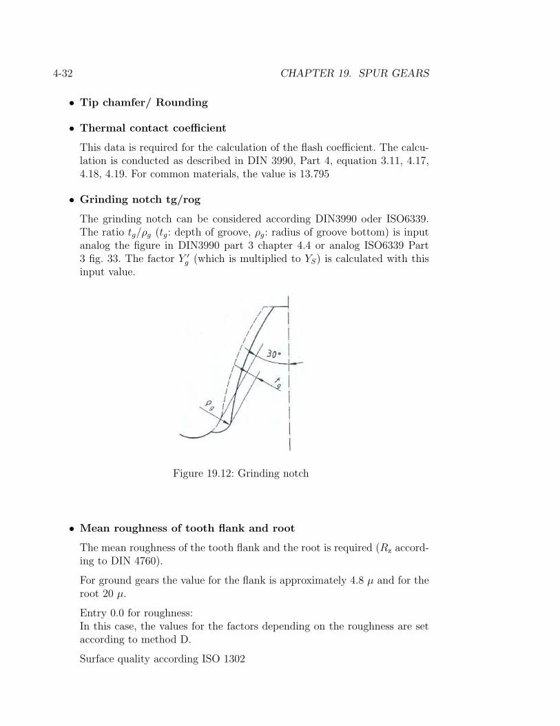
4-32 CHAPTER 19. SPUR GEARS
• Tip chamfer/ Rounding
• Thermal contact coefficient
This data is required for the calculation of the flash coefficient. The calcu-lation is conducted as described in DIN 3990, Part 4, equation 3.11, 4.17,4.18, 4.19. For common materials, the value is 13.795
• Grinding notch tg/rog
The grinding notch can be considered according DIN3990 oder ISO6339.The ratio tg/ρg (tg: depth of groove, ρg: radius of groove bottom) is inputanalog the figure in DIN3990 part 3 chapter 4.4 or analog ISO6339 Part3 fig. 33. The factor Y ′
g (which is multiplied to YS) is calculated with thisinput value.
Figure 19.12: Grinding notch
• Mean roughness of tooth flank and root
The mean roughness of the tooth flank and the root is required (Rz accord-ing to DIN 4760).
For ground gears the value for the flank is approximately 4.8 µ and for theroot 20 µ.
Entry 0.0 for roughness:In this case, the values for the factors depending on the roughness are setaccording to method D.
Surface quality according ISO 1302

19.3. INPUT INTERFACES 4-33
Class Roughness (µ) ProcedureRa Rz Rt
N1 0.025 0.3 0.6N2 0.05 0.6 1N3 0.1 1.1 1 Lapped/PolishedN4 0.2 1.8 1.6 Lapped/PolishedN5 0.4 2.8 2.5 HonedN6 0.8 4.8 2.5 GroundN7 1.6 8 4 Turned with diamondN8 3.2 16 4 MilledN9 6.3 32 8 Turned
N10 12.5 57 16N11 25.0 110 16 SawedN12 50.0 220 25
• Technology Factor
The technology factor takes into consideration the changes in root strengthdue to machining. This factor is not described in the Standards (ISO, DIN,or AGMA), and consequently set to 1.0.
According to Linke [55]:
Type of machining
Shot-peeningApplies to case-hardened or carbonitrided tooth forms;not ground into the hardened layer
RollingApplies to flame or induction hardened tooth forms;not ground into the hardened layer
GrindingApplies to case-hardened or carbonitrided tooth forms
Cutting MachiningDoes not apply to ground tooth form!( )
Technology Factor YT
1.2
1.3
General : 0.7With CBN Grinding Disks : 1.0
1
Figure 19.13: Technology factor according to Linke

4-34 CHAPTER 19. SPUR GEARS
The following values apply according to direction from Bureau Veritas/RINA[64]:
Type of machining
Shot-Peening, Case-Hardened steel
Shot-Peening, Heat-Treated steel
Shot-Peening, Nitrided steel
Technology Factor YT
1.2
1.1
1.0
Figure 19.14: Technology factor according to direction from Bureau Veritas/RINA
19.3.7.3 Wheel: Tolerances
• Tooth thickness deviations
The geometry of the gears is calculated for backlash free state. To pre-vent the gears from jamming, the tooth thickness is manufactured slightlysmaller (than the theoretical value). This decrease of the tooth thicknessis called tooth thickness deviation. The upper tooth thickness deviationrepresents the maximal allowable thickness and the lower the minimal.
Example:
Tooth thickness without backlash: 4.560 mmUpper deviation: -.050 mmLower deviation: -.060 mmActual tooth thickness: 4.500 . . . 4.510 mm
19.3. INPUT INTERFACES 4-35
The following input options are available in the field Tooth thickness
tolerances:
a) Choosing a tolerance according DIN 3967 (for gear with module from0.5 mm)
Proposals according to Niemann [61], P.84.
Casted rims a29, a30Rims (normal backlash) a28Rims (tight backlash) bc26Turbo gears (high temperatures) ab25Polymer machines c25, cd25Locomotive gear trains cd25Standard mechanical engineering,Heavy machinery, not reversing b26Standard mechanical engineering,Heavy machinery, reversing c25,c24,cd25,cd24,d25,d24,e25,e24Automobiles d26Agricultural vehicles e27, e28Machine tools f24, f25Printing machines f24, g24Measuring gearboxes g22
b) Choosing a tolerance according DIN 54805 (for precision engineering)
Proposals according to DIN 54805, part 2: Allowances for precisionengineeringStandard gear fitting according DIN 58405 sheet 2Material Process Centre distance Tooth thickness
tolerance toleranceSteel hardened grinding 5J 5fSteel heat treated very fine milled 6J 6fLight metal fine milled 7J 7fLight metal fine milled 8J 8fSteel/Laminated material very fine milled 6J 6eSteel/Laminated material very fine milled 7J 7d/7cLight metal fine milled 8J 8d/8cPolymers milled 9J 9e/9dPolymers injection moulded 10J 10e
c) Choosing individual tolerances or tolerances according to the old ver-sion of DIN 3967.
Special tolerance tables can be added without problems, please referto the description in the chapter ’Data Base’ (chapter 7).
d) Direct input of the deviation in the entry field
Choose tooth thickness tolerance ⇒ Own input. You can thenenter your own data. Please note that the tooth thickness deviation,the normal or circumferential backlash (per wheel) and the base tan-

4-36 CHAPTER 19. SPUR GEARS
gent length depend on each other. The (negative) base tangent lengthcorresponds to the normal backlash.
e) Calculation of tooth thickness tolerances from given base tangentlenght or measure over rolls.
Tooth thickness tolerances can be calculated from measured data withthe sizing button as the calculation of profile shift from measureddata (see 19.3.7.1). The tolerances can be calculated from base tangentlength, measure over balls or rolls or from the manufacturing profileshift.
Remark: c.f. racks, chap 19.8.
• Additional measures for prefabrication
Normally, the final contour of the gear wheel is used to calculate gear wheelgeometry and strength. When entering the reference profile, you have toenter the values for the final tooth form.
Many gear wheels are milled with additional measures, then they are hard-ened and finally grinded. Normally the tooth flank is grinded but not thetooth root.
In this case, the tooth circle is created by the cutter, the flank in thegrinding process. To consider this case correctly, set in KISSsoft underSettings ⇒ Module-Specific ⇒ Calculations the flag Calculating
with manufacturing addendum modification (c.f. 19.4.6.7.
Under ’Own Input’ the sizing button will show the grinding allowance ac-cording to DIN 3972 (using reference profile III). Additionally, the referenceprofiles III and IV according to DIN 3972 can be chosen from the list. Userdefined tolerances can be added to the databank.
Enter as reference profile the profile of the manufacturing tool (Exception:haP*). For the tooth thickness deviations (tolerances), the tooth thicknessdeviation of the finished toothing (As) and additionally the ’addendummodification for prefabrication’ (As.add.pre) have to be entered. This ad-dendum is added in KISSsoft to the measure of the finished toothing. Theprefabrication is therefore calculated with the tooth thickness deviation As+ As.add.pre. KISSsoft calculates the reference profile which correspondsto the final tooth form. With this value, tooth form as well as the factorsYF and YS for tooth root strength are calculated. The root circles are cal-culated from the reference profile for prefabrication. The control data (e.g.tooth width) are calculated and printed for preliminary and finished toothforms.
Important exception: The addendum haP* is the theoretical tooth heightwith which the theoretical tip circle will be calculated. The corresponding

19.3. INPUT INTERFACES 4-37
minimal dedendum cutter hfø* required to generate the profile withoutinterference with the profile to be generated, is given in the protocol.
• Calculating roll and ball measures
This measurement procedure is described in the DIN 3960 (1980) in figures22, 24, 25, 26.
For helical gears, this measure is different for balls and rolls. KISSsoft there-fore calculates both. The calculation is complicated and can only be solvedwith an iterative method.
1. Calculation of the theoretical measurement body diameter DM accord-ing equ. 2.99 with equ. 2.100, 2.101, 2.102.
2. From the list in the data-base, the next available diameter is used.
3. Calculating roll measurements (here only shown on the example of theradial single ball measure)
– Backlash free measure: inv(αKt) according equ. 2.103 withaddendum modification x, solved iteratively for αKt; dK accordingequ. 2.104; MrK according equ. 2.105.αKt : Profile angle in transverse section on ballcentre-circledK : Diameter on ballcentre-circleMrK : Radial one-ball measure
– Actual measure: inv(αKt) according equ. 2.103 withmanufacturing- addendum modification factor xE (calculatedfrom the deviation according equ. 2.114), solved iteratively forαKt, then as above.
Remark: All references refer to DIN 3960 (Edition 1980)
19.3.8 Pair-Specific Entries
With button Pair 1-2, all entries concerning the gear wheel pair can be obtained:
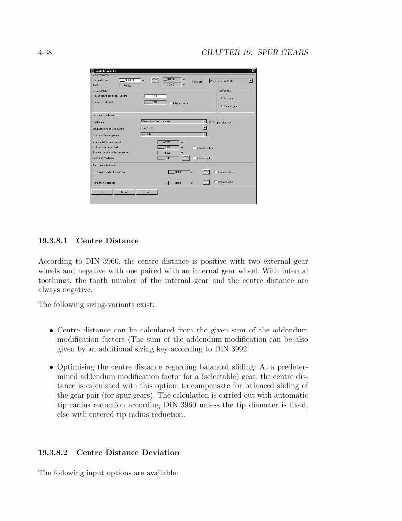
4-38 CHAPTER 19. SPUR GEARS
19.3.8.1 Centre Distance
According to DIN 3960, the centre distance is positive with two external gearwheels and negative with one paired with an internal gear wheel. With internaltoothings, the tooth number of the internal gear and the centre distance arealways negative.
The following sizing-variants exist:
• Centre distance can be calculated from the given sum of the addendummodification factors (The sum of the addendum modification can be alsogiven by an additional sizing key according to DIN 3992.
• Optimising the centre distance regarding balanced sliding: At a predeter-mined addendum modification factor for a (selectable) gear, the centre dis-tance is calculated with this option, to compensate for balanced sliding ofthe gear pair (for spur gears). The calculation is carried out with automatictip radius reduction according DIN 3960 unless the tip diameter is fixed,else with entered tip radius reduction.
19.3.8.2 Centre Distance Deviation
The following input options are available:

19.3. INPUT INTERFACES 4-39
a) Choosing a tolerance according to ISO (z.B. js6). Proposals according toNiemann [61].
Cast turning rims js10Turning rims (normal backlash) js9Turning rims (tight backlash) js9Turbo gears (high temperatures) js6Polymer machines js7Locomotive gear trains js7Standard mechanical engineering, heavy machinery, not reversing js7Standard mechanical engineering, heavy machinery, reversing js6, js7Automobiles js7Agricultural vehicles js8Machine tools js6Printing machines js6Measuring gearboxes js5
b) Choosing individual tolerances
Special tolerance tables can be added without problems, please refer to thedescription in appendix B-7 or the corresponding chapter in the descriptionof the data base tool (c.f. chap 7.
c) Direct input of deviations in the user interface
Choose Own input in the centre distance tolerance section. You can thenenter the values.
19.3.8.3 Face Load Coefficient
Spur gearsThe face load coefficient KHβ takes into account the influence of an uneven dis-tribution of the load over the face width on the flank surface pressure, the toothroot stress and the scoring. The calculation, as defined in the DIN 3990, is basedon the approximative determination of the deformation of the pinion. This canbe very inaccurate in many cases!
If you have determined the exact tooth trace deviation due to deformation (tor-sion and bending) using the KISSsoft Shaft Calculation, you may correct thevalue determined by the standard and obtain a much better result.
The calculation of face load coefficient following methode C2 according toFormulae:

4-40 CHAPTER 19. SPUR GEARS
Factor Input Number of equationKHβ (41)/(43) (6.04)/(6.06)Fβy (45) (6.08)Fβx contact pattern not proven (69) (6.26)
favourable position of the contact pattern (70) (6.27)ideal contact pattern (71) (6.28)
fsh (74) (6.39)fsh0 Input for toothtrace equation
without crowning 0.023 · γ (75) (6.31)crowning 0.012 · γ (78) (6.34)end relief 0.016 · γ (79) (6.35)full tooth trace modification 0.000 · γ *1 *1
light crowning 0.023 · γ *2 *2
helix correction only 0.0023 · γ *2 *2
helix correction+crowning 0.0023 · γ *2 *2
γ single helical (76) (6.32)double helical (77) (6.33)
fma Input for toothtrace equationwithout crowning 1.0 · fHβ (95) (6.51)crowning 0.5 · fHβ (96) (6.53)end relief 0.7 · fHβ (97) (6.52)full tooth trace modification 0.5 · fHβ *1 *1
light crowning 0.5 · fHβ *2 *2
helix correction only 1.0 · fHβ *2 *2
helix correction+crowning 0.5 · fHβ *2 *2
*1) Analog ISO 6336, equation (60) oder DIN 3990 equation(6.20)*2) Analog ISO 9085, table 4
Planetary gear trainsChoosing the support of planets: on pins or in the planet carrier. Larger planetgears are normally supported on the fixed axle in the planet carrier. For smallerplanet gears it is no longer possible to mount the bearings in the gear. Thebearings can then be positioned on bolts connected on both sides to the planetcarrier. This results in slightly higher face load coefficients.
The calculation is carried out according to the following formula, where the lengthof the bolt is assumed lp = 1.5 ∗ b.
The calculation of face load coefficient for planet carriers following methode C1according to Formulae:
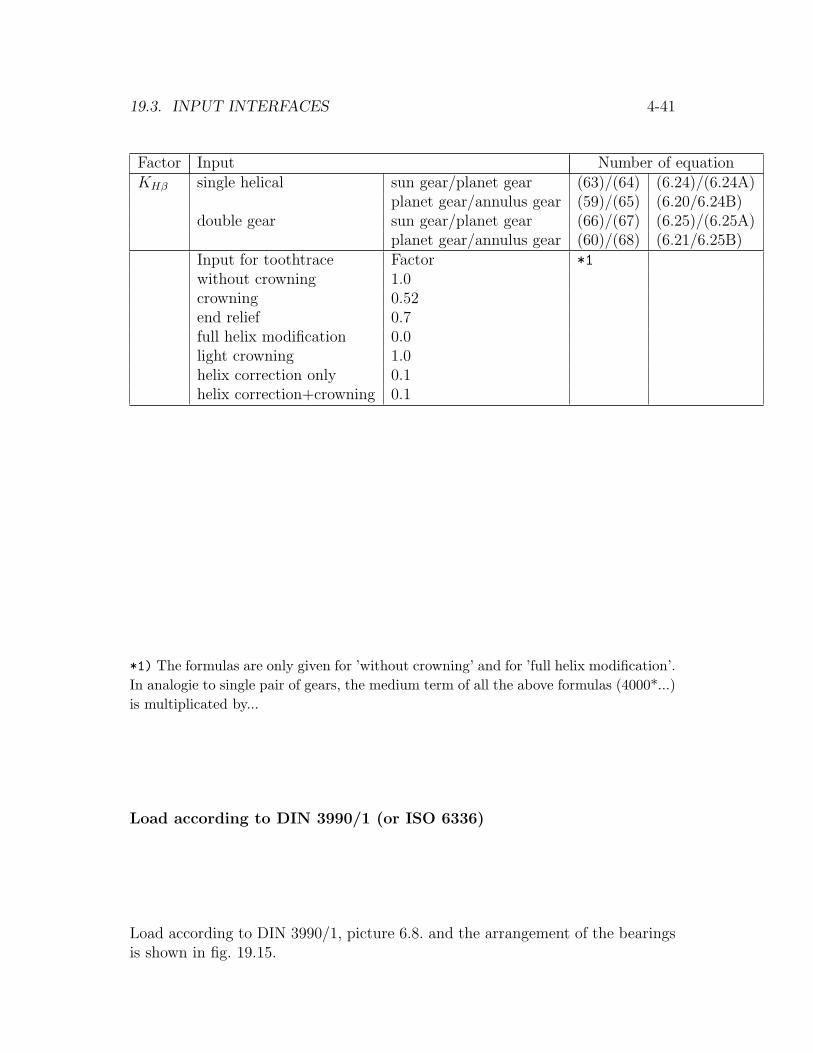
19.3. INPUT INTERFACES 4-41
Factor Input Number of equationKHβ single helical sun gear/planet gear (63)/(64) (6.24)/(6.24A)
planet gear/annulus gear (59)/(65) (6.20/6.24B)double gear sun gear/planet gear (66)/(67) (6.25)/(6.25A)
planet gear/annulus gear (60)/(68) (6.21/6.25B)Input for toothtrace Factor *1
without crowning 1.0crowning 0.52end relief 0.7full helix modification 0.0light crowning 1.0helix correction only 0.1helix correction+crowning 0.1
*1) The formulas are only given for ’without crowning’ and for ’full helix modification’.In analogie to single pair of gears, the medium term of all the above formulas (4000*...)is multiplicated by...
Load according to DIN 3990/1 (or ISO 6336)
Load according to DIN 3990/1, picture 6.8. and the arrangement of the bearingsis shown in fig. 19.15.

4-42 CHAPTER 19. SPUR GEARS
/labelLastfallDIN3990
Figure 19.15: Loadcase according to DIN 3990/1, fig. 6.8
Load according to AGMA 2001
Definition of s and s1 according to AGMA 2001, fig. 13-3. In the figure below,arrangement of bearings/ supports according to AGMA 2001 is shown.
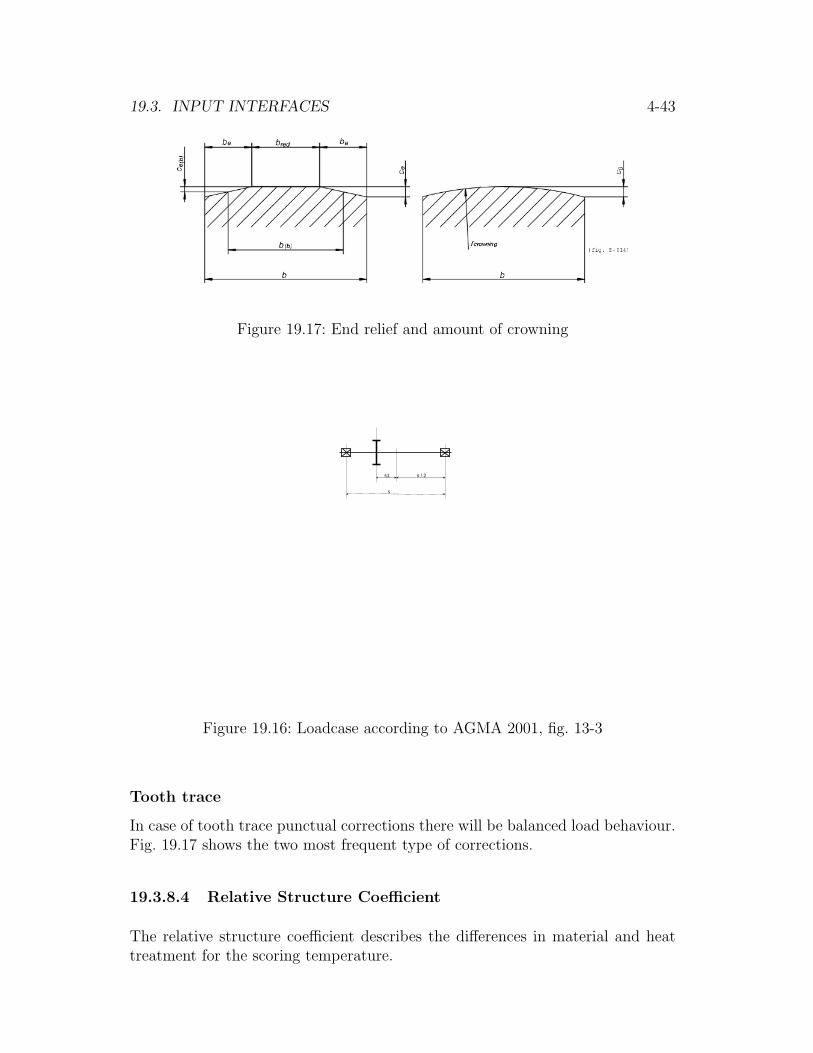
19.3. INPUT INTERFACES 4-43
Figure 19.17: End relief and amount of crowning
s
s1 s / 2
Figure 19.16: Loadcase according to AGMA 2001, fig. 13-3
Tooth trace
In case of tooth trace punctual corrections there will be balanced load behaviour.Fig. 19.17 shows the two most frequent type of corrections.
19.3.8.4 Relative Structure Coefficient
The relative structure coefficient describes the differences in material and heattreatment for the scoring temperature.

4-44 CHAPTER 19. SPUR GEARS
Structure coefficient according DIN 3990, Part 4:
Heat treated steels 1.00Phosphated steels 1.25Coppered steels 1.50Nitrided steels 1.50Case hardened steels 1.15 (with low austenite content)Case hardened steels 1.00 (with normal austenite content)Case hardened steels 0.85 (with high austenite content)Stainless steels 0.45
19.3.8.5 Dynamic Factor
The dynamic factor is calculated according to the chosen calculation method. Thedynamic factor considers additional loads due to natural oscillations (resonance)in the mesh of teeth. It can also be entered manually, based upon more precisemeasurements.
19.3.8.6 Transverse Coefficient
The transverse coefficient KHα is calculated according to the chosen calculationmethod. The transverse coefficient considers uneven loadcharacteristics over sev-eral teeth. In special cases, the transverse coefficient becomes unrealisticly large.If the transverse coefficient shall be limited, choose Influence Value and pre-scribe a value.
19.4 Settings
You find the following settings under Settings ⇒ Module-specific.

19.4. SETTINGS 4-45
These settings for spur gears are extremely comprehensive, allowing the activationof the most varied special functions. Normally, it is not necessary to change thesesettings.
19.4.1 General Settings
19.4.1.1 Material Treatment
You find this setting under Settings ⇒ Module-specific ⇒ General.
For the calculation of spur gears according ISO 6336 or AGMA, this is an im-portant setting. The setting ’Normal (Material Quality ML)’ further reducesthe permitted material loading in the fatigue strength region, i.e. flank and root,(the limited-life factors YNT and ZNT become 0.85 at 1010 load cycles). With thesetting ’Increased Specification (Material Quality MQ)’ YNT and ZNT areset to 0.92 at 1010 load cycles (according to specifications in ISO 9085).
The option ’Highest Specification (Material Quality ME)’ has no reduc-tion. More information is available in the description of the standard itself.

4-46 CHAPTER 19. SPUR GEARS
This approach of the ISO 6336 is one of the major differences between the DIN3990 and the ISO and the reason for lower margins of safety for calculationaccording to ISO 6336.
19.4.1.2 Manufacture tolerances according to method
The manufacture tolerances given in the protocol, and certain coefficients usedin the stress calculations, are determined according to DIN 3961, ISO 1324 orAGAMA 2015 Norms. Which of the three norms is to be used can be predeter-mined in the Setting ’Corresponding stress norm’ where the most appropriatenorm for the stress calculation method will be used (e. g. the ISO 1324 will beused when the ISO 6336 calculation method is employed).
19.4.1.3 Increasing the Interval for Allowable Addendum Modifica-tion (Z19c)
The range of the possible addendum modification (−1.2 <= x <= +1.5) can beincreased significantly with this option. This is useful for special cases and canbe applied for: spur gears, bevel gears, worms, crossed helical gears.
You find this option under Settings ⇒ Module-Specific ⇒ General.
19.4.1.4 No Automatic Modification of Tip Diameter
You find this option under Settings ⇒ Module-Specific ⇒ General. Themodification of tip diameter is normally carried out automatically according toDIN 3960 after the addendum modification sum to achieve sufficient bottomclearing. You can switch this automatism off and enter the modification of tipdiameter automatically under special inputs (c.f. 19.3.7.1).
19.4.1.5 Entering Speed (Number of Load Changes)
If you activate this option, you can enter the speed in the main interface inbehind Power. You can, however, not enter the service life in hours with thisoption. The service life is calculated from the nominal speed n as follows
H = NL/n/60 (19.1)
(NL: speed, number of load changes)

19.4. SETTINGS 4-47
19.4.1.6 Calculate on in Case of Geometry Errors
You find this option under Settings ⇒ Module-Specific ⇒ General.
Even in case of big geometry errors, the program does not stop the calculation.This option allows the calculation to go on in critical cases but the results shouldbe used very carefully.
19.4.1.7 Automatic Tip Chamfer
If KISSsoft notices contact interference, it sets automatically a sufficient tip cham-fer to avoid contact interference.
If the required tip chamfer (to avoid contact interference) is larger than 0.25 ·mn
(Module), KISSsoft issues an error message and does not calculate for tip chamfer.
If no tip chamfer because of contact interference is required, a small tip chamferis set as follows:
Module (mn) ≤ 1.0 mm: 0.1 ·mn
Module (mn) ≤ 4.0 mm: 0.05 ·mn, but maximal 0.1 mmModule (mn) ≤ 10.0 mm: 0.04 ·mn, but maximal 0.2 mmModule (mn) ≥ 10.0 mm: 0.4 mm
19.4.1.8 Tooth Numbers with Floating Points
You find this option under Settings ⇒ Module-Specific ⇒ General.
KISSsoft can calculate with floating point tooth numbers, e.g. when the gearwheel is only a segment or when the teeth are not symmetric.
19.4.1.9 Keeping Tip Circle in Case of Addendum Modification
You find this option under Settings⇒ Module-Specific⇒ General. Normally,KISSsoft keeps the reference profile and tip and root circle are adapted. If thisoption is acivated, however, the tip circle is kept and the reference profile isadapted if the addendum modification is changed. The tip circle is kept as longas tooth number and transverse module are kept.
19.4.1.10 Keeping Root Circle in Case of Addendum Modification
You find this option under Settings ⇒ Module-Specific ⇒ General.

4-48 CHAPTER 19. SPUR GEARS
Normally, KISSsoft keeps the reference profile and tip and root circle are adapted.If this option is activated, however, the root circle is kept and the reference profileis adapted if the addendum modification is changed. The root circle is kept aslong as tooth number and transverse module are kept.
19.4.1.11 Coefficient for Minimal Tooth Thickness
You find this option under Settings ⇒ Module-Specific ⇒ General.
On account of manufacturing, you must not go beyond a minimal tooth thicknessin the tooth tip. The minimal tooth thickness is: Module ∗ Factor. According toDIN 3960, the factor is normally 0.2.
19.4.1.12 Minimum Tip Clearance
You find this option under Settings ⇒ Module-Specific ⇒ General.
The tip clearance is the distance between the tip of a gear and the root of a matinggear. A minimum tip clearance can be given. If the clearance (with considerationof potential tip and root variation) is reduced beyond this minimum value, thena warning will be shown.
19.4.1.13 Power-on Time
You find this option under Settings ⇒ Module-Specific ⇒ General.
The power-on time is considered when calculating the number of load changes(multiplied by the service life).
19.4.2 Entries for Calculations According to AGMA
You find the following fields under Settings ⇒ Module-Specific ⇒ AGMA:
19.4.2.1 Drive Type
The face load according to AGMA depends upon the tooth contact pattern atthe mounting.
19.4.2.2 Mounting Procedure
The face load according to AGMA depends upon the tooth contact pattern atthe mounting.

19.4. SETTINGS 4-49
19.4.2.3 Stress Cycle Factor
According to AGMA(depending upon material mostly by 107 load changes), theoperational life factor when reaching the fatigue limit is 1. For higher load changevalues, this factor will be reduced reaching the value the Norm indicates for1010 load changes. For usual drives (’General Application’) this value is for thededendum YN=0.9 and for the flank ZN=0.85. The Norm does not indicate how toproceed in case of load changes higher than 1010. Comparing with the AGMA SpurGear Calculation Program shows that the values for YN and ZN are extrapolatedfor load changes over 1010. We have done the same in KISSsoft.
19.4.2.4 Tooth Form Factor Y
The tooth form factor can be calculated from the positions ’Suggestion of theAGMA’ or ’Application of force always at head’ or ’Application at force alwaysat single tooth contact’.
19.4.2.5 Determining the Tooth Form Factor Y Graphically
AGMA offers a method to calculate the tooth form factor Y for outer gear wheelsbut not for internal toothings. According to AGMA, internal toothings can onlybe calculated by a graphical method. To do so, the exact tooth form is drawnand the values are measured (root radius etc.).
KISSsoft can now calculate these values in determining the tooth form. Theparameters (root radius, lever arm, tooth root width) derive from this value. Todetermine the tooth from factor Y and the stress correction factor Kf , KISSsoftuses an improved method. As in the method according to Obsieger (c.f. chap19.4.6.2) the point of the tooth root is determined where the factor I(= Y/Kf ∗...)is smallest (this point has the heaviest load).
19.4.2.6 Reliability factors KR
Requirements of Application KR
Fewer than one failure in 10 000 1.50Fewer than one failure in 1000 1.25Fewer than one failure in 100 1.00Fewer than one failure in 10 0.85Fewer than one failure in 2 0.70
4-50 CHAPTER 19. SPUR GEARS
19.4.3 Settings for Plastics
You find this options under Settings ⇒ Module-Specific ⇒ Plastic.
19.4.3.1 Calculating Contact Temperature
For the calculation of the tooth strength of polymer gears, the temperature ofthe tooth at the root and the flank is calculated (according Niemann or accordingto experimental formulae). If this option is deactivated, the temperature is as-sumed to the equal to the oil/grease temperature (in case of dry running ambienttemperature).
For this, the friction coefficient µ from the material file is read. When plasticsare paired, the mean value
µ = (µ1 + µ2)/2 (19.2)
is used for the total friction. When plastics and steel are paired, the followingvalue is entered for steel in the formula:
Oil lubrication: 0.04Grease lubrication: 0.09Dry running: 0.20
Remark:According to Niemann, PA is for oil lubrication µ = 0.04, for grease lubricationµ = 0.09, for dry running µ = 0.4; for POM with oil lubrication µ = 0.04, withgrease lubrication µ = 0.09, with dry running µ = 0.2.
The exponent κ (in the formula ...(v ∗mn)κ... is read from the material data base.
When plastics are paired, KISSsoft substitutes for κ the mean value
κ = (κ1 + κ2)/2 (19.3)
For pairings plastic/steel, KISSsoft uses for κ the value of the plastic.
Remark:According to Niemann, κ = 0.75 rot PA, κ = 0.4 for POM.
19.4.3.2 Type of casing
The input of the type of casing has an influence of the contact temperature. Fora open casing the temperature the temperature will be the least. The surface ofthe casing will be approximated through dimensions of gears.

19.4. SETTINGS 4-51
19.4.3.3 Calculation of flank safety
For gears made out of plastics, the flank safety will be determined by the Hertzianstress, (according to VDI 2545, as for the calculation for steel gears) with the ac-cepted value for plastics σHlim. However, measures carried out for plastic gearshave frequently shown that the tooth flanks wear out, similarly to what hap-pens to worm wheels made out of plastics. That is why KISSsoft also offers asalternative the calculation of the wear safety. The calculation of the flank safetycon σHlim will be carried out should the data for σHlim be available in the mate-rials database (or in the inserted Materials file with extended data). The wearsafety calculation will be carried out should the Materials Database contain thewear safety data. Should data for both calculations be available, then both cal-culations will be carried out. It is possible to choose which of the two safetieswill be displayed on the main window, with the selection option ’Calculation offlank safety’. Should the data for only one of the calculations be available, thecorresponding safety will automatically be displayed.
19.4.3.4 Permissible maximal wear
In the wear safety calculation, a permissible limiting value must be preestablished(see 19.4.3.3). A usual value for plastics is 50% wear of the tooth thickness onthe reference circle. Should a little wear or no wear be tolerable, a value of 5-10%is recommended.
19.4.3.5 Allow simplified calculation according to DIN3990/ISO6336
This option allows the calculation of plastic gears with the methods used for steelgears. The calculation is carried out with the fatigue resistance values, containedin the Materials Database. The values for the included plastics are valid for oillubrication, 70◦ temperature and a load change of 108. Contrary to the calculationaccording to VDI 2545, the resistance values do not depend on temperature andtype of lubrication.
The calculation is done as for tempered steel with the corresponding WohlerDiagram according to DIN 3990.
19.4.4 Settings for Planetary gears
19.4.4.1 Checking for Assembly Mountabilities (Planetary Gears)
You find this field under Settings ⇒ Module-specific ⇒ Planet.
4-52 CHAPTER 19. SPUR GEARS
Planets are usually mounted on a planet holder with constant pitch (for threeplanet 120 degrees etc.). For this case special boundary conditions must be set toallow the mounting of the planetary gear train. If the flag check is set, KISSsoftautomatically checks the feasibility of the gears which are to be assembled.
For the case of an uneven distribution of the planets KISSsoft module Z19g canbe used to calculate the centres of the planets.( Select under Calculation ⇒Centre points Z19g)
19.4.5 Settings for Sizings
19.4.5.1 Nominal Transverse Contact Ratio
You find this field under Settings ⇒ Module-specific ⇒ Sizings.
The desired nominal transverse contact ratio for the sizing of deep tooth formscan be determined in this option. See also sizing of deep tooth forms (Z01x) (c.f.chap 8 and chap 25.1.2).
19.4.5.2 Prescriptions in the Rough Sizing (Z3)
• Module ratio b/mn
The ratio tooth width / normal module is a characteristic measure for areasonable sizing of gear wheel trains. Too narrow gears do not guaranteethe axial stiffness of the teeth, b/mn should therefore be larger than 6 (seeNiemann, panel 22.1/7)!
Too wide gears influence the load critically which should be carried evenlyover the entire tooth width, depending on design and tooth quality b/mn
should be smaller than 15..40 (see Niemann, panel 22.1/10).
• Pitch diameter ratio b/d1
The ratio of the tooth width / pinion pitch diameter is a characteristic mea-sure for the reasonable sizing of gear wheels. Depending on the heat treat-ment this should be smaller than 0.8. . . 1.6 (see Niemann, panel 22.1/5).
• Centre distance ratio b/a
The ratio of the tooth width / centre distance is a characteristic measure forthe sizing of standardised modular gear boxes. Depending on the stiffness ofthe housing this value should be smaller than 0.3..0.5 (see Niemann, panel22.1/6).

19.4. SETTINGS 4-53
19.4.6 Settings for Calculations
You find this fields under Settings ⇒ Module-Specific ⇒ CALCULATIONS.
19.4.6.1 Calculation with manufacturing addendum modification(Z19a)
The spur gear geometry according DIN 3960 is based on the calculation of the(theoretically) backlash free mesh. Therefore the sum of the addendum modifi-cation of the gears is determined by the centre distance. This option allows thedefinition of the addendum modification independent of the centre distance. Itcan be very useful to check boundary conditions (backlash, overlap ratio etc.) forgears with changing or varying centre distance (e.g. big tolerance range).
The Norm stipulates the calculation of the spur gears circumferential force Ft
to be done with the pitch diameter. This is not quite correct because the forceinput takes place at the pitch circle. Selecting the option ’Calculation with man-ufactured addendum modification’, the circumferential force will be calculated atthe pitch circle and documented in the protocol. This occurs because, with thisoption, the influence of the center distance modification has to be assessed andis an influent factor in the force input.
19.4.6.2 Tooth form factor YF and YS according to graphical method(Z19i)
Tooth form and stress correction factors are calculated – according to DIN 3990or ISO 6336 – at the point of the tooth root makes with the tooth center line anangle of 30◦. This method is, especially for internal gear wheels, very inaccurate.
The method according to Obsieger [63] is more accurate. It calculates, based onthe tooth form, for all points in the root area the product from tooth form fac-tor YF and stress correction factor YS and determines the maximal value. Thestrength is calculated with this maximal value. The factors YF and YS are calcu-lated according to the formulae in DIN 3990 and ISO 6336.
Especially with special tooth forms and with internal toothings, this method ishighly recommended. If desired, it can also be used in the strength calculationaccording to DIN 3990 and ISO 6336 as well as in the fine sizing (Z04).
Remark:If you choose a tooth form calculation according to graphical method, KISSsoftcalculates the tooth form before each strength calculation (with the material dataentered in the tooth form calculation Z5, or with the pre-defined standard values).

4-54 CHAPTER 19. SPUR GEARS
The maximal value of the product from tooth form factor and stress correctionfactor is determined in this way and then used for the strength calculation.
19.4.6.3 ISO 6336 with enlargements planed
The ISO 6336 is under revision. The changes which are being discussed withinthe ISO Committee concern essentially internal gears. This option allows thecalculation with the corresponding modifications. This calculation has no legalobligation and should only be used for testing purposes!
19.4.6.4 Tooth contact stiffness cg calculated with tooth form
The tooth stiffness cg is calculated with approximative formulasaccording to thestandards (DIN 3990, ISO 6336, etc.) bestimmt. With the option calculation
of tooth stiffness the stiffness is calculated from the effective tooth form (seecontact stiffness(Z24) (19.7.13)). The calculated medium value of the contactstiffness will be used in the strength calculations and also in the fine sizing (Z04).
The singular tooth stiffness c’ is calculated from cg, with c’ analog to the formulafor cg (DIN oder ISO). For small load per width (w · KA < 100N/mm2) areduction of contact stiffness is assumed in DIN and ISO because the values forKV , KHβ, etc will be too big for little loading. The formula according ISO 6336is used:
cg = cg · (fmb
100.0)0.25
fmb = KA · w
19.4.6.5 Calculate the usable tip circle diameter, dNa, dNf (and un-dercut) from tooth form
In the tooth form calculation the manufacturing process is simulated and theeffective undercut is calculated. With the option Calculate undercut from
tooth form the tooth form is generated in each calculation and, if available,the undercut is determined and introduced into the calculation. The transversecontact ratio as well as the root- and tip circles (generated usable circles) will becorrespondingly calculated. In the fine sizing (Z04) the calculation procedure willnot be used since solutions with undercut are normally discarded.
If the option was not selected, the root- and tip circles will be determined by theusual methods for involutes, without considering undercuts (see for instance DIN3960). The reference to the undercut will also be derived from DIN 3960.
19.4. SETTINGS 4-55
19.4.6.6 Calculating momentum mass from the tooth form
The momentum of mass (only for area tip- to root diameter) is calculated basedon the tooth form. KISSsoft automatically calculates the tooth form for everycalculation and determines the momentum of mass from the actual tooth form.The result will appear in the calculation protocol. In the fine sizing (Z04), thecalculation will also be used and documented.
19.4.6.7 Calculation of the transport volume of gear wheel pumps
The basic option Z26 carries out the calculation of the transported volume(without consideration of any feed-back volume). If this option is activated (un-der Settings⇒ Module-Specific⇒ Calculations), then the transported vol-ume is calculated through the exact numeric integration of the tooth space, andsubsequently given as output in the report documentation. In addition, the trans-portable volume for each design variant generated by the optimisation function(Z4) will also be given. Because of this, the largest possible transport volume canbe quickly established.
19.4.6.8 Consider grinding allowance on tools for roughing
Normally, gear wheel geometry and strength are computed from the final contourof the gear wheel. When entering the reference profile, you have to enter thevalues for the final tooth form.
Many gear wheels are milled with additional measures, then they are hardenedand finally grinded. Normally the tooth flank is grinded but not the tooth root.
The allowance for the prefabrication can be entered under Tolerances (c.f.19.3.7.3) if the flag is on. The root circle is then determined from the allowancesfor pre-treatment, the tooth thickness from the allowances for additional treat-ment.
When the reference profile of the gear wheel is entered, the profile of the prefabri-cation tool has to be entered. KISSsoft calculates, based on the grinding addition,the final profile. The data for the strength calculation (tooth root stress) derivesfrom the final profile. In the report, both profiles are issued. We recommend con-trolling in the reports. If, e.g., a protuberance tool is chosen for prefabrication,the final profile can have a protuberance, depending on the grinding addition.Notice: if there is another difference between the reference profile for prefabrica-tion and the reference for final treatment as described above, this option mustnot be employed. In this case, rough state and final state have to be calculatedseperately.

4-56 CHAPTER 19. SPUR GEARS
19.4.6.9 Surface coating
Planned expansion, not yet important.
19.4.6.10 Consider protuberance above given difference of angle
If the difference of angle between protuberance and buckling root to pressureangle is greater than maximal difference defined here, the influence of utizabletip and root diameters and the contact ratio will be considered. The calculatedcontact ratio will get smaller.
In the calculation with allowance for prefabrication tools (see 19.4.6.7) the buck-ling root flank of the finished tooth form will be influenced by this setting (see19.3.7.1).
19.4.7 Nominal Safeties
You find these fields under Settings ⇒ Module-Specific ⇒ Nominal
safeties, corresponding statements in chapter 25.2.4.
The predetermined nominal safety values are important for all service life calcu-lations for both rough and fine sizing.
19.4.7.1 Minimal Required safety factors for AGMA calculations
In the tooth strength calculation of AGMA 2001 the ’Allowable bending stressnumber [sat]’ is – compared to ISO 6336 – too small by factor of 2. In the ISO6336 the value for sat is very similar to the AGMA value, but has to be multipliedby 2.0 (Stress-Correction-Factor reference gear Yst). So when calculating Toothresistance by AGMA2001, the resulting safety coefficient will be about only 50%of the result compared to ISO 6336.
Therefore the minimal required safety factor for tooth resistance is smaller forcalculations following AGMA 2001, see also chapter 25.2.4.
19.4.8 Rating
You find this field under Settings ⇒ Module-Specific ⇒ Rating.
The factors to rate a spur gear pairing in the fine sizing regarding noise can beentered in this place. Further information under 19.5.2.3.
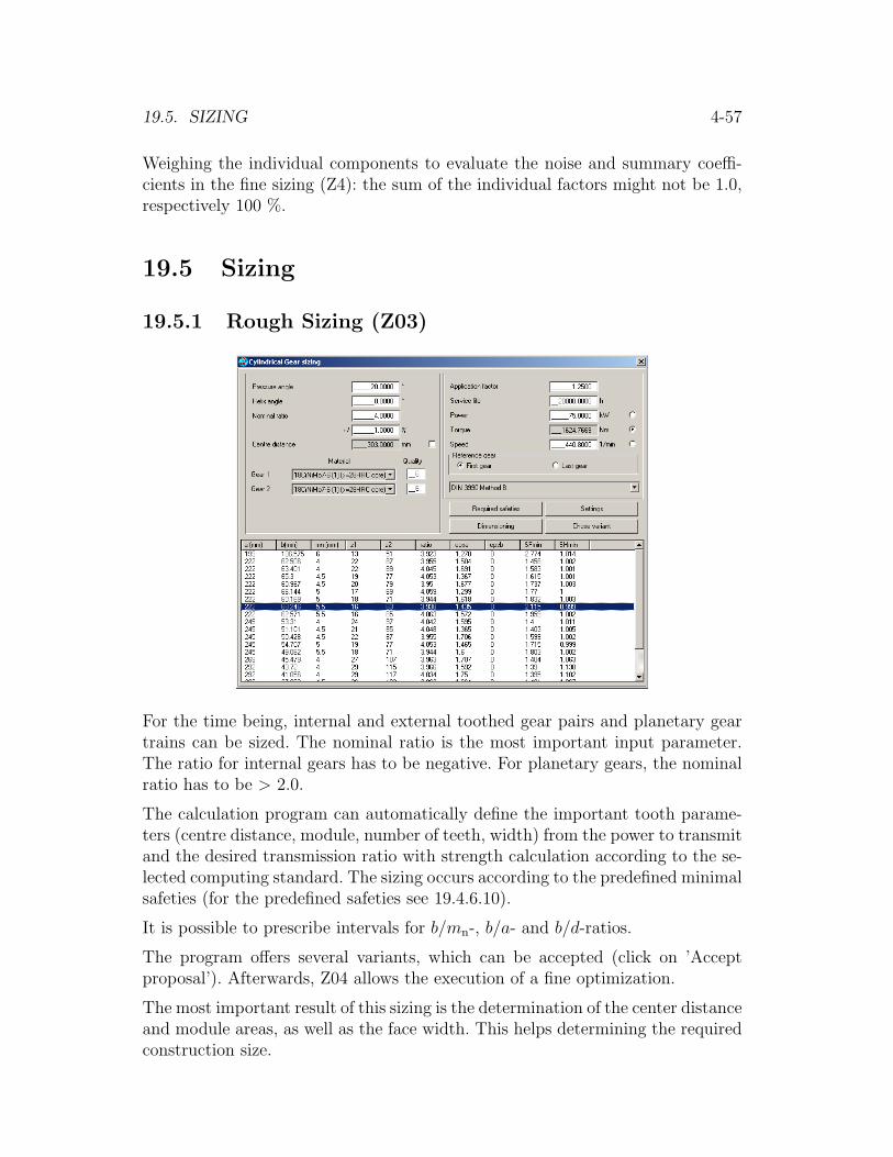
19.5. SIZING 4-57
Weighing the individual components to evaluate the noise and summary coeffi-cients in the fine sizing (Z4): the sum of the individual factors might not be 1.0,respectively 100 %.
19.5 Sizing
19.5.1 Rough Sizing (Z03)
For the time being, internal and external toothed gear pairs and planetary geartrains can be sized. The nominal ratio is the most important input parameter.The ratio for internal gears has to be negative. For planetary gears, the nominalratio has to be > 2.0.
The calculation program can automatically define the important tooth parame-ters (centre distance, module, number of teeth, width) from the power to transmitand the desired transmission ratio with strength calculation according to the se-lected computing standard. The sizing occurs according to the predefined minimalsafeties (for the predefined safeties see 19.4.6.10).
It is possible to prescribe intervals for b/mn-, b/a- and b/d-ratios.
The program offers several variants, which can be accepted (click on ’Acceptproposal’). Afterwards, Z04 allows the execution of a fine optimization.
The most important result of this sizing is the determination of the center distanceand module areas, as well as the face width. This helps determining the requiredconstruction size.

4-58 CHAPTER 19. SPUR GEARS
Centre distance and the sum of addendum modifications can be prescribed inparticular cases. Notice that, in these cases, the sizing variants of the programare limited.
19.5.1.1 Strength-Sizing of Planetary Gears
During the rough sizing of planet stages a standing rim is presupposed. If the rimturns, the speeds must be adapted after the rough sizing.
19.5.1.2 Different Prescriptions in the Rough Sizing
• Recommended number of teeth according to Niemann
Table of the usual number of teeth on the pinion, Niemann, panel 22.1/8.
Ratio u 1 2 4 8proposed treatmentheat treated up to 230 HB 32..60 29..55 25..50 22..45more than 300 HB 30..50 27..45 23..40 20..35Grey iron 26..45 23..40 21..35 18..30nitrided 24..40 21..35 19..31 16..26case hardened 21..32 19..29 16..25 14..22
These values can be accessed with the sizing button.
• Module ratio b/mn, Pitch diameter ratio b/d1, Centre distance ratiob/a see chapter 19.4.5.2.
19.5.2 Spur Gear Fine Sizing (Z04)
The fine sizing (geometry variant calculation) is one of the most powerful optionsof the KISSsoft spur gear calculation program.
After you have entered nominal ratio, centre distance and the intervals for moduleand helix angle, the program calculates and issues suggestions for number of teeth,module, slope and addendum modification factor with a statement of deviationfrom the nominal ratio, specific sliding and contact ratio. This module also allowssizing of planetary gear trains and spur gears with interchangeable gears.
All found variants are evaluated regarding different criterias (noise, vibration,precision of ratio, weight, strength, etc.).
Important parameters can be limited if required (tip diameter, root diameter,minimum number of teeth, tolerable undercut etc.).
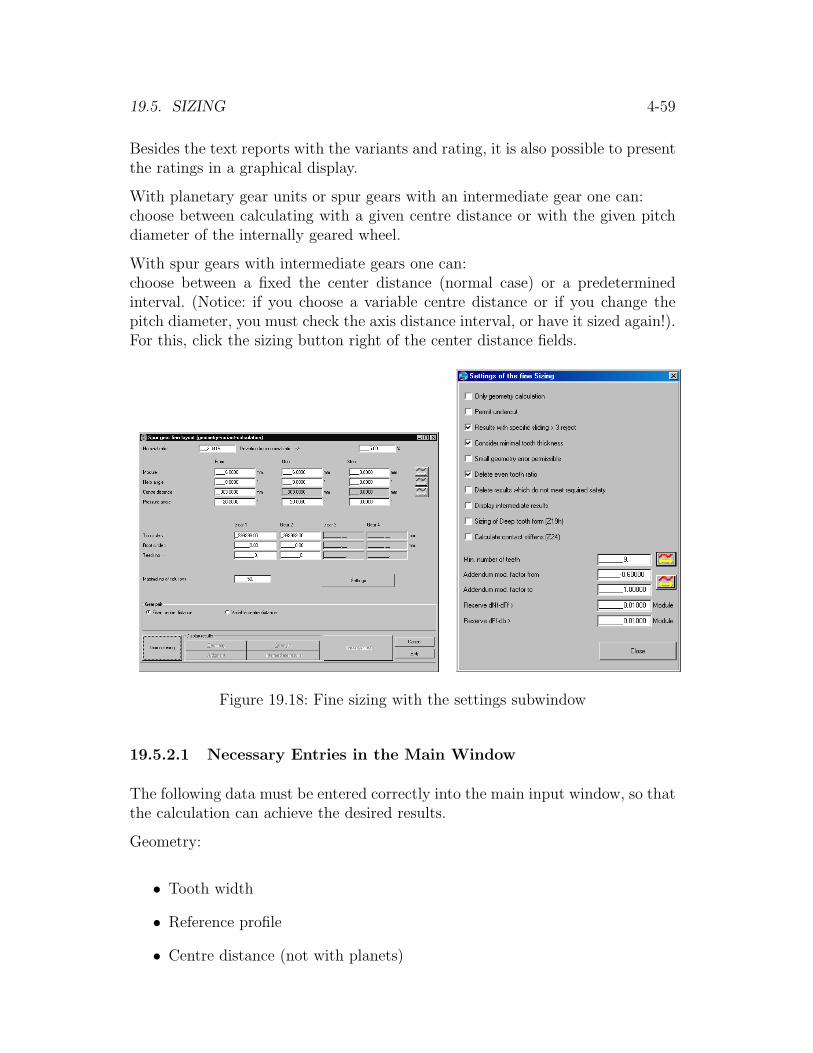
19.5. SIZING 4-59
Besides the text reports with the variants and rating, it is also possible to presentthe ratings in a graphical display.
With planetary gear units or spur gears with an intermediate gear one can:choose between calculating with a given centre distance or with the given pitchdiameter of the internally geared wheel.
With spur gears with intermediate gears one can:choose between a fixed the center distance (normal case) or a predeterminedinterval. (Notice: if you choose a variable centre distance or if you change thepitch diameter, you must check the axis distance interval, or have it sized again!).For this, click the sizing button right of the center distance fields.
Figure 19.18: Fine sizing with the settings subwindow
19.5.2.1 Necessary Entries in the Main Window
The following data must be entered correctly into the main input window, so thatthe calculation can achieve the desired results.
Geometry:
• Tooth width
• Reference profile
• Centre distance (not with planets)
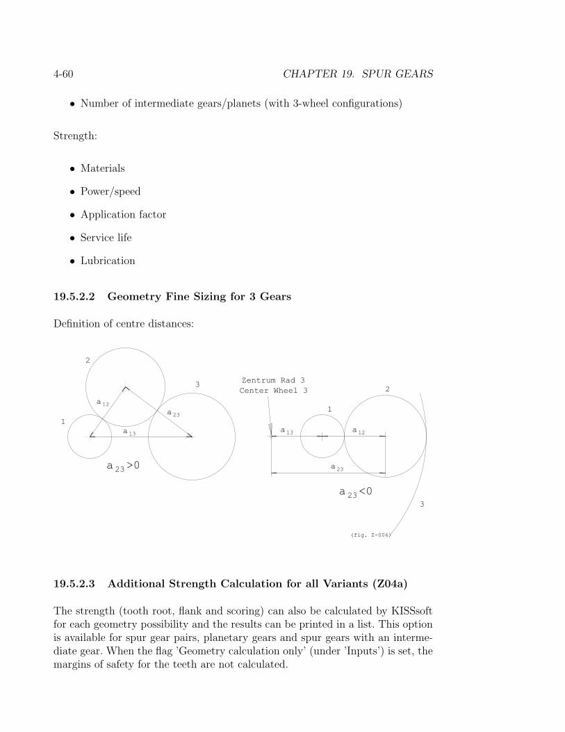
4-60 CHAPTER 19. SPUR GEARS
• Number of intermediate gears/planets (with 3-wheel configurations)
Strength:
• Materials
• Power/speed
• Application factor
• Service life
• Lubrication
19.5.2.2 Geometry Fine Sizing for 3 Gears
Definition of centre distances:
19.5.2.3 Additional Strength Calculation for all Variants (Z04a)
The strength (tooth root, flank and scoring) can also be calculated by KISSsoftfor each geometry possibility and the results can be printed in a list. This optionis available for spur gear pairs, planetary gears and spur gears with an interme-diate gear. When the flag ’Geometry calculation only’ (under ’Inputs’) is set, themargins of safety for the teeth are not calculated.

19.5. SIZING 4-61
19.5.2.4 Rating the Variants
This is a short description for rating the best variants (press ’Rating’). Notice,however, that these criteria do not apply to every case, they must be questionedin certain applications!
Analysis of the results (Assessment of important characteristics)
Comment:
No. = Number of the variant
Noise = Noise level (0 = low, 1 = high)
(Weights: 8.3%:eps.a 8.3%:eps.b 33.3%:eps.g 16.7%:SumX 8.3%:alfa.n
8.3%:zetaMax/Min 16.7%:Vqual)
diff_i = Deviation from the nominal ratio in %
kg = Weight in kg
Slide = Specific sliding (maximum value)
v.Slide = Sliding velocity (m/s, maximum value)
AC/AE = Begin working depth AC / working depth AE
(Friction)
s_Rig = Variant on the siffness during rolling (N/mm/mym)
(Calculation WITHOUT taking into account the exact tooth-shape)
1-eta = Losses in (1.0-total efficiency)
Safety = Safety (Tooth root and flank, 0 = high, 1 = medium, 2 = low)
(SF-min: 1.40/ 1.40/ 1.40 SH-min: 1.00/ 1.00/ 1.00)
Summary = Overall assessment (weighted)
(50.0%:Noise 50.0%:s_Rig 20.0%:diff_i 10.0%:kg 35.0%:Slide 0.0%:v.Slide
0.0%:AC/AE 10.0%:1-eta 100.0%:Safety)
(For this table it can be said in general: the smaller the value the better!)
No. Noise diff_i kg Slide v.Slide AC/AE s_Rig 1-eta Safety Summary
1 0.774 2.796 66.718 1.236 0.843 0.520 6.766 0.644 0.532 0.296
2 0.765 2.796 66.516 1.018 0.847 0.473 6.829 0.639 0.531 0.293
3 0.757 2.796 66.316 0.833 0.915 0.424 6.839 0.654 0.531 0.292
4 0.711 4.167 66.998 1.546 0.875 0.506 6.471 0.718 0.527 0.299
5 0.704 4.167 66.795 1.245 0.922 0.460 6.600 0.716 0.525 0.295
6 0.694 4.167 66.593 0.998 0.991 0.413 6.602 0.735 0.524 0.293
7 0.774 -2.632 65.729 1.184 0.864 0.525 6.801 0.610 0.510 0.285
8 0.766 -2.632 65.535 0.983 0.854 0.477 6.863 0.604 0.510 0.284
9 0.759 -2.632 65.343 0.809 0.924 0.429 6.874 0.616 0.511 0.282
10 0.608 0.000 66.226 1.886 0.928 0.499 5.867 0.759 0.499 0.273
11 0.604 0.000 66.029 1.484 1.001 0.453 6.066 0.758 0.498 0.269
12 0.603 0.000 65.834 1.167 1.072 0.407 6.216 0.780 0.498 0.266
13 0.519 1.316 66.358 2.531 0.991 0.487 3.816 0.845 0.498 0.286
14 0.512 1.316 66.160 1.885 1.065 0.441 3.989 0.848 0.496 0.280
15 0.514 -3.846 65.422 2.395 0.998 0.492 3.847 0.804 0.479 0.285
16 0.508 -3.846 65.231 1.813 1.074 0.447 3.824 0.805 0.476 0.280
Analysis of the results
(with the variant index in decreasing order)
Best variant for accurate ratio: 10 11 12 13 14 7 8 9 2 3 ...
Best variant for noise: 16 14 15 13 12 11 10 6 5 4 ...
Best solutions for weight: 16 9 15 8 7 12 11 14 10 3 ...
Best variants relative to friction (AC/AE): 12 6 3 9 14 16 11 5 2 8 ...
Best solution for stiffness: 13 16 15 14 10 11 12 4 5 6 ...
Best variant for strength: 16 15 14 11 12 13 10 8 7 9 ...
Best overall variants (summary) : 12 11 10 14 16 9 8 15 7 13 ...

4-62 CHAPTER 19. SPUR GEARS
• Rating the variants for precision of the number of teeth ratio:
It rates the deviation from the actual to the theoretical number of teethratio
• Rating the variants for noise:
Rating is based on several criteria with the following weighting:35% : (1) Integer total contact ratio10% : (2) Integer transverse contact ratio10% : (3) Integer overlap ratio10% : (4) Small sum of addendum modification (if possible < 0.5)5% : (5) Small pressure angle (if possible < 25 deg)
10% : (6) Small specific sliding20% : (7) High quality
Formeln: (1) a1 = 1−√
Abw()
Abw() = εg − next whole number(2) a2 = . . . (as a1, with εa)(3) a3 = . . . (as a1, with εb)(4) a4 = 0.5− (x1 + x2)(5) a5 = (25− αn)/10(5) a6 = 1−min(4, max(ζf1, ζf2))/4(7) a7 = (12−Q)/10
Result: 0.35 · a1 + 0.1 · a2 + 0.1 · a3 + 0.1 · a4 + 0.05 · a5 + 0.1 · a6 + 0.2 · a7
The stated ratings can be modified under Settings ⇒ Module-Specific
⇒ Rating (c.f. 19.4.7.1).
Bibliography for Noise optimization: WZL Series 11: Vibration technique:Noise abatement. Sizing of special involute gears for a vibration- and noise-free running. Dipl. Ing. Sepp Lachenmaier, Aachen. VDI Publishers LtdDusseldorf 1983, ISSN 0506-3159, VDI Series 11 No. 54.
• Weight (is a price indication for the manufacturing)
• Specific sliding (maximal value)
• Sliding speed (maximal value)
• Ratio AC/AEAC: Length of the path of contact from the start of contact to the pitchpointAE: Total length of the path of contactWithin the AC area, the gear mesh occur ’percussion sliding’ (the slidingspeed of the driving gear is higher than that of the driven gear).This area being critical for non-lubricated plastic gears, this ratio shouldbe as small as possible.
19.5. SIZING 4-63
• Rating the variants for vibrations:
Variation of total stiffness of the meshing (the smaller the variation thebetter).
• Rating the variants for strength:
Rating the margins of safety of root and flank regarding the nominal safetymargin. Margins below the nominal safety margin are considered as highlynegative points, while large reserves above the nominal safety margin havelittle influence.
• Ratings ’Summary’:
The ratings ’Summary’ weights the individual rating components to obtaina total rating coefficient. The weights of the individual components can beset in Settings ⇒ Module-Specific ⇒ Rating. This weighing dependsmainly upon the chosen variant (e. g. if an optimal noise abatement orvariant is chosen).
19.5.2.5 Limits of Tip Diameter
Solutions whose tip diameter exceed the indicated value are rejected.
If no restraint is desired, enter: 0 or 1010
Practical application of this option: If a gear has to be installed in a given box,it may not touch the wall.
19.5.2.6 Limiting the Root Diameter
Solutions where the root diameter remains below the indicated value are rejected.
If no restraint is desired, enter: 0
Practical application of this option: If a gear is installed in a gear box on rollerbearings, a minimum thickness of material between the bore and the root diam-eter has to be provided.
19.5.2.7 Limiting the Tooth Number
Do not use this option in the normal case!
If no restraint is desired, enter: 0
Practical application of this option: sizing a planet gear stage, which should passinto an existing internal gear rim (in this case, the module and the number ofteeth of the gear 3 are given).
4-64 CHAPTER 19. SPUR GEARS
19.5.2.8 Maximal Number of Variants
Suggestion: 50 . . . 200
If the program finds more than the requested number of solutions, it issues anote in the protocol. Notice: do only carry out a final rating when all possiblesolutions are displayed, or you risk that the optimal solution is not rated!
19.5.2.9 Special functions under ’Settings’
´Settings of the fine sizing´
1. Only geomety calculation
With this option set, no stress calculation will be carried out.
2. Permit Undercut
With this option set, the variants with undercut will not be rejected.
3. Results with specific sliding > 3 reject
The specific sliding is usually not outside the limits +3 and -3.
4. Consider minimal tooth thickness
With this option set, variants with the tip tooth thickness below the min-imal tooth thickness will be rejected (see Settings ⇒ Module-Specific
⇒ General).
5. Permissible Small Geometry Errors
Undercut, pointed cogs and similar geometry errors are tolerated whencalculating the variants.
If you want to find solutions with the number of teeth below 7, or in otherspecial cases, then this option must be used. We recommend not to use thisoption in normal cases!
6. Without Integer Tooth Number Ratios
With this option set, results with integer number of teeth ratios are rejected.
7. Delete results which do not meet required safety
The variants outside the preestablished minimal safeties will be rejected(see Settings ⇒ Module-Specific ⇒ Required safeties.
19.5. SIZING 4-65
8. Display intermediate results
This option, when set, produces in addition a very comprehensive docu-ment, in which intermediate results of the search for feasible variants willbe displayed. This document is only foreseen for exceptional cases.
9. Sizing of Deep Toothings (Z01x)
For deep toothings, special reference profiles with larger tip- and root-heights are used. The sizing function calculates the required reference pro-file based upon the desired transverse contact ratio. If this function is alsoset in the gear wheel fine sizing, the reference profile will be calculated forevery issued variant in such a way as to exactly achieve the predeterminednominal transverse contact ratio. Thus, only the variants corresponding tothe desired transverse contact ratio will be displayed.
The nominal transverse contact ratio can be predefined under Settings⇒Module-Specific ⇒ Sizing.
10. Contact Stiffness calculate (Z24)
With this option set, KISSsoft calculates for each variant the exact toothprofile and the stiffness derivation. The larger the stiffness derivation, thelarger are the vibrations caused by the gear wheels. The stiffness derivationis issued in the report; the smaller this value, the better the vibration-characteristics.
11. Minimal Tooth Number
Reasonable minimal tooth number:
With helical toothing: 7 . . . 9With spur gearing: 10 . . . 12
Important suggestion:
If you want to find solutions with tooth numbers below 7, use the optionAllow small geometry errors.
12. Range of Permissible Addendum Modification
Reasonable values:
External gearing: -0.6 . . . 1.0Internal gearing: -1.0 . . . 0.6
13. Safety margin from root utilizable circle dNf to root form circledFf
In a case where the root utilizable circle encroaches onto the root form circle,contact interference occurs. A minimum value for the distance betweenthese circles representing of that between the utilizable and manufactured

4-66 CHAPTER 19. SPUR GEARS
involute can be defined here. The given value is the minimum difference ofboth diameters representing double the distance between the circles.
14. Safety margin from root form circle dFf to base circle dB
In a case where the manufactured involute is close to the base circle, agreater amount of tool wear occurs during manufacture. A minimum valuefor the distance between these circles can be defined. The given value is theminimum difference between the two diameters, representing double thedistance between the circles.
19.6 Tooth Form Calculations (Z05)
The tooth form calculation, besides the actual tooth form definition (based on thesimulation of the manufacturing with a well defined tool), offers several additionalextremely useful procedures such as:
• Tooth profile modifications with profile correction and tooth root contouroptimization.
• Definiftion of several stages in the manufacturing process using a variety oftools.
• Calculation of the tool (hob or cutter gear) needed to manufacture a geartooth form (e.g. by importing CAD profiles or other modified tooth forms).
• Tooth form modification routines for generating injection casting mouldsor manufacturing with shaping-cutters.
Special tutorials are available such as the No. 010 ’Plastic gears’ which deal withspecial tooth profile modifications. These tutorials can be downloaded from ourhomepage ’www.KISSsoft.ch’.

19.6. TOOTH FORM CALCULATIONS (Z05) 4-67
Figure 19.19: Main window tooth form calculation
19.6.1 Operations
The calculation of the tooth form can be carried out through a series of individualoperations. These operations can be defined sequentially including manufaturewith hob or cutter, as well as subsequent flank modifications such as roundingsor tip relief. Each operation can be given a label for easy identification at a laterpoint.
New operations can be selected from a pop-up menu shown by a right mouse clickon an item in the tree structure. The new operation will be carried out on theform at the selected step, and inserted directly after it in the tree structure. Anexisting operation can be deactivated using the same pop-up menu. The optionChoose as result sets this operation as the final form to be produced. This isthe result which will be shown in the graphic representation and used for thestrength calculation. By default, the last operation in the list will be used unlessit is a modified form used for form gearing, wire erosion, or cutter gear.
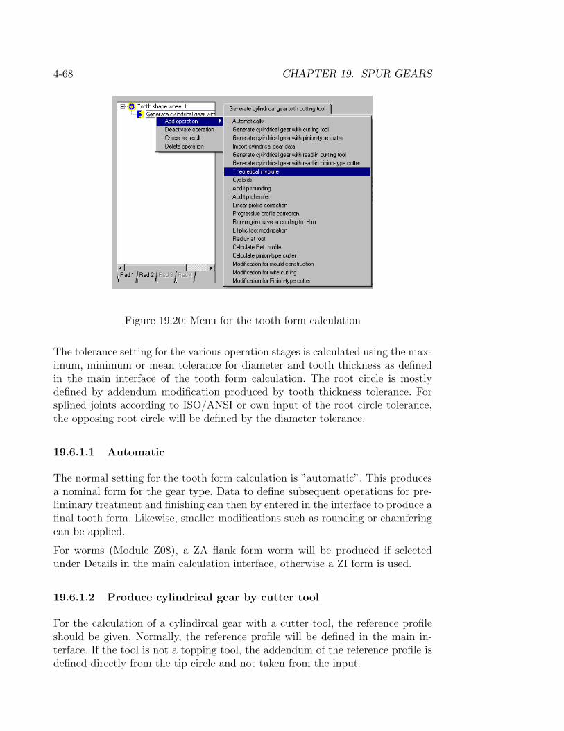
4-68 CHAPTER 19. SPUR GEARS
Figure 19.20: Menu for the tooth form calculation
The tolerance setting for the various operation stages is calculated using the max-imum, minimum or mean tolerance for diameter and tooth thickness as definedin the main interface of the tooth form calculation. The root circle is mostlydefined by addendum modification produced by tooth thickness tolerance. Forsplined joints according to ISO/ANSI or own input of the root circle tolerance,the opposing root circle will be defined by the diameter tolerance.
19.6.1.1 Automatic
The normal setting for the tooth form calculation is ”automatic”. This producesa nominal form for the gear type. Data to define subsequent operations for pre-liminary treatment and finishing can then by entered in the interface to produce afinal tooth form. Likewise, smaller modifications such as rounding or chamferingcan be applied.
For worms (Module Z08), a ZA flank form worm will be produced if selectedunder Details in the main calculation interface, otherwise a ZI form is used.
19.6.1.2 Produce cylindrical gear by cutter tool
For the calculation of a cylindircal gear with a cutter tool, the reference profileshould be given. Normally, the reference profile will be defined in the main in-terface. If the tool is not a topping tool, the addendum of the reference profile isdefined directly from the tip circle and not taken from the input.
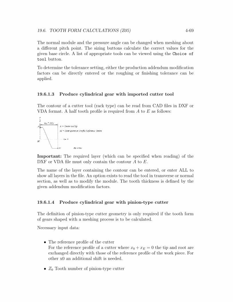
19.6. TOOTH FORM CALCULATIONS (Z05) 4-69
The normal module and the pressure angle can be changed when meshing abouta different pitch point. The sizing buttons calculate the correct values for thegiven base circle. A list of appropriate tools can be viewed using the Choice of
tool button.
To determine the tolerance setting, either the production addendum modificationfactors can be directly entered or the roughing or finishing tolerance can beapplied.
19.6.1.3 Produce cylindrical gear with imported cutter tool
The contour of a cutter tool (rack type) can be read from CAD files in DXF orVDA format. A half tooth profile is required from A to E as follows:
Important: The required layer (which can be specified when reading) of theDXF or VDA file must only contain the contour A to E.
The name of the layer containing the contour can be entered, or enter ALL toshow all layers in the file. An option exists to read the tool in transverse or normalsection, as well as to modify the module. The tooth thickness is defined by thegiven addendum modification factors.
19.6.1.4 Produce cylindrical gear with pinion-type cutter
The definition of pinion-type cutter geometry is only required if the tooth formof gears shaped with a meshing process is to be calculated.
Necessary input data:
• The reference profile of the cutterFor the reference profile of a cutter where x0 + xE = 0 the tip and root areexchanged directly with those of the reference profile of the work piece. Forother x0 an additional shift is needed.
• Z0 Tooth number of pinion-type cutter

4-70 CHAPTER 19. SPUR GEARS
• X0 Addendum modification pinion-type cutter(if X0 is not known, the addendum modification on the tip diameter or thetooth width can be calculated over the spur gear calculation – c.f. chapter19.3.7.1)
• - alternatively
– f0 length of the phase on the cutter or
– ρ0 radius of the rounding on the cutter
see picture Z-003/2.
Tooth form modifications: see 19.6.1.11
19.6.1.5 Produce cylindrical gear with imported pinion-type cutter
The contour of a cutter can be imported from CAD in DXF or VDA format. Itmust be defined as a half or full tooth from tip (at A) to the root (at E).
A : Centre tooth tip: contour beginningE : Centre tooth gap: contour endM : Centre point (xm, ym required)z : Tooth number
Important: The required layer (which can be specified when reading) of theDXF or VDA file must only contain the contour A to E.
The number of teeth on the cutter and manufacturing distance must also beentered.
19.6.1.6 Import cylindrical gear
A cylindrical gear form can be read from a DXF or VDA file. For this, a halftooth form must be defined in a specified layer (or layer selected from a list oflayers found in the file):

19.6. TOOTH FORM CALCULATIONS (Z05) 4-71
A : Centre tooth tip: contour beginningE : Centre tooth gap: contour endM : Centre point (xm, ym required)z : Tooth number
Important: The required layer (which can be specified when reading) of theDXF or VDA file must only contain the contour A to E.
19.6.1.7 Add tip rounding
A tip rounding can be applied to a tooth form. The rounding can be applied ineither the axial or transverse section.
19.6.1.8 Add tip chamfer
A tip chamfer can be applied to a given tooth form. It can be applied in either theaxial or transverse sections, and is defined by a starting diameter and an anglerelative to the tip.
19.6.1.9 Linear profile correction
Linear profile correction implies that from a given start diameter the tooth thick-ness is reduced linearly to a maximum reduction value (Ca per flank) at thetip.
19.6.1.10 Progressive profile correction
Progressive profile correction implies that from a given start diameter the tooththickness is reduced to a maximum reduction value (Ca per flank) at the tipsubject to the equation:
∆As = 2Ca
(d− dbegin
da − dbegin
)factor/5
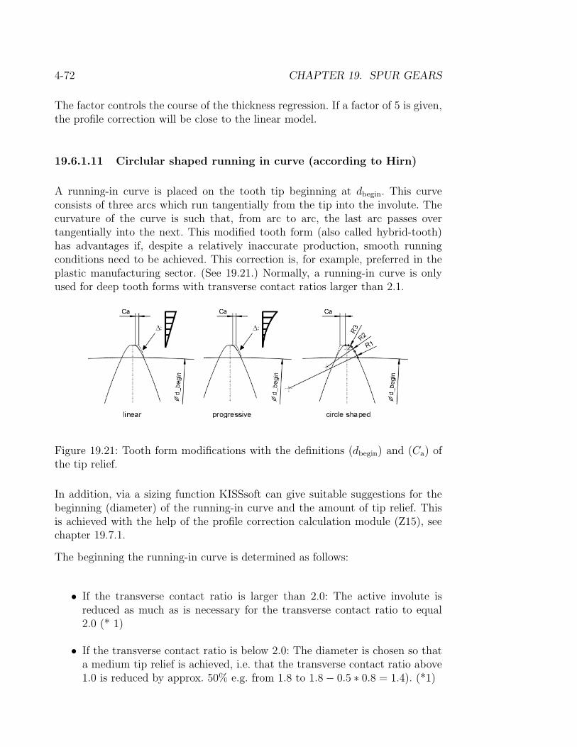
4-72 CHAPTER 19. SPUR GEARS
The factor controls the course of the thickness regression. If a factor of 5 is given,the profile correction will be close to the linear model.
19.6.1.11 Circlular shaped running in curve (according to Hirn)
A running-in curve is placed on the tooth tip beginning at dbegin. This curveconsists of three arcs which run tangentially from the tip into the involute. Thecurvature of the curve is such that, from arc to arc, the last arc passes overtangentially into the next. This modified tooth form (also called hybrid-tooth)has advantages if, despite a relatively inaccurate production, smooth runningconditions need to be achieved. This correction is, for example, preferred in theplastic manufacturing sector. (See 19.21.) Normally, a running-in curve is onlyused for deep tooth forms with transverse contact ratios larger than 2.1.
Figure 19.21: Tooth form modifications with the definitions (dbegin) and (Ca) ofthe tip relief.
In addition, via a sizing function KISSsoft can give suitable suggestions for thebeginning (diameter) of the running-in curve and the amount of tip relief. Thisis achieved with the help of the profile correction calculation module (Z15), seechapter 19.7.1.
The beginning the running-in curve is determined as follows:
• If the transverse contact ratio is larger than 2.0: The active involute isreduced as much as is necessary for the transverse contact ratio to equal2.0 (* 1)
• If the transverse contact ratio is below 2.0: The diameter is chosen so thata medium tip relief is achieved, i.e. that the transverse contact ratio above1.0 is reduced by approx. 50% e.g. from 1.8 to 1.8− 0.5 ∗ 0.8 = 1.4). (*1)

19.6. TOOTH FORM CALCULATIONS (Z05) 4-73
(*1): exact Definition:Transverse contact ratio > 2.0 : dBegin = Minimum (dPointD, dPointE0.2)Transverse contact ratio < 2.0 : dBegin = Minimum (dPointDE, dPointE0.2)
The relief Ca at the tip is determined as follows:
• Tooth tip thickness below 0.21 ∗mn: 0.5 ∗ Tooth thickness− 0.01 ∗mn
• Tooth tip thickness above 0.21 ∗mn: 0.10 ∗mn . . . 0.12 ∗mn
19.6.1.12 Optimised root radius (elliptical)
The root contour is replaced by an elliptical contour which fits tangentially tothe flank- and root circles. The aim is to reach an as large as possible curvatureradius. The contour course may be a influenced by a factor from 1-20. The sizingbutton for the utilised root diameter is used to define the start diameter for themodification. The length on the root circle which is not to be modified can beset to > 0.0 if an area of the tooth form encroaches the root circle. This makessense if, for example, the root circle is to be measured using rollers.
To ensure the largest tooth thickness in the root is allowable, the gear modifica-tions should be checked by meshing with the mating gear.
19.6.1.13 Root radius
The root contour is replaced by an exact arc of circle with a definable radius.The modification should be checked by meshing with the mating gear.
19.6.1.14 Theoretical involute
The tooth form will be constructed by calculation from the equation definition.The involute is defined by module and pressure angle with tip and root diametersalso give as limits to the development of the curve. The tooth thickness is deter-mined from the addendum modification factor. In addition, a root radius can bedefined (in the transverse section). This option is appropriate for involute gearswhich could not be produced by the generation procedure (e.g. internal gearswith 4 teeth) or for a machining operation like form grinding.

4-74 CHAPTER 19. SPUR GEARS
19.6.1.15 Cycloid
The cycloid is defined by two circle arcs with tip and root diamater values. Thetooth thickness on the pitch diameter is determined by the allowance in the maincalculation. The roller circle 1 rolls on the inside of the pitch circle and thereforecuts the root flank, the roller circle 2 rolls on the outside and generates thetip. The roller circle 1 of the first wheel should correspond to the roller circleof the second wheel. The sizing of a cycloid toothing is faciliated if, during theoptimisation, the counter wheel is calculated from the first wheel. By this, themeshing line is known and the course of tension (Z25) and the kinematics (Z27)can be calculated.
Strength and geometrical properties of cycloid gearing can be analysed using themodlues for stress (Z25) and kinematics (Z27).
19.6.1.16 Circular - Arc gearing
The special circle shaped tooth forms can be defined by the radius of the toothflank and the tooth thickness on the pitch circle. The root is set into a circle. Tocomply with the standards, the module for circle shaped toothing calculation inKISSsoft has to be improved.
19.6.1.17 Meshing with counter tooth form
For all gears (except gear 1) the tooth form can be calculated from the countergear (as gear 1). The manufacturing distance as well as the tip circle can beentered. Backlash between the gears can be produced on the one hand by a re-duction in manufacturing distance, or on the other by direct entry of a tangentialbacklash value. The tip clearance is achieved by an enlargement of the tip circleof the tool.
19.6.1.18 Calculate reference profile
The reference profile for an existing tooth form can be calculated. This can beused for the manufacture of a special hob or cutter gear. The manufacturingdistance can be changed for this calculation. This has a distinct influence on theability to produce the part by meshing. The value to be entered for the addendummodification, in contrast, changes nothing on the profile, only the datum position.
Using the calculated reference profile as a tool, the original tooth form is thencalculated. The two tooth forms (original and calculated) can be compared andevaluated to see how accurate the manufatured form will be to the required form.
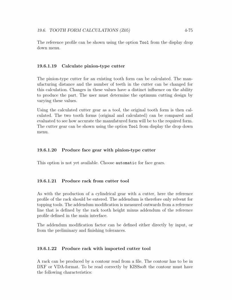
19.6. TOOTH FORM CALCULATIONS (Z05) 4-75
The reference profile can be shown using the option Tool from the display dropdown menu.
19.6.1.19 Calculate pinion-type cutter
The pinion-type cutter for an existing tooth form can be calculated. The man-ufacturing distance and the number of teeth in the cutter can be changed forthis calculation. Changes in these values have a distinct influence on the abilityto produce the part. The user must determine the optimum cutting design byvarying these values.
Using the calculated cutter gear as a tool, the original tooth form is then cal-culated. The two tooth forms (original and calculated) can be compared andevaluated to see how accurate the manufatured form will be to the required form.The cutter gear can be shown using the option Tool from display the drop downmenu.
19.6.1.20 Produce face gear with pinion-type cutter
This option is not yet available. Choose automatic for face gears.
19.6.1.21 Produce rack from cutter tool
As with the production of a cylindrical gear with a cutter, here the referenceprofile of the rack should be entered. The addendum is therefore only relvent fortopping tools. The addendum modification is measured outwards from a referenceline that is defined by the rack tooth height minus addendum of the referenceprofile defined in the main interface.
The addendum modification factor can be defined either directly by input, orfrom the preliminary and finishing tolerances.
19.6.1.22 Produce rack with imported cutter tool
A rack can be produced by a contour read from a file. The contour has to be inDXF or VDA-format. To be read correctly by KISSsoft the contour must havethe following characteristics:

4-76 CHAPTER 19. SPUR GEARS
Important: The required layer (which can be specified when reading) of theDXF or VDA file must only contain the contour A to E.
In addition to the contour, the manufacturing distance must be entered. Thereference line for the centre distance can then be defined from the rack (see 19.8).
19.6.1.23 Produce rack with pinion-type cutter
As with the production of a gear with a pinion-type cutter, here the referenceprofile of the cutter gear is to be given. The addendum modification is mea-sured outwards from a reference line defined by the rack tooth height minus theaddendum of the reference profile defined in the main interface.
The addendum modification factor can be defined either directly by input, orfrom the preliminary and finishing tolerances.
19.6.1.24 Produce rack with imported pinion-type cutter
A rack can be produced by a pinion-type cutter contour read from a file. Thetooth number of the cutter and manufacturing distance must also be defined.The contour has to be in DXF or VDA-format. To be read correctly by KISSsoftthe contour must have the following characteristics:

19.6. TOOTH FORM CALCULATIONS (Z05) 4-77
A : Tip centre: Begin ContourE : Centre of tooth space: End contourM : Midpoint (xm, ym to be entered)z : Tooth number
Important: The required layer (which can be specified when reading) of theDXF or VDA file must only contain the contour A to E.
19.6.1.25 Read rack form from DXF file
A rack can be produced by contour read directly from a file if in the followingformat:
Important: In the layer which can be defined when reading, the file (DXF orVDA) must only contain the contour A to E.
19.6.1.26 Produce ZA-worm
This function is only available under automatic at this point.
19.6.1.27 Produce worm using imported axial section
A worm can be produced by a contour read from a file. The contour has to bein DXF or VDA-format. The contour corresponds to a cutter tool contour in thedatum position but with the origin on the axis of the worm. To be read correctlyby KISSsoft the contour must have the following characteristics:
Important: The required layer (which can be specified when reading) of theDXF or VDA file must only contain the contour A to E.

4-78 CHAPTER 19. SPUR GEARS
19.6.1.28 Modification for the mould form
When manufacturing gears from plastics by injection moulding, the materialmight shrink when it cools down. To be able to manufacture exact tooth forms,however, the tool must be enlarged by the amount it shrinks. The shrinkage,depending on the material, may happen rather in radial than in tangential di-rection. If the same values are entered for radial and tangential values, then thesame expansion is applied in all directions.The modifications only affect the tooth form in the transverse section. Whenproducing a 3D volume model an expansion in the axial direction is not consid-ered.If an expanded 3D model of a helical tooth form is required (as long as the expan-sion is the same in all 3 axes) it can be achieved by the following: Module(mn),Centre Distance(a) and Face Width (b) expanded using the desired expansion fac-tor (Factor = 1.02, such that mnnew = mn∗1.02; anew = 1.02∗a, b1new = b2∗1.02,b2new = b2 ∗ 1.02). (Give no expansion in the tooth form calculation). Throughthis modification, the lead p*z is also increased by the same factor (this impliesthat the angle of rotation of the spiral over the tooth width remains the same).
Typical values are:
• Radial Shrinkage ca. 2
• Tangential Schrinkage ca. 2
Calculating Electrodes and Casting Forms for Manufacturing Spur andWorm Gears
Gear wheels are often produced by pressure casting procedures. Several phasesare needed to produce a form:
1. Checking the data of the gear- or worm wheel to produceEntering the data, if possible of the pairing (Worm/wheel or spur gear/spurgear) with checking geometry, meshing tolerance etc.
2. Calculating the contour of the casting formCalculating the tooth form considering
• Nominal tooth thickness deviation
• Radial expansion
• Tangential expansion
The contour produced in this way serves as a check of the produced mouldform.

19.6. TOOTH FORM CALCULATIONS (Z05) 4-79
19.6.1.29 Modification for Electrodes
1. Calculating as before, but additionally considering:
• Spark gap
The calculated contour is the ideal electrode.
2. Calculating the milling cutter for the production of the electrodeDetermining the reference profile of the electrode calculated under point 3.Transforming the reference profile from transverse section to normal section.
The ideal milling cutter profile is given by this data and the cutter can nowbe produced with the usual procedures.
Technical explanations:
The spark gap is the gap between electrode and tool produced while eroding.This gap has to be considered and the electrode has to be produced thinner, bythe value of the spark gap. In case of an electrode formed like a gear wheel, thetooth becomes thinner.
When producing plastic gear wheels in injection casting forms , a shrinkage hap-pens when the plastic becomes solid. To compensate for that loss, the castingform is made a little larger. This is made by tangential or radial strain. With ra-dial strain, the tooth form is stretched in radial direction, with tangential strainthe tooth is thickened and the tooth gap is inclined.
Normal values:
• Spark gap 0.03 . . . 0.07 mm
Inserted pieces: When the gear has to be injected around an insertion piece, itsexternal diameter must be introduced. The radial strains will then be calculatedfrom this external diameter.
19.6.1.30 Modification for Manufacturing of pinion-type Cutter
The effective cutting angle and the draft angle of the shaping cutter result ina distortion of the tooth form in the projection of the shaping cutter in thehorizontal plane. The conversion carried out here distorts the tooth form in thehorizontal plane so that, for the manufactured shaping cutter, the projectionproduces the exact tooth form.

4-80 CHAPTER 19. SPUR GEARS
φ = Effective cutting angleξ = Tip draft angle in axis sectionM = Shaping cutter centre line
By grinding at an angle φ (effective cutting angle) Q moves to P (see figure Z-018). If the projection of P (i.e. P ′) is correct (exact contour in the horizontalplane), P must be equal to Q in the H-plane.
PP ′ = (ra − rp) ∗ tan(φ) (19.4)
P ′Q = (PP ′) ∗ tan(ξ) (19.5)
hence : P′Q = (ra − rp) ∗ tan(φ) ∗ tan(ξ) (19.6)
Converting the tooth form:
Given: exact tooth form given in polar co-ordinate notation P = r (angle)Task: calculate tooth form in H-plane P’ = r’ (angle)Solution r′ = r + tan(φ) · tan(ξ) · (ra − r)
19.6.2 Tooth form display
A variety of display options are available in the tooth form calculation interface:
• Tooth form of the gearThe tooth form for the selected gear is shown.

19.6. TOOTH FORM CALCULATIONS (Z05) 4-81
• Tooling for the gearThe tool for the currently selected gear will be displayed (if applicable).
• Manufacturing of the gearThe gear and tool will be displayed as a mating pair. The gear is the lowercontour, and the tool is shown above.
• Gear pairTwo gears can be viewed as a meshing pair.
Figure 19.22: Graphical display of tooth form
In the display of a mating gear pair, the positions during mesh can be indexedtogether ( Buttons < and > ) , or the position of gear 2 can be changed indepen-dently (Buttons < 2 or 2 > ). It is also possible to enter the rotational positionrequired directly as a factor of the pitch.
The >> button provides access to further display options:
• Under Display, the line thickness can be changed, and various significantdesign parameters (da, df , dFa, dFf , db, dw) can be visualised.

4-82 CHAPTER 19. SPUR GEARS
• In the single gear display, the options Transverse section, Axial
section und Normal section can be used to view the gear form in varioussections. There are two variants for the normal section; the plane throughthe tooth tip or the tooth space. For the manufacture of a grinding disk,the section through the tooth space is definitive. Using the option Tooth
for export a half tooth form can be displayed, which can also be importedinto the tooth form calculation.
• The option Display gear can be used to display further operation stagesin the tooth form calculation. This is also possible for a tool–work piecepairing. This permits an easy evaluation of which regions of the tooth formare produced from which tools.
• A collision check (Z05j, Z05k) can also be activated. Then the collisions(overlap points of mating profiles) are highlighted as red squares, and con-tacting points as blue squares.
• The option Join flanks brings the selceted flank of the gear pair intocontact.
• The Save tooth profile option saves the state of the current form. Thesewill be displayed in further calculations of the current gear pair to providea comparison of the changes applied.
• The Delete memory option deletes the saved gear forms. The saved gearforms will be automatically deleted if the tooth numbers are changes.
The left mouse click allows the display to be shifted, while the right mouse buttonactivates a measuring function in the display area. The buttons + and − can beused to zoom in/out.
19.7 Various Calculations in the Menu ’Calcu-
lations’
In the menubar of the spur gear calculation under calculations, you find severalcalculations that can be very helpful with individual problems.

19.7. VARIOUS CALCULATIONS IN THE MENU ’CALCULATIONS’ 4-83
Figure 19.23: List with the additional calculations
19.7.1 Drawing (schematically)
The gear wheels can be displayed individually or as pairs (schematically), intransverse and axis section. This display of tooth form is not very helpful forspur gears, it is normally used for bevel and worm gears. The actual display is inCalculations ⇒ Tooth Form.
19.7.2 Calculating Contact Length to Verify the Involuteand Suggestions for Optimal Profile Corrections)
Calculation of the points A to E of the path of contact with the corresponding in-volute length. Output of the diameters, radii, involute lengths and contact length

4-84 CHAPTER 19. SPUR GEARS
for the involute validation program (for the gear and the paired opposing gear).Reference values for the tip relief are given according to the different methods. Itwould make more sense to select an average value.
The precise understanding of the calculated values requires a corresponding ex-perience in the gear wheel manufacturing.
19.7.2.1 Calculating and Sizing of Profile Correction
Basics
a) The tip relief on the driven gear wheel reduces the impact when they comeinto contact, the tip relief on the driving wheel reduces the impact whenthey leave contact. Hence, tip reliefs are normally provided on both wheels,in special cases only on the driven wheel.
b) The amount of tip relief is calculated in KiSSsoft for the maximal permanenttorque. For gear wheels which have not always the same service torque, forboth pinion and wheel, 50-70
c) The length of the correction is also calculated in KISSsoft, the so-calledlong correction stretches from point E until point D of the contact line, theso-called short correction only until point H −DE (centre between D andE). Normally, the short correction is taken.
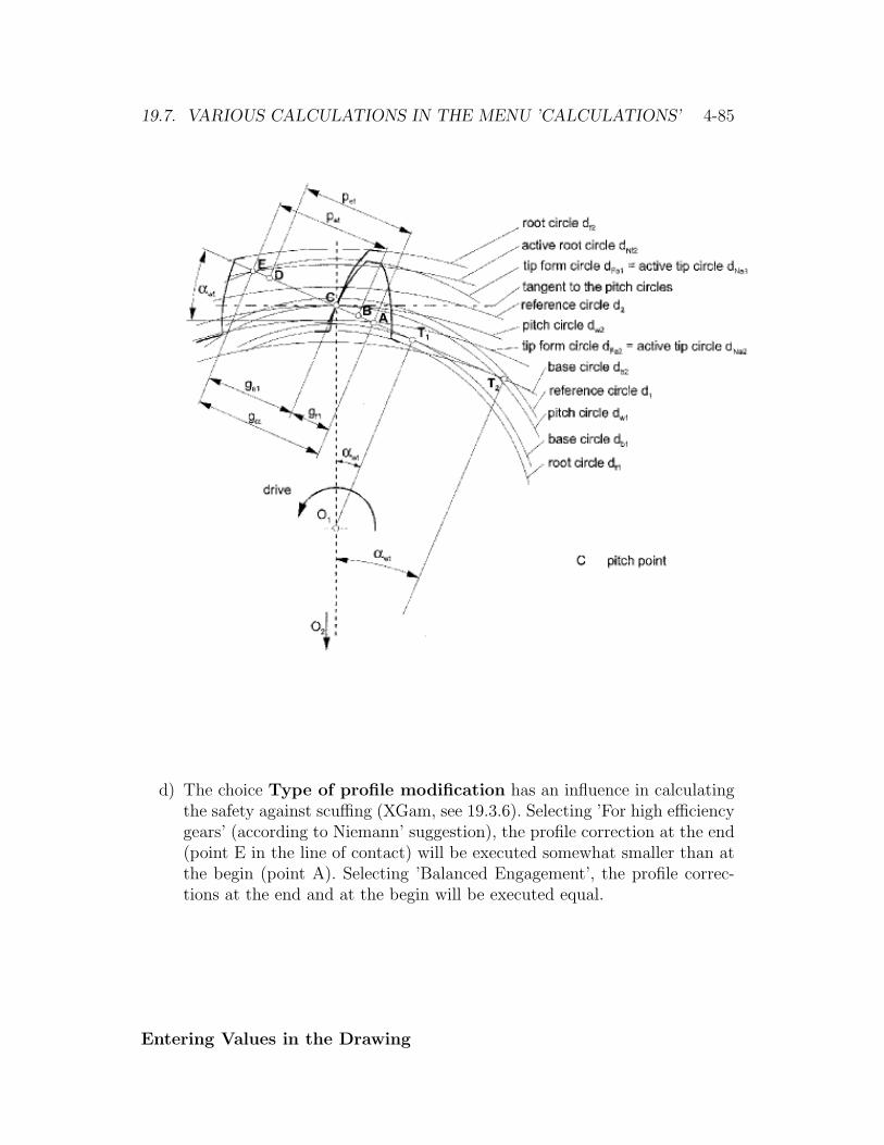
19.7. VARIOUS CALCULATIONS IN THE MENU ’CALCULATIONS’ 4-85
d) The choice Type of profile modification has an influence in calculatingthe safety against scuffing (XGam, see 19.3.6). Selecting ’For high efficiencygears’ (according to Niemann’ suggestion), the profile correction at the end(point E in the line of contact) will be executed somewhat smaller than atthe begin (point A). Selecting ’Balanced Engagement’, the profile correc-tions at the end and at the begin will be executed equal.
Entering Values in the Drawing

4-86 CHAPTER 19. SPUR GEARS
The description, where the involute test diagram on the left side and on the rightside the sidecut of the corresponding tooth were displayed, serves as pattern.The lengths in the involute test diagram are the contact lengths Ly according toDIN 3960. The last point on the foot is the point A (end of the active involute).The tip relief value A suggested by the program, is determined by the resultaverage value according to Niemann. A somewhat higher value for the line ofcontact begin (C.I) is set at the tip of the driven wheel, at the tip of the drivingwheel the value for the line of contact end (C.II). Selecting the profile correction’Balanced Engagement’, the value for the line of contact end will be set to C.I.
Pinion Wheelb = Ly(A)− Ly(E) b = Ly(E)− Ly(A)c = Ly(H −DE)− Ly(E) c = Ly(H − AB)− Ly(A)d = ra−y(A)− ra−y(E) d = ra−y(E)− ra−y(A)e = ra−y(H −DE)− ra−y(E) e = ra−y(H − AB)− ra−y(A)
Important:
a) When calculating the addendum modification, the tip chamfer must beentered. Else, the program does not calculate with the active involute.
b) The calculation of the tooth contact stiffness is executed according to theselected calculation method. Alternatively, it is possible to determine thecontact stiffness from the tooth profile (see 19.4.6.4).
c) The notation of the points on the path of contact is defined according toDIN 3960. When the pinion is driving, the tip modification is to be carriedout on the pinion from H −DE to E (or alternatively D to E) and on the
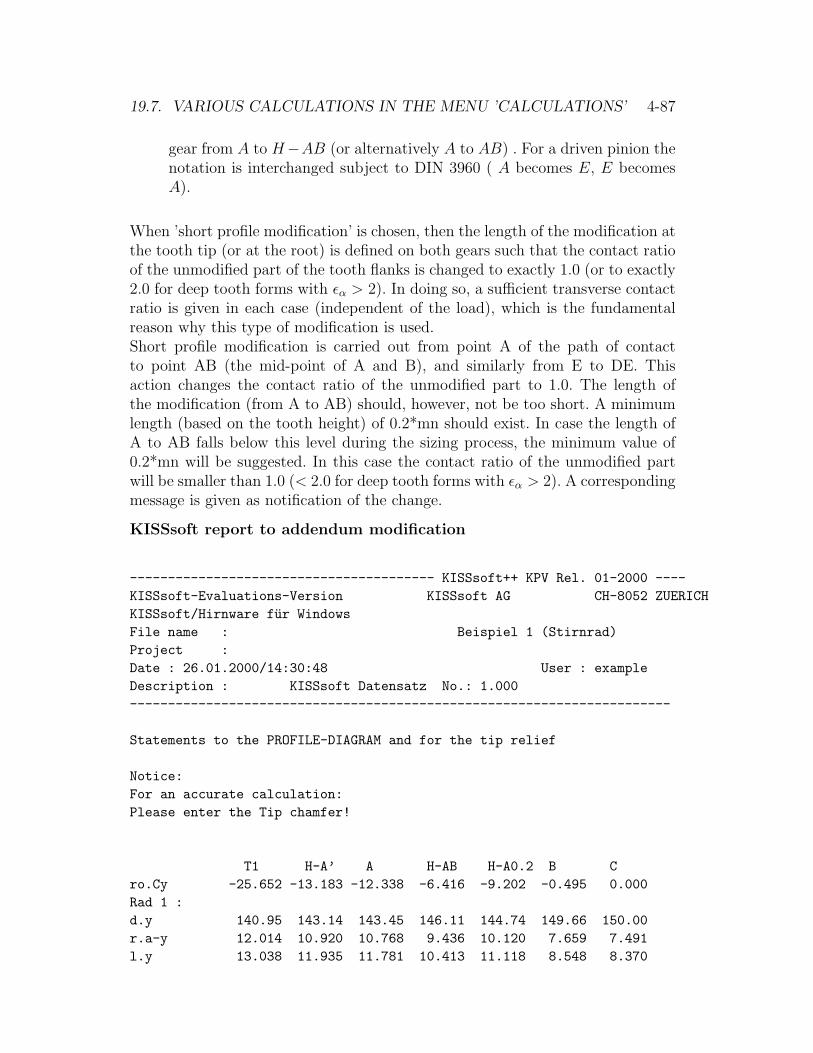
19.7. VARIOUS CALCULATIONS IN THE MENU ’CALCULATIONS’ 4-87
gear from A to H−AB (or alternatively A to AB) . For a driven pinion thenotation is interchanged subject to DIN 3960 ( A becomes E, E becomesA).
When ’short profile modification’ is chosen, then the length of the modification atthe tooth tip (or at the root) is defined on both gears such that the contact ratioof the unmodified part of the tooth flanks is changed to exactly 1.0 (or to exactly2.0 for deep tooth forms with εα > 2). In doing so, a sufficient transverse contactratio is given in each case (independent of the load), which is the fundamentalreason why this type of modification is used.Short profile modification is carried out from point A of the path of contactto point AB (the mid-point of A and B), and similarly from E to DE. Thisaction changes the contact ratio of the unmodified part to 1.0. The length ofthe modification (from A to AB) should, however, not be too short. A minimumlength (based on the tooth height) of 0.2*mn should exist. In case the length ofA to AB falls below this level during the sizing process, the minimum value of0.2*mn will be suggested. In this case the contact ratio of the unmodified partwill be smaller than 1.0 (< 2.0 for deep tooth forms with εα > 2). A correspondingmessage is given as notification of the change.
KISSsoft report to addendum modification
---------------------------------------- KISSsoft++ KPV Rel. 01-2000 ----KISSsoft-Evaluations-Version KISSsoft AG CH-8052 ZUERICHKISSsoft/Hirnware fur WindowsFile name : Beispiel 1 (Stirnrad)Project :Date : 26.01.2000/14:30:48 User : exampleDescription : KISSsoft Datensatz No.: 1.000-----------------------------------------------------------------------
Statements to the PROFILE-DIAGRAM and for the tip relief
Notice:For an accurate calculation:Please enter the Tip chamfer!
T1 H-A’ A H-AB H-A0.2 B Cro.Cy -25.652 -13.183 -12.338 -6.416 -9.202 -0.495 0.000Rad 1 :d.y 140.95 143.14 143.45 146.11 144.74 149.66 150.00r.a-y 12.014 10.920 10.768 9.436 10.120 7.659 7.491l.y 13.038 11.935 11.781 10.413 11.118 8.548 8.370

4-88 CHAPTER 19. SPUR GEARS
L.y (ro.y) 42.869 30.401 29.555 23.634 26.420 17.713 17.218h.BP - - -5.580 -3.555 -4.508 -1.530 -1.360Rad 2 :d.y - - 465.02 460.55 462.62 456.34 456.00r.a-y - - 0.000 2.235 1.200 4.339 4.509l.y - - 0.000 2.414 1.299 4.665 4.846L.y (ro.y) - - 0.000 5.921 3.136 11.843 12.338h.BP - - 5.889 3.864 4.817 1.839 1.670
C D H-E0.2 H-DE E H-E’ T2ro.Cy 0.000 5.375 14.861 11.296 17.218 21.902 77.981Rad 1 :d.y 150.00 154.01 162.58 159.15 164.98 - -r.a-y 7.491 5.487 1.200 2.916 0.000 - -l.y 8.370 6.209 1.394 3.353 0.000 - -L.y (ro.y) 17.218 11.843 2.357 5.921 0.000 - -h.BP -1.360 0.478 3.722 2.503 4.528 - -Rad 2 :d.y 456.00 452.44 446.71 448.78 445.40 442.93 428.50r.a-y 4.509 6.291 9.155 8.121 9.809 11.042 18.259l.y 4.846 6.735 9.739 8.660 10.421 11.698 19.037L.y (ro.y) 12.338 17.713 27.198 23.634 29.555 34.240 90.318h.BP 1.670 -0.169 -3.413 -2.194 -4.219 - -
Proposal for addendum modification according to different sources:Partial load for the layout (%) 100.00
Short profile correction, Tip relief
MAAG (my) 23.466J.Theissen (VDI-Report 626) (my) 47.494Niemann C.I (Pt. A) i/e (my) 47.494/57.494Niemann C.II (Pt. E) i/e (my) 37.494/47.494
Proposal for Tool dataReference profile Gear 1Buckling root flank (in module) 0.417Buckling root flank angle (deg) 21.288(Tip relief (my) 52)
Reference profile Gear 2Buckling root flank (in module) 0.644Buckling root flank angle (deg) 21.288(Tip relief (my) 52)

19.7. VARIOUS CALCULATIONS IN THE MENU ’CALCULATIONS’ 4-89
Specification in the drawing (Fig. Z-023)a = 0.052 0.052 (mm)
+- 0.005 0.005 (mm)b = 29.555 29.555 (mm)c = 5.921 5.921 (mm)d = 10.768 9.809 (mm)e = 2.916 2.235 (mm)f = 0.000 0.000 (mm)
Notice: my := 10^-6 m
ro.Cy Length on the path of contact (mm)d.y Diameter (mm)r.a-y Radius difference (d.a-d.y)/2 (mm)l.y Length of involute (mm)L.y (ro.y) Contact length, DIN 3960(2.12)(mm)h.BP Height at reference profile (mm)
Points on the line of contact:T1 Base circle gear 1A Begin of contact (Tip diameter gear 2)B Inside single contact pointC Pitch diameterD Outside single contact pointE End of contact (Tip diameter gear 1)T2 Base circle gear 2H-AB Mean between A and BH-DE Mean between D and EH-A0.2 approx. 0.20*mn under tip circle (wheel2)H-E0.2 approx. 0.20*mn under tip circle (wheel1)H-A’ Theoretical begin of contact if paired with rackH-E’ Theoretical end of contact if paired with rack
19.7.3 Calculation of the tooth thickness for any diameter
With the menu item Calculations⇒ Chordial tooth thickness you can cal-culate the normal tooth thickness and the normal gap width for any diameter.
The output is the tooth thickness as an arc length and as a length of the chord.The height above the chord is also stated for the measurement of the tooththickness (c.f. chapter 25.1.5).

4-90 CHAPTER 19. SPUR GEARS
19.7.4 Tolerances for Gear Manufacturing
Manufacturing tolerances are calculated corresponding to appropriate Standards(such as ISO1328, DIN3961, etc). The specifications in the standards apply tospecific areas, for example ISO1328 for modules from 0.5 to 70. These areas canbe subdivided, for example ISO1328 by module in ranges of 0.50, 2.0, 3.5, 6.0,10.0, 16.0, 25.0, 40.0 and 70.0. Within one of these stages, the tolerances canbe read from a table. The calculation of the tolerances is carried out subject tothe formulae in the Standards, in which the geometric middle of the appropriatemodule range and not the real value, i.e. the current module, is used (for examplethe calculation of the tolerances with module 2.25 is treated in the formula asModule = (2.0 ∗ 3.5)0.5 = 2.646).
For actual values which are outside of the specified ranges, the formulae cannot be applied. Indeed, there are for these cases in parts no Standards at allfrom which equations can be taken and utilised. In cases where the values areoutside defined ranges, simply taking smallest or largest (as appropriate) definedtolerance gives distinctly too large tolerances (for example Module 01.mm). Ittherefore makes sense to carry out the calculation with the actual value.
In this case the procedure in KISSsoft will be as follows:
• Actual value >= 0.8*Smallest stage and Actual Value < Smallest Value:Calculation of tolerances with value of the smallest value
• Actual value < 0.8*Smallest stage:Calculation of tolerances with the actual value
• Actual value > Largest stage:Calculation of tolerances with the actual value
Example:mn = 0.3: Tolerance calculation with mn=0.3 (Actual value)mn = 0.45: Tolerance calculation with mn=0.5 (Smallest stage value)mn = 100: Tolerance calculation with mn=100 (Actual value)
The protocol issues a list of all manufacturing tolerances for spur gears accordingto DIN 3961, ISO 1328, BS 436, DIN 58405, AGMA 2015 and the (replaced)AGMA 2000.
For the functions:
G = UniformityL = NoiseT = Load capacityN = General
19.7. VARIOUS CALCULATIONS IN THE MENU ’CALCULATIONS’ 4-91
the following listed tolerances are especially important:
Individual deviationsProfile deviationsProfile-Angular deviation
L N Profile total-deviationL T Normal base pitch deviation
Pitch stepG L Pitch-Total deviation
Pitch-Tension deviationG L Concentricity deviation
Tooth thickness deviationTooth trace total deviation
L T N Tooth trace angle deviationTooth trace form deviation
Roll deviationG N Two flank roll deviationG L N Two flank roll jumpG Single flank roll deviationG L Single flank roll jump
19.7.5 Crowning
For the sizing of the crowning within the KISSsoft spur gear calculation, there isonly one proposal regarding the ISO 6336. For more exact crowning sizings, usemodule W10 within the KISSsoft shaft calculation (See chapter 15.5.11).
19.7.6 Calculating the Centre Points of Planets or GearWheels (Z19g)
For planets:The centre points of planetary gear trains are calculated in such a way thatplanets can be inserted.
For gear wheel chains (3-wheels):When the distance between the first and the last wheel is entered, the positionof the intermediate wheels is calculated, regarding production conditions.

4-92 CHAPTER 19. SPUR GEARS
19.7.7 Specific Sliding(Z19e)
The course of specific sliding (ratio sliding- to tangential speed) is displayedgraphically for pinion and gear over the length of path of contact. The case withthe minimal center distance and the maximal usable tip diameters is marked with’ and the case with the maximal center distance and minimal diameters is markedwith ”. So the variation of the specific sliding according to the tolerance fieldscan be estimated quickly.
When entering the addendum modification in the ’N’ window, you can also obtainthe sizing function proposals for addendum modifications to compensate specificsliding.
19.7.8 Flashtemperature Course
The flashtemperature (local temperature on the tooth flank in the moment theteeth come into contact) is displayed graphically in the tooth contact drawing.Hence, the point with the highest temperature can be seen and measures can beintroduced to improve the state (addendum modification).
19.7.9 Hardness Depth (Z22)
The optimal hardness depth (for case- or nitrite-hardened gear wheels) is cal-culated; the course of stress (shear stress) in the depth (vertical to the flanksurface) is displayed. The values are stated directly in HV-values, as calculationswith hardness depths always compute with HV- or HRC-values. If the materialdata base contains values of an already measured hardness course, the programissues a warning when unsatisfying hardness conditions are to be displayed.
Tip: The stipulated hardness depth (EHT) should be indicated on gear wheeltechnical drawings. Usually, the hardness depth specifications demand that aminimal hardness of HV550 could be detected be at the correspondent depth.
19.7.10 Rating
The gear wheel can be rated according to different criteria. This function servesto compare toothings with different proposals for the fine sizing. C.f. chapters19.6 and 19.3.7.1.

19.7. VARIOUS CALCULATIONS IN THE MENU ’CALCULATIONS’ 4-93
19.7.11 Wohler Line Material
Display of the Wohler line for tooth root and flank.
19.7.12 Course of Safety
The course of safety is displayed depending on the service life.
19.7.13 Calculation with path of contact under load
The contact path is calculated with consideration of the load. The stiffness of thegear contact is calculated according Petersen (see 19.7.13) or set to a constantvalue if the module Z24 is missing. A factor for the load can be input and alsoa value for a pitch error. The proposal for the pitch error is calculated according√
f 2pt1 + f 2
pt2.
For helical gears the calculation is made with several sections of spur gears with-out a coupling between the sections.
19.7.13.1 Contact Stiffness and Transmission Error (Z24)
Graphical display of the contact stiffness. The calculation of the contact stiffness iscarried out based on the actual tooth form. Considered are tooth deviation, toothbody deformation and flattening through Hertzian stress. Calculations accordingto D. Petersen, Dissertation Braunschweg(Prof Roth), 1989.
For helical tooth gearing, the total stiffness is calculated using the section model(tooth face width divided into 100 sections and addition of individual stiffness oneach). Refer to [55], p.203. The transmission error is calculated subject to [61],and this error in the tangential direction, ∆s amounts to:∆s = (Fbt/b) ∗ (q/c′) where (q/c′) is replaced by cgam.Fbt = Ft/cos(αt)
19.7.13.2 Kinematics (Z27)
Based on the actual tooth form and the actual contact Line, various kinematicvalues can be calculated and displayed on the contact line:
• specific sliding
• sliding coefficients Kg

4-94 CHAPTER 19. SPUR GEARS
• sliding speed
• variation as ratio
With this program module, special toothings as e.g. cycloid toothings can berated.
19.7.13.3 Course of Stress Along the Flank Line (Z25)
Because of the actual tooth form, the hertzian stress at rolling is calculatedexactly and displayed. in the same way, the tooth root stress, which is foundaccording to the procedure of Obsieger (see 19.4.6.2), is calculated and displayed.
19.7.14 Calculating Service Life (Z18)
After the input or the confirmation of the minimal required margins of safetyfor root and flank, the predicted service life is calculated for all gears (in hours)depending on the defined load. Calculation according DIN 3990, Part 6 (February1994), using the Palgren-Miner rule.
The fatigue resistance range can be calculated differently from the DIN 3990choosing a modificated Woehler line (see below).
Reported is the predicted life of the system (all gears in the configuration).
Modifications of the Woehler line in the fatigue resistance range
In usual Woehler diagrams the fatigue resistance is reached after a certain amountof load cycles. After this point the permissible stress does not change anymore.This behaviour is named after Miner.
Recent research has shown that no fatigue resistance as such exists and a modi-fication of the Woehler diagram is required.
In the fatigue resistance range the following modifications can therefore be ap-plied:
• according to Corten/Dolan
• according to Haibach
• or the usual procedure according to Miner (corresponds to DIN 3990)
Figure Z-017 shows the corresponding characteristics. The gear life calculationwith equivalent design loads, the Miner approach, according to experience, givestoo optimistic results. The Haibach approach is recommended.

19.7. VARIOUS CALCULATIONS IN THE MENU ’CALCULATIONS’ 4-95
19.7.14.1 Option Z18a: Calculation of the Gear Life for EquivalentDesign Loads
As an addition to Z18 this module allows the incorporation of equivalent designloads. Arbitrary design load can be defined with information about frequency,power/torque and speed.
Equivalent design load
The calculation of the expected life is done according to DIN 3990, part 6 and isbased in the Palmgren-Mine rule.
Provided are three equivalent design loads according to DIN 15020 (crane build-ing) and norm collectivities. Separate equivalent design loads can be entered.
A equivalent design load contains several elements (up to 50 or 300 if read fromfiles), describing the frequency of the occurrence, speed and power or torque.The data is always based in the input of the nominal power (as in window power-torque-speed) for the reference gear. The values are stored as coefficients to assureaccurate updates in case of changes of the nominal power.
If two speeds not equal zero are input in the calculation of planetary gears twoequivalent design loads can be chosen. At the second equivalent design load onlythe factor for speed is used.
Remark:In this calculation, the load dependence of the K-coefficients is taken into account(K-coefficients are: dynamic, face load - and transverse coefficients). If the resultsare to be checked, file Z18-H1.TMP (in the TMP-file) contains the results.
See chapter 19.7.15.
4-96 CHAPTER 19. SPUR GEARS
19.7.15 Sizing for Torque (Z16)
For spur gears, bevel gears and worms, the calculation of the maximal permissabletorque is determined taking into account the required service life, nominal marginsof safety (for tooth breaking, pitting, scoring, for worms in addition wear andtemperature safety).
Option Z16a:Torque sizing for equivalent design loads
In addition to Z16 the same calculation for equivalent design loads. Up to 50elements of the design load (or up to 300 if read from files) can be defined (inthe database tool) with information about frequency, power/torque and speed.All equivalent design loads according DIN 15020 (crane building) are included.
The fatigue resistance range can in be calculated differently from the DIN 3990choosing a modificated Woehler line (c.f. 19.7.14).
If two speeds not equal zero are input in the calculation of planetary gears twoequivalent design loads can be chosen. At the second equivalent design load onlythe factor for speed is used.
Remark:In this calculation, the load dependence of the K-coefficients is taken into account(K-coefficients are: dynamic, face load - and frontal coefficients). If the resultsare to be checked, file Z18-H1.tmp contains intermediate results.
19.7.16 Safety with load spectra
If the required lifetime, the power rating, application factor (which is usuallyset to 1.0 if a load spectra is used) and the applicable load spectra are defined,the resulting safety factors for root and flanc are calculated. The safety factorsagainst scuffing will be calculated and reported using the highest load of theload spectra. For more detailed information on load spectra and Wohler line seechapter 19.7.14.
19.7.17 Operating Backlash (Z12)
In addition to the calculation of the theoretical backlash, the calculation of theacceptance backlash (considering the tooth error, axis wrenching according toDIN 3964 (c.f. table 19.4), form- and position-deviation) and the operating back-lash (considering the temperature difference between the gears and the housing)are carried out according to DIN 3967. For plastic gears the additional influenceof swelling is taken into account.

19.7. VARIOUS CALCULATIONS IN THE MENU ’CALCULATIONS’ 4-97
Bearingcentre-distance LG Axisposition-Accuracy
(Nominal Measure) 1 2 3 4 5 6 7 8 9 10 11 12in mm
up to 50 5 6 8 10 12 16 20 25 32 40 50 63above 50
up to 125 6 8 10 12 16 20 25 32 40 50 63 80above 125up to 280 8 10 12 16 20 25 32 40 50 63 80 100above 280up to 560 10 12 16 20 25 32 40 50 63 80 100 125above 560
up to 1000 12 16 20 25 32 40 50 63 80 100 125 160above 1000up to 1600 16 20 25 32 40 50 63 80 100 125 160 200above 1600up to 2500 20 25 32 40 50 63 80 100 125 160 200 250above 2500up to 3150 25 32 40 50 63 80 100 125 160 200 250 320
Table 19.4: Axis wrenching according to DIN 3964
With a module < 1 the additional calculation of the circumferential backlash willbe carried out according to DIN 58405. Instead, with the module < 1, the playreduction due to individual engagement deviation will not be determined sinceDIN 3967 is not valid for Module < 1.
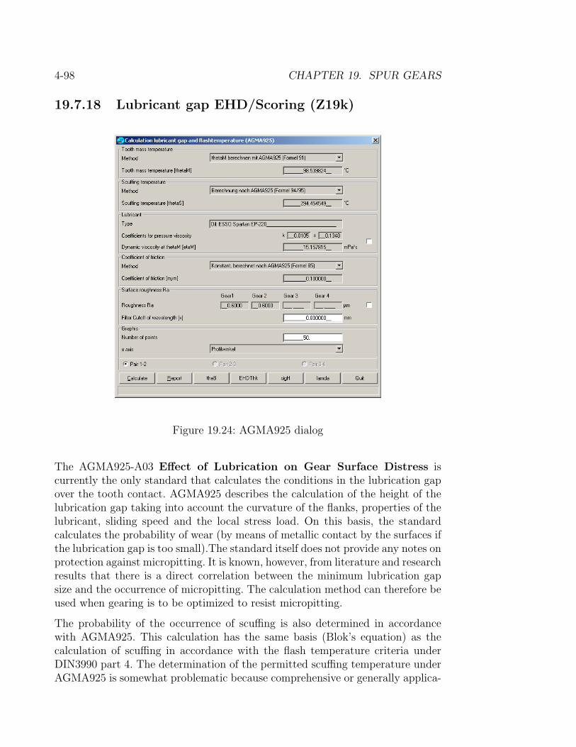
4-98 CHAPTER 19. SPUR GEARS
19.7.18 Lubricant gap EHD/Scoring (Z19k)
Figure 19.24: AGMA925 dialog
The AGMA925-A03 Effect of Lubrication on Gear Surface Distress iscurrently the only standard that calculates the conditions in the lubrication gapover the tooth contact. AGMA925 describes the calculation of the height of thelubrication gap taking into account the curvature of the flanks, properties of thelubricant, sliding speed and the local stress load. On this basis, the standardcalculates the probability of wear (by means of metallic contact by the surfaces ifthe lubrication gap is too small).The standard itself does not provide any notes onprotection against micropitting. It is known, however, from literature and researchresults that there is a direct correlation between the minimum lubrication gapsize and the occurrence of micropitting. The calculation method can therefore beused when gearing is to be optimized to resist micropitting.
The probability of the occurrence of scuffing is also determined in accordancewith AGMA925. This calculation has the same basis (Blok’s equation) as thecalculation of scuffing in accordance with the flash temperature criteria underDIN3990 part 4. The determination of the permitted scuffing temperature underAGMA925 is somewhat problematic because comprehensive or generally applica-

19.7. VARIOUS CALCULATIONS IN THE MENU ’CALCULATIONS’ 4-99
ble notes are missing in this area. In particular there is no reference to the scuffingload load capacity specification according to the FZG test. Oils with active EPadditives therefore have a tendency to be undervalued.
19.7.19 Deformation of Gear Rims (for Internal Gears)(Z23)
The rim can be deformed considerably through the tooth forces during meshingif for constructive reasons gear rims of internal gears are manufactured relativelythin. This program calculates the conditions at the point of contact and in thecentre between the points of contact (from two adjacent planetary gears) thebending stress and tangential stress as well as the radial deformation.
19.7.20 Master gear (Z29)
This calculation module in KISSsoft permits the sizing and control of mastergears.
For the double-flank rolling gear test, a master gear is needed which is meshedtogether with the test gear on a testing machine. During the checking procedure,the gear being tested and the master gear are pushed slightly together in an axialmanner along the centre line so that they are free of clearance. The variation ofthe centre distance is measured, and the maximum value determined in this wayis the total radial composite deviation.
In order to obtain a confident statement on the running behaviour of the wheelbeing tested after installation in the gear system, the active involute of the gearbeing tested should be shifted as completely as possible. On the other hand, themaster gear must under no circumstances encroach too far into the root area. Ifthe root form circle of the gear being tested is undercut, a disruption in contactwill occur, which has a massive and misleading effect on the measurement result.

4-100 CHAPTER 19. SPUR GEARS
Figure 19.25: Master gear calculation dialog
For each gear, a calculation can call up the design of the required master gear.On opening the design, the appropriate standard master gear in accordance withDIN3970 is suggested. Selecting Control tip circle master gear allows theuser to see whether an existing master gear can be used. The calculation checksthe maximum and minimum tolerance of the master gear tooth thickness in thearea where involute meshing occurs. The report shows which area of the activeinvolute were checked and which were not. If the root form circle is undercut,a warning is given that the tip diameter of the master gear must be reduced.By selecting Dimensioning of master gear tip circle, a master gear that isoptimally suited for the checking of the gear being tested is determined.
The calculation is available for spur gears and helical gears with a minimum totalnumber of teeth greater than four.
With the button Save master gear can the data of the master gear as well asthe mating master gear - gear wheel as KISSsoft file be stored.
19.7.21 Gear pumps (Z26/Z26a)
Description of Gear Pump basis option on chap. 19.4.6.7.
KISSsoft offers a very complex option for the calculation of the significant prop-erties of gear pumps (both internally and externally geared).
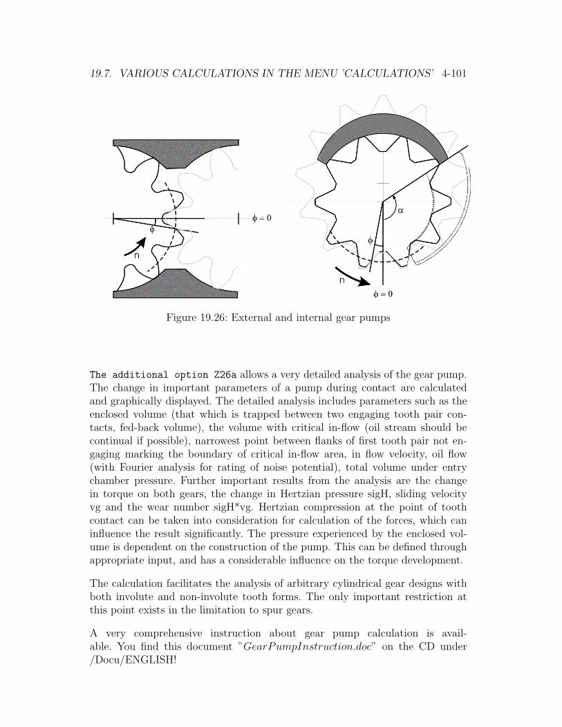
19.7. VARIOUS CALCULATIONS IN THE MENU ’CALCULATIONS’ 4-101
Figure 19.26: External and internal gear pumps
The additional option Z26a allows a very detailed analysis of the gear pump.The change in important parameters of a pump during contact are calculatedand graphically displayed. The detailed analysis includes parameters such as theenclosed volume (that which is trapped between two engaging tooth pair con-tacts, fed-back volume), the volume with critical in-flow (oil stream should becontinual if possible), narrowest point between flanks of first tooth pair not en-gaging marking the boundary of critical in-flow area, in flow velocity, oil flow(with Fourier analysis for rating of noise potential), total volume under entrychamber pressure. Further important results from the analysis are the changein torque on both gears, the change in Hertzian pressure sigH, sliding velocityvg and the wear number sigH*vg. Hertzian compression at the point of toothcontact can be taken into consideration for calculation of the forces, which caninfluence the result significantly. The pressure experienced by the enclosed vol-ume is dependent on the construction of the pump. This can be defined throughappropriate input, and has a considerable influence on the torque development.
The calculation facilitates the analysis of arbitrary cylindrical gear designs withboth involute and non-involute tooth forms. The only important restriction atthis point exists in the limitation to spur gears.
A very comprehensive instruction about gear pump calculation is avail-able. You find this document ”GearPumpInstruction.doc” on the CD under/Docu/ENGLISH!

4-102 CHAPTER 19. SPUR GEARS
19.8 Calculation of Racks
The following points require special attention when calculating racks:
1. Life: Enter high number of required hours (e.g. 1’000’000 h), if the fatigueresistance of pinion and rack is to be calculated.
2. Tooth quality according DIN 3962 usually 9 (or higher)
3. Load according DIN 3990/1 Figure 6.8 B (usually) refer Figure Z-002 inchap. 19.3.8.3
4. The tooth trace deviation from the shaft calculation has to be increased toavoid errors in the shaft angle
5. According to DIN 3961 the pitch diameter of the pinion is used for thecalculation of tolerances .
6. Tooth thickness deviations according DIN 3967 depend on the pitch diame-ter which does not exist in racks. Therefore the pitch diameter of the pinionis used for the determination of the deviations.
Figure 19.27: Rack: centre distance and height.
Chapter 20
Bevel and Hypoid GearCalculations
Calculation of strength and geometry of straight, skew and spiral cut bevel gears.Geometry and control measures according to DIN 3971 and DIN 3975, strengthcalculations according to DIN 3991 (= Method of the equivalent spur gear tooth-ing) or ISO 10300. The calculation includes the geometry of bevel gears, but onlyas far as it does not depend on the toothing type and is required for the stresscalculation. Please compare this with the calculation examples in the manual.The calculation of the centre, outer and inner tip and pitch diameter is also car-ried out for straight, skew, Gleason and Klingelnberg cut bevel gears.Bevel gears according to Klingelnberg can be calculated for manufacturability(c.f. chap. 20.2.1.1).
20.1 Calculation Basis
The geometry of bevel gears is calculated according to DIN 3971. The strengthcalculation is carried out in two steps. First, a virtual spur gear toothing isdetermined and used for the strength calculation of spur gears. This procedureis described in [24], in [45] and in [62].
Additionally, manufactures of bevel gear tool machines (such as Klingelnberg,FRG) have own methods which differ slightly from the two methods mentionedabove.
Hypoid bevel gears (bevel gears with pinion offset; especially used in crossed-axisgear boxes for vehicles) are laid out according to Niemann. This method, however,is not very comprehensive. The strength is calculated via an equivalent virtual
4-103
4-104 CHAPTER 20. BEVEL AND HYPOID GEAR CALCULATIONS
bevel gear toothing. Safety against scoring, which is important for hypoid gears,is calculated with a specific procedure (according to [62]).
20.1.1 Calculating Bevel Gears according to Klin-gelnberg, Gleason and Oerlikon
There are different procedures for manufacturing bevel gears. Unlike spur gears,bevel gears can have differently shaped cones, depending on their manufacturingprocedure. Nowadays, most high-speed bevel gears (spiral toothed) are manu-factured according to KLINGELNBERG, GLEASON and OERLIKON. Simpler,straight toothed bevel gears are produced with simpler procedures.
The strength calculations according to DIN 3991 or according to ISO 10300 con-sider only the conditions (module, helix angle) in the centre of the toothwidth. The form of the cone (and the manufacturing procedure) are not con-sidered. The KISSsoft-Strength-Calculation can therefore be used forall kinds of manufacturing (including KLINGELNBERG and GLEA-SON). This takes into account that the load capacity of spirally toothed bevelgears depends only little on the kind of manufacturing procedure.The input facilities in the main window of the KISSsoft bevel gear cal-culation expect therefore module and helix angle to be entered for the centreof the tooth width.
The geometry-calculation in KISssoft calculates in the same way the exact con-ditions (diameter, tooth thickness) in the centre of the toot width. The diameteron the outer and inner end of the tooth width are calculated as they depend onthe kind of manufacturing procedure. Small deviations can show up, especiallybecause de GLEASON procedure is insufficiently described in the literature.
• KLINGELNBERG-Procedure:
The KISSsoft-option Z07a (and Z07b for hypoid gears) allows calculatingthe complete geometry, strength and also checking the kind of manufactureaccording to the Klingelnberg-standard. Only the setting-parameters forthe chosen Klingelnberg-machine are not calculated. Unlike Gleason, theKlingelnberg procedures are documented comprehensively and published.In Klingelnberg-programs, the data (module, helix angle) always apply tothe centre of the tooth width (as long as not explicitly stated else).
• GLEASON-Procedure:
Unfortunately, the Gleason company keeps their formulae for their geometrycalculations secret. Bevel gears designed by Gleason. Depending on thecalculation program used by Gleason, the data (module, helix angle) are

20.2. INPUT INTERFACES 4-105
stated either for the outer end of the tooth width or for the centre. Thereforebe careful when interpreting Gleason data!KISSsoft-option Z07d allows converting Gleason data on the outer end ofthe tooth width into data in the centre. In this way, the strength calculationcan be carried out.
With Z07d, also the approximate dimensions of the bevel can be calculatedaccording to Gleason, if the bevel gear was sized in the KISSsoft bevel gearcalculation. The calculation is not 100If GLEASON-data is only stated withmodule / helix angle on the outer end of the tooth width, these data canbe entered directly in KISSsoft under File⇒ Project⇒ Calculation⇒Convert into GLEASON-Data.
• OERLIKON-Procedure:
The procedure according to OERLIKON mainly corresponds to the proce-dure according to KLINGELNBERG. KISSsoft-option Z07a can thereforebe used for this calculation.
20.2 Input Interfaces
20.2.1 Main Window
Input fields:
• Application factor
• Methods for strength calculation (bevel gears)
• Number of teeth (bevel gears)
• Centre distance (bevel gears)
• Helix angle (in middle of the tooth width)
• Normal module (in middle of the tooth width)
• Material
Input fields during additional inputs: siehe Kap. 19.3.7.2Input fields during tolerances: siehe Kap. 19.3.7.3

4-106 CHAPTER 20. BEVEL AND HYPOID GEAR CALCULATIONS
20.2.1.1 Methods for Strength Calculations
The user can choose between the following methods:
• To calculate bevel gears:
1. ISO 10300, 1994, Part 1,2,3 ’Calculation of Load Capacity of BevelGears’
2. Calculations according to DIN 3991.(DIN 3991, Parts 1, 2, 3, 4 ’Tragfahigkeitsberechnung von Kegelradern’[=’Strength calculations of bevel gears’])
The standard calculation method of KISSsoft is Method B, tooth formfactors are calculated according to Method C.
3. Calculation according to KLINGELNBERG-Werknorm KN 3028 andKN 3030 (the Klingelnberg-calculations are based mainly on the DIN-Norms)
Issues the same results as the reference program of the Klingelnbergcompany.
• For the calculations of Hypoid gears (bevel gears with a pinion offset):
4. According to ISO (in progress, not available yet)
5. According to DIN (in progress, not available yet)
6. Calculation according to KLINGELNBERG-Werknorm KN3029 andKN3030 (Calculations are mainly based on the DIN-Norms)
Issues the same results as the reference program of the Klingelnberg com-pany.
• Static strength calculation:
Same method as used for spur/helical gears, see chapter 19.3.1.14
• Differential:
For Differential the static strength calculation is applied. The calculationis executed with the highest circumferential force F1 or F2, see figure

20.2. INPUT INTERFACES 4-107
Output M/ 2
M = 2 * F1 * l1 + 2 * F2 * l2F1 = F2 * l4 / l3l1 = SQRT(SQR(Rm1)-SQR(dm1 / 2))-0.5*Tan(delta1)*( dam1 - dm1)l2 = dam2 / 2l3 = dam1 / 2l4 = SQRT(SQR(Rm2)-SQR(dm2 / 2))-0.5*Tan(delta2)*(dam2- dm2)
20.2.1.2 Number of Teeth
Reference values for bevel gears with a shaft angle of 90 degrees (u : Ratio, z1 :Number of teeth on the pinion, taken from: Niemann,III,24/4)for

4-108 CHAPTER 20. BEVEL AND HYPOID GEAR CALCULATIONS
u 1 1.25 2 2.5 3 4 5 6z1= 18..40 17..36 15..30 13..26 12..23 10..18 8..14 7..11
20.2.1.3 Helix Angle
The angle in the middle of the tooth width is entered as the helix angle. (In thespiral teeth according to Klingelnberg or Gleason, the helix angle changes alongthe tooth width.
The spiral angle (at the centre of the tooth width) of hypoid gears is entered forgear 2 and gear 1 (pinion) as follows:
This setting can be changed in the menu in Settings.
The helix angle in the centre of the tooth can be chosen freely. For optimumoperating characteristics an angle in the range of (30◦ − 45◦) should be chosen.Only choose smaller values if the bearing load has to be reduced.
20.2.1.4 Normal Module
The normal module in the centre of the tooth width for bevel and hypoid gearshas to be entered. With hypoid gears the normal module and the helix angledepend on each other. Usually the normal module is calculated from the helixangle.
This setting can be changed in the menu in Settings.
20.2.2 Gear Specific Inputs
Entry fields:
• Reference profile
• Addendum modification coefficient
• Tooth thickness variation coefficient
• Tooth quality according DIN 3965
• Helix angle (left or right; see 19.3.1.4)
For the input fields for additional entries, see Chapter 19.3.7.2.For the input fields for tolerances, see Chapter 19.3.7.3.
20.2. INPUT INTERFACES 4-109
20.2.2.1 Addendum Modification Coefficient
Reference values for bevel gears with shaft angle 90 degrees (u : Ratio, x : Ad-dendum modification, Source: Niemann,III,24/4) for
u 1 1.12 1.25 1.6 2 2.5 3 4 5 6x = 0.00 0.10 0.19 0.27 0.33 0.38 0.40 0.43 0.44 0.45
Sizing:
• Undercut at pinion: the proposition issues the minimal value needed toavoid undercut.
• Balanced sliding: the proposition issues the addendum modification re-quired for balanced specific sliding between pinion and wheel.
A proposition for bevel-gears is only possible if you are calculating according toKlingelnberg.
20.2.2.2 The Tooth Thickness Variation Coefficient
Reference values for bevel-gears shaft angle 90 Degrees (u : Ratio, xs : tooththickness variation coefficient, Source: Niemann [62]) for
u 1 1.12 1.25 1.6 2 2.5 3 4 5 6xs = 0.00 0.010 0.018 0.024 0.030 0.039 0.048 0.065 0.082 0.100
20.2.3 Pair Specific Input Window
To it the topics belong:
• Centre distance und centre distance allowance (Kap. 20.2.3.1)
• Relative structure coefficient (siehe Kap. 19.3.8.4)
• Shaft angle (Kap. 20.2.3.2)
• Dynamic coefficient (siehe Kap. 19.3.8.5)
20.2.3.1 Centre Distance
The axes of two bevel gears intersect at one point so that the centre distance ofthe axes is zero. In special cases (especially in the automobile industry), bevelgears are made with a centre distance; this pair is then called hypoid gear pair.

4-110 CHAPTER 20. BEVEL AND HYPOID GEAR CALCULATIONS
20.2.3.2 Shaft Angle
The shaft angle of bevel-gears is usually 90 degrees. The program, however, cancompute with any angle.
20.2.4 Interfaces: Additional Inputs
20.2.4.1 Factors for Bevel Gears and Manufacturing Methods
• Bevel gear cone forms:
The following cone forms are available:
– Cone form according to DIN 3971 Figure 1
– Cone form according to DIN 3971 Figure 2 (Gleason)
– Cone form according to DIN 3971 Figure 3 (Klingelnberg)
• Manufacturing methods:

20.2. INPUT INTERFACES 4-111
Method Achievable tooth quality (DIN 3965)Only milling 8Lapping 7Hard toothing 6Grinding 6
• Bearing application factor (according to ISO 10300):
Bearing of pinion and bevel gear: Bearing application factora b c
- both on both sides 1.00 1.05 1.20- one on both sides, one overhung 1.00 1.10 1.32- both overhung 1.00 1.25 1.50
a : Contact pattern tested in gear box for total loadb : Contact pattern tested in gear box for part loadc : Contact pattern tested randomly
• Bearing application factor according to G. Niemann, MaschinenelementeIII, 1983, p.47
Bearing of pitch and bevel gear: Bearing application factor- both on both sides 1.10- one on both sides, one overhung 1.25- both overhung 1.50
• According to the standard, the width coefficient (KHβ, KFβ, KBβ) is calcu-lated from the bearing application factor (KHβbe) as follows:
KHβ = KFβ = KBβ = 1.5 ·KHβbe (20.1)
• Bevel gear factor (flank)
– according ISO 10300:Bevel gear factor (flank): 0.80
– according to Niemann:Bevel gear factor (flank): 0.85
• Bevel gear factor (root):
– nach ISO 10300Bevel gear factor calculated by KISSsoft according to ISO 10300, Part3
– according to NiemannBevel gear factor (root): 1.00

4-112 CHAPTER 20. BEVEL AND HYPOID GEAR CALCULATIONS
• Input of the cutter radius:
The input will have an influence the face coefficient tooth root KFβ
(calculation according to ISO 10300) for spiral bevel gears.The cutter radius is a machine-depent value: 25-450 mm.
20.2.4.2 Additional Factors for Hypoid Gears
Bevel gears with a positive pinion offset usually benefit from better loading con-ditions if the concave flanks of the pinion are driving, i.e. the direction of rotationand the direction of the spiral of the driving pinion are the same.
This type of flank is therefore mostly used for driving operation (in vehicles)and the other type of flank is used the wheel driving the pinion. Generally, theconcave flank on the pinion is called the drive side (index Z) and the convexeflank is called the coast side (index S). On the bevel gear the concave flank iscalled the coast side (index S) and the convexe flank the drive side (index Z).
The normal working pressure angle is increased by the boundary pressure angleon the drive side and is decreased by the boundary pressure angle on the coastside compared to the pressure angle in the transverse section. To consider this asmaller normal pressure angle is usually used on the drive side than on the coastside.
In case there is no certain information given, the calculation should be carriedout with the pressure angle in the transverse section. KISSsoft can also generatea suggestion according to the Klingelnberg factory norm.
20.3 Settings
For spur gear settings, see in principle (chapter 19.4).
Special input fields for bevel gears:
• Calculation according to Klingelnberg working practicesThe calculation of the dynamic factor Kv according to Klingelnberg is car-ried out with the help of the factor K1 either for projected calculations onthe grounds of the intended manufacturing method (lapped, HPG) or onthe basis of the identified tooth quality (in Manual KN3030, Table 5.2-1 or5.2-2).

20.4. SIZING OF BEVEL AND HYPOID GEARS 4-113
20.4 Sizing of Bevel and Hypoid Gears
The sizing of bevel and Hypoid gears according to suggestions of the Klingelnbergcompany results in geometrically sensible laid out gear pairs. The sizing is notexact regarding the nominal safety for tooth fracture and pitting, but it is basedon general experience. The re-calculation of the toothing laid out in the afore-mentioned way will therefore lead to a slight discrepancy from required nominalsafety factors.
But it is very easy to achieve the required safety factors: Change the modulusand proportionally the tooth width so that the strength of the teeth increases ordecreases.
Input fields:
• Centre distance
• Mean spiralling angle
• Ratio of length of the reference cone to the tooth width (Re/b)
• Ratio of tooth width to the normal module (b/mn)
20.4.1 Ratio Reference Cone Length - Tooth Width Re/b
The ratio outer reference cone length - tooth width should be chosen accordingto the operation conditions the power transmission is designed for. The followingvalues should be used:
Light to medium stressed power transmissionsfor machines and vehicles: 3.5 ≤ (Re/b) ≤ 5.0Heavily stressed power transmissionfor machines and vehicles: 3.0 ≤ (Re/b) ≤ 3.5
20.4.2 Ratio Tooth width - Normal Module b/mn
The normal module should be within in a certain range compared to the toothwidth. Only special reasons allow ratio outside the following values:
Surface hardened bevel gearswith the danger of tooth fracture: 7 ≤ (b/mn) ≤ 10 . . . (12)Non-hardened bevel gears with the dangerof pitting or heat treated bevel gears: 10 ≤ (b/mn) ≤ 12 . . . (14)

4-114 CHAPTER 20. BEVEL AND HYPOID GEAR CALCULATIONS
20.5 The Menu-Item Calculations
In the ’Bevel and Hypoid Gears’ menu bar, under ’Calculations’ there are manysupplementary calculations which go beyond the essential verification of gearwheels and which, depending upon the type of problem, could be of great help.Most of these calculations are described in chapter 19.7; hereafter, only the spe-cially developed calculations for bevel gearwheels are mentioned.
20.5.1 Conversion to the GLEASON-Geometry (Z7d)
Converting bevel gear data according to the Gleason procedure into analoguedata according to DIN 3971 and DIN 3991 and vice versa.
The transverse and the normal module at the outer cone is included in the centrecone and additional properties of the cone geometry according to the Gleasonprocedure are taken into account. This operation therefore allows carrying outstrength and sizing calculations according to DIN 3991 of bevel gears which havebeen made with the Gleason procedure.
20.5.2 Tip and Root Circles(´Momentum´) and ToothThickness (Z7c)
Calculation of all necessary dimensions needed to design bevel gear drawings (tipand root diameter at the outer and inner cone and the tooth thickness dimensionsat the outer and inner cone diameter). Bevel gear cone forms: see 20.2.4
For the bevel gear calculation for the CAD interface see picture 20.1.
Some of the values calculated here are already contained in the main report (Z7).
20.6 Calculation of Bevel Gears According to
Klingelnberg
20.6.1 Bevel Gears with Cyklo-Palloid-Toothing
Geometry, manufacturing and strength calculation of bevel gears according toKlingelnberg.
According to the Klingelnberg factory standard KN 3028 (Geometry and Man-ufacturing) and KN 3030 (Stress analysis), a complete analysis for bevel gearswith cyklo-palloid-toothing is carried out:
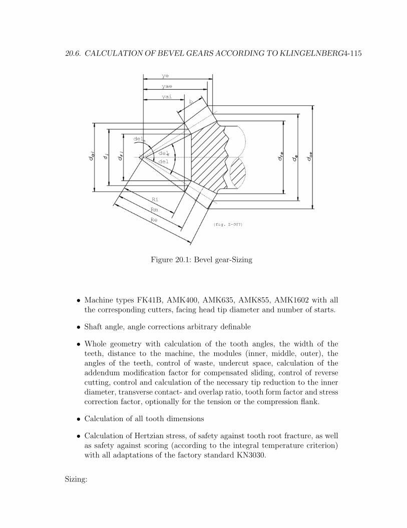
20.6. CALCULATION OF BEVEL GEARS ACCORDING TO KLINGELNBERG4-115
Figure 20.1: Bevel gear-Sizing
• Machine types FK41B, AMK400, AMK635, AMK855, AMK1602 with allthe corresponding cutters, facing head tip diameter and number of starts.
• Shaft angle, angle corrections arbitrary definable
• Whole geometry with calculation of the tooth angles, the width of theteeth, distance to the machine, the modules (inner, middle, outer), theangles of the teeth, control of waste, undercut space, calculation of theaddendum modification factor for compensated sliding, control of reversecutting, control and calculation of the necessary tip reduction to the innerdiameter, transverse contact- and overlap ratio, tooth form factor and stresscorrection factor, optionally for the tension or the compression flank.
• Calculation of all tooth dimensions
• Calculation of Hertzian stress, of safety against tooth root fracture, as wellas safety against scoring (according to the integral temperature criterion)with all adaptations of the factory standard KN3030.
Sizing:

4-116 CHAPTER 20. BEVEL AND HYPOID GEAR CALCULATIONS
• Determination of the main coefficients by a rough calculation (on the basisof the power data and the rated transmission ratio) with the possibility toinfluence the number of teeth on the pinion, of the modules, of the diameter(of the bevel gear) and of the face width.
• Determination of addendum modification for:
– Minimal required coefficient to avoid undercut
– Balanced sliding.
20.6.2 Hypoid Gears with Cyklo-Palloid-Toothing
Geometry, manufacturing and stress analysis of hypoid gears (bevel gears withpinion offset) according to Klingelnberg.
According to the Klingelnberg factory standard KN3028 (Geometry and Man-ufacturing) and KN3030 (Stress analysis), a complete analysis for gears withzyklo-palloid-toothing is performed:
• Machine types FK41B, KNC40, KNC60, AMK855, AMK1602 with all thecorresponding cutters, facing head tip diameter and number of starts.
• Shaft angle, angle corrections, pressure angle for pressure and tension flankarbitrarily definable
• Entire geometry with calculation of the tooth angles, tooth width, distanceto the machine, modules (inner, middle, outer), angles of the teeth, inspec-tion of undercut space, calculation of addendum modification factor forcompensated sliding, inspection for reverse cutting, check and calculationof the necessary tip reduction to the inner diameter, transverse contact-and overlap ratio, tooth form factor and stress correction factor, optionallyfor the tension or the compression flank.
• Calculation of all tooth dimensions.
• Calculation of pitting, tooth root and scoring margin of safety (accordingin integral temperature criteria for virtual worm gears) with all settings ofthe factory standard KN 3030.
Sizing:
• Determination of main parameters using a rough calculation (based on thepower data an nominal ration) with the possibility to influence number ofteeth of pinion, module, pitch diameter (wheel) and face width

20.6. CALCULATION OF BEVEL GEARS ACCORDING TO KLINGELNBERG4-117
• Proposition for a suitable pressure angle on the tension and the pressureflank
• Determining the addendum modification for the minimal required value toavoid undercut
• Calculating the spiral angle (middle of wheel) from the module or vice-versa

4-118 CHAPTER 20. BEVEL AND HYPOID GEAR CALCULATIONS
20.6.3 General Information to Klingelnberg-Calculations
20.6.3.1 Normal Module Range for Klingelnberg Machines
Machine Cutter flight radius Normal moduleFK41B 25 , 30 0.25 . . . 1.6
30 (0.25) 0.75 . . . 1.6AMK400 55 (1.2) 2.0 . . . 4.0
100 2.4 . . . 5.5135 3.5 . . . 8.0170 (3.5) 6.5 . . . 9.0 (12)
KNC40 30 1.0 . . . 1.655 1.2 . . . 4.075 2.0 . . . 4.5
100 2.4 . . . 5.5135 3.5 . . . 8.0
AMK635 55 (1.2) . . . . . . (4.0)100 (2.5) 3.5 . . . 5.5135 3.5 . . . 8.0170 6.5 . . . 9.0 (12)210 7.0 . . . 9.0 (12)
KNC60 75 2.0 . . . 4.5100 2.4 . . . 5.5135 3.5 . . . 8.0170 6.5 . . . 13
AMK855 135 3.5 . . . 8.0170 6.5 . . . 13210 7.0 . . . 13 (15)260 7.0 . . . 13 (15)
AMK1602 270 (8.0) 10 . . . 17350 14 . . . 25450 17 . . . 30 (34)
20.6.3.2 Minimal Safety Factors
The following safety factors are recommended:
Flank 1.1 . . . 1.2Root 1.5 . . . 1.6Scoring 1.8 . . . 2.0

20.7. DETERMINING TOOTHING DATA OF UNKNOWN BEVEL GEAR TEETH4-119
20.6.3.3 Quality of toothing according to Klingelnberg-Bevel gears
heat treated bevel gears 7lapped bevel gears (6) 7hard toothed bevel gears 6
20.6.3.4 Surface Roughness (Tooth Root)
heat treated bevel gears 0.016 mmlapped bevel gears 0.016 mmhard toothed bevel gears 0.008 mm
20.6.3.5 Lubrication Coefficient, Speed Factor, Roughness Coefficient
The product of these factors is valid for:
milled wheels 0.85lapped wheels 0.92hard toothed wheels 1.00
20.6.3.6 Single Normal Pitch Error
Calculation according to DIN 3965.
20.6.3.7 Meshing Spring Stiffness
20N/(mm ∗ µm)
20.7 Determining Toothing Data of Unknown
Bevel Gear Teeth
Given:
Determined by measuring:
• Tooth width (according to 20.1), number of teeth
• Outer diameter outside (dae1, dae2) and inside (dai1, dai2)

4-120 CHAPTER 20. BEVEL AND HYPOID GEAR CALCULATIONS
• Installation dimension (LW1, LW2)see picture 20.1 (ye=LH, yai=LW, yae=LW+LA)
• Tooth depth outside and inside
Rating:
• Pressure angle
• Helix angle in the centre of the tooth width
Procedure:
Does the helix angle increase from inside to outside (spiral cut)?Yes: Is the tooth depth constant?
Yes: → Klingelnberg toothingNo: → Gleason
No: Is the tooth depth constant?Yes: → Toothing according to DIN 3971, figure 3No: → Toothing according to DIN 3971, figure 1
• for: Klingelnberg toothing
1. Module (mn) = Tooth height/2.25
2. Enter data in KISSsoft. Assume addendum modification factor (x1) asthe addendum modification factor for balanced sliding.
3. By carrying out several calculations with different helix angles (β) andby comparing nominal and actual dimensions (dae, dae, LW ) the helixangle can be determined accurately to an even number.
4. Fine tuning can be achieved by varying the addendum modificationfactor (in the region of minimum addendum modification factor ...addendum modification factor for balanced sliding).
5. An exact agreement between the nominal and actual values cannotbe achieved, but the results are more than sufficient from a practicalpoint of view.
Example (by Grono & Co GmbH (Ltd.)):
Z1 = 13, Z2 = 36b1 = 78.5, b2 = 78.5mmTooth depth constant 18.9mmdae1 etc. see following table

20.7. DETERMINING TOOTHING DATA OF UNKNOWN BEVEL GEAR TEETH4-121
Pressure angle = 20◦, spiral cut, no defined helix angle.mn = 18.9/2.25 = 8.4Enter data, assume β 25◦, according to KISSsoftx1 for minimal addendum modification factor = 0.1624x1 for addendum modification factor for balanced sliding = 0.3882
NOMINAL β β β β25 deg 35 deg 35 deg 35 degx=0.38 x=0.38 x=0.16 x=0.35
dae1 181.5 164.8 181.9 178.3 181.3dae2 447.0 399.1 446.5 447.7 446.7dai1 127.5 111.5 128.6 125.0 127.9dai2 299.0 251.5 298.8 300.1 299.0LW1 144.2 120.0 143.7 144.3 143.8LW2 48.4 39.9 48.5 46.7 48.2
Results: last column
• for: Glaeson toothing

4-122 CHAPTER 20. BEVEL AND HYPOID GEAR CALCULATIONS
Chapter 21
Face Gears (Z6)
Calculation module that calculates the geometry of face gears (straight anddiagonally-toothed) coupled with helical pinion gears (at the moment withoutany offset of axes and an angle between the axes of 90◦). 2D views with shape oftooth simultaneously on the inside, at the centre and on the outside or, alterna-tively, in any desired cross section. Checking undercut and tooth tip is performedgraphically in the two dimensional view, while head height can be varied to pre-vent pointed tooth tip. 3D views with the possibility of exporting the files (OptionK05g). The shape of the tooth is calculated by simulating construction with ashaping cutter. Calculation of strength is approximated using the correspondingbevel gear.
21.1 Additions/Notes
• Calculation of the pressure angle of a face gear is performed, both theoret-ically as also deduced from the tooth profile, by calculating the shape ofthe tooth, the frontal pressure angle in the partial height of the face gearis listed in the protocol for the inside, centre and outside.
• Production of a longitudinally crowned tooth: a crowned tooth (tooth flank)of the face gears can be produced using shaping cutter with one or two teethmore than the pinion. The ”Save” function can be used in the 2D view tomake a very careful check of the differences between the shapes of the teethproduced (starting with shapping cutter and the same number of teeth asthe pinion for the calculation of the shape of the tooth, saving it and thenthe number of teeth of the shapping cutter is increased). If the width of theface gear (bv) is moved, the crown may however move to one side!
4-123

4-124 CHAPTER 21. FACE GEARS (Z6)
21.2 Design
21.2.1 Important notes on how to design face gears
Design of face gears with KISSsoft is very different from the usual method forexample with cylindrical gears because of the complex shape of the teeth. Thegeometry of face gear teeth must be designed so that they do not form an pointedtooth and have no (or at least little) undercutting on the inside. These checksmust be carried in the calculation of the tooth shape. In the actual geometricalcalculation, the conversion to the corresponding bevel gear and the correspondinghelical gear I performed, and checks are performed on the corresponding helicalgear. These checks, however, only concern the geometrical conditions in the basecircle. The shape of the tooth for a face gear is calculated for a number of sectionsacross the length of the tooth. The default number of cross sections can be set inthe menu ’Settings for toothform calculation’ which is a sub menu of the menu’Tooth shape calculation - Checking manufacture’ in input section B (Factors for3D Graphics). In the 2D view, the shape of the teeth are shown simultaneouslyat the internal and external ends of the tooth width as well as in the base circle.It is also obvious here (in the 2D view) whether the thickness of the head of thetooth and the undercut of the tooth are acceptable.
Displaying a desired cross section: in the 2D view, the button >> activates thedisplay of a desired cross section.
The following measures are possible to avoid a pointed tooth and/or undercutting:
• Shifting the tooth width (bv) usually towards the outside
• Reducing the tooth width
• Changing the pressure angle
• Reducing the tip circle in the outer part of the tooth width
21.3 Input values
21.3.1 Width of the face gear b and shifting bv
Width of the face gear b and shifting bv of the tooth width bv are input directlyin the main menu ’Gear2’.

21.3. INPUT VALUES 4-125
Figure 21.1: Tooth width
21.3.2 Sizing of width of tooth
The maximum possible tooth width b of the face gear and the optimum centreoffset bv are proposed by the software by pressing the sizing button next to thefield for the centre offset bv (in the main window).These values are calculatedusing the maximum and minimum pressure angle defined by the user. The laterare defined in Settings ⇒ Module-specific ⇒ Sizings.
21.3.3 Tooth height haFG, reduction of head height hakand mounting distance of the face gear aFG
The height of the face gear tooth is entered in the menu S ’Additional inputsgear 2’. Reduction of head height hak and the length of the reduction of thehead height is also entered in this menu. When making changes to head heightit is advisable to increase the number of cross sections calculated (usually from5 to around 10). The default number of cross sections can be set in the menu’Settings for toothform calculation’ which is a sub menu of the menu ’Tooth shapecalculation - Checking manufacture’ in input section B (Factors for 3D Graphics).See picture 21.2
21.3.4 Definition of the sense of rotation and the hand ofgear on the face gear
See picture 21.3

4-126 CHAPTER 21. FACE GEARS (Z6)
l_hakehake
hfFGhaFG
l_haki
haki
Figure 21.2: Definitions at the face gear

21.4. CALCULATIONS 4-127
Figure 21.3: Hand of gear (face gear): right; Hand of gear (pinion): left; Sense ofrotation: right
21.4 Calculations
21.4.1 Calculation of the lines of contact
Through Calculation ⇒ Line of contact the line of contact of the pinionand of the face gear are shown:
Note the inclination of the line of contact from the inside tip of tooth to theoutside (root of tooth). The bold line w shows the contact in the pitch point, theother lines show the contact during ovtation of the pinion (1/10 of a tooth perline). The next bold line shows the contact with the next tooth. This characteristicpattern of the lines of contact of a face gear with helix angle = 0◦ is siilar to thatof a helical gear with helix angle not equal 0. The reduced of the contact ratio(εa)over the tooth width and the small active height on the inside of the face geartooth are well vivible.
21.4.2 Hertzian pressure and tooth root stress
Through Calculationn⇒ Stresses, the stresses over the tooth width are shown.For the calculation of stresses, the tooth is divided in segments which are then cal-culated as a rack and pinion pair according to ISO6336, DIN3990 or AGMA2001.For the calculation, a constant line loud is assumed. This results in a slightlydifferent torque for each segment, due to the different working pitch diameter.

4-128 CHAPTER 21. FACE GEARS (Z6)
Figure 21.4: Lines of contact
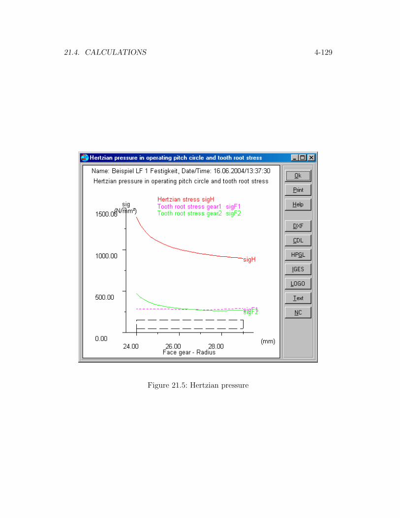
21.4. CALCULATIONS 4-129
Figure 21.5: Hertzian pressure
4-130 CHAPTER 21. FACE GEARS (Z6)
The stress values calculated for each segment are written to two tables, Z60-H1.TMP and Z60-H2.TMP.
21.4.3 Calculation of the scoring safety (and glidingspeeds safety)
Since the gliding speeds and the hertzian pressure vary considerably over thetooth width, the calculation of the scoring safety is problematic. Akahori [2]encountered severel problems with scoring at high gliding speeds. It is hencesensible to pay attention to this question. A possible approach could again be todivide the tooth into segments which are then investigated seperatedly. Figure21.6 shows the scoring safety (flash and integral) along the width of the tooth. Inorder to get realistic results the calculation for each segment into be performedusing the same mass temperature. During the developement of the calculationcode, it was shown that the safety against scoring using the integral temperatureis not a continous function. This happens when the point E of the line of actionapproaches the pitch point. Then, the transformation of the flank temperaturein E into the average flank temperature according to DIN 3990 yields inaccurateresulta. It is hence recommended to use the flash temperature criterion.
The safety against scoring is shown through Calculation ⇒ Safety Scoring.
The gliding speeds are important to know for different application (e.g. plas-tics, operation lubrication). They are shown through (Calculation ⇒ Gliding
speed).
21.4.4 Calculation of the pressure angle, analysis of un-dercut
The pressure angle in different locations (inside to outside) is calculated accordingto the formula([3]).
d2 = (mn ∗ z2 ∗ cos(αn))/cos(α2)
, z2 number of teeth of the face gear, αn pressure angle at d2 d2, αn pressureangle of the pinion at the pitch circle, mn Module of the pinion, see [3]. Moreover,every time the 2D representation of the face gear is shown, the exact shape ofthe tooth is calculated by simulating the meshing with the pinion, yielding thepressure angles over the tooth width. The angles, calculated according to thesetwo methods (form formula above and from simulation of the meshing) correspondwell to each other with exception of the pressure angle on the inside. This differentbetween theory (formula above) and simulation (meshing) signals that the toothhas undercut. This can also be seen in 2D view.

21.4. CALCULATIONS 4-131
Figure 21.6: Safety against scoring according to flash and integral temperatureand gliding speed for tip and root. The geometry of the face gear corresponds tothe one used by Akahori [2].

4-132 CHAPTER 21. FACE GEARS (Z6)
21.5 Problems in the production of the 3D
shape
When error messages appear in the production of the 3D shape (image displaystops and a message appears), the problem can usually be solved by modifyingthe A factor (’Settings for toothform calculation’ menu which is a sub menuof the menu ’Tooth shape calculation - Checking manufacture’-Factors for 3DGraphics), e.g. 0.01 to 0.03. N.B. This factor influences the form of the splinesand should not be set at higher than 0.5.
21.6 Selection of given tools from a list
For time effective manufacturing of prototypes, it’s important to be able to useexisting tools. The milling cutters and shaping cutters as used by ASS/CrownGear. The tool data is stored in a file (Z60-ASS.dat or Z60-001.dat) and can be

21.6. SELECTION OF GIVEN TOOLS FROM A LIST 4-133
modified using a text editor.
To integrate own cutters, delete file Z60-ASS.dat and create a Z60-001.dat filewith the existing cutter integrated.
The data format per tool is as follows:< Typ > | < mn > | < alfan > | < beta > | < z0 > | < x0 > | < hfP2∗ >
< Typ > 0=milling cutter 1=shaping cutter< mn > Normal module< alfan > Pressure angle< beta > helix angle< z0 > No. of tooth< x0 > addendum modification< hfP2∗ > Tooth root height face gear (or tool tip height)
Example:0|1.0|20.0|0.0|12|0.4|1.1670|1.5|20.0|0.0|15|0.35|1.167

4-134 CHAPTER 21. FACE GEARS (Z6)
Chapter 22
Worm Gears (Z8)
Calculating worm geometry according to DIN 3975. Tooth thickness, control mea-sures (tooth width, roll and ball measure) according to DIN 3960. Productiontolerances according to DIN 3974.
Sizing of tooth width, centre distance, lead angle etc. Product calculation accord-ing to DIN 3996 (1998 edition) with: efficiency, temperature safety, pitting safety,wear safety, safety against breaking and bending. Data for several worm materialsare provided by KISSsoft, the calculation can also be applied to plastics.
Calculates also the torque of start under load, which is very important for thesizing of drives.
Flank forms: ZA, ZE, ZH, ZI, ZK, ZN.
• Option Z08a
Control measures for worms and worm gears.For worm gears with flank forms ZA, ZI (or ZE), ZK, ZN the control mea-sures are calculated taking into account the tooth thickness deviation: threewire measure and tooth thickness for the worm, measure over the balls andbacklash free centre distance for the pair.
• Option Z19b
Worm gear sizing with normal module.
Dimensions of worm gears: see figure Z-011
4-135

4-136 CHAPTER 22. WORM GEARS (Z8)
22.1 Calculation Basis
The fundamental geometrical ideas about worm gear design are defined in DIN3975. Additions and other important definitions, such as i.e. different worm flankforms (ZA, ZE or ZI, ZH, ZK, ZN), can be found in [62]. Be careful with wormmodules without closer specifications; it can be a spur, axial or normal module,depending on individual definitions. An investigation is therefore necessary.
The strength calculation (tooth fracture, pitting, wear and temperature safeties)is described in DIN 3996. The calculation method is, compared to the spur gearcalculation, very simple.
During manufacture, worms can be controlled with the so-called three wires mea-surement. This is principally similar to the two balls measurement of worm gears(similar to spur gears). The calculation of the three wires measurement is verycomplex. A suitable calculation method for the usual flank forms was developedby G. Bock [4] from the Federal Institute in Braunschweig, FRG. This methodconsiders the worm flank form and is used in KISSsoft.

22.2. INPUT INTERFACES 4-137
22.2 Input Interfaces
22.2.1 Main Window
• Strength calculation methods
The methods according to Niemann/Winter [62] and according to DIN 3996are not very different. KISSsoft recommends the method according to DIN3996, as it the most comprehensive. The Niemann method is not moreimplemented in KISSsoft.
The calculation according to DIN contains different methods (A, B, C, D).KISSsoft always uses the most accurate and documented method, usually,method B. Unfortunately, the calculation method is not suitable for allmaterials (see chapter 22.2.2.1).
The DIN 3996 is a calculation procedure for:
– Efficiency
– Wear and wear-safety
– Notch-safety
– Tooth root safety
– Safety against bending
– Temperature safety
Comments:
– Grease lubrication: not mentioned in DIN 3996. KISSsoft uses for thiscalculation the values for oil bath lubrication. The influence of thekind of lubrication on the results is immaterial.
– Fatigue resistance factors for permissible tooth foot stress: the stan-dard indicates two different values. In the data base, the lower usedvalue is entered, if plastic deformation of the teeth is not acceptable.
22.2.2 Inputs Worm Gear
22.2.2.1 Gear Wheel Data
• Tooth width
Wheel tooth and wheel rim width: see picture Z-022.
For the worm wheel, enter the width b2R in the main window; the otherwidths will be calculated.

4-138 CHAPTER 22. WORM GEARS (Z8)
• Materials for worm gears
The strength calculation for worm gears according to DIN 3996 bases onexperienced values which were found for the following materials:
Worm:
– Case-hardening steel (mostly 16MnCr5), HRC = 58 . . . 62
– Heat treatable steel (mostly 42CrMo4), flamme hardened or by electricinduction, HRC = 50 . . . 56
– Nitriding steel (mostly 31CrMoV9), gas-nitrided
Worm gear:
– Bronze (GZ-CuSn12, GZ-CuSn12Ni, GZ-CuAl10Ni)
– Cast (GGG40, GG25)
– Polyamid (PA-12, cast)
22.2.2.2 Additional Inputs
See chap. 19.3.7.2
For worms, you can additionally (in the ’S’ window) enter outer diameter and tipgroove radius according to DIN 3975; see picture Z-011.A proposal will be given according to DIN 3975-1-2002:de2 = da2 + mxrk = a− da2/2
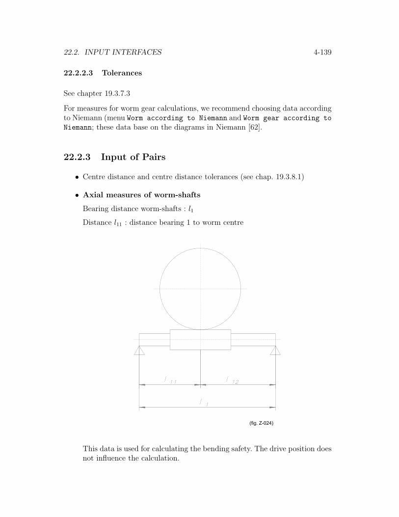
22.2. INPUT INTERFACES 4-139
22.2.2.3 Tolerances
See chapter 19.3.7.3
For measures for worm gear calculations, we recommend choosing data accordingto Niemann (menu Worm according to Niemann and Worm gear according to
Niemann; these data base on the diagrams in Niemann [62].
22.2.3 Input of Pairs
• Centre distance and centre distance tolerances (see chap. 19.3.8.1)
• Axial measures of worm-shafts
Bearing distance worm-shafts : l1
Distance l11 : distance bearing 1 to worm centre
This data is used for calculating the bending safety. The drive position doesnot influence the calculation.

4-140 CHAPTER 22. WORM GEARS (Z8)
22.2.4 Special Inputs
• Number of radial sealing rings
The number of radial sealing rings on the worm-shaft is required to calculatethe sealing loss-power. The sealing rings on the worm gear shaft are notconsidered since they have, because of the low speed, a negligible loss ofpower.(Calculation formulae in DIN 3996).
• Permissible tooth thickness decrease
The permissible tooth thickness decrease is required to calculate the wearsafety and is considered in the calculation of tooth root safety. The permis-sible tooth thickness decrease δS) is computed by a factor to be entered inKISSsoft.
δS = Modul ∗ Faktor (22.1)
If you enter 0.0, the permissible tooth thickness decrease is not considered.
• Permissible mass decrease
The permissible mass decrease on the worm can be limited. The wear safetyis accordingly defined by this value. Entering 0.0 means that the permissiblemass decrease is not considered.
Remark: the worm wheel mass decrease is not calculated because the normconsiders that the pinion being considerably harder then the worm wheel,therefore, there is no wear.
• Shape of flank
The shape of flank depends on production features. ZA-, ZN-, ZK-, andZI-worms hardly differ in efficiency and permissible flank stress. ZC- andZH-worms can have better flank stress qualities, but other significant dis-advantages.
ZA-Form: Produced with rotating steel (straight flanks), ad-justed in axis section
ZN-Form: Produced with rotating steel (straight flanks), ad-justed in normal section
ZI-Form: Produced with hobbing (Worm flank is involute)ZK-Form: Produced with grinding wheel (straight flanks),
adjusted in normal sectionZC-, ZH-Form: Produced with special tools for concave flanks
Further instructions: [38], with pictures on pages G136 and S79.

22.3. SETTINGS 4-141
• Support of gear-box /Bearing loss-power
When calculating the bearing loss-power, the program distinguishes be-tween:
– Adjusted bearing arrangement (Roller bearing)
– Fixing-floating bearing arrangement (Roller bearing)
– Journal bearing
The inputs concern the worm shaft. For supports with roller bearings, thepower loss is roughly calculated with approximate formulas according toDIN 3996, for journal bearings the power loss has to be entered manually.
22.2.5 Lubricant
Basic information: see chapter 19.3.5. Often, synthetic lubricants (polyglykoles)are used for worms.
• Polyglykol with EO:PO = 0:1 (EO: Ethylengylkol, PO: Propylenglykol)
• Polyglykol with EO:PO = 1:1
Sometimes, it is hard to receive comprehensive informations from the lubricantproducers. For normal cases, you can assume EO:PO = 0:1.
22.3 Settings
22.3.1 Nominal Safeties
Tooth root safety : standard 1.1Pitting safety : standard 1.0Wear safety : standard 1.1Bending safety : standard 1.0Temperature safety : standard 1.1
22.3.2 Axis Angle
The axis angle is given (90 degrees), as the strength calculation according to DIN3996 assumes this value. You can, however, calculate with a different axis anglethrough Crossed helical gears.

4-142 CHAPTER 22. WORM GEARS (Z8)
22.3.3 Standard Reference Gearbox
The calculation bases on the data of a standard reference gear box that has beeninvestigated. The set data correspond to the data of the reference gearbox in theDIN 3996. You can adjust the settings if you have own investigated or experiencedvalues. You find further information in DIN 3996.
22.3.4 Start-up Time
The start-up time is considered in the calculation of the number of load changes(multiplied by the service life).
When calculating the temperature, the start-up time is considered additionallyfor the calculation of the produced heat.
22.3.5 Calculating Worms with Sizing over the NormalModule (Z19b)
The geometry of worm pairs is computed with the axial module (or the transversemodule of the worm gear). After activating the opion Calculation with normal
module all factors of the reference profile will be calculated with the normalmodule (module of the cutter). This has an influence on tip and root circle. Theprofile shift x ∗mx (mx fur Axialmodul) won’t be changed.
The formula for the tip diameter (mn for normal modulus) is:
da1 = dm1 + 2 ∗mn ∗ haP
da2 = d2 + 2 ∗mx ∗ x2 + 2 ∗mn ∗ haP
root diameter:
df1 = dm1 − 2 ∗mn ∗ hfP
df2 = d2 + 2 ∗mx ∗ x2 − 2 ∗mn ∗ hfP
22.4 Calculations
22.4.1 Sizing of Torque (Z16)
• The Stress-Cycle Diagram (Wohler line) can not be used in the modifiedform.

22.4. CALCULATIONS 4-143
• Sizing always according to nominal safeties for tooth breaking, pitting andwearing. If one of these safeties is immaterial for your calculation, you canset in Settings⇒ Module-specific⇒ Nominal safeties the value zerofor the corresponding safety.

4-144 CHAPTER 22. WORM GEARS (Z8)

Chapter 23
Cross Helical Gears/WormsPrecision Mechanics
Cross helical gears are helical spur gears which are mounted on intersecting shafts.The shaft angle is normally 90 degrees. The two gears have contact only in onepoint; contrarily, the contact between the previous mentioned gear types is line-wise. Cross helical gears can only transmit small forces and are therefore usuallyused for control purposes.
In precision mechanics, a worm gear is often produces as a helical spur gear. Thissimplifies the production and the mounting. The geometry of a worm gear iscalculated, in this case, as helical gear, since, with addendum modification otherthan zero, the helix angle of the wheel and the lead angle of the worm differ fromeach other.
This version contains the calculation and geometry check of helical gears for anyaxis angle. Control- and fabrication measures are calculated. For the calculationof the safety against scoring, a special procedure is provided.
23.1 Calculation Basis
The calculation of helical gears (spur gears mounted on intersecting shafts) isdone according to Niemann [61]. The present version contains the calculationand geometry check of helical gears with any shaft angle. Checking- and manu-facturing dimensions are calculated.
The geometry and strength calculation is described in [62]. Especially the calcu-lation of the safety against scoring is (similar to the bevel-hypoid gears) given asa special procedure.
4-145
4-146CHAPTER 23. CROSS HELICAL GEARS/WORMS PRECISION MECHANICS
23.2 Input Interfaces
The corresponding subsections of chapter 19.3 are valid for cross helical gears aswell.
23.3 Settings
The corresponding subsections of chapter 19.4 are valid for cross helical gears aswell.
Axis angle: the standard axis angle is 90 degrees. Any axis angle can be computed.
23.4 Sizing
23.4.1 Helix Angle Gear Wheel 1
KISSsoft calculates the helix angle of gear wheel 1 (sum of addendum modification0.0) based on centre distance, number of teeth and axis angle.
Frequently, two or more helix angles are possible. The software displays a messagewith all solutions found (if more then one) and sets the solution which is closerto the already input values. It can also happen that there is no solution. In suchcase either the center distance or the module has to be changed.
23.4.2 Axis Distance
The centre distance calculation (sum of addendum modification 0.0) bases onhelix angle (gear wheel 1), axis angle and tooth number.
23.5 Strength Calculation
For the time being, there is only one strength calculation for worms, i.e. theaxis angle 90◦ and z1 < 5, according to Hirn or Hochst available. The strenghtcalculation for crossed helical gears according ISO6336/Niemann is for numberof teeth greater 5 z1 > 5 usable.
Important: with the calculation method according to Hirn, also the materialpairing is chosen, the material of the wheel is only for information purpose anddoes not influence the strength calculation!

23.5. STRENGTH CALCULATION 4-147
23.5.1 Strength of Worms according to Hochst
For worm gears made of hostaform (POM) paired with steel worms, a strengthcalculation according to Hochst is provided. The permissible load value
c =F2
fzbmπ
is a measure for temperature stess. Also the permissible flank pressure and theblocking strength of the worm are checked. For blocking strength, not the per-manent stress but the maximal stress is important.
23.5.2 Strength of Worms According to Hirn
The worm calculation according to Hirn bases on an outdated issue of NiemannMaschinenelemente. Calculated are temperature safety, flank safety, root safetyas well as safety against deviation. The material values cannot be compared tothe values of the worm calculation according to DIN 3996, the safeties, however,are similar.
23.5.3 Strength of Crossed Helical Gears accordingISO6336/Niemann
The strenght calculation for crossed helical gears with z1 > 5 can be made ac-cording to Niemann/ISO6336. A calculation for the root stress, resistance againstpitting and scoring is made.

4-148CHAPTER 23. CROSS HELICAL GEARS/WORMS PRECISION MECHANICS
Chapter 24
Splined Joints according to DIN5480
The geometry and the control measures of splined shafts and hubs accordingto DIN 5480 (Edition 1986), ISO 4156, ANSI B92.1 or ANSI B92.2M are cal-culated very elegantly. The tolerance system according to DIN 5480 sheet 14 isentirely included. The strength calculation according to Niemann or DIN 5466 iscontained.
24.1 Calculation Basis
Often, involute short cut toothings are used for couplings. Widely spread aretoothings with large application angles (30 degrees) and a shortened tooth depth(ca 50% of normal spur gears) for increased strength. Also the coupling toothingaccording to DIN 5480 is widely spread. Strength is calculated according to theusual methods, [5] or [42].
Remark:The momentum of mass is calculated as follows: inner diameter of shaft is di = 0.0,outer diameter of hub is di = df + 4 ∗mn (rounded). The momentum of mass isdetermined for the cylinder between di and (da + df)/2.
4-149

4-150 CHAPTER 24. SPLINED JOINTS ACCORDING TO DIN 5480
24.2 Input Interfaces
24.2.1 Calculation Method
When choosing Definitions according to DIN 5480, a selection list contain-ing geometry data recommended by DIN 5480 is displayed. You can choose thedesired data by Read Data. Additionally, apart from a complete list, there is foreach norm an entry with the series of preferences. In the recommended modules,only the recommended number of teeth appears. It is very easy to expand thislist, by introducing the desired profile in the M02C-001.DAT file (required are: da1,da2, m, z, x ∗m).
With the button Select Data, is possible, to select the desired option. Withthe selection of Own Input one can enter any geometry; this means that onemust enter especially the normal module, the number of teeth and the addendummodification.
With Inputs you can fill in any geometry data. Do not forget to enter normalmodule, tooth number and addendum modification factor as well.
24.2.2 Normal Module, Tooth Number, Addendum Mod-ification Factor
These inputs can only be modified in Inputs.
24.2.3 Other Input Fields
Please read the corresponding subsection in chapter 19.
The window Tolerances and measures contains, unlike the same interface inthe spur gear calculation, an additional point:
Tolerance system according to DIN 5480
With the tolerance system according to DIN 5480, part 4, you can either calculatethe tolerances for single mesurements (when checking the toothing by measuringthe tooth distance or by rolls) or for callipers.
The tolerance distance for calliper data is larger because of Taylor’s law (see DIN5480, part 14).
Tolerance system according ANSI 92.1 and ISO4156/ANSI 92.2M
All the standard tolerances are available.
24.3. SETTINGS 4-151
Introduction of tooth thickness tolerances with ’Own Input’:In accordance with the usual tolerance system (as for cylindrical gears), the tooththickness deviation [As] introduced corresponds to the EFFECTIVE tooth toler-ance [As.Svmax, As.Svmin]. The is tooth thickness deviation for the ACTUALtooth tolerance [As.Smax, As.Smin]is calculated by the programm according tothe rules:As.Smax = As.Svmax - lamdaAs.Smin = As.Svmin - lamda
24.2.4 Pin Diameter for DIN 5480
According to DIN 5480, section 1, pin diameters according to DIN 3977 mustbe uset. These diameters are used by KISSsoft, but we have noticed that onlya part of the possible pins according to DIN 3977 are contained in the tables ofDIN 5480. This explains the difference. If necessary, the diameters provided byKISSsoft can be changed in the file z0rollen.dat.
24.3 Settings
The corresponding subsections of chapter 19.4 are valid for splined joints as well.
24.4 Sizings
KISSsoft offers no Sizings.
24.5 Strength Calculation
The strength calculation is either performed according to Niemann (see 10.2.4)or according to DIN 5466. The part2 of DIN 5466 is only available in a draft untilnow. Therefore it is not fully documented here. For the calculation according toDIN 5466 and Niemann additional inputs can be found in the window ’Special-inputs’.

4-152 CHAPTER 24. SPLINED JOINTS ACCORDING TO DIN 5480

Chapter 25
Answers to FAQs
The of the most frequently asked FAQs are contained in the following chapter.
25.1 Answers to Geometry Calculations
25.1.1 Precision Mechanics
Precision mechanics gears can easily be calculated with KISSsoft.
Reference profile and geometry are calculated according to DIN 54800 etc. Thestrength calculation is carried out according to DIN 3990, ISO 6336 or AGMA,since no specific strength calculation exists for precision mechanics. For interpre-tation purposes, the topic on ’determining the nominal margins of safety for gearcalculations’ is therefore important (see chap. 25.2.4).
If the gears are manufactured with intersecting tools, the tip circle can be usedto measure the tooth thickness. It is important that, in this case, the tooth tipheight in the reference profile is entered exactly according to the tool used. Inthe calculation procedure of the manufactured tip circle, the tip relief (k ∗mn) isnot taken into account. The following formula is used:
daeff = d + 2 ∗mn ∗ xeff + 2 ∗mn ∗ haP (25.1)
If the module is smaller than or equal 3.0, the tip circle tolerances are printed inthe report. Naturally, you can adapt this in the report file.
4-153
4-154 CHAPTER 25. ANSWERS TO FAQS
25.1.2 Deep Tooth Form or Spur Gears with Large Trans-verse Contact Ratio
The deep tooth form is used appropriately for specific applications (e.g. for silentmeshing, straight cut gears).
Deep toothed gears can be calculated with KISSsoft without any problem. Thereference profile has to be chosen accordingly deep for the geometry calculation:
Normal profile depth: e.g. mn ∗ (1.25 + 1.0)For deep tooth forms: e.g. mn ∗ (1.45 + 1.25)
Please notice that, with this type of gears, errors such as undercut or pointedcog occur much more often. To be able to generate a functioning gear pair, it isnecessary to set the number of teeth on the pinion to 20 or more. According toDIN 3990, the strength calculation is on the safe side with a transverse contactratio of more than 2.0.
The geometry-variation-calculation module (module Z04 and Z04a) is very suit-able for the optimal sizing of deep tooth form pairs!
C.f. chap 19.3.7.1 and chap 8.
25.1.3 Pairing External Gear - Internal Gear Wheel withSmall Differences in Tooth number
With a pairing of a pinion (with e.g. 39 teeth) with an internally geared wheel(with e.g. 40 teeth) with a small difference in the number of teeth, an overlapoutside of the meshing can occur at the point of contact. This effect is checkedand indicated through an error message.
In order to design a working pairing of this kind of gear wheels, choose thefollowing strategy:
• Reference profile: short toothing
• Pressure angle: As large as possible
• Sum of the addendum modification coefficient: must be negative.
• Addendum modification coefficient: approx. 0.4 . . . 0.7

25.1. ANSWERS TO GEOMETRY CALCULATIONS 4-155
25.1.4 Undercut or Insufficient Range of the Usable In-volute
(Frequent error message in the geometry calculation of spur gears.)
An insufficient Range of the usable involute occurs if the tip of the counterwheelmeshes so deep in the root of the affected gear that it touches the root rounding.In such points, the wear is larger. This can cause problems and should be avoided.
To avoid undercut and inspect the usable involute, you should calculate the toothform with KISSsoft.(KISSsoft calculates with the exact manufacturing data while DIN 3960 usessimplified data.)
25.1.5 Tooth Thickness at the Tip
The tooth thickness at the tip circle is normally calculated for the tip diameter(for intersecting tools which generate the tip circle at the upper tooth thick-ness deviation). The tooth thickness is valid for backlash free conditions. Thetooth thickness with the measures are displayed in the window Calculations⇒Chordal tooth thickness (c.f. chap. 19.7.3).
To check the geometry, use the following rule: the tooth thickness at the tipshould be at least 0.2 ∗ module (According to DIN 3960). If the limit too low,KISSsoft issues a warning message. Under Module-specific Settings this limit(0.2 ∗Module) can be altered.
25.1.6 Special Toothings
Toothings with non-involute flanks are considered special toothings. The referenceprofile (i.e. the transverse section through milling or hobbing) of special toothingshas not a straight line as tooth trace. However, they are still manufactured byrolling. In the tooth form calculation, special toothings can be read from CADor be defined directly. The counter wheel can be generated over Generate tooth
form from counter wheel.
With the simulation of the manufacturing, the tooth form and from these resultsthe geometry can be determined. No information can be found about the strengthcalculation, but certain tooth forms can be calculated according to the spur gearprocedure. C.f. chap. ’Hertzian Stress’ 19.7.13.3.

4-156 CHAPTER 25. ANSWERS TO FAQS
25.1.7 Calculating Spur Gears Manufactured according toDIN 3972
Profile I and II are profiles for final treatment and can be used in KISSsoft withoutproblems. The tools can be chosen from the selection list (reference profiles).
Profile III and IV belong to tools for prefabrication. For the gear wheel strengthcalculation, only the final contour should always be used; these profiles shouldonly be used as prefabrication tools.
The reference profiles depend from the module in accordance with the followingformulae:
Profile III hfP = 1.25 + 0.25 ·m−2/3n haP = 1.0 ρfP = 0.2
Profile IV hfP = 1.25 + 0.60 ·m−2/3n haP = 1.0 ρfP = 0.2
Above the - button (next to the input of the reference profile), there is aselection key, by means of which the profiles II and III according to DIN 3972 arelisted. Please note that the data depend from the module. Should the module bechanged, a correct reference profile must be selected again.
The corresponding preliminary treatment measures should be chosen as follows:
Profile III Measure = +0.5 · 3√
mn tan(αn)Profile IV Measure = +1.2 · 3
√mn tan(αn)
The sizing button, next to the field Measures for prefabrication (in the Tol-erance window) recommends each time the measures corresponding to profileIII.
In order to be able to carry out the calculations with the preliminary treat-ment tool, it is necessary to activate the corresponding method in Settings ⇒Module-specific ⇒ Calculations (chapter ZahnradAufmass).
25.2 Answers to Strength Calculation
25.2.1 Differences Between Different Gear Box Calcula-tion Programs
When the calculations are carried out according to DIN 3990 or ISO 6336 andthen compared with different gear box calculation programs, there are differencesin the results. These differences are due to different details; but even if the inputof these details are the same, different results are obtained.

25.2. ANSWERS TO STRENGTH CALCULATION 4-157
Therefore, a frequent customerquestion is whether KISSsoft cal-culates correctly at all.
The main calculation procedure of the KISSsoft spur gear calculation is based onDIN 3990 or ISO 6336 respectively, and it follows exactly the procedure accordingto Method B. As DIN 3990 and ISO 6336 offer different calculation methods (B,C, D) and sub-methods, it is not surprising that other calculation programs obtainslightly different results. Most programs do not calculate consequently accordingto Method B, they use partly Method C, which is easier to program, or evenMethod D.
To give the user an additional certainty, KISSsoft includes the calculation variant”FVA-program”. This variant leads to exactly the same results as from the FVA-program ST+, which was developed at the Technical University of Munich; thisprogram can be used as a reference program. The small differences between theKISSsoft calculation according to DIN 3990 and the FVA-program come from thesmall additional derivations of the FVA-program from the standard procedure ofDIN 3990.
25.2.2 Difference Between Spur Gear Calculations Ac-cording to ISO 6336 and According to DIN 3990
The strength calculation according to ISO 6336 is based mainly on DIN 3990.Most differences are small and influence the calculated margins of safety for toothroot, flank and scoring only slightly.
The main difference occurs when calculating the lifetime factor (ZNT and YNT).When calculating the fatigue strength (according to DIN from 107 to 109 cycles,depending on the material and on the calculation method) the lifetime factordecreases according to ISO for materials with ’normal qualities’ from 1.0 to 0.85at 1010 cycles. The factor remains at 1.0 for materials with ’optimal treatment’.
The margin of safety for root and flank regarding the fatigue strength is thereforesignificantly smaller according to calculations based on ISO 6336 (15% less)!With an ’optimal material treatment’ or for lower cycle numbers in the range ofendurance strength, the margins of safety are practically equal.

4-158 CHAPTER 25. ANSWERS TO FAQS
25.2.3 Calculation According to Method B or C (DIN3990, 3991, ISO 6336)
Spur gears:
The calculation according to method B or C is explained in the ISO 6336 orDIN 3990 standard. Method B is much more sophisticated and should thereforebe preferred. KISSsoft employs method B by default. However, method B is notsufficient for internal gears and we suggest calculating method C.
Even if method C is activated, all calculations are still carried out according tomethod B except for the root strength and the tooth form coefficients which aredefined according to method C.
Notice: with internal toothings, calculations are most accurate if the exact toothshape is considered (c.f. ’Tooth form factor according to grafic Method’, chapter19.4.6.2).
Bevel gears:
The calculation of the tooth form coefficients is carried out according to methodC.

25.2. ANSWERS TO STRENGTH CALCULATION 4-159
25.2.4 Nominal Margins of Safety for Gear Calculations
Determining the nominal margins of safety (for tooth root, flank , scoring) forgears in specific applications, e.g. standard type industrial gear-boxes, vehicles,power presses, etc., is a very important step in the gear calculation.
The norms (DIN 3990 or ISO 6336) hardly offer any suggestions on this, and inDIN 3990, part 21 for industrial gear-boxes, the following recommendation aremade:
Minimal margin of safety for the root: 1.4Minimal margin of safety for the flank: 1.0
AGMA2001 gives no specification of minimum root safety factor. In AGMA6006(draft for the design of gearboxes in wind-turbines) there is a note stating thatroot safety factor of SFmin = 1.56 is specified according to ISO 6336, while forAGMA a value of SFmin = 1.0 will suffice. This corresponds to our own experiencein which calculations according to AGMA give a much lower root safety factor.Accordingly, a value based on AGMA but analogous to ISO of 1.4x1.0/1.65 =0.90 is recommended for root safety factor (SFmin) in industrial gear boxes.
According to Niemann for scoring:
Minimal margin of safety for scoring (integral temperature): 1.8Minimal margin of safety for scoring (flash temperature): 2.0
For precision mechanics, (module ¡ 1.5) the standards do not make any sugges-tions. Since the methods and formulae derive from analysis of larger gear wheels,the factors for smaller modules are very conservative (mostly too large). Accord-ing to common experience, the nominal safety margins are significantly smallerthan for gear wheels with larger module (root 0.8; flank 0.6).
Determining the safety margins in the gear wheel calculation
The nominal safety margins can be kept with the following easy steps:
1. The basic settings of the calculation (e.g. application factor, lubricant, toothquality, machining, . . . ) must be determined very carefully.
2. A few gears which have been in use for some years are to be considered andre-calculated using KISSsoft (without changing the basic settings, unlessfor substantial reasons). You should use gears from which you know thatthey have worked without problems over the designed service life of themachine. You should also use gears which failed in service.
3. Based on the margins of safety which the program has determined for theknown cases, you can choose your minimal margin of safety up to whichthe operational safety of the machine can be ensured.

4-160 CHAPTER 25. ANSWERS TO FAQS
4. With these values as reference values, you can now carry out the sizing cal-culations for new gears. Naturally, you can modify at any time the minimalmargin of safety based on tests and experience.
25.2.5 Insufficient Safety Against Scoring
The safety against scoring can be increased by:
• Choice of lubricant
• Addendum modification
• Different sizing of the addendum modification
The calculation of the addendum modification is (unlike the calculations of toothroot and flank) still controversial. Do not worry too much about this calculation.
25.2.6 Hardness Ratio Factor (Strengthening of a Non-Hardened Gear)
When pairing a hardened gear with a non-hardened pinion (e.g. a pinion made of17CrNiMo6 with a gear made of 42CrMo4), this results in the positive effect ofan increased strength in the flank of the non-hardened gear. This effect is takeninto account by the hardness ratio factor (factor in the region of 1.0 to 1.2).According to DIN 3990 or ISO 6336, the surface roughness of the hardened wheelmust be small (ground surface) otherwise there will be no improvement in theload carrying capacity.
25.2.7 Determining the Scoring Load Level (Oilspecifica-tion)
According to Niemann [61], page 166, the torque on the test wheel is increasedsubsequently during trial, until scoring occurs. This load level is indicated in theoilspecification (example: no scoring at load level 10; scoring at load level 11:scoring load level of the oil is 11).
For the calculation of the scoring load capacity, the same force level has to beindicated (in the oilspecification) (in the above example: 11) (according to Nie-mann [61], page 341). The calculation of the safety against scoring determinesthe prescribed safeties against scoring, which are larger than 1.0. This guaranteesfor the necessary reserve, as the actual scoring torque is inaccurate in trial dueto subsequently increased torque.

25.3. ABBREVIATIONS IN THE GEAR CALCULATION 4-161
25.3 Abbreviations in the Gear Calculation
Abbr. Abbr.In Standards In KISSsoft
a a Centre distance (mm)ad a.d Reference centre distance (mm)Aa A.a Centre distance deviation (mm)Ase A.se Allowance of tooth thickness (mm)αen alf.en Angle of load application (deg)αn alf.n Pressure angle at transverse section (deg)αPro alf.Pro Protuberance angle (deg)αt alf.t Pressure angle at pitch circle (deg)αwt alf.wt Working transverse pressure angle (deg)b b Facewidth (mm)BM B.M Therm. contact factor (N/mm/s.5/K)β beta Helix angel at Pitch diameter (grd)βb beta.b Base helix angle (deg)c c Bottom clearance (mm)c′ c’ Singular tooth stiffness (N/mm · µm)cg c.g Meshing spring stiffness (N/mm · µm)d d Pitch diameter (mm)da d.a Tip diameter (mm)db d.b Base diameter (mm)df d.f Root diameter (mm)df(xE) d.f(x.E) Root circle with addendum mod. for Ase (mm)di d.i Internal diameter gearbody (mm)dNa d.Na Usable tip diameter (mm)dNf d.Nf Required usable root diameter (mm)dNf(0) d.Nf(0) Manufactured usable root circle (rack) (mm)dsh d.sh Outside diameter of pinion shaft (mm)dw d.w Operating pitch diameter (mm)DM D.M Theor. Measurementbody diameter (mm)
D.M eff Eff. Measurementbody diameter (mm)efn e.fn Normal tooth space as tip cylinder (mm)ηtot eta.tot Total efficiencyεa eps.a Transverse contact ratioεb eps.b Overlap ratioεg eps.g Total contact ratioff f.f Profile deviation (µm)fHβ f.Hb Tooth trace angle deviation (µm)fma f.ma from production tolerances (µm)fpe f.pe Normal base pitch deviation (µm)fsh f.sh and deformation of shaft (µm)Fa F.a Axial force (N)Fβy F.by Tooth trace deviation (working) (µm)Fn F.n Normal force (N)Fr F.r Radial force (N)

4-162 CHAPTER 25. ANSWERS TO FAQS
Abbr. Abbr.in Normen etc. in KISSsoft
Ft F.t Nominal circum. force at pitch circle (N)Fase.d Tip chamfer (mm)
gα g.a Length of path of contact (mm)Γ Gamma Coordinate gamma (point of highest temp.)h h Tooth depth (mm)haP h.aP Addendum Reference profile (module)hF h.F Bending lever arm (mm)hfP h.fP Dedendum Reference profile (module)hk h.k Protuberance height (module)ha ha Reference chordal height (mm)H H Service life in hoursI I AGMA: Geometry factor for pitting resistanceImpuls Impuls Driving gear (+) / driven gear (–)jn j.n Normal backlash (mm)jt j.t Circumferential backlash (transverse section) (mm)jtSys j.tSys Circumferential backlash of entire system (mm); (◦) for planet configurationk k No of teeth over which to measurek ∗mn k * m.n Modification of tip diam. (mm)KA K.A Application factorKBα K.Ba Transverse coefficient - ScoringKBβ K.Bb Face coefficient - ScoringKBγ K.Bg Helix angle coefficient - ScoringKf K.f AGMA: Stress correction factorKFα K.Fa Transverse coefficient - Tooth rootKFβ K.Fb Face coefficient - Tooth rootKHα K.Ha Transverse coefficient - flankKHβ K.Hb Face coefficient - flankKHβbe K.Hbbe Bearing application factorKV K.V Dynamic coefficientKwb K.wb Alternating bending coefficientl l Bearing distance l of pinion shaft (mm)mn m.n Normal module (mm)mRed m.Red Reduced mass (kg/mm)mt m.t Transverse module (mm)MdK M.dK Theor. dimension over balls (mm)MdKeff M.dK eff Actual dimension over balls (mm)MdReff M.dR eff Actual dimension over rolls (mm)MrK M.rK Theor. dim. center to ball (mm)MrKeff M.rK eff Actual dim. center to ball (mm)µm mu.m Mean coef. of friction (acc. Niemann)µm my.m Mean coefficient of frictionµµ my.my Coefficient of frictionn n Speed (rpm)nE1 n.E1 Resonance speed (min−1)N N Nominal speedNL N.L No of load changes (in mio.)ν100 nu.100 Kinem. viscosity oil at 100 C (mm2/s)ν40 nu.40 Kinem. viscosity oil at 40 C (mm2/s)

25.3. ABBREVIATIONS IN THE GEAR CALCULATION 4-163
Abbr. Abbr.In Standards In KISSsoft
pbt p.bt Base pitch (mm)pet p.et Transverse pitch on contact-path (mm)pt p.t Pitch (mm)P P Nominal Power (kW )PVZ P.VZ Power loss from gear load (kW )PVZtot P.VZtot Gesamtverlustleistung (kW )PWaelzL P.WaelzL Meshpower (kW )RZ R.Z Mean roughness tooth flank (µm)RZ R.Z Mean roughness tooth root (µm)ρF ro.F Tooth root radius (mm)ρfP ro.fP Tooth root radius Refer. profile (module)ρOil ro.Oil Specific densi. oil at 15C (kg/dm3)s s Distance of pinion shaft (mm)san s.an Normal Tooth thickness at Tip cyl. (mm)sFn s.Fn Tooth thickness at root (mm)smn s.mn Normal chordal tooth thickness without backlash (mm)
s.mn e/i Normal tooth thickness with backlash (mm) (e: upper, i:lower)SB S.B Safety coefficient for scoring (flash-temp)SF S.F Safety for Tooth root stressSH S.H Safety for stress at single tooth contactSHw S.Hw Safety for surface pressure at pitch diameterSSint S.Sint Safety coefficient for scoring (intg.-temp.)SSL S.SL Safety referring to transfered torqueσF sig.F (Effective) Tooth root stress (N/mm2)σF0 sig.F0 Local tooth root stress (N/mm2)σFlim sig.Flim Fatigue str. tooth root tension (N/mm2)σFP sig.FP Permissible tooth root stress (N/mm2)σH sig.H Surface pressure at Operating pitch diameter (N/mm2)σH0 sig.H0 Nominal value surface pressure (N/mm2)σHB/D sig.HB/D Surface pressure single tooth con. (N/mm2)σHlim sig.Hlim Fatigue str. Hertzian stress (N/mm2)σHP sig.HP Permissible surface pressure (N/mm2)σs sig.s Yield point (N/mm2)∑
xi Summe x.i Sum of the addendum modificationT T Torque (Nm)θB the.B Highest contact temp. (oC)θint the.int Integral-tooth flank temperature (oC)θm the.m Tooth mass temperature (oC)θM−C the.M-C Tooth mass temperature (oC)θOil the.Oil Oil temperature (oC)θs the.s Scoring temperature (oC)θSint the.Sint Scoring temperature (oC)u u Gear ratiov v Circumferential speed at Pitch diam. (m/s)vga v.ga Maximal sliding speed at tip (m/s)
Vqual Quality according to DIN 3962 or ISO 1328w w Tangent.load at pitch per mm (N/mm)Wk W.k Base tangent length (no backlash) (mm)
W.k e/i Actual base tangent length (mm) (e: upper, i:lower)

4-164 CHAPTER 25. ANSWERS TO FAQS
Abbr. Abbr.In standards In KISSsoft
x x Addendum modification coefficientxE x.E Production addendum mod. for Ase
Xαβ X.alfbet Angle factorXB X.B Geometry-factorXBE X.B.E Geometry-factorXCa X.Ca Tip relief-factorXe X.e Contact ratio factorXΓ X.Gam Distribution factorXM X.M Flash factorXQ X.Q Meshing factorXS X.S Lubrication coefficient (Scoring)XWrelT X.WrelT Relative structure coefficient (Scoring)ya y.a Running in value (µm)yb y.b Running in value (µm)Y Y AGMA: tooth form factorYb Y.b Helix angle factorYdrel Y.d.rel Support factorYe Y.e Contact ratio factorYF Y.F Tooth form factorYNT Y.NT Limited-life factorYR Y.R Surface-factorYS Y.S Stress correction factorYst Y.st Stress correction coefficientYX Y.X Size coefficient (Tooth root)z z Number of teethzn z.n Virtual gear no. of teethZβ Z.b Helix angle factorZB/D Z.B/D Single tooth contact factorZE Z.E Elasticity coefficient (N5/mm)Zε Z.e Contact ratio factorZH Z.H Zone factorZL Z.L Lubrication factorZNT Z.NT Limited-life factorZR Z.R Roughness-factorZV Z.V Speed factorZW Z.W Material mating factorZX Z.X Size coefficient (flank)ζw zet.W Wear sliding coef. by Niemannζa zet.a Specific sliding at the tipζf zet.f Specific sliding at the root

Part V
Additional calculation modules
5-1


Chapter 26
Strength Assessment with localstresses
26.1 General
The calculation is started under Calculation ⇒ Diverse ⇒ Stress analysis
with local stresses.
26.1.1 Functionality of the software
The analysis program delivers a complete, well documented proof of integrity forstatic and fatigue strength in a point of proof W.
The proof is delivered along the local stress concept as described in the FKM-guideline ”Rechnerischer Festigkeitsnachweis fur Maschinenbauteile”. The basicprinicple is to estimate the lifetime based on the elastic-plastic, local stress in thecritical section compared to the S-N curve derived from the un-notched probeunder uniaxial load. In the course of the FKM-guideline, the local stress conceptis modified to a purely elastic load situation. Precondition for the use is hencean elastic material state. In this context, the concept used is not really a localconcept as the elastic-plastic notch root strain concept but a concept close to thenominal stress concept except that the notch coefficient is ”on the other side ofthe equation”. It is a useful tool for the static and high cycle fatigue proof.
Input: Stress amplitudes and stress ratio at the proof point and at a supportpoint. Or the stress amplitudes / stress ratio at the proof point and an estimatefor the support coefficient. Furthermore, for the calculation of the design factors,parameters like surface roughness, heat treatment and so on are required. Then,load data like number of cycles, temperature, collective are also required.
5-3

5-4 CHAPTER 26. STRENGTH ASSESSMENT WITH LOCAL STRESSES
Output: A static and fatigue utilisation (inverse of a safety number) is calculated.The proof is documented in detail.
26.1.2 FKM Guideline’s Area of Application
The software is based on the FKM-guideline ”Rechnerischer Festigkeitsnachweisfur Maschinenbauteile”, sections 3 and 4. The guideline is applicable for mechan-ical engineering and similar applications. Their use has to be agreed on by theparties involved in the proof. The proof of fatigue strength can either be for finiteor infinite life. Other analytic proogs like brittle facture, stability or deforma-tion are not covered. The guideline is applicable for iron and aluminium alloys,for normal or elevated temperatures, for machined or welded members and inparticular for
• members with geometrical notches
• welded members
• under static loads
• under fatigue loads from about (N > 104) cycles as individual or collectiveload
• for rolled or forged steel, also inox, mix cast iron alloys as well as aluminum.
• for single step or multi step load collectives
• aluminium alloys (cast and rolled)
• from -40C to 500C for steels
• from -25C to 500C for cast iron
• from -25C to 200C for aluminium
• for non-corrosive media only
The guideline is not applicable if the proof is required using other standars orcodes or if specific codes (e.g. for bolted joints) are available/applicable.
The analysis with nominal stresses is to be preferred for simple 1D and 2d mem-bers. The analysis using local stresses is to be applied for 3D parts or in generalif FEM or BEM is used or if the nominal stresse cannot readily be calculated.
26.2. BACKGROUND 5-5
26.1.3 Literature
[1] FKM Richtlinie, Rechnerischer Festigkeitsnachweis fur Maschinenbauteile, 4.,erweiterte Ausgabe 2002, VDMA Verlag
[2] E. Haibach, Stand der FKM-Richtlinie und zuarbeitender Forschungsarbeiten,VDI Berichte 1689, VDI Verlag
[3] H. Mertens, A. Linke, Sicherheit und Genauigkeit beim Festigkeitsnachweis,VDI Berichte 1689, VDI Verlag
[4] B. Hanel, FKM Richtlinie, Rechnerischer Festigkeitsnachweis fur Maschinen-bauteile - Erfahrungen und Weiterentwicklung, VDI Berichte 1689, VDI Verlag
[5] H. Zenner, C. M. Sonsino, T. Jung, F. Yousefi, M. Kuppers, Lebensdauer-Software, VDI Berichte 1689, VDI Verlag
[6] E. Haibach, Betriebsfeste Bauteile, Konstruktionsbucher Band 38, SpringerVerlag 1992
[7] H. Gudehus, H. Zenner, Leitfaden fur eine Betriebsfestigkeitsrechnung, 4. Au-flage, Stahleisenverlag 1999
[8] D. Schlottmann, Auslegung von Konstruktionselementen, Springer Verlag1995
[9] Synthetische Wohlerlinien fur Eisenwerkstoffe, StudiengesellschaftStahlanwendung e.V., 1999
[10] E. Haibach, Betriebsfestigkeit, Verfahren und Daten zur Bauteilberechnung,2. Auflage, Springer Verlag 2002
[11] W. Matek, D. Muhs, H. Wittel, M. Becker, D. Jannasch, Roloff/MatekMaschinenelemente, 15. Auflage, Vieweg 2001
26.2 Background
26.2.1 The FKM-guidline: Strength Assessment Calcula-tion for Machine Elements
The idea for the guideline came up during a DVM meeting in May 1990 inBerlin, when experts from the german federal republic and the german democraticrepublic met. The objective was to combine the standards from the then twocountries (VDI in the west and TGL in the east) in a new guideline. Basis of thenew guideline are in particular the former TGL standards for strength calcualtion,the VDI guideline 2226, the DIN 18800, EC3 and the recommendations by theIIW. Current findings in the research of fatigue strength of metallic parts were
5-6 CHAPTER 26. STRENGTH ASSESSMENT WITH LOCAL STRESSES
also considered. The guideline is now available as the fourth edition. The guidelineis now well accepted.
26.2.2 Validity of lifetime calculation
It is well known that the accuracy of lifetime calculations is not satisfying. Be-tween analysis and experiment, deviations with respect to the lifetime of an orderof magnitude are common. For lifetime calculation, three concepts are available:nominal stress concept, local concept and fracutre mechanics concept. The codesused to be based on the nominal stress concept only. At the moment, the otherconcepts find more and more acceptance. Possible sources of error in the lifetimecalculation using the local concept are:
Load Assumption
We must stress that, the prerequisite for the measurement of the operationalfatigue resistance of components is that the load assumption be as precise aspossible. Possible mistakes in the load assumption can strongly influence the re-sult of the life expectancy calculation, which influence can exceed the inadequateprecision of the many life expectancy evaluation methods available. We recom-mend the introduction of experimental checking of the given assumptions. Thus,it is possible to eliminate any assumption uncertainties by carrying out a latermeasurement. This is especially adequate because such a measurement can beexecuted in a non-destructive way and may be meaningful for future construc-tions.
Local stresses
Local stresses can either be calculated or measured. It is necessary to know thegeometry of the part in detail, considering radii and thickness of the part. It alsohas to be verified - through e.g. performing a convergence check - that the localstresses are not underestimated. Another problem is that residual stresses are notaccounted for.
Combined stresses
In case of a combined stress, a proof should be invariant to the definition of theco-ordinates system. However, the slope of the S-N curves for shear and normalstresses are usually different. Hence, the calcualted damages are not invariant tothe choice of co-ordinates system.
Materials’ Specs
Since - usually - materials data are not derived from a finished part by mea-surement, the engineer has to used tabulated values. Their variation is a furtherdifficulty. Furhtermore, it is not possible to define fatigue strength by the ultimate

26.2. BACKGROUND 5-7
and yield strength only. In the FKM guideline, the fatigue strength however isestimated based on ultiamte strength and type of material only.
Cyclic stress strain curve
Memory effects are not accounted for if collectives are used.
Support factor
There are several models used to determine the support factor. According toplenty of comparisons between calculation and experiment, the evaluation of sup-port factor presents many uncertainties.
Manufacturing Processes
The local concept assumes a certain volume element from a cyclic material’sbehaviour. The influence of manufacturing, especially, the properties of the sur-face layer roughness, material state and residual stress must be considered. Inaddition, the calculation shows clear limitations at the present moment.
Damage Parameters
A series of Damage parameters have been suggested to determine the meanstress and the multi-axial influences. The most known Damage parameter PSWT(Smith, Watson and Topper), corresponds to a mean stress sensivity of aboutM=0.41 for tempered steels, but may present totally different values for lowerclass steels and, for instance for Aluminum forgeable alloys, The use of PSWTshould be taken as a considerable source of errors. This implies the question of towhat extents the internal stress influences can be determined but which, in prac-tice, are known in exceptional cases only. From the point of view of proportionalload, the damage parameters to determine the multiaxiality are still nowadaysa far-reaching object of research. The influence of multi-axial states of stress onthe life expectancy depends upon materials since different damage mechanismscan appear, according to their ductility.
Damage accumulation
In most cases, damage accumulation is still performed using the linear hypothesisaccording to Palmgren-Miner. The shortcomings of this method have been knownfor a long time, however, no other method has found wide acceptance yet. Modi-fications with respect to those stress amplitudes below the fatigue limit howeverhave been established by different authors.
In conclusion, it is stated that only relative life time calculations are reliable.

5-8 CHAPTER 26. STRENGTH ASSESSMENT WITH LOCAL STRESSES
Figure 26.1: Main window, selection of type of part
26.3 Encoding in KISSsoft
26.3.1 Main menue
26.3.1.1 Selection of part type
Choose from 1D, 2D or 3D parts. They use different stress values to describetheir stress state. Using the local stress concept, 3D parts are the most commoncase. See FKM-guideline for definition of stresses.
1D parts: For beams, rods and shafts, the following co-ordinates system is appli-cable: x: direction of part, y and z are the major axes of the cross section whereIy > Iz.
2D parts: For shells, plates and the like, the following co-ordinates system applies:x and y are in plane, z is normal to the plane. Normal and shear stress in zdirection are neglected.
3D parts: Principal stresses S1, S2 and S3 are required in the proof point W(usually on the surface of the part). S1 and S2 are in the direction of the surfaceand S3 is normal to the surface pointing inwards. In general, a stress gradientnormal to the surface exists for all stresses and two stress gradients parallel to

26.3. ENCODING IN KISSSOFT 5-9
Figure 26.2: Stress state at the proof and the support point. Distance from proofpoint to support point.
the surface. Only the stress gradients for S1 and S2 normal to the surface areconsidered. No stress gradient for S3 is considered.
26.3.1.2 Definition of stress state at the proof point W and at thesupport point
If the support factor is to be defined through the stress state at the supportpoint, then the stresses in the proof point W and in the support point B and thedistance between B and W has to be given (compressive stresses to be definedwith negative sign):

5-10 CHAPTER 26. STRENGTH ASSESSMENT WITH LOCAL STRESSES
Figure 26.3: Module specific settings
26.3.2 Module specific settings
26.3.2.1 General settings
Factor KF according to section 5.12, section 4.3.1
The notch factor is estimated in order to calculated the surface coefficient. Flagset: Kf is calculated according to section 5.12. Flag not set: Kf is used accordingto table 4.3.1 in the FKM guideline
Calculation of G without 2/deff, section 4.3.2.1
In General Data, Input of Data at the Support Point: If flag is set, the relativestress gradient is calculated according to the equations as given in 4.3.17. Theycontain terms for tension/compression, torsion and bending. If no bending ispresent, it is questionable whether the second term is sensible or not. If the flagis set, the second term in equation 4.3.17 is calculated without this second term.
Enter mean stresses and amplitudes
26.3. ENCODING IN KISSSOFT 5-11
Choice Material data
• Material value at reference diameter:Values are taken from database (at reference diameter) and multiplied withK1 (technological size coefficient
• Rm, Rp from data depending on size, sigW at reference diameter:Yield and ultimate strength are taken from database (for respective diame-ter, without adding K1), alternating strength is taken for reference diameterand multiplied with K1.
• Rm, Rp from data depending on size, sigW constant:As above, but alternating strength taken from databse for respective diam-eter, without adding K1
• Rm, Rp from data depending on size, sigW calculated with Rm:Alternating strength is calculated from ultimate strength (according to for-mulas given in FKM), ultimate strength is taken from database for respec-tive diameter.
26.3.2.2 Required safeties
The FKM guideline is one of the few codes giving specific, detailed guidelinesfor the definition of required safeties depending on damage, inspection and soon. They are valid together with safe load assumptions and a mean probabilityof survival for the strength values of Pu=97.5%. Based on the material, damagein case of failure, probability of ocurrence of peak load, inspection and testing,safety factors are defined. Alternatively, the safety factors can be defined by theuser directly.
jm safety number against ultimate strengthjmt safety number against creep strengthjp safety number against yield strengthjpt safety number against yield strenght at elevated temperaturejD safety number against fatigue
26.3.3 General Data
26.3.3.1 General information
Entry of data at the support point, section 4.3.2.1, formula 4.3.17, footnote 12, page 110
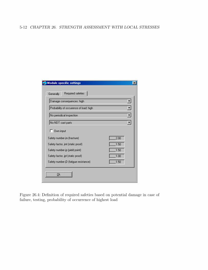
5-12 CHAPTER 26. STRENGTH ASSESSMENT WITH LOCAL STRESSES
Figure 26.4: Definition of required safeties based on potential damage in case offailure, testing, probability of occurrence of highest load

26.3. ENCODING IN KISSSOFT 5-13
Figure 26.5: Manual definition of safeties

5-14 CHAPTER 26. STRENGTH ASSESSMENT WITH LOCAL STRESSES
Figure 26.6: General data
26.3. ENCODING IN KISSSOFT 5-15
If flag is set: support factor/relative stress gradient is calculated using the val-ues given for the support point. For this, the stresses and the distance betweensupport point and proof point are required. If the flag is not set: support fac-tor/relative stress gradient is estimated according to formula 4.3.17. Two radiifor the two directions of the surface and a typical member size need to be defined.See also: module specific settings, calculation of G without 2/deff above.
Loading direction as entered, section 4.1.0, 5.10
Flag set: the analysis is performed for synchronous stresses. Flag not set: Theanalysis is performed for non-synchronous stresses. It can be assumed, that thelater is conservative.
Choice material data, section 3.2.1
The parts normative strengths Rm and Rp are calcualted from the semifinishedproduct normative strengths Rm,N and Rp,N or from strengths as define on thedrawings Rm,Z. As a special case, parts as-is strengths Rm,I and Rp,I can be used.See in addition General settings, last paragraph (26.3.2.1).
Cycle number
If calculation method according to Miner elementa is selected, entries above NDyield constant utilisations
Temperature
Define temperature in degree celsius. Permissible values are defined for differentmaterials in the FKM guideline, see also above. Based on the temperature andthe type of material, the temperature coefficient KT,D is defined.
Duration of temperature
Duration during which the part is exposed to the above defined temperature.
Thickness of protective layer, aluminium, section 4.3.4, figure 4.3.4
The factor KS which is based on the prototctive layer thickness, considers theinfluence of the increased strength of the protective layer formed on the surfaceof aluminium parts.
Surface strengthening factor KV, section 4.3.4 table 4.3.5
The surface strengthening factor KV considers the influence of a surface layertreatment e.g. rolling.
26.3.3.2 S-N curve, section 4.4.3.1
Miner elementar, section 4.4.3.1 If a load collective is used, analysis usuallyis performed using damage accumulation according to Miner elementar
5-16 CHAPTER 26. STRENGTH ASSESSMENT WITH LOCAL STRESSES
Miner consequent, section 4.4.3.1 Using damage accumulation Miner con-sequent, it is considered that the fatigue limit is being reduced with increasingdamage. The reduction is valid for KD,σ=1*10e6.
26.3.3.3 Overload Cases
Different assumptions can be made in the Smith chart to calculate the partsstrength. For example, using a constant mean stress, the resulting permissiblestress amplitude is higher then when assuming a constant stress ratio. The reasonfo this is the limiting curves have an angle below 45 degrees (influence of meanstress). Which assumption applies depends upon the expected stress change inthe part under a permissible operational fatigue stress. The choice of the overloadcase can thus be important in deciding whether a part is or is not overloaded [11].
Stress Cases
• Overload case F1 (constant mean stress): under constant mean stress, thedeflection stress will increase with an increase of the decisive operationalload.
• Overlaod case F2 (constant stress ratio): with an increase of the operationalload, the maximal-to-minimal operational load ratio does not change. Usu-ally, compared with other overload cases, this case gives conservative resultsand should thus be used in borderline cases.
• Overlaod case F3 (constant minimal stress): with an increase of the opera-tional load, the minimal operational load does not change.
• Overlaod case F4 (constant maximal stress): with an increase of the oper-ational load, the maximal operational load does not change.
26.3.4 Stress ratio
Using the value R for the stress ratio, the mean stress is considered in the analy-sis. Compared to the case with no mean stress, the S-N curve is moved to higherbearable stresses for negative mean stress and to lower bearable stresses for pos-itive mean stress. The relation between the permissible stress amplitude and themean stress depends on the material and is called mean stress sensitivity. Themean stress sensitivity generally increases with increasing ultimate strength.
Here, R is defined from -1 to +1

26.3. ENCODING IN KISSSOFT 5-17
Figure 26.7: Define stress ratio for all three direction
Figure 26.8: Own input for stress ratio

5-18 CHAPTER 26. STRENGTH ASSESSMENT WITH LOCAL STRESSES
Figure 26.9: Choose surface roughness by selection of manufacturing process orby selection of roughness directly
26.3.5 Surface roughness
The surface roughness factor considers the influence of the surface roughness.It is determined comparing the permissible stress amplitude for probes with nosurface roughness (polished) and a given surface roughness. For polished surfacess,the surface roughness factor is 1.0, for cast or rolled (untreated) parts, a meanroughness of Rz=200um is assumed.
26.3.6 Load collective
The already available collectives may be directly selected.
It is possible, with the database tool, to create and introduce a new load col-lective: in KISSsoft, select Service/Database Tool/Database Open Collectives
and introduce the new collective’s data.
• Name: Load collective’s name. Own designation as it will show up in theselection list.
• Number of Load Elements: Number of load elements, maximal 50.

26.3. ENCODING IN KISSSOFT 5-19
Figure 26.10: Selection of load collective for the three stress directions
• Torque instead of Power: internal variable, which, is set at torque also fordriving mechanism’s databases.
• File Name: file containing Collective data from an external application,header line with // comments.
• Frequency: relative load element frequency, for instance, 10 %=0.1.
• P: relative load magnitude, for instance, 10 %=0.1.
• n: set at 1. Internal variable also for driving mechanism’s databases.

5-20 CHAPTER 26. STRENGTH ASSESSMENT WITH LOCAL STRESSES
Figure 26.11: Select database
Figure 26.12: Definition of load collectives
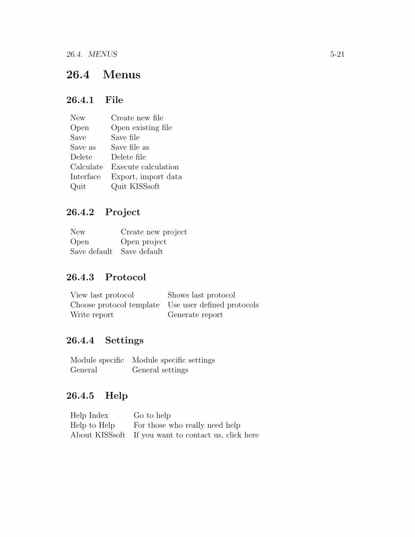
26.4. MENUS 5-21
26.4 Menus
26.4.1 File
New Create new fileOpen Open existing fileSave Save fileSave as Save file asDelete Delete fileCalculate Execute calculationInterface Export, import dataQuit Quit KISSsoft
26.4.2 Project
New Create new projectOpen Open projectSave default Save default
26.4.3 Protocol
View last protocol Shows last protocolChoose protocol template Use user defined protocolsWrite report Generate report
26.4.4 Settings
Module specific Module specific settingsGeneral General settings
26.4.5 Help
Help Index Go to helpHelp to Help For those who really need helpAbout KISSsoft If you want to contact us, click here

5-22 CHAPTER 26. STRENGTH ASSESSMENT WITH LOCAL STRESSES

Chapter 27
Hardness conversion
27.1 Description of the hardness conversion
The calculation is started under Calculation ⇒ Diverse ⇒ Hardness
conversion.
This module offers hardness conversion according to DIN 50150, edition 10/2000.The conversion is valid for low-alloy and cast steels based on the data basesincluded, the tensile strength can be translated to the corresponding Vickers,Brinell or Rockwell hardness or vice versa. The conversion from hardness totensile strength should only be used if direct measurement of the tensile strengthis not possible. Intermediate values for the hardness conversion are interpolatedfrom tabulated values. The following limitations apply:
• Tensile strength Rm: 255...2180 N/mm2
• Vickers hardness HV: 80...940 HV
• Brinell hardness HB: 76...618 HB
• Rockwell hardness HRB: 41...105 HRB
• Rockwell hardness HRF: 82,6...115,1 HRF
• Rockwell hardness HRC: 20,3...68 HRC
• Rockwell hardness HRA: 60,7...85,6 HRA
• Rockwell hardness HRD: 40,3...76,9 HRD
• Rockwell hardness HR 15N: 69,6...93,2 HR 15N
5-23
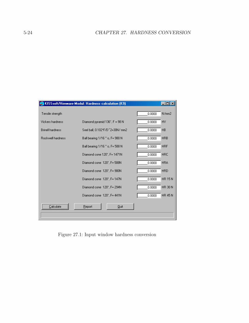
5-24 CHAPTER 27. HARDNESS CONVERSION
Figure 27.1: Input window hardness conversion

27.1. DESCRIPTION OF THE HARDNESS CONVERSION 5-25
• Rockwell hardness HR 30N: 41,7...84,4 HR 30N
• Rockwell hardness HR 45N: 19,9...75,4 HR 45N

5-26 CHAPTER 27. HARDNESS CONVERSION

Chapter 28
Tolerance Calculation
28.1 Description of the Tolerance Calculation
The tolerance calculation is started using Calculation⇒ Diverse⇒ Tolerance
calculation.
In this module the nominal dimension and the allowance for various elementscan be entered from which a total tolerance can then be determined. In thiscalculation the largest and smallest dimension for the dimension chain can bedefined with constant distribution (arithmetic sum) as well as square root of thetolerance squares (normal distribution). Additionally, the nominal and expectedvalue of the dimension chain with corresponding allowances are calculated.
In the tolerance interface (see Fig 28.1) the general tolerance is selected, whichshould be used for the nominal size. Below this is the compiled list of all enterednominal dimension with tolerances.
Explanation of the individual buttons which can influence the list:
• New: A sub-window is opened in which a new entry can be given in.
• Change: A sub-window is opened in which a selected entry can be edited.(Also possible with a double-click on the required entry).
• Delete: Deletes the selected entry.
• ∧: Changes the position of the selected entry to the one above.
• ∨: Changes the position of the selected entry to the one below.
The direction of the nominal dimension can be defined with the ’+’ and ’-’symbols. In order to calculate a closing dimension, the total dimension ’+’ andthe intermediate dimension ’-’ are entered.
5-27
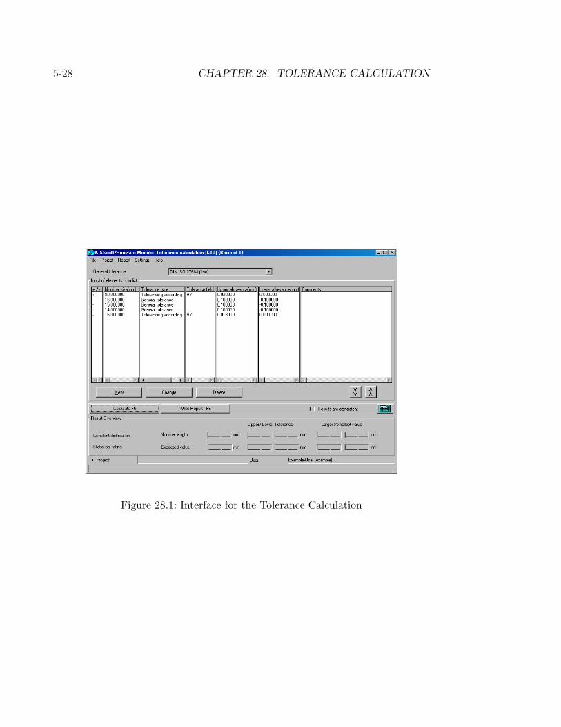
5-28 CHAPTER 28. TOLERANCE CALCULATION
Figure 28.1: Interface for the Tolerance Calculation
Chapter 29
Hertzian Stress
29.1 Calculation of the Hertzian Stress
The Hertzian stress option can be started using option Calculation⇒ Diverse
⇒ Hertzian Stress.
In this module, the Hertzian pressure between two bodies in contact is calculated.During the loaded meshing of a gear pair, an elliptical flattening (due to compres-sive deformation) exists about a contact point, and a quadratic flattening abouta contact line. The maximum pressure (Hertzian stress) as well as the nearingof both bodies (ball, cylinder, ellipsoid, plane; convex or concave) are calculatedusing Hertzian equations. The calculations have been taken from Niemann I, 3rdEdition [60]. As basis for calculation of point contact, it is assumed that the di-ameters of the bodies in contact are defined in two main planes, from which areplacement diameter is defined. There is only one plane for a linear contact, anda replacement diameter. Additionally, the position and amount of the maximumprinciple stress on the inside of the body as well as the maximum shear stress aredefined.
In the Hertzian Stress window (see fig. 29.1) the normal force, the configuration,as well as the diameter (additionally required for contact lines with bearing alongtheir length leff) and material of the contacting bodies can be defined.The following configurations can be selected:
• Ball - Ball
• Ball - Cylinder
• Ball - Ellipsoid
• Ball - Plane
5-29

5-30 CHAPTER 29. HERTZIAN STRESS
Figure 29.1: Window for the Hertzian Stress calculation
• Ellipsoid - Ellipsoid
• Ellipsoid - Cylinder
• Ellipsoid - Plane
• Cylinder - Cylinder
• Cylinder - Plane
A picture appears in the window for each combination so that the input for thecalculation is easier to understand.There is also a possibility to size normal forces. If a calculation has already beencarried out, the sizing button next to the normal force entry can be pressedgenerating an input field for the required Hertzian Stress. The normal force willbe calculated from this value.In the concave curvature condition, the diameter must be given in as negative.Negative diameters are only possible in body 2.

Part VI
KISSsys
6-1

Chapter 30
KISSsys: Calculation Systems
30.1 General Information
KISSsys is an extension for KISSsoft, a calculating program which can size, opti-mize and check shafts, gear wheels or shaft-hub connections. On the other hand,KISSsys is suitable for the management of machine element systems.
Some specific connections between certain different calculations already exist inKISSsoft. This way, bearing forces can be taken out of their shaft calculation andit is possible to place gear wheels on one shaft. But if larger systems like a morecomplex gear unit with several shafts and gear wheels are to be inspected, thepower and speed for each gear wheel still have to be entered separately. Shouldvarious load cases be calculated, each load must be updated in every calculation.
Unlike KISSsoft, in which each single calculation is important, KISSsys enablesa bird’s-eye view of the whole as a system. KISSsys is not to be thought of asa replacement, but as an extension for the existing software KISSsoft. KISSsysuses the reliable calculation modules to administrate connections between certainelements and delegates their calculation to KISSsoft.
30.1.1 Structure
KISSsys is based on an object administration called Classcad. Classcad managesthe administration of KISSsys elements, evaluates expressions for variables andprovides an interpreter so that the user can also draw up functions for otherparticular reasons.
On top of this basis, a user interface and a direct connection to KISSsoft isprovided. This is also where the users’ paths divide. The functionality of the userinterface is different for the regular user whose main usage of the program would
6-3
6-4 CHAPTER 30. KISSSYS: CALCULATION SYSTEMS
be to change and/or check data and examine their results and administratorswho want to draw up new systems or change their structure which requires abetter understanding of the program.
30.1.2 KISSsys Implementation
KISSsys essentially supplies an array of calculations and can display all calcula-tions which belong to a certain system simultaneously so that it is possible for theuser to see all results at a glance. This makes it much easier to decide which gearwheels or shafts are more important than others which can significantly reducethe amount of labor involved in the process.
KISSsys can also provide connections between certain variables e.g. calculate agearbox’s speed from its ratio and its input speed or display power transmission,so the load only has to be entered a minimal amount of times. This enables theuser to check a complex system for various load cases in a relatively short amountof time.
The program can also create tables for load cases or variants. This way, the loaddata only has to be entered once. The data for variants of a certain constructioncan also be produced so that all calculations for a specific load can be performedwith one touch of a button.
For example, should the worst scenario for a certain shaft with unknown directionof a radial force be determined, e.g. of a belt drive or tackle, the direction of whichwould be found out only after its installation procedure, one could rotate the forceby 360 degrees in KISSsys step by step.
KISSsys is not only useful in matters which concern construction, but can alsobe used in distribution. For instance, KISSsys can create a plan for a standardgear box. Should a customer ask for other load applications, one could check ifhis/her demands would fit the requirements for such a construction.
You can find several application examples in the KISSsoft CD or in our Web site.
30.2 Graphical User Interface
The graphical user interface provides several views of administered data. Datacan be recorded in tables, which is particularly useful to get an overall view of thesituation. Another option would be a tree structure which illustrates the hierarchyof a complex construction. The two-dimensional structures are meant to be usedfor the portrayal of the kinetic coupling of a system, whereas the system as awhole or different parts of a system can be shown 3-dimensionally.

30.2. GRAPHICAL USER INTERFACE 6-5
In the following chapter, the different variants for implementation available with-out administrator rights will be portrayed.
Figure 30.1: The KISSsys user interface with tree view, diagram view, 3D–view,tables and 2D–diagram
30.2.1 Tree Structure View
This view (on the left-hand side of fig. 30.1) enables a clear view of the hierarchyof different elements in a certain system, e.g. a building structure. There is abitmap beside the name of each element which identifies its type. Blue coloredbitmaps stand for KISSsoft calculations, red for variables like numbers, functionsor sign chains. A pop-up-menu can be opened with a click of the right mousebutton, with which functions for a certain element can be displayed.
For each element there is a properties–dialogue which can be displayed. Anoverall view of the data elements or the variables is available in the properties–dialogue. However, they can only be changed by the administrator here.
For each KISSsoft calculation the corresponding KISSsoft–module can be startedin the pop-up-menu over kSoftInterface; the calculation data may be changedand assessed with kSoftReportand Calculate performs the calculation withoutthe user interface in the background. Data exchange with KISSsoft is only possiblewith KISSsys calculation elements.

6-6 CHAPTER 30. KISSSYS: CALCULATION SYSTEMS
30.2.2 Diagram View
The kinetic coupling is portrayed in diagram view(right in fig. 30.1. The elementstructure has nothing to do with the calculations at first. The calculations onlyuse the shaft, gear and connection data and can be entered and deleted as desired.
The structure exists of shafts and their elements — gear wheels, forces, cou-plings and bearings. The kinetic coupling between the shafts can be establishedwith connections. The connection possesses the calculation instructions for thetransfer of the speed to the next element (usually just the translation)and theconnection also transfers the torque, dissipated with a certain efficiency.
With speed/torque–elements the entered torque and a certain speed can be con-firmed. The user must decide if the speed and torque are known or if they shouldbe calculated by KISSsoft. The number of pre-assigned values must correspondto the number of degrees of freedom.
The elements in the diagram view can be shifted with the left mouse button.The right mouse button provides a pop-up-menu as in the tree structure view. Azoom factor and a subgroup for the display can be selected.
30.2.3 Table View
With Show in the pop-up menu, the tables can be displayed in Tree or Diagramview. The table contents will be established during system set-up. The figuresshown in black are not changeable, but the red numbers or texts may be edited.In a special table for user interfaces there are panels with a blue backgroundwhere a function can be started by double-clicking the left mouse button.
Table contents can be printed or copied with Strg-C and inserted in a tablecalculation.
30.2.4 3D View
The windows for 3D view can be displayed by Show in the pop-up-menu in thetree structure view. The left mouse button rotates the figure, the right zooms inor out and the middle can shift the figure. One of the main views can be chosenvia menu or the toolbars.
The 3D view offers the possibility to transfer the 3D geometry into the CADsystem. The function can be called in the pop-up-menu. The elements are gen-erated in the 3D viewer PARTgear and can be exported from there in variousCAD formats if the license is available and if graphic elements are selected under

30.3. EXTENDED FUNCTIONALITY FOR DEVELOPERS 6-7
System.kSys3DElements. If a 3D–Kernel is available and solids are generated aCAD–file can be directly generated.
30.2.5 Message Output
In the lower area of the program window (as in fig. 30.1) there is an outputwindow for messages. Error messages and warnings from KISSsoft calculationsare shown under messages. Calls from KISSsoft are recorded under KISSsoft,yet this view is usually not necessary.
30.3 Extended Functionality for Developers
For users who wish to develop the program there are further functions availableother than those described above.
• Template data can be displayed under data⇒open template. It is thenshown as a tree structure under template.
• New elements may be inserted in the tree structure view by ”copy” and”insert”. These new elements are supplied as copies from the class tree ortemplate data.
• It is possible to delete elements and modify their labels with the pop-up-menu.
• Data in the properties–dialogue can be edited. New variables may beadded and deleted.
• Hidden variables are shown and all functions can be performed.
• The messages may be suppressed with Options⇒Suppress Messages.
30.3.1 The Properties–dialogue
The KISSsys properties–dialogue can be displayed in the tree structure view orthe diagram for an element with the pop-up-menu. Here, new variables may beadded or modified. Only one properties–dialogue is available, a second is notdisplayed.
In fig. 30.2 the properties–dialogue is shown. On the left-hand side, there is atree structure to choose the desired data element, on the right there is a dialoguefor the chosen variable. The following panels are available for the variables:
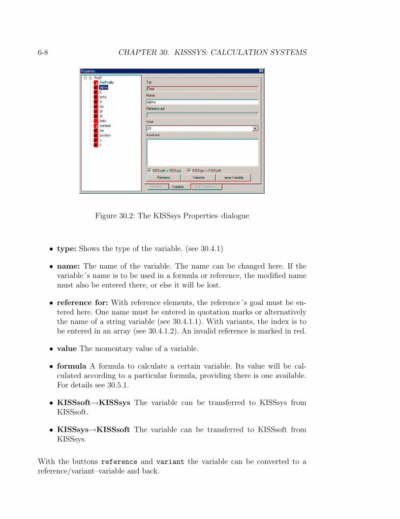
6-8 CHAPTER 30. KISSSYS: CALCULATION SYSTEMS
Figure 30.2: The KISSsys Properties–dialogue
• type: Shows the type of the variable. (see 30.4.1)
• name: The name of the variable. The name can be changed here. If thevariable´s name is to be used in a formula or reference, the modified namemust also be entered there, or else it will be lost.
• reference for: With reference elements, the reference´s goal must be en-tered here. One name must be entered in quotation marks or alternativelythe name of a string variable (see 30.4.1.1). With variants, the index is tobe entered in an array (see 30.4.1.2). An invalid reference is marked in red.
• value The momentary value of a variable.
• formula A formula to calculate a certain variable. Its value will be cal-culated according to a particular formula, providing there is one available.For details see 30.5.1.
• KISSsoft→KISSsys The variable can be transferred to KISSsys fromKISSsoft.
• KISSsys→KISSsoft The variable can be transferred to KISSsoft fromKISSsys.
With the buttons reference and variant the variable can be converted to areference/variant–variable and back.
30.4. EXISTING ELEMENTS 6-9
30.3.2 Table View
The tables´ format is set in the hidden variable definition. The following typesof tables exist:
• tables for calculations: This table is best for the portrayal of data be-longing to several elements of the same type. The format of the definitionis:
[[typ,rows,columns],["variable1","variable2",..],
[element1,element2,..]]
With type one, all values displayed, with type two, all values not contain-ing a formula and with type three, all values also marked with the flagKISSsys→KISSsoft may be edited. The number of lines or columns is notneeded.
• Table for arrays or variants: In this table, arrays or variant variablesare each shown in a column. The format of the definition is:
[[typ,rows,columns],["variable1","variable2",..]]
With type 21, every value shown can be edited. With type 22, all values notcontaining a formula and with type 23, all values also marked with the flagKISSsys→KISSsoft can be edited. The number of columns is not needed.
• Table for user interface: Can be configurated freely. The definition is[[typ,rows,columns],[[A1,B1],[A2,B2]]]. The contents can be enteredvia pop-up-menu and must not be changed in definition. Since the definitionis modified interactively, no formulas should be placed here. The number oflines or columns should also only be changed by dialogue, or else informationabout reference elements will be lost.
30.4 Existing Elements
30.4.1 Variables
The following variables may be used:
• Real: The value of a number .
• String: A string. Enter in quotation marks, e.g. ”text”.

6-10 CHAPTER 30. KISSSYS: CALCULATION SYSTEMS
• Roint: A coordinate or a vector with three components. Enter {1,2,3}.
• Array: A one-, two- or three-dimensional panel. Enter e.g.[”Text”,1.23,{1,2,3},[1,2]].
• Function: A function that may be performed. Enter via its specific inputwindow.
• ElementID:The ID of a classcad object. Displays as $31, to enter, entername of object without quotation marks.
• List:Is shown as pull-down list, functions as a number in the interpreter(the index of the list beginning with 0). The list is then defined over themenu point Edit list as an array, for example [”one”,”two”,”three”].
• Database List: The name from the KISSsoft data base is displayed in apull-down list. In the interpreter, this type also acts as a number accordingto the data base ID. The data bank classification is defined over the menupoint Edit list by an array: [”data base”,”table”]
The variables each have a name, a certain value, an expression and various flags.Should an expression exist, the variable´s value will be determined by its expres-sion. Therefore, expressions are suitable for entering formulas. However, should aformula be entered in the input field for the value, the formula will be evaluatedimmediately and its result will be assigned and the formula itself will be lost. Theflags KISSsoft->KISSsysand KISSsys->KISSsoft determine how the data ex-change between the two programs should happen. The only variables exchangedare the ones marked with the according flag.
With functions, only the function is placed in the formula, whereas its value hasno meaning.
For the data types Real, String, Point, List und Database List, there arealso reference elements and variant elements.
30.4.1.1 References
A reference element acts just like every other variable, the only difference beingthat its data is taken from another variable. A valid name must be entered as ob-jective of the reference element. This objective must be registered as a string - ei-ther as a name in quotation marks or as a formula resulting in a string, like a stringconcatenation (e.g. gear1+".z" where gear1 is a string or "gearwheel1.z"). Aninvalid reference is marked in red.
30.4. EXISTING ELEMENTS 6-11
30.4.1.2 Variants
The variant elements administer a panel of variables internally which acts as anormal variable on the outside. The variant receives an index variable indicatingthe specific panel as supplementary data. This index variable is to be entered asan Array of variables (e.g.[System.index]). With these data types, equivalentdesign tools or system variants can be deposited, the results can be displayed intables.
30.4.2 Calculation Elements
All elements for KISSsoft calculations are derived from classes beginning with thename kSoft. In the tree view, they each have a bitmap with a blue background.
The calculation elements have an array of functions:
• Calculate: performs KISSsoft calculation in the background.
• kSoftInterface: starts KISSsoft interactively
• kSoftReport: performs the calculation and displays its report.
• Flags set: The flags for the data exchange between KISSsoft and KISSsyswill be set accordingly to de desired savinging destination:
– Save in KISSsys: Data will be transmitted in both directions.
– Save in KISSsoft: Data with a specific formula will be transmittedfrom KISSsys to KISSsoft. All other data will be transmitted in theopposite direction only.
This function sets the flags once upon starting. It will not be active for laterchanges.
• kSoftModule: This hidden function supplies the expression for the KISS-soft module
• getTranslationTable: This hidden function delivers the transla-tion table for variable names from KISSsys to KISSsoft. The trans-lation table in the calculation element may be extended throughthe Array TranslationTable: For instance, an entry such as[["eps a min","ZP[0].Eps.aEffI"],["eps a max","ZP[0].Eps.aEffE"],extends the link of the variables eps a min und eps a max with the corre-sponding KISSsoft variables.Till now, the KISSsoft variable names couldonly be taken from the protocol template *.rpt.

6-12 CHAPTER 30. KISSSYS: CALCULATION SYSTEMS
• getUtilization: This function returns the utilization, the ratio betweennominal safety/actual safety.
In the variable fileName, a KISSsoft analysis file can be defined which is loadedbefore other variables are transferred when the analysis is launched. Using thevariable savingMode, it can be defined whether this KISSsoft analysis file is savedautomatically:
• Don’t ask and don’t save On closing of KISSsoft you won’t be asked, ifthe KISSsoft file should be saved.
• Ask for saving On closing of KISSsoft you will be asked if the file shouldbe saved. (standard behaviour of KISSsoft)
• Save automatically The calculation file is saved automatically withoutasking.
• Save file in KISSsys No filename is used in the variable fileName, butthe whole calculation file is appended to the KISSsys element.
30.4.2.1 Link between Calculations and Elements
There are some extensions, which automatically link the calculations with theshafts and the gears. This can be achieved with the function Dialog. In case ofimportant modifications such as, for instance, the addition of other stress elementsto the shaft, this dialog should be called again in order the link could be updated.
30.4.2.2 Calculation-data Saving Strategy
There are several possible ways of saving the calculation data:
1. All data are to be saved in the KISSsys-File and the access to the calculationtakes place through KISSsys only: select in KISSsys savingMode Save file
in KISSsys. Flags should preferably be set for bidirectional transfer.
2. All data are to be saved in the KISSsys-File and it can also be processedfrom outside the KISSsys: select Ask for saving or Save automatically
under savingMode gewahlt. The flags must be set to SetFlags with Save
in KISSsoft. We must stress here that, the Calculation-data will be firstloaded from the KISSsoft-File the first time Calculation is called. That iswhy kSoftCalculate must be called once after having opened the KISSsys-File.

30.4. EXISTING ELEMENTS 6-13
30.4.2.3 Importing existing KISSsoft Calculations
In case it is desirable to transfer existing KISSsoft Element Calculations to a newKISSsys system, simply read the files in a KISSsoft Window. However, there aresome points to consider:
• The file name in fileName in KISSsys Calculation Element will be changed.The name must either be changed or deleted.
• In Shaft Elements, the force elements and the bearings will beoverwritten. Hence, it is necessary to call the Dialog or theUpdateShaftElementsfunction after importing the calculation. The Forceelements and the bearings, as well as their positions, cannot be imported.These data must be input in KISSsys.
• We must stress that, in gears, the wheel sequence must be respected.
30.4.3 Shaft Elements
Various elements may be placed on shafts. They are also transferred to the KISS-soft shaft calculation. The variable position determines their shaft position.
• kSysHelicalGear: A helical gear.
• kSysBevelGear: A bevel gear. The bearing of the peak is determined bythe variable direction.
• kSysWorm: A worm.
• kSysWormGear: A worm gear.
• kSysCoupling: Coupling. Its diameter d and width b can be entered forthe 3-D display.
• kSysBearing: A general bearing. Losses may be considered in Tloss. Thedirection of the torque loss should be determined by -sign(speed) in theexpression.
• kSysRollerBearing: A roller bearing. The bearing geometry will be readfrom the KISSsoft lager database for each refresh. Losses may be consideredin Tloss. The torque loss direction should be established in the formula with-sign(speed).

6-14 CHAPTER 30. KISSSYS: CALCULATION SYSTEMS
• kSysCentricalLoad:A centrical load. In KISSsys, the torque (Ty) is al-ways noted and not its power. This torque is also considered in the kineticcalculation.
• kSysMass: An additional mass on the shaft.
• kSysRopeSheave: A rope sheave. The cable stress, unlike the torque, willnot be calculated through the connection. The user must make sure thatthe cable stress is the same on the two pulleys.
30.4.4 Connection Elements
• kSysGearPairConstraint: A connection between two bevel gears or he-lical gears.
• kSysPlanetaryGearPairConstraint: A connection between a gear wheeland a planet. The manner of the pairing (sun–planet, planet–internal gearor planet–planet) can be chosen. Both gear wheels must be entered in thisorder. The number of planets should be defined in the variable NofPlanetsin the coupling of the planet carrier.
• kSysPlanetaryBevelGearConstraint: A connection between a gearwheel and a planetary bevel gear for conical differentials. As for the plan-etary connection, the sequence of the conical wheels and the number ofplanets must be defined. No efficiency can be input here.
• kSysWormGearConstraint: A connection between a worm and wormgear. A further option is to define two efficiencies (eta1 und eta2) for thedriving worm or wheel.
• kSysCouplingConstraint: A connection with translation 1 between twocouplings. The enforcement of the cinematic conditions can be activated ordeactivated. It is also possible to account for slippage, e.g. for disk couplingsor synchronization. The torque in the connection is calculated by defaultbut can be modified manually.
• kSysBeltConstraint: A connection between belt pulleys. The transmis-sion ratio will be calculated from the diameter ratio. A slip and an efficiencymay be input here. The transmission ratio and the sign should be consideredwhen inputting the slip. The calculation takes place as: n1−d2/d1 ·n2 = slip
With the function setConfig(slipConstraint r/[slipConstraint r,
slip r], torqueConstraint r/[torqueConstraint r, torque r]) theconnection can be activated or deactivated:
30.4. EXISTING ELEMENTS 6-15
1. closed without slip: setConfig([TRUE, 0], FALSE),
2. open without torque: setConfig(FALSE, FALSE),
3. open with torque: setConfig(FALSE, [TRUE, 20])
• kSysSpeedOrForce: An element to constrain speed or torque as inputor output. Speed or torque can be input values or can be calculated byKISSsys. Instead of the torque also a power can be given.
With the function setConfig(speedConstraint r,
torqueConstraint r/[torqueConstraint r, type r, torque r])
the constraints can be changed. The valid values for the type of load are:0..torque with sign, 1..torque driving, 2..torque driven, 3..power driving,4..power driven. Examples:
1. speed and torque given: setConfig(TRUE, TRUE),
2. speed and torque with absolut value given: setConfig(TRUE, [TRUE,
0, 20]),
3. only driving power given: setConfig(FALSE, [TRUE, 3, 20])
30.4.5 Display of Elements in 3D-View
Each element has a function OnRefresh3DView for generating the 3D-view. Ifneeded this function can be overwritten for an element. The color of an elementcan be changes with the variable kSys 3DColor defined for the range from 0 to255, the transparency can be set with the variable kSys 3DTransparency in therange from 0 to 1. These variables have to be appended when required.
30.4.6 System settings
There are a number of settings in the element System:
• kSoftAcceptChanges In the sefault setting yes changes in KISSsoft willbe transfered to KISSsys. With the selection no no changes will be trans-feren from KISSsoft and if asked is selected you will be asked if the changesin KISSsoft should be transfered to KISSsys.
• kSysKinematicFunc During the calculation of kinematics the functionOnCalcTorque can be called. The default implementation of this functioncalls the calculation of bearing reactions of all shafts.

6-16 CHAPTER 30. KISSSYS: CALCULATION SYSTEMS
• kSysKinematicMode The kinematics can be calculated iteratively. Iter-ations for torque are necessary if losses should be considered. Iterationsfor speed are only necessary if formulas are given for the speed of someelements.
• kSys3DElements For the 3D-View either graphical or solid elements (3D-Kernel required) may be displayed. Graphical elements will be faster todisplay; however, 3D-elements are more detailed and it is possible to includea existing housing.
• project name The name of the project is displayed in KISSsoft reports.
• project contract The contract number is also used in the KISSsoft re-ports.
30.5 Programming in the Interpreter
It is possible to program in variable expressions and in functions.
30.5.1 Expressions in Variables
The programming variants in expressions are limited. No local variables may beused.
The operators for the data types are listed in table 30.1. In addition, there is anarray of mathematical functions available which are listed in the table 30.2.
data type operations descriptionReal +,- addition and subtraction
*,/ multiplication und division<,>=,=,!=,>=,> comparison operators!,AND,OR boolean operators
String +,LEN concatenation and length operators<,>=,=,!=,>=,>,! comparatie operators
Point +,- addition und subtraction*,** scalar– und vector multiplication:x,:y,:z access to componentsLEN vector length
Array [],+,LEN indexing, concatenation and length operator
Table 30.1: Admissable Operators for Data Types
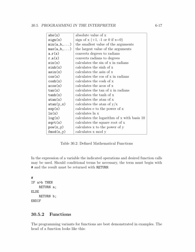
30.5. PROGRAMMING IN THE INTERPRETER 6-17
abs(x) absolute value of xsign(x) sign of x (+1, -1 or 0 if x=0)min(a,b,...) the smallest value of the argumentsmax(a,b,...) the largest value of the argumentsa r(x) converts degrees to radiansr a(x) converts radians to degreessin(x) calculates the sin of x in radianssinh(x) calculates the sinh of xasin(x) calculates the asin of xcos(x) calculates the cos of x in radianscosh(x) calculates the cosh of xacos(x) calculates the acos of xtan(x) calculates the tan of x in radianstanh(x) calculates the tanh of xatan(x) calculates the atan of xatan(y,x) calculates the atan of y/xexp(x) calculates e to the power of xln(x) calculates ln xlog(x) calculates the logarithm of x with basis 10sqrt(x) calculates the square root of xpow(x,y) calculates x to the power of yfmod(x,y) calculates x mod y
Table 30.2: Defined Mathematical Functions
In the expression of a variable the indicated operations and desired function callsmay be used. Should conditional terms be necessary, the term must begin with# and the result must be returned with RETURN:
#
IF a>b THEN
RETURN a;
ELSE
RETURN b;
ENDIF
30.5.2 Functions
The programming variants for functions are best demonstrated in examples. Thehead of a function looks like this:

6-18 CHAPTER 30. KISSSYS: CALCULATION SYSTEMS
// transferred variables from the calling program
PAR Parameter1, Parameter2;
// declaration of constants
CONST PI=3.1415926, E=2.71828;
// declaration of local variables
VAR a,b,c,d;
The lines beginning with // are comments. Each one of these three lines mustonly be used once, the declared variables must be separated by commas. Anynot initialized parameter or variable will be VOID. This can be tested withISVOID(variable).
For conditional statements, there are two variants: IF– or SWITCH–statements:
// IF-statement with optional ELSIF and ELSE block
IF Parameter1 > 5 THEN
a = sin(PI*Parameter1);
ELSIF Parameter1 < 0 THEN
a = Parameter1;
ELSE
a = 0;
ENDIF
// SWITCH statement with choice of numbers or text
SWITCH Parameter2
CASE "zero": b = 0;
CASE "one": b = 1;
DEFAULT: b = 5;
ENDSWITCH
For loops, four different program variants exist:
// FOR loop with optimal step length
FOR a = 1 TO 8 STEP 2 DO
b = b + a;
IF b>100 THEN
BREAK; // ends the loop
ENDIF
NEXT
// WHILE loop

30.5. PROGRAMMING IN THE INTERPRETER 6-19
WHILE b<100 DO
b = b*10;
WHEND
// DO loop
DO
b = b*10;
UNTIL b>100;
// FORALL the loop is performed for all elements of an array
c = [1,2,3,4,5,6,7,8,9];
a = 0;
FORALL c d DO // d receives the value of an element of c
a = a + d;
NEXT
There is a special syntax for the calling of functions which belong to objects.Thestandard method is the entry of an object name followed by a dot and the nameof the function. The name of a certain object can also be contained in a localvariable with which the object may be modified for the calling of the functionduring running time.
// The function OBJ_GetMember is summoned for object1.
object1.OBJ_GetMember("nameofvariable");
// a is a type string local variable with the name of an object
a = "object1";
// A service function for object1 is called
b = a.OBJ_GetMember("nameofvariable");
// calls for the function constructed by the user for object1.
a.UserFunction();
// the function constructed by the user is called for the
// current object
userfunction();
// the function constructed by the user is called for the
// parent object
^.userfunction();

6-20 CHAPTER 30. KISSSYS: CALCULATION SYSTEMS
Variable names are searched for in relevance to the current object. For example,should object.z be used in an expression, the program tries to find the variableunder the current object first. If it is not found there, it is then searched for inthe parent object (one step higher in the hierarchy,(according to ^.object.z)and so on.
30.5.3 Important Service Functions
OBJ GetChildren() supplies an array with all child objects.OBJ GetName() supplies the name of the object.OBJ GetId() supplies the ID of the object.OBJ HasMember() verifies if a variable exists.OBJ GetMember() supplies the variable of the current object.OBJ FindMember() supplies the variable of the current
or parent object.
Table 30.3: Important service functions
30.5.4 Variable Dialogues
Variable dialogues can be created in interpreter functions for entering variables.The call is:
res = CADH VarDialogue([”title”, width, height, spacing],
[dialoguelement1], [dialoguelement2], ...);
The title is displayed in the headline of the dialogue, width and length determinethe dimensions of the dialogue in pixels. The spacing of the dialogue (between 0and 1) describes the ratio of the width of the panel description to the dialoguewidth (the standard being .4) After this definition of the dialogue size, the desiredamount of arrays with the definition of each dialogue element may follow.
The return value is an array. Its first value is res[0]=1 if the dialogue is endedwith Ok, otherwise it is zero. The further elements of the returned array supplythe results of the input panels.
The following is the standard way to determine the type of a variable: str=String,n=Int, r=Real, b=Bool. For example, Descr str would imply that the variableDescr is a string variable.

30.5. PROGRAMMING IN THE INTERPRETER 6-21
30.5.4.1 Dialogue Elements for the Variable Dialogue
For the variable dialogues the following dialogue elements are available:
• Horizontal Grouping:The horizontal grouping provides a frame in whicheach dialogue element is placed next to another. Their position must alwaysbe defined by a vertical group, i.e. all dialogue elements in a horizontalgrouping have to be defined in a vertical group. A horizontal group is definedas follows:
[C:VDGL HORZ,descr str,spaceabove n,spacebelow n,[Dialoguelem]]
– C:VDGL HORZ:Definition of the type of horizontal grouping.
– descr:Description of the horizontal grouping. If ”descr” is not anempty string, a frame around the horizontal group will be shown .
– spaceabove:Space above the horizontal group to the next element.
– spacebelow:Space below the horizontal group to the next dialogueelement. t. ”spacebelow” and ”spaceabove” must be entered in pixels.
– [Dialoguelem]:An array of elements to define the elements in thehorizontal grouping. This array must only contain elements of the typeVDGL Vert.
• Vertical Grouping:The vertical grouping provides a framein which each dialogue element is placed under another.The width of the dialogue elements is determined bythe vertical group. A vertical group is defined as follows:[C:VDGL Vert,descr str,[XStart r,XEnd r],XPart r,[Diag],margin n]
– C:VDGL Vert:Definition of the type of vertical grouping.
– descr:Description of the vertical grouping. A frame around the group-ing is always shown.
– [XStart,XEnd]:XStart und XEnd define a factor (between 0 and 1)for the width of the vertical group with reference to the width of theparent dialogue and the x-position of the vertical group.
– XPart:Factor between 0 and 1 which positions the ratio of the promptsize to the entry size of the dialogue panels (the prompt being thetext assigned to a certain panel). Should XPart be -1, the prompt isautomatically positioned over the dialogue element.
– [Diag]:Element array defining the dialogue elements in the verticalgrouping.

6-22 CHAPTER 30. KISSSYS: CALCULATION SYSTEMS
– margin:Margin is an optional parameter which defines the offset of thedialogue elements according to the margin of the vertical group, i.e.the dialogue elements have a distance from the right and left marginsof the vertical group, their length being ”margin”.
• RealEditWindow:Provides an editbox to enter a floating point number.
[C:VDGL Real,Prompt str,Constraint r,res,res,positions n]
– C:VDGL Real:Defines the type of RealEditWindow.
– Prompt:Text for the input window.
– Constraint:Defines the constraint value.
– res:There is room reserved here for two optional parame-ters which are not of use at the moment. However, thesepositions may not be left empty in definition. For example,[C:VDGL Real,Prompt,Constraint,0,0,positions] would be a correctsolution but not [C:VDGL Real,Prompt,Constraint,,,positions]).
– digits:Digits is an optional parameter defining the number of digitsfollowing a decimal point in an input panel.
– output value:The output value is the value entered.
• IntEditpanel:Provides an editbox in order to enter a whole number.
[C:VDGL Int,Promt str,Constraint n]
– C:VDGL Int:Defines the type of IntEditpanel.
– Prompt:The text assigned to the input field.
– Constraint:Defines the constraint value.
– output value:The output value is the value entered.
• StringEditpanel:Provides an editbox to enter text as desired.
[C:VDGL Str,Prompt str,constraint str]
– C:VDGL Str:Defines the type of StringEditpanel.
– Prompt:The text assigned to the input window.
– constraint:Text describing the constraint.
– output value:The output value is the string entered.
• textdisplay:Creates a text display. Should an empty string be entered astext, the panel may also be used in order to define a distance.
[C:VDGL Prompt,Prompt str,panelheight n]
– C:VDGL Prompt:Defines the type of text display.
30.5. PROGRAMMING IN THE INTERPRETER 6-23
– Prompt:Panel text.
– panelheight:height of the text display.
• IntComboBox:Provides a combobox to enter a whole number.
[C:VDGL IntCom,Prompt str,[entry n],con n/[Ind n],0,0,AsVal b]
– C:VDGL IntCom:Defines the type of combobox.
– Prompt:Text assigned to the combobox.
– [entry]:Array of available list elements (in the case of an Intcom-bobox, the components must be whole numbers).
– con/[Ind]:The value of a constraint existing in the list may be deter-mined either directly by ”con”, or a certain value in a specific positionin the list may be defined as the value of a constraint by ”Ind”(thefirst element of the list being in position 0).”con” or rather ”[Ind]” areoptional parameters.
– AsVal:Should the optional parameter ”AsVal” be entered and notequal zero, the output value is the value entered. If this is not thecase, the output value is the index of the selected entry.
• IntEditComboBox:Provides a combobox for entering a whole num-ber which may also be edited. Entered numbers must be whole.[C:VDGL IntComE,Prompt str,[entry n],con n/[Ind n]]
– as in IntComboBox
– output value:The output value is the value entered.
• RealComboBox:Provides a combobox in order to enter a fliesskommazahl.
[C:VDGL RealCom,Prompt str,[Eintr r],Vor r/[Ind n],0,0,AsVal b]
– as in IntComboBox
• RealEditComboBox:Provides a combobox in order toenter a fliesskommazahl which may also be edited.[C:VDGL RealComE,Prompt str,[entry r],con r/[Ind n]]
– as in IntComboBox
– output value:The output value is the value entered.
StringComboBox:Provides a combobox for entering strings.
[C:VDGL StrCom,Prompt str,[entry str],con str/[Ind n],AsPos n]
– as in IntComboBox

6-24 CHAPTER 30. KISSSYS: CALCULATION SYSTEMS
– AsPos:Unlike with IntComboBox, the output value is the index ofthe selected panel, providing that the optional parameter ”AsPos” isgiven and does not equal zero. Otherwise, the output value is the valueentered.
• StringEditComboBox:Provides a combobox to enter a string which mayalso be edited.
[C:VDGL StrCom,Prompt str,[entry str],con str/[Ind n]]
– as in IntComboBox
– output value:The output value is the string entered.
• codebutton:
• servicebutton:
30.5.4.2 Application of Variable Dialogues
Figure 30.3: Example of a possible variable dialogue
The following is the program code corresponding to the variable dialogue as shownin figure 30.3, in which as many elements as possible are used.
//VARIABLE DECLARATION
VAR res,result1,result2,result3,result4,result5,fullResult;

30.5. PROGRAMMING IN THE INTERPRETER 6-25
res = CADH_VarDialog(["Example of a possible variable dialogue",500,400,0.4],
[C:VDLG_StrCom,"StrCOMBOBOX1:",["wheel1","wheel2","wheel3"],[2],0],
[C:VDLG_Prompt,"TEXT1:",30],
[C:VDLG_IntCom,"IntCOMBOBOX1:",[12,17,19],17,0,0,1],
//HORIZONTAL UNIT WITH ONE VERTICAL UNIT
[C:VDLG_HORZ,"HORIZONTALUNIT1",20,10,
[ //Remember to insert brackets
[C:VDLG_VERT,"VERTICALUNIT1",[0.3,0.9],0.4,
[
[C:VDLG_Str,"StringPanel:","testing program"],
[C:VDLG_RealComE,"RealCOMBOBOX1",[5.3,7.1,9.1],2]
],
20
]
] //Remember to insert brackets
],
//HORIZONTAL UNIT WITH TWO VERTICAL UNITS
[C:VDLG_HORZ,"HORIZONTALUNIT2",10,10,
[
[C:VDLG_VERT,"VERTICALUNIT2",[0.01,0.35],-1,
[
[C:VDLG_Int,"IntPanel:",6],
[C:VDLG_StrComE,"StrCOMBOBOX2:",["Gear1","Gear2"],[0]]
],
10
],
[C:VDLG_VERT,"VERTICALUNIT3",[0.4,1],-1,
[
[C:VDLG_Real,"RealPanel:",5.6,0,0,3],
[C:VDLG_IntComE,"IntCOMBOBOX2:",[5,7,9],7]
]
]
]
]
);

6-26 CHAPTER 30. KISSSYS: CALCULATION SYSTEMS
//In res[0], 1 is returned if the OK button is pressed, otherwise 0
IF res[0] THEN
//EXAMPLE OF HOW RESULTS CAN BE RETURNED
result1 = res[1]; //res[1]= wheel3
result2 = res[2]; //res[2]= TEXT1
result3 = res[3]; //res[3]= 17
result4 = res[4]; //res[4]= [["test program",5.3]]
result5 = res[5]; //res[5]= [[6,"Gear1"],[5.6,7]]
fullResult=res;
//res=["wheel3","TEXT1",17,[["test program",5.3]],[[6,"Gear1"],[5.6,7]]]
CADH_Message(fullResult);
ENDIF
30.5.4.3 Interaction With Variable Dialogues
Interactions with variable dialogues are possible. Selections in lists and changesin input windows can evoke callbacks to a certain user-defined function. It is thenpossible to change dialogue elements out of this callback routine.
The registration of a local function as a callback happens via the entry of thevariable dialogue´s title:
res = CADH VarDialog([[”title”,PROC(Callback)], width, height,
spacing], [dialoguelement1], [dialoguelement2], ...);
From now on, the local callback function is elicited by changes in the dialogue.The function is declared as follows:
PAR res;
PROC Callback
PAR handle, elemNo, event, eventPar;
IF TYP(elemNo)=STRING THEN
IF elemNo="@combo" AND event=C:CBN_SELCHANGE THEN
IF eventPar=0 THEN // own input, enable input
CADH_VarDialogAccess(handle,[["@input1",C:VDLG_ENABLE,TRUE]]);
ELSE // disable input, set value to zero

30.5. PROGRAMMING IN THE INTERPRETER 6-27
CADH_VarDialogAccess(handle,[["@input1",C:VDLG_ENABLE,FALSE],
["@input1",c:VDLG_ASSIGN,0]]);
ENDIF
ENDIF
ENDIF
ENDPROC
res = CADH_VarDialog([["title",PROC(Callback)], 400, 400 0.4],
[[C:VDLG_Real,"@input1"],"Input1:",2],
[[C:VDLG_StrCom,"@combo"],"Selection:",
["own input","calculate"],[0],TRUE]);
A handle is assigned to the dialogue as a transfer parameter; furthermore, theelement´s identification, the event and additional parameters. The possible eventsare:
element type event parameterDialogue initiation none
WM INITDIALOGUE
Combobox selection momentary valueCBN SELCHANGE
Input window exit field momentary valueWM KILLFOCUS
button activates noneBN CLICKED
Either the number of the element according to the index in the result array orthe name of the element is handed over as an element number. A name can bedefined – as in the example above – by handing over an array with with type andname for the dialogue element in its first element.
Access to the dialogue out of the callback routine occurs via the function:
CADH VarDialogAccess(handle, [[elemNo, action, param],[elemNo,
action, param],...]
whereas the following actions are permitted:
action description parameterVDLG ASSIGN assignment to input window new valueVDLG SELECT selection in combobox [position]/valueVDLG ENABLE activate or deactivate TRUE/FALSEVDLG SETFOCUS focus on new element ID of the element
If no action is stated, the value of the input window is returned as an array withas many elements as transfer parameters.

6-28 CHAPTER 30. KISSSYS: CALCULATION SYSTEMS
30.5.5 Displaying and Formatting of 2D Plots
The KISSsys program allows graphs to be generated based on data arrays whichcan be entered directly or referenced to a variable defined in the user interface. Astructure to define graph can be entered in the ”Expression” field after selectingksys2DPlot/properties/data. The function allows for simultaneous graphing ofseveral plots and chart types. The structure can be of some length for morecomplex graphs, and is best considered in three sections :
• Axes ( 1 or 2 axis system definitions must be given)
• XY-Line Plotting
• Bar Chart
The structure can be further broken down to define the individual properties ofeach section. Both the axes and the individual plots can be customised to assistin the analysis of the results.
30.5.5.1 The Axis Format (af)
At least one axis definition should be given, but a second can be added if required.In each axis system to be used, a sub-structure representing characteristics shouldbe entered as :
[ | Xaxisname str , | min x r , | max x r ] , [ | Yaxisname str ,
| min y r , | max y r ] , [ axiscolour str/array , | axiscross x r ,
axiscross y r ] , [ | scaleinterval x r , | scaleinterval y r , [ |
exponential x n , | exponential y n ]
Where :
• XAxisname :Identifies X axis data.
• YAxisname :Identifies Y axis data.
• min :Sets a lower limit for the axis if required.
• max :Sets an upeer limit for the axis if required.
• axiscolour : Text string definition of line colour(red,green,blue,yellow,white,grey,cyan,brown,magenta,purple,black), oras an array [ r n , g n , b n ] (where r,g,b are red,green and blue colourparameters less than 256) .

30.5. PROGRAMMING IN THE INTERPRETER 6-29
• axiscross : Set intersection point of the axis with opposite axis.
• scaleinterval : Can be used to increase axis scale divisions.
• exponential : If this value is set to 1 and the data is compatible the datawill be plotted against a log scale of base 10.
30.5.5.2 The XY-Line Plot Format (dg l)
For XY-line plot information, a single data group representing x and y data pointsshould be entered as :
grouptype n , [ dataarray x r ] , [ dataarray y r ] , [ |
linename str , | |linecolour str/array , | linestyle n ] , |
assignaxis n
Where :
• grouptype : = 1 (Identifies line plot).
• dataarray : Contains x or y co-ordinate data elements.
• linename : NA.
• linecolour : Text string or array definition of line colour.
• linestyle : Number definition of line style (0- Solid, 1- Striped, 2- Dash,3- Dot +Dash, 4- Dot+Dot+Dash)
• assignaxis : Enter 1 or 2 to plot x-y data against corresponding axissystems.
30.5.5.3 The Bar Chart Format (dg b)
For bar chart information, a single data group with n array elements should beentered as :
grouptype n , [ dataarray 1 r , ... , |dataarray n r ]
, [ barcolour str/array ] , | bargroupname 1 str , [ |
barelementlabel 1 str , ... , barelementlabel 1 str ] , |
barclass n
Where :
• grouptype := 2 (Identifies bar chart).
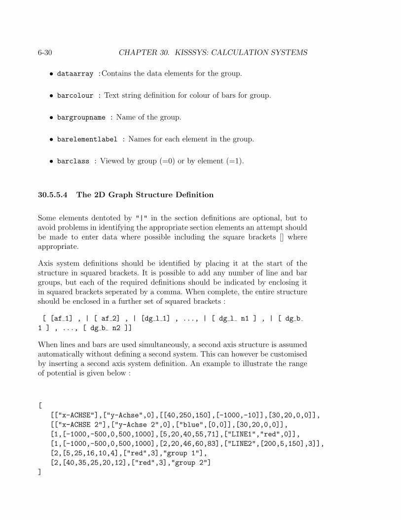
6-30 CHAPTER 30. KISSSYS: CALCULATION SYSTEMS
• dataarray :Contains the data elements for the group.
• barcolour : Text string definition for colour of bars for group.
• bargroupname : Name of the group.
• barelementlabel : Names for each element in the group.
• barclass : Viewed by group (=0) or by element (=1).
30.5.5.4 The 2D Graph Structure Definition
Some elements dentoted by "|" in the section definitions are optional, but toavoid problems in identifying the appropriate section elements an attempt shouldbe made to enter data where possible including the square brackets [] whereappropriate.
Axis system definitions should be identified by placing it at the start of thestructure in squared brackets. It is possible to add any number of line and bargroups, but each of the required definitions should be indicated by enclosing itin squared brackets seperated by a comma. When complete, the entire structureshould be enclosed in a further set of squared brackets :
[ [af 1] , | [ af 2] , | [dg l 1] , ..., | [ dg l n1 ] , | [ dg b
1 ] , ..., [ dg b n2 ]]
When lines and bars are used simultaneously, a second axis structure is assumedautomatically without defining a second system. This can however be customisedby inserting a second axis system definition. An example to illustrate the rangeof potential is given below :
[
[["x-ACHSE"],["y-Achse",0],[[40,250,150],[-1000,-10]],[30,20,0,0]],
[["x-ACHSE 2"],["y-Achse 2",0],["blue",[0,0]],[30,20,0,0]],
[1,[-1000,-500,0,500,1000],[5,20,40,55,71],["LINE1","red",0]],
[1,[-1000,-500,0,500,1000],[2,20,46,60,83],["LINE2",[200,5,150],3]],
[2,[5,25,16,10,4],["red",3],"group 1"],
[2,[40,35,25,20,12],["red",3],"group 2"]
]

30.5. PROGRAMMING IN THE INTERPRETER 6-31
This example produces simultaneous graphing of two lines and two bar datagroups within two axis systems.
30.5.5.5 Viewing Graph and Editing Display
After defining a graph structure, the resulting graph can be viewed by selectingksys2DPlot/properties/show. Any changes to the format made in the ”Expres-sion” field, or data in the user interface can be assessed by pressing ”Refresh”button on the graph window, or by re-running the ”show” graph generation.

6-32 CHAPTER 30. KISSSYS: CALCULATION SYSTEMS

Part VII
Appendix: Bibliography andIndex
7-1


Bibliography
[1] A.G.M.A. - Fundamental Rating Factors and Calculation Methods for Invo-lute Spur and Helical Gear Teeth. Norm 2001-B88, 1988
[2] Akahori H., Sato Y., Nishida T., Kubo A.: Prove di durata di Face Gear.Organi di trasmissione, 2002, Nr.12 oder MTP2001-Fukuoka, The JSME Int.Conference, 2001, Japan.
[3] Basstein G., Sijtstra A.: Neue Entwicklung bei Auslegungen und Fertigungvon Kronenradern. Antriebstechnik, 32(1993), Nr.11
[4] Bock G., Nocj R., Steiner O.: Zahndickenmessung an Getriebeschneckennach der Dreidrahtmethode. Physikalisch-Technische Bundesanstalt, Braun-schweig, 1974
[5] Decker K.H.: Maschinenelemente. Carl Hanser Verlag Munchen, 10. Auflage,1990
[6] Dietrich G., Stahl H.: Matrizen und Determinanten in der Technik. VEBVerlag Leipzig, 5. Auflage, ca. 1960
[7] DIN 732-1 (Entwurf): Thermisch zulassige Betriebsdrehzahl, DIN Taschen-buch 24, Beuth Verlag Berlin, 1995
[8] DIN 732-2 (Entwurf): Thermische Bezugsdrehzahl, DIN Taschenbuch 24,Beuth Verlag Berlin, 1995
[9] DIN 743: Tragfahigkeitsberechnung von Wellen und Achsen. Oktober 2001
[10] DIN 867: Bezugsprofile fur Evolventenverzahnungen an Stirnradern (Zylin-derradern) fur den allgemeinen Maschinenbau und den Schwermaschinenbau.Ausgabe Februar 1986
[11] DIN 2091: Drehstabfedern mit rundem Querschnitt: Berechnung und Kon-struktion. DIN Taschenbuch 29, Beuth Verlag Berlin, 2003
[12] DIN 2092: Tellerfedern: Berechnung. DIN Taschenbuch 29, Beuth VerlagBerlin, 2003
7-3

7-4 BIBLIOGRAPHY
[13] DIN 2093: Tellerfedern: Masse, Qualitatsanforderungen. DIN Taschenbuch29, Beuth Verlag Berlin, 2003
[14] DIN 2095: Zylindrische Schraubenfedern aus runden Drahten: Gutevorschriftfur kaltgeformte Druckfedern. DIN Taschenbuch 29, Beuth Verlag Berlin,2003
[15] DIN 2096: Zylindrische Schraubenfedern aus runden Drahten und Staben:Gutevorschrift fur warmgeformte Druckfedern. DIN Taschenbuch 29, BeuthVerlag Berlin, 2003
[16] DIN 2097: Zylindrische Schraubenfedern aus runden Drahten:Gutevorschriften fur kaltgeformte Zugfedern. DIN Taschenbuch 29,Beuth Verlag Berlin, 2003
[17] DIN 2194: Zylindrische Schraubenfedern aus runden Drahten und Staben:Kaltgeformte Drehfedern (Schenkelfedern), Gutenorm. DIN Taschenbuch 29,Beuth Verlag Berlin, 2003
[18] DIN 3960: Begriffe und Bestimmungsgrossen fur Stirnrader und Stirnrad-paare mit Evolventenverzahnung. Ausgabe Dezember 1987
[19] DIN 3961: Toleranzen fur Stirnradverzahnungen, Grundlagen. 1978
[20] DIN 3967: Flankenspiel, Zahndickenabmasse, Zahndickentoleranzen. 1978
[21] DIN 3971: Begriffe und Bestimmungsgrossen fur Kegelrader und Kegelrad-paare. Ausgabe Juli 1980
[22] DIN 3975: Begriffe und Bestimmungsgrossen fur Zylinderschneckengetriebemit Achsenwinkel 90 Grad. Ausgabe Juli 1976
[23] DIN 3990: Tragfahigkeitsberechnung von Stirnradern. Teil 1,2,3,4,5,11 und21. Ausgabe Dez. 1987
[24] DIN 3991: Tragfahigkeitsberechnungen von Kegelradern. 1990
[25] DIN 5480: Zahnwellen-Verbindungen mit Evolventenflanken. Teil 1 bis 15.Marz 1986
[26] DIN 6885: Passfedern. Blatt 1-3. 1968
[27] DIN 6892: Passfedern – Berechnung und Gestaltung. 1998
[28] DIN 7151: ISO Grundtoleranzen fur Langenmasse bis 500 mm. 1964
[29] DIN 7190: Berechnung und Anwendung von Pressverbanden. Februar 2001

BIBLIOGRAPHY 7-5
[30] DIN EN 13906-1: Druckfedern: Berechnung und Konstruktion. DIN Taschen-buch 29, Beuth Verlag Berlin, 2003
[31] DIN EN 13906-2: Zugfedern: Berechnung und Konstruktion. DIN Taschen-buch 29, Beuth Verlag Berlin, 2003
[32] DIN EN 13906-3: Drehfedern: Berechnung und Konstruktion. DIN Taschen-buch 29, Beuth Verlag Berlin, 2003
[33] DIN 31652: Hydrodynamische Radial-Gleitlager im stationaren Bereich. DINTaschenbuch 198, Beuth Verlag Berlin, 1991
[34] DIN 31653: Hydrodynamische Axial-Gleitlager im station”aren Bereich. DINTaschenbuch 198, Beuth Verlag Berlin, 1991
[35] DIN 31654: Hydrodynamische Axial-Gleitlager im station”aren Bereich. DINTaschenbuch 198, Beuth Verlag Berlin, 1991
[36] DIN 58400: Bezugsprofil fur Evolventenverzahnungen an Stirnradern in derFeinwerktechnik. Ausgabe Juni 1984
[37] DIN 58405: Abmasse fur die Feinwerktechnik, Teil 2.
[38] Dubbel H.: Taschenbuch fur den Maschinenbau. Springer Verlag Berlin, 15.Auflage, 1986
[39] Eschmann P.: Die Walzlagerpraxis. R.Oldenburg Verlag Munchen, 1978
[40] FAG: Standardprogramm. Katalog WL 41510, 3. Ausgabe 1995
[41] FKM 183: Rechnerischer Festigkeitsnachweis fur Maschinenbauteile. VDMAVerlag Frankfurt, 5. Auflage, 2003
[42] Hanchen R., Decker K.H.: Neue Festigkeitslehre fur den Maschinenbau. CarlHanser Verlag Munchen, 3. Auflage, 1967
[43] Hirn H.: Computergestutzte Zahnradoptimierung. Fink GmbH, Druck undVerlag Pfullingen, 1999
[44] ISO 6336: Calculation of load capacity of spur and helical gears. Teil1,2,3,4,5. Ausgabe 1996
[45] ISO/DIS 10300: Calculation of Load Capacity of Bevel Gears. Teil 1,2,3.Entwurf 1993
[46] Kissling U.: KISSsoft - eine praxisgerechte Maschinenelemente-Software.antriebstechnik 27 (1988), Nr. 12, S. 34-40

7-6 BIBLIOGRAPHY
[47] Kissling U.: Auslegung von Maschinenelementen. CIM Management 11 4,1995
[48] Kissling U.: Technische Berechnungen auf Personal Computern. VDI-Z 130(1988), Nr. 5, S. 45-52
[49] Klingelnberg-Werknorm 3028: Auslegung eines Kegelradgetriebes ohneAchsversatz. Ausgabe-Nr. 2
[50] Klingelnberg-Werknorm 3029: Auslegung eines Kegelradgetriebes mitAchsversatz. Ausgabe-Nr. 2
[51] Klingelnberg-Werknorm 3030: Tragfahigkeits-Berechnung fur Spi-ralkegelrader. Ausgabe-Nr. 1
[52] Klotter K.: Technische Schwingungslehre, Band 2. Springer Verlag Berlin, 2.Auflage, 1960
[53] Kollmann F.: Welle-Nabe-Verbindungen. Springer Verlag Berlin, 1984
[54] Lang O., Steinhilper R.: Gleitlager. Konstruktionsbucher Band 31, SpringerVerlag Berlin, 1978
[55] Linke H.: Stirnradverzahnung. Carl Hanser Verlag Munchen, 1996
[56] MAAG-Taschenbuch. 2. erweiterte Auflage, Zurich, 1985
[57] Massa E.: Costruzione di macchine. Editori Masson Italia, Milano, 1981
[58] Matek W., Muks D., Wittel H.: Roloff/Matek Maschinenelemente. ViewegVerlag Braunschweig, 11. Auflage, 1987
[59] Matthias K.: Schraubenkrafte in einer Flanschverbindung. Maschinenbau,Berlin 34 (1985) 11, S. 517.
[60] Niemann G.: Maschinenelemente, Band 1. Springer Verlag Berlin, 2001
[61] Niemann G.: Maschinenelemente, Band 2. Springer Verlag Berlin, 1983
[62] Niemann G.: Maschinenelemente, Band 3. Springer Verlag Berlin, 1985
[63] Obsieger: Zahnformfaktoren von Aussen- und Innenverzahnungen.Zeitschrift Konstruktion 32 (1980), S. 443-447.
[64] Rules for The Classification of Naval Ships (FREMM 3.1), Bureau Veritas,March 2004
[65] SKF: Hauptkatalog 4000 T. Ausgabe 1989

BIBLIOGRAPHY 7-7
[66] Spinnler Prof.: Manual de calcul d’organes des machines. EPFL Lausanne,1990
[67] VDI 2226: Festigkeitsberechnung metallischer Bauteile.
[68] VDI 2227: Festigkeitsberechnung.
[69] VDI 2230: Systematische Berechnung hochbeanspruchter Schrauben-verbindungen, Blatt 1. Februar 2003
[70] VDI 2545: Zahnrader aus thermoplastischen Kunststoffen. Ausgabe 1981

Index
Abbreviations, 4-161Addendum modification factor
From measured data, 4-26Adhesive coefficient
Taper interference fit, 2-7AGMA, 4-48AGMA 2001, 4-42AGMA 2001-B88, 4-14AGMA 2001-C95, 4-15AGMA 6004-F88, 4-15Alternating bending factor, 4-30ANSI B92.1, 4-150ANSI B92.2M, 4-150Application factor, 2-11
Spur gear, 4-11Axial journal bearings
Hydro dynamic, 3-89Axis wrenching, 4-97
Balance grading, 3-9Bearing, 3-11Bearings, 3-21Bearing calculation
Data transfer from shaft calcula-tion, 3-62
Belts, 2-53Bending Critical Speed, 3-37Bending line, 3-31Bevel gear, 4-103
Calculation basis, 4-103Klingelnberg, 4-114Momentum, 4-114Settings, 4-112Sizing, 4-113Toothing data, 4-119Tooth thickness, 4-114
BezugsprofilDIN 3972, 4-25
Bolted joints, 2-25Bracket connection, 2-41Buckling, 3-39Buckling root flank, 4-23
CADgeometry data, 1-78
CAD-Interface, 1-71Calculations
Modul-Specific, 4-53Shafts, 3-31
Calculation basisHelical gear, 4-145Splined joints, 4-149Splined shafts, 4-149
Calculation systems, 6-3Centre distance, 4-38
Deviation, 4-38Spur gear, 4-11
Chamfer/ tooth end, 4-31Coast side, 4-112Configurations
Spur gear, 4-5Connecting elements, 2-3Contact length, 4-83Contact stiffness, 4-93Coordinate system
Shaft calculation, 3-8Coupling, 3-24Course of shearing force, 3-31Cross helical gears, 4-145
Sizing, 4-146Cross hole, 3-48Cross sections, 3-45
7-8
INDEX 7-9
Crowning, 3-62, 4-91
Data Interface, 1-71Deep toothing
Sizing, 4-65Deep tooth form, 4-154Deformation, 3-62DIN 125A, 2-28DIN 126, 2-28DIN 13, 2-28DIN 2076, 2-67, 2-69, 2-71DIN 2077, 2-67, 2-69, 2-71DIN 2091, 2-74DIN 2092, 2-73DIN 2093, 2-73DIN 2095, 2-67DIN 2096, 2-67, 2-69DIN 2097, 2-68DIN 2194, 2-71DIN 3964, 4-97DIN 3967, 4-35DIN 3972, 4-25, 4-156DIN 3990, 4-41, 4-157, 4-158
Part 41 (automobile gearboxes), 4-14
DIN 5480, 4-149, 4-150DIN 558, 2-28DIN 58405, 4-35DIN 601, 2-28DIN 6885, 2-8DIN 6888, 2-20DIN 6892, 2-8
Methode B, 2-11DIN 7160, 4-39DIN 743, 2-8
Calculation, 3-55DIN 84, 2-28DIN 912, 2-28DIN 931, 2-28DIN 933, 2-28DIN 934, 2-28DIN 960, 2-28DIN 961, 2-28
Disc springs, 2-73Dowels, 2-20Drive side, 4-112Dynamic factor, 4-44
Editor, 1-57Electrodes, 4-78EN 10270-1, 2-67, 2-69, 2-71EN 10270-2, 2-67, 2-69, 2-71EN 10270-3, 2-67, 2-69, 2-71EN 13906-1, 2-67EN 13906-2, 2-68EN 13906-3, 2-71Equivalent design loads
life, 4-95Equi design load
Torque sizing gear wheels, 4-96
Face gear, 4-123Face load coefficient, 4-39Feather-Key connection, 2-8Feather key, 3-47
Force application, 2-10Feather key length
Supporting, 2-10FKM, 3-56Flange connections, 2-40Flashtemperature course, 4-92Foot relief, 4-30Forces, 3-22Force application
Feather key, 2-10Force application factor, 2-32Force balance, 3-31Friction factor
Interference fit, 2-5FVA spur gear calculation, 4-17
Garter springs, 2-67Gear pumps, 4-100Gear rim
Deformation, 4-99Gear wheel pumps
Haul volume, 4-55
7-10 INDEX
GeneralModul-Specific, 4-45
Geometry errors, 4-47Gleason-Geometry, 4-114Glued joints, 2-22Groove-Toothing and splined shaft, 3-
47
Hanchen + Decker, 3-50Hardness ratio factor, 4-160Helix angle, 4-9Hertzian stress, 4-94Hypoid gear, 4-103
Individually entering notch factors, 3-48
Inner diameter, 4-30Interference fit, 2-4, 3-47
Conical, 2-6Internal gear
Deformation Gear Rim, 4-99Involute
Verification, 4-83ISO 262, 2-28ISO 272, 2-28ISO 273, 2-28ISO 4014, 2-28ISO 4016, 2-28ISO 4017, 2-28ISO 4018, 2-28ISO 4762, 2-28ISO 6336, 4-14, 4-157, 4-158ISO 898, 2-28ISO 9085, 4-17ISO 940, 2-28ISO 949, 2-28
Journal bearingsCalculation, 3-83
Journal bearing calculationData transfer from shaft calcula-
tion, 3-62
Kinds of bearings
Classification, 3-65Kinematics (helical gear), 4-93KISSedit, 1-57KISSsys, 6-3
3D view, 6-6Calculation elements, 6-11Connection elements, 6-14Diagram view, 6-6Graphical user interface, 6-4Mathematical functions, 6-17Plots, 6-28Programming, 6-16Saving Strategy, 6-12Shaft elements, 6-13System settings, 6-15Table definition, 6-9Torque introduction, 6-15Variables, 6-9Variable dialogues, 6-20
Large transverse contact ratio, 4-154Lay-out, 3-29Leg springs, 2-71Lifetime
Spur gear, 4-12Line of Flex, 3-31Load cycles, 4-29Load factor
Feather key, 2-12Lubrication, 4-19
Magnetic tension, 3-25Mass, 3-24Master gear, 4-99Material
Data base, 1-33Spur gear, 4-10
MaterialsShaft strength, 3-59
Material treatment, 4-45Maximal load factor, 3-49Micro-gliding, 2-6Modification of tip diameter, 4-28

INDEX 7-11
ModuleSpur gear, 4-9
Momentum balance, 3-31Momentum of mass, 4-55Mountability
Planetary trains, 4-51Multi-Spline, 2-14
Nominal SafetiesFKM-Guideline, 3-57Module-Specific, 4-56
Notch effectsIntersections, 3-48
Notch factors, 3-61Number of load changes, 4-46Number of planets
Planetary trains, 4-21
Only geometry, 4-14Operating backlash, 4-96
Pairing external gear, 4-154Permissible pressure
Feather key, 2-13Planet
Modul-Specific, 4-51Planetary trains
Mountability, 4-51Plastic
Modul-Specific, 4-50Tooth form, 4-79
PlasticsCalculate temperature, 4-50Calculation method, 4-15Temperature, 4-50
Polygon, 2-18Power
Spur gear, 4-12Precision mechanics, 4-153Pressure angle
Spur gear, 4-9Profile correction, 4-84
Racks, 4-102
Radial journal bearingsHydro dynamic, 3-83
RatingModule-Specific, 4-56
Reference profile, 4-22Relative structure coefficient, 4-43Report, 1-57
Template, see ReporttemplateReporttemplate
FOR-loop, 1-65Format, 1-61IF-condition, 1-63Name, 1-58Variables, 1-61
Roller bearingCalculation, 3-66Friction Moment, 3-76Thermal limit of operating speed,
3-73Roller bearing calculation
Data transfer from shaft calcula-tion, 3-62
Root circle, 4-29Root circle deviations, 4-29Rotational natural frequency, 3-39Rough sizing
Spur gear, 4-57Running-in curve, 4-72
SafetyNominal margins, 4-159With load spectrum, 4-96
Scoring, 4-98Screws
Coefficient of friction, 2-35Configurations, 2-39Definition geometry, 2-30High and low temperatures, 2-43Input of additional screws, 2-48Strength re-calculation, 2-27Tension diagram, 2-45Tightening factor, 2-35
Section Modulus, 3-61

7-12 INDEX
Service factor, 2-11Service life
Spur gear, 4-94Settings
Shafts, 3-12Shaft-Hub-Connections, 2-3Shaft end, 3-11Shaft recesses, 3-46Shaft strength, 3-40
DIN 743, 3-55Hanchen + Decker, 3-50
Shaping cutterManufacture, 4-79
Shoulder, 3-45Shoulder with conical transition, 3-46Shoulder with relief groove, 3-45Sizing, 3-44
Spur gear, 4-57Sizings
Modul-Specific, 4-52Smooth shaft, 3-48Soldered joints, 2-22Specific sliding, 4-25Splined joints, 4-149
Geometry, 4-149Splines, 2-16Spur gear
Calculation basis, 4-6Geometry variant program, 4-58optimizing, 4-58
Startparameter, 1-27Strength
Shafts, 3-40Strength calculation
Helical gear, 4-146Spur gear, 4-14
Stress ratio factor, 3-53Surface factors, 3-61
Taper interference fit, see interfer-ence fit, conical
Technology Factor, 4-33Tension conditions, 3-48
Tension springs, 2-68Thermal contact coefficient, 4-32Thread, 3-46Tip chamfer, 4-47Tip circle, 4-28Tip circle deviations, 4-28Tip relief, 4-30Tolerances, 4-34
For the gear manufacturing, 4-90Tooth form, 4-66
Modifications for casting, 4-78Tooth form factor
Graphical method, 4-49, 4-53Tooth number, 4-9Tooth thickness, 4-89
Additional measures for prefabrica-tion, 4-36
From measured data, 4-36Measure, 4-34
Tooth thickness at the tip, 4-155Tooth trace, 4-43Torque, 3-8
Sizing gear wheels, 4-96Torsion bar springs, 2-74Transmission error, 4-93Transverse coefficient, 4-44
VDI 2230, 2-26VDI 2545, 4-15
Welded joints, 2-24Width
Spur gear, 4-9Woehler line, 4-94Woodruff key, 2-19Worm gear, 4-135
Settings, 4-141Tolerances, 4-139
Related Documents