GROMACS Documentation Release 2019.3 GROMACS development team Jun 14, 2019

Welcome message from author
This document is posted to help you gain knowledge. Please leave a comment to let me know what you think about it! Share it to your friends and learn new things together.
Transcript
GROMACS DocumentationRelease 2019.3
GROMACS development team
Jun 14, 2019
CONTENTS
1 Downloads 21.1 Source code . . . . . . . . . . . . . . . . . . . . . . . . . . . . . . . . . . . . . . . . . . . . . 21.2 Regression tests . . . . . . . . . . . . . . . . . . . . . . . . . . . . . . . . . . . . . . . . . . . 2
2 Installation guide 32.1 Introduction to building GROMACS . . . . . . . . . . . . . . . . . . . . . . . . . . . . . . . . 3
2.1.1 Quick and dirty installation . . . . . . . . . . . . . . . . . . . . . . . . . . . . . . . . . 32.1.2 Quick and dirty cluster installation . . . . . . . . . . . . . . . . . . . . . . . . . . . . . 32.1.3 Typical installation . . . . . . . . . . . . . . . . . . . . . . . . . . . . . . . . . . . . . 42.1.4 Building older versions . . . . . . . . . . . . . . . . . . . . . . . . . . . . . . . . . . . 4
2.2 Prerequisites . . . . . . . . . . . . . . . . . . . . . . . . . . . . . . . . . . . . . . . . . . . . . 42.2.1 Platform . . . . . . . . . . . . . . . . . . . . . . . . . . . . . . . . . . . . . . . . . . . 42.2.2 Compiler . . . . . . . . . . . . . . . . . . . . . . . . . . . . . . . . . . . . . . . . . . 52.2.3 Compiling with parallelization options . . . . . . . . . . . . . . . . . . . . . . . . . . . 52.2.4 CMake . . . . . . . . . . . . . . . . . . . . . . . . . . . . . . . . . . . . . . . . . . . 62.2.5 Fast Fourier Transform library . . . . . . . . . . . . . . . . . . . . . . . . . . . . . . . 62.2.6 Other optional build components . . . . . . . . . . . . . . . . . . . . . . . . . . . . . . 8
2.3 Doing a build of GROMACS . . . . . . . . . . . . . . . . . . . . . . . . . . . . . . . . . . . . 82.3.1 Configuring with CMake . . . . . . . . . . . . . . . . . . . . . . . . . . . . . . . . . . 82.3.2 Compiling and linking . . . . . . . . . . . . . . . . . . . . . . . . . . . . . . . . . . . 152.3.3 Installing GROMACS . . . . . . . . . . . . . . . . . . . . . . . . . . . . . . . . . . . . 162.3.4 Getting access to GROMACS after installation . . . . . . . . . . . . . . . . . . . . . . 162.3.5 Testing GROMACS for correctness . . . . . . . . . . . . . . . . . . . . . . . . . . . . 162.3.6 Testing GROMACS for performance . . . . . . . . . . . . . . . . . . . . . . . . . . . . 172.3.7 Having difficulty? . . . . . . . . . . . . . . . . . . . . . . . . . . . . . . . . . . . . . . 17
2.4 Special instructions for some platforms . . . . . . . . . . . . . . . . . . . . . . . . . . . . . . . 182.4.1 Building on Windows . . . . . . . . . . . . . . . . . . . . . . . . . . . . . . . . . . . . 182.4.2 Building on Cray . . . . . . . . . . . . . . . . . . . . . . . . . . . . . . . . . . . . . . 182.4.3 Building on Solaris . . . . . . . . . . . . . . . . . . . . . . . . . . . . . . . . . . . . . 182.4.4 Fujitsu PRIMEHPC . . . . . . . . . . . . . . . . . . . . . . . . . . . . . . . . . . . . . 192.4.5 Intel Xeon Phi . . . . . . . . . . . . . . . . . . . . . . . . . . . . . . . . . . . . . . . . 19
2.5 Tested platforms . . . . . . . . . . . . . . . . . . . . . . . . . . . . . . . . . . . . . . . . . . . 19
3 User guide 203.1 Getting started . . . . . . . . . . . . . . . . . . . . . . . . . . . . . . . . . . . . . . . . . . . . 20
3.1.1 Flow Chart . . . . . . . . . . . . . . . . . . . . . . . . . . . . . . . . . . . . . . . . . 203.1.2 Setting up your environment . . . . . . . . . . . . . . . . . . . . . . . . . . . . . . . . 223.1.3 Flowchart of typical simulation . . . . . . . . . . . . . . . . . . . . . . . . . . . . . . . 223.1.4 Important files . . . . . . . . . . . . . . . . . . . . . . . . . . . . . . . . . . . . . . . . 223.1.5 Tutorial material . . . . . . . . . . . . . . . . . . . . . . . . . . . . . . . . . . . . . . 243.1.6 Background reading . . . . . . . . . . . . . . . . . . . . . . . . . . . . . . . . . . . . . 24
3.2 System preparation . . . . . . . . . . . . . . . . . . . . . . . . . . . . . . . . . . . . . . . . . . 243.2.1 Steps to consider . . . . . . . . . . . . . . . . . . . . . . . . . . . . . . . . . . . . . . 243.2.2 Tips and tricks . . . . . . . . . . . . . . . . . . . . . . . . . . . . . . . . . . . . . . . 25
i
3.3 Managing long simulations . . . . . . . . . . . . . . . . . . . . . . . . . . . . . . . . . . . . . 263.3.1 Appending to output files . . . . . . . . . . . . . . . . . . . . . . . . . . . . . . . . . . 263.3.2 Backing up your files . . . . . . . . . . . . . . . . . . . . . . . . . . . . . . . . . . . . 273.3.3 Extending a .tpr file . . . . . . . . . . . . . . . . . . . . . . . . . . . . . . . . . . . . . 273.3.4 Changing mdp options for a restart . . . . . . . . . . . . . . . . . . . . . . . . . . . . . 273.3.5 Restarts without checkpoint files . . . . . . . . . . . . . . . . . . . . . . . . . . . . . . 273.3.6 Are continuations exact? . . . . . . . . . . . . . . . . . . . . . . . . . . . . . . . . . . 273.3.7 Reproducibility . . . . . . . . . . . . . . . . . . . . . . . . . . . . . . . . . . . . . . . 28
3.4 Answers to frequently asked questions (FAQs) . . . . . . . . . . . . . . . . . . . . . . . . . . . 293.4.1 Questions regarding GROMACS installation . . . . . . . . . . . . . . . . . . . . . . . . 293.4.2 Questions concerning system preparation and preprocessing . . . . . . . . . . . . . . . 293.4.3 Questions regarding simulation methodology . . . . . . . . . . . . . . . . . . . . . . . 303.4.4 Parameterization and Force Fields . . . . . . . . . . . . . . . . . . . . . . . . . . . . . 303.4.5 Analysis and Visualization . . . . . . . . . . . . . . . . . . . . . . . . . . . . . . . . . 31
3.5 Force fields in GROMACS . . . . . . . . . . . . . . . . . . . . . . . . . . . . . . . . . . . . . . 313.5.1 AMBER . . . . . . . . . . . . . . . . . . . . . . . . . . . . . . . . . . . . . . . . . . . 313.5.2 CHARMM . . . . . . . . . . . . . . . . . . . . . . . . . . . . . . . . . . . . . . . . . 323.5.3 GROMOS . . . . . . . . . . . . . . . . . . . . . . . . . . . . . . . . . . . . . . . . . . 333.5.4 OPLS . . . . . . . . . . . . . . . . . . . . . . . . . . . . . . . . . . . . . . . . . . . . 33
3.6 Non-bonded cut-off schemes . . . . . . . . . . . . . . . . . . . . . . . . . . . . . . . . . . . . . 333.6.1 Non-bonded scheme feature comparison . . . . . . . . . . . . . . . . . . . . . . . . . . 333.6.2 Performance . . . . . . . . . . . . . . . . . . . . . . . . . . . . . . . . . . . . . . . . . 343.6.3 How to use the Verlet scheme . . . . . . . . . . . . . . . . . . . . . . . . . . . . . . . . 353.6.4 Further information . . . . . . . . . . . . . . . . . . . . . . . . . . . . . . . . . . . . . 35
3.7 Command-line reference . . . . . . . . . . . . . . . . . . . . . . . . . . . . . . . . . . . . . . . 353.7.1 molecular dynamics simulation suite . . . . . . . . . . . . . . . . . . . . . . . . . . . . 353.7.2 gmx anadock . . . . . . . . . . . . . . . . . . . . . . . . . . . . . . . . . . . . . . . . 403.7.3 gmx anaeig . . . . . . . . . . . . . . . . . . . . . . . . . . . . . . . . . . . . . . . . . 413.7.4 gmx analyze . . . . . . . . . . . . . . . . . . . . . . . . . . . . . . . . . . . . . . . . . 433.7.5 gmx angle . . . . . . . . . . . . . . . . . . . . . . . . . . . . . . . . . . . . . . . . . . 463.7.6 gmx awh . . . . . . . . . . . . . . . . . . . . . . . . . . . . . . . . . . . . . . . . . . 473.7.7 gmx bar . . . . . . . . . . . . . . . . . . . . . . . . . . . . . . . . . . . . . . . . . . . 483.7.8 gmx bundle . . . . . . . . . . . . . . . . . . . . . . . . . . . . . . . . . . . . . . . . . 503.7.9 gmx check . . . . . . . . . . . . . . . . . . . . . . . . . . . . . . . . . . . . . . . . . . 513.7.10 gmx chi . . . . . . . . . . . . . . . . . . . . . . . . . . . . . . . . . . . . . . . . . . . 523.7.11 gmx cluster . . . . . . . . . . . . . . . . . . . . . . . . . . . . . . . . . . . . . . . . . 553.7.12 gmx clustsize . . . . . . . . . . . . . . . . . . . . . . . . . . . . . . . . . . . . . . . . 583.7.13 gmx confrms . . . . . . . . . . . . . . . . . . . . . . . . . . . . . . . . . . . . . . . . 593.7.14 gmx convert-tpr . . . . . . . . . . . . . . . . . . . . . . . . . . . . . . . . . . . . . . . 603.7.15 gmx covar . . . . . . . . . . . . . . . . . . . . . . . . . . . . . . . . . . . . . . . . . . 613.7.16 gmx current . . . . . . . . . . . . . . . . . . . . . . . . . . . . . . . . . . . . . . . . . 623.7.17 gmx density . . . . . . . . . . . . . . . . . . . . . . . . . . . . . . . . . . . . . . . . . 643.7.18 gmx densmap . . . . . . . . . . . . . . . . . . . . . . . . . . . . . . . . . . . . . . . . 653.7.19 gmx densorder . . . . . . . . . . . . . . . . . . . . . . . . . . . . . . . . . . . . . . . 673.7.20 gmx dielectric . . . . . . . . . . . . . . . . . . . . . . . . . . . . . . . . . . . . . . . . 683.7.21 gmx dipoles . . . . . . . . . . . . . . . . . . . . . . . . . . . . . . . . . . . . . . . . . 693.7.22 gmx disre . . . . . . . . . . . . . . . . . . . . . . . . . . . . . . . . . . . . . . . . . . 713.7.23 gmx distance . . . . . . . . . . . . . . . . . . . . . . . . . . . . . . . . . . . . . . . . 733.7.24 gmx do_dssp . . . . . . . . . . . . . . . . . . . . . . . . . . . . . . . . . . . . . . . . 743.7.25 gmx dos . . . . . . . . . . . . . . . . . . . . . . . . . . . . . . . . . . . . . . . . . . . 753.7.26 gmx dump . . . . . . . . . . . . . . . . . . . . . . . . . . . . . . . . . . . . . . . . . . 773.7.27 gmx dyecoupl . . . . . . . . . . . . . . . . . . . . . . . . . . . . . . . . . . . . . . . . 783.7.28 gmx dyndom . . . . . . . . . . . . . . . . . . . . . . . . . . . . . . . . . . . . . . . . 793.7.29 gmx editconf . . . . . . . . . . . . . . . . . . . . . . . . . . . . . . . . . . . . . . . . 793.7.30 gmx eneconv . . . . . . . . . . . . . . . . . . . . . . . . . . . . . . . . . . . . . . . . 823.7.31 gmx enemat . . . . . . . . . . . . . . . . . . . . . . . . . . . . . . . . . . . . . . . . . 833.7.32 gmx energy . . . . . . . . . . . . . . . . . . . . . . . . . . . . . . . . . . . . . . . . . 843.7.33 gmx filter . . . . . . . . . . . . . . . . . . . . . . . . . . . . . . . . . . . . . . . . . . 87
ii
3.7.34 gmx freevolume . . . . . . . . . . . . . . . . . . . . . . . . . . . . . . . . . . . . . . . 883.7.35 gmx gangle . . . . . . . . . . . . . . . . . . . . . . . . . . . . . . . . . . . . . . . . . 893.7.36 gmx genconf . . . . . . . . . . . . . . . . . . . . . . . . . . . . . . . . . . . . . . . . 913.7.37 gmx genion . . . . . . . . . . . . . . . . . . . . . . . . . . . . . . . . . . . . . . . . . 913.7.38 gmx genrestr . . . . . . . . . . . . . . . . . . . . . . . . . . . . . . . . . . . . . . . . 933.7.39 gmx grompp . . . . . . . . . . . . . . . . . . . . . . . . . . . . . . . . . . . . . . . . . 943.7.40 gmx gyrate . . . . . . . . . . . . . . . . . . . . . . . . . . . . . . . . . . . . . . . . . 963.7.41 gmx h2order . . . . . . . . . . . . . . . . . . . . . . . . . . . . . . . . . . . . . . . . . 973.7.42 gmx hbond . . . . . . . . . . . . . . . . . . . . . . . . . . . . . . . . . . . . . . . . . 983.7.43 gmx helix . . . . . . . . . . . . . . . . . . . . . . . . . . . . . . . . . . . . . . . . . . 1013.7.44 gmx helixorient . . . . . . . . . . . . . . . . . . . . . . . . . . . . . . . . . . . . . . . 1023.7.45 gmx help . . . . . . . . . . . . . . . . . . . . . . . . . . . . . . . . . . . . . . . . . . 1033.7.46 gmx hydorder . . . . . . . . . . . . . . . . . . . . . . . . . . . . . . . . . . . . . . . . 1033.7.47 gmx insert-molecules . . . . . . . . . . . . . . . . . . . . . . . . . . . . . . . . . . . . 1043.7.48 gmx lie . . . . . . . . . . . . . . . . . . . . . . . . . . . . . . . . . . . . . . . . . . . 1053.7.49 gmx make_edi . . . . . . . . . . . . . . . . . . . . . . . . . . . . . . . . . . . . . . . 1063.7.50 gmx make_ndx . . . . . . . . . . . . . . . . . . . . . . . . . . . . . . . . . . . . . . . 1093.7.51 gmx mdmat . . . . . . . . . . . . . . . . . . . . . . . . . . . . . . . . . . . . . . . . . 1103.7.52 gmx mdrun . . . . . . . . . . . . . . . . . . . . . . . . . . . . . . . . . . . . . . . . . 1113.7.53 gmx mindist . . . . . . . . . . . . . . . . . . . . . . . . . . . . . . . . . . . . . . . . . 1153.7.54 gmx mk_angndx . . . . . . . . . . . . . . . . . . . . . . . . . . . . . . . . . . . . . . 1163.7.55 gmx morph . . . . . . . . . . . . . . . . . . . . . . . . . . . . . . . . . . . . . . . . . 1173.7.56 gmx msd . . . . . . . . . . . . . . . . . . . . . . . . . . . . . . . . . . . . . . . . . . 1183.7.57 gmx nmeig . . . . . . . . . . . . . . . . . . . . . . . . . . . . . . . . . . . . . . . . . 1193.7.58 gmx nmens . . . . . . . . . . . . . . . . . . . . . . . . . . . . . . . . . . . . . . . . . 1213.7.59 gmx nmr . . . . . . . . . . . . . . . . . . . . . . . . . . . . . . . . . . . . . . . . . . . 1223.7.60 gmx nmtraj . . . . . . . . . . . . . . . . . . . . . . . . . . . . . . . . . . . . . . . . . 1233.7.61 gmx order . . . . . . . . . . . . . . . . . . . . . . . . . . . . . . . . . . . . . . . . . . 1243.7.62 gmx pairdist . . . . . . . . . . . . . . . . . . . . . . . . . . . . . . . . . . . . . . . . . 1253.7.63 gmx pdb2gmx . . . . . . . . . . . . . . . . . . . . . . . . . . . . . . . . . . . . . . . . 1273.7.64 gmx pme_error . . . . . . . . . . . . . . . . . . . . . . . . . . . . . . . . . . . . . . . 1293.7.65 gmx polystat . . . . . . . . . . . . . . . . . . . . . . . . . . . . . . . . . . . . . . . . 1303.7.66 gmx potential . . . . . . . . . . . . . . . . . . . . . . . . . . . . . . . . . . . . . . . . 1313.7.67 gmx principal . . . . . . . . . . . . . . . . . . . . . . . . . . . . . . . . . . . . . . . . 1323.7.68 gmx rama . . . . . . . . . . . . . . . . . . . . . . . . . . . . . . . . . . . . . . . . . . 1333.7.69 gmx rdf . . . . . . . . . . . . . . . . . . . . . . . . . . . . . . . . . . . . . . . . . . . 1343.7.70 gmx report-methods . . . . . . . . . . . . . . . . . . . . . . . . . . . . . . . . . . . . . 1353.7.71 gmx rms . . . . . . . . . . . . . . . . . . . . . . . . . . . . . . . . . . . . . . . . . . . 1363.7.72 gmx rmsdist . . . . . . . . . . . . . . . . . . . . . . . . . . . . . . . . . . . . . . . . . 1383.7.73 gmx rmsf . . . . . . . . . . . . . . . . . . . . . . . . . . . . . . . . . . . . . . . . . . 1393.7.74 gmx rotacf . . . . . . . . . . . . . . . . . . . . . . . . . . . . . . . . . . . . . . . . . . 1403.7.75 gmx rotmat . . . . . . . . . . . . . . . . . . . . . . . . . . . . . . . . . . . . . . . . . 1413.7.76 gmx saltbr . . . . . . . . . . . . . . . . . . . . . . . . . . . . . . . . . . . . . . . . . . 1423.7.77 gmx sans . . . . . . . . . . . . . . . . . . . . . . . . . . . . . . . . . . . . . . . . . . 1433.7.78 gmx sasa . . . . . . . . . . . . . . . . . . . . . . . . . . . . . . . . . . . . . . . . . . 1443.7.79 gmx saxs . . . . . . . . . . . . . . . . . . . . . . . . . . . . . . . . . . . . . . . . . . 1463.7.80 gmx select . . . . . . . . . . . . . . . . . . . . . . . . . . . . . . . . . . . . . . . . . . 1473.7.81 gmx sham . . . . . . . . . . . . . . . . . . . . . . . . . . . . . . . . . . . . . . . . . . 1493.7.82 gmx sigeps . . . . . . . . . . . . . . . . . . . . . . . . . . . . . . . . . . . . . . . . . 1503.7.83 gmx solvate . . . . . . . . . . . . . . . . . . . . . . . . . . . . . . . . . . . . . . . . . 1513.7.84 gmx sorient . . . . . . . . . . . . . . . . . . . . . . . . . . . . . . . . . . . . . . . . . 1533.7.85 gmx spatial . . . . . . . . . . . . . . . . . . . . . . . . . . . . . . . . . . . . . . . . . 1543.7.86 gmx spol . . . . . . . . . . . . . . . . . . . . . . . . . . . . . . . . . . . . . . . . . . 1563.7.87 gmx tcaf . . . . . . . . . . . . . . . . . . . . . . . . . . . . . . . . . . . . . . . . . . . 1573.7.88 gmx traj . . . . . . . . . . . . . . . . . . . . . . . . . . . . . . . . . . . . . . . . . . . 1583.7.89 gmx trajectory . . . . . . . . . . . . . . . . . . . . . . . . . . . . . . . . . . . . . . . . 1603.7.90 gmx trjcat . . . . . . . . . . . . . . . . . . . . . . . . . . . . . . . . . . . . . . . . . . 1613.7.91 gmx trjconv . . . . . . . . . . . . . . . . . . . . . . . . . . . . . . . . . . . . . . . . . 162
iii
3.7.92 gmx trjorder . . . . . . . . . . . . . . . . . . . . . . . . . . . . . . . . . . . . . . . . . 1653.7.93 gmx tune_pme . . . . . . . . . . . . . . . . . . . . . . . . . . . . . . . . . . . . . . . 1663.7.94 gmx vanhove . . . . . . . . . . . . . . . . . . . . . . . . . . . . . . . . . . . . . . . . 1703.7.95 gmx velacc . . . . . . . . . . . . . . . . . . . . . . . . . . . . . . . . . . . . . . . . . 1723.7.96 gmx view . . . . . . . . . . . . . . . . . . . . . . . . . . . . . . . . . . . . . . . . . . 1733.7.97 gmx wham . . . . . . . . . . . . . . . . . . . . . . . . . . . . . . . . . . . . . . . . . 1743.7.98 gmx wheel . . . . . . . . . . . . . . . . . . . . . . . . . . . . . . . . . . . . . . . . . 1783.7.99 gmx x2top . . . . . . . . . . . . . . . . . . . . . . . . . . . . . . . . . . . . . . . . . . 1783.7.100 gmx xpm2ps . . . . . . . . . . . . . . . . . . . . . . . . . . . . . . . . . . . . . . . . 1793.7.101 Command-line interface and conventions . . . . . . . . . . . . . . . . . . . . . . . . . 1813.7.102 Commands by name . . . . . . . . . . . . . . . . . . . . . . . . . . . . . . . . . . . . 1823.7.103 Commands by topic . . . . . . . . . . . . . . . . . . . . . . . . . . . . . . . . . . . . . 1853.7.104 Special topics . . . . . . . . . . . . . . . . . . . . . . . . . . . . . . . . . . . . . . . . 1893.7.105 Command changes between versions . . . . . . . . . . . . . . . . . . . . . . . . . . . . 197
3.8 Molecular dynamics parameters (.mdp options) . . . . . . . . . . . . . . . . . . . . . . . . . . . 2013.8.1 General information . . . . . . . . . . . . . . . . . . . . . . . . . . . . . . . . . . . . . 201
3.9 Useful mdrun features . . . . . . . . . . . . . . . . . . . . . . . . . . . . . . . . . . . . . . . . 2393.9.1 Re-running a simulation . . . . . . . . . . . . . . . . . . . . . . . . . . . . . . . . . . 2393.9.2 Running a simulation in reproducible mode . . . . . . . . . . . . . . . . . . . . . . . . 2403.9.3 Running multi-simulations . . . . . . . . . . . . . . . . . . . . . . . . . . . . . . . . . 2403.9.4 Controlling the length of the simulation . . . . . . . . . . . . . . . . . . . . . . . . . . 2413.9.5 Running a membrane protein embedding simulation . . . . . . . . . . . . . . . . . . . . 241
3.10 Getting good performance from mdrun . . . . . . . . . . . . . . . . . . . . . . . . . . . . . . . 2423.10.1 Hardware background information . . . . . . . . . . . . . . . . . . . . . . . . . . . . . 2423.10.2 Work distribution by parallelization in GROMACS . . . . . . . . . . . . . . . . . . . . 2433.10.3 Parallelization schemes . . . . . . . . . . . . . . . . . . . . . . . . . . . . . . . . . . . 2443.10.4 Running mdrun within a single node . . . . . . . . . . . . . . . . . . . . . . . . . . . . 2473.10.5 Running mdrun on more than one node . . . . . . . . . . . . . . . . . . . . . . . . . . 2513.10.6 Approaching the scaling limit . . . . . . . . . . . . . . . . . . . . . . . . . . . . . . . 2523.10.7 Finding out how to run mdrun better . . . . . . . . . . . . . . . . . . . . . . . . . . . . 2533.10.8 Running mdrun with GPUs . . . . . . . . . . . . . . . . . . . . . . . . . . . . . . . . . 2553.10.9 Running the OpenCL version of mdrun . . . . . . . . . . . . . . . . . . . . . . . . . . 2573.10.10 Performance checklist . . . . . . . . . . . . . . . . . . . . . . . . . . . . . . . . . . . 258
3.11 Common errors when using GROMACS . . . . . . . . . . . . . . . . . . . . . . . . . . . . . . 2593.11.1 Common errors during usage . . . . . . . . . . . . . . . . . . . . . . . . . . . . . . . . 2603.11.2 Errors in pdb2gmx . . . . . . . . . . . . . . . . . . . . . . . . . . . . . . . . . . . . . 2603.11.3 Errors in grompp . . . . . . . . . . . . . . . . . . . . . . . . . . . . . . . . . . . . . . 2623.11.4 Errors in mdrun . . . . . . . . . . . . . . . . . . . . . . . . . . . . . . . . . . . . . . . 266
3.12 Terminology . . . . . . . . . . . . . . . . . . . . . . . . . . . . . . . . . . . . . . . . . . . . . 2683.12.1 Pressure . . . . . . . . . . . . . . . . . . . . . . . . . . . . . . . . . . . . . . . . . . . 2683.12.2 Periodic boundary conditions . . . . . . . . . . . . . . . . . . . . . . . . . . . . . . . . 2693.12.3 Thermostats . . . . . . . . . . . . . . . . . . . . . . . . . . . . . . . . . . . . . . . . . 2703.12.4 Energy conservation . . . . . . . . . . . . . . . . . . . . . . . . . . . . . . . . . . . . 2713.12.5 Average structure . . . . . . . . . . . . . . . . . . . . . . . . . . . . . . . . . . . . . . 2713.12.6 Blowing up . . . . . . . . . . . . . . . . . . . . . . . . . . . . . . . . . . . . . . . . . 2723.12.7 Diagnosing an unstable system . . . . . . . . . . . . . . . . . . . . . . . . . . . . . . . 2723.12.8 Molecular dynamics . . . . . . . . . . . . . . . . . . . . . . . . . . . . . . . . . . . . 2733.12.9 Force field . . . . . . . . . . . . . . . . . . . . . . . . . . . . . . . . . . . . . . . . . . 274
3.13 Environment Variables . . . . . . . . . . . . . . . . . . . . . . . . . . . . . . . . . . . . . . . . 2743.13.1 Output Control . . . . . . . . . . . . . . . . . . . . . . . . . . . . . . . . . . . . . . . 2743.13.2 Debugging . . . . . . . . . . . . . . . . . . . . . . . . . . . . . . . . . . . . . . . . . 2753.13.3 Performance and Run Control . . . . . . . . . . . . . . . . . . . . . . . . . . . . . . . 2763.13.4 OpenCL management . . . . . . . . . . . . . . . . . . . . . . . . . . . . . . . . . . . . 2793.13.5 Analysis and Core Functions . . . . . . . . . . . . . . . . . . . . . . . . . . . . . . . . 280
3.14 Floating point arithmetic . . . . . . . . . . . . . . . . . . . . . . . . . . . . . . . . . . . . . . . 2803.15 Security when using GROMACS . . . . . . . . . . . . . . . . . . . . . . . . . . . . . . . . . . 2813.16 Policy for deprecating GROMACS functionality . . . . . . . . . . . . . . . . . . . . . . . . . . 281
iv
4 Short How-To guides 2824.1 Beginners . . . . . . . . . . . . . . . . . . . . . . . . . . . . . . . . . . . . . . . . . . . . . . . 282
4.1.1 Resources . . . . . . . . . . . . . . . . . . . . . . . . . . . . . . . . . . . . . . . . . . 2824.2 Adding a Residue to a Force Field . . . . . . . . . . . . . . . . . . . . . . . . . . . . . . . . . . 282
4.2.1 Adding a new residue . . . . . . . . . . . . . . . . . . . . . . . . . . . . . . . . . . . . 2824.2.2 Modifying a force field . . . . . . . . . . . . . . . . . . . . . . . . . . . . . . . . . . . 283
4.3 Water solvation . . . . . . . . . . . . . . . . . . . . . . . . . . . . . . . . . . . . . . . . . . . . 2834.4 Non water solvent . . . . . . . . . . . . . . . . . . . . . . . . . . . . . . . . . . . . . . . . . . 283
4.4.1 Making a non-aqueous solvent box . . . . . . . . . . . . . . . . . . . . . . . . . . . . . 2834.5 Mixed solvent . . . . . . . . . . . . . . . . . . . . . . . . . . . . . . . . . . . . . . . . . . . . 2844.6 Making Disulfide Bonds . . . . . . . . . . . . . . . . . . . . . . . . . . . . . . . . . . . . . . . 2844.7 Running membrane simulations in GROMACS . . . . . . . . . . . . . . . . . . . . . . . . . . . 284
4.7.1 Running Membrane Simulations . . . . . . . . . . . . . . . . . . . . . . . . . . . . . . 2844.7.2 Adding waters with genbox . . . . . . . . . . . . . . . . . . . . . . . . . . . . . . . . . 2854.7.3 External material . . . . . . . . . . . . . . . . . . . . . . . . . . . . . . . . . . . . . . 285
4.8 Parameterization of novel molecules . . . . . . . . . . . . . . . . . . . . . . . . . . . . . . . . . 2854.8.1 Exotic Species . . . . . . . . . . . . . . . . . . . . . . . . . . . . . . . . . . . . . . . 286
4.9 Potential of Mean Force . . . . . . . . . . . . . . . . . . . . . . . . . . . . . . . . . . . . . . . 2864.10 Single-Point Energy . . . . . . . . . . . . . . . . . . . . . . . . . . . . . . . . . . . . . . . . . 2874.11 Carbon Nanotube . . . . . . . . . . . . . . . . . . . . . . . . . . . . . . . . . . . . . . . . . . . 287
4.11.1 Robert Johnson’s Tips . . . . . . . . . . . . . . . . . . . . . . . . . . . . . . . . . . . 2874.11.2 Andrea Minoia’s tutorial . . . . . . . . . . . . . . . . . . . . . . . . . . . . . . . . . . 288
4.12 Visualization Software . . . . . . . . . . . . . . . . . . . . . . . . . . . . . . . . . . . . . . . . 2884.12.1 Topology bonds vs Rendered bonds . . . . . . . . . . . . . . . . . . . . . . . . . . . . 289
4.13 Extracting Trajectory Information . . . . . . . . . . . . . . . . . . . . . . . . . . . . . . . . . . 2894.14 External tools to perform trajectory analysis . . . . . . . . . . . . . . . . . . . . . . . . . . . . . 2894.15 Plotting Data . . . . . . . . . . . . . . . . . . . . . . . . . . . . . . . . . . . . . . . . . . . . . 290
4.15.1 Software . . . . . . . . . . . . . . . . . . . . . . . . . . . . . . . . . . . . . . . . . . . 2904.16 Micelle Clustering . . . . . . . . . . . . . . . . . . . . . . . . . . . . . . . . . . . . . . . . . . 290
5 Reference Manual 2925.1 Preface and Disclaimer . . . . . . . . . . . . . . . . . . . . . . . . . . . . . . . . . . . . . . . . 292
5.1.1 Citation information . . . . . . . . . . . . . . . . . . . . . . . . . . . . . . . . . . . . 2935.1.2 GROMACS is Free Software . . . . . . . . . . . . . . . . . . . . . . . . . . . . . . . . 293
5.2 Introduction . . . . . . . . . . . . . . . . . . . . . . . . . . . . . . . . . . . . . . . . . . . . . 2945.2.1 Computational Chemistry and Molecular Modeling . . . . . . . . . . . . . . . . . . . . 2945.2.2 Molecular Dynamics Simulations . . . . . . . . . . . . . . . . . . . . . . . . . . . . . 2955.2.3 Energy Minimization and Search Methods . . . . . . . . . . . . . . . . . . . . . . . . . 297
5.3 Definitions and Units . . . . . . . . . . . . . . . . . . . . . . . . . . . . . . . . . . . . . . . . . 2995.3.1 Notation . . . . . . . . . . . . . . . . . . . . . . . . . . . . . . . . . . . . . . . . . . . 2995.3.2 MD units . . . . . . . . . . . . . . . . . . . . . . . . . . . . . . . . . . . . . . . . . . 2995.3.3 Reduced units . . . . . . . . . . . . . . . . . . . . . . . . . . . . . . . . . . . . . . . . 3005.3.4 Mixed or Double precision . . . . . . . . . . . . . . . . . . . . . . . . . . . . . . . . . 301
5.4 Algorithms . . . . . . . . . . . . . . . . . . . . . . . . . . . . . . . . . . . . . . . . . . . . . . 3025.4.1 Periodic boundary conditions . . . . . . . . . . . . . . . . . . . . . . . . . . . . . . . . 3025.4.2 The group concept . . . . . . . . . . . . . . . . . . . . . . . . . . . . . . . . . . . . . 3055.4.3 Molecular Dynamics . . . . . . . . . . . . . . . . . . . . . . . . . . . . . . . . . . . . 3065.4.4 Shell molecular dynamics . . . . . . . . . . . . . . . . . . . . . . . . . . . . . . . . . . 3295.4.5 Constraint algorithms . . . . . . . . . . . . . . . . . . . . . . . . . . . . . . . . . . . . 3295.4.6 Simulated Annealing . . . . . . . . . . . . . . . . . . . . . . . . . . . . . . . . . . . . 3335.4.7 Stochastic Dynamics . . . . . . . . . . . . . . . . . . . . . . . . . . . . . . . . . . . . 3335.4.8 Brownian Dynamics . . . . . . . . . . . . . . . . . . . . . . . . . . . . . . . . . . . . 3345.4.9 Energy Minimization . . . . . . . . . . . . . . . . . . . . . . . . . . . . . . . . . . . . 3345.4.10 Normal-Mode Analysis . . . . . . . . . . . . . . . . . . . . . . . . . . . . . . . . . . . 3355.4.11 Free energy calculations . . . . . . . . . . . . . . . . . . . . . . . . . . . . . . . . . . 3365.4.12 Replica exchange . . . . . . . . . . . . . . . . . . . . . . . . . . . . . . . . . . . . . . 3385.4.13 Essential Dynamics sampling . . . . . . . . . . . . . . . . . . . . . . . . . . . . . . . . 3405.4.14 Expanded Ensemble . . . . . . . . . . . . . . . . . . . . . . . . . . . . . . . . . . . . 340
v
5.4.15 Parallelization . . . . . . . . . . . . . . . . . . . . . . . . . . . . . . . . . . . . . . . . 3405.4.16 Domain decomposition . . . . . . . . . . . . . . . . . . . . . . . . . . . . . . . . . . . 341
5.5 Interaction function and force fields . . . . . . . . . . . . . . . . . . . . . . . . . . . . . . . . . 3475.5.1 Non-bonded interactions . . . . . . . . . . . . . . . . . . . . . . . . . . . . . . . . . . 3475.5.2 Bonded interactions . . . . . . . . . . . . . . . . . . . . . . . . . . . . . . . . . . . . . 3525.5.3 Restraints . . . . . . . . . . . . . . . . . . . . . . . . . . . . . . . . . . . . . . . . . . 3635.5.4 Polarization . . . . . . . . . . . . . . . . . . . . . . . . . . . . . . . . . . . . . . . . . 3735.5.5 Free energy interactions . . . . . . . . . . . . . . . . . . . . . . . . . . . . . . . . . . . 3745.5.6 Methods . . . . . . . . . . . . . . . . . . . . . . . . . . . . . . . . . . . . . . . . . . . 3785.5.7 Virtual interaction sites . . . . . . . . . . . . . . . . . . . . . . . . . . . . . . . . . . . 3795.5.8 Long Range Electrostatics . . . . . . . . . . . . . . . . . . . . . . . . . . . . . . . . . 3825.5.9 Long Range Van der Waals interactions . . . . . . . . . . . . . . . . . . . . . . . . . . 3845.5.10 Force field . . . . . . . . . . . . . . . . . . . . . . . . . . . . . . . . . . . . . . . . . . 388
5.6 Topologies . . . . . . . . . . . . . . . . . . . . . . . . . . . . . . . . . . . . . . . . . . . . . . 3915.6.1 Particle type . . . . . . . . . . . . . . . . . . . . . . . . . . . . . . . . . . . . . . . . . 3915.6.2 Parameter files . . . . . . . . . . . . . . . . . . . . . . . . . . . . . . . . . . . . . . . 3935.6.3 Molecule definition . . . . . . . . . . . . . . . . . . . . . . . . . . . . . . . . . . . . . 3965.6.4 Constraint algorithms . . . . . . . . . . . . . . . . . . . . . . . . . . . . . . . . . . . . 3975.6.5 pdb2gmx input files . . . . . . . . . . . . . . . . . . . . . . . . . . . . . . . . . . . . . 3985.6.6 File formats . . . . . . . . . . . . . . . . . . . . . . . . . . . . . . . . . . . . . . . . . 4055.6.7 Force field organization . . . . . . . . . . . . . . . . . . . . . . . . . . . . . . . . . . . 418
5.7 File formats . . . . . . . . . . . . . . . . . . . . . . . . . . . . . . . . . . . . . . . . . . . . . . 4205.7.1 Summary of file formats . . . . . . . . . . . . . . . . . . . . . . . . . . . . . . . . . . 4205.7.2 File format details . . . . . . . . . . . . . . . . . . . . . . . . . . . . . . . . . . . . . . 421
5.8 Special Topics . . . . . . . . . . . . . . . . . . . . . . . . . . . . . . . . . . . . . . . . . . . . 4355.8.1 Free energy implementation . . . . . . . . . . . . . . . . . . . . . . . . . . . . . . . . 4355.8.2 Potential of mean force . . . . . . . . . . . . . . . . . . . . . . . . . . . . . . . . . . . 4365.8.3 Non-equilibrium pulling . . . . . . . . . . . . . . . . . . . . . . . . . . . . . . . . . . 4365.8.4 The pull code . . . . . . . . . . . . . . . . . . . . . . . . . . . . . . . . . . . . . . . . 4375.8.5 Adaptive biasing with AWH . . . . . . . . . . . . . . . . . . . . . . . . . . . . . . . . 4405.8.6 Enforced Rotation . . . . . . . . . . . . . . . . . . . . . . . . . . . . . . . . . . . . . . 4485.8.7 Electric fields . . . . . . . . . . . . . . . . . . . . . . . . . . . . . . . . . . . . . . . . 4585.8.8 Computational Electrophysiology . . . . . . . . . . . . . . . . . . . . . . . . . . . . . 4595.8.9 Calculating a PMF using the free-energy code . . . . . . . . . . . . . . . . . . . . . . . 4625.8.10 Removing fastest degrees of freedom . . . . . . . . . . . . . . . . . . . . . . . . . . . 4625.8.11 Viscosity calculation . . . . . . . . . . . . . . . . . . . . . . . . . . . . . . . . . . . . 4655.8.12 Tabulated interaction functions . . . . . . . . . . . . . . . . . . . . . . . . . . . . . . . 4665.8.13 Mixed Quantum-Classical simulation techniques . . . . . . . . . . . . . . . . . . . . . 4685.8.14 MiMiC Hybrid Quantum Mechanical/Molecular Mechanical simulations . . . . . . . . . 4715.8.15 Using VMD plug-ins for trajectory file I/O . . . . . . . . . . . . . . . . . . . . . . . . . 4755.8.16 Interactive Molecular Dynamics . . . . . . . . . . . . . . . . . . . . . . . . . . . . . . 4755.8.17 Embedding proteins into the membranes . . . . . . . . . . . . . . . . . . . . . . . . . . 476
5.9 Run parameters and Programs . . . . . . . . . . . . . . . . . . . . . . . . . . . . . . . . . . . . 4775.9.1 Online documentation . . . . . . . . . . . . . . . . . . . . . . . . . . . . . . . . . . . 4775.9.2 File types . . . . . . . . . . . . . . . . . . . . . . . . . . . . . . . . . . . . . . . . . . 4775.9.3 Run Parameters . . . . . . . . . . . . . . . . . . . . . . . . . . . . . . . . . . . . . . . 477
5.10 Analysis . . . . . . . . . . . . . . . . . . . . . . . . . . . . . . . . . . . . . . . . . . . . . . . 4785.10.1 Using Groups . . . . . . . . . . . . . . . . . . . . . . . . . . . . . . . . . . . . . . . . 4785.10.2 Looking at your trajectory . . . . . . . . . . . . . . . . . . . . . . . . . . . . . . . . . 4815.10.3 General properties . . . . . . . . . . . . . . . . . . . . . . . . . . . . . . . . . . . . . 4815.10.4 Radial distribution functions . . . . . . . . . . . . . . . . . . . . . . . . . . . . . . . . 4825.10.5 Correlation functions . . . . . . . . . . . . . . . . . . . . . . . . . . . . . . . . . . . . 4835.10.6 Curve fitting in GROMACS . . . . . . . . . . . . . . . . . . . . . . . . . . . . . . . . 4855.10.7 Mean Square Displacement . . . . . . . . . . . . . . . . . . . . . . . . . . . . . . . . . 4865.10.8 Bonds/distances, angles and dihedrals . . . . . . . . . . . . . . . . . . . . . . . . . . . 4875.10.9 Radius of gyration and distances . . . . . . . . . . . . . . . . . . . . . . . . . . . . . . 4885.10.10 Root mean square deviations in structure . . . . . . . . . . . . . . . . . . . . . . . . . . 4895.10.11 Covariance analysis . . . . . . . . . . . . . . . . . . . . . . . . . . . . . . . . . . . . . 490
vi
5.10.12 Dihedral principal component analysis . . . . . . . . . . . . . . . . . . . . . . . . . . . 4925.10.13 Hydrogen bonds . . . . . . . . . . . . . . . . . . . . . . . . . . . . . . . . . . . . . . . 4925.10.14 Protein-related items . . . . . . . . . . . . . . . . . . . . . . . . . . . . . . . . . . . . 4935.10.15 Interface-related items . . . . . . . . . . . . . . . . . . . . . . . . . . . . . . . . . . . 495
5.11 Some implementation details . . . . . . . . . . . . . . . . . . . . . . . . . . . . . . . . . . . . 4975.11.1 Single Sum Virial in GROMACS . . . . . . . . . . . . . . . . . . . . . . . . . . . . . . 4975.11.2 Optimizations . . . . . . . . . . . . . . . . . . . . . . . . . . . . . . . . . . . . . . . . 500
5.12 Averages and fluctuations . . . . . . . . . . . . . . . . . . . . . . . . . . . . . . . . . . . . . . 5025.12.1 Formulae for averaging . . . . . . . . . . . . . . . . . . . . . . . . . . . . . . . . . . . 5025.12.2 Implementation . . . . . . . . . . . . . . . . . . . . . . . . . . . . . . . . . . . . . . . 503
5.13 Bibliography . . . . . . . . . . . . . . . . . . . . . . . . . . . . . . . . . . . . . . . . . . . . . 506
6 Developer Guide 5156.1 Contribute to GROMACS . . . . . . . . . . . . . . . . . . . . . . . . . . . . . . . . . . . . . . 515
6.1.1 Checklist . . . . . . . . . . . . . . . . . . . . . . . . . . . . . . . . . . . . . . . . . . 5166.1.2 Preparing code for submission . . . . . . . . . . . . . . . . . . . . . . . . . . . . . . . 5176.1.3 Alternatives . . . . . . . . . . . . . . . . . . . . . . . . . . . . . . . . . . . . . . . . . 5176.1.4 Do you have more questions? . . . . . . . . . . . . . . . . . . . . . . . . . . . . . . . . 5176.1.5 Removing functionality . . . . . . . . . . . . . . . . . . . . . . . . . . . . . . . . . . . 517
6.2 Codebase overview . . . . . . . . . . . . . . . . . . . . . . . . . . . . . . . . . . . . . . . . . . 5186.2.1 Source code organization . . . . . . . . . . . . . . . . . . . . . . . . . . . . . . . . . . 5186.2.2 Documentation organization . . . . . . . . . . . . . . . . . . . . . . . . . . . . . . . . 520
6.3 Build system overview . . . . . . . . . . . . . . . . . . . . . . . . . . . . . . . . . . . . . . . . 5216.3.1 Build types . . . . . . . . . . . . . . . . . . . . . . . . . . . . . . . . . . . . . . . . . 5226.3.2 CMake cache variables . . . . . . . . . . . . . . . . . . . . . . . . . . . . . . . . . . . 5236.3.3 External libraries . . . . . . . . . . . . . . . . . . . . . . . . . . . . . . . . . . . . . . 5266.3.4 Special targets . . . . . . . . . . . . . . . . . . . . . . . . . . . . . . . . . . . . . . . . 5266.3.5 Passing information to source code . . . . . . . . . . . . . . . . . . . . . . . . . . . . . 527
6.4 GROMACS change management . . . . . . . . . . . . . . . . . . . . . . . . . . . . . . . . . . 5286.4.1 Getting started . . . . . . . . . . . . . . . . . . . . . . . . . . . . . . . . . . . . . . . 5286.4.2 Code Review . . . . . . . . . . . . . . . . . . . . . . . . . . . . . . . . . . . . . . . . 5316.4.3 FAQs . . . . . . . . . . . . . . . . . . . . . . . . . . . . . . . . . . . . . . . . . . . . 5326.4.4 More git tips . . . . . . . . . . . . . . . . . . . . . . . . . . . . . . . . . . . . . . . . 535
6.5 Relocatable binaries . . . . . . . . . . . . . . . . . . . . . . . . . . . . . . . . . . . . . . . . . 5386.5.1 Finding shared libraries . . . . . . . . . . . . . . . . . . . . . . . . . . . . . . . . . . . 5386.5.2 Finding data files . . . . . . . . . . . . . . . . . . . . . . . . . . . . . . . . . . . . . . 5396.5.3 Known issues . . . . . . . . . . . . . . . . . . . . . . . . . . . . . . . . . . . . . . . . 540
6.6 Documentation generation . . . . . . . . . . . . . . . . . . . . . . . . . . . . . . . . . . . . . . 5416.6.1 Building the GROMACS documentation . . . . . . . . . . . . . . . . . . . . . . . . . . 5416.6.2 Needed build tools . . . . . . . . . . . . . . . . . . . . . . . . . . . . . . . . . . . . . 541
6.7 Style guidelines . . . . . . . . . . . . . . . . . . . . . . . . . . . . . . . . . . . . . . . . . . . 5426.7.1 Guidelines for code formatting . . . . . . . . . . . . . . . . . . . . . . . . . . . . . . . 5426.7.2 Guidelines for #include directives . . . . . . . . . . . . . . . . . . . . . . . . . . . . . 5446.7.3 Naming conventions . . . . . . . . . . . . . . . . . . . . . . . . . . . . . . . . . . . . 5456.7.4 Allowed language features . . . . . . . . . . . . . . . . . . . . . . . . . . . . . . . . . 5476.7.5 Guidelines for creating meaningful redmine issue reports . . . . . . . . . . . . . . . . . 5506.7.6 Guidelines for formatting of git commits . . . . . . . . . . . . . . . . . . . . . . . . . . 5516.7.7 Error handling . . . . . . . . . . . . . . . . . . . . . . . . . . . . . . . . . . . . . . . . 552
6.8 Development-time tools . . . . . . . . . . . . . . . . . . . . . . . . . . . . . . . . . . . . . . . 5536.8.1 Using Doxygen . . . . . . . . . . . . . . . . . . . . . . . . . . . . . . . . . . . . . . . 5536.8.2 Understanding Jenkins builds . . . . . . . . . . . . . . . . . . . . . . . . . . . . . . . . 5656.8.3 releng repository . . . . . . . . . . . . . . . . . . . . . . . . . . . . . . . . . . . . . . 5686.8.4 Source tree checker scripts . . . . . . . . . . . . . . . . . . . . . . . . . . . . . . . . . 5946.8.5 Automatic source code formatting . . . . . . . . . . . . . . . . . . . . . . . . . . . . . 5976.8.6 Unit testing . . . . . . . . . . . . . . . . . . . . . . . . . . . . . . . . . . . . . . . . . 6006.8.7 Physical validation . . . . . . . . . . . . . . . . . . . . . . . . . . . . . . . . . . . . . 6026.8.8 Change management . . . . . . . . . . . . . . . . . . . . . . . . . . . . . . . . . . . . 6056.8.9 Build system . . . . . . . . . . . . . . . . . . . . . . . . . . . . . . . . . . . . . . . . 605
vii

6.8.10 Code formatting and style . . . . . . . . . . . . . . . . . . . . . . . . . . . . . . . . . 6066.9 Known issues relevant for developers . . . . . . . . . . . . . . . . . . . . . . . . . . . . . . . . 607
6.9.1 FP exceptions with CUDA 7.0 . . . . . . . . . . . . . . . . . . . . . . . . . . . . . . . 6076.9.2 Issues with GPU timer with OpenCL . . . . . . . . . . . . . . . . . . . . . . . . . . . . 607
7 Doxygen documentation 608
viii

GROMACS Documentation, Release 2019.3
The release notes can be found online at http://manual.gromacs.org/current/release-notes/index.html
CONTENTS 1
CHAPTER
ONE
DOWNLOADS
Please reference this documentation as https://doi.org/10.5281/zenodo.3243834.
To cite the source code for this release, please cite https://doi.org/10.5281/zenodo.3243833.
1.1 Source code
• As ftp ftp://ftp.gromacs.org/pub/gromacs/gromacs-2019.3.tar.gz
• As http http://ftp.gromacs.org/pub/gromacs/gromacs-2019.3.tar.gz
• (md5sum 88ef44802f4e1b1749d8953e8d11a679)
Other source code versions may be found at the web site.
1.2 Regression tests
• http://gerrit.gromacs.org/download/regressiontests-2019.3.tar.gz
• (md5sum d60f1a930705248d9779f37325736af3)
2
CHAPTER
TWO
INSTALLATION GUIDE
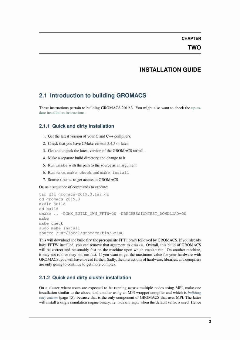
2.1 Introduction to building GROMACS
These instructions pertain to building GROMACS 2019.3. You might also want to check the up-to-date installation instructions.
2.1.1 Quick and dirty installation
1. Get the latest version of your C and C++ compilers.
2. Check that you have CMake version 3.4.3 or later.
3. Get and unpack the latest version of the GROMACS tarball.
4. Make a separate build directory and change to it.
5. Run cmake with the path to the source as an argument
6. Run make, make check, and make install
7. Source GMXRC to get access to GROMACS
Or, as a sequence of commands to execute:
tar xfz gromacs-2019.3.tar.gzcd gromacs-2019.3mkdir buildcd buildcmake .. -DGMX_BUILD_OWN_FFTW=ON -DREGRESSIONTEST_DOWNLOAD=ONmakemake checksudo make installsource /usr/local/gromacs/bin/GMXRC
This will download and build first the prerequisite FFT library followed by GROMACS. If you alreadyhave FFTW installed, you can remove that argument to cmake. Overall, this build of GROMACSwill be correct and reasonably fast on the machine upon which cmake ran. On another machine,it may not run, or may not run fast. If you want to get the maximum value for your hardware withGROMACS, you will have to read further. Sadly, the interactions of hardware, libraries, and compilersare only going to continue to get more complex.
2.1.2 Quick and dirty cluster installation
On a cluster where users are expected to be running across multiple nodes using MPI, make oneinstallation similar to the above, and another using an MPI wrapper compiler and which is buildingonly mdrun (page 15), because that is the only component of GROMACS that uses MPI. The latterwill install a single simulation engine binary, i.e. mdrun_mpi when the default suffix is used. Hence
3
GROMACS Documentation, Release 2019.3
it is safe and common practice to install this into the same location where the non-MPI build isinstalled.
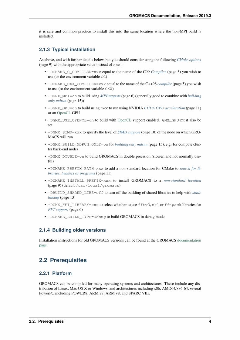
2.1.3 Typical installation
As above, and with further details below, but you should consider using the following CMake options(page 9) with the appropriate value instead of xxx :
• -DCMAKE_C_COMPILER=xxx equal to the name of the C99 Compiler (page 5) you wish touse (or the environment variable CC)
• -DCMAKE_CXX_COMPILER=xxx equal to the name of the C++98 compiler (page 5) you wishto use (or the environment variable CXX)
• -DGMX_MPI=on to build using MPI support (page 6) (generally good to combine with buildingonly mdrun (page 15))
• -DGMX_GPU=on to build using nvcc to run using NVIDIA CUDA GPU acceleration (page 11)or an OpenCL GPU
• -DGMX_USE_OPENCL=on to build with OpenCL support enabled. GMX_GPU must also beset.
• -DGMX_SIMD=xxx to specify the level of SIMD support (page 10) of the node on which GRO-MACS will run
• -DGMX_BUILD_MDRUN_ONLY=on for building only mdrun (page 15), e.g. for compute clus-ter back-end nodes
• -DGMX_DOUBLE=on to build GROMACS in double precision (slower, and not normally use-ful)
• -DCMAKE_PREFIX_PATH=xxx to add a non-standard location for CMake to search for li-braries, headers or programs (page 11)
• -DCMAKE_INSTALL_PREFIX=xxx to install GROMACS to a non-standard location(page 9) (default /usr/local/gromacs)
• -DBUILD_SHARED_LIBS=off to turn off the building of shared libraries to help with staticlinking (page 13)
• -DGMX_FFT_LIBRARY=xxx to select whether to use fftw3, mkl or fftpack libraries forFFT support (page 6)
• -DCMAKE_BUILD_TYPE=Debug to build GROMACS in debug mode
2.1.4 Building older versions
Installation instructions for old GROMACS versions can be found at the GROMACS documentationpage.
2.2 Prerequisites
2.2.1 Platform
GROMACS can be compiled for many operating systems and architectures. These include any dis-tribution of Linux, Mac OS X or Windows, and architectures including x86, AMD64/x86-64, severalPowerPC including POWER8, ARM v7, ARM v8, and SPARC VIII.
2.2. Prerequisites 4
GROMACS Documentation, Release 2019.3
2.2.2 Compiler
GROMACS can be compiled on any platform with ANSI C99 and C++11 compilers, and their re-spective standard C/C++ libraries. Good performance on an OS and architecture requires choosing agood compiler. We recommend gcc, because it is free, widely available and frequently provides thebest performance.
You should strive to use the most recent version of your compiler. Since we require full C++11support the minimum supported compiler versions are
• GNU (gcc) 4.8.1
• Intel (icc) 17.0.1
• LLVM (clang) 3.3
• Microsoft (MSVC) 2017 (C++14 is used)
Other compilers may work (Cray, Pathscale, older clang) but do not offer competitive performance.We recommend against PGI because the performance with C++ is very bad.
The xlc compiler is not supported and version 16.1 does not compile on POWER architectures forGROMACS-2019.3. We recommend to use the gcc compiler instead, as it is being extensively tested.
You may also need the most recent version of other compiler toolchain components beside the com-piler itself (e.g. assembler or linker); these are often shipped by your OS distribution’s binutils pack-age.
C++11 support requires adequate support in both the compiler and the C++ library. The gcc andMSVC compilers include their own standard libraries and require no further configuration. For con-figuration of other compilers, read on.
On Linux, both the Intel and clang compiler use the libstdc++ which comes with gcc as the defaultC++ library. For GROMACS, we require the compiler to support libstc++ version 4.8.1 or higher. Toselect a particular libstdc++ library, use:
• For Intel: -DGMX_STDLIB_CXX_FLAGS=-gcc-name=/path/to/gcc/binary ormake sure that the correct gcc version is first in path (e.g. by loading the gcc module). It canalso be useful to add -DCMAKE_CXX_LINK_FLAGS="-Wl,-rpath,/path/to/gcc/lib64 -L/path/to/gcc/lib64" to ensure linking works correctly.
• For clang: -DCMAKE_CXX_FLAGS=--gcc-toolchain=/path/to/gcc/folder.This folder should contain include/c++.
On Windows with the Intel compiler, the MSVC standard library is used, and at least MSVC 2017 isrequired. Load the enviroment variables with vcvarsall.bat.
To build with any compiler and clang’s libcxx standard library, use -DGMX_STDLIB_CXX_-FLAGS=-stdlib=libc++ -DGMX_STDLIB_LIBRARIES='-lc++abi -lc++'.
If you are running on Mac OS X, the best option is the Intel compiler. Both clang and gcc will work,but they produce lower performance and each have some shortcomings. clang 3.8 now offers supportfor OpenMP, and so may provide decent performance.
For all non-x86 platforms, your best option is typically to use gcc or the vendor’s default or recom-mended compiler, and check for specialized information below.
For updated versions of gcc to add to your Linux OS, see
• Ubuntu: Ubuntu toolchain ppa page
• RHEL/CentOS: EPEL page or the RedHat Developer Toolset
2.2.3 Compiling with parallelization options
For maximum performance you will need to examine how you will use GROMACS and what hard-ware you plan to run on. Often OpenMP parallelism is an advantage for GROMACS, but support for
2.2. Prerequisites 5
GROMACS Documentation, Release 2019.3
this is generally built into your compiler and detected automatically.
GPU support
GROMACS has excellent support for NVIDIA GPUs supported via CUDA. On Linux, NVIDIACUDA toolkit with minimum version 7.0 is required, and the latest version is strongly encouraged.Using Microsoft MSVC compiler requires version 9.0. NVIDIA GPUs with at least NVIDIA computecapability 3.0 are required. You are strongly recommended to get the latest CUDA version and driverthat supports your hardware, but beware of possible performance regressions in newer CUDA versionson older hardware. While some CUDA compilers (nvcc) might not officially support recent versionsof gcc as the back-end compiler, we still recommend that you at least use a gcc version recent enoughto get the best SIMD support for your CPU, since GROMACS always runs some code on the CPU.It is most reliable to use the same C++ compiler version for GROMACS code as used as the hostcompiler for nvcc.
To make it possible to use other accelerators, GROMACS also includes OpenCL support. The min-imum OpenCL version required is 1.2 and only 64-bit implementations are supported. The currentOpenCL implementation is recommended for use with GCN-based AMD GPUs, and on Linux we rec-ommend the ROCm runtime. Intel integrated GPUs are supported with the Neo drivers. OpenCL isalso supported with NVIDIA GPUs, but using the latest NVIDIA driver (which includes the NVIDIAOpenCL runtime) is recommended. Also note that there are performance limitations (inherent to theNVIDIA OpenCL runtime). It is not possible to configure both CUDA and OpenCL support in thesame build of GROMACS, nor to support both Intel and other vendors’ GPUs with OpenCL. A 64-bitimplementation of OpenCL is required and therefore OpenCL is only supported on 64-bit platforms.
MPI support
GROMACS can run in parallel on multiple cores of a single workstation using its built-in thread-MPI.No user action is required in order to enable this.
If you wish to run in parallel on multiple machines across a network, you will need to have
• an MPI library installed that supports the MPI 1.3 standard, and
• wrapper compilers that will compile code using that library.
The GROMACS team recommends OpenMPI version 1.6 (or higher), MPICH version 1.4.1 (orhigher), or your hardware vendor’s MPI installation. The most recent version of either of these islikely to be the best. More specialized networks might depend on accelerations only available in thevendor’s library. LAM-MPI might work, but since it has been deprecated for years, it is not supported.
For example, depending on your actual MPI library, use cmake -DCMAKE_C_COMPILER=mpicc-DCMAKE_CXX_COMPILER=mpicxx -DGMX_MPI=on.
2.2.4 CMake
GROMACS builds with the CMake build system, requiring at least version 3.4.3. You can checkwhether CMake is installed, and what version it is, with cmake --version. If you need to installCMake, then first check whether your platform’s package management system provides a suitableversion, or visit the CMake installation page for pre-compiled binaries, source code and installationinstructions. The GROMACS team recommends you install the most recent version of CMake youcan.
2.2.5 Fast Fourier Transform library
Many simulations in GROMACS make extensive use of fast Fourier transforms, and a software libraryto perform these is always required. We recommend FFTW (version 3 or higher only) or Intel MKL.The choice of library can be set with cmake -DGMX_FFT_LIBRARY=<name>, where <name>
2.2. Prerequisites 6
GROMACS Documentation, Release 2019.3
is one of fftw3, mkl, or fftpack. FFTPACK is bundled with GROMACS as a fallback, andis acceptable if simulation performance is not a priority. When choosing MKL, GROMACS willalso use MKL for BLAS and LAPACK (see linear algebra libraries (page 14)). Generally, there is noadvantage in using MKL with GROMACS, and FFTW is often faster. With PME GPU offload supportusing CUDA, a GPU-based FFT library is required. The CUDA-based GPU FFT library cuFFT is partof the CUDA toolkit (required for all CUDA builds) and therefore no additional software componentis needed when building with CUDA GPU acceleration.
Using FFTW
FFTW is likely to be available for your platform via its package management system, but there canbe compatibility and significant performance issues associated with these packages. In particular,GROMACS simulations are normally run in “mixed” floating-point precision, which is suited forthe use of single precision in FFTW. The default FFTW package is normally in double precision,and good compiler options to use for FFTW when linked to GROMACS may not have been used.Accordingly, the GROMACS team recommends either
• that you permit the GROMACS installation to download and build FFTW from source automat-ically for you (use cmake -DGMX_BUILD_OWN_FFTW=ON), or
• that you build FFTW from the source code.
If you build FFTW from source yourself, get the most recent version and follow the FFTW in-stallation guide. Choose the precision for FFTW (i.e. single/float vs. double) to match whetheryou will later use mixed or double precision for GROMACS. There is no need to compile FFTWwith threading or MPI support, but it does no harm. On x86 hardware, compile with both--enable-sse2 and --enable-avx for FFTW-3.3.4 and earlier. From FFTW-3.3.5, you shouldalso add --enable-avx2 also. On Intel processors supporting 512-wide AVX, including KNL, add--enable-avx512 also. FFTW will create a fat library with codelets for all different instructionsets, and pick the fastest supported one at runtime. On ARM architectures with NEON SIMD sup-port and IBM Power8 and later, you definitely want version 3.3.5 or later, and to compile it with--enable-neon and --enable-vsx, respectively, for SIMD support. If you are using a Cray,there is a special modified (commercial) version of FFTs using the FFTW interface which can beslightly faster.
Using MKL
Use MKL bundled with Intel compilers by setting up the compiler environment, e.g., throughsource /path/to/compilervars.sh intel64 or similar before running CMake includ-ing setting -DGMX_FFT_LIBRARY=mkl.
If you need to customize this further, use
cmake -DGMX_FFT_LIBRARY=mkl \-DMKL_LIBRARIES="/full/path/to/libone.so;/full/path/to/libtwo.so" \-DMKL_INCLUDE_DIR="/full/path/to/mkl/include"
The full list and order(!) of libraries you require are found in Intel’s MKL documentation for yoursystem.
Using ARM Performance Libraries
The ARM Performance Libraries provides FFT transforms implementation for ARM architec-tures. Preliminary support is provided for ARMPL in GROMACS through its FFTW-compatibleAPI. Assuming that the ARM HPC toolchain environment including the ARMPL paths are setup (e.g. through loading the appropriate modules like module load Module-Prefix/arm-hpc-compiler-X.Y/armpl/X.Y) use the following cmake options:
2.2. Prerequisites 7
GROMACS Documentation, Release 2019.3
cmake -DGMX_FFT_LIBRARY=fftw3 \-DFFTWF_LIBRARY="${ARMPL_DIR}/lib/libarmpl_lp64.so" \-DFFTWF_INCLUDE_DIR=${ARMPL_DIR}/include
2.2.6 Other optional build components
• Run-time detection of hardware capabilities can be improved by linking with hwloc, which isautomatically enabled if detected.
• Hardware-optimized BLAS and LAPACK libraries are useful for a few of the GROMACS utili-ties focused on normal modes and matrix manipulation, but they do not provide any benefits fornormal simulations. Configuring these is discussed at linear algebra libraries (page 14).
• The built-in GROMACS trajectory viewer gmx view requires X11 and Motif/Lesstif librariesand header files. You may prefer to use third-party software for visualization, such as VMD orPyMol.
• An external TNG library for trajectory-file handling can be used by setting -DGMX_-EXTERNAL_TNG=yes, but TNG 1.7.10 is bundled in the GROMACS source already.
• The lmfit library for Levenberg-Marquardt curve fitting is used in GROMACS. Only lmfit 7.0is supported. A reduced version of that library is bundled in the GROMACS distribution,and the default build uses it. That default may be explicitly enabled with -DGMX_USE_-LMFIT=internal. To use an external lmfit library, set -DGMX_USE_LMFIT=external,and adjust CMAKE_PREFIX_PATH as needed. lmfit support can be disabled with -DGMX_-USE_LMFIT=none.
• zlib is used by TNG for compressing some kinds of trajectory data
• Building the GROMACS documentation is optional, and requires ImageMagick, pdflatex, bib-tex, doxygen, python 2.7, sphinx 1.6.1, and pygments.
• The GROMACS utility programs often write data files in formats suitable for the Grace plottingtool, but it is straightforward to use these files in other plotting programs, too.
2.3 Doing a build of GROMACS
This section will cover a general build of GROMACS with CMake (page 6), but it is not an exhaustivediscussion of how to use CMake. There are many resources available on the web, which we suggestyou search for when you encounter problems not covered here. The material below applies specifi-cally to builds on Unix-like systems, including Linux, and Mac OS X. For other platforms, see thespecialist instructions below.
2.3.1 Configuring with CMake
CMake will run many tests on your system and do its best to work out how to build GROMACS foryou. If your build machine is the same as your target machine, then you can be sure that the defaultsand detection will be pretty good. However, if you want to control aspects of the build, or you arecompiling on a cluster head node for back-end nodes with a different architecture, there are a fewthings you should consider specifying.
The best way to use CMake to configure GROMACS is to do an “out-of-source” build, by makinganother directory from which you will run CMake. This can be outside the source directory, or asubdirectory of it. It also means you can never corrupt your source code by trying to build it! So,the only required argument on the CMake command line is the name of the directory containing theCMakeLists.txt file of the code you want to build. For example, download the source tarball anduse
2.3. Doing a build of GROMACS 8
GROMACS Documentation, Release 2019.3
tar xfz gromacs-2019.3.tgzcd gromacs-2019.3mkdir build-gromacscd build-gromacscmake ..
You will see cmake report a sequence of results of tests and detections done by the GROMACS buildsystem. These are written to the cmake cache, kept in CMakeCache.txt. You can edit this fileby hand, but this is not recommended because you could make a mistake. You should not attempt tomove or copy this file to do another build, because file paths are hard-coded within it. If you messthings up, just delete this file and start again with cmake.
If there is a serious problem detected at this stage, then you will see a fatal error and some suggestionsfor how to overcome it. If you are not sure how to deal with that, please start by searching on the web(most computer problems already have known solutions!) and then consult the gmx-users mailinglist. There are also informational warnings that you might like to take on board or not. Piping theoutput of cmake through less or tee can be useful, too.
Once cmake returns, you can see all the settings that were chosen and information about them byusing e.g. the curses interface
ccmake ..
You can actually use ccmake (available on most Unix platforms) directly in the first step, but thenmost of the status messages will merely blink in the lower part of the terminal rather than be writtento standard output. Most platforms including Linux, Windows, and Mac OS X even have nativegraphical user interfaces for cmake, and it can create project files for almost any build environmentyou want (including Visual Studio or Xcode). Check out running CMake for general advice on whatyou are seeing and how to navigate and change things. The settings you might normally want tochange are already presented. You may make changes, then re-configure (using c), so that it getsa chance to make changes that depend on yours and perform more checking. It may take severalconfiguration passes to reach the desired configuration, in particular if you need to resolve errors.
When you have reached the desired configuration with ccmake, the build system can be generatedby pressing g. This requires that the previous configuration pass did not reveal any additional settings(if it did, you need to configure once more with c). With cmake, the build system is generated aftereach pass that does not produce errors.
You cannot attempt to change compilers after the initial run of cmake. If you need to change, cleanup, and start again.
Where to install GROMACS
GROMACS is installed in the directory to which CMAKE_INSTALL_PREFIX points. It may notbe the source directory or the build directory. You require write permissions to this directory. Thus,without super-user privileges, CMAKE_INSTALL_PREFIX will have to be within your home direc-tory. Even if you do have super-user privileges, you should use them only for the installation phase,and never for configuring, building, or running GROMACS!
Using CMake command-line options
Once you become comfortable with setting and changing options, you may know in advance howyou will configure GROMACS. If so, you can speed things up by invoking cmake and passing thevarious options at once on the command line. This can be done by setting cache variable at thecmake invocation using -DOPTION=VALUE. Note that some environment variables are also takeninto account, in particular variables like CC and CXX.
For example, the following command line
2.3. Doing a build of GROMACS 9
GROMACS Documentation, Release 2019.3
cmake .. -DGMX_GPU=ON -DGMX_MPI=ON -DCMAKE_INSTALL_PREFIX=/home/marydoe/→˓programs
can be used to build with CUDA GPUs, MPI and install in a custom location. You can even save thatin a shell script to make it even easier next time. You can also do this kind of thing with ccmake, butyou should avoid this, because the options set with -D will not be able to be changed interactively inthat run of ccmake.
SIMD support
GROMACS has extensive support for detecting and using the SIMD capabilities of many modernHPC CPU architectures. If you are building GROMACS on the same hardware you will run it on,then you don’t need to read more about this, unless you are getting configuration warnings you do notunderstand. By default, the GROMACS build system will detect the SIMD instruction set supportedby the CPU architecture (on which the configuring is done), and thus pick the best available SIMDparallelization supported by GROMACS. The build system will also check that the compiler andlinker used also support the selected SIMD instruction set and issue a fatal error if they do not.
Valid values are listed below, and the applicable value with the largest number in the list is generallythe one you should choose. In most cases, choosing an inappropriate higher number will lead tocompiling a binary that will not run. However, on a number of processor architectures choosing thehighest supported value can lead to performance loss, e.g. on Intel Skylake-X/SP and AMD Zen.
1. None For use only on an architecture either lacking SIMD, or to which GROMACS has not yetbeen ported and none of the options below are applicable.
2. SSE2 This SIMD instruction set was introduced in Intel processors in 2001, and AMD in 2003.Essentially all x86 machines in existence have this, so it might be a good choice if you need tosupport dinosaur x86 computers too.
3. SSE4.1 Present in all Intel core processors since 2007, but notably not in AMD Magny-Cours.Still, almost all recent processors support this, so this can also be considered a good baseline ifyou are content with slow simulations and prefer portability between reasonably modern pro-cessors.
4. AVX_128_FMA AMD Bulldozer, Piledriver (and later Family 15h) processors have this.
5. AVX_256 Intel processors since Sandy Bridge (2011). While this code will work on the AMDBulldozer and Piledriver processors, it is significantly less efficient than the AVX_128_FMAchoice above - do not be fooled to assume that 256 is better than 128 in this case.
6. AVX2_128 AMD Zen microarchitecture processors (2017); it will enable AVX2 with 3-wayfused multiply-add instructions. While the Zen microarchitecture does support 256-bit AVX2instructions, hence AVX2_256 is also supported, 128-bit will generally be faster, in particularwhen the non-bonded tasks run on the CPU – hence the default AVX2_128. With GPU offloadhowever AVX2_256 can be faster on Zen processors.
7. AVX2_256 Present on Intel Haswell (and later) processors (2013), and it will also enable Intel3-way fused multiply-add instructions.
8. AVX_512 Skylake-X desktop and Skylake-SP Xeon processors (2017); it will generally befastest on the higher-end desktop and server processors with two 512-bit fused multiply-addunits (e.g. Core i9 and Xeon Gold). However, certain desktop and server models (e.g. XeonBronze and Silver) come with only one AVX512 FMA unit and therefore on these processorsAVX2_256 is faster (compile- and runtime checks try to inform about such cases). Additionally,with GPU accelerated runs AVX2_256 can also be faster on high-end Skylake CPUs with both512-bit FMA units enabled.
9. AVX_512_KNL Knights Landing Xeon Phi processors
10. Sparc64_HPC_ACE Fujitsu machines like the K computer have this.
11. IBM_VMX Power6 and similar Altivec processors have this.
2.3. Doing a build of GROMACS 10
GROMACS Documentation, Release 2019.3
12. IBM_VSX Power7, Power8, Power9 and later have this.
13. ARM_NEON 32-bit ARMv7 with NEON support.
14. ARM_NEON_ASIMD 64-bit ARMv8 and later.
The CMake configure system will check that the compiler you have chosen can target the architectureyou have chosen. mdrun will check further at runtime, so if in doubt, choose the lowest number youthink might work, and see what mdrun says. The configure system also works around many knownissues in many versions of common HPC compilers.
A further GMX_SIMD=Reference option exists, which is a special SIMD-like implementationwritten in plain C that developers can use when developing support in GROMACS for new SIMDarchitectures. It is not designed for use in production simulations, but if you are using an architecturewith SIMD support to which GROMACS has not yet been ported, you may wish to try this optioninstead of the default GMX_SIMD=None, as it can often out-perform this when the auto-vectorizationin your compiler does a good job. And post on the GROMACS mailing lists, because GROMACScan probably be ported for new SIMD architectures in a few days.
CMake advanced options
The options that are displayed in the default view of ccmake are ones that we think a reasonablenumber of users might want to consider changing. There are a lot more options available, whichyou can see by toggling the advanced mode in ccmake on and off with t. Even there, most of thevariables that you might want to change have a CMAKE_ or GMX_ prefix. There are also some optionsthat will be visible or not according to whether their preconditions are satisfied.
Helping CMake find the right libraries, headers, or programs
If libraries are installed in non-default locations their location can be specified using the followingvariables:
• CMAKE_INCLUDE_PATH for header files
• CMAKE_LIBRARY_PATH for libraries
• CMAKE_PREFIX_PATH for header, libraries and binaries (e.g. /usr/local).
The respective include, lib, or bin is appended to the path. For each of these variables, a list ofpaths can be specified (on Unix, separated with “:”). These can be set as enviroment variables like:
CMAKE_PREFIX_PATH=/opt/fftw:/opt/cuda cmake ..
(assuming bash shell). Alternatively, these variables are also cmake options, so they can be set like-DCMAKE_PREFIX_PATH=/opt/fftw:/opt/cuda.
The CC and CXX environment variables are also useful for indicating to cmake which compilers touse. Similarly, CFLAGS/CXXFLAGS can be used to pass compiler options, but note that these willbe appended to those set by GROMACS for your build platform and build type. You can customizesome of this with advanced CMake options such as CMAKE_C_FLAGS and its relatives.
See also the page on CMake environment variables.
CUDA GPU acceleration
If you have the CUDA Toolkit installed, you can use cmake with:
cmake .. -DGMX_GPU=ON -DCUDA_TOOLKIT_ROOT_DIR=/usr/local/cuda
(or whichever path has your installation). In some cases, you might need to specify manually whichof your C++ compilers should be used, e.g. with the advanced option CUDA_HOST_COMPILER.
2.3. Doing a build of GROMACS 11
GROMACS Documentation, Release 2019.3
By default, code will be generated for the most common CUDA architectures. However, to reducebuild time and binary size we do not generate code for every single possible architecture, which inrare cases (say, Tegra systems) can result in the default build not being able to use some GPUs. Ifthis happens, or if you want to remove some architectures to reduce binary size and build time, youcan alter the target CUDA architectures. This can be done either with the GMX_CUDA_TARGET_SMor GMX_CUDA_TARGET_COMPUTE CMake variables, which take a semicolon delimited string withthe two digit suffixes of CUDA (virtual) architectures names, for instance “35;50;51;52;53;60”. Fordetails, see the “Options for steering GPU code generation” section of the nvcc man / help or Chapter6. of the nvcc manual.
The GPU acceleration has been tested on AMD64/x86-64 platforms with Linux, Mac OS X andWindows operating systems, but Linux is the best-tested and supported of these. Linux running onPOWER 8, ARM v7 and v8 CPUs also works well.
Experimental support is available for compiling CUDA code, both for host and device, using clang(version 3.9 or later). A CUDA toolkit (>= v7.0) is still required but it is used only for GPU devicecode generation and to link against the CUDA runtime library. The clang CUDA support simplifiescompilation and provides benefits for development (e.g. allows the use code sanitizers in CUDAhost-code). Additionally, using clang for both CPU and GPU compilation can be beneficial to avoidcompatibility issues between the GNU toolchain and the CUDA toolkit. clang for CUDA can be trig-gered using the GMX_CLANG_CUDA=ON CMake option. Target architectures can be selected withGMX_CUDA_TARGET_SM, virtual architecture code is always embedded for all requested architec-tures (hence GMX_CUDA_TARGET_COMPUTE is ignored). Note that this is mainly a developer-oriented feature and it is not recommended for production use as the performance can be significantlylower than that of code compiled with nvcc (and it has also received less testing). However, notethat with clang 5.0 the performance gap is significantly narrowed (at the time of writing, about 20%slower GPU kernels), so this version could be considered in non performance-critical use-cases.
OpenCL GPU acceleration
The primary targets of the GROMACS OpenCL support is accelerating simulations on AMD andIntel hardware. For AMD, we target both discrete GPUs and APUs (integrated CPU+GPU chips),and for Intel we target the integrated GPUs found on modern workstation and mobile hardware. TheGROMACS OpenCL on NVIDIA GPUs works, but performance and other limitations make it lesspractical (for details see the user guide).
To build GROMACS with OpenCL support enabled, two components are required: the OpenCL head-ers and the wrapper library that acts as a client driver loader (so-called ICD loader). The additional,runtime-only dependency is the vendor-specific GPU driver for the device targeted. This also con-tains the OpenCL compiler. As the GPU compute kernels are compiled on-demand at run time, thisvendor-specific compiler and driver is not needed for building GROMACS. The former, compile-timedependencies are standard components, hence stock versions can be obtained from most Linux dis-tribution repositories (e.g. opencl-headers and ocl-icd-libopencl1 on Debian/Ubuntu).Only the compatibility with the required OpenCL version 1.2 needs to be ensured. Alternatively, theheaders and library can also be obtained from vendor SDKs (e.g. from AMD), which must be installedin a path found in CMAKE_PREFIX_PATH (or via the environment variables AMDAPPSDKROOT orCUDA_PATH).
To trigger an OpenCL build the following CMake flags must be set
cmake .. -DGMX_GPU=ON -DGMX_USE_OPENCL=ON
To build with support for Intel integrated GPUs, it is required to add -DGMX_OPENCL_NB_-CLUSTER_SIZE=4 to the cmake command line, so that the GPU kernels match the characteristicsof the hardware. The Neo driver is recommended.
On Mac OS, an AMD GPU can be used only with OS version 10.10.4 and higher; earlier OS versionsare known to run incorrectly.
By default, any clFFT library on the system will be used with GROMACS, but if none is found thenthe code will fall back on a version bundled with GROMACS. To require GROMACS to link with an
2.3. Doing a build of GROMACS 12
GROMACS Documentation, Release 2019.3
external library, use
cmake .. -DGMX_GPU=ON -DGMX_USE_OPENCL=ON -DclFFT_ROOT_DIR=/path/to/your/→˓clFFT -DGMX_EXTERNAL_CLFFT=TRUE
Static linking
Dynamic linking of the GROMACS executables will lead to a smaller disk footprint when installed,and so is the default on platforms where we believe it has been tested repeatedly and found to work.In general, this includes Linux, Windows, Mac OS X and BSD systems. Static binaries take morespace, but on some hardware and/or under some conditions they are necessary, most commonly whenyou are running a parallel simulation using MPI libraries (e.g. Cray).
• To link GROMACS binaries statically against the internal GROMACS libraries, set-DBUILD_SHARED_LIBS=OFF.
• To link statically against external (non-system) libraries as well, set -DGMX_PREFER_-STATIC_LIBS=ON. Note, that in general cmake picks up whatever is available, so thisoption only instructs cmake to prefer static libraries when both static and shared are avail-able. If no static version of an external library is available, even when the aforementionedoption is ON, the shared library will be used. Also note that the resulting binaries will stillbe dynamically linked against system libraries on platforms where that is the default. To usestatic system libraries, additional compiler/linker flags are necessary, e.g. -static-libgcc-static-libstdc++.
• To attempt to link a fully static binary set -DGMX_BUILD_SHARED_EXE=OFF. This willprevent CMake from explicitly setting any dynamic linking flags. This option also sets-DBUILD_SHARED_LIBS=OFF and -DGMX_PREFER_STATIC_LIBS=ON by default, butthe above caveats apply. For compilers which don’t default to static linking, the required flagshave to be specified. On Linux, this is usually CFLAGS=-static CXXFLAGS=-static.
gmxapi external API
For dynamic linking builds and on non-Windows platforms, an extra library and headersare installed by setting -DGMXAPI=ON (default). Build targets gmxapi-cppdocs andgmxapi-cppdocs-dev produce documentation in docs/api-user and docs/api-dev, re-spectively. For more project information and use cases, refer to the tracked Issue 2585, associatedGitHub gmxapi projects, or DOI 10.1093/bioinformatics/bty484.
gmxapi is not yet tested on Windows or with static linking, but these use cases are targeted for futureversions.
Portability aspects
A GROMACS build will normally not be portable, not even across hardware with the same baseinstruction set, like x86. Non-portable hardware-specific optimizations are selected at configure-time, such as the SIMD instruction set used in the compute kernels. This selection will be done bythe build system based on the capabilities of the build host machine or otherwise specified to cmakeduring configuration.
Often it is possible to ensure portability by choosing the least common denominator of SIMD support,e.g. SSE2 for x86, and ensuring the you use cmake -DGMX_USE_RDTSCP=off if any of the targetCPU architectures does not support the RDTSCP instruction. However, we discourage attempts to usea single GROMACS installation when the execution environment is heterogeneous, such as a mixof AVX and earlier hardware, because this will lead to programs (especially mdrun) that run slowlyon the new hardware. Building two full installations and locally managing how to call the correctone (e.g. using a module system) is the recommended approach. Alternatively, as at the momentthe GROMACS tools do not make strong use of SIMD acceleration, it can be convenient to create
2.3. Doing a build of GROMACS 13
GROMACS Documentation, Release 2019.3
an installation with tools portable across different x86 machines, but with separate mdrun binariesfor each architecture. To achieve this, one can first build a full installation with the least-common-denominator SIMD instruction set, e.g. -DGMX_SIMD=SSE2, then build separate mdrun binariesfor each architecture present in the heterogeneous environment. By using custom binary and librarysuffixes for the mdrun-only builds, these can be installed to the same location as the “generic” toolsinstallation. Building just the mdrun binary (page 15) is possible by setting the -DGMX_BUILD_-MDRUN_ONLY=ON option.
Linear algebra libraries
As mentioned above, sometimes vendor BLAS and LAPACK libraries can provide performance en-hancements for GROMACS when doing normal-mode analysis or covariance analysis. For simplic-ity, the text below will refer only to BLAS, but the same options are available for LAPACK. Bydefault, CMake will search for BLAS, use it if it is found, and otherwise fall back on a version ofBLAS internal to GROMACS. The cmake option -DGMX_EXTERNAL_BLAS=on will be set ac-cordingly. The internal versions are fine for normal use. If you need to specify a non-standard pathto search, use -DCMAKE_PREFIX_PATH=/path/to/search. If you need to specify a librarywith a non-standard name (e.g. ESSL on Power machines or ARMPL on ARM machines), then set-DGMX_BLAS_USER=/path/to/reach/lib/libwhatever.a.
If you are using Intel MKL for FFT, then the BLAS and LAPACK it provides are used automatically.This could be over-ridden with GMX_BLAS_USER, etc.
On Apple platforms where the Accelerate Framework is available, these will be automatically usedfor BLAS and LAPACK. This could be over-ridden with GMX_BLAS_USER, etc.
Building with MiMiC QM/MM support
MiMiC QM/MM interface integration will require linking against MiMiC communication library,that establishes the communication channel between GROMACS and CPMD. The MiMiC Commu-nication library can be downloaded here. Compile and install it. Check that the installation folderof the MiMiC library is added to CMAKE_PREFIX_PATH if it is installed in non-standard location.Building QM/MM-capable version requires double-precision version of GROMACS compiled withMPI support:
• -DGMX_DOUBLE=ON -DGMX_MPI -DGMX_MIMIC=ON
Changing the names of GROMACS binaries and libraries
It is sometimes convenient to have different versions of the same GROMACS programs installed.The most common use cases have been single and double precision, and with and without MPI. Thismechanism can also be used to install side-by-side multiple versions of mdrun optimized for differentCPU architectures, as mentioned previously.
By default, GROMACS will suffix programs and libraries for such builds with _d for double preci-sion and/or _mpi for MPI (and nothing otherwise). This can be controlled manually with GMX_-DEFAULT_SUFFIX (ON/OFF), GMX_BINARY_SUFFIX (takes a string) and GMX_LIBS_-SUFFIX (also takes a string). For instance, to set a custom suffix for programs and libraries, onemight specify:
cmake .. -DGMX_DEFAULT_SUFFIX=OFF -DGMX_BINARY_SUFFIX=_mod -DGMX_LIBS_→˓SUFFIX=_mod
Thus the names of all programs and libraries will be appended with _mod.
2.3. Doing a build of GROMACS 14
GROMACS Documentation, Release 2019.3
Changing installation tree structure
By default, a few different directories under CMAKE_INSTALL_PREFIX are used when when GRO-MACS is installed. Some of these can be changed, which is mainly useful for packaging GROMACSfor various distributions. The directories are listed below, with additional notes about some of them.Unless otherwise noted, the directories can be renamed by editing the installation paths in the mainCMakeLists.txt.
bin/ The standard location for executables and some scripts. Some of the scripts hardcode theabsolute installation prefix, which needs to be changed if the scripts are relocated. The name ofthe directory can be changed using CMAKE_INSTALL_BINDIR CMake variable.
include/gromacs/ The standard location for installed headers.
lib/ The standard location for libraries. The default depends on the system, and is determined byCMake. The name of the directory can be changed using CMAKE_INSTALL_LIBDIR CMakevariable.
lib/pkgconfig/ Information about the installed libgromacs library for pkg-config is in-stalled here. The lib/ part adapts to the installation location of the libraries. The installed filescontain the installation prefix as absolute paths.
share/cmake/ CMake package configuration files are installed here.
share/gromacs/ Various data files and some documentation go here. The first part can bechanged using CMAKE_INSTALL_DATADIR, and the second by using GMX_INSTALL_-DATASUBDIR Using these CMake variables is the preferred way of changing the installationpath for share/gromacs/top/, since the path to this directory is built into libgromacsas well as some scripts, both as a relative and as an absolute path (the latter as a fallback ifeverything else fails).
share/man/ Installed man pages go here.
2.3.2 Compiling and linking
Once you have configured with cmake, you can build GROMACS with make. It is expected that thiswill always complete successfully, and give few or no warnings. The CMake-time tests GROMACSmakes on the settings you choose are pretty extensive, but there are probably a few cases we have notthought of yet. Search the web first for solutions to problems, but if you need help, ask on gmx-users,being sure to provide as much information as possible about what you did, the system you are buildingon, and what went wrong. This may mean scrolling back a long way through the output of make tofind the first error message!
If you have a multi-core or multi-CPU machine with N processors, then using
make -j N
will generally speed things up by quite a bit. Other build generator systems supported by cmake (e.g.ninja) also work well.
Building only mdrun
This is now supported with the cmake option -DGMX_BUILD_MDRUN_ONLY=ON, which will builda different version of libgromacs and the mdrun program. Naturally, now make install in-stalls only those products. By default, mdrun-only builds will default to static linking against GRO-MACS libraries, because this is generally a good idea for the targets for which an mdrun-only buildis desirable.
2.3. Doing a build of GROMACS 15
GROMACS Documentation, Release 2019.3
2.3.3 Installing GROMACS
Finally, make install will install GROMACS in the directory given in CMAKE_INSTALL_-PREFIX. If this is a system directory, then you will need permission to write there, and you shoulduse super-user privileges only for make install and not the whole procedure.
2.3.4 Getting access to GROMACS after installation
GROMACS installs the script GMXRC in the bin subdirectory of the installation directory (e.g. /usr/local/gromacs/bin/GMXRC), which you should source from your shell:
source /your/installation/prefix/here/bin/GMXRC
It will detect what kind of shell you are running and set up your environment for using GROMACS.You may wish to arrange for your login scripts to do this automatically; please search the web forinstructions on how to do this for your shell.
Many of the GROMACS programs rely on data installed in the share/gromacs subdirectory of theinstallation directory. By default, the programs will use the environment variables set in the GMXRCscript, and if this is not available they will try to guess the path based on their own location. Thisusually works well unless you change the names of directories inside the install tree. If you still needto do that, you might want to recompile with the new install location properly set, or edit the GMXRCscript.
2.3.5 Testing GROMACS for correctness
Since 2011, the GROMACS development uses an automated system where every new code changeis subject to regression testing on a number of platforms and software combinations. While thisimproves reliability quite a lot, not everything is tested, and since we increasingly rely on cuttingedge compiler features there is non-negligible risk that the default compiler on your system couldhave bugs. We have tried our best to test and refuse to use known bad versions in cmake, but westrongly recommend that you run through the tests yourself. It only takes a few minutes, after whichyou can trust your build.
The simplest way to run the checks is to build GROMACS with -DREGRESSIONTEST_DOWNLOAD,and run make check. GROMACS will automatically download and run the tests for you. Alter-natively, you can download and unpack the GROMACS regression test suite http://gerrit.gromacs.org/download/regressiontests-2019.3.tar.gz tarball yourself and use the advanced cmake optionREGRESSIONTEST_PATH to specify the path to the unpacked tarball, which will then be usedfor testing. If the above does not work, then please read on.
The regression tests are also available from the download section. Once you have downloaded them,unpack the tarball, source GMXRC as described above, and run ./gmxtest.pl all inside theregression tests folder. You can find more options (e.g. adding double when using double precision,or -only expanded to run just the tests whose names match “expanded”) if you just execute thescript without options.
Hopefully, you will get a report that all tests have passed. If there are individual failed tests it couldbe a sign of a compiler bug, or that a tolerance is just a tiny bit too tight. Check the output files thescript directs you too, and try a different or newer compiler if the errors appear to be real. If youcannot get it to pass the regression tests, you might try dropping a line to the gmx-users mailing list,but then you should include a detailed description of your hardware, and the output of gmx mdrun-version (which contains valuable diagnostic information in the header).
A build with -DGMX_BUILD_MDRUN_ONLY cannot be tested with make check from the buildtree, because most of the tests require a full build to run things like grompp. To test such an mdrunfully requires installing it to the same location as a normal build of GROMACS, downloading theregression tests tarball manually as described above, sourcing the correct GMXRC and running the perlscript manually. For example, from your GROMACS source directory:
2.3. Doing a build of GROMACS 16
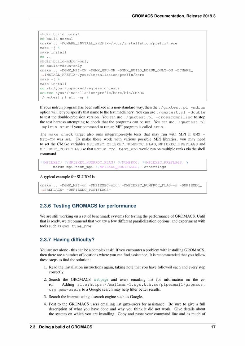
GROMACS Documentation, Release 2019.3
mkdir build-normalcd build-normalcmake .. -DCMAKE_INSTALL_PREFIX=/your/installation/prefix/heremake -j 4make installcd ..mkdir build-mdrun-onlycd build-mdrun-onlycmake .. -DGMX_MPI=ON -DGMX_GPU=ON -DGMX_BUILD_MDRUN_ONLY=ON -DCMAKE_→˓INSTALL_PREFIX=/your/installation/prefix/heremake -j 4make installcd /to/your/unpacked/regressiontestssource /your/installation/prefix/here/bin/GMXRC./gmxtest.pl all -np 2
If your mdrun program has been suffixed in a non-standard way, then the ./gmxtest.pl -mdrunoption will let you specify that name to the test machinery. You can use ./gmxtest.pl -doubleto test the double-precision version. You can use ./gmxtest.pl -crosscompiling to stopthe test harness attempting to check that the programs can be run. You can use ./gmxtest.pl-mpirun srun if your command to run an MPI program is called srun.
The make check target also runs integration-style tests that may run with MPI if GMX_-MPI=ON was set. To make these work with various possible MPI libraries, you may needto set the CMake variables MPIEXEC, MPIEXEC_NUMPROC_FLAG, MPIEXEC_PREFLAGS andMPIEXEC_POSTFLAGS so that mdrun-mpi-test_mpiwould run on multiple ranks via the shellcommand
${MPIEXEC} ${MPIEXEC_NUMPROC_FLAG} ${NUMPROC} ${MPIEXEC_PREFLAGS} \mdrun-mpi-test_mpi ${MPIEXEC_POSTFLAGS} -otherflags
A typical example for SLURM is
cmake .. -DGMX_MPI=on -DMPIEXEC=srun -DMPIEXEC_NUMPROC_FLAG=-n -DMPIEXEC_→˓PREFLAGS= -DMPIEXEC_POSTFLAGS=
2.3.6 Testing GROMACS for performance
We are still working on a set of benchmark systems for testing the performance of GROMACS. Untilthat is ready, we recommend that you try a few different parallelization options, and experiment withtools such as gmx tune_pme.
2.3.7 Having difficulty?
You are not alone - this can be a complex task! If you encounter a problem with installing GROMACS,then there are a number of locations where you can find assistance. It is recommended that you followthese steps to find the solution:
1. Read the installation instructions again, taking note that you have followed each and every stepcorrectly.
2. Search the GROMACS webpage and users emailing list for information on the er-ror. Adding site:https://mailman-1.sys.kth.se/pipermail/gromacs.org_gmx-users to a Google search may help filter better results.
3. Search the internet using a search engine such as Google.
4. Post to the GROMACS users emailing list gmx-users for assistance. Be sure to give a fulldescription of what you have done and why you think it did not work. Give details aboutthe system on which you are installing. Copy and paste your command line and as much of
2.3. Doing a build of GROMACS 17
GROMACS Documentation, Release 2019.3
the output as you think might be relevant - certainly from the first indication of a problem.In particular, please try to include at least the header from the mdrun logfile, and preferablythe entire file. People who might volunteer to help you do not have time to ask you interactivedetailed follow-up questions, so you will get an answer faster if you provide as much informationas you think could possibly help. High quality bug reports tend to receive rapid high qualityanswers.
2.4 Special instructions for some platforms
2.4.1 Building on Windows
Building on Windows using native compilers is rather similar to building on Unix, so please start byreading the above. Then, download and unpack the GROMACS source archive. Make a folder inwhich to do the out-of-source build of GROMACS. For example, make it within the folder unpackedfrom the source archive, and call it build-gromacs.
For CMake, you can either use the graphical user interface provided on Windows, or you can use acommand line shell with instructions similar to the UNIX ones above. If you open a shell from withinyour IDE (e.g. Microsoft Visual Studio), it will configure the environment for you, but you mightneed to tweak this in order to get either a 32-bit or 64-bit build environment. The latter provides thefastest executable. If you use a normal Windows command shell, then you will need to either set upthe environment to find your compilers and libraries yourself, or run the vcvarsall.bat batchscript provided by MSVC (just like sourcing a bash script under Unix).
With the graphical user interface, you will be asked about what compilers to use at the initial config-uration stage, and if you use the command line they can be set in a similar way as under UNIX.
Unfortunately -DGMX_BUILD_OWN_FFTW=ON (see Using FFTW (page 7)) does not work on Win-dows, because there is no supported way to build FFTW on Windows. You can either build FFTWsome other way (e.g. MinGW), or use the built-in fftpack (which may be slow), or using MKL(page 7).
For the build, you can either load the generated solutions file into e.g. Visual Studio, or use thecommand line with cmake --build so the right tools get used.
2.4.2 Building on Cray
GROMACS builds mostly out of the box on modern Cray machines, but you may need to specify theuse of static binaries with -DGMX_BUILD_SHARED_EXE=off, and you may need to set the F77environmental variable to ftn when compiling FFTW. The ARM ThunderX2 Cray XC50 machinesdiffer only in that the recommended compiler is the ARM HPC Compiler (armclang).
2.4.3 Building on Solaris
The built-in GROMACS processor detection does not work on Solaris, so it is strongly recommendedthat you build GROMACS with -DGMX_HWLOC=on and ensure that the CMAKE_PREFIX_PATHincludes the path where the hwloc headers and libraries can be found. At least version 1.11.8 of hwlocis recommended.
Oracle Developer Studio is not a currently supported compiler (and does not currently compile GRO-MACS correctly, perhaps because the thread-MPI atomics are incorrectly implemented in GRO-MACS).
2.4. Special instructions for some platforms 18
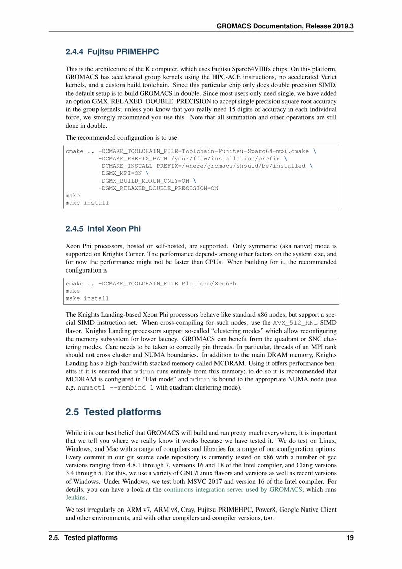
GROMACS Documentation, Release 2019.3
2.4.4 Fujitsu PRIMEHPC
This is the architecture of the K computer, which uses Fujitsu Sparc64VIIIfx chips. On this platform,GROMACS has accelerated group kernels using the HPC-ACE instructions, no accelerated Verletkernels, and a custom build toolchain. Since this particular chip only does double precision SIMD,the default setup is to build GROMACS in double. Since most users only need single, we have addedan option GMX_RELAXED_DOUBLE_PRECISION to accept single precision square root accuracyin the group kernels; unless you know that you really need 15 digits of accuracy in each individualforce, we strongly recommend you use this. Note that all summation and other operations are stilldone in double.
The recommended configuration is to use
cmake .. -DCMAKE_TOOLCHAIN_FILE=Toolchain-Fujitsu-Sparc64-mpi.cmake \-DCMAKE_PREFIX_PATH=/your/fftw/installation/prefix \-DCMAKE_INSTALL_PREFIX=/where/gromacs/should/be/installed \-DGMX_MPI=ON \-DGMX_BUILD_MDRUN_ONLY=ON \-DGMX_RELAXED_DOUBLE_PRECISION=ON
makemake install
2.4.5 Intel Xeon Phi
Xeon Phi processors, hosted or self-hosted, are supported. Only symmetric (aka native) mode issupported on Knights Corner. The performance depends among other factors on the system size, andfor now the performance might not be faster than CPUs. When building for it, the recommendedconfiguration is
cmake .. -DCMAKE_TOOLCHAIN_FILE=Platform/XeonPhimakemake install
The Knights Landing-based Xeon Phi processors behave like standard x86 nodes, but support a spe-cial SIMD instruction set. When cross-compiling for such nodes, use the AVX_512_KNL SIMDflavor. Knights Landing processors support so-called “clustering modes” which allow reconfiguringthe memory subsystem for lower latency. GROMACS can benefit from the quadrant or SNC clus-tering modes. Care needs to be taken to correctly pin threads. In particular, threads of an MPI rankshould not cross cluster and NUMA boundaries. In addition to the main DRAM memory, KnightsLanding has a high-bandwidth stacked memory called MCDRAM. Using it offers performance ben-efits if it is ensured that mdrun runs entirely from this memory; to do so it is recommended thatMCDRAM is configured in “Flat mode” and mdrun is bound to the appropriate NUMA node (usee.g. numactl --membind 1 with quadrant clustering mode).
2.5 Tested platforms
While it is our best belief that GROMACS will build and run pretty much everywhere, it is importantthat we tell you where we really know it works because we have tested it. We do test on Linux,Windows, and Mac with a range of compilers and libraries for a range of our configuration options.Every commit in our git source code repository is currently tested on x86 with a number of gccversions ranging from 4.8.1 through 7, versions 16 and 18 of the Intel compiler, and Clang versions3.4 through 5. For this, we use a variety of GNU/Linux flavors and versions as well as recent versionsof Windows. Under Windows, we test both MSVC 2017 and version 16 of the Intel compiler. Fordetails, you can have a look at the continuous integration server used by GROMACS, which runsJenkins.
We test irregularly on ARM v7, ARM v8, Cray, Fujitsu PRIMEHPC, Power8, Google Native Clientand other environments, and with other compilers and compiler versions, too.
2.5. Tested platforms 19
CHAPTER
THREE
USER GUIDE
This guide provides
• material introducing GROMACS
• practical advice for making effective use of GROMACS.
For getting, building and installing GROMACS, see the Installation guide (page 3). For backgroundon algorithms and implementations, see the reference manual part (page 292) of the documentation.
Please reference this documentation as https://doi.org/10.5281/zenodo.3243834.
To cite the source code for this release, please cite https://doi.org/10.5281/zenodo.3243833.
3.1 Getting started
3.1.1 Flow Chart
This is a flow chart of a typical GROMACS MD run of a protein in a box of water. A more detailedexample is available in Getting started (page 20). Several steps of energy minimization may benecessary, these consist of cycles: gmx grompp (page 94) -> gmx mdrun (page 111).
20
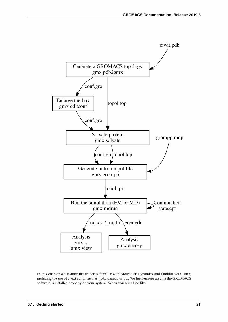
GROMACS Documentation, Release 2019.3
eiwit.pdb
Generate a GROMACS topologygmx pdb2gmx
grompp.mdp
Enlarge the boxgmx editconf
conf.gro
Solvate proteingmx solvate
topol.top
conf.gro
Generate mdrun input filegmx grompp
conf.gro topol.top
Run the simulation (EM or MD)gmx mdrun
topol.tpr
Continuationstate.cpt
Analysisgmx ...
gmx view
traj.xtc / traj.trr
Analysisgmx energy
ener.edr
In this chapter we assume the reader is familiar with Molecular Dynamics and familiar with Unix,including the use of a text editor such as jot, emacs or vi. We furthermore assume the GROMACSsoftware is installed properly on your system. When you see a line like
3.1. Getting started 21
GROMACS Documentation, Release 2019.3
ls -l
you are supposed to type the contents of that line on your computer terminal.
3.1.2 Setting up your environment
In order to check whether you have access to GROMACS, please start by entering the command:
gmx -version
This command should print out information about the version of GROMACS installed. If this, incontrast, returns the phrase
gmx: command not found.
then you have to find where your version of GROMACS is installed. In the default case, the binariesare located in /usr/local/gromacs/bin, however, you can ask your local system administratorfor more information, and then follow the advice for Getting access to GROMACS after installation(page 16).
3.1.3 Flowchart of typical simulation
A typical simulation workflow with GROMACS is illustrated here (page 20).
3.1.4 Important files
Here is an overview of the most important GROMACS file types that you will encounter.
Molecular Topology file (.top)
The molecular topology file is generated by the program gmx pdb2gmx (page 127). gmx pdb2gmx(page 127) translates a pdb (page 427) structure file of any peptide or protein to a molecular topologyfile. This topology file contains a complete description of all the interactions in your peptide orprotein.
Topology #include file mechanism
When constructing a system topology in a top (page 429) file for presentation to grompp, GROMACSuses a built-in version of the so-called C preprocessor, cpp (in GROMACS 3, it really was cpp). cppinterprets lines like:
#include "ions.itp"
by looking for the indicated file in the current directory, the GROMACS share/top directory as indi-cated by the GMXLIB environment variable, and any directory indicated by a -I flag in the value ofthe include run parameter (page 201) in the mdp (page 425) file. It either finds this file or reportsa warning. (Note that when you supply a directory name, you should use Unix-style forward slashes‘/’, not Windows-style backslashes ‘’ for separators.) When found, it then uses the contents exactly asif you had cut and pasted the included file into the main file yourself. Note that you shouldn’t go anddo this copy-and-paste yourself, since the main purposes of the include file mechanism are to re-useprevious work, make future changes easier, and prevent typos.
Further, cpp interprets code such as:
3.1. Getting started 22
GROMACS Documentation, Release 2019.3
#ifdef POSRES_WATER; Position restraint for each water oxygen[ position_restraints ]; i funct fcx fcy fcz
1 1 1000 1000 1000#endif
by testing whether the preprocessor variable POSRES_WATER was defined somewhere (i.e. “if de-fined”). This could be done with #define POSRES_WATER earlier in the top (page 429) file (or its#include files), with a -D flag in the include run parameter as above, or on the command line tocpp. The function of the -D flag is borrowed from the similar usage in cpp. The string that follows-D must match exactly; using -DPOSRES will not trigger #ifdef POSRE or #ifdef DPOSRES.This mechanism allows you to change your mdp (page 425) file to choose whether or not you want po-sition restraints on your solvent, rather than your top (page 429) file. Note that preprocessor variablesare not the same as shell environment variables.
Molecular Structure file (.gro, .pdb)
When gmx pdb2gmx (page 127) is executed to generate a molecular topology, it also translates thestructure file (pdb (page 427) file) to a GROMOS structure file (gro (page 423) file). The maindifference between a pdb (page 427) file and a gromos file is their format and that a gro (page 423)file can also hold velocities. However, if you do not need the velocities, you can also use a pdb(page 427) file in all programs. To generate a box of solvent molecules around the peptide, theprogram gmx solvate (page 151) is used. First the program gmx editconf (page 79) should be usedto define a box of appropriate size around the molecule. gmx solvate (page 151) solvates a solutemolecule (the peptide) into any solvent (in this case, water). The output of gmx solvate (page 151)is a gromos structure file of the peptide solvated in water. gmx solvate (page 151) also changes themolecular topology file (generated by gmx pdb2gmx (page 127)) to add solvent to the topology.
Molecular Dynamics parameter file (.mdp)
The Molecular Dynamics Parameter (mdp (page 425)) file contains all information about the Molecu-lar Dynamics simulation itself e.g. time-step, number of steps, temperature, pressure etc. The easiestway of handling such a file is by adapting a sample mdp (page 425) file. A sample mdp file (page 425)is available.
Index file (.ndx)
Sometimes you may need an index file to specify actions on groups of atoms (e.g. temperaturecoupling, accelerations, freezing). Usually the default index groups will be sufficient, so for thisdemo we will not consider the use of index files.
Run input file (.tpr)
The next step is to combine the molecular structure (gro (page 423) file), topology (top (page 429) file)MD-parameters (mdp (page 425) file) and (optionally) the index file (ndx (page 426)) to generate arun input file (tpr (page 431) extension). This file contains all information needed to start a simulationwith GROMACS. The gmx grompp (page 94) program processes all input files and generates the runinput tpr (page 431) file.
Trajectory file (.trr, .tng, or .xtc)
Once the run input file is available, we can start the simulation. The program which starts the simula-tion is called gmx mdrun (page 111) (or sometimes just mdrun, or mdrun_mpi). The only input file ofgmx mdrun (page 111) that you usually need in order to start a run is the run input file (tpr (page 431)
3.1. Getting started 23
GROMACS Documentation, Release 2019.3
file). The typical output files of gmx mdrun (page 111) are the trajectory file (trr (page 431) file), alogfile (log (page 424) file), and perhaps a checkpoint file (cpt (page 421) file).
3.1.5 Tutorial material
There are several tutorials available that cover aspects of using GROMACS. Further information canalso be found in the How to (page 282) section.
3.1.6 Background reading
• Berendsen, H.J.C., Postma, J.P.M., van Gunsteren, W.F., Hermans, J. (1981) IntermolecularForces, chapter Interaction models for water in relation to protein hydration, pp 331-342. Dor-drecht: D. Reidel Publishing Company Dordrecht
• Kabsch, W., Sander, C. (1983). Dictionary of protein secondary structure: Pattern recognitionof hydrogen-bonded and geometrical features. Biopolymers 22, 2577–2637.
• Mierke, D.F., Kessler, H. (1991). Molecular dynamics with dimethyl sulfoxide as a solvent.Conformation of a cyclic hexapeptide. J. Am. Chem. Soc. 113, 9446.
• Stryer, L. (1988). Biochemistry vol. 1, p. 211. New York: Freeman, 3 edition.
3.2 System preparation
There are many ways to prepare a simulation system to run with GROMACS. These often vary withthe kind of scientific question being considered, or the model physics involved. A protein-ligandatomistic free-energy simulation might need a multi-state topology, while a coarse-grained simulationmight need to manage defaults that suit systems with higher density.
3.2.1 Steps to consider
The following general guidance should help with planning successful simulations. Some stages areoptional for some kinds of simulations.
1. Clearly identify the property or phenomena of interest to be studied by performing the simula-tion. Do not continue further until you are clear on this! Do not run your simulation and thenseek to work out how to use it to test your hypothesis, because it may be unsuitable, or therequired information was not saved.
2. Select the appropriate tools to be able to perform the simulation and observe the property orphenomena of interest. It is important to read and familiarize yourself with publications byother researchers on similar systems. Choices of tools include:
• software with which to perform the simulation (consideration of force field may influencethis decision)
• the force field, which describes how the particles within the system interact with each other.Select one that is appropriate for the system being studied and the property or phenomena ofinterest. This is a very important and non-trivial step! Consider now how you will analyzeyour simulation data to make your observations.
3. Obtain or generate the initial coordinate file for each molecule to be placed within the system.Many different software packages are able to build molecular structures and assemble them intosuitable configurations.
4. Generate the raw starting structure for the system by placing the molecules within the coordi-nate file as appropriate. Molecules may be specifically placed or arranged randomly. Several
3.2. System preparation 24
GROMACS Documentation, Release 2019.3
non-GROMACS tools are useful here; within GROMACS gmx solvate (page 151), gmx insert-molecules (page 104) and gmx genconf (page 91) solve frequent problems.
5. Obtain or generate the topology file for the system, using (for example) gmx pdb2gmx(page 127), gmx x2top (page 178), SwissParam (for CHARMM forcefield), PRODRG (forGROMOS96 43A1), Automated Topology Builder (for GROMOS96 53A6), MKTOP (forOPLS/AA) or your favourite text editor in concert with chapter 5 of the GROMACS ReferenceManual. For the AMBER force fields, antechamber or acpype might be appropriate.
6. Describe a simulation box (e.g. using gmx editconf (page 79)) whose size is appropriate for theeventual density you would like, fill it with solvent (e.g. using gmx solvate (page 151)), andadd any counter-ions needed to neutralize the system (e.g. using gmx grompp (page 94) andgmx insert-molecules (page 104)). In these steps you may need to edit your topology file to staycurrent with your coordinate file.
7. Run an energy minimization on the system (using gmx grompp (page 94) and gmx mdrun(page 111)). This is required to sort out any bad starting structures caused during generationof the system, which may cause the production simulation to crash. It may be necessary alsoto minimize your solute structure in vacuo before introducing solvent molecules (or your lipidbilayer or whatever else). You should consider using flexible water models and not using bondconstraints or frozen groups. The use of position restraints and/or distance restraints should beevaluated carefully.
8. Select the appropriate simulation parameters for the equilibration simulation (defined in mdp(page 425) file). You need to choose simulation parameters that are consistent with how forcefield was derived. You may need to simulate at NVT with position restraints on your solventand/or solute to get the temperature almost right, then relax to NPT to fix the density (whichshould be done with Berendsen until after the density is stabilized, before a further switch toa barostat that produces the correct ensemble), then move further (if needed) to reach yourproduction simulation ensemble (e.g. NVT, NVE). If you have problems here with the systemblowing up (page 272), consider using the suggestions on that page, e.g. position restraints onsolutes, or not using bond constraints, or using smaller integration timesteps, or several gentlerheating stage(s).
9. Run the equilibration simulation for sufficient time so that the system relaxes sufficiently in thetarget ensemble to allow the production run to be commenced (using gmx grompp (page 94) andgmx mdrun (page 111), then gmx energy (page 84) and trajectory visualization tools).
10. Select the appropriate simulation parameters for the production simulation (defined in mdp(page 425) file). In particular, be careful not to re-generate the velocities. You still need tobe consistent with how the force field was derived and how to measure the property or phenom-ena of interest.
3.2.2 Tips and tricks
Database files
The share/top directory of a GROMACS installation contains numerous plain-text helper fileswith the .dat file extension. Some of the command-line tools (see Command-line reference(page 35)) refer to these, and each tool documents which files it uses, and how they are used.
If you need to modify these files (e.g. to introduce new atom types with VDW radii into vdwradii.dat), you can copy the file from your installation directory into your working directory, and theGROMACS tools will automatically load the copy from your working directory rather than the stan-dard one. To suppress all the standard definitions, use an empty file in the working directory.
3.2. System preparation 25
GROMACS Documentation, Release 2019.3
3.3 Managing long simulations
Molecular simulations often extend beyond the lifetime of a single UNIX command-line process. It isuseful to be able to stop and restart the simulation in a way that is equivalent to a single run. When gmxmdrun (page 111) is halted, it writes a checkpoint file that can restart the simulation exactly as if therewas no interruption. To do this, the checkpoint retains a full-precision version of the positions andvelocities, along with state information necessary to restart algorithms e.g. that implement coupling toexternal thermal reservoirs. A restart can be attempted using e.g. a gro (page 423) file with velocities,but since the gro (page 423) file has significantly less precision, and none of the coupling algorithmswill have their state carried over, such a restart is less continuous than a normal MD step.
Such a checkpoint file is also written periodically by gmx mdrun (page 111) during the run. Theinterval is given by the -cpt flag to gmx mdrun (page 111). When gmx mdrun (page 111) attemps towrite each successive checkpoint file, it first renames the old file with the suffix _prev, so that evenif something goes wrong while writing the new checkpoint file, only recent progress can be lost.
gmx mdrun (page 111) can be halted in several ways:
• the number of simulation nsteps (page 203) can expire
• the user issues a termination signal (e.g. with Ctrl-C on the terminal)
• the job scheduler issues a termination signal when time expires
• when gmx mdrun (page 111) detects that the length specified with -maxh has elapsed (thisoption is useful to help cooperate with a job scheduler, but can be problematic if jobs can besuspended)
• some kind of catastrophic failure, such as loss of power, or a disk filling up, or a network failing
To use the checkpoint file for a restart, use a command line such as
gmx mdrun -cpi state
which directs mdrun to use the checkpoint file (which is named state.cpt by default). You canchoose to give the output checkpoint file a different name with the -cpo flag, but if so then youmust provide that name as input to -cpi when you later use that file. You can query the contents ofcheckpoint files with gmx check (page 51) and gmx dump (page 77).
3.3.1 Appending to output files
By default, gmx mdrun (page 111) will append to the old output files. If the previous part ended ina regular way, then the performance data at the end of the log file will will be removed, some newinformation about the run context written, and the simulation will proceed. Otherwise, mdrun willtruncate all the output files back to the time of the last written checkpoint file, and continue fromthere, as if the simulation stopped at that checkpoint in a regular way.
You can choose not to append the output files by using the -noappend flag, which forces mdrunto write each output to a separate file, whose name includes a “.partXXXX” string to describe whichsimulation part is contained in this file. This numbering starts from zero and increases monotonicallyas simulations are restarted, but does not reflect the number of simulation steps in each part. Thesimulation-part (page 203) option can be used to set this number manually in gmx grompp(page 94), which can be useful if data has been lost, e.g. through filesystem failure or user error.
Appending will not work if any output files have been modified or removed after mdrun wrote them,because the checkpoint file maintains a checksum of each file that it will verify before it writes tothem again. In such cases, you must either restore the file, name them as the checkpoint file expects,or continue with -noappend. If your original run used -deffnm, and you want appending, thenyour continuations must also use -deffnm.
3.3. Managing long simulations 26
GROMACS Documentation, Release 2019.3
3.3.2 Backing up your files
You should arrange to back up your simulation files frequently. Network file systems on clusters canbe configured in more or less conservative ways, and this can lead gmx mdrun (page 111) to be toldthat a checkpoint file has been written to disk when actually it is still in memory somewhere andvulnerable to a power failure or disk that fills or fails in the meantime. The UNIX tool rsync can bea useful way to periodically copy your simulation output to a remote storage location, which workssafely even while the simulation is underway. Keeping a copy of the final checkpoint file from eachpart of a job submitted to a cluster can be useful if a file system is unreliable.
3.3.3 Extending a .tpr file
If the simulation described by tpr (page 431) file has completed and should be extended, use the gmxconvert-tpr (page 60) tool to extend the run, e.g.
gmx convert-tpr -s previous.tpr -extend timetoextendby -o next.tprgmx mdrun -s next.tpr -cpi state.cpt
The time can also be extended using the -until and -nsteps options. Note that the original mdp(page 425) file may have generated velocities, but that is a one-time operation within gmx grompp(page 94) that is never performed again by any other tool.
3.3.4 Changing mdp options for a restart
If you wish to make changes to your simulations settings other than length, then you should do so inthe mdp (page 425) file or topology, and then call
gmx grompp -f possibly-changed.mdp -p possibly-changed.top -c state.cpt -→˓o new.tprgmx mdrun -s new.tpr -cpi state.cpt
to instruct gmx grompp (page 94) to copy the full-precision coordinates in the checkpoint file intothe new tpr (page 431) file. You should consider your choices for tinit (page 203), init-step(page 203), nsteps (page 203) and simulation-part (page 203). You should generally notregenerate velocities with gen-vel (page 216), and generally select continuation (page 217)so that constraints are not re-applied before the first integration step.
3.3.5 Restarts without checkpoint files
It used to be possible to continue simulations without the checkpoint files. As this approach could beunreliable or lead to unphysical results, only restarts from checkpoints are permitted now.
3.3.6 Are continuations exact?
If you had a computer with unlimited precision, or if you integrated the time-discretized equationsof motion by hand, exact continuation would lead to identical results. But since practical computershave limited precision and MD is chaotic, trajectories will diverge very rapidly even if one bit isdifferent. Such trajectories will all be equally valid, but eventually very different. Continuationusing a checkpoint file, using the same code compiled with the same compiler and running on thesame computer architecture using the same number of processors without GPUs (see next section)would lead to binary identical results. However, by default the actual work load will be balancedacross the hardware according to the observed execution times. Such trajectories are in principle notreproducible, and in particular a run that took place in more than one part will not be identical withan equivalent run in one part - but neither of them is better in any sense.
3.3. Managing long simulations 27
GROMACS Documentation, Release 2019.3
3.3.7 Reproducibility
The following factors affect the reproducibility of a simulation, and thus its output:
• Precision (mixed / double) with double giving “better” reproducibility.
• Number of cores, due to different order in which forces are accumulated. For instance (a+b)+cis not necessarily binary identical to a+(b+c) in floating-point arithmetic.
• Type of processors. Even within the same processor family there can be slight differences.
• Optimization level when compiling.
• Optimizations at run time: e.g. the FFTW library that is typically used for fast Fourier trans-forms determines at startup which version of their algorithms is fastest, and uses that for theremainder of the calculations. Since the speed estimate is not deterministic, the results may varyfrom run to run.
• Random numbers used for instance as a seed for generating velocities (in GROMACS at thepreprocessing stage).
• Uninitialized variables in the code (but there shouldn’t be any)
• Dynamic linking to different versions of shared libraries (e.g. for FFTs)
• Dynamic load balancing, since particles are redistributed to processors based on elapsed wall-clock time, which will lead to (a+b)+c != a+(b+c) issues as above
• Number of PME-only ranks (for parallel PME simulations)
• MPI reductions typically do not guarantee the order of the operations, and so the absence ofassociativity for floating-point arithmetic means the result of a reduction depends on the orderactually chosen
• On GPUs, the reduction of e.g. non-bonded forces has a non-deterministic summation order, soany fast implementation is non-reprodudible by design.
The important question is whether it is a problem if simulations are not completely reproducible.The answer is yes and no. Reproducibility is a cornerstone of science in general, and hence it isimportant. The Central Limit Theorem tells us that in the case of infinitely long simulations, allobservables converge to their equilibrium values. Molecular simulations in GROMACS adhere tothis theorem, and hence, for instance, the energy of your system will converge to a finite value, thediffusion constant of your water molecules will converge to a finite value, and so on. That meansall the important observables, which are the values you would like to get out of your simulation, arereproducible. Each individual trajectory is not reproducible, however.
However, there are a few cases where it would be useful if trajectories were reproducible, too. Theseinclude developers doing debugging, and searching for a rare event in a trajectory when, if it occurs,you want to have manually saved your checkpoint file so you can restart the simulation under differentconditions, e.g. writing output much more frequently.
In order to obtain this reproducible trajectory, it is important to look over the list above and eliminatethe factors that could affect it. Further, using
gmx mdrun -reprod
will eliminate all sources of non-reproducibility that it can, i.e. same executable + same hardware +same shared libraries + same run input file + same command line parameters will lead to reproducibleresults.
3.3. Managing long simulations 28
GROMACS Documentation, Release 2019.3
3.4 Answers to frequently asked questions (FAQs)
3.4.1 Questions regarding GROMACS installation
1. Do I need to compile all utilities with MPI?
With one rarely-used exception (pme_error (page 129)), only the mdrun (page 111) binaryis able to use the MPI (page 6) parallelism. So you only need to use the -DGMX_MPI=onflag when configuring (page 8) for a build intended to run the main simulation engine mdrun(page 111).
2. Should my version be compiled using double precision?
In general, GROMACS only needs to be build in its default mixed-precision mode. For moredetails, see the discussion in Chapter 2 of the reference manual. Sometimes, usage may also de-pend on your target system, and should be decided upon according to the individual instructions(page 18).
3.4.2 Questions concerning system preparation and preprocessing
1. Where can I find a solvent coordinate file (page 420) for use with solvate (page 151)?
Suitable equilibrated boxes of solvent structure files (page 420) can be found in the $GMXDIR/share/gromacs/top directory. That location will be searched by default by solvate(page 151), for example by using -cs spc216.gro as an argument. Other solvent boxescan be prepared by the user as described on the manual page for solvate (page 151) and else-where. Note that suitable topology files will be needed for the solvent boxes to be useful ingrompp (page 94). These are available for some force fields, and may be found in the respectivesubfolder of $GMXDIR/share/gromacs/top.
2. How to prevent solvate (page 151) from placing waters in undesired places?
Water placement is generally well behaved when solvating proteins, but can be difficult whensetting up membrane or micelle simulations. In those cases, waters may be placed in between thealkyl chains of the lipids, leading to problems later during the simulation (page 272). You caneither remove those waters by hand (and do the accounting for molecule types in the topology(page 429) file), or set up a local copy of the vdwradii.dat file from the $GMXLIB directory,specific for your project and located in your working directory. In it, you can increase the vdWradius of the atoms, to suppress such interstitial insertions. Recommended e.g. at a commontutorial is the use of 0.375 instead of 0.15.
1. How do I provide multiple definitions of bonds / dihedrals in a topology?
You can add additional bonded terms beyond those that are normally defined for a residue(e.g. when defining a special ligand) by including additional copies of the respective linesunder the [ bonds ], [ pairs ], [ angles ] and [ dihedrals ] sections in the[ moleculetype ] section for your molecule, found either in the itp (page 424) file or thetopology (page 429) file. This will add those extra terms to the potential energy evaluation, butwill not remove the previous ones. So be careful with duplicate entries. Also keep in mindthat this does not apply to duplicated entries for [ bondtypes ], [ angletypes ], or[ dihedraltypes ], in force-field definition files, where duplicates overwrite the previousvalues.
2. Do I really need a gro (page 423) file?
The gro (page 423) file is used in GROMACS as a unified structure file (page 420) format thatcan be read by all utilities. The large majority of GROMACS routines can also use other filetypes such as pdb (page 427), with the limitations that no velocities are available in this case(page 23). If you need a text-based format with more digits of precision, the g96 (page 423)format is suitable and supported.
3.4. Answers to frequently asked questions (FAQs) 29

GROMACS Documentation, Release 2019.3
3. Do I always need to run pdb2gmx (page 127) when I already produced an itp (page 424) fileelsewhere?
You don’t need to prepare additional files if you already have all itp (page 424) and top(page 429) files prepared through other tools.
Examples for those are CHARMM-GUI, ATB (Automated Topology Builder), pmx. and PRO-DRG.
4. How can I build in missing atoms?
GROMACS has no support for building coordinates of missing non-hydrogen atoms. If yoursystem is missing some part, you will have to add the missing pieces using external programsto avoid the missing atom (page 261) error. This can be done using programs such as Chimerain combination with Modeller, Swiss PDB Viewer, Maestro. Do not run a simulation that hadmissing atoms unless you know exactly why it will be stable.
5. Why is the total charge of my system not an integer like it should be?
In floating point (page 280) math, real numbers can not be displayed to arbitrary precision (formore on this, see e.g. Wikipedia). This means that very small differences to the final integervalue will persist, and GROMACS will not lie to you and round those values up or down. Ifyour charge differs from the integer value by a larger amount, e.g. at least 0.01, this usuallymeans that something went wrong during your system preparation
3.4.3 Questions regarding simulation methodology
1. Should I couple a handful of ions to their own temperature-coupling bath?
No. You need to consider the minimal size of your temperature coupling groups, as explainedin Thermostats (page 270) and more specifically in What not to do (page 270), as well as theimplementation of your chosen thermostat as described in the reference manual.
2. Why do my grompp restarts always start from time zero?
You can choose different values for tinit (page 203) and init-step (page 203).
3. Why can’t I do conjugate gradient minimization with constraints?
Minimization with the conjugate gradient scheme can not be performed with constraints asdescribed in the reference manual, and some additional information on Wikipedia.
4. How do I hold atoms in place in my energy minimization or simulation?
Groups may be frozen in place using freeze groups (see the reference manual). It is morecommon to use a set of position restraints, to place penalties on movement of the atoms. Filesthat control this kind of behaviour can be created using genrestr (page 93).
5. How do I extend a completed a simulation to longer times?
Please see the section on Managing long simulations (page 26). You can either prepare a newmdp (page 425) file, or extend the simulation time in the original tpr (page 431) file usingconvert-tpr (page 60).
6. How should I compute a single-point energy?
This is best achieved with the -rerun option to mdrun (page 111). See the Re-running asimulation (page 239) section.
3.4.4 Parameterization and Force Fields
1. I want to simulate a molecule (protein, DNA, etc.) which complexes with various transitionmetal ions, iron-sulfur clusters, or other exotic species. Parameters for these exotic speciesaren’t available in force field X. What should I do?
3.4. Answers to frequently asked questions (FAQs) 30
GROMACS Documentation, Release 2019.3
First, you should consider how well MD (page 273) will actually describe your system (e.g.see some of the recent literature). Many species are infeasible to model without either atomicpolarizability, or QM treatments. Then you need to prepare your own set of parameters and adda new residue to your force field (page 274) of choice. Then you will have to validate that yoursystem behaves in a physical way, before continuing your simulation studies. You could also tryto build a more simplified model that does not rely on the complicated additions, as long as itstill represents the correct real object in the laboratory.
2. Should I take parameters from one force field and apply them inside another that is missingthem?
NO. Molecules parametrized for a given force field (page 274) will not behave in a physicalmanner when interacting with other molecules that have been parametrized according to differ-ent standards. If your required molecule is not included in the force field you need to use, youwill have to parametrize it yourself according to the methodology of this force field.
3.4.5 Analysis and Visualization
1. Why am I seeing bonds being created when I watch the trajectory?
Most visualization softwares determine the bond status of atoms depending on a set of prede-fined distances. So the bonding pattern created by them might not be the one defined in yourtopology (page 429) file. What matters is the information encoded in there. If the software hasread a tpr (page 431) file, then the information is in reliable agreement with the topology yousupplied to grompp (page 94).
2. When visualizing a trajectory from a simulation using PBC, why are there holes or my peptideleaving the simulation box?
Those holes and molecules moving around are just a result of molecules ranging over the boxboundaries and wrapping around (page 269), and are not a reason for concern. You can fix thevisualization using trjconv (page 162) to prepare the structure for analysis.
3. Why is my total simulation time not an integer like it should be?
As the simulation time is calculated using floating point arithmetic (page 280), rounding errorscan occur but are not of concern.
3.5 Force fields in GROMACS
3.5.1 AMBER
AMBER (Assisted Model Building and Energy Refinement) refers both to a set of molecular mechan-ical force fields (page 274) for the simulation of biomolecules and a package of molecular simulationprograms.
GROMACS versions higher than 4.5 support the following AMBER force fields natively:
• AMBER94
• AMBER96
• AMBER99
• AMBER99SB
• AMBER99SB-ILDN
• AMBER03
• AMBERGS
3.5. Force fields in GROMACS 31
GROMACS Documentation, Release 2019.3
Information concerning the force field can be found using the following information:
• AMBER Force Fields - background about the AMBER force fields
• AMBER Programs - information about the AMBER suite of programs for molecular simulation
• ANTECHAMBER/GAFF - Generalized Amber Force Field (GAFF) which is supposed toprovide parameters suitable for small molecules that are compatible with the AMBER pro-tein/nucleic acid force fields. It is available either together with AMBER, or through the an-techamber package, which is also distributed separately. There are scripts available for con-verting AMBER systems (set up, for example, with GAFF) to GROMACS (amb2gmx.pl, oracpypi.py), but they do require an AMBER installation to work.
Older GROMACS versions need a separate installation of the ffamber ports:
• Using AMBER Force Field in GROMACS - known as the “ffamber ports,” a number of AMBERforce fields, complete with documentation.
• Using the ffamber ports with GROMACS requires that the input structure files adhere to theAMBER nomenclature for residues. Problematic residues involve termini (prefixed with N andC), lysine (either LYN or LYP), histidine (HID, HIE, or HIS), and cysteine (CYN or CYX).Please see the ffamber documentation.
3.5.2 CHARMM
CHARMM (Chemistry at HARvard Macromolecular Mechanics) is a both a set of force fields and asoftware package for molecular dynamics (page 273) simulations and analysis. Includes united atom(CHARMM19) and all atom (CHARMM22, CHARMM27, CHARMM36) force fields (page 274).The CHARMM27 force field has been ported to GROMACS and is officially supported as of version4.5. CHARMM36 force field files can be obtained from the MacKerell lab website, which regularlyproduces up-to-date CHARMM force field files in GROMACS format.
For using CHARMM36 in GROMACS 5.0 and newer, please use the following settings in the mdp(page 425) file:
constraints = h-bondscutoff-scheme = Verletvdwtype = cutoffvdw-modifier = force-switchrlist = 1.2rvdw = 1.2rvdw-switch = 1.0coulombtype = PMErcoulomb = 1.2DispCorr = no
Note that dispersion correction should be applied in the case of lipid monolayers, but not bilayers.
Please also note that the switching distance is a matter of some debate in lipid bilayer simulations, andit is dependent to some extent on the nature of the lipid. Some studies have found that an 0.8-1.0 nmswitch is appropriate, others argue 0.8-1.2 nm is best, and yet others stand by 1.0-1.2 nm. The user iscautioned to thoroughly investigate the force field literature for their chosen lipid(s) before beginninga simulation!
Anyone using very old versions of GROMACS may find this script useful:
CHARMM to GROMACS - perl scripts intended to facilitate calculations using GRO-MACS programs and CHARMM forcefields (needed for GROMACS versions < 4.5).(link)
3.5. Force fields in GROMACS 32
GROMACS Documentation, Release 2019.3
3.5.3 GROMOS
GROMOS is is a general-purpose molecular dynamics computer simulation package for the study ofbiomolecular systems. It also incorporates its own force field covering proteins, nucleotides, sugarsetc. and can be applied to chemical and physical systems ranging from glasses and liquid crystals, topolymers and crystals and solutions of biomolecules.
GROMACS supports the GROMOS force fields, with all parameters provided in the distribution for43a1, 43a2, 45a3, 53a5, 53a6 and 54a7. The GROMOS force fields are united atom force fields(page 274), i.e. without explicit aliphatic (non-polar) hydrogens.
• GROMOS 53a6 - in GROMACS format (J. Comput. Chem. 2004 vol. 25 (13): 1656-1676).
• GROMOS 53a5 - in GROMACS format (J. Comput. Chem. 2004 vol. 25 (13): 1656-1676).
• GROMOS 43a1p - 43a1 modified to contain SEP (phosphoserine), TPO (phosphothreonine),and PTR (phosphotyrosine) (all PO42- forms), and SEPH, TPOH, PTRH (PO4H- forms).
3.5.4 OPLS
OPLS (Optimized Potential for Liquid Simulations) is a set of force fields developed by Prof. WilliamL. Jorgensen for condensed phase simulations, with the latest version being OPLS-AA/M.
The standard implementations for those force fields are the BOSS and MCPRO programs developedby the Jorgensen group
As there is no central web-page to point to, the user is advised to consult the original literature for theunited atom (OPLS-UA) and all atom (OPLS-AA) force fields, as well as the Jorgensen group page
3.6 Non-bonded cut-off schemes
The default cut-off scheme in GROMACS 2019.3 is based on classical buffered Verlet lists. Theseare implemented extremely efficiently on modern CPUs and accelerators, and support nearly all ofthe algorithms used in GROMACS.
Before version 4.6, GROMACS always used pair-lists based on groups of particles. These groupsof particles were originally charge-groups, which were necessary with plain cut-off electrostatics.With the use of PME (or reaction-field with a buffer), charge groups are no longer necessary (andare ignored in the Verlet scheme). In GROMACS 4.6 and later, the group-based cut-off scheme isstill available, but is deprecated since 5.0. It is still available mainly for backwards compatibility,to support the algorithms that have not yet been converted, and for the few cases where it may allowfaster simulations with bio-molecular systems dominated by water.
Without PME, the group cut-off scheme should generally be combined with a buffered pair-list tohelp avoid artifacts. However, the group-scheme kernels that can implement this are much slowerthan either the unbuffered group-scheme kernels, or the buffered Verlet-scheme kernels. Use of theVerlet scheme is strongly encouraged for all kinds of simulations, because it is easier and faster to runcorrectly. In particular, GPU acceleration is available only with the Verlet scheme.
The Verlet scheme uses properly buffered lists with exact cut-offs. The size of the buffer is chosenwith verlet-buffer-tolerance (page 207) to permit a certain level of drift. Both the LJ andCoulomb potential are shifted to zero by subtracting the value at the cut-off. This ensures that theenergy is the integral of the force. Still it is advisable to have small forces at the cut-off, hence to usePME or reaction-field with infinite epsilon.
3.6.1 Non-bonded scheme feature comparison
All GROMACS 2019.3 features not directly related to non-bonded interactions are supported in bothschemes. Eventually, all non-bonded features will be supported in the Verlet scheme. A table describ-
3.6. Non-bonded cut-off schemes 33
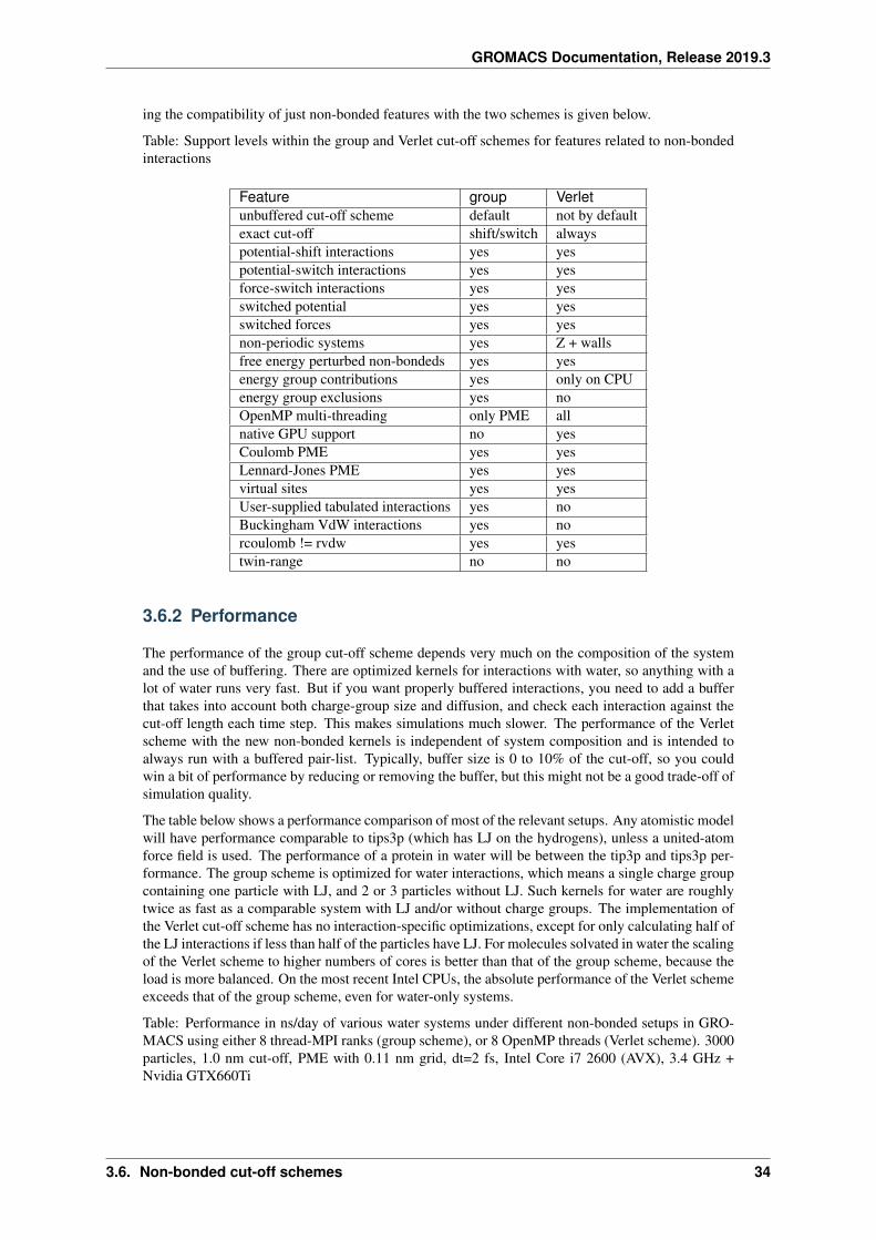
GROMACS Documentation, Release 2019.3
ing the compatibility of just non-bonded features with the two schemes is given below.
Table: Support levels within the group and Verlet cut-off schemes for features related to non-bondedinteractions
Feature group Verletunbuffered cut-off scheme default not by defaultexact cut-off shift/switch alwayspotential-shift interactions yes yespotential-switch interactions yes yesforce-switch interactions yes yesswitched potential yes yesswitched forces yes yesnon-periodic systems yes Z + wallsfree energy perturbed non-bondeds yes yesenergy group contributions yes only on CPUenergy group exclusions yes noOpenMP multi-threading only PME allnative GPU support no yesCoulomb PME yes yesLennard-Jones PME yes yesvirtual sites yes yesUser-supplied tabulated interactions yes noBuckingham VdW interactions yes norcoulomb != rvdw yes yestwin-range no no
3.6.2 Performance
The performance of the group cut-off scheme depends very much on the composition of the systemand the use of buffering. There are optimized kernels for interactions with water, so anything with alot of water runs very fast. But if you want properly buffered interactions, you need to add a bufferthat takes into account both charge-group size and diffusion, and check each interaction against thecut-off length each time step. This makes simulations much slower. The performance of the Verletscheme with the new non-bonded kernels is independent of system composition and is intended toalways run with a buffered pair-list. Typically, buffer size is 0 to 10% of the cut-off, so you couldwin a bit of performance by reducing or removing the buffer, but this might not be a good trade-off ofsimulation quality.
The table below shows a performance comparison of most of the relevant setups. Any atomistic modelwill have performance comparable to tips3p (which has LJ on the hydrogens), unless a united-atomforce field is used. The performance of a protein in water will be between the tip3p and tips3p per-formance. The group scheme is optimized for water interactions, which means a single charge groupcontaining one particle with LJ, and 2 or 3 particles without LJ. Such kernels for water are roughlytwice as fast as a comparable system with LJ and/or without charge groups. The implementation ofthe Verlet cut-off scheme has no interaction-specific optimizations, except for only calculating half ofthe LJ interactions if less than half of the particles have LJ. For molecules solvated in water the scalingof the Verlet scheme to higher numbers of cores is better than that of the group scheme, because theload is more balanced. On the most recent Intel CPUs, the absolute performance of the Verlet schemeexceeds that of the group scheme, even for water-only systems.
Table: Performance in ns/day of various water systems under different non-bonded setups in GRO-MACS using either 8 thread-MPI ranks (group scheme), or 8 OpenMP threads (Verlet scheme). 3000particles, 1.0 nm cut-off, PME with 0.11 nm grid, dt=2 fs, Intel Core i7 2600 (AVX), 3.4 GHz +Nvidia GTX660Ti
3.6. Non-bonded cut-off schemes 34
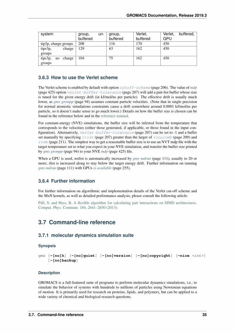
GROMACS Documentation, Release 2019.3
system group, un-buffered
group,buffered
Verlet,buffered
Verlet, buffered,GPU
tip3p, charge groups 208 116 170 450tips3p, chargegroups
129 63 162 450
tips3p, no chargegroups
104 75 162 450
3.6.3 How to use the Verlet scheme
The Verlet scheme is enabled by default with option cutoff-scheme (page 206). The value of mdp(page 425) option verlet-buffer-tolerance (page 207) will add a pair-list buffer whose sizeis tuned for the given energy drift (in kJ/mol/ns per particle). The effective drift is usually muchlower, as gmx grompp (page 94) assumes constant particle velocities. (Note that in single precisionfor normal atomistic simulations constraints cause a drift somewhere around 0.0001 kJ/mol/ns perparticle, so it doesn’t make sense to go much lower.) Details on how the buffer size is chosen can befound in the reference below and in the reference manual.
For constant-energy (NVE) simulations, the buffer size will be inferred from the temperature thatcorresponds to the velocities (either those generated, if applicable, or those found in the input con-figuration). Alternatively, verlet-buffer-tolerance (page 207) can be set to -1 and a bufferset manually by specifying rlist (page 207) greater than the larger of rcoulomb (page 209) andrvdw (page 211). The simplest way to get a reasonable buffer size is to use an NVT mdp file with thetarget temperature set to what you expect in your NVE simulation, and transfer the buffer size printedby gmx grompp (page 94) to your NVE mdp (page 425) file.
When a GPU is used, nstlist is automatically increased by gmx mdrun (page 111), usually to 20 ormore; rlist is increased along to stay below the target energy drift. Further information on runninggmx mdrun (page 111) with GPUs is available (page 255).
3.6.4 Further information
For further information on algorithmic and implementation details of the Verlet cut-off scheme andthe MxN kernels, as well as detailed performance analysis, please consult the following article:
Páll, S. and Hess, B. A flexible algorithm for calculating pair interactions on SIMD architectures.Comput. Phys. Commun. 184, 2641–2650 (2013).
3.7 Command-line reference
3.7.1 molecular dynamics simulation suite
Synopsis
gmx [-[no]h] [-[no]quiet] [-[no]version] [-[no]copyright] [-nice <int>][-[no]backup]
Description
GROMACS is a full-featured suite of programs to perform molecular dynamics simulations, i.e., tosimulate the behavior of systems with hundreds to millions of particles using Newtonian equationsof motion. It is primarily used for research on proteins, lipids, and polymers, but can be applied to awide variety of chemical and biological research questions.
3.7. Command-line reference 35
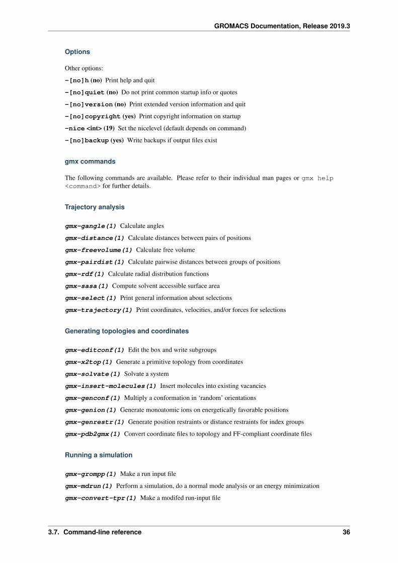
GROMACS Documentation, Release 2019.3
Options
Other options:
-[no]h (no) Print help and quit
-[no]quiet (no) Do not print common startup info or quotes
-[no]version (no) Print extended version information and quit
-[no]copyright (yes) Print copyright information on startup
-nice <int> (19) Set the nicelevel (default depends on command)
-[no]backup (yes) Write backups if output files exist
gmx commands
The following commands are available. Please refer to their individual man pages or gmx help<command> for further details.
Trajectory analysis
gmx-gangle(1) Calculate angles
gmx-distance(1) Calculate distances between pairs of positions
gmx-freevolume(1) Calculate free volume
gmx-pairdist(1) Calculate pairwise distances between groups of positions
gmx-rdf(1) Calculate radial distribution functions
gmx-sasa(1) Compute solvent accessible surface area
gmx-select(1) Print general information about selections
gmx-trajectory(1) Print coordinates, velocities, and/or forces for selections
Generating topologies and coordinates
gmx-editconf(1) Edit the box and write subgroups
gmx-x2top(1) Generate a primitive topology from coordinates
gmx-solvate(1) Solvate a system
gmx-insert-molecules(1) Insert molecules into existing vacancies
gmx-genconf(1) Multiply a conformation in ‘random’ orientations
gmx-genion(1) Generate monoatomic ions on energetically favorable positions
gmx-genrestr(1) Generate position restraints or distance restraints for index groups
gmx-pdb2gmx(1) Convert coordinate files to topology and FF-compliant coordinate files
Running a simulation
gmx-grompp(1) Make a run input file
gmx-mdrun(1) Perform a simulation, do a normal mode analysis or an energy minimization
gmx-convert-tpr(1) Make a modifed run-input file
3.7. Command-line reference 36
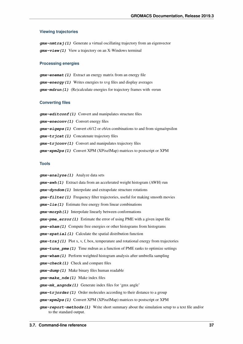
GROMACS Documentation, Release 2019.3
Viewing trajectories
gmx-nmtraj(1) Generate a virtual oscillating trajectory from an eigenvector
gmx-view(1) View a trajectory on an X-Windows terminal
Processing energies
gmx-enemat(1) Extract an energy matrix from an energy file
gmx-energy(1) Writes energies to xvg files and display averages
gmx-mdrun(1) (Re)calculate energies for trajectory frames with -rerun
Converting files
gmx-editconf(1) Convert and manipulates structure files
gmx-eneconv(1) Convert energy files
gmx-sigeps(1) Convert c6/12 or c6/cn combinations to and from sigma/epsilon
gmx-trjcat(1) Concatenate trajectory files
gmx-trjconv(1) Convert and manipulates trajectory files
gmx-xpm2ps(1) Convert XPM (XPixelMap) matrices to postscript or XPM
Tools
gmx-analyze(1) Analyze data sets
gmx-awh(1) Extract data from an accelerated weight histogram (AWH) run
gmx-dyndom(1) Interpolate and extrapolate structure rotations
gmx-filter(1) Frequency filter trajectories, useful for making smooth movies
gmx-lie(1) Estimate free energy from linear combinations
gmx-morph(1) Interpolate linearly between conformations
gmx-pme_error(1) Estimate the error of using PME with a given input file
gmx-sham(1) Compute free energies or other histograms from histograms
gmx-spatial(1) Calculate the spatial distribution function
gmx-traj(1) Plot x, v, f, box, temperature and rotational energy from trajectories
gmx-tune_pme(1) Time mdrun as a function of PME ranks to optimize settings
gmx-wham(1) Perform weighted histogram analysis after umbrella sampling
gmx-check(1) Check and compare files
gmx-dump(1) Make binary files human readable
gmx-make_ndx(1) Make index files
gmx-mk_angndx(1) Generate index files for ‘gmx angle’
gmx-trjorder(1) Order molecules according to their distance to a group
gmx-xpm2ps(1) Convert XPM (XPixelMap) matrices to postscript or XPM
gmx-report-methods(1) Write short summary about the simulation setup to a text file and/orto the standard output.
3.7. Command-line reference 37
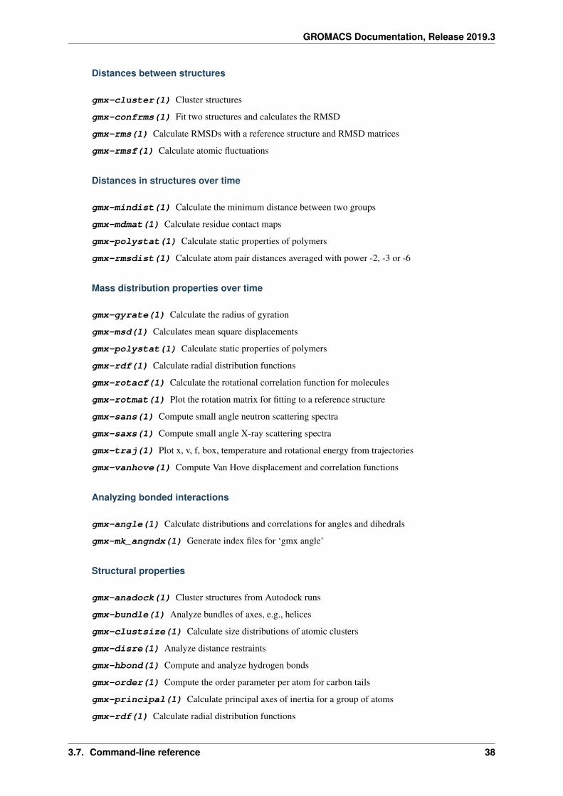
GROMACS Documentation, Release 2019.3
Distances between structures
gmx-cluster(1) Cluster structures
gmx-confrms(1) Fit two structures and calculates the RMSD
gmx-rms(1) Calculate RMSDs with a reference structure and RMSD matrices
gmx-rmsf(1) Calculate atomic fluctuations
Distances in structures over time
gmx-mindist(1) Calculate the minimum distance between two groups
gmx-mdmat(1) Calculate residue contact maps
gmx-polystat(1) Calculate static properties of polymers
gmx-rmsdist(1) Calculate atom pair distances averaged with power -2, -3 or -6
Mass distribution properties over time
gmx-gyrate(1) Calculate the radius of gyration
gmx-msd(1) Calculates mean square displacements
gmx-polystat(1) Calculate static properties of polymers
gmx-rdf(1) Calculate radial distribution functions
gmx-rotacf(1) Calculate the rotational correlation function for molecules
gmx-rotmat(1) Plot the rotation matrix for fitting to a reference structure
gmx-sans(1) Compute small angle neutron scattering spectra
gmx-saxs(1) Compute small angle X-ray scattering spectra
gmx-traj(1) Plot x, v, f, box, temperature and rotational energy from trajectories
gmx-vanhove(1) Compute Van Hove displacement and correlation functions
Analyzing bonded interactions
gmx-angle(1) Calculate distributions and correlations for angles and dihedrals
gmx-mk_angndx(1) Generate index files for ‘gmx angle’
Structural properties
gmx-anadock(1) Cluster structures from Autodock runs
gmx-bundle(1) Analyze bundles of axes, e.g., helices
gmx-clustsize(1) Calculate size distributions of atomic clusters
gmx-disre(1) Analyze distance restraints
gmx-hbond(1) Compute and analyze hydrogen bonds
gmx-order(1) Compute the order parameter per atom for carbon tails
gmx-principal(1) Calculate principal axes of inertia for a group of atoms
gmx-rdf(1) Calculate radial distribution functions
3.7. Command-line reference 38
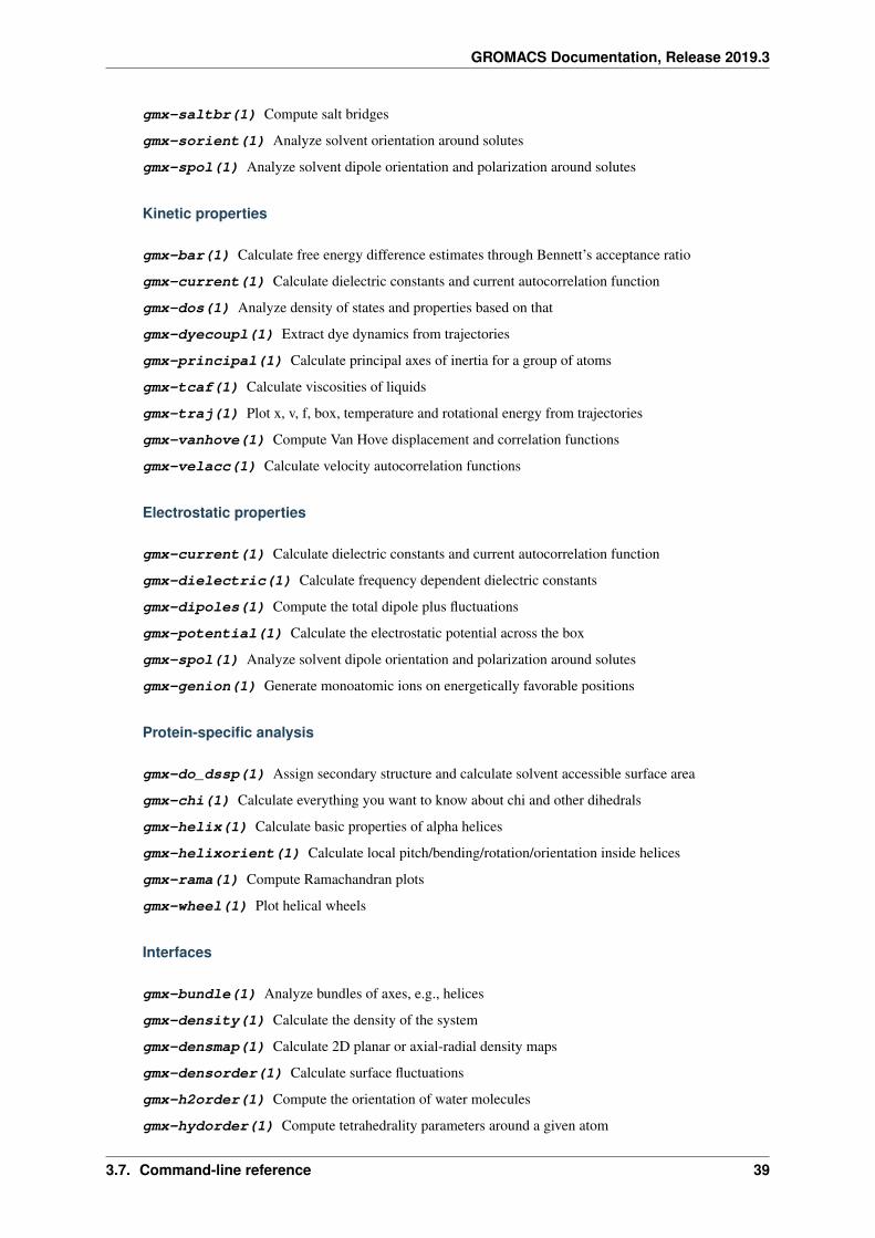
GROMACS Documentation, Release 2019.3
gmx-saltbr(1) Compute salt bridges
gmx-sorient(1) Analyze solvent orientation around solutes
gmx-spol(1) Analyze solvent dipole orientation and polarization around solutes
Kinetic properties
gmx-bar(1) Calculate free energy difference estimates through Bennett’s acceptance ratio
gmx-current(1) Calculate dielectric constants and current autocorrelation function
gmx-dos(1) Analyze density of states and properties based on that
gmx-dyecoupl(1) Extract dye dynamics from trajectories
gmx-principal(1) Calculate principal axes of inertia for a group of atoms
gmx-tcaf(1) Calculate viscosities of liquids
gmx-traj(1) Plot x, v, f, box, temperature and rotational energy from trajectories
gmx-vanhove(1) Compute Van Hove displacement and correlation functions
gmx-velacc(1) Calculate velocity autocorrelation functions
Electrostatic properties
gmx-current(1) Calculate dielectric constants and current autocorrelation function
gmx-dielectric(1) Calculate frequency dependent dielectric constants
gmx-dipoles(1) Compute the total dipole plus fluctuations
gmx-potential(1) Calculate the electrostatic potential across the box
gmx-spol(1) Analyze solvent dipole orientation and polarization around solutes
gmx-genion(1) Generate monoatomic ions on energetically favorable positions
Protein-specific analysis
gmx-do_dssp(1) Assign secondary structure and calculate solvent accessible surface area
gmx-chi(1) Calculate everything you want to know about chi and other dihedrals
gmx-helix(1) Calculate basic properties of alpha helices
gmx-helixorient(1) Calculate local pitch/bending/rotation/orientation inside helices
gmx-rama(1) Compute Ramachandran plots
gmx-wheel(1) Plot helical wheels
Interfaces
gmx-bundle(1) Analyze bundles of axes, e.g., helices
gmx-density(1) Calculate the density of the system
gmx-densmap(1) Calculate 2D planar or axial-radial density maps
gmx-densorder(1) Calculate surface fluctuations
gmx-h2order(1) Compute the orientation of water molecules
gmx-hydorder(1) Compute tetrahedrality parameters around a given atom
3.7. Command-line reference 39
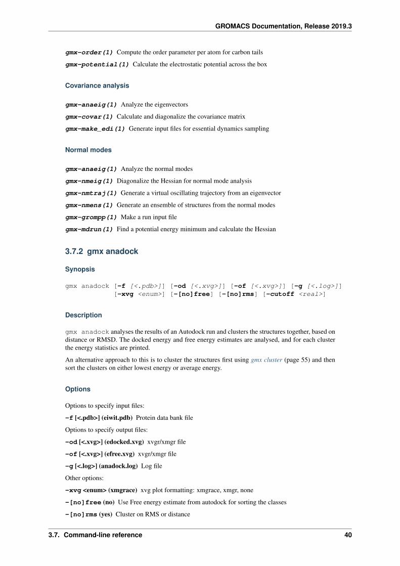
GROMACS Documentation, Release 2019.3
gmx-order(1) Compute the order parameter per atom for carbon tails
gmx-potential(1) Calculate the electrostatic potential across the box
Covariance analysis
gmx-anaeig(1) Analyze the eigenvectors
gmx-covar(1) Calculate and diagonalize the covariance matrix
gmx-make_edi(1) Generate input files for essential dynamics sampling
Normal modes
gmx-anaeig(1) Analyze the normal modes
gmx-nmeig(1) Diagonalize the Hessian for normal mode analysis
gmx-nmtraj(1) Generate a virtual oscillating trajectory from an eigenvector
gmx-nmens(1) Generate an ensemble of structures from the normal modes
gmx-grompp(1) Make a run input file
gmx-mdrun(1) Find a potential energy minimum and calculate the Hessian
3.7.2 gmx anadock
Synopsis
gmx anadock [-f [<.pdb>]] [-od [<.xvg>]] [-of [<.xvg>]] [-g [<.log>]][-xvg <enum>] [-[no]free] [-[no]rms] [-cutoff <real>]
Description
gmx anadock analyses the results of an Autodock run and clusters the structures together, based ondistance or RMSD. The docked energy and free energy estimates are analysed, and for each clusterthe energy statistics are printed.
An alternative approach to this is to cluster the structures first using gmx cluster (page 55) and thensort the clusters on either lowest energy or average energy.
Options
Options to specify input files:
-f [<.pdb>] (eiwit.pdb) Protein data bank file
Options to specify output files:
-od [<.xvg>] (edocked.xvg) xvgr/xmgr file
-of [<.xvg>] (efree.xvg) xvgr/xmgr file
-g [<.log>] (anadock.log) Log file
Other options:
-xvg <enum> (xmgrace) xvg plot formatting: xmgrace, xmgr, none
-[no]free (no) Use Free energy estimate from autodock for sorting the classes
-[no]rms (yes) Cluster on RMS or distance
3.7. Command-line reference 40
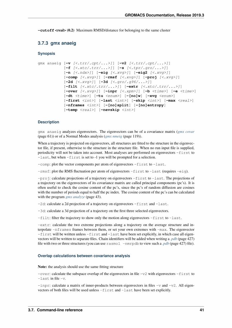
GROMACS Documentation, Release 2019.3
-cutoff <real> (0.2) Maximum RMSD/distance for belonging to the same cluster
3.7.3 gmx anaeig
Synopsis
gmx anaeig [-v [<.trr/.cpt/...>]] [-v2 [<.trr/.cpt/...>]][-f [<.xtc/.trr/...>]] [-s [<.tpr/.gro/...>]][-n [<.ndx>]] [-eig [<.xvg>]] [-eig2 [<.xvg>]][-comp [<.xvg>]] [-rmsf [<.xvg>]] [-proj [<.xvg>]][-2d [<.xvg>]] [-3d [<.gro/.g96/...>]][-filt [<.xtc/.trr/...>]] [-extr [<.xtc/.trr/...>]][-over [<.xvg>]] [-inpr [<.xpm>]] [-b <time>] [-e <time>][-dt <time>] [-tu <enum>] [-[no]w] [-xvg <enum>][-first <int>] [-last <int>] [-skip <int>] [-max <real>][-nframes <int>] [-[no]split] [-[no]entropy][-temp <real>] [-nevskip <int>]
Description
gmx anaeig analyzes eigenvectors. The eigenvectors can be of a covariance matrix (gmx covar(page 61)) or of a Normal Modes analysis (gmx nmeig (page 119)).
When a trajectory is projected on eigenvectors, all structures are fitted to the structure in the eigenvec-tor file, if present, otherwise to the structure in the structure file. When no run input file is supplied,periodicity will not be taken into account. Most analyses are performed on eigenvectors -first to-last, but when -first is set to -1 you will be prompted for a selection.
-comp: plot the vector components per atom of eigenvectors -first to -last.
-rmsf: plot the RMS fluctuation per atom of eigenvectors -first to -last (requires -eig).
-proj: calculate projections of a trajectory on eigenvectors -first to -last. The projections ofa trajectory on the eigenvectors of its covariance matrix are called principal components (pc’s). It isoften useful to check the cosine content of the pc’s, since the pc’s of random diffusion are cosineswith the number of periods equal to half the pc index. The cosine content of the pc’s can be calculatedwith the program gmx analyze (page 43).
-2d: calculate a 2d projection of a trajectory on eigenvectors -first and -last.
-3d: calculate a 3d projection of a trajectory on the first three selected eigenvectors.
-filt: filter the trajectory to show only the motion along eigenvectors -first to -last.
-extr: calculate the two extreme projections along a trajectory on the average structure and in-terpolate -nframes frames between them, or set your own extremes with -max. The eigenvector-first will be written unless -first and -last have been set explicitly, in which case all eigen-vectors will be written to separate files. Chain identifiers will be added when writing a .pdb (page 427)file with two or three structures (you can use rasmol -nmrpdb to view such a .pdb (page 427) file).
Overlap calculations between covariance analysis
Note: the analysis should use the same fitting structure
-over: calculate the subspace overlap of the eigenvectors in file -v2 with eigenvectors -first to-last in file -v.
-inpr: calculate a matrix of inner-products between eigenvectors in files -v and -v2. All eigen-vectors of both files will be used unless -first and -last have been set explicitly.
3.7. Command-line reference 41
GROMACS Documentation, Release 2019.3
When -v and -v2 are given, a single number for the overlap between the covariance matrices isgenerated. Note that the eigenvalues are by default read from the timestamp field in the eigenvectorinput files, but when -eig, or -eig2 are given, the corresponding eigenvalues are used instead. Theformulas are:
difference = sqrt(tr((sqrt(M1) - sqrt(M2))^2))normalized overlap = 1 - difference/sqrt(tr(M1) + tr(M2))
shape overlap = 1 - sqrt(tr((sqrt(M1/tr(M1)) - sqrt(M2/tr(M2)))^2))
where M1 and M2 are the two covariance matrices and tr is the trace of a matrix. The numbers areproportional to the overlap of the square root of the fluctuations. The normalized overlap is the mostuseful number, it is 1 for identical matrices and 0 when the sampled subspaces are orthogonal.
When the -entropy flag is given an entropy estimate will be computed based on the Quasiharmonicapproach and based on Schlitter’s formula.
Options
Options to specify input files:
-v [<.trr/.cpt/. . . >] (eigenvec.trr) Full precision trajectory: trr (page 431) cpt (page 421) tng(page 429)
-v2 [<.trr/.cpt/. . . >] (eigenvec2.trr) (Optional) Full precision trajectory: trr (page 431) cpt(page 421) tng (page 429)
-f [<.xtc/.trr/. . . >] (traj.xtc) (Optional) Trajectory: xtc (page 432) trr (page 431) cpt (page 421)gro (page 423) g96 (page 423) pdb (page 427) tng (page 429)
-s [<.tpr/.gro/. . . >] (topol.tpr) (Optional) Structure+mass(db): tpr (page 431) gro (page 423) g96(page 423) pdb (page 427) brk ent
-n [<.ndx>] (index.ndx) (Optional) Index file
-eig [<.xvg>] (eigenval.xvg) (Optional) xvgr/xmgr file
-eig2 [<.xvg>] (eigenval2.xvg) (Optional) xvgr/xmgr file
Options to specify output files:
-comp [<.xvg>] (eigcomp.xvg) (Optional) xvgr/xmgr file
-rmsf [<.xvg>] (eigrmsf.xvg) (Optional) xvgr/xmgr file
-proj [<.xvg>] (proj.xvg) (Optional) xvgr/xmgr file
-2d [<.xvg>] (2dproj.xvg) (Optional) xvgr/xmgr file
-3d [<.gro/.g96/. . . >] (3dproj.pdb) (Optional) Structure file: gro (page 423) g96 (page 423) pdb(page 427) brk ent esp
-filt [<.xtc/.trr/. . . >] (filtered.xtc) (Optional) Trajectory: xtc (page 432) trr (page 431) cpt(page 421) gro (page 423) g96 (page 423) pdb (page 427) tng (page 429)
-extr [<.xtc/.trr/. . . >] (extreme.pdb) (Optional) Trajectory: xtc (page 432) trr (page 431) cpt(page 421) gro (page 423) g96 (page 423) pdb (page 427) tng (page 429)
-over [<.xvg>] (overlap.xvg) (Optional) xvgr/xmgr file
-inpr [<.xpm>] (inprod.xpm) (Optional) X PixMap compatible matrix file
Other options:
-b <time> (0) Time of first frame to read from trajectory (default unit ps)
-e <time> (0) Time of last frame to read from trajectory (default unit ps)
-dt <time> (0) Only use frame when t MOD dt = first time (default unit ps)
3.7. Command-line reference 42
GROMACS Documentation, Release 2019.3
-tu <enum> (ps) Unit for time values: fs, ps, ns, us, ms, s
-[no]w (no) View output .xvg (page 434), .xpm (page 432), .eps (page 422) and .pdb (page 427)files
-xvg <enum> (xmgrace) xvg plot formatting: xmgrace, xmgr, none
-first <int> (1) First eigenvector for analysis (-1 is select)
-last <int> (-1) Last eigenvector for analysis (-1 is till the last)
-skip <int> (1) Only analyse every nr-th frame
-max <real> (0) Maximum for projection of the eigenvector on the average structure, max=0 givesthe extremes
-nframes <int> (2) Number of frames for the extremes output
-[no]split (no) Split eigenvector projections where time is zero
-[no]entropy (no) Compute entropy according to the Quasiharmonic formula or Schlitter’smethod.
-temp <real> (298.15) Temperature for entropy calculations
-nevskip <int> (6) Number of eigenvalues to skip when computing the entropy due to the quasiharmonic approximation. When you do a rotational and/or translational fit prior to the covari-ance analysis, you get 3 or 6 eigenvalues that are very close to zero, and which should not betaken into account when computing the entropy.
3.7.4 gmx analyze
Synopsis
gmx analyze [-f [<.xvg>]] [-ac [<.xvg>]] [-msd [<.xvg>]] [-cc [<.xvg>]][-dist [<.xvg>]] [-av [<.xvg>]] [-ee [<.xvg>]][-fitted [<.xvg>]] [-g [<.log>]] [-[no]w] [-xvg <enum>][-[no]time] [-b <real>] [-e <real>] [-n <int>] [-[no]d][-bw <real>] [-errbar <enum>] [-[no]integrate][-aver_start <real>] [-[no]xydy] [-[no]regression][-[no]luzar] [-temp <real>] [-fitstart <real>][-fitend <real>] [-filter <real>] [-[no]power][-[no]subav] [-[no]oneacf] [-acflen <int>][-[no]normalize] [-P <enum>] [-fitfn <enum>][-beginfit <real>] [-endfit <real>]
Description
gmx analyze reads an ASCII file and analyzes data sets. A line in the input file may start with atime (see option -time) and any number of y-values may follow. Multiple sets can also be read whenthey are separated by & (option -n); in this case only one y-value is read from each line. All linesstarting with # and @ are skipped. All analyses can also be done for the derivative of a set (option-d).
All options, except for -av and -power, assume that the points are equidistant in time.
gmx analyze always shows the average and standard deviation of each set, as well as the rela-tive deviation of the third and fourth cumulant from those of a Gaussian distribution with the samestandard deviation.
Option -ac produces the autocorrelation function(s). Be sure that the time interval between datapoints is much shorter than the time scale of the autocorrelation.
Option -cc plots the resemblance of set i with a cosine of i/2 periods. The formula is:
3.7. Command-line reference 43
GROMACS Documentation, Release 2019.3
2 (integral from 0 to T of y(t) cos(i pi t) dt)^2 / integral from 0 to T→˓of y^2(t) dt
This is useful for principal components obtained from covariance analysis, since the principal com-ponents of random diffusion are pure cosines.
Option -msd produces the mean square displacement(s).
Option -dist produces distribution plot(s).
Option -av produces the average over the sets. Error bars can be added with the option -errbar.The errorbars can represent the standard deviation, the error (assuming the points are independent) orthe interval containing 90% of the points, by discarding 5% of the points at the top and the bottom.
Option -ee produces error estimates using block averaging. A set is divided in a number of blocksand averages are calculated for each block. The error for the total average is calculated from thevariance between averages of the m blocks B_i as follows: error^2 = sum (B_i - <B>)^2 / (m*(m-1)).These errors are plotted as a function of the block size. Also an analytical block average curve isplotted, assuming that the autocorrelation is a sum of two exponentials. The analytical curve for theblock average is:
f(t) = sigma``*``sqrt(2/T ( alpha (tau_1 ((exp(-t/tau_1) - 1) tau_1/t→˓+ 1)) +
(1-alpha) (tau_2 ((exp(-t/tau_2) - 1) tau_2/t +→˓1)))),
where T is the total time. alpha, tau_1 and tau_2 are obtained by fitting f^2(t) to error^2. When theactual block average is very close to the analytical curve, the error is sigma‘‘*‘‘sqrt(2/T (a tau_1 +(1-a) tau_2)). The complete derivation is given in B. Hess, J. Chem. Phys. 116:209-217, 2002.
Option -filter prints the RMS high-frequency fluctuation of each set and over all sets with respectto a filtered average. The filter is proportional to cos(pi t/len) where t goes from -len/2 to len/2. lenis supplied with the option -filter. This filter reduces oscillations with period len/2 and len by afactor of 0.79 and 0.33 respectively.
Option -g fits the data to the function given with option -fitfn.
Option -power fits the data to b t^a, which is accomplished by fitting to a t + b on log-log scale. Allpoints after the first zero or with a negative value are ignored.
Option -luzar performs a Luzar & Chandler kinetics analysis on output from gmx hbond (page 98).The input file can be taken directly from gmx hbond -ac, and then the same result should beproduced.
Option -fitfn performs curve fitting to a number of different curves that make sense in the contextof molecular dynamics, mainly exponential curves. More information is in the manual. To check theoutput of the fitting procedure the option -fitted will print both the original data and the fittedfunction to a new data file. The fitting parameters are stored as comment in the output file.
Options
Options to specify input files:
-f [<.xvg>] (graph.xvg) xvgr/xmgr file
Options to specify output files:
-ac [<.xvg>] (autocorr.xvg) (Optional) xvgr/xmgr file
-msd [<.xvg>] (msd.xvg) (Optional) xvgr/xmgr file
-cc [<.xvg>] (coscont.xvg) (Optional) xvgr/xmgr file
-dist [<.xvg>] (distr.xvg) (Optional) xvgr/xmgr file
-av [<.xvg>] (average.xvg) (Optional) xvgr/xmgr file
3.7. Command-line reference 44
GROMACS Documentation, Release 2019.3
-ee [<.xvg>] (errest.xvg) (Optional) xvgr/xmgr file
-fitted [<.xvg>] (fitted.xvg) (Optional) xvgr/xmgr file
-g [<.log>] (fitlog.log) (Optional) Log file
Other options:
-[no]w (no) View output .xvg (page 434), .xpm (page 432), .eps (page 422) and .pdb (page 427)files
-xvg <enum> (xmgrace) xvg plot formatting: xmgrace, xmgr, none
-[no]time (yes) Expect a time in the input
-b <real> (-1) First time to read from set
-e <real> (-1) Last time to read from set
-n <int> (1) Read this number of sets separated by &
-[no]d (no) Use the derivative
-bw <real> (0.1) Binwidth for the distribution
-errbar <enum> (none) Error bars for -av: none, stddev, error, 90
-[no]integrate (no) Integrate data function(s) numerically using trapezium rule
-aver_start <real> (0) Start averaging the integral from here
-[no]xydy (no) Interpret second data set as error in the y values for integrating
-[no]regression (no) Perform a linear regression analysis on the data. If -xydy is set a secondset will be interpreted as the error bar in the Y value. Otherwise, if multiple data sets are presenta multilinear regression will be performed yielding the constant A that minimize chi^2 = (y -A_0 x_0 - A_1 x_1 - . . . - A_N x_N)^2 where now Y is the first data set in the input file andx_i the others. Do read the information at the option -time.
-[no]luzar (no) Do a Luzar and Chandler analysis on a correlation function and related as pro-duced by gmx hbond (page 98). When in addition the -xydy flag is given the second and fourthcolumn will be interpreted as errors in c(t) and n(t).
-temp <real> (298.15) Temperature for the Luzar hydrogen bonding kinetics analysis (K)
-fitstart <real> (1) Time (ps) from which to start fitting the correlation functions in order toobtain the forward and backward rate constants for HB breaking and formation
-fitend <real> (60) Time (ps) where to stop fitting the correlation functions in order to obtain theforward and backward rate constants for HB breaking and formation. Only with -gem
-filter <real> (0) Print the high-frequency fluctuation after filtering with a cosine filter of thislength
-[no]power (no) Fit data to: b t^a
-[no]subav (yes) Subtract the average before autocorrelating
-[no]oneacf (no) Calculate one ACF over all sets
-acflen <int> (-1) Length of the ACF, default is half the number of frames
-[no]normalize (yes) Normalize ACF
-P <enum> (0) Order of Legendre polynomial for ACF (0 indicates none): 0, 1, 2, 3
-fitfn <enum> (none) Fit function: none, exp, aexp, exp_exp, exp5, exp7, exp9
-beginfit <real> (0) Time where to begin the exponential fit of the correlation function
-endfit <real> (-1) Time where to end the exponential fit of the correlation function, -1 is untilthe end
3.7. Command-line reference 45
GROMACS Documentation, Release 2019.3
3.7.5 gmx angle
Synopsis
gmx angle [-f [<.xtc/.trr/...>]] [-n [<.ndx>]] [-od [<.xvg>]][-ov [<.xvg>]] [-of [<.xvg>]] [-ot [<.xvg>]] [-oh [<.xvg>]][-oc [<.xvg>]] [-or [<.trr>]] [-b <time>] [-e <time>][-dt <time>] [-[no]w] [-xvg <enum>] [-type <enum>][-[no]all] [-binwidth <real>] [-[no]periodic][-[no]chandler] [-[no]avercorr] [-acflen <int>][-[no]normalize] [-P <enum>] [-fitfn <enum>][-beginfit <real>] [-endfit <real>]
Description
gmx angle computes the angle distribution for a number of angles or dihedrals.
With option -ov, you can plot the average angle of a group of angles as a function of time. With the-all option, the first graph is the average and the rest are the individual angles.
With the -of option, gmx angle also calculates the fraction of trans dihedrals (only for dihedrals)as function of time, but this is probably only fun for a select few.
With option -oc, a dihedral correlation function is calculated.
It should be noted that the index file must contain atom triplets for angles or atom quadruplets fordihedrals. If this is not the case, the program will crash.
With option -or, a trajectory file is dumped containing cos and sin of selected dihedral angles, whichsubsequently can be used as input for a principal components analysis using gmx covar (page 61).
Option -ot plots when transitions occur between dihedral rotamers of multiplicity 3 and -oh recordsa histogram of the times between such transitions, assuming the input trajectory frames are equallyspaced in time.
Options
Options to specify input files:
-f [<.xtc/.trr/. . . >] (traj.xtc) Trajectory: xtc (page 432) trr (page 431) cpt (page 421) gro(page 423) g96 (page 423) pdb (page 427) tng (page 429)
-n [<.ndx>] (angle.ndx) Index file
Options to specify output files:
-od [<.xvg>] (angdist.xvg) xvgr/xmgr file
-ov [<.xvg>] (angaver.xvg) (Optional) xvgr/xmgr file
-of [<.xvg>] (dihfrac.xvg) (Optional) xvgr/xmgr file
-ot [<.xvg>] (dihtrans.xvg) (Optional) xvgr/xmgr file
-oh [<.xvg>] (trhisto.xvg) (Optional) xvgr/xmgr file
-oc [<.xvg>] (dihcorr.xvg) (Optional) xvgr/xmgr file
-or [<.trr>] (traj.trr) (Optional) Trajectory in portable xdr format
Other options:
-b <time> (0) Time of first frame to read from trajectory (default unit ps)
-e <time> (0) Time of last frame to read from trajectory (default unit ps)
3.7. Command-line reference 46
GROMACS Documentation, Release 2019.3
-dt <time> (0) Only use frame when t MOD dt = first time (default unit ps)
-[no]w (no) View output .xvg (page 434), .xpm (page 432), .eps (page 422) and .pdb (page 427)files
-xvg <enum> (xmgrace) xvg plot formatting: xmgrace, xmgr, none
-type <enum> (angle) Type of angle to analyse: angle, dihedral, improper, ryckaert-bellemans
-[no]all (no) Plot all angles separately in the averages file, in the order of appearance in the indexfile.
-binwidth <real> (1) binwidth (degrees) for calculating the distribution
-[no]periodic (yes) Print dihedral angles modulo 360 degrees
-[no]chandler (no) Use Chandler correlation function (N[trans] = 1, N[gauche] = 0) rather thancosine correlation function. Trans is defined as phi < -60 or phi > 60.
-[no]avercorr (no) Average the correlation functions for the individual angles/dihedrals
-acflen <int> (-1) Length of the ACF, default is half the number of frames
-[no]normalize (yes) Normalize ACF
-P <enum> (0) Order of Legendre polynomial for ACF (0 indicates none): 0, 1, 2, 3
-fitfn <enum> (none) Fit function: none, exp, aexp, exp_exp, exp5, exp7, exp9
-beginfit <real> (0) Time where to begin the exponential fit of the correlation function
-endfit <real> (-1) Time where to end the exponential fit of the correlation function, -1 is untilthe end
Known Issues
• Counting transitions only works for dihedrals with multiplicity 3
3.7.6 gmx awh
Synopsis
gmx awh [-f [<.edr>]] [-s [<.tpr>]] [-o [<.xvg>]] [-fric [<.xvg>]][-b <time>] [-e <time>] [-[no]w] [-xvg <enum>] [-skip <int>][-[no]more] [-[no]kt]
Description
gmx awh extracts AWH data from an energy file. One or two files are written per AWH bias pertime frame. The bias index, if more than one, is appended to the file, as well as the time of the frame.By default only the PMF is printed. With -more the bias, target and coordinate distributions arealso printed. With -more the bias, target and coordinate distributions are also printed, as well asthe metric sqrt(det(friction_tensor)) normalized such that the average is 1. Option -fric prints allcomponents of the friction tensor to an additional set of files.
Options
Options to specify input files:
-f [<.edr>] (ener.edr) Energy file
-s [<.tpr>] (topol.tpr) Portable xdr run input file
3.7. Command-line reference 47
GROMACS Documentation, Release 2019.3
Options to specify output files:
-o [<.xvg>] (awh.xvg) xvgr/xmgr file
-fric [<.xvg>] (friction.xvg) (Optional) xvgr/xmgr file
Other options:
-b <time> (0) Time of first frame to read from trajectory (default unit ps)
-e <time> (0) Time of last frame to read from trajectory (default unit ps)
-[no]w (no) View output .xvg (page 434), .xpm (page 432), .eps (page 422) and .pdb (page 427)files
-xvg <enum> (xmgrace) xvg plot formatting: xmgrace, xmgr, none
-skip <int> (0) Skip number of frames between data points
-[no]more (no) Print more output
-[no]kt (no) Print free energy output in units of kT instead of kJ/mol
3.7.7 gmx bar
Synopsis
gmx bar [-f [<.xvg> [...]]] [-g [<.edr> [...]]] [-o [<.xvg>]][-oi [<.xvg>]] [-oh [<.xvg>]] [-[no]w] [-xvg <enum>][-b <real>] [-e <real>] [-temp <real>] [-prec <int>][-nbmin <int>] [-nbmax <int>] [-nbin <int>] [-[no]extp]
Description
gmx bar calculates free energy difference estimates through Bennett’s acceptance ratio method(BAR). It also automatically adds series of individual free energies obtained with BAR into a com-bined free energy estimate.
Every individual BAR free energy difference relies on two simulations at different states: say stateA and state B, as controlled by a parameter, lambda (see the .mdp (page 425) parameter init_-lambda). The BAR method calculates a ratio of weighted average of the Hamiltonian differenceof state B given state A and vice versa. The energy differences to the other state must be calculatedexplicitly during the simulation. This can be done with the .mdp (page 425) option foreign_-lambda.
Input option -f expects multiple dhdl.xvg files. Two types of input files are supported:
• Files with more than one y-value. The files should have columns with dH/dlambda and Delta-lambda. The lambda values are inferred from the legends: lambda of the simulation from thelegend of dH/dlambda and the foreign lambda values from the legends of Delta H
• Files with only one y-value. Using the -extp option for these files, it is assumed that the y-valueis dH/dlambda and that the Hamiltonian depends linearly on lambda. The lambda value of thesimulation is inferred from the subtitle (if present), otherwise from a number in the subdirectoryin the file name.
The lambda of the simulation is parsed from dhdl.xvg file’s legend containing the string ‘dH’, theforeign lambda values from the legend containing the capitalized letters ‘D’ and ‘H’. The temperatureis parsed from the legend line containing ‘T =’.
The input option -g expects multiple .edr (page 422) files. These can contain either lists of energydifferences (see the .mdp (page 425) option separate_dhdl_file), or a series of histograms(see the .mdp (page 425) options dh_hist_size and dh_hist_spacing). The temperatureand lambda values are automatically deduced from the ener.edr file.
3.7. Command-line reference 48
GROMACS Documentation, Release 2019.3
In addition to the .mdp (page 425) option foreign_lambda, the energy difference can also beextrapolated from the dH/dlambda values. This is done with the‘‘-extp‘‘ option, which assumes thatthe system’s Hamiltonian depends linearly on lambda, which is not normally the case.
The free energy estimates are determined using BAR with bisection, with the precision of the outputset with -prec. An error estimate taking into account time correlations is made by splitting the datainto blocks and determining the free energy differences over those blocks and assuming the blocksare independent. The final error estimate is determined from the average variance over 5 blocks. Arange of block numbers for error estimation can be provided with the options -nbmin and -nbmax.
gmx bar tries to aggregate samples with the same ‘native’ and ‘foreign’ lambda values, but alwaysassumes independent samples. Note that when aggregating energy differences/derivatives with differ-ent sampling intervals, this is almost certainly not correct. Usually subsequent energies are correlatedand different time intervals mean different degrees of correlation between samples.
The results are split in two parts: the last part contains the final results in kJ/mol, together with theerror estimate for each part and the total. The first part contains detailed free energy difference esti-mates and phase space overlap measures in units of kT (together with their computed error estimate).The printed values are:
• lam_A: the lambda values for point A.
• lam_B: the lambda values for point B.
• DG: the free energy estimate.
• s_A: an estimate of the relative entropy of B in A.
• s_B: an estimate of the relative entropy of A in B.
• stdev: an estimate expected per-sample standard deviation.
The relative entropy of both states in each other’s ensemble can be interpreted as a measure of phasespace overlap: the relative entropy s_A of the work samples of lambda_B in the ensemble of lambda_-A (and vice versa for s_B), is a measure of the ‘distance’ between Boltzmann distributions of the twostates, that goes to zero for identical distributions. See Wu & Kofke, J. Chem. Phys. 123 084109(2005) for more information.
The estimate of the expected per-sample standard deviation, as given in Bennett’s original BAR paper:Bennett, J. Comp. Phys. 22, p 245 (1976). Eq. 10 therein gives an estimate of the quality of sampling(not directly of the actual statistical error, because it assumes independent samples).
To get a visual estimate of the phase space overlap, use the -oh option to write series of histograms,together with the -nbin option.
Options
Options to specify input files:
-f [<.xvg> [. . . ]] (dhdl.xvg) (Optional) xvgr/xmgr file
-g [<.edr> [. . . ]] (ener.edr) (Optional) Energy file
Options to specify output files:
-o [<.xvg>] (bar.xvg) (Optional) xvgr/xmgr file
-oi [<.xvg>] (barint.xvg) (Optional) xvgr/xmgr file
-oh [<.xvg>] (histogram.xvg) (Optional) xvgr/xmgr file
Other options:
-[no]w (no) View output .xvg (page 434), .xpm (page 432), .eps (page 422) and .pdb (page 427)files
-xvg <enum> (xmgrace) xvg plot formatting: xmgrace, xmgr, none
3.7. Command-line reference 49
GROMACS Documentation, Release 2019.3
-b <real> (0) Begin time for BAR
-e <real> (-1) End time for BAR
-temp <real> (-1) Temperature (K)
-prec <int> (2) The number of digits after the decimal point
-nbmin <int> (5) Minimum number of blocks for error estimation
-nbmax <int> (5) Maximum number of blocks for error estimation
-nbin <int> (100) Number of bins for histogram output
-[no]extp (no) Whether to linearly extrapolate dH/dl values to use as energies
3.7.8 gmx bundle
Synopsis
gmx bundle [-f [<.xtc/.trr/...>]] [-s [<.tpr/.gro/...>]] [-n [<.ndx>]][-ol [<.xvg>]] [-od [<.xvg>]] [-oz [<.xvg>]][-ot [<.xvg>]] [-otr [<.xvg>]] [-otl [<.xvg>]][-ok [<.xvg>]] [-okr [<.xvg>]] [-okl [<.xvg>]][-oa [<.pdb>]] [-b <time>] [-e <time>] [-dt <time>][-tu <enum>] [-xvg <enum>] [-na <int>] [-[no]z]
Description
gmx bundle analyzes bundles of axes. The axes can be for instance helix axes. The program readstwo index groups and divides both of them in -na parts. The centers of mass of these parts define thetops and bottoms of the axes. Several quantities are written to file: the axis length, the distance andthe z-shift of the axis mid-points with respect to the average center of all axes, the total tilt, the radialtilt and the lateral tilt with respect to the average axis.
With options -ok, -okr and -okl the total, radial and lateral kinks of the axes are plotted. An extraindex group of kink atoms is required, which is also divided into -na parts. The kink angle is definedas the angle between the kink-top and the bottom-kink vectors.
With option -oa the top, mid (or kink when -ok is set) and bottom points of each axis are writtento a .pdb (page 427) file each frame. The residue numbers correspond to the axis numbers. Whenviewing this file with Rasmol, use the command line option -nmrpdb, and type set axis trueto display the reference axis.
Options
Options to specify input files:
-f [<.xtc/.trr/. . . >] (traj.xtc) Trajectory: xtc (page 432) trr (page 431) cpt (page 421) gro(page 423) g96 (page 423) pdb (page 427) tng (page 429)
-s [<.tpr/.gro/. . . >] (topol.tpr) Structure+mass(db): tpr (page 431) gro (page 423) g96 (page 423)pdb (page 427) brk ent
-n [<.ndx>] (index.ndx) (Optional) Index file
Options to specify output files:
-ol [<.xvg>] (bun_len.xvg) xvgr/xmgr file
-od [<.xvg>] (bun_dist.xvg) xvgr/xmgr file
-oz [<.xvg>] (bun_z.xvg) xvgr/xmgr file
3.7. Command-line reference 50

GROMACS Documentation, Release 2019.3
-ot [<.xvg>] (bun_tilt.xvg) xvgr/xmgr file
-otr [<.xvg>] (bun_tiltr.xvg) xvgr/xmgr file
-otl [<.xvg>] (bun_tiltl.xvg) xvgr/xmgr file
-ok [<.xvg>] (bun_kink.xvg) (Optional) xvgr/xmgr file
-okr [<.xvg>] (bun_kinkr.xvg) (Optional) xvgr/xmgr file
-okl [<.xvg>] (bun_kinkl.xvg) (Optional) xvgr/xmgr file
-oa [<.pdb>] (axes.pdb) (Optional) Protein data bank file
Other options:
-b <time> (0) Time of first frame to read from trajectory (default unit ps)
-e <time> (0) Time of last frame to read from trajectory (default unit ps)
-dt <time> (0) Only use frame when t MOD dt = first time (default unit ps)
-tu <enum> (ps) Unit for time values: fs, ps, ns, us, ms, s
-xvg <enum> (xmgrace) xvg plot formatting: xmgrace, xmgr, none
-na <int> (0) Number of axes
-[no]z (no) Use the z-axis as reference instead of the average axis
3.7.9 gmx check
Synopsis
gmx check [-f [<.xtc/.trr/...>]] [-f2 [<.xtc/.trr/...>]] [-s1 [<.tpr>]][-s2 [<.tpr>]] [-c [<.tpr/.gro/...>]] [-e [<.edr>]][-e2 [<.edr>]] [-n [<.ndx>]] [-m [<.tex>]] [-vdwfac <real>][-bonlo <real>] [-bonhi <real>] [-[no]rmsd] [-tol <real>][-abstol <real>] [-[no]ab] [-lastener <string>]
Description
gmx check reads a trajectory (.tng (page 429), .trr (page 431) or .xtc (page 432)), an energy file(.edr (page 422)) or an index file (.ndx (page 426)) and prints out useful information about them.
Option -c checks for presence of coordinates, velocities and box in the file, for close contacts (smallerthan -vdwfac and not bonded, i.e. not between -bonlo and -bonhi, all relative to the sum ofboth Van der Waals radii) and atoms outside the box (these may occur often and are no problem). Ifvelocities are present, an estimated temperature will be calculated from them.
If an index file, is given its contents will be summarized.
If both a trajectory and a .tpr (page 431) file are given (with -s1) the program will check whetherthe bond lengths defined in the tpr file are indeed correct in the trajectory. If not you may have non-matching files due to e.g. deshuffling or due to problems with virtual sites. With these flags, gmxcheck provides a quick check for such problems.
The program can compare two run input (.tpr (page 431)) files when both -s1 and -s2 are supplied.When comparing run input files this way, the default relative tolerance is reduced to 0.000001 andthe absolute tolerance set to zero to find any differences not due to minor compiler optimizationdifferences, although you can of course still set any other tolerances through the options. Similarlya pair of trajectory files can be compared (using the -f2 option), or a pair of energy files (using the-e2 option).
For free energy simulations the A and B state topology from one run input file can be compared withoptions -s1 and -ab.
3.7. Command-line reference 51
GROMACS Documentation, Release 2019.3
Options
Options to specify input files:
-f [<.xtc/.trr/. . . >] (traj.xtc) (Optional) Trajectory: xtc (page 432) trr (page 431) cpt (page 421)gro (page 423) g96 (page 423) pdb (page 427) tng (page 429)
-f2 [<.xtc/.trr/. . . >] (traj.xtc) (Optional) Trajectory: xtc (page 432) trr (page 431) cpt (page 421)gro (page 423) g96 (page 423) pdb (page 427) tng (page 429)
-s1 [<.tpr>] (top1.tpr) (Optional) Portable xdr run input file
-s2 [<.tpr>] (top2.tpr) (Optional) Portable xdr run input file
-c [<.tpr/.gro/. . . >] (topol.tpr) (Optional) Structure+mass(db): tpr (page 431) gro (page 423) g96(page 423) pdb (page 427) brk ent
-e [<.edr>] (ener.edr) (Optional) Energy file
-e2 [<.edr>] (ener2.edr) (Optional) Energy file
-n [<.ndx>] (index.ndx) (Optional) Index file
Options to specify output files:
-m [<.tex>] (doc.tex) (Optional) LaTeX file
Other options:
-vdwfac <real> (0.8) Fraction of sum of VdW radii used as warning cutoff
-bonlo <real> (0.4) Min. fract. of sum of VdW radii for bonded atoms
-bonhi <real> (0.7) Max. fract. of sum of VdW radii for bonded atoms
-[no]rmsd (no) Print RMSD for x, v and f
-tol <real> (0.001) Relative tolerance for comparing real values defined as 2*(a-b)/(|a|+|b|)
-abstol <real> (0.001) Absolute tolerance, useful when sums are close to zero.
-[no]ab (no) Compare the A and B topology from one file
-lastener <string> Last energy term to compare (if not given all are tested). It makes sense togo up until the Pressure.
3.7.10 gmx chi
Synopsis
gmx chi [-s [<.gro/.g96/...>]] [-f [<.xtc/.trr/...>]] [-ss [<.dat>]][-o [<.xvg>]] [-p [<.pdb>]] [-jc [<.xvg>]] [-corr [<.xvg>]][-g [<.log>]] [-ot [<.xvg>]] [-oh [<.xvg>]] [-rt [<.xvg>]][-cp [<.xvg>]] [-b <time>] [-e <time>] [-dt <time>] [-[no]w][-xvg <enum>] [-r0 <int>] [-[no]phi] [-[no]psi] [-[no]omega][-[no]rama] [-[no]viol] [-[no]periodic] [-[no]all] [-[no]rad][-[no]shift] [-binwidth <int>] [-core_rotamer <real>][-maxchi <enum>] [-[no]normhisto] [-[no]ramomega][-bfact <real>] [-[no]chi_prod] [-[no]HChi] [-bmax <real>][-acflen <int>] [-[no]normalize] [-P <enum>] [-fitfn <enum>][-beginfit <real>] [-endfit <real>]
3.7. Command-line reference 52
GROMACS Documentation, Release 2019.3
Description
gmx chi computes phi, psi, omega, and chi dihedrals for all your amino acid backbone andsidechains. It can compute dihedral angle as a function of time, and as histogram distributions. Thedistributions (histo-(dihedral)(RESIDUE).xvg) are cumulative over all residues of eachtype.
If option -corr is given, the program will calculate dihedral autocorrelation functions. The functionused is C(t) = <cos(chi(tau)) cos(chi(tau+t))>. The use of cosines rather than angles themselves, re-solves the problem of periodicity. (Van der Spoel & Berendsen (1997), Biophys. J. 72, 2032-2041).Separate files for each dihedral of each residue (corr(dihedral)(RESIDUE)(nresnr).xvg) are output, as well as a file containing the information for all residues (argument of -corr).
With option -all, the angles themselves as a function of time for each residue are printed to separatefiles (dihedral)(RESIDUE)(nresnr).xvg. These can be in radians or degrees.
A log file (argument -g) is also written. This contains
• information about the number of residues of each type.
• The NMR ^3J coupling constants from the Karplus equation.
• a table for each residue of the number of transitions between rotamers per nanosecond, and theorder parameter S^2 of each dihedral.
• a table for each residue of the rotamer occupancy.
All rotamers are taken as 3-fold, except for omega and chi dihedrals to planar groups (i.e. chi_2 ofaromatics, Asp and Asn; chi_3 of Glu and Gln; and chi_4 of Arg), which are 2-fold. “rotamer 0”means that the dihedral was not in the core region of each rotamer. The width of the core region canbe set with -core_rotamer
The S^2 order parameters are also output to an .xvg (page 434) file (argument -o ) and optionally asa .pdb (page 427) file with the S^2 values as B-factor (argument -p). The total number of rotamertransitions per timestep (argument -ot), the number of transitions per rotamer (argument -rt), andthe ^3J couplings (argument -jc), can also be written to .xvg (page 434) files. Note that the analysisof rotamer transitions assumes that the supplied trajectory frames are equally spaced in time.
If -chi_prod is set (and -maxchi > 0), cumulative rotamers, e.g. 1+9(chi_1-1)+3(chi_-2-1)+(chi_3-1) (if the residue has three 3-fold dihedrals and -maxchi >= 3) are calcu-lated. As before, if any dihedral is not in the core region, the rotamer is taken to be0. The occupancies of these cumulative rotamers (starting with rotamer 0) are written tothe file that is the argument of -cp, and if the -all flag is given, the rotamers as func-tions of time are written to chiproduct(RESIDUE)(nresnr).xvg and their occupancies tohisto-chiproduct(RESIDUE)(nresnr).xvg.
The option -r generates a contour plot of the average omega angle as a function of the phi and psiangles, that is, in a Ramachandran plot the average omega angle is plotted using color coding.
Options
Options to specify input files:
-s [<.gro/.g96/. . . >] (conf.gro) Structure file: gro (page 423) g96 (page 423) pdb (page 427) brkent esp tpr (page 431)
-f [<.xtc/.trr/. . . >] (traj.xtc) Trajectory: xtc (page 432) trr (page 431) cpt (page 421) gro(page 423) g96 (page 423) pdb (page 427) tng (page 429)
-ss [<.dat>] (ssdump.dat) (Optional) Generic data file
Options to specify output files:
-o [<.xvg>] (order.xvg) xvgr/xmgr file
-p [<.pdb>] (order.pdb) (Optional) Protein data bank file
3.7. Command-line reference 53
GROMACS Documentation, Release 2019.3
-jc [<.xvg>] (Jcoupling.xvg) xvgr/xmgr file
-corr [<.xvg>] (dihcorr.xvg) (Optional) xvgr/xmgr file
-g [<.log>] (chi.log) Log file
-ot [<.xvg>] (dihtrans.xvg) (Optional) xvgr/xmgr file
-oh [<.xvg>] (trhisto.xvg) (Optional) xvgr/xmgr file
-rt [<.xvg>] (restrans.xvg) (Optional) xvgr/xmgr file
-cp [<.xvg>] (chiprodhisto.xvg) (Optional) xvgr/xmgr file
Other options:
-b <time> (0) Time of first frame to read from trajectory (default unit ps)
-e <time> (0) Time of last frame to read from trajectory (default unit ps)
-dt <time> (0) Only use frame when t MOD dt = first time (default unit ps)
-[no]w (no) View output .xvg (page 434), .xpm (page 432), .eps (page 422) and .pdb (page 427)files
-xvg <enum> (xmgrace) xvg plot formatting: xmgrace, xmgr, none
-r0 <int> (1) starting residue
-[no]phi (no) Output for phi dihedral angles
-[no]psi (no) Output for psi dihedral angles
-[no]omega (no) Output for omega dihedrals (peptide bonds)
-[no]rama (no) Generate phi/psi and chi_1/chi_2 Ramachandran plots
-[no]viol (no) Write a file that gives 0 or 1 for violated Ramachandran angles
-[no]periodic (yes) Print dihedral angles modulo 360 degrees
-[no]all (no) Output separate files for every dihedral.
-[no]rad (no) in angle vs time files, use radians rather than degrees.
-[no]shift (no) Compute chemical shifts from phi/psi angles
-binwidth <int> (1) bin width for histograms (degrees)
-core_rotamer <real> (0.5) only the central -core_rotamer*(360/multiplicity) belongs toeach rotamer (the rest is assigned to rotamer 0)
-maxchi <enum> (0) calculate first ndih chi dihedrals: 0, 1, 2, 3, 4, 5, 6
-[no]normhisto (yes) Normalize histograms
-[no]ramomega (no) compute average omega as a function of phi/psi and plot it in an .xpm(page 432) plot
-bfact <real> (-1) B-factor value for .pdb (page 427) file for atoms with no calculated dihedralorder parameter
-[no]chi_prod (no) compute a single cumulative rotamer for each residue
-[no]HChi (no) Include dihedrals to sidechain hydrogens
-bmax <real> (0) Maximum B-factor on any of the atoms that make up a dihedral, for the dihedralangle to be considere in the statistics. Applies to database work where a number of X-Raystructures is analyzed. -bmax <= 0 means no limit.
-acflen <int> (-1) Length of the ACF, default is half the number of frames
-[no]normalize (yes) Normalize ACF
-P <enum> (0) Order of Legendre polynomial for ACF (0 indicates none): 0, 1, 2, 3
3.7. Command-line reference 54
GROMACS Documentation, Release 2019.3
-fitfn <enum> (none) Fit function: none, exp, aexp, exp_exp, exp5, exp7, exp9
-beginfit <real> (0) Time where to begin the exponential fit of the correlation function
-endfit <real> (-1) Time where to end the exponential fit of the correlation function, -1 is untilthe end
Known Issues
• Produces MANY output files (up to about 4 times the number of residues in the protein, twicethat if autocorrelation functions are calculated). Typically several hundred files are output.
• phi and psi dihedrals are calculated in a non-standard way, using H-N-CA-C for phi insteadof C(-)-N-CA-C, and N-CA-C-O for psi instead of N-CA-C-N(+). This causes (usually small)discrepancies with the output of other tools like gmx rama (page 133).
• -r0 option does not work properly
• Rotamers with multiplicity 2 are printed in chi.log as if they had multiplicity 3, with the 3rd(g(+)) always having probability 0
3.7.11 gmx cluster
Synopsis
gmx cluster [-f [<.xtc/.trr/...>]] [-s [<.tpr/.gro/...>]] [-n [<.ndx>]][-dm [<.xpm>]] [-om [<.xpm>]] [-o [<.xpm>]] [-g [<.log>]][-dist [<.xvg>]] [-ev [<.xvg>]] [-conv [<.xvg>]][-sz [<.xvg>]] [-tr [<.xpm>]] [-ntr [<.xvg>]][-clid [<.xvg>]] [-cl [<.xtc/.trr/...>]][-clndx [<.ndx>]] [-b <time>] [-e <time>] [-dt <time>][-tu <enum>] [-[no]w] [-xvg <enum>] [-[no]dista][-nlevels <int>] [-cutoff <real>] [-[no]fit][-max <real>] [-skip <int>] [-[no]av] [-wcl <int>][-nst <int>] [-rmsmin <real>] [-method <enum>][-minstruct <int>] [-[no]binary] [-M <int>] [-P <int>][-seed <int>] [-niter <int>] [-nrandom <int>][-kT <real>] [-[no]pbc]
Description
gmx cluster can cluster structures using several different methods. Distances between structurescan be determined from a trajectory or read from an .xpm (page 432) matrix file with the -dm option.RMS deviation after fitting or RMS deviation of atom-pair distances can be used to define the distancebetween structures.
single linkage: add a structure to a cluster when its distance to any element of the cluster is less thancutoff.
Jarvis Patrick: add a structure to a cluster when this structure and a structure in the cluster have eachother as neighbors and they have a least P neighbors in common. The neighbors of a structure are theM closest structures or all structures within cutoff.
Monte Carlo: reorder the RMSD matrix using Monte Carlo such that the order of the frames is usingthe smallest possible increments. With this it is possible to make a smooth animation going from onestructure to another with the largest possible (e.g.) RMSD between them, however the intermediatesteps should be as small as possible. Applications could be to visualize a potential of mean forceensemble of simulations or a pulling simulation. Obviously the user has to prepare the trajectory well(e.g. by not superimposing frames). The final result can be inspect visually by looking at the matrix.xpm (page 432) file, which should vary smoothly from bottom to top.
3.7. Command-line reference 55
GROMACS Documentation, Release 2019.3
diagonalization: diagonalize the RMSD matrix.
gromos: use algorithm as described in Daura et al. (Angew. Chem. Int. Ed. 1999, 38, pp 236-240).Count number of neighbors using cut-off, take structure with largest number of neighbors with allits neighbors as cluster and eliminate it from the pool of clusters. Repeat for remaining structures inpool.
When the clustering algorithm assigns each structure to exactly one cluster (single linkage, JarvisPatrick and gromos) and a trajectory file is supplied, the structure with the smallest average distanceto the others or the average structure or all structures for each cluster will be written to a trajectoryfile. When writing all structures, separate numbered files are made for each cluster.
Two output files are always written:
• -o writes the RMSD values in the upper left half of the matrix and a graphical depiction of theclusters in the lower right half When -minstruct = 1 the graphical depiction is black whentwo structures are in the same cluster. When -minstruct > 1 different colors will be used foreach cluster.
• -g writes information on the options used and a detailed list of all clusters and their members.
Additionally, a number of optional output files can be written:
• -dist writes the RMSD distribution.
• -ev writes the eigenvectors of the RMSD matrix diagonalization.
• -sz writes the cluster sizes.
• -tr writes a matrix of the number transitions between cluster pairs.
• -ntr writes the total number of transitions to or from each cluster.
• -clid writes the cluster number as a function of time.
• -clndx writes the frame numbers corresponding to the clusters to the specified index file to beread into trjconv.
• -cl writes average (with option -av) or central structure of each cluster or writes numberedfiles with cluster members for a selected set of clusters (with option -wcl, depends on -nstand -rmsmin). The center of a cluster is the structure with the smallest average RMSD fromall other structures of the cluster.
Options
Options to specify input files:
-f [<.xtc/.trr/. . . >] (traj.xtc) (Optional) Trajectory: xtc (page 432) trr (page 431) cpt (page 421)gro (page 423) g96 (page 423) pdb (page 427) tng (page 429)
-s [<.tpr/.gro/. . . >] (topol.tpr) Structure+mass(db): tpr (page 431) gro (page 423) g96 (page 423)pdb (page 427) brk ent
-n [<.ndx>] (index.ndx) (Optional) Index file
-dm [<.xpm>] (rmsd.xpm) (Optional) X PixMap compatible matrix file
Options to specify output files:
-om [<.xpm>] (rmsd-raw.xpm) X PixMap compatible matrix file
-o [<.xpm>] (rmsd-clust.xpm) X PixMap compatible matrix file
-g [<.log>] (cluster.log) Log file
-dist [<.xvg>] (rmsd-dist.xvg) (Optional) xvgr/xmgr file
-ev [<.xvg>] (rmsd-eig.xvg) (Optional) xvgr/xmgr file
-conv [<.xvg>] (mc-conv.xvg) (Optional) xvgr/xmgr file
3.7. Command-line reference 56
GROMACS Documentation, Release 2019.3
-sz [<.xvg>] (clust-size.xvg) (Optional) xvgr/xmgr file
-tr [<.xpm>] (clust-trans.xpm) (Optional) X PixMap compatible matrix file
-ntr [<.xvg>] (clust-trans.xvg) (Optional) xvgr/xmgr file
-clid [<.xvg>] (clust-id.xvg) (Optional) xvgr/xmgr file
-cl [<.xtc/.trr/. . . >] (clusters.pdb) (Optional) Trajectory: xtc (page 432) trr (page 431) cpt(page 421) gro (page 423) g96 (page 423) pdb (page 427) tng (page 429)
-clndx [<.ndx>] (clusters.ndx) (Optional) Index file
Other options:
-b <time> (0) Time of first frame to read from trajectory (default unit ps)
-e <time> (0) Time of last frame to read from trajectory (default unit ps)
-dt <time> (0) Only use frame when t MOD dt = first time (default unit ps)
-tu <enum> (ps) Unit for time values: fs, ps, ns, us, ms, s
-[no]w (no) View output .xvg (page 434), .xpm (page 432), .eps (page 422) and .pdb (page 427)files
-xvg <enum> (xmgrace) xvg plot formatting: xmgrace, xmgr, none
-[no]dista (no) Use RMSD of distances instead of RMS deviation
-nlevels <int> (40) Discretize RMSD matrix in this number of levels
-cutoff <real> (0.1) RMSD cut-off (nm) for two structures to be neighbor
-[no]fit (yes) Use least squares fitting before RMSD calculation
-max <real> (-1) Maximum level in RMSD matrix
-skip <int> (1) Only analyze every nr-th frame
-[no]av (no) Write average instead of middle structure for each cluster
-wcl <int> (0) Write the structures for this number of clusters to numbered files
-nst <int> (1) Only write all structures if more than this number of structures per cluster
-rmsmin <real> (0) minimum rms difference with rest of cluster for writing structures
-method <enum> (linkage) Method for cluster determination: linkage, jarvis-patrick, monte-carlo, diagonalization, gromos
-minstruct <int> (1) Minimum number of structures in cluster for coloring in the .xpm(page 432) file
-[no]binary (no) Treat the RMSD matrix as consisting of 0 and 1, where the cut-off is given by-cutoff
-M <int> (10) Number of nearest neighbors considered for Jarvis-Patrick algorithm, 0 is use cutoff
-P <int> (3) Number of identical nearest neighbors required to form a cluster
-seed <int> (0) Random number seed for Monte Carlo clustering algorithm (0 means generate)
-niter <int> (10000) Number of iterations for MC
-nrandom <int> (0) The first iterations for MC may be done complete random, to shuffle theframes
-kT <real> (0.001) Boltzmann weighting factor for Monte Carlo optimization (zero turns off uphillsteps)
-[no]pbc (yes) PBC check
3.7. Command-line reference 57
GROMACS Documentation, Release 2019.3
3.7.12 gmx clustsize
Synopsis
gmx clustsize [-f [<.xtc/.trr/...>]] [-s [<.tpr>]] [-n [<.ndx>]][-o [<.xpm>]] [-ow [<.xpm>]] [-nc [<.xvg>]][-mc [<.xvg>]] [-ac [<.xvg>]] [-hc [<.xvg>]][-temp [<.xvg>]] [-mcn [<.ndx>]] [-b <time>] [-e <time>][-dt <time>] [-tu <enum>] [-[no]w] [-xvg <enum>][-cut <real>] [-[no]mol] [-[no]pbc] [-nskip <int>][-nlevels <int>] [-ndf <int>] [-rgblo <vector>][-rgbhi <vector>]
Description
gmx clustsize computes the size distributions of molecular/atomic clusters in the gas phase. Theoutput is given in the form of an .xpm (page 432) file. The total number of clusters is written to an.xvg (page 434) file.
When the -mol option is given clusters will be made out of molecules rather than atoms, whichallows clustering of large molecules. In this case an index file would still contain atom numbers oryour calculation will die with a SEGV.
When velocities are present in your trajectory, the temperature of the largest cluster will be printed in aseparate .xvg (page 434) file assuming that the particles are free to move. If you are using constraints,please correct the temperature. For instance water simulated with SHAKE or SETTLE will yield atemperature that is 1.5 times too low. You can compensate for this with the -ndf option. Rememberto take the removal of center of mass motion into account.
The -mc option will produce an index file containing the atom numbers of the largest cluster.
Options
Options to specify input files:
-f [<.xtc/.trr/. . . >] (traj.xtc) Trajectory: xtc (page 432) trr (page 431) cpt (page 421) gro(page 423) g96 (page 423) pdb (page 427) tng (page 429)
-s [<.tpr>] (topol.tpr) (Optional) Portable xdr run input file
-n [<.ndx>] (index.ndx) (Optional) Index file
Options to specify output files:
-o [<.xpm>] (csize.xpm) X PixMap compatible matrix file
-ow [<.xpm>] (csizew.xpm) X PixMap compatible matrix file
-nc [<.xvg>] (nclust.xvg) xvgr/xmgr file
-mc [<.xvg>] (maxclust.xvg) xvgr/xmgr file
-ac [<.xvg>] (avclust.xvg) xvgr/xmgr file
-hc [<.xvg>] (histo-clust.xvg) xvgr/xmgr file
-temp [<.xvg>] (temp.xvg) (Optional) xvgr/xmgr file
-mcn [<.ndx>] (maxclust.ndx) (Optional) Index file
Other options:
-b <time> (0) Time of first frame to read from trajectory (default unit ps)
-e <time> (0) Time of last frame to read from trajectory (default unit ps)
3.7. Command-line reference 58
GROMACS Documentation, Release 2019.3
-dt <time> (0) Only use frame when t MOD dt = first time (default unit ps)
-tu <enum> (ps) Unit for time values: fs, ps, ns, us, ms, s
-[no]w (no) View output .xvg (page 434), .xpm (page 432), .eps (page 422) and .pdb (page 427)files
-xvg <enum> (xmgrace) xvg plot formatting: xmgrace, xmgr, none
-cut <real> (0.35) Largest distance (nm) to be considered in a cluster
-[no]mol (no) Cluster molecules rather than atoms (needs .tpr (page 431) file)
-[no]pbc (yes) Use periodic boundary conditions
-nskip <int> (0) Number of frames to skip between writing
-nlevels <int> (20) Number of levels of grey in .xpm (page 432) output
-ndf <int> (-1) Number of degrees of freedom of the entire system for temperature calculation. Ifnot set, the number of atoms times three is used.
-rgblo <vector> (1 1 0) RGB values for the color of the lowest occupied cluster size
-rgbhi <vector> (0 0 1) RGB values for the color of the highest occupied cluster size
3.7.13 gmx confrms
Synopsis
gmx confrms [-f1 [<.tpr/.gro/...>]] [-f2 [<.gro/.g96/...>]][-n1 [<.ndx>]] [-n2 [<.ndx>]] [-o [<.gro/.g96/...>]][-no [<.ndx>]] [-[no]w] [-[no]one] [-[no]mw] [-[no]pbc][-[no]fit] [-[no]name] [-[no]label] [-[no]bfac]
Description
gmx confrms computes the root mean square deviation (RMSD) of two structures after least-squares fitting the second structure on the first one. The two structures do NOT need to have thesame number of atoms, only the two index groups used for the fit need to be identical. With -nameonly matching atom names from the selected groups will be used for the fit and RMSD calculation.This can be useful when comparing mutants of a protein.
The superimposed structures are written to file. In a .pdb (page 427) file the two structures willbe written as separate models (use rasmol -nmrpdb). Also in a .pdb (page 427) file, B-factorscalculated from the atomic MSD values can be written with -bfac.
Options
Options to specify input files:
-f1 [<.tpr/.gro/. . . >] (conf1.gro) Structure+mass(db): tpr (page 431) gro (page 423) g96(page 423) pdb (page 427) brk ent
-f2 [<.gro/.g96/. . . >] (conf2.gro) Structure file: gro (page 423) g96 (page 423) pdb (page 427) brkent esp tpr (page 431)
-n1 [<.ndx>] (fit1.ndx) (Optional) Index file
-n2 [<.ndx>] (fit2.ndx) (Optional) Index file
Options to specify output files:
-o [<.gro/.g96/. . . >] (fit.pdb) Structure file: gro (page 423) g96 (page 423) pdb (page 427) brk entesp
3.7. Command-line reference 59
GROMACS Documentation, Release 2019.3
-no [<.ndx>] (match.ndx) (Optional) Index file
Other options:
-[no]w (no) View output .xvg (page 434), .xpm (page 432), .eps (page 422) and .pdb (page 427)files
-[no]one (no) Only write the fitted structure to file
-[no]mw (yes) Mass-weighted fitting and RMSD
-[no]pbc (no) Try to make molecules whole again
-[no]fit (yes) Do least squares superposition of the target structure to the reference
-[no]name (no) Only compare matching atom names
-[no]label (no) Added chain labels A for first and B for second structure
-[no]bfac (no) Output B-factors from atomic MSD values
3.7.14 gmx convert-tpr
Synopsis
gmx convert-tpr [-s [<.tpr>]] [-n [<.ndx>]] [-o [<.tpr>]][-extend <real>] [-until <real>] [-nsteps <int>][-[no]zeroq]
Description
gmx convert-tpr can edit run input files in three ways.
1. by modifying the number of steps in a run input file with options -extend, -until or -nsteps(nsteps=-1 means unlimited number of steps)
2. by creating a .tpx file for a subset of your original tpx file, which is useful when you want to removethe solvent from your .tpx file, or when you want to make e.g. a pure Calpha .tpx file. Note that youmay need to use -nsteps -1 (or similar) to get this to work. WARNING: this .tpx file is not fullyfunctional.
3. by setting the charges of a specified group to zero. This is useful when doing free energy estimatesusing the LIE (Linear Interaction Energy) method.
Options
Options to specify input files:
-s [<.tpr>] (topol.tpr) Portable xdr run input file
-n [<.ndx>] (index.ndx) (Optional) Index file
Options to specify output files:
-o [<.tpr>] (tprout.tpr) Portable xdr run input file
Other options:
-extend <real> (0) Extend runtime by this amount (ps)
-until <real> (0) Extend runtime until this ending time (ps)
-nsteps <int> (0) Change the number of steps
-[no]zeroq (no) Set the charges of a group (from the index) to zero
3.7. Command-line reference 60
GROMACS Documentation, Release 2019.3
3.7.15 gmx covar
Synopsis
gmx covar [-f [<.xtc/.trr/...>]] [-s [<.tpr/.gro/...>]] [-n [<.ndx>]][-o [<.xvg>]] [-v [<.trr/.cpt/...>]][-av [<.gro/.g96/...>]] [-l [<.log>]] [-ascii [<.dat>]][-xpm [<.xpm>]] [-xpma [<.xpm>]] [-b <time>] [-e <time>][-dt <time>] [-tu <enum>] [-xvg <enum>] [-[no]fit][-[no]ref] [-[no]mwa] [-last <int>] [-[no]pbc]
Description
gmx covar calculates and diagonalizes the (mass-weighted) covariance matrix. All structures arefitted to the structure in the structure file. When this is not a run input file periodicity will not be takeninto account. When the fit and analysis groups are identical and the analysis is non mass-weighted,the fit will also be non mass-weighted.
The eigenvectors are written to a trajectory file (-v). When the same atoms are used for the fit andthe covariance analysis, the reference structure for the fit is written first with t=-1. The average (orreference when -ref is used) structure is written with t=0, the eigenvectors are written as frameswith the eigenvector number and eigenvalue as step number and timestamp, respectively.
The eigenvectors can be analyzed with gmx anaeig (page 41).
Option -ascii writes the whole covariance matrix to an ASCII file. The order of the elements is:x1x1, x1y1, x1z1, x1x2, . . .
Option -xpm writes the whole covariance matrix to an .xpm (page 432) file.
Option -xpma writes the atomic covariance matrix to an .xpm (page 432) file, i.e. for each atom pairthe sum of the xx, yy and zz covariances is written.
Note that the diagonalization of a matrix requires memory and time that will increase at least as fastas than the square of the number of atoms involved. It is easy to run out of memory, in which case thistool will probably exit with a ‘Segmentation fault’. You should consider carefully whether a reducedset of atoms will meet your needs for lower costs.
Options
Options to specify input files:
-f [<.xtc/.trr/. . . >] (traj.xtc) Trajectory: xtc (page 432) trr (page 431) cpt (page 421) gro(page 423) g96 (page 423) pdb (page 427) tng (page 429)
-s [<.tpr/.gro/. . . >] (topol.tpr) Structure+mass(db): tpr (page 431) gro (page 423) g96 (page 423)pdb (page 427) brk ent
-n [<.ndx>] (index.ndx) (Optional) Index file
Options to specify output files:
-o [<.xvg>] (eigenval.xvg) xvgr/xmgr file
-v [<.trr/.cpt/. . . >] (eigenvec.trr) Full precision trajectory: trr (page 431) cpt (page 421) tng(page 429)
-av [<.gro/.g96/. . . >] (average.pdb) Structure file: gro (page 423) g96 (page 423) pdb (page 427)brk ent esp
-l [<.log>] (covar.log) Log file
-ascii [<.dat>] (covar.dat) (Optional) Generic data file
3.7. Command-line reference 61
GROMACS Documentation, Release 2019.3
-xpm [<.xpm>] (covar.xpm) (Optional) X PixMap compatible matrix file
-xpma [<.xpm>] (covara.xpm) (Optional) X PixMap compatible matrix file
Other options:
-b <time> (0) Time of first frame to read from trajectory (default unit ps)
-e <time> (0) Time of last frame to read from trajectory (default unit ps)
-dt <time> (0) Only use frame when t MOD dt = first time (default unit ps)
-tu <enum> (ps) Unit for time values: fs, ps, ns, us, ms, s
-xvg <enum> (xmgrace) xvg plot formatting: xmgrace, xmgr, none
-[no]fit (yes) Fit to a reference structure
-[no]ref (no) Use the deviation from the conformation in the structure file instead of from theaverage
-[no]mwa (no) Mass-weighted covariance analysis
-last <int> (-1) Last eigenvector to write away (-1 is till the last)
-[no]pbc (yes) Apply corrections for periodic boundary conditions
3.7.16 gmx current
Synopsis
gmx current [-s [<.tpr/.gro/...>]] [-n [<.ndx>]] [-f [<.xtc/.trr/...>]][-o [<.xvg>]] [-caf [<.xvg>]] [-dsp [<.xvg>]][-md [<.xvg>]] [-mj [<.xvg>]] [-mc [<.xvg>]] [-b <time>][-e <time>] [-dt <time>] [-[no]w] [-xvg <enum>][-sh <int>] [-[no]nojump] [-eps <real>] [-bfit <real>][-efit <real>] [-bvit <real>] [-evit <real>][-temp <real>]
Description
gmx current is a tool for calculating the current autocorrelation function, the correlation of therotational and translational dipole moment of the system, and the resulting static dielectric constant.To obtain a reasonable result, the index group has to be neutral. Furthermore, the routine is capableof extracting the static conductivity from the current autocorrelation function, if velocities are given.Additionally, an Einstein-Helfand fit can be used to obtain the static conductivity.
The flag -caf is for the output of the current autocorrelation function and -mc writes the correlationof the rotational and translational part of the dipole moment in the corresponding file. However, thisoption is only available for trajectories containing velocities. Options -sh and -tr are responsi-ble for the averaging and integration of the autocorrelation functions. Since averaging proceeds byshifting the starting point through the trajectory, the shift can be modified with -sh to enable thechoice of uncorrelated starting points. Towards the end, statistical inaccuracy grows and integratingthe correlation function only yields reliable values until a certain point, depending on the number offrames. The option -tr controls the region of the integral taken into account for calculating the staticdielectric constant.
Option -temp sets the temperature required for the computation of the static dielectric constant.
Option -eps controls the dielectric constant of the surrounding medium for simulations using a Re-action Field or dipole corrections of the Ewald summation (-eps=0 corresponds to tin-foil boundaryconditions).
3.7. Command-line reference 62
GROMACS Documentation, Release 2019.3
-[no]nojump unfolds the coordinates to allow free diffusion. This is required to get a continuoustranslational dipole moment, required for the Einstein-Helfand fit. The results from the fit allow thedetermination of the dielectric constant for system of charged molecules. However, it is also possibleto extract the dielectric constant from the fluctuations of the total dipole moment in folded coordinates.But this option has to be used with care, since only very short time spans fulfill the approximation thatthe density of the molecules is approximately constant and the averages are already converged. Tobe on the safe side, the dielectric constant should be calculated with the help of the Einstein-Helfandmethod for the translational part of the dielectric constant.
Options
Options to specify input files:
-s [<.tpr/.gro/. . . >] (topol.tpr) Structure+mass(db): tpr (page 431) gro (page 423) g96 (page 423)pdb (page 427) brk ent
-n [<.ndx>] (index.ndx) (Optional) Index file
-f [<.xtc/.trr/. . . >] (traj.xtc) Trajectory: xtc (page 432) trr (page 431) cpt (page 421) gro(page 423) g96 (page 423) pdb (page 427) tng (page 429)
Options to specify output files:
-o [<.xvg>] (current.xvg) xvgr/xmgr file
-caf [<.xvg>] (caf.xvg) (Optional) xvgr/xmgr file
-dsp [<.xvg>] (dsp.xvg) xvgr/xmgr file
-md [<.xvg>] (md.xvg) xvgr/xmgr file
-mj [<.xvg>] (mj.xvg) xvgr/xmgr file
-mc [<.xvg>] (mc.xvg) (Optional) xvgr/xmgr file
Other options:
-b <time> (0) Time of first frame to read from trajectory (default unit ps)
-e <time> (0) Time of last frame to read from trajectory (default unit ps)
-dt <time> (0) Only use frame when t MOD dt = first time (default unit ps)
-[no]w (no) View output .xvg (page 434), .xpm (page 432), .eps (page 422) and .pdb (page 427)files
-xvg <enum> (xmgrace) xvg plot formatting: xmgrace, xmgr, none
-sh <int> (1000) Shift of the frames for averaging the correlation functions and the mean-squaredisplacement.
-[no]nojump (yes) Removes jumps of atoms across the box.
-eps <real> (0) Dielectric constant of the surrounding medium. The value zero corresponds toinfinity (tin-foil boundary conditions).
-bfit <real> (100) Begin of the fit of the straight line to the MSD of the translational fraction ofthe dipole moment.
-efit <real> (400) End of the fit of the straight line to the MSD of the translational fraction of thedipole moment.
-bvit <real> (0.5) Begin of the fit of the current autocorrelation function to a*t^b.
-evit <real> (5) End of the fit of the current autocorrelation function to a*t^b.
-temp <real> (300) Temperature for calculating epsilon.
3.7. Command-line reference 63
GROMACS Documentation, Release 2019.3
3.7.17 gmx density
Synopsis
gmx density [-f [<.xtc/.trr/...>]] [-n [<.ndx>]] [-s [<.tpr>]][-ei [<.dat>]] [-o [<.xvg>]] [-b <time>] [-e <time>][-dt <time>] [-[no]w] [-xvg <enum>] [-d <string>][-sl <int>] [-dens <enum>] [-ng <int>] [-[no]center][-[no]symm] [-[no]relative]
Description
gmx density computes partial densities across the box, using an index file.
For the total density of NPT simulations, use gmx energy (page 84) instead.
Option -center performs the histogram binning relative to the center of an arbitrary group, inabsolute box coordinates. If you are calculating profiles along the Z axis box dimension bZ, outputwould be from -bZ/2 to bZ/2 if you center based on the entire system. Note that this behaviour haschanged in GROMACS 5.0; earlier versions merely performed a static binning in (0,bZ) and shiftedthe output. Now we compute the center for each frame and bin in (-bZ/2,bZ/2).
Option -symm symmetrizes the output around the center. This will automatically turn on -centertoo. Option -relative performs the binning in relative instead of absolute box coordinates, andscales the final output with the average box dimension along the output axis. This can be used incombination with -center.
Densities are in kg/m^3, and number densities or electron densities can also be calculated. For elec-tron densities, a file describing the number of electrons for each type of atom should be providedusing -ei. It should look like:
2atomname = nrelectronsatomname = nrelectrons
The first line contains the number of lines to read from the file. There should be one line for eachunique atom name in your system. The number of electrons for each atom is modified by its atomicpartial charge.
IMPORTANT CONSIDERATIONS FOR BILAYERS
One of the most common usage scenarios is to calculate the density of various groups across a lipidbilayer, typically with the z axis being the normal direction. For short simulations, small systems, andfixed box sizes this will work fine, but for the more general case lipid bilayers can be complicated. Thefirst problem that while both proteins and lipids have low volume compressibility, lipids have quitehigh area compressiblity. This means the shape of the box (thickness and area/lipid) will fluctuatesubstantially even for a fully relaxed system. Since GROMACS places the box between the originand positive coordinates, this in turn means that a bilayer centered in the box will move a bit up/downdue to these fluctuations, and smear out your profile. The easiest way to fix this (if you want pressurecoupling) is to use the -center option that calculates the density profile with respect to the center ofthe box. Note that you can still center on the bilayer part even if you have a complex non-symmetricsystem with a bilayer and, say, membrane proteins - then our output will simply have more values onone side of the (center) origin reference.
Even the centered calculation will lead to some smearing out the output profiles, as lipids themselvesare compressed and expanded. In most cases you probably want this (since it corresponds to macro-scopic experiments), but if you want to look at molecular details you can use the -relative optionto attempt to remove even more of the effects of volume fluctuations.
Finally, large bilayers that are not subject to a surface tension will exhibit undulatory fluctuations,where there are ‘waves’ forming in the system. This is a fundamental property of the biological
3.7. Command-line reference 64
GROMACS Documentation, Release 2019.3
system, and if you are comparing against experiments you likely want to include the undulationsmearing effect.
Options
Options to specify input files:
-f [<.xtc/.trr/. . . >] (traj.xtc) Trajectory: xtc (page 432) trr (page 431) cpt (page 421) gro(page 423) g96 (page 423) pdb (page 427) tng (page 429)
-n [<.ndx>] (index.ndx) (Optional) Index file
-s [<.tpr>] (topol.tpr) Portable xdr run input file
-ei [<.dat>] (electrons.dat) (Optional) Generic data file
Options to specify output files:
-o [<.xvg>] (density.xvg) xvgr/xmgr file
Other options:
-b <time> (0) Time of first frame to read from trajectory (default unit ps)
-e <time> (0) Time of last frame to read from trajectory (default unit ps)
-dt <time> (0) Only use frame when t MOD dt = first time (default unit ps)
-[no]w (no) View output .xvg (page 434), .xpm (page 432), .eps (page 422) and .pdb (page 427)files
-xvg <enum> (xmgrace) xvg plot formatting: xmgrace, xmgr, none
-d <string> (Z) Take the normal on the membrane in direction X, Y or Z.
-sl <int> (50) Divide the box in this number of slices.
-dens <enum> (mass) Density: mass, number, charge, electron
-ng <int> (1) Number of groups of which to compute densities.
-[no]center (no) Perform the binning relative to the center of the (changing) box. Useful forbilayers.
-[no]symm (no) Symmetrize the density along the axis, with respect to the center. Useful forbilayers.
-[no]relative (no) Use relative coordinates for changing boxes and scale output by averagedimensions.
Known Issues
• When calculating electron densities, atomnames are used instead of types. This is bad.
3.7.18 gmx densmap
Synopsis
gmx densmap [-f [<.xtc/.trr/...>]] [-s [<.tpr/.gro/...>]] [-n [<.ndx>]][-od [<.dat>]] [-o [<.xpm>]] [-b <time>] [-e <time>][-dt <time>] [-[no]w] [-bin <real>] [-aver <enum>][-xmin <real>] [-xmax <real>] [-n1 <int>] [-n2 <int>][-amax <real>] [-rmax <real>] [-[no]mirror] [-[no]sums][-unit <enum>] [-dmin <real>] [-dmax <real>]
3.7. Command-line reference 65
GROMACS Documentation, Release 2019.3
Description
gmx densmap computes 2D number-density maps. It can make planar and axial-radial densitymaps. The output .xpm (page 432) file can be visualized with for instance xv and can be converted topostscript with xpm2ps. Optionally, output can be in text form to a .dat (page 421) file with -od,instead of the usual .xpm (page 432) file with -o.
The default analysis is a 2-D number-density map for a selected group of atoms in the x-y plane. Theaveraging direction can be changed with the option -aver. When -xmin and/or -xmax are set onlyatoms that are within the limit(s) in the averaging direction are taken into account. The grid spacingis set with the option -bin. When -n1 or -n2 is non-zero, the grid size is set by this option. Boxsize fluctuations are properly taken into account.
When options -amax and -rmax are set, an axial-radial number-density map is made. Three groupsshould be supplied, the centers of mass of the first two groups define the axis, the third defines theanalysis group. The axial direction goes from -amax to +amax, where the center is defined as themidpoint between the centers of mass and the positive direction goes from the first to the secondcenter of mass. The radial direction goes from 0 to rmax or from -rmax to +rmax when the -mirroroption has been set.
The normalization of the output is set with the -unit option. The default produces a true numberdensity. Unit nm-2 leaves out the normalization for the averaging or the angular direction. Optioncount produces the count for each grid cell. When you do not want the scale in the output to gofrom zero to the maximum density, you can set the maximum with the option -dmax.
Options
Options to specify input files:
-f [<.xtc/.trr/. . . >] (traj.xtc) Trajectory: xtc (page 432) trr (page 431) cpt (page 421) gro(page 423) g96 (page 423) pdb (page 427) tng (page 429)
-s [<.tpr/.gro/. . . >] (topol.tpr) (Optional) Structure+mass(db): tpr (page 431) gro (page 423) g96(page 423) pdb (page 427) brk ent
-n [<.ndx>] (index.ndx) (Optional) Index file
Options to specify output files:
-od [<.dat>] (densmap.dat) (Optional) Generic data file
-o [<.xpm>] (densmap.xpm) X PixMap compatible matrix file
Other options:
-b <time> (0) Time of first frame to read from trajectory (default unit ps)
-e <time> (0) Time of last frame to read from trajectory (default unit ps)
-dt <time> (0) Only use frame when t MOD dt = first time (default unit ps)
-[no]w (no) View output .xvg (page 434), .xpm (page 432), .eps (page 422) and .pdb (page 427)files
-bin <real> (0.02) Grid size (nm)
-aver <enum> (z) The direction to average over: z, y, x
-xmin <real> (-1) Minimum coordinate for averaging
-xmax <real> (-1) Maximum coordinate for averaging
-n1 <int> (0) Number of grid cells in the first direction
-n2 <int> (0) Number of grid cells in the second direction
-amax <real> (0) Maximum axial distance from the center
3.7. Command-line reference 66
GROMACS Documentation, Release 2019.3
-rmax <real> (0) Maximum radial distance
-[no]mirror (no) Add the mirror image below the axial axis
-[no]sums (no) Print density sums (1D map) to stdout
-unit <enum> (nm-3) Unit for the output: nm-3, nm-2, count
-dmin <real> (0) Minimum density in output
-dmax <real> (0) Maximum density in output (0 means calculate it)
3.7.19 gmx densorder
Synopsis
gmx densorder [-s [<.tpr>]] [-f [<.xtc/.trr/...>]] [-n [<.ndx>]][-o [<.dat>]] [-or [<.out> [...]]] [-og [<.xpm> [...]]][-Spect [<.out> [...]]] [-b <time>] [-e <time>][-dt <time>] [-[no]w] [-[no]1d] [-bw <real>][-bwn <real>] [-order <int>] [-axis <string>][-method <enum>] [-d1 <real>] [-d2 <real>][-tblock <int>] [-nlevel <int>]
Description
gmx densorder reduces a two-phase density distribution along an axis, computed over a MDtrajectory, to 2D surfaces fluctuating in time, by a fit to a functional profile for interfacial densities. Atime-averaged spatial representation of the interfaces can be output with the option -tavg.
Options
Options to specify input files:
-s [<.tpr>] (topol.tpr) Portable xdr run input file
-f [<.xtc/.trr/. . . >] (traj.xtc) Trajectory: xtc (page 432) trr (page 431) cpt (page 421) gro(page 423) g96 (page 423) pdb (page 427) tng (page 429)
-n [<.ndx>] (index.ndx) Index file
Options to specify output files:
-o [<.dat>] (Density4D.dat) (Optional) Generic data file
-or [<.out> [. . . ]] (hello.out) (Optional) Generic output file
-og [<.xpm> [. . . ]] (interface.xpm) (Optional) X PixMap compatible matrix file
-Spect [<.out> [. . . ]] (intfspect.out) (Optional) Generic output file
Other options:
-b <time> (0) Time of first frame to read from trajectory (default unit ps)
-e <time> (0) Time of last frame to read from trajectory (default unit ps)
-dt <time> (0) Only use frame when t MOD dt = first time (default unit ps)
-[no]w (no) View output .xvg (page 434), .xpm (page 432), .eps (page 422) and .pdb (page 427)files
-[no]1d (no) Pseudo-1d interface geometry
-bw <real> (0.2) Binwidth of density distribution tangential to interface
3.7. Command-line reference 67
GROMACS Documentation, Release 2019.3
-bwn <real> (0.05) Binwidth of density distribution normal to interface
-order <int> (0) Order of Gaussian filter, order 0 equates to NO filtering
-axis <string> (Z) Axis Direction - X, Y or Z
-method <enum> (bisect) Interface location method: bisect, functional
-d1 <real> (0) Bulk density phase 1 (at small z)
-d2 <real> (1000) Bulk density phase 2 (at large z)
-tblock <int> (100) Number of frames in one time-block average
-nlevel <int> (100) Number of Height levels in 2D - XPixMaps
3.7.20 gmx dielectric
Synopsis
gmx dielectric [-f [<.xvg>]] [-d [<.xvg>]] [-o [<.xvg>]] [-c [<.xvg>]][-b <time>] [-e <time>] [-dt <time>] [-[no]w][-xvg <enum>] [-[no]x1] [-eint <real>] [-bfit <real>][-efit <real>] [-tail <real>] [-A <real>] [-tau1 <real>][-tau2 <real>] [-eps0 <real>] [-epsRF <real>][-fix <int>] [-ffn <enum>] [-nsmooth <int>]
Description
gmx dielectric calculates frequency dependent dielectric constants from the autocorrelationfunction of the total dipole moment in your simulation. This ACF can be generated by gmx dipoles(page 69). The functional forms of the available functions are:
• One parameter: y = exp(-a_1 x),
• Two parameters: y = a_2 exp(-a_1 x),
• Three parameters: y = a_2 exp(-a_1 x) + (1 - a_2) exp(-a_3 x).
Start values for the fit procedure can be given on the command line. It is also possible to fix parametersat their start value, use -fix with the number of the parameter you want to fix.
Three output files are generated, the first contains the ACF, an exponential fit to it with 1, 2 or 3parameters, and the numerical derivative of the combination data/fit. The second file contains the realand imaginary parts of the frequency-dependent dielectric constant, the last gives a plot known as theCole-Cole plot, in which the imaginary component is plotted as a function of the real component. Fora pure exponential relaxation (Debye relaxation) the latter plot should be one half of a circle.
Options
Options to specify input files:
-f [<.xvg>] (dipcorr.xvg) xvgr/xmgr file
Options to specify output files:
-d [<.xvg>] (deriv.xvg) xvgr/xmgr file
-o [<.xvg>] (epsw.xvg) xvgr/xmgr file
-c [<.xvg>] (cole.xvg) xvgr/xmgr file
Other options:
-b <time> (0) Time of first frame to read from trajectory (default unit ps)
3.7. Command-line reference 68
GROMACS Documentation, Release 2019.3
-e <time> (0) Time of last frame to read from trajectory (default unit ps)
-dt <time> (0) Only use frame when t MOD dt = first time (default unit ps)
-[no]w (no) View output .xvg (page 434), .xpm (page 432), .eps (page 422) and .pdb (page 427)files
-xvg <enum> (xmgrace) xvg plot formatting: xmgrace, xmgr, none
-[no]x1 (yes) use first column as x-axis rather than first data set
-eint <real> (5) Time to end the integration of the data and start to use the fit
-bfit <real> (5) Begin time of fit
-efit <real> (500) End time of fit
-tail <real> (500) Length of function including data and tail from fit
-A <real> (0.5) Start value for fit parameter A
-tau1 <real> (10) Start value for fit parameter tau1
-tau2 <real> (1) Start value for fit parameter tau2
-eps0 <real> (80) epsilon0 of your liquid
-epsRF <real> (78.5) epsilon of the reaction field used in your simulation. A value of 0 meansinfinity.
-fix <int> (0) Fix parameters at their start values, A (2), tau1 (1), or tau2 (4)
-ffn <enum> (none) Fit function: none, exp, aexp, exp_exp, exp5, exp7, exp9
-nsmooth <int> (3) Number of points for smoothing
3.7.21 gmx dipoles
Synopsis
gmx dipoles [-en [<.edr>]] [-f [<.xtc/.trr/...>]] [-s [<.tpr>]][-n [<.ndx>]] [-o [<.xvg>]] [-eps [<.xvg>]] [-a [<.xvg>]][-d [<.xvg>]] [-c [<.xvg>]] [-g [<.xvg>]][-adip [<.xvg>]] [-dip3d [<.xvg>]] [-cos [<.xvg>]][-cmap [<.xpm>]] [-slab [<.xvg>]] [-b <time>] [-e <time>][-dt <time>] [-[no]w] [-xvg <enum>] [-mu <real>][-mumax <real>] [-epsilonRF <real>] [-skip <int>][-temp <real>] [-corr <enum>] [-[no]pairs] [-[no]quad][-ncos <int>] [-axis <string>] [-sl <int>][-gkratom <int>] [-gkratom2 <int>] [-rcmax <real>][-[no]phi] [-nlevels <int>] [-ndegrees <int>][-acflen <int>] [-[no]normalize] [-P <enum>][-fitfn <enum>] [-beginfit <real>] [-endfit <real>]
Description
gmx dipoles computes the total dipole plus fluctuations of a simulation system. From this youcan compute e.g. the dielectric constant for low-dielectric media. For molecules with a net charge,the net charge is subtracted at center of mass of the molecule.
The file Mtot.xvg contains the total dipole moment of a frame, the components as well as thenorm of the vector. The file aver.xvg contains <|mu|^2> and |<mu>|^2 during the simulation. Thefile dipdist.xvg contains the distribution of dipole moments during the simulation The value of-mumax is used as the highest value in the distribution graph.
3.7. Command-line reference 69
GROMACS Documentation, Release 2019.3
Furthermore, the dipole autocorrelation function will be computed when option -corr is used. Theoutput file name is given with the -c option. The correlation functions can be averaged over allmolecules (mol), plotted per molecule separately (molsep) or it can be computed over the totaldipole moment of the simulation box (total).
Option -g produces a plot of the distance dependent Kirkwood G-factor, as well as the average cosineof the angle between the dipoles as a function of the distance. The plot also includes gOO and hOOaccording to Nymand & Linse, J. Chem. Phys. 112 (2000) pp 6386-6395. In the same plot, wealso include the energy per scale computed by taking the inner product of the dipoles divided by thedistance to the third power.
EXAMPLES
gmx dipoles -corr mol -P 1 -o dip_sqr -mu 2.273 -mumax 5.0
This will calculate the autocorrelation function of the molecular dipoles using a first order Legendrepolynomial of the angle of the dipole vector and itself a time t later. For this calculation 1001 frameswill be used. Further, the dielectric constant will be calculated using an -epsilonRF of infinity(default), temperature of 300 K (default) and an average dipole moment of the molecule of 2.273(SPC). For the distribution function a maximum of 5.0 will be used.
Options
Options to specify input files:
-en [<.edr>] (ener.edr) (Optional) Energy file
-f [<.xtc/.trr/. . . >] (traj.xtc) Trajectory: xtc (page 432) trr (page 431) cpt (page 421) gro(page 423) g96 (page 423) pdb (page 427) tng (page 429)
-s [<.tpr>] (topol.tpr) Portable xdr run input file
-n [<.ndx>] (index.ndx) (Optional) Index file
Options to specify output files:
-o [<.xvg>] (Mtot.xvg) xvgr/xmgr file
-eps [<.xvg>] (epsilon.xvg) xvgr/xmgr file
-a [<.xvg>] (aver.xvg) xvgr/xmgr file
-d [<.xvg>] (dipdist.xvg) xvgr/xmgr file
-c [<.xvg>] (dipcorr.xvg) (Optional) xvgr/xmgr file
-g [<.xvg>] (gkr.xvg) (Optional) xvgr/xmgr file
-adip [<.xvg>] (adip.xvg) (Optional) xvgr/xmgr file
-dip3d [<.xvg>] (dip3d.xvg) (Optional) xvgr/xmgr file
-cos [<.xvg>] (cosaver.xvg) (Optional) xvgr/xmgr file
-cmap [<.xpm>] (cmap.xpm) (Optional) X PixMap compatible matrix file
-slab [<.xvg>] (slab.xvg) (Optional) xvgr/xmgr file
Other options:
-b <time> (0) Time of first frame to read from trajectory (default unit ps)
-e <time> (0) Time of last frame to read from trajectory (default unit ps)
-dt <time> (0) Only use frame when t MOD dt = first time (default unit ps)
-[no]w (no) View output .xvg (page 434), .xpm (page 432), .eps (page 422) and .pdb (page 427)files
-xvg <enum> (xmgrace) xvg plot formatting: xmgrace, xmgr, none
3.7. Command-line reference 70
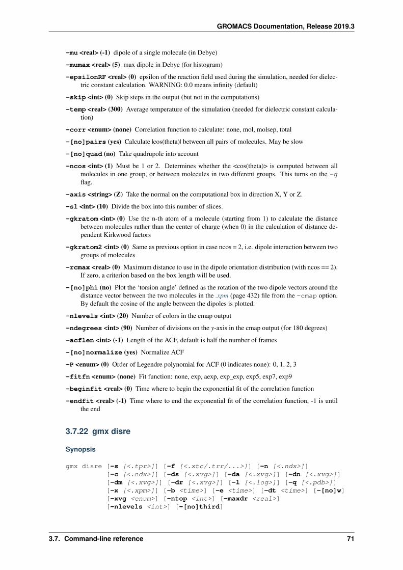
GROMACS Documentation, Release 2019.3
-mu <real> (-1) dipole of a single molecule (in Debye)
-mumax <real> (5) max dipole in Debye (for histogram)
-epsilonRF <real> (0) epsilon of the reaction field used during the simulation, needed for dielec-tric constant calculation. WARNING: 0.0 means infinity (default)
-skip <int> (0) Skip steps in the output (but not in the computations)
-temp <real> (300) Average temperature of the simulation (needed for dielectric constant calcula-tion)
-corr <enum> (none) Correlation function to calculate: none, mol, molsep, total
-[no]pairs (yes) Calculate |cos(theta)| between all pairs of molecules. May be slow
-[no]quad (no) Take quadrupole into account
-ncos <int> (1) Must be 1 or 2. Determines whether the <cos(theta)> is computed between allmolecules in one group, or between molecules in two different groups. This turns on the -gflag.
-axis <string> (Z) Take the normal on the computational box in direction X, Y or Z.
-sl <int> (10) Divide the box into this number of slices.
-gkratom <int> (0) Use the n-th atom of a molecule (starting from 1) to calculate the distancebetween molecules rather than the center of charge (when 0) in the calculation of distance de-pendent Kirkwood factors
-gkratom2 <int> (0) Same as previous option in case ncos = 2, i.e. dipole interaction between twogroups of molecules
-rcmax <real> (0) Maximum distance to use in the dipole orientation distribution (with ncos == 2).If zero, a criterion based on the box length will be used.
-[no]phi (no) Plot the ‘torsion angle’ defined as the rotation of the two dipole vectors around thedistance vector between the two molecules in the .xpm (page 432) file from the -cmap option.By default the cosine of the angle between the dipoles is plotted.
-nlevels <int> (20) Number of colors in the cmap output
-ndegrees <int> (90) Number of divisions on the y-axis in the cmap output (for 180 degrees)
-acflen <int> (-1) Length of the ACF, default is half the number of frames
-[no]normalize (yes) Normalize ACF
-P <enum> (0) Order of Legendre polynomial for ACF (0 indicates none): 0, 1, 2, 3
-fitfn <enum> (none) Fit function: none, exp, aexp, exp_exp, exp5, exp7, exp9
-beginfit <real> (0) Time where to begin the exponential fit of the correlation function
-endfit <real> (-1) Time where to end the exponential fit of the correlation function, -1 is untilthe end
3.7.22 gmx disre
Synopsis
gmx disre [-s [<.tpr>]] [-f [<.xtc/.trr/...>]] [-n [<.ndx>]][-c [<.ndx>]] [-ds [<.xvg>]] [-da [<.xvg>]] [-dn [<.xvg>]][-dm [<.xvg>]] [-dr [<.xvg>]] [-l [<.log>]] [-q [<.pdb>]][-x [<.xpm>]] [-b <time>] [-e <time>] [-dt <time>] [-[no]w][-xvg <enum>] [-ntop <int>] [-maxdr <real>][-nlevels <int>] [-[no]third]
3.7. Command-line reference 71
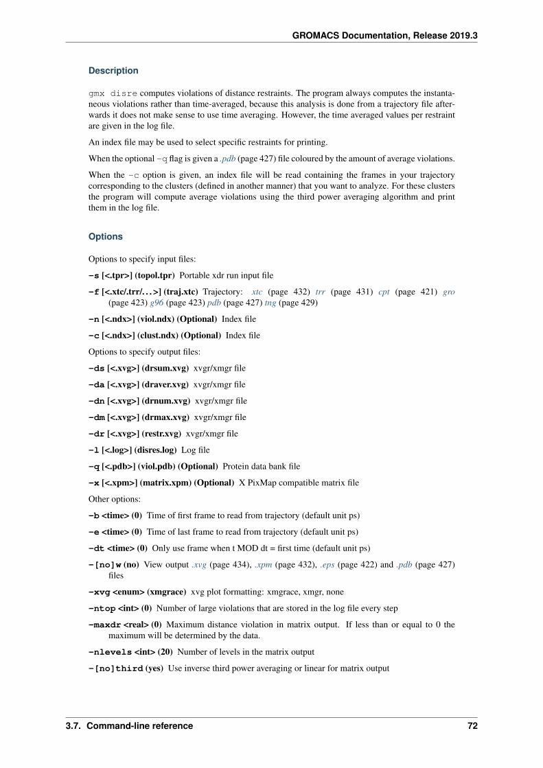
GROMACS Documentation, Release 2019.3
Description
gmx disre computes violations of distance restraints. The program always computes the instanta-neous violations rather than time-averaged, because this analysis is done from a trajectory file after-wards it does not make sense to use time averaging. However, the time averaged values per restraintare given in the log file.
An index file may be used to select specific restraints for printing.
When the optional -q flag is given a .pdb (page 427) file coloured by the amount of average violations.
When the -c option is given, an index file will be read containing the frames in your trajectorycorresponding to the clusters (defined in another manner) that you want to analyze. For these clustersthe program will compute average violations using the third power averaging algorithm and printthem in the log file.
Options
Options to specify input files:
-s [<.tpr>] (topol.tpr) Portable xdr run input file
-f [<.xtc/.trr/. . . >] (traj.xtc) Trajectory: xtc (page 432) trr (page 431) cpt (page 421) gro(page 423) g96 (page 423) pdb (page 427) tng (page 429)
-n [<.ndx>] (viol.ndx) (Optional) Index file
-c [<.ndx>] (clust.ndx) (Optional) Index file
Options to specify output files:
-ds [<.xvg>] (drsum.xvg) xvgr/xmgr file
-da [<.xvg>] (draver.xvg) xvgr/xmgr file
-dn [<.xvg>] (drnum.xvg) xvgr/xmgr file
-dm [<.xvg>] (drmax.xvg) xvgr/xmgr file
-dr [<.xvg>] (restr.xvg) xvgr/xmgr file
-l [<.log>] (disres.log) Log file
-q [<.pdb>] (viol.pdb) (Optional) Protein data bank file
-x [<.xpm>] (matrix.xpm) (Optional) X PixMap compatible matrix file
Other options:
-b <time> (0) Time of first frame to read from trajectory (default unit ps)
-e <time> (0) Time of last frame to read from trajectory (default unit ps)
-dt <time> (0) Only use frame when t MOD dt = first time (default unit ps)
-[no]w (no) View output .xvg (page 434), .xpm (page 432), .eps (page 422) and .pdb (page 427)files
-xvg <enum> (xmgrace) xvg plot formatting: xmgrace, xmgr, none
-ntop <int> (0) Number of large violations that are stored in the log file every step
-maxdr <real> (0) Maximum distance violation in matrix output. If less than or equal to 0 themaximum will be determined by the data.
-nlevels <int> (20) Number of levels in the matrix output
-[no]third (yes) Use inverse third power averaging or linear for matrix output
3.7. Command-line reference 72
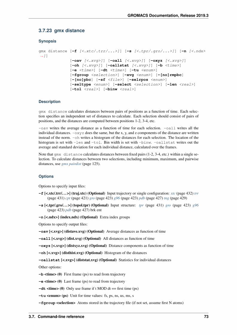
GROMACS Documentation, Release 2019.3
3.7.23 gmx distance
Synopsis
gmx distance [-f [<.xtc/.trr/...>]] [-s [<.tpr/.gro/...>]] [-n [<.ndx>→˓]]
[-oav [<.xvg>]] [-oall [<.xvg>]] [-oxyz [<.xvg>]][-oh [<.xvg>]] [-oallstat [<.xvg>]] [-b <time>][-e <time>] [-dt <time>] [-tu <enum>][-fgroup <selection>] [-xvg <enum>] [-[no]rmpbc][-[no]pbc] [-sf <file>] [-selrpos <enum>][-seltype <enum>] [-select <selection>] [-len <real>][-tol <real>] [-binw <real>]
Description
gmx distance calculates distances between pairs of positions as a function of time. Each selec-tion specifies an independent set of distances to calculate. Each selection should consist of pairs ofpositions, and the distances are computed between positions 1-2, 3-4, etc.
-oav writes the average distance as a function of time for each selection. -oall writes all theindividual distances. -oxyz does the same, but the x, y, and z components of the distance are writteninstead of the norm. -oh writes a histogram of the distances for each selection. The location of thehistogram is set with -len and -tol. Bin width is set with -binw. -oallstat writes out theaverage and standard deviation for each individual distance, calculated over the frames.
Note that gmx distance calculates distances between fixed pairs (1-2, 3-4, etc.) within a single se-lection. To calculate distances between two selections, including minimum, maximum, and pairwisedistances, use gmx pairdist (page 125).
Options
Options to specify input files:
-f [<.xtc/.trr/. . . >] (traj.xtc) (Optional) Input trajectory or single configuration: xtc (page 432) trr(page 431) cpt (page 421) gro (page 423) g96 (page 423) pdb (page 427) tng (page 429)
-s [<.tpr/.gro/. . . >] (topol.tpr) (Optional) Input structure: tpr (page 431) gro (page 423) g96(page 423) pdb (page 427) brk ent
-n [<.ndx>] (index.ndx) (Optional) Extra index groups
Options to specify output files:
-oav [<.xvg>] (distave.xvg) (Optional) Average distances as function of time
-oall [<.xvg>] (dist.xvg) (Optional) All distances as function of time
-oxyz [<.xvg>] (distxyz.xvg) (Optional) Distance components as function of time
-oh [<.xvg>] (disthist.xvg) (Optional) Histogram of the distances
-oallstat [<.xvg>] (diststat.xvg) (Optional) Statistics for individual distances
Other options:
-b <time> (0) First frame (ps) to read from trajectory
-e <time> (0) Last frame (ps) to read from trajectory
-dt <time> (0) Only use frame if t MOD dt == first time (ps)
-tu <enum> (ps) Unit for time values: fs, ps, ns, us, ms, s
-fgroup <selection> Atoms stored in the trajectory file (if not set, assume first N atoms)
3.7. Command-line reference 73
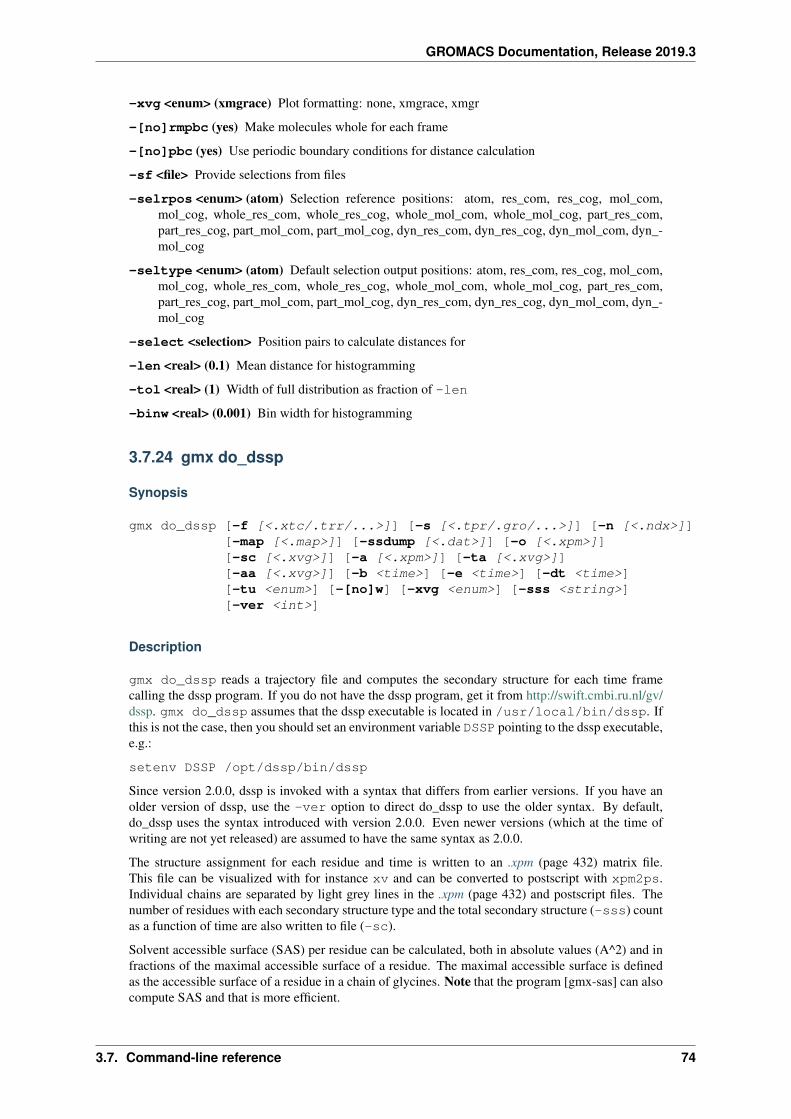
GROMACS Documentation, Release 2019.3
-xvg <enum> (xmgrace) Plot formatting: none, xmgrace, xmgr
-[no]rmpbc (yes) Make molecules whole for each frame
-[no]pbc (yes) Use periodic boundary conditions for distance calculation
-sf <file> Provide selections from files
-selrpos <enum> (atom) Selection reference positions: atom, res_com, res_cog, mol_com,mol_cog, whole_res_com, whole_res_cog, whole_mol_com, whole_mol_cog, part_res_com,part_res_cog, part_mol_com, part_mol_cog, dyn_res_com, dyn_res_cog, dyn_mol_com, dyn_-mol_cog
-seltype <enum> (atom) Default selection output positions: atom, res_com, res_cog, mol_com,mol_cog, whole_res_com, whole_res_cog, whole_mol_com, whole_mol_cog, part_res_com,part_res_cog, part_mol_com, part_mol_cog, dyn_res_com, dyn_res_cog, dyn_mol_com, dyn_-mol_cog
-select <selection> Position pairs to calculate distances for
-len <real> (0.1) Mean distance for histogramming
-tol <real> (1) Width of full distribution as fraction of -len
-binw <real> (0.001) Bin width for histogramming
3.7.24 gmx do_dssp
Synopsis
gmx do_dssp [-f [<.xtc/.trr/...>]] [-s [<.tpr/.gro/...>]] [-n [<.ndx>]][-map [<.map>]] [-ssdump [<.dat>]] [-o [<.xpm>]][-sc [<.xvg>]] [-a [<.xpm>]] [-ta [<.xvg>]][-aa [<.xvg>]] [-b <time>] [-e <time>] [-dt <time>][-tu <enum>] [-[no]w] [-xvg <enum>] [-sss <string>][-ver <int>]
Description
gmx do_dssp reads a trajectory file and computes the secondary structure for each time framecalling the dssp program. If you do not have the dssp program, get it from http://swift.cmbi.ru.nl/gv/dssp. gmx do_dssp assumes that the dssp executable is located in /usr/local/bin/dssp. Ifthis is not the case, then you should set an environment variable DSSP pointing to the dssp executable,e.g.:
setenv DSSP /opt/dssp/bin/dssp
Since version 2.0.0, dssp is invoked with a syntax that differs from earlier versions. If you have anolder version of dssp, use the -ver option to direct do_dssp to use the older syntax. By default,do_dssp uses the syntax introduced with version 2.0.0. Even newer versions (which at the time ofwriting are not yet released) are assumed to have the same syntax as 2.0.0.
The structure assignment for each residue and time is written to an .xpm (page 432) matrix file.This file can be visualized with for instance xv and can be converted to postscript with xpm2ps.Individual chains are separated by light grey lines in the .xpm (page 432) and postscript files. Thenumber of residues with each secondary structure type and the total secondary structure (-sss) countas a function of time are also written to file (-sc).
Solvent accessible surface (SAS) per residue can be calculated, both in absolute values (A^2) and infractions of the maximal accessible surface of a residue. The maximal accessible surface is definedas the accessible surface of a residue in a chain of glycines. Note that the program [gmx-sas] can alsocompute SAS and that is more efficient.
3.7. Command-line reference 74
GROMACS Documentation, Release 2019.3
Finally, this program can dump the secondary structure in a special file ssdump.dat for usage in theprogram gmx chi (page 52). Together these two programs can be used to analyze dihedral propertiesas a function of secondary structure type.
Options
Options to specify input files:
-f [<.xtc/.trr/. . . >] (traj.xtc) Trajectory: xtc (page 432) trr (page 431) cpt (page 421) gro(page 423) g96 (page 423) pdb (page 427) tng (page 429)
-s [<.tpr/.gro/. . . >] (topol.tpr) Structure+mass(db): tpr (page 431) gro (page 423) g96 (page 423)pdb (page 427) brk ent
-n [<.ndx>] (index.ndx) (Optional) Index file
-map [<.map>] (ss.map) (Library) File that maps matrix data to colors
Options to specify output files:
-ssdump [<.dat>] (ssdump.dat) (Optional) Generic data file
-o [<.xpm>] (ss.xpm) X PixMap compatible matrix file
-sc [<.xvg>] (scount.xvg) xvgr/xmgr file
-a [<.xpm>] (area.xpm) (Optional) X PixMap compatible matrix file
-ta [<.xvg>] (totarea.xvg) (Optional) xvgr/xmgr file
-aa [<.xvg>] (averarea.xvg) (Optional) xvgr/xmgr file
Other options:
-b <time> (0) Time of first frame to read from trajectory (default unit ps)
-e <time> (0) Time of last frame to read from trajectory (default unit ps)
-dt <time> (0) Only use frame when t MOD dt = first time (default unit ps)
-tu <enum> (ps) Unit for time values: fs, ps, ns, us, ms, s
-[no]w (no) View output .xvg (page 434), .xpm (page 432), .eps (page 422) and .pdb (page 427)files
-xvg <enum> (xmgrace) xvg plot formatting: xmgrace, xmgr, none
-sss <string> (HEBT) Secondary structures for structure count
-ver <int> (2) DSSP major version. Syntax changed with version 2
3.7.25 gmx dos
Synopsis
gmx dos [-f [<.trr/.cpt/...>]] [-s [<.tpr>]] [-n [<.ndx>]][-vacf [<.xvg>]] [-mvacf [<.xvg>]] [-dos [<.xvg>]][-g [<.log>]] [-b <time>] [-e <time>] [-dt <time>] [-[no]w][-xvg <enum>] [-[no]v] [-[no]recip] [-[no]abs] [-[no]normdos][-T <real>] [-toler <real>] [-acflen <int>] [-[no]normalize][-P <enum>] [-fitfn <enum>] [-beginfit <real>][-endfit <real>]
3.7. Command-line reference 75
GROMACS Documentation, Release 2019.3
Description
gmx dos computes the Density of States from a simulations. In order for this to be meaningfulthe velocities must be saved in the trajecotry with sufficiently high frequency such as to cover allvibrations. For flexible systems that would be around a few fs between saving. Properties basedon the DoS are printed on the standard output. Note that the density of states is calculated fromthe mass-weighted autocorrelation, and by default only from the square of the real component ratherthan absolute value. This means the shape can differ substantially from the plain vibrational powerspectrum you can calculate with gmx velacc.
Options
Options to specify input files:
-f [<.trr/.cpt/. . . >] (traj.trr) Full precision trajectory: trr (page 431) cpt (page 421) tng (page 429)
-s [<.tpr>] (topol.tpr) Portable xdr run input file
-n [<.ndx>] (index.ndx) (Optional) Index file
Options to specify output files:
-vacf [<.xvg>] (vacf.xvg) xvgr/xmgr file
-mvacf [<.xvg>] (mvacf.xvg) xvgr/xmgr file
-dos [<.xvg>] (dos.xvg) xvgr/xmgr file
-g [<.log>] (dos.log) Log file
Other options:
-b <time> (0) Time of first frame to read from trajectory (default unit ps)
-e <time> (0) Time of last frame to read from trajectory (default unit ps)
-dt <time> (0) Only use frame when t MOD dt = first time (default unit ps)
-[no]w (no) View output .xvg (page 434), .xpm (page 432), .eps (page 422) and .pdb (page 427)files
-xvg <enum> (xmgrace) xvg plot formatting: xmgrace, xmgr, none
-[no]v (yes) Be loud and noisy.
-[no]recip (no) Use cm^-1 on X-axis instead of 1/ps for DoS plots.
-[no]abs (no) Use the absolute value of the Fourier transform of the VACF as the Density ofStates. Default is to use the real component only
-[no]normdos (no) Normalize the DoS such that it adds up to 3N. This should usually not benecessary.
-T <real> (298.15) Temperature in the simulation
-toler <real> (1e-06) [HIDDEN]Tolerance when computing the fluidicity using bisection algo-rithm
-acflen <int> (-1) Length of the ACF, default is half the number of frames
-[no]normalize (yes) Normalize ACF
-P <enum> (0) Order of Legendre polynomial for ACF (0 indicates none): 0, 1, 2, 3
-fitfn <enum> (none) Fit function: none, exp, aexp, exp_exp, exp5, exp7, exp9
-beginfit <real> (0) Time where to begin the exponential fit of the correlation function
-endfit <real> (-1) Time where to end the exponential fit of the correlation function, -1 is untilthe end
3.7. Command-line reference 76
GROMACS Documentation, Release 2019.3
Known Issues
• This program needs a lot of memory: total usage equals the number of atoms times 3 timesnumber of frames times 4 (or 8 when run in double precision).
3.7.26 gmx dump
Synopsis
gmx dump [-s [<.tpr>]] [-f [<.xtc/.trr/...>]] [-e [<.edr>]][-cp [<.cpt>]] [-p [<.top>]] [-mtx [<.mtx>]] [-om [<.mdp>]][-[no]nr] [-[no]param] [-[no]sys] [-[no]orgir]
Description
gmx dump reads a run input file (.tpr (page 431)), a trajectory (.trr (page 431)/.xtc (page 432)//tng), an energy file (.edr (page 422)) or a checkpoint file (.cpt (page 421)) and prints that to standardoutput in a readable format. This program is essential for checking your run input file in case ofproblems.
The program can also preprocess a topology to help finding problems. Note that currently settingGMXLIB is the only way to customize directories used for searching include files.
Options
Options to specify input files:
-s [<.tpr>] (topol.tpr) (Optional) Portable xdr run input file
-f [<.xtc/.trr/. . . >] (traj.xtc) (Optional) Trajectory: xtc (page 432) trr (page 431) cpt (page 421)gro (page 423) g96 (page 423) pdb (page 427) tng (page 429)
-e [<.edr>] (ener.edr) (Optional) Energy file
-cp [<.cpt>] (state.cpt) (Optional) Checkpoint file
-p [<.top>] (topol.top) (Optional) Topology file
-mtx [<.mtx>] (hessian.mtx) (Optional) Hessian matrix
Options to specify output files:
-om [<.mdp>] (grompp.mdp) (Optional) grompp input file with MD parameters
Other options:
-[no]nr (yes) Show index numbers in output (leaving them out makes comparison easier, but cre-ates a useless topology)
-[no]param (no) Show parameters for each bonded interaction (for comparing dumps, it is usefulto combine this with -nonr)
-[no]sys (no) List the atoms and bonded interactions for the whole system instead of for eachmolecule type
-[no]orgir (no) Show input parameters from tpr as they were written by the version that pro-duced the file, instead of how the current version reads them
Known Issues
• Position restraint output from -sys -s is broken
3.7. Command-line reference 77
GROMACS Documentation, Release 2019.3
3.7.27 gmx dyecoupl
Synopsis
gmx dyecoupl [-f [<.xtc/.trr/...>]] [-n [<.ndx>]] [-ot [<.xvg>]][-oe [<.xvg>]] [-o [<.dat>]] [-rhist [<.xvg>]][-khist [<.xvg>]] [-b <time>] [-e <time>] [-tu <enum>][-[no]w] [-xvg <enum>] [-[no]pbcdist] [-[no]norm][-bins <int>] [-R0 <real>]
Description
gmx dyecoupl extracts dye dynamics from trajectory files. Currently, R and kappa^2 betweendyes is extracted for (F)RET simulations with assumed dipolar coupling as in the Foerster equation.It further allows the calculation of R(t) and kappa^2(t), R and kappa^2 histograms and averages, aswell as the instantaneous FRET efficiency E(t) for a specified Foerster radius R_0 (switch -R0). Theinput dyes have to be whole (see res and mol pbc options in trjconv). The dye transition dipolemoment has to be defined by at least a single atom pair, however multiple atom pairs can be providedin the index file. The distance R is calculated on the basis of the COMs of the given atom pairs.The -pbcdist option calculates distances to the nearest periodic image instead to the distance inthe box. This works however only, for periodic boundaries in all 3 dimensions. The -norm option(area-) normalizes the histograms.
Options
Options to specify input files:
-f [<.xtc/.trr/. . . >] (traj.xtc) Trajectory: xtc (page 432) trr (page 431) cpt (page 421) gro(page 423) g96 (page 423) pdb (page 427) tng (page 429)
-n [<.ndx>] (index.ndx) Index file
Options to specify output files:
-ot [<.xvg>] (rkappa.xvg) (Optional) xvgr/xmgr file
-oe [<.xvg>] (insteff.xvg) (Optional) xvgr/xmgr file
-o [<.dat>] (rkappa.dat) (Optional) Generic data file
-rhist [<.xvg>] (rhist.xvg) (Optional) xvgr/xmgr file
-khist [<.xvg>] (khist.xvg) (Optional) xvgr/xmgr file
Other options:
-b <time> (0) Time of first frame to read from trajectory (default unit ps)
-e <time> (0) Time of last frame to read from trajectory (default unit ps)
-tu <enum> (ps) Unit for time values: fs, ps, ns, us, ms, s
-[no]w (no) View output .xvg (page 434), .xpm (page 432), .eps (page 422) and .pdb (page 427)files
-xvg <enum> (xmgrace) xvg plot formatting: xmgrace, xmgr, none
-[no]pbcdist (no) Distance R based on PBC
-[no]norm (no) Normalize histograms
-bins <int> (50) # of histogram bins
-R0 <real> (-1) Foerster radius including kappa^2=2/3 in nm
3.7. Command-line reference 78
GROMACS Documentation, Release 2019.3
3.7.28 gmx dyndom
Synopsis
gmx dyndom [-f [<.pdb>]] [-n [<.ndx>]] [-o [<.xtc/.trr/...>]][-firstangle <real>] [-lastangle <real>] [-nframe <int>][-maxangle <real>] [-trans <real>] [-head <vector>][-tail <vector>]
Description
gmx dyndom reads a .pdb (page 427) file output from DynDom (http://www.cmp.uea.ac.uk/dyndom/). It reads the coordinates, the coordinates of the rotation axis, and an index file contain-ing the domains. Furthermore, it takes the first and last atom of the arrow file as command linearguments (head and tail) and finally it takes the translation vector (given in DynDom info file) andthe angle of rotation (also as command line arguments). If the angle determined by DynDom is given,one should be able to recover the second structure used for generating the DynDom output. Becauseof limited numerical accuracy this should be verified by computing an all-atom RMSD (using gmxconfrms (page 59)) rather than by file comparison (using diff).
The purpose of this program is to interpolate and extrapolate the rotation as found by DynDom. As aresult unphysical structures with long or short bonds, or overlapping atoms may be produced. Visualinspection, and energy minimization may be necessary to validate the structure.
Options
Options to specify input files:
-f [<.pdb>] (dyndom.pdb) Protein data bank file
-n [<.ndx>] (domains.ndx) Index file
Options to specify output files:
-o [<.xtc/.trr/. . . >] (rotated.xtc) Trajectory: xtc (page 432) trr (page 431) gro (page 423) g96(page 423) pdb (page 427) tng (page 429)
Other options:
-firstangle <real> (0) Angle of rotation about rotation vector
-lastangle <real> (0) Angle of rotation about rotation vector
-nframe <int> (11) Number of steps on the pathway
-maxangle <real> (0) DymDom dtermined angle of rotation about rotation vector
-trans <real> (0) Translation (Angstrom) along rotation vector (see DynDom info file)
-head <vector> (0 0 0) First atom of the arrow vector
-tail <vector> (0 0 0) Last atom of the arrow vector
3.7.29 gmx editconf
Synopsis
gmx editconf [-f [<.gro/.g96/...>]] [-n [<.ndx>]] [-bf [<.dat>]][-o [<.gro/.g96/...>]] [-mead [<.pqr>]] [-[no]w][-[no]ndef] [-bt <enum>] [-box <vector>][-angles <vector>] [-d <real>] [-[no]c][-center <vector>] [-aligncenter <vector>]
3.7. Command-line reference 79
GROMACS Documentation, Release 2019.3
[-align <vector>] [-translate <vector>][-rotate <vector>] [-[no]princ] [-scale <vector>][-density <real>] [-[no]pbc] [-resnr <int>] [-[no]grasp][-rvdw <real>] [-[no]sig56] [-[no]vdwread] [-[no]atom][-[no]legend] [-label <string>] [-[no]conect]
Description
gmx editconf converts generic structure format to .gro (page 423), .g96 or .pdb (page 427).
The box can be modified with options -box, -d and -angles. Both -box and -d will center thesystem in the box, unless -noc is used. The -center option can be used to shift the geometriccenter of the system from the default of (x/2, y/2, z/2) implied by -c to some other value.
Option -bt determines the box type: triclinic is a triclinic box, cubic is a rectangular boxwith all sides equal dodecahedron represents a rhombic dodecahedron and octahedron is atruncated octahedron. The last two are special cases of a triclinic box. The length of the three boxvectors of the truncated octahedron is the shortest distance between two opposite hexagons. Relativeto a cubic box with some periodic image distance, the volume of a dodecahedron with this sameperiodic distance is 0.71 times that of the cube, and that of a truncated octahedron is 0.77 times.
Option -box requires only one value for a cubic, rhombic dodecahedral, or truncated octahedral box.
With -d and a triclinic box the size of the system in the x-, y-, and z-directions is used. With-d and cubic, dodecahedron or octahedron boxes, the dimensions are set to the diameter ofthe system (largest distance between atoms) plus twice the specified distance.
Option -angles is only meaningful with option -box and a triclinic box and cannot be used withoption -d.
When -n or -ndef is set, a group can be selected for calculating the size and the geometric center,otherwise the whole system is used.
-rotate rotates the coordinates and velocities.
-princ aligns the principal axes of the system along the coordinate axes, with the longest axisaligned with the x-axis. This may allow you to decrease the box volume, but beware that moleculescan rotate significantly in a nanosecond.
Scaling is applied before any of the other operations are performed. Boxes and coordinates can bescaled to give a certain density (option -density). Note that this may be inaccurate in case a .gro(page 423) file is given as input. A special feature of the scaling option is that when the factor -1 isgiven in one dimension, one obtains a mirror image, mirrored in one of the planes. When one uses -1in three dimensions, a point-mirror image is obtained.
Groups are selected after all operations have been applied.
Periodicity can be removed in a crude manner. It is important that the box vectors at the bottom ofyour input file are correct when the periodicity is to be removed.
When writing .pdb (page 427) files, B-factors can be added with the -bf option. B-factors are readfrom a file with with following format: first line states number of entries in the file, next lines statean index followed by a B-factor. The B-factors will be attached per residue unless the number ofB-factors is larger than the number of the residues or unless the -atom option is set. Obviously, anytype of numeric data can be added instead of B-factors. -legend will produce a row of CA atomswith B-factors ranging from the minimum to the maximum value found, effectively making a legendfor viewing.
With the option -mead a special .pdb (page 427) (.pqr) file for the MEAD electrostatics program(Poisson-Boltzmann solver) can be made. A further prerequisite is that the input file is a run inputfile. The B-factor field is then filled with the Van der Waals radius of the atoms while the occupancyfield will hold the charge.
The option -grasp is similar, but it puts the charges in the B-factor and the radius in the occupancy.
3.7. Command-line reference 80
GROMACS Documentation, Release 2019.3
Option -align allows alignment of the principal axis of a specified group against the given vector,with an optional center of rotation specified by -aligncenter.
Finally, with option -label, editconf can add a chain identifier to a .pdb (page 427) file, whichcan be useful for analysis with e.g. Rasmol.
To convert a truncated octrahedron file produced by a package which uses a cubic box with the cornerscut off (such as GROMOS), use:
gmx editconf -f in -rotate 0 45 35.264 -bt o -box veclen -o out
where veclen is the size of the cubic box times sqrt(3)/2.
Options
Options to specify input files:
-f [<.gro/.g96/. . . >] (conf.gro) Structure file: gro (page 423) g96 (page 423) pdb (page 427) brkent esp tpr (page 431)
-n [<.ndx>] (index.ndx) (Optional) Index file
-bf [<.dat>] (bfact.dat) (Optional) Generic data file
Options to specify output files:
-o [<.gro/.g96/. . . >] (out.gro) (Optional) Structure file: gro (page 423) g96 (page 423) pdb(page 427) brk ent esp
-mead [<.pqr>] (mead.pqr) (Optional) Coordinate file for MEAD
Other options:
-[no]w (no) View output .xvg (page 434), .xpm (page 432), .eps (page 422) and .pdb (page 427)files
-[no]ndef (no) Choose output from default index groups
-bt <enum> (triclinic) Box type for -box and -d: triclinic, cubic, dodecahedron, octahedron
-box <vector> (0 0 0) Box vector lengths (a,b,c)
-angles <vector> (90 90 90) Angles between the box vectors (bc,ac,ab)
-d <real> (0) Distance between the solute and the box
-[no]c (no) Center molecule in box (implied by -box and -d)
-center <vector> (0 0 0) Shift the geometrical center to (x,y,z)
-aligncenter <vector> (0 0 0) Center of rotation for alignment
-align <vector> (0 0 0) Align to target vector
-translate <vector> (0 0 0) Translation
-rotate <vector> (0 0 0) Rotation around the X, Y and Z axes in degrees
-[no]princ (no) Orient molecule(s) along their principal axes
-scale <vector> (1 1 1) Scaling factor
-density <real> (1000) Density (g/L) of the output box achieved by scaling
-[no]pbc (no) Remove the periodicity (make molecule whole again)
-resnr <int> (-1) Renumber residues starting from resnr
-[no]grasp (no) Store the charge of the atom in the B-factor field and the radius of the atom inthe occupancy field
3.7. Command-line reference 81
GROMACS Documentation, Release 2019.3
-rvdw <real> (0.12) Default Van der Waals radius (in nm) if one can not be found in the databaseor if no parameters are present in the topology file
-[no]sig56 (no) Use rmin/2 (minimum in the Van der Waals potential) rather than sigma/2
-[no]vdwread (no) Read the Van der Waals radii from the file vdwradii.dat rather than com-puting the radii based on the force field
-[no]atom (no) Force B-factor attachment per atom
-[no]legend (no) Make B-factor legend
-label <string> (A) Add chain label for all residues
-[no]conect (no) Add CONECT records to a .pdb (page 427) file when written. Can only bedone when a topology is present
Known Issues
• For complex molecules, the periodicity removal routine may break down, in that case you canuse gmx trjconv (page 162).
3.7.30 gmx eneconv
Synopsis
gmx eneconv [-f [<.edr> [...]]] [-o [<.edr>]] [-b <real>] [-e <real>][-dt <real>] [-offset <real>] [-[no]settime] [-[no]sort][-[no]rmdh] [-scalefac <real>] [-[no]error]
Description
With multiple files specified for the -f option:
Concatenates several energy files in sorted order. In the case of double time frames, the one in thelater file is used. By specifying -settime you will be asked for the start time of each file. Theinput files are taken from the command line, such that the command gmx eneconv -f *.edr-o fixed.edr should do the trick.
With one file specified for -f:
Reads one energy file and writes another, applying the -dt, -offset, -t0 and -settime optionsand converting to a different format if necessary (indicated by file extentions).
-settime is applied first, then -dt/-offset followed by -b and -e to select which frames towrite.
Options
Options to specify input files:
-f [<.edr> [. . . ]] (ener.edr) Energy file
Options to specify output files:
-o [<.edr>] (fixed.edr) Energy file
Other options:
-b <real> (-1) First time to use
-e <real> (-1) Last time to use
3.7. Command-line reference 82
GROMACS Documentation, Release 2019.3
-dt <real> (0) Only write out frame when t MOD dt = offset
-offset <real> (0) Time offset for -dt option
-[no]settime (no) Change starting time interactively
-[no]sort (yes) Sort energy files (not frames)
-[no]rmdh (no) Remove free energy block data
-scalefac <real> (1) Multiply energy component by this factor
-[no]error (yes) Stop on errors in the file
Known Issues
• When combining trajectories the sigma and E^2 (necessary for statistics) are not updated cor-rectly. Only the actual energy is correct. One thus has to compute statistics in another way.
3.7.31 gmx enemat
Synopsis
gmx enemat [-f [<.edr>]] [-groups [<.dat>]] [-eref [<.dat>]][-emat [<.xpm>]] [-etot [<.xvg>]] [-b <time>] [-e <time>][-dt <time>] [-[no]w] [-xvg <enum>] [-[no]sum][-skip <int>] [-[no]mean] [-nlevels <int>] [-max <real>][-min <real>] [-[no]coulsr] [-[no]coul14] [-[no]ljsr][-[no]lj14] [-[no]bhamsr] [-[no]free] [-temp <real>]
Description
gmx enemat extracts an energy matrix from the energy file (-f). With -groups a file must besupplied with on each line a group of atoms to be used. For these groups matrix of interaction energieswill be extracted from the energy file by looking for energy groups with names corresponding to pairsof groups of atoms, e.g. if your -groups file contains:
2ProteinSOL
then energy groups with names like ‘Coul-SR:Protein-SOL’ and ‘LJ:Protein-SOL’ are expected inthe energy file (although gmx enemat is most useful if many groups are analyzed simultaneously).Matrices for different energy types are written out separately, as controlled by the -[no]coul,-[no]coulr, -[no]coul14, -[no]lj, -[no]lj14, -[no]bham and -[no]free options.Finally, the total interaction energy energy per group can be calculated (-etot).
An approximation of the free energy can be calculated using: E_free = E_0 + kT log(<exp((E-E_-0)/kT)>), where ‘<>’ stands for time-average. A file with reference free energies can be supplied tocalculate the free energy difference with some reference state. Group names (e.g. residue names) inthe reference file should correspond to the group names as used in the -groups file, but a appendednumber (e.g. residue number) in the -groups will be ignored in the comparison.
Options
Options to specify input files:
-f [<.edr>] (ener.edr) (Optional) Energy file
-groups [<.dat>] (groups.dat) Generic data file
3.7. Command-line reference 83
GROMACS Documentation, Release 2019.3
-eref [<.dat>] (eref.dat) (Optional) Generic data file
Options to specify output files:
-emat [<.xpm>] (emat.xpm) X PixMap compatible matrix file
-etot [<.xvg>] (energy.xvg) xvgr/xmgr file
Other options:
-b <time> (0) Time of first frame to read from trajectory (default unit ps)
-e <time> (0) Time of last frame to read from trajectory (default unit ps)
-dt <time> (0) Only use frame when t MOD dt = first time (default unit ps)
-[no]w (no) View output .xvg (page 434), .xpm (page 432), .eps (page 422) and .pdb (page 427)files
-xvg <enum> (xmgrace) xvg plot formatting: xmgrace, xmgr, none
-[no]sum (no) Sum the energy terms selected rather than display them all
-skip <int> (0) Skip number of frames between data points
-[no]mean (yes) with -groups extracts matrix of mean energies instead of matrix for eachtimestep
-nlevels <int> (20) number of levels for matrix colors
-max <real> (1e+20) max value for energies
-min <real> (-1e+20) min value for energies
-[no]coulsr (yes) extract Coulomb SR energies
-[no]coul14 (no) extract Coulomb 1-4 energies
-[no]ljsr (yes) extract Lennard-Jones SR energies
-[no]lj14 (no) extract Lennard-Jones 1-4 energies
-[no]bhamsr (no) extract Buckingham SR energies
-[no]free (yes) calculate free energy
-temp <real> (300) reference temperature for free energy calculation
3.7.32 gmx energy
Synopsis
gmx energy [-f [<.edr>]] [-f2 [<.edr>]] [-s [<.tpr>]] [-o [<.xvg>]][-viol [<.xvg>]] [-pairs [<.xvg>]] [-corr [<.xvg>]][-vis [<.xvg>]] [-evisco [<.xvg>]] [-eviscoi [<.xvg>]][-ravg [<.xvg>]] [-odh [<.xvg>]] [-b <time>] [-e <time>][-[no]w] [-xvg <enum>] [-[no]fee] [-fetemp <real>][-zero <real>] [-[no]sum] [-[no]dp] [-nbmin <int>][-nbmax <int>] [-[no]mutot] [-[no]aver] [-nmol <int>][-[no]fluct_props] [-[no]driftcorr] [-[no]fluc][-[no]orinst] [-[no]ovec] [-acflen <int>] [-[no]normalize][-P <enum>] [-fitfn <enum>] [-beginfit <real>][-endfit <real>]
3.7. Command-line reference 84
GROMACS Documentation, Release 2019.3
Description
gmx energy extracts energy components from an energy file. The user is prompted to interactivelyselect the desired energy terms.
Average, RMSD, and drift are calculated with full precision from the simulation (see printed manual).Drift is calculated by performing a least-squares fit of the data to a straight line. The reported totaldrift is the difference of the fit at the first and last point. An error estimate of the average is givenbased on a block averages over 5 blocks using the full-precision averages. The error estimate can beperformed over multiple block lengths with the options -nbmin and -nbmax. Note that in mostcases the energy files contains averages over all MD steps, or over many more points than the numberof frames in energy file. This makes the gmx energy statistics output more accurate than the .xvg(page 434) output. When exact averages are not present in the energy file, the statistics mentionedabove are simply over the single, per-frame energy values.
The term fluctuation gives the RMSD around the least-squares fit.
Some fluctuation-dependent properties can be calculated provided the correct energy terms are se-lected, and that the command line option -fluct_props is given. The following properties will becomputed:
Property Energy terms neededHeat capacity C_p (NPT sims): Enthalpy, TempHeat capacity C_v (NVT sims): Etot, TempThermal expansion coeff. (NPT): Enthalpy, Vol, TempIsothermal compressibility: Vol, TempAdiabatic bulk modulus: Vol, Temp
You always need to set the number of molecules -nmol. The C_p/C_v computations do not includeany corrections for quantum effects. Use the gmx dos (page 75) program if you need that (and youdo).
Option -odh extracts and plots the free energy data (Hamiltoian differences and/or the Hamiltonianderivative dhdl) from the ener.edr file.
With -fee an estimate is calculated for the free-energy difference with an ideal gas state:
Delta A = A(N,V,T) - A_idealgas(N,V,T) = kT ln(<exp(U_pot/kT)>)Delta G = G(N,p,T) - G_idealgas(N,p,T) = kT ln(<exp(U_pot/kT)>)
where k is Boltzmann’s constant, T is set by -fetemp and the average is over the ensemble (or timein a trajectory). Note that this is in principle only correct when averaging over the whole (Boltzmann)ensemble and using the potential energy. This also allows for an entropy estimate using:
Delta S(N,V,T) = S(N,V,T) - S_idealgas(N,V,T) = (<U_pot> - Delta A)/TDelta S(N,p,T) = S(N,p,T) - S_idealgas(N,p,T) = (<U_pot> + pV - Delta G)/T
When a second energy file is specified (-f2), a free energy difference is calculated:
dF = -kT ln(<exp(-(E_B-E_A)/kT)>_A) ,
where E_A and E_B are the energies from the first and second energy files, and the average is overthe ensemble A. The running average of the free energy difference is printed to a file specified by-ravg. Note that the energies must both be calculated from the same trajectory.
Options
Options to specify input files:
-f [<.edr>] (ener.edr) Energy file
3.7. Command-line reference 85

GROMACS Documentation, Release 2019.3
-f2 [<.edr>] (ener.edr) (Optional) Energy file
-s [<.tpr>] (topol.tpr) (Optional) Portable xdr run input file
Options to specify output files:
-o [<.xvg>] (energy.xvg) xvgr/xmgr file
-viol [<.xvg>] (violaver.xvg) (Optional) xvgr/xmgr file
-pairs [<.xvg>] (pairs.xvg) (Optional) xvgr/xmgr file
-corr [<.xvg>] (enecorr.xvg) (Optional) xvgr/xmgr file
-vis [<.xvg>] (visco.xvg) (Optional) xvgr/xmgr file
-evisco [<.xvg>] (evisco.xvg) (Optional) xvgr/xmgr file
-eviscoi [<.xvg>] (eviscoi.xvg) (Optional) xvgr/xmgr file
-ravg [<.xvg>] (runavgdf.xvg) (Optional) xvgr/xmgr file
-odh [<.xvg>] (dhdl.xvg) (Optional) xvgr/xmgr file
Other options:
-b <time> (0) Time of first frame to read from trajectory (default unit ps)
-e <time> (0) Time of last frame to read from trajectory (default unit ps)
-[no]w (no) View output .xvg (page 434), .xpm (page 432), .eps (page 422) and .pdb (page 427)files
-xvg <enum> (xmgrace) xvg plot formatting: xmgrace, xmgr, none
-[no]fee (no) Do a free energy estimate
-fetemp <real> (300) Reference temperature for free energy calculation
-zero <real> (0) Subtract a zero-point energy
-[no]sum (no) Sum the energy terms selected rather than display them all
-[no]dp (no) Print energies in high precision
-nbmin <int> (5) Minimum number of blocks for error estimate
-nbmax <int> (5) Maximum number of blocks for error estimate
-[no]mutot (no) Compute the total dipole moment from the components
-[no]aver (no) Also print the exact average and rmsd stored in the energy frames (only when 1term is requested)
-nmol <int> (1) Number of molecules in your sample: the energies are divided by this number
-[no]fluct_props (no) Compute properties based on energy fluctuations, like heat capacity
-[no]driftcorr (no) Useful only for calculations of fluctuation properties. The drift in the ob-servables will be subtracted before computing the fluctuation properties.
-[no]fluc (no) Calculate autocorrelation of energy fluctuations rather than energy itself
-[no]orinst (no) Analyse instantaneous orientation data
-[no]ovec (no) Also plot the eigenvectors with -oten
-acflen <int> (-1) Length of the ACF, default is half the number of frames
-[no]normalize (yes) Normalize ACF
-P <enum> (0) Order of Legendre polynomial for ACF (0 indicates none): 0, 1, 2, 3
-fitfn <enum> (none) Fit function: none, exp, aexp, exp_exp, exp5, exp7, exp9
-beginfit <real> (0) Time where to begin the exponential fit of the correlation function
3.7. Command-line reference 86

GROMACS Documentation, Release 2019.3
-endfit <real> (-1) Time where to end the exponential fit of the correlation function, -1 is untilthe end
3.7.33 gmx filter
Synopsis
gmx filter [-f [<.xtc/.trr/...>]] [-s [<.tpr/.gro/...>]] [-n [<.ndx>]][-ol [<.xtc/.trr/...>]] [-oh [<.xtc/.trr/...>]][-b <time>] [-e <time>] [-dt <time>] [-[no]w] [-nf <int>][-[no]all] [-[no]nojump] [-[no]fit]
Description
gmx filter performs frequency filtering on a trajectory. The filter shape is cos(pi t/A) + 1 from-A to +A, where A is given by the option -nf times the time step in the input trajectory. This filterreduces fluctuations with period A by 85%, with period 2*A by 50% and with period 3*A by 17%for low-pass filtering. Both a low-pass and high-pass filtered trajectory can be written.
Option -ol writes a low-pass filtered trajectory. A frame is written every -nf input frames. Thisratio of filter length and output interval ensures a good suppression of aliasing of high-frequencymotion, which is useful for making smooth movies. Also averages of properties which are linear inthe coordinates are preserved, since all input frames are weighted equally in the output. When allframes are needed, use the -all option.
Option -oh writes a high-pass filtered trajectory. The high-pass filtered coordinates are added to thecoordinates from the structure file. When using high-pass filtering use -fit or make sure you use atrajectory that has been fitted on the coordinates in the structure file.
Options
Options to specify input files:
-f [<.xtc/.trr/. . . >] (traj.xtc) Trajectory: xtc (page 432) trr (page 431) cpt (page 421) gro(page 423) g96 (page 423) pdb (page 427) tng (page 429)
-s [<.tpr/.gro/. . . >] (topol.tpr) (Optional) Structure+mass(db): tpr (page 431) gro (page 423) g96(page 423) pdb (page 427) brk ent
-n [<.ndx>] (index.ndx) (Optional) Index file
Options to specify output files:
-ol [<.xtc/.trr/. . . >] (lowpass.xtc) (Optional) Trajectory: xtc (page 432) trr (page 431) gro(page 423) g96 (page 423) pdb (page 427) tng (page 429)
-oh [<.xtc/.trr/. . . >] (highpass.xtc) (Optional) Trajectory: xtc (page 432) trr (page 431) gro(page 423) g96 (page 423) pdb (page 427) tng (page 429)
Other options:
-b <time> (0) Time of first frame to read from trajectory (default unit ps)
-e <time> (0) Time of last frame to read from trajectory (default unit ps)
-dt <time> (0) Only use frame when t MOD dt = first time (default unit ps)
-[no]w (no) View output .xvg (page 434), .xpm (page 432), .eps (page 422) and .pdb (page 427)files
-nf <int> (10) Sets the filter length as well as the output interval for low-pass filtering
-[no]all (no) Write all low-pass filtered frames
3.7. Command-line reference 87
GROMACS Documentation, Release 2019.3
-[no]nojump (yes) Remove jumps of atoms across the box
-[no]fit (no) Fit all frames to a reference structure
3.7.34 gmx freevolume
Synopsis
gmx freevolume [-f [<.xtc/.trr/...>]] [-s [<.tpr/.gro/...>]][-n [<.ndx>]] [-o [<.xvg>]] [-b <time>] [-e <time>][-dt <time>] [-tu <enum>] [-fgroup <selection>][-xvg <enum>] [-[no]rmpbc] [-sf <file>][-selrpos <enum>] [-select <selection>] [-radius <real>][-seed <int>] [-ninsert <int>]
Description
gmx freevolume calculates the free volume in a box as a function of time. The free volume isplotted as a fraction of the total volume. The program tries to insert a probe with a given radius,into the simulations box and if the distance between the probe and any atom is less than the sums ofthe van der Waals radii of both atoms, the position is considered to be occupied, i.e. non-free. Byusing a probe radius of 0, the true free volume is computed. By using a larger radius, e.g. 0.14 nm,roughly corresponding to a water molecule, the free volume for a hypothetical particle with that sizewill be produced. Note however, that since atoms are treated as hard-spheres these number are veryapproximate, and typically only relative changes are meaningful, for instance by doing a series ofsimulations at different temperature.
The group specified by the selection is considered to delineate non-free volume. The number ofinsertions per unit of volume is important to get a converged result. About 1000/nm^3 yields anoverall standard deviation that is determined by the fluctuations in the trajectory rather than by thefluctuations due to the random numbers.
The results are critically dependent on the van der Waals radii; we recommend to use the values dueto Bondi (1964).
The Fractional Free Volume (FFV) that some authors like to use is given by 1 - 1.3*(1-Free Volume).This value is printed on the terminal.
Options
Options to specify input files:
-f [<.xtc/.trr/. . . >] (traj.xtc) (Optional) Input trajectory or single configuration: xtc (page 432) trr(page 431) cpt (page 421) gro (page 423) g96 (page 423) pdb (page 427) tng (page 429)
-s [<.tpr/.gro/. . . >] (topol.tpr) (Optional) Input structure: tpr (page 431) gro (page 423) g96(page 423) pdb (page 427) brk ent
-n [<.ndx>] (index.ndx) (Optional) Extra index groups
Options to specify output files:
-o [<.xvg>] (freevolume.xvg) (Optional) Computed free volume
Other options:
-b <time> (0) First frame (ps) to read from trajectory
-e <time> (0) Last frame (ps) to read from trajectory
-dt <time> (0) Only use frame if t MOD dt == first time (ps)
-tu <enum> (ps) Unit for time values: fs, ps, ns, us, ms, s
3.7. Command-line reference 88
GROMACS Documentation, Release 2019.3
-fgroup <selection> Atoms stored in the trajectory file (if not set, assume first N atoms)
-xvg <enum> (xmgrace) Plot formatting: none, xmgrace, xmgr
-[no]rmpbc (yes) Make molecules whole for each frame
-sf <file> Provide selections from files
-selrpos <enum> (atom) Selection reference positions: atom, res_com, res_cog, mol_com,mol_cog, whole_res_com, whole_res_cog, whole_mol_com, whole_mol_cog, part_res_com,part_res_cog, part_mol_com, part_mol_cog, dyn_res_com, dyn_res_cog, dyn_mol_com, dyn_-mol_cog
-select <selection> Atoms that are considered as part of the excluded volume
-radius <real> (0) Radius of the probe to be inserted (nm, 0 yields the true free volume)
-seed <int> (0) Seed for random number generator (0 means generate).
-ninsert <int> (1000) Number of probe insertions per cubic nm to try for each frame in the tra-jectory.
3.7.35 gmx gangle
Synopsis
gmx gangle [-f [<.xtc/.trr/...>]] [-s [<.tpr/.gro/...>]] [-n [<.ndx>]][-oav [<.xvg>]] [-oall [<.xvg>]] [-oh [<.xvg>]][-b <time>] [-e <time>] [-dt <time>] [-tu <enum>][-fgroup <selection>] [-xvg <enum>] [-[no]rmpbc][-[no]pbc] [-sf <file>] [-selrpos <enum>][-seltype <enum>] [-g1 <enum>] [-g2 <enum>] [-binw <real>][-group1 <selection>] [-group2 <selection>]
Description
gmx gangle computes different types of angles between vectors. It supports both vectors definedby two positions and normals of planes defined by three positions. The z axis or the local normalof a sphere can also be used as one of the vectors. There are also convenience options ‘angle’ and‘dihedral’ for calculating bond angles and dihedrals defined by three/four positions.
The type of the angle is specified with -g1 and -g2. If -g1 is angle or dihedral, -g2 shouldnot be specified. In this case, -group1 should specify one or more selections, and each shouldcontain triplets or quartets of positions that define the angles to be calculated.
If -g1 is vector or plane, -group1 should specify selections that contain either pairs (vector)or triplets (plane) of positions. For vectors, the positions set the endpoints of the vector, and forplanes, the three positions are used to calculate the normal of the plane. In both cases, -g2 specifiesthe other vector to use (see below).
With -g2 vector or -g2 plane, -group2 should specify another set of vectors. -group1and -group2 should specify the same number of selections. It is also allowed to only have a singleselection for one of the options, in which case the same selection is used with each selection in theother group. Similarly, for each selection in -group1, the corresponding selection in -group2should specify the same number of vectors or a single vector. In the latter case, the angle is calculatedbetween that single vector and each vector from the other selection.
With -g2 sphnorm, each selection in -group2 should specify a single position that is the centerof the sphere. The second vector is calculated as the vector from the center to the midpoint of thepositions specified by -group1.
With -g2 z, -group2 is not necessary, and angles between the first vectors and the positive Z axisare calculated.
3.7. Command-line reference 89
GROMACS Documentation, Release 2019.3
With -g2 t0, -group2 is not necessary, and angles are calculated from the vectors as they are inthe first frame.
There are three options for output: -oav writes an xvg file with the time and the average angle foreach frame. -oall writes all the individual angles. -oh writes a histogram of the angles. The binwidth can be set with -binw. For -oav and -oh, separate average/histogram is computed for eachselection in -group1.
Options
Options to specify input files:
-f [<.xtc/.trr/. . . >] (traj.xtc) (Optional) Input trajectory or single configuration: xtc (page 432) trr(page 431) cpt (page 421) gro (page 423) g96 (page 423) pdb (page 427) tng (page 429)
-s [<.tpr/.gro/. . . >] (topol.tpr) (Optional) Input structure: tpr (page 431) gro (page 423) g96(page 423) pdb (page 427) brk ent
-n [<.ndx>] (index.ndx) (Optional) Extra index groups
Options to specify output files:
-oav [<.xvg>] (angaver.xvg) (Optional) Average angles as a function of time
-oall [<.xvg>] (angles.xvg) (Optional) All angles as a function of time
-oh [<.xvg>] (anghist.xvg) (Optional) Histogram of the angles
Other options:
-b <time> (0) First frame (ps) to read from trajectory
-e <time> (0) Last frame (ps) to read from trajectory
-dt <time> (0) Only use frame if t MOD dt == first time (ps)
-tu <enum> (ps) Unit for time values: fs, ps, ns, us, ms, s
-fgroup <selection> Atoms stored in the trajectory file (if not set, assume first N atoms)
-xvg <enum> (xmgrace) Plot formatting: none, xmgrace, xmgr
-[no]rmpbc (yes) Make molecules whole for each frame
-[no]pbc (yes) Use periodic boundary conditions for distance calculation
-sf <file> Provide selections from files
-selrpos <enum> (atom) Selection reference positions: atom, res_com, res_cog, mol_com,mol_cog, whole_res_com, whole_res_cog, whole_mol_com, whole_mol_cog, part_res_com,part_res_cog, part_mol_com, part_mol_cog, dyn_res_com, dyn_res_cog, dyn_mol_com, dyn_-mol_cog
-seltype <enum> (atom) Default selection output positions: atom, res_com, res_cog, mol_com,mol_cog, whole_res_com, whole_res_cog, whole_mol_com, whole_mol_cog, part_res_com,part_res_cog, part_mol_com, part_mol_cog, dyn_res_com, dyn_res_cog, dyn_mol_com, dyn_-mol_cog
-g1 <enum> (angle) Type of analysis/first vector group: angle, dihedral, vector, plane
-g2 <enum> (none) Type of second vector group: none, vector, plane, t0, z, sphnorm
-binw <real> (1) Binwidth for -oh in degrees
-group1 <selection> First analysis/vector selection
-group2 <selection> Second analysis/vector selection
3.7. Command-line reference 90
GROMACS Documentation, Release 2019.3
3.7.36 gmx genconf
Synopsis
gmx genconf [-f [<.gro/.g96/...>]] [-trj [<.xtc/.trr/...>]][-o [<.gro/.g96/...>]] [-nbox <vector>] [-dist <vector>][-seed <int>] [-[no]rot] [-maxrot <vector>][-[no]renumber]
Description
gmx genconf multiplies a given coordinate file by simply stacking them on top of each other, likea small child playing with wooden blocks. The program makes a grid of user-defined proportions(-nbox), and interspaces the grid point with an extra space -dist.
When option -rot is used the program does not check for overlap between molecules on grid points.It is recommended to make the box in the input file at least as big as the coordinates + van der Waalsradius.
If the optional trajectory file is given, conformations are not generated, but read from this file andtranslated appropriately to build the grid.
Options
Options to specify input files:
-f [<.gro/.g96/. . . >] (conf.gro) Structure file: gro (page 423) g96 (page 423) pdb (page 427) brkent esp tpr (page 431)
-trj [<.xtc/.trr/. . . >] (traj.xtc) (Optional) Trajectory: xtc (page 432) trr (page 431) cpt(page 421) gro (page 423) g96 (page 423) pdb (page 427) tng (page 429)
Options to specify output files:
-o [<.gro/.g96/. . . >] (out.gro) Structure file: gro (page 423) g96 (page 423) pdb (page 427) brk entesp
Other options:
-nbox <vector> (1 1 1) Number of boxes
-dist <vector> (0 0 0) Distance between boxes
-seed <int> (0) Random generator seed (0 means generate)
-[no]rot (no) Randomly rotate conformations
-maxrot <vector> (180 180 180) Maximum random rotation
-[no]renumber (yes) Renumber residues
Known Issues
• The program should allow for random displacement of lattice points.
3.7.37 gmx genion
Synopsis
gmx genion [-s [<.tpr>]] [-n [<.ndx>]] [-p [<.top>]][-o [<.gro/.g96/...>]] [-np <int>] [-pname <string>]
3.7. Command-line reference 91
GROMACS Documentation, Release 2019.3
[-pq <int>] [-nn <int>] [-nname <string>] [-nq <int>][-rmin <real>] [-seed <int>] [-conc <real>] [-[no]neutral]
Description
gmx genion randomly replaces solvent molecules with monoatomic ions. The group of solventmolecules should be continuous and all molecules should have the same number of atoms. The usershould add the ion molecules to the topology file or use the -p option to automatically modify thetopology.
The ion molecule type, residue and atom names in all force fields are the capitalized elementnames without sign. This molecule name should be given with -pname or -nname, and the[molecules] section of your topology updated accordingly, either by hand or with -p. Do notuse an atom name instead!
Ions which can have multiple charge states get the multiplicity added, without sign, for the uncommonstates only.
For larger ions, e.g. sulfate we recommended using gmx insert-molecules (page 104).
Options
Options to specify input files:
-s [<.tpr>] (topol.tpr) Portable xdr run input file
-n [<.ndx>] (index.ndx) (Optional) Index file
Options to specify input/output files:
-p [<.top>] (topol.top) (Optional) Topology file
Options to specify output files:
-o [<.gro/.g96/. . . >] (out.gro) Structure file: gro (page 423) g96 (page 423) pdb (page 427) brk entesp
Other options:
-np <int> (0) Number of positive ions
-pname <string> (NA) Name of the positive ion
-pq <int> (1) Charge of the positive ion
-nn <int> (0) Number of negative ions
-nname <string> (CL) Name of the negative ion
-nq <int> (-1) Charge of the negative ion
-rmin <real> (0.6) Minimum distance between ions
-seed <int> (0) Seed for random number generator (0 means generate)
-conc <real> (0) Specify salt concentration (mol/liter). This will add sufficient ions to reach up tothe specified concentration as computed from the volume of the cell in the input .tpr (page 431)file. Overrides the -np and -nn options.
-[no]neutral (no) This option will add enough ions to neutralize the system. These ions areadded on top of those specified with -np/-nn or -conc.
Known Issues
• If you specify a salt concentration existing ions are not taken into account. In effect you thereforespecify the amount of salt to be added.
3.7. Command-line reference 92
GROMACS Documentation, Release 2019.3
3.7.38 gmx genrestr
Synopsis
gmx genrestr [-f [<.gro/.g96/...>]] [-n [<.ndx>]] [-o [<.itp>]][-of [<.ndx>]] [-fc <vector>] [-freeze <real>][-[no]disre] [-disre_dist <real>] [-disre_frac <real>][-disre_up2 <real>] [-cutoff <real>] [-[no]constr]
Description
gmx genrestr produces an #include file for a topology containing a list of atom numbers and threeforce constants for the x-, y-, and z-direction based on the contents of the -f file. A single isotropicforce constant may be given on the command line instead of three components.
WARNING: Position restraints are interactions within molecules, therefore they must be includedwithin the correct [ moleculetype ] block in the topology. The atom indices within the [position_restraints ] block must be within the range of the atom indices for that moleculetype. Since the atom numbers in every moleculetype in the topology start at 1 and the numbers in theinput file for gmx genrestr number consecutively from 1, gmx genrestr will only produce auseful file for the first molecule. You may wish to edit the resulting index file to remove the lines forlater atoms, or construct a suitable index group to provide as input to gmx genrestr.
The -of option produces an index file that can be used for freezing atoms. In this case, the input filemust be a .pdb (page 427) file.
With the -disre option, half a matrix of distance restraints is generated instead of position restraints.With this matrix, that one typically would apply to Calpha atoms in a protein, one can maintain theoverall conformation of a protein without tieing it to a specific position (as with position restraints).
Options
Options to specify input files:
-f [<.gro/.g96/. . . >] (conf.gro) Structure file: gro (page 423) g96 (page 423) pdb (page 427) brkent esp tpr (page 431)
-n [<.ndx>] (index.ndx) (Optional) Index file
Options to specify output files:
-o [<.itp>] (posre.itp) Include file for topology
-of [<.ndx>] (freeze.ndx) (Optional) Index file
Other options:
-fc <vector> (1000 1000 1000) Force constants (kJ/mol nm^2)
-freeze <real> (0) If the -of option or this one is given an index file will be written containingatom numbers of all atoms that have a B-factor less than the level given here
-[no]disre (no) Generate a distance restraint matrix for all the atoms in index
-disre_dist <real> (0.1) Distance range around the actual distance for generating distance re-straints
-disre_frac <real> (0) Fraction of distance to be used as interval rather than a fixed distance. Ifthe fraction of the distance that you specify here is less than the distance given in the previousoption, that one is used instead.
-disre_up2 <real> (1) Distance between upper bound for distance restraints, and the distance atwhich the force becomes constant (see manual)
3.7. Command-line reference 93
GROMACS Documentation, Release 2019.3
-cutoff <real> (-1) Only generate distance restraints for atoms pairs within cutoff (nm)
-[no]constr (no) Generate a constraint matrix rather than distance restraints. Constraints of type2 will be generated that do generate exclusions.
3.7.39 gmx grompp
Synopsis
gmx grompp [-f [<.mdp>]] [-c [<.gro/.g96/...>]] [-r [<.gro/.g96/...>]][-rb [<.gro/.g96/...>]] [-n [<.ndx>]] [-p [<.top>]][-t [<.trr/.cpt/...>]] [-e [<.edr>]][-ref [<.trr/.cpt/...>]] [-po [<.mdp>]] [-pp [<.top>]][-o [<.tpr>]] [-imd [<.gro>]] [-[no]v] [-time <real>][-[no]rmvsbds] [-maxwarn <int>] [-[no]zero] [-[no]renum]
Description
gmx grompp (the gromacs preprocessor) reads a molecular topology file, checks the validity of thefile, expands the topology from a molecular description to an atomic description. The topology filecontains information about molecule types and the number of molecules, the preprocessor copies eachmolecule as needed. There is no limitation on the number of molecule types. Bonds and bond-anglescan be converted into constraints, separately for hydrogens and heavy atoms. Then a coordinate fileis read and velocities can be generated from a Maxwellian distribution if requested. gmx gromppalso reads parameters for gmx mdrun (page 111) (eg. number of MD steps, time step, cut-off), andothers such as NEMD parameters, which are corrected so that the net acceleration is zero. Eventuallya binary file is produced that can serve as the sole input file for the MD program.
gmx grompp uses the atom names from the topology file. The atom names in the coordinate file(option -c) are only read to generate warnings when they do not match the atom names in the topol-ogy. Note that the atom names are irrelevant for the simulation as only the atom types are used forgenerating interaction parameters.
gmx grompp uses a built-in preprocessor to resolve includes, macros, etc. The preprocessor sup-ports the following keywords:
#ifdef VARIABLE#ifndef VARIABLE#else#endif#define VARIABLE#undef VARIABLE#include "filename"#include <filename>
The functioning of these statements in your topology may be modulated by using the following twoflags in your .mdp (page 425) file:
define = -DVARIABLE1 -DVARIABLE2include = -I/home/john/doe
For further information a C-programming textbook may help you out. Specifying the -pp flag willget the pre-processed topology file written out so that you can verify its contents.
When using position restraints, a file with restraint coordinates must be supplied with -r (can be thesame file as supplied for -c). For free energy calculations, separate reference coordinates for the Btopology can be supplied with -rb, otherwise they will be equal to those of the A topology.
Starting coordinates can be read from trajectory with -t. The last frame with coordinates and ve-locities will be read, unless the -time option is used. Only if this information is absent will the
3.7. Command-line reference 94
GROMACS Documentation, Release 2019.3
coordinates in the -c file be used. Note that these velocities will not be used when gen_vel =yes in your .mdp (page 425) file. An energy file can be supplied with -e to read Nose-Hooverand/or Parrinello-Rahman coupling variables.
gmx grompp can be used to restart simulations (preserving continuity) by supplying just a check-point file with -t. However, for simply changing the number of run steps to extend a run, using gmxconvert-tpr (page 60) is more convenient than gmx grompp. You then supply the old checkpointfile directly to gmx mdrun (page 111) with -cpi. If you wish to change the ensemble or thingslike output frequency, then supplying the checkpoint file to gmx grompp with -t along with a new.mdp (page 425) file with -f is the recommended procedure. Actually preserving the ensemble (ifpossible) still requires passing the checkpoint file to gmx mdrun (page 111) -cpi.
By default, all bonded interactions which have constant energy due to virtual site constructions willbe removed. If this constant energy is not zero, this will result in a shift in the total energy. All bondedinteractions can be kept by turning off -rmvsbds. Additionally, all constraints for distances whichwill be constant anyway because of virtual site constructions will be removed. If any constraintsremain which involve virtual sites, a fatal error will result.
To verify your run input file, please take note of all warnings on the screen, and correct where nec-essary. Do also look at the contents of the mdout.mdp file; this contains comment lines, as well asthe input that gmx grompp has read. If in doubt, you can start gmx grompp with the -debugoption which will give you more information in a file called grompp.log (along with real debuginfo). You can see the contents of the run input file with the gmx dump (page 77) program. gmx check(page 51) can be used to compare the contents of two run input files.
The -maxwarn option can be used to override warnings printed by gmx grompp that otherwisehalt output. In some cases, warnings are harmless, but usually they are not. The user is advised tocarefully interpret the output messages before attempting to bypass them with this option.
Options
Options to specify input files:
-f [<.mdp>] (grompp.mdp) grompp input file with MD parameters
-c [<.gro/.g96/. . . >] (conf.gro) Structure file: gro (page 423) g96 (page 423) pdb (page 427) brkent esp tpr (page 431)
-r [<.gro/.g96/. . . >] (restraint.gro) (Optional) Structure file: gro (page 423) g96 (page 423) pdb(page 427) brk ent esp tpr (page 431)
-rb [<.gro/.g96/. . . >] (restraint.gro) (Optional) Structure file: gro (page 423) g96 (page 423) pdb(page 427) brk ent esp tpr (page 431)
-n [<.ndx>] (index.ndx) (Optional) Index file
-p [<.top>] (topol.top) Topology file
-t [<.trr/.cpt/. . . >] (traj.trr) (Optional) Full precision trajectory: trr (page 431) cpt (page 421) tng(page 429)
-e [<.edr>] (ener.edr) (Optional) Energy file
Options to specify input/output files:
-ref [<.trr/.cpt/. . . >] (rotref.trr) (Optional) Full precision trajectory: trr (page 431) cpt(page 421) tng (page 429)
Options to specify output files:
-po [<.mdp>] (mdout.mdp) grompp input file with MD parameters
-pp [<.top>] (processed.top) (Optional) Topology file
-o [<.tpr>] (topol.tpr) Portable xdr run input file
-imd [<.gro>] (imdgroup.gro) (Optional) Coordinate file in Gromos-87 format
3.7. Command-line reference 95
GROMACS Documentation, Release 2019.3
Other options:
-[no]v (no) Be loud and noisy
-time <real> (-1) Take frame at or first after this time.
-[no]rmvsbds (yes) Remove constant bonded interactions with virtual sites
-maxwarn <int> (0) Number of allowed warnings during input processing. Not for normal use andmay generate unstable systems
-[no]zero (no) Set parameters for bonded interactions without defaults to zero instead of gener-ating an error
-[no]renum (yes) Renumber atomtypes and minimize number of atomtypes
3.7.40 gmx gyrate
Synopsis
gmx gyrate [-f [<.xtc/.trr/...>]] [-s [<.tpr/.gro/...>]] [-n [<.ndx>]][-o [<.xvg>]] [-acf [<.xvg>]] [-b <time>] [-e <time>][-dt <time>] [-[no]w] [-xvg <enum>] [-nmol <int>] [-[no]q][-[no]p] [-[no]moi] [-nz <int>] [-acflen <int>][-[no]normalize] [-P <enum>] [-fitfn <enum>][-beginfit <real>] [-endfit <real>]
Description
gmx gyrate computes the radius of gyration of a molecule and the radii of gyration about the x-,y- and z-axes, as a function of time. The atoms are explicitly mass weighted.
The axis components corresponds to the mass-weighted root-mean-square of the radii componentsorthogonal to each axis, for example:
Rg(x) = sqrt((sum_i m_i (R_i(y)^2 + R_i(z)^2))/(sum_i m_i)).
With the -nmol option the radius of gyration will be calculated for multiple molecules by splittingthe analysis group in equally sized parts.
With the option -nz 2D radii of gyration in the x-y plane of slices along the z-axis are calculated.
Options
Options to specify input files:
-f [<.xtc/.trr/. . . >] (traj.xtc) Trajectory: xtc (page 432) trr (page 431) cpt (page 421) gro(page 423) g96 (page 423) pdb (page 427) tng (page 429)
-s [<.tpr/.gro/. . . >] (topol.tpr) Structure+mass(db): tpr (page 431) gro (page 423) g96 (page 423)pdb (page 427) brk ent
-n [<.ndx>] (index.ndx) (Optional) Index file
Options to specify output files:
-o [<.xvg>] (gyrate.xvg) xvgr/xmgr file
-acf [<.xvg>] (moi-acf.xvg) (Optional) xvgr/xmgr file
Other options:
-b <time> (0) Time of first frame to read from trajectory (default unit ps)
-e <time> (0) Time of last frame to read from trajectory (default unit ps)
3.7. Command-line reference 96
GROMACS Documentation, Release 2019.3
-dt <time> (0) Only use frame when t MOD dt = first time (default unit ps)
-[no]w (no) View output .xvg (page 434), .xpm (page 432), .eps (page 422) and .pdb (page 427)files
-xvg <enum> (xmgrace) xvg plot formatting: xmgrace, xmgr, none
-nmol <int> (1) The number of molecules to analyze
-[no]q (no) Use absolute value of the charge of an atom as weighting factor instead of mass
-[no]p (no) Calculate the radii of gyration about the principal axes.
-[no]moi (no) Calculate the moments of inertia (defined by the principal axes).
-nz <int> (0) Calculate the 2D radii of gyration of this number of slices along the z-axis
-acflen <int> (-1) Length of the ACF, default is half the number of frames
-[no]normalize (yes) Normalize ACF
-P <enum> (0) Order of Legendre polynomial for ACF (0 indicates none): 0, 1, 2, 3
-fitfn <enum> (none) Fit function: none, exp, aexp, exp_exp, exp5, exp7, exp9
-beginfit <real> (0) Time where to begin the exponential fit of the correlation function
-endfit <real> (-1) Time where to end the exponential fit of the correlation function, -1 is untilthe end
3.7.41 gmx h2order
Synopsis
gmx h2order [-f [<.xtc/.trr/...>]] [-n [<.ndx>]] [-nm [<.ndx>]][-s [<.tpr>]] [-o [<.xvg>]] [-b <time>] [-e <time>][-dt <time>] [-[no]w] [-xvg <enum>] [-d <string>][-sl <int>]
Description
gmx h2order computes the orientation of water molecules with respect to the normal of the box.The program determines the average cosine of the angle between the dipole moment of water and anaxis of the box. The box is divided in slices and the average orientation per slice is printed. Eachwater molecule is assigned to a slice, per time frame, based on the position of the oxygen. When-nm is used, the angle between the water dipole and the axis from the center of mass to the oxygen iscalculated instead of the angle between the dipole and a box axis.
Options
Options to specify input files:
-f [<.xtc/.trr/. . . >] (traj.xtc) Trajectory: xtc (page 432) trr (page 431) cpt (page 421) gro(page 423) g96 (page 423) pdb (page 427) tng (page 429)
-n [<.ndx>] (index.ndx) Index file
-nm [<.ndx>] (index.ndx) (Optional) Index file
-s [<.tpr>] (topol.tpr) Portable xdr run input file
Options to specify output files:
-o [<.xvg>] (order.xvg) xvgr/xmgr file
Other options:
3.7. Command-line reference 97
GROMACS Documentation, Release 2019.3
-b <time> (0) Time of first frame to read from trajectory (default unit ps)
-e <time> (0) Time of last frame to read from trajectory (default unit ps)
-dt <time> (0) Only use frame when t MOD dt = first time (default unit ps)
-[no]w (no) View output .xvg (page 434), .xpm (page 432), .eps (page 422) and .pdb (page 427)files
-xvg <enum> (xmgrace) xvg plot formatting: xmgrace, xmgr, none
-d <string> (Z) Take the normal on the membrane in direction X, Y or Z.
-sl <int> (0) Calculate order parameter as function of boxlength, dividing the box in this numberof slices.
Known Issues
• The program assigns whole water molecules to a slice, based on the first atom of three in theindex file group. It assumes an order O,H,H. Name is not important, but the order is. If thisdemand is not met, assigning molecules to slices is different.
3.7.42 gmx hbond
Synopsis
gmx hbond [-f [<.xtc/.trr/...>]] [-s [<.tpr>]] [-n [<.ndx>]][-num [<.xvg>]] [-g [<.log>]] [-ac [<.xvg>]][-dist [<.xvg>]] [-ang [<.xvg>]] [-hx [<.xvg>]][-hbn [<.ndx>]] [-hbm [<.xpm>]] [-don [<.xvg>]][-dan [<.xvg>]] [-life [<.xvg>]] [-nhbdist [<.xvg>]][-b <time>] [-e <time>] [-dt <time>] [-tu <enum>][-xvg <enum>] [-a <real>] [-r <real>] [-[no]da][-r2 <real>] [-abin <real>] [-rbin <real>] [-[no]nitacc][-[no]contact] [-shell <real>] [-fitstart <real>][-fitend <real>] [-temp <real>] [-dump <int>][-max_hb <real>] [-[no]merge] [-acflen <int>][-[no]normalize] [-P <enum>] [-fitfn <enum>][-beginfit <real>] [-endfit <real>]
Description
gmx hbond computes and analyzes hydrogen bonds. Hydrogen bonds are determined based on cut-offs for the angle Hydrogen - Donor - Acceptor (zero is extended) and the distance Donor - Acceptor(or Hydrogen - Acceptor using -noda). OH and NH groups are regarded as donors, O is an acceptoralways, N is an acceptor by default, but this can be switched using -nitacc. Dummy hydrogenatoms are assumed to be connected to the first preceding non-hydrogen atom.
You need to specify two groups for analysis, which must be either identical or non-overlapping. Allhydrogen bonds between the two groups are analyzed.
If you set -shell, you will be asked for an additional index group which should contain exactly oneatom. In this case, only hydrogen bonds between atoms within the shell distance from the one atomare considered.
With option -ac, rate constants for hydrogen bonding can be derived with the model of Luzar andChandler (Nature 379:55, 1996; J. Chem. Phys. 113:23, 2000). If contact kinetics are analyzed byusing the -contact option, then n(t) can be defined as either all pairs that are not within contact distancer at time t (corresponding to leaving the -r2 option at the default value 0) or all pairs that are within
3.7. Command-line reference 98

GROMACS Documentation, Release 2019.3
distance r2 (corresponding to setting a second cut-off value with option -r2). See mentioned literaturefor more details and definitions.
Output:
• -num: number of hydrogen bonds as a function of time.
• -ac: average over all autocorrelations of the existence functions (either 0 or 1) of all hydrogenbonds.
• -dist: distance distribution of all hydrogen bonds.
• -ang: angle distribution of all hydrogen bonds.
• -hx: the number of n-n+i hydrogen bonds as a function of time where n and n+i stand forresidue numbers and i ranges from 0 to 6. This includes the n-n+3, n-n+4 and n-n+5 hydrogenbonds associated with helices in proteins.
• -hbn: all selected groups, donors, hydrogens and acceptors for selected groups, all hydrogenbonded atoms from all groups and all solvent atoms involved in insertion.
• -hbm: existence matrix for all hydrogen bonds over all frames, this also contains informationon solvent insertion into hydrogen bonds. Ordering is identical to that in -hbn index file.
• -dan: write out the number of donors and acceptors analyzed for each timeframe. This isespecially useful when using -shell.
• -nhbdist: compute the number of HBonds per hydrogen in order to compare results to RamanSpectroscopy.
Note: options -ac, -life, -hbn and -hbm require an amount of memory proportional to the totalnumbers of donors times the total number of acceptors in the selected group(s).
Options
Options to specify input files:
-f [<.xtc/.trr/. . . >] (traj.xtc) Trajectory: xtc (page 432) trr (page 431) cpt (page 421) gro(page 423) g96 (page 423) pdb (page 427) tng (page 429)
-s [<.tpr>] (topol.tpr) Portable xdr run input file
-n [<.ndx>] (index.ndx) (Optional) Index file
Options to specify output files:
-num [<.xvg>] (hbnum.xvg) xvgr/xmgr file
-g [<.log>] (hbond.log) (Optional) Log file
-ac [<.xvg>] (hbac.xvg) (Optional) xvgr/xmgr file
-dist [<.xvg>] (hbdist.xvg) (Optional) xvgr/xmgr file
-ang [<.xvg>] (hbang.xvg) (Optional) xvgr/xmgr file
-hx [<.xvg>] (hbhelix.xvg) (Optional) xvgr/xmgr file
-hbn [<.ndx>] (hbond.ndx) (Optional) Index file
-hbm [<.xpm>] (hbmap.xpm) (Optional) X PixMap compatible matrix file
-don [<.xvg>] (donor.xvg) (Optional) xvgr/xmgr file
-dan [<.xvg>] (danum.xvg) (Optional) xvgr/xmgr file
-life [<.xvg>] (hblife.xvg) (Optional) xvgr/xmgr file
-nhbdist [<.xvg>] (nhbdist.xvg) (Optional) xvgr/xmgr file
Other options:
3.7. Command-line reference 99
GROMACS Documentation, Release 2019.3
-b <time> (0) Time of first frame to read from trajectory (default unit ps)
-e <time> (0) Time of last frame to read from trajectory (default unit ps)
-dt <time> (0) Only use frame when t MOD dt = first time (default unit ps)
-tu <enum> (ps) Unit for time values: fs, ps, ns, us, ms, s
-xvg <enum> (xmgrace) xvg plot formatting: xmgrace, xmgr, none
-a <real> (30) Cutoff angle (degrees, Hydrogen - Donor - Acceptor)
-r <real> (0.35) Cutoff radius (nm, X - Acceptor, see next option)
-[no]da (yes) Use distance Donor-Acceptor (if TRUE) or Hydrogen-Acceptor (FALSE)
-r2 <real> (0) Second cutoff radius. Mainly useful with -contact and -ac
-abin <real> (1) Binwidth angle distribution (degrees)
-rbin <real> (0.005) Binwidth distance distribution (nm)
-[no]nitacc (yes) Regard nitrogen atoms as acceptors
-[no]contact (no) Do not look for hydrogen bonds, but merely for contacts within the cut-offdistance
-shell <real> (-1) when > 0, only calculate hydrogen bonds within # nm shell around one particle
-fitstart <real> (1) Time (ps) from which to start fitting the correlation functions in order toobtain the forward and backward rate constants for HB breaking and formation. With -gemfitwe suggest -fitstart 0
-fitend <real> (60) Time (ps) to which to stop fitting the correlation functions in order to obtainthe forward and backward rate constants for HB breaking and formation (only with -gemfit)
-temp <real> (298.15) Temperature (K) for computing the Gibbs energy corresponding to HBbreaking and reforming
-dump <int> (0) Dump the first N hydrogen bond ACFs in a single .xvg (page 434) file for debug-ging
-max_hb <real> (0) Theoretical maximum number of hydrogen bonds used for normalizing HBautocorrelation function. Can be useful in case the program estimates it wrongly
-[no]merge (yes) H-bonds between the same donor and acceptor, but with different hydrogen aretreated as a single H-bond. Mainly important for the ACF.
-acflen <int> (-1) Length of the ACF, default is half the number of frames
-[no]normalize (yes) Normalize ACF
-P <enum> (0) Order of Legendre polynomial for ACF (0 indicates none): 0, 1, 2, 3
-fitfn <enum> (none) Fit function: none, exp, aexp, exp_exp, exp5, exp7, exp9
-beginfit <real> (0) Time where to begin the exponential fit of the correlation function
-endfit <real> (-1) Time where to end the exponential fit of the correlation function, -1 is untilthe end
Known Issues
• The option -sel that used to work on selected hbonds is out of order, and therefore not availablefor the time being.
3.7. Command-line reference 100
GROMACS Documentation, Release 2019.3
3.7.43 gmx helix
Synopsis
gmx helix [-s [<.tpr>]] [-n [<.ndx>]] [-f [<.xtc/.trr/...>]][-cz [<.gro/.g96/...>]] [-b <time>] [-e <time>][-dt <time>] [-[no]w] [-r0 <int>] [-[no]q] [-[no]F][-[no]db] [-[no]ev] [-ahxstart <int>] [-ahxend <int>]
Description
gmx helix computes all kinds of helix properties. First, the peptide is checked to find the longesthelical part, as determined by hydrogen bonds and phi/psi angles. That bit is fitted to an ideal helixaround the z-axis and centered around the origin. Then the following properties are computed:
• Helix radius (file radius.xvg). This is merely the RMS deviation in two dimensions forall Calpha atoms. it is calculated as sqrt((sum_i (x^2(i)+y^2(i)))/N) where N is the number ofbackbone atoms. For an ideal helix the radius is 0.23 nm.
• Twist (file twist.xvg). The average helical angle per residue is calculated. For an alpha-helixit is 100 degrees, for 3-10 helices it will be smaller, and for 5-helices it will be larger.
• Rise per residue (file rise.xvg). The helical rise per residue is plotted as the difference inz-coordinate between Calpha atoms. For an ideal helix, this is 0.15 nm.
• Total helix length (file len-ahx.xvg). The total length of the helix in nm. This is simply theaverage rise (see above) times the number of helical residues (see below).
• Helix dipole, backbone only (file dip-ahx.xvg).
• RMS deviation from ideal helix, calculated for the Calpha atoms only (file rms-ahx.xvg).
• Average Calpha - Calpha dihedral angle (file phi-ahx.xvg).
• Average phi and psi angles (file phipsi.xvg).
• Ellipticity at 222 nm according to Hirst and Brooks.
Options
Options to specify input files:
-s [<.tpr>] (topol.tpr) Portable xdr run input file
-n [<.ndx>] (index.ndx) Index file
-f [<.xtc/.trr/. . . >] (traj.xtc) Trajectory: xtc (page 432) trr (page 431) cpt (page 421) gro(page 423) g96 (page 423) pdb (page 427) tng (page 429)
Options to specify output files:
-cz [<.gro/.g96/. . . >] (zconf.gro) Structure file: gro (page 423) g96 (page 423) pdb (page 427) brkent esp
Other options:
-b <time> (0) Time of first frame to read from trajectory (default unit ps)
-e <time> (0) Time of last frame to read from trajectory (default unit ps)
-dt <time> (0) Only use frame when t MOD dt = first time (default unit ps)
-[no]w (no) View output .xvg (page 434), .xpm (page 432), .eps (page 422) and .pdb (page 427)files
-r0 <int> (1) The first residue number in the sequence
3.7. Command-line reference 101
GROMACS Documentation, Release 2019.3
-[no]q (no) Check at every step which part of the sequence is helical
-[no]F (yes) Toggle fit to a perfect helix
-[no]db (no) Print debug info
-[no]ev (no) Write a new ‘trajectory’ file for ED
-ahxstart <int> (0) First residue in helix
-ahxend <int> (0) Last residue in helix
3.7.44 gmx helixorient
Synopsis
gmx helixorient [-s [<.tpr>]] [-f [<.xtc/.trr/...>]] [-n [<.ndx>]][-oaxis [<.dat>]] [-ocenter [<.dat>]] [-orise [<.xvg>]][-oradius [<.xvg>]] [-otwist [<.xvg>]][-obending [<.xvg>]] [-otilt [<.xvg>]] [-orot [<.xvg>]][-b <time>] [-e <time>] [-dt <time>] [-xvg <enum>][-[no]sidechain] [-[no]incremental]
Description
gmx helixorient calculates the coordinates and direction of the average axis inside an alphahelix, and the direction/vectors of both the Calpha and (optionally) a sidechain atom relative to theaxis.
As input, you need to specify an index group with Calpha atoms corresponding to an alpha-helix ofcontinuous residues. Sidechain directions require a second index group of the same size, containingthe heavy atom in each residue that should represent the sidechain.
Note that this program does not do any fitting of structures.
We need four Calpha coordinates to define the local direction of the helix axis.
The tilt/rotation is calculated from Euler rotations, where we define the helix axis as the local x-axis,the residues/Calpha vector as y, and the z-axis from their cross product. We use the Euler Y-Z-Xrotation, meaning we first tilt the helix axis (1) around and (2) orthogonal to the residues vector, andfinally apply the (3) rotation around it. For debugging or other purposes, we also write out the actualEuler rotation angles as theta[1-3].xvg
Options
Options to specify input files:
-s [<.tpr>] (topol.tpr) Portable xdr run input file
-f [<.xtc/.trr/. . . >] (traj.xtc) Trajectory: xtc (page 432) trr (page 431) cpt (page 421) gro(page 423) g96 (page 423) pdb (page 427) tng (page 429)
-n [<.ndx>] (index.ndx) (Optional) Index file
Options to specify output files:
-oaxis [<.dat>] (helixaxis.dat) Generic data file
-ocenter [<.dat>] (center.dat) Generic data file
-orise [<.xvg>] (rise.xvg) xvgr/xmgr file
-oradius [<.xvg>] (radius.xvg) xvgr/xmgr file
-otwist [<.xvg>] (twist.xvg) xvgr/xmgr file
3.7. Command-line reference 102
GROMACS Documentation, Release 2019.3
-obending [<.xvg>] (bending.xvg) xvgr/xmgr file
-otilt [<.xvg>] (tilt.xvg) xvgr/xmgr file
-orot [<.xvg>] (rotation.xvg) xvgr/xmgr file
Other options:
-b <time> (0) Time of first frame to read from trajectory (default unit ps)
-e <time> (0) Time of last frame to read from trajectory (default unit ps)
-dt <time> (0) Only use frame when t MOD dt = first time (default unit ps)
-xvg <enum> (xmgrace) xvg plot formatting: xmgrace, xmgr, none
-[no]sidechain (no) Calculate sidechain directions relative to helix axis too.
-[no]incremental (no) Calculate incremental rather than total rotation/tilt.
3.7.45 gmx help
3.7.46 gmx hydorder
Synopsis
gmx hydorder [-f [<.xtc/.trr/...>]] [-n [<.ndx>]] [-s [<.tpr>]][-o [<.xpm> [...]]] [-or [<.out> [...]]][-Spect [<.out> [...]]] [-b <time>] [-e <time>][-dt <time>] [-[no]w] [-d <enum>] [-bw <real>][-sgang1 <real>] [-sgang2 <real>] [-tblock <int>][-nlevel <int>]
Description
gmx hydorder computes the tetrahedrality order parameters around a given atom. Both angle andistance order parameters are calculated. See P.-L. Chau and A.J. Hardwick, Mol. Phys., 93, (1998),511-518. for more details.
gmx hydorder calculates the order parameter in a 3d-mesh in the box, and with 2 phases in the boxgives the user the option to define a 2D interface in time separating the faces by specifying parameters-sgang1 and -sgang2 (it is important to select these judiciously).
Options
Options to specify input files:
-f [<.xtc/.trr/. . . >] (traj.xtc) Trajectory: xtc (page 432) trr (page 431) cpt (page 421) gro(page 423) g96 (page 423) pdb (page 427) tng (page 429)
-n [<.ndx>] (index.ndx) Index file
-s [<.tpr>] (topol.tpr) Portable xdr run input file
Options to specify output files:
-o [<.xpm> [. . . ]] (intf.xpm) X PixMap compatible matrix file
-or [<.out> [. . . ]] (raw.out) (Optional) Generic output file
-Spect [<.out> [. . . ]] (intfspect.out) (Optional) Generic output file
Other options:
-b <time> (0) Time of first frame to read from trajectory (default unit ps)
3.7. Command-line reference 103
GROMACS Documentation, Release 2019.3
-e <time> (0) Time of last frame to read from trajectory (default unit ps)
-dt <time> (0) Only use frame when t MOD dt = first time (default unit ps)
-[no]w (no) View output .xvg (page 434), .xpm (page 432), .eps (page 422) and .pdb (page 427)files
-d <enum> (z) Direction of the normal on the membrane: z, x, y
-bw <real> (1) Binwidth of box mesh
-sgang1 <real> (1) tetrahedral angle parameter in Phase 1 (bulk)
-sgang2 <real> (1) tetrahedral angle parameter in Phase 2 (bulk)
-tblock <int> (1) Number of frames in one time-block average
-nlevel <int> (100) Number of Height levels in 2D - XPixMaps
3.7.47 gmx insert-molecules
Synopsis
gmx insert-molecules [-f [<.gro/.g96/...>]] [-ci [<.gro/.g96/...>]][-ip [<.dat>]] [-n [<.ndx>]] [-o [<.gro/.g96/...>]][-replace <selection>] [-sf <file>] [-selrpos <enum>][-box <vector>] [-nmol <int>] [-try <int>] [-seed <int>][-radius <real>] [-scale <real>] [-dr <vector>][-rot <enum>]
Description
gmx insert-molecules inserts -nmol copies of the system specified in the -ci input file.The insertions take place either into vacant space in the solute conformation given with -f, or intoan empty box given by -box. Specifying both -f and -box behaves like -f, but places a new boxaround the solute before insertions. Any velocities present are discarded.
It is possible to also insert into a solvated configuration and replace solvent atoms with the insertedatoms. To do this, use -replace to specify a selection that identifies the atoms that can be replaced.The tool assumes that all molecules in this selection consist of single residues: each residue from thisselection that overlaps with the inserted molecules will be removed instead of preventing insertion.
By default, the insertion positions are random (with initial seed specified by -seed). The programiterates until -nmol molecules have been inserted in the box. Molecules are not inserted where thedistance between any existing atom and any atom of the inserted molecule is less than the sum basedon the van der Waals radii of both atoms. A database (vdwradii.dat) of van der Waals radii isread by the program, and the resulting radii scaled by -scale. If radii are not found in the database,those atoms are assigned the (pre-scaled) distance -radius. Note that the usefulness of those radiidepends on the atom names, and thus varies widely with force field.
A total of -nmol * -try insertion attempts are made before giving up. Increase -try if you haveseveral small holes to fill. Option -rot specifies whether the insertion molecules are randomlyoriented before insertion attempts.
Alternatively, the molecules can be inserted only at positions defined in positions.dat (-ip). That fileshould have 3 columns (x,y,z), that give the displacements compared to the input molecule position(-ci). Hence, if that file should contain the absolute positions, the molecule must be centered on(0,0,0) before using gmx insert-molecules (e.g. from gmx editconf (page 79) -center).Comments in that file starting with # are ignored. Option -dr defines the maximally allowed dis-placements during insertial trials. -try and -rot work as in the default mode (see above).
3.7. Command-line reference 104
GROMACS Documentation, Release 2019.3
Options
Options to specify input files:
-f [<.gro/.g96/. . . >] (protein.gro) (Optional) Existing configuration to insert into: gro (page 423)g96 (page 423) pdb (page 427) brk ent esp tpr (page 431)
-ci [<.gro/.g96/. . . >] (insert.gro) Configuration to insert: gro (page 423) g96 (page 423) pdb(page 427) brk ent esp tpr (page 431)
-ip [<.dat>] (positions.dat) (Optional) Predefined insertion trial positions
-n [<.ndx>] (index.ndx) (Optional) Extra index groups
Options to specify output files:
-o [<.gro/.g96/. . . >] (out.gro) Output configuration after insertion: gro (page 423) g96 (page 423)pdb (page 427) brk ent esp
Other options:
-replace <selection> Atoms that can be removed if overlapping
-sf <file> Provide selections from files
-selrpos <enum> (atom) Selection reference positions: atom, res_com, res_cog, mol_com,mol_cog, whole_res_com, whole_res_cog, whole_mol_com, whole_mol_cog, part_res_com,part_res_cog, part_mol_com, part_mol_cog, dyn_res_com, dyn_res_cog, dyn_mol_com, dyn_-mol_cog
-box <vector> (0 0 0) Box size (in nm)
-nmol <int> (0) Number of extra molecules to insert
-try <int> (10) Try inserting -nmol times -try times
-seed <int> (0) Random generator seed (0 means generate)
-radius <real> (0.105) Default van der Waals distance
-scale <real> (0.57) Scale factor to multiply Van der Waals radii from the database inshare/gromacs/top/vdwradii.dat. The default value of 0.57 yields density close to 1000 g/l forproteins in water.
-dr <vector> (0 0 0) Allowed displacement in x/y/z from positions in -ip file
-rot <enum> (xyz) Rotate inserted molecules randomly: xyz, z, none
3.7.48 gmx lie
Synopsis
gmx lie [-f [<.edr>]] [-o [<.xvg>]] [-b <time>] [-e <time>] [-dt <time>→˓]
[-[no]w] [-xvg <enum>] [-Elj <real>] [-Eqq <real>][-Clj <real>] [-Cqq <real>] [-ligand <string>]
Description
gmx lie computes a free energy estimate based on an energy analysis from nonbonded energies.One needs an energy file with the following components: Coul-(A-B) LJ-SR (A-B) etc.
To utilize g_lie correctly, two simulations are required: one with the molecule of interest boundto its receptor and one with the molecule in water. Both need to utilize energygrps such thatCoul-SR(A-B), LJ-SR(A-B), etc. terms are written to the .edr (page 422) file. Values from themolecule-in-water simulation are necessary for supplying suitable values for -Elj and -Eqq.
3.7. Command-line reference 105
GROMACS Documentation, Release 2019.3
Options
Options to specify input files:
-f [<.edr>] (ener.edr) Energy file
Options to specify output files:
-o [<.xvg>] (lie.xvg) xvgr/xmgr file
Other options:
-b <time> (0) Time of first frame to read from trajectory (default unit ps)
-e <time> (0) Time of last frame to read from trajectory (default unit ps)
-dt <time> (0) Only use frame when t MOD dt = first time (default unit ps)
-[no]w (no) View output .xvg (page 434), .xpm (page 432), .eps (page 422) and .pdb (page 427)files
-xvg <enum> (xmgrace) xvg plot formatting: xmgrace, xmgr, none
-Elj <real> (0) Lennard-Jones interaction between ligand and solvent
-Eqq <real> (0) Coulomb interaction between ligand and solvent
-Clj <real> (0.181) Factor in the LIE equation for Lennard-Jones component of energy
-Cqq <real> (0.5) Factor in the LIE equation for Coulomb component of energy
-ligand <string> (none) Name of the ligand in the energy file
3.7.49 gmx make_edi
Synopsis
gmx make_edi [-f [<.trr/.cpt/...>]] [-eig [<.xvg>]][-s [<.tpr/.gro/...>]] [-n [<.ndx>]][-tar [<.gro/.g96/...>]] [-ori [<.gro/.g96/...>]][-o [<.edi>]] [-xvg <enum>] [-mon <string>][-linfix <string>] [-linacc <string>] [-radfix <string>][-radacc <string>] [-radcon <string>] [-flood <string>][-outfrq <int>] [-slope <real>] [-linstep <string>][-accdir <string>] [-radstep <real>] [-maxedsteps <int>][-eqsteps <int>] [-deltaF0 <real>] [-deltaF <real>][-tau <real>] [-Eflnull <real>] [-T <real>][-alpha <real>] [-[no]restrain] [-[no]hessian][-[no]harmonic] [-constF <string>]
Description
gmx make_edi generates an essential dynamics (ED) sampling input file to be used with mdrunbased on eigenvectors of a covariance matrix (gmx covar (page 61)) or from a normal modes anal-ysis (gmx nmeig (page 119)). ED sampling can be used to manipulate the position along collectivecoordinates (eigenvectors) of (biological) macromolecules during a simulation. Particularly, it maybe used to enhance the sampling efficiency of MD simulations by stimulating the system to explorenew regions along these collective coordinates. A number of different algorithms are implemented todrive the system along the eigenvectors (-linfix, -linacc, -radfix, -radacc, -radcon),to keep the position along a certain (set of) coordinate(s) fixed (-linfix), or to only monitor theprojections of the positions onto these coordinates (-mon).
References:
3.7. Command-line reference 106
GROMACS Documentation, Release 2019.3
A. Amadei, A.B.M. Linssen, B.L. de Groot, D.M.F. van Aalten and H.J.C. Berendsen; An efficientmethod for sampling the essential subspace of proteins., J. Biomol. Struct. Dyn. 13:615-626 (1996)
B.L. de Groot, A. Amadei, D.M.F. van Aalten and H.J.C. Berendsen; Towards an exhaustive samplingof the configurational spaces of the two forms of the peptide hormone guanylin, J. Biomol. Struct.Dyn. 13 : 741-751 (1996)
B.L. de Groot, A.Amadei, R.M. Scheek, N.A.J. van Nuland and H.J.C. Berendsen; An extendedsampling of the configurational space of HPr from E. coli Proteins: Struct. Funct. Gen. 26: 314-322(1996)
You will be prompted for one or more index groups that correspond to the eigenvectors, referencestructure, target positions, etc.
-mon: monitor projections of the coordinates onto selected eigenvectors.
-linfix: perform fixed-step linear expansion along selected eigenvectors.
-linacc: perform acceptance linear expansion along selected eigenvectors. (steps in the desireddirections will be accepted, others will be rejected).
-radfix: perform fixed-step radius expansion along selected eigenvectors.
-radacc: perform acceptance radius expansion along selected eigenvectors. (steps in the desireddirection will be accepted, others will be rejected). Note: by default the starting MD structure willbe taken as origin of the first expansion cycle for radius expansion. If -ori is specified, you will beable to read in a structure file that defines an external origin.
-radcon: perform acceptance radius contraction along selected eigenvectors towards a target struc-ture specified with -tar.
NOTE: each eigenvector can be selected only once.
-outfrq: frequency (in steps) of writing out projections etc. to .xvg (page 434) file
-slope: minimal slope in acceptance radius expansion. A new expansion cycle will be started if thespontaneous increase of the radius (in nm/step) is less than the value specified.
-maxedsteps: maximum number of steps per cycle in radius expansion before a new cycle isstarted.
Note on the parallel implementation: since ED sampling is a ‘global’ thing (collective coordinatesetc.), at least on the ‘protein’ side, ED sampling is not very parallel-friendly from an implementationpoint of view. Because parallel ED requires some extra communication, expect the performance to belower as in a free MD simulation, especially on a large number of ranks and/or when the ED groupcontains a lot of atoms.
Please also note that if your ED group contains more than a single protein, then the .tpr (page 431)file must contain the correct PBC representation of the ED group. Take a look on the initial RMSDfrom the reference structure, which is printed out at the start of the simulation; if this is much higherthan expected, one of the ED molecules might be shifted by a box vector.
All ED-related output of mdrun (specify with -eo) is written to a .xvg (page 434) file as a functionof time in intervals of OUTFRQ steps.
Note that you can impose multiple ED constraints and flooding potentials in a single simulation(on different molecules) if several .edi (page 422) files were concatenated first. The constraints areapplied in the order they appear in the .edi (page 422) file. Depending on what was specified in the.edi (page 422) input file, the output file contains for each ED dataset
• the RMSD of the fitted molecule to the reference structure (for atoms involved in fitting prior tocalculating the ED constraints)
• projections of the positions onto selected eigenvectors
FLOODING:
3.7. Command-line reference 107
GROMACS Documentation, Release 2019.3
with -flood, you can specify which eigenvectors are used to compute a flooding potential, whichwill lead to extra forces expelling the structure out of the region described by the covariance matrix.If you switch -restrain the potential is inverted and the structure is kept in that region.
The origin is normally the average structure stored in the eigvec.trr file. It can be changed with-ori to an arbitrary position in configuration space. With -tau, -deltaF0, and -Eflnull youcontrol the flooding behaviour. Efl is the flooding strength, it is updated according to the rule ofadaptive flooding. Tau is the time constant of adaptive flooding, high tau means slow adaption (i.e.growth). DeltaF0 is the flooding strength you want to reach after tau ps of simulation. To use constantEfl set -tau to zero.
-alpha is a fudge parameter to control the width of the flooding potential. A value of 2 has beenfound to give good results for most standard cases in flooding of proteins. alpha basically accountsfor incomplete sampling, if you sampled further the width of the ensemble would increase, this ismimicked by alpha > 1. For restraining, alpha < 1 can give you smaller width in the restrainingpotential.
RESTART and FLOODING: If you want to restart a crashed flooding simulation please find the valuesdeltaF and Efl in the output file and manually put them into the .edi (page 422) file under DELTA_F0and EFL_NULL.
Options
Options to specify input files:
-f [<.trr/.cpt/. . . >] (eigenvec.trr) Full precision trajectory: trr (page 431) cpt (page 421) tng(page 429)
-eig [<.xvg>] (eigenval.xvg) (Optional) xvgr/xmgr file
-s [<.tpr/.gro/. . . >] (topol.tpr) Structure+mass(db): tpr (page 431) gro (page 423) g96 (page 423)pdb (page 427) brk ent
-n [<.ndx>] (index.ndx) (Optional) Index file
-tar [<.gro/.g96/. . . >] (target.gro) (Optional) Structure file: gro (page 423) g96 (page 423) pdb(page 427) brk ent esp tpr (page 431)
-ori [<.gro/.g96/. . . >] (origin.gro) (Optional) Structure file: gro (page 423) g96 (page 423) pdb(page 427) brk ent esp tpr (page 431)
Options to specify output files:
-o [<.edi>] (sam.edi) ED sampling input
Other options:
-xvg <enum> (xmgrace) xvg plot formatting: xmgrace, xmgr, none
-mon <string> Indices of eigenvectors for projections of x (e.g. 1,2-5,9) or 1-100:10 means 1 11 2131 . . . 91
-linfix <string> Indices of eigenvectors for fixed increment linear sampling
-linacc <string> Indices of eigenvectors for acceptance linear sampling
-radfix <string> Indices of eigenvectors for fixed increment radius expansion
-radacc <string> Indices of eigenvectors for acceptance radius expansion
-radcon <string> Indices of eigenvectors for acceptance radius contraction
-flood <string> Indices of eigenvectors for flooding
-outfrq <int> (100) Frequency (in steps) of writing output in .xvg (page 434) file
-slope <real> (0) Minimal slope in acceptance radius expansion
3.7. Command-line reference 108
GROMACS Documentation, Release 2019.3
-linstep <string> Stepsizes (nm/step) for fixed increment linear sampling (put in quotes! “1.02.3 5.1 -3.1”)
-accdir <string> Directions for acceptance linear sampling - only sign counts! (put in quotes!“-1 +1 -1.1”)
-radstep <real> (0) Stepsize (nm/step) for fixed increment radius expansion
-maxedsteps <int> (0) Maximum number of steps per cycle
-eqsteps <int> (0) Number of steps to run without any perturbations
-deltaF0 <real> (150) Target destabilization energy for flooding
-deltaF <real> (0) Start deltaF with this parameter - default 0, nonzero values only needed forrestart
-tau <real> (0.1) Coupling constant for adaption of flooding strength according to deltaF0, 0 =infinity i.e. constant flooding strength
-Eflnull <real> (0) The starting value of the flooding strength. The flooding strength is updatedaccording to the adaptive flooding scheme. For a constant flooding strength use -tau 0.
-T <real> (300) T is temperature, the value is needed if you want to do flooding
-alpha <real> (1) Scale width of gaussian flooding potential with alpha^2
-[no]restrain (no) Use the flooding potential with inverted sign -> effects as quasiharmonicrestraining potential
-[no]hessian (no) The eigenvectors and eigenvalues are from a Hessian matrix
-[no]harmonic (no) The eigenvalues are interpreted as spring constant
-constF <string> Constant force flooding: manually set the forces for the eigenvectors selectedwith -flood (put in quotes! “1.0 2.3 5.1 -3.1”). No other flooding parameters are needed whenspecifying the forces directly.
3.7.50 gmx make_ndx
Synopsis
gmx make_ndx [-f [<.gro/.g96/...>]] [-n [<.ndx> [...]]] [-o [<.ndx>]][-natoms <int>] [-[no]twin]
Description
Index groups are necessary for almost every GROMACS program. All these programs can generatedefault index groups. You ONLY have to use gmx make_ndx when you need SPECIAL indexgroups. There is a default index group for the whole system, 9 default index groups for proteins, anda default index group is generated for every other residue name.
When no index file is supplied, also gmx make_ndx will generate the default groups. With theindex editor you can select on atom, residue and chain names and numbers. When a run input file issupplied you can also select on atom type. You can use boolean operations, you can split groups intochains, residues or atoms. You can delete and rename groups. Type ‘h’ in the editor for more details.
The atom numbering in the editor and the index file starts at 1.
The -twin switch duplicates all index groups with an offset of -natoms, which is useful for Com-putational Electrophysiology double-layer membrane setups.
See also gmx select (page 147) -on, which provides an alternative way for constructing index groups.It covers nearly all of gmx make_ndx functionality, and in many cases much more.
3.7. Command-line reference 109
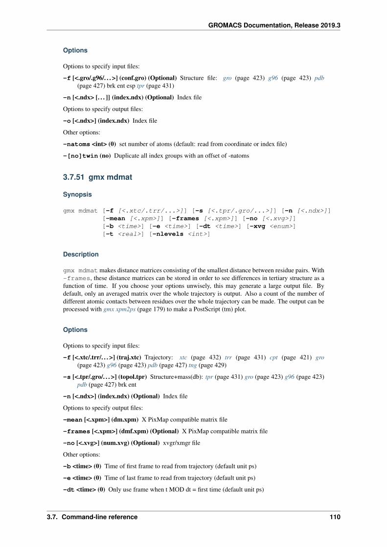
GROMACS Documentation, Release 2019.3
Options
Options to specify input files:
-f [<.gro/.g96/. . . >] (conf.gro) (Optional) Structure file: gro (page 423) g96 (page 423) pdb(page 427) brk ent esp tpr (page 431)
-n [<.ndx> [. . . ]] (index.ndx) (Optional) Index file
Options to specify output files:
-o [<.ndx>] (index.ndx) Index file
Other options:
-natoms <int> (0) set number of atoms (default: read from coordinate or index file)
-[no]twin (no) Duplicate all index groups with an offset of -natoms
3.7.51 gmx mdmat
Synopsis
gmx mdmat [-f [<.xtc/.trr/...>]] [-s [<.tpr/.gro/...>]] [-n [<.ndx>]][-mean [<.xpm>]] [-frames [<.xpm>]] [-no [<.xvg>]][-b <time>] [-e <time>] [-dt <time>] [-xvg <enum>][-t <real>] [-nlevels <int>]
Description
gmx mdmat makes distance matrices consisting of the smallest distance between residue pairs. With-frames, these distance matrices can be stored in order to see differences in tertiary structure as afunction of time. If you choose your options unwisely, this may generate a large output file. Bydefault, only an averaged matrix over the whole trajectory is output. Also a count of the number ofdifferent atomic contacts between residues over the whole trajectory can be made. The output can beprocessed with gmx xpm2ps (page 179) to make a PostScript (tm) plot.
Options
Options to specify input files:
-f [<.xtc/.trr/. . . >] (traj.xtc) Trajectory: xtc (page 432) trr (page 431) cpt (page 421) gro(page 423) g96 (page 423) pdb (page 427) tng (page 429)
-s [<.tpr/.gro/. . . >] (topol.tpr) Structure+mass(db): tpr (page 431) gro (page 423) g96 (page 423)pdb (page 427) brk ent
-n [<.ndx>] (index.ndx) (Optional) Index file
Options to specify output files:
-mean [<.xpm>] (dm.xpm) X PixMap compatible matrix file
-frames [<.xpm>] (dmf.xpm) (Optional) X PixMap compatible matrix file
-no [<.xvg>] (num.xvg) (Optional) xvgr/xmgr file
Other options:
-b <time> (0) Time of first frame to read from trajectory (default unit ps)
-e <time> (0) Time of last frame to read from trajectory (default unit ps)
-dt <time> (0) Only use frame when t MOD dt = first time (default unit ps)
3.7. Command-line reference 110
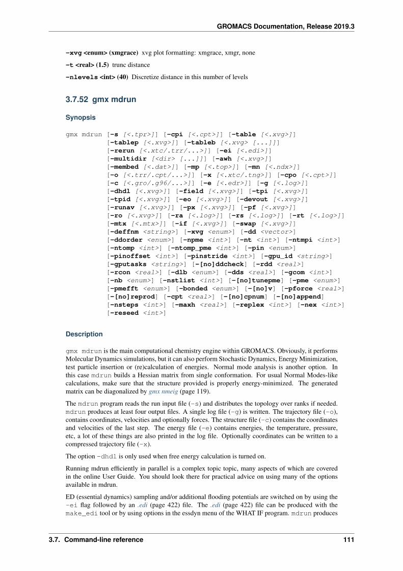
GROMACS Documentation, Release 2019.3
-xvg <enum> (xmgrace) xvg plot formatting: xmgrace, xmgr, none
-t <real> (1.5) trunc distance
-nlevels <int> (40) Discretize distance in this number of levels
3.7.52 gmx mdrun
Synopsis
gmx mdrun [-s [<.tpr>]] [-cpi [<.cpt>]] [-table [<.xvg>]][-tablep [<.xvg>]] [-tableb [<.xvg> [...]]][-rerun [<.xtc/.trr/...>]] [-ei [<.edi>]][-multidir [<dir> [...]]] [-awh [<.xvg>]][-membed [<.dat>]] [-mp [<.top>]] [-mn [<.ndx>]][-o [<.trr/.cpt/...>]] [-x [<.xtc/.tng>]] [-cpo [<.cpt>]][-c [<.gro/.g96/...>]] [-e [<.edr>]] [-g [<.log>]][-dhdl [<.xvg>]] [-field [<.xvg>]] [-tpi [<.xvg>]][-tpid [<.xvg>]] [-eo [<.xvg>]] [-devout [<.xvg>]][-runav [<.xvg>]] [-px [<.xvg>]] [-pf [<.xvg>]][-ro [<.xvg>]] [-ra [<.log>]] [-rs [<.log>]] [-rt [<.log>]][-mtx [<.mtx>]] [-if [<.xvg>]] [-swap [<.xvg>]][-deffnm <string>] [-xvg <enum>] [-dd <vector>][-ddorder <enum>] [-npme <int>] [-nt <int>] [-ntmpi <int>][-ntomp <int>] [-ntomp_pme <int>] [-pin <enum>][-pinoffset <int>] [-pinstride <int>] [-gpu_id <string>][-gputasks <string>] [-[no]ddcheck] [-rdd <real>][-rcon <real>] [-dlb <enum>] [-dds <real>] [-gcom <int>][-nb <enum>] [-nstlist <int>] [-[no]tunepme] [-pme <enum>][-pmefft <enum>] [-bonded <enum>] [-[no]v] [-pforce <real>][-[no]reprod] [-cpt <real>] [-[no]cpnum] [-[no]append][-nsteps <int>] [-maxh <real>] [-replex <int>] [-nex <int>][-reseed <int>]
Description
gmx mdrun is the main computational chemistry engine within GROMACS. Obviously, it performsMolecular Dynamics simulations, but it can also perform Stochastic Dynamics, Energy Minimization,test particle insertion or (re)calculation of energies. Normal mode analysis is another option. Inthis case mdrun builds a Hessian matrix from single conformation. For usual Normal Modes-likecalculations, make sure that the structure provided is properly energy-minimized. The generatedmatrix can be diagonalized by gmx nmeig (page 119).
The mdrun program reads the run input file (-s) and distributes the topology over ranks if needed.mdrun produces at least four output files. A single log file (-g) is written. The trajectory file (-o),contains coordinates, velocities and optionally forces. The structure file (-c) contains the coordinatesand velocities of the last step. The energy file (-e) contains energies, the temperature, pressure,etc, a lot of these things are also printed in the log file. Optionally coordinates can be written to acompressed trajectory file (-x).
The option -dhdl is only used when free energy calculation is turned on.
Running mdrun efficiently in parallel is a complex topic topic, many aspects of which are coveredin the online User Guide. You should look there for practical advice on using many of the optionsavailable in mdrun.
ED (essential dynamics) sampling and/or additional flooding potentials are switched on by using the-ei flag followed by an .edi (page 422) file. The .edi (page 422) file can be produced with themake_edi tool or by using options in the essdyn menu of the WHAT IF program. mdrun produces
3.7. Command-line reference 111
GROMACS Documentation, Release 2019.3
a .xvg (page 434) output file that contains projections of positions, velocities and forces onto selectedeigenvectors.
When user-defined potential functions have been selected in the .mdp (page 425) file the -tableoption is used to pass mdrun a formatted table with potential functions. The file is read from eitherthe current directory or from the GMXLIB directory. A number of pre-formatted tables are presentedin the GMXLIB dir, for 6-8, 6-9, 6-10, 6-11, 6-12 Lennard-Jones potentials with normal Coulomb.When pair interactions are present, a separate table for pair interaction functions is read using the-tablep option.
When tabulated bonded functions are present in the topology, interaction functions are read usingthe -tableb option. For each different tabulated interaction type used, a table file name must begiven. For the topology to work, a file name given here must match a character sequence before thefile extension. That sequence is: an underscore, then a ‘b’ for bonds, an ‘a’ for angles or a ‘d’ fordihedrals, and finally the matching table number index used in the topology. Note that, these optionsare deprecated, and in future will be available via grompp.
The options -px and -pf are used for writing pull COM coordinates and forces when pulling isselected in the .mdp (page 425) file.
Finally some experimental algorithms can be tested when the appropriate options have been given.Currently under investigation are: polarizability.
The option -membed does what used to be g_membed, i.e. embed a protein into a membrane. Thismodule requires a number of settings that are provided in a data file that is the argument of this option.For more details in membrane embedding, see the documentation in the user guide. The options -mnand -mp are used to provide the index and topology files used for the embedding.
The option -pforce is useful when you suspect a simulation crashes due to too large forces. Withthis option coordinates and forces of atoms with a force larger than a certain value will be printed tostderr. It will also terminate the run when non-finite forces are present.
Checkpoints containing the complete state of the system are written at regular intervals (option -cpt)to the file -cpo, unless option -cpt is set to -1. The previous checkpoint is backed up to state_-prev.cpt to make sure that a recent state of the system is always available, even when the sim-ulation is terminated while writing a checkpoint. With -cpnum all checkpoint files are kept andappended with the step number. A simulation can be continued by reading the full state from file withoption -cpi. This option is intelligent in the way that if no checkpoint file is found, GROMACS justassumes a normal run and starts from the first step of the .tpr (page 431) file. By default the outputwill be appending to the existing output files. The checkpoint file contains checksums of all outputfiles, such that you will never loose data when some output files are modified, corrupt or removed.There are three scenarios with -cpi:
* no files with matching names are present: new output files are written
* all files are present with names and checksums matching those stored in the checkpoint file: filesare appended
* otherwise no files are modified and a fatal error is generated
With -noappend new output files are opened and the simulation part number is added to all outputfile names. Note that in all cases the checkpoint file itself is not renamed and will be overwritten,unless its name does not match the -cpo option.
With checkpointing the output is appended to previously written output files, unless -noappend isused or none of the previous output files are present (except for the checkpoint file). The integrityof the files to be appended is verified using checksums which are stored in the checkpoint file. Thisensures that output can not be mixed up or corrupted due to file appending. When only some of theprevious output files are present, a fatal error is generated and no old output files are modified andno new output files are opened. The result with appending will be the same as from a single run.The contents will be binary identical, unless you use a different number of ranks or dynamic loadbalancing or the FFT library uses optimizations through timing.
With option -maxh a simulation is terminated and a checkpoint file is written at the first neighborsearch step where the run time exceeds -maxh*0.99 hours. This option is particularly useful in
3.7. Command-line reference 112
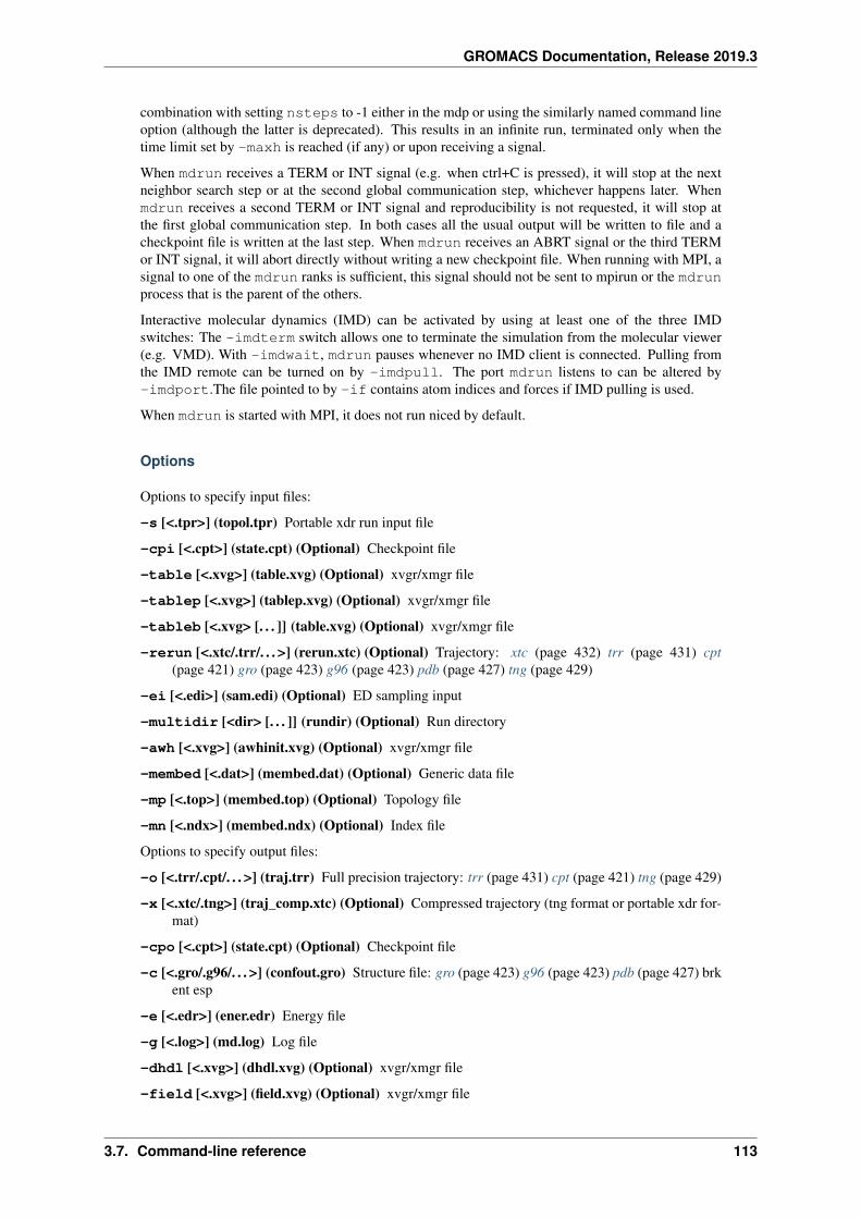
GROMACS Documentation, Release 2019.3
combination with setting nsteps to -1 either in the mdp or using the similarly named command lineoption (although the latter is deprecated). This results in an infinite run, terminated only when thetime limit set by -maxh is reached (if any) or upon receiving a signal.
When mdrun receives a TERM or INT signal (e.g. when ctrl+C is pressed), it will stop at the nextneighbor search step or at the second global communication step, whichever happens later. Whenmdrun receives a second TERM or INT signal and reproducibility is not requested, it will stop atthe first global communication step. In both cases all the usual output will be written to file and acheckpoint file is written at the last step. When mdrun receives an ABRT signal or the third TERMor INT signal, it will abort directly without writing a new checkpoint file. When running with MPI, asignal to one of the mdrun ranks is sufficient, this signal should not be sent to mpirun or the mdrunprocess that is the parent of the others.
Interactive molecular dynamics (IMD) can be activated by using at least one of the three IMDswitches: The -imdterm switch allows one to terminate the simulation from the molecular viewer(e.g. VMD). With -imdwait, mdrun pauses whenever no IMD client is connected. Pulling fromthe IMD remote can be turned on by -imdpull. The port mdrun listens to can be altered by-imdport.The file pointed to by -if contains atom indices and forces if IMD pulling is used.
When mdrun is started with MPI, it does not run niced by default.
Options
Options to specify input files:
-s [<.tpr>] (topol.tpr) Portable xdr run input file
-cpi [<.cpt>] (state.cpt) (Optional) Checkpoint file
-table [<.xvg>] (table.xvg) (Optional) xvgr/xmgr file
-tablep [<.xvg>] (tablep.xvg) (Optional) xvgr/xmgr file
-tableb [<.xvg> [. . . ]] (table.xvg) (Optional) xvgr/xmgr file
-rerun [<.xtc/.trr/. . . >] (rerun.xtc) (Optional) Trajectory: xtc (page 432) trr (page 431) cpt(page 421) gro (page 423) g96 (page 423) pdb (page 427) tng (page 429)
-ei [<.edi>] (sam.edi) (Optional) ED sampling input
-multidir [<dir> [. . . ]] (rundir) (Optional) Run directory
-awh [<.xvg>] (awhinit.xvg) (Optional) xvgr/xmgr file
-membed [<.dat>] (membed.dat) (Optional) Generic data file
-mp [<.top>] (membed.top) (Optional) Topology file
-mn [<.ndx>] (membed.ndx) (Optional) Index file
Options to specify output files:
-o [<.trr/.cpt/. . . >] (traj.trr) Full precision trajectory: trr (page 431) cpt (page 421) tng (page 429)
-x [<.xtc/.tng>] (traj_comp.xtc) (Optional) Compressed trajectory (tng format or portable xdr for-mat)
-cpo [<.cpt>] (state.cpt) (Optional) Checkpoint file
-c [<.gro/.g96/. . . >] (confout.gro) Structure file: gro (page 423) g96 (page 423) pdb (page 427) brkent esp
-e [<.edr>] (ener.edr) Energy file
-g [<.log>] (md.log) Log file
-dhdl [<.xvg>] (dhdl.xvg) (Optional) xvgr/xmgr file
-field [<.xvg>] (field.xvg) (Optional) xvgr/xmgr file
3.7. Command-line reference 113
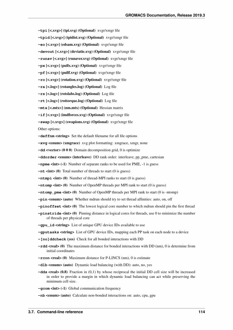
GROMACS Documentation, Release 2019.3
-tpi [<.xvg>] (tpi.xvg) (Optional) xvgr/xmgr file
-tpid [<.xvg>] (tpidist.xvg) (Optional) xvgr/xmgr file
-eo [<.xvg>] (edsam.xvg) (Optional) xvgr/xmgr file
-devout [<.xvg>] (deviatie.xvg) (Optional) xvgr/xmgr file
-runav [<.xvg>] (runaver.xvg) (Optional) xvgr/xmgr file
-px [<.xvg>] (pullx.xvg) (Optional) xvgr/xmgr file
-pf [<.xvg>] (pullf.xvg) (Optional) xvgr/xmgr file
-ro [<.xvg>] (rotation.xvg) (Optional) xvgr/xmgr file
-ra [<.log>] (rotangles.log) (Optional) Log file
-rs [<.log>] (rotslabs.log) (Optional) Log file
-rt [<.log>] (rottorque.log) (Optional) Log file
-mtx [<.mtx>] (nm.mtx) (Optional) Hessian matrix
-if [<.xvg>] (imdforces.xvg) (Optional) xvgr/xmgr file
-swap [<.xvg>] (swapions.xvg) (Optional) xvgr/xmgr file
Other options:
-deffnm <string> Set the default filename for all file options
-xvg <enum> (xmgrace) xvg plot formatting: xmgrace, xmgr, none
-dd <vector> (0 0 0) Domain decomposition grid, 0 is optimize
-ddorder <enum> (interleave) DD rank order: interleave, pp_pme, cartesian
-npme <int> (-1) Number of separate ranks to be used for PME, -1 is guess
-nt <int> (0) Total number of threads to start (0 is guess)
-ntmpi <int> (0) Number of thread-MPI ranks to start (0 is guess)
-ntomp <int> (0) Number of OpenMP threads per MPI rank to start (0 is guess)
-ntomp_pme <int> (0) Number of OpenMP threads per MPI rank to start (0 is -ntomp)
-pin <enum> (auto) Whether mdrun should try to set thread affinities: auto, on, off
-pinoffset <int> (0) The lowest logical core number to which mdrun should pin the first thread
-pinstride <int> (0) Pinning distance in logical cores for threads, use 0 to minimize the numberof threads per physical core
-gpu_id <string> List of unique GPU device IDs available to use
-gputasks <string> List of GPU device IDs, mapping each PP task on each node to a device
-[no]ddcheck (yes) Check for all bonded interactions with DD
-rdd <real> (0) The maximum distance for bonded interactions with DD (nm), 0 is determine frominitial coordinates
-rcon <real> (0) Maximum distance for P-LINCS (nm), 0 is estimate
-dlb <enum> (auto) Dynamic load balancing (with DD): auto, no, yes
-dds <real> (0.8) Fraction in (0,1) by whose reciprocal the initial DD cell size will be increasedin order to provide a margin in which dynamic load balancing can act while preserving theminimum cell size.
-gcom <int> (-1) Global communication frequency
-nb <enum> (auto) Calculate non-bonded interactions on: auto, cpu, gpu
3.7. Command-line reference 114
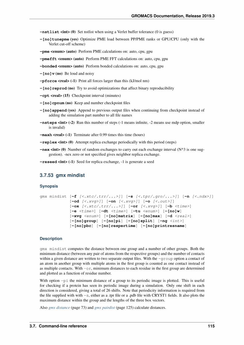
GROMACS Documentation, Release 2019.3
-nstlist <int> (0) Set nstlist when using a Verlet buffer tolerance (0 is guess)
-[no]tunepme (yes) Optimize PME load between PP/PME ranks or GPU/CPU (only with theVerlet cut-off scheme)
-pme <enum> (auto) Perform PME calculations on: auto, cpu, gpu
-pmefft <enum> (auto) Perform PME FFT calculations on: auto, cpu, gpu
-bonded <enum> (auto) Perform bonded calculations on: auto, cpu, gpu
-[no]v (no) Be loud and noisy
-pforce <real> (-1) Print all forces larger than this (kJ/mol nm)
-[no]reprod (no) Try to avoid optimizations that affect binary reproducibility
-cpt <real> (15) Checkpoint interval (minutes)
-[no]cpnum (no) Keep and number checkpoint files
-[no]append (yes) Append to previous output files when continuing from checkpoint instead ofadding the simulation part number to all file names
-nsteps <int> (-2) Run this number of steps (-1 means infinite, -2 means use mdp option, smalleris invalid)
-maxh <real> (-1) Terminate after 0.99 times this time (hours)
-replex <int> (0) Attempt replica exchange periodically with this period (steps)
-nex <int> (0) Number of random exchanges to carry out each exchange interval (N^3 is one sug-gestion). -nex zero or not specified gives neighbor replica exchange.
-reseed <int> (-1) Seed for replica exchange, -1 is generate a seed
3.7.53 gmx mindist
Synopsis
gmx mindist [-f [<.xtc/.trr/...>]] [-s [<.tpr/.gro/...>]] [-n [<.ndx>]][-od [<.xvg>]] [-on [<.xvg>]] [-o [<.out>]][-ox [<.xtc/.trr/...>]] [-or [<.xvg>]] [-b <time>][-e <time>] [-dt <time>] [-tu <enum>] [-[no]w][-xvg <enum>] [-[no]matrix] [-[no]max] [-d <real>][-[no]group] [-[no]pi] [-[no]split] [-ng <int>][-[no]pbc] [-[no]respertime] [-[no]printresname]
Description
gmx mindist computes the distance between one group and a number of other groups. Both theminimum distance (between any pair of atoms from the respective groups) and the number of contactswithin a given distance are written to two separate output files. With the -group option a contact ofan atom in another group with multiple atoms in the first group is counted as one contact instead ofas multiple contacts. With -or, minimum distances to each residue in the first group are determinedand plotted as a function of residue number.
With option -pi the minimum distance of a group to its periodic image is plotted. This is usefulfor checking if a protein has seen its periodic image during a simulation. Only one shift in eachdirection is considered, giving a total of 26 shifts. Note that periodicity information is required fromthe file supplied with with -s, either as a .tpr file or a .pdb file with CRYST1 fields. It also plots themaximum distance within the group and the lengths of the three box vectors.
Also gmx distance (page 73) and gmx pairdist (page 125) calculate distances.
3.7. Command-line reference 115
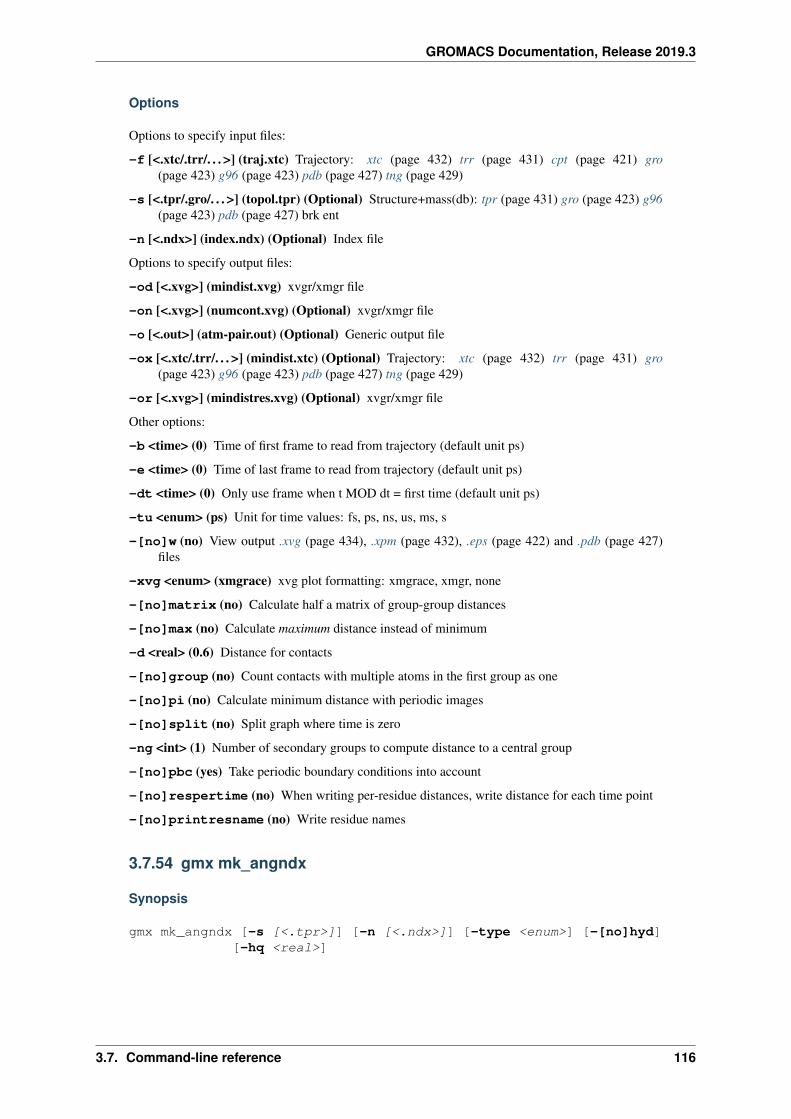
GROMACS Documentation, Release 2019.3
Options
Options to specify input files:
-f [<.xtc/.trr/. . . >] (traj.xtc) Trajectory: xtc (page 432) trr (page 431) cpt (page 421) gro(page 423) g96 (page 423) pdb (page 427) tng (page 429)
-s [<.tpr/.gro/. . . >] (topol.tpr) (Optional) Structure+mass(db): tpr (page 431) gro (page 423) g96(page 423) pdb (page 427) brk ent
-n [<.ndx>] (index.ndx) (Optional) Index file
Options to specify output files:
-od [<.xvg>] (mindist.xvg) xvgr/xmgr file
-on [<.xvg>] (numcont.xvg) (Optional) xvgr/xmgr file
-o [<.out>] (atm-pair.out) (Optional) Generic output file
-ox [<.xtc/.trr/. . . >] (mindist.xtc) (Optional) Trajectory: xtc (page 432) trr (page 431) gro(page 423) g96 (page 423) pdb (page 427) tng (page 429)
-or [<.xvg>] (mindistres.xvg) (Optional) xvgr/xmgr file
Other options:
-b <time> (0) Time of first frame to read from trajectory (default unit ps)
-e <time> (0) Time of last frame to read from trajectory (default unit ps)
-dt <time> (0) Only use frame when t MOD dt = first time (default unit ps)
-tu <enum> (ps) Unit for time values: fs, ps, ns, us, ms, s
-[no]w (no) View output .xvg (page 434), .xpm (page 432), .eps (page 422) and .pdb (page 427)files
-xvg <enum> (xmgrace) xvg plot formatting: xmgrace, xmgr, none
-[no]matrix (no) Calculate half a matrix of group-group distances
-[no]max (no) Calculate maximum distance instead of minimum
-d <real> (0.6) Distance for contacts
-[no]group (no) Count contacts with multiple atoms in the first group as one
-[no]pi (no) Calculate minimum distance with periodic images
-[no]split (no) Split graph where time is zero
-ng <int> (1) Number of secondary groups to compute distance to a central group
-[no]pbc (yes) Take periodic boundary conditions into account
-[no]respertime (no) When writing per-residue distances, write distance for each time point
-[no]printresname (no) Write residue names
3.7.54 gmx mk_angndx
Synopsis
gmx mk_angndx [-s [<.tpr>]] [-n [<.ndx>]] [-type <enum>] [-[no]hyd][-hq <real>]
3.7. Command-line reference 116
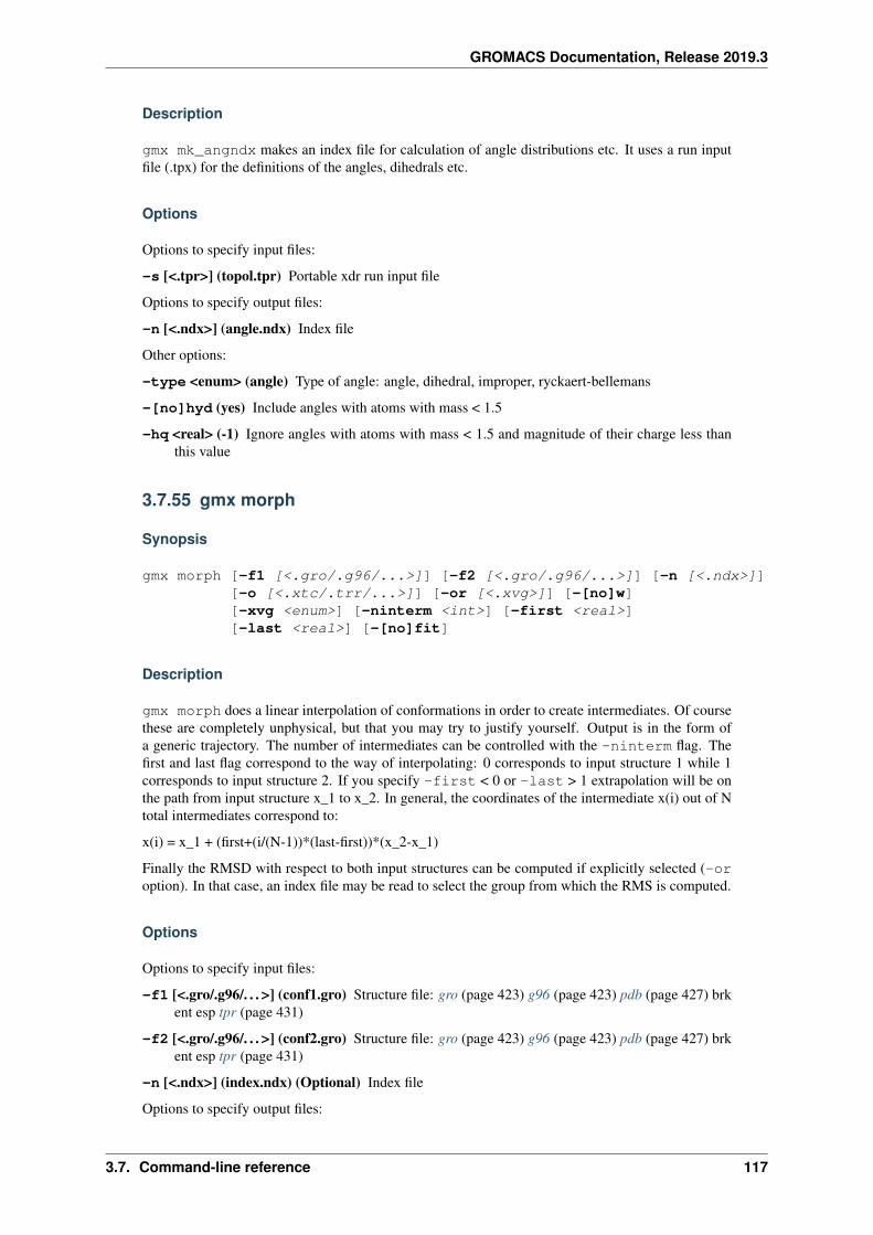
GROMACS Documentation, Release 2019.3
Description
gmx mk_angndx makes an index file for calculation of angle distributions etc. It uses a run inputfile (.tpx) for the definitions of the angles, dihedrals etc.
Options
Options to specify input files:
-s [<.tpr>] (topol.tpr) Portable xdr run input file
Options to specify output files:
-n [<.ndx>] (angle.ndx) Index file
Other options:
-type <enum> (angle) Type of angle: angle, dihedral, improper, ryckaert-bellemans
-[no]hyd (yes) Include angles with atoms with mass < 1.5
-hq <real> (-1) Ignore angles with atoms with mass < 1.5 and magnitude of their charge less thanthis value
3.7.55 gmx morph
Synopsis
gmx morph [-f1 [<.gro/.g96/...>]] [-f2 [<.gro/.g96/...>]] [-n [<.ndx>]][-o [<.xtc/.trr/...>]] [-or [<.xvg>]] [-[no]w][-xvg <enum>] [-ninterm <int>] [-first <real>][-last <real>] [-[no]fit]
Description
gmx morph does a linear interpolation of conformations in order to create intermediates. Of coursethese are completely unphysical, but that you may try to justify yourself. Output is in the form ofa generic trajectory. The number of intermediates can be controlled with the -ninterm flag. Thefirst and last flag correspond to the way of interpolating: 0 corresponds to input structure 1 while 1corresponds to input structure 2. If you specify -first < 0 or -last > 1 extrapolation will be onthe path from input structure x_1 to x_2. In general, the coordinates of the intermediate x(i) out of Ntotal intermediates correspond to:
x(i) = x_1 + (first+(i/(N-1))*(last-first))*(x_2-x_1)
Finally the RMSD with respect to both input structures can be computed if explicitly selected (-oroption). In that case, an index file may be read to select the group from which the RMS is computed.
Options
Options to specify input files:
-f1 [<.gro/.g96/. . . >] (conf1.gro) Structure file: gro (page 423) g96 (page 423) pdb (page 427) brkent esp tpr (page 431)
-f2 [<.gro/.g96/. . . >] (conf2.gro) Structure file: gro (page 423) g96 (page 423) pdb (page 427) brkent esp tpr (page 431)
-n [<.ndx>] (index.ndx) (Optional) Index file
Options to specify output files:
3.7. Command-line reference 117
GROMACS Documentation, Release 2019.3
-o [<.xtc/.trr/. . . >] (interm.xtc) Trajectory: xtc (page 432) trr (page 431) cpt (page 421) gro(page 423) g96 (page 423) pdb (page 427) tng (page 429)
-or [<.xvg>] (rms-interm.xvg) (Optional) xvgr/xmgr file
Other options:
-[no]w (no) View output .xvg (page 434), .xpm (page 432), .eps (page 422) and .pdb (page 427)files
-xvg <enum> (xmgrace) xvg plot formatting: xmgrace, xmgr, none
-ninterm <int> (11) Number of intermediates
-first <real> (0) Corresponds to first generated structure (0 is input x_1, see above)
-last <real> (1) Corresponds to last generated structure (1 is input x_2, see above)
-[no]fit (yes) Do a least squares fit of the second to the first structure before interpolating
3.7.56 gmx msd
Synopsis
gmx msd [-f [<.xtc/.trr/...>]] [-s [<.tpr/.gro/...>]] [-n [<.ndx>]][-o [<.xvg>]] [-mol [<.xvg>]] [-pdb [<.pdb>]] [-b <time>][-e <time>] [-tu <enum>] [-[no]w] [-xvg <enum>][-type <enum>] [-lateral <enum>] [-[no]ten] [-ngroup <int>][-[no]mw] [-[no]rmcomm] [-tpdb <time>] [-trestart <time>][-beginfit <time>] [-endfit <time>]
Description
gmx msd computes the mean square displacement (MSD) of atoms from a set of initial positions.This provides an easy way to compute the diffusion constant using the Einstein relation. The timebetween the reference points for the MSD calculation is set with -trestart. The diffusion constantis calculated by least squares fitting a straight line (D*t + c) through the MSD(t) from -beginfitto -endfit (note that t is time from the reference positions, not simulation time). An error estimategiven, which is the difference of the diffusion coefficients obtained from fits over the two halves ofthe fit interval.
There are three, mutually exclusive, options to determine different types of mean square displacement:-type, -lateral and -ten. Option -ten writes the full MSD tensor for each group, the orderin the output is: trace xx yy zz yx zx zy.
If -mol is set, gmx msd plots the MSD for individual molecules (including making molecules wholeacross periodic boundaries): for each individual molecule a diffusion constant is computed for itscenter of mass. The chosen index group will be split into molecules.
The default way to calculate a MSD is by using mass-weighted averages. This can be turned off with-nomw.
With the option -rmcomm, the center of mass motion of a specific group can be removed. Fortrajectories produced with GROMACS this is usually not necessary, as gmx mdrun (page 111) usuallyalready removes the center of mass motion. When you use this option be sure that the whole systemis stored in the trajectory file.
The diffusion coefficient is determined by linear regression of the MSD, where, unlike for the normaloutput of D, the times are weighted according to the number of reference points, i.e. short times havea higher weight. Also when -beginfit is -1, fitting starts at 10% and when -endfit is -1, fittinggoes to 90%. Using this option one also gets an accurate error estimate based on the statistics betweenindividual molecules. Note that this diffusion coefficient and error estimate are only accurate whenthe MSD is completely linear between -beginfit and -endfit.
3.7. Command-line reference 118
GROMACS Documentation, Release 2019.3
Option -pdb writes a .pdb (page 427) file with the coordinates of the frame at time -tpdb within the B-factor field the square root of the diffusion coefficient of the molecule. This option impliesoption -mol.
Options
Options to specify input files:
-f [<.xtc/.trr/. . . >] (traj.xtc) Trajectory: xtc (page 432) trr (page 431) cpt (page 421) gro(page 423) g96 (page 423) pdb (page 427) tng (page 429)
-s [<.tpr/.gro/. . . >] (topol.tpr) Structure+mass(db): tpr (page 431) gro (page 423) g96 (page 423)pdb (page 427) brk ent
-n [<.ndx>] (index.ndx) (Optional) Index file
Options to specify output files:
-o [<.xvg>] (msd.xvg) xvgr/xmgr file
-mol [<.xvg>] (diff_mol.xvg) (Optional) xvgr/xmgr file
-pdb [<.pdb>] (diff_mol.pdb) (Optional) Protein data bank file
Other options:
-b <time> (0) Time of first frame to read from trajectory (default unit ps)
-e <time> (0) Time of last frame to read from trajectory (default unit ps)
-tu <enum> (ps) Unit for time values: fs, ps, ns, us, ms, s
-[no]w (no) View output .xvg (page 434), .xpm (page 432), .eps (page 422) and .pdb (page 427)files
-xvg <enum> (xmgrace) xvg plot formatting: xmgrace, xmgr, none
-type <enum> (no) Compute diffusion coefficient in one direction: no, x, y, z
-lateral <enum> (no) Calculate the lateral diffusion in a plane perpendicular to: no, x, y, z
-[no]ten (no) Calculate the full tensor
-ngroup <int> (1) Number of groups to calculate MSD for
-[no]mw (yes) Mass weighted MSD
-[no]rmcomm (no) Remove center of mass motion
-tpdb <time> (0) The frame to use for option -pdb (ps)
-trestart <time> (10) Time between restarting points in trajectory (ps)
-beginfit <time> (-1) Start time for fitting the MSD (ps), -1 is 10%
-endfit <time> (-1) End time for fitting the MSD (ps), -1 is 90%
3.7.57 gmx nmeig
Synopsis
gmx nmeig [-f [<.mtx>]] [-s [<.tpr>]] [-of [<.xvg>]] [-ol [<.xvg>]][-os [<.xvg>]] [-qc [<.xvg>]] [-v [<.trr/.cpt/...>]][-xvg <enum>] [-[no]m] [-first <int>] [-last <int>][-maxspec <int>] [-T <real>] [-P <real>] [-sigma <int>][-scale <real>] [-linear_toler <real>] [-[no]constr][-width <real>]
3.7. Command-line reference 119
GROMACS Documentation, Release 2019.3
Description
gmx nmeig calculates the eigenvectors/values of a (Hessian) matrix, which can be calculated withgmx mdrun (page 111). The eigenvectors are written to a trajectory file (-v). The structure is writtenfirst with t=0. The eigenvectors are written as frames with the eigenvector number and eigenvaluewritten as step number and timestamp, respectively. The eigenvectors can be analyzed with gmxanaeig (page 41). An ensemble of structures can be generated from the eigenvectors with gmx nmens(page 121). When mass weighting is used, the generated eigenvectors will be scaled back to plainCartesian coordinates before generating the output. In this case, they will no longer be exactly or-thogonal in the standard Cartesian norm, but in the mass-weighted norm they would be.
This program can be optionally used to compute quantum corrections to heat capacity and enthalpyby providing an extra file argument -qcorr. See the GROMACS manual, Chapter 1, for details.The result includes subtracting a harmonic degree of freedom at the given temperature. The totalcorrection is printed on the terminal screen. The recommended way of getting the corrections out is:
gmx nmeig -s topol.tpr -f nm.mtx -first 7 -last 10000 -T 300 -qc[-constr]
The -constr option should be used when bond constraints were used during the simulation for allthe covalent bonds. If this is not the case, you need to analyze the quant_corr.xvg file yourself.
To make things more flexible, the program can also take virtual sites into account when computingquantum corrections. When selecting -constr and -qc, the -begin and -end options will be setautomatically as well.
Based on a harmonic analysis of the normal mode frequencies, thermochemical properties S0 (Stan-dard Entropy), Cv (Heat capacity at constant volume), Zero-point energy and the internal energy arecomputed, much in the same manner as popular quantum chemistry programs.
Options
Options to specify input files:
-f [<.mtx>] (hessian.mtx) Hessian matrix
-s [<.tpr>] (topol.tpr) Portable xdr run input file
Options to specify output files:
-of [<.xvg>] (eigenfreq.xvg) xvgr/xmgr file
-ol [<.xvg>] (eigenval.xvg) xvgr/xmgr file
-os [<.xvg>] (spectrum.xvg) (Optional) xvgr/xmgr file
-qc [<.xvg>] (quant_corr.xvg) (Optional) xvgr/xmgr file
-v [<.trr/.cpt/. . . >] (eigenvec.trr) Full precision trajectory: trr (page 431) cpt (page 421) tng(page 429)
Other options:
-xvg <enum> (xmgrace) xvg plot formatting: xmgrace, xmgr, none
-[no]m (yes) Divide elements of Hessian by product of sqrt(mass) of involved atoms prior to diag-onalization. This should be used for ‘Normal Modes’ analysis
-first <int> (1) First eigenvector to write away
-last <int> (50) Last eigenvector to write away. -1 is use all dimensions.
-maxspec <int> (4000) Highest frequency (1/cm) to consider in the spectrum
-T <real> (298.15) Temperature for computing entropy, quantum heat capacity and enthalpy whenusing normal mode calculations to correct classical simulations
-P <real> (1) Pressure (bar) when computing entropy
3.7. Command-line reference 120
GROMACS Documentation, Release 2019.3
-sigma <int> (1) Number of symmetric copies used when computing entropy. E.g. for water thenumber is 2, for NH3 it is 3 and for methane it is 12.
-scale <real> (1) Factor to scale frequencies before computing thermochemistry values
-linear_toler <real> (1e-05) Tolerance for determining whether a compound is linear as de-termined from the ration of the moments inertion Ix/Iy and Ix/Iz.
-[no]constr (no) If constraints were used in the simulation but not in the normal mode analysisyou will need to set this for computing the quantum corrections.
-width <real> (1) Width (sigma) of the gaussian peaks (1/cm) when generating a spectrum
3.7.58 gmx nmens
Synopsis
gmx nmens [-v [<.trr/.cpt/...>]] [-e [<.xvg>]] [-s [<.tpr/.gro/...>]][-n [<.ndx>]] [-o [<.xtc/.trr/...>]] [-xvg <enum>][-temp <real>] [-seed <int>] [-num <int>] [-first <int>][-last <int>]
Description
gmx nmens generates an ensemble around an average structure in a subspace that is defined by a setof normal modes (eigenvectors). The eigenvectors are assumed to be mass-weighted. The positionalong each eigenvector is randomly taken from a Gaussian distribution with variance kT/eigenvalue.
By default the starting eigenvector is set to 7, since the first six normal modes are the translationaland rotational degrees of freedom.
Options
Options to specify input files:
-v [<.trr/.cpt/. . . >] (eigenvec.trr) Full precision trajectory: trr (page 431) cpt (page 421) tng(page 429)
-e [<.xvg>] (eigenval.xvg) xvgr/xmgr file
-s [<.tpr/.gro/. . . >] (topol.tpr) Structure+mass(db): tpr (page 431) gro (page 423) g96 (page 423)pdb (page 427) brk ent
-n [<.ndx>] (index.ndx) (Optional) Index file
Options to specify output files:
-o [<.xtc/.trr/. . . >] (ensemble.xtc) Trajectory: xtc (page 432) trr (page 431) gro (page 423) g96(page 423) pdb (page 427) tng (page 429)
Other options:
-xvg <enum> (xmgrace) xvg plot formatting: xmgrace, xmgr, none
-temp <real> (300) Temperature in Kelvin
-seed <int> (0) Random seed (0 means generate)
-num <int> (100) Number of structures to generate
-first <int> (7) First eigenvector to use (-1 is select)
-last <int> (-1) Last eigenvector to use (-1 is till the last)
3.7. Command-line reference 121
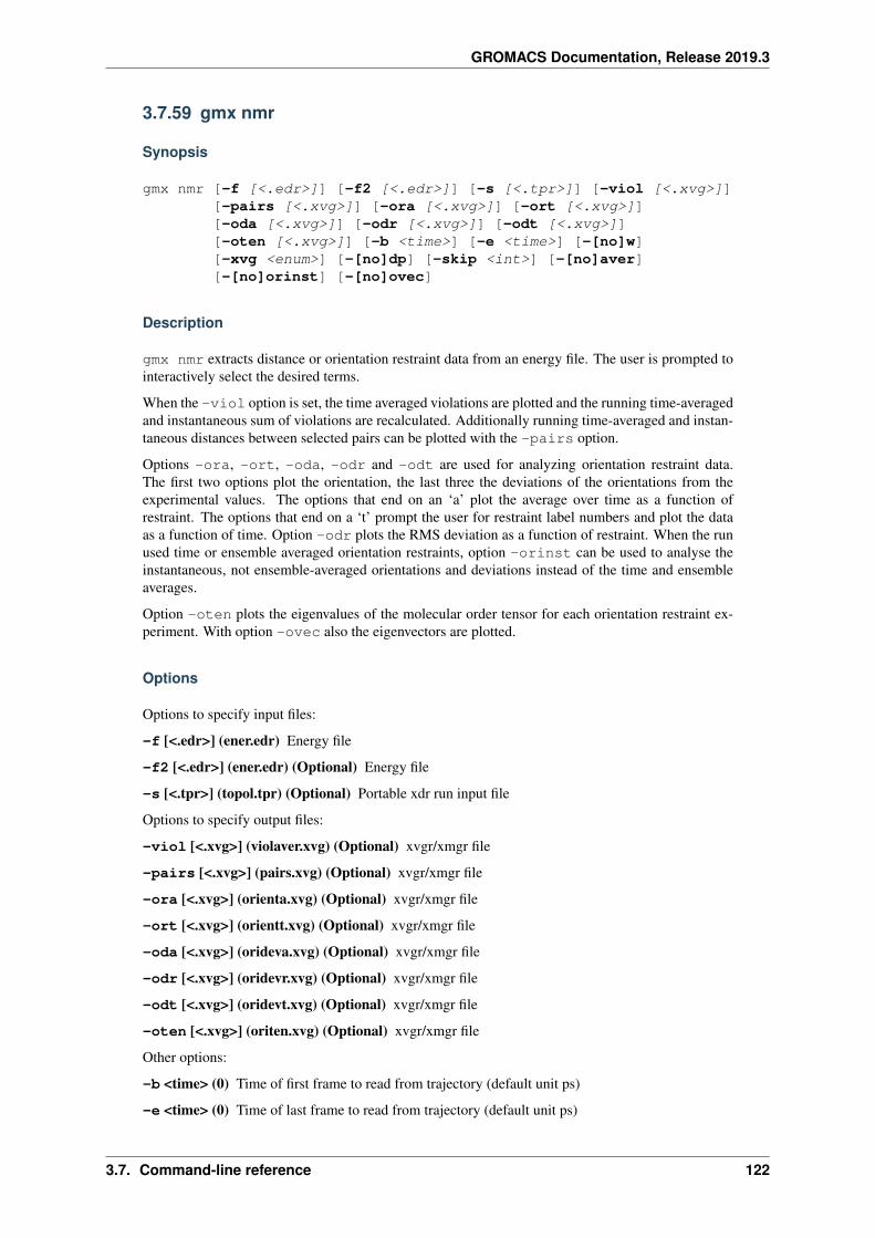
GROMACS Documentation, Release 2019.3
3.7.59 gmx nmr
Synopsis
gmx nmr [-f [<.edr>]] [-f2 [<.edr>]] [-s [<.tpr>]] [-viol [<.xvg>]][-pairs [<.xvg>]] [-ora [<.xvg>]] [-ort [<.xvg>]][-oda [<.xvg>]] [-odr [<.xvg>]] [-odt [<.xvg>]][-oten [<.xvg>]] [-b <time>] [-e <time>] [-[no]w][-xvg <enum>] [-[no]dp] [-skip <int>] [-[no]aver][-[no]orinst] [-[no]ovec]
Description
gmx nmr extracts distance or orientation restraint data from an energy file. The user is prompted tointeractively select the desired terms.
When the -viol option is set, the time averaged violations are plotted and the running time-averagedand instantaneous sum of violations are recalculated. Additionally running time-averaged and instan-taneous distances between selected pairs can be plotted with the -pairs option.
Options -ora, -ort, -oda, -odr and -odt are used for analyzing orientation restraint data.The first two options plot the orientation, the last three the deviations of the orientations from theexperimental values. The options that end on an ‘a’ plot the average over time as a function ofrestraint. The options that end on a ‘t’ prompt the user for restraint label numbers and plot the dataas a function of time. Option -odr plots the RMS deviation as a function of restraint. When the runused time or ensemble averaged orientation restraints, option -orinst can be used to analyse theinstantaneous, not ensemble-averaged orientations and deviations instead of the time and ensembleaverages.
Option -oten plots the eigenvalues of the molecular order tensor for each orientation restraint ex-periment. With option -ovec also the eigenvectors are plotted.
Options
Options to specify input files:
-f [<.edr>] (ener.edr) Energy file
-f2 [<.edr>] (ener.edr) (Optional) Energy file
-s [<.tpr>] (topol.tpr) (Optional) Portable xdr run input file
Options to specify output files:
-viol [<.xvg>] (violaver.xvg) (Optional) xvgr/xmgr file
-pairs [<.xvg>] (pairs.xvg) (Optional) xvgr/xmgr file
-ora [<.xvg>] (orienta.xvg) (Optional) xvgr/xmgr file
-ort [<.xvg>] (orientt.xvg) (Optional) xvgr/xmgr file
-oda [<.xvg>] (orideva.xvg) (Optional) xvgr/xmgr file
-odr [<.xvg>] (oridevr.xvg) (Optional) xvgr/xmgr file
-odt [<.xvg>] (oridevt.xvg) (Optional) xvgr/xmgr file
-oten [<.xvg>] (oriten.xvg) (Optional) xvgr/xmgr file
Other options:
-b <time> (0) Time of first frame to read from trajectory (default unit ps)
-e <time> (0) Time of last frame to read from trajectory (default unit ps)
3.7. Command-line reference 122
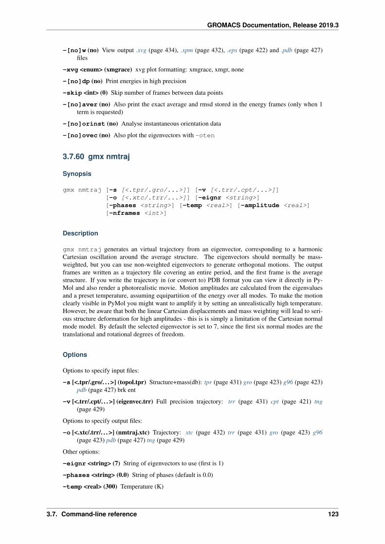
GROMACS Documentation, Release 2019.3
-[no]w (no) View output .xvg (page 434), .xpm (page 432), .eps (page 422) and .pdb (page 427)files
-xvg <enum> (xmgrace) xvg plot formatting: xmgrace, xmgr, none
-[no]dp (no) Print energies in high precision
-skip <int> (0) Skip number of frames between data points
-[no]aver (no) Also print the exact average and rmsd stored in the energy frames (only when 1term is requested)
-[no]orinst (no) Analyse instantaneous orientation data
-[no]ovec (no) Also plot the eigenvectors with -oten
3.7.60 gmx nmtraj
Synopsis
gmx nmtraj [-s [<.tpr/.gro/...>]] [-v [<.trr/.cpt/...>]][-o [<.xtc/.trr/...>]] [-eignr <string>][-phases <string>] [-temp <real>] [-amplitude <real>][-nframes <int>]
Description
gmx nmtraj generates an virtual trajectory from an eigenvector, corresponding to a harmonicCartesian oscillation around the average structure. The eigenvectors should normally be mass-weighted, but you can use non-weighted eigenvectors to generate orthogonal motions. The outputframes are written as a trajectory file covering an entire period, and the first frame is the averagestructure. If you write the trajectory in (or convert to) PDB format you can view it directly in Py-Mol and also render a photorealistic movie. Motion amplitudes are calculated from the eigenvaluesand a preset temperature, assuming equipartition of the energy over all modes. To make the motionclearly visible in PyMol you might want to amplify it by setting an unrealistically high temperature.However, be aware that both the linear Cartesian displacements and mass weighting will lead to seri-ous structure deformation for high amplitudes - this is is simply a limitation of the Cartesian normalmode model. By default the selected eigenvector is set to 7, since the first six normal modes are thetranslational and rotational degrees of freedom.
Options
Options to specify input files:
-s [<.tpr/.gro/. . . >] (topol.tpr) Structure+mass(db): tpr (page 431) gro (page 423) g96 (page 423)pdb (page 427) brk ent
-v [<.trr/.cpt/. . . >] (eigenvec.trr) Full precision trajectory: trr (page 431) cpt (page 421) tng(page 429)
Options to specify output files:
-o [<.xtc/.trr/. . . >] (nmtraj.xtc) Trajectory: xtc (page 432) trr (page 431) gro (page 423) g96(page 423) pdb (page 427) tng (page 429)
Other options:
-eignr <string> (7) String of eigenvectors to use (first is 1)
-phases <string> (0.0) String of phases (default is 0.0)
-temp <real> (300) Temperature (K)
3.7. Command-line reference 123
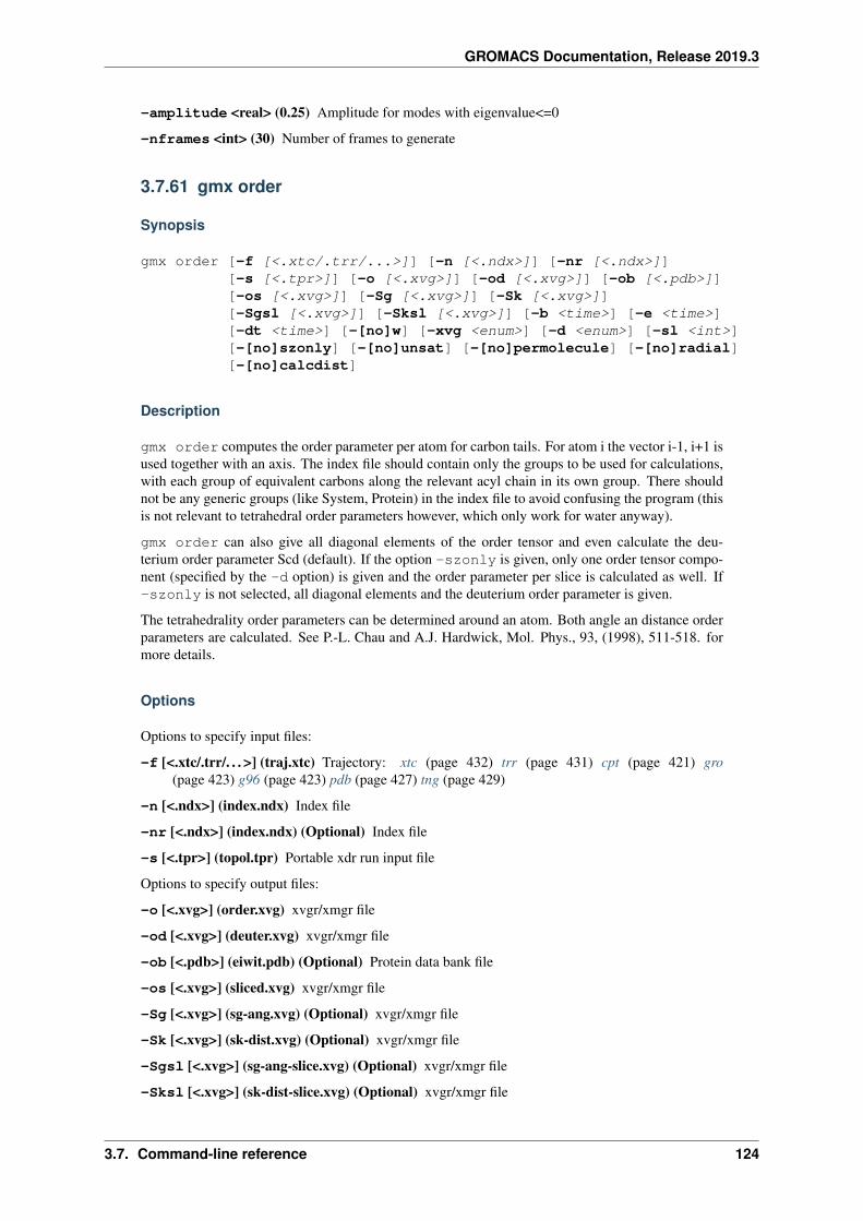
GROMACS Documentation, Release 2019.3
-amplitude <real> (0.25) Amplitude for modes with eigenvalue<=0
-nframes <int> (30) Number of frames to generate
3.7.61 gmx order
Synopsis
gmx order [-f [<.xtc/.trr/...>]] [-n [<.ndx>]] [-nr [<.ndx>]][-s [<.tpr>]] [-o [<.xvg>]] [-od [<.xvg>]] [-ob [<.pdb>]][-os [<.xvg>]] [-Sg [<.xvg>]] [-Sk [<.xvg>]][-Sgsl [<.xvg>]] [-Sksl [<.xvg>]] [-b <time>] [-e <time>][-dt <time>] [-[no]w] [-xvg <enum>] [-d <enum>] [-sl <int>][-[no]szonly] [-[no]unsat] [-[no]permolecule] [-[no]radial][-[no]calcdist]
Description
gmx order computes the order parameter per atom for carbon tails. For atom i the vector i-1, i+1 isused together with an axis. The index file should contain only the groups to be used for calculations,with each group of equivalent carbons along the relevant acyl chain in its own group. There shouldnot be any generic groups (like System, Protein) in the index file to avoid confusing the program (thisis not relevant to tetrahedral order parameters however, which only work for water anyway).
gmx order can also give all diagonal elements of the order tensor and even calculate the deu-terium order parameter Scd (default). If the option -szonly is given, only one order tensor compo-nent (specified by the -d option) is given and the order parameter per slice is calculated as well. If-szonly is not selected, all diagonal elements and the deuterium order parameter is given.
The tetrahedrality order parameters can be determined around an atom. Both angle an distance orderparameters are calculated. See P.-L. Chau and A.J. Hardwick, Mol. Phys., 93, (1998), 511-518. formore details.
Options
Options to specify input files:
-f [<.xtc/.trr/. . . >] (traj.xtc) Trajectory: xtc (page 432) trr (page 431) cpt (page 421) gro(page 423) g96 (page 423) pdb (page 427) tng (page 429)
-n [<.ndx>] (index.ndx) Index file
-nr [<.ndx>] (index.ndx) (Optional) Index file
-s [<.tpr>] (topol.tpr) Portable xdr run input file
Options to specify output files:
-o [<.xvg>] (order.xvg) xvgr/xmgr file
-od [<.xvg>] (deuter.xvg) xvgr/xmgr file
-ob [<.pdb>] (eiwit.pdb) (Optional) Protein data bank file
-os [<.xvg>] (sliced.xvg) xvgr/xmgr file
-Sg [<.xvg>] (sg-ang.xvg) (Optional) xvgr/xmgr file
-Sk [<.xvg>] (sk-dist.xvg) (Optional) xvgr/xmgr file
-Sgsl [<.xvg>] (sg-ang-slice.xvg) (Optional) xvgr/xmgr file
-Sksl [<.xvg>] (sk-dist-slice.xvg) (Optional) xvgr/xmgr file
3.7. Command-line reference 124
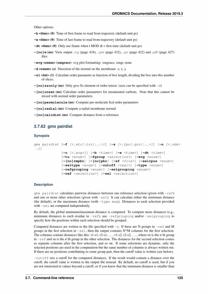
GROMACS Documentation, Release 2019.3
Other options:
-b <time> (0) Time of first frame to read from trajectory (default unit ps)
-e <time> (0) Time of last frame to read from trajectory (default unit ps)
-dt <time> (0) Only use frame when t MOD dt = first time (default unit ps)
-[no]w (no) View output .xvg (page 434), .xpm (page 432), .eps (page 422) and .pdb (page 427)files
-xvg <enum> (xmgrace) xvg plot formatting: xmgrace, xmgr, none
-d <enum> (z) Direction of the normal on the membrane: z, x, y
-sl <int> (1) Calculate order parameter as function of box length, dividing the box into this numberof slices.
-[no]szonly (no) Only give Sz element of order tensor. (axis can be specified with -d)
-[no]unsat (no) Calculate order parameters for unsaturated carbons. Note that this cannot bemixed with normal order parameters.
-[no]permolecule (no) Compute per-molecule Scd order parameters
-[no]radial (no) Compute a radial membrane normal
-[no]calcdist (no) Compute distance from a reference
3.7.62 gmx pairdist
Synopsis
gmx pairdist [-f [<.xtc/.trr/...>]] [-s [<.tpr/.gro/...>]] [-n [<.ndx>→˓]]
[-o [<.xvg>]] [-b <time>] [-e <time>] [-dt <time>][-tu <enum>] [-fgroup <selection>] [-xvg <enum>][-[no]rmpbc] [-[no]pbc] [-sf <file>] [-selrpos <enum>][-seltype <enum>] [-cutoff <real>] [-type <enum>][-refgrouping <enum>] [-selgrouping <enum>][-ref <selection>] [-sel <selection>]
Description
gmx pairdist calculates pairwise distances between one reference selection (given with -ref)and one or more other selections (given with -sel). It can calculate either the minimum distance(the default), or the maximum distance (with -type max). Distances to each selection providedwith -sel are computed independently.
By default, the global minimum/maximum distance is computed. To compute more distances (e.g.,minimum distances to each residue in -ref), use -refgrouping and/or -selgrouping tospecify how the positions within each selection should be grouped.
Computed distances are written to the file specified with -o. If there are N groups in -ref and Mgroups in the first selection in -sel, then the output contains N*M columns for the first selection.The columns contain distances like this: r1-s1, r2-s1, . . . , r1-s2, r2-s2, . . . , where rn is the n’th groupin -ref and sn is the n’th group in the other selection. The distances for the second selection comesas separate columns after the first selection, and so on. If some selections are dynamic, only theselected positions are used in the computation but the same number of columns is always written out.If there are no positions contributing to some group pair, then the cutoff value is written (see below).
-cutoff sets a cutoff for the computed distances. If the result would contain a distance over thecutoff, the cutoff value is written to the output file instead. By default, no cutoff is used, but if youare not interested in values beyond a cutoff, or if you know that the minimum distance is smaller than
3.7. Command-line reference 125
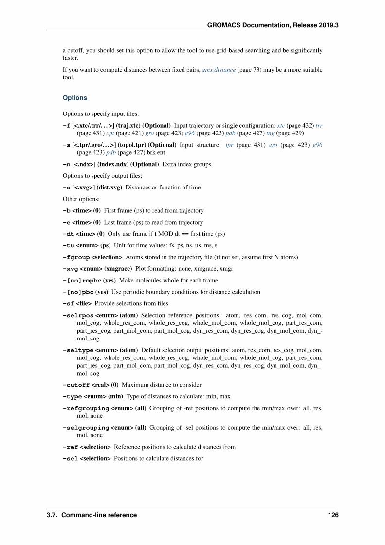
GROMACS Documentation, Release 2019.3
a cutoff, you should set this option to allow the tool to use grid-based searching and be significantlyfaster.
If you want to compute distances between fixed pairs, gmx distance (page 73) may be a more suitabletool.
Options
Options to specify input files:
-f [<.xtc/.trr/. . . >] (traj.xtc) (Optional) Input trajectory or single configuration: xtc (page 432) trr(page 431) cpt (page 421) gro (page 423) g96 (page 423) pdb (page 427) tng (page 429)
-s [<.tpr/.gro/. . . >] (topol.tpr) (Optional) Input structure: tpr (page 431) gro (page 423) g96(page 423) pdb (page 427) brk ent
-n [<.ndx>] (index.ndx) (Optional) Extra index groups
Options to specify output files:
-o [<.xvg>] (dist.xvg) Distances as function of time
Other options:
-b <time> (0) First frame (ps) to read from trajectory
-e <time> (0) Last frame (ps) to read from trajectory
-dt <time> (0) Only use frame if t MOD dt == first time (ps)
-tu <enum> (ps) Unit for time values: fs, ps, ns, us, ms, s
-fgroup <selection> Atoms stored in the trajectory file (if not set, assume first N atoms)
-xvg <enum> (xmgrace) Plot formatting: none, xmgrace, xmgr
-[no]rmpbc (yes) Make molecules whole for each frame
-[no]pbc (yes) Use periodic boundary conditions for distance calculation
-sf <file> Provide selections from files
-selrpos <enum> (atom) Selection reference positions: atom, res_com, res_cog, mol_com,mol_cog, whole_res_com, whole_res_cog, whole_mol_com, whole_mol_cog, part_res_com,part_res_cog, part_mol_com, part_mol_cog, dyn_res_com, dyn_res_cog, dyn_mol_com, dyn_-mol_cog
-seltype <enum> (atom) Default selection output positions: atom, res_com, res_cog, mol_com,mol_cog, whole_res_com, whole_res_cog, whole_mol_com, whole_mol_cog, part_res_com,part_res_cog, part_mol_com, part_mol_cog, dyn_res_com, dyn_res_cog, dyn_mol_com, dyn_-mol_cog
-cutoff <real> (0) Maximum distance to consider
-type <enum> (min) Type of distances to calculate: min, max
-refgrouping <enum> (all) Grouping of -ref positions to compute the min/max over: all, res,mol, none
-selgrouping <enum> (all) Grouping of -sel positions to compute the min/max over: all, res,mol, none
-ref <selection> Reference positions to calculate distances from
-sel <selection> Positions to calculate distances for
3.7. Command-line reference 126
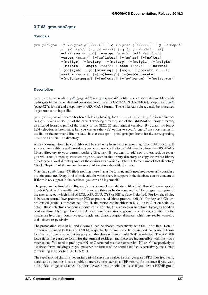
GROMACS Documentation, Release 2019.3
3.7.63 gmx pdb2gmx
Synopsis
gmx pdb2gmx [-f [<.gro/.g96/...>]] [-o [<.gro/.g96/...>]] [-p [<.top>]][-i [<.itp>]] [-n [<.ndx>]] [-q [<.gro/.g96/...>]][-chainsep <enum>] [-merge <enum>] [-ff <string>][-water <enum>] [-[no]inter] [-[no]ss] [-[no]ter][-[no]lys] [-[no]arg] [-[no]asp] [-[no]glu] [-[no]gln][-[no]his] [-angle <real>] [-dist <real>] [-[no]una][-[no]ignh] [-[no]missing] [-[no]v] [-posrefc <real>][-vsite <enum>] [-[no]heavyh] [-[no]deuterate][-[no]chargegrp] [-[no]cmap] [-[no]renum] [-[no]rtpres]
Description
gmx pdb2gmx reads a .pdb (page 427) (or .gro (page 423)) file, reads some database files, addshydrogens to the molecules and generates coordinates in GROMACS (GROMOS), or optionally .pdb(page 427), format and a topology in GROMACS format. These files can subsequently be processedto generate a run input file.
gmx pdb2gmx will search for force fields by looking for a forcefield.itp file in subdirecto-ries <forcefield>.ff of the current working directory and of the GROMACS library directoryas inferred from the path of the binary or the GMXLIB environment variable. By default the force-field selection is interactive, but you can use the -ff option to specify one of the short names inthe list on the command line instead. In that case gmx pdb2gmx just looks for the corresponding<forcefield>.ff directory.
After choosing a force field, all files will be read only from the corresponding force field directory. Ifyou want to modify or add a residue types, you can copy the force field directory from the GROMACSlibrary directory to your current working directory. If you want to add new protein residue types,you will need to modify residuetypes.dat in the library directory or copy the whole librarydirectory to a local directory and set the environment variable GMXLIB to the name of that directory.Check Chapter 5 of the manual for more information about file formats.
Note that a .pdb (page 427) file is nothing more than a file format, and it need not necessarily contain aprotein structure. Every kind of molecule for which there is support in the database can be converted.If there is no support in the database, you can add it yourself.
The program has limited intelligence, it reads a number of database files, that allow it to make specialbonds (Cys-Cys, Heme-His, etc.), if necessary this can be done manually. The program can promptthe user to select which kind of LYS, ASP, GLU, CYS or HIS residue is desired. For Lys the choiceis between neutral (two protons on NZ) or protonated (three protons, default), for Asp and Glu un-protonated (default) or protonated, for His the proton can be either on ND1, on NE2 or on both. Bydefault these selections are done automatically. For His, this is based on an optimal hydrogen bondingconformation. Hydrogen bonds are defined based on a simple geometric criterion, specified by themaximum hydrogen-donor-acceptor angle and donor-acceptor distance, which are set by -angleand -dist respectively.
The protonation state of N- and C-termini can be chosen interactively with the -ter flag. Defaulttermini are ionized (NH3+ and COO-), respectively. Some force fields support zwitterionic formsfor chains of one residue, but for polypeptides these options should NOT be selected. The AMBERforce fields have unique forms for the terminal residues, and these are incompatible with the -termechanism. You need to prefix your N- or C-terminal residue names with “N” or “C” respectively touse these forms, making sure you preserve the format of the coordinate file. Alternatively, use namedterminating residues (e.g. ACE, NME).
The separation of chains is not entirely trivial since the markup in user-generated PDB files frequentlyvaries and sometimes it is desirable to merge entries across a TER record, for instance if you wanta disulfide bridge or distance restraints between two protein chains or if you have a HEME group
3.7. Command-line reference 127
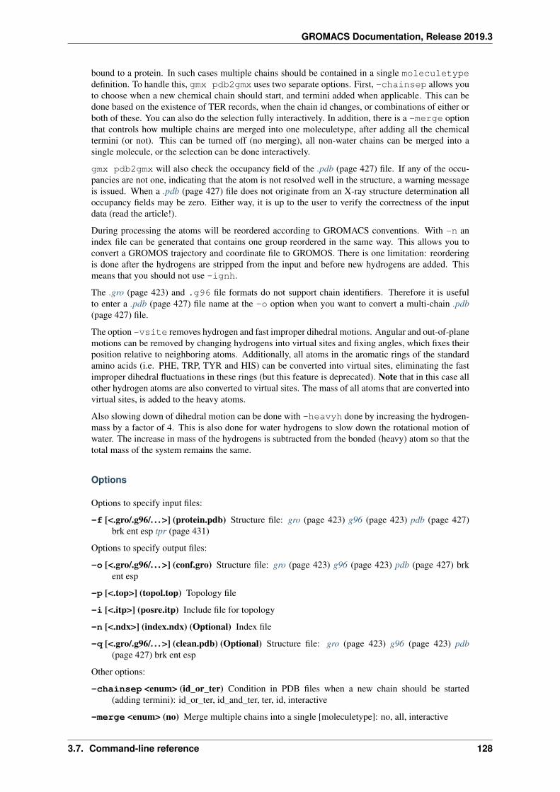
GROMACS Documentation, Release 2019.3
bound to a protein. In such cases multiple chains should be contained in a single moleculetypedefinition. To handle this, gmx pdb2gmx uses two separate options. First, -chainsep allows youto choose when a new chemical chain should start, and termini added when applicable. This can bedone based on the existence of TER records, when the chain id changes, or combinations of either orboth of these. You can also do the selection fully interactively. In addition, there is a -merge optionthat controls how multiple chains are merged into one moleculetype, after adding all the chemicaltermini (or not). This can be turned off (no merging), all non-water chains can be merged into asingle molecule, or the selection can be done interactively.
gmx pdb2gmx will also check the occupancy field of the .pdb (page 427) file. If any of the occu-pancies are not one, indicating that the atom is not resolved well in the structure, a warning messageis issued. When a .pdb (page 427) file does not originate from an X-ray structure determination alloccupancy fields may be zero. Either way, it is up to the user to verify the correctness of the inputdata (read the article!).
During processing the atoms will be reordered according to GROMACS conventions. With -n anindex file can be generated that contains one group reordered in the same way. This allows you toconvert a GROMOS trajectory and coordinate file to GROMOS. There is one limitation: reorderingis done after the hydrogens are stripped from the input and before new hydrogens are added. Thismeans that you should not use -ignh.
The .gro (page 423) and .g96 file formats do not support chain identifiers. Therefore it is usefulto enter a .pdb (page 427) file name at the -o option when you want to convert a multi-chain .pdb(page 427) file.
The option -vsite removes hydrogen and fast improper dihedral motions. Angular and out-of-planemotions can be removed by changing hydrogens into virtual sites and fixing angles, which fixes theirposition relative to neighboring atoms. Additionally, all atoms in the aromatic rings of the standardamino acids (i.e. PHE, TRP, TYR and HIS) can be converted into virtual sites, eliminating the fastimproper dihedral fluctuations in these rings (but this feature is deprecated). Note that in this case allother hydrogen atoms are also converted to virtual sites. The mass of all atoms that are converted intovirtual sites, is added to the heavy atoms.
Also slowing down of dihedral motion can be done with -heavyh done by increasing the hydrogen-mass by a factor of 4. This is also done for water hydrogens to slow down the rotational motion ofwater. The increase in mass of the hydrogens is subtracted from the bonded (heavy) atom so that thetotal mass of the system remains the same.
Options
Options to specify input files:
-f [<.gro/.g96/. . . >] (protein.pdb) Structure file: gro (page 423) g96 (page 423) pdb (page 427)brk ent esp tpr (page 431)
Options to specify output files:
-o [<.gro/.g96/. . . >] (conf.gro) Structure file: gro (page 423) g96 (page 423) pdb (page 427) brkent esp
-p [<.top>] (topol.top) Topology file
-i [<.itp>] (posre.itp) Include file for topology
-n [<.ndx>] (index.ndx) (Optional) Index file
-q [<.gro/.g96/. . . >] (clean.pdb) (Optional) Structure file: gro (page 423) g96 (page 423) pdb(page 427) brk ent esp
Other options:
-chainsep <enum> (id_or_ter) Condition in PDB files when a new chain should be started(adding termini): id_or_ter, id_and_ter, ter, id, interactive
-merge <enum> (no) Merge multiple chains into a single [moleculetype]: no, all, interactive
3.7. Command-line reference 128
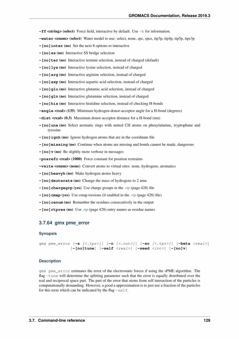
GROMACS Documentation, Release 2019.3
-ff <string> (select) Force field, interactive by default. Use -h for information.
-water <enum> (select) Water model to use: select, none, spc, spce, tip3p, tip4p, tip5p, tips3p
-[no]inter (no) Set the next 8 options to interactive
-[no]ss (no) Interactive SS bridge selection
-[no]ter (no) Interactive termini selection, instead of charged (default)
-[no]lys (no) Interactive lysine selection, instead of charged
-[no]arg (no) Interactive arginine selection, instead of charged
-[no]asp (no) Interactive aspartic acid selection, instead of charged
-[no]glu (no) Interactive glutamic acid selection, instead of charged
-[no]gln (no) Interactive glutamine selection, instead of charged
-[no]his (no) Interactive histidine selection, instead of checking H-bonds
-angle <real> (135) Minimum hydrogen-donor-acceptor angle for a H-bond (degrees)
-dist <real> (0.3) Maximum donor-acceptor distance for a H-bond (nm)
-[no]una (no) Select aromatic rings with united CH atoms on phenylalanine, tryptophane andtyrosine
-[no]ignh (no) Ignore hydrogen atoms that are in the coordinate file
-[no]missing (no) Continue when atoms are missing and bonds cannot be made, dangerous
-[no]v (no) Be slightly more verbose in messages
-posrefc <real> (1000) Force constant for position restraints
-vsite <enum> (none) Convert atoms to virtual sites: none, hydrogens, aromatics
-[no]heavyh (no) Make hydrogen atoms heavy
-[no]deuterate (no) Change the mass of hydrogens to 2 amu
-[no]chargegrp (yes) Use charge groups in the .rtp (page 428) file
-[no]cmap (yes) Use cmap torsions (if enabled in the .rtp (page 428) file)
-[no]renum (no) Renumber the residues consecutively in the output
-[no]rtpres (no) Use .rtp (page 428) entry names as residue names
3.7.64 gmx pme_error
Synopsis
gmx pme_error [-s [<.tpr>]] [-o [<.out>]] [-so [<.tpr>]] [-beta <real>][-[no]tune] [-self <real>] [-seed <int>] [-[no]v]
Description
gmx pme_error estimates the error of the electrostatic forces if using the sPME algorithm. Theflag -tune will determine the splitting parameter such that the error is equally distributed over thereal and reciprocal space part. The part of the error that stems from self interaction of the particles iscomputationally demanding. However, a good a approximation is to just use a fraction of the particlesfor this term which can be indicated by the flag -self.
3.7. Command-line reference 129
GROMACS Documentation, Release 2019.3
Options
Options to specify input files:
-s [<.tpr>] (topol.tpr) Portable xdr run input file
Options to specify output files:
-o [<.out>] (error.out) Generic output file
-so [<.tpr>] (tuned.tpr) (Optional) Portable xdr run input file
Other options:
-beta <real> (-1) If positive, overwrite ewald_beta from .tpr (page 431) file with this value
-[no]tune (no) Tune the splitting parameter such that the error is equally distributed between realand reciprocal space
-self <real> (1) If between 0.0 and 1.0, determine self interaction error from just this fraction ofthe charged particles
-seed <int> (0) Random number seed used for Monte Carlo algorithm when -self is set to avalue between 0.0 and 1.0
-[no]v (no) Be loud and noisy
3.7.65 gmx polystat
Synopsis
gmx polystat [-s [<.tpr>]] [-f [<.xtc/.trr/...>]] [-n [<.ndx>]][-o [<.xvg>]] [-v [<.xvg>]] [-p [<.xvg>]] [-i [<.xvg>]][-b <time>] [-e <time>] [-dt <time>] [-tu <enum>][-[no]w] [-xvg <enum>] [-[no]mw] [-[no]pc]
Description
gmx polystat plots static properties of polymers as a function of time and prints the average.
By default it determines the average end-to-end distance and radii of gyration of polymers. It asksfor an index group and split this into molecules. The end-to-end distance is then determined usingthe first and the last atom in the index group for each molecules. For the radius of gyration the totaland the three principal components for the average gyration tensor are written. With option -v theeigenvectors are written. With option -pc also the average eigenvalues of the individual gyrationtensors are written. With option -i the mean square internal distances are written.
With option -p the persistence length is determined. The chosen index group should consist of atomsthat are consecutively bonded in the polymer mainchains. The persistence length is then determinedfrom the cosine of the angles between bonds with an index difference that is even, the odd pairs arenot used, because straight polymer backbones are usually all trans and therefore only every secondbond aligns. The persistence length is defined as number of bonds where the average cos reaches avalue of 1/e. This point is determined by a linear interpolation of log(<cos>).
Options
Options to specify input files:
-s [<.tpr>] (topol.tpr) Portable xdr run input file
-f [<.xtc/.trr/. . . >] (traj.xtc) Trajectory: xtc (page 432) trr (page 431) cpt (page 421) gro(page 423) g96 (page 423) pdb (page 427) tng (page 429)
3.7. Command-line reference 130
GROMACS Documentation, Release 2019.3
-n [<.ndx>] (index.ndx) (Optional) Index file
Options to specify output files:
-o [<.xvg>] (polystat.xvg) xvgr/xmgr file
-v [<.xvg>] (polyvec.xvg) (Optional) xvgr/xmgr file
-p [<.xvg>] (persist.xvg) (Optional) xvgr/xmgr file
-i [<.xvg>] (intdist.xvg) (Optional) xvgr/xmgr file
Other options:
-b <time> (0) Time of first frame to read from trajectory (default unit ps)
-e <time> (0) Time of last frame to read from trajectory (default unit ps)
-dt <time> (0) Only use frame when t MOD dt = first time (default unit ps)
-tu <enum> (ps) Unit for time values: fs, ps, ns, us, ms, s
-[no]w (no) View output .xvg (page 434), .xpm (page 432), .eps (page 422) and .pdb (page 427)files
-xvg <enum> (xmgrace) xvg plot formatting: xmgrace, xmgr, none
-[no]mw (yes) Use the mass weighting for radii of gyration
-[no]pc (no) Plot average eigenvalues
3.7.66 gmx potential
Synopsis
gmx potential [-f [<.xtc/.trr/...>]] [-n [<.ndx>]] [-s [<.tpr>]][-o [<.xvg>]] [-oc [<.xvg>]] [-of [<.xvg>]] [-b <time>][-e <time>] [-dt <time>] [-[no]w] [-xvg <enum>][-d <string>] [-sl <int>] [-cb <int>] [-ce <int>][-tz <real>] [-[no]spherical] [-ng <int>] [-[no]correct]
Description
gmx potential computes the electrostatical potential across the box. The potential is calculatedby first summing the charges per slice and then integrating twice of this charge distribution. Periodicboundaries are not taken into account. Reference of potential is taken to be the left side of the box.It is also possible to calculate the potential in spherical coordinates as function of r by calculatinga charge distribution in spherical slices and twice integrating them. epsilon_r is taken as 1, but 2 ismore appropriate in many cases.
Options
Options to specify input files:
-f [<.xtc/.trr/. . . >] (traj.xtc) Trajectory: xtc (page 432) trr (page 431) cpt (page 421) gro(page 423) g96 (page 423) pdb (page 427) tng (page 429)
-n [<.ndx>] (index.ndx) Index file
-s [<.tpr>] (topol.tpr) Portable xdr run input file
Options to specify output files:
-o [<.xvg>] (potential.xvg) xvgr/xmgr file
-oc [<.xvg>] (charge.xvg) xvgr/xmgr file
3.7. Command-line reference 131
GROMACS Documentation, Release 2019.3
-of [<.xvg>] (field.xvg) xvgr/xmgr file
Other options:
-b <time> (0) Time of first frame to read from trajectory (default unit ps)
-e <time> (0) Time of last frame to read from trajectory (default unit ps)
-dt <time> (0) Only use frame when t MOD dt = first time (default unit ps)
-[no]w (no) View output .xvg (page 434), .xpm (page 432), .eps (page 422) and .pdb (page 427)files
-xvg <enum> (xmgrace) xvg plot formatting: xmgrace, xmgr, none
-d <string> (Z) Take the normal on the membrane in direction X, Y or Z.
-sl <int> (10) Calculate potential as function of boxlength, dividing the box in this number ofslices.
-cb <int> (0) Discard this number of first slices of box for integration
-ce <int> (0) Discard this number of last slices of box for integration
-tz <real> (0) Translate all coordinates by this distance in the direction of the box
-[no]spherical (no) Calculate in spherical coordinates
-ng <int> (1) Number of groups to consider
-[no]correct (no) Assume net zero charge of groups to improve accuracy
Known Issues
• Discarding slices for integration should not be necessary.
3.7.67 gmx principal
Synopsis
gmx principal [-f [<.xtc/.trr/...>]] [-s [<.tpr/.gro/...>]][-n [<.ndx>]] [-a1 [<.xvg>]] [-a2 [<.xvg>]][-a3 [<.xvg>]] [-om [<.xvg>]] [-b <time>] [-e <time>][-dt <time>] [-tu <enum>] [-[no]w] [-xvg <enum>][-[no]foo]
Description
gmx principal calculates the three principal axes of inertia for a group of atoms. NOTE: Oldversions of GROMACS wrote the output data in a strange transposed way. As of GROMACS 5.0, theoutput file paxis1.dat contains the x/y/z components of the first (major) principal axis for each frame,and similarly for the middle and minor axes in paxis2.dat and paxis3.dat.
Options
Options to specify input files:
-f [<.xtc/.trr/. . . >] (traj.xtc) Trajectory: xtc (page 432) trr (page 431) cpt (page 421) gro(page 423) g96 (page 423) pdb (page 427) tng (page 429)
-s [<.tpr/.gro/. . . >] (topol.tpr) Structure+mass(db): tpr (page 431) gro (page 423) g96 (page 423)pdb (page 427) brk ent
3.7. Command-line reference 132
GROMACS Documentation, Release 2019.3
-n [<.ndx>] (index.ndx) (Optional) Index file
Options to specify output files:
-a1 [<.xvg>] (paxis1.xvg) xvgr/xmgr file
-a2 [<.xvg>] (paxis2.xvg) xvgr/xmgr file
-a3 [<.xvg>] (paxis3.xvg) xvgr/xmgr file
-om [<.xvg>] (moi.xvg) xvgr/xmgr file
Other options:
-b <time> (0) Time of first frame to read from trajectory (default unit ps)
-e <time> (0) Time of last frame to read from trajectory (default unit ps)
-dt <time> (0) Only use frame when t MOD dt = first time (default unit ps)
-tu <enum> (ps) Unit for time values: fs, ps, ns, us, ms, s
-[no]w (no) View output .xvg (page 434), .xpm (page 432), .eps (page 422) and .pdb (page 427)files
-xvg <enum> (xmgrace) xvg plot formatting: xmgrace, xmgr, none
-[no]foo (no) Dummy option to avoid empty array
3.7.68 gmx rama
Synopsis
gmx rama [-f [<.xtc/.trr/...>]] [-s [<.tpr>]] [-o [<.xvg>]] [-b <time>][-e <time>] [-dt <time>] [-[no]w] [-xvg <enum>]
Description
gmx rama selects the phi/psi dihedral combinations from your topology file and computes these asa function of time. Using simple Unix tools such as grep you can select out specific residues.
Options
Options to specify input files:
-f [<.xtc/.trr/. . . >] (traj.xtc) Trajectory: xtc (page 432) trr (page 431) cpt (page 421) gro(page 423) g96 (page 423) pdb (page 427) tng (page 429)
-s [<.tpr>] (topol.tpr) Portable xdr run input file
Options to specify output files:
-o [<.xvg>] (rama.xvg) xvgr/xmgr file
Other options:
-b <time> (0) Time of first frame to read from trajectory (default unit ps)
-e <time> (0) Time of last frame to read from trajectory (default unit ps)
-dt <time> (0) Only use frame when t MOD dt = first time (default unit ps)
-[no]w (no) View output .xvg (page 434), .xpm (page 432), .eps (page 422) and .pdb (page 427)files
-xvg <enum> (xmgrace) xvg plot formatting: xmgrace, xmgr, none
3.7. Command-line reference 133
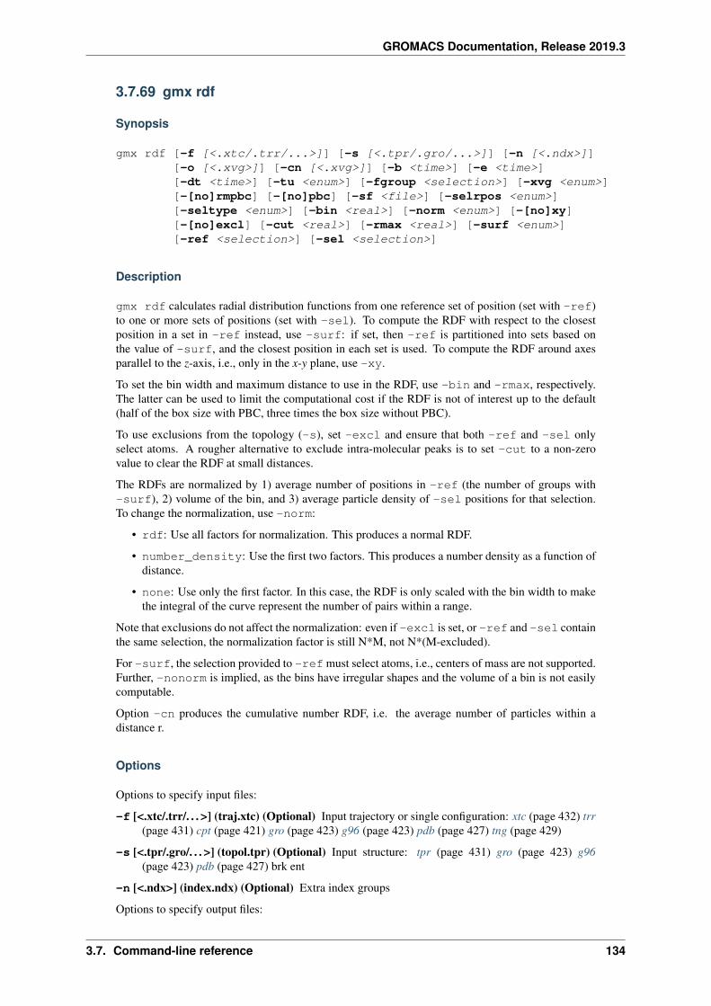
GROMACS Documentation, Release 2019.3
3.7.69 gmx rdf
Synopsis
gmx rdf [-f [<.xtc/.trr/...>]] [-s [<.tpr/.gro/...>]] [-n [<.ndx>]][-o [<.xvg>]] [-cn [<.xvg>]] [-b <time>] [-e <time>][-dt <time>] [-tu <enum>] [-fgroup <selection>] [-xvg <enum>][-[no]rmpbc] [-[no]pbc] [-sf <file>] [-selrpos <enum>][-seltype <enum>] [-bin <real>] [-norm <enum>] [-[no]xy][-[no]excl] [-cut <real>] [-rmax <real>] [-surf <enum>][-ref <selection>] [-sel <selection>]
Description
gmx rdf calculates radial distribution functions from one reference set of position (set with -ref)to one or more sets of positions (set with -sel). To compute the RDF with respect to the closestposition in a set in -ref instead, use -surf: if set, then -ref is partitioned into sets based onthe value of -surf, and the closest position in each set is used. To compute the RDF around axesparallel to the z-axis, i.e., only in the x-y plane, use -xy.
To set the bin width and maximum distance to use in the RDF, use -bin and -rmax, respectively.The latter can be used to limit the computational cost if the RDF is not of interest up to the default(half of the box size with PBC, three times the box size without PBC).
To use exclusions from the topology (-s), set -excl and ensure that both -ref and -sel onlyselect atoms. A rougher alternative to exclude intra-molecular peaks is to set -cut to a non-zerovalue to clear the RDF at small distances.
The RDFs are normalized by 1) average number of positions in -ref (the number of groups with-surf), 2) volume of the bin, and 3) average particle density of -sel positions for that selection.To change the normalization, use -norm:
• rdf: Use all factors for normalization. This produces a normal RDF.
• number_density: Use the first two factors. This produces a number density as a function ofdistance.
• none: Use only the first factor. In this case, the RDF is only scaled with the bin width to makethe integral of the curve represent the number of pairs within a range.
Note that exclusions do not affect the normalization: even if -excl is set, or -ref and -sel containthe same selection, the normalization factor is still N*M, not N*(M-excluded).
For -surf, the selection provided to -ref must select atoms, i.e., centers of mass are not supported.Further, -nonorm is implied, as the bins have irregular shapes and the volume of a bin is not easilycomputable.
Option -cn produces the cumulative number RDF, i.e. the average number of particles within adistance r.
Options
Options to specify input files:
-f [<.xtc/.trr/. . . >] (traj.xtc) (Optional) Input trajectory or single configuration: xtc (page 432) trr(page 431) cpt (page 421) gro (page 423) g96 (page 423) pdb (page 427) tng (page 429)
-s [<.tpr/.gro/. . . >] (topol.tpr) (Optional) Input structure: tpr (page 431) gro (page 423) g96(page 423) pdb (page 427) brk ent
-n [<.ndx>] (index.ndx) (Optional) Extra index groups
Options to specify output files:
3.7. Command-line reference 134
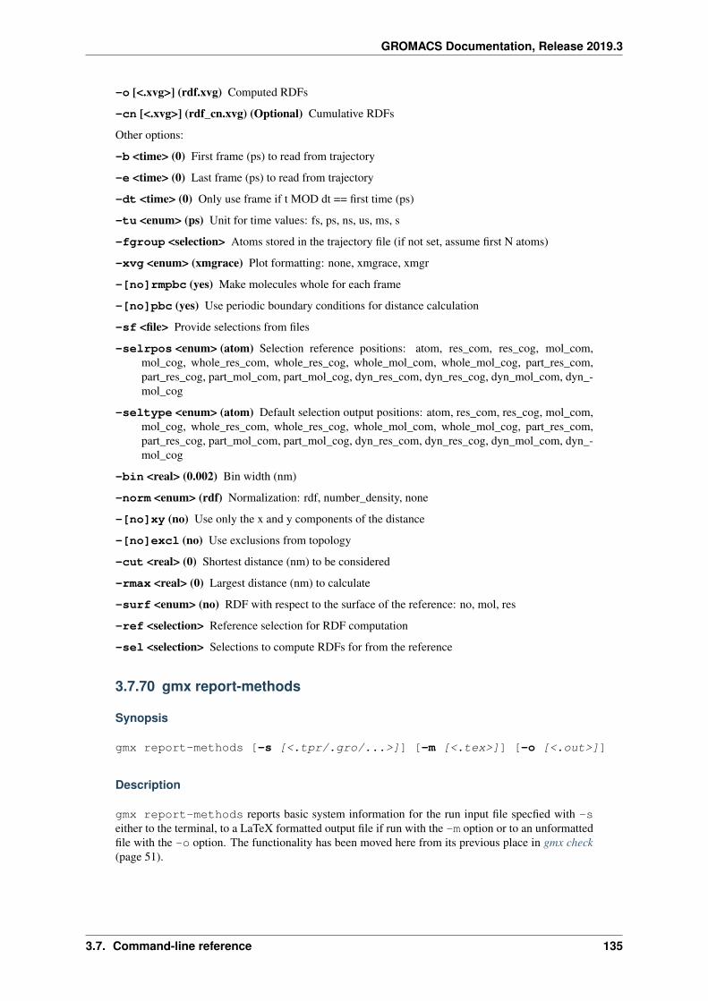
GROMACS Documentation, Release 2019.3
-o [<.xvg>] (rdf.xvg) Computed RDFs
-cn [<.xvg>] (rdf_cn.xvg) (Optional) Cumulative RDFs
Other options:
-b <time> (0) First frame (ps) to read from trajectory
-e <time> (0) Last frame (ps) to read from trajectory
-dt <time> (0) Only use frame if t MOD dt == first time (ps)
-tu <enum> (ps) Unit for time values: fs, ps, ns, us, ms, s
-fgroup <selection> Atoms stored in the trajectory file (if not set, assume first N atoms)
-xvg <enum> (xmgrace) Plot formatting: none, xmgrace, xmgr
-[no]rmpbc (yes) Make molecules whole for each frame
-[no]pbc (yes) Use periodic boundary conditions for distance calculation
-sf <file> Provide selections from files
-selrpos <enum> (atom) Selection reference positions: atom, res_com, res_cog, mol_com,mol_cog, whole_res_com, whole_res_cog, whole_mol_com, whole_mol_cog, part_res_com,part_res_cog, part_mol_com, part_mol_cog, dyn_res_com, dyn_res_cog, dyn_mol_com, dyn_-mol_cog
-seltype <enum> (atom) Default selection output positions: atom, res_com, res_cog, mol_com,mol_cog, whole_res_com, whole_res_cog, whole_mol_com, whole_mol_cog, part_res_com,part_res_cog, part_mol_com, part_mol_cog, dyn_res_com, dyn_res_cog, dyn_mol_com, dyn_-mol_cog
-bin <real> (0.002) Bin width (nm)
-norm <enum> (rdf) Normalization: rdf, number_density, none
-[no]xy (no) Use only the x and y components of the distance
-[no]excl (no) Use exclusions from topology
-cut <real> (0) Shortest distance (nm) to be considered
-rmax <real> (0) Largest distance (nm) to calculate
-surf <enum> (no) RDF with respect to the surface of the reference: no, mol, res
-ref <selection> Reference selection for RDF computation
-sel <selection> Selections to compute RDFs for from the reference
3.7.70 gmx report-methods
Synopsis
gmx report-methods [-s [<.tpr/.gro/...>]] [-m [<.tex>]] [-o [<.out>]]
Description
gmx report-methods reports basic system information for the run input file specfied with -seither to the terminal, to a LaTeX formatted output file if run with the -m option or to an unformattedfile with the -o option. The functionality has been moved here from its previous place in gmx check(page 51).
3.7. Command-line reference 135
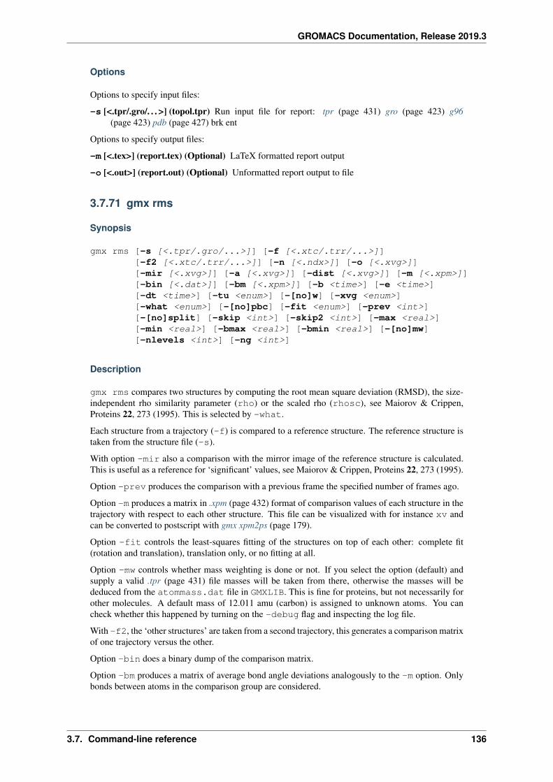
GROMACS Documentation, Release 2019.3
Options
Options to specify input files:
-s [<.tpr/.gro/. . . >] (topol.tpr) Run input file for report: tpr (page 431) gro (page 423) g96(page 423) pdb (page 427) brk ent
Options to specify output files:
-m [<.tex>] (report.tex) (Optional) LaTeX formatted report output
-o [<.out>] (report.out) (Optional) Unformatted report output to file
3.7.71 gmx rms
Synopsis
gmx rms [-s [<.tpr/.gro/...>]] [-f [<.xtc/.trr/...>]][-f2 [<.xtc/.trr/...>]] [-n [<.ndx>]] [-o [<.xvg>]][-mir [<.xvg>]] [-a [<.xvg>]] [-dist [<.xvg>]] [-m [<.xpm>]][-bin [<.dat>]] [-bm [<.xpm>]] [-b <time>] [-e <time>][-dt <time>] [-tu <enum>] [-[no]w] [-xvg <enum>][-what <enum>] [-[no]pbc] [-fit <enum>] [-prev <int>][-[no]split] [-skip <int>] [-skip2 <int>] [-max <real>][-min <real>] [-bmax <real>] [-bmin <real>] [-[no]mw][-nlevels <int>] [-ng <int>]
Description
gmx rms compares two structures by computing the root mean square deviation (RMSD), the size-independent rho similarity parameter (rho) or the scaled rho (rhosc), see Maiorov & Crippen,Proteins 22, 273 (1995). This is selected by -what.
Each structure from a trajectory (-f) is compared to a reference structure. The reference structure istaken from the structure file (-s).
With option -mir also a comparison with the mirror image of the reference structure is calculated.This is useful as a reference for ‘significant’ values, see Maiorov & Crippen, Proteins 22, 273 (1995).
Option -prev produces the comparison with a previous frame the specified number of frames ago.
Option -m produces a matrix in .xpm (page 432) format of comparison values of each structure in thetrajectory with respect to each other structure. This file can be visualized with for instance xv andcan be converted to postscript with gmx xpm2ps (page 179).
Option -fit controls the least-squares fitting of the structures on top of each other: complete fit(rotation and translation), translation only, or no fitting at all.
Option -mw controls whether mass weighting is done or not. If you select the option (default) andsupply a valid .tpr (page 431) file masses will be taken from there, otherwise the masses will bededuced from the atommass.dat file in GMXLIB. This is fine for proteins, but not necessarily forother molecules. A default mass of 12.011 amu (carbon) is assigned to unknown atoms. You cancheck whether this happened by turning on the -debug flag and inspecting the log file.
With -f2, the ‘other structures’ are taken from a second trajectory, this generates a comparison matrixof one trajectory versus the other.
Option -bin does a binary dump of the comparison matrix.
Option -bm produces a matrix of average bond angle deviations analogously to the -m option. Onlybonds between atoms in the comparison group are considered.
3.7. Command-line reference 136
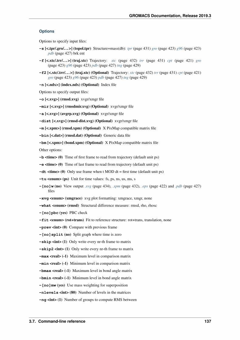
GROMACS Documentation, Release 2019.3
Options
Options to specify input files:
-s [<.tpr/.gro/. . . >] (topol.tpr) Structure+mass(db): tpr (page 431) gro (page 423) g96 (page 423)pdb (page 427) brk ent
-f [<.xtc/.trr/. . . >] (traj.xtc) Trajectory: xtc (page 432) trr (page 431) cpt (page 421) gro(page 423) g96 (page 423) pdb (page 427) tng (page 429)
-f2 [<.xtc/.trr/. . . >] (traj.xtc) (Optional) Trajectory: xtc (page 432) trr (page 431) cpt (page 421)gro (page 423) g96 (page 423) pdb (page 427) tng (page 429)
-n [<.ndx>] (index.ndx) (Optional) Index file
Options to specify output files:
-o [<.xvg>] (rmsd.xvg) xvgr/xmgr file
-mir [<.xvg>] (rmsdmir.xvg) (Optional) xvgr/xmgr file
-a [<.xvg>] (avgrp.xvg) (Optional) xvgr/xmgr file
-dist [<.xvg>] (rmsd-dist.xvg) (Optional) xvgr/xmgr file
-m [<.xpm>] (rmsd.xpm) (Optional) X PixMap compatible matrix file
-bin [<.dat>] (rmsd.dat) (Optional) Generic data file
-bm [<.xpm>] (bond.xpm) (Optional) X PixMap compatible matrix file
Other options:
-b <time> (0) Time of first frame to read from trajectory (default unit ps)
-e <time> (0) Time of last frame to read from trajectory (default unit ps)
-dt <time> (0) Only use frame when t MOD dt = first time (default unit ps)
-tu <enum> (ps) Unit for time values: fs, ps, ns, us, ms, s
-[no]w (no) View output .xvg (page 434), .xpm (page 432), .eps (page 422) and .pdb (page 427)files
-xvg <enum> (xmgrace) xvg plot formatting: xmgrace, xmgr, none
-what <enum> (rmsd) Structural difference measure: rmsd, rho, rhosc
-[no]pbc (yes) PBC check
-fit <enum> (rot+trans) Fit to reference structure: rot+trans, translation, none
-prev <int> (0) Compare with previous frame
-[no]split (no) Split graph where time is zero
-skip <int> (1) Only write every nr-th frame to matrix
-skip2 <int> (1) Only write every nr-th frame to matrix
-max <real> (-1) Maximum level in comparison matrix
-min <real> (-1) Minimum level in comparison matrix
-bmax <real> (-1) Maximum level in bond angle matrix
-bmin <real> (-1) Minimum level in bond angle matrix
-[no]mw (yes) Use mass weighting for superposition
-nlevels <int> (80) Number of levels in the matrices
-ng <int> (1) Number of groups to compute RMS between
3.7. Command-line reference 137
GROMACS Documentation, Release 2019.3
3.7.72 gmx rmsdist
Synopsis
gmx rmsdist [-f [<.xtc/.trr/...>]] [-s [<.tpr/.gro/...>]] [-n [<.ndx>]][-equiv [<.dat>]] [-o [<.xvg>]] [-rms [<.xpm>]][-scl [<.xpm>]] [-mean [<.xpm>]] [-nmr3 [<.xpm>]][-nmr6 [<.xpm>]] [-noe [<.dat>]] [-b <time>] [-e <time>][-dt <time>] [-[no]w] [-xvg <enum>] [-nlevels <int>][-max <real>] [-[no]sumh] [-[no]pbc]
Description
gmx rmsdist computes the root mean square deviation of atom distances, which has the advan-tage that no fit is needed like in standard RMS deviation as computed by gmx rms (page 136). Thereference structure is taken from the structure file. The RMSD at time t is calculated as the RMS ofthe differences in distance between atom-pairs in the reference structure and the structure at time t.
gmx rmsdist can also produce matrices of the rms distances, rms distances scaled with the meandistance and the mean distances and matrices with NMR averaged distances (1/r^3 and 1/r^6 averag-ing). Finally, lists of atom pairs with 1/r^3 and 1/r^6 averaged distance below the maximum distance(-max, which will default to 0.6 in this case) can be generated, by default averaging over equivalenthydrogens (all triplets of hydrogens named *[123]). Additionally a list of equivalent atoms can besupplied (-equiv), each line containing a set of equivalent atoms specified as residue number andname and atom name; e.g.:
HB* 3 SER HB1 3 SER HB2
Residue and atom names must exactly match those in the structure file, including case. Specifyingnon-sequential atoms is undefined.
Options
Options to specify input files:
-f [<.xtc/.trr/. . . >] (traj.xtc) Trajectory: xtc (page 432) trr (page 431) cpt (page 421) gro(page 423) g96 (page 423) pdb (page 427) tng (page 429)
-s [<.tpr/.gro/. . . >] (topol.tpr) Structure+mass(db): tpr (page 431) gro (page 423) g96 (page 423)pdb (page 427) brk ent
-n [<.ndx>] (index.ndx) (Optional) Index file
-equiv [<.dat>] (equiv.dat) (Optional) Generic data file
Options to specify output files:
-o [<.xvg>] (distrmsd.xvg) xvgr/xmgr file
-rms [<.xpm>] (rmsdist.xpm) (Optional) X PixMap compatible matrix file
-scl [<.xpm>] (rmsscale.xpm) (Optional) X PixMap compatible matrix file
-mean [<.xpm>] (rmsmean.xpm) (Optional) X PixMap compatible matrix file
-nmr3 [<.xpm>] (nmr3.xpm) (Optional) X PixMap compatible matrix file
-nmr6 [<.xpm>] (nmr6.xpm) (Optional) X PixMap compatible matrix file
-noe [<.dat>] (noe.dat) (Optional) Generic data file
Other options:
-b <time> (0) Time of first frame to read from trajectory (default unit ps)
3.7. Command-line reference 138
GROMACS Documentation, Release 2019.3
-e <time> (0) Time of last frame to read from trajectory (default unit ps)
-dt <time> (0) Only use frame when t MOD dt = first time (default unit ps)
-[no]w (no) View output .xvg (page 434), .xpm (page 432), .eps (page 422) and .pdb (page 427)files
-xvg <enum> (xmgrace) xvg plot formatting: xmgrace, xmgr, none
-nlevels <int> (40) Discretize RMS in this number of levels
-max <real> (-1) Maximum level in matrices
-[no]sumh (yes) Average distance over equivalent hydrogens
-[no]pbc (yes) Use periodic boundary conditions when computing distances
3.7.73 gmx rmsf
Synopsis
gmx rmsf [-f [<.xtc/.trr/...>]] [-s [<.tpr/.gro/...>]] [-n [<.ndx>]][-q [<.pdb>]] [-oq [<.pdb>]] [-ox [<.pdb>]] [-o [<.xvg>]][-od [<.xvg>]] [-oc [<.xvg>]] [-dir [<.log>]] [-b <time>][-e <time>] [-dt <time>] [-[no]w] [-xvg <enum>] [-[no]res][-[no]aniso] [-[no]fit]
Description
gmx rmsf computes the root mean square fluctuation (RMSF, i.e. standard deviation) of atomicpositions in the trajectory (supplied with -f) after (optionally) fitting to a reference frame (suppliedwith -s).
With option -oq the RMSF values are converted to B-factor values, which are written to a .pdb(page 427) file. By default, the coordinates in this output file are taken from the structure file providedwith -s,although you can also use coordinates read from a different .pdb (page 427) fileprovided with-q. There is very little error checking, so in this caseit is your responsibility to make sure all atomsin the structure fileand .pdb (page 427) file correspond exactly to each other.
Option -ox writes the B-factors to a file with the average coordinates in the trajectory.
With the option -od the root mean square deviation with respect to the reference structure is calcu-lated.
With the option -aniso, gmx rmsf will compute anisotropic temperature factors and then it willalso output average coordinates and a .pdb (page 427) file with ANISOU records (corresonding to the-oq or -ox option). Please note that the U values are orientation-dependent, so before comparisonwith experimental data you should verify that you fit to the experimental coordinates.
When a .pdb (page 427) input file is passed to the program and the -aniso flag is set a correlationplot of the Uij will be created, if any anisotropic temperature factors are present in the .pdb (page 427)file.
With option -dir the average MSF (3x3) matrix is diagonalized. This shows the directions in whichthe atoms fluctuate the most and the least.
Options
Options to specify input files:
-f [<.xtc/.trr/. . . >] (traj.xtc) Trajectory: xtc (page 432) trr (page 431) cpt (page 421) gro(page 423) g96 (page 423) pdb (page 427) tng (page 429)
3.7. Command-line reference 139
GROMACS Documentation, Release 2019.3
-s [<.tpr/.gro/. . . >] (topol.tpr) Structure+mass(db): tpr (page 431) gro (page 423) g96 (page 423)pdb (page 427) brk ent
-n [<.ndx>] (index.ndx) (Optional) Index file
-q [<.pdb>] (eiwit.pdb) (Optional) Protein data bank file
Options to specify output files:
-oq [<.pdb>] (bfac.pdb) (Optional) Protein data bank file
-ox [<.pdb>] (xaver.pdb) (Optional) Protein data bank file
-o [<.xvg>] (rmsf.xvg) xvgr/xmgr file
-od [<.xvg>] (rmsdev.xvg) (Optional) xvgr/xmgr file
-oc [<.xvg>] (correl.xvg) (Optional) xvgr/xmgr file
-dir [<.log>] (rmsf.log) (Optional) Log file
Other options:
-b <time> (0) Time of first frame to read from trajectory (default unit ps)
-e <time> (0) Time of last frame to read from trajectory (default unit ps)
-dt <time> (0) Only use frame when t MOD dt = first time (default unit ps)
-[no]w (no) View output .xvg (page 434), .xpm (page 432), .eps (page 422) and .pdb (page 427)files
-xvg <enum> (xmgrace) xvg plot formatting: xmgrace, xmgr, none
-[no]res (no) Calculate averages for each residue
-[no]aniso (no) Compute anisotropic termperature factors
-[no]fit (yes) Do a least squares superposition before computing RMSF. Without this you mustmake sure that the reference structure and the trajectory match.
3.7.74 gmx rotacf
Synopsis
gmx rotacf [-f [<.xtc/.trr/...>]] [-s [<.tpr>]] [-n [<.ndx>]][-o [<.xvg>]] [-b <time>] [-e <time>] [-dt <time>][-[no]w] [-xvg <enum>] [-[no]d] [-[no]aver][-acflen <int>] [-[no]normalize] [-P <enum>][-fitfn <enum>] [-beginfit <real>] [-endfit <real>]
Description
gmx rotacf calculates the rotational correlation function for molecules. Atom triplets (i,j,k) mustbe given in the index file, defining two vectors ij and jk. The rotational ACF is calculated as theautocorrelation function of the vector n = ij x jk, i.e. the cross product of the two vectors. Since threeatoms span a plane, the order of the three atoms does not matter. Optionally, by invoking the -dswitch, you can calculate the rotational correlation function for linear molecules by specifying atompairs (i,j) in the index file.
EXAMPLES
gmx rotacf -P 1 -nparm 2 -fft -n index -o rotacf-x-P1 -faexpfit-x-P1 -beginfit 2.5 -endfit 20.0
3.7. Command-line reference 140
GROMACS Documentation, Release 2019.3
This will calculate the rotational correlation function using a first order Legendre polynomial of theangle of a vector defined by the index file. The correlation function will be fitted from 2.5 ps until20.0 ps to a two-parameter exponential.
Options
Options to specify input files:
-f [<.xtc/.trr/. . . >] (traj.xtc) Trajectory: xtc (page 432) trr (page 431) cpt (page 421) gro(page 423) g96 (page 423) pdb (page 427) tng (page 429)
-s [<.tpr>] (topol.tpr) Portable xdr run input file
-n [<.ndx>] (index.ndx) Index file
Options to specify output files:
-o [<.xvg>] (rotacf.xvg) xvgr/xmgr file
Other options:
-b <time> (0) Time of first frame to read from trajectory (default unit ps)
-e <time> (0) Time of last frame to read from trajectory (default unit ps)
-dt <time> (0) Only use frame when t MOD dt = first time (default unit ps)
-[no]w (no) View output .xvg (page 434), .xpm (page 432), .eps (page 422) and .pdb (page 427)files
-xvg <enum> (xmgrace) xvg plot formatting: xmgrace, xmgr, none
-[no]d (no) Use index doublets (vectors) for correlation function instead of triplets (planes)
-[no]aver (yes) Average over molecules
-acflen <int> (-1) Length of the ACF, default is half the number of frames
-[no]normalize (yes) Normalize ACF
-P <enum> (0) Order of Legendre polynomial for ACF (0 indicates none): 0, 1, 2, 3
-fitfn <enum> (none) Fit function: none, exp, aexp, exp_exp, exp5, exp7, exp9
-beginfit <real> (0) Time where to begin the exponential fit of the correlation function
-endfit <real> (-1) Time where to end the exponential fit of the correlation function, -1 is untilthe end
3.7.75 gmx rotmat
Synopsis
gmx rotmat [-f [<.xtc/.trr/...>]] [-s [<.tpr/.gro/...>]] [-n [<.ndx>]][-o [<.xvg>]] [-b <time>] [-e <time>] [-dt <time>][-[no]w] [-xvg <enum>] [-ref <enum>] [-skip <int>][-[no]fitxy] [-[no]mw]
Description
gmx rotmat plots the rotation matrix required for least squares fitting a conformation onto thereference conformation provided with -s. Translation is removed before fitting. The output are thethree vectors that give the new directions of the x, y and z directions of the reference conformation,for example: (zx,zy,zz) is the orientation of the reference z-axis in the trajectory frame.
3.7. Command-line reference 141
GROMACS Documentation, Release 2019.3
This tool is useful for, for instance, determining the orientation of a molecule at an interface, possiblyon a trajectory produced with gmx trjconv -fit rotxy+transxy to remove the rotation inthe x-y plane.
Option -ref determines a reference structure for fitting, instead of using the structure from -s. Thestructure with the lowest sum of RMSD’s to all other structures is used. Since the computational costof this procedure grows with the square of the number of frames, the -skip option can be useful. Afull fit or only a fit in the x-y plane can be performed.
Option -fitxy fits in the x-y plane before determining the rotation matrix.
Options
Options to specify input files:
-f [<.xtc/.trr/. . . >] (traj.xtc) Trajectory: xtc (page 432) trr (page 431) cpt (page 421) gro(page 423) g96 (page 423) pdb (page 427) tng (page 429)
-s [<.tpr/.gro/. . . >] (topol.tpr) Structure+mass(db): tpr (page 431) gro (page 423) g96 (page 423)pdb (page 427) brk ent
-n [<.ndx>] (index.ndx) (Optional) Index file
Options to specify output files:
-o [<.xvg>] (rotmat.xvg) xvgr/xmgr file
Other options:
-b <time> (0) Time of first frame to read from trajectory (default unit ps)
-e <time> (0) Time of last frame to read from trajectory (default unit ps)
-dt <time> (0) Only use frame when t MOD dt = first time (default unit ps)
-[no]w (no) View output .xvg (page 434), .xpm (page 432), .eps (page 422) and .pdb (page 427)files
-xvg <enum> (xmgrace) xvg plot formatting: xmgrace, xmgr, none
-ref <enum> (none) Determine the optimal reference structure: none, xyz, xy
-skip <int> (1) Use every nr-th frame for -ref
-[no]fitxy (no) Fit the x/y rotation before determining the rotation
-[no]mw (yes) Use mass weighted fitting
3.7.76 gmx saltbr
Synopsis
gmx saltbr [-f [<.xtc/.trr/...>]] [-s [<.tpr>]] [-b <time>] [-e <time>][-dt <time>] [-t <real>] [-[no]sep]
Description
gmx saltbr plots the distance between all combination of charged groups as a function of time.The groups are combined in different ways. A minimum distance can be given (i.e. a cut-off), suchthat groups that are never closer than that distance will not be plotted.
Output will be in a number of fixed filenames, min-min.xvg, plus-min.xvg and plus-plus.xvg, or files for every individual ion pair if the -sep option is selected. In this case, files are namedas sb-(Resname)(Resnr)-(Atomnr). There may be many such files.
3.7. Command-line reference 142
GROMACS Documentation, Release 2019.3
Options
Options to specify input files:
-f [<.xtc/.trr/. . . >] (traj.xtc) Trajectory: xtc (page 432) trr (page 431) cpt (page 421) gro(page 423) g96 (page 423) pdb (page 427) tng (page 429)
-s [<.tpr>] (topol.tpr) Portable xdr run input file
Other options:
-b <time> (0) Time of first frame to read from trajectory (default unit ps)
-e <time> (0) Time of last frame to read from trajectory (default unit ps)
-dt <time> (0) Only use frame when t MOD dt = first time (default unit ps)
-t <real> (1000) Groups that are never closer than this distance are not plotted
-[no]sep (no) Use separate files for each interaction (may be MANY)
3.7.77 gmx sans
Synopsis
gmx sans [-s [<.tpr>]] [-f [<.xtc/.trr/...>]] [-n [<.ndx>]][-d [<.dat>]] [-pr [<.xvg>]] [-sq [<.xvg>]][-prframe [<.xvg>]] [-sqframe [<.xvg>]] [-b <time>][-e <time>] [-dt <time>] [-tu <enum>] [-xvg <enum>][-bin <real>] [-mode <enum>] [-mcover <real>][-method <enum>] [-[no]pbc] [-grid <real>] [-startq <real>][-endq <real>] [-qstep <real>] [-seed <int>]
Description
gmx sans computes SANS spectra using Debye formula. It currently uses topology file (since itneed to assigne element for each atom).
Parameters:
-pr Computes normalized g(r) function averaged over trajectory
-prframe Computes normalized g(r) function for each frame
-sq Computes SANS intensity curve averaged over trajectory
-sqframe Computes SANS intensity curve for each frame
-startq Starting q value in nm
-endq Ending q value in nm
-qstep Stepping in q space
Note: When using Debye direct method computational cost increases as 1/2 * N * (N - 1) where N isatom number in group of interest.
WARNING: If sq or pr specified this tool can produce large number of files! Up to two times largerthan number of frames!
3.7. Command-line reference 143
GROMACS Documentation, Release 2019.3
Options
Options to specify input files:
-s [<.tpr>] (topol.tpr) Portable xdr run input file
-f [<.xtc/.trr/. . . >] (traj.xtc) Trajectory: xtc (page 432) trr (page 431) cpt (page 421) gro(page 423) g96 (page 423) pdb (page 427) tng (page 429)
-n [<.ndx>] (index.ndx) (Optional) Index file
-d [<.dat>] (nsfactor.dat) (Optional) Generic data file
Options to specify output files:
-pr [<.xvg>] (pr.xvg) xvgr/xmgr file
-sq [<.xvg>] (sq.xvg) xvgr/xmgr file
-prframe [<.xvg>] (prframe.xvg) (Optional) xvgr/xmgr file
-sqframe [<.xvg>] (sqframe.xvg) (Optional) xvgr/xmgr file
Other options:
-b <time> (0) Time of first frame to read from trajectory (default unit ps)
-e <time> (0) Time of last frame to read from trajectory (default unit ps)
-dt <time> (0) Only use frame when t MOD dt = first time (default unit ps)
-tu <enum> (ps) Unit for time values: fs, ps, ns, us, ms, s
-xvg <enum> (xmgrace) xvg plot formatting: xmgrace, xmgr, none
-bin <real> (0.2) [HIDDEN]Binwidth (nm)
-mode <enum> (direct) Mode for sans spectra calculation: direct, mc
-mcover <real> (-1) Monte-Carlo coverage should be -1(default) or (0,1]
-method <enum> (debye) [HIDDEN]Method for sans spectra calculation: debye, fft
-[no]pbc (yes) Use periodic boundary conditions for computing distances
-grid <real> (0.05) [HIDDEN]Grid spacing (in nm) for FFTs
-startq <real> (0) Starting q (1/nm)
-endq <real> (2) Ending q (1/nm)
-qstep <real> (0.01) Stepping in q (1/nm)
-seed <int> (0) Random seed for Monte-Carlo
3.7.78 gmx sasa
Synopsis
gmx sasa [-f [<.xtc/.trr/...>]] [-s [<.tpr/.gro/...>]] [-n [<.ndx>]][-o [<.xvg>]] [-odg [<.xvg>]] [-or [<.xvg>]] [-oa [<.xvg>]][-tv [<.xvg>]] [-q [<.pdb>]] [-b <time>] [-e <time>][-dt <time>] [-tu <enum>] [-fgroup <selection>][-xvg <enum>] [-[no]rmpbc] [-[no]pbc] [-sf <file>][-selrpos <enum>] [-probe <real>] [-ndots <int>] [-[no]prot][-dgs <real>] [-surface <selection>] [-output <selection>]
3.7. Command-line reference 144
GROMACS Documentation, Release 2019.3
Description
gmx sasa computes solvent accessible surface areas. See Eisenhaber F, Lijnzaad P, Argos P, SanderC, & Scharf M (1995) J. Comput. Chem. 16, 273-284 for the algorithm used. With -q, the Connollysurface can be generated as well in a .pdb (page 427) file where the nodes are represented as atomsand the edges connecting the nearest nodes as CONECT records. -odg allows for estimation ofsolvation free energies from per-atom solvation energies per exposed surface area.
The program requires a selection for the surface calculation to be specified with -surface. Thisshould always consist of all non-solvent atoms in the system. The area of this group is always cal-culated. Optionally, -output can specify additional selections, which should be subsets of thecalculation group. The solvent-accessible areas for these groups are also extracted from the full sur-face.
The average and standard deviation of the area over the trajectory can be calculated per residue andatom (options -or and -oa).
With the -tv option the total volume and density of the molecule can be computed. With -pbc(the default), you must ensure that your molecule/surface group is not split across PBC. Otherwise,you will get non-sensical results. Please also consider whether the normal probe radius is appropriatein this case or whether you would rather use, e.g., 0. It is good to keep in mind that the results forvolume and density are very approximate. For example, in ice Ih, one can easily fit water moleculesin the pores which would yield a volume that is too low, and surface area and density that are both toohigh.
Options
Options to specify input files:
-f [<.xtc/.trr/. . . >] (traj.xtc) (Optional) Input trajectory or single configuration: xtc (page 432) trr(page 431) cpt (page 421) gro (page 423) g96 (page 423) pdb (page 427) tng (page 429)
-s [<.tpr/.gro/. . . >] (topol.tpr) (Optional) Input structure: tpr (page 431) gro (page 423) g96(page 423) pdb (page 427) brk ent
-n [<.ndx>] (index.ndx) (Optional) Extra index groups
Options to specify output files:
-o [<.xvg>] (area.xvg) Total area as a function of time
-odg [<.xvg>] (dgsolv.xvg) (Optional) Estimated solvation free energy as a function of time
-or [<.xvg>] (resarea.xvg) (Optional) Average area per residue
-oa [<.xvg>] (atomarea.xvg) (Optional) Average area per atom
-tv [<.xvg>] (volume.xvg) (Optional) Total volume and density as a function of time
-q [<.pdb>] (connolly.pdb) (Optional) PDB file for Connolly surface
Other options:
-b <time> (0) First frame (ps) to read from trajectory
-e <time> (0) Last frame (ps) to read from trajectory
-dt <time> (0) Only use frame if t MOD dt == first time (ps)
-tu <enum> (ps) Unit for time values: fs, ps, ns, us, ms, s
-fgroup <selection> Atoms stored in the trajectory file (if not set, assume first N atoms)
-xvg <enum> (xmgrace) Plot formatting: none, xmgrace, xmgr
-[no]rmpbc (yes) Make molecules whole for each frame
-[no]pbc (yes) Use periodic boundary conditions for distance calculation
3.7. Command-line reference 145
GROMACS Documentation, Release 2019.3
-sf <file> Provide selections from files
-selrpos <enum> (atom) Selection reference positions: atom, res_com, res_cog, mol_com,mol_cog, whole_res_com, whole_res_cog, whole_mol_com, whole_mol_cog, part_res_com,part_res_cog, part_mol_com, part_mol_cog, dyn_res_com, dyn_res_cog, dyn_mol_com, dyn_-mol_cog
-probe <real> (0.14) Radius of the solvent probe (nm)
-ndots <int> (24) Number of dots per sphere, more dots means more accuracy
-[no]prot (yes) Output the protein to the Connolly .pdb (page 427) file too
-dgs <real> (0) Default value for solvation free energy per area (kJ/mol/nm^2)
-surface <selection> Surface calculation selection
-output <selection> Output selection(s)
3.7.79 gmx saxs
Synopsis
gmx saxs [-f [<.xtc/.trr/...>]] [-s [<.tpr/.gro/...>]] [-n [<.ndx>]][-d [<.dat>]] [-sq [<.xvg>]] [-b <time>] [-e <time>][-dt <time>] [-xvg <enum>] [-ng <int>] [-startq <real>][-endq <real>] [-energy <real>]
Description
gmx saxs calculates SAXS structure factors for given index groups based on Cromer’s method.Both topology and trajectory files are required.
Options
Options to specify input files:
-f [<.xtc/.trr/. . . >] (traj.xtc) Trajectory: xtc (page 432) trr (page 431) cpt (page 421) gro(page 423) g96 (page 423) pdb (page 427) tng (page 429)
-s [<.tpr/.gro/. . . >] (topol.tpr) Structure+mass(db): tpr (page 431) gro (page 423) g96 (page 423)pdb (page 427) brk ent
-n [<.ndx>] (index.ndx) (Optional) Index file
-d [<.dat>] (sfactor.dat) (Optional) Generic data file
Options to specify output files:
-sq [<.xvg>] (sq.xvg) xvgr/xmgr file
Other options:
-b <time> (0) Time of first frame to read from trajectory (default unit ps)
-e <time> (0) Time of last frame to read from trajectory (default unit ps)
-dt <time> (0) Only use frame when t MOD dt = first time (default unit ps)
-xvg <enum> (xmgrace) xvg plot formatting: xmgrace, xmgr, none
-ng <int> (1) Number of groups to compute SAXS
-startq <real> (0) Starting q (1/nm)
-endq <real> (60) Ending q (1/nm)
3.7. Command-line reference 146
GROMACS Documentation, Release 2019.3
-energy <real> (12) Energy of the incoming X-ray (keV)
3.7.80 gmx select
Synopsis
gmx select [-f [<.xtc/.trr/...>]] [-s [<.tpr/.gro/...>]] [-n [<.ndx>]][-os [<.xvg>]] [-oc [<.xvg>]] [-oi [<.dat>]][-on [<.ndx>]] [-om [<.xvg>]] [-of [<.xvg>]][-ofpdb [<.pdb>]] [-olt [<.xvg>]] [-b <time>] [-e <time>][-dt <time>] [-tu <enum>] [-fgroup <selection>][-xvg <enum>] [-[no]rmpbc] [-[no]pbc] [-sf <file>][-selrpos <enum>] [-seltype <enum>] [-select <selection>][-[no]norm] [-[no]cfnorm] [-resnr <enum>][-pdbatoms <enum>] [-[no]cumlt]
Description
gmx select writes out basic data about dynamic selections. It can be used for some simple analy-ses, or the output can be combined with output from other programs and/or external analysis programsto calculate more complex things. For detailed help on the selection syntax, please use gmx helpselections.
Any combination of the output options is possible, but note that -om only operates on the first selec-tion. Also note that if you provide no output options, no output is produced.
With -os, calculates the number of positions in each selection for each frame. With -norm, theoutput is between 0 and 1 and describes the fraction from the maximum number of positions (e.g., forselection ‘resname RA and x < 5’ the maximum number of positions is the number of atoms in RAresidues). With -cfnorm, the output is divided by the fraction covered by the selection. -norm and-cfnorm can be specified independently of one another.
With -oc, the fraction covered by each selection is written out as a function of time.
With -oi, the selected atoms/residues/molecules are written out as a function of time. In the output,the first column contains the frame time, the second contains the number of positions, followed by theatom/residue/molecule numbers. If more than one selection is specified, the size of the second groupimmediately follows the last number of the first group and so on.
With -on, the selected atoms are written as a index file compatible with make_ndx and the analyzingtools. Each selection is written as a selection group and for dynamic selections a group is written foreach frame.
For residue numbers, the output of -oi can be controlled with -resnr: number (default) printsthe residue numbers as they appear in the input file, while index prints unique numbers assigned tothe residues in the order they appear in the input file, starting with 1. The former is more intuitive, butif the input contains multiple residues with the same number, the output can be less useful.
With -om, a mask is printed for the first selection as a function of time. Each line in the outputcorresponds to one frame, and contains either 0/1 for each atom/residue/molecule possibly selected.1 stands for the atom/residue/molecule being selected for the current frame, 0 for not selected.
With -of, the occupancy fraction of each position (i.e., the fraction of frames where the position isselected) is printed.
With -ofpdb, a PDB file is written out where the occupancy column is filled with the occupancyfraction of each atom in the selection. The coordinates in the PDB file will be those from the inputtopology. -pdbatoms can be used to control which atoms appear in the output PDB file: with allall atoms are present, with maxsel all atoms possibly selected by the selection are present, and withselected only atoms that are selected at least in one frame are present.
3.7. Command-line reference 147
GROMACS Documentation, Release 2019.3
With -olt, a histogram is produced that shows the number of selected positions as a function of thetime the position was continuously selected. -cumlt can be used to control whether subintervals oflonger intervals are included in the histogram.
-om, -of, and -olt only make sense with dynamic selections.
To plot coordinates for selections, use gmx trajectory (page 160).
Options
Options to specify input files:
-f [<.xtc/.trr/. . . >] (traj.xtc) (Optional) Input trajectory or single configuration: xtc (page 432) trr(page 431) cpt (page 421) gro (page 423) g96 (page 423) pdb (page 427) tng (page 429)
-s [<.tpr/.gro/. . . >] (topol.tpr) (Optional) Input structure: tpr (page 431) gro (page 423) g96(page 423) pdb (page 427) brk ent
-n [<.ndx>] (index.ndx) (Optional) Extra index groups
Options to specify output files:
-os [<.xvg>] (size.xvg) (Optional) Number of positions in each selection
-oc [<.xvg>] (cfrac.xvg) (Optional) Covered fraction for each selection
-oi [<.dat>] (index.dat) (Optional) Indices selected by each selection
-on [<.ndx>] (index.ndx) (Optional) Index file from the selection
-om [<.xvg>] (mask.xvg) (Optional) Mask for selected positions
-of [<.xvg>] (occupancy.xvg) (Optional) Occupied fraction for selected positions
-ofpdb [<.pdb>] (occupancy.pdb) (Optional) PDB file with occupied fraction for selected posi-tions
-olt [<.xvg>] (lifetime.xvg) (Optional) Lifetime histogram
Other options:
-b <time> (0) First frame (ps) to read from trajectory
-e <time> (0) Last frame (ps) to read from trajectory
-dt <time> (0) Only use frame if t MOD dt == first time (ps)
-tu <enum> (ps) Unit for time values: fs, ps, ns, us, ms, s
-fgroup <selection> Atoms stored in the trajectory file (if not set, assume first N atoms)
-xvg <enum> (xmgrace) Plot formatting: none, xmgrace, xmgr
-[no]rmpbc (yes) Make molecules whole for each frame
-[no]pbc (yes) Use periodic boundary conditions for distance calculation
-sf <file> Provide selections from files
-selrpos <enum> (atom) Selection reference positions: atom, res_com, res_cog, mol_com,mol_cog, whole_res_com, whole_res_cog, whole_mol_com, whole_mol_cog, part_res_com,part_res_cog, part_mol_com, part_mol_cog, dyn_res_com, dyn_res_cog, dyn_mol_com, dyn_-mol_cog
-seltype <enum> (atom) Default selection output positions: atom, res_com, res_cog, mol_com,mol_cog, whole_res_com, whole_res_cog, whole_mol_com, whole_mol_cog, part_res_com,part_res_cog, part_mol_com, part_mol_cog, dyn_res_com, dyn_res_cog, dyn_mol_com, dyn_-mol_cog
-select <selection> Selections to analyze
3.7. Command-line reference 148
GROMACS Documentation, Release 2019.3
-[no]norm (no) Normalize by total number of positions with -os
-[no]cfnorm (no) Normalize by covered fraction with -os
-resnr <enum> (number) Residue number output type with -oi and -on: number, index
-pdbatoms <enum> (all) Atoms to write with -ofpdb: all, maxsel, selected
-[no]cumlt (yes) Cumulate subintervals of longer intervals in -olt
3.7.81 gmx sham
Synopsis
gmx sham [-f [<.xvg>]] [-ge [<.xvg>]] [-ene [<.xvg>]] [-dist [<.xvg>]][-histo [<.xvg>]] [-bin [<.ndx>]] [-lp [<.xpm>]][-ls [<.xpm>]] [-lsh [<.xpm>]] [-lss [<.xpm>]][-ls3 [<.pdb>]] [-g [<.log>]] [-[no]w] [-xvg <enum>][-[no]time] [-b <real>] [-e <real>] [-ttol <real>][-n <int>] [-[no]d] [-[no]sham] [-tsham <real>][-pmin <real>] [-dim <vector>] [-ngrid <vector>][-xmin <vector>] [-xmax <vector>] [-pmax <real>][-gmax <real>] [-emin <real>] [-emax <real>][-nlevels <int>]
Description
gmx sham makes multi-dimensional free-energy, enthalpy and entropy plots. gmx sham reads oneor more .xvg (page 434) files and analyzes data sets. The basic purpose of gmx sham is to plotGibbs free energy landscapes (option -ls) by Bolzmann inverting multi-dimensional histograms(option -lp), but it can also make enthalpy (option -lsh) and entropy (option -lss) plots. Thehistograms can be made for any quantities the user supplies. A line in the input file may start witha time (see option -time) and any number of y-values may follow. Multiple sets can also be readwhen they are separated by & (option -n), in this case only one y-value is read from each line. Alllines starting with # and @ are skipped.
Option -ge can be used to supply a file with free energies when the ensemble is not a Boltzmannensemble, but needs to be biased by this free energy. One free energy value is required for each(multi-dimensional) data point in the -f input.
Option -ene can be used to supply a file with energies. These energies are used as a weightingfunction in the single histogram analysis method by Kumar et al. When temperatures are supplied (asa second column in the file), an experimental weighting scheme is applied. In addition the vales areused for making enthalpy and entropy plots.
With option -dim, dimensions can be gives for distances. When a distance is 2- or 3-dimensional, thecircumference or surface sampled by two particles increases with increasing distance. Depending onwhat one would like to show, one can choose to correct the histogram and free-energy for this volumeeffect. The probability is normalized by r and r^2 for dimensions of 2 and 3, respectively. A valueof -1 is used to indicate an angle in degrees between two vectors: a sin(angle) normalization will beapplied. Note that for angles between vectors the inner-product or cosine is the natural quantity touse, as it will produce bins of the same volume.
Options
Options to specify input files:
-f [<.xvg>] (graph.xvg) xvgr/xmgr file
-ge [<.xvg>] (gibbs.xvg) (Optional) xvgr/xmgr file
3.7. Command-line reference 149
GROMACS Documentation, Release 2019.3
-ene [<.xvg>] (esham.xvg) (Optional) xvgr/xmgr file
Options to specify output files:
-dist [<.xvg>] (ener.xvg) (Optional) xvgr/xmgr file
-histo [<.xvg>] (edist.xvg) (Optional) xvgr/xmgr file
-bin [<.ndx>] (bindex.ndx) (Optional) Index file
-lp [<.xpm>] (prob.xpm) (Optional) X PixMap compatible matrix file
-ls [<.xpm>] (gibbs.xpm) (Optional) X PixMap compatible matrix file
-lsh [<.xpm>] (enthalpy.xpm) (Optional) X PixMap compatible matrix file
-lss [<.xpm>] (entropy.xpm) (Optional) X PixMap compatible matrix file
-ls3 [<.pdb>] (gibbs3.pdb) (Optional) Protein data bank file
-g [<.log>] (shamlog.log) (Optional) Log file
Other options:
-[no]w (no) View output .xvg (page 434), .xpm (page 432), .eps (page 422) and .pdb (page 427)files
-xvg <enum> (xmgrace) xvg plot formatting: xmgrace, xmgr, none
-[no]time (yes) Expect a time in the input
-b <real> (-1) First time to read from set
-e <real> (-1) Last time to read from set
-ttol <real> (0) Tolerance on time in appropriate units (usually ps)
-n <int> (1) Read this number of sets separated by lines containing only an ampersand
-[no]d (no) Use the derivative
-[no]sham (yes) Turn off energy weighting even if energies are given
-tsham <real> (298.15) Temperature for single histogram analysis
-pmin <real> (0) Minimum probability. Anything lower than this will be set to zero
-dim <vector> (1 1 1) Dimensions for distances, used for volume correction (max 3 values, dimen-sions > 3 will get the same value as the last)
-ngrid <vector> (32 32 32) Number of bins for energy landscapes (max 3 values, dimensions > 3will get the same value as the last)
-xmin <vector> (0 0 0) Minimum for the axes in energy landscape (see above for > 3 dimensions)
-xmax <vector> (1 1 1) Maximum for the axes in energy landscape (see above for > 3 dimensions)
-pmax <real> (0) Maximum probability in output, default is calculate
-gmax <real> (0) Maximum free energy in output, default is calculate
-emin <real> (0) Minimum enthalpy in output, default is calculate
-emax <real> (0) Maximum enthalpy in output, default is calculate
-nlevels <int> (25) Number of levels for energy landscape
3.7.82 gmx sigeps
Synopsis
gmx sigeps [-o [<.xvg>]] [-[no]w] [-xvg <enum>] [-c6 <real>][-cn <real>] [-pow <int>] [-sig <real>] [-eps <real>]
3.7. Command-line reference 150
GROMACS Documentation, Release 2019.3
[-A <real>] [-B <real>] [-C <real>] [-qi <real>][-qj <real>] [-sigfac <real>]
Description
gmx sigeps is a simple utility that converts C6/C12 or C6/Cn combinations to sigma and epsilon,or vice versa. It can also plot the potential in file. In addition, it makes an approximation of aBuckingham potential to a Lennard-Jones potential.
Options
Options to specify output files:
-o [<.xvg>] (potje.xvg) xvgr/xmgr file
Other options:
-[no]w (no) View output .xvg (page 434), .xpm (page 432), .eps (page 422) and .pdb (page 427)files
-xvg <enum> (xmgrace) xvg plot formatting: xmgrace, xmgr, none
-c6 <real> (0.001) C6
-cn <real> (1e-06) Constant for repulsion
-pow <int> (12) Power of the repulsion term
-sig <real> (0.3) sigma
-eps <real> (1) epsilon
-A <real> (100000) Buckingham A
-B <real> (32) Buckingham B
-C <real> (0.001) Buckingham C
-qi <real> (0) qi
-qj <real> (0) qj
-sigfac <real> (0.7) Factor in front of sigma for starting the plot
3.7.83 gmx solvate
Synopsis
gmx solvate [-cp [<.gro/.g96/...>]] [-cs [<.gro/.g96/...>]][-p [<.top>]] [-o [<.gro/.g96/...>]] [-box <vector>][-radius <real>] [-scale <real>] [-shell <real>][-maxsol <int>] [-[no]vel]
Description
gmx solvate can do one of 2 things:
1) Generate a box of solvent. Specify -cs and -box. Or specify -cs and -cp with a structure filewith a box, but without atoms.
2) Solvate a solute configuration, e.g. a protein, in a bath of solvent molecules. Specify -cp (solute)and -cs (solvent). The box specified in the solute coordinate file (-cp) is used, unless -box is set.
3.7. Command-line reference 151
GROMACS Documentation, Release 2019.3
If you want the solute to be centered in the box, the program gmx editconf (page 79) has sophisti-cated options to change the box dimensions and center the solute. Solvent molecules are removedfrom the box where the distance between any atom of the solute molecule(s) and any atom of thesolvent molecule is less than the sum of the scaled van der Waals radii of both atoms. A database(vdwradii.dat) of van der Waals radii is read by the program, and the resulting radii scaled by-scale. If radii are not found in the database, those atoms are assigned the (pre-scaled) distance-radius. Note that the usefulness of those radii depends on the atom names, and thus varies widelywith force field.
The default solvent is Simple Point Charge water (SPC), with coordinates from $GMXLIB/spc216.gro. These coordinates can also be used for other 3-site water models, since a short equibilibrationwill remove the small differences between the models. Other solvents are also supported, as well asmixed solvents. The only restriction to solvent types is that a solvent molecule consists of exactly oneresidue. The residue information in the coordinate files is used, and should therefore be more or lessconsistent. In practice this means that two subsequent solvent molecules in the solvent coordinate fileshould have different residue number. The box of solute is built by stacking the coordinates read fromthe coordinate file. This means that these coordinates should be equlibrated in periodic boundaryconditions to ensure a good alignment of molecules on the stacking interfaces. The -maxsol optionsimply adds only the first -maxsol solvent molecules and leaves out the rest that would have fittedinto the box. This can create a void that can cause problems later. Choose your volume wisely.
Setting -shell larger than zero will place a layer of water of the specified thickness (nm) aroundthe solute. Hint: it is a good idea to put the protein in the center of a box first (using gmx editconf(page 79)).
Finally, gmx solvate will optionally remove lines from your topology file in which a number ofsolvent molecules is already added, and adds a line with the total number of solvent molecules in yourcoordinate file.
Options
Options to specify input files:
-cp [<.gro/.g96/. . . >] (protein.gro) (Optional) Structure file: gro (page 423) g96 (page 423) pdb(page 427) brk ent esp tpr (page 431)
-cs [<.gro/.g96/. . . >] (spc216.gro) (Library) Structure file: gro (page 423) g96 (page 423) pdb(page 427) brk ent esp tpr (page 431)
Options to specify input/output files:
-p [<.top>] (topol.top) (Optional) Topology file
Options to specify output files:
-o [<.gro/.g96/. . . >] (out.gro) Structure file: gro (page 423) g96 (page 423) pdb (page 427) brk entesp
Other options:
-box <vector> (0 0 0) Box size (in nm)
-radius <real> (0.105) Default van der Waals distance
-scale <real> (0.57) Scale factor to multiply Van der Waals radii from the database inshare/gromacs/top/vdwradii.dat. The default value of 0.57 yields density close to 1000 g/l forproteins in water.
-shell <real> (0) Thickness of optional water layer around solute
-maxsol <int> (0) Maximum number of solvent molecules to add if they fit in the box. If zero(default) this is ignored
-[no]vel (no) Keep velocities from input solute and solvent
3.7. Command-line reference 152
GROMACS Documentation, Release 2019.3
Known Issues
• Molecules must be whole in the initial configurations.
3.7.84 gmx sorient
Synopsis
gmx sorient [-f [<.xtc/.trr/...>]] [-s [<.tpr/.gro/...>]] [-n [<.ndx>]][-o [<.xvg>]] [-no [<.xvg>]] [-ro [<.xvg>]][-co [<.xvg>]] [-rc [<.xvg>]] [-b <time>] [-e <time>][-dt <time>] [-[no]w] [-xvg <enum>] [-[no]com] [-[no]v23][-rmin <real>] [-rmax <real>] [-cbin <real>][-rbin <real>] [-[no]pbc]
Description
gmx sorient analyzes solvent orientation around solutes. It calculates two angles between thevector from one or more reference positions to the first atom of each solvent molecule:
• theta_1: the angle with the vector from the first atom of the solvent molecule to the midpointbetween atoms 2 and 3.
• theta_2: the angle with the normal of the solvent plane, defined by the same three atoms, or,when the option -v23 is set, the angle with the vector between atoms 2 and 3.
The reference can be a set of atoms or the center of mass of a set of atoms. The group of solventatoms should consist of 3 atoms per solvent molecule. Only solvent molecules between -rmin and-rmax are considered for -o and -no each frame.
-o: distribution of cos(theta_1) for rmin<=r<=rmax.
-no: distribution of cos(theta_2) for rmin<=r<=rmax.
-ro: <cos(theta_1)> and <3cos(^2theta_2)-1> as a function of the distance.
-co: the sum over all solvent molecules within distance r of cos(theta_1) and 3cos(^2(theta_2)-1) asa function of r.
-rc: the distribution of the solvent molecules as a function of r
Options
Options to specify input files:
-f [<.xtc/.trr/. . . >] (traj.xtc) Trajectory: xtc (page 432) trr (page 431) cpt (page 421) gro(page 423) g96 (page 423) pdb (page 427) tng (page 429)
-s [<.tpr/.gro/. . . >] (topol.tpr) Structure+mass(db): tpr (page 431) gro (page 423) g96 (page 423)pdb (page 427) brk ent
-n [<.ndx>] (index.ndx) (Optional) Index file
Options to specify output files:
-o [<.xvg>] (sori.xvg) xvgr/xmgr file
-no [<.xvg>] (snor.xvg) xvgr/xmgr file
-ro [<.xvg>] (sord.xvg) xvgr/xmgr file
-co [<.xvg>] (scum.xvg) xvgr/xmgr file
-rc [<.xvg>] (scount.xvg) xvgr/xmgr file
3.7. Command-line reference 153
GROMACS Documentation, Release 2019.3
Other options:
-b <time> (0) Time of first frame to read from trajectory (default unit ps)
-e <time> (0) Time of last frame to read from trajectory (default unit ps)
-dt <time> (0) Only use frame when t MOD dt = first time (default unit ps)
-[no]w (no) View output .xvg (page 434), .xpm (page 432), .eps (page 422) and .pdb (page 427)files
-xvg <enum> (xmgrace) xvg plot formatting: xmgrace, xmgr, none
-[no]com (no) Use the center of mass as the reference position
-[no]v23 (no) Use the vector between atoms 2 and 3
-rmin <real> (0) Minimum distance (nm)
-rmax <real> (0.5) Maximum distance (nm)
-cbin <real> (0.02) Binwidth for the cosine
-rbin <real> (0.02) Binwidth for r (nm)
-[no]pbc (no) Check PBC for the center of mass calculation. Only necessary when your referencegroup consists of several molecules.
3.7.85 gmx spatial
Synopsis
gmx spatial [-s [<.tpr/.gro/...>]] [-f [<.xtc/.trr/...>]] [-n [<.ndx>]][-b <time>] [-e <time>] [-dt <time>] [-[no]w] [-[no]pbc][-[no]div] [-ign <int>] [-bin <real>] [-nab <int>]
Description
gmx spatial calculates the spatial distribution function and outputs it in a form that can be read byVMD as Gaussian98 cube format. For a system of 32,000 atoms and a 50 ns trajectory, the SDF canbe generated in about 30 minutes, with most of the time dedicated to the two runs through trjconvthat are required to center everything properly. This also takes a whole bunch of space (3 copies of thetrajectory file). Still, the pictures are pretty and very informative when the fitted selection is properlymade. 3-4 atoms in a widely mobile group (like a free amino acid in solution) works well, or select theprotein backbone in a stable folded structure to get the SDF of solvent and look at the time-averagedsolvation shell. It is also possible using this program to generate the SDF based on some arbitraryCartesian coordinate. To do that, simply omit the preliminary gmx trjconv (page 162) steps.
Usage:
1. Use gmx make_ndx (page 109) to create a group containing the atoms around which you wantthe SDF
2. gmx trjconv -s a.tpr -f a.tng -o b.tng -boxcenter tric -urcompact -pbc none
3. gmx trjconv -s a.tpr -f b.tng -o c.tng -fit rot+trans
4. run gmx spatial on the c.tng output of step #3.
5. Load grid.cube into VMD and view as an isosurface.
Note that systems such as micelles will require gmx trjconv -pbc cluster between steps 1and 2.
3.7. Command-line reference 154
GROMACS Documentation, Release 2019.3
Warnings
The SDF will be generated for a cube that contains all bins that have some non-zero occupancy.However, the preparatory -fit rot+trans option to gmx trjconv (page 162) implies that yoursystem will be rotating and translating in space (in order that the selected group does not). Thereforethe values that are returned will only be valid for some region around your central group/coordinatethat has full overlap with system volume throughout the entire translated/rotated system over thecourse of the trajectory. It is up to the user to ensure that this is the case.
Risky options
To reduce the amount of space and time required, you can output only the coords that are going tobe used in the first and subsequent run through gmx trjconv (page 162). However, be sure to set the-nab option to a sufficiently high value since memory is allocated for cube bins based on the initialcoordinates and the -nab option value.
Options
Options to specify input files:
-s [<.tpr/.gro/. . . >] (topol.tpr) Structure+mass(db): tpr (page 431) gro (page 423) g96 (page 423)pdb (page 427) brk ent
-f [<.xtc/.trr/. . . >] (traj.xtc) Trajectory: xtc (page 432) trr (page 431) cpt (page 421) gro(page 423) g96 (page 423) pdb (page 427) tng (page 429)
-n [<.ndx>] (index.ndx) (Optional) Index file
Other options:
-b <time> (0) Time of first frame to read from trajectory (default unit ps)
-e <time> (0) Time of last frame to read from trajectory (default unit ps)
-dt <time> (0) Only use frame when t MOD dt = first time (default unit ps)
-[no]w (no) View output .xvg (page 434), .xpm (page 432), .eps (page 422) and .pdb (page 427)files
-[no]pbc (no) Use periodic boundary conditions for computing distances
-[no]div (yes) Calculate and apply the divisor for bin occupancies based on atoms/minimal cubesize. Set as TRUE for visualization and as FALSE (-nodiv) to get accurate counts per frame
-ign <int> (-1) Do not display this number of outer cubes (positive values may reduce boundaryspeckles; -1 ensures outer surface is visible)
-bin <real> (0.05) Width of the bins (nm)
-nab <int> (4) Number of additional bins to ensure proper memory allocation
Known Issues
• When the allocated memory is not large enough, a segmentation fault may occur. This is usuallydetected and the program is halted prior to the fault while displaying a warning message sug-gesting the use of the -nab (Number of Additional Bins) option. However, the program doesnot detect all such events. If you encounter a segmentation fault, run it again with an increased-nab value.
3.7. Command-line reference 155
GROMACS Documentation, Release 2019.3
3.7.86 gmx spol
Synopsis
gmx spol [-f [<.xtc/.trr/...>]] [-s [<.tpr>]] [-n [<.ndx>]][-o [<.xvg>]] [-b <time>] [-e <time>] [-dt <time>] [-[no]w][-xvg <enum>] [-[no]com] [-refat <int>] [-rmin <real>][-rmax <real>] [-dip <real>] [-bw <real>]
Description
gmx spol analyzes dipoles around a solute; it is especially useful for polarizable water. A group ofreference atoms, or a center of mass reference (option -com) and a group of solvent atoms is required.The program splits the group of solvent atoms into molecules. For each solvent molecule the distanceto the closest atom in reference group or to the COM is determined. A cumulative distribution ofthese distances is plotted. For each distance between -rmin and -rmax the inner product of thedistance vector and the dipole of the solvent molecule is determined. For solvent molecules with netcharge (ions), the net charge of the ion is subtracted evenly from all atoms in the selection of eachion. The average of these dipole components is printed. The same is done for the polarization, wherethe average dipole is subtracted from the instantaneous dipole. The magnitude of the average dipoleis set with the option -dip, the direction is defined by the vector from the first atom in the selectedsolvent group to the midpoint between the second and the third atom.
Options
Options to specify input files:
-f [<.xtc/.trr/. . . >] (traj.xtc) Trajectory: xtc (page 432) trr (page 431) cpt (page 421) gro(page 423) g96 (page 423) pdb (page 427) tng (page 429)
-s [<.tpr>] (topol.tpr) Portable xdr run input file
-n [<.ndx>] (index.ndx) (Optional) Index file
Options to specify output files:
-o [<.xvg>] (scdist.xvg) xvgr/xmgr file
Other options:
-b <time> (0) Time of first frame to read from trajectory (default unit ps)
-e <time> (0) Time of last frame to read from trajectory (default unit ps)
-dt <time> (0) Only use frame when t MOD dt = first time (default unit ps)
-[no]w (no) View output .xvg (page 434), .xpm (page 432), .eps (page 422) and .pdb (page 427)files
-xvg <enum> (xmgrace) xvg plot formatting: xmgrace, xmgr, none
-[no]com (no) Use the center of mass as the reference position
-refat <int> (1) The reference atom of the solvent molecule
-rmin <real> (0) Maximum distance (nm)
-rmax <real> (0.32) Maximum distance (nm)
-dip <real> (0) The average dipole (D)
-bw <real> (0.01) The bin width
3.7. Command-line reference 156
GROMACS Documentation, Release 2019.3
3.7.87 gmx tcaf
Synopsis
gmx tcaf [-f [<.trr/.cpt/...>]] [-s [<.tpr/.gro/...>]] [-n [<.ndx>]][-ot [<.xvg>]] [-oa [<.xvg>]] [-o [<.xvg>]] [-of [<.xvg>]][-oc [<.xvg>]] [-ov [<.xvg>]] [-b <time>] [-e <time>][-dt <time>] [-[no]w] [-xvg <enum>] [-[no]mol] [-[no]k34][-wt <real>] [-acflen <int>] [-[no]normalize] [-P <enum>][-fitfn <enum>] [-beginfit <real>] [-endfit <real>]
Description
gmx tcaf computes tranverse current autocorrelations. These are used to estimate the shear viscos-ity, eta. For details see: Palmer, Phys. Rev. E 49 (1994) pp 359-366.
Transverse currents are calculated using the k-vectors (1,0,0) and (2,0,0) each also in the y- and z-direction, (1,1,0) and (1,-1,0) each also in the 2 other planes (these vectors are not independent) and(1,1,1) and the 3 other box diagonals (also not independent). For each k-vector the sine and cosine areused, in combination with the velocity in 2 perpendicular directions. This gives a total of 16*2*2=64transverse currents. One autocorrelation is calculated fitted for each k-vector, which gives 16 TCAFs.Each of these TCAFs is fitted to f(t) = exp(-v)(cosh(Wv) + 1/W sinh(Wv)), v = -t/(2 tau), W = sqrt(1- 4 tau eta/rho k^2), which gives 16 values of tau and eta. The fit weights decay exponentially withtime constant w (given with -wt) as exp(-t/w), and the TCAF and fit are calculated up to time 5*w.The eta values should be fitted to 1 - a eta(k) k^2, from which one can estimate the shear viscosity atk=0.
When the box is cubic, one can use the option -oc, which averages the TCAFs over all k-vectors withthe same length. This results in more accurate TCAFs. Both the cubic TCAFs and fits are written to-oc The cubic eta estimates are also written to -ov.
With option -mol, the transverse current is determined of molecules instead of atoms. In this case,the index group should consist of molecule numbers instead of atom numbers.
The k-dependent viscosities in the -ov file should be fitted to eta(k) = eta_0 (1 - a k^2) to obtain theviscosity at infinite wavelength.
Note: make sure you write coordinates and velocities often enough. The initial, non-exponential, partof the autocorrelation function is very important for obtaining a good fit.
Options
Options to specify input files:
-f [<.trr/.cpt/. . . >] (traj.trr) Full precision trajectory: trr (page 431) cpt (page 421) tng (page 429)
-s [<.tpr/.gro/. . . >] (topol.tpr) (Optional) Structure+mass(db): tpr (page 431) gro (page 423) g96(page 423) pdb (page 427) brk ent
-n [<.ndx>] (index.ndx) (Optional) Index file
Options to specify output files:
-ot [<.xvg>] (transcur.xvg) (Optional) xvgr/xmgr file
-oa [<.xvg>] (tcaf_all.xvg) xvgr/xmgr file
-o [<.xvg>] (tcaf.xvg) xvgr/xmgr file
-of [<.xvg>] (tcaf_fit.xvg) xvgr/xmgr file
-oc [<.xvg>] (tcaf_cub.xvg) (Optional) xvgr/xmgr file
-ov [<.xvg>] (visc_k.xvg) xvgr/xmgr file
3.7. Command-line reference 157
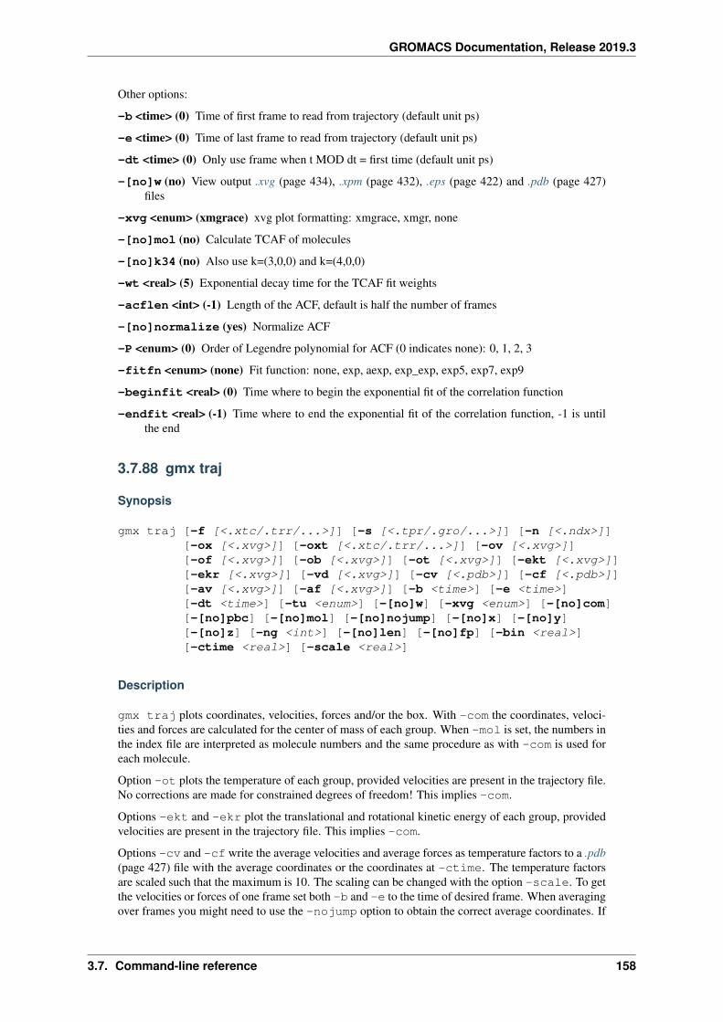
GROMACS Documentation, Release 2019.3
Other options:
-b <time> (0) Time of first frame to read from trajectory (default unit ps)
-e <time> (0) Time of last frame to read from trajectory (default unit ps)
-dt <time> (0) Only use frame when t MOD dt = first time (default unit ps)
-[no]w (no) View output .xvg (page 434), .xpm (page 432), .eps (page 422) and .pdb (page 427)files
-xvg <enum> (xmgrace) xvg plot formatting: xmgrace, xmgr, none
-[no]mol (no) Calculate TCAF of molecules
-[no]k34 (no) Also use k=(3,0,0) and k=(4,0,0)
-wt <real> (5) Exponential decay time for the TCAF fit weights
-acflen <int> (-1) Length of the ACF, default is half the number of frames
-[no]normalize (yes) Normalize ACF
-P <enum> (0) Order of Legendre polynomial for ACF (0 indicates none): 0, 1, 2, 3
-fitfn <enum> (none) Fit function: none, exp, aexp, exp_exp, exp5, exp7, exp9
-beginfit <real> (0) Time where to begin the exponential fit of the correlation function
-endfit <real> (-1) Time where to end the exponential fit of the correlation function, -1 is untilthe end
3.7.88 gmx traj
Synopsis
gmx traj [-f [<.xtc/.trr/...>]] [-s [<.tpr/.gro/...>]] [-n [<.ndx>]][-ox [<.xvg>]] [-oxt [<.xtc/.trr/...>]] [-ov [<.xvg>]][-of [<.xvg>]] [-ob [<.xvg>]] [-ot [<.xvg>]] [-ekt [<.xvg>]][-ekr [<.xvg>]] [-vd [<.xvg>]] [-cv [<.pdb>]] [-cf [<.pdb>]][-av [<.xvg>]] [-af [<.xvg>]] [-b <time>] [-e <time>][-dt <time>] [-tu <enum>] [-[no]w] [-xvg <enum>] [-[no]com][-[no]pbc] [-[no]mol] [-[no]nojump] [-[no]x] [-[no]y][-[no]z] [-ng <int>] [-[no]len] [-[no]fp] [-bin <real>][-ctime <real>] [-scale <real>]
Description
gmx traj plots coordinates, velocities, forces and/or the box. With -com the coordinates, veloci-ties and forces are calculated for the center of mass of each group. When -mol is set, the numbers inthe index file are interpreted as molecule numbers and the same procedure as with -com is used foreach molecule.
Option -ot plots the temperature of each group, provided velocities are present in the trajectory file.No corrections are made for constrained degrees of freedom! This implies -com.
Options -ekt and -ekr plot the translational and rotational kinetic energy of each group, providedvelocities are present in the trajectory file. This implies -com.
Options -cv and -cf write the average velocities and average forces as temperature factors to a .pdb(page 427) file with the average coordinates or the coordinates at -ctime. The temperature factorsare scaled such that the maximum is 10. The scaling can be changed with the option -scale. To getthe velocities or forces of one frame set both -b and -e to the time of desired frame. When averagingover frames you might need to use the -nojump option to obtain the correct average coordinates. If
3.7. Command-line reference 158
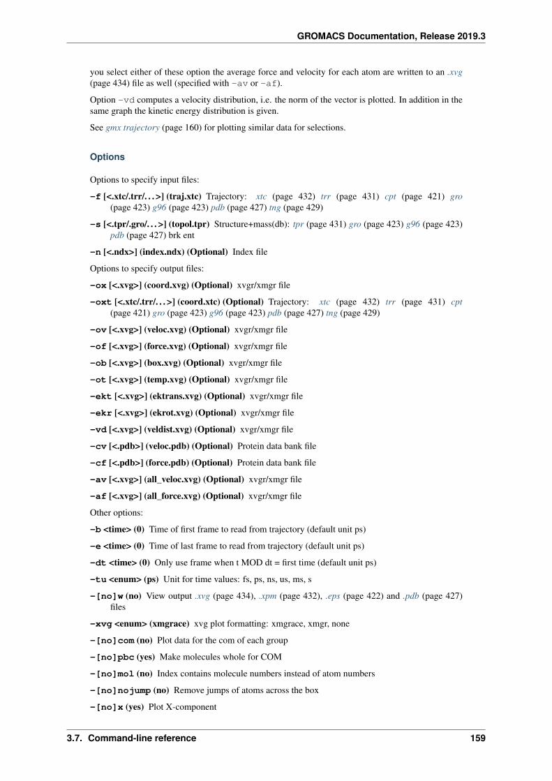
GROMACS Documentation, Release 2019.3
you select either of these option the average force and velocity for each atom are written to an .xvg(page 434) file as well (specified with -av or -af).
Option -vd computes a velocity distribution, i.e. the norm of the vector is plotted. In addition in thesame graph the kinetic energy distribution is given.
See gmx trajectory (page 160) for plotting similar data for selections.
Options
Options to specify input files:
-f [<.xtc/.trr/. . . >] (traj.xtc) Trajectory: xtc (page 432) trr (page 431) cpt (page 421) gro(page 423) g96 (page 423) pdb (page 427) tng (page 429)
-s [<.tpr/.gro/. . . >] (topol.tpr) Structure+mass(db): tpr (page 431) gro (page 423) g96 (page 423)pdb (page 427) brk ent
-n [<.ndx>] (index.ndx) (Optional) Index file
Options to specify output files:
-ox [<.xvg>] (coord.xvg) (Optional) xvgr/xmgr file
-oxt [<.xtc/.trr/. . . >] (coord.xtc) (Optional) Trajectory: xtc (page 432) trr (page 431) cpt(page 421) gro (page 423) g96 (page 423) pdb (page 427) tng (page 429)
-ov [<.xvg>] (veloc.xvg) (Optional) xvgr/xmgr file
-of [<.xvg>] (force.xvg) (Optional) xvgr/xmgr file
-ob [<.xvg>] (box.xvg) (Optional) xvgr/xmgr file
-ot [<.xvg>] (temp.xvg) (Optional) xvgr/xmgr file
-ekt [<.xvg>] (ektrans.xvg) (Optional) xvgr/xmgr file
-ekr [<.xvg>] (ekrot.xvg) (Optional) xvgr/xmgr file
-vd [<.xvg>] (veldist.xvg) (Optional) xvgr/xmgr file
-cv [<.pdb>] (veloc.pdb) (Optional) Protein data bank file
-cf [<.pdb>] (force.pdb) (Optional) Protein data bank file
-av [<.xvg>] (all_veloc.xvg) (Optional) xvgr/xmgr file
-af [<.xvg>] (all_force.xvg) (Optional) xvgr/xmgr file
Other options:
-b <time> (0) Time of first frame to read from trajectory (default unit ps)
-e <time> (0) Time of last frame to read from trajectory (default unit ps)
-dt <time> (0) Only use frame when t MOD dt = first time (default unit ps)
-tu <enum> (ps) Unit for time values: fs, ps, ns, us, ms, s
-[no]w (no) View output .xvg (page 434), .xpm (page 432), .eps (page 422) and .pdb (page 427)files
-xvg <enum> (xmgrace) xvg plot formatting: xmgrace, xmgr, none
-[no]com (no) Plot data for the com of each group
-[no]pbc (yes) Make molecules whole for COM
-[no]mol (no) Index contains molecule numbers instead of atom numbers
-[no]nojump (no) Remove jumps of atoms across the box
-[no]x (yes) Plot X-component
3.7. Command-line reference 159
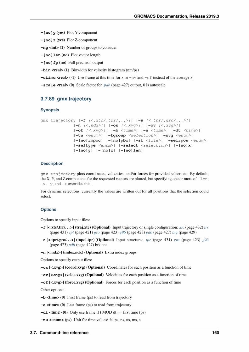
GROMACS Documentation, Release 2019.3
-[no]y (yes) Plot Y-component
-[no]z (yes) Plot Z-component
-ng <int> (1) Number of groups to consider
-[no]len (no) Plot vector length
-[no]fp (no) Full precision output
-bin <real> (1) Binwidth for velocity histogram (nm/ps)
-ctime <real> (-1) Use frame at this time for x in -cv and -cf instead of the average x
-scale <real> (0) Scale factor for .pdb (page 427) output, 0 is autoscale
3.7.89 gmx trajectory
Synopsis
gmx trajectory [-f [<.xtc/.trr/...>]] [-s [<.tpr/.gro/...>]][-n [<.ndx>]] [-ox [<.xvg>]] [-ov [<.xvg>]][-of [<.xvg>]] [-b <time>] [-e <time>] [-dt <time>][-tu <enum>] [-fgroup <selection>] [-xvg <enum>][-[no]rmpbc] [-[no]pbc] [-sf <file>] [-selrpos <enum>][-seltype <enum>] [-select <selection>] [-[no]x][-[no]y] [-[no]z] [-[no]len]
Description
gmx trajectory plots coordinates, velocities, and/or forces for provided selections. By default,the X, Y, and Z components for the requested vectors are plotted, but specifying one or more of -len,-x, -y, and -z overrides this.
For dynamic selections, currently the values are written out for all positions that the selection couldselect.
Options
Options to specify input files:
-f [<.xtc/.trr/. . . >] (traj.xtc) (Optional) Input trajectory or single configuration: xtc (page 432) trr(page 431) cpt (page 421) gro (page 423) g96 (page 423) pdb (page 427) tng (page 429)
-s [<.tpr/.gro/. . . >] (topol.tpr) (Optional) Input structure: tpr (page 431) gro (page 423) g96(page 423) pdb (page 427) brk ent
-n [<.ndx>] (index.ndx) (Optional) Extra index groups
Options to specify output files:
-ox [<.xvg>] (coord.xvg) (Optional) Coordinates for each position as a function of time
-ov [<.xvg>] (veloc.xvg) (Optional) Velocities for each position as a function of time
-of [<.xvg>] (force.xvg) (Optional) Forces for each position as a function of time
Other options:
-b <time> (0) First frame (ps) to read from trajectory
-e <time> (0) Last frame (ps) to read from trajectory
-dt <time> (0) Only use frame if t MOD dt == first time (ps)
-tu <enum> (ps) Unit for time values: fs, ps, ns, us, ms, s
3.7. Command-line reference 160
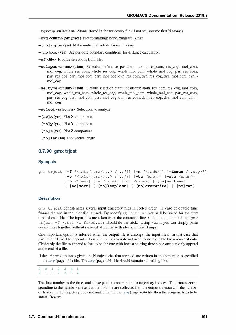
GROMACS Documentation, Release 2019.3
-fgroup <selection> Atoms stored in the trajectory file (if not set, assume first N atoms)
-xvg <enum> (xmgrace) Plot formatting: none, xmgrace, xmgr
-[no]rmpbc (yes) Make molecules whole for each frame
-[no]pbc (yes) Use periodic boundary conditions for distance calculation
-sf <file> Provide selections from files
-selrpos <enum> (atom) Selection reference positions: atom, res_com, res_cog, mol_com,mol_cog, whole_res_com, whole_res_cog, whole_mol_com, whole_mol_cog, part_res_com,part_res_cog, part_mol_com, part_mol_cog, dyn_res_com, dyn_res_cog, dyn_mol_com, dyn_-mol_cog
-seltype <enum> (atom) Default selection output positions: atom, res_com, res_cog, mol_com,mol_cog, whole_res_com, whole_res_cog, whole_mol_com, whole_mol_cog, part_res_com,part_res_cog, part_mol_com, part_mol_cog, dyn_res_com, dyn_res_cog, dyn_mol_com, dyn_-mol_cog
-select <selection> Selections to analyze
-[no]x (yes) Plot X component
-[no]y (yes) Plot Y component
-[no]z (yes) Plot Z component
-[no]len (no) Plot vector length
3.7.90 gmx trjcat
Synopsis
gmx trjcat [-f [<.xtc/.trr/...> [...]]] [-n [<.ndx>]] [-demux [<.xvg>]][-o [<.xtc/.trr/...> [...]]] [-tu <enum>] [-xvg <enum>][-b <time>] [-e <time>] [-dt <time>] [-[no]settime][-[no]sort] [-[no]keeplast] [-[no]overwrite] [-[no]cat]
Description
gmx trjcat concatenates several input trajectory files in sorted order. In case of double timeframes the one in the later file is used. By specifying -settime you will be asked for the starttime of each file. The input files are taken from the command line, such that a command like gmxtrjcat -f *.trr -o fixed.trr should do the trick. Using -cat, you can simply pasteseveral files together without removal of frames with identical time stamps.
One important option is inferred when the output file is amongst the input files. In that case thatparticular file will be appended to which implies you do not need to store double the amount of data.Obviously the file to append to has to be the one with lowest starting time since one can only appendat the end of a file.
If the -demux option is given, the N trajectories that are read, are written in another order as specifiedin the .xvg (page 434) file. The .xvg (page 434) file should contain something like:
0 0 1 2 3 4 52 1 0 2 3 5 4
The first number is the time, and subsequent numbers point to trajectory indices. The frames corre-sponding to the numbers present at the first line are collected into the output trajectory. If the numberof frames in the trajectory does not match that in the .xvg (page 434) file then the program tries to besmart. Beware.
3.7. Command-line reference 161
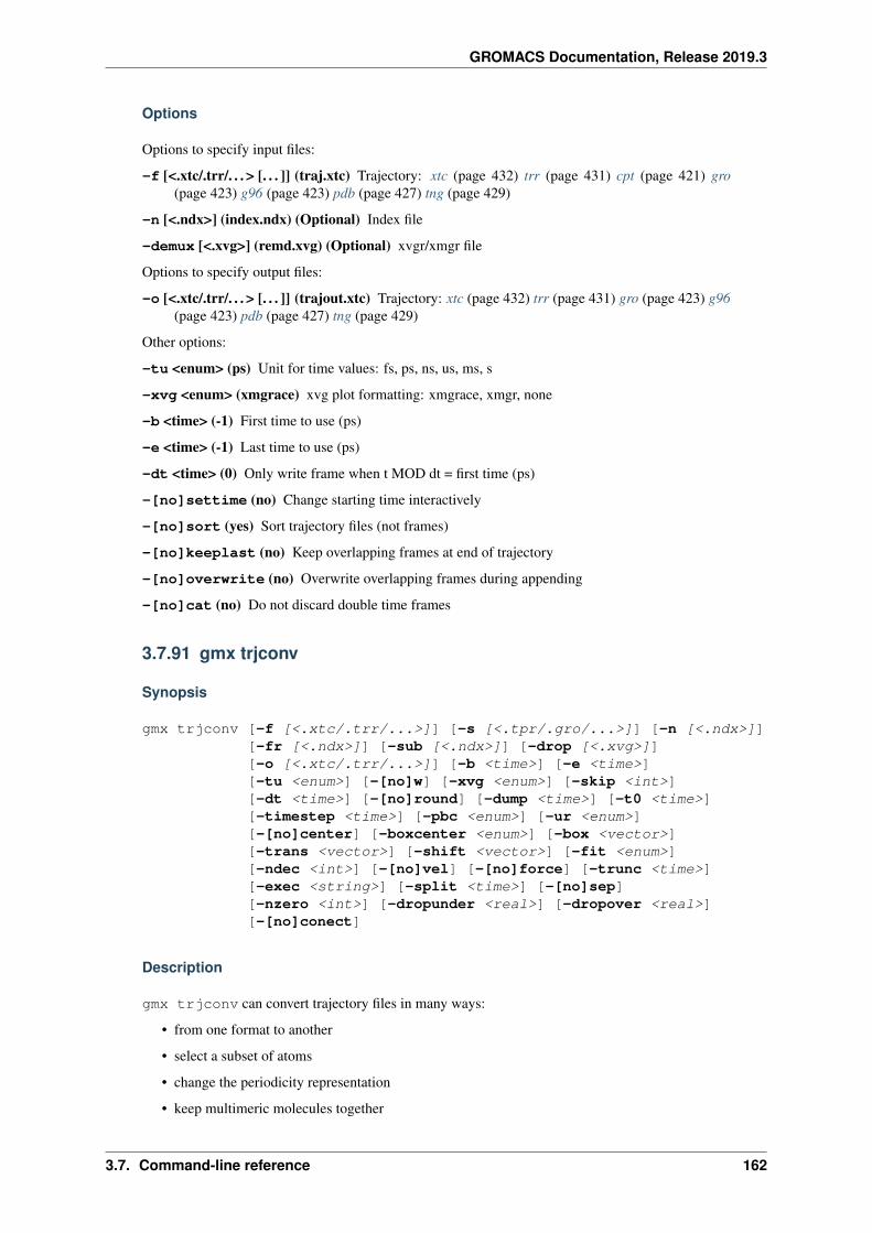
GROMACS Documentation, Release 2019.3
Options
Options to specify input files:
-f [<.xtc/.trr/. . . > [. . . ]] (traj.xtc) Trajectory: xtc (page 432) trr (page 431) cpt (page 421) gro(page 423) g96 (page 423) pdb (page 427) tng (page 429)
-n [<.ndx>] (index.ndx) (Optional) Index file
-demux [<.xvg>] (remd.xvg) (Optional) xvgr/xmgr file
Options to specify output files:
-o [<.xtc/.trr/. . . > [. . . ]] (trajout.xtc) Trajectory: xtc (page 432) trr (page 431) gro (page 423) g96(page 423) pdb (page 427) tng (page 429)
Other options:
-tu <enum> (ps) Unit for time values: fs, ps, ns, us, ms, s
-xvg <enum> (xmgrace) xvg plot formatting: xmgrace, xmgr, none
-b <time> (-1) First time to use (ps)
-e <time> (-1) Last time to use (ps)
-dt <time> (0) Only write frame when t MOD dt = first time (ps)
-[no]settime (no) Change starting time interactively
-[no]sort (yes) Sort trajectory files (not frames)
-[no]keeplast (no) Keep overlapping frames at end of trajectory
-[no]overwrite (no) Overwrite overlapping frames during appending
-[no]cat (no) Do not discard double time frames
3.7.91 gmx trjconv
Synopsis
gmx trjconv [-f [<.xtc/.trr/...>]] [-s [<.tpr/.gro/...>]] [-n [<.ndx>]][-fr [<.ndx>]] [-sub [<.ndx>]] [-drop [<.xvg>]][-o [<.xtc/.trr/...>]] [-b <time>] [-e <time>][-tu <enum>] [-[no]w] [-xvg <enum>] [-skip <int>][-dt <time>] [-[no]round] [-dump <time>] [-t0 <time>][-timestep <time>] [-pbc <enum>] [-ur <enum>][-[no]center] [-boxcenter <enum>] [-box <vector>][-trans <vector>] [-shift <vector>] [-fit <enum>][-ndec <int>] [-[no]vel] [-[no]force] [-trunc <time>][-exec <string>] [-split <time>] [-[no]sep][-nzero <int>] [-dropunder <real>] [-dropover <real>][-[no]conect]
Description
gmx trjconv can convert trajectory files in many ways:
• from one format to another
• select a subset of atoms
• change the periodicity representation
• keep multimeric molecules together
3.7. Command-line reference 162
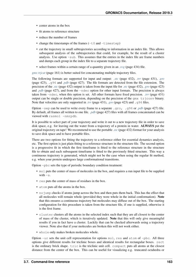
GROMACS Documentation, Release 2019.3
• center atoms in the box
• fit atoms to reference structure
• reduce the number of frames
• change the timestamps of the frames (-t0 and -timestep)
• cut the trajectory in small subtrajectories according to information in an index file. This allowssubsequent analysis of the subtrajectories that could, for example, be the result of a clusteranalysis. Use option -sub. This assumes that the entries in the index file are frame numbersand dumps each group in the index file to a separate trajectory file.
• select frames within a certain range of a quantity given in an .xvg (page 434) file.
gmx trjcat (page 161) is better suited for concatenating multiple trajectory files.
The following formats are supported for input and output: .xtc (page 432), .trr (page 431), .gro(page 423), .g96 and .pdb (page 427). The file formats are detected from the file extension. Theprecision of the .xtc (page 432) output is taken from the input file for .xtc (page 432), .gro (page 423)and .pdb (page 427), and from the -ndec option for other input formats. The precision is alwaystaken from -ndec, when this option is set. All other formats have fixed precision. .trr (page 431)output can be single or double precision, depending on the precision of the gmx trjconv binary.Note that velocities are only supported in .trr (page 431), .gro (page 423) and .g96 files.
Option -sep can be used to write every frame to a separate .gro, .g96 or .pdb (page 427) file.By default, all frames all written to one file. .pdb (page 427) files with all frames concatenated can beviewed with rasmol -nmrpdb.
It is possible to select part of your trajectory and write it out to a new trajectory file in order to savedisk space, e.g. for leaving out the water from a trajectory of a protein in water. ALWAYS put theoriginal trajectory on tape! We recommend to use the portable .xtc (page 432) format for your analysisto save disk space and to have portable files.
There are two options for fitting the trajectory to a reference either for essential dynamics analysis,etc. The first option is just plain fitting to a reference structure in the structure file. The second optionis a progressive fit in which the first timeframe is fitted to the reference structure in the structurefile to obtain and each subsequent timeframe is fitted to the previously fitted structure. This way acontinuous trajectory is generated, which might not be the case when using the regular fit method,e.g. when your protein undergoes large conformational transitions.
Option -pbc sets the type of periodic boundary condition treatment:
• mol puts the center of mass of molecules in the box, and requires a run input file to be suppliedwith -s.
• res puts the center of mass of residues in the box.
• atom puts all the atoms in the box.
• nojump checks if atoms jump across the box and then puts them back. This has the effect thatall molecules will remain whole (provided they were whole in the initial conformation). Notethat this ensures a continuous trajectory but molecules may diffuse out of the box. The startingconfiguration for this procedure is taken from the structure file, if one is supplied, otherwise itis the first frame.
• cluster clusters all the atoms in the selected index such that they are all closest to the centerof mass of the cluster, which is iteratively updated. Note that this will only give meaningfulresults if you in fact have a cluster. Luckily that can be checked afterwards using a trajectoryviewer. Note also that if your molecules are broken this will not work either.
• whole only makes broken molecules whole.
Option -ur sets the unit cell representation for options mol, res and atom of -pbc. All threeoptions give different results for triclinic boxes and identical results for rectangular boxes. rectis the ordinary brick shape. tric is the triclinic unit cell. compact puts all atoms at the closestdistance from the center of the box. This can be useful for visualizing e.g. truncated octahedra or
3.7. Command-line reference 163
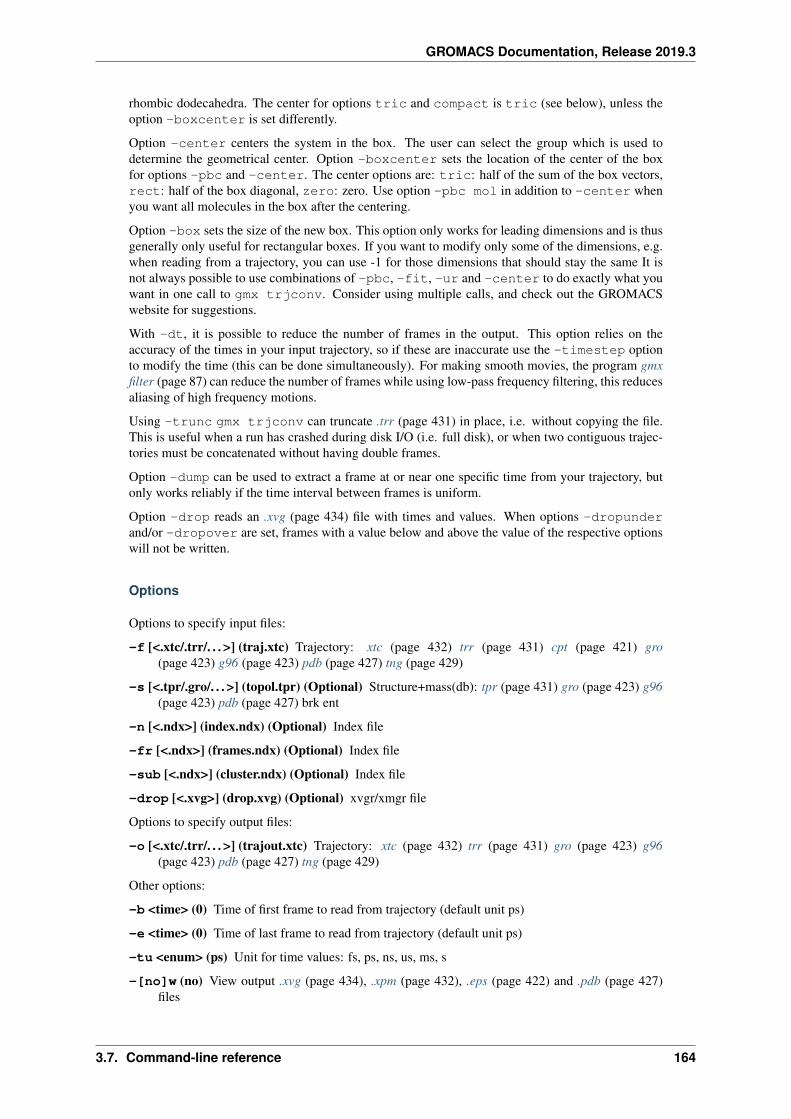
GROMACS Documentation, Release 2019.3
rhombic dodecahedra. The center for options tric and compact is tric (see below), unless theoption -boxcenter is set differently.
Option -center centers the system in the box. The user can select the group which is used todetermine the geometrical center. Option -boxcenter sets the location of the center of the boxfor options -pbc and -center. The center options are: tric: half of the sum of the box vectors,rect: half of the box diagonal, zero: zero. Use option -pbc mol in addition to -center whenyou want all molecules in the box after the centering.
Option -box sets the size of the new box. This option only works for leading dimensions and is thusgenerally only useful for rectangular boxes. If you want to modify only some of the dimensions, e.g.when reading from a trajectory, you can use -1 for those dimensions that should stay the same It isnot always possible to use combinations of -pbc, -fit, -ur and -center to do exactly what youwant in one call to gmx trjconv. Consider using multiple calls, and check out the GROMACSwebsite for suggestions.
With -dt, it is possible to reduce the number of frames in the output. This option relies on theaccuracy of the times in your input trajectory, so if these are inaccurate use the -timestep optionto modify the time (this can be done simultaneously). For making smooth movies, the program gmxfilter (page 87) can reduce the number of frames while using low-pass frequency filtering, this reducesaliasing of high frequency motions.
Using -trunc gmx trjconv can truncate .trr (page 431) in place, i.e. without copying the file.This is useful when a run has crashed during disk I/O (i.e. full disk), or when two contiguous trajec-tories must be concatenated without having double frames.
Option -dump can be used to extract a frame at or near one specific time from your trajectory, butonly works reliably if the time interval between frames is uniform.
Option -drop reads an .xvg (page 434) file with times and values. When options -dropunderand/or -dropover are set, frames with a value below and above the value of the respective optionswill not be written.
Options
Options to specify input files:
-f [<.xtc/.trr/. . . >] (traj.xtc) Trajectory: xtc (page 432) trr (page 431) cpt (page 421) gro(page 423) g96 (page 423) pdb (page 427) tng (page 429)
-s [<.tpr/.gro/. . . >] (topol.tpr) (Optional) Structure+mass(db): tpr (page 431) gro (page 423) g96(page 423) pdb (page 427) brk ent
-n [<.ndx>] (index.ndx) (Optional) Index file
-fr [<.ndx>] (frames.ndx) (Optional) Index file
-sub [<.ndx>] (cluster.ndx) (Optional) Index file
-drop [<.xvg>] (drop.xvg) (Optional) xvgr/xmgr file
Options to specify output files:
-o [<.xtc/.trr/. . . >] (trajout.xtc) Trajectory: xtc (page 432) trr (page 431) gro (page 423) g96(page 423) pdb (page 427) tng (page 429)
Other options:
-b <time> (0) Time of first frame to read from trajectory (default unit ps)
-e <time> (0) Time of last frame to read from trajectory (default unit ps)
-tu <enum> (ps) Unit for time values: fs, ps, ns, us, ms, s
-[no]w (no) View output .xvg (page 434), .xpm (page 432), .eps (page 422) and .pdb (page 427)files
3.7. Command-line reference 164
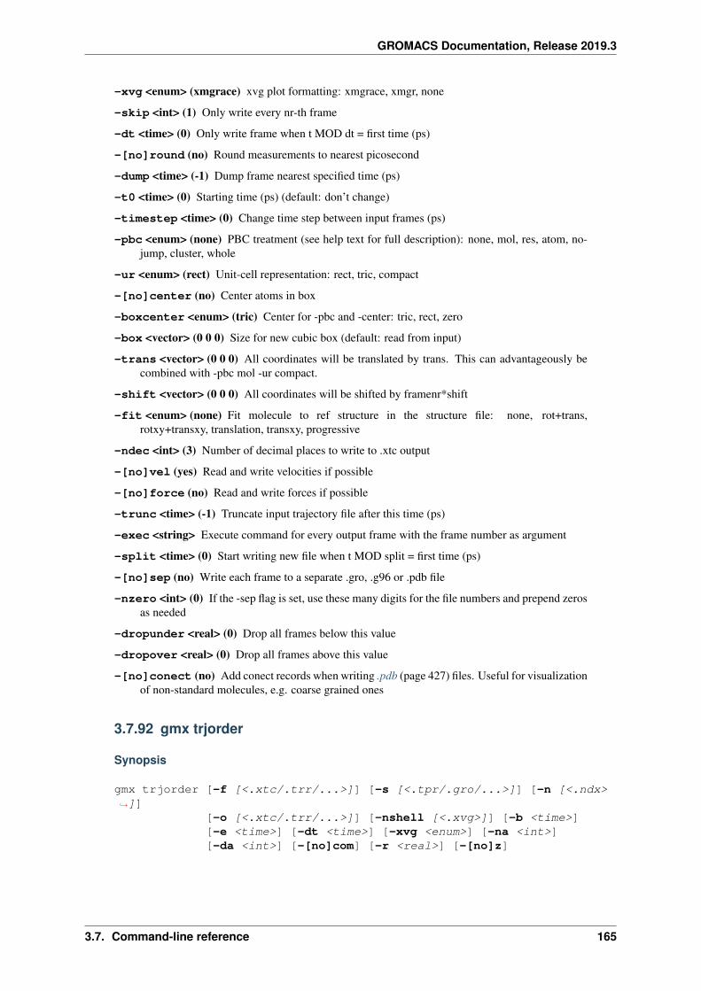
GROMACS Documentation, Release 2019.3
-xvg <enum> (xmgrace) xvg plot formatting: xmgrace, xmgr, none
-skip <int> (1) Only write every nr-th frame
-dt <time> (0) Only write frame when t MOD dt = first time (ps)
-[no]round (no) Round measurements to nearest picosecond
-dump <time> (-1) Dump frame nearest specified time (ps)
-t0 <time> (0) Starting time (ps) (default: don’t change)
-timestep <time> (0) Change time step between input frames (ps)
-pbc <enum> (none) PBC treatment (see help text for full description): none, mol, res, atom, no-jump, cluster, whole
-ur <enum> (rect) Unit-cell representation: rect, tric, compact
-[no]center (no) Center atoms in box
-boxcenter <enum> (tric) Center for -pbc and -center: tric, rect, zero
-box <vector> (0 0 0) Size for new cubic box (default: read from input)
-trans <vector> (0 0 0) All coordinates will be translated by trans. This can advantageously becombined with -pbc mol -ur compact.
-shift <vector> (0 0 0) All coordinates will be shifted by framenr*shift
-fit <enum> (none) Fit molecule to ref structure in the structure file: none, rot+trans,rotxy+transxy, translation, transxy, progressive
-ndec <int> (3) Number of decimal places to write to .xtc output
-[no]vel (yes) Read and write velocities if possible
-[no]force (no) Read and write forces if possible
-trunc <time> (-1) Truncate input trajectory file after this time (ps)
-exec <string> Execute command for every output frame with the frame number as argument
-split <time> (0) Start writing new file when t MOD split = first time (ps)
-[no]sep (no) Write each frame to a separate .gro, .g96 or .pdb file
-nzero <int> (0) If the -sep flag is set, use these many digits for the file numbers and prepend zerosas needed
-dropunder <real> (0) Drop all frames below this value
-dropover <real> (0) Drop all frames above this value
-[no]conect (no) Add conect records when writing .pdb (page 427) files. Useful for visualizationof non-standard molecules, e.g. coarse grained ones
3.7.92 gmx trjorder
Synopsis
gmx trjorder [-f [<.xtc/.trr/...>]] [-s [<.tpr/.gro/...>]] [-n [<.ndx>→˓]]
[-o [<.xtc/.trr/...>]] [-nshell [<.xvg>]] [-b <time>][-e <time>] [-dt <time>] [-xvg <enum>] [-na <int>][-da <int>] [-[no]com] [-r <real>] [-[no]z]
3.7. Command-line reference 165
GROMACS Documentation, Release 2019.3
Description
gmx trjorder orders molecules according to the smallest distance to atoms in a reference groupor on z-coordinate (with option -z). With distance ordering, it will ask for a group of reference atomsand a group of molecules. For each frame of the trajectory the selected molecules will be reorderedaccording to the shortest distance between atom number -da in the molecule and all the atoms inthe reference group. The center of mass of the molecules can be used instead of a reference atom bysetting -da to 0. All atoms in the trajectory are written to the output trajectory.
gmx trjorder can be useful for e.g. analyzing the n waters closest to a protein. In that casethe reference group would be the protein and the group of molecules would consist of all the wateratoms. When an index group of the first n waters is made, the ordered trajectory can be used with anyGROMACS program to analyze the n closest waters.
If the output file is a .pdb (page 427) file, the distance to the reference target will be stored in theB-factor field in order to color with e.g. Rasmol.
With option -nshell the number of molecules within a shell of radius -r around the referencegroup are printed.
Options
Options to specify input files:
-f [<.xtc/.trr/. . . >] (traj.xtc) Trajectory: xtc (page 432) trr (page 431) cpt (page 421) gro(page 423) g96 (page 423) pdb (page 427) tng (page 429)
-s [<.tpr/.gro/. . . >] (topol.tpr) Structure+mass(db): tpr (page 431) gro (page 423) g96 (page 423)pdb (page 427) brk ent
-n [<.ndx>] (index.ndx) (Optional) Index file
Options to specify output files:
-o [<.xtc/.trr/. . . >] (ordered.xtc) (Optional) Trajectory: xtc (page 432) trr (page 431) gro(page 423) g96 (page 423) pdb (page 427) tng (page 429)
-nshell [<.xvg>] (nshell.xvg) (Optional) xvgr/xmgr file
Other options:
-b <time> (0) Time of first frame to read from trajectory (default unit ps)
-e <time> (0) Time of last frame to read from trajectory (default unit ps)
-dt <time> (0) Only use frame when t MOD dt = first time (default unit ps)
-xvg <enum> (xmgrace) xvg plot formatting: xmgrace, xmgr, none
-na <int> (3) Number of atoms in a molecule
-da <int> (1) Atom used for the distance calculation, 0 is COM
-[no]com (no) Use the distance to the center of mass of the reference group
-r <real> (0) Cutoff used for the distance calculation when computing the number of molecules ina shell around e.g. a protein
-[no]z (no) Order molecules on z-coordinate
3.7.93 gmx tune_pme
Synopsis
gmx tune_pme [-s [<.tpr>]] [-cpi [<.cpt>]] [-table [<.xvg>]][-tablep [<.xvg>]] [-tableb [<.xvg>]]
3.7. Command-line reference 166
GROMACS Documentation, Release 2019.3
[-rerun [<.xtc/.trr/...>]] [-ei [<.edi>]] [-p [<.out>]][-err [<.log>]] [-so [<.tpr>]] [-o [<.trr/.cpt/...>]][-x [<.xtc/.tng>]] [-cpo [<.cpt>]][-c [<.gro/.g96/...>]] [-e [<.edr>]] [-g [<.log>]][-dhdl [<.xvg>]] [-field [<.xvg>]] [-tpi [<.xvg>]][-tpid [<.xvg>]] [-eo [<.xvg>]] [-devout [<.xvg>]][-runav [<.xvg>]] [-px [<.xvg>]] [-pf [<.xvg>]][-ro [<.xvg>]] [-ra [<.log>]] [-rs [<.log>]][-rt [<.log>]] [-mtx [<.mtx>]] [-swap [<.xvg>]][-bo [<.trr/.cpt/...>]] [-bx [<.xtc>]] [-bcpo [<.cpt>]][-bc [<.gro/.g96/...>]] [-be [<.edr>]] [-bg [<.log>]][-beo [<.xvg>]] [-bdhdl [<.xvg>]] [-bfield [<.xvg>]][-btpi [<.xvg>]] [-btpid [<.xvg>]] [-bdevout [<.xvg>]][-brunav [<.xvg>]] [-bpx [<.xvg>]] [-bpf [<.xvg>]][-bro [<.xvg>]] [-bra [<.log>]] [-brs [<.log>]][-brt [<.log>]] [-bmtx [<.mtx>]] [-bdn [<.ndx>]][-bswap [<.xvg>]] [-xvg <enum>] [-mdrun <string>][-np <int>] [-npstring <enum>] [-ntmpi <int>] [-r <int>][-max <real>] [-min <real>] [-npme <enum>] [-fix <int>][-rmax <real>] [-rmin <real>] [-[no]scalevdw][-ntpr <int>] [-steps <int>] [-resetstep <int>][-nsteps <int>] [-[no]launch] [-[no]bench] [-[no]check][-gpu_id <string>] [-[no]append] [-[no]cpnum][-deffnm <string>]
Description
For a given number -np or -ntmpi of ranks, gmx tune_pme systematically times gmx mdrun(page 111) with various numbers of PME-only ranks and determines which setting is fastest. It willalso test whether performance can be enhanced by shifting load from the reciprocal to the real spacepart of the Ewald sum. Simply pass your .tpr (page 431) file to gmx tune_pme together with otheroptions for gmx mdrun (page 111) as needed.
gmx tune_pme needs to call gmx mdrun (page 111) and so requires that you specify how to callmdrun with the argument to the -mdrun parameter. Depending how you have built GROMACS,values such as ‘gmx mdrun’, ‘gmx_d mdrun’, or ‘mdrun_mpi’ might be needed.
The program that runs MPI programs can be set in the environment variable MPIRUN (defaults to‘mpirun’). Note that for certain MPI frameworks, you need to provide a machine- or hostfile. Thiscan also be passed via the MPIRUN variable, e.g.
export MPIRUN="/usr/local/mpirun -machinefile hosts" Note that in suchcases it is normally necessary to compile and/or run gmx tune_pme without MPI support, so thatit can call the MPIRUN program.
Before doing the actual benchmark runs, gmx tune_pme will do a quick check whether gmx mdrun(page 111) works as expected with the provided parallel settings if the -check option is activated(the default). Please call gmx tune_pme with the normal options you would pass to gmx mdrun(page 111) and add -np for the number of ranks to perform the tests on, or -ntmpi for the numberof threads. You can also add -r to repeat each test several times to get better statistics.
gmx tune_pme can test various real space / reciprocal space workloads for you. With -ntpr youcontrol how many extra .tpr (page 431) files will be written with enlarged cutoffs and smaller Fouriergrids respectively. Typically, the first test (number 0) will be with the settings from the input .tpr(page 431) file; the last test (number ntpr) will have the Coulomb cutoff specified by -rmax witha somewhat smaller PME grid at the same time. In this last test, the Fourier spacing is multipliedwith rmax/rcoulomb. The remaining .tpr (page 431) files will have equally-spaced Coulomb radii(and Fourier spacings) between these extremes. Note that you can set -ntpr to 1 if you just seek theoptimal number of PME-only ranks; in that case your input .tpr (page 431) file will remain unchanged.
3.7. Command-line reference 167
GROMACS Documentation, Release 2019.3
For the benchmark runs, the default of 1000 time steps should suffice for most MD systems. Thedynamic load balancing needs about 100 time steps to adapt to local load imbalances, therefore thetime step counters are by default reset after 100 steps. For large systems (>1M atoms), as well as fora higher accuracy of the measurements, you should set -resetstep to a higher value. From the‘DD’ load imbalance entries in the md.log output file you can tell after how many steps the load issufficiently balanced. Example call:
gmx tune_pme -np 64 -s protein.tpr -launch
After calling gmx mdrun (page 111) several times, detailed performance information is available inthe output file perf.out. Note that during the benchmarks, a couple of temporary files are written(options -b*), these will be automatically deleted after each test.
If you want the simulation to be started automatically with the optimized parameters, use the com-mand line option -launch.
Basic support for GPU-enabled mdrun exists. Give a string containing the IDs of the GPUs that youwish to use in the optimization in the -gpu_id command-line argument. This works exactly likemdrun -gpu_id, does not imply a mapping, and merely declares the eligible set of GPU devices.gmx-tune_pme will construct calls to mdrun that use this set appropriately. gmx-tune_pme doesnot support -gputasks.
Options
Options to specify input files:
-s [<.tpr>] (topol.tpr) Portable xdr run input file
-cpi [<.cpt>] (state.cpt) (Optional) Checkpoint file
-table [<.xvg>] (table.xvg) (Optional) xvgr/xmgr file
-tablep [<.xvg>] (tablep.xvg) (Optional) xvgr/xmgr file
-tableb [<.xvg>] (table.xvg) (Optional) xvgr/xmgr file
-rerun [<.xtc/.trr/. . . >] (rerun.xtc) (Optional) Trajectory: xtc (page 432) trr (page 431) cpt(page 421) gro (page 423) g96 (page 423) pdb (page 427) tng (page 429)
-ei [<.edi>] (sam.edi) (Optional) ED sampling input
Options to specify output files:
-p [<.out>] (perf.out) Generic output file
-err [<.log>] (bencherr.log) Log file
-so [<.tpr>] (tuned.tpr) Portable xdr run input file
-o [<.trr/.cpt/. . . >] (traj.trr) Full precision trajectory: trr (page 431) cpt (page 421) tng (page 429)
-x [<.xtc/.tng>] (traj_comp.xtc) (Optional) Compressed trajectory (tng format or portable xdr for-mat)
-cpo [<.cpt>] (state.cpt) (Optional) Checkpoint file
-c [<.gro/.g96/. . . >] (confout.gro) Structure file: gro (page 423) g96 (page 423) pdb (page 427) brkent esp
-e [<.edr>] (ener.edr) Energy file
-g [<.log>] (md.log) Log file
-dhdl [<.xvg>] (dhdl.xvg) (Optional) xvgr/xmgr file
-field [<.xvg>] (field.xvg) (Optional) xvgr/xmgr file
-tpi [<.xvg>] (tpi.xvg) (Optional) xvgr/xmgr file
-tpid [<.xvg>] (tpidist.xvg) (Optional) xvgr/xmgr file
3.7. Command-line reference 168
GROMACS Documentation, Release 2019.3
-eo [<.xvg>] (edsam.xvg) (Optional) xvgr/xmgr file
-devout [<.xvg>] (deviatie.xvg) (Optional) xvgr/xmgr file
-runav [<.xvg>] (runaver.xvg) (Optional) xvgr/xmgr file
-px [<.xvg>] (pullx.xvg) (Optional) xvgr/xmgr file
-pf [<.xvg>] (pullf.xvg) (Optional) xvgr/xmgr file
-ro [<.xvg>] (rotation.xvg) (Optional) xvgr/xmgr file
-ra [<.log>] (rotangles.log) (Optional) Log file
-rs [<.log>] (rotslabs.log) (Optional) Log file
-rt [<.log>] (rottorque.log) (Optional) Log file
-mtx [<.mtx>] (nm.mtx) (Optional) Hessian matrix
-swap [<.xvg>] (swapions.xvg) (Optional) xvgr/xmgr file
-bo [<.trr/.cpt/. . . >] (bench.trr) Full precision trajectory: trr (page 431) cpt (page 421) tng(page 429)
-bx [<.xtc>] (bench.xtc) Compressed trajectory (portable xdr format): xtc
-bcpo [<.cpt>] (bench.cpt) Checkpoint file
-bc [<.gro/.g96/. . . >] (bench.gro) Structure file: gro (page 423) g96 (page 423) pdb (page 427) brkent esp
-be [<.edr>] (bench.edr) Energy file
-bg [<.log>] (bench.log) Log file
-beo [<.xvg>] (benchedo.xvg) (Optional) xvgr/xmgr file
-bdhdl [<.xvg>] (benchdhdl.xvg) (Optional) xvgr/xmgr file
-bfield [<.xvg>] (benchfld.xvg) (Optional) xvgr/xmgr file
-btpi [<.xvg>] (benchtpi.xvg) (Optional) xvgr/xmgr file
-btpid [<.xvg>] (benchtpid.xvg) (Optional) xvgr/xmgr file
-bdevout [<.xvg>] (benchdev.xvg) (Optional) xvgr/xmgr file
-brunav [<.xvg>] (benchrnav.xvg) (Optional) xvgr/xmgr file
-bpx [<.xvg>] (benchpx.xvg) (Optional) xvgr/xmgr file
-bpf [<.xvg>] (benchpf.xvg) (Optional) xvgr/xmgr file
-bro [<.xvg>] (benchrot.xvg) (Optional) xvgr/xmgr file
-bra [<.log>] (benchrota.log) (Optional) Log file
-brs [<.log>] (benchrots.log) (Optional) Log file
-brt [<.log>] (benchrott.log) (Optional) Log file
-bmtx [<.mtx>] (benchn.mtx) (Optional) Hessian matrix
-bdn [<.ndx>] (bench.ndx) (Optional) Index file
-bswap [<.xvg>] (benchswp.xvg) (Optional) xvgr/xmgr file
Other options:
-xvg <enum> (xmgrace) xvg plot formatting: xmgrace, xmgr, none
-mdrun <string> Command line to run a simulation, e.g. ‘gmx mdrun’ or ‘mdrun_mpi’
-np <int> (1) Number of ranks to run the tests on (must be > 2 for separate PME ranks)
3.7. Command-line reference 169
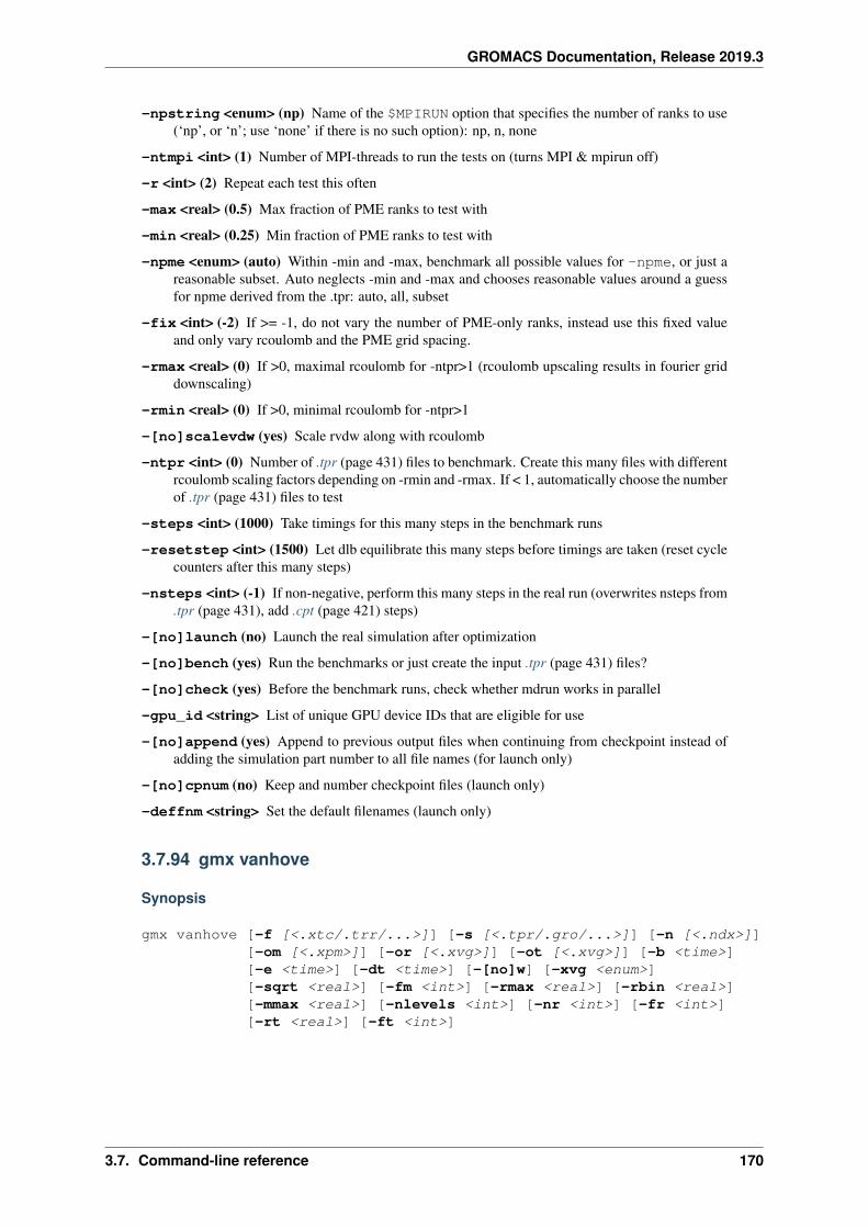
GROMACS Documentation, Release 2019.3
-npstring <enum> (np) Name of the $MPIRUN option that specifies the number of ranks to use(‘np’, or ‘n’; use ‘none’ if there is no such option): np, n, none
-ntmpi <int> (1) Number of MPI-threads to run the tests on (turns MPI & mpirun off)
-r <int> (2) Repeat each test this often
-max <real> (0.5) Max fraction of PME ranks to test with
-min <real> (0.25) Min fraction of PME ranks to test with
-npme <enum> (auto) Within -min and -max, benchmark all possible values for -npme, or just areasonable subset. Auto neglects -min and -max and chooses reasonable values around a guessfor npme derived from the .tpr: auto, all, subset
-fix <int> (-2) If >= -1, do not vary the number of PME-only ranks, instead use this fixed valueand only vary rcoulomb and the PME grid spacing.
-rmax <real> (0) If >0, maximal rcoulomb for -ntpr>1 (rcoulomb upscaling results in fourier griddownscaling)
-rmin <real> (0) If >0, minimal rcoulomb for -ntpr>1
-[no]scalevdw (yes) Scale rvdw along with rcoulomb
-ntpr <int> (0) Number of .tpr (page 431) files to benchmark. Create this many files with differentrcoulomb scaling factors depending on -rmin and -rmax. If < 1, automatically choose the numberof .tpr (page 431) files to test
-steps <int> (1000) Take timings for this many steps in the benchmark runs
-resetstep <int> (1500) Let dlb equilibrate this many steps before timings are taken (reset cyclecounters after this many steps)
-nsteps <int> (-1) If non-negative, perform this many steps in the real run (overwrites nsteps from.tpr (page 431), add .cpt (page 421) steps)
-[no]launch (no) Launch the real simulation after optimization
-[no]bench (yes) Run the benchmarks or just create the input .tpr (page 431) files?
-[no]check (yes) Before the benchmark runs, check whether mdrun works in parallel
-gpu_id <string> List of unique GPU device IDs that are eligible for use
-[no]append (yes) Append to previous output files when continuing from checkpoint instead ofadding the simulation part number to all file names (for launch only)
-[no]cpnum (no) Keep and number checkpoint files (launch only)
-deffnm <string> Set the default filenames (launch only)
3.7.94 gmx vanhove
Synopsis
gmx vanhove [-f [<.xtc/.trr/...>]] [-s [<.tpr/.gro/...>]] [-n [<.ndx>]][-om [<.xpm>]] [-or [<.xvg>]] [-ot [<.xvg>]] [-b <time>][-e <time>] [-dt <time>] [-[no]w] [-xvg <enum>][-sqrt <real>] [-fm <int>] [-rmax <real>] [-rbin <real>][-mmax <real>] [-nlevels <int>] [-nr <int>] [-fr <int>][-rt <real>] [-ft <int>]
3.7. Command-line reference 170
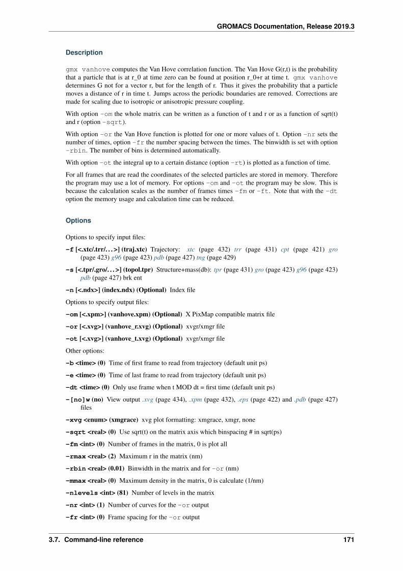
GROMACS Documentation, Release 2019.3
Description
gmx vanhove computes the Van Hove correlation function. The Van Hove G(r,t) is the probabilitythat a particle that is at r_0 at time zero can be found at position r_0+r at time t. gmx vanhovedetermines G not for a vector r, but for the length of r. Thus it gives the probability that a particlemoves a distance of r in time t. Jumps across the periodic boundaries are removed. Corrections aremade for scaling due to isotropic or anisotropic pressure coupling.
With option -om the whole matrix can be written as a function of t and r or as a function of sqrt(t)and r (option -sqrt).
With option -or the Van Hove function is plotted for one or more values of t. Option -nr sets thenumber of times, option -fr the number spacing between the times. The binwidth is set with option-rbin. The number of bins is determined automatically.
With option -ot the integral up to a certain distance (option -rt) is plotted as a function of time.
For all frames that are read the coordinates of the selected particles are stored in memory. Thereforethe program may use a lot of memory. For options -om and -ot the program may be slow. This isbecause the calculation scales as the number of frames times -fm or -ft. Note that with the -dtoption the memory usage and calculation time can be reduced.
Options
Options to specify input files:
-f [<.xtc/.trr/. . . >] (traj.xtc) Trajectory: xtc (page 432) trr (page 431) cpt (page 421) gro(page 423) g96 (page 423) pdb (page 427) tng (page 429)
-s [<.tpr/.gro/. . . >] (topol.tpr) Structure+mass(db): tpr (page 431) gro (page 423) g96 (page 423)pdb (page 427) brk ent
-n [<.ndx>] (index.ndx) (Optional) Index file
Options to specify output files:
-om [<.xpm>] (vanhove.xpm) (Optional) X PixMap compatible matrix file
-or [<.xvg>] (vanhove_r.xvg) (Optional) xvgr/xmgr file
-ot [<.xvg>] (vanhove_t.xvg) (Optional) xvgr/xmgr file
Other options:
-b <time> (0) Time of first frame to read from trajectory (default unit ps)
-e <time> (0) Time of last frame to read from trajectory (default unit ps)
-dt <time> (0) Only use frame when t MOD dt = first time (default unit ps)
-[no]w (no) View output .xvg (page 434), .xpm (page 432), .eps (page 422) and .pdb (page 427)files
-xvg <enum> (xmgrace) xvg plot formatting: xmgrace, xmgr, none
-sqrt <real> (0) Use sqrt(t) on the matrix axis which binspacing # in sqrt(ps)
-fm <int> (0) Number of frames in the matrix, 0 is plot all
-rmax <real> (2) Maximum r in the matrix (nm)
-rbin <real> (0.01) Binwidth in the matrix and for -or (nm)
-mmax <real> (0) Maximum density in the matrix, 0 is calculate (1/nm)
-nlevels <int> (81) Number of levels in the matrix
-nr <int> (1) Number of curves for the -or output
-fr <int> (0) Frame spacing for the -or output
3.7. Command-line reference 171
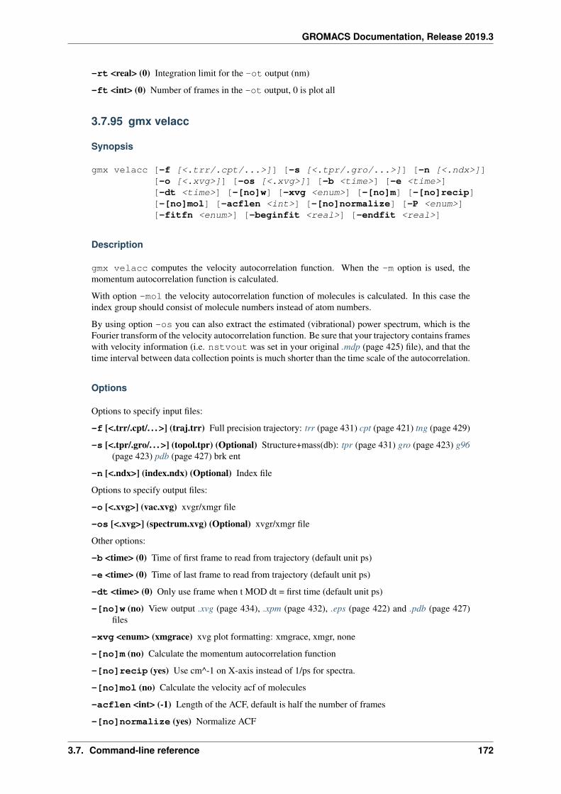
GROMACS Documentation, Release 2019.3
-rt <real> (0) Integration limit for the -ot output (nm)
-ft <int> (0) Number of frames in the -ot output, 0 is plot all
3.7.95 gmx velacc
Synopsis
gmx velacc [-f [<.trr/.cpt/...>]] [-s [<.tpr/.gro/...>]] [-n [<.ndx>]][-o [<.xvg>]] [-os [<.xvg>]] [-b <time>] [-e <time>][-dt <time>] [-[no]w] [-xvg <enum>] [-[no]m] [-[no]recip][-[no]mol] [-acflen <int>] [-[no]normalize] [-P <enum>][-fitfn <enum>] [-beginfit <real>] [-endfit <real>]
Description
gmx velacc computes the velocity autocorrelation function. When the -m option is used, themomentum autocorrelation function is calculated.
With option -mol the velocity autocorrelation function of molecules is calculated. In this case theindex group should consist of molecule numbers instead of atom numbers.
By using option -os you can also extract the estimated (vibrational) power spectrum, which is theFourier transform of the velocity autocorrelation function. Be sure that your trajectory contains frameswith velocity information (i.e. nstvout was set in your original .mdp (page 425) file), and that thetime interval between data collection points is much shorter than the time scale of the autocorrelation.
Options
Options to specify input files:
-f [<.trr/.cpt/. . . >] (traj.trr) Full precision trajectory: trr (page 431) cpt (page 421) tng (page 429)
-s [<.tpr/.gro/. . . >] (topol.tpr) (Optional) Structure+mass(db): tpr (page 431) gro (page 423) g96(page 423) pdb (page 427) brk ent
-n [<.ndx>] (index.ndx) (Optional) Index file
Options to specify output files:
-o [<.xvg>] (vac.xvg) xvgr/xmgr file
-os [<.xvg>] (spectrum.xvg) (Optional) xvgr/xmgr file
Other options:
-b <time> (0) Time of first frame to read from trajectory (default unit ps)
-e <time> (0) Time of last frame to read from trajectory (default unit ps)
-dt <time> (0) Only use frame when t MOD dt = first time (default unit ps)
-[no]w (no) View output .xvg (page 434), .xpm (page 432), .eps (page 422) and .pdb (page 427)files
-xvg <enum> (xmgrace) xvg plot formatting: xmgrace, xmgr, none
-[no]m (no) Calculate the momentum autocorrelation function
-[no]recip (yes) Use cm^-1 on X-axis instead of 1/ps for spectra.
-[no]mol (no) Calculate the velocity acf of molecules
-acflen <int> (-1) Length of the ACF, default is half the number of frames
-[no]normalize (yes) Normalize ACF
3.7. Command-line reference 172
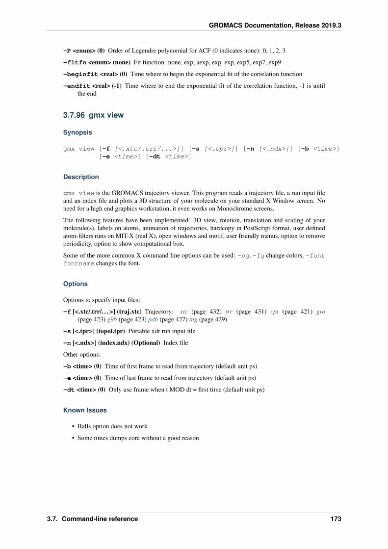
GROMACS Documentation, Release 2019.3
-P <enum> (0) Order of Legendre polynomial for ACF (0 indicates none): 0, 1, 2, 3
-fitfn <enum> (none) Fit function: none, exp, aexp, exp_exp, exp5, exp7, exp9
-beginfit <real> (0) Time where to begin the exponential fit of the correlation function
-endfit <real> (-1) Time where to end the exponential fit of the correlation function, -1 is untilthe end
3.7.96 gmx view
Synopsis
gmx view [-f [<.xtc/.trr/...>]] [-s [<.tpr>]] [-n [<.ndx>]] [-b <time>][-e <time>] [-dt <time>]
Description
gmx view is the GROMACS trajectory viewer. This program reads a trajectory file, a run input fileand an index file and plots a 3D structure of your molecule on your standard X Window screen. Noneed for a high end graphics workstation, it even works on Monochrome screens.
The following features have been implemented: 3D view, rotation, translation and scaling of yourmolecule(s), labels on atoms, animation of trajectories, hardcopy in PostScript format, user definedatom-filters runs on MIT-X (real X), open windows and motif, user friendly menus, option to removeperiodicity, option to show computational box.
Some of the more common X command line options can be used: -bg, -fg change colors, -fontfontname changes the font.
Options
Options to specify input files:
-f [<.xtc/.trr/. . . >] (traj.xtc) Trajectory: xtc (page 432) trr (page 431) cpt (page 421) gro(page 423) g96 (page 423) pdb (page 427) tng (page 429)
-s [<.tpr>] (topol.tpr) Portable xdr run input file
-n [<.ndx>] (index.ndx) (Optional) Index file
Other options:
-b <time> (0) Time of first frame to read from trajectory (default unit ps)
-e <time> (0) Time of last frame to read from trajectory (default unit ps)
-dt <time> (0) Only use frame when t MOD dt = first time (default unit ps)
Known Issues
• Balls option does not work
• Some times dumps core without a good reason
3.7. Command-line reference 173
GROMACS Documentation, Release 2019.3
3.7.97 gmx wham
Synopsis
gmx wham [-ix [<.dat>]] [-if [<.dat>]] [-it [<.dat>]] [-ip [<.dat>]][-is [<.dat>]] [-iiact [<.dat>]] [-tab [<.dat>]][-o [<.xvg>]] [-hist [<.xvg>]] [-oiact [<.xvg>]][-bsres [<.xvg>]] [-bsprof [<.xvg>]] [-xvg <enum>][-min <real>] [-max <real>] [-[no]auto] [-bins <int>][-temp <real>] [-tol <real>] [-[no]v] [-b <real>][-e <real>] [-dt <real>] [-[no]histonly] [-[no]boundsonly][-[no]log] [-unit <enum>] [-zprof0 <real>] [-[no]cycl][-[no]sym] [-[no]ac] [-acsig <real>] [-ac-trestart <real>][-nBootstrap <int>] [-bs-method <enum>] [-bs-tau <real>][-bs-seed <int>] [-histbs-block <int>] [-[no]vbs]
Description
gmx wham is an analysis program that implements the Weighted Histogram Analysis Method(WHAM). It is intended to analyze output files generated by umbrella sampling simulations to com-pute a potential of mean force (PMF).
gmx wham is currently not fully up to date. It only supports pull setups where the first pull coordi-nate(s) is/are umbrella pull coordinates and, if multiple coordinates need to be analyzed, all used thesame geometry and dimensions. In most cases this is not an issue.
At present, three input modes are supported.
• With option -it, the user provides a file which contains the file names of the umbrella simu-lation run-input files (.tpr (page 431) files), AND, with option -ix, a file which contains filenames of the pullx mdrun output files. The .tpr (page 431) and pullx files must be in corre-sponding order, i.e. the first .tpr (page 431) created the first pullx, etc.
• Same as the previous input mode, except that the the user provides the pull force output filenames (pullf.xvg) with option -if. From the pull force the position in the umbrella poten-tial is computed. This does not work with tabulated umbrella potentials.
• With option -ip, the user provides file names of (gzipped) .pdo files, i.e. the GROMACS 3.3umbrella output files. If you have some unusual reaction coordinate you may also generate yourown .pdo files and feed them with the -ip option into to gmx wham. The .pdo file header mustbe similar to the following:
# UMBRELLA 3.0# Component selection: 0 0 1# nSkip 1# Ref. Group 'TestAtom'# Nr. of pull groups 2# Group 1 'GR1' Umb. Pos. 5.0 Umb. Cons. 1000.0# Group 2 'GR2' Umb. Pos. 2.0 Umb. Cons. 500.0#####
The number of pull groups, umbrella positions, force constants, and names may (of course)differ. Following the header, a time column and a data column for each pull group follows (i.e.the displacement with respect to the umbrella center). Up to four pull groups are possible per.pdo file at present.
By default, all pull coordinates found in all pullx/pullf files are used in WHAM. If only some of thepull coordinates should be used, a pull coordinate selection file (option -is) can be provided. Theselection file must contain one line for each tpr file in tpr-files.dat. Each of these lines must containone digit (0 or 1) for each pull coordinate in the tpr file. Here, 1 indicates that the pull coordinate is
3.7. Command-line reference 174
GROMACS Documentation, Release 2019.3
used in WHAM, and 0 means it is omitted. Example: If you have three tpr files, each containing 4pull coordinates, but only pull coordinates 1 and 2 should be used, coordsel.dat looks like this:
1 1 0 01 1 0 01 1 0 0
By default, the output files are:
``-o`` PMF output file``-hist`` Histograms output file
Always check whether the histograms sufficiently overlap.
The umbrella potential is assumed to be harmonic and the force constants are read from the .tpr(page 431) or .pdo files. If a non-harmonic umbrella force was applied a tabulated potential can beprovided with -tab.
WHAM options
• -bins Number of bins used in analysis
• -temp Temperature in the simulations
• -tol Stop iteration if profile (probability) changed less than tolerance
• -auto Automatic determination of boundaries
• -min,-max Boundaries of the profile
The data points that are used to compute the profile can be restricted with options -b, -e, and -dt.Adjust -b to ensure sufficient equilibration in each umbrella window.
With -log (default) the profile is written in energy units, otherwise (with -nolog) as probability.The unit can be specified with -unit. With energy output, the energy in the first bin is defined tobe zero. If you want the free energy at a different position to be zero, set -zprof0 (useful withbootstrapping, see below).
For cyclic or periodic reaction coordinates (dihedral angle, channel PMF without osmotic gradient),the option -cycl is useful. gmx wham will make use of the periodicity of the system and generatea periodic PMF. The first and the last bin of the reaction coordinate will assumed be be neighbors.
Option -sym symmetrizes the profile around z=0 before output, which may be useful for, e.g. mem-branes.
Parallelization
If available, the number of OpenMP threads used by gmx wham can be controlled by setting theOMP_NUM_THREADS environment variable.
Autocorrelations
With -ac, gmx wham estimates the integrated autocorrelation time (IACT) tau for each umbrellawindow and weights the respective window with 1/[1+2*tau/dt]. The IACTs are written to the filedefined with -oiact. In verbose mode, all autocorrelation functions (ACFs) are written to hist_-autocorr.xvg. Because the IACTs can be severely underestimated in case of limited sampling,option -acsig allows one to smooth the IACTs along the reaction coordinate with a Gaussian (sigmaprovided with -acsig, see output in iact.xvg). Note that the IACTs are estimated by simpleintegration of the ACFs while the ACFs are larger 0.05. If you prefer to compute the IACTs bya more sophisticated (but possibly less robust) method such as fitting to a double exponential, you
3.7. Command-line reference 175
GROMACS Documentation, Release 2019.3
can compute the IACTs with gmx analyze (page 43) and provide them to gmx wham with the fileiact-in.dat (option -iiact), which should contain one line per input file (.pdo or pullx/f file)and one column per pull coordinate in the respective file.
Error analysis
Statistical errors may be estimated with bootstrap analysis. Use it with care, otherwise the statisticalerror may be substantially underestimated. More background and examples for the bootstrap tech-nique can be found in Hub, de Groot and Van der Spoel, JCTC (2010) 6: 3713-3720. -nBootstrapdefines the number of bootstraps (use, e.g., 100). Four bootstrapping methods are supported and se-lected with -bs-method.
• b-hist Default: complete histograms are considered as independent data points, and the boot-strap is carried out by assigning random weights to the histograms (“Bayesian bootstrap”). Notethat each point along the reaction coordinate must be covered by multiple independent his-tograms (e.g. 10 histograms), otherwise the statistical error is underestimated.
• hist Complete histograms are considered as independent data points. For each bootstrap, Nhistograms are randomly chosen from the N given histograms (allowing duplication, i.e. sam-pling with replacement). To avoid gaps without data along the reaction coordinate blocks ofhistograms (-histbs-block) may be defined. In that case, the given histograms are dividedinto blocks and only histograms within each block are mixed. Note that the histograms withineach block must be representative for all possible histograms, otherwise the statistical error isunderestimated.
• traj The given histograms are used to generate new random trajectories, such that the gen-erated data points are distributed according the given histograms and properly autocorrelated.The autocorrelation time (ACT) for each window must be known, so use -ac or provide theACT with -iiact. If the ACT of all windows are identical (and known), you can also providethem with -bs-tau. Note that this method may severely underestimate the error in case oflimited sampling, that is if individual histograms do not represent the complete phase space atthe respective positions.
• traj-gauss The same as method traj, but the trajectories are not bootstrapped from theumbrella histograms but from Gaussians with the average and width of the umbrella histograms.That method yields similar error estimates like method traj.
Bootstrapping output:
• -bsres Average profile and standard deviations
• -bsprof All bootstrapping profiles
With -vbs (verbose bootstrapping), the histograms of each bootstrap are written, and, with bootstrapmethod traj, the cumulative distribution functions of the histograms.
Options
Options to specify input files:
-ix [<.dat>] (pullx-files.dat) (Optional) Generic data file
-if [<.dat>] (pullf-files.dat) (Optional) Generic data file
-it [<.dat>] (tpr-files.dat) (Optional) Generic data file
-ip [<.dat>] (pdo-files.dat) (Optional) Generic data file
-is [<.dat>] (coordsel.dat) (Optional) Generic data file
-iiact [<.dat>] (iact-in.dat) (Optional) Generic data file
-tab [<.dat>] (umb-pot.dat) (Optional) Generic data file
3.7. Command-line reference 176
GROMACS Documentation, Release 2019.3
Options to specify output files:
-o [<.xvg>] (profile.xvg) xvgr/xmgr file
-hist [<.xvg>] (histo.xvg) xvgr/xmgr file
-oiact [<.xvg>] (iact.xvg) (Optional) xvgr/xmgr file
-bsres [<.xvg>] (bsResult.xvg) (Optional) xvgr/xmgr file
-bsprof [<.xvg>] (bsProfs.xvg) (Optional) xvgr/xmgr file
Other options:
-xvg <enum> (xmgrace) xvg plot formatting: xmgrace, xmgr, none
-min <real> (0) Minimum coordinate in profile
-max <real> (0) Maximum coordinate in profile
-[no]auto (yes) Determine min and max automatically
-bins <int> (200) Number of bins in profile
-temp <real> (298) Temperature
-tol <real> (1e-06) Tolerance
-[no]v (no) Verbose mode
-b <real> (50) First time to analyse (ps)
-e <real> (1e+20) Last time to analyse (ps)
-dt <real> (0) Analyse only every dt ps
-[no]histonly (no) Write histograms and exit
-[no]boundsonly (no) Determine min and max and exit (with -auto)
-[no]log (yes) Calculate the log of the profile before printing
-unit <enum> (kJ) Energy unit in case of log output: kJ, kCal, kT
-zprof0 <real> (0) Define profile to 0.0 at this position (with -log)
-[no]cycl (no) Create cyclic/periodic profile. Assumes min and max are the same point.
-[no]sym (no) Symmetrize profile around z=0
-[no]ac (no) Calculate integrated autocorrelation times and use in wham
-acsig <real> (0) Smooth autocorrelation times along reaction coordinate with Gaussian of thissigma
-ac-trestart <real> (1) When computing autocorrelation functions, restart computing every ..(ps)
-nBootstrap <int> (0) nr of bootstraps to estimate statistical uncertainty (e.g., 200)
-bs-method <enum> (b-hist) Bootstrap method: b-hist, hist, traj, traj-gauss
-bs-tau <real> (0) Autocorrelation time (ACT) assumed for all histograms. Use option -ac ifACT is unknown.
-bs-seed <int> (-1) Seed for bootstrapping. (-1 = use time)
-histbs-block <int> (8) When mixing histograms only mix within blocks of-histbs-block.
-[no]vbs (no) Verbose bootstrapping. Print the CDFs and a histogram file for each bootstrap.
3.7. Command-line reference 177
GROMACS Documentation, Release 2019.3
3.7.98 gmx wheel
Synopsis
gmx wheel [-f [<.dat>]] [-o [<.eps>]] [-r0 <int>] [-rot0 <real>][-T <string>] [-[no]nn]
Description
gmx wheel plots a helical wheel representation of your sequence. The input sequence is in the .dat(page 421) file where the first line contains the number of residues and each consecutive line containsa residue name.
Options
Options to specify input files:
-f [<.dat>] (nnnice.dat) Generic data file
Options to specify output files:
-o [<.eps>] (plot.eps) Encapsulated PostScript (tm) file
Other options:
-r0 <int> (1) The first residue number in the sequence
-rot0 <real> (0) Rotate around an angle initially (90 degrees makes sense)
-T <string> Plot a title in the center of the wheel (must be shorter than 10 characters, or it willoverwrite the wheel)
-[no]nn (yes) Toggle numbers
3.7.99 gmx x2top
Synopsis
gmx x2top [-f [<.gro/.g96/...>]] [-o [<.top>]] [-r [<.rtp>]][-ff <string>] [-[no]v] [-nexcl <int>] [-[no]H14][-[no]alldih] [-[no]remdih] [-[no]pairs] [-name <string>][-[no]pbc] [-[no]pdbq] [-[no]param] [-[no]round][-kb <real>] [-kt <real>] [-kp <real>]
Description
gmx x2top generates a primitive topology from a coordinate file. The program assumes all hy-drogens are present when defining the hybridization from the atom name and the number of bonds.The program can also make an .rtp (page 428) entry, which you can then add to the .rtp (page 428)database.
When -param is set, equilibrium distances and angles and force constants will be printed in thetopology for all interactions. The equilibrium distances and angles are taken from the input coordi-nates, the force constant are set with command line options. The force fields somewhat supportedcurrently are:
G53a5 GROMOS96 53a5 Forcefield (official distribution)
oplsaa OPLS-AA/L all-atom force field (2001 aminoacid dihedrals)
3.7. Command-line reference 178
GROMACS Documentation, Release 2019.3
The corresponding data files can be found in the library directory with name atomname2type.n2t. Check Chapter 5 of the manual for more information about file formats. By default, the forcefield selection is interactive, but you can use the -ff option to specify one of the short names aboveon the command line instead. In that case gmx x2top just looks for the corresponding file.
Options
Options to specify input files:
-f [<.gro/.g96/. . . >] (conf.gro) Structure file: gro (page 423) g96 (page 423) pdb (page 427) brkent esp tpr (page 431)
Options to specify output files:
-o [<.top>] (out.top) (Optional) Topology file
-r [<.rtp>] (out.rtp) (Optional) Residue Type file used by pdb2gmx
Other options:
-ff <string> (oplsaa) Force field for your simulation. Type “select” for interactive selection.
-[no]v (no) Generate verbose output in the top file.
-nexcl <int> (3) Number of exclusions
-[no]H14 (yes) Use 3rd neighbour interactions for hydrogen atoms
-[no]alldih (no) Generate all proper dihedrals
-[no]remdih (no) Remove dihedrals on the same bond as an improper
-[no]pairs (yes) Output 1-4 interactions (pairs) in topology file
-name <string> (ICE) Name of your molecule
-[no]pbc (yes) Use periodic boundary conditions.
-[no]pdbq (no) Use the B-factor supplied in a .pdb (page 427) file for the atomic charges
-[no]param (yes) Print parameters in the output
-[no]round (yes) Round off measured values
-kb <real> (400000) Bonded force constant (kJ/mol/nm^2)
-kt <real> (400) Angle force constant (kJ/mol/rad^2)
-kp <real> (5) Dihedral angle force constant (kJ/mol/rad^2)
Known Issues
• The atom type selection is primitive. Virtually no chemical knowledge is used
• Periodic boundary conditions screw up the bonding
• No improper dihedrals are generated
• The atoms to atomtype translation table is incomplete (atomname2type.n2t file in the datadirectory). Please extend it and send the results back to the GROMACS crew.
3.7.100 gmx xpm2ps
Synopsis
gmx xpm2ps [-f [<.xpm>]] [-f2 [<.xpm>]] [-di [<.m2p>]] [-do [<.m2p>]][-o [<.eps>]] [-xpm [<.xpm>]] [-[no]w] [-[no]frame]
3.7. Command-line reference 179
GROMACS Documentation, Release 2019.3
[-title <enum>] [-[no]yonce] [-legend <enum>][-diag <enum>] [-size <real>] [-bx <real>] [-by <real>][-rainbow <enum>] [-gradient <vector>] [-skip <int>][-[no]zeroline] [-legoffset <int>] [-combine <enum>][-cmin <real>] [-cmax <real>]
Description
gmx xpm2ps makes a beautiful color plot of an XPixelMap file. Labels and axis can be displayed,when they are supplied in the correct matrix format. Matrix data may be generated by programs suchas gmx do_dssp (page 74), gmx rms (page 136) or gmx mdmat (page 110).
Parameters are set in the .m2p file optionally supplied with -di. Reasonable defaults are provided.Settings for the y-axis default to those for the x-axis. Font names have a defaulting hierarchy: titlefont-> legendfont; titlefont -> (xfont -> yfont -> ytickfont) -> xtickfont, e.g. setting titlefont sets all fonts,setting xfont sets yfont, ytickfont and xtickfont.
When no .m2p file is supplied, many settings are taken from command line options. The mostimportant option is -size, which sets the size of the whole matrix in postscript units. This optioncan be overridden with the -bx and -by options (and the corresponding parameters in the .m2pfile), which set the size of a single matrix element.
With -f2 a second matrix file can be supplied. Both matrix files will be read simultaneously andthe upper left half of the first one (-f) is plotted together with the lower right half of the second one(-f2). The diagonal will contain values from the matrix file selected with -diag. Plotting of thediagonal values can be suppressed altogether by setting -diag to none. In this case, a new colormap will be generated with a red gradient for negative numbers and a blue for positive. If the colorcoding and legend labels of both matrices are identical, only one legend will be displayed, else twoseparate legends are displayed. With -combine, an alternative operation can be selected to combinethe matrices. The output range is automatically set to the actual range of the combined matrix. Thiscan be overridden with -cmin and -cmax.
-title can be set to none to suppress the title, or to ylabel to show the title in the Y-labelposition (alongside the y-axis).
With the -rainbow option, dull grayscale matrices can be turned into attractive color pictures.
Merged or rainbowed matrices can be written to an XPixelMap file with the -xpm option.
Options
Options to specify input files:
-f [<.xpm>] (root.xpm) X PixMap compatible matrix file
-f2 [<.xpm>] (root2.xpm) (Optional) X PixMap compatible matrix file
-di [<.m2p>] (ps.m2p) (Optional, Library) Input file for mat2ps
Options to specify output files:
-do [<.m2p>] (out.m2p) (Optional) Input file for mat2ps
-o [<.eps>] (plot.eps) (Optional) Encapsulated PostScript (tm) file
-xpm [<.xpm>] (root.xpm) (Optional) X PixMap compatible matrix file
Other options:
-[no]w (no) View output .xvg (page 434), .xpm (page 432), .eps (page 422) and .pdb (page 427)files
-[no]frame (yes) Display frame, ticks, labels, title and legend
-title <enum> (top) Show title at: top, once, ylabel, none
3.7. Command-line reference 180
GROMACS Documentation, Release 2019.3
-[no]yonce (no) Show y-label only once
-legend <enum> (both) Show legend: both, first, second, none
-diag <enum> (first) Diagonal: first, second, none
-size <real> (400) Horizontal size of the matrix in ps units
-bx <real> (0) Element x-size, overrides -size (also y-size when -by is not set)
-by <real> (0) Element y-size
-rainbow <enum> (no) Rainbow colors, convert white to: no, blue, red
-gradient <vector> (0 0 0) Re-scale colormap to a smooth gradient from white {1,1,1} to {r,g,b}
-skip <int> (1) only write out every nr-th row and column
-[no]zeroline (no) insert line in .xpm (page 432) matrix where axis label is zero
-legoffset <int> (0) Skip first N colors from .xpm (page 432) file for the legend
-combine <enum> (halves) Combine two matrices: halves, add, sub, mult, div
-cmin <real> (0) Minimum for combination output
-cmax <real> (0) Maximum for combination output
GROMACS includes many tools for preparing, running and analyzing molecular dynamics simula-tions. These are all structured as part of a single gmx wrapper binary, and invoked with commandslike gmx grompp. mdrun (page 111) is the only other binary that can be built (page 15); in thenormal build it can be run with gmx mdrun. Documentation for these can be found at the respectivesections below, as well as on man pages (e.g., gmx-grompp(1)) and with gmx help commandor gmx command -h.
If you’ve installed an MPI version of GROMACS, by default the gmx binary is called gmx_mpi andyou should adapt accordingly.
3.7.101 Command-line interface and conventions
All GROMACS commands require an option before any arguments (i.e., all command-line argumentsneed to be preceded by an argument starting with a dash, and values not starting with a dash arearguments to the preceding option). Most options, except for boolean flags, expect an argument(or multiple in some cases) after the option name. The argument must be a separate command-lineargument, i.e., separated by space, as in -f traj.xtc. If more than one argument needs to begiven to an option, they should be similarly separated from each other. Some options also havedefault arguments, i.e., just specifying the option without any argument uses the default argument. Ifan option is not specified at all, a default value is used; in the case of optional files, the default mightbe not to use that file (see below).
All GROMACS command options start with a single dash, whether they are single- or multiple-letteroptions. However, two dashes are also recognized (starting from 5.1).
In addition to command-specific options, some options are handled by the gmx wrapper, and can bespecified for any command. See wrapper binary help (page 35) for the list of such options. Theseoptions are recognized both before the command name (e.g., gmx -quiet grompp) as well asafter the command name (e.g., gmx grompp -quiet). There is also a -hidden option that canbe specified in combination with -h to show help for advanced/developer-targeted options.
Most analysis commands can process a trajectory with fewer atoms than the run input or structurefile, but only if the trajectory consists of the first n atoms of the run input or structure file.
Handling specific types of command-line options
boolean options Boolean flags can be specified like -pbc and negated like -nopbc. It is alsopossible to use an explicit value like -pbc no and -pbc yes.
3.7. Command-line reference 181
GROMACS Documentation, Release 2019.3
file name options Options that accept files names have features that support using default file names(where the default file name is specific to that option):
• If a required option is not set, the default is used.
• If an option is marked optional, the file is not used unless the option is set (or other condi-tions make the file required).
• If an option is set, and no file name is provided, the default is used.
All such options will accept file names without a file extension. The extension is automaticallyappended in such a case. When multiple input formats are accepted, such as a generic structureformat, the directory will be searched for files of each type with the supplied or default name.When no file with a recognized extension is found, an error is given. For output files withmultiple formats, a default file type will be used.
Some file formats can also be read from compressed (.Z or .gz) formats.
enum options Enumerated options (enum) should be used with one of the arguments listed in the op-tion description. The argument may be abbreviated, and the first match to the shortest argumentin the list will be selected.
vector options Some options accept a vector of values. Either 1 or 3 parameters can be supplied;when only one parameter is supplied the two other values are also set to this value.
selection options See Selection syntax and usage (page 189).
3.7.102 Commands by name
• gmx (page 35) - molecular dynamics simulation suite
• gmx anadock (page 40) - Cluster structures from Autodock runs
• gmx anaeig (page 41) - Analyze eigenvectors/normal modes
• gmx analyze (page 43) - Analyze data sets
• gmx angle (page 46) - Calculate distributions and correlations for angles and dihedrals
• gmx awh (page 47) - Extract data from an accelerated weight histogram (AWH) run
• gmx bar (page 48) - Calculate free energy difference estimates through Bennett’s acceptanceratio
• gmx bundle (page 50) - Analyze bundles of axes, e.g., helices
• gmx check (page 51) - Check and compare files
• gmx chi (page 52) - Calculate everything you want to know about chi and other dihedrals
• gmx cluster (page 55) - Cluster structures
• gmx clustsize (page 58) - Calculate size distributions of atomic clusters
• gmx confrms (page 59) - Fit two structures and calculates the RMSD
• gmx convert-tpr (page 60) - Make a modifed run-input file
• gmx covar (page 61) - Calculate and diagonalize the covariance matrix
• gmx current (page 62) - Calculate dielectric constants and current autocorrelation function
• gmx density (page 64) - Calculate the density of the system
• gmx densmap (page 65) - Calculate 2D planar or axial-radial density maps
• gmx densorder (page 67) - Calculate surface fluctuations
• gmx dielectric (page 68) - Calculate frequency dependent dielectric constants
• gmx dipoles (page 69) - Compute the total dipole plus fluctuations
3.7. Command-line reference 182

GROMACS Documentation, Release 2019.3
• gmx disre (page 71) - Analyze distance restraints
• gmx distance (page 73) - Calculate distances between pairs of positions
• gmx do_dssp (page 74) - Assign secondary structure and calculate solvent accessible surfacearea
• gmx dos (page 75) - Analyze density of states and properties based on that
• gmx dump (page 77) - Make binary files human readable
• gmx dyecoupl (page 78) - Extract dye dynamics from trajectories
• gmx dyndom (page 79) - Interpolate and extrapolate structure rotations
• gmx editconf (page 79) - Convert and manipulates structure files
• gmx eneconv (page 82) - Convert energy files
• gmx enemat (page 83) - Extract an energy matrix from an energy file
• gmx energy (page 84) - Writes energies to xvg files and display averages
• gmx filter (page 87) - Frequency filter trajectories, useful for making smooth movies
• gmx freevolume (page 88) - Calculate free volume
• gmx gangle (page 89) - Calculate angles
• gmx genconf (page 91) - Multiply a conformation in ‘random’ orientations
• gmx genion (page 91) - Generate monoatomic ions on energetically favorable positions
• gmx genrestr (page 93) - Generate position restraints or distance restraints for index groups
• gmx grompp (page 94) - Make a run input file
• gmx gyrate (page 96) - Calculate the radius of gyration
• gmx h2order (page 97) - Compute the orientation of water molecules
• gmx hbond (page 98) - Compute and analyze hydrogen bonds
• gmx helix (page 101) - Calculate basic properties of alpha helices
• gmx helixorient (page 102) - Calculate local pitch/bending/rotation/orientation inside helices
• gmx help (page 103) - Print help information
• gmx hydorder (page 103) - Compute tetrahedrality parameters around a given atom
• gmx insert-molecules (page 104) - Insert molecules into existing vacancies
• gmx lie (page 105) - Estimate free energy from linear combinations
• gmx make_edi (page 106) - Generate input files for essential dynamics sampling
• gmx make_ndx (page 109) - Make index files
• gmx mdmat (page 110) - Calculate residue contact maps
• gmx mdrun (page 111) - Perform a simulation, do a normal mode analysis or an energy mini-mization
• gmx mindist (page 115) - Calculate the minimum distance between two groups
• gmx mk_angndx (page 116) - Generate index files for ‘gmx angle’
• gmx morph (page 117) - Interpolate linearly between conformations
• gmx msd (page 118) - Calculates mean square displacements
• gmx nmeig (page 119) - Diagonalize the Hessian for normal mode analysis
• gmx nmens (page 121) - Generate an ensemble of structures from the normal modes
• gmx nmr (page 122) - Analyze nuclear magnetic resonance properties from an energy file
3.7. Command-line reference 183

GROMACS Documentation, Release 2019.3
• gmx nmtraj (page 123) - Generate a virtual oscillating trajectory from an eigenvector
• gmx order (page 124) - Compute the order parameter per atom for carbon tails
• gmx pairdist (page 125) - Calculate pairwise distances between groups of positions
• gmx pdb2gmx (page 127) - Convert coordinate files to topology and FF-compliant coordinatefiles
• gmx pme_error (page 129) - Estimate the error of using PME with a given input file
• gmx polystat (page 130) - Calculate static properties of polymers
• gmx potential (page 131) - Calculate the electrostatic potential across the box
• gmx principal (page 132) - Calculate principal axes of inertia for a group of atoms
• gmx rama (page 133) - Compute Ramachandran plots
• gmx rdf (page 134) - Calculate radial distribution functions
• gmx report-methods (page 135) - Write short summary about the simulation setup to a text fileand/or to the standard output.
• gmx rms (page 136) - Calculate RMSDs with a reference structure and RMSD matrices
• gmx rmsdist (page 138) - Calculate atom pair distances averaged with power -2, -3 or -6
• gmx rmsf (page 139) - Calculate atomic fluctuations
• gmx rotacf (page 140) - Calculate the rotational correlation function for molecules
• gmx rotmat (page 141) - Plot the rotation matrix for fitting to a reference structure
• gmx saltbr (page 142) - Compute salt bridges
• gmx sans (page 143) - Compute small angle neutron scattering spectra
• gmx sasa (page 144) - Compute solvent accessible surface area
• gmx saxs (page 146) - Compute small angle X-ray scattering spectra
• gmx select (page 147) - Print general information about selections
• gmx sham (page 149) - Compute free energies or other histograms from histograms
• gmx sigeps (page 150) - Convert c6/12 or c6/cn combinations to and from sigma/epsilon
• gmx solvate (page 151) - Solvate a system
• gmx sorient (page 153) - Analyze solvent orientation around solutes
• gmx spatial (page 154) - Calculate the spatial distribution function
• gmx spol (page 156) - Analyze solvent dipole orientation and polarization around solutes
• gmx tcaf (page 157) - Calculate viscosities of liquids
• gmx traj (page 158) - Plot x, v, f, box, temperature and rotational energy from trajectories
• gmx trajectory (page 160) - Print coordinates, velocities, and/or forces for selections
• gmx trjcat (page 161) - Concatenate trajectory files
• gmx trjconv (page 162) - Convert and manipulates trajectory files
• gmx trjorder (page 165) - Order molecules according to their distance to a group
• gmx tune_pme (page 166) - Time mdrun as a function of PME ranks to optimize settings
• gmx vanhove (page 170) - Compute Van Hove displacement and correlation functions
• gmx velacc (page 172) - Calculate velocity autocorrelation functions
• gmx view (page 173) - View a trajectory on an X-Windows terminal
• gmx wham (page 174) - Perform weighted histogram analysis after umbrella sampling
3.7. Command-line reference 184
GROMACS Documentation, Release 2019.3
• gmx wheel (page 178) - Plot helical wheels
• gmx x2top (page 178) - Generate a primitive topology from coordinates
• gmx xpm2ps (page 179) - Convert XPM (XPixelMap) matrices to postscript or XPM
3.7.103 Commands by topic
Trajectory analysis
gmx gangle (page 89) Calculate angles
gmx distance (page 73) Calculate distances between pairs of positions
gmx freevolume (page 88) Calculate free volume
gmx pairdist (page 125) Calculate pairwise distances between groups of positions
gmx rdf (page 134) Calculate radial distribution functions
gmx sasa (page 144) Compute solvent accessible surface area
gmx select (page 147) Print general information about selections
gmx trajectory (page 160) Print coordinates, velocities, and/or forces for selections
Generating topologies and coordinates
gmx editconf (page 79) Edit the box and write subgroups
gmx x2top (page 178) Generate a primitive topology from coordinates
gmx solvate (page 151) Solvate a system
gmx insert-molecules (page 104) Insert molecules into existing vacancies
gmx genconf (page 91) Multiply a conformation in ‘random’ orientations
gmx genion (page 91) Generate monoatomic ions on energetically favorable positions
gmx genrestr (page 93) Generate position restraints or distance restraints for index groups
gmx pdb2gmx (page 127) Convert coordinate files to topology and FF-compliant coordinate files
Running a simulation
gmx grompp (page 94) Make a run input file
gmx mdrun (page 111) Perform a simulation, do a normal mode analysis or an energy minimization
gmx convert-tpr (page 60) Make a modifed run-input file
Viewing trajectories
gmx nmtraj (page 123) Generate a virtual oscillating trajectory from an eigenvector
gmx view (page 173) View a trajectory on an X-Windows terminal
Processing energies
gmx enemat (page 83) Extract an energy matrix from an energy file
gmx energy (page 84) Writes energies to xvg files and display averages
gmx mdrun (page 111) (Re)calculate energies for trajectory frames with -rerun
3.7. Command-line reference 185
GROMACS Documentation, Release 2019.3
Converting files
gmx editconf (page 79) Convert and manipulates structure files
gmx eneconv (page 82) Convert energy files
gmx sigeps (page 150) Convert c6/12 or c6/cn combinations to and from sigma/epsilon
gmx trjcat (page 161) Concatenate trajectory files
gmx trjconv (page 162) Convert and manipulates trajectory files
gmx xpm2ps (page 179) Convert XPM (XPixelMap) matrices to postscript or XPM
Tools
gmx analyze (page 43) Analyze data sets
gmx awh (page 47) Extract data from an accelerated weight histogram (AWH) run
gmx dyndom (page 79) Interpolate and extrapolate structure rotations
gmx filter (page 87) Frequency filter trajectories, useful for making smooth movies
gmx lie (page 105) Estimate free energy from linear combinations
gmx morph (page 117) Interpolate linearly between conformations
gmx pme_error (page 129) Estimate the error of using PME with a given input file
gmx sham (page 149) Compute free energies or other histograms from histograms
gmx spatial (page 154) Calculate the spatial distribution function
gmx traj (page 158) Plot x, v, f, box, temperature and rotational energy from trajectories
gmx tune_pme (page 166) Time mdrun as a function of PME ranks to optimize settings
gmx wham (page 174) Perform weighted histogram analysis after umbrella sampling
gmx check (page 51) Check and compare files
gmx dump (page 77) Make binary files human readable
gmx make_ndx (page 109) Make index files
gmx mk_angndx (page 116) Generate index files for ‘gmx angle’
gmx trjorder (page 165) Order molecules according to their distance to a group
gmx xpm2ps (page 179) Convert XPM (XPixelMap) matrices to postscript or XPM
gmx report-methods (page 135) Write short summary about the simulation setup to a text file and/orto the standard output.
Distances between structures
gmx cluster (page 55) Cluster structures
gmx confrms (page 59) Fit two structures and calculates the RMSD
gmx rms (page 136) Calculate RMSDs with a reference structure and RMSD matrices
gmx rmsf (page 139) Calculate atomic fluctuations
3.7. Command-line reference 186
GROMACS Documentation, Release 2019.3
Distances in structures over time
gmx mindist (page 115) Calculate the minimum distance between two groups
gmx mdmat (page 110) Calculate residue contact maps
gmx polystat (page 130) Calculate static properties of polymers
gmx rmsdist (page 138) Calculate atom pair distances averaged with power -2, -3 or -6
Mass distribution properties over time
gmx gyrate (page 96) Calculate the radius of gyration
gmx msd (page 118) Calculates mean square displacements
gmx polystat (page 130) Calculate static properties of polymers
gmx rdf (page 134) Calculate radial distribution functions
gmx rotacf (page 140) Calculate the rotational correlation function for molecules
gmx rotmat (page 141) Plot the rotation matrix for fitting to a reference structure
gmx sans (page 143) Compute small angle neutron scattering spectra
gmx saxs (page 146) Compute small angle X-ray scattering spectra
gmx traj (page 158) Plot x, v, f, box, temperature and rotational energy from trajectories
gmx vanhove (page 170) Compute Van Hove displacement and correlation functions
Analyzing bonded interactions
gmx angle (page 46) Calculate distributions and correlations for angles and dihedrals
gmx mk_angndx (page 116) Generate index files for ‘gmx angle’
Structural properties
gmx anadock (page 40) Cluster structures from Autodock runs
gmx bundle (page 50) Analyze bundles of axes, e.g., helices
gmx clustsize (page 58) Calculate size distributions of atomic clusters
gmx disre (page 71) Analyze distance restraints
gmx hbond (page 98) Compute and analyze hydrogen bonds
gmx order (page 124) Compute the order parameter per atom for carbon tails
gmx principal (page 132) Calculate principal axes of inertia for a group of atoms
gmx rdf (page 134) Calculate radial distribution functions
gmx saltbr (page 142) Compute salt bridges
gmx sorient (page 153) Analyze solvent orientation around solutes
gmx spol (page 156) Analyze solvent dipole orientation and polarization around solutes
3.7. Command-line reference 187
GROMACS Documentation, Release 2019.3
Kinetic properties
gmx bar (page 48) Calculate free energy difference estimates through Bennett’s acceptance ratio
gmx current (page 62) Calculate dielectric constants and current autocorrelation function
gmx dos (page 75) Analyze density of states and properties based on that
gmx dyecoupl (page 78) Extract dye dynamics from trajectories
gmx principal (page 132) Calculate principal axes of inertia for a group of atoms
gmx tcaf (page 157) Calculate viscosities of liquids
gmx traj (page 158) Plot x, v, f, box, temperature and rotational energy from trajectories
gmx vanhove (page 170) Compute Van Hove displacement and correlation functions
gmx velacc (page 172) Calculate velocity autocorrelation functions
Electrostatic properties
gmx current (page 62) Calculate dielectric constants and current autocorrelation function
gmx dielectric (page 68) Calculate frequency dependent dielectric constants
gmx dipoles (page 69) Compute the total dipole plus fluctuations
gmx potential (page 131) Calculate the electrostatic potential across the box
gmx spol (page 156) Analyze solvent dipole orientation and polarization around solutes
gmx genion (page 91) Generate monoatomic ions on energetically favorable positions
Protein-specific analysis
gmx do_dssp (page 74) Assign secondary structure and calculate solvent accessible surface area
gmx chi (page 52) Calculate everything you want to know about chi and other dihedrals
gmx helix (page 101) Calculate basic properties of alpha helices
gmx helixorient (page 102) Calculate local pitch/bending/rotation/orientation inside helices
gmx rama (page 133) Compute Ramachandran plots
gmx wheel (page 178) Plot helical wheels
Interfaces
gmx bundle (page 50) Analyze bundles of axes, e.g., helices
gmx density (page 64) Calculate the density of the system
gmx densmap (page 65) Calculate 2D planar or axial-radial density maps
gmx densorder (page 67) Calculate surface fluctuations
gmx h2order (page 97) Compute the orientation of water molecules
gmx hydorder (page 103) Compute tetrahedrality parameters around a given atom
gmx order (page 124) Compute the order parameter per atom for carbon tails
gmx potential (page 131) Calculate the electrostatic potential across the box
3.7. Command-line reference 188
GROMACS Documentation, Release 2019.3
Covariance analysis
gmx anaeig (page 41) Analyze the eigenvectors
gmx covar (page 61) Calculate and diagonalize the covariance matrix
gmx make_edi (page 106) Generate input files for essential dynamics sampling
Normal modes
gmx anaeig (page 41) Analyze the normal modes
gmx nmeig (page 119) Diagonalize the Hessian for normal mode analysis
gmx nmtraj (page 123) Generate a virtual oscillating trajectory from an eigenvector
gmx nmens (page 121) Generate an ensemble of structures from the normal modes
gmx grompp (page 94) Make a run input file
gmx mdrun (page 111) Find a potential energy minimum and calculate the Hessian
3.7.104 Special topics
The information in these topics is also accessible through gmx help topic on the command line.
Selection syntax and usage
Selection syntax and usage
Selections are used to select atoms/molecules/residues for analysis. In contrast to traditional indexfiles, selections can be dynamic, i.e., select different atoms for different trajectory frames. The GRO-MACS manual contains a short introductory section to selections in the Analysis chapter, includingsuggestions on how to get familiar with selections if you are new to the concept. The subtopics listedbelow provide more details on the technical and syntactic aspects of selections.
Each analysis tool requires a different number of selections and the selections are interpreted dif-ferently. The general idea is still the same: each selection evaluates to a set of positions, where aposition can be an atom position or center-of-mass or center-of-geometry of a set of atoms. The toolthen uses these positions for its analysis to allow very flexible processing. Some analysis tools mayhave limitations on the types of selections allowed.
Specifying selections from command line
If no selections are provided on the command line, you are prompted to type the selections interac-tively (a pipe can also be used to provide the selections in this case for most tools). While this workswell for testing, it is easier to provide the selections from the command line if they are complex or forscripting.
Each tool has different command-line arguments for specifying selections (see the help for the indi-vidual tools). You can either pass a single string containing all selections (separated by semicolons),or multiple strings, each containing one selection. Note that you need to quote the selections to protectthem from the shell.
If you set a selection command-line argument, but do not provide any selections, you are prompted totype the selections for that argument interactively. This is useful if that selection argument is optional,in which case it is not normally prompted for.
To provide selections from a file, use -sf file.dat in the place of the selection for a selectionargument (e.g., -select -sf file.dat). In general, the -sf argument reads selections from
3.7. Command-line reference 189
GROMACS Documentation, Release 2019.3
the provided file and assigns them to selection arguments that have been specified up to that point,but for which no selections have been provided. As a special case, -sf provided on its own, withoutpreceding selection arguments, assigns the selections to all (yet unset) required selections (i.e., thosethat would be promted interactively if no selections are provided on the command line).
To use groups from a traditional index file, use argument -n to provide a file. See the “syntax”subtopic for how to use them. If this option is not provided, default groups are generated. The defaultgroups are generated with the same logic as for non-selection tools.
Depending on the tool, two additional command-line arguments may be available to control the be-havior:
• -seltype can be used to specify the default type of positions to calculate for each selection.
• -selrpos can be used to specify the default type of positions used in selecting atoms bycoordinates.
See the “positions” subtopic for more information on these options.
Tools that take selections apply them to a structure/topology and/or a trajectory file. If the tool takesboth (typically as -s for structure/topology and -f for trajectory), then the trajectory file is only usedfor coordinate information, and all other information, such as atom names and residue information,is read from the structure/topology file. If the tool only takes a structure file, or if only that inputparameter is provided, then also the coordinates are taken from that file. For example, to select atomsfrom a .pdb/.gro file in a tool that provides both options, pass it as -s (only). There is no warningif the trajectory file specifies, e.g., different atom names than the structure file. Only the number ofatoms is checked. Many selection-enabled tools also provide an -fgroup option to specify the atomindices that are present in the trajectory for cases where the trajectory only has a subset of atoms fromthe topology/structure file.
Selection syntax
A set of selections consists of one or more selections, separated by semicolons. Each selection definesa set of positions for the analysis. Each selection can also be preceded by a string that gives a name forthe selection for use in, e.g., graph legends. If no name is provided, the string used for the selectionis used automatically as the name.
For interactive input, the syntax is slightly altered: line breaks can also be used to separate selections.followed by a line break can be used to continue a line if necessary. Notice that the above only appliesto real interactive input, not if you provide the selections, e.g., from a pipe.
It is possible to use variables to store selection expressions. A variable is defined with the followingsyntax:
VARNAME = EXPR ;
where EXPR is any valid selection expression. After this, VARNAME can be used anywhere whereEXPR would be valid.
Selections are composed of three main types of expressions, those that define atoms (ATOM_EXPR),those that define positions (POS_EXPR), and those that evaluate to numeric values (NUM_EXPR).Each selection should be a POS_EXPR or a ATOM_EXPR (the latter is automatically converted topositions). The basic rules are as follows:
• An expression like NUM_EXPR1 < NUM_EXPR2 evaluates to an ATOM_EXPR that selects allthe atoms for which the comparison is true.
• Atom expressions can be combined with boolean operations such as not ATOM_EXPR,ATOM_EXPR and ATOM_EXPR, or ATOM_EXPR or ATOM_EXPR. Parentheses can beused to alter the evaluation order.
• ATOM_EXPR expressions can be converted into POS_EXPR expressions in various ways, seethe “positions” subtopic for more details.
3.7. Command-line reference 190
GROMACS Documentation, Release 2019.3
• POS_EXPR can be converted into NUM_EXPR using syntax like “x of POS_EXPR”. Cur-rently, this is only supported for single positions like in expression “x of cog of ATOM_-EXPR”.
Some keywords select atoms based on string values such as the atom name. For these keywords,it is possible to use wildcards (name "C*") or regular expressions (e.g., resname "R[AB]").The match type is automatically guessed from the string: if it contains other characters than letters,numbers, ‘*’, or ‘?’, it is interpreted as a regular expression. To force the matching to use literal stringmatching, use name = "C*" to match a literal C*. To force other type of matching, use ‘?’ or ‘~’in place of ‘=’ to force wildcard or regular expression matching, respectively.
Strings that contain non-alphanumeric characters should be enclosed in double quotes as in the ex-amples. For other strings, the quotes are optional, but if the value conflicts with a reserved keyword,a syntax error will occur. If your strings contain uppercase letters, this should not happen.
Index groups provided with the -n command-line option or generated by default can be accessed withgroup NR or group NAME, where NR is a zero-based index of the group and NAME is part of thename of the desired group. The keyword group is optional if the whole selection is provided froman index group. To see a list of available groups in the interactive mode, press enter in the beginningof a line.
Specifying positions in selections
Possible ways of specifying positions in selections are:
1. A constant position can be defined as [XX, YY, ZZ], where XX, YY and ZZ are real numbers.
2. com of ATOM_EXPR [pbc] or cog of ATOM_EXPR [pbc] calculate the center ofmass/geometry of ATOM_EXPR. If pbc is specified, the center is calculated iteratively to tryto deal with cases where ATOM_EXPR wraps around periodic boundary conditions.
3. POSTYPE of ATOM_EXPR calculates the specified positions for the atoms in ATOM_EXPR.POSTYPE can be atom, res_com, res_cog, mol_com or mol_cog, with an optional pre-fix whole_ part_ or dyn_. whole_ calculates the centers for the whole residue/molecule,even if only part of it is selected. part_ prefix calculates the centers for the selected atoms,but uses always the same atoms for the same residue/molecule. The used atoms are determinedfrom the the largest group allowed by the selection. dyn_ calculates the centers strictly only forthe selected atoms. If no prefix is specified, whole selections default to part_ and other placesdefault to whole_. The latter is often desirable to select the same molecules in different tools,while the first is a compromise between speed (dyn_ positions can be slower to evaluate thanpart_) and intuitive behavior.
4. ATOM_EXPR, when given for whole selections, is handled as 3. above, using the position typefrom the command-line argument -seltype.
Selection keywords that select atoms based on their positions, such as dist from, use by defaultthe positions defined by the -selrpos command-line option. This can be overridden by prependinga POSTYPE specifier to the keyword. For example, res_com dist from POS evaluates theresidue center of mass distances. In the example, all atoms of a residue are either selected or not,based on the single distance calculated.
Arithmetic expressions in selections
Basic arithmetic evaluation is supported for numeric expressions. Supported operations are addition,subtraction, negation, multiplication, division, and exponentiation (using ^). Result of a division byzero or other illegal operations is undefined.
3.7. Command-line reference 191
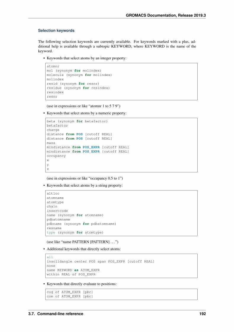
GROMACS Documentation, Release 2019.3
Selection keywords
The following selection keywords are currently available. For keywords marked with a plus, ad-ditional help is available through a subtopic KEYWORD, where KEYWORD is the name of thekeyword.
• Keywords that select atoms by an integer property:
atomnrmol (synonym for molindex)molecule (synonym for molindex)molindexresid (synonym for resnr)residue (synonym for resindex)resindexresnr
(use in expressions or like “atomnr 1 to 5 7 9”)
• Keywords that select atoms by a numeric property:
beta (synonym for betafactor)betafactorchargedistance from POS [cutoff REAL]distance from POS [cutoff REAL]massmindistance from POS_EXPR [cutoff REAL]mindistance from POS_EXPR [cutoff REAL]occupancyxyz
(use in expressions or like “occupancy 0.5 to 1”)
• Keywords that select atoms by a string property:
altlocatomnameatomtypechaininsertcodename (synonym for atomname)pdbatomnamepdbname (synonym for pdbatomname)resnametype (synonym for atomtype)
(use like “name PATTERN [PATTERN] . . . ”)
• Additional keywords that directly select atoms:
allinsolidangle center POS span POS_EXPR [cutoff REAL]nonesame KEYWORD as ATOM_EXPRwithin REAL of POS_EXPR
• Keywords that directly evaluate to positions:
cog of ATOM_EXPR [pbc]com of ATOM_EXPR [pbc]
3.7. Command-line reference 192
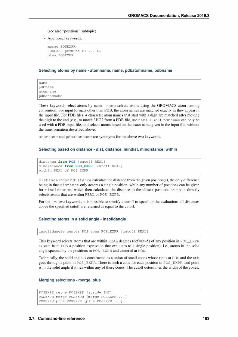
GROMACS Documentation, Release 2019.3
(see also “positions” subtopic)
• Additional keywords:
merge POSEXPRPOSEXPR permute P1 ... PNplus POSEXPR
Selecting atoms by name - atomname, name, pdbatomname, pdbname
namepdbnameatomnamepdbatomname
These keywords select atoms by name. name selects atoms using the GROMACS atom namingconvention. For input formats other than PDB, the atom names are matched exactly as they appear inthe input file. For PDB files, 4 character atom names that start with a digit are matched after movingthe digit to the end (e.g., to match 3HG2 from a PDB file, use name HG23). pdbname can only beused with a PDB input file, and selects atoms based on the exact name given in the input file, withoutthe transformation described above.
atomname and pdbatomname are synonyms for the above two keywords.
Selecting based on distance - dist, distance, mindist, mindistance, within
distance from POS [cutoff REAL]mindistance from POS_EXPR [cutoff REAL]within REAL of POS_EXPR
distance and mindistance calculate the distance from the given position(s), the only differencebeing in that distance only accepts a single position, while any number of positions can be givenfor mindistance, which then calculates the distance to the closest position. within directlyselects atoms that are within REAL of POS_EXPR.
For the first two keywords, it is possible to specify a cutoff to speed up the evaluation: all distancesabove the specified cutoff are returned as equal to the cutoff.
Selecting atoms in a solid angle - insolidangle
insolidangle center POS span POS_EXPR [cutoff REAL]
This keyword selects atoms that are within REAL degrees (default=5) of any position in POS_EXPRas seen from POS a position expression that evaluates to a single position), i.e., atoms in the solidangle spanned by the positions in POS_EXPR and centered at POS.
Technically, the solid angle is constructed as a union of small cones whose tip is at POS and the axisgoes through a point in POS_EXPR. There is such a cone for each position in POS_EXPR, and pointis in the solid angle if it lies within any of these cones. The cutoff determines the width of the cones.
Merging selections - merge, plus
POSEXPR merge POSEXPR [stride INT]POSEXPR merge POSEXPR [merge POSEXPR ...]POSEXPR plus POSEXPR [plus POSEXPR ...]
3.7. Command-line reference 193
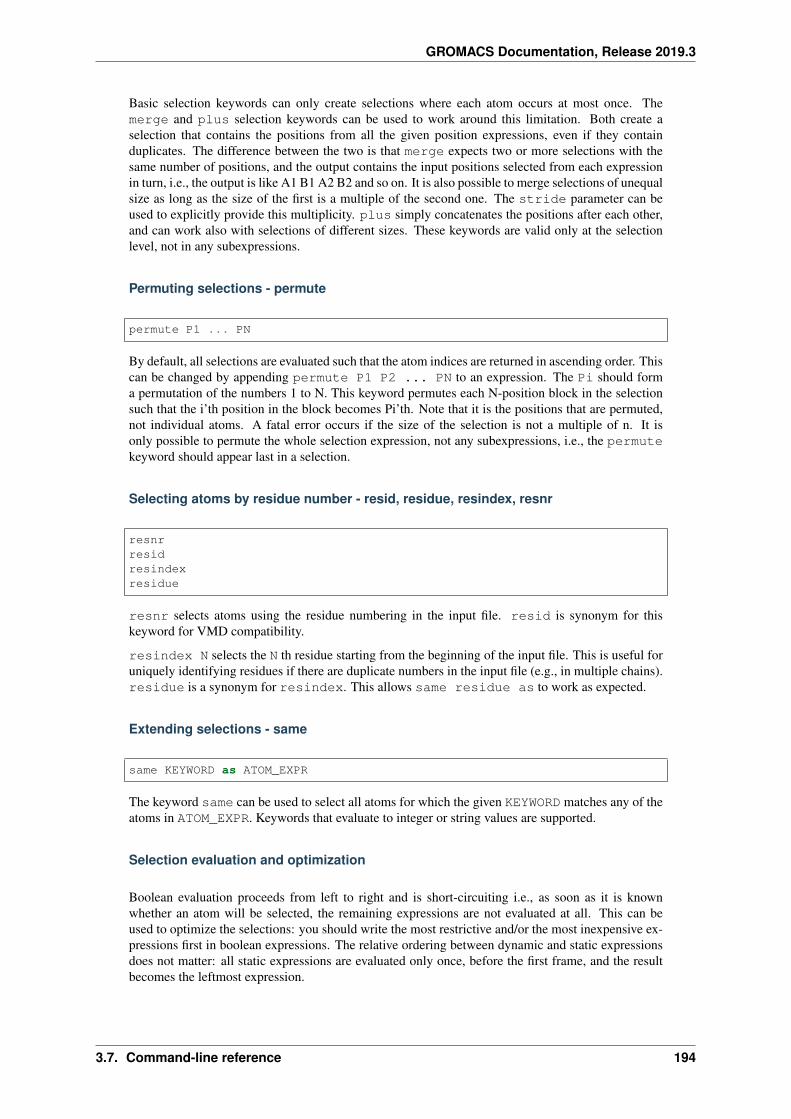
GROMACS Documentation, Release 2019.3
Basic selection keywords can only create selections where each atom occurs at most once. Themerge and plus selection keywords can be used to work around this limitation. Both create aselection that contains the positions from all the given position expressions, even if they containduplicates. The difference between the two is that merge expects two or more selections with thesame number of positions, and the output contains the input positions selected from each expressionin turn, i.e., the output is like A1 B1 A2 B2 and so on. It is also possible to merge selections of unequalsize as long as the size of the first is a multiple of the second one. The stride parameter can beused to explicitly provide this multiplicity. plus simply concatenates the positions after each other,and can work also with selections of different sizes. These keywords are valid only at the selectionlevel, not in any subexpressions.
Permuting selections - permute
permute P1 ... PN
By default, all selections are evaluated such that the atom indices are returned in ascending order. Thiscan be changed by appending permute P1 P2 ... PN to an expression. The Pi should forma permutation of the numbers 1 to N. This keyword permutes each N-position block in the selectionsuch that the i’th position in the block becomes Pi’th. Note that it is the positions that are permuted,not individual atoms. A fatal error occurs if the size of the selection is not a multiple of n. It isonly possible to permute the whole selection expression, not any subexpressions, i.e., the permutekeyword should appear last in a selection.
Selecting atoms by residue number - resid, residue, resindex, resnr
resnrresidresindexresidue
resnr selects atoms using the residue numbering in the input file. resid is synonym for thiskeyword for VMD compatibility.
resindex N selects the N th residue starting from the beginning of the input file. This is useful foruniquely identifying residues if there are duplicate numbers in the input file (e.g., in multiple chains).residue is a synonym for resindex. This allows same residue as to work as expected.
Extending selections - same
same KEYWORD as ATOM_EXPR
The keyword same can be used to select all atoms for which the given KEYWORD matches any of theatoms in ATOM_EXPR. Keywords that evaluate to integer or string values are supported.
Selection evaluation and optimization
Boolean evaluation proceeds from left to right and is short-circuiting i.e., as soon as it is knownwhether an atom will be selected, the remaining expressions are not evaluated at all. This can beused to optimize the selections: you should write the most restrictive and/or the most inexpensive ex-pressions first in boolean expressions. The relative ordering between dynamic and static expressionsdoes not matter: all static expressions are evaluated only once, before the first frame, and the resultbecomes the leftmost expression.
3.7. Command-line reference 194
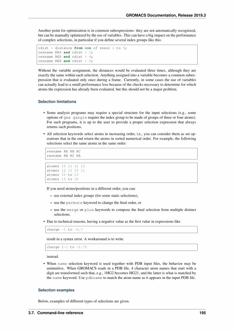
GROMACS Documentation, Release 2019.3
Another point for optimization is in common subexpressions: they are not automatically recognized,but can be manually optimized by the use of variables. This can have a big impact on the performanceof complex selections, in particular if you define several index groups like this:
rdist = distance from com of resnr 1 to 5;resname RES and rdist < 2;resname RES and rdist < 4;resname RES and rdist < 6;
Without the variable assignment, the distances would be evaluated three times, although they areexactly the same within each selection. Anything assigned into a variable becomes a common subex-pression that is evaluated only once during a frame. Currently, in some cases the use of variablescan actually lead to a small performance loss because of the checks necessary to determine for whichatoms the expression has already been evaluated, but this should not be a major problem.
Selection limitations
• Some analysis programs may require a special structure for the input selections (e.g., someoptions of gmx gangle require the index group to be made of groups of three or four atoms).For such programs, it is up to the user to provide a proper selection expression that alwaysreturns such positions.
• All selection keywords select atoms in increasing order, i.e., you can consider them as set op-erations that in the end return the atoms in sorted numerical order. For example, the followingselections select the same atoms in the same order:
resname RA RB RCresname RB RC RA
atomnr 10 11 12 13atomnr 12 13 10 11atomnr 10 to 13atomnr 13 to 10
If you need atoms/positions in a different order, you can:
– use external index groups (for some static selections),
– use the permute keyword to change the final order, or
– use the merge or plus keywords to compose the final selection from multiple distinctselections.
• Due to technical reasons, having a negative value as the first value in expressions like
charge -1 to -0.7
result in a syntax error. A workaround is to write
charge {-1 to -0.7}
instead.
• When name selection keyword is used together with PDB input files, the behavior may beunintuitive. When GROMACS reads in a PDB file, 4 character atom names that start with adigit are transformed such that, e.g., 1HG2 becomes HG21, and the latter is what is matched bythe name keyword. Use pdbname to match the atom name as it appears in the input PDB file.
Selection examples
Below, examples of different types of selections are given.
3.7. Command-line reference 195
GROMACS Documentation, Release 2019.3
• Selection of all water oxygens:
resname SOL and name OW
• Centers of mass of residues 1 to 5 and 10:
res_com of resnr 1 to 5 10
• All atoms farther than 1 nm of a fixed position:
not within 1 of [1.2, 3.1, 2.4]
• All atoms of a residue LIG within 0.5 nm of a protein (with a custom name):
"Close to protein" resname LIG and within 0.5 of group "Protein"
• All protein residues that have at least one atom within 0.5 nm of a residue LIG:
group "Protein" and same residue as within 0.5 of resname LIG
• All RES residues whose COM is between 2 and 4 nm from the COM of all of them:
rdist = res_com distance from com of resname RESresname RES and rdist >= 2 and rdist <= 4
• Selection like with duplicate atoms like C1 C2 C2 C3 C3 C4 . . . C8 C9:
name "C[1-8]" merge name "C[2-9]"
This can be used with gmx distance to compute C1-C2, C2-C3 etc. distances.
• Selection with atoms in order C2 C1:
name C1 C2 permute 2 1
This can be used with gmx gangle to get C2->C1 vectors instead of C1->C2.
• Selection with COMs of two index groups:
com of group 1 plus com of group 2
This can be used with gmx distance to compute the distance between these two COMs.
• Fixed vector along x (can be used as a reference with gmx gangle):
[0, 0, 0] plus [1, 0, 0]
• The following examples explain the difference between the various position types. This selec-tion selects a position for each residue where any of the three atoms C[123] has x < 2. Thepositions are computed as the COM of all three atoms. This is the default behavior if you justwrite res_com of.
part_res_com of name C1 C2 C3 and x < 2
This selection does the same, but the positions are computed as COM positions of wholeresidues:
whole_res_com of name C1 C2 C3 and x < 2
Finally, this selection selects the same residues, but the positions are computed as COM ofexactly those atoms atoms that match the x < 2 criterion:
3.7. Command-line reference 196
GROMACS Documentation, Release 2019.3
dyn_res_com of name C1 C2 C3 and x < 2
• Without the of keyword, the default behavior is different from above, but otherwise the rulesare the same:
name C1 C2 C3 and res_com x < 2
works as if whole_res_com was specified, and selects the three atoms from residues whoseCOM satisfiex x < 2. Using
name C1 C2 C3 and part_res_com x < 2
instead selects residues based on the COM computed from the C[123] atoms.
3.7.105 Command changes between versions
Starting from GROMACS 5.0, some of the analysis commands (and a few other commands as well)have changed significantly.
One main driver for this has been that many new tools mentioned below now accept selections throughone or more command-line options instead of prompting for a static index group. To take full ad-vantage of selections, the interface to the commands has changed somewhat, and some previouscommand-line options are no longer present as the same effect can be achieved with suitable se-lections. Please see Selection syntax and usage (page 189) additional information on how to useselections.
In the process, some old analysis commands have been removed in favor of more powerful func-tionality that is available through an alternative tool. For removed or replaced commands, this pagedocuments how to perform the same tasks with new tools. For new commands, a brief note on theavailable features is given. See the linked help for the new commands for a full description.
This section lists only major changes; minor changes like additional/removed options or bug fixes arenot typically included.
For more information about changed features, please check out the release notes (page ??).
Version 2018
gmx trajectory
new
gmx trajectory (page 160) has been introduced as a selection-enabled version of gmx traj (page 158).It supports output of coordinates, velocities, and/or forces for positions calculated for selections.
Version 2016
Analysis on arbitrary subsets of atoms
Tools implemented in the new analysis framework can now operate upon trajectories that match onlya subset of the atoms in the input structure file.
gmx insert-molecules
improved
3.7. Command-line reference 197
GROMACS Documentation, Release 2019.3
gmx insert-molecules (page 104) has gained an option -replace that makes it possible to insertmolecules into a solvated configuration, replacing any overlapping solvent atoms. In a fully solvatedbox, it is also possible to insert into a certain region of the solvent only by selecting a subset of thesolvent atoms (-replace takes a selection that can also contain expressions like not within 1of ...).
gmx rdf
improved
The normalization for the output RDF can now also be the radial number density.
gmx genconf
simplified
Removed -block, -sort and -shuffle.
Version 5.1
General
Symbolic links from 5.0 are no longer supported. The only way to invoke a command is through gmx<command>.
gmx pairdist
new
gmx pairdist (page 125) has been introduced as a selection-enabled replacement for gmx mindist(page 115) (gmx mindist still exists unchanged). It can calculate min/max pairwise distancesbetween a pair of selections, including, e.g., per-residue minimum distances or distances from asingle point to a set of residue-centers-of-mass.
gmx rdf
rewritten
gmx rdf (page 134) has been rewritten for 5.1 to use selections for specifying the points from whichthe RDFs are calculated. The interface is mostly the same, except that there are new command-lineoptions to specify the selections. The following additional changes have been made:
• -com and -rdf options have been removed. Equivalent functionality is available throughselections:
– -com can be replaced with a com of <selection> as the reference selection.
– -rdf can be replaced with a suitable set of selections (e.g., res_com of<selection>) and/or using -seltype.
• -rmax option is added to specify a cutoff for the RDFs. If set to a value that is significantlysmaller than half the box size, it can speed up the calculation significantly if a grid-based neigh-borhood search can be used.
• -hq and -fade options have been removed, as they are simply postprocessing steps on the rawnumbers that can be easily done after the analysis.
3.7. Command-line reference 198
GROMACS Documentation, Release 2019.3
Version 5.0
General
Version 5.0 introduced the gmx wrapper binary. For backwards compatibility, this version still createssymbolic links by default for old tools: e.g., g_order <options> is equivalent to gmx order<options>, and g_order is simply a symbolic link on the file system.
g_bond
replaced
This tool has been removed in 5.0. A replacement is gmx distance (page 73).
You can provide your existing index file to gmx distance (page 73), and it will calculate the samedistances. The differences are:
• -blen and -tol options have different default values.
• You can control the output histogram with -binw.
• -aver and -averdist options are not present. Instead, you can choose between the differentthings to calculate using -oav (corresponds to -d with -averdist), -oall (corresponds to-d without -averdist), -oh (corresponds to -o with -aver), and -oallstat (corre-sponds to -l without -aver).
You can produce any combination of output files. Compared to g_bond, gmx distance -oallis currently missing labels for the output columns.
g_dist
replaced
This tool has been removed in 5.0. A replacement is gmx distance (page 73) (for most options) orgmx select (page 147) (for -dist or -lt).
If you had index groups A and B in index.ndx for g_dist, you can use the following commandto compute the same distance with gmx distance:
gmx distance -n index.ndx -select 'com of group "A" plus com of group "B"→˓' -oxyz -oall
The -intra switch is replaced with -nopbc.
If you used -dist D, you can do the same calculation with gmx select:
gmx select -n index.ndx -select 'group "B" and within D of com of group "A→˓"' -on/-oi/-os/-olt
You can select the output option that best suits your post-processing needs (-olt is a replacementfor g_dist -dist -lt)
gmx distance
new
gmx distance (page 73) has been introduced as a selection-enabled replacement for various tools thatcomputed distances between fixed pairs of atoms (or centers-of-mass of groups). It has a combinationof the features of g_bond and g_dist, allowing computation of one or multiple distances, eitherbetween atom-atom pairs or centers-of-mass of groups, and providing a combination of output optionsthat were available in one of the tools.
3.7. Command-line reference 199
GROMACS Documentation, Release 2019.3
gmx gangle
new
gmx gangle (page 89) has been introduced as a selection-enabled replacement for g_sgangle. Inaddition to supporting atom-atom vectors, centers-of-mass can be used as endpoints of the vectors,and there are a few additional angle types that can be calculated. The command also has basic sup-port for calculating normal angles between three atoms and/or centers-of-mass, making it a partialreplacement for gmx angle (page 46) as well.
gmx protonate
replaced
This was a very old tool originally written for united atom force fields, where it was necessary togenerate all hydrogens after running a trajectory in order to calculate e.g. distance restraint violations.The functionality to simply protonate a structure is available in gmx pdb2gmx (page 127). If there issignificant interest, we might reintroduce it after moving to new topology formats in the future.
gmx freevolume
new
This tool has been introduced in 5.0. It uses a Monte Carlo sampling method to calculate the fractionof free volume within the box (using a probe of a given size).
g_sas
rewritten
This tool has been rewritten in 5.0, and renamed to gmx sasa (page 144) (the underlying surface areacalculation algorithm is still the same).
The main difference in the new tool is support for selections. Instead of prompting for an index group,a (potentially dynamic) selection for the calculation can be given with -surface. Any number ofoutput groups can be given with -output, allowing multiple parts of the surface area to be computedin a single run. The total area of the -surface group is now always calculated.
The tool no longer automatically divides the surface into hydrophobic and hydrophilic areas, andthere is no -f_index option. The same effects can be obtained by defining suitable selections for-output. If you want output that contains the same numbers as with the old tool for a calculationgroup A and output group B, you can use
gmx sasa -surface 'group "A"' -output '"Hydrophobic" group "A" and charge→˓{-0.2 to 0.2}; "Hydrophilic" group "B" and not charge {-0.2 to 0.2};→˓"Total" group "B"'
Solvation free energy estimates are now calculated only if separately requested with -odg, and arewritten into a separate file.
Output option -i for a position restraint file is not currently implemented in the new tool, but wouldnot be very difficult to add if requested.
g_sgangle
replaced
3.7. Command-line reference 200
GROMACS Documentation, Release 2019.3
This tool has been removed in 5.0. A replacement is gmx gangle (page 89) (for angle calculation) andgmx distance (page 73) (for -od, -od1, -od2).
If you had index groups A and B in index.ndx for g_sgangle, you can use the following commandto compute the same angle with gmx gangle:
gmx gangle -n index.ndx -g1 vector/plane -group1 'group "A"' -g2 vector/→˓plane -group2 'group "B"' -oav
You need to select either vector or plane for the -g1 and -g2 options depending on which oneyour index groups specify.
If you only had a single index group A in index.ndx and you used g_sgangle -z or -one, you canuse:
gmx gangle -n index.ndx -g1 vector/plane -group1 'group "A"' -g2 z/t0 -oav
For the distances, you can use gmx distance (page 73) to compute one or more distances as you want.Both distances between centers of groups or individual atoms are supported using the new selectionsyntax.
genbox
This tool has been split to gmx solvate (page 151) and gmx insert-molecules (page 104).
tpbconv
This tool has been renamed gmx convert-tpr (page 60).
3.8 Molecular dynamics parameters (.mdp options)
3.8.1 General information
Default values are given in parentheses, or listed first among choices. The first option in the list isalways the default option. Units are given in square brackets. The difference between a dash and anunderscore is ignored.
A sample mdp file (page 425) is available. This should be appropriate to start a normal simulation.Edit it to suit your specific needs and desires.
Preprocessing
includedirectories to include in your topology. Format: -I/home/john/mylib -I../otherlib
definedefines to pass to the preprocessor, default is no defines. You can use any defines to controloptions in your customized topology files. Options that act on existing top (page 429) filemechanisms include
-DFLEXIBLE will use flexible water instead of rigid water into your topology, thiscan be useful for normal mode analysis.
-DPOSRES will trigger the inclusion of posre.itp into your topology, used forimplementing position restraints.
3.8. Molecular dynamics parameters (.mdp options) 201
GROMACS Documentation, Release 2019.3
Run control
integrator(Despite the name, this list includes algorithms that are not actually integrators over time.integrator=steep (page 202) and all entries following it are in this category)
mdA leap-frog algorithm for integrating Newton’s equations of motion.
md-vvA velocity Verlet algorithm for integrating Newton’s equations of motion. For constantNVE simulations started from corresponding points in the same trajectory, the trajectoriesare analytically, but not binary, identical to the integrator=md (page 202) leap-frogintegrator. The the kinetic energy, which is determined from the whole step velocities andis therefore slightly too high. The advantage of this integrator is more accurate, reversibleNose-Hoover and Parrinello-Rahman coupling integration based on Trotter expansion, aswell as (slightly too small) full step velocity output. This all comes at the cost off extracomputation, especially with constraints and extra communication in parallel. Note that fornearly all production simulations the integrator=md (page 202) integrator is accurateenough.
md-vv-avekA velocity Verlet algorithm identical to integrator=md-vv (page 202), except that thekinetic energy is determined as the average of the two half step kinetic energies as in theintegrator=md (page 202) integrator, and this thus more accurate. With Nose-Hooverand/or Parrinello-Rahman coupling this comes with a slight increase in computational cost.
sdAn accurate and efficient leap-frog stochastic dynamics integrator. With constraints, co-ordinates needs to be constrained twice per integration step. Depending on the compu-tational cost of the force calculation, this can take a significant part of the simulationtime. The temperature for one or more groups of atoms (tc-grps (page 213)) is setwith ref-t (page 213), the inverse friction constant for each group is set with tau-t(page 213). The parameter tcoupl (page 212) is ignored. The random generator is ini-tialized with ld-seed (page 204). When used as a thermostat, an appropriate value fortau-t (page 213) is 2 ps, since this results in a friction that is lower than the internal fric-tion of water, while it is high enough to remove excess heat NOTE: temperature deviationsdecay twice as fast as with a Berendsen thermostat with the same tau-t (page 213).
bdAn Euler integrator for Brownian or position Langevin dynamics, the velocity is the forcedivided by a friction coefficient (bd-fric (page 204)) plus random thermal noise (ref-t(page 213)). When bd-fric (page 204) is 0, the friction coefficient for each particle iscalculated as mass/ tau-t (page 213), as for the integrator integrator=sd (page 202).The random generator is initialized with ld-seed (page 204).
steepA steepest descent algorithm for energy minimization. The maximum step size is emstep(page 204), the tolerance is emtol (page 204).
cgA conjugate gradient algorithm for energy minimization, the tolerance is emtol(page 204). CG is more efficient when a steepest descent step is done every once in awhile, this is determined by nstcgsteep (page 204). For a minimization prior to a nor-mal mode analysis, which requires a very high accuracy, GROMACS should be compiledin double precision.
l-bfgsA quasi-Newtonian algorithm for energy minimization according to the low-memoryBroyden-Fletcher-Goldfarb-Shanno approach. In practice this seems to converge faster thanConjugate Gradients, but due to the correction steps necessary it is not (yet) parallelized.
3.8. Molecular dynamics parameters (.mdp options) 202
GROMACS Documentation, Release 2019.3
nmNormal mode analysis is performed on the structure in the tpr (page 431) file. GROMACSshould be compiled in double precision.
tpiTest particle insertion. The last molecule in the topology is the test particle. A trajectorymust be provided to mdrun -rerun. This trajectory should not contain the molecule tobe inserted. Insertions are performed nsteps (page 203) times in each frame at randomlocations and with random orientiations of the molecule. When nstlist (page 206) islarger than one, nstlist (page 206) insertions are performed in a sphere with radiusrtpi (page 205) around a the same random location using the same pair list. Since pairlist construction is expensive, one can perform several extra insertions with the same listalmost for free. The random seed is set with ld-seed (page 204). The temperature forthe Boltzmann weighting is set with ref-t (page 213), this should match the temperatureof the simulation of the original trajectory. Dispersion correction is implemented correctlyfor TPI. All relevant quantities are written to the file specified with mdrun -tpi. Thedistribution of insertion energies is written to the file specified with mdrun -tpid. Notrajectory or energy file is written. Parallel TPI gives identical results to single-node TPI.For charged molecules, using PME with a fine grid is most accurate and also efficient, sincethe potential in the system only needs to be calculated once per frame.
tpicTest particle insertion into a predefined cavity location. The procedure is the same as forintegrator=tpi (page 203), except that one coordinate extra is read from the trajec-tory, which is used as the insertion location. The molecule to be inserted should be centeredat 0,0,0. GROMACS does not do this for you, since for different situations a different wayof centering might be optimal. Also rtpi (page 205) sets the radius for the sphere aroundthis location. Neighbor searching is done only once per frame, nstlist (page 206) isnot used. Parallel integrator=tpic (page 203) gives identical results to single-rankintegrator=tpic (page 203).
mimicEnable MiMiC QM/MM coupling to run hybrid molecular dynamics. Keey in mind thatits required to launch CPMD compiled with MiMiC as well. In this mode all optionsregarding integration (T-coupling, P-coupling, timestep and number of steps) are ignoredas CPMD will do the integration instead. Options related to forces computation (cutoffs,PME parameters, etc.) are working as usual. Atom selection to define QM atoms is readfrom QMMM-grps (page 236)
tinit(0) [ps] starting time for your run (only makes sense for time-based integrators)
dt(0.001) [ps] time step for integration (only makes sense for time-based integrators)
nsteps(0) maximum number of steps to integrate or minimize, -1 is no maximum
init-step(0) The starting step. The time at step i in a run is calculated as: t = tinit (page 203) + dt(page 203) * (init-step (page 203) + i). The free-energy lambda is calculated as: lambda= init-lambda (page 229) + delta-lambda (page 229) * (init-step (page 203) + i).Also non-equilibrium MD parameters can depend on the step number. Thus for exact restarts orredoing part of a run it might be necessary to set init-step (page 203) to the step number ofthe restart frame. gmx convert-tpr (page 60) does this automatically.
simulation-part(0) A simulation can consist of multiple parts, each of which has a part number. This optionspecifies what that number will be, which helps keep track of parts that are logically the samesimulation. This option is generally useful to set only when coping with a crashed simulationwhere files were lost.
3.8. Molecular dynamics parameters (.mdp options) 203
GROMACS Documentation, Release 2019.3
comm-mode
LinearRemove center of mass translational velocity
AngularRemove center of mass translational and rotational velocity
Linear-acceleration-correctionRemove center of mass translational velocity. Correct the center of mass position assuminglinear acceleration over nstcomm (page 204) steps. This is useful for cases where anacceleration is expected on the center of mass which is nearly constant over nstcomm(page 204) steps. This can occur for example when pulling on a group using an absolutereference.
NoneNo restriction on the center of mass motion
nstcomm(100) [steps] frequency for center of mass motion removal
comm-grpsgroup(s) for center of mass motion removal, default is the whole system
Langevin dynamics
bd-fric(0) [amu ps-1] Brownian dynamics friction coefficient. When bd-fric (page 204) is 0, thefriction coefficient for each particle is calculated as mass/ tau-t (page 213).
ld-seed(-1) [integer] used to initialize random generator for thermal noise for stochastic and Browniandynamics. When ld-seed (page 204) is set to -1, a pseudo random seed is used. When runningBD or SD on multiple processors, each processor uses a seed equal to ld-seed (page 204) plusthe processor number.
Energy minimization
emtol(10.0) [kJ mol-1 nm-1] the minimization is converged when the maximum force is smaller thanthis value
emstep(0.01) [nm] initial step-size
nstcgsteep(1000) [steps] frequency of performing 1 steepest descent step while doing conjugate gradientenergy minimization.
nbfgscorr(10) Number of correction steps to use for L-BFGS minimization. A higher number is (at leasttheoretically) more accurate, but slower.
Shell Molecular Dynamics
When shells or flexible constraints are present in the system the positions of the shells and the lengthsof the flexible constraints are optimized at every time step until either the RMS force on the shells andconstraints is less than emtol (page 204), or a maximum number of iterations niter (page 204)has been reached. Minimization is converged when the maximum force is smaller than emtol(page 204). For shell MD this value should be 1.0 at most.
3.8. Molecular dynamics parameters (.mdp options) 204
GROMACS Documentation, Release 2019.3
niter(20) maximum number of iterations for optimizing the shell positions and the flexible con-straints.
fcstep(0) [ps2] the step size for optimizing the flexible constraints. Should be chosen as mu/(d2V/dq2)where mu is the reduced mass of two particles in a flexible constraint and d2V/dq2 is the secondderivative of the potential in the constraint direction. Hopefully this number does not differ toomuch between the flexible constraints, as the number of iterations and thus the runtime is verysensitive to fcstep. Try several values!
Test particle insertion
rtpi(0.05) [nm] the test particle insertion radius, see integrators integrator=tpi (page 203)and integrator=tpic (page 203)
Output control
nstxout(0) [steps] number of steps that elapse between writing coordinates to the output trajectory file(trr (page 431)), the last coordinates are always written
nstvout(0) [steps] number of steps that elapse between writing velocities to the output trajectory file (trr(page 431)), the last velocities are always written
nstfout(0) [steps] number of steps that elapse between writing forces to the output trajectory file (trr(page 431)), the last forces are always written.
nstlog(1000) [steps] number of steps that elapse between writing energies to the log file, the lastenergies are always written
nstcalcenergy(100) number of steps that elapse between calculating the energies, 0 is never. This optionis only relevant with dynamics. This option affects the performance in parallel simulations,because calculating energies requires global communication between all processes which canbecome a bottleneck at high parallelization.
nstenergy(1000) [steps] number of steps that elapse between writing energies to energy file, the last ener-gies are always written, should be a multiple of nstcalcenergy (page 205). Note that theexact sums and fluctuations over all MD steps modulo nstcalcenergy (page 205) are storedin the energy file, so gmx energy (page 84) can report exact energy averages and fluctuations alsowhen nstenergy (page 205) > 1
nstxout-compressed(0) [steps] number of steps that elapse between writing position coordinates using lossy com-pression (xtc (page 432) file)
compressed-x-precision(1000) [real] precision with which to write to the compressed trajectory file
compressed-x-grpsgroup(s) to write to the compressed trajectory file, by default the whole system is written (ifnstxout-compressed (page 205) > 0)
energygrpsgroup(s) for which to write to write short-ranged non-bonded potential energies to the energyfile (not supported on GPUs)
3.8. Molecular dynamics parameters (.mdp options) 205
GROMACS Documentation, Release 2019.3
Neighbor searching
cutoff-scheme
VerletGenerate a pair list with buffering. The buffer size is automatically set based onverlet-buffer-tolerance (page 207), unless this is set to -1, in which caserlist (page 207) will be used. This option has an explicit, exact cut-off at rvdw(page 211) equal to rcoulomb (page 209), unless PME or Ewald is used, in whichcase rcoulomb (page 209) > rvdw (page 211) is allowed. Currently only cut-off,reaction-field, PME or Ewald electrostatics and plain LJ are supported. Some gmxmdrun (page 111) functionality is not yet supported with the cutoff-scheme=Verlet(page 206) scheme, but gmx grompp (page 94) checks for this. Native GPU accel-eration is only supported with cutoff-scheme=Verlet (page 206). With GPU-accelerated PME or with separate PME ranks, gmx mdrun (page 111) will automaticallytune the CPU/GPU load balance by scaling rcoulomb (page 209) and the grid spac-ing. This can be turned off with mdrun -notunepme. cutoff-scheme=Verlet(page 206) is faster than cutoff-scheme=group (page 206) when there is no water, orif cutoff-scheme=group (page 206) would use a pair-list buffer to conserve energy.
groupGenerate a pair list for groups of atoms. These groups correspond to the charge groupsin the topology. This was the only cut-off treatment scheme before version 4.6, and isdeprecated since 5.1. There is no explicit buffering of the pair list. This enables efficientforce calculations for water, but energy is only conserved when a buffer is explicitly added.
nstlist
10. [steps]
>0Frequency to update the neighbor list. When this is 0, the neighbor list is made only once.With energy minimization the pair list will be updated for every energy evaluation whennstlist (page 206) is greater than 0. With cutoff-scheme=Verlet (page 206)and verlet-buffer-tolerance (page 207) set, nstlist (page 206) is actually aminimum value and gmx mdrun (page 111) might increase it, unless it is set to 1. Withparallel simulations and/or non-bonded force calculation on the GPU, a value of 20 or 40often gives the best performance. With cutoff-scheme=group (page 206) and non-exact cut-off’s, nstlist (page 206) will affect the accuracy of your simulation and it cannot be chosen freely.
0The neighbor list is only constructed once and never updated. This is mainly useful forvacuum simulations in which all particles see each other.
<0Unused.
ns-type
gridMake a grid in the box and only check atoms in neighboring grid cells when constructing anew neighbor list every nstlist (page 206) steps. In large systems grid search is muchfaster than simple search.
simpleCheck every atom in the box when constructing a new neighbor list every nstlist(page 206) steps (only with cutoff-scheme=group (page 206) cut-off scheme).
pbc
3.8. Molecular dynamics parameters (.mdp options) 206
GROMACS Documentation, Release 2019.3
xyzUse periodic boundary conditions in all directions.
noUse no periodic boundary conditions, ignore the box. To simulate without cut-offs, set allcut-offs and nstlist (page 206) to 0. For best performance without cut-offs on a singleMPI rank, set nstlist (page 206) to zero and ns-type=simple (page 206).
xyUse periodic boundary conditions in x and y directions only. This works only withns-type=grid (page 206) and can be used in combination with walls (page 218). With-out walls or with only one wall the system size is infinite in the z direction. Thereforepressure coupling or Ewald summation methods can not be used. These disadvantages donot apply when two walls are used.
periodic-molecules
nomolecules are finite, fast molecular PBC can be used
yesfor systems with molecules that couple to themselves through the periodic boundary con-ditions, this requires a slower PBC algorithm and molecules are not made whole in theoutput
verlet-buffer-tolerance(0.005) [kJ mol-1 ps-1]
Useful only with the cutoff-scheme=Verlet (page 206) cutoff-scheme (page 206).This sets the maximum allowed error for pair interactions per particle caused by the Verletbuffer, which indirectly sets rlist (page 207). As both nstlist (page 206) and the Verletbuffer size are fixed (for performance reasons), particle pairs not in the pair list can occasionallyget within the cut-off distance during nstlist (page 206) -1 steps. This causes very smalljumps in the energy. In a constant-temperature ensemble, these very small energy jumps canbe estimated for a given cut-off and rlist (page 207). The estimate assumes a homogeneousparticle distribution, hence the errors might be slightly underestimated for multi-phase systems.(See the reference manual for details). For longer pair-list life-time (nstlist (page 206) -1) * dt (page 203) the buffer is overestimated, because the interactions between particles areignored. Combined with cancellation of errors, the actual drift of the total energy is usually oneto two orders of magnitude smaller. Note that the generated buffer size takes into account thatthe GROMACS pair-list setup leads to a reduction in the drift by a factor 10, compared to asimple particle-pair based list. Without dynamics (energy minimization etc.), the buffer is 5%of the cut-off. For NVE simulations the initial temperature is used, unless this is zero, in whichcase a buffer of 10% is used. For NVE simulations the tolerance usually needs to be loweredto achieve proper energy conservation on the nanosecond time scale. To override the automatedbuffer setting, use verlet-buffer-tolerance (page 207) =-1 and set rlist (page 207)manually.
rlist(1) [nm] Cut-off distance for the short-range neighbor list. With thecutoff-scheme=Verlet (page 206) cutoff-scheme (page 206), this is by de-fault set by the verlet-buffer-tolerance (page 207) option and the value of rlist(page 207) is ignored.
Electrostatics
coulombtype
Cut-offPlain cut-off with pair list radius rlist (page 207) and Coulomb cut-off rcoulomb
3.8. Molecular dynamics parameters (.mdp options) 207
GROMACS Documentation, Release 2019.3
(page 209), where rlist (page 207) >= rcoulomb (page 209).
EwaldClassical Ewald sum electrostatics. The real-space cut-off rcoulomb (page 209) shouldbe equal to rlist (page 207). Use e.g. rlist (page 207) =0.9, rcoulomb (page 209)=0.9. The highest magnitude of wave vectors used in reciprocal space is controlled byfourierspacing (page 211). The relative accuracy of direct/reciprocal space is con-trolled by ewald-rtol (page 212).
NOTE: Ewald scales as O(N3/2) and is thus extremely slow for large systems. It is includedmainly for reference - in most cases PME will perform much better.
PMEFast smooth Particle-Mesh Ewald (SPME) electrostatics. Direct space is similar to theEwald sum, while the reciprocal part is performed with FFTs. Grid dimensions are con-trolled with fourierspacing (page 211) and the interpolation order with pme-order(page 212). With a grid spacing of 0.1 nm and cubic interpolation the electrostatic forceshave an accuracy of 2-3*10-4. Since the error from the vdw-cutoff is larger than this youmight try 0.15 nm. When running in parallel the interpolation parallelizes better than theFFT, so try decreasing grid dimensions while increasing interpolation.
P3M-ADParticle-Particle Particle-Mesh algorithm with analytical derivative for for long range elec-trostatic interactions. The method and code is identical to SPME, except that the influencefunction is optimized for the grid. This gives a slight increase in accuracy.
Reaction-FieldReaction field electrostatics with Coulomb cut-off rcoulomb (page 209), where rlist(page 207) >= rvdw (page 211). The dielectric constant beyond the cut-off isepsilon-rf (page 209). The dielectric constant can be set to infinity by settingepsilon-rf (page 209) =0.
Generalized-Reaction-FieldGeneralized reaction field with Coulomb cut-off rcoulomb (page 209), where rlist(page 207) >= rcoulomb (page 209). The dielectric constant beyond the cut-off isepsilon-rf (page 209). The ionic strength is computed from the number of charged(i.e. with non zero charge) charge groups. The temperature for the GRF potential is setwith ref-t (page 213).
Reaction-Field-zeroIn GROMACS, normal reaction-field electrostatics withcutoff-scheme=group (page 206) leads to bad energy conservation.coulombtype=Reaction-Field-zero (page 208) solves this by making thepotential zero beyond the cut-off. It can only be used with an infinite dielectric constant(epsilon-rf (page 209) =0), because only for that value the force vanishes at thecut-off. rlist (page 207) should be 0.1 to 0.3 nm larger than rcoulomb (page 209)to accommodate the size of charge groups and diffusion between neighbor list updates.This, and the fact that table lookups are used instead of analytical functions makereaction-field-zero computationally more expensive than normal reaction-field.
ShiftAnalogous to vdwtype=Shift (page 210) for vdwtype (page 210). You might want touse coulombtype=Reaction-Field-zero (page 208) instead, which has a similarpotential shape, but has a physical interpretation and has better energies due to the exclusioncorrection terms.
Encad-ShiftThe Coulomb potential is decreased over the whole range, using the definition from theEncad simulation package.
SwitchAnalogous to vdwtype=Switch (page 210) for vdwtype (page 210).
3.8. Molecular dynamics parameters (.mdp options) 208
GROMACS Documentation, Release 2019.3
Switching the Coulomb potential can lead to serious artifacts, advice: usecoulombtype=Reaction-Field-zero (page 208) instead.
Usergmx mdrun (page 111) will now expect to find a file table.xvg with user-defined poten-tial functions for repulsion, dispersion and Coulomb. When pair interactions are present,gmx mdrun (page 111) also expects to find a file tablep.xvg for the pair interac-tions. When the same interactions should be used for non-bonded and pair interactionsthe user can specify the same file name for both table files. These files should contain 7columns: the x value, f(x), -f'(x), g(x), -g'(x), h(x), -h'(x), where f(x)is the Coulomb function, g(x) the dispersion function and h(x) the repulsion function.When vdwtype (page 210) is not set to User the values for g, -g', h and -h' are ig-nored. For the non-bonded interactions x values should run from 0 to the largest cut-offdistance + table-extension (page 211) and should be uniformly spaced. For the pairinteractions the table length in the file will be used. The optimal spacing, which is used fornon-user tables, is 0.002 nm when you run in mixed precision or 0.0005 nm when yourun in double precision. The function value at x=0 is not important. More information isin the printed manual.
PME-SwitchA combination of PME and a switch function for the direct-space part (see above).rcoulomb (page 209) is allowed to be smaller than rlist (page 207). This is mainly use-ful constant energy simulations (note that using PME with cutoff-scheme=Verlet(page 206) will be more efficient).
PME-UserA combination of PME and user tables (see above). rcoulomb (page 209) is allowed tobe smaller than rlist (page 207). The PME mesh contribution is subtracted from the usertable by gmx mdrun (page 111). Because of this subtraction the user tables should containabout 10 decimal places.
PME-User-SwitchA combination of PME-User and a switching function (see above). The switching functionis applied to final particle-particle interaction, i.e. both to the user supplied function andthe PME Mesh correction part.
coulomb-modifier
Potential-shift-VerletSelects Potential-shift with the Verlet cutoff-scheme, as it is (nearly) free; selects None withthe group cutoff-scheme.
Potential-shiftShift the Coulomb potential by a constant such that it is zero at the cut-off. This makes thepotential the integral of the force. Note that this does not affect the forces or the sampling.
NoneUse an unmodified Coulomb potential. With the group scheme this means no exact cut-offis used, energies and forces are calculated for all pairs in the pair list.
rcoulomb-switch(0) [nm] where to start switching the Coulomb potential, only relevant when force or potentialswitching is used
rcoulomb(1) [nm] The distance for the Coulomb cut-off. Note that with PME this value can be increasedby the PME tuning in gmx mdrun (page 111) along with the PME grid spacing.
epsilon-r(1) The relative dielectric constant. A value of 0 means infinity.
epsilon-rf(0) The relative dielectric constant of the reaction field. This is only used with reaction-field
3.8. Molecular dynamics parameters (.mdp options) 209
GROMACS Documentation, Release 2019.3
electrostatics. A value of 0 means infinity.
Van der Waals
vdwtype
Cut-offPlain cut-off with pair list radius rlist (page 207) and VdW cut-off rvdw (page 211),where rlist (page 207) >= rvdw (page 211).
PMEFast smooth Particle-mesh Ewald (SPME) for VdW interactions. The grid dimensionsare controlled with fourierspacing (page 211) in the same way as for electrostat-ics, and the interpolation order is controlled with pme-order (page 212). The relativeaccuracy of direct/reciprocal space is controlled by ewald-rtol-lj (page 212), andthe specific combination rules that are to be used by the reciprocal routine are set usinglj-pme-comb-rule (page 212).
ShiftThis functionality is deprecated and replaced by using vdwtype=Cut-off (page 210)with vdw-modifier=Force-switch (page 210). The LJ (not Buckingham) poten-tial is decreased over the whole range and the forces decay smoothly to zero betweenrvdw-switch (page 211) and rvdw (page 211). The neighbor search cut-off rlist(page 207) should be 0.1 to 0.3 nm larger than rvdw (page 211) to accommodate the sizeof charge groups and diffusion between neighbor list updates.
SwitchThis functionality is deprecated and replaced by using vdwtype=Cut-off (page 210)with vdw-modifier=Potential-switch (page 211). The LJ (not Buckingham)potential is normal out to rvdw-switch (page 211), after which it is switched off to reachzero at rvdw (page 211). Both the potential and force functions are continuously smooth,but be aware that all switch functions will give rise to a bulge (increase) in the force (sincewe are switching the potential). The neighbor search cut-off rlist (page 207) should be0.1 to 0.3 nm larger than rvdw (page 211) to accommodate the size of charge groups anddiffusion between neighbor list updates.
Encad-ShiftThe LJ (not Buckingham) potential is decreased over the whole range, using the definitionfrom the Encad simulation package.
UserSee user for coulombtype (page 207). The function value at zero is not important. Whenyou want to use LJ correction, make sure that rvdw (page 211) corresponds to the cut-offin the user-defined function. When coulombtype (page 207) is not set to User the valuesfor the f and -f' columns are ignored.
vdw-modifier
Potential-shift-VerletSelects Potential-shift with the Verlet cutoff-scheme, as it is (nearly) free; selects None withthe group cutoff-scheme.
Potential-shiftShift the Van der Waals potential by a constant such that it is zero at the cut-off. Thismakes the potential the integral of the force. Note that this does not affect the forces or thesampling.
NoneUse an unmodified Van der Waals potential. With the group scheme this means no exactcut-off is used, energies and forces are calculated for all pairs in the pair list.
3.8. Molecular dynamics parameters (.mdp options) 210
GROMACS Documentation, Release 2019.3
Force-switchSmoothly switches the forces to zero between rvdw-switch (page 211) and rvdw(page 211). This shifts the potential shift over the whole range and switches it to zeroat the cut-off. Note that this is more expensive to calculate than a plain cut-off and it is notrequired for energy conservation, since Potential-shift conserves energy just as well.
Potential-switchSmoothly switches the potential to zero between rvdw-switch (page 211) and rvdw(page 211). Note that this introduces articifically large forces in the switching region andis much more expensive to calculate. This option should only be used if the force field youare using requires this.
rvdw-switch(0) [nm] where to start switching the LJ force and possibly the potential, only relevant whenforce or potential switching is used
rvdw(1) [nm] distance for the LJ or Buckingham cut-off
DispCorr
nodon’t apply any correction
EnerPresapply long range dispersion corrections for Energy and Pressure
Enerapply long range dispersion corrections for Energy only
Tables
table-extension(1) [nm] Extension of the non-bonded potential lookup tables beyond the largest cut-off distance.The value should be large enough to account for charge group sizes and the diffusion betweenneighbor-list updates. Without user defined potential the same table length is used for the lookuptables for the 1-4 interactions, which are always tabulated irrespective of the use of tables forthe non-bonded interactions. The value of table-extension (page 211) in no way affectsthe values of rlist (page 207), rcoulomb (page 209), or rvdw (page 211).
energygrp-tableWhen user tables are used for electrostatics and/or VdW, here one can give pairs of energygroups for which seperate user tables should be used. The two energy groups will be appendedto the table file name, in order of their definition in energygrps (page 205), seperated byunderscores. For example, if energygrps = Na Cl Sol and energygrp-table =Na Na Na Cl, gmx mdrun (page 111) will read table_Na_Na.xvg and table_Na_-Cl.xvg in addition to the normal table.xvg which will be used for all other energy grouppairs.
Ewald
fourierspacing(0.12) [nm] For ordinary Ewald, the ratio of the box dimensions and the spacing determines alower bound for the number of wave vectors to use in each (signed) direction. For PME andP3M, that ratio determines a lower bound for the number of Fourier-space grid points that willbe used along that axis. In all cases, the number for each direction can be overridden by enteringa non-zero value for that fourier-nx (page 212) direction. For optimizing the relative loadof the particle-particle interactions and the mesh part of PME, it is useful to know that theaccuracy of the electrostatics remains nearly constant when the Coulomb cut-off and the PME
3.8. Molecular dynamics parameters (.mdp options) 211
GROMACS Documentation, Release 2019.3
grid spacing are scaled by the same factor. Note that this spacing can be scaled up along withrcoulomb (page 209) by the PME tuning in gmx mdrun (page 111).
fourier-nx
fourier-ny
fourier-nz(0) Highest magnitude of wave vectors in reciprocal space when using Ewald. Grid size whenusing PME or P3M. These values override fourierspacing (page 211) per direction. Thebest choice is powers of 2, 3, 5 and 7. Avoid large primes. Note that these grid sizes canbe reduced along with scaling up rcoulomb (page 209) by the PME tuning in gmx mdrun(page 111).
pme-order(4) Interpolation order for PME. 4 equals cubic interpolation. You might try 6/8/10 when run-ning in parallel and simultaneously decrease grid dimension.
ewald-rtol(10-5) The relative strength of the Ewald-shifted direct potential at rcoulomb (page 209) isgiven by ewald-rtol (page 212). Decreasing this will give a more accurate direct sum, butthen you need more wave vectors for the reciprocal sum.
ewald-rtol-lj(10-3) When doing PME for VdW-interactions, ewald-rtol-lj (page 212) is used to con-trol the relative strength of the dispersion potential at rvdw (page 211) in the same way asewald-rtol (page 212) controls the electrostatic potential.
lj-pme-comb-rule(Geometric) The combination rules used to combine VdW-parameters in the reciprocal part ofLJ-PME. Geometric rules are much faster than Lorentz-Berthelot and usually the recommendedchoice, even when the rest of the force field uses the Lorentz-Berthelot rules.
GeometricApply geometric combination rules
Lorentz-BerthelotApply Lorentz-Berthelot combination rules
ewald-geometry
3dThe Ewald sum is performed in all three dimensions.
3dcThe reciprocal sum is still performed in 3D, but a force and potential correction applied inthe z dimension to produce a pseudo-2D summation. If your system has a slab geometry inthe x-y plane you can try to increase the z-dimension of the box (a box height of 3 times theslab height is usually ok) and use this option.
epsilon-surface(0) This controls the dipole correction to the Ewald summation in 3D. The default value of zeromeans it is turned off. Turn it on by setting it to the value of the relative permittivity of theimaginary surface around your infinite system. Be careful - you shouldn’t use this if you havefree mobile charges in your system. This value does not affect the slab 3DC variant of the longrange corrections.
Temperature coupling
tcoupl
3.8. Molecular dynamics parameters (.mdp options) 212
GROMACS Documentation, Release 2019.3
noNo temperature coupling.
berendsenTemperature coupling with a Berendsen thermostat to a bath with temperature ref-t(page 213), with time constant tau-t (page 213). Several groups can be coupled sep-arately, these are specified in the tc-grps (page 213) field separated by spaces.
nose-hooverTemperature coupling using a Nose-Hoover extended ensemble. The reference temperatureand coupling groups are selected as above, but in this case tau-t (page 213) controlsthe period of the temperature fluctuations at equilibrium, which is slightly different froma relaxation time. For NVT simulations the conserved energy quantity is written to theenergy and log files.
andersenTemperature coupling by randomizing a fraction of the particle velocities at each timestep.Reference temperature and coupling groups are selected as above. tau-t (page 213) is theaverage time between randomization of each molecule. Inhibits particle dynamics some-what, but little or no ergodicity issues. Currently only implemented with velocity Verlet,and not implemented with constraints.
andersen-massiveTemperature coupling by randomizing velocities of all particles at infrequent timesteps.Reference temperature and coupling groups are selected as above. tau-t (page 213) isthe time between randomization of all molecules. Inhibits particle dynamics somewhat, butlittle or no ergodicity issues. Currently only implemented with velocity Verlet.
v-rescaleTemperature coupling using velocity rescaling with a stochastic term (JCP 126, 014101).This thermostat is similar to Berendsen coupling, with the same scaling using tau-t(page 213), but the stochastic term ensures that a proper canonical ensemble is generated.The random seed is set with ld-seed (page 204). This thermostat works correctly evenfor tau-t (page 213) =0. For NVT simulations the conserved energy quantity is writtento the energy and log file.
nsttcouple(-1) The frequency for coupling the temperature. The default value of -1 sets nsttcouple(page 213) equal to nstlist (page 206), unless nstlist (page 206) <=0, then a value of 10is used. For velocity Verlet integrators nsttcouple (page 213) is set to 1.
nh-chain-length(10) The number of chained Nose-Hoover thermostats for velocity Verlet integrators, the leap-frog integrator=md (page 202) integrator only supports 1. Data for the NH chain vari-ables is not printed to the edr (page 422) file by default, but can be turned on with theprint-nose-hoover-chains option.
print-nose-hoover-chain-variables
noDo not store Nose-Hoover chain variables in the energy file.
yesStore all positions and velocities of the Nose-Hoover chain in the energy file.
tc-grpsgroups to couple to separate temperature baths
tau-t[ps] time constant for coupling (one for each group in tc-grps (page 213)), -1 means notemperature coupling
ref-t[K] reference temperature for coupling (one for each group in tc-grps (page 213))
3.8. Molecular dynamics parameters (.mdp options) 213
GROMACS Documentation, Release 2019.3
Pressure coupling
pcoupl
noNo pressure coupling. This means a fixed box size.
BerendsenExponential relaxation pressure coupling with time constant tau-p (page 215). The boxis scaled every nstpcouple (page 215) steps. It has been argued that this does not yielda correct thermodynamic ensemble, but it is the most efficient way to scale a box at thebeginning of a run.
Parrinello-RahmanExtended-ensemble pressure coupling where the box vectors are subject to an equation ofmotion. The equation of motion for the atoms is coupled to this. No instantaneous scalingtakes place. As for Nose-Hoover temperature coupling the time constant tau-p (page 215)is the period of pressure fluctuations at equilibrium. This is probably a better method whenyou want to apply pressure scaling during data collection, but beware that you can get verylarge oscillations if you are starting from a different pressure. For simulations where theexact fluctations of the NPT ensemble are important, or if the pressure coupling time is veryshort it may not be appropriate, as the previous time step pressure is used in some steps ofthe GROMACS implementation for the current time step pressure.
MTTKMartyna-Tuckerman-Tobias-Klein implementation, only useable withintegrator=md-vv (page 202) or integrator=md-vv-avek (page 202),very similar to Parrinello-Rahman. As for Nose-Hoover temperature coupling the timeconstant tau-p (page 215) is the period of pressure fluctuations at equilibrium. This isprobably a better method when you want to apply pressure scaling during data collection,but beware that you can get very large oscillations if you are starting from a differentpressure. Currently (as of version 5.1), it only supports isotropic scaling, and only workswithout constraints.
pcoupltypeSpecifies the kind of isotropy of the pressure coupling used. Each kind takes one or more valuesfor compressibility (page 215) and ref-p (page 215). Only a single value is permittedfor tau-p (page 215).
isotropicIsotropic pressure coupling with time constant tau-p (page 215). One value each forcompressibility (page 215) and ref-p (page 215) is required.
semiisotropicPressure coupling which is isotropic in the x and y direction, but different in the z direction.This can be useful for membrane simulations. Two values each for compressibility(page 215) and ref-p (page 215) are required, for x/y and z directions respectively.
anisotropicSame as before, but 6 values are needed for xx, yy, zz, xy/yx, xz/zx and yz/zy com-ponents, respectively. When the off-diagonal compressibilities are set to zero, a rectangularbox will stay rectangular. Beware that anisotropic scaling can lead to extreme deformationof the simulation box.
surface-tensionSurface tension coupling for surfaces parallel to the xy-plane. Uses normal pressure cou-pling for the z-direction, while the surface tension is coupled to the x/y dimensions of thebox. The first ref-p (page 215) value is the reference surface tension times the num-ber of surfaces bar nm, the second value is the reference z-pressure bar. The twocompressibility (page 215) values are the compressibility in the x/y and z direc-tion respectively. The value for the z-compressibility should be reasonably accurate since
3.8. Molecular dynamics parameters (.mdp options) 214
GROMACS Documentation, Release 2019.3
it influences the convergence of the surface-tension, it can also be set to zero to have a boxwith constant height.
nstpcouple(-1) The frequency for coupling the pressure. The default value of -1 sets nstpcouple(page 215) equal to nstlist (page 206), unless nstlist (page 206) <=0, then a value of 10is used. For velocity Verlet integrators nstpcouple (page 215) is set to 1.
tau-p(1) [ps] The time constant for pressure coupling (one value for all directions).
compressibility[bar-1] The compressibility (NOTE: this is now really in bar-1) For water at 1 atm and 300 Kthe compressibility is 4.5e-5 bar-1. The number of required values is implied by pcoupltype(page 214).
ref-p[bar] The reference pressure for coupling. The number of required values is implied bypcoupltype (page 214).
refcoord-scaling
noThe reference coordinates for position restraints are not modified. Note that with this optionthe virial and pressure might be ill defined, see here (page 364) for more details.
allThe reference coordinates are scaled with the scaling matrix of the pressure coupling.
comScale the center of mass of the reference coordinates with the scaling matrix of the pressurecoupling. The vectors of each reference coordinate to the center of mass are not scaled.Only one COM is used, even when there are multiple molecules with position restraints.For calculating the COM of the reference coordinates in the starting configuration, periodicboundary conditions are not taken into account. Note that with this option the virial andpressure might be ill defined, see here (page 364) for more details.
Simulated annealing
Simulated annealing is controlled separately for each temperature group in GROMACS. The refer-ence temperature is a piecewise linear function, but you can use an arbitrary number of points foreach group, and choose either a single sequence or a periodic behaviour for each group. The actualannealing is performed by dynamically changing the reference temperature used in the thermostatalgorithm selected, so remember that the system will usually not instantaneously reach the referencetemperature!
annealingType of annealing for each temperature group
noNo simulated annealing - just couple to reference temperature value.
singleA single sequence of annealing points. If your simulation is longer than the time of the lastpoint, the temperature will be coupled to this constant value after the annealing sequencehas reached the last time point.
periodicThe annealing will start over at the first reference point once the last reference time isreached. This is repeated until the simulation ends.
annealing-npointsA list with the number of annealing reference/control points used for each temperature group.
3.8. Molecular dynamics parameters (.mdp options) 215
GROMACS Documentation, Release 2019.3
Use 0 for groups that are not annealed. The number of entries should equal the number oftemperature groups.
annealing-timeList of times at the annealing reference/control points for each group. If you are using periodicannealing, the times will be used modulo the last value, i.e. if the values are 0, 5, 10, and 15, thecoupling will restart at the 0ps value after 15ps, 30ps, 45ps, etc. The number of entries shouldequal the sum of the numbers given in annealing-npoints (page 215).
annealing-tempList of temperatures at the annealing reference/control points for each group. The number ofentries should equal the sum of the numbers given in annealing-npoints (page 215).
Confused? OK, let’s use an example. Assume you have two temperature groups, set thegroup selections to annealing = single periodic, the number of points of each groupto annealing-npoints = 3 4, the times to annealing-time = 0 3 6 0 2 4 6 andfinally temperatures to annealing-temp = 298 280 270 298 320 320 298. The firstgroup will be coupled to 298K at 0ps, but the reference temperature will drop linearly to reach 280Kat 3ps, and then linearly between 280K and 270K from 3ps to 6ps. After this is stays constant, at270K. The second group is coupled to 298K at 0ps, it increases linearly to 320K at 2ps, where itstays constant until 4ps. Between 4ps and 6ps it decreases to 298K, and then it starts over with thesame pattern again, i.e. rising linearly from 298K to 320K between 6ps and 8ps. Check the summaryprinted by gmx grompp (page 94) if you are unsure!
Velocity generation
gen-vel
noDo not generate velocities. The velocities are set to zero when there are no velocities in theinput structure file.
yesGenerate velocities in gmx grompp (page 94) according to a Maxwell distribution at tem-perature gen-temp (page 216), with random seed gen-seed (page 216). This is onlymeaningful with integrator=md (page 202).
gen-temp(300) [K] temperature for Maxwell distribution
gen-seed(-1) [integer] used to initialize random generator for random velocities, when gen-seed(page 216) is set to -1, a pseudo random seed is used.
Bonds
constraintsControls which bonds in the topology will be converted to rigid holonomic constraints. Note thattypical rigid water models do not have bonds, but rather a specialized [settles] directive,so are not affected by this keyword.
noneNo bonds converted to constraints.
h-bondsConvert the bonds with H-atoms to constraints.
all-bondsConvert all bonds to constraints.
3.8. Molecular dynamics parameters (.mdp options) 216
GROMACS Documentation, Release 2019.3
h-anglesConvert all bonds to constraints and convert the angles that involve H-atoms to bond-constraints.
all-anglesConvert all bonds to constraints and all angles to bond-constraints.
constraint-algorithmChooses which solver satisfies any non-SETTLE holonomic constraints.
LINCSLINear Constraint Solver. With domain decomposition the parallel version P-LINCS isused. The accuracy in set with lincs-order (page 217), which sets the number ofmatrices in the expansion for the matrix inversion. After the matrix inversion correctionthe algorithm does an iterative correction to compensate for lengthening due to rotation.The number of such iterations can be controlled with lincs-iter (page 217). The rootmean square relative constraint deviation is printed to the log file every nstlog (page 205)steps. If a bond rotates more than lincs-warnangle (page 217) in one step, a warningwill be printed both to the log file and to stderr. LINCS should not be used with coupledangle constraints.
SHAKESHAKE is slightly slower and less stable than LINCS, but does work with angle constraints.The relative tolerance is set with shake-tol (page 217), 0.0001 is a good value for“normal” MD. SHAKE does not support constraints between atoms on different nodes,thus it can not be used with domain decompositon when inter charge-group constraints arepresent. SHAKE can not be used with energy minimization.
continuationThis option was formerly known as unconstrained-start.
noapply constraints to the start configuration and reset shells
yesdo not apply constraints to the start configuration and do not reset shells, useful for exactconinuation and reruns
shake-tol(0.0001) relative tolerance for SHAKE
lincs-order(4) Highest order in the expansion of the constraint coupling matrix. When constraints formtriangles, an additional expansion of the same order is applied on top of the normal expansiononly for the couplings within such triangles. For “normal” MD simulations an order of 4 usu-ally suffices, 6 is needed for large time-steps with virtual sites or BD. For accurate energy min-imization an order of 8 or more might be required. With domain decomposition, the cell sizeis limited by the distance spanned by lincs-order (page 217) +1 constraints. When onewants to scale further than this limit, one can decrease lincs-order (page 217) and increaselincs-iter (page 217), since the accuracy does not deteriorate when (1+ lincs-iter(page 217) )* lincs-order (page 217) remains constant.
lincs-iter(1) Number of iterations to correct for rotational lengthening in LINCS. For normal runs a singlestep is sufficient, but for NVE runs where you want to conserve energy accurately or for accurateenergy minimization you might want to increase it to 2.
lincs-warnangle(30) [deg] maximum angle that a bond can rotate before LINCS will complain
morse
nobonds are represented by a harmonic potential
3.8. Molecular dynamics parameters (.mdp options) 217
GROMACS Documentation, Release 2019.3
yesbonds are represented by a Morse potential
Energy group exclusions
energygrp-exclPairs of energy groups for which all non-bonded interactions are excluded. An example: if youhave two energy groups Protein and SOL, specifying energygrp-excl = ProteinProtein SOL SOL would give only the non-bonded interactions between the protein and thesolvent. This is especially useful for speeding up energy calculations with mdrun -rerunand for excluding interactions within frozen groups.
Walls
nwall(0) When set to 1 there is a wall at z=0, when set to 2 there is also a wall at z=z-box. Wallscan only be used with pbc (page 206) =xy. When set to 2, pressure coupling and Ewaldsummation can be used (it is usually best to use semiisotropic pressure coupling with the x/ycompressibility set to 0, as otherwise the surface area will change). Walls interact wit the restof the system through an optional wall-atomtype (page 218). Energy groups wall0 andwall1 (for nwall (page 218) =2) are added automatically to monitor the interaction of energygroups with each wall. The center of mass motion removal will be turned off in the z-direction.
wall-atomtypethe atom type name in the force field for each wall. By (for example) defining a special wallatom type in the topology with its own combination rules, this allows for independent tuning ofthe interaction of each atomtype with the walls.
wall-type
9-3LJ integrated over the volume behind the wall: 9-3 potential
10-4LJ integrated over the wall surface: 10-4 potential
12-6direct LJ potential with the z distance from the wall
tableuser defined potentials indexed with the z distance from the wall, the tables are read analogouslyto the energygrp-table (page 211) option, where the first name is for a “normal” energygroup and the second name is wall0 or wall1, only the dispersion and repulsion columns areused
wall-r-linpot(-1) [nm] Below this distance from the wall the potential is continued linearly and thus the forceis constant. Setting this option to a postive value is especially useful for equilibration whensome atoms are beyond a wall. When the value is <=0 (<0 for wall-type (page 218) =table),a fatal error is generated when atoms are beyond a wall.
wall-density[nm-3] / [nm-2] the number density of the atoms for each wall for wall types 9-3 and 10-4
wall-ewald-zfac(3) The scaling factor for the third box vector for Ewald summation only, the minimum is2. Ewald summation can only be used with nwall (page 218) =2, where one should useewald-geometry (page 212) =3dc. The empty layer in the box serves to decrease the un-physical Coulomb interaction between periodic images.
3.8. Molecular dynamics parameters (.mdp options) 218

GROMACS Documentation, Release 2019.3
COM pulling
Note that where pulling coordinates are applicable, there can be more than one (set withpull-ncoords (page 220)) and multiple related mdp (page 425) variables will exist accordingly.Documentation references to things like pull-coord1-vec (page 222) should be understood toapply to to the applicable pulling coordinate, eg. the second pull coordinate is described by pull-coord2-vec, pull-coord2-k, and so on.
pull
noNo center of mass pulling. All the following pull options will be ignored (and if present inthe mdp (page 425) file, they unfortunately generate warnings)
yesCenter of mass pulling will be applied on 1 or more groups using 1 or more pull coordinates.
pull-cylinder-r(1.5) [nm] the radius of the cylinder for pull-coord1-geometry=cylinder (page 221)
pull-constr-tol(10-6) the relative constraint tolerance for constraint pulling
pull-print-com
nodo not print the COM for any group
yesprint the COM of all groups for all pull coordinates
pull-print-ref-value
nodo not print the reference value for each pull coordinate
yesprint the reference value for each pull coordinate
pull-print-components
noonly print the distance for each pull coordinate
yesprint the distance and Cartesian components selected in pull-coord1-dim (page 222)
pull-nstxout(50) frequency for writing out the COMs of all the pull group (0 is never)
pull-nstfout(50) frequency for writing out the force of all the pulled group (0 is never)
pull-pbc-ref-prev-step-com
noUse the reference atom (pull-group1-pbcatom (page 220)) for the treatment of peri-odic boundary conditions.
yesUse the COM of the previous step as reference for the treatment of periodic boundary con-ditions. The reference is initialized using the reference atom (pull-group1-pbcatom
3.8. Molecular dynamics parameters (.mdp options) 219
GROMACS Documentation, Release 2019.3
(page 220)), which should be located centrally in the group. Using the COM from theprevious step can be useful if one or more pull groups are large.
pull-xout-average
noWrite the instantaneous coordinates for all the pulled groups.
yesWrite the average coordinates (since last output) for all the pulled groups. N.b., someanalysis tools might expect instantaneous pull output.
pull-fout-average
noWrite the instantaneous force for all the pulled groups.
yesWrite the average force (since last output) for all the pulled groups. N.b., some analysistools might expect instantaneous pull output.
pull-ngroups(1) The number of pull groups, not including the absolute reference group, when used. Pullgroups can be reused in multiple pull coordinates. Below only the pull options for group 1 aregiven, further groups simply increase the group index number.
pull-ncoords(1) The number of pull coordinates. Below only the pull options for coordinate 1 are given,further coordinates simply increase the coordinate index number.
pull-group1-nameThe name of the pull group, is looked up in the index file or in the default groups to obtain theatoms involved.
pull-group1-weightsOptional relative weights which are multiplied with the masses of the atoms to give the totalweight for the COM. The number should be 0, meaning all 1, or the number of atoms in the pullgroup.
pull-group1-pbcatom(0) The reference atom for the treatment of periodic boundary conditions inside the group (thishas no effect on the treatment of the pbc between groups). This option is only importantwhen the diameter of the pull group is larger than half the shortest box vector. For deter-mining the COM, all atoms in the group are put at their periodic image which is closest topull-group1-pbcatom (page 220). A value of 0 means that the middle atom (numberwise) is used, which is only safe for small groups. gmx grompp (page 94) checks that the max-imum distance from the reference atom (specifically chosen, or not) to the other atoms in thegroup is not too large. This parameter is not used with pull-coord1-geometry (page 221)cylinder. A value of -1 turns on cosine weighting, which is useful for a group of molecules in aperiodic system, e.g. a water slab (see Engin et al. J. Chem. Phys. B 2010).
pull-coord1-type
umbrellaCenter of mass pulling using an umbrella potential between the reference group and one ormore groups.
constraintCenter of mass pulling using a constraint between the reference group and one or moregroups. The setup is identical to the option umbrella, except for the fact that a rigid con-straint is applied instead of a harmonic potential.
3.8. Molecular dynamics parameters (.mdp options) 220
GROMACS Documentation, Release 2019.3
constant-forceCenter of mass pulling using a linear potential and therefore a constant force. For thisoption there is no reference position and therefore the parameters pull-coord1-init(page 222) and pull-coord1-rate (page 222) are not used.
flat-bottomAt distances above pull-coord1-init (page 222) a harmonic potential is applied,otherwise no potential is applied.
flat-bottom-highAt distances below pull-coord1-init (page 222) a harmonic potential is applied,otherwise no potential is applied.
external-potentialAn external potential that needs to be provided by another module.
pull-coord1-potential-providerThe name of the external module that provides the potential for the case wherepull-coord1-type (page 220) is external-potential.
pull-coord1-geometry
distancePull along the vector connecting the two groups. Components can be selected withpull-coord1-dim (page 222).
directionPull in the direction of pull-coord1-vec (page 222).
direction-periodicAs pull-coord1-geometry=direction (page 221), but allows the distance to belarger than half the box size. With this geometry the box should not be dynamic (e.g. nopressure scaling) in the pull dimensions and the pull force is not added to virial.
direction-relativeAs pull-coord1-geometry=direction (page 221), but the pull vector is the vectorthat points from the COM of a third to the COM of a fourth pull group. This means that4 groups need to be supplied in pull-coord1-groups (page 222). Note that the pullforce will give rise to a torque on the pull vector, which is turn leads to forces perpendicularto the pull vector on the two groups defining the vector. If you want a pull group to movebetween the two groups defining the vector, simply use the union of these two groups asthe reference group.
cylinderDesigned for pulling with respect to a layer where the reference COM is givenby a local cylindrical part of the reference group. The pulling is in the direc-tion of pull-coord1-vec (page 222). From the first of the two groups inpull-coord1-groups (page 222) a cylinder is selected around the axis going throughthe COM of the second group with direction pull-coord1-vec (page 222) with radiuspull-cylinder-r (page 219). Weights of the atoms decrease continously to zero asthe radial distance goes from 0 to pull-cylinder-r (page 219) (mass weighting isalso used). The radial dependence gives rise to radial forces on both pull groups. Note thatthe radius should be smaller than half the box size. For tilted cylinders they should be evensmaller than half the box size since the distance of an atom in the reference group fromthe COM of the pull group has both a radial and an axial component. This geometry is notsupported with constraint pulling.
anglePull along an angle defined by four groups. The angle is defined as the angle between twovectors: the vector connecting the COM of the first group to the COM of the second groupand the vector connecting the COM of the third group to the COM of the fourth group.
3.8. Molecular dynamics parameters (.mdp options) 221
GROMACS Documentation, Release 2019.3
angle-axisAs pull-coord1-geometry=angle (page 221) but the second vector is given bypull-coord1-vec (page 222). Thus, only the two groups that define the first vectorneed to be given.
dihedralPull along a dihedral angle defined by six groups. These pairwise define three vectors: thevector connecting the COM of group 1 to the COM of group 2, the COM of group 3 to theCOM of group 4, and the COM of group 5 to the COM group 6. The dihedral angle is thendefined as the angle between two planes: the plane spanned by the the two first vectors andthe plane spanned the two last vectors.
pull-coord1-groupsThe group indices on which this pull coordinate will operate. The number of group indicesrequired is geometry dependent. The first index can be 0, in which case an absolute referenceof pull-coord1-origin (page 222) is used. With an absolute reference the system isno longer translation invariant and one should think about what to do with the center of massmotion.
pull-coord1-dim(Y Y Y) Selects the dimensions that this pull coordinate acts on and that areprinted to the output files when pull-print-components (page 219) =pull-coord1-start=yes (page 222). With pull-coord1-geometry (page 221) =pull-coord1-geometry=distance (page 221), only Cartesian components set to Ycontribute to the distance. Thus setting this to Y Y N results in a distance in the x/y plane. Withother geometries all dimensions with non-zero entries in pull-coord1-vec (page 222)should be set to Y, the values for other dimensions only affect the output.
pull-coord1-origin(0.0 0.0 0.0) The pull reference position for use with an absolute reference.
pull-coord1-vec(0.0 0.0 0.0) The pull direction. gmx grompp (page 94) normalizes the vector.
pull-coord1-start
nodo not modify pull-coord1-init (page 222)
yesadd the COM distance of the starting conformation to pull-coord1-init (page 222)
pull-coord1-init(0.0) [nm] or [deg] The reference distance or reference angle at t=0.
pull-coord1-rate(0) [nm/ps] or [deg/ps] The rate of change of the reference position or reference angle.
pull-coord1-k(0) [kJ mol-1 nm-2] or [kJ mol-1 nm-1] or [kJ mol-1 rad-2] or [kJ mol-1 rad-1] The force constant.For umbrella pulling this is the harmonic force constant in kJ mol-1 nm-2 (or kJ mol-1 rad-2 forangles). For constant force pulling this is the force constant of the linear potential, and thusthe negative (!) of the constant force in kJ mol-1 nm-1 (or kJ mol-1 rad-1 for angles). Note thatfor angles the force constant is expressed in terms of radians (while pull-coord1-init(page 222) and pull-coord1-rate (page 222) are expressed in degrees).
pull-coord1-kB(pull-k1) [kJ mol-1 nm-2] or [kJ mol-1 nm-1] or [kJ mol-1 rad-2] or [kJ mol-1 rad-1] Aspull-coord1-k (page 222), but for state B. This is only used when free-energy(page 229) is turned on. The force constant is then (1 - lambda) * pull-coord1-k (page 222)+ lambda * pull-coord1-kB (page 222).
3.8. Molecular dynamics parameters (.mdp options) 222
GROMACS Documentation, Release 2019.3
AWH adaptive biasing
awh
noNo biasing.
yesAdaptively bias a reaction coordinate using the AWH method and estimate the correspond-ing PMF. The PMF and other AWH data are written to energy file at an interval set byawh-nstout (page 223) and can be extracted with the gmx awh tool. The AWH coor-dinate can be multidimensional and is defined by mapping each dimension to a pull coor-dinate index. This is only allowed if pull-coord1-type=external-potential(page 221) and pull-coord1-potential-provider (page 221) = awh for the con-cerned pull coordinate indices. Pull geometry ‘direction-periodic’ is not supported byAWH.
awh-potential
convolvedThe applied biasing potential is the convolution of the bias function and a set of harmonicumbrella potentials (see awh-potential=umbrella (page 223) below). This resultsin a smooth potential function and force. The resolution of the potential is set by the forceconstant of each umbrella, see awh1-dim1-force-constant (page 226).
umbrellaThe potential bias is applied by controlling the position of an harmonic potential usingMonte-Carlo sampling. The force constant is set with awh1-dim1-force-constant(page 226). The umbrella location is sampled using Monte-Carlo every awh-nstsample(page 223) steps. There are no advantages to using an umbrella. This option is mainly forcomparison and testing purposes.
awh-share-multisim
noAWH will not share biases across simulations started with gmx mdrun (page 111) option-multidir. The biases will be independent.
yesWith gmx mdrun (page 111) and option -multidir the bias and PMF estimates for bi-ases with awh1-share-group (page 225) >0 will be shared across simulations with thebiases with the same awh1-share-group (page 225) value. The simulations shouldhave the same AWH settings for sharing to make sense. gmx mdrun (page 111) will checkwhether the simulations are technically compatible for sharing, but the user should checkthat bias sharing physically makes sense.
awh-seed(-1) Random seed for Monte-Carlo sampling the umbrella position, where -1 indicates to gener-ate a seed. Only used with awh-potential=umbrella (page 223).
awh-nstout(100000) Number of steps between printing AWH data to the energy file, should be a multipleof nstenergy (page 205).
awh-nstsample(10) Number of steps between sampling of the coordinate value. This sampling is the basis forupdating the bias and estimating the PMF and other AWH observables.
awh-nsamples-update(10) The number of coordinate samples used for each AWH update. The update interval in stepsis awh-nstsample (page 223) times this value.
3.8. Molecular dynamics parameters (.mdp options) 223
GROMACS Documentation, Release 2019.3
awh-nbias(1) The number of biases, each acting on its own coordinate. The following options should bespecified for each bias although below only the options for bias number 1 is shown. Options forother bias indices are obtained by replacing ‘1’ by the bias index.
awh1-error-init(10.0) [kJ mol-1] Estimated initial average error of the PMF for this bias. This value to-gether with the given diffusion constant(s) awh1-dim1-diffusion (page 226) determinethe initial biasing rate. The error is obviously not known a priori. Only a rough esti-mate of awh1-error-init (page 224) is needed however. As a general guideline, leaveawh1-error-init (page 224) to its default value when starting a new simulation. Onthe other hand, when there is a priori knowledge of the PMF (e.g. when an initial PMF es-timate is provided, see the awh1-user-data (page 225) option) then awh1-error-init(page 224) should reflect that knowledge.
awh1-growth
exp-linear
Each bias keeps a reference weight histogram for the coordinate samples. Its size sets the mag-nitude of the bias function and free energy estimate updates (few samples corresponds to largeupdates and vice versa). Thus, its growth rate sets the maximum convergence rate. By default,there is an initial stage in which the histogram grows close to exponentially (but slower than thesampling rate). In the final stage that follows, the growth rate is linear and equal to the samplingrate (set by awh-nstsample (page 223)). The initial stage is typically necessary for efficientconvergence when starting a new simulation where high free energy barriers have not yet beenflattened by the bias.
linear
As awh1-growth=exp-linear (page 224) but skip the initial stage. This maybe useful if there is a priori knowledge (see awh1-error-init (page 224)) whicheliminates the need for an initial stage. This is also the setting compatible withawh1-target=local-boltzmann (page 225).
awh1-equilibrate-histogram
noDo not equilibrate histogram.
yesBefore entering the initial stage (see awh1-growth=exp-linear (page 224)), makesure the histogram of sampled weights is following the target distribution closely enough(specifically, at least 80% of the target region needs to have a local relative error of less than20%). This option would typically only be used when awh1-share-group (page 225)> 0 and the initial configurations poorly represent the target distribution.
awh1-target
constantThe bias is tuned towards a constant (uniform) coordinate distribution in the definedsampling interval (defined by [awh1-dim1-start (page 226), awh1-dim1-end(page 226)]).
cutoffSimilar to awh1-target=constant (page 224), but the target distribution is propor-tional to 1/(1 + exp(F - awh1-target=cutoff (page 224))), where F is the free energyrelative to the estimated global minimum. This provides a smooth switch of a flat targetdistribution in regions with free energy lower than the cut-off to a Boltzmann distributionin regions with free energy higher than the cut-off.
3.8. Molecular dynamics parameters (.mdp options) 224
GROMACS Documentation, Release 2019.3
boltzmannThe target distribution is a Boltzmann distribtution with a scaled beta (inverse temperature)factor given by awh1-target-beta-scaling (page 225). E.g., a value of 0.1 wouldgive the same coordinate distribution as sampling with a simulation temperature scaled by10.
local-boltzmannSame target distribution and use of awh1-target-beta-scaling (page 225) but theconvergence towards the target distribution is inherently local i.e., the rate of change of thebias only depends on the local sampling. This local convergence property is only compati-ble with awh1-growth=linear (page 224), since for awh1-growth=exp-linear(page 224) histograms are globally rescaled in the initial stage.
awh1-target-beta-scaling(0) For awh1-target=boltzmann (page 224) and awh1-target=local-boltzmann(page 225) it is the unitless beta scaling factor taking values in (0,1).
awh1-target-cutoff(0) [kJ mol-1] For awh1-target=cutoff (page 224) this is the cutoff, should be > 0.
awh1-user-data
noInitialize the PMF and target distribution with default values.
yesInitialize the PMF and target distribution with user provided data. For awh-nbias(page 223) = 1, gmx mdrun (page 111) will expect a file awhinit.xvg to be presentin the run directory. For multiple biases, gmx mdrun (page 111) expects files awhinit1.xvg, awhinit2.xvg, etc. The file name can be changed with the -awh option. The firstawh1-ndim (page 225) columns of each input file should contain the coordinate values,such that each row defines a point in coordinate space. Column awh1-ndim (page 225)+ 1 should contain the PMF value for each point. The target distribution column can eitherfollow the PMF (column awh1-ndim (page 225) + 2) or be in the same column as writtenby gmx awh (page 47).
awh1-share-group
0Do not share the bias.
positiveShare the bias and PMF estimates within and/or between simulations. Within a simula-tion, the bias will be shared between biases that have the same awh1-share-group(page 225) index (note that the current code does not support this). Withawh-share-multisim=yes (page 223) and gmx mdrun (page 111) option-multidir the bias will also be shared across simulations. Sharing may increase conver-gence initially, although the starting configurations can be critical, especially when sharingbetween many biases. Currently, positive group values should start at 1 and increase by 1for each subsequent bias that is shared.
awh1-ndim(1) [integer] Number of dimensions of the coordinate, each dimension maps to 1 pull coordinate.The following options should be specified for each such dimension. Below only the options fordimension number 1 is shown. Options for other dimension indices are obtained by replacing‘1’ by the dimension index.
awh1-dim1-coord-provider
pullThe module providing the reaction coordinate for this dimension. Currently AWH can only
3.8. Molecular dynamics parameters (.mdp options) 225
GROMACS Documentation, Release 2019.3
act on pull coordinates.
awh1-dim1-coord-index(1) Index of the pull coordinate defining this coordinate dimension.
awh1-dim1-force-constant(0) [kJ mol-1 nm-2] or [kJ mol-1 rad-2] Force constant for the (convolved) umbrella potential(s)along this coordinate dimension.
awh1-dim1-start(0.0) [nm] or [rad] Start value of the sampling interval along this dimension. The rangeof allowed values depends on the relevant pull geometry (see pull-coord1-geometry(page 221)). For dihedral geometries awh1-dim1-start (page 226) greater thanawh1-dim1-end (page 226) is allowed. The interval will then wrap around from +period/2to -period/2. For the direction geometry, the dimension is made periodic when the direction isalong a box vector and covers more than 95% of the box length. Note that one should not applypressure coupling along a periodic dimension.
awh1-dim1-end(0.0) [nm] or [rad] End value defining the sampling interval together with awh1-dim1-start(page 226).
awh1-dim1-diffusion(10-5) [nm2/ps] or [rad2/ps] Estimated diffusion constant for this coordinate dimension determin-ing the initial biasing rate. This needs only be a rough estimate and should not critically affectthe results unless it is set to something very low, leading to slow convergence, or very high,forcing the system far from equilibrium. Not setting this value explicitly generates a warning.
awh1-dim1-cover-diameter(0.0) [nm] or [rad] Diameter that needs to be sampled by a single simulation arounda coordinate value before the point is considered covered in the initial stage (seeawh1-growth=exp-linear (page 224)). A value > 0 ensures that for each covering there isa continuous transition of this diameter across each coordinate value. This is trivially true for in-dependent simulations but not for for multiple bias-sharing simulations (awh1-share-group(page 225)>0). For a diameter = 0, covering occurs as soon as the simulations have sampled thewhole interval, which for many sharing simulations does not guarantee transitions across freeenergy barriers. On the other hand, when the diameter >= the sampling interval length, coveringoccurs when a single simulation has independently sampled the whole interval.
Enforced rotation
These mdp (page 425) parameters can be used enforce the rotation of a group of atoms, e.g. a proteinsubunit. The reference manual describes in detail 13 different potentials that can be used to achievesuch a rotation.
rotation
noNo enforced rotation will be applied. All enforced rotation options will be ignored (and ifpresent in the mdp (page 425) file, they unfortunately generate warnings).
yesApply the rotation potential specified by rot-type0 (page 226) to the group of atomsgiven under the rot-group0 (page 226) option.
rot-ngroups(1) Number of rotation groups.
rot-group0Name of rotation group 0 in the index file.
3.8. Molecular dynamics parameters (.mdp options) 226
GROMACS Documentation, Release 2019.3
rot-type0(iso) Type of rotation potential that is applied to rotation group 0. Can be of of the follow-ing: iso, iso-pf, pm, pm-pf, rm, rm-pf, rm2, rm2-pf, flex, flex-t, flex2, orflex2-t.
rot-massw0(no) Use mass weighted rotation group positions.
rot-vec0(1.0 0.0 0.0) Rotation vector, will get normalized.
rot-pivot0(0.0 0.0 0.0) [nm] Pivot point for the potentials iso, pm, rm, and rm2.
rot-rate0(0) [degree ps-1] Reference rotation rate of group 0.
rot-k0(0) [kJ mol-1 nm-2] Force constant for group 0.
rot-slab-dist0(1.5) [nm] Slab distance, if a flexible axis rotation type was chosen.
rot-min-gauss0(0.001) Minimum value (cutoff) of Gaussian function for the force to be evaluated (for theflexible axis potentials).
rot-eps0(0.0001) [nm2] Value of additive constant epsilon for rm2* and flex2* potentials.
rot-fit-method0(rmsd) Fitting method when determining the actual angle of a rotation group (can be one ofrmsd, norm, or potential).
rot-potfit-nsteps0(21) For fit type potential, the number of angular positions around the reference angle forwhich the rotation potential is evaluated.
rot-potfit-step0(0.25) For fit type potential, the distance in degrees between two angular positions.
rot-nstrout(100) Output frequency (in steps) for the angle of the rotation group, as well as for the torqueand the rotation potential energy.
rot-nstsout(1000) Output frequency for per-slab data of the flexible axis potentials, i.e. angles, torques andslab centers.
NMR refinement
disre
noignore distance restraint information in topology file
simplesimple (per-molecule) distance restraints.
ensembledistance restraints over an ensemble of molecules in one simulation box. Nor-mally, one would perform ensemble averaging over multiple simulations, using mdrun
3.8. Molecular dynamics parameters (.mdp options) 227
GROMACS Documentation, Release 2019.3
-multidir. The environment variable GMX_DISRE_ENSEMBLE_SIZE sets the num-ber of systems within each ensemble (usually equal to the number of directories suppliedto mdrun -multidir).
disre-weighting
equaldivide the restraint force equally over all atom pairs in the restraint
conservativethe forces are the derivative of the restraint potential, this results in an weighting of theatom pairs to the reciprocal seventh power of the displacement. The forces are conservativewhen disre-tau (page 228) is zero.
disre-mixed
nothe violation used in the calculation of the restraint force is the time-averaged violation
yesthe violation used in the calculation of the restraint force is the square root of the productof the time-averaged violation and the instantaneous violation
disre-fc(1000) [kJ mol-1 nm-2] force constant for distance restraints, which is multiplied by a (possibly)different factor for each restraint given in the fac column of the interaction in the topology file.
disre-tau(0) [ps] time constant for distance restraints running average. A value of zero turns off timeaveraging.
nstdisreout(100) [steps] period between steps when the running time-averaged and instantaneous distancesof all atom pairs involved in restraints are written to the energy file (can make the energy filevery large)
orire
noignore orientation restraint information in topology file
yesuse orientation restraints, ensemble averaging can be performed with mdrun-multidir
orire-fc(0) [kJ mol-1] force constant for orientation restraints, which is multiplied by a (possibly) dif-ferent weight factor for each restraint, can be set to zero to obtain the orientations from a freesimulation
orire-tau(0) [ps] time constant for orientation restraints running average. A value of zero turns off timeaveraging.
orire-fitgrpfit group for orientation restraining. This group of atoms is used to determine the rotation Rof the system with respect to the reference orientation. The reference orientation is the startingconformation of the first subsystem. For a protein, backbone is a reasonable choice
nstorireout(100) [steps] period between steps when the running time-averaged and instantaneous orienta-tions for all restraints, and the molecular order tensor are written to the energy file (can makethe energy file very large)
3.8. Molecular dynamics parameters (.mdp options) 228
GROMACS Documentation, Release 2019.3
Free energy calculations
free-energy
noOnly use topology A.
yesInterpolate between topology A (lambda=0) to topology B (lambda=1) and write the deriva-tive of the Hamiltonian with respect to lambda (as specified with dhdl-derivatives(page 231)), or the Hamiltonian differences with respect to other lambda values (as speci-fied with foreign lambda) to the energy file and/or to dhdl.xvg, where they can be pro-cessed by, for example gmx bar (page 48). The potentials, bond-lengths and angles areinterpolated linearly as described in the manual. When sc-alpha (page 230) is largerthan zero, soft-core potentials are used for the LJ and Coulomb interactions.
expandedTurns on expanded ensemble simulation, where the alchemical state becomes a dynamic vari-able, allowing jumping between different Hamiltonians. See the expanded ensemble optionsfor controlling how expanded ensemble simulations are performed. The different Hamiltoniansused in expanded ensemble simulations are defined by the other free energy options.
init-lambda(-1) starting value for lambda (float). Generally, this should only be used with slow growth (i.e.nonzero delta-lambda (page 229)). In other cases, init-lambda-state (page 229)should be specified instead. Must be greater than or equal to 0.
delta-lambda(0) increment per time step for lambda
init-lambda-state(-1) starting value for the lambda state (integer). Specifies which columm of the lambdavector (coul-lambdas (page 229), vdw-lambdas (page 229), bonded-lambdas(page 229), restraint-lambdas (page 229), mass-lambdas (page 230),temperature-lambdas (page 230), fep-lambdas (page 229)) should be used.This is a zero-based index: init-lambda-state (page 229) 0 means the first column, andso on.
fep-lambdas[array] Zero, one or more lambda values for which Delta H values will be determined and writ-ten to dhdl.xvg every nstdhdl (page 231) steps. Values must be between 0 and 1. Free energydifferences between different lambda values can then be determined with gmx bar (page 48).fep-lambdas (page 229) is different from the other -lambdas keywords because all compo-nents of the lambda vector that are not specified will use fep-lambdas (page 229) (includingrestraint-lambdas (page 229) and therefore the pull code restraints).
coul-lambdas[array] Zero, one or more lambda values for which Delta H values will be determined andwritten to dhdl.xvg every nstdhdl (page 231) steps. Values must be between 0 and 1. Onlythe electrostatic interactions are controlled with this component of the lambda vector (and onlyif the lambda=0 and lambda=1 states have differing electrostatic interactions).
vdw-lambdas[array] Zero, one or more lambda values for which Delta H values will be determined and writtento dhdl.xvg every nstdhdl (page 231) steps. Values must be between 0 and 1. Only the vander Waals interactions are controlled with this component of the lambda vector.
bonded-lambdas[array] Zero, one or more lambda values for which Delta H values will be determined andwritten to dhdl.xvg every nstdhdl (page 231) steps. Values must be between 0 and 1. Onlythe bonded interactions are controlled with this component of the lambda vector.
3.8. Molecular dynamics parameters (.mdp options) 229
GROMACS Documentation, Release 2019.3
restraint-lambdas[array] Zero, one or more lambda values for which Delta H values will be determined andwritten to dhdl.xvg every nstdhdl (page 231) steps. Values must be between 0 and 1. Onlythe restraint interactions: dihedral restraints, and the pull code restraints are controlled with thiscomponent of the lambda vector.
mass-lambdas[array] Zero, one or more lambda values for which Delta H values will be determined andwritten to dhdl.xvg every nstdhdl (page 231) steps. Values must be between 0 and 1. Onlythe particle masses are controlled with this component of the lambda vector.
temperature-lambdas[array] Zero, one or more lambda values for which Delta H values will be determined andwritten to dhdl.xvg every nstdhdl (page 231) steps. Values must be between 0 and 1. Onlythe temperatures controlled with this component of the lambda vector. Note that these lambdasshould not be used for replica exchange, only for simulated tempering.
calc-lambda-neighbors(1) Controls the number of lambda values for which Delta H values will be calculated andwritten out, if init-lambda-state (page 229) has been set. A positive value will limitthe number of lambda points calculated to only the nth neighbors of init-lambda-state(page 229): for example, if init-lambda-state (page 229) is 5 and this parameter has avalue of 2, energies for lambda points 3-7 will be calculated and writen out. A value of -1 meansall lambda points will be written out. For normal BAR such as with gmx bar (page 48), a valueof 1 is sufficient, while for MBAR -1 should be used.
sc-alpha(0) the soft-core alpha parameter, a value of 0 results in linear interpolation of the LJ andCoulomb interactions
sc-r-power(6) the power of the radial term in the soft-core equation. Possible values are 6 and 48. 6 is morestandard, and is the default. When 48 is used, then sc-alpha should generally be much lower(between 0.001 and 0.003).
sc-coul(no) Whether to apply the soft-core free energy interaction transformation to the Columbic in-teraction of a molecule. Default is no, as it is generally more efficient to turn off the Coulomicinteractions linearly before turning off the van der Waals interactions. Note that it is onlytaken into account when lambda states are used, not with couple-lambda0 (page 230)/ couple-lambda1 (page 231), and you can still turn off soft-core interactions by settingsc-alpha (page 230) to 0.
sc-power(0) the power for lambda in the soft-core function, only the values 1 and 2 are supported
sc-sigma(0.3) [nm] the soft-core sigma for particles which have a C6 or C12 parameter equal to zero ora sigma smaller than sc-sigma (page 230)
couple-moltypeHere one can supply a molecule type (as defined in the topology) for calculating solvation orcoupling free energies. There is a special option system that couples all molecule types in thesystem. This can be useful for equilibrating a system starting from (nearly) random coordinates.free-energy (page 229) has to be turned on. The Van der Waals interactions and/or chargesin this molecule type can be turned on or off between lambda=0 and lambda=1, depending on thesettings of couple-lambda0 (page 230) and couple-lambda1 (page 231). If you wantto decouple one of several copies of a molecule, you need to copy and rename the moleculedefinition in the topology.
couple-lambda0
3.8. Molecular dynamics parameters (.mdp options) 230
GROMACS Documentation, Release 2019.3
vdw-qall interactions are on at lambda=0
vdwthe charges are zero (no Coulomb interactions) at lambda=0
qthe Van der Waals interactions are turned at lambda=0; soft-core interactions will be re-quired to avoid singularities
nonethe Van der Waals interactions are turned off and the charges are zero at lambda=0; soft-coreinteractions will be required to avoid singularities.
couple-lambda1analogous to couple-lambda1 (page 231), but for lambda=1
couple-intramol
noAll intra-molecular non-bonded interactions for moleculetype couple-moltype(page 230) are replaced by exclusions and explicit pair interactions. In this manner thedecoupled state of the molecule corresponds to the proper vacuum state without periodicityeffects.
yesThe intra-molecular Van der Waals and Coulomb interactions are also turned on/off. Thiscan be useful for partitioning free-energies of relatively large molecules, where the intra-molecular non-bonded interactions might lead to kinetically trapped vacuum conforma-tions. The 1-4 pair interactions are not turned off.
nstdhdl(100) the frequency for writing dH/dlambda and possibly Delta H to dhdl.xvg, 0 means noouput, should be a multiple of nstcalcenergy (page 205).
dhdl-derivatives(yes)
If yes (the default), the derivatives of the Hamiltonian with respect to lambda at each nstdhdl(page 231) step are written out. These values are needed for interpolation of linear energydifferences with gmx bar (page 48) (although the same can also be achieved with the rightforeign lambda setting, that may not be as flexible), or with thermodynamic integration
dhdl-print-energy(no)
Include either the total or the potential energy in the dhdl file. Options are ‘no’, ‘potential’, or‘total’. This information is needed for later free energy analysis if the states of interest are atdifferent temperatures. If all states are at the same temperature, this information is not needed.‘potential’ is useful in case one is using mdrun -rerun to generate the dhdl.xvg file.When rerunning from an existing trajectory, the kinetic energy will often not be correct, andthus one must compute the residual free energy from the potential alone, with the kinetic energycomponent computed analytically.
separate-dhdl-file
yesThe free energy values that are calculated (as specified with the foreign lambda anddhdl-derivatives (page 231) settings) are written out to a separate file, with thedefault name dhdl.xvg. This file can be used directly with gmx bar (page 48).
noThe free energy values are written out to the energy output file (ener.edr, in accumulated
3.8. Molecular dynamics parameters (.mdp options) 231
GROMACS Documentation, Release 2019.3
blocks at every nstenergy (page 205) steps), where they can be extracted with gmxenergy (page 84) or used directly with gmx bar (page 48).
dh-hist-size(0) If nonzero, specifies the size of the histogram into which the Delta H values (specified withforeign lambda) and the derivative dH/dl values are binned, and written to ener.edr. This can beused to save disk space while calculating free energy differences. One histogram gets writtenfor each foreign lambda and two for the dH/dl, at every nstenergy (page 205) step. Be awarethat incorrect histogram settings (too small size or too wide bins) can introduce errors. Do notuse histograms unless you’re certain you need it.
dh-hist-spacing(0.1) Specifies the bin width of the histograms, in energy units. Used in conjunction withdh-hist-size (page 232). This size limits the accuracy with which free energies can becalculated. Do not use histograms unless you’re certain you need it.
Expanded Ensemble calculations
nstexpandedThe number of integration steps beween attempted moves changing the system Hamiltonian inexpanded ensemble simulations. Must be a multiple of nstcalcenergy (page 205), but canbe greater or less than nstdhdl (page 231).
lmc-stats
noNo Monte Carlo in state space is performed.
metropolis-transitionUses the Metropolis weights to update the expanded ensemble weight of each state.Min{1,exp(-(beta_new u_new - beta_old u_old)}
barker-transitionUses the Barker transition critera to update the expanded ensemble weight of each state i,defined by exp(-beta_new u_new)/(exp(-beta_new u_new)+exp(-beta_old u_old))
wang-landauUses the Wang-Landau algorithm (in state space, not energy space) to update the expandedensemble weights.
min-varianceUses the minimum variance updating method of Escobedo et al. to update the expandedensemble weights. Weights will not be the free energies, but will rather emphasize statesthat need more sampling to give even uncertainty.
lmc-mc-move
noNo Monte Carlo in state space is performed.
metropolis-transitionRandomly chooses a new state up or down, then uses the Metropolis critera to decidewhether to accept or reject: Min{1,exp(-(beta_new u_new - beta_old u_old)}
barker-transitionRandomly chooses a new state up or down, then uses the Barker transition critera to decidewhether to accept or reject: exp(-beta_new u_new)/(exp(-beta_new u_new)+exp(-beta_oldu_old))
gibbsUses the conditional weights of the state given the coordinate (exp(-beta_i u_i) / sum_kexp(beta_i u_i) to decide which state to move to.
3.8. Molecular dynamics parameters (.mdp options) 232
GROMACS Documentation, Release 2019.3
metropolized-gibbsUses the conditional weights of the state given the coordinate (exp(-beta_i u_i) / sum_kexp(beta_i u_i) to decide which state to move to, EXCLUDING the current state, then usesa rejection step to ensure detailed balance. Always more efficient that Gibbs, though onlymarginally so in many situations, such as when only the nearest neighbors have decentphase space overlap.
lmc-seed(-1) random seed to use for Monte Carlo moves in state space. When lmc-seed (page 233) isset to -1, a pseudo random seed is us
mc-temperatureTemperature used for acceptance/rejection for Monte Carlo moves. If not specified, the temper-ature of the simulation specified in the first group of ref-t (page 213) is used.
wl-ratio(0.8) The cutoff for the histogram of state occupancies to be reset, and the free energy incremen-tor to be changed from delta to delta * wl-scale (page 233). If we define the Nratio = (numberof samples at each histogram) / (average number of samples at each histogram). wl-ratio(page 233) of 0.8 means that means that the histogram is only considered flat if all Nratio > 0.8AND simultaneously all 1/Nratio > 0.8.
wl-scale(0.8) Each time the histogram is considered flat, then the current value of the Wang-Landau in-crementor for the free energies is multiplied by wl-scale (page 233). Value must be between0 and 1.
init-wl-delta(1.0) The initial value of the Wang-Landau incrementor in kT. Some value near 1 kT is usuallymost efficient, though sometimes a value of 2-3 in units of kT works better if the free energydifferences are large.
wl-oneovert(no) Set Wang-Landau incrementor to scale with 1/(simulation time) in the large sample limit.There is significant evidence that the standard Wang-Landau algorithms in state space presentedhere result in free energies getting ‘burned in’ to incorrect values that depend on the initial state.when wl-oneovert (page 233) is true, then when the incrementor becomes less than 1/N,where N is the mumber of samples collected (and thus proportional to the data collection time,hence ‘1 over t’), then the Wang-Lambda incrementor is set to 1/N, decreasing every step. Oncethis occurs, wl-ratio (page 233) is ignored, but the weights will still stop updating when theequilibration criteria set in lmc-weights-equil (page 234) is achieved.
lmc-repeats(1) Controls the number of times that each Monte Carlo swap type is performed each iteration. Inthe limit of large numbers of Monte Carlo repeats, then all methods converge to Gibbs sampling.The value will generally not need to be different from 1.
lmc-gibbsdelta(-1) Limit Gibbs sampling to selected numbers of neighboring states. For Gibbs sampling,it is sometimes inefficient to perform Gibbs sampling over all of the states that are defined.A positive value of lmc-gibbsdelta (page 233) means that only states plus or minuslmc-gibbsdelta (page 233) are considered in exchanges up and down. A value of -1 meansthat all states are considered. For less than 100 states, it is probably not that expensive to includeall states.
lmc-forced-nstart(0) Force initial state space sampling to generate weights. In order to come up with reasonableinitial weights, this setting allows the simulation to drive from the initial to the final lambdastate, with lmc-forced-nstart (page 233) steps at each state before moving on to the nextlambda state. If lmc-forced-nstart (page 233) is sufficiently long (thousands of steps,perhaps), then the weights will be close to correct. However, in most cases, it is probably betterto simply run the standard weight equilibration algorithms.
3.8. Molecular dynamics parameters (.mdp options) 233
GROMACS Documentation, Release 2019.3
nst-transition-matrix(-1) Frequency of outputting the expanded ensemble transition matrix. A negative numbermeans it will only be printed at the end of the simulation.
symmetrized-transition-matrix(no) Whether to symmetrize the empirical transition matrix. In the infinite limit the matrix willbe symmetric, but will diverge with statistical noise for short timescales. Forced symmetrization,by using the matrix T_sym = 1/2 (T + transpose(T)), removes problems like the existence of(small magnitude) negative eigenvalues.
mininum-var-min(100) The min-variance strategy (option of lmc-stats (page 232) is only valid forlarger number of samples, and can get stuck if too few samples are used at each state.mininum-var-min (page 234) is the minimum number of samples that each state that areallowed before the min-variance strategy is activated if selected.
init-lambda-weightsThe initial weights (free energies) used for the expanded ensemble states. Default is a vectorof zero weights. format is similar to the lambda vector settings in fep-lambdas (page 229),except the weights can be any floating point number. Units are kT. Its length must match thelambda vector lengths.
lmc-weights-equil
noExpanded ensemble weights continue to be updated throughout the simulation.
yesThe input expanded ensemble weights are treated as equilibrated, and are not updatedthroughout the simulation.
wl-deltaExpanded ensemble weight updating is stopped when the Wang-Landau incrementor fallsbelow this value.
number-all-lambdaExpanded ensemble weight updating is stopped when the number of samples at all of thelambda states is greater than this value.
number-stepsExpanded ensemble weight updating is stopped when the number of steps is greater thanthe level specified by this value.
number-samplesExpanded ensemble weight updating is stopped when the number of total samples acrossall lambda states is greater than the level specified by this value.
count-ratioExpanded ensemble weight updating is stopped when the ratio of samples at the least sam-pled lambda state and most sampled lambda state greater than this value.
simulated-tempering(no) Turn simulated tempering on or off. Simulated tempering is implemented as expandedensemble sampling with different temperatures instead of different Hamiltonians.
sim-temp-low(300) [K] Low temperature for simulated tempering.
sim-temp-high(300) [K] High temperature for simulated tempering.
simulated-tempering-scalingControls the way that the temperatures at intermediate lambdas are calculated from thetemperature-lambdas (page 230) part of the lambda vector.
3.8. Molecular dynamics parameters (.mdp options) 234
GROMACS Documentation, Release 2019.3
linearLinearly interpolates the temperatures using the values of temperature-lambdas(page 230), i.e. if sim-temp-low (page 234) =300, sim-temp-high (page 234) =400,then lambda=0.5 correspond to a temperature of 350. A nonlinear set of temperatures canalways be implemented with uneven spacing in lambda.
geometricInterpolates temperatures geometrically between sim-temp-low (page 234) andsim-temp-high (page 234). The i:th state has temperature sim-temp-low(page 234) * (sim-temp-high (page 234) / sim-temp-low (page 234)) raised tothe power of (i/(ntemps-1)). This should give roughly equal exchange for constant heatcapacity, though of course things simulations that involve protein folding have very highheat capacity peaks.
exponentialInterpolates temperatures exponentially between sim-temp-low (page 234)and sim-temp-high (page 234). The i:th state has temperaturesim-temp-low (page 234) + (sim-temp-high (page 234) - sim-temp-low(page 234))*((exp(temperature-lambdas (page 230) (i))-1)/(exp(1.0)-i)).
Non-equilibrium MD
acc-grpsgroups for constant acceleration (e.g. Protein Sol) all atoms in groups Protein and Sol willexperience constant acceleration as specified in the accelerate (page 235) line
accelerate(0) [nm ps-2] acceleration for acc-grps (page 235); x, y and z for each group (e.g. 0.1 0.00.0 -0.1 0.0 0.0 means that first group has constant acceleration of 0.1 nm ps-2 in Xdirection, second group the opposite).
freezegrpsGroups that are to be frozen (i.e. their X, Y, and/or Z position will not be updated; e.g. LipidSOL). freezedim (page 235) specifies for which dimension(s) the freezing applies. To avoidspurious contributions to the virial and pressure due to large forces between completely frozenatoms you need to use energy group exclusions, this also saves computing time. Note thatcoordinates of frozen atoms are not scaled by pressure-coupling algorithms.
freezedimdimensions for which groups in freezegrps (page 235) should be frozen, specify Y or N forX, Y and Z and for each group (e.g. Y Y N N N N means that particles in the first group canmove only in Z direction. The particles in the second group can move in any direction).
cos-acceleration(0) [nm ps-2] the amplitude of the acceleration profile for calculating the viscosity. The accel-eration is in the X-direction and the magnitude is cos-acceleration (page 235) cos(2 piz/boxheight). Two terms are added to the energy file: the amplitude of the velocity profile and1/viscosity.
deform(0 0 0 0 0 0) [nm ps-1] The velocities of deformation for the box elements: a(x) b(y) c(z) b(x)c(x) c(y). Each step the box elements for which deform (page 235) is non-zero are calculatedas: box(ts)+(t-ts)*deform, off-diagonal elements are corrected for periodicity. The coordinatesare transformed accordingly. Frozen degrees of freedom are (purposely) also transformed. Thetime ts is set to t at the first step and at steps at which x and v are written to trajectory to ensureexact restarts. Deformation can be used together with semiisotropic or anisotropic pressurecoupling when the appropriate compressibilities are set to zero. The diagonal elements can beused to strain a solid. The off-diagonal elements can be used to shear a solid or a liquid.
3.8. Molecular dynamics parameters (.mdp options) 235
GROMACS Documentation, Release 2019.3
Electric fields
electric-field-x
electric-field-y
electric-field-zHere you can specify an electric field that optionally can be alternating and pulsed. The generalexpression for the field has the form of a gaussian laser pulse:
𝐸(𝑡) = 𝐸0 exp
[− (𝑡− 𝑡0)2
2𝜎2
]cos [𝜔(𝑡− 𝑡0)]
For example, the four parameters for direction x are set in the fields of electric-field-x(page 236) (and similar for electric-field-y and electric-field-z) like
electric-field-x = E0 omega t0 sigma
with units (respectively) V nm-1, ps-1, ps, ps.
In the special case that sigma = 0, the exponential term is omitted and only the cosine termis used. If also omega = 0 a static electric field is applied.
Read more at Electric fields (page 458) and in ref. 146 (page 513).
Mixed quantum/classical molecular dynamics
QMMM
noNo QM/MM.
yesDo a QM/MM simulation. Several groups can be described at different QM levels sepa-rately. These are specified in the QMMM-grps (page 236) field separated by spaces. Thelevel of ab initio theory at which the groups are described is specified by QMmethod(page 236) and QMbasis (page 236) Fields. Describing the groups at different levels oftheory is only possible with the ONIOM QM/MM scheme, specified by QMMMscheme(page 236).
QMMM-grpsgroups to be descibed at the QM level (works also in case of MiMiC QM/MM)
QMMMscheme
normalnormal QM/MM. There can only be one QMMM-grps (page 236) that is modelled at theQMmethod (page 236) and QMbasis (page 236) level of ab initio theory. The rest of thesystem is described at the MM level. The QM and MM subsystems interact as follows:MM point charges are included in the QM one-electron hamiltonian and all Lennard-Jonesinteractions are described at the MM level.
ONIOMThe interaction between the subsystem is described using the ONIOM method by Mo-rokuma and co-workers. There can be more than one QMMM-grps (page 236) each mod-eled at a different level of QM theory (QMmethod (page 236) and QMbasis (page 236)).
QMmethod(RHF) Method used to compute the energy and gradients on the QM atoms. Available meth-ods are AM1, PM3, RHF, UHF, DFT, B3LYP, MP2, CASSCF, and MMVB. For CASSCF, thenumber of electrons and orbitals included in the active space is specified by CASelectrons(page 237) and CASorbitals (page 237).
3.8. Molecular dynamics parameters (.mdp options) 236
GROMACS Documentation, Release 2019.3
QMbasis(STO-3G) Basis set used to expand the electronic wavefuntion. Only Gaussian basis setsare currently available, i.e. STO-3G, 3-21G, 3-21G*, 3-21+G*, 6-21G, 6-31G,6-31G*, 6-31+G*, and 6-311G.
QMcharge(0) [integer] The total charge in e of the QMMM-grps (page 236). In case there are morethan one QMMM-grps (page 236), the total charge of each ONIOM layer needs to be specifiedseparately.
QMmult(1) [integer] The multiplicity of the QMMM-grps (page 236). In case there are more than oneQMMM-grps (page 236), the multiplicity of each ONIOM layer needs to be specified separately.
CASorbitals(0) [integer] The number of orbitals to be included in the active space when doing a CASSCFcomputation.
CASelectrons(0) [integer] The number of electrons to be included in the active space when doing a CASSCFcomputation.
SH
noNo surface hopping. The system is always in the electronic ground-state.
yesDo a QM/MM MD simulation on the excited state-potential energy surface and enforcea diabatic hop to the ground-state when the system hits the conical intersection hyperlinein the course the simulation. This option only works in combination with the CASSCFmethod.
Computational Electrophysiology
Use these options to switch on and control ion/water position exchanges in “Computational Electro-physiology” simulation setups. (See the reference manual for details).
swapcoords
noDo not enable ion/water position exchanges.
X ; Y ; ZAllow for ion/water position exchanges along the chosen direction. In a typical setup withthe membranes parallel to the x-y plane, ion/water pairs need to be exchanged in Z directionto sustain the requested ion concentrations in the compartments.
swap-frequency(1) The swap attempt frequency, i.e. every how many time steps the ion counts per compartmentare determined and exchanges made if necessary. Normally it is not necessary to check at everytime step. For typical Computational Electrophysiology setups, a value of about 100 is sufficientand yields a negligible performance impact.
split-group0Name of the index group of the membrane-embedded part of channel #0. The center of massof these atoms defines one of the compartment boundaries and should be chosen such that it isnear the center of the membrane.
split-group1Channel #1 defines the position of the other compartment boundary.
3.8. Molecular dynamics parameters (.mdp options) 237
GROMACS Documentation, Release 2019.3
massw-split0(no) Defines whether or not mass-weighting is used to calculate the split group center.
noUse the geometrical center.
yesUse the center of mass.
massw-split1(no) As above, but for split-group #1.
solvent-groupName of the index group of solvent molecules.
coupl-steps(10) Average the number of ions per compartment over these many swap attempt steps. Thiscan be used to prevent that ions near a compartment boundary (diffusing through a channel, e.g.)lead to unwanted back and forth swaps.
iontypes(1) The number of different ion types to be controlled. These are during the simulation ex-changed with solvent molecules to reach the desired reference numbers.
iontype0-nameName of the first ion type.
iontype0-in-A(-1) Requested (=reference) number of ions of type 0 in compartment A. The default value of -1means: use the number of ions as found in time step 0 as reference value.
iontype0-in-B(-1) Reference number of ions of type 0 for compartment B.
bulk-offsetA(0.0) Offset of the first swap layer from the compartment A midplane. By default (i.e. bulk offset= 0.0), ion/water exchanges happen between layers at maximum distance (= bulk concentration)to the split group layers. However, an offset b (-1.0 < b < +1.0) can be specified to offset the bulklayer from the middle at 0.0 towards one of the compartment-partitioning layers (at +/- 1.0).
bulk-offsetB(0.0) Offset of the other swap layer from the compartment B midplane.
threshold(1) Only swap ions if threshold difference to requested count is reached.
cyl0-r(2.0) [nm] Radius of the split cylinder #0. Two split cylinders (mimicking the channel pores) canoptionally be defined relative to the center of the split group. With the help of these cylindersit can be counted which ions have passed which channel. The split cylinder definition has noimpact on whether or not ion/water swaps are done.
cyl0-up(1.0) [nm] Upper extension of the split cylinder #0.
cyl0-down(1.0) [nm] Lower extension of the split cylinder #0.
cyl1-r(2.0) [nm] Radius of the split cylinder #1.
cyl1-up(1.0) [nm] Upper extension of the split cylinder #1.
cyl1-down(1.0) [nm] Lower extension of the split cylinder #1.
3.8. Molecular dynamics parameters (.mdp options) 238
GROMACS Documentation, Release 2019.3
User defined thingies
user1-grps
user2-grps
userint1 (0)
userint2 (0)
userint3 (0)
userint4 (0)
userreal1 (0)
userreal2 (0)
userreal3 (0)
userreal4 (0)These you can use if you modify code. You can pass integers and reals and groups to yoursubroutine. Check the inputrec definition in src/gromacs/mdtypes/inputrec.h
Removed features
These features have been removed from GROMACS, but so that old mdp (page 425) and tpr(page 431) files cannot be mistakenly misused, we still parse this option. gmx grompp (page 94)and gmx mdrun (page 111) will issue a fatal error if this is set.
adress(no)
implicit-solvent(no)
3.9 Useful mdrun features
This section discusses features in gmx mdrun (page 111) that don’t fit well elsewhere.
3.9.1 Re-running a simulation
The rerun feature allows you to take any trajectory file traj.trr and compute quantities basedupon the coordinates in that file using the model physics supplied in the topol.tpr file. It canbe used with command lines like mdrun -s topol -rerun traj.trr. That tpr (page 431)could be different from the one that generated the trajectory. This can be used to compute the energyor forces for exactly the coordinates supplied as input, or to extract quantities based on subsets of themolecular system (see gmx convert-tpr (page 60) and gmx trjconv (page 162)). It is easier to do acorrect “single-point” energy evaluation with this feature than a 0-step simulation.
Neighbor searching is performed for every frame in the trajectory independently of the value innstlist (page 206), since gmx mdrun (page 111) can no longer assume anything about how thestructures were generated. Naturally, no update or constraint algorithms are ever used.
The rerun feature cannot, in general, compute many of the quantities reported during full simulations.It does only take positions as input (ignoring potentially present velocities), and does only reportpotential energies, volume and density, dH/dl terms, and restraint information. It does notably notreport kinetic, total or conserved energy, temperature, virial or pressure.
3.9. Useful mdrun features 239
GROMACS Documentation, Release 2019.3
3.9.2 Running a simulation in reproducible mode
It is generally difficult to run an efficient parallel MD simulation that is based primarily on floating-point arithmetic and is fully reproducible. By default, gmx mdrun (page 111) will observe how thingsare going and vary how the simulation is conducted in order to optimize throughput. However, thereis a “reproducible mode” available with mdrun -reprod that will systematically eliminate allsources of variation within that run; repeated invocations on the same input and hardware will be bi-nary identical. However, running in this mode on different hardware, or with a different compiler, etc.will not be reproducible. This should normally only be used when investigating possible problems.
3.9.3 Running multi-simulations
There are numerous situations where running a related set of simulations within the same invocationof mdrun are necessary or useful. Running a replica-exchange simulation requires it, as do simulationsusing ensemble-based distance or orientation restraints. Running a related series of lambda points fora free-energy computation is also convenient to do this way.
This feature requires configuring |Gromacs| with an external MPI library (page 6) so that the set ofsimulations can communicate. The n simulations within the set can use internal MPI parallelism also,so that mpirun -np x mdrun_mpi for x a multiple of n will use x/n ranks per simulation.
There are two ways of organizing files when running such simulations. All of the normal mechanismswork in either case, including -deffnm.
-multidir You must create a set of n directories for the n simulations, place all the relevant inputfiles in those directories (e.g. named topol.tpr), and run with mpirun -np x gmx_-mpi mdrun -s topol -multidir <names-of-directories>. If the order of thesimulations within the multi-simulation is significant, then you are responsible for ordering theirnames when you provide them to -multidir. Be careful with shells that do filename globbingdictionary-style, e.g. dir1 dir10 dir11 ... dir2 .... This option is generally themost convenient to use. gmx mdrun -table for the group cutoff-scheme works only in thismode.
Examples running multi-simulations
mpirun -np 32 gmx_mpi mdrun -multidir a b c d
Starts a multi-simulation on 32 ranks with 4 simulations. The input and output files are found indirectories a, b, c, and d.
mpirun -np 32 gmx_mpi mdrun -multidir a b c d -gputasks 0000000011111111
Starts the same multi-simulation as before. On a machine with two physical nodes and two GPUs pernode, there will be 16 MPI ranks per node, and 8 MPI ranks per simulation. The 16 MPI ranks doingPP work on a node are mapped to the GPUs with IDs 0 and 1, even though they come from more thanone simulation. They are mapped in the order indicated, so that the PP ranks from each simulationuse a single GPU. However, the order 0101010101010101 could run faster.
Running replica-exchange simulations
When running a multi-simulation, using gmx mdrun -replex n means that a replica exchangeis attempted every given number of steps. The number of replicas is set with -multidir option,described above. All run input files should use a different value for the coupling parameter (e.g.temperature), which ascends over the set of input files. The random seed for replica exchange is setwith -reseed. After every exchange, the velocities are scaled and neighbor searching is performed.See the Reference Manual for more details on how replica exchange functions in GROMACS.
3.9. Useful mdrun features 240
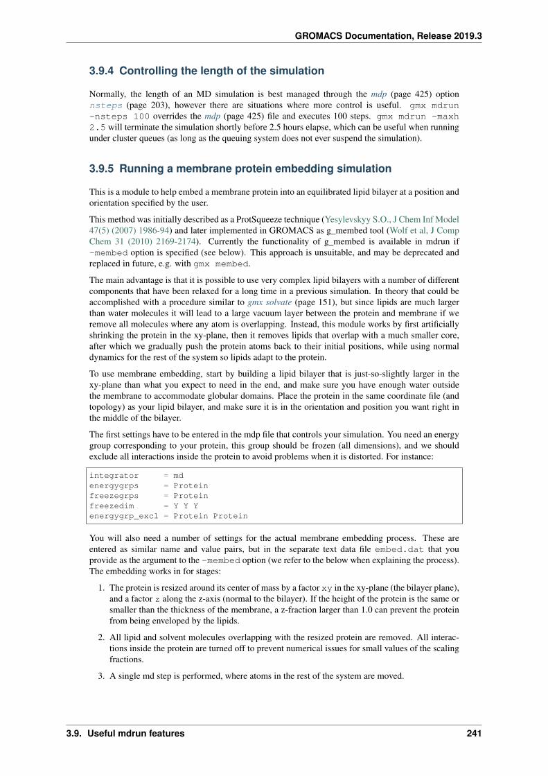
GROMACS Documentation, Release 2019.3
3.9.4 Controlling the length of the simulation
Normally, the length of an MD simulation is best managed through the mdp (page 425) optionnsteps (page 203), however there are situations where more control is useful. gmx mdrun-nsteps 100 overrides the mdp (page 425) file and executes 100 steps. gmx mdrun -maxh2.5 will terminate the simulation shortly before 2.5 hours elapse, which can be useful when runningunder cluster queues (as long as the queuing system does not ever suspend the simulation).
3.9.5 Running a membrane protein embedding simulation
This is a module to help embed a membrane protein into an equilibrated lipid bilayer at a position andorientation specified by the user.
This method was initially described as a ProtSqueeze technique (Yesylevskyy S.O., J Chem Inf Model47(5) (2007) 1986-94) and later implemented in GROMACS as g_membed tool (Wolf et al, J CompChem 31 (2010) 2169-2174). Currently the functionality of g_membed is available in mdrun if-membed option is specified (see below). This approach is unsuitable, and may be deprecated andreplaced in future, e.g. with gmx membed.
The main advantage is that it is possible to use very complex lipid bilayers with a number of differentcomponents that have been relaxed for a long time in a previous simulation. In theory that could beaccomplished with a procedure similar to gmx solvate (page 151), but since lipids are much largerthan water molecules it will lead to a large vacuum layer between the protein and membrane if weremove all molecules where any atom is overlapping. Instead, this module works by first artificiallyshrinking the protein in the xy-plane, then it removes lipids that overlap with a much smaller core,after which we gradually push the protein atoms back to their initial positions, while using normaldynamics for the rest of the system so lipids adapt to the protein.
To use membrane embedding, start by building a lipid bilayer that is just-so-slightly larger in thexy-plane than what you expect to need in the end, and make sure you have enough water outsidethe membrane to accommodate globular domains. Place the protein in the same coordinate file (andtopology) as your lipid bilayer, and make sure it is in the orientation and position you want right inthe middle of the bilayer.
The first settings have to be entered in the mdp file that controls your simulation. You need an energygroup corresponding to your protein, this group should be frozen (all dimensions), and we shouldexclude all interactions inside the protein to avoid problems when it is distorted. For instance:
integrator = mdenergygrps = Proteinfreezegrps = Proteinfreezedim = Y Y Yenergygrp_excl = Protein Protein
You will also need a number of settings for the actual membrane embedding process. These areentered as similar name and value pairs, but in the separate text data file embed.dat that youprovide as the argument to the -membed option (we refer to the below when explaining the process).The embedding works in for stages:
1. The protein is resized around its center of mass by a factor xy in the xy-plane (the bilayer plane),and a factor z along the z-axis (normal to the bilayer). If the height of the protein is the same orsmaller than the thickness of the membrane, a z-fraction larger than 1.0 can prevent the proteinfrom being enveloped by the lipids.
2. All lipid and solvent molecules overlapping with the resized protein are removed. All interac-tions inside the protein are turned off to prevent numerical issues for small values of the scalingfractions.
3. A single md step is performed, where atoms in the rest of the system are moved.
3.9. Useful mdrun features 241
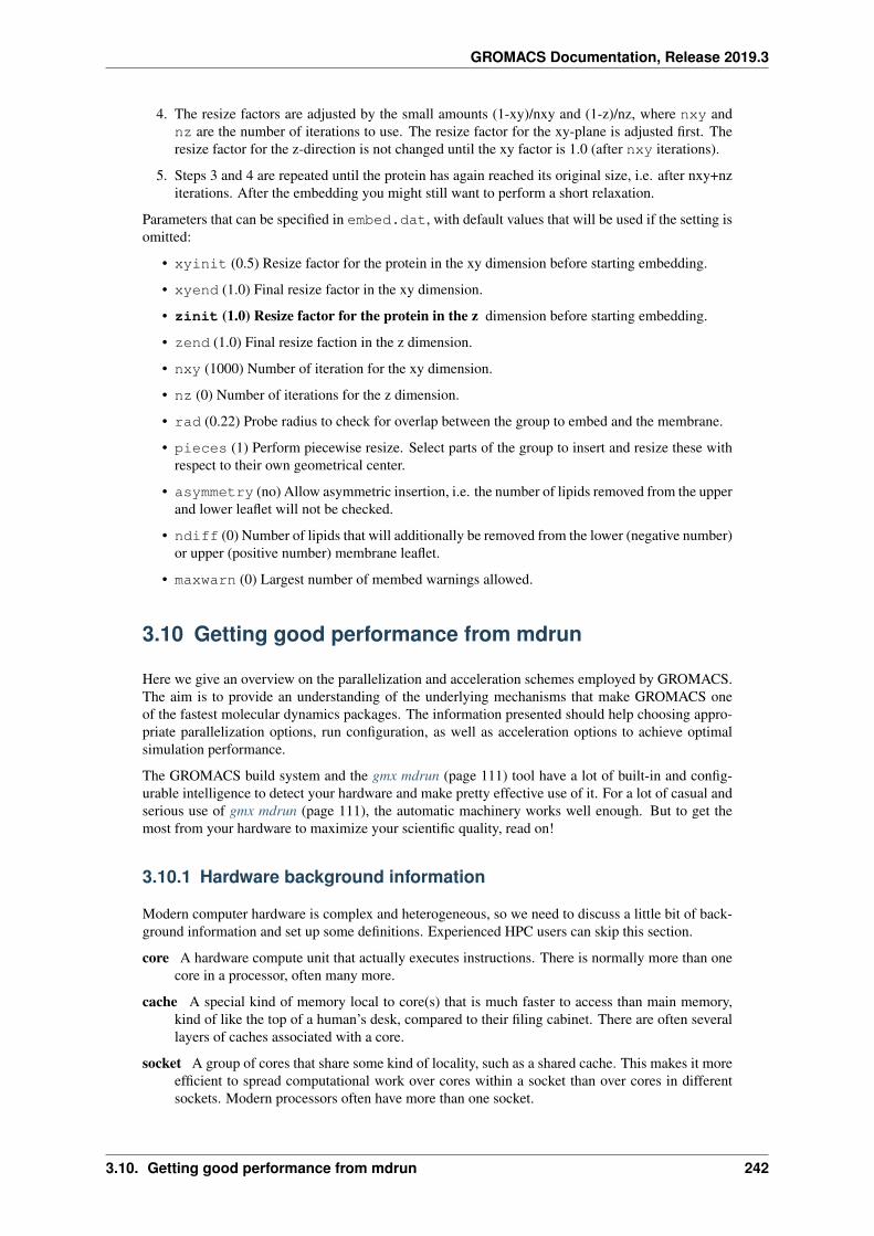
GROMACS Documentation, Release 2019.3
4. The resize factors are adjusted by the small amounts (1-xy)/nxy and (1-z)/nz, where nxy andnz are the number of iterations to use. The resize factor for the xy-plane is adjusted first. Theresize factor for the z-direction is not changed until the xy factor is 1.0 (after nxy iterations).
5. Steps 3 and 4 are repeated until the protein has again reached its original size, i.e. after nxy+nziterations. After the embedding you might still want to perform a short relaxation.
Parameters that can be specified in embed.dat, with default values that will be used if the setting isomitted:
• xyinit (0.5) Resize factor for the protein in the xy dimension before starting embedding.
• xyend (1.0) Final resize factor in the xy dimension.
• zinit (1.0) Resize factor for the protein in the z dimension before starting embedding.
• zend (1.0) Final resize faction in the z dimension.
• nxy (1000) Number of iteration for the xy dimension.
• nz (0) Number of iterations for the z dimension.
• rad (0.22) Probe radius to check for overlap between the group to embed and the membrane.
• pieces (1) Perform piecewise resize. Select parts of the group to insert and resize these withrespect to their own geometrical center.
• asymmetry (no) Allow asymmetric insertion, i.e. the number of lipids removed from the upperand lower leaflet will not be checked.
• ndiff (0) Number of lipids that will additionally be removed from the lower (negative number)or upper (positive number) membrane leaflet.
• maxwarn (0) Largest number of membed warnings allowed.
3.10 Getting good performance from mdrun
Here we give an overview on the parallelization and acceleration schemes employed by GROMACS.The aim is to provide an understanding of the underlying mechanisms that make GROMACS oneof the fastest molecular dynamics packages. The information presented should help choosing appro-priate parallelization options, run configuration, as well as acceleration options to achieve optimalsimulation performance.
The GROMACS build system and the gmx mdrun (page 111) tool have a lot of built-in and config-urable intelligence to detect your hardware and make pretty effective use of it. For a lot of casual andserious use of gmx mdrun (page 111), the automatic machinery works well enough. But to get themost from your hardware to maximize your scientific quality, read on!
3.10.1 Hardware background information
Modern computer hardware is complex and heterogeneous, so we need to discuss a little bit of back-ground information and set up some definitions. Experienced HPC users can skip this section.
core A hardware compute unit that actually executes instructions. There is normally more than onecore in a processor, often many more.
cache A special kind of memory local to core(s) that is much faster to access than main memory,kind of like the top of a human’s desk, compared to their filing cabinet. There are often severallayers of caches associated with a core.
socket A group of cores that share some kind of locality, such as a shared cache. This makes it moreefficient to spread computational work over cores within a socket than over cores in differentsockets. Modern processors often have more than one socket.
3.10. Getting good performance from mdrun 242
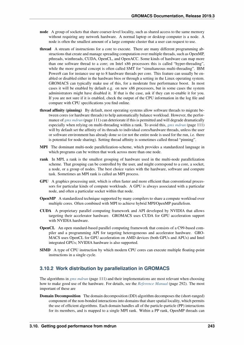
GROMACS Documentation, Release 2019.3
node A group of sockets that share coarser-level locality, such as shared access to the same memorywithout requiring any network hardware. A normal laptop or desktop computer is a node. Anode is often the smallest amount of a large compute cluster that a user can request to use.
thread A stream of instructions for a core to execute. There are many different programming ab-stractions that create and manage spreading computation over multiple threads, such as OpenMP,pthreads, winthreads, CUDA, OpenCL, and OpenACC. Some kinds of hardware can map morethan one software thread to a core; on Intel x86 processors this is called “hyper-threading”,while the more general concept is often called SMT for “simultaneous multi-threading”. IBMPower8 can for instance use up to 8 hardware threads per core. This feature can usually be en-abled or disabled either in the hardware bios or through a setting in the Linux operating system.GROMACS can typically make use of this, for a moderate free performance boost. In mostcases it will be enabled by default e.g. on new x86 processors, but in some cases the systemadministrators might have disabled it. If that is the case, ask if they can re-enable it for you.If you are not sure if it is enabled, check the output of the CPU information in the log file andcompare with CPU specifications you find online.
thread affinity (pinning) By default, most operating systems allow software threads to migrate be-tween cores (or hardware threads) to help automatically balance workload. However, the perfor-mance of gmx mdrun (page 111) can deteriorate if this is permitted and will degrade dramaticallyespecially when relying on multi-threading within a rank. To avoid this, gmx mdrun (page 111)will by default set the affinity of its threads to individual cores/hardware threads, unless the useror software environment has already done so (or not the entire node is used for the run, i.e. thereis potential for node sharing). Setting thread affinity is sometimes called thread “pinning”.
MPI The dominant multi-node parallelization-scheme, which provides a standardized language inwhich programs can be written that work across more than one node.
rank In MPI, a rank is the smallest grouping of hardware used in the multi-node parallelizationscheme. That grouping can be controlled by the user, and might correspond to a core, a socket,a node, or a group of nodes. The best choice varies with the hardware, software and computetask. Sometimes an MPI rank is called an MPI process.
GPU A graphics processing unit, which is often faster and more efficient than conventional proces-sors for particular kinds of compute workloads. A GPU is always associated with a particularnode, and often a particular socket within that node.
OpenMP A standardized technique supported by many compilers to share a compute workload overmultiple cores. Often combined with MPI to achieve hybrid MPI/OpenMP parallelism.
CUDA A proprietary parallel computing framework and API developed by NVIDIA that allowstargeting their accelerator hardware. GROMACS uses CUDA for GPU acceleration supportwith NVIDIA hardware.
OpenCL An open standard-based parallel computing framework that consists of a C99-based com-piler and a programming API for targeting heterogeneous and accelerator hardware. GRO-MACS uses OpenCL for GPU acceleration on AMD devices (both GPUs and APUs) and Intelintegrated GPUs; NVIDIA hardware is also supported.
SIMD A type of CPU instruction by which modern CPU cores can execute multiple floating-pointinstructions in a single cycle.
3.10.2 Work distribution by parallelization in GROMACS
The algorithms in gmx mdrun (page 111) and their implementations are most relevant when choosinghow to make good use of the hardware. For details, see the Reference Manual (page 292). The mostimportant of these are
Domain Decomposition The domain decomposition (DD) algorithm decomposes the (short-ranged)component of the non-bonded interactions into domains that share spatial locality, which permitsthe use of efficient algorithms. Each domain handles all of the particle-particle (PP) interactionsfor its members, and is mapped to a single MPI rank. Within a PP rank, OpenMP threads can
3.10. Getting good performance from mdrun 243
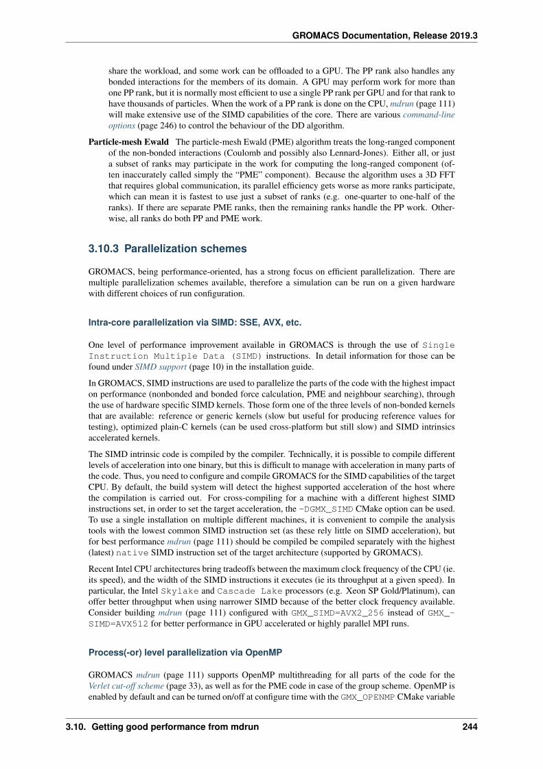
GROMACS Documentation, Release 2019.3
share the workload, and some work can be offloaded to a GPU. The PP rank also handles anybonded interactions for the members of its domain. A GPU may perform work for more thanone PP rank, but it is normally most efficient to use a single PP rank per GPU and for that rank tohave thousands of particles. When the work of a PP rank is done on the CPU, mdrun (page 111)will make extensive use of the SIMD capabilities of the core. There are various command-lineoptions (page 246) to control the behaviour of the DD algorithm.
Particle-mesh Ewald The particle-mesh Ewald (PME) algorithm treats the long-ranged componentof the non-bonded interactions (Coulomb and possibly also Lennard-Jones). Either all, or justa subset of ranks may participate in the work for computing the long-ranged component (of-ten inaccurately called simply the “PME” component). Because the algorithm uses a 3D FFTthat requires global communication, its parallel efficiency gets worse as more ranks participate,which can mean it is fastest to use just a subset of ranks (e.g. one-quarter to one-half of theranks). If there are separate PME ranks, then the remaining ranks handle the PP work. Other-wise, all ranks do both PP and PME work.
3.10.3 Parallelization schemes
GROMACS, being performance-oriented, has a strong focus on efficient parallelization. There aremultiple parallelization schemes available, therefore a simulation can be run on a given hardwarewith different choices of run configuration.
Intra-core parallelization via SIMD: SSE, AVX, etc.
One level of performance improvement available in GROMACS is through the use of SingleInstruction Multiple Data (SIMD) instructions. In detail information for those can befound under SIMD support (page 10) in the installation guide.
In GROMACS, SIMD instructions are used to parallelize the parts of the code with the highest impacton performance (nonbonded and bonded force calculation, PME and neighbour searching), throughthe use of hardware specific SIMD kernels. Those form one of the three levels of non-bonded kernelsthat are available: reference or generic kernels (slow but useful for producing reference values fortesting), optimized plain-C kernels (can be used cross-platform but still slow) and SIMD intrinsicsaccelerated kernels.
The SIMD intrinsic code is compiled by the compiler. Technically, it is possible to compile differentlevels of acceleration into one binary, but this is difficult to manage with acceleration in many parts ofthe code. Thus, you need to configure and compile GROMACS for the SIMD capabilities of the targetCPU. By default, the build system will detect the highest supported acceleration of the host wherethe compilation is carried out. For cross-compiling for a machine with a different highest SIMDinstructions set, in order to set the target acceleration, the -DGMX_SIMD CMake option can be used.To use a single installation on multiple different machines, it is convenient to compile the analysistools with the lowest common SIMD instruction set (as these rely little on SIMD acceleration), butfor best performance mdrun (page 111) should be compiled be compiled separately with the highest(latest) native SIMD instruction set of the target architecture (supported by GROMACS).
Recent Intel CPU architectures bring tradeoffs between the maximum clock frequency of the CPU (ie.its speed), and the width of the SIMD instructions it executes (ie its throughput at a given speed). Inparticular, the Intel Skylake and Cascade Lake processors (e.g. Xeon SP Gold/Platinum), canoffer better throughput when using narrower SIMD because of the better clock frequency available.Consider building mdrun (page 111) configured with GMX_SIMD=AVX2_256 instead of GMX_-SIMD=AVX512 for better performance in GPU accelerated or highly parallel MPI runs.
Process(-or) level parallelization via OpenMP
GROMACS mdrun (page 111) supports OpenMP multithreading for all parts of the code for theVerlet cut-off scheme (page 33), as well as for the PME code in case of the group scheme. OpenMP isenabled by default and can be turned on/off at configure time with the GMX_OPENMP CMake variable
3.10. Getting good performance from mdrun 244
GROMACS Documentation, Release 2019.3
and at run-time with the -ntomp option (or the OMP_NUM_THREADS environment variable). TheOpenMP implementation is quite efficient and scales well for up to 12-24 threads on Intel and 6-8threads on AMD CPUs.
Node level parallelization via GPU offloading and thread-MPI
Multithreading with thread-MPI
The thread-MPI library implements a subset of the MPI 1.1 specification, based on the system thread-ing support. Both POSIX pthreads and Windows threads are supported, thus providing great portabil-ity to most UNIX/Linux and Windows operating systems. Acting as a drop-in replacement for MPI,thread-MPI enables compiling and running mdrun (page 111) on a single machine (i.e. not acrossa network) without MPI. Additionally, it not only provides a convenient way to use computers withmulticore CPU(s), but thread-MPI does in some cases make mdrun (page 111) run slightly faster thanwith MPI.
Thread-MPI is included in the GROMACS source and it is the default parallelization since version4.5, practically rendering the serial mdrun (page 111) deprecated. Compilation with thread-MPI iscontrolled by the GMX_THREAD_MPI CMake variable.
Thread-MPI is compatible with most mdrun (page 111) features and parallelization schemes, includ-ing OpenMP, GPUs; it is not compatible with MPI and multi-simulation runs.
By default, the thread-MPI mdrun will use all available cores in the machine by starting an appropriatenumber of ranks or OpenMP threads to occupy all of them. The number of ranks can be controlledusing the -nt and -ntmpi options. -nt represents the total number of threads to be used (whichcan be a mix of thread-MPI and OpenMP threads with the Verlet scheme (page 33)).
Hybrid/heterogeneous acceleration
Hybrid acceleration means distributing compute work between available CPUs and GPUs to improvesimulation performance. Along the Verlet cut-off scheme (page 33) new non-bonded algorithms havebeen developed with the aim of efficient acceleration both on CPUs and GPUs.
The most compute-intensive parts of simulations, non-bonded force calculation, as well as possiblythe PME and bonded force calculation can be offloaded to GPUs and carried out simultaneously withremaining CPU work. Native GPU acceleration is supported with the Verlet cut-off scheme (page 33)(not with the group scheme) with PME, reaction-field, and plain cut-off electrostatics. For moreinformation about the GPU kernels, please see the Installation guide (page 6).
The native GPU acceleration can be turned on or off, either at run-time using the mdrun (page 111)-nb option, or at configuration time using the GMX_GPU CMake variable.
To efficiently use all compute resource available, CPU and GPU computation is done simultaneously.Overlapping with the OpenMP multithreaded bonded force and PME long-range electrostatic calcu-lations on the CPU, non-bonded forces are calculated on the GPU. Multiple GPUs, both in a singlenode as well as across multiple nodes, are supported using domain-decomposition. A single GPU isassigned to the non-bonded workload of a domain, therefore, the number GPUs used has to matchthe number of of MPI processes (or thread-MPI threads) the simulation is started with. The availableCPU cores are partitioned among the processes (or thread-MPI threads) and a set of cores with a GPUdo the calculations on the respective domain.
With PME electrostatics, mdrun (page 111) supports automated CPU-GPU load-balancing by shiftingworkload from the PME mesh calculations, done on the CPU, to the particle-particle non-bondedcalculations, done on the GPU. At startup a few iterations of tuning are executed during the first 100to 1000 MD steps. These iterations involve scaling the electrostatics cut-off and PME grid spacing todetermine the value that gives optimal CPU-GPU load balance. The cut-off value provided using thercoulomb (page 209) =rvdw mdp (page 425) option represents the minimum electrostatics cut-offthe tuning starts with and therefore should be chosen as small as possible (but still reasonable for thephysics simulated). The Lennard-Jones cut-off rvdw is kept fixed. We don’t allow scaling to shorter
3.10. Getting good performance from mdrun 245
GROMACS Documentation, Release 2019.3
cut-off as we don’t want to change rvdw and there would be no performance gain in the Verlet cut-offscheme.
While the automated CPU-GPU load balancing always attempts to find the optimal cut-off setting, itmight not always be possible to balance CPU and GPU workload. This happens when the CPU threadsfinish calculating the bonded forces and PME faster than the GPU the non-bonded force calculation,even with the shortest possible cut-off. In such cases the CPU will wait for the GPU and this timewill show up as Wait GPU local in the cycle and timing summary table at the end of the log file.
Parallelization over multiple nodes via MPI
At the heart of the MPI parallelization in GROMACS is the neutral-territory domain decomposition(page 243) with dynamic load balancing. To parallelize simulations across multiple machines (e.g.nodes of a cluster) mdrun (page 111) needs to be compiled with MPI which can be enabled using theGMX_MPI CMake variable.
Controlling the domain decomposition algorithm
This section lists options that affect how the domain decomposition algorithm decomposes the work-load to the available parallel hardware.
-rdd Can be used to set the required maximum distance for inter charge-group bonded interactions.Communication for two-body bonded interactions below the non-bonded cut-off distance alwayscomes for free with the non-bonded communication. Particles beyond the non-bonded cut-offare only communicated when they have missing bonded interactions; this means that the extracost is minor and nearly independent of the value of -rdd. With dynamic load balancing,option -rdd also sets the lower limit for the domain decomposition cell sizes. By default -rddis determined by gmx mdrun (page 111) based on the initial coordinates. The chosen value willbe a balance between interaction range and communication cost.
-ddcheck On by default. When inter charge-group bonded interactions are beyond the bondedcut-off distance, gmx mdrun (page 111) terminates with an error message. For pair interactionsand tabulated bonds that do not generate exclusions, this check can be turned off with the option-noddcheck.
-rcon When constraints are present, option -rcon influences the cell size limit as well. Particlesconnected by NC constraints, where NC is the LINCS order plus 1, should not be beyond thesmallest cell size. A error message is generated when this happens, and the user should changethe decomposition or decrease the LINCS order and increase the number of LINCS iterations.By default gmx mdrun (page 111) estimates the minimum cell size required for P-LINCS in aconservative fashion. For high parallelization, it can be useful to set the distance required forP-LINCS with -rcon.
-dds Sets the minimum allowed x, y and/or z scaling of the cells with dynamic load balancing. gmxmdrun (page 111) will ensure that the cells can scale down by at least this factor. This option isused for the automated spatial decomposition (when not using -dd) as well as for determiningthe number of grid pulses, which in turn sets the minimum allowed cell size. Under certaincircumstances the value of -dds might need to be adjusted to account for high or low spatialinhomogeneity of the system.
Multi-level parallelization: MPI and OpenMP
The multi-core trend in CPU development substantiates the need for multi-level parallelization. Cur-rent multiprocessor machines can have 2-4 CPUs with a core count as high as 64. As the memoryand cache subsystem is lagging more and more behind the multicore evolution, this emphasizes non-uniform memory access (NUMA) effects, which can become a performance bottleneck. At the sametime, all cores share a network interface. In a purely MPI-parallel scheme, all MPI processes use the
3.10. Getting good performance from mdrun 246
GROMACS Documentation, Release 2019.3
same network interface, and although MPI intra-node communication is generally efficient, commu-nication between nodes can become a limiting factor to parallelization. This is especially pronouncedin the case of highly parallel simulations with PME (which is very communication intensive) andwith ''fat'' nodes connected by a slow network. Multi-level parallelism aims to address theNUMA and communication related issues by employing efficient intra-node parallelism, typicallymultithreading.
Combining OpenMP with MPI creates an additional overhead especially when running separatemulti-threaded PME nodes. Depending on the architecture, input system size, as well as other fac-tors, MPI+OpenMP runs can be as fast and faster already at small number of processes (e.g. multi-processor Intel Westmere or Sandy Bridge), but can also be considerably slower (e.g. multi-processorAMD Interlagos machines). However, there is a more pronounced benefit of multi-level paralleliza-tion in highly parallel runs.
Separate PME nodes
On CPU nodes, particle-particle (PP) and PME calculations are done in the same process one afteranother. As PME requires all-to-all global communication, this is most of the time the limiting factorto scaling on a large number of cores. By designating a subset of nodes for PME calculations only,performance of parallel runs can be greatly improved.
OpenMP mutithreading in PME nodes is also possible and is supported with both group and Verletcut-off schemes. Using multi-threading in PME can can improve performance at high parallelization.The reason for this is that with N>1 threads the number of processes communicating, and therefore thenumber of messages, is reduced by a factor of N. But note that modern communication networks canprocess several messages simultaneously, such that it could be advantageous to have more processescommunicating.
Separate PME nodes are not used at low parallelization, the switch at higher parallelization happensautomatically (at > 16 processes). The number of PME nodes is estimated by mdrun. If the PMEload is higher than the PP load, mdrun will automatically balance the load, but this leads to additional(non-bonded) calculations. This avoids the idling of a large fraction of the nodes; usually 3/4 of thenodes are PP nodes. But to ensure the best absolute performance of highly parallel runs, it is advisableto tweak this number which is automated by the tune_pme (page 166) tool.
The number of PME nodes can be set manually on the mdrun (page 111) command line using the-npme option, the number of PME threads can be specified on the command line with -ntomp_pmeor alternatively using the GMX_PME_NUM_THREADS environment variable. The latter is especiallyuseful when running on compute nodes with different number of cores as it enables setting differentnumber of PME threads on different nodes.
3.10.4 Running mdrun within a single node
gmx mdrun (page 111) can be configured and compiled in several different ways that are efficient touse within a single node. The default configuration using a suitable compiler will deploy a multi-levelhybrid parallelism that uses CUDA, OpenMP and the threading platform native to the hardware. Forprogramming convenience, in GROMACS, those native threads are used to implement on a singlenode the same MPI scheme as would be used between nodes, but much more efficient; this is calledthread-MPI. From a user’s perspective, real MPI and thread-MPI look almost the same, and GRO-MACS refers to MPI ranks to mean either kind, except where noted. A real external MPI can be usedfor gmx mdrun (page 111) within a single node, but runs more slowly than the thread-MPI version.
By default, gmx mdrun (page 111) will inspect the hardware available at run time and do its best tomake fairly efficient use of the whole node. The log file, stdout and stderr are used to print diagnosticsthat inform the user about the choices made and possible consequences.
A number of command-line parameters are available to modify the default behavior.
3.10. Getting good performance from mdrun 247
GROMACS Documentation, Release 2019.3
-nt The total number of threads to use. The default, 0, will start as many threads as available cores.Whether the threads are thread-MPI ranks, and/or OpenMP threads within such ranks dependson other settings.
-ntmpi The total number of thread-MPI ranks to use. The default, 0, will start one rank per GPU(if present), and otherwise one rank per core.
-ntomp The total number of OpenMP threads per rank to start. The default, 0, will start one threadon each available core. Alternatively, mdrun (page 111) will honor the appropriate systemenvironment variable (e.g. OMP_NUM_THREADS) if set. Note that the maximum number ofOpenMP threads (per rank) is, for efficiency reasons, limited to 64. While it is rarely beneficialto use a number of threads higher than this, the GMX_OPENMP_MAX_THREADS CMakevariable can be used to increase the limit.
-npme The total number of ranks to dedicate to the long-ranged component of PME, if used. Thedefault, -1, will dedicate ranks only if the total number of threads is at least 12, and will usearound a quarter of the ranks for the long-ranged component.
-ntomp_pme When using PME with separate PME ranks, the total number of OpenMP threads perseparate PME rank. The default, 0, copies the value from -ntomp.
-pin Can be set to “auto,” “on” or “off” to control whether mdrun (page 111) will attempt to set theaffinity of threads to cores. Defaults to “auto,” which means that if mdrun (page 111) detectsthat all the cores on the node are being used for mdrun (page 111), then it should behave like“on,” and attempt to set the affinities (unless they are already set by something else).
-pinoffset If -pin on, specifies the logical core number to which mdrun (page 111) shouldpin the first thread. When running more than one instance of mdrun (page 111) on a node, usethis option to to avoid pinning threads from different mdrun (page 111) instances to the samecore.
-pinstride If -pin on, specifies the stride in logical core numbers for the cores to which mdrun(page 111) should pin its threads. When running more than one instance of mdrun (page 111)on a node, use this option to avoid pinning threads from different mdrun (page 111) instances tothe same core. Use the default, 0, to minimize the number of threads per physical core - this letsmdrun (page 111) manage the hardware-, OS- and configuration-specific details of how to maplogical cores to physical cores.
-ddorder Can be set to “interleave,” “pp_pme” or “cartesian.” Defaults to “interleave,” whichmeans that any separate PME ranks will be mapped to MPI ranks in an order like PP, PP, PME,PP, PP, PME, etc. This generally makes the best use of the available hardware. “pp_pme” mapsall PP ranks first, then all PME ranks. “cartesian” is a special-purpose mapping generally usefulonly on special torus networks with accelerated global communication for Cartesian communi-cators. Has no effect if there are no separate PME ranks.
-nb Used to set where to execute the short-range non-bonded interactions. Can be set to “auto”,“cpu”, “gpu.” Defaults to “auto,” which uses a compatible GPU if available. Setting “cpu”requires that no GPU is used. Setting “gpu” requires that a compatible GPU is available andwill be used.
-pme Used to set where to execute the long-range non-bonded interactions. Can be set to “auto”,“cpu”, “gpu.” Defaults to “auto,” which uses a compatible GPU if available. Setting “gpu”requires that a compatible GPU is available and will be used. Multiple PME ranks are notsupported with PME on GPU, so if a GPU is used for the PME calculation -npme must be set to1.
-bonded Used to set where to execute the bonded interactions that are part of the PP workload for adomain. Can be set to “auto”, “cpu”, “gpu.” Defaults to “auto,” which uses a compatible CUDAGPU only when one is available, a GPU is handling short-ranged interactions, and the CPU ishandling long-ranged interaction work (electrostatic or LJ). The work for the bonded interac-tions takes place on the same GPU as the short-ranged interactions, and cannot be independentlyassigned. Setting “gpu” requires that a compatible GPU is available and will be used.
3.10. Getting good performance from mdrun 248
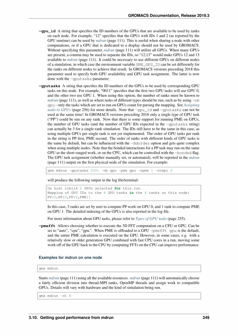
GROMACS Documentation, Release 2019.3
-gpu_id A string that specifies the ID numbers of the GPUs that are available to be used by rankson each node. For example, “12” specifies that the GPUs with IDs 1 and 2 (as reported by theGPU runtime) can be used by mdrun (page 111). This is useful when sharing a node with othercomputations, or if a GPU that is dedicated to a display should not be used by GROMACS.Without specifying this parameter, mdrun (page 111) will utilize all GPUs. When many GPUsare present, a comma may be used to separate the IDs, so “12,13” would make GPUs 12 and 13available to mdrun (page 111). It could be necessary to use different GPUs on different nodesof a simulation, in which case the environment variable GMX_GPU_ID can be set differently forthe ranks on different nodes to achieve that result. In GROMACS versions preceding 2018 thisparameter used to specify both GPU availability and GPU task assignment. The latter is nowdone with the -gputasks parameter.
-gputasks A string that specifies the ID numbers of the GPUs to be used by corresponding GPUtasks on this node. For example, “0011” specifies that the first two GPU tasks will use GPU 0,and the other two use GPU 1. When using this option, the number of ranks must be known tomdrun (page 111), as well as where tasks of different types should be run, such as by using -nbgpu - only the tasks which are set to run on GPUs count for parsing the mapping. See Assigningtasks to GPUs (page 256) for more details. Note that -gpu_id and -gputasks can not beused at the same time! In GROMACS versions preceding 2018 only a single type of GPU task(“PP”) could be run on any rank. Now that there is some support for running PME on GPUs,the number of GPU tasks (and the number of GPU IDs expected in the -gputasks string)can actually be 3 for a single-rank simulation. The IDs still have to be the same in this case, asusing multiple GPUs per single rank is not yet implemented. The order of GPU tasks per rankin the string is PP first, PME second. The order of ranks with different kinds of GPU tasks isthe same by default, but can be influenced with the -ddorder option and gets quite complexwhen using multiple nodes. Note that the bonded interactions for a PP task may run on the sameGPU as the short-ranged work, or on the CPU, which can be controlled with the -bonded flag.The GPU task assignment (whether manually set, or automated), will be reported in the mdrun(page 111) output on the first physical node of the simulation. For example:
gmx mdrun -gputasks 0001 -nb gpu -pme gpu -npme 1 -ntmpi 4
will produce the following output in the log file/terminal:
On host tcbl14 2 GPUs selected for this run.Mapping of GPU IDs to the 4 GPU tasks in the 4 ranks on this node:PP:0,PP:0,PP:0,PME:1
In this case, 3 ranks are set by user to compute PP work on GPU 0, and 1 rank to compute PMEon GPU 1. The detailed indexing of the GPUs is also reported in the log file.
For more information about GPU tasks, please refer to Types of GPU tasks (page 255).
-pmefft Allows choosing whether to execute the 3D FFT computation on a CPU or GPU. Can beset to “auto”, “cpu”, “gpu.”. When PME is offloaded to a GPU -pmefft gpu is the default,and the entire PME calculation is executed on the GPU. However, in some cases, e.g. with arelatively slow or older generation GPU combined with fast CPU cores in a run, moving somework off of the GPU back to the CPU by computing FFTs on the CPU can improve performance.
Examples for mdrun on one node
gmx mdrun
Starts mdrun (page 111) using all the available resources. mdrun (page 111) will automatically choosea fairly efficient division into thread-MPI ranks, OpenMP threads and assign work to compatibleGPUs. Details will vary with hardware and the kind of simulation being run.
gmx mdrun -nt 8
3.10. Getting good performance from mdrun 249
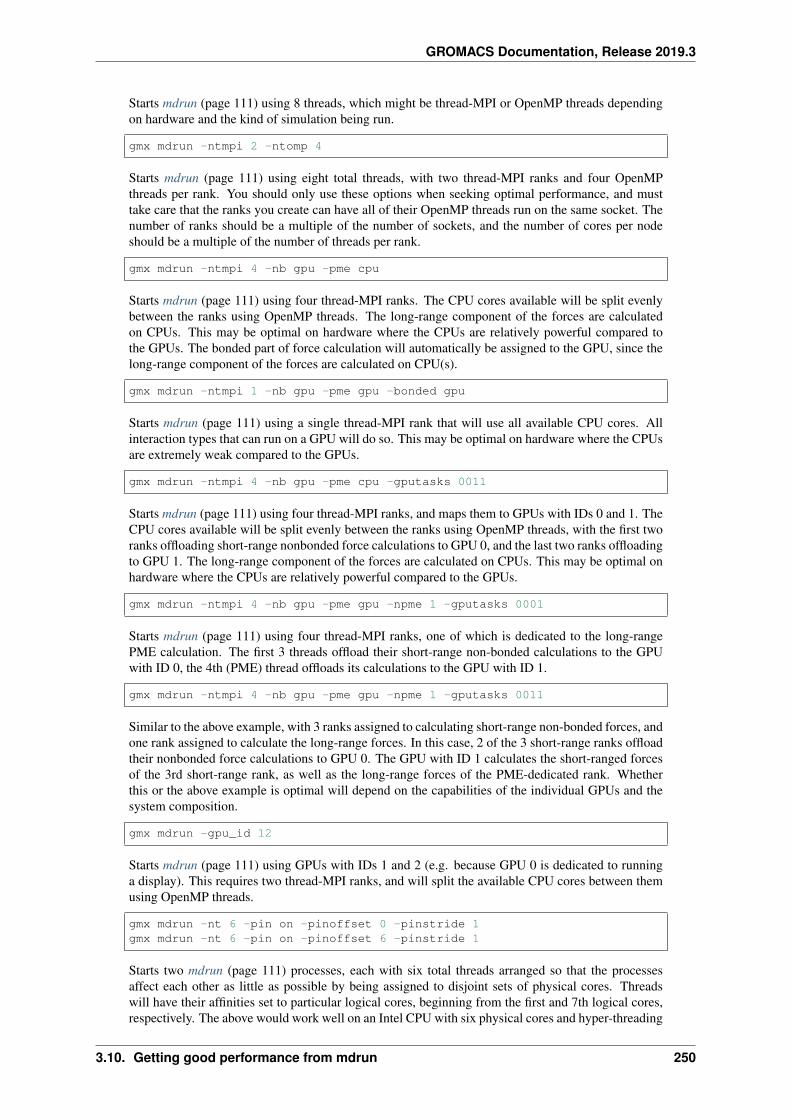
GROMACS Documentation, Release 2019.3
Starts mdrun (page 111) using 8 threads, which might be thread-MPI or OpenMP threads dependingon hardware and the kind of simulation being run.
gmx mdrun -ntmpi 2 -ntomp 4
Starts mdrun (page 111) using eight total threads, with two thread-MPI ranks and four OpenMPthreads per rank. You should only use these options when seeking optimal performance, and musttake care that the ranks you create can have all of their OpenMP threads run on the same socket. Thenumber of ranks should be a multiple of the number of sockets, and the number of cores per nodeshould be a multiple of the number of threads per rank.
gmx mdrun -ntmpi 4 -nb gpu -pme cpu
Starts mdrun (page 111) using four thread-MPI ranks. The CPU cores available will be split evenlybetween the ranks using OpenMP threads. The long-range component of the forces are calculatedon CPUs. This may be optimal on hardware where the CPUs are relatively powerful compared tothe GPUs. The bonded part of force calculation will automatically be assigned to the GPU, since thelong-range component of the forces are calculated on CPU(s).
gmx mdrun -ntmpi 1 -nb gpu -pme gpu -bonded gpu
Starts mdrun (page 111) using a single thread-MPI rank that will use all available CPU cores. Allinteraction types that can run on a GPU will do so. This may be optimal on hardware where the CPUsare extremely weak compared to the GPUs.
gmx mdrun -ntmpi 4 -nb gpu -pme cpu -gputasks 0011
Starts mdrun (page 111) using four thread-MPI ranks, and maps them to GPUs with IDs 0 and 1. TheCPU cores available will be split evenly between the ranks using OpenMP threads, with the first tworanks offloading short-range nonbonded force calculations to GPU 0, and the last two ranks offloadingto GPU 1. The long-range component of the forces are calculated on CPUs. This may be optimal onhardware where the CPUs are relatively powerful compared to the GPUs.
gmx mdrun -ntmpi 4 -nb gpu -pme gpu -npme 1 -gputasks 0001
Starts mdrun (page 111) using four thread-MPI ranks, one of which is dedicated to the long-rangePME calculation. The first 3 threads offload their short-range non-bonded calculations to the GPUwith ID 0, the 4th (PME) thread offloads its calculations to the GPU with ID 1.
gmx mdrun -ntmpi 4 -nb gpu -pme gpu -npme 1 -gputasks 0011
Similar to the above example, with 3 ranks assigned to calculating short-range non-bonded forces, andone rank assigned to calculate the long-range forces. In this case, 2 of the 3 short-range ranks offloadtheir nonbonded force calculations to GPU 0. The GPU with ID 1 calculates the short-ranged forcesof the 3rd short-range rank, as well as the long-range forces of the PME-dedicated rank. Whetherthis or the above example is optimal will depend on the capabilities of the individual GPUs and thesystem composition.
gmx mdrun -gpu_id 12
Starts mdrun (page 111) using GPUs with IDs 1 and 2 (e.g. because GPU 0 is dedicated to runninga display). This requires two thread-MPI ranks, and will split the available CPU cores between themusing OpenMP threads.
gmx mdrun -nt 6 -pin on -pinoffset 0 -pinstride 1gmx mdrun -nt 6 -pin on -pinoffset 6 -pinstride 1
Starts two mdrun (page 111) processes, each with six total threads arranged so that the processesaffect each other as little as possible by being assigned to disjoint sets of physical cores. Threadswill have their affinities set to particular logical cores, beginning from the first and 7th logical cores,respectively. The above would work well on an Intel CPU with six physical cores and hyper-threading
3.10. Getting good performance from mdrun 250
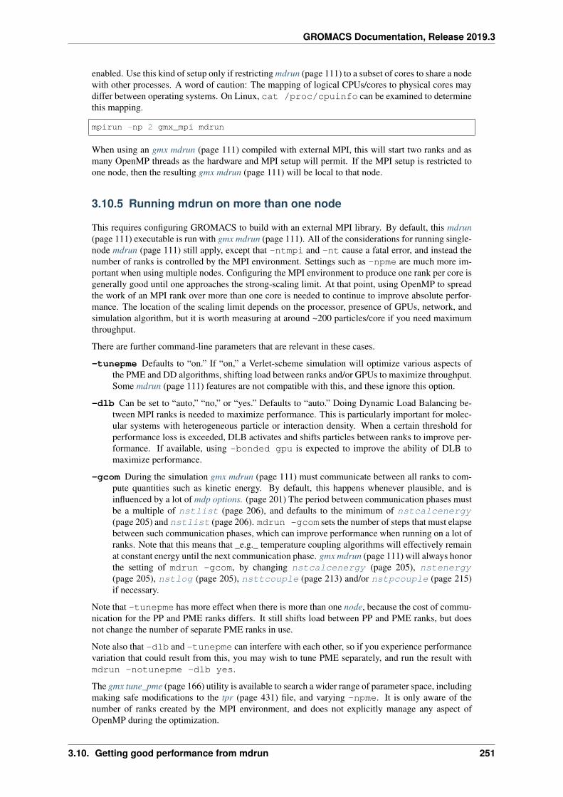
GROMACS Documentation, Release 2019.3
enabled. Use this kind of setup only if restricting mdrun (page 111) to a subset of cores to share a nodewith other processes. A word of caution: The mapping of logical CPUs/cores to physical cores maydiffer between operating systems. On Linux, cat /proc/cpuinfo can be examined to determinethis mapping.
mpirun -np 2 gmx_mpi mdrun
When using an gmx mdrun (page 111) compiled with external MPI, this will start two ranks and asmany OpenMP threads as the hardware and MPI setup will permit. If the MPI setup is restricted toone node, then the resulting gmx mdrun (page 111) will be local to that node.
3.10.5 Running mdrun on more than one node
This requires configuring GROMACS to build with an external MPI library. By default, this mdrun(page 111) executable is run with gmx mdrun (page 111). All of the considerations for running single-node mdrun (page 111) still apply, except that -ntmpi and -nt cause a fatal error, and instead thenumber of ranks is controlled by the MPI environment. Settings such as -npme are much more im-portant when using multiple nodes. Configuring the MPI environment to produce one rank per core isgenerally good until one approaches the strong-scaling limit. At that point, using OpenMP to spreadthe work of an MPI rank over more than one core is needed to continue to improve absolute perfor-mance. The location of the scaling limit depends on the processor, presence of GPUs, network, andsimulation algorithm, but it is worth measuring at around ~200 particles/core if you need maximumthroughput.
There are further command-line parameters that are relevant in these cases.
-tunepme Defaults to “on.” If “on,” a Verlet-scheme simulation will optimize various aspects ofthe PME and DD algorithms, shifting load between ranks and/or GPUs to maximize throughput.Some mdrun (page 111) features are not compatible with this, and these ignore this option.
-dlb Can be set to “auto,” “no,” or “yes.” Defaults to “auto.” Doing Dynamic Load Balancing be-tween MPI ranks is needed to maximize performance. This is particularly important for molec-ular systems with heterogeneous particle or interaction density. When a certain threshold forperformance loss is exceeded, DLB activates and shifts particles between ranks to improve per-formance. If available, using -bonded gpu is expected to improve the ability of DLB tomaximize performance.
-gcom During the simulation gmx mdrun (page 111) must communicate between all ranks to com-pute quantities such as kinetic energy. By default, this happens whenever plausible, and isinfluenced by a lot of mdp options. (page 201) The period between communication phases mustbe a multiple of nstlist (page 206), and defaults to the minimum of nstcalcenergy(page 205) and nstlist (page 206). mdrun -gcom sets the number of steps that must elapsebetween such communication phases, which can improve performance when running on a lot ofranks. Note that this means that _e.g._ temperature coupling algorithms will effectively remainat constant energy until the next communication phase. gmx mdrun (page 111) will always honorthe setting of mdrun -gcom, by changing nstcalcenergy (page 205), nstenergy(page 205), nstlog (page 205), nsttcouple (page 213) and/or nstpcouple (page 215)if necessary.
Note that -tunepme has more effect when there is more than one node, because the cost of commu-nication for the PP and PME ranks differs. It still shifts load between PP and PME ranks, but doesnot change the number of separate PME ranks in use.
Note also that -dlb and -tunepme can interfere with each other, so if you experience performancevariation that could result from this, you may wish to tune PME separately, and run the result withmdrun -notunepme -dlb yes.
The gmx tune_pme (page 166) utility is available to search a wider range of parameter space, includingmaking safe modifications to the tpr (page 431) file, and varying -npme. It is only aware of thenumber of ranks created by the MPI environment, and does not explicitly manage any aspect ofOpenMP during the optimization.
3.10. Getting good performance from mdrun 251
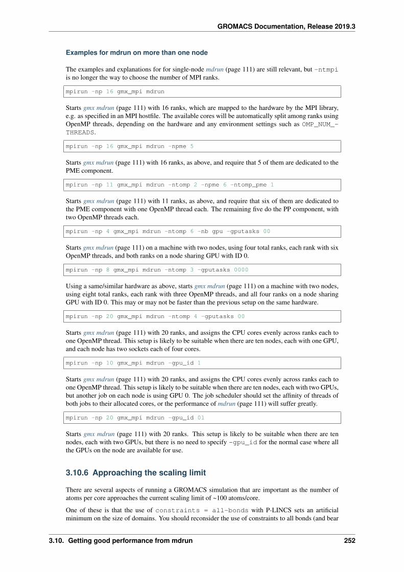
GROMACS Documentation, Release 2019.3
Examples for mdrun on more than one node
The examples and explanations for for single-node mdrun (page 111) are still relevant, but -ntmpiis no longer the way to choose the number of MPI ranks.
mpirun -np 16 gmx_mpi mdrun
Starts gmx mdrun (page 111) with 16 ranks, which are mapped to the hardware by the MPI library,e.g. as specified in an MPI hostfile. The available cores will be automatically split among ranks usingOpenMP threads, depending on the hardware and any environment settings such as OMP_NUM_-THREADS.
mpirun -np 16 gmx_mpi mdrun -npme 5
Starts gmx mdrun (page 111) with 16 ranks, as above, and require that 5 of them are dedicated to thePME component.
mpirun -np 11 gmx_mpi mdrun -ntomp 2 -npme 6 -ntomp_pme 1
Starts gmx mdrun (page 111) with 11 ranks, as above, and require that six of them are dedicated tothe PME component with one OpenMP thread each. The remaining five do the PP component, withtwo OpenMP threads each.
mpirun -np 4 gmx_mpi mdrun -ntomp 6 -nb gpu -gputasks 00
Starts gmx mdrun (page 111) on a machine with two nodes, using four total ranks, each rank with sixOpenMP threads, and both ranks on a node sharing GPU with ID 0.
mpirun -np 8 gmx_mpi mdrun -ntomp 3 -gputasks 0000
Using a same/similar hardware as above, starts gmx mdrun (page 111) on a machine with two nodes,using eight total ranks, each rank with three OpenMP threads, and all four ranks on a node sharingGPU with ID 0. This may or may not be faster than the previous setup on the same hardware.
mpirun -np 20 gmx_mpi mdrun -ntomp 4 -gputasks 00
Starts gmx mdrun (page 111) with 20 ranks, and assigns the CPU cores evenly across ranks each toone OpenMP thread. This setup is likely to be suitable when there are ten nodes, each with one GPU,and each node has two sockets each of four cores.
mpirun -np 10 gmx_mpi mdrun -gpu_id 1
Starts gmx mdrun (page 111) with 20 ranks, and assigns the CPU cores evenly across ranks each toone OpenMP thread. This setup is likely to be suitable when there are ten nodes, each with two GPUs,but another job on each node is using GPU 0. The job scheduler should set the affinity of threads ofboth jobs to their allocated cores, or the performance of mdrun (page 111) will suffer greatly.
mpirun -np 20 gmx_mpi mdrun -gpu_id 01
Starts gmx mdrun (page 111) with 20 ranks. This setup is likely to be suitable when there are tennodes, each with two GPUs, but there is no need to specify -gpu_id for the normal case where allthe GPUs on the node are available for use.
3.10.6 Approaching the scaling limit
There are several aspects of running a GROMACS simulation that are important as the number ofatoms per core approaches the current scaling limit of ~100 atoms/core.
One of these is that the use of constraints = all-bonds with P-LINCS sets an artificialminimum on the size of domains. You should reconsider the use of constraints to all bonds (and bear
3.10. Getting good performance from mdrun 252

GROMACS Documentation, Release 2019.3
in mind possible consequences on the safe maximum for dt), or change lincs_order and lincs_itersuitably.
3.10.7 Finding out how to run mdrun better
The Wallcycle module is used for runtime performance measurement of gmx mdrun (page 111). Atthe end of the log file of each run, the “Real cycle and time accounting” section provides a tablewith runtime statistics for different parts of the gmx mdrun (page 111) code in rows of the table. Thetable contains colums indicating the number of ranks and threads that executed the respective part ofthe run, wall-time and cycle count aggregates (across all threads and ranks) averaged over the entirerun. The last column also shows what precentage of the total runtime each row represents. Notethat the gmx mdrun (page 111) timer resetting functionalities (-resethway and -resetstep) reset theperformance counters and therefore are useful to avoid startup overhead and performance instability(e.g. due to load balancing) at the beginning of the run.
The performance counters are:
• Particle-particle during Particle mesh Ewald
• Domain decomposition
• Domain decomposition communication load
• Domain decomposition communication bounds
• Virtual site constraints
• Send X to Particle mesh Ewald
• Neighbor search
• Launch GPU operations
• Communication of coordinates
• Force
• Waiting + Communication of force
• Particle mesh Ewald
• PME redist. X/F
• PME spread
• PME gather
• PME 3D-FFT
• PME 3D-FFT Communication
• PME solve Lennard-Jones
• PME solve LJ
• PME solve Elec
• PME wait for particle-particle
• Wait + Receive PME force
• Wait GPU nonlocal
• Wait GPU local
• Wait PME GPU spread
• Wait PME GPU gather
• Reduce PME GPU Force
• Non-bonded position/force buffer operations
3.10. Getting good performance from mdrun 253

GROMACS Documentation, Release 2019.3
• Virtual site spread
• COM pull force
• AWH (accelerated weight histogram method)
• Write trajectory
• Update
• Constraints
• Communication of energies
• Enforced rotation
• Add rotational forces
• Position swapping
• Interactive MD
As performance data is collected for every run, they are essential to assessing and tuning the per-formance of gmx mdrun (page 111) performance. Therefore, they benefit both code developers aswell as users of the program. The counters are an average of the time/cycles different parts of thesimulation take, hence can not directly reveal fluctuations during a single run (although comparisonsacross multiple runs are still very useful).
Counters will appear in an MD log file only if the related parts of the code were executed during thegmx mdrun (page 111) run. There is also a special counter called “Rest” which indicates the amountof time not accounted for by any of the counters above. Therefore, a significant amount “Rest” time(more than a few percent) will often be an indication of parallelization inefficiency (e.g. serial code)and it is recommended to be reported to the developers.
An additional set of subcounters can offer more fine-grained inspection of performance. They are:
• Domain decomposition redistribution
• DD neighbor search grid + sort
• DD setup communication
• DD make topology
• DD make constraints
• DD topology other
• Neighbor search grid local
• NS grid non-local
• NS search local
• NS search non-local
• Bonded force
• Bonded-FEP force
• Restraints force
• Listed buffer operations
• Nonbonded pruning
• Nonbonded force
• Launch non-bonded GPU tasks
• Launch PME GPU tasks
• Ewald force correction
• Non-bonded position buffer operations
3.10. Getting good performance from mdrun 254
GROMACS Documentation, Release 2019.3
• Non-bonded force buffer operations
Subcounters are geared toward developers and have to be enabled during compilation. See Buildsystem overview (page 521) for more information.
3.10.8 Running mdrun with GPUs
Types of GPU tasks
To better understand the later sections on different GPU use cases for calculation of short range(page 255) and PME (page 255), we first introduce the concept of different GPU tasks. When think-ing about running a simulation, several different kinds of interactions between the atoms have to becalculated (for more information please refer to the reference manual). The calculation can thus besplit into several distinct parts that are largely independent of each other (hence can be calculated inany order, e.g. sequentially or concurrently), with the information from each of them combined at theend of time step to obtain the final forces on each atom and to propagate the system to the next timepoint. For a better understanding also please see the section on domain decomposition (page 243).
Of all calculations required for an MD step, GROMACS aims to optimize performance bottom-up foreach step from the lowest level (SIMD unit, cores, sockets, accelerators, etc.). Therefore many of theindividual computation units are highly tuned for the lowest level of hardware parallelism: the SIMDunits. Additionally, with GPU accelerators used as co-processors, some of the work can be offloaded,that is calculated simultaneously/concurrently with the CPU on the accelerator device, with the resultbeing communicated to the CPU. Right now, GROMACS supports GPU accelerator offload of twotasks: the short-range nonbonded interactions in real space (page 255), and PME (page 255).
Please note that the solving of PME on GPU is still only the initial version supporting thisbehaviour, and comes with a set of limitations outlined further below.
Right now, we generally support short-range nonbonded offload with and without dynamic pruningon a wide range of GPU accelerators (both NVIDIA and AMD). This is compatible with the grandmajority of the features and parallelization modes and can be used to scale to large machines.
Simultaneously offloading both short-range nonbonded and long-range PME work to GPU accelera-tors is a new feature that that has some restrictions in terms of feature and parallelization compatibility(please see the section below (page 255)).
GPU computation of short range nonbonded interactions
Using the GPU for the short-ranged nonbonded interactions provides the majority of the availablespeed-up compared to run using only the CPU. Here, the GPU acts as an accelerator that can effec-tively parallelize this problem and thus reduce the calculation time.
GPU accelerated calculation of PME
GROMACS now allows the offloading of the PME calculation to the GPU, to further reduce the loadon the CPU and improve usage overlap between CPU and GPU. Here, the solving of PME will beperformed in addition to the calculation of the short range interactions on the same GPU as the shortrange interactions.
Known limitations
Please note again the limitations outlined below!
• Only compilation with CUDA is supported.
• Only a PME order of 4 is supported on GPUs.
3.10. Getting good performance from mdrun 255
GROMACS Documentation, Release 2019.3
• PME will run on a GPU only when exactly one rank has a PME task, ie. decompositions withmultiple ranks doing PME are not supported.
• Only single precision is supported.
• Free energy calculations where charges are perturbed are not supported, because only singlePME grids can be calculated.
• Only dynamical integrators are supported (ie. leap-frog, Velocity Verlet, stochastic dynamics)
• LJ PME is not supported on GPUs.
GPU accelerated calculation of bonded interactions (CUDA only)
GROMACS now allows the offloading of the bonded part of the PP workload to a CUDA-compatibleGPU. This is treated as part of the PP work, and requires that the short-ranged non-bonded task alsoruns on a GPU. It is an advantage usually only when the CPU is relatively weak compared with theGPU, perhaps because its workload is too large for the available cores. This would likely be the casefor free-energy calculations.
Assigning tasks to GPUs
Depending on which tasks should be performed on which hardware, different kinds of calculationscan be combined on the same or different GPUs, according to the information provided for runningmdrun (page 111).
It is possible to assign the calculation of the different computational tasks to the same GPU, meaningthat they will share the computational resources on the same device, or to different processing unitsthat will each perform one task each.
One overview over the possible task assignments is given below:
GROMACS version 2018:
Two different types of assignable GPU accelerated tasks are available, NB and PME. EachPP rank has a NB task that can be offloaded to a GPU. If there is only one rank with aPME task (including if that rank is a PME-only rank), then that task can be offloaded to aGPU. Such a PME task can run wholly on the GPU, or have its latter stages run only onthe CPU.
Limitations are that PME on GPU does not support PME domain decomposition, so thatonly one PME task can be offloaded to a single GPU assigned to a separate PME rank,while NB can be decomposed and offloaded to multiple GPUs.
GROMACS version 2019:
No new assignable GPU tasks are available, but any bonded interactions may run on thesame GPU as the short-ranged interactions for a PP task. This can be influenced with the-bonded flag.
Performance considerations for GPU tasks
1. The performance balance depends on the speed and number of CPU cores you have vs the speedand number of GPUs you have.
2. With slow/old GPUs and/or fast/modern CPUs with many cores, it might make more sense tolet the CPU do PME calculation, with the GPUs focused on the calculation of the NB.
3. With fast/modern GPUs and/or slow/old CPUs with few cores, it generally helps to have theGPU do PME.
3.10. Getting good performance from mdrun 256
GROMACS Documentation, Release 2019.3
4. Offloading bonded work to a GPU will often not improve simulation performance as efficientCPU-based kernels can complete the bonded computation before the GPU is done with otheroffloaded work. Therefore, gmx mdrun will default to no bonded offload when PME is offloaded.Typical cases where performance can be improvement with bonded offload are: with significantbonded work (e.g. pure lipid or mostly polymer systems with little solvent), with very fewand/or slow CPU cores per GPU, or when the CPU does other computation (e.g. PME, freeenergy).
5. It is possible to use multiple GPUs with PME offload by letting e.g. 3 MPI ranks use one GPUeach for short-range interactions, while a fourth rank does the PME on its GPU.
6. The only way to know for sure what alternative is best for your machine is to test and checkperformance.
Reducing overheads in GPU accelerated runs
In order for CPU cores and GPU(s) to execute concurrently, tasks are launched and executed asyn-chronously on the GPU(s) while the CPU cores execute non-offloaded force computation (like long-range PME electrostatics). Asynchronous task launches are handled by GPU device driver and requireCPU involvement. Therefore, the work of scheduling GPU tasks will incur an overhead that can insome cases significantly delay or interfere with the CPU execution.
Delays in CPU execution are caused by the latency of launching GPU tasks, an overhead that canbecome significant as simulation ns/day increases (i.e. with shorter wall-time per step). The overheadis measured by gmx mdrun (page 111) and reported in the performance summary section of the logfile (“Launch GPU ops” row). A few percent of runtime spent in this category is normal, but in fast-iterating and multi-GPU parallel runs 10% or larger overheads can be observed. In general, a usercan do little to avoid such overheads, but there are a few cases where tweaks can give performancebenefits. In single-rank runs timing of GPU tasks is by default enabled and, while in most casesits impact is small, in fast runs performance can be affected. The performance impact will be mostsignificant on NVIDIA GPUs with CUDA, less on AMD and Intel with OpenCL. In these cases,when more than a few percent of “Launch GPU ops” time is observed, it is recommended to turnoff timing by setting the GMX_DISABLE_GPU_TIMING environment variable. In parallel runs withmany ranks sharing a GPU, launch overheads can also be reduced by starting fewer thread-MPI orMPI ranks per GPU; e.g. most often one rank per thread or core is not optimal.
The second type of overhead, interference of the GPU driver with CPU computation, is caused bythe scheduling and coordination of GPU tasks. A separate GPU driver thread can require CPU re-sources which may clash with the concurrently running non-offloaded tasks, potentially degradingthe performance of PME or bonded force computation. This effect is most pronounced when usingAMD GPUs with OpenCL with older driver releases (e.g. fglrx 12.15). To minimize the overheadit is recommended to leave a CPU hardware thread unused when launching gmx mdrun (page 111),especially on CPUs with high core counts and/or HyperThreading enabled. E.g. on a machine with a4-core CPU and eight threads (via HyperThreading) and an AMD GPU, try gmx mdrun -ntomp7 -pin on. This will leave free CPU resources for the GPU task scheduling reducing interferencewith CPU computation. Note that assigning fewer resources to gmx mdrun (page 111) CPU com-putation involves a tradeoff which may outweigh the benefits of reduced GPU driver overhead, inparticular without HyperThreading and with few CPU cores.
3.10.9 Running the OpenCL version of mdrun
Currently supported hardware architectures are: - GCN-based AMD GPUs; - NVIDIA GPUs (withat least OpenCL 1.2 support); - Intel iGPUs. Make sure that you have the latest drivers installed. ForAMD GPUs, the compute-oriented ROCm stack is recommended; alternatively, the AMDGPU-PROstack is also compatible; using the outdated and unsupported fglrx proprietary driver and runtime isnot recommended (but for certain older hardware that may be the only way to obtain support). Inaddition Mesa version 17.0 or newer with LLVM 4.0 or newer is also supported. For NVIDIA GPUs,using the proprietary driver is required as the open source nouveau driver (available in Mesa) doesnot provide the OpenCL support. For Intel integrated GPUs, the Neo driver is recommended. TODO:
3.10. Getting good performance from mdrun 257
GROMACS Documentation, Release 2019.3
add more Intel driver recommendations The minimum OpenCL version required is 1.2. See also theknown limitations (page 258).
Devices from the AMD GCN architectures (all series) are compatible and regularly tested; NVIDIAKepler and later (compute capability 3.0) are known to work, but before doing production runs alwaysmake sure that the GROMACS tests pass successfully on the hardware.
The OpenCL GPU kernels are compiled at run time. Hence, building the OpenCL program can takea few seconds, introducing a slight delay in the gmx mdrun (page 111) startup. This is not normally aproblem for long production MD, but you might prefer to do some kinds of work, e.g. that runs veryfew steps, on just the CPU (e.g. see -nb above).
The same -gpu_id option (or GMX_GPU_ID environment variable) used to select CUDA devices,or to define a mapping of GPUs to PP ranks, is used for OpenCL devices.
Some other OpenCL management (page 279) environment variables may be of interest to developers.
Known limitations of the OpenCL support
Limitations in the current OpenCL support of interest to GROMACS users:
• Intel integrated GPUs are supported. Intel CPUs and Xeon Phi are not supported.
• Due to blocking behavior of some asynchronous task enqueuing functions in the NVIDIAOpenCL runtime, with the affected driver versions there is almost no performance gain whenusing NVIDIA GPUs. The issue affects NVIDIA driver versions up to 349 series, but it knownto be fixed 352 and later driver releases.
• On NVIDIA GPUs the OpenCL kernels achieve much lower performance than the equivalentCUDA kernels due to limitations of the NVIDIA OpenCL compiler.
• PME is currently only supported on AMD devices, because of known issues with devices fromother vendors
Limitations of interest to GROMACS developers:
• The current implementation is not compatible with OpenCL devices that are not usingwarp/wavefronts or for which the warp/wavefront size is not a multiple of 32
3.10.10 Performance checklist
There are many different aspects that affect the performance of simulations in GROMACS. Mostsimulations require a lot of computational resources, therefore it can be worthwhile to optimize the useof those resources. Several issues mentioned in the list below could lead to a performance differenceof a factor of 2. So it can be useful go through the checklist.
GROMACS configuration
• Don’t use double precision unless you’re absolute sure you need it.
• Compile the FFTW library (yourself) with the correct flags on x86 (in most cases, the correctflags are automatically configured).
• On x86, use gcc or icc as the compiler (not pgi or the Cray compiler).
• On POWER, use gcc instead of IBM’s xlc.
• Use a new compiler version, especially for gcc (e.g. from version 5 to 6 the performance of thecompiled code improved a lot).
• MPI library: OpenMPI usually has good performance and causes little trouble.
• Make sure your compiler supports OpenMP (some versions of Clang don’t).
3.10. Getting good performance from mdrun 258
GROMACS Documentation, Release 2019.3
• If you have GPUs that support either CUDA or OpenCL, use them.
– Configure with -DGMX_GPU=ON (add -DGMX_USE_OPENCL=ON for OpenCL).
– For CUDA, use the newest CUDA available for your GPU to take advantage of the latestperformance enhancements.
– Use a recent GPU driver.
– Make sure you use an gmx mdrun (page 111) with GMX_SIMD appropriate for the CPUarchitecture; the log file will contain a warning note if suboptimal setting is used. However,prefer AVX2` over ``AVX512 in GPU or highly parallel MPI runs (for more informa-tion see the intra-core parallelization information (page 244)).
– If compiling on a cluster head node, make sure that GMX_SIMD is appropriate for thecompute nodes.
Run setup
• For an approximately spherical solute, use a rhombic dodecahedron unit cell.
• When using a time-step of 2 fs, use constraints=h-bonds (page 216) (and notconstraints=all-bonds (page 216)), since this is faster, especially with GPUs, and mostforce fields have been parametrized with only bonds involving hydrogens constrained.
• You can increase the time-step to 4 or 5 fs when using virtual interaction sites (gmx pdb2gmx-vsite h).
• For massively parallel runs with PME, you might need to try different numbers of PME ranks(gmx mdrun -npme ???) to achieve best performance; gmx tune_pme (page 166) can helpautomate this search.
• For massively parallel runs (also gmx mdrun -multidir), or with a slow network, globalcommunication can become a bottleneck and you can reduce it with gmx mdrun -gcom (notethat this does affect the frequency of temperature and pressure coupling).
Checking and improving performance
• Look at the end of the md.log file to see the performance and the cycle counters and wall-clocktime for different parts of the MD calculation. The PP/PME load ratio is also printed, with awarning when a lot of performance is lost due to imbalance.
• Adjust the number of PME ranks and/or the cut-off and PME grid-spacing when there is a largePP/PME imbalance. Note that even with a small reported imbalance, the automated PME-tuningmight have reduced the initial imbalance. You could still gain performance by changing the mdpparameters or increasing the number of PME ranks.
• If the neighbor searching takes a lot of time, increase nstlist (with the Verlet cut-off scheme, thisautomatically adjusts the size of the neighbour list to do more non-bonded computation to keepenergy drift constant).
– If Comm. energies takes a lot of time (a note will be printed in the log file), increasenstcalcenergy or use mdrun -gcom.
– If all communication takes a lot of time, you might be running on too many cores, or youcould try running combined MPI/OpenMP parallelization with 2 or 4 OpenMP threads perMPI process.
3.11 Common errors when using GROMACS
The vast majority of error messages generated by GROMACS are descriptive, informing the userwhere the exact error lies. Some errors that arise are noted below, along with more details on what
3.11. Common errors when using GROMACS 259
GROMACS Documentation, Release 2019.3
the issue is and how to solve it.
3.11.1 Common errors during usage
Out of memory when allocating
The program has attempted to assign memory to be used in the calculation, but is unable to due toinsufficient memory.
Possible solutions are:
• reduce the scope of the number of atoms selected for analysis.
• reduce the length of trajectory file being processed.
• in some cases confusion between Ångström and nm may lead to users generating a pdb2gmx(page 127) water box that is 103 times larger than what they think it is (e.g. gmx solvate(page 151)).
• use a computer with more memory.
• install more memory in the computer.
The user should bear in mind that the cost in time and/or memory for various activities will scalewith the number of atoms/groups/residues N or the simulation length T as order N, NlogN, or N2 (ormaybe worse!) and the same for T, depending on the type of activity. If it takes a long time, have athink about what you are doing, and the underlying algorithm (see the Reference manual, man page,or use the -h flag for the utility), and see if there’s something sensible you can do that has betterscaling properties.
3.11.2 Errors in pdb2gmx
Residue ‘XXX’ not found in residue topology database
This means that the force field you have selected while running pdb2gmx (page 127) does not have anentry in the residue database (page 428) for XXX. The residue database (page 428) entry is necessaryboth for stand-alone molecules (e.g. formaldehyde) or a peptide (standard or non-standard). Thisentry defines the atom types, connectivity, bonded and non-bonded interaction types for the residueand is necessary to use pdb2gmx (page 127) to build a top (page 429) file. A residue database(page 428) entry may be missing simply because the database does not contain the residue at all, orbecause the name is different.
For new users, this error appears because they are running pdb2gmx (page 127) on a PDB (page 427)file they have, without consideration of the contents of the file. A force field (page 274) is not magical,it can only deal with molecules or residues (building blocks) that are provided in the residue database(page 428) or included otherwise.
If you want to use pdb2gmx (page 127) to automatically generate your topology, you have to ensurethat the appropriate rtp (page 428) entry is present within the desired force field (page 274) and hasthe same name as the building block you are trying to use. If you call your molecule “HIS,” thenpdb2gmx (page 127) will try to build histidine, based on the [ HIS ] entry in the rtp (page 428)file, so it will look for the exact atomic entries for histidine, no more no less.
If you want a topology (page 429) for an arbitrary molecule, you cannot use pdb2gmx (page 127)(unless you build the rtp (page 428) entry yourself). You will have to build that entry by hand, or useanother program (such as x2top (page 178) or one of the scripts contributed by users) to build the top(page 429) file.
If there is not an entry for this residue in the database, then the options for obtaining the force fieldparameters are:
3.11. Common errors when using GROMACS 260
GROMACS Documentation, Release 2019.3
• see if there is a different name being used for the residue in the residue database (page 428) andrename as appropriate,
• parameterize the residue / molecule yourself (lots of work, even for an expert),
• find a topology file (page 429) for the molecule, convert it to an itp (page 424) file and include itin your top (page 429) file,
• use another force field (page 274) which has parameters available for this,
• search the primary literature for publications for parameters for the residue that are consistentwith the force field that is being used.
Long bonds and/or missing atoms
There are probably atoms missing earlier in the pdb (page 427) file which makes pdb2gmx (page 127)go crazy. Check the screen output of pdb2gmx (page 127), as it will tell you which one is missing.Then add the atoms in your pdb (page 427) file, energy minimization will put them in the right place,or fix the side chain with e.g. the WHAT IF program.
Chain identifier ‘X’ was used in two non-sequential blocks
This means that within the coordinate file (page 420) fed to pdb2gmx (page 127), the X chain hasbeen split, possibly by the incorrect insertion of one molecule within another. The solution is simple:move the inserted molecule to a location within the file so that it is not splitting another molecule.This message may also mean that the same chain identifier has been used for two separate chains. Inthat case, rename the second chain to a unique identifier.
WARNING: atom X is missing in residue XXX Y in the pdb file
Related to the long bonds/missing atoms error above, this error is usually quite obvious in its meaning.That is, pdb2gmx (page 127) expects certain atoms within the given residue, based on the entries inthe force field rtp (page 428) file. There are several cases to which this error applies:
• Missing hydrogen atoms; the error message may be suggesting that an entry in the hdb(page 424) file is missing. More likely, the nomenclature of your hydrogen atoms simply doesnot match what is expected by the rtp (page 428) entry. In this case, use -ignh to allowpdb2gmx (page 127) to add the correct hydrogens for you, or re-name the problematic atoms.
• A terminal residue (usually the N-terminus) is missing H atoms; this usually suggests that theproper -ter option has not been supplied or chosen properly. In the case of the AMBER forcefields (page 31), nomenclature is typically the problem. N-terminal and C-terminal residuesmust be prefixed by N and C, respectively. For example, an N-terminal alanine should not belisted in the pdb (page 427) file as ALA, but rather NALA, as specified in the ffamber instructions.
• Atoms are simply missing in the structure file provided to pdb2gmx (page 127); look forREMARK 465 and REMARK 470 entries in the pdb (page 427) file. These atoms will haveto be modeled in using external software. There is no GROMACS tool to re-construct incom-plete models.
Contrary to what the error message says, the use of the option -missing is almost always inap-propriate. The -missing option should only be used to generate specialized topologies for aminoacid-like molecules to take advantage of rtp (page 428) entries. If you find yourself using -missingin order to generate a topology for a protein or nucleic acid, don’t; the topology produced is likelyphysically unrealistic.
3.11. Common errors when using GROMACS 261
GROMACS Documentation, Release 2019.3
Atom X in residue YYY not found in rtp entry
If you are attempting to assemble a topology using pdb2gmx (page 127), the atom names are expectedto match those found in the rtp (page 428) file that define the building block(s) in your structure.In most cases, the problem arises from a naming mismatch, so simply re-name the atoms in yourcoordinate file (page 420) appropriately. In other cases, you may be supplying a structure that hasresidues that do not conform to the expectations of the force field (page 274), in which case youshould investigate why such a difference is occurring and make a decision based on what you find -use a different force field (page 274), manually edit the structure, etc.
No force fields found (files with name ‘forcefield.itp’ in subdirectories ending on ‘.ff’)
This means your environment is not configured to use GROMACS properly, because pdb2gmx(page 127) cannot find its databases of forcefield information. This could happen because a GRO-MACS installation was moved from one location to another. Either follow the instructions aboutgetting access to |Gromacs| after installation (page 16) or re-install GROMACS before doing so.
3.11.3 Errors in grompp
Found a second defaults directive file
This is caused by the [defaults] directive appearing more than once in the topology (page 429) orforce field (page 274) files for the system - it can only appear once. A typical cause of this is a seconddefaults being set in an included topology (page 429) file, itp (page 424), that has been sourced fromsomewhere else. For specifications on how the topology files work, see the reference manual, Section5.6.:
[ defaults ]; nbfunc comb-rule gen-pairs fudgeLJ fudgeQQ1 1 no 1.0 1.0
One solution is to simply comment out (or delete) the lines of code out in the file where it is includedfor the second time i.e.,:
;[ defaults ]; nbfunc comb-rule gen-pairs fudgeLJ fudgeQQ;1 1 no 1.0 1.0
A better approach to finding a solution is to re-think what you are doing. The [defaults] directiveshould only be appearing at the top of your top (page 429) file where you choose the force field(page 274). If you are trying to mix two force fields (page 274), then you are asking for trouble. Ifa molecule itp (page 424) file tries to choose a force field, then whoever produced it is asking fortrouble.
Invalid order for directive xxx
The directives in the .top and .itp files have rules about the order in which they can appear, and thiserror is seen when the order is violated. Consider the examples and discussion in chapter 5 of thereference manual, and/or from tutorial material. The include file mechanism (page 22) cannot be usedto #include a file in just any old location, because they contain directives and these have to beproperly placed.
In particular, Invalid order for directive defaults is a result of defaults being set inthe topology (page 429) or force field (page 274) files in the inappropriate location; the [defaults]section can only appear once and must be the first directive in the topology (page 429). The[defaults] directive is typically present in the force field (page 274) file (forcefield.itp), andis added to the topology (page 429) when you #include this file in the system topology.
3.11. Common errors when using GROMACS 262
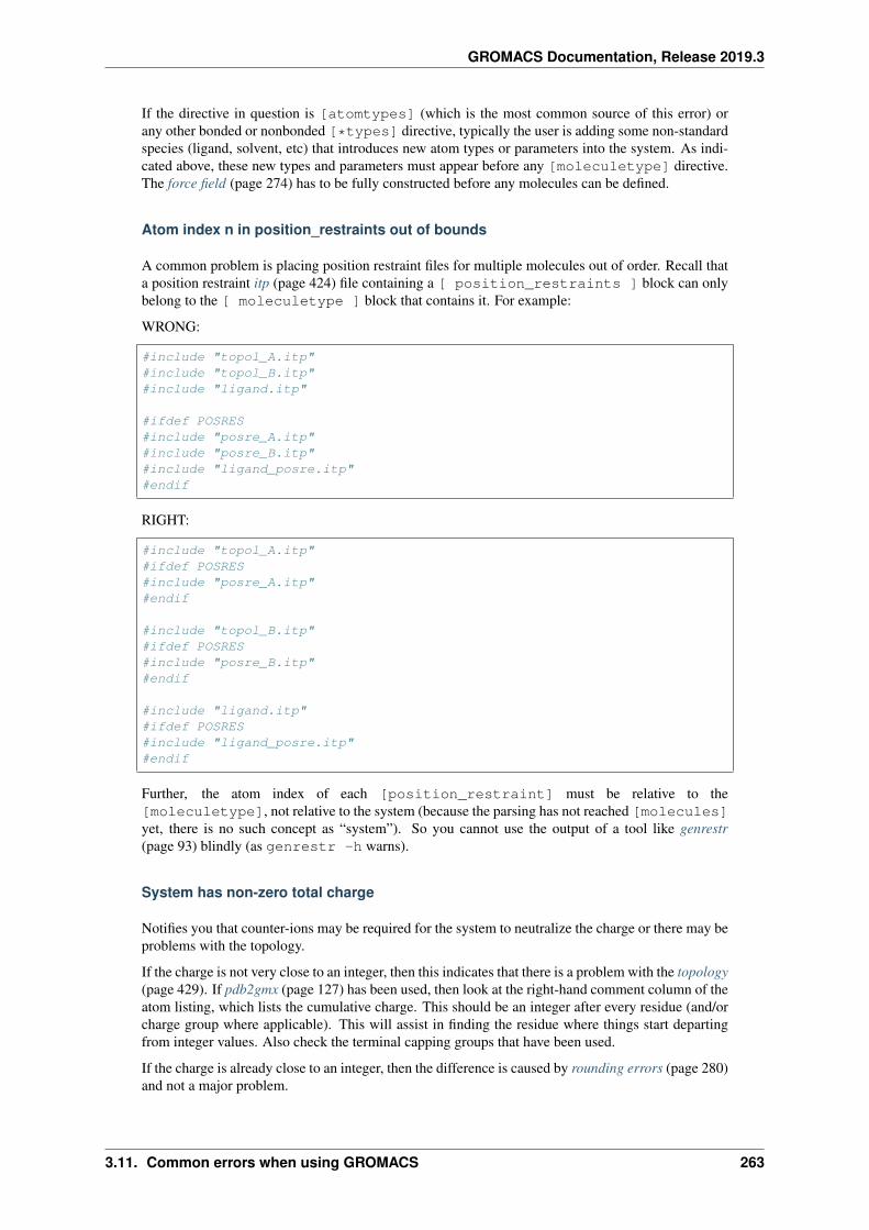
GROMACS Documentation, Release 2019.3
If the directive in question is [atomtypes] (which is the most common source of this error) orany other bonded or nonbonded [*types] directive, typically the user is adding some non-standardspecies (ligand, solvent, etc) that introduces new atom types or parameters into the system. As indi-cated above, these new types and parameters must appear before any [moleculetype] directive.The force field (page 274) has to be fully constructed before any molecules can be defined.
Atom index n in position_restraints out of bounds
A common problem is placing position restraint files for multiple molecules out of order. Recall thata position restraint itp (page 424) file containing a [ position_restraints ] block can onlybelong to the [ moleculetype ] block that contains it. For example:
WRONG:
#include "topol_A.itp"#include "topol_B.itp"#include "ligand.itp"
#ifdef POSRES#include "posre_A.itp"#include "posre_B.itp"#include "ligand_posre.itp"#endif
RIGHT:
#include "topol_A.itp"#ifdef POSRES#include "posre_A.itp"#endif
#include "topol_B.itp"#ifdef POSRES#include "posre_B.itp"#endif
#include "ligand.itp"#ifdef POSRES#include "ligand_posre.itp"#endif
Further, the atom index of each [position_restraint] must be relative to the[moleculetype], not relative to the system (because the parsing has not reached [molecules]yet, there is no such concept as “system”). So you cannot use the output of a tool like genrestr(page 93) blindly (as genrestr -h warns).
System has non-zero total charge
Notifies you that counter-ions may be required for the system to neutralize the charge or there may beproblems with the topology.
If the charge is not very close to an integer, then this indicates that there is a problem with the topology(page 429). If pdb2gmx (page 127) has been used, then look at the right-hand comment column of theatom listing, which lists the cumulative charge. This should be an integer after every residue (and/orcharge group where applicable). This will assist in finding the residue where things start departingfrom integer values. Also check the terminal capping groups that have been used.
If the charge is already close to an integer, then the difference is caused by rounding errors (page 280)and not a major problem.
3.11. Common errors when using GROMACS 263
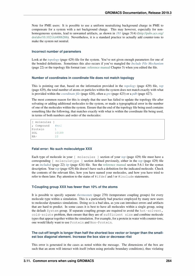
GROMACS Documentation, Release 2019.3
Note for PME users: It is possible to use a uniform neutralizing background charge in PME tocompensate for a system with a net background charge. This may however, especially for non-homogeneous systems, lead to unwanted artifacts, as shown in 181 (page 514) (http://pubs.acs.org/doi/abs/10.1021/ct400626b). Nevertheless, it is a standard practice to actually add counter-ions tomake the system net neutral.
Incorrect number of parameters
Look at the topology (page 429) file for the system. You’ve not given enough parameters for one ofthe bonded definitions. Sometimes this also occurs if you’ve mangled the Include File Mechanism(page 22) or the topology file format (see: reference manual Chapter 5) when you edited the file.
Number of coordinates in coordinate file does not match topology
This is pointing out that, based on the information provided in the topology (page 429) file, top(page 429), the total number of atoms or particles within the system does not match exactly with whatis provided within the coordinate file (page 420), often a gro (page 423) or a pdb (page 427).
The most common reason for this is simply that the user has failed to update the topology file aftersolvating or adding additional molecules to the system, or made a typographical error in the numberof one of the molecules within the system. Ensure that the end of the topology file being used containssomething like the following, that matches exactly with what is within the coordinate file being used,in terms of both numbers and order of the molecules:
[ molecules ]; Compound #molProtein 1SOL 10189NA+ 10
Fatal error: No such moleculetype XXX
Each type of molecule in your [ molecules ] section of your top (page 429) file must have acorresponding [ moleculetype ] section defined previously, either in the top (page 429) fileor an included (page 22) itp (page 424) file. See the reference manual section 5.6.1 for the syntaxdescription. Your top (page 429) file doesn’t have such a definition for the indicated molecule. Checkthe contents of the relevant files, how you have named your molecules, and how you have tried torefer to them later. Pay attention to the status of #ifdef and / or #include statements.
T-Coupling group XXX has fewer than 10% of the atoms
It is possible to specify separate thermostats (page 270) (temperature coupling groups) for everymolecule type within a simulation. This is a particularly bad practice employed by many new usersto molecular dynamics simulations. Doing so is a bad idea, as you can introduce errors and artifactsthat are hard to predict. In some cases it is best to have all molecules within a single group, usingthe default System group. If separate coupling groups are required to avoid the hot-solvent,cold-solute problem, then ensure that they are of sufficient size and combine moleculetypes that appear together within the simulation. For example, for a protein in water with counter-ions,one would likely want to use Protein and Non-Protein.
The cut-off length is longer than half the shortest box vector or longer than the small-est box diagonal element. Increase the box size or decrease rlist
This error is generated in the cases as noted within the message. The dimensions of the box aresuch that an atom will interact with itself (when using periodic boundary conditions), thus violating
3.11. Common errors when using GROMACS 264
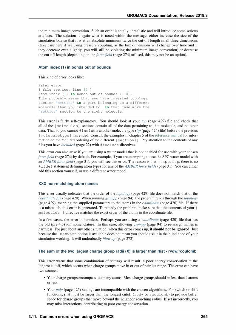
GROMACS Documentation, Release 2019.3
the minimum image convention. Such an event is totally unrealistic and will introduce some seriousartefacts. The solution is again what is noted within the message, either increase the size of thesimulation box so that it is at an absolute minimum twice the cut-off length in all three dimensions(take care here if are using pressure coupling, as the box dimensions will change over time and ifthey decrease even slightly, you will still be violating the minimum image convention) or decreasethe cut-off length (depending on the force field (page 274) utilised, this may not be an option).
Atom index (1) in bonds out of bounds
This kind of error looks like:
Fatal error:[ file spc.itp, line 32 ]Atom index (1) in bonds out of bounds (1-0).This probably means that you have inserted topologysection "settles" in a part belonging to a differentmolecule than you intended to. in that case move the"settles" section to the right molecule.
This error is fairly self-explanatory. You should look at your top (page 429) file and check thatall of the [molecules] sections contain all of the data pertaining to that molecule, and no otherdata. That is, you cannot #include another molecule type (itp (page 424) file) before the previous[moleculetype] has ended. Consult the examples in chapter 5 of the reference manual for infor-mation on the required ordering of the different [sections]. Pay attention to the contents of anyfiles you have included (page 22) with #include directives.
This error can also arise if you are using a water model that is not enabled for use with your chosenforce field (page 274) by default. For example, if you are attempting to use the SPC water model withan AMBER force field (page 31), you will see this error. The reason is that, in spc.itp, there is no#ifdef statement defining atom types for any of the AMBER force fields (page 31). You can eitheradd this section yourself, or use a different water model.
XXX non-matching atom names
This error usually indicates that the order of the topology (page 429) file does not match that of thecoordinate file (page 420). When running grompp (page 94), the program reads through the topology(page 429), mapping the supplied parameters to the atoms in the coordinate (page 420) file. If thereis a mismatch, this error is generated. To remedy the problem, make sure that the contents of your [molecules ] directive matches the exact order of the atoms in the coordinate file.
In a few cases, the error is harmless. Perhaps you are using a coordinate (page 420) file that hasthe old (pre-4.5) ion nomenclature. In this case, allowing grompp (page 94) to re-assign names isharmless. For just about any other situation, when this error comes up, it should not be ignored. Justbecause the -maxwarn option is available does not mean you should use it in the blind hope of yoursimulation working. It will undoubtedly blow up (page 272).
The sum of the two largest charge group radii (X) is larger than rlist - rvdw/rcoulomb
This error warns that some combination of settings will result in poor energy conservation at thelongest cutoff, which occurs when charge groups move in or out of pair list range. The error can havetwo sources:
• Your charge groups encompass too many atoms. Most charge groups should be less than 4 atomsor less.
• Your mdp (page 425) settings are incompatible with the chosen algorithms. For switch or shiftfunctions, rlist must be larger than the longest cutoff (rvdw or rcoulomb) to provide bufferspace for charge groups that move beyond the neighbor searching radius. If set incorrectly, youmay miss interactions, contributing to poor energy conservation.
3.11. Common errors when using GROMACS 265
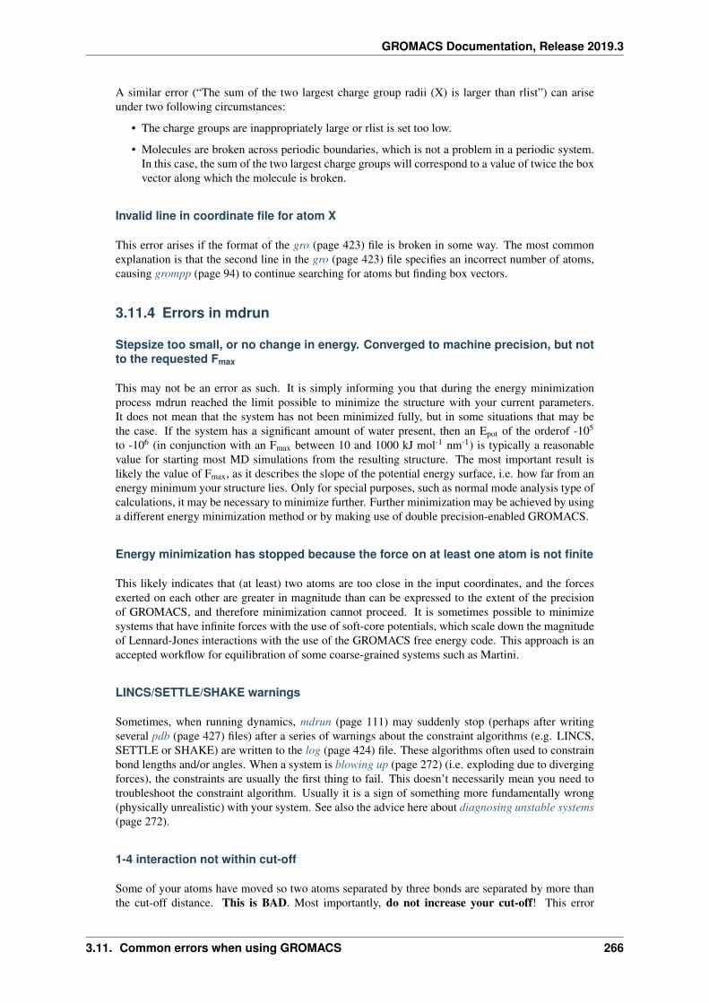
GROMACS Documentation, Release 2019.3
A similar error (“The sum of the two largest charge group radii (X) is larger than rlist”) can ariseunder two following circumstances:
• The charge groups are inappropriately large or rlist is set too low.
• Molecules are broken across periodic boundaries, which is not a problem in a periodic system.In this case, the sum of the two largest charge groups will correspond to a value of twice the boxvector along which the molecule is broken.
Invalid line in coordinate file for atom X
This error arises if the format of the gro (page 423) file is broken in some way. The most commonexplanation is that the second line in the gro (page 423) file specifies an incorrect number of atoms,causing grompp (page 94) to continue searching for atoms but finding box vectors.
3.11.4 Errors in mdrun
Stepsize too small, or no change in energy. Converged to machine precision, but notto the requested Fmax
This may not be an error as such. It is simply informing you that during the energy minimizationprocess mdrun reached the limit possible to minimize the structure with your current parameters.It does not mean that the system has not been minimized fully, but in some situations that may bethe case. If the system has a significant amount of water present, then an Epot of the orderof -105
to -106 (in conjunction with an Fmax between 10 and 1000 kJ mol-1 nm-1) is typically a reasonablevalue for starting most MD simulations from the resulting structure. The most important result islikely the value of Fmax, as it describes the slope of the potential energy surface, i.e. how far from anenergy minimum your structure lies. Only for special purposes, such as normal mode analysis type ofcalculations, it may be necessary to minimize further. Further minimization may be achieved by usinga different energy minimization method or by making use of double precision-enabled GROMACS.
Energy minimization has stopped because the force on at least one atom is not finite
This likely indicates that (at least) two atoms are too close in the input coordinates, and the forcesexerted on each other are greater in magnitude than can be expressed to the extent of the precisionof GROMACS, and therefore minimization cannot proceed. It is sometimes possible to minimizesystems that have infinite forces with the use of soft-core potentials, which scale down the magnitudeof Lennard-Jones interactions with the use of the GROMACS free energy code. This approach is anaccepted workflow for equilibration of some coarse-grained systems such as Martini.
LINCS/SETTLE/SHAKE warnings
Sometimes, when running dynamics, mdrun (page 111) may suddenly stop (perhaps after writingseveral pdb (page 427) files) after a series of warnings about the constraint algorithms (e.g. LINCS,SETTLE or SHAKE) are written to the log (page 424) file. These algorithms often used to constrainbond lengths and/or angles. When a system is blowing up (page 272) (i.e. exploding due to divergingforces), the constraints are usually the first thing to fail. This doesn’t necessarily mean you need totroubleshoot the constraint algorithm. Usually it is a sign of something more fundamentally wrong(physically unrealistic) with your system. See also the advice here about diagnosing unstable systems(page 272).
1-4 interaction not within cut-off
Some of your atoms have moved so two atoms separated by three bonds are separated by more thanthe cut-off distance. This is BAD. Most importantly, do not increase your cut-off! This error
3.11. Common errors when using GROMACS 266
GROMACS Documentation, Release 2019.3
actually indicates that the atoms have very large velocities, which usually means that (part of) yourmolecule(s) is (are) blowing up (page 272). If you are using LINCS for constraints, you probably alsoalready got a number of LINCS warnings. When using SHAKE this will give rise to a SHAKE error,which halts your simulation before the 1-4 not within cutoff error can appear.
There can be a number of reasons for the large velocities in your system. If it happens at the beginningof the simulation, your system might be not equilibrated well enough (e.g. it contains some badcontacts). Try a(nother) round of energy minimization to fix this. Otherwise you might have a veryhigh temperature, and/or a timestep that is too large. Experiment with these parameters until the errorstops occurring. If this doesn’t help, check the validity of the parameters in your topology (page 429)!
Simulation running but no output
Not an error as such, but mdrun appears to be chewing up CPU time but nothing is being written tothe output files. There are a number of reasons why this may occur:
• Your simulation might simply be (very) slow (page 242), and since output is buffered, it cantake quite some time for output to appear in the respective files. If you are trying to fix someproblems and you want to get output as fast as possible, you can set the environment variableGMX_LOG_BUFFER to 0.
• Something might be going wrong in your simulation, causing e.g. not-a-numbers (NAN) to begenerated (these are the result of e.g. division by zero). Subsequent calculations with NAN’swill generate floating point exceptions which slow everything down by orders of magnitude.
• You might have all nst* parameters (see your mdp (page 425) file) set to 0, this will suppressmost output.
• Your disk might be full. Eventually this will lead to mdrun (page 111) crashing, but since outputis buffered, it might take a while for mdrun to realize it can’t write.
Can not do Conjugate Gradients with constraints
This means you can’t do energy minimization with the conjugate gradient algorithm if your topologyhas constraints defined. Please check the reference manual.
Pressure scaling more than 1%
This error tends to be generated when the simulation box begins to oscillate (due to large pressuresand / or small coupling constants), the system starts to resonate and then crashes (page 272). This canmean that the system isn’t equilibrated sufficiently before using pressure coupling. Therefore, better/ more equilibration may fix the issue.
It is recommended to observe the system trajectory prior and during the crash. This may indicate if aparticular part of the system / structure is the problem.
In some cases, if the system has been equilibrated sufficiently, this error can mean that the pressurecoupling constant, tau-p (page 215), is too small (particularly when using the Berendsen weakcoupling method). Increasing that value will slow down the response to pressure changes and maystop the resonance from occurring. You are also more likely to see this error if you use Parrinello-Rahman pressure coupling on a system that is not yet equilibrated - start with the much more forgivingBerendsen method first, then switch to other algorithms.
This error can also appear when using a timestep that is too large, e.g. 5 fs, in the absence of con-straints and / or virtual sites.
Range Checking error
This usually means your simulation is blowing up (page 272). Probably you need to do better energyminimization and/or equilibration and/or topology design.
3.11. Common errors when using GROMACS 267
GROMACS Documentation, Release 2019.3
X particles communicated to PME node Y are more than a cell length out of the domaindecomposition cell of their charge group
This is another way that mdrun (page 111) tells you your system is blowing up (page 272). If youhave particles that are flying across the system, you will get this fatal error. The message indicatesthat some piece of your system is tearing apart (hence out of the “cell of their charge group”). Referto the Blowing Up (page 272) page for advice on how to fix this issue.
A charge group moved too far between two domain decomposition steps.
See information above.
Software inconsistency error: Some interactions seem to be assigned multiple times
See information above
There is no domain decomposition for n ranks that is compatible with the given boxand a minimum cell size of x nm
This means you tried to run a parallel calculation, and when mdrun (page 111) tried to partition yoursimulation cell into chunks, it couldn’t. The minimum cell size is controlled by the size of the largestcharge group or bonded interaction and the largest of rvdw, rlist and rcoulomb, some othereffects of bond constraints, and a safety margin. Thus it is not possible to run a small simulationwith large numbers of processors. So, if grompp (page 94) warned you about a large charge group,pay attention and reconsider its size. mdrun (page 111) prints a breakdown of how it computed thisminimum size in the log (page 424) file, so you can perhaps find a cause there.
If you didn’t think you were running a parallel calculation, be aware that from 4.5, GROMACS usesthread-based parallelism by default. To prevent this, give mdrun (page 111) the -ntmpi 1 commandline option. Otherwise, you might be using an MPI-enabled GROMACS and not be aware of the fact.
3.12 Terminology
3.12.1 Pressure
The pressure in molecular dynamics can be computed from the kinetic energy and the virial.
Fluctuation
Whether or not pressure coupling is used within a simulation, the pressure value for the simulationbox will oscillate significantly. Instantaneous pressure is meaningless, and not well-defined. Overa picosecond time scale it usually will not be a good indicator of the true pressure. This variationis entirely normal due to the fact that pressure is a macroscopic property and can only be measuredproperly as time average, while it is being measured and/or adjusted with pressure coupling on themicroscopic scale. How much it varies and the speed at which it does depends on the number of atomsin the system, the type of pressure coupling used and the value of the coupling constants. Fluctuationsof the order of hundreds of bar are typical. For a box of 216 waters, fluctuations of 500-600 bar arestandard. Since the fluctuations go down with the square root of the number of particles, a system of21600 water molecules (100 times larger) will still have pressure fluctuations of 50-60 bar.
3.12. Terminology 268
GROMACS Documentation, Release 2019.3
3.12.2 Periodic boundary conditions
Periodic boundary conditions (PBC) are used in molecular dynamics simulations to avoid problemswith boundary effects caused by finite size, and make the system more like an infinite one, at the costof possible periodicity effects.
Beginners visualizing a trajectory sometimes think they are observing a problem when
• the molecule(s) does not stay in the centre of the box, or
• it appears that (parts of) the molecule(s) diffuse out of the box, or
• holes are created, or
• broken molecules appear, or
• their unit cell was a rhombic dodecahedron or cubic octahedron but it looks like a slanted cubeafter the simulation, or
• crazy bonds all across the simulation cell appear.
This is not a problem or error that is occuring, it is what you should expect.
The existence of PBC means that any atom that leaves a simulation box by, say, the right-hand face,then enters the simulation box by the left-hand face. In the example of a large protein, if you look atthe face of the simulation box that is opposite to the one from which the protein is protruding, thena hole in the solvent will be visible. The reason that the molecule(s) move from where they wereinitially located within the box is (for the vast majority of simulations) they are free to diffuse around.And so they do. They are not held in a magic location of the box. The box is not centered aroundanything while performing the simulation. Molecules are not made whole as a matter of course.Moreover, any periodic cell shape can be expressed as a parallelepiped (a.k.a. triclinic cell), andGROMACS does so internally regardless of the initial shape of the box.
These visual issues can be fixed after the conclusion of the simulation by judicious use of the optionalinputs to gmx trjconv (page 162) to process the trajectory files. Similarly, analyses such as RMSDof atomic positions can be flawed when a reference structure is compared with a structure that needsadjusting for periodicity effects, and the solution with gmx trjconv (page 162) follows the same lines.Some complex cases needing more than one operation will require more than one invocation of gmxtrjconv (page 162) in order to work.
For further information, see the corresponding section in the Reference Manual (page 302).
Suggested workflow
Fixing periodicity effects with gmx trjconv (page 162) to suit visualization or analysis can be tricky.Multiple invocations can be necessary. You may need to create custom index groups (e.g. to keep yourligand with your protein) Following the steps below in order (omitting those not required) should helpget a pleasant result. You will need to consult gmx trjconv -h to find out the details for eachstep. That’s deliberate – there is no magic “do what I want” recipe. You have to decide what youwant, first. :-)
1. First make your molecules whole if you want them whole.
2. Cluster your molecules/particles if you want them clustered.
3. If you want jumps removed, extract the first frame from the trajectory to use as the reference,and then use -pbc nojump with that first frame as reference.
4. Center your system using some criterion. Doing so shifts the system, so don’t use -pbcnojump after this step.
5. Perhaps put everything in some box with the other -pbc or -ur options.
6. Fit the resulting trajectory to some (other) reference structure (if desired), and don’t use anyPBC related option afterwards.
3.12. Terminology 269
GROMACS Documentation, Release 2019.3
With point three, the issue is that gmx trjconv (page 162) removes the jumps from the first frameusing the reference structure provided with -s. If the reference structure (run input file) is not clus-tered/whole, using -pbc nojump will undo steps 1 and 2.
3.12.3 Thermostats
Thermostats are designed to help a simulation sample from the correct ensemble (i.e. NVT or NPT)by modulating the temperature of the system in some fashion. First, we need to establish what wemean by temperature. In simulations, the “instantaneous (kinetic) temperature” is usually computedfrom the kinetic energy of the system using the equipartition theorem. In other words, the temperatureis computed from the system’s total kinetic energy.
So, what’s the goal of a thermostat? Actually, it turns out the goal is not to keep the temperatureconstant, as that would mean fixing the total kinetic energy, which would be silly and not the aim ofNVT or NPT. Rather, it’s to ensure that the average temperature of a system be correct.
To see why this is the case, imagine a glass of water sitting in a room. Suppose you can look veryclosely at a few molecules in some small region of the glass, and measure their kinetic energies. Youwould not expect the kinetic energy of this small number of particles to remain precisely constant;rather, you’d expect fluctuations in the kinetic energy due to the small number of particles. As youaverage over larger and larger numbers of particles, the fluctuations in the average get smaller andsmaller, so finally by the time you look at the whole glass, you say it has “constant temperature”.
Molecular dynamics simulations are often fairly small compared to a glass of water, so we have biggerfluctuations. So it’s really more appropriate here to think of the role of a thermostat as ensuring thatwe have
1. the correct average temperature, and
2. the fluctuations of the correct size.
See the relevant section in the Reference Manual (page 317) for details on how temperature couplingis applied and the types currently available.
What to do
Some hints on practices that generally are a good idea:
• Preferably, use a thermostat that samples the correct distribution of temperatures (for examples,see the corresponding manual section), in addition to giving you the correct average temperature.
• At least: use a thermostat that gives you the correct average temperature, and apply it to com-ponents of your system for which they are justified (see the first bullet in What not to do(page 270)). In some cases, using tc-grps = System may lead to the “hot solvent/coldsolute” problem described in the 3rd reference in Further reading (page 271).
What not to do
Some hints on practices that generally not a good idea to use:
• Do not use separate thermostats for every component of your system. Some molecular dynamicsthermostats only work well in the thermodynamic limit. A group must be of sufficient size tojustify its own thermostat. If you use one thermostat for, say, a small molecule, another forprotein, and another for water, you are likely introducing errors and artifacts that are hard topredict. In particular, do not couple ions in aqueous solvent in a separate group from thatsolvent. For a protein simulation, using tc-grps = Protein Non-Protein is usuallybest.
• Do not use thermostats that work well only in the limit of a large number of degrees of freedomfor systems with few degrees of freedom. For example, do not use Nosé-Hoover or Berendsen
3.12. Terminology 270
GROMACS Documentation, Release 2019.3
thermostats for types of free energy calculations where you will have a component of the systemwith very few degrees of freedom in an end state (i.e. a noninteracting small molecule).
Further reading
1. Cheng, A. & Merz, K. M. Application of the nosé- hoover chain algorithm to the study of proteindynamics. *J. Phys. Chem.* **100** (5), 1927–1937 (1996).
2. Mor, A., Ziv, G. & Levy, Y. Simulations of proteins with inhomogeneous degrees of freedom:the effect of thermostats. *J. Comput. Chem.* **29** (12), 1992–1998 (2008).
3. Lingenheil, M., Denschlag, R., Reichold, R. & Tavan, P. The “hot-solvent/cold-solute” problemrevisited. *J. Chem. Theory Comput.* **4** (8), 1293–1306 (2008).
3.12.4 Energy conservation
In principle, a molecular dynamics simulation should conserve the total energy, the total momentumand (in a non-periodic system) the total angular momentum. A number of algorithmic and numericalissues make that this is not always the case:
• Cut-off treatment and/or long-range electrostatics treatment (see Van Der Spoel, D. & vanMaaren, P. J. The origin of layer structure artifacts in simulations of liquid water. J. Chem.Theor. Comp. 2, 1–11 (2006).)
• Treatment of pair lists,
• Constraint algorithms (see e.g. Hess, B. P-LINCS: A parallel linear constraint solver for molec-ular simulation. J. Chem. Theor. Comp. 4, 116–122 (2008).).
• The integration timestep.
• Temperature coupling (page 270) and pressure coupling (page 268).
• Round-off error (in particular in single precision), for example subtracting large numbers (Lip-pert, R. A. et al. A common, avoidable source of error in molecular dynamics integrators. J.Chem. Phys. 126, 046101 (2007).).
• The choice of the integration algorithm (in GROMACS this is normally leap-frog).
• Removal of center of mass motion: when doing this in more than one group the conservation ofenergy will be violated.
3.12.5 Average structure
Various GROMACS utilities can compute average structures. Presumably the idea for this comesfrom something like an ensemble-average NMR structure. In some cases, it makes sense to calculatean average structure (as a step on the way to calculating root-mean-squared fluctuations (RMSF), forexample, one needs the average position of all of the atoms).
However, it’s important to remember that an average structure isn’t necessarily meaningful. By wayof analogy, suppose I alternate holding a ball in my left hand, then in my right hand. What’s theaverage position of the ball? Halfway in between – even though I always have it either in my lefthand or my right hand. Similarly, for structures, averages will tend to be meaningless anytime thereare separate metastable conformational states. This can happen on a sidechain level, or for someregions of backbone, or even whole helices or components of the secondary structure.
Thus, if you derive an average structure from a molecular dynamics simulation, and find artifacts likeunphysical bond lengths, weird structures, etc., this doesn’t necessarily mean something is wrong. Itjust shows the above: an average structure from a simulation is not necessarily a physically meaning-ful structure.
3.12. Terminology 271
GROMACS Documentation, Release 2019.3
3.12.6 Blowing up
Blowing up is a highly technical term used to describe a common sort of simulation failure. In brief,it describes a failure typically due to an unacceptably large force that ends up resulting in a failure ofthe integrator.
To give a bit more background, it’s important to remember that molecular dynamics numerically inte-grates Newton’s equations of motion by taking small, discrete timesteps, and using these timesteps todetermine new velocities and positions from velocities, positions, and forces at the previous timestep.If forces become too large at one timestep, this can result in extremely large changes in veloc-ity/position when going to the next timestep. Typically, this will result in a cascade of errors: oneatom experiences a very large force one timestep, and thus goes shooting across the system in an un-controlled way in the next timestep, overshooting its preferred location or landing on top of anotheratom or something similar. This then results in even larger forces the next timestep, more uncon-trolled motions, and so on. Ultimately, this will cause the simulation package to crash in some way,since it can’t cope with such situations. In simulations with constraints, the first symptom of this willusually be some LINCS or SHAKE warning or error – not because the constraints are the source ofthe problem, but just because they’re the first thing to crash. Similarly, in simulations with domaindecomposition, you may see messages about particles being more than a cell length out of the domaindecomposition cell of their charge group, which are symptomatic of your underlying problem, and notthe domain decomposition algorithm itself. Likewise for warnings about tabulated or 1-4 interactionsbeing outside the distance supported by the table. This can happen on one computer system whileanother resulted in a stable simulation because of the impossibility of numerical reproducibility ofthese calculations on different computer systems.
Possible causes include:
• you didn’t minimize well enough,
• you have a bad starting structure, perhaps with steric clashes,
• you are using too large a timestep (particularly given your choice of constraints),
• you are doing particle insertion in free energy calculations without using soft core,
• you are using inappropriate pressure coupling (e.g. when you are not in equilibrium, Berendsencan be best while relaxing the volume, but you will need to switch to a more accurate pressure-coupling algorithm later),
• you are using inappropriate temperature coupling, perhaps on inappropriate groups, or
• your position restraints are to coordinates too different from those present in the system, or
• you have a single water molecule somewhere within the system that is isolated from the otherwater molecules, or
• you are experiencing a bug in gmx mdrun (page 111).
Because blowing up is due, typically, to forces that are too large for a particular timestep size, thereare a couple of basic solutions:
• make sure the forces don’t get that large, or
• use a smaller timestep.
Better system preparation is a way to make sure that forces don’t get large, if the problems are occur-ring near the beginning of a simulation.
3.12.7 Diagnosing an unstable system
Troubleshooting a system that is blowing up can be challenging, especially for an inexperienced user.Here are a few general tips that one may find useful when addressing such a scenario:
3.12. Terminology 272
GROMACS Documentation, Release 2019.3
1. If the crash is happening relatively early (within a few steps), set nstxout (ornstxout-compressed) to 1, capturing all possible frames. Watch the resulting trajectoryto see which atoms/residues/molecules become unstable first.
2. Simplify the problem to try to establish a cause:
• If you have a new box of solvent, try minimizing and simulating a single molecule to seeif the instability is due to some inherent problem with the molecule’s topology or if insteadthere are clashes in your starting configuration.
• If you have a protein-ligand system, try simulating the protein alone in the desired solvent.If it is stable, simulate the ligand in vacuo to see if its topology gives stable configurations,energies, etc.
• Remove the use of fancy algorithms, particularly if you haven’t equilibrated thoroughlyfirst
3. Monitor various components of the system’s energy using gmx energy (page 84). If an in-tramolecular term is spiking, that may indicate improper bonded parameters, for example.
4. Make sure you haven’t been ignoring error messages (missing atoms when running gmxpdb2gmx (page 127), mismatching names when running gmx grompp (page 94), etc.) or us-ing work-arounds (like using gmx grompp -maxwarn when you shouldn’t be) to make sureyour topology is intact and being interpreted correctly.
5. Make sure you are using appropriate settings in your mdp (page 425) file for the force field youhave chosen and the type of system you have. Particularly important settings are treatment ofcutoffs, proper neighbor searching interval (nstlist), and temperature coupling. Impropersettings can lead to a breakdown in the model physics, even if the starting configuration of thesystem is reasonable.
When using no explict solvent, starting your equilibration with a smaller time step than your produc-tion run can help energy equipartition more stably.
There are several common situations in which instability frequently arises, usually in the introductionof new species (ligands or other molecules) into the system. To determine the source of the problem,simplify the system (e.g. the case of a protein-ligand complex) in the following way.
1. Does the protein (in water) minimize adequately by itself? This is a test of the integrity of thecoordinates and system preparation. If this fails, something probably went wrong when runninggmx pdb2gmx (page 127) (see below), or maybe gmx genion (page 91) placed an ion very closeto the protein (it is random, after all).
2. Does the ligand minimize in vacuo? This is a test of the topology. If it does not, check yourparameterization of the ligand and any implementation of new parameters in force field files.
3. (If previous item is successful) Does the ligand minimize in water, and/or does a short simulationof the ligand in water succeed?
Other sources of possible problems are in the biomolecule topology itself.
1. Did you use -missing when running gmx pdb2gmx (page 127)? If so, don’t. Reconstructmissing coordinates rather than ignoring them.
2. Did you override long/short bond warnings by changing the lengths? If so, don’t. You probablyhave missing atoms or some terrible input geometry.
3.12.8 Molecular dynamics
Molecular dynamics (MD) is computer simulation with atoms and/or molecules interacting usingsome basic laws of physics. The GROMACS Reference Manual (page 306) provides a good generalintroduction to this area, as well as specific material for use with GROMACS. The first few chaptersare mandatory reading for anybody wishing to use GROMACS and not waste time.
3.12. Terminology 273
GROMACS Documentation, Release 2019.3
• Introduction to molecular modeling (slides, video)] - theoretical framework, modeling levels,limitations and possibilities, systems and methods (Erik Lindahl).
Books
There a several text books around.
Good introductory books are: * A. Leach (2001) Molecular Modeling: Principles and Applications.* T. Schlick (2002) Molecular Modeling and Simulation
With programming background: * D. Rapaport (1996) The Art of Molecular Dynamics Simulation *D. Frenkel, B. Smith (2001) Understanding Molecular Simulation
More from the physicist’s view: * M. Allen, D. Tildesley (1989) Computer simulation of liquids* H.J.C. Berendsen (2007) Simulating the Physical World: Hierarchical Modeling from QuantumMechanics to Fluid Dynamics
Types / Ensembles
• NVE - number of particles (N), system volume (V) and energy (E) are constant / conserved.
• NVT - number of particles (N), system volume (V) and temperature (T) are constant / conserved.(See thermostats (page 270) for more on constant temperature).
• NPT - number of particles (N), system pressure (P) and temperature (T) are constant / conserved.(See pressure coupling (page 268) for more on constant pressure).
3.12.9 Force field
Force fields are sets of potential functions and parametrized interactions that can be used to studyphysical systems. A general introduction to their history, function and use is beyond the scope ofthis guide, and the user is asked to consult either the relevant literature or try to start at the relevantWikipedia page.
3.13 Environment Variables
GROMACS programs may be influenced by the use of environment variables. First of all, the vari-ables set in the GMXRC file are essential for running and compiling GROMACS. Some other usefulenvironment variables are listed in the following sections. Most environment variables function bybeing set in your shell to any non-NULL value. Specific requirements are described below if othervalues need to be set. You should consult the documentation for your shell for instructions on howto set environment variables in the current shell, or in configuration files for future shells. Note thatrequirements for exporting environment variables to jobs run under batch control systems vary andyou should consult your local documentation for details.
3.13.1 Output Control
GMX_CONSTRAINTVIR Print constraint virial and force virial energy terms.
GMX_DUMP_NL Neighbour list dump level; default 0.
GMX_MAXBACKUP GROMACS automatically backs up old copies of files when trying to write anew file of the same name, and this variable controls the maximum number of backups that willbe made, default 99. If set to 0 it fails to run if any output file already exists. And if set to -1 itoverwrites any output file without making a backup.
GMX_NO_QUOTES if this is explicitly set, no cool quotes will be printed at the end of a program.
3.13. Environment Variables 274
GROMACS Documentation, Release 2019.3
GMX_SUPPRESS_DUMP prevent dumping of step files during (for example) blowing up during fail-ure of constraint algorithms.
GMX_TPI_DUMP dump all configurations to a pdb (page 427) file that have an interaction energyless than the value set in this environment variable.
GMX_VIEW_XPM GMX_VIEW_XVG, GMX_VIEW_EPS and GMX_VIEW_PDB, commands used toautomatically view xvg (page 434), xpm (page 432), eps (page 422) and pdb (page 427) filetypes, respectively; they default to xv, xmgrace, ghostview and rasmol. Set to empty todisable automatic viewing of a particular file type. The command will be forked off and run inthe background at the same priority as the GROMACS tool (which might not be what you want).Be careful not to use a command which blocks the terminal (e.g. vi), since multiple instancesmight be run.
GMX_LOG_BUFFER the size of the buffer for file I/O. When set to 0, all file I/O will be unbufferedand therefore very slow. This can be handy for debugging purposes, because it ensures that allfiles are always totally up-to-date.
GMX_LOGO_COLOR set display color for logo in gmx view (page 173).
GMX_PRINT_LONGFORMAT use long float format when printing decimal values.
GMX_COMPELDUMP Applies for computational electrophysiology setups only (see reference man-ual). The initial structure gets dumped to pdb (page 427) file, which allows to check whethermultimeric channels have the correct PBC representation.
GMX_TRAJECTORY_IO_VERBOSITY Defaults to 1, which prints frame count e.g. when readingtrajectory files. Set to 0 for quiet operation.
GMX_ENABLE_GPU_TIMING Enables GPU timings in the log file for CUDA. Note that CUDAtimings are incorrect with multiple streams, as happens with domain decomposition or withboth non-bondeds and PME on the GPU (this is also the main reason why they are not turnedon by default).
GMX_DISABLE_GPU_TIMING Disables GPU timings in the log file for OpenCL.
3.13.2 Debugging
GMX_PRINT_DEBUG_LINES when set, print debugging info on line numbers.
GMX_DD_NST_DUMP number of steps that elapse between dumping the current DD to a PDB file(default 0). This only takes effect during domain decomposition, so it should typically be 0(never), 1 (every DD phase) or a multiple of nstlist (page 206).
GMX_DD_NST_DUMP_GRID number of steps that elapse between dumping the current DD grid to aPDB file (default 0). This only takes effect during domain decomposition, so it should typicallybe 0 (never), 1 (every DD phase) or a multiple of nstlist (page 206).
GMX_DD_DEBUG general debugging trigger for every domain decomposition (default 0, meaningoff). Currently only checks global-local atom index mapping for consistency.
GMX_DD_NPULSE over-ride the number of DD pulses used (default 0, meaning no over-ride). Nor-mally 1 or 2.
GMX_DISABLE_ALTERNATING_GPU_WAIT disables the specialized polling wait path used towait for the PME and nonbonded GPU tasks completion to overlap to do the reduction of theresulting forces that arrive first. Setting this variable switches to the generic path with fixedwaiting order.
There are a number of extra environment variables like these that are used in debugging - check thecode!
3.13. Environment Variables 275
GROMACS Documentation, Release 2019.3
3.13.3 Performance and Run Control
GMX_DO_GALACTIC_DYNAMICS planetary simulations are made possible (just for fun) by set-ting this environment variable, which allows setting epsilon-r (page 209) to -1 in the mdp(page 425) file. Normally, epsilon-r (page 209) must be greater than zero to prevent a fatalerror. See webpage for example input files for a planetary simulation.
GMX_BONDED_NTHREAD_UNIFORM Value of the number of threads per rank from which to switchfrom uniform to localized bonded interaction distribution; optimal value dependent on systemand hardware, default value is 4.
GMX_CUDA_NB_EWALD_TWINCUT force the use of twin-range cutoff kernel even if rvdw(page 211) equals rcoulomb (page 209) after PP-PME load balancing. The switch to twin-range kernels is automated, so this variable should be used only for benchmarking.
GMX_CUDA_NB_ANA_EWALD force the use of analytical Ewald kernels. Should be used only forbenchmarking.
GMX_CUDA_NB_TAB_EWALD force the use of tabulated Ewald kernels. Should be used only forbenchmarking.
GMX_DISABLE_CUDA_TIMING Deprecated. Use GMX_DISABLE_GPU_TIMING instead.
GMX_CYCLE_ALL times all code during runs. Incompatible with threads.
GMX_CYCLE_BARRIER calls MPI_Barrier before each cycle start/stop call.
GMX_DD_ORDER_ZYX build domain decomposition cells in the order (z, y, x) rather than the default(x, y, z).
GMX_DD_USE_SENDRECV2 during constraint and vsite communication, use a pair of MPI_-Sendrecv calls instead of two simultaneous non-blocking calls (default 0, meaning off). Mightbe faster on some MPI implementations.
GMX_DLB_BASED_ON_FLOPS do domain-decomposition dynamic load balancing based on flopcount rather than measured time elapsed (default 0, meaning off). This makes the load balancingreproducible, which can be useful for debugging purposes. A value of 1 uses the flops; a value> 1 adds (value - 1)*5% of noise to the flops to increase the imbalance and the scaling.
GMX_DLB_MAX_BOX_SCALING maximum percentage box scaling permitted per domain-decomposition load-balancing step (default 10)
GMX_DD_RECORD_LOAD record DD load statistics for reporting at end of the run (default 1, mean-ing on)
GMX_DETAILED_PERF_STATS when set, print slightly more detailed performance information tothe log (page 424) file. The resulting output is the way performance summary is reported inversions 4.5.x and thus may be useful for anyone using scripts to parse log (page 424) files orstandard output.
GMX_DISABLE_SIMD_KERNELS disables architecture-specific SIMD-optimized (SSE2, SSE4.1,AVX, etc.) non-bonded kernels thus forcing the use of plain C kernels.
GMX_DISABLE_GPU_TIMING timing of asynchronously executed GPU operations can have anon-negligible overhead with short step times. Disabling timing can improve performance inthese cases.
GMX_DISABLE_GPU_DETECTION when set, disables GPU detection even if gmx mdrun(page 111) was compiled with GPU support.
GMX_GPU_APPLICATION_CLOCKS setting this variable to a value of “0”, “ON”, or “DISABLE”(case insensitive) allows disabling the CUDA GPU allication clock support.
GMX_DISRE_ENSEMBLE_SIZE the number of systems for distance restraint ensemble averaging.Takes an integer value.
3.13. Environment Variables 276
GROMACS Documentation, Release 2019.3
GMX_EMULATE_GPU emulate GPU runs by using algorithmically equivalent CPU reference codeinstead of GPU-accelerated functions. As the CPU code is slow, it is intended to be used onlyfor debugging purposes.
GMX_ENX_NO_FATAL disable exiting upon encountering a corrupted frame in an edr (page 422)file, allowing the use of all frames up until the corruption.
GMX_FORCE_UPDATE update forces when invoking mdrun -rerun.
GMX_GPU_ID set in the same way as mdrun -gpu_id, GMX_GPU_ID allows the user to specifydifferent GPU IDs for different ranks, which can be useful for selecting different devices ondifferent compute nodes in a cluster. Cannot be used in conjunction with mdrun -gpu_id.
GMX_GPUTASKS set in the same way as mdrun -gputasks, GMX_GPUTASKS allows the map-ping of GPU tasks to GPU device IDs to be different on different ranks, if e.g. the MPI runtimepermits this variable to be different for different ranks. Cannot be used in conjunction withmdrun -gputasks. Has all the same requirements as mdrun -gputasks.
GMX_IGNORE_FSYNC_FAILURE_ENV allow gmx mdrun (page 111) to continue even if a file ismissing.
GMX_LJCOMB_TOL when set to a floating-point value, overrides the default tolerance of 1e-5 forforce-field floating-point parameters.
GMX_MAXCONSTRWARN if set to -1, gmx mdrun (page 111) will not exit if it produces too manyLINCS warnings.
GMX_NB_GENERIC use the generic C kernel. Should be set if using the group-based cutoff schemeand also sets GMX_NO_SOLV_OPT to be true, thus disabling solvent optimizations as well.
GMX_NB_MIN_CI neighbor list balancing parameter used when running on GPU. Sets the targetminimum number pair-lists in order to improve multi-processor load-balance for better perfor-mance with small simulation systems. Must be set to a non-negative integer, the 0 value disableslist splitting. The default value is optimized for supported GPUs therefore changing it is not nec-essary for normal usage, but it can be useful on future architectures.
GMX_NBLISTCG use neighbor list and kernels based on charge groups.
GMX_NBNXN_CYCLE when set, print detailed neighbor search cycle counting.
GMX_NBNXN_EWALD_ANALYTICAL force the use of analytical Ewald non-bonded kernels, mutu-ally exclusive of GMX_NBNXN_EWALD_TABLE.
GMX_NBNXN_EWALD_TABLE force the use of tabulated Ewald non-bonded kernels, mutually ex-clusive of GMX_NBNXN_EWALD_ANALYTICAL.
GMX_NBNXN_SIMD_2XNN force the use of 2x(N+N) SIMD CPU non-bonded kernels, mutuallyexclusive of GMX_NBNXN_SIMD_4XN.
GMX_NBNXN_SIMD_4XN force the use of 4xN SIMD CPU non-bonded kernels, mutually exclusiveof GMX_NBNXN_SIMD_2XNN.
GMX_NOOPTIMIZEDKERNELS deprecated, use GMX_DISABLE_SIMD_KERNELS instead.
GMX_NO_ALLVSALL disables optimized all-vs-all kernels.
GMX_NO_CART_REORDER used in initializing domain decomposition communicators. Rank re-ordering is default, but can be switched off with this environment variable.
GMX_NO_LJ_COMB_RULE force the use of LJ paremeter lookup instead of using combination rulesin the non-bonded kernels.
GMX_NO_INT, GMX_NO_TERM, GMX_NO_USR1 disable signal handlers for SIGINT, SIGTERM,and SIGUSR1, respectively.
GMX_NO_NODECOMM do not use separate inter- and intra-node communicators.
GMX_NO_NONBONDED skip non-bonded calculations; can be used to estimate the possible perfor-mance gain from adding a GPU accelerator to the current hardware setup – assuming that this
3.13. Environment Variables 277

GROMACS Documentation, Release 2019.3
is fast enough to complete the non-bonded calculations while the CPU does bonded force andPME computation. Freezing the particles will be required to stop the system blowing up.
GMX_PULL_PARTICIPATE_ALL disable the default heuristic for when to use a separate pull MPIcommunicator (at >=32 ranks).
GMX_NOPREDICT shell positions are not predicted.
GMX_NO_SOLV_OPT turns off solvent optimizations; automatic if GMX_NB_GENERIC is enabled.
GMX_NO_UPDATEGROUPS turns off update groups. May allow for a decomposition of more do-mains for small systems at the cost of communication during update.
GMX_NSCELL_NCG the ideal number of charge groups per neighbor searching grid cell is hard-coded to a value of 10. Setting this environment variable to any other integer value overridesthis hard-coded value.
GMX_PME_NUM_THREADS set the number of OpenMP or PME threads; overrides the default set bygmx mdrun (page 111); can be used instead of the -npme command line option, also useful toset heterogeneous per-process/-node thread count.
GMX_PME_P3M use P3M-optimized influence function instead of smooth PME B-spline interpola-tion.
GMX_PME_THREAD_DIVISION PME thread division in the format “x y z” for all three dimen-sions. The sum of the threads in each dimension must equal the total number of PME threads(set in GMX_PME_NTHREADS).
GMX_PMEONEDD if the number of domain decomposition cells is set to 1 for both x and y, decom-pose PME in one dimension.
GMX_REQUIRE_SHELL_INIT require that shell positions are initiated.
GMX_REQUIRE_TABLES require the use of tabulated Coulombic and van der Waals interactions.
GMX_SCSIGMA_MIN the minimum value for soft-core sigma. Note that this value is set using thesc-sigma (page 230) keyword in the mdp (page 425) file, but this environment variable canbe used to reproduce pre-4.5 behavior with respect to this parameter.
GMX_TPIC_MASSES should contain multiple masses used for test particle insertion into a cavity.The center of mass of the last atoms is used for insertion into the cavity.
GMX_USE_GRAPH use graph for bonded interactions.
GMX_VERLET_BUFFER_RES resolution of buffer size in Verlet cutoff scheme. The default valueis 0.001, but can be overridden with this environment variable.
HWLOC_XMLFILE Not strictly a GROMACS environment variable, but on large machines the hwlocdetection can take a few seconds if you have lots of MPI processes. If you run the hwloccommand lstopo out.xml and set this environment variable to point to the location of this file,the hwloc library will use the cached information instead, which can be faster.
MPIRUN the mpirun command used by gmx tune_pme (page 166).
MDRUN the gmx mdrun (page 111) command used by gmx tune_pme (page 166).
GMX_DISABLE_DYNAMICPRUNING disables dynamic pair-list pruning. Note that gmx mdrun(page 111) will still tune nstlist to the optimal value picked assuming dynamic pruning. Thusfor good performance the -nstlist option should be used.
GMX_NSTLIST_DYNAMICPRUNING overrides the dynamic pair-list pruning interval chosenheuristically by mdrun. Values should be between the pruning frequency value (1 for CPUand 2 for GPU) and nstlist (page 206) - 1.
GMX_USE_TREEREDUCE use tree reduction for nbnxn force reduction. Potentially faster for largenumber of OpenMP threads (if memory locality is important).
3.13. Environment Variables 278
GROMACS Documentation, Release 2019.3
3.13.4 OpenCL management
Currently, several environment variables exist that help customize some aspects of the OpenCL ver-sion of GROMACS. They are mostly related to the runtime compilation of OpenCL kernels, but theyare also used in device selection.
GMX_OCL_NOGENCACHE If set, disable caching for OpenCL kernel builds. Caching is normallyuseful so that future runs can re-use the compiled kernels from previous runs. Currently, cachingis always disabled, until we solve concurrency issues.
GMX_OCL_GENCACHE Enable OpenCL binary caching. Only intended to be used for developmentand (expert) testing as neither concurrency nor cache invalidation is implemented safely!
GMX_OCL_NOFASTGEN If set, generate and compile all algorithm flavors, otherwise only the flavorrequired for the simulation is generated and compiled.
GMX_OCL_DISABLE_FASTMATH Prevents the use of -cl-fast-relaxed-math compileroption.
GMX_OCL_DUMP_LOG If defined, the OpenCL build log is always written to the mdrun log file.Otherwise, the build log is written to the log file only when an error occurs.
GMX_OCL_VERBOSE If defined, it enables verbose mode for OpenCL kernel build. Currently avail-able only for NVIDIA GPUs. See GMX_OCL_DUMP_LOG for details about how to obtain theOpenCL build log.
GMX_OCL_DUMP_INTERM_FILES
If defined, intermediate language code corresponding to the OpenCL build process is savedto file. Caching has to be turned off in order for this option to take effect (see GMX_OCL_-NOGENCACHE).
• NVIDIA GPUs: PTX code is saved in the current directory with the name device_-name.ptx
• AMD GPUs: .IL/.ISA files will be created for each OpenCL kernel built.For details about where these files are created check AMD documentation for-save-temps compiler option.
GMX_OCL_DEBUG Use in conjunction with OCL_FORCE_CPU or with an AMD device. It adds thedebug flag to the compiler options (-g).
GMX_OCL_NOOPT Disable optimisations. Adds the option cl-opt-disable to the compileroptions.
GMX_OCL_FORCE_CPU Force the selection of a CPU device instead of a GPU. This exists only fordebugging purposes. Do not expect GROMACS to function properly with this option on, it issolely for the simplicity of stepping in a kernel and see what is happening.
GMX_OCL_DISABLE_I_PREFETCH Disables i-atom data (type or LJ parameter) prefetch allow-ing testing.
GMX_OCL_ENABLE_I_PREFETCH Enables i-atom data (type or LJ parameter) prefetch allowingtesting on platforms where this behavior is not default.
GMX_OCL_NB_ANA_EWALD Forces the use of analytical Ewald kernels. Equivalent of CUDA en-vironment variable GMX_CUDA_NB_ANA_EWALD
GMX_OCL_NB_TAB_EWALD Forces the use of tabulated Ewald kernel. Equivalent of CUDA envi-ronment variable GMX_OCL_NB_TAB_EWALD
GMX_OCL_NB_EWALD_TWINCUT Forces the use of twin-range cutoff kernel. Equivalent of CUDAenvironment variable GMX_CUDA_NB_EWALD_TWINCUT
GMX_OCL_FILE_PATH Use this parameter to force GROMACS to load the OpenCL kernels froma custom location. Use it only if you want to override GROMACS default behavior, or if youwant to test your own kernels.
3.13. Environment Variables 279
GROMACS Documentation, Release 2019.3
GMX_OCL_DISABLE_COMPATIBILITY_CHECK Disables the hardware compatibility check.Useful for developers and allows testing the OpenCL kernels on non-supported platforms (likeIntel iGPUs) without source code modification.
3.13.5 Analysis and Core Functions
GMX_QM_ACCURACY accuracy in Gaussian L510 (MC-SCF) component program.
GMX_QM_ORCA_BASENAME prefix of tpr (page 431) files, used in Orca calculations for input andoutput file names.
GMX_QM_CPMCSCF when set to a nonzero value, Gaussian QM calculations will iteratively solvethe CP-MCSCF equations.
GMX_QM_MODIFIED_LINKS_DIR location of modified links in Gaussian.
DSSP used by gmx do_dssp (page 74) to point to the dssp executable (not just its path).
GMX_QM_GAUSS_DIR directory where Gaussian is installed.
GMX_QM_GAUSS_EXE name of the Gaussian executable.
GMX_DIPOLE_SPACING spacing used by gmx dipoles (page 69).
GMX_MAXRESRENUM sets the maximum number of residues to be renumbered by gmx grompp(page 94). A value of -1 indicates all residues should be renumbered.
GMX_NO_FFRTP_TER_RENAME Some force fields (like AMBER) use specific names for N- andC- terminal residues (NXXX and CXXX) as rtp (page 428) entries that are normally renamed.Setting this environment variable disables this renaming.
GMX_PATH_GZIP gunzip executable, used by gmx wham (page 174).
GMX_FONT name of X11 font used by gmx view (page 173).
GMXTIMEUNIT the time unit used in output files, can be anything in fs, ps, ns, us, ms, s, m or h.
GMX_QM_GAUSSIAN_MEMORY memory used for Gaussian QM calculation.
MULTIPROT name of the multiprot executable, used by the contributed program do_-multiprot.
NCPUS number of CPUs to be used for Gaussian QM calculation
GMX_ORCA_PATH directory where Orca is installed.
GMX_QM_SA_STEP simulated annealing step size for Gaussian QM calculation.
GMX_QM_GROUND_STATE defines state for Gaussian surface hopping calculation.
GMX_TOTAL name of the total executable used by the contributed do_shift program.
GMX_ENER_VERBOSE make gmx energy (page 84) and gmx eneconv (page 82) loud and noisy.
VMD_PLUGIN_PATH where to find VMD plug-ins. Needed to be able to read file formats recog-nized only by a VMD plug-in.
VMDDIR base path of VMD installation.
GMX_USE_XMGR sets viewer to xmgr (deprecated) instead of xmgrace.
3.14 Floating point arithmetic
GROMACS spends its life doing arithmetic on real numbers, often summing many millions of them.These real numbers are encoded on computers in so-called binary floating-point representation. Thisrepresentation is somewhat like scientific exponential notation (but uses binary rather than decimal),and is necessary for the fastest possible speed for calculations. Unfortunately the laws of algebra
3.14. Floating point arithmetic 280

GROMACS Documentation, Release 2019.3
only approximately apply to binary floating-point. In part, this is because some real numbers thatare represented simply and exactly in decimal (like 1/5=0.2) have no exact representation in binaryfloating-point, just as 1/3 cannot be represented in decimal. There are many sources you can findwith a search engine that discuss this issue more exhaustively, such as Wikipedia and David Gold-berg’s 1991 paper What every computer scientist should know about floating-point arithmetic (article,addendum). Bruce Dawson also has a written a number of very valuable blog posts on modernfloating-point programming at his Random ASCII site that are worth reading.
So, the sum of a large number of binary representations of exact decimal numbers need not equalthe expected algebraic or decimal result. Users observe this phenomenon in sums of partial chargesexpressed to two decimal places that sometimes only approximate the integer total charge to whichthey contribute (however a deviation in the first decimal place would always be indicative of a badly-formed topology). When GROMACS has to represent such floating-point numbers in output, it some-times uses a computer form of scientific notation known as E notation. In such notation, a numberlike -9.999971e-01 is actually -0.9999971, which is close enough to -1 for purposes of assessing thetotal charge of a system.
It is also not appropriate for GROMACS to guess to round things, because such rounding relies onassumptions about the inputs that need not be true. Instead the user needs to understand how theirtools work.
3.15 Security when using GROMACS
We advise the users of GROMACS to be careful when using GROMACS with files obtained from anunknown source (e.g. the Internet).
We cannot guarantee that the program won’t crash with serious errors that could cause execution ofcode with the same privileges as GROMACS and e.g. delete the contents of your home directory..
Files that the user has created themselves don’t carry those risks, but may still misbehave and crashor consume large amounts of resources upon malformed input.
Run input files obtained from outside sources should be treated with the same caution as an executablefile from the same source.
3.16 Policy for deprecating GROMACS functionality
Occasionally functionality ceases being useful, is unable to be fixed or maintained, or its user interfaceneeds to be improved. The development team does this sparingly. Broken functionality might beremoved without notice if nobody willing to fix it can be found. Working functionality will be changedonly after announcing in the previous major release the intent to remove and/or change the form ofsuch functionality. Thus there is typically a year for users and external tool providers to prepare forsuch changes, and contact the GROMACS developers to see how they might be affected and how bestto adapt. There is a current list (page ??) of deprecated functionality.
3.15. Security when using GROMACS 281
CHAPTER
FOUR
SHORT HOW-TO GUIDES
A number of short guides are presented here to help users getting started with simulations. Moredetailed tutorials are available for example at the http://www.mdtutorials.com/.
4.1 Beginners
For those just starting out with GROMACS and / or Molecular Dynamics Simulations (page 273) itcan be very daunting. It is highly recommended that the various and extensive documentation thathas been made available for GROMACS is read first, plus papers published in the area of interest.
4.1.1 Resources
• GROMACS Reference Manual (page 292) - very detailed document that can also act as a verygood introduction for MD (page 273) in general.
• Flow Chart (page 20)- simple flow chart of a typical GROMACS MD run of a protein in a boxof water.
• Molecular dynamics simulations and GROMACS introduction (slides, video) - force fields, in-tegrators, control of temperature and pressure (Berk Hess).
4.2 Adding a Residue to a Force Field
4.2.1 Adding a new residue
If you have the need to introduce a new residue into an existing force field so that you can usepdb2gmx (page 127), or modify an existing one, there are several files you will need to modify. Youmust consult the Reference Manual (page 292) for description of the required format. Follow thesesteps:
1. Add the residue to the rtp (page 428) file for your chosen force field. You might be able tocopy an existing residue, rename it and modify it suitably, or you may need to use an externaltopology generation tool and adapt the results to the rtp (page 428) format.
2. If you need hydrogens to be able to be added to your residue, create an entry in the relevant hdb(page 424) file.
3. If you are introducing new atom types, add them to the atomtypes.atp andffnonbonded.itp files.
4. If you require any new bonded types, add them to ffbonded.itp.
5. Add your residue to residuetypes.dat with the appropriate specification (Protein, DNA,Ion, etc).
6. If the residue involves special connectivity to other residues, update specbond.dat.
282
GROMACS Documentation, Release 2019.3
Note that if all you are doing is simulating some weird ligand in water, or some weird ligand witha normal protein, then the above is more work than generating a standalone itp (page 424) file con-taining a [moleculetype] (for example, by modifying the top (page 429) produced by someparameterization server), and inserting an #include of that itp (page 424) file into a top (page 429)generated for the system without that weird ligand.
4.2.2 Modifying a force field
Modifying a force field is best done by making a full copy of the installed forcefield directory andresiduetypes.dat into your local working directory:
cp -r $GMXLIB/residuetypes.dat $GMXLIB/amber99sb.ff .
Then, modify those local copies as above. pdb2gmx (page 127) will then find both the original andmodified version and you can choose the modified version interactively from the list, or if you use thepdb2gmx (page 127) -ff option the local version will override the system version.
4.3 Water solvation
When using solvate (page 151) to generate a box of solvent, you need to supply a pre-equilibrated boxof a suitable solvent for solvate (page 151) to stack around your solute(s), and then to truncate to givethe simulation volume you desire. When using any 3-point model (e.g. SPC, SPC/E or TIP3P) youshould specify -cs spc216.gro which will take this file from the gromacs/share/topdirectory. Other water models (e.g. TIP4P and TIP5P) are available as well. Check the contentsof the /share/top subdirectory of your GROMACS installation. After solvation, you should thenbe sure to equilibrate for at least 5-10ps at the desired temperature. You will need to select the rightwater model in your top (page 429) file, either with the -water flag to pdb2gmx (page 127), or byediting your top (page 429) file appropriately by hand.
For information about how to use solvents other than pure water, please see Non-Water Solvation(page 283) or Mixed Solvents (page 284).
4.4 Non water solvent
It is possible to use solvents other than water in GROMACS. The only requirements are that you havea pre-equilibrated box of whatever solvent you need, and suitable parameters for this species in asimulation. One can then pass the solvent box to the -cs switch of solvate (page 151) to accomplishsolvation.
A series of about 150 different equilibrated liquids validated for use with GROMACS, and for theOPLS/AA and GAFF force fields, can be found at virtualchemistry.
4.4.1 Making a non-aqueous solvent box
Choose a box density and box size. The size does not have to be that of your eventual simulation box- a 1nm cube is probably fine. Generate a single molecule of the solvent. Work out how much volumea single molecule would have in the box of your chosen density and size. Use editconf (page 79)to place a box of that size around your single molecule. Then use editconf (page 79) to move themolecule a little bit off center. Then use genconf (page 91) -rot to replicate that box into a largeone of the right size and density. Then equilibrate thoroughly to remove the residual ordering of themolecules, using NVT and periodic boundary conditions. Now you have a box you can pass to solvate(page 151) -cs, which will replicate it to fit the size of the actual simulation box.
4.3. Water solvation 283
GROMACS Documentation, Release 2019.3
4.5 Mixed solvent
A common question that new users have is how to create a system with mixed solvent (urea or DMSOat a given concentration in water, for example). The simplest procedure for accomplishing this task isas follows:
• Determine the number of co-solvent molecules necessary, given the box dimensions of yoursystem.
• Generate a coordinate file of a single molecule of your co-solvent (i.e., urea.gro).
• Use the -ci -nmol options of gmx insert-molecules (page 104) to add the required numberof co-solvent molecules to the box.
• Fill the remainder of the box with water (or whatever your other solvent is) using gmx solvate(page 151) or gmx insert-molecules (page 104).
• Edit your topology (page 429) to #include the appropriate itp (page 424) files, as well asmake changes to the [ molecules ] directive to account for all the species in your system.
4.6 Making Disulfide Bonds
The easiest way to do this is by using the mechanism implemented with the specbond.dat fileand pdb2gmx (page 127). You may find pdb2gmx (page 127) -ss yes is useful. The sulfur atomswill need to be in the same unit that pdb2gmx (page 127) is converting to a moleculetype, soinvoking pdb2gmx (page 127) -chainsep’ correctly may be required. See pdb2gmx (page 127)-h. This requires that the two sulfur atoms be within a distance + tolerance (usually 10%) in order tobe recognised as a disulfide. If your sulfur atoms are not this close, then either you can
• edit the contents of specbond.dat to allow the bond formation and do energy minimizationvery carefully to allow the bond to relax to a sensible length, or
• run a preliminary EM or MD with a distance restraint (and no disulfide bond) between thesesulfur atoms with a large force constant so that they approach within the existing specbond.dat range to provide a suitable coordinate file for a second invocation of pdb2gmx (page 127).
Otherwise, editing your top (page 429) file by hand is the only option.
4.7 Running membrane simulations in GROMACS
4.7.1 Running Membrane Simulations
Users frequently encounter problems when running simulations of lipid bilayers, especially when aprotein is involved. Users seeking to simulate membrane proteins may find this tutorial useful.
One protocol for the simulation of membrane proteins consists of the following steps:
1. Choose a force field for which you have parameters for the protein and lipids.
2. Insert the protein into the membrane. (For instance, use g_membed on a pre-formed bilayer ordo a coarse-grained self-assembly simulation and then convert back to the atomistic representa-tion.)
3. Solvate the system and add ions to neutralize excess charges and adjust the final ion concentra-tion.
4. Energy minimize.
5. Let the membrane adjust to the protein. Typically run MD for ~5-10ns with restraints (1000kJ/(mol nm2) on all protein heavy atoms.
4.5. Mixed solvent 284
GROMACS Documentation, Release 2019.3
6. Equilibrate without restraints.
7. Run production MD.
4.7.2 Adding waters with genbox
When generating waters around a pre-formed lipid membrane with solvate (page 151) you may findthat water molecules get introduced into interstices in the membrane. There are several approaches toremoving these, including
• a short MD run to get the hydrophobic effect to exclude these waters. In general this is sufficientto reach a water-free hydrophobic phase, as the molecules are usually expelled quickly and with-out disrupting the general structure. If your setup relies on a completely water-free hydrophobicphase at the start, you can try to follow the advice below:
• Set the -radius option in gmx solvate (page 151) to change the water exclusion radius,
• copy vdwradii.dat from your $GMXLIB location to the working directory, and edit it toincrease the radii of your lipid atoms (between 0.35 and 0.5nm is suggested for carbon) toprevent solvate (page 151) from seeing interstices large enough for water insertion,
• editing your structure by hand to delete them (remembering to adjust your atom count for gro(page 423) files and to account for any changes in the topology (page 429)), or
• use a script someone wrote to remove them.
4.7.3 External material
• Membrane simulations slides , membrane simulations video - (Erik Lindahl).
• GROMACS tutorial for membrane protein simulations - designed to demonstrate what sorts ofquestions and problems occur when simulating proteins that are embedded within a lipid bilayer.
• Combining the OPLS-AA forcefield with the Berger lipids A detailed description of the moti-vation, method, and testing.
• Several Topologies for membrane proteins with different force fields gaff, charmm bergerShirley W. I. Siu, Robert Vacha, Pavel Jungwirth, Rainer A. Böckmann: Biomolecular simu-lations of membranes: Physical properties from different force fields.
• Lipidbook is a public repository for force-field parameters of lipids, detergents and othermolecules that are used in the simulation of membranes and membrane proteins. It is describedin: J. Domanski, P. Stansfeld, M.S.P. Sansom, and O. Beckstein. J. Membrane Biol. 236 (2010),255—258. doi:10.1007/s00232-010-9296-8.
4.8 Parameterization of novel molecules
Most of your parametrization questions/problems can be resolved very simply, by remembering thefollowing two rules:
• You should not mix and match force fields. Force fields (page 274) are (at best) designed tobe self-consistent, and will not typically work well with other force fields. If you simulate partof your system with one force field and another part with a different force field which is notparametrized with the first force field in mind, your results will probably be questionable, andhopefully reviewers will be concerned. Pick a force field. Use that force field.
• If you need to develop new parameters, derive them in a manner consistent with how the restof the force field was originally derived, which means that you will need to review the originalliterature. There isn’t a single right way to derive force field parameters; what you need is toderive parameters that are consistent with the rest of the force field. How you go about doingthis depends on which force field you want to use. For example, with AMBER force fields,
4.8. Parameterization of novel molecules 285
GROMACS Documentation, Release 2019.3
deriving parameters for a non-standard amino acid would probably involve doing a number ofdifferent quantum calculations, while deriving GROMOS or OPLS parameters might involvemore (a) fitting various fluid and liquid-state properties, and (b) adjusting parameters basedon experience/chemical intuition/analogy. Some suggestions for automated approaches can befound here (page 24).
It would be wise to have a reasonable amount of simulation experience with GROMACS beforeattempting to parametrize new force fields, or new molecules for existing force fields. These are experttopics, and not suitable for giving to (say) undergraduate students for a research project, unless youlike expensive quasi-random number generators. A very thorough knowledge of Chapter 5 (page 347)of the GROMACS Reference Manual will be required. If you haven’t been warned strongly enough,please read below about parametrization for exotic species.
Another bit of advice: Don’t be more haphazard in obtaining parameters than you would be buyingfine jewellery. Just because the guy on the street offers to sell you a diamond necklace for $10doesn’t mean that’s where you should buy one. Similarly, it isn’t necessarily the best strategy to justdownload parameters for your molecule of interest from the website of someone you’ve never heardof, especially if they don’t explain how they got the parameters.
Be forewarned about using PRODRG topologies without verifying their contents: the artifacts ofdoing so are now published, along with some tips for properly deriving parameters for the GROMOSfamily of force fields.
4.8.1 Exotic Species
So, you want to simulate a protein/nucleic acid system, but it binds various exotic metal ions (ruthe-nium?), or there is an iron-sulfur cluster essential for its functionality, or similar. But, (unfortunately?)there aren’t parameters available for these in the force field you want to use. What should you do?You shoot an e-mail to the GROMACS users emailing list, and get referred to the FAQs.
If you really insist on simulating these in molecular dynamics, you’ll need to obtain parameters forthem, either from the literature, or by doing your own parametrization. But before doing so, it’s prob-ably important to stop and think, as sometimes there is a reason there may not already be parametersfor such atoms/clusters. In particular, here are a couple of basic questions you can ask yourself to seewhether it’s reasonable to develop/obtain standard parameters for these and use them in moleculardynamics:
• Are quantum effects (i.e. charge transfer) likely to be important? (i.e., if you have a divalentmetal ion in an enzyme active site and are interested in studying enzyme functionality, this isprobably a huge issue).
• Are standard force field parametrization techniques used for my force field of choice likelyto fail for an atom/cluster of this type? (i.e. because Hartree-Fock 6-31G* can’t adequatelydescribe transition metals, for example)
If the answer to either of these questions is “Yes”, you may want to consider doing your simulationswith something other than classical molecular dynamics.
Even if the answer to both of these is “No”, you probably want to consult with someone who is anexpert on the compounds you’re interested in, before attempting your own parametrization. Further,you probably want to try parametrizing something more straightforward before you embark on oneof these.
4.9 Potential of Mean Force
The potential of mean force (PMF) is defined as the potential that gives an average force over allthe configurations of a given system. There are several ways to calculate the PMF in GROMACS,probably the most common of which is to make use of the pull code. The steps for obtaining a PMFusing umbrella sampling, which allows for sampling of statistically-improbable states, are:
4.9. Potential of Mean Force 286
GROMACS Documentation, Release 2019.3
• Generate a series of configurations along a reaction coordinate (from a steered MD simulation,a normal MD simulation, or from some arbitrarily-created configurations)
• Use umbrella sampling to restrain these configurations within sampling windows.
• Use gmx wham (page 174) to make use of the WHAM algorithm to reconstruct a PMF curve.
A more detailed tutorial is linked here for umbrella sampling.
4.10 Single-Point Energy
Computing the energy of a single configuration is an operation that is sometimes useful. The bestway to do this with GROMACS is with the mdrun (page 111) -rerun mechanism, which applies themodel physics in the tpr (page 431) to the configuration in the trajectory or coordinate file suppliedto mdrun.
mdrun -s input.tpr -rerun configuration.pdb
Note that the configuration supplied must match the topology you used when generating the tpr(page 431) file with grompp (page 94). The configuration you supplied to grompp (page 94) is ir-relevant, except perhaps for atom names. You can also use this feature with energy groups (see theReference manual), or with a trajectory of multiple configurations (and in this case, by default mdrun(page 111) will do neighbour searching for each configuration, because it can make no assumptionsabout the inputs being similar).
A zero-step energy minimization does a step before reporting the energy, and a zero-step MD runhas (avoidable) complications related to catering to possible restarts in the presence of constraints, soneither of those procedures are recommended.
4.11 Carbon Nanotube
4.11.1 Robert Johnson’s Tips
Taken from Robert Johnson’s posts on the gmx-users mailing list.
• Be absolutely sure that the “terminal” carbon atoms are sharing a bond in the topology file.
• Use periodic_molecules = yes in your mdp (page 425) file for input in gmx grompp(page 94).
• Even if the topology is correct, crumpling may occur if you place the nanotube in a box of wrongdimension, so use VMD to visualize the nanotube and its periodic images and make sure thatthe space between images is correct. If the spacing is too small or too big, there will be a largeamount of stress induced in the tube which will lead to crumpling or stretching.
• Don’t apply pressure coupling along the axis of the nanotube. In fact, for debugging purposes, itmight be better to turn off pressure coupling altogether until you figure out if anything is goingwrong, and if so, what.
• When using x2top (page 178) with a specific force field, things are assumed about the connec-tivity of the molecule. The terminal carbon atoms of your nanotube will only be bonded to, atmost, 2 other carbons, if periodic, or one if non-periodic and capped with hydrogens.
• You can generate an “infinite” nanotube with the -pbc option to x2top (page 178). Here, x2top(page 178) will recognize that the terminal C atoms actually share a chemical bond. Thus, whenyou use grompp (page 94) you won’t get an error about a single bonded C.
4.10. Single-Point Energy 287
GROMACS Documentation, Release 2019.3
4.11.2 Andrea Minoia’s tutorial
Modeling Carbon Nanotubes with GROMACS (also archived as http://www.webcitation.org/66u2xJJ3O) contains everything to set up simple simulations of a CNT using OPLS-AA parame-ters. Structures of simple CNTs can be easily generated e.g. by buildCstruct (Python script that alsoadds terminal hydrogens) or TubeGen Online (just copy and paste the PDB output into a file and nameit cnt.pdb).
To make it work with modern GROMACS you’ll probably want to do the following:
• make a directory cnt_oplsaa.ff
• In this directory, create the following files, using the data from the tutorial page:
– forcefield.itp from the file in section itp (page 424)
– atomnames2types.n2t from the file in section n2t (page 427)
– aminoacids.rtp from the file in section rtp (page 428)
• generate a topology with the custom forcefield (the cnt_oplsaa.ff directory must be in the samedirectory as where the gmx x2top (page 178) command is run or it must be found on theGMXLIB path), -noparam instructs gmx x2top (page 178) to not use bond/angle/dihedralforce constants from the command line (-kb, -ka, -kd) but rely on the force field files; however,this necessitates the next step (fixing the dihedral functions)
gmx x2top -f cnt.gro -o cnt.top -ff cnt_oplsaa -name CNT -noparam
The function type for the dihedrals is set to ‘1’ by gmx x2top (page 178) but the force field filespecifies type ‘3’. Therefore, replace func type ‘1’ with ‘3’ in the [ dihedrals ] section of thetopology file. A quick way is to use sed (but you might have to adapt this to your operating system;also manually look at the top file and check that you only changed the dihedral func types):
sed -i~ '/\[ dihedrals \]/,/\[ system \]/s/1 *$/3/' cnt.top
Once you have the topology you can set up your system. For instance, a simple in-vacuo simulation(using your favourite parameters in em.mdp (page 425) and md.mdp (page 425)):
Put into a slightly bigger box:
gmx editconf -f cnt.gro -o boxed.gro -bt dodecahedron -d 1
Energy minimise in vacuuo:
gmx grompp -f em.mdp -c boxed.gro -p cnt.top -o em.tprgmx mdrun -v -deffnm em
MD in vacuuo:
gmx grompp -f md.mdp -c em.gro -p cnt.top -o md.tprgmx mdrun -v -deffnm md
Look at trajectory:
gmx trjconv -f md.xtc -s md.tpr -o md_centered.xtc -pbc mol -centergmx trjconv -s md.tpr -f md_centered.xtc -o md_fit.xtc -fit rot+transvmd em.gro md_fit.xtc
4.12 Visualization Software
Some programs that are useful for visualizing either a trajectory file and/or a coordinate file are:
4.12. Visualization Software 288
GROMACS Documentation, Release 2019.3
• VMD - a molecular visualization program for displaying, animating, and analyzing largebiomolecular systems using 3-D graphics and built-in scripting. Reads GROMACS trajecto-ries.
• PyMOL - capable molecular viewer with support for animations, high-quality rendering, crys-tallography, and other common molecular graphics activities. Does not read GROMACS trajec-tories in default configuration, requiring conversion to PDB or similar format. When compiledwith VMD plugins, trr (page 431) & xtc (page 432) files can be loaded.
• Rasmol - the derivative software Protein Explorer (below) might be a better alternative, but theChime component requires windows. Rasmol works fine on Unix.
• Protein Explorer - a RasMol-derivative, is the easiest-to-use and most powerful software forlooking at macromolecular structure and its relation to function. It runs on Windows or Macin-tosh/PPC computers.
• Chimera - A full featured, Python-based visualization program with all sorts of features for useon any platform. The current version reads GROMACS trajectories.
• Molscript - This is a script-driven program form high-quality display of molecular 3D structuresin both schematic and detailed representations. You can get an academic license for free fromAvatar.
Also if appropriate libraries were found at configure-time, gmx view (page 173) can useful.
4.12.1 Topology bonds vs Rendered bonds
Remember that each of these visualization tools is only looking at the coordinate file you gave it(except when you give gmx view (page 173) a tpr (page 431) file). Thus it’s not using your topologywhich is described in either your top (page 429) file or your tpr (page 431) file. Each of these programsmakes their own guesses about where the chemical bonds are for rendering purposes, so do not besurprised if the heuristics do not always match your topology.
4.13 Extracting Trajectory Information
There are several techniques available for finding information in GROMACS trajectory (trr(page 431), xtc (page 432), tng (page 429)) files.
• use the GROMACS trajectory analysis utilities
• use gmx traj (page 158) to write a xvg (page 434) file and read that in an external program asabove
• write your own C code using gromacs/share/template/template.cpp as a template
• use gmx dump (page 77) and redirect the shell output to a file and read that in an external programlike MATLAB, or Mathematica or other spreadsheet software.
4.14 External tools to perform trajectory analysis
In recent years several external tools have matured sufficiently to analyse diverse sets of trajectorydata from several simulation packages. Below is a short list of tools that are known to be able toanalyse GROMACS trajectory data.
• MDTraj
• MDAnalysis
• LOOS
4.13. Extracting Trajectory Information 289
GROMACS Documentation, Release 2019.3
4.15 Plotting Data
The various GROMACS analysis utilities can generate xvg (page 434) files. These are text files thathave been specifically formatted for direct use in Grace. You can, however, in all GROMACS analysisprograms turn off the Grace specific codes by running the programs with the -xvg none option.This circumvents problems with tools like gnuplot and Excel (see below).
Note that Grace uses some embedded backslash codes to indicate superscripts, normal script, etc. inunits. So “Area (nmS2N)” is nm squared.
4.15.1 Software
Some software packages that can be used to graph data in a xvg (page 434) file:
• Grace - WYSIWYG 2D plotting tool for the X Window System and M*tif. Grace runs onpractically any version of Unix-like OS, provided that you can satisfy its library dependencies(Lesstif is a valid free alternative to Motif). It is also available for the other common operationsystems.
• gnuplot - portable command-line driven interactive data and function plotting utility for UNIX,IBM OS/2, MS Windows, DOS, Macintosh, VMS, Atari and many other platforms. Rememberto use:
set datafile commentschars "#@&"
to avoid gnuplot trying to interpret Grace-specific commands in the xvg (page 434) file or usethe -xvg none option when running the analysis program. For simple usage,:
plot "file.xvg" using 1:2 with lines
is a hack that will achieve the right result.
• MS Excel - change the file extension to .csv and open the file (when prompted, choose to ignorethe first 20 or so rows and select fixed-width columns, if you are using German MS Excelversion, you have to change decimal delimiter from “,” to “.”, or use your favourite *nix tool.
• Sigma Plot A commercial tool for windows with some useful analysis tools in it.
• R - freely available language and environment for statistical computing and graphics whichprovides a wide variety of statistical and graphical techniques: linear and nonlinear modelling,statistical tests, time series analysis, classification, clustering, etc.
• SPSS A commercial tool (Statistical Product and Service Solutions), which can also plot andanalyse data.
4.16 Micelle Clustering
This is necessary for the gmx spatial (page 154) tool if you have a fully-formed single aggregateand want to generate the spatial distribution function for that aggregate or for solvent around thataggregate.
Clustering to ensure that the micelle is not split across a periodic boundary condition (page 269)border is an essential step prior to calculating properties such as the radius of gyration and the radialdistribution function. Without this step your results will be incorrect (a sign of this error is unex-plained huge fluctuations in the calculated value when the visualized trajectory looks fine).
Three steps are required:
• use trjconv (page 162) -pbc cluster to obtain a single frame that has all of the lipids in theunit cell. This must be the first frame of your trajectory. A similar frame from some previoustimepoint will not work.
4.15. Plotting Data 290

GROMACS Documentation, Release 2019.3
• use grompp (page 94) to make a new tpr (page 431) file based on the frame that was output fromthe step above.
• use trjconv (page 162) -pbc nojump to produce the desired trajectory using the newly pro-duced tpr (page 431) file.
More explicitly, the same steps are:
gmx trjconv -f a.xtc -o a_cluster.gro -e 0.001 -pbc clustergmx grompp -f a.mdp -c a_cluster.gro -o a_cluster.tprgmx trjconv -f a.xtc -o a_cluster.xtc -s a_cluster.tpr -pbc nojump
4.16. Micelle Clustering 291
CHAPTER
FIVE
REFERENCE MANUAL
This part of the documentation covers implementation details of GROMACS.
For quick simulation set-up and short explanations, please refer to the User guide (page 20).
Help with the installation of GROMACS can be found in the Install guide (page 3).
If you want to help with developing GROMACS, your are most welcome to read up on the DeveloperGuide (page 515) and continue right away with coding for GROMACS.
5.1 Preface and Disclaimer
GROMACS - 2019.3
Contributions from:
Emile Apol, Rossen Apostolov, Paul Bauer, Herman J.C. Berendsen, Pär Bjelkmar, Christian Blau,Viacheslav Bolnykh, Kevin Boyd, Aldert van Buuren, Rudi van Drunen, Anton Feenstra, GerritGroenhof, Anca Hamuraru, Vincent Hindriksen, M. Eric Irrgang, Aleksei Iupinov, Christoph Jung-hans, Joe Jordan, Dimitrios Karkoulis, Peter Kasson, Jiri Kraus, Carsten Kutzner, Per Larsson, JustinA. Lemkul, Viveca Lindahl, Magnus Lundborg, Erik Marklund,Pascal Merz, Pieter Meulenhoff,Teemu Murtola, Szilárd Páll, Sander Pronk, Roland Schulz, Michael Shirts, Alexey Shvetsov, Al-fons Sijbers, Peter Tieleman, Teemu Virolainen, Christian Wennberg, and Maarten Wolf.
Mark Abraham, Berk Hess, David van der Spoel, and Erik Lindahl.
© 1991 – 2000:
Department of Biophysical Chemistry, University of Groningen. Nijenborgh 4, 9747 AGGroningen, The Netherlands.
© 2001 – 2019:
The GROMACS development teams at the Royal Institute of Technology and UppsalaUniversity, Sweden.
This manual is not complete and has no pretension to be so due to lack of time of the contributors –our first priority is to improve the software. It is worked on continuously, which in some cases mightmean the information is not entirely correct.
Comments on form and content are welcome, please send them to one of the mailing lists (see ourwebpage or this section on how to contribute (page 515)), or open an issue on our redmine. Cor-rections can also be made in the GROMACS git source repository and uploaded to the GROMACSgerrit.
We release an updated version of the manual whenever we release a new version of the software, soin general it is a good idea to use a manual with the same major and minor release number as yourGROMACS installation.
292
GROMACS Documentation, Release 2019.3
5.1.1 Citation information
When citing this document in any scientific publication please refer to it as:
M.J. Abraham, D. van der Spoel, E. Lindahl, B. Hess, and the GROMACS→˓development team,GROMACS User Manual version 2019.3,http://www.gromacs.org
However, we prefer that you cite (some of) the GROMACS papers:
• Bekker et al. (1993) (page 506)
• Berendsen et al. (1995) (page 506)
• Lindahl et al. (2001) (page 506)
• van der Spoel at al. (2005) (page 506)
• Hess et al. (2008) (page 506)
• Pronk et al. (2013) (page 506)
• Pall et al. (2015) (page 506)
• Abraham et al. (2015) (page 506)
when you publish your results. Any future development depends on academic research grants, sincethe package is distributed as free software!
5.1.2 GROMACS is Free Software
The entire GROMACS package is available under the GNU Lesser General Public License (LGPL),version 2.1. This means it’s free as in free speech, not just that you can use it without paying us money.You can redistribute GROMACS and/or modify it under the terms of the LGPL as published by theFree Software Foundation; either version 2.1 of the License, or (at your option) any later version. Fordetails, check the COPYING file in the source code or consult this page.
The GROMACS source code and selected set of binary packages are available on our homepage,www.gromacs.org. Have fun.
5.1. Preface and Disclaimer 293
GROMACS Documentation, Release 2019.3
5.2 Introduction
5.2.1 Computational Chemistry and Molecular Modeling
GROMACS is an engine to perform molecular dynamics simulations and energy minimization. Theseare two of the many techniques that belong to the realm of computational chemistry and molecularmodeling. Computational chemistry is just a name to indicate the use of computational techniques inchemistry, ranging from quantum mechanics of molecules to dynamics of large complex molecularaggregates. Molecular modeling indicates the general process of describing complex chemical sys-tems in terms of a realistic atomic model, with the goal being to understand and predict macroscopicproperties based on detailed knowledge on an atomic scale. Often, molecular modeling is used todesign new materials, for which the accurate prediction of physical properties of realistic systems isrequired.
Macroscopic physical properties can be distinguished by
1. static equilibrium properties, such as the binding constant of an inhibitor to an enzyme, theaverage potential energy of a system, or the radial distribution function of a liquid, and
2. dynamic or non-equilibrium properties, such as the viscosity of a liquid, diffusion processesin membranes, the dynamics of phase changes, reaction kinetics, or the dynamics of defects incrystals.
The choice of technique depends on the question asked and on the feasibility of the method to yieldreliable results at the present state of the art. Ideally, the (relativistic) time-dependent Schrödingerequation describes the properties of molecular systems with high accuracy, but anything more com-plex than the equilibrium state of a few atoms cannot be handled at this ab initio level. Thus, ap-proximations are necessary; the higher the complexity of a system and the longer the time span of theprocesses of interest is, the more severe the required approximations are. At a certain point (reachedvery much earlier than one would wish), the ab initio approach must be augmented or replaced byempirical parameterization of the model used. Where simulations based on physical principles ofatomic interactions still fail due to the complexity of the system, molecular modeling is based en-tirely on a similarity analysis of known structural and chemical data. The QSAR methods (Quantita-tive Structure-Activity Relations) and many homology-based protein structure predictions belong tothe latter category.
Macroscopic properties are always ensemble averages over a representative statistical ensemble (ei-ther equilibrium or non-equilibrium) of molecular systems. For molecular modeling, this has twoimportant consequences:
• The knowledge of a single structure, even if it is the structure of the global energy minimum,is not sufficient. It is necessary to generate a representative ensemble at a given temperature,in order to compute macroscopic properties. But this is not enough to compute thermody-namic equilibrium properties that are based on free energies, such as phase equilibria, bindingconstants, solubilities, relative stability of molecular conformations, etc. The computation offree energies and thermodynamic potentials requires special extensions of molecular simulationtechniques.
• While molecular simulations, in principle, provide atomic details of the structures and motions,such details are often not relevant for the macroscopic properties of interest. This opens theway to simplify the description of interactions and average over irrelevant details. The scienceof statistical mechanics provides the theoretical framework for such simplifications. There is ahierarchy of methods ranging from considering groups of atoms as one unit, describing motionin a reduced number of collective coordinates, averaging over solvent molecules with potentialsof mean force combined with stochastic dynamics 9 (page 506), to mesoscopic dynamics de-scribing densities rather than atoms and fluxes as response to thermodynamic gradients ratherthan velocities or accelerations as response to forces 10 (page 506).
For the generation of a representative equilibrium ensemble two methods are available:
1. Monte Carlo simulations and
5.2. Introduction 294
GROMACS Documentation, Release 2019.3
2. Molecular Dynamics simulations.
For the generation of non-equilibrium ensembles and for the analysis of dynamic events, only thesecond method is appropriate. While Monte Carlo simulations are more simple than MD (they donot require the computation of forces), they do not yield significantly better statistics than MD ina given amount of computer time. Therefore, MD is the more universal technique. If a startingconfiguration is very far from equilibrium, the forces may be excessively large and the MD simulationmay fail. In those cases, a robust energy minimization is required. Another reason to perform anenergy minimization is the removal of all kinetic energy from the system: if several “snapshots”from dynamic simulations must be compared, energy minimization reduces the thermal noise in thestructures and potential energies so that they can be compared better.
5.2.2 Molecular Dynamics Simulations
MD simulations solve Newton’s equations of motion for a system of 𝑁 interacting atoms:
𝑚𝑖𝜕2r𝑖𝜕𝑡2
= F𝑖, 𝑖 = 1 . . . 𝑁. (5.1)
The forces are the negative derivatives of a potential function 𝑉 (r1, r2, . . . , r𝑁 ):
F𝑖 = −𝜕𝑉𝜕r𝑖
(5.2)
The equations are solved simultaneously in small time steps. The system is followed for some time,taking care that the temperature and pressure remain at the required values, and the coordinates arewritten to an output file at regular intervals. The coordinates as a function of time represent a tra-jectory of the system. After initial changes, the system will usually reach an equilibrium state. Byaveraging over an equilibrium trajectory, many macroscopic properties can be extracted from theoutput file.
It is useful at this point to consider the limitations of MD simulations. The user should be aware ofthose limitations and always perform checks on known experimental properties to assess the accuracyof the simulation. We list the approximations below.
The simulations are classical
• Using Newton’s equation of motion automatically implies the use of classical mechanics todescribe the motion of atoms. This is all right for most atoms at normal temperatures, butthere are exceptions. Hydrogen atoms are quite light and the motion of protons is sometimes ofessential quantum mechanical character. For example, a proton may tunnel through a potentialbarrier in the course of a transfer over a hydrogen bond. Such processes cannot be properlytreated by classical dynamics! Helium liquid at low temperature is another example whereclassical mechanics breaks down. While helium may not deeply concern us, the high frequencyvibrations of covalent bonds should make us worry! The statistical mechanics of a classicalharmonic oscillator differs appreciably from that of a real quantum oscillator when the resonancefrequency 𝜈 approximates or exceeds 𝑘𝐵𝑇/ℎ. Now at room temperature the wavenumber 𝜎 =1/𝜆 = 𝜈/𝑐 at which ℎ𝜈 = 𝑘𝐵𝑇 is approximately 200 cm−1. Thus, all frequencies higher than,say, 100 cm−1 may misbehave in classical simulations. This means that practically all bondand bond-angle vibrations are suspect, and even hydrogen-bonded motions as translational orlibrational H-bond vibrations are beyond the classical limit (see Table 5.1) What can we do?
5.2. Introduction 295
GROMACS Documentation, Release 2019.3
Table 5.1: Typical vibrational frequencies (wavenumbers) in moleculesand hydrogen-bonded liquids. Compare 𝑘𝑇/ℎ = 200 cm−1 at 300 K.
type of bond type of vibration wavenumber cm −1
C-H, O-H, N-H stretch 3000–3500C=C, C=O stretch 1700–2000HOH bending 1600C-C stretch 1400–1600H2CX sciss, rock 1000–1500CCC bending 800–1000O-H· · ·O libration 400–700O-H· · ·O stretch 50–200
• Well, apart from real quantum-dynamical simulations, we can do one of two things:
1. If we perform MD simulations using harmonic oscillators for bonds, we should make cor-rections to the total internal energy 𝑈 = 𝐸𝑘𝑖𝑛 +𝐸𝑝𝑜𝑡 and specific heat 𝐶𝑉 (and to entropy𝑆 and free energy𝐴 or𝐺 if those are calculated). The corrections to the energy and specificheat of a one-dimensional oscillator with frequency 𝜈 are: 11 (page 506)
𝑈𝑄𝑀 = 𝑈 𝑐𝑙 + 𝑘𝑇
(1
2𝑥− 1 +
𝑥
𝑒𝑥 − 1
)(5.3)
𝐶𝑄𝑀𝑉 = 𝐶𝑐𝑙
𝑉 + 𝑘
(𝑥2𝑒𝑥
(𝑒𝑥 − 1)2− 1
)(5.4)
where 𝑥 = ℎ𝜈/𝑘𝑇 . The classical oscillator absorbs too much energy (𝑘𝑇 ), while the high-frequency quantum oscillator is in its ground state at the zero-point energy level of 1
2ℎ𝜈.
2. We can treat the bonds (and bond angles) as constraints in the equations of motion. Therationale behind this is that a quantum oscillator in its ground state resembles a constrainedbond more closely than a classical oscillator. A good practical reason for this choice isthat the algorithm can use larger time steps when the highest frequencies are removed. Inpractice the time step can be made four times as large when bonds are constrained thanwhen they are oscillators 12 (page 506). GROMACS has this option for the bonds andbond angles. The flexibility of the latter is rather essential to allow for the realistic motionand coverage of configurational space 13 (page 506).
Electrons are in the ground state In MD we use a conservative force field that is a function of thepositions of atoms only. This means that the electronic motions are not considered: the electronsare supposed to adjust their dynamics instantly when the atomic positions change (the Born-Oppenheimer approximation), and remain in their ground state. This is really all right, almostalways. But of course, electron transfer processes and electronically excited states can not betreated. Neither can chemical reactions be treated properly, but there are other reasons to shyaway from reactions for the time being.
Force fields are approximate Force fields provide the forces. They are not really a part of the simu-lation method and their parameters can be modified by the user as the need arises or knowledgeimproves. But the form of the forces that can be used in a particular program is subject to lim-itations. The force field that is incorporated in GROMACS is described in Chapter 4. In thepresent version the force field is pair-additive (apart from long-range Coulomb forces), it can-not incorporate polarizabilities, and it does not contain fine-tuning of bonded interactions. Thisurges the inclusion of some limitations in this list below. For the rest it is quite useful and fairlyreliable for biologically-relevant macromolecules in aqueous solution!
The force field is pair-additive This means that all non-bonded forces result from the sum of non-bonded pair interactions. Non pair-additive interactions, the most important example of which isinteraction through atomic polarizability, are represented by effective pair potentials. Only av-erage non pair-additive contributions are incorporated. This also means that the pair interactionsare not pure, i.e., they are not valid for isolated pairs or for situations that differ appreciably from
5.2. Introduction 296
GROMACS Documentation, Release 2019.3
the test systems on which the models were parameterized. In fact, the effective pair potentialsare not that bad in practice. But the omission of polarizability also means that electrons in atomsdo not provide a dielectric constant as they should. For example, real liquid alkanes have a di-electric constant of slightly more than 2, which reduce the long-range electrostatic interactionbetween (partial) charges. Thus, the simulations will exaggerate the long-range Coulomb terms.Luckily, the next item compensates this effect a bit.
Long-range interactions are cut off In this version, GROMACS always uses a cut-off radius forthe Lennard-Jones interactions and sometimes for the Coulomb interactions as well. The“minimum-image convention” used by GROMACS requires that only one image of each parti-cle in the periodic boundary conditions is considered for a pair interaction, so the cut-off radiuscannot exceed half the box size. That is still pretty big for large systems, and trouble is onlyexpected for systems containing charged particles. But then truly bad things can happen, likeaccumulation of charges at the cut-off boundary or very wrong energies! For such systems,you should consider using one of the implemented long-range electrostatic algorithms, such asparticle-mesh Ewald 14 (page 506), 15 (page 506).
Boundary conditions are unnatural Since system size is small (even 10,000 particles is small), acluster of particles will have a lot of unwanted boundary with its environment (vacuum). Wemust avoid this condition if we wish to simulate a bulk system. As such, we use periodicboundary conditions to avoid real phase boundaries. Since liquids are not crystals, somethingunnatural remains. This item is mentioned last because it is the least of the evils. For largesystems, the errors are small, but for small systems with a lot of internal spatial correlation,the periodic boundaries may enhance internal correlation. In that case, beware of, and test, theinfluence of system size. This is especially important when using lattice sums for long-rangeelectrostatics, since these are known to sometimes introduce extra ordering.
5.2.3 Energy Minimization and Search Methods
As mentioned in sec. Computational Chemistry and Molecular Modeling (page 294), in many casesenergy minimization is required. GROMACS provides a number of methods for local energy mini-mization, as detailed in sec. Energy Minimization (page 334).
The potential energy function of a (macro)molecular system is a very complex landscape (or hyper-surface) in a large number of dimensions. It has one deepest point, the global minimum and a verylarge number of local minima, where all derivatives of the potential energy function with respect tothe coordinates are zero and all second derivatives are non-negative. The matrix of second derivatives,which is called the Hessian matrix, has non-negative eigenvalues; only the collective coordinates thatcorrespond to translation and rotation (for an isolated molecule) have zero eigenvalues. In betweenthe local minima there are saddle points, where the Hessian matrix has only one negative eigenvalue.These points are the mountain passes through which the system can migrate from one local minimumto another.
Knowledge of all local minima, including the global one, and of all saddle points would enable usto describe the relevant structures and conformations and their free energies, as well as the dynam-ics of structural transitions. Unfortunately, the dimensionality of the configurational space and thenumber of local minima is so high that it is impossible to sample the space at a sufficient numberof points to obtain a complete survey. In particular, no minimization method exists that guaranteesthe determination of the global minimum in any practical amount of time. Impractical methods exist,some much faster than others 16 (page 506). However, given a starting configuration, it is possibleto find the nearest local minimum. “Nearest” in this context does not always imply “nearest” in ageometrical sense (i.e., the least sum of square coordinate differences), but means the minimum thatcan be reached by systematically moving down the steepest local gradient. Finding this nearest localminimum is all that GROMACS can do for you, sorry! If you want to find other minima and hopeto discover the global minimum in the process, the best advice is to experiment with temperature-coupled MD: run your system at a high temperature for a while and then quench it slowly down tothe required temperature; do this repeatedly! If something as a melting or glass transition temperatureexists, it is wise to stay for some time slightly below that temperature and cool down slowly accordingto some clever scheme, a process called simulated annealing. Since no physical truth is required, you
5.2. Introduction 297
GROMACS Documentation, Release 2019.3
can use your imagination to speed up this process. One trick that often works is to make hydrogenatoms heavier (mass 10 or so): although that will slow down the otherwise very rapid motions ofhydrogen atoms, it will hardly influence the slower motions in the system, while enabling you to in-crease the time step by a factor of 3 or 4. You can also modify the potential energy function duringthe search procedure, e.g. by removing barriers (remove dihedral angle functions or replace repulsivepotentials by soft-core potentials 17 (page 506)), but always take care to restore the correct functionsslowly. The best search method that allows rather drastic structural changes is to allow excursions intofour-dimensional space 18 (page 506), but this requires some extra programming beyond the standardcapabilities of GROMACS.
Three possible energy minimization methods are:
• Those that require only function evaluations. Examples are the simplex method and its variants.A step is made on the basis of the results of previous evaluations. If derivative information isavailable, such methods are inferior to those that use this information.
• Those that use derivative information. Since the partial derivatives of the potential energy withrespect to all coordinates are known in MD programs (these are equal to minus the forces) thisclass of methods is very suitable as modification of MD programs.
• Those that use second derivative information as well. These methods are superior in their con-vergence properties near the minimum: a quadratic potential function is minimized in one step!The problem is that for 𝑁 particles a 3𝑁 × 3𝑁 matrix must be computed, stored, and inverted.Apart from the extra programming to obtain second derivatives, for most systems of interestthis is beyond the available capacity. There are intermediate methods that build up the Hessianmatrix on the fly, but they also suffer from excessive storage requirements. So GROMACS willshy away from this class of methods.
The steepest descent method, available in GROMACS, is of the second class. It simply takes a step inthe direction of the negative gradient (hence in the direction of the force), without any considerationof the history built up in previous steps. The step size is adjusted such that the search is fast, but themotion is always downhill. This is a simple and sturdy, but somewhat stupid, method: its convergencecan be quite slow, especially in the vicinity of the local minimum! The faster-converging conjugategradient method (see e.g. 19 (page 506)) uses gradient information from previous steps. In general,steepest descents will bring you close to the nearest local minimum very quickly, while conjugate gra-dients brings you very close to the local minimum, but performs worse far away from the minimum.GROMACS also supports the L-BFGS minimizer, which is mostly comparable to conjugate gradientmethod, but in some cases converges faster.
5.2. Introduction 298
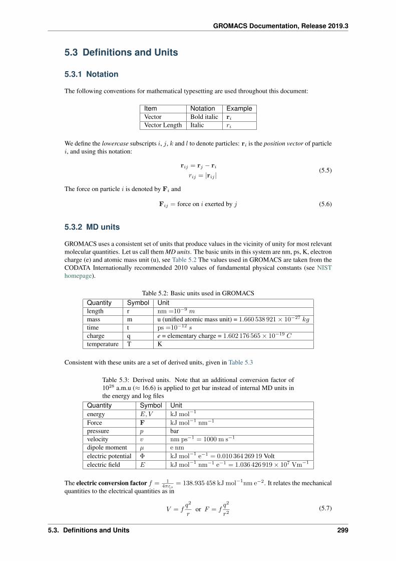
GROMACS Documentation, Release 2019.3
5.3 Definitions and Units
5.3.1 Notation
The following conventions for mathematical typesetting are used throughout this document:
Item Notation ExampleVector Bold italic r𝑖Vector Length Italic 𝑟𝑖
We define the lowercase subscripts 𝑖, 𝑗, 𝑘 and 𝑙 to denote particles: r𝑖 is the position vector of particle𝑖, and using this notation:
r𝑖𝑗 = r𝑗 − r𝑖
𝑟𝑖𝑗 = |r𝑖𝑗 |(5.5)
The force on particle 𝑖 is denoted by F𝑖 and
F𝑖𝑗 = force on 𝑖 exerted by 𝑗 (5.6)
5.3.2 MD units
GROMACS uses a consistent set of units that produce values in the vicinity of unity for most relevantmolecular quantities. Let us call them MD units. The basic units in this system are nm, ps, K, electroncharge (e) and atomic mass unit (u), see Table 5.2 The values used in GROMACS are taken from theCODATA Internationally recommended 2010 values of fundamental physical constants (see NISThomepage).
Table 5.2: Basic units used in GROMACSQuantity Symbol Unitlength r nm =10−9 𝑚mass m u (unified atomic mass unit) = 1.660 538 921 × 10−27 𝑘𝑔time t ps =10−12 𝑠charge q e = elementary charge = 1.602 176 565 × 10−19 𝐶temperature T K
Consistent with these units are a set of derived units, given in Table 5.3
Table 5.3: Derived units. Note that an additional conversion factor of1028 a.m.u (≈ 16.6) is applied to get bar instead of internal MD units inthe energy and log files
Quantity Symbol Unitenergy 𝐸, 𝑉 kJ mol−1
Force F kJ mol−1 nm−1
pressure 𝑝 barvelocity 𝑣 nm ps−1 = 1000 m s−1
dipole moment 𝜇 e nm
electric potential Φ kJ mol−1 e−1 = 0.010 364 269 19 Voltelectric field 𝐸 kJ mol−1 nm−1 e−1 = 1.036 426 919 × 107 Vm−1
The electric conversion factor 𝑓 = 14𝜋𝜀𝑜
= 138.935 458 kJ mol−1nm e−2. It relates the mechanicalquantities to the electrical quantities as in
𝑉 = 𝑓𝑞2
𝑟or 𝐹 = 𝑓
𝑞2
𝑟2(5.7)
5.3. Definitions and Units 299
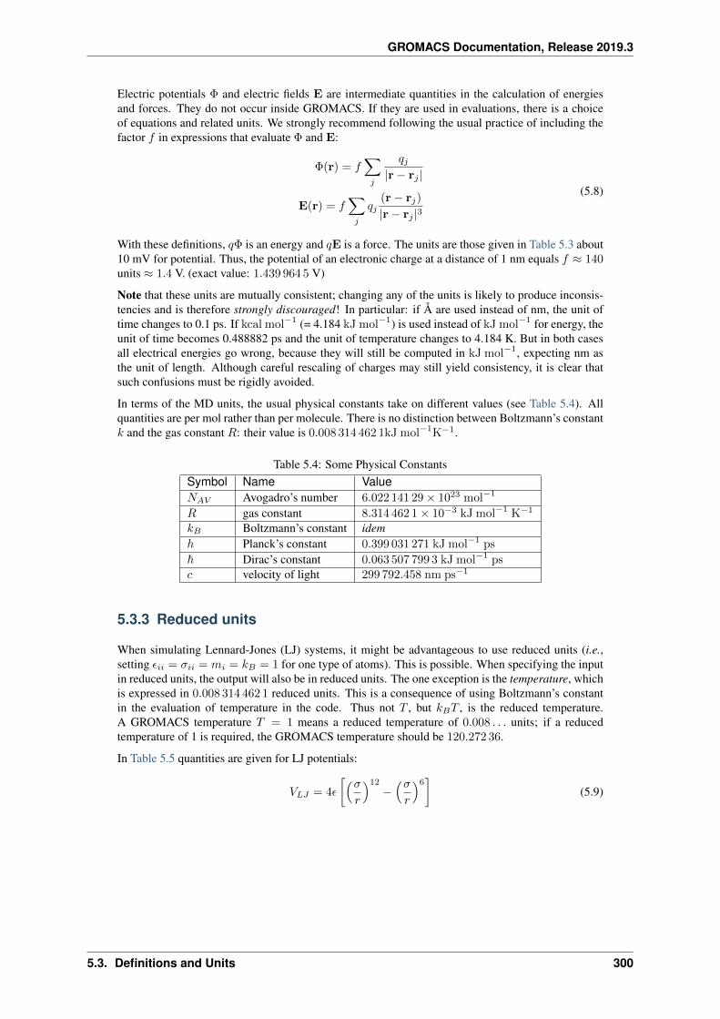
GROMACS Documentation, Release 2019.3
Electric potentials Φ and electric fields E are intermediate quantities in the calculation of energiesand forces. They do not occur inside GROMACS. If they are used in evaluations, there is a choiceof equations and related units. We strongly recommend following the usual practice of including thefactor 𝑓 in expressions that evaluate Φ and E:
Φ(r) = 𝑓∑𝑗
𝑞𝑗|r− r𝑗 |
E(r) = 𝑓∑𝑗
𝑞𝑗(r− r𝑗)
|r− r𝑗 |3(5.8)
With these definitions, 𝑞Φ is an energy and 𝑞E is a force. The units are those given in Table 5.3 about10 mV for potential. Thus, the potential of an electronic charge at a distance of 1 nm equals 𝑓 ≈ 140units ≈ 1.4 V. (exact value: 1.439 964 5 V)
Note that these units are mutually consistent; changing any of the units is likely to produce inconsis-tencies and is therefore strongly discouraged! In particular: if Å are used instead of nm, the unit oftime changes to 0.1 ps. If kcal mol−1 (= 4.184 kJ mol−1) is used instead of kJ mol−1 for energy, theunit of time becomes 0.488882 ps and the unit of temperature changes to 4.184 K. But in both casesall electrical energies go wrong, because they will still be computed in kJ mol−1, expecting nm asthe unit of length. Although careful rescaling of charges may still yield consistency, it is clear thatsuch confusions must be rigidly avoided.
In terms of the MD units, the usual physical constants take on different values (see Table 5.4). Allquantities are per mol rather than per molecule. There is no distinction between Boltzmann’s constant𝑘 and the gas constant 𝑅: their value is 0.008 314 462 1kJ mol−1K−1.
Table 5.4: Some Physical ConstantsSymbol Name Value𝑁𝐴𝑉 Avogadro’s number 6.022 141 29 × 1023 mol−1
𝑅 gas constant 8.314 462 1 × 10⁻³ kJ mol−1 K−1
𝑘𝐵 Boltzmann’s constant idemℎ Planck’s constant 0.399 031 271 kJ mol−1 ps
~ Dirac’s constant 0.063 507 799 3 kJ mol−1 ps𝑐 velocity of light 299 792.458 nm ps−1
5.3.3 Reduced units
When simulating Lennard-Jones (LJ) systems, it might be advantageous to use reduced units (i.e.,setting 𝜖𝑖𝑖 = 𝜎𝑖𝑖 = 𝑚𝑖 = 𝑘𝐵 = 1 for one type of atoms). This is possible. When specifying the inputin reduced units, the output will also be in reduced units. The one exception is the temperature, whichis expressed in 0.008 314 462 1 reduced units. This is a consequence of using Boltzmann’s constantin the evaluation of temperature in the code. Thus not 𝑇 , but 𝑘𝐵𝑇 , is the reduced temperature.A GROMACS temperature 𝑇 = 1 means a reduced temperature of 0.008 . . . units; if a reducedtemperature of 1 is required, the GROMACS temperature should be 120.272 36.
In Table 5.5 quantities are given for LJ potentials:
𝑉𝐿𝐽 = 4𝜖
[(𝜎𝑟
)12−(𝜎𝑟
)6](5.9)
5.3. Definitions and Units 300
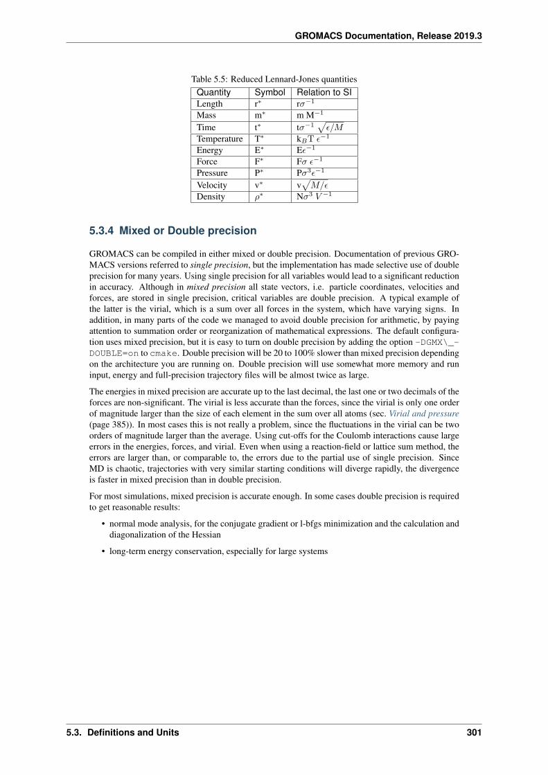
GROMACS Documentation, Release 2019.3
Table 5.5: Reduced Lennard-Jones quantitiesQuantity Symbol Relation to SILength r* r𝜎−1
Mass m* m M−1
Time t* t𝜎−1√𝜖/𝑀
Temperature T* k𝐵T 𝜖−1
Energy E* E𝜖−1
Force F* F𝜎 𝜖−1
Pressure P* P𝜎3𝜖−1
Velocity v* v√𝑀/𝜖
Density 𝜌* N𝜎3 𝑉 −1
5.3.4 Mixed or Double precision
GROMACS can be compiled in either mixed or double precision. Documentation of previous GRO-MACS versions referred to single precision, but the implementation has made selective use of doubleprecision for many years. Using single precision for all variables would lead to a significant reductionin accuracy. Although in mixed precision all state vectors, i.e. particle coordinates, velocities andforces, are stored in single precision, critical variables are double precision. A typical example ofthe latter is the virial, which is a sum over all forces in the system, which have varying signs. Inaddition, in many parts of the code we managed to avoid double precision for arithmetic, by payingattention to summation order or reorganization of mathematical expressions. The default configura-tion uses mixed precision, but it is easy to turn on double precision by adding the option -DGMX\_-DOUBLE=on to cmake. Double precision will be 20 to 100% slower than mixed precision dependingon the architecture you are running on. Double precision will use somewhat more memory and runinput, energy and full-precision trajectory files will be almost twice as large.
The energies in mixed precision are accurate up to the last decimal, the last one or two decimals of theforces are non-significant. The virial is less accurate than the forces, since the virial is only one orderof magnitude larger than the size of each element in the sum over all atoms (sec. Virial and pressure(page 385)). In most cases this is not really a problem, since the fluctuations in the virial can be twoorders of magnitude larger than the average. Using cut-offs for the Coulomb interactions cause largeerrors in the energies, forces, and virial. Even when using a reaction-field or lattice sum method, theerrors are larger than, or comparable to, the errors due to the partial use of single precision. SinceMD is chaotic, trajectories with very similar starting conditions will diverge rapidly, the divergenceis faster in mixed precision than in double precision.
For most simulations, mixed precision is accurate enough. In some cases double precision is requiredto get reasonable results:
• normal mode analysis, for the conjugate gradient or l-bfgs minimization and the calculation anddiagonalization of the Hessian
• long-term energy conservation, especially for large systems
5.3. Definitions and Units 301
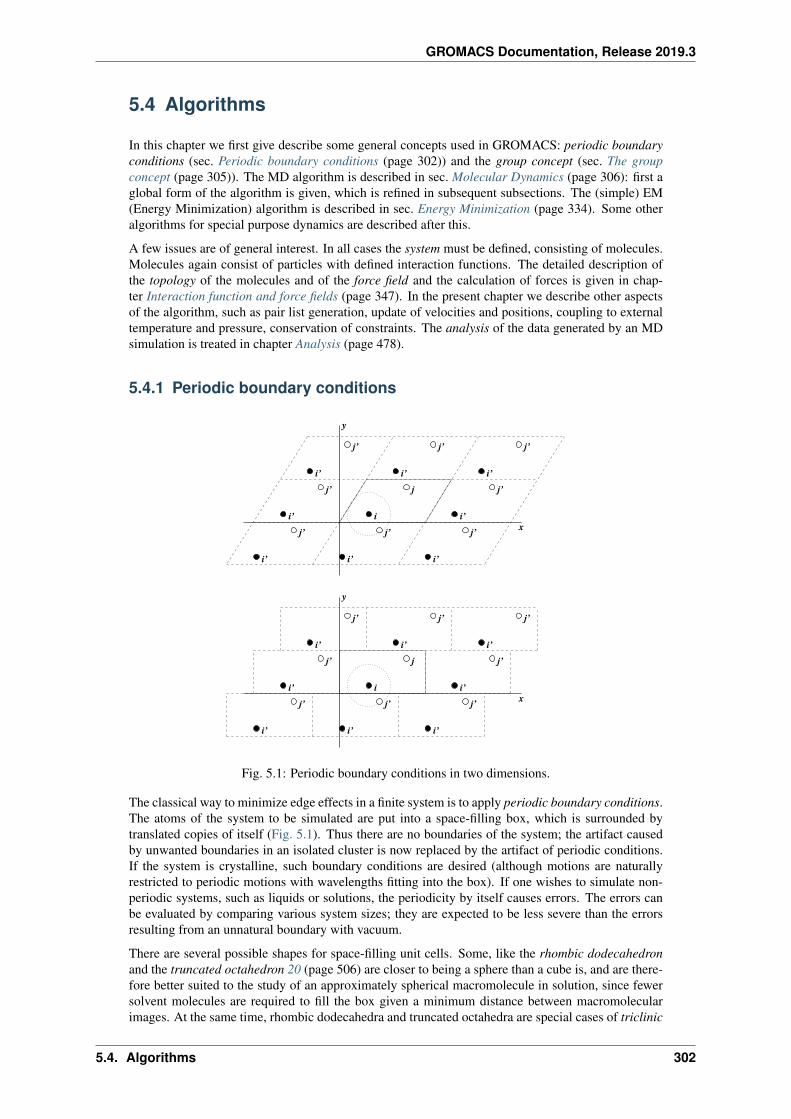
GROMACS Documentation, Release 2019.3
5.4 Algorithms
In this chapter we first give describe some general concepts used in GROMACS: periodic boundaryconditions (sec. Periodic boundary conditions (page 302)) and the group concept (sec. The groupconcept (page 305)). The MD algorithm is described in sec. Molecular Dynamics (page 306): first aglobal form of the algorithm is given, which is refined in subsequent subsections. The (simple) EM(Energy Minimization) algorithm is described in sec. Energy Minimization (page 334). Some otheralgorithms for special purpose dynamics are described after this.
A few issues are of general interest. In all cases the system must be defined, consisting of molecules.Molecules again consist of particles with defined interaction functions. The detailed description ofthe topology of the molecules and of the force field and the calculation of forces is given in chap-ter Interaction function and force fields (page 347). In the present chapter we describe other aspectsof the algorithm, such as pair list generation, update of velocities and positions, coupling to externaltemperature and pressure, conservation of constraints. The analysis of the data generated by an MDsimulation is treated in chapter Analysis (page 478).
5.4.1 Periodic boundary conditions
j’ j’
i’ i’i’
i’
j’
i’ i’
y
x
y
x
j’ j’i’
i’
i’ij’
j’ j’j’i’ii’
j’j’
j’
ji’ i’i’
j’i’ i’
j’
j’j’
j
Fig. 5.1: Periodic boundary conditions in two dimensions.
The classical way to minimize edge effects in a finite system is to apply periodic boundary conditions.The atoms of the system to be simulated are put into a space-filling box, which is surrounded bytranslated copies of itself (Fig. 5.1). Thus there are no boundaries of the system; the artifact causedby unwanted boundaries in an isolated cluster is now replaced by the artifact of periodic conditions.If the system is crystalline, such boundary conditions are desired (although motions are naturallyrestricted to periodic motions with wavelengths fitting into the box). If one wishes to simulate non-periodic systems, such as liquids or solutions, the periodicity by itself causes errors. The errors canbe evaluated by comparing various system sizes; they are expected to be less severe than the errorsresulting from an unnatural boundary with vacuum.
There are several possible shapes for space-filling unit cells. Some, like the rhombic dodecahedronand the truncated octahedron 20 (page 506) are closer to being a sphere than a cube is, and are there-fore better suited to the study of an approximately spherical macromolecule in solution, since fewersolvent molecules are required to fill the box given a minimum distance between macromolecularimages. At the same time, rhombic dodecahedra and truncated octahedra are special cases of triclinic
5.4. Algorithms 302
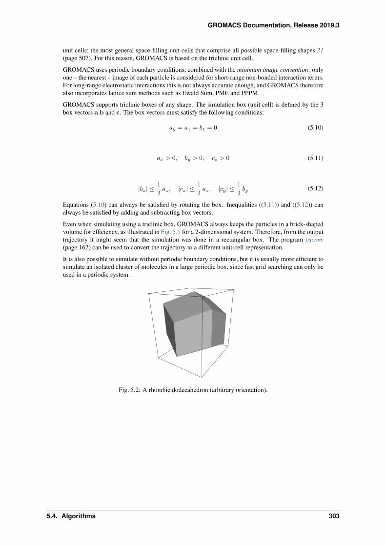
GROMACS Documentation, Release 2019.3
unit cells; the most general space-filling unit cells that comprise all possible space-filling shapes 21(page 507). For this reason, GROMACS is based on the triclinic unit cell.
GROMACS uses periodic boundary conditions, combined with the minimum image convention: onlyone – the nearest – image of each particle is considered for short-range non-bonded interaction terms.For long-range electrostatic interactions this is not always accurate enough, and GROMACS thereforealso incorporates lattice sum methods such as Ewald Sum, PME and PPPM.
GROMACS supports triclinic boxes of any shape. The simulation box (unit cell) is defined by the 3box vectors a,b and c. The box vectors must satisfy the following conditions:
𝑎𝑦 = 𝑎𝑧 = 𝑏𝑧 = 0 (5.10)
𝑎𝑥 > 0, 𝑏𝑦 > 0, 𝑐𝑧 > 0 (5.11)
|𝑏𝑥| ≤1
2𝑎𝑥, |𝑐𝑥| ≤
1
2𝑎𝑥, |𝑐𝑦| ≤
1
2𝑏𝑦 (5.12)
Equations (5.10) can always be satisfied by rotating the box. Inequalities ((5.11)) and ((5.12)) canalways be satisfied by adding and subtracting box vectors.
Even when simulating using a triclinic box, GROMACS always keeps the particles in a brick-shapedvolume for efficiency, as illustrated in Fig. 5.1 for a 2-dimensional system. Therefore, from the outputtrajectory it might seem that the simulation was done in a rectangular box. The program trjconv(page 162) can be used to convert the trajectory to a different unit-cell representation.
It is also possible to simulate without periodic boundary conditions, but it is usually more efficient tosimulate an isolated cluster of molecules in a large periodic box, since fast grid searching can only beused in a periodic system.
Fig. 5.2: A rhombic dodecahedron (arbitrary orientation).
5.4. Algorithms 303
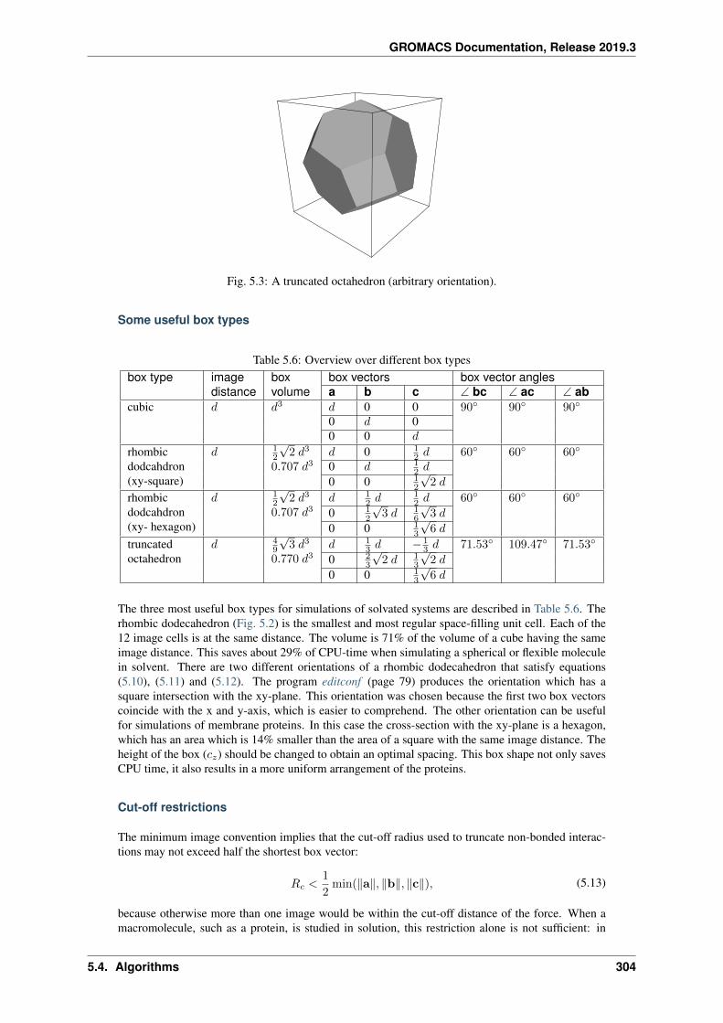
GROMACS Documentation, Release 2019.3
Fig. 5.3: A truncated octahedron (arbitrary orientation).
Some useful box types
Table 5.6: Overview over different box typesbox type image
distanceboxvolume
box vectors box vector anglesa b c ∠ bc ∠ ac ∠ ab
cubic 𝑑 𝑑3 𝑑 0 0 90∘ 90∘ 90∘
0 𝑑 00 0 𝑑
rhombicdodcahdron(xy-square)
𝑑 12
√2 𝑑3
0.707 𝑑3𝑑 0 1
2 𝑑 60∘ 60∘ 60∘
0 𝑑 12 𝑑
0 0 12
√2 𝑑
rhombicdodcahdron(xy- hexagon)
𝑑 12
√2 𝑑3
0.707 𝑑3𝑑 1
2 𝑑12 𝑑 60∘ 60∘ 60∘
0 12
√3 𝑑 1
6
√3 𝑑
0 0 13
√6 𝑑
truncatedoctahedron
𝑑 49
√3 𝑑3
0.770 𝑑3𝑑 1
3 𝑑 − 13 𝑑 71.53∘ 109.47∘ 71.53∘
0 23
√2 𝑑 1
3
√2 𝑑
0 0 13
√6 𝑑
The three most useful box types for simulations of solvated systems are described in Table 5.6. Therhombic dodecahedron (Fig. 5.2) is the smallest and most regular space-filling unit cell. Each of the12 image cells is at the same distance. The volume is 71% of the volume of a cube having the sameimage distance. This saves about 29% of CPU-time when simulating a spherical or flexible moleculein solvent. There are two different orientations of a rhombic dodecahedron that satisfy equations(5.10), (5.11) and (5.12). The program editconf (page 79) produces the orientation which has asquare intersection with the xy-plane. This orientation was chosen because the first two box vectorscoincide with the x and y-axis, which is easier to comprehend. The other orientation can be usefulfor simulations of membrane proteins. In this case the cross-section with the xy-plane is a hexagon,which has an area which is 14% smaller than the area of a square with the same image distance. Theheight of the box (𝑐𝑧) should be changed to obtain an optimal spacing. This box shape not only savesCPU time, it also results in a more uniform arrangement of the proteins.
Cut-off restrictions
The minimum image convention implies that the cut-off radius used to truncate non-bonded interac-tions may not exceed half the shortest box vector:
𝑅𝑐 <1
2min(‖a‖, ‖b‖, ‖c‖), (5.13)
because otherwise more than one image would be within the cut-off distance of the force. When amacromolecule, such as a protein, is studied in solution, this restriction alone is not sufficient: in
5.4. Algorithms 304
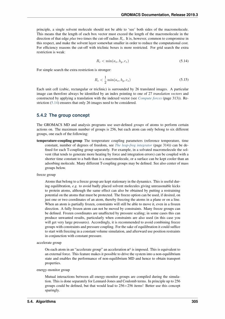
GROMACS Documentation, Release 2019.3
principle, a single solvent molecule should not be able to ‘see’ both sides of the macromolecule.This means that the length of each box vector must exceed the length of the macromolecule in thedirection of that edge plus two times the cut-off radius 𝑅𝑐. It is, however, common to compromise inthis respect, and make the solvent layer somewhat smaller in order to reduce the computational cost.For efficiency reasons the cut-off with triclinic boxes is more restricted. For grid search the extrarestriction is weak:
𝑅𝑐 < min(𝑎𝑥, 𝑏𝑦, 𝑐𝑧) (5.14)
For simple search the extra restriction is stronger:
𝑅𝑐 <1
2min(𝑎𝑥, 𝑏𝑦, 𝑐𝑧) (5.15)
Each unit cell (cubic, rectangular or triclinic) is surrounded by 26 translated images. A particularimage can therefore always be identified by an index pointing to one of 27 translation vectors andconstructed by applying a translation with the indexed vector (see Compute forces (page 313)). Re-striction (5.14) ensures that only 26 images need to be considered.
5.4.2 The group concept
The GROMACS MD and analysis programs use user-defined groups of atoms to perform certainactions on. The maximum number of groups is 256, but each atom can only belong to six differentgroups, one each of the following:
temperature-coupling group The temperature coupling parameters (reference temperature, timeconstant, number of degrees of freedom, see The leap-frog integrator (page 314)) can be de-fined for each T-coupling group separately. For example, in a solvated macromolecule the sol-vent (that tends to generate more heating by force and integration errors) can be coupled with ashorter time constant to a bath than is a macromolecule, or a surface can be kept cooler than anadsorbing molecule. Many different T-coupling groups may be defined. See also center of massgroups below.
freeze group
Atoms that belong to a freeze group are kept stationary in the dynamics. This is useful dur-ing equilibration, e.g. to avoid badly placed solvent molecules giving unreasonable kicksto protein atoms, although the same effect can also be obtained by putting a restrainingpotential on the atoms that must be protected. The freeze option can be used, if desired, onjust one or two coordinates of an atom, thereby freezing the atoms in a plane or on a line.When an atom is partially frozen, constraints will still be able to move it, even in a frozendirection. A fully frozen atom can not be moved by constraints. Many freeze groups canbe defined. Frozen coordinates are unaffected by pressure scaling; in some cases this canproduce unwanted results, particularly when constraints are also used (in this case youwill get very large pressures). Accordingly, it is recommended to avoid combining freezegroups with constraints and pressure coupling. For the sake of equilibration it could sufficeto start with freezing in a constant volume simulation, and afterward use position restraintsin conjunction with constant pressure.
accelerate group
On each atom in an “accelerate group” an acceleration a𝑔 is imposed. This is equivalent toan external force. This feature makes it possible to drive the system into a non-equilibriumstate and enables the performance of non-equilibrium MD and hence to obtain transportproperties.
energy-monitor group
Mutual interactions between all energy-monitor groups are compiled during the simula-tion. This is done separately for Lennard-Jones and Coulomb terms. In principle up to 256groups could be defined, but that would lead to 256×256 items! Better use this conceptsparingly.
5.4. Algorithms 305
GROMACS Documentation, Release 2019.3
All non-bonded interactions between pairs of energy-monitor groups can be excluded (seedetails in the User Guide). Pairs of particles from excluded pairs of energy-monitor groupsare not put into the pair list. This can result in a significant speedup for simulations whereinteractions within or between parts of the system are not required.
center of mass group
In GROMACS, the center of mass (COM) motion can be removed, for either the completesystem or for groups of atoms. The latter is useful, e.g. for systems where there is limitedfriction (e.g. gas systems) to prevent center of mass motion to occur. It makes sense to usethe same groups for temperature coupling and center of mass motion removal.
Compressed position output group
In order to further reduce the size of the compressed trajectory file (xtc (page 432) or tng(page 429)), it is possible to store only a subset of all particles. All x-compression groupsthat are specified are saved, the rest are not. If no such groups are specified, than all atomsare saved to the compressed trajectory file.
The use of groups in GROMACS tools is described in sec. Using Groups (page 478).
5.4.3 Molecular Dynamics
THE GLOBAL MD ALGORITHM
1. Input initial conditionsPotential interaction 𝑉 as a function of atom positionsPositions r of all atoms in the systemVelocities v of all atoms in the system⇓
repeat 2,3,4 for the required number of steps:
2. Compute forcesThe force on any atom
F𝑖 = −𝜕𝑉𝜕r𝑖
is computed by calculating the force between non-bonded atom pairs:F𝑖 =
∑𝑗 F𝑖𝑗
plus the forces due to bonded interactions (which may depend on 1, 2, 3, or 4 atoms), plusrestraining and/or external forces.The potential and kinetic energies and the pressure tensor may be computed.⇓3. Update configurationThe movement of the atoms is simulated by numerically solving Newton’s equations of motion
5.4. Algorithms 306
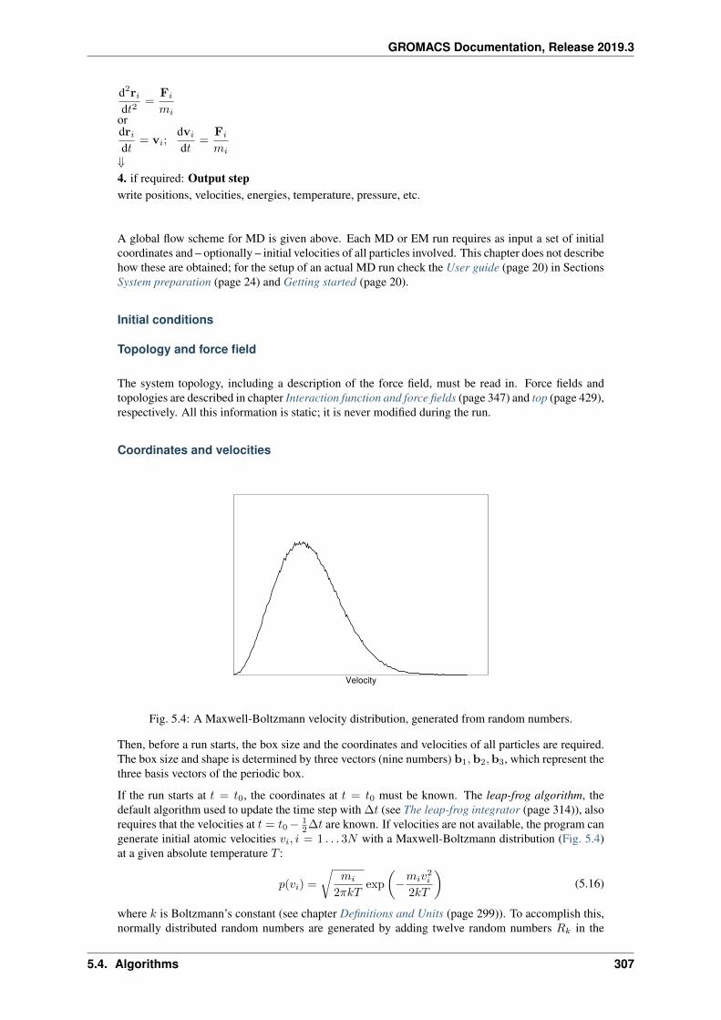
GROMACS Documentation, Release 2019.3
d2r𝑖d𝑡2
=F𝑖
𝑚𝑖ordr𝑖d𝑡
= v𝑖;dv𝑖
d𝑡=
F𝑖
𝑚𝑖
⇓4. if required: Output stepwrite positions, velocities, energies, temperature, pressure, etc.
A global flow scheme for MD is given above. Each MD or EM run requires as input a set of initialcoordinates and – optionally – initial velocities of all particles involved. This chapter does not describehow these are obtained; for the setup of an actual MD run check the User guide (page 20) in SectionsSystem preparation (page 24) and Getting started (page 20).
Initial conditions
Topology and force field
The system topology, including a description of the force field, must be read in. Force fields andtopologies are described in chapter Interaction function and force fields (page 347) and top (page 429),respectively. All this information is static; it is never modified during the run.
Coordinates and velocities
Velocity
Fig. 5.4: A Maxwell-Boltzmann velocity distribution, generated from random numbers.
Then, before a run starts, the box size and the coordinates and velocities of all particles are required.The box size and shape is determined by three vectors (nine numbers) b1,b2,b3, which represent thethree basis vectors of the periodic box.
If the run starts at 𝑡 = 𝑡0, the coordinates at 𝑡 = 𝑡0 must be known. The leap-frog algorithm, thedefault algorithm used to update the time step with ∆𝑡 (see The leap-frog integrator (page 314)), alsorequires that the velocities at 𝑡 = 𝑡0− 1
2∆𝑡 are known. If velocities are not available, the program cangenerate initial atomic velocities 𝑣𝑖, 𝑖 = 1 . . . 3𝑁 with a Maxwell-Boltzmann distribution (Fig. 5.4)at a given absolute temperature 𝑇 :
𝑝(𝑣𝑖) =
√𝑚𝑖
2𝜋𝑘𝑇exp
(−𝑚𝑖𝑣
2𝑖
2𝑘𝑇
)(5.16)
where 𝑘 is Boltzmann’s constant (see chapter Definitions and Units (page 299)). To accomplish this,normally distributed random numbers are generated by adding twelve random numbers 𝑅𝑘 in the
5.4. Algorithms 307
GROMACS Documentation, Release 2019.3
range 0 ≤ 𝑅𝑘 < 1 and subtracting 6.0 from their sum. The result is then multiplied by the standarddeviation of the velocity distribution
√𝑘𝑇/𝑚𝑖. Since the resulting total energy will not correspond
exactly to the required temperature 𝑇 , a correction is made: first the center-of-mass motion is removedand then all velocities are scaled so that the total energy corresponds exactly to 𝑇 (see (5.21)).
Center-of-mass motion
The center-of-mass velocity is normally set to zero at every step; there is (usually) no net externalforce acting on the system and the center-of-mass velocity should remain constant. In practice, how-ever, the update algorithm introduces a very slow change in the center-of-mass velocity, and thereforein the total kinetic energy of the system – especially when temperature coupling is used. If suchchanges are not quenched, an appreciable center-of-mass motion can develop in long runs, and thetemperature will be significantly misinterpreted. Something similar may happen due to overall rota-tional motion, but only when an isolated cluster is simulated. In periodic systems with filled boxes,the overall rotational motion is coupled to other degrees of freedom and does not cause such problems.
Neighbor searching
As mentioned in chapter Interaction function and force fields (page 347), internal forces are eithergenerated from fixed (static) lists, or from dynamic lists. The latter consist of non-bonded interactionsbetween any pair of particles. When calculating the non-bonded forces, it is convenient to have allparticles in a rectangular box. As shown in Fig. 5.1, it is possible to transform a triclinic box into arectangular box. The output coordinates are always in a rectangular box, even when a dodecahedronor triclinic box was used for the simulation. (5.10) ensures that we can reset particles in a rectangularbox by first shifting them with box vector c, then with b and finally with a. Equations (5.12), (5.13)and (5.14) ensure that we can find the 14 nearest triclinic images within a linear combination thatdoes not involve multiples of box vectors.
Pair lists generation
The non-bonded pair forces need to be calculated only for those pairs 𝑖, 𝑗 for which the distance 𝑟𝑖𝑗between 𝑖 and the nearest image of 𝑗 is less than a given cut-off radius 𝑅𝑐. Some of the particle pairsthat fulfill this criterion are excluded, when their interaction is already fully accounted for by bondedinteractions. GROMACS employs a pair list that contains those particle pairs for which non-bondedforces must be calculated. The pair list contains particles 𝑖, a displacement vector for particle 𝑖, andall particles 𝑗 that are within rlist of this particular image of particle 𝑖. The list is updated everynstlist steps.
To make the neighbor list, all particles that are close (i.e. within the neighbor list cut-off) to agiven particle must be found. This searching, usually called neighbor search (NS) or pair search,involves periodic boundary conditions and determining the image (see sec. Periodic boundary con-ditions (page 302)). The search algorithm is 𝑂(𝑁), although a simpler 𝑂(𝑁2) algorithm is stillavailable under some conditions.
Cut-off schemes: group versus Verlet
From version 4.6, GROMACS supports two different cut-off scheme setups: the original one basedon particle groups and one using a Verlet buffer. There are some important differences that affectresults, performance and feature support. The group scheme can be made to work (almost) like theVerlet scheme, but this will lead to a decrease in performance. The group scheme is especially fastfor water molecules, which are abundant in many simulations, but on the most recent x86 processors,this advantage is negated by the better instruction-level parallelism available in the Verlet-schemeimplementation. The group scheme is deprecated in version 5.0, and will be removed in a futureversion. For practical details of choosing and setting up cut-off schemes, please see the User Guide.
5.4. Algorithms 308
GROMACS Documentation, Release 2019.3
In the group scheme, a neighbor list is generated consisting of pairs of groups of at least one particle.These groups were originally charge groups (see sec. Charge groups (page 313)), but with a propertreatment of long-range electrostatics, performance in unbuffered simulations is their only advantage.A pair of groups is put into the neighbor list when their center of geometry is within the cut-offdistance. Interactions between all particle pairs (one from each charge group) are calculated for acertain number of MD steps, until the neighbor list is updated. This setup is efficient, as the neighborsearch only checks distance between charge-group pair, not particle pairs (saves a factor of 3× 3 = 9with a three-particle water model) and the non-bonded force kernels can be optimized for, say, a watermolecule “group”. Without explicit buffering, this setup leads to energy drift as some particle pairswhich are within the cut-off don’t interact and some outside the cut-off do interact. This can be causedby
• particles moving across the cut-off between neighbor search steps, and/or
• for charge groups consisting of more than one particle, particle pairs moving in/out of the cut-offwhen their charge group center of geometry distance is outside/inside of the cut-off.
Explicitly adding a buffer to the neighbor list will remove such artifacts, but this comes at a highcomputational cost. How severe the artifacts are depends on the system, the properties in which youare interested, and the cut-off setup.
The Verlet cut-off scheme uses a buffered pair list by default. It also uses clusters of particles, butthese are not static as in the group scheme. Rather, the clusters are defined spatially and consist of 4or 8 particles, which is convenient for stream computing, using e.g. SSE, AVX or CUDA on GPUs.At neighbor search steps, a pair list is created with a Verlet buffer, ie. the pair-list cut-off is larger thanthe interaction cut-off. In the non-bonded kernels, interactions are only computed when a particle pairis within the cut-off distance at that particular time step. This ensures that as particles move betweenpair search steps, forces between nearly all particles within the cut-off distance are calculated. Wesay nearly all particles, because GROMACS uses a fixed pair list update frequency for efficiency. Aparticle-pair, whose distance was outside the cut-off, could possibly move enough during this fixednumber of steps that its distance is now within the cut-off. This small chance results in a small energydrift, and the size of the chance depends on the temperature. When temperature coupling is used, thebuffer size can be determined automatically, given a certain tolerance on the energy drift.
The Verlet cut-off scheme is implemented in a very efficient fashion based on clusters of particles. Thesimplest example is a cluster size of 4 particles. The pair list is then constructed based on cluster pairs.The cluster-pair search is much faster searching based on particle pairs, because 4 × 4 = 16 particlepairs are put in the list at once. The non-bonded force calculation kernel can then calculate manyparticle-pair interactions at once, which maps nicely to SIMD or SIMT units on modern hardware,which can perform multiple floating operations at once. These non-bonded kernels are much fasterthan the kernels used in the group scheme for most types of systems, particularly on newer hardware.
Additionally, when the list buffer is determined automatically as described below, we also applydynamic pair list pruning. The pair list can be constructed infrequently, but that can lead to a lotof pairs in the list that are outside the cut-off range for all or most of the life time of this pair list.Such pairs can be pruned out by applying a cluster-pair kernel that only determines which clustersare in range. Because of the way the non-bonded data is regularized in GROMACS, this kernel isan order of magnitude faster than the search and the interaction kernel. On the GPU this pruning isoverlapped with the integration on the CPU, so it is free in most cases. Therefore we can prune every4-10 integration steps with little overhead and significantly reduce the number of cluster pairs in theinteraction kernel. This procedure is applied automatically, unless the user set the pair-list buffer sizemanually.
Energy drift and pair-list buffering
For a canonical (NVT) ensemble, the average energy error caused by diffusion of 𝑗 particles fromoutside the pair-list cut-off 𝑟ℓ to inside the interaction cut-off 𝑟𝑐 over the lifetime of the list canbe determined from the atomic displacements and the shape of the potential at the cut-off. Thedisplacement distribution along one dimension for a freely moving particle with mass 𝑚 over time 𝑡at temperature 𝑇 is a Gaussian 𝐺(𝑥) of zero mean and variance 𝜎2 = 𝑡2𝑘𝐵𝑇/𝑚. For the distance
5.4. Algorithms 309
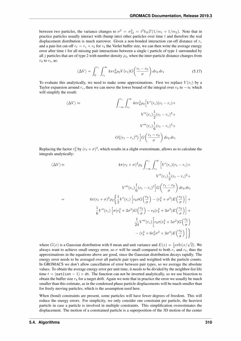
GROMACS Documentation, Release 2019.3
between two particles, the variance changes to 𝜎2 = 𝜎212 = 𝑡2𝑘𝐵𝑇 (1/𝑚1 + 1/𝑚2). Note that in
practice particles usually interact with (bump into) other particles over time 𝑡 and therefore the realdisplacement distribution is much narrower. Given a non-bonded interaction cut-off distance of 𝑟𝑐and a pair-list cut-off 𝑟ℓ = 𝑟𝑐 + 𝑟𝑏 for 𝑟𝑏 the Verlet buffer size, we can then write the average energyerror after time 𝑡 for all missing pair interactions between a single 𝑖 particle of type 1 surrounded byall 𝑗 particles that are of type 2 with number density 𝜌2, when the inter-particle distance changes from𝑟0 to 𝑟𝑡, as:
⟨∆𝑉 ⟩ =
∫ 𝑟𝑐
0
∫ ∞
𝑟ℓ
4𝜋𝑟20𝜌2𝑉 (𝑟𝑡)𝐺
(𝑟𝑡 − 𝑟0𝜎
)𝑑𝑟0 𝑑𝑟𝑡 (5.17)
To evaluate this analytically, we need to make some approximations. First we replace 𝑉 (𝑟𝑡) by aTaylor expansion around 𝑟𝑐, then we can move the lower bound of the integral over 𝑟0 to −∞ whichwill simplify the result:
⟨∆𝑉 ⟩ ≈∫ 𝑟𝑐
−∞
∫ ∞
𝑟ℓ
4𝜋𝑟20𝜌2
[𝑉 ′(𝑟𝑐)(𝑟𝑡 − 𝑟𝑐)+
𝑉 ′′(𝑟𝑐)1
2(𝑟𝑡 − 𝑟𝑐)
2+
𝑉 ′′′(𝑟𝑐)1
6(𝑟𝑡 − 𝑟𝑐)
3+
𝑂((𝑟𝑡 − 𝑟𝑐)
4) ]𝐺
(𝑟𝑡 − 𝑟0𝜎
)𝑑𝑟0 𝑑𝑟𝑡
Replacing the factor 𝑟20 by (𝑟ℓ + 𝜎)2, which results in a slight overestimate, allows us to calculate theintegrals analytically:
⟨∆𝑉 ⟩≈ 4𝜋(𝑟ℓ + 𝜎)2𝜌2
∫ 𝑟𝑐
−∞
∫ ∞
𝑟ℓ
[𝑉 ′(𝑟𝑐)(𝑟𝑡 − 𝑟𝑐)+
𝑉 ′′(𝑟𝑐)1
2(𝑟𝑡 − 𝑟𝑐)
2+
𝑉 ′′′(𝑟𝑐)1
6(𝑟𝑡 − 𝑟𝑐)
3]𝐺
(𝑟𝑡 − 𝑟0𝜎
)𝑑𝑟0 𝑑𝑟𝑡
= 4𝜋(𝑟ℓ + 𝜎)2𝜌2
{1
2𝑉 ′(𝑟𝑐)
[𝑟𝑏𝜎𝐺
(𝑟𝑏𝜎
)− (𝑟2𝑏 + 𝜎2)𝐸
(𝑟𝑏𝜎
)]+
1
6𝑉 ′′(𝑟𝑐)
[𝜎(𝑟2𝑏 + 2𝜎2)𝐺
(𝑟𝑏𝜎
)− 𝑟𝑏(𝑟
2𝑏 + 3𝜎2)𝐸
(𝑟𝑏𝜎
)]+
1
24𝑉 ′′′(𝑟𝑐)
[𝑟𝑏𝜎(𝑟2𝑏 + 5𝜎2)𝐺
(𝑟𝑏𝜎
)− (𝑟4𝑏 + 6𝑟2𝑏𝜎
2 + 3𝜎4)𝐸(𝑟𝑏𝜎
)]}where 𝐺(𝑥) is a Gaussian distribution with 0 mean and unit variance and 𝐸(𝑥) = 1
2erfc(𝑥/√
2). Wealways want to achieve small energy error, so 𝜎 will be small compared to both 𝑟𝑐 and 𝑟ℓ, thus theapproximations in the equations above are good, since the Gaussian distribution decays rapidly. Theenergy error needs to be averaged over all particle pair types and weighted with the particle counts.In GROMACS we don’t allow cancellation of error between pair types, so we average the absolutevalues. To obtain the average energy error per unit time, it needs to be divided by the neighbor-list lifetime 𝑡 = (nstlist − 1) × dt. The function can not be inverted analytically, so we use bisection toobtain the buffer size 𝑟𝑏 for a target drift. Again we note that in practice the error we usually be muchsmaller than this estimate, as in the condensed phase particle displacements will be much smaller thanfor freely moving particles, which is the assumption used here.
When (bond) constraints are present, some particles will have fewer degrees of freedom. This willreduce the energy errors. For simplicity, we only consider one constraint per particle, the heaviestparticle in case a particle is involved in multiple constraints. This simplification overestimates thedisplacement. The motion of a constrained particle is a superposition of the 3D motion of the center
5.4. Algorithms 310
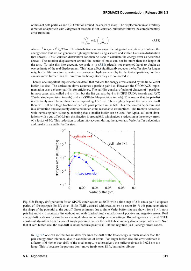
GROMACS Documentation, Release 2019.3
of mass of both particles and a 2D rotation around the center of mass. The displacement in an arbitrarydirection of a particle with 2 degrees of freedom is not Gaussian, but rather follows the complementaryerror function:
√𝜋
2√
2𝜎erfc
(|𝑟|√2𝜎
)(5.18)
where 𝜎2 is again 𝑡2𝑘𝐵𝑇/𝑚. This distribution can no longer be integrated analytically to obtain theenergy error. But we can generate a tight upper bound using a scaled and shifted Gaussian distribution(not shown). This Gaussian distribution can then be used to calculate the energy error as describedabove. The rotation displacement around the center of mass can not be more than the length ofthe arm. To take this into account, we scale 𝜎 in (5.18) (details not presented here) to obtain anoverestimate of the real displacement. This latter effect significantly reduces the buffer size for longerneighborlist lifetimes in e.g. water, as constrained hydrogens are by far the fastest particles, but theycan not move further than 0.1 nm from the heavy atom they are connected to.
There is one important implementation detail that reduces the energy errors caused by the finite Verletbuffer list size. The derivation above assumes a particle pair-list. However, the GROMACS imple-mentation uses a cluster pair-list for efficiency. The pair list consists of pairs of clusters of 4 particlesin most cases, also called a 4 × 4 list, but the list can also be 4 × 8 (GPU CUDA kernels and AVX256-bit single precision kernels) or 4×2 (SSE double-precision kernels). This means that the pair-listis effectively much larger than the corresponding 1 × 1 list. Thus slightly beyond the pair-list cut-offthere will still be a large fraction of particle pairs present in the list. This fraction can be determinedin a simulation and accurately estimated under some reasonable assumptions. The fraction decreaseswith increasing pair-list range, meaning that a smaller buffer can be used. For typical all-atom simu-lations with a cut-off of 0.9 nm this fraction is around 0.9, which gives a reduction in the energy errorsof a factor of 10. This reduction is taken into account during the automatic Verlet buffer calculationand results in a smaller buffer size.
0 0.02 0.04 0.06 0.08 0.1Verlet buffer (nm)
10−6
10−5
10−4
10−3
10−2
drift
per
ato
m (k
J/m
ol/p
s) estimate 1x1
estimate 4x4
double precision
mixed precision
Fig. 5.5: Energy drift per atom for an SPC/E water system at 300K with a time step of 2 fs and a pair-list updateperiod of 10 steps (pair-list life time: 18 fs). PME was used with ewald-rtol set to 10−5; this parameter affectsthe shape of the potential at the cut-off. Error estimates due to finite Verlet buffer size are shown for a 1 × 1 atompair list and 4 × 4 atom pair list without and with (dashed line) cancellation of positive and negative errors. Realenergy drift is shown for simulations using double- and mixed-precision settings. Rounding errors in the SETTLEconstraint algorithm from the use of single precision causes the drift to become negative at large buffer size. Notethat at zero buffer size, the real drift is small because positive (H-H) and negative (O-H) energy errors cancel.
In Fig. 5.5 one can see that for small buffer sizes the drift of the total energy is much smaller than thepair energy error tolerance, due to cancellation of errors. For larger buffer size, the error estimate isa factor of 6 higher than drift of the total energy, or alternatively the buffer estimate is 0.024 nm toolarge. This is because the protons don’t move freely over 18 fs, but rather vibrate.
5.4. Algorithms 311
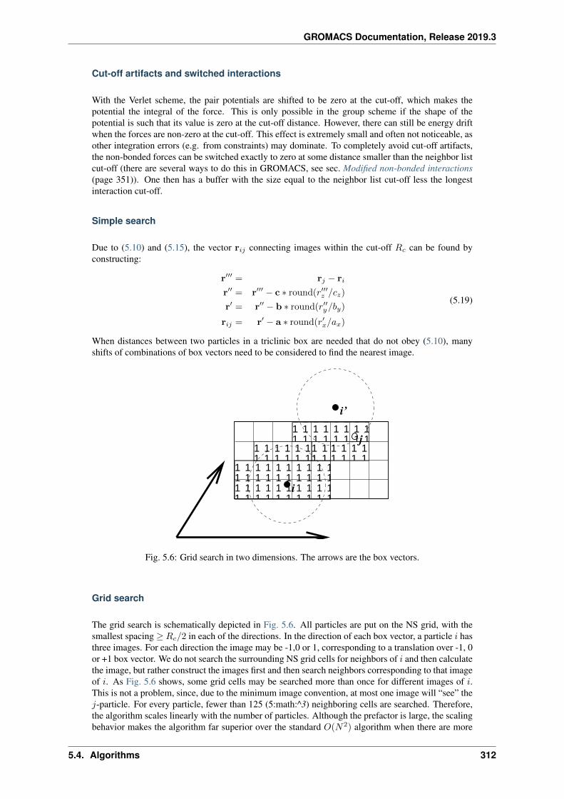
GROMACS Documentation, Release 2019.3
Cut-off artifacts and switched interactions
With the Verlet scheme, the pair potentials are shifted to be zero at the cut-off, which makes thepotential the integral of the force. This is only possible in the group scheme if the shape of thepotential is such that its value is zero at the cut-off distance. However, there can still be energy driftwhen the forces are non-zero at the cut-off. This effect is extremely small and often not noticeable, asother integration errors (e.g. from constraints) may dominate. To completely avoid cut-off artifacts,the non-bonded forces can be switched exactly to zero at some distance smaller than the neighbor listcut-off (there are several ways to do this in GROMACS, see sec. Modified non-bonded interactions(page 351)). One then has a buffer with the size equal to the neighbor list cut-off less the longestinteraction cut-off.
Simple search
Due to (5.10) and (5.15), the vector r𝑖𝑗 connecting images within the cut-off 𝑅𝑐 can be found byconstructing:
r′′′ = r𝑗 − r𝑖
r′′ = r′′′ − c * round(𝑟′′′𝑧 /𝑐𝑧)
r′ = r′′ − b * round(𝑟′′𝑦/𝑏𝑦)
r𝑖𝑗 = r′ − a * round(𝑟′𝑥/𝑎𝑥)
(5.19)
When distances between two particles in a triclinic box are needed that do not obey (5.10), manyshifts of combinations of box vectors need to be considered to find the nearest image.
0 0 0 00 0 0 01 1 1 11 1 1 1
0 0 0 0 0 0 0 0 00 0 0 0 0 0 0 0 00 0 0 0 0 0 0 0 0
1 1 1 1 1 1 1 1 11 1 1 1 1 1 1 1 11 1 1 1 1 1 1 1 1
0 0 0 0 0 0 0 0 0 0 00 0 0 0 0 0 0 0 0 0 00 0 0 0 0 0 0 0 0 0 00 0 0 0 0 0 0 0 0 0 0
1 1 1 1 1 1 1 1 1 1 11 1 1 1 1 1 1 1 1 1 11 1 1 1 1 1 1 1 1 1 11 1 1 1 1 1 1 1 1 1 1
0 0 0 0 0 00 0 0 0 0 01 1 1 1 1 11 1 1 1 1 1
0 0 00 0 01 1 11 1 1
j
i
i’
0 0 0 0 00 0 0 0 00 0 0 0 00 0 0 0 00 0 0 0 00 0 0 0 00 0 0 0 00 0 0 0 0
1 1 1 1 11 1 1 1 11 1 1 1 11 1 1 1 11 1 1 1 11 1 1 1 11 1 1 1 11 1 1 1 1
Fig. 5.6: Grid search in two dimensions. The arrows are the box vectors.
Grid search
The grid search is schematically depicted in Fig. 5.6. All particles are put on the NS grid, with thesmallest spacing ≥ 𝑅𝑐/2 in each of the directions. In the direction of each box vector, a particle 𝑖 hasthree images. For each direction the image may be -1,0 or 1, corresponding to a translation over -1, 0or +1 box vector. We do not search the surrounding NS grid cells for neighbors of 𝑖 and then calculatethe image, but rather construct the images first and then search neighbors corresponding to that imageof 𝑖. As Fig. 5.6 shows, some grid cells may be searched more than once for different images of 𝑖.This is not a problem, since, due to the minimum image convention, at most one image will “see” the𝑗-particle. For every particle, fewer than 125 (5:math:^3) neighboring cells are searched. Therefore,the algorithm scales linearly with the number of particles. Although the prefactor is large, the scalingbehavior makes the algorithm far superior over the standard 𝑂(𝑁2) algorithm when there are more
5.4. Algorithms 312
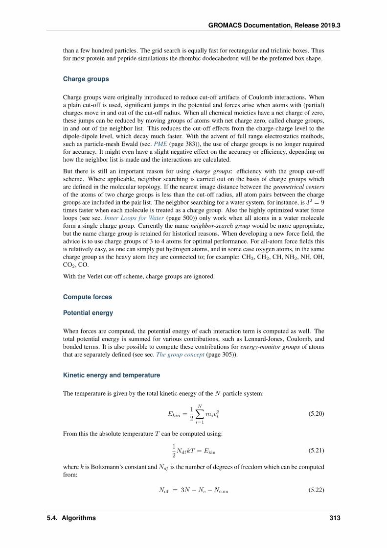
GROMACS Documentation, Release 2019.3
than a few hundred particles. The grid search is equally fast for rectangular and triclinic boxes. Thusfor most protein and peptide simulations the rhombic dodecahedron will be the preferred box shape.
Charge groups
Charge groups were originally introduced to reduce cut-off artifacts of Coulomb interactions. Whena plain cut-off is used, significant jumps in the potential and forces arise when atoms with (partial)charges move in and out of the cut-off radius. When all chemical moieties have a net charge of zero,these jumps can be reduced by moving groups of atoms with net charge zero, called charge groups,in and out of the neighbor list. This reduces the cut-off effects from the charge-charge level to thedipole-dipole level, which decay much faster. With the advent of full range electrostatics methods,such as particle-mesh Ewald (sec. PME (page 383)), the use of charge groups is no longer requiredfor accuracy. It might even have a slight negative effect on the accuracy or efficiency, depending onhow the neighbor list is made and the interactions are calculated.
But there is still an important reason for using charge groups: efficiency with the group cut-offscheme. Where applicable, neighbor searching is carried out on the basis of charge groups whichare defined in the molecular topology. If the nearest image distance between the geometrical centersof the atoms of two charge groups is less than the cut-off radius, all atom pairs between the chargegroups are included in the pair list. The neighbor searching for a water system, for instance, is 32 = 9times faster when each molecule is treated as a charge group. Also the highly optimized water forceloops (see sec. Inner Loops for Water (page 500)) only work when all atoms in a water moleculeform a single charge group. Currently the name neighbor-search group would be more appropriate,but the name charge group is retained for historical reasons. When developing a new force field, theadvice is to use charge groups of 3 to 4 atoms for optimal performance. For all-atom force fields thisis relatively easy, as one can simply put hydrogen atoms, and in some case oxygen atoms, in the samecharge group as the heavy atom they are connected to; for example: CH3, CH2, CH, NH2, NH, OH,CO2, CO.
With the Verlet cut-off scheme, charge groups are ignored.
Compute forces
Potential energy
When forces are computed, the potential energy of each interaction term is computed as well. Thetotal potential energy is summed for various contributions, such as Lennard-Jones, Coulomb, andbonded terms. It is also possible to compute these contributions for energy-monitor groups of atomsthat are separately defined (see sec. The group concept (page 305)).
Kinetic energy and temperature
The temperature is given by the total kinetic energy of the 𝑁 -particle system:
𝐸𝑘𝑖𝑛 =1
2
𝑁∑𝑖=1
𝑚𝑖𝑣2𝑖 (5.20)
From this the absolute temperature 𝑇 can be computed using:
1
2𝑁df𝑘𝑇 = 𝐸kin (5.21)
where 𝑘 is Boltzmann’s constant and𝑁𝑑𝑓 is the number of degrees of freedom which can be computedfrom:
𝑁df = 3𝑁 −𝑁𝑐 −𝑁com (5.22)
5.4. Algorithms 313
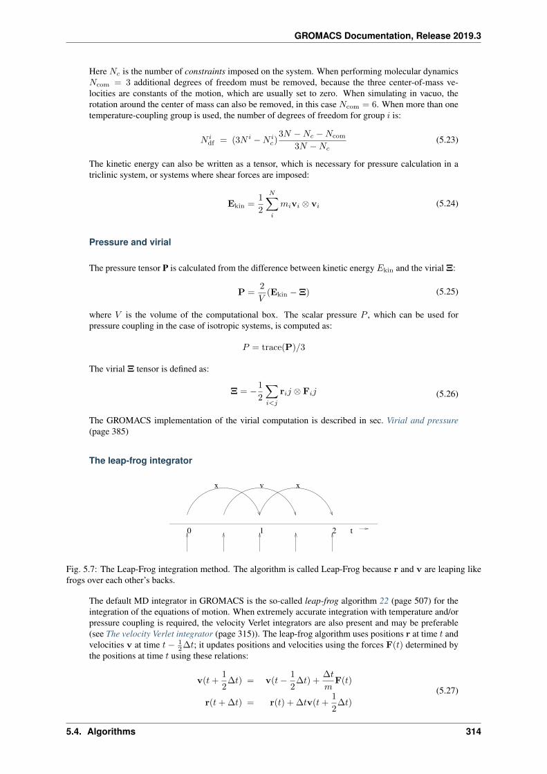
GROMACS Documentation, Release 2019.3
Here 𝑁𝑐 is the number of constraints imposed on the system. When performing molecular dynamics𝑁com = 3 additional degrees of freedom must be removed, because the three center-of-mass ve-locities are constants of the motion, which are usually set to zero. When simulating in vacuo, therotation around the center of mass can also be removed, in this case 𝑁com = 6. When more than onetemperature-coupling group is used, the number of degrees of freedom for group 𝑖 is:
𝑁 𝑖df = (3𝑁 𝑖 −𝑁 𝑖
𝑐)3𝑁 −𝑁𝑐 −𝑁com
3𝑁 −𝑁𝑐(5.23)
The kinetic energy can also be written as a tensor, which is necessary for pressure calculation in atriclinic system, or systems where shear forces are imposed:
Ekin =1
2
𝑁∑𝑖
𝑚𝑖v𝑖 ⊗ v𝑖 (5.24)
Pressure and virial
The pressure tensor P is calculated from the difference between kinetic energy 𝐸kin and the virial Ξ:
P =2
𝑉(Ekin −Ξ) (5.25)
where 𝑉 is the volume of the computational box. The scalar pressure 𝑃 , which can be used forpressure coupling in the case of isotropic systems, is computed as:
𝑃 = trace(P)/3
The virial Ξ tensor is defined as:
Ξ = −1
2
∑𝑖<𝑗
r𝑖𝑗 ⊗ F𝑖𝑗 (5.26)
The GROMACS implementation of the virial computation is described in sec. Virial and pressure(page 385)
The leap-frog integrator
1 20 t
x v x
Fig. 5.7: The Leap-Frog integration method. The algorithm is called Leap-Frog because r and v are leaping likefrogs over each other’s backs.
The default MD integrator in GROMACS is the so-called leap-frog algorithm 22 (page 507) for theintegration of the equations of motion. When extremely accurate integration with temperature and/orpressure coupling is required, the velocity Verlet integrators are also present and may be preferable(see The velocity Verlet integrator (page 315)). The leap-frog algorithm uses positions r at time 𝑡 andvelocities v at time 𝑡− 1
2∆𝑡; it updates positions and velocities using the forces F(𝑡) determined bythe positions at time 𝑡 using these relations:
v(𝑡+1
2∆𝑡) = v(𝑡− 1
2∆𝑡) +
∆𝑡
𝑚F(𝑡)
r(𝑡+ ∆𝑡) = r(𝑡) + ∆𝑡v(𝑡+1
2∆𝑡)
(5.27)
5.4. Algorithms 314
GROMACS Documentation, Release 2019.3
The algorithm is visualized in Fig. 5.7. It produces trajectories that are identical to the Verlet 23(page 507) algorithm, whose position-update relation is
r(𝑡+ ∆𝑡) = 2r(𝑡) − r(𝑡− ∆𝑡) +1
𝑚F(𝑡)∆𝑡2 +𝑂(∆𝑡4) (5.28)
The algorithm is of third order in r and is time-reversible. See ref. 24 (page 507) for the merits of thisalgorithm and comparison with other time integration algorithms.
The equations of motion are modified for temperature coupling and pressure coupling, and extendedto include the conservation of constraints, all of which are described below.
The velocity Verlet integrator
The velocity Verlet algorithm25 (page 507) is also implemented in GROMACS, though it is not yetfully integrated with all sets of options. In velocity Verlet, positions r and velocities v at time 𝑡 areused to integrate the equations of motion; velocities at the previous half step are not required.
v(𝑡+1
2∆𝑡) = v(𝑡) +
∆𝑡
2𝑚F(𝑡)
r(𝑡+ ∆𝑡) = r(𝑡) + ∆𝑡v(𝑡+1
2∆𝑡)
v(𝑡+ ∆𝑡) = v(𝑡+1
2∆𝑡) +
∆𝑡
2𝑚F(𝑡+ ∆𝑡)
(5.29)
or, equivalently,
r(𝑡+ ∆𝑡) = r(𝑡) + ∆𝑡v +∆𝑡2
2𝑚F(𝑡)
v(𝑡+ ∆𝑡) = v(𝑡) +∆𝑡
2𝑚[F(𝑡) + F(𝑡+ ∆𝑡)]
(5.30)
With no temperature or pressure coupling, and with corresponding starting points, leap-frog andvelocity Verlet will generate identical trajectories, as can easily be verified by hand from the equationsabove. Given a single starting file with the same starting point x(0) and v(0), leap-frog and velocityVerlet will not give identical trajectories, as leap-frog will interpret the velocities as corresponding to𝑡 = − 1
2∆𝑡, while velocity Verlet will interpret them as corresponding to the timepoint 𝑡 = 0.
Understanding reversible integrators: The Trotter decomposition
To further understand the relationship between velocity Verlet and leap-frog integration, we introducethe reversible Trotter formulation of dynamics, which is also useful to understanding implementationsof thermostats and barostats in GROMACS.
A system of coupled, first-order differential equations can be evolved from time 𝑡 = 0 to time 𝑡 byapplying the evolution operator
Γ(𝑡) = exp(𝑖𝐿𝑡)Γ(0)
𝑖𝐿 = Γ · ∇Γ,
where 𝐿 is the Liouville operator, and Γ is the multidimensional vector of independent variables(positions and velocities). A short-time approximation to the true operator, accurate at time ∆𝑡 =𝑡/𝑃 , is applied 𝑃 times in succession to evolve the system as
Γ(𝑡) =
𝑃∏𝑖=1
exp(𝑖𝐿∆𝑡)Γ(0) (5.31)
For NVE dynamics, the Liouville operator is
𝑖𝐿 =
𝑁∑𝑖=1
v𝑖 · ∇r𝑖 +
𝑁∑𝑖=1
1
𝑚𝑖F(𝑟𝑖) · ∇v𝑖 . (5.32)
5.4. Algorithms 315
GROMACS Documentation, Release 2019.3
This can be split into two additive operators
𝑖𝐿1 =
𝑁∑𝑖=1
1
𝑚𝑖F(𝑟𝑖) · ∇v𝑖
𝑖𝐿2 =
𝑁∑𝑖=1
v𝑖 · ∇r𝑖
Then a short-time, symmetric, and thus reversible approximation of the true dynamics will be
exp(𝑖𝐿∆𝑡) = exp(𝑖𝐿21
2∆𝑡) exp(𝑖𝐿1∆𝑡) exp(𝑖𝐿2
1
2∆𝑡) + 𝒪(∆𝑡3). (5.33)
This corresponds to velocity Verlet integration. The first exponential term over 12∆𝑡 corresponds to
a velocity half-step, the second exponential term over ∆𝑡 corresponds to a full velocity step, and thelast exponential term over 1
2∆𝑡 is the final velocity half step. For future times 𝑡 = 𝑛∆𝑡, this becomes
exp(𝑖𝐿𝑛∆𝑡) ≈(
exp(𝑖𝐿21
2∆𝑡) exp(𝑖𝐿1∆𝑡) exp(𝑖𝐿2
1
2∆𝑡)
)𝑛
≈ exp(𝑖𝐿21
2∆𝑡)
(exp(𝑖𝐿1∆𝑡) exp(𝑖𝐿2∆𝑡)
)𝑛−1
exp(𝑖𝐿1∆𝑡) exp(𝑖𝐿21
2∆𝑡)
This formalism allows us to easily see the difference between the different flavors of Verlet integrators.The leap-frog integrator can be seen as starting with (5.33) with the exp (𝑖𝐿1∆𝑡) term, instead of thehalf-step velocity term, yielding
exp(𝑖𝐿𝑛∆𝑡) = exp (𝑖𝐿1∆𝑡) exp (𝑖𝐿2∆𝑡) + 𝒪(∆𝑡3). (5.34)
Here, the full step in velocity is between 𝑡− 12∆𝑡 and 𝑡+ 1
2∆𝑡, since it is a combination of the velocityhalf steps in velocity Verlet. For future times 𝑡 = 𝑛∆𝑡, this becomes
exp(𝑖𝐿𝑛∆𝑡) ≈(
exp (𝑖𝐿1∆𝑡) exp (𝑖𝐿2∆𝑡)
)𝑛
. (5.35)
Although at first this does not appear symmetric, as long as the full velocity step is between 𝑡− 12∆𝑡
and 𝑡+ 12∆𝑡, then this is simply a way of starting velocity Verlet at a different place in the cycle.
Even though the trajectory and thus potential energies are identical between leap-frog and velocityVerlet, the kinetic energy and temperature will not necessarily be the same. Standard velocity Verletuses the velocities at the 𝑡 to calculate the kinetic energy and thus the temperature only at time 𝑡; thekinetic energy is then a sum over all particles
𝐾𝐸full(𝑡) =∑𝑖
(1
2𝑚𝑖v𝑖(𝑡)
)2
=∑𝑖
1
2𝑚𝑖
(1
2v𝑖(𝑡−
1
2∆𝑡) +
1
2v𝑖(𝑡+
1
2∆𝑡)
)2
,
with the square on the outside of the average. Standard leap-frog calculates the kinetic energy at time𝑡 based on the average kinetic energies at the timesteps 𝑡 + 1
2∆𝑡 and 𝑡 − 12∆𝑡, or the sum over all
particles
𝐾𝐸average(𝑡) =∑𝑖
1
2𝑚𝑖
(1
2v𝑖(𝑡−
1
2∆𝑡)2 +
1
2v𝑖(𝑡+
1
2∆𝑡)2
), (5.36)
where the square is inside the average.
A non-standard variant of velocity Verlet which averages the kinetic energies 𝐾𝐸(𝑡 + 12∆𝑡) and
𝐾𝐸(𝑡 − 12∆𝑡), exactly like leap-frog, is also now implemented in GROMACS (as mdp (page 425)
5.4. Algorithms 316
GROMACS Documentation, Release 2019.3
file option integrator=md-vv-avek (page 202)). Without temperature and pressure coupling,velocity Verlet with half-step-averaged kinetic energies and leap-frog will be identical up to numer-ical precision. For temperature- and pressure-control schemes, however, velocity Verlet with half-step-averaged kinetic energies and leap-frog will be different, as will be discussed in the section inthermostats and barostats.
The half-step-averaged kinetic energy and temperature are slightly more accurate for a given stepsize; the difference in average kinetic energies using the half-step-averaged kinetic energies (integrator=md (page 202) and integrator=md-vv-avek (page 202) ) will be closer tothe kinetic energy obtained in the limit of small step size than will the full-step kinetic energy (usingintegrator=md-vv (page 202)). For NVE simulations, this difference is usually not significant,since the positions and velocities of the particles are still identical; it makes a difference in the waythe the temperature of the simulations are interpreted, but not in the trajectories that are produced.Although the kinetic energy is more accurate with the half-step-averaged method, meaning that itchanges less as the timestep gets large, it is also more noisy. The RMS deviation of the total energy ofthe system (sum of kinetic plus potential) in the half-step-averaged kinetic energy case will be higher(about twice as high in most cases) than the full-step kinetic energy. The drift will still be the same,however, as again, the trajectories are identical.
For NVT simulations, however, there will be a difference, as discussed in the section on temperaturecontrol, since the velocities of the particles are adjusted such that kinetic energies of the simulations,which can be calculated either way, reach the distribution corresponding to the set temperature. Inthis case, the three methods will not give identical results.
Because the velocity and position are both defined at the same time 𝑡 the velocity Verlet integratorcan be used for some methods, especially rigorously correct pressure control methods, that are notactually possible with leap-frog. The integration itself takes negligibly more time than leap-frog,but twice as many communication calls are currently required. In most cases, and especially forlarge systems where communication speed is important for parallelization and differences betweenthermodynamic ensembles vanish in the 1/𝑁 limit, and when only NVT ensembles are required, leap-frog will likely be the preferred integrator. For pressure control simulations where the fine details ofthe thermodynamics are important, only velocity Verlet allows the true ensemble to be calculated. Ineither case, simulation with double precision may be required to get fine details of thermodynamicscorrect.
Multiple time stepping
Several other simulation packages uses multiple time stepping for bonds and/or the PME mesh forces.In GROMACS we have not implemented this (yet), since we use a different philosophy. Bonds canbe constrained (which is also a more sound approximation of a physical quantum oscillator), whichallows the smallest time step to be increased to the larger one. This not only halves the numberof force calculations, but also the update calculations. For even larger time steps, angle vibrationsinvolving hydrogen atoms can be removed using virtual interaction sites (see sec. Removing fastestdegrees of freedom (page 462)), which brings the shortest time step up to PME mesh update frequencyof a multiple time stepping scheme.
Temperature coupling
While direct use of molecular dynamics gives rise to the NVE (constant number, constant volume,constant energy ensemble), most quantities that we wish to calculate are actually from a constant tem-perature (NVT) ensemble, also called the canonical ensemble. GROMACS can use the weak-couplingscheme of Berendsen 26 (page 507), stochastic randomization through the Andersen thermostat 27(page 507), the extended ensemble Nosé-Hoover scheme 28 (page 507), 29 (page 507), or a velocity-rescaling scheme 30 (page 507) to simulate constant temperature, with advantages of each of theschemes laid out below.
There are several other reasons why it might be necessary to control the temperature of the system(drift during equilibration, drift as a result of force truncation and integration errors, heating due toexternal or frictional forces), but this is not entirely correct to do from a thermodynamic standpoint,
5.4. Algorithms 317
GROMACS Documentation, Release 2019.3
and in some cases only masks the symptoms (increase in temperature of the system) rather than theunderlying problem (deviations from correct physics in the dynamics). For larger systems, errors inensemble averages and structural properties incurred by using temperature control to remove slowdrifts in temperature appear to be negligible, but no completely comprehensive comparisons havebeen carried out, and some caution must be taking in interpreting the results.
When using temperature and/or pressure coupling the total energy is no longer conserved. Insteadthere is a conserved energy quantity the formula of which will depend on the combination or tem-perature and pressure coupling algorithm used. For all coupling algorithms, except for Andersentemperature coupling and Parrinello-Rahman pressure coupling combined with shear stress, the con-served energy quantity is computed and stored in the energy and log file. Note that this quantity willnot be conserved when external forces are applied to the system, such as pulling on group with achanging distance or an electric field. Furthermore, how well the energy is conserved depends on theaccuracy of all algorithms involved in the simulation. Usually the algorithms that cause most drift areconstraints and the pair-list buffer, depending on the parameters used.
Berendsen temperature coupling
The Berendsen algorithm mimics weak coupling with first-order kinetics to an external heat bath withgiven temperature 𝑇0. See ref. 31 (page 507) for a comparison with the Nosé-Hoover scheme. Theeffect of this algorithm is that a deviation of the system temperature from 𝑇0 is slowly correctedaccording to:
d𝑇d𝑡
=𝑇0 − 𝑇
𝜏(5.37)
which means that a temperature deviation decays exponentially with a time constant 𝜏 . This methodof coupling has the advantage that the strength of the coupling can be varied and adapted to the userrequirement: for equilibration purposes the coupling time can be taken quite short (e.g. 0.01 ps),but for reliable equilibrium runs it can be taken much longer (e.g. 0.5 ps) in which case it hardlyinfluences the conservative dynamics.
The Berendsen thermostat suppresses the fluctuations of the kinetic energy. This means that one doesnot generate a proper canonical ensemble, so rigorously, the sampling will be incorrect. This errorscales with 1/𝑁 , so for very large systems most ensemble averages will not be affected significantly,except for the distribution of the kinetic energy itself. However, fluctuation properties, such as theheat capacity, will be affected. A similar thermostat which does produce a correct ensemble is thevelocity rescaling thermostat 30 (page 507) described below.
The heat flow into or out of the system is affected by scaling the velocities of each particle every step,or every 𝑛TC steps, with a time-dependent factor 𝜆, given by:
𝜆 =
[1 +
𝑛TC∆𝑡
𝜏𝑇
{𝑇0
𝑇 (𝑡− 12∆𝑡)
− 1
}]1/2(5.38)
The parameter 𝜏𝑇 is close, but not exactly equal, to the time constant 𝜏 of the temperature coupling((5.37)):
𝜏 = 2𝐶𝑉 𝜏𝑇 /𝑁𝑑𝑓𝑘 (5.39)
where 𝐶𝑉 is the total heat capacity of the system, 𝑘 is Boltzmann’s constant, and 𝑁𝑑𝑓 is the totalnumber of degrees of freedom. The reason that 𝜏 = 𝜏𝑇 is that the kinetic energy change causedby scaling the velocities is partly redistributed between kinetic and potential energy and hence thechange in temperature is less than the scaling energy. In practice, the ratio 𝜏/𝜏𝑇 ranges from 1(gas) to 2 (harmonic solid) to 3 (water). When we use the term temperature coupling time constant,we mean the parameter 𝜏𝑇 . Note that in practice the scaling factor 𝜆 is limited to the range of 0.8<= 𝜆 <= 1.25, to avoid scaling by very large numbers which may crash the simulation. In normaluse, 𝜆 will always be much closer to 1.0.
The thermostat modifies the kinetic energy at each scaling step by:
∆𝐸𝑘 = (𝜆− 1)2𝐸𝑘 (5.40)
5.4. Algorithms 318
GROMACS Documentation, Release 2019.3
The sum of these changes over the run needs to subtracted from the total energy to obtain the con-served energy quantity.
Velocity-rescaling temperature coupling
The velocity-rescaling thermostat 30 (page 507) is essentially a Berendsen thermostat (see above)with an additional stochastic term that ensures a correct kinetic energy distribution by modifying itaccording to
d𝐾 = (𝐾0 −𝐾)d𝑡𝜏𝑇
+ 2
√𝐾𝐾0
𝑁𝑓
d𝑊√𝜏𝑇, (5.41)
where𝐾 is the kinetic energy,𝑁𝑓 the number of degrees of freedom and d𝑊 a Wiener process. Thereare no additional parameters, except for a random seed. This thermostat produces a correct canonicalensemble and still has the advantage of the Berendsen thermostat: first order decay of temperaturedeviations and no oscillations.
Andersen thermostat
One simple way to maintain a thermostatted ensemble is to take an 𝑁𝑉 𝐸 integrator and periodicallyre-select the velocities of the particles from a Maxwell-Boltzmann distribution 27 (page 507). Thiscan either be done by randomizing all the velocities simultaneously (massive collision) every 𝜏𝑇 /∆𝑡steps (andersen-massive), or by randomizing every particle with some small probability everytimestep (andersen), equal to ∆𝑡/𝜏 , where in both cases ∆𝑡 is the timestep and 𝜏𝑇 is a character-istic coupling time scale. Because of the way constraints operate, all particles in the same constraintgroup must be randomized simultaneously. Because of parallelization issues, the andersen versioncannot currently (5.0) be used in systems with constraints. andersen-massive can be used re-gardless of constraints. This thermostat is also currently only possible with velocity Verlet algorithms,because it operates directly on the velocities at each timestep.
This algorithm completely avoids some of the ergodicity issues of other thermostatting algorithms, asenergy cannot flow back and forth between energetically decoupled components of the system as invelocity scaling motions. However, it can slow down the kinetics of system by randomizing correlatedmotions of the system, including slowing sampling when 𝜏𝑇 is at moderate levels (less than 10 ps).This algorithm should therefore generally not be used when examining kinetics or transport propertiesof the system 32 (page 507).
Nosé-Hoover temperature coupling
The Berendsen weak-coupling algorithm is extremely efficient for relaxing a system to the targettemperature, but once the system has reached equilibrium it might be more important to probe acorrect canonical ensemble. This is unfortunately not the case for the weak-coupling scheme.
To enable canonical ensemble simulations, GROMACS also supports the extended-ensemble ap-proach first proposed by Nosé 28 (page 507) and later modified by Hoover 29 (page 507). Thesystem Hamiltonian is extended by introducing a thermal reservoir and a friction term in the equa-tions of motion. The friction force is proportional to the product of each particle’s velocity and afriction parameter, 𝜉. This friction parameter (or heat bath variable) is a fully dynamic quantity withits own momentum (𝑝𝜉) and equation of motion; the time derivative is calculated from the differencebetween the current kinetic energy and the reference temperature.
In this formulation, the particles´ equations of motion in the global MD scheme (page 306) are re-placed by:
d2r𝑖d𝑡2
=F𝑖
𝑚𝑖− 𝑝𝜉𝑄
dr𝑖d𝑡, (5.42)
5.4. Algorithms 319
GROMACS Documentation, Release 2019.3
where the equation of motion for the heat bath parameter 𝜉 is:
d𝑝𝜉d𝑡
= (𝑇 − 𝑇0) . (5.43)
The reference temperature is denoted 𝑇0, while 𝑇 is the current instantaneous temperature of the sys-tem. The strength of the coupling is determined by the constant 𝑄 (usually called the mass parameterof the reservoir) in combination with the reference temperature. 1
The conserved quantity for the Nosé-Hoover equations of motion is not the total energy, but rather
𝐻 =
𝑁∑𝑖=1
p𝑖
2𝑚𝑖+ 𝑈 (r1, r2, . . . , r𝑁 ) +
𝑝2𝜉2𝑄
+𝑁𝑓𝑘𝑇𝜉, (5.44)
where 𝑁𝑓 is the total number of degrees of freedom.
In our opinion, the mass parameter is a somewhat awkward way of describing coupling strength, es-pecially due to its dependence on reference temperature (and some implementations even include thenumber of degrees of freedom in your system when defining 𝑄). To maintain the coupling strength,one would have to change𝑄 in proportion to the change in reference temperature. For this reason, weprefer to let the GROMACS user work instead with the period 𝜏𝑇 of the oscillations of kinetic energybetween the system and the reservoir instead. It is directly related to 𝑄 and 𝑇0 via:
𝑄 =𝜏2𝑇𝑇04𝜋2
. (5.45)
This provides a much more intuitive way of selecting the Nosé-Hoover coupling strength (similarto the weak-coupling relaxation), and in addition 𝜏𝑇 is independent of system size and referencetemperature.
It is however important to keep the difference between the weak-coupling scheme and the Nosé-Hoover algorithm in mind: Using weak coupling you get a strongly damped exponential relaxation,while the Nosé-Hoover approach produces an oscillatory relaxation. The actual time it takes to relaxwith Nosé-Hoover coupling is several times larger than the period of the oscillations that you select.These oscillations (in contrast to exponential relaxation) also means that the time constant normallyshould be 4–5 times larger than the relaxation time used with weak coupling, but your mileage mayvary.
Nosé-Hoover dynamics in simple systems such as collections of harmonic oscillators, can be noner-godic, meaning that only a subsection of phase space is ever sampled, even if the simulations were torun for infinitely long. For this reason, the Nosé-Hoover chain approach was developed, where eachof the Nosé-Hoover thermostats has its own Nosé-Hoover thermostat controlling its temperature. Inthe limit of an infinite chain of thermostats, the dynamics are guaranteed to be ergodic. Using just afew chains can greatly improve the ergodicity, but recent research has shown that the system will stillbe nonergodic, and it is still not entirely clear what the practical effect of this 33 (page 507). Cur-rently, the default number of chains is 10, but this can be controlled by the user. In the case of chains,the equations are modified in the following way to include a chain of thermostatting particles 34(page 507):
d2r𝑖d𝑡2
=F𝑖
𝑚𝑖− 𝑝𝜉1𝑄1
dr𝑖d𝑡
d𝑝𝜉1d𝑡
= (𝑇 − 𝑇0) − 𝑝𝜉1𝑝𝜉2𝑄2
d𝑝𝜉𝑖=2...𝑁
d𝑡=
(𝑝2𝜉𝑖−1
𝑄𝑖−1− 𝑘𝑇
)− 𝑝𝜉𝑖
𝑝𝜉𝑖+1
𝑄𝑖+1
d𝑝𝜉𝑁d𝑡
=
(𝑝2𝜉𝑁−1
𝑄𝑁−1− 𝑘𝑇
)1 Note that some derivations, an alternative notation 𝜉alt = 𝑣𝜉 = 𝑝𝜉/𝑄 is used.
5.4. Algorithms 320
GROMACS Documentation, Release 2019.3
The conserved quantity for Nosé-Hoover chains is
𝐻 =
𝑁∑𝑖=1
p𝑖
2𝑚𝑖+ 𝑈 (r1, r2, . . . , r𝑁 ) +
𝑀∑𝑘=1
𝑝2𝜉𝑘2𝑄′
𝑘
+𝑁𝑓𝑘𝑇𝜉1 + 𝑘𝑇
𝑀∑𝑘=2
𝜉𝑘 (5.46)
The values and velocities of the Nosé-Hoover thermostat variables are generally not included in theoutput, as they take up a fair amount of space and are generally not important for analysis of simu-lations, but by setting an mdp (page 425) option the values of all the positions and velocities of allNosé-Hoover particles in the chain are written to the edr (page 422) file. Leap-frog simulations cur-rently can only have Nosé-Hoover chain lengths of 1, but this will likely be updated in later version.
As described in the integrator section, for temperature coupling, the temperature that the algorithmattempts to match to the reference temperature is calculated differently in velocity Verlet and leap-frogdynamics. Velocity Verlet (md-vv) uses the full-step kinetic energy, while leap-frog and md-vv-avekuse the half-step-averaged kinetic energy.
We can examine the Trotter decomposition again to better understand the differences between theseconstant-temperature integrators. In the case of Nosé-Hoover dynamics (for simplicity, using a chainwith 𝑁 = 1, with more details in Ref. 35 (page 507)), we split the Liouville operator as
𝑖𝐿 = 𝑖𝐿1 + 𝑖𝐿2 + 𝑖𝐿NHC, (5.47)
where
𝑖𝐿1 =
𝑁∑𝑖=1
[p𝑖
𝑚𝑖
]· 𝜕
𝜕r𝑖
𝑖𝐿2 =
𝑁∑𝑖=1
F𝑖 ·𝜕
𝜕p𝑖
𝑖𝐿NHC =
𝑁∑𝑖=1
−𝑝𝜉𝑄v𝑖 · ∇v𝑖
+𝑝𝜉𝑄
𝜕
𝜕𝜉+ (𝑇 − 𝑇0)
𝜕
𝜕𝑝𝜉
For standard velocity Verlet with Nosé-Hoover temperature control, this becomes
exp(𝑖𝐿∆𝑡) = exp (𝑖𝐿NHC∆𝑡/2) exp (𝑖𝐿2∆𝑡/2)
exp (𝑖𝐿1∆𝑡) exp (𝑖𝐿2∆𝑡/2) exp (𝑖𝐿NHC∆𝑡/2) + 𝒪(∆𝑡3).
For half-step-averaged temperature control using md-vv-avek, this decomposition will not work, sincewe do not have the full step temperature until after the second velocity step. However, we can con-struct an alternate decomposition that is still reversible, by switching the place of the NHC and veloc-ity portions of the decomposition:
exp(𝑖𝐿∆𝑡) = exp (𝑖𝐿2∆𝑡/2) exp (𝑖𝐿NHC∆𝑡/2) exp (𝑖𝐿1∆𝑡)
exp (𝑖𝐿NHC∆𝑡/2) exp (𝑖𝐿2∆𝑡/2) + 𝒪(∆𝑡3)
This formalism allows us to easily see the difference between the different flavors of velocity Verletintegrator. The leap-frog integrator can be seen as starting with (5.48) just before the exp (𝑖𝐿1∆𝑡)term, yielding:
exp(𝑖𝐿∆𝑡) = exp (𝑖𝐿1∆𝑡) exp (𝑖𝐿NHC∆𝑡/2)
exp (𝑖𝐿2∆𝑡) exp (𝑖𝐿NHC∆𝑡/2) + 𝒪(∆𝑡3)
and then using some algebra tricks to solve for some quantities are required before they are actuallycalculated 36 (page 507).
Group temperature coupling
In GROMACS temperature coupling can be performed on groups of atoms, typically a protein andsolvent. The reason such algorithms were introduced is that energy exchange between different com-ponents is not perfect, due to different effects including cut-offs etc. If now the whole system is
5.4. Algorithms 321
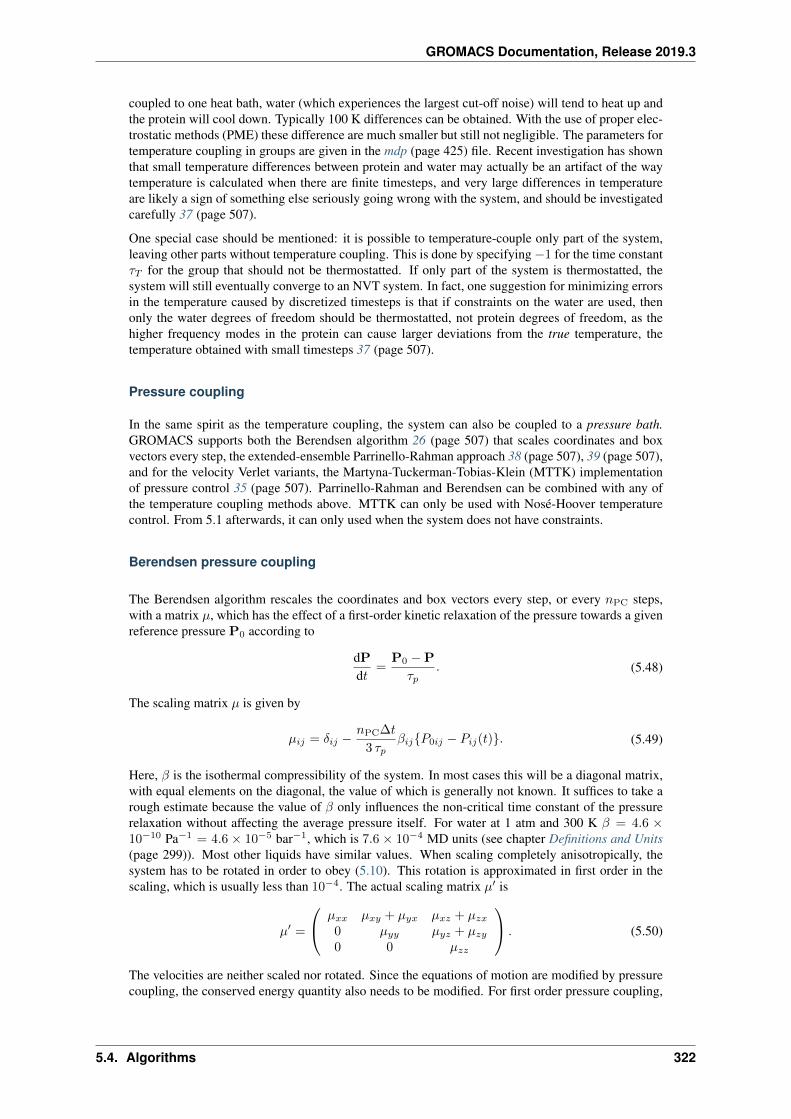
GROMACS Documentation, Release 2019.3
coupled to one heat bath, water (which experiences the largest cut-off noise) will tend to heat up andthe protein will cool down. Typically 100 K differences can be obtained. With the use of proper elec-trostatic methods (PME) these difference are much smaller but still not negligible. The parameters fortemperature coupling in groups are given in the mdp (page 425) file. Recent investigation has shownthat small temperature differences between protein and water may actually be an artifact of the waytemperature is calculated when there are finite timesteps, and very large differences in temperatureare likely a sign of something else seriously going wrong with the system, and should be investigatedcarefully 37 (page 507).
One special case should be mentioned: it is possible to temperature-couple only part of the system,leaving other parts without temperature coupling. This is done by specifying −1 for the time constant𝜏𝑇 for the group that should not be thermostatted. If only part of the system is thermostatted, thesystem will still eventually converge to an NVT system. In fact, one suggestion for minimizing errorsin the temperature caused by discretized timesteps is that if constraints on the water are used, thenonly the water degrees of freedom should be thermostatted, not protein degrees of freedom, as thehigher frequency modes in the protein can cause larger deviations from the true temperature, thetemperature obtained with small timesteps 37 (page 507).
Pressure coupling
In the same spirit as the temperature coupling, the system can also be coupled to a pressure bath.GROMACS supports both the Berendsen algorithm 26 (page 507) that scales coordinates and boxvectors every step, the extended-ensemble Parrinello-Rahman approach 38 (page 507), 39 (page 507),and for the velocity Verlet variants, the Martyna-Tuckerman-Tobias-Klein (MTTK) implementationof pressure control 35 (page 507). Parrinello-Rahman and Berendsen can be combined with any ofthe temperature coupling methods above. MTTK can only be used with Nosé-Hoover temperaturecontrol. From 5.1 afterwards, it can only used when the system does not have constraints.
Berendsen pressure coupling
The Berendsen algorithm rescales the coordinates and box vectors every step, or every 𝑛PC steps,with a matrix 𝜇, which has the effect of a first-order kinetic relaxation of the pressure towards a givenreference pressure P0 according to
dPd𝑡
=P0 −P
𝜏𝑝. (5.48)
The scaling matrix 𝜇 is given by
𝜇𝑖𝑗 = 𝛿𝑖𝑗 −𝑛PC∆𝑡
3 𝜏𝑝𝛽𝑖𝑗{𝑃0𝑖𝑗 − 𝑃𝑖𝑗(𝑡)}. (5.49)
Here, 𝛽 is the isothermal compressibility of the system. In most cases this will be a diagonal matrix,with equal elements on the diagonal, the value of which is generally not known. It suffices to take arough estimate because the value of 𝛽 only influences the non-critical time constant of the pressurerelaxation without affecting the average pressure itself. For water at 1 atm and 300 K 𝛽 = 4.6 ×10⁻¹⁰ Pa−1 = 4.6 × 10⁻⁵ bar−1, which is 7.6 × 10⁻⁴ MD units (see chapter Definitions and Units(page 299)). Most other liquids have similar values. When scaling completely anisotropically, thesystem has to be rotated in order to obey (5.10). This rotation is approximated in first order in thescaling, which is usually less than 10−4. The actual scaling matrix 𝜇′ is
𝜇′ =
⎛⎝ 𝜇𝑥𝑥 𝜇𝑥𝑦 + 𝜇𝑦𝑥 𝜇𝑥𝑧 + 𝜇𝑧𝑥
0 𝜇𝑦𝑦 𝜇𝑦𝑧 + 𝜇𝑧𝑦
0 0 𝜇𝑧𝑧
⎞⎠ . (5.50)
The velocities are neither scaled nor rotated. Since the equations of motion are modified by pressurecoupling, the conserved energy quantity also needs to be modified. For first order pressure coupling,
5.4. Algorithms 322
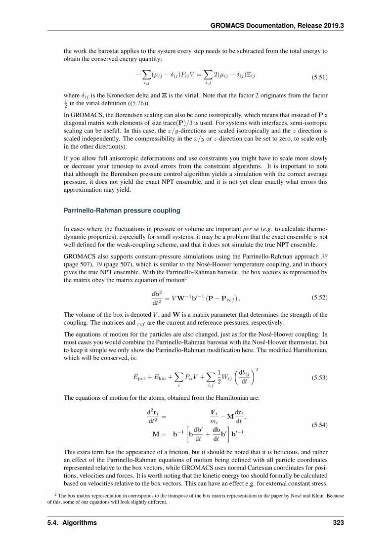
GROMACS Documentation, Release 2019.3
the work the barostat applies to the system every step needs to be subtracted from the total energy toobtain the conserved energy quantity:
−∑𝑖,𝑗
(𝜇𝑖𝑗 − 𝛿𝑖𝑗)𝑃𝑖𝑗𝑉 =∑𝑖,𝑗
2(𝜇𝑖𝑗 − 𝛿𝑖𝑗)Ξ𝑖𝑗 (5.51)
where 𝛿𝑖𝑗 is the Kronecker delta and Ξ is the virial. Note that the factor 2 originates from the factor12 in the virial definition ((5.26)).
In GROMACS, the Berendsen scaling can also be done isotropically, which means that instead of P adiagonal matrix with elements of size trace(P)/3 is used. For systems with interfaces, semi-isotropicscaling can be useful. In this case, the 𝑥/𝑦-directions are scaled isotropically and the 𝑧 direction isscaled independently. The compressibility in the 𝑥/𝑦 or 𝑧-direction can be set to zero, to scale onlyin the other direction(s).
If you allow full anisotropic deformations and use constraints you might have to scale more slowlyor decrease your timestep to avoid errors from the constraint algorithms. It is important to notethat although the Berendsen pressure control algorithm yields a simulation with the correct averagepressure, it does not yield the exact NPT ensemble, and it is not yet clear exactly what errors thisapproximation may yield.
Parrinello-Rahman pressure coupling
In cases where the fluctuations in pressure or volume are important per se (e.g. to calculate thermo-dynamic properties), especially for small systems, it may be a problem that the exact ensemble is notwell defined for the weak-coupling scheme, and that it does not simulate the true NPT ensemble.
GROMACS also supports constant-pressure simulations using the Parrinello-Rahman approach 38(page 507), 39 (page 507), which is similar to the Nosé-Hoover temperature coupling, and in theorygives the true NPT ensemble. With the Parrinello-Rahman barostat, the box vectors as represented bythe matrix obey the matrix equation of motion2
db2
d𝑡2= 𝑉W−1b′−1 (P−P𝑟𝑒𝑓 ) . (5.52)
The volume of the box is denoted 𝑉 , and W is a matrix parameter that determines the strength of thecoupling. The matrices and 𝑟𝑒𝑓 are the current and reference pressures, respectively.
The equations of motion for the particles are also changed, just as for the Nosé-Hoover coupling. Inmost cases you would combine the Parrinello-Rahman barostat with the Nosé-Hoover thermostat, butto keep it simple we only show the Parrinello-Rahman modification here. The modified Hamiltonian,which will be conserved, is:
𝐸pot + 𝐸kin +∑𝑖
𝑃𝑖𝑖𝑉 +∑𝑖,𝑗
1
2𝑊𝑖𝑗
(d𝑏𝑖𝑗d𝑡
)2
(5.53)
The equations of motion for the atoms, obtained from the Hamiltonian are:
d2r𝑖d𝑡2
=F𝑖
𝑚𝑖−M
dr𝑖d𝑡,
M = b−1
[b
db′
d𝑡+
dbd𝑡
b′]b′−1.
(5.54)
This extra term has the appearance of a friction, but it should be noted that it is ficticious, and ratheran effect of the Parrinello-Rahman equations of motion being defined with all particle coordinatesrepresented relative to the box vectors, while GROMACS uses normal Cartesian coordinates for posi-tions, velocities and forces. It is worth noting that the kinetic energy too should formally be calculatedbased on velocities relative to the box vectors. This can have an effect e.g. for external constant stress,
2 The box matrix representation in corresponds to the transpose of the box matrix representation in the paper by Nosé and Klein. Becauseof this, some of our equations will look slightly different.
5.4. Algorithms 323
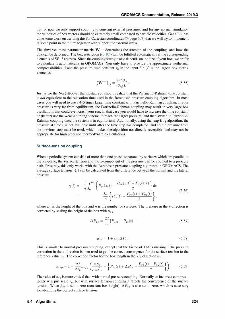
GROMACS Documentation, Release 2019.3
but for now we only support coupling to constant external pressures, and for any normal simulationthe velocities of box vectors should be extremely small compared to particle velocities. Gang Liu hasdone some work on deriving this for Cartesian coordinates40 (page 507) that we will try to implementat some point in the future together with support for external stress.
The (inverse) mass parameter matrix W−1 determines the strength of the coupling, and how thebox can be deformed. The box restriction ((5.10)) will be fulfilled automatically if the correspondingelements of W−1 are zero. Since the coupling strength also depends on the size of your box, we preferto calculate it automatically in GROMACS. You only have to provide the approximate isothermalcompressibilities 𝛽 and the pressure time constant 𝜏𝑝 in the input file (𝐿 is the largest box matrixelement):
(W−1
)𝑖𝑗
=4𝜋2𝛽𝑖𝑗3𝜏2𝑝𝐿
. (5.55)
Just as for the Nosé-Hoover thermostat, you should realize that the Parrinello-Rahman time constantis not equivalent to the relaxation time used in the Berendsen pressure coupling algorithm. In mostcases you will need to use a 4–5 times larger time constant with Parrinello-Rahman coupling. If yourpressure is very far from equilibrium, the Parrinello-Rahman coupling may result in very large boxoscillations that could even crash your run. In that case you would have to increase the time constant,or (better) use the weak-coupling scheme to reach the target pressure, and then switch to Parrinello-Rahman coupling once the system is in equilibrium. Additionally, using the leap-frog algorithm, thepressure at time 𝑡 is not available until after the time step has completed, and so the pressure fromthe previous step must be used, which makes the algorithm not directly reversible, and may not beappropriate for high precision thermodynamic calculations.
Surface-tension coupling
When a periodic system consists of more than one phase, separated by surfaces which are parallel tothe 𝑥𝑦-plane, the surface tension and the 𝑧-component of the pressure can be coupled to a pressurebath. Presently, this only works with the Berendsen pressure coupling algorithm in GROMACS. Theaverage surface tension 𝛾(𝑡) can be calculated from the difference between the normal and the lateralpressure
𝛾(𝑡) =1
𝑛
∫ 𝐿𝑧
0
{𝑃𝑧𝑧(𝑧, 𝑡) − 𝑃𝑥𝑥(𝑧, 𝑡) + 𝑃𝑦𝑦(𝑧, 𝑡)
2
}d𝑧
=𝐿𝑧
𝑛
{𝑃𝑧𝑧(𝑡) − 𝑃𝑥𝑥(𝑡) + 𝑃𝑦𝑦(𝑡)
2
},
(5.56)
where 𝐿𝑧 is the height of the box and 𝑛 is the number of surfaces. The pressure in the z-direction iscorrected by scaling the height of the box with 𝜇𝑧𝑧
∆𝑃𝑧𝑧 =∆𝑡
𝜏𝑝{𝑃0𝑧𝑧 − 𝑃𝑧𝑧(𝑡)} (5.57)
𝜇𝑧𝑧 = 1 + 𝛽𝑧𝑧∆𝑃𝑧𝑧 (5.58)
This is similar to normal pressure coupling, except that the factor of 1/3 is missing. The pressurecorrection in the 𝑧-direction is then used to get the correct convergence for the surface tension to thereference value 𝛾0. The correction factor for the box length in the 𝑥/𝑦-direction is
𝜇𝑥/𝑦 = 1 +∆𝑡
2 𝜏𝑝𝛽𝑥/𝑦
(𝑛𝛾0𝜇𝑧𝑧𝐿𝑧
−{𝑃𝑧𝑧(𝑡) + ∆𝑃𝑧𝑧 −
𝑃𝑥𝑥(𝑡) + 𝑃𝑦𝑦(𝑡)
2
})(5.59)
The value of 𝛽𝑧𝑧 is more critical than with normal pressure coupling. Normally an incorrect compress-ibility will just scale 𝜏𝑝, but with surface tension coupling it affects the convergence of the surfacetension. When 𝛽𝑧𝑧 is set to zero (constant box height), ∆𝑃𝑧𝑧 is also set to zero, which is necessaryfor obtaining the correct surface tension.
5.4. Algorithms 324
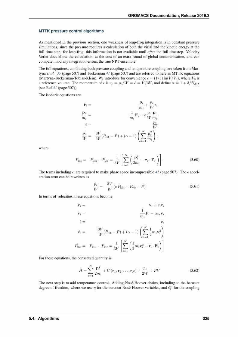
GROMACS Documentation, Release 2019.3
MTTK pressure control algorithms
As mentioned in the previous section, one weakness of leap-frog integration is in constant pressuresimulations, since the pressure requires a calculation of both the virial and the kinetic energy at thefull time step; for leap-frog, this information is not available until after the full timestep. VelocityVerlet does allow the calculation, at the cost of an extra round of global communication, and cancompute, mod any integration errors, the true NPT ensemble.
The full equations, combining both pressure coupling and temperature coupling, are taken from Mar-tyna et al. 35 (page 507) and Tuckerman 41 (page 507) and are referred to here as MTTK equations(Martyna-Tuckerman-Tobias-Klein). We introduce for convenience 𝜖 = (1/3) ln(𝑉/𝑉0), where 𝑉0 isa reference volume. The momentum of 𝜖 is 𝑣𝜖 = 𝑝𝜖/𝑊 = �� = �� /3𝑉 , and define 𝛼 = 1 + 3/𝑁𝑑𝑜𝑓
(see Ref 41 (page 507))
The isobaric equations are
r𝑖 =p𝑖
𝑚𝑖+𝑝𝜖𝑊
r𝑖
p𝑖
𝑚𝑖=
1
𝑚𝑖F𝑖 − 𝛼
𝑝𝜖𝑊
p𝑖
𝑚𝑖
�� =𝑝𝜖𝑊
𝑝𝜖𝑊
=3𝑉
𝑊(𝑃int − 𝑃 ) + (𝛼− 1)
(𝑁∑
𝑛=1
p2𝑖
𝑚𝑖
),
where
𝑃int = 𝑃kin − 𝑃vir =1
3𝑉
[𝑁∑𝑖=1
(p2𝑖
2𝑚𝑖− r𝑖 · F𝑖
)]. (5.60)
The terms including 𝛼 are required to make phase space incompressible 41 (page 507). The 𝜖 accel-eration term can be rewritten as
𝑝𝜖𝑊
=3𝑉
𝑊(𝛼𝑃kin − 𝑃vir − 𝑃 ) (5.61)
In terms of velocities, these equations become
r𝑖 = v𝑖 + 𝑣𝜖r𝑖
v𝑖 =1
𝑚𝑖F𝑖 − 𝛼𝑣𝜖v𝑖
�� = 𝑣𝜖
𝑣𝜖 =3𝑉
𝑊(𝑃int − 𝑃 ) + (𝛼− 1)
(𝑁∑
𝑛=1
1
2𝑚𝑖v
2𝑖
)
𝑃int = 𝑃kin − 𝑃vir =1
3𝑉
[𝑁∑𝑖=1
(1
2𝑚𝑖v
2𝑖 − r𝑖 · F𝑖
)]
For these equations, the conserved quantity is
𝐻 =
𝑁∑𝑖=1
p2𝑖
2𝑚𝑖+ 𝑈 (r1, r2, . . . , r𝑁 ) +
𝑝𝜖2𝑊
+ 𝑃𝑉 (5.62)
The next step is to add temperature control. Adding Nosé-Hoover chains, including to the barostatdegree of freedom, where we use 𝜂 for the barostat Nosé-Hoover variables, and 𝑄′ for the coupling
5.4. Algorithms 325
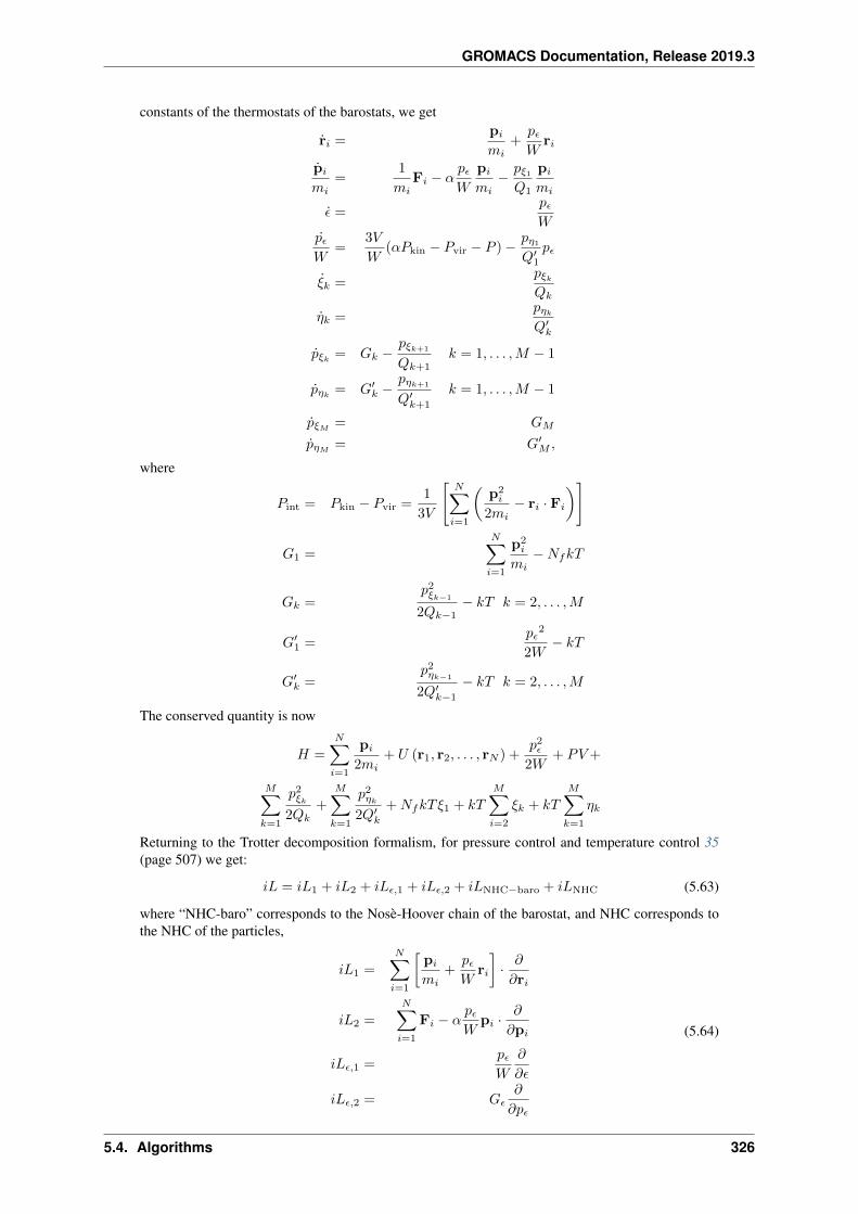
GROMACS Documentation, Release 2019.3
constants of the thermostats of the barostats, we get
r𝑖 =p𝑖
𝑚𝑖+𝑝𝜖𝑊
r𝑖
p𝑖
𝑚𝑖=
1
𝑚𝑖F𝑖 − 𝛼
𝑝𝜖𝑊
p𝑖
𝑚𝑖− 𝑝𝜉1𝑄1
p𝑖
𝑚𝑖
�� =𝑝𝜖𝑊
𝑝𝜖𝑊
=3𝑉
𝑊(𝛼𝑃kin − 𝑃vir − 𝑃 ) − 𝑝𝜂1
𝑄′1
𝑝𝜖
𝜉𝑘 =𝑝𝜉𝑘𝑄𝑘
��𝑘 =𝑝𝜂𝑘
𝑄′𝑘
��𝜉𝑘 = 𝐺𝑘 −𝑝𝜉𝑘+1
𝑄𝑘+1𝑘 = 1, . . . ,𝑀 − 1
��𝜂𝑘= 𝐺′
𝑘 −𝑝𝜂𝑘+1
𝑄′𝑘+1
𝑘 = 1, . . . ,𝑀 − 1
��𝜉𝑀 = 𝐺𝑀
��𝜂𝑀= 𝐺′
𝑀 ,
where
𝑃int = 𝑃kin − 𝑃vir =1
3𝑉
[𝑁∑𝑖=1
(p2𝑖
2𝑚𝑖− r𝑖 · F𝑖
)]
𝐺1 =
𝑁∑𝑖=1
p2𝑖
𝑚𝑖−𝑁𝑓𝑘𝑇
𝐺𝑘 =𝑝2𝜉𝑘−1
2𝑄𝑘−1− 𝑘𝑇 𝑘 = 2, . . . ,𝑀
𝐺′1 =
𝑝𝜖2
2𝑊− 𝑘𝑇
𝐺′𝑘 =
𝑝2𝜂𝑘−1
2𝑄′𝑘−1
− 𝑘𝑇 𝑘 = 2, . . . ,𝑀
The conserved quantity is now
𝐻 =
𝑁∑𝑖=1
p𝑖
2𝑚𝑖+ 𝑈 (r1, r2, . . . , r𝑁 ) +
𝑝2𝜖2𝑊
+ 𝑃𝑉+
𝑀∑𝑘=1
𝑝2𝜉𝑘2𝑄𝑘
+
𝑀∑𝑘=1
𝑝2𝜂𝑘
2𝑄′𝑘
+𝑁𝑓𝑘𝑇𝜉1 + 𝑘𝑇
𝑀∑𝑖=2
𝜉𝑘 + 𝑘𝑇
𝑀∑𝑘=1
𝜂𝑘
Returning to the Trotter decomposition formalism, for pressure control and temperature control 35(page 507) we get:
𝑖𝐿 = 𝑖𝐿1 + 𝑖𝐿2 + 𝑖𝐿𝜖,1 + 𝑖𝐿𝜖,2 + 𝑖𝐿NHC−baro + 𝑖𝐿NHC (5.63)
where “NHC-baro” corresponds to the Nosè-Hoover chain of the barostat, and NHC corresponds tothe NHC of the particles,
𝑖𝐿1 =
𝑁∑𝑖=1
[p𝑖
𝑚𝑖+𝑝𝜖𝑊
r𝑖
]· 𝜕
𝜕r𝑖
𝑖𝐿2 =
𝑁∑𝑖=1
F𝑖 − 𝛼𝑝𝜖𝑊
p𝑖 ·𝜕
𝜕p𝑖
𝑖𝐿𝜖,1 =𝑝𝜖𝑊
𝜕
𝜕𝜖
𝑖𝐿𝜖,2 = 𝐺𝜖𝜕
𝜕𝑝𝜖
(5.64)
5.4. Algorithms 326
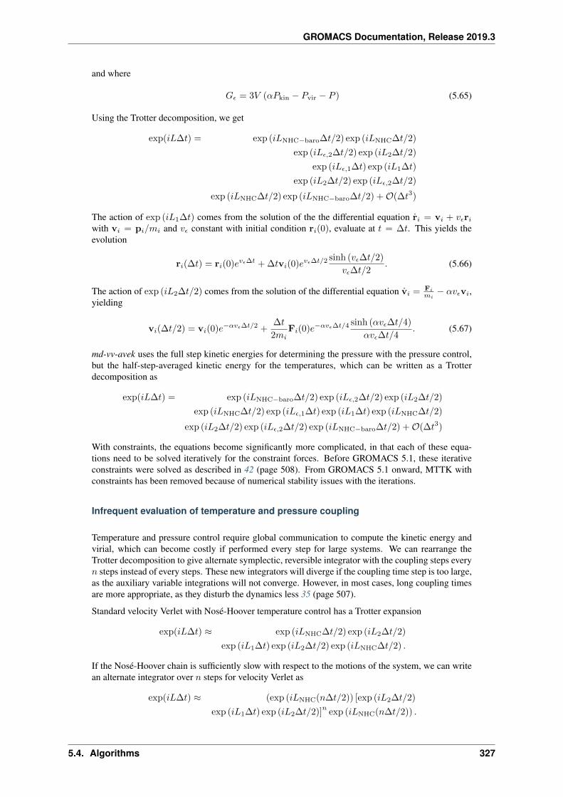
GROMACS Documentation, Release 2019.3
and where
𝐺𝜖 = 3𝑉 (𝛼𝑃kin − 𝑃vir − 𝑃 ) (5.65)
Using the Trotter decomposition, we get
exp(𝑖𝐿∆𝑡) = exp (𝑖𝐿NHC−baro∆𝑡/2) exp (𝑖𝐿NHC∆𝑡/2)
exp (𝑖𝐿𝜖,2∆𝑡/2) exp (𝑖𝐿2∆𝑡/2)
exp (𝑖𝐿𝜖,1∆𝑡) exp (𝑖𝐿1∆𝑡)
exp (𝑖𝐿2∆𝑡/2) exp (𝑖𝐿𝜖,2∆𝑡/2)
exp (𝑖𝐿NHC∆𝑡/2) exp (𝑖𝐿NHC−baro∆𝑡/2) + 𝒪(∆𝑡3)
The action of exp (𝑖𝐿1∆𝑡) comes from the solution of the the differential equation r𝑖 = v𝑖 + 𝑣𝜖r𝑖with v𝑖 = p𝑖/𝑚𝑖 and 𝑣𝜖 constant with initial condition r𝑖(0), evaluate at 𝑡 = ∆𝑡. This yields theevolution
r𝑖(∆𝑡) = r𝑖(0)𝑒𝑣𝜖Δ𝑡 + ∆𝑡v𝑖(0)𝑒𝑣𝜖Δ𝑡/2 sinh (𝑣𝜖∆𝑡/2)
𝑣𝜖∆𝑡/2. (5.66)
The action of exp (𝑖𝐿2∆𝑡/2) comes from the solution of the differential equation v𝑖 = F𝑖
𝑚𝑖− 𝛼𝑣𝜖v𝑖,
yielding
v𝑖(∆𝑡/2) = v𝑖(0)𝑒−𝛼𝑣𝜖Δ𝑡/2 +∆𝑡
2𝑚𝑖F𝑖(0)𝑒−𝛼𝑣𝜖Δ𝑡/4 sinh (𝛼𝑣𝜖∆𝑡/4)
𝛼𝑣𝜖∆𝑡/4. (5.67)
md-vv-avek uses the full step kinetic energies for determining the pressure with the pressure control,but the half-step-averaged kinetic energy for the temperatures, which can be written as a Trotterdecomposition as
exp(𝑖𝐿∆𝑡) = exp (𝑖𝐿NHC−baro∆𝑡/2) exp (𝑖𝐿𝜖,2∆𝑡/2) exp (𝑖𝐿2∆𝑡/2)
exp (𝑖𝐿NHC∆𝑡/2) exp (𝑖𝐿𝜖,1∆𝑡) exp (𝑖𝐿1∆𝑡) exp (𝑖𝐿NHC∆𝑡/2)
exp (𝑖𝐿2∆𝑡/2) exp (𝑖𝐿𝜖,2∆𝑡/2) exp (𝑖𝐿NHC−baro∆𝑡/2) + 𝒪(∆𝑡3)
With constraints, the equations become significantly more complicated, in that each of these equa-tions need to be solved iteratively for the constraint forces. Before GROMACS 5.1, these iterativeconstraints were solved as described in 42 (page 508). From GROMACS 5.1 onward, MTTK withconstraints has been removed because of numerical stability issues with the iterations.
Infrequent evaluation of temperature and pressure coupling
Temperature and pressure control require global communication to compute the kinetic energy andvirial, which can become costly if performed every step for large systems. We can rearrange theTrotter decomposition to give alternate symplectic, reversible integrator with the coupling steps every𝑛 steps instead of every steps. These new integrators will diverge if the coupling time step is too large,as the auxiliary variable integrations will not converge. However, in most cases, long coupling timesare more appropriate, as they disturb the dynamics less 35 (page 507).
Standard velocity Verlet with Nosé-Hoover temperature control has a Trotter expansion
exp(𝑖𝐿∆𝑡) ≈ exp (𝑖𝐿NHC∆𝑡/2) exp (𝑖𝐿2∆𝑡/2)
exp (𝑖𝐿1∆𝑡) exp (𝑖𝐿2∆𝑡/2) exp (𝑖𝐿NHC∆𝑡/2) .
If the Nosé-Hoover chain is sufficiently slow with respect to the motions of the system, we can writean alternate integrator over 𝑛 steps for velocity Verlet as
exp(𝑖𝐿∆𝑡) ≈ (exp (𝑖𝐿NHC(𝑛∆𝑡/2)) [exp (𝑖𝐿2∆𝑡/2)
exp (𝑖𝐿1∆𝑡) exp (𝑖𝐿2∆𝑡/2)]𝑛
exp (𝑖𝐿NHC(𝑛∆𝑡/2)) .
5.4. Algorithms 327
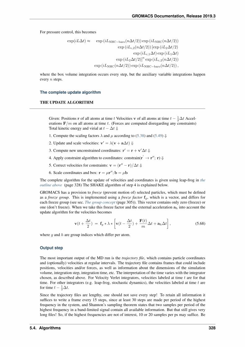
GROMACS Documentation, Release 2019.3
For pressure control, this becomes
exp(𝑖𝐿∆𝑡) ≈ exp (𝑖𝐿NHC−baro(𝑛∆𝑡/2)) exp (𝑖𝐿NHC(𝑛∆𝑡/2))
exp (𝑖𝐿𝜖,2(𝑛∆𝑡/2)) [exp (𝑖𝐿2∆𝑡/2)
exp (𝑖𝐿𝜖,1∆𝑡) exp (𝑖𝐿1∆𝑡)
exp (𝑖𝐿2∆𝑡/2)]𝑛
exp (𝑖𝐿𝜖,2(𝑛∆𝑡/2))
exp (𝑖𝐿NHC(𝑛∆𝑡/2)) exp (𝑖𝐿NHC−baro(𝑛∆𝑡/2)) ,
where the box volume integration occurs every step, but the auxiliary variable integrations happenevery 𝑛 steps.
The complete update algorithm
THE UPDATE ALGORITHM
Given: Positions r of all atoms at time 𝑡 Velocities v of all atoms at time 𝑡 − 12∆𝑡 Accel-
erations F/𝑚 on all atoms at time 𝑡. (Forces are computed disregarding any constraints)Total kinetic energy and virial at 𝑡− ∆𝑡 ⇓
1. Compute the scaling factors 𝜆 and 𝜇 according to (5.38) and (5.49) ⇓
2. Update and scale velocities: v′ = 𝜆(v + a∆𝑡) ⇓
3. Compute new unconstrained coordinates: r′ = r + v′∆𝑡 ⇓
4. Apply constraint algorithm to coordinates: constrain(r′ → r′′; r) ⇓
5. Correct velocities for constraints: v = (r′′ − r)/∆𝑡 ⇓
6. Scale coordinates and box: r = 𝜇r′′;b = 𝜇b
The complete algorithm for the update of velocities and coordinates is given using leap-frog in theoutline above (page 328) The SHAKE algorithm of step 4 is explained below.
GROMACS has a provision to freeze (prevent motion of) selected particles, which must be definedas a freeze group. This is implemented using a freeze factor f𝑔 , which is a vector, and differs foreach freeze group (see sec. The group concept (page 305)). This vector contains only zero (freeze) orone (don’t freeze). When we take this freeze factor and the external acceleration aℎ into account theupdate algorithm for the velocities becomes
v(𝑡+∆𝑡
2) = f𝑔 * 𝜆 *
[v(𝑡− ∆𝑡
2) +
F(𝑡)
𝑚∆𝑡+ aℎ∆𝑡
], (5.68)
where 𝑔 and ℎ are group indices which differ per atom.
Output step
The most important output of the MD run is the trajectory file, which contains particle coordinatesand (optionally) velocities at regular intervals. The trajectory file contains frames that could includepositions, velocities and/or forces, as well as information about the dimensions of the simulationvolume, integration step, integration time, etc. The interpretation of the time varies with the integratorchosen, as described above. For Velocity Verlet integrators, velocities labeled at time 𝑡 are for thattime. For other integrators (e.g. leap-frog, stochastic dynamics), the velocities labeled at time 𝑡 arefor time 𝑡− 1
2∆𝑡.
Since the trajectory files are lengthy, one should not save every step! To retain all information itsuffices to write a frame every 15 steps, since at least 30 steps are made per period of the highestfrequency in the system, and Shannon’s sampling theorem states that two samples per period of thehighest frequency in a band-limited signal contain all available information. But that still gives verylong files! So, if the highest frequencies are not of interest, 10 or 20 samples per ps may suffice. Be
5.4. Algorithms 328
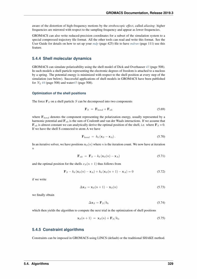
GROMACS Documentation, Release 2019.3
aware of the distortion of high-frequency motions by the stroboscopic effect, called aliasing: higherfrequencies are mirrored with respect to the sampling frequency and appear as lower frequencies.
GROMACS can also write reduced-precision coordinates for a subset of the simulation system to aspecial compressed trajectory file format. All the other tools can read and write this format. See theUser Guide for details on how to set up your mdp (page 425) file to have mdrun (page 111) use thisfeature.
5.4.4 Shell molecular dynamics
GROMACS can simulate polarizability using the shell model of Dick and Overhauser 43 (page 508).In such models a shell particle representing the electronic degrees of freedom is attached to a nucleusby a spring. The potential energy is minimized with respect to the shell position at every step of thesimulation (see below). Successful applications of shell models in GROMACS have been publishedfor 𝑁2 44 (page 508) and water45 (page 508).
Optimization of the shell positions
The force F𝑆 on a shell particle 𝑆 can be decomposed into two components
F𝑆 = F𝑏𝑜𝑛𝑑 + F𝑛𝑏 (5.69)
where F𝑏𝑜𝑛𝑑 denotes the component representing the polarization energy, usually represented by aharmonic potential and F𝑛𝑏 is the sum of Coulomb and van der Waals interactions. If we assume thatF𝑛𝑏 is almost constant we can analytically derive the optimal position of the shell, i.e. where F𝑆 = 0.If we have the shell S connected to atom A we have
F𝑏𝑜𝑛𝑑 = 𝑘𝑏 (x𝑆 − x𝐴) . (5.70)
In an iterative solver, we have positions x𝑆(𝑛) where 𝑛 is the iteration count. We now have at iteration𝑛
F𝑛𝑏 = F𝑆 − 𝑘𝑏 (x𝑆(𝑛) − x𝐴) (5.71)
and the optimal position for the shells 𝑥𝑆(𝑛+ 1) thus follows from
F𝑆 − 𝑘𝑏 (x𝑆(𝑛) − x𝐴) + 𝑘𝑏 (x𝑆(𝑛+ 1) − x𝐴) = 0 (5.72)
if we write
∆x𝑆 = x𝑆(𝑛+ 1) − x𝑆(𝑛) (5.73)
we finally obtain
∆x𝑆 = F𝑆/𝑘𝑏 (5.74)
which then yields the algorithm to compute the next trial in the optimization of shell positions
x𝑆(𝑛+ 1) = x𝑆(𝑛) + F𝑆/𝑘𝑏. (5.75)
5.4.5 Constraint algorithms
Constraints can be imposed in GROMACS using LINCS (default) or the traditional SHAKE method.
5.4. Algorithms 329
GROMACS Documentation, Release 2019.3
SHAKE
The SHAKE 46 (page 508) algorithm changes a set of unconstrained coordinates r′
to a set of coor-dinates r′′ that fulfill a list of distance constraints, using a set r reference, as
SHAKE(r′→ r′′; r) (5.76)
This action is consistent with solving a set of Lagrange multipliers in the constrained equations ofmotion. SHAKE needs a relative tolerance; it will continue until all constraints are satisfied withinthat relative tolerance. An error message is given if SHAKE cannot reset the coordinates because thedeviation is too large, or if a given number of iterations is surpassed.
Assume the equations of motion must fulfill 𝐾 holonomic constraints, expressed as
𝜎𝑘(r1 . . . r𝑁 ) = 0; 𝑘 = 1 . . .𝐾. (5.77)
For example, (r1 − r2)2 − 𝑏2 = 0. Then the forces are defined as
− 𝜕
𝜕r𝑖
(𝑉 +
𝐾∑𝑘=1
𝜆𝑘𝜎𝑘
), (5.78)
where 𝜆𝑘 are Lagrange multipliers which must be solved to fulfill the constraint equations. Thesecond part of this sum determines the constraint forces G𝑖, defined by
G𝑖 = −𝐾∑
𝑘=1
𝜆𝑘𝜕𝜎𝑘𝜕r𝑖
(5.79)
The displacement due to the constraint forces in the leap-frog or Verlet algorithm is equal to(G𝑖/𝑚𝑖)(∆𝑡)
2. Solving the Lagrange multipliers (and hence the displacements) requires the so-lution of a set of coupled equations of the second degree. These are solved iteratively by SHAKE.SETTLE (page 330)
SETTLE
For the special case of rigid water molecules, that often make up more than 80% of the simula-tion system we have implemented the SETTLE algorithm 47 (page 508) (sec. Constraint algorithms(page 397)).
For velocity Verlet, an additional round of constraining must be done, to constrain the velocities of thesecond velocity half step, removing any component of the velocity parallel to the bond vector. Thisstep is called RATTLE, and is covered in more detail in the original Andersen paper 48 (page 508).
LINCS
The LINCS algorithm
LINCS is an algorithm that resets bonds to their correct lengths after an unconstrained update 49(page 508). The method is non-iterative, as it always uses two steps. Although LINCS is based onmatrices, no matrix-matrix multiplications are needed. The method is more stable and faster thanSHAKE, but it can only be used with bond constraints and isolated angle constraints, such as theproton angle in OH. Because of its stability, LINCS is especially useful for Brownian dynamics.LINCS has two parameters, which are explained in the subsection parameters. The parallel versionof LINCS, P-LINCS, is described in subsection Constraints in parallel (page 343).
5.4. Algorithms 330
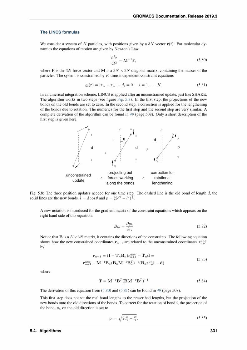
GROMACS Documentation, Release 2019.3
The LINCS formulas
We consider a system of 𝑁 particles, with positions given by a 3𝑁 vector r(𝑡). For molecular dy-namics the equations of motion are given by Newton’s Law
d2r
d𝑡2= M−1F, (5.80)
where F is the 3𝑁 force vector and M is a 3𝑁 × 3𝑁 diagonal matrix, containing the masses of theparticles. The system is constrained by 𝐾 time-independent constraint equations
𝑔𝑖(r) = |r𝑖1 − r𝑖2 | − 𝑑𝑖 = 0 𝑖 = 1, . . . ,𝐾. (5.81)
In a numerical integration scheme, LINCS is applied after an unconstrained update, just like SHAKE.The algorithm works in two steps (see figure Fig. 5.8). In the first step, the projections of the newbonds on the old bonds are set to zero. In the second step, a correction is applied for the lengtheningof the bonds due to rotation. The numerics for the first step and the second step are very similar. Acomplete derivation of the algorithm can be found in 49 (page 508). Only a short description of thefirst step is given here.
000
111
0 00 01 11 1
0011
0 00 00 0
1 11 11 1
000
111
0011
0 0 0 0 0 00 0 0 0 0 00 0 0 0 0 00 0 0 0 0 00 0 0 0 0 0
1 1 1 1 1 11 1 1 1 1 11 1 1 1 1 11 1 1 1 1 11 1 1 1 1 1
unconstrainedupdate
correction forrotational
lengthening
projecting outforces working
along the bonds
θ
dl d
pd
Fig. 5.8: The three position updates needed for one time step. The dashed line is the old bond of length 𝑑, thesolid lines are the new bonds. 𝑙 = 𝑑 cos 𝜃 and 𝑝 = (2𝑑2 − 𝑙2)
12 .
A new notation is introduced for the gradient matrix of the constraint equations which appears on theright hand side of this equation:
𝐵ℎ𝑖 =𝜕𝑔ℎ𝜕𝑟𝑖
(5.82)
Notice that B is a𝐾×3𝑁 matrix, it contains the directions of the constraints. The following equationshows how the new constrained coordinates r𝑛+1 are related to the unconstrained coordinates r𝑢𝑛𝑐𝑛+1
by
r𝑛+1 = (I−T𝑛B𝑛)r𝑢𝑛𝑐𝑛+1 + T𝑛d =
r𝑢𝑛𝑐𝑛+1 −M−1B𝑛(B𝑛M−1B𝑇
𝑛 )−1(B𝑛r𝑢𝑛𝑐𝑛+1 − d)
(5.83)
where
T = M−1B𝑇 (BM−1B𝑇 )−1 (5.84)
The derivation of this equation from (5.80) and (5.81) can be found in 49 (page 508).
This first step does not set the real bond lengths to the prescribed lengths, but the projection of thenew bonds onto the old directions of the bonds. To correct for the rotation of bond 𝑖, the projection ofthe bond, 𝑝𝑖, on the old direction is set to
𝑝𝑖 =√
2𝑑2𝑖 − 𝑙2𝑖 , (5.85)
5.4. Algorithms 331
GROMACS Documentation, Release 2019.3
where 𝑙𝑖 is the bond length after the first projection. The corrected positions are
r*𝑛+1 = (I−T𝑛B𝑛)r𝑛+1 + T𝑛p. (5.86)
This correction for rotational effects is actually an iterative process, but during MD only one iterationis applied. The relative constraint deviation after this procedure will be less than 0.0001 for everyconstraint. In energy minimization, this might not be accurate enough, so the number of iterations isequal to the order of the expansion (see below).
Half of the CPU time goes to inverting the constraint coupling matrix B𝑛M−1B𝑇
𝑛 , which has to bedone every time step. This 𝐾 × 𝐾 matrix has 1/𝑚𝑖1 + 1/𝑚𝑖2 on the diagonal. The off-diagonalelements are only non-zero when two bonds are connected, then the element is cos𝜑/𝑚𝑐, where 𝑚𝑐
is the mass of the atom connecting the two bonds and 𝜑 is the angle between the bonds.
The matrix T is inverted through a power expansion. A 𝐾 × 𝐾 matrix S is introduced which isthe inverse square root of the diagonal of B𝑛M
−1B𝑇𝑛 . This matrix is used to convert the diagonal
elements of the coupling matrix to one:
(B𝑛M−1B𝑇
𝑛 )−1 = SS−1(B𝑛M−1B𝑇
𝑛 )−1S−1S
= S(SB𝑛M−1B𝑇
𝑛S)−1S = S(I−A𝑛)−1S(5.87)
The matrix A𝑛 is symmetric and sparse and has zeros on the diagonal. Thus a simple trick can beused to calculate the inverse:
(I−A𝑛)−1 = I + A𝑛 + A2𝑛 + A3
𝑛 + . . . (5.88)
This inversion method is only valid if the absolute values of all the eigenvalues of A𝑛 are smallerthan one. In molecules with only bond constraints, the connectivity is so low that this will alwaysbe true, even if ring structures are present. Problems can arise in angle-constrained molecules. Byconstraining angles with additional distance constraints, multiple small ring structures are introduced.This gives a high connectivity, leading to large eigenvalues. Therefore LINCS should NOT be usedwith coupled angle-constraints.
For molecules with all bonds constrained the eigenvalues of 𝐴 are around 0.4. This means that witheach additional order in the expansion (5.88) the deviations decrease by a factor 0.4. But for relativelyisolated triangles of constraints the largest eigenvalue is around 0.7. Such triangles can occur whenremoving hydrogen angle vibrations with an additional angle constraint in alcohol groups or whenconstraining water molecules with LINCS, for instance with flexible constraints. The constraints insuch triangles converge twice as slow as the other constraints. Therefore, starting with GROMACS4, additional terms are added to the expansion for such triangles
(I−A𝑛)−1 ≈ I + A𝑛 + . . .+ A𝑁𝑖𝑛 +
(A*
𝑛 + . . .+ A*𝑛𝑁𝑖
)A𝑁𝑖
𝑛 (5.89)
where 𝑁𝑖 is the normal order of the expansion and A* only contains the elements of A that coupleconstraints within rigid triangles, all other elements are zero. In this manner, the accuracy of angleconstraints comes close to that of the other constraints, while the series of matrix vector multiplica-tions required for determining the expansion only needs to be extended for a few constraint couplings.This procedure is described in the P-LINCS paper50 (page 508).
The LINCS Parameters
The accuracy of LINCS depends on the number of matrices used in the expansion (5.88). For MDcalculations a fourth order expansion is enough. For Brownian dynamics with large time steps aneighth order expansion may be necessary. The order is a parameter in the mdp (page 425) file. Theimplementation of LINCS is done in such a way that the algorithm will never crash. Even when it isimpossible to to reset the constraints LINCS will generate a conformation which fulfills the constraintsas well as possible. However, LINCS will generate a warning when in one step a bond rotates overmore than a predefined angle. This angle is set by the user in the mdp (page 425) file.
5.4. Algorithms 332
GROMACS Documentation, Release 2019.3
5.4.6 Simulated Annealing
The well known simulated annealing (SA) protocol is supported in GROMACS, and you can evencouple multiple groups of atoms separately with an arbitrary number of reference temperatures thatchange during the simulation. The annealing is implemented by simply changing the current refer-ence temperature for each group in the temperature coupling, so the actual relaxation and couplingproperties depends on the type of thermostat you use and how hard you are coupling it. Since we arechanging the reference temperature it is important to remember that the system will NOT instanta-neously reach this value - you need to allow for the inherent relaxation time in the coupling algorithmtoo. If you are changing the annealing reference temperature faster than the temperature relaxationyou will probably end up with a crash when the difference becomes too large.
The annealing protocol is specified as a series of corresponding times and reference temperaturesfor each group, and you can also choose whether you only want a single sequence (after which thetemperature will be coupled to the last reference value), or if the annealing should be periodic andrestart at the first reference point once the sequence is completed. You can mix and match both typesof annealing and non-annealed groups in your simulation.
5.4.7 Stochastic Dynamics
Stochastic or velocity Langevin dynamics adds a friction and a noise term to Newton’s equations ofmotion, as
𝑚𝑖d2r𝑖d𝑡2
= −𝑚𝑖𝛾𝑖dr𝑖d𝑡
+ F𝑖(r) +∘r𝑖, (5.90)
where 𝛾𝑖 is the friction constant [1/ps] and∘r𝑖(𝑡) is a noise process with ⟨∘𝑟𝑖(𝑡)
∘𝑟𝑗(𝑡 + 𝑠)⟩ =
2𝑚𝑖𝛾𝑖𝑘𝐵𝑇𝛿(𝑠)𝛿𝑖𝑗 . When 1/𝛾𝑖 is large compared to the time scales present in the system, one couldsee stochastic dynamics as molecular dynamics with stochastic temperature-coupling. But any pro-cesses that take longer than 1/𝛾𝑖, e.g. hydrodynamics, will be dampened. Since each degree offreedom is coupled independently to a heat bath, equilibration of fast modes occurs rapidly. For sim-ulating a system in vacuum there is the additional advantage that there is no accumulation of errors forthe overall translational and rotational degrees of freedom. When 1/𝛾𝑖 is small compared to the timescales present in the system, the dynamics will be completely different from MD, but the sampling isstill correct.
In GROMACS there is one simple and efficient implementation. Its accuracy is equivalent to thenormal MD leap-frog and Velocity Verlet integrator. It is nearly identical to the common way of dis-cretizing the Langevin equation, but the friction and velocity term are applied in an impulse fashion 51(page 508). It can be described as:
v′ = v(𝑡− 1
2∆𝑡) +
1
𝑚F(𝑡)∆𝑡
∆v = −𝛼v′(𝑡+1
2∆𝑡) +
√𝑘𝐵𝑇
𝑚(1 − 𝛼2) r𝐺𝑖
r(𝑡+ ∆𝑡) = r(𝑡) +
(v′ +
1
2∆v
)∆𝑡
(5.91)
v(𝑡+1
2∆𝑡) = v′ + ∆v
𝛼 = 1 − 𝑒−𝛾Δ𝑡(5.92)
where r𝐺𝑖 is Gaussian distributed noise with 𝜇 = 0, 𝜎 = 1. The velocity is first updated a full timestep without friction and noise to get v′, identical to the normal update in leap-frog. The friction andnoise are then applied as an impulse at step 𝑡+ ∆𝑡. The advantage of this scheme is that the velocity-dependent terms act at the full time step, which makes the correct integration of forces that dependon both coordinates and velocities, such as constraints and dissipative particle dynamics (DPD, notimplented yet), straightforward. With constraints, the coordinate update (5.92) is split into a normal
5.4. Algorithms 333
GROMACS Documentation, Release 2019.3
leap-frog update and a ∆v. After both of these updates the constraints are applied to coordinates andvelocities.
When using SD as a thermostat, an appropriate value for 𝛾 is e.g. 0.5 ps−1, since this results in afriction that is lower than the internal friction of water, while it still provides efficient thermostatting.
5.4.8 Brownian Dynamics
In the limit of high friction, stochastic dynamics reduces to Brownian dynamics, also called positionLangevin dynamics. This applies to over-damped systems, i.e. systems in which the inertia effectsare negligible. The equation is
dr𝑖d𝑡
=1
𝛾𝑖F𝑖(r) +
∘r𝑖 (5.93)
where 𝛾𝑖 is the friction coefficient [amu/ps] and∘r𝑖(𝑡) is a noise process with ⟨∘𝑟𝑖(𝑡)
∘𝑟𝑗(𝑡 + 𝑠)⟩ =
2𝛿(𝑠)𝛿𝑖𝑗𝑘𝐵𝑇/𝛾𝑖. In GROMACS the equations are integrated with a simple, explicit scheme
r𝑖(𝑡+ ∆𝑡) = r𝑖(𝑡) +∆𝑡
𝛾𝑖F𝑖(r(𝑡)) +
√2𝑘𝐵𝑇
∆𝑡
𝛾𝑖r𝐺𝑖, (5.94)
where r𝐺𝑖 is Gaussian distributed noise with 𝜇 = 0, 𝜎 = 1. The friction coefficients 𝛾𝑖 can bechosen the same for all particles or as 𝛾𝑖 = 𝑚𝑖 𝛾𝑖, where the friction constants 𝛾𝑖 can be differentfor different groups of atoms. Because the system is assumed to be over-damped, large timesteps canbe used. LINCS should be used for the constraints since SHAKE will not converge for large atomicdisplacements. BD is an option of the mdrun (page 111) program.
5.4.9 Energy Minimization
Energy minimization in GROMACS can be done using steepest descent, conjugate gradients, or l-bfgs (limited-memory Broyden-Fletcher-Goldfarb-Shanno quasi-Newtonian minimizer. . . we preferthe abbreviation). EM is just an option of the mdrun (page 111) program.
Steepest Descent
Although steepest descent is certainly not the most efficient algorithm for searching, it is robust andeasy to implement.
We define the vector r as the vector of all 3𝑁 coordinates. Initially a maximum displacement ℎ0 (e.g.0.01 nm) must be given.
First the forces F and potential energy are calculated. New positions are calculated by
r𝑛+1 = r𝑛 +F𝑛
max(|F𝑛|)ℎ𝑛, (5.95)
where ℎ𝑛 is the maximum displacement and F𝑛 is the force, or the negative gradient of the potential𝑉 . The notation max(|F𝑛|) means the largest scalar force on any atom. The forces and energy areagain computed for the new positions
If (𝑉𝑛+1 < 𝑉𝑛) the new positions are accepted and ℎ𝑛+1 = 1.2ℎ𝑛.If (𝑉𝑛+1 ≥ 𝑉𝑛) the new positions are rejected and ℎ𝑛 = 0.2ℎ𝑛.
5.4. Algorithms 334
GROMACS Documentation, Release 2019.3
The algorithm stops when either a user-specified number of force evaluations has been performed (e.g.100), or when the maximum of the absolute values of the force (gradient) components is smaller thana specified value 𝜖. Since force truncation produces some noise in the energy evaluation, the stoppingcriterion should not be made too tight to avoid endless iterations. A reasonable value for 𝜖 can beestimated from the root mean square force 𝑓 a harmonic oscillator would exhibit at a temperature 𝑇 .This value is
𝑓 = 2𝜋𝜈√
2𝑚𝑘𝑇 , (5.96)
where 𝜈 is the oscillator frequency, 𝑚 the (reduced) mass, and 𝑘 Boltzmann’s constant. For a weakoscillator with a wave number of 100 cm−1 and a mass of 10 atomic units, at a temperature of 1 K,𝑓 = 7.7 kJ mol−1 nm:math:^{-1}. A value for 𝜖 between 1 and 10 is acceptable.
Conjugate Gradient
Conjugate gradient is slower than steepest descent in the early stages of the minimization, but becomesmore efficient closer to the energy minimum. The parameters and stop criterion are the same as forsteepest descent. In GROMACS conjugate gradient can not be used with constraints, including theSETTLE algorithm for water 47 (page 508), as this has not been implemented. If water is presentit must be of a flexible model, which can be specified in the mdp (page 425) file by define =-DFLEXIBLE.
This is not really a restriction, since the accuracy of conjugate gradient is only required for minimiza-tion prior to a normal-mode analysis, which cannot be performed with constraints. For most otherpurposes steepest descent is efficient enough.
L-BFGS
The original BFGS algorithm works by successively creating better approximations of the inverseHessian matrix, and moving the system to the currently estimated minimum. The memory require-ments for this are proportional to the square of the number of particles, so it is not practical for largesystems like biomolecules. Instead, we use the L-BFGS algorithm of Nocedal 52 (page 508), 53(page 508), which approximates the inverse Hessian by a fixed number of corrections from previoussteps. This sliding-window technique is almost as efficient as the original method, but the memoryrequirements are much lower - proportional to the number of particles multiplied with the correctionsteps. In practice we have found it to converge faster than conjugate gradients, but due to the correc-tion steps it is not yet parallelized. It is also noteworthy that switched or shifted interactions usuallyimprove the convergence, since sharp cut-offs mean the potential function at the current coordinatesis slightly different from the previous steps used to build the inverse Hessian approximation.
5.4.10 Normal-Mode Analysis
Normal-mode analysis 54 (page 508)56 (page 508) can be performed using GROMACS, by diago-nalization of the mass-weighted Hessian 𝐻:
𝑅𝑇𝑀−1/2𝐻𝑀−1/2𝑅 = diag(𝜆1, . . . , 𝜆3𝑁 )
𝜆𝑖 = (2𝜋𝜔𝑖)2
(5.97)
where 𝑀 contains the atomic masses, 𝑅 is a matrix that contains the eigenvectors as columns, 𝜆𝑖 arethe eigenvalues and 𝜔𝑖 are the corresponding frequencies.
First the Hessian matrix, which is a 3𝑁 × 3𝑁 matrix where 𝑁 is the number of atoms, needs to becalculated:
𝐻𝑖𝑗 =𝜕2𝑉
𝜕𝑥𝑖𝜕𝑥𝑗(5.98)
5.4. Algorithms 335
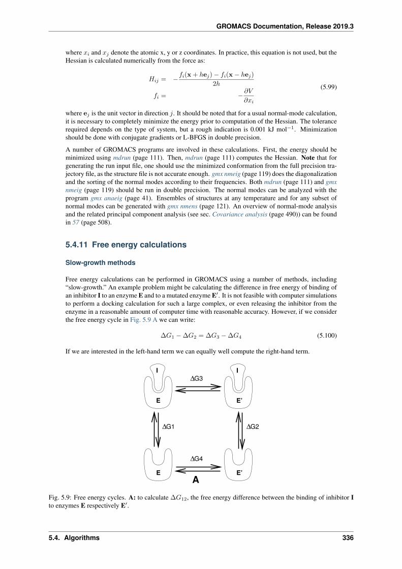
GROMACS Documentation, Release 2019.3
where 𝑥𝑖 and 𝑥𝑗 denote the atomic x, y or z coordinates. In practice, this equation is not used, but theHessian is calculated numerically from the force as:
𝐻𝑖𝑗 = −𝑓𝑖(x + ℎe𝑗) − 𝑓𝑖(x− ℎe𝑗)
2ℎ
𝑓𝑖 = − 𝜕𝑉
𝜕𝑥𝑖
(5.99)
where e𝑗 is the unit vector in direction 𝑗. It should be noted that for a usual normal-mode calculation,it is necessary to completely minimize the energy prior to computation of the Hessian. The tolerancerequired depends on the type of system, but a rough indication is 0.001 kJ mol−1. Minimizationshould be done with conjugate gradients or L-BFGS in double precision.
A number of GROMACS programs are involved in these calculations. First, the energy should beminimized using mdrun (page 111). Then, mdrun (page 111) computes the Hessian. Note that forgenerating the run input file, one should use the minimized conformation from the full precision tra-jectory file, as the structure file is not accurate enough. gmx nmeig (page 119) does the diagonalizationand the sorting of the normal modes according to their frequencies. Both mdrun (page 111) and gmxnmeig (page 119) should be run in double precision. The normal modes can be analyzed with theprogram gmx anaeig (page 41). Ensembles of structures at any temperature and for any subset ofnormal modes can be generated with gmx nmens (page 121). An overview of normal-mode analysisand the related principal component analysis (see sec. Covariance analysis (page 490)) can be foundin 57 (page 508).
5.4.11 Free energy calculations
Slow-growth methods
Free energy calculations can be performed in GROMACS using a number of methods, including“slow-growth.” An example problem might be calculating the difference in free energy of binding ofan inhibitor I to an enzyme E and to a mutated enzyme E′. It is not feasible with computer simulationsto perform a docking calculation for such a large complex, or even releasing the inhibitor from theenzyme in a reasonable amount of computer time with reasonable accuracy. However, if we considerthe free energy cycle in Fig. 5.9 A we can write:
∆𝐺1 − ∆𝐺2 = ∆𝐺3 − ∆𝐺4 (5.100)
If we are interested in the left-hand term we can equally well compute the right-hand term.
I
E’E
I
E E’
G1Δ ΔG2
ΔG4
ΔG3
AFig. 5.9: Free energy cycles. A: to calculate ∆𝐺12, the free energy difference between the binding of inhibitor Ito enzymes E respectively E′.
5.4. Algorithms 336
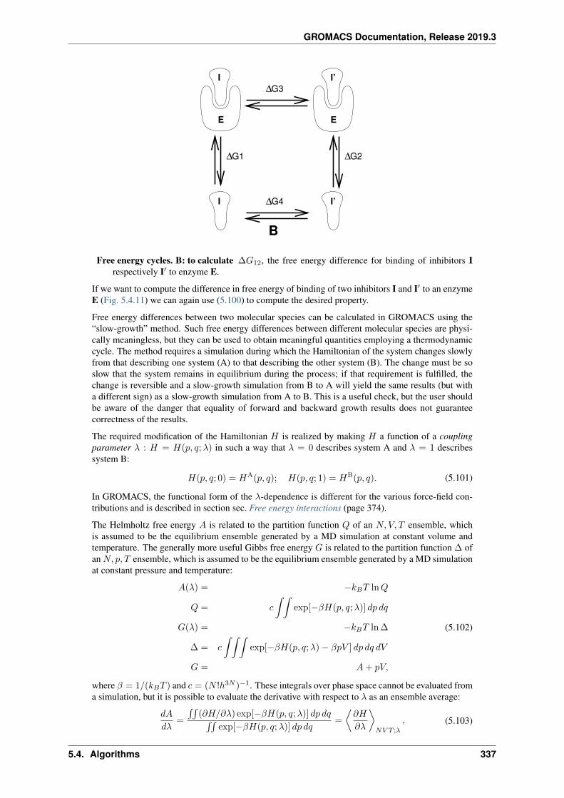
GROMACS Documentation, Release 2019.3
G1Δ ΔG2
ΔG3
I I’
E
I
E
I’
ΔG4
B
Free energy cycles. B: to calculate ∆𝐺12, the free energy difference for binding of inhibitors Irespectively I′ to enzyme E.
If we want to compute the difference in free energy of binding of two inhibitors I and I′ to an enzymeE (Fig. 5.4.11) we can again use (5.100) to compute the desired property.
Free energy differences between two molecular species can be calculated in GROMACS using the“slow-growth” method. Such free energy differences between different molecular species are physi-cally meaningless, but they can be used to obtain meaningful quantities employing a thermodynamiccycle. The method requires a simulation during which the Hamiltonian of the system changes slowlyfrom that describing one system (A) to that describing the other system (B). The change must be soslow that the system remains in equilibrium during the process; if that requirement is fulfilled, thechange is reversible and a slow-growth simulation from B to A will yield the same results (but witha different sign) as a slow-growth simulation from A to B. This is a useful check, but the user shouldbe aware of the danger that equality of forward and backward growth results does not guaranteecorrectness of the results.
The required modification of the Hamiltonian 𝐻 is realized by making 𝐻 a function of a couplingparameter 𝜆 : 𝐻 = 𝐻(𝑝, 𝑞;𝜆) in such a way that 𝜆 = 0 describes system A and 𝜆 = 1 describessystem B:
𝐻(𝑝, 𝑞; 0) = 𝐻A(𝑝, 𝑞); 𝐻(𝑝, 𝑞; 1) = 𝐻B(𝑝, 𝑞). (5.101)
In GROMACS, the functional form of the 𝜆-dependence is different for the various force-field con-tributions and is described in section sec. Free energy interactions (page 374).
The Helmholtz free energy 𝐴 is related to the partition function 𝑄 of an 𝑁,𝑉, 𝑇 ensemble, whichis assumed to be the equilibrium ensemble generated by a MD simulation at constant volume andtemperature. The generally more useful Gibbs free energy 𝐺 is related to the partition function ∆ ofan𝑁, 𝑝, 𝑇 ensemble, which is assumed to be the equilibrium ensemble generated by a MD simulationat constant pressure and temperature:
𝐴(𝜆) = −𝑘𝐵𝑇 ln𝑄
𝑄 = 𝑐
∫ ∫exp[−𝛽𝐻(𝑝, 𝑞;𝜆)] 𝑑𝑝 𝑑𝑞
𝐺(𝜆) = −𝑘𝐵𝑇 ln ∆
∆ = 𝑐
∫ ∫ ∫exp[−𝛽𝐻(𝑝, 𝑞;𝜆) − 𝛽𝑝𝑉 ] 𝑑𝑝 𝑑𝑞 𝑑𝑉
𝐺 = 𝐴+ 𝑝𝑉,
(5.102)
where 𝛽 = 1/(𝑘𝐵𝑇 ) and 𝑐 = (𝑁 !ℎ3𝑁 )−1. These integrals over phase space cannot be evaluated froma simulation, but it is possible to evaluate the derivative with respect to 𝜆 as an ensemble average:
𝑑𝐴
𝑑𝜆=
∫∫(𝜕𝐻/𝜕𝜆) exp[−𝛽𝐻(𝑝, 𝑞;𝜆)] 𝑑𝑝 𝑑𝑞∫∫
exp[−𝛽𝐻(𝑝, 𝑞;𝜆)] 𝑑𝑝 𝑑𝑞=
⟨𝜕𝐻
𝜕𝜆
⟩𝑁𝑉 𝑇 ;𝜆
, (5.103)
5.4. Algorithms 337
GROMACS Documentation, Release 2019.3
with a similar relation for 𝑑𝐺/𝑑𝜆 in the 𝑁, 𝑝, 𝑇 ensemble. The difference in free energy between Aand B can be found by integrating the derivative over 𝜆:
𝐴B(𝑉, 𝑇 ) −𝐴A(𝑉, 𝑇 ) =
∫ 1
0
⟨𝜕𝐻
𝜕𝜆
⟩𝑁𝑉 𝑇 ;𝜆
𝑑𝜆 (5.104)
𝐺B(𝑝, 𝑇 ) −𝐺A(𝑝, 𝑇 ) =
∫ 1
0
⟨𝜕𝐻
𝜕𝜆
⟩𝑁𝑝𝑇 ;𝜆
𝑑𝜆. (5.105)
If one wishes to evaluate 𝐺B(𝑝, 𝑇 ) −𝐺A(𝑝, 𝑇 ), the natural choice is a constant-pressure simulation.However, this quantity can also be obtained from a slow-growth simulation at constant volume, start-ing with system A at pressure 𝑝 and volume 𝑉 and ending with system B at pressure 𝑝𝐵 , by applyingthe following small (but, in principle, exact) correction:
𝐺B(𝑝) −𝐺A(𝑝) = 𝐴B(𝑉 ) −𝐴A(𝑉 ) −∫ 𝑝B
𝑝
[𝑉 B(𝑝′) − 𝑉 ] 𝑑𝑝′ (5.106)
Here we omitted the constant 𝑇 from the notation. This correction is roughly equal to − 12 (𝑝B −
𝑝)∆𝑉 = (∆𝑉 )2/(2𝜅𝑉 ), where ∆𝑉 is the volume change at 𝑝 and 𝜅 is the isothermal compressibil-ity. This is usually small; for example, the growth of a water molecule from nothing in a bath of 1000water molecules at constant volume would produce an additional pressure of as much as 22 bar, buta correction to the Helmholtz free energy of just -1 kJ mol−1. In Cartesian coordinates, the kineticenergy term in the Hamiltonian depends only on the momenta, and can be separately integrated and,in fact, removed from the equations. When masses do not change, there is no contribution from thekinetic energy at all; otherwise the integrated contribution to the free energy is − 3
2𝑘𝐵𝑇 ln(𝑚B/𝑚A).Note that this is only true in the absence of constraints.
Thermodynamic integration
GROMACS offers the possibility to integrate (5.104) or eq. (5.105) in one simulation over the fullrange from A to B. However, if the change is large and insufficient sampling can be expected, the usermay prefer to determine the value of ⟨𝑑𝐺/𝑑𝜆⟩ accurately at a number of well-chosen intermediatevalues of 𝜆. This can easily be done by setting the stepsize delta_lambda to zero. Each simulationcan be equilibrated first, and a proper error estimate can be made for each value of 𝑑𝐺/𝑑𝜆 from thefluctuation of 𝜕𝐻/𝜕𝜆. The total free energy change is then determined afterward by an appropriatenumerical integration procedure.
GROMACS now also supports the use of Bennett’s Acceptance Ratio 58 (page 508) for calculatingvalues of ∆G for transformations from state A to state B using the program gmx bar (page 48). Thesame data can also be used to calculate free energies using MBAR 59 (page 508), though the analysiscurrently requires external tools from the external pymbar package.
The 𝜆-dependence for the force-field contributions is described in detail in section sec. Free energyinteractions (page 374).
5.4.12 Replica exchange
Replica exchange molecular dynamics (REMD) is a method that can be used to speed up the samplingof any type of simulation, especially if conformations are separated by relatively high energy barriers.It involves simulating multiple replicas of the same system at different temperatures and randomlyexchanging the complete state of two replicas at regular intervals with the probability:
𝑃 (1 ↔ 2) = min
(1, exp
[(1
𝑘𝐵𝑇1− 1
𝑘𝐵𝑇2
)(𝑈1 − 𝑈2)
])(5.107)
where 𝑇1 and 𝑇2 are the reference temperatures and 𝑈1 and 𝑈2 are the instantaneous potential en-ergies of replicas 1 and 2 respectively. After exchange the velocities are scaled by (𝑇1/𝑇2)±0.5
5.4. Algorithms 338
GROMACS Documentation, Release 2019.3
and a neighbor search is performed the next step. This combines the fast sampling and frequentbarrier-crossing of the highest temperature with correct Boltzmann sampling at all the different tem-peratures 60 (page 508), 61 (page 508). We only attempt exchanges for neighboring temperaturesas the probability decreases very rapidly with the temperature difference. One should not attemptexchanges for all possible pairs in one step. If, for instance, replicas 1 and 2 would exchange, thechance of exchange for replicas 2 and 3 not only depends on the energies of replicas 2 and 3, but alsoon the energy of replica 1. In GROMACS this is solved by attempting exchange for all odd pairs onodd attempts and for all even pairs on even attempts. If we have four replicas: 0, 1, 2 and 3, ordered intemperature and we attempt exchange every 1000 steps, pairs 0-1 and 2-3 will be tried at steps 1000,3000 etc. and pair 1-2 at steps 2000, 4000 etc.
How should one choose the temperatures? The energy difference can be written as:
𝑈1 − 𝑈2 = 𝑁𝑑𝑓𝑐
2𝑘𝐵(𝑇1 − 𝑇2) (5.108)
where 𝑁𝑑𝑓 is the total number of degrees of freedom of one replica and 𝑐 is 1 for harmonic potentialsand around 2 for protein/water systems. If 𝑇2 = (1 + 𝜖)𝑇1 the probability becomes:
𝑃 (1 ↔ 2) = exp
(− 𝜖2𝑐𝑁𝑑𝑓
2(1 + 𝜖)
)≈ exp
(−𝜖2 𝑐
2𝑁𝑑𝑓
)(5.109)
Thus for a probability of 𝑒−2 ≈ 0.135 one obtains 𝜖 ≈ 2/√𝑐𝑁𝑑𝑓 . With all bonds constrained one
has 𝑁𝑑𝑓 ≈ 2𝑁𝑎𝑡𝑜𝑚𝑠 and thus for 𝑐 = 2 one should choose 𝜖 as 1/√𝑁𝑎𝑡𝑜𝑚𝑠. However there is one
problem when using pressure coupling. The density at higher temperatures will decrease, leading tohigher energy 62 (page 508), which should be taken into account. The GROMACS website features aso-called REMD calculator, that lets you type in the temperature range and the number of atoms,and based on that proposes a set of temperatures.
An extension to the REMD for the isobaric-isothermal ensemble was proposed by Okabe et al. 63(page 508). In this work the exchange probability is modified to:
𝑃 (1 ↔ 2) = min
(1, exp
[(1
𝑘𝐵𝑇1− 1
𝑘𝐵𝑇2
)(𝑈1 − 𝑈2) +
(𝑃1
𝑘𝐵𝑇1− 𝑃2
𝑘𝐵𝑇2
)(𝑉1 − 𝑉2)
])(5.110)
where 𝑃1 and 𝑃2 are the respective reference pressures and 𝑉1 and 𝑉2 are the respective instantaneousvolumes in the simulations. In most cases the differences in volume are so small that the secondterm is negligible. It only plays a role when the difference between 𝑃1 and 𝑃2 is large or in phasetransitions.
Hamiltonian replica exchange is also supported in GROMACS. In Hamiltonian replica exchange, eachreplica has a different Hamiltonian, defined by the free energy pathway specified for the simulation.The exchange probability to maintain the correct ensemble probabilities is:
𝑃 (1 ↔ 2) = min
(1, exp
[(1
𝑘𝐵𝑇− 1
𝑘𝐵𝑇
)((𝑈1(𝑥2) − 𝑈1(𝑥1)) + (𝑈2(𝑥1) − 𝑈2(𝑥2)))
])(5.111)
The separate Hamiltonians are defined by the free energy functionality of GROMACS, with swapsmade between the different values of 𝜆 defined in the mdp file.
Hamiltonian and temperature replica exchange can also be performed simultaneously, using the ac-ceptance criteria:
𝑃 (1 ↔ 2) = min
(1, exp
[(1
𝑘𝐵𝑇−)
(𝑈1(𝑥2) − 𝑈1(𝑥1)
𝑘𝐵𝑇1+𝑈2(𝑥1) − 𝑈2(𝑥2)
𝑘𝐵𝑇2)
])(5.112)
Gibbs sampling replica exchange has also been implemented in GROMACS 64 (page 509). In Gibbssampling replica exchange, all possible pairs are tested for exchange, allowing swaps between replicasthat are not neighbors.
Gibbs sampling replica exchange requires no additional potential energy calculations. However thereis an additional communication cost in Gibbs sampling replica exchange, as for some permutations,
5.4. Algorithms 339
GROMACS Documentation, Release 2019.3
more than one round of swaps must take place. In some cases, this extra communication cost mightaffect the efficiency.
All replica exchange variants are options of the mdrun (page 111) program. It will only work whenMPI is installed, due to the inherent parallelism in the algorithm. For efficiency each replica can runon a separate rank. See the manual page of mdrun (page 111) on how to use these multinode features.
5.4.13 Essential Dynamics sampling
The results from Essential Dynamics (see sec. Covariance analysis (page 490)) of a protein can beused to guide MD simulations. The idea is that from an initial MD simulation (or from other sources)a definition of the collective fluctuations with largest amplitude is obtained. The position along one ormore of these collective modes can be constrained in a (second) MD simulation in a number of waysfor several purposes. For example, the position along a certain mode may be kept fixed to monitorthe average force (free-energy gradient) on that coordinate in that position. Another application is toenhance sampling efficiency with respect to usual MD 65 (page 509), 66 (page 509). In this case,the system is encouraged to sample its available configuration space more systematically than in adiffusion-like path that proteins usually take.
Another possibility to enhance sampling is flooding. Here a flooding potential is added to certain(collective) degrees of freedom to expel the system out of a region of phase space 67 (page 509).
The procedure for essential dynamics sampling or flooding is as follows. First, the eigenvectors andeigenvalues need to be determined using covariance analysis (gmx covar (page 61)) or normal-modeanalysis (gmx nmeig (page 119)). Then, this information is fed into make_edi (page 106), which hasmany options for selecting vectors and setting parameters, see gmx make_edi -h. The generatededi (page 422) input file is then passed to mdrun (page 111).
5.4.14 Expanded Ensemble
In an expanded ensemble simulation 68 (page 509), both the coordinates and the thermodynamicensemble are treated as configuration variables that can be sampled over. The probability of anygiven state can be written as:
𝑃 (��, 𝑘) ∝ exp (−𝛽𝑘𝑈𝑘 + 𝑔𝑘) , (5.113)
where 𝛽𝑘 = 1𝑘𝐵𝑇𝑘
is the 𝛽 corresponding to the 𝑘th thermodynamic state, and 𝑔𝑘 is a user-specifiedweight factor corresponding to the 𝑘th state. This space is therefore a mixed, generalized, or expandedensemble which samples from multiple thermodynamic ensembles simultaneously. 𝑔𝑘 is chosen togive a specific weighting of each subensemble in the expanded ensemble, and can either be fixed, ordetermined by an iterative procedure. The set of 𝑔𝑘 is frequently chosen to give each thermodynamicensemble equal probability, in which case 𝑔𝑘 is equal to the free energy in non-dimensional units, butthey can be set to arbitrary values as desired. Several different algorithms can be used to equilibratethese weights, described in the mdp option listings.
In GROMACS, this space is sampled by alternating sampling in the 𝑘 and �� directions. Samplingin the �� direction is done by standard molecular dynamics sampling; sampling between the differentthermodynamics states is done by Monte Carlo, with several different Monte Carlo moves supported.The 𝑘 states can be defined by different temperatures, or choices of the free energy 𝜆 variable, or both.Expanded ensemble simulations thus represent a serialization of the replica exchange formalism,allowing a single simulation to explore many thermodynamic states.
5.4.15 Parallelization
The CPU time required for a simulation can be reduced by running the simulation in parallel overmore than one core. Ideally, one would want to have linear scaling: running on 𝑁 cores makesthe simulation 𝑁 times faster. In practice this can only be achieved for a small number of cores.The scaling will depend a lot on the algorithms used. Also, different algorithms can have differentrestrictions on the interaction ranges between atoms.
5.4. Algorithms 340
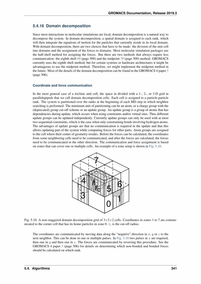
GROMACS Documentation, Release 2019.3
5.4.16 Domain decomposition
Since most interactions in molecular simulations are local, domain decomposition is a natural way todecompose the system. In domain decomposition, a spatial domain is assigned to each rank, whichwill then integrate the equations of motion for the particles that currently reside in its local domain.With domain decomposition, there are two choices that have to be made: the division of the unit cellinto domains and the assignment of the forces to domains. Most molecular simulation packages usethe half-shell method for assigning the forces. But there are two methods that always require lesscommunication: the eighth shell 69 (page 509) and the midpoint 70 (page 509) method. GROMACScurrently uses the eighth shell method, but for certain systems or hardware architectures it might beadvantageous to use the midpoint method. Therefore, we might implement the midpoint method inthe future. Most of the details of the domain decomposition can be found in the GROMACS 4 paper 5(page 506).
Coordinate and force communication
In the most general case of a triclinic unit cell, the space in divided with a 1-, 2-, or 3-D grid inparallelepipeds that we call domain decomposition cells. Each cell is assigned to a particle-particlerank. The system is partitioned over the ranks at the beginning of each MD step in which neighborsearching is performed. The minimum unit of partitioning can be an atom, or a charge group with the(deprecated) group cut-off scheme or an update group. An update group is a group of atoms that hasdependencies during update, which occurs when using constraints and/or virtual sites. Thus differentupdate groups can be updated independenly. Currently update groups can only be used with at mosttwo sequential constraints, which is the case when only constraining bonds involving hydrogen atoms.The advantages of update groups are that no communication is required in the update and that thisallows updating part of the system while computing forces for other parts. Atom groups are assignedto the cell where their center of geometry resides. Before the forces can be calculated, the coordinatesfrom some neighboring cells need to be communicated, and after the forces are calculated, the forcesneed to be communicated in the other direction. The communication and force assignment is basedon zones that can cover one or multiple cells. An example of a zone setup is shown in Fig. 5.10.
0 0 0 0 0 0 0 0 0 0 0 0 0 0 0 00 0 0 0 0 0 0 0 0 0 0 0 0 0 0 00 0 0 0 0 0 0 0 0 0 0 0 0 0 0 00 0 0 0 0 0 0 0 0 0 0 0 0 0 0 00 0 0 0 0 0 0 0 0 0 0 0 0 0 0 00 0 0 0 0 0 0 0 0 0 0 0 0 0 0 00 0 0 0 0 0 0 0 0 0 0 0 0 0 0 00 0 0 0 0 0 0 0 0 0 0 0 0 0 0 00 0 0 0 0 0 0 0 0 0 0 0 0 0 0 0
1 1 1 1 1 1 1 1 1 1 1 1 1 1 1 11 1 1 1 1 1 1 1 1 1 1 1 1 1 1 11 1 1 1 1 1 1 1 1 1 1 1 1 1 1 11 1 1 1 1 1 1 1 1 1 1 1 1 1 1 11 1 1 1 1 1 1 1 1 1 1 1 1 1 1 11 1 1 1 1 1 1 1 1 1 1 1 1 1 1 11 1 1 1 1 1 1 1 1 1 1 1 1 1 1 11 1 1 1 1 1 1 1 1 1 1 1 1 1 1 11 1 1 1 1 1 1 1 1 1 1 1 1 1 1 1
0 0 0 0 0 0 0 00 0 0 0 0 0 0 00 0 0 0 0 0 0 00 0 0 0 0 0 0 0
1 1 1 1 1 1 1 11 1 1 1 1 1 1 11 1 1 1 1 1 1 11 1 1 1 1 1 1 1
0 0 0 0 00 0 0 0 00 0 0 0 0
1 1 1 1 11 1 1 1 11 1 1 1 1
0 0 0 0 0 00 0 0 0 0 00 0 0 0 0 00 0 0 0 0 00 0 0 0 0 00 0 0 0 0 00 0 0 0 0 00 0 0 0 0 00 0 0 0 0 00 0 0 0 0 00 0 0 0 0 00 0 0 0 0 00 0 0 0 0 00 0 0 0 0 0
1 1 1 1 1 11 1 1 1 1 11 1 1 1 1 11 1 1 1 1 11 1 1 1 1 11 1 1 1 1 11 1 1 1 1 11 1 1 1 1 11 1 1 1 1 11 1 1 1 1 11 1 1 1 1 11 1 1 1 1 11 1 1 1 1 11 1 1 1 1 1
0 0 0 0 0 0 0 0 00 0 0 0 0 0 0 0 00 0 0 0 0 0 0 0 00 0 0 0 0 0 0 0 00 0 0 0 0 0 0 0 00 0 0 0 0 0 0 0 00 0 0 0 0 0 0 0 00 0 0 0 0 0 0 0 00 0 0 0 0 0 0 0 00 0 0 0 0 0 0 0 00 0 0 0 0 0 0 0 00 0 0 0 0 0 0 0 0
1 1 1 1 1 1 1 1 11 1 1 1 1 1 1 1 11 1 1 1 1 1 1 1 11 1 1 1 1 1 1 1 11 1 1 1 1 1 1 1 11 1 1 1 1 1 1 1 11 1 1 1 1 1 1 1 11 1 1 1 1 1 1 1 11 1 1 1 1 1 1 1 11 1 1 1 1 1 1 1 11 1 1 1 1 1 1 1 11 1 1 1 1 1 1 1 1
0 0 0 00 0 0 00 0 0 00 0 0 00 0 0 00 0 0 00 0 0 00 0 0 00 0 0 00 0 0 00 0 0 00 0 0 00 0 0 00 0 0 00 0 0 0
1 1 1 11 1 1 11 1 1 11 1 1 11 1 1 11 1 1 11 1 1 11 1 1 11 1 1 11 1 1 11 1 1 11 1 1 11 1 1 11 1 1 11 1 1 1
0 0 0 0 0 00 0 0 0 0 00 0 0 0 0 00 0 0 0 0 00 0 0 0 0 00 0 0 0 0 00 0 0 0 0 00 0 0 0 0 00 0 0 0 0 00 0 0 0 0 00 0 0 0 0 00 0 0 0 0 00 0 0 0 0 0
1 1 1 1 1 11 1 1 1 1 11 1 1 1 1 11 1 1 1 1 11 1 1 1 1 11 1 1 1 1 11 1 1 1 1 11 1 1 1 1 11 1 1 1 1 11 1 1 1 1 11 1 1 1 1 11 1 1 1 1 11 1 1 1 1 1
0 0 0 00 0 0 00 0 0 00 0 0 00 0 0 00 0 0 00 0 0 00 0 0 00 0 0 00 0 0 00 0 0 00 0 0 00 0 0 00 0 0 00 0 0 0
1 1 1 11 1 1 11 1 1 11 1 1 11 1 1 11 1 1 11 1 1 11 1 1 11 1 1 11 1 1 11 1 1 11 1 1 11 1 1 11 1 1 11 1 1 1
0 0 0 0 0 00 0 0 0 0 00 0 0 0 0 00 0 0 0 0 00 0 0 0 0 00 0 0 0 0 00 0 0 0 0 00 0 0 0 0 00 0 0 0 0 00 0 0 0 0 00 0 0 0 0 00 0 0 0 0 00 0 0 0 0 00 0 0 0 0 00 0 0 0 0 00 0 0 0 0 00 0 0 0 0 0
1 1 1 1 1 11 1 1 1 1 11 1 1 1 1 11 1 1 1 1 11 1 1 1 1 11 1 1 1 1 11 1 1 1 1 11 1 1 1 1 11 1 1 1 1 11 1 1 1 1 11 1 1 1 1 11 1 1 1 1 11 1 1 1 1 11 1 1 1 1 11 1 1 1 1 11 1 1 1 1 11 1 1 1 1 1
7
30
4cr
165
Fig. 5.10: A non-staggered domain decomposition grid of 3×2×2 cells. Coordinates in zones 1 to 7 are commu-nicated to the corner cell that has its home particles in zone 0. 𝑟𝑐 is the cut-off radius.
The coordinates are communicated by moving data along the “negative” direction in 𝑥, 𝑦 or 𝑧 to thenext neighbor. This can be done in one or multiple pulses. In Fig. 5.10 two pulses in 𝑥 are required,then one in 𝑦 and then one in 𝑧. The forces are communicated by reversing this procedure. See theGROMACS 4 paper 5 (page 506) for details on determining which non-bonded and bonded forcesshould be calculated on which rank.
5.4. Algorithms 341
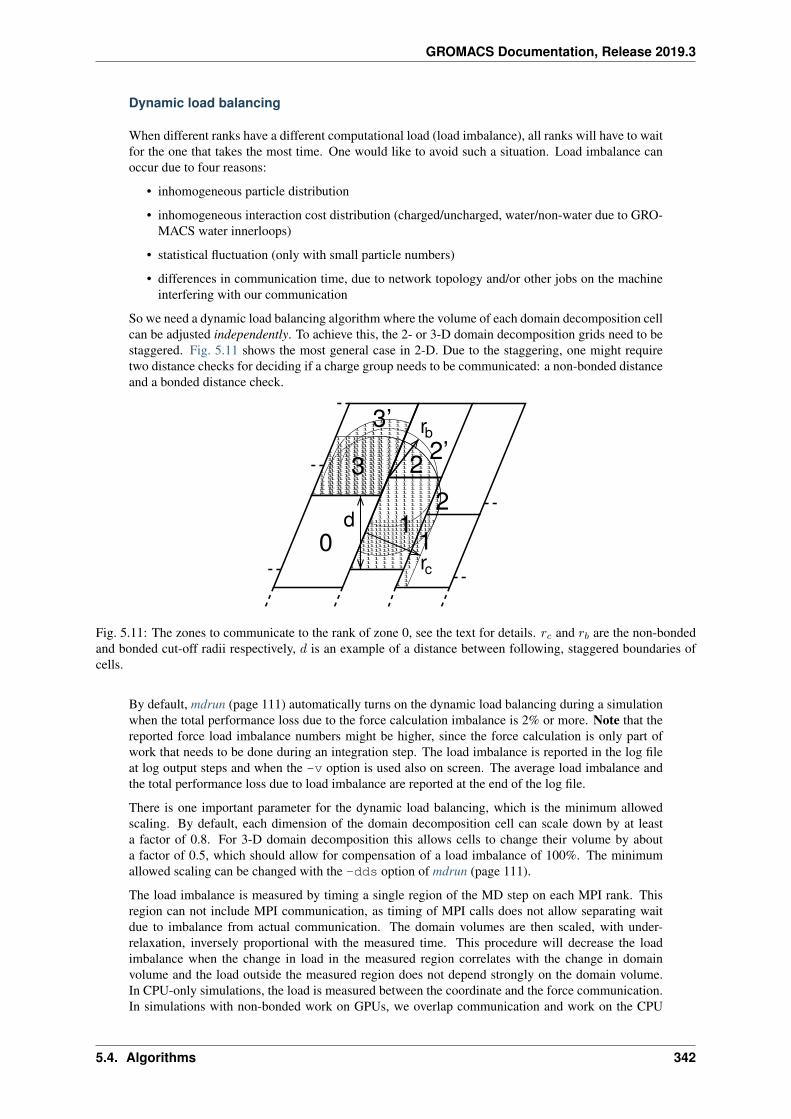
GROMACS Documentation, Release 2019.3
Dynamic load balancing
When different ranks have a different computational load (load imbalance), all ranks will have to waitfor the one that takes the most time. One would like to avoid such a situation. Load imbalance canoccur due to four reasons:
• inhomogeneous particle distribution
• inhomogeneous interaction cost distribution (charged/uncharged, water/non-water due to GRO-MACS water innerloops)
• statistical fluctuation (only with small particle numbers)
• differences in communication time, due to network topology and/or other jobs on the machineinterfering with our communication
So we need a dynamic load balancing algorithm where the volume of each domain decomposition cellcan be adjusted independently. To achieve this, the 2- or 3-D domain decomposition grids need to bestaggered. Fig. 5.11 shows the most general case in 2-D. Due to the staggering, one might requiretwo distance checks for deciding if a charge group needs to be communicated: a non-bonded distanceand a bonded distance check.
0 0 0 0 0 0 0 0 0 0 0 0 0 0 0 00 0 0 0 0 0 0 0 0 0 0 0 0 0 0 00 0 0 0 0 0 0 0 0 0 0 0 0 0 0 00 0 0 0 0 0 0 0 0 0 0 0 0 0 0 00 0 0 0 0 0 0 0 0 0 0 0 0 0 0 00 0 0 0 0 0 0 0 0 0 0 0 0 0 0 00 0 0 0 0 0 0 0 0 0 0 0 0 0 0 00 0 0 0 0 0 0 0 0 0 0 0 0 0 0 00 0 0 0 0 0 0 0 0 0 0 0 0 0 0 00 0 0 0 0 0 0 0 0 0 0 0 0 0 0 00 0 0 0 0 0 0 0 0 0 0 0 0 0 0 00 0 0 0 0 0 0 0 0 0 0 0 0 0 0 00 0 0 0 0 0 0 0 0 0 0 0 0 0 0 00 0 0 0 0 0 0 0 0 0 0 0 0 0 0 00 0 0 0 0 0 0 0 0 0 0 0 0 0 0 00 0 0 0 0 0 0 0 0 0 0 0 0 0 0 00 0 0 0 0 0 0 0 0 0 0 0 0 0 0 00 0 0 0 0 0 0 0 0 0 0 0 0 0 0 00 0 0 0 0 0 0 0 0 0 0 0 0 0 0 00 0 0 0 0 0 0 0 0 0 0 0 0 0 0 00 0 0 0 0 0 0 0 0 0 0 0 0 0 0 00 0 0 0 0 0 0 0 0 0 0 0 0 0 0 00 0 0 0 0 0 0 0 0 0 0 0 0 0 0 00 0 0 0 0 0 0 0 0 0 0 0 0 0 0 00 0 0 0 0 0 0 0 0 0 0 0 0 0 0 00 0 0 0 0 0 0 0 0 0 0 0 0 0 0 00 0 0 0 0 0 0 0 0 0 0 0 0 0 0 00 0 0 0 0 0 0 0 0 0 0 0 0 0 0 00 0 0 0 0 0 0 0 0 0 0 0 0 0 0 00 0 0 0 0 0 0 0 0 0 0 0 0 0 0 00 0 0 0 0 0 0 0 0 0 0 0 0 0 0 0
1 1 1 1 1 1 1 1 1 1 1 1 1 1 1 11 1 1 1 1 1 1 1 1 1 1 1 1 1 1 11 1 1 1 1 1 1 1 1 1 1 1 1 1 1 11 1 1 1 1 1 1 1 1 1 1 1 1 1 1 11 1 1 1 1 1 1 1 1 1 1 1 1 1 1 11 1 1 1 1 1 1 1 1 1 1 1 1 1 1 11 1 1 1 1 1 1 1 1 1 1 1 1 1 1 11 1 1 1 1 1 1 1 1 1 1 1 1 1 1 11 1 1 1 1 1 1 1 1 1 1 1 1 1 1 11 1 1 1 1 1 1 1 1 1 1 1 1 1 1 11 1 1 1 1 1 1 1 1 1 1 1 1 1 1 11 1 1 1 1 1 1 1 1 1 1 1 1 1 1 11 1 1 1 1 1 1 1 1 1 1 1 1 1 1 11 1 1 1 1 1 1 1 1 1 1 1 1 1 1 11 1 1 1 1 1 1 1 1 1 1 1 1 1 1 11 1 1 1 1 1 1 1 1 1 1 1 1 1 1 11 1 1 1 1 1 1 1 1 1 1 1 1 1 1 11 1 1 1 1 1 1 1 1 1 1 1 1 1 1 11 1 1 1 1 1 1 1 1 1 1 1 1 1 1 11 1 1 1 1 1 1 1 1 1 1 1 1 1 1 11 1 1 1 1 1 1 1 1 1 1 1 1 1 1 11 1 1 1 1 1 1 1 1 1 1 1 1 1 1 11 1 1 1 1 1 1 1 1 1 1 1 1 1 1 11 1 1 1 1 1 1 1 1 1 1 1 1 1 1 11 1 1 1 1 1 1 1 1 1 1 1 1 1 1 11 1 1 1 1 1 1 1 1 1 1 1 1 1 1 11 1 1 1 1 1 1 1 1 1 1 1 1 1 1 11 1 1 1 1 1 1 1 1 1 1 1 1 1 1 11 1 1 1 1 1 1 1 1 1 1 1 1 1 1 11 1 1 1 1 1 1 1 1 1 1 1 1 1 1 11 1 1 1 1 1 1 1 1 1 1 1 1 1 1 1
0 0 0 0 0 0 0 0 0 0 00 0 0 0 0 0 0 0 0 0 00 0 0 0 0 0 0 0 0 0 00 0 0 0 0 0 0 0 0 0 00 0 0 0 0 0 0 0 0 0 00 0 0 0 0 0 0 0 0 0 00 0 0 0 0 0 0 0 0 0 00 0 0 0 0 0 0 0 0 0 00 0 0 0 0 0 0 0 0 0 00 0 0 0 0 0 0 0 0 0 00 0 0 0 0 0 0 0 0 0 00 0 0 0 0 0 0 0 0 0 00 0 0 0 0 0 0 0 0 0 00 0 0 0 0 0 0 0 0 0 00 0 0 0 0 0 0 0 0 0 00 0 0 0 0 0 0 0 0 0 00 0 0 0 0 0 0 0 0 0 00 0 0 0 0 0 0 0 0 0 00 0 0 0 0 0 0 0 0 0 00 0 0 0 0 0 0 0 0 0 00 0 0 0 0 0 0 0 0 0 00 0 0 0 0 0 0 0 0 0 00 0 0 0 0 0 0 0 0 0 00 0 0 0 0 0 0 0 0 0 00 0 0 0 0 0 0 0 0 0 00 0 0 0 0 0 0 0 0 0 00 0 0 0 0 0 0 0 0 0 00 0 0 0 0 0 0 0 0 0 00 0 0 0 0 0 0 0 0 0 0
1 1 1 1 1 1 1 1 1 1 11 1 1 1 1 1 1 1 1 1 11 1 1 1 1 1 1 1 1 1 11 1 1 1 1 1 1 1 1 1 11 1 1 1 1 1 1 1 1 1 11 1 1 1 1 1 1 1 1 1 11 1 1 1 1 1 1 1 1 1 11 1 1 1 1 1 1 1 1 1 11 1 1 1 1 1 1 1 1 1 11 1 1 1 1 1 1 1 1 1 11 1 1 1 1 1 1 1 1 1 11 1 1 1 1 1 1 1 1 1 11 1 1 1 1 1 1 1 1 1 11 1 1 1 1 1 1 1 1 1 11 1 1 1 1 1 1 1 1 1 11 1 1 1 1 1 1 1 1 1 11 1 1 1 1 1 1 1 1 1 11 1 1 1 1 1 1 1 1 1 11 1 1 1 1 1 1 1 1 1 11 1 1 1 1 1 1 1 1 1 11 1 1 1 1 1 1 1 1 1 11 1 1 1 1 1 1 1 1 1 11 1 1 1 1 1 1 1 1 1 11 1 1 1 1 1 1 1 1 1 11 1 1 1 1 1 1 1 1 1 11 1 1 1 1 1 1 1 1 1 11 1 1 1 1 1 1 1 1 1 11 1 1 1 1 1 1 1 1 1 11 1 1 1 1 1 1 1 1 1 1
0 0 00 0 00 0 00 0 00 0 00 0 0
1 1 11 1 11 1 11 1 11 1 11 1 1
0 0 0 0 0 0 0 0 0 00 0 0 0 0 0 0 0 0 00 0 0 0 0 0 0 0 0 00 0 0 0 0 0 0 0 0 00 0 0 0 0 0 0 0 0 00 0 0 0 0 0 0 0 0 00 0 0 0 0 0 0 0 0 00 0 0 0 0 0 0 0 0 00 0 0 0 0 0 0 0 0 00 0 0 0 0 0 0 0 0 00 0 0 0 0 0 0 0 0 00 0 0 0 0 0 0 0 0 00 0 0 0 0 0 0 0 0 00 0 0 0 0 0 0 0 0 00 0 0 0 0 0 0 0 0 00 0 0 0 0 0 0 0 0 0
1 1 1 1 1 1 1 1 1 11 1 1 1 1 1 1 1 1 11 1 1 1 1 1 1 1 1 11 1 1 1 1 1 1 1 1 11 1 1 1 1 1 1 1 1 11 1 1 1 1 1 1 1 1 11 1 1 1 1 1 1 1 1 11 1 1 1 1 1 1 1 1 11 1 1 1 1 1 1 1 1 11 1 1 1 1 1 1 1 1 11 1 1 1 1 1 1 1 1 11 1 1 1 1 1 1 1 1 11 1 1 1 1 1 1 1 1 11 1 1 1 1 1 1 1 1 11 1 1 1 1 1 1 1 1 11 1 1 1 1 1 1 1 1 1
0 0 0 0 0 0 0 0 0 0 00 0 0 0 0 0 0 0 0 0 00 0 0 0 0 0 0 0 0 0 00 0 0 0 0 0 0 0 0 0 00 0 0 0 0 0 0 0 0 0 00 0 0 0 0 0 0 0 0 0 00 0 0 0 0 0 0 0 0 0 00 0 0 0 0 0 0 0 0 0 00 0 0 0 0 0 0 0 0 0 00 0 0 0 0 0 0 0 0 0 00 0 0 0 0 0 0 0 0 0 00 0 0 0 0 0 0 0 0 0 00 0 0 0 0 0 0 0 0 0 0
1 1 1 1 1 1 1 1 1 1 11 1 1 1 1 1 1 1 1 1 11 1 1 1 1 1 1 1 1 1 11 1 1 1 1 1 1 1 1 1 11 1 1 1 1 1 1 1 1 1 11 1 1 1 1 1 1 1 1 1 11 1 1 1 1 1 1 1 1 1 11 1 1 1 1 1 1 1 1 1 11 1 1 1 1 1 1 1 1 1 11 1 1 1 1 1 1 1 1 1 11 1 1 1 1 1 1 1 1 1 11 1 1 1 1 1 1 1 1 1 11 1 1 1 1 1 1 1 1 1 1
0 00 00 00 00 00 0
1 11 11 11 11 11 1
0 0 0 0 0 0 0 00 0 0 0 0 0 0 00 0 0 0 0 0 0 00 0 0 0 0 0 0 00 0 0 0 0 0 0 00 0 0 0 0 0 0 0
1 1 1 1 1 1 1 11 1 1 1 1 1 1 11 1 1 1 1 1 1 11 1 1 1 1 1 1 11 1 1 1 1 1 1 11 1 1 1 1 1 1 1
0 0 0 00 0 0 00 0 0 00 0 0 00 0 0 00 0 0 00 0 0 00 0 0 00 0 0 00 0 0 00 0 0 0
1 1 1 11 1 1 11 1 1 11 1 1 11 1 1 11 1 1 11 1 1 11 1 1 11 1 1 11 1 1 11 1 1 1
1 12
d0
3 2
3’
rc
rb2’
Fig. 5.11: The zones to communicate to the rank of zone 0, see the text for details. 𝑟𝑐 and 𝑟𝑏 are the non-bondedand bonded cut-off radii respectively, 𝑑 is an example of a distance between following, staggered boundaries ofcells.
By default, mdrun (page 111) automatically turns on the dynamic load balancing during a simulationwhen the total performance loss due to the force calculation imbalance is 2% or more. Note that thereported force load imbalance numbers might be higher, since the force calculation is only part ofwork that needs to be done during an integration step. The load imbalance is reported in the log fileat log output steps and when the -v option is used also on screen. The average load imbalance andthe total performance loss due to load imbalance are reported at the end of the log file.
There is one important parameter for the dynamic load balancing, which is the minimum allowedscaling. By default, each dimension of the domain decomposition cell can scale down by at leasta factor of 0.8. For 3-D domain decomposition this allows cells to change their volume by abouta factor of 0.5, which should allow for compensation of a load imbalance of 100%. The minimumallowed scaling can be changed with the -dds option of mdrun (page 111).
The load imbalance is measured by timing a single region of the MD step on each MPI rank. Thisregion can not include MPI communication, as timing of MPI calls does not allow separating waitdue to imbalance from actual communication. The domain volumes are then scaled, with under-relaxation, inversely proportional with the measured time. This procedure will decrease the loadimbalance when the change in load in the measured region correlates with the change in domainvolume and the load outside the measured region does not depend strongly on the domain volume.In CPU-only simulations, the load is measured between the coordinate and the force communication.In simulations with non-bonded work on GPUs, we overlap communication and work on the CPU
5.4. Algorithms 342
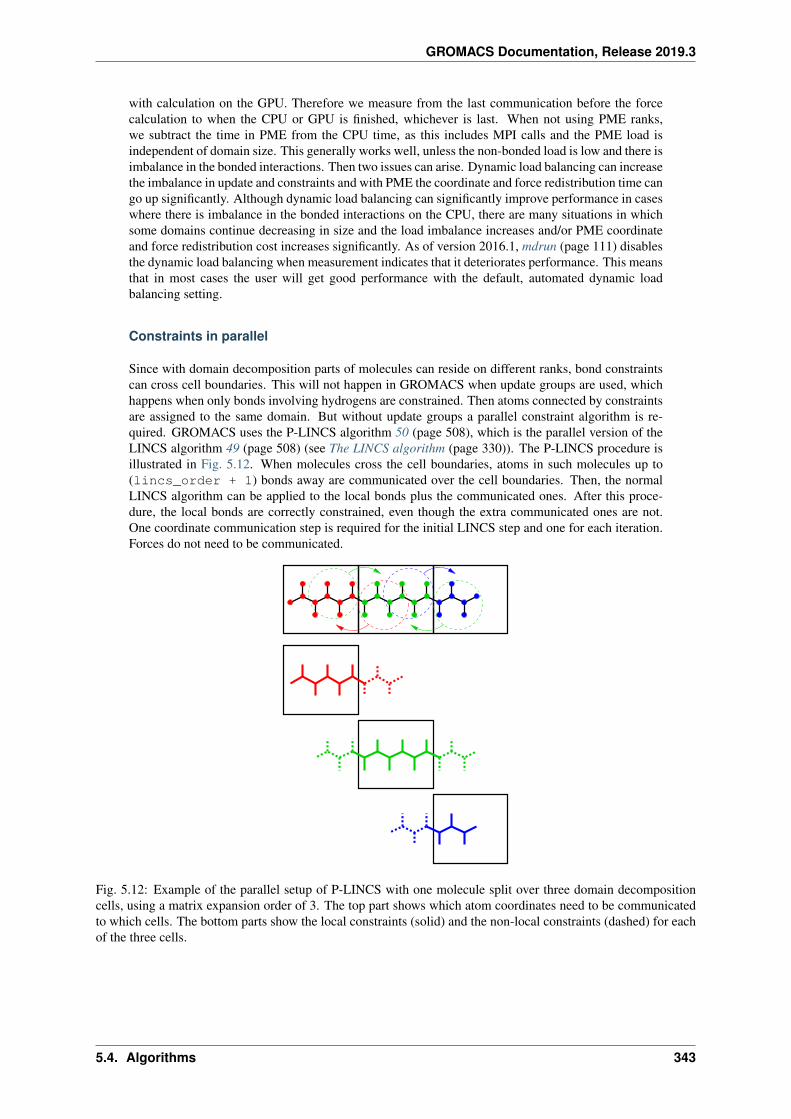
GROMACS Documentation, Release 2019.3
with calculation on the GPU. Therefore we measure from the last communication before the forcecalculation to when the CPU or GPU is finished, whichever is last. When not using PME ranks,we subtract the time in PME from the CPU time, as this includes MPI calls and the PME load isindependent of domain size. This generally works well, unless the non-bonded load is low and there isimbalance in the bonded interactions. Then two issues can arise. Dynamic load balancing can increasethe imbalance in update and constraints and with PME the coordinate and force redistribution time cango up significantly. Although dynamic load balancing can significantly improve performance in caseswhere there is imbalance in the bonded interactions on the CPU, there are many situations in whichsome domains continue decreasing in size and the load imbalance increases and/or PME coordinateand force redistribution cost increases significantly. As of version 2016.1, mdrun (page 111) disablesthe dynamic load balancing when measurement indicates that it deteriorates performance. This meansthat in most cases the user will get good performance with the default, automated dynamic loadbalancing setting.
Constraints in parallel
Since with domain decomposition parts of molecules can reside on different ranks, bond constraintscan cross cell boundaries. This will not happen in GROMACS when update groups are used, whichhappens when only bonds involving hydrogens are constrained. Then atoms connected by constraintsare assigned to the same domain. But without update groups a parallel constraint algorithm is re-quired. GROMACS uses the P-LINCS algorithm 50 (page 508), which is the parallel version of theLINCS algorithm 49 (page 508) (see The LINCS algorithm (page 330)). The P-LINCS procedure isillustrated in Fig. 5.12. When molecules cross the cell boundaries, atoms in such molecules up to(lincs_order + 1) bonds away are communicated over the cell boundaries. Then, the normalLINCS algorithm can be applied to the local bonds plus the communicated ones. After this proce-dure, the local bonds are correctly constrained, even though the extra communicated ones are not.One coordinate communication step is required for the initial LINCS step and one for each iteration.Forces do not need to be communicated.
Fig. 5.12: Example of the parallel setup of P-LINCS with one molecule split over three domain decompositioncells, using a matrix expansion order of 3. The top part shows which atom coordinates need to be communicatedto which cells. The bottom parts show the local constraints (solid) and the non-local constraints (dashed) for eachof the three cells.
5.4. Algorithms 343
GROMACS Documentation, Release 2019.3
Interaction ranges
Domain decomposition takes advantage of the locality of interactions. This means that there willbe limitations on the range of interactions. By default, mdrun (page 111) tries to find the optimalbalance between interaction range and efficiency. But it can happen that a simulation stops with anerror message about missing interactions, or that a simulation might run slightly faster with shorterinteraction ranges. A list of interaction ranges and their default values is given in Table 5.7
Table 5.7: The interaction ranges with domain decomposition.interaction range option defaultnon-bonded 𝑟𝑐=max(𝑟list,𝑟VdW,𝑟Coul) mdp (page 425) filetwo-body bonded max(𝑟mb,𝑟𝑐) mdrun (page 111) -rdd starting conf. + 10%multi-bodybonded
𝑟mb mdrun (page 111) -rdd starting conf. + 10%
constraints 𝑟con mdrun (page 111)-rcon
est. from bondlengths
virtual sites 𝑟con mdrun (page 111)-rcon
0
In most cases the defaults of mdrun (page 111) should not cause the simulation to stop with anerror message of missing interactions. The range for the bonded interactions is determined from thedistance between bonded charge-groups in the starting configuration, with 10% added for headroom.For the constraints, the value of 𝑟con is determined by taking the maximum distance that (lincs_-order + 1) bonds can cover when they all connect at angles of 120 degrees. The actual constraintcommunication is not limited by 𝑟con, but by the minimum cell size 𝐿𝐶 , which has the followinglower limit:
𝐿𝐶 ≥ max(𝑟mb, 𝑟con) (5.114)
Without dynamic load balancing the system is actually allowed to scale beyond this limit when pres-sure scaling is used. Note that for triclinic boxes, 𝐿𝐶 is not simply the box diagonal componentdivided by the number of cells in that direction, rather it is the shortest distance between the tricliniccells borders. For rhombic dodecahedra this is a factor of
√3/2 shorter along 𝑥 and 𝑦.
When 𝑟mb > 𝑟𝑐, mdrun (page 111) employs a smart algorithm to reduce the communication. Simplycommunicating all charge groups within 𝑟mb would increase the amount of communication enor-mously. Therefore only charge-groups that are connected by bonded interactions to charge groupswhich are not locally present are communicated. This leads to little extra communication, but alsoto a slightly increased cost for the domain decomposition setup. In some cases, e.g. coarse-grainedsimulations with a very short cut-off, one might want to set 𝑟mb by hand to reduce this cost.
Multiple-Program, Multiple-Data PME parallelization
Electrostatics interactions are long-range, therefore special algorithms are used to avoid summationover many atom pairs. In GROMACS this is usually PME (sec. PME (page 383)). Since with PME allparticles interact with each other, global communication is required. This will usually be the limitingfactor for scaling with domain decomposition. To reduce the effect of this problem, we have comeup with a Multiple-Program, Multiple-Data approach 5 (page 506). Here, some ranks are selectedto do only the PME mesh calculation, while the other ranks, called particle-particle (PP) ranks, doall the rest of the work. For rectangular boxes the optimal PP to PME rank ratio is usually 3:1, forrhombic dodecahedra usually 2:1. When the number of PME ranks is reduced by a factor of 4, thenumber of communication calls is reduced by about a factor of 16. Or put differently, we can nowscale to 4 times more ranks. In addition, for modern 4 or 8 core machines in a network, the effectivenetwork bandwidth for PME is quadrupled, since only a quarter of the cores will be using the networkconnection on each machine during the PME calculations.
mdrun (page 111) will by default interleave the PP and PME ranks. If the ranks are not number con-secutively inside the machines, one might want to use mdrun (page 111) -ddorder pp_pme. For
5.4. Algorithms 344
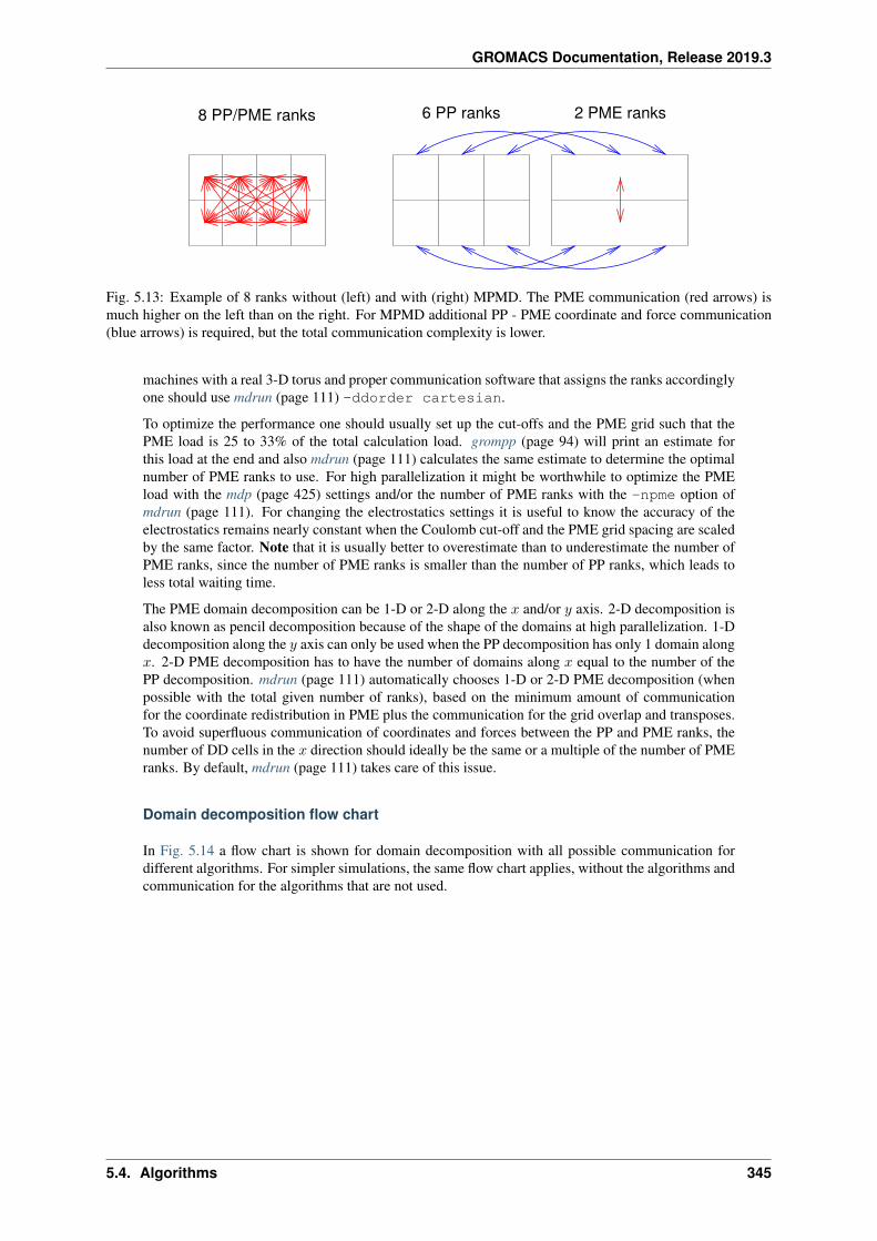
GROMACS Documentation, Release 2019.3
6 PP ranks 2 PME ranks8 PP/PME ranks
Fig. 5.13: Example of 8 ranks without (left) and with (right) MPMD. The PME communication (red arrows) ismuch higher on the left than on the right. For MPMD additional PP - PME coordinate and force communication(blue arrows) is required, but the total communication complexity is lower.
machines with a real 3-D torus and proper communication software that assigns the ranks accordinglyone should use mdrun (page 111) -ddorder cartesian.
To optimize the performance one should usually set up the cut-offs and the PME grid such that thePME load is 25 to 33% of the total calculation load. grompp (page 94) will print an estimate forthis load at the end and also mdrun (page 111) calculates the same estimate to determine the optimalnumber of PME ranks to use. For high parallelization it might be worthwhile to optimize the PMEload with the mdp (page 425) settings and/or the number of PME ranks with the -npme option ofmdrun (page 111). For changing the electrostatics settings it is useful to know the accuracy of theelectrostatics remains nearly constant when the Coulomb cut-off and the PME grid spacing are scaledby the same factor. Note that it is usually better to overestimate than to underestimate the number ofPME ranks, since the number of PME ranks is smaller than the number of PP ranks, which leads toless total waiting time.
The PME domain decomposition can be 1-D or 2-D along the 𝑥 and/or 𝑦 axis. 2-D decomposition isalso known as pencil decomposition because of the shape of the domains at high parallelization. 1-Ddecomposition along the 𝑦 axis can only be used when the PP decomposition has only 1 domain along𝑥. 2-D PME decomposition has to have the number of domains along 𝑥 equal to the number of thePP decomposition. mdrun (page 111) automatically chooses 1-D or 2-D PME decomposition (whenpossible with the total given number of ranks), based on the minimum amount of communicationfor the coordinate redistribution in PME plus the communication for the grid overlap and transposes.To avoid superfluous communication of coordinates and forces between the PP and PME ranks, thenumber of DD cells in the 𝑥 direction should ideally be the same or a multiple of the number of PMEranks. By default, mdrun (page 111) takes care of this issue.
Domain decomposition flow chart
In Fig. 5.14 a flow chart is shown for domain decomposition with all possible communication fordifferent algorithms. For simpler simulations, the same flow chart applies, without the algorithms andcommunication for the algorithms that are not used.
5.4. Algorithms 345
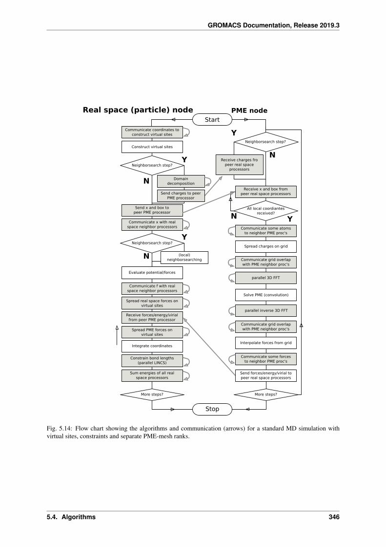
GROMACS Documentation, Release 2019.3
Start
Real space (particle) node PME node
Y
Y
Y
Y
N
N
N
N
Communicate coordinates to construct virtual sites
Construct virtual sites
Neighborsearch step?
Neighborsearch step?
Neighborsearch step?
Domain decomposition
Send charges to peer PME processor
Send x and box to peer PME processor
Communicate x with real space neighbor processors
(local) neighborsearching
Evaluate potential/forces
Communicate f with real space neighbor processors
Spread real space forces on virtual sites
Receive forces/energy/virial from peer PME processor
Spread PME forces on virtual sites
Integrate coordinates
Constrain bond lengths (parallel LINCS)
Sum energies of all real space processors
More steps? More steps?
Stop
Receive charges fro peer real space
processors
Receive x and box from peer real space processors
All local coordiantes received?
Communicate some atoms to neighbor PME proc's
Spread charges on grid
Communicate grid overlap with PME neighbor proc's
parallel 3D FFT
Solve PME (convolution)
parallel inverse 3D FFT
Communicate grid overlap with PME neighbor proc's
Interpolate forces from grid
Communicate some forces to neighbor PME proc's
Send forces/energy/virial to peer real space processors
Fig. 5.14: Flow chart showing the algorithms and communication (arrows) for a standard MD simulation withvirtual sites, constraints and separate PME-mesh ranks.
5.4. Algorithms 346
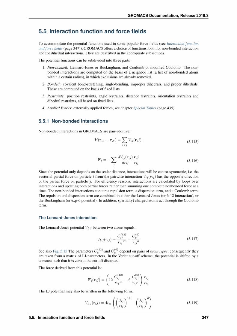
GROMACS Documentation, Release 2019.3
5.5 Interaction function and force fields
To accommodate the potential functions used in some popular force fields (see Interaction functionand force fields (page 347)), GROMACS offers a choice of functions, both for non-bonded interactionand for dihedral interactions. They are described in the appropriate subsections.
The potential functions can be subdivided into three parts
1. Non-bonded: Lennard-Jones or Buckingham, and Coulomb or modified Coulomb. The non-bonded interactions are computed on the basis of a neighbor list (a list of non-bonded atomswithin a certain radius), in which exclusions are already removed.
2. Bonded: covalent bond-stretching, angle-bending, improper dihedrals, and proper dihedrals.These are computed on the basis of fixed lists.
3. Restraints: position restraints, angle restraints, distance restraints, orientation restraints anddihedral restraints, all based on fixed lists.
4. Applied Forces: externally applied forces, see chapter Special Topics (page 435).
5.5.1 Non-bonded interactions
Non-bonded interactions in GROMACS are pair-additive:
𝑉 (r1, . . . r𝑁 ) =∑𝑖<𝑗
𝑉𝑖𝑗(r𝑖𝑗); (5.115)
F𝑖 = −∑𝑗
𝑑𝑉𝑖𝑗(𝑟𝑖𝑗)
𝑑𝑟𝑖𝑗
r𝑖𝑗
𝑟𝑖𝑗(5.116)
Since the potential only depends on the scalar distance, interactions will be centro-symmetric, i.e. thevectorial partial force on particle 𝑖 from the pairwise interaction 𝑉𝑖𝑗(𝑟𝑖𝑗) has the opposite directionof the partial force on particle 𝑗. For efficiency reasons, interactions are calculated by loops overinteractions and updating both partial forces rather than summing one complete nonbonded force at atime. The non-bonded interactions contain a repulsion term, a dispersion term, and a Coulomb term.The repulsion and dispersion term are combined in either the Lennard-Jones (or 6-12 interaction), orthe Buckingham (or exp-6 potential). In addition, (partially) charged atoms act through the Coulombterm.
The Lennard-Jones interaction
The Lennard-Jones potential 𝑉𝐿𝐽 between two atoms equals:
𝑉𝐿𝐽(𝑟𝑖𝑗) =𝐶
(12)𝑖𝑗
𝑟𝑖𝑗12−𝐶
(6)𝑖𝑗
𝑟𝑖𝑗6(5.117)
See also Fig. 5.15 The parameters 𝐶(12)𝑖𝑗 and 𝐶(6)
𝑖𝑗 depend on pairs of atom types; consequently theyare taken from a matrix of LJ-parameters. In the Verlet cut-off scheme, the potential is shifted by aconstant such that it is zero at the cut-off distance.
The force derived from this potential is:
F𝑖(r𝑖𝑗) =
(12
𝐶(12)𝑖𝑗
𝑟𝑖𝑗13− 6
𝐶(6)𝑖𝑗
𝑟𝑖𝑗7
)r𝑖𝑗𝑟𝑖𝑗
(5.118)
The LJ potential may also be written in the following form:
𝑉𝐿𝐽(r𝑖𝑗) = 4𝜖𝑖𝑗
((𝜎𝑖𝑗𝑟𝑖𝑗
)12
−(𝜎𝑖𝑗𝑟𝑖𝑗
)6)
(5.119)
5.5. Interaction function and force fields 347
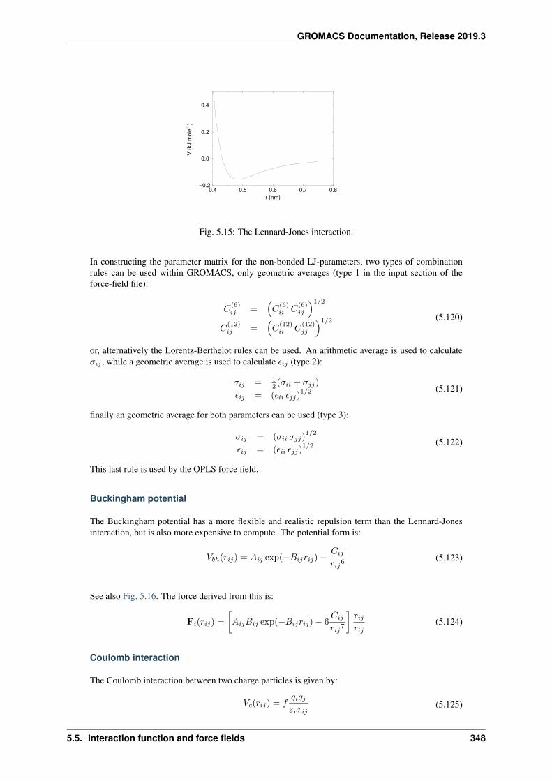
GROMACS Documentation, Release 2019.3
0.4 0.5 0.6 0.7 0.8r (nm)
–0.2
0.0
0.2
0.4
V(k
Jm
ole–1
)
Fig. 5.15: The Lennard-Jones interaction.
In constructing the parameter matrix for the non-bonded LJ-parameters, two types of combinationrules can be used within GROMACS, only geometric averages (type 1 in the input section of theforce-field file):
𝐶(6)𝑖𝑗 =
(𝐶
(6)𝑖𝑖 𝐶
(6)𝑗𝑗
)1/2𝐶
(12)𝑖𝑗 =
(𝐶
(12)𝑖𝑖 𝐶
(12)𝑗𝑗
)1/2 (5.120)
or, alternatively the Lorentz-Berthelot rules can be used. An arithmetic average is used to calculate𝜎𝑖𝑗 , while a geometric average is used to calculate 𝜖𝑖𝑗 (type 2):
𝜎𝑖𝑗 = 12 (𝜎𝑖𝑖 + 𝜎𝑗𝑗)
𝜖𝑖𝑗 = (𝜖𝑖𝑖 𝜖𝑗𝑗)1/2 (5.121)
finally an geometric average for both parameters can be used (type 3):
𝜎𝑖𝑗 = (𝜎𝑖𝑖 𝜎𝑗𝑗)1/2
𝜖𝑖𝑗 = (𝜖𝑖𝑖 𝜖𝑗𝑗)1/2 (5.122)
This last rule is used by the OPLS force field.
Buckingham potential
The Buckingham potential has a more flexible and realistic repulsion term than the Lennard-Jonesinteraction, but is also more expensive to compute. The potential form is:
𝑉𝑏ℎ(𝑟𝑖𝑗) = 𝐴𝑖𝑗 exp(−𝐵𝑖𝑗𝑟𝑖𝑗) −𝐶𝑖𝑗
𝑟𝑖𝑗6(5.123)
See also Fig. 5.16. The force derived from this is:
F𝑖(𝑟𝑖𝑗) =
[𝐴𝑖𝑗𝐵𝑖𝑗 exp(−𝐵𝑖𝑗𝑟𝑖𝑗) − 6
𝐶𝑖𝑗
𝑟𝑖𝑗7
]r𝑖𝑗𝑟𝑖𝑗
(5.124)
Coulomb interaction
The Coulomb interaction between two charge particles is given by:
𝑉𝑐(𝑟𝑖𝑗) = 𝑓𝑞𝑖𝑞𝑗𝜀𝑟𝑟𝑖𝑗
(5.125)
5.5. Interaction function and force fields 348
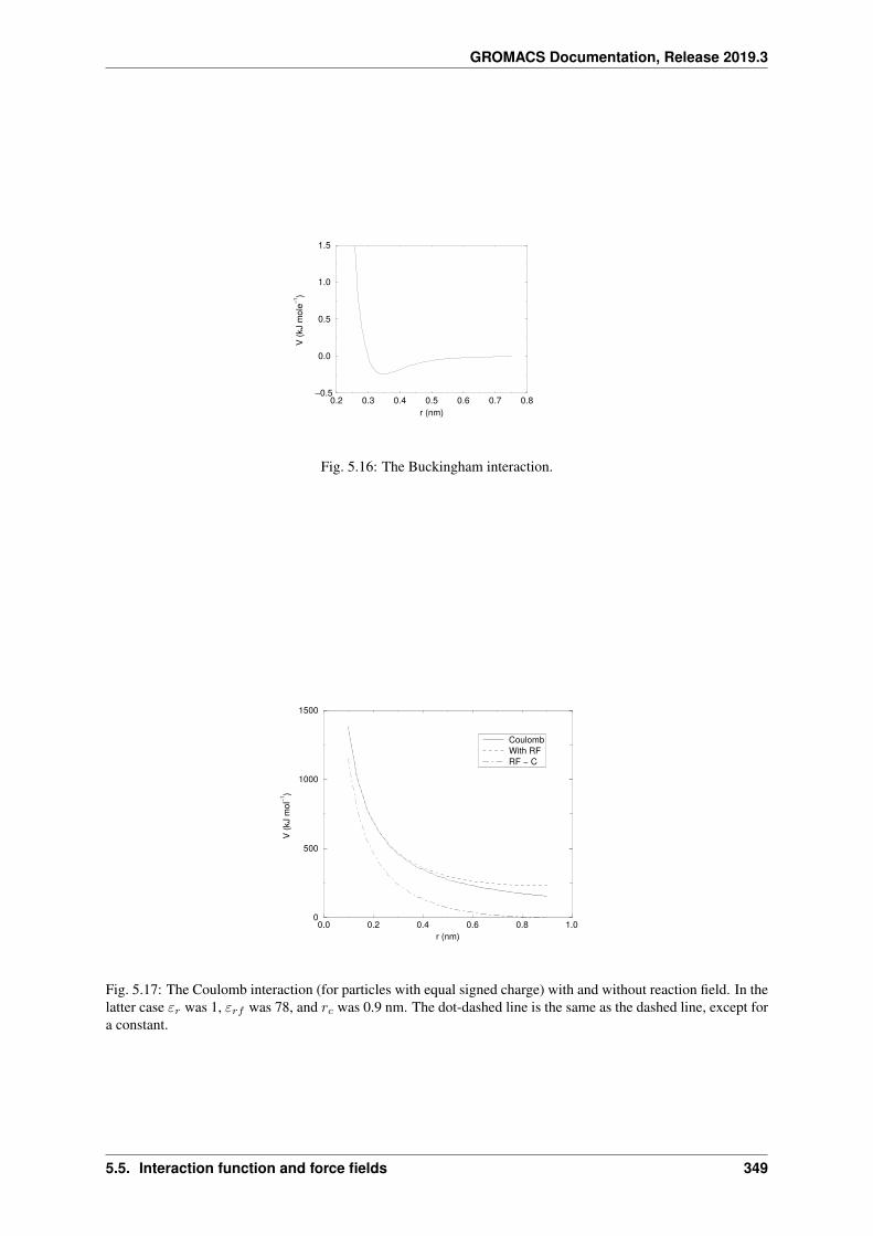
GROMACS Documentation, Release 2019.3
0.2 0.3 0.4 0.5 0.6 0.7 0.8r (nm)
–0.5
0.0
0.5
1.0
1.5
V(k
Jm
ole–1
)
Fig. 5.16: The Buckingham interaction.
0.0 0.2 0.4 0.6 0.8 1.0r (nm)
0
500
1000
1500
V (k
J m
ol−1
)
CoulombWith RFRF − C
Fig. 5.17: The Coulomb interaction (for particles with equal signed charge) with and without reaction field. In thelatter case 𝜀𝑟 was 1, 𝜀𝑟𝑓 was 78, and 𝑟𝑐 was 0.9 nm. The dot-dashed line is the same as the dashed line, except fora constant.
5.5. Interaction function and force fields 349
GROMACS Documentation, Release 2019.3
See also Fig. 5.17, where 𝑓 = 14𝜋𝜀0
= 138.935 458 (see chapter Definitions and Units (page 299))
The force derived from this potential is:
F𝑖(r𝑖𝑗) = 𝑓𝑞𝑖𝑞𝑗𝜀𝑟𝑟𝑖𝑗2
r𝑖𝑗𝑟𝑖𝑗
(5.126)
A plain Coulomb interaction should only be used without cut-off or when all pairs fall within thecut-off, since there is an abrupt, large change in the force at the cut-off. In case you do want to use acut-off, the potential can be shifted by a constant to make the potential the integral of the force. Withthe group cut-off scheme, this shift is only applied to non-excluded pairs. With the Verlet cut-offscheme, the shift is also applied to excluded pairs and self interactions, which makes the potentialequivalent to a reaction field with 𝜀𝑟𝑓 = 1 (see below).
In GROMACS the relative dielectric constant 𝜀𝑟 may be set in the in the input for grompp (page 94).
Coulomb interaction with reaction field
The Coulomb interaction can be modified for homogeneous systems by assuming a constant dielectricenvironment beyond the cut-off 𝑟𝑐 with a dielectric constant of 𝜀𝑟𝑓 . The interaction then reads:
𝑉𝑐𝑟𝑓 = 𝑓𝑞𝑖𝑞𝑗𝜀𝑟𝑟𝑖𝑗
[1 +
𝜀𝑟𝑓 − 𝜀𝑟2𝜀𝑟𝑓 + 𝜀𝑟
𝑟𝑖𝑗3
𝑟3𝑐
]− 𝑓
𝑞𝑖𝑞𝑗𝜀𝑟𝑟𝑐
3𝜀𝑟𝑓2𝜀𝑟𝑓 + 𝜀𝑟
(5.127)
in which the constant expression on the right makes the potential zero at the cut-off 𝑟𝑐. For chargedcut-off spheres this corresponds to neutralization with a homogeneous background charge. We canrewrite (5.127) for simplicity as
𝑉𝑐𝑟𝑓 = 𝑓𝑞𝑖𝑞𝑗𝜀𝑟
[1
𝑟𝑖𝑗+ 𝑘𝑟𝑓 𝑟𝑖𝑗
2 − 𝑐𝑟𝑓
](5.128)
with
𝑘𝑟𝑓 =1
𝑟3𝑐
𝜀𝑟𝑓 − 𝜀𝑟(2𝜀𝑟𝑓 + 𝜀𝑟)
(5.129)
𝑐𝑟𝑓 =1
𝑟𝑐+ 𝑘𝑟𝑓 𝑟
2𝑐 =
1
𝑟𝑐
3𝜀𝑟𝑓(2𝜀𝑟𝑓 + 𝜀𝑟)
(5.130)
For large 𝜀𝑟𝑓 the 𝑘𝑟𝑓 goes to 𝑟−3𝑐 /2, while for 𝜀𝑟𝑓 = 𝜀𝑟 the correction vanishes. In Fig. 5.17 the
modified interaction is plotted, and it is clear that the derivative with respect to 𝑟𝑖𝑗 (= -force) goes tozero at the cut-off distance. The force derived from this potential reads:
F𝑖(r𝑖𝑗) = 𝑓𝑞𝑖𝑞𝑗𝜀𝑟
[1
𝑟𝑖𝑗2− 2𝑘𝑟𝑓𝑟𝑖𝑗
]r𝑖𝑗𝑟𝑖𝑗
(5.131)
The reaction-field correction should also be applied to all excluded atoms pairs, including self pairs,in which case the normal Coulomb term in (5.127) and (5.131) is absent.
Tironi et al. have introduced a generalized reaction field in which the dielectric continuum beyondthe cut-off 𝑟𝑐 also has an ionic strength 𝐼 71 (page 509). In this case we can rewrite the constants 𝑘𝑟𝑓and 𝑐𝑟𝑓 using the inverse Debye screening length 𝜅:
𝜅2 =2𝐼 𝐹 2
𝜀0𝜀𝑟𝑓𝑅𝑇=
𝐹 2
𝜀0𝜀𝑟𝑓𝑅𝑇
𝐾∑𝑖=1
𝑐𝑖𝑧2𝑖
𝑘𝑟𝑓 =1
𝑟3𝑐
(𝜀𝑟𝑓 − 𝜀𝑟)(1 + 𝜅𝑟𝑐) + 12𝜀𝑟𝑓 (𝜅𝑟𝑐)
2
(2𝜀𝑟𝑓 + 𝜀𝑟)(1 + 𝜅𝑟𝑐) + 𝜀𝑟𝑓 (𝜅𝑟𝑐)2
(5.132)
𝑐𝑟𝑓 =1
𝑟𝑐
3𝜀𝑟𝑓 (1 + 𝜅𝑟𝑐 + 12 (𝜅𝑟𝑐)
2)
(2𝜀𝑟𝑓 + 𝜀𝑟)(1 + 𝜅𝑟𝑐) + 𝜀𝑟𝑓 (𝜅𝑟𝑐)2(5.133)
where 𝐹 is Faraday’s constant, 𝑅 is the ideal gas constant, 𝑇 the absolute temperature, 𝑐𝑖 the molarconcentration for species 𝑖 and 𝑧𝑖 the charge number of species 𝑖 where we have 𝐾 different species.In the limit of zero ionic strength (𝜅 = 0) (5.132) and (5.133) reduce to the simple forms of (5.129)and (5.130) respectively.
5.5. Interaction function and force fields 350
GROMACS Documentation, Release 2019.3
Modified non-bonded interactions
In GROMACS, the non-bonded potentials can be modified by a shift function, also called a force-switch function, since it switches the force to zero at the cut-off. The purpose of this is to replace thetruncated forces by forces that are continuous and have continuous derivatives at the cut-off radius.With such forces the time integration produces smaller errors. But note that for Lennard-Jones inter-actions these errors are usually smaller than other errors, such as integration errors at the repulsivepart of the potential. For Coulomb interactions we advise against using a shifted potential and for useof a reaction field or a proper long-range method such as PME.
There is no fundamental difference between a switch function (which multiplies the potential with afunction) and a shift function (which adds a function to the force or potential) 72 (page 509). Theswitch function is a special case of the shift function, which we apply to the force function 𝐹 (𝑟),related to the electrostatic or van der Waals force acting on particle 𝑖 by particle 𝑗 as:
F𝑖 = 𝑐 𝐹 (𝑟𝑖𝑗)r𝑖𝑗
𝑟𝑖𝑗(5.134)
For pure Coulomb or Lennard-Jones interactions 𝐹 (𝑟) = 𝐹𝛼(𝑟) = 𝛼 𝑟−(𝛼+1). The switched force𝐹𝑠(𝑟) can generally be written as:
𝐹𝑠(𝑟) = 𝐹𝛼(𝑟) 𝑟 < 𝑟1𝐹𝑠(𝑟) = 𝐹𝛼(𝑟) + 𝑆(𝑟) 𝑟1 ≤ 𝑟 < 𝑟𝑐𝐹𝑠(𝑟) = 0 𝑟𝑐 ≤ 𝑟
(5.135)
When 𝑟1 = 0 this is a traditional shift function, otherwise it acts as a switch function. The corre-sponding shifted potential function then reads:
𝑉𝑠(𝑟) =
∫ ∞
𝑟
𝐹𝑠(𝑥) 𝑑𝑥 (5.136)
The GROMACS force switch function 𝑆𝐹 (𝑟) should be smooth at the boundaries, therefore thefollowing boundary conditions are imposed on the switch function:
𝑆𝐹 (𝑟1) = 0𝑆′𝐹 (𝑟1) = 0𝑆𝐹 (𝑟𝑐) = −𝐹𝛼(𝑟𝑐)𝑆′𝐹 (𝑟𝑐) = −𝐹 ′
𝛼(𝑟𝑐)
(5.137)
A 3𝑟𝑑 degree polynomial of the form
𝑆𝐹 (𝑟) = 𝐴(𝑟 − 𝑟1)2 +𝐵(𝑟 − 𝑟1)3 (5.138)
fulfills these requirements. The constants A and B are given by the boundary condition at 𝑟𝑐:
𝐴 = −𝛼 (𝛼+ 4)𝑟𝑐 − (𝛼+ 1)𝑟1
𝑟𝛼+2𝑐 (𝑟𝑐 − 𝑟1)2
𝐵 = 𝛼(𝛼+ 3)𝑟𝑐 − (𝛼+ 1)𝑟1
𝑟𝛼+2𝑐 (𝑟𝑐 − 𝑟1)3
(5.139)
Thus the total force function is:
𝐹𝑠(𝑟) =𝛼
𝑟𝛼+1+𝐴(𝑟 − 𝑟1)2 +𝐵(𝑟 − 𝑟1)3 (5.140)
and the potential function reads:
𝑉𝑠(𝑟) =1
𝑟𝛼− 𝐴
3(𝑟 − 𝑟1)3 − 𝐵
4(𝑟 − 𝑟1)4 − 𝐶 (5.141)
where
𝐶 =1
𝑟𝛼𝑐− 𝐴
3(𝑟𝑐 − 𝑟1)3 − 𝐵
4(𝑟𝑐 − 𝑟1)4 (5.142)
5.5. Interaction function and force fields 351
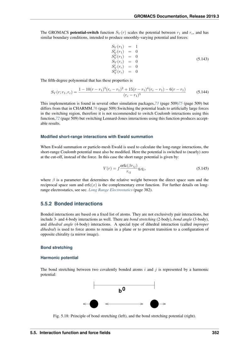
GROMACS Documentation, Release 2019.3
The GROMACS potential-switch function 𝑆𝑉 (𝑟) scales the potential between 𝑟1 and 𝑟𝑐, and hassimilar boundary conditions, intended to produce smoothly-varying potential and forces:
𝑆𝑉 (𝑟1) = 1𝑆′𝑉 (𝑟1) = 0𝑆′′𝑉 (𝑟1) = 0𝑆𝑉 (𝑟𝑐) = 0𝑆′𝑉 (𝑟𝑐) = 0𝑆′′𝑉 (𝑟𝑐) = 0
(5.143)
The fifth-degree polynomial that has these properties is
𝑆𝑉 (𝑟; 𝑟1, 𝑟𝑐) =1 − 10(𝑟 − 𝑟1)3(𝑟𝑐 − 𝑟1)2 + 15(𝑟 − 𝑟1)4(𝑟𝑐 − 𝑟1) − 6(𝑟 − 𝑟1)
(𝑟𝑐 − 𝑟1)5(5.144)
This implementation is found in several other simulation packages,73 (page 509)75 (page 509) butdiffers from that in CHARMM.76 (page 509) Switching the potential leads to artificially large forcesin the switching region, therefore it is not recommended to switch Coulomb interactions using thisfunction,72 (page 509) but switching Lennard-Jones interactions using this function produces accept-able results.
Modified short-range interactions with Ewald summation
When Ewald summation or particle-mesh Ewald is used to calculate the long-range interactions, theshort-range Coulomb potential must also be modified. Here the potential is switched to (nearly) zeroat the cut-off, instead of the force. In this case the short range potential is given by:
𝑉 (𝑟) = 𝑓erfc(𝛽𝑟𝑖𝑗)
𝑟𝑖𝑗𝑞𝑖𝑞𝑗 , (5.145)
where 𝛽 is a parameter that determines the relative weight between the direct space sum and thereciprocal space sum and erfc(𝑥) is the complementary error function. For further details on long-range electrostatics, see sec. Long Range Electrostatics (page 382).
5.5.2 Bonded interactions
Bonded interactions are based on a fixed list of atoms. They are not exclusively pair interactions, butinclude 3- and 4-body interactions as well. There are bond stretching (2-body), bond angle (3-body),and dihedral angle (4-body) interactions. A special type of dihedral interaction (called improperdihedral) is used to force atoms to remain in a plane or to prevent transition to a configuration ofopposite chirality (a mirror image).
Bond stretching
Harmonic potential
The bond stretching between two covalently bonded atoms 𝑖 and 𝑗 is represented by a harmonicpotential:
b0
Fig. 5.18: Principle of bond stretching (left), and the bond stretching potential (right).
5.5. Interaction function and force fields 352
GROMACS Documentation, Release 2019.3
𝑉𝑏 (𝑟𝑖𝑗) =1
2𝑘𝑏𝑖𝑗(𝑟𝑖𝑗 − 𝑏𝑖𝑗)
2 (5.146)
See also Fig. 5.18, with the force given by:
F𝑖(r𝑖𝑗) = 𝑘𝑏𝑖𝑗(𝑟𝑖𝑗 − 𝑏𝑖𝑗)r𝑖𝑗𝑟𝑖𝑗
(5.147)
Fourth power potential
In the GROMOS-96 force field 77 (page 509), the covalent bond potential is, for reasons of compu-tational efficiency, written as:
𝑉𝑏 (𝑟𝑖𝑗) =1
4𝑘𝑏𝑖𝑗(𝑟𝑖𝑗
2 − 𝑏2𝑖𝑗)2 (5.148)
The corresponding force is:
F𝑖(r𝑖𝑗) = 𝑘𝑏𝑖𝑗(𝑟𝑖𝑗2 − 𝑏2𝑖𝑗) r𝑖𝑗 (5.149)
The force constants for this form of the potential are related to the usual harmonic force constant𝑘𝑏,harm (sec. Bond stretching (page 352)) as
2𝑘𝑏𝑏2𝑖𝑗 = 𝑘𝑏,harm (5.150)
The force constants are mostly derived from the harmonic ones used in GROMOS-87 78 (page 509).Although this form is computationally more efficient (because no square root has to be evaluated), itis conceptually more complex. One particular disadvantage is that since the form is not harmonic, theaverage energy of a single bond is not equal to 1
2𝑘𝑇 as it is for the normal harmonic potential.
Morse potential bond stretching
For some systems that require an anharmonic bond stretching potential, the Morse potential 79(page 509) between two atoms i and j is available in GROMACS. This potential differs from theharmonic potential in that it has an asymmetric potential well and a zero force at infinite distance.The functional form is:
𝑉𝑚𝑜𝑟𝑠𝑒(𝑟𝑖𝑗) = 𝐷𝑖𝑗 [1 − exp(−𝛽𝑖𝑗(𝑟𝑖𝑗 − 𝑏𝑖𝑗))]2, (5.151)
See also Fig. 5.19, and the corresponding force is:
F𝑚𝑜𝑟𝑠𝑒(r𝑖𝑗) = 2𝐷𝑖𝑗𝛽𝑖𝑗 exp(−𝛽𝑖𝑗(𝑟𝑖𝑗 − 𝑏𝑖𝑗))*[1 − exp(−𝛽𝑖𝑗(𝑟𝑖𝑗 − 𝑏𝑖𝑗))]
r𝑖𝑗𝑟𝑖𝑗 ,
(5.152)
where 𝐷𝑖𝑗 is the depth of the well in kJ/mol, 𝛽𝑖𝑗 defines the steepness of the well (in nm−1), and𝑏𝑖𝑗 is the equilibrium distance in nm. The steepness parameter 𝛽𝑖𝑗 can be expressed in terms of thereduced mass of the atoms i and j, the fundamental vibration frequency 𝜔𝑖𝑗 and the well depth 𝐷𝑖𝑗 :
𝛽𝑖𝑗 = 𝜔𝑖𝑗
√𝜇𝑖𝑗
2𝐷𝑖𝑗(5.153)
and because 𝜔 =√𝑘/𝜇, one can rewrite 𝛽𝑖𝑗 in terms of the harmonic force constant 𝑘𝑖𝑗 :
𝛽𝑖𝑗 =
√𝑘𝑖𝑗
2𝐷𝑖𝑗
(5.154)
For small deviations (𝑟𝑖𝑗 − 𝑏𝑖𝑗), one can approximate the exp-term to first-order using a Taylorexpansion:
exp(−𝑥) ≈ 1 − 𝑥 (5.155)
5.5. Interaction function and force fields 353
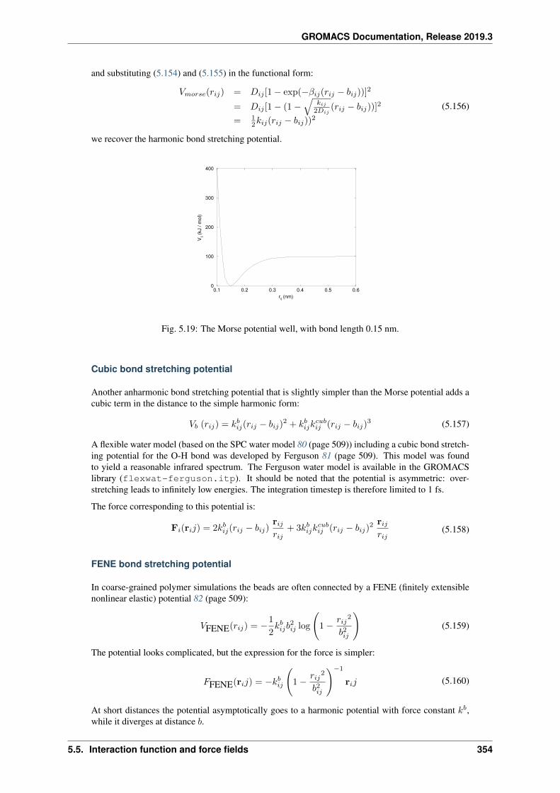
GROMACS Documentation, Release 2019.3
and substituting (5.154) and (5.155) in the functional form:
𝑉𝑚𝑜𝑟𝑠𝑒(𝑟𝑖𝑗) = 𝐷𝑖𝑗 [1 − exp(−𝛽𝑖𝑗(𝑟𝑖𝑗 − 𝑏𝑖𝑗))]2
= 𝐷𝑖𝑗 [1 − (1 −√
𝑘𝑖𝑗
2𝐷𝑖𝑗(𝑟𝑖𝑗 − 𝑏𝑖𝑗))]
2
= 12𝑘𝑖𝑗(𝑟𝑖𝑗 − 𝑏𝑖𝑗))
2
(5.156)
we recover the harmonic bond stretching potential.
0.1 0.2 0.3 0.4 0.5 0.6rij (nm)
0
100
200
300
400
V ij(k
J / m
ol)
Fig. 5.19: The Morse potential well, with bond length 0.15 nm.
Cubic bond stretching potential
Another anharmonic bond stretching potential that is slightly simpler than the Morse potential adds acubic term in the distance to the simple harmonic form:
𝑉𝑏 (𝑟𝑖𝑗) = 𝑘𝑏𝑖𝑗(𝑟𝑖𝑗 − 𝑏𝑖𝑗)2 + 𝑘𝑏𝑖𝑗𝑘
𝑐𝑢𝑏𝑖𝑗 (𝑟𝑖𝑗 − 𝑏𝑖𝑗)
3 (5.157)
A flexible water model (based on the SPC water model 80 (page 509)) including a cubic bond stretch-ing potential for the O-H bond was developed by Ferguson 81 (page 509). This model was foundto yield a reasonable infrared spectrum. The Ferguson water model is available in the GROMACSlibrary (flexwat-ferguson.itp). It should be noted that the potential is asymmetric: over-stretching leads to infinitely low energies. The integration timestep is therefore limited to 1 fs.
The force corresponding to this potential is:
F𝑖(r𝑖𝑗) = 2𝑘𝑏𝑖𝑗(𝑟𝑖𝑗 − 𝑏𝑖𝑗)r𝑖𝑗𝑟𝑖𝑗
+ 3𝑘𝑏𝑖𝑗𝑘𝑐𝑢𝑏𝑖𝑗 (𝑟𝑖𝑗 − 𝑏𝑖𝑗)
2 r𝑖𝑗𝑟𝑖𝑗
(5.158)
FENE bond stretching potential
In coarse-grained polymer simulations the beads are often connected by a FENE (finitely extensiblenonlinear elastic) potential 82 (page 509):
𝑉FENE(𝑟𝑖𝑗) = −1
2𝑘𝑏𝑖𝑗𝑏
2𝑖𝑗 log
(1 − 𝑟𝑖𝑗
2
𝑏2𝑖𝑗
)(5.159)
The potential looks complicated, but the expression for the force is simpler:
𝐹FENE(r𝑖𝑗) = −𝑘𝑏𝑖𝑗
(1 − 𝑟𝑖𝑗
2
𝑏2𝑖𝑗
)−1
r𝑖𝑗 (5.160)
At short distances the potential asymptotically goes to a harmonic potential with force constant 𝑘𝑏,while it diverges at distance 𝑏.
5.5. Interaction function and force fields 354
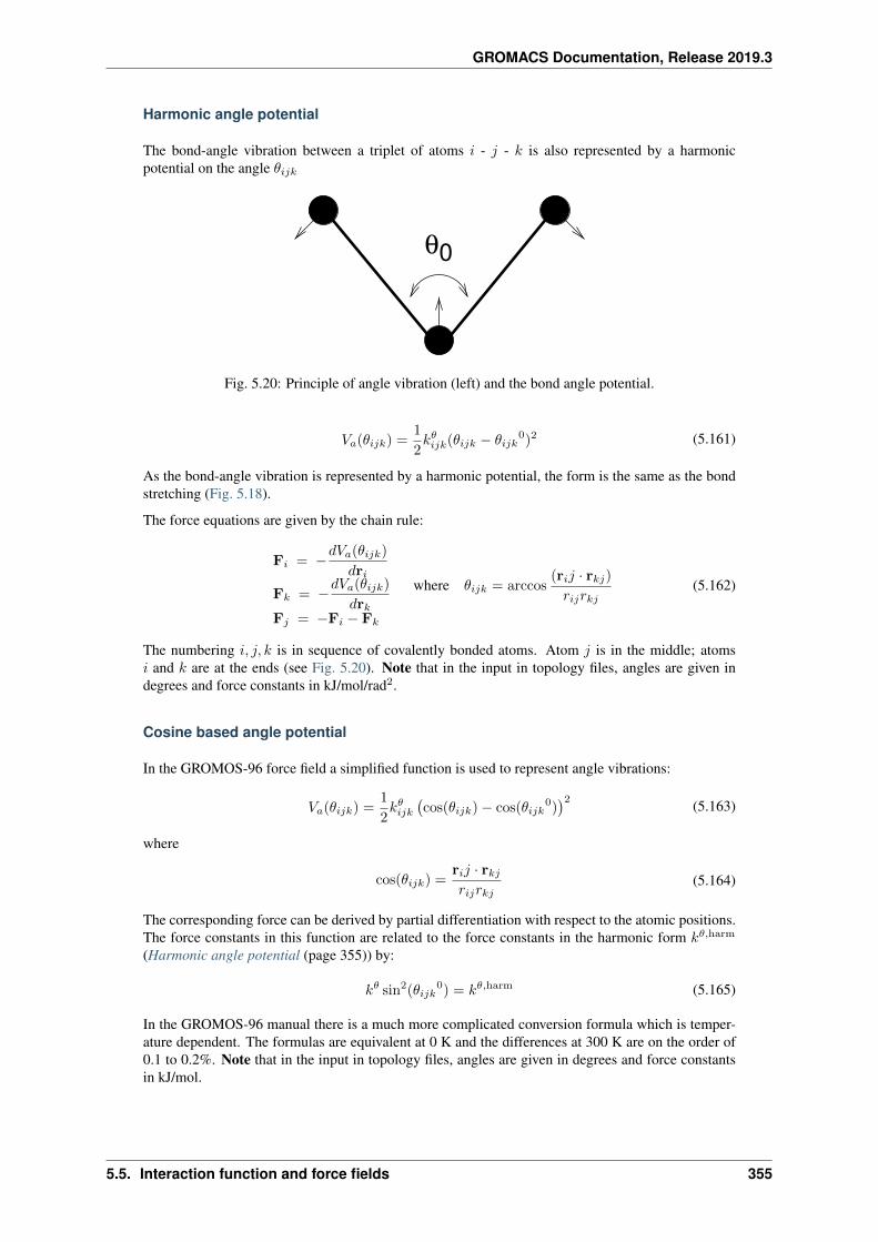
GROMACS Documentation, Release 2019.3
Harmonic angle potential
The bond-angle vibration between a triplet of atoms 𝑖 - 𝑗 - 𝑘 is also represented by a harmonicpotential on the angle 𝜃𝑖𝑗𝑘
θ0
Fig. 5.20: Principle of angle vibration (left) and the bond angle potential.
𝑉𝑎(𝜃𝑖𝑗𝑘) =1
2𝑘𝜃𝑖𝑗𝑘(𝜃𝑖𝑗𝑘 − 𝜃𝑖𝑗𝑘
0)2 (5.161)
As the bond-angle vibration is represented by a harmonic potential, the form is the same as the bondstretching (Fig. 5.18).
The force equations are given by the chain rule:
F𝑖 = −𝑑𝑉𝑎(𝜃𝑖𝑗𝑘)
𝑑r𝑖
F𝑘 = −𝑑𝑉𝑎(𝜃𝑖𝑗𝑘)
𝑑r𝑘F𝑗 = −F𝑖 − F𝑘
where 𝜃𝑖𝑗𝑘 = arccos(r𝑖𝑗 · r𝑘𝑗)𝑟𝑖𝑗𝑟𝑘𝑗
(5.162)
The numbering 𝑖, 𝑗, 𝑘 is in sequence of covalently bonded atoms. Atom 𝑗 is in the middle; atoms𝑖 and 𝑘 are at the ends (see Fig. 5.20). Note that in the input in topology files, angles are given indegrees and force constants in kJ/mol/rad2.
Cosine based angle potential
In the GROMOS-96 force field a simplified function is used to represent angle vibrations:
𝑉𝑎(𝜃𝑖𝑗𝑘) =1
2𝑘𝜃𝑖𝑗𝑘
(cos(𝜃𝑖𝑗𝑘) − cos(𝜃𝑖𝑗𝑘
0))2 (5.163)
where
cos(𝜃𝑖𝑗𝑘) =r𝑖𝑗 · r𝑘𝑗𝑟𝑖𝑗𝑟𝑘𝑗
(5.164)
The corresponding force can be derived by partial differentiation with respect to the atomic positions.The force constants in this function are related to the force constants in the harmonic form 𝑘𝜃,harm
(Harmonic angle potential (page 355)) by:
𝑘𝜃 sin2(𝜃𝑖𝑗𝑘0) = 𝑘𝜃,harm (5.165)
In the GROMOS-96 manual there is a much more complicated conversion formula which is temper-ature dependent. The formulas are equivalent at 0 K and the differences at 300 K are on the order of0.1 to 0.2%. Note that in the input in topology files, angles are given in degrees and force constantsin kJ/mol.
5.5. Interaction function and force fields 355
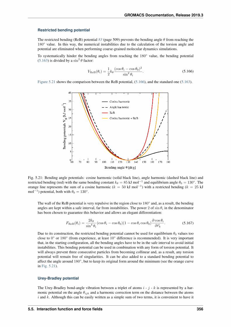
GROMACS Documentation, Release 2019.3
Restricted bending potential
The restricted bending (ReB) potential 83 (page 509) prevents the bending angle 𝜃 from reaching the180∘ value. In this way, the numerical instabilities due to the calculation of the torsion angle andpotential are eliminated when performing coarse-grained molecular dynamics simulations.
To systematically hinder the bending angles from reaching the 180∘ value, the bending potential(5.163) is divided by a sin2 𝜃 factor:
𝑉ReB(𝜃𝑖) =1
2𝑘𝜃
(cos 𝜃𝑖 − cos 𝜃0)2
sin2 𝜃𝑖. (5.166)
Figure 5.21 shows the comparison between the ReB potential, (5.166), and the standard one (5.163).
Fig. 5.21: Bending angle potentials: cosine harmonic (solid black line), angle harmonic (dashed black line) andrestricted bending (red) with the same bending constant 𝑘𝜃 = 85 kJ mol−1 and equilibrium angle 𝜃0 = 130∘. Theorange line represents the sum of a cosine harmonic (𝑘 = 50 kJ mol−1) with a restricted bending (𝑘 = 25 kJmol−1) potential, both with 𝜃0 = 130∘.
The wall of the ReB potential is very repulsive in the region close to 180∘ and, as a result, the bendingangles are kept within a safe interval, far from instabilities. The power 2 of sin 𝜃𝑖 in the denominatorhas been chosen to guarantee this behavior and allows an elegant differentiation:
𝐹ReB(𝜃𝑖) =2𝑘𝜃
sin4 𝜃𝑖(cos 𝜃𝑖 − cos 𝜃0)(1 − cos 𝜃𝑖 cos 𝜃0)
𝜕 cos 𝜃𝑖𝜕��𝑘
. (5.167)
Due to its construction, the restricted bending potential cannot be used for equilibrium 𝜃0 values tooclose to 0∘ or 180∘ (from experience, at least 10∘ difference is recommended). It is very importantthat, in the starting configuration, all the bending angles have to be in the safe interval to avoid initialinstabilities. This bending potential can be used in combination with any form of torsion potential. Itwill always prevent three consecutive particles from becoming collinear and, as a result, any torsionpotential will remain free of singularities. It can be also added to a standard bending potential toaffect the angle around 180∘, but to keep its original form around the minimum (see the orange curvein Fig. 5.21).
Urey-Bradley potential
The Urey-Bradley bond-angle vibration between a triplet of atoms 𝑖 - 𝑗 - 𝑘 is represented by a har-monic potential on the angle 𝜃𝑖𝑗𝑘 and a harmonic correction term on the distance between the atoms𝑖 and 𝑘. Although this can be easily written as a simple sum of two terms, it is convenient to have it
5.5. Interaction function and force fields 356
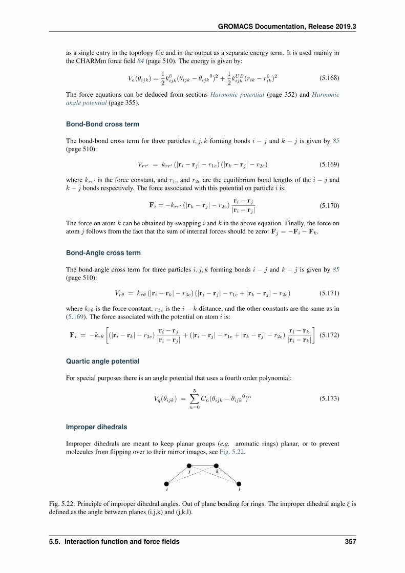
GROMACS Documentation, Release 2019.3
as a single entry in the topology file and in the output as a separate energy term. It is used mainly inthe CHARMm force field 84 (page 510). The energy is given by:
𝑉𝑎(𝜃𝑖𝑗𝑘) =1
2𝑘𝜃𝑖𝑗𝑘(𝜃𝑖𝑗𝑘 − 𝜃𝑖𝑗𝑘
0)2 +1
2𝑘𝑈𝐵𝑖𝑗𝑘 (𝑟𝑖𝑘 − 𝑟0𝑖𝑘)2 (5.168)
The force equations can be deduced from sections Harmonic potential (page 352) and Harmonicangle potential (page 355).
Bond-Bond cross term
The bond-bond cross term for three particles 𝑖, 𝑗, 𝑘 forming bonds 𝑖 − 𝑗 and 𝑘 − 𝑗 is given by 85(page 510):
𝑉𝑟𝑟′ = 𝑘𝑟𝑟′ (|r𝑖 − r𝑗 | − 𝑟1𝑒) (|r𝑘 − r𝑗 | − 𝑟2𝑒) (5.169)
where 𝑘𝑟𝑟′ is the force constant, and 𝑟1𝑒 and 𝑟2𝑒 are the equilibrium bond lengths of the 𝑖 − 𝑗 and𝑘 − 𝑗 bonds respectively. The force associated with this potential on particle 𝑖 is:
F𝑖 = −𝑘𝑟𝑟′ (|r𝑘 − r𝑗 | − 𝑟2𝑒)r𝑖 − r𝑗|r𝑖 − r𝑗 |
(5.170)
The force on atom 𝑘 can be obtained by swapping 𝑖 and 𝑘 in the above equation. Finally, the force onatom 𝑗 follows from the fact that the sum of internal forces should be zero: F𝑗 = −F𝑖 − F𝑘.
Bond-Angle cross term
The bond-angle cross term for three particles 𝑖, 𝑗, 𝑘 forming bonds 𝑖 − 𝑗 and 𝑘 − 𝑗 is given by 85(page 510):
𝑉𝑟𝜃 = 𝑘𝑟𝜃 (|r𝑖 − r𝑘| − 𝑟3𝑒) (|r𝑖 − r𝑗 | − 𝑟1𝑒 + |r𝑘 − r𝑗 | − 𝑟2𝑒) (5.171)
where 𝑘𝑟𝜃 is the force constant, 𝑟3𝑒 is the 𝑖 − 𝑘 distance, and the other constants are the same as in(5.169). The force associated with the potential on atom 𝑖 is:
F𝑖 = −𝑘𝑟𝜃[(|r𝑖 − r𝑘| − 𝑟3𝑒)
r𝑖 − r𝑗|r𝑖 − r𝑗 |
+ (|r𝑖 − r𝑗 | − 𝑟1𝑒 + |r𝑘 − r𝑗 | − 𝑟2𝑒)r𝑖 − r𝑘|r𝑖 − r𝑘|
](5.172)
Quartic angle potential
For special purposes there is an angle potential that uses a fourth order polynomial:
𝑉𝑞(𝜃𝑖𝑗𝑘) =
5∑𝑛=0
𝐶𝑛(𝜃𝑖𝑗𝑘 − 𝜃𝑖𝑗𝑘0)𝑛 (5.173)
Improper dihedrals
Improper dihedrals are meant to keep planar groups (e.g. aromatic rings) planar, or to preventmolecules from flipping over to their mirror images, see Fig. 5.22.
k
li
j
Fig. 5.22: Principle of improper dihedral angles. Out of plane bending for rings. The improper dihedral angle 𝜉 isdefined as the angle between planes (i,j,k) and (j,k,l).
5.5. Interaction function and force fields 357
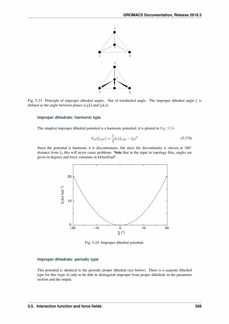
GROMACS Documentation, Release 2019.3
i
kj
l
k
i
j
l
Fig. 5.23: Principle of improper dihedral angles. Out of tetrahedral angle. The improper dihedral angle 𝜉 isdefined as the angle between planes (i,j,k) and (j,k,l).
Improper dihedrals: harmonic type
The simplest improper dihedral potential is a harmonic potential; it is plotted in Fig. 5.24.
𝑉𝑖𝑑(𝜉𝑖𝑗𝑘𝑙) =1
2𝑘𝜉(𝜉𝑖𝑗𝑘𝑙 − 𝜉0)2 (5.174)
Since the potential is harmonic it is discontinuous, but since the discontinuity is chosen at 180∘
distance from 𝜉0 this will never cause problems. Note that in the input in topology files, angles aregiven in degrees and force constants in kJ/mol/rad2.
–20 –10 0 10 20ξ
0
10
20
V i (k
J m
ol–1
)
(°)
Fig. 5.24: Improper dihedral potential.
Improper dihedrals: periodic type
This potential is identical to the periodic proper dihedral (see below). There is a separate dihedraltype for this (type 4) only to be able to distinguish improper from proper dihedrals in the parametersection and the output.
5.5. Interaction function and force fields 358
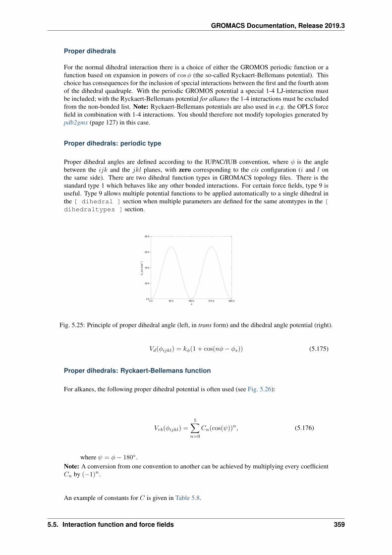
GROMACS Documentation, Release 2019.3
Proper dihedrals
For the normal dihedral interaction there is a choice of either the GROMOS periodic function or afunction based on expansion in powers of cos𝜑 (the so-called Ryckaert-Bellemans potential). Thischoice has consequences for the inclusion of special interactions between the first and the fourth atomof the dihedral quadruple. With the periodic GROMOS potential a special 1-4 LJ-interaction mustbe included; with the Ryckaert-Bellemans potential for alkanes the 1-4 interactions must be excludedfrom the non-bonded list. Note: Ryckaert-Bellemans potentials are also used in e.g. the OPLS forcefield in combination with 1-4 interactions. You should therefore not modify topologies generated bypdb2gmx (page 127) in this case.
Proper dihedrals: periodic type
Proper dihedral angles are defined according to the IUPAC/IUB convention, where 𝜑 is the anglebetween the 𝑖𝑗𝑘 and the 𝑗𝑘𝑙 planes, with zero corresponding to the cis configuration (𝑖 and 𝑙 onthe same side). There are two dihedral function types in GROMACS topology files. There is thestandard type 1 which behaves like any other bonded interactions. For certain force fields, type 9 isuseful. Type 9 allows multiple potential functions to be applied automatically to a single dihedral inthe [ dihedral ] section when multiple parameters are defined for the same atomtypes in the [dihedraltypes ] section.
0.0 90.0 180.0 270.0 360.0φ
0.0
20.0
40.0
60.0
80.0
V d(k
J m
ole–1
)
Fig. 5.25: Principle of proper dihedral angle (left, in trans form) and the dihedral angle potential (right).
𝑉𝑑(𝜑𝑖𝑗𝑘𝑙) = 𝑘𝜑(1 + cos(𝑛𝜑− 𝜑𝑠)) (5.175)
Proper dihedrals: Ryckaert-Bellemans function
For alkanes, the following proper dihedral potential is often used (see Fig. 5.26):
𝑉𝑟𝑏(𝜑𝑖𝑗𝑘𝑙) =
5∑𝑛=0
𝐶𝑛(cos(𝜓))𝑛, (5.176)
where 𝜓 = 𝜑− 180∘.Note: A conversion from one convention to another can be achieved by multiplying every coefficient𝐶𝑛 by (−1)𝑛.
An example of constants for 𝐶 is given in Table 5.8.
5.5. Interaction function and force fields 359
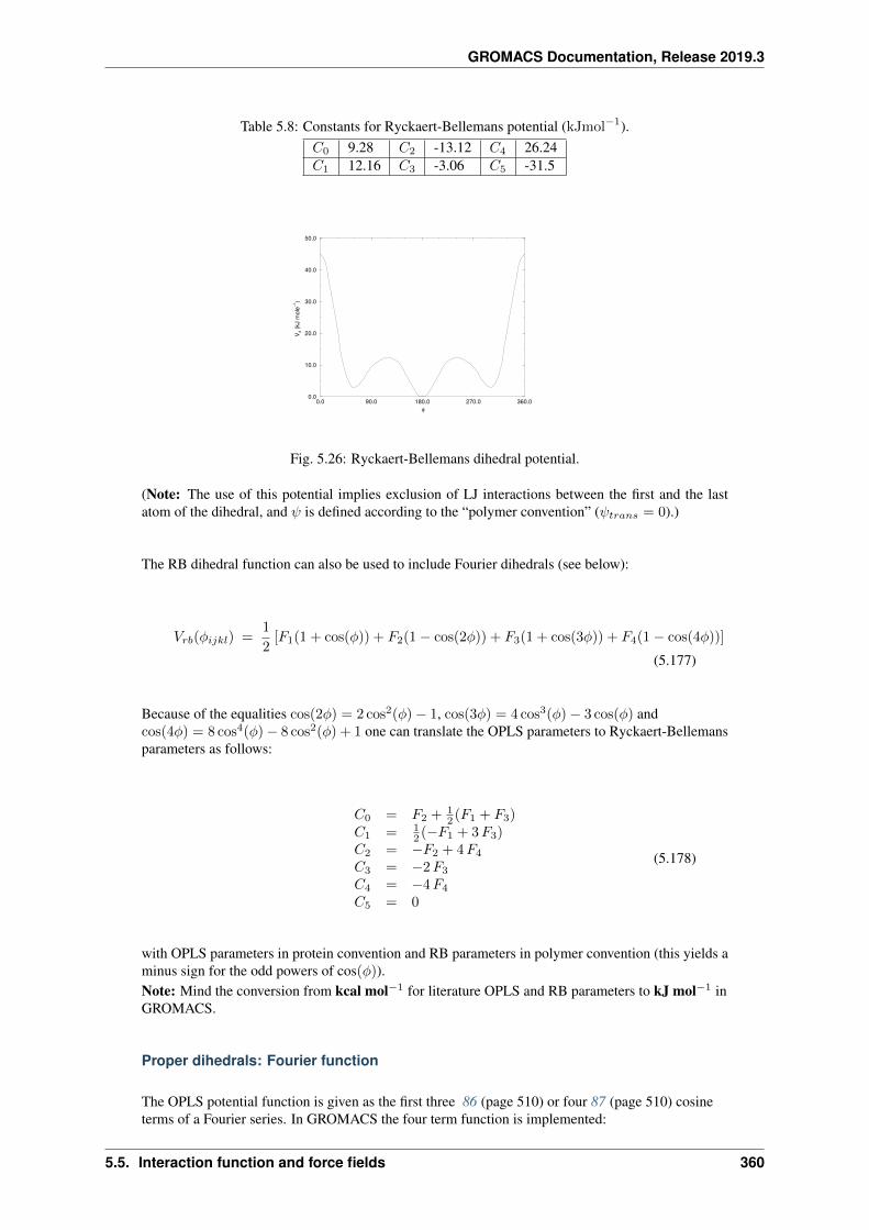
GROMACS Documentation, Release 2019.3
Table 5.8: Constants for Ryckaert-Bellemans potential (kJmol−1).𝐶0 9.28 𝐶2 -13.12 𝐶4 26.24𝐶1 12.16 𝐶3 -3.06 𝐶5 -31.5
0.0 90.0 180.0 270.0 360.0φ
0.0
10.0
20.0
30.0
40.0
50.0
V d(k
J m
ole–1
)
Fig. 5.26: Ryckaert-Bellemans dihedral potential.
(Note: The use of this potential implies exclusion of LJ interactions between the first and the lastatom of the dihedral, and 𝜓 is defined according to the “polymer convention” (𝜓𝑡𝑟𝑎𝑛𝑠 = 0).)
The RB dihedral function can also be used to include Fourier dihedrals (see below):
𝑉𝑟𝑏(𝜑𝑖𝑗𝑘𝑙) =1
2[𝐹1(1 + cos(𝜑)) + 𝐹2(1 − cos(2𝜑)) + 𝐹3(1 + cos(3𝜑)) + 𝐹4(1 − cos(4𝜑))]
(5.177)
Because of the equalities cos(2𝜑) = 2 cos2(𝜑) − 1, cos(3𝜑) = 4 cos3(𝜑) − 3 cos(𝜑) andcos(4𝜑) = 8 cos4(𝜑) − 8 cos2(𝜑) + 1 one can translate the OPLS parameters to Ryckaert-Bellemansparameters as follows:
𝐶0 = 𝐹2 + 12 (𝐹1 + 𝐹3)
𝐶1 = 12 (−𝐹1 + 3𝐹3)
𝐶2 = −𝐹2 + 4𝐹4
𝐶3 = −2𝐹3
𝐶4 = −4𝐹4
𝐶5 = 0
(5.178)
with OPLS parameters in protein convention and RB parameters in polymer convention (this yields aminus sign for the odd powers of cos(𝜑)).Note: Mind the conversion from kcal mol−1 for literature OPLS and RB parameters to kJ mol−1 inGROMACS.
Proper dihedrals: Fourier function
The OPLS potential function is given as the first three 86 (page 510) or four 87 (page 510) cosineterms of a Fourier series. In GROMACS the four term function is implemented:
5.5. Interaction function and force fields 360
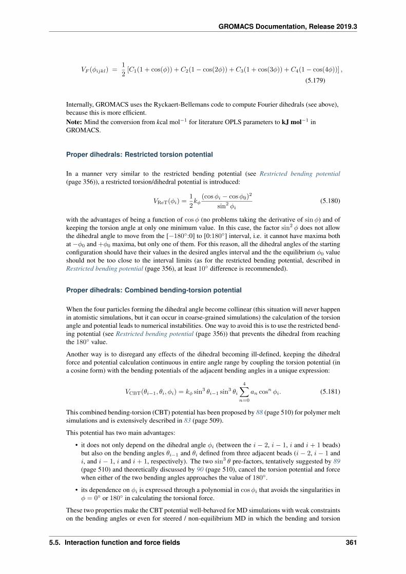
GROMACS Documentation, Release 2019.3
𝑉𝐹 (𝜑𝑖𝑗𝑘𝑙) =1
2[𝐶1(1 + cos(𝜑)) + 𝐶2(1 − cos(2𝜑)) + 𝐶3(1 + cos(3𝜑)) + 𝐶4(1 − cos(4𝜑))] ,
(5.179)
Internally, GROMACS uses the Ryckaert-Bellemans code to compute Fourier dihedrals (see above),because this is more efficient.Note: Mind the conversion from kcal mol−1 for literature OPLS parameters to kJ mol−1 inGROMACS.
Proper dihedrals: Restricted torsion potential
In a manner very similar to the restricted bending potential (see Restricted bending potential(page 356)), a restricted torsion/dihedral potential is introduced:
𝑉ReT(𝜑𝑖) =1
2𝑘𝜑
(cos𝜑𝑖 − cos𝜑0)2
sin2 𝜑𝑖(5.180)
with the advantages of being a function of cos𝜑 (no problems taking the derivative of sin𝜑) and ofkeeping the torsion angle at only one minimum value. In this case, the factor sin2 𝜑 does not allowthe dihedral angle to move from the [−180∘:0] to [0:180∘] interval, i.e. it cannot have maxima bothat −𝜑0 and +𝜑0 maxima, but only one of them. For this reason, all the dihedral angles of the startingconfiguration should have their values in the desired angles interval and the the equilibrium 𝜑0 valueshould not be too close to the interval limits (as for the restricted bending potential, described inRestricted bending potential (page 356), at least 10∘ difference is recommended).
Proper dihedrals: Combined bending-torsion potential
When the four particles forming the dihedral angle become collinear (this situation will never happenin atomistic simulations, but it can occur in coarse-grained simulations) the calculation of the torsionangle and potential leads to numerical instabilities. One way to avoid this is to use the restricted bend-ing potential (see Restricted bending potential (page 356)) that prevents the dihedral from reachingthe 180∘ value.
Another way is to disregard any effects of the dihedral becoming ill-defined, keeping the dihedralforce and potential calculation continuous in entire angle range by coupling the torsion potential (ina cosine form) with the bending potentials of the adjacent bending angles in a unique expression:
𝑉CBT(𝜃𝑖−1, 𝜃𝑖, 𝜑𝑖) = 𝑘𝜑 sin3 𝜃𝑖−1 sin3 𝜃𝑖
4∑𝑛=0
𝑎𝑛 cos𝑛 𝜑𝑖. (5.181)
This combined bending-torsion (CBT) potential has been proposed by 88 (page 510) for polymer meltsimulations and is extensively described in 83 (page 509).
This potential has two main advantages:
• it does not only depend on the dihedral angle 𝜑𝑖 (between the 𝑖 − 2, 𝑖 − 1, 𝑖 and 𝑖 + 1 beads)but also on the bending angles 𝜃𝑖−1 and 𝜃𝑖 defined from three adjacent beads (𝑖 − 2, 𝑖 − 1 and𝑖, and 𝑖 − 1, 𝑖 and 𝑖 + 1, respectively). The two sin3 𝜃 pre-factors, tentatively suggested by 89(page 510) and theoretically discussed by 90 (page 510), cancel the torsion potential and forcewhen either of the two bending angles approaches the value of 180∘.
• its dependence on 𝜑𝑖 is expressed through a polynomial in cos𝜑𝑖 that avoids the singularities in𝜑 = 0∘ or 180∘ in calculating the torsional force.
These two properties make the CBT potential well-behaved for MD simulations with weak constraintson the bending angles or even for steered / non-equilibrium MD in which the bending and torsion
5.5. Interaction function and force fields 361
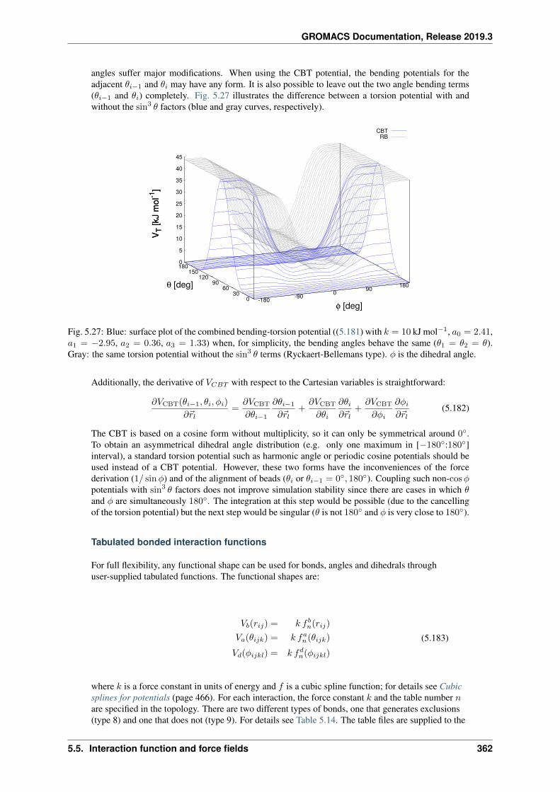
GROMACS Documentation, Release 2019.3
angles suffer major modifications. When using the CBT potential, the bending potentials for theadjacent 𝜃𝑖−1 and 𝜃𝑖 may have any form. It is also possible to leave out the two angle bending terms(𝜃𝑖−1 and 𝜃𝑖) completely. Fig. 5.27 illustrates the difference between a torsion potential with andwithout the sin3 𝜃 factors (blue and gray curves, respectively).
-180 -90 0 90 180
030
6090
120150
1800
5
10
15
20
25
30
35
40
45V T
[kJ
mol
-1]
CBTRB
φ [deg]
θ [deg]
V T[k
J m
ol-1
]
Fig. 5.27: Blue: surface plot of the combined bending-torsion potential ((5.181) with 𝑘 = 10 kJ mol−1, 𝑎0 = 2.41,𝑎1 = −2.95, 𝑎2 = 0.36, 𝑎3 = 1.33) when, for simplicity, the bending angles behave the same (𝜃1 = 𝜃2 = 𝜃).Gray: the same torsion potential without the sin3 𝜃 terms (Ryckaert-Bellemans type). 𝜑 is the dihedral angle.
Additionally, the derivative of 𝑉𝐶𝐵𝑇 with respect to the Cartesian variables is straightforward:
𝜕𝑉CBT(𝜃𝑖−1, 𝜃𝑖, 𝜑𝑖)
𝜕��𝑙=𝜕𝑉CBT
𝜕𝜃𝑖−1
𝜕𝜃𝑖−1
𝜕��𝑙+𝜕𝑉CBT
𝜕𝜃𝑖
𝜕𝜃𝑖𝜕��𝑙
+𝜕𝑉CBT
𝜕𝜑𝑖
𝜕𝜑𝑖𝜕��𝑙
(5.182)
The CBT is based on a cosine form without multiplicity, so it can only be symmetrical around 0∘.To obtain an asymmetrical dihedral angle distribution (e.g. only one maximum in [−180∘:180∘]interval), a standard torsion potential such as harmonic angle or periodic cosine potentials should beused instead of a CBT potential. However, these two forms have the inconveniences of the forcederivation (1/ sin𝜑) and of the alignment of beads (𝜃𝑖 or 𝜃𝑖−1 = 0∘, 180∘). Coupling such non-cos𝜑potentials with sin3 𝜃 factors does not improve simulation stability since there are cases in which 𝜃and 𝜑 are simultaneously 180∘. The integration at this step would be possible (due to the cancellingof the torsion potential) but the next step would be singular (𝜃 is not 180∘ and 𝜑 is very close to 180∘).
Tabulated bonded interaction functions
For full flexibility, any functional shape can be used for bonds, angles and dihedrals throughuser-supplied tabulated functions. The functional shapes are:
𝑉𝑏(𝑟𝑖𝑗) = 𝑘 𝑓 𝑏𝑛(𝑟𝑖𝑗)
𝑉𝑎(𝜃𝑖𝑗𝑘) = 𝑘 𝑓𝑎𝑛(𝜃𝑖𝑗𝑘)
𝑉𝑑(𝜑𝑖𝑗𝑘𝑙) = 𝑘 𝑓𝑑𝑛(𝜑𝑖𝑗𝑘𝑙)
(5.183)
where 𝑘 is a force constant in units of energy and 𝑓 is a cubic spline function; for details see Cubicsplines for potentials (page 466). For each interaction, the force constant 𝑘 and the table number 𝑛are specified in the topology. There are two different types of bonds, one that generates exclusions(type 8) and one that does not (type 9). For details see Table 5.14. The table files are supplied to the
5.5. Interaction function and force fields 362
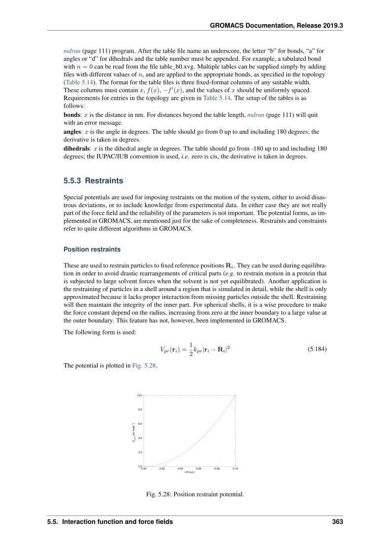
GROMACS Documentation, Release 2019.3
mdrun (page 111) program. After the table file name an underscore, the letter “b” for bonds, “a” forangles or “d” for dihedrals and the table number must be appended. For example, a tabulated bondwith 𝑛 = 0 can be read from the file table_b0.xvg. Multiple tables can be supplied simply by addingfiles with different values of 𝑛, and are applied to the appropriate bonds, as specified in the topology(Table 5.14). The format for the table files is three fixed-format columns of any suitable width.These columns must contain 𝑥, 𝑓(𝑥), −𝑓 ′(𝑥), and the values of 𝑥 should be uniformly spaced.Requirements for entries in the topology are given in Table 5.14. The setup of the tables is asfollows:bonds: 𝑥 is the distance in nm. For distances beyond the table length, mdrun (page 111) will quitwith an error message.angles: 𝑥 is the angle in degrees. The table should go from 0 up to and including 180 degrees; thederivative is taken in degrees.dihedrals: 𝑥 is the dihedral angle in degrees. The table should go from -180 up to and including 180degrees; the IUPAC/IUB convention is used, i.e. zero is cis, the derivative is taken in degrees.
5.5.3 Restraints
Special potentials are used for imposing restraints on the motion of the system, either to avoid disas-trous deviations, or to include knowledge from experimental data. In either case they are not reallypart of the force field and the reliability of the parameters is not important. The potential forms, as im-plemented in GROMACS, are mentioned just for the sake of completeness. Restraints and constraintsrefer to quite different algorithms in GROMACS.
Position restraints
These are used to restrain particles to fixed reference positions R𝑖. They can be used during equilibra-tion in order to avoid drastic rearrangements of critical parts (e.g. to restrain motion in a protein thatis subjected to large solvent forces when the solvent is not yet equilibrated). Another application isthe restraining of particles in a shell around a region that is simulated in detail, while the shell is onlyapproximated because it lacks proper interaction from missing particles outside the shell. Restrainingwill then maintain the integrity of the inner part. For spherical shells, it is a wise procedure to makethe force constant depend on the radius, increasing from zero at the inner boundary to a large value atthe outer boundary. This feature has not, however, been implemented in GROMACS.
The following form is used:
𝑉𝑝𝑟(r𝑖) =1
2𝑘𝑝𝑟|r𝑖 −R𝑖|2 (5.184)
The potential is plotted in Fig. 5.28.
0.00 0.02 0.04 0.06 0.08 0.10r-R (nm)
0.0
2.0
4.0
6.0
8.0
10.0
V posr
e(k
Jm
ole–1
)
Fig. 5.28: Position restraint potential.
5.5. Interaction function and force fields 363
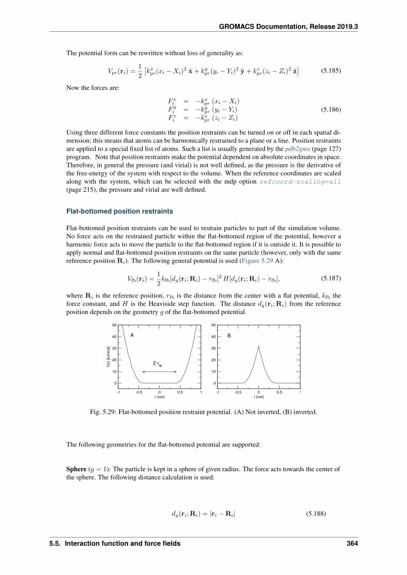
GROMACS Documentation, Release 2019.3
The potential form can be rewritten without loss of generality as:
𝑉𝑝𝑟(r𝑖) =1
2
[𝑘𝑥𝑝𝑟(𝑥𝑖 −𝑋𝑖)
2 x + 𝑘𝑦𝑝𝑟(𝑦𝑖 − 𝑌𝑖)2 y + 𝑘𝑧𝑝𝑟(𝑧𝑖 − 𝑍𝑖)
2 z]
(5.185)
Now the forces are:
𝐹 𝑥𝑖 = −𝑘𝑥𝑝𝑟 (𝑥𝑖 −𝑋𝑖)𝐹 𝑦𝑖 = −𝑘𝑦𝑝𝑟 (𝑦𝑖 − 𝑌𝑖)𝐹 𝑧𝑖 = −𝑘𝑧𝑝𝑟 (𝑧𝑖 − 𝑍𝑖)
(5.186)
Using three different force constants the position restraints can be turned on or off in each spatial di-mension; this means that atoms can be harmonically restrained to a plane or a line. Position restraintsare applied to a special fixed list of atoms. Such a list is usually generated by the pdb2gmx (page 127)program. Note that position restraints make the potential dependent on absolute coordinates in space.Therefore, in general the pressure (and virial) is not well defined, as the pressure is the derivative ofthe free-energy of the system with respect to the volume. When the reference coordinates are scaledalong with the system, which can be selected with the mdp option refcoord-scaling=all(page 215), the pressure and virial are well defined.
Flat-bottomed position restraints
Flat-bottomed position restraints can be used to restrain particles to part of the simulation volume.No force acts on the restrained particle within the flat-bottomed region of the potential, however aharmonic force acts to move the particle to the flat-bottomed region if it is outside it. It is possible toapply normal and flat-bottomed position restraints on the same particle (however, only with the samereference position R𝑖). The following general potential is used (Figure 5.29 A):
𝑉fb(r𝑖) =1
2𝑘fb[𝑑𝑔(r𝑖;R𝑖) − 𝑟fb]2𝐻[𝑑𝑔(r𝑖;R𝑖) − 𝑟fb], (5.187)
where R𝑖 is the reference position, 𝑟fb is the distance from the center with a flat potential, 𝑘fb theforce constant, and 𝐻 is the Heaviside step function. The distance 𝑑𝑔(r𝑖;R𝑖) from the referenceposition depends on the geometry 𝑔 of the flat-bottomed potential.
-1 -0.5 0 0.5 1r [nm]
0
10
20
30
40
50
V(r)
[kJ/
mol
]
-1 -0.5 0 0.5 1r [nm]
0
10
20
30
40
50
2 rfb
A B
Fig. 5.29: Flat-bottomed position restraint potential. (A) Not inverted, (B) inverted.
The following geometries for the flat-bottomed potential are supported:
Sphere (𝑔 = 1): The particle is kept in a sphere of given radius. The force acts towards the center ofthe sphere. The following distance calculation is used:
𝑑𝑔(r𝑖;R𝑖) = |r𝑖 −R𝑖| (5.188)
5.5. Interaction function and force fields 364
GROMACS Documentation, Release 2019.3
Cylinder (𝑔 = 6, 7, 8): The particle is kept in a cylinder of given radius parallel to the 𝑥 (𝑔 = 6), 𝑦(𝑔 = 7), or 𝑧-axis (𝑔 = 8). For backwards compatibility, setting 𝑔 = 2 is mapped to 𝑔 = 8 in thecode so that old tpr (page 431) files and topologies work. The force from the flat-bottomed potentialacts towards the axis of the cylinder. The component of the force parallel to the cylinder axis is zero.For a cylinder aligned along the 𝑧-axis:
𝑑𝑔(r𝑖;R𝑖) =√
(𝑥𝑖 −𝑋𝑖)2 + (𝑦𝑖 − 𝑌𝑖)2 (5.189)
Layer (𝑔 = 3, 4, 5): The particle is kept in a layer defined by the thickness and the normal of thelayer. The layer normal can be parallel to the 𝑥, 𝑦, or 𝑧-axis. The force acts parallel to the layernormal.
𝑑𝑔(r𝑖;R𝑖) = |𝑥𝑖 −𝑋𝑖|, or 𝑑𝑔(r𝑖;R𝑖) = |𝑦𝑖 − 𝑌𝑖|, or 𝑑𝑔(r𝑖;R𝑖) = |𝑧𝑖 − 𝑍𝑖|.(5.190)
It is possible to apply multiple independent flat-bottomed position restraints of different geometryon one particle. For example, applying a cylinder and a layer in 𝑧 keeps a particle within a disk.Applying three layers in 𝑥, 𝑦, and 𝑧 keeps the particle within a cuboid.
In addition, it is possible to invert the restrained region with the unrestrained region, leading to apotential that acts to keep the particle outside of the volume defined by R𝑖, 𝑔, and 𝑟fb. That feature isswitched on by defining a negative 𝑟fb in the topology. The following potential is used (Figure 5.29B):
𝑉 invfb (r𝑖) =
1
2𝑘fb[𝑑𝑔(r𝑖;R𝑖) − |𝑟fb|]2𝐻[−(𝑑𝑔(r𝑖;R𝑖) − |𝑟fb|)]. (5.191)
Angle restraints
These are used to restrain the angle between two pairs of particles or between one pair of particlesand the 𝑧-axis. The functional form is similar to that of a proper dihedral. For two pairs of atoms:
𝑉𝑎𝑟(r𝑖, r𝑗 , r𝑘, r𝑙) = 𝑘𝑎𝑟(1 − cos(𝑛(𝜃 − 𝜃0))), where 𝜃 = arccos
(r𝑗 − r𝑖‖r𝑗 − r𝑖‖
· r𝑙 − r𝑘‖r𝑙 − r𝑘‖
)(5.192)
For one pair of atoms and the 𝑧-axis:
𝑉𝑎𝑟(r𝑖, r𝑗) = 𝑘𝑎𝑟(1 − cos(𝑛(𝜃 − 𝜃0))), where 𝜃 = arccos
⎛⎝ r𝑗 − r𝑖‖r𝑗 − r𝑖‖
·
⎛⎝ 001
⎞⎠⎞⎠ (5.193)
A multiplicity (𝑛) of 2 is useful when you do not want to distinguish between parallel and anti-parallelvectors. The equilibrium angle 𝜃 should be between 0 and 180 degrees for multiplicity 1 and between0 and 90 degrees for multiplicity 2.
Dihedral restraints
These are used to restrain the dihedral angle 𝜑 defined by four particles as in an improper dihedral(sec. Improper dihedrals (page 357)) but with a slightly modified potential. Using:
𝜑′ = (𝜑− 𝜑0) MOD 2𝜋 (5.194)
5.5. Interaction function and force fields 365
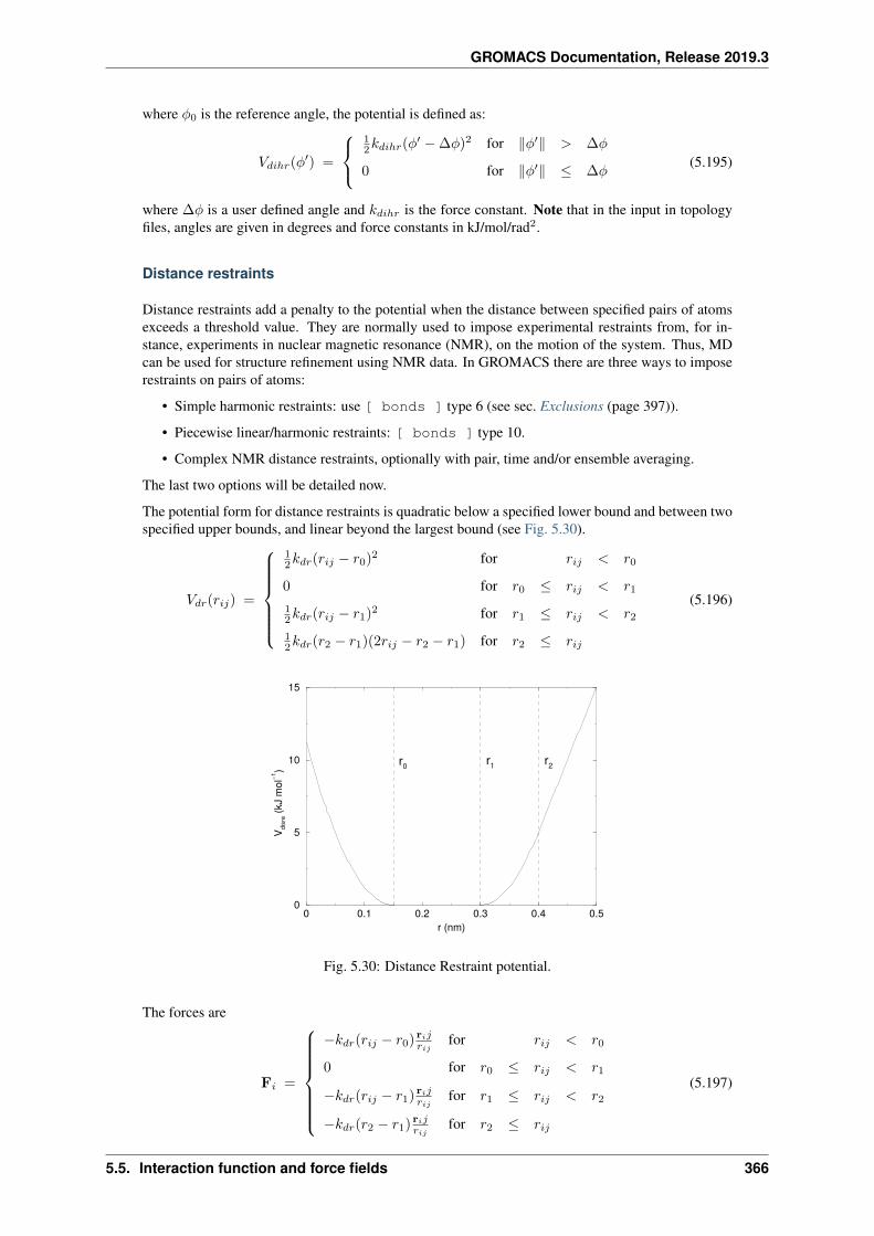
GROMACS Documentation, Release 2019.3
where 𝜑0 is the reference angle, the potential is defined as:
𝑉𝑑𝑖ℎ𝑟(𝜑′) =
⎧⎨⎩12𝑘𝑑𝑖ℎ𝑟(𝜑′ − ∆𝜑)2 for ‖𝜑′‖ > ∆𝜑
0 for ‖𝜑′‖ ≤ ∆𝜑(5.195)
where ∆𝜑 is a user defined angle and 𝑘𝑑𝑖ℎ𝑟 is the force constant. Note that in the input in topologyfiles, angles are given in degrees and force constants in kJ/mol/rad2.
Distance restraints
Distance restraints add a penalty to the potential when the distance between specified pairs of atomsexceeds a threshold value. They are normally used to impose experimental restraints from, for in-stance, experiments in nuclear magnetic resonance (NMR), on the motion of the system. Thus, MDcan be used for structure refinement using NMR data. In GROMACS there are three ways to imposerestraints on pairs of atoms:
• Simple harmonic restraints: use [ bonds ] type 6 (see sec. Exclusions (page 397)).
• Piecewise linear/harmonic restraints: [ bonds ] type 10.
• Complex NMR distance restraints, optionally with pair, time and/or ensemble averaging.
The last two options will be detailed now.
The potential form for distance restraints is quadratic below a specified lower bound and between twospecified upper bounds, and linear beyond the largest bound (see Fig. 5.30).
𝑉𝑑𝑟(𝑟𝑖𝑗) =
⎧⎪⎪⎪⎪⎪⎨⎪⎪⎪⎪⎪⎩
12𝑘𝑑𝑟(𝑟𝑖𝑗 − 𝑟0)2 for 𝑟𝑖𝑗 < 𝑟0
0 for 𝑟0 ≤ 𝑟𝑖𝑗 < 𝑟1
12𝑘𝑑𝑟(𝑟𝑖𝑗 − 𝑟1)2 for 𝑟1 ≤ 𝑟𝑖𝑗 < 𝑟2
12𝑘𝑑𝑟(𝑟2 − 𝑟1)(2𝑟𝑖𝑗 − 𝑟2 − 𝑟1) for 𝑟2 ≤ 𝑟𝑖𝑗
(5.196)
0 0.1 0.2 0.3 0.4 0.5r (nm)
0
5
10
15
V disr
e(k
J m
ol−1
)
r0 r1 r2
Fig. 5.30: Distance Restraint potential.
The forces are
F𝑖 =
⎧⎪⎪⎪⎪⎪⎪⎨⎪⎪⎪⎪⎪⎪⎩
−𝑘𝑑𝑟(𝑟𝑖𝑗 − 𝑟0) r𝑖𝑗𝑟𝑖𝑗
for 𝑟𝑖𝑗 < 𝑟0
0 for 𝑟0 ≤ 𝑟𝑖𝑗 < 𝑟1
−𝑘𝑑𝑟(𝑟𝑖𝑗 − 𝑟1) r𝑖𝑗𝑟𝑖𝑗
for 𝑟1 ≤ 𝑟𝑖𝑗 < 𝑟2
−𝑘𝑑𝑟(𝑟2 − 𝑟1) r𝑖𝑗𝑟𝑖𝑗
for 𝑟2 ≤ 𝑟𝑖𝑗
(5.197)
5.5. Interaction function and force fields 366
GROMACS Documentation, Release 2019.3
For restraints not derived from NMR data, this functionality will usually suffice and a section of [bonds ] type 10 can be used to apply individual restraints between pairs of atoms, see Topology file(page 405). For applying restraints derived from NMR measurements, more complex functionalitymight be required, which is provided through the [ distance_restraints ] section and isdescribed below.
Time averaging
Distance restraints based on instantaneous distances can potentially reduce the fluctuations in amolecule significantly. This problem can be overcome by restraining to a time averaged distance 91(page 510). The forces with time averaging are:
F𝑖 =
⎧⎪⎪⎪⎪⎪⎪⎨⎪⎪⎪⎪⎪⎪⎩
−𝑘𝑎𝑑𝑟(𝑟𝑖𝑗 − 𝑟0) r𝑖𝑗𝑟𝑖𝑗
for 𝑟𝑖𝑗 < 𝑟0
0 for 𝑟0 ≤ 𝑟𝑖𝑗 < 𝑟1
−𝑘𝑎𝑑𝑟(𝑟𝑖𝑗 − 𝑟1) r𝑖𝑗𝑟𝑖𝑗
for 𝑟1 ≤ 𝑟𝑖𝑗 < 𝑟2
−𝑘𝑎𝑑𝑟(𝑟2 − 𝑟1) r𝑖𝑗𝑟𝑖𝑗
for 𝑟2 ≤ 𝑟𝑖𝑗
(5.198)
where 𝑟𝑖𝑗 is given by an exponential running average with decay time 𝜏 :
𝑟𝑖𝑗 = < 𝑟−3𝑖𝑗 >−1/3 (5.199)
The force constant 𝑘𝑎𝑑𝑟 is switched on slowly to compensate for the lack of history at the beginning ofthe simulation:
𝑘𝑎𝑑𝑟 = 𝑘𝑑𝑟
(1 − exp
(− 𝑡
𝜏
))(5.200)
Because of the time averaging, we can no longer speak of a distance restraint potential.
This way an atom can satisfy two incompatible distance restraints on average by moving between twopositions. An example would be an amino acid side-chain that is rotating around its 𝜒 dihedral angle,thereby coming close to various other groups. Such a mobile side chain can give rise to multipleNOEs that can not be fulfilled by a single structure.
The computation of the time averaged distance in the mdrun (page 111) program is done in thefollowing fashion:
𝑟−3𝑖𝑗(0) = 𝑟𝑖𝑗(0)−3
𝑟−3𝑖𝑗(𝑡) = 𝑟−3
𝑖𝑗(𝑡− ∆𝑡) exp(−Δ𝑡
𝜏
)+ 𝑟𝑖𝑗(𝑡)
−3[1 − exp
(−Δ𝑡
𝜏
)] (5.201)
When a pair is within the bounds, it can still feel a force because the time averaged distance can stillbe beyond a bound. To prevent the protons from being pulled too close together, a mixed approach canbe used. In this approach, the penalty is zero when the instantaneous distance is within the bounds,otherwise the violation is the square root of the product of the instantaneous violation and the timeaveraged violation:
F𝑖 =
⎧⎪⎪⎪⎨⎪⎪⎪⎩𝑘𝑎𝑑𝑟√
(𝑟𝑖𝑗 − 𝑟0)(𝑟𝑖𝑗 − 𝑟0) r𝑖𝑗𝑟𝑖𝑗
for 𝑟𝑖𝑗 < 𝑟0 and 𝑟𝑖𝑗 < 𝑟0
−𝑘𝑎𝑑𝑟 min(√
(𝑟𝑖𝑗 − 𝑟1)(𝑟𝑖𝑗 − 𝑟1), 𝑟2 − 𝑟1
)r𝑖𝑗𝑟𝑖𝑗
for 𝑟𝑖𝑗 > 𝑟1 and 𝑟𝑖𝑗 > 𝑟1
0 otherwise(5.202)
Averaging over multiple pairs
Sometimes it is unclear from experimental data which atom pair gives rise to a single NOE, in otheroccasions it can be obvious that more than one pair contributes due to the symmetry of the system,e.g. a methyl group with three protons. For such a group, it is not possible to distinguish between
5.5. Interaction function and force fields 367
GROMACS Documentation, Release 2019.3
the protons, therefore they should all be taken into account when calculating the distance betweenthis methyl group and another proton (or group of protons). Due to the physical nature of magneticresonance, the intensity of the NOE signal is inversely proportional to the sixth power of the inter-atomic distance. Thus, when combining atom pairs, a fixed list of 𝑁 restraints may be taken together,where the apparent “distance” is given by:
𝑟𝑁 (𝑡) =
[𝑁∑
𝑛=1
𝑟𝑛(𝑡)−6
]−1/6
(5.203)
where we use 𝑟𝑖𝑗 or (5.199) for the 𝑟𝑛. The 𝑟𝑁 of the instantaneous and time-averaged distances canbe combined to do a mixed restraining, as indicated above. As more pairs of protons contribute to thesame NOE signal, the intensity will increase, and the summed “distance” will be shorter than any ofits components due to the reciprocal summation.
There are two options for distributing the forces over the atom pairs. In the conservative option, theforce is defined as the derivative of the restraint potential with respect to the coordinates. This resultsin a conservative potential when time averaging is not used. The force distribution over the pairs isproportional to 𝑟−6. This means that a close pair feels a much larger force than a distant pair, whichmight lead to a molecule that is “too rigid.” The other option is an equal force distribution. In thiscase each pair feels 1/𝑁 of the derivative of the restraint potential with respect to 𝑟𝑁 . The advantageof this method is that more conformations might be sampled, but the non-conservative nature of theforces can lead to local heating of the protons.
It is also possible to use ensemble averaging using multiple (protein) molecules. In this case thebounds should be lowered as in:
𝑟1 = 𝑟1 *𝑀−1/6
𝑟2 = 𝑟2 *𝑀−1/6 (5.204)
where 𝑀 is the number of molecules. The GROMACS preprocessor grompp (page 94) can do thisautomatically when the appropriate option is given. The resulting “distance” is then used to calculatethe scalar force according to:
F𝑖 =
⎧⎪⎨⎪⎩0 𝑟𝑁 < 𝑟1
𝑘𝑑𝑟(𝑟𝑁 − 𝑟1) r𝑖𝑗𝑟𝑖𝑗
𝑟1 ≤ 𝑟𝑁 < 𝑟2
𝑘𝑑𝑟(𝑟2 − 𝑟1) r𝑖𝑗𝑟𝑖𝑗
𝑟𝑁 ≥ 𝑟2
(5.205)
where 𝑖 and 𝑗 denote the atoms of all the pairs that contribute to the NOE signal.
Using distance restraints
A list of distance restrains based on NOE data can be added to a molecule definition in your topologyfile, like in the following example:
[ distance_restraints ]; ai aj type index type' low up1 up2 fac10 16 1 0 1 0.0 0.3 0.4 1.010 28 1 1 1 0.0 0.3 0.4 1.010 46 1 1 1 0.0 0.3 0.4 1.016 22 1 2 1 0.0 0.3 0.4 2.516 34 1 3 1 0.0 0.5 0.6 1.0
In this example a number of features can be found. In columns ai and aj you find the atom numbersof the particles to be restrained. The type column should always be 1. As explained in Distancerestraints (page 366), multiple distances can contribute to a single NOE signal. In the topology thiscan be set using the index column. In our example, the restraints 10-28 and 10-46 both have index1, therefore they are treated simultaneously. An extra requirement for treating restraints together isthat the restraints must be on successive lines, without any other intervening restraint. The type’column will usually be 1, but can be set to 2 to obtain a distance restraint that will never be time- and
5.5. Interaction function and force fields 368
GROMACS Documentation, Release 2019.3
ensemble-averaged; this can be useful for restraining hydrogen bonds. The columns low, up1, andup2 hold the values of 𝑟0, 𝑟1, and 𝑟2 from (5.196). In some cases it can be useful to have differentforce constants for some restraints; this is controlled by the column fac. The force constant in theparameter file is multiplied by the value in the column fac for each restraint. Information for eachrestraint is stored in the energy file and can be processed and plotted with gmx nmr (page 122).
Orientation restraints
This section describes how orientations between vectors, as measured in certain NMR experiments,can be calculated and restrained in MD simulations. The presented refinement methodology anda comparison of results with and without time and ensemble averaging have been published 92(page 510).
Theory
In an NMR experiment, orientations of vectors can be measured when a molecule does not tumblecompletely isotropically in the solvent. Two examples of such orientation measurements are residualdipolar couplings (between two nuclei) or chemical shift anisotropies. An observable for a vector r𝑖can be written as follows:
𝛿𝑖 =2
3tr(SD𝑖) (5.206)
where S is the dimensionless order tensor of the molecule. The tensor D𝑖 is given by:
D𝑖 =𝑐𝑖
‖r𝑖‖𝛼
⎛⎝ 3𝑥𝑥− 1 3𝑥𝑦 3𝑥𝑧3𝑥𝑦 3𝑦𝑦 − 1 3𝑦𝑧3𝑥𝑧 3𝑦𝑧 3𝑧𝑧 − 1
⎞⎠ (5.207)
with: 𝑥 =𝑟𝑖,𝑥‖r𝑖‖
, 𝑦 =𝑟𝑖,𝑦‖r𝑖‖
, 𝑧 =𝑟𝑖,𝑧‖r𝑖‖ (5.208)
For a dipolar coupling r𝑖 is the vector connecting the two nuclei, 𝛼 = 3 and the constant 𝑐𝑖 is givenby:
𝑐𝑖 =𝜇0
4𝜋𝛾𝑖1𝛾
𝑖2
~4𝜋
(5.209)
where 𝛾𝑖1 and 𝛾𝑖2 are the gyromagnetic ratios of the two nuclei.
The order tensor is symmetric and has trace zero. Using a rotation matrix T it can be transformedinto the following form:
T𝑇ST = 𝑠
⎛⎝ − 12 (1 − 𝜂) 0 0
0 − 12 (1 + 𝜂) 0
0 0 1
⎞⎠ (5.210)
where −1 ≤ 𝑠 ≤ 1 and 0 ≤ 𝜂 ≤ 1. 𝑠 is called the order parameter and 𝜂 the asymmetry of theorder tensor S. When the molecule tumbles isotropically in the solvent, 𝑠 is zero, and no orientationaleffects can be observed because all 𝛿𝑖 are zero.
Calculating orientations in a simulation
For reasons which are explained below, the D matrices are calculated which respect to a referenceorientation of the molecule. The orientation is defined by a rotation matrix R, which is needed toleast-squares fit the current coordinates of a selected set of atoms onto a reference conformation. Thereference conformation is the starting conformation of the simulation. In case of ensemble averaging,
5.5. Interaction function and force fields 369
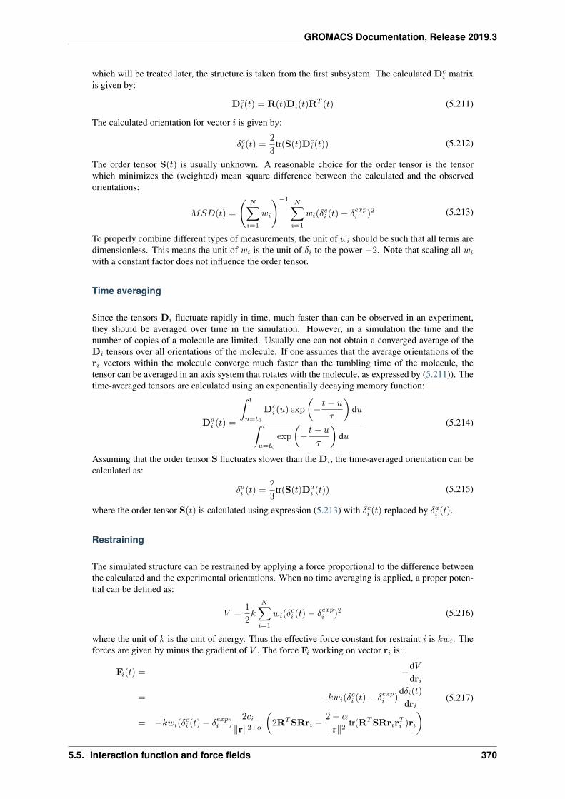
GROMACS Documentation, Release 2019.3
which will be treated later, the structure is taken from the first subsystem. The calculated D𝑐𝑖 matrix
is given by:
D𝑐𝑖 (𝑡) = R(𝑡)D𝑖(𝑡)R
𝑇 (𝑡) (5.211)
The calculated orientation for vector 𝑖 is given by:
𝛿𝑐𝑖 (𝑡) =2
3tr(S(𝑡)D𝑐
𝑖 (𝑡)) (5.212)
The order tensor S(𝑡) is usually unknown. A reasonable choice for the order tensor is the tensorwhich minimizes the (weighted) mean square difference between the calculated and the observedorientations:
𝑀𝑆𝐷(𝑡) =
(𝑁∑𝑖=1
𝑤𝑖
)−1 𝑁∑𝑖=1
𝑤𝑖(𝛿𝑐𝑖 (𝑡) − 𝛿𝑒𝑥𝑝𝑖 )2 (5.213)
To properly combine different types of measurements, the unit of 𝑤𝑖 should be such that all terms aredimensionless. This means the unit of 𝑤𝑖 is the unit of 𝛿𝑖 to the power −2. Note that scaling all 𝑤𝑖
with a constant factor does not influence the order tensor.
Time averaging
Since the tensors D𝑖 fluctuate rapidly in time, much faster than can be observed in an experiment,they should be averaged over time in the simulation. However, in a simulation the time and thenumber of copies of a molecule are limited. Usually one can not obtain a converged average of theD𝑖 tensors over all orientations of the molecule. If one assumes that the average orientations of ther𝑖 vectors within the molecule converge much faster than the tumbling time of the molecule, thetensor can be averaged in an axis system that rotates with the molecule, as expressed by (5.211)). Thetime-averaged tensors are calculated using an exponentially decaying memory function:
D𝑎𝑖 (𝑡) =
∫ 𝑡
𝑢=𝑡0
D𝑐𝑖 (𝑢) exp
(− 𝑡− 𝑢
𝜏
)d𝑢∫ 𝑡
𝑢=𝑡0
exp
(− 𝑡− 𝑢
𝜏
)d𝑢
(5.214)
Assuming that the order tensor S fluctuates slower than the D𝑖, the time-averaged orientation can becalculated as:
𝛿𝑎𝑖 (𝑡) =2
3tr(S(𝑡)D𝑎
𝑖 (𝑡)) (5.215)
where the order tensor S(𝑡) is calculated using expression (5.213) with 𝛿𝑐𝑖 (𝑡) replaced by 𝛿𝑎𝑖 (𝑡).
Restraining
The simulated structure can be restrained by applying a force proportional to the difference betweenthe calculated and the experimental orientations. When no time averaging is applied, a proper poten-tial can be defined as:
𝑉 =1
2𝑘
𝑁∑𝑖=1
𝑤𝑖(𝛿𝑐𝑖 (𝑡) − 𝛿𝑒𝑥𝑝𝑖 )2 (5.216)
where the unit of 𝑘 is the unit of energy. Thus the effective force constant for restraint 𝑖 is 𝑘𝑤𝑖. Theforces are given by minus the gradient of 𝑉 . The force F𝑖 working on vector r𝑖 is:
F𝑖(𝑡) = −d𝑉dr𝑖
= −𝑘𝑤𝑖(𝛿𝑐𝑖 (𝑡) − 𝛿𝑒𝑥𝑝𝑖 )
d𝛿𝑖(𝑡)dr𝑖
= −𝑘𝑤𝑖(𝛿𝑐𝑖 (𝑡) − 𝛿𝑒𝑥𝑝𝑖 )
2𝑐𝑖‖r‖2+𝛼
(2R𝑇SRr𝑖 −
2 + 𝛼
‖r‖2tr(R𝑇SRr𝑖r
𝑇𝑖 )r𝑖
) (5.217)
5.5. Interaction function and force fields 370
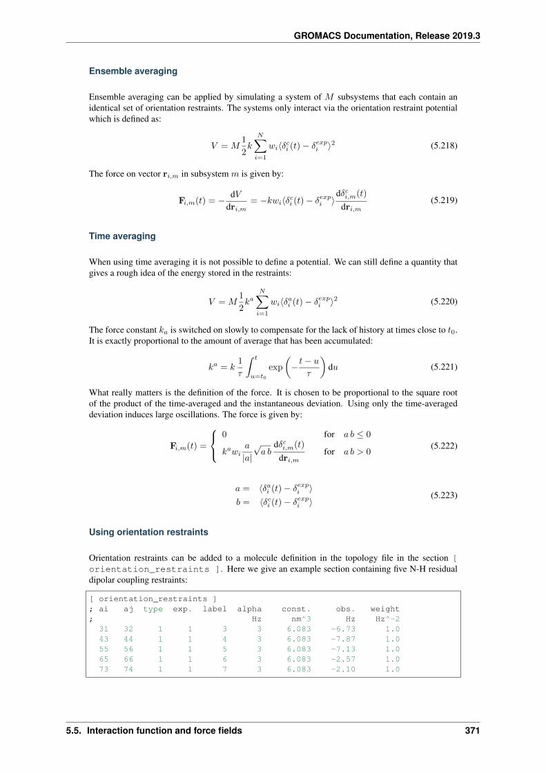
GROMACS Documentation, Release 2019.3
Ensemble averaging
Ensemble averaging can be applied by simulating a system of 𝑀 subsystems that each contain anidentical set of orientation restraints. The systems only interact via the orientation restraint potentialwhich is defined as:
𝑉 = 𝑀1
2𝑘
𝑁∑𝑖=1
𝑤𝑖⟨𝛿𝑐𝑖 (𝑡) − 𝛿𝑒𝑥𝑝𝑖 ⟩2 (5.218)
The force on vector r𝑖,𝑚 in subsystem 𝑚 is given by:
F𝑖,𝑚(𝑡) = − d𝑉dr𝑖,𝑚
= −𝑘𝑤𝑖⟨𝛿𝑐𝑖 (𝑡) − 𝛿𝑒𝑥𝑝𝑖 ⟩d𝛿𝑐𝑖,𝑚(𝑡)
dr𝑖,𝑚(5.219)
Time averaging
When using time averaging it is not possible to define a potential. We can still define a quantity thatgives a rough idea of the energy stored in the restraints:
𝑉 = 𝑀1
2𝑘𝑎
𝑁∑𝑖=1
𝑤𝑖⟨𝛿𝑎𝑖 (𝑡) − 𝛿𝑒𝑥𝑝𝑖 ⟩2 (5.220)
The force constant 𝑘𝑎 is switched on slowly to compensate for the lack of history at times close to 𝑡0.It is exactly proportional to the amount of average that has been accumulated:
𝑘𝑎 = 𝑘1
𝜏
∫ 𝑡
𝑢=𝑡0
exp
(− 𝑡− 𝑢
𝜏
)d𝑢 (5.221)
What really matters is the definition of the force. It is chosen to be proportional to the square rootof the product of the time-averaged and the instantaneous deviation. Using only the time-averageddeviation induces large oscillations. The force is given by:
F𝑖,𝑚(𝑡) =
⎧⎨⎩0 for 𝑎 𝑏 ≤ 0
𝑘𝑎𝑤𝑖𝑎
|𝑎|√𝑎 𝑏
d𝛿𝑐𝑖,𝑚(𝑡)
dr𝑖,𝑚for 𝑎 𝑏 > 0
(5.222)
𝑎 = ⟨𝛿𝑎𝑖 (𝑡) − 𝛿𝑒𝑥𝑝𝑖 ⟩𝑏 = ⟨𝛿𝑐𝑖 (𝑡) − 𝛿𝑒𝑥𝑝𝑖 ⟩
(5.223)
Using orientation restraints
Orientation restraints can be added to a molecule definition in the topology file in the section [orientation_restraints ]. Here we give an example section containing five N-H residualdipolar coupling restraints:
[ orientation_restraints ]; ai aj type exp. label alpha const. obs. weight; Hz nm^3 Hz Hz^-231 32 1 1 3 3 6.083 -6.73 1.043 44 1 1 4 3 6.083 -7.87 1.055 56 1 1 5 3 6.083 -7.13 1.065 66 1 1 6 3 6.083 -2.57 1.073 74 1 1 7 3 6.083 -2.10 1.0
5.5. Interaction function and force fields 371

GROMACS Documentation, Release 2019.3
The unit of the observable is Hz, but one can choose any other unit. In columns ai and aj you findthe atom numbers of the particles to be restrained. The type column should always be 1. The exp.column denotes the experiment number, starting at 1. For each experiment a separate order tensor Sis optimized. The label should be a unique number larger than zero for each restraint. The alphacolumn contains the power 𝛼 that is used in (5.207)) to calculate the orientation. The const. columncontains the constant 𝑐𝑖 used in the same equation. The constant should have the unit of the observabletimes nm𝛼. The column obs. contains the observable, in any unit you like. The last column containsthe weights 𝑤𝑖; the unit should be the inverse of the square of the unit of the observable.
Some parameters for orientation restraints can be specified in the grompp (page 94) mdp (page 425)file, for a study of the effect of different force constants and averaging times and ensemble averagingsee 92 (page 510). Information for each restraint is stored in the energy file and can be processed andplotted with gmx nmr (page 122).
5.5. Interaction function and force fields 372
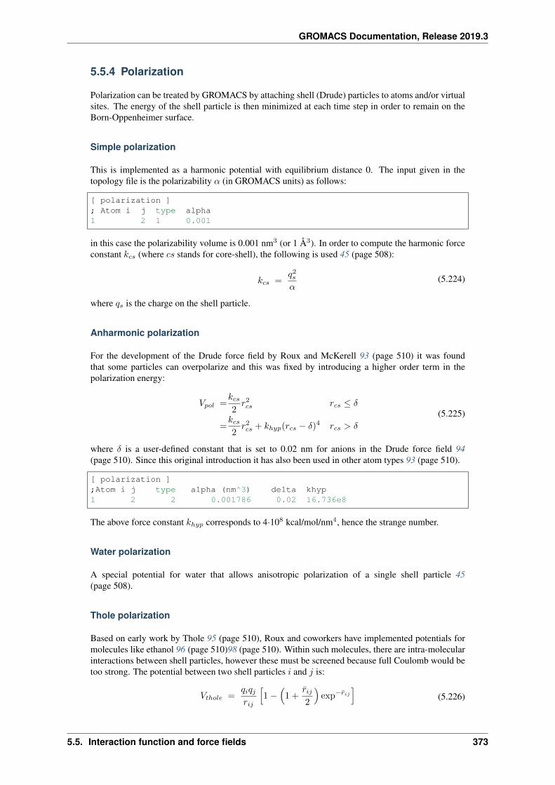
GROMACS Documentation, Release 2019.3
5.5.4 Polarization
Polarization can be treated by GROMACS by attaching shell (Drude) particles to atoms and/or virtualsites. The energy of the shell particle is then minimized at each time step in order to remain on theBorn-Oppenheimer surface.
Simple polarization
This is implemented as a harmonic potential with equilibrium distance 0. The input given in thetopology file is the polarizability 𝛼 (in GROMACS units) as follows:
[ polarization ]; Atom i j type alpha1 2 1 0.001
in this case the polarizability volume is 0.001 nm3 (or 1 Å3). In order to compute the harmonic forceconstant 𝑘𝑐𝑠 (where 𝑐𝑠 stands for core-shell), the following is used 45 (page 508):
𝑘𝑐𝑠 =𝑞2𝑠𝛼
(5.224)
where 𝑞𝑠 is the charge on the shell particle.
Anharmonic polarization
For the development of the Drude force field by Roux and McKerell 93 (page 510) it was foundthat some particles can overpolarize and this was fixed by introducing a higher order term in thepolarization energy:
𝑉𝑝𝑜𝑙 =𝑘𝑐𝑠2𝑟2𝑐𝑠 𝑟𝑐𝑠 ≤ 𝛿
=𝑘𝑐𝑠2𝑟2𝑐𝑠 + 𝑘ℎ𝑦𝑝(𝑟𝑐𝑠 − 𝛿)4 𝑟𝑐𝑠 > 𝛿
(5.225)
where 𝛿 is a user-defined constant that is set to 0.02 nm for anions in the Drude force field 94(page 510). Since this original introduction it has also been used in other atom types 93 (page 510).
[ polarization ];Atom i j type alpha (nm^3) delta khyp1 2 2 0.001786 0.02 16.736e8
The above force constant 𝑘ℎ𝑦𝑝 corresponds to 4·108 kcal/mol/nm4, hence the strange number.
Water polarization
A special potential for water that allows anisotropic polarization of a single shell particle 45(page 508).
Thole polarization
Based on early work by Thole 95 (page 510), Roux and coworkers have implemented potentials formolecules like ethanol 96 (page 510)98 (page 510). Within such molecules, there are intra-molecularinteractions between shell particles, however these must be screened because full Coulomb would betoo strong. The potential between two shell particles 𝑖 and 𝑗 is:
𝑉𝑡ℎ𝑜𝑙𝑒 =𝑞𝑖𝑞𝑗𝑟𝑖𝑗
[1 −
(1 +
𝑟𝑖𝑗2
)exp−𝑟𝑖𝑗
](5.226)
5.5. Interaction function and force fields 373
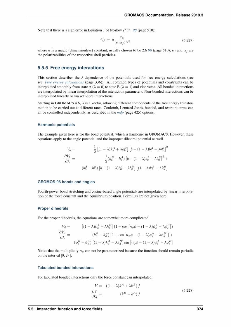
GROMACS Documentation, Release 2019.3
Note that there is a sign error in Equation 1 of Noskov et al. 98 (page 510):
𝑟𝑖𝑗 = 𝑎𝑟𝑖𝑗
(𝛼𝑖𝛼𝑗)1/6(5.227)
where 𝑎 is a magic (dimensionless) constant, usually chosen to be 2.6 98 (page 510); 𝛼𝑖 and 𝛼𝑗 arethe polarizabilities of the respective shell particles.
5.5.5 Free energy interactions
This section describes the 𝜆-dependence of the potentials used for free energy calculations (seesec. Free energy calculations (page 336)). All common types of potentials and constraints can beinterpolated smoothly from state A (𝜆 = 0) to state B (𝜆 = 1) and vice versa. All bonded interactionsare interpolated by linear interpolation of the interaction parameters. Non-bonded interactions can beinterpolated linearly or via soft-core interactions.
Starting in GROMACS 4.6, 𝜆 is a vector, allowing different components of the free energy transfor-mation to be carried out at different rates. Coulomb, Lennard-Jones, bonded, and restraint terms canall be controlled independently, as described in the mdp (page 425) options.
Harmonic potentials
The example given here is for the bond potential, which is harmonic in GROMACS. However, theseequations apply to the angle potential and the improper dihedral potential as well.
𝑉𝑏 =1
2
[(1 − 𝜆)𝑘𝐴𝑏 + 𝜆𝑘𝐵𝑏
] [𝑏− (1 − 𝜆)𝑏𝐴0 − 𝜆𝑏𝐵0
]2𝜕𝑉𝑏𝜕𝜆
=1
2(𝑘𝐵𝑏 − 𝑘𝐴𝑏 )
[𝑏− (1 − 𝜆)𝑏𝐴0 + 𝜆𝑏𝐵0
]2+
(𝑏𝐴0 − 𝑏𝐵0 )[𝑏− (1 − 𝜆)𝑏𝐴0 − 𝜆𝑏𝐵0
] [(1 − 𝜆)𝑘𝐴𝑏 + 𝜆𝑘𝐵𝑏
]GROMOS-96 bonds and angles
Fourth-power bond stretching and cosine-based angle potentials are interpolated by linear interpola-tion of the force constant and the equilibrium position. Formulas are not given here.
Proper dihedrals
For the proper dihedrals, the equations are somewhat more complicated:
𝑉𝑑 =[(1 − 𝜆)𝑘𝐴𝑑 + 𝜆𝑘𝐵𝑑
] (1 + cos
[𝑛𝜑𝜑− (1 − 𝜆)𝜑𝐴𝑠 − 𝜆𝜑𝐵𝑠
])𝜕𝑉𝑑𝜕𝜆
= (𝑘𝐵𝑑 − 𝑘𝐴𝑑 )(1 + cos
[𝑛𝜑𝜑− (1 − 𝜆)𝜑𝐴𝑠 − 𝜆𝜑𝐵𝑠
])+
(𝜑𝐵𝑠 − 𝜑𝐴𝑠 )[(1 − 𝜆)𝑘𝐴𝑑 − 𝜆𝑘𝐵𝑑
]sin[𝑛𝜑𝜑− (1 − 𝜆)𝜑𝐴𝑠 − 𝜆𝜑𝐵𝑠
]Note: that the multiplicity 𝑛𝜑 can not be parameterized because the function should remain periodicon the interval [0, 2𝜋].
Tabulated bonded interactions
For tabulated bonded interactions only the force constant can interpolated:
𝑉 = ((1 − 𝜆)𝑘𝐴 + 𝜆𝑘𝐵) 𝑓
𝜕𝑉
𝜕𝜆= (𝑘𝐵 − 𝑘𝐴) 𝑓
(5.228)
5.5. Interaction function and force fields 374
GROMACS Documentation, Release 2019.3
Coulomb interaction
The Coulomb interaction between two particles of which the charge varies with 𝜆 is:
𝑉𝑐 =𝑓
𝜀𝑟𝑓𝑟𝑖𝑗
[(1 − 𝜆)𝑞𝐴𝑖 𝑞
𝐴𝑗 + 𝜆 𝑞𝐵𝑖 𝑞
𝐵𝑗
]𝜕𝑉𝑐𝜕𝜆
=𝑓
𝜀𝑟𝑓𝑟𝑖𝑗
[−𝑞𝐴𝑖 𝑞𝐴𝑗 + 𝑞𝐵𝑖 𝑞
𝐵𝑗
] (5.229)
where 𝑓 = 14𝜋𝜀0
= 138.935 458 (see chapter Definitions and Units (page 299)).
Coulomb interaction with reaction field
The Coulomb interaction including a reaction field, between two particles of which the charge varieswith 𝜆 is:
𝑉𝑐 = 𝑓
[1
𝑟𝑖𝑗+ 𝑘𝑟𝑓 𝑟𝑖𝑗
2 − 𝑐𝑟𝑓
] [(1 − 𝜆)𝑞𝐴𝑖 𝑞
𝐴𝑗 + 𝜆 𝑞𝐵𝑖 𝑞
𝐵𝑗
]𝜕𝑉𝑐𝜕𝜆
= 𝑓
[1
𝑟𝑖𝑗+ 𝑘𝑟𝑓 𝑟𝑖𝑗
2 − 𝑐𝑟𝑓
] [−𝑞𝐴𝑖 𝑞𝐴𝑗 + 𝑞𝐵𝑖 𝑞
𝐵𝑗
] (5.230)
Note that the constants 𝑘𝑟𝑓 and 𝑐𝑟𝑓 are defined using the dielectric constant 𝜀𝑟𝑓 of the medium (seesec. Coulomb interaction with reaction field (page 350)).
Lennard-Jones interaction
For the Lennard-Jones interaction between two particles of which the atom type varies with 𝜆 we canwrite:
𝑉𝐿𝐽 =(1 − 𝜆)𝐶𝐴
12 + 𝜆𝐶𝐵12
𝑟𝑖𝑗12− (1 − 𝜆)𝐶𝐴
6 + 𝜆𝐶𝐵6
𝑟𝑖𝑗6
𝜕𝑉𝐿𝐽
𝜕𝜆=
𝐶𝐵12 − 𝐶𝐴
12
𝑟𝑖𝑗12− 𝐶𝐵
6 − 𝐶𝐴6
𝑟𝑖𝑗6
(5.231)
It should be noted that it is also possible to express a pathway from state A to state B using 𝜎 and 𝜖(see (5.119)). It may seem to make sense physically to vary the force field parameters 𝜎 and 𝜖 ratherthan the derived parameters 𝐶12 and 𝐶6. However, the difference between the pathways in parameterspace is not large, and the free energy itself does not depend on the pathway, so we use the simpleformulation presented above.
Kinetic Energy
When the mass of a particle changes, there is also a contribution of the kinetic energy to the freeenergy (note that we can not write the momentum p as m v, since that would result in the sign of 𝜕𝐸𝑘
𝜕𝜆being incorrect 99 (page 510)):
𝐸𝑘 =1
2
p2
(1 − 𝜆)𝑚𝐴 + 𝜆𝑚𝐵
𝜕𝐸𝑘
𝜕𝜆= −1
2
p2(𝑚𝐵 −𝑚𝐴)
((1 − 𝜆)𝑚𝐴 + 𝜆𝑚𝐵)2
(5.232)
after taking the derivative, we can insert p = m v, such that:
𝜕𝐸𝑘
𝜕𝜆= −1
2v2(𝑚𝐵 −𝑚𝐴) (5.233)
5.5. Interaction function and force fields 375
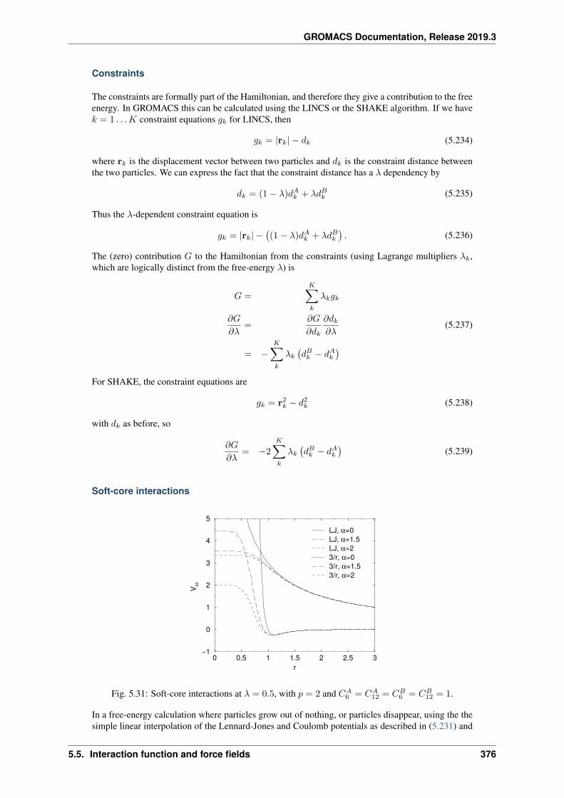
GROMACS Documentation, Release 2019.3
Constraints
The constraints are formally part of the Hamiltonian, and therefore they give a contribution to the freeenergy. In GROMACS this can be calculated using the LINCS or the SHAKE algorithm. If we have𝑘 = 1 . . .𝐾 constraint equations 𝑔𝑘 for LINCS, then
𝑔𝑘 = |r𝑘| − 𝑑𝑘 (5.234)
where r𝑘 is the displacement vector between two particles and 𝑑𝑘 is the constraint distance betweenthe two particles. We can express the fact that the constraint distance has a 𝜆 dependency by
𝑑𝑘 = (1 − 𝜆)𝑑𝐴𝑘 + 𝜆𝑑𝐵𝑘 (5.235)
Thus the 𝜆-dependent constraint equation is
𝑔𝑘 = |r𝑘| −((1 − 𝜆)𝑑𝐴𝑘 + 𝜆𝑑𝐵𝑘
). (5.236)
The (zero) contribution 𝐺 to the Hamiltonian from the constraints (using Lagrange multipliers 𝜆𝑘,which are logically distinct from the free-energy 𝜆) is
𝐺 =
𝐾∑𝑘
𝜆𝑘𝑔𝑘
𝜕𝐺
𝜕𝜆=
𝜕𝐺
𝜕𝑑𝑘
𝜕𝑑𝑘𝜕𝜆
= −𝐾∑𝑘
𝜆𝑘(𝑑𝐵𝑘 − 𝑑𝐴𝑘
)(5.237)
For SHAKE, the constraint equations are
𝑔𝑘 = r2𝑘 − 𝑑2𝑘 (5.238)
with 𝑑𝑘 as before, so
𝜕𝐺
𝜕𝜆= −2
𝐾∑𝑘
𝜆𝑘(𝑑𝐵𝑘 − 𝑑𝐴𝑘
)(5.239)
Soft-core interactions
0 0.5 1 1.5 2 2.5 3r
−1
0
1
2
3
4
5
V sc
LJ, α=0LJ, α=1.5LJ, α=23/r, α=03/r, α=1.53/r, α=2
Fig. 5.31: Soft-core interactions at 𝜆 = 0.5, with 𝑝 = 2 and 𝐶𝐴6 = 𝐶𝐴
12 = 𝐶𝐵6 = 𝐶𝐵
12 = 1.
In a free-energy calculation where particles grow out of nothing, or particles disappear, using the thesimple linear interpolation of the Lennard-Jones and Coulomb potentials as described in (5.231) and
5.5. Interaction function and force fields 376
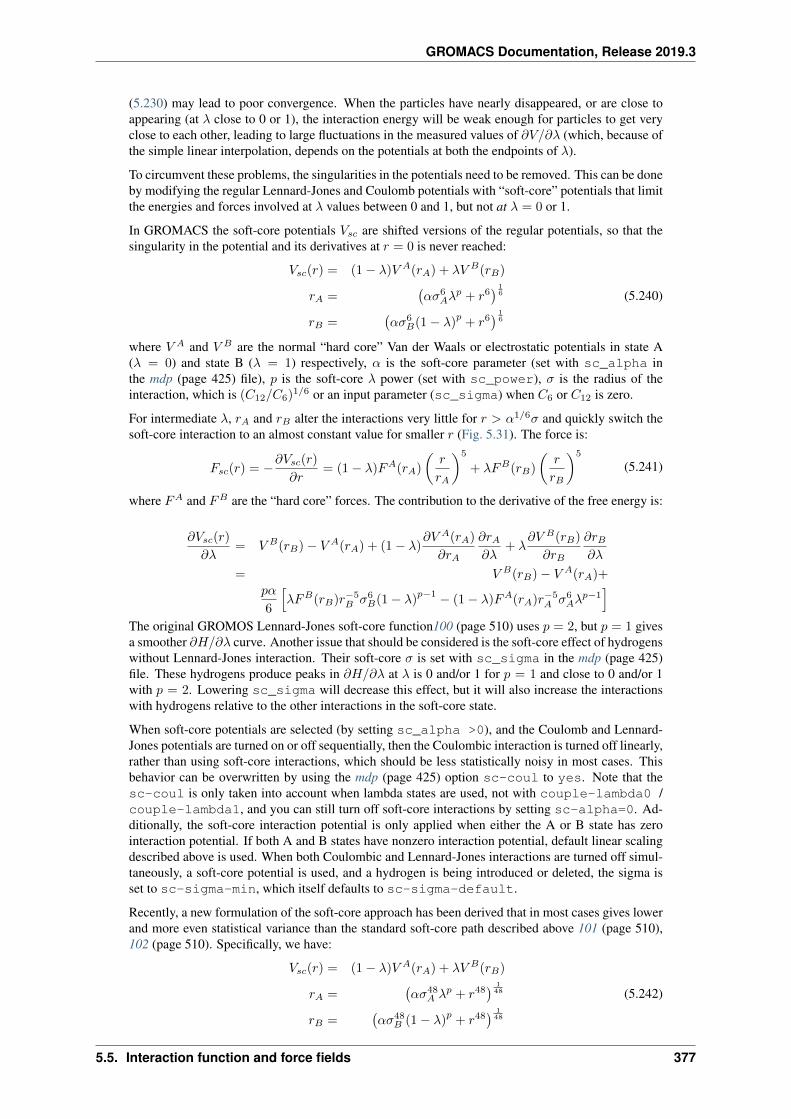
GROMACS Documentation, Release 2019.3
(5.230) may lead to poor convergence. When the particles have nearly disappeared, or are close toappearing (at 𝜆 close to 0 or 1), the interaction energy will be weak enough for particles to get veryclose to each other, leading to large fluctuations in the measured values of 𝜕𝑉/𝜕𝜆 (which, because ofthe simple linear interpolation, depends on the potentials at both the endpoints of 𝜆).
To circumvent these problems, the singularities in the potentials need to be removed. This can be doneby modifying the regular Lennard-Jones and Coulomb potentials with “soft-core” potentials that limitthe energies and forces involved at 𝜆 values between 0 and 1, but not at 𝜆 = 0 or 1.
In GROMACS the soft-core potentials 𝑉𝑠𝑐 are shifted versions of the regular potentials, so that thesingularity in the potential and its derivatives at 𝑟 = 0 is never reached:
𝑉𝑠𝑐(𝑟) = (1 − 𝜆)𝑉 𝐴(𝑟𝐴) + 𝜆𝑉 𝐵(𝑟𝐵)
𝑟𝐴 =(𝛼𝜎6
𝐴𝜆𝑝 + 𝑟6
) 16
𝑟𝐵 =(𝛼𝜎6
𝐵(1 − 𝜆)𝑝
+ 𝑟6) 1
6
(5.240)
where 𝑉 𝐴 and 𝑉 𝐵 are the normal “hard core” Van der Waals or electrostatic potentials in state A(𝜆 = 0) and state B (𝜆 = 1) respectively, 𝛼 is the soft-core parameter (set with sc_alpha inthe mdp (page 425) file), 𝑝 is the soft-core 𝜆 power (set with sc_power), 𝜎 is the radius of theinteraction, which is (𝐶12/𝐶6)1/6 or an input parameter (sc_sigma) when 𝐶6 or 𝐶12 is zero.
For intermediate 𝜆, 𝑟𝐴 and 𝑟𝐵 alter the interactions very little for 𝑟 > 𝛼1/6𝜎 and quickly switch thesoft-core interaction to an almost constant value for smaller 𝑟 (Fig. 5.31). The force is:
𝐹𝑠𝑐(𝑟) = −𝜕𝑉𝑠𝑐(𝑟)𝜕𝑟
= (1 − 𝜆)𝐹𝐴(𝑟𝐴)
(𝑟
𝑟𝐴
)5
+ 𝜆𝐹𝐵(𝑟𝐵)
(𝑟
𝑟𝐵
)5
(5.241)
where 𝐹𝐴 and 𝐹𝐵 are the “hard core” forces. The contribution to the derivative of the free energy is:
𝜕𝑉𝑠𝑐(𝑟)
𝜕𝜆= 𝑉 𝐵(𝑟𝐵) − 𝑉 𝐴(𝑟𝐴) + (1 − 𝜆)
𝜕𝑉 𝐴(𝑟𝐴)
𝜕𝑟𝐴
𝜕𝑟𝐴𝜕𝜆
+ 𝜆𝜕𝑉 𝐵(𝑟𝐵)
𝜕𝑟𝐵
𝜕𝑟𝐵𝜕𝜆
= 𝑉 𝐵(𝑟𝐵) − 𝑉 𝐴(𝑟𝐴)+𝑝𝛼
6
[𝜆𝐹𝐵(𝑟𝐵)𝑟−5
𝐵 𝜎6𝐵(1 − 𝜆)
𝑝−1 − (1 − 𝜆)𝐹𝐴(𝑟𝐴)𝑟−5𝐴 𝜎6
𝐴𝜆𝑝−1]
The original GROMOS Lennard-Jones soft-core function100 (page 510) uses 𝑝 = 2, but 𝑝 = 1 givesa smoother 𝜕𝐻/𝜕𝜆 curve. Another issue that should be considered is the soft-core effect of hydrogenswithout Lennard-Jones interaction. Their soft-core 𝜎 is set with sc_sigma in the mdp (page 425)file. These hydrogens produce peaks in 𝜕𝐻/𝜕𝜆 at 𝜆 is 0 and/or 1 for 𝑝 = 1 and close to 0 and/or 1with 𝑝 = 2. Lowering sc_sigma will decrease this effect, but it will also increase the interactionswith hydrogens relative to the other interactions in the soft-core state.
When soft-core potentials are selected (by setting sc_alpha >0), and the Coulomb and Lennard-Jones potentials are turned on or off sequentially, then the Coulombic interaction is turned off linearly,rather than using soft-core interactions, which should be less statistically noisy in most cases. Thisbehavior can be overwritten by using the mdp (page 425) option sc-coul to yes. Note that thesc-coul is only taken into account when lambda states are used, not with couple-lambda0 /couple-lambda1, and you can still turn off soft-core interactions by setting sc-alpha=0. Ad-ditionally, the soft-core interaction potential is only applied when either the A or B state has zerointeraction potential. If both A and B states have nonzero interaction potential, default linear scalingdescribed above is used. When both Coulombic and Lennard-Jones interactions are turned off simul-taneously, a soft-core potential is used, and a hydrogen is being introduced or deleted, the sigma isset to sc-sigma-min, which itself defaults to sc-sigma-default.
Recently, a new formulation of the soft-core approach has been derived that in most cases gives lowerand more even statistical variance than the standard soft-core path described above 101 (page 510),102 (page 510). Specifically, we have:
𝑉𝑠𝑐(𝑟) = (1 − 𝜆)𝑉 𝐴(𝑟𝐴) + 𝜆𝑉 𝐵(𝑟𝐵)
𝑟𝐴 =(𝛼𝜎48
𝐴 𝜆𝑝 + 𝑟48
) 148
𝑟𝐵 =(𝛼𝜎48
𝐵 (1 − 𝜆)𝑝
+ 𝑟48) 1
48
(5.242)
5.5. Interaction function and force fields 377
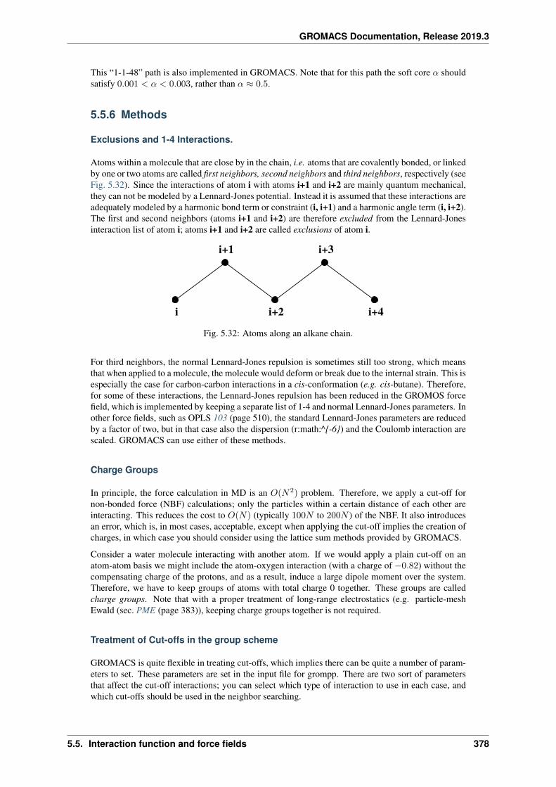
GROMACS Documentation, Release 2019.3
This “1-1-48” path is also implemented in GROMACS. Note that for this path the soft core 𝛼 shouldsatisfy 0.001 < 𝛼 < 0.003, rather than 𝛼 ≈ 0.5.
5.5.6 Methods
Exclusions and 1-4 Interactions.
Atoms within a molecule that are close by in the chain, i.e. atoms that are covalently bonded, or linkedby one or two atoms are called first neighbors, second neighbors and third neighbors, respectively (seeFig. 5.32). Since the interactions of atom i with atoms i+1 and i+2 are mainly quantum mechanical,they can not be modeled by a Lennard-Jones potential. Instead it is assumed that these interactions areadequately modeled by a harmonic bond term or constraint (i, i+1) and a harmonic angle term (i, i+2).The first and second neighbors (atoms i+1 and i+2) are therefore excluded from the Lennard-Jonesinteraction list of atom i; atoms i+1 and i+2 are called exclusions of atom i.
i+1 i+3
i i+2 i+4
Fig. 5.32: Atoms along an alkane chain.
For third neighbors, the normal Lennard-Jones repulsion is sometimes still too strong, which meansthat when applied to a molecule, the molecule would deform or break due to the internal strain. This isespecially the case for carbon-carbon interactions in a cis-conformation (e.g. cis-butane). Therefore,for some of these interactions, the Lennard-Jones repulsion has been reduced in the GROMOS forcefield, which is implemented by keeping a separate list of 1-4 and normal Lennard-Jones parameters. Inother force fields, such as OPLS 103 (page 510), the standard Lennard-Jones parameters are reducedby a factor of two, but in that case also the dispersion (r:math:^{-6}) and the Coulomb interaction arescaled. GROMACS can use either of these methods.
Charge Groups
In principle, the force calculation in MD is an 𝑂(𝑁2) problem. Therefore, we apply a cut-off fornon-bonded force (NBF) calculations; only the particles within a certain distance of each other areinteracting. This reduces the cost to 𝑂(𝑁) (typically 100𝑁 to 200𝑁 ) of the NBF. It also introducesan error, which is, in most cases, acceptable, except when applying the cut-off implies the creation ofcharges, in which case you should consider using the lattice sum methods provided by GROMACS.
Consider a water molecule interacting with another atom. If we would apply a plain cut-off on anatom-atom basis we might include the atom-oxygen interaction (with a charge of −0.82) without thecompensating charge of the protons, and as a result, induce a large dipole moment over the system.Therefore, we have to keep groups of atoms with total charge 0 together. These groups are calledcharge groups. Note that with a proper treatment of long-range electrostatics (e.g. particle-meshEwald (sec. PME (page 383)), keeping charge groups together is not required.
Treatment of Cut-offs in the group scheme
GROMACS is quite flexible in treating cut-offs, which implies there can be quite a number of param-eters to set. These parameters are set in the input file for grompp. There are two sort of parametersthat affect the cut-off interactions; you can select which type of interaction to use in each case, andwhich cut-offs should be used in the neighbor searching.
5.5. Interaction function and force fields 378
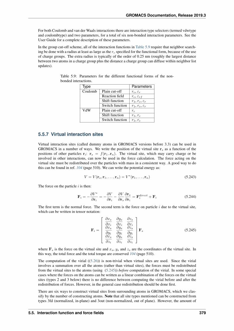
GROMACS Documentation, Release 2019.3
For both Coulomb and van der Waals interactions there are interaction type selectors (termed vdwtypeand coulombtype) and two parameters, for a total of six non-bonded interaction parameters. See theUser Guide for a complete description of these parameters.
In the group cut-off scheme, all of the interaction functions in Table 5.9 require that neighbor search-ing be done with a radius at least as large as the 𝑟𝑐 specified for the functional form, because of the useof charge groups. The extra radius is typically of the order of 0.25 nm (roughly the largest distancebetween two atoms in a charge group plus the distance a charge group can diffuse within neighbor listupdates).
Table 5.9: Parameters for the different functional forms of the non-bonded interactions.
Type ParametersCoulomb Plain cut-off 𝑟𝑐, 𝜀𝑟
Reaction field 𝑟𝑐, 𝜀𝑟𝑓Shift function 𝑟1, 𝑟𝑐, 𝜀𝑟Switch function 𝑟1, 𝑟𝑐, 𝜀𝑟
VdW Plain cut-off 𝑟𝑐Shift function 𝑟1, 𝑟𝑐Switch function 𝑟1, 𝑟𝑐
5.5.7 Virtual interaction sites
Virtual interaction sites (called dummy atoms in GROMACS versions before 3.3) can be used inGROMACS in a number of ways. We write the position of the virtual site r𝑠 as a function of thepositions of other particles r𝑖: r𝑠 = 𝑓(r1..r𝑛). The virtual site, which may carry charge or beinvolved in other interactions, can now be used in the force calculation. The force acting on thevirtual site must be redistributed over the particles with mass in a consistent way. A good way to dothis can be found in ref. 104 (page 510). We can write the potential energy as:
𝑉 = 𝑉 (r𝑠, r1, . . . , r𝑛) = 𝑉 *(r1, . . . , r𝑛) (5.243)
The force on the particle 𝑖 is then:
F𝑖 = −𝜕𝑉*
𝜕r𝑖= −𝜕𝑉
𝜕r𝑖− 𝜕𝑉
𝜕r𝑠
𝜕r𝑠𝜕r𝑖
= F𝑑𝑖𝑟𝑒𝑐𝑡𝑖 + F𝑖 (5.244)
The first term is the normal force. The second term is the force on particle 𝑖 due to the virtual site,which can be written in tensor notation:
F𝑖 =
⎡⎢⎢⎢⎢⎢⎣𝜕𝑥𝑠𝜕𝑥𝑖
𝜕𝑦𝑠𝜕𝑥𝑖
𝜕𝑧𝑠𝜕𝑥𝑖
𝜕𝑥𝑠𝜕𝑦𝑖
𝜕𝑦𝑠𝜕𝑦𝑖
𝜕𝑧𝑠𝜕𝑦𝑖
𝜕𝑥𝑠𝜕𝑧𝑖
𝜕𝑦𝑠𝜕𝑧𝑖
𝜕𝑧𝑠𝜕𝑧𝑖
⎤⎥⎥⎥⎥⎥⎦F𝑠 (5.245)
where F𝑠 is the force on the virtual site and 𝑥𝑠, 𝑦𝑠 and 𝑧𝑠 are the coordinates of the virtual site. Inthis way, the total force and the total torque are conserved 104 (page 510).
The computation of the virial ((5.26)) is non-trivial when virtual sites are used. Since the virialinvolves a summation over all the atoms (rather than virtual sites), the forces must be redistributedfrom the virtual sites to the atoms (using (5.245)) before computation of the virial. In some specialcases where the forces on the atoms can be written as a linear combination of the forces on the virtualsites (types 2 and 3 below) there is no difference between computing the virial before and after theredistribution of forces. However, in the general case redistribution should be done first.
There are six ways to construct virtual sites from surrounding atoms in GROMACS, which we clas-sify by the number of constructing atoms. Note that all site types mentioned can be constructed fromtypes 3fd (normalized, in-plane) and 3out (non-normalized, out of plane). However, the amount of
5.5. Interaction function and force fields 379
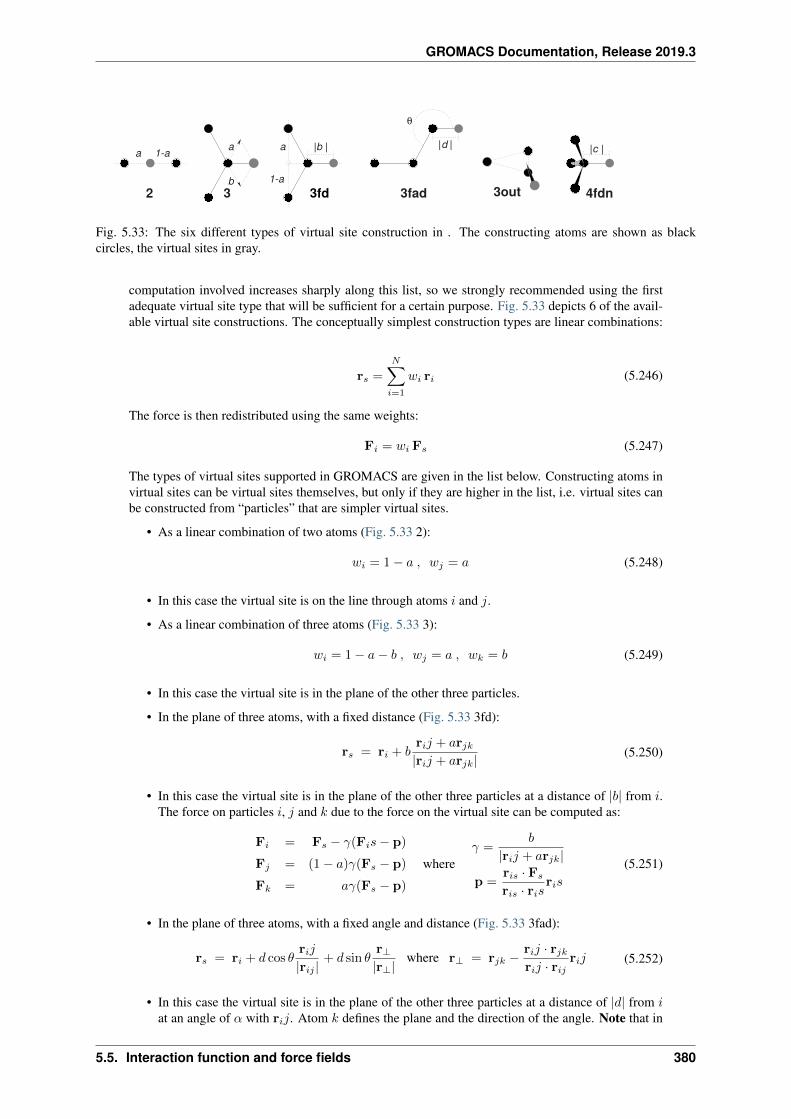
GROMACS Documentation, Release 2019.3
| |
3fd
| || |1-a a
b
a
1-a
a
2 3fad 3out 4fdn
cb
3
θ
d
Fig. 5.33: The six different types of virtual site construction in . The constructing atoms are shown as blackcircles, the virtual sites in gray.
computation involved increases sharply along this list, so we strongly recommended using the firstadequate virtual site type that will be sufficient for a certain purpose. Fig. 5.33 depicts 6 of the avail-able virtual site constructions. The conceptually simplest construction types are linear combinations:
r𝑠 =
𝑁∑𝑖=1
𝑤𝑖 r𝑖 (5.246)
The force is then redistributed using the same weights:
F𝑖 = 𝑤𝑖 F𝑠 (5.247)
The types of virtual sites supported in GROMACS are given in the list below. Constructing atoms invirtual sites can be virtual sites themselves, but only if they are higher in the list, i.e. virtual sites canbe constructed from “particles” that are simpler virtual sites.
• As a linear combination of two atoms (Fig. 5.33 2):
𝑤𝑖 = 1 − 𝑎 , 𝑤𝑗 = 𝑎 (5.248)
• In this case the virtual site is on the line through atoms 𝑖 and 𝑗.
• As a linear combination of three atoms (Fig. 5.33 3):
𝑤𝑖 = 1 − 𝑎− 𝑏 , 𝑤𝑗 = 𝑎 , 𝑤𝑘 = 𝑏 (5.249)
• In this case the virtual site is in the plane of the other three particles.
• In the plane of three atoms, with a fixed distance (Fig. 5.33 3fd):
r𝑠 = r𝑖 + 𝑏r𝑖𝑗 + 𝑎r𝑗𝑘|r𝑖𝑗 + 𝑎r𝑗𝑘|
(5.250)
• In this case the virtual site is in the plane of the other three particles at a distance of |𝑏| from 𝑖.The force on particles 𝑖, 𝑗 and 𝑘 due to the force on the virtual site can be computed as:
F𝑖 = F𝑠 − 𝛾(F𝑖𝑠− p)
F𝑗 = (1 − 𝑎)𝛾(F𝑠 − p)
F𝑘 = 𝑎𝛾(F𝑠 − p)
where𝛾 =
𝑏
|r𝑖𝑗 + 𝑎r𝑗𝑘|
p =r𝑖𝑠 · F𝑠
r𝑖𝑠 · r𝑖𝑠r𝑖𝑠
(5.251)
• In the plane of three atoms, with a fixed angle and distance (Fig. 5.33 3fad):
r𝑠 = r𝑖 + 𝑑 cos 𝜃r𝑖𝑗
|r𝑖𝑗 |+ 𝑑 sin 𝜃
r⊥|r⊥|
where r⊥ = r𝑗𝑘 − r𝑖𝑗 · r𝑗𝑘r𝑖𝑗 · r𝑖𝑗
r𝑖𝑗 (5.252)
• In this case the virtual site is in the plane of the other three particles at a distance of |𝑑| from 𝑖at an angle of 𝛼 with r𝑖𝑗. Atom 𝑘 defines the plane and the direction of the angle. Note that in
5.5. Interaction function and force fields 380
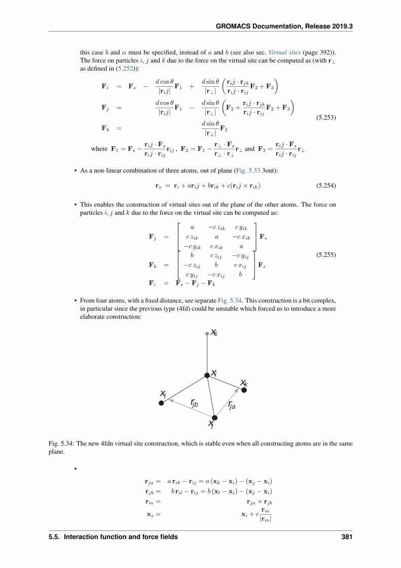
GROMACS Documentation, Release 2019.3
this case 𝑏 and 𝛼 must be specified, instead of 𝑎 and 𝑏 (see also sec. Virtual sites (page 392)).The force on particles 𝑖, 𝑗 and 𝑘 due to the force on the virtual site can be computed as (with r⊥as defined in (5.252)):
F𝑖 = F𝑠 − 𝑑 cos 𝜃
|r𝑖𝑗|F1 +
𝑑 sin 𝜃
|r⊥|
(r𝑖𝑗 · r𝑗𝑘r𝑖𝑗 · r𝑖𝑗
F2 + F3
)F𝑗 =
𝑑 cos 𝜃
|r𝑖𝑗|F1 − 𝑑 sin 𝜃
|r⊥|
(F2 +
r𝑖𝑗 · r𝑗𝑘r𝑖𝑗 · r𝑖𝑗
F2 + F3
)F𝑘 =
𝑑 sin 𝜃
|r⊥|F2
where F1 = F𝑠 −r𝑖𝑗 · F𝑠
r𝑖𝑗 · r𝑖𝑗r𝑖𝑗 , F2 = F1 −
r⊥ · F𝑠
r⊥ · r⊥r⊥ and F3 =
r𝑖𝑗 · F𝑠
r𝑖𝑗 · r𝑖𝑗r⊥
(5.253)
• As a non-linear combination of three atoms, out of plane (Fig. 5.33 3out):
r𝑠 = r𝑖 + 𝑎r𝑖𝑗 + 𝑏r𝑖𝑘 + 𝑐(r𝑖𝑗 × r𝑖𝑘) (5.254)
• This enables the construction of virtual sites out of the plane of the other atoms. The force onparticles 𝑖, 𝑗 and 𝑘 due to the force on the virtual site can be computed as:
F𝑗 =
⎡⎢⎣ 𝑎 −𝑐 𝑧𝑖𝑘 𝑐 𝑦𝑖𝑘
𝑐 𝑧𝑖𝑘 𝑎 −𝑐 𝑥𝑖𝑘−𝑐 𝑦𝑖𝑘 𝑐 𝑥𝑖𝑘 𝑎
⎤⎥⎦F𝑠
F𝑘 =
⎡⎢⎣ 𝑏 𝑐 𝑧𝑖𝑗 −𝑐 𝑦𝑖𝑗−𝑐 𝑧𝑖𝑗 𝑏 𝑐 𝑥𝑖𝑗
𝑐 𝑦𝑖𝑗 −𝑐 𝑥𝑖𝑗 𝑏
⎤⎥⎦F𝑠
F𝑖 = F𝑠 − F𝑗 − F𝑘
(5.255)
• From four atoms, with a fixed distance, see separate Fig. 5.34. This construction is a bit complex,in particular since the previous type (4fd) could be unstable which forced us to introduce a moreelaborate construction:
x
xx
x
i
j
k
l
sx
rjajbr
Fig. 5.34: The new 4fdn virtual site construction, which is stable even when all constructing atoms are in the sameplane.
•
r𝑗𝑎 = 𝑎 r𝑖𝑘 − r𝑖𝑗 = 𝑎 (x𝑘 − x𝑖) − (x𝑗 − x𝑖)
r𝑗𝑏 = 𝑏 r𝑖𝑙 − r𝑖𝑗 = 𝑏 (x𝑙 − x𝑖) − (x𝑗 − x𝑖)
r𝑚 = r𝑗𝑎 × r𝑗𝑏
x𝑠 = x𝑖 + 𝑐r𝑚|r𝑚|
5.5. Interaction function and force fields 381
GROMACS Documentation, Release 2019.3
• In this case the virtual site is at a distance of |𝑐| from 𝑖, while 𝑎 and 𝑏 are parameters. Notethat the vectors r𝑖𝑘 and r𝑖𝑗 are not normalized to save floating-point operations. The forceon particles 𝑖, 𝑗, 𝑘 and 𝑙 due to the force on the virtual site are computed through chain rulederivatives of the construction expression. This is exact and conserves energy, but it does lead torelatively lengthy expressions that we do not include here (over 200 floating-point operations).The interested reader can look at the source code in vsite.c. Fortunately, this vsite type isnormally only used for chiral centers such as 𝐶𝛼 atoms in proteins.
The new 4fdn construct is identified with a ‘type’ value of 2 in the topology. The earlier 4fdtype is still supported internally (‘type’ value 1), but it should not be used for new simulations.All current GROMACS tools will automatically generate type 4fdn instead.
• A linear combination of 𝑁 atoms with relative weights 𝑎𝑖. The weight for atom 𝑖 is:
𝑤𝑖 = 𝑎𝑖
⎛⎝ 𝑁∑𝑗=1
𝑎𝑗
⎞⎠−1
(5.256)
• There are three options for setting the weights:
• center of geometry: equal weights
• center of mass: 𝑎𝑖 is the mass of atom 𝑖; when in free-energy simulations the mass of the atomis changed, only the mass of the A-state is used for the weight
• center of weights: 𝑎𝑖 is defined by the user
5.5.8 Long Range Electrostatics
Ewald summation
The total electrostatic energy of 𝑁 particles and their periodic images is given by
𝑉 =𝑓
2
∑𝑛𝑥
∑𝑛𝑦
∑𝑛𝑧*
𝑁∑𝑖
𝑁∑𝑗
𝑞𝑖𝑞𝑗r𝑖𝑗,n
. (5.257)
(𝑛𝑥, 𝑛𝑦, 𝑛𝑧) = n is the box index vector, and the star indicates that terms with 𝑖 = 𝑗 should beomitted when (𝑛𝑥, 𝑛𝑦, 𝑛𝑧) = (0, 0, 0). The distance r𝑖𝑗,n is the real distance between the charges andnot the minimum-image. This sum is conditionally convergent, but very slow.
Ewald summation was first introduced as a method to calculate long-range interactions of the periodicimages in crystals 105 (page 511). The idea is to convert the single slowly-converging sum (5.257)into two quickly-converging terms and a constant term:
𝑉 = 𝑉dir + 𝑉rec + 𝑉0
𝑉dir =𝑓
2
𝑁∑𝑖,𝑗
∑𝑛𝑥
∑𝑛𝑦
∑𝑛𝑧*
𝑞𝑖𝑞𝑗erfc(𝛽𝑟𝑖𝑗,n)
𝑟𝑖𝑗,n
𝑉rec =𝑓
2𝜋𝑉
𝑁∑𝑖,𝑗
𝑞𝑖𝑞𝑗∑𝑚𝑥
∑𝑚𝑦
∑𝑚𝑧*
exp(−(𝜋m/𝛽)2 + 2𝜋𝑖m · (r𝑖 − r𝑗)
)m2
𝑉0 = − 𝑓𝛽√𝜋
𝑁∑𝑖
𝑞2𝑖 ,
(5.258)
where 𝛽 is a parameter that determines the relative weight of the direct and reciprocal sums andm = (𝑚𝑥,𝑚𝑦,𝑚𝑧). In this way we can use a short cut-off (of the order of 1 nm) in the directspace sum and a short cut-off in the reciprocal space sum (e.g. 10 wave vectors in each direction).Unfortunately, the computational cost of the reciprocal part of the sum increases as 𝑁2 (or 𝑁3/2 witha slightly better algorithm) and it is therefore not realistic for use in large systems.
5.5. Interaction function and force fields 382
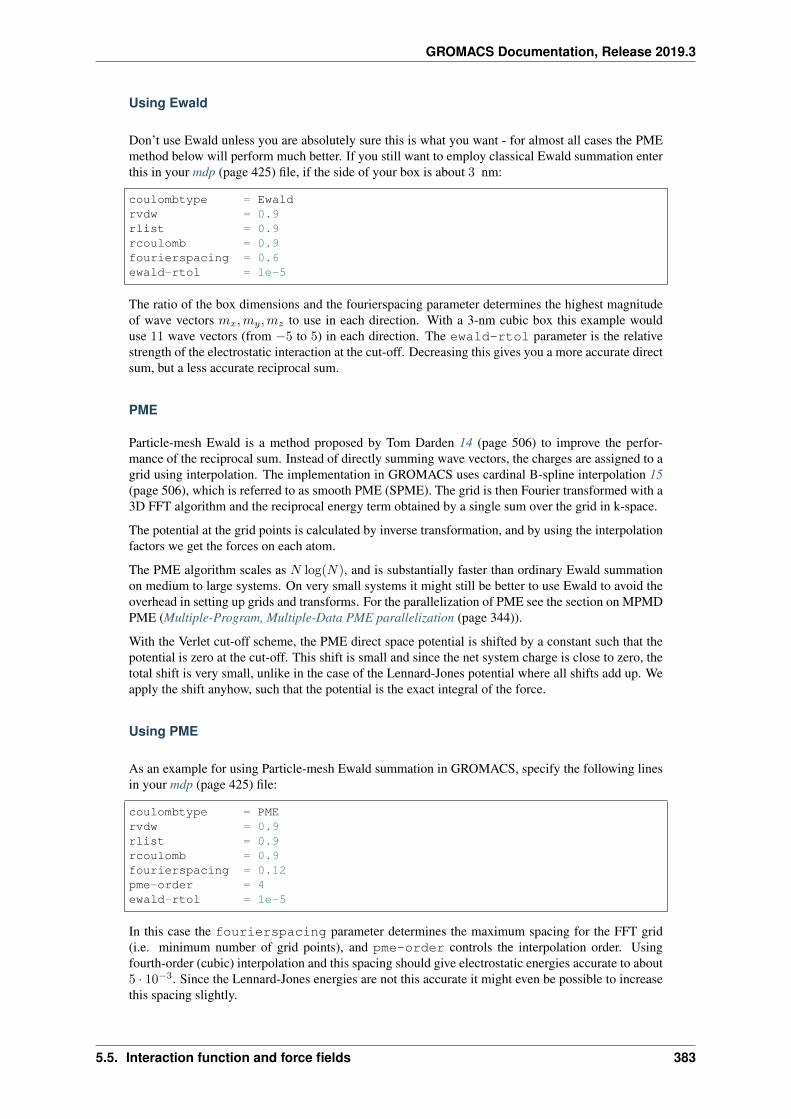
GROMACS Documentation, Release 2019.3
Using Ewald
Don’t use Ewald unless you are absolutely sure this is what you want - for almost all cases the PMEmethod below will perform much better. If you still want to employ classical Ewald summation enterthis in your mdp (page 425) file, if the side of your box is about 3 nm:
coulombtype = Ewaldrvdw = 0.9rlist = 0.9rcoulomb = 0.9fourierspacing = 0.6ewald-rtol = 1e-5
The ratio of the box dimensions and the fourierspacing parameter determines the highest magnitudeof wave vectors 𝑚𝑥,𝑚𝑦,𝑚𝑧 to use in each direction. With a 3-nm cubic box this example woulduse 11 wave vectors (from −5 to 5) in each direction. The ewald-rtol parameter is the relativestrength of the electrostatic interaction at the cut-off. Decreasing this gives you a more accurate directsum, but a less accurate reciprocal sum.
PME
Particle-mesh Ewald is a method proposed by Tom Darden 14 (page 506) to improve the perfor-mance of the reciprocal sum. Instead of directly summing wave vectors, the charges are assigned to agrid using interpolation. The implementation in GROMACS uses cardinal B-spline interpolation 15(page 506), which is referred to as smooth PME (SPME). The grid is then Fourier transformed with a3D FFT algorithm and the reciprocal energy term obtained by a single sum over the grid in k-space.
The potential at the grid points is calculated by inverse transformation, and by using the interpolationfactors we get the forces on each atom.
The PME algorithm scales as 𝑁 log(𝑁), and is substantially faster than ordinary Ewald summationon medium to large systems. On very small systems it might still be better to use Ewald to avoid theoverhead in setting up grids and transforms. For the parallelization of PME see the section on MPMDPME (Multiple-Program, Multiple-Data PME parallelization (page 344)).
With the Verlet cut-off scheme, the PME direct space potential is shifted by a constant such that thepotential is zero at the cut-off. This shift is small and since the net system charge is close to zero, thetotal shift is very small, unlike in the case of the Lennard-Jones potential where all shifts add up. Weapply the shift anyhow, such that the potential is the exact integral of the force.
Using PME
As an example for using Particle-mesh Ewald summation in GROMACS, specify the following linesin your mdp (page 425) file:
coulombtype = PMErvdw = 0.9rlist = 0.9rcoulomb = 0.9fourierspacing = 0.12pme-order = 4ewald-rtol = 1e-5
In this case the fourierspacing parameter determines the maximum spacing for the FFT grid(i.e. minimum number of grid points), and pme-order controls the interpolation order. Usingfourth-order (cubic) interpolation and this spacing should give electrostatic energies accurate to about5 · 10−3. Since the Lennard-Jones energies are not this accurate it might even be possible to increasethis spacing slightly.
5.5. Interaction function and force fields 383
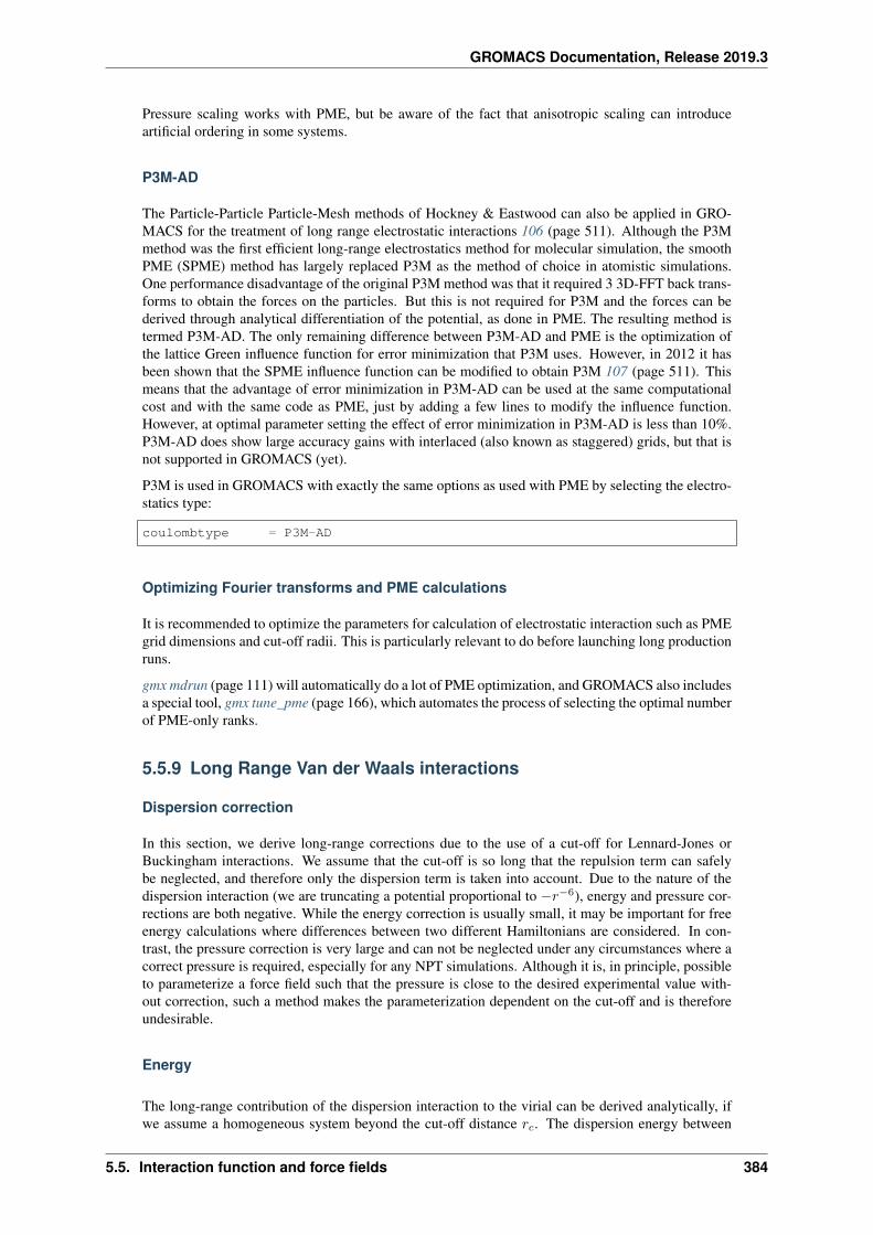
GROMACS Documentation, Release 2019.3
Pressure scaling works with PME, but be aware of the fact that anisotropic scaling can introduceartificial ordering in some systems.
P3M-AD
The Particle-Particle Particle-Mesh methods of Hockney & Eastwood can also be applied in GRO-MACS for the treatment of long range electrostatic interactions 106 (page 511). Although the P3Mmethod was the first efficient long-range electrostatics method for molecular simulation, the smoothPME (SPME) method has largely replaced P3M as the method of choice in atomistic simulations.One performance disadvantage of the original P3M method was that it required 3 3D-FFT back trans-forms to obtain the forces on the particles. But this is not required for P3M and the forces can bederived through analytical differentiation of the potential, as done in PME. The resulting method istermed P3M-AD. The only remaining difference between P3M-AD and PME is the optimization ofthe lattice Green influence function for error minimization that P3M uses. However, in 2012 it hasbeen shown that the SPME influence function can be modified to obtain P3M 107 (page 511). Thismeans that the advantage of error minimization in P3M-AD can be used at the same computationalcost and with the same code as PME, just by adding a few lines to modify the influence function.However, at optimal parameter setting the effect of error minimization in P3M-AD is less than 10%.P3M-AD does show large accuracy gains with interlaced (also known as staggered) grids, but that isnot supported in GROMACS (yet).
P3M is used in GROMACS with exactly the same options as used with PME by selecting the electro-statics type:
coulombtype = P3M-AD
Optimizing Fourier transforms and PME calculations
It is recommended to optimize the parameters for calculation of electrostatic interaction such as PMEgrid dimensions and cut-off radii. This is particularly relevant to do before launching long productionruns.
gmx mdrun (page 111) will automatically do a lot of PME optimization, and GROMACS also includesa special tool, gmx tune_pme (page 166), which automates the process of selecting the optimal numberof PME-only ranks.
5.5.9 Long Range Van der Waals interactions
Dispersion correction
In this section, we derive long-range corrections due to the use of a cut-off for Lennard-Jones orBuckingham interactions. We assume that the cut-off is so long that the repulsion term can safelybe neglected, and therefore only the dispersion term is taken into account. Due to the nature of thedispersion interaction (we are truncating a potential proportional to −𝑟−6), energy and pressure cor-rections are both negative. While the energy correction is usually small, it may be important for freeenergy calculations where differences between two different Hamiltonians are considered. In con-trast, the pressure correction is very large and can not be neglected under any circumstances where acorrect pressure is required, especially for any NPT simulations. Although it is, in principle, possibleto parameterize a force field such that the pressure is close to the desired experimental value with-out correction, such a method makes the parameterization dependent on the cut-off and is thereforeundesirable.
Energy
The long-range contribution of the dispersion interaction to the virial can be derived analytically, ifwe assume a homogeneous system beyond the cut-off distance 𝑟𝑐. The dispersion energy between
5.5. Interaction function and force fields 384
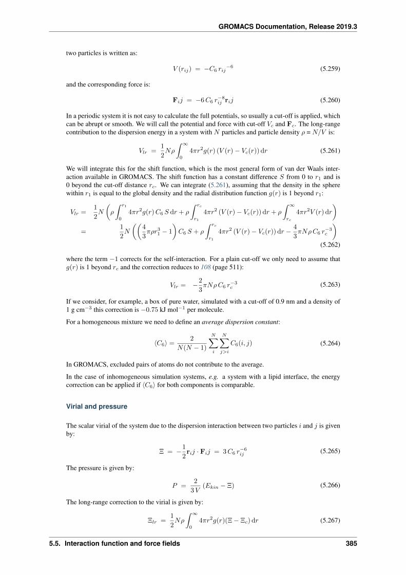
GROMACS Documentation, Release 2019.3
two particles is written as:
𝑉 (𝑟𝑖𝑗) = −𝐶6 𝑟𝑖𝑗−6 (5.259)
and the corresponding force is:
F𝑖𝑗 = −6𝐶6 𝑟−8𝑖𝑗 r𝑖𝑗 (5.260)
In a periodic system it is not easy to calculate the full potentials, so usually a cut-off is applied, whichcan be abrupt or smooth. We will call the potential and force with cut-off 𝑉𝑐 and F𝑐. The long-rangecontribution to the dispersion energy in a system with 𝑁 particles and particle density 𝜌 = 𝑁/𝑉 is:
𝑉𝑙𝑟 =1
2𝑁𝜌
∫ ∞
0
4𝜋𝑟2𝑔(𝑟) (𝑉 (𝑟) − 𝑉𝑐(𝑟)) d𝑟 (5.261)
We will integrate this for the shift function, which is the most general form of van der Waals inter-action available in GROMACS. The shift function has a constant difference 𝑆 from 0 to 𝑟1 and is0 beyond the cut-off distance 𝑟𝑐. We can integrate (5.261), assuming that the density in the spherewithin 𝑟1 is equal to the global density and the radial distribution function 𝑔(𝑟) is 1 beyond 𝑟1:
𝑉𝑙𝑟 =1
2𝑁
(𝜌
∫ 𝑟1
0
4𝜋𝑟2𝑔(𝑟)𝐶6 𝑆 d𝑟 + 𝜌
∫ 𝑟𝑐
𝑟1
4𝜋𝑟2 (𝑉 (𝑟) − 𝑉𝑐(𝑟)) d𝑟 + 𝜌
∫ ∞
𝑟𝑐
4𝜋𝑟2𝑉 (𝑟) d𝑟
)=
1
2𝑁
((4
3𝜋𝜌𝑟31 − 1
)𝐶6 𝑆 + 𝜌
∫ 𝑟𝑐
𝑟1
4𝜋𝑟2 (𝑉 (𝑟) − 𝑉𝑐(𝑟)) d𝑟 − 4
3𝜋𝑁𝜌𝐶6 𝑟
−3𝑐
)(5.262)
where the term −1 corrects for the self-interaction. For a plain cut-off we only need to assume that𝑔(𝑟) is 1 beyond 𝑟𝑐 and the correction reduces to 108 (page 511):
𝑉𝑙𝑟 = −2
3𝜋𝑁𝜌𝐶6 𝑟
−3𝑐 (5.263)
If we consider, for example, a box of pure water, simulated with a cut-off of 0.9 nm and a density of1 g cm−3 this correction is −0.75 kJ mol−1 per molecule.
For a homogeneous mixture we need to define an average dispersion constant:
⟨𝐶6⟩ =2
𝑁(𝑁 − 1)
𝑁∑𝑖
𝑁∑𝑗>𝑖
𝐶6(𝑖, 𝑗) (5.264)
In GROMACS, excluded pairs of atoms do not contribute to the average.
In the case of inhomogeneous simulation systems, e.g. a system with a lipid interface, the energycorrection can be applied if ⟨𝐶6⟩ for both components is comparable.
Virial and pressure
The scalar virial of the system due to the dispersion interaction between two particles 𝑖 and 𝑗 is givenby:
Ξ = −1
2r𝑖𝑗 · F𝑖𝑗 = 3𝐶6 𝑟
−6𝑖𝑗 (5.265)
The pressure is given by:
𝑃 =2
3𝑉(𝐸𝑘𝑖𝑛 − Ξ) (5.266)
The long-range correction to the virial is given by:
Ξ𝑙𝑟 =1
2𝑁𝜌
∫ ∞
0
4𝜋𝑟2𝑔(𝑟)(Ξ − Ξ𝑐) d𝑟 (5.267)
5.5. Interaction function and force fields 385
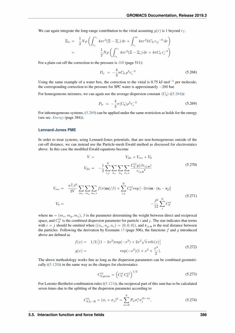
GROMACS Documentation, Release 2019.3
We can again integrate the long-range contribution to the virial assuming 𝑔(𝑟) is 1 beyond 𝑟1:
Ξ𝑙𝑟 =1
2𝑁𝜌
(∫ 𝑟𝑐
𝑟1
4𝜋𝑟2(Ξ − Ξ𝑐) d𝑟 +
∫ ∞
𝑟𝑐
4𝜋𝑟23𝐶6 𝑟𝑖𝑗−6 d𝑟
)=
1
2𝑁𝜌
(∫ 𝑟𝑐
𝑟1
4𝜋𝑟2(Ξ − Ξ𝑐) d𝑟 + 4𝜋𝐶6 𝑟−3𝑐
)For a plain cut-off the correction to the pressure is 108 (page 511):
𝑃𝑙𝑟 = −4
3𝜋𝐶6 𝜌
2𝑟−3𝑐 (5.268)
Using the same example of a water box, the correction to the virial is 0.75 kJ mol−1 per molecule,the corresponding correction to the pressure for SPC water is approximately −280 bar.
For homogeneous mixtures, we can again use the average dispersion constant ⟨𝐶6⟩ ((5.264)):
𝑃𝑙𝑟 = −4
3𝜋⟨𝐶6⟩𝜌2𝑟−3
𝑐 (5.269)
For inhomogeneous systems, (5.269) can be applied under the same restriction as holds for the energy(see sec. Energy (page 384)).
Lennard-Jones PME
In order to treat systems, using Lennard-Jones potentials, that are non-homogeneous outside of thecut-off distance, we can instead use the Particle-mesh Ewald method as discussed for electrostaticsabove. In this case the modified Ewald equations become
𝑉 = 𝑉dir + 𝑉rec + 𝑉0
𝑉dir = −1
2
𝑁∑𝑖,𝑗
∑𝑛𝑥
∑𝑛𝑦
∑𝑛𝑧*
𝐶𝑖𝑗6 𝑔(𝛽𝑟𝑖𝑗,n)
𝑟𝑖𝑗,n6
(5.270)
𝑉rec =𝜋
32 𝛽3
2𝑉
∑𝑚𝑥
∑𝑚𝑦
∑𝑚𝑧*
𝑓(𝜋|m|/𝛽) ×𝑁∑𝑖,𝑗
𝐶𝑖𝑗6 exp [−2𝜋𝑖m · (ri − rj)]
𝑉0 = −𝛽6
12
𝑁∑𝑖
𝐶𝑖𝑖6
(5.271)
where m = (𝑚𝑥,𝑚𝑦,𝑚𝑧), 𝛽 is the parameter determining the weight between direct and reciprocalspace, and 𝐶𝑖𝑗
6 is the combined dispersion parameter for particle 𝑖 and 𝑗. The star indicates that termswith 𝑖 = 𝑗 should be omitted when ((𝑛𝑥, 𝑛𝑦, 𝑛𝑧) = (0, 0, 0)), and r𝑖𝑗,n is the real distance betweenthe particles. Following the derivation by Essmann 15 (page 506), the functions 𝑓 and 𝑔 introducedabove are defined as
𝑓(𝑥) = 1/3[(1 − 2𝑥2)exp(−𝑥2) + 2𝑥3
√𝜋 erfc(𝑥)
]𝑔(𝑥) = exp(−𝑥2)(1 + 𝑥2 +
𝑥4
2).
(5.272)
The above methodology works fine as long as the dispersion parameters can be combined geometri-cally ((5.120)) in the same way as the charges for electrostatics
𝐶𝑖𝑗6,geom =
(𝐶𝑖𝑖
6 𝐶𝑗𝑗6
)1/2(5.273)
For Lorentz-Berthelot combination rules ((5.121)), the reciprocal part of this sum has to be calculatedseven times due to the splitting of the dispersion parameter according to
𝐶𝑖𝑗6,L−B = (𝜎𝑖 + 𝜎𝑗)
6 =
6∑𝑛=0
𝑃𝑛𝜎𝑛𝑖 𝜎
(6−𝑛)𝑗 , (5.274)
5.5. Interaction function and force fields 386
GROMACS Documentation, Release 2019.3
for 𝑃𝑛 the Pascal triangle coefficients. This introduces a non-negligible cost to the reciprocal part,requiring seven separate FFTs, and therefore this has been the limiting factor in previous attempts toimplement LJ-PME. A solution to this problem is to use geometrical combination rules in order tocalculate an approximate interaction parameter for the reciprocal part of the potential, yielding a totalinteraction of
𝑉 (𝑟 < 𝑟𝑐) = 𝐶dir6 𝑔(𝛽𝑟)𝑟−6⏟ ⏞ Direct space
+𝐶recip6,geom[1 − 𝑔(𝛽𝑟)]𝑟−6⏟ ⏞
Reciprocal space
= 𝐶recip6,geom𝑟
−6 +(𝐶dir
6 − 𝐶recip6,geom
)𝑔(𝛽𝑟)𝑟−6
𝑉 (𝑟 > 𝑟𝑐) = 𝐶recip6,geom[1 − 𝑔(𝛽𝑟)]𝑟−6⏟ ⏞
Reciprocal space
.
This will preserve a well-defined Hamiltonian and significantly increase the performance of the sim-ulations. The approximation does introduce some errors, but since the difference is located in theinteractions calculated in reciprocal space, the effect will be very small compared to the total in-teraction energy. In a simulation of a lipid bilayer, using a cut-off of 1.0 nm, the relative error intotal dispersion energy was below 0.5%. A more thorough discussion of this can be found in 109(page 511).
In GROMACS we now perform the proper calculation of this interaction by subtracting, from thedirect-space interactions, the contribution made by the approximate potential that is used in the recip-rocal part
𝑉dir = 𝐶dir6 𝑟−6 − 𝐶recip
6 [1 − 𝑔(𝛽𝑟)]𝑟−6. (5.275)
This potential will reduce to the expression in (5.270) when 𝐶dir6 = 𝐶recip
6 , and the total interactionis given by
𝑉 (𝑟 < 𝑟𝑐) = 𝐶dir6 𝑟−6 − 𝐶recip
6 [1 − 𝑔(𝛽𝑟)]𝑟−6⏟ ⏞ Direct space
+𝐶recip6 [1 − 𝑔(𝛽𝑟)]𝑟−6⏟ ⏞
Reciprocal space
= 𝐶dir6 𝑟−6
𝑉 (𝑟 > 𝑟𝑐) = 𝐶recip6 [1 − 𝑔(𝛽𝑟)]𝑟−6. (5.276)
For the case when 𝐶dir6 = 𝐶recip
6 this will retain an unmodified LJ force up to the cut-off, and theerror is an order of magnitude smaller than in simulations where the direct-space interactions do notaccount for the approximation used in reciprocal space. When using a VdW interaction modifier ofpotential-shift, the constant (
−𝐶dir6 + 𝐶recip
6 [1 − 𝑔(𝛽𝑟𝑐)])𝑟−6𝑐 (5.277)
is added to (5.276) in order to ensure that the potential is continuous at the cutoff. Note that, in thesame way as (5.275), this degenerates into the expected −𝐶6𝑔(𝛽𝑟𝑐)𝑟
−6𝑐 when 𝐶dir
6 = 𝐶recip6 . In
addition to this, a long-range dispersion correction can be applied to correct for the approximationusing a combination rule in reciprocal space. This correction assumes, as for the cut-off LJ potential, auniform particle distribution. But since the error of the combination rule approximation is very smallthis long-range correction is not necessary in most cases. Also note that this homogenous correctiondoes not correct the surface tension, which is an inhomogeneous property.
Using LJ-PME
As an example for using Particle-mesh Ewald summation for Lennard-Jones interactions in GRO-MACS, specify the following lines in your mdp (page 425) file:
5.5. Interaction function and force fields 387
GROMACS Documentation, Release 2019.3
vdwtype = PMErvdw = 0.9vdw-modifier = Potential-Shiftrlist = 0.9rcoulomb = 0.9fourierspacing = 0.12pme-order = 4ewald-rtol-lj = 0.001lj-pme-comb-rule = geometric
The same Fourier grid and interpolation order are used if both LJ-PME and electrostatic PMEare active, so the settings for fourierspacing and pme-order are common to both.ewald-rtol-lj controls the splitting between direct and reciprocal space in the same way asewald-rtol. In addition to this, the combination rule to be used in reciprocal space is determinedby lj-pme-comb-rule. If the current force field uses Lorentz-Berthelot combination rules, it ispossible to set lj-pme-comb-rule = geometric in order to gain a significant increase in per-formance for a small loss in accuracy. The details of this approximation can be found in the sectionabove.
Note that the use of a complete long-range dispersion correction means that as with Coulomb PME,rvdw is now a free parameter in the method, rather than being necessarily restricted by the force-fieldparameterization scheme. Thus it is now possible to optimize the cutoff, spacing, order and toleranceterms for accuracy and best performance.
Naturally, the use of LJ-PME rather than LJ cut-off adds computation and communication done forthe reciprocal-space part, so for best performance in balancing the load of parallel simulations usingPME-only ranks, more such ranks should be used. It may be possible to improve upon the automaticload-balancing used by mdrun (page 111).
5.5.10 Force field
A force field is built up from two distinct components:
• The set of equations (called the potential functions) used to generate the potential energies andtheir derivatives, the forces. These are described in detail in the previous chapter.
• The parameters used in this set of equations. These are not given in this manual, but in the datafiles corresponding to your GROMACS distribution.
Within one set of equations various sets of parameters can be used. Care must be taken that thecombination of equations and parameters form a consistent set. It is in general dangerous to makead hoc changes in a subset of parameters, because the various contributions to the total force areusually interdependent. This means in principle that every change should be documented, verified bycomparison to experimental data and published in a peer-reviewed journal before it can be used.
GROMACS 2019.3 includes several force fields, and additional ones are available on the website.If you do not know which one to select we recommend GROMOS-96 for united-atom setups andOPLS-AA/L for all-atom parameters. That said, we describe the available options in some detail.
All-hydrogen force field
The GROMOS-87-based all-hydrogen force field is almost identical to the normal GROMOS-87 forcefield, since the extra hydrogens have no Lennard-Jones interaction and zero charge. The only differ-ences are in the bond angle and improper dihedral angle terms. This force field is only useful whenyou need the exact hydrogen positions, for instance for distance restraints derived from NMR mea-surements. When citing this force field please read the previous paragraph.
5.5. Interaction function and force fields 388
GROMACS Documentation, Release 2019.3
GROMOS-96
GROMACS supports the GROMOS-96 force fields 77 (page 509). All parameters for the 43A1,43A2 (development, improved alkane dihedrals), 45A3, 53A5, and 53A6 parameter sets are included.All standard building blocks are included and topologies can be built automatically by pdb2gmx(page 127).
The GROMOS-96 force field is a further development of the GROMOS-87 force field. It has im-provements over the GROMOS-87 force field for proteins and small molecules. Note that the sugarparameters present in 53A6 do correspond to those published in 2004110 (page 511), which are dif-ferent from those present in 45A4, which is not included in GROMACS at this time. The 45A4parameter set corresponds to a later revision of these parameters. The GROMOS-96 force field is not,however, recommended for use with long alkanes and lipids. The GROMOS-96 force field differsfrom the GROMOS-87 force field in a few respects:
• the force field parameters
• the parameters for the bonded interactions are not linked to atom types
• a fourth power bond stretching potential (Fourth power potential (page 353))
• an angle potential based on the cosine of the angle (Cosine based angle potential (page 355))
There are two differences in implementation between GROMACS and GROMOS-96 which can leadto slightly different results when simulating the same system with both packages:
• in GROMOS-96 neighbor searching for solvents is performed on the first atom of the solventmolecule. This is not implemented in GROMACS, but the difference with searching by centersof charge groups is very small
• the virial in GROMOS-96 is molecule-based. This is not implemented in GROMACS, whichuses atomic virials
The GROMOS-96 force field was parameterized with a Lennard-Jones cut-off of 1.4 nm, so be sure touse a Lennard-Jones cut-off (rvdw) of at least 1.4. A larger cut-off is possible because the Lennard-Jones potential and forces are almost zero beyond 1.4 nm.
GROMOS-96 files
GROMACS can read and write GROMOS-96 coordinate and trajectory files. These files should havethe extension g96 (page 423). Such a file can be a GROMOS-96 initial/final configuration file, acoordinate trajectory file, or a combination of both. The file is fixed format; all floats are written as15.9, and as such, files can get huge. GROMACS supports the following data blocks in the givenorder:
• Header block:
TITLE (mandatory)
• Frame blocks:
TIMESTEP (optional)POSITION/POSITIONRED (mandatory)VELOCITY/VELOCITYRED (optional)BOX (optional)
See the GROMOS-96 manual 77 (page 509) for a complete description of the blocks. Note that allGROMACS programs can read compressed (.Z) or gzipped (.gz) files.
5.5. Interaction function and force fields 389
GROMACS Documentation, Release 2019.3
OPLS/AA
AMBER
GROMACS provides native support for the following AMBER force fields:
• AMBER94 111 (page 511)
• AMBER96 112 (page 511)
• AMBER99 113 (page 511)
• AMBER99SB 114 (page 511)
• AMBER99SB-ILDN 115 (page 511)
• AMBER03 116 (page 511)
• AMBERGS 117 (page 511)
CHARMM
GROMACS supports the CHARMM force field for proteins 118 (page 511), 119 (page 511),lipids 120 (page 511) and nucleic acids 121 (page 511), 122 (page 511). The protein parameters(and to some extent the lipid and nucleic acid parameters) were thoroughly tested – both by compar-ing potential energies between the port and the standard parameter set in the CHARMM molecularsimulation package, as well by how the protein force field behaves together with GROMACS-specifictechniques such as virtual sites (enabling long time steps) recently implemented 123 (page 512) – andthe details and results are presented in the paper by Bjelkmar et al. 124 (page 512). The nucleic acidparameters, as well as the ones for HEME, were converted and tested by Michel Cuendet.
When selecting the CHARMM force field in pdb2gmx (page 127) the default option is to use CMAP(for torsional correction map). To exclude CMAP, use -nocmap. The basic form of the CMAPterm implemented in GROMACS is a function of the 𝜑 and 𝜓 backbone torsion angles. This term isdefined in the rtp file by a [ cmap ] statement at the end of each residue supporting CMAP. Thefollowing five atom names define the two torsional angles. Atoms 1-4 define 𝜑, and atoms 2-5 define𝜓. The corresponding atom types are then matched to the correct CMAP type in the cmap.itp filethat contains the correction maps.
A port of the CHARMM36 force field for use with GROMACS is also available at the MacKerell labwebpage.
For branched polymers or other topologies not supported by pdb2gmx (page 127), it is possible to useTopoTools 125 (page 512) to generate a GROMACS top file.
Coarse-grained force fields
Coarse-graining is a systematic way of reducing the number of degrees of freedom representing asystem of interest. To achieve this, typically whole groups of atoms are represented by single beadsand the coarse-grained force fields describes their effective interactions. Depending on the choice ofparameterization, the functional form of such an interaction can be complicated and often tabulatedpotentials are used.
Coarse-grained models are designed to reproduce certain properties of a reference system. This canbe either a full atomistic model or even experimental data. Depending on the properties to reproducethere are different methods to derive such force fields. An incomplete list of methods is given below:
• Conserving free energies
– Simplex method
– MARTINI force field (see next section)
5.5. Interaction function and force fields 390
GROMACS Documentation, Release 2019.3
• Conserving distributions (like the radial distribution function), so-called structure-based coarse-graining
– (iterative) Boltzmann inversion
– Inverse Monte Carlo
• Conversing forces
– Force matching
Note that coarse-grained potentials are state dependent (e.g. temperature, density,. . . ) and shouldbe re-parametrized depending on the system of interest and the simulation conditions. This canfor example be done using the Versatile Object-oriented Toolkit for Coarse-Graining Applications(VOTCA) (???). The package was designed to assists in systematic coarse-graining, provides imple-mentations for most of the algorithms mentioned above and has a well tested interface to GROMACS.It is available as open source and further information can be found at www.votca.org.
MARTINI
The MARTINI force field is a coarse-grain parameter set that allows for the construction of manysystems, including proteins and membranes.
PLUM
The PLUM force field 126 (page 512) is an example of a solvent-free protein-membrane model forwhich the membrane was derived from structure-based coarse-graining 127 (page 512). A GRO-MACS implementation can be found at code.google.com/p/plumx.
5.6 Topologies
GROMACS must know on which atoms and combinations of atoms the various contributions to thepotential functions (see chapter Interaction function and force fields (page 347)) must act. It mustalso know what parameters must be applied to the various functions. All this is described in thetopology file top (page 429), which lists the constant attributes of each atom. There are many moreatom types than elements, but only atom types present in biological systems are parameterized in theforce field, plus some metals, ions and silicon. The bonded and special interactions are determinedby fixed lists that are included in the topology file. Certain non-bonded interactions must be excluded(first and second neighbors), as these are already treated in bonded interactions. In addition, there aredynamic attributes of atoms - their positions, velocities and forces. These do not strictly belong to themolecular topology, and are stored in the coordinate file gro (page 423) (positions and velocities), ortrajectory file trr (page 431) (positions, velocities, forces).
This chapter describes the setup of the topology file, the top (page 429) file and the database files:what the parameters stand for and how/where to change them if needed. First, all file formats areexplained. Section Force-field files (page 418) describes the organization of the files in each forcefield.
Note: if you construct your own topologies, we encourage you to upload them to our topology archiveat our webpage! Just imagine how thankful you’d have been if your topology had been available therebefore you started. The same goes for new force fields or modified versions of the standard forcefields - contribute them to the force field archive!
5.6.1 Particle type
In GROMACS, there are three types of particles , see Table 5.10. Only regular atoms and virtualinteraction sites are used in GROMACS; shells are necessary for polarizable models like the Shell-Water models 45 (page 508).
5.6. Topologies 391
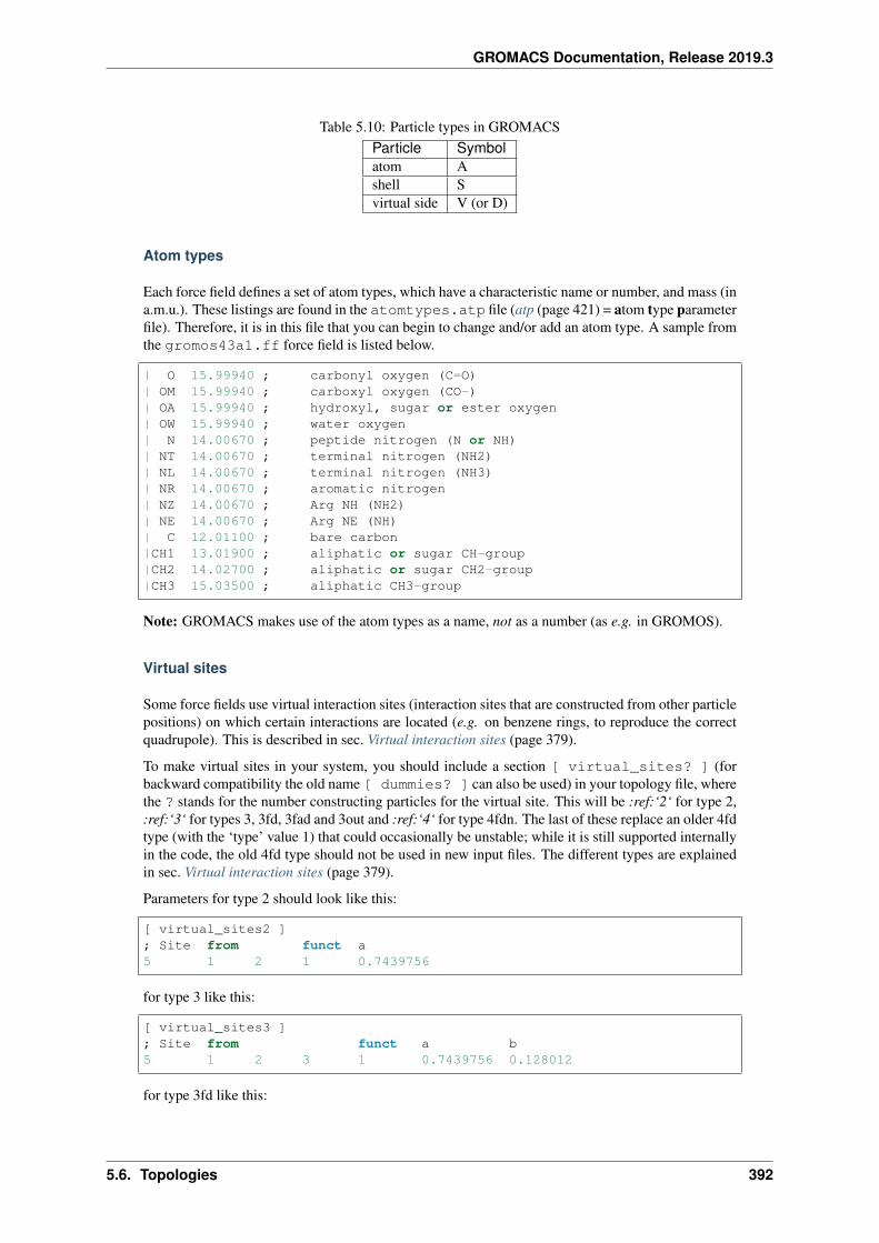
GROMACS Documentation, Release 2019.3
Table 5.10: Particle types in GROMACSParticle Symbolatom Ashell Svirtual side V (or D)
Atom types
Each force field defines a set of atom types, which have a characteristic name or number, and mass (ina.m.u.). These listings are found in the atomtypes.atp file (atp (page 421) = atom type parameterfile). Therefore, it is in this file that you can begin to change and/or add an atom type. A sample fromthe gromos43a1.ff force field is listed below.
| O 15.99940 ; carbonyl oxygen (C=O)| OM 15.99940 ; carboxyl oxygen (CO-)| OA 15.99940 ; hydroxyl, sugar or ester oxygen| OW 15.99940 ; water oxygen| N 14.00670 ; peptide nitrogen (N or NH)| NT 14.00670 ; terminal nitrogen (NH2)| NL 14.00670 ; terminal nitrogen (NH3)| NR 14.00670 ; aromatic nitrogen| NZ 14.00670 ; Arg NH (NH2)| NE 14.00670 ; Arg NE (NH)| C 12.01100 ; bare carbon|CH1 13.01900 ; aliphatic or sugar CH-group|CH2 14.02700 ; aliphatic or sugar CH2-group|CH3 15.03500 ; aliphatic CH3-group
Note: GROMACS makes use of the atom types as a name, not as a number (as e.g. in GROMOS).
Virtual sites
Some force fields use virtual interaction sites (interaction sites that are constructed from other particlepositions) on which certain interactions are located (e.g. on benzene rings, to reproduce the correctquadrupole). This is described in sec. Virtual interaction sites (page 379).
To make virtual sites in your system, you should include a section [ virtual_sites? ] (forbackward compatibility the old name [ dummies? ] can also be used) in your topology file, wherethe ? stands for the number constructing particles for the virtual site. This will be :ref:‘2‘ for type 2,:ref:‘3‘ for types 3, 3fd, 3fad and 3out and :ref:‘4‘ for type 4fdn. The last of these replace an older 4fdtype (with the ‘type’ value 1) that could occasionally be unstable; while it is still supported internallyin the code, the old 4fd type should not be used in new input files. The different types are explainedin sec. Virtual interaction sites (page 379).
Parameters for type 2 should look like this:
[ virtual_sites2 ]; Site from funct a5 1 2 1 0.7439756
for type 3 like this:
[ virtual_sites3 ]; Site from funct a b5 1 2 3 1 0.7439756 0.128012
for type 3fd like this:
5.6. Topologies 392
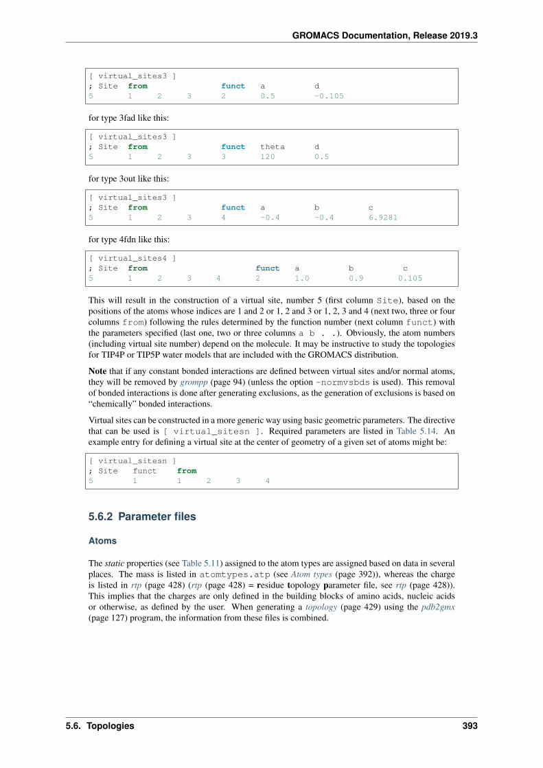
GROMACS Documentation, Release 2019.3
[ virtual_sites3 ]; Site from funct a d5 1 2 3 2 0.5 -0.105
for type 3fad like this:
[ virtual_sites3 ]; Site from funct theta d5 1 2 3 3 120 0.5
for type 3out like this:
[ virtual_sites3 ]; Site from funct a b c5 1 2 3 4 -0.4 -0.4 6.9281
for type 4fdn like this:
[ virtual_sites4 ]; Site from funct a b c5 1 2 3 4 2 1.0 0.9 0.105
This will result in the construction of a virtual site, number 5 (first column Site), based on thepositions of the atoms whose indices are 1 and 2 or 1, 2 and 3 or 1, 2, 3 and 4 (next two, three or fourcolumns from) following the rules determined by the function number (next column funct) withthe parameters specified (last one, two or three columns a b . .). Obviously, the atom numbers(including virtual site number) depend on the molecule. It may be instructive to study the topologiesfor TIP4P or TIP5P water models that are included with the GROMACS distribution.
Note that if any constant bonded interactions are defined between virtual sites and/or normal atoms,they will be removed by grompp (page 94) (unless the option -normvsbds is used). This removalof bonded interactions is done after generating exclusions, as the generation of exclusions is based on“chemically” bonded interactions.
Virtual sites can be constructed in a more generic way using basic geometric parameters. The directivethat can be used is [ virtual_sitesn ]. Required parameters are listed in Table 5.14. Anexample entry for defining a virtual site at the center of geometry of a given set of atoms might be:
[ virtual_sitesn ]; Site funct from5 1 1 2 3 4
5.6.2 Parameter files
Atoms
The static properties (see Table 5.11) assigned to the atom types are assigned based on data in severalplaces. The mass is listed in atomtypes.atp (see Atom types (page 392)), whereas the chargeis listed in rtp (page 428) (rtp (page 428) = residue topology parameter file, see rtp (page 428)).This implies that the charges are only defined in the building blocks of amino acids, nucleic acidsor otherwise, as defined by the user. When generating a topology (page 429) using the pdb2gmx(page 127) program, the information from these files is combined.
5.6. Topologies 393
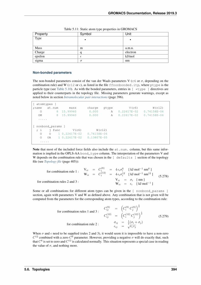
GROMACS Documentation, Release 2019.3
Table 5.11: Static atom type properties in GROMACSProperty Symbol UnitType • •
Mass m a.m.u.Charge q electronepsilon 𝜖 kJ/molsigma 𝜎 nm
Non-bonded parameters
The non-bonded parameters consist of the van der Waals parameters V (c6 or 𝜎, depending on thecombination rule) and W (c12 or 𝜖), as listed in the file ffnonbonded.itp, where ptype is theparticle type (see Table 5.10). As with the bonded parameters, entries in [ *type ] directives areapplied to their counterparts in the topology file. Missing parameters generate warnings, except asnoted below in section Intramolecular pair interactions (page 396).
[ atomtypes ];name at.num mass charge ptype V(c6) W(c12)
O 8 15.99940 0.000 A 0.22617E-02 0.74158E-06OM 8 15.99940 0.000 A 0.22617E-02 0.74158E-06.....
[ nonbond_params ]; i j func V(c6) W(c12)
O O 1 0.22617E-02 0.74158E-06O OA 1 0.22617E-02 0.13807E-05.....
Note that most of the included force fields also include the at.num. column, but this same infor-mation is implied in the OPLS-AA bond_type column. The interpretation of the parameters V andW depends on the combination rule that was chosen in the [ defaults ] section of the topologyfile (see Topology file (page 405)):
for combination rule 1 :V𝑖𝑖 = 𝐶
(6)𝑖 = 4 𝜖𝑖𝜎
6𝑖 [ kJ mol−1 nm6 ]
W𝑖𝑖 = 𝐶(12)𝑖 = 4 𝜖𝑖𝜎
12𝑖 [ kJ mol−1 nm12 ]
for combination rules 2 and 3 :V𝑖𝑖 = 𝜎𝑖 [ nm ]W𝑖𝑖 = 𝜖𝑖 [ kJ mol−1 ]
(5.278)
Some or all combinations for different atom types can be given in the [ nonbond_params ]section, again with parameters V and W as defined above. Any combination that is not given will becomputed from the parameters for the corresponding atom types, according to the combination rule:
for combination rules 1 and 3 :𝐶
(6)𝑖𝑗 =
(𝐶
(6)𝑖 𝐶
(6)𝑗
) 12
𝐶(12)𝑖𝑗 =
(𝐶
(12)𝑖 𝐶
(12)𝑗
) 12
for combination rule 2 :𝜎𝑖𝑗 = 1
2 (𝜎𝑖 + 𝜎𝑗)𝜖𝑖𝑗 =
√𝜖𝑖 𝜖𝑗
(5.279)
When 𝜎 and 𝜖 need to be supplied (rules 2 and 3), it would seem it is impossible to have a non-zero𝐶12 combined with a zero 𝐶6 parameter. However, providing a negative 𝜎 will do exactly that, suchthat𝐶6 is set to zero and𝐶12 is calculated normally. This situation represents a special case in readingthe value of 𝜎, and nothing more.
5.6. Topologies 394
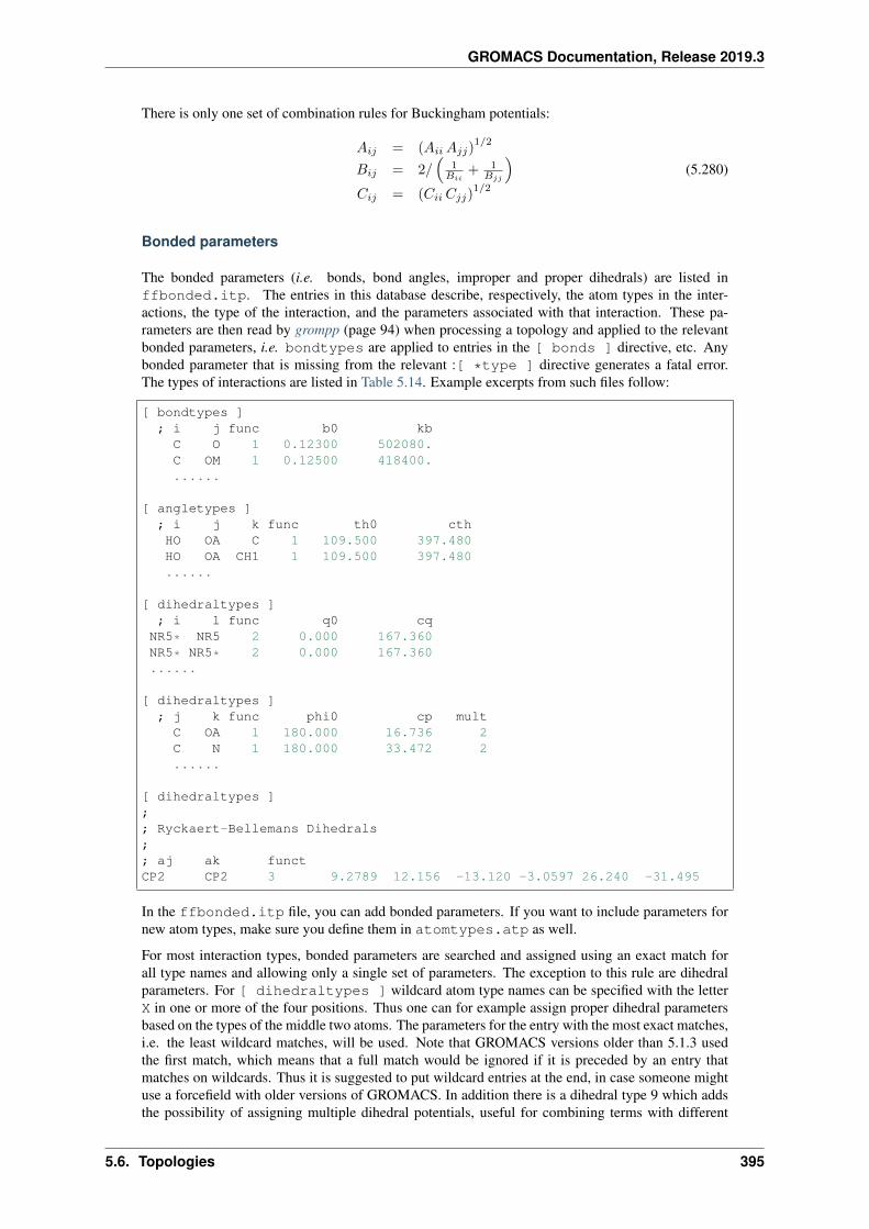
GROMACS Documentation, Release 2019.3
There is only one set of combination rules for Buckingham potentials:
𝐴𝑖𝑗 = (𝐴𝑖𝑖𝐴𝑗𝑗)1/2
𝐵𝑖𝑗 = 2/(
1𝐵𝑖𝑖
+ 1𝐵𝑗𝑗
)𝐶𝑖𝑗 = (𝐶𝑖𝑖 𝐶𝑗𝑗)
1/2
(5.280)
Bonded parameters
The bonded parameters (i.e. bonds, bond angles, improper and proper dihedrals) are listed inffbonded.itp. The entries in this database describe, respectively, the atom types in the inter-actions, the type of the interaction, and the parameters associated with that interaction. These pa-rameters are then read by grompp (page 94) when processing a topology and applied to the relevantbonded parameters, i.e. bondtypes are applied to entries in the [ bonds ] directive, etc. Anybonded parameter that is missing from the relevant :[ *type ] directive generates a fatal error.The types of interactions are listed in Table 5.14. Example excerpts from such files follow:
[ bondtypes ]; i j func b0 kb
C O 1 0.12300 502080.C OM 1 0.12500 418400.......
[ angletypes ]; i j k func th0 cthHO OA C 1 109.500 397.480HO OA CH1 1 109.500 397.480......
[ dihedraltypes ]; i l func q0 cq
NR5* NR5 2 0.000 167.360NR5* NR5* 2 0.000 167.360......
[ dihedraltypes ]; j k func phi0 cp mult
C OA 1 180.000 16.736 2C N 1 180.000 33.472 2......
[ dihedraltypes ];; Ryckaert-Bellemans Dihedrals;; aj ak functCP2 CP2 3 9.2789 12.156 -13.120 -3.0597 26.240 -31.495
In the ffbonded.itp file, you can add bonded parameters. If you want to include parameters fornew atom types, make sure you define them in atomtypes.atp as well.
For most interaction types, bonded parameters are searched and assigned using an exact match forall type names and allowing only a single set of parameters. The exception to this rule are dihedralparameters. For [ dihedraltypes ] wildcard atom type names can be specified with the letterX in one or more of the four positions. Thus one can for example assign proper dihedral parametersbased on the types of the middle two atoms. The parameters for the entry with the most exact matches,i.e. the least wildcard matches, will be used. Note that GROMACS versions older than 5.1.3 usedthe first match, which means that a full match would be ignored if it is preceded by an entry thatmatches on wildcards. Thus it is suggested to put wildcard entries at the end, in case someone mightuse a forcefield with older versions of GROMACS. In addition there is a dihedral type 9 which addsthe possibility of assigning multiple dihedral potentials, useful for combining terms with different
5.6. Topologies 395
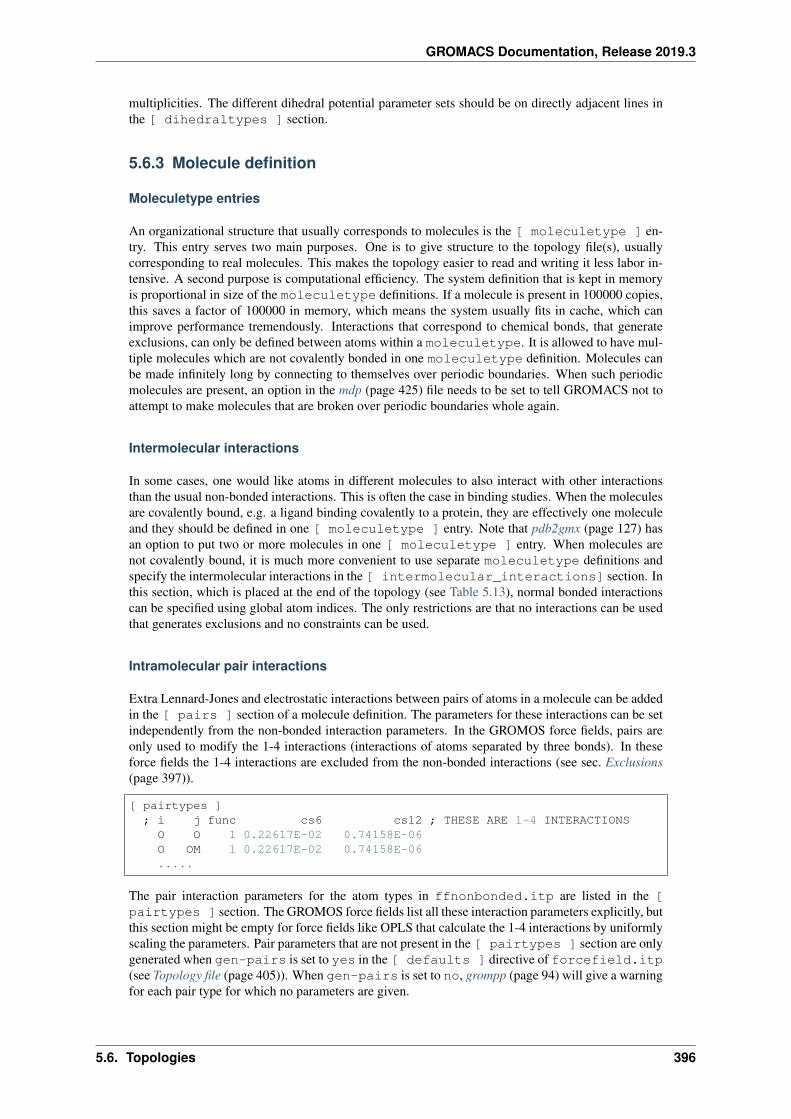
GROMACS Documentation, Release 2019.3
multiplicities. The different dihedral potential parameter sets should be on directly adjacent lines inthe [ dihedraltypes ] section.
5.6.3 Molecule definition
Moleculetype entries
An organizational structure that usually corresponds to molecules is the [ moleculetype ] en-try. This entry serves two main purposes. One is to give structure to the topology file(s), usuallycorresponding to real molecules. This makes the topology easier to read and writing it less labor in-tensive. A second purpose is computational efficiency. The system definition that is kept in memoryis proportional in size of the moleculetype definitions. If a molecule is present in 100000 copies,this saves a factor of 100000 in memory, which means the system usually fits in cache, which canimprove performance tremendously. Interactions that correspond to chemical bonds, that generateexclusions, can only be defined between atoms within a moleculetype. It is allowed to have mul-tiple molecules which are not covalently bonded in one moleculetype definition. Molecules canbe made infinitely long by connecting to themselves over periodic boundaries. When such periodicmolecules are present, an option in the mdp (page 425) file needs to be set to tell GROMACS not toattempt to make molecules that are broken over periodic boundaries whole again.
Intermolecular interactions
In some cases, one would like atoms in different molecules to also interact with other interactionsthan the usual non-bonded interactions. This is often the case in binding studies. When the moleculesare covalently bound, e.g. a ligand binding covalently to a protein, they are effectively one moleculeand they should be defined in one [ moleculetype ] entry. Note that pdb2gmx (page 127) hasan option to put two or more molecules in one [ moleculetype ] entry. When molecules arenot covalently bound, it is much more convenient to use separate moleculetype definitions andspecify the intermolecular interactions in the [ intermolecular_interactions] section. Inthis section, which is placed at the end of the topology (see Table 5.13), normal bonded interactionscan be specified using global atom indices. The only restrictions are that no interactions can be usedthat generates exclusions and no constraints can be used.
Intramolecular pair interactions
Extra Lennard-Jones and electrostatic interactions between pairs of atoms in a molecule can be addedin the [ pairs ] section of a molecule definition. The parameters for these interactions can be setindependently from the non-bonded interaction parameters. In the GROMOS force fields, pairs areonly used to modify the 1-4 interactions (interactions of atoms separated by three bonds). In theseforce fields the 1-4 interactions are excluded from the non-bonded interactions (see sec. Exclusions(page 397)).
[ pairtypes ]; i j func cs6 cs12 ; THESE ARE 1-4 INTERACTIONS
O O 1 0.22617E-02 0.74158E-06O OM 1 0.22617E-02 0.74158E-06.....
The pair interaction parameters for the atom types in ffnonbonded.itp are listed in the [pairtypes ] section. The GROMOS force fields list all these interaction parameters explicitly, butthis section might be empty for force fields like OPLS that calculate the 1-4 interactions by uniformlyscaling the parameters. Pair parameters that are not present in the [ pairtypes ] section are onlygenerated when gen-pairs is set to yes in the [ defaults ] directive of forcefield.itp(see Topology file (page 405)). When gen-pairs is set to no, grompp (page 94) will give a warningfor each pair type for which no parameters are given.
5.6. Topologies 396
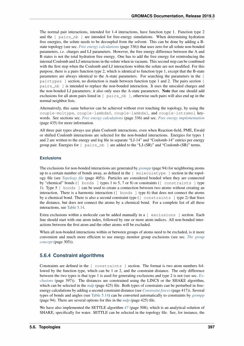
GROMACS Documentation, Release 2019.3
The normal pair interactions, intended for 1-4 interactions, have function type 1. Function type 2and the [ pairs_nb ] are intended for free-energy simulations. When determining hydrationfree energies, the solute needs to be decoupled from the solvent. This can be done by adding a B-state topology (see sec. Free energy calculations (page 336)) that uses zero for all solute non-bondedparameters, i.e. charges and LJ parameters. However, the free energy difference between the A andB states is not the total hydration free energy. One has to add the free energy for reintroducing theinternal Coulomb and LJ interactions in the solute when in vacuum. This second step can be combinedwith the first step when the Coulomb and LJ interactions within the solute are not modified. For thispurpose, there is a pairs function type 2, which is identical to function type 1, except that the B-stateparameters are always identical to the A-state parameters. For searching the parameters in the [pairtypes ] section, no distinction is made between function type 1 and 2. The pairs section [pairs_nb ] is intended to replace the non-bonded interaction. It uses the unscaled charges andthe non-bonded LJ parameters; it also only uses the A-state parameters. Note that one should addexclusions for all atom pairs listed in [ pairs_nb ], otherwise such pairs will also end up in thenormal neighbor lists.
Alternatively, this same behavior can be achieved without ever touching the topology, by using thecouple-moltype, couple-lambda0, couple-lambda1, and couple-intramol key-words. See sections sec. Free energy calculations (page 336) and sec. Free energy implementation(page 435) for more information.
All three pair types always use plain Coulomb interactions, even when Reaction-field, PME, Ewaldor shifted Coulomb interactions are selected for the non-bonded interactions. Energies for types 1and 2 are written to the energy and log file in separate “LJ-14” and “Coulomb-14” entries per energygroup pair. Energies for [ pairs_nb ] are added to the “LJ-(SR)” and “Coulomb-(SR)” terms.
Exclusions
The exclusions for non-bonded interactions are generated by grompp (page 94) for neighboring atomsup to a certain number of bonds away, as defined in the [ moleculetype ] section in the topol-ogy file (see Topology file (page 405)). Particles are considered bonded when they are connectedby “chemical” bonds ([ bonds ] types 1 to 5, 7 or 8) or constraints ([ constraints ] type1). Type 5 [ bonds ] can be used to create a connection between two atoms without creating aninteraction. There is a harmonic interaction ([ bonds ] type 6) that does not connect the atomsby a chemical bond. There is also a second constraint type ([ constraints ] type 2) that fixesthe distance, but does not connect the atoms by a chemical bond. For a complete list of all theseinteractions, see Table 5.14.
Extra exclusions within a molecule can be added manually in a [ exclusions ] section. Eachline should start with one atom index, followed by one or more atom indices. All non-bonded inter-actions between the first atom and the other atoms will be excluded.
When all non-bonded interactions within or between groups of atoms need to be excluded, is it moreconvenient and much more efficient to use energy monitor group exclusions (see sec. The groupconcept (page 305)).
5.6.4 Constraint algorithms
Constraints are defined in the [ constraints ] section. The format is two atom numbers fol-lowed by the function type, which can be 1 or 2, and the constraint distance. The only differencebetween the two types is that type 1 is used for generating exclusions and type 2 is not (see sec. Ex-clusions (page 397)). The distances are constrained using the LINCS or the SHAKE algorithm,which can be selected in the mdp (page 425) file. Both types of constraints can be perturbed in free-energy calculations by adding a second constraint distance (see Constraint forces (page 417)). Severaltypes of bonds and angles (see Table 5.14) can be converted automatically to constraints by grompp(page 94). There are several options for this in the mdp (page 425) file.
We have also implemented the SETTLE algorithm 47 (page 508), which is an analytical solution ofSHAKE, specifically for water. SETTLE can be selected in the topology file. See, for instance, the
5.6. Topologies 397
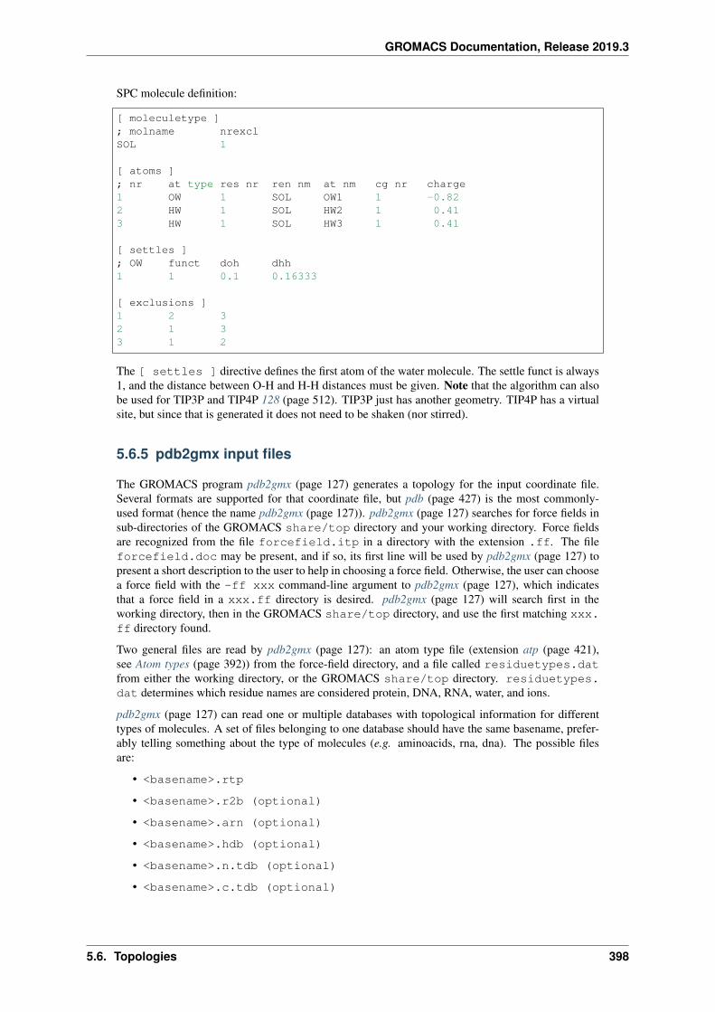
GROMACS Documentation, Release 2019.3
SPC molecule definition:
[ moleculetype ]; molname nrexclSOL 1
[ atoms ]; nr at type res nr ren nm at nm cg nr charge1 OW 1 SOL OW1 1 -0.822 HW 1 SOL HW2 1 0.413 HW 1 SOL HW3 1 0.41
[ settles ]; OW funct doh dhh1 1 0.1 0.16333
[ exclusions ]1 2 32 1 33 1 2
The [ settles ] directive defines the first atom of the water molecule. The settle funct is always1, and the distance between O-H and H-H distances must be given. Note that the algorithm can alsobe used for TIP3P and TIP4P 128 (page 512). TIP3P just has another geometry. TIP4P has a virtualsite, but since that is generated it does not need to be shaken (nor stirred).
5.6.5 pdb2gmx input files
The GROMACS program pdb2gmx (page 127) generates a topology for the input coordinate file.Several formats are supported for that coordinate file, but pdb (page 427) is the most commonly-used format (hence the name pdb2gmx (page 127)). pdb2gmx (page 127) searches for force fields insub-directories of the GROMACS share/top directory and your working directory. Force fieldsare recognized from the file forcefield.itp in a directory with the extension .ff. The fileforcefield.doc may be present, and if so, its first line will be used by pdb2gmx (page 127) topresent a short description to the user to help in choosing a force field. Otherwise, the user can choosea force field with the -ff xxx command-line argument to pdb2gmx (page 127), which indicatesthat a force field in a xxx.ff directory is desired. pdb2gmx (page 127) will search first in theworking directory, then in the GROMACS share/top directory, and use the first matching xxx.ff directory found.
Two general files are read by pdb2gmx (page 127): an atom type file (extension atp (page 421),see Atom types (page 392)) from the force-field directory, and a file called residuetypes.datfrom either the working directory, or the GROMACS share/top directory. residuetypes.dat determines which residue names are considered protein, DNA, RNA, water, and ions.
pdb2gmx (page 127) can read one or multiple databases with topological information for differenttypes of molecules. A set of files belonging to one database should have the same basename, prefer-ably telling something about the type of molecules (e.g. aminoacids, rna, dna). The possible filesare:
• <basename>.rtp
• <basename>.r2b (optional)
• <basename>.arn (optional)
• <basename>.hdb (optional)
• <basename>.n.tdb (optional)
• <basename>.c.tdb (optional)
5.6. Topologies 398
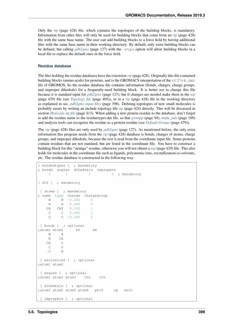
GROMACS Documentation, Release 2019.3
Only the rtp (page 428) file, which contains the topologies of the building blocks, is mandatory.Information from other files will only be used for building blocks that come from an rtp (page 428)file with the same base name. The user can add building blocks to a force field by having additionalfiles with the same base name in their working directory. By default, only extra building blocks canbe defined, but calling pdb2gmx (page 127) with the -rtpo option will allow building blocks in alocal file to replace the default ones in the force field.
Residue database
The files holding the residue databases have the extension rtp (page 428). Originally this file containedbuilding blocks (amino acids) for proteins, and is the GROMACS interpretation of the rt37c4.datfile of GROMOS. So the residue database file contains information (bonds, charges, charge groups,and improper dihedrals) for a frequently-used building block. It is better not to change this filebecause it is standard input for pdb2gmx (page 127), but if changes are needed make them in the top(page 429) file (see Topology file (page 405)), or in a rtp (page 428) file in the working directoryas explained in sec. pdb2gmx input files (page 398). Defining topologies of new small molecules isprobably easier by writing an include topology file itp (page 424) directly. This will be discussed insection Molecule.itp file (page 413). When adding a new protein residue to the database, don’t forgetto add the residue name to the residuetypes.dat file, so that grompp (page 94), make_ndx (page 109)and analysis tools can recognize the residue as a protein residue (see Default Groups (page 479)).
The rtp (page 428) files are only used by pdb2gmx (page 127). As mentioned before, the only extrainformation this program needs from the rtp (page 428) database is bonds, charges of atoms, chargegroups, and improper dihedrals, because the rest is read from the coordinate input file. Some proteinscontain residues that are not standard, but are listed in the coordinate file. You have to construct abuilding block for this “strange” residue, otherwise you will not obtain a top (page 429) file. This alsoholds for molecules in the coordinate file such as ligands, polyatomic ions, crystallization co-solvents,etc. The residue database is constructed in the following way:
[ bondedtypes ] ; mandatory; bonds angles dihedrals impropers
1 1 1 2 ; mandatory
[ GLY ] ; mandatory
[ atoms ] ; mandatory; name type charge chargegroup
N N -0.280 0H H 0.280 0
CA CH2 0.000 1C C 0.380 2O O -0.380 2
[ bonds ] ; optional;atom1 atom2 b0 kb
N HN CA
CA CC O
-C N
[ exclusions ] ; optional;atom1 atom2
[ angles ] ; optional;atom1 atom2 atom3 th0 cth
[ dihedrals ] ; optional;atom1 atom2 atom3 atom4 phi0 cp mult
[ impropers ] ; optional
5.6. Topologies 399
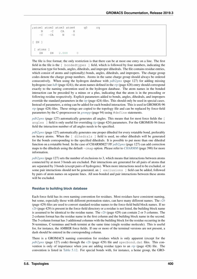
GROMACS Documentation, Release 2019.3
;atom1 atom2 atom3 atom4 q0 cqN -C CA H
-C -CA N -O
[ ZN ]
[ atoms ]ZN ZN 2.000 0
The file is free format; the only restriction is that there can be at most one entry on a line. The firstfield in the file is the [ bondedtypes ] field, which is followed by four numbers, indicating theinteraction type for bonds, angles, dihedrals, and improper dihedrals. The file contains residue entries,which consist of atoms and (optionally) bonds, angles, dihedrals, and impropers. The charge groupcodes denote the charge group numbers. Atoms in the same charge group should always be orderedconsecutively. When using the hydrogen database with pdb2gmx (page 127) for adding missinghydrogens (see hdb (page 424)), the atom names defined in the rtp (page 428) entry should correspondexactly to the naming convention used in the hydrogen database. The atom names in the bondedinteraction can be preceded by a minus or a plus, indicating that the atom is in the preceding orfollowing residue respectively. Explicit parameters added to bonds, angles, dihedrals, and impropersoverride the standard parameters in the itp (page 424) files. This should only be used in special cases.Instead of parameters, a string can be added for each bonded interaction. This is used in GROMOS-96rtp (page 428) files. These strings are copied to the topology file and can be replaced by force-fieldparameters by the C-preprocessor in grompp (page 94) using #define statements.
pdb2gmx (page 127) automatically generates all angles. This means that for most force fields the [angles ] field is only useful for overriding itp (page 424) parameters. For the GROMOS-96 forcefield the interaction number of all angles needs to be specified.
pdb2gmx (page 127) automatically generates one proper dihedral for every rotatable bond, preferablyon heavy atoms. When the [ dihedrals ] field is used, no other dihedrals will be generatedfor the bonds corresponding to the specified dihedrals. It is possible to put more than one dihedralfunction on a rotatable bond. In the case of CHARMM27 FF pdb2gmx (page 127) can add correctionmaps to the dihedrals using the default -cmap option. Please refer to CHARMM (page 390) for moreinformation.
pdb2gmx (page 127) sets the number of exclusions to 3, which means that interactions between atomsconnected by at most 3 bonds are excluded. Pair interactions are generated for all pairs of atoms thatare separated by 3 bonds (except pairs of hydrogens). When more interactions need to be excluded, orsome pair interactions should not be generated, an [ exclusions ] field can be added, followedby pairs of atom names on separate lines. All non-bonded and pair interactions between these atomswill be excluded.
Residue to building block database
Each force field has its own naming convention for residues. Most residues have consistent naming,but some, especially those with different protonation states, can have many different names. The r2b(page 429) files are used to convert standard residue names to the force-field build block names. If nor2b (page 429) is present in the force-field directory or a residue is not listed, the building block nameis assumed to be identical to the residue name. The r2b (page 429) can contain 2 or 5 columns. The2-column format has the residue name in the first column and the building block name in the second.The 5-column format has 3 additional columns with the building block for the residue occurring in theN-terminus, C-terminus and both termini at the same time (single residue molecule). This is usefulfor, for instance, the AMBER force fields. If one or more of the terminal versions are not present, adash should be entered in the corresponding column.
There is a GROMACS naming convention for residues which is only apparent (except for thepdb2gmx (page 127) code) through the r2b (page 429) file and specbond.dat files. This con-vention is only of importance when you are adding residue types to an rtp (page 428) file. Theconvention is listed in Table 5.12. For special bonds with, for instance, a heme group, the GRO-
5.6. Topologies 400
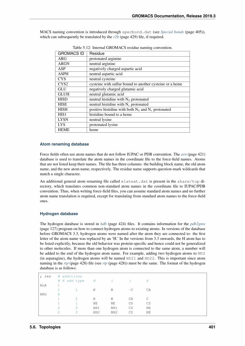
GROMACS Documentation, Release 2019.3
MACS naming convention is introduced through specbond.dat (see Special bonds (page 405)),which can subsequently be translated by the r2b (page 429) file, if required.
Table 5.12: Internal GROMACS residue naming convention.GROMACS ID ResidueARG protonated arginineARGN neutral arginineASP negatively charged aspartic acidASPH neutral aspartic acidCYS neutral cysteineCYS2 cysteine with sulfur bound to another cysteine or a hemeGLU negatively charged glutamic acidGLUH neutral glutamic acidHISD neutral histidine with N𝛿 protonatedHISE neutral histidine with N𝜖 protonatedHISH positive histidine with both N𝛿 and N𝜖 protonatedHIS1 histidine bound to a hemeLYSN neutral lysineLYS protonated lysineHEME heme
Atom renaming database
Force fields often use atom names that do not follow IUPAC or PDB convention. The arn (page 421)database is used to translate the atom names in the coordinate file to the force-field names. Atomsthat are not listed keep their names. The file has three columns: the building block name, the old atomname, and the new atom name, respectively. The residue name supports question-mark wildcards thatmatch a single character.
An additional general atom renaming file called xlateat.dat is present in the share/top di-rectory, which translates common non-standard atom names in the coordinate file to IUPAC/PDBconvention. Thus, when writing force-field files, you can assume standard atom names and no furtheratom name translation is required, except for translating from standard atom names to the force-fieldones.
Hydrogen database
The hydrogen database is stored in hdb (page 424) files. It contains information for the pdb2gmx(page 127) program on how to connect hydrogen atoms to existing atoms. In versions of the databasebefore GROMACS 3.3, hydrogen atoms were named after the atom they are connected to: the firstletter of the atom name was replaced by an ‘H.’ In the versions from 3.3 onwards, the H atom has tobe listed explicitly, because the old behavior was protein-specific and hence could not be generalizedto other molecules. If more than one hydrogen atom is connected to the same atom, a number willbe added to the end of the hydrogen atom name. For example, adding two hydrogen atoms to ND2(in asparagine), the hydrogen atoms will be named HD21 and HD22. This is important since atomnaming in the rtp (page 428) file (see rtp (page 428)) must be the same. The format of the hydrogendatabase is as follows:
; res # additions# H add type H i j k
ALA 11 1 H N -C CA
ARG 41 2 H N CA C1 1 HE NE CD CZ2 3 HH1 NH1 CZ NE2 3 HH2 NH2 CZ NE
5.6. Topologies 401

GROMACS Documentation, Release 2019.3
On the first line we see the residue name (ALA or ARG) and the number of kinds of hydrogen atomsthat may be added to this residue by the hydrogen database. After that follows one line for eachaddition, on which we see:
• The number of H atoms added
• The method for adding H atoms, which can be any of:
1. one planar hydrogen, e.g. rings or peptide bondOne hydrogen atom (n) is generated, lying in the plane of atoms (i,j,k) on the planebisecting angle (j-i-k) at a distance of 0.1 nm from atom i, such that the angles (n-i-j) and(n-i-k) are > 90o.
2. one single hydrogen, e.g. hydroxylOne hydrogen atom (n) is generated at a distance of 0.1 nm from atom i, such that angle(n-i-j)=109.5 degrees and dihedral (n-i-j-k)=trans.
3. two planar hydrogens, e.g. ethylene -C=CH2, or amide -C(=O)NH2
Two hydrogens (n1,n2) are generated at a distance of 0.1 nm from atom i, such that angle(n1-i-j)=(n2-i-j)=120 degrees and dihedral (n1-i-j-k)=cis and (n2-i-j-k)=trans, such thatnames are according to IUPAC standards 129 (page 512).
4. two or three tetrahedral hydrogens, e.g. -CH3
Three (n1,n2,n3) or two (n1,n2) hydrogens are generated at a distance of 0.1 nm fromatom i, such that angle (n1-i-j)=(n2-i-j)=(n3-i-j)=109.47:math:^{rm o}, dihedral(n1-i-j-k)=trans, (n2-i-j-k)=trans+120 and (n3-i-j-k)=trans+240:math:^{rm o}.
5. one tetrahedral hydrogen, e.g. C3* CH*One hydrogen atom (n:math:^prime) is generated at a distance of 0.1 nm from atom i intetrahedral conformation such that angle(n:math:^prime-i-j)=(n:math:^prime-i-k)=(n:math:^prime-i-l)=109.47:math:^{rm o}.
6. two tetrahedral hydrogens, e.g. C-CH2*-C*Two hydrogen atoms (n1,n2) are generated at a distance of 0.1 nm from atom i intetrahedral conformation on the plane bisecting angle j-i-k with angle(n1-i-n2)=(n1-i-j)=(n1-i-k)=109.47:math:^{rm o}.
7. two water hydrogensTwo hydrogens are generated around atom i according to SPC 80 (page 509) watergeometry. The symmetry axis will alternate between three coordinate axes in bothdirections.
8. three water “hydrogens”Two hydrogens are generated around atom i according to SPC 80 (page 509) watergeometry. The symmetry axis will alternate between three coordinate axes in bothdirections. In addition, an extra particle is generated on the position of the oxygen with thefirst letter of the name replaced by ‘M’. This is for use with four-atom water models suchas TIP4P 128 (page 512).
9. four water “hydrogens”Same as above, except that two additional particles are generated on the position of theoxygen, with names ‘LP1’ and ‘LP2.’ This is for use with five-atom water models such asTIP5P 130 (page 512).
• The name of the new H atom (or its prefix, e.g. HD2 for the asparagine example given earlier).
• Three or four control atoms (i,j,k,l), where the first always is the atom to which the H atoms areconnected. The other two or three depend on the code selected. For water, there is only onecontrol atom.
Some more exotic cases can be approximately constructed from the above tools, and with suitableuse of energy minimization are good enough for beginning MD simulations. For example secondaryamine hydrogen, nitrenyl hydrogen (C = NH) and even ethynyl hydrogen could be approximatelyconstructed using method 2 above for hydroxyl hydrogen.
5.6. Topologies 402
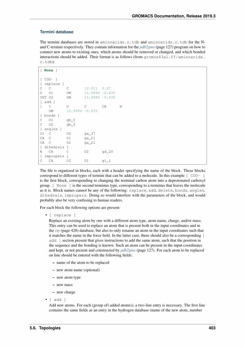
GROMACS Documentation, Release 2019.3
Termini database
The termini databases are stored in aminoacids.n.tdb and aminoacids.c.tdb for the N-and C-termini respectively. They contain information for the pdb2gmx (page 127) program on how toconnect new atoms to existing ones, which atoms should be removed or changed, and which bondedinteractions should be added. Their format is as follows (from gromos43a1.ff/aminoacids.c.tdb):
[ None ]
[ COO- ][ replace ]C C C 12.011 0.27O O1 OM 15.9994 -0.635OXT O2 OM 15.9994 -0.635[ add ]2 8 O C CA N
OM 15.9994 -0.635[ bonds ]C O1 gb_5C O2 gb_5[ angles ]O1 C O2 ga_37CA C O1 ga_21CA C O2 ga_21[ dihedrals ]N CA C O2 gd_20[ impropers ]C CA O2 O1 gi_1
The file is organized in blocks, each with a header specifying the name of the block. These blockscorrespond to different types of termini that can be added to a molecule. In this example [ COO- ]is the first block, corresponding to changing the terminal carbon atom into a deprotonated carboxylgroup. [ None ] is the second terminus type, corresponding to a terminus that leaves the moleculeas it is. Block names cannot be any of the following: replace, add, delete, bonds, angles,dihedrals, impropers. Doing so would interfere with the parameters of the block, and wouldprobably also be very confusing to human readers.
For each block the following options are present:
• [ replace ]
Replace an existing atom by one with a different atom type, atom name, charge, and/or mass.This entry can be used to replace an atom that is present both in the input coordinates and inthe rtp (page 428) database, but also to only rename an atom in the input coordinates such thatit matches the name in the force field. In the latter case, there should also be a corresponding [add ] section present that gives instructions to add the same atom, such that the position inthe sequence and the bonding is known. Such an atom can be present in the input coordinatesand kept, or not present and constructed by pdb2gmx (page 127). For each atom to be replacedon line should be entered with the following fields:
– name of the atom to be replaced
– new atom name (optional)
– new atom type
– new mass
– new charge
• [ add ]
Add new atoms. For each (group of) added atom(s), a two-line entry is necessary. The first linecontains the same fields as an entry in the hydrogen database (name of the new atom, number
5.6. Topologies 403
GROMACS Documentation, Release 2019.3
of atoms, type of addition, control atoms, see hdb (page 424)), but the possible types ofaddition are extended by two more, specifically for C-terminal additions:
1. two carboxyl oxygens, -COO−
Two oxygens (n1,n2) are generated according to rule 3, at a distance of 0.136 nm fromatom i and an angle (n1-i-j)=(n2-i-j)=117 degrees
2. carboxyl oxygens and hydrogen, -COOHTwo oxygens (n1,n2) are generated according to rule 3, at distances of 0.123 nm and 0.125nm from atom i for n1 and n2, respectively, and angles (n1-i-j)=121 and (n2-i-j)=115degrees. One hydrogen (n:math:^prime) is generated around n2 according to rule 2, wheren-i-j and n-i-j-k should be read as n′-n2-i and n′-n2-i-j, respectively.
After this line, another line follows that specifies the details of the added atom(s), in the sameway as for replacing atoms, i.e.:
– atom type
– mass
– charge
– charge group (optional)
Like in the hydrogen database (see rtp (page 428)), when more than one atom is connected toan existing one, a number will be appended to the end of the atom name. Note that, like in thehydrogen database, the atom name is now on the same line as the control atoms, whereas it wasat the beginning of the second line prior to GROMACS version 3.3. When the charge groupfield is left out, the added atom will have the same charge group number as the atom that it isbonded to.
• [ delete ]
Delete existing atoms. One atom name per line.
• [ bonds ], [ angles ], [ dihedrals ] and [ impropers ]
Add additional bonded parameters. The format is identical to that used in the rtp (page 428)file, see rtp (page 428).
Virtual site database
Since we cannot rely on the positions of hydrogens in input files, we need a special input file to decidethe geometries and parameters with which to add virtual site hydrogens. For more complex virtualsite constructs (e.g. when entire aromatic side chains are made rigid) we also need information aboutthe equilibrium bond lengths and angles for all atoms in the side chain. This information is specifiedin the vsd (page 431) file for each force field. Just as for the termini, there is one such file for eachclass of residues in the rtp (page 428) file.
The virtual site database is not really a very simple list of information. The first couple of sectionsspecify which mass centers (typically called MCH3/MNH:math:_3) to use for CH3, NH3, and NH2
groups. Depending on the equilibrium bond lengths and angles between the hydrogens and heavyatoms we need to apply slightly different constraint distances between these mass centers. Note thatwe do not have to specify the actual parameters (that is automatic), just the type of mass center to use.To accomplish this, there are three sections names [ CH3 ], [ NH3 ], and [ NH2 ]. For eachof these we expect three columns. The first column is the atom type bound to the 2/3 hydrogens, thesecond column is the next heavy atom type which this is bound, and the third column the type of masscenter to use. As a special case, in the [ NH2 ] section it is also possible to specify planar inthe second column, which will use a different construction without mass center. There are currentlydifferent opinions in some force fields whether an NH2 group should be planar or not, but we try hardto stick to the default equilibrium parameters of the force field.
The second part of the virtual site database contains explicit equilibrium bond lengths and angles forpairs/triplets of atoms in aromatic side chains. These entries are currently read by specific routines inthe virtual site generation code, so if you would like to extend it e.g. to nucleic acids you would also
5.6. Topologies 404
GROMACS Documentation, Release 2019.3
need to write new code there. These sections are named after the short amino acid names ([ PHE ],[ TYR ], [ TRP ], [ HID ], [ HIE ], [ HIP ]), and simply contain 2 or 3 columns withatom names, followed by a number specifying the bond length (in nm) or angle (in degrees). Notethat these are approximations of the equilibrated geometry for the entire molecule, which might notbe identical to the equilibrium value for a single bond/angle if the molecule is strained.
Special bonds
The primary mechanism used by pdb2gmx (page 127) to generate inter-residue bonds relies on head-to-tail linking of backbone atoms in different residues to build a macromolecule. In some cases (e.g.disulfide bonds, a heme group, branched polymers), it is necessary to create inter-residue bonds thatdo not lie on the backbone. The file specbond.dat takes care of this function. It is necessary thatthe residues belong to the same [ moleculetype ]. The -merge and -chainsep functionsof pdb2gmx (page 127) can be useful when managing special inter-residue bonds between differentchains.
The first line of specbond.dat indicates the number of entries that are in the file. If you add a newentry, be sure to increment this number. The remaining lines in the file provide the specifications forcreating bonds. The format of the lines is as follows:
resA atomA nbondsA resB atomB nbondsB length newresA newresB
The columns indicate:
1. resA The name of residue A that participates in the bond.
2. atomA The name of the atom in residue A that forms the bond.
3. nbondsA The total number of bonds atomA can form.
4. resB The name of residue B that participates in the bond.
5. atomB The name of the atom in residue B that forms the bond.
6. nbondsB The total number of bonds atomB can form.
7. length The reference length for the bond. If atomA and atomB are not within length ±10% in the coordinate file supplied to pdb2gmx (page 127), no bond will be formed.
8. newresA The new name of residue A, if necessary. Some force fields use e.g. CYS2 for acysteine in a disulfide or heme linkage.
9. newresB The new name of residue B, likewise.
5.6.6 File formats
Topology file
The topology file is built following the GROMACS specification for a molecular topology. A top(page 429) file can be generated by pdb2gmx (page 127). All possible entries in the topology file arelisted in Tables 5.13 and 5.14. Also tabulated are: all the units of the parameters, which interactionscan be perturbed for free energy calculations, which bonded interactions are used by grompp (page 94)for generating exclusions, and which bonded interactions can be converted to constraints by grompp(page 94).
5.6. Topologies 405
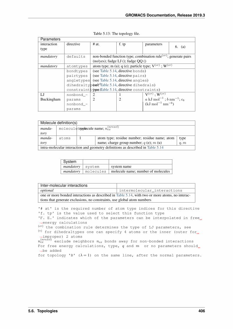
GROMACS Documentation, Release 2019.3
Table 5.13: The topology file.Parametersinteractiontype
directive # at. f. tp parameters6. (a)
mandatory defaults non-bonded function type; combination rule(𝑐𝑟); generate pairs(no/yes); fudge LJ (); fudge QQ ()
mandatory atomtypes atom type; m (u); q (e); particle type; V(𝑐𝑟) ; W(𝑐𝑟)
bondtypespairtypesangletypesdihedraltypes(*)
constrainttypes
(see Table 5.14, directive bonds)(see Table 5.14, directive pairs)(see Table 5.14, directive angles)(see Table 5.14, directive dihedrals)(see Table 5.14, directive constraints)
LJBuckingham
nonbond_-paramsnonbond_-params
22
12
V(𝑐𝑟) ; W(𝑐𝑟)
𝑎 kJ mol−1 ; 𝑏 nm−1; 𝑐6(kJ mol−1 nm−6)
Molecule definition(s)manda-tory
moleculetypemolecule name; 𝑛(𝑛𝑟𝑒𝑥𝑐𝑙)𝑒𝑥
manda-tory
atoms 1 atom type; residue number; residue name; atomname; charge group number; 𝑞 (e); 𝑚 (u)
type𝑞,𝑚
intra-molecular interaction and geometry definitions as described in Table 5.14
Systemmandatory system system namemandatory molecules molecule name; number of molecules
Inter-molecular interactionsoptional intermolecular_interactionsone or more bonded interactions as described in Table 5.14, with two or more atoms, no interac-tions that generate exclusions, no constraints, use global atom numbers
'# at' is the required number of atom type indices for this directive'f. tp' is the value used to select this function type'F. E.' indicates which of the parameters can be interpolated in free
→˓energy calculations(𝑐𝑟) the combination rule determines the type of LJ parameters, see(*) for dihedraltypes one can specify 4 atoms or the inner (outer for
→˓improper) 2 atoms𝑛(𝑛𝑟𝑒𝑥𝑐𝑙)𝑒𝑥 exclude neighbors 𝑛𝑒𝑥 bonds away for non-bonded interactions
For free energy calculations, type, 𝑞 and 𝑚 or no parameters should→˓be addedfor topology 'B' (𝜆 = 1) on the same line, after the normal parameters.
5.6. Topologies 406
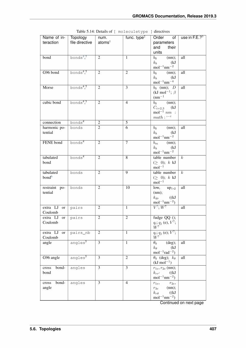
GROMACS Documentation, Release 2019.3
Table 5.14: Details of [ moleculetype ] directivesName of in-teraction
Topologyfile directive
num.atoms1
func. type2 Order ofparametersand theirunits
use in F.E.?3
bond bonds4,5 2 1 𝑏0 (nm);𝑘𝑏 (kJmol−1nm−2
all
G96 bond bonds4,5 2 2 𝑏0 (nm);𝑘𝑏 (kJmol−1nm−4
all
Morse bonds4,5 2 3 𝑏0 (nm); 𝐷(kJ mol−1; 𝛽(nm−1
all
cubic bond bonds4,5 2 4 𝑏0 (nm);𝐶𝑖=2,3 (kJmol−1 𝑛𝑚 :𝑚𝑎𝑡ℎ : ‘−𝑖
connection bonds4 2 5harmonic po-tential
bonds 2 6 𝑏0 (nm);𝑘𝑏 (kJmol−1nm−2
all
FENE bond bonds4 2 7 𝑏𝑚 (nm);𝑘𝑏 (kJmol−1nm−2
tabulatedbond
bonds4 2 8 table number(≥ 0); 𝑘 kJmol−1
𝑘
tabulatedbond6
bonds 2 9 table number(≥ 0); 𝑘 kJmol−1
𝑘
restraint po-tential
bonds 2 10 low, up1,2(nm);𝑘𝑑𝑟 ((kJmol−1nm−2)
all
extra LJ orCoulomb
pairs 2 1 𝑉 7; 𝑊 7 all
extra LJ orCoulomb
pairs 2 2 fudge QQ ();𝑞𝑖; 𝑞𝑗 (e), 𝑉 7;𝑊 7
extra LJ orCoulomb
pairs_nb 2 1 𝑞𝑖; 𝑞𝑗 (e); 𝑉 7;𝑊 7
angle angles5 3 1 𝜃0 (deg);𝑘𝜃 (kJmol−1rad−2)
all
G96 angle angles5 3 2 𝜃0 (deg); 𝑘𝜃(kJ mol−1)
all
cross bond-bond
angles 3 3 𝑟1𝑒, 𝑟2𝑒 (nm);𝑘𝑟𝑟′ ((kJmol−1nm−2)
cross bond-angle
angles 3 4 𝑟1𝑒, 𝑟2𝑒,𝑟3𝑒 (nm);𝑘𝑟𝜃 ((kJmol−1nm−2)
Continued on next page
5.6. Topologies 407
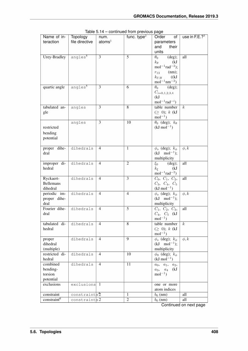
GROMACS Documentation, Release 2019.3
Table 5.14 – continued from previous pageName of in-teraction
Topologyfile directive
num.atoms1
func. type2 Order ofparametersand theirunits
use in F.E.?3
Urey-Bradley angles5 3 5 𝜃0 (deg);𝑘𝜃 (kJmol−1rad−2);𝑟13 (nm);𝑘𝑈𝐵 ((kJmol−1nm−2)
all
quartic angle angles5 3 6 𝜃0 (deg);𝐶𝑖=0,1,2,3,4
(kJmol−1rad−𝑖)
tabulated an-gle
angles 3 8 table number(≥ 0); 𝑘 (kJmol−1)
𝑘
restrictedbendingpotential
angles 3 10 𝜃0 (deg); 𝑘𝜃(kJ mol−1)
proper dihe-dral
dihedrals 4 1 𝜑𝑠 (deg); 𝑘𝜑(kJ mol−1);multiplicity
𝜑, 𝑘
improper di-hedral
dihedrals 4 2 𝜉0 (deg);𝑘𝜉 (kJmol−1rad−2)
all
Ryckaert-Bellemansdihedral
dihedrals 4 3 𝐶0, 𝐶1, 𝐶2,𝐶3, 𝐶4, 𝐶5
(kJ mol−1)
all
periodic im-proper dihe-dral
dihedrals 4 4 𝜑𝑠 (deg); 𝑘𝜑(kJ mol−1);multiplicity
𝜑, 𝑘
Fourier dihe-dral
dihedrals 4 5 𝐶1, 𝐶2, 𝐶3,𝐶4, 𝐶5 (kJmol−1)
all
tabulated di-hedral
dihedrals 4 8 table number(≥ 0); 𝑘 (kJmol−1)
𝑘
properdihedral(multiple)
dihedrals 4 9 𝜑𝑠 (deg); 𝑘𝜑(kJ mol−1);multiplicity
𝜑, 𝑘
restricted di-hedral
dihedrals 4 10 𝜑0 (deg); 𝑘𝜑(kJ mol−1)
combinedbending-torsionpotential
dihedrals 4 11 𝑎0, 𝑎1, 𝑎2,𝑎3, 𝑎4 (kJmol−1)
exclusions exclusions 1 one or moreatom indices
constraint constraints42 1 𝑏0 (nm) allconstraint6 constraints2 2 𝑏0 (nm) all
Continued on next page
5.6. Topologies 408
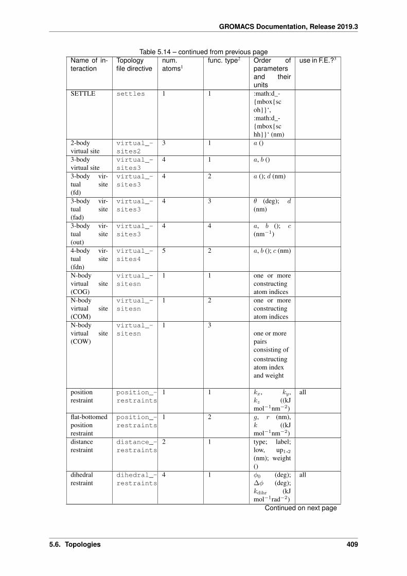
GROMACS Documentation, Release 2019.3
Table 5.14 – continued from previous pageName of in-teraction
Topologyfile directive
num.atoms1
func. type2 Order ofparametersand theirunits
use in F.E.?3
SETTLE settles 1 1 :math:d_-{mbox{scoh}}‘,:math:d_-{mbox{schh}}‘ (nm)
2-bodyvirtual site
virtual_-sites2
3 1 𝑎 ()
3-bodyvirtual site
virtual_-sites3
4 1 𝑎, 𝑏 ()
3-body vir-tual site(fd)
virtual_-sites3
4 2 𝑎 (); 𝑑 (nm)
3-body vir-tual site(fad)
virtual_-sites3
4 3 𝜃 (deg); 𝑑(nm)
3-body vir-tual site(out)
virtual_-sites3
4 4 𝑎, 𝑏 (); 𝑐(nm−1)
4-body vir-tual site(fdn)
virtual_-sites4
5 2 𝑎, 𝑏 (); 𝑐 (nm)
N-bodyvirtual site(COG)
virtual_-sitesn
1 1 one or moreconstructingatom indices
N-bodyvirtual site(COM)
virtual_-sitesn
1 2 one or moreconstructingatom indices
N-bodyvirtual site(COW)
virtual_-sitesn
1 3one or morepairsconsisting ofconstructingatom indexand weight
positionrestraint
position_-restraints
1 1 𝑘𝑥, 𝑘𝑦 ,𝑘𝑧 ((kJmol−1nm−2)
all
flat-bottomedpositionrestraint
position_-restraints
1 2 𝑔, 𝑟 (nm),𝑘 ((kJmol−1nm−2)
distancerestraint
distance_-restraints
2 1 type; label;low, up1,2(nm); weight()
dihedralrestraint
dihedral_-restraints
4 1 𝜑0 (deg);∆𝜑 (deg);𝑘dihr (kJmol−1rad−2)
all
Continued on next page
5.6. Topologies 409
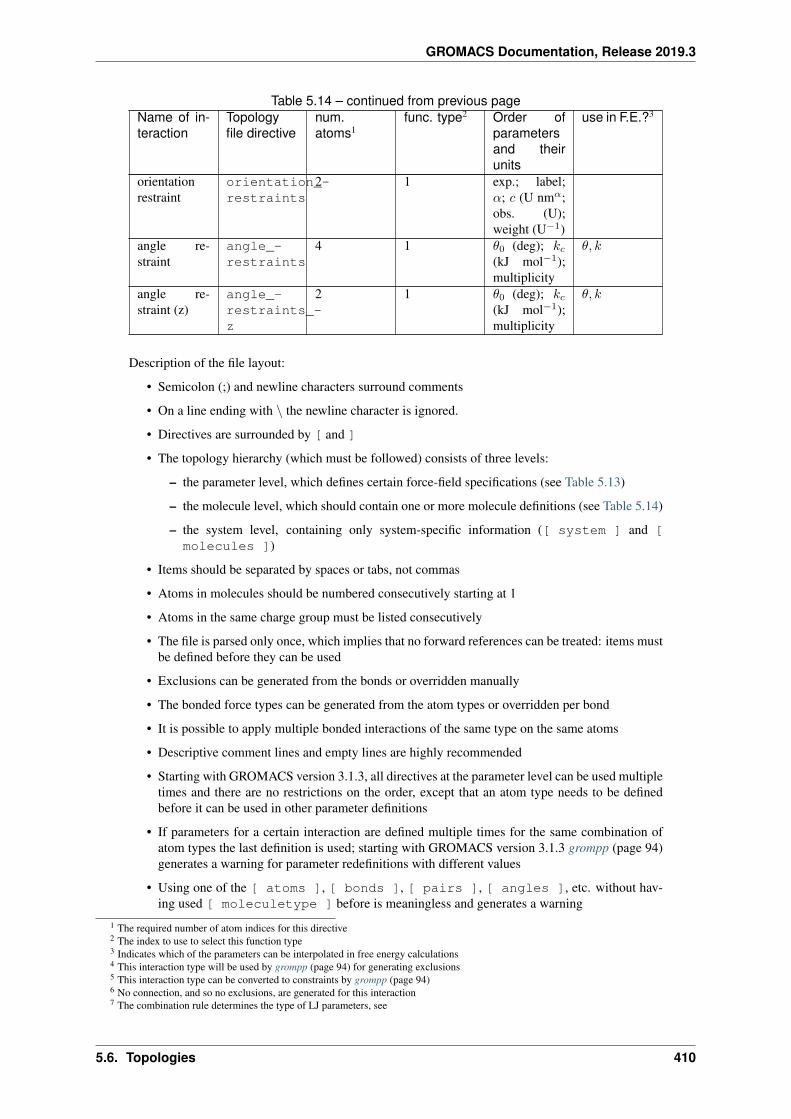
GROMACS Documentation, Release 2019.3
Table 5.14 – continued from previous pageName of in-teraction
Topologyfile directive
num.atoms1
func. type2 Order ofparametersand theirunits
use in F.E.?3
orientationrestraint
orientation_-restraints
2 1 exp.; label;𝛼; 𝑐 (U nm𝛼;obs. (U);weight (U−1)
angle re-straint
angle_-restraints
4 1 𝜃0 (deg); 𝑘𝑐(kJ mol−1);multiplicity
𝜃, 𝑘
angle re-straint (z)
angle_-restraints_-z
2 1 𝜃0 (deg); 𝑘𝑐(kJ mol−1);multiplicity
𝜃, 𝑘
Description of the file layout:
• Semicolon (;) and newline characters surround comments
• On a line ending with ∖ the newline character is ignored.
• Directives are surrounded by [ and ]
• The topology hierarchy (which must be followed) consists of three levels:
– the parameter level, which defines certain force-field specifications (see Table 5.13)
– the molecule level, which should contain one or more molecule definitions (see Table 5.14)
– the system level, containing only system-specific information ([ system ] and [molecules ])
• Items should be separated by spaces or tabs, not commas
• Atoms in molecules should be numbered consecutively starting at 1
• Atoms in the same charge group must be listed consecutively
• The file is parsed only once, which implies that no forward references can be treated: items mustbe defined before they can be used
• Exclusions can be generated from the bonds or overridden manually
• The bonded force types can be generated from the atom types or overridden per bond
• It is possible to apply multiple bonded interactions of the same type on the same atoms
• Descriptive comment lines and empty lines are highly recommended
• Starting with GROMACS version 3.1.3, all directives at the parameter level can be used multipletimes and there are no restrictions on the order, except that an atom type needs to be definedbefore it can be used in other parameter definitions
• If parameters for a certain interaction are defined multiple times for the same combination ofatom types the last definition is used; starting with GROMACS version 3.1.3 grompp (page 94)generates a warning for parameter redefinitions with different values
• Using one of the [ atoms ], [ bonds ], [ pairs ], [ angles ], etc. without hav-ing used [ moleculetype ] before is meaningless and generates a warning
1 The required number of atom indices for this directive2 The index to use to select this function type3 Indicates which of the parameters can be interpolated in free energy calculations4 This interaction type will be used by grompp (page 94) for generating exclusions5 This interaction type can be converted to constraints by grompp (page 94)6 No connection, and so no exclusions, are generated for this interaction7 The combination rule determines the type of LJ parameters, see
5.6. Topologies 410
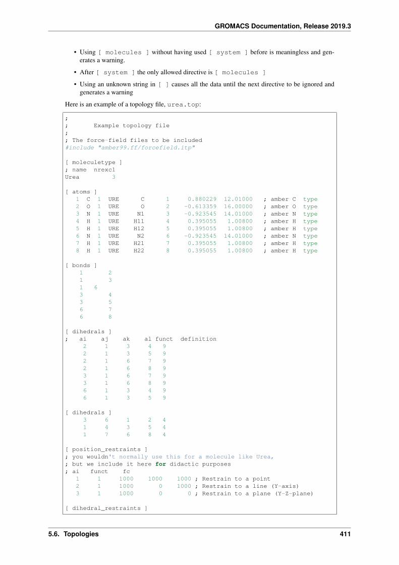
GROMACS Documentation, Release 2019.3
• Using [ molecules ] without having used [ system ] before is meaningless and gen-erates a warning.
• After [ system ] the only allowed directive is [ molecules ]
• Using an unknown string in [ ] causes all the data until the next directive to be ignored andgenerates a warning
Here is an example of a topology file, urea.top:
;; Example topology file;; The force-field files to be included#include "amber99.ff/forcefield.itp"
[ moleculetype ]; name nrexclUrea 3
[ atoms ]1 C 1 URE C 1 0.880229 12.01000 ; amber C type2 O 1 URE O 2 -0.613359 16.00000 ; amber O type3 N 1 URE N1 3 -0.923545 14.01000 ; amber N type4 H 1 URE H11 4 0.395055 1.00800 ; amber H type5 H 1 URE H12 5 0.395055 1.00800 ; amber H type6 N 1 URE N2 6 -0.923545 14.01000 ; amber N type7 H 1 URE H21 7 0.395055 1.00800 ; amber H type8 H 1 URE H22 8 0.395055 1.00800 ; amber H type
[ bonds ]1 21 31 63 43 56 76 8
[ dihedrals ]; ai aj ak al funct definition
2 1 3 4 92 1 3 5 92 1 6 7 92 1 6 8 93 1 6 7 93 1 6 8 96 1 3 4 96 1 3 5 9
[ dihedrals ]3 6 1 2 41 4 3 5 41 7 6 8 4
[ position_restraints ]; you wouldn't normally use this for a molecule like Urea,; but we include it here for didactic purposes; ai funct fc
1 1 1000 1000 1000 ; Restrain to a point2 1 1000 0 1000 ; Restrain to a line (Y-axis)3 1 1000 0 0 ; Restrain to a plane (Y-Z-plane)
[ dihedral_restraints ]
5.6. Topologies 411
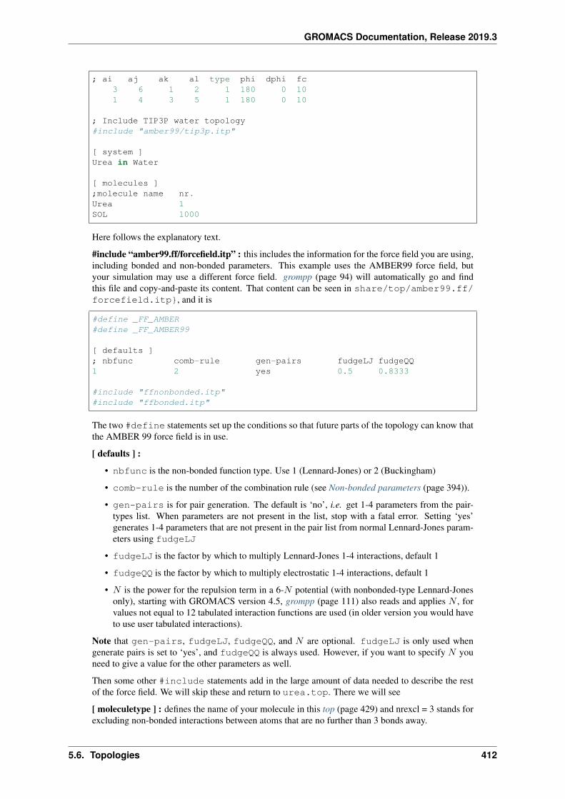
GROMACS Documentation, Release 2019.3
; ai aj ak al type phi dphi fc3 6 1 2 1 180 0 101 4 3 5 1 180 0 10
; Include TIP3P water topology#include "amber99/tip3p.itp"
[ system ]Urea in Water
[ molecules ];molecule name nr.Urea 1SOL 1000
Here follows the explanatory text.
#include “amber99.ff/forcefield.itp” : this includes the information for the force field you are using,including bonded and non-bonded parameters. This example uses the AMBER99 force field, butyour simulation may use a different force field. grompp (page 94) will automatically go and findthis file and copy-and-paste its content. That content can be seen in share/top/amber99.ff/forcefield.itp}, and it is
#define _FF_AMBER#define _FF_AMBER99
[ defaults ]; nbfunc comb-rule gen-pairs fudgeLJ fudgeQQ1 2 yes 0.5 0.8333
#include "ffnonbonded.itp"#include "ffbonded.itp"
The two #define statements set up the conditions so that future parts of the topology can know thatthe AMBER 99 force field is in use.
[ defaults ] :
• nbfunc is the non-bonded function type. Use 1 (Lennard-Jones) or 2 (Buckingham)
• comb-rule is the number of the combination rule (see Non-bonded parameters (page 394)).
• gen-pairs is for pair generation. The default is ‘no’, i.e. get 1-4 parameters from the pair-types list. When parameters are not present in the list, stop with a fatal error. Setting ‘yes’generates 1-4 parameters that are not present in the pair list from normal Lennard-Jones param-eters using fudgeLJ
• fudgeLJ is the factor by which to multiply Lennard-Jones 1-4 interactions, default 1
• fudgeQQ is the factor by which to multiply electrostatic 1-4 interactions, default 1
• 𝑁 is the power for the repulsion term in a 6-𝑁 potential (with nonbonded-type Lennard-Jonesonly), starting with GROMACS version 4.5, grompp (page 111) also reads and applies 𝑁 , forvalues not equal to 12 tabulated interaction functions are used (in older version you would haveto use user tabulated interactions).
Note that gen-pairs, fudgeLJ, fudgeQQ, and 𝑁 are optional. fudgeLJ is only used whengenerate pairs is set to ‘yes’, and fudgeQQ is always used. However, if you want to specify 𝑁 youneed to give a value for the other parameters as well.
Then some other #include statements add in the large amount of data needed to describe the restof the force field. We will skip these and return to urea.top. There we will see
[ moleculetype ] : defines the name of your molecule in this top (page 429) and nrexcl = 3 stands forexcluding non-bonded interactions between atoms that are no further than 3 bonds away.
5.6. Topologies 412
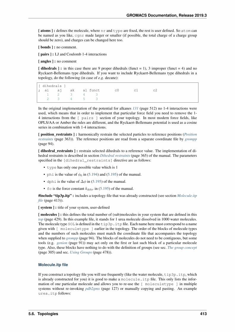
GROMACS Documentation, Release 2019.3
[ atoms ] : defines the molecule, where nr and type are fixed, the rest is user defined. So atom canbe named as you like, cgnr made larger or smaller (if possible, the total charge of a charge groupshould be zero), and charges can be changed here too.
[ bonds ] : no comment.
[ pairs ] : LJ and Coulomb 1-4 interactions
[ angles ] : no comment
[ dihedrals ] : in this case there are 9 proper dihedrals (funct = 1), 3 improper (funct = 4) and noRyckaert-Bellemans type dihedrals. If you want to include Ryckaert-Bellemans type dihedrals in atopology, do the following (in case of e.g. decane):
[ dihedrals ]; ai aj ak al funct c0 c1 c2
1 2 3 4 32 3 4 5 3
In the original implementation of the potential for alkanes 131 (page 512) no 1-4 interactions wereused, which means that in order to implement that particular force field you need to remove the 1-4 interactions from the [ pairs ] section of your topology. In most modern force fields, likeOPLS/AA or Amber the rules are different, and the Ryckaert-Bellemans potential is used as a cosineseries in combination with 1-4 interactions.
[ position_restraints ] : harmonically restrain the selected particles to reference positions (Positionrestraints (page 363)). The reference positions are read from a separate coordinate file by grompp(page 94).
[ dihedral_restraints ] : restrain selected dihedrals to a reference value. The implementation of di-hedral restraints is described in section Dihedral restraints (page 365) of the manual. The parametersspecified in the [dihedral_restraints] directive are as follows:
• type has only one possible value which is 1
• phi is the value of 𝜑0 in (5.194) and (5.195) of the manual.
• dphi is the value of ∆𝜑 in (5.195) of the manual.
• fc is the force constant 𝑘𝑑𝑖ℎ𝑟 in (5.195) of the manual.
#include “tip3p.itp” : includes a topology file that was already constructed (see section Molecule.itpfile (page 413)).
[ system ] : title of your system, user-defined
[ molecules ] : this defines the total number of (sub)molecules in your system that are defined in thistop (page 429). In this example file, it stands for 1 urea molecule dissolved in 1000 water molecules.The molecule type SOL is defined in the tip3p.itp file. Each name here must correspond to a namegiven with [ moleculetype ] earlier in the topology. The order of the blocks of molecule typesand the numbers of such molecules must match the coordinate file that accompanies the topologywhen supplied to grompp (page 94). The blocks of molecules do not need to be contiguous, but sometools (e.g. genion (page 91)) may act only on the first or last such block of a particular moleculetype. Also, these blocks have nothing to do with the definition of groups (see sec. The group concept(page 305) and sec. Using Groups (page 478)).
Molecule.itp file
If you construct a topology file you will use frequently (like the water molecule, tip3p.itp, whichis already constructed for you) it is good to make a molecule.itp file. This only lists the infor-mation of one particular molecule and allows you to re-use the [ moleculetype ] in multiplesystems without re-invoking pdb2gmx (page 127) or manually copying and pasting. An exampleurea.itp follows:
5.6. Topologies 413
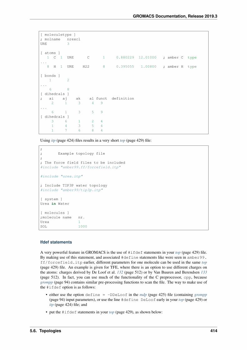
GROMACS Documentation, Release 2019.3
[ moleculetype ]; molname nrexclURE 3
[ atoms ]1 C 1 URE C 1 0.880229 12.01000 ; amber C type
...8 H 1 URE H22 8 0.395055 1.00800 ; amber H type
[ bonds ]1 2
...6 8
[ dihedrals ]; ai aj ak al funct definition
2 1 3 4 9...
6 1 3 5 9[ dihedrals ]
3 6 1 2 41 4 3 5 41 7 6 8 4
Using itp (page 424) files results in a very short top (page 429) file:
;; Example topology file;; The force field files to be included#include "amber99.ff/forcefield.itp"
#include "urea.itp"
; Include TIP3P water topology#include "amber99/tip3p.itp"
[ system ]Urea in Water
[ molecules ];molecule name nr.Urea 1SOL 1000
Ifdef statements
A very powerful feature in GROMACS is the use of #ifdef statements in your top (page 429) file.By making use of this statement, and associated #define statements like were seen in amber99.ff/forcefield.itp earlier, different parameters for one molecule can be used in the same top(page 429) file. An example is given for TFE, where there is an option to use different charges onthe atoms: charges derived by De Loof et al. 132 (page 512) or by Van Buuren and Berendsen 133(page 512). In fact, you can use much of the functionality of the C preprocessor, cpp, becausegrompp (page 94) contains similar pre-processing functions to scan the file. The way to make use ofthe #ifdef option is as follows:
• either use the option define = -DDeLoof in the mdp (page 425) file (containing grompp(page 94) input parameters), or use the line #define DeLoof early in your top (page 429) oritp (page 424) file; and
• put the #ifdef statements in your top (page 429), as shown below:
5.6. Topologies 414
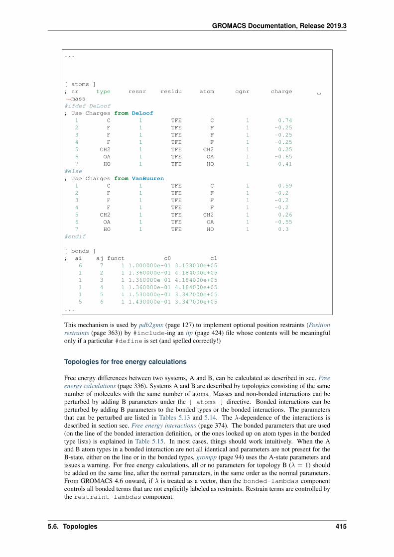
GROMACS Documentation, Release 2019.3
...
[ atoms ]; nr type resnr residu atom cgnr charge→˓mass#ifdef DeLoof; Use Charges from DeLoof
1 C 1 TFE C 1 0.742 F 1 TFE F 1 -0.253 F 1 TFE F 1 -0.254 F 1 TFE F 1 -0.255 CH2 1 TFE CH2 1 0.256 OA 1 TFE OA 1 -0.657 HO 1 TFE HO 1 0.41
#else; Use Charges from VanBuuren
1 C 1 TFE C 1 0.592 F 1 TFE F 1 -0.23 F 1 TFE F 1 -0.24 F 1 TFE F 1 -0.25 CH2 1 TFE CH2 1 0.266 OA 1 TFE OA 1 -0.557 HO 1 TFE HO 1 0.3
#endif
[ bonds ]; ai aj funct c0 c1
6 7 1 1.000000e-01 3.138000e+051 2 1 1.360000e-01 4.184000e+051 3 1 1.360000e-01 4.184000e+051 4 1 1.360000e-01 4.184000e+051 5 1 1.530000e-01 3.347000e+055 6 1 1.430000e-01 3.347000e+05
...
This mechanism is used by pdb2gmx (page 127) to implement optional position restraints (Positionrestraints (page 363)) by #include-ing an itp (page 424) file whose contents will be meaningfulonly if a particular #define is set (and spelled correctly!)
Topologies for free energy calculations
Free energy differences between two systems, A and B, can be calculated as described in sec. Freeenergy calculations (page 336). Systems A and B are described by topologies consisting of the samenumber of molecules with the same number of atoms. Masses and non-bonded interactions can beperturbed by adding B parameters under the [ atoms ] directive. Bonded interactions can beperturbed by adding B parameters to the bonded types or the bonded interactions. The parametersthat can be perturbed are listed in Tables 5.13 and 5.14. The 𝜆-dependence of the interactions isdescribed in section sec. Free energy interactions (page 374). The bonded parameters that are used(on the line of the bonded interaction definition, or the ones looked up on atom types in the bondedtype lists) is explained in Table 5.15. In most cases, things should work intuitively. When the Aand B atom types in a bonded interaction are not all identical and parameters are not present for theB-state, either on the line or in the bonded types, grompp (page 94) uses the A-state parameters andissues a warning. For free energy calculations, all or no parameters for topology B (𝜆 = 1) shouldbe added on the same line, after the normal parameters, in the same order as the normal parameters.From GROMACS 4.6 onward, if 𝜆 is treated as a vector, then the bonded-lambdas componentcontrols all bonded terms that are not explicitly labeled as restraints. Restrain terms are controlled bythe restraint-lambdas component.
5.6. Topologies 415
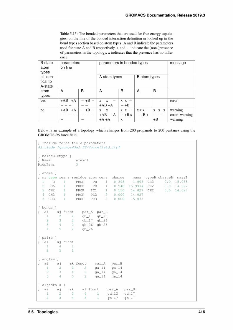
GROMACS Documentation, Release 2019.3
Table 5.15: The bonded parameters that are used for free energy topolo-gies, on the line of the bonded interaction definition or looked up in thebond types section based on atom types. A and B indicate the parametersused for state A and B respectively, + and − indicate the (non-)presenceof parameters in the topology, x indicates that the presence has no influ-ence.
B-stateatomtypesall iden-tical toA-stateatomtypes
parameterson line
parameters in bonded types message
A atom types B atom types
A B A B A B
yes +AB +A− − −
− +B −− −
x x −+AB +A
x x −− +B
error
no +AB +A− − − −−
− +B −− − −−
x x −+AB +A+A +A
x x −− +B xx
x x x −− +B +
x x x− − −+B
warningerror warningwarning
Below is an example of a topology which changes from 200 propanols to 200 pentanes using theGROMOS-96 force field.
; Include force field parameters#include "gromos43a1.ff/forcefield.itp"
[ moleculetype ]; Name nrexclPropPent 3
[ atoms ]; nr type resnr residue atom cgnr charge mass typeB chargeB massB1 H 1 PROP PH 1 0.398 1.008 CH3 0.0 15.0352 OA 1 PROP PO 1 -0.548 15.9994 CH2 0.0 14.0273 CH2 1 PROP PC1 1 0.150 14.027 CH2 0.0 14.0274 CH2 1 PROP PC2 2 0.000 14.0275 CH3 1 PROP PC3 2 0.000 15.035
[ bonds ]; ai aj funct par_A par_B
1 2 2 gb_1 gb_262 3 2 gb_17 gb_263 4 2 gb_26 gb_264 5 2 gb_26
[ pairs ]; ai aj funct
1 4 12 5 1
[ angles ]; ai aj ak funct par_A par_B
1 2 3 2 ga_11 ga_142 3 4 2 ga_14 ga_143 4 5 2 ga_14 ga_14
[ dihedrals ]; ai aj ak al funct par_A par_B
1 2 3 4 1 gd_12 gd_172 3 4 5 1 gd_17 gd_17
5.6. Topologies 416
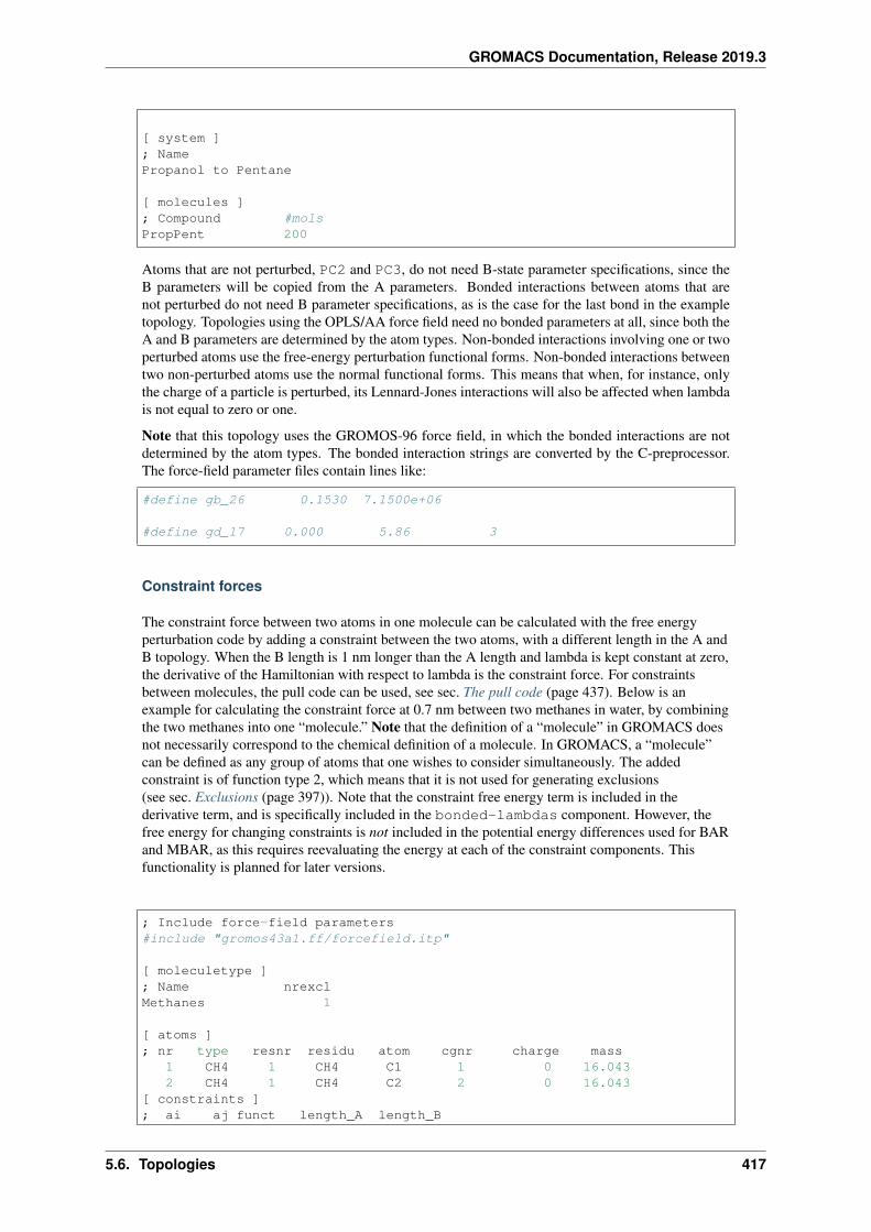
GROMACS Documentation, Release 2019.3
[ system ]; NamePropanol to Pentane
[ molecules ]; Compound #molsPropPent 200
Atoms that are not perturbed, PC2 and PC3, do not need B-state parameter specifications, since theB parameters will be copied from the A parameters. Bonded interactions between atoms that arenot perturbed do not need B parameter specifications, as is the case for the last bond in the exampletopology. Topologies using the OPLS/AA force field need no bonded parameters at all, since both theA and B parameters are determined by the atom types. Non-bonded interactions involving one or twoperturbed atoms use the free-energy perturbation functional forms. Non-bonded interactions betweentwo non-perturbed atoms use the normal functional forms. This means that when, for instance, onlythe charge of a particle is perturbed, its Lennard-Jones interactions will also be affected when lambdais not equal to zero or one.
Note that this topology uses the GROMOS-96 force field, in which the bonded interactions are notdetermined by the atom types. The bonded interaction strings are converted by the C-preprocessor.The force-field parameter files contain lines like:
#define gb_26 0.1530 7.1500e+06
#define gd_17 0.000 5.86 3
Constraint forces
The constraint force between two atoms in one molecule can be calculated with the free energyperturbation code by adding a constraint between the two atoms, with a different length in the A andB topology. When the B length is 1 nm longer than the A length and lambda is kept constant at zero,the derivative of the Hamiltonian with respect to lambda is the constraint force. For constraintsbetween molecules, the pull code can be used, see sec. The pull code (page 437). Below is anexample for calculating the constraint force at 0.7 nm between two methanes in water, by combiningthe two methanes into one “molecule.” Note that the definition of a “molecule” in GROMACS doesnot necessarily correspond to the chemical definition of a molecule. In GROMACS, a “molecule”can be defined as any group of atoms that one wishes to consider simultaneously. The addedconstraint is of function type 2, which means that it is not used for generating exclusions(see sec. Exclusions (page 397)). Note that the constraint free energy term is included in thederivative term, and is specifically included in the bonded-lambdas component. However, thefree energy for changing constraints is not included in the potential energy differences used for BARand MBAR, as this requires reevaluating the energy at each of the constraint components. Thisfunctionality is planned for later versions.
; Include force-field parameters#include "gromos43a1.ff/forcefield.itp"
[ moleculetype ]; Name nrexclMethanes 1
[ atoms ]; nr type resnr residu atom cgnr charge mass
1 CH4 1 CH4 C1 1 0 16.0432 CH4 1 CH4 C2 2 0 16.043
[ constraints ]; ai aj funct length_A length_B
5.6. Topologies 417
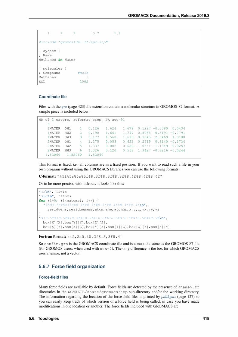
GROMACS Documentation, Release 2019.3
1 2 2 0.7 1.7
#include "gromos43a1.ff/spc.itp"
[ system ]; NameMethanes in Water
[ molecules ]; Compound #molsMethanes 1SOL 2002
Coordinate file
Files with the gro (page 423) file extension contain a molecular structure in GROMOS-87 format. Asample piece is included below:
MD of 2 waters, reformat step, PA aug-9161WATER OW1 1 0.126 1.624 1.679 0.1227 -0.0580 0.04341WATER HW2 2 0.190 1.661 1.747 0.8085 0.3191 -0.77911WATER HW3 3 0.177 1.568 1.613 -0.9045 -2.6469 1.31802WATER OW1 4 1.275 0.053 0.622 0.2519 0.3140 -0.17342WATER HW2 5 1.337 0.002 0.680 -1.0641 -1.1349 0.02572WATER HW3 6 1.326 0.120 0.568 1.9427 -0.8216 -0.0244
1.82060 1.82060 1.82060
This format is fixed, i.e. all columns are in a fixed position. If you want to read such a file in yourown program without using the GROMACS libraries you can use the following formats:
C-format: “%5i%5s%5s%5i%8.3f%8.3f%8.3f%8.4f%8.4f%8.4f”
Or to be more precise, with title etc. it looks like this:
"%s\n", Title"%5d\n", natomsfor (i=0; (i<natoms); i++) {"%5d%-5s%5s%5d%8.3f%8.3f%8.3f%8.4f%8.4f%8.4f\n",residuenr,residuename,atomname,atomnr,x,y,z,vx,vy,vz
}"%10.5f%10.5f%10.5f%10.5f%10.5f%10.5f%10.5f%10.5f%10.5f\n",box[X][X],box[Y][Y],box[Z][Z],box[X][Y],box[X][Z],box[Y][X],box[Y][Z],box[Z][X],box[Z][Y]
Fortran format: (i5,2a5,i5,3f8.3,3f8.4)
So confin.gro is the GROMACS coordinate file and is almost the same as the GROMOS-87 file(for GROMOS users: when used with ntx=7). The only difference is the box for which GROMACSuses a tensor, not a vector.
5.6.7 Force field organization
Force-field files
Many force fields are available by default. Force fields are detected by the presence of <name>.ffdirectories in the $GMXLIB/share/gromacs/top sub-directory and/or the working directory.The information regarding the location of the force field files is printed by pdb2gmx (page 127) soyou can easily keep track of which version of a force field is being called, in case you have mademodifications in one location or another. The force fields included with GROMACS are:
5.6. Topologies 418
GROMACS Documentation, Release 2019.3
• AMBER03 protein, nucleic AMBER94 (Duan et al., J. Comp. Chem. 24, 1999-2012, 2003)
• AMBER94 force field (Cornell et al., JACS 117, 5179-5197, 1995)
• AMBER96 protein, nucleic AMBER94 (Kollman et al., Acc. Chem. Res. 29, 461-469, 1996)
• AMBER99 protein, nucleic AMBER94 (Wang et al., J. Comp. Chem. 21, 1049-1074, 2000)
• AMBER99SB protein, nucleic AMBER94 (Hornak et al., Proteins 65, 712-725, 2006)
• AMBER99SB-ILDN protein, nucleic AMBER94 (Lindorff-Larsen et al., Proteins 78, 1950-58,2010)
• AMBERGS force field (Garcia & Sanbonmatsu, PNAS 99, 2782-2787, 2002)
• CHARMM27 all-atom force field (CHARM22 plus CMAP for proteins)
• GROMOS96 43a1 force field
• GROMOS96 43a2 force field (improved alkane dihedrals)
• GROMOS96 45a3 force field (Schuler JCC 2001 22 1205)
• GROMOS96 53a5 force field (JCC 2004 vol 25 pag 1656)
• GROMOS96 53a6 force field (JCC 2004 vol 25 pag 1656)
• GROMOS96 54a7 force field (Eur. Biophys. J. (2011), 40„ 843-856, DOI: 10.1007/s00249-011-0700-9)
• OPLS-AA/L all-atom force field (2001 aminoacid dihedrals)
A force field is included at the beginning of a topology file with an #include statement followedby <name>.ff/forcefield.itp. This statement includes the force-field file, which, in turn,may include other force-field files. All the force fields are organized in the same way. An example ofthe amber99.ff/forcefield.itp was shown in Topology file (page 405).
For each force field, there several files which are only used by pdb2gmx (page 127). These are:residue databases (rtp (page 428)) the hydrogen database (hdb (page 424)), two termini databases(.n.tdb and .c.tdb, see ) and the atom type database (atp (page 421)), which contains only themasses. Other optional files are described in sec. pdb2gmx input files (page 398).
Changing force-field parameters
If one wants to change the parameters of few bonded interactions in a molecule, this is most easilyaccomplished by typing the parameters behind the definition of the bonded interaction directly in thetop (page 429) file under the [ moleculetype ] section (see Topology file (page 405) for theformat and units). If one wants to change the parameters for all instances of a certain interaction onecan change them in the force-field file or add a new [ ???types ] section after including the forcefield. When parameters for a certain interaction are defined multiple times, the last definition is used.As of GROMACS version 3.1.3, a warning is generated when parameters are redefined with a differentvalue. Changing the Lennard-Jones parameters of an atom type is not recommended, because in theGROMOS force fields the Lennard-Jones parameters for several combinations of atom types are notgenerated according to the standard combination rules. Such combinations (and possibly others thatdo follow the combination rules) are defined in the [ nonbond_params ] section, and changingthe Lennard-Jones parameters of an atom type has no effect on these combinations.
Adding atom types
As of GROMACS version 3.1.3, atom types can be added in an extra [ atomtypes ] sectionafter the inclusion of the normal force field. After the definition of the new atom type(s), additionalnon-bonded and pair parameters can be defined. In pre-3.1.3 versions of GROMACS, the new atomtypes needed to be added in the [ atomtypes ] section of the force-field files, because all non-bonded parameters above the last [ atomtypes ] section would be overwritten using the standardcombination rules.
5.6. Topologies 419
GROMACS Documentation, Release 2019.3
5.7 File formats
5.7.1 Summary of file formats
Parameter files
mdp (page 425) run parameters, input for gmx grompp (page 94) and gmx convert-tpr (page 60)
m2p (page 424) input for gmx xpm2ps (page 179)
Structure files
gro (page 423) GROMACS format
g96 (page 423) GROMOS-96 format
pdb (page 427) brookhaven Protein DataBank format
Structure+mass(db): tpr (page 431), gro (page 423), g96 (page 423), or pdb (page 427) Structureand mass input for analysis tools. When gro or pdb is used approximate masses will be readfrom the mass database.
Topology files
top (page 429) system topology (ascii)
itp (page 424) include topology (ascii)
rtp (page 428) residue topology (ascii)
ndx (page 426) index file (ascii)
n2t (page 427) atom naming definition (ascii)
atp (page 421) atom type library (ascii)
r2b (page 429) residue to building block mapping (ascii)
arn (page 421) atom renaming database (ascii)
hdb (page 424) hydrogen atom database (ascii)
vsd (page 431) virtual site database (ascii)
tdb (page 429) termini database (ascii)
Run Input files
tpr (page 431) system topology, parameters, coordinates and velocities (binary, portable)
Trajectory files
tng (page 429) Any kind of data (compressed, portable, any precision)
trr (page 431) x, v and f (binary, full precision, portable)
xtc (page 432) x only (compressed, portable, any precision)
gro (page 423) x and v (ascii, any precision)
g96 (page 423) x only (ascii, fixed high precision)
pdb (page 427) x only (ascii, reduced precision)
5.7. File formats 420
GROMACS Documentation, Release 2019.3
Formats for full-precision data: tng (page 429) or trr (page 431)
Generic trajectory formats: tng (page 429), xtc (page 432), trr (page 431), gro (page 423), g96(page 423), or pdb (page 427)
Energy files
ene (page 422) energies, temperature, pressure, box size, density and virials (binary)
edr (page 422) energies, temperature, pressure, box size, density and virials (binary, portable)
Generic energy formats: edr (page 422) or ene (page 422)
Other files
dat (page 421) generic, preferred for input
edi (page 422) essential dynamics constraints input for gmx mdrun (page 111)
eps (page 422) Encapsulated Postscript
log (page 424) log file
map (page 425) colormap input for gmx do_dssp (page 74)
mtx (page 426) binary matrix data
out (page 427) generic, preferred for output
tex (page 429) LaTeX input
xpm (page 432) ascii matrix data, use gmx xpm2ps (page 179) to convert to eps (page 422)
xvg (page 434) xvgr input
5.7.2 File format details
atp
The atp file contains general information about atom types, like the atom number and the mass inatomic mass units.
arn
The arn file allows the renaming of atoms from their force field names to the names as defined byIUPAC/PDB, to allow easier visualization and identification.
cpt
The cpt file extension stands for portable checkpoint file. The complete state of the simulation isstored in the checkpoint file, including extended thermostat/barostat variables, random number statesand NMR time averaged data. With domain decomposition also the some decomposition setup infor-mation is stored.
See also gmx mdrun (page 111).
dat
Files with the dat file extension contain generic input or output. As it is not possible to categorize alldata file formats, GROMACS has a generic file format called dat of which no format is given.
5.7. File formats 421
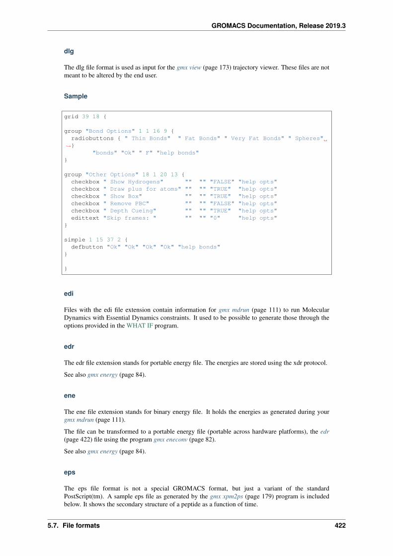
GROMACS Documentation, Release 2019.3
dlg
The dlg file format is used as input for the gmx view (page 173) trajectory viewer. These files are notmeant to be altered by the end user.
Sample
grid 39 18 {
group "Bond Options" 1 1 16 9 {radiobuttons { " Thin Bonds" " Fat Bonds" " Very Fat Bonds" " Spheres"
→˓}"bonds" "Ok" " F" "help bonds"
}
group "Other Options" 18 1 20 13 {checkbox " Show Hydrogens" "" "" "FALSE" "help opts"checkbox " Draw plus for atoms" "" "" "TRUE" "help opts"checkbox " Show Box" "" "" "TRUE" "help opts"checkbox " Remove PBC" "" "" "FALSE" "help opts"checkbox " Depth Cueing" "" "" "TRUE" "help opts"edittext "Skip frames: " "" "" "0" "help opts"
}
simple 1 15 37 2 {defbutton "Ok" "Ok" "Ok" "Ok" "help bonds"
}
}
edi
Files with the edi file extension contain information for gmx mdrun (page 111) to run MolecularDynamics with Essential Dynamics constraints. It used to be possible to generate those through theoptions provided in the WHAT IF program.
edr
The edr file extension stands for portable energy file. The energies are stored using the xdr protocol.
See also gmx energy (page 84).
ene
The ene file extension stands for binary energy file. It holds the energies as generated during yourgmx mdrun (page 111).
The file can be transformed to a portable energy file (portable across hardware platforms), the edr(page 422) file using the program gmx eneconv (page 82).
See also gmx energy (page 84).
eps
The eps file format is not a special GROMACS format, but just a variant of the standardPostScript(tm). A sample eps file as generated by the gmx xpm2ps (page 179) program is includedbelow. It shows the secondary structure of a peptide as a function of time.
5.7. File formats 422
GROMACS Documentation, Release 2019.3
g96
A file with the g96 extension can be a GROMOS-96 initial/final configuration file or a coordinatetrajectory file or a combination of both. The file is fixed format, all floats are written as 15.9 (files canget huge). GROMACS supports the following data blocks in the given order:
• Header block:
– TITLE (mandatory)
• Frame blocks:
– TIMESTEP (optional)
– POSITION/POSITIONRED (mandatory)
– VELOCITY/VELOCITYRED (optional)
– BOX (optional)
See the GROMOS-96 manual for a complete description of the blocks.
Note that all GROMACS programs can read compressed or g-zipped files.
gro
Files with the gro file extension contain a molecular structure in Gromos87 format. gro files can beused as trajectory by simply concatenating files. An attempt will be made to read a time value fromthe title string in each frame, which should be preceded by ‘t=’, as in the sample below.
A sample piece is included below:
MD of 2 waters, t= 0.061WATER OW1 1 0.126 1.624 1.679 0.1227 -0.0580 0.04341WATER HW2 2 0.190 1.661 1.747 0.8085 0.3191 -0.77911WATER HW3 3 0.177 1.568 1.613 -0.9045 -2.6469 1.31802WATER OW1 4 1.275 0.053 0.622 0.2519 0.3140 -0.17342WATER HW2 5 1.337 0.002 0.680 -1.0641 -1.1349 0.02572WATER HW3 6 1.326 0.120 0.568 1.9427 -0.8216 -0.0244
1.82060 1.82060 1.82060
Lines contain the following information (top to bottom):
• title string (free format string, optional time in ps after ‘t=’)
• number of atoms (free format integer)
• one line for each atom (fixed format, see below)
• box vectors (free format, space separated reals), values: v1(x) v2(y) v3(z) v1(y) v1(z) v2(x)v2(z) v3(x) v3(y), the last 6 values may be omitted (they will be set to zero). GROMACS onlysupports boxes with v1(y)=v1(z)=v2(z)=0.
This format is fixed, ie. all columns are in a fixed position. Optionally (for now only yet with trjconv)you can write gro files with any number of decimal places, the format will then be n+5 positionswith n decimal places (n+1 for velocities) in stead of 8 with 3 (with 4 for velocities). Upon reading,the precision will be inferred from the distance between the decimal points (which will be n+5).Columns contain the following information (from left to right):
• residue number (5 positions, integer)
5.7. File formats 423
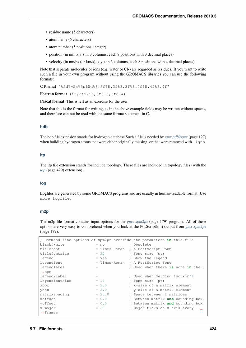
GROMACS Documentation, Release 2019.3
• residue name (5 characters)
• atom name (5 characters)
• atom number (5 positions, integer)
• position (in nm, x y z in 3 columns, each 8 positions with 3 decimal places)
• velocity (in nm/ps (or km/s), x y z in 3 columns, each 8 positions with 4 decimal places)
Note that separate molecules or ions (e.g. water or Cl-) are regarded as residues. If you want to writesuch a file in your own program without using the GROMACS libraries you can use the followingformats:
C format "%5d%-5s%5s%5d%8.3f%8.3f%8.3f%8.4f%8.4f%8.4f"
Fortran format (i5,2a5,i5,3f8.3,3f8.4)
Pascal format This is left as an exercise for the user
Note that this is the format for writing, as in the above example fields may be written without spaces,and therefore can not be read with the same format statement in C.
hdb
The hdb file extension stands for hydrogen database Such a file is needed by gmx pdb2gmx (page 127)when building hydrogen atoms that were either originally missing, or that were removed with -ignh.
itp
The itp file extension stands for include topology. These files are included in topology files (with thetop (page 429) extension).
log
Logfiles are generated by some GROMACS programs and are usually in human-readable format. Usemore logfile.
m2p
The m2p file format contains input options for the gmx xpm2ps (page 179) program. All of theseoptions are very easy to comprehend when you look at the PosScript(tm) output from gmx xpm2ps(page 179).
; Command line options of xpm2ps override the parameters in this fileblack&white = no ; Obsoletetitlefont = Times-Roman ; A PostScript Fonttitlefontsize = 20 ; Font size (pt)legend = yes ; Show the legendlegendfont = Times-Roman ; A PostScript Fontlegendlabel = ; Used when there is none in the .→˓xpmlegend2label = ; Used when merging two xpm'slegendfontsize = 14 ; Font size (pt)xbox = 2.0 ; x-size of a matrix elementybox = 2.0 ; y-size of a matrix elementmatrixspacing = 20.0 ; Space between 2 matricesxoffset = 0.0 ; Between matrix and bounding boxyoffset = 0.0 ; Between matrix and bounding boxx-major = 20 ; Major ticks on x axis every ..→˓frames
5.7. File formats 424
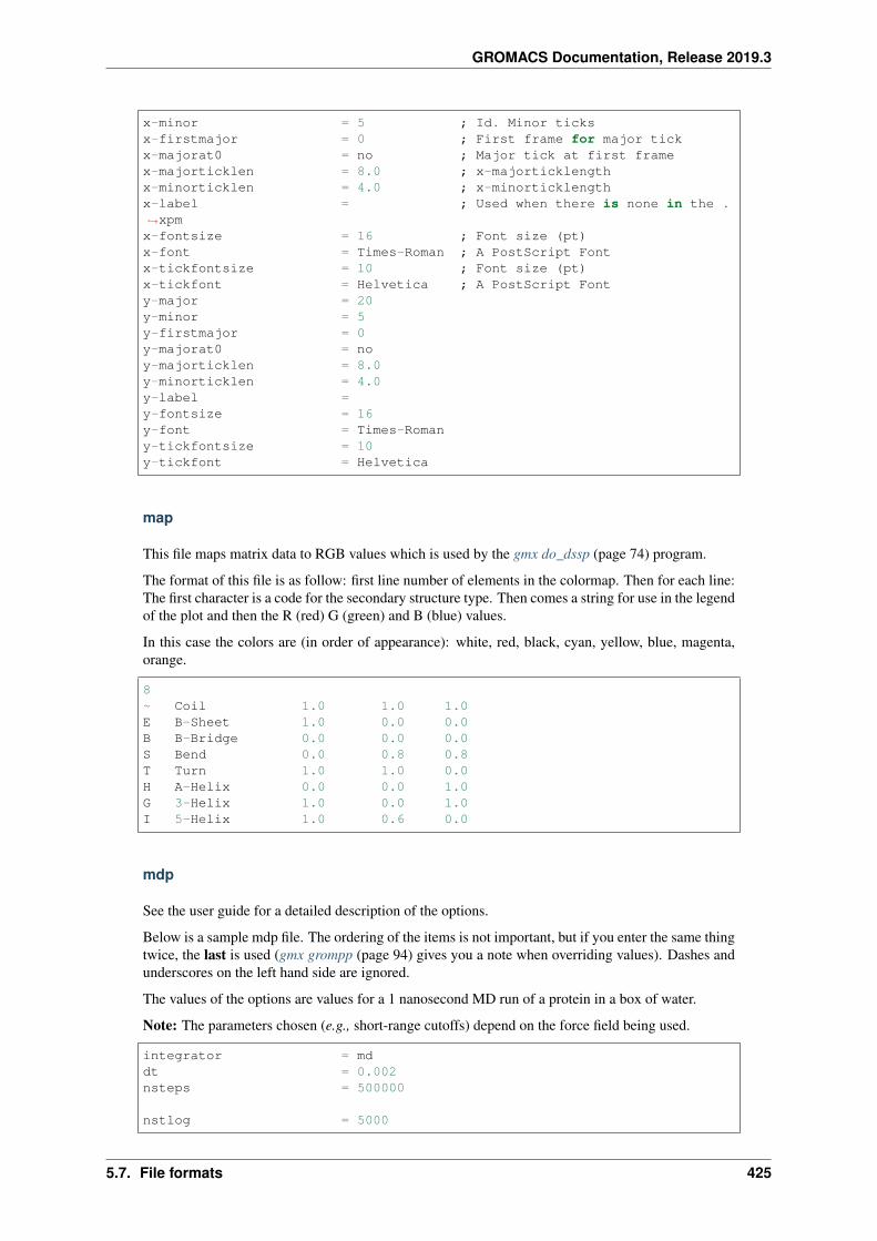
GROMACS Documentation, Release 2019.3
x-minor = 5 ; Id. Minor ticksx-firstmajor = 0 ; First frame for major tickx-majorat0 = no ; Major tick at first framex-majorticklen = 8.0 ; x-majorticklengthx-minorticklen = 4.0 ; x-minorticklengthx-label = ; Used when there is none in the .→˓xpmx-fontsize = 16 ; Font size (pt)x-font = Times-Roman ; A PostScript Fontx-tickfontsize = 10 ; Font size (pt)x-tickfont = Helvetica ; A PostScript Fonty-major = 20y-minor = 5y-firstmajor = 0y-majorat0 = noy-majorticklen = 8.0y-minorticklen = 4.0y-label =y-fontsize = 16y-font = Times-Romany-tickfontsize = 10y-tickfont = Helvetica
map
This file maps matrix data to RGB values which is used by the gmx do_dssp (page 74) program.
The format of this file is as follow: first line number of elements in the colormap. Then for each line:The first character is a code for the secondary structure type. Then comes a string for use in the legendof the plot and then the R (red) G (green) and B (blue) values.
In this case the colors are (in order of appearance): white, red, black, cyan, yellow, blue, magenta,orange.
8~ Coil 1.0 1.0 1.0E B-Sheet 1.0 0.0 0.0B B-Bridge 0.0 0.0 0.0S Bend 0.0 0.8 0.8T Turn 1.0 1.0 0.0H A-Helix 0.0 0.0 1.0G 3-Helix 1.0 0.0 1.0I 5-Helix 1.0 0.6 0.0
mdp
See the user guide for a detailed description of the options.
Below is a sample mdp file. The ordering of the items is not important, but if you enter the same thingtwice, the last is used (gmx grompp (page 94) gives you a note when overriding values). Dashes andunderscores on the left hand side are ignored.
The values of the options are values for a 1 nanosecond MD run of a protein in a box of water.
Note: The parameters chosen (e.g., short-range cutoffs) depend on the force field being used.
integrator = mddt = 0.002nsteps = 500000
nstlog = 5000
5.7. File formats 425
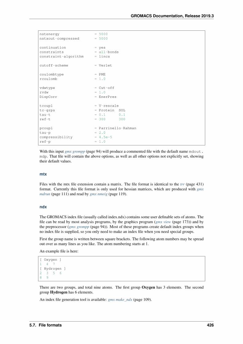
GROMACS Documentation, Release 2019.3
nstenergy = 5000nstxout-compressed = 5000
continuation = yesconstraints = all-bondsconstraint-algorithm = lincs
cutoff-scheme = Verlet
coulombtype = PMErcoulomb = 1.0
vdwtype = Cut-offrvdw = 1.0DispCorr = EnerPres
tcoupl = V-rescaletc-grps = Protein SOLtau-t = 0.1 0.1ref-t = 300 300
pcoupl = Parrinello-Rahmantau-p = 2.0compressibility = 4.5e-5ref-p = 1.0
With this input gmx grompp (page 94) will produce a commented file with the default name mdout.mdp. That file will contain the above options, as well as all other options not explicitly set, showingtheir default values.
mtx
Files with the mtx file extension contain a matrix. The file format is identical to the trr (page 431)format. Currently this file format is only used for hessian matrices, which are produced with gmxmdrun (page 111) and read by gmx nmeig (page 119).
ndx
The GROMACS index file (usually called index.ndx) contains some user definable sets of atoms. Thefile can be read by most analysis programs, by the graphics program (gmx view (page 173)) and bythe preprocessor (gmx grompp (page 94)). Most of these programs create default index groups whenno index file is supplied, so you only need to make an index file when you need special groups.
First the group name is written between square brackets. The following atom numbers may be spreadout over as many lines as you like. The atom numbering starts at 1.
An example file is here:
[ Oxygen ]1 4 7[ Hydrogen ]2 3 5 68 9
There are two groups, and total nine atoms. The first group Oxygen has 3 elements. The secondgroup Hydrogen has 6 elements.
An index file generation tool is available: gmx make_ndx (page 109).
5.7. File formats 426
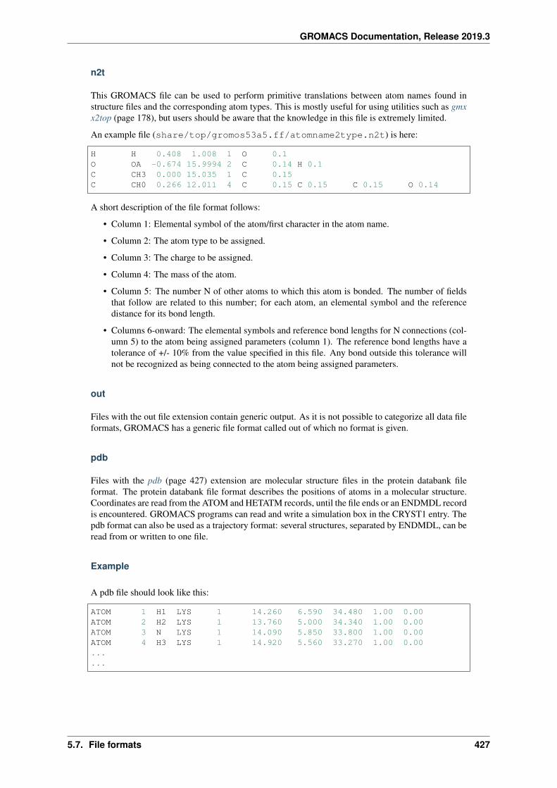
GROMACS Documentation, Release 2019.3
n2t
This GROMACS file can be used to perform primitive translations between atom names found instructure files and the corresponding atom types. This is mostly useful for using utilities such as gmxx2top (page 178), but users should be aware that the knowledge in this file is extremely limited.
An example file (share/top/gromos53a5.ff/atomname2type.n2t) is here:
H H 0.408 1.008 1 O 0.1O OA -0.674 15.9994 2 C 0.14 H 0.1C CH3 0.000 15.035 1 C 0.15C CH0 0.266 12.011 4 C 0.15 C 0.15 C 0.15 O 0.14
A short description of the file format follows:
• Column 1: Elemental symbol of the atom/first character in the atom name.
• Column 2: The atom type to be assigned.
• Column 3: The charge to be assigned.
• Column 4: The mass of the atom.
• Column 5: The number N of other atoms to which this atom is bonded. The number of fieldsthat follow are related to this number; for each atom, an elemental symbol and the referencedistance for its bond length.
• Columns 6-onward: The elemental symbols and reference bond lengths for N connections (col-umn 5) to the atom being assigned parameters (column 1). The reference bond lengths have atolerance of +/- 10% from the value specified in this file. Any bond outside this tolerance willnot be recognized as being connected to the atom being assigned parameters.
out
Files with the out file extension contain generic output. As it is not possible to categorize all data fileformats, GROMACS has a generic file format called out of which no format is given.
pdb
Files with the pdb (page 427) extension are molecular structure files in the protein databank fileformat. The protein databank file format describes the positions of atoms in a molecular structure.Coordinates are read from the ATOM and HETATM records, until the file ends or an ENDMDL recordis encountered. GROMACS programs can read and write a simulation box in the CRYST1 entry. Thepdb format can also be used as a trajectory format: several structures, separated by ENDMDL, can beread from or written to one file.
Example
A pdb file should look like this:
ATOM 1 H1 LYS 1 14.260 6.590 34.480 1.00 0.00ATOM 2 H2 LYS 1 13.760 5.000 34.340 1.00 0.00ATOM 3 N LYS 1 14.090 5.850 33.800 1.00 0.00ATOM 4 H3 LYS 1 14.920 5.560 33.270 1.00 0.00......
5.7. File formats 427
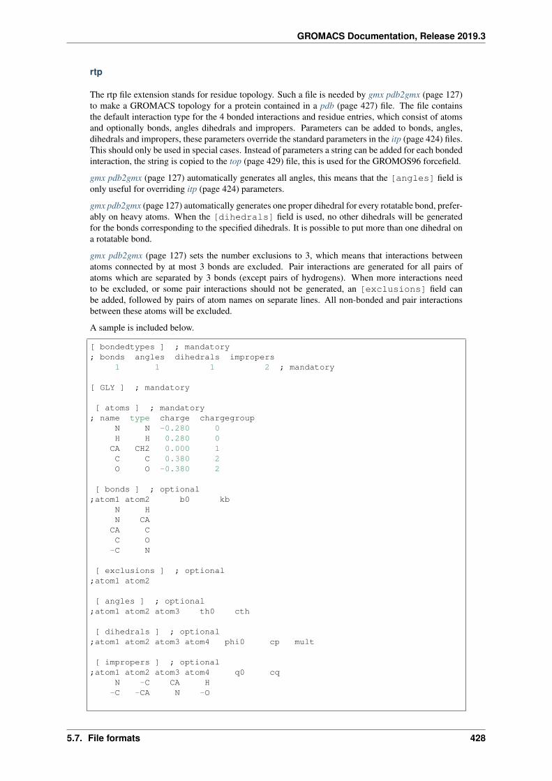
GROMACS Documentation, Release 2019.3
rtp
The rtp file extension stands for residue topology. Such a file is needed by gmx pdb2gmx (page 127)to make a GROMACS topology for a protein contained in a pdb (page 427) file. The file containsthe default interaction type for the 4 bonded interactions and residue entries, which consist of atomsand optionally bonds, angles dihedrals and impropers. Parameters can be added to bonds, angles,dihedrals and impropers, these parameters override the standard parameters in the itp (page 424) files.This should only be used in special cases. Instead of parameters a string can be added for each bondedinteraction, the string is copied to the top (page 429) file, this is used for the GROMOS96 forcefield.
gmx pdb2gmx (page 127) automatically generates all angles, this means that the [angles] field isonly useful for overriding itp (page 424) parameters.
gmx pdb2gmx (page 127) automatically generates one proper dihedral for every rotatable bond, prefer-ably on heavy atoms. When the [dihedrals] field is used, no other dihedrals will be generatedfor the bonds corresponding to the specified dihedrals. It is possible to put more than one dihedral ona rotatable bond.
gmx pdb2gmx (page 127) sets the number exclusions to 3, which means that interactions betweenatoms connected by at most 3 bonds are excluded. Pair interactions are generated for all pairs ofatoms which are separated by 3 bonds (except pairs of hydrogens). When more interactions needto be excluded, or some pair interactions should not be generated, an [exclusions] field canbe added, followed by pairs of atom names on separate lines. All non-bonded and pair interactionsbetween these atoms will be excluded.
A sample is included below.
[ bondedtypes ] ; mandatory; bonds angles dihedrals impropers
1 1 1 2 ; mandatory
[ GLY ] ; mandatory
[ atoms ] ; mandatory; name type charge chargegroup
N N -0.280 0H H 0.280 0
CA CH2 0.000 1C C 0.380 2O O -0.380 2
[ bonds ] ; optional;atom1 atom2 b0 kb
N HN CA
CA CC O
-C N
[ exclusions ] ; optional;atom1 atom2
[ angles ] ; optional;atom1 atom2 atom3 th0 cth
[ dihedrals ] ; optional;atom1 atom2 atom3 atom4 phi0 cp mult
[ impropers ] ; optional;atom1 atom2 atom3 atom4 q0 cq
N -C CA H-C -CA N -O
5.7. File formats 428
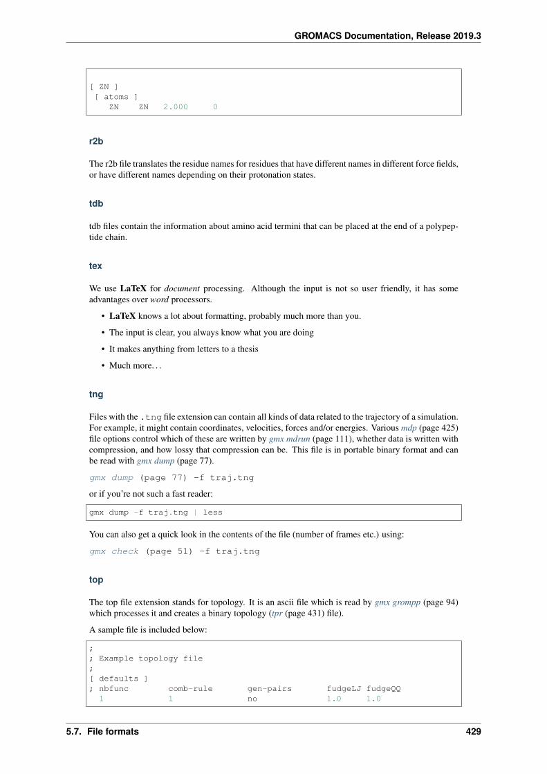
GROMACS Documentation, Release 2019.3
[ ZN ][ atoms ]
ZN ZN 2.000 0
r2b
The r2b file translates the residue names for residues that have different names in different force fields,or have different names depending on their protonation states.
tdb
tdb files contain the information about amino acid termini that can be placed at the end of a polypep-tide chain.
tex
We use LaTeX for document processing. Although the input is not so user friendly, it has someadvantages over word processors.
• LaTeX knows a lot about formatting, probably much more than you.
• The input is clear, you always know what you are doing
• It makes anything from letters to a thesis
• Much more. . .
tng
Files with the .tng file extension can contain all kinds of data related to the trajectory of a simulation.For example, it might contain coordinates, velocities, forces and/or energies. Various mdp (page 425)file options control which of these are written by gmx mdrun (page 111), whether data is written withcompression, and how lossy that compression can be. This file is in portable binary format and canbe read with gmx dump (page 77).
gmx dump (page 77) -f traj.tng
or if you’re not such a fast reader:
gmx dump -f traj.tng | less
You can also get a quick look in the contents of the file (number of frames etc.) using:
gmx check (page 51) -f traj.tng
top
The top file extension stands for topology. It is an ascii file which is read by gmx grompp (page 94)which processes it and creates a binary topology (tpr (page 431) file).
A sample file is included below:
;; Example topology file;[ defaults ]; nbfunc comb-rule gen-pairs fudgeLJ fudgeQQ1 1 no 1.0 1.0
5.7. File formats 429
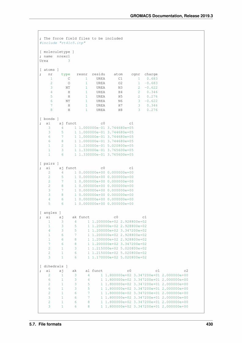
GROMACS Documentation, Release 2019.3
; The force field files to be included#include "rt41c5.itp"
[ moleculetype ]; name nrexclUrea 3
[ atoms ]; nr type resnr residu atom cgnr charge
1 C 1 UREA C1 1 0.6832 O 1 UREA O2 1 -0.6833 NT 1 UREA N3 2 -0.6224 H 1 UREA H4 2 0.3465 H 1 UREA H5 2 0.2766 NT 1 UREA N6 3 -0.6227 H 1 UREA H7 3 0.3468 H 1 UREA H8 3 0.276
[ bonds ]; ai aj funct c0 c1
3 4 1 1.000000e-01 3.744680e+053 5 1 1.000000e-01 3.744680e+056 7 1 1.000000e-01 3.744680e+056 8 1 1.000000e-01 3.744680e+051 2 1 1.230000e-01 5.020800e+051 3 1 1.330000e-01 3.765600e+051 6 1 1.330000e-01 3.765600e+05
[ pairs ]; ai aj funct c0 c1
2 4 1 0.000000e+00 0.000000e+002 5 1 0.000000e+00 0.000000e+002 7 1 0.000000e+00 0.000000e+002 8 1 0.000000e+00 0.000000e+003 7 1 0.000000e+00 0.000000e+003 8 1 0.000000e+00 0.000000e+004 6 1 0.000000e+00 0.000000e+005 6 1 0.000000e+00 0.000000e+00
[ angles ]; ai aj ak funct c0 c1
1 3 4 1 1.200000e+02 2.928800e+021 3 5 1 1.200000e+02 2.928800e+024 3 5 1 1.200000e+02 3.347200e+021 6 7 1 1.200000e+02 2.928800e+021 6 8 1 1.200000e+02 2.928800e+027 6 8 1 1.200000e+02 3.347200e+022 1 3 1 1.215000e+02 5.020800e+022 1 6 1 1.215000e+02 5.020800e+023 1 6 1 1.170000e+02 5.020800e+02
[ dihedrals ]; ai aj ak al funct c0 c1 c2
2 1 3 4 1 1.800000e+02 3.347200e+01 2.000000e+006 1 3 4 1 1.800000e+02 3.347200e+01 2.000000e+002 1 3 5 1 1.800000e+02 3.347200e+01 2.000000e+006 1 3 5 1 1.800000e+02 3.347200e+01 2.000000e+002 1 6 7 1 1.800000e+02 3.347200e+01 2.000000e+003 1 6 7 1 1.800000e+02 3.347200e+01 2.000000e+002 1 6 8 1 1.800000e+02 3.347200e+01 2.000000e+003 1 6 8 1 1.800000e+02 3.347200e+01 2.000000e+00
5.7. File formats 430
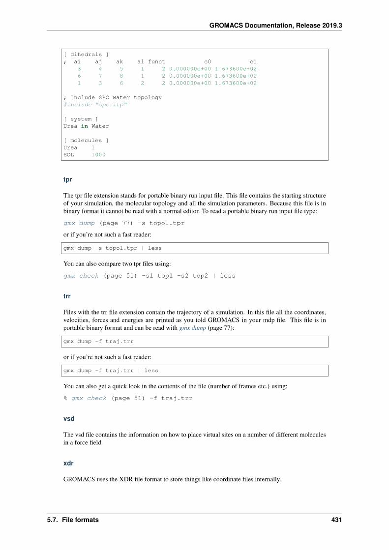
GROMACS Documentation, Release 2019.3
[ dihedrals ]; ai aj ak al funct c0 c1
3 4 5 1 2 0.000000e+00 1.673600e+026 7 8 1 2 0.000000e+00 1.673600e+021 3 6 2 2 0.000000e+00 1.673600e+02
; Include SPC water topology#include "spc.itp"
[ system ]Urea in Water
[ molecules ]Urea 1SOL 1000
tpr
The tpr file extension stands for portable binary run input file. This file contains the starting structureof your simulation, the molecular topology and all the simulation parameters. Because this file is inbinary format it cannot be read with a normal editor. To read a portable binary run input file type:
gmx dump (page 77) -s topol.tpr
or if you’re not such a fast reader:
gmx dump -s topol.tpr | less
You can also compare two tpr files using:
gmx check (page 51) -s1 top1 -s2 top2 | less
trr
Files with the trr file extension contain the trajectory of a simulation. In this file all the coordinates,velocities, forces and energies are printed as you told GROMACS in your mdp file. This file is inportable binary format and can be read with gmx dump (page 77):
gmx dump -f traj.trr
or if you’re not such a fast reader:
gmx dump -f traj.trr | less
You can also get a quick look in the contents of the file (number of frames etc.) using:
% gmx check (page 51) -f traj.trr
vsd
The vsd file contains the information on how to place virtual sites on a number of different moleculesin a force field.
xdr
GROMACS uses the XDR file format to store things like coordinate files internally.
5.7. File formats 431
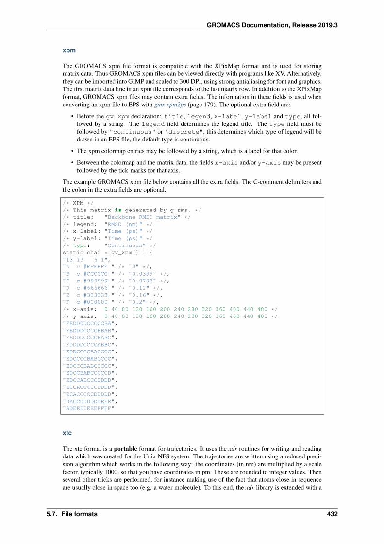
GROMACS Documentation, Release 2019.3
xpm
The GROMACS xpm file format is compatible with the XPixMap format and is used for storingmatrix data. Thus GROMACS xpm files can be viewed directly with programs like XV. Alternatively,they can be imported into GIMP and scaled to 300 DPI, using strong antialiasing for font and graphics.The first matrix data line in an xpm file corresponds to the last matrix row. In addition to the XPixMapformat, GROMACS xpm files may contain extra fields. The information in these fields is used whenconverting an xpm file to EPS with gmx xpm2ps (page 179). The optional extra field are:
• Before the gv_xpm declaration: title, legend, x-label, y-label and type, all fol-lowed by a string. The legend field determines the legend title. The type field must befollowed by "continuous" or "discrete", this determines which type of legend will bedrawn in an EPS file, the default type is continuous.
• The xpm colormap entries may be followed by a string, which is a label for that color.
• Between the colormap and the matrix data, the fields x-axis and/or y-axis may be presentfollowed by the tick-marks for that axis.
The example GROMACS xpm file below contains all the extra fields. The C-comment delimiters andthe colon in the extra fields are optional.
/* XPM *//* This matrix is generated by g_rms. *//* title: "Backbone RMSD matrix" *//* legend: "RMSD (nm)" *//* x-label: "Time (ps)" *//* y-label: "Time (ps)" *//* type: "Continuous" */static char * gv_xpm[] = {"13 13 6 1","A c #FFFFFF " /* "0" */,"B c #CCCCCC " /* "0.0399" */,"C c #999999 " /* "0.0798" */,"D c #666666 " /* "0.12" */,"E c #333333 " /* "0.16" */,"F c #000000 " /* "0.2" */,/* x-axis: 0 40 80 120 160 200 240 280 320 360 400 440 480 *//* y-axis: 0 40 80 120 160 200 240 280 320 360 400 440 480 */"FEDDDDCCCCCBA","FEDDDCCCCBBAB","FEDDDCCCCBABC","FDDDDCCCCABBC","EDDCCCCBACCCC","EDCCCCBABCCCC","EDCCCBABCCCCC","EDCCBABCCCCCD","EDCCABCCCDDDD","ECCACCCCCDDDD","ECACCCCCDDDDD","DACCDDDDDDEEE","ADEEEEEEEFFFF"
xtc
The xtc format is a portable format for trajectories. It uses the xdr routines for writing and readingdata which was created for the Unix NFS system. The trajectories are written using a reduced preci-sion algorithm which works in the following way: the coordinates (in nm) are multiplied by a scalefactor, typically 1000, so that you have coordinates in pm. These are rounded to integer values. Thenseveral other tricks are performed, for instance making use of the fact that atoms close in sequenceare usually close in space too (e.g. a water molecule). To this end, the xdr library is extended with a
5.7. File formats 432
GROMACS Documentation, Release 2019.3
special routine to write 3-D float coordinates. The routine was originally written by Frans van Hoeselas part of an Europort project. An updated version of it can be obtained through this link.
All the data is stored using calls to xdr routines.
int magic A magic number, for the current file version its value is 1995.
int natoms The number of atoms in the trajectory.
int step The simulation step.
float time The simulation time.
float box[3][3] The computational box which is stored as a set of three basis vectors, to allow fortriclinic PBC. For a rectangular box the box edges are stored on the diagonal of the matrix.
3dfcoord x[natoms] The coordinates themselves stored in reduced precision. Please note that whenthe number of atoms is smaller than 9 no reduced precision is used.
Using xtc in your “C” programs
To read and write these files the following “C” routines are available:
/* All functions return 1 if successful, 0 otherwise */
extern int open_xtc(XDR *xd,char *filename,char *mode);/* Open a file for xdr I/O */
extern void close_xtc(XDR *xd);/* Close the file for xdr I/O */
extern int read_first_xtc(XDR *xd,char *filename,int *natoms,int *step,real *time,matrix box,rvec **x,real *prec);
/* Open xtc file, read xtc file first time, allocate memory for x */
extern int read_next_xtc(XDR *xd,int *natoms,int *step,real *time,matrix box,rvec *x,real *prec);
/* Read subsequent frames */
extern int write_xtc(XDR *xd,int natoms,int step,real time,matrix box,rvec *x,real prec);
/* Write a frame to xtc file */
To use the library function include "gromacs/fileio/xtcio.h" in your file and link with-lgmx.$(CPU).
Using xtc in your FORTRAN programs
To read and write these in a FORTRAN program use the calls to readxtc and writextc as in thefollowing sample program which reads and xtc file and copies it to a new one:
program testxtc
parameter (maxatom=10000,maxx=3*maxatom)integer xd,xd2,natoms,step,ret,ireal time,box(9),x(maxx)
call xdrfopen(xd,"test.xtc","r",ret)print *,'opened test.xtc, ret=',ret
5.7. File formats 433
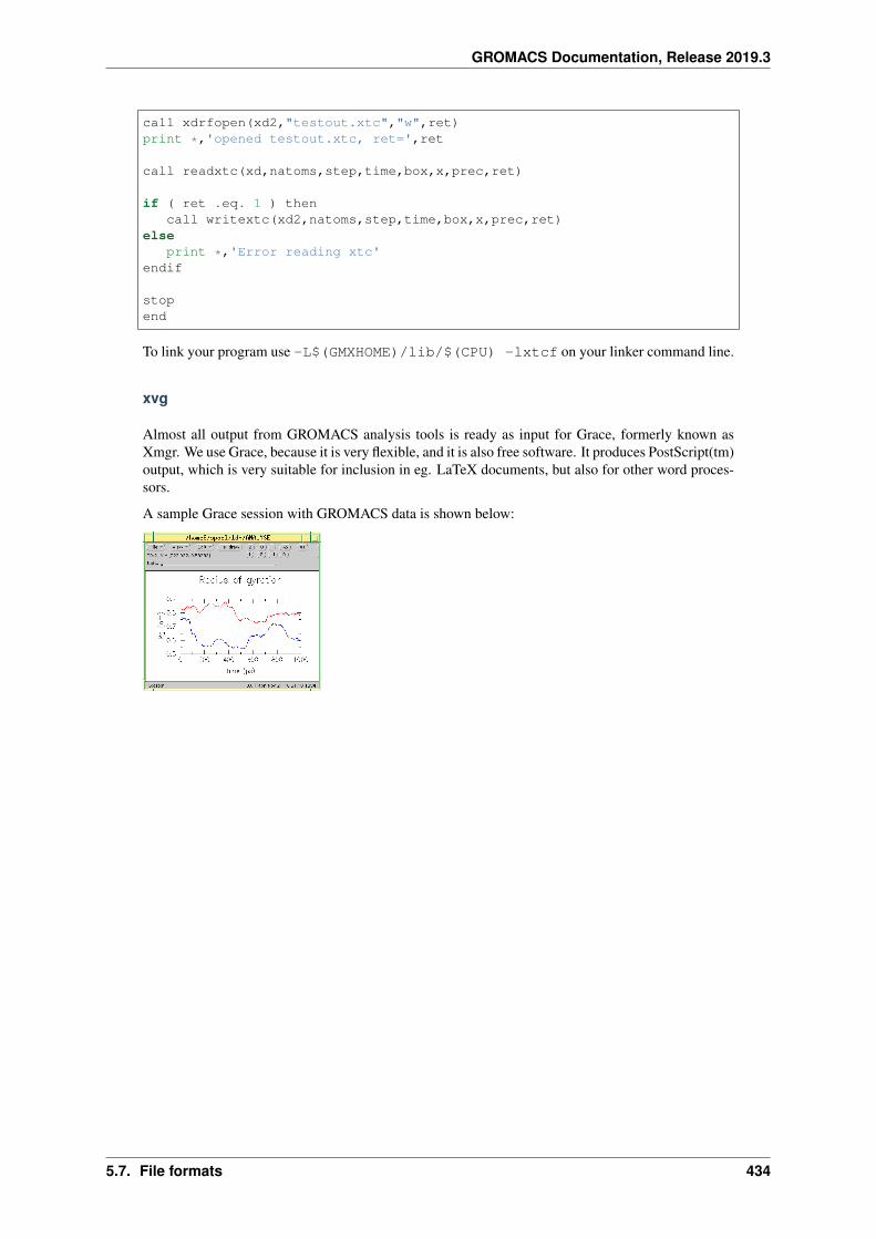
GROMACS Documentation, Release 2019.3
call xdrfopen(xd2,"testout.xtc","w",ret)print *,'opened testout.xtc, ret=',ret
call readxtc(xd,natoms,step,time,box,x,prec,ret)
if ( ret .eq. 1 ) thencall writextc(xd2,natoms,step,time,box,x,prec,ret)
elseprint *,'Error reading xtc'
endif
stopend
To link your program use -L$(GMXHOME)/lib/$(CPU) -lxtcf on your linker command line.
xvg
Almost all output from GROMACS analysis tools is ready as input for Grace, formerly known asXmgr. We use Grace, because it is very flexible, and it is also free software. It produces PostScript(tm)output, which is very suitable for inclusion in eg. LaTeX documents, but also for other word proces-sors.
A sample Grace session with GROMACS data is shown below:
5.7. File formats 434
GROMACS Documentation, Release 2019.3
5.8 Special Topics
This section covers some of the more specialized topics concerning the use of GROMACS for specificscientific problems.
5.8.1 Free energy implementation
For free energy calculations, there are two things that must be specified; the end states, and the path-way connecting the end states. The end states can be specified in two ways. The most straightforwardis through the specification of end states in the topology file. Most potential forms support both an𝐴 state and a 𝐵 state. Whenever both states are specified, the 𝐴 state corresponds to the initial freeenergy state, and the 𝐵 state corresponds to the final state.
In some cases, the end state can also be defined in some cases without altering the topology, solelythrough the mdp (page 425) file, through the use of the couple-moltype, couple-lambda0,couple-lambda1, and couple-intramol mdp (page 425) keywords. Any molecule typeselected in couple-moltype will automatically have a 𝐵 state implicitly constructed (andthe 𝐴 state redefined) according to the couple-lambda keywords. couple-lambda0and couple-lambda1 define the non-bonded parameters that are present in the 𝐴 state(couple-lambda0) and the 𝐵 state (couple-lambda1). The choices are q, vdw, and vdw-q;these indicate the Coulombic, van der Waals, or both parameters that are turned on in the respectivestate.
Once the end states are defined, then the path between the end states has to be defined. This path isdefined solely in the .mdp file. Starting in 4.6, 𝜆 is a vector of components, with Coulombic, van derWaals, bonded, restraint, and mass components all able to be adjusted independently. This makes itpossible to turn off the Coulombic term linearly, and then the van der Waals using soft core, all in thesame simulation. This is especially useful for replica exchange or expanded ensemble simulations,where it is important to sample all the way from interacting to non-interacting states in the samesimulation to improve sampling.
fep-lambdas is the default array of 𝜆 values ranging from 0 to 1. All of the other lambda arraysuse the values in this array if they are not specified. The previous behavior, where the pathwayis controlled by a single 𝜆 variable, can be preserved by using only fep-lambdas to define thepathway.
For example, if you wanted to first to change the Coulombic terms, then the van der Waals terms,changing bonded at the same time rate as the van der Waals, but changing the restraints throughoutthe first two-thirds of the simulation, then you could use this 𝜆 vector:
coul-lambdas = 0.0 0.2 0.5 1.0 1.0 1.0 1.0 1.0 1.0 1.0vdw-lambdas = 0.0 0.0 0.0 0.0 0.4 0.5 0.6 0.7 0.8 1.0bonded-lambdas = 0.0 0.0 0.0 0.0 0.4 0.5 0.6 0.7 0.8 1.0restraint-lambdas = 0.0 0.0 0.1 0.2 0.3 0.5 0.7 1.0 1.0 1.0
This is also equivalent to:
fep-lambdas = 0.0 0.0 0.0 0.0 0.4 0.5 0.6 0.7 0.8 1.0coul-lambdas = 0.0 0.2 0.5 1.0 1.0 1.0 1.0 1.0 1.0 1.0restraint-lambdas = 0.0 0.0 0.1 0.2 0.3 0.5 0.7 1.0 1.0 1.0
The fep-lambda array, in this case, is being used as the default to fill in the bonded and van derWaals 𝜆 arrays. Usually, it’s best to fill in all arrays explicitly, just to make sure things are properlyassigned.
If you want to turn on only restraints going from 𝐴 to 𝐵, then it would be:
restraint-lambdas = 0.0 0.1 0.2 0.4 0.6 1.0
and all of the other components of the 𝜆 vector would be left in the 𝐴 state.
5.8. Special Topics 435
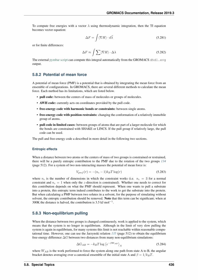
GROMACS Documentation, Release 2019.3
To compute free energies with a vector 𝜆 using thermodynamic integration, then the TI equationbecomes vector equation:
∆𝐹 =
∫⟨∇𝐻⟩ · 𝑑�� (5.281)
or for finite differences:
∆𝐹 ≈∫ ∑
⟨∇𝐻⟩ · ∆𝜆 (5.282)
The external pymbar script can compute this integral automatically from the GROMACS dhdl.xvgoutput.
5.8.2 Potential of mean force
A potential of mean force (PMF) is a potential that is obtained by integrating the mean force from anensemble of configurations. In GROMACS, there are several different methods to calculate the meanforce. Each method has its limitations, which are listed below.
• pull code: between the centers of mass of molecules or groups of molecules.
• AWH code: currently acts on coordinates provided by the pull code.
• free-energy code with harmonic bonds or constraints: between single atoms.
• free-energy code with position restraints: changing the conformation of a relatively immobilegroup of atoms.
• pull code in limited cases: between groups of atoms that are part of a larger molecule for whichthe bonds are constrained with SHAKE or LINCS. If the pull group if relatively large, the pullcode can be used.
The pull and free-energy code a described in more detail in the following two sections.
Entropic effects
When a distance between two atoms or the centers of mass of two groups is constrained or restrained,there will be a purely entropic contribution to the PMF due to the rotation of the two groups 134(page 512). For a system of two non-interacting masses the potential of mean force is:
𝑉𝑝𝑚𝑓 (𝑟) = −(𝑛𝑐 − 1)𝑘𝐵𝑇 log(𝑟) (5.283)
where 𝑛𝑐 is the number of dimensions in which the constraint works (i.e. 𝑛𝑐 = 3 for a normalconstraint and 𝑛𝑐 = 1 when only the 𝑧-direction is constrained). Whether one needs to correct forthis contribution depends on what the PMF should represent. When one wants to pull a substrateinto a protein, this entropic term indeed contributes to the work to get the substrate into the protein.But when calculating a PMF between two solutes in a solvent, for the purpose of simulating withoutsolvent, the entropic contribution should be removed. Note that this term can be significant; when at300K the distance is halved, the contribution is 3.5 kJ mol−1.
5.8.3 Non-equilibrium pulling
When the distance between two groups is changed continuously, work is applied to the system, whichmeans that the system is no longer in equilibrium. Although in the limit of very slow pulling thesystem is again in equilibrium, for many systems this limit is not reachable within reasonable compu-tational time. However, one can use the Jarzynski relation 135 (page 512) to obtain the equilibriumfree-energy difference ∆𝐺 between two distances from many non-equilibrium simulations:
∆𝐺𝐴𝐵 = −𝑘𝐵𝑇 log⟨𝑒−𝛽𝑊𝐴𝐵
⟩𝐴
(5.284)
where 𝑊𝐴𝐵 is the work performed to force the system along one path from state A to B, the angularbracket denotes averaging over a canonical ensemble of the initial state A and 𝛽 = 1/𝑘𝐵𝑇 .
5.8. Special Topics 436
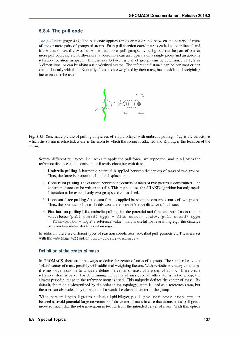
GROMACS Documentation, Release 2019.3
5.8.4 The pull code
The pull code (page 437) The pull code applies forces or constraints between the centers of massof one or more pairs of groups of atoms. Each pull reaction coordinate is called a “coordinate” andit operates on usually two, but sometimes more, pull groups. A pull group can be part of one ormore pull coordinates. Furthermore, a coordinate can also operate on a single group and an absolutereference position in space. The distance between a pair of groups can be determined in 1, 2 or3 dimensions, or can be along a user-defined vector. The reference distance can be constant or canchange linearly with time. Normally all atoms are weighted by their mass, but an additional weightingfactor can also be used.
V
zz link spring
rup
Fig. 5.35: Schematic picture of pulling a lipid out of a lipid bilayer with umbrella pulling. 𝑉𝑟𝑢𝑝 is the velocity atwhich the spring is retracted, 𝑍𝑙𝑖𝑛𝑘 is the atom to which the spring is attached and 𝑍𝑠𝑝𝑟𝑖𝑛𝑔 is the location of thespring.
Several different pull types, i.e. ways to apply the pull force, are supported, and in all cases thereference distance can be constant or linearly changing with time.
1. Umbrella pulling A harmonic potential is applied between the centers of mass of two groups.Thus, the force is proportional to the displacement.
2. Constraint pulling The distance between the centers of mass of two groups is constrained. Theconstraint force can be written to a file. This method uses the SHAKE algorithm but only needs1 iteration to be exact if only two groups are constrained.
3. Constant force pulling A constant force is applied between the centers of mass of two groups.Thus, the potential is linear. In this case there is no reference distance of pull rate.
4. Flat bottom pulling Like umbrella pulling, but the potential and force are zero for coordinatevalues below (pull-coord?-type = flat-bottom) or above (pull-coord?-type= flat-bottom-high) a reference value. This is useful for restraining e.g. the distancebetween two molecules to a certain region.
In addition, there are different types of reaction coordinates, so-called pull geometries. These are setwith the mdp (page 425) option pull-coord?-geometry.
Definition of the center of mass
In GROMACS, there are three ways to define the center of mass of a group. The standard way is a“plain” center of mass, possibly with additional weighting factors. With periodic boundary conditionsit is no longer possible to uniquely define the center of mass of a group of atoms. Therefore, areference atom is used. For determining the center of mass, for all other atoms in the group, theclosest periodic image to the reference atom is used. This uniquely defines the center of mass. Bydefault, the middle (determined by the order in the topology) atom is used as a reference atom, butthe user can also select any other atom if it would be closer to center of the group.
When there are large pull groups, such as a lipid bilayer, pull-pbc-ref-prev-step-com canbe used to avoid potential large movements of the center of mass in case that atoms in the pull groupmove so much that the reference atom is too far from the intended center of mass. With this option
5.8. Special Topics 437
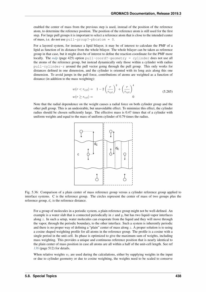
GROMACS Documentation, Release 2019.3
enabled the center of mass from the previous step is used, instead of the position of the referenceatom, to determine the reference position. The position of the reference atom is still used for the firststep. For large pull groups it is important to select a reference atom that is close to the intended centerof mass, i.e. do not use pull-group?-pbcatom = 0.
For a layered system, for instance a lipid bilayer, it may be of interest to calculate the PMF of alipid as function of its distance from the whole bilayer. The whole bilayer can be taken as referencegroup in that case, but it might also be of interest to define the reaction coordinate for the PMF morelocally. The mdp (page 425) option pull-coord?-geometry = cylinder does not use allthe atoms of the reference group, but instead dynamically only those within a cylinder with radiuspull-cylinder-r around the pull vector going through the pull group. This only works fordistances defined in one dimension, and the cylinder is oriented with its long axis along this onedimension. To avoid jumps in the pull force, contributions of atoms are weighted as a function ofdistance (in addition to the mass weighting):
𝑤(𝑟 < 𝑟cyl) = 1 − 2
(𝑟
𝑟cyl
)2
+
(𝑟
𝑟cyl
)4
𝑤(𝑟 ≥ 𝑟cyl) = 0
(5.285)
Note that the radial dependence on the weight causes a radial force on both cylinder group and theother pull group. This is an undesirable, but unavoidable effect. To minimize this effect, the cylinderradius should be chosen sufficiently large. The effective mass is 0.47 times that of a cylinder withuniform weights and equal to the mass of uniform cylinder of 0.79 times the radius.
c
cd
cd
Fig. 5.36: Comparison of a plain center of mass reference group versus a cylinder reference group applied tointerface systems. C is the reference group. The circles represent the center of mass of two groups plus thereference group, 𝑑𝑐 is the reference distance.
For a group of molecules in a periodic system, a plain reference group might not be well-defined. Anexample is a water slab that is connected periodically in 𝑥 and 𝑦, but has two liquid-vapor interfacesalong 𝑧. In such a setup, water molecules can evaporate from the liquid and they will move throughthe vapor, through the periodic boundary, to the other interface. Such a system is inherently periodicand there is no proper way of defining a “plain” center of mass along 𝑧. A proper solution is to usinga cosine shaped weighting profile for all atoms in the reference group. The profile is a cosine with asingle period in the unit cell. Its phase is optimized to give the maximum sum of weights, includingmass weighting. This provides a unique and continuous reference position that is nearly identical tothe plain center of mass position in case all atoms are all within a half of the unit-cell length. See ref136 (page 512) for details.
When relative weights 𝑤𝑖 are used during the calculations, either by supplying weights in the inputor due to cylinder geometry or due to cosine weighting, the weights need to be scaled to conserve
5.8. Special Topics 438
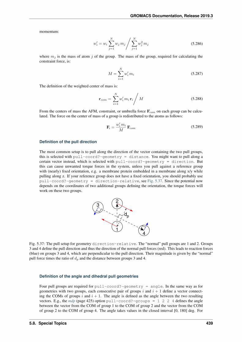
GROMACS Documentation, Release 2019.3
momentum:
𝑤′𝑖 = 𝑤𝑖
𝑁∑𝑗=1
𝑤𝑗 𝑚𝑗
⧸𝑁∑𝑗=1
𝑤2𝑗 𝑚𝑗 (5.286)
where 𝑚𝑗 is the mass of atom 𝑗 of the group. The mass of the group, required for calculating theconstraint force, is:
𝑀 =
𝑁∑𝑖=1
𝑤′𝑖𝑚𝑖 (5.287)
The definition of the weighted center of mass is:
r𝑐𝑜𝑚 =
𝑁∑𝑖=1
𝑤′𝑖𝑚𝑖 r𝑖
⧸𝑀 (5.288)
From the centers of mass the AFM, constraint, or umbrella force F𝑐𝑜𝑚 on each group can be calcu-lated. The force on the center of mass of a group is redistributed to the atoms as follows:
F𝑖 =𝑤′
𝑖𝑚𝑖
𝑀F𝑐𝑜𝑚 (5.289)
Definition of the pull direction
The most common setup is to pull along the direction of the vector containing the two pull groups,this is selected with pull-coord?-geometry = distance. You might want to pull along acertain vector instead, which is selected with pull-coord?-geometry = direction. Butthis can cause unwanted torque forces in the system, unless you pull against a reference groupwith (nearly) fixed orientation, e.g. a membrane protein embedded in a membrane along x/y whilepulling along z. If your reference group does not have a fixed orientation, you should probably usepull-coord?-geometry = direction-relative, see Fig. 5.37. Since the potential nowdepends on the coordinates of two additional groups defining the orientation, the torque forces willwork on these two groups.
3
4
dp
2
1
Fig. 5.37: The pull setup for geometry direction-relative. The “normal” pull groups are 1 and 2. Groups3 and 4 define the pull direction and thus the direction of the normal pull forces (red). This leads to reaction forces(blue) on groups 3 and 4, which are perpendicular to the pull direction. Their magnitude is given by the “normal”pull force times the ratio of 𝑑𝑝 and the distance between groups 3 and 4.
Definition of the angle and dihedral pull geometries
Four pull groups are required for pull-coord?-geometry = angle. In the same way as forgeometries with two groups, each consecutive pair of groups 𝑖 and 𝑖 + 1 define a vector connect-ing the COMs of groups 𝑖 and 𝑖 + 1. The angle is defined as the angle between the two resultingvectors. E.g., the mdp (page 425) option pull-coord?-groups = 1 2 2 4 defines the anglebetween the vector from the COM of group 1 to the COM of group 2 and the vector from the COMof group 2 to the COM of group 4. The angle takes values in the closed interval [0, 180] deg. For
5.8. Special Topics 439
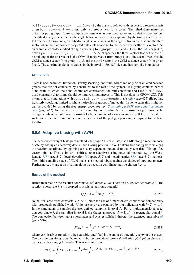
GROMACS Documentation, Release 2019.3
pull-coord?-geometry = angle-axis the angle is defined with respect to a reference axisgiven by pull-coord?-vec and only two groups need to be given. The dihedral geometry re-quires six pull groups. These pair up in the same way as described above and so define three vectors.The dihedral angle is defined as the angle between the two planes spanned by the two first and the twolast vectors. Equivalently, the dihedral angle can be seen as the angle between the first and the thirdvector when these vectors are projected onto a plane normal to the second vector (the axis vector). Asan example, consider a dihedral angle involving four groups: 1, 5, 8 and 9. Here, the mdp (page 425)option pull-coord?-groups = 8 1 1 5 5 9 specifies the three vectors that define the di-hedral angle: the first vector is the COM distance vector from group 8 to 1, the second vector is theCOM distance vector from group 1 to 5, and the third vector is the COM distance vector from group5 to 9. The dihedral angle takes values in the interval (-180, 180] deg and has periodic boundaries.
Limitations
There is one theoretical limitation: strictly speaking, constraint forces can only be calculated betweengroups that are not connected by constraints to the rest of the system. If a group contains part ofa molecule of which the bond lengths are constrained, the pull constraint and LINCS or SHAKEbond constraint algorithms should be iterated simultaneously. This is not done in GROMACS. Thismeans that for simulations with constraints = all-bonds in the mdp (page 425) file pullingis, strictly speaking, limited to whole molecules or groups of molecules. In some cases this limitationcan be avoided by using the free energy code, see sec. Calculating a PMF using the free-energycode (page 462). In practice, the errors caused by not iterating the two constraint algorithms can benegligible when the pull group consists of a large amount of atoms and/or the pull force is small. Insuch cases, the constraint correction displacement of the pull group is small compared to the bondlengths.
5.8.5 Adaptive biasing with AWH
The accelerated weight histogram method 137 (page 512) calculates the PMF along a reaction coor-dinate by adding an adaptively determined biasing potential. AWH flattens free energy barriers alongthe reaction coordinate by applying a history-dependent potential to the system that “fills up” freeenergy minima. This is similar in spirit to other adaptive biasing potential methods, e.g. the Wang-Landau 138 (page 512), local elevation 139 (page 512) and metadynamics 140 (page 512) methods.The initial sampling stage of AWH makes the method robust against the choice of input parameters.Furthermore, the target distribution along the reaction coordinate may be chosen freely.
Basics of the method
Rather than biasing the reaction coordinate 𝜉(𝑥) directly, AWH acts on a reference coordinate 𝜆. Thereaction coordinate 𝜉(𝑥) is coupled to 𝜆 with a harmonic potential
𝑄(𝜉, 𝜆) =1
2𝛽𝑘(𝜉 − 𝜆)2, (5.290)
so that for large force constants 𝑘, 𝜉 ≈ 𝜆. Note the use of dimensionless energies for compatibilitywith previously published work. Units of energy are obtained by multiplication with 𝑘𝐵𝑇 = 1/𝛽.In the simulation, 𝜆 samples the user-defined sampling interval 𝐼 . For a multidimensional reac-tion coordinate 𝜉, the sampling interval is the Cartesian product 𝐼 = Π𝜇𝐼𝜇 (a rectangular domain).The connection between atom coordinates and 𝜆 is established through the extended ensemble 68(page 509),
𝑃 (𝑥, 𝜆) =1
𝒵𝑒𝑔(𝜆)−𝑄(𝜉(𝑥),𝜆)−𝑉 (𝑥), (5.291)
where 𝑔(𝜆) is a bias function (a free variable) and 𝑉 (𝑥) is the unbiased potential energy of the system.The distribution along 𝜆 can be tuned to be any predefined target distribution 𝜌(𝜆) (often chosen tobe flat) by choosing 𝑔(𝜆) wisely. This is evident from
𝑃 (𝜆) =
∫𝑃 (𝑥, 𝜆)𝑑𝑥 =
1
𝒵𝑒𝑔(𝜆)
∫𝑒−𝑄(𝜉(𝑥),𝜆)−𝑉 (𝑥)𝑑𝑥 ≡ 1
𝒵𝑒𝑔(𝜆)−𝐹 (𝜆), (5.292)
5.8. Special Topics 440
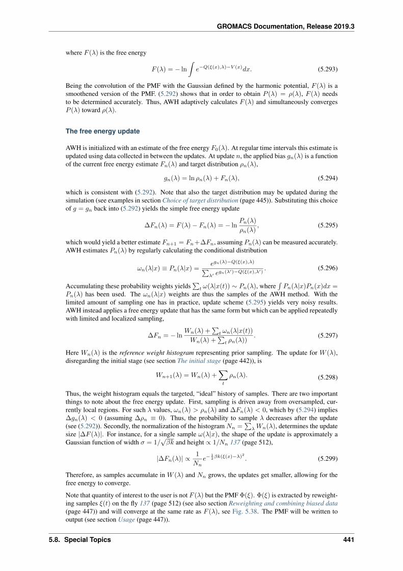
GROMACS Documentation, Release 2019.3
where 𝐹 (𝜆) is the free energy
𝐹 (𝜆) = − ln
∫𝑒−𝑄(𝜉(𝑥),𝜆)−𝑉 (𝑥)𝑑𝑥. (5.293)
Being the convolution of the PMF with the Gaussian defined by the harmonic potential, 𝐹 (𝜆) is asmoothened version of the PMF. (5.292) shows that in order to obtain 𝑃 (𝜆) = 𝜌(𝜆), 𝐹 (𝜆) needsto be determined accurately. Thus, AWH adaptively calculates 𝐹 (𝜆) and simultaneously converges𝑃 (𝜆) toward 𝜌(𝜆).
The free energy update
AWH is initialized with an estimate of the free energy 𝐹0(𝜆). At regular time intervals this estimate isupdated using data collected in between the updates. At update 𝑛, the applied bias 𝑔𝑛(𝜆) is a functionof the current free energy estimate 𝐹𝑛(𝜆) and target distribution 𝜌𝑛(𝜆),
𝑔𝑛(𝜆) = ln 𝜌𝑛(𝜆) + 𝐹𝑛(𝜆), (5.294)
which is consistent with (5.292). Note that also the target distribution may be updated during thesimulation (see examples in section Choice of target distribution (page 445)). Substituting this choiceof 𝑔 = 𝑔𝑛 back into (5.292) yields the simple free energy update
∆𝐹𝑛(𝜆) = 𝐹 (𝜆) − 𝐹𝑛(𝜆) = − ln𝑃𝑛(𝜆)
𝜌𝑛(𝜆), (5.295)
which would yield a better estimate 𝐹𝑛+1 = 𝐹𝑛+∆𝐹𝑛, assuming 𝑃𝑛(𝜆) can be measured accurately.AWH estimates 𝑃𝑛(𝜆) by regularly calculating the conditional distribution
𝜔𝑛(𝜆|𝑥) ≡ 𝑃𝑛(𝜆|𝑥) =𝑒𝑔𝑛(𝜆)−𝑄(𝜉(𝑥),𝜆)∑𝜆′ 𝑒𝑔𝑛(𝜆
′)−𝑄(𝜉(𝑥),𝜆′). (5.296)
Accumulating these probability weights yields∑
𝑡 𝜔(𝜆|𝑥(𝑡)) ∼ 𝑃𝑛(𝜆), where∫𝑃𝑛(𝜆|𝑥)𝑃𝑛(𝑥)𝑑𝑥 =
𝑃𝑛(𝜆) has been used. The 𝜔𝑛(𝜆|𝑥) weights are thus the samples of the AWH method. With thelimited amount of sampling one has in practice, update scheme (5.295) yields very noisy results.AWH instead applies a free energy update that has the same form but which can be applied repeatedlywith limited and localized sampling,
∆𝐹𝑛 = − ln𝑊𝑛(𝜆) +
∑𝑡 𝜔𝑛(𝜆|𝑥(𝑡))
𝑊𝑛(𝜆) +∑
𝑡 𝜌𝑛(𝜆)). (5.297)
Here 𝑊𝑛(𝜆) is the reference weight histogram representing prior sampling. The update for 𝑊 (𝜆),disregarding the initial stage (see section The initial stage (page 442)), is
𝑊𝑛+1(𝜆) = 𝑊𝑛(𝜆) +∑𝑡
𝜌𝑛(𝜆). (5.298)
Thus, the weight histogram equals the targeted, “ideal” history of samples. There are two importantthings to note about the free energy update. First, sampling is driven away from oversampled, cur-rently local regions. For such 𝜆 values, 𝜔𝑛(𝜆) > 𝜌𝑛(𝜆) and ∆𝐹𝑛(𝜆) < 0, which by (5.294) implies∆𝑔𝑛(𝜆) < 0 (assuming ∆𝜌𝑛 ≡ 0). Thus, the probability to sample 𝜆 decreases after the update(see (5.292)). Secondly, the normalization of the histogram 𝑁𝑛 =
∑𝜆𝑊𝑛(𝜆), determines the update
size |∆𝐹 (𝜆)|. For instance, for a single sample 𝜔(𝜆|𝑥), the shape of the update is approximately aGaussian function of width 𝜎 = 1/
√𝛽𝑘 and height ∝ 1/𝑁𝑛 137 (page 512),
|∆𝐹𝑛(𝜆)| ∝ 1
𝑁𝑛𝑒−
12𝛽𝑘(𝜉(𝑥)−𝜆)2 . (5.299)
Therefore, as samples accumulate in 𝑊 (𝜆) and 𝑁𝑛 grows, the updates get smaller, allowing for thefree energy to converge.
Note that quantity of interest to the user is not 𝐹 (𝜆) but the PMF Φ(𝜉). Φ(𝜉) is extracted by reweight-ing samples 𝜉(𝑡) on the fly 137 (page 512) (see also section Reweighting and combining biased data(page 447)) and will converge at the same rate as 𝐹 (𝜆), see Fig. 5.38. The PMF will be written tooutput (see section Usage (page 447)).
5.8. Special Topics 441
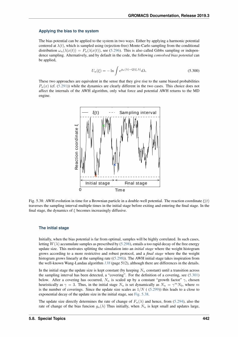
GROMACS Documentation, Release 2019.3
Applying the bias to the system
The bias potential can be applied to the system in two ways. Either by applying a harmonic potentialcentered at 𝜆(𝑡), which is sampled using (rejection-free) Monte-Carlo sampling from the conditionaldistribution 𝜔𝑛(𝜆|𝑥(𝑡)) = 𝑃𝑛(𝜆|𝑥(𝑡)), see (5.296). This is also called Gibbs sampling or indepen-dence sampling. Alternatively, and by default in the code, the following convolved bias potential canbe applied,
𝑈𝑛(𝜉) = − ln
∫𝑒𝑔𝑛(𝜆)−𝑄(𝜉,𝜆)𝑑𝜆. (5.300)
These two approaches are equivalent in the sense that they give rise to the same biased probabilities𝑃𝑛(𝑥) (cf. (5.291)) while the dynamics are clearly different in the two cases. This choice does notaffect the internals of the AWH algorithm, only what force and potential AWH returns to the MDengine.
0 Tim e
Re
act
ion
co
ord
ina
te ξ
Init ial stage Final stage
ξ(t) Sam pling interval
Fig. 5.38: AWH evolution in time for a Brownian particle in a double-well potential. The reaction coordinate 𝜉(𝑡)traverses the sampling interval multiple times in the initial stage before exiting and entering the final stage. In thefinal stage, the dynamics of 𝜉 becomes increasingly diffusive.
The initial stage
Initially, when the bias potential is far from optimal, samples will be highly correlated. In such cases,letting𝑊 (𝜆) accumulate samples as prescribed by (5.298), entails a too rapid decay of the free energyupdate size. This motivates splitting the simulation into an initial stage where the weight histogramgrows according to a more restrictive and robust protocol, and a final stage where the the weighthistogram grows linearly at the sampling rate ((5.298)). The AWH initial stage takes inspiration fromthe well-known Wang-Landau algorithm 138 (page 512), although there are differences in the details.
In the initial stage the update size is kept constant (by keeping 𝑁𝑛 constant) until a transition acrossthe sampling interval has been detected, a “covering”. For the definition of a covering, see (5.301)below. After a covering has occurred, 𝑁𝑛 is scaled up by a constant “growth factor” 𝛾, chosenheuristically as 𝛾 = 3. Thus, in the initial stage 𝑁𝑛 is set dynamically as 𝑁𝑛 = 𝛾𝑚𝑁0, where 𝑚is the number of coverings. Since the update size scales as 1/𝑁 ( (5.299)) this leads to a close toexponential decay of the update size in the initial stage, see Fig. 5.38.
The update size directly determines the rate of change of 𝐹𝑛(𝜆) and hence, from (5.294), also therate of change of the bias funcion 𝑔𝑛(𝜆) Thus initially, when 𝑁𝑛 is kept small and updates large,
5.8. Special Topics 442
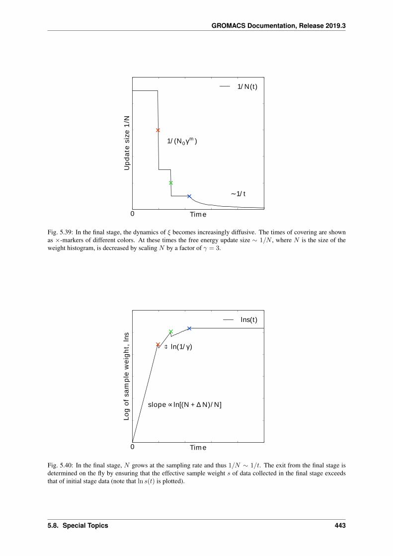
GROMACS Documentation, Release 2019.3
0 Tim e
Up
da
te s
ize
1/N
1/ (N0γm )
∼1/ t
1/ N(t)
Fig. 5.39: In the final stage, the dynamics of 𝜉 becomes increasingly diffusive. The times of covering are shownas ×-markers of different colors. At these times the free energy update size ∼ 1/𝑁 , where 𝑁 is the size of theweight histogram, is decreased by scaling 𝑁 by a factor of 𝛾 = 3.
0 Tim e
Log
of
sam
ple
we
igh
t, l
ns
ln(1/ γ)
slope ∝ ln[(N + ∆ N)/ N]
lns(t)
Fig. 5.40: In the final stage, 𝑁 grows at the sampling rate and thus 1/𝑁 ∼ 1/𝑡. The exit from the final stage isdetermined on the fly by ensuring that the effective sample weight 𝑠 of data collected in the final stage exceedsthat of initial stage data (note that ln 𝑠(𝑡) is plotted).
5.8. Special Topics 443
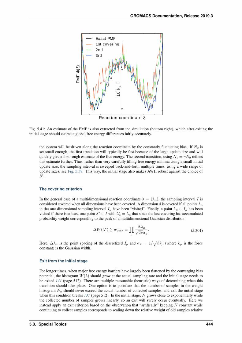
GROMACS Documentation, Release 2019.3
React ion coordinate ξ
PM
F Φ
(ξ)
10
kB
T
Exact PMF
1st covering
2nd
3rd
Fig. 5.41: An estimate of the PMF is also extracted from the simulation (bottom right), which after exiting theinitial stage should estimate global free energy differences fairly accurately.
the system will be driven along the reaction coordinate by the constantly fluctuating bias. If 𝑁0 isset small enough, the first transition will typically be fast because of the large update size and willquickly give a first rough estimate of the free energy. The second transition, using 𝑁1 = 𝛾𝑁0 refinesthis estimate further. Thus, rather than very carefully filling free energy minima using a small initialupdate size, the sampling interval is sweeped back-and-forth multiple times, using a wide range ofupdate sizes, see Fig. 5.38. This way, the initial stage also makes AWH robust against the choice of𝑁0.
The covering criterion
In the general case of a multidimensional reaction coordinate 𝜆 = (𝜆𝜇), the sampling interval 𝐼 isconsidered covered when all dimensions have been covered. A dimension 𝑑 is covered if all points 𝜆𝜇in the one-dimensional sampling interval 𝐼𝜇 have been “visited”. Finally, a point 𝜆𝜇 ∈ 𝐼𝜇 has beenvisited if there is at least one point 𝜆* ∈ 𝐼 with 𝜆*𝜇 = 𝜆𝜇 that since the last covering has accumulatedprobability weight corresponding to the peak of a multidimensional Gaussian distribution
∆𝑊 (𝜆*) ≥ 𝑤peak ≡∏𝜇
∆𝜆𝜇√2𝜋𝜎𝑘
. (5.301)
Here, ∆𝜆𝜇 is the point spacing of the discretized 𝐼𝜇 and 𝜎𝑘 = 1/√𝛽𝑘𝜇 (where 𝑘𝜇 is the force
constant) is the Gaussian width.
Exit from the initial stage
For longer times, when major free energy barriers have largely been flattened by the converging biaspotential, the histogram 𝑊 (𝜆) should grow at the actual sampling rate and the initial stage needs tobe exited 141 (page 512). There are multiple reasonable (heuristic) ways of determining when thistransition should take place. One option is to postulate that the number of samples in the weighthistogram 𝑁𝑛 should never exceed the actual number of collected samples, and exit the initial stagewhen this condition breaks 137 (page 512). In the initial stage, 𝑁 grows close to exponentially whilethe collected number of samples grows linearly, so an exit will surely occur eventually. Here weinstead apply an exit criterion based on the observation that “artifically” keeping 𝑁 constant whilecontinuing to collect samples corresponds to scaling down the relative weight of old samples relative
5.8. Special Topics 444
GROMACS Documentation, Release 2019.3
to new ones. Similarly, the subsequent scaling up of 𝑁 by a factor 𝛾 corresponds to scaling up theweight of old data. Briefly, the exit criterion is devised such that the weight of a sample collectedafter the initial stage is always larger or equal to the weight of a sample collected during the initialstage, see Fig. 5.38. This is consistent with scaling down early, noisy data.
The initial stage exit criterion will now be described in detail. We start out at the beginning of acovering stage, so that 𝑁 has just been scaled by 𝛾 and is now kept constant. Thus, the first sampleof this stage has the weight 𝑠 = 1/𝛾 relative to the last sample of the previous covering stage. Weassume that ∆𝑁 samples are collected and added to 𝑊 for each update . To keep 𝑁 constant, 𝑊needs to be scaled down by a factor 𝑁/(𝑁 + ∆𝑁) after every update. Equivalently, this means thatnew data is scaled up relative to old data by the inverse factor. Thus, after ∆𝑛 updates a new samplehas the relative weight 𝑠 = (1/𝛾)[(𝑁𝑛 + ∆𝑁)/𝑁𝑛]Δ𝑛. Now assume covering occurs at this time. Tocontinue to the next covering stage, 𝑁 should be scaled by 𝛾, which corresponds to again multiplying𝑠 by 1/𝛾. If at this point 𝑠 ≥ 𝛾, then after rescaling 𝑠 ≥ 1; i.e. overall the relative weight of a newsample relative to an old sample is still growing fast. If on the contrary 𝑠 < 𝛾, and this defines theexit from the initial stage, then the initial stage is over and from now 𝑁 simply grows at the samplingrate (see (5.298)). To really ensure that 𝑠 ≥ 1 holds before exiting, so that samples after the exit haveat least the sample weight of older samples, the last covering stage is extended by a sufficient numberof updates.
Choice of target distribution
The target distribution 𝜌(𝜆) is traditionally chosen to be uniform
𝜌const(𝜆) = const. (5.302)
This choice exactly flattens 𝐹 (𝜆) in user-defined sampling interval 𝐼 . Generally, 𝜌(𝜆) = 0, 𝜆 /∈ 𝐼 .In certain cases other choices may be preferable. For instance, in the multidimensional case therectangular sampling interval is likely to contain regions of very high free energy, e.g. where atomsare clashing. To exclude such regions, 𝜌(𝜆) can specified by the following function of the free energy
𝜌cut(𝜆) ∝ 1
1 + 𝑒𝐹 (𝜆)−𝐹cut, (5.303)
where 𝐹cut is a free energy cutoff (relative to min𝜆 𝐹 (𝜆)). Thus, regions of the sampling intervalwhere 𝐹 (𝜆) > 𝐹cut will be exponentially suppressed (in a smooth fashion). Alternatively, very highfree energy regions could be avoided while still flattening more moderate free energy barriers bytargeting a Boltzmann distribution corresponding to scaling 𝛽 = 1/𝑘𝐵𝑇 by a factor 0 < 𝑠𝛽 < 1,
𝜌Boltz(𝜆) ∝ 𝑒−𝑠𝛽𝐹 (𝜆), (5.304)
The parameter 𝑠𝛽 determines to what degree the free energy landscape is flattened; the lower 𝑠𝛽 , theflatter. Note that both 𝜌cut(𝜆) and 𝜌Boltz(𝜆) depend on 𝐹 (𝜆), which needs to be substituted by thecurrent best estimate 𝐹𝑛(𝜆). Thus, the target distribution is also updated (consistently with (5.294)).
There is in fact an alternative approach to obtaining 𝜌Boltz(𝜆) as the limiting target distribution inAWH, which is particular in the way the weight histogram 𝑊 (𝜆) and the target distribution 𝜌 areupdated and coupled to each other. This yields an evolution of the bias potential which is very similarto that of well-tempered metadynamics 142 (page 512), see 137 (page 512) for details. Because ofthe popularity and success of well-tempered metadynamics, this is a special case worth considering.In this case 𝜌 is a function of the reference weight histogram
𝜌Boltz,loc(𝜆) ∝𝑊 (𝜆), (5.305)
and the update of the weight histogram is modified (cf. (5.298))
𝑊𝑛+1(𝜆) = 𝑊𝑛(𝜆) + 𝑠𝛽∑𝑡
𝜔(𝜆|𝑥(𝑡)). (5.306)
5.8. Special Topics 445
GROMACS Documentation, Release 2019.3
Thus, here the weight histogram equals the real history of samples, but scaled by 𝑠𝛽 . This targetdistribution is called local Boltzmann since 𝑊 is only modified locally, where sampling has takenplace. We see that when 𝑠𝛽 ≈ 0 the histogram essentially does not grow and the size of the freeenergy update will stay at a constant value (as in the original formulation of metadynamics). Thus,the free energy estimate will not converge, but continue to fluctuate around the correct value. Thisillustrates the inherent coupling between the convergence and choice of target distribution for thisspecial choice of target. Furthermore note that when using 𝜌 = 𝜌Boltz,loc there is no initial stage(section The initial stage (page 442)). The rescaling of the weight histogram applied in the initialstage is a global operation, which is incompatible 𝜌Boltz,loc only depending locally on the samplinghistory.
Lastly, the target distribution can be modulated by arbitrary probability weights
𝜌(𝜆) = 𝜌0(𝜆)𝑤user(𝜆). (5.307)
where 𝑤user(𝜆) is provided by user data and in principle 𝜌0(𝜆) can be any of the target distributionsmentioned above.
Multiple independent or sharing biases
Multiple independent bias potentials may be applied within one simulation. This only makes senseif the biased coordinates 𝜉(1), 𝜉(2), . . . evolve essentially independently from one another. A typicalexample of this would be when applying an independent bias to each monomer of a protein. Fur-thermore, multiple AWH simulations can be launched in parallel, each with a (set of) indepedendentbiases.
If the defined sampling interval is large relative to the diffusion time of the reaction coordinate,traversing the sampling interval multiple times as is required by the initial stage (section The ini-tial stage (page 442)) may take an infeasible mount of simulation time. In these cases it could beadvantageous to parallelize the work and have a group of multiple “walkers” 𝜉(𝑖)(𝑡) share a singlebias potential. This can be achieved by collecting samples from all 𝜉(𝑖) of the same sharing groupinto a single histogram and update a common free energy estimate. Samples can be shared betweenwalkers within the simulation and/or between multiple simulations. However, currently only sharingbetween simulations is supported in the code while all biases within a simulation are independent.
Note that when attempting to shorten the simulation time by using bias-sharing walkers, care must betaken to ensure the simulations are still long enough to properly explore and equilibrate all regionsof the sampling interval. To begin, the walkers in a group should be decorrelated and distributedapproximately according to the target distribution before starting to refine the free energy. This canbe achieved e.g. by “equilibrating” the shared weight histogram before letting it grow; for instance,𝑊 (𝜆)/𝑁 ≈ 𝜌(𝜆) with some tolerance.
Furthermore, the “covering” or transition criterion of the initial stage should to be generalized todetect when the sampling interval has been collectively traversed. One alternative is to just use thesame criterion as for a single walker (but now with more samples), see (5.301). However, in contrastto the single walker case this does not ensure that any real transitions across the sampling intervalhas taken place; in principle all walkers could be sampling only very locally and still cover the wholeinterval. Just as with a standard umbrella sampling procedure, the free energy may appear to beconverged while in reality simulations sampling closeby 𝜆 values are sampling disconnected regionsof phase space. A stricter criterion, which helps avoid such issues, is to require that before a simulationmarks a point 𝜆𝜇 along dimension 𝜇 as visited, and shares this with the other walkers, also all pointswithin a certain diameter 𝐷cover should have been visited (i.e. fulfill (5.301)). Increasing 𝐷cover
increases robustness, but may slow down convergence. For the maximum value of 𝐷cover, equal tothe length of the sampling interval, the sampling interval is considered covered when at least onewalker has independently traversed the sampling interval.
5.8. Special Topics 446
GROMACS Documentation, Release 2019.3
Reweighting and combining biased data
Often one may want to, post-simulation, calculate the unbiased PMF Φ(𝑢) of another variable 𝑢(𝑥).Φ(𝑢) can be estimated using 𝜉-biased data by reweighting (“unbiasing”) the trajectory using the biaspotential 𝑈𝑛(𝑡), see (5.300). Essentially, one bins the biased data along 𝑢 and removes the effect of𝑈𝑛(𝑡) by dividing the weight of samples 𝑢(𝑡) by 𝑒−𝑈𝑛(𝑡)(𝜉(𝑡)),
Φ(𝑢) = − ln∑𝑡
1𝑢(𝑢(𝑡))𝑒𝑈𝑛(𝑡)(𝜉(𝑡)𝒵𝑛(𝑡). (5.308)
Here the indicator function 1𝑢 denotes the binning procedure: 1𝑢(𝑢′) = 1 if 𝑢′ falls into the binlabeled by 𝑢 and 0 otherwise. The normalization factor 𝒵𝑛 =
∫𝑒−Φ(𝜉)−𝑈𝑛(𝜉)𝑑𝜉 is the partition
function of the extended ensemble. As can be seen 𝒵𝑛 depends on Φ(𝜉), the PMF of the (biased)reaction coordinate 𝜉 (which is calculated and written to file by the AWH simulation). It is advisableto use only final stage data in the reweighting procedure due to the rapid change of the bias potentialduring the initial stage. If one would include initial stage data, one should use the sample weights thatare inferred by the repeated rescaling of the histogram in the initial stage, for the sake of consistency.Initial stage samples would then in any case be heavily scaled down relative to final stage samples.Note that (5.308) can also be used to combine data from multiple simulations (by adding another sumalso over the trajectory set). Furthermore, when multiple independent AWH biases have generateda set of PMF estimates {Φ(𝑖)(𝜉)}, a combined best estimate Φ(𝜉) can be obtained by applying self-consistent exponential averaging. More details on this procedure and a derivation of (5.308) (usingslightly different notation) can be found in 143 (page 512).
The friction metric
During the AWH simulation, the following time-integrated force correlation function is calculated,
𝜂𝜇𝜈(𝜆) = 𝛽
∫ ∞
0
⟨𝛿ℱ𝜇(𝑥(𝑡), 𝜆)𝛿ℱ𝜈(𝑥(0), 𝜆)𝜔(𝜆|𝑥(𝑡))𝜔(𝜆|𝑥(0))⟩⟨𝜔2(𝜆|𝑥)⟩
𝑑𝑡. (5.309)
Here ℱ𝜇(𝑥, 𝜆) = 𝑘𝜇(𝜉𝜇(𝑥)−𝜆𝜇) is the force along dimension 𝜇 from an harmonic potential centeredat 𝜆 and 𝛿ℱ𝜇(𝑥, 𝜆) = ℱ𝜇(𝑥, 𝜆) − ⟨ℱ𝜇(𝑥, 𝜆)⟩ is the deviation of the force. The factors 𝜔(𝜆|𝑥(𝑡)),see (5.296), reweight the samples. 𝜂𝜇𝜈(𝜆) is a friction tensor 144 (page 512). Its matrix elements areinversely proportional to local diffusion coefficients. A measure of sampling (in)efficiency at each 𝜆is given by
𝜂12 (𝜆) =
√det 𝜂𝜇𝜈(𝜆). (5.310)
A large value of 𝜂12 (𝜆) indicates slow dynamics and long correlation times, which may require more
sampling.
Usage
AWH stores data in the energy file (edr (page 422)) with a frequency set by the user. The data– the PMF, the convolved bias, distributions of the 𝜆 and 𝜉 coordinates, etc. – can be extractedafter the simulation using the gmx awh (page 47) tool. Furthermore, the trajectory of the reactioncoordinate 𝜉(𝑡) is printed to the pull output file pullx.xvg. The log file (log (page 424)) also containsinformation; check for messages starting with “awh”, they will tell you about covering and potentialsampling issues.
Setting the initial update size
The initial value of the weight histogram size 𝑁 sets the initial update size (and the rate of change ofthe bias). When 𝑁 is kept constant, like in the initial stage, the average variance of the free energyscales as 𝜀2 ∼ 1/(𝑁𝐷) 137 (page 512), for a simple model system with constant diffusion 𝐷 along
5.8. Special Topics 447
GROMACS Documentation, Release 2019.3
the reaction coordinate. This provides a ballpark estimate used by AWH to initialize 𝑁 in terms ofmore meaningful quantities
1
𝑁0=
1
𝑁0(𝜀0, 𝐷)∼ 𝐷𝜀20. (5.311)
Essentially, this tells us that a slower system (small 𝐷) requires more samples (larger 𝑁0) to attainthe same level of accuracy (𝜀0) at a given sampling rate. Conversely, for a system of given diffusion,how to choose the initial biasing rate depends on how good the initial accuracy is. Both the initialerror 𝜀0 and the diffusion 𝐷 only need to be roughly estimated or guessed. In the typical case, onewould only tweak the 𝐷 parameter, and use a default value for 𝜀0. For good convergence, 𝐷 shouldbe chosen as large as possible (while maintaining a stable system) giving large initial bias updatesand fast initial transitions. Choosing 𝐷 too small can lead to slow initial convergence. It may be agood idea to run a short trial simulation and after the first covering check the maximum free energydifference of the PMF estimate. If this is much larger than the expected magnitude of the free energybarriers that should be crossed, then the system is probably being pulled too hard and 𝐷 should bedecreased. 𝜀0 on the other hand, would only be tweaked when starting an AWH simulation using afairly accurate guess of the PMF as input.
Tips for efficient sampling
The force constant 𝑘 should be larger than the curvature of the PMF landscape. If this is not the case,the distributions of the reaction coordinate 𝜉 and the reference coordinate 𝜆, will differ significantlyand warnings will be printed in the log file. One can choose 𝑘 as large as the time step supports.This will neccessarily increase the number of points of the discretized sampling interval 𝐼 . In generalhowever, it should not affect the performance of the simulation noticeably because the AWH updateis implemented such that only sampled points are accessed at free energy update time.
As with any method, the choice of reaction coordinate(s) is critical. If a single reaction coordinatedoes not suffice, identifying a second reaction coordinate and sampling the two-dimensional land-scape may help. In this case, using a target distribution with a free energy cutoff (see (5.303)) mightbe required to avoid sampling uninteresting regions of very high free energy. Obtaining accurate freeenergies for reaction coordinates of much higher dimensionality than 3 or possibly 4 is generally notfeasible.
Monitoring the transition rate of 𝜉(𝑡), across the sampling interval is also advisable. For reliablestatistics (e.g. when reweighting the trajectory as described in section Reweighting and combiningbiased data (page 447)), one would generally want to observe at least a few transitions after havingexited the initial stage. Furthermore, if the dynamics of the reaction coordinate suddenly changes,this may be a sign of e.g. a reaction coordinate problem.
Difficult regions of sampling may also be detected by calculating the friction tensor 𝜂𝜇𝜈(𝜆) in thesampling interval, see section The friction metric (page 447). 𝜂𝜇𝜈(𝜆) as well as the sampling effi-ciency measure 𝜂
12 (𝜆) ((5.310)) are written to the energy file and can be extracted with gmx awh
(page 47). A high peak in 𝜂12 (𝜆) indicates that this region requires longer time to sample properly.
5.8.6 Enforced Rotation
This module can be used to enforce the rotation of a group of atoms, as e.g. a protein subunit. Thereare a variety of rotation potentials, among them complex ones that allow flexible adaptations of boththe rotated subunit as well as the local rotation axis during the simulation. An example applicationcan be found in ref. 145 (page 513).
5.8. Special Topics 448
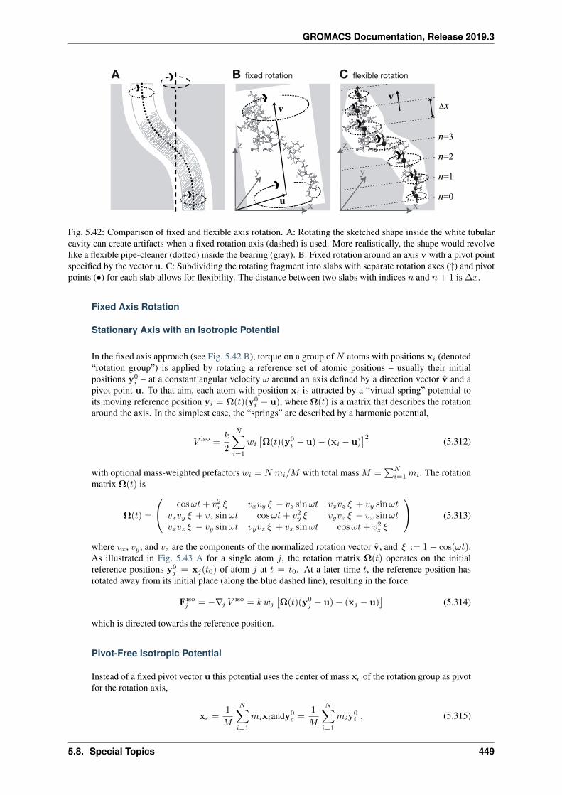
GROMACS Documentation, Release 2019.3
Fig. 5.42: Comparison of fixed and flexible axis rotation. A: Rotating the sketched shape inside the white tubularcavity can create artifacts when a fixed rotation axis (dashed) is used. More realistically, the shape would revolvelike a flexible pipe-cleaner (dotted) inside the bearing (gray). B: Fixed rotation around an axis v with a pivot pointspecified by the vector u. C: Subdividing the rotating fragment into slabs with separate rotation axes (↑) and pivotpoints (∙) for each slab allows for flexibility. The distance between two slabs with indices 𝑛 and 𝑛+ 1 is ∆𝑥.
Fixed Axis Rotation
Stationary Axis with an Isotropic Potential
In the fixed axis approach (see Fig. 5.42 B), torque on a group of 𝑁 atoms with positions x𝑖 (denoted“rotation group”) is applied by rotating a reference set of atomic positions – usually their initialpositions y0
𝑖 – at a constant angular velocity 𝜔 around an axis defined by a direction vector v and apivot point u. To that aim, each atom with position x𝑖 is attracted by a “virtual spring” potential toits moving reference position y𝑖 = Ω(𝑡)(y0
𝑖 − u), where Ω(𝑡) is a matrix that describes the rotationaround the axis. In the simplest case, the “springs” are described by a harmonic potential,
𝑉 iso =𝑘
2
𝑁∑𝑖=1
𝑤𝑖
[Ω(𝑡)(y0
𝑖 − u) − (x𝑖 − u)]2 (5.312)
with optional mass-weighted prefactors 𝑤𝑖 = 𝑁 𝑚𝑖/𝑀 with total mass 𝑀 =∑𝑁
𝑖=1𝑚𝑖. The rotationmatrix Ω(𝑡) is
Ω(𝑡) =
⎛⎝ cos𝜔𝑡+ 𝑣2𝑥 𝜉 𝑣𝑥𝑣𝑦 𝜉 − 𝑣𝑧 sin𝜔𝑡 𝑣𝑥𝑣𝑧 𝜉 + 𝑣𝑦 sin𝜔𝑡𝑣𝑥𝑣𝑦 𝜉 + 𝑣𝑧 sin𝜔𝑡 cos𝜔𝑡+ 𝑣2𝑦 𝜉 𝑣𝑦𝑣𝑧 𝜉 − 𝑣𝑥 sin𝜔𝑡𝑣𝑥𝑣𝑧 𝜉 − 𝑣𝑦 sin𝜔𝑡 𝑣𝑦𝑣𝑧 𝜉 + 𝑣𝑥 sin𝜔𝑡 cos𝜔𝑡+ 𝑣2𝑧 𝜉
⎞⎠ (5.313)
where 𝑣𝑥, 𝑣𝑦 , and 𝑣𝑧 are the components of the normalized rotation vector v, and 𝜉 := 1 − cos(𝜔𝑡).As illustrated in Fig. 5.43 A for a single atom 𝑗, the rotation matrix Ω(𝑡) operates on the initialreference positions y0
𝑗 = x𝑗(𝑡0) of atom 𝑗 at 𝑡 = 𝑡0. At a later time 𝑡, the reference position hasrotated away from its initial place (along the blue dashed line), resulting in the force
Fiso𝑗 = −∇𝑗 𝑉
iso = 𝑘 𝑤𝑗
[Ω(𝑡)(y0
𝑗 − u) − (x𝑗 − u)]
(5.314)
which is directed towards the reference position.
Pivot-Free Isotropic Potential
Instead of a fixed pivot vector u this potential uses the center of mass x𝑐 of the rotation group as pivotfor the rotation axis,
x𝑐 =1
𝑀
𝑁∑𝑖=1
𝑚𝑖x𝑖andy0𝑐 =
1
𝑀
𝑁∑𝑖=1
𝑚𝑖y0𝑖 , (5.315)
5.8. Special Topics 449
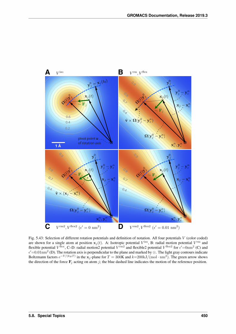
GROMACS Documentation, Release 2019.3
V rm, V flexV iso
V rm2, V flex2 (ε′ = 0.01 nm2)V rm2, V flex2 (ε′ = 0 nm2)
Fig. 5.43: Selection of different rotation potentials and definition of notation. All four potentials 𝑉 (color coded)are shown for a single atom at position x𝑗(𝑡). A: Isotropic potential 𝑉 iso, B: radial motion potential 𝑉 rm andflexible potential 𝑉 flex, C–D: radial motion2 potential 𝑉 rm2 and flexible2 potential 𝑉 flex2 for 𝜖′=0nm2 (C) and𝜖′=0.01nm2 (D). The rotation axis is perpendicular to the plane and marked by ⊗. The light gray contours indicateBoltzmann factors 𝑒−𝑉/(𝑘𝐵𝑇 ) in the x𝑗-plane for 𝑇 = 300K and 𝑘=200kJ/(mol · nm2). The green arrow showsthe direction of the force F𝑗 acting on atom 𝑗; the blue dashed line indicates the motion of the reference position.
5.8. Special Topics 450
GROMACS Documentation, Release 2019.3
which yields the “pivot-free” isotropic potential
𝑉 iso−pf =𝑘
2
𝑁∑𝑖=1
𝑤𝑖
[Ω(𝑡)(y0
𝑖 − y0𝑐) − (x𝑖 − x𝑐)
]2, (5.316)
with forces
Fiso−pf𝑗 = 𝑘 𝑤𝑗
[Ω(𝑡)(y0
𝑗 − y0𝑐) − (x𝑗 − x𝑐)
]. (5.317)
Without mass-weighting, the pivot x𝑐 is the geometrical center of the group.
Parallel Motion Potential Variant
The forces generated by the isotropic potentials (eqns. (5.312) and (5.316)) also contain componentsparallel to the rotation axis and thereby restrain motions along the axis of either the whole rotationgroup (in case of 𝑉 iso) or within the rotation group, in case of 𝑉 iso−pf .
For cases where unrestrained motion along the axis is preferred, we have implemented a “parallelmotion” variant by eliminating all components parallel to the rotation axis for the potential. This isachieved by projecting the distance vectors between reference and actual positions
r𝑖 = Ω(𝑡)(y0𝑖 − u) − (x𝑖 − u) (5.318)
onto the plane perpendicular to the rotation vector,
r⊥𝑖 := r𝑖 − (r𝑖 · v)v (5.319)
yielding
𝑉 pm =𝑘
2
𝑁∑𝑖=1
𝑤𝑖(r⊥𝑖 )2
=𝑘
2
𝑁∑𝑖=1
𝑤𝑖
{Ω(𝑡)(y0
𝑖 − u) − (x𝑖 − u)
−{[Ω(𝑡)(y0
𝑖 − u) − (x𝑖 − u)]· v}v}2
and similarly
Fpm𝑗 = 𝑘 𝑤𝑗 r
⊥𝑗 (5.320)
Pivot-Free Parallel Motion Potential
Replacing in eqn. (5.320) the fixed pivot u by the center of mass xc yields the pivot-free variant ofthe parallel motion potential. With
s𝑖 = Ω(𝑡)(y0𝑖 − y0
𝑐) − (x𝑖 − x𝑐) (5.321)
the respective potential and forces are
𝑉 pm−pf =𝑘
2
𝑁∑𝑖=1
𝑤𝑖(s⊥𝑖 )2 (5.322)
Fpm−pf𝑗 = 𝑘 𝑤𝑗 s
⊥𝑗 (5.323)
5.8. Special Topics 451
GROMACS Documentation, Release 2019.3
Radial Motion Potential
In the above variants, the minimum of the rotation potential is either a single point at the referenceposition y𝑖 (for the isotropic potentials) or a single line through y𝑖 parallel to the rotation axis (forthe parallel motion potentials). As a result, radial forces restrict radial motions of the atoms. Thetwo subsequent types of rotation potentials, 𝑉 rm and 𝑉 rm2, drastically reduce or even eliminate thiseffect. The first variant, 𝑉 rm (Fig. 5.43 B), eliminates all force components parallel to the vectorconnecting the reference atom and the rotation axis,
𝑉 rm =𝑘
2
𝑁∑𝑖=1
𝑤𝑖 [p𝑖 · (x𝑖 − u)]2, (5.324)
with
p𝑖 :=v ×Ω(𝑡)(y0
𝑖 − u)
‖v ×Ω(𝑡)(y0𝑖 − u)‖
. (5.325)
This variant depends only on the distance p𝑖 · (x𝑖 − u) of atom 𝑖 from the plane spanned by v andΩ(𝑡)(y0
𝑖 − u). The resulting force is
Frm𝑗 = −𝑘 𝑤𝑗 [p𝑗 · (x𝑗 − u)] p𝑗 . (5.326)
Pivot-Free Radial Motion Potential
Proceeding similar to the pivot-free isotropic potential yields a pivot-free version of the above poten-tial. With
q𝑖 :=v ×Ω(𝑡)(y0
𝑖 − y0𝑐)
‖v ×Ω(𝑡)(y0𝑖 − y0
𝑐)‖, (5.327)
the potential and force for the pivot-free variant of the radial motion potential read
𝑉 rm−pf =𝑘
2
𝑁∑𝑖=1
𝑤𝑖 [q𝑖 · (x𝑖 − x𝑐)]2, (5.328)
Frm−pf𝑗 = −𝑘 𝑤𝑗 [q𝑗 · (x𝑗 − x𝑐)] q𝑗 + 𝑘
𝑚𝑗
𝑀
𝑁∑𝑖=1
𝑤𝑖 [q𝑖 · (x𝑖 − x𝑐)] q𝑖 . (5.329)
Radial Motion 2 Alternative Potential
As seen in Fig. 5.43 B, the force resulting from 𝑉 rm still contains a small, second-order radial com-ponent. In most cases, this perturbation is tolerable; if not, the following alternative, 𝑉 rm2, fullyeliminates the radial contribution to the force, as depicted in Fig. 5.43 C,
𝑉 rm2 =𝑘
2
𝑁∑𝑖=1
𝑤𝑖
[(v × (x𝑖 − u)) ·Ω(𝑡)(y0
𝑖 − u)]2
‖v × (x𝑖 − u)‖2 + 𝜖′, (5.330)
where a small parameter 𝜖′ has been introduced to avoid singularities. For 𝜖′=0nm2, the equipotentialplanes are spanned by x𝑖 −u and v, yielding a force perpendicular to x𝑖 −u, thus not contracting orexpanding structural parts that moved away from or toward the rotation axis.
Choosing a small positive 𝜖′ (e.g., 𝜖′=0.01nm2, Fig. 5.43 D) in the denominator of eqn. (5.330) yieldsa well-defined potential and continuous forces also close to the rotation axis, which is not the case for𝜖′=0nm2 (Fig. 5.43 C). With
r𝑖 := Ω(𝑡)(y0𝑖 − u)
s𝑖 :=v × (x𝑖 − u)
‖v × (x𝑖 − u)‖≡ Ψ𝑖 v × (x𝑖 − u)
Ψ*𝑖 :=
1
‖v × (x𝑖 − u)‖2 + 𝜖′
(5.331)
5.8. Special Topics 452
GROMACS Documentation, Release 2019.3
the force on atom 𝑗 reads
Frm2𝑗 = −𝑘
{𝑤𝑗 (s𝑗 · r𝑗)
[Ψ*𝑗
Ψ𝑗r𝑗 −
Ψ*2𝑗
Ψ3𝑗
(s𝑗 · r𝑗)s𝑗
]}× v. (5.332)
Pivot-Free Radial Motion 2 Potential
The pivot-free variant of the above potential is
𝑉 rm2−pf =𝑘
2
𝑁∑𝑖=1
𝑤𝑖
[(v × (x𝑖 − x𝑐)) ·Ω(𝑡)(y0
𝑖 − y𝑐)]2
‖v × (x𝑖 − x𝑐)‖2 + 𝜖′. (5.333)
With
r𝑖 := Ω(𝑡)(y0𝑖 − y𝑐)
s𝑖 :=v × (x𝑖 − x𝑐)
‖v × (x𝑖 − x𝑐)‖≡ Ψ𝑖 v × (x𝑖 − x𝑐)
Ψ*𝑖 :=
1
‖v × (x𝑖 − x𝑐)‖2 + 𝜖′
(5.334)
the force on atom 𝑗 reads
F𝑗rm2−pf = −𝑘
{𝑤𝑗 (s𝑗 · r𝑗)
[Ψ*𝑗
Ψ𝑗r𝑗 −
Ψ*2𝑗
Ψ3𝑗
(s𝑗 · r𝑗)s𝑗
]}× v
+𝑘𝑚𝑗
𝑀
{𝑁∑𝑖=1
𝑤𝑖 (s𝑖 · r𝑖)[
Ψ*𝑖
Ψ𝑖r𝑖 −
Ψ*2𝑖
Ψ3𝑖
(s𝑖 · r𝑖) s𝑖]}
× v .
Flexible Axis Rotation
As sketched in Fig. 5.42 A–B, the rigid body behavior of the fixed axis rotation scheme is a drawbackfor many applications. In particular, deformations of the rotation group are suppressed when theequilibrium atom positions directly depend on the reference positions. To avoid this limitation, eqns.(5.328) and (5.333) will now be generalized towards a “flexible axis” as sketched in Fig. 5.42 C. Thiswill be achieved by subdividing the rotation group into a set of equidistant slabs perpendicular to therotation vector, and by applying a separate rotation potential to each of these slabs. Fig. 5.42 C showsthe midplanes of the slabs as dotted straight lines and the centers as thick black dots.
To avoid discontinuities in the potential and in the forces, we define “soft slabs” by weighing thecontributions of each slab 𝑛 to the total potential function 𝑉 flex by a Gaussian function
𝑔𝑛(x𝑖) = Γ exp(−𝛽
2𝑛(x𝑖)
2𝜎2
), (5.335)
centered at the midplane of the 𝑛th slab. Here 𝜎 is the width of the Gaussian function, ∆𝑥 the distancebetween adjacent slabs, and
𝛽𝑛(x𝑖) := x𝑖 · v − 𝑛∆𝑥 . (5.336)
A most convenient choice is 𝜎 = 0.7∆𝑥 and
1/Γ =∑𝑛∈𝑍
exp(−
(𝑛− 14 )2
2 · 0.72
)≈ 1.75464 , (5.337)
which yields a nearly constant sum, essentially independent of x𝑖 (dashed line in Fig. 5.44), i.e.,∑𝑛∈𝑍
𝑔𝑛(x𝑖) = 1 + 𝜖(x𝑖) , (5.338)
5.8. Special Topics 453
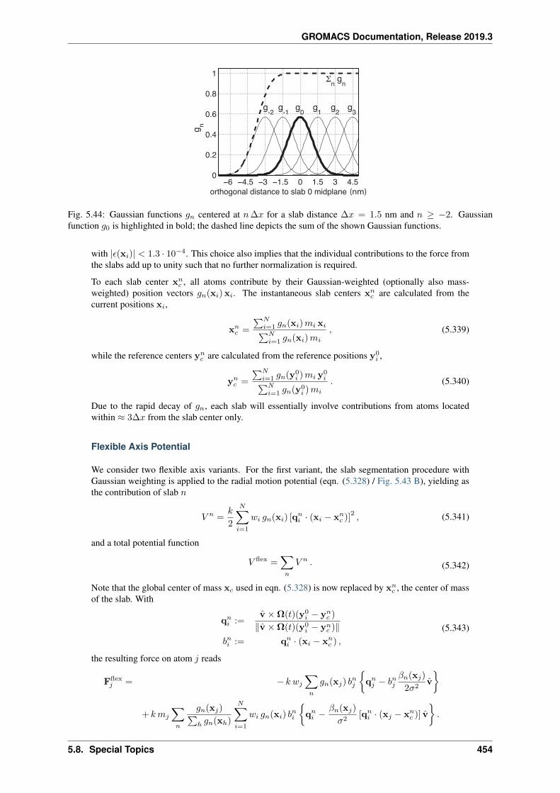
GROMACS Documentation, Release 2019.3
Fig. 5.44: Gaussian functions 𝑔𝑛 centered at 𝑛∆𝑥 for a slab distance ∆𝑥 = 1.5 nm and 𝑛 ≥ −2. Gaussianfunction 𝑔0 is highlighted in bold; the dashed line depicts the sum of the shown Gaussian functions.
with |𝜖(x𝑖)| < 1.3 · 10−4. This choice also implies that the individual contributions to the force fromthe slabs add up to unity such that no further normalization is required.
To each slab center x𝑛𝑐 , all atoms contribute by their Gaussian-weighted (optionally also mass-
weighted) position vectors 𝑔𝑛(x𝑖)x𝑖. The instantaneous slab centers x𝑛𝑐 are calculated from the
current positions x𝑖,
x𝑛𝑐 =
∑𝑁𝑖=1 𝑔𝑛(x𝑖)𝑚𝑖 x𝑖∑𝑁𝑖=1 𝑔𝑛(x𝑖)𝑚𝑖
, (5.339)
while the reference centers y𝑛𝑐 are calculated from the reference positions y0
𝑖 ,
y𝑛𝑐 =
∑𝑁𝑖=1 𝑔𝑛(y0
𝑖 )𝑚𝑖 y0𝑖∑𝑁
𝑖=1 𝑔𝑛(y0𝑖 )𝑚𝑖
. (5.340)
Due to the rapid decay of 𝑔𝑛, each slab will essentially involve contributions from atoms locatedwithin ≈ 3∆𝑥 from the slab center only.
Flexible Axis Potential
We consider two flexible axis variants. For the first variant, the slab segmentation procedure withGaussian weighting is applied to the radial motion potential (eqn. (5.328) / Fig. 5.43 B), yielding asthe contribution of slab 𝑛
𝑉 𝑛 =𝑘
2
𝑁∑𝑖=1
𝑤𝑖 𝑔𝑛(x𝑖) [q𝑛𝑖 · (x𝑖 − x𝑛
𝑐 )]2, (5.341)
and a total potential function
𝑉 flex =∑𝑛
𝑉 𝑛 . (5.342)
Note that the global center of mass x𝑐 used in eqn. (5.328) is now replaced by x𝑛𝑐 , the center of mass
of the slab. With
q𝑛𝑖 :=
v ×Ω(𝑡)(y0𝑖 − y𝑛
𝑐 )
‖v ×Ω(𝑡)(y0𝑖 − y𝑛
𝑐 )‖𝑏𝑛𝑖 := q𝑛
𝑖 · (x𝑖 − x𝑛𝑐 ) ,
(5.343)
the resulting force on atom 𝑗 reads
Fflex𝑗 = − 𝑘 𝑤𝑗
∑𝑛
𝑔𝑛(x𝑗) 𝑏𝑛𝑗
{q𝑛𝑗 − 𝑏𝑛𝑗
𝛽𝑛(x𝑗)
2𝜎2v
}
+ 𝑘𝑚𝑗
∑𝑛
𝑔𝑛(x𝑗)∑ℎ 𝑔𝑛(xℎ)
𝑁∑𝑖=1
𝑤𝑖 𝑔𝑛(x𝑖) 𝑏𝑛𝑖
{q𝑛𝑖 − 𝛽𝑛(x𝑗)
𝜎2[q𝑛
𝑖 · (x𝑗 − x𝑛𝑐 )] v
}.
5.8. Special Topics 454
GROMACS Documentation, Release 2019.3
Note that for 𝑉 flex, as defined, the slabs are fixed in space and so are the reference centers y𝑛𝑐 . If
during the simulation the rotation group moves too far in v direction, it may enter a region where– due to the lack of nearby reference positions – no reference slab centers are defined, renderingthe potential evaluation impossible. We therefore have included a slightly modified version of thispotential that avoids this problem by attaching the midplane of slab 𝑛 = 0 to the center of mass of therotation group, yielding slabs that move with the rotation group. This is achieved by subtracting thecenter of mass x𝑐 of the group from the positions,
x𝑖 = x𝑖 − x𝑐 , and y0𝑖 = y0
𝑖 − y0𝑐 , (5.344)
such that
𝑉 flex−t =𝑘
2
∑𝑛
𝑁∑𝑖=1
𝑤𝑖 𝑔𝑛(x𝑖)
[v ×Ω(𝑡)(y0
𝑖 − y𝑛𝑐 )
‖v ×Ω(𝑡)(y0𝑖 − y𝑛
𝑐 )‖· (x𝑖 − x𝑛
𝑐 )
]2. (5.345)
To simplify the force derivation, and for efficiency reasons, we here assume x𝑐 to be constant, andthus 𝜕x𝑐/𝜕𝑥 = 𝜕x𝑐/𝜕𝑦 = 𝜕x𝑐/𝜕𝑧 = 0. The resulting force error is small (of order 𝑂(1/𝑁) or𝑂(𝑚𝑗/𝑀) if mass-weighting is applied) and can therefore be tolerated. With this assumption, theforces Fflex−t have the same form as eqn. (5.344).
Flexible Axis 2 Alternative Potential
In this second variant, slab segmentation is applied to 𝑉 rm2 (eqn. (5.333)), resulting in a flexible axispotential without radial force contributions (Fig. 5.43 C),
𝑉 flex2 =𝑘
2
𝑁∑𝑖=1
∑𝑛
𝑤𝑖 𝑔𝑛(x𝑖)
[(v × (x𝑖 − x𝑛
𝑐 )) ·Ω(𝑡)(y0𝑖 − y𝑛
𝑐 )]2
‖v × (x𝑖 − x𝑛𝑐 )‖2 + 𝜖′
(5.346)
With
r𝑛𝑖 := Ω(𝑡)(y0𝑖 − y𝑛
𝑐 )
s𝑛𝑖 :=v × (x𝑖 − x𝑛
𝑐 )
‖v × (x𝑖 − x𝑛𝑐 )‖
≡ 𝜓𝑖 v × (x𝑖 − x𝑛𝑐 )
𝜓*𝑖 :=
1
‖v × (x𝑖 − x𝑛𝑐 )‖2 + 𝜖′
𝑊𝑛𝑗 :=
𝑔𝑛(x𝑗)𝑚𝑗∑ℎ 𝑔𝑛(xℎ)𝑚ℎ
S𝑛 :=
𝑁∑𝑖=1
𝑤𝑖 𝑔𝑛(x𝑖) (s𝑛𝑖 · r𝑛𝑖 )
[𝜓*𝑖
𝜓𝑖r𝑛𝑖 − 𝜓*2
𝑖
𝜓3𝑖
(s𝑛𝑖 · r𝑛𝑖 ) s𝑛𝑖
](5.347)
the force on atom 𝑗 reads
F𝑗flex2 = −𝑘
{∑𝑛
𝑤𝑗 𝑔𝑛(x𝑗) (s𝑛𝑗 · r𝑛𝑗 )
[𝜓*𝑗
𝜓𝑗r𝑛𝑗 −
𝜓*2𝑗
𝜓3𝑗
(s𝑛𝑗 · r𝑛𝑗 ) s𝑛𝑗
]}× v
+𝑘
{∑𝑛
𝑊𝑛𝑗 S𝑛
}× v − 𝑘
{∑𝑛
𝑊𝑛𝑗
𝛽𝑛(x𝑗)
𝜎2
1
𝜓𝑗s𝑛𝑗 · S𝑛
}v
+𝑘
2
{∑𝑛
𝑤𝑗 𝑔𝑛(x𝑗)𝛽𝑛(x𝑗)
𝜎2
𝜓*𝑗
𝜓2𝑗
(s𝑛𝑗 · r𝑛𝑗 )2
}v.
Applying transformation (5.344) yields a “translation-tolerant” version of the flexible2 potential,𝑉 flex2−t. Again, assuming that 𝜕x𝑐/𝜕𝑥, 𝜕x𝑐/𝜕𝑦, 𝜕x𝑐/𝜕𝑧 are small, the resulting equations for𝑉 flex2−t and Fflex2−t are similar to those of 𝑉 flex2 and Fflex2.
5.8. Special Topics 455
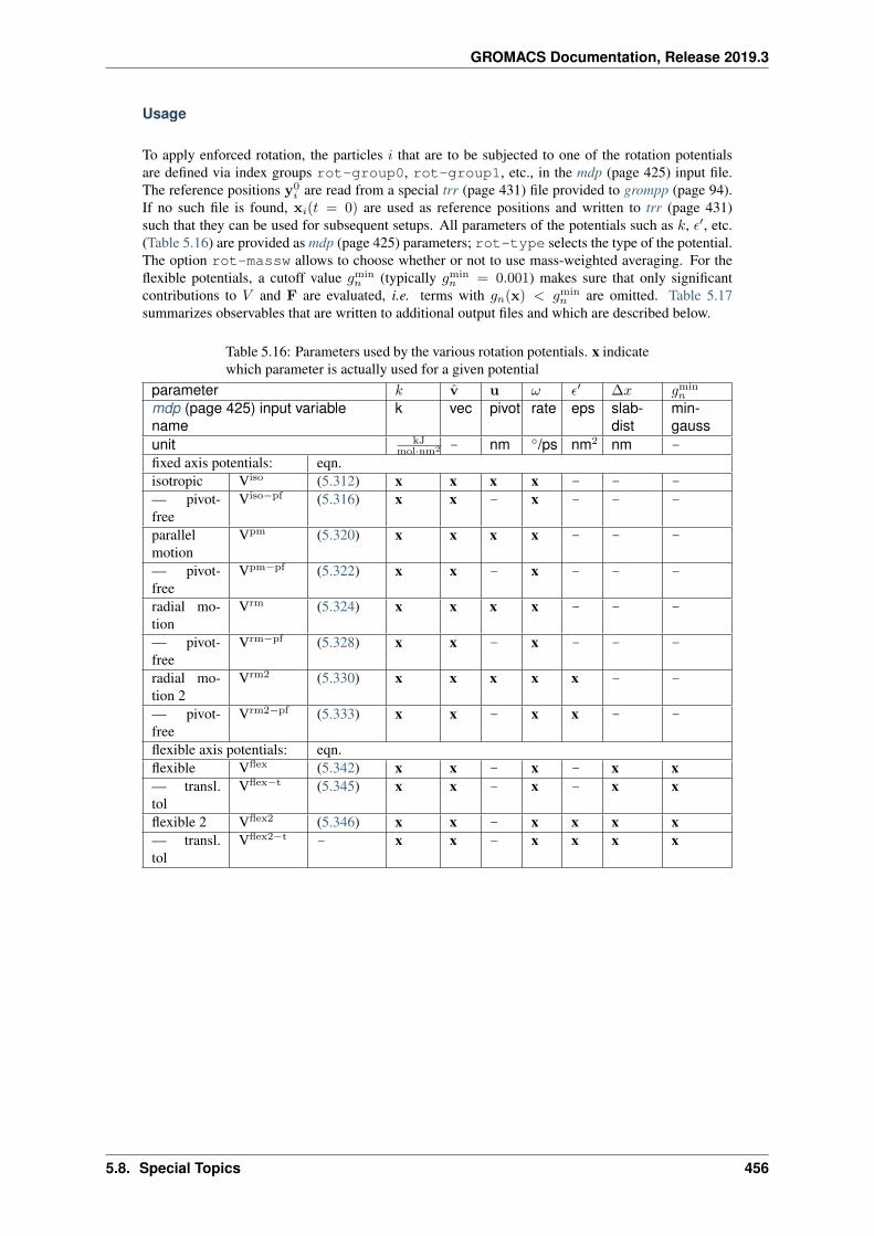
GROMACS Documentation, Release 2019.3
Usage
To apply enforced rotation, the particles 𝑖 that are to be subjected to one of the rotation potentialsare defined via index groups rot-group0, rot-group1, etc., in the mdp (page 425) input file.The reference positions y0
𝑖 are read from a special trr (page 431) file provided to grompp (page 94).If no such file is found, x𝑖(𝑡 = 0) are used as reference positions and written to trr (page 431)such that they can be used for subsequent setups. All parameters of the potentials such as 𝑘, 𝜖′, etc.(Table 5.16) are provided as mdp (page 425) parameters; rot-type selects the type of the potential.The option rot-massw allows to choose whether or not to use mass-weighted averaging. For theflexible potentials, a cutoff value 𝑔min
𝑛 (typically 𝑔min𝑛 = 0.001) makes sure that only significant
contributions to 𝑉 and F are evaluated, i.e. terms with 𝑔𝑛(x) < 𝑔min𝑛 are omitted. Table 5.17
summarizes observables that are written to additional output files and which are described below.
Table 5.16: Parameters used by the various rotation potentials. x indicatewhich parameter is actually used for a given potential
parameter 𝑘 v u 𝜔 𝜖′ ∆𝑥 𝑔min𝑛
mdp (page 425) input variablename
k vec pivot rate eps slab-dist
min-gauss
unit kJmol·nm2 - nm ∘/ps nm2 nm -
fixed axis potentials: eqn.isotropic Viso (5.312) x x x x - - -— pivot-free
Viso−pf (5.316) x x - x - - -
parallelmotion
Vpm (5.320) x x x x - - -
— pivot-free
Vpm−pf (5.322) x x - x - - -
radial mo-tion
Vrm (5.324) x x x x - - -
— pivot-free
Vrm−pf (5.328) x x - x - - -
radial mo-tion 2
Vrm2 (5.330) x x x x x - -
— pivot-free
Vrm2−pf (5.333) x x - x x - -
flexible axis potentials: eqn.flexible Vflex (5.342) x x - x - x x— transl.tol
Vflex−t (5.345) x x - x - x x
flexible 2 Vflex2 (5.346) x x - x x x x— transl.tol
Vflex2−t - x x - x x x x
5.8. Special Topics 456
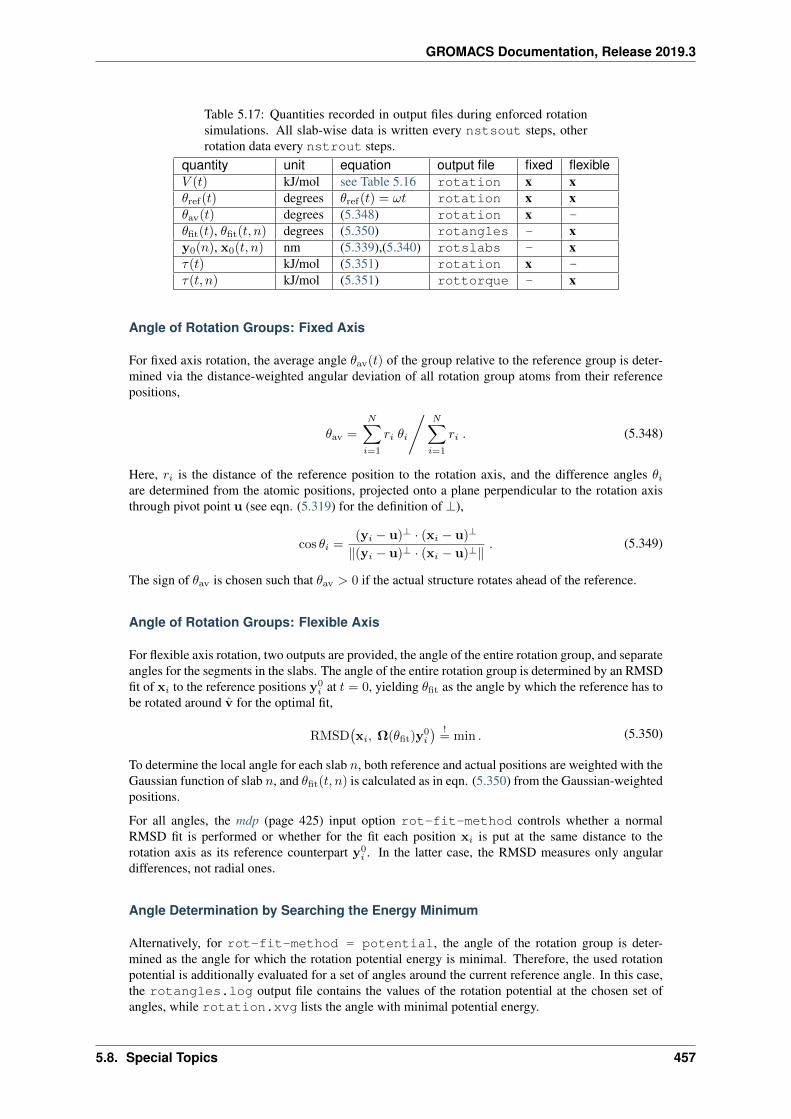
GROMACS Documentation, Release 2019.3
Table 5.17: Quantities recorded in output files during enforced rotationsimulations. All slab-wise data is written every nstsout steps, otherrotation data every nstrout steps.
quantity unit equation output file fixed flexible𝑉 (𝑡) kJ/mol see Table 5.16 rotation x x𝜃ref(𝑡) degrees 𝜃ref(𝑡) = 𝜔𝑡 rotation x x𝜃av(𝑡) degrees (5.348) rotation x -𝜃fit(𝑡), 𝜃fit(𝑡, 𝑛) degrees (5.350) rotangles - xy0(𝑛), x0(𝑡, 𝑛) nm (5.339),(5.340) rotslabs - x𝜏(𝑡) kJ/mol (5.351) rotation x -𝜏(𝑡, 𝑛) kJ/mol (5.351) rottorque - x
Angle of Rotation Groups: Fixed Axis
For fixed axis rotation, the average angle 𝜃av(𝑡) of the group relative to the reference group is deter-mined via the distance-weighted angular deviation of all rotation group atoms from their referencepositions,
𝜃av =𝑁∑𝑖=1
𝑟𝑖 𝜃𝑖
⧸𝑁∑𝑖=1
𝑟𝑖 . (5.348)
Here, 𝑟𝑖 is the distance of the reference position to the rotation axis, and the difference angles 𝜃𝑖are determined from the atomic positions, projected onto a plane perpendicular to the rotation axisthrough pivot point u (see eqn. (5.319) for the definition of ⊥),
cos 𝜃𝑖 =(y𝑖 − u)⊥ · (x𝑖 − u)⊥
‖(y𝑖 − u)⊥ · (x𝑖 − u)⊥‖. (5.349)
The sign of 𝜃av is chosen such that 𝜃av > 0 if the actual structure rotates ahead of the reference.
Angle of Rotation Groups: Flexible Axis
For flexible axis rotation, two outputs are provided, the angle of the entire rotation group, and separateangles for the segments in the slabs. The angle of the entire rotation group is determined by an RMSDfit of x𝑖 to the reference positions y0
𝑖 at 𝑡 = 0, yielding 𝜃fit as the angle by which the reference has tobe rotated around v for the optimal fit,
RMSD(x𝑖, Ω(𝜃fit)y
0𝑖
) != min . (5.350)
To determine the local angle for each slab 𝑛, both reference and actual positions are weighted with theGaussian function of slab 𝑛, and 𝜃fit(𝑡, 𝑛) is calculated as in eqn. (5.350) from the Gaussian-weightedpositions.
For all angles, the mdp (page 425) input option rot-fit-method controls whether a normalRMSD fit is performed or whether for the fit each position x𝑖 is put at the same distance to therotation axis as its reference counterpart y0
𝑖 . In the latter case, the RMSD measures only angulardifferences, not radial ones.
Angle Determination by Searching the Energy Minimum
Alternatively, for rot-fit-method = potential, the angle of the rotation group is deter-mined as the angle for which the rotation potential energy is minimal. Therefore, the used rotationpotential is additionally evaluated for a set of angles around the current reference angle. In this case,the rotangles.log output file contains the values of the rotation potential at the chosen set ofangles, while rotation.xvg lists the angle with minimal potential energy.
5.8. Special Topics 457
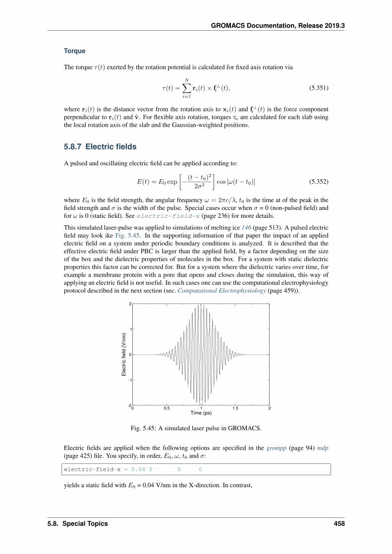
GROMACS Documentation, Release 2019.3
Torque
The torque 𝜏(𝑡) exerted by the rotation potential is calculated for fixed axis rotation via
𝜏(𝑡) =
𝑁∑𝑖=1
r𝑖(𝑡) × f⊥𝑖 (𝑡), (5.351)
where r𝑖(𝑡) is the distance vector from the rotation axis to x𝑖(𝑡) and f⊥𝑖 (𝑡) is the force componentperpendicular to r𝑖(𝑡) and v. For flexible axis rotation, torques 𝜏𝑛 are calculated for each slab usingthe local rotation axis of the slab and the Gaussian-weighted positions.
5.8.7 Electric fields
A pulsed and oscillating electric field can be applied according to:
𝐸(𝑡) = 𝐸0 exp
[− (𝑡− 𝑡0)2
2𝜎2
]cos [𝜔(𝑡− 𝑡0)] (5.352)
where 𝐸0 is the field strength, the angular frequency 𝜔 = 2𝜋𝑐/𝜆, 𝑡0 is the time at of the peak in thefield strength and 𝜎 is the width of the pulse. Special cases occur when 𝜎 = 0 (non-pulsed field) andfor 𝜔 is 0 (static field). See electric-field-x (page 236) for more details.
This simulated laser-pulse was applied to simulations of melting ice 146 (page 513). A pulsed electricfield may look ike Fig. 5.45. In the supporting information of that paper the impact of an appliedelectric field on a system under periodic boundary conditions is analyzed. It is described that theeffective electric field under PBC is larger than the applied field, by a factor depending on the sizeof the box and the dielectric properties of molecules in the box. For a system with static dielectricproperties this factor can be corrected for. But for a system where the dielectric varies over time, forexample a membrane protein with a pore that opens and closes during the simulation, this way ofapplying an electric field is not useful. In such cases one can use the computational electrophysiologyprotocol described in the next section (sec. Computational Electrophysiology (page 459)).
0 0.5 1 1.5 2Time (ps)
-2
-1
0
1
2
Elec
tric
field
(V/n
m)
Fig. 5.45: A simulated laser pulse in GROMACS.
Electric fields are applied when the following options are specified in the grompp (page 94) mdp(page 425) file. You specify, in order, 𝐸0, 𝜔, 𝑡0 and 𝜎:
electric-field-x = 0.04 0 0 0
yields a static field with 𝐸0 = 0.04 V/nm in the X-direction. In contrast,
5.8. Special Topics 458
GROMACS Documentation, Release 2019.3
electric-field-x = 2.0 150 5 0
yields an oscillating electric field with 𝐸0 = 2 V/nm, 𝜔 = 150/ps and 𝑡0 = 5 ps. Finally
electric-field-x = 2.0 150 5 1
yields an pulsed-oscillating electric field with 𝐸0 = 2 V/nm, 𝜔 = 150/ps and 𝑡0 = 5 ps and 𝜎 = 1 ps.Read more in ref. 146 (page 513). Note that the input file format is changed from the undocumentedolder version. A figure like Fig. 5.45 may be produced by passing the -field option to gmx mdrun(page 111).
5.8.8 Computational Electrophysiology
The Computational Electrophysiology (CompEL) protocol 147 (page 513) allows the simulation ofion flux through membrane channels, driven by transmembrane potentials or ion concentration gra-dients. Just as in real cells, CompEL establishes transmembrane potentials by sustaining a smallimbalance of charges ∆𝑞 across the membrane, which gives rise to a potential difference ∆𝑈 accord-ing to the membrane capacitance:
∆𝑈 = ∆𝑞/𝐶𝑚𝑒𝑚𝑏𝑟𝑎𝑛𝑒 (5.353)
The transmembrane electric field and concentration gradients are controlled by mdp (page 425) op-tions, which allow the user to set reference counts for the ions on either side of the membrane. If adifference between the actual and the reference numbers persists over a certain time span, specifiedby the user, a number of ion/water pairs are exchanged between the compartments until the referencenumbers are restored. Alongside the calculation of channel conductance and ion selectivity, CompELsimulations also enable determination of the channel reversal potential, an important characteristicobtained in electrophysiology experiments.
In a CompEL setup, the simulation system is divided into two compartments A and B with inde-pendent ion concentrations. This is best achieved by using double bilayer systems with a copy (orcopies) of the channel/pore of interest in each bilayer (Fig. 5.46 A, B). If the channel axes point inthe same direction, channel flux is observed simultaneously at positive and negative potentials in thisway, which is for instance important for studying channel rectification.
The potential difference ∆𝑈 across the membrane is easily calculated with the gmx potential(page 131) utility. By this, the potential drop along 𝑧 or the pore axis is exactly known in eachtime interval of the simulation (Fig. 5.46 C). Type and number of ions 𝑛𝑖 of charge 𝑞𝑖, traversing thechannel in the simulation, are written to the swapions.xvg output file, from which the average channelconductance 𝐺 in each interval ∆𝑡 is determined by:
𝐺 =
∑𝑖 𝑛𝑖𝑞𝑖
∆𝑡∆𝑈. (5.354)
The ion selectivity is calculated as the number flux ratio of different species. Best results are obtainedby averaging these values over several overlapping time intervals.
The calculation of reversal potentials is best achieved using a small set of simulations in which agiven transmembrane concentration gradient is complemented with small ion imbalances of varyingmagnitude. For example, if one compartment contains 1M salt and the other 0.1M, and given chargeneutrality otherwise, a set of simulations with ∆𝑞 = 0 𝑒, ∆𝑞 = 2 𝑒, ∆𝑞 = 4 𝑒 could be used. Fittinga straight line through the current-voltage relationship of all obtained 𝐼-𝑈 pairs near zero current willthen yield 𝑈𝑟𝑒𝑣 .
Usage
The following mdp (page 425) options control the CompEL protocol:
5.8. Special Topics 459
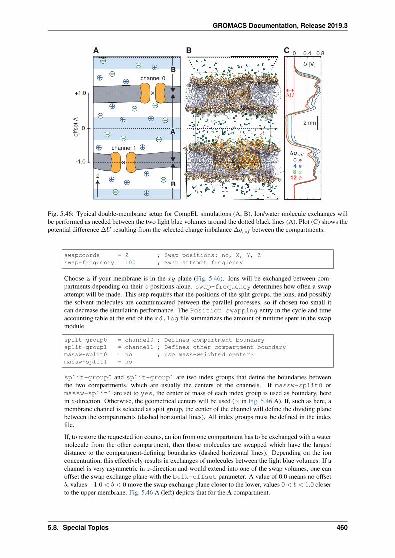
GROMACS Documentation, Release 2019.3
B
B
A B CU [V]
z
A
0 0.4 0.8
2 nm
qref
4 e8 e
12 e
0 e
U
channel 1
channel 0
0
+1.0
-1.0
offs
et A
Fig. 5.46: Typical double-membrane setup for CompEL simulations (A, B). Ion/water molecule exchanges willbe performed as needed between the two light blue volumes around the dotted black lines (A). Plot (C) shows thepotential difference ∆𝑈 resulting from the selected charge imbalance ∆𝑞𝑟𝑒𝑓 between the compartments.
swapcoords = Z ; Swap positions: no, X, Y, Zswap-frequency = 100 ; Swap attempt frequency
Choose Z if your membrane is in the 𝑥𝑦-plane (Fig. 5.46). Ions will be exchanged between com-partments depending on their 𝑧-positions alone. swap-frequency determines how often a swapattempt will be made. This step requires that the positions of the split groups, the ions, and possiblythe solvent molecules are communicated between the parallel processes, so if chosen too small itcan decrease the simulation performance. The Position swapping entry in the cycle and timeaccounting table at the end of the md.log file summarizes the amount of runtime spent in the swapmodule.
split-group0 = channel0 ; Defines compartment boundarysplit-group1 = channel1 ; Defines other compartment boundarymassw-split0 = no ; use mass-weighted center?massw-split1 = no
split-group0 and split-group1 are two index groups that define the boundaries betweenthe two compartments, which are usually the centers of the channels. If massw-split0 ormassw-split1 are set to yes, the center of mass of each index group is used as boundary, herein 𝑧-direction. Otherwise, the geometrical centers will be used (× in Fig. 5.46 A). If, such as here, amembrane channel is selected as split group, the center of the channel will define the dividing planebetween the compartments (dashed horizontal lines). All index groups must be defined in the indexfile.
If, to restore the requested ion counts, an ion from one compartment has to be exchanged with a watermolecule from the other compartment, then those molecules are swapped which have the largestdistance to the compartment-defining boundaries (dashed horizontal lines). Depending on the ionconcentration, this effectively results in exchanges of molecules between the light blue volumes. If achannel is very asymmetric in 𝑧-direction and would extend into one of the swap volumes, one canoffset the swap exchange plane with the bulk-offset parameter. A value of 0.0 means no offset𝑏, values −1.0 < 𝑏 < 0 move the swap exchange plane closer to the lower, values 0 < 𝑏 < 1.0 closerto the upper membrane. Fig. 5.46 A (left) depicts that for the A compartment.
5.8. Special Topics 460
GROMACS Documentation, Release 2019.3
solvent-group = SOL ; Group containing the solvent moleculesiontypes = 3 ; Number of different ion types to controliontype0-name = NA ; Group name of the ion typeiontype0-in-A = 51 ; Reference count of ions of type 0 in Aiontype0-in-B = 35 ; Reference count of ions of type 0 in Biontype1-name = Kiontype1-in-A = 10iontype1-in-B = 38iontype2-name = CLiontype2-in-A = -1iontype2-in-B = -1
The group name of solvent molecules acting as exchange partners for the ions has to be set withsolvent-group. The number of different ionic species under control of the CompEL protocolis given by the iontypes parameter, while iontype0-name gives the name of the index groupcontaining the atoms of this ionic species. The reference number of ions of this type can be setwith the iontype0-in-A and iontype0-in-B options for compartments A and B, respectively.Obviously, the sum of iontype0-in-A and iontype0-in-B needs to equal the number of ionsin the group defined by iontype0-name. A reference number of -1 means: use the number ofions as found at the beginning of the simulation as the reference value.
coupl-steps = 10 ; Average over these many swap stepsthreshold = 1 ; Do not swap if < threshold
If coupl-steps is set to 1, then the momentary ion distribution determines whether ions are ex-changed. coupl-steps > 1 will use the time-average of ion distributions over the selected num-ber of attempt steps instead. This can be useful, for example, when ions diffuse near compartmentboundaries, which would lead to numerous unproductive ion exchanges. A threshold of 1 meansthat a swap is performed if the average ion count in a compartment differs by at least 1 from therequested values. Higher thresholds will lead to toleration of larger differences. Ions are exchangeduntil the requested number ± the threshold is reached.
cyl0-r = 5.0 ; Split cylinder 0 radius (nm)cyl0-up = 0.75 ; Split cylinder 0 upper extension (nm)cyl0-down = 0.75 ; Split cylinder 0 lower extension (nm)cyl1-r = 5.0 ; same for other channelcyl1-up = 0.75cyl1-down = 0.75
The cylinder options are used to define virtual geometric cylinders around the channel’s pore to trackhow many ions of which type have passed each channel. Ions will be counted as having traveledthrough a channel according to the definition of the channel’s cylinder radius, upper and lower ex-tension, relative to the location of the respective split group. This will not affect the actual flux orexchange, but will provide you with the ion permeation numbers across each of the channels. Notethat an ion can only be counted as passing through a particular channel if it is detected within thedefined split cylinder in a swap step. If swap-frequency is chosen too high, a particular ion maybe detected in compartment A in one swap step, and in compartment B in the following swap step, soit will be unclear through which of the channels it has passed.
A double-layered system for CompEL simulations can be easily prepared by duplicating an exist-ing membrane/channel MD system in the direction of the membrane normal (typically 𝑧) with gmxeditconf (page 79) -translate 0 0 <l_z>, where l_z is the box length in that direction. Ifyou have already defined index groups for the channel for the single-layered system, gmx make_-ndx (page 109) -n index.ndx -twin will provide you with the groups for the double-layeredsystem.
To suppress large fluctuations of the membranes along the swap direction, it may be useful to applya harmonic potential (acting only in the swap dimension) between each of the two channel and/orbilayer centers using umbrella pulling (see section The pull code (page 437)).
5.8. Special Topics 461
GROMACS Documentation, Release 2019.3
Multimeric channels
If a split group consists of more than one molecule, the correct PBC image of all molecules withrespect to each other has to be chosen such that the channel center can be correctly determined. GRO-MACS assumes that the starting structure in the tpr (page 431) file has the correct PBC representation.Set the following environment variable to check whether that is the case:
• GMX_COMPELDUMP: output the starting structure after it has been made whole to pdb(page 427) file.
5.8.9 Calculating a PMF using the free-energy code
The free-energy coupling-parameter approach (see sec. Free energy calculations (page 336)) providesseveral ways to calculate potentials of mean force. A potential of mean force between two atoms canbe calculated by connecting them with a harmonic potential or a constraint. For this purpose thereare special potentials that avoid the generation of extra exclusions, see sec. Exclusions (page 397).When the position of the minimum or the constraint length is 1 nm more in state B than in state A,the restraint or constraint force is given by 𝜕𝐻/𝜕𝜆. The distance between the atoms can be changedas a function of 𝜆 and time by setting delta-lambda in the mdp (page 425) file. The results shouldbe identical (although not numerically due to the different implementations) to the results of the pullcode with umbrella sampling and constraint pulling. Unlike the pull code, the free energy code canalso handle atoms that are connected by constraints.
Potentials of mean force can also be calculated using position restraints. With position restraints,atoms can be linked to a position in space with a harmonic potential (see Position restraints(page 363)). These positions can be made a function of the coupling parameter 𝜆. The positionsfor the A and the B states are supplied to grompp (page 94) with the -r and -rb options, respec-tively. One could use this approach to do targeted MD; note that we do not encourage the use oftargeted MD for proteins. A protein can be forced from one conformation to another by using theseconformations as position restraint coordinates for state A and B. One can then slowly change 𝜆 from0 to 1. The main drawback of this approach is that the conformational freedom of the protein isseverely limited by the position restraints, independent of the change from state A to B. Also, theprotein is forced from state A to B in an almost straight line, whereas the real pathway might be verydifferent. An example of a more fruitful application is a solid system or a liquid confined betweenwalls where one wants to measure the force required to change the separation between the boundariesor walls. Because the boundaries (or walls) already need to be fixed, the position restraints do notlimit the system in its sampling.
5.8.10 Removing fastest degrees of freedom
The maximum time step in MD simulations is limited by the smallest oscillation period that can befound in the simulated system. Bond-stretching vibrations are in their quantum-mechanical groundstate and are therefore better represented by a constraint instead of a harmonic potential.
For the remaining degrees of freedom, the shortest oscillation period (as measured from a simulation)is 13 fs for bond-angle vibrations involving hydrogen atoms. Taking as a guideline that with a Verlet(leap-frog) integration scheme a minimum of 5 numerical integration steps should be performed perperiod of a harmonic oscillation in order to integrate it with reasonable accuracy, the maximum timestep will be about 3 fs. Disregarding these very fast oscillations of period 13 fs, the next shortestperiods are around 20 fs, which will allow a maximum time step of about 4 fs.
Removing the bond-angle degrees of freedom from hydrogen atoms can best be done by definingthem as virtual interaction sites instead of normal atoms. Whereas a normal atom is connected to themolecule with bonds, angles and dihedrals, a virtual site’s position is calculated from the position ofthree nearby heavy atoms in a predefined manner (see also sec. Virtual interaction sites (page 379)).For the hydrogens in water and in hydroxyl, sulfhydryl, or amine groups, no degrees of freedom canbe removed, because rotational freedom should be preserved. The only other option available to slowdown these motions is to increase the mass of the hydrogen atoms at the expense of the mass of
5.8. Special Topics 462
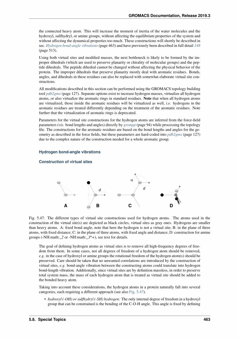
GROMACS Documentation, Release 2019.3
the connected heavy atom. This will increase the moment of inertia of the water molecules and thehydroxyl, sulfhydryl, or amine groups, without affecting the equilibrium properties of the system andwithout affecting the dynamical properties too much. These constructions will shortly be described insec. Hydrogen bond-angle vibrations (page 463) and have previously been described in full detail 148(page 513).
Using both virtual sites and modified masses, the next bottleneck is likely to be formed by the im-proper dihedrals (which are used to preserve planarity or chirality of molecular groups) and the pep-tide dihedrals. The peptide dihedral cannot be changed without affecting the physical behavior of theprotein. The improper dihedrals that preserve planarity mostly deal with aromatic residues. Bonds,angles, and dihedrals in these residues can also be replaced with somewhat elaborate virtual site con-structions.
All modifications described in this section can be performed using the GROMACS topology buildingtool pdb2gmx (page 127). Separate options exist to increase hydrogen masses, virtualize all hydrogenatoms, or also virtualize the aromatic rings in standard residues. Note that when all hydrogen atomsare virtualized, those inside the aromatic residues will be virtualized as well, i.e. hydrogens in thearomatic residues are treated differently depending on the treatment of the aromatic residues. Notefurther that the virtualization of aromatic rings is deprecated.
Parameters for the virtual site constructions for the hydrogen atoms are inferred from the force-fieldparameters (vis. bond lengths and angles) directly by grompp (page 94) while processing the topologyfile. The constructions for the aromatic residues are based on the bond lengths and angles for the ge-ometry as described in the force fields, but these parameters are hard-coded into pdb2gmx (page 127)due to the complex nature of the construction needed for a whole aromatic group.
Hydrogen bond-angle vibrations
Construction of virtual sites
D
d
α
d
BA C
0 0 00 0 01 1 11 1 1
0 0 0 00 0 0 01 1 1 11 1 1 1
0 0 0 00 0 0 01 1 1 11 1 1 1
0 0 0 00 0 0 01 1 1 11 1 1 1
0 0 0 00 0 0 01 1 1 11 1 1 1
0 0 00 0 00 0 0
1 1 11 1 11 1 1
0 0 01 1 1
0 0 00 0 00 0 0
1 1 11 1 11 1 1
0 0 0 00 0 0 00 0 0 0
1 1 1 11 1 1 11 1 1 1
Fig. 5.47: The different types of virtual site constructions used for hydrogen atoms. The atoms used in theconstruction of the virtual site(s) are depicted as black circles, virtual sites as gray ones. Hydrogens are smallerthan heavy atoms. A: fixed bond angle, note that here the hydrogen is not a virtual site; B: in the plane of threeatoms, with fixed distance; C: in the plane of three atoms, with fixed angle and distance; D: construction for aminegroups (-NH:math:_2 or -NH:math:_3^+), see text for details.
The goal of defining hydrogen atoms as virtual sites is to remove all high-frequency degrees of free-dom from them. In some cases, not all degrees of freedom of a hydrogen atom should be removed,e.g. in the case of hydroxyl or amine groups the rotational freedom of the hydrogen atom(s) should bepreserved. Care should be taken that no unwanted correlations are introduced by the construction ofvirtual sites, e.g. bond-angle vibration between the constructing atoms could translate into hydrogenbond-length vibration. Additionally, since virtual sites are by definition massless, in order to preservetotal system mass, the mass of each hydrogen atom that is treated as virtual site should be added tothe bonded heavy atom.
Taking into account these considerations, the hydrogen atoms in a protein naturally fall into severalcategories, each requiring a different approach (see also Fig. 5.47).
• hydroxyl (-OH) or sulfhydryl (-SH) hydrogen: The only internal degree of freedom in a hydroxylgroup that can be constrained is the bending of the C-O-H angle. This angle is fixed by defining
5.8. Special Topics 463
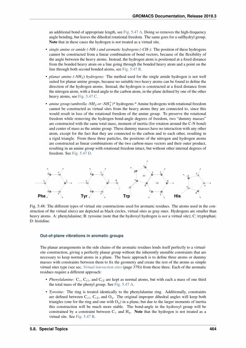
GROMACS Documentation, Release 2019.3
an additional bond of appropriate length, see Fig. 5.47 A. Doing so removes the high-frequencyangle bending, but leaves the dihedral rotational freedom. The same goes for a sulfhydryl group.Note that in these cases the hydrogen is not treated as a virtual site.
• single amine or amide (-NH-) and aromatic hydrogens (-CH-): The position of these hydrogenscannot be constructed from a linear combination of bond vectors, because of the flexibility ofthe angle between the heavy atoms. Instead, the hydrogen atom is positioned at a fixed distancefrom the bonded heavy atom on a line going through the bonded heavy atom and a point on theline through both second bonded atoms, see Fig. 5.47 B.
• planar amine (-NH2) hydrogens: The method used for the single amide hydrogen is not wellsuited for planar amine groups, because no suitable two heavy atoms can be found to define thedirection of the hydrogen atoms. Instead, the hydrogen is constructed at a fixed distance fromthe nitrogen atom, with a fixed angle to the carbon atom, in the plane defined by one of the otherheavy atoms, see Fig. 5.47 C.
• amine group (umbrella -NH2 or -NH+3 )* hydrogens:* Amine hydrogens with rotational freedom
cannot be constructed as virtual sites from the heavy atoms they are connected to, since thiswould result in loss of the rotational freedom of the amine group. To preserve the rotationalfreedom while removing the hydrogen bond-angle degrees of freedom, two “dummy masses”are constructed with the same total mass, moment of inertia (for rotation around the C-N bond)and center of mass as the amine group. These dummy masses have no interaction with any otheratom, except for the fact that they are connected to the carbon and to each other, resulting ina rigid triangle. From these three particles, the positions of the nitrogen and hydrogen atomsare constructed as linear combinations of the two carbon-mass vectors and their outer product,resulting in an amine group with rotational freedom intact, but without other internal degrees offreedom. See Fig. 5.47 D.
ε
η
ζδ
ε
γ
ε
δ ε
δ
εδ
γ
ζε
η
εδ
γ
Phe Tyr HisTrp
ζ
ε
ζ
εδ
γ
δδ
0 0 0 00 0 0 01 1 1 11 1 1 1
0 0 0 00 0 0 00 0 0 0
1 1 1 11 1 1 11 1 1 1
0 0 0 00 0 0 01 1 1 11 1 1 1
0 0 00 0 00 0 0
1 1 11 1 11 1 1
0 0 00 0 01 1 11 1 1
0 0 0 00 0 0 01 1 1 11 1 1 1
0 00 01 11 1
0 0 00 0 01 1 11 1 1
0 0 00 0 01 1 11 1 1
0 0 00 0 00 0 0
1 1 11 1 11 1 1
0 0 00 0 00 0 0
1 1 11 1 11 1 1
0 0 00 0 01 1 11 1 1
0 0 0 00 0 0 00 0 0 0
1 1 1 11 1 1 11 1 1 1
0 0 00 0 00 0 0
1 1 11 1 11 1 1
Fig. 5.48: The different types of virtual site constructions used for aromatic residues. The atoms used in the con-struction of the virtual site(s) are depicted as black circles, virtual sites as gray ones. Hydrogens are smaller thanheavy atoms. A: phenylalanine; B: tyrosine (note that the hydroxyl hydrogen is not a virtual site); C: tryptophan;D: histidine.
Out-of-plane vibrations in aromatic groups
The planar arrangements in the side chains of the aromatic residues lends itself perfectly to a virtual-site construction, giving a perfectly planar group without the inherently unstable constraints that arenecessary to keep normal atoms in a plane. The basic approach is to define three atoms or dummymasses with constraints between them to fix the geometry and create the rest of the atoms as simplevirtual sites type (see sec. Virtual interaction sites (page 379)) from these three. Each of the aromaticresidues require a different approach:
• Phenylalanine: C𝛾 , C𝜖1, and C𝜖2 are kept as normal atoms, but with each a mass of one thirdthe total mass of the phenyl group. See Fig. 5.47 A.
• Tyrosine: The ring is treated identically to the phenylalanine ring. Additionally, constraintsare defined between C𝜖1, C𝜖2, and O𝜂 . The original improper dihedral angles will keep bothtriangles (one for the ring and one with O𝜂) in a plane, but due to the larger moments of inertiathis construction will be much more stable. The bond-angle in the hydroxyl group will beconstrained by a constraint between C𝛾 and H𝜂 . Note that the hydrogen is not treated as avirtual site. See Fig. 5.47 B.
5.8. Special Topics 464
GROMACS Documentation, Release 2019.3
• Tryptophan: C𝛽 is kept as a normal atom and two dummy masses are created at the center ofmass of each of the rings, each with a mass equal to the total mass of the respective ring (C𝛿2
and C𝜖2 are each counted half for each ring). This keeps the overall center of mass and themoment of inertia almost (but not quite) equal to what it was. See Fig. 5.47 C.
• Histidine: C𝛾 , C𝜖1 and N𝜖2 are kept as normal atoms, but with masses redistributed such thatthe center of mass of the ring is preserved. See Fig. 5.47 D.
5.8.11 Viscosity calculation
The shear viscosity is a property of liquids that can be determined easily by experiment. It is usefulfor parameterizing a force field because it is a kinetic property, while most other properties which areused for parameterization are thermodynamic. The viscosity is also an important property, since itinfluences the rates of conformational changes of molecules solvated in the liquid.
The viscosity can be calculated from an equilibrium simulation using an Einstein relation:
𝜂 =1
2
𝑉
𝑘𝐵𝑇lim𝑡→∞
dd𝑡
⟨(∫ 𝑡0+𝑡
𝑡0
𝑃𝑥𝑧(𝑡′)d𝑡′)2⟩
𝑡0
(5.355)
This can be done with gmx energy (page 84). This method converges very slowly 149 (page 513),and as such a nanosecond simulation might not be long enough for an accurate determination of theviscosity. The result is very dependent on the treatment of the electrostatics. Using a (short) cut-off results in large noise on the off-diagonal pressure elements, which can increase the calculatedviscosity by an order of magnitude.
GROMACS also has a non-equilibrium method for determining the viscosity 149 (page 513). Thismakes use of the fact that energy, which is fed into system by external forces, is dissipated throughviscous friction. The generated heat is removed by coupling to a heat bath. For a Newtonian liquidadding a small force will result in a velocity gradient according to the following equation:
𝑎𝑥(𝑧) +𝜂
𝜌
𝜕2𝑣𝑥(𝑧)
𝜕𝑧2= 0 (5.356)
Here we have applied an acceleration 𝑎𝑥(𝑧) in the 𝑥-direction, which is a function of the 𝑧-coordinate.In GROMACS the acceleration profile is:
𝑎𝑥(𝑧) = 𝐴 cos
(2𝜋𝑧
𝑙𝑧
)(5.357)
where 𝑙𝑧 is the height of the box. The generated velocity profile is:
𝑣𝑥(𝑧) = 𝑉 cos
(2𝜋𝑧
𝑙𝑧
)(5.358)
𝑉 = 𝐴𝜌
𝜂
(𝑙𝑧2𝜋
)2
(5.359)
The viscosity can be calculated from 𝐴 and 𝑉 :
𝜂 =𝐴
𝑉𝜌
(𝑙𝑧2𝜋
)2
(5.360)
In the simulation 𝑉 is defined as:
𝑉 =
𝑁∑𝑖=1
𝑚𝑖𝑣𝑖,𝑥2 cos
(2𝜋𝑧
𝑙𝑧
)𝑁∑𝑖=1
𝑚𝑖
(5.361)
5.8. Special Topics 465
GROMACS Documentation, Release 2019.3
The generated velocity profile is not coupled to the heat bath. Moreover, the velocity profile is ex-cluded from the kinetic energy. One would like 𝑉 to be as large as possible to get good statistics.However, the shear rate should not be so high that the system gets too far from equilibrium. Themaximum shear rate occurs where the cosine is zero, the rate being:
shmax = max𝑧
𝜕𝑣𝑥(𝑧)
𝜕𝑧
= 𝐴
𝜌
𝜂
𝑙𝑧2𝜋
(5.362)
For a simulation with: 𝜂 = 10−3 [kgm:math:^{-1}s−1], 𝜌 = 103[kgm:math:^{-3}] and 𝑙𝑧 = 2𝜋[nm],shmax = 1[psnm:math:^{-1}] 𝐴. This shear rate should be smaller than one over the longest correla-tion time in the system. For most liquids, this will be the rotation correlation time, which is around 10ps. In this case, 𝐴 should be smaller than 0.1[nmps−2]. When the shear rate is too high, the observedviscosity will be too low. Because 𝑉 is proportional to the square of the box height, the optimal box iselongated in the 𝑧-direction. In general, a simulation length of 100 ps is enough to obtain an accuratevalue for the viscosity.
The heat generated by the viscous friction is removed by coupling to a heat bath. Because thiscoupling is not instantaneous the real temperature of the liquid will be slightly lower than the observedtemperature. Berendsen derived this temperature shift 31 (page 507), which can be written in termsof the shear rate as:
𝑇𝑠 =𝜂 𝜏
2𝜌𝐶𝑣sh2
max (5.363)
where 𝜏 is the coupling time for the Berendsen thermostat and 𝐶𝑣 is the heat capacity. Using the val-ues of the example above, 𝜏 = 10−13 [s] and𝐶𝑣 = 2·103[J kg−1K−1], we get: 𝑇𝑠 = 25[Kps:math:^{-2}]sh2max. When we want the shear rate to be smaller than 1/10[ps:math:^{-1}], 𝑇𝑠 is smaller than0.25[K], which is negligible.
Note that the system has to build up the velocity profile when starting from an equilibrium state. Thisbuild-up time is of the order of the correlation time of the liquid.
Two quantities are written to the energy file, along with their averages and fluctuations: 𝑉 and 1/𝜂,as obtained from ((5.360)).
5.8.12 Tabulated interaction functions
Cubic splines for potentials
In some of the inner loops of GROMACS, look-up tables are used for computation of potential andforces. The tables are interpolated using a cubic spline algorithm. There are separate tables forelectrostatic, dispersion, and repulsion interactions, but for the sake of caching performance thesehave been combined into a single array. The cubic spline interpolation for 𝑥𝑖 ≤ 𝑥 < 𝑥𝑖+1 looks likethis:
𝑉𝑠(𝑥) = 𝐴0 +𝐴1 𝜖+𝐴2 𝜖2 +𝐴3 𝜖
3 (5.364)
where the table spacing ℎ and fraction 𝜖 are given by:
ℎ = 𝑥𝑖+1 − 𝑥𝑖
𝜖 = (𝑥− 𝑥𝑖)/ℎ(5.365)
so that 0 ≤ 𝜖 < 1. From this, we can calculate the derivative in order to determine the forces:
−𝑉 ′𝑠 (𝑥) = −d𝑉𝑠(𝑥)
d𝜖
d𝜖
d𝑥= −(𝐴1 + 2𝐴2 𝜖+ 3𝐴3 𝜖
2)/ℎ (5.366)
The four coefficients are determined from the four conditions that 𝑉𝑠 and −𝑉 ′𝑠 at both ends of each
interval should match the exact potential 𝑉 and force −𝑉 ′. This results in the following errors for
5.8. Special Topics 466
GROMACS Documentation, Release 2019.3
each interval:
|𝑉𝑠 − 𝑉 |𝑚𝑎𝑥 = 𝑉 ′′′′ ℎ4
384+𝑂(ℎ5)
|𝑉 ′𝑠 − 𝑉 ′|𝑚𝑎𝑥 = 𝑉 ′′′′ ℎ3
72√
3+𝑂(ℎ4)
|𝑉 ′′𝑠 − 𝑉 ′′|𝑚𝑎𝑥 = 𝑉 ′′′′ℎ
2
12+𝑂(ℎ3)
(5.367)
V and V’ are continuous, while V” is the first discontinuous derivative. The number of points pernanometer is 500 and 2000 for mixed- and double-precision versions of GROMACS, respectively.This means that the errors in the potential and force will usually be smaller than the mixed precisionaccuracy.
GROMACS stores 𝐴0, 𝐴1, 𝐴2 and 𝐴3. The force routines get a table with these four parameters anda scaling factor 𝑠 that is equal to the number of points per nm. (Note that ℎ is 𝑠−1). The algorithmgoes a little something like this:
1. Calculate distance vector (r𝑖𝑗) and distance r𝑖𝑗
2. Multiply r𝑖𝑗 by 𝑠 and truncate to an integer value 𝑛0 to get a table index
3. Calculate fractional component (𝜖 = 𝑠r𝑖𝑗 − 𝑛0) and 𝜖2
4. Do the interpolation to calculate the potential 𝑉 and the scalar force 𝑓
5. Calculate the vector force F by multiplying 𝑓 with r𝑖𝑗
Note that table look-up is significantly slower than computation of the most simple Lennard-Jonesand Coulomb interaction. However, it is much faster than the shifted Coulomb function used inconjunction with the PPPM method. Finally, it is much easier to modify a table for the potential (andget a graphical representation of it) than to modify the inner loops of the MD program.
User-specified potential functions
You can also use your own potential functions without editing the GROMACS code. The potentialfunction should be according to the following equation
𝑉 (𝑟𝑖𝑗) =𝑞𝑖𝑞𝑗4𝜋𝜖0
𝑓(𝑟𝑖𝑗) + 𝐶6 𝑔(𝑟𝑖𝑗) + 𝐶12 ℎ(𝑟𝑖𝑗) (5.368)
where 𝑓 , 𝑔, and ℎ are user defined functions. Note that if 𝑔(𝑟) represents a normal dispersion in-teraction, 𝑔(𝑟) should be < 0. C6, C12 and the charges are read from the topology. Also note thatcombination rules are only supported for Lennard-Jones and Buckingham, and that your tables shouldmatch the parameters in the binary topology.
When you add the following lines in your mdp (page 425) file:
rlist = 1.0coulombtype = Userrcoulomb = 1.0vdwtype = Userrvdw = 1.0
mdrun (page 111) will read a single non-bonded table file, or multiple when energygrp-table isset (see below). The name of the file(s) can be set with the mdrun (page 111) option -table. Thetable file should contain seven columns of table look-up data in the order: 𝑥, 𝑓(𝑥), −𝑓 ′(𝑥), 𝑔(𝑥),−𝑔′(𝑥), ℎ(𝑥), −ℎ′(𝑥). The 𝑥 should run from 0 to 𝑟𝑐 + 1 (the value of table_extension canbe changed in the mdp (page 425) file). You can choose the spacing you like; for the standard tablesGROMACS uses a spacing of 0.002 and 0.0005 nm when you run in mixed and double precision,respectively. In this context, 𝑟𝑐 denotes the maximum of the two cut-offs rvdw and rcoulomb (seeabove). These variables need not be the same (and need not be 1.0 either). Some functions used forpotentials contain a singularity at 𝑥 = 0, but since atoms are normally not closer to each other than
5.8. Special Topics 467
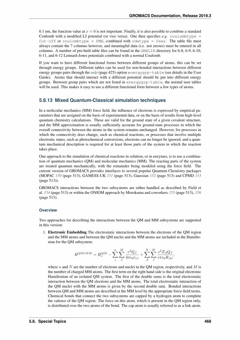
GROMACS Documentation, Release 2019.3
0.1 nm, the function value at 𝑥 = 0 is not important. Finally, it is also possible to combine a standardCoulomb with a modified LJ potential (or vice versa). One then specifies e.g. coulombtype =Cut-off or coulombtype = PME, combined with vdwtype = User. The table file mustalways contain the 7 columns however, and meaningful data (i.e. not zeroes) must be entered in allcolumns. A number of pre-built table files can be found in the GMXLIB directory for 6-8, 6-9, 6-10,6-11, and 6-12 Lennard-Jones potentials combined with a normal Coulomb.
If you want to have different functional forms between different groups of atoms, this can be setthrough energy groups. Different tables can be used for non-bonded interactions between differentenergy groups pairs through the mdp (page 425) option energygrp-table (see details in the UserGuide). Atoms that should interact with a different potential should be put into different energygroups. Between group pairs which are not listed in energygrp-table, the normal user tableswill be used. This makes it easy to use a different functional form between a few types of atoms.
5.8.13 Mixed Quantum-Classical simulation techniques
In a molecular mechanics (MM) force field, the influence of electrons is expressed by empirical pa-rameters that are assigned on the basis of experimental data, or on the basis of results from high-levelquantum chemistry calculations. These are valid for the ground state of a given covalent structure,and the MM approximation is usually sufficiently accurate for ground-state processes in which theoverall connectivity between the atoms in the system remains unchanged. However, for processes inwhich the connectivity does change, such as chemical reactions, or processes that involve multipleelectronic states, such as photochemical conversions, electrons can no longer be ignored, and a quan-tum mechanical description is required for at least those parts of the system in which the reactiontakes place.
One approach to the simulation of chemical reactions in solution, or in enzymes, is to use a combina-tion of quantum mechanics (QM) and molecular mechanics (MM). The reacting parts of the systemare treated quantum mechanically, with the remainder being modeled using the force field. Thecurrent version of GROMACS provides interfaces to several popular Quantum Chemistry packages(MOPAC 150 (page 513), GAMESS-UK 151 (page 513), Gaussian 152 (page 513) and CPMD 153(page 513)).
GROMACS interactions between the two subsystems are either handled as described by Field etal. 154 (page 513) or within the ONIOM approach by Morokuma and coworkers 155 (page 513), 156(page 513).
Overview
Two approaches for describing the interactions between the QM and MM subsystems are supportedin this version:
1. Electronic Embedding The electrostatic interactions between the electrons of the QM regionand the MM atoms and between the QM nuclei and the MM atoms are included in the Hamilto-nian for the QM subsystem:
𝐻𝑄𝑀/𝑀𝑀 = 𝐻𝑄𝑀𝑒 −
𝑛∑𝑖
𝑀∑𝐽
𝑒2𝑄𝐽
4𝜋𝜖0𝑟𝑖𝐽+
𝑁∑𝐴
𝑀∑𝐽
𝑒2𝑍𝐴𝑄𝐽
𝑒𝜋𝜖0𝑅𝐴𝐽,
where 𝑛 and 𝑁 are the number of electrons and nuclei in the QM region, respectively, and 𝑀 isthe number of charged MM atoms. The first term on the right hand side is the original electronicHamiltonian of an isolated QM system. The first of the double sums is the total electrostaticinteraction between the QM electrons and the MM atoms. The total electrostatic interaction ofthe QM nuclei with the MM atoms is given by the second double sum. Bonded interactionsbetween QM and MM atoms are described at the MM level by the appropriate force-field terms.Chemical bonds that connect the two subsystems are capped by a hydrogen atom to completethe valence of the QM region. The force on this atom, which is present in the QM region only,is distributed over the two atoms of the bond. The cap atom is usually referred to as a link atom.
5.8. Special Topics 468
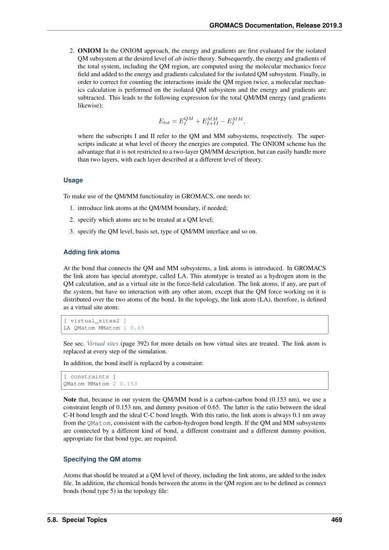
GROMACS Documentation, Release 2019.3
2. ONIOM In the ONIOM approach, the energy and gradients are first evaluated for the isolatedQM subsystem at the desired level of ab initio theory. Subsequently, the energy and gradients ofthe total system, including the QM region, are computed using the molecular mechanics forcefield and added to the energy and gradients calculated for the isolated QM subsystem. Finally, inorder to correct for counting the interactions inside the QM region twice, a molecular mechan-ics calculation is performed on the isolated QM subsystem and the energy and gradients aresubtracted. This leads to the following expression for the total QM/MM energy (and gradientslikewise):
𝐸𝑡𝑜𝑡 = 𝐸𝑄𝑀𝐼 + 𝐸𝑀𝑀
𝐼+𝐼𝐼 − 𝐸𝑀𝑀𝐼 ,
where the subscripts I and II refer to the QM and MM subsystems, respectively. The super-scripts indicate at what level of theory the energies are computed. The ONIOM scheme has theadvantage that it is not restricted to a two-layer QM/MM description, but can easily handle morethan two layers, with each layer described at a different level of theory.
Usage
To make use of the QM/MM functionality in GROMACS, one needs to:
1. introduce link atoms at the QM/MM boundary, if needed;
2. specify which atoms are to be treated at a QM level;
3. specify the QM level, basis set, type of QM/MM interface and so on.
Adding link atoms
At the bond that connects the QM and MM subsystems, a link atoms is introduced. In GROMACSthe link atom has special atomtype, called LA. This atomtype is treated as a hydrogen atom in theQM calculation, and as a virtual site in the force-field calculation. The link atoms, if any, are part ofthe system, but have no interaction with any other atom, except that the QM force working on it isdistributed over the two atoms of the bond. In the topology, the link atom (LA), therefore, is definedas a virtual site atom:
[ virtual_sites2 ]LA QMatom MMatom 1 0.65
See sec. Virtual sites (page 392) for more details on how virtual sites are treated. The link atom isreplaced at every step of the simulation.
In addition, the bond itself is replaced by a constraint:
[ constraints ]QMatom MMatom 2 0.153
Note that, because in our system the QM/MM bond is a carbon-carbon bond (0.153 nm), we use aconstraint length of 0.153 nm, and dummy position of 0.65. The latter is the ratio between the idealC-H bond length and the ideal C-C bond length. With this ratio, the link atom is always 0.1 nm awayfrom the QMatom, consistent with the carbon-hydrogen bond length. If the QM and MM subsystemsare connected by a different kind of bond, a different constraint and a different dummy position,appropriate for that bond type, are required.
Specifying the QM atoms
Atoms that should be treated at a QM level of theory, including the link atoms, are added to the indexfile. In addition, the chemical bonds between the atoms in the QM region are to be defined as connectbonds (bond type 5) in the topology file:
5.8. Special Topics 469
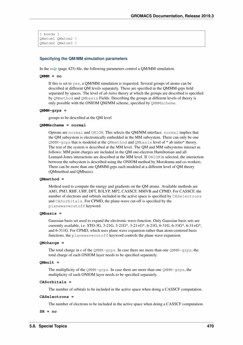
GROMACS Documentation, Release 2019.3
[ bonds ]QMatom1 QMatom2 5QMatom2 QMatom3 5
Specifying the QM/MM simulation parameters
In the mdp (page 425) file, the following parameters control a QM/MM simulation.
QMMM = no
If this is set to yes, a QM/MM simulation is requested. Several groups of atoms can bedescribed at different QM levels separately. These are specified in the QMMM-grps fieldseparated by spaces. The level of ab initio theory at which the groups are described is specifiedby QMmethod and QMbasis Fields. Describing the groups at different levels of theory isonly possible with the ONIOM QM/MM scheme, specified by QMMMscheme.
QMMM-grps =
groups to be described at the QM level
QMMMscheme = normal
Options are normal and ONIOM. This selects the QM/MM interface. normal implies thatthe QM subsystem is electronically embedded in the MM subsystem. There can only be oneQMMM-grps that is modeled at the QMmethod and QMbasis level of * ab initio* theory.The rest of the system is described at the MM level. The QM and MM subsystems interact asfollows: MM point charges are included in the QM one-electron Hamiltonian and allLennard-Jones interactions are described at the MM level. If ONIOM is selected, the interactionbetween the subsystem is described using the ONIOM method by Morokuma and co-workers.There can be more than one QMMM-grps each modeled at a different level of QM theory(QMmethod and QMbasis).
QMmethod =
Method used to compute the energy and gradients on the QM atoms. Available methods areAM1, PM3, RHF, UHF, DFT, B3LYP, MP2, CASSCF, MMVB and CPMD. For CASSCF, thenumber of electrons and orbitals included in the active space is specified by CASelectronsand CASorbitals. For CPMD, the plane-wave cut-off is specified by theplanewavecutoff keyword.
QMbasis =
Gaussian basis set used to expand the electronic wave-function. Only Gaussian basis sets arecurrently available, i.e. STO-3G, 3-21G, 3-21G*, 3-21+G*, 6-21G, 6-31G, 6-31G*, 6-31+G*,and 6-311G. For CPMD, which uses plane wave expansion rather than atom-centered basisfunctions, the planewavecutoff keyword controls the plane wave expansion.
QMcharge =
The total charge in e of the QMMM-grps. In case there are more than one QMMM-grps, thetotal charge of each ONIOM layer needs to be specified separately.
QMmult =
The multiplicity of the QMMM-grps. In case there are more than one QMMM-grps, themultiplicity of each ONIOM layer needs to be specified separately.
CASorbitals =
The number of orbitals to be included in the active space when doing a CASSCF computation.
CASelectrons =
The number of electrons to be included in the active space when doing a CASSCF computation.
SH = no
5.8. Special Topics 470
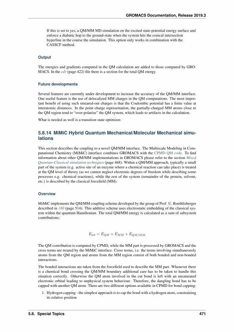
GROMACS Documentation, Release 2019.3
If this is set to yes, a QM/MM MD simulation on the excited state-potential energy surface andenforce a diabatic hop to the ground-state when the system hits the conical intersectionhyperline in the course the simulation. This option only works in combination with theCASSCF method.
Output
The energies and gradients computed in the QM calculation are added to those computed by GRO-MACS. In the edr (page 422) file there is a section for the total QM energy.
Future developments
Several features are currently under development to increase the accuracy of the QM/MM interface.One useful feature is the use of delocalized MM charges in the QM computations. The most impor-tant benefit of using such smeared-out charges is that the Coulombic potential has a finite value atinteratomic distances. In the point charge representation, the partially-charged MM atoms close tothe QM region tend to “over-polarize” the QM system, which leads to artifacts in the calculation.
What is needed as well is a transition state optimizer.
5.8.14 MiMiC Hybrid Quantum Mechanical/Molecular Mechanical simu-lations
This section describes the coupling to a novel QM/MM interface. The Multiscale Modeling in Com-putational Chemistry (MiMiC) interface combines GROMACS with the CPMD QM code. To findinformation about other QM/MM implementations in GROMACS please refer to the section MixedQuantum-Classical simulation techniques (page 468). Within a QM/MM approach, typically a smallpart of the system (e.g. active site of an enzyme where a chemical reaction can take place) is treatedat the QM level of theory (as we cannot neglect electronic degrees of freedom while descibing someprocesses e.g. chemical reactions), while the rest of the system (remainder of the protein, solvent,etc.) is described by the classical forcefield (MM).
Overview
MiMiC implements the QM/MM coupling scheme developed by the group of Prof. U. Roethlisbergerdescribed in 180 (page 514). This additive scheme uses electrostatic embedding of the classical sys-tem within the quantum Hamiltonian. The total QM/MM energy is calculated as a sum of subsystemcontributions:
𝐸𝑡𝑜𝑡 = 𝐸𝑄𝑀 + 𝐸𝑀𝑀 + 𝐸𝑄𝑀/𝑀𝑀
The QM contribution is computed by CPMD, while the MM part is processed by GROMACS and thecross terms are treated by the MiMiC interface. Cross terms, i.e. the terms involving simultaneouslyatoms from the QM region and atoms from the MM region consist of both bonded and non-bondedinteractions.
The bonded interactions are taken from the forcefield used to describe the MM part. Whenever thereis a chemical bond crossing the QM/MM boundary additional care has to be taken to handle thissituation correctly. Otherwise the QM atom involved in the cut bond is left with an unsaturatedelectronic orbital leading to unphysical system behaviour. Therefore, the dangling bond has to becapped with another QM atom. There are two different options available in CPMD for bond capping:
1. Hydrogen capping - the simplest approach is to cap the bond with a hydrogen atom, constrainingits relative position
5.8. Special Topics 471
GROMACS Documentation, Release 2019.3
2. Link atom pseudo-potential - this strategy uses an ad-hoc pseudo-potential developed to cap thebond. This pseudo-potential would represent the real atom and, thus, will not require the bondconstraint.
As in standard forcefields, the non-bonded contributions to 𝐸𝑄𝑀/𝑀𝑀 can be separated into van derWaals and electrostatic contributions. The first contribution is again taken from the MM forcefield.The second part of non-bonded interactions is handled by MiMiC within the electrostatic embeddingapproach. This adds additional terms to the Hamiltonian of the system:
𝐸𝑒𝑠𝑄𝑀/𝑀𝑀 = −
𝑁𝑚𝑚∑𝑎
𝑄𝑎
∫𝜌(r)
𝑟4𝑐,𝑎 − |Ra − r|4
𝑟5𝑐,𝑎 − |Ra − r|5𝑑r +
𝑁𝑚𝑚∑𝑎
𝑁𝑞𝑚∑𝑛
𝑄𝑎𝑍𝑛
𝑟4𝑐,𝑎 − |Ra −Rn|4
𝑟5𝑐,𝑎 − |Ra −Rn|5
where 𝑁𝑚𝑚 is a number of MM atoms 𝑁𝑞𝑚, is the number of QM atoms and 𝑟𝑐,𝑎 is the covalent ra-dius of the MM atoms. The first term above corresponds to the damped Coulomb interaction betweenthe eletronic density 𝜌(r) of the QM region and the MM atoms. The damping is needed due to thefact that CPMD uses a plane-wave basis set to expand the electronic wavefunction. Unlike localizedbasis sets, plane waves are delocalized and this may give a rise to the so-called electron spill-outproblem: positively charged MM atoms may artificially overpolarize the electronic cloud due to theabsence of quantum mechanical effects (e.g. Pauli repusion) that would normally prevent it (in a fullyquantum system). This functional form of the damped Coulomb potential from the equation abovewas introduced in 180 (page 514).
Since computing the integrals in the first term above can be computational extremely expensive,MiMiC also implements hierarchical electrostatic embedding scheme in order to mitigate the enor-mous computational effort needed to compute 𝑁𝑚𝑚 integrals over the electronic grid. Within thisscheme the MM atoms are grouped into two shells according to the distance from the QM region:the short-ranged and long-ranged one. For the MM atoms in the short-ranged shell the QM/MM in-teractions are calculated using the equation above. In contrast to that, the interactions involving MMatoms from the long-ranged shell are computed using the multipolar expansion of the QM electrostaticpotential. More details about it can be found in 180 (page 514).
Application coupling model
Unlike the majority of QM/MM interfaces, MiMiC uses a loose coupling between partner codes. Thismeans that instead of compiling both codes into a single binary MiMiC builds separate executablesfor CPMD and GROMACS. The user will then prepare the input for both codes and run them simul-taneously. Each of the codes is running using a separate pool of MPI processes and communicate thenecessary data (e.g. coordinates, energies and forces) through MPI client-server mechanism. WithinMiMiC framework CPMD acts as a server and GROMACS becomes the client.
Software prerequisites
1. GROMACS version 2019+. Newer major releases may support multiple versions of MiMiC.
2. CPMD version 4.1+.
Usage
After Building with MiMiC QM/MM support (page 14), to run a MiMiC QM/MM simulation oneneeds to:
1. Get and compile CPMD with MiMiC support.
2. Do a normal classical equilibration with GROMACS.
3. Create an index group representing QM atoms within GROMACS. Keep in mind that this groupshould also include link atoms bound to atoms in the QM region, as they have to be treated atquantum level.
5.8. Special Topics 472
GROMACS Documentation, Release 2019.3
4. Prepare input for CPMD and GROMACS according to the recommendations below.
5. Run both CPMD and GROMACS as two independent instances within a single batch job.
Preparing the input file for GROMACS
In order to setup the mdp (page 425) file for a MiMiC simulation one needs to add two options:
1. integrator=mimic (page 203) to enable MiMiC workflow within GROMACS.
2. QMMM-grps=<name_of_qm_index_group> to indicate all the atoms that are going to behandled by CPMD.
Since CPMD is going to perform the MD integration, only mdp (page 425) options relating to forcecalculation and output are active.
After setting up the mdp (page 425) file one can run grompp (page 94) as usual. grompp (page 94)will set the charges of all the QM atoms to zero to avoid double-counting of Coulomb interac-tions. Moreover, it will update non-bonded exclusion lists to exclude LJ interactions between QMatoms (since they will be described by CPMD). Finally, it will remove bonds between QM atoms(if present). We recommend to output the preprocessed topology file using gmx grompp -pp<preprocessed_topology_file> as it will help to prepare the input for CPMD in an auto-mated way.
Preparing the input file for CPMD
This section will only describe the MiMiC-related input in CPMD - for the configuration of a DFT-related options - please refer to the CPMD manual. After preparing the input for GROMACS andhaving obtained the preprocessed topology file, simply run the Python preprocessor script providedwithin the MiMiC distribution to obtain MiMiC-related part of the CPMD input file. The usage of thescript is simple:
prepare-qmmm.py <index_file> <gro_file> <preprocessed_topology_file> <qm_→˓group_name>
Be advised that for MiMiC it is crucial that the forcefield contains the data about the element numberof each atom type! If it does not provide it, the preprocessor will fail with the error:
It looks like the forcefield that you are using has no information about→˓the element number.The element number is needed to run QM/MM simulations.
Given all the relevant information the script will print the part of the CPMD input that is related toMiMiC. Here is the sample output with the short descriptions of keywords that can be found in thispart of CPMD input:
&MIMICPATHS1<some_absolute_path>BOX35.77988547402689 35.77988547402689 35.77988547402689OVERLAPS32 13 1 12 14 1 22 15 1 3&END
&ATOMSO
5.8. Special Topics 473
GROMACS Documentation, Release 2019.3
117.23430225802002 17.76342557295923 18.576007806615877H218.557110545368047 19.086233860307257 18.72718589659850617.57445296048094 16.705178943080806 17.06422690678956&ENDSuggested QM box size [12.661165036045407, 13.71941166592383, 13.→˓00131573850633]
&MIMIC section contains MiMiC settings:
PATHS indicates number of MM client codes involved in the simulation and the absolutepath to each of their respective folder. Keep in mind that this path has to point to the folder,where GROMACS is going to be run – otherwise it will cause a deadlock in CPMD! Thenext line contains the number of MM codes (1 in this case) and next 𝑁 lines contain pathsto their respective working directories
BOX indicates the size of the whole simulation box in Bohr in an X Y Z format
OVERLAPS - sets the number and IDs of atoms within GROMACS that are going to betreated by CPMD. The format is the following:
<code_id> <atom_id_in_code> <host_code_id> <atom_id_in_that_code>
CPMD host code id is always ID 1. Therefore, in a QM/MM simulation GROMACS willhave code ID 2.
(OPTIONAL) LONG-RANGE COUPLING - enables the faster multipole coupling foratoms located at a certain distance from the QM box
(OPTIONAL) CUTOFF DISTANCE - the next line contains the cutoff for explicitCoulomb coupling (20 Bohr by default if LONG-RANGE COUPLING is present)
(OPTIONAL) MULTIPOLE ORDER - The next line will contain the order at which themultipolar exansion will be truncated (default 2, maximum 20).
The &ATOMS section of CPMD input file contains all the QM atoms within the system and has adefault CPMD formatting. Please refer to the CPMD manual to adjust it to your needs(one will needto set the correct pseudo-potential for each atom species).
Finally, the preprocessor suggests the size of the QM box where the electronic density is going to becontained. The suggested value is not final - further adjustment by user may be required.
Running a MiMiC QM/MM simulation
In order to run the simulation, one will need to run both GROMACS and CPMD within one job. Thisis easily done within the vast majority of queueing systems. For example in case of SLURM queuesystem one can use two job steps within one job. Here is the example job script running a 242-nodeslurm job, allocating 2 nodes to GROMACS and 240 nodes to CPMD (both codes are launched in thesame folder):
#!/bin/bash -x#SBATCH --nodes=242#SBATCH --output=mpi-out.%j#SBATCH --error=mpi-err.%j#SBATCH --time=00:25:00#SBATCH --partition=batch
# *** start of job script ***
srun -N2 --ntasks-per-node=6 --cpus-per-task=4 -r0 gmx_mpi_d mdrun -→˓deffnm mimic -ntomp 4 &
5.8. Special Topics 474
GROMACS Documentation, Release 2019.3
srun -N240 --ntasks-per-node=6 --cpus-per-task=4 -r2 cpmd.x benchmark.inp→˓<path_to_pp_folder> > benchmark-240-4.out &wait
Known Issues
OpenMPI prior to version 3.x.x has a bug preventing the usage of MiMiC completely - please usenewer versions or other MPI distributions.
With IntelMPI communication between CPMD and GROMACS may result in a deadlock in somesituations. If it happens, setting an IntelMPI-related environment variable may help:
export FI_OFI_RXM_USE_SRX=1
5.8.15 Using VMD plug-ins for trajectory file I/O
GROMACS tools are able to use the plug-ins found in an existing installation of VMD in order toread and write trajectory files in formats that are not native to GROMACS. You will be able to supplyan AMBER DCD-format trajectory filename directly to GROMACS tools, for example.
This requires a VMD installation not older than version 1.8, that your system provides the dlopenfunction so that programs can determine at run time what plug-ins exist, and that you build sharedlibraries when building GROMACS. CMake will find the vmd executable in your path, and from it, orthe environment variable VMDDIR at configuration or run time, locate the plug-ins. Alternatively, theVMD_PLUGIN_PATH can be used at run time to specify a path where these plug-ins can be found.Note that these plug-ins are in a binary format, and that format must match the architecture of themachine attempting to use them.
5.8.16 Interactive Molecular Dynamics
GROMACS supports the interactive molecular dynamics (IMD) protocol as implemented by VMDto control a running simulation in NAMD. IMD allows to monitor a running GROMACS simulationfrom a VMD client. In addition, the user can interact with the simulation by pulling on atoms, residuesor fragments with a mouse or a force-feedback device. Additional information about the GROMACSimplementation and an exemplary GROMACS IMD system can be found on this homepage.
Simulation input preparation
The GROMACS implementation allows transmission and interaction with a part of the running sim-ulation only, e.g. in cases where no water molecules should be transmitted or pulled. The group isspecified via the mdp (page 425) option IMD-group. When IMD-group is empty, the IMD pro-tocol is disabled and cannot be enabled via the switches in mdrun (page 111). To interact with theentire system, IMD-group can be set to System. When using grompp (page 94), a gro (page 423)file to be used as VMD input is written out (-imd switch of grompp (page 94)).
Starting the simulation
Communication between VMD and GROMACS is achieved via TCP sockets and thus enables con-trolling an mdrun (page 111) running locally or on a remote cluster. The port for the connection canbe specified with the -imdport switch of mdrun (page 111), 8888 is the default. If a port numberof 0 or smaller is provided, GROMACS automatically assigns a free port to use with IMD.
Every 𝑁 steps, the mdrun (page 111) client receives the applied forces from VMD and sends the newpositions to the client. VMD permits increasing or decreasing the communication frequency interac-tively. By default, the simulation starts and runs even if no IMD client is connected. This behavior
5.8. Special Topics 475
GROMACS Documentation, Release 2019.3
is changed by the -imdwait switch of mdrun (page 111). After startup and whenever the clienthas disconnected, the integration stops until reconnection of the client. When the -imdterm switchis used, the simulation can be terminated by pressing the stop button in VMD. This is disabled bydefault. Finally, to allow interacting with the simulation (i.e. pulling from VMD) the -imdpullswitch has to be used. Therefore, a simulation can only be monitored but not influenced from theVMD client when none of -imdwait, -imdterm or -imdpull are set. However, since the IMDprotocol requires no authentication, it is not advisable to run simulations on a host directly reachablefrom an insecure environment. Secure shell forwarding of TCP can be used to connect to running sim-ulations not directly reachable from the interacting host. Note that the IMD command line switches ofmdrun (page 111) are hidden by default and show up in the help text only with gmx mdrun (page 111)-h -hidden.
Connecting from VMD
In VMD, first the structure corresponding to the IMD group has to be loaded (File → New Molecule).Then the IMD connection window has to be used (Extensions → Simulation → IMD Connect(NAMD)). In the IMD connection window, hostname and port have to be specified and followed bypressing Connect. Detach Sim allows disconnecting without terminating the simulation, while StopSim ends the simulation on the next neighbor searching step (if allowed by -imdterm).
The timestep transfer rate allows adjusting the communication frequency between simulation andIMD client. Setting the keep rate loads every 𝑁 th frame into VMD instead of discarding them whena new one is received. The displayed energies are in SI units in contrast to energies displayed fromNAMD simulations.s
5.8.17 Embedding proteins into the membranes
GROMACS is capable of inserting the protein into pre-equilibrated lipid bilayers with minimal per-turbation of the lipids using the method, which was initially described as a ProtSqueeze technique,157 (page 513) and later implemented as g_membed tool 158 (page 513). Currently the functionalityof g_membed is available in mdrun as described in the user guide.
This method works by first artificially shrinking the protein in the 𝑥𝑦-plane, then it removes lipids thatoverlap with that much smaller core. Then the protein atoms are gradually resized back to their initialconfiguration, using normal dynamics for the rest of the system, so the lipids adapt to the protein.Further lipids are removed as required.
5.8. Special Topics 476
GROMACS Documentation, Release 2019.3
5.9 Run parameters and Programs
5.9.1 Online documentation
We install standard UNIX man pages for all the programs. If you have sourced the GMXRC scriptin the GROMACS binary directory for your host they should already be present in your MANPATHenvironment variable, and you should be able to type e.g. man gmx-grompp. You can also use the-h flag on the command line (e.g. gmx grompp (page 94) -h) to see the same information, as well asgmx help grompp. The list of all programs are available from gmx help (page 103).
5.9.2 File types
Information about different file types can be found in File formats (page 420).
GROMACS files written in XDR format can be read on any architecture with GROMACS version 1.6or later if the configuration script found the XDR libraries on your system. They should always bepresent on UNIX since they are necessary for NFS support.
5.9.3 Run Parameters
The descriptions of mdp (page 425) parameters can be found at under the link above both in yourlocal GROMACS installation, or here (page 201).
5.9. Run parameters and Programs 477
GROMACS Documentation, Release 2019.3
5.10 Analysis
In this chapter different ways of analyzing your trajectory are described. The names of the corre-sponding analysis programs are given. Specific information on the in- and output of these programscan be found in the tool documentation here (page 35). The output files are often produced as finishedGrace/Xmgr graphs.
First, in sec. Using Groups (page 478), the group concept in analysis is explained. Selections(page 480) explains a newer concept of dynamic selections, which is currently supported by a fewtools. Then, the different analysis tools are presented.
5.10.1 Using Groups
In chapter Algorithms (page 302), it was explained how groups of atoms can be used in mdrun(page 111) (see sec. The group concept (page 305)). In most analysis programs, groups of atomsmust also be chosen. Most programs can generate several default index groups, but groups canalways be read from an index file. Let’s consider the example of a simulation of a binary mixture ofcomponents A and B. When we want to calculate the radial distribution function (RDF) 𝑔𝐴𝐵(𝑟) of Awith respect to B, we have to calculate:
4𝜋𝑟2𝑔𝐴𝐵(𝑟) = 𝑉
𝑁𝐴∑𝑖∈𝐴
𝑁𝐵∑𝑗∈𝐵
𝑃 (𝑟) (5.369)
where 𝑉 is the volume and 𝑃 (𝑟) is the probability of finding a B atom at distance 𝑟 from an A atom.
By having the user define the atom numbers for groups A and B in a simple file, we can calculate this𝑔𝐴𝐵 in the most general way, without having to make any assumptions in the RDF program about thetype of particles.
Groups can therefore consist of a series of atom numbers, but in some cases also of molecule numbers.It is also possible to specify a series of angles by triples of atom numbers, dihedrals by quadruples ofatom numbers and bonds or vectors (in a molecule) by pairs of atom numbers. When appropriate thetype of index file will be specified for the following analysis programs. To help creating such indexfile (page 426) index.ndx), there are a couple of programs to generate them, using either your inputconfiguration or the topology. To generate an index file consisting of a series of atom numbers (as inthe example of 𝑔𝐴𝐵), use gmx make_ndx (page 109) or gmx select (page 147). To generate an indexfile with angles or dihedrals, use gmx mk_angndx (page 116). Of course you can also make them byhand. The general format is presented here:
[ Oxygen ]1 4 7
[ Hydrogen ]2 3 5 68 9
First, the group name is written between square brackets. The following atom numbers may be spreadout over as many lines as you like. The atom numbering starts at 1.
Each tool that can use groups will offer the available alternatives for the user to choose. That choicecan be made with the number of the group, or its name. In fact, the first few letters of the groupname will suffice if that will distinguish the group from all others. There are ways to use Unix shellfeatures to choose group names on the command line, rather than interactively. Consult our webpagefor suggestions.
5.10. Analysis 478
GROMACS Documentation, Release 2019.3
Default Groups
When no index file is supplied to analysis tools or grompp (page 94), a number of default groups aregenerated to choose from:
System
all atoms in the system
Protein
all protein atoms
Protein-H
protein atoms excluding hydrogens
C-alpha
C𝛼 atoms
Backbone
protein backbone atoms; N, C𝛼 and C
MainChain
protein main chain atoms: N, C𝛼, C and O, including oxygens in C-terminus
MainChain+Cb
protein main chain atoms including C𝛽
MainChain+H
protein main chain atoms including backbone amide hydrogens and hydrogens on theN-terminus
SideChain
protein side chain atoms; that is all atoms except N, C𝛼, C, O, backbone amide hydrogens,oxygens in C-terminus and hydrogens on the N-terminus
SideChain-H
protein side chain atoms excluding all hydrogens
Prot-Masses
protein atoms excluding dummy masses (as used in virtual site constructions of NH3 groupsand tryptophan side-chains), see also sec. Virtual sites (page 392); this group is only includedwhen it differs from the Protein group
Non-Protein
all non-protein atoms
DNA
all DNA atoms
RNA
all RNA atoms
Water
water molecules (names like SOL, WAT, HOH, etc.) See residuetypes.dat for a fulllisting
non-Water
anything not covered by the Water group
Ion
5.10. Analysis 479
GROMACS Documentation, Release 2019.3
any name matching an Ion entry in residuetypes.dat
Water_and_Ions
combination of the Water and Ions groups
molecule_name
for all residues/molecules which are not recognized as protein, DNA, or RNA; one group perresidue/molecule name is generated
Other
all atoms which are neither protein, DNA, nor RNA.
Empty groups will not be generated. Most of the groups only contain protein atoms. An atom isconsidered a protein atom if its residue name is listed in the residuetypes.dat file and is listedas a “Protein” entry. The process for determinding DNA, RNA, etc. is analogous. If you need tomodify these classifications, then you can copy the file from the library directory into your workingdirectory and edit the local copy.
Selections
gmx select (page 147)Currently, a few analysis tools support an extended concept of (dynamic) selections. There are threemain differences to traditional index groups:
• The selections are specified as text instead of reading fixed atom indices from a file, using asyntax similar to VMD. The text can be entered interactively, provided on the command line, orfrom a file.
• The selections are not restricted to atoms, but can also specify that the analysis is to be performedon, e.g., center-of-mass positions of a group of atoms. Some tools may not support selectionsthat do not evaluate to single atoms, e.g., if they require information that is available only forsingle atoms, like atom names or types.
• The selections can be dynamic, i.e., evaluate to different atoms for different trajectory frames.This allows analyzing only a subset of the system that satisfies some geometric criteria.
As an example of a simple selection, resname ABC and within 2 of resname DEF selectsall atoms in residues named ABC that are within 2nm of any atom in a residue named DEF.
Tools that accept selections can also use traditional index files similarly to older tools: it is possibleto give an ndx (page 426) file to the tool, and directly select a group from the index file as a selection,either by group number or by group name. The index groups can also be used as a part of a morecomplicated selection.
To get started, you can run gmx select (page 147) with a single structure, and use the interactiveprompt to try out different selections. The tool provides, among others, output options -on and-ofpdb to write out the selected atoms to an index file and to a pdb (page 427) file, respectively.This does not allow testing selections that evaluate to center-of-mass positions, but other selectionscan be tested and the result examined.
The detailed syntax and the individual keywords that can be used in selections can be accessed by typ-ing help in the interactive prompt of any selection-enabled tool, as well as with gmx help (page 103)selections. The help is divided into subtopics that can be accessed with, e.g., help syntax/ gmxhelp (page 103) selections syntax. Some individual selection keywords have extended helpas well, which can be accessed with, e.g., help keywords within.
The interactive prompt does not currently provide much editing capabilities. If you need them, youcan run the program under rlwrap.
5.10. Analysis 480
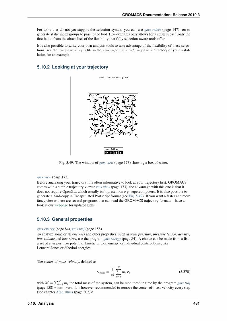
GROMACS Documentation, Release 2019.3
For tools that do not yet support the selection syntax, you can use gmx select (page 147) -on togenerate static index groups to pass to the tool. However, this only allows for a small subset (only thefirst bullet from the above list) of the flexibility that fully selection-aware tools offer.
It is also possible to write your own analysis tools to take advantage of the flexibility of these selec-tions: see the template.cpp file in the share/gromacs/template directory of your instal-lation for an example.
5.10.2 Looking at your trajectory
Fig. 5.49: The window of gmx view (page 173) showing a box of water.
gmx view (page 173)Before analyzing your trajectory it is often informative to look at your trajectory first. GROMACScomes with a simple trajectory viewer gmx view (page 173); the advantage with this one is that itdoes not require OpenGL, which usually isn’t present on e.g. supercomputers. It is also possible togenerate a hard-copy in Encapsulated Postscript format (see Fig. 5.49). If you want a faster and morefancy viewer there are several programs that can read the GROMACS trajectory formats – have alook at our webpage for updated links.
5.10.3 General properties
gmx energy (page 84), gmx traj (page 158)To analyze some or all energies and other properties, such as total pressure, pressure tensor, density,box-volume and box-sizes, use the program gmx energy (page 84). A choice can be made from a lista set of energies, like potential, kinetic or total energy, or individual contributions, likeLennard-Jones or dihedral energies.
The center-of-mass velocity, defined as
v𝑐𝑜𝑚 =1
𝑀
𝑁∑𝑖=1
𝑚𝑖v𝑖 (5.370)
with 𝑀 =∑𝑁
𝑖=1𝑚𝑖 the total mass of the system, can be monitored in time by the program gmx traj(page 158) -com -ov. It is however recommended to remove the center-of-mass velocity every step(see chapter Algorithms (page 302))!
5.10. Analysis 481
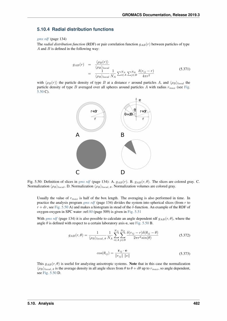
GROMACS Documentation, Release 2019.3
5.10.4 Radial distribution functions
gmx rdf (page 134)The radial distribution function (RDF) or pair correlation function 𝑔𝐴𝐵(𝑟) between particles of type𝐴 and 𝐵 is defined in the following way:
𝑔𝐴𝐵(𝑟) =⟨𝜌𝐵(𝑟)⟩⟨𝜌𝐵⟩𝑙𝑜𝑐𝑎𝑙
=1
⟨𝜌𝐵⟩𝑙𝑜𝑐𝑎𝑙1
𝑁𝐴
∑𝑁𝐴
𝑖∈𝐴
∑𝑁𝐵
𝑗∈𝐵
𝛿(𝑟𝑖𝑗 − 𝑟)
4𝜋𝑟2
(5.371)
with ⟨𝜌𝐵(𝑟)⟩ the particle density of type 𝐵 at a distance 𝑟 around particles 𝐴, and ⟨𝜌𝐵⟩𝑙𝑜𝑐𝑎𝑙 theparticle density of type 𝐵 averaged over all spheres around particles 𝐴 with radius 𝑟𝑚𝑎𝑥 (see Fig.5.50 C).
r
r+dr r+dr
rθ+dθ
θ
e
A B
DC
Fig. 5.50: Definition of slices in gmx rdf (page 134): A. 𝑔𝐴𝐵(𝑟). B. 𝑔𝐴𝐵(𝑟, 𝜃). The slices are colored gray. C.Normalization ⟨𝜌𝐵⟩𝑙𝑜𝑐𝑎𝑙. D. Normalization ⟨𝜌𝐵⟩𝑙𝑜𝑐𝑎𝑙, 𝜃. Normalization volumes are colored gray.
Usually the value of 𝑟𝑚𝑎𝑥 is half of the box length. The averaging is also performed in time. Inpractice the analysis program gmx rdf (page 134) divides the system into spherical slices (from 𝑟 to𝑟+ 𝑑𝑟, see Fig. 5.50 A) and makes a histogram in stead of the 𝛿-function. An example of the RDF ofoxygen-oxygen in SPC water :ref:80 (page 509) is given in Fig. 5.51
With gmx rdf (page 134) it is also possible to calculate an angle dependent rdf 𝑔𝐴𝐵(𝑟, 𝜃), where theangle 𝜃 is defined with respect to a certain laboratory axis e, see Fig. 5.50 B.
𝑔𝐴𝐵(𝑟, 𝜃) =1
⟨𝜌𝐵⟩𝑙𝑜𝑐𝑎𝑙, 𝜃1
𝑁𝐴
𝑁𝐴∑𝑖∈𝐴
𝑁𝐵∑𝑗∈𝐵
𝛿(𝑟𝑖𝑗 − 𝑟)𝛿(𝜃𝑖𝑗 − 𝜃)
2𝜋𝑟2𝑠𝑖𝑛(𝜃)(5.372)
𝑐𝑜𝑠(𝜃𝑖𝑗) =r𝑖𝑗 · e
‖𝑟𝑖𝑗‖ ‖𝑒‖ (5.373)
This 𝑔𝐴𝐵(𝑟, 𝜃) is useful for analyzing anisotropic systems. Note that in this case the normalization⟨𝜌𝐵⟩𝑙𝑜𝑐𝑎𝑙, 𝜃 is the average density in all angle slices from 𝜃 to 𝜃+ 𝑑𝜃 up to 𝑟𝑚𝑎𝑥, so angle dependent,see Fig. 5.50 D.
5.10. Analysis 482
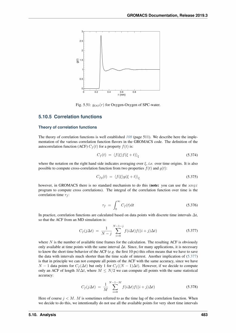
GROMACS Documentation, Release 2019.3
0 0.2 0.4 0.6 0.8r (nm)
0
0.5
1
1.5
2
2.5
3
g(r)
Fig. 5.51: 𝑔𝑂𝑂(𝑟) for Oxygen-Oxygen of SPC-water.
5.10.5 Correlation functions
Theory of correlation functions
The theory of correlation functions is well established 108 (page 511). We describe here the imple-mentation of the various correlation function flavors in the GROMACS code. The definition of theautocorrelation function (ACF) 𝐶𝑓 (𝑡) for a property 𝑓(𝑡) is:
𝐶𝑓 (𝑡) = ⟨𝑓(𝜉)𝑓(𝜉 + 𝑡)⟩𝜉 (5.374)
where the notation on the right hand side indicates averaging over 𝜉, i.e. over time origins. It is alsopossible to compute cross-correlation function from two properties 𝑓(𝑡) and 𝑔(𝑡):
𝐶𝑓𝑔(𝑡) = ⟨𝑓(𝜉)𝑔(𝜉 + 𝑡)⟩𝜉 (5.375)
however, in GROMACS there is no standard mechanism to do this (note: you can use the xmgrprogram to compute cross correlations). The integral of the correlation function over time is thecorrelation time 𝜏𝑓 :
𝜏𝑓 =
∫ ∞
0
𝐶𝑓 (𝑡)d𝑡 (5.376)
In practice, correlation functions are calculated based on data points with discrete time intervals ∆t,so that the ACF from an MD simulation is:
𝐶𝑓 (𝑗∆𝑡) =1
𝑁 − 𝑗
𝑁−1−𝑗∑𝑖=0
𝑓(𝑖∆𝑡)𝑓((𝑖+ 𝑗)∆𝑡) (5.377)
where 𝑁 is the number of available time frames for the calculation. The resulting ACF is obviouslyonly available at time points with the same interval ∆t. Since, for many applications, it is necessaryto know the short time behavior of the ACF (e.g. the first 10 ps) this often means that we have to savethe data with intervals much shorter than the time scale of interest. Another implication of (5.377)is that in principle we can not compute all points of the ACF with the same accuracy, since we have𝑁 − 1 data points for 𝐶𝑓 (∆𝑡) but only 1 for 𝐶𝑓 ((𝑁 − 1)∆𝑡). However, if we decide to computeonly an ACF of length 𝑀∆𝑡, where 𝑀 ≤ 𝑁/2 we can compute all points with the same statisticalaccuracy:
𝐶𝑓 (𝑗∆𝑡) =1
𝑀
𝑁−1−𝑀∑𝑖=0
𝑓(𝑖∆𝑡)𝑓((𝑖+ 𝑗)∆𝑡) (5.378)
Here of course 𝑗 < 𝑀 . 𝑀 is sometimes referred to as the time lag of the correlation function. Whenwe decide to do this, we intentionally do not use all the available points for very short time intervals
5.10. Analysis 483
GROMACS Documentation, Release 2019.3
(𝑗 << 𝑀 ), but it makes it easier to interpret the results. Another aspect that may not be neglectedwhen computing ACFs from simulation is that usually the time origins 𝜉 ((5.374)) are not statisticallyindependent, which may introduce a bias in the results. This can be tested using a block-averagingprocedure, where only time origins with a spacing at least the length of the time lag are included, e.g.using 𝑘 time origins with spacing of 𝑀∆𝑡 (where 𝑘𝑀 ≤ 𝑁 ):
𝐶𝑓 (𝑗∆𝑡) =1
𝑘
𝑘−1∑𝑖=0
𝑓(𝑖𝑀∆𝑡)𝑓((𝑖𝑀 + 𝑗)∆𝑡) (5.379)
However, one needs very long simulations to get good accuracy this way, because there are manyfewer points that contribute to the ACF.
Using FFT for computation of the ACF
The computational cost for calculating an ACF according to (5.377) is proportional to 𝑁2, whichis considerable. However, this can be improved by using fast Fourier transforms to do the convolu-tion 108 (page 511).
Special forms of the ACF
There are some important varieties on the ACF, e.g. the ACF of a vector p:
𝐶p(𝑡) =
∫ ∞
0
𝑃𝑛(cos∠ (p(𝜉),p(𝜉 + 𝑡)) d𝜉 (5.380)
where 𝑃𝑛(𝑥) is the 𝑛𝑡ℎ order Legendre polynomial.1 Such correlation times can actually be obtainedexperimentally using e.g. NMR or other relaxation experiments. GROMACS can compute correla-tions using the 1𝑠𝑡 and 2𝑛𝑑 order Legendre polynomial ((5.380)). This can also be used for rotationalautocorrelation (gmx rotacf (page 140)) and dipole autocorrelation (gmx dipoles (page 69)).
In order to study torsion angle dynamics, we define a dihedral autocorrelation function as 159(page 513):
𝐶(𝑡) = ⟨cos(𝜃(𝜏) − 𝜃(𝜏 + 𝑡))⟩𝜏 (5.381)
Note that this is not a product of two functions as is generally used for correlation functions, but itmay be rewritten as the sum of two products:
𝐶(𝑡) = ⟨cos(𝜃(𝜏)) cos(𝜃(𝜏 + 𝑡)) + sin(𝜃(𝜏)) sin(𝜃(𝜏 + 𝑡))⟩𝜏 (5.382)
Some Applications
The program gmx velacc (page 172) calculates the velocity autocorrelation function.
𝐶v(𝜏) = ⟨v𝑖(𝜏) · v𝑖(0)⟩𝑖∈𝐴 (5.383)
The self diffusion coefficient can be calculated using the Green-Kubo relation 108 (page 511):
𝐷𝐴 =1
3
∫ ∞
0
⟨v𝑖(𝑡) · v𝑖(0)⟩𝑖∈𝐴 𝑑𝑡 (5.384)
which is just the integral of the velocity autocorrelation function. There is a widely-held belief that thevelocity ACF converges faster than the mean square displacement (sec. Mean Square Displacement(page 486)), which can also be used for the computation of diffusion constants. However, Allen &Tildesley 108 (page 511) warn us that the long-time contribution to the velocity ACF can not beignored, so care must be taken.
1 𝑃0(𝑥) = 1, 𝑃1(𝑥) = 𝑥, 𝑃2(𝑥) = (3𝑥2 − 1)/2
5.10. Analysis 484
GROMACS Documentation, Release 2019.3
Another important quantity is the dipole correlation time. The dipole correlation function for particlesof type 𝐴 is calculated as follows by gmx dipoles (page 69):
𝐶𝜇(𝜏) = ⟨𝜇𝑖(𝜏) · 𝜇𝑖(0)⟩𝑖∈𝐴 (5.385)
with 𝜇𝑖 =∑
𝑗∈𝑖 r𝑗𝑞𝑗 . The dipole correlation time can be computed using (5.376). For some applica-tions see (???).
The viscosity of a liquid can be related to the correlation time of the Pressure tensor P 160 (page 513),161 (page 513). gmx energy (page 84) can compute the viscosity, but this is not very accurate 149(page 513), and actually the values do not converge.
5.10.6 Curve fitting in GROMACS
Sum of exponential functions
Sometimes it is useful to fit a curve to an analytical function, for example in the case of autocorrelationfunctions with noisy tails. GROMACS is not a general purpose curve-fitting tool however and there-fore GROMACS only supports a limited number of functions. Table 5.18 lists the available optionswith the corresponding command-line options. The underlying routines for fitting use the Levenberg-Marquardt algorithm as implemented in the lmfit package 162 (page 513) (a bare-bones version ofwhich is included in GROMACS in which an option for error-weighted fitting was implemented).
Table 5.18: Overview of fitting functions supported in (most) analysistools that compute autocorrelation functions. The Note column describesproperties of the output parameters.
Command line op-tion
Functional form 𝑓(𝑡) Note
exp 𝑒−𝑡/𝑎0
aexp 𝑎1𝑒−𝑡/𝑎0
exp_exp 𝑎1𝑒−𝑡/𝑎0 + (1 − 𝑎1)𝑒−𝑡/𝑎2 𝑎2 ≥ 𝑎0 ≥ 0
exp5 𝑎1𝑒−𝑡/𝑎0 + 𝑎3𝑒
−𝑡/𝑎2 + 𝑎4 𝑎2 ≥ 𝑎0 ≥ 0
exp7 𝑎1𝑒−𝑡/𝑎0 + 𝑎3𝑒
−𝑡/𝑎2 + 𝑎5𝑒−𝑡/𝑎4 + 𝑎6 𝑎4 ≥ 𝑎2 ≥ 𝑎0 ≥ 0
exp9 𝑎1𝑒−𝑡/𝑎0+𝑎3𝑒
−𝑡/𝑎2+𝑎5𝑒−𝑡/𝑎4+𝑎7𝑒
−𝑡/𝑎6+𝑎8 𝑎6 ≥ 𝑎4 ≥ 𝑎2 ≥𝑎0 ≥ 0
Error estimation
Under the hood GROMACS implements some more fitting functions, namely a function to estimatethe error in time-correlated data due to Hess 149 (page 513):
𝜀2(𝑡) = 𝛼𝜏1
(1 +
𝜏1𝑡
(𝑒−𝑡/𝜏1 − 1
))+ (1 − 𝛼)𝜏2
(1 +
𝜏2𝑡
(𝑒−𝑡/𝜏2 − 1
))(5.386)
where 𝜏1 and 𝜏2 are time constants (with 𝜏2 ≥ 𝜏1) and 𝛼 usually is close to 1 (in the fitting procedureit is enforced that 0 ≤ 𝛼 ≤ 1). This is used in gmx analyze (page 43) for error estimation using
lim𝑡→∞
𝜀(𝑡) = 𝜎
√2(𝛼𝜏1 + (1 − 𝛼)𝜏2)
𝑇(5.387)
where 𝜎 is the standard deviation of the data set and 𝑇 is the total simulation time 149 (page 513).
Interphase boundary demarcation
In order to determine the position and width of an interface, Steen-Sæthre et al. fitted a density profileto the following function
𝑓(𝑥) =𝑎0 + 𝑎1
2− 𝑎0 − 𝑎1
2erf
(𝑥− 𝑎2𝑎23
)(5.388)
5.10. Analysis 485
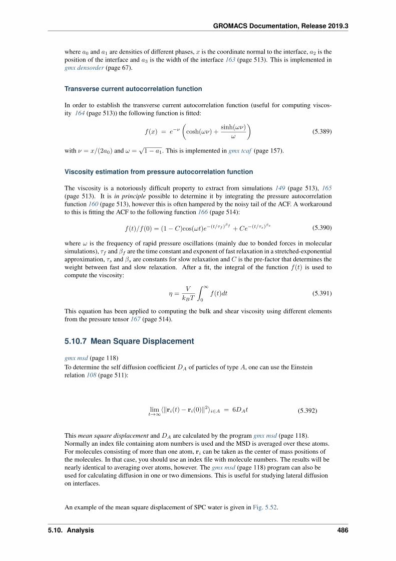
GROMACS Documentation, Release 2019.3
where 𝑎0 and 𝑎1 are densities of different phases, 𝑥 is the coordinate normal to the interface, 𝑎2 is theposition of the interface and 𝑎3 is the width of the interface 163 (page 513). This is implemented ingmx densorder (page 67).
Transverse current autocorrelation function
In order to establish the transverse current autocorrelation function (useful for computing viscos-ity 164 (page 513)) the following function is fitted:
𝑓(𝑥) = 𝑒−𝜈
(cosh(𝜔𝜈) +
sinh(𝜔𝜈)
𝜔
)(5.389)
with 𝜈 = 𝑥/(2𝑎0) and 𝜔 =√
1 − 𝑎1. This is implemented in gmx tcaf (page 157).
Viscosity estimation from pressure autocorrelation function
The viscosity is a notoriously difficult property to extract from simulations 149 (page 513), 165(page 513). It is in principle possible to determine it by integrating the pressure autocorrelationfunction 160 (page 513), however this is often hampered by the noisy tail of the ACF. A workaroundto this is fitting the ACF to the following function 166 (page 514):
𝑓(𝑡)/𝑓(0) = (1 − 𝐶)cos(𝜔𝑡)𝑒−(𝑡/𝜏𝑓 )𝛽𝑓
+ 𝐶𝑒−(𝑡/𝜏𝑠)𝛽𝑠 (5.390)
where 𝜔 is the frequency of rapid pressure oscillations (mainly due to bonded forces in molecularsimulations), 𝜏𝑓 and 𝛽𝑓 are the time constant and exponent of fast relaxation in a stretched-exponentialapproximation, 𝜏𝑠 and 𝛽𝑠 are constants for slow relaxation and 𝐶 is the pre-factor that determines theweight between fast and slow relaxation. After a fit, the integral of the function 𝑓(𝑡) is used tocompute the viscosity:
𝜂 =𝑉
𝑘𝐵𝑇
∫ ∞
0
𝑓(𝑡)𝑑𝑡 (5.391)
This equation has been applied to computing the bulk and shear viscosity using different elementsfrom the pressure tensor 167 (page 514).
5.10.7 Mean Square Displacement
gmx msd (page 118)To determine the self diffusion coefficient 𝐷𝐴 of particles of type 𝐴, one can use the Einsteinrelation 108 (page 511):
lim𝑡→∞
⟨‖r𝑖(𝑡) − r𝑖(0)‖2⟩𝑖∈𝐴 = 6𝐷𝐴𝑡 (5.392)
This mean square displacement and 𝐷𝐴 are calculated by the program gmx msd (page 118).Normally an index file containing atom numbers is used and the MSD is averaged over these atoms.For molecules consisting of more than one atom, r𝑖 can be taken as the center of mass positions ofthe molecules. In that case, you should use an index file with molecule numbers. The results will benearly identical to averaging over atoms, however. The gmx msd (page 118) program can also beused for calculating diffusion in one or two dimensions. This is useful for studying lateral diffusionon interfaces.
An example of the mean square displacement of SPC water is given in Fig. 5.52.
5.10. Analysis 486
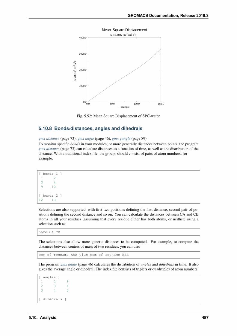
GROMACS Documentation, Release 2019.3
0.0 50.0 100.0 150.0Time (ps)
0.0
1000.0
2000.0
3000.0
4000.0
MS
D (10
-5cm
2s-1
)
Mean Square DisplacementD = 3.5027 (10
-5cm
2s
-1)
Fig. 5.52: Mean Square Displacement of SPC-water.
5.10.8 Bonds/distances, angles and dihedrals
gmx distance (page 73), gmx angle (page 46), gmx gangle (page 89)To monitor specific bonds in your modules, or more generally distances between points, the programgmx distance (page 73) can calculate distances as a function of time, as well as the distribution of thedistance. With a traditional index file, the groups should consist of pairs of atom numbers, forexample:
[ bonds_1 ]1 23 49 10
[ bonds_2 ]12 13
Selections are also supported, with first two positions defining the first distance, second pair of po-sitions defining the second distance and so on. You can calculate the distances between CA and CBatoms in all your residues (assuming that every residue either has both atoms, or neither) using aselection such as:
name CA CB
The selections also allow more generic distances to be computed. For example, to compute thedistances between centers of mass of two residues, you can use:
com of resname AAA plus com of resname BBB
The program gmx angle (page 46) calculates the distribution of angles and dihedrals in time. It alsogives the average angle or dihedral. The index file consists of triplets or quadruples of atom numbers:
[ angles ]1 2 32 3 43 4 5
[ dihedrals ]
5.10. Analysis 487
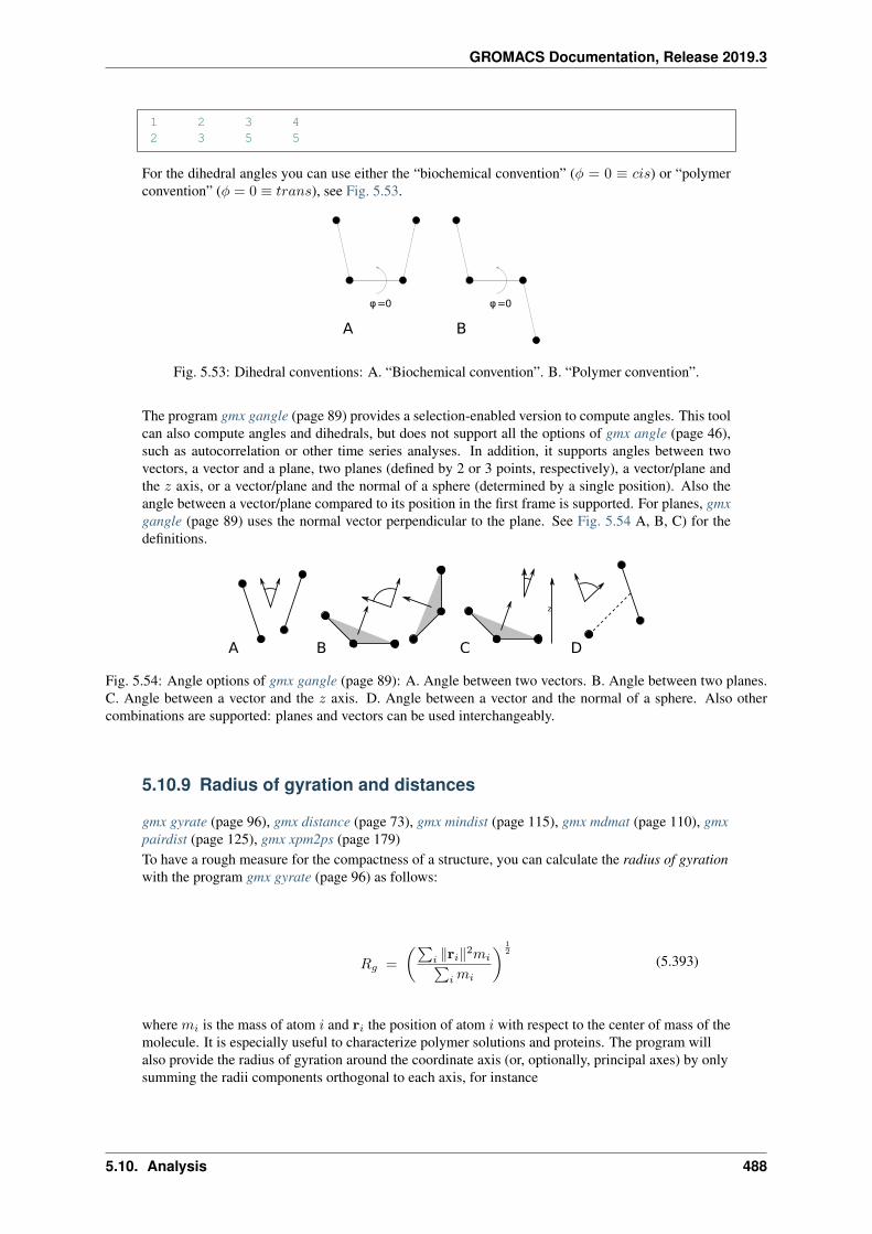
GROMACS Documentation, Release 2019.3
1 2 3 42 3 5 5
For the dihedral angles you can use either the “biochemical convention” (𝜑 = 0 ≡ 𝑐𝑖𝑠) or “polymerconvention” (𝜑 = 0 ≡ 𝑡𝑟𝑎𝑛𝑠), see Fig. 5.53.
φ= 0φ= 0
A B
Fig. 5.53: Dihedral conventions: A. “Biochemical convention”. B. “Polymer convention”.
The program gmx gangle (page 89) provides a selection-enabled version to compute angles. This toolcan also compute angles and dihedrals, but does not support all the options of gmx angle (page 46),such as autocorrelation or other time series analyses. In addition, it supports angles between twovectors, a vector and a plane, two planes (defined by 2 or 3 points, respectively), a vector/plane andthe 𝑧 axis, or a vector/plane and the normal of a sphere (determined by a single position). Also theangle between a vector/plane compared to its position in the first frame is supported. For planes, gmxgangle (page 89) uses the normal vector perpendicular to the plane. See Fig. 5.54 A, B, C) for thedefinitions.
A B C
z
D
Fig. 5.54: Angle options of gmx gangle (page 89): A. Angle between two vectors. B. Angle between two planes.C. Angle between a vector and the 𝑧 axis. D. Angle between a vector and the normal of a sphere. Also othercombinations are supported: planes and vectors can be used interchangeably.
5.10.9 Radius of gyration and distances
gmx gyrate (page 96), gmx distance (page 73), gmx mindist (page 115), gmx mdmat (page 110), gmxpairdist (page 125), gmx xpm2ps (page 179)To have a rough measure for the compactness of a structure, you can calculate the radius of gyrationwith the program gmx gyrate (page 96) as follows:
𝑅𝑔 =
(∑𝑖 ‖r𝑖‖2𝑚𝑖∑
𝑖𝑚𝑖
) 12
(5.393)
where 𝑚𝑖 is the mass of atom 𝑖 and r𝑖 the position of atom 𝑖 with respect to the center of mass of themolecule. It is especially useful to characterize polymer solutions and proteins. The program willalso provide the radius of gyration around the coordinate axis (or, optionally, principal axes) by onlysumming the radii components orthogonal to each axis, for instance
5.10. Analysis 488
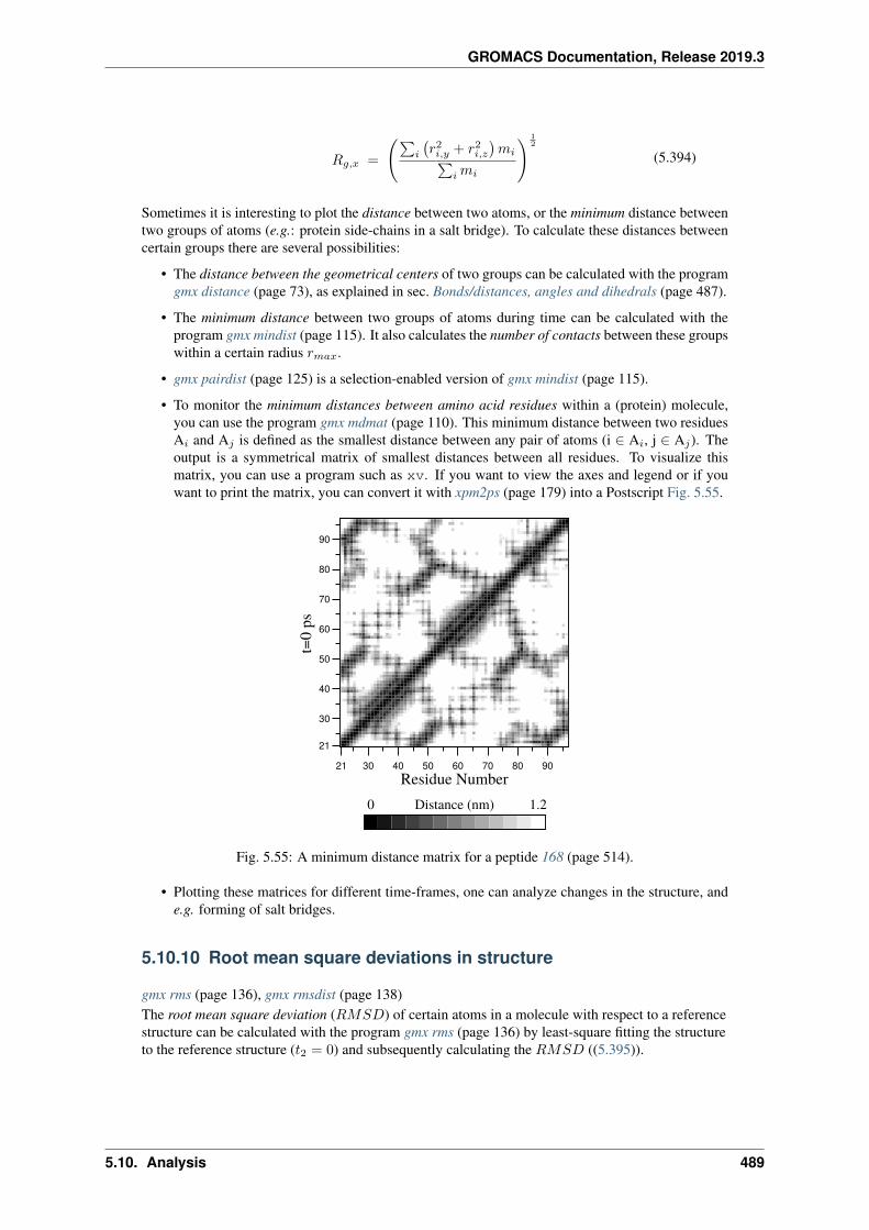
GROMACS Documentation, Release 2019.3
𝑅𝑔,𝑥 =
(∑𝑖
(𝑟2𝑖,𝑦 + 𝑟2𝑖,𝑧
)𝑚𝑖∑
𝑖𝑚𝑖
) 12
(5.394)
Sometimes it is interesting to plot the distance between two atoms, or the minimum distance betweentwo groups of atoms (e.g.: protein side-chains in a salt bridge). To calculate these distances betweencertain groups there are several possibilities:
• The distance between the geometrical centers of two groups can be calculated with the programgmx distance (page 73), as explained in sec. Bonds/distances, angles and dihedrals (page 487).
• The minimum distance between two groups of atoms during time can be calculated with theprogram gmx mindist (page 115). It also calculates the number of contacts between these groupswithin a certain radius 𝑟𝑚𝑎𝑥.
• gmx pairdist (page 125) is a selection-enabled version of gmx mindist (page 115).
• To monitor the minimum distances between amino acid residues within a (protein) molecule,you can use the program gmx mdmat (page 110). This minimum distance between two residuesA𝑖 and A𝑗 is defined as the smallest distance between any pair of atoms (i ∈ A𝑖, j ∈ A𝑗). Theoutput is a symmetrical matrix of smallest distances between all residues. To visualize thismatrix, you can use a program such as xv. If you want to view the axes and legend or if youwant to print the matrix, you can convert it with xpm2ps (page 179) into a Postscript Fig. 5.55.
21 30 40 50 60 70 80 90
21
30
40
50
60
70
80
90
t=0
ps
Residue Number0 Distance (nm) 1.2
Fig. 5.55: A minimum distance matrix for a peptide 168 (page 514).
• Plotting these matrices for different time-frames, one can analyze changes in the structure, ande.g. forming of salt bridges.
5.10.10 Root mean square deviations in structure
gmx rms (page 136), gmx rmsdist (page 138)The root mean square deviation (𝑅𝑀𝑆𝐷) of certain atoms in a molecule with respect to a referencestructure can be calculated with the program gmx rms (page 136) by least-square fitting the structureto the reference structure (𝑡2 = 0) and subsequently calculating the 𝑅𝑀𝑆𝐷 ((5.395)).
5.10. Analysis 489

GROMACS Documentation, Release 2019.3
𝑅𝑀𝑆𝐷(𝑡1, 𝑡2) =
[1
𝑀
𝑁∑𝑖=1
𝑚𝑖‖r𝑖(𝑡1) − r𝑖(𝑡2)‖2] 1
2
(5.395)
where 𝑀 =∑𝑁
𝑖=1𝑚𝑖 and r𝑖(𝑡) is the position of atom 𝑖 at time 𝑡. Note that fitting does not have touse the same atoms as the calculation of the 𝑅𝑀𝑆𝐷; e.g. a protein is usually fitted on the backboneatoms (N,C:math:_{alpha},C), but the 𝑅𝑀𝑆𝐷 can be computed of the backbone or of the wholeprotein.
Instead of comparing the structures to the initial structure at time 𝑡 = 0 (so for example a crystalstructure), one can also calculate (5.395) with a structure at time 𝑡2 = 𝑡1− 𝜏 . This gives some insightin the mobility as a function of 𝜏 . A matrix can also be made with the 𝑅𝑀𝑆𝐷 as a function of 𝑡1 and𝑡2, which gives a nice graphical interpretation of a trajectory. If there are transitions in a trajectory,they will clearly show up in such a matrix.
Alternatively the 𝑅𝑀𝑆𝐷 can be computed using a fit-free method with the program gmx rmsdist(page 138):
𝑅𝑀𝑆𝐷(𝑡) =
⎡⎣ 1
𝑁2
𝑁∑𝑖=1
𝑁∑𝑗=1
‖r𝑖𝑗(𝑡) − r𝑖𝑗(0)‖2⎤⎦ 1
2
(5.396)
where the distance r𝑖𝑗 between atoms at time 𝑡 is compared with the distance between the same atomsat time 0.
5.10.11 Covariance analysis
Covariance analysis, also called principal component analysis or essential dynamics 169 (page 514),can find correlated motions. It uses the covariance matrix 𝐶 of the atomic coordinates:
𝐶𝑖𝑗 =⟨𝑀
12𝑖𝑖 (𝑥𝑖 − ⟨𝑥𝑖⟩)𝑀
12𝑗𝑗(𝑥𝑗 − ⟨𝑥𝑗⟩)
⟩(5.397)
where𝑀 is a diagonal matrix containing the masses of the atoms (mass-weighted analysis) or the unitmatrix (non-mass weighted analysis). 𝐶 is a symmetric 3𝑁 × 3𝑁 matrix, which can be diagonalizedwith an orthonormal transformation matrix 𝑅:
𝑅𝑇𝐶𝑅 = diag(𝜆1, 𝜆2, . . . , 𝜆3𝑁 ) where 𝜆1 ≥ 𝜆2 ≥ . . . ≥ 𝜆3𝑁 (5.398)
The columns of 𝑅 are the eigenvectors, also called principal or essential modes. 𝑅 defines a trans-formation to a new coordinate system. The trajectory can be projected on the principal modes to givethe principal components 𝑝𝑖(𝑡):
p(𝑡) = 𝑅𝑇𝑀12 (x(𝑡) − ⟨x⟩) (5.399)
The eigenvalue 𝜆𝑖 is the mean square fluctuation of principal component 𝑖. The first few principalmodes often describe collective, global motions in the system. The trajectory can be filtered alongone (or more) principal modes. For one principal mode 𝑖 this goes as follows:
x𝑓 (𝑡) = ⟨x⟩ +𝑀− 12𝑅*𝑖 𝑝𝑖(𝑡) (5.400)
When the analysis is performed on a macromolecule, one often wants to remove the overall rotationand translation to look at the internal motion only. This can be achieved by least square fitting to areference structure. Care has to be taken that the reference structure is representative for the ensemble,since the choice of reference structure influences the covariance matrix.
5.10. Analysis 490
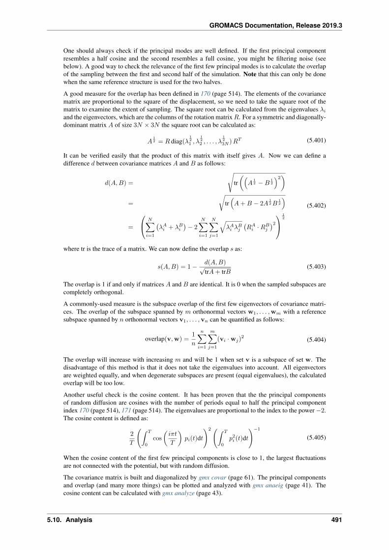
GROMACS Documentation, Release 2019.3
One should always check if the principal modes are well defined. If the first principal componentresembles a half cosine and the second resembles a full cosine, you might be filtering noise (seebelow). A good way to check the relevance of the first few principal modes is to calculate the overlapof the sampling between the first and second half of the simulation. Note that this can only be donewhen the same reference structure is used for the two halves.
A good measure for the overlap has been defined in 170 (page 514). The elements of the covariancematrix are proportional to the square of the displacement, so we need to take the square root of thematrix to examine the extent of sampling. The square root can be calculated from the eigenvalues 𝜆𝑖and the eigenvectors, which are the columns of the rotation matrix𝑅. For a symmetric and diagonally-dominant matrix 𝐴 of size 3𝑁 × 3𝑁 the square root can be calculated as:
𝐴12 = 𝑅 diag(𝜆
121 , 𝜆
122 , . . . , 𝜆
12
3𝑁 )𝑅𝑇 (5.401)
It can be verified easily that the product of this matrix with itself gives 𝐴. Now we can define adifference 𝑑 between covariance matrices 𝐴 and 𝐵 as follows:
𝑑(𝐴,𝐵) =
√tr((
𝐴12 −𝐵
12
)2)=
√tr(𝐴+𝐵 − 2𝐴
12𝐵
12
)
=
⎛⎝ 𝑁∑𝑖=1
(𝜆𝐴𝑖 + 𝜆𝐵𝑖
)− 2
𝑁∑𝑖=1
𝑁∑𝑗=1
√𝜆𝐴𝑖 𝜆
𝐵𝑗
(𝑅𝐴
𝑖 ·𝑅𝐵𝑗
)2⎞⎠ 12
(5.402)
where tr is the trace of a matrix. We can now define the overlap 𝑠 as:
𝑠(𝐴,𝐵) = 1 − 𝑑(𝐴,𝐵)√tr𝐴+ tr𝐵
(5.403)
The overlap is 1 if and only if matrices 𝐴 and 𝐵 are identical. It is 0 when the sampled subspaces arecompletely orthogonal.
A commonly-used measure is the subspace overlap of the first few eigenvectors of covariance matri-ces. The overlap of the subspace spanned by 𝑚 orthonormal vectors w1, . . . ,w𝑚 with a referencesubspace spanned by 𝑛 orthonormal vectors v1, . . . ,v𝑛 can be quantified as follows:
overlap(v,w) =1
𝑛
𝑛∑𝑖=1
𝑚∑𝑗=1
(v𝑖 ·w𝑗)2 (5.404)
The overlap will increase with increasing 𝑚 and will be 1 when set v is a subspace of set w. Thedisadvantage of this method is that it does not take the eigenvalues into account. All eigenvectorsare weighted equally, and when degenerate subspaces are present (equal eigenvalues), the calculatedoverlap will be too low.
Another useful check is the cosine content. It has been proven that the the principal componentsof random diffusion are cosines with the number of periods equal to half the principal componentindex 170 (page 514), 171 (page 514). The eigenvalues are proportional to the index to the power −2.The cosine content is defined as:
2
𝑇
(∫ 𝑇
0
cos
(𝑖𝜋𝑡
𝑇
)𝑝𝑖(𝑡)d𝑡
)2(∫ 𝑇
0
𝑝2𝑖 (𝑡)d𝑡
)−1
(5.405)
When the cosine content of the first few principal components is close to 1, the largest fluctuationsare not connected with the potential, but with random diffusion.
The covariance matrix is built and diagonalized by gmx covar (page 61). The principal componentsand overlap (and many more things) can be plotted and analyzed with gmx anaeig (page 41). Thecosine content can be calculated with gmx analyze (page 43).
5.10. Analysis 491
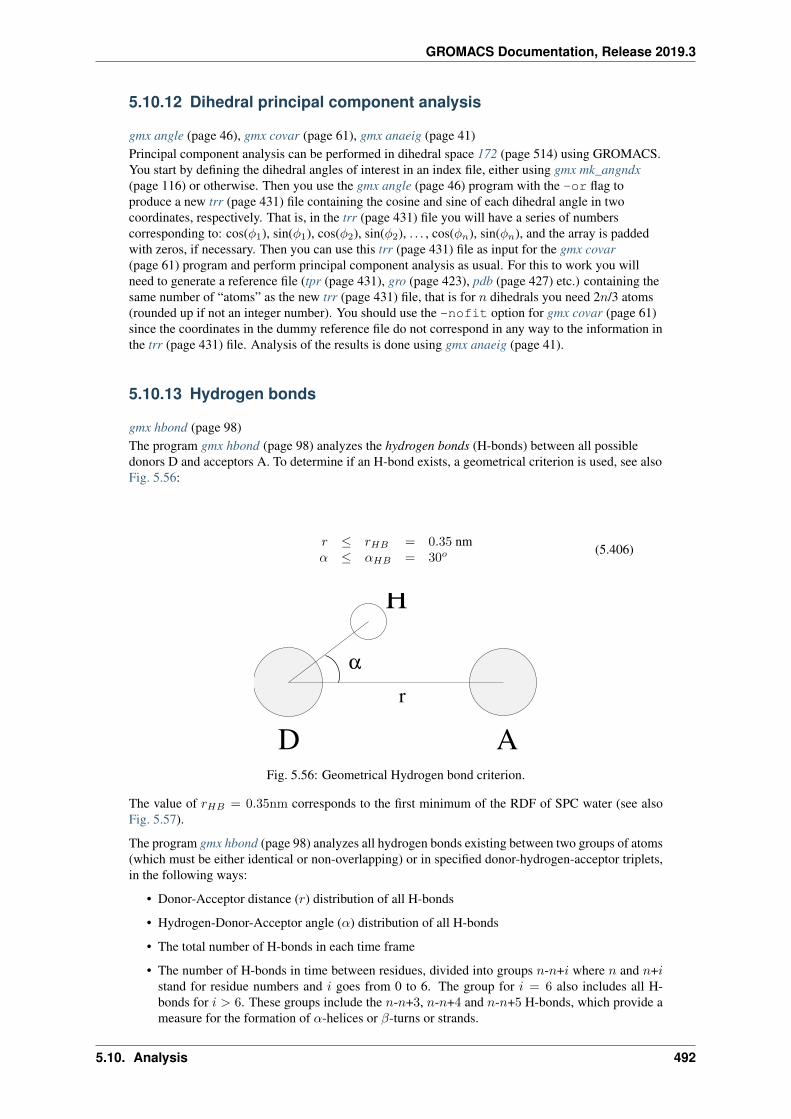
GROMACS Documentation, Release 2019.3
5.10.12 Dihedral principal component analysis
gmx angle (page 46), gmx covar (page 61), gmx anaeig (page 41)Principal component analysis can be performed in dihedral space 172 (page 514) using GROMACS.You start by defining the dihedral angles of interest in an index file, either using gmx mk_angndx(page 116) or otherwise. Then you use the gmx angle (page 46) program with the -or flag toproduce a new trr (page 431) file containing the cosine and sine of each dihedral angle in twocoordinates, respectively. That is, in the trr (page 431) file you will have a series of numberscorresponding to: cos(𝜑1), sin(𝜑1), cos(𝜑2), sin(𝜑2), . . . , cos(𝜑𝑛), sin(𝜑𝑛), and the array is paddedwith zeros, if necessary. Then you can use this trr (page 431) file as input for the gmx covar(page 61) program and perform principal component analysis as usual. For this to work you willneed to generate a reference file (tpr (page 431), gro (page 423), pdb (page 427) etc.) containing thesame number of “atoms” as the new trr (page 431) file, that is for 𝑛 dihedrals you need 2𝑛/3 atoms(rounded up if not an integer number). You should use the -nofit option for gmx covar (page 61)since the coordinates in the dummy reference file do not correspond in any way to the information inthe trr (page 431) file. Analysis of the results is done using gmx anaeig (page 41).
5.10.13 Hydrogen bonds
gmx hbond (page 98)The program gmx hbond (page 98) analyzes the hydrogen bonds (H-bonds) between all possibledonors D and acceptors A. To determine if an H-bond exists, a geometrical criterion is used, see alsoFig. 5.56:
𝑟 ≤ 𝑟𝐻𝐵 = 0.35 nm𝛼 ≤ 𝛼𝐻𝐵 = 30𝑜
(5.406)
D
H
α
Ar
Fig. 5.56: Geometrical Hydrogen bond criterion.
The value of 𝑟𝐻𝐵 = 0.35nm corresponds to the first minimum of the RDF of SPC water (see alsoFig. 5.57).
The program gmx hbond (page 98) analyzes all hydrogen bonds existing between two groups of atoms(which must be either identical or non-overlapping) or in specified donor-hydrogen-acceptor triplets,in the following ways:
• Donor-Acceptor distance (𝑟) distribution of all H-bonds
• Hydrogen-Donor-Acceptor angle (𝛼) distribution of all H-bonds
• The total number of H-bonds in each time frame
• The number of H-bonds in time between residues, divided into groups 𝑛-𝑛+𝑖 where 𝑛 and 𝑛+𝑖stand for residue numbers and 𝑖 goes from 0 to 6. The group for 𝑖 = 6 also includes all H-bonds for 𝑖 > 6. These groups include the 𝑛-𝑛+3, 𝑛-𝑛+4 and 𝑛-𝑛+5 H-bonds, which provide ameasure for the formation of 𝛼-helices or 𝛽-turns or strands.
5.10. Analysis 492
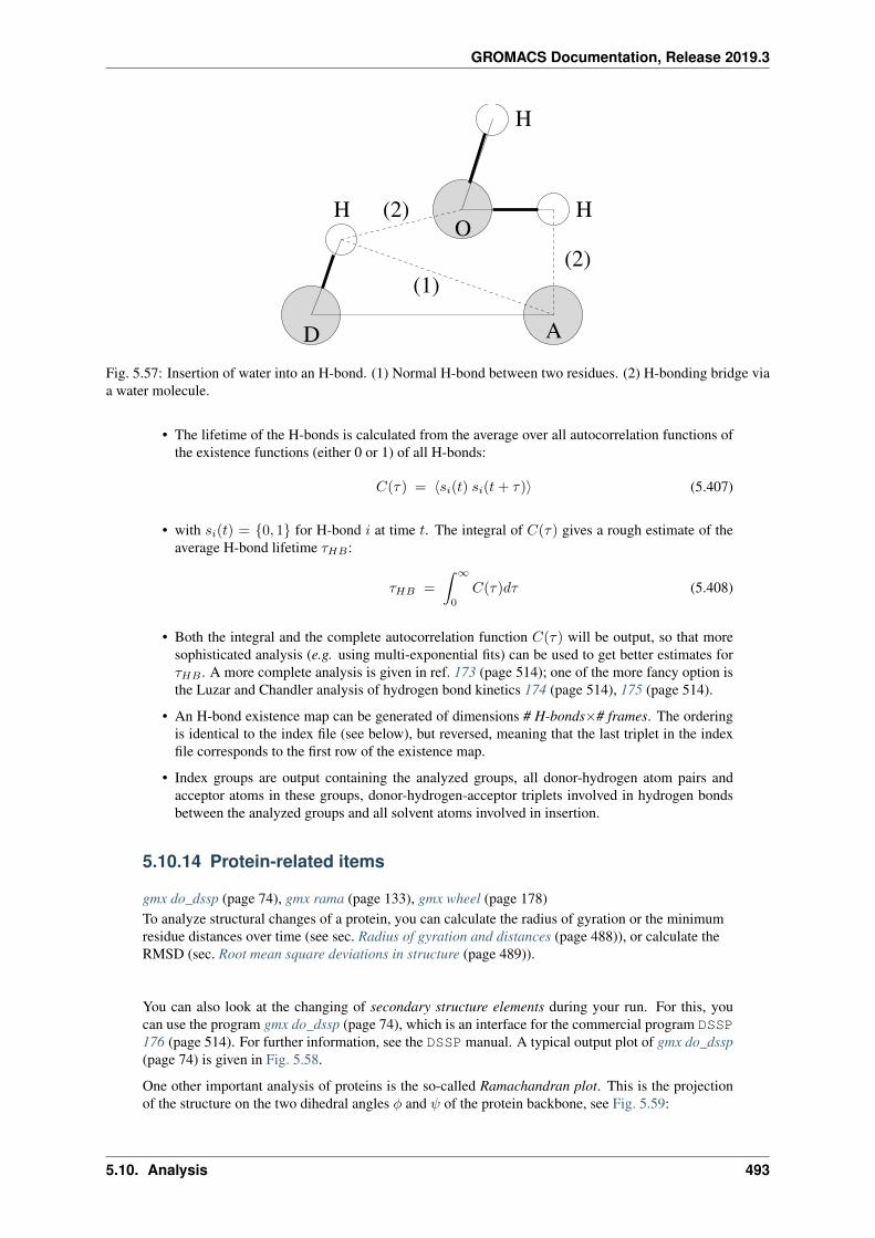
GROMACS Documentation, Release 2019.3
O
D A
H
H
H
(1)(2)
(2)
Fig. 5.57: Insertion of water into an H-bond. (1) Normal H-bond between two residues. (2) H-bonding bridge viaa water molecule.
• The lifetime of the H-bonds is calculated from the average over all autocorrelation functions ofthe existence functions (either 0 or 1) of all H-bonds:
𝐶(𝜏) = ⟨𝑠𝑖(𝑡) 𝑠𝑖(𝑡+ 𝜏)⟩ (5.407)
• with 𝑠𝑖(𝑡) = {0, 1} for H-bond 𝑖 at time 𝑡. The integral of 𝐶(𝜏) gives a rough estimate of theaverage H-bond lifetime 𝜏𝐻𝐵 :
𝜏𝐻𝐵 =
∫ ∞
0
𝐶(𝜏)𝑑𝜏 (5.408)
• Both the integral and the complete autocorrelation function 𝐶(𝜏) will be output, so that moresophisticated analysis (e.g. using multi-exponential fits) can be used to get better estimates for𝜏𝐻𝐵 . A more complete analysis is given in ref. 173 (page 514); one of the more fancy option isthe Luzar and Chandler analysis of hydrogen bond kinetics 174 (page 514), 175 (page 514).
• An H-bond existence map can be generated of dimensions # H-bonds×# frames. The orderingis identical to the index file (see below), but reversed, meaning that the last triplet in the indexfile corresponds to the first row of the existence map.
• Index groups are output containing the analyzed groups, all donor-hydrogen atom pairs andacceptor atoms in these groups, donor-hydrogen-acceptor triplets involved in hydrogen bondsbetween the analyzed groups and all solvent atoms involved in insertion.
5.10.14 Protein-related items
gmx do_dssp (page 74), gmx rama (page 133), gmx wheel (page 178)To analyze structural changes of a protein, you can calculate the radius of gyration or the minimumresidue distances over time (see sec. Radius of gyration and distances (page 488)), or calculate theRMSD (sec. Root mean square deviations in structure (page 489)).
You can also look at the changing of secondary structure elements during your run. For this, youcan use the program gmx do_dssp (page 74), which is an interface for the commercial program DSSP176 (page 514). For further information, see the DSSP manual. A typical output plot of gmx do_dssp(page 74) is given in Fig. 5.58.
One other important analysis of proteins is the so-called Ramachandran plot. This is the projectionof the structure on the two dihedral angles 𝜑 and 𝜓 of the protein backbone, see Fig. 5.59:
5.10. Analysis 493
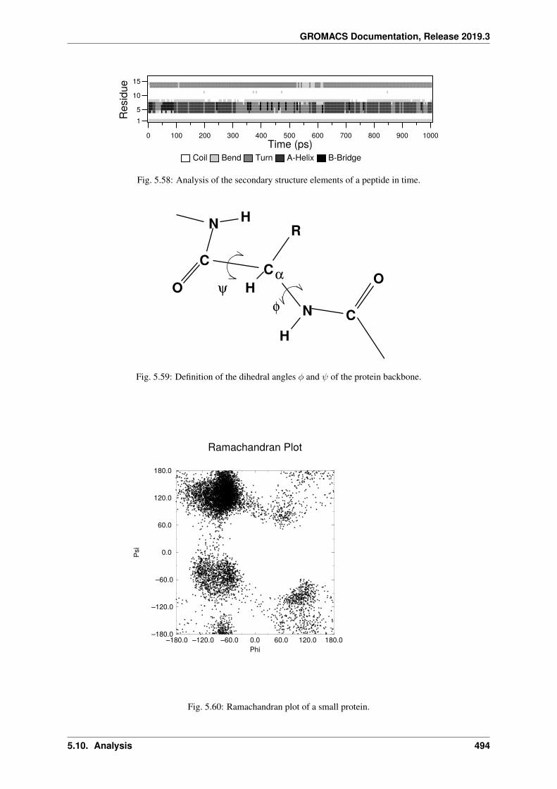
GROMACS Documentation, Release 2019.3
0 100 200 300 400 500 600 700 800 900 1000
15
10
15
Res
idue
Time (ps)Coil Bend Turn A-Helix B-Bridge
Fig. 5.58: Analysis of the secondary structure elements of a peptide in time.
C
O
N
CH
R
C
Oα
N
H
H
ψφ
Fig. 5.59: Definition of the dihedral angles 𝜑 and 𝜓 of the protein backbone.
–180.0 –120.0 –60.0 0.0 60.0 120.0 180.0Phi
–180.0
–120.0
–60.0
0.0
60.0
120.0
180.0
Psi
Ramachandran Plot
Fig. 5.60: Ramachandran plot of a small protein.
5.10. Analysis 494
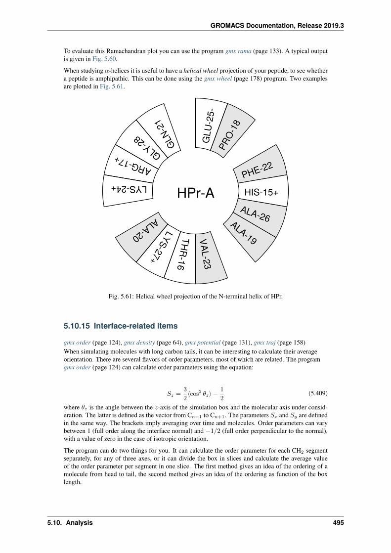
GROMACS Documentation, Release 2019.3
To evaluate this Ramachandran plot you can use the program gmx rama (page 133). A typical outputis given in Fig. 5.60.
When studying 𝛼-helices it is useful to have a helical wheel projection of your peptide, to see whethera peptide is amphipathic. This can be done using the gmx wheel (page 178) program. Two examplesare plotted in Fig. 5.61.
HPr-A HIS-15+THR-16
ARG-17+
PRO-
18ALA-19
ALA-20
GLN-
21
PHE-22
VAL-23
LYS-24+
GLU
-25-
ALA-26LYS-27+
GLY-28
Fig. 5.61: Helical wheel projection of the N-terminal helix of HPr.
5.10.15 Interface-related items
gmx order (page 124), gmx density (page 64), gmx potential (page 131), gmx traj (page 158)When simulating molecules with long carbon tails, it can be interesting to calculate their averageorientation. There are several flavors of order parameters, most of which are related. The programgmx order (page 124) can calculate order parameters using the equation:
𝑆𝑧 =3
2⟨cos2 𝜃𝑧⟩ −
1
2(5.409)
where 𝜃𝑧 is the angle between the 𝑧-axis of the simulation box and the molecular axis under consid-eration. The latter is defined as the vector from C𝑛−1 to C𝑛+1. The parameters 𝑆𝑥 and 𝑆𝑦 are definedin the same way. The brackets imply averaging over time and molecules. Order parameters can varybetween 1 (full order along the interface normal) and −1/2 (full order perpendicular to the normal),with a value of zero in the case of isotropic orientation.
The program can do two things for you. It can calculate the order parameter for each CH2 segmentseparately, for any of three axes, or it can divide the box in slices and calculate the average valueof the order parameter per segment in one slice. The first method gives an idea of the ordering of amolecule from head to tail, the second method gives an idea of the ordering as function of the boxlength.
5.10. Analysis 495
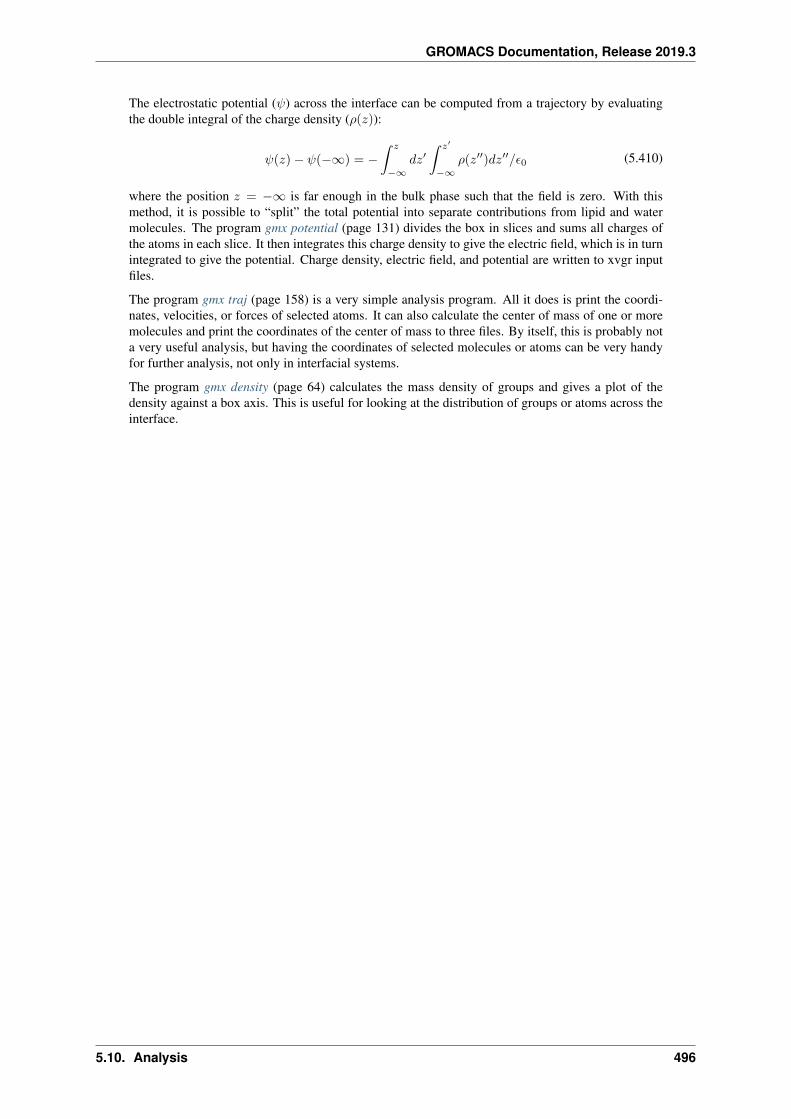
GROMACS Documentation, Release 2019.3
The electrostatic potential (𝜓) across the interface can be computed from a trajectory by evaluatingthe double integral of the charge density (𝜌(𝑧)):
𝜓(𝑧) − 𝜓(−∞) = −∫ 𝑧
−∞𝑑𝑧′∫ 𝑧′
−∞𝜌(𝑧′′)𝑑𝑧′′/𝜖0 (5.410)
where the position 𝑧 = −∞ is far enough in the bulk phase such that the field is zero. With thismethod, it is possible to “split” the total potential into separate contributions from lipid and watermolecules. The program gmx potential (page 131) divides the box in slices and sums all charges ofthe atoms in each slice. It then integrates this charge density to give the electric field, which is in turnintegrated to give the potential. Charge density, electric field, and potential are written to xvgr inputfiles.
The program gmx traj (page 158) is a very simple analysis program. All it does is print the coordi-nates, velocities, or forces of selected atoms. It can also calculate the center of mass of one or moremolecules and print the coordinates of the center of mass to three files. By itself, this is probably nota very useful analysis, but having the coordinates of selected molecules or atoms can be very handyfor further analysis, not only in interfacial systems.
The program gmx density (page 64) calculates the mass density of groups and gives a plot of thedensity against a box axis. This is useful for looking at the distribution of groups or atoms across theinterface.
5.10. Analysis 496
GROMACS Documentation, Release 2019.3
5.11 Some implementation details
In this chapter we will present some implementation details. This is far from complete, but we deemedit necessary to clarify some things that would otherwise be hard to understand.
5.11.1 Single Sum Virial in GROMACS
The virial Ξ can be written in full tensor form as:
Ξ = −1
2
𝑁∑𝑖<𝑗
r𝑖𝑗 ⊗ F𝑖𝑗 (5.411)
where ⊗ denotes the direct product of two vectors.1 When this is computed in the inner loop of anMD program 9 multiplications and 9 additions are needed.2
Here it is shown how it is possible to extract the virial calculation from the inner loop 177 (page 514).
Virial
In a system with periodic boundary conditions, the periodicity must be taken into account for thevirial:
Ξ = −1
2
𝑁∑𝑖<𝑗
r𝑛𝑖𝑗 ⊗ F𝑖𝑗 (5.412)
where r𝑛𝑖𝑗 denotes the distance vector of the nearest image of atom 𝑖 from atom 𝑗. In this definitionwe add a shift vector 𝛿𝑖 to the position vector r𝑖 of atom 𝑖. The difference vector r𝑛𝑖𝑗 is thus equal to:
r𝑛𝑖𝑗 = r𝑖 + 𝛿𝑖 − r𝑗 (5.413)
or in shorthand:
r𝑛𝑖𝑗 = r𝑛𝑖 − r𝑗 (5.414)
In a triclinic system, there are 27 possible images of 𝑖; when a truncated octahedron is used, there are15 possible images.
Virial from non-bonded forces
Here the derivation for the single sum virial in the non-bonded force routine is given. There are acouple of considerations that are special to GROMACS that we take into account:
• When calculating short-range interactions, we apply the minimum image convention and onlyconsider the closest image of each neighbor - and in particular we never allow interactionsbetween a particle and any of its periodic images. For all the equations below, this means 𝑖 = 𝑗.
• In general, either the 𝑖 or 𝑗 particle might be shifted to a neighbor cell to get the closest inter-action (shift 𝛿𝑖𝑗). However, with minimum image convention there can be at most 27 differentshifts for particles in the central cell, and for typical (very short-ranged) biomolecular interac-tions there are typically only a few different shifts involved for each particle, not to mention thateach interaction can only be present for one shift.
1 Note that some derivations, an alternative notation 𝜉alt = 𝑣𝜉 = 𝑝𝜉/𝑄 is used.2 The calculation of Lennard-Jones and Coulomb forces is about 50 floating point operations.
5.11. Some implementation details 497
GROMACS Documentation, Release 2019.3
• For the GROMACS nonbonded interactions we use this to split the neighborlist of each 𝑖 particleinto multiple separate lists, where each list has a constant shift 𝛿𝑖 for the 𝑖 partlcle. We canrepresent this as a sum over shifts (for which we use index 𝑠), with the constraint that eachparticle interaction can only contribute to one of the terms in this sum, and the shift is no longerdependent on the 𝑗 particles. For any sum that does not contain complex dependence on 𝑠, thismeans the sum trivially reduces to just the sum over 𝑖 and/or 𝑗.
• To simplify some of the sums, we replace sums over 𝑗 < 𝑖 with double sums over all particles(remember, 𝑖 = 𝑗) and divide by 2.
Starting from the above definition of the virial, we then get
Ξ = −1
2
𝑁∑𝑖<𝑗
r𝑛𝑖𝑗 ⊗ F𝑖𝑗
= −1
2
𝑁∑𝑖<𝑗
(r𝑖 + 𝛿𝑖𝑗 − r𝑗) ⊗ F𝑖𝑗
= −1
4
𝑁∑𝑖=1
𝑁∑𝑗=1
(r𝑖 + 𝛿𝑖𝑗 − r𝑗) ⊗ F𝑖𝑗
= −1
4
𝑁∑𝑖=1
∑𝑠
𝑁∑𝑗=1
(r𝑖 + 𝛿𝑖,𝑠 − r𝑗) ⊗ F𝑖𝑗,𝑠
= −1
4
𝑁∑𝑖=
∑𝑠
𝑁∑𝑗=1
((r𝑖 + 𝛿𝑖,𝑠) ⊗ F𝑖𝑗,𝑠 − r𝑗 ⊗ F𝑖𝑗,𝑠)
= −1
4
𝑁∑𝑖=1
∑𝑠
𝑁∑𝑗=1
(r𝑖 + 𝛿𝑖,𝑠) ⊗ F𝑖𝑗,𝑠 +1
4
𝑁∑𝑖=1
∑𝑠
𝑁∑𝑗=1
r𝑗 ⊗ F𝑖𝑗,𝑠
= −1
4
𝑁∑𝑖=1
∑𝑠
𝑁∑𝑗=1
(r𝑖 + 𝛿𝑖,𝑠) ⊗ F𝑖𝑗,𝑠 +1
4
𝑁∑𝑖=1
𝑁∑𝑗=1
r𝑗 ⊗ F𝑖𝑗
= −1
4
∑𝑠
𝑁∑𝑖=1
(r𝑖 + 𝛿𝑖,𝑠) ⊗𝑁∑𝑗=1
F𝑖𝑗,𝑠 +1
4
𝑁∑𝑗=1
r𝑗 ⊗𝑁∑𝑖=1
F𝑖𝑗
= −1
4
∑𝑠
𝑁∑𝑖=1
(r𝑖 + 𝛿𝑖,𝑠) ⊗𝑁∑𝑗=1
F𝑖𝑗,𝑠 −1
4
𝑁∑𝑗=1
r𝑗 ⊗𝑁∑𝑖=1
F𝑗𝑖
= −1
4
∑𝑠
𝑁∑𝑖=1
(r𝑖 + 𝛿𝑖,𝑠) ⊗ F𝑖,𝑠 −1
4
𝑁∑𝑗=1
r𝑗 ⊗ F𝑗
= −1
4
⎛⎝ 𝑁∑𝑖=1
r𝑖 ⊗ F𝑖 +
𝑁∑𝑗=1
r𝑗 ⊗ F𝑗
⎞⎠− 1
4
∑𝑠
𝑁∑𝑖=1
𝛿𝑖,𝑠 ⊗ F𝑖,𝑠
= −1
2
𝑁∑𝑖=1
r𝑖 ⊗ F𝑖 −1
4
∑𝑠
𝑁∑𝑖=1
𝛿𝑖,𝑠 ⊗ F𝑖,𝑠
= −1
2
𝑁∑𝑖=1
r𝑖 ⊗ F𝑖 −1
4
∑𝑠
𝛿𝑠 ⊗ F𝑠
= Ξ0 + Ξ1
In the second-last stage, we have used the property that each shift vector itself does not depend on thecoordinates of particle 𝑖, so it is possible to sum up all forces corresponding to each shift vector (inthe nonbonded kernels), and then just use a sum over the different shift vectors outside the kernels.
5.11. Some implementation details 498
GROMACS Documentation, Release 2019.3
We have also used
F𝑖 =
𝑁∑𝑗=1
F𝑖𝑗
F𝑗 =
𝑁∑𝑖=1
F𝑗𝑖
(5.415)
which is the total force on 𝑖 with respect to 𝑗. Because we use Newton’s Third Law:
F𝑖𝑗 = −F𝑗𝑖 (5.416)
we must, in the implementation, double the term containing the shift 𝛿𝑖. Similarly, in a few places wehave summed the shift-dependent force over all shifts to come up with the total force per interactionor particle.
This separates the total virial Ξ into a component Ξ0 that is a single sum over particles, and a secondcomponent Ξ1 that describes the influence of the particle shifts, and that is only a sum over thedifferent shift vectors.
The intra-molecular shift (mol-shift)
For the bonded forces and SHAKE it is possible to make a mol-shift list, in which the periodicity isstored. We simple have an array mshift in which for each atom an index in the shiftvec array is stored.
The algorithm to generate such a list can be derived from graph theory, considering each particle in amolecule as a bead in a graph, the bonds as edges.
1. Represent the bonds and atoms as bidirectional graph
2. Make all atoms white
3. Make one of the white atoms black (atom 𝑖) and put it in the central box
4. Make all of the neighbors of 𝑖 that are currently white, gray
5. Pick one of the gray atoms (atom 𝑗), give it the correct periodicity with respect to any of itsblack neighbors and make it black
6. Make all of the neighbors of 𝑗 that are currently white, gray
7. If any gray atom remains, go to [5]
8. If any white atom remains, go to [3]
Using this algorithm we can
• optimize the bonded force calculation as well as SHAKE
• calculate the virial from the bonded forces in the single sum method again
Find a representation of the bonds as a bidirectional graph.
Virial from Covalent Bonds
Since the covalent bond force gives a contribution to the virial, we have:
𝑏 = ‖r𝑛𝑖𝑗‖
𝑉𝑏 =1
2𝑘𝑏(𝑏− 𝑏0)2
F𝑖 = −∇𝑉𝑏
= 𝑘𝑏(𝑏− 𝑏0)r𝑛𝑖𝑗𝑏
F𝑗 = −F𝑖
(5.417)
5.11. Some implementation details 499
GROMACS Documentation, Release 2019.3
The virial contribution from the bonds then is:
Ξ𝑏 = −1
2(r𝑛𝑖 ⊗ F𝑖 + r𝑗 ⊗ F𝑗)
= −1
2r𝑛𝑖𝑗 ⊗ F𝑖
(5.418)
Virial from SHAKE
An important contribution to the virial comes from shake. Satisfying the constraints a force G thatis exerted on the particles “shaken.” If this force does not come out of the algorithm (as in standardSHAKE) it can be calculated afterward (when using leap-frog) by:
∆r𝑖 = r𝑖(𝑡+ ∆𝑡) − [r𝑖(𝑡) + v𝑖(𝑡−∆𝑡
2)∆𝑡+
F𝑖
𝑚𝑖∆𝑡2]
G𝑖 =𝑚𝑖∆r𝑖
∆𝑡2𝑖
(5.419)
This does not help us in the general case. Only when no periodicity is needed (like in rigid water) thiscan be used, otherwise we must add the virial calculation in the inner loop of SHAKE.
When it is applicable the virial can be calculated in the single sum way:
Ξ = −1
2
𝑁𝑐∑𝑖
r𝑖 ⊗ F𝑖 (5.420)
where 𝑁𝑐 is the number of constrained atoms.
5.11.2 Optimizations
Here we describe some of the algorithmic optimizations used in GROMACS, apart from parallelism.
Inner Loops for Water
GROMACS uses special inner loops to calculate non-bonded interactions for water molecules withother atoms, and yet another set of loops for interactions between pairs of water molecules. Therehighly optimized loops for two types of water models. For three site models similar to SPC 80(page 509), i.e.:
1. There are three atoms in the molecule.
2. The whole molecule is a single charge group.
3. The first atom has Lennard-Jones (sec. The Lennard-Jones interaction (page 347)) and Coulomb(sec. Coulomb interaction (page 348)) interactions.
4. Atoms two and three have only Coulomb interactions, and equal charges.
These loops also works for the SPC/E 178 (page 514) and TIP3P 128 (page 512) water models. Andfor four site water models similar to TIP4P 128 (page 512):
1. There are four atoms in the molecule.
2. The whole molecule is a single charge group.
3. The first atom has only Lennard-Jones (sec. The Lennard-Jones interaction (page 347)) interac-tions.
4. Atoms two and three have only Coulomb (sec. Coulomb interaction (page 348)) interactions,and equal charges.
5. Atom four has only Coulomb interactions.
5.11. Some implementation details 500

GROMACS Documentation, Release 2019.3
The benefit of these implementations is that there are more floating-point operations in a single loop,which implies that some compilers can schedule the code better. However, it turns out that even someof the most advanced compilers have problems with scheduling, implying that manual tweaking isnecessary to get optimum performance. This may include common-sub-expression elimination, ormoving code around.
5.11. Some implementation details 501
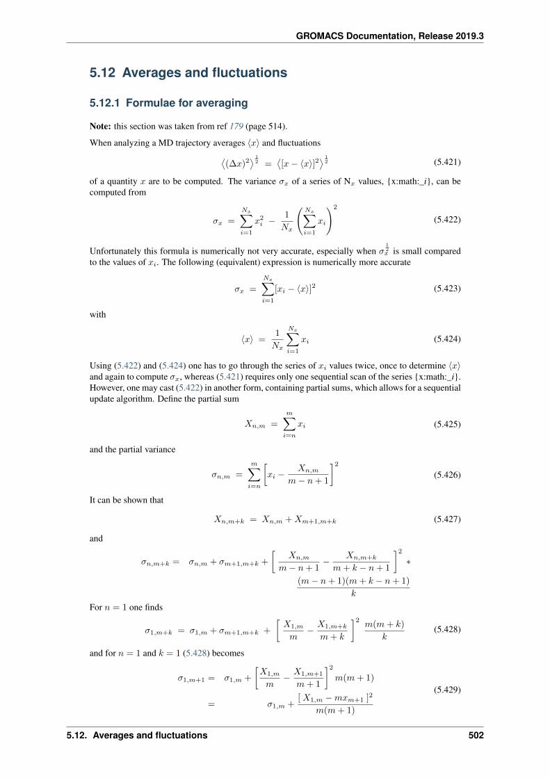
GROMACS Documentation, Release 2019.3
5.12 Averages and fluctuations
5.12.1 Formulae for averaging
Note: this section was taken from ref 179 (page 514).
When analyzing a MD trajectory averages ⟨𝑥⟩ and fluctuations⟨(∆𝑥)2
⟩ 12 =
⟨[𝑥− ⟨𝑥⟩]2
⟩ 12 (5.421)
of a quantity 𝑥 are to be computed. The variance 𝜎𝑥 of a series of N𝑥 values, {x:math:_i}, can becomputed from
𝜎𝑥 =
𝑁𝑥∑𝑖=1
𝑥2𝑖 − 1
𝑁𝑥
(𝑁𝑥∑𝑖=1
𝑥𝑖
)2
(5.422)
Unfortunately this formula is numerically not very accurate, especially when 𝜎12𝑥 is small compared
to the values of 𝑥𝑖. The following (equivalent) expression is numerically more accurate
𝜎𝑥 =
𝑁𝑥∑𝑖=1
[𝑥𝑖 − ⟨𝑥⟩]2 (5.423)
with
⟨𝑥⟩ =1
𝑁𝑥
𝑁𝑥∑𝑖=1
𝑥𝑖 (5.424)
Using (5.422) and (5.424) one has to go through the series of 𝑥𝑖 values twice, once to determine ⟨𝑥⟩and again to compute 𝜎𝑥, whereas (5.421) requires only one sequential scan of the series {x:math:_i}.However, one may cast (5.422) in another form, containing partial sums, which allows for a sequentialupdate algorithm. Define the partial sum
𝑋𝑛,𝑚 =
𝑚∑𝑖=𝑛
𝑥𝑖 (5.425)
and the partial variance
𝜎𝑛,𝑚 =
𝑚∑𝑖=𝑛
[𝑥𝑖 −
𝑋𝑛,𝑚
𝑚− 𝑛+ 1
]2(5.426)
It can be shown that
𝑋𝑛,𝑚+𝑘 = 𝑋𝑛,𝑚 +𝑋𝑚+1,𝑚+𝑘 (5.427)
and
𝜎𝑛,𝑚+𝑘 = 𝜎𝑛,𝑚 + 𝜎𝑚+1,𝑚+𝑘 +
[𝑋𝑛,𝑚
𝑚− 𝑛+ 1− 𝑋𝑛,𝑚+𝑘
𝑚+ 𝑘 − 𝑛+ 1
]2*
(𝑚− 𝑛+ 1)(𝑚+ 𝑘 − 𝑛+ 1)
𝑘
For 𝑛 = 1 one finds
𝜎1,𝑚+𝑘 = 𝜎1,𝑚 + 𝜎𝑚+1,𝑚+𝑘 +
[𝑋1,𝑚
𝑚− 𝑋1,𝑚+𝑘
𝑚+ 𝑘
]2𝑚(𝑚+ 𝑘)
𝑘(5.428)
and for 𝑛 = 1 and 𝑘 = 1 (5.428) becomes
𝜎1,𝑚+1 = 𝜎1,𝑚 +
[𝑋1,𝑚
𝑚− 𝑋1,𝑚+1
𝑚+ 1
]2𝑚(𝑚+ 1)
= 𝜎1,𝑚 +[ 𝑋1,𝑚 −𝑚𝑥𝑚+1 ]2
𝑚(𝑚+ 1)
(5.429)
5.12. Averages and fluctuations 502
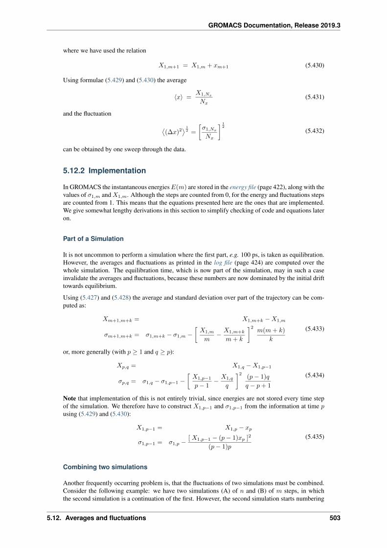
GROMACS Documentation, Release 2019.3
where we have used the relation
𝑋1,𝑚+1 = 𝑋1,𝑚 + 𝑥𝑚+1 (5.430)
Using formulae (5.429) and (5.430) the average
⟨𝑥⟩ =𝑋1,𝑁𝑥
𝑁𝑥(5.431)
and the fluctuation
⟨(∆𝑥)2
⟩ 12 =
[𝜎1,𝑁𝑥
𝑁𝑥
] 12
(5.432)
can be obtained by one sweep through the data.
5.12.2 Implementation
In GROMACS the instantaneous energies𝐸(𝑚) are stored in the energy file (page 422), along with thevalues of 𝜎1,𝑚 and𝑋1,𝑚. Although the steps are counted from 0, for the energy and fluctuations stepsare counted from 1. This means that the equations presented here are the ones that are implemented.We give somewhat lengthy derivations in this section to simplify checking of code and equations lateron.
Part of a Simulation
It is not uncommon to perform a simulation where the first part, e.g. 100 ps, is taken as equilibration.However, the averages and fluctuations as printed in the log file (page 424) are computed over thewhole simulation. The equilibration time, which is now part of the simulation, may in such a caseinvalidate the averages and fluctuations, because these numbers are now dominated by the initial drifttowards equilibrium.
Using (5.427) and (5.428) the average and standard deviation over part of the trajectory can be com-puted as:
𝑋𝑚+1,𝑚+𝑘 = 𝑋1,𝑚+𝑘 −𝑋1,𝑚
𝜎𝑚+1,𝑚+𝑘 = 𝜎1,𝑚+𝑘 − 𝜎1,𝑚 −[𝑋1,𝑚
𝑚− 𝑋1,𝑚+𝑘
𝑚+ 𝑘
]2𝑚(𝑚+ 𝑘)
𝑘
(5.433)
or, more generally (with 𝑝 ≥ 1 and 𝑞 ≥ 𝑝):
𝑋𝑝,𝑞 = 𝑋1,𝑞 −𝑋1,𝑝−1
𝜎𝑝,𝑞 = 𝜎1,𝑞 − 𝜎1,𝑝−1 −[𝑋1,𝑝−1
𝑝− 1− 𝑋1,𝑞
𝑞
]2(𝑝− 1)𝑞
𝑞 − 𝑝+ 1
(5.434)
Note that implementation of this is not entirely trivial, since energies are not stored every time stepof the simulation. We therefore have to construct 𝑋1,𝑝−1 and 𝜎1,𝑝−1 from the information at time 𝑝using (5.429) and (5.430):
𝑋1,𝑝−1 = 𝑋1,𝑝 − 𝑥𝑝
𝜎1,𝑝−1 = 𝜎1,𝑝 −[ 𝑋1,𝑝−1 − (𝑝− 1)𝑥𝑝 ]2
(𝑝− 1)𝑝
(5.435)
Combining two simulations
Another frequently occurring problem is, that the fluctuations of two simulations must be combined.Consider the following example: we have two simulations (A) of 𝑛 and (B) of 𝑚 steps, in whichthe second simulation is a continuation of the first. However, the second simulation starts numbering
5.12. Averages and fluctuations 503
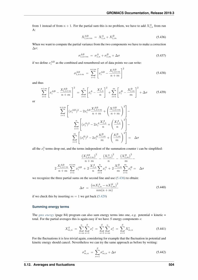
GROMACS Documentation, Release 2019.3
from 1 instead of from 𝑛 + 1. For the partial sum this is no problem, we have to add 𝑋𝐴1,𝑛 from run
A:
𝑋𝐴𝐵1,𝑛+𝑚 = 𝑋𝐴
1,𝑛 +𝑋𝐵1,𝑚 (5.436)
When we want to compute the partial variance from the two components we have to make a correction∆𝜎:
𝜎𝐴𝐵1,𝑛+𝑚 = 𝜎𝐴
1,𝑛 + 𝜎𝐵1,𝑚 + ∆𝜎 (5.437)
if we define 𝑥𝐴𝐵𝑖 as the combined and renumbered set of data points we can write:
𝜎𝐴𝐵1,𝑛+𝑚 =
𝑛+𝑚∑𝑖=1
[𝑥𝐴𝐵𝑖 −
𝑋𝐴𝐵1,𝑛+𝑚
𝑛+𝑚
]2(5.438)
and thus
𝑛+𝑚∑𝑖=1
[𝑥𝐴𝐵𝑖 −
𝑋𝐴𝐵1,𝑛+𝑚
𝑛+𝑚
]2=
𝑛∑𝑖=1
[𝑥𝐴𝑖 −
𝑋𝐴1,𝑛
𝑛
]2+
𝑚∑𝑖=1
[𝑥𝐵𝑖 −
𝑋𝐵1,𝑚
𝑚
]2+ ∆𝜎 (5.439)
or
𝑛+𝑚∑𝑖=1
⎡⎣(𝑥𝐴𝐵𝑖 )2 − 2𝑥𝐴𝐵
𝑖
𝑋𝐴𝐵1,𝑛+𝑚
𝑛+𝑚+
(𝑋𝐴𝐵
1,𝑛+𝑚
𝑛+𝑚
)2⎤⎦−
𝑛∑𝑖=1
⎡⎣(𝑥𝐴𝑖 )2 − 2𝑥𝐴𝑖𝑋𝐴
1,𝑛
𝑛+
(𝑋𝐴
1,𝑛
𝑛
)2⎤⎦−
𝑚∑𝑖=1
⎡⎣(𝑥𝐵𝑖 )2 − 2𝑥𝐵𝑖𝑋𝐵
1,𝑚
𝑚+
(𝑋𝐵
1,𝑚
𝑚
)2⎤⎦ = ∆𝜎
all the 𝑥2𝑖 terms drop out, and the terms independent of the summation counter 𝑖 can be simplified:(𝑋𝐴𝐵
1,𝑛+𝑚
)2𝑛+𝑚
−(𝑋𝐴
1,𝑛
)2𝑛
−(𝑋𝐵
1,𝑚
)2𝑚
−
2𝑋𝐴𝐵
1,𝑛+𝑚
𝑛+𝑚
𝑛+𝑚∑𝑖=1
𝑥𝐴𝐵𝑖 + 2
𝑋𝐴1,𝑛
𝑛
𝑛∑𝑖=1
𝑥𝐴𝑖 + 2𝑋𝐵
1,𝑚
𝑚
𝑚∑𝑖=1
𝑥𝐵𝑖 = ∆𝜎
we recognize the three partial sums on the second line and use (5.436) to obtain:
∆𝜎 =
(𝑚𝑋𝐴
1,𝑛 − 𝑛𝑋𝐵1,𝑚
)2𝑛𝑚(𝑛+𝑚)
(5.440)
if we check this by inserting 𝑚 = 1 we get back (5.429)
Summing energy terms
The gmx energy (page 84) program can also sum energy terms into one, e.g. potential + kinetic =total. For the partial averages this is again easy if we have 𝑆 energy components 𝑠:
𝑋𝑆𝑚,𝑛 =
𝑛∑𝑖=𝑚
𝑆∑𝑠=1
𝑥𝑠𝑖 =
𝑆∑𝑠=1
𝑛∑𝑖=𝑚
𝑥𝑠𝑖 =
𝑆∑𝑠=1
𝑋𝑠𝑚,𝑛 (5.441)
For the fluctuations it is less trivial again, considering for example that the fluctuation in potential andkinetic energy should cancel. Nevertheless we can try the same approach as before by writing:
𝜎𝑆𝑚,𝑛 =
𝑆∑𝑠=1
𝜎𝑠𝑚,𝑛 + ∆𝜎 (5.442)
5.12. Averages and fluctuations 504
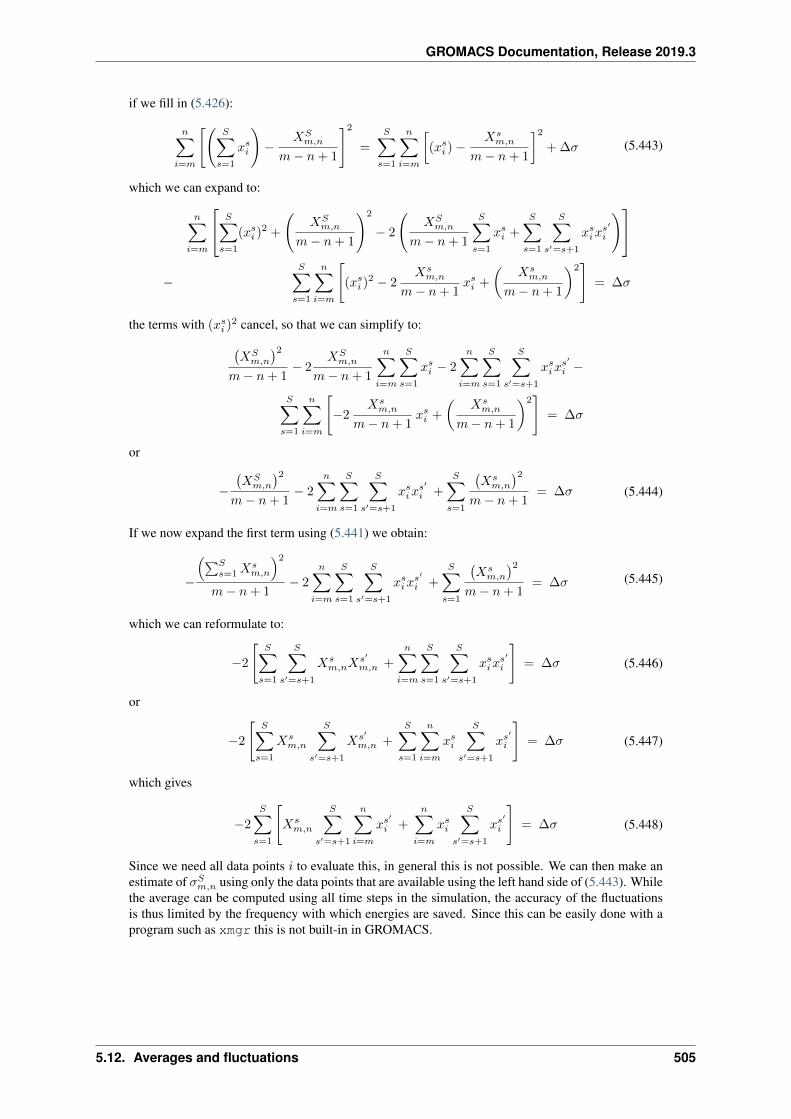
GROMACS Documentation, Release 2019.3
if we fill in (5.426):
𝑛∑𝑖=𝑚
[(𝑆∑
𝑠=1
𝑥𝑠𝑖
)−
𝑋𝑆𝑚,𝑛
𝑚− 𝑛+ 1
]2=
𝑆∑𝑠=1
𝑛∑𝑖=𝑚
[(𝑥𝑠𝑖 ) −
𝑋𝑠𝑚,𝑛
𝑚− 𝑛+ 1
]2+ ∆𝜎 (5.443)
which we can expand to:
𝑛∑𝑖=𝑚
⎡⎣ 𝑆∑𝑠=1
(𝑥𝑠𝑖 )2 +
(𝑋𝑆
𝑚,𝑛
𝑚− 𝑛+ 1
)2
− 2
(𝑋𝑆
𝑚,𝑛
𝑚− 𝑛+ 1
𝑆∑𝑠=1
𝑥𝑠𝑖 +
𝑆∑𝑠=1
𝑆∑𝑠′=𝑠+1
𝑥𝑠𝑖𝑥𝑠′
𝑖
)⎤⎦−
𝑆∑𝑠=1
𝑛∑𝑖=𝑚
[(𝑥𝑠𝑖 )
2 − 2𝑋𝑠
𝑚,𝑛
𝑚− 𝑛+ 1𝑥𝑠𝑖 +
(𝑋𝑠
𝑚,𝑛
𝑚− 𝑛+ 1
)2]
= ∆𝜎
the terms with (𝑥𝑠𝑖 )2 cancel, so that we can simplify to:(𝑋𝑆
𝑚,𝑛
)2𝑚− 𝑛+ 1
− 2𝑋𝑆
𝑚,𝑛
𝑚− 𝑛+ 1
𝑛∑𝑖=𝑚
𝑆∑𝑠=1
𝑥𝑠𝑖 − 2
𝑛∑𝑖=𝑚
𝑆∑𝑠=1
𝑆∑𝑠′=𝑠+1
𝑥𝑠𝑖𝑥𝑠′
𝑖 −
𝑆∑𝑠=1
𝑛∑𝑖=𝑚
[−2
𝑋𝑠𝑚,𝑛
𝑚− 𝑛+ 1𝑥𝑠𝑖 +
(𝑋𝑠
𝑚,𝑛
𝑚− 𝑛+ 1
)2]
= ∆𝜎
or
−(𝑋𝑆
𝑚,𝑛
)2𝑚− 𝑛+ 1
− 2
𝑛∑𝑖=𝑚
𝑆∑𝑠=1
𝑆∑𝑠′=𝑠+1
𝑥𝑠𝑖𝑥𝑠′
𝑖 +
𝑆∑𝑠=1
(𝑋𝑠
𝑚,𝑛
)2𝑚− 𝑛+ 1
= ∆𝜎 (5.444)
If we now expand the first term using (5.441) we obtain:
−
(∑𝑆𝑠=1𝑋
𝑠𝑚,𝑛
)2𝑚− 𝑛+ 1
− 2
𝑛∑𝑖=𝑚
𝑆∑𝑠=1
𝑆∑𝑠′=𝑠+1
𝑥𝑠𝑖𝑥𝑠′
𝑖 +
𝑆∑𝑠=1
(𝑋𝑠
𝑚,𝑛
)2𝑚− 𝑛+ 1
= ∆𝜎 (5.445)
which we can reformulate to:
−2
[𝑆∑
𝑠=1
𝑆∑𝑠′=𝑠+1
𝑋𝑠𝑚,𝑛𝑋
𝑠′
𝑚,𝑛 +
𝑛∑𝑖=𝑚
𝑆∑𝑠=1
𝑆∑𝑠′=𝑠+1
𝑥𝑠𝑖𝑥𝑠′
𝑖
]= ∆𝜎 (5.446)
or
−2
[𝑆∑
𝑠=1
𝑋𝑠𝑚,𝑛
𝑆∑𝑠′=𝑠+1
𝑋𝑠′
𝑚,𝑛 +
𝑆∑𝑠=1
𝑛∑𝑖=𝑚
𝑥𝑠𝑖
𝑆∑𝑠′=𝑠+1
𝑥𝑠′
𝑖
]= ∆𝜎 (5.447)
which gives
−2
𝑆∑𝑠=1
[𝑋𝑠
𝑚,𝑛
𝑆∑𝑠′=𝑠+1
𝑛∑𝑖=𝑚
𝑥𝑠′
𝑖 +
𝑛∑𝑖=𝑚
𝑥𝑠𝑖
𝑆∑𝑠′=𝑠+1
𝑥𝑠′
𝑖
]= ∆𝜎 (5.448)
Since we need all data points 𝑖 to evaluate this, in general this is not possible. We can then make anestimate of 𝜎𝑆
𝑚,𝑛 using only the data points that are available using the left hand side of (5.443). Whilethe average can be computed using all time steps in the simulation, the accuracy of the fluctuationsis thus limited by the frequency with which energies are saved. Since this can be easily done with aprogram such as xmgr this is not built-in in GROMACS.
5.12. Averages and fluctuations 505
GROMACS Documentation, Release 2019.3
5.13 Bibliography
1 H. Bekker, H.J.C. Berendsen, E.J. Dijkstra, S. Achterop, R. van Drunen, D. van der Spoel, A.Sijbers, and H. Keegstra et al., “Gromacs: A parallel computer for molecular dynamics simulations”;pp. 252–256 in Physics computing 92. Edited by R.A. de Groot and J. Nadrchal. World Scientific,Singapore, 1993.2 H.J.C. Berendsen, D. van der Spoel, and R. van Drunen, “GROMACS: A message-passing parallelmolecular dynamics implementation,” Comp. Phys. Comm., 91 43–56 (1995).3 E. Lindahl, B. Hess, and D. van der Spoel, “GROMACS 3.0: A package for molecular simulationand trajectory analysis,” J. Mol. Mod., 7 306–317 (2001).4 D. van der Spoel, E. Lindahl, B. Hess, G. Groenhof, A.E. Mark, and H.J.C. Berendsen, “GRO-MACS: Fast, Flexible and Free,” J. Comp. Chem., 26 1701–1718 (2005).5 B. Hess, C. Kutzner, D. van der Spoel, and E. Lindahl, “GROMACS 4: Algorithms for Highly Effi-cient, Load-Balanced, and Scalable Molecular Simulation,” J. Chem. Theory Comput., 4 [3] 435–447(2008).6 S. Pronk, S. Páll, R. Schulz, P. Larsson, P. Bjelkmar, R. Apostolov, M.R. Shirts, and J.C. Smithet al., “GROMACS 4.5: A high-throughput and highly parallel open source molecular simulationtoolkit,” Bioinformatics, 29 [7] 845–854 (2013).7 S. Páll, M.J. Abraham, C. Kutzner, B. Hess, and E. Lindahl, “Tackling exascale software challengesin molecular dynamics simulations with GROMACS”; pp. 3–27 in Solving software challenges forexascale. Edited by S. Markidis and E. Laure. Springer International Publishing Switzerland, Lon-don, 2015.8 M.J. Abraham, T. Murtola, R. Schulz, S. Páll, J.C. Smith, B. Hess, and E. Lindahl, “GROMACS:High performance molecular simulations through multi-level parallelism from laptops to supercom-puters,” SoftwareX, 1–2 19–25 (2015).9 W.F. van Gunsteren and H.J.C. Berendsen, “Computer simulation of molecular dynamics: Method-ology, applications, and perspectives in chemistry,” Angew. Chem. Int. Ed. Engl., 29 992–1023(1990).10 J.G.E.M. Fraaije, “Dynamic density functional theory for microphase separation kinetics of blockcopolymer melts,” J. Chem. Phys., 99 9202–9212 (1993).11 D.A. McQuarrie, Statistical mechanics. Harper & Row, New York, 1976.12 W.F. van Gunsteren and H.J.C. Berendsen, “Algorithms for macromolecular dynamics and con-straint dynamics,” Mol. Phys., 34 1311–1327 (1977).13 W.F. van Gunsteren and M. Karplus, “Effect of constraints on the dynamics of macromolecules,”Macromolecules, 15 1528–1544 (1982).14 T. Darden, D. York, and L. Pedersen, “Particle mesh Ewald: An N∙log(N) method for Ewald sumsin large systems,” J. Chem. Phys., 98 10089–10092 (1993).15 U. Essmann, L. Perera, M.L. Berkowitz, T. Darden, H. Lee, and L.G. Pedersen, “A smooth particlemesh ewald potential,” J. Chem. Phys., 103 8577–8592 (1995).16 S. Geman and D. Geman, “Stochastic relaxation, Gibbs distributions and the Bayesian restorationof images,” IEEE Trans. Patt. Anal. Mach. Int., 6 721 (1984).17 M. Nilges, G.M. Clore, and A.M. Gronenborn, “Determination of three-dimensional structures ofproteins from interproton distance data by dynamical simulated annealing from a random array ofatoms,” FEBS Lett., 239 129–136 (1988).18 R.C. van Schaik, H.J.C. Berendsen, A.E. Torda, and W.F. van Gunsteren, “A structure refinementmethod based on molecular dynamics in 4 spatial dimensions,” J. Mol. Biol., 234 751–762 (1993).19 K. Zimmerman, “All purpose molecular mechanics simulator and energy minimizer,” J. Comp.Chem., 12 310–319 (1991).
5.13. Bibliography 506
GROMACS Documentation, Release 2019.3
20 D.J. Adams, E.M. Adams, and G.J. Hills, “The computer simulation of polar liquids,” Mol. Phys.,38 387–400 (1979).21 H. Bekker, E.J. Dijkstra, M.K.R. Renardus, and H.J.C. Berendsen, “An efficient, box shape in-dependent non-bonded force and virial algorithm for molecular dynamics,” Mol. Sim., 14 137–152(1995).22 R.W. Hockney, S.P. Goel, and J. Eastwood, “Quiet High Resolution Computer Models of a Plasma,”J. Comp. Phys., 14 148–158 (1974).23 L. Verlet., “Computer experiments on classical fluids. I. Thermodynamical properties of Lennard-Jones molecules,” Phys. Rev., 159 98–103 (1967).24 H.J.C. Berendsen and W.F. van Gunsteren, “Practical algorithms for dynamics simulations”; in1986.25 W.C. Swope, H.C. Andersen, P.H. Berens, and K.R. Wilson, “A computer-simulation method forthe calculation of equilibrium-constants for the formation of physical clusters of molecules: Applica-tion to small water clusters,” J. Chem. Phys., 76 637–649 (1982).26 H.J.C. Berendsen, J.P.M. Postma, A. DiNola, and J.R. Haak, “Molecular dynamics with couplingto an external bath,” J. Chem. Phys., 81 3684–3690 (1984).27 H.C. Andersen, “Molecular dynamics simulations at constant pressure and/or temperature,” J.Chem. Phys., 72 2384 (1980).28 S. Nosé, “A molecular dynamics method for simulations in the canonical ensemble,” Mol. Phys.,52 255–268 (1984).29 W.G. Hoover, “Canonical dynamics: Equilibrium phase-space distributions,” Phys. Rev. **A**, 311695–1697 (1985).30 G. Bussi, D. Donadio, and M. Parrinello, “Canonical sampling through velocity rescaling,” J.Chem. Phys., 126 014101 (2007).31 H.J.C. Berendsen, “Transport properties computed by linear response through weak coupling toa bath”; pp. 139–155 in Computer simulations in material science. Edited by M. Meyer and V.Pontikis. Kluwer, 1991.32 J.E. Basconi and M.R. Shirts, “Effects of temperature control algorithms on transport propertiesand kinetics in molecular dynamics simulations,” J. Chem. Theory Comput., 9 [7] 2887–2899 (2013).33 B. Cooke and S.J. Schmidler, “Preserving the Boltzmann ensemble in replica-exchange moleculardynamics,” J. Chem. Phys., 129 164112 (2008).34 G.J. Martyna, M.L. Klein, and M.E. Tuckerman, “Nosé-Hoover chains: The canonical ensemblevia continuous dynamics,” J. Chem. Phys., 97 2635–2643 (1992).35 G.J. Martyna, M.E. Tuckerman, D.J. Tobias, and M.L. Klein, “Explicit reversible integrators forextended systems dynamics,” Mol. Phys., 87 1117–1157 (1996).36 B.L. Holian, A.F. Voter, and R. Ravelo, “Thermostatted molecular dynamics: How to avoid theToda demon hidden in Nosé-Hoover dynamics,” Phys. Rev. E, 52 [3] 2338–2347 (1995).37 M.P. Eastwood, K.A. Stafford, R.A. Lippert, M.Ø. Jensen, P. Maragakis, C. Predescu, R.O. Dror,and D.E. Shaw, “Equipartition and the calculation of temperature in biomolecular simulations,” J.Chem. Theory Comput., ASAP DOI: 10.1021/ct9002916 (2010).38 M. Parrinello and A. Rahman, “Polymorphic transitions in single crystals: A new molecular dy-namics method,” J. Appl. Phys., 52 7182–7190 (1981).39 S. Nosé and M.L. Klein, “Constant pressure molecular dynamics for molecular systems,” Mol.Phys., 50 1055–1076 (1983).40 G. Liu, “Dynamical equations for the period vectors in a periodic system under constant externalstress,” Can. J. Phys., 93 974–978 (2015).
5.13. Bibliography 507
GROMACS Documentation, Release 2019.3
41 M.E. Tuckerman, J. Alejandre, R. López-Rendón, A.L. Jochim, and G.J. Martyna, “A Liouville-operator derived measure-preserving integrator for molecular dynamics simulations in the isothermal-isobaric ensemble,” J. Phys. A., 59 5629–5651 (2006).42 T.-Q. Yu, J. Alejandre, R. Lopez-Rendon, G.J. Martyna, and M.E. Tuckerman, “Measure-preserving integrators for molecular dynamics in the isothermal-isobaric ensemble derived from theliouville operator,” Chem. Phys., 370 294–305 (2010).43 B.G. Dick and A.W. Overhauser, “Theory of the dielectric constants of alkali halide crystals,” Phys.Rev., 112 90–103 (1958).44 P.C. Jordan, P.J. van Maaren, J. Mavri, D. van der Spoel, and H.J.C. Berendsen, “Towards phasetransferable potential functions: Methodology and application to nitrogen,” J. Chem. Phys., 1032272–2285 (1995).45 P.J. van Maaren and D. van der Spoel, “Molecular dynamics simulations of a water with a novelshell-model potential,” J. Phys. Chem. B., 105 2618–2626 (2001).46 J.P. Ryckaert, G. Ciccotti, and H.J.C. Berendsen, “Numerical integration of the cartesian equa-tions of motion of a system with constraints; molecular dynamics of n-alkanes,” J. Comp. Phys., 23327–341 (1977).47 S. Miyamoto and P.A. Kollman, “SETTLE: An analytical version of the SHAKE and RATTLEalgorithms for rigid water models,” J. Comp. Chem., 13 952–962 (1992).48 H.C. Andersen, “RATTLE: A ‘Velocity’ version of the SHAKE algorithm for molecular dynamicscalculations,” J. Comp. Phys., 52 24–34 (1983).49 B. Hess, H. Bekker, H.J.C. Berendsen, and J.G.E.M. Fraaije, “LINCS: A linear constraint solverfor molecular simulations,” J. Comp. Chem., 18 1463–1472 (1997).50 B. Hess, “P-LINCS: A parallel linear constraint solver for molecular simulation,” J. Chem. TheoryComput., 4 116–122 (2007).51 N. Goga, A.J. Rzepiela, A.H. de Vries, S.J. Marrink, and H.J.C. Berendsen, “Efficient algorithmsfor Langevin and DPD dynamics,” J. Chem. Theory Comput., 8 3637–3649 (2012).52 R.H. Byrd, P. Lu, and J. Nocedal, “A limited memory algorithm for bound constrained optimiza-tion,” SIAM J. Scientif. Statistic. Comput., 16 1190–1208 (1995).53 C. Zhu, R.H. Byrd, and J. Nocedal, “L-BFGS-B: Algorithm 778: L-BFGS-B, FORTRAN routinesfor large scale bound constrained optimization,” ACM Trans. Math. Softw., 23 550–560 (1997).54 M. Levitt, C. Sander, and P.S. Stern, “The normal modes of a protein: Native bovine pancreatictrypsin inhibitor,” Int. J. Quant. Chem: Quant. Biol. Symp., 10 181–199 (1983).55 N. Go, T. Noguti, and T. Nishikawa, “Dynamics of a small globular protein in terms of low-frequency vibrational modes,” Proc. Natl. Acad. Sci. USA, 80 3696–3700 (1983).56 B. Brooks and M. Karplus, “Harmonic dynamics of proteins: Normal modes and fluctuations inbovine pancreatic trypsin inhibitor,” Proc. Natl. Acad. Sci. USA, 80 6571–6575 (1983).57 S. Hayward and N. Go, “Collective variable description of native protein dynamics,” Annu. Rev.Phys. Chem., 46 223–250 (1995).58 C.H. Bennett, “Efficient Estimation of Free Energy Differences from Monte Carlo Data,” J. Comp.Phys., 22 245–268 (1976).59 M.R. Shirts and J.D. Chodera, “Statistically optimal analysis of multiple equilibrium simulations,”J. Chem. Phys., 129 124105 (2008).60 K. Hukushima and K. Nemoto, “Exchange Monte Carlo Method and Application to Spin GlassSimulations,” J. Phys. Soc. Jpn., 65 1604–1608 (1996).61 Y. Sugita and Y. Okamoto, “Replica-exchange molecular dynamics method for protein folding,”Chem. Phys. Lett., 314 141–151 (1999).62 M. Seibert, A. Patriksson, B. Hess, and D. van der Spoel, “Reproducible polypeptide folding andstructure prediction using molecular dynamics simulations,” J. Mol. Biol., 354 173–183 (2005).
5.13. Bibliography 508
GROMACS Documentation, Release 2019.3
63 T. Okabe, M. Kawata, Y. Okamoto, and M. Mikami, “Replica-exchange Monte Carlo method forthe isobaric-isothermal ensemble,” Chem. Phys. Lett., 335 435–439 (2001).64 J.D. Chodera and M.R. Shirts, “Replica exchange and expanded ensemble simulations as gibbssampling: Simple improvements for enhanced mixing,” J. Chem. Phys., 135 194110 (2011).65 B.L. de Groot, A. Amadei, D.M.F. van Aalten, and H.J.C. Berendsen, “Towards an exhaustivesampling of the configurational spaces of the two forms of the peptide hormone guanylin,” J. Biomol.Str. Dyn., 13 [5] 741–751 (1996).66 B.L. de Groot, A. Amadei, R.M. Scheek, N.A.J. van Nuland, and H.J.C. Berendsen, “An extendedsampling of the configurational space of HPr from E. coli,” PROTEINS: Struct. Funct. Gen., 26314–322 (1996).67 O.E. Lange, L.V. Schafer, and H. Grubmuller, “Flooding in GROMACS: Accelerated barrier cross-ings in molecular dynamics,” J. Comp. Chem., 27 1693–1702 (2006).68 A.P. Lyubartsev, A.A. Martsinovski, S.V. Shevkunov, and P.N. Vorontsov-Velyaminov, “New ap-proach to Monte Carlo calculation of the free energy: Method of expanded ensembles,” J. Chem.Phys., 96 1776–1783 (1992).69 S.Y. Liem, D. Brown, and J.H.R. Clarke, “Molecular dynamics simulations on distributed memorymachines,” Comput. Phys. Commun., 67 [2] 261–267 (1991).70 K.J. Bowers, R.O. Dror, and D.E. Shaw, “The midpoint method for parallelization of particlesimulations,” J. Chem. Phys., 124 [18] 184109–184109 (2006).71 I.G. Tironi, R. Sperb, P.E. Smith, and W.F. van Gunsteren, “A generalized reaction field method formolecular dynamics simulations,” J. Chem. Phys., 102 5451–5459 (1995).72 D. van der Spoel and P.J. van Maaren, “The origin of layer structure artifacts in simulations ofliquid water,” J. Chem. Theory Comput., 2 1–11 (2006).73 I. Ohmine, H. Tanaka, and P.G. Wolynes, “Large local energy fluctuations in water. II. Cooperativemotions and fluctuations,” J. Chem. Phys., 89 5852–5860 (1988).74 D.B. Kitchen, F. Hirata, J.D. Westbrook, R. Levy, D. Kofke, and M. Yarmush, “Conserving energyduring molecular dynamics simulations of water, proteins, and proteins in water,” J. Comp. Chem.,11 1169–1180 (1990).75 J. Guenot and P.A. Kollman, “Conformational and energetic effects of truncating nonbonded inter-actions in an aqueous protein dynamics simulation,” J. Comp. Chem., 14 295–311 (1993).76 P.J. Steinbach and B.R. Brooks, “New spherical-cutoff methods for long-range forces in macro-molecular simulation,” J. Comp. Chem., 15 667–683 (1994).77 W.F. van Gunsteren, S.R. Billeter, A.A. Eising, P.H. Hünenberger, P. Krüger, A.E. Mark,W.R.P. Scott, and I.G. Tironi, Biomolecular simulation: The GROMOS96 manual and user guide.Hochschulverlag AG an der ETH Zürich, Zürich, Switzerland, 1996.78 W.F. van Gunsteren and H.J.C. Berendsen, Gromos-87 manual. Biomos BV, Nijenborgh 4, 9747AG Groningen, The Netherlands, 1987.79 P.M. Morse, “Diatomic molecules according to the wave mechanics. II. vibrational levels.” Phys.Rev., 34 57–64 (1929).80 H.J.C. Berendsen, J.P.M. Postma, W.F. van Gunsteren, and J. Hermans, “Interaction models forwater in relation to protein hydration”; pp. 331–342 in Intermolecular forces. Edited by B. Pullman.D. Reidel Publishing Company, Dordrecht, 1981.81 D.M. Ferguson, “Parametrization and evaluation of a flexible water model,” J. Comp. Chem., 16501–511 (1995).82 H.R. Warner Jr., “Kinetic theory and rheology of dilute suspensions of finitely extendible dumb-bells,” Ind. Eng. Chem. Fundam., 11 [3] 379–387 (1972).
5.13. Bibliography 509
GROMACS Documentation, Release 2019.3
83 M. Bulacu, N. Goga, W. Zhao, G. Rossi, L. Monticelli, X. Periole, D. Tieleman, and S. Marrink,“Improved angle potentials for coarse-grained molecular dynamics simulations,” J. Chem. Phys., 123[11] (2005).84 B.R. Brooks, R.E. Bruccoleri, B.D. Olafson, D.J. States, S. Swaminathan, and M. Karplus,“CHARMM: A program for macromolecular energy, minimization, and dynamics calculation,” J.Comp. Chem., 4 187–217 (1983).85 C.P. Lawrence and J.L. Skinner, “Flexible TIP4P model for molecular dynamics simulation ofliquid water,” Chem. Phys. Lett., 372 842–847 (2003).86 W.L. Jorgensen, D.S. Maxwell, and J. Tirado-Rives, “Development and testing of the oPLS all-atom force field on conformational energetics and properties of organic liquids,” J. Am. Chem. Soc.,118 11225–11236 (1996).87 M.J. Robertson, J. Tirado-Rives, and W.L. Jorgensen, “Improved peptide and protein torsionalenergetics with the oPLS-aA force field,” J. Chem. Theory Comput., 11 3499–3509 (2015).88 M. Bulacu and E. van der Giessen, “Effect of bending and torsion rigidity on self-diffusion inpolymer melts: A molecular-dynamics study,” JCTC, 9 [8] 3282–3292 (2013).89 R.A. Scott and H. Scheraga, “Conformational analysis of macromolecules,” J. Chem. Phys., 443054–3069 (1966).90 L. Pauling, The nature of chemical bond. Cornell University Press, Ithaca; New York, 1960.91 A.E. Torda, R.M. Scheek, and W.F. van Gunsteren, “Time-dependent distance restraints in molec-ular dynamics simulations,” Chem. Phys. Lett., 157 289–294 (1989).92 B. Hess and R.M. Scheek, “Orientation restraints in molecular dynamics simulations using timeand ensemble averaging,” J. Magn. Reson., 164 19–27 (2003).93 P.E.M. Lopes, J. Huang, J. Shim, Y. Luo, H. Li, B. Roux, and J. MacKerell Alexander D., “Polar-izable force field for peptides and proteins based on the classical drude oscillator,” J. Chem. TheoryComput, 9 5430–5449 (2013).94 H. Yu, T.W. Whitfield, E. Harder, G. Lamoureux, I. Vorobyov, V.M. Anisimov, A.D. MacKerell,Jr., and B. Roux, “Simulating Monovalent and Divalent Ions in Aqueous Solution Using a DrudePolarizable Force Field,” J. Chem. Theory Comput., 6 774–786 (2010).95 B.T. Thole, “Molecular polarizabilities with a modified dipole interaction,” Chem. Phys., 59341–345 (1981).96 G. Lamoureux and B. Roux, “Modeling induced polarization with classical drude oscillators: The-ory and molecular dynamics simulation algorithm,” J. Chem. Phys., 119 3025–3039 (2003).97 G. Lamoureux, A.D. MacKerell, and B. Roux, “A simple polarizable model of water based onclassical drude oscillators,” J. Chem. Phys., 119 5185–5197 (2003).98 S.Y. Noskov, G. Lamoureux, and B. Roux, “Molecular dynamics study of hydration in ethanol-water mixtures using a polarizable force field,” J. Phys. Chem. B., 109 6705–6713 (2005).99 W.F. van Gunsteren and A.E. Mark, “Validation of molecular dynamics simulations,” J. Chem.Phys., 108 6109–6116 (1998).100 T.C. Beutler, A.E. Mark, R.C. van Schaik, P.R. Greber, and W.F. van Gunsteren, “Avoiding singu-larities and numerical instabilities in free energy calculations based on molecular simulations,” Chem.Phys. Lett., 222 529–539 (1994).101 T.T. Pham and M.R. Shirts, “Identifying low variance pathways for free energy calculations ofmolecular transformations in solution phase,” J. Chem. Phys., 135 034114 (2011).102 T.T. Pham and M.R. Shirts, “Optimal pairwise and non-pairwise alchemical pathways for freeenergy calculations of molecular transformation in solution phase,” J. Chem. Phys., 136 124120(2012).103 W.L. Jorgensen and J. Tirado-Rives, “The OPLS potential functions for proteins. energy mini-mizations for crystals of cyclic peptides and crambin,” J. Am. Chem. Soc., 110 1657–1666 (1988).
5.13. Bibliography 510
GROMACS Documentation, Release 2019.3
104 H.J.C. Berendsen and W.F. van Gunsteren, “Molecular dynamics simulations: Techniques andapproaches”; pp. 475–500 in Molecular liquids-dynamics and interactions. Edited by A.J.B. et al.Reidel, Dordrecht, The Netherlands, 1984.105 P.P. Ewald, “Die Berechnung optischer und elektrostatischer Gitterpotentiale,” Ann. Phys., 64253–287 (1921).106 R.W. Hockney and J.W. Eastwood, Computer simulation using particles. McGraw-Hill, NewYork, 1981.107 V. Ballenegger, J.J. Cerdà, and C. Holm, “How to convert SPME to P3M: Influence functions anderror estimates,” J. Chem. Theory Comput., 8 [3] 936–947 (2012).108 M.P. Allen and D.J. Tildesley, Computer simulations of liquids. Oxford Science Publications,Oxford, 1987.109 C.L. Wennberg, T. Murtola, B. Hess, and E. Lindahl, “Lennard-Jones Lattice Summation in Bi-layer Simulations Has Critical Effects on Surface Tension and Lipid Properties,” J. Chem. TheoryComput., 9 3527–3537 (2013).110 C. Oostenbrink, A. Villa, A.E. Mark, and W.F. Van Gunsteren, “A biomolecular force field basedon the free enthalpy of hydration and solvation: The GROMOS force-field parameter sets 53A5 and53A6,” Journal of Computational Chemistry, 25 [13] 1656–1676 (2004).111 W.D. Cornell, P. Cieplak, C.I. Bayly, I.R. Gould, K.R. Merz Jr., D.M. Ferguson, D.C. Spellmeyer,and T. Fox et al., “A Second Generation Force Field for the Simulation of Proteins, Nucleic Acids,and Organic Molecules,” J. Am. Chem. Soc., 117 [19] 5179–5197 (1995).112 P.A. Kollman, “Advances and Continuing Challenges in Achieving Realistic and Predictive Sim-ulations of the Properties of Organic and Biological Molecules,” Acc. Chem. Res., 29 [10] 461–469(1996).113 J. Wang, P. Cieplak, and P.A. Kollman, “How Well Does a Restrained Electrostatic Poten-tial (RESP) Model Perform in Calculating Conformational Energies of Organic and BiologicalMolecules?” J. Comp. Chem., 21 [12] 1049–1074 (2000).114 V. Hornak, R. Abel, A. Okur, B. Strockbine, A. Roitberg, and C. Simmerling, “Comparison ofMultiple Amber Force Fields and Development of Improved Protein Backbone Parameters,” PRO-TEINS: Struct. Funct. Gen., 65 712–725 (2006).115 K. Lindorff-Larsen, S. Piana, K. Palmo, P. Maragakis, J.L. Klepeis, R.O. Dorr, and D.E. Shaw,“Improved side-chain torsion potentials for the AMBER ff99SB protein force field,” PROTEINS:Struct. Funct. Gen., 78 1950–1958 (2010).116 Y. Duan, C. Wu, S. Chowdhury, M.C. Lee, G. Xiong, W. Zhang, R. Yang, and P. Cieplak et al.,“A Point-Charge Force Field for Molecular Mechanics Simulations of Proteins Based on Condensed-Phase Quantum Mechanical Calculations,” J. Comp. Chem., 24 [16] 1999–2012 (2003).117 A.E. García and K.Y. Sanbonmatsu, “𝛼-Helical stabilization by side chain shielding of backbonehydrogen bonds,” Proc. Natl. Acad. Sci. USA, 99 [5] 2782–2787 (2002).118 J. MacKerell A. D., M. Feig, and C.L. Brooks III, “Extending the treatment of backbone ener-getics in protein force fields: Limitations of gas-phase quantum mechanics in reproducing proteinconformational distributions in molecular dynamics simulations,” J. Comp. Chem., 25 [11] 1400–15(2004).119 A.D. MacKerell, D. Bashford, Bellott, R.L. Dunbrack, J.D. Evanseck, M.J. Field, S. Fischer, andJ. Gao et al., “All-atom empirical potential for molecular modeling and dynamics studies of proteins,”J. Phys. Chem. B., 102 [18] 3586–3616 (1998).120 S.E. Feller and A.D. MacKerell, “An improved empirical potential energy function for molecularsimulations of phospholipids,” J. Phys. Chem. B., 104 [31] 7510–7515 (2000).121 N. Foloppe and A.D. MacKerell, “All-atom empirical force field for nucleic acids: I. Parameteroptimization based on small molecule and condensed phase macromolecular target data,” J. Comp.Chem., 21 [2] 86–104 (2000).
5.13. Bibliography 511
GROMACS Documentation, Release 2019.3
122 A.D. MacKerell and N.K. Banavali, “All-atom empirical force field for nucleic acids: II. appli-cation to molecular dynamics simulations of DNA and RNA in solution,” J. Comp. Chem., 21 [2]105–120 (2000).123 P. Larsson and E. Lindahl, “A High-Performance Parallel-Generalized Born Implementation En-abled by Tabulated Interaction Rescaling,” J. Comp. Chem., 31 [14] 2593–2600 (2010).124 P. Bjelkmar, P. Larsson, M.A. Cuendet, B. Hess, and E. Lindahl, “Implementation of theCHARMM force field in GROMACS: Analysis of protein stability effects from correction maps,virtual interaction sites, and water models,” J. Chem. Theory Comput., 6 459–466 (2010).125 A. Kohlmeyer and J. Vermaas, TopoTools: Release 1.6 with CHARMM export in topogromacs,(2016).126 T. Bereau, Z.-J. Wang, and M. Deserno, Solvent-free coarse-grained model for unbiased high-resolution protein-lipid interactions, (n.d.).127 Z.-J. Wang and M. Deserno, “A systematically coarse-grained solvent-free model for quantitativephospholipid bilayer simulations,” J. Phys. Chem. B., 114 [34] 11207–11220 (2010).128 W.L. Jorgensen, J. Chandrasekhar, J.D. Madura, R.W. Impey, and M.L. Klein, “Comparison ofsimple potential functions for simulating liquid water,” J. Chem. Phys., 79 926–935 (1983).129 IUPAC-IUB Commission on Biochemical Nomenclature, “Abbreviations and Symbols for theDescription of the Conformation of Polypeptide Chains. Tentative Rules (1969),” Biochemistry, 93471–3478 (1970).130 M.W. Mahoney and W.L. Jorgensen, “A five-site model for liquid water and the reproduction ofthe density anomaly by rigid, nonpolarizable potential functions,” J. Chem. Phys., 112 8910–8922(2000).131 J.P. Ryckaert and A. Bellemans, “Molecular dynamics of liquid alkanes,” Far. Disc. Chem. Soc.,66 95–106 (1978).132 H. de Loof, L. Nilsson, and R. Rigler, “Molecular dynamics simulations of galanin in aqueous andnonaqueous solution,” J. Am. Chem. Soc., 114 4028–4035 (1992).133 A.R. van Buuren and H.J.C. Berendsen, “Molecular Dynamics simulation of the stability of a 22residue alpha-helix in water and 30% trifluoroethanol,” Biopolymers, 33 1159–1166 (1993).134 R.M. Neumann, “Entropic approach to Brownian Movement,” Am. J. Phys., 48 354–357 (1980).135 C. Jarzynski, “Nonequilibrium equality for free energy differences,” Phys. Rev. Lett., 78 [14]2690–2693 ().136 M.S. O. Engin A. Villa and B. Hess, “Driving forces for adsorption of amphiphilic peptides toair-water interface,” J. Phys. Chem. B., (2010).137 V. Lindahl, J. Lidmar, and B. Hess, “Accelerated weight histogram method for exploring freeenergy landscapes,” The Journal of chemical physics, 141 [4] 044110 (2014).138 F. Wang and D. Landau, “Efficient, multiple-range random walk algorithm to calculate the densityof states,” Physical review letters, 86 [10] 2050 (2001).139 T. Huber, A.E. Torda, and W.F. van Gunsteren, “Local elevation: A method for improving thesearching properties of molecular dynamics simulation,” Journal of computer-aided molecular de-sign, 8 [6] 695–708 (1994).140 A. Laio and M. Parrinello, “Escaping free-energy minima,” Proceedings of the National Academyof Sciences, 99 [20] 12562–12566 (2002).141 R. Belardinelli and V. Pereyra, “Fast algorithm to calculate density of states,” Physical Review E,75 [4] 046701 (2007).142 A. Barducci, G. Bussi, and M. Parrinello, “Well-tempered metadynamics: A smoothly convergingand tunable free-energy method,” Physical review letters, 100 [2] 020603 (2008).143 V. Lindahl, A. Villa, and B. Hess, “Sequence dependency of canonical base pair opening in thedNA double helix,” PLoS computational biology, 13 [4] e1005463 (2017).
5.13. Bibliography 512
GROMACS Documentation, Release 2019.3
144 D.A. Sivak and G.E. Crooks, “Thermodynamic metrics and optimal paths,” Physical review letters,108 [19] 190602 (2012).145 C. Kutzner, J. Czub, and H. Grubmüller, “Keep it flexible: Driving macromolecular rotary motionsin atomistic simulations with GROMACS,” J. Chem. Theory Comput., 7 1381–1393 (2011).146 C. Caleman and D. van der Spoel, “Picosecond Melting of Ice by an Infrared Laser Pulse - Asimulation study,” Angew. Chem., Int. Ed. Engl., 47 1417–1420 (2008).147 C. Kutzner, H. Grubmüller, B.L. de Groot, and U. Zachariae, “Computational electrophysiology:The molecular dynamics of ion channel permeation and selectivity in atomistic detail,” Biophys. J.,101 809–817 (2011).148 K.A. Feenstra, B. Hess, and H.J.C. Berendsen, “Improving efficiency of large time-scale moleculardynamics simulations of hydrogen-rich systems,” J. Comp. Chem., 20 786–798 (1999).149 B. Hess, “Determining the shear viscosity of model liquids from molecular dynamics,” J. Chem.Phys., 116 209–217 (2002).150 M.J.S. Dewar, “Development and status of MINDO/3 and MNDO,” J. Mol. Struct., 100 41 (1983).151 M.F. Guest, R.J. Harrison, J.H. van Lenthe, and L.C.H. van Corler, “Computational chemistryon the FPS-X64 scientific computers - Experience on single- and multi-processor systems,” Theor.Chim. Act., 71 117 (1987).152 M.J. Frisch, G.W. Trucks, H.B. Schlegel, G.E. Scuseria, M.A. Robb, J.R. Cheeseman, J.A. Mont-gomery Jr., and T. Vreven et al., Gaussian 03, Revision C.02, (n.d.).153 R. Car and M. Parrinello, “Unified approach for molecular dynamics and density-functional the-ory,” Phys. Rev. Lett., 55 2471–2474 (1985).154 M. Field, P.A. Bash, and M. Karplus, “A combined quantum mechanical and molecular mechanicalpotential for molecular dynamics simulation,” J. Comp. Chem., 11 700 (1990).155 F. Maseras and K. Morokuma, “IMOMM: A New Ab Initio + Molecular Mechanics Geometry Op-timization Scheme of Equilibrium Structures and Transition States,” J. Comp. Chem., 16 1170–1179(1995).156 M. Svensson, S. Humbel, R.D.J. Froes, T. Matsubara, S. Sieber, and K. Morokuma, “ONIOMa multilayered integrated MO + MM method for geometry optimizations and single point energypredictions. a test for Diels-Alder reactions and Pt(P(t-Bu)3)2 + H2 oxidative addition,” J. Phys.Chem., 100 19357 (1996).157 S. Yesylevskyy, “ProtSqueeze: Simple and effective automated tool for setting up membraneprotein simulations,” J. Chem. Inf. Model., 47 1986–1994 (2007).158 M. Wolf, M. Hoefling, C. Aponte-Santamaría, H. Grubmüller, and G. Groenhof, “g_membed:Efficient insertion of a membrane protein into an equilibrated lipid bilayer with minimal perturbation,”J. Comp. Chem., 31 2169–2174 (2010).159 D. van der Spoel and H.J.C. Berendsen, “Molecular dynamics simulations of Leu-enkephalin inwater and DMSO,” Biophys. J., 72 2032–2041 (1997).160 P.E. Smith and W.F. van Gunsteren, “The Viscosity of SPC and SPC/E Water,” Chem. Phys. Lett.,215 315–318 (1993).161 S. Balasubramanian, C.J. Mundy, and M.L. Klein, “Shear viscosity of polar fluids: Moleculardynamics calculations of water,” J. Chem. Phys., 105 11190–11195 (1996).162 J. Wuttke, Lmfit, (2013).163 B. Steen-Sæthre, A.C. Hoffmann, and D. van der Spoel, “Order parameters and algorithmic ap-proaches for detection and demarcation of interfaces in hydrate-fluid and ice-fluid systems,” J. Chem.Theor. Comput., 10 5606–5615 (2014).164 B.J. Palmer, “Transverse-current autocorrelation-function calculations of the shear viscosity formolecular liquids.” Phys. Rev. E, 49 359–366 (1994).
5.13. Bibliography 513
GROMACS Documentation, Release 2019.3
165 E.J.W. Wensink, A.C. Hoffmann, P.J. van Maaren, and D. van der Spoel, “Dynamic properties ofwater/alcohol mixtures studied by computer simulation,” J. Chem. Phys., 119 7308–7317 (2003).166 G.-J. Guo, Y.-G. Zhang, K. Refson, and Y.-J. Zhao, “Viscosity and stress autocorrelation functionin supercooled water: A molecular dynamics study,” Mol. Phys., 100 2617–2627 (2002).167 G.S. Fanourgakis, J.S. Medina, and R. Prosmiti, “Determining the bulk viscosity of rigid watermodels,” J. Phys. Chem. A, 116 2564–2570 (2012).168 D. van der Spoel, H.J. Vogel, and H.J.C. Berendsen, “Molecular dynamics simulations of N-terminal peptides from a nucleotide binding protein,” PROTEINS: Struct. Funct. Gen., 24 450–466(1996).169 A. Amadei, A.B.M. Linssen, and H.J.C. Berendsen, “Essential dynamics of proteins,” PROTEINS:Struct. Funct. Gen., 17 412–425 (1993).170 B. Hess, “Convergence of sampling in protein simulations,” Phys. Rev. **E**, 65 031910 (2002).171 B. Hess, “Similarities between principal components of protein dynamics and random diffusion,”Phys. Rev. **E**, 62 8438–8448 (2000).172 Y. Mu, P.H. Nguyen, and G. Stock, “Energy landscape of a small peptide revelaed by dihedralangle principal component analysis,” PROTEINS: Struct. Funct. Gen., 58 45–52 (2005).173 D. van der Spoel, P.J. van Maaren, P. Larsson, and N. Timneanu, “Thermodynamics of hydrogenbonding in hydrophilic and hydrophobic media,” J. Phys. Chem. B., 110 4393–4398 (2006).174 A. Luzar and D. Chandler, “Hydrogen-bond kinetics in liquid water,” Nature, 379 55–57 (1996).175 A. Luzar, “Resolving the hydrogen bond dynamics conundrum,” J. Chem. Phys., 11310663–10675 (2000).176 W. Kabsch and C. Sander, “Dictionary of protein secondary structure: Pattern recognition ofhydrogen-bonded and geometrical features,” Biopolymers, 22 2577–2637 (1983).177 H. Bekker, H.J.C. Berendsen, E.J. Dijkstra, S. Achterop, R. v. Drunen, D. v. d. Spoel, A. Sijbers,and H. Keegstra et al., “Gromacs Method of Virial Calculation Using a Single Sum”; pp. 257–261 inPhysics computing 92. Edited by R.A. de Groot and J. Nadrchal. World Scientific, Singapore, 1993.178 H.J.C. Berendsen, J.R. Grigera, and T.P. Straatsma, “The missing term in effective pair potentials,”J. Phys. Chem., 91 6269–6271 (1987).179 W.F. van Gunsteren and H.J.C. Berendsen, Molecular dynamics of simple systems, (1994).180 A. Laio, J. VandeVondele, U. Rothlisberger, A Hamiltonian electrostatic coupling scheme forhybrid Car-Parrinello molecular dynamics simulations, (2002).181 Hub, J. S., de Groot, B. L., Grubmüller, H., Groenhof, G., “Quantifying artifacts in Ewald simula-tions of inhomogeneous systems with a net charge,” J. Chem. Theory Comput., 10, 381–390 (2014).
5.13. Bibliography 514
CHAPTER
SIX
DEVELOPER GUIDE
This set of pages contains guidelines, instructions, and explanations related to GROMACS develop-ment. The actual code is documented in Doxygen documentation linked below.
The focus is (at least for now) on things that are tightly tied to the code itself, such as helper scripts thatreside in the source repository and organization of the code itself, and may require the documentationto be updated in sync.
The guide is currently split into a few main parts:
• Overview of the GROMACS codebase.
• Collection of overview pages that describe some important implementation aspects.
• Generic guidelines to follow when developing GROMACS. For some of the guidelines, scriptsexist (see below) to automatically reformat the code and/or enforce the guidelines for eachcommit.
• Instructions on what tools are used, and how to use them.
The full code documentation generated from Doxygen can be found in the online documenta-tion. It is not included here in order to save the trees.
Some overview documentation that is closely related to the actual C/C++ code appears in the Doxygendocumentation, while some other overview content is in the developer guide. The reasons are partiallytechnical, but crosslinks between the developer guide and the Doxygen documentation are providedwhenever related content appears split between the two sources.
The documentation does not yet cover all areas, but more content is being (slowly) added. Wiki pagesat http://www.gromacs.org/Developer_Zone may contain additional information (much of it outdated,though), and can be linked from relevant locations in the developer guide.
6.1 Contribute to GROMACS
GROMACS is a community-driven project, and we love getting contributions from people. Contri-butions are welcome in many forms, including improvements to documentation, patches to fix bugs,advice on the forums, bug reports that let us reproduce the issue, and new functionality.
If you are planning to contribute new functionality to GROMACS, we strongly encourage you to getin contact with us first at an early stage. New things can lead to exciting science, and we love that.However, the subsequent code maintenance is time-consuming and requires both “up front” and long-term commitment from you, and others who might not share your particular scientific enthusiasm.Please read this page first, and at least post on the developer mailing list. Sometimes we’ll be able tosave you a lot of time even at the planning stage!
Much of the documentation is found alongside the source code in the git repository. If you havechanges to suggest there, those contributions can be done using the same mechanism as the sourcecode contributions, and will be reviewed in similar ways.
515
GROMACS Documentation, Release 2019.3
6.1.1 Checklist
Before you send us your code for review and inclusion into GROMACS, please make sure that youhave checked all the points on this list:
• Usefulness: Your code should have wide applicability within the scientific community. You arewelcome to have smaller projects tracking our code, but we are not prepared to include andmaintain code that will only have limited application. Evidence that people are already usingyour code or method is one good way to show that your code is useful. Scientific publicationsis another, but those publications should ideally come from several different research groups toshow widespread adoption of the method.
• Advance discussion: Please communicate with the other developers, e.g. on the developer mail-ing list mailing list, or redmine to let them know of the general nature of your plans. This willprevent duplicate or wasted effort. It is also a good idea to search those resources as well as theliterature and WWW for other projects that may be relevant.
• Verifiable: If you propose a new method that passes the first check, please make sure that we caneasily verify that it will be correct from a physics point of view. That must include documenta-tion (both in the source code and as later additions to the user guide and/or reference manual)that a capable graduate student can read and understand well enough to use your method appro-priately. The source code documentation will also help in maintenance and later development.
This will be facilitated by the inclusions of unit tests for your code, as described in the sectionon how to write new tests (page 602).
We also need some form of automated high-level test of your code, because people who do notunderstand its details need to be able to change the infrastructure that you depend on. GRO-MACS uses automated continuous-integration testing implemented by our jenkins (page 565)server, and we need quick feedback about whether your code would be affected by a proposedchange. This means the users of your feature can continue to do good science based upon trust-worthy results generated by new versions of GROMACS released after you’ve contributed yourfeature.
• Structured change process: Reviewing code for correctness, quality and performance is a verytime consuming process, which we are committed to because it is necessary in order to deliversoftware that is of high enough quality for reliable scientific results. However, human beingsare busy and have short attention spans, and a proposed change affecting 10,000 lines of codeis likely to generate little enthusiasm from other developers to review it. Your local git commithistory is likely full of changes that are no longer present in the version you’d like to contribute,so we can’t reasonably review that, either. It might be reasonable to break the process intomanageable pieces, such as
– the functionality to read the mdp settings (page 201) you might require and write a tpr(page 431),
– the functionality for mdrun (page 111) to execute the simplest form of your feature,
– further extensions and/or optimizations for your feature, and
– functionality for an analysis tool to do useful things with the simulation output.
Do get in touch with us, e.g. on the developer mailing list, to exchange ideas here.
• Timeliness: We make an annual release of GROMACS, with a feature freeze (and git branchfork) on a fixed date, which is agreed more than six months in advance. We still need a monthor more to do quality testing on that branch, after the fork and before the release, so there’s aperiod when we cannot accept certain kinds of potentially risky changes. (The master branchwill remain open for all kinds of changes, but it is likely that the focus of many of the coredevelopers will be on the release process.) If you have a large change to propose, you need to
– make a group of smaller changes,
– negotiate in advance who will do the code review, and
6.1. Contribute to GROMACS 516
GROMACS Documentation, Release 2019.3
– have them available for review and improvement months(!) before that date. Even smallerchanges are unlikely to be prioritized by others for review in the last month or so!
• Coding style: Please make sure that your code follows all the coding style (page 542) and codeformatting (page 542) guidelines. This will make the code review go more smoothly on bothsides. There are a number of tools already included with GROMACS to facilitate this, pleasehave a look at the respective part of the documentation (page 597).
• Code documentation: To ensure proper code documentation, please follow the instructions pro-vided for the use of doxygen (page 553). In addition to this, the new functionality should bedocumented in the manual and possibly the user guide .
• In addition to coding style, please also follow the instructions given concerning the commit style(page 551). This will also facilitate the code review process.
6.1.2 Preparing code for submission
GROMACS revision control uses a git repository managed by Gerrit (page 528). Instead of ac-cepting “pull requests”, GROMACS changes are submitted as individual commits on the tip of themaster branch hosted at https://gerrit.gromacs.org. Preparing, submitting, and managing patchesfor a change requires a little bit of set-up. Refer to GROMACS change management (page 528) forinformation about
• accessing the GROMACS Gerrit server
• structure of the repository
• source control without merge commits
• git usage that may be less common in other development work flows
6.1.3 Alternatives
GROMACS has a public mirror available on GitHub at https://github.com/gromacs/gromacs. Youmay wish to fork the project under your own GitHub account and make your feature available thatway. This should help you to generate a following of users that would help make the case for con-tributing the feature to the core. This process would then still need to follow the remaining criteriaoutlined here.
There is a project underway to develop a stable API for GROMACS, which promises to be a greattool for permitting innovation while ensuring ongoing quality of the core functionality. You mightprefer to plan to port your functionality to that API when it becomes available. Do keep in touch onthe developer mailing list, so you’ll be the first to know when such functionality is ready for peopleto explore!
6.1.4 Do you have more questions?
If you have questions regarding these points, or would like feedback on your ideas for contributing,please feel free to contact us through the developer mailing list. If your code is of interest to the widerGROMACS community, we will be happy to assist you in the process of including it in the mainsource tree.
6.1.5 Removing functionality
This is occasionally necessary, and there is policy for such occasions (page 281). For users, there arealso lists of anticipated changes (page ??) and deprecated functionality (page ??) as of GROMACS2019.
6.1. Contribute to GROMACS 517
GROMACS Documentation, Release 2019.3
6.2 Codebase overview
The root directory of the GROMACS repository only contains CMakeLists.txt (the root file forthe CMake build system), a few files supporting the build system, and a few standard informative files(README etc.). The INSTALL is generated for source packages from docs/install-guide/index.rst.
All other content is in the following top-level directories:
admin/ Contains various scripts for developer use, as well as configuration files and scripts forsome of the tools used.
cmake/ Contains code fragments and find modules for CMake. Some content here is copied and/oradapted from newer versions of CMake than the minimum currently supported. Default sup-pression file for valgrind is also included here. See Build system overview (page 521) for detailsof the build system.
docs/ Contains the build system logic and source code for all documentation, both user-facing anddeveloper-facing. Some of the documentation is generated from the source code under src/;see Documentation organization (page 520). This directory also contains some developer scriptsthat use the Doxygen documentation for their operation.
scripts/ Contains the templates for GMXRC script, some other installed scripts, as well as instal-lation rules for all these scripts.
share/ Contains data files that will be installed under share/. These include a template forwriting C++ analysis tools, and data files used by GROMACS.
src/ Contains all source code. See Source code organization (page 518).
tests/ Contains build system logic for some high-level tests. Currently, only the regression testbuild system logic, while other tests are under src/.
6.2.1 Source code organization
The following figure shows a high-level view of components of what gets built from the source codeunder src/ and how the code is organized. The build system is described in detail in Build systemoverview (page 521). With default options, the green and white components are built as part of thedefault target. If GMX_BUILD_MDRUN_ONLY is ON, then the blue and white components are builtinstead; libgromacs_mdrun is built from a subset of the code used for libgromacs. Thegray parts are for testing, and are by default only built as part of the tests target, but if GMX_-DEVELOPER_BUILD is ON, then these are included in the default build target. See Unit testing(page 600) for details of the testing side.
6.2. Codebase overview 518
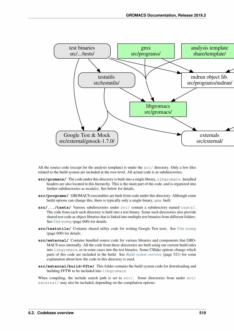
GROMACS Documentation, Release 2019.3
externalssrc/external/
Google Test & Mocksrc/external/gmock-1.7.0/
libgromacssrc/gromacs/
libgromacs_mdrunsrc/gromacs/
testutilssrc/testutils/
mdrun object lib.src/programs/mdrun/
gmxsrc/programs/
analysis templateshare/template/
mdrunsrc/programs/
test binariessrc/.../tests/
All the source code (except for the analysis template) is under the src/ directory. Only a few filesrelated to the build system are included at the root level. All actual code is in subdirectories:
src/gromacs/ The code under this directory is built into a single library, libgromacs. Installedheaders are also located in this hierarchy. This is the main part of the code, and is organized intofurther subdirectories as modules. See below for details.
src/programs/ GROMACS executables are built from code under this directory. Although somebuild options can change this, there is typically only a single binary, gmx, built.
src/.../tests/ Various subdirectories under src/ contain a subdirectory named tests/.The code from each such directory is built into a test binary. Some such directories also provideshared test code as object libraries that is linked into multiple test binaries from different folders.See Unit testing (page 600) for details.
src/testutils/ Contains shared utility code for writing Google Test tests. See Unit testing(page 600) for details.
src/external/ Contains bundled source code for various libraries and components that GRO-MACS uses internally. All the code from these directories are built using our custom build rulesinto libgromacs, or in some cases into the test binaries. Some CMake options change whichparts of this code are included in the build. See Build system overview (page 521) for someexplanation about how the code in this directory is used.
src/external/build-fftw/ This folder contains the build system code for downloading andbuilding FFTW to be included into libgromacs.
When compiling, the include search path is set to src/. Some directories from under src/external/ may also be included, depending on the compilation options.
6.2. Codebase overview 519
GROMACS Documentation, Release 2019.3
Organization under src/gromacs/
The libgromacs library is built from code under src/gromacs/. Again, the top-level directorycontains build and installation rules for the library, and public API convenience headers. These con-venience headers provide the main installed headers that other code can use. They do not contain anydeclarations, but only include a suitable set of headers from the subdirectories. They typically alsocontain high-level Doxygen documentation for the subdirectory with the same name: module.hcorresponds to module/.
The code is organized into subdirectories. These subdirectories are denoted as modules throughoutthis documentation. Each module consists of a set of routines that do some well-defined task or acollection of tasks.
Installed headers are a subset of the headers under src/gromacs/. They are installed into a corre-sponding hierarchy under include/gromacs/ in the installation directory. Comments at the topof the header files contain a note about their visibility: public (installed), intra-library (can be usedfrom inside the library), or intra-module/intra-file. All headers should compile by themselves, withinstalled headers doing so without reference to variables defined in config.h or requiring otherheaders to be included before it. Not installed headers are allowed to include config.h. Cyclicinclude dependencies prevent this, and must be avoided because of this. This is best guaranteed byincluding every header in some source file as the first header, even before config.h. This is partlyenforced by Source tree checker scripts (page 594), which is run by Jenkins and votes accordingly inGerrit.
Code inside the library should not unnecessarily include headers. In particular, headers should notinclude other headers if a forward declaration of a type is enough for the header. Within the librarysource files, include only headers from other modules that are necessary for that file. You can use thepublic API header if you really require everything declared in it.
intra-module/intra-file.
See Naming conventions (page 545) for some common naming patterns for files that can help locatingdeclarations.
Tests, and data required for them, are in a tests/ subdirectory under the module directory. See Unittesting (page 600) for more details.
6.2.2 Documentation organization
All documentation (including this developer guide) is produced from source files under docs/, ex-cept for some command-line help that is generated from the source code (by executing the compiledgmx binary). The build system provides various custom targets that build the documentation; seeBuild system overview (page 521) for details.
docs/fragments/ Contains reStructuredText fragments used through .. include:: mecha-nism from various places in the documentation.
User documentation
docs/install-guide/ Contains reStructuredText source files for building the install guide sec-tion of the user documentation, as well as the INSTALL file for the source package. The buildrules are in docs/CMakeLists.txt.
docs/reference-manual/ Contains reStructuredText source files to generate the referencemanual for html and LaTeX.
docs/manual/ Contains LaTeX helper files to build the reference (PDF) manual.
docs/user-guide/ Contains reStructuredText source files used to build the user guide sectionof the user documentation. The build rules are in docs/CMakeLists.txt.
6.2. Codebase overview 520
GROMACS Documentation, Release 2019.3
docs/how-to/ Contains reStructuredText source files building the how-to section of the user fo-cused documentation.
Unix man pages
Man pages for programs are generated by running the gmx executable after compiling it, and thenusing Sphinx on the reStructuredText files that gmx writes out.
The build rules for the man pages are in docs/CMakeLists.txt.
Developer guide
docs/dev-manual/ Contains reStructuredText source files used to build the developer guide.The build rules are in docs/CMakeLists.txt.
The organization of the developer guide is explained on the front page of the guide (page 515).
Doxygen documentation
docs/doxygen/ Contains the build rules and some overview content for the Doxygen documen-tation. See Using Doxygen (page 553) for details of how the Doxygen documentation is builtand organized.
The Doxygen documentation is made of a few different parts. Use the list below as a guideline onwhere to look for a particular kind of content. Since the documentation has been written over a longperiod of time and the approach has evolved, not all the documentation yet follows these guidelines,but this is where we are aiming at.
documentation pages These contain mainly overview content, from general-level introduction downinto explanation of some particular areas of individual modules. These are generally the placeto start familiarizing with the code or a new area of the code. They can be reached by linksfrom the main page, and also through cross-links from places in the documentation where thatinformation is relevant to understand the context.
module documentation These contain mainly techical content, explaining the general implementa-tion of a particular module and listing the classes, functions etc. in the module. They comple-ment pages that describe the concepts. They can be reached from the Modules tab, and alsofrom all individual classes, functions etc. that make up the module.
class documentation These document the usage of an individual class, and in some cases that ofclosely related classes. Where necessary (and time allowing), a broader overview is given on aseparate page and/or in the module documentation.
method documentation These document the individual method. Typically, the class documentationor other overview content is the place to look for how different methods interact.
file and namespace documentation These are generally only placeholders for links, and do not con-tain much else. The main content is the list of classes and other entities declared in that file.
6.3 Build system overview
The GROMACS build system uses CMake (version 3.4.3 or newer is required) to generate the actualbuild system for the build tool choosen by the user. See CMake documentation for general introduc-tion to CMake and how to use it. This documentation focuses on how the GROMACS build systemis organized and implemented, and what features it provides to developers (some of which may be ofinterest to advanced users).
Most developers use make or ninja as the underlying build system, so there can be parts of the buildsystem that are specifically designed for command-line consumption with these tools, and may not
6.3. Build system overview 521
GROMACS Documentation, Release 2019.3
work ideally with other environments, but basic building should be possible with all the environmentssupported by CMake.
Also, the build system and version control is designed for out-of-source builds. In-source buildsmostly work (there are a few custom targets that do not), but no particular effort has been put to, e.g.,having .gitignore files that exclude all the build outputs, or to have the clean target remove allpossible build outputs.
6.3.1 Build types
Build types is a CMake concept that provides overall control of how the build tools are used on thegiven platform to produce executable code. These can be set in CMake in various ways, includingon a command line such as cmake -DCMAKE_BUILD_TYPE=Debug. GROMACS supports thefollowing standard CMake build types:
Release Fully optimized code intended for use in production simulation. This is the default.
Debug Compiled code intended for use with debugging tools, with low optimization levels and debuginformation for symbols.
RelWithDebInfo As Release, but with debug information for symbol names, which can help debug-ging issues that only emerge in optimized code.
MinSizeRel As Release, but optimized to minimize the size of the resulting executable. This is nevera concern for GROMACS installations, so should not be used, but probably works.
Additionally, GROMACS provides the following build types for development and testing. Theirimplementations can be found in cmake/gmxBuildTypeXXX.cmake.
Reference This build type compiles a version of GROMACS aimed solely at correctness. All paral-lelization and optimization possibilities are disabled. This build type is compiled with gcc 4.7to generate the regression test reference values, against which all other GROMACS builds aretested.
RelWithAssert As Release, but removes -DNDEBUG from compiler command lines, which makesall assertion statements active (and can have other safety-related side effects in GROMACS andcode upon which it depends)
Profile As Release, but adds -pg for use with profiling tools. This is not likely to be effective forprofiling the performance of gmx mdrun (page 111), but can be useful for the tools.
TSAN Builds GROMACS for use with ThreadSanitzer in gcc >= 4.8 and clang >= 3.4 (http://clang.llvm.org/docs/ThreadSanitizer.html) to detect data races. This disables the use of atomics inThreadMPI, preferring the mutex-based implementation.
ASAN Builds GROMACS for use with AddressSanitzer in gcc >= 4.8 and clang >= 3.4 (http://clang.llvm.org/docs/AddressSanitizer.html) to detect many kinds of memory mis-use. By default,AddressSanitizer includes LeakSanitizer.
MSAN Builds GROMACS for use with AddressSanitzer in clang >= 3.4 (http://clang.llvm.org/docs/MemorySanitizer.html) to detect reads of unitialized memory. This functionality requires thatdependencies of the GROMACS build have been built in a compatible way (roughly, staticlibraries with -g -fsanitize=memory -fno-omit-frame-pointer), which gener-ally requires at least the C++ standard library to have been built specially. The path where theincludes and libraries for dependencies should be found for this build type is set in the CMakecache variable GMX_MSAN_PATH. Only internal XDR and internal fftpack are supported at thistime.
For all of the sanitizer builds, to get readable stack traces, you may need to ensure thatthe ASAN_SYMBOLIZER_PATH environment variable (or your PATH) include that of thellvm-symbolizer binary.
With some generators, CMake generates the build system for more than a single CMAKE_BUILD_-TYPE from one pass over the CMakeLists.txt files, so any code that uses CMAKE_BUILD_-
6.3. Build system overview 522
GROMACS Documentation, Release 2019.3
TYPE in CMakeLists.txt directly will break. GROMACS does use such CMake code, so we donot fully support all these build types in such generators (which includes Visual Studio).
6.3.2 CMake cache variables
This section provides a (currently incomplete) list of cache variables that developers or advancedusers can set to affect what CMake generates and/or what will get built.
Compiler flags
Standard CMake mechanism for specifying the compiler flags is to use CMAKE_C_FLAGS/CMAKE_-CXX_FLAGS for flags that affect all build types, and CMAKE_C_FLAGS_buildtype/CMAKE_-CXX_FLAGS_buildtype for flags that only affect a specific build type. CMake provides somedefault flags.
GROMACS determines its own set of default flags, grouped into two categories:
• Generic flags that are appended to the above default CMake flag variables (possibly for multiplebuild types), generally specifying optimization flags to use and controlling compiler warnings.
• Specific flags for certain features that the build system determines to be necessary for successfulcompilation. One example is flags that determine what SIMD instruction set the compiler isallowed to use/needs to support.
All of the above flags are only added after testing that they work with the provided compiler.
There is one cache variable to control the behavior of automatic compiler flags:
GMX_SKIP_DEFAULT_CFLAGSIf set ON, the build system will not add any compiler flags automatically (neither generic norspecific as defined above), and will skip most linker flags as well. The default flags that wouldhave been added are instead printed out when cmake is run, and the user can set the flagsthemselves using the CMake variables. If OFF (the default), the flags are added as describedabove.
The code the determine the default generic flags is in cmake/gmxCFlags.cmake. Code that setsthe specific flags (e.g., SIMD flags) is in the main CMakeLists.txt; search for GMX_SKIP_-DEFAULT_CFLAGS (page 523). The variables used there can be traced back to the locations wherethe actual flags to use are determined.
Variables affecting compilation/linking
GMX_BROKEN_CALLOC
GMX_BUILD_FOR_COVERAGESpecial variable set ON by Jenkins when doing a build for the coverage job. Allows the buildsystem to set options to produce as useful coverage metrics as possible. Currently, it disablesall asserts to avoid them showing up as poor conditional coverage. Defaults to OFF, and thereshould not be any need to change this in a manual build.
GMX_BUILD_MDRUN_ONLYIf set ON, the build system is configured to only build and install a single mdrun executable.To be fully functional, the installed mdrun requires a standard GROMACS installation (withGMX_BUILD_MDRUN_ONLY=OFF) in the same installation prefix, as the mdrun-only builddoes not install any data files or scripts, only the binary. This is intended for cases where onewants to/needs to compile one or more instances of mdrun with different build options (e.g.,MPI or SIMD) than the full installation with the other utilities. Defaults to OFF, in which casea single gmx executable is built and installed, together with all the supporting files. mdrun canbe executed as gmx mdrun.
GMX_BUILD_OWN_FFTW
6.3. Build system overview 523
GROMACS Documentation, Release 2019.3
GMX_BUILD_SHARED_EXE
GMX_COMPILER_WARNINGSIf set ON, various compiler warnings are enabled for compilers that Jenkins uses for verification.Defaults to OFF when building from a source tarball so that users compiling with versions nottested on Jenkins are not exposed to our rather aggressive warning flags that can trigger a lot ofwarnings with, e.g., new versions of the compilers we use. When building from a git repository,defaults to ON.
GMX_CYCLE_SUBCOUNTERSIf set to ON, enables performance subcounters that offer more fine-grained mdrun performancemeasurement and evaluation than the default counters. See Getting good performance frommdrun (page 242) for the description of subcounters which are available. Defaults to OFF.
GMX_ENABLE_CCACHEIf set to ON, attempts to set up the ccache caching compiler wrapper to speed up repeated builds.The ccache executable is searched for with find_package() if CMake is being run witha compatible build type. If the executable is found and a compatible compiler is configured,CMake launch wrapper scripts are set. If enabled, the ccache executable location discoveredby CMake must be accessible during build, as well. Defaults to OFF to minimize build systemcomplexity.
GMX_INSTALL_DATASUBDIRSets the subdirectory under CMAKE_INSTALL_DATADIR where GROMACS-specific read-only architecture-independent data files are installed. The default is gromacs, which means thefiles will go under share/gromacs. To alter the share part, change CMAKE_INSTALL_-DATADIR. See Relocatable binaries (page 538) for how this influences the build.
GMX_DOUBLEMany part of GROMACS are implemented in terms of “real” precision, which is actually eithera single- or double-precision type, according to the value of this flag. Some parts of the codedeliberately use single- or double-precision types, and these are unaffected by this setting. Seereference manual for further information.
GMX_RELAXED_DOUBLE_PRECISIONPermit a double-precision configuration to compute some quantities to single-precision accu-racy. Particularly on architectures where only double-precision SIMD is available (e.g. Sparcmachines such as the K computer), it is faster to default to GMX_DOUBLE=ON and use SIMDthan to use GMX_DOUBLE=OFF and use no SIMD. However, if the user does not need fulldouble precision, then some optimizations can achieve the equivalent of single-precision results(e.g. fewer Newton-Raphson iterations for a reciprocal square root computation).
GMX_EXTRAE
GMX_EXTERNAL_BLAS
GMX_EXTERNAL_LAPACK
GMX_EXTERNAL_TNG
GMX_FFT_LIBRARY
GMX_GIT_VERSION_INFOWhether to generate version information dynamically from git for each build (e.g., HEAD com-mit hash). Defaults to ON if the build is from a git repository and git is found, otherwise OFF.If OFF, static version information from cmake/gmxVersionInfo.cmake is used.
GMX_GPU
GMX_CLANG_CUDAUse clang for compiling CUDA GPU code, both host and device.
GMX_CUDA_CLANG_FLAGSPass additional CUDA-only compiler flags to clang using this variable.
6.3. Build system overview 524
GROMACS Documentation, Release 2019.3
CMAKE_INSTALL_LIBDIRSets the installation directory for libraries (default is determined by standard CMake packageGNUInstallDirs). See Relocatable binaries (page 538) for how this influences the build.
GMX_LOAD_PLUGINS
GMX_MPI
GMX_OPENMP
GMX_PREFER_STATIC_LIBS
GMX_SIMD
GMX_SOFTWARE_INVSQRT
GMX_THREAD_MPI
GMX_USE_RDTSCP
GMX_USE_TNG
GMX_VMD_PLUGIN_PATH
GMX_X11
GMX_XMLCurrently, this option has no effect on the compilation or linking, since there is no code outsidethe tests that would use libxml2.
Variables affecting the all target
BUILD_TESTINGStandard variable created by CTest that enables/disables all tests. Defaults to ON.
GMX_BUILD_HELPControls handling of man pages and shell completions. Possible values:
OFF (default for builds from release source distribution) Man pages and shell completionsare not generated as part of the all target, and only installed if compiling from a sourcepackage.
AUTO (default for builds from development version) Shell completions are generated by ex-ecuting the gmx binary as part of the all target. If it fails, a message is printed, but thebuild succeeds. Man pages need to be generated manually by invoking the man target. Manpages and shell completions are installed if they have been successfully generated.
ON Works the same as AUTO, except that if invoking the gmx binary fails, the build fails aswell.
GMX_DEVELOPER_BUILDIf set ON, the all target will include also the test binaries using Google Test (if GMX_BUILD_-UNITTESTS (page 526) is ON). Also, GMX_COMPILER_WARNINGS (page 524) is alwaysenabled. In the future, other developer convenience features (as well as features inconvenientfor a general user) can be added to the set controlled by this variable.
Variables affecting special targets
GMXAPIIf set ON, the additional gmxapi C++ library is configured and the gmxapi head-ers will be installed. Provides the additional build tree targets gmxapi-cppdocs andgmxapi-cppdocs-dev when Doxygen is available. Also exports CMake configurationfiles for gmxapi that allow find_package(gmxapi) to import the Gromacs::gmxapiCMake target in client projects that search the GROMACS installation root.
6.3. Build system overview 525
GROMACS Documentation, Release 2019.3
GMX_BUILD_MANUALIf set ON, CMake detection for LaTeX and other prerequisites for the reference PDF manualis done, and the manual target for building the manual is generated. If OFF (the default), alldetection is skipped and the manual cannot be built.
GMX_BUILD_TARBALLIf set ON, -dev suffix is stripped off from version strings and some other version info logic isadjusted such that the man pages and other documentation generated from this build is suitablefor releasing (on the web page and/or in the source distribution package). Defaults to OFF.
GMX_BUILD_UNITTESTSIf ON, test binaries using Google Test are built (either as the separate tests targer, or also aspart of the all target, depending on GMX_DEVELOPER_BUILD (page 525)). All dependenciesrequired for building the tests (Google Test and Google Mock frameworks, and tinyxml2) areincluded in src/external/. Defaults to ON if BUILD_TESTING (page 525) is ON.
GMX_COMPACT_DOXYGENIf set ON, Doxygen configuration is changed to avoid generating large dependency graphs, whichmakes it significantly faster to run Doxygen and reduces disk usage. This is typically usefulwhen developing the documentation to reduce the build times. Defaults to OFF.
REGRESSIONTEST_DOWNLOADIf set ON, CMake will download the regression tests and extract them to a local directory.REGRESSIONTEST_PATH (page 526) is set to the extracted tests. Note that this happensduring the configure phase, not during the build. After the download is done, the variable isautomatically reset to OFF again to avoid repeated downloads. Can be set to ON to downloadagain. Defaults to OFF.
REGRESSIONTEST_PATHPath to extracted regression test suite matching the source tree (the directory containinggmxtest.pl) If set, CTest tests are generated to run the regression tests. Defaults to empty.
SOURCE_MD5SUMSets the MD5 sum of the release tarball when generating the HTML documentation. It getsinserted into the download section of the HTML pages.
6.3.3 External libraries
6.3.4 Special targets
In addition to the default all target, the generated build system has several custom targets that areintended to be explicitly built to perform various tasks (some of these may also run automatically).There are various other targets as well used internally by these, but those are typically not intended tobe invoked directly.
check Builds all the binaries needed by the tests and runs the tests. If some types of tests are notavailable, shows a note to the user. This is the main target intended for normal users to run thetests. See Unit testing (page 600).
check-source Runs a custom Python checker script to check for various source-level issues. UsesDoxygen XML documentation as well as rudimentary parsing of some parts of the source files.This target is used as part of the Jenkins documentation job. All CMake code is currently indocs/doxygen/. See Source tree checker scripts (page 594).
completion Runs the compiled gmx executable to generate shell command-line completion defini-tions. This target is only added if GMX_BUILD_HELP (page 525) is not OFF, and it is run au-tomatically as part of the default all target. See GMX_BUILD_HELP (page 525). All CMakecode is in src/programs/.
dep-graphs* Builds include dependency graphs for the source files using dot from graphviz. AllCMake code is in docs/doxygen/. See Source tree checker scripts (page 594).
6.3. Build system overview 526
GROMACS Documentation, Release 2019.3
doxygen-* Targets that run Doxygen to generate the documentation. The doxygen-all targetruns as part of the webpage target, which in turn runs as part of the Jenkins documentation job.All CMake code is in docs/doxygen/. See Using Doxygen (page 553).
gmxapi-cppdocs Builds API documentation for gmxapi. Useful to authors of client software. Doc-umentation is generated in docs/api-user in the build directory.
gmxapi-cppdocs-dev Extract documentation for gmxapi and GROMACS developers to docs/api-dev.
install-guide Runs Sphinx to generate a plain-text INSTALL file for the source package. The files isgenerated at docs/install-guide/text/, from where it gets put at the root of the sourcepackage by CPack. All CMake code is in docs/.
man Runs Sphinx to generate man pages for the programs. Internally, also runs the compiled gmxexecutable to generate the input files for Sphinx. All CMake code is in docs/. See GMX_-BUILD_HELP (page 525) for information on when the man pages are installed.
manual Runs LaTeX to generate the reference PDF manual. All CMake code is in docs/manual/.See GMX_BUILD_MANUAL (page 525).
package_source Standard target created by CPack that builds a source package. This target is usedto generate the released source packages.
test Standard target created by CTest that runs all the registered tests. Note that this does not buildthe test binaries, only runs them, so you need to first ensure that they are up-to-date. See Unittesting (page 600).
tests Builds all the binaries needed by the tests (but not gmx). See Unit testing (page 600).
webpage Collection target that runs the other documentation targets to generate the full set of HTML(and linked) documentaion. This target is used as part of the Jenkins documentation job. AllCMake code is in docs/.
webpage-sphinx Runs Sphinx to generate most content for the HTML documentation (the set of webpages this developer guide is also part of). Internally, also runs the compiled gmx executable togenerate some input files for Sphinx. All CMake code is in docs/.
6.3.5 Passing information to source code
The build system uses a few different mechanisms to influence the compilation:
• On the highest level, some CMake options select what files will be compiled.
• Some options are passed on the compiler command line using -D or equivalent, such that theyare available in every compilation unit. This should be used with care to keep the compilercommand lines manageable. You can find the current set of such defines with
git grep add_definitions
• A few header files are generated using CMake configure_file() and included in the de-sired source files. These files must exist for the compilation to pass. Only a few files use an#ifdef HAVE_CONFIG_H to protect against inclusion in case the define is not set; this isused in files that may get compiled outside the main build system.
buildinfo.h Contains various strings about the build environment, used mainly for out-putting version information to log files and when requested.
config.h Contains defines for conditional compilation within source files.
gmxpre-config.h Included by gmxpre.h as the first thing in every source file. Shouldonly contain defines that are required before any other header for correct operation. For ex-ample, defines that affect the behavior of system headers fall in this category. See Doxygendocumentation for gmxpre.h.
6.3. Build system overview 527
GROMACS Documentation, Release 2019.3
All the above files get generated in src/.
Additionally, the following file is generated by the build system:
baseversion-gen.cpp Provides definitions for declarations in baseversion-gen.hfor version info output. The contents are generated either from Git version info, or fromstatic version info if not building from a git repository.
6.4 GROMACS change management
This documentation assumes the reader is already familiary with using git for managing file revi-sions.
• Getting started (page 528)
– Creating the SSH key for Gerrit (page 529)
– Setting up a local repository to work with gerrit (page 529)
– Install the commit hook (page 530)
– Uploading a commit for review (page 530)
– Uploading a draft commit for review (page 530)
– After uploading a commit (page 530)
• Code Review (page 531)
– Reviewing someone else’s uploaded commit (page 531)
– Guide for reviewing (page 531)
– Use of Verify (page 532)
– Further information (page 532)
• FAQs (page 532)
– How do I access gerrit behind a proxy? (page 532)
– How do I link fixes with Redmine issues? (page 532)
– How can I submit conflicting changes? (page 532)
– How do I upload an update to a pending change? (page 533)
– How do I get a copy of my commit for which someone else has uploaded a patch?(page 533)
– How do I submit lots of independent commits (e.g. bug fixes)? (page 533)
– How can I avoid needing to remember all these arcane git commands? (page 534)
– How can I get my patch in gerrit to have a different parent? (page 534)
– How can I revert a change back to an old patchset? (page 534)
– How do I handle common errors (page 534)
• More git tips (page 535)
6.4.1 Getting started
1. Go to https://gerrit.gromacs.org
6.4. GROMACS change management 528
GROMACS Documentation, Release 2019.3
2. Click Register (you can choose any OpenID provider including any existing Google/Yahoo ac-count. If you manually enter the URL make sure to start with http(s)://)
3. Choose a username and add an ssh key
See here for a quick intro into Gerrit.
Creating the SSH key for Gerrit
In order to push your commits to gerrit server, you must have an SSH key in your computer whichmatches with the one registered in your Gerrit user account. To do so, you first need to create thisunique SSH key. You will be asked to enter a passphrase. This is optional with respect to Gerrit, butit is a good security practice to have it.
To proceed with the creation of the SSH key, type the following commands from your terminal win-dow:
$ cd ~/.ssh
$ ssh-keygen -t rsa -C "[email protected]"
Please substitute the email string in the command above with the same email address which you usedto register the account in Gerrit.
Now you have created your public SSH key, which you need to copy/paste into your Gerrit profile.First, open it with the following command:
$ cat id_rsa.pub
Copy all the contents of the file id_rsa.pub in your clipboard, and switch to your favorite web browserwhere you logged in to Gerrit GROMACS page. Click on your username at the top right corner of theGerrit webpage and select “Settings”. You should now be in your Gerrit profile settings page, whereyou should see a vertical menu.
From this vertical menu, select “SSH Public Keys”, then click the button “Add Key . . . ” and an editbox will appear below the button. Here you need to paste the contents of id_rsa.pub file, which youpreviously copied to your clipboard.
Now you are ready to operate!
Setting up a local repository to work with gerrit
Either clone using:
$ git clone ssh://[email protected]/gromacs.git
(replace USER with your username)
or change the remote url using:
$ git remote set-url origin ssh://[email protected]/gromacs.git
(change USER with the username you’ve registered)
Or add a new remote url using:
$ git remote add upload ssh://[email protected]/gromacs.git
If you are working with a GROMACS repository other than the source code, then you should substi-tute e.g. regressiontests.git or releng.git instead of gromacs.git above.
Be sure to configure your user name and e-mail to match those registered to Gerrit:
6.4. GROMACS change management 529

GROMACS Documentation, Release 2019.3
git config [--global] user.name "Your Name"git config [--global] user.email "[email protected]"
It is optional if you want to set those settings for git on a global level, or just for the current repository.
If necessary, register the e-mail address you want to use with Gerrit.
Install the commit hook
Differently from a simple usage of git, with Gerrit a Change-ID is needed at the end of each commitmessage. Gerrit uses Change-IDs to understand whether your new commit is patching a previouscommit or it should be regarded as a separate, different patch, uncorrelated with your previouslypushed commits.
To allow git to append such Change-IDs automatically after each commit, type the following com-mand:
$ scp -p [email protected]:hooks/commit-msg .git/hooks/
(change USER with the username you’ve registered in Gerrit)
Note: This commit hook needs to be added to the repo where the commit will occur, not the repowhere the push to upstream will occur (should they be different).
Uploading a commit for review
Make sure your HEAD is up to date (use git pull --rebase origin if someone else hascommitted since you last pulled), check that your commit message follows the Guidelines for format-ting of git commits (page 551), make your commit and then use
$ git push origin HEAD:refs/for/BRANCH
Replace BRANCH with the branch it should be committed to. Master has a number of sub branchesthat can be used to show what the patch is relevant to such as OpenCL and tools-cleanup. These canbe pushed to by specifying them after the branch, for example BRANCH/domdec-cleanup.
When updating/replacing an existing change, make sure the commit message has the same Change-ID. Please see the section Ammending a change <gmx-ammend-change> below.
Uploading a draft commit for review
Uploading a draft lets you share a change which isn’t ready yet for review for merging. It is onlyvisible to those people you invite as reviewers, which you need to add explicitly. You upload achange as a draft by uploading it to refs/drafts/branch instead of refs/for/branch. Typically you wantto push to refs/drafts/master.
Jenkins is not automatically triggered for drafts, but if you add “Jenkins Buildbot” as a reviewer, itlearns that you might be interested in having it try out your code. Then, you can go to Jenkins andlog in with your OpenID. Then go to http://jenkins.gromacs.org/gerrit_manual_trigger/ and tell it tosearch for the commit for which you want to trigger the build agents. For example, https://gerrit.gromacs.org/#/c/1238/ is 1238 (but maybe SHA or ChangeID will work, too).
After uploading a commit
Use
6.4. GROMACS change management 530
GROMACS Documentation, Release 2019.3
$ git reset --keep HEAD^
to reset your branch to the HEAD before the commit you just uploaded. This allows you to keep yourrepo in sync with what every other repo thinks is the HEAD. In particular, if you have another patchto upload (or worse, have to pull in other people’s patches, and then have a new patch), you probablydo not want to have the second patch depend on the first one. If the first one is rejected, you havemade extra work for yourself sorting out the mess. Your repo still knows about the commit, and youcan cherry-pick it to somewhere if you want to use it.
6.4.2 Code Review
Reviewing someone else’s uploaded commit
The reviewing workflow is the following:
1. https://gerrit.gromacs.org/#q/status:open shows all open changes
2. A change needs a +2 and usually +1 review, as well as a +2 verified to be allowed to be merged.
3. Usually a patch goes through several cycles of voting, commenting and updating before it be-comes merged, with votes from the developers indicating if they think that change hat progressedenough to be included.
4. A change is submitted for merging and post-submit testing by clicking “Submit” by one of themain developers. This should be done by the reviewer after voting +2. After a patch is submittedit is replicated to the main git server.
Do not review your own code. The point of the policy is that at least two non-authors have voted+1, and that the issues are resolved in the opinion of the person who applies a +2 before a merge. Ifyou have uploaded a minor fix to someone else’s patch, use your judgement in whether to vote on thepatch +1.
Guide for reviewing
• First and foremost, check correctness to the extent possible;
• As portability and performance are the most important things (after correctness) do check forpotential issues;
• Check adherence to the GROMACS coding standards (page 542);
• We should try to ensure that commits that implement bugfixes (as well as important features andtasks) get a Redmine entry created and linked. The linking is done automatically by Redmineif the commit message contains keyword “#issueID”, the valid syntax is explained below.
• If the commit is a bugfix:
– if present in Redmine it has to contain a valid reference to the issue;
– if it’s a major bug, there has to be a bug report filed in Redmine (with urgent or immediatepriority) and referenced appropriately.
• If the commit is a feature/task implementation:
– if it’s present in Redmine it has to contain a valid reference to the issue;
– If no current issue is currently present and the change would benefit of one for future ex-planation on why it was added, a new redmine issue should be created.
6.4. GROMACS change management 531
GROMACS Documentation, Release 2019.3
Use of Verify
Jenkins has been installed for automated build testing. So it isn’t required to vote “verify +2” anymore.As the testing is not always perfect, and because test coverage can be spotty, developers can stillmanually vote to indicate that a change performs as intended. Please note that this should not beabused to bypass Jenkins testing. The vote from the test suite should only be discarded if failures arecaused by unrelated issues.
Further information
Currently it is possible to review your own code. It is undesirable to review your own code, becausethat defeats the point. It will be deactivated if it is being abused and those responsible may lose theirvoting rights.
For further documentation:
• GROMACS specific manual
• General tutorials
6.4.3 FAQs
How do I access gerrit behind a proxy?
If you are behind a firewall blocking port 22, you can use socat to overcome this problem by addingthe following block to your ~/.ssh/config
Host gerrit.gromacs.orgUser USERHostname gerrit.gromacs.orgProxyCommand socat - PROXY:YOURPROXY:gerrit.gromacs.org,
→˓proxyport=PORT
Replace YOURPROXY, PORT and USER, (but not PROXY!) with your own settings.
How do I link fixes with Redmine issues?
The linking of commits that relate to an existing issue is done automatically by Redmine if the gitcommit message contains a reference to the Redmine entry through the issueID, the numeric ID ofthe respective issue (bug, feature, task). The general syntax of a git comit reference is [keyword]#issueID.
The following two types of refereces are possible:
• For bugfix commits the issueID should be preceeded by the “Fixes” keyword;
• For commits related to a general issue (e.g. partial implementation of feature or partial fix), theissueID should be preceeded by the “Refs” keyword;
An example commit message header:
This commit refs #1, #2 and fixes #3
How can I submit conflicting changes?
When there are several, mutually conflicting changes in gerrit pending for review, the submission ofthe 2nd and subsequent ones will fail. Those need to be resolved locally and updated by
6.4. GROMACS change management 532
GROMACS Documentation, Release 2019.3
$ git pull --rebase
Then fix the conflicts and use
$ git push
Please add a comment (review without voting) saying that it was rebased with/without conflicts, tohelp the reviewer.
How do I upload an update to a pending change?
First, obtain the code you want to update. If you haven’t changed your local repository, then youalready have it. Maybe you can check out the branch again, or consult your git reflog. Otherwise, youshould go to gerrit, select the latest patch set (remembering that others may have contributed to yourwork), and use the “Download” link to give you a “Checkout” command that you can run, e.g.
$ git fetch ssh://[email protected]/gromacs refs/changes/?/?/? &&→˓git checkout FETCH_HEAD
Make your changes, then add them to the index, and use
$ git commit --amend$ git push origin HEAD:refs/for/BRANCH
When amending the previous commit message, leave the “Change-Id” intact so that gerrit can recog-nize this is an update and not open a new issue.
DO NOT rebase your patch set and update it in one step. If both are done in one step, the diff betweenpatch set versions has both kinds of changes. This makes it difficult for the reviewer, because it is notclear what parts have to be re-reviewed. If you need to update and rebase your change please do itin two steps (order doesn’t matter). gerrit has a feature that allows you to rebase within gerrit, whichcreates the desired independent patch for that rebase (if the rebase is clean).
How do I get a copy of my commit for which someone else has uploaded a patch?
Gerrit makes this easy. You can download the updated commit in various ways, and even copy amagic git command to your clipboard to use in your shell.
You can select the kind of git operation you want to do (cherry-pick is best if you are currently in thecommit that was the parent, checkout is best if you just want to get the commit and not worry aboutthe current state of your checked out git branch) and how you want to get it. The icon on the far rightwill paste the magic shell command into your clipboard, for you to paste into a terminal to use.
How do I submit lots of independent commits (e.g. bug fixes)?
Simply pushing a whole commit tree of unrelated fixes creates dependencies between them that makefor trouble when one of them needs to be changed. Instead, from an up-to-date repo, create andcommit the first change (or git cherry-pick it from an existing other branch). Upload it to gerrit. Thendo
$ git reset --keep HEAD^
This will revert to the old HEAD, and allow you to work on a new commit that will be independent ofthe one you’ve already uploaded. The one you’ve uploaded won’t appear in the commit history untilit’s been reviewed and accepted on gerrit and you’ve pulled from the main repo, however the versionof it you uploaded still exists in your repo. You can see it with git show or git checkout using its hash- which you can get from the gerrit server or by digging in the internals of your repo.
6.4. GROMACS change management 533
GROMACS Documentation, Release 2019.3
How can I avoid needing to remember all these arcane git commands?
In your .gitconfig, having set the git remote for the gerrit repo to upload, use something like thefollowing to make life easier:
[alias]upload-r2018 = push origin HEAD:refs/for/release-2018upload-r2016 = push origin HEAD:refs/for/release-2016upload-master = push origin HEAD:refs/for/masterupload-reset = reset --keep HEAD^
How can I get my patch in gerrit to have a different parent?
Sometimes, some other patch under review is a relevant point from which to start work. For simplechanges without conflicts to the previous work, you can use the Gerrit web UI to either rebase orcherry-pick the change you are working on.
If this is not possible, you can still use the canned gerrit checkouts to (say) checkout out patch 2117and start work:
git fetch https://gerrit.gromacs.org/gromacs refs/changes/17/2117/2 &&→˓git checkout FETCH_HEAD
Other times you might have already uploaded a patch (e.g. patch 1 of 2145), but now see that someconcurrent work makes more sense as a parent commit (e.g. patch 2 of 2117), so check it out asabove, and then use the canned gerrit cherry-pick:
git fetch https://gerrit.gromacs.org/gromacs refs/changes/45/2145/1 &&→˓git cherry-pick FETCH_HEAD
Resolve any merge commits, check things look OK, and then upload. Because the ChangeId of 2145hasn’t changed, and nothing about 2117 has changed, the second patch set of 2145 will reflect thestate of 2145 now having 2117 as a parent.
This can also be useful for constructing a short development branch where the commits are somehowdependent, but should be separated for review purposes. This technique is useful when constructinga series of commits that will contribute to a release.
How can I revert a change back to an old patchset?
If a change accidentally gets updated or when a patchset is incorrect, you might want to revert to anolder patchset. This can be done by fetching an old patchset, running git commit –amend to update thetime stamp in the commit and pushing the commit back up to gerrit. Note that without the amendingyou will get an error from the remote telling you that there are no new changes.
How do I handle common errors
error: server certificate verification failed. CAfile. . .
If you try to cherry-pick a change from the server, you’ll probably get the error:
$ git fetch https://gerrit.gromacs.org/p/gromacs refs/changes/09/109/1 &&→˓git cherry-pick FETCH_HEADerror: server certificate verification failed.CAfile: /etc/ssl/certs/ca-certificates.crtCRLfile: none while accessing https://gerrit.gromacs.org/p/gromacs/info/→˓refs
6.4. GROMACS change management 534
GROMACS Documentation, Release 2019.3
fatal: HTTP request failed
As explained here, the problem is with git not trusting the certificate and as a workaround one can setglobally
$ git config --global --add http.sslVerify false
or prepend GIT_SSL_NO_VERIFY=1 to the command
$ GIT_SSL_NO_VERIFY=1 git fetch https://gerrit.gromacs.org/p/gromacs→˓refs/changes/09/109/1 \&& git cherry-pick FETCH_HEAD
Various error messages and their meanings
http://review.coreboot.org/Documentation/error-messages.html
6.4.4 More git tips
Q: Are there some other useful git configuration settings?
A: If you need to work with branches that have large differences (in particular, if a lot of files havemoved), it can be helpful to set
git config diff.renamelimit 5000
to increase the limit of inexact renames that Git considers. The default value is not sufficient, forexample, if you need to do a merge or a cherry-pick from a release branch to master.
Q: How do I use git rebase (also git pull --rebase)?
A: Assume you have a local feature branch checked out, that it is based on master, and master hasgotten new commits. You can then do
git rebase master
to move your commits on top of the newest commit in master. This will save each commit you did,and replay them on top of master. If any commit results in conflicts, you need to resolve them as usual(including marking them as resolved using git add), and then use
git rebase --continue
Note that unless you are sure about what you are doing, you should not use any commands thatcreate or delete commits (git commit, or git checkout or git reset without paths). git rebase--continue will create the commit after conflicts have been resolved, with the original commitmessage (you will get a chance to edit it).
If you realize that the conflicts are too messy to resolve (or that you made a mistake that resulted inmessy conflicts), you can use
git rebase --abort
to get back into the state you started from (before the original git rebase master invocation). If therebase is already finished, and you realize you made a mistake, you can get back where you started
6.4. GROMACS change management 535

GROMACS Documentation, Release 2019.3
with (use git log <my-branch>@{1} and/or git reflog <my-branch> to check that this is where youwant to go)
git reset --hard <my-branch>@{1}
Q: How do I prepare several commits at once?
A: Assume I have multiple independent changes in my working tree. Use
git add [-p] [file]
to add one independent change at a time to the index. Use
git diff --cached
to check that the index contains the changes you want. You can then commit this one change:
git commit
If you want to test that the change works, use to temporarily store away other changes, and do yourtesting.
git stash
If the testing fails, you can amend your existing commit with git commit --amend. After youare satisfied, you can push the commit into gerrit for review. If you stashed away your changes andyou want the next change to be reviewed independently, do
git reset --hard HEAD^git stash pop
(only do this if you pushed the previous change to gerrit, otherwise it is difficult to get the old changesback!) and repeat until each independent change is in its own commit. If you skip the git reset--hard step, you can also prepare a local feature branch from your changes.
Q: How do I edit an earlier commit?
A: If you want to edit the latest commit, you can simply do the changes and use
git commit --amend
If you want to edit some other commit, and commits after that have not changed the same lines, youcan do the changes as usual and use
git commit --fixup <commit>
or
git commit --squash <commit>
where <commit> is the commit you want to change (the difference is that --fixup keeps the originalcommit message, while --squash allows you to input additional notes and then edit the originalcommit message during git rebase -i). You can do multiple commits in this way. You can alsomix --fixup/--squash commits with normal commits. When you are done, use
git rebase -i --autosquash <base-branch>
6.4. GROMACS change management 536

GROMACS Documentation, Release 2019.3
to merge the --fixup/--squash commits to the commits they amend. See separate question ongit rebase -i on how to choose <base-branch>.
In this kind of workflow, you should try to avoid to change the same lines in multiple commits (exceptin --fixup/--squash commits), but if you have already changed some lines and want to edit anearlier commit, you can use
git rebase -i <base-branch>
but you likely need to resolve some conflicts later. See git rebase -i question later.
Q: How do I split a commit?
A: The instructions below apply to splitting the HEAD commit; see above how to use git rebase-i to get an earlier commit as HEAD to split it.
The simplest case is if you want to split a commit A into a chain A’-B-C, where A’ is the first newcommit, and contains most of the original commit, including the commit message. Then you can do
git reset -p HEAD^ [-- <paths>]git commit --amend
to selectively remove parts from commit A, but leave them in your working tree. Then you can createone or more commits of the remaining changes as described in other tips.
If you want to split a commit A into a chain where the original commit message is reused for some-thing else than the first commit (e.g., B-A’-C), then you can do
git reset HEAD^
to remove the HEAD commit, but leave everything in your working tree. Then you can create yourcommits as described in other tips. When you come to a point where you want to reuse the originalcommit message, you can use
git reflog
to find how to refer to your original commit as HEAD@{n}, and then do
git commit -c HEAD@{n}
Q: How do I use git rebase -i to only edit local commits?
A: Assume that you have a local feature branch checked out, this branch has three commits, and thatit is based on master. Further, assume that master has gotten a few more commits after you branchedoff. If you want to use git rebase -i to edit your feature branch (see above), you probably wantto do
git rebase -i HEAD~3
followed by a separate
git rebase master
The first command allows you to edit your local branch without getting conflicts from changes inmaster. The latter allows you to resolve those conflicts in a separate rebase run. If you feel braveenough, you can also do both at the same time using
git rebase -i master
6.4. GROMACS change management 537
GROMACS Documentation, Release 2019.3
Interacting with Gerrit
This section is intended for using git to interact with gerrit; interacting with the web UI may be betterdealt with on a separate page.
Q: How do I move a change from a branch to another?
A: Moving one or a few changes is most easily done using git cherry-pick. To move a singlechange, first do
git checkout <target-branch>
Then, open the change/patch set in Gerrit that you want to move, select “cherry-pick” in the Downloadsection for that patch set, and copy/paste the given command:
git fetch ... refs/changes/... && git cherry-pick FETCH_HEAD
Resolve any conflicts and do
git commit [-a]
You can also cherry-pick multiple changes this way to move a small topic branch. Before pushingthe change to Gerrit, remove the lines about conflicts from the commit message, as they don’t serveany useful purpose in the history. You can type that information into the change as a Gerrit commentif it helps the review process. Note that Gerrit creates a new change for the target branch, even ifChange-Ids are same in the commits. You need to manually abandon the change in the wrong branch.
6.5 Relocatable binaries
GROMACS (mostly) implements the concept of relocatable binaries, i.e., that after initial installa-tion to CMAKE_INSTALL_PREFIX (or binary packaging with CPack), the whole installation treecan be moved to a different folder and GROMACS continues to work without further changes to theinstallation tree. This page explains how this is implemented, and the known limitations in the imple-mentation. This information is mainly of interest to developers who need to understand this or changethe code, but it can also be useful for people installing or packaging GROMACS.
A related feature that needs to be considered in all the code related to this is that the executablesshould work directly when executed from the build tree, before installation. In such a case, the datafiles should also be looked up from the source tree to make development easy.
6.5.1 Finding shared libraries
If GROMACS is built with dynamic linking, the first part of making the binaries relocatable is to makeit possible for the executable to find libgromacs, no matter how it is executed. On platforms thatsupport a relative RPATH, this is used to make the GROMACS executables find the libgromacsfrom the same installation prefix. This makes the executables fully relocatable when it comes tolinking, as long as the relative folder structure between the executables and the library is kept thesame.
If the RPATH mechanism does not work, GMXRC also adds the absolute path to the libgromacsinstalled with it to LD_LIBRARY_PATH. On platforms that support this, this makes the linker searchfor the library here, but it is less robust, e.g., when mixing calls to different versions of GROMACS.Note that GMXRC is currently not relocatable, but hardcodes the absolute path.
On native Windows, DLLs are not fully supported; it is currently only possible to compile a DLL withMinGW, not with Visual Studio or with Intel compilers. In this case, the DLLs are placed in the bin/directory instead of lib/ (automatically by CMake, based on the generic binary type assignment in
6.5. Relocatable binaries 538
GROMACS Documentation, Release 2019.3
CMakeLists.txt). Windows automatically searches DLLs from the executable directory, so thecorrect DLL should always be found.
For external libraries, standard CMake linking mechanisms are used and RPATH for the externaldependencies is included in the executable; on Windows, dynamic linking may require extra effort tomake the loader locate the correct external libraries.
To support executing the built binaries from the build tree without installation (critical for executingtests during development), standard CMake mechanism is used: when the binaries are built, theRPATH is set to the build tree, and during installation, the RPATH in the binaries is rewritten byCMake to the final (relative) value. As an extra optimization, if the installation tree has the samerelative folder structure as the build tree, the final relative RPATH is used already during the initialbuild.
The RPATH settings are in the root CMakeLists.txt. It is possible to disable the use of RPATHduring installation with standard CMake variables, such as setting CMAKE_SKIP_INSTALL_-RPATH=ON.
6.5.2 Finding data files
The other, GROMACS-specific part, of making the binaries relocatable is to make them able to finddata files from the installation tree. Such data files are used for multiple purposes, including showingthe quotes at the end of program execution. If the quote database is not found, the quotes are simplynot printed, but other files (mostly used by system preparation tools like gmx pdb2gmx (page 127)and gmx grompp (page 94), and by various analysis tools for static data) will cause fatal errors if notfound.
There are several considerations here:
• For relocation to work, finding the data files cannot rely on any hard-coded absolute path, butit must find out the location of the executing code by inspecting the system. As a fallback,environment variables or such set by GMXRC or similar could be used (but currently are not).
• When running executables from the build tree, it is desirable that they will automatically usethe data files from the matching source tree to facilitate easy testing. The data files are notcopied into the build tree, and the user is free to choose any relative locations for the source andbuild trees. Also, the data files are not in the same relative path in the source tree and in theinstallation tree (the source tree has share/top/, the installation tree share/gromacs/top/; the latter is customizable during CMake configuration).
• In addition to GROMACS executables, programs that link against libgromacs need to beable to find the data files if they call certain functions in the library. In this case, the executablemay not be in the same directory where GROMACS is. In case of static linking, no part of thecode is actually loaded from the GROMACS installation prefix, which makes it impossible tofind the data files without external information.
• The user can always use the GMXLIB environment variable to provide alternative locationsfor the data files, but ideally this should never be necessary for using the data files from theinstallation.
Not all the above considerations are fully addressed by the current implementation, which works likethis:
1. It finds the path to the current executable based on argv[0]. If the value contains a directory,this is interpreted as absolute or as relative to the current working directory. If there is nodirectory, then a file by that name is searched from the directories listed in PATH. On Windows,the current directory is also searched before PATH. If a file with a matching name is found, thisis used without further checking.
2. If the executable is found and is a symbolic link, the symbolic links are traversed until a real fileis found. Note that links in the directory name are not resolved, and if some of the links containrelative paths, the end result may contain .. components and such.
6.5. Relocatable binaries 539
GROMACS Documentation, Release 2019.3
3. If an absolute path to the executable was found, the code checks whether the executable islocated in the build output directory (using stat() or similar to account for possible symboliclinks in the directory components). If it is, then the hard-coded source tree location is returned.
4. If an absolute path to the executable was found and it was not in the build tree, then all parent di-rectories are checked. If a parent directory contains share/gromacs/top/gurgle.dat,this directory is returned as the installation prefix. The file name gurgle.dat and the lo-cation are considered unique enough to ensure that the correct directory has been found. Theinstallation directory for read-only architecture-independent data files can be customized duringCMake configuration by setting CMAKE_INSTALL_DATADIR, and the subdirectory under thisthat hosts the GROMACS-specific data is set by GMX_INSTALL_DATASUBDIR.
Note that this search does not resolve symbolic links or normalize the input path beforehand: ifthere are .. components and symbolic links in the path, the search may proceed to unexpecteddirectories, but this should not be an issue as the correct installation prefix should be foundbefore encountering such symbolic links (as long as the bin/ directory is not a symbolic link).
5. If the data files have not been found yet, try a few hard-coded guesses (like the original installa-tion CMAKE_INSTALL_PREFIX and /usr/local/). The first guess that contains suitablefiles (gurgle.dat) is returned.
6. If still nothing is found, return CMAKE_INSTALL_PREFIX and let the subsequent data fileopening fail.
The above logic to find the installation prefix is in src/gromacs/commandline/cmdlineprogramcontext.cpp. Note that code that links to libgromacs can provide analternative implementation for gmx::IProgramContext for locating the data files, and is thenfully responsible of the above considerations.
Information about the used data directories is printed into the console output (unless run with-quiet), as well as to (some) error messages when locating data files, to help diagnosing issues.
There is no mechanism to disable this probing search or affect the process during compilation time,except for the CMake variables mentioned above.
6.5.3 Known issues
• GMXRC is not relocatable: it hardcodes the absolute installation path in one assignment withinthe script, which no longer works after relocation. Contributions to get rid of this on all theshells the GMXRC currently supports are welcome.
• There is no version checking in the search for the data files; in case of issues with the search, itmay happen that the installation prefix from some other installation of GROMACS is returnedinstead, and only cryptic errors about missing or invalid files may reveal this.
• If the searching for the installation prefix is not successful, hard-coded absolute guesses are used,and one of those returned. These guesses include the absolute path in CMAKE_INSTALL_-PREFIX used during compilation of libgromacs, which will be incorrect after relocation.
• The search for the installation prefix is based on the locating the executable. This does notwork for programs that link against libgromacs, but are not installed in the same prefix. Forsuch cases, the hard-coded guesses will be used, so the search will not find the correct datafiles after relocation. The calling code can, however, programmatically provide the GROMACSinstallation prefix, but ideally this would work without offloading work to the calling code.
• One option to (partially) solve the two above issues would be to use the GMXDATA environmentvariable set by GMXRC as the fallback (currently this environment variable is set, but very rarelyused).
• Installed pkg-config files are not relocatable: they hardcode the absolute installation path.
6.5. Relocatable binaries 540
GROMACS Documentation, Release 2019.3
6.6 Documentation generation
6.6.1 Building the GROMACS documentation
For now, there are multiple components, formats and tools for the GROMACS documentation, whichis aimed primarily at version-specific deployment of the complete documentation on the website andin the release tarball.
This is quite complex, because the dependencies for building the documentation must not get in theway of building the code (particularly when cross-compiling), and yet the code must build and run inorder for some documentation to be generated. Also, man page documentation (and command-linecompletions) must be built from the wrapper binary, in order to be bundled into the tarball. This helpsensure that the functionality and the documentation remain in sync.
The outputs of interest to most developers are generally produced in the docs/html/ subdirectoryof the build tree.
You need to enable at least some of the following CMake options:
GMX_BUILD_MANUAL Option needed for trying to build the PDF reference manual (requires LaTeXand ImageMagick). See GMX_BUILD_MANUAL (page 525).
GMX_BUILD_HELP Option that controls 1) whether shell completions are built automatically, and2) whether built man pages are installed if available (the user still needs to build the man targetmanually before installing). See GMX_BUILD_HELP (page 525).
Some documentation cannot be built if the CMake option GMX_BUILD_MDRUN_ONLY is enabled,or when cross-compiling, as it requires executing the gmx binary.
The following make targets are the most useful:
manual Builds the PDF reference manual.
man Makes man pages from the wrapper binary with Sphinx.
doxygen-all Makes the code documentation with Doxygen.
install-guide Makes the INSTALL file for the tarball with Sphinx.
webpage-sphinx Makes all the components of the GROMACS webpage that require Sphinx,including install guide and user guide.
webpage Makes the complete GROMACS webpage, requires everything. When complete, you canbrowse docs/html/index.html to find everything.
If built from a release tarball, the SOURCE_MD5SUM, SOURCE_TARBALL,REGRESSIONTESTS_MD5SUM, and REGRESSIONTESTS_TARBALL CMake variablescan be set to pass in the md5sum values and names of those tarballs, for embedding into thefinal deployment to the GROMACS website.
6.6.2 Needed build tools
The following tools are used in building parts of the documentation.
Doxygen Doxygen is used to extract documentation from source code comments. Also some otheroverview content is laid out by Doxygen from Markdown source files. Currently, version 1.8.5 isrequired for a warning-free build. Thorough explanation of the Doxygen setup and instructionsfor documenting the source code can be found on a separate page: Using Doxygen (page 553).
graphviz (dot) The Doxygen documentation uses dot from graphviz for building some graphs. Thetool is not mandatory, but the Doxygen build will produce warnings if it is not available, and thegraphs are omitted from the documentation.
mscgen The Doxygen documentation uses mscgen for building some graphs. As with dot, the toolis not mandatory, but not having it available will result in warnings and missing graphs.
6.6. Documentation generation 541
GROMACS Documentation, Release 2019.3
Doxygen issue checker Doxygen produces warnings about some incorrect uses and wrong docu-mentation, but there are many common mistakes that it does not detect. GROMACS uses anadditional, custom Python script to check for such issues. This is most easily invoked througha check-source target in the build system. The script also checks that documentation for aheader matches its use in the source code (e.g., that a header documented as internal to a moduleis not actually used from outside the module). These checks are run in Jenkins as part of theDocumentation job. Details for the custom checker are on a separate page (common for severalcheckers): Source tree checker scripts (page 594).
module dependency graphs GROMACS uses a custom Python script to generate an annotated de-pendency graph for the code, showing #include dependencies between modules. The generatedgraph is embedded into the Doxygen documentation: Module dependency graph This scriptshares most of its implementation with the custom checkers, and is documented on the samepage: Source tree checker scripts (page 594).
Sphinx Sphinx; at least version 1.6.1 is used for building some parts of the documentation fromreStructuredText source files.
LaTeX Also requires ImageMagick for converting graphics file formats.
linkchecker The linkchecker program is used together with the linkcheckerrc file to ensure that allthe links in the documentation can be resolved correctly.
documentation exported from source files For man pages, HTML documentation of command-line options for executables, and for shell completions, the gmx binary has explicit C++ code toexport the information required. The build system provides targets that then invoke the built gmxbinary to produce these documentation items. The generated items are packaged into source tar-balls so that this is not necessary when building from a source distribution (since in general,it will not work in cross-compilation scenarios). To build and install these from a git distribu-tion, explicit action is required. See Doxygen documentation on the wrapper binary for someadditional details.
6.7 Style guidelines
Different style guidelines are available under the respective sections of this page.
6.7.1 Guidelines for code formatting
The following list provides the general formatting/indentation rules for GROMACS code (C/C++):
• Basic indentation is four spaces.
• Keep lines at a reasonable length. Keep every line at least below 120 characters. If you end upindenting very deeply, consider splitting the code into functions.
• Do not use tabs, only spaces. Most editors can be configured to generate spaces even whenpressing tab. Tabs (in particular when mixed with spaces) easily break indentation in contextswhere settings are not exactly equal (e.g., in git diff output).
• No trailing whitespace.
• Use braces always for delimiting blocks, even when there is only a single statement in an ifblock or similar.
• Put braces on their own lines. The only exception is short one-line inline functions in C++classes, which can be put on a single line.
• Use spaces liberally.
• extern "C" and namespace blocks are not indented, but all others (including class andswitch bodies) are. Namespace blocks have to have a closing comment with the name of it.
Additionally:
6.7. Style guidelines 542
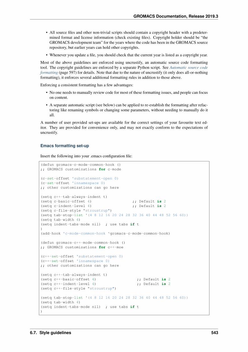
GROMACS Documentation, Release 2019.3
• All source files and other non-trivial scripts should contain a copyright header with a predeter-mined format and license information (check existing files). Copyright holder should be “theGROMACS development team” for the years where the code has been in the GROMACS sourcerepository, but earlier years can hold other copyrights.
• Whenever you update a file, you should check that the current year is listed as a copyright year.
Most of the above guidelines are enforced using uncrustify, an automatic source code formattingtool. The copyright guidelines are enforced by a separate Python script. See Automatic source codeformatting (page 597) for details. Note that due to the nature of uncrustify (it only does all-or-nothingformatting), it enforces several additional formatting rules in addition to those above.
Enforcing a consistent formatting has a few advantages:
• No one needs to manually review code for most of these formatting issues, and people can focuson content.
• A separate automatic script (see below) can be applied to re-establish the formatting after refac-toring like renaming symbols or changing some parameters, without needing to manually do itall.
A number of user provided set-ups are available for the correct settings of your favourite text ed-itor. They are provided for convenience only, and may not exactly conform to the expectations ofuncrustify.
Emacs formatting set-up
Insert the following into your .emacs configuration file:
(defun gromacs-c-mode-common-hook ();; GROMACS customizations for c-mode
(c-set-offset 'substatement-open 0)(c-set-offset 'innamespace 0);; other customizations can go here
(setq c++-tab-always-indent t)(setq c-basic-offset 4) ;; Default is 2(setq c-indent-level 4) ;; Default is 2(setq c-file-style "stroustrup")(setq tab-stop-list '(4 8 12 16 20 24 28 32 36 40 44 48 52 56 60))(setq tab-width 4)(setq indent-tabs-mode nil) ; use tabs if t)(add-hook 'c-mode-common-hook 'gromacs-c-mode-common-hook)
(defun gromacs-c++-mode-common-hook ();; GROMACS customizations for c++-moe
(c++-set-offset 'substatement-open 0)(c++-set-offset 'innamespace 0);; other customizations can go here
(setq c++-tab-always-indent t)(setq c++-basic-offset 4) ;; Default is 2(setq c++-indent-level 4) ;; Default is 2(setq c++-file-style "stroustrup")
(setq tab-stop-list '(4 8 12 16 20 24 28 32 36 40 44 48 52 56 60))(setq tab-width 4)(setq indent-tabs-mode nil) ; use tabs if t)
6.7. Style guidelines 543
GROMACS Documentation, Release 2019.3
(add-hook 'c++-mode-common-hook 'gromacs-c++-mode-common-hook)
This configuration is based on content from stackoverflow.
Eclipse/cdt formatting set-up
For correct formatting, please use this profile.
6.7.2 Guidelines for #include directives
The following include order is used in GROMACS. An empty line should appear between each group,and headers within each group sorted alphabetically.
1. Each source file should include gmxpre.h first.
2. If a source file has a corresponding header, it should be included next. If the header is in thesame directory as the source, then it is included without any path (i.e., relative to the source),otherwise relative to src/ (the latter case should be rare).
3. If the file depends on defines from config.h, that comes next.
4. This is followed by standard C/C++ headers, grouped as follows:
(a) Standard C headers (e.g., <stdio.h>)
(b) C++ versions of the above (e.g., <cstdio>)
(c) Standard C++ headers (e.g., <vector>)
Preferably, only one of the first two groups is present, but this is not enforced.
5. This is followed by other system headers: platform-specific headers such as <unistd.h>, aswell as external libraries such as <gtest/gtest.h>.
6. GROMACS-specific libraries from src/external/, such as "thread_mpi/threads.h".
7. GROMACS-specific headers that are not internal to the including module, included with a pathrelative to src/.
8. In test files, headers not internal to the module, but specific to testing code, are in a separateblock at this point, paths relative to src/.
9. Finally, GROMACS headers that are internal to the including module are included using a rel-ative path (but never with a path starting with ../; such headers go into group 7 instead). Fortest files, this group contains headers that are internal to tests for that module.
All GROMACS headers are included with quotes ("gromacs/utility/path.h"), other head-ers with angle brackets (<stdio.h>). Headers under src/external/ are generally includedwith quotes (whenever the include path is relative to src/, as well as for thread-MPI and TNG),but larger third-party entities are included as if they were provided by the system. The latter groupcurrently includes gtest/gmock.
If there are any conditionally included headers (typically, only when some #defines from config.h are set), these should be included at the end of their respective group. Note that the automaticchecker/sorter script does not act on such headers, nor on comments that are between #include state-ments; it is up to the author of the code to put the headers in proper order in such cases. Trailingcomments on the same line as #include statements are preserved and do not affect the checker/sorter.
The guidelines are enforced by an automatic checker script that can also sort/reformat include state-ments to follow the guidelines. See Source tree checker scripts (page 594) for details.
Enforcing a consistent order and style has a few advantages:
6.7. Style guidelines 544
GROMACS Documentation, Release 2019.3
• It makes it easy at a quick glance to find the dependencies of a file, without scanning through along list of unorganized #includes.
• Including the header corresponding to the source file first makes most headers included first insome source file, revealing potential problems where headers would not compile unless someother header would be included first. With this order, the person working on the header ismost likely to see these problems instead of someone else seeing them later when refactoringunrelated code.
• Consistent usage of paths in #include directives makes it easy to use grep to find all uses of aheader, as well as all include dependencies between two modules.
• An automatic script can be used to re-establish clean code after semi-automatic refactoring likerenaming an include file with sed, without causing other unnecessary changes.
6.7.3 Naming conventions
The conventions here should be applied to all new code, and with common sense when modifyingexisting code. For example, renaming a widely used, existing function to follow these conventionsmay not be justified unless the whole code is getting a rework.
Currently, this only documents the present state of the code: no particular attempt has been made toconsolidate the naming.
Files
• C++ source files have a .cpp extension, C source files .c, and headers for both use .h.
• For source file file.c/file.cpp, declarations that are visible outside the source file shouldgo into a correspondingly named header: file.h. Some code may deviate from this rule toimprove readability and/or usability of the API, but this should then be clearly documented.
There can also be a file-impl.h file that declares classes or functions that are not accessibleoutside the module. If the whole file only declares symbols internal to the module, then the-impl.h suffix is omitted.
In most cases, declarations that are not used outside a single source file are in the source file.
• Use suffix -doc.h for files that contain only Doxygen documentation for some module or such,for cases where there is no natural single header for putting the documentation.
• For C++ files, prefer naming the file the same as the (main) class it contains. Currently allfile names are all-lowercase, even though class names contain capital letters. It is OK to usecommonly known abbreviations, and/or omit the name of the containing directory if that wouldcause unnecessary repetition (e.g., as a common prefix to every file name in the directory) andthe remaining part of the name is unique enough.
• Avoid having multiple files with the same name in different places within the same library. Inaddition to making things harder to find, C++ source files with the same name can cause obscureproblems with some compilers. Currently, unit tests are an exception to the rule (there is onlyone particular compiler that had problems with this, and a workaround is possible if/when thatstarts to affect more than a few of the test files).
Common guidelines for C and C++ code
• Preprocessor macros should be all upper-case. Do not use leading underscores, as all such namesare reserved according to the C/C++ standard.
• Name include guards like GMX_DIRNAME_HEADERNAME_H.
• Avoid abbreviations that are not obvious to a general reader.
6.7. Style guidelines 545
GROMACS Documentation, Release 2019.3
• If you use acronyms (e.g., PME, DD) in names, follow the Microsoft policy on casing: twoletters is uppercase (DD), three or more is lowercase (Pme). If the first letter would be lowercasein the context where it is used (e.g., at the beginning of a function name, or anywhere in a Cfunction name), it is clearest to use all-lowercase acronym.
C code
• All function and variable names are lowercase, with underscores as word separators whereneeded for clarity.
• All functions that are part of the public API should start with gmx_. Preferably, other functionsshould as well. Some parts of the code use a _gmx_ prefix for internal functions, but strictlyspeaking, these are reserved names, so, e.g., a trailing underscore would be better.
• Old C code and changes to it can still use the hungarian notation for booleans and enumeratedvariable names, as well as enum values, where they are prefixed with b and e respectively,or you can gradually move to the C++ practice below. Whatever you choose, avoid complexabbreviations.
C++ code
• Use CamelCase for all names. Start types (such as classes, structs, and typedefs) with a capitalletter, other names (functions, variables) with a lowercase letter. You may use an all-lowercasename with underscores if your class closely resembles an external construct (e.g., a standardlibrary construct) named that way.
• C++ interfaces are named with an I prefix, such as in ICommandLineModule. This keepsinterfaces identifiable, without introducing too much clutter (as the interface is typically usedquite widely, spelling out Interface would make many of the names unnecessarily long).
• Abstract base classes are typically named with an Abstract prefix.
• Member variables are named with a trailing underscore.
• Accessors for a variable foo_ are named foo() and setFoo().
• Global variables are named with a g_ prefix.
• Static class variables are named with a s_ prefix.
• Global constants are often named with a c_ prefix.
• If the main responsibility of a file is to implement a particular class, then the name of the fileshould match that class, except for possible abbreviations to avoid repetition in file names (e.g.,if all classes within a module start with the module name, omitting or abbreviating the modulename is OK). Currently, all source file names are lowercase, but this casing difference should bethe only difference.
• For new C++ code, avoid using the hungarian notation that is a descendant from the C code (i.e.,the practice of using a b prefix for boolean variables and an e prefix for enumerated variablesand/or values). Instead, make the names long with a good description of what they control,typically including a verb for boolean variables, like foundAtom.
• It is a good idea to include the name of the enum type as a base in the name of enum values,e.g., HelpOutputFormat_Console, in particular for settings exposed to other modules.
• Prefer to use enumerated types and values instead of booleans as control parameters to functions.It is reasonably easy to understand what the argument HelpOutputFormat_Console iscontroling, while it is almost impossible to decipher TRUE in the same place without checkingthe documentation for the role of the parameter.
The rationale for the trailing underscore and the global/static prefixes is that it is immediately clearwhether a variable referenced in a method is local to the function or has wider scope, improving thereadability of the code.
6.7. Style guidelines 546
GROMACS Documentation, Release 2019.3
Unit tests
• Test fixtures (the first parameter to TEST/TEST_F) are named with a Test suffix.
• Classes meant as base classes for test fixtures (or as names to be typedefed to be fixtures) arenamed with a TestBase or Fixture suffix.
• The CTest test is named with CamelCase, ending with Tests (e.g., OptionsUnitTests).
• The test binary is named with the name of the module and a -test suffix.
6.7.4 Allowed language features
Most of these are not strict rules, but you should have a very good reason for deviating from them.
Portability considerations
GROMACS uses C99 for C files and C++11 for C++ files. C++ has a lot of features, but to keep thesource code maintainable and easy to read, we will avoid using some of them in GROMACS code.The basic principle is to keep things as simple as possible. For compatiblity, certain work-aroundsare required because not all compilers support these standards fully.
• MSVC supports only a subset of C99 and work-arounds are required in those cases.
• Before 7.0 (partial support in 6.5) CUDA didn’t support C++11. Therefore any header file whichis needed (or likely will be nedded) by CUDA should not use C++11.
• We should be able to use virtually all C++ features outside of the header files required by CUDAcode (and OpenCL kernels), since we have gradually moved to compilers that have full supportfor C++11.
C++ Standard Library
GROMACS code must support the lowest common denominator of C++11 standard library featuresavailable on supported platforms. Some modern features are useful enough to warrant back-porting.Consistent and forward-compatible headers are provided in src/gromacs/compat/ as describedin the Library documentation
General considerations
As a baseline, GROMACS follows the C++ Core Guidelines c++ guidelines, unless our own morespecific guidelines below say otherwise. We tend to be more restrictive in some areas, both becausewe depend on the code compiling with a lot of different C++ compilers, and because we want toincrease readability. However, GROMACS is an advanced projects in constant development, and asour needs evolve we will both relax and tighten many of these points. Some of these changes happennaturally as part of agreements in code review, while major parts where we don’t agree should bepushed to a redmine thread. Large changes should be suggested early in the development cycle foreach release so we avoid being hit by last-minute compiler bugs just before a release.
• Use namespaces. Everything in libgromacs should be in a gmx namespace. Don’t use usingin headers except possibly for aliasing some commonly-used names, and avoid file-level blanketusing namespace gmx and similar. If only a small number of gmx namespace symbolsneeded in a not-yet-updated file, consider importing just those symbols. See also here.
• Use STL, but do not use iostreams outside of the unit tests. iostreams can have a negative impacton performance compared to other forms of string streams, depending on the use case. Also,they don’t always play well with using C stdio routines at the same time, which are usedextensively in the current code. However, since Google tests rely on iostreams, you should useit in the unit test code.
6.7. Style guidelines 547
GROMACS Documentation, Release 2019.3
• Don’t use non-const references as function parameters. They make it impossible to tell whethera variable passed as a parameter may change as a result of a function call without looking up theprototype.
• Use not_null<T> pointers wherever possible to convey the semantics that apointer to a valid is required, and a reference is inappropriate. See also here<http://isocpp.github.io/CppCoreGuidelines/CppCoreGuidelines#Ri-nullptr> and here.
• Don’t use C-style casts; use const_cast, static_cast or reinterpret_cast asappropriate. See the point on RTTI for dynamic_cast. For emphasizing type (e.g.intentional integer division) use constructor syntax. For creating real constants use the user-defined literal _real (e.g. 2.5_real instead of static_cast<real>(2.5)).
• Avoid overloading functions unless all variants really do the same thing, just with differenttypes. Instead, consider making the function names more descriptive.
• Avoid using default function arguments. They can lead to the code being less readable thanwithout (see here). If you think that your specific case improves readability (see here), you canjustify their use.
• Don’t overload operators before thorough consideration whether it really is the best thing to do.Never overload &&, ||, or the comma operator, because it’s impossible to keep their originalbehavior with respect to evaluation order.
• Try to avoid complex templates, complex template specialization or techniques like SFINAE asmuch as possible. If nothing else, they can make the code more difficult to understand.
• Don’t use multiple inheritance. Inheriting from multiple pure interfaces is OK, as long as atmost one base class (which should be the first base class) has any code. Please also refer to theexplanation here and here.
• Don’t write excessively deep inheritance graphs. Try to not inherit implementation just to savea bit of coding; follow the principle “inherit to be reused, not to reuse.” Also, you should notmix implementation and interface inheritance. For explanation please see here.
• Don’t include unnecessary headers.
• Make liberal use of assertions to help document your intentions (but prefer to write the codesuch that no assertion is necessary).
• Prefer GMX_ASSERT() and GMX_RELEASE_ASSERT() to naked assert() because theformer permit you to add descriptive text.
• Use gmx::Mutex rather than pthreads, std or raw thread-MPI mutexes.
• Use proper enums for variable whose type can only contain one of a limited set of values. C++is much better than C in catching errors in such code. Ideally, all enums should be typed enums,please see here.
• When writing a new class, think whether it will be necessary to make copies of that class.If not, declare the copy constructor and the assignment operator as private and don’t definethem, making any attempt to copy objects of that class fail. If you allow copies, either pro-vide the copy constructor and the assignment operator, or write a clear comment that thecompiler-generated ones will do (and make sure that they do what you want). src/gromacs/utility/classhelpers.h has some convenience macros for doing this well. Startingfrom c++11, you can also use deleted functions in this case.
• Declare all constructors with one parameter as explicit unless you really know what you aredoing. Otherwise, they can be used for implicit type conversions, which can make the codedifficult to understand, or even hide bugs that would be otherwise reported by the compiler.For the same reason, don’t declare operators for converting your classes to other types withoutthorough consideration. For an explanation, please see here.
• Write const-correct code (no const_cast unless absolutely necessary).
• Avoid using RTTI (run-time type information, in practice dynamic_cast and typeid) un-less you really need it. The cost of RTTI is very high, both in binary size (which you always pay
6.7. Style guidelines 548
GROMACS Documentation, Release 2019.3
if you compile with it) and in execution time (which you pay only if you use it). If your problemseems to require RTTI, think about whether there would be an alternative design that wouldn’t.Such alternative designs are often better.
• Don’t depend on compiler metadata propagation. struct elements and captured lambda param-eters tend to have restrict and alignment qualifiers discarded by compilers, so when youlater define an instance of that structure or allocate memory to hold it, the data member mightnot be aligned at all.
• Plan for code that runs in compute-sensitive kernels to have useful data layout for re-use, align-ment for SIMD memory operations
• Recognize that some parts of the code have different requirements - compute kernels, mdrunsetup code, high-level MD-loop code, simulation setup tools, and analysis tools have differentneeds, and the trade-off point between correctness vs reviewer time vs developer time vs compiletime vs run time will differ.
Implementing exceptions for error handling
See Error handling (page 552) for the approach to handling run-time errors, ie. use exceptions.
• Write exception-safe code. All new code has to offer at least the basic or nothrow guarantee tomake this feasible.
• Use std (or custom) containers wherever possible.
• Use smart pointers for memory management. By default, use std::unique_ptrand gmx::unique_cptr in assocation with any necessary raw new or snew calls.std::shared_ptr can be used wherever responsibility for lifetime must be shared. Neveruse malloc.
• Use RAII for managing resources (memory, mutexes, file handles, . . . ).
• It is preferable to avoid calling a function which might throw an exception from a legacy functionwhich is not exception safe. However, we make the practical exception to permit the use offeatures such as std::vector and std::string that could throw std::bad_allocwhen out of memory. In particular, GROMACS has a lot of old C-style memory handling thatchecking tools continue to issue valid warnings about as the tools acquire more functionality,and fixing these with old constructs is an inefficient use of developer time.
• Functions / methods should be commented whether they are exception safe, whether they mightthrow an exception (even indirectly), and if so, which exception(s) they might throw.
Preprocessor considerations
• Don’t use preprocessor defines for things other than directly related to configuring the build.Use templates or inline functions to generate code, and enums or const variables for constants.
• Preprocessing variables used for configuring the build should be organized so that a valid valueis always defined, i.e. we never test whether one of our preprocessor variables is defined, ratherwe test what value it has. This is much more robust under maintance, because a compiler cantell you that the variable is undefined.
• Avoid code with lengthy segments whose compilation depends on #if (or worse, #ifdef).
• Prefer to organize the definition of a const variable at the top of the source code file, and use thatin the code. This helps keep all compilation paths built in all configurations, which reduces theincidence of silent bugs.
• Indent nested preprocessor conditions if nesting is necessary and the result looks clearer thanwithout indenting.
6.7. Style guidelines 549
GROMACS Documentation, Release 2019.3
• Please strongly consider a comment repeating the preprocessor condition at the end of the re-gion, if a lengthy region is neccessary and benefits from that. For long regions this greatly helpsin understanding and debugging the code.
6.7.5 Guidelines for creating meaningful redmine issue reports
This section gives some started on how to generate useful issues on the GROMACS redmine issuetracker. The information here comes to a large extent directly from there, to help you in preparingyour reports.
What to report
Please only report issues you have confirmed to be caused by GROMACS behaving in an unintendedway, and that you have investigated to the best of your ability. If you have large simulations fail atsome point, try to also trigger the problem with smaller test cases that are more easily debuggable.
Bugs resulting from the use third-party software should be investigated first to make sure that the faultis in GROMACS and not in other parts of the toolchain.
Please don’t submit generic issues resulting from system instabilities and systems Blowing up(page 272).
What should be included
The report should include a general description of the problem with GROMACS indicating both theexpected behaviour and the actual outcome. If the issue causes program crashes, the report shouldindicate where the crash happens and if possible include the stack trace right up to the crash.
All bugs should include the necessary information for the developers to reproduce the errors, includ-ing if needed minimal input files (*tpr, *top, *mdp, etc), run commands or minimal version of runscripts, how you compiled GROMACS and if possible the system architecture.
The emphasis should be on having a minimal working example that is easy to follow for the devel-opers, that does not result in any warnings or errors in itself. If your example generates errors, yourissue will likely not be considered as real, or at the minimum it will be much harder to analyse to findthe actual issue.
If your inputs are sensitive, then it is possible to create private Redmine issues so that the developerteam can have access to solve the problem, while preventing widespread visibility on the internet.
Supporting the developers
In general you should be able to answer questions posed to you by the developers working on theprogram, if you want to help them in fixing the bug you found. This may include things such asexplaining run scripts or simulation set-up, as well as confirming issues with different versions of theprogram and different combinations of supported libraries and compilers.
Please refrain from setting things such as target version or deciding on unreasonable priorities. Ifyou decide to fix the issue on your own, please adhere to the other standards mentioned on the re-lated pages Guidelines for code formatting (page 542) and Guidelines for formatting of git commits(page 551).
General issue workflow
The general issue workflow is shown in the figure below:
6.7. Style guidelines 550
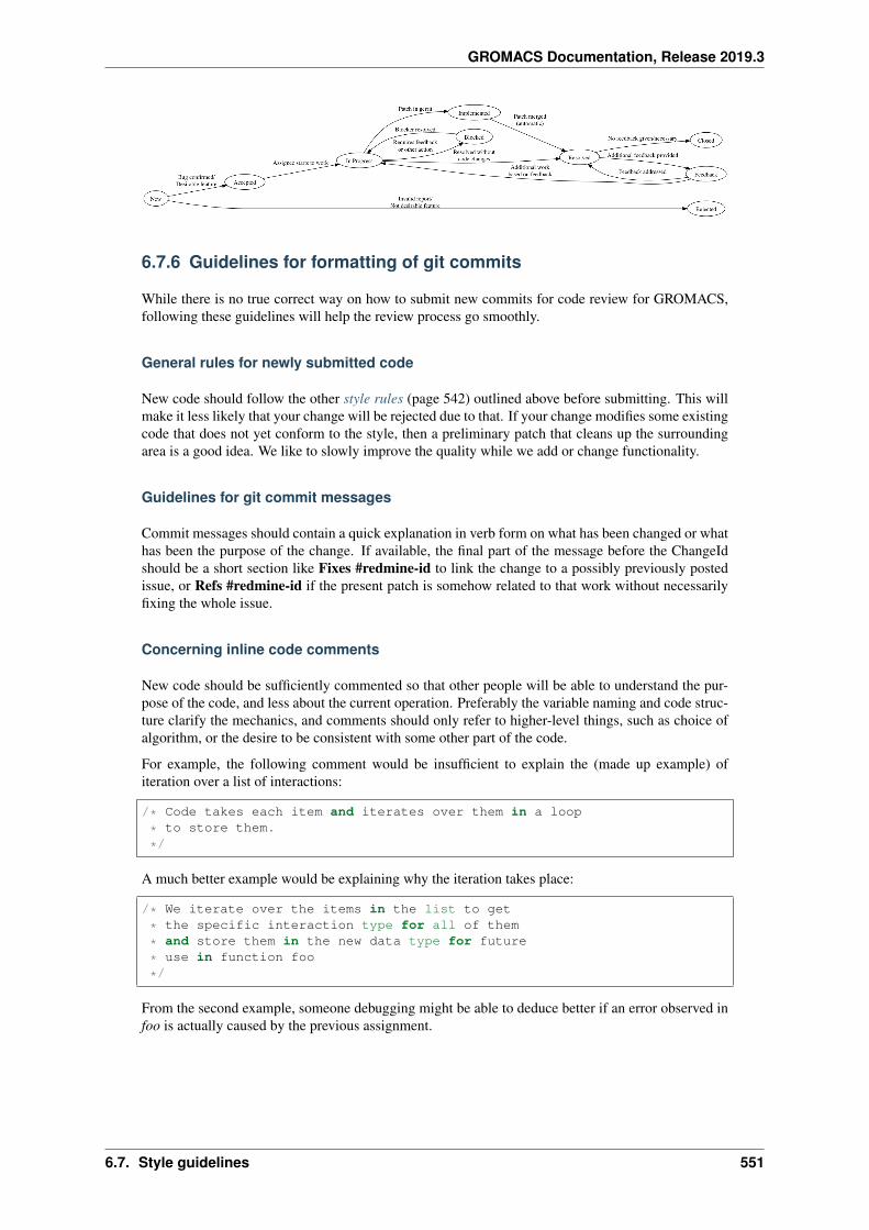
GROMACS Documentation, Release 2019.3
6.7.6 Guidelines for formatting of git commits
While there is no true correct way on how to submit new commits for code review for GROMACS,following these guidelines will help the review process go smoothly.
General rules for newly submitted code
New code should follow the other style rules (page 542) outlined above before submitting. This willmake it less likely that your change will be rejected due to that. If your change modifies some existingcode that does not yet conform to the style, then a preliminary patch that cleans up the surroundingarea is a good idea. We like to slowly improve the quality while we add or change functionality.
Guidelines for git commit messages
Commit messages should contain a quick explanation in verb form on what has been changed or whathas been the purpose of the change. If available, the final part of the message before the ChangeIdshould be a short section like Fixes #redmine-id to link the change to a possibly previously postedissue, or Refs #redmine-id if the present patch is somehow related to that work without necessarilyfixing the whole issue.
Concerning inline code comments
New code should be sufficiently commented so that other people will be able to understand the pur-pose of the code, and less about the current operation. Preferably the variable naming and code struc-ture clarify the mechanics, and comments should only refer to higher-level things, such as choice ofalgorithm, or the desire to be consistent with some other part of the code.
For example, the following comment would be insufficient to explain the (made up example) ofiteration over a list of interactions:
/* Code takes each item and iterates over them in a loop
* to store them.
*/
A much better example would be explaining why the iteration takes place:
/* We iterate over the items in the list to get
* the specific interaction type for all of them
* and store them in the new data type for future
* use in function foo
*/
From the second example, someone debugging might be able to deduce better if an error observed infoo is actually caused by the previous assignment.
6.7. Style guidelines 551
GROMACS Documentation, Release 2019.3
6.7.7 Error handling
To make GROMACS behave like a proper library, we need to change the way errors etc. are handled.Basically, the library should not print out anything to stdio/stderr unless it is part of the API specifica-tion, and even then, there should be a way for the user to suppress the output. Also, the library shouldnormally not terminate the program without the user having control over this. There are differenttypes of errors, which also affects the handling. Different cases are discussed separately below, splitby the way they are handled. These guidelines are starting to take their final form, although detailsmay still change.
• For programming errors, i.e., errors that should never occur if the program is correctly written,it’s acceptable to assert and terminate the program. This applies to both errors in the library anderrors in user code or user input that calls the library. Older code tends to still use assert()calls, but new code should prefer more expressive functionality such as GMX_RELEASE_-ASSERT(). This version of the macro will result in asserts that are still present when the buildtype is Release, which is what we want by default. In performance-sensitive parts of the code, itis acceptable to rather use GMX_ASSERT() to avoid the performance penalty of a branch whenthe code is compiled for production use. By default, Jenkins builds the RelWithAssert buildtype.
• For some errors it might be feasible to recover gracefully and continue execution. In this case,your APIs should be defined so that the API-user/programmer does not have to check separatelywhether the problem was due to a programming error, but it’s better to e.g. use exceptions forrecoverable errors and asserts for programming errors.
• Exceptions should only be used for unexpected errors, e.g., out of memory or file system IOerrors. As a general guideline, incorrect user input should not produce an untrapped exceptionresulting in execution termination telling the user an exception occured. Instead, you shouldcatch exceptions in an earlier stack frame, make a suitable decision about diagnostic messages,and then decide how execution should be terminated.
• There is a global list of possible exceptions in src/gromacs/utility/exceptions.h, and the library should throw one of these when it fails, possibly providing a more detaileddescription of the reason for the failure. The types of exceptions can be extended, and currentlyinclude:
– Out of memory (e.g. std::bad_alloc)
– File I/O error (e.g. not found)
– Invalid user input (could not be understood)
– Inconsistent user input (parsed correctly, but has internal conflicts)
– Simulation instability
– Invalid API call/value/internal error (an assertion might also be used in such cases)
– In the internals of a module called from code that is not exception safe, you can use excep-tions for error handling, but avoid propagating them to caller code.
• Avoid using exceptions to propagate errors across regions that start or join threads with OpenMP,since OpenMP cannot make guarantees about whether exceptions are caught or if the programwill crash. Currently we catch all exceptions before we leave an OpenMP threaded region.If you throw an exception, make sure that it is caught and handled appropriately in the samethread/OpenMP section.
• There are also cases where a library routine wants to report a warning or a non-fatal error, butis still able to continue processing. In this case you should try to collect all issues and reportand report them (similar to what grompp does with notes, warnings and errors) instead of justreturning the first error. It is irritating to users if they fix the reported error, but then they keepgetting a new error message every time the rerun the program.
• A function should not fail as part of its normal operation. However, doing nothing can beconsidered normal operation. A function accessing data should typically also be callable when
6.7. Style guidelines 552
GROMACS Documentation, Release 2019.3
no such data is available, but still return through normal means. If the failure is not normal, it isOK to rather throw an exception.
For coding guidelines to make this all work, see Implementing exceptions for error handling(page 549).
Guidelines for code formatting (page 542) Guidelines for indentation and other code formatting.
Guidelines for #include directives (page 544) Guidelines for #include style (ordering, paths to use,etc.).
Naming conventions (page 545) Naming conventions for files and various code constructs.
Allowed language features (page 547) Allowed language features.
Error handling (page 552) How to handle errors at run time
General guidelines for Doxygen markup (page 555) Guidelines for using Doxygen to document thesource code are currently in a section on the page on general Doxygen usage.
Guidelines for creating meaningful redmine issue reports (page 550) Guidelines for preparing andformatting bug reports on redmine.
Guidelines for formatting of git commits (page 551) Guidelines for formatting git commits whensending in proposed fixes for code review.
6.8 Development-time tools
Several tools have their own individual pages and are listed below.
6.8.1 Using Doxygen
This page documents how Doxygen is set up in the GROMACS source tree, as well as guidelinesfor adding new Doxygen comments. Examples are included, as well as tips and tricks for avoidingDoxygen warnings. The guidelines focus on C++ code and other new code that follows the newmodule layout. Parts of the guidelines are still applicable to documenting older code (e.g., withingmxlib/ or mdlib/), in particular the guidelines about formatting the Doxygen comments andthe use of \internal. See Documentation organization (page 520) for the overall structure of thedocumentation.
To get started quickly, you only need to read the first two sections to understand the overall structureof the documentation, and take a look at the examples at the end. The remaining sections provide thedetails for understanding why the examples are the way they are, and for more complex situations.They are meant more as a reference to look up solutions for particular problems, rather than single-time reading. To understand or find individual Doxygen commands, you should first look at Doxygendocumentation (http://www.stack.nl/~dimitri/doxygen/manual/index.html).
Documentation flavors
The GROMACS source tree is set up to produce several different levels of Doxygen documentation:
1. Public API documentation (suffix -user), which documents functions and classes exportedfrom the library and intended for use outside the GROMACS library.
2. Library API documentation (suffix -lib), which additionally includes functions and classesthat are designed to be used from other parts of GROMACS, as well as some guidelines that aremostly of interest to developers.
3. Full documentation (suffix -full), which includes (nearly) all (documented) functions andclasses in the source tree.
6.8. Development-time tools 553
GROMACS Documentation, Release 2019.3
4. Maximally verbose documentation (suffix -dev) with everything doxygen can extract as wellas additional internal links.
Each subsequent level of documentation includes all the documentation from the levels above it. Thesuffixes above refer to the suffixes of Doxygen input and output files, as well as the name of the outputdirectory. When all the flavors have been built, the front pages of the documentation contain links tothe other flavors, and explain the differences in more detail.
As a general guideline, the public API documentation should be kept free of anything that a userlinking against an unmodified GROMACS does not see. In other words, the public API documentationshould mainly document the contents of installed headers, and provide the necessary overview ofusing those. Also, verbosity requirements for the public API documentation are higher: ideally,readers of the documentation could immediately start using the API based on the documentation,without any need to look at the implementation.
Similarly, the library API documentation should not contain things that other modules in GROMACScan or should never call. In particular, anything declared locally in source files should be only avail-able in the full documentation. Also, if something is documented, and is not identified to be in thelibrary API, then it should not be necessary to call that function from outside its module.
Building the documentation
If you simply want to see up-to-date documentation, you can go to http://jenkins.gromacs.org/job/Documentation_Nightly_master/javadoc/html-lib/index.xhtml to see the documentation for the cur-rent development version. Jenkins also runs Doxygen for all changes pushed to Gerrit for release-5-0and master branches, and the resulting documentation can be viewed from the link posted by Jenkins.The Doxygen build is marked as unstable if it introduces any Doxygen warnings.
You may need to build the documentation locally if you want to check the results afteradding/modifying a significant amount of comments. This is recommended in particular if you donot have much experience with Doxygen. It is a good idea to build with all the different settings tosee that the result is what you want, and that you do not produce any warnings. For local work, itis generally a good idea to set GMX_COMPACT_DOXYGEN=ON CMake option, which removes somelarge generated graphs from the documentation and speeds up the process significantly. There arealso “fast” versions of the make targets that skip the additional diagrams built for the lib level andlower.
All files related to Doxygen reside in the docs/doxygen/ subdirectory in the source andbuild trees. In a freshly checked out source tree, this directory contains various Doxyfile-*.cmakein files. When you run CMake, corresponding files Doxyfile-user, Doxyfile-lib,Doxyfile-full, Doxyfile-dev are generated at the corresponding location in the build tree.There is also a Doxyfile-common.cmakein, which is used to produce Doxyfile-common.This file contains settings that are shared between all the input files. Doxyfile-compact providesthe extra settings for GMX_COMPACT_DOXYGEN=ON.
You can run Doxygen directly with one of the generated files (all output will be producedunder the current working directory), or build one of the doxygen-user, doxygen-lib,doxygen-full, doxygen-dev targets. The targets run Doxygen in a quieter mode and onlyshow the warnings if there were any, and put the output under docs/html/doxygen/ in the buildtree, so that the Doxygen build cooperates with the broader webpage target. The doxygen-alltarget builds all three targets with less typing.
The generated documentation is put under html-user/, html-lib/, html-full/, and/orhtml-dev/. Open index.xhtml file from one of these subdirectories to start browsing (forGROMACS developers, the html-lib/ is a reasonable starting point). Log files with all Doxygenwarnings are also produced as docs/doxygen/doxygen-*.log, so you can inspect them afterthe run.
You will need Doxygen 1.8.5 to build the current documentation. Other versions may work, butlikely also produce warnings. Additionally, graphviz and mscgen are required for some graphs in thedocumentation, and latex for formulas. Working versions are likely available through most package
6.8. Development-time tools 554
GROMACS Documentation, Release 2019.3
managers. It is possible to build the documentation without these tools, but you will see some errorsand the related figures will be missing from the documentation.
General guidelines for Doxygen markup
Doxygen provides quite a few different alternative styles for documenting the source code. There aresubtleties in how Doxygen treats the different types of comments, and this also depends somewhaton the Doxygen configuration. It is possible to change the meaning of a comment by just changingthe style of comment it is enclosed in. To avoid such issues, and to avoid needing to manage allthe alternatives, a single style throughout the source tree is preferable. When it comes to treatmentof styles, GROMACS uses the default Doxygen configuration with one exception: JAVADOC_-AUTOBRIEF is set ON to allow more convenient one-line brief descriptions in C code.
Majority of existing comments in GROMACS uses Qt-style comments (/*! and //! instead of /**and ///, \brief instead of @brief etc.), so these should be used also for new documentation.There is a single exception for brief comments in C code; see below.
Similarly, existing comments use /*! for multiline comments in both C and C++ code, instead ofusing multiple //! lines for C++. The rationale is that since the code will be a mixture of bothlanguages for a long time, it is more uniform to use similar style in both. Also, since files will likelytransition from C to C++ gradually, rewriting the comments because of different style issues shouldnot generally be necessary. Finally, multi-line //! comments can work differently depending onDoxygen configuration, so it is better to avoid that ambiguity.
When adding comments, ensure that a short brief description is always produced. This is used invarious listings, and should briefly explain the purpose of the method without unnecessarily expandingthose lists. The basic guideline is to start all comment blocks with \brief (possibly after someother Doxygen commands). If you want to avoid the \brief for one-liners, you can use //!, butthe description must fit on a single line; otherwise, it is not interpreted as a brief comment. Note inparticular that a simple /*! without a \brief does not produce a brief description. Also note that\brief marks the whole following paragraph as a brief description, so you should insert an emptyline after the intended brief description.
In C code, // comments must be avoided because some compilers do not like them. If you wantto avoid the \brief for one-liners in C code, use /** instead of //!. If you do this, the briefdescription should not contain unescaped periods except at the end. Because of this, you shouldprefer //! in C++ code.
Put the documentation comments in the header file that contains the declaration, if such a headerexists. Implementation-specific comments that do not influence how a method is used can go intothe source file, just before the method definition, with an \internal tag in the beginning of thecomment block. Doxygen-style comments within functions are not generally usable.
At times, you may need to exclude some part of a header or a source file such that Doxygen does notsee it at all. In general, you should try to avoid this, but it may be necessary to remove some functionsthat you do not want to appear in the public API documentation, and which would generate warningsif left undocumented, or to avoid Doxygen warnings from code it does not understand. Prefer \condand \endcond to do this. If \cond does not work for you, you can also use #ifndef DOXYGEN.If you exclude a class method in a header, you also need to exclude it in the source code to avoidwarnings.
GROMACS specifics
The general guidelines on the style of Doxygen comments were given above. This section introducesGROMACS specific constructs currently used in Doxygen documentation, as well as how GRO-MACS uses Doxygen groups to organize the documentation.
Some consistency checks are done automatically using custom scripts. See Source tree checker scripts(page 594) for details.
6.8. Development-time tools 555
GROMACS Documentation, Release 2019.3
Controlling documentation visibility
To control in which level of documentation a certain function appears, three different mechanisms areused:
• Global Doxygen configuration. This is mainly used to include declarations local to source filesonly in the full documentation. You can find the details from the Doxyfile-*.cmakeinfiles, and some of them are also mentioned below on individual code constructs.
• The standard Doxygen command \internal marks the documentation to be only extractedinto the full documentation (INTERNAL_DOCS is ON only for the full documentation). Thisshould be used as a first command in a comment block to exclude all the documentation. Itis possible to use \internal and \endinternal to exclude individual paragraphs, but\if internal is preferred (see below). In addition, GROMACS-specific custom Doxygencommand \libinternal is provided, which should be used the same way to exclude the doc-umentation from the public API documentation. This command expands to either \internalor to a no-op, depending on the documentation level.
• Doxygen commands \if and \cond can be used with section names libapi and internalto only include the documentation in library API and the full documentation, respectively.libapi is also defined in the full documentation. These are declared using ENABLED_-SECTIONS in the Doxygen configuration files.
Examples of locations where it is necessary to use these explicit commands are given below in thesections on individual code constructs.
Modules as Doxygen groups
As described in Source code organization (page 518), each subdirectory under src/gromacs/represents a module, i.e., a somewhat coherent collection of routines. Doxygen cannot automaticallygenerate a list of routines in a module; it only extracts various alphabetical indexes that contain moreor less all documented functions and classes. To help reading the documentation, the routines for amodule should be visible in one place.
GROMACS uses Doxygen groups to achieve this: for each documented module, there is a\defgroup definition for the module, and all the relevant classes and functions need to be man-ually added to this group using \ingroup and \addtogroup. The group page also provides anatural place for overview documentation about the module, and can be navigated to directly fromthe “Modules” tab in the generated documentation.
Some notes about using \addtogroup are in order:
• \addtogroup only adds the elements that it directly contains into the group. If it contains anamespace declaration, only the namespace is added to the group, but none of the namespacecontents are. For this reason, \addtogroup should go within the innermost scope, around themembers that should actually be added.
• If the module should not appear in the public API documentation, its definition (\defgroup)should be prefixed with a \libinternal. In this case, also all \addtogroup commandsfor this module should be similarly prefixed. Otherwise, they create the group in the public APIdocumentation, but without any of the content from the \defgroup definition. This may alsocause the contents of the \addtogroup section to appear in the public API documentation,even if it otherwise would not.
Public API and library API groups
In addition to the module groups, two fixed groups are provided: group_publicapi andgroup_libraryapi. Classes and files can be added to these groups using GROMACS specificcustom \inpublicapi and \inlibraryapi commands. The generated group documentationpages are not very useful, but annotated classes and files show the API definition under the name,
6.8. Development-time tools 556
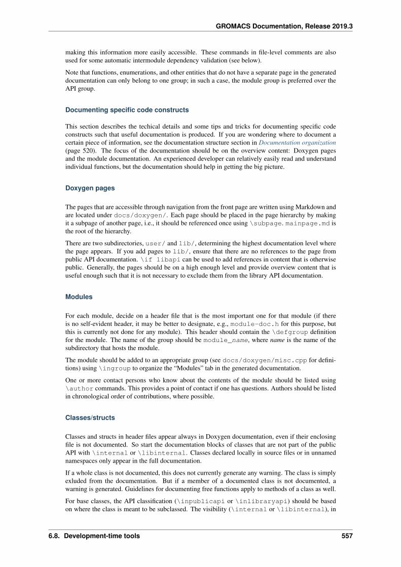
GROMACS Documentation, Release 2019.3
making this information more easily accessible. These commands in file-level comments are alsoused for some automatic intermodule dependency validation (see below).
Note that functions, enumerations, and other entities that do not have a separate page in the generateddocumentation can only belong to one group; in such a case, the module group is preferred over theAPI group.
Documenting specific code constructs
This section describes the techical details and some tips and tricks for documenting specific codeconstructs such that useful documentation is produced. If you are wondering where to document acertain piece of information, see the documentation structure section in Documentation organization(page 520). The focus of the documentation should be on the overview content: Doxygen pagesand the module documentation. An experienced developer can relatively easily read and understandindividual functions, but the documentation should help in getting the big picture.
Doxygen pages
The pages that are accessible through navigation from the front page are written using Markdown andare located under docs/doxygen/. Each page should be placed in the page hierarchy by makingit a subpage of another page, i.e., it should be referenced once using \subpage. mainpage.md isthe root of the hierarchy.
There are two subdirectories, user/ and lib/, determining the highest documentation level wherethe page appears. If you add pages to lib/, ensure that there are no references to the page frompublic API documentation. \if libapi can be used to add references in content that is otherwisepublic. Generally, the pages should be on a high enough level and provide overview content that isuseful enough such that it is not necessary to exclude them from the library API documentation.
Modules
For each module, decide on a header file that is the most important one for that module (if thereis no self-evident header, it may be better to designate, e.g., module-doc.h for this purpose, butthis is currently not done for any module). This header should contain the \defgroup definitionfor the module. The name of the group should be module_name, where name is the name of thesubdirectory that hosts the module.
The module should be added to an appropriate group (see docs/doxygen/misc.cpp for defini-tions) using \ingroup to organize the “Modules” tab in the generated documentation.
One or more contact persons who know about the contents of the module should be listed using\author commands. This provides a point of contact if one has questions. Authors should be listedin chronological order of contributions, where possible.
Classes/structs
Classes and structs in header files appear always in Doxygen documentation, even if their enclosingfile is not documented. So start the documentation blocks of classes that are not part of the publicAPI with \internal or \libinternal. Classes declared locally in source files or in unnamednamespaces only appear in the full documentation.
If a whole class is not documented, this does not currently generate any warning. The class is simplyexluded from the documentation. But if a member of a documented class is not documented, awarning is generated. Guidelines for documenting free functions apply to methods of a class as well.
For base classes, the API classification (\inpublicapi or \inlibraryapi) should be basedon where the class is meant to be subclassed. The visibility (\internal or \libinternal), in
6.8. Development-time tools 557
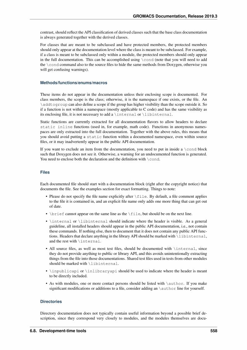
GROMACS Documentation, Release 2019.3
contrast, should reflect the API classification of derived classes such that the base class documentationis always generated together with the derived classes.
For classes that are meant to be subclassed and have protected members, the protected membersshould only appear at the documentation level where the class is meant to be subclassed. For example,if a class is meant to be subclassed only within a module, the protected members should only appearin the full documentation. This can be accomplished using \cond (note that you will need to addthe \cond command also to the source files to hide the same methods from Doxygen, otherwise youwill get confusing warnings).
Methods/functions/enums/macros
These items do not appear in the documentation unless their enclosing scope is documented. Forclass members, the scope is the class; otherwise, it is the namespace if one exists, or the file. An\addtogroup can also define a scope if the group has higher visibility than the scope outside it. Soif a function is not within a namespace (mostly applicable to C code) and has the same visibility asits enclosing file, it is not necessary to add a \internal or \libinternal.
Static functions are currently extracted for all documentation flavors to allow headers to declarestatic inline functions (used in, for example, math code). Functions in anonymous names-paces are only extracted into the full documentation. Together with the above rules, this means thatyou should avoid putting a static function within a documented namespace, even within sourcefiles, or it may inadvertently appear in the public API documentation.
If you want to exclude an item from the documentation, you need to put in inside a \cond blocksuch that Doxygen does not see it. Otherwise, a warning for an undocumented function is generated.You need to enclose both the declaration and the definition with \cond.
Files
Each documented file should start with a documentation block (right after the copyright notice) thatdocuments the file. See the examples section for exact formatting. Things to note:
• Please do not specify the file name explicitly after \file. By default, a file comment appliesto the file it is contained in, and an explicit file name only adds one more thing that can get outof date.
• \brief cannot appear on the same line as the \file, but should be on the next line.
• \internal or \libinternal should indicate where the header is visible. As a generalguideline, all installed headers should appear in the public API documentation, i.e., not containthese commands. If nothing else, then to document that it does not contain any public API func-tions. Headers that declare anything in the library API should be marked with \libinternal,and the rest with \internal.
• All source files, as well as most test files, should be documented with \internal, sincethey do not provide anything to public or library API, and this avoids unintentionally extractingthings from the file into those documentations. Shared test files used in tests from other modulesshould be marked with \libinternal.
• \inpublicapi or \inlibraryapi should be used to indicate where the header is meantto be directly included.
• As with modules, one or more contact persons should be listed with \author. If you makesignificant modifications or additions to a file, consider adding an \author line for yourself.
Directories
Directory documentation does not typically contain useful information beyond a possible brief de-scription, since they correspond very closely to modules, and the modules themselves are docu-
6.8. Development-time tools 558
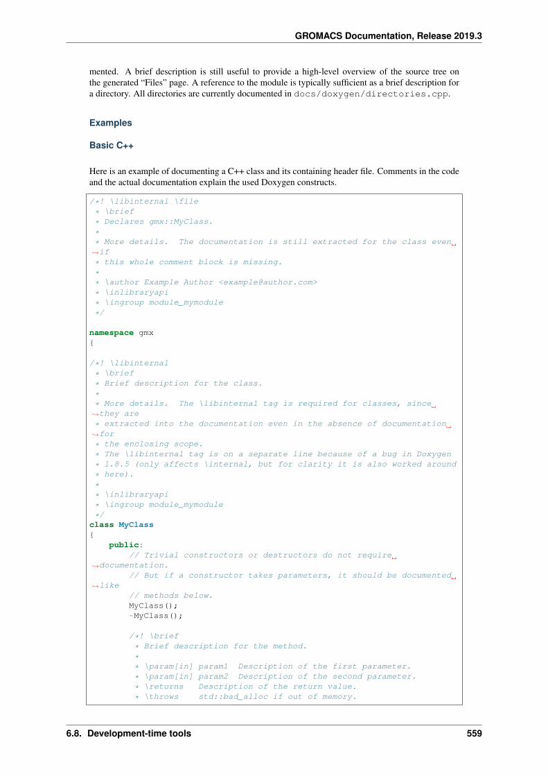
GROMACS Documentation, Release 2019.3
mented. A brief description is still useful to provide a high-level overview of the source tree onthe generated “Files” page. A reference to the module is typically sufficient as a brief description fora directory. All directories are currently documented in docs/doxygen/directories.cpp.
Examples
Basic C++
Here is an example of documenting a C++ class and its containing header file. Comments in the codeand the actual documentation explain the used Doxygen constructs.
/*! \libinternal \file
* \brief
* Declares gmx::MyClass.
** More details. The documentation is still extracted for the class even→˓if
* this whole comment block is missing.
** \author Example Author <[email protected]>
* \inlibraryapi
* \ingroup module_mymodule
*/
namespace gmx{
/*! \libinternal
* \brief
* Brief description for the class.
** More details. The \libinternal tag is required for classes, since→˓they are
* extracted into the documentation even in the absence of documentation→˓for
* the enclosing scope.
* The \libinternal tag is on a separate line because of a bug in Doxygen
* 1.8.5 (only affects \internal, but for clarity it is also worked around
* here).
** \inlibraryapi
* \ingroup module_mymodule
*/class MyClass{
public:// Trivial constructors or destructors do not require
→˓documentation.// But if a constructor takes parameters, it should be documented
→˓like// methods below.MyClass();~MyClass();
/*! \brief
* Brief description for the method.
** \param[in] param1 Description of the first parameter.
* \param[in] param2 Description of the second parameter.
* \returns Description of the return value.
* \throws std::bad_alloc if out of memory.
6.8. Development-time tools 559
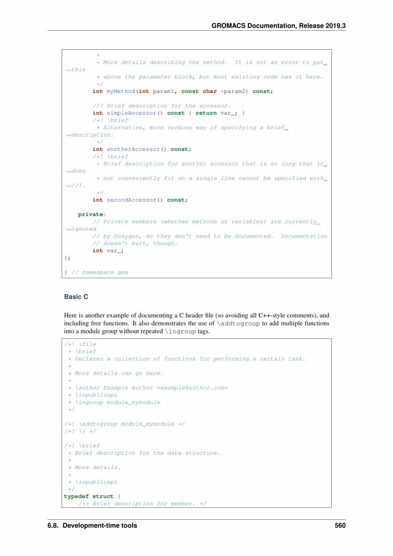
GROMACS Documentation, Release 2019.3
** More details describing the method. It is not an error to put
→˓this
* above the parameter block, but most existing code has it here.
*/int myMethod(int param1, const char *param2) const;
//! Brief description for the accessor.int simpleAccessor() const { return var_; }/*! \brief
* Alternative, more verbose way of specifying a brief→˓description.
*/int anotherAccessor() const;/*! \brief
* Brief description for another accessor that is so long that it→˓does
* not conveniently fit on a single line cannot be specified with→˓//!.
*/int secondAccessor() const;
private:// Private members (whether methods or variables) are currently
→˓ignored// by Doxygen, so they don't need to be documented. Documentation// doesn't hurt, though.int var_;
};
} // namespace gmx
Basic C
Here is another example of documenting a C header file (so avoiding all C++-style comments), andincluding free functions. It also demonstrates the use of \addtogroup to add multiple functionsinto a module group without repeated \ingroup tags.
/*! \file
* \brief
* Declares a collection of functions for performing a certain task.
** More details can go here.
** \author Example Author <[email protected]>
* \inpublicapi
* \ingroup module_mymodule
*/
/*! \addtogroup module_mymodule *//*! \{ */
/*! \brief
* Brief description for the data structure.
** More details.
** \inpublicapi
*/typedef struct {
/** Brief description for member. */
6.8. Development-time tools 560
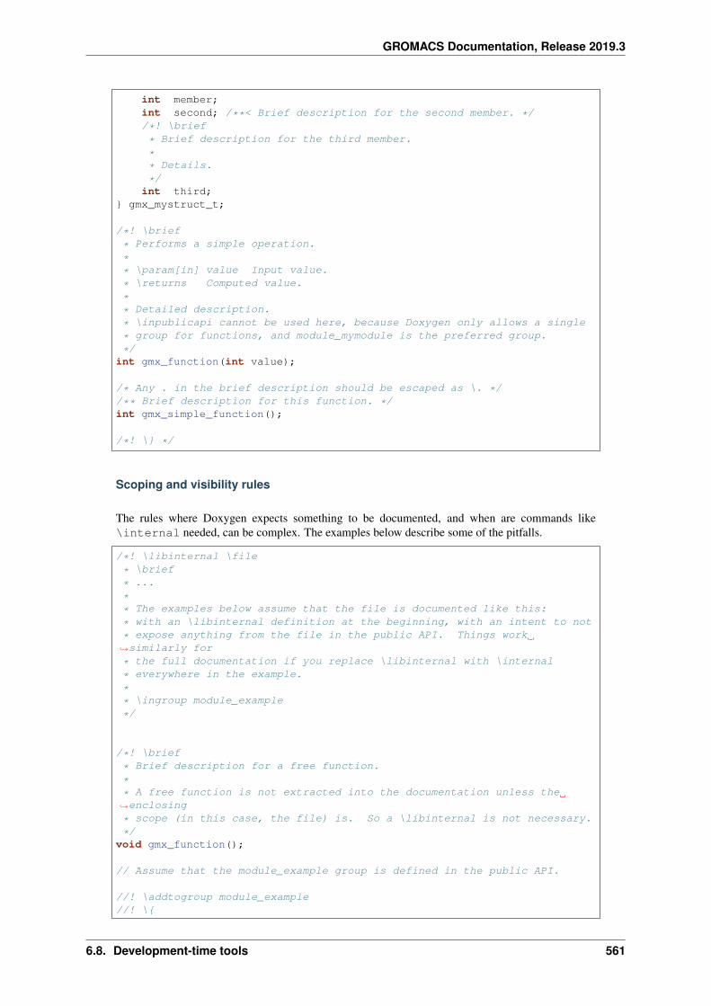
GROMACS Documentation, Release 2019.3
int member;int second; /**< Brief description for the second member. *//*! \brief
* Brief description for the third member.
** Details.
*/int third;
} gmx_mystruct_t;
/*! \brief
* Performs a simple operation.
** \param[in] value Input value.
* \returns Computed value.
** Detailed description.
* \inpublicapi cannot be used here, because Doxygen only allows a single
* group for functions, and module_mymodule is the preferred group.
*/int gmx_function(int value);
/* Any . in the brief description should be escaped as \. *//** Brief description for this function. */int gmx_simple_function();
/*! \} */
Scoping and visibility rules
The rules where Doxygen expects something to be documented, and when are commands like\internal needed, can be complex. The examples below describe some of the pitfalls.
/*! \libinternal \file
* \brief
* ...
** The examples below assume that the file is documented like this:
* with an \libinternal definition at the beginning, with an intent to not
* expose anything from the file in the public API. Things work→˓similarly for
* the full documentation if you replace \libinternal with \internal
* everywhere in the example.
** \ingroup module_example
*/
/*! \brief
* Brief description for a free function.
** A free function is not extracted into the documentation unless the→˓enclosing
* scope (in this case, the file) is. So a \libinternal is not necessary.
*/void gmx_function();
// Assume that the module_example group is defined in the public API.
//! \addtogroup module_example//! \{
6.8. Development-time tools 561
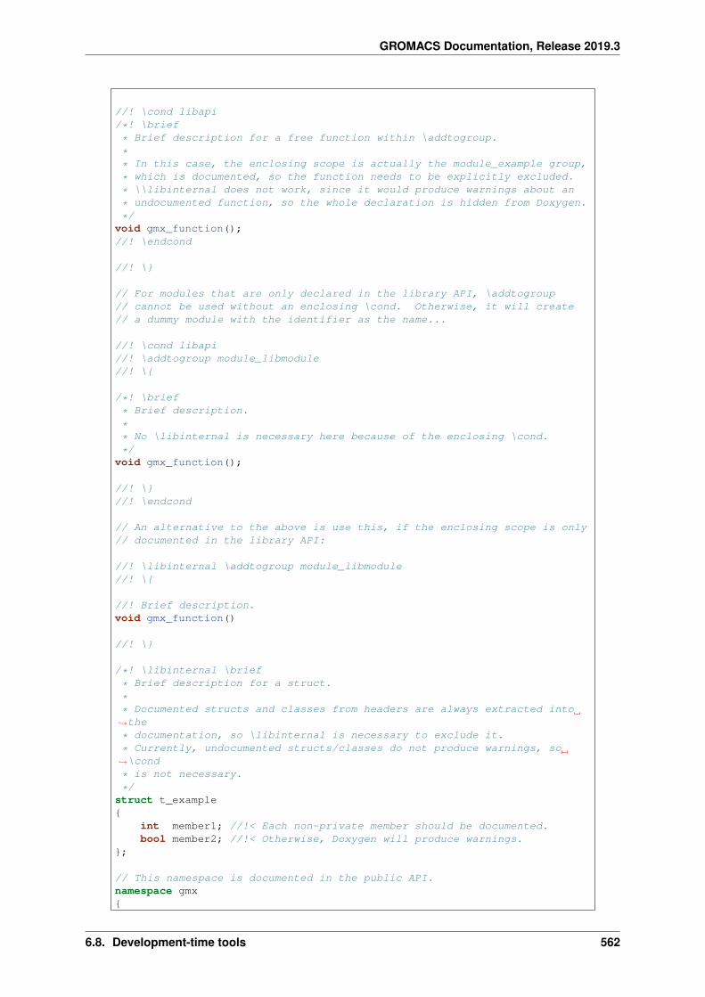
GROMACS Documentation, Release 2019.3
//! \cond libapi/*! \brief
* Brief description for a free function within \addtogroup.
** In this case, the enclosing scope is actually the module_example group,
* which is documented, so the function needs to be explicitly excluded.
* \\libinternal does not work, since it would produce warnings about an
* undocumented function, so the whole declaration is hidden from Doxygen.
*/void gmx_function();//! \endcond
//! \}
// For modules that are only declared in the library API, \addtogroup// cannot be used without an enclosing \cond. Otherwise, it will create// a dummy module with the identifier as the name...
//! \cond libapi//! \addtogroup module_libmodule//! \{
/*! \brief
* Brief description.
** No \libinternal is necessary here because of the enclosing \cond.
*/void gmx_function();
//! \}//! \endcond
// An alternative to the above is use this, if the enclosing scope is only// documented in the library API:
//! \libinternal \addtogroup module_libmodule//! \{
//! Brief description.void gmx_function()
//! \}
/*! \libinternal \brief
* Brief description for a struct.
** Documented structs and classes from headers are always extracted into→˓the
* documentation, so \libinternal is necessary to exclude it.
* Currently, undocumented structs/classes do not produce warnings, so→˓\cond
* is not necessary.
*/struct t_example{
int member1; //!< Each non-private member should be documented.bool member2; //!< Otherwise, Doxygen will produce warnings.
};
// This namespace is documented in the public API.namespace gmx{
6.8. Development-time tools 562
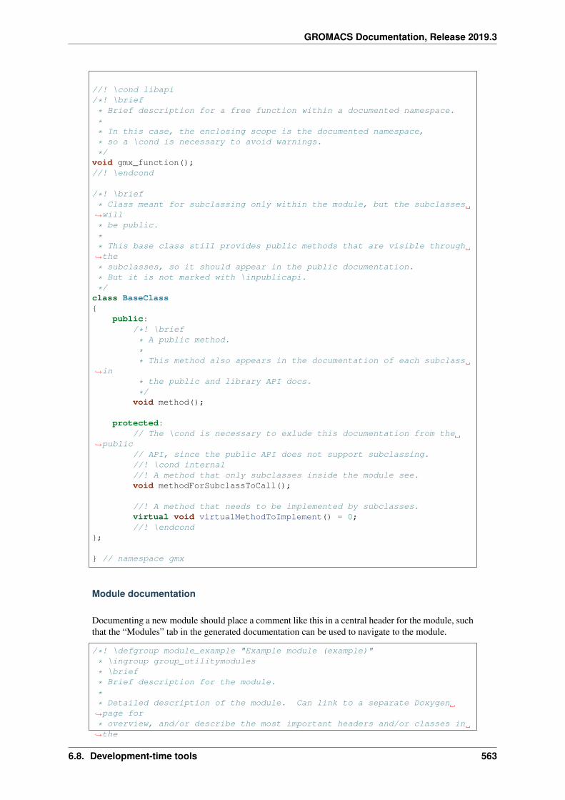
GROMACS Documentation, Release 2019.3
//! \cond libapi/*! \brief
* Brief description for a free function within a documented namespace.
** In this case, the enclosing scope is the documented namespace,
* so a \cond is necessary to avoid warnings.
*/void gmx_function();//! \endcond
/*! \brief
* Class meant for subclassing only within the module, but the subclasses→˓will
* be public.
** This base class still provides public methods that are visible through→˓the
* subclasses, so it should appear in the public documentation.
* But it is not marked with \inpublicapi.
*/class BaseClass{
public:/*! \brief
* A public method.
** This method also appears in the documentation of each subclass
→˓in
* the public and library API docs.
*/void method();
protected:// The \cond is necessary to exlude this documentation from the
→˓public// API, since the public API does not support subclassing.//! \cond internal//! A method that only subclasses inside the module see.void methodForSubclassToCall();
//! A method that needs to be implemented by subclasses.virtual void virtualMethodToImplement() = 0;//! \endcond
};
} // namespace gmx
Module documentation
Documenting a new module should place a comment like this in a central header for the module, suchthat the “Modules” tab in the generated documentation can be used to navigate to the module.
/*! \defgroup module_example "Example module (example)"
* \ingroup group_utilitymodules
* \brief
* Brief description for the module.
** Detailed description of the module. Can link to a separate Doxygen→˓page for
* overview, and/or describe the most important headers and/or classes in→˓the
6.8. Development-time tools 563
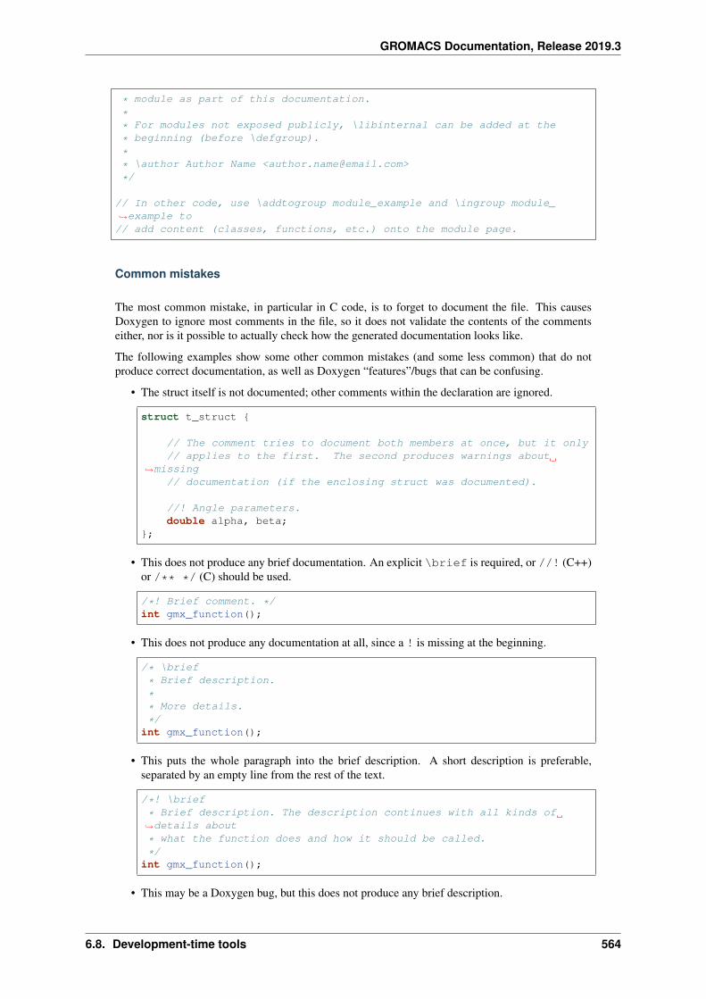
GROMACS Documentation, Release 2019.3
* module as part of this documentation.
** For modules not exposed publicly, \libinternal can be added at the
* beginning (before \defgroup).
** \author Author Name <[email protected]>
*/
// In other code, use \addtogroup module_example and \ingroup module_→˓example to// add content (classes, functions, etc.) onto the module page.
Common mistakes
The most common mistake, in particular in C code, is to forget to document the file. This causesDoxygen to ignore most comments in the file, so it does not validate the contents of the commentseither, nor is it possible to actually check how the generated documentation looks like.
The following examples show some other common mistakes (and some less common) that do notproduce correct documentation, as well as Doxygen “features”/bugs that can be confusing.
• The struct itself is not documented; other comments within the declaration are ignored.
struct t_struct {
// The comment tries to document both members at once, but it only// applies to the first. The second produces warnings about
→˓missing// documentation (if the enclosing struct was documented).
//! Angle parameters.double alpha, beta;
};
• This does not produce any brief documentation. An explicit \brief is required, or //! (C++)or /** */ (C) should be used.
/*! Brief comment. */int gmx_function();
• This does not produce any documentation at all, since a ! is missing at the beginning.
/* \brief
* Brief description.
** More details.
*/int gmx_function();
• This puts the whole paragraph into the brief description. A short description is preferable,separated by an empty line from the rest of the text.
/*! \brief
* Brief description. The description continues with all kinds of→˓details about
* what the function does and how it should be called.
*/int gmx_function();
• This may be a Doxygen bug, but this does not produce any brief description.
6.8. Development-time tools 564
GROMACS Documentation, Release 2019.3
/** \internal Brief description. */int gmx_function();
• If the first declaration below appears in a header, and the second in a source file, then Doxygendoes not associate them correctly and complains about missing documentation for the latter. Thesolution is to explicitly add a namespace prefix also in the source file, even though the compilerdoes not require it.
// Header file//! Example function with a namespace-qualified parameter type.int gmx_function(const gmx::SomeClass ¶m);
// Source fileusing gmx::SomeClass;
int gmx_function(const SomeClass ¶m);
• This puts the namespace into the mentioned module, instead of the contents of the namespace.\addtogroup should go within the innermost scope.
//! \addtogroup module_example//! \{
namespace gmx{
//! Function intended to be part of module_example.int gmx_function();
}
Existing code
More examples you can find by looking at existing code in the source tree. In particular new C++ codesuch as that in the src/gromacs/analysisdata/ and src/gromacs/options/ subdirec-tories contains a large amount of code documented mostly along these guidelines. Some commentsin src/gromacs/selection/ (in particular, any C-like code) predate the introduction of theseguidelines, so those are not the best examples.
6.8.2 Understanding Jenkins builds
This page documents what different Jenkins builds actually run from the GROMACS source tree. Thepurpose is two-fold:
• Provide information on how to interpret Jenkins failures and how to run the same tasks locally todiagnose issues (in most cases, referring to the special targets described in Build system overview(page 521)).
• Provide information on what changes in the build system (or other parts of the repository) needspecial care to not break Jenkins builds.
Separate page documents how to interact with the Jenkins UI for these builds: Interacting with buildsin Jenkins (page 588). How to do common things with Jenkins builds (page 592) has information onhow to do common things with Jenkins builds.
Pre-submit verification
The following builds are triggered for each patch set uploaded to Gerrit.
6.8. Development-time tools 565
GROMACS Documentation, Release 2019.3
Compilation and tests
The main build compiles GROMACS with different configurations and runs the tests. The configura-tions used for Jenkins verification are specified in admin/builds/pre-submit-matrix.txt.
The exact build sequence can be found in admin/builds/gromacs.py, including the logic thattranslates the build options in the matrix file to CMake options.
Documentation
This build builds various types of documentation:
• PDF reference manual using LaTeX
• Doxygen documentation extracted from the source code
• Set of HTML pages containing an installation guide, a user guide, and a developer guide, aswell as links to the above. This set of HTML pages can be browsed from Jenkins.
• Man pages
• INSTALL text file
The last three require building the gmx binary and running it, so compilation failures will also showin this build. All log files that contain warnings are archived as artifacts in the build, and presenceof any warnings marks the build unstable. Brief description of which part failed is reported back toGerrit.
Additionally, the build runs some source code checks that rely on the Doxygen documentation. Seethe description of the check-source target in Source tree checker scripts (page 594).
Using Doxygen (page 553) provides general guidelines for Doxygen usage, which can be helpful inunderstanding and solving Doxygen warnings and some of the check-source issues. Guidelinesfor #include directives (page 544) provides guidelines for #include order and style, which is anotherpart of check-source checks.
The exact build sequence is in admin/builds/documentation.py. See that file for details ofwhat it exactly builds and how. Most changes in the documentation build system will require changesin this script, but Jenkins configuration should be more static.
clang static analysis
The file admin/builds/clang-analyzer.py specifies the exact build sequence and theCMake cache variables used for clang static analysis. This file also specifies the clang version usedfor the analysis, as well as the C++ compiler used (clang-static-analyzer-<version>).
To run the analysis outside Jenkins, you should run both cmake and make under scan-buildcommand using the same CMake cache variables as in the build script. When you do the initialCMake configuration with scan-build, it sets the C++ compiler to the analyzer. Note that usingscan-build like this will also analyze C code, but Jenkins ignores C code for analysis. This canresult in extra warnings, which can be suppressed by manually setting CMAKE_C_COMPILER to avalue other than Clang static analyzer.
uncrustify
This build checks the source code for formatting such as consistent indentation and use of braces, aswell as for copyright headers. See Guidelines for code formatting (page 542) for the guidelines thatare enforced.
The exact build sequence is in admin/builds/uncrustify.py, which essentially just runs
6.8. Development-time tools 566
GROMACS Documentation, Release 2019.3
admin/uncrustify.sh check --rev=HEAD^
If the any changes are required, the build is marked unstable. If the script completely fails (shouldbe rare), the build fails. A file with issues found by the script is archived as an artifact in the build,and a summary is reported back to Gerrit (or the actual issues if there are only a few). See Automaticsource code formatting (page 597) for more details on uncrustify and on scripts to run it.
On-demand builds
These builds can be triggered on request for certain changes in Gerrit, or manually from Jenkins. SeeTriggering builds (page 588) for details on how to trigger these.
Coverage
This build compiles one configuration of GROMACS with instrumentation for coverage, runs thetests, and produces a coverage report using gcovr. The report can be browsed on Jenkins.
The exact build sequence is in admin/builds/coverage.py, including specification of theconfiguration tested.
Source tarball
This build creates the source tarball for distribution. Some of the content that is put into the tarball isgenerated by executing the gmx binary, so this build also compiles the source code (with a minimalset of options).
The build compiles the code and those targets that generate content necessary for the tarball, followedby building the package_source target. After that, it just generates a file that is used by otherbuilds.
The exact build sequence is in admin/builds/source-package.py.
Release workflow
This build creates source and regressiontest tarballs, builds, installs, and tests a few configurationusing those, and builds documentation to be placed on the documentation web site for a new release.The set of configurations tested is specified in admin/builds/release-matrix.txt.
The exact build sequence is desribed in Build & test release tarballs (page 575). The build usesthe source tarball build as a subbuild, and parts of the build are executed using admin/builds/gromacs.py and admin/builds/documentation.py.
admin/builds/get-version-info.py is used for getting the version information from thesource tree as part of this workflow.
admin/builds/update-regtest-hash.py has logic to update the regressiontests tarballMD5 sum for the released tarball automatically.
Updating regressiontests data
Sometimes we add new tests to the regressiontests repository. Also, as the source code or data fileschange, it is sometimes necessary to update regressiontests. This requires a particular CMake buildtype and both a single and double-precision build of GROMACS to generate all the data. Jenkins canautomate much of the tedium here.
6.8. Development-time tools 567
GROMACS Documentation, Release 2019.3
• Upload a regressiontests change that lacks the relevant reference data (either because you deletedthe outdated data, or because the test is new). Jenkins will do the normal thing, which we ignore.There is now a Gerrit patch number for that change, symbolized here with MMMM.
• Go to change MMMM on gerrit, select the patch set you want to update with new reference data(usually the latest one), and comment
[JENKINS] Update
to update against the HEAD of the matching source-code branch, or
[JENKINS] Cross-verify NNNN update
to update from builds of GROMACS from the latest version of Gerrit source-code patch NNNN.You will need to do this when functionality changes in NNNN affect either the layout of the filesin the reference data, or the results of the simulation, or the results of the subsequent analysis.
• Eventually, Jenkins will upload a new version of the regressiontests patch to Gerrit, which willcontain the updated regressiontest data. That upload will again trigger Jenkins to do the normalpre-submit verify, which will now pass (but perhaps will only pass under cross-verify with patchNNNN, as above).
• Later, if you later need to verify an updated version of source-code patch NNNN against thenewly generated reference data, go to the source-code patch NNNN and comment
[JENKINS] Cross-verify MMMM
6.8.3 releng repository
Jenkins scripts (releng Python module)
The main scripts used for Jenkins build are collected into a releng Python package in the relengrepository.
Build overview
Folder structure
In all builds, the folder structure in the workspace looks like this:
$WORKSPACE/releng/gromacs/[regressiontests/]logs/
[unsuccessful-reason.log][<category>/]*
[build/]
Python build script
Builds using the releng Python scripts use the following sequence:
1. Jenkins (or the pipeline script) does some preparatory steps (see Jenkins configuration(page 584)), including checking out the releng repo.
2. Jenkins imports the releng Python package, and calls run_build().
3. The releng script checks out the gromacs repo if not yet done by Jenkins.
6.8. Development-time tools 568
GROMACS Documentation, Release 2019.3
4. The releng script locates a Python build script from the gromacs repo based on the build typegiven to run_build(), and loads the code. The build script provides some configuration settingsas global variables, and a do_build() function that provides the actual build steps.
5. If the build script requires regression tests, the releng script now checks out theregressiontests repo.
6. The releng script prepares the build environment, such as initializing environment variables andgeneric CMake options such as the used compilers. The build environment can be influenced bybuild options passed to run_build(). Some build options passed to run_build() only set param-eters that the build script can access to influence how to do the build (not all build scripts usethese parameters). See Build options (page 572) for details on the supported build options. Thisstep also includes setting up a separate build directory for out-of-source builds if so requestedby the build script.
7. The releng script calls do_build() provided by the build script. do_build() receives a build con-text that it can use to access information about the build environment, build parameters, and theworkspace. The context also provides methods to run CMake, to build targets, to copy logs to acommon location in the workspace, to mark the build unstable, and other such helper functionsto help interacting with Jenkins in an uniform manner. See releng Python API (page 576) fordetails on the API available to the build script.
8. The build script provides the steps to do the actual build, typically calling methods in the buildcontext to interact with the CMake build system or Jenkins where required.
9. When the build script returns, or raises a BuildError exception to indicate a build failure, thereleng script does some final processing to handle reason reporting for unsuccessful (unstableor failed) builds.
10. Jenkins does various post-build actions, such as publishing or parsing logs from the commonlog location, and using the unsuccessful reason reported from the script as the failure messageto report back to Gerrit.
Pipeline builds
The subdirectory workflow/ contains Groovy scripts for use with the Jenkins Pipeline plugin. Thegeneral sequence for these builds is as follows:
1. Jenkins allocates a node for loading the Groovy script.
2. Jenkins checks out the releng repo using a shell script. We do not use an SCM step hereto avoid showing this checkout on the build summary page. The summary page only worksreasonably with at most one Git checkout within the pipeline, and the pipeline script should bein control of what this checkout is.
3. Jenkins loads the desired pipeline script from workflow/.
4. The pipeline script further loads utils.groovy as its first statement. Any other statements atthe top level of the pipeline script are also executed in the context of the node/workspace wherethe script is being loaded. The pipeline script should do a return this as its last statement.
5. As part of the statements run in the initial workspace context, the pipeline script typically callsutils.initBuildRevisions() as the first action, which in turn calls releng.get_-build_revisions() in Python. This will parse the various *_REFSPEC variables comingfrom build parameters and accessible as environment variables in the Python script. The Pythonscript returns new values for the project-specific *_REFSPEC and *_HASH variables, wherevalues like GERRIT_REFSPEC have been applied. These are set into the environment for therest of the build. The returned information is also used to print information on the build summarypage about which commits from each repository are built.
6. In the same context, the pipeline script typically calls utils.checkoutDefaultProject() next. This performs the SCM checkout for the build
6.8. Development-time tools 569
GROMACS Documentation, Release 2019.3
in a way that shows the changes on the front page. TODO: Consider if we would actually wantto skip this part, as it is causing issues like JENKINS-19022.
7. Depending on the type of the build, Jenkins may also call other functions defined in the pipelinescript in this node/workspace context. This is necessary if some values need to be passed fromJenkins configuration to the pipeline script for code that runs in this context.
8. Jenkins calls doBuild() defined in the pipeline script outside of any node/workspace context.Depending on the pipeline script, some parameters may be passed.
9. The pipeline script has full control over the build from now on, until the end.
See Jenkins configuration (page 584) for more details on the configuration.
See Pipeline build overview (page 574) for more details on what kinds of builds the pipeline scriptsare currently used for.
Matrix builds
The releng scripts also support creating Jenkins matrix builds that load the configuration matrix fromthe gromacs repository. These files are located under admin/builds/. The format of suchmatrix files is one configuration per line. Empty lines are ignored, and comments can be started with#.
The build host assignment happens through a set of labels: build options that affect the possible hostfor building the configuration map to labels (the mapping is defined in options.py), and the set oflabels supported by each build agent is defined in agents.py.
The building is orchestrated by a pipeline build that loads and preprocesses the configuration matrix,and then triggers a matrix build that takes the configuration axis values as a build parameter. Thematrix build uses the standard sequence with releng Python scripts.
See Pipeline build overview (page 574) and Jenkins configuration (page 584) for more details.
Input environment variables
The following environment variables are used by the releng Python scripts for input from the Jenkinsjob (or from a pipeline build script):
GROMACS_REFSPEC REGRESSIONTESTS_REFSPEC RELENG_REFSPEC Refspecs for therepositories used for fetching the change to build. Note that they will not always be used foran actual checkout; for example, Jenkins always needs to do the checkout for releng. Forpipeline builds, the first two can also have an empty value or auto (the latter is needed sinceJenkins cannot set environment variables to an empty value), in which case get_build_-revisions() resolves them to actual refspecs for the remainder of the build. The values canalso be overridden by GERRIT_REFSPEC or CHECKOUT_REFSPEC.
GROMACS_HASH REGRESSIONTESTS_HASH RELENG_HASH If set, these provide hashes tocheck out, corresponding to the refspecs. Thees can be used to build a fixed commit from arefspec such as refs/heads/master, even if multiple checkouts are done at different times.It is assumed that fetching the corresponding refspec will make the commit with the providedhash available.
CHECKOUT_PROJECT Needs to be set to the project (gromacs, regressiontests, orreleng) that Jenkins has checked out. If not set, the scripts assume releng.
CHECKOUT_REFSPEC Refspec used to checkout CHECKOUT_PROJECT. If set, this will overridethe project-specific refspec variable.
GERRIT_PROJECT GERRIT_REFSPEC These are set by Gerrit Trigger, and override values fromthe project-specific refspec variable. GERRIT_PROJECT is also used in some cases for inter-preting GERRIT_EVENT_COMMENT_TEXT.
6.8. Development-time tools 570
GROMACS Documentation, Release 2019.3
GERRIT_BRANCH This is set by Gerrit Trigger to identify the branch that triggered the build. It isused to support the same job triggering from multiple branches, getting the refspecs for associ-ated repos right.
GERRIT_EVENT_COMMENT_TEXT This is set by Gerrit Trigger when the build is triggered by acomment added in Jenkins. The text is expected to be base64-encoded (the default in GerritTrigger). See Triggering builds (page 588) for recognized ways of triggering builds throughthis.
MANUAL_COMMENT_TEXT If GERRIT_EVENT_COMMENT_TEXT is not set, the value from thisvariable is used instead (without base64-decoding or removing [JENKINS] tags). This allowscreating a test Jenkins job that can be manually triggered.
NODE_NAME Name of the host where the build is running. This is used for some host-specific logicin configuring the compilation. This is set by Jenkins automatically.
WORKSPACE Path to the root of the Jenkins workspace where the build is running. This is set byJenkins automatically.
STATUS_FILE Path to the file to write on completion of the build, containing the build status and thereason for failed builds. Defaults to logs/unsuccessful-reason.log. If the extensionis .json, the file is written as JSON, which is used in pipeline builds to allow programmaticprocessing of the results. For pipeline builds, the .json file can also contain a return value thatprovides structured information for further processing in the pipeline script.
NO_PROPAGATE_FAILURE If set to a non-empty value, the build script will exit with a zero exitcode even if the build fails because of a BuildError or ConfigurationError. Only unexpectedexceptions will cause a non-zero exit code. The information in STATUS_FILE can be used todetermine whether the build failed or not.
Output
To communicate back to the Jenkins job (or the pipeline build script), the releng scripts use thefollowing mechanisms:
exit code The script exits with a non-zero exit code if the build fails, unless NO_PROPAGATE_-FAILURE is set. If the environment variable is set, only an unexpected exception will cause anon-zero exit code.
status file In freestyle jobs, STATUS_FILE is not specified, and logs/unsuccessful-reason.log is written if the build fails or is unstable. This is intended tobe used as the unsuccessful message for Gerrit Trigger in non-pipeline builds.
In pipeline builds, STATUS_FILE is specified as a JSON file, and contains additional informa-tion about the result of the execution. This is used to communicate success/failure back to thepipeline script, as well as reason for failures and in some cases, additional return values in caseof success.
A reasonable effort is done to try to delete this file at the start of the script, so that old versionswould not be left if the script fails. Even on unexpected errors, a reasonable effort is made toproduce the file and include the exception information in it. If producing this file fails, it istreated as an unexpected error.
console outout If the build is unstable, it also ensures that the word FAILED appears in the consolelog. This can be used in non-pipeline builds to mark the build unstable.
other files (specific to build scripts) The build script can produce other relevant output in logs/folder and in the build folder (which is typically gromacs/ for in-source builds and build/for out-of-source builds).
6.8. Development-time tools 571
GROMACS Documentation, Release 2019.3
Build options
Currently, the following build options can be passed from Jenkins to run_build() to influence thebuild environment (and as part of a configuration line in a matrix specification). These are typicallyused for multi-configuration jobs; for jobs that only build a single configuration, the configuration istypically hard-coded in the build script. For boolean options, multiple formats are accepted. E.g., anOpenMP build can be specified as openmp or openmp=yes, and no-OpenMP as no-openmp oropenmp=no. The defaults that are used if a particular option is not specified are determined by thebuild script.
build-jobs=N Use the specified number of parallel jobs for building.
out-of-source Do the build out-of-source, even if an in-source build would be supported.
cmake-X.Y.Z Use the specified CMake version to generate the build system.
gcc-X.Y Use the specified gcc version as the compiler.
armclang-X.Y Use the specified armclang version as the compiler.
clang-X.Y Use the specified clang version as the compiler.
libcxx-X.Y Use the specified libc++ version (currently only supported with exactly clang-X.Y)
clang-static-analyzer-X.Y Use the specified clang static analyzer as the compiler.
icc-X.Y Use Intel compiler (version is currently ignored; it is for informational purposes only andshould match whatever is installed on the build nodes).
msvc-YYYY Use the specified MSVC version as the compiler.
doxygen-X.Y.Z Use the specified Doxygen version for the documentation build.
cuda-X.Y Use the specified CUDA version.
opencl-X.Y Use the specified OpenCL version.
amdappsdk-X.Y Use the specified AMD SDK version. Deprecated.
armhpc-X.Y Use the specified ARM HPC compiler toolchain with the specified version; this sets upthe environment for either armclang with the same version or the bundled gcc.
phi Build for Xeon Phi.
tsan Use thread sanitizer for the build.
atlas Use ATLAS as an external BLAS/LAPACK library.
x11 Build also gmx view (i.e., use GMX_X11=ON).
simd=SIMD Use the specified SIMD instruction set. If not set, SIMD is not used.
gpuhw=VENDOR Use a GPU with the “VENDOR” vendor or “none” if no GPU should be used.
mpi Do an MPI build.
Build scripts can define additional options that only influence the behavior of the build scripts. This isused for matrix builds in gromacs.py for options that do not influence build the build environmentor place requirements on the build host. This allows adding new options when the GROMACS buildsystem changes and new combinations need to be tested, without changing releng.
Build system changes
This section collects information on how different types of changes to the GROMACS CMake buildsystem, the releng scripts, and/or Jenkins configuration are handled to keep the CI builds working.Critical part in these changes is to try to keep builds working for older changes still pending reviewin Gerrit. However, the flipside is that if rebases are not forced, some problems may slip past if someolder change is not compatible with the new CI builds.
6.8. Development-time tools 572
GROMACS Documentation, Release 2019.3
Different cases for changes are below. The distinction may not always be clear-cut, but the generalapproach should be well covered.
1. Compatible change in main repo, no change in releng. In this case, all changes are absorbed inthe build script in the main repo. Old changes will build with the old build script, new changeswith the new, and all builds will pass. Old changes do not trigger the new functionality, so if thenew build script contains new tests or such, they may get silently broken by old changes if theyare not rebased (in this respect, the case is similar to the third item below).
An example of this type of change is reorganization or renaming of CMake cache variables orbuild targets, while still keeping the same or similar functionality. Some types of tests can alsobe added with this approach.
2. Compatible change in releng, no change in main repo. In this case, all changes are absorbed inthe releng script. As soon as the releng change is merged, both old and new changes will buildwith the changed script, and all builds will pass.
An example of this type of change is software updates or node reconfiguration in Jenkins thataffects, e.g., paths to certain programs. Also many bug fixes to the releng scripts fall here.
3. Breaking change in main repo, backwards-compatible change in releng. In this case, changesin the main repo build scripts require changes in releng that do not break old builds. The mainrepo change will not build until releng changes are merged; the releng change can be mergedsafely without breaking old builds. To verify the releng change with its corresponding main repochange, the releng change can be uploaded to Gerrit and then the on-demand cross-verificationmechanism used (see Interacting with builds in Jenkins (page 588)). After the releng change ismerged, the main change build can be triggered and it will pass.
Builds for old changes will continue to work throughout this process, but they will ignore pos-sible new build parameters or such, potentially breaking the new change.
An example of this type of change would be additional methods or parameters required in relengto be able to implement new build tasks.
4. Breaking change in releng, compatible change in main repo. In this case, changes or additionalbuild configurations in the releng and/or Jenkins cause old builds to break. As soon as thechanges in releng are merged, all old changes in Gerrit need to be rebased.
Testing releng scripts
Currently, there are limited unit tests for some parts of the Python scripts. They require a backport ofunittest.mock to be installed, and can be executed with
python -m releng.test
The only way to fully test the releng script is to upload a change to Gerrit and let Jenkins build it.In principle, it is possible to run the script in an environment that exactly matches a Jenkins node(including paths to all required tools and all relevant environment variables that Jenkins sets), but thatcan be tedious to set up. However, it is possible to execute most of the code from the command lineusing
python releng <options>
This requires that you have your projects checked out in the same layout as in Jenkins: the gromacs,regressiontests, and releng repositories should be in sibling directories, with directory names matchingthe repository names.
Please note that even though the command-line mode does not perform most of the actions that thereal build script does (unless you run it with --run), it can still write to some files etc.
Refactoring to better support mock execution is in progress, combined with extending the scope ofunit tests.
6.8. Development-time tools 573
GROMACS Documentation, Release 2019.3
Pipeline build overview
This page documents specifics of different pipeline build scripts, as well as giving an overview of com-mon Groovy code used from different pipeline scripts. Behavior shared across all pipeline builds isdescribed in Jenkins scripts (releng Python module) (page 568) and Jenkins configuration (page 584).
Matrix build launcher
matrix-launcher.groovy is a relatively simple pipeline script where the actual build is per-formed by a normal matrix build. The pipeline contains the following steps:
1. In the initial node context, the bootstrap script calls loadMatrixConfigs() and passesthe name of the matrix to use. This calls releng.prepare_multi_configuration_-build(), and reads the build axis into a local variable.
2. The bootstrap script calls doBuild() with the name of the matrix job to trigger. The pipelinetriggers the matrix job, forwarding all relevant build parameters to it and adding the build con-figuration axis as an additional parameter.
3. After the matrix build finishes, the pipeline calls releng.process_multi_-configuration_build_results(), which uses the Jenkins REST API to get informa-tion about the results of the individual configurations. The information is used to construct afailure message to Gerrit, as well as checking that all configurations were actually built.
4. The pipeline adds a link to the matrix build to the build summary page (while the build isrunning, the link can be found from the console log). The summary also includes the result ofeach configuration, and direct links to the build summary pages of each configuration. The buildstatus of the matrix build is also propagated to the status of the pipeline job.
5. As the last step in the build, the pipeline sets the URL to post back to Gerrit to point to thematrix build. This means that the presence of this launcher job is mostly invisible during normalusage. Only if the pipeline itself fails before reaching this step, you actually see a link to thelauncher job in Gerrit.
Gromacs pre-submit pipeline
For now, the gromacs-presubmit.groovy is essentially the same as the matrix launcher script,except that it supports multiple branches. This is done by receiving a prefix of the matrix jobs indoBuild(), and appending the name of the branch (deduced from the refspecs) in the pipeline.
The intention is for this pipeline to expand to cover also other pre-submit verification, adding flexi-bility and reducing the need for separate builds for different purposes.
Gromacs post-submit pipeline
For now, the gromacs-postsubmit.groovy is essentially the same as the matrix launcherscript, except that it supports multiple branches like the presubmit pipeline.
The intention is for this pipeline to expand to cover also other post-submit verification if needed andadd flexibility.
releng pre-submit pipeline
releng-presubmit.groovy speficies steps to run to verify changes to releng repository inGerrit.
As with gromacs-presubmit.groovy, the intention is for this to assume more responsibilityfor pre-submit verification.
6.8. Development-time tools 574
GROMACS Documentation, Release 2019.3
Clang static analysis
clang-analyzer.groovy is a simple pipeline that performs static analysis using Clang. Themain reason for using a pipeline build instead of a freestyle job is to make it easy to dynamicallydecide the node where the analysis runs, depending on which version of the analyzer should be used.The sequence is:
1. In the initial node context, the pipeline calls utils.read_build_script_config() toget the build options defined in the clang-analyzer.py build script in the source repo.This is stored in a local variable.
2. The bootstrap script calls doBuild() without parameters. The pipeline allocates a node basedon the build options, and runs the clang-analyzer.py build script there with releng.
3. After the releng script finishes, the pipeline publishes a HTML report produced by the analyzer(if it exists), and scans for compiler warnings from the console log to show them on the buildpage.
Build & test release tarballs
release.groovy is a more complex pipeline that coordinates the building and testing of the tar-balls for a release. The packaging of the tarballs is handled by two separate, non-pipeline Jenkinsjobs, one for the source code and one for the regressiontests. The general sequence is:
1. In addition to common preparation, the pipeline reads a set of configurations to test fromrelease-matrix.txt in the source repo as with matrix builds. It also extracts versioninformation from the source repository (using get-version-info.py build script), sincethe regressiontests repository does not contain this.
2. The bootstrap script calls doBuild() with the names of the packaging jobs as parameters.
3. The pipeline checks the latest successful builds in the packaging builds, and if these are notbuilt from the correct commit, it triggers new builds for them. The regressiontests tarball isbuilt first, and its MD5 sum is checked against the one specified in the source tarball. For aRELEASE build, a mismatch fails the build, otherwise it only produces a note in the consoleoutput. The packaging builds also compute MD5 sums for the tarballs, and these are accessiblefrom Jenkins.
4. After the tarballs are available, the pipeline runs each configuration from the test matrix inparallel, using run_build(), and the standard gromacs.py build script from the sourcetarball. A summary is posted to the build summary page (for each configuration, on which hostit was built and whether it was successful, unstable, or failed), but compiler warnings etc. arecurrently only available from the console log (available for a single configuration with somebrowsing under “Pipeline Steps”).
5. If all tests passed, the pipeline then does a final documentation build from the source tarball,which will produce the HTML pages for the documentation website. The generated pages areavailable from the Jenkins project page, as well as from a link on the build summary page. Ifthe RELEASE build parameter is set, a tarball containing all the documentation is also archivedas an artifact.
In addition to the refspecs to build, the pipeline uses two additional build parameters:
RELEASE If set, the -dev suffix is stripped from all the tarballs, and from content within them.Note that currently, the -dev suffixes never appear in the generated website, irrespective of this
FORCE_REPACKAGING If set, the tarballs are rebuilt, even if ones built from the correct refspecsand with the same value of RELEASE is available. This is useful if only releng or Jenkinsconfiguration has changed in a way that influences the tarballs.
The pipeline and the level of testing is still a work-in-progress, but it already covers most of whatthe earlier builds did, and remaining content should not be too hard to add. Missing functionality isindicated with TODOs in the pipeline script or in the build scripts in the source repo.
6.8. Development-time tools 575
GROMACS Documentation, Release 2019.3
On-demand launcher
ondemand.groovy handles builds that are triggered with a [JENKINS] comment from Ger-rit. For many cases, the actual builds are done using separate, non-pipeline jobs triggered from thepipeline. The general sequence is:
1. In the context of the initial checkout, the pipeline uses releng.get_actions_from_-triggering_comment() to parse the comment from Gerrit, as well as the initial refspecs.This replaces utils.initBuildRevisions() from other pipelines, but returns exactlythe same information to the pipeline script (in addition to the information specific to the on-demand build). This function will also read information from the gromacs repository, e.g., tofill out the matrix options into the returned data structure. It also posts cross-verify messages toGerrit if needed.
2. The bootstrap script calls doBuild() without parameters. The pipeline runs the requestedbuilds in parallel, based on the data structure it got in step 1. All relevant build parameters areforwarded. Some actions are handled directly within the pipeline instead of triggering a separatebuild.
3. After the builds finish, the pipeline adds links to the triggered builds to the build summary page(while the build is running, the link can be found from the console log). The pipeline then usesreleng.do_ondemand_post_build() to construct the message to post back to Gerrit,as well as to perform other actions such as posting cross-verify messages. The combined buildstatus of the builds is also propagated to the status of the pipeline job.
Common Groovy scripts
utils.groovy
TODO
matrixbuild.groovy
TODO
packaging.groovy
TODO
releng Python API
Build script definition
The build script is required to provide one function:
do_build(context)Called to run the actual build. The context parameter is an instance of BuildContext, and can beused to access the build environment and to interact with Jenkins. The function can signal fatalbuild errors by raising BuildError directly; typically, this is done by methods in BuildContext ifthey fail to execute the requested commands.
When the function is called, the current working directory is set to the build directory (whetherthe build is in- or out-of-source).
The build script can also set a few global variables to influence the behavior of the build:
6.8. Development-time tools 576
GROMACS Documentation, Release 2019.3
build_optionsIf this list value is set to a non-empty list, then these build options are used to initialize the buildenvironment. Useful for non-matrix builds that want to, e.g., specify the compiler to use.
build_out_of_sourceIf this boolean value is set to True, the build will be executed out-of-source. By default, thebuild will be in-source.
extra_optionsIf this dictionary is set, it declares additional build options that the script understands. This canbe used to declare options that only influence the build script; releng declares only options thataffect the build environment or the build host assignment. Syntax is as follows:
extra_options = {'opt': Option.simple,'opt-bool': Option.bool,'opt-str': Option.string
}
The values of the build options can be read from context.opts in do_build(). SeeOptionTypes documentation for the available option types: in the build script, Optionis bound to OptionTypes.
Technically, the value in the dictionary is a callable that gets called with the name of the optionto create an internal handler class for processing the option.
extra_projectsIf this list value is set to a non-empty list, then these repositories are also checked out beforeexecuting the build. releng and gromacs repositories are always checked out. Currently,only Project.REGRESSIONTESTS makes sense to specify here.
When the build script is loaded, various enums from the releng package are injected into the globalscope to make them easy to access.
API for build scripts
The build script gets input and perfoms most tasks by using data and methods in a BuildContextinstance:
class releng.context.BuildContext(factory, job_type, opts, script_settings)Top-level interface for build scripts to the releng package.
job_typeJobType – Type/scope of the build job (e.g., per-patchset, nightly).
envBuildEnvironment – Access to build environment details like paths to executables. Many ofthe environment properties, such as selecting the compiler, are handled by the build contexttransparently, without the build script needing to access this.
optsBuildOptions – Access to all build options.
paramsBuildParameters – Access to Jenkins build parameters (through environment variables).
workspaceWorkspace – Access to the build workspace. Can be used to get paths to various parts inthe workspace for changing directories and for producing log files.
build_target(target=None, parallel=True, keep_going=False, target_descr=None,failure_string=None, continue_on_failure=False)
Builds a given target.
6.8. Development-time tools 577
GROMACS Documentation, Release 2019.3
run_cmake() must have been called to generate the build system.Parameters
• target (Optional[str]) – Name of the target to build. If None, thedefault (all) target is built.
• parallel (Optional[bool]) – Whether parallel building is supported.• keep_going (Optional[bool]) – Whether to continue building after
first error.• target_descr (str or None) – If given, customizes the error message
when the target fails to build. Should fit the initial part of the sentence “. . .failed to build”. Ignored if failure_string is specified.
• failure_string (str or None) – If given, this message is used as thefailure message if the target fails to build.
• continue_on_failure (Optional[bool]) – If True and the targetfails to build, the failure is only reported and self.failed is set to True.
Raises BuildError – If the target fails to build, and continue_on_-failure is not specified.
chdir(path)Changes the working directory for subsequent run_cmd() calls.
compute_md5(path)Computes MD5 hash of a file.
Parameters path (str) – Path to the file to compute the hash for.Returns String with the computed hash in hexadecimal.Return type str
failedWhether the build has already failed.
This can be used in combination with build_target() argument continue_on_failure if thebuild script needs to test whether some previous target already has built. If the build scriptwants to stop the build in such a case, it can simply return; the build will always be markedfailed if this property is True.
get_doc_cmake_options(doxygen_version, sphinx_version)Returns non-GROMACS-specific CMake options to set for documentation builds.
make_archive(path, root_dir=None, use_git=False, prefix=None)Creates a tar.gz archive.
Parameters• path (str) – Path to the archive to create without extension.• root_dir (str) – Root directory from which the archive should be created.
mark_unstable(reason, details=None)Marks the build unstable.
Parameters• reason (str) – Reason printed to the build console log for the failure.• details (Optional[List[str]]) – Reason(s) reported back to Gerrit.
If not provided, reason is used.
process_clang_analyzer_results()Processes results from clang analyzer.
process_coverage_results(exclude=None)Processes results from coverage runs.
Uses gcovr to process all coverage files found in the workspace (from running a buildcompiled with –coverage).
Parameters exclude (List[str]) – Exclusions to pass to gcovr -e (regexs).
process_cppcheck_results(xml_pattern)Processes results from cppcheck.
6.8. Development-time tools 578
GROMACS Documentation, Release 2019.3
This method massages the XML output into a form the Jenkins CppCheck plugin can han-dle. It could also contain logic that would report additional information about the issuesback to Jenkins.
Parameters• xml_pattern (str) – Pattern that matches all XML files produced by• cppcheck. –
publish_logs(logs, category=None)Copies provided log(s) to Jenkins.
This should be used for any files that are produced during the build and that need to beparsed by Jenkins (except for special cases where a separate method is provided, such asprocess_cppcheck_results()). This allows Jenkins configuration stay the same even if thefiles are relocated because of build system or repository reorganization. Alternatively, thebuild script can use workspace.get_path_for_logfile() to directly produce the log files intoan invariant location.
Parameters• logs (List[str]) – Paths to files that need to be copied.• category (Optional[str]) – Category for the log file. Log files in
the same category are put into a common subdirectory (with the name of thecategory), allowing Jenkins to glob them for, e.g., parsing warnings.
read_cmake_variable_file(path)Reads a file with CMake variable declarations (set commands).
Parameters path (str) – Path to the file to read.Returns variables found from the file, with their values.Return type Dict
replace_in_file(path, pattern, repl)Performs re.sub() on contents of a file.
Parameters• path (str) – Path to the file to process.• pattern (str) – Pattern to replace.• repl – See re.sub()
run_cmake(options)Runs CMake with the provided options.
Options from the environment, such as for selecting compilers, are added automatically.
The working directory should be the build directory. Currently, does not support runningCMake multiple times.
Parameters options (Dict[str,str]) – Dictionary of macro definitions topass to CMake using -D.
Raises BuildError – If CMake fails to configure the build system.
run_cmd(cmd, ignore_failure=False, use_return_code=False, use_output=False, fail-ure_message=None, **kwargs)
Runs a command via subprocess.
This wraps subprocess.call() and check_call() with error-handling code and other generichandling such as ensuring proper output flushing and using bash as the shell on Unix.
Any arguments accepted by subprocess.call() or check_call() can also be passed, e.g. cwdor env to make such calls in stateless ways.
Parameters• cmd (str/list) – Command to execute (as for subprocess.call()).• ignore_failure (Optional[bool]) – If True, failure to run the
command is ignored.• use_return_code (Optional[bool]) – If True, exit code from the
command is returned. Otherwise, non-zero return code fails the build unlessignore_failure is set.
6.8. Development-time tools 579
GROMACS Documentation, Release 2019.3
• use_output (Optional[bool]) – If True, the output from the com-mand is returned. Mutually exclusive with use_return_code.
• failure_message (Optional[str]) – If set, provides a friendly mes-sage about what in the build fails if this command fails. This will be reportedback to Gerrit.
Returns Command return code (if use_return_code=True).Return type int
run_ctest(args, memcheck=False, failure_string=None)Runs tests using CTest.
The build is marked unstable if any test fails.Parameters
• args (List[str]) – Additional arguments to pass to CTest.• memcheck (Optional[bool]) – If true, run CTest with a memory
checker.• failure_string (Optional[str]) – If give, this message is used as
the failure message reported to Gerrit if the tests fail.
set_version_info(version, regtest_md5sum)Provides source version information from a build script.
This method supports the get-version-info.py build script and allows that script to pass outthe version information without writing it into a file that would then be read back.
write_package_info(project, file_name, version)Writes an information file for a tar package.
The file has a specific format that allows reading the information in a downstream build,and using the package instead of a git checkout.
Parameters• project (Project) – Project for which the package is done.• file_name (str) – Name of the package file (with extension, without any
path). Currently the file needs to be in the current working directory.• version (str) – Version for the package.
write_property_file(path, values)Writes a property file at given path.
Parameters• path (str) – Path to the file to write.• values (Dict) – Dictionary of key/value pairs to write.
The build context contains attributes of the following classes to access additional information:
class releng.environment.BuildEnvironment(factory)Provides access to the build environment.
Most details of the build environment are handled transparently based on the provided buildoptions, and the build script does not need to consider this. For build scripts, the main interfacethis class provides is to find locations of some special executables (such as cppcheck) that maybe needed for the build. Compiler selection is handled without special action from build scripts.
In rare cases, the build scripts may benefit from inspecting the attributes in this class to deter-mine, e.g., the operating system running the build or the compiler being used.
systemSystem – Operating system of the build node.
compilerCompiler or None – Selected compiler.
compiler_versionstring – Version number for the selected compiler.
c_compilerstr or None – Name of the C compiler executable.
6.8. Development-time tools 580
GROMACS Documentation, Release 2019.3
cxx_compilerstr or None – Name of the C++ compiler executable.
libcxx_versionstr or None – Version of libc++ to use
doxygen_commandstr – Name of the doxygen executable.
gcov_commandstr – Name of the gcov executable.
cmake_commandstr – Name of the CMake executable.
ctest_commandstr – Name of the CTest executable.
cmake_versionstr – Version of the CMake executable.
cmake_generatorstr or None – CMake generator being used.
armhpc_versionstr or None – The version of the ARM HPC toolchain.
armpl_dirstr or None – the ARM Perf Libraries directory
cuda_rootstr or None – Root of the CUDA toolkit being used (for passing to CUDA_TOOLKIT_-ROOT_DIR CMake option).
opencl_versionstr or None – OpenCL API version expected to be detected.
cuda_host_compilerstr or None – Full path to the host compiler used with CUDA (for passing to CUDA_-HOST_COMPILER CMake option).
amdappsdk_rootstr or None – Root of the AMD SDK being used (for using as AMDAPPSDKROOT envi-ronment variable).
extra_cmake_optionsDict[str, str] – Additional options to pass to CMake.
append_path_env(path)Appends a path to the executable search path (PATH).
get_cppcheck_command(version)Returns path to the cppcheck executable of given version.
Parameters version (str) – cppcheck version to use.
get_doxygen_command(version)Returns path to the Doxygen executable of given version.
Parameters version (str) – Doxygen version to use.
get_uncrustify_command()Returns path to the uncrustify executable.
prepend_path_env(path)Prepends a path to the executable search path (PATH).
set_env_var(variable, value)Sets environment variable to be used for further commands.
6.8. Development-time tools 581
GROMACS Documentation, Release 2019.3
All subsequent commands run with BuildContext.run_cmd() etc. will use the environmentvariable.
Parameters• variable (str) – Name of environment variable to set.• value (str) – Value to set the variable to. As a convenience, if the value is
None, nothing is done.
class releng.options.BuildOptions(handlers, opts)Values for all build options.
This class provides read-only access to the values of all build options. A build optionnamed mdrun-only is accessible as opts.mdrun_only and opts['mdrun-only'],whichever is more convenient. The keys for all build options are always available. If an optionis not specified, the corresponding value is None.
For simple flag options that can only be set or unset, the stored value is True if the option isset.
For boolean options, the stored value is False or True. For example, no-mpi and mpi=noare both stored as opts.mpi == True.
For options like gcc-4.8, the value is stored as opts.gcc == '4.8'. Similarly,build-jobs=2 is stored as opts.build_jobs == '2'.
class releng.integration.BuildParameters(factory)Access to build parameters.
class releng.workspace.Workspace(factory)Provides access to set up, query, and act within the build workspace, particularly involvingoperations on the git repositories associated with the projects.
Methods are provided for accessing the build directory (whether in- or out-of-source), as well asthe root directories of all checked-out projects. Also, methods to access a common log directory(for logs that need to be post-processed in Jenkins) are provided. Implements functionality forupdating commits with new files.
rootstr – Root directory of the workspace.
install_dirstr – Directory for test installation.
build_dirBuild directory for building gromacs.
Returns either the gromacs project directory or a separate build directory, depending onwhether the build is in- or out-of-source.
clean_build_dir()Ensures that the current build dir is in the initial state (empty).
get_log_dir(category=None)Returns directory for log files.
The directory is created if necessary.Parameters category (Optional[str]) – Category for the log directory.
Log files in the same category are put into a common subdirectory (with thename of the category), allowing Jenkins to glob them for, e.g., parsing warnings.
Returns Absolute path for the requested log directory.Return type str
get_path_for_logfile(name, category=None)Returns path for producing a log file in a common location.
Directories are created as necessary, but the caller is responsible of creating the actual file.Parameters
6.8. Development-time tools 582
GROMACS Documentation, Release 2019.3
• name (str) – Name for the log file without directory components, but withextension.
• category (Optional[str]) – Category for the log file. Log files inthe same category are put into a common subdirectory (with the name of thecategory), allowing Jenkins to glob them for, e.g., parsing warnings.
Returns Absolute path for the requested log.Return type str
get_project_dir(project)Returns project directory of a given project.
Parameters project (Project) – Project whose directory should be returned.Returns Absolute path to the project directory.Return type str
upload_revision(project, file_glob=’*’)Upload a new version of the patch that triggered this build, but only if files in the globchanged and it came from the specified project.
Parameters• project (Project) – Enum value to choose which project might be up-
dated• file_glob (str) – glob describing the files to add to the patch
API for Jenkins
The following functions from the releng package are intended to be called from scripts in Jenkinsbuild configuration or from pipeline scripts (see Jenkins configuration (page 584)).
releng.run_build(build, job_type, opts, project=’gromacs’)Main entry point for Jenkins builds.
Runs the build with the given build script and build parameters. Before calling this script, thejob should have checked out the releng repository to a releng/ subdirectory of the workspace,and the repository that triggered the build, similarly in a subdirectory of the workspace.
See Jenkins scripts (releng Python module) (page 568) for more details on the general buildorganization.
Parameters
• build (str) – Build type identifying the build script to use. Names withoutdirectory separators are interpreted as gromacs/admin/builds/build.py, i.e., loaded from the main repository.
• job_type (JobType) – Type/scope of the job that can, e.g., influence thescope of testing. Not all build scripts use the value.
• opts (List[str]) – This is mainly intended for multi-configuration builds.Build scripts not intended for such builds may simply ignore most of the param-eters that can be influenced by these options.
releng.read_build_script_config(script_name)Reads build options specified in a build script.
Parameters script_name (str) – Name of the build script (see run_build()).
releng.prepare_multi_configuration_build(configfile)Main entry point for preparing matrix builds.
Reads a file with configurations to use (one configuration per line, with a list of space-separatedbuild options on each line; comments starting with # and empty lines ignored).
Parameters configfile (str) – File that contains the configurations to use.Names without directory separators are interpreted as gromacs/admin/builds/configfile.txt.
6.8. Development-time tools 583
GROMACS Documentation, Release 2019.3
releng.get_actions_from_triggering_comment()Processes Gerrit comment that triggered the build.
Parses the comment that triggered an on-demand build and returns a structure that tells theworkflow build what it needs to do.
releng.do_ondemand_post_build(inputfile)Does processing after on-demand builds have finished.
Reads a JSON file that provides information about the builds (and things forwarded from theoutput of get_actions_from_triggering_comment()), and returns a structure that specifies whatto post back to Gerrit.
Can also perform other actions related to processing the build results, such as posting cross-verify messages.
Parameters inputfile (str) – File to read the input from, relative to working dir.
releng.get_build_revisions()Provides information about revisions used in the build.
Returns a structure that provides a list of projects and their revisions used in this build.
releng.read_source_version_info()Reads version info from the source repository.
Returns a structure that provides version information from the source repository.
Jenkins configuration
This page explains common Jenkins configuration used in GROMACS builds. You may want to firstread Jenkins scripts (releng Python module) (page 568) to understand how the actual builds are done.
Job configuration for freestyle projects
Configuration for Jenkins projects that use the releng scripts are described here. The description inthis section applies directly to freestyle (non-pipeline) builds. Pipeline builds also apply the sameprinciples, but similarities and differences are described in the next section.
SCM checkout configuration
• Jenkins SCM configuration should be used to check out the repository from where the build istriggered as a subdirectory of the workspace, with the same name as the repository (this createsthe layout described in Jenkins scripts (releng Python module) (page 568)). Using the triggeringrepository is necessary for the Git Plugin to show reasonable change lists for the builds etc.,although the build in reality always starts from the releng repository.
• The build script always needs to check out the releng repository if it did not trigger the build,and start the build from there.
• The releng script will check out remaining repositories if necessary.
Build parameters and environment variables
Various *_REFSPEC environment variables (see Input environment variables (page 570)) need to beset in one way or another. The suggested approach is to use build parameters as below:
To create a build that allows both intuitive parameterized builds with given refspecs and Gerrit Triggerbuilds, the following configuration is recommended:
6.8. Development-time tools 584
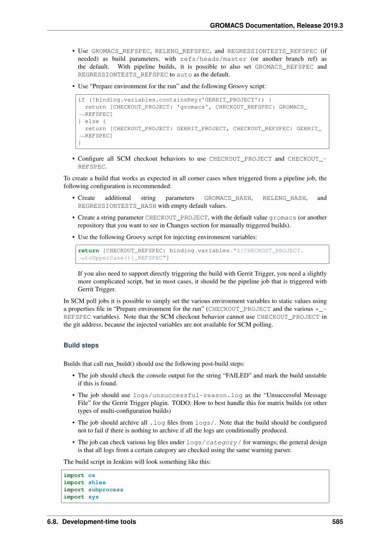
GROMACS Documentation, Release 2019.3
• Use GROMACS_REFSPEC, RELENG_REFSPEC, and REGRESSIONTESTS_REFSPEC (ifneeded) as build parameters, with refs/heads/master (or another branch ref) asthe default. With pipeline builds, it is possible to also set GROMACS_REFSPEC andREGRESSIONTESTS_REFSPEC to auto as the default.
• Use “Prepare environment for the run” and the following Groovy script:
if (!binding.variables.containsKey('GERRIT_PROJECT')) {return [CHECKOUT_PROJECT: 'gromacs', CHECKOUT_REFSPEC: GROMACS_
→˓REFSPEC]} else {
return [CHECKOUT_PROJECT: GERRIT_PROJECT, CHECKOUT_REFSPEC: GERRIT_→˓REFSPEC]}
• Configure all SCM checkout behaviors to use CHECKOUT_PROJECT and CHECKOUT_-REFSPEC.
To create a build that works as expected in all corner cases when triggered from a pipeline job, thefollowing configuration is recommended:
• Create additional string parameters GROMACS_HASH, RELENG_HASH, andREGRESSIONTESTS_HASH with empty default values.
• Create a string parameter CHECKOUT_PROJECT, with the default value gromacs (or anotherrepository that you want to see in Changes section for manually triggered builds).
• Use the following Groovy script for injecting environment variables:
return [CHECKOUT_REFSPEC: binding.variables."${CHECKOUT_PROJECT.→˓toUpperCase()}_REFSPEC"]
If you also need to support directly triggering the build with Gerrit Trigger, you need a slightlymore complicated script, but in most cases, it should be the pipeline job that is triggered withGerrit Trigger.
In SCM poll jobs it is possible to simply set the various environment variables to static values usinga properties file in “Prepare environment for the run” (CHECKOUT_PROJECT and the various *_-REFSPEC variables). Note that the SCM checkout behavior cannot use CHECKOUT_PROJECT inthe git address, because the injected variables are not available for SCM polling.
Build steps
Builds that call run_build() should use the following post-build steps:
• The job should check the console output for the string “FAILED” and mark the build unstableif this is found.
• The job should use logs/unsuccessful-reason.log as the “Unsuccessful MessageFile” for the Gerrit Trigger plugin. TODO: How to best handle this for matrix builds (or othertypes of multi-configuration builds)
• The job should archive all .log files from logs/. Note that the build should be configurednot to fail if there is nothing to archive if all the logs are conditionally produced.
• The job can check various log files under logs/category/ for warnings; the general designis that all logs from a certain category are checked using the same warning parser.
The build script in Jenkins will look something like this:
import osimport shleximport subprocessimport sys
6.8. Development-time tools 585
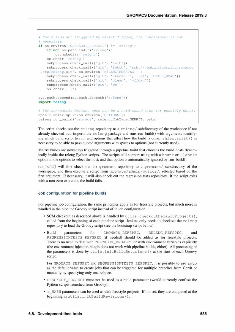
GROMACS Documentation, Release 2019.3
# For builds not triggered by Gerrit Trigger, the conditional is not# necessary.if os.environ['CHECKOUT_PROJECT'] != 'releng':
if not os.path.isdir('releng'):os.makedirs('releng')
os.chdir('releng')subprocess.check_call(['git', 'init'])subprocess.check_call(['git', 'fetch', 'ssh://[email protected].
→˓org/releng.git', os.environ['RELENG_REFSPEC']])subprocess.check_call(['git', 'checkout', '-qf', 'FETCH_HEAD'])subprocess.check_call(['git', 'clean', '-ffdxq'])subprocess.check_call(['git', 'gc'])os.chdir('..')
sys.path.append(os.path.abspath('releng'))import releng
# For non-matrix builds, opts can be a hard-coded list (or possibly None).opts = shlex.split(os.environ['OPTIONS'])releng.run_build('gromacs', releng.JobType.GERRIT, opts)
The script checks out the releng repository to a releng/ subdirectory of the workspace if notalready checked out, imports the releng package and runs run_build() with arguments identify-ing which build script to run, and options that affect how the build is done. shlex.split() isnecessary to be able to pass quoted arguments with spaces to options (not currently used).
Matrix builds are nowadays triggered through a pipeline build that chooses the build hosts dynam-ically inside the releng Python scripts. The scripts still support using with a host= or a label=option in the options to select the host, and that option is automatically ignored by run_build().
run_build() will first check out the gromacs repository to a gromacs/ subdirectory of theworkspace, and then execute a script from gromacs/admin/builds/, selected based on thefirst argument. If necessary, it will also check out the regression tests repository. If the script exitswith a non-zero exit code, the build fails.
Job configuration for pipeline builds
For pipeline job configuration, the same principles apply as for freestyle projects, but much more ishandled in the pipeline Groovy script instead of in job configuration.
• SCM checkout as described above is handled by utils.checkoutDefaultProject(),called from the beginning of each pipeline script. Jenkins only needs to checkout the relengrepository to load the Groovy script (see the bootstrap script below).
• Build parameters for GROMACS_REFSPEC, RELENG_REFSPEC, andREGRESSIONTESTS_REFSPEC (if needed) should be added as for freestyle projects.There is no need to deal with CHECKOUT_PROJECT or with environment variables explicitly(the environment injection plugin does not work with pipeline builds, either). All processing ofthe parameters is done by utils.initBuildRevisions() at the start of each Groovyscript.
For GROMACS_REFSPEC and REGRESSIONTESTS_REFSPEC, it is possible to use autoas the default value to create jobs that can be triggered for multiple branches from Gerrit ormanually by specifying only one refspec.
• CHECKOUT_PROJECT must not be used as a build parameter (would currently confuse thePython scripts launched from Groovy).
• *_HASH parameters can be used as with freestyle projects. If not set, they are computed at thebeginning in utils.initBuildRevisions().
6.8. Development-time tools 586
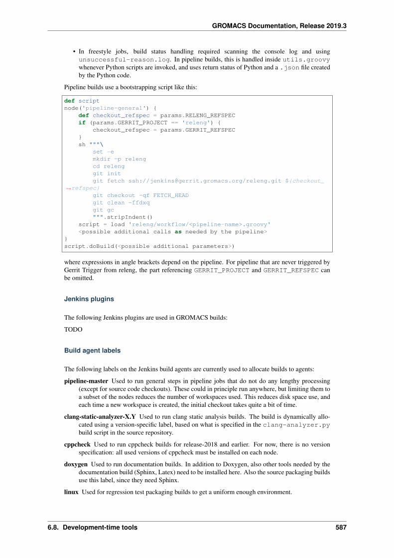
GROMACS Documentation, Release 2019.3
• In freestyle jobs, build status handling required scanning the console log and usingunsuccessful-reason.log. In pipeline builds, this is handled inside utils.groovywhenever Python scripts are invoked, and uses return status of Python and a .json file createdby the Python code.
Pipeline builds use a bootstrapping script like this:
def scriptnode('pipeline-general') {
def checkout_refspec = params.RELENG_REFSPECif (params.GERRIT_PROJECT == 'releng') {
checkout_refspec = params.GERRIT_REFSPEC}sh """\
set -emkdir -p relengcd relenggit initgit fetch ssh://[email protected]/releng.git ${checkout_
→˓refspec}git checkout -qf FETCH_HEADgit clean -ffdxqgit gc""".stripIndent()
script = load 'releng/workflow/<pipeline-name>.groovy'<possible additional calls as needed by the pipeline>
}script.doBuild(<possible additional parameters>)
where expressions in angle brackets depend on the pipeline. For pipeline that are never triggered byGerrit Trigger from releng, the part referencing GERRIT_PROJECT and GERRIT_REFSPEC canbe omitted.
Jenkins plugins
The following Jenkins plugins are used in GROMACS builds:
TODO
Build agent labels
The following labels on the Jenkins build agents are currently used to allocate builds to agents:
pipeline-master Used to run general steps in pipeline jobs that do not do any lengthy processing(except for source code checkouts). These could in principle run anywhere, but limiting them toa subset of the nodes reduces the number of workspaces used. This reduces disk space use, andeach time a new workspace is created, the initial checkout takes quite a bit of time.
clang-static-analyzer-X.Y Used to run clang static analysis builds. The build is dynamically allo-cated using a version-specific label, based on what is specified in the clang-analyzer.pybuild script in the source repository.
cppcheck Used to run cppcheck builds for release-2018 and earlier. For now, there is no versionspecification: all used versions of cppcheck must be installed on each node.
doxygen Used to run documentation builds. In addition to Doxygen, also other tools needed by thedocumentation build (Sphinx, Latex) need to be installed here. Also the source packaging buildsuse this label, since they need Sphinx.
linux Used for regression test packaging builds to get a uniform enough environment.
6.8. Development-time tools 587
GROMACS Documentation, Release 2019.3
windows Should not be currently used, but has been used to restrict Unix-specific things in pipelinesto not run on Windows agents.
In other cases, agents are explicitly assigned to a node. Multi-configuration builds are currentlyassigned to nodes based on information in agents.py, not on labels configured in Jenkins.
Interacting with builds in Jenkins
This page documents what kind of information GROMACS builds provide in Jenkins, how to accessit, and how to interact with the builds (e.g., trigger new ones). This also covers how the builds appearwhen reported back to Gerrit for builds triggered from there.
General
• General information about what a build does and how is typically available on the project pagein Jenkins (i.e., one level up from an individual build). Additional documentation is avail-able at Understanding Jenkins builds (page 565) (what the builds do), Pipeline build overview(page 574) (what the pipeline builds do) and Jenkins configuration (page 584) (on how Jenkinsis configured).
• The Changes section on any build summary page typically shows the changes that the buildcontains. For builds triggered from Gerrit, this is the title of the commit in Gerrit. For man-ually triggered builds, this is generally the newest change from the gromacs repository thatis included in the build. To see the full list of changes across all repositories (across all threerepositories), look at the console log. For pipeline jobs, this information is also available on thebuild summary page under Built revisions.
• Because of interplay between the three repositories and the Jenkins configuration, it is not al-ways possible for old changes to get a green build from Jenkins. A typical case is if change X hasbeen merged to gromacs, and change Y to regressiontests, and tests added/changed inY need X to pass. In such a case, any changes whose git ancestry does not include change X willget an unstable vote, even if they earlier passed Jenkins verification. So if you get seeminglyunrelated errors when uploading new versions of old changes, please check whether rebasingsolves the issue.
Also, no particular effort is put into maintaining releng backwards compatibility over longperiods of time if such a rebasing need already exists. This means that your build may also failwith mysterious Python errors from releng if the API has changed, if such a rebasing needexists and your change is particularly old.
Triggering builds
Gerrit automatically triggers builds for any change uploaded. This includes changes uploaded toregressiontests and releng, but the set of builds triggered depends on the repository. For any change,the build will be done with the change from Gerrit, combined with the latest merged change from theother repositories. For verifying simultaneous changes to more than one repository (most commonly,gromacs and one of the others), see on-demand builds and manual triggering below.
For drafts, Jenkins has to be added manually as reviewer so that Jenkins sees the change. It will startreviewing from the next patch set you upload to the draft, or you can trigger a build manually (seebelow).
If a change from Gerrit does not automatically trigger a build (e.g., because Jenkins was down whenyou uploaded your change), you can manually recreate the event using Query and Trigger GerritPatches on Jenkins main page.
If a change from Gerrit got built, but there was a technical/temporary problem with the build, you canuse Rebuild or Rebuild All links on the build summary page. This will do the build again and post theresults again to Gerrit. Rebuild builds only the build where it was clicked (it uses the results of the
6.8. Development-time tools 588
GROMACS Documentation, Release 2019.3
other, already done builds when reporting back). Rebuild All rebuilds all the triggered builds, in caseall or most of them had problems. It is not possible to rebuild only a part of the matrix job.
On-demand builds
Some types of builds are not automatically triggered from Gerrit when a patch set is uploaded, butinstead need to be requested with a specifically formatted comment in Gerrit. The general formatfor the comment is [JENKINS] followed by keywords for the build(s) requested. This mechanismcan also be used for cross-verification, i.e., verifying a different combination of changes than what istriggered by default. The general format is:
[JENKINS] [ Cross-verify <NNNN> [quiet] | release-<YYYY> ] [<builds>]
If Cross-verify is specified, it builds the current change together with the latest patch set ofchange number NNNN from Gerrit (should be from another project). If quiet is not specified,results are posted back to both changes (the NNNN change only if it is still open), but the vote is notaffected. For cross-verification with releng changes, the [JENKINS] comment needs to be posted inthe releng change to ensure that the correct releng scripts are used throughout the build.
If release-<YYYY> (name of a release branch) is specified, it builds the current change togetherwith release branch HEADs from other repositories. This only makes sense for releng changes, whereit should be run at least once before merging if there is a possibility that the changes impact buildsin the release branches. These do not run automatically (at least for now) to reduce peak load, andmake testing releng changes easier (since in many cases, the test builds that are actually interestingwill only run after the matrix builds have been cleared from the queue).
If neither of the above is specified, then the requested builds are built for this change.
With any of the above variants, possible builds are:
• Coverage: Triggers a coverage build.
• clang-analyzer: Triggers the per-patchset clang static analysis build.
• Documentation: Triggers the per-patchset documentation build.
• Nightly: Triggers a matrix build with the nightly matrix specified in the gromacs repository.
• Package: Triggers a packaging build. When triggered from a source or a regression testschange, packages that repository. When triggered from releng, packages both.
• Pre-submit: Triggers a matrix build with the pre-submit matrix specified in the gromacsrepository.
• Post-submit: Triggers a matrix build with the post-submit matrix specified in the gromacsrepository.
• Regtest-package: Triggers a packaging build of regression tests (mainly makes sense forreleng changes).
• Release: Triggers a release pipeline build for testing the release process. If no-dev is alsospecified (as Release no-dev), the pipeline builds the tarballs without -dev suffixes foractually doing a release.
• Uncrustify: Triggers the per-patchset uncrustify code style checker build.
• Update: When triggered from a regressiontests change, generates reference data for tests thatare missing it, and uploads those back to Gerrit.
• Update-regtest-hash: When triggered from a source change, generates the latest release-versioned regressiontests tarball for that branch, and updates the MD5 in the source repositoryto match this tarball.
More than one build can be requested with a single comment; the keywords should be separated bywhitespace. When the requested builds complete, a link to the build is posted back. In case there isjust a single build, the link points directly to it. If there are multiple, the link points to a pipeline build
6.8. Development-time tools 589
GROMACS Documentation, Release 2019.3
and the individual builds can be accessed through links on the build summary page (some types ofbuilds execute directly as part of the pipeline, and all information is accessible directly from the buildsummary page).
If no builds are specified, a default set of builds is triggered. For cross-verification (including therelease branch variant) from releng, it triggers all per-patchset builds. Otherwise, only the pre-submitmatrix build is triggered.
There can be also other content in the Gerrit comment that requests a build. The [JENKINS] tagmust appear at the start of a paragraph, and that paragraph as a whole will be interpreted as keywordsintended for Jenkins.
Manual triggering
To manually trigger a build (e.g., for testing job configuration changes), use Build with Parameters onthe project page, for the same builds that are triggered from Gerrit. Enter the refspecs (like refs/changes/53/2053/1) for the combination you want to build. This will not report anything backto Gerrit. The refspec for changes in Gerrit is of the form refs/changes/MM/NNMM/PP, whereNNMM is the number of the change and PP is the patch set number. You can see the refspec, e.g., inthe download links on the change page. Depending on how the job does the checkout, Jenkins mayagain need to be added as a reviewer for draft changes before manual triggering is possible.
For some pipeline jobs, the default values for other refspecs than releng are auto. If left at that value,the value will be interpreted as the head of the branch that matches the other refspecs. For example, ifREGRESSIONTESTS_REFSPEC is auto, and GROMACS_REFSPEC specifies a Gerrit change fromrelease-2019 branch, then regression tests will be used from the same branch.
Individual build types
These sections specify details of particular build types.
Matrix builds
Current matrix/multi-configuration builds are actually composed of two different Jenkins jobs: atriggering pipeline build (see Matrix build launcher (page 574)), and a child matrix build. Normally,a link to the child matrix build gets posted to Gerrit, and it mostly looks like a normal matrix build.Only if the triggering pipeline job fails, you will get a link to it.
Failed tests and compiler errors/warnings are aggregated on the matrix build summary page acrossall configurations, and you can navigate to individual issues through these links. If this is not suf-ficient to understand why the build fails/is unstable, you can check the console output of individualconfiguration builds by clicking on the build ball in the configuration matrix.
To retrigger a build triggered from Gerrit, you will need to navigate to the parent pipeline job. Youwill find the link towards the top of the build summary page, as “Started by upstream project . . .build number NNN”, and clicking on the build number will take you to the parent build. You can alsoretrigger the job directly from the dropdown that is available next to the build number link.
Similarly, to trigger a matrix build manually, you will need to do that for the pipeline job.
Documentation
TODO
6.8. Development-time tools 590
GROMACS Documentation, Release 2019.3
clang static analyzer
The build summary page shows the number of warnings/issues found in the console output of theanalyzer. You can see the individual issues through the link. Note that issues reported from code inthe header are not handled well by the tools we use, and we ignore those, but they are still shown inthis list.
The build is unstable only if there are issues found from source files (not headers). Details on eachissue is accessible through Analysis Report link on the left. This also includes the steps that theanalyzer thinks leads to the issue.
cppcheck
Summary of the changes is visible on the build summary page, and individual issues can be browsedby clicking on the links. The build is unstable if any issues are found.
uncrustify
To see the full list of issues, look at the console log.
releng
The build fails if any Python unit test in the releng repository fails. The actual reason can be seenin the console log, but currently there are no other indicators posted back to Gerrit or to the buildsummary page.
Known issues and limitations
The following issues, limitations, and potentially confusing behavior with the current Jenkins setupare known:
• Post-submit builds are triggered by Gerrit Trigger, but the results are not posted back to Gerrit.This is because new Gerrit versions are not compatible with the way the plugin posts the results(see JENKINS-39132).
• If builds are aborted, some bogus errors can get reported back to Gerrit, but the build statusshould say ABORTED. This is because there is no reasonable way to detect in all cases whethera build got aborted or failed because of other reasons. This is related to JENKINS-28822.
• If Jenkins gets restarted while builds triggered from Gerrit are running/queued, some of thesebuilds may get resumed after the restart. The in-memory state of Gerrit Trigger is not properlymaintained, and the vote from Jenkins only reflects the results from a subset of the builds. Youcan see this happening in Gerrit if there are less links to different builds than usual when Jenkinsvotes.
On-demand builds
• Only one on-demand build can be run at a time for the same patch set. If you post another[JENKINS] comment to a patch set before the previous such build has finished, such a com-ment will get silently ignored. This is how Gerrit Trigger plugin works.
• If an on-demand build is aborted (either manually, or because of a timeout), Jenkins votes -2on the change in Gerrit. For all other build results (either success or failure), Jenkins does notchange its vote (the pre-submit verification vote stays). This is a limitation in Gerrit Trigger (seeJENKINS-38743).
6.8. Development-time tools 591
GROMACS Documentation, Release 2019.3
Matrix builds
• If the build was aborted, there is no visual cue in the configuration matrix for the configurationsthat were not yet finished by the time the build was aborted. They look exactly like configu-rations that were not run at all. The summary of the triggering pipeline shows the links moreclearly.
• If the set of configurations has changed (in particular, if you are building a change in Gerrit thatchanges the configurations), the configuration matrix on the build summary page may not reflectthe actual configurations used (see JENKINS-30437). You can see the actual configurations thatwere built and their results from the console log, and navigate to the individual configurationsfrom there. Note, however, that the links in the console log take you to the project page, not tothe individual build, so you will need to click another time to get to the actual build. The childconfiguration builds always have the same build number as the matrix parent.
• If a matrix build contains configurations that are assigned to build agents that are not part ofthe (static) matrix node axis, these are not built. The matrix build still passes, but the triggeringpipeline build will detect this issue. The matrix build still shows up as successful in such ascenario, but the link posted to Gerrit says it failed.
How to do common things with Jenkins builds
See also Interacting with builds in Jenkins (page 588).
Add a new configuration to a build
To add a new configuration to an existing matrix build, the required steps vary a bit depending on howsimilar your configuration is to existing ones:
1. If the new configuration is just a new combination of existing options, it is sufficient to add theconfiguration to the respective file under admin/builds/, and test that it works. Changes topre-submit-matrix.txt will automatically get verified when you upload your changesto Gerrit.
(a) If your combination requires a specific combination of software that is not yet available,you will need to update releng/agents.py in the releng repo, and possibly installthat combination of software on a agent.
2. If the new configuration requires new options, but those options do not affect where the configu-ration can be built (i.e., do not require special software on the build agents), you need to updateadmin/builds/gromacs.py to specify the options and how they affect the build, and thenadd the configurations to the matrix in admin/builds/.
3. If the new configuration requires new options that affect job placement, you need to update
• releng/options.py to specify the new option and a label for it,
• releng/agents.py to specify which build agents support the option,
• possibly releng/environment.py to specify special CMake options or other config-uration (e.g., changes to PATH) that is required for the build to work with this option (ifyou need this, you also need to specify in releng/options.py that your new functionin releng/environment.py should be called to process your new option),
• possibly admin/builds/gromacs.py if your new option affects the build beyond thechanges above, and
• finally add the configuration to the matrix and test it.
6.8. Development-time tools 592
GROMACS Documentation, Release 2019.3
Add a new build agent
To add a new agent to be used for builds, the steps are outlined below:
1. Install the agent so that Jenkins can connect to it and the agent can connect to Gerrit (thisconfiguration is currently outside the scope of this documentation).
2. Install necessary software on the agent to be used in the builds (compilers and other tools).Please see releng/environment.py for how various programs are located, and installthem on the new agent to be found in the same way (if something seems awkward, the approachshould be changed on all agents, not by adding more variability).
3. Ensure that the agent is listed in releng/agents.py and has the correct labels and otherconstraints defined appropriately.
4. Ensure that the agent has relevant labels defined in Jenkins if it needs to run builds that rely onthem (see Jenkins configuration (page 584)).
If the agent does not get automatically used, follow steps above for adding a new configuration to usethe agent if it is intended for building one or more matrix configurations.
Add builds for a new release branch
After creating a release branch (in both gromacs and regressiontests repositories; relengis only using a single branch (master)), the following steps are needed to have full Jenkins buildsrunning for it:
• Clone all per-branch jobs in Jenkins from those for master. Currently this includes pre-submit,post-submit, and nightly matrix jobs, triggering pipelines for them, a nightly documentationbuild, and a release pipeline including two packaging builds. Work is in progress to remove theneed for per-branch pre-submit and post-submit triggering pipelines.
Adjust the Gerrit Trigger and/or SCM configuration and/or job parameter defaults for the clonedjobs to trigger from the correct branch. Also adjust the job descriptions if they contain branch-specific information.
Adjust the pipeline jobs to reference the correct per-branch jobs (the matrix jobs are referencedfrom the triggering pipelines, and the packaging jobs from the release pipeline).
Note that Copy Project link in Jenkins is not visible for pipeline jobs; you can achieve the sameeffect by selecting New Item at the top level and copying from an existing item.
TODO: The number of jobs required here could be reduced.
• Adjust the Gerrit Trigger configuration for jobs that are not branch-specific and add the newbranches as appropriate. Remove obsolete release branches from the triggering configuration.This step impacts non-matrix pre-submit verification jobs, and an on-demand pipeline job. Notethat Releng_PreSubmit is only triggered from releng and does not need to be considered here.
TODO: Consider either reducing the number of jobs affected, or consider using dynamic trig-gering configuration to be able to specify the supported branches in a single location.
• Adjust the list of branches for which workflow/releng-presubmit.groovy verifiesthe matrix configurations by editing the pipeline script.
Separate releng repository hosts various development-time scripts for GROMACS. Currently, thisis used for build scripts on the Jenkins CI system, but in the future, other scripts that do not have astrong connection to a particular code version could also live here, as well as documentation that canevolve separately from the source code (if not on the wiki).
The releng repository currently contains two main parts:
• releng Python package contains Python scripts used for Jenkins builds.
6.8. Development-time tools 593
GROMACS Documentation, Release 2019.3
• workflow subdirectory contains Groovy scripts for use with the Pipeline plugin (formerlyWorkflow plugin) for running jobs with more complicated control flow in Jenkins.
These are documented on separate pages above.
6.8.4 Source tree checker scripts
There is a set of Python scripts, currently under docs/doxygen/, that check various aspects of thesource tree for consistency. The script is based on producing an abstract representation of the sourcetree from various sources:
• List of files in the source tree (for overall layout of the source tree)
• List of installed headers (extracted from the generated build system)
• git attributes (to limit the scope of some checks)
• Doxygen XML documentation:
– For tags about public/private nature of documented headers and other constructs
– For actual documented constructs, to check them for consistency
• Hard-coded knowledge about the GROMACS source tree layout
This representation is then used for various purposes:
• Checking Doxygen documentation elements for common mistakes: missing brief descriptions,mismatches in file and class visibility, etc.
• Checking for consistent usage and documentation of headers: e.g., a header that is documentedas internal to a module should not be used outside that module.
• Checking for module-level cyclic dependencies
• Checking for consistent style and order of #include directives (see Guidelines for #include di-rectives (page 544))
• Actually sorting and reformatting #include directives to adhere to the checked style
• Generating dependency graphs between modules and for files within modules
The checks are run as part of a single check-source target, but are described in separate sec-tions below. In addition to printing the issues to stderr, the script also writes them into docs/doxygen/check-source.log for later inspection. Jenkins runs the checks as part of the Docu-mentation job, and the build is marked unstable if any issues are found.
For correct functionality, the scripts depend on correct usage of Doxygen annotations described inUsing Doxygen (page 553), in particular the visibility and API definitions in file-level comments.
For some false positives from the script, the suppression mechanism described below is the easiestway to silence the script, but otherwise the goal would be to minimize the number of suppressions.
The scripts require Python 2.7 (other versions may work, but have not been tested).
To understand how the scripts work internally, see comments in the Python source files under docs/doxygen/.
Checker details
The check-source target currently checks for a few different types of issues. These are listed indetail below, mainly related to documentation and include dependencies. Note in particular that theinclude dependency checks are much stricter for code in modules/directories that are documented witha \defgroup: all undocumented code is assumed to be internal to such modules. The rationale isthat such code has gotten some more attention, and some effort should also have been put into definingwhat is the external interface of the module and documenting it.
6.8. Development-time tools 594
GROMACS Documentation, Release 2019.3
• For all Doxygen documentation (currently does not apply for members that do not appear in thedocumentation):
– If a member has documentation, it should have a brief description.
– A note is issued for in-body documentation for functions, since this is ignored by our currentsettings.
– If a class has documentation, it should have public documentation only if it appears in aninstalled header.
– If a class and its containing file has documentation, the class documentation should not bevisible if the file documentation is not.
• For all files:
– Consistent usage of
#include "..." // This should be used for GROMACS headers
and
#include <...> // This should be used for system and external→˓headers
– Installed headers must not include non-installed headers. Headers can be marked for installwithin CMakeLists.txt files of their respective modules, using gmx_install_-headers().
– All source files must include “gmxpre.h” as the first header.
– A source/header file should include “config.h,” “gromacs/simd/simd.h”, or“gromacs/ewald/pme-simd.h” if and only if it uses a macro declared in such files.
– If the file has a git attribute to identify it as a candidate for include sorting, the include sorterdescribed below should not produce any changes (i.e., the file should follow Guidelines for#include directives (page 544)).
• For documented files:
– Installed headers should have public documentation, and other files should not.
– The API level specified for a file should not be higher than where its documentation isvisible. For example, only publicly documented headers should be specified as part of thepublic API.
– If an \ingroup module_foo exists, it should match the subdirectory that the file isactually part of in the file system.
– If a \defgroup module_foo exists for the subdirectory where the file is, the fileshould contain \ingroup module_foo.
– Files should not include other files whose documentation visibility is lower (if the includedfile is not documented, the check is skipped).
• For files that are part of documented modules (\defgroup module_foo exists for the sub-directory), or are explicitly documented to be internal or in the library API:
– Such files should not be included from outside their module if they are undocumented (fordocumented modules) or are not specified as part of library or public API.
• For all modules:
– There should not be cyclic include dependencies between modules.
As a side effect, the XML extraction makes Doxygen parse all comments in the code, even if they donot appear in the documentation. This can reveal latent issues in the comments, like invalid Doxygensyntax. The messages from the XML parsing are stored in docs/doxygen/doxygen-xml.login the build tree, similar to other Doxygen runs.
6.8. Development-time tools 595
GROMACS Documentation, Release 2019.3
Suppressing issues
The script is not currently perfect (either because of unfinished implementation, or because Doxygenbugs or incompleteness of the Doxygen XML output), and the current code also contains issues thatthe script detects, but the authors have not fixed. To allow the script to still be used, doxygen/suppressions.txt contains a list of issues that are filtered out from the report. The syntax issimple:
<file>: <text>
where <file> is a path to the file that reports the message, and <text> is the text reported. Bothsupport * as a wildcard. If <file> is empty, the suppression matches only messages that do nothave an associated file. <file> is matched against the trailing portion of the file name to make itwork even though the script reports absolute paths. Empty lines and lines starting with # are ignored.
To add a suppression for an issue, the line that reports the issue can be copied into suppressions.txt, and the line number (if any) removed. If the issue does not have a file name (or a pseudo-file)associated, a leading : must be added. To cover many similar issues, parts of the line can then bereplaced with wildcards.
A separate suppression mechanism is in place for cyclic dependencies: to suppress a cycle betweenmoduleA and moduleB, add a line with format
moduleA -> moduleB
into doxygen/cycle-suppressions.txt. This suppresses all cycles that contain the men-tioned edge. Since a cycle contains multiple edges, the suppression should be made for the edge thatis determined to be an incorrect dependency. This also affects the layout of the include dependencygraphs (see below): the suppressed edge is not considered when determining the dependency order,and is shown as invalid in the graph.
Include order sorting
The script checks include ordering according to Guidelines for #include directives (page 544). If it isnot obvious how the includes should be changed to make the script happy, or bulk changes are neededin multiple files, e.g., because of a header rename or making a previously public header private, it ispossible to run a Python script that does the sorting:
docs/doxygen/includesorter.py -S . -B ../build <files>
The script needs to know the location of the source tree (given with -S) and the build tree (given with-B), and sorts the given files. To sort the whole source tree, one can also use:
admin/reformat_all.sh includesort -B=../build
For the sorter to work correctly, the build tree should contain up-to-date list of installed files andDoxygen XML documentation. The former is created automatically when cmake is run, and thelatter can be built using the doxygen-xml target.
Note that currently, the sorter script does not change between angle brackets and quotes in includestatements.
Include dependency graphs
The same set of Python scripts can also produce include dependency graphs with some additionalannotations compared to what, e.g., Doxygen produces for a directory dependency graph. Currently,a module-level graph is automatically built when the Doxygen documentation is built and embeddedin the documentation (not in the public API documentation). The graph, together with a legend, is ona separate page: Module dependency graph
6.8. Development-time tools 596
GROMACS Documentation, Release 2019.3
The Python script produces the graphs in a format suitable for dot (from the graphviz package)to lay them out. The build system also provides a dep-graphs target that generates PNG filesfrom the intermediate dot files. In addition to the module-level graph, a file-level graph is producedfor each module, showing the include dependencies within that module. The file-level graphs canonly be viewed as the PNG files, with some explanation of the notation below. Currently, these aremostly for eye candy, but they can also be used for analyzing problematic dependencies to clean upthe architecture.
Both the intermediate .dot files and the final PNG files are put under docs/doxygen/depgraphs/ in the build tree.
File graphs
The graphs are written to module_name-deps.dot.png.
Node colors:
light blue public API (installed) headers
dark blue library API headers
gray source files
light green test files
white other files
Each edge signifies an include dependency; there is no additional information currently included.
6.8.5 Automatic source code formatting
The source code can be automatically formatted using uncrustify, an automatic source code formattingtool, to follow the guidelines in Guidelines for code formatting (page 542). Additionally, Pythonscripts are used for a few other automatic formatting/checking tasks. The overview tools page containsa list of these tools: Code formatting and style (page 606). This page provides more details foruncrustify and copyright scripts.
Jenkins uses these same scripts (in particular, uncrustify.sh and the check-source target)to enforce that the code stays invariant under such formatting.
Setting up uncrustify
A patched version of uncrustify is used for GROMACS. To set this up, you need to do these (once):
1. Change to a directory under which you want to build uncrustify and run:
git clone -b gromacs git://github.com/rolandschulz/uncrustify.gitcd uncrustify./configuremake
2. Copy the binary src/uncrustify into a directory of your choice (/path/to/uncrustify below).
Alternatively, if you are running Linux, you can try whether the binary from http://redmine.gromacs.org/issues/845 works for you.
In order to use the binary for uncrustify.sh and for the pre-commit hook, you also need to runthis in each of your GROMACS repositories:
git config hooks.uncrustifypath /path/to/uncrustify
6.8. Development-time tools 597
GROMACS Documentation, Release 2019.3
Alternatively, if you just want to use uncrustify.sh, you can set the UNCRUSTIFY environmentvariable to /path/to/uncrustify.
Using the pre-commit hook or git filters needs additional setup; see the respective sections below.
What is automatically formatted?
To identify which files are subject to automatic formatting, the scripts use git filters, specified in .gitattributes files. Only files that have the attribute filter set to one of the below values areprocessed:
• filter=uncrustify: uncrustify is run, copyright headers are checked, and include orderis enforced
• filter=uncrustify_only: only uncrustify is run
• filter=includesort: include order is enforced and copyright headers are checked
• filter=copyright: only copyright headers are checked
Other files are ignored by uncrustify.sh and reformat_all.sh scripts (see below).
Scripts
copyright.py
This script provides low-level functionality to check and update copyright headers in C/C++ sourcefiles, as well as in several other types of files like CMake and Python scripts.
This file is also used as a loadable Python module for kernel generators, and provides the functionalityto generate conformant copyright headers for such scripts.
The script is similar to uncrustify in that there is rarely need to run it directly, but instead the bashscripts below use it internally. You can run the script with --help option if you want to see what alloptions it provides if you need to do some maintenance on the copyright headers themselves.
uncrustify.sh
This script runs uncrustify and copyright.py on modified files and reports/applies the results. Bydefault, the current HEAD commit is compared to the work tree, and files that
1. are different between these two trees and
2. change under uncrustify and/or have outdated copyright header
are reported. This behavior can be changed by
1. Specifying an --rev=REV argument, which uses REV instead of HEAD as the base of thecomparison. A typical use case is to specify --rev=HEAD^ to check the HEAD commit.
2. Specifying an action:
• check-*: reports the files that uncrustify changes
• diff-*: prints the actual diff of what would change
• update-*: applies the changes to the repository
• *-workdir: operates on the working directory (files on disk)
• *-index: operates on the index of the repository
For convenience, if you omit the workdir/index suffix, workdir is assumed (i.e., diff equalsdiff-workdir).
6.8. Development-time tools 598
GROMACS Documentation, Release 2019.3
3. Specifying --uncrustify=off, which does not run uncrustify.
4. Specifying --copyright=<mode>, which alters the level of copyright checking is done:
off does not check copyright headers at all
year only update copyright year in new-format copyright headers
add in addition to year, add copyright headers to files that do not have any
update in addition to year and add, also update new-format copyright headers if they arebroken or outdated
replace replace any copyright header with a new-format copyright header
full do all of the above
By default, update-* refuses to update dirty files (i.e., that differ between the disk and the index)to make it easy to revert the changes. This can be overridden by adding a -f/--force option.
git pre-commit hook
If you want to run uncrustify.sh automatically for changes you make, you can configure apre-commit hook using admin/git-pre-commit:
1. Copy the git-pre-commit script to .git/hooks/pre-commit.
2. Specify the path to uncrustify for the hook if you have not already done so:
git config hooks.uncrustifypath /path/to/uncrustify
3. Set the operation mode for the hook:
git config hooks.uncrustifymode checkgit config hooks.copyrightmode update
With this configuration, all source files modified in the commit are run through uncrustify and checkedfor correct copyright headers. If any file would be changed by uncrustify.sh, the names of thosefiles are reported and the commit is prevented. The issues can be fixed by running uncrustify.shmanually.
To disable the hook without removing the pre-commit file, you can set
git config hooks.uncrustifymode offgit config hooks.copyrightmode off
To disable it temporarily for a commit, set NO_FORMAT_CHECK environment variable. For exam-ple,
NO_FORMAT_CHECK=1 git commit -a
You can also run git commit --no-verify, but that also disables other hooks, such as theChange-Id commit-msg hook used by Gerrit.
Note that when you run git commit --amend, the hook is only run for the changes that aregetting amended, not for the whole commit. During a rebase, the hook is not run.
The actual work is done by the admin/uncrustify.sh script, which gets run with thecheck-index action, and with --uncrustify and --copyright getting set according tothe git config settings.
6.8. Development-time tools 599
GROMACS Documentation, Release 2019.3
reformat_all.sh
This script runs uncrustify, copyright.py, or the include sorter for all applicable files in the sourcetree. See reformat_all.sh -h for the invocation.
The script can also produce the list of files for which these commands would be run. To do this, specifylist-files on the command line and use --filter=<type> to specify which command to getthe file list for. This can be used together with, e.g., xargs to run other scripts on the same set offiles.
For all the operations, it is also possible to apply patters (of the same style that various git commandsaccept, i.e., src/*.cpp matches all .cpp files recursively under src/). The patterns can bespecified with --pattern=<pattern>, and multiple --pattern arguments can be given.
As with uncrustify.sh, -f/--force is necessary if the working tree and the git index do notmatch.
Using git filters
An alternative to using a pre-commit hook to automatically apply uncrustify on changes is to use agit filter (does not require uncrustify.sh, only the .gitattributes file). You can run
git config filter.uncrustify.clean \"/path/to/uncrustify -c admin/uncrustify.cfg -q -l cpp"
To configure a filter for all files that specify filter=uncrustify attribute.
The pre-commit hook + manually running uncrustify.sh gives better/more intuitive control(with the filter, it is possible to have a work tree that is different from HEAD and still have an emptygit diff) and provides better performance for changes that modify many files. It is the only waythat currently also checks the copyright headers.
The filter allows one to transparently merge branches that have not been run through uncrustify, andis applied more consistently (the pre-commit hook is not run for every commit, e.g., during a rebase).
6.8.6 Unit testing
The main goal of unit tests in GROMACS is to help developers while developing the code. Theyfocus on testing functionality of a certain module or a group of closely related modules. They aredesigned for quick execution, such that they are easy to run after every change to check that nothinghas been broken.
Finding, building and running
As described in Source code organization (page 518), src/gromacs/ is divided into modules, eachcorresponding to a subdirectory. If available, unit tests for that module can be found in a tests/subdirectory under the top-level module directory. Typically, tests for code in file.h in the moduleis in a corresponding tests/file.cpp. Not all files have corresponding tests, as it may not makesense to test that individual file in isolation. Focus of the tests is on functionality exposed outsidethe module. Some of the tests, in particular for higher-level modules, are more like integration tests,and test the functionality of multiple modules. Shared code used to implement the tests is in src/external/gmock-1.7.0/ and src/testutils/ (see below).
The tests are built if BUILD_TESTING=ON (the default) and GMX_BUILD_UNITTESTS=ON (thedefault) in CMake. Each module produces a separate unit test binary (module-test) under bin/,which can execute all the tests for that module.
The tests can be executed in a few different ways:
6.8. Development-time tools 600
GROMACS Documentation, Release 2019.3
• Build the test target (e.g., make test): This runs all the tests using CTest. This includesalso the regression tests if CMake has been told where to find them (regression tests are not dis-cussed further on this page). If some of the tests fail, this only prints basic summary information(only a pass/fail status for each test binary or regression test class). You can execute the failingtest binaries individually to get more information on the failure. Note that make test doesnot rebuild the test binaries if you have changed the source code, so you need to separately runmake or make tests. The latter only builds the test binaries and their dependencies.
• Build the check target (e.g., make check): This behaves the same as the test target, witha few extensions:
1. Test binaries are rebuilt if they are outdated before the tests are run.
2. If a test fails, the output of the test binary is shown.
3. If unit tests and/or regression tests are not available, a message is printed.
• Directly executing a test binary. This provides the most useful output for diagnosing failures, andallows debugging test failures. The output identifies the individual test(s) that fail, and showsthe results of all failing assertions. Some tests also add extra information to failing assertions tomake it easier to identify the reason. It is possible to control which tests are run using commandline options. Execute the binary with -h to get additional information.
When executed using CTest, the tests produce XML output in Testing/Temporary/, containingthe result of each test as well as failure messages. This XML is used by Jenkins for reporting thetest status for individual tests. Note that if a test crashes or fails because of an assert or a gmx_fatal()call, no XML is produced for the binary, and Jenkins does not report anything for the test binary. Theactual error is only visible in the console output.
Unit testing framework
The tests are written using Google Test, which provides a framework for writing unit tests and com-piling them into a test binary. Most of the command line options provided by the test binaries areimplemented by Google Test. See the Google Test Primer for an introduction. Some tests also useGoogle Mock, which provides a framework for creating mock implementations of C++ classes. Bothcomponents are included in the source tree under src/external/gmock-1.7.0/, and are com-piled as part of the unit test build.
src/testutils/ contains GROMACS-specific shared test code. This includes a few parts:
• CMake macros for declaring test binaries. These take care of providing the main() methodfor the test executables and initializing the other parts of the framework, so that the test codein modules can focus on the actual tests. This is the only part of the framework that you needto know to be able to write simple tests: you can use gmx_add_unit_test() in CMake tocreate your test binary and start writing the actual tests right away. See src/testutils/TestMacros.cmake and existing CMake code for examples how to use them.
• Generic test fixtures and helper classes. The C++ API is documented on Doxygen page fortestutils. Functionality here includes locating test input files from the source directory and con-structing temporary files, adding custom command line options to the test binary, some customtest assertions for better exception and floating-point handling, utilities for constructing com-mand line argument arrays, and test fixtures for tests that need to test long strings for correctnessand for tests that execute legacy code where stdin reading etc. cannot be easily mocked.
• Some classes and functions to support the above. This code is for internal use of the CMakemachinery to build and set up the test binaries, and to customize Google Test to suit our envi-ronment.
• Simple framework for building tests that check the results against reference data that is generatedby the same test code. This can be used if it is not easy to verify the results of the code withC/C++ code alone, but manual inspection of the results is manageable. The general approach isdocumented on the Doxygen page on using the reference data.
6.8. Development-time tools 601
GROMACS Documentation, Release 2019.3
In addition to src/testutils/, some of the module test directories may provide reusabletest code that is used in higher-level tests. For example, the src/gromacs/analysisdata/tests/ provides test fixtures, a mock implementation for gmx::IAnalysisDataModule, and somehelper classes that are also used in src/gromacs/trajectoryanalysis/tests/. Thesecases are handled using CMake object libraries that are linked to all the test binaries that need them.
Getting started with new tests
To start working with new tests, you should first read the Google Test documentation to get a basicunderstanding of the testing framework, and read the above description to understand how the tests areorganized in GROMACS. It is not necessary to understand all the details, but an overall understandinghelps to get started.
Writing a basic test is straightforward, and you can look at existing tests for examples. The exist-ing tests have a varying level of complexity, so here are some pointers to find tests that use certainfunctionality:
• src/gromacs/utility/tests/stringutil.cpp contains very simple tests for func-tions. These do not use any fancy functionality, only plain Google Test assertions. The onlything required for these tests is the TEST() macro and the block following it, plus headersrequired to make them compile.
• The same file contains also simple tests using the reference framework to check line wrap-ping (the tests for gmx::TextLineWrapper). The test fixture for these tests is in src/testutils/stringtest.h/.cpp. The string test fixture also demonstrates how to add acustom command line option to the test binary to influence the test execution.
• src/gromacs/selection/tests/ contains more complex use of the reference frame-work. This is the code the reference framework was originally written for. src/gromacs/selection/tests/selectioncollection.cpp is the main file to look at.
• For more complex tests that do not use the reference framework, but instead do more complexverification in code, you can look at src/gromacs/selection/tests/nbsearch.cpp.
• For complex tests with mock-up classes and the reference framework, you can look at src/gromacs/analysisdata/tests/.
Here are some things to keep in mind when working with the unit tests:
• Try to keep the execution time for the tests as short as possible, while covering the most im-portant paths in the code under test. Generally, tests should take seconds instead of minutes torun, so that no one needs to hesitate before running the tests after they have done some changes.Long-running tests should go somewhere else than in the unit test set. Note that Jenkins runsmany of the tests under Valgrind, so heavy tests are going to slow down also that part of theverification.
• Try to produce useful messages when a test assertion fails. The assertion message should tellwhat went wrong, with no need to run the test itself under a debugger (e.g., if the assertion iswithin a loop, and the loop index is relevant for understanding why the assertion fails, it shouldbe included in the message). Even better if even a user can understand what goes wrong, but themain audience for the messages is the developer who caused the test to fail.
6.8.7 Physical validation
Physical validation tests check whether simulation results correspond to physical (or mathematical)expectations.
Unlike the existing tests, we are not be able to keep these tests in the “seconds, not minutes” timeframe, rather aiming for “hours, not days”. They should therefore be ran periodically, but probablynot for every build.
6.8. Development-time tools 602
GROMACS Documentation, Release 2019.3
Also, given the long run time, it will in many cases be necessary to separate running of the systems(e.g. to run it at a specific time, or on a different resource), such that the make script does give theoption to
• prepare run files and an execution script,
• analyze already present simulations,
• or prepare, run and analyze in one go.
Test description
Currently, simulation results are tested against three physically / mathematically expected results:
• Integrator convergence: A symplectic integrator can be shown to conserve a constant of motion(such as the energy in a micro-canonical simulation) up to a fluctuation that is quadratic in timestep chosen. Comparing two or more constant-of-motion trajectories realized using differenttime steps (but otherwise unchanged simulation parameters) allows a check of the symplecticityof the integration. Note that lack of symplecticity does not necessarily imply an error in theintegration algorithm, it can also hint at physical violations in other parts of the model, such asnon-continuous potential functions, imprecise handling of constraints, etc.
• Kinetic energy distribution: The kinetic energy trajectory of a (equilibrated) system sampling acanonical or an isothermal-isobaric ensemble is expected to be Maxwell-Boltzmann distributed.The similarity between the physically expected and the observed distribution allows to validatethe sampled kinetic energy ensemble.
• Distribution of configurational quantities: As the distribution of configurational quantities likethe potential energy or the volume are in general not known analytically, testing the likelihood ofa trajectory sampling a given ensemble is less straightforward than for the kinetic energy. How-ever, generally, the ratio of the probability distribution between samples of the same ensemble atdifferent state points (e.g. at different temperatures, different pressures) is known. Comparingtwo simulations at different state points therefore allows a validation of the sampled ensemble.
The physical validation included in GROMACS tests a range of the most-used settings on severalsystems. The general philosophy is to leave most settings to default values with the exception ofthe ones explicitly tested in order to be sensitive to changes in the default values. The test set willbe enlarged as we discover interesting test systems and corner cases. Under double precision, someadditional tests are ran, and some other tests are ran using a lower tolerance.
Integrator convergence
All simulations performed under NVE on Argon (1000 atoms) and water (900 molecules) systems.As these tests are very sensitive to numerical imprecision, they are performed with long-range cor-rections for both Lennard-Jones and electrostatic interactions, with a very low pair-list tolerance(verlet-buffer-tolerance = 1e-10), and high LINCS settings where applicable.
Argon:
• Integrators: - integrator = md - integrator = md-vv
• Long-range corrections LJ: - vdwtype = PME - vdwtype = cut-off, vdw-modifier= force-switch, rvdw-switch = 0.8
Water:
• Integrators: - integrator = md - integrator = md-vv
• Long-range corrections LJ: - vdwtype = PME - vdwtype = cut-off, vdw-modifier= force-switch, rvdw-switch = 0.8
• Long-range corrections electrostatics: - coulombtype = PME, fourierspacing = 0.05
6.8. Development-time tools 603
GROMACS Documentation, Release 2019.3
• Constraint algorithms: - constraint-algorithm = lincs, lincs-order = 6,lincs-iter = 2 - constraint-algorithm = none - SETTLE
Ensemble tests
The generated ensembles are tested with Argon (1000 atoms) and water (900 molecules, with SET-TLE and PME) systems, in the following combinations:
• integrator = md, tcoupl = v-rescale, tau-t = 0.1, ref-t = 87.0 (Ar-gon) or ref-t = 298.15 (Water)
• integrator = md, tcoupl = v-rescale, tau-t = 0.1, ref-t = 87.0 (Ar-gon) or ref-t = 298.15 (Water), pcoupl = parrinello-rahman, ref-p = 1.0,compressibility = 4.5e-5
• integrator = md-vv, tcoupl = v-rescale, tau-t = 0.1, ref-t = 87.0(Argon) or ref-t = 298.15 (Water)
• integrator = md-vv, tcoupl = nose-hoover, tau-t = 1.0, ref-t =87.0 (Argon) or ref-t = 298.15 (Water), pcoupl = mttk, ref-p = 1.0,compressibility = 4.5e-5
All thermostats are applied to the entire system (tc-grps = system). The simulations run for1ns at 2fs time step with Verlet cut-off. All other settings left to default values.
Building and testing using the build system
Since these tests can not be ran at the same frequency as the current tests, they are kept strictly opt-invia -DGMX_PHYSICAL_VALIDATION=ON, with -DGMX_PHYSICAL_VALIDATION=OFF be-ing the default. Independently of that, all previously existing build targets are unchanged, includingmake check.
If physical validation is turned on, a number of additional make targets can be used:
• make check is unchanged, it builds the main binaries and the unit tests, then runs the unittests and, if available, the regression tests.
• make check-phys builds the main binaries, then runs the physical validation tests. Warn-ing: This requires to simulate all systems and might take several hours on a average machine!
• make check-all combines make check and make check-phys.
As the simulations needed to perform the physical validation tests may take long, it might be advan-tageous to run them on an external resource. To enable this, two additional make targets are present:
• make check-phys-prepare prepares all simulation files under tests/physicalvalidation of the build directory, as well as a rudimentary run script inthe same directory.
• make check-phys-analyze runs the same tests as make check-phys, but does notsimulate the systems. Instead, this target assumes that the results can be found under tests/physicalvalidation of the build directory.
The intended usage of these additional targets is to prepare the simulation files, then run them on adifferent resource or at a different time, and later analyze them. If you want to use this, be aware (i)that the run script generated is very simple and might need (considerable) tuning to work with yoursetup, and (ii) that the analysis script is sensitive to the folder structure, so make sure to preserve itwhen copying the results to / from another resource.
Additionally to the mentioned make targets, a number of internal make targets are defined.These are not intended to be used directly, but are necessary to support the functionality de-scribed above, especially the complex dependencies. These internal targets include run-ctest,run-ctest-nophys, run-ctest-phys and run-ctest-phys-analyze running the
6.8. Development-time tools 604
GROMACS Documentation, Release 2019.3
different tests, run-physval-sims running the simulations for physical validation, andmissing-tests-notice, missing-tests-notice-all, missing-phys-val-phys,missing-phys-val-phys-analyze and missing-phys-val-all notifying users aboutmissing tests.
Direct usage of the python script
The make commands mentioned above are calling the python script tests/physicalvalidation/gmx_physicalvalidation.py, which can be used independentlyof the make system. Use the -h flag for the general usage information, and the --tests for moredetails on the available physical validations.
The script requires a json file defining the tests as an input. Among other options, it allows to definethe GROMACS binary and the working directory to be used, and to decide whether to only preparethe simulations, prepare and run the simulations, only analyze the simulations, or do all three steps atonce.
Adding new tests
The available tests are listed in the systems.json (tests standardly used for single precision builds)and systems_d.json (tests standardly used for double precision builds) files in the same directory,the GROMACS files are in the folder systems/.
The json files lists the different test. Each test has a "name" attribute, which needs to be unique,a "dir" attribute, which denotes the directory of the system (inside the systems/ directory) tobe tested, and a "test" attribute which lists the validations to be performed on the system. Addi-tionally, the optional "grompp_args" and "mdrun_args" attributes allow to pass specific argu-ments to gmx grompp or gmx mdrun, respectively. A single test can contain several validations,and several independent tests can be performed on the same input files.
To add a new test to a present system, add the test name and the arguments to the json file(s). Touse a new system, add a subfolder in the systems/ directory containing input/system.{gro,mdp,top} files defining your system.
6.8.8 Change management
GROMACS change management is supported by the following tools. (For change submission guide-lines, refer to Contribute to GROMACS (page 515).)
git GROMACS uses git as the version control system. Instructions for setting up git for GROMACS,as well as tips and tricks for its use, can be found in GROMACS change management (page 528).
Other basic tutorial material for git can be found on the web.
Gerrit All code changes go through a code review system at http://gerrit.gromacs.org.
Jenkins All changes pushed to Gerrit are automatically compiled and otherwise checked on variousplatforms using a continuous integration system at http://jenkins.gromacs.org. UnderstandingJenkins builds (page 565) documents how Jenkins interacts with the build system, providinginformation on how to replicate the builds Jenkins does (e.g., to diagnose issues). releng repos-itory (page 568) provides more information on the technical implementation of the builds.
Redmine Bugs and issues, as well as some random features and discussions, are tracked at http://redmine.gromacs.org.
6.8.9 Build system
CMake Main tool used in the build system.
6.8. Development-time tools 605
GROMACS Documentation, Release 2019.3
packaging for distribution (CPack)
unit testing (CTest) GROMACS uses a unit testing framework based on Google C++ Testing Frame-work (gtest) and CTest. All unit tests are automatically run on Jenkins for each commit. Detailscan be found on a separate page on Unit testing (page 600).
regression tests
clang-tidy clang-tidy is used for static code analysis. clang-tidy is easy to install. It is con-tained in the llvm binary package. Only version 7.0.* with libstdc++<7 or libc++ is sup-ported. Others might miss tests or give false positives. It is run automatically on Jenkins foreach commit. Many checks have fixes which can automatically be applied. To run it, thebuild has to be configured with cmake -DGMX_CLANG_TIDY=ON -DGMX_OPENMP=no-DCMAKE_BUILD_TYPE=Debug -DCMAKE_EXPORT_COMPILE_COMMANDS=on. AnyCMAKE_BUILD_TYPE which enables asserts (e.g. ASAN) works. Such a configured buildwill run both the compiler as well as clang-tidy when building. The name of the clang-tidyexecutable is set with
-DCLANG_TIDY=..., and the full path to it can be set with -DCLANG_TIDY_EXE=....To apply the automatic fixes to the issue identified clang-tidy should be run sepereately(running clang-tidy with -fix as part of the build can corrupt header files). To fix aspecific file run clang-tidy -fix -header-filter '.*' {file}, to fix allfiles in parallel run-clang-tidy.py -fix -header-filter '.*' '(?<!/selection/parser\.cpp|selection/scanner\.cpp)$', and to fix all modifiedfiles run-clang-tidy.py -fix -header-filter '.*' $(git diff HEAD--name-only). The run-clang-tidy.py script is in the share/clang/ subfolder of thellvm distribution. clang-tidy has to be able to find the compile_commands.json file.Eithe run from the build folder or add a symlink to the source folder.
clang static analyzer
coverage
6.8.10 Code formatting and style
The tools and scripts listed below are used to automatically check/apply formatting that follows GRO-MACS style guidelines described on a separate page: Style guidelines (page 542).
uncrustify uncrustify is used for automatic indentation and other formatting of the source code tofollow Guidelines for code formatting (page 542). All code must remain invariant under uncrus-tify with the config at admin/uncrustify.cfg. A patched version of uncrustify is used.See Automatic source code formatting (page 597) for details.
admin/copyright.py This Python script adds and formats copyright headers in source files.uncrustify.sh (see below) uses the script to check/update copyright years on changed filesautomatically.
admin/uncrustify.sh This bash script runs uncrustify and copyright.py for all files thathave local changes and checks that they conform to the prescribed style. Optionally, the scriptcan also apply changes to make the files conform. This script is automatically run by Jenkins toensure that all commits adhere to Guidelines for code formatting (page 542). If the uncrustifyjob does not succeed, it means that this script has something to complain. See Automatic sourcecode formatting (page 597) for details.
admin/git-pre-commit This sample git pre-commit hook can be used if one wants to applyuncrustify.sh automatically before every commit to check for formatting issues. See Au-tomatic source code formatting (page 597) for details.
docs/doxygen/includesorter.py This Python script sorts and reformats #include direc-tives according to the guidelines at Guidelines for #include directives (page 544). Details aredocumented on a separate page (with the whole suite of Python scripts used for source codechecks): Include order sorting (page 596).
6.8. Development-time tools 606
GROMACS Documentation, Release 2019.3
include directive checker In its present form, the above include sorter script cannot be conve-niently applied in uncrustify.sh. To check for issues, it is instead integrated into acheck-source build target. When this target is built, it also checks for include formattingissues. Internally, it uses the sorter script. This check is run in Jenkins as part of the Docu-mentation job. Details for the checking mechanism are on a separate page (common for severalcheckers): Source tree checker scripts (page 594).
admin/reformat_all.sh This bash script runs uncrustify/copyright.py/include sorteron all relevant files in the source tree (or in a particular directory). The script can also pro-duce the list of files where these scripts are applied, for use with other scripts. See Automaticsource code formatting (page 597) for details.
git attributes git attributes (specified in .gitattributes files) are used to annotate which filesare subject to automatic formatting checks (and for automatic reformatting by the above scripts).See man gitattributes for an overview of the mechanism. We use the filter attributeto specify the type of automatic checking/formatting to apply. Custom attributes are used forspecifying some build system dependencies for easier processing in CMake.
include-what-you-use
6.9 Known issues relevant for developers
This is a non-exhaustive list of known issues that have been observed and can be of interest fordevelopers. These have not been solved because they are either outside the scope of the GROMACSproject or are are simply too difficult or tedious to address ourselves.
6.9.1 FP exceptions with CUDA 7.0
When using CUDA 7.0 in a Debug build, if the PME FFT task is offloaded to a GPU, a floating pointexception will abort the mdrun (page 111) execution. The exception originates from the CUDA FFT(cuFFT) library. To avoid this issue, we advise using a later CUDA version.
6.9.2 Issues with GPU timer with OpenCL
When building using OpenCL in Debug mode, it can happen that the GPU timer state gets corrupted,leading to an assertion failure during the mdrun (page 111). This seems to be related to the load ofother, unrelated tasks on the GPU.
6.9. Known issues relevant for developers 607

CHAPTER
SEVEN
DOXYGEN DOCUMENTATION
The doxygen code documentation is available on the GROMACS webpage.
608
Related Documents