Manipulation of Proteins, Cells, & Endoscopy Optics with Piezoelectric Devices A Dissertation Presented to the Faculty of the Graduate School of Cornell University In Partial Fulfillment of the Requirements for the Degree of Doctor of Philosophy by Grant David Meyer May 2008

Welcome message from author
This document is posted to help you gain knowledge. Please leave a comment to let me know what you think about it! Share it to your friends and learn new things together.
Transcript

Manipulation of Proteins, Cells, & Endoscopy Optics with Piezoelectric Devices
A Dissertation
Presented to the Faculty of the Graduate School
of Cornell University
In Partial Fulfillment of the Requirements for the Degree of
Doctor of Philosophy
by
Grant David Meyer
May 2008
iii

© 2008 Grant David Meyer
iv

Manipulation of Proteins, Cells, & Endoscopy Optics with Piezoelectric Devices
Grant David Meyer, Ph.D.
Cornell University 2008
Piezoelectric devices convert electrical energy into mechanical energy yielding
static deflection or oscillatory motion. With quartz crystal resonators, surface acoustic
wave devices, and lead zirconate titanate actuators, proteins, cells, and endoscope
optics were manipulated. Chapters two through five detail accelerated protein and cell
release from planar substrates with quartz crystal resonators and surface acoustic wave
devices. Targeted applications include immunoassays, cell separation, and cell
membrane permeation. Results demonstrate acoustic wave dissipation into the fluid
resting upon the oscillating surface accelerated nonspecific binding removal, while
minimally removing bound antigen from antibodies, a common immunoassay
challenge. An optimal difference in specific vs. nonspecific protein release rates was
found at 100 mW using 5 MHz quartz crystal resonators. Because surface acoustic
wave devices produce higher peak fluid velocities, approximately 10-fold relative to
quartz crystal resonators, nonspecific protein and cell release experiments were
extended to surface acoustic wave devices. Surface acoustic wave induced protein
desorption, nonspecific cell release, and spatially dependent cell membrane
permeation results are presented. In chapter six we detail a miniature two-dimensional
fiber optic scanner design, fabrication, and fiber characterization methods for a real-
time in vivo multi-photon endoscope.
v

BIOGRAPHICAL SKETCH
Family, friends, and fine professors have all contributed to Grant’s current state. It
is with warmest regards and sincere gratitude that he thanks each group for their time,
thoughts, opinions, patience, and intellectual contributions.
He is particularly thankful to have had parents, Richard and Debbie who required
dedication to academics, yet encouraged participation in, and attended, myriad
sporting events, ranging from baseball to racquetball. He truly benefited from this
balanced approach. Raised with “in-house” tutors possessing satellite and medical
research expertise, it is no surprise his interests reside at the physical/biological
interface.
His sisters, Lindsay and Lauren, taught him much about the other half of society,
of which, admittedly, he has primitive understanding. Having narrowly escaped his
early, unrefined club swinging years, each can attest to his failure to progress from
barbaric beginnings.
Raised in the shadow of the Atomic Age, surrounded by academic excellence
diffusing from nuclear power, he was exposed to many physicists, chemists, and
mathematicians. Notable individuals include Professors James Brozik and Robert
Duncan who are extraordinary role models and fine men.
Influenced by this environment, Grant pursued physics, chemistry, and pure
mathematics at the University of New Mexico. He then traveled east to pursue
biosensor and molecular diagnostics R&D with alacrity. In the East he was influenced
by the many notable individuals listed in the Acknowledgment section.
iii

ACKNOWLEDGMENT
Professor Harold Craighead most significantly influenced this work. His
analytical rigor and quest for meaningful results are core values often uttered, but
rarely found.
Professors Barbara Baird and Mike Shuler both provided constructive
encouragement, which caused me to pursue a better understanding of proteins at the
molecular level and better quantitative methods.
Chris Schaffer, Larry Walker, & Dr. Shivaun Archer each provided opportunities
for growth and much needed constructive re-direction. Each has significantly
contributed to solid students.
The nocturnal Rob Ilic was an interesting clean-room tutor and extraordinary
character. His inexhaustible energy and extensive fabrication knowledge are rare
assets.
Numerous lab members fielded myriad questions, which contributed to a better of
understanding of my experiments. I thank you all for your time and help.
Working with the Professors Watt Webb, Chris Xu, and Dr. Hyungsik Lim to
develop a real-time in vivo tissue imaging endoscope was a particularly rewarding
conclusion to my time at Cornell. I thank each of you for the opportunity to pursue
this novel surgical device. Future patients and taxpayers will undoubtedly benefit
from your hard work.
Behind the scenes there were many individuals coordinating meetings, re-orienting
confused graduate students, and diligently ensuring system components engage. I am
thankful to Lorraine Capogrossi, Vicki Dann, and Mark Williams for their support.
John Jaquette always pushed me to differentiate my skills. His keen grasp of
reality and social awareness are remarkable.
Gene Fitzgerald, Abe Stroock, & Andreas Wankerl were strong sources of
iv

positivity and indomitable spirits. I thank each of you for your unrelenting optimism
genuine dedication to the innovation process.
Professor McAdams, my favorite irascible economics professor, significantly
improved my ability to understand the “big” picture. His ability to keep his eye on the
ball is remarkable.
John Mannion, Andrew Chadeayne, Andrew Holmberg, Dave Manke, Bryan
Ricchetti, Daniel Freedman, Mike Goulet, José Morán-Mirabal, Don Aubrecht, Felix
Zamora, Peter Merkx & the Men of Mystery were boundless sources of energy,
creativity, and interesting conversation—a truly unique cast of characters.
v

CONTENTS
Biographical Sketch……………………………………………………………………………iii
Acknowledgment..………………………………………………………………………………iv
CHAPTER ONE.....………...……………………………………………….………..1
Introduction
CHAPTER TWO.....………...………………………………………………………..6
Nonspecific Binding Removal from Protein Microarrays Using Thickness Shear
Mode Resonators
CHAPTER THREE ………………………………………………...………………25
Modulating Protein Release Kinetics with Nanoscale Fluctuations
CHAPTER FOUR……………………………………………………………….…..48
Nonspecifically Bound Protein Removal from a Microfluidic Channel with an
Integrated Surface Acoustic Wave Device
CHAPTER FIVE………………………………………………………………….…70
Nonspecific Cell Removal & Controlled Membrane Permeation with Surface
Acoustic Wave Devices
CHAPTER SIX…...…………………………………………………………………93
Design, Fabrication, & Characterization of a Fiber Optic Endoscope Scanner for
Clinical In Vivo Multi-Photon Tissue Imaging
vi

vii
CHAPTER SEVEN ………………………………………………...………….…122
Conclusions & Future Device Utility (Speculative)

CHAPTER ONE
Introduction
I. GENERAL DISSERTATION OVERVIEW
This work concerns two distinct applications: (1) Acoustic wave devices employed
in ex vivo bioassay (lab chip) applications, and (2) A two-dimensional raster scanning
piezoelectric device designed to integrate a single mode optical fiber into an
endoscope probe for in vivo multiphoton microscopy. Chapters two through five
address application one, and chapter six addresses application two.
II. QUARTZ CRYSTSAL RESONATORS & SURFACE ACOUSTIC WAVE
DEVICES
Quartz crystal resonators and surface acoustic waves driven at milliwatt power
levels dissipate mechanical energy into fluid confined near the oscillating surface.
Oscillations impart kinetic energy to the fluid and biological constituents present in
the sample volume. Chapters two through five present results detailing acoustic wave
induced protein desorption, the fluid mechanics near the surface, nonspecifically
bound cell release, and cell membrane permeation.
Initial experiments targeted protein microarrays because the success of this
technology hinges upon a strong signal relative to background. Protein microarrays
are high information density bioassays that, if accurate, provide information valuable
in early disease diagnosis. While elegant patterning methods exist, diagnostic validity
is crippled by nonspecific binding and device fouling. Nonspecifically bound
biomolecules create false signal, block sensor receptors, and foul detectors. As
1

biomarker detection (electrochemical, gravimetric or optical) is pushed to lower
levels, nonspecific binding becomes increasingly problematic.
Commonly, nonspecific binding is mitigated by surfactant addition or extensive
washing. Additional steps and chemicals add complexity to devices promised to be
portable, robust, simple and accurate. Using quartz crystal resonators and surface
acoustic wave devices, low affinity proteins and cells were removed from protein
microarrays, improving protein spot uniformity, signal reproducibility, and signal-to-
background levels.
While potentially powerful, protein microarrays (i.e. multiplexed immunoassays)
often yield false positives and negatives, a significant barrier to broad research and
clinical implementation [1]. Nonspecific binding creates false positives/negatives and
limits sensitivity and specificity. Low sensitivity can make biomarkers undetectable at
physiologic concentrations, but more importantly, poor specificity can lead to false
signal. Blocking non-sensing control areas is routine, but frustratingly, crucial sensing
areas cannot be blocked. Strict standards for diagnostic repeatability, reproducibility,
and validity require that nonspecific binding be limited.
We demonstrate nonspecific binding removal from protein microarrays with quartz
crystal resonators (QCR) in chapters two and three, nonspecifically bound protein
removal from a microchannel in chapter four, and nonspecifically bound cell removal
with surface acoustic wave devices (SAW) in chapter five. QCR and SAW devices,
routinely employed as gravimetric transducers in chemical and biological sensing,
were used to remove nonspecifically bound protein and cells by driving resonators at
power levels above typical sensing RF-input powers. We hypothesized, as did Nyborg
in 1958, that shear stress “should be significant in continuous removal of loosely
adhering surface layers” [2]. The data presented in chapters two through five confirm
and chronicle results arising from this statement.
2

III. COMPARING QUARTZ CRYSTAL RESONATORS & SURFACE
ACOUSTIC WAVE DEVICES
A quartz crystal resonator (QCR) and surface acoustic wave (SAW) device are
pictured in Figure 1. The QCR operates at 5 MHz, while the SAW operates at 100
MHz. Results indicate SAW devices generate acoustic velocities approximately 10-
fold larger than QCR devices (2 mm/s (QCR) vs. 2 cm/s (SAW)) at a given input
power. The lower quartz crystal velocity arises from the gold electrode evaporated
upon the quartz and lower operating frequency.
In addition to higher fluid velocities, SAW devices can be individually patterned to
localize and excite specific chip areas (i.e. acoustic wave energy input can be
directional and localized). Further, proper device placement and SAW design yield
active areas with both mixing and sensing capabilities.
Figure 1.1. (a) Quartz crystal resonator photograph. (b) Surface acoustic wave device photographs (interdigital transducers are depicted in the inset).
IV. MULTIPHOTON MICROSCOPY FOR MEDICAL ENDOSCOPY: A
TWO-DIMENSIONAL PIEZOELECTRIC RASTER SCANNER
Localized tissue excitation and the resulting localized photon emission make multi-
photon microscopy well-suited for biomedical imaging. Extending multiphoton
microscopy into the medical clinic requires femtosecond pulse delivery in vivo. Often
interesting tissue lies in areas difficult to image (e.g. intestines, bladders, colons, and
3

other cavities). Hence, a small endoscope probe meeting surgical demands is
imperative.
In addition to size and maneuverability constraints, single mode fiber optic cables
delivering femtosecond pulses to the tissue must be scanned to obtain an acceptable
field-of-view large enough to image hundreds of cells.
To this end, integrating multiphoton microscopy into existing clinical endoscope
form factors, a two-dimensional piezoelectric raster scanner was designed, fabricated
and tested to determine x, y fiber deflection values. Suggested design modifications
are listed in the conclusion.
4

REFERENCES
[1] M. May, “A Quest for Specificity with Antibody Microarrays”, Genomics &
Proteomics, Mar 2004, vol. 4 no. 2, 39-42.
[2] W. Nyborg, “Acoustic Streaming”, Physical Acoustics, vol II - part B, Ed. Mason:
Academic Press, 1965, 265-331.
5

CHAPTER TWO
Nonspecific Binding Removal from Protein Microarrays Using Thickness
Shear Mode Resonators
Grant D. Meyer, José M. Morán-Mirabal, Darren W. Branch, and Harold G.
Craighead, Member, IEEE
(© [2006] IEEE. Reprinted with permission, from IEEE SENSORS JOURNAL,
VOL. 6, NO. 2, APRIL 2006)
ABSTRACT
Nonspecific binding is a universal problem that reduces bioassay sensitivity and
specificity. We demonstrate that ultrasonic waves, generated by 5-MHz quartz crystal
resonators, accelerate nonspecifically bound protein desorption from sensing and non-
sensing areas of micropatterned protein arrays, controllably and nondestructively
cleaning the micropatterns. Non-sensing area fluorescent intensity values dropped by
more than 85% and sensing area fluorescent intensity dropped 77% due to nonspecific
binding removal at an input power of 14W. After patterning, antibody films were
many layers thick with nonspecifically bound protein, and protein aggregates obscured
patterns. Quartz crystal resonators removed excess antibody layers and aggregates
leaving highly uniform films, as evidenced by smaller spatial variations in fluorescent
intensity and atomic force microscope surface roughness values. Fluorescent intensity
values obtained after 14-W QCR operation were more repeatable and uniform.
6

Index Terms—Nonspecific binding, protein microarray, quartz crystal resonator,
ultrasonic.
I. INTRODUCTION
Nonspecific binding decreases bioassay sensitivity, specificity, and reproducibility,
which limit optical, electrochemical, and gravimetric biosensors, and can alter
statistical analyses performed on microarrays [1], [2]. While appropriate surface
chemistry may reduce nonspecific binding on non-sensing areas, this chemistry cannot
be applied to sensing areas where specific binding occurs. These areas can
nonspecifically bind solution components leading to inflated, falsely positive signal.
Alternatively, nonspecific binding to non-sensing control areas reduces sensitivity,
leading to false negatives.
Antibody aggregates also create experimental difficulties in microarray processing.
Producing aggregation resistant antibodies may reduce aggregate formation [3], but
requires additional time and cost. Nondestructive nonspecific binding removal
improves data quality, simplifies analysis, and increases assay fidelity.
Quartz crystal resonators (QCRs) are commercially available and commonly used
in the microelectronics industry. Routinely, resonators have been used as ultra-
sensitive mass detectors, and are typically referred to as quartz crystal microbalances
[4]. We demonstrate the ability of compact, reliable quartz crystal resonators to
remove nonspecific binding, and improve fluorescent biosensor signal accuracy.
To create model micropatterned surfaces having both specifically and
nonspecifically bound protein, QCRs were coated with parylene-C,
photolithographically patterned, and etched [5]. Protein G was then covalently linked
to lithographically defined gold areas, and parylene-C was removed, leaving patterned
protein G squares. Patterned protein G squares measuring 20 x 20 μm defined sensing
7

areas. The surrounding area defined the non-sensing control area [see Figure 1(a)].
Fluorescently tagged antibody (IgG goat anti-mouse) and antigen (IgG mouse anti-
rabbit) were added in succession to yield the model system. Experiments were carried
out to test the hypothesis that shear stress could selectively remove nonspecifically
bound protein G and immunoglobulins, while maintaining specifically bound antibody
activity.
Shear wave penetration generates mechanical stress on proteins to reduce the
activation energy of desorption, which expedites nonspecifically bound protein
removal. To calculate the wave penetration decay length, the following equation was
used
1/2
0
L
Lfηδ
π ρ⎛ ⎞
= ⎜ ⎟⎝ ⎠
where ηL is the fluid viscosity, ρL is the fluid density, and f0 is the fundamental
frequency [4]. For a 5-MHz resonator operated in buffer, δ = 250 nm. In the model
covalent linking system used, the Stokes’ radius for protein G is 3 nm, 5.5 nm for an
IgG, and the covalent thiol linker is 1 nm long. The film thickness for a system with
covalently bound protein G, antibody, and antigen should be about 29 nm [6], well
within one decay length. Hence, the entire protein system becomes entrained, and a
similar shear stress is present throughout the multilayer system.
II. EXPERIMENTAL
A. Parylene-C Micropatterning
QCRs operating at 5 MHz were purchased from Maxtek, Inc. Resonators were
washed with acetone, isopropanol, and dried under nitrogen. Polyethylene oxide (0.1%
by weight dilution in DI water, 900 000 MW, Sigma) was spun on devices prior to
Parylene-C deposition at 2000 rpm (Laurell Technologies, WS-400A spinner).
8

Parylene-C was deposited to a thickness of 1.5 μm +/- 0.1 μm (SCS-Cookson).
Positive tone Shipley photoresist (1827) was spun over the parylene-C film at 2000
rpm, and soft baked at 90 °C for 60 s. A contact mask with 20 μm squares was used to
define features in the photoresist. AZ 300 MIF developer defined squares, which were
then etched in an oxygen plasma. Care was taken to ensure all parylene in etched
regions was removed, but little gold was sputtered. After micropatterning, photoresist
was removed using acetone, isopropanol, and dried under nitrogen.
B. Surface Modification and Biological Tethering
Dithiobis[succinimidylpropionate] (DSP—Pierce Biotechnology, Inc.) was used to
covalently link amines of protein G to open gold areas. Instructions were followed
according to manufacturer specification with a 5-min sonication step and 20-s
centrifugation at 2000 rpm being the only additions to the protocol. The sonication
step was added to ensure maximum solvation. The centrifugation step was included to
precipitate undissolved DSP. Only the supernatant was used in device preparation.
These steps were added to ensure saturation and excess DSP pellet formation,
respectively. Protein G was necessary to properly orient the Fc region of IgG toward
the gold surface leaving the Fab regions to bind antigen. Protein G was incubated at a
concentration of 1 mg/mL for 2–4 h prior to washing.
After covalent protein G linkage to the resonator surface, the parylene-C layer was
peeled from the resonator leaving the patterned protein G surrounded by the original
gold electrode. Antibodies were labeled with Alexa Fluor 488 and Alexa Fluor 594,
respectively, following the Molecular Probes protocol. Antibodies [polyclonal IgG
goat anti-mouse (H + L) and antigen [polyclonal IgG mouse anti-rabbit (H + L)] were
then added in successive 2–4 h incubation steps at 200 μg/mL. All proteins were
obtained from Pierce Biotechnology, Inc.
9

Typically, rigorous repetitive substrate washing steps are required to remove
nonspecific binding. Nonspecific binding removal results presented are in addition to
rigorous washing. Each resonator was washed three times after each incubation step.
Initial fluorescent intensity images were obtained after rigorous washing.
C. Resonator Fixture
The flow cell was machined out of two polycarbonate pieces (lid and base). A
silicone seal was cast into the machined lid, and silicone tubing was cured into the
silicone seal of the lid. The bottom half was machined to accept pogo pins for
electrical contact. A photograph of the assembled fixture is shown in Figure 1.
Resonators were kept wet at all times prior to insertion into the flow cell. The flow
cell was optimized for convenient electrical and fluidic connection to each resonator,
as well as in situ observation, while still allowing repeated removal for quantitative
imaging. The flow cell volume was 250 μL.
D. Electronic Equipment
The resonator input was generated by an Agilent (SA4402B) spectrum analyzer and
amplified with an ENI 325LA broadband power amplifier. After liquid loading, each
resonator was scanned over a large span to find the resonant frequency near 5 MHz.
Figure 2.1. QCR flow cell with integrated fluidics and electrical connections.
10

The span about the center frequency was reduced to provide a relatively constant
drive amplitude near resonance. Note that the span was not set to zero because mass
desorption and temperature fluctuations shift the resonant peak. To account for shifts
the analyzer was set to auto-track the resonant peak. Power delivered to a QCR was
determined by measuring the return loss of the resonators and subtracting from the
amplified output power.
Amplifier output powers reported within this chapter are significantly larger than
the power reaching the transducer. Reported power is the peak amplifier output power
reached during a frequency sweep. Input power levels reported in chapter three are
adjusted to report the power dissipated into the fluid volume. Calorimetry
measurements indicate only 1% of the amplifier power is transmitted into the fluid
volume resting upon the resonator.
E. Imaging
Prepared resonators were imaged with a 20X NA 0.7 water immersion objective
prior to placement in the flow cell. Images were taken near the center (active area) of
each resonator, and all images were taken after removal from the flow cell.
Photobleaching was observed during prolonged exposure; for accurate quantitation,
the number of exposures was minimized. Quantitated images were taken in RGB
mode with gain 8 and exposure times of 400 ms (488 nm) and 200 ms (594 nm) with
an Olympus AX70 microscope and SPOT RT CCD. A filter cube transmitting
fluorescence at both wavelengths (488 and 594 nm) was used to capture images
without excessive photobleaching. Images used for quantitative analysis, therefore,
result from photons emitted at both wavelengths. Critical to accurate background
quantitation, gamma was always defined to be one, so as not to bias the image toward
high intensity or low intensity pixels. Each image shown is unaltered beyond simple
rotation and cropping. Images were taken at 1520 x 1080 pixel resolution, rotated, and
11

cropped to approximately 600 x 900 pixels. Image cropping was necessary to reduce
systematic non-uniform illumination error. Rotation was performed prior to analysis to
ensure algorithm fidelity.
F. Image Analysis
Image analysis code was written to discriminate between signal and background
pixels. Complicating matters in intensity thresholding was nonspecific protein binding
and protein aggregation [7]. Aggregates, ranging from nanometers to microns, bind
strongly to both nonpatterned and patterned areas. Since a thresholding method based
solely on intensity associates these bright particles as signal, the signal is improperly
inflated and background deflated. Figure 2 demonstrates the algorithm result after
intensity thresholding Figure 2(a) and areal thresholding Figure 2(b). Arrays were
used to compute the average signal, background, signal-to-background and standard
deviation values. Statistics were generated from 540,000 pixel populations.
Figure 2.2. Digital image thresholding based on intensity and areal discrimination. (a) Fluorescent intensity image after pixel intensity discrimination and conversion to logical array. (b) Fluorescent intensity image after pixel intensity discrimination, areal discrimination, and conversion to logical array.
G. Atomic Force Microscopy Images
Atomic force microscope (AFM) measurements were made in tapping mode
(Digital Instruments 3100 AFM). Devices were dried under nitrogen, and scanned
with TESP cantilevers (Veeco).
12

III. RESULTS
A. Fluorescence Confirming Nonspecific Binding to Patterned Sensing Areas
Micropatterns clearly defined sensing and non-sensing areas. The non-sensing area
acted as a control for both fluorescence and AFM experiments. Figure 3(a) and (c)
shows the sensing and non-sensing regions. Digital image segregation of sensing and
non-sensing areas was only achievable with a clearly defined pattern (see Section II-
F). Signal was defined as fluorescent intensity from the sensing squares. Background
was defined as fluorescent intensity from the non-sensing area.
The optimal pH value of four maintained specific antibody/protein G interactions
and removed the most nonspecific binding during resonator operation. Work from
Åkerström et al. indicated that the region of IgG has the highest affinity for protein G
at pH 4. Results at this pH follow in Figure 3. Fluorescent intensity values from
Figure 3(a) and (c) were normalized after 3 mL of pH 4 PBS buffer was washed
through the flow cell at 1 mL/min to remove fluid flow effects from data. Figure 3(a)
was captured at experiment start and Figure 3(c) was captured after 20 min at 3.5 W
input power.
Images analyzed throughout experiments demonstrated significant removal of
nonspecifically bound protein adsorbed to both the micropatterned protein sensing
array and non-sensing surface. Average signal and background values from Figure
3(a) and (c) are plotted in Figure 3(e) and (f). Intermediate data points were extracted
from images not shown. Removal significantly improved sensing and non-sensing area
fluorescent intensity uniformity. This result is evident in Figure 3(e) and (f). With
resonator operation, fluorescent intensity standard deviation values became
progressively smaller compared to the control.
At low power levels (i.e., 3.5 W), nonspecific binding was removed primarily from
non-sensing areas. Hence, the signal-to-background ratio value increased markedly. In
13

contrast, such significant nonspecifically bound protein removal from sensing areas
occurred at 14 W that signal-to-background values increased only marginally [see
Figure 3(g)]. It is crucial to observe that at 14 W, the signal-to-background ratio
remained constant after high power operation. This indicates that QCR operation sets
an affinity threshold. Above this threshold, specifically bound antibodies with
affinities greater than the removal stress exerted by the QCR were retained, while
nonspecifically bound antibodies were removed.
A constant signal-to-background ratio also indicates that the Fc–protein G and
antibody-antigen binding interactions were maintained. Hence, after QCR operation,
fluorescent intensity values resulting from specifically bound protein left after
resonator operation accurately define the true signal. Pattern uniformity markedly
improved, as demonstrated in Figure 3(h) and (i), further validating the presence of
only specifically bound species.
Fluorescent intensity from nonspecifically bound protein on non-sensing areas
dropped by more than 85% and by 77% on sensing squares after resonator operation at
14 W, corresponding well with the AFM film thickness reduction demonstrated in the
following AFM data section. Fluorescent intensity drops reported include nonspecific
binding removal with fluid flow.
14

Figure 2.3. Qualitative and quantitative results demonstrating effects of QCR operation. (a) Initial fluorescent intensity image demonstrating nonspecifically bound protein and protein aggregation after pH 4 buffer pumped through flow cell at 1 mL/min for 3 min (IgG goat anti-mouse labeled with 488, IgG mouse anti-rabbit labeled with 594). (b) Initial surface chemistry illustration for Figure 3(a). (c) Image fluorescent intensity after driving QCR 20 min (3.5 W, pH 4). (d) Surface chemistry schematic after resonator activation for Figure 3(c). (e) Fluorescent intensity from sensing squares versus time at three power levels. Fluorescent intensity is from both 488 and 594 probes. Lines added to guide the eye, and fluorescent intensity standard deviation bars demonstrate fluorescence intensity nonuniformity in captured images. (f) Fluorescent intensity from non-sensing area versus time. (g) Average fluorescent square intensity divided by non-sensing area average intensity versus time plot at 3.5 and 14 W power levels. (h) Three-dimensional fluorescent intensity plot demonstrating aggregate intensity compared to pattern intensity before QCR operation. (i) Three-dimensional fluorescent intensity plot demonstrating uniform pattern fluorescent intensity after QCR operation (3.5 W, 20 min, pH 4).
15

16

To further confirm nonspecifically bound protein removal from patterned sensing
areas, a resonator was patterned with nonfluorescent covalently bound protein G,
followed by washing, parylene-C film removal, and incubation with nonfluorescent
IgG goat anti-mouse. The resonator was then incubated for 4 h with Alexa 594 labeled
protein G and washed. If protein G regions where antibodies are attached has only
protein G—Fc region interactions, fluorescently tagged protein G should not bind to
patterned areas to a greater degree than the non-sensing control area.
However, in Figure 4(a), the pattern is highly visible and brighter than the
background. Protein G must have bound to nonspecifically bound IgG goat anti-
mouse. After resonator operation at 24.7 W, nonspecifically bound IgG goat anti-
mouse bound to 594 labeled protein G were removed [see Figure 4(c)].
The maximum input power of 24.7 W was used in later experiments to verify that
antibody film integrity was maintained at maximum power and to ensure that
fluorescent intensity values after QCR operation at 14 W matched higher power
operation fluorescent intensity values. Comparable fluorescent intensity signal values
were obtained after QCR operation at both 14 and 24.7 W, which indicated that
equivalent nonspecific binding protein quantities were removed at both 14 and 24.7
W. This experiment demonstrates a crucial point: Patterned IgG present after
immobilization may not be covalently/specifically attached. Pattern heterogeneity has
been demonstrated to reduce result repeatability and alters adsorption kinetics [8].
To eliminate the possibility that specifically bound IgG goat anti-mouse was
removed and the antigen bound directly to the covalently bound protein G, a resonator
was prepared with IgG goat anti-mouse labeled with Alexa 488. After operation (24.7
W, 2 min, pH = 4), Figure 4(d) was captured with an 100X objective. At this
magnification, it is evident that the pattern was uniform and the IgG goat anti-mouse
capture layer was still present.
17

Figure 2.4. Fluorescence data confirming nonspecific protein binding to sensing area and maintained antibody activity after QCR operation. (a) Initial fluorescent intensity image demonstrating protein G binding to Fc region of nonspecifically bound IgG goat anti-mouse on sensing and non-sensing areas. Nonspecifically bound IgG goat anti-mouse (unlabeled) causes fluorescently labeled protein G to bind. (b) Initial surface chemistry illustration for Figure 4(a). (c) Fluorescent protein G and nonspecifically bound (unlabeled) IgG goat anti-mouse removed with QCR operation (24.7 W, 2 min, pH 4). (d) Additional fluorescent intensity image from different resonator prepared with unlabeled protein G and only Alexa 488 labeled IgG goat anti-mouse and driven (24.7W, 2 min, pH 4). High magnification demonstrates single square uniformity and antibody capture layer presence. (e) Surface chemistry illustration for Figure 4(c). Antibody (IgG goat anti-mouse) was Alexa 488 labeled for inset 4(d). (f) Fluorescent intensity image captured after Antigen (Alexa Fluor 594 labeled IgG mouse anti-rabbit) was added to demonstrate antibody activity after high-power QCR operation. (g) Surface chemistry after antigen addition for Figure 4(f). Note that the resonator could be cleaned again with activation.
Adding Alexa 594 labeled antigen (IgG mouse anti-rabbit) demonstrated that the
specifically bound IgG goat anti-mouse (unlabeled), bound to the patterned protein G
squares, was still active after high shear [see Figure 4(f)].
To illustrate the fluorescent labeling in each fluorescent image, corresponding
surface chemistry schematics are shown following the respective fluorescent intensity
image [see Figure 4(b), (e), and (g)], which is paired with Figure 4(a), (c), and (f),
respectively. Figure 4(d) has identical surface chemistry to Figure 4(c), but with
Alexa 488 labeled IgG goat anti-mouse on a separately prepared device.
18

After QCR operation more reproducible values were obtained. Three images were
taken from different areas on each of two separate resonator surfaces on two
identically prepared devices driven for 20 min at 3.5 W. Results from each device are
shown in Figure 5. Both inter and intra-device fluorescent intensity signal values
varied significantly before operation. Intra-device signal variability was as high as
37% from area to area, while inter-device signal variability was as high as 24% in two
identical device preparations. After QCR operation, intra-device fluorescent intensity
signal values varied by only 9%, and inter-device fluorescent intensity signal values
varied by 14% in the worst case scenarios.
B. AFM Data Confirming Nonspecific Binding on Patterned Sensing Areas and
Subsequent Removal with QCR
Resonator operation removed nonspecifically bound protein and aggregates on all
areas. To ensure that only nonspecifically bound protein removal occurred, AFM
images were obtained using dried resonators. No resonator was operated after drying.
Three separate resonators were imaged, two before, and one after operation. The
first image was taken with a resonator prepared with patterned protein G, IgG goat
anti-mouse, and antigen. Parylene was removed prior to IgG and antigen incubation
steps. The pattern is visible, but is blanketed by nonspecifically bound protein layers,
and large protein aggregates [see Figure 6(a) and (b)].
To determine the absolute pattern height, the entire protocol (linker, protein G, IgG
goat anti-mouse, and antigen) was repeated without removing parylene until the end.
Washing steps were performed after each incubation step and after parylene removal.
The film thickness was much greater than the expected 29 nm, indicating that multiple
layers existed on the patterned sensing areas [see Figure 6(c) and (d)].
19

Figure 2.5. Fluorescent intensity signal and background data before and after 3.5 W QCR operation for 20 min. Three unique areas imaged on each of two separate identically prepared QCRs. (a), (b) Trial 1: Initial/final fluorescent intensity signal values from three areas on the first QCR surface. (c), (d) Trial 2: Initial/final fluorescent intensity signal values from three areas on the second QCR surface. (e), (f) Trial 1: Initial/final fluorescent intensity background values from three areas on the first QCR surface. (g), (h) Trial 2: Initial/final fluorescent intensity background values from three areas on the second QCR surface.
20

Another resonator was prepared as described in the introduction and operated at
high power (24.7 W, 2 min, pH = 4). This power level significantly reduced pattern
intensity. Contrary to what might be expected, the film was not sheared from the
surface, but, in fact, a film thickness much closer to 29 nm was found [see Figure 6(e)
and (f)]. Intensity data combined with AFM results indicated that film uniformity was
significantly improved after QCR operation. At this power, sensing area chemistry
accurately matched the intended chemistry, not a mixture of specifically and
nonspecifically bound antibody.
C. Antibody Capture Layer Removal
At pH 2.8 protein G/IgG interactions are disrupted. To explore additional
purification and preconcentration applications, buffer was switched from the
incubation buffer (pH 7.4) to pH 2.8 with the resonator operating at 1.8 W. Rapid
antibody elution resulted. After 5 min, the resonator was removed and imaged. Both
nonspecifically and specifically bound protein were removed with 94% efficiency.
Hence, QCRs could be used to purify antigen and later release it for downstream
analysis. Adding a new antibody as a capture layer may yield a regenerated surface.
This process was not explored beyond IgG release.
21

Figure 2.6. AFM data confirming nonspecific protein binding on patterned sensing areas and subsequent removal with QCR. (a) Initial AFM image demonstrating nonspecifically bound IgG blanketing patterned area and protein aggregate size. (b) Line scan across AFM image 6(a). (c) AFM image after parylene removal (linker, protein G, IgG goat anti-mouse, antigen all incubated prior to parylene removal). Baseline was gold surface. (d) Line scan across AFM image 6(c). (e) Pattern after QCR operation at 24.7 W. (f) Line scan across AFM image 6(e). Note significant thickness drop compared to Figure 6(d).
22

IV. CONCLUSION
Biosensors and bioassays should ideally be fast, simple, and accurate. Most
importantly, neither false positives nor false negatives should result. Nonspecific
binding can create false signal, or mask true signal. It also increases assay variability
and decreases assay accuracy. We have demonstrated an approach to remove
nonspecific binding and improve assay reproducibility and signal validity. Our results
confirm quartz crystal resonator operation increases pattern uniformity and simplifies
data analysis. This problem is chemically intractable on areas with sensing molecules,
and, hence, this mechanical approach should prove valuable for high
sensitivity/specificity bioassays, protein-protein interaction studies, library screening,
purification, and biosensors. This method may be extended using alternative
mechanisms to generate shear stress at a substrate surface.
ACKNOWLEDGMENT
The authors would like to thank M. Zalalutdinov, K. Aubin, R. Reichenbach, and R.
Ilic for electrical engineering and fabrication help.
23

REFERENCES
[1] A. W. Liew, H. Yan, and M. Yang, “Robust adaptive spot segmentation of DNA
microarray images,” Pattern Recognit., vol. 36, pp. 1251–1254, 2003.
[2] Y. Chen et al., “Ratio statistics of gene expression levels and applications to
microarray data analysis,” Bioinformatics, vol. 18, no. 9, pp. 1207–1215, 2002.
[3] L. Jespers, O. Schon, K. Famm, and G. Winter, “Aggregation resistant domain
antibodies selected on phage by heat denaturation,” Nature Biotechnol., vol. 22, no. 9,
pp. 1161–1165, Sep. 2004.
[4] L. McKenna, MI. Newton, G. McHale, R. Lockland, and J. Schroeder,
“Compressional acoustic wave generation in microdroplets of water in contact with
quartz crystal resonators,” J. Appl. Phys., vol. 89, no. 1, pp. 676–680.
[5] B. Ilic and H. G. Craighead, “Topographical patterning of chemically sensitive
biological materials using a polymer based dry lift off,” Biomed. Microdevices, vol. 2,
no. 4, pp. 317–322, 2000.
[6] B. Åkerström and L. Björck, “A physicochemical study of protein G, a molecule
with unique immunoglobulin G-binding properties,” J. Biol. Chem., vol. 261, no. 22,
pp. 10 240–10 247, Aug. 1986.
[7] N. Otsu, “A threshold selection method from gray level histograms,” IEEE Trans.
Syst., Man, Cybern., vol. SMC-9, no. 1, pp. 62–66, Jan. 1979.
[8] R. Vijayendran and D. Leckband, “A quantitative assessment of heterogeneity for
surface-immobilized proteins,” Anal. Chem., vol. 73, pp. 471–480, 2001.
24

CHAPTER THREE
Modulating Protein Release Kinetics with Nanoscale Oscillations
Grant Meyer & Harold G. Craighead*
Cornell University, School of Applied Physics, Clark Hall, Ithaca, New York 14853
E-mail: [email protected], *[email protected]
ABSTRACT
Proteins are folded amino-acid strands with nanoscale dimension. Within and
between proteins, nanoscale fluctuations influence protein-protein interaction kinetics.
We demonstrate improved mass transport and modulate protein kinetics with
nanoscale oscillations introduced by quartz crystal resonators. Nanoscale oscillations
dissipate in fluid resting upon the resonator causing time-varying, localized changes in
pressure, velocity, and temperature, altering molecular energy-level distributions.
Energy-level redistribution changes system equilibrium, routinely characterized with
rate constants (kon and koff). When applied to immunoassays, the kinetic release
constant (koff) for antigen release was increased by up to one order of magnitude,
while the kinetic constant for nonspecifically bound bovine serum albumin release was
increased by two orders of magnitude. Quantitative analysis yielded an optimal power
of 100 mW for nonspecific binding release. Choosing the optimal power rapidly
removed nonspecifically bound protein with minimal antigen loss in seconds. Kinetic
data are presented to quantify the increase in the bound-to-free transition probabilities
25

for high-affinity, specific, antigen release from an antibody, and low-affinity,
nonspecific, protein elution resulting from nanoscale quartz crystal resonator
oscillations. Affinity probes are indispensable in molecular diagnostic, biosensor, and
biotherapeutic applications, and, hence, this method has potential immunoassay,
affinity probe screening, and rapid sensor surface regeneration utility.
I. INTRODUCTION
Clinical immunoassay manuscripts were first published in the 1960s [1]. Nearly
fifty years later, rapid, reliable bioassays often prove cumbersome, requiring extensive
automation, routine calibration, and rigorous field testing. Often, complex protein
engineering is required to improve probe affinity and specificity. Alternatively,
expensive monoclonal antibodies are raised and screened for high affinity/ specificity.
Because significant effort is required to yield one affinity/specificity matured
recombinant protein, it is not surprising multiplexed arrays remain largely in the
research phase. Detailed immunoassay history is discussed by Ekins [2].
While large array feasibility is debatable [3], the problem nonspecific binding
presents is not. Articles suggest protein cross-reactivity and nonspecific binding may
prove “insurmountable” when addressing multiplexed immunoassays or microarrays
[4]. Rather than accept this argument, we sought to better understand the statistical
mechanics behind protein-protein interactions and employ this knowledge to
accelerate immunoassays. Leveraging this knowledge, we produce results
demonstrating an increase in the rate constant disparity between strongly and weakly
bound protein yielding optimal nonspecific binding removal.
Nearly all immunoassays rely on a solid support and affinity probes to separate
bound and free sample constituents (see Figure 1). However, when performing
affinity-based separation in a microfluidic or on-chip system, “it is not practical to
26

provide vigorous washing of the type advocated to achieve >99.99% separation
efficiency” [5]. Such separation steps are termed washing steps. Inefficient washing
increases assay time requirements. Incomplete washing leaves nonspecific signal,
while excessive washing elutes true signal, potentially causing a falsely negative or
positive result.
Figure 3.1. The standard solid-support immunoassay and chemical kinetics of strongly and weakly binding proteins. (a) Surface chemistry for fluorescence microscopy experiments. Protein spatial orientation at elution experiment initiation. (b) Protein spatial orientation as experiment progresses. Protein elutes as buffer is exchanged. Release is dependent upon temperature and protein amino-acid structure/dynamics (i.e. affinity). Antibodies bind antigen with high affinity. Background proteins bind nonspecifically, commonly, with lower affinity
While ubiquitous, solid supports alter the physical forces exerted on immobilized
biomolecules. Extensive literature details surface chemistries and alterations in
protein properties [6-10]. Importantly, Fang et al. indicate protein adsorption can be
mitigated, yet not prevented, with improved surface chemistry.
Technologies routinely used to determine ligand-receptor kinetic parameters include
surface plasmon resonance (SPR), fluorescence-based measurements, and force-based
measurements [11-18]. Although tremendous economic and human resources fuel
improvement and validation, assays still prove challenging. Perennial concerns
include nonspecific binding, promiscuous binding, and cross-reactivity [14, 15]. To
27

our knowledge nonspecific binding, promiscuous binding, and cross-reactivity all refer
to low-affinity binding to immobilized capture molecules. For our purposes we term
low-affinity binding to be non-specific binding because no catalytic component is
involved (i.e. we are concerned only with protein—protein interaction rather than
enzyme catalysis). Further, in developing rapid kinetic-based screening of human Fab
fragments, Steukers et al. discuss challenges in identifying and screening high-affinity
Fab fragments.
In addition to nonspecific binding, avidity, mass transport, steric hindrance, and
aggregation may also affect assay results [19, 20]. In this work, we detail how phonon
attenuation at the solid-support reduces nonspecific binding and improves mass
transport. Our previous work details nonspecific binding, protein aggregate removal,
and the experimental setup [21].
Quartz crystal resonators are commercially available, robust, and easily excited
with proper electrical equipment. Devices are well-suited for multiplexing, standard
fabrication processes, and existing immunoassay surface chemistries. Resonators
operate with a 5 MHz fundamental frequency. Excitation generates nanoscale surface
deformation, which couples into liquid resting on the resonator surface. The resonator
surface acts as a solid-support for protein/antibody immobilization.
Kessler & Dunn discuss acoustic wave propagation creating time-varying, localized
changes in pressure, density, and temperature. Acoustic wave energy absorption by
proteins alters molecular energy level populations. Through this mechanism, wave
motion perturbs molecular equilibria at rates which depend on the sound frequency
[22]. We hypothesized nanoscale oscillations generated by quartz crystal resonators
could increase the bound-to-free transition probability for weakly and strongly
adsorbed protein without markedly increasing temperature or altering reagent pH.
28

II. EXPERIMENTAL METHODS & MATERIALS
All quartz crystal resonators were obtained from Maxtek. Operating frequency,
controlled by crystal thickness, was 5 MHz for all devices. AT-cut Quartz crystals
were coated with chrome/gold.
Devices were cleaned with acetone, methanol, ethanol, isopropyl alcohol, and dried
with nitrogen. The covalent linkage protocol is detailed in Reference 21. Protein G
was incubated on dithiobis[succinimidylpropionate] devices for 2-3 hours followed by
extensive washing and buffer immersion for 30 minutes. Antibody was added and
incubated for 30 minutes followed by extensive washing. BSA labeled with
AlexaFluor 594 (0.5 mg/mL) and Anthrax PA labeled with AlexaFluor 488 (20
micrograms/mL) were incubated on devices for 30 minutes simultaneously for
nonspecific release kinetics. Two 30 second immersions in 5 mL IgG binding buffer
were performed prior to fixture insertion.
Protein G and BSA were obtained from Pierce Biotechnology, Inc. The
monoclonal antibody was obtained from List Laboratories, Inc. Anthrax protective
antigen was obtained from Biodesign International, Inc.
Devices were excited using an Agilent spectrum analyzer (1 sec sweep, span 20
kHz about the device center frequency at ~5 MHz, SA4402B). AC-Voltage output
was amplified by a ENI 325LA broad-band power amplifier.
The buffer used for all experiments was IgG binding buffer obtained from Pierce
Biotechnology, Inc. Buffer pH was 8.0. This buffer was used given manufacturer
documentation indicating product optimization for the Protein G/ Antibody Fc region
interaction. Flow rate through the QCR fixture was 1 mL/min.
The fixture holding the resonator in place was machined from Lexan. A coverglass
was used to create a window over the QCR active area. To minimize protein binding
29

to the coverglass, the coverglass was coated with PEG-silane obtained from Gelest,
Inc. A photograph depicting the device fixture is pictured in Reference 21. Buffer
temperature measurements were made using a Lake Shore thermocouple system.
III. RECEPTOR—LIGAND BINDING KINETICS
Protein—protein interaction kinetics are modeled in the literature as receptor—
ligand interactions. Written chemically,
on
off
k
kR L C+ (1)
Antigen (ligand—L) binds to surface bound antibodies (receptor—R) with
characteristic rate constants kon and koff, which characterize protein adsorption and
desorption rates. Written in differential form, Equation 1 becomes,
on offdC k RL k Cdt
= − (2)
In this work we characterize,
offkC R L⎯⎯→ + (3)
This equation holds if konRL = 0. This assumption is valid if rapid transport away
from the surface upon release makes L, the free solution ligand concentration, zero.
Given the high fluid velocities generated by QCRs and constant pure buffer infusion,
this assumption is reasonable.
30

In differential form, Equation 3 becomes,
offdC k Cdt
= − (4)
Increasing QCR input power increases fluctuation amplitude and average buffer—
protein collision frequency. Acoustic oscillations alter system equilibria (i.e. QCR
introduced oscillations shift kon and koff) [22, 23]. We quantify the power-dependent
change in koff = koff (P), where P is the power input by the QCR.
0( 0)C t C C1= = + (5)
In Equation 5, C, the total protein—substrate complex number is fragmented to
explicitly account for multiple binding affinities (i.e. multiple koff values). Solving
Equation 4, where k0,1 are the release rate constants with the initial condition given in
Equation 5 yields,
0 0 1( ) exp( ) exp( )C t C k t C k t= − + − 1
1
(7)
In our experiments, C is proportional to the fluorescent signal intensity, and,
therefore, we write,
0 0 1( ) exp( / ) exp( / )I t I t I tτ τ= − + − (8)
Where
31

0,10,1
1kτ
= (9)
In instances where a protein sub-population has a slow kinetic release constant
(relative to the experimental time-scale) we can treat the system as an exponential
decay with an additional constant quantifying the strongly bound sub-population
quantity. Experimental data fit well with a first order exponential decay. In the
respective limit,
1τ ⎯⎯→∞ (10)
0 0( ) exp( / ) 1I t I t Iτ= − + (11)
Equation 11 was used to fit intensity data in Figure 2. Decay time and rate constant
(τ0 and koff) values for nonspecifically (BSA) and specifically (PA) bound protein are
listed in Tables 1 and 2. Fitting data to Equation 11 provides information about
protein—substrate release time constants and strongly bound population proportions.
By incrementally increasing the input power reaching the QCR, we can quantify the
influence QCR input power has on protein desorption kinetics.
Protein binding and release kinetics under physiological conditions are excited
solely by thermal fluctuations. We introduce periodic nanoscale oscillations with a
period of ~200 nanoseconds into a system containing buffer and proteins. The
oscillations introduced by quartz crystal resonators increase the translational kinetic
energy of free buffer/protein molecules, modulate solvation kinetics, and induce
conformational transitions for bound buffer/protein molecules as detailed in
References 24-27. Protein release rates increase with oscillation amplitude. A
32

power-dependent rate constant increase is demonstrated for both high and low-affinity
interactions.
Proteins immobilized on the resonator surface, the solid-support, include Anthrax
protective antigen (PA) bound to a monoclonal antibody against an epitope on PA, and
bovine serum albumin (BSA) bound nonspecifically. The antibody-antigen interaction
is a high-affinity interaction, while the BSA binds with low-affinity (i.e.
nonspecifically).
Oscillations generated by quartz crystal resonators increase mass transport at the
solid-liquid interface via forced-convection, apply a hydrodynamic drag force to
bound biomolecules, influence solvation, and dissipate energy into conformational
transitions.
At the low input powers chosen, chemical kinetics are influenced without
significant temperature changes. The average temperature range was between 24.0 at
ambient temperature and 32.0 +/- 0.5 °C depending upon resonator input power.
Hence, this method should prove valuable in biotechnology, lab-chip, multiplexed
assays, and high-throughput affinity screening applications. We acknowledge
temperature is a critical factor influencing kinetics, perhaps significantly.
Temperature values indicate the power delivered to the fluid did not exceed
physiological temperature (i.e. 37 °C).
IV. RESULTS
To test our hypothesis, rate constant increase for a weak, nonspecific interaction,
generating rapid release while minimally altering a strong, specific interaction, we
analyzed two interactions: (1) The strong interaction between monoclonal antibody
against Anthrax protective antigen and Anthrax protective antigen (PA), and (2) The
weak interaction between bovine serum albumin (BSA) and immobilized
antibody/antigen. PA was fluorescently tagged to emit green photons and BSA was
33

fluorescently tagged to emit red photons. Protein orientations and kinetic release
curves are shown in Figure 2.
Figure 3.2. (a,b,c) PA surface chemistry and desorption curves for incrementally increasing resonator power levels. (d,e,f) BSA surface chemistry and desorption curves for incrementally increasing resonator power levels. Error bars represent the deviation from the mean value generated from two elution experiments repeated at each input power. Table 3.1. Protein desorption fit parameters and rate constants for PA. Reference Figure 2(c). I(t) = I0 exp(-t/τPA) + I1
Power dissipated into fluid volume
Ι0
τ (PA) (s)
Ι1
koff (PA) (s-1)
0 mW
0.34 +/- 0.01
444 +/- 16
0.66 +/- 0.01
0.0023
25 mW
0.53 +/- 0.01
429 +/- 3
0.47 +/- 0.01
0.0024
50 mW
0.62 +/- 0.03
370 +/- 2
0.35 +/- 0.02
0.0027
100 mW
0.71 +/- 0.01
245 +/- 1
0.23 +/- 0.01
0.0041
400 mW
0.77 +/- 0.01
146 +/- 1
0.20 +/- 0.01
0.0068
850 mW
0.83 +/- 0.01
57 +/- 1
0.17 +/- 0.01
0.0233
34

Table 3.2. Protein desorption fit parameters and rate constants for BSA. Reference Figure 2(f). I(t) = I0 exp(-t/τBSA) + I1
Power dissipated into fluid volume
Ι0
τ (BSA) (s)
Ι1
koff (BSA) (s-1)
0 mW
0.86 +/- 0.01
215 +/- 5
0.14 +/- 0.01
0.0047
25 mW
0.75 +/- 0.01
45 +/- 1
0.18 +/- 0.01
0.0222
50 mW
0.96 +/- 0.01
29 +/- 1
0.01 +/- 0.01
0.0345
100 mW
0.96 +/- 0.02
< 5
0.04 +/- 0.02
> 0.2
400 mW
0.96 +/- 0.02
< 5
0.04 +/- 0.02
> 0.2
850 mW
0.96 +/- 0.02
< 5
0.04 +/- 0.02
> 0.2
Intra-frame Error Analysis
Individual kinetic curves were generated by computing the mean image
intensity from 1,372,800 pixel populations (1392 x 1080 pixels). A small number of
pixels were saturated in experiments. Presumably, pinholes in the gold provide
nucleation sites around which protein aggregates, resulting in higher intensity pixels.
Aggregate pixel percentages are listed in Tables 3 & 4. Pixel population percentages
were computed by calculating a mean frame intensity value, the intra-frame standard
deviation value, and the number of pixels with intensity three standard deviations
above the mean. The last number was divided by the total pixel population size to
generate a percentage.
35
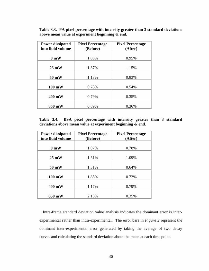
Table 3.3. PA pixel percentage with intensity greater than 3 standard deviations above mean value at experiment beginning & end. Power dissipated into fluid volume
Pixel Percentage (Before)
Pixel Percentage (After)
0 mW
1.03%
0.95%
25 mW
1.37%
1.15%
50 mW
1.13%
0.83%
100 mW
0.78%
0.54%
400 mW
0.79%
0.35%
850 mW
0.89%
0.36%
Table 3.4. BSA pixel percentage with intensity greater than 3 standard deviations above mean value at experiment beginning & end. Power dissipated into fluid volume
Pixel Percentage (Before)
Pixel Percentage (After)
0 mW
1.07%
0.78%
25 mW
1.51%
1.09%
50 mW
1.31%
0.64%
100 mW
1.85%
0.72%
400 mW
1.17%
0.79%
850 mW
2.13%
0.35%
Intra-frame standard deviation value analysis indicates the dominant error is inter-
experimental rather than intra-experimental. The error bars in Figure 2 represent the
dominant inter-experimental error generated by taking the average of two decay
curves and calculating the standard deviation about the mean at each time point.
36

Note: Producing a standard deviation value, by definition, assumes a Gaussian pixel
intensity distribution. The pixel intensity histograms exhibit Gaussian distribution
characteristics with slight Lorentzian character, a “fatter” tail shifting the pixel
distribution slightly towards higher intensity (<1% mean bias toward higher intensity).
Lorentzian character commonly indicates an autocatalytic process is present.
Aggregation exhibits self-similar (non-Gaussian) character. Data indicate this
deviation from a Gaussian distribution is slight.
Figure 3(a) plots the nonspecific/specific intensity ratio vs. time using fit parameters
listed in Tables 1 & 2. Figure 3(b) plots the desorption decay constant ratio at each
experimental power.
Figure 3.3. (a) Nonspecific/specific intensity ratio vs. time. Curves generated using model fit parameters listed in Tables 1 & 2. (b) Desorption rate disparity factor (Rτ) at each power. Data points generated by dividing τ (BSA) by τ(PA) at each power (line added to guide the eye).
Figure 4 plots the curves in Figure 3(a) with confidence bands generated by including
the upper and lower bounds resulting from inter-experimental measurement error.
37

Figure 3.4. Nonspecific/specific intensity ratio plots with standard deviation upper/lower bounds plotted for individual curves (Center curves are identical to those plotted in Figure 3(a)).
Protein interactions are strongly influenced by pH. Changing pH disrupts surface
immobilized protein interactions. Changing pH from 8 to 3, in effect, “turns off”
specific interactions. Affinity is reduced because protein solvation is changed and
protein structure is altered. Measuring elution upon buffer exchange demonstrates the
diffusion limitation at the interface. By activating the resonator we clearly observe
improved transport and accelerated solvent exchange at the solid support. Mass
transport at the interface is slow, and, therefore, commonly problematic for SPR and
electrochemical measurements. Figure 5 depicts the effect schematically in 5(a,b) and
kinetically in 5(c).
38

Figure 3.5. Antigen/Antibody release kinetics upon changing buffer pH from 8 to 3. Changing pH alters the solvation, and, hence, non-covalent interactions are disrupted. Resonator activation accelerates solvent exchange and transport away from the diffusion limited region near the solid-support. Table 3.5. Protein desorption decay constants for Antigen/Antibody release upon changing buffer pH from 8 to 3. Reference Figure 5(c). I(t) = I0 exp(-t/τPA) + I1
Power dissipated into fluid volume
Ι0
τ (PA) (s)
Ι1
koff (PA) (s-1)
0 mW
0.93 +/- 0.01
163 +/- 2
0.13 +/- 0.01
0.0061
400 mW
0.87 +/- 0.01
7 +/- 1
0.01 +/- 0.01
0.1429
V. DISCUSSION
Although adsorbed protein is bound in a strong potential well, the particle cannot be
treated as a solid, but rather, as a biopolymer with subdiffusive behavior interacting
with the bath. Energy injected by the resonator alters protein solvation and induces
amino acid strand fluctuations, accelerating protein desorption.
A rigorous release rate model for koff developed to understand stochastic release
from an energy-well with a saddle-type transition state was developed by Kramer’s
from Smoluchowski theory. The bound-to-free transition probability is considered a
diffusive flux of thermalized states along a specific reaction coordinate. More recently,
39

manuscripts discuss the complexity of ligand-receptor interactions [28-32]. Evans
stresses the importance of loading rate (ΔF/Δt) and discusses the following two
equations arising from Kramers’ theory for the transition probability given an energy-
well with a saddle-type transition state. Kramers’ result is:
1 1 exp[ ]b
off A B
Ek Tτ τ−
= (12)
In this equation, 1/τoff is the overdamped attempt frequency, 1/τA represents the
attempt frequency created by white noise excitation (kBT) neglecting viscous damping
(~109-1010 sec-1), Eb is the energy well depth, kB is Boltzmann’s constant and T is
temperature. Given more explicitly by Evans,
exp[ ]boff
bs ts B
EDkl l k T
−= (13)
Equation 13 details the relationship between a protein’s release rate and mass
transport (diffusion constant—D), bound state energy-well parameters (lbs, lts, and Eb),
and thermal excitation (kBT). The prefactor in Equation 13 defines the rate at which
an antigen would diffuse from a binding site lacking affinity for the antigen (i.e.
without a potential well trapping the antigen in a bound state). Parameters will depend
upon temperature, buffer composition, and mixture constituents. QCR introduced
oscillations influence mass transport, bound-state parameters, and the average thermal
fluctuation magnitude. Hence, we report only koff values (note that koff = 1/τoff).
When the fluid velocity generated by the resonator exceeds the diffusive velocity,
protein is no longer diffusing, but rather transported by forced convection. Hence,
transport from a binding site is no longer diffusion limited.
40

Convection—Diffusion & Surface Volume Reactions
In addressing the fluid mechanics and chemical kinetics present for the surface—
volume reaction represented in Figures 2 & 5, Edwards discusses four distinct
timescales (convection, diffusion near the wall, diffusion into the binding surface, and
reaction at the binding surface). Shear flow generated by the resonator alters each
timescale by moving protein and fluid with an average velocity higher than the root-
mean-squared diffusive velocity, increasing transport in the binding region, and
shifting equilibria for receptor-ligand interactions (see Table 6 for average protein and
water diffusion rates and Table 7 for peak instantaneous velocities, peak surface
deformation amplitudes, and peak loading rates generated by quartz crystal
resonators).
In Figures 2(f) & 5(c), the 0 W data for BSA release and IgG/PA release upon pH
change, respectively, are not fit perfectly by an exponential decay in the initial few
seconds. This occurs because the assumption of small Damköhler (Da) number breaks
down (See Edwards for a detailed discussion [33]). Qualitatively, the flow velocity
near the wall is slow, yet the release kinetics are fast. Hence, for the first few seconds,
while the fluorescently tagged protein is diffusing from the diffusion-limited solid-
liquid interface, the intensity does not decay exponentially. Fortunately, resonator
activation improves mass transport in the diffusion-limited boundary layer, and, hence,
curves with resonator power input are fit well by a single exponential decay.
VI. CONCLUSION
Our hypothesis, desorption rate could be optimized to yield improved specific and
nonspecific species separation, is supported by data in Figures 2 & 5. With
immunoassay miniaturization and fluid-based microsystem development having clear
41

benefit from a sample size, speed, and reagent consumption perspective, yet troubling
from a separation perspective, as noted by Kricka & Wild [5], we anticipate this
method will find utility in immunoassay, molecular diagnostic, and lab chip
applications.
The diffusion-limited boundary layer routinely complicates surface plasmon
resonance assays and electrochemical measurements. Integrating ultrasonic
transducers with such systems may prove useful in molecular screening and diffusion
limited fuel-cell applications [34]. Additionally, nanoscale oscillations altering system
equilibrium may prove useful for separations such as HPLC, or affinity
chromatography applications.
42

APPENDIX
Table 3.6. RMS average diffusive displacement per second for protein in water and the self-diffusion of water molecules at 25 °C (Reference 35 & 36 respectively). Root-mean-square velocity computed using solution in Reference 37.
RMS average diffusive displacement (μm/sec)
Protein (IgG – MW = 155,000) 15
Water 117
Convective Transport—Near Field Fluid Velocity Profile
The experimental set-up is influenced by two energy inputs (pressure driven flow
and quartz crystal resonator activation).
( , )x pressure resonatorz tν ν ν= + (14)
Both inputs transport the fluid, the first symmetrically, the second asymmetrically
(with respect to coordinate z, which defines the channel height), with energy localized
to the first few microns above the solid-support. More explicitly,
2 max2
6 [ ] exp[( 1) ]exp( )2resonator resonator
U Hz z i z i tH
ων ν ωη
= − + − − (15)
43

Table 3.7. Experimentally Measured Input Power Levels and calculated applied voltages, deformation amplitudes, peak instantaneous velocities at the resonator surface, and peak loading rates on surface immobilized protein molecules [38,39]. Input Power
(mW) Voltage Deformation
Amp Peak Fluid
Velocity Peak Protein Loading Rate
25 mW 18 mV 1 Å 500 μm/sec 5.5 x 10⁴ pN/sec
50 mW 30 mV 2 Å 1000 μm/sec 9.5 x 10⁴ pN/sec
100 mW 41 mV 3 Å 1300 μm/sec 1.3 x 10⁵ pN/sec
400 mW 85 mV 5 Å 2800 μm/sec 2.3 x 10⁵ pN/sec
850 mW 123 mV 8 Å 4000 μm/sec 3.8 x 10⁵ pN/sec
44

REFERENCES
[1] Price, C.P. Clinical Chemistry, 1998, vol. 44(10), 2071-2074.
[2] Ekins, R.P. Clinical Chemistry, 1998, vol. 44(9), 2015-2030.
[3] May, M. Genomics & Proteomics, March 2004.
[4] Hitt, E. Genomics & Proteomics, October 2003.
[5] Kricka, L.J. & Wild, D. The Immunoassay Handbook, Third Edition, David Wild
Ed., ELSEVIER Ltd.: Oxford, 2005, 298-299.
[6] Roberts, C. et al., JACS, 1998, 120, 6548-6555.
[7] Ruiz-Taylor, L.A et al. PNAS, January 30, 2001, vol. 98, no. 3, 852-857.
[8] Fang, F., Satulovsky, J., & Szleifer I., Biophysical Journal, vol. 89, September
2005, 1516-1533.
[9] Wazawa, T et al. Analytical Chemistry, 2006, 78, 2549-2556.
[10] Shengfu, C., Lingyun, L., & Shaoyi J. Langmuir, 2006, 22, 2418-2421.
[11] Steukers, M. et al., J. Immunological Methods, 20 March 2006, vol. 310, iss.
1-2, 126-135.
[12] Rathanaswami, P. et al., Biochemical & Biophysical Research
Communications, 334, 2005, 1004-1013.
[13] Gribbon, P. & Sewing, A. Drug Discovery Today, 8(22): 1035-1043.
[14] Huber, W. J Molecular Recognition, 2005, 18: 273-281.
[15] Sinha, N., Mohan, S., Lipschultz, C., & Smith-Gill, S.J. Biophysical Journal,
vol. 83, Dec. 2002, 2946-2968.
[16] Blank, K. et al., PNAS, 30 September 2003, vol. 100, no. 120, 11356-11360.
[17] Evans, E. Faraday Discuss., 1998, 111, 1-16.
[18] Leckband, D. Annu. Rev. Biophys. Biomol. Struct., 2000, 29:1-26.
[19] Myska, D.G. Curr. Opin. Biotechnol., 1997, 8, 50-57.
[20] Myska, D.G. J. Molecular. Recogntion, 1999 12, 279-284.
45

[21] Meyer, G.D., Morán-Mirabal, J.M., Branch, D.W., and Craighead, H.G., IEEE
Sensors Journal, vol. 6, no. 2, April 2006.
[22] Kessler, L.W. & Dunn, F., J. Phys. Chem, December 1969, 73(12), 4256-
4263.
[23] Grimshaw, D., Heywood, P.J., & Wyn-Jones, E. J. Chem. Soc. Faraday Trans.
II, 1973, 69, 756-762.
[24] Kremkau, F.W. & Cowgill, R.W. J. Acoust. Soc. Am., November 1984, 76(5),
1330-1335.
[25] Kremkau, F.W. & Cowgill, R.W. J. Acoust. Soc. Am., March 1985, 77(3),
1217-1221.
[26] Kremkau, F.W. J. Acoust. Soc. Am., June 1988, 83(6), 2410-2415.
[27] Choi, P.K., Bae, J.R., & Takagi, K. J. Acoust. Soc. Am., February 1990, 87(2),
874-881.
[28] Evans, E. Faraday Discuss., 1998, 111, 1-16.
[29] Merkel, R. et al. Nature, 7 January 1999, vol. 397, 50-53.
[30] Evans, E. Annu. Rev. Biophys. Biomol. Struct., 2001, 30:105-128.
[31] Evans, E. & Calderwood, D.A., Science, 25 May 2007, vol 316, 1148-1152.
[32] Fersht, A. Structure & Mechanism in Protein Science: A Guide to Enzyme
Catalysis & Protein Profiling, 1998, W. H. Freeman & Company: New York.
[33] Edwards, D. A. IMA Journal of Applied Mathematics, August 1999, 63(1), 89-
112.
[34] Yoon, S.K. , Fichtl, G. W. & Kenis, P.J.A., Lab Chip, 6, 1516-1524, 2006.
[35] Jossang, T., Feder, J., & Rosenqvist, E., J. of Protein Chem, vol 7, no. 2,
1988.
[36] Mills, R., J. Phys. Chem., vol 77, no. 5, 1973.
46

[37] Pathria, R.K., Statistical Mechanics, Second Edition, 1996, Butterworth-
Heinemann, Woburn, Ma.
[38] Kanazawa, K., Faraday Discuss. 107, 77 (1997).
[39] Borovsky, B., Mason, B.L., & Krim, J., J. Applied Physics, vol. 88, no. 7, 1
October 2000, 4017-4021.
47

CHAPTER FOUR
Nonspecifically Bound Protein Removal from a Microfluidic Channel with an
Integrated Surface Acoustic Wave Device
Don M. Aubrecht, Grant Meyer, & Harold G. Craighead
Cornell University, School of Applied Physics, Clark Hall, Ithaca, New York
14853
ABSTRACT
Protein adsorption to micro/nanoscale devices, commonly termed nonspecific
binding or fouling, can block fluid channels, inhibit sensor function, and decrease
signal-to-background ratios in analytical systems. We detail nonspecifically bound
protein removal from a microchannel integrated with a surface acoustic wave device.
Fluorescently tagged bovine serum albumin was used as a model protein given its high
concentration in blood and propensity to bind nonspecifically. The average albumin
release constant was increased by one order of magnitude with 250 microwatts
delivered to the fluid volume and yielding a 97% reduction in fluorescent intensity in
strongly excited microchannel regions. Accelerated desorption results from the
localized generation of acoustic waves. Averaged over 1 min with a 3 μL/min flow
rate, the temperature change in the fluid volume did not exceed 1.2 +/- 1°C.
Calculations indicate 5 cm/sec peak fluid velocities are achievable at the solid—liquid
interface, indicating advective fluid velocities near the interface exceed average
diffusive values. High fluid velocities are achieved without additional reagent
48

introduction or buffer pH alteration. Achieving comparable microchannel velocities
nanometers from the device surface with pressure driven flow requires a 3.3 mL/min
volumetric flow rate—a large volumetric flow-rate requiring significant pressure
generation. Achieving comparable electroosmotic flow velocities requires 2,500-
15,000 V—a difficult potential to generate or switch quickly. Controlled cell, particle,
and molecule release are routine analytical demands which prove challenging on-chip.
Surface acoustic wave device integration is a potential solution.
I. INTRODUCTION
Surface acoustic wave (SAW) device development has focused on chemical
sensing applications [1, 2]. Recently, SAW devices have been modified for fluid
sensing and transport applications including microfluidic mixing [3, 4]. DNA and
protein microarray integration with ultrasonic devices improves signal-to-background
ratios, pattern uniformity, reduces hybridization times, and removes nonspecific
binding [5-7]. Recent works details nonspecifically bound protein removal from
implantable biosensors to reduce fouling [8].
The literature details laminar flow-based methods successful in removing
microparticles from surfaces [9, 10]. This method, alternatively, generates high fluid
velocities in small fluid volumes by converting an electrical signal into resonant
mechanical motion. Resonant motion advects fluid near the device surface and
generates acoustic streaming (i.e. steady streaming) in the fluid volume resting upon
the SAW device beyond the Stokes’ layer [11]. As stated by Mulvaney et al., laminar
flow-based force discrimination with nanoscale particles is impractical at any practical
microfluidic flow rate [10]. In this work, bovine serum albumin (BSA), with a
hydrodynamic radius of ~5nm, is rapidly released with surface acoustic waves.
This work adds to previous literature by demonstrating and measuring accelerated
protein desorption kinetics as a function of input power. Protein release events are
49

stochastic (i.e. the result of random fluctuations). As a result we measure the average
release rate characterized by the release rate constant koff.
Figure 1(a) depicts a device layout viewed from the top. Microfluidic channels
provide well-defined fluid volumes localizing analyte near the transducer where
acoustic wave energy dissipates into the fluid. Surface acoustic wave energy
dissipates into the microchannel volume as drawn in Figure 1(b). The frames in
Figure 1(c,d) detail channel wall materials, protein adsorption, acoustic wave energy
input from right and left, and average release rates which depend upon channel
material.
Figure 4.1. (a) Device layout and microchannel orientation. (b) Wave propagation through the fluid volume encapsulated by the microchannel. Phonons generated in the piezoelectric crystal dissipate kinetic energy into the viscous fluid volume. The energy distribution can be controlled in all three spatial coordinates and time. (c) Microchannel cross-section delineating channel materials, protein adsorption to each material, and acoustic wave energy impinging from left and right surface acoustic wave transducers (d) Microchannel cross-section detailing multiple kinetic release constants. Each material binds and releases protein with average binding and release values. Protein release rates are modulated with surface acoustic wave input power.
50

With appropriate photolithographic patterning, transducer design, and electronic
equipment, the velocity and energy distributions in the fluidic channel can be
controlled in each spatial dimension and in time.
( , , , )x y z tν ν= (1)
21 ( , , , )2
E dV E x yρν⇒ = =∫ z t (2)
The peak velocity generated at the fluid-SAW device boundary (ωA) with a
deformation amplitude of 0.5 nm and frequency of 100 MHz is 5 cm/sec [12]. The
three dimensional flow profile resulting from resonator activation is complex [13].
A fundamental problem often ignored in the microfluidics and sensing literature is
nonspecific binding. It is either addressed as a systematic error or ignored with the
assumption of disposability. Sensor designs introduce nanoparticles, polymer
monoliths, and complex three-dimensional structures with large surface areas binding
proteins nonspecifically. Such material heterogeneities complicate chemical
passivation. Further, it is assumed, incorrectly, chemical passivation will eliminate
nonspecific binding. Rather, a correct understanding includes protein concentrations
and adsorption/desorption kinetics. The question, couched appropriately, becomes,
“On what timescale and to what degree is nonspecific binding problematic for this
assay?”
Many assays are conveniently performed at room temperature (~25 °C), while most
human biochemistry occurs at ~37 °C. The Boltzmann constant-temperature product
(kBT) is the energetic input driving biological reactions. Many short-lived bound
states become thermodynamically favorable, and relatively long-lived, at lower
temperature. Efficiently eluting weakly bound material blocking channels, fouling
51

sensor surfaces, and increasing background levels, is often experimentally
challenging.
Numerous publications detail chemical remedies reducing nonspecific binding.
Common methods include channel passivation with poly(ethyleneglycol) (PEG) and
newer, reportedly more stable, phosphorylcholine chemistries [14-17]. While
chemical methodologies can modify nonspecific binding kinetics favorably, we stress
the time and concentration dependencies. Time critical experiments require additional
remediation methods combining chemical improvement with active, accelerated
removal when high sample background levels exist. An extensive study by Fang et al.
details protein chemical kinetic dependencies upon surface-grafted polymer chain-
length, protein molecular weight, temperature, and graft density [17]. The authors
state nonspecific binding will occur under any passivation conditions. It is just a
matter of time.
Kessler & Dunn discuss acoustic wave propagation in a fluid causing time-varying,
localized changes in pressure, density, and temperature. Acoustic wave energy
absorption alters molecular energy level distributions. Wave motion perturbs
molecular equilibria at rates which depend on the sound frequency [18, 19]. We
hypothesized surface acoustic waves generated by a piezoelectric transducer could
increase the bound-to-free transition probability for protein adsorbed to inorganic
surfaces without markedly increasing temperature or shifting pH.
This on-chip fluid transport method is notable because: (1) It is simple, and may
eliminate reagents, which expire and introduce variation with storage time, lot
number, UV exposure, and environmental exposure. (2) SAW devices have been
developed extensively for sensing applications. It is reasonable to consider
microsystems providing sensing capability at low-power and improved transport and
surface regeneration function at higher-power. (3) Fabrication is simple, requiring
52

basic photolithography and metal deposition. (4) Lithium niobate (LiNbO3)
chemistry is similar to traditional SiO2 chemistries introducing affinity separation and
release capability with affinity probe immobilization. (5) Procedures in microfluidic
systems can be performed under no-flow conditions (volumetric flow rate Q = 0).
This eliminates analyte dilution and reagent volume consumption. (6) Devices are
easily scaled in dimension/number, individually excitable, and electrical pulse
characteristics can be controlled to minimize heating. (7) The acoustic penetration
depth into the fluid is controlled via frequency—controlling the energy density
spatially within the microchannel. (8) Integration with existing semiconductor
processes may be possible using piezo-active aluminum nitride films, though a
reduced mechanical coupling coefficient may limit utility if low power consumption is
important. (9) Active device applications will be required in situations where
disposable devices are impractical and surface regeneration required (e.g. remote
environment placement where maintenance or replacement is inconvenient). (10)
Achieving high fluid velocities on-chip is realizable under real-world constraints.
Pressure driven flow requires a high volumetric flow rate (~3.3 mL/min).
Electroosmotic flow requires high voltage (2,500-15,000 V) (See Appendix for detail).
An area where devices may find particular utility is protein preconcentration.
Preconcentration is a common step performed when dealing with dilute analytes [20].
Protein capture may be specific, requiring affinity probes, or nonspecific, employing
hydrophobic surface chemistries. Acoustic activation may prove useful in capturing
and rapidly eluting protein strongly bound to a surface without pH change or marked
temperature increase.
53

II. METHODS & MATERIALS
To test our hypothesis and demonstrate integration with traditional
photolithographic processes and materials, we fabricated SAW devices on 128° YX
lithium niobate (LiNbO3) wafers obtained from Crystal Technology, Inc. Standard
photolithography followed by 10 nm chromium and 90 nm gold evaporation steps was
used to produce interdigital transducers. Devices were diced and individually
photopatterned with SU-8 2010. Figure 2(a) is a device photograph showing an
isolated number of interdigital electrodes (IDTs), and Figure 2(b) a device photograph
with an integrated microchannel viewed from the top. A photodefined 100 micron
channel (drawn as a black dotted line) [21] was capped using a coverslip spin coated
with poly(dimethysiloxane) (PDMS) at 4000 rpm. The coverglass/PDMS cap was
then pressed against the SU-8 channel to form a sealed channel. PDMS was exposed
to an oxygen plasma at the high power setting for 1 minute with air as the process gas
(Harrick Plasma).
The dimension d defines the SAW device center frequency. With a dual split-
finger geometry, the center frequency (νcenter) = 8d. Devices were designed to operate
at ~100 MHz. For nonspecific binding removal experiments using fully packaged
devices, 95 MHz was found to be the frequency with lowest insertion loss, as
measured with a spectrum analyzer. Devices were driven at 95 MHz, a span 10 kHz,
and a 5 second sweep time.
Figure 2(c) is a photograph detailing the board layout and SAW device placement
in the fixture. Figure 2(d) is an edge-on view with the device sealed and fixture
pressure applied via screws.
54

Figure 4.2. SAW device interdigital transducer geometry, packaging, and experimental set-up schematic. (a) Dual split-finger interdigital electrode geometry. Finger width defines center frequency. (b) Diced lithium niobate device measuring 21 x 14 mm. Microchannel placement outlined as black dotted-line to indicate position and shape. (c) Top-view photograph detailing IC board and device placement. (d) Packaged device illustration (View: edge-on) depicts electrical and fluidic connections from nonpatterned wafer side and optical microchannel imaging access from top.
Fluid channels were coupled through the chip by gluing silicone tubing to holes
sandblasted through the lithium niobate after dicing and SU-8 photopatterning. The
fluidically and electronically integrated chip was packaged by machining an insulating
plastic (Delrin) fixture to accept pogo pins. Wrap-around electrodes were added with
silver paint to connect bond pads to pogo-pins. A power-splitter was used to apply a
voltage to both transducers.
Microchannels fabricated with PDMS and SU-8 were tested to determine power
dissipation into microchannel materials. Frequency sweeps with and without channel
materials are plotted in Figure 3.
The difference in attenuation is clearly demonstrated by insertion loss values of 35
dBm for an SU-8 microchannel and >60 dB for a PDMS microchannel at 95 MHz.
The insertion loss for a device with no channel was 25 dBm at 95 MHz. Further
55

optimization with unidirectional transducers would improve channel excitation
efficiency.
Figure 4.3. SAW device insertion loss without a channel (squares), with a sealed SU-8 channel (circles), and with a PDMS microchannel (triangles).
Insertion loss measurements for SU-8 and PDMS demonstrate the large disparity in
wave velocity. The wave velocity in PDMS is significantly lower than in SU-8,
causing a > 60 dBm insertion loss. Hence, SU-8 channels were used for experiments.
III. RESULTS
A 10X PBS buffer solution containing 55 μg/mL BSA fluorescently tagged with
AlexaFluor 594 was passed through packaged microchannels for 1 min at 3 μL/min.
This concentration is approximately three orders of magnitude lower than plasma
concentrations, which has albumin concentrations ranging from 30-54 mg/mL. Pure
buffer was driven through the channel until unadsorbed BSA was purged. After
purge, the fluorescent intensity decay was quantified over 10 minutes. A shutter was
used to block excitation between image capture frames.
Each frame was cropped and averaged over 500 ± 100 pixels to isolate the channel
pixels and quantify fluorescent intensity vs. time. In Figure 4(a) the microchannel
was imaged after BSA incubation and buffer purge. Figure 4(b) is an image captured
56

at experiment end. Fluorescent intensity images were incrementally captured at 30
second intervals. Significant removal occurred in ~2 minutes with 97 +/- 3% removal
in highly excited microchannel regions for a device driven at 95 MHz with 250 μW
reaching the fluid volume and a 3 μL/min buffer flow rate. Power dependent elution
results are quantified in Figure 4(c).
Removal had a periodic spatial dependence pictured in Figure 4(b). A standing
wave is generated in the channel resulting from complex diffraction patterns generated
by microchannel incorporation. Protein removal at anti-nodes, caused by a standing-
wave in the microchannel, is reduced. This indicates a non-uniform fluid velocity in
the microchannel. Importantly, this result indicates the removal mechanism is
hydrodynamically influenced.
Figure 4.4. SAW Activation Fluorescence Microscopy Results (a) AlexaFluor 594 labeled BSA bound to an SU-8 microchannel after buffer wash step. (b) Fluorescent image after surface acoustic wave excitation for 10 minutes. Intensity is highest at standing wave anti-nodes, where the surface acoustic wave streaming velocity is lowest, indicating release is hydrodynamically influenced. (c) Fluorescent intensity vs. time for BSA release with incrementally increasing power delivered to the fluid volume. Protein elution rate increases with increasing input power.
Although complex chemical kinetics and flow patterns occur in the microchannel,
we can measure release kinetics. Written chemically, protein adsorption/desorption
reactions can be written as,
57

on
off
k
kA B C+ (3)
Protein (B) binds to surface atoms (A) with characteristic rate constants kon and koff
characterizing protein adsorption and desorption. The time-dependent quantity of
interest is the number of proteins interacting with the substrate to form a protein—
substrate complex C. Bound protein quantities will depend upon the number of
available surface binding sites and protein concentration. Kinetic models are detailed
by Lauffenberger & Linderman [22]. Written in differential form, Equation 3
becomes,
on offdC k AB k Cdt
= − (4)
In this work we characterize,
offkC A B⎯⎯→ + (5)
This equation holds if konAB = 0. This assumption is valid if rapid transport away
from the surface upon release makes B, the free protein concentration, zero. Given the
high fluid velocities generated by SAW devices and constant pure buffer infusion, this
assumption is reasonable. Equation 5 reduces to a simple differential equation given
in Equation 6.
offdC k Cdt
= − (6)
We quantify the power-dependent change in koff = koff (P), where P is the power
input by the SAW transducers. Acoustic oscillations alter system equilibrium (i.e.
SAW introduced oscillations shift kon and koff) [18, 19]. Increasing input power
increases oscillation amplitude.
58

Systems with advective and diffusive mass transport decoupled from surface
reaction kinetics are commonly modeled with the following differential equation,
which assumes multiple release rate constants,
0 0 1 1 2 2dC k C k C k Cdt
= − − − −… (7)
0 1 2( 0)C t C C C= = + + +… (8)
In Equations 7, C, the total protein—substrate complex number, is fragmented to
explicitly account for multiple binding affinities (i.e. multiple koff release rates).
Solving this differential equation, where k0,1,2… are the release rate constants with the
initial condition given in Equation 8 gives,
0 0 1 1 2 2( ) exp( ) exp( ) exp( )C t C k t C k t C k t= − + − + − +… (9)
In our experiments, C is proportional to the fluorescent signal intensity, and,
therefore, we write,
0 0 1 1 2 2( ) exp( / ) exp( / ) exp( / )I t I t I t I tτ τ τ= − + − + − +… (10)
Where
0,1,2,0,1,2,
1kτ
=……
(11)
In instances where a protein sub-population has a slow kinetic release constant
(relative to the experimental time-scale) we can treat the system as an exponential
59

decay with an additional constant quantifying the strongly bound sub-population. In
the respective limits,
1,2,...τ → ∞ (12)
0 0( ) exp( / ) 1I t I t Iτ= − + (13)
0 0 1 1( ) exp( / ) exp( / ) 2I t I t I t Iτ τ= − + − + (14)
Equations 13 and 14 were used to fit intensity data in Figure 4. Decay time and
rate constant (τ0,1 and k1,2) values are listed in Tables 2 and 3. Fitting data to
Equations 13 and 14 provides information about protein—substrate release time
constants and bound population proportions. By increasing the input power reaching
the SAW device, we can quantify the influence device input power has on protein
desorption.
First Order Exponential Fit Data – I(t) = I0 exp(-t/τ0) + I1
Equation 13 gives the exponential fit used to reduce the intensity decay results
obtained in the experiment to three fit parameters.
Table 4.1. First Order Exponential Decay Fit Data – I(t) = I0 exp(-t/τ0) + I1
I0 τ0 (min) I1 R2 koff (sec-1)
0 μW 0.67 +/- 0.20 16.53 +/- 6.67 0.29 +/- 0.20 0.981 1.0 x 10⁻³
30 μW 0.51 +/- 0.02 3.15 +/- 0.31 0.46 +/- 0.02 0.980 5.3 x 10⁻³
60 μW 0.70 +/- 0.02 2.44 +/- 0.14 0.25 +/- 0.01 0.992 6.8 x 10⁻³
125 μW 0.86 +/- 0.04 1.01 +/- 0.09 0.19 +/- 0.01 0.972 1.7 x 10⁻²
250 μW 0.97 +/- 0.01 1.10 +/- 0.03 0.02 +/- 0.01 0.997 1.5 x 10⁻²
60

Second Order Exponential Decay Fit Data – I(t) = I0 exp(-t/τ0) + I1 exp(-t/τ1) + I2
A simple exponential decay fits the first four intensity curves well (i.e. fitting with
a second order decay yields redundant or experimentally unreasonable values).
However, the last curve-fit improves with a second order decay. The value for τ1
indicates some BSA is strongly bound and elutes slowly compared to protein releasing
with the decay constant τ0. The slowly eluting protein is thought to elute from highly
hydrophobic SU-8 walls, the PDMS cap and anti-nodes where the fluid velocity is
low. Equation 14 was used to fit the 250 μW curve. Table 4.2. Second Order Exponential Decay Fit Data – I(t) = I0 exp(-t/τ0) +… …I1 exp(-t/τ1) + I2
I0 τ0 (min) I1 τ1 (min) I2 R2 k1,2off (sec-1)
250 μW 0.87 +/- 0.04
0.92 +/- 0.04 0.15 +/- 0.02
6.86 +/- 0.53 -0.03 +/-0.04 0.9995 1.8 x 10⁻²
2.4 x 10⁻³
IV. DISCUSSION
Protein release from a bound state depends upon temperature, energy-well
properties, and mass transport at the interface. The temperature change can be
calculated from Equation 15,
/T E m CΔ = Δ (15)
Where ΔT is the temperature change, ΔE is the energy input, m is the fluid volume
mass and C is the heat capacity of the fluid. A figure of merit routinely used in
chemical kinetics is a doubling in rate constant value with a 10°C increase in
temperature [23]. Assuming full dissipation of attenuated power into heat, the
temperature was calculated to rise no more than 1.2 +/- 1 °C if averaged over 1 minute
with 250 μW delivered to the fluid volume of 3 μL. This temperature change
61

increases the thermal energy in the system, ultimately increasing the protein
desorption rate. While clearly influencing the protein release rate, this temperature
does not account for the order of magnitude increase. Accelerated release arises from
both a temperature change and hydrodynamic induced bound-to-free transitions.
Extensive work by many theoreticians has detailed complex nonequilibrium statistical
mechanics and protein subdiffusion which contribute to protein binding and release
[24-32].
V. CONCLUSION
Rapid protein elution and mixing without pressure driven or electrokinetic flow is
achievable only with an active device. This method has utility in preconcentration and
controlled release applications (e.g. affinity probe screening, mass spectrometry, and
biosensors). Results demonstrate power-dependent nonspecific binding removal.
Broader applicability to systems where ultrasonic manipulation can disrupt particle—
substrate interactions may exist (e.g. cell manipulation, bead-based sorting, and
sensing). Numerous literature articles site the integration of superparamagnetic beads,
nanoparticles, quantum dots, and cells with micro/nanofluidic systems where capture
and release capabilities are critical.
62

APPENDIX
Fluid Transport Mechanisms
Fluids can be transported thermally and with pressure, electric fields, or acoustic
waves [33, 36, 37, 38]. The respective equations for thermally generated RMS
displacement per second, pressure driven flow, electroosmotic flow, and acoustically
generated flow are given by Equations 16-19.
2 6r D< > = t (16)
Understanding fluid transport in the microchannel requires knowledge of the fluid
velocity. When considering fluid velocities in a microfluidic channel, diffusive values
provide an average velocity metric. Table 1 lists the average root-mean-square (RMS)
protein displacement per second for protein (IgG – MW = 155,000) in water and
water’s self-diffusion constant.
Table 4.3. RMS diffusive displacement values for protein & water molecules at 25°C. (References 34 & 35 respectively). Root-mean-square velocities computed using solution in Reference 33.
RMS Displacement per second (microns) Protein (IgG – MW = 155,000) 15 Water 117
22
6 [ ]pressureU Hz z
Hν = − (17)
electroosmotic E VL
εζ εζνη η
− −= = (18)
63

max exp[( 1) ]exp( )2resonator resonator i z iω tν ν ωη
= − − (19)
Experimental Fluid Velocity Profile
Fluid is transported in our system by pressure driven and SAW generated
components.
( , )x pressure resonatorz tν ν ν= + (20)
Pressure driven flow transports the fluid symmetrically about the channel cross-
section, while SAW generated flow is asymmetric with respect to the z-coordinate
defining the channel height. The SAW generated shear velocity fluid transport
contribution in the near field limit (within the Stokes’s layer) is given by Equation 21,
2 max2
6 [ ] exp[( 1) ]exp( )2resonator resonator
U Hz z i z i tH
ων ν ωη
= − + − − (21)
The coordinates are as depicted in Figure 1. Table 4 lists symbols, symbol names,
units, and values used in calculations where applicable.
Table 4.4. Symbols, symbol names, units, and relevant values.
Symbol Symbol Name Value SI Units
r Displacement - m
D Diffusion Constant Refs. 34,35 m2/s
t Time - s
U Mean Flow Velocity 5000 μm/sec m/s
H Channel Height 100 μm m
ε Buffer Permittivity 4.4 x 10⁻¹⁰ C2/(N·m2) C2/(N·m2)
ζ Zeta Potential -5 to -30 mV V
64

Table 4.4 (continued)
η Kinematic Viscosity (Water 25°C) 1 x 10⁻⁶ m2/s m2/s
E Electric Field - V/m
L Channel Length 1 cm m
V Voltage - V maxresonator Aν ω= Peak Velocity 5 cm/sec m/s
ω Frequency 100 MHz 1/s
A Amplitude 0.5 nm m
ACKNOWLEDGMENT
Work was supported by the Cornell LIFE Program. The authors wish to thank Rob
Ilic for extensive and timely fabrication support performed in the Cornell Nanoscale
Facility and John Mannion, Stephen Levy, and Prof. Watt W. Webb for useful
electrokinetic and fluid mechanics discussions. We have also benefited from chemical
kinetics discussions with Prof. David Manke.
65

REFERENCES
[1] J. Smith & V. Hinson-Smith, “The New Era of SAW Devices”, Analytical
Chemistry, 3505-3507, 1 June 2006.
[2] C.M. Harris, “Seeing SAW Potential”, Analytical Chemistry, 355-358A, 1 August
2003.
[3] W.K. Tseng et al., “Active micro-mixers using surface acoustic waves on Y-cut
128° LiNbO3”, J. Micromech. Microeng., 16(2006) 539-548.
[4] G.G. Yaralioglu, “Ultrasonic Mixing in Microfluidic Channels Using Integrated
Transducers”, Anal. Chem. 2004, 76, 3694-3698.
[5] A. Toegl, R. Kirchner, C. Gauer, & A. Wixforth, “Enhancing Results of
Microarray Hybridizations Through Microagitation”, J. Biomolecular Techniques, vol.
14, iss. 3, Sept 2003.
[6] M. Hartmann, A. Toegl, R. Kirchner, & M.F. Templin, “Increasing robustness and
sensitivity of protein microarrays through microagitation and automation”, Analytica
Chemica Acta, 564 (2006), 66-73.
[7] Meyer, G.D., Morán-Mirabal, J.M., Branch, D.W., and Craighead, H.G.,
“Nonspecific Binding Removal From Protein Microarrays Using Thickness Shear
Mode Resonators”, IEEE Sensors Journal, vol. 6, no. 2, April 2006.
[8] PYJ. Yeh, “Electric field and vibration-assisted nanomolecule desorption and anti-
biofouling for biosensor applications”, Colloids & Surfaces B-Biointerfaces, 59(1):
67-73, 1 Sept. 2007.
[9] Y. Zhang, V.T. Milam, D.J. Graves, & D.A. Hammer, “Differential Adhesion of
Microspheres Mediated by DNA Hybridization I: Experiment”, Biophysical Journal,
vol. 90, June 2006, 4128-4136.
66

[10] S.P. Mulvaney et al., “Rapid, femtomolar bioassays in complex matrices
combining microfluidics and magnetoelectronics”, Biosensors & Bioelectronics,
23(2007) 191-200.
[11] L.D. Landau & E.M. Lifshitz, Fluid Mechanics, Second Edition, 1987,
Butterworth-Heinemann, Linacre House, Jordan Hill, Oxford OX2 8DP.
[12] T. Uchida, T. Suzuki, & S. Shiokawa, “Investigation of Acoustic Streaming
Excited by Surface Acoustic Waves”, IEEE Ultrasonics Symposium, 1995, 1081-
1084.
[13] Z. Guttenberg et al. “Flow profiling of a surface-acoustic-wave nanopump”,
Physical Review E, 70 (2004), 056311.
[14] D. Wu, B. Zhao, Z. Dai, J. Qin and B. Lin, “Grafting epoxy-modified
hydrophilic polymers onto poly(dimethylsiloxane) microfluidic chip to resist
nonspecific protein adsorption”, Lab-on-a-Chip, 2006, 6, 942.
[15] C. Roberts, C.S. Chen, M. Mrksich, V. Martichonok, D. E. Ingber, & G.M.
Whitesides, “Using Mixed Self-Assembled Monolayers Presenting RGD and
(EG)3OH Groups To Characterize Long-Term Attachment of Bovine Capillary
Endothelial Cells to Surfaces”, J. Am. Chem. Soc. 1998, 120, 6548-6555.
[16] Y. Wang, M. Bachman, C. E. Sims, G. P. Li, & N. L. Allbritton, “Simple
Photografting Method to Chemically Modify and Micropattern the Surface of SU-8
Photoresist”, Langmuir 2006, 22, 2719-2725.
[17] F. Fang, J. Satulovsky, & I. Szleifer, “Kinetics of Protein Adsorption and
Desorption on Surfaces with Grafted Polymers”, Biophysical Journal, vol. 89 Sept.
2005 1516–1533.
[18] L.W. Kessler & F. Dunn, “Ultrasonic Investigation of the Conformal Changes of
Bovine Serum Albumin in Aqueous Solution”, J. Phys. Chem., vol. 73(12), Dec. 1969,
4256-4263.
67

[19] D. Grimshaw, P.J. Heywood, E. Wyn-Jones, “Proton Transfer in some Amino-
acids Studied by the Ultrasonic Method”, Faraday II, 1972, 756-762.
[20] D.L. Huber, R. P. Manginell, M. A. Samara, B.-Il Kim, B. Bunker, “Programmed
Adsorption and Release of Proteins in a Microfluidic Device”, Science, vol 301, 18
July 2003, 352-354.
[21] Francs, L.A., Friedt, J.-M., Bartic, C., Campitelli, A., “A SU-8 liquid cell for
surface acoustic wave biosensors”, 2004 Proc. SPIE 5455:353-363.
[22] Lauffenburger, D.A. and Linderman, J., Receptors: Models for Binding,
Trafficking, and Signaling, 1993, Oxford University Press, Inc., New York.
[23] Personal communication with Dr. David Manke, May 2007.
[24] E. Evans , “Probing the Relation Between Force-Lifetime and Chemistry in
Single Molecular Bonds”. Annu. Rev. Biophys. Biomol. Struct. 30:105-128, 2001.
[25] R. Zwanzig, Nonequilibrium Statistical Mechanics, Oxford University Press,
2001.
[26] P. Hanggi, “Escape from a Metastable State”, Journal of Statistical Physics, vol.
42, Nos. 1/2, 1986, 105-148.
[27] D. Chandler, “Roles of Classical Dynamics and Quantum Dynamics on Activated
Processes Occurring in Liquids”, Journal of Statistical Physics, vol. 42, Nos. 1/2,
1986, 49-67.
[28] W. Min & S. Xie, “Kramers model with a power-law friction kernel: Dispersed
kinetics and dynamic disorder of biochemical reactions”, Phys. Rev. E 73, 010902(R ),
2006.
[29] N. Agmon & J.J. Hopfield, “Transient Kinetics of Chemical Reactions with
Bounded Diffusion Perpendicular to the Reaction Coordinate: Intramolecular
Processes with Slow Conformational Changes”, J. Chem. Phys., 78(11), 1 June 1983,
6947-6959.
68

[30] E. Z. Eisenmesser, D. A. Bosco, M. Akke, D. Kern, “Enzyme Dynamics During
Catalysis”, Science, vol 295, 22 February 2002, 1520-1523.
[31] G. Zaccai, “How soft is a protein? A Protein Dynamics Force Constant Measured
by Neutron Scattering”, Science, vol. 288, 2 June 2000, 1604-1607.
[32] S. Benkovic and S. Hammes-Schiffer, “A perspective on Enzyme Catalysis”,
Science, vol 301, 29 August 2003, 1196-1202.
[33] Pathria, R.K., Statistical Mechanics, Second Edition, 1996, Butterworth-
Heinemann, Woburn, Ma.
[34] Jossang, T., Feder, J., & Rosenqvist, E., “Photon Correlation Spectroscopy of
Human IgG”, J. of Protein Chem, vol 7, no. 2, 1988.
[35] Mills, R., “Self-Diffusion in Normal and Heavy Water in the Range 1-45°”, J.
Phys. Chem., 77, 685 (1973).
[36] W. M. Deen, Analysis of Transport Phenomena, 1998, Oxford University Press.
[37] B. J. Kirby & E. F. Hasselbrink Jr., “Zeta potential of microfluidic substrates: 1.
Theory, experimental techniques, and effects on separations”, Electrophoresis, 2004,
25, 187-202.
[38] D. P. Telionis, Unsteady Viscous Flows, 1981, Springer –Verlag New York Inc.
69

CHAPTER FIVE
Nonspecific Cell Removal & Controlled Membrane Permeation with Surface
Acoustic Wave Devices Grant Meyer, José M. Morán-Mirabal, & Harold G. Craighead
Cornell University, School of Applied Physics, USA
ABSTRACT In small fluid volumes mixing is difficult, diffusion is slow, and nonspecific
adsorption is problematic. Surface acoustic wave devices generate high fluid velocities
in small volumes. Noting diffusive limitations and nonspecific adhesion problems and
a potential acoustic wave solution, we performed affinity-based cell separation and
time-dependent membrane permeation experiments on surface acoustic wave devices.
Flow velocity measurements were used to calculate the force applied to bound cells
and demonstrate spatial mass transport control in microfluidic channels. Separation
and permeation results obtained with fluorescence and scanning electron microscopy
are presented. Affinity-based capture and nonspecifically bound cell removal results
were obtained with green fluorescent E. coli binding to covalently immobilized
antibodies. Red fluorescent S. aureus was used as nonspecific bacteria to demonstrate
E. coli specificity. Devices incubated with red and green bacteria were imaged before
and after surface acoustic wave device excitation. Fluorescent image analysis yielded
88% removal of nonspecifically bound E. coli bound to non-protein patterned areas, a
12% loss of E. coli bound to protein patterned areas, and 99% removal of
70
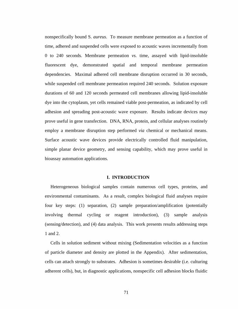
nonspecifically bound S. aureus. To measure membrane permeation as a function of
time, adhered and suspended cells were exposed to acoustic waves incrementally from
0 to 240 seconds. Membrane permeation vs. time, assayed with lipid-insoluble
fluorescent dye, demonstrated spatial and temporal membrane permeation
dependencies. Maximal adhered cell membrane disruption occurred in 30 seconds,
while suspended cell membrane permeation required 240 seconds. Solution exposure
durations of 60 and 120 seconds permeated cell membranes allowing lipid-insoluble
dye into the cytoplasm, yet cells remained viable post-permeation, as indicated by cell
adhesion and spreading post-acoustic wave exposure. Results indicate devices may
prove useful in gene transfection. DNA, RNA, protein, and cellular analyses routinely
employ a membrane disruption step performed via chemical or mechanical means.
Surface acoustic wave devices provide electrically controlled fluid manipulation,
simple planar device geometry, and sensing capability, which may prove useful in
bioassay automation applications.
I. INTRODUCTION
Heterogeneous biological samples contain numerous cell types, proteins, and
environmental contaminants. As a result, complex biological fluid analyses require
four key steps: (1) separation, (2) sample preparation/amplification (potentially
involving thermal cycling or reagent introduction), (3) sample analysis
(sensing/detection), and (4) data analysis. This work presents results addressing steps
1 and 2.
Cells in solution sediment without mixing (Sedimentation velocities as a function
of particle diameter and density are plotted in the Appendix). After sedimentation,
cells can attach strongly to substrates. Adhesion is sometimes desirable (i.e. culturing
adherent cells), but, in diagnostic applications, nonspecific cell adhesion blocks fluidic
71

channels and sensor elements. Removal routinely requires significant force.
Assuming the force applied to bound nano/microparticles is applied
hydrodynamically, the force scales linearly with fluid velocity. Integrated transducers
which improve fluid transport, expedite sample preparation steps, and provide sensing
capability are important for bioassay automation and rapid analysis.
Affinity probe-based separations provide high affinity/specificity and rapid results
(routinely tens of minutes) [1, 2]. Nanogram/mL analyte concentrations are routinely
achievable in practice, however, theoretically, attomolar/zeptomolar sensitivities are
achievable. Kinetic and mass transport limitations creating sub-optimal, real-world,
limitations are discussed by Kuznezow [3-5]. Importantly, immunoassays are
routinely used to detect proteins, hormones, or cytokines—all molecules with low
molecular weight and high average diffusive velocities relative to cells.
Circulating tumor cell detection requires rare cell separation after cells shed into
blood. A volume metric for high background biological sample analysis is circulating
tumor cell isolation. Circulating tumor cells are shed by all major carcinomas into
peripheral blood [6]. The volume used, 7.5 mL, represents a large volume to be
sampled. Volumes used in Allard’s experiments were spiked with an average of 319
endothelial cells to generate positive controls. Such values are important to consider
for lab-on-a-chip device design. A 7.5 mL blood volume contains ~30-50 billion red
blood cells. Simple math gives an optimistic signal-to-background ratio of ~1 x 10⁻⁸.
Clearly, if intracellular analyses are required, separation prior to lysis is required.
Improving mass transport in complex biological fluids, where diffusion is slow and
sedimentation proves problematic, is critical. Cellular and macromolecular mass
transport from solution to surfaces, including rapid protein adsorption relative to cell
capture is discussed in Reference 7.
72

Nonspecific binding, sedimentation, contamination, and poor mass transport make
fluid analysis steps 1 and 2 difficult. Difficulties can be mitigated by advection, which
accelerates mixing. Achieving high fluid velocities in small volumes without analyte
dilution is difficult. Our previous work discusses fabrication protocols, bioassay mass
transport improvement, and nonspecific binding removal with ultrasonic devices [8-
10]. In this work, nonspecific cell release and controlled membrane permeation
results obtained with surface acoustic waves are detailed.
Surface acoustic wave devices are produced with standard semiconductor tools and
routinely used in telecommunications and chemical/biological sensing [11, 12].
Because acoustic wave devices generate significant fluid velocities, localize energy
injection to the solid-liquid interface, and are controlled electrically, we hypothesized
SAW devices could separate cells based on affinity (separation) and controllably
disrupt captured cell membranes based on acoustic wave exposure duration and
proximity to the transducer (sample preparation). Numerous manuscripts detail
ultrasound-based fluid mixing results [13-16]. We sought to build upon this literature
to demonstrate biological separation and membrane permeation utility.
Device Layout
Experiments required convenient packaging for electrical connection, fluid
localization, and optical interrogation. Figure 1 presents the device electrode detail,
fluid reservoir location relative to electrodes, supporting circuit board integration with
a machined Lexan fixture, and device placement after assembly in the fixture
73

Figure 5.1. (a) Dual split-finger interdigital electrode geometry. Finger width defines center frequency (~100 MHz). (b) Diced lithium niobate device measuring 21 x 14 mm with PDMS reservoir placement marked in black. (c) Top view photograph detailing supporting circuit board and SAW device placement (d) Packaged device illustration (edge-on view) depicts electrical connections and fluid reservoir detail.
Protein patterning was used to demonstrate affinity-based cell capture and
nonspecifically bound cell removal from unmodified substrate. Patterning on SAW
substrates with a parylene-based masking process was used to define protein
microspots and non protein patterned regions. With well-developed silane chemistry
it is possible to covalently attach specific receptors on SAW substrates [17]. Pattern
placement, a bright-field pattern image, and schematic (edge-on view) are shown in
Figure 2.
74

Figure 5.2. (a) SAW electrode diagram and micropattern image detailing SAW device layout with surface micropattern. (b) Bright-field micropattern image. (c) Fluid volume diagram (edge-on view) depicting cells binding to protein microspots and sedimentation (nonspecific adsorption). Cells sediment and physically block transducer/sensor surface.
II. RESULTS & DISCUSSION A. Fluid Velocity Measurements & Particle Manipulation in Microfluidic Channels
Measuring the fluid velocity with microparticle velocimetry allows force calc-
ulation. At microwatt power levels delivered to the fluid it is possible to achieve
velocities exceeding 2 cm/sec. Transducer design and fluid viscosity determine the
velocity distribution within the channel. Activating an individual transducer can shift
particle distributions from 3D to 2D or vice versa. Bead distributions before and after
SAW excitation are shown in Figure 3(a, c). A 2D velocity map co-planar to the
SAW substrate is depicted in Figure 3(b) (Traveling waves impinge from a transducer
patterned to the left of the microchannel).
75

Figure 5.3. (a) Microchannel with 14 micron beads diffusing in buffer (blue line overlay marks microchannel wall location). (b) Microparticle velocimetry profile inside a microfluidic channel. Heat map indicates areas of highest velocity. Velocities measured in excess of 2 cm/sec in the red region. (c) Advection pushes beads to the channel wall.
B. Forces Acting on an Immobilized Sphere in Solution
In addition to adhesive forces, particles and cells adhering to a solid-support are
acted upon by two forces—stochastic thermal fluctuations and hydrodynamic drag.
The average force applied by thermally induced buffer collisions with cells exerts
negligible force (pN) relative to hydrodynamic drag (nN). A physical force schematic
(Figure 4(a)), force vs. cell diameter (Figure 4(b)), and an SEM image detailing an
RBL mast cell cytoskeletal response to the applied hydrodynamic force are shown in
Figure 4(c). Figure 4(c) images an RBL mast cell responding (binding) to a bovine
serum albumin—dinitrophenyl (BSA-DNP) microspot. The cell creates a podosome
in response to the stimulus (BSA-DNP). The hydrodynamic drag force pulls the cell
away from the attachment area causing cytoskeletal rearrangement.
The hydrodynamic drag force calculated for a sphere immobilized upon a solid
support [18] is,
1.7(3 )F Dvπμ= (1)
Where μ is the dynamic viscosity, D is the particle diameter, and v is the fluid
velocity.
76

Figure 5.4. (a) Thermal fluctuations and shear flow exert forces on an immobilized sphere at an interface. (b) Calculated force on a spherical particle vs. particle diameter with v = 0.5, 1, and 2 cm/sec. (c) RBL Mast cell binding to a protein patterned microspot. Shear flow generated by surface acoustic wave dissipation into fluid resting upon the solid support applies a hydrodynamic force to cells. SEM image demonstrates cytoskeletal/membrane deformation resulting from the applied hydrodynamic force.
C. Selective Cell Capture & Membrane Permeation
Complex biological samples contain many cell types. Often information about the
entire cell population is unnecessary. Rather, isolation and detailed analysis of one or
a few cell types is desired. Splitting the cell population into two sets (signal and
background), we can define a separation ratio. NS represents signal at experiment
start, N’S represents signal at experiment end, and NB defines background.
'B S
S
N NRN+
= (2)
We seek to drive NB to zero while maximizing N’S. Ideal separation would yield
NS/N’S = 1, assuming no signal cells bound nonspecifically to the background region
bind to protein microspots. This ratio was chosen to provide a metric accounting for
background and signal cells removal with shear flow generated by SAW device
activation. Schematic experiment representations, fluorescent images, and
quantitative values derived from fluorescent images before and after SAW activation
for 60 seconds at 250 microwatts are presented in Figure 5 (Image analysis methods
77

are discussed in the Appendix). The values for R before and after SAW activation are
1.87 and 1.14 respectively.
Figure 5.5. (a,b,c) Diagram, fluorescent image, and red/green bacteria counts for fluorescent image in (b) before SAW device activation. (d,e,f) Diagram, fluorescent image, and red/green bacteria counts for fluorescent image in (e) after SAW device activation. Device activated for 60 seconds with 250 microwatts delivered to the fluid.
Although fluorescence data indicating preferential binding to protein microspots
are promising, SEM images provide a clear verification cells bind to protein patterned
spots. Figure 6 demonstrates RBL Mast cell localization on BSA-DNP patterned
microspots. IgE receptors present on RBL Mast cells bind to BSA-DNP specifically
causing cell adhesion to protein spots.
78

Figure 5.6. (a,b) SEM images with RBL Mast cells bound specifically to BSA-DNP protein microspots.
D. Membrane Permeation
High fluid velocities near the SAW device surface and SEM images in Figures 4 &
6 suggested devices could potentially permeate cell membranes. RBL Mast cells were
incubated on substrates for 60 minutes. After incubation, devices were driven at 250
microwatts for 300 seconds. Cells were fixed and sputtered with gold/palladium.
Figure 7(a) presents a control SEM image with immobilized cells adhering via
integrins and transmembrane proteins to a SAW device surface. Figure 7(b) presents
an SEM image taken between the SAW transducers after activation demonstrating
significant membrane disruption. Figure 5.7. (a,b) SEM images displaying RBL Mast cells adhered to SAW surfaces without acoustic exposure (a) and with exposure at 250 microwatts for 300 seconds (b).
79

SEM images provide clear membrane disruption evidence, yet prove time
consuming and difficult to quantify. Fluorescence provides a convenient and
immediate method for quantifying membrane permeation vs. SAW exposure time.
Fluorescence microscopy quantifying lipid-soluble and lipid- insoluble dye intensity is
a convenient method used to quantify cell membrane permeation.
Transformed ovarian surface epithelial cells were incubated in PDMS reservoirs
placed between SAW transducers (reference Figure 1) for 60 minutes to allow
sedimentation and adhesion. Devices were driven with 250 microwatts delivered to
the fluid volume for 0, 5, 30, and 240 seconds. After SAW exposure, reservoir fluid
volumes were exchanged for HBSS buffer followed by a 15 minute fluorescent
nucleic acid dye incubation (a one-to-one mixture containing green (lipid-soluble) and
red (lipid-insoluble), HBSS wash step, and one hour 4% glutaraldehyde fixation step.
Figure 8(a, b, c) shows red, green, and combined fluorescent images after SAW
exposure for 0 sec (a1, b1, c1), 5 sec (a2, b2, c2), 30 sec (a3, b3, c3), and 240 sec (a4,
b4, c4). Figure 8(d) plots red intensity vs. time. Figure 5.8. Transformed ovarian surface epithelial cells excited after nonspecific adhesion. (a1–green, b1–red , c1–combined) Control and (a2,b2,c2; a3,b3,c3; a4,b4,c4) three separate devices excited at 250 microwatts for increasing exposure times (5, 30, 240 seconds). Green dye is lipid-soluble. Red dye is lipid-insoluble (membrane impermeant), and, therefore, cannot diffuse through lipid bilayers unless disrupted. (d) Red fluorescence vs. SAW exposure time plot.
80

In addition to adherent cell membrane permeation, we performed a similar
experiment on cells in solution. Transformed ovarian surface epithelial cells in
suspension were added to PDMS reservoirs and immediately driven for 15, 30, 60,
120, and 240 seconds. After exposure, solution volumes contained in the PDMS
reservoirs were mixed with one-to-one red/green nucleic acid dye solution for 15
minutes and fixed with 4% glutaraldehyde for 1 hour. The fluid volume was then
exchanged with fresh HBSS buffer. Cells sedimented during dye and fixation
incubation steps. Remaining cells were imaged to obtain red and green fluorescent
intensity values vs. time. In performing this assay many cells were lost with buffer
exchange. Hence, cell population numbers imaged were lower than adherent cell
populations.
Figure 9(a,b,c) shows red, green, and combined fluorescent images after SAW
exposure for 0 sec (a1, b1, c1), 15 sec (a2, b2, c2), 30 sec (a3, b3, c3), 60 sec (a4, b4,
c4), 120 sec (a5, b5, c5), and 240 sec (a6, b6, c6). Figure 9(d) plots red intensity vs.
time. Figure 5.9. Transformed ovarian surface epithelial cells excited in solution. (a1, b1, c1) Control and (a2, b2, c2; a3, b3, c3; a4, b4, c4; a5, b5, c5; a6, b6, c6) five separate devices imaged after 250 microwatt exposure for 15, 30, 60, 120, and 240 seconds. Green dye is lipid soluble. Red dye is membrane impermeant, and, therefore, cannot diffuse through lipid bilayers into cells unless permeated. Red fluorescence demonstrates membrane disruption. (d) Red fluorescence vs. SAW exposure time plot.
81

Interestingly, cells in solution exposed to acoustic waves for 60 and 120 seconds
adhered and extended lamellipodia (Figure 10) indicating exposure permeates cell
membranes without disrupting cytoskeletal remodeling function. Results suggest
devices may prove useful in gene transfection automation.
Figure 5.10. Transformed ovarian surface epithelial cell fluorescent images demonstrating cell viability post-SAW excitation. (a1-green, b1-red, c1-combined, d1-contrast/brightness adjusted) Epithelial cell extending lamellipodia after acoustic wave exposure for 60 seconds. (a2, b2, c2, d2) Epithelial cells extending lamellipodia after acoustic wave exposure for 120 seconds. Cells exposed for 240 seconds did not extend lamellipodia.
III. CONCLUSION & FUTURE WORK
Results demonstrate nonspecific bacterial cell removal, RBL Mast cell capture, and
time-dependent transformed ovarian surface epithelial cell membrane permeation. A
practical automation application where devices may find utility exists in releasing
adherent cells cultured on-chip. Cell culture requires significant costs, both human
and material, which may be reduced with automation. As cells proliferate, release
requires careful laboratory cleanliness, skilled cell culture technologists, and
significant time. Automating steps and eliminating environmental contamination risks
is clearly desirable. Mechanical release required when passing cells after proliferation
and spreading is routinely achieved by sharply knocking (“rapping”) flasks, after
trypsin addition. This is a combined chemical/mechanical release process. When
82

flasks are rapped, the removal mechanism is an impulsive mechanical shock to the
flask wall. Automating this process would reduce variation in experiments rich in
biological variability alone.
Obtaining release kinetics for nonspecific and specifically bound cells would prove
useful. Further work is required to determine the lysis mechanism.
Red fluorescent signal intensity vs. time plots indicate cells captured at the device
surface are quickly permeated while cells in solution require extended exposure.
Future work will seek to leverage energy localization at the transducer surface to
improve cell capture from large volumes and selectively permeate bound cells post-
separation for intracellular molecular diagnostic applications.
We have treated the mammalian and bacterial cell types in this study superficially,
neglecting significant differences which exist between cell types. Bacterial cells are
typically resilient and smaller in dimension when compared to mammalian cells.
Further work is required to determine whether SAW devices lyse bacterial cells.
IV. METHODS & MATERIALS
A. Microfabricated Chips
SAW device fabrication is detailed in Reference 8. The parylene patterning process
is detailed in References 19 and 20.
B. Device Packaging – Macro/Microscale
Printed circuit boards were obtained from ExpressPCB. Fixtures were machined
from Lexan using standard machine shop equipment. Press-to-seal silicone isolator
wells (PDMS reservoirs) were obtained from Grace Bio-Labs, Inc.
C. Protein Patterning
83

Protein patterned SAW devices were prepared by the following steps. Devices were
cleaned with acetone and isopropanol. 3-Aminopropyltrimethoxysilane (APTES)
solution was prepared with 100% ethanol in 18 MΩ water 90:10 volume/volume (v/v).
To this solution was added 1% glacial acetic acid and 1% APTES with glass pipettors.
Devices were immersed in APTES solution for 2 hours and immediately rinsed in 18
MΩ water three 3 times and dried with nitrogen upon removal. Silanized substrates
were incubated for 30 minutes with 2.5% glutardialdehyde in PBS buffer and washed
three times with 5 minute incubations between buffer wash steps. Protein (BSA-DNP
was generously provided by the Baird group and antibody against E. coli 0157:H7
obtained from Kirkegaard & Perry Laboratories Inc.) was incubated for 2 hours and
washed three times. RBL Mast cells and bacterial cells were incubated upon this
surface chemistry with appropriate receptors molecules attached.
D. Fluorescence Measurements
The LIVE/DEAD® Reduced Biohazard Viability/Cytotoxicity Kit #1 (L-7013) was
purchased from Invitrogen. Buffers and dye solution mixture protocols are listed in
product literature.
E. Cell Line Information
Mast Cells: RBL-2H3 Mast cells were maintained as monolayers in culture and
harvested with Trypsin-EDTA (Life Technologies, Rockville, MD, USA) 3–5 days
after passage. Cells were suspended at 2 × 10⁶ cells/mL in a buffered saline solution
(BSS: 135 mM NaCl, 5.0 mM KCl, 1.8 mM CaCl2, 1.0 mM MgCl2, 5.6 mM glucose
and 20 mM HEPES, pH 7.4) and incubated on SAW devices coated with BSA-DNP
(protein-hapten conjugate). Mast cells were sensitized with anti-DNP IgE.
Epithelial Cells: Transformed ovarian surface epithelial cells OSN1 were used for
membrane permeation analysis. Cells were suspended at 1 × 10⁶ cells/mL in a
buffered saline solution. Cell line details reside in Reference 21.
84

Bacterial Cells: Heat killed formalin fixed PANSORBIN® Staphylococcus aureus
cells were obtained from Calbiochem. Heat killed, fixed H7:O157 Escherichia coli
cells were purchased from Sigma-Aldrich. Cells were suspended in PBS buffer at a
cell concentration of 1 x 10⁸ cells/mL and mixed one-to-one for specific/nonspecific
release experiments.
F. SEM Parameters & Sample Preparation Protocol
To fix cells and prevent cell morphology changes after SAW excitation the following
steps were performed. Buffer was exchanged in PDMS reservoirs three times with 10X
PBS buffer. Fixation with a 2.5% glutaraldehyde solution in phosphate buffer for 15
minutes was used to crosslink proteins. The fixation was quenched with PBS solution
exchange and incubation in a solution containing 25 mM glycine in PBS for 10 minutes.
Samples were incubated in a 0.2% BSA and 0.2% fish gelatin in PBS for 15 minutes.
The samples were then washed three times with PBS. The following buffer mixture
was substituted for PBS at pH 7.4 (3:1 0.2M NaH2PO4:0.2 M Na2HPO4) with three
successive washes and 5 minute incubation times. Buffer was then exchanged with 18
MΩ water three times with 5 minute incubations.
To prepare samples for SEM imaging samples were dehydrated incrementally with
10%, 30%, 50%, 70% and 90% ethanol in 18 MΩ water (v/v) and incubated for 5
minutes. Samples were washed three times in 100% ethanol and dried in a Bal-Tec
CPD 030 critical point dryer followed by gold/palladium sputtering. Scanning electron
microscopy (SEM) was performed using a LEO 1550 FE-SEM, with an in-lens
secondary electron detector.
85

APPENDIX
A. Acoustic Wavelength and Cell Diameter
Fluorescence results demonstrate cell membrane permeation. Transformed ovarian
surface epithelial cells exposed to surface acoustic waves have a diameter of 10
microns. Exposing cells to pressure wave peaks and troughs exerts a stress across the
cell membrane and applies hydrodynamic drag to immobilized cells. The 5 second
SAW exposure image of adhered cells has isolated bright red regions which indicate
significant membrane rupture (Figure 8(b2)). It is likely this occurs because
unattached membrane separates from the area adhered to the solid-support creating a
large tear permeable to red dye.
Cells excited in free solution are transiently exposed to amplitude peaks and
troughs. Free solution fluorescent images appear more uniform, potentially indicating
multiple permeation points on the cell membrane.
Figure 5.11. SAW Amplitude as a function of distance for a 95 MHz SAW device. Depending upon cell diameter, cells may be exposed to multiple pressure wave peaks and troughs.
86

B. Mean Capture Time & Sedimentation Calculations (One Dimensional Diffusion)
Applications such as circulating tumor cell capture require probing fluid volumes
measured in milliliters. Probing large volumes requires convective transport for rapid
analysis. To determine timescales for diffusion and sedimentation relevant to our
system we followed the simple constructs outlined by Berg [22]. Ignoring gravity, a
valid assumption for proteins and nanoscale objects, a random walk model with an
absorbing and reflecting interface was used to determine the mean time to capture.
Even proteins, which diffuse rapidly, when compared to cells, may take many minutes
to be captured by diffusive transport. Figure 12 depicts the model schematic.
Equation 3 was used to plot the mean time to capture vs. protein radius and
microchannel height. 22
avgB
rbtk T
πμ= (3)
Figure 5.12. Diffusion with a reflecting and absorbing surface. Thermal excitation causes Brownian motion. The particle is perturbed randomly until capture.
87

Figure 5.13. Theoretical mean time to capture for diffusion limited nano/microscale particle transport in whole blood. Plots assume a 25 °C temperature.
C. Sedimentation Velocities
Cells and microparticles settle with time. Mixing adds energy to the system. This
energetic input can be used to overcome gravitational and adhesive forces. Equation 4
was used to determine settling velocity vs. density and cell/particle radius (Equation 4
does not include Brownian motion).
22 ( )
9s g
sed
rv
ρ ρμ−
= (4)
88

Figure 5.14. Theoretical sedimentation velocities for spherical nano/microscale particles residing in serum vs. particle density and radius.
D. Image Analysis
Fluorescent image analyses used to quantify membrane permeation experiments
required image intensity thresholding and mean pixel population intensity calculation.
Thresholding was required to define signal and background pixels (MATLAB was
used for image analyses). Computing nonspecific/specific cell release from
fluorescence data required image processing to define patterned and nonpatterned
pixel areas. Image intensity thresholding, Fourier analysis used to generate regions-
of-interest, and overlay with brightfield images are depicted in Figure 15.
Raw membrane permeation fluorescent images were analyzed to determine relative
intensity shifts in red (lipid-insoluble) dye intensity. Intensity thresholding was used
to isolate pixel populations.
89

Figure 15. (a) Bacterial adhesion to protein micropatterns demonstrated with fluorescence microscopy. (b) Image intensity threshold applied to fluorescent image (a). (c) Fast Fourier Transform applied to image as depicted in (b) with 90 degree clockwise rotation. (d) Fast Fourier Transform applied to image as depicted in (b) (e) Images (c) and (d) added. (f) Bounding protein micropattern boxes generated from FFT overlay bright-field open areas. (g) Bright-field image demonstrating micropattern open areas accessible to protein immobilization chemistry. Red circles define regions of interest from brightfield image. (h) Fluorescent image with red overlay pattern generated from (g).
ACKNOWLEDGMENT
We thank the Baird lab for generous Mast cell and BSA-DNP donations. The
transformed ovarian surface epithelial cell line OSN1 was developed and kindly
provided by Andrea Flesken-Nikitin Alexander Nikitin, and Becky Williams. Flow
velocity data and microsphere images were generously provided by Darren Branch.
90

REFERENCES
[1] Kricka, L.J. & Wild, D. The Immunoassay Handbook, Third Edition, David Wild
Ed., ELSEVIER Ltd.: Oxford, 2005, 298-299.
[2] Ekins, R.P. Clinical Chemistry, 1998, vol. 44(9), 2015-2030.
[3] Klenin, K., Kusnezow, W., Langowski, J., The Journal of Chemical Physics,
2005, 122, 214715.
[4] Kusnezow, W. et al. Proteomics, 2006, 6, 794-803.
[5] Kusnezow, W. et al. Molecular & Cellular Proteomics, 5, 2006, 1681-1696.
[6] Allard, W. J. et al., “Tumor Cells Circulate in the Peripheral Blood of All Major
Carcinomas but not in Healthy Subjects or Patients With Nonmalignant Diseases”,
Clinical Cancer Research, Vol. 10, 6897–6904, October 15, 2004.
[7] D. Kim, W. Cha, & R.L. Beissinger, “Mass Transport of Macromolecules in
Solution to Surfaces”, J. Colloid & Interface Science, vol. 159, 1-8, 1993.
[8] Meyer, G.D., Morán-Mirabal, J.M., Branch, D.W., and Craighead, H.G., IEEE
Sensors Journal, vol. 6, no. 2, April 2006.
[9] Aubrecht, D.M., Meyer, G., & Craighead, H. G., Sensors & Actuators B.
[10] Meyer, G., & Craighead, H. G., Analytical Chem.,
[11] J. Smith & V. Hinson-Smith, “The New Era of SAW Devices”, Analytical
Chemistry, 3505-3507, 1 June 2006.
[12] C.M. Harris, “Seeing SAW Potential”, Analytical Chemistry, 355-358A, 1 August
2003.
[13] G.G. Yaralioglu, “Ultrasonic Mixing in Microfluidic Channels Using Integrated
Transducers”, Anal. Chem. 2004, 76, 3694-3698.
[14] A. Toegl, R. Kirchner, C. Gauer, & A. Wixforth, “Enhancing Results of
Microarray Hybridizations Through Microagitation”, J. Biomolecular Techniques, vol.
14, iss. 3, Sept 2003.
91

[15] M. Hartmann, A. Toegl, R. Kirchner, & M.F. Templin, “Increasing robustness
and sensitivity of protein microarrays through microagitation and automation”,
Analytica Chemica Acta, 564 (2006), 66-73.
[16] Kuznetsova, L. A. & Coakley, W.T., Biosensors & Bioelectronics, 2007, 22,
1567-1577.
[17] S. Seeger et al. “Preparation & Characterization of Antibody Films on Litthium
Niobate Surfaces”, Synthetic Microstructures in Biological Research, Plenum Press,
New York, Eds. J.M. Schnur & M. Peckerar, 1992.
[18] M. A. Hubbe, “Theory of Detachment of Colloidal Particles from Flat Surfaces
Exposed to Flow”, Colloids & Surfaces, 12 (1984) 151-178.
[19] B. Ilic and H. G. Craighead, Biomed. Microdevices, vol. 2, no. 4, pp. 317–322,
2000.
[20] J. M. Moran-Mirabal, J. B. Edel, G. D. Meyer, D. Throckmorton, A.
K. Singh, & Harold G. Craighead, “Micrometer-Sized Supported Lipid Bilayer Arrays
for Bacterial Toxin Binding Studies through TIRFM”, Biophysical Journal, v.89, July
2005, 296-305.
[21] Corney, D. C., Flesken-Nikitin, A., Godwin, A. K., Wang, W. and Nikitin, A.Yu.
“MicroRNA-34b and -34c are targets of p53 and cooperate in control of cell
proliferation and adhesion-independent growth”, 2007, Cancer Res . In revision.
[22] H. C. Berg, Random Walks in Biology, Princeton University Press, 1983, 37-64.
92

CHAPTER SIX
Design, Fabrication, & Characterization of a Fiber Optic Endoscope Scanner for Clinical In Vivo Multiphoton Tissue
Imaging
Grant Meyer, Hyungsik Lim, Chris Xu, Harold G. Craighead, & Watt W. Webb
Cornell University, School of Applied Physics, USA
ABSTRACT
While multiphoton microscopy is extensively chronicled in the biomedical tissue
imaging literature, a clinically optimized multiphoton endoscope yielding real-time, in
vivo tissue images is absent. We produce a two-dimensional piezoelectric raster
scanner design, fabrication, and electrical/mechanical characterization methods
necessary to integrate a single mode fiber into a multiphoton endoscope geometry
meeting clinical and surgical demands. A two-dimensional scanner prototype made
with PZT piezoelectric sheet is detailed and characterized. The key characterization
values include photon emission angles vs. input voltage, fiber deflection amplitudes
vs. input voltage, and higher order frequency contributions to single mode fiber
motion. Scanner design improvements and mechanical mode profiles arising from an
established model and experiment are also discussed.
93

I. INTRODUCTION
Medical endoscopes are used in clinical and surgical procedures to yield qualitative
in vivo tissue images. While numerous research and clinical endoscope designs exist,
most video endoscopes image large tissue areas (i.e. cm2) and rarely produce
quantitative results. Surgeons require a square centimeter field-of-view to find
diseased tissue on large organs (e.g. bladders, intestines, lungs, and colons). After a
surgeon isolates regions of interest and biopsies the questionable tissue, the sample is
transferred to pathology for hematoxylin and eosin (H&E) staining, pathologist
analysis, and tumor grading (if cancerous). Following tissue analysis, pathologists
may suggest additional diseased tissue excision, requiring further surgical and
analytical work cycles. This division of labor introduces significant discomfort,
inconvenience, and time delay into risky surgical procedures. Introducing high-
resolution multiphoton imaging into medical endoscopes would extend nonlinear
biomedical imaging techniques into clinical and surgical procedures to reduce patient
burden and surgeon risk.
Tissue biopsy procedures are time and resource intensive, not to mention painful.
Tissue biopsy routinely requires general anesthesia, precipitating inpatient costs,
which far exceed outpatient costs. Developing real-time, minimally invasive clinical
instruments shifting inpatient procedures to outpatient procedures has clear patient and
societal benefit. Unlocking patient and societal benefits requires a transition from
traditional histopathology techniques (i.e. H&E staining) to advanced microscopy and
digital image processing tools currently residing in basic research institutions. A high-
resolution biomedical tissue imaging technology, detailed by Zipfel, Williams, &
Webb, is multiphoton microscopy [1]. Microscopy embodiments and in vivo imaging
utility are given in References 2-5.
94

Figure 6.1. Current clinical tissue harvesting, staining, and analysis practices. A real-time medical endoscope could, potentially, simplify the steps outlined by the dotted line and reduce cycle times.
Multiphoton microscopy typically requires 100 femtosecond laser pulses to excite
tissue. Pulses are transmitted via single-mode fiber optic cable optimally designed to
transmit femtosecond pulses. Single-mode fiber optic cable has a 6 micron air core to
guide photons. Because the core is only 6 microns, and the beam is demagnified
before reaching the tissue, only a small tissue area is excited by photons. Hence, the
single mode fiber optic cable must be translated in two dimensions to obtain a larger
field of view (FOV). Piezoelectric devices convert a voltage into a mechanical
deformation, meeting fiber actuation requirements.
Numerous two and three dimensional optical scanning designs exist. Scanners
yielding Lissajous fiber motion are discussed in References 4 and 6. Alternatively,
Myiang et al. detail a spiral scanning endoscope [7]. A system using dual-wedge
rotating optics is detailed in Reference 8. Recently, Jurgen and Denk detailed a
“trimorph” piezo system designed to produce large fiber tip deflections via a lever
principle [9]. Denk’s design provides random access imaging capability necessary for
95

imaging a large area to find a region of interest followed by magnification (i.e. zoom)
to image a local area with higher resolution.
In this work we produce a raster scanner design and characterization methods. A
raster scanning method was chosen because the fiber tip motion is simple relative to
Lissajous and spiral scanning motions. The chosen design is compact, blocking little
tissue emitted light. The two-dimensional PZT actuator prototype produces a slow (1
Hz—x-axis) oscillatory and resonant (790 Hz—y-axis) fiber tip deflection.
II. TWO-DIMENSIONAL PIEZO SCANNER DESIGN
A. Endoscope Design—Distal End
The piezo scanner is integrated at the distal end near the tissue to be imaged. A
diagram detailing scanner placement inside the endoscope housing and the optical
Figure 6.2. Endoscope Side View Schematic – Distal End. (a) Diagram depicts coaxial cables, scanner elements, and optics abutting tissue. (b) Optical component side-view. Fiber optic cable must be scanned in two-dimensions to excite a tissue area.
components necessary to create low and high magnification images is drawn in Figure
2. The laser system, detectors, and electronic equipment necessary to drive and
96

monitor the piezo scanner inputs and outputs as well as photon counting equipment
reside at the proximal end. B. Piezoelectric Fiber Scanner Design
Two piezo elements are required to create two-dimensional raster scanning fiber
motion. Each electrically isolated piezoceramic bender is cut from a larger sheet and
integrated into optically transparent FDA grade polycarbonate for placement inside the
stainless steel housing. A schematic depicting each piezoceramic bender, the fiber tip
overhang, prototype design dimensions, and ideal deformation distances is depicted in
Figure 3. Motion generated by the x-axis piezo is expected to scan at 1 Hz over a 0.5
mm distance. Motion generated by the y-axis piezo excites the fiber tip near
resonance at ~1 kHz creating a 1 mm fiber deflection. Prototype characterization will
experimentally determine deflection amplitudes, frequencies, and mode shape.
Figure 6.3. Initial Two-Dimensional Piezo Scanner Design. A 1.0 mm resonant y-axis deflection and non-resonant 0.5 mm x-axis deflection are depicted (far right). Calculations indicate a ~1 kHz resonant oscillation is expected with a 10 mm fiber overhang length (See Figure 4 for detail). C. Fiber Overhang Distance—Resonant Frequency Calculations
The fiber tip overhang is an important parameter in the prototype design. This
distance controls the y-axis resonant fiber frequency. A 1 kHz y-axis frequency is
required for rapid image acquisition.
97

Figure 6.4. Fiber resonant frequency vs. fiber tip overhang (distance from y-axis piezo element).
22EI
Lβ
Aν
π ρ= (1)
Table 6.1. Resonant Frequency Calculation Parameters
Parameter Symbol Value Shape/Mode Parameter β 3.52, 22.4 Fiber Overhang Length L 5-20 mm
Young’s Modulus (Silica) E 7.17 x 10¹⁰ Nm-2
Density (Silica) ρ 2.7 x 10³ kg/m3
Fiber Radius R 62.5 microns Fiber Cross-Sectional Area A πR2
Second Moment of Area I πR4/4
D. Piezo Bender Current Consumption Calculation
Given the clinical application, it is important to consider the peak current supplied
to the piezoelectric sheet. Equation 2, where I is current, f is frequency, C is
capacitance and V is voltage, produces this quantity.
2Peak PeakI fCVπ= (2)
98

E. Optical Design Constraints
Clinical tissue imaging requires macro and microscale fields-of-view. Joint
discussions with surgeons and pathologists isolated three fields-of-view meeting
clinical and surgical needs. Details are listed in Table 2.
Table 6.2. Imaging Modes & Corresponding Fields-of-View Video MPM (Low Mag) MPM (High Mag)
FOV 1 cm x 1 cm 200 μm x 200 μm 50 μm x 50 μm
III. MATERIALS & COMPONENTS
A. Small & Large Endoscope Cross-Sections, PZT Material Cross-Section, &
Prototype Images
Designing an endoscope for clinical use places material restrictions on our design.
Figure 5(a) details the prototype two-dimensional bender and PZT piezoceramic
cross-sections. Initially, a design with a 2 mm radius was pursued. In future, a larger
endoscope with a 4 mm radius may be pursued to improve tissue-emitted photon
collection. Figure 5(b) images PZT sheet supplied by Piezo Systems Inc (T234-
H4CL-303X). PZT(5H) was cut to meet prototype dimensional requirements with a
diamond saw. The piezoceramic sheet cross-section include two nickel electrodes,
which contact electrical wires, a proprietary bonding material, and the center
piezoceramic PZT(5H). Figure 5(c) shows polycarbonate plugs machined from
optically clear sheet (Makrolon—Bayer Medical Grade Polymers) inserted into
medical grade 316 stainless steel. The assembled bender was epoxied into a
polycarbonate plug (Miller-Stephenson 907). Figures 5(d,e) prototype images capture
top and side views.
99

Figure 6.5. Prototype Cross-Section Diagram and Fabrication Detail. (a) Small and large diameter endoscope cross-sections. (b) Supplied PZT(5H) piezoceramic sheet. (c) Optically transparent FDA grade polycarbonate machined to fit stainless steel housing and x,y-axis piezo bender elements. (d) Prototype with fiber attached to y-axis bender. (e) Prototype integrated with standard optical alignment fixture side-view.
B. Single Mode Optical Fiber Detail
The single mode fiber optic cable visible in Figure 5(d) has a complex geometry
(Supplier—Crystal Fibre). Figure 6(a) is a SMF cross-section schematic with
dimensions. Figure 6(b) is a SMF air cladding and air core scanning electron
microscope image detailing the SMF air core cross-section with dimensions (Crystal
Fibre). Figure 6(c) depicts a 100X magnified microscope image of a SMF showing
100

acrylate coating and silica cladding (side-view). Figure 6(d) depicts a 100X
magnified microscope image of a cleaved silica fiber tip (side-view).
Figure 6.6. Single Mode Fiber (SMF) Detail – Optimized for 780 nm, 100 femtosecond laser pulses. (a) SMF cross-section and dimensions. (b) Air cladding and air core cross-sections with dimensions. (c) Fiber side-view depicting acrylate coating and silica cladding (d) Cleaved silica fiber tip.
C. Electronic Equipment
Piezoceramic devices were driven sinusoidally (AC) and incrementally (DC) with
an Agilent waveform generator and broadband power amplifier obtained from Piezo
Systems Inc (EPA-104-115).
101

IV. FABRICATION
A. Initial Two-dimensional Bender
Assembling the components outlined in Figure 5 yields the prototype detailed in
Figure 7. Figure 7 shows the experimental orientation and dimensions.
Figure 6.7. Two-Dimensional Piezoelectric Scanner Prototype.
B. Position Sensitive Detector (PSD) and Signal Conditioning Circuit
Measuring fiber tip position vs. time is an important prototype measurement. A
device optimized for two-dimensional position measurement is the position sensitive
detector (PSD—OSI Optoelectronics—DL-20). The DL-20 duo-lateral PSD has two
photosensitive thin-film resistive layers. The photocurrent measured can resolve 0.5
micron light spot movements according to company documentation. The 20 x 20 mm
active area has a 1.00 microsecond rise time, which is sufficient for prototype drive
frequencies. Figure 8(a) is a PSD active area and packaging image. Figure 8(b)
images a signal conditioning board integrated with PSD outputs. The entire unit is
housed in a metal box machined to accept an optical post for proper axial alignment
(See Figure 19).
102

Figure 6.8. Position Sensitive Detector and Signal Conditioning Circuit (a) Packaged Position Sensitive Detector (PSD) (b) Signal Conditioning Circuit.
The signal conditioning board in Figure 8(b) was purchased from Hamamatsu
(C4757) and is designed to work with Hamamatsu detectors. The circuit was retrofit
to work with the DL-20 PSD. The circuit block diagram is reproduced in Figure 9.
The detector was used to measure spot position by measuring outputs V5,V6,V7, &
V8.
Figure 6.9. Signal Conditioning Circuit Block Diagram.
103

Laser spot position vs. time was measured using a National Instruments 6024E
DAQ card with a 200 kS/s maximum sampling rate. The board outputs were
processed with the Equations 3 & 4 (L-left, T-top).
56
L
L R
RX XVXV X X
−= =
+ (3)
78
T
T B
Y YVYV Y Y
B−= =
+ (4)
The PSD output voltage vs. calibrated x-axis displacements is plotted and linearly
fit in Figure 10. Note fit (detector) linearity. The supplier stated error in position
detection across a 16 mm linear distance is 0.2 mm.
Figure 6.10. Two-dimensional Piezoelectric Scanner Prototype.
V. SINGLE MODE FIBER CHARACTERIZATION
A. Resonant Fiber Mode Characterization—Digital Image Processing
Characterizing the fiber deflection vs. length is critical for lens design and
mechanical mode characterization. A digital image taken with a Nikon CoolPix
104

camera is pictured in Figure 11(a). The image was processed to define fiber pixels
and further processed to define the fiber deflection curve extrema (See Figure
11(b,c)). The curves from Figure 11(c) are plotted in Figure 11(d). The fiber image
is reproduced in Figure 15(b).
Figure 6.11. Fiber Deflection Characterization with Digital Images (side-view). (a) Cropped fiber photograph. (b) Cropped fiber with fiber sweep area defined in black. (c) Upper and lower extrema defined to generate curve fit data. (d) Fiber extrema defined and plotted. Upper and lower curves were fit to obtain photon emission angles θ1,2.
Images were processed in this way to define the photon emission angles vs.
supplied voltage reaching piezo devices.
B. Photon Emission Angle Measurement—A Key Parameter for Lens Design
Photon emission angles at the fiber tip are important for lens design (Refer to
Figure 2 for lens placement relative to two dimensional raster scanner). Hence, the
tangent line at the fiber tip must be determined. Defining the tangent line requires
curve fitting. The resulting curves and parameters allow photon emission angle
calculation. Figure 12 draws typical fiber profiles with increasing deflection
amplitudes representing increased force applied via the supplied piezo voltage.
105

Figure 6.12. Fiber Deflection Diagram. (a) Fiber defection vs. length. Increasing force imparted by piezo increases deflection distance (D). (b) Fiber tip tangent line and photon emission angle parameter definitions.
Figure 13(b) defines the axes and parameters necessary for photon emission
calculation. The tangent as a function of angle and deflection parameters is given in
Equation 5.
tancrit
h dDx dx
θ = = (5)
The photon emission angle is computed as,
1tan dDdx
θ − ⎛= ⎜⎝ ⎠
⎞⎟ (6)
Fiber deflection images must be fit to a model to generate expressions for D(x,t).
Theoretically, beam deflection as a function of distance from a fixed point is given in
Equation 7 (See Reference 10).
30 1
41( , ) cos
( )i i
iii
F l X Xx t tEI k l
υ ω∞
== ∑ (7)
Equation 7 is an analytical expression for the beam deflection vs. length, however,
the free end boundary conditions yield transcendental equations. Hence, the general
106

mode shape is known, but not the analytical expression. The expression for a mode i
has the general form given in Equation 8.
( )1 2(cos cosh ) (sin sinh ) cosi i i i i i iD F k x k x F k x k x tiω= − + − (8)
The derivative of Equation 8 is necessary to compute the photon emission angle.
( )1 2(sin sinh ) (cos cosh ) cosii i i i i i i i i
dD F k k x k x F k k x k x tdx
ω= − + + − (9)
The terms kil are computed in Reference 10 and reproduced in Table 3. Table 6.3. Consecutive roots for a beam with one end fixed and one end free [10]
k1l k2l k3l k4l k5l k6l 1.875 4.694 7.855 10.996 14.137 17.279
Table 6.4. Experimental Fiber Overhang Lengths—(l)
Broadband Piezo
Prototype Piezo
l 11.5 mm 9.0 mm
Data were also fit to an allometric (increasing monotonically with fiber length)
deflection equation and compared to beam theory data fits.
cD a bx= + (10)
1cdD cbx
dx−= (11)
C. Initial Fiber Deflection Mode Shape Analysis with a Broadband Piezo Device.
While we wish to characterize the prototype, each prototype requires time to
fabricate. Initially, broadband piezoelectric devices, which are commercially available
and simple to integrate with optical fibers, were used for SMF characterization. The
SMF used optimally propagates light at 1300 nm. The fiber placement on the
107

broadband piezo and digital images used to analyze fiber deflection are compiled in
Figure 13(a-f).
Figure 6.13. Broadband Piezo Fiber Characterization Images. (a) Fiber orientation on broadband piezo element. (b) Fiber with 0V supplied. (c) Fiber deflection with 20 VPP supplied to piezo at 900 Hz. (d) Fiber deflection with 40 VPP supplied to piezo at 900 Hz. (e) Fiber image cropped from (c) (f) Fiber image cropped from (d).
Images presented in Figure 13(e,f) were digitally process to define upper and lower
deflection extrema. Edges and data fits are plotted in Figure 14(a-d). Observe the ~
1mm deflection at 20 V and ~2 mm deflection at 40 V supplied to the broadband
piezo.
108

Figure 6.14. Fiber Edge Data and Data Fits (See Figure 13(e,f)). The allometric curve fit data plotted in Figure 14 are presented in Table 5. Table 6.5. Allometric Data Fit Parameters & Fitting Quality Metrics Extracted from Data in Figure 14. cD a bx= +
Curve Fit Offset (a) Coefficient (b) Power (c) 20 Vpp Upper Ext. 0.037 ± 0.002 0.010 ± 0.001 1.69 ± 0.02 20 Vpp Lower Ext. 0.033 ± 0.002 0.009 ± 0.001 1.71 ± 0.02 40 Vpp Upper Ext. 0.054 ± 0.003 0.024 ± 0.001 1.70 ± 0.02 40 Vpp Lower Ext. 0.008 ± 0.004 0.021 ± 0.001 1.70 ± 0.02
Curve Fit R2 χ2/DOF 20 Vpp Upper Ext. 0.99546 0.00018 20 Vpp Lower Ext. 0.99429 0.00020 40 Vpp Upper Ext. 0.99713 0.00043 40 Vpp Lower Ext. 0.99553 0.00053
The beam theory curve fit data plotted in Figure 14 are presented in Table 6.
Table 6.6. Beam Theory Data Fit Parameters & Fitting Quality Metrics Extracted from Data in Figure 14. 1 1 1 1 2 1 1(cos cosh ) (sin sinh )D F k x k x F k x k x= − + −
Curve Fit k1 (fixed) F1 F2 20 Vpp Upper Ext. 0.1630 -0.349 ± 0.006 0.276 ± 0.011 20 Vpp Lower Ext. 0.1630 -0.316 ± 0.005 0.246 ± 0.010 40 Vpp Upper Ext. 0.1630 -0.811 ± 0.011 0.671 ± 0.023 40 Vpp Lower Ext. 0.1630 -0.621 ± 0.006 0.433 ± 0.014
Curve Fit R2 χ2/DOF
20 Vpp Upper Ext. 0.98461 0.00062 20 Vpp Lower Ext. 0.98487 0.00052 40 Vpp Upper Ext. 0.99631 0.00043 40 Vpp Lower Ext. 0.99142 0.00128
109

Allometric and beam theory photon emission angles arising from values in Tables 5
& 6 are presented in Table 7. Table 6.7. Broadband Piezo Photon Emission Angles (y-axis).
θEmission (Allometric) θEmission (Beam Theory)20 Vpp Upper Ext. 5.21° ± 0.87° 4.75° ± 0.58° 20 Vpp Lower Ext. 4.98° ± 0.89° 4.42° ± 0.51° 40 Vpp Upper Ext. 12.71° ± 1.31° 10.02° ± 1.12° 40 Vpp Lower Ext. 11.16° ± 1.22° 10.19° ± 0.65°
D. Fiber Deflection Mode Shape Analysis with Prototype Deflection Data
Confident in the fabrication, digital edge extraction algorithm, and mode shape
analysis, the prototype was driven at 790 Hz with voltages supplied at 20 V and 40 V.
The images compiled in Figure 15 demonstrate resonant fiber motion when actuated
with x and y axis PZT bending elements. Figure 15(b,c) images capture the fiber
motion with the y-axis piezo excited at 790 Hz. Figure 15(e,f) images capture the
fiber motion with the x-axis piezo excited at 790 Hz.
Figure 6.15. Prototype Fiber Characterization (Side-View Pictures). (a) Fiber with 0V supplied to piezo element. (b) Fiber with 20 VPP supplied to piezo at 790 Hz (y-axis deflection). (c) Fiber deflection with 40 VPP supplied to piezo at 790 Hz (y-axis deflection). (d) Fiber top view with 0V supplied to piezo element. (e) Fiber with 20 VPP supplied to piezo at 790 Hz (x-axis deflection). (f) Fiber deflection with 40 VPP supplied to piezo at 790 Hz (x-axis deflection).
110

Figure 6.16. Fiber Edge Data and Data Fits (y-axis deflection data).
The allometric curve fit data plotted in Figure 16 are presented in Table 8. Table 6.8. Data Fit Parameters Extracted from Data in Figure 16. cD a bx= +
Curve Fit Offset (a) Coefficient (b) Power (c) 20 Vpp Upper Ext. -0.008 ± 0.001 0.011 ± 0.001 1.64 ± 0.02 20 Vpp Lower Ext. -0.010 ± 0.001 0.008 ± 0.001 1.74 ± 0.02 40 Vpp Upper Ext. -0.015 ± 0.001 0.030 ± 0.001 1.51 ± 0.008 40 Vpp Lower Ext. -0.008 ± 0.001 0.023 ± 0.001 1.64 ± 0.010
Curve Fit R2 χ2/DOF 20 Vpp Upper Ext. 0.99324 0.00009 20 Vpp Lower Ext. 0.99219 0.00009 40 Vpp Upper Ext. 0.99829 0.00011 40 Vpp Lower Ext. 0.99778 0.00014
The beam theory curve fit data plotted in Figure 16 are presented in Table 9. Table 6.9. Data Fit Parameters & Fitting Quality Metrics Extracted from Data in Figure 16. 1 1 1 1 2 1 1(cos cosh ) (sin sinh )D F k x k x F k x k x= − + −
Curve Fit k1 (fixed) F1 F2 20 Vpp Upper Ext. 0.2083 -0.161 ± 0.002 0.095 ± 0.004 20 Vpp Lower Ext. 0.2083 -0.125 ± 0.002 0.048 ± 0.004 40 Vpp Upper Ext. 0.2083 -0.410 ± 0.002 0.312 ± 0.003 40 Vpp Lower Ext. 0.2083 -0.374 ± 0.002 0.242 ± 0.003
Curve Fit R2 χ2/DOF 20 Vpp Upper Ext. 0.99343 0.00009 20 Vpp Lower Ext. 0.99099 0.00010 40 Vpp Upper Ext. 0.99887 0.00007 40 Vpp Lower Ext. 0.99882 0.00008
111

Allometric and beam theory photon emission angles arising from values in Tables 8
& 9 are presented in Table 10. Table 6.10. Prototype Photon Emission Angles (y-axis).
θEmission (Allometric) θEmission (Beam Theory)20 Vpp Upper Ext. 4.00° ± 0.86° 4.09° ± 0.26° 20 Vpp Lower Ext. 3.95° ± 0.86° 4.22° ± 0.26° 40 Vpp Upper Ext. 7.87° ± 0.48° 7.55° ± 0.22° 40 Vpp Lower Ext. 8.70° ± 0.67° 8.59° ± 0.22°
E. DC Fiber Deflection Results—Digital Image Processing
While resonant motion in the y-direction is desired, the slow raster scanning motion
in the x-direction is non-resonant (1 Hz). To test the x-direction piezo bender
deflection, the fiber tip in Figure 17 was imaged at 20 V increments with 4X
magnification. Forward and reverse actuation image sets are compiled in Figure 17.
Figure 17(a,c) images the fiber at positive and negative extremes (+80 to -80 V, and -
80 to +80 respectively). Figures 17(b,d) overlays all incremented images in forward
and reverse directions.
Figure 6.17. DC Fiber Deflection Pictures. Single mode fibers were imaged at 20 V increments from +80V to -80V and -80V to +80V. (a) Fiber images at +80 V incremented at 20 V intervals to -80 V. (b) Fiber images between +/-80 V added to (a) (c) Fiber images at -80 V incremented at 20 V intervals to +80 V. (d) Fiber images between -/+80 V added to (c).
112

The mean fiber tip deflection per 20 V increment (forward and reverse increment
progression) and measurement uncertainty are listed in Table 11. Table 6.11. DC Fiber Deflection Data Obtained from Images in Figure 17.
Mean Deflection per 20 Volts Measurement Uncertainty
Forward (+4V to -4V) 28 microns 4 microns Reverse (-4V to + 4V) 29 microns 4 microns
The pixel size at 4X magnification for the Photometrics Cascade 512b camera used
was 4 microns. This value is slightly larger than the statistical standard deviation
value computed from the digitally analyzed image set (3.5-3.7 microns). Hence, the
measurement uncertainty value reported is 4 microns, as it is reasonable to assume a 1
pixel error in defining the fiber tip.
F. AC Fiber Deflection Results—Digital Image Processing
Driving the prototype x-axis PZT bender at 20 V, 100 V, & 200 V at 1 Hz
generated the data points plotted in Figure 18. The blue lines result from data fit to a
sine wave.
Figure 6.18. AC Fiber Deflection Data & Sine Wave Data Fits.
113

Table 12 lists the amplitude, period, and measurement uncertainties obtained from
data fits. Table 6.12. AC Fiber Deflection Data Fit Parameters – sin(2 / )D A tπ τ=
Applied Voltage Amplitude (A) Period (τ) 20 VPP 10 ± 4 microns 0.98538 ± 0.00104 s-1
100 VPP 65 ± 4 microns 0.98572 ± 0.00010 s-1 200 VPP 144 ± 4 microns 0.98564 ± 0.00004 s-1
The amplitude data listed in Table 12 were used to compute the deflection angle
and measurement uncertainty for a 35 +/ 0.1 mm prototype length with linear fiber
deflection assumed. Table 6.13. Prototype Photon Emission Angle vs. VPP (x-axis).
Applied Voltage θEmission 20 VPP 0.032° ± 0.007° 100 VPP 0.212° ± 0.007° 200 VPP 0.472° ± 0.007°
Data from Table 13 indicate the prototype must be extended from the current length
of 35.2 mm to 60.7 mm to achieve a 500 micron deflection at the fiber tip or supplied
a higher voltage.
G. Resonant Fiber Frequency Measurement with Position Sensitive Detector (PSD)
Measuring small SMF oscillations requires an optical table and optical
positioning/alignment components. The PSD fiber measurement layout is pictured in
Figure 19.
114

Figure 6.19. Fiber Characterization Layout for Analysis with PSD.
With the optical system pictured in Figure 19, magnitude vs. frequency data were
captured. Data obtained with the PSD are compiled in Figures 20 & 21. The
broadband piezo actuated fiber closely follows the input drive frequency at 900 Hz.
As the input power is increased, the magnitude at 900 Hz (and higher harmonics)
increases. The fiber was driven predominately in the y-direction as demonstrated
when comparing Figure 20(a,c,e) to Figure 20(b,d,f). The y-axis deflection
magnitude was found to be ~25 fold higher in the y-direction when compared to the x-
direction data. Figures 20(a,b,c,d) are plotted on a logarithmic scale, while Figures
20(e,f) are plotted on a linear scale.
115

Figure 6.20. AC Fiber Deflection FFT Data. (a) PSD x-axis frequency response (dB vs. frequency). (b) PSD y-axis frequency response (dB vs. frequency). (c) PSD x-axis frequency response near 900 Hz input signal (dB vs. frequency). (d) PSD y-axis frequency response near 900 Hz input signal (dB vs. frequency). (e) PSD x-axis frequency response near 900 Hz input signal (amplitude vs. frequency). (f) PSD y-axis frequency response near 900 Hz input signal (amplitude vs. frequency).
The magnitude vs. frequency data also quantify the contributions from higher order
modes. Figure 21 plots frequency response data from 900 Hz to 5500 Hz. Peaks at
1800, 2700, & 3600 Hz resulting from the piezo drive and a second order fiber mode
contribution at 4500 Hz are notable. Data suggest such contributions are small,
though non-negligible.
116

Figure 6.21. AC Fiber Deflection FFT Data (Frequency range from fundamental to second order resonant mode at ~4500Hz). Note piezo and fiber tip overhang harmonics at ~1800, 2700, 3600, & 4500 Hz.
VI. CONCLUSIONS
This work outlines the design, fabrication, characterization, and analysis necessary
to operate and understand a two-dimensional raster scanning system. Data obtained
must be internalized and integrated into the broader system understanding to assess
clinical feasibility. The fast scanning prototype deflection values are acceptable, while
the slow scan deflection amplitude must be increased. Alternative device geometries
will be pursued in future iterations.
VII. NOTES REGARDING FUTURE DIRECTION
A. Prototype Fabrication Improvements
Prototype packaging can be improved. Conveniently, flexible electrodes patterned
on robust Kapton material have been developed for complex packaging applications.
The material and electrodes are pictured in Figure 22. Incorporating such high aspect
ratio materials into the current prototype would reduce emitted photon absorption by
wiring material.
117

Figure 6.22. Flexible Electronics. Future designs will integrate Kapton patterned with electrodes to reduce scanner cross-sectional area.
Similarly, PZT sheet dicing can be automated with existing semi-conductor
processing technology. Figure 23 shows a state-of-the-art dicing saw used by chip
manufacturers to carefully and repeatably dice high value silicon devices.
Figure 6.23. Semiconductor Wafer Dicing Saw (Kulicke & Soffa).
B. Hydraulic Zoom
The design discussed and characterized neglects fiber motion in the z-direction
(coaxial to the steel housing). Future designs will potentially incorporate a hydraulic
zoom capability. Alternative methods include a servo motor, which may act directly
on the fiber optic system.
118

VIII. POTENTIAL OPPORTUNITIES FOR DESIGN DIFFERENTIATION
A. Integrated Strain Gauges for Closed Loop Operation
Future designs may include integrated strain gauges to monitor piezo deflection
carefully and operate electromechanical components in a closed-loop control system.
B. Sol Gel Derived PZT Film Fiber Coating
Reducing the bender cross-sectional area is an area targeted for improvement, as
this would increase photon collection (i.e. reduce photon absorption by scanner
materials). A micron scale sol-gel derived PZT fiber coating is detailed in Reference
11.
C. Kapton—PZT Laminates
NASA has developed Kapton encapsulated PZT fibers for actuation purposes.
Producing fully encapsulated fibers in Kapton (a space polymer suitable for autoclave
cycling) would yield a robust, fully packaged actuator with a small cross-sectional
area.
ACKNOWLEDGMENT
This work has been supported with funding from the National Institutes of Health.
119

REFERENCES
[1] W.R. Zipfel, R.M. Williams, & W.W. Webb, “Nonlinear Magic: multiphoton
microscopy in the biosciences”, Nature Biotechnology, vol. 21, no. 11, November
2003, 1369-1377.
[2] F. Helmchen, M.S. Fee, D.W. Tank, & W. Denk, “A Miniature Head-Mounted
Two-Photon Microcsope: High-Resolution Brain Imaging in Freely Moving
Animals”, Neuron, vol. 31, September 27, 2001, 903-912.
[3] B.A. Flusberg et al., “Fiber Optic Two-Photon Fluorescence Microendoscopy:
Towards Brain Imaging in Freely Moving Mice”, Conference on Lasers & Electro-
Optics 2005, 2233-2235.
[4] B.A. Flusberg et al., “In vivo imaging using a portable 3.9 gram two-photon
fluorescence microendoscope”, Optics Letters, vol. 30, no. 17, September 1, 2005,
2272-2274.
[5] B.A. Flusberg et al., “Fiber-optic fluorescence imaging”, Nature Methods, vol. 2,
no. 12, December 2005, 941-950.
[6] D.A. Roberts & R.A. Syms, “1D and 2D laser line scan generation using a fibre
optic resonant scanner”, Micro-Opto-Electro-Mechanical Systems—Proc. SPIE, vol.
4075 (2000), 62-73.
[7] M.T. Myaing, D.J. MacDonald, & X. Li, “Fiber-optic scanning two-photon
fluorescence endoscope”, Optics Letters, vol. 31, no. 8, April 15, 2006, 1076-1078.
[8] W.C. Warger II & C.A. DiMarzio, “Dual-Wedge Scanning Confocal Reflectance
Microscope”, Optics Letters, vol. 32, no. 15, August 2007, 2140-2142.
[9] J. Sawinski & W. Denk, “Miniature random-access fiber scanner for in vivo
multiphoton imaging”, J. Applied Physics, 102, 034701, 2007.
[10] W. Weaver, Jr., S.P. Timoshenko, & D.H. Young, Vibration Problems in
Engineering, Fifth Ed., John Wiley & Sons, Inc., 1990.
120

[11] D.A. Barrow, R. Noteboom, & M. Sayer, “Design & Fabrication of Macroscopic
Piezoelectric Actuators Based on Thick PZT Films”, Integrated Ferroelectrics, vol. 8,
1995, 1-11.
121

CHAPTER SEVEN
Conclusions & Future Device Utility (Speculative)
Piezoelectric devices are used in applications ranging from satellites to nanoscale
positioners. In this work we sought to extend utility to biological sample preparation,
microscale mixing, and immunoassays.
Microfluidic mixing is an area where devices have clear utility. Numerous authors
have discussed this application. We can envision improved mass transport and
electrically controlled fluid flow requiring no additional reagent addition proving
useful in biological screening and immunoassays. Assays would screen for proteins,
affinity probes, nano/microparticles, or cells, based on affinity. Performing such
operations with pressure driven flow or electrokinetic flow is impractical in our view.
Devices are clearly useful in rapidly removing weakly bound material. Results
demonstrating rapid nonspecific binding removal are encouraging. By combining
good chemistry, biochemical probe engineering, and effective washing, assays can be
optimized to yield higher signal-to-background ratios. Higher signal-to-background
ratios can be obtained in a shorter time with ultrasonic device incorporation.
When considering protein desorption from an interface, we sought to measure the
relative contributions from mass transport alteration, thermal fluctuations, and
acoustically induced conformational changes accelerating protein desorption. Not for
lack of effort, we found this challenge difficult in the presented optical interrogation
set-up. Single molecule studies will prove far superior in extracting binding and
release information. Perhaps our notes will streamline this process, or be integrated
with single molecule devices to rapidly transport antigen to sparsely populated
122

123
receptor surfaces in diffusion limited situations. Because binding events would be rare
in low-concentrations sample solutions devices may have utility.
We suspect device utility may not arise from a single capability (e.g. mixing or
accelerated protein desorption). Rather utility may exist where a single device can
rapidly mix, separate, and sense in a single fluid volume. Combining fast sample
preparation, separation, and analysis without complex, high surface area,
microstructures, is desirable in my view. We anticipate and respect the significant
engineering and manufacturing energy necessary to bring this technology into
competitive markets.
The dimensional scanner produced meets size constraints, however, the length must
be extended or voltage increased to achieve the desired 0.5 mm scan range. We are
currently fabricating a longer slow access piezo and shortening the fast scan piezo to
improve slow scan deformation amplitude. The suggested improvements listed within
chapter six will further reduce the prototype cross-sectional area and improve
packaging. The actuator and lens design demands are significant, requiring careful
consideration to package properly.
Given the limited slow-scan fiber motion distance, exploring alternative geometries
is noted. Aligning multiple fibers separated by cladding and either simultaneously, or
incrementally exciting multiple single mode fibers may present a viable alternative
meeting instrument design demands.
Related Documents