Manfiolds

INTRODUCTION TO MANIFOLDS: SIMPLE TO COMPLEX

WITH SOME NUMERICAL COMPUTATIONS

A PROJECT REPORT

submitted in partial fulfilment of the requirements

for the award of the degree of

MASTER OF SCIENCEin

PHYSICS

By

SIDHARTH KSHATRIYA

PH05C026

under the guidance of

Dr. SURESH GOVINDARAJAN

DEPARTMENT OF PHYSICS

INDIAN INSTITUTE OF TECHNOLOGY

CHENNAI - 600 036

April 2007

CERTIFICATE

The project titled Introduction to Manifolds: Simple to Complex (with some nu-

merical computations), was completed by Mr. Sidharth Kshatriya under my guidance

during the academic year 2006-2007. I certify that this is an original project report resulting

from the work completed during this period.

Date: Dr. Suresh Govindarajan

Place: Department of Physics, IIT Madras

i

ACKNOWLEDGEMENTS

I am grateful to my guide Dr. Suresh Govindarajan for spending many afternoons discussing

Manifolds with me. His high energy levels and love for Physics was inspirational and infec-

tious! Thank you for your kind mentorship and words of encouragement when everything

seemed so tough!

I would like to thank my parents for whole-heartedly supporting me in my career change

from the corporate world into that of academics. Thank you for encouraging me to pursue

my dream!

I would like to thank Rupa Rajamani for being my reservior of strength.

Sidharth Kshatriya

ii

ABSTRACT

This project report aims to introduce Manifolds. Manifolds are fundamental structures in

Differential Geometry. The study of Manifolds is useful in various branches of Theoretical

Physics, especially High Energy Physics and General Relativity. For instance, Einstein’s

theory of General Relativity conjectures that space-time forms a 4 dimensional pseudo-

Riemannian Manifold. Superstring Theory explains the compactification of extra dimensions

by using Calabi-Yau Manifolds.

Manifolds are abstract mathematical spaces that look locally like Rn but may have a

more complicated large scale structure. The surface of Earth is a simple example: At small

distances it looks like the Euclidean R2 but from far away it is S2, the two dimensional

surface of a sphere. The behaviour at the small scale and large scale can be totally different.

For instance, in R2 parallel lines never meet while all lines eventually meet in S2. Because all

Manifolds are locally like Euclidean Space we can develop common mathematical techniques

to study extremely different kinds of spaces.

We can define increasingly complicated structures on Manifolds so that we may do

Calculus on them or define concepts of distance and angles on them. We may also want to

study Manifolds in terms of complex variables and perform Complex Calculus on them. In

this report we look at the whole hierarchy of Manifolds. We start from Simple Manifolds and

progress to Differentiable Manifolds, Riemannian Manifolds and lastly Complex Manifolds.

Within Complex Manifolds we study Hermetian Manifolds and Kahler Manifolds. Orbifolds,

another special kind of Manifold, are also introduced. All the related mathematics and

concepts such as Vector Fields, Tangent Spaces, Metrics, Curvature, Parallel Transport and

Connection are explained.

Subsequently, numerical calculations are performed on the C3/Z3 Orbifold. C3/Z3 is

a Kahler Manifold, important in String Theory. Given a potential function we calculate

Ricci-flat (and non-flat) metrics and the Ricci curvature for this Orbifold.

iii

CONTENTS

CERTIFICATE i

ACKNOWLEDGEMENTS ii

ABSTRACT iii

LIST OF FIGURES vi

1 SIMPLE & DIFFERENTIAL MANIFOLDS 1

1.1 What is a Manifold? . . . . . . . . . . . . . . . . . . . . . . . . . . . . . . . 1

1.2 Simple Manifolds . . . . . . . . . . . . . . . . . . . . . . . . . . . . . . . . . 2

1.2.1 Motivating Manifolds through a Canonical Example . . . . . . . . . . 3

1.2.2 Some Formalism: Charts & Atlases . . . . . . . . . . . . . . . . . . . 5

1.2.3 The Three Rules of Manifolds . . . . . . . . . . . . . . . . . . . . . . 6

1.3 Some Basic Concepts . . . . . . . . . . . . . . . . . . . . . . . . . . . . . . . 7

1.3.1 Tangent Spaces . . . . . . . . . . . . . . . . . . . . . . . . . . . . . . 7

1.3.2 Vector Fields . . . . . . . . . . . . . . . . . . . . . . . . . . . . . . . 9

2 RIEMANNIAN MANIFOLDS 10

2.1 Some Prelimaries . . . . . . . . . . . . . . . . . . . . . . . . . . . . . . . . . 10

2.1.1 Curvature and Parallel Transport . . . . . . . . . . . . . . . . . . . . 10

2.1.2 Covariant Derivative / Connection . . . . . . . . . . . . . . . . . . . 11

2.1.3 Riemann Curvature . . . . . . . . . . . . . . . . . . . . . . . . . . . . 12

2.2 Riemannian Manifolds & Metrics . . . . . . . . . . . . . . . . . . . . . . . . 13

3 COMPLEX MANIFOLDS 14

3.1 Introduction . . . . . . . . . . . . . . . . . . . . . . . . . . . . . . . . . . . . 14

3.2 The Stereographic Projection Example: Continued . . . . . . . . . . . . . . 15

3.3 Some Formalism . . . . . . . . . . . . . . . . . . . . . . . . . . . . . . . . . 15

3.4 Hermetian Manifolds . . . . . . . . . . . . . . . . . . . . . . . . . . . . . . . 16

3.5 Kahler Manifolds . . . . . . . . . . . . . . . . . . . . . . . . . . . . . . . . . 16

4 ORBIFOLDS 17

5 NUMERICAL COMPUTATIONS 18

5.1 Visualization of C3/Z3 . . . . . . . . . . . . . . . . . . . . . . . . . . . . . . 18

5.2 Visualization of C3/Z5 . . . . . . . . . . . . . . . . . . . . . . . . . . . . . . 19

5.3 Calculation of Ricci Scalar for C3/Z3 . . . . . . . . . . . . . . . . . . . . . . 19

5.4 Looking at the absolute value of the Ricci Scalars . . . . . . . . . . . . . . . 20

CONCLUSION 23

APPENDIX A 24

APPENDIX B 25

APPENDIX C 26

APPENDIX D 32

APPENDIX E 35

REFERENCES 36

v

LIST OF FIGURES

1.1 What is a Manifold? . . . . . . . . . . . . . . . . . . . . . . . . . . . . . . . 1

1.2 As we travel across the line from P1 to P2, φ undergoes a jump from 2π to 0 2

1.3 North Pole Projection Streographic Coordinates . . . . . . . . . . . . . . . . 3

1.4 South Pole Projection Streographic Coordinates . . . . . . . . . . . . . . . . 4

1.5 Vectors can’t just start and end anywhere like in Rn . . . . . . . . . . . . . . 7

1.6 Tangent Space . . . . . . . . . . . . . . . . . . . . . . . . . . . . . . . . . . . 8

1.7 How do we get displacement from one point to another? . . . . . . . . . . . 8

2.1 Concept of Covariant Derivatives. Diagram adapted from [2, pg. 298] . . . . 11

2.2 Concept of Covariant Derivatives II. Diagram adapted from [3, pg. 433] . . . 12

2.3 What is a metric? . . . . . . . . . . . . . . . . . . . . . . . . . . . . . . . . . 13

5.1 The C3/Z3 polytope from two different angles. t = 0.3 . . . . . . . . . . . . 18

5.2 c3modz5 . . . . . . . . . . . . . . . . . . . . . . . . . . . . . . . . . . . . . . 19

5.3 Looking at Ricci scalars produced by potential G = Gp (above) and G =

Gp + f(y3) (below) . . . . . . . . . . . . . . . . . . . . . . . . . . . . . . . . 21

5.4 Looking at potential (in cyan) G = Gp (above) and G = Gp + f(y3) (below) . 22

NOTE: All figures have been made by me

vi

CHAPTER 1

SIMPLE & DIFFERENTIAL MANIFOLDS

1.1 What is a Manifold?

Figure 1.1: What is a Manifold?

A few examples of Manifolds are illustrated above. A Torus, R3, a sphere, an arbitrary

curve or surface (in general an arbitrary n dimensional object), the surface of a human being

etc. are all valid examples of a Manifold. A Manifold can be compact (have boundaries) like

a sphere or a cone or it can be infinite like R3,Rn, Cn.

Given that Manifolds can come in such a wide variety of different shapes and sizes how

can we study all of them together? The answer is simple. At a high enough “magnification”

or in mathematical terminology locally each manifold resembles Rn 1. The surface of Earth

is a simple example: At small distances it looks like the Euclidean R2 but from far away it

is S2, the two dimensional surface of a sphere. This property allows us to depict parts of

the Earth’s surface in maps which are R2. But this fails if we want to show large parts of

the Earth on the map and we get all kinds of distortions in showing the Earth in the R2

representation.

Note that the behaviour locally and at large scale can be totally different. For instance,

locally S2 is like R2 where parallel lines never meet while all lines eventually meet in S2.1If its a complex space it will resemble Cn 1

1.2 Simple Manifolds

So now that we know what a Manifold is, we would like to assign coordinates to the points

on it. In the case of the surface of a sphere of radius 1 we could say that each point

has a coordinate (x, y, z) where x2 + y2 + z2 = 1. This is not very elegant because its a 2

dimensional surface and we are using 3 coordinates to represent it. One should be able to

use only two coordinates. So lets do that. We represent a point P on the surface as (θ, φ)

where θ is the polar angle and φ is the azimuthal angle. θ ∈ [0, π) and φ ∈ [0, 2π).

Figure 1.2: As we travel across the line from P1 to P2, φ undergoes a jump from 2π to 0

However the (θ, φ) representation has its own problems. For instance, lets travel from

point P1 to P2 (see figure) . As we do that, the φ coordinate “jumps” from 2π to 0 when we

cross the line φ = 0 line 2.

This “jump” is not desirable and makes this coordinate system less than ideal

(these “jumps” may cause problems in differentiation, taking limits etc). This “jump”

also occurs with θ when it goes beyond π. We can solve this “jump” problem

by allowing φ to increase beyond 2π and θ to increase beyond π. So each point

(θ, φ) ≡ (θ + πn, φ+ 2πm) where m,n ∈ Z. In other words, each point can be represented

by multiple coordinates. Again this is not a satisfactory solution.

Another problem that we notice is that φ is undefined when θ = π or θ = 0.

Is is possible to find a coordinate system in which each point has a unique coordinate

and there are no “jumps” in the coordinate values for nearby points? The answer is YES!

(But with a few complications)

2strictly speaking, since φ < 2π the jump is from some 2π − ε to 0 where ε is arbitrarily small

2

1.2.1 Motivating Manifolds through a Canonical Example

1.2.1.1 North Pole Stereographic Projection

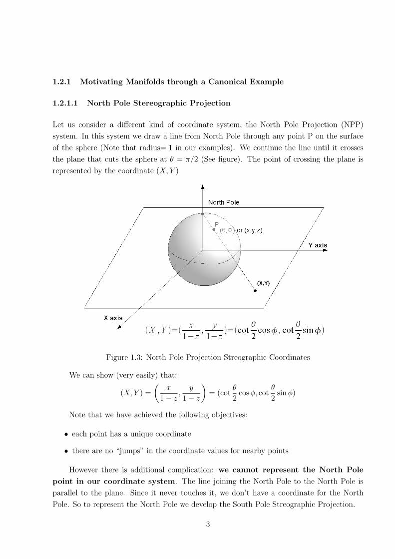
Let us consider a different kind of coordinate system, the North Pole Projection (NPP)

system. In this system we draw a line from North Pole through any point P on the surface

of the sphere (Note that radius= 1 in our examples). We continue the line until it crosses

the plane that cuts the sphere at θ = π/2 (See figure). The point of crossing the plane is

represented by the coordinate (X, Y )

Figure 1.3: North Pole Projection Streographic Coordinates

We can show (very easily) that:

(X, Y ) =

(x

1− z,

y

1− z

)= (cot

θ

2cosφ, cot

θ

2sinφ)

Note that we have achieved the following objectives:

• each point has a unique coordinate

• there are no “jumps” in the coordinate values for nearby points

However there is additional complication: we cannot represent the North Pole

point in our coordinate system. The line joining the North Pole to the North Pole is

parallel to the plane. Since it never touches it, we don’t have a coordinate for the North

Pole. So to represent the North Pole we develop the South Pole Streographic Projection.

3

1.2.1.2 South Pole Stereographic Projection

Similar to above, let us take a line from the South Pole through the point P and see where

it cuts the θ = π/2 plane. Let the point be (U, V ) (See figure). We call the coordinate the

South Pole Projection (SPP) coordinate.

Figure 1.4: South Pole Projection Streographic Coordinates

This coordinate system gives the North Pole coordinate as (U, V ) = (0, 0). We can

represent the North Pole in it but we cannot now represent the South Pole in it. The line

from the South Pole to the South Pole never touches the coordinate plane.

Essentially we have achieved the following. We have two local coordinate systems. They

are called local because they do not represent all the points in the Manifold. The SPP system

gives coordinates for points in

S2 − {South Pole}

and the NPP system gives coordinates for points in

S2 − {North Pole}

Using multiple local coordinate systems (in our example two) we can always cover an arbi-

trary Manifold such that each point has a coordinate in at least one coordinate system.

However there is an important consistency criterion for the points that have coordinates

in multiple coordinate functions. We require that for such points the transition function for

4

coordinates from one local system to another be smooth. In our example, the mathematical

function that takes us from (U, V ) to (X,Y ) (or vice versa) must be smooth. If the transition

function is infinitely differentiable then the Manifold is a Differentiable Manifold.

1.2.2 Some Formalism: Charts & Atlases

We now develop some formalism. The formalism and notation is similar to [1, pg. 133]

but we motivate it with our own illustration. In the above diagram we have “patched” some

Manifold M having dimension m with open sets Ui such that⋃Ui = M where i = 1...4.

Each point should be present in at least one Ui. Regions with overlaps are shown in hatched

lines. These regions are also marked U1∩U2 etc. We may even have regions like U1∩U2∩U3

for some other Manifold but for simplicity we assume that is not the case here. Of course,

the nature of the overlaps between Ui and the number of Ui required to cover the whole

Manifold depends on the Manifold itself.

Each Ui is associated with a map ϕi that takes a point and gives its coordinates in the

local coordinate system U ′i . Given a point P ∈ Ui, ϕi(P ) = (x1

i , x2i , ..., x

mi ). The superscripts

here are not powers but just labels to distinguish between the coordinate components. It is

important to note that points exist in a Manifold regardless of what coordinates they have.

Points have an existence independent from their representation in some local coordinate

system.

Lets look at some representative points on the diagram. Take P3 ∈ U1. ϕ1(P3)

5

has some coordinate in the local coordinate system U ′1 on the lower right hand side

(e.g. (23,3.5) if m = 2 3). Take P2 ∈ U1 ∩ U2. We have two coordinates representations

ϕ1(P2) and ϕ2(P2).

Let ψ12 be a map that takes us from U ′1 to U ′

2. Restated, ψ12(xµ) ≡ ϕ2ϕ

−11 . We can

understand this as the following: Let xµ where (1 ≤ µ ≤ m) be the local coordinate (in

system U ′1) of a point A ∈ U1 ∩ U2. The inverse map ϕ−1

1 acts on a local coordinate xµ in

U ′1 and gives us A. Then the map ϕ2 acts on point A and gives us the local coordinates yν

(1 ≤ ν ≤ m) in the system U ′2. In general ψij(x

µ) ≡ ϕjϕ−1i .

In function notation we can represent ψ12 as m functions

x1(y1, y2, ..., ym)

x2(y1, y2, ..., ym)

x3(y1, y2, ..., ym)

...

xm(y1, y2, ..., ym)

These m functions are called transition functions because they allow us to go

from the local coordinate system (x1, x2, ..., xm) ∈ U ′1 to another local coordinate system

(y1, y2, ..., ym) ∈ U ′2. For the Manifold to be a Differentiable Manifold each of these func-

tions must be infinitely differentiable or C∞.

In general, if zµi is the coordinate in the ith local system then all the transition functions

zµi (z1

j , z2j , z

3j , ..., z

mj ) should be C∞ where 1 ≤ i, j, µ ≤ m. Note that the transition functions

only make sense on points that are present in the originating “patch” and the destination

“patch”.

1.2.3 The Three Rules of Manifolds

We summarize our introduction to Manifolds with three rules (from [1, pg. 132]:

• Nearby Points have nearby coordinates in at least one coordinate system

• Every point has unique coordinates in each coordinate system that contains it

• If two coordinate systems overlap, then in the region of the overlap, local coordinates

of the point are related to each other in a sufficiently smooth way3we are using cartesian coordinates in the U ′

1 local coordinate system. This is just an example. We mayuse polar or any other coordinate system

6

1.3 Some Basic Concepts

We introduce Tangent Spaces and Vector Fields. These concepts are fundamental to under-

standing Manifolds.

1.3.1 Tangent Spaces

Figure 1.5: Vectors can’t just start and end anywhere like in Rn

In R3, vectors can start and end anywhere. In the above diagram we have shown that.

However in other Manifolds like S2 this is not true. It does not make sense for a vector to

start and end anywhere. In the above diagram we have shown two invalid examples for S2

of vectors that start on the surface and then cut through the Manifold onto another point.

S2 is a two dimensional Manifold. The body of the vectors is, in a way, traveling outside the

Manifold. What is the solution?

The solution is to require each vector to live in a Tangent Space. As the name implies,

the Tangent Space is tangent to the Manifold. Each point on the Manifold has its own

Tangent Space. The Tangent Space has the same dimensionality as the Manifold itself.

The Tangent Space at the point P on Manifold M is denoted by TP (M). In our diagram

we show two Tangent Spaces on the Manifold TP2(M), TP1(M) at the points P2 and P1

respectively. A few example vectors are drawn in each Tangent Space. So we require that

vectors only live in tangent spaces.

In the example of S2 each tangent space is R2. This makes intuitive sense because

7

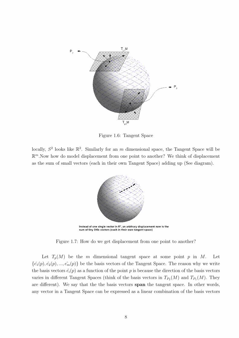
Figure 1.6: Tangent Space

locally, S2 looks like R2. Similarly for an m dimensional space, the Tangent Space will be

Rm.Now how do model displacement from one point to another? We think of displacement

as the sum of small vectors (each in their own Tangent Space) adding up (See diagram).

Figure 1.7: How do we get displacement from one point to another?

Let Tp(M) be the m dimensional tangent space at some point p in M . Let

{e1(p), e2(p), ..., em(p)} be the basis vectors of the Tangent Space. The reason why we write

the basis vectors ei(p) as a function of the point p is because the direction of the basis vectors

varies in different Tangent Spaces (think of the basis vectors in TP2(M) and TP1(M). They

are different). We say that the the basis vectors span the tangent space. In other words,

any vector in a Tangent Space can be expressed as a linear combination of the basis vectors

8

for that Tangent Space. In the mathematician’s notation these basis vectors are written as:

{ ∂

∂x1,∂

∂x2, · · · , ∂

∂xm}

There are mathematical reasons why you may want to write basis vectors in the

above notation. The concept of partial derivatives captures the concept of basis vectors

well. However we do not loose very much if we mentally convert the above expression to

{e1(p), e2(p), ..., em(p)} for understanding purposes.

1.3.2 Vector Fields

A vector field in Rn means you have a vector at each point in space. The vector could be in

an arbitrary direction. A vector field on a Manifold means that you have a vector at each

point on the Manifold. However, the vector direction at a point can only be in any direction

inside the Tangent Space for that point.

9

CHAPTER 2

RIEMANNIAN MANIFOLDS

2.1 Some Prelimaries

To study Riemannian Manifolds and metrics, we first introduce some simple concepts.

2.1.1 Curvature and Parallel Transport

A very intuitive understanding of curvature in space can be obtained by understanding

parallel transport on S2. Follow the vector along the path shown in the diagram. At each

point, the vector is in the Tangent Space of that point. We take care not to shift or twist

the vector in any other way. We shift it “parallel to itself.”

A suprising thing happens. Over a closed path, the starting vector is different from the

ending vector. When this happens, we say that the Manifold has curvature over the path.

This phenomenon does not happen in Rn.

We will now measure curvature mathematically. For that we need to understand co-

variant derivatives or a connection.10

2.1.2 Covariant Derivative / Connection

Figure 2.1: Concept of Covariant Derivatives. Diagram adapted from [2, pg. 298]

Suppose we have a smoothly varying vector (or a tensor) field over a Manifold. We

should be able to capture the way it is changing by calculating its “derivative.” This deriva-

tive should have the same value regardless of the local coordinates we use to calculate it. In

other words, we need to define a “covariant” derivative. The covariant derivative allows us

express more complicated concepts like curvature and torsion in space.

Look at the Manifold in the above figure. It is a good example of a vector field. We

centre our interest on how the vector field varies along the red dashed curve. The vector

field at various points on the curve is shown by black arrows. How much is a vector field

varying with respect to the vector at point P? It is tough to say because the Manifold has

curvature (and we simply cannot subtract two vectors at different points on the Manifold

to get a difference as we did in Rn). In order to compare the change we parallely transport

the vector from point P . The parallely transported vector is depicted in green. Now we can

calculate the difference ∆v. In the case of covariant derivatives we are interested in change

only in a particular direction and not over a curve. In our diagram the direction that we are

interested in is w. We think of a covariant derivative of a vector field in the direction w.

Assume we are in some local coordinate system with coordinates xα. We define the

covariant derivative of a vector field v(xα) in direction w as:

∇wv(xα) = limε→0

(v(xα + wαε))‖ transport to xα − v(xα)

ε(Notation from [3, pg. 433])

11

Figure 2.2: Concept of Covariant Derivatives II. Diagram adapted from [3, pg. 433]

Properties of the covariant derivative:

∇w+u = ∇w +∇u

∇λw = λ∇w

∇w(E + N) = ∇wE +∇wN

Leibnitz Law:

∇w(λE) = λ∇wE + E∇wλ

NOTE: E,N are vector fields. λ is some scalar function.

2.1.3 Riemann Curvature

Riemann curvature R(L,M,N) where L,M,N are vector fields is defined as:

R(L,M,N) =(∇L∇M −∇M∇L −∇[L,M]

)[L,M] ≡ LM−MN. Note that R maps three vectors to a vector. In tensorial notation:

R(L,M,N) = LaM bN cRabcd

Rabcd is the Riemannian curvature tensor. Ricci Curvature Rac

Rac = Radcd

and Ricci scalar S

S = gacRac

12

2.2 Riemannian Manifolds & Metrics

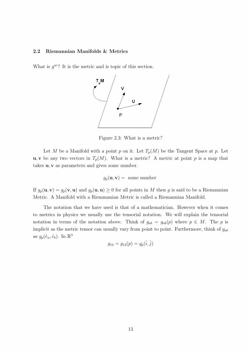
What is gac? It is the metric and is topic of this section.

Figure 2.3: What is a metric?

Let M be a Manifold with a point p on it. Let Tp(M) be the Tangent Space at p. Let

u,v be any two vectors in Tp(M). What is a metric? A metric at point p is a map that

takes u,v as parameters and gives some number.

gp(u,v) = some number

If gp(u,v) = gp(v,u) and gp(u,u) ≥ 0 for all points in M then g is said to be a Riemannian

Metric. A Manifold with a Riemmanian Metric is called a Riemannian Manifold.

The notation that we have used is that of a mathematician. However when it comes

to metrics in physics we usually use the tensorial notation. We will explain the tensorial

notation in terms of the notation above. Think of gab = gab(p) where p ∈ M . The p is

implicit as the metric tensor can usually vary from point to point. Furthermore, think of gab

as gp(ea, eb). In R3

g12 = g12(p) = gp(i, j)

13

CHAPTER 3

COMPLEX MANIFOLDS

3.1 Introduction

In a Complex Manifold, each coordinate is complex. A Complex Manifold of dimension m

looks like Cm locally. The transition functions from one local coordinate system to another

satisfy the Cauchy-Riemann conditions i.e. are holomorphic.

Let z be a complex coordinate expressed in terms of its real components. zµ = xµ + iyµ

for some local patch U1. Let w be a complex coordinate expressed in terms of its real

components wν = uν + ivν for another patch U2. Let U1 ∩ U2 6= ∅. Then the transition

functions satisfy the Cauchy-Riemann conditions:

∂uν

∂xµ=∂vν

∂yµ(3.1)

∂uν

∂yµ= −∂v

ν

∂xµ(3.2)

An equivalent way of saying this is that:

wν(z1, z2, · · · , zm, z1, z2, · · · , zm) = wν(z1, z2, · · · , zm)

In other words, wν is not a function of zi. As always 1 ≤ µ, ν ≤ m.

Proof:

If wν is not a function of zi ⇒ ∂wν

∂zµ = 0

Now:

∂wν

∂zµ=

∂uν + ivν

∂(xµ − iyµ)

=∂uν

∂xµ− 1

i

∂uν

∂yµ+ i

(∂vν

∂xµ− 1

i

∂vν

∂yµ

)=

(∂uν

∂xµ− ∂vν

∂yµ

)+ i

(∂vν

∂xµ+∂uν

∂yµ

)= 0 + i0 = 0 (from 3.1 and 3.2)

Hence proved.

14

3.2 The Stereographic Projection Example: Continued

Stereographic coordinates of a point P (x, y, z) on a unit sphere

North Pole Projection:

(X, Y ) = (x

1− z,

y

1− z)

South Pole Projection:

(U, V ) = (x

1 + z,−y

1 + z)

Let

Z = X + iY ⇒ Z = X − iY

Let

W = U + iV ⇒ W = U − iV

W =x− iy

1 + z

=1− z

1 + z

(x

1− z− iy

1− z

)=

1− z

1 + z(X − iY )

=X − iY

1+z1−z

=X − iY

X2 + Y 2

=1

Z

W (Z, Z) = 1Z

W does not depend on Z Therefore S2 is a complex manifold of complex dimension 1

3.3 Some Formalism

Tangent Space Tp(M) of a Real Manifold of dimension m is spanned by m vectors

{ ∂

∂x1,∂

∂x2, ...,

∂

∂xm}

Tangent Space Tp(M) of a Complex Manifold of dimension m is spanned by 2m vectors

{ ∂

∂x1,∂

∂x2, ...,

∂

∂xm;∂

∂y1,∂

∂y2, ...,

∂

∂ym}

Note that we are in some arbitrary local patch with coordinates zµ = xµ + yµ. We define:

∂

∂zµ≡ 1

2{ ∂

∂xµ− i

∂

∂yµ}

15

∂

∂zµ≡ 1

2{ ∂

∂xµ+ i

∂

∂yµ}

Given the above definitions we can alternatively say that the tangent space Tp(M) of the

Complex Manifold is spanned by:

{ ∂

∂z1,∂

∂z2, ...,

∂

∂zm;∂

∂z1,∂

∂z2, ...,

∂

∂zm}

Let us define a map Jp such that:

Jp ∂/∂xµ = ∂/∂xµ and Jp ∂/∂y

µ = −∂/∂xµ

from the Cauchy-Riemann relations we can show that

Jp∂/∂uµ = ∂/∂vµ and Jp∂/∂v

µ = −∂/∂uµ

where zµ = xµ + yµ and wµ = uµ + vµ are local coordinates on two patches. What is

interesting is that the Cauchy Riemann conditions on the transition functions allows Jp to

have the same consistent definition on another patch. So while we can have Jp on any patch

of a manifold it is only in complex manifolds that Jp “spreads” like this.

3.4 Hermetian Manifolds

Hermetian Manifolds are Manifolds which satisfy

gp(JpX, JpY ) = gp(X, Y )

3.5 Kahler Manifolds

Kahler Manifolds are a special kind of Hermetian Manifold in which the metric g can be

expressed in terms of a potential function K

gµv = ∂µ∂vK

This is useful because we need to only keep track of the potential instead of a whole metric

tensor.

16

CHAPTER 4

ORBIFOLDS

Orbifolds are a special kind of Manifold. To understand Orbifolds we first need to understand

equivalence relations. An equivalence relation ∼ is a relation which satisfies:

• a ∼ a

• if a ∼ b then b ∼ a

• if a ∼ b and b ∼ c then a ∼ c

According to [1, pg. 38] “Given a set X and an equivalence relation ∼, we have a

partition of X into mutually disjoint subsets called equivalence classes. A class [a] is

made of all the elements x in X such that x ∼ a. [a] ≡ {x ∈ X|x ∼ a}”

The set of all the mutually disjoint classes refered to above is called quotient space.

The notation is X/ ∼. We motivate a very elegant example (from [1, pg. 39]). Let x, y ∈ R.

Also let x ∼ y iff y = x + 2πn, n ∈ Z. Now [x] = {· · · , x − 2πn, x + 2πn, x + 4πn, · · ·}. A

little bit of thought convinces us that R/ ∼= S1 where S1 is a circle. We look at another

example (from [1, pg. 41]). Let us have a Disc D2 of radius 1 on R2.

D2 = {x2 + y2 ≤ 1, x, y ∈ R}

. Two points (x1, y1) and (x2, y2) in D2 are equivalent iff x21 + y2

1 = 1 and x22, y

22 = 1 (both

are on the edge of the Disc). All points on the edge of the disc are equivalent. Now imagine

a rubber sheet shaped like a disc. If we stuck all the edges of the disc together we would get

a sphere S2. Therefore D2/ ∼= S2. There is another way of saying this. All the points on

the edge of the disc were equivalent and they made a circle S1. So D2/S1 = S2.

In general if we have quotient space A = M/B and if M is a Manifold and B is a

discrete group acting on M thenA is an Orbifold. A simple example is C/Z3. Z3 = {1, ω, ω2}(cube roots of unity). Lets take z ∈ C. Now {z, zω, zω2} are all equivalent to each other.

We are left with only one third of the complex plane. This one third is the Orbifold C/Z3.

17

CHAPTER 5

NUMERICAL COMPUTATIONS

For this part of the project three tasks were performed:

• The C3/Z3 orbifold was represented in terms of a polytope and visualized in 3D

• The C3/Z5 orbifold was represented in terms of a polytope and visualized in 3D

• Given a potential for C3/Z3 various metrics (Ricci flat and non flat) were calculated.

After calculating the metric, the Ricci tensor was calculated. The Ricci scalar was also

calculated and represented graphically.

5.1 Visualization of C3/Z3

The C3/Z3 orbifold can be represented mathematically as a polytope 1. with the following

properties:

• xi > 0 where i = 1, 2, 3

• (t− x1 − x2 + 3x3) > 0 where t = blow-up parameter (a constant)

Figure 5.1: The C3/Z3 polytope from two different angles. t = 0.3

The program to achieve this is placed in Appendix A.1According to the Wikipedia “In geometry polytope means, first, the generalization to any dimension ofpolygon in two dimensions, polyhedron in three dimensions, and polychoron in four dimensions”

18

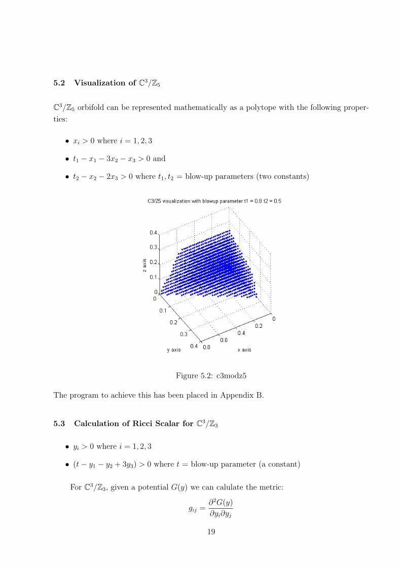
5.2 Visualization of C3/Z5

C3/Z5 orbifold can be represented mathematically as a polytope with the following proper-

ties:

• xi > 0 where i = 1, 2, 3

• t1 − x1 − 3x2 − x3 > 0 and

• t2 − x2 − 2x3 > 0 where t1, t2 = blow-up parameters (two constants)

Figure 5.2: c3modz5

The program to achieve this has been placed in Appendix B.

5.3 Calculation of Ricci Scalar for C3/Z3

• yi > 0 where i = 1, 2, 3

• (t− y1 − y2 + 3y3) > 0 where t = blow-up parameter (a constant)

For C3/Z3, given a potential G(y) we can calulate the metric:

gij =∂2G(y)

∂yi∂yj

19

gij = inverse of the matrix gij

Given the metric we can calculate the Ricci Tensor and Scalar:

Rcd = Ricci Tensor = −1

2gfd ∂2gce

∂ye∂yf

R = Ricci Scalar = Rijgij

See [4] for a detailed treatment of above formulae. Now, given a seed potential:

Gp =1

2(y1 ln y1 + y2 ln y2 + y3 ln y3 + (t− y1 − y2 + 3y3) ln (t− y1 − y2 + 3y3))

And a correction term f(y) such that:

f(y) =1

2((y − λt) ln(y − λt) + (y − λ∗t) ln(y − λ∗t)− (3y + t) ln(3y + t))

A Ricci flat metric can be obtained from the potential G = Gp + f(y3)

We perform the following steps on the computer:

• We create a representation of the C3/Z3 polytope with a discrete set of points in

a volume from say (0.04, 0.04, 0.04) to (1, 1, 1). Each point may be separated from

another by a small enough δ

• We calculate the Ricci Scalar at each point in the polytope given seed potential Gp

• We calculate the Ricci Scalar at each point in the polytope given potential G = Gp +

f(y3)

• We take a slice of the polytope at some y3 = 0.7 (say) and depict the absolute value

of the Ricci scalar on the z–axis and the y1 and y2 coordinates on the x and y axes

respectively

The programs to achieve this have been placed in Appendix C,D. A small note on using

the programs is given in Appendix E.

5.4 Looking at the absolute value of the Ricci Scalars

We take a slice of the polytope at some y3 = 0.7 (say) and depict the absolute value of the

Ricci scalar on the z–axis and the y1 and y2 coordinates on the x and y axes respectively.

We perform this for the seed metric Gp and the Ricci–flat metric Gp + f(y3). We get the

following figures (for minimum separation between points as 0.02 (δ)):

20

Figure 5.3: Looking at Ricci scalars produced by potential G = Gp (above) and

G = Gp + f(y3) (below)

The red points in the graph are the (y1, y2) points where the Ricci Scalar exists (and the

polytope exists).The green points in the graph are the points where the polytope exists but

we do not know the value of the Ricci Scalar as we don’t have enough values for numerical

differentiation.

Notice, that except at the edges, the surface of the curve is flat. In fact, this edge

behaviour is due to a numerical artifact of computation. The theoretical value of the Ricci

Scalar for the Guillemin metric (see [4, pg. 6] is:

12(t2 + 72y23)

(t+ 12y3)3

For t = 0.3 and y3 = 0.7 (we also call it z in the graph) theoretical value of S = 0.64 (to

two decimal places). We get experimental value of 0.82 (when δ = 0.02 and the boundaries

of the polytope are from (0.04, 0.04, 0.04) to (1, 1, 1))

The next graph is same as the previous graph except we now show the value of the

potential in cyan colour.

Does the Ricci Scalar reach its theoretical value of 0.64 for G = Gp?

We cannot numerically prove this but as we decrease the δ, our values should converge

21

Figure 5.4: Looking at potential (in cyan) G = Gp (above) and G = Gp + f(y3) (below)

to 0.64. For polytope boundary (0.04, 0.04, 0.04) to (1, 1, 1))

δ Ricci Scalar Average

0.05 1.05

0.04 1.00

0.03 0.93

0.02 0.82

0.015 0.77

Does the Ricci Scalar Vanish for G = Gp + f(y3)?

Again, we cannot numerically prove this but we can however establish a trend. As we

decrease delta we should see the Ricci Scalar Average tend to 0. For polytope boundary

(0.04, 0.04, 0.04) to (1, 1, 1))

δ Ricci Scalar Average

0.05 0.43

0.04 0.37

0.03 0.29

0.02 0.18

0.015 0.12

22

CONCLUSION

We have given an comprehensive introduction to Manifolds. We looked at the whole hierarchy

of Manifolds. We started from Simple Manifolds and progressed to Differentiable Manifolds,

Riemannian Manifolds and Complex Manifolds. Within Complex Manifolds we studied

Hermetian Manifolds and Kahler Manifolds. Orbifolds, another special kind of Manifold,

were also introduced. All the related mathematics and concepts such as Vector Fields,

Tangent Spaces, Metrics, Curvature, Parallel Transport and Connection were explained.

In Chapter 5 we also performed some numerical computations on C3/Z3 and C3/Z5.

We have gained theoretical and computational knowledge about Manifolds and Differ-

ential Geometry in this project.

23

APPENDIX A

Code for c3modz3 polytope visualize.m

% Visualize the C3/Z3 Polytope

% t is the blowup parameter

t=.3;

clear x1p;

clear x2p;

clear x3p;

% Generate points in the polytope

j=0;

delta=0.05;

for x1=0:delta:1

for x2=0:delta:1

for x3=0:delta:1

if t-x1-x2+3*x3 > 0

j=j+1;

x1p(j) = x1;

x2p(j) = x2;

x3p(j) = x3;

end

end

end

end

grid on;

hold on;

xlabel(’x1’);

ylabel(’x2’);

zlabel(’x3’);

title(’C3/Z3 for blowup parameter t=0.3’);

plot3(x1p,x2p,x3p,’.’);

24

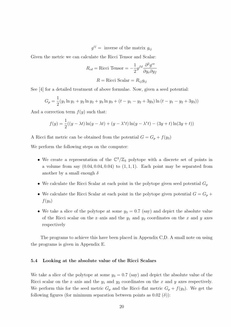
APPENDIX B

Code for c3modz5 polytope visualize.m

% Visualize the C3/Z5 polytope

j=0;

% t1, t2 are the blowup parameters

t1=.8;t2=.5;

clear x1p;

clear x2p;

clear x3p;

delta = 0.02;

endx=2;endy=2;endz=2;

for x1=0.0:delta:endx

for x2=0.0:delta:endy

for x3=0.0:delta:endz

if t1-x1-3*x2-x3 > 0 && t2-x2-2*x3 > 0

j=j+1;

x1p(j) = x1;

x2p(j) = x2;

x3p(j) = x3;

end

end

end

end

x = [x1p; x2p; x3p];

hold on;

grid on;

axis square;

title([’C3/Z5 visualization with blowup parameter t1 = ’,num2str(t1),

’ t2 = ’,num2str(t2)]);

xlabel(’x axis’);

ylabel(’y axis’);

zlabel(’z axis’);

plot3(x1p,x2p,x3p,’.’);

hold off;

25

APPENDIX C

Code for c3modz3 metrics and ricci.m (Please excuse the bad formatting. The code lines

were long and have been made to wrap around so that they fit on the page)

function [polytope,G ,g_high ,g_low , Ricci] = c3modz3_metrics_and_ricci

(startx, starty, startz, endx, endy, endz, t, delta,guil)

%Example parameters

%t=.3;startx=0.04;starty=0.04;startz=0.04;endx=1;endy=1;endz=1;delta=0.04;

%guil=false

% startx, starty, startz should be small and positive otherwise we will

% have log of zero issues in the calculation of the guillemnin metric

% if guil == true then only the guillemin metric is used to calculate the

% Ricci tensors

% g_low = g_{ij} = \frac{\partial^2 G(x)}{\partial x^i \partial x^j}

% G(x) is the symplectic potential (see report for expression)

% g_high = g^{ij} = matrix inverse of g_{ij}

% Ricci = R_{cd} = Ricci Tensor = -0.5 g^{fd}\frac{\partial^2 g^{ce}}

% {\partial x^e \partial x^f}

% R = Ricci Scalar = g_{ij} R_{ij}

% See Arxiv hep-th/9803192

% Generate points in the polytope

j=0;k=0;l=0;

lengx = length(startx:delta:endx);

lengy = length(starty:delta:endy);

lengz = length(startz:delta:endz);

polytope.startx = startx;

polytope.starty = starty;

polytope.startz = startz;

polytope.endx = endx;

polytope.endy = endy;

polytope.endz = endz;

polytope.t = t;

polytope.delta = delta;

26

polytope.guil = guil;

polytope.lengx = lengx;

polytope.lengy = lengy;

polytope.lengz = lengz;

polytope.exists = zeros(lengx, lengy, lengz,’uint8’);

for x1=startx:delta:endx

j=j+1;

for x2=starty:delta:endy

k=k+1;

for x3=startz:delta:endz

l=l+1;

if t-x1-x2+3*x3 > 0

polytope.exists(j,k,l) = true;

else

polytope.exists(j,k,l) = false;

end

end

l=0;

end

k=0;

end

j=0;

lamb = (-3+i*sqrt(3))/6;

G=zeros(lengx, lengy, lengz);

for k=1:lengx

for l=1:lengy

for m=1:lengz

x = startx+(k-1)*delta;

y = starty+(l-1)*delta;

z = startz+(m-1)*delta;

if(polytope.exists(k,l,m))

Gp = 1/2 * (x*log(x) + y*log(y) + z*log(z)) + 1/2 *

(t-x-y+3*z)*log(t-x-y+3*z);

27

if (guil)

G(k,l,m) = Gp;

else

f = 1/2*((z-lamb*t)*log(z-lamb*t) + (z-conj(lamb)*t)

*log(z-conj(lamb)*t) - (3*z+t)*log(3*z+ t));

G(k,l,m) = Gp + f;

end

else

G(k,l,m) = NaN;

end

end

end

end

% calculate g tensor at each point (k,l,m)

nan_array = [NaN NaN NaN;NaN NaN NaN;NaN NaN NaN];

A = zeros(2,2);

for k=1:lengx-2

for l=1:lengy-2

for m=1:lengz-2

A(1,1) = ((G(k+2,l,m)-G(k+1,l,m)) - (G(k+1,l,m) - G(k,l,m)))

/(delta^2);

A(2,2) = ((G(k,l+2,m)-G(k,l+1,m)) - (G(k,l+1,m) - G(k,l,m)))

/(delta^2);

A(3,3) = ((G(k,l,m+2)-G(k,l,m+1)) - (G(k,l,m+1) - G(k,l,m)))

/(delta^2);

% Actually we could use symmetry properties in which A(2,1) =

% A(1,2) and so on but we avoid that for now so that the least

% assumptions are made as possible.

A(2,1) = ((G(k+1,l+1,m)-G(k,l+1,m)) - (G(k+1,l,m) - G(k,l,m)))

/(delta^2);

A(1,2) = ((G(k+1,l+1,m)-G(k+1,l,m)) - (G(k,l+1,m) - G(k,l,m)))

/(delta^2);

A(3,1) = ((G(k+1,l,m+1)-G(k,l,m+1)) - (G(k+1,l,m) - G(k,l,m)))

/(delta^2);

28

A(1,3) = ((G(k+1,l,m+1)-G(k+1,l,m)) - (G(k,l,m+1) - G(k,l,m)))

/(delta^2);

A(3,2) = ((G(k,l+1,m+1)-G(k,l,m+1)) - (G(k,l+1,m) - G(k,l,m)))

/(delta^2);

A(2,3) = ((G(k,l+1,m+1)-G(k,l+1,m)) - (G(k,l,m+1) - G(k,l,m)))

/(delta^2);

%Are there any NaNs?

if(sum(sum(isnan(A))) > 0)

g_high(k,l,m).tensor = nan_array;

g_high(k,l,m).exists = false;

g_low(k,l,m).tensor = nan_array;

g_low(k,l,m).exists = false;

else

B = inv(A);

g_low(k,l,m).tensor = A;

g_low(k,l,m).exists = true;

g_high(k,l,m).tensor = B;

g_high(k,l,m).exists = true;

end

end

end

end

%Calculate Ricci tensor for each point

R=zeros(3,3);

for k=1:lengx-4

for l=1:lengy-4

for m=1:lengz-4

ricci_exists = true;

% Calculate Ricci tensor

for c=1:3

for d=1:3

% e = 1, f = 1

dd(1,1) = -1/2*g_high(k,l,m).tensor(1,d)*

29

((g_high(k+2,l,m).tensor(c,1) - g_high(k+1,l,m).tensor(c,1)) -

(g_high(k+1,l,m).tensor(c,1) - g_high(k,l,m).tensor(c,1)))/(delta^2);

% e = 2, f = 2


((g_high(k,l+2,m).tensor(c,2) - g_high(k,l+1,m).tensor(c,2)) -

(g_high(k,l+1,m).tensor(c,2) - g_high(k,l,m).tensor(c,2)))/(delta^2);

% e = 3, f = 3


((g_high(k,l,m+2).tensor(c,3) - g_high(k,l,m+1).tensor(c,3)) -

(g_high(k,l,m+1).tensor(c,3) - g_high(k,l,m).tensor(c,3)))/(delta^2);

% Actually we could use symmetry properties in which d(2,1) =

% d(1,2) and so on but we avoid that for now so that the least

% assumptions are made as possible.

% e = 2, f = 1


((g_high(k+1,l+1,m).tensor(c,2) - g_high(k,l+1,m).tensor(c,2)) -


% e = 1, f = 2


((g_high(k+1,l+1,m).tensor(c,1) - g_high(k+1,l,m).tensor(c,1)) -


% e = 3, f = 1


((g_high(k+1,l,m+1).tensor(c,3) - g_high(k,l,m+1).tensor(c,3)) -


% e = 1, f = 3


((g_high(k+1,l,m+1).tensor(c,1) - g_high(k+1,l,m).tensor(c,1)) -


% e = 3, f = 2


((g_high(k,l+1,m+1).tensor(c,3) - g_high(k,l,m+1).tensor(c,3)) -


% e = 2, f = 3

30


((g_high(k,l+1,m+1).tensor(c,2) - g_high(k,l+1,m).tensor(c,2)) -


%Are there any NaNs?

R(c,d) = sum(sum(dd));

if(R(c,d) == NaN)

%The ricci tensor does not exist for k,l,m

%combination

ricci_exists = false;

R = nan_array;

break;

end

end %d

if(ricci_exists == false)

break;

end

end %c

Ricci(k,l,m).exists = ricci_exists;

Ricci(k,l,m).tensor = R;

% Calculate Ricci Scalar

ricci_scalar = 0;

if ricci_exists

for p=1:3

for q=1:3

ricci_scalar = ricci_scalar +

g_low(k,l,m).tensor(p,q)*Ricci(k,l,m).tensor(p,q);

end

end

end

Ricci(k,l,m).scalar = ricci_scalar;

end %m

end %l

end %k

31

APPENDIX D

Code for visualize c3modz3 ricci.m

function visualize_c3modz3_ricci(polytope, G, Ricci, visualize_G, z, skip)

% Visualize the curvature (Ricci Scalar) through the polytope

% Can visualize the polytope at various slices of z

% Ricci scalar value is on the z-axis

% if visualize_G == true then the potential is graphed

% Sometimes there are too many data points so we may want to skip, say,

% every 4 or 8. so set skip parameter to 8. default should be 1

hold on;

grid on;

startx = polytope.startx;

starty = polytope.starty;

startz = polytope.startz;

endx = polytope.endx;

endy = polytope.endy;

endz = polytope.endz;

delta = polytope.delta;

t = polytope.t;

lengx = polytope.lengx;

lengy = polytope.lengy;

lengz = polytope.lengz;

m=floor((z-startz)/delta);

for k=1:skip:lengx-4

for l=1:skip:lengy-4

height(k,l)=abs(Ricci(k,l,m).scalar);

end

end

% Mark x,y points at given z for which the polytope exists

32

for k=1:skip:lengx

for l=1:skip:lengy

x = startx + (k-1)*delta;

y = starty + (l-1)*delta;

if(polytope.exists(k,l,m))

plot3(x,y,0,’.g’);

end

if(visualize_G)

plot3(x,y,G(k,l,m),’.c’);

end

end

end

% Mark x,y points at given z for which the Ricci tensor exists

ricci_scalar_sum = 0;

for k=1:skip:lengx-4

for l=1:skip:lengy-4



if(Ricci(k,l,m).exists)

plot3(x,y,0,’.r’);

end

end

end

% Calculate ricci_scalar_sum

% Do it without the skips

for k=1:lengx-4

for l=1:lengy-4



if(Ricci(k,l,m).exists)

ricci_scalar_sum = ricci_scalar_sum + Ricci(k,l,m).scalar;

33

end

end

end

ricci_scalar_avg = ricci_scalar_sum / ((lengy-4)*(lengx-4))

disp(’Theoretical value of seed metric ricci scalar’);

seed_metric_ricci_scalar = 12*(t^2+72*z^2)/(t+12*z)^3

xlabel(’x axis’);

ylabel(’y axis’);

zlabel(’Ricci scalar (absolute value)’);

if(visualize_G)

title([’Ricci scalar for z=’,num2str(z),’ t = ’, num2str(t),\ ’ (value

of potential in cyan)’]);

else

title([’Ricci scalar for z=’,num2str(z),’ t = ’, num2str(t)]);

end

x = startx:delta:endx;

y = starty:delta:endy;

[xg, yg] = meshgrid(x(1:skip:lengx-4),y(1:skip:lengy-4));

surf(xg, yg, height(1:skip:lengx-4, 1:skip:lengy-4));

34

APPENDIX E

Sample Command Invocations

In order to generate a C3/Z3 polytope from (0.04,0.04,0.04) to (1,1,1) with a distance between

adjacent points 0.04 we issue the following command at the MATLAB command line:

[poly,G,g_l,g_h,ricci]=c3modz3_metrics_and_ricci(0.04,0.04,0.04,1,1,1,0.3,0.04,false);

Please see the program code for understanding details about various options.

• poly structure contains information on which points the polytope is present in, between

(0.04,0.04,0.04) to (1,1,1). It also contains some other book keeping information about

the C3/Z3 polytope.

• G contains the value of the potential at each point in the polytope.

• g l structure contains the value of gij at each point in the polytope.

• g h structure contains the value of gij at each point in the polytope.

• ricci structure contains the Ricci tensor and the Ricci scalar for each point on the

polytope.

To visualize the Ricci Scalar for the polytope at the z=0.7 slice we issue the command:

visualize_c3modz3_ricci(poly,G,ricci,false,0.7,1)

We may want to compare the Ricci scalars with the potentials G = Gp and G = Gp + f(y3).

In such cases we issue the following 4 commands in sequence:

[polyt,Gt,glt,ght,riccit]=c3modz3_metrics_and_ricci(0.04,0.04,0.04,1,1,1,0.3,0.04,true);

[poly,G,gl,gh,ricci]=c3modz3_metrics_and_ricci(0.04,0.04,0.04,1,1,1,0.3,0.04,false);

visualize_c3modz3_ricci(polyt,Gt,riccit,false,0.7,1)

visualize_c3modz3_ricci(poly,G,ricci,false,0.7,1)

35

REFERENCES

[1] Mikio NAKAHARA: Geometry, Topology and Physics (Graduate Student Series in

Physics), Adam Hilger, Bristol & New York, 1990

[2] Roger PENROSE: The Road to Reality: A Complete Guide to the Laws of the Uni-

verse, Vintage Books, 2005

[3] James B. HARTLE: Gravitation: An Introduction to Einstein’s theory of General Rel-

ativity, Pearson Education, Inc., 2003

[4] Koushik RAY: A Ricci-flat metric on D-brane orbifolds, ArXiv hep-th/9803192

SOME OTHER USEFUL RESOURCES

[5] Michael SPIVAK: A Comprehensive Introduction to Differential Geometry: Volume

I, 2nd Edition, Publish or Perish, Inc. (Houston, Texas), 1979

[6] K.F. RILEY, M.P. HOBSON, S.J. BENCE: Mathematical Methods for Physics and

Engineering, 2nd Edition (Reprinted with Corrections), Cambridge University Press,

2003

[7] Tohru EGUCHI, Peter B. GILKEY, Andrew J. HANSON: Gravitation, Gauge

Theories and Differential Geometry, Physics Reports (Review Section of Physics Letters)

66(6) (1980), North Holland Publishing Company (Amsterdam)

36

Manfiolds

Documents

complex manifolds

study of manifolds

riemannian manifolds

kahler manifolds

differentiable manifolds

hermetian manifolds

tostudy manifolds

hierarchy of manifolds