Managing Debt Stability

MANAGING DEBT STABILITY

EMANUELE BACCHIOCCHI ALESSANDRO MISSALE

CESIFO WORKING PAPER NO. 1388 CATEGORY 5: FISCAL POLICY, MACROECONOMICS AND GROWTH

JANUARY 2005

An electronic version of the paper may be downloaded • from the SSRN website: www.SSRN.com • from the CESifo website: www.CESifo.de

CESifo Working Paper No. 1388

MANAGING DEBT STABILITY

Abstract This paper presents a simple model in which debt management stabilizes the debt-to-GDP ratio in face of shocks to real returns and output growth and thus supports fiscal restraint in ensuring sustainability. The optimal composition of public debt is derived by looking at the relative impact of the risk and cost of alternative debt instruments on the cost of missing the stabilization target. The optimal debt structure is a function of the expected return differentials between debt instruments, of the conditional variance of their returns and of the conditional covariances of their returns with output growth and inflation. We then explore how the relevant covariances and thus the optimal choice of debt instruments depend on the monetary regime and on Central Bank preferences for output stabilization, inflation control and interest-rate smoothing. Finally, we estimate the composition of public debt that would have supported debt stabilization in OECD countries over the last two decades. The empirical evidence suggests that the public debt should have a long maturity and a large share of it should be indexed to the price level.

JEL Code: E63, H63.

Keywords: debt management, debt structure, debt stabilization, inflation indexation, interest rates.

Emanuele Bacchiocchi University of Milan

Department of Political Economics Via Conservatorio 7

20122 Milan Italy

[email protected]

Alessandro Missale University of Milan

Department of Political Economics Via Conservatorio 7

20122 Milan Italy

[email protected]

We thank Adam Posen, Henning Bhon and other seminar participants at the CESifo and LBI Conference on Debt Sustainability for helpful comments and suggestions. The authors are associated with Università di Milano.

1. Introduction

No mention is made of debt management in the debate on debt sustainability, but a care-ful choice of debt instruments is needed to control interest payments and debt accumulation.Interest-cost minimization is important especially in countries where the level of debt is high andinterest payments absorb a large share of the budget. In the same countries avoiding the risk thatunfavorable shocks to real returns or output growth lead the debt on an unsustainable path isequally important.

We want to examine whether a concern for debt sustainability justifies the lengthening of debtmaturity that has occurred in OECD countries. We are also interested in assessing the scope forinflation-indexed bonds that have been issued only in France, Italy, Sweden and the UK whilehave been discontinued in the US. To address these issues we rely on a simple model in which debtmanagement stabilizes the debt-to-GDP ratio in face of shocks to real returns and GDP growthand thus supports fiscal restraint in ensuring sustainability.

The optimal debt composition is derived by looking at the relative impact of the risk andcost of alternative debt instruments on the cost of missing the stabilization target. This allowsto price risk against the expected cost of debt service and thus to find the optimal combinationalong the trade off between cost and risk minimization. The optimal debt structure is a functionof the expected return differentials between debt instruments, of the conditional variance of theirreturns, and of the conditional covariances of their nominal returns with output growth andinflation.

We show that debt stabilization is achieved by funding at low cost, and by issuing instrumentsthat provide a hedge against variations in the debt ratio due to lower-than-expected inflation andoutput growth. For instance, inflation-indexed bonds provide a hedge against variations in thedebt ratio due to lower-than-expected inflation. Fixed-rate bonds (as opposed to short-term bills)help to stabilize the debt ratio in cyclical downturns if interest rates and output are negativelycorrelated.

We find that a stronger fiscal reaction to the debt ratio reduces the importance of expectedreturn differentials for the choice of the debt instruments. In fact, if debt sustainability is onaverage ensured by a restrictive fiscal stance, minimizing the expected cost of debt service becomesless important than avoiding the risk that unfavorable shocks to real returns or output growthlead the debt on an unsustainable path.

Then, we explore how the relevant covariances between the short-term interest rate, inflationand output growth, and thus the optimal choice of debt instruments, depend on the monetaryregime and on Central Bank preferences for output relative to inflation stabilization and interest-rate smoothing. In particular, we compare the implications for debt management of an inflation-targeting regime with those of a fixed-exchange regime.

Finally, we estimate the composition of public debt that would have supported debt stabi-lization in OECD countries over the past two decades (not taking into account the implicationsof expected cost differentials). We estimate the conditional covariances between output growth,inflation, and the short-term interest rate using the residuals of forecasting regressions run onyearly data for the period 1960 to 2003. The empirical evidence suggests that, a part from cost

2

considerations, the public debt should have a long maturity and a large share of it should beindexed to the price level.

The paper is organized as follows. Section 2 introduces a simple model of debt stabilizationthat trades off cost and risk minimization. Then, the optimal debt composition is derived inSection 3 as a function of the risk premia on government bonds and the stochastic relationsbetween output growth, inflation and the interest rate. Section 4 examines the implications fordebt management of alternative monetary regimes. Section 5 presents estimates of the stabilizingdebt structure for OECD countries. Section 6 concludes.

2. The government problem

In this section we present a simple model where debt management stabilizes the debt ratioand thus helps to ensure debt sustainability. Debt stabilization calls for funding at low cost butalso for minimizing the risk of large payments due to unexpected changes in interest rates andinflation. Hence, the choice of debt instruments trades off the risk and the expected cost of debtservice.

Risk minimization is accomplished by choosing debt instruments which both ensure a lowreturn variability and provide a hedge against an unexpected economic slowdown (see e.g. Bohn1990). Reducing the uncertainty of debt returns, for any expected cost of debt service, is valuablein that it lowers the probability that higher than expected real return and/or lower than expectedoutput growth set the debt ratio on an unsustainable path.

To provide insurance against variations in the debt ratio due to lower economic growth, publicbonds should be indexed to nominal GDP. However, this would be a costly innovation. Indeed,a high premium would have to be paid: i) for insurance; ii) for the illiquidity of the market and;iii) for the delay in the release of GDP data and their revisions. Therefore, we focus on threemain funding instruments currently available to OECD governments: short-term bills (or floatingrate notes), fixed-rate long-term bonds and inflation-indexed bonds. We do not consider debtdenominated in foreign currency as these instruments are no longer issued by EU governmentssince the start of the EMU (see Favero et al. 2000).

To examine the role of short- and long-term debt we consider a two period model. Over a twoperiod horizon public debt accumulation is approximately equal to

Bt+1 = (1 +Xt+1 +Xt)Bt−1 − St (1)

where Bt+1 is the debt-to-GDP ratio, St is the primary surplus (relative to GDP) decided at timet for time t+1 and Xt+1 is the real rate of return on public debt minus the rate of output growth:

Xt+1 = It+1 − πdt+1 − yt+1 (2)

where It+1 is the nominal rate of return, πdt+1 is the rate of inflation measured by the GDP deflator

and yt+1 is the growth rate of GDP.In order to ensure a sustainable debt, we assume that the government chooses the primary

surplus as an increasing function of the debt ratio:

SPt = θBt−1 + (Xt −Et−1Xt)Bt−1 (3)

Therefore, the government not only reacts to a higher debt ratio as in Bohn (1998), but italso offsets the increase in the debt ratio due to a higher-than-expected real return net of output

3

growth. The idea is that the government tends to correct a rise in the debt ratio due to pastunfavorable shocks such as unexpectedly high returns or low output growth.

Substituting the fiscal rule (3) in equation (1), the change in the debt ratio over the twoperiods is equal to

Bt+1 −Bt−1 = (Et−1Xt+1 +Et−1Xt − θ)Bt−1 + (Xt+1 −Et−1Xt+1)Bt−1 (4)

Equation (4) shows that, even if the primary surplus is expected to stabilize the debt ratio,so that (Et−1Xt+1+Et−1Xt− θ)Bt−1 < 0, in general, θ might not be high enough to prevent thedebt ratio from rising if the real return on debt turns out to be particularly high or the growthrate of GDP particularly low. In particular, if such shocks are permanent the debt ratio may notbe stationary. Quoting Bohn (1998): a sufficiently high θ can ”keep the debt-to-GDP stationaryin the future unless interest rates and growth rates move very unfavorably”. In the present modelthe debt ratio may indeed rise either because of shocks to real interest rates and/or to outputgrowth.

The two terms on the right-hand-side of equation (4) show that the role of debt managementin ensuring debt sustainability is twofold. Debt instruments can be chosen either to reduce theexpected real return on public debt or to minimize the impact of unfavorable shocks such asunexpectedly high returns or low output growth.

We assume that the government chooses the composition of the debt to stabilize the debtratio and that deviations above the stabilization target, here set equal to Bt−1 for simplicity, areincreasingly costly. Hence, at time t− 1 the government minimizes the following quadratic loss1

L = mEt−1(Bt+1 −Bt−1) + w2Et−1(Bt+1 −Bt−1)2 (5)

with m+ w(Bt+1 −Bt−1) ≥ 0.2There are at least three reasons why the minimization of equation (5) is a sensible objective.

First, even a rigorous fiscal rule may not prevent that an unexpected economic slowdown leadsthe debt ratio onto an unsustainable path. Second, an increase in the debt ratio, according tothe fiscal rule (3), requires a revision in the government budget; i.e. a higher primary surplushas to be planned for the following year. Such revisions are costly either because of distortionarytaxation or because of political reasons. Third, unlike debt sustainability, debt stabilization isa visible, well defined and politically relevant goal. Therefore, there are economic, political andpractical reasons as to why the government efforts are in general directed at preventing a rise inthe debt ratio rather than at ensuring that the intertemporal budget constraint holds.

Debt stabilization can be pursued by a combination of policies regarding the choice of primarysurpluses and the choice of debt instruments. In what follows we take the choice of θ as given

1The analysis can be extended to the case the debt ratio must not exceed a giventhreshold. In a previous version of the paper the government was assumed to minimize the probability that the

debt ratio exceeded Bt−1, but the assumption of a constant penalty independent of the deviation from the targetcan be hardly justified except when debt stabilization is a priority as in Brazil (see Missale and Giavazzi 2004).Moreover, if maximizing the probability of debt stabilization is the only objective of the government this providesan incentive for debt contingent (or derivative) schemes that raise the probability of success in exchange for largepayments and thus larger debt deviations in the case of failure. We are indebted to Adam Posen and Henning Bohnfor raising these points.

2This is the standard assumption with the quadratic utility function that avoids the consideration of losses fromlarge negative deviation from the target.

4

and focus on the role of debt management. The government can choose between short-termbills (or floating-rate notes), inflation-indexed bonds and fixed-rate long-term bonds. We takethe time period as corresponding to one year and assume that short-term bills have a one-yearmaturity while bonds have a two-year maturity. Focusing on a two-year horizon is obviously arough approximation given that both inflation-indexed bonds and fixed-rate bonds are issued withmuch longer maturities. A partial justification for this assumption is provided by the monetarypolicy model presented in the following section, in which the effects of economic shocks last onlytwo periods.

The composition of the debt chosen at the end of period t−1 affects the nominal rate of returnbetween time t and t+ 1, It+1, as follows

It+1 = its+ (RIt−1 + πt+1)h+Rt−1(1− s− h) (6)

where s is the share of short-term debt, h is the share of inflation-indexed debt, πt+1 is CPIinflation and it denotes the short-term interest rate between period t and t+1, which determinesthe nominal rate of return on one-year bills. The interest rate it is not known at time t− 1 whenthe composition of the debt is chosen. The nominal return on fixed-rate bonds is equal to thelong-term interest rate at which fixed-rate bonds are issued, Rt−1, and is thus known at timet − 1. Finally, the nominal rate of return on inflation-indexed bonds is equal to the sum of thereal interest rate, RIt−1, known at the time of issuance, and the rate of CPI inflation, πt+1, towhich the bonds are indexed.

3. The choice of debt maturity and indexation

The Treasury chooses the composition of the debt at time t−1, and thus s and h, to minimizethe expected loss function (5) subject to equations (4), (2) and (6).

The first order conditions are equal to

Et−1(it + it−1 − 2Rt−1)[m+w(Bt+1 −Bt−1)] = 0 (7)

Et−1(2RIt−1 + πt+1 +Et−1πt − 2Rt−1)[m+ w(Bt+1 −Bt−1)] = 0 (8)

Equations (7) and (8) show that the debt structure is optimal only if the marginal cost of adebt increase, that is associated with the interest cost of additional funding in a particular type ofdebt, is equalized across debt instruments. If this were not the case, the government could reduceits loss by changing the debt structure; e.g. by substituting fixed-rate bonds for short-term billsor vice versa.3

To gain further intuition the difference between the nominal rate of return on short-term billsand fixed-rate bonds can be written as

it + it−1 − 2Rt−1 = it −Et−1it − TPt−1 (9)

where TPt−1 is (two times) the term premium on long-term fixed-rate bonds.Therefore the expected cost of funding with short-term bills is lower than fixed-rate bonds

because of the term premium but, ex-post, the cost may be greater if the short-term rate turnsout to be higher than expected.

3The argument assumes that there are non-negative constraints to the choice of debt instruments.

5

The difference between the nominal rate of return on price-indexed bonds and fixed-rate bondsis equal to

2RIt−1 + πt+1 +Et−1πt − 2Rt−1 = πt+1 −Et−1πt+1 − IPt−1 (10)

where IPt−1 is (two times) the inflation risk premium.Substituting the return differentials (9) and (10) in the first order conditions (7) and (8) yields

Et−1(it −Et−1it)[m+ w(Bt+1 −Bt−1)] = TPt−1Et−1[m+ w(Bt+1 −Bt−1)] (11)

Et−1(πt+1 −Et−1πt+1)[m+ w(Bt+1 −Bt−1)] = IPt−1Et−1[m+ w(Bt+1 −Bt−1)] (12)

Equations (11) and (12) show the trade off between the risk and expected cost of debt servicethat characterizes the choice of debt instruments. For instance, equation (11) shows that issuingshort-term bills is optimal until the uncertainty of their return is expected to raise the marginalcost of deviating from the stabilization target as much as paying the term premium on fixed-ratebonds. The expected marginal gain of reducing the cost of debt servicing by issuing short-termbills must be equal to the marginal cost of deviating from the stabilization target because of thegreater risk exposure. Hence, the marginal cost of deviating from the stabilization target can beused to price risk against the expected cost of debt service and thus find the optimal combinationalong the trade off between cost and risk minimization.

Substituting equations (4), (2) and (6) in the first order conditions (11) and (12) yields theoptimal shares of short-term debt, s∗, and inflation-indexed debt, h∗:

s∗ =Covt−1(πdt+1it)

V art−1(it) + TP 2t−1+

Covt−1(yt+1it)V art−1(it) + TP 2t−1

− h∗ Covt−1(πt+1it)V art−1(it) + TP 2t−1

+

−h∗ IPt−1TPt−1V art−1(it) + TP 2t−1

+TPt−1[m− w(θ −X)Bt−1](V art−1(it) + TP 2t−1)wBt−1

(13)

h∗ =Covt−1(πdt+1πt+1)

V art−1(πt+1) + IP 2t−1+

Covt−1(yt+1πt+1)V art−1(πt+1) + IP 2t−1

− s∗ Covt−1(πt+1it)V art−1(πt+1) + IP 2t−1

+

−s∗ IPt−1TPt−1V art−1(πt+1) + IP 2t−1

+IPt−1[m−w(θ −X)Bt−1]

(V art−1(πt+1) + IP 2t−1)wBt−1(14)

where V art−1(.) and Covt−1(.) denote variances and covariances conditional on the informationavailable at time t− 1 and (θ−X)Bt−1 = θBt−1− [2Rt−1−Et−1(yt+1+ yt+ πdt+1+ πdt )]Bt−1 > 0is the expected reduction of the debt ratio when all the debt is financed with fixed-rate long-termbonds.

The optimal debt shares, s∗ and h∗, depend on both risk and cost considerations. Risk isminimized if a debt instrument provides insurance against variations in the debt ratio due tooutput and inflation uncertainty, and if the conditional variance of its returns is relatively low.This is captured by the first two terms in equations (13) and (14).

Equation (13) shows that short-term debt is optimal for risk minimization if the short-terminterest rate and thus the interest payments are positively correlated with unanticipated outputgrowth and inflation. To pay low interests when output growth and inflation are unexpectedlylow is valuable because slow nominal growth increases the debt ratio. Instruments with returns

6

correlated to nominal output growth help to stabilize the debt ratio, thus reducing the risk that itwill grow above target. On the other hand, the case for short-term debt weakens as the conditionalvariance of the short-term interest rate increases, thus producing unnecessary fluctuations ininterest payments. The first two terms in equation (13) also decrease with the term premiumbecause a higher premium reduces the insurance motivation for the choice of short-term debt.

Equation (14) shows that the optimal share of inflation-indexed debt increases with the covari-ance between output growth and inflation. If this covariance is positive, lower interest paymentson inflation-indexed debt provide an insurance against unexpected slowdowns in economic activ-ity that raise the debt-to-GDP ratio. However, some inflation-indexed debt would be optimaleven if the covariance between output and inflation were zero. The reason is that CPI indexationprovides a good hedge against an increase in the debt ratio due to lower than expected GDPinflation. On the other hand a higher inflation volatility or a higher inflation-risk premium reducethe importance of insurance motivations for the choice of inflation-indexed bonds.

Risk minimization also depends on the conditional covariances between the returns on thevarious debt instruments. For instance, a positive covariance between the returns of two types ofdebt makes the two instruments substitutes in the government portfolio. This is captured by thethird term in equations (13) and (14).

Leaving aside cost considerations, the government should choose the debt composition whichoffers the best insurance against the risk of deflation and low growth. But insurance is costly;higher expected returns are generally required on hedging instruments, and this leads on averageto greater debt accumulation. Debt stabilization thus implies a trade off between cost and riskminimization. The effects of expected return differentials on the optimal debt composition arecaptured by the last two terms of equations (13) and (14).

The third term shows that the optimal share of short-term debt and inflation-indexed debtdecreases with the risk premium of the other type of debt. The last term in equation (13) showsthat a higher term premium TPt−1, namely a lower expected return of short-term bills relative tofixed-rate bonds, increases the optimal share of short-term debt. A higher inflation-risk premium,IPt−1, does the same with the share of inflation-indexed debt. Finally, the impact of the expectedreturn differentials on the optimal shares of short-term bills and indexed bonds decreases withthe variance of their returns as this makes the cost advantage of such instruments less important.

More important, the impact of the expected cost differentials, TPt−1 and IPt−1, depends onthe expected reduction of the debt ratio (θ − X)Bt−1. A stronger fiscal reaction to the debtratio, θ, clearly reduces the importance of the expected return differentials for the choice ofdebt instruments. Intuitively, as debt sustainability is on average ensured by a restrictive fiscalstance, cost considerations become less important than insurance motivations for the choice of debtinstruments. In other words, if debt stabilization may fail only for large unfavorable realizations ofreal returns or output growth, then debt management should be mostly concerned with providinginsurance against such events. This result possibly explains why in countries where the dynamicsof the debt is out of control interest-cost minimization is the main goal of debt management.

The optimal debt composition depends on both risk and cost considerations. In the followingsections, we focus on insurance considerations and, building on the intuition in Bohn (1988),investigate the role of monetary policy in determining the stochastic structure of the economyand thus the optimal debt composition.

7

4. Monetary policy and debt management

The stochastic relations between output, inflation and the short-term interest rate depend onthe reaction of the monetary authority to macroeconomic shocks affecting the economy. Therefore,the monetary regime should play an important role in the choice of debt maturity and indexation.

In this section we rely on a simple aggregate demand and supply model to examine theimplications of alternative monetary regimes for the choice of debt instruments.

The supply side of the economy is modeled as a backward looking Phillips curve:

πt+1 = πt + cyt+1 + ut+1 (15)

where c measures the impact of the output gap, yt+1, on inflation πt+1. Inflation is affected byan i.i.d. supply shock, ut, with mean zero and variance equal to σ

2u.

Equation (15) implies important nominal rigidities and backward looking behavior in thatcurrent inflation entirely depends on lagged inflation as opposed to expected inflation, but itsempirical performance is satisfactorily (see Fuhrer 1997).

The aggregate demand is equal to

yt+1 = ρyt − a(it −Etπt+1 − r̄) + vt+1 (16)

where it −Etπt+1 is the real interest rate between period t and t+ 1. The impact of the interestrate depends on the parameter a, while ρ measures output auto-correlation. Finally, vt+1 is ani.i.d. demand shock with mean zero and variance equal to σ2v .

The Central Bank controls aggregate demand and thus output and inflation with a lag throughthe choice of the nominal interest rate, it set at the beginning of period t.

4.1 Inflation targeting

In an inflation-targeting regime the Central Bank aims at maintaining expected inflation closeto the target and, possibly, at stabilizing output. Then, assuming a concern for interest-ratevolatility, the loss function of the Central Bank is equal to

LIT = Et(πt+1 − πT )2 + λEty2t+1 + α(it − it−1)2 (17)

where πT is the inflation target, and λ and α are the (publicly known) weights given by theCentral Bank to output stabilization and interest-rate smoothing relative to the inflation target.

The Central Bank chooses the short-term interest rate, it, to minimize the loss function (17)subject to equations (16) and (15). The interest rate rule is, thus, equal to

it = µit−1 + (1− µ)[πT + r̄ + β(πt − πT ) + γyt] (18)

where

β =c+ aλ

ac2 + aλ; γ =

ρ

aµ =

α(1− ac)2a2c2 + a2λ+ α(1− ac)2

and where ac < 1 ensures that an increase in the interest rate reduces the inflation rate. Hence,the reaction to current inflation is greater than one, β > 1, and decreases with the weight, λ,assigned to output stabilization. Finally, the degree of interest-rate smoothing is captured by µwhich is increasing in α.

8

The interest rate rule (17) can be combined with the aggregate demand (16) and the aggregatesupply (15) to derive the conditional covariances between output, inflation and the interest rate.In what follows we examine how such covariances are affected by the preferences of the CentralBank regarding output stabilization and interest rate smoothing.

4.1.1 Inflation targeting and debt management

Monetary policy affects the conditional covariances between output, inflation and the interestrate that determine the optimal composition of public debt. The (two-period ahead) unanticipatedcomponents of inflation, output and the interest rate are equal to

πt+1 −Et−1πt+1 =λ

c2 + λ(πt −Et−1πt) + µzc[β(πt −Et−1πt) + γ(yt −Et−1yt)] + ut+1 + cvt+1(19)

yt+1 −Et−1yt+1 = − c

c2 + λ(πt −Et−1πt) + µz[β(πt −Et−1πt) + γ(yt −Et−1yt)] + vt+1 (20)

it −Et−1it = (1− µ)[β(πt −Et−1πt) + γ(yt −Et−1yt)] (21)

where z = a/(1− ac) > 0.

Noting that V art−1(πt) = c2σ2v + σ2u, V art−1(yt) = σ2v and Covt−1(ytπt) = cσ2v , we derive thefollowing correlation coefficients of equations (13) and (14):

Covt−1(yt+1it)V art−1(it)

= − c[c(γ + cβ)σ2v + βσ2u]

(c2 + λ)(1− µ)[(γ + cβ)2σ2v + β2σ2u]+

µz

1− µ (22)

Covt−1(πt+1it)V art−1(it)

=λ[c(γ + cβ)σ2v + βσ2u]

(c2 + λ)(1− µ)[(γ + cβ)2σ2v + β2σ2u]+µzc

1− µ (23)

Covt−1(πt+1yt+1)V art−1(πt+1)

=cσ2v − cλ

(c2+λ)2(c2σ2v + σ2u) + µzH

c2σ2v + σ2u +λ2

(c2+λ)2(c2σ2v + σ2u) + µczQ

(24)

where

H = µcz[(γ + cβ)2σ2v + β2σ2u]−c2 − λ

c2 + λ[c(γ + cβ)σ2v + βσ2u]

Q = µcz[(γ + cβ)2σ2v + β2σ2u] +2λ

c2 + λ[c(γ + cβ)σ2v + βσ2u]

The correlation coefficients in equations (22), (23) and (24) determine the composition ofpublic debt that offers the best insurance against the risk of deflation and low growth, namelywhen expected return differentials are not taken into account.

To examine these correlations it is useful to leave aside interest-rate smoothing for a moment;i.e. to assume µ = 0. In this case, the conditional covariance between output and the interest ratein equation (22) is always negative because the interest rate lowers inflation through a contractionof aggregate demand. This negative correlation decreases with λ because a more flexible inflationtargeting implies a weaker reaction of the interest rate to inflationary pressure.

The conditional covariance between the interest rate and inflation in equation (23) dependson the weight λ that the monetary authority assigns to output stabilization. In a strict inflationtargeting, i.e. with λ = 0, this covariance is zero since inflation may differ from its expectation

9

two periods earlier only because of contemporaneous shocks (see equation (19)). Intuitively, ifthe control of inflation is the only objective of monetary policy, then inflation is expected tobe uncorrelated with the policy instrument, it. On the other hand, if the authorities also careabout output stabilization, i.e. if λ > 0, the interest-rate reaction does not eliminate inflationarypressures and the covariance between inflation and the interest rate is positive. Therefore, in theabsence of interest-rate smoothing, a role for short-term debt emerges only if λ > c, that is, onlyif the monetary authority cares sufficiently about output stabilization.

Focusing on the choice of inflation-indexed debt, we observe that the correlation coefficient inequation (24) is positive for λ = 0, it increases with the variance of demand shocks relative to thevariance of supply shocks, and decreases with λ. The intuition for these results is as follows. Theconditional covariance between output and inflation depends on demand and supply shocks oc-curring at time t+1 and on the correlation induced by monetary policy. Contemporaneous shockslead to a positive covariance that increases with the variance of demand relative to supply shocks.The effect of monetary policy depends instead on the weight assigned to output stabilization. Ina strict inflation targeting, with λ = 0, unanticipated inflation only depends on contemporaneousshocks and the policy effect vanishes. In a flexible inflation targeting the authorities give up in-flation stability and this induces a negative covariance between output and inflation. As a result,the overall covariance decreases and may turn out to be negative for a high weight λ, assignedto output stabilization. A higher inflation volatility also reduces the correlation coefficient inequation (24).

To conclude, in the absence of interest-rate smoothing, there is little or no role for short-termdebt. In particular, if the monetary authority only aims at controlling inflation, the debt shouldeither have a long maturity or be indexed to the inflation rate. As implied by tax-smoothing, theoptimal share of indexed debt increases with the variance of demand relative to supply shocks(see Missale 1997). On the other hand, if the monetary authority also aims at stabilizing output,then a lower share of inflation-indexed debt is needed to stabilize the debt ratio and a role forshort-term debt may emerge.

4.1.2 Debt management and Central Bank preferences

The analysis of the previous section suggests that the preferences of the Central Bank, inparticular, the weight, λ, assigned to output stabilization plays an important role for the choiceof debt instruments (for given expected return differentials). A concern for output stabilizationunambiguously favors short-term debt while the optimal shares of long-term debt and inflation-indexed debt are greater the ”more conservative” is the Central Bank in its anti-inflationarypolicy. It is worth noting that these results are not affected by the consideration of interest-ratesmoothing.

The result that a higher share of debt should be indexed to the price level when the monetaryauthority strictly control inflation is interesting in that it reverses the implications of the time-consistency literature that inflation-indexed debt helps the monetary authority to control inflationby reducing the incentive to inflate.

The analysis also provides insights in how the optimal debt structure may have changed forcountries joining the EMU, as policy making moved from national central banks to the EuropeanCentral Bank (ECB). If the ECB were less concerned with output fluctuations than the nationalauthorities, then, everything else being equal, the optimal policy would call for lengthening the

10

maturity of the debt and issuing inflation indexed debt.

4.1.3 Interest rate smoothing

In this section we relax the assumption that µ = 0 to focus on the implications of interest-ratesmoothing. Equations (23) shows that the correlation coefficient between the short-term interestrate and next period inflation increases with the degree of interest-rate smoothing, µ. Intuitively,a concern for interest rate volatility weakens the short-run reaction of the monetary authorityto inflationary pressure and leads to a lower variance of the interest rate. More important, asnext period inflation is not fully stabilized, current inflationary shocks tend to persist, and thisgenerates a positive covariance between next period inflation and the interest rate.

The correlation coefficient between output growth and the interest rate in equation (22) alsoincreases with the degree of interest-rate smoothing. This is because the impact on output is lowerthe weaker the interest-rate reaction and this reduces the negative covariance between output andthe interest rate.

Hence interest-rate smoothing favors short-term debt besides cost considerations. Short-termdebt may even be optimal for insurance if the positive correlation of the interest rate with inflationprevails over the negative correlation with output, which may happen for a sufficiently high λ andµ.

The effect of interest-rate smoothing on the correlation coefficient between output and in-flation in equation (24) is ambiguous and so are its implications for inflation-indexed debt. Aweaker interest-rate reaction leads to higher inflation volatility, but its effect on the covariancebetween output and inflation is non-linear and depends on the weight, λ, assigned to output sta-bilization. In a strict inflation targeting, the covariance between output and inflation decreasesbecause the authorities give up inflation stability in exchange for interest-rate stability and thisgenerates a policy-induced negative covariance between output and inflation. However, this effectis reversed as µ increases and the negative impact on output is reduced. A similar effect arisesin a flexible inflation targeting, since the policy-induced covariance between output and inflationis negative. Finally, a greater variance of demand relative to supply shock makes it more likelythat interest-rate smoothing reduces the correlation between output and inflation, and thus theneed for inflation indexed debt.

To conclude, interest-rate smoothing makes a case for short-term debt. In particular, a positiveamount of short-term debt can be optimal for debt stabilization even in a strict inflation-targetingregime, that is, even if the Central Bank does not aim at stabilizing output. In the latter caseshort-term debt should be issued in exchange for inflation-indexed debt as (some) smoothingreduces the need for indexation.

4.2 Fixed exchange rate

In a fixed exchange-rate regime the Central Bank maintains the parity by pegging the interestrate to the interest rate of the leader country possibly augmented by a currency premium. Tothe extent that the monetary authority has some flexibility in pursuing domestic stabilizationobjectives, its loss function is equal to

LFE = Et(πt+1 − πT )2 + λEty2t+1 + ε(it − i∗t − Pet)2 (25)

where Pet denotes the currency premium, that is, the sum of expected depreciation, the country

11

risk premium and the foreign-exchange premium. Finally, ε is the weight given by the CentralBank to the objective of maintaining the exchange rate fixed.

To simplify the analysis we assume that the exchange rate and foreign output do not affectdomestic demand and thus that the structure of the domestic economy is still represented byequations (15) and (16).

The interest rate rule in a fixed exchange regime is derived by minimizing the loss function(25) subject to (15) and (16), and is equal to

it = η(i∗t + Pet) + (1− η)[πT + r̄ + β(πt − πT ) + γyt] (26)

where η is an increasing function of ε and captures the extent of interest-rate pegging.Assuming that the monetary authority of the leader country sets the interest rate to stabilize

foreign inflation and output; i.e. i∗t = πT∗ + r̄∗ + β∗(π∗t − πT∗) + γ∗y∗t , the domestic interest raterule is equal to

it = η[Pet + πT∗ + r̄∗ + β∗(π∗t − πT∗) + γ∗y∗t ] + (1− η)[πT + r̄ + β(πt − πT ) + γyt] (27)

The interest rate rule (27) can be combined with the aggregate demand (16) and the aggregatesupply (15) to derive the conditional covariances between output, inflation and the interest rate.

4.2.1 Fixed exchange rate and debt management

The implications of interest rate pegging for debt management depend on how shocks to thecurrency premium and foreign monetary policy affect the conditional covariances between output,inflation and the interest rate. To understand the role of foreign policy it is useful to look at theunanticipated component of the domestic interest rate that is equal to

it −Et−1it = ηet + (1− η)[β(πt −Et−1πt) + γ(yt −Et−1yt)] ++ η[β∗(π∗t −Et−1π∗t ) + γ∗(y∗t −Et−1y∗t )] (28)

where et = Pet −Et−1Pet defines the unanticipated component of the currency premium due toshocks to the country risk premium and expected depreciation. We assume that et, has meanzero, variance equal to σ2e , and is uncorrelated to supply and demand shocks ut and vt.

Equation (28) shows that the domestic interest rate differs from that prevailing under inflationtargeting either because of shocks to the currency premium or because of imported monetarypolicy. The latter may differ from the optimal policy under inflation targeting for two reasons.First, the timing and magnitude of foreign demand and supply shocks are, in general, different fromthose of domestic shocks. Second, the economic structure and thus the transmission mechanismof monetary policy may vary across countries, as captured by the reaction parameters, β∗ andγ∗. In what follows we focus on each aspect at a time starting from the effects of shocks to thecurrency premium.

4.2.2 Currency premium shocks and debt management

To focus on the effect of shocks to the country risk premium and expected depreciation, weassume that the domestic and foreign economy are identical and experience the same demand andsupply shocks.

12

The (two-period ahead) unanticipated components of inflation, output and the interest rateare equal to

πt+1 −Et−1πt+1 =λ

c2 + λ(πt −Et−1πt) + ut+1 + cvt+1 − czηet (29)

yt+1 −Et−1yt+1 = − c

c2 + λ(πt −Et−1πt) + vt+1 − zηet (30)

it −Et−1it = ηet + [β(πt −Et−1πt) + γ(yt −Et−1yt)] (31)

where z = a/(1− ac) > 0.Equations (29), (30) and (31) are the same as in an inflation targeting regime except for the

shocks to the currency premium. The latter has the same impact on the economy as an interestrate shock, namely, as a change in interest rate unrelated to supply and demand shocks.

The correlation coefficients of equations (13) and (14) can be derived using (29), (30) and (31)and be expressed in terms of their counterparts (22), (23) and (24) under inflation targeting:

CovFEt−1(yt+1it)V arFEt−1(it)

=CovITt−1(yt+1it)− η2zσ2eV arITt−1(it) + η2σ2e

(32)

CovFEt−1(πt+1it)V arFEt−1(it)

=CovITt−1(πt+1it)− η2czσ2eV arITt−1(it) + η2σ2e

(33)

CovFEt−1(πt+1yt+1)V arFEt−1(πt+1)

=CovITt−1(yt+1πt+1) + η2cz2σ2eV arITt−1(πt+1) + η2c2z2σ2e

(34)

Equations (31) and (32) show that the correlation coefficients of output and inflation withthe interest rate are lower than the corresponding coefficients under inflation targeting. This isbecause shocks to the currency premium lead to changes in the interest rate which are unrelated todemand and supply shocks. Since output and inflation fall as the interest rate rises, this generatesa negative covariance of the interest rate with both output and inflation.

Therefore shocks to the country risk premium or to expected depreciation make a strong caseagainst short-term debt; its share should be lower than in an inflation-targeting regime.

By contrast inflation-indexed debt can provide a partial insurance against shocks of the cur-rency premium; the correlation coefficient between output and inflation in equation (33) is alwayshigher than the corresponding coefficient under inflation targeting.4 This is because changes inthe interest rate make output and inflation move in the same direction thus reinforcing the positivecovariance induced by demand shocks. It is, however, worth noting that this result hinges on theability of the Central Bank to maintain the exchange rate fixed. If an increase in the country riskpremium triggered a depreciation, then the resulting inflation would lead to a negative covariancewith output and thus to the opposite result.

To conclude, countries that experience substantial variations in the interest rate due to shocksto the currency premium should abstain from short-term funding of public debt and rely on long-term bonds. If a currency crisis cannot be ruled out, fixed-rate bonds provide the best insuranceagainst such event.

4The condition CovITt−1(yt+1πt+1)/V arITt−1(πt+1) < 1/c is verified for λ = 0 and thus for any λ.

13

4.2.3 Imported monetary policy and debt management

To understand the implications for debt management of imported monetary policy it is usefulto focus on the case where the domestic and foreign economy have the same structure but are hitby different shocks. A simple formalization of this hypothesis is to assume that:

u∗t = kut v∗t = kvt

By varying the parameter k we can examine the case of: i) greater foreign shocks, k > 1; ii)smaller foreign shocks, 0 < k < 1, and; iii) asymmetric shocks, k < 0.

Noting that π∗t −Et−1π∗t = k(πt−Et−1πt) and y∗t −Et−1y∗t = k(yt−Et−1yt), the unanticipatedcomponents of inflation, output and the interest rate are equal to

πt+1 −Et−1πt+1 = [1− cz(δβ − 1)](πt −Et−1πt) + czγ(1− δ)(yt −Et−1yt) + ut+1 + cvt+1(35)yt+1 −Et−1yt+1 = −z(δβ − 1)(πt −Et−1πt) + +zγ(1− δ)(yt −Et−1yt) + vt+1 (36)

it −Et−1it = δ[β(πt −Et−1πt) + γ(yt −Et−1yt)] (37)

where δ = 1− η + ηk.Equations (35), (36) and (37) allow us to derive the following correlation coefficients:

Covt−1(yt+1it)V art−1(it)

= −z(δβ − 1)[c(γ + cβ)σ2v + βσ2u]

δ[(γ + cβ)2σ2v + β2σ2u]+zγ(1− δ)(γ + cβ)σ2vδ[(γ + cβ)2σ2v + β2σ2u]

(38)

Covt−1(πt+1it)V art−1(it)

=[1− cz(δβ − 1)][c(γ + cβ)σ2v + βσ2u]

δ[(γ + cβ)2σ2v + β2σ2u]+czγ(1− δ)(γ + cβ)σ2vδ[(γ + cβ)2σ2v + β2σ2u]

(39)

Covt−1(πt+1yt+1)V art−1(πt+1)

=cσ2v − z(δβ − 1)[1− cz(δβ − 1)](c2σ2v + σ2u) + [1− zγ(1− δ)]zγ(1− δ)cσ2v

(c2σ2v + σ2u){1 + [1− cz(δβ − 1)]2}+ zγ(1− δ)[zγ(1− δ)− 2− 2cz(δβ − 1)]c2σ2v(40)

Equations (38) and (39) can be compared to equations (22) and (23) to show that whetherthe correlation coefficients of output and inflation with the interest rate are greater or lower thanthe corresponding coefficients under inflation targeting depends on δ = 1− η + ηk. If 0 < δ < 1both coefficients are greater than those under inflation targeting and so is the optimal share ofshort-term debt. In this case the shocks hitting the foreign economy are smaller than the domesticshocks (and possibly negatively correlated, −(1− η)/η < k < 1), which implies a reaction by theforeign Central Bank that is weaker than what would be optimal for the domestic country. Onthe contrary, if δ > 1 or δ < 0, both coefficients are smaller than those under inflation targeting,suggesting little or no role for short-term debt in stabilizing the debt ratio. Interestingly, the caseagainst short-term debt arises either because of greater foreign, k > 1, or because of negativelycorrelated shocks, k < −(1 − η)/η. In the former case the imported monetary policy leads to atoo strong interest-rate reaction, while in the latter it implies a pro-cyclical reaction.

The implications for inflation-indexed debt depend on the correlation between output andinflation in equation (40). Whether this correlation is greater or lower than under inflationtargeting, it does not only depend on δ, but also on the values of other parameters and thevariance of demand relative to supply shocks. For instance, in the case λ = 0, the correlationbetween output and inflation is greater than under inflation targeting if δ > 1 or if δ < δ̄ < 1,

14

where δ̄ can be positive or negative depending on the variance of demand relative to supply shocks.Hence, the optimal share of inflation-indexed debt is greater than under inflation targeting forlarge shocks to the foreign economy leading to a too strong interest-rate reaction and in the caseof small or asymmetric foreign shocks implying a pro-cyclical imported monetary policy.

Therefore, differences in the magnitude and correlation of domestic and foreign shocks in afixed exchange regime may favor inflation-indexed bonds, and possibly long-term conventionalbonds as stabilizing instruments when the foreign policy reaction is too strong or asymmetric fordomestic stabilization purposes.

4.2.4 Different transmission mechanisms and debt management

The results of the previous section hinge on the hypothesis that the structures of the domesticand foreign economy are the same. In what follows we show how the implications of different eco-nomic structures for the choice of debt instruments can be derived using the framework developedso far.

A first case to consider is when the aggregate demand of the foreign economy is more sensitiveto the interest rate than the domestic demand; i.e. when a∗ > a. If we restrict the analysis to thecase where both monetary authorities do not care about output stabilization, then β∗ = (a/a∗)βand γ∗ = (a/a∗)γ. Assuming that the two countries experience the same shocks, the interest-ratereaction is equal to

it −Et−1it = φ[β(πt −Et−1πt) + γ(yt −Et−1yt)] (41)

where φ = (a/a∗)η + (1− η) < 1.Because φ < 1 the implications for debt management of a greater sensitivity of the aggregate

demand of the leader country to the interest rate are the same of those derived earlier under theassumption of a lower variance of foreign shocks. In particular, the optimal share of short-termdebt is higher than under inflation targeting because the stronger foreign transmission mechanismimplies a weaker reaction by the foreign Central Bank to the same shocks.

A second case to consider is when foreign inflation is less sensitive to the output gap thandomestic inflation; i.e. when c∗ < c. If both monetary authorities do not care about outputstabilization, then β∗ = (c/c∗)β and γ∗ = γ. Then, assuming that the two countries experiencethe same shocks, the unanticipated component of the interest rate is equal to

it −Et−1it = [β̄(πt −Et−1πt) + γ(yt −Et−1yt)] (42)

where β̄ = [(c/c∗)η + (1 − η)]β is a weighted average of the foreign and domestic interest-ratereactions to inflation shocks, and thus is greater than the domestic reaction under inflation target-ing, β. This suggests that a lower sensitivity of foreign inflation to the output gap has the sameimplications for debt management as those derived earlier for a stronger preference of the CentralBank for inflation control relative to output stabilization. In particular, the stronger reaction toinflationary pressure would reduce the optimal share of short-term debt while it would increasethe share of inflation-indexed debt.

5. Estimating the optimal debt structure

In this section we estimate the composition of public debt that would have supported debtstabilization in OECD countries over the past two decades when cost considerations are not taken

15

into account, namely when expected return differentials, TPt−1 and IPt−1 are set to zero. Thedebt composition is obtained by estimating the correlation coefficients in equations (13) and (14)using yearly series of output growth, CPI inflation, GDP inflation, and the short-term interestrate for the period 1960-2003.5

The conditional correlation coefficients are obtained in two steps. First, the unanticipatedcomponents of output growth, CPI inflation, GDP inflation and the short-term interest rate areestimated as the residuals of forecasting equations in their second lags (in the first lag for theinterest rate). Second, the correlation coefficients are obtained as the coefficients of the regressionsof the residuals of output growth and GDP inflation on the residuals of the interest rate, and as thecoefficients of the regression of the residuals of output growth and GDP inflation on the residualsof CPI inflation. The first stage regressions are run recursively using only the information availableup to the time when the forecast is made with a constant window of fifteen years. This impliesthat the series of residuals starts in 1976 or 1980, depending on data availability, despite the factthat the sample period runs from 1960 to 2003.

The estimated coefficients are shown in Table 1; they are remarkably consistent with thestochastic structure derived from the monetary policy model developed in section 4. As expected,the correlation coefficients between output growth and the interest rate are negative and sig-nificant for all countries considered except for Spain and Sweden. The coefficients of inflationon the interest rate, though positive, display a different pattern across countries. In Japan, theNetherlands, Spain and the UK, the hypothesis of no conditional correlation between inflationand the interest rate cannot be rejected at the 5% significant level, while in Italy at the 10%level. The absence of a relation is consistent with strict inflation targeting regimes where theauthorities place no weight on output stabilization. All the other countries exhibit instead a sig-nificant positive correlation between inflation and the interest rate. The coefficient is particularlyhigh for Belgium, Denmark, Germany and the US. This evidence is consistent with monetaryregimes where monetary authorities have a concern for output stabilization and/or interest-ratesmoothing. This evidence is also consistent with a fixed exchange regime when the interest-ratereaction of the leader countries is weaker than that needed to fully stabilize domestic inflation.

The last column of Table 1 shows that the correlation coefficient between output and inflationis negative but not significant for all countries considered except for Denmark, France, the UK andthe US. This is also evidence of a preference for output stabilization and interest-rate smoothingin the conduct of monetary policy.

The estimated coefficients in Table 1 allow us to derive the debt compositions that would havesupported debt stabilization over the past two decades when expected cost considerations are nottaken into account.

The optimal debt compositions are shown in Table 2. Short-term debt should not have beenissued in Denmark, France, Italy, Japan, the Netherlands, Spain, the UK and the US. Thesecountries exhibit a significant negative correlation between output growth and the interest ratethat is not offset by the positive correlation between inflation and the interest rate. This evidencesuggests that short-term debt in these countries had a role in stabilizing the debt ratio onlybecause of its lower expected return. By contrast, in Ireland, Sweden and, to a lesser extent, inBelgium short-term debt also had a role in stabilizing the debt ratio against variations in output

5All data are taken from OECD National Accounts and Main Economic Indicators. In the case of Denmark,Italy, Spain and Sweden we use the long-term interest rate because of the unavailability of sufficiently long seriesfor the short-term interest rate.

16

growth and inflation, because the correlation between inflation and the interest rate was high andsignificant.

Indexation to CPI inflation naturally provides insurance against lower-than-expected inflation.The optimal share of inflation-indexed debt is particularly high in Belgium, Germany, Ireland,Italy, Japan, the Netherlands, Spain, Sweden and the UK where the correlation between outputgrowth and inflation is positive or not significant (except for the UK). Thus, insurance consid-erations suggest a large scope for indexation in these countries in sharp contrast with the littleor no reliance on such bonds by actual debt management. The fact that such bonds have beenissued only in France, Italy, Sweden, the UK, and the US, and often in limited amounts, can beexplained only in part by the cost of introducing such bonds or by their illiquidity.

Finally, a large share of fixed-rate long-term debt should have been issued in Denmark, France,the Netherlands, and the US where short-term debt played no stabilizing role while the insuranceprovided by inflation indexation was partly offset by the negative correlation between inflationand output growth. In fact, the actual debt maturity in these countries is among the longest inthe OECD.

6. Conclusions

In this paper we have presented a model in which debt management stabilizes the debt ratioin face of shocks to real returns and output growth. Although the model is very simple, it helpsthink about the role of debt management in ensuring debt sustainability, a theme that has, sofar, received scant attention in the literature.

The analysis highlights two reasons why the choice of debt instruments is important for debtsustainability. Debt instruments can be chosen to minimize the expected return on public debtand thus the rate at which the debt accumulates. But debt instruments can also be chosen toinsulate the debt ratio from unfavorable shocks such as unexpectedly high returns or low outputgrowth. If such shocks are persistent, they may lead the debt on an unsustainable path. Avoidingsuch risk is a crucial task of debt management.

This finding motivates a further analysis of the stochastic relations between the returns on themain funding instruments with inflation and output growth that affect the dynamics of the debtratio. We have investigated the role of short-term bills, fixed-rate bonds and inflation-indexedbonds in providing insurance against lower-than-expected inflation and GDP growth in OECDcountries over the past two decades.

The empirical evidence suggests that the public debt should have a long maturity and a largeshare of it should be indexed to the price level. Little or no insurance is instead provided byshort-term debt; a role for such instrument in stabilizing the public debt arises only because ofits lower expected return.

Although it is tempting to translate these findings into policy indications, caution is neededas the future relevance of the estimated relations is uncertain. Indeed, such relations may reflectthe prevalence of particular shocks in the past. Moreover, the estimated optimal compositions donot take into account the implications of expected cost differentials. These may in part explainwhy OECD governments have so far relied on short-term debt and issued limited amounts ofinflation-indexed bonds. However, the estimated optimal share of inflation-indexed bonds is solarge that we take this evidence as suggestive of the potential gains that governments could obtainif they issued such bonds.

17

References

Bohn, H. (1988). “Why Do We Have Nominal Government Debt?,” Journal of Monetary Eco-nomics, 21: 127-140.

Bohn, H. (1990). “Tax Smoothing with Financial Instruments,” American Economic Review,80(5): 1217-1230.

Bohn, H. (1998). “The behavior of US deficits” Quarterly Journal of Economics, 113: 949-963.

Fuhrer, J. C. (1997). “The (Un)Importance of Forward Looking Behavior in Price Setting,”Journal of Money Credit and Banking, 29: 338-350.

Missale, A. (1997). “Managing the Public Debt: The Optimal Taxation Approach,” Journal ofEconomic Surveys, 11(3): 235-265.

Missale, A. and F. Giavazzi (2004). “Public Debt Management in Brazil,” NBERWorking Paper10394.

18

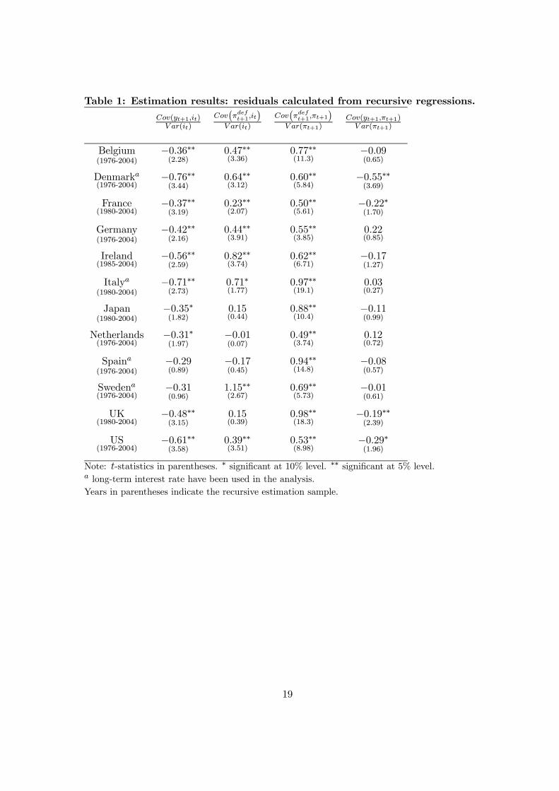
Table 1: Estimation results: residuals calculated from recursive regressions.

Cov(yt+1,it)V ar(it)

Cov¡πdeft+1,it

¢V ar(it)

Cov¡πdeft+1,πt+1

¢V ar(πt+1)

Cov(yt+1,πt+1)V ar(πt+1)

Belgium(1976-2004)

−0.36∗∗(2.28)

0.47∗∗(3.36)

0.77∗∗(11.3)

−0.09(0.65)

Denmarka(1976-2004)

−0.76∗∗(3.44)

0.64∗∗(3.12)

0.60∗∗(5.84)

−0.55∗∗(3.69)

France(1980-2004)

−0.37∗∗(3.19)

0.23∗∗(2.07)

0.50∗∗(5.61)

−0.22∗(1.70)

Germany(1976-2004)

−0.42∗∗(2.16)

0.44∗∗(3.91)

0.55∗∗(3.85)

0.22(0.85)

Ireland(1985-2004)

−0.56∗∗(2.59)

0.82∗∗(3.74)

0.62∗∗(6.71)

−0.17(1.27)

Italya

(1980-2004)−0.71∗∗(2.73)

0.71∗(1.77)

0.97∗∗(19.1)

0.03(0.27)

Japan(1980-2004)

−0.35∗(1.82)

0.15(0.44)

0.88∗∗(10.4)

−0.11(0.99)

Netherlands(1976-2004)

−0.31∗(1.97)

−0.01(0.07)

0.49∗∗(3.74)

0.12(0.72)

Spaina

(1976-2004)−0.29(0.89)

−0.17(0.45)

0.94∗∗(14.8)

−0.08(0.57)

Swedena(1976-2004)

−0.31(0.96)

1.15∗∗(2.67)

0.69∗∗(5.73)

−0.01(0.61)

UK(1980-2004)

−0.48∗∗(3.15)

0.15(0.39)

0.98∗∗(18.3)

−0.19∗∗(2.39)

US(1976-2004)

−0.61∗∗(3.58)

0.39∗∗(3.51)

0.53∗∗(8.98)

−0.29∗(1.96)

Note: t-statistics in parentheses. ∗ significant at 10% level. ∗∗ significant at 5% level.a long-term interest rate have been used in the analysis.

Years in parentheses indicate the recursive estimation sample.

19

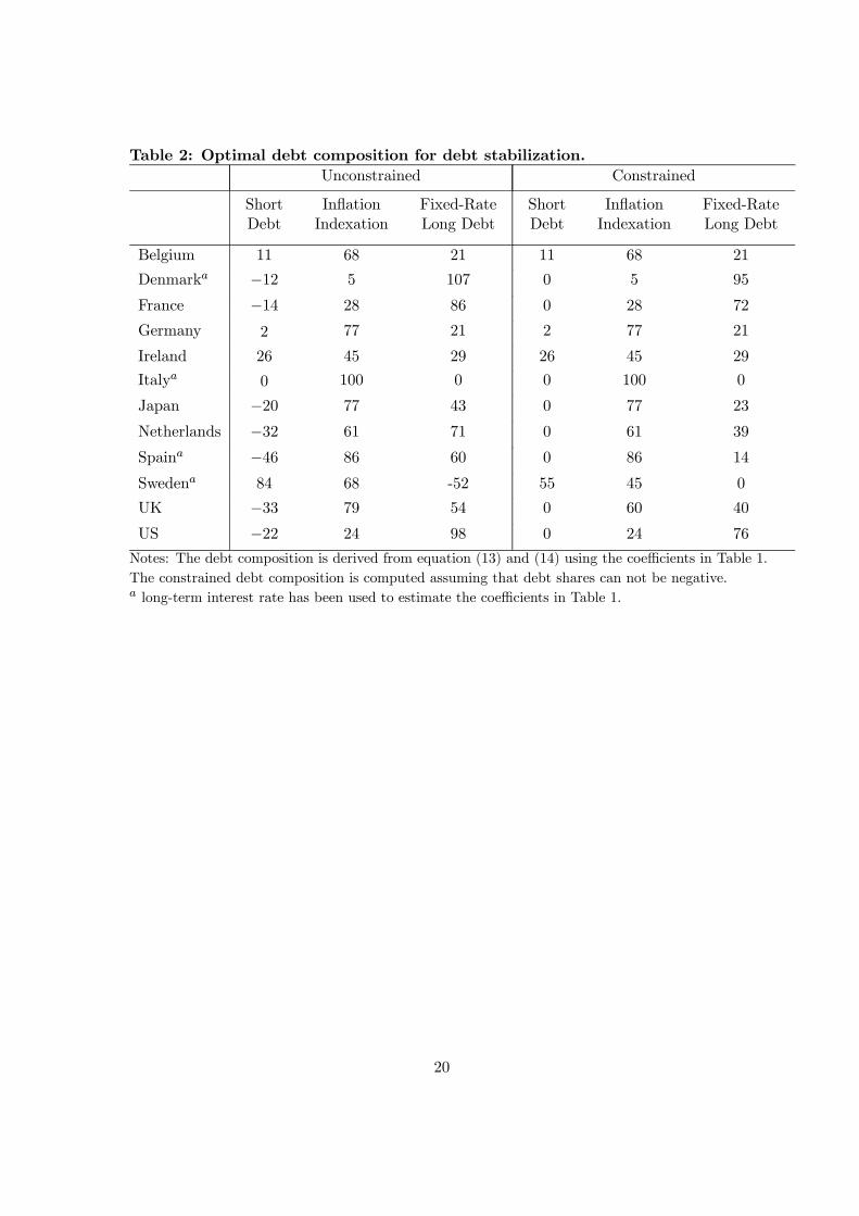
Table 2: Optimal debt composition for debt stabilization.

Unconstrained Constrained

ShortDebt

InflationIndexation

Fixed-RateLong Debt

ShortDebt

InflationIndexation

Fixed-RateLong Debt

Belgium 11 68 21 11 68 21

Denmarka −12 5 107 0 5 95

France −14 28 86 0 28 72

Germany 2 77 21 2 77 21

Ireland 26 45 29 26 45 29

Italya 0 100 0 0 100 0

Japan −20 77 43 0 77 23

Netherlands −32 61 71 0 61 39

Spaina −46 86 60 0 86 14

Swedena 84 68 -52 55 45 0

UK −33 79 54 0 60 40

US −22 24 98 0 24 76

Notes: The debt composition is derived from equation (13) and (14) using the coefficients in Table 1.

The constrained debt composition is computed assuming that debt shares can not be negative.a long-term interest rate has been used to estimate the coefficients in Table 1.

20

CESifo Working Paper Series (for full list see www.cesifo.de)

___________________________________________________________________________ 1325 Jianpei Li and Elmar Wolfstetter, Partnership Dissolution, Complementarity, and

Investment Incentives, November 2004 1326 Hans Fehr, Sabine Jokisch and Laurence J. Kotlikoff, Fertility, Mortality, and the

Developed World’s Demographic Transition, November 2004 1327 Adam Elbourne and Jakob de Haan, Asymmetric Monetary Transmission in EMU: The

Robustness of VAR Conclusions and Cecchetti’s Legal Family Theory, November 2004 1328 Karel-Jan Alsem, Steven Brakman, Lex Hoogduin and Gerard Kuper, The Impact of

Newspapers on Consumer Confidence: Does Spin Bias Exist?, November 2004 1329 Chiona Balfoussia and Mike Wickens, Macroeconomic Sources of Risk in the Term

Structure, November 2004 1330 Ludger Wößmann, The Effect Heterogeneity of Central Exams: Evidence from TIMSS,

TIMSS-Repeat and PISA, November 2004 1331 M. Hashem Pesaran, Estimation and Inference in Large Heterogeneous Panels with a

Multifactor Error Structure, November 2004 1332 Maarten C. W. Janssen, José Luis Moraga-González and Matthijs R. Wildenbeest, A

Note on Costly Sequential Search and Oligopoly Pricing, November 2004 1333 Martin Peitz and Patrick Waelbroeck, An Economist’s Guide to Digital Music,

November 2004 1335 Lutz Hendricks, Why Does Educational Attainment Differ Across U.S. States?,

November 2004 1336 Jay Pil Choi, Antitrust Analysis of Tying Arrangements, November 2004 1337 Rafael Lalive, Jan C. van Ours and Josef Zweimueller, How Changes in Financial

Incentives Affect the Duration of Unemployment, November 2004 1338 Robert Woods, Fiscal Stabilisation and EMU, November 2004 1339 Rainald Borck and Matthias Wrede, Political Economy of Commuting Subsidies,

November 2004 1340 Marcel Gérard, Combining Dutch Presumptive Capital Income Tax and US Qualified

Intermediaries to Set Forth a New System of International Savings Taxation, November 2004

1341 Bruno S. Frey, Simon Luechinger and Alois Stutzer, Calculating Tragedy: Assessing the

Costs of Terrorism, November 2004 1342 Johannes Becker and Clemens Fuest, A Backward Looking Measure of the Effective

Marginal Tax Burden on Investment, November 2004 1343 Heikki Kauppi, Erkki Koskela and Rune Stenbacka, Equilibrium Unemployment and

Capital Intensity Under Product and Labor Market Imperfections, November 2004 1344 Helge Berger and Till Müller, How Should Large and Small Countries Be Represented

in a Currency Union?, November 2004 1345 Bruno Jullien, Two-Sided Markets and Electronic Intermediaries, November 2004 1346 Wolfgang Eggert and Martin Kolmar, Contests with Size Effects, December 2004 1347 Stefan Napel and Mika Widgrén, The Inter-Institutional Distribution of Power in EU

Codecision, December 2004 1348 Yin-Wong Cheung and Ulf G. Erlandsson, Exchange Rates and Markov Switching

Dynamics, December 2004 1349 Hartmut Egger and Peter Egger, Outsourcing and Trade in a Spatial World, December

2004 1350 Paul Belleflamme and Pierre M. Picard, Piracy and Competition, December 2004 1351 Jon Strand, Public-Good Valuation and Intrafamily Allocation, December 2004 1352 Michael Berlemann, Marcus Dittrich and Gunther Markwardt, The Value of Non-

Binding Announcements in Public Goods Experiments: Some Theory and Experimental Evidence, December 2004

1353 Camille Cornand and Frank Heinemann, Optimal Degree of Public Information

Dissemination, December 2004 1354 Matteo Governatori and Sylvester Eijffinger, Fiscal and Monetary Interaction: The Role

of Asymmetries of the Stability and Growth Pact in EMU, December 2004 1355 Fred Ramb and Alfons J. Weichenrieder, Taxes and the Financial Structure of German

Inward FDI, December 2004 1356 José Luis Moraga-González and Jean-Marie Viaene, Dumping in Developing and

Transition Economies, December 2004 1357 Peter Friedrich, Anita Kaltschütz and Chang Woon Nam, Significance and

Determination of Fees for Municipal Finance, December 2004

1358 M. Hashem Pesaran and Paolo Zaffaroni, Model Averaging and Value-at-Risk Based

Evaluation of Large Multi Asset Volatility Models for Risk Management, December 2004

1359 Fwu-Ranq Chang, Optimal Growth and Impatience: A Phase Diagram Analysis,

December 2004 1360 Elise S. Brezis and François Crouzet, The Role of Higher Education Institutions:

Recruitment of Elites and Economic Growth, December 2004 1361 B. Gabriela Mundaca and Jon Strand, A Risk Allocation Approach to Optimal

Exchange Rate Policy, December 2004 1362 Christa Hainz, Quality of Institutions, Credit Markets and Bankruptcy, December 2004 1363 Jerome L. Stein, Optimal Debt and Equilibrium Exchange Rates in a Stochastic

Environment: an Overview, December 2004 1364 Frank Heinemann, Rosemarie Nagel and Peter Ockenfels, Measuring Strategic

Uncertainty in Coordination Games, December 2004 1365 José Luis Moraga-González and Jean-Marie Viaene, Anti-Dumping, Intra-Industry

Trade and Quality Reversals, December 2004 1366 Harry Grubert, Tax Credits, Source Rules, Trade and Electronic Commerce: Behavioral

Margins and the Design of International Tax Systems, December 2004 1367 Hans-Werner Sinn, EU Enlargement, Migration and the New Constitution, December

2004 1368 Josef Falkinger, Noncooperative Support of Public Norm Enforcement in Large

Societies, December 2004 1369 Panu Poutvaara, Public Education in an Integrated Europe: Studying to Migrate and

Teaching to Stay?, December 2004 1370 András Simonovits, Designing Benefit Rules for Flexible Retirement with or without

Redistribution, December 2004 1371 Antonis Adam, Macroeconomic Effects of Social Security Privatization in a Small

Unionized Economy, December 2004 1372 Andrew Hughes Hallett, Post-Thatcher Fiscal Strategies in the U.K.: An Interpretation,

December 2004 1373 Hendrik Hakenes and Martin Peitz, Umbrella Branding and the Provision of Quality,

December 2004

1374 Sascha O. Becker, Karolina Ekholm, Robert Jäckle and Marc-Andreas Mündler,

Location Choice and Employment Decisions: A Comparison of German and Swedish Multinationals, January 2005

1375 Christian Gollier, The Consumption-Based Determinants of the Term Structure of

Discount Rates, January 2005 1376 Giovanni Di Bartolomeo, Jacob Engwerda, Joseph Plasmans, Bas van Aarle and

Tomasz Michalak, Macroeconomic Stabilization Policies in the EMU: Spillovers, Asymmetries, and Institutions, January 2005

1377 Luis H. R. Alvarez and Erkki Koskela, Progressive Taxation and Irreversible

Investment under Uncertainty, January 2005 1378 Theodore C. Bergstrom and John L. Hartman, Demographics and the Political

Sustainability of Pay-as-you-go Social Security, January 2005 1379 Bruno S. Frey and Margit Osterloh, Yes, Managers Should Be Paid Like Bureaucrats,

January 2005 1380 Oliver Hülsewig, Eric Mayer and Timo Wollmershäuser, Bank Loan Supply and

Monetary Policy Transmission in Germany: An Assessment Based on Matching Impulse Responses, January 2005

1381 Alessandro Balestrino and Umberto Galmarini, On the Redistributive Properties of

Presumptive Taxation, January 2005 1382 Christian Gollier, Optimal Illusions and Decisions under Risk, January 2005 1383 Daniel Mejía and Marc St-Pierre, Unequal Opportunities and Human Capital Formation,

January 2005 1384 Luis H. R. Alvarez and Erkki Koskela, Optimal Harvesting under Resource Stock and

Price Uncertainty, January 2005 1385 Ruslan Lukach, Peter M. Kort and Joseph Plasmans, Optimal R&D Investment

Strategies with Quantity Competition under the Threat of Superior Entry, January 2005 1386 Alfred Greiner, Uwe Koeller and Willi Semmler, Testing Sustainability of German

Fiscal Policy. Evidence for the Period 1960 – 2003, January 2005 1387 Gebhard Kirchgässner and Tobias Schulz, Expected Closeness or Mobilisation: Why

Do Voters Go to the Polls? Empirical Results for Switzerland, 1981 – 1999, January 2005

1388 Emanuele Bacchiocchi and Alessandro Missale, Managing Debt Stability, January 2005