Managerial Economics Introduction

Business economics is a “Applied Economics” uses economic theory and quantitative methods to analyze business enterprises and relationship of firms with labour, Capital and product markets alongwith main focus of “Firm’s managerial decision making process”.

Five basic Steps :

Define the ProblemDefine the objectiveIdentify Possible SolutionSelect the best possible solutionImplement the best Decision

Define the Problem:

A U.S. based company, which invented the copying machine in 1959 was doing business as monopolist but in 1979 found itself unable to compete with Japanese copiers, which were of better quality.

Determining Objective of the Firm:

In this case, Xerox had to decide whether to try to meet the competition or leave the copier market to Japanese and move on to develop more technologically advanced product. But Xerox decided to face head-on competition and stay in the market.

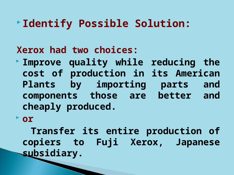
Identify Possible Solution: Xerox had two choices: Improve quality while reducing the cost

of production in its American Plants by importing parts and components those are better and cheaply produced.

or Transfer its entire production of

copiers to Fuji Xerox, Japanese subsidiary.

Select the best possible solution:

Integration of development and production and quality control effort in its domestic plants with the direct involvement of Fuji Xerox.

As well as import parts or components that Fuji Xerox could best produce in Japan.

Implement the Decision: Xerox greatly increased employee Xerox greatly increased employee

involvementinvolvement Greatly reduced inventories and number of Greatly reduced inventories and number of

suppliers suppliers Used Fuji Xerox to produce in Japan those Used Fuji Xerox to produce in Japan those

parts or components that could be better parts or components that could be better supplied from Japan supplied from Japan

To monitor progress in countrywide quality-To monitor progress in countrywide quality-control program and customer satisfactioncontrol program and customer satisfaction.

Business or managerial economics primarily evaluates the implications of alternative course of action and choose best course of action.

In this case, there is a need for optimizing

behavior. As:

The marketing vice-president strives to maximize sales revenue subject to a given advertising budget.

The production manager attempts to minimize cost and maximize production subject to producing a specified output.

Division’s president attempts to maximize profit.

The firm is an entity that organizes factor of production in order to produce goods and services to meet the demands of consumers and other firms and activity is directed by managers.

The foremost goal of the firm is to

maximize the present value of the firm of all future profit by efficient allocation of resources with financial and technological constraints.

Business or Accounting Profit = Revenue – Explicit Cost (out of pocket expenditure on market supplied resources for the production.

Example: A businessman, who invested Rs. 20 lakh

in a retail store and started business. The projected income statement for the year prepared by an accountant as:

Sales Rs. 9,00,000Less: Cost of goods sold Rs. 4,00,000 Gross Profit Rs. 5,00,000 Less: Advt. Rs. 1,00,000 Deprecation Rs. 1,00,000 Taxes Rs. 30,000 Miscellaneous expenses Rs. 50,000 Rs.2,80,000Net Accounting Profit Rs. 2,20,000

Economic Profit (above normal profit) = Revenue - explicit cost + Implicit cost (value of the owner-supplied resources used by the firm in its own production)

Example : There are two implicit costs are involved as: Rs. 20 Lakh invested in business, next best alternative (Opportunity cost) use for this money is a bank account paying a 5 % interest rate. This investment will return Rs. 1 lakh @

The manager’s time and talent is another implicit cost as the annual wage return on an MBA degree holder may be Rs. 6 Lakh per year. This is implicit or opportunity cost of managing business.

Sales Rs. 9,00,000Less: Cost of goods sold Rs. 4,00,000 Gross Profit Rs. 5,00,000 Less: Advt. Rs. 1,00,000 Deprecation Rs. 1,00,000 Tax Rs. 30,000 Miscellaneous expenses Rs. 50,000 Rs.2,80,000Net Accounting Profit Rs. 2,20,000

Less: Implicit cost : Return to Rs. 20 Lakh RS. 1,00,000 invested capital Foregone wages Rs. 6 00,000 Rs. 7,00,000 Economic Profit (loss) Rs. (-) 4,80,000

Profit rates of firms usually varies industry to industry. like firms in steel, textile and rail-roads generally earn low profit than firms in pharmaceutical, office equipment and other high–technology industries as per given theory:

Frictional Theory :

Profit arise as a result of friction or disturbances from long-run equilibrium. In long-run perfectly competitive firms tend to earn normal profit, due to free entry and exit. As in short-run, profit is made more firms are attracted to the industry in the long-run and it leads to firms earning only a normal return on investment.

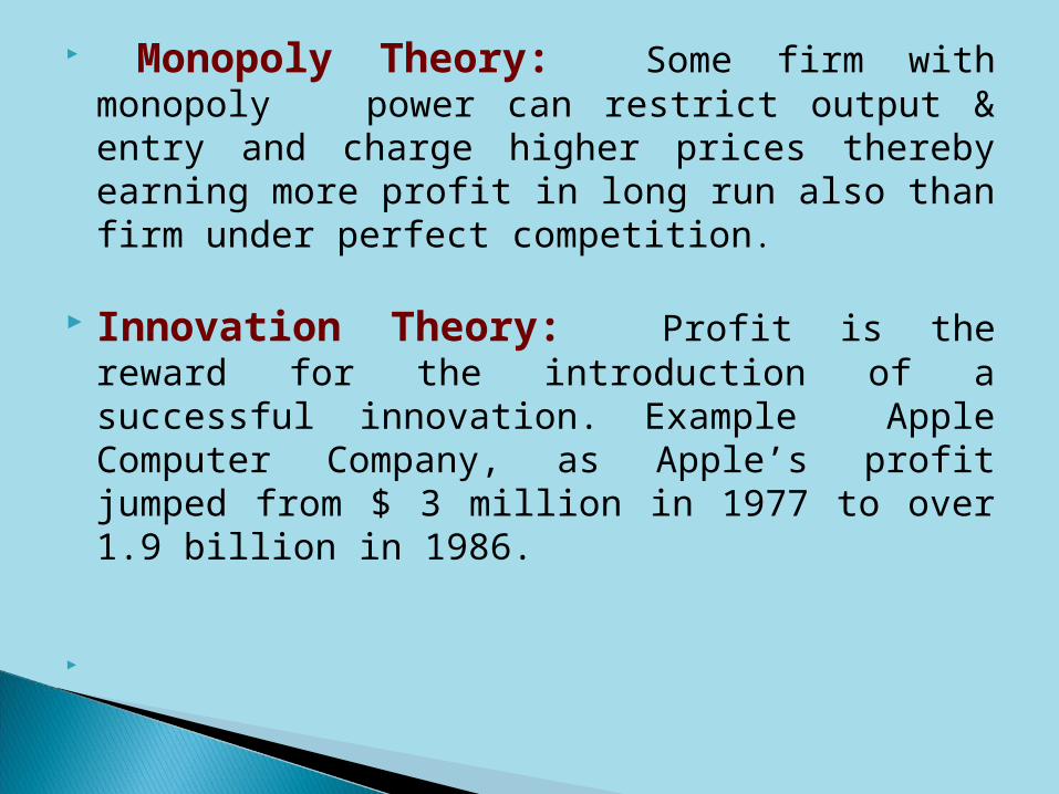
Monopoly Theory: Some firm with monopoly power can restrict output & entry and charge higher prices thereby earning more profit in long run also than firm under perfect competition.

Innovation Theory: Profit is the reward for the introduction of a successful innovation. Example Apple Computer Company, as Apple’s profit jumped from $ 3 million in 1977 to over 1.9 billion in 1986.

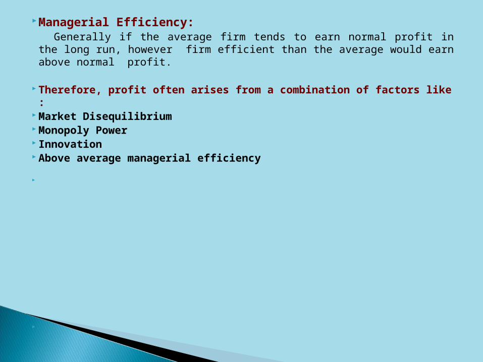
Managerial Efficiency: Generally if the average firm tends to earn normal profit in the long run,

however firm efficient than the average would earn above normal profit.

Therefore, profit often arises from a combination of factors like : Market Disequilibrium Monopoly Power Innovation Above average managerial efficiency

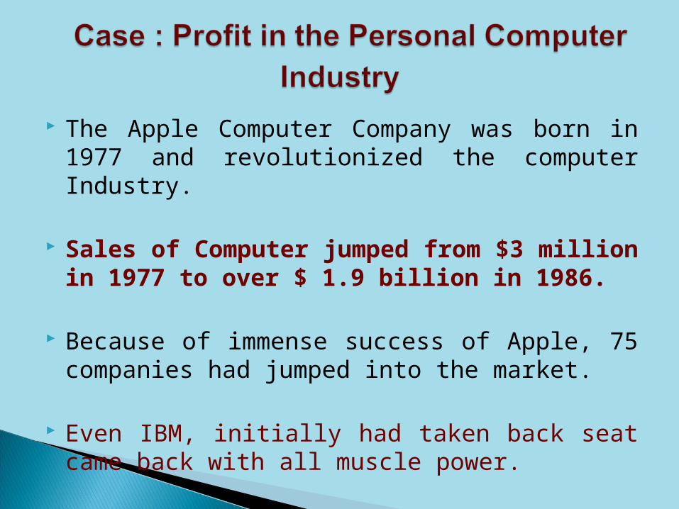
The Apple Computer Company was born in 1977 and revolutionized the computer Industry.

Sales of Computer jumped from $3 million in 1977 to over $ 1.9 billion in 1986.

Because of immense success of Apple, 75 companies had jumped into the market.

Even IBM, initially had taken back seat came back with all muscle power.

Because of increased competition, many of the early entrants had dropped out by 1986 and profit fell sharply.

Profit margin for the 11 largest company averaged 6.5% from 1986 to 1990, which was 11.55 during 1980-1985.

Afterward PC makers became engaged in a price war with PC prices falling by 20-40% per year.

PC soon became practically a commodity & this industry became not profit oriented.

After suffering with losses, in 1997 Apple’s CEO revived the company by simplifying its confusing product line by introducing a series of successful new products as:

iPod iPhone iPad

Because of innovative products APPLE earned huge profit.

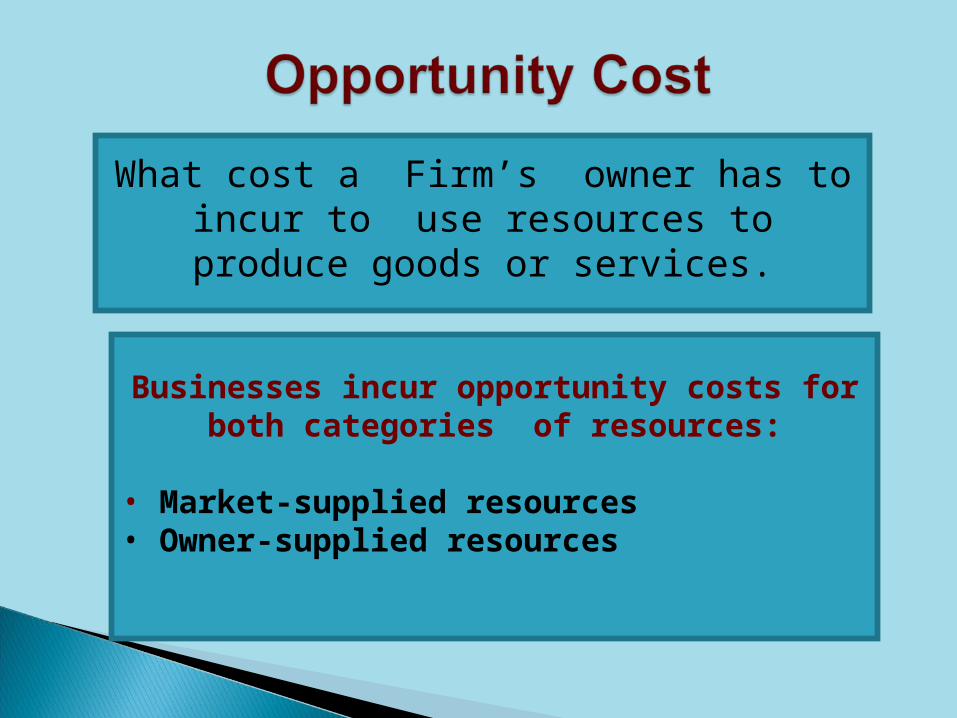
What cost a Firm’s owner has to incur to use resources to produce goods or services.

Businesses incur opportunity costs for both categories of resources:

• Market-supplied resources • Owner-supplied resources

Hema is full-time homemaker and also takes tuition and knits sweater in spare time.

While in summer holidays, she bought some dress material from Dubai for which she paid Rs. 50 per meter.

This material could be sold back to the local fabric shop in Cochin in Rs.150 per meter.

Hema is considering using that material to make dresses, which she would sell to her friends and neighbor.

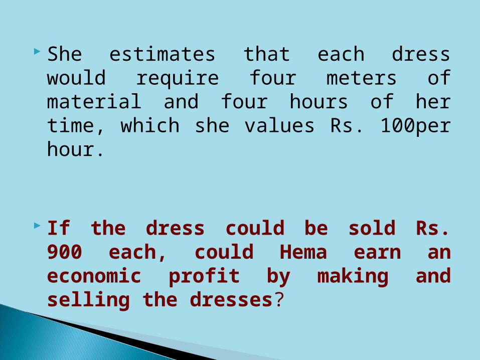
She estimates that each dress would require four meters of material and four hours of her time, which she values Rs. 100per hour.

If the dress could be sold Rs. 900 each, could Hema earn an economic profit by making and selling the dresses?

Opportunity cost of owner’s resource : Rs. 100 (Hema’s own time)

True opportunity cost of the material : Rs. 150 (the amount she could receive

by selling it to the Cochin fabric shop)

Revenue : Rs. 900 Less : 4 Hour of labour

@ Rs.100/hr Rs. 400 4 meters of material

@ Rs. 150/mtr. Rs. 600 Economic Profit :(loss) Rs. (-) 100

If Hema had not included the value of her time and had used the historic price of Rs 50/mtr. as cost of material, profit would have estimated:

Revenue : Rs. 900

Less : 4 meters of material @ Rs. 50/mtr. Rs. 200 Accounting Profit : Rs. 700

The Sarbanes-Oxley Act focuses on detecting & preventing fraud via improved auditing and used proper measure of profit by considering:

Economic Profit based on implicit cost+ Explicit Cost

In General, companies follow “General Accepted Accounting Principle” to measure Profit, which is not based on implicit cost.

In 2002, the 500 listed firms employed about $3 trillion of equity capital which has a opportunity cost of $300 billion at the rate of 10 percent @ return.

This cost was completely ignored under GAAP and measured accounting profit of these 500 firms was just $118 billion.

After subtracting this opportunity cost of equity capital from aggregate accounting profit, the resulting economic profit reveals that these 500 companies experienced a loss of $182 billion in 2002

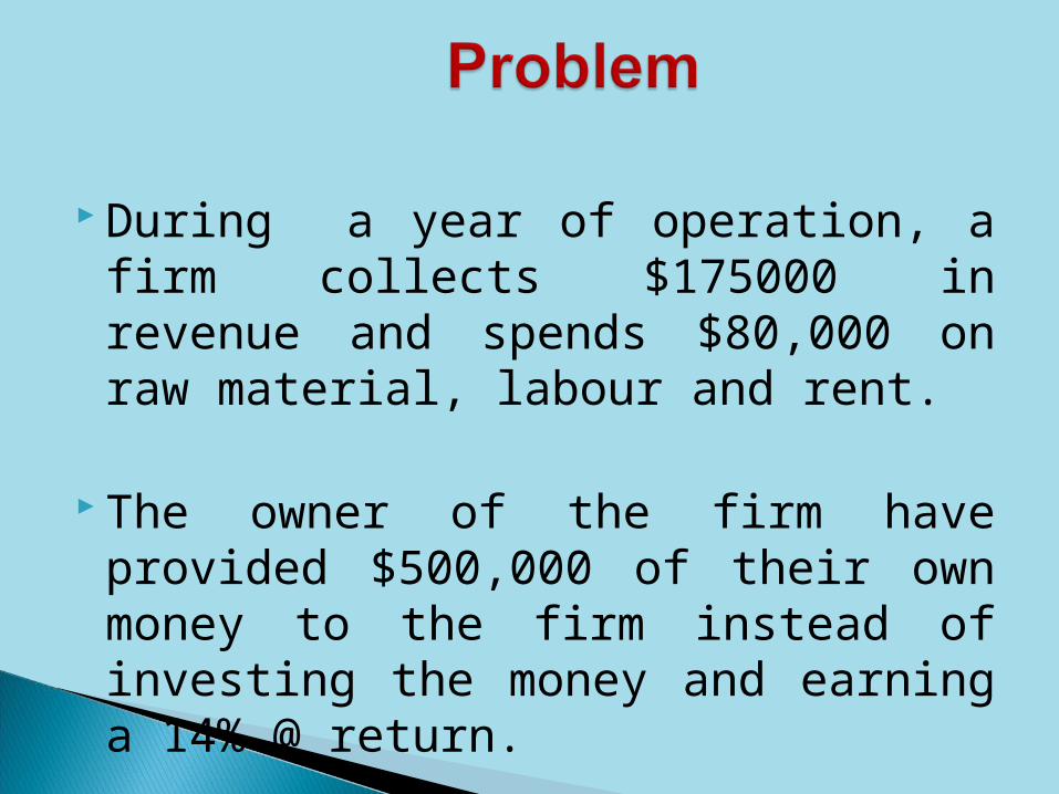
During a year of operation, a firm collects $175000 in revenue and spends $80,000 on raw material, labour and rent.

The owner of the firm have provided $500,000 of their own money to the firm instead of investing the money and earning a 14% @ return.

The Explicit Cost of the Firm --- The implicit cost of the firm --- Total Economic Cost-----

Firm’s Accounting Profit ---- Firm’s Economic Profit---

If the owner could earn 20% @ on the money they have invested in the firm , the economic

Profit would be---- (when revenue is $ 175000/-)

The Cost of attending a private college for one year is $6000 for tuition, $2000 for the room, $1,500 for meals and $500 for books and supplies. The student could also have earned $15000 by getting a job instead of going to college and 10 percent interest on expenses he or she incurs at the beginning of the

year.

Calculate following cost of attending college:

Explicit Cost

Implicit Cost

Economic Cost

Quantity Total Cost Average Cost TC/Q

Marginal Cost TC/ Q

0 $20 -- --

1 140 $140 $120

2 160 80 20

3 180 60 20

4 240 60 60

5 480 96 240

Total-Cost function of the US steel industry in 1930 was estimated to be:

TC = 182 + 56Q

TC curve is linear with fixed cost of $182 million per year

MC of $56 million for each million tons of steel produced with horizontal MC curve

AC curve declining continuously .

Q (Million Tons)

182+56Q TC (Million of Dollars)

AC (Million of dollars)

MC (million of dollars)

0 182+0 $182 ---- --

1 182+56 238 $238 $56

2 182+112 294 147 56

3 182+168 350 117 56

4 182+224 406 102 56

$

400

300

200

100

G

H

B

C

DTC

0 1

H B C D

2 3 4

AC

MC

Many times, firms are faced some questions like:

◦What is the level of output to be produced in the short run?

◦What is the point where operations should be closed

These questions can be answered by marginal analysis.

.

M0

0

H

Q

.

.

TC

TR

OUTPUT

TR &TC

MC

MR

E

M Q NL

J

K

F

G

B

OUTPUT

MR& MC

S

As long as MR exceeds MC of production, it will profitable for the firm to expand output. In this case firm will be adding more to total revenue than to total cost and so its total profit increasing .

As upto OQ output level MR > MC

At point E MR = MC at output level of OQ.

If output is expanded beyond OQ level MR <MC. In this case firm will be adding less to its TR than to its cost. It will not be profitable and will cause total profit to fall.

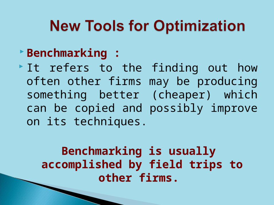
Benchmarking : It refers to the finding out how often other

firms may be producing something better (cheaper) which can be copied and possibly improve on its techniques.

Benchmarking is usually accomplished by field trips to other firms.

This technique has now become a standard tool for improving productivity and quality at a large number of American and Indian firms:

IBM FORD XEROX IOC ONGC SBI

Benchmarking requires :

1.Picking a specific process and identifying a few firms that do a better job.

2.Sending on the benchmarking mission the people who will actually have to make the changes.

Benchmarking can result in dramatic cost reductions and increase productivity.

The first benchmarking mission by a US firm was undertaken by Xerox in 1979, when it realized that Japanese were selling copiers for less than Xerox’s production cost.

Ultimately Xerox had to imitate Japanese production process and able to recapture its lost market.

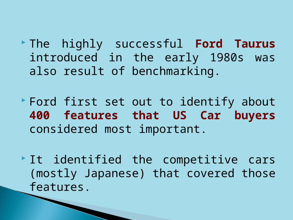
The highly successful Ford Taurus introduced in the early 1980s was also result of benchmarking.

Ford first set out to identify about 400 features that US Car buyers considered most important.

It identified the competitive cars (mostly Japanese) that covered those features.

In 1992, Taurus was redesigned once again based on new round of benchmarking. As

Ford benchmarked:

Door handles and fuel economy against the Chevy Lumina

The halogen headlamps and tilt wheel against the Honda Accord

Easy to change Taillight bulbs and express window control against Nissan’s Maxima

Remote Radio controls against the Pontiac Grand Prix.

It applies quality-improvement method to all the firm’s process. As:

Production Process Customer services Sales Marketing Finance

Companies those have successfully used TQM are:

Xerox Motorola (was able to reduce $700mil. in

manufacturing costs over five years) General Electric Marriot Harley Davidson Ford

In recent years, TQM Model was extended to include innovation, knowledge and the management of partnership.

Now, new concept of Six Sigma has been added to TQM.

It refers to the situation in which everything from product design to manufacturing and all proceeds are practically flawless with fewer than 3.4 defects per million procedures/products.

Two Sigma would mean that 95 percent of the products are non-defective.

Six Sigma means that 99.99966 percent are non-defective or 3.4 defects per million – practically perfection.

Economics normally make a distinction between “Short- Run” and “ Long-Run”.

By Short -Run , the reference is to the time period when the structure of industry , the size of firm and the scale of plant are not alterable;

The time is so short that any change in the scale of output has to be brought about by changing the intensity of exploiting the fixed factors like land and machineries.

In ”long- Run” all factors become variable ; then enough time is available to adjust the scale of plant, size of firm and the structure of industry so as to change the volume of output.

Future profit is reflected by the “Time Value of Money”.

Time Value of Money refers that future profits must be discounted to the present because it is accounted by adding Risk Premium to the discount rate.

Therefore, A Rupee to be received in future is not worth a rupee today (it is less than a rupee).

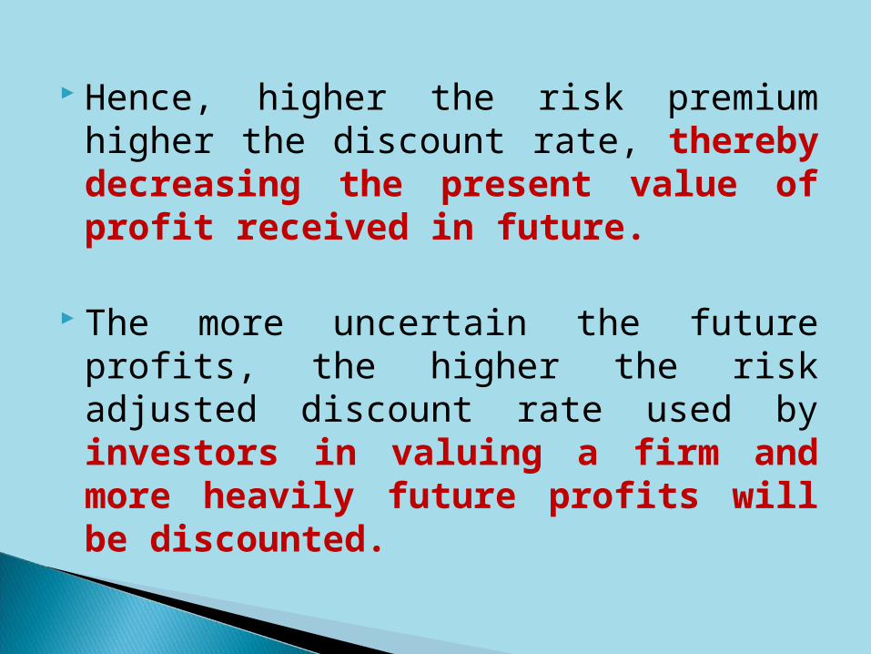
Hence, higher the risk premium higher the discount rate, thereby decreasing the present value of profit received in future.

The more uncertain the future profits, the higher the risk adjusted discount rate used by investors in valuing a firm and more heavily future profits will be discounted.

The primary objective of the Firm is to maximize wealth or value of the firm .

The Value of a firm:

Price for which firm can be sold, which equals the present value of the future Economic profit generated by the firm.

Example There is expectation to get $100 after one year as profit.

How much money would you accept now rather than wait one year for guaranteed payment of $100.

Risk premium is 6% $x(1.06) = $100 ={100/(1.06)}

= $94.34

Mathematically :

PV = Л1 + Л2 + Лn (1+r)¹ (1+r)² (1+r)n

n

= ∑ Лt

t =1 (1+r)t

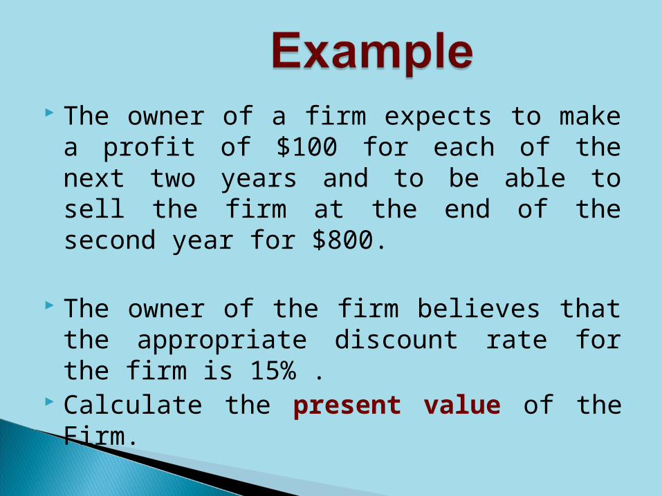
The owner of a firm expects to make a profit of $100 for each of the next two years and to be able to sell the firm at the end of the second year for $800.

The owner of the firm believes that the appropriate discount rate for the firm is 15% .

Calculate the present value of the Firm.

PV = $100 + $100 + $800 (1.15) (1.15)2 (1.15)2= $ 100 + $100 + $800 1.15 1.3225 1.3225

= $86.96+$75.61+ $604.91= $767.48

Periods

8% 10% 12%

1 0.9259 0.9091 0.8929

2 0.8573 0.83264 0.7929

3 0.7938 0.7513 0.7118

4 0.7350 0.6830 0.6355

6 0.6302 0.5645 0.5066

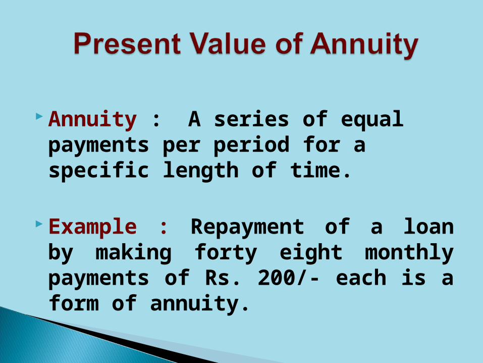
Annuity : A series of equal payments per period for a specific length of time.

Example : Repayment of a loan by making forty eight monthly payments of Rs. 200/- each is a form of annuity.

Formula for the present value of an annuity of “A” Rs. Per period for n periods and discount rate of r : (Present Value Annuity Factor)

PV = A __1__ + A __1__ + A __1__ (1+r)1 (1+r)2 (1+r)n OR n

A ∑ __1____ t=1 (1+r)t

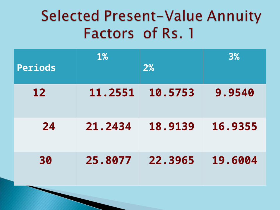
Periods

1% 2% 3%

12 11.2551 10.5753 9.9540

24 21.2434 18.9139 16.9355

30 25.8077 22.3965 19.6004

Consider the Present value of an annuity of Rs. 3,522 per month for thirty years .

With an interest of 1 percent per month.

30

P V =3522 ∑ ( __1____)t

t-1 (1+.01)t

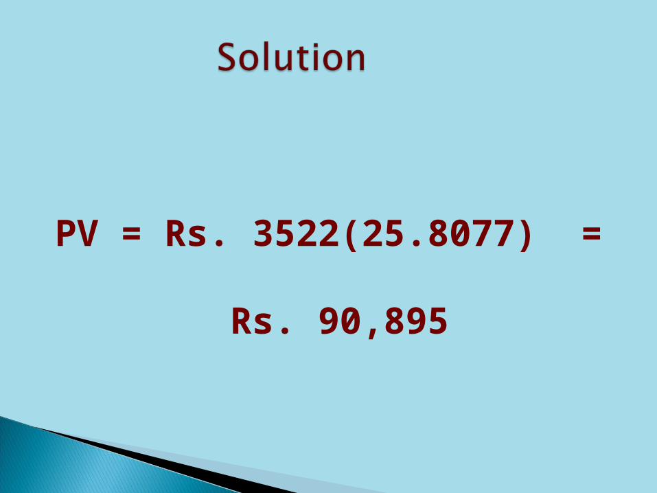
PV = Rs. 3522(25.8077) =

Rs. 90,895

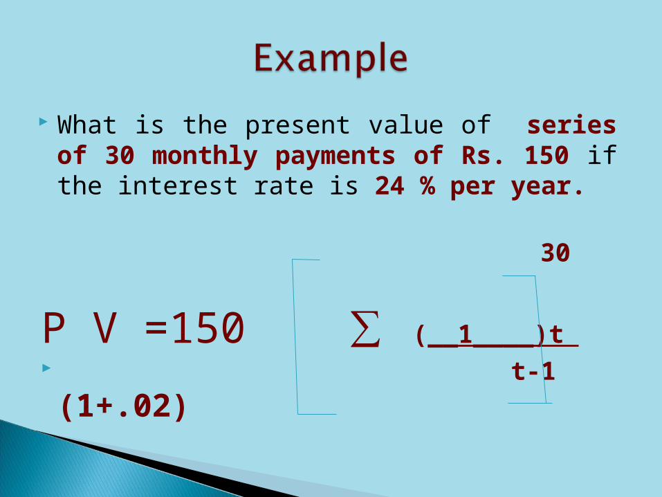
What is the present value of series of 30 monthly payments of Rs. 150 if the interest rate is 24 % per year.

30

P V =150 ∑ (__1____)t t-1 (1+.02)

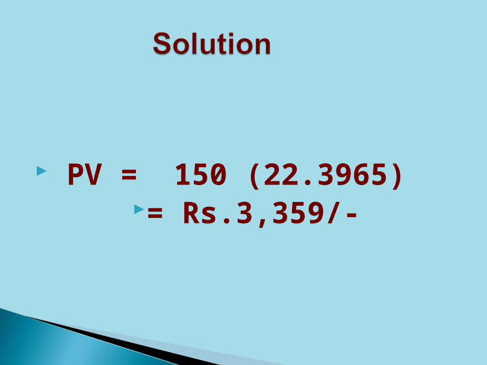
PV = 150 (22.3965)= Rs.3,359/-

Mr. Peter started earning $2,000 a month in an MNC in Gurgaon in 2008. As per his appointment contract, he gets a salary hike of 10 percent every year.

Suppose, in India, the annual rate of Inflation is 5% for the last five years.

How much will his salary be in 2013?

Using a Discount rate of 6.5 percent, calculate the present value of $1000 payment to be received at the end of:

One Year Two Year Three Year