Manage Productivity to Maximize Profit Course No: K08-005 Credit: 8 PDH Richard Grimes, MPA, CPT Continuing Education and Development, Inc. 22 Stonewall Court Woodcliff Lake, NJ 07677 P: (877) 322-5800 [email protected]

Welcome message from author
This document is posted to help you gain knowledge. Please leave a comment to let me know what you think about it! Share it to your friends and learn new things together.
Transcript

Manage Productivity to Maximize Profit Course No: K08-005
Credit: 8 PDH
Richard Grimes, MPA, CPT
Continuing Education and Development, Inc.22 Stonewall CourtWoodcliff Lake, NJ 07677
P: (877) [email protected]
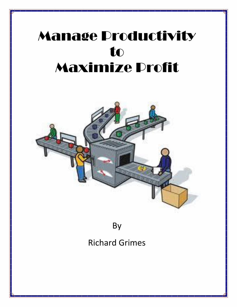
Manage Productivityto
Maximize Profit
By
Richard Grimes
Manage Productivity to Maximize Profit ©Richard Grimes 2013 Page 2
Table of Contents
COURSE OVERVIEW...................................................................................................................................................4
LEARNING OUTCOMES .............................................................................................................................................. 5
PRODUCTIVE OR BUSY?............................................................................................................................................. 6
PRACTICE EXERCISE #1 .......................................................................................................................................................7
THE VALUE OF SETTING MEASURABLE GOALS........................................................................................................... 8
THE ELEMENTS OF MEASURABLE GOALS ................................................................................................................................9
PRACTICE EXERCISE............................................................................................................................................................9
ANALYZING YOUR FLOOR PLANS............................................................................................................................. 11
ANALYZING YOUR WORK FLOWS ............................................................................................................................ 13
PRACTICE EXERCISE: ANALYZING WORK FLOW ......................................................................................................................14
Comments about the Workflow.............................................................................................................................15
ESTABLISHING PRODUCTION EQUILIBRIUM ............................................................................................................ 16
DETERMINING LINE ADEQUACY .............................................................................................................................. 17
PRODUCTION PLANNING ........................................................................................................................................ 24
PRACTICE ACTIVITY ..........................................................................................................................................................25
HOW MANY WORKSTATIONS AND EMPLOYEES WILL WE NEED? ............................................................................ 29
PRACTICE EXERCISE..........................................................................................................................................................29
HOW EFFICIENTLY ARE YOUR EMPLOYEES WORKING?............................................................................................ 31
HOW PRODUCTIVELY ARE YOUR EMPLOYEES WORKING?....................................................................................... 32
PRODUCTION CAPACITY TODAY AND TOMORROW ................................................................................................ 33
STAFF AND EQUIPMENT CAPACITIES ....................................................................................................................................34
Current Staff Capacity and Cost.............................................................................................................................34
PRACTICE ACTIVITY ..........................................................................................................................................................36
Practical Application Challenge .............................................................................................................................37
Manage Productivity to Maximize Profit ©Richard Grimes 2013 Page 3
Current Equipment Capacity and Cost ...................................................................................................................39
PRACTICE EXERCISE..........................................................................................................................................................40
BREAK EVEN ANALYSIS............................................................................................................................................ 41
BREAK EVEN PRACTICE EXERCISE ........................................................................................................................................42
PREDICTING FUTURE DEMAND ............................................................................................................................... 47
PRIORITIZING OPINIONS BY A “FORCED CHOICE” METHOD..................................................................................... 47
MEASURABLE FORECASTING METHODS.................................................................................................................. 50
SIMPLE AVERAGE (“SA”)..................................................................................................................................................50
SIMPLE MOVING AVERAGE (“SMA”)..................................................................................................................................52
WEIGHTED MOVING AVERAGE (“WMA”)...........................................................................................................................53
CHANGE MEASUREMENT ANALYSIS (CMA)..........................................................................................................................56
PREDICTING SEASONAL TRENDS .........................................................................................................................................58
MAKING PREDICTIONS WITHOUT USEFUL TREND DATA...........................................................................................................59
PRACTICAL PROBLEM SOLVING ............................................................................................................................... 60
LESSONS FROM THE PAST ....................................................................................................................................... 63
Manage Productivity to Maximize Profit ©Richard Grimes 2013 Page 4
COURSE OVERVIEW
This course is for people wanting a basic understanding of the design and management of efficient work
processes in any environment for any product. Public organizations will benefit as much as private
because work efficiency and productivity is essential to both. The concepts presented here are universal
whether processing legal documents or building toasters on an assembly line.
Plenty of practice exercises (with answers following) give students the opportunity to understand the
concepts of production planning, equilibrium, and efficiency and apply them in their own work. Students
will be able to measure existing production capacity and forecast future demand while analyzing data to
determine breakeven points for equipment purchase or leasing and creating optimal staffing strategies
with full or part-time help.
Profitability (efficiency in the public sector arena) only comes when we make the most efficient and
effective use of our existing resources and available data.
Manage Productivity to Maximize Profit ©Richard Grimes 2013 Page 5
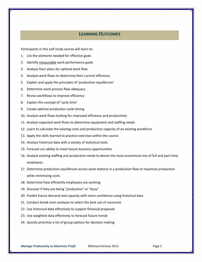
LEARNING OUTCOMES
Participants in this self-study course will learn to:
1. List the elements needed for effective goals
2. Identify measurable work performance goals
3. Analyze floor plans for optimal work flow
4. Analyze work flows to determine their current efficiency
5. Explain and apply the principles of ‘production equilibrium’
6. Determine work process flow adequacy
7. Revise workflows to improve efficiency
8. Explain the concept of ‘cycle time’
9. Create optimal production cycle timing
10. Analyze work flows looking for improved efficiency and productivity
11. Analyze expected work flows to determine equipment and staffing needs
12. Learn to calculate the existing costs and production capacity of an existing workforce
13. Apply the skills learned to practice exercises within the course
14. Analyze historical data with a variety of statistical tools
15. Forecast our ability to meet future business opportunities
16. Analyze existing staffing and production needs to devise the most economical mix of full and part-time
employees
17. Determine production equilibrium across work stations in a production flow to maximize production
while minimizing costs
18. Determine how efficiently employees are working
19. Discover if they are being “productive” or “busy”
20. Predict future demand and capacity with more confidence using historical data
21. Conduct break-even analyses to select the best use of resources
22. Use historical data effectively to support financial proposals
23. Use weighted data effectively to forecast future trends
24. Quickly prioritize a list of group options for decision making

Manage Productivity to Maximize Profit ©Richard Grimes 2013 Page 6
PRODUCTIVE OR BUSY?
Do you think a person can be very busy but not very productive? How could this happen?
It is because task requirements are not always well defined. Sometimes people are just “busy”
because they were not told all three elements of productivity. But, when you focus a task with
the three critical performance standards of productivity, they will include “how much”
(quantity), “how well” (quality) and “by when” (time), you establish goals and they become
productive.
The light bulb in a lamp is physically the same as a laser beam.
However, the laser has all of its energy narrowly focused upon a particular point that gives it
incredible power. How could you compare parts of your workday to the light bulb and the
laser beam?
When do you feel more satisfied with your work: when you are acting like a light bulb or a laser beam?
Which condition(s) ultimately makes your job more enjoyable and your work more productive?
How can you use the light bulb and laser beam example in a discussion with your employees?
Why would you want to do that?
Manage Productivity to Maximize Profit ©Richard Grimes 2013 Page 7
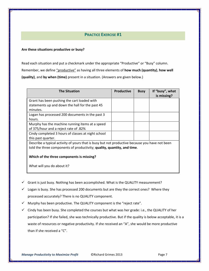
PRACTICE EXERCISE #1
Are these situations productive or busy?
Read each situation and put a checkmark under the appropriate “Productive” or “Busy” column.
Remember, we define “productive” as having all three elements of how much (quantity), how well
(quality), and by when (time) present in a situation. (Answers are given below.)
The Situation Productive Busy If “busy”, whatis missing?
Grant has been pushing the cart loaded withstatements up and down the hall for the past 45minutes.Logan has processed 200 documents in the past 3hours.Murphy has the machine running items at a speedof 375/hour and a reject rate of .82%Cindy completed 3 hours of classes at night schoolthis past quarter.Describe a typical activity of yours that is busy but not productive because you have not beentold the three components of productivity; quality, quantity, and time.
Which of the three components is missing?
What will you do about it?
Grant is just busy. Nothing has been accomplished. What is the QUALITY measurement?
Logan is busy. She has processed 200 documents but are they the correct ones? Where they
processed accurately? There is no QUALITY component.
Murphy has been productive. The QUALITY component is the “reject rate”.
Cindy has been busy. She completed the courses but what was her grade: i.e., the QUALITY of her
participation? If she failed, she was technically productive. But if the quality is below acceptable, it is a
waste of resources or negative productivity. If she received an “A”, she would be more productive
than if she received a “C”.
Manage Productivity to Maximize Profit ©Richard Grimes 2013 Page 8
THE VALUE OF SETTING MEASURABLE GOALS
There are at least four reasons why you should set measurable goals:
1) Knowing where you are going will help you plan to get there.
How do you plan your vacations?
a) Start planning with the ultimate destination and work backward budgeting time and money
necessary to make it happen (Time and money are measurables)
b) Just leave the house on the first day of vacation and see where you end up?
2) Measurable goals (milestones) along the way to your ultimate destination help you track your
progress.
Just as mileage signs along the interstate help you track your progress toward your goal, creating
personal milestones help you track your progress.
3) Planning helps you prevent problems
If you plan your vacation well enough, you will have enough money and time to get to where you want
to go, spend time there enjoying your vacation, and afford to come back home afterward. (Or would
you prefer to stay until your time and money runs out and see what happens next?)
4) Measurable goals help you enjoy your life at work more
Having measurable goals helps you focus your efforts on their accomplishment and not have to guess
whether you are doing what you hope will make your boss happy.
How does this lack of clarification affect you and your work?
It probably undermines your confidence and keeps you from going “all out” because you fear you may
have to undo some work.

Manage Productivity to Maximize Profit ©Richard Grimes 2013 Page 9
THE ELEMENTS OF MEASURABLE GOALS
An effective, measurable goal requires at least these elements:
Realistic (in the mind of the person doing the work) – The person must feel they have some chance
of success or they will not bother trying.
Quantifiable – It must tell the person HOW MUCH (Quantity), HOW WELL (Quality), and BY WHEN
(Time). This knowledge helps them gauge their own progress toward the ultimate goal.
Job Related – He/she must understand how his/her personal goals support the goals of the
department, which support the goals of the division.
Doable – They must involve his/her doing something that can be observed and measured. A goal
that calls for “Understanding how work flows through the IP Department” is useless. It only becomes
useful if he/she must do something that demonstrations his/her understanding such as explain the
work flow or identify a specific work area in the flow such as Balancing.
PRACTICE EXERCISE
Devise a scaled reward system for the family’s two teenagers to “be more helpful
around the house”. Just define specific tasks with quality, quantity, and time. Give a
basic (good) level of expectation, a better one and the top level.
Here is one example. You may make up as many as you think appropriate. You can
defend it because it is available to both, expected of both, and both know what the
expectations are.
Activity - “Cleaning the floors” Reward= $x
1. Vacuum the carpets: all rooms and all floors where there is carpet. 1.00X
2. All of #1 and vacuum everywhere there are hardwood floors 1.25X
3. All of #2 above, damp mop all bathroom tile floors, spray polish wood floors 1.50 X
Manage Productivity to Maximize Profit ©Richard Grimes 2013 Page 10
The activities for the teenagers are certainly measurable – you can visually inspect to see that they did
those tasks – but are they productive?
Technically speaking, they are NOT because there are no time or quality criteria specified. (Of course,
they are implied but since teenagers and employees are not mind readers, you cannot be sure their
definition of “vacuum the carpets” means the same as yours does.)
You would make them technically productive by specifying what “vacuum the carpet” means in terms of
residue picked up: i.e., QUALITY.
Do you want a “get on your hands and knees and get every possible piece of lint, pet hair, dust,
and dirt out so it’s spotless” kind of result or is “run the vacuum slowly over it and pick up what it
can get in one pass ” satisfactory?
Next, how much TIME do they have to do it? Obviously, vacuuming the room at the desired quality level in
ten minutes is more productive than doing it in fifteen minutes.
Manage Productivity to Maximize Profit ©Richard Grimes 2013 Page 11
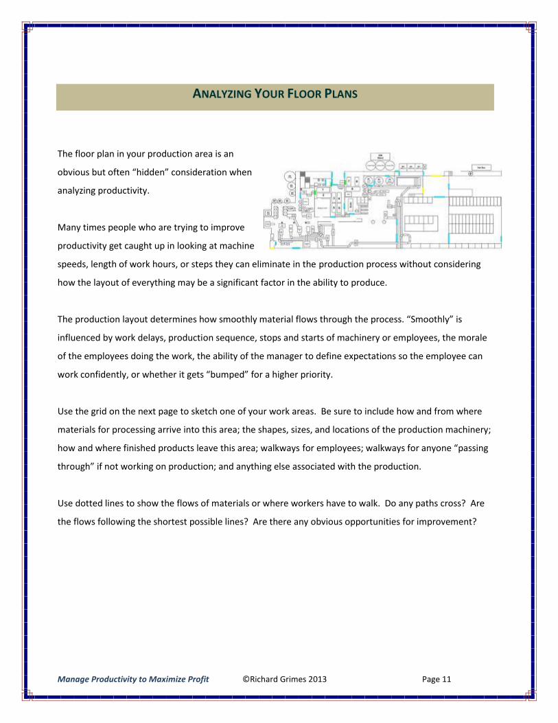
ANALYZING YOUR FLOOR PLANS
The floor plan in your production area is an
obvious but often “hidden” consideration when
analyzing productivity.
Many times people who are trying to improve
productivity get caught up in looking at machine
speeds, length of work hours, or steps they can eliminate in the production process without considering
how the layout of everything may be a significant factor in the ability to produce.
The production layout determines how smoothly material flows through the process. “Smoothly” is
influenced by work delays, production sequence, stops and starts of machinery or employees, the morale
of the employees doing the work, the ability of the manager to define expectations so the employee can
work confidently, or whether it gets “bumped” for a higher priority.
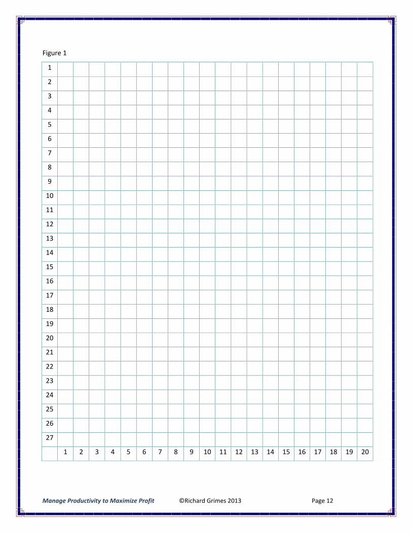
Use the grid on the next page to sketch one of your work areas. Be sure to include how and from where
materials for processing arrive into this area; the shapes, sizes, and locations of the production machinery;
how and where finished products leave this area; walkways for employees; walkways for anyone “passing
through” if not working on production; and anything else associated with the production.
Use dotted lines to show the flows of materials or where workers have to walk. Do any paths cross? Are
the flows following the shortest possible lines? Are there any obvious opportunities for improvement?
Manage Productivity to Maximize Profit ©Richard Grimes 2013 Page 12
Figure 1
1
2
3
4
5
6
7
8
9
10
11
12
13
14
15
16
17
18
19
20
21
22
23
24
25
26
27
1 2 3 4 5 6 7 8 9 10 11 12 13 14 15 16 17 18 19 20
Manage Productivity to Maximize Profit ©Richard Grimes 2013 Page 13
ANALYZING YOUR WORK FLOWS
After you look at the floor layout, the next step is to look at the work processes,
themselves. You should look at every segment of the assembly line whether
you work in a factory producing automobiles or an office producing finished
documents. However, before starting to look at the work process and the
employees doing it, you should be aware of a phenomenon discovered in the
late 1920s
The Hawthorne Studies (or experiments) were conducted from 1927 to 1932 at
the Western Electric Hawthorne Works in Chicago by a researcher from the
Harvard Business School. The studies grew out of preliminary experiments at
the plant from 1924 to 1927 on what factors or changes would influence
productivity. In particular, they wanted to find out what effect fatigue and
monotony had on job productivity and how to control them through such
variables as rest breaks, work hours, temperature and humidity.
They discovered more than they anticipated. The more they adjusted the length of work hours and breaks
up and down, the more productivity increased. The more they diminished illumination, the more
productivity increased. In short, productivity increased in every situation until exhaustion or too little
illumination in the factory physically prevented more production.
They discovered that the singling out a particular group of employees for special attention (even if it was
for longer hours and diminished lighting) made the employees feel special which made them increase
productivity to get more attention! (You can read more about this experiment at
http://en.wikipedia.org/wiki/Hawthorne_effect.)
The reason we mention the Hawthorne Studies in this section on analyzing workflows is that you may
unintentionally influence the workflow just by watching the employees work. Their production times may
be much different than normal. We suggest you make several observations as unobtrusively as possible
and average the times.
Manage Productivity to Maximize Profit ©Richard Grimes 2013 Page 14
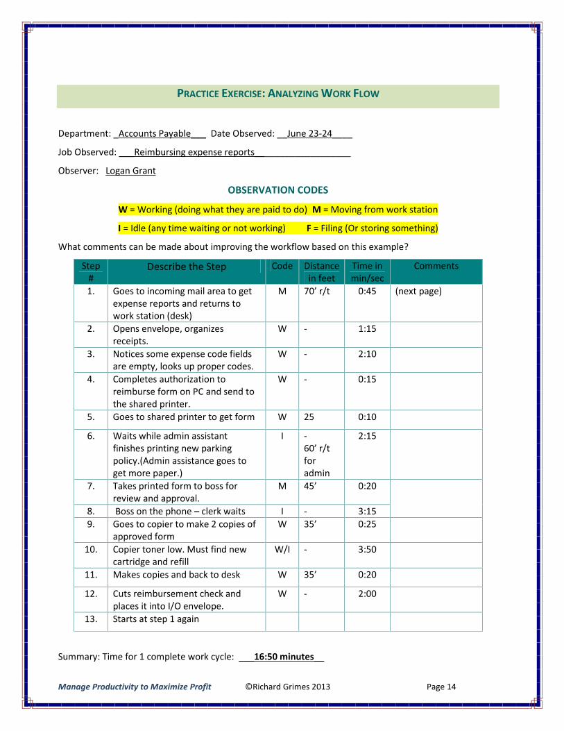
PRACTICE EXERCISE: ANALYZING WORK FLOW
Department: _Accounts Payable___ Date Observed: __June 23-24____
Job Observed: ___Reimbursing expense reports___________________
Observer: Logan Grant
OBSERVATION CODES
W = Working (doing what they are paid to do) M = Moving from work station
I = Idle (any time waiting or not working) F = Filing (Or storing something)
What comments can be made about improving the workflow based on this example?
Step#
Describe the Step Code Distancein feet
Time inmin/sec
Comments
1. Goes to incoming mail area to getexpense reports and returns towork station (desk)
M 70’ r/t 0:45 (next page)
2. Opens envelope, organizesreceipts.
W - 1:15
3. Notices some expense code fieldsare empty, looks up proper codes.
W - 2:10
4. Completes authorization toreimburse form on PC and send tothe shared printer.
W - 0:15
5. Goes to shared printer to get form W 25 0:10
6. Waits while admin assistantfinishes printing new parkingpolicy.(Admin assistance goes toget more paper.)
I -60’ r/tforadmin
2:15
7. Takes printed form to boss forreview and approval.
M 45’ 0:20
8. Boss on the phone – clerk waits I - 3:159. Goes to copier to make 2 copies of
approved formW 35’ 0:25
10. Copier toner low. Must find newcartridge and refill
W/I - 3:50
11. Makes copies and back to desk W 35’ 0:20
12. Cuts reimbursement check andplaces it into I/O envelope.
W - 2:00
13. Starts at step 1 again
Summary: Time for 1 complete work cycle: ___16:50 minutes__
Manage Productivity to Maximize Profit ©Richard Grimes 2013 Page 15
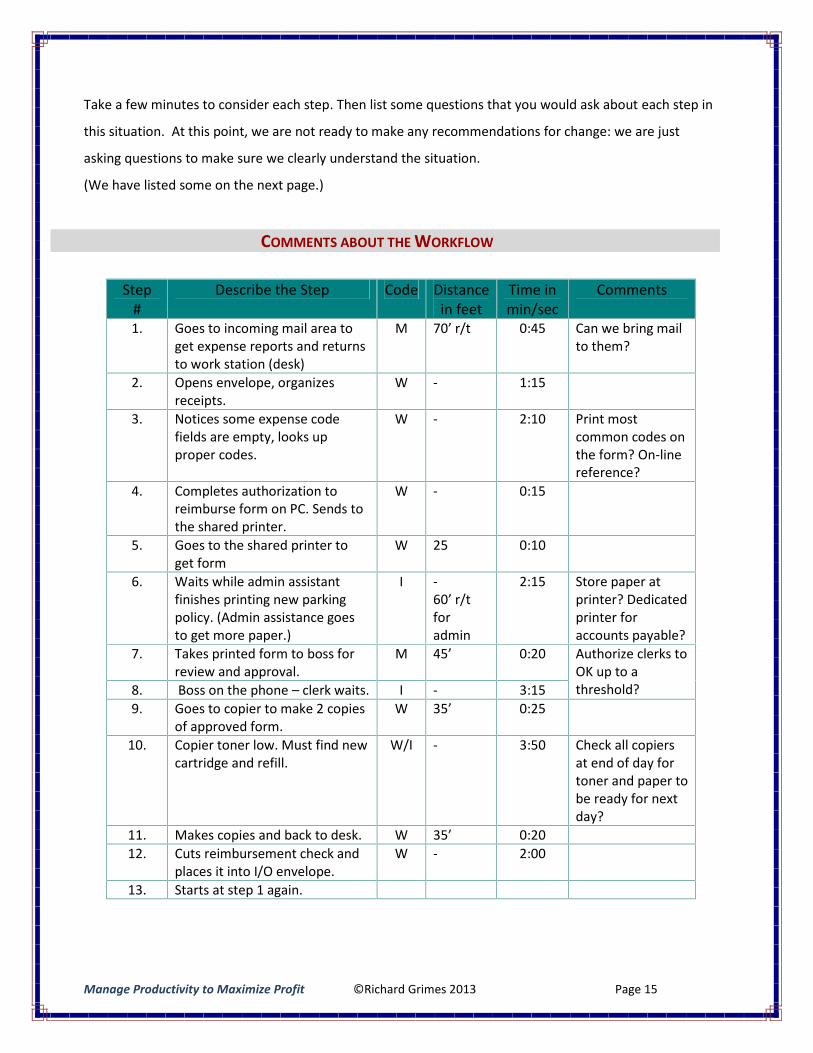
Take a few minutes to consider each step. Then list some questions that you would ask about each step in
this situation. At this point, we are not ready to make any recommendations for change: we are just
asking questions to make sure we clearly understand the situation.
(We have listed some on the next page.)
COMMENTS ABOUT THE WORKFLOW
Step#
Describe the Step Code Distancein feet
Time inmin/sec
Comments
1. Goes to incoming mail area toget expense reports and returnsto work station (desk)
M 70’ r/t 0:45 Can we bring mailto them?
2. Opens envelope, organizesreceipts.
W - 1:15
3. Notices some expense codefields are empty, looks upproper codes.
W - 2:10 Print mostcommon codes onthe form? On-linereference?
4. Completes authorization toreimburse form on PC. Sends tothe shared printer.
W - 0:15
5. Goes to the shared printer toget form
W 25 0:10
6. Waits while admin assistantfinishes printing new parkingpolicy. (Admin assistance goesto get more paper.)
I -60’ r/tforadmin
2:15 Store paper atprinter? Dedicatedprinter foraccounts payable?
7. Takes printed form to boss forreview and approval.
M 45’ 0:20 Authorize clerks toOK up to athreshold?8. Boss on the phone – clerk waits. I - 3:15
9. Goes to copier to make 2 copiesof approved form.
W 35’ 0:25
10. Copier toner low. Must find newcartridge and refill.
W/I - 3:50 Check all copiersat end of day fortoner and paper tobe ready for nextday?
11. Makes copies and back to desk. W 35’ 0:2012. Cuts reimbursement check and
places it into I/O envelope.W - 2:00
13. Starts at step 1 again.
Manage Productivity to Maximize Profit ©Richard Grimes 2013 Page 16
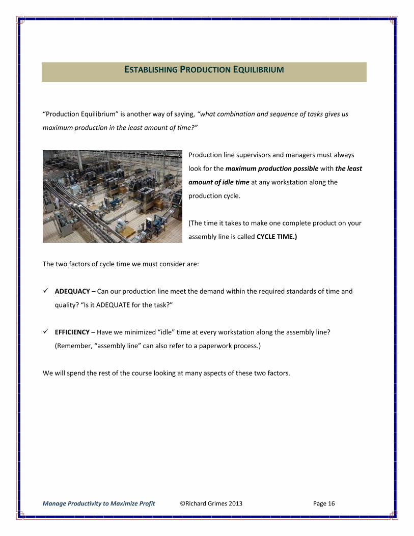
ESTABLISHING PRODUCTION EQUILIBRIUM
“Production Equilibrium” is another way of saying, “what combination and sequence of tasks gives us
maximum production in the least amount of time?”
Production line supervisors and managers must always
look for the maximum production possible with the least
amount of idle time at any workstation along the
production cycle.
(The time it takes to make one complete product on your
assembly line is called CYCLE TIME.)
The two factors of cycle time we must consider are:
ADEQUACY – Can our production line meet the demand within the required standards of time and
quality? “Is it ADEQUATE for the task?”
EFFICIENCY – Have we minimized “idle” time at every workstation along the assembly line?
(Remember, “assembly line” can also refer to a paperwork process.)
We will spend the rest of the course looking at many aspects of these two factors.
Manage Productivity to Maximize Profit ©Richard Grimes 2013 Page 17
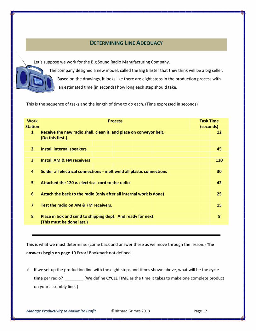
DETERMINING LINE ADEQUACY
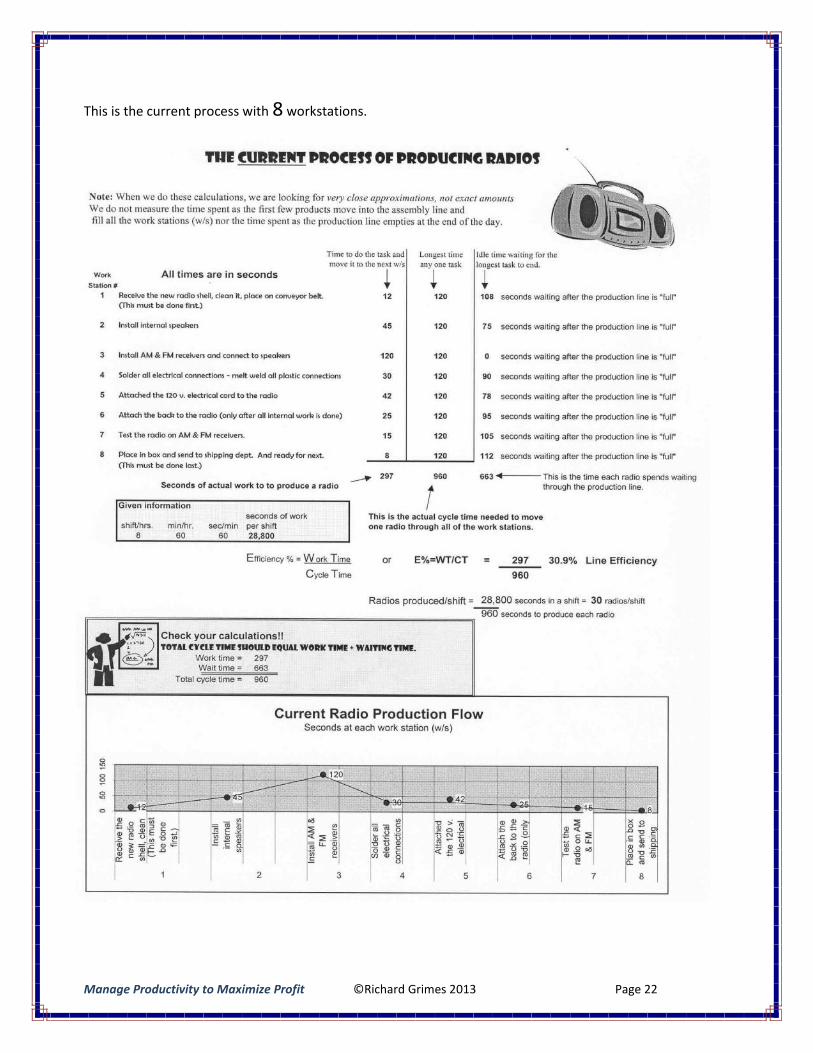
Let’s suppose we work for the Big Sound Radio Manufacturing Company.
The company designed a new model, called the Big Blaster that they think will be a big seller.
Based on the drawings, it looks like there are eight steps in the production process with
an estimated time (in seconds) how long each step should take.
This is the sequence of tasks and the length of time to do each. (Time expressed in seconds)
WorkStation
Process Task Time(seconds)
1 Receive the new radio shell, clean it, and place on conveyor belt. 12(Do this first.)
2 Install internal speakers 45
3 Install AM & FM receivers 120
4 Solder all electrical connections - melt weld all plastic connections 30
5 Attached the 120 v. electrical cord to the radio 42
6 Attach the back to the radio (only after all internal work is done) 25
7 Test the radio on AM & FM receivers. 15
8 Place in box and send to shipping dept. And ready for next. 8(This must be done last.)
This is what we must determine: (come back and answer these as we move through the lesson.) The
answers begin on page 19 Error! Bookmark not defined.
If we set up the production line with the eight steps and times shown above, what will be the cycle
time per radio? ________ (We define CYCLE TIME as the time it takes to make one complete product
on your assembly line. )
Manage Productivity to Maximize Profit ©Richard Grimes 2013 Page 18
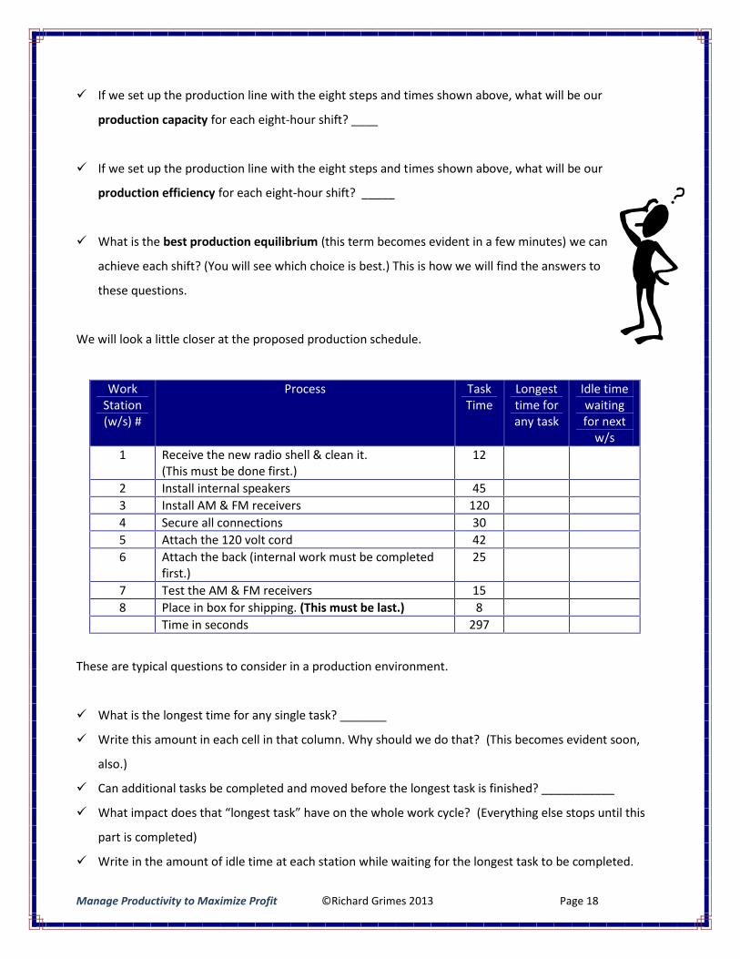
If we set up the production line with the eight steps and times shown above, what will be our
production capacity for each eight-hour shift? ____
If we set up the production line with the eight steps and times shown above, what will be our
production efficiency for each eight-hour shift? _____
What is the best production equilibrium (this term becomes evident in a few minutes) we can
achieve each shift? (You will see which choice is best.) This is how we will find the answers to
these questions.
We will look a little closer at the proposed production schedule.
WorkStation(w/s) #
Process TaskTime
Longesttime forany task
Idle timewaitingfor next
w/s1 Receive the new radio shell & clean it.
(This must be done first.)12
2 Install internal speakers 453 Install AM & FM receivers 1204 Secure all connections 305 Attach the 120 volt cord 426 Attach the back (internal work must be completed
first.)25
7 Test the AM & FM receivers 158 Place in box for shipping. (This must be last.) 8
Time in seconds 297
These are typical questions to consider in a production environment.
What is the longest time for any single task? _______
Write this amount in each cell in that column. Why should we do that? (This becomes evident soon,
also.)
Can additional tasks be completed and moved before the longest task is finished? ___________
What impact does that “longest task” have on the whole work cycle? (Everything else stops until this
part is completed)
Write in the amount of idle time at each station while waiting for the longest task to be completed.
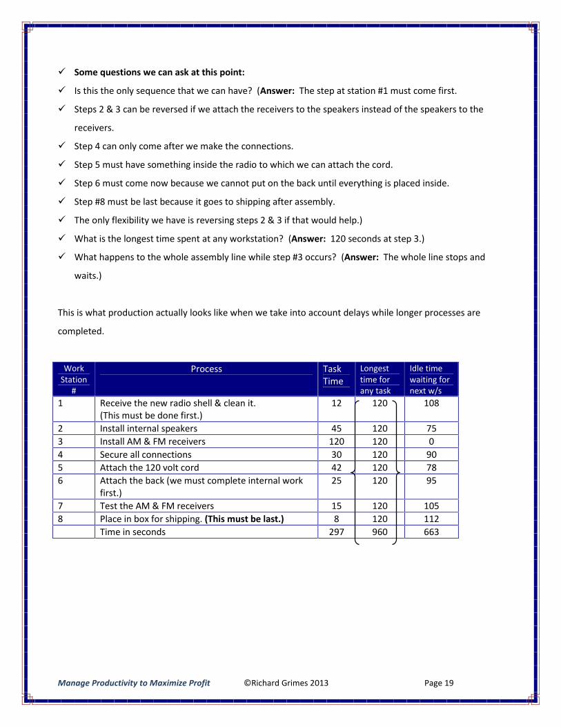
Manage Productivity to Maximize Profit ©Richard Grimes 2013 Page 19
Some questions we can ask at this point:
Is this the only sequence that we can have? (Answer: The step at station #1 must come first.
Steps 2 & 3 can be reversed if we attach the receivers to the speakers instead of the speakers to the
receivers.
Step 4 can only come after we make the connections.
Step 5 must have something inside the radio to which we can attach the cord.
Step 6 must come now because we cannot put on the back until everything is placed inside.
Step #8 must be last because it goes to shipping after assembly.
The only flexibility we have is reversing steps 2 & 3 if that would help.)
What is the longest time spent at any workstation? (Answer: 120 seconds at step 3.)
What happens to the whole assembly line while step #3 occurs? (Answer: The whole line stops and
waits.)
This is what production actually looks like when we take into account delays while longer processes are
completed.
WorkStation
#
Process TaskTime
Longesttime forany task
Idle timewaiting fornext w/s
1 Receive the new radio shell & clean it.(This must be done first.)
12 120 108
2 Install internal speakers 45 120 753 Install AM & FM receivers 120 120 04 Secure all connections 30 120 905 Attach the 120 volt cord 42 120 786 Attach the back (we must complete internal work
first.)25 120 95
7 Test the AM & FM receivers 15 120 1058 Place in box for shipping. (This must be last.) 8 120 112
Time in seconds 297 960 663
Manage Productivity to Maximize Profit ©Richard Grimes 2013 Page 20
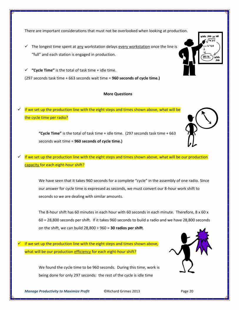
There are important considerations that must not be overlooked when looking at production.
The longest time spent at any workstation delays every workstation once the line is
“full” and each station is engaged in production.
“Cycle Time” is the total of task time + idle time.
(297 seconds task time + 663 seconds wait time = 960 seconds of cycle time.)
More Questions
If we set up the production line with the eight steps and times shown above, what will be
the cycle time per radio?
“Cycle Time” is the total of task time + idle time. (297 seconds task time + 663
seconds wait time = 960 seconds of cycle time.)
If we set up the production line with the eight steps and times shown above, what will be our production
capacity for each eight-hour shift?
We have seen that it takes 960 seconds for a complete “cycle” in the assembly of one radio. Since
our answer for cycle time is expressed as seconds, we must convert our 8-hour work shift to
seconds so we are dealing with similar amounts.
The 8-hour shift has 60 minutes in each hour with 60 seconds in each minute. Therefore, 8 x 60 x
60 = 28,800 seconds per shift. If it takes 960 seconds to build a radio and we have 28,800 seconds
on the shift, we can build 28,800 ÷ 960 = 30 radios per shift.
If we set up the production line with the eight steps and times shown above,
what will be our production efficiency for each eight-hour shift?
We found the cycle time to be 960 seconds. During this time, work is
being done for only 297 seconds: the rest of the cycle is idle time
Manage Productivity to Maximize Profit ©Richard Grimes 2013 Page 21
waiting for the longest task to be completed so the line can move again.
The efficiency of the line is determined by dividing the total work time within a cycle by the length
of the cycle. This is 297 ÷ 960 = 30.9% efficient.
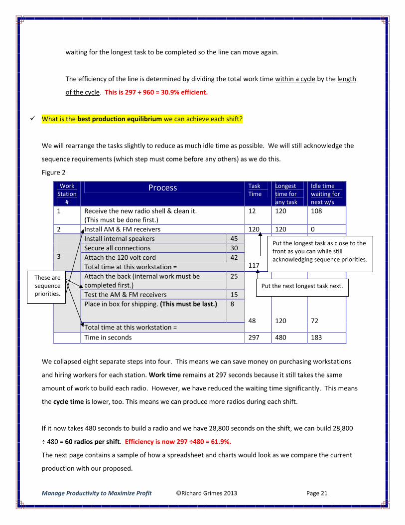
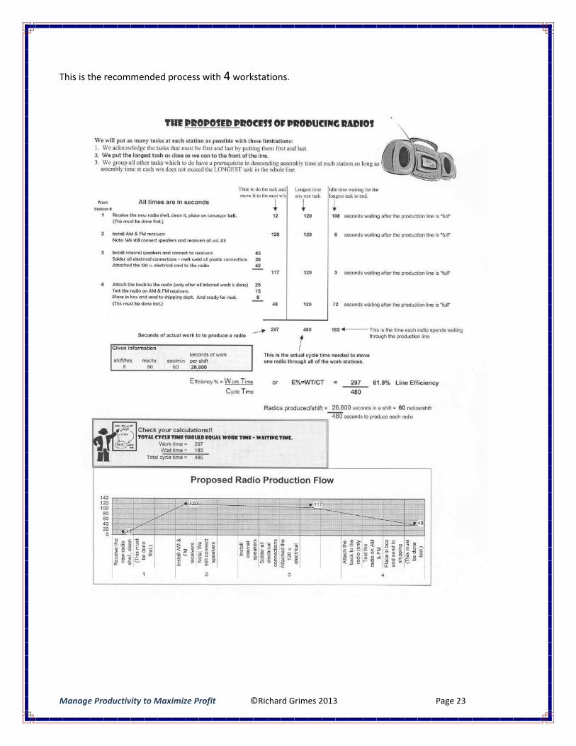
What is the best production equilibrium we can achieve each shift?
We will rearrange the tasks slightly to reduce as much idle time as possible. We will still acknowledge the
sequence requirements (which step must come before any others) as we do this.
Figure 2
WorkStation
#
Process TaskTime
Longesttime forany task
Idle timewaiting fornext w/s
1 Receive the new radio shell & clean it.(This must be done first.)
12 120 108
2 Install AM & FM receivers 120 120 0
3
Install internal speakers 45
117 120 3
Secure all connections 30Attach the 120 volt cord 42Total time at this workstation =
4
Attach the back (internal work must becompleted first.)
25
48 120 72
Test the AM & FM receivers 15Place in box for shipping. (This must be last.) 8
Total time at this workstation =Time in seconds 297 480 183
We collapsed eight separate steps into four. This means we can save money on purchasing workstations
and hiring workers for each station. Work time remains at 297 seconds because it still takes the same
amount of work to build each radio. However, we have reduced the waiting time significantly. This means
the cycle time is lower, too. This means we can produce more radios during each shift.
If it now takes 480 seconds to build a radio and we have 28,800 seconds on the shift, we can build 28,800
÷ 480 = 60 radios per shift. Efficiency is now 297 ÷480 = 61.9%.
The next page contains a sample of how a spreadsheet and charts would look as we compare the current
production with our proposed.
Put the next longest task next.These aresequencepriorities.
Put the longest task as close to thefront as you can while stillacknowledging sequence priorities.
Manage Productivity to Maximize Profit ©Richard Grimes 2013 Page 22
This is the current process with 8 workstations.
Manage Productivity to Maximize Profit ©Richard Grimes 2013 Page 23
This is the recommended process with 4 workstations.
Manage Productivity to Maximize Profit ©Richard Grimes 2013 Page 24
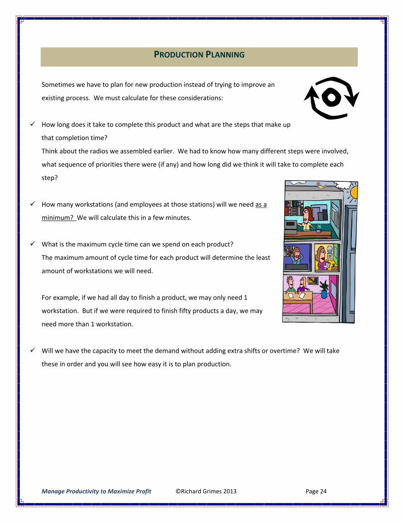
PRODUCTION PLANNING
Sometimes we have to plan for new production instead of trying to improve an
existing process. We must calculate for these considerations:
How long does it take to complete this product and what are the steps that make up
that completion time?
Think about the radios we assembled earlier. We had to know how many different steps were involved,
what sequence of priorities there were (if any) and how long did we think it will take to complete each
step?
How many workstations (and employees at those stations) will we need as a
minimum? We will calculate this in a few minutes.
What is the maximum cycle time can we spend on each product?
The maximum amount of cycle time for each product will determine the least
amount of workstations we will need.
For example, if we had all day to finish a product, we may only need 1
workstation. But if we were required to finish fifty products a day, we may
need more than 1 workstation.
Will we have the capacity to meet the demand without adding extra shifts or overtime? We will take
these in order and you will see how easy it is to plan production.
Manage Productivity to Maximize Profit ©Richard Grimes 2013 Page 25
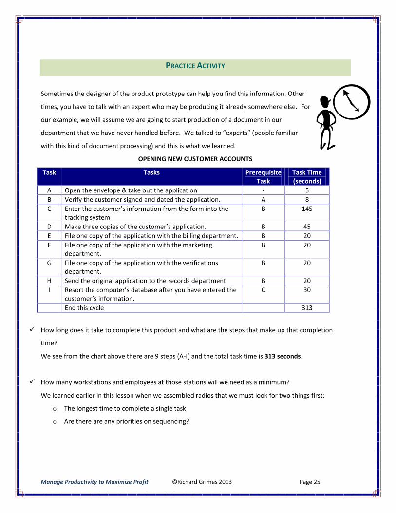
PRACTICE ACTIVITY
Sometimes the designer of the product prototype can help you find this information. Other
times, you have to talk with an expert who may be producing it already somewhere else. For
our example, we will assume we are going to start production of a document in our
department that we have never handled before. We talked to “experts” (people familiar
with this kind of document processing) and this is what we learned.
OPENING NEW CUSTOMER ACCOUNTS
Task Tasks PrerequisiteTask
Task Time(seconds)
A Open the envelope & take out the application - 5B Verify the customer signed and dated the application. A 8C Enter the customer’s information from the form into the
tracking systemB 145
D Make three copies of the customer’s application. B 45E File one copy of the application with the billing department. B 20F File one copy of the application with the marketing
department.B 20
G File one copy of the application with the verificationsdepartment.
B 20
H Send the original application to the records department B 20I Resort the computer’s database after you have entered the
customer’s information.C 30
End this cycle 313
How long does it take to complete this product and what are the steps that make up that completion
time?
We see from the chart above there are 9 steps (A-I) and the total task time is 313 seconds.
How many workstations and employees at those stations will we need as a minimum?
We learned earlier in this lesson when we assembled radios that we must look for two things first:
o The longest time to complete a single task
o Are there are any priorities on sequencing?
Manage Productivity to Maximize Profit ©Richard Grimes 2013 Page 26
In this example, we see the longest single task (“C”) is 145 seconds. Also, the only priorities are that “A”
must come first; make sure the customer signed and dated it “B” and task “I” cannot be completed until
task “C” is finished. We can rearrange the tasks into a sequence like this to minimize cycle time. (Can you
suggest any other arrangements?)
Note: Although technically tasks “A” & “B” are separate steps, we know that we can open the envelope,
take out the application and verify if the customer signed and dated it at this one workstation.
PRODUCTION LAYOUT “A” (Wkstn = Work Station)
Wkstn
Tasks & Completion Time inseconds
PrerequisiteTask
Task Time(seconds)
Longesttask time
Delay Time
#1
A Open the envelope & takeout the application
5
A 13 145 132B Verify the customer signedand dated the application.
8
#2 C Enter the customer’s informationfrom the form into the tracking
system = 145 secondsB 145 145 0
#3
D Make three copies of thecustomer’s application.
45
B 125 145 20
E File one copy of theapplication with the billingdepartment.
20
F File one copy of theapplication with themarketing department.
20
G File one copy of theapplication with theverifications department.
20
H Send the originalapplication to the recordsdepartment
20
#4I Resort the computer’s database
after you have entered thecustomer’s information = 30seconds
C 30 145 115
End this cycle 313 580 267We see that the least number of workstations that we need is 4.
What is the efficiency of this arrangement?
313 seconds (total task time)/580 seconds (total cycle time) = 53.9% efficient
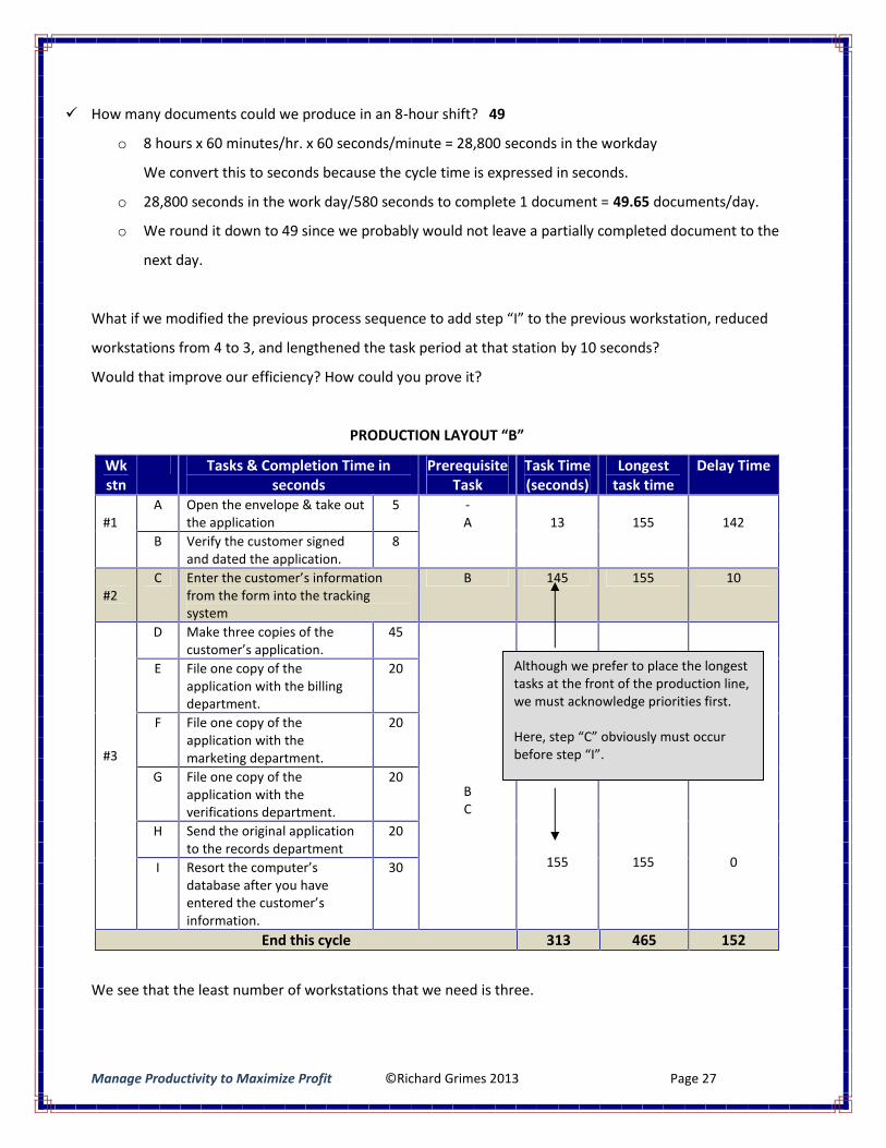
Manage Productivity to Maximize Profit ©Richard Grimes 2013 Page 27
How many documents could we produce in an 8-hour shift? 49
o 8 hours x 60 minutes/hr. x 60 seconds/minute = 28,800 seconds in the workday
We convert this to seconds because the cycle time is expressed in seconds.
o 28,800 seconds in the work day/580 seconds to complete 1 document = 49.65 documents/day.
o We round it down to 49 since we probably would not leave a partially completed document to the
next day.
What if we modified the previous process sequence to add step “I” to the previous workstation, reduced
workstations from 4 to 3, and lengthened the task period at that station by 10 seconds?
Would that improve our efficiency? How could you prove it?
PRODUCTION LAYOUT “B”
Wkstn
Tasks & Completion Time inseconds
PrerequisiteTask
Task Time(seconds)
Longesttask time
Delay Time
#1A Open the envelope & take out
the application5 -
A 13 155 142B Verify the customer signed
and dated the application.8
#2C Enter the customer’s information
from the form into the trackingsystem
B 145 155 10
#3
D Make three copies of thecustomer’s application.
45
BC
155 155 0
E File one copy of theapplication with the billingdepartment.
20
F File one copy of theapplication with themarketing department.
20
G File one copy of theapplication with theverifications department.
20
H Send the original applicationto the records department
20
I Resort the computer’sdatabase after you haveentered the customer’sinformation.
30
End this cycle 313 465 152
We see that the least number of workstations that we need is three.
Although we prefer to place the longesttasks at the front of the production line,we must acknowledge priorities first.
Here, step “C” obviously must occurbefore step “I”.
Manage Productivity to Maximize Profit ©Richard Grimes 2013 Page 28
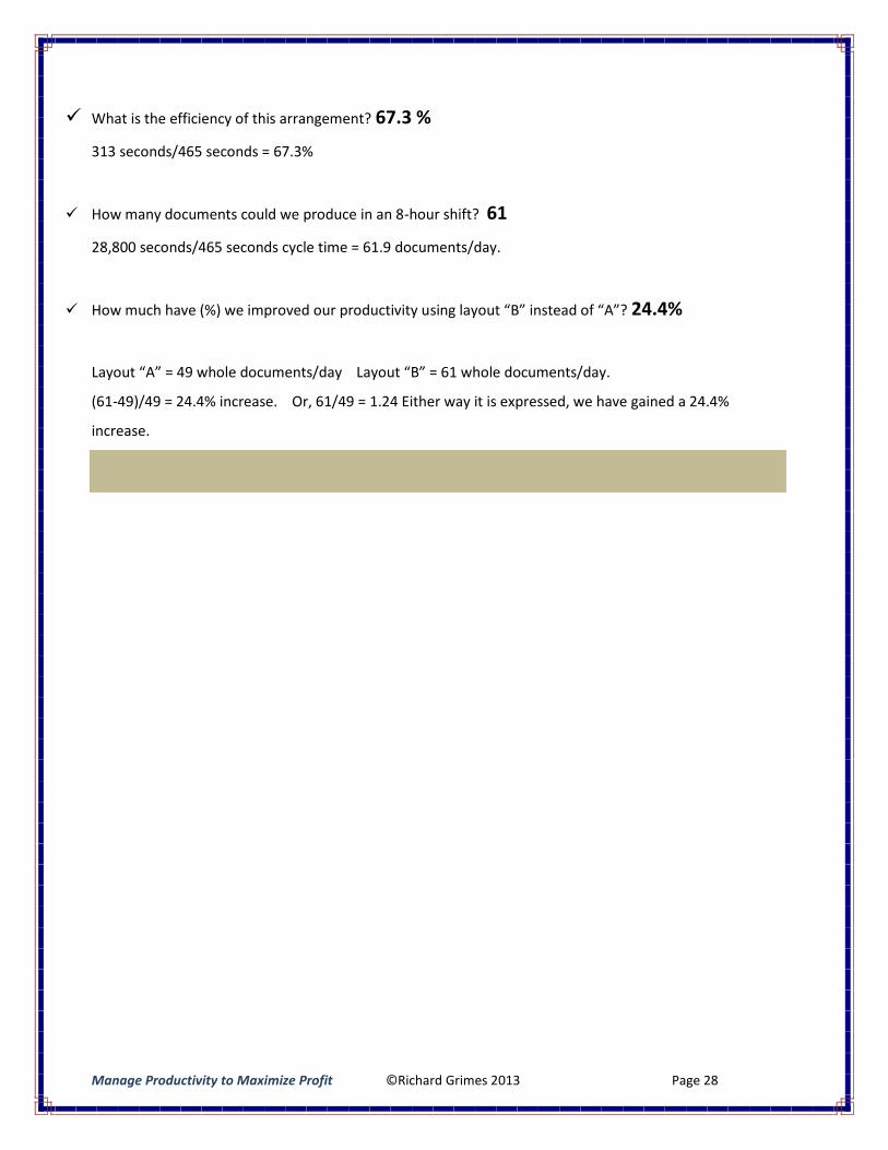
What is the efficiency of this arrangement? 67.3 %
313 seconds/465 seconds = 67.3%
How many documents could we produce in an 8-hour shift? 61
28,800 seconds/465 seconds cycle time = 61.9 documents/day.
How much have (%) we improved our productivity using layout “B” instead of “A”? 24.4%
Layout “A” = 49 whole documents/day Layout “B” = 61 whole documents/day.
(61-49)/49 = 24.4% increase. Or, 61/49 = 1.24 Either way it is expressed, we have gained a 24.4%
increase.
Manage Productivity to Maximize Profit ©Richard Grimes 2013 Page 29
HOW MANY WORKSTATIONS AND EMPLOYEES WILL WE NEED?
First, we will calculate the maximum cycle time we have available to complete each product. It is easy to
do; here is how:
1. Calculate the amount of available work time you have in a
work period. This may be expressed as a “day” or a shift.
2. Make sure you clarify how you define a “day”: is it 8 hours,
10 hours or the product of all three shifts?
3. Determine the demand (how many products you must produce) during that work period. “Products”
may be radios, tee shirts, or completed documents.
4. Divide the available work time by the number of products you must finish to discover the maximum
cycle time available to produce each unit.
PRACTICE EXERCISE
We are considering placing a bid on a contract to produce 150 documents in a day. How many
workstations and employees will we need?
We will break it down step-by-step.
We have an 8-hour day during which we must process 150 documents. We divide the available time to
produce it (8 hours) by the amount of products we must make. This becomes 8 hours ÷ 150 products =
.053 hours maximum cycle time per product.
Although this is mathematically correct (.053 hours), we can express it more clearly. We will convert the 8-
hour day to minutes and see what we get.
Manage Productivity to Maximize Profit ©Richard Grimes 2013 Page 30
8 hours in the work period x 60 minutes in an hour = 480 minutes
Let us calculate the maximum cycle time again. 480 minutes ÷ 150 products = 3.2 minutes maximum cycle
time per product.
It is getting clearer because we can understand 3.2 minutes per product cycle time much easier than .053
hours. Let us take it another step and see if it gets any better:
480 minutes in the work period x 60 seconds in a minute = 28,800 seconds
28,800 seconds ÷ 150 products = 192 seconds maximum cycle time per product.
Now we have something we can easily work with. We see that we only have 192 seconds to produce
each product if we are to achieve our requirement of 150 per work period.
Look back at our calculations on production layouts “A” and “B”. We first calculated we would need 580
seconds to process a document with four workstations using layout “A”. Then we combined tasks into
three workstations on layout “B” and calculated we could reduce production time down to 465 seconds.
PRODUCTION LAYOUT “A”
If we need 580 seconds to produce a document with layout “A” (with four workstations) and must
complete a document within 192 seconds, we must have 580 ÷ 192 = 3.02 layouts like “A”.
However, since we cannot have less than a complete work process (the “.02” remainder), we must have 4
layouts like “A” and realize that we are not getting maximum use out of the 4th one. Four workstations
mean four employees must be hired for each type “A” layout. Four layouts mean the company will have
to hire 16 people. That can be expensive!
PRODUCTION LAYOUT “B”
If we need 465 seconds to produce a document with layout “B” (with three workstations) and must
complete a document within 192 seconds, we must have 465 ÷ 192 = 2.4 layouts like “B”.
Manage Productivity to Maximize Profit ©Richard Grimes 2013 Page 31
But, since we cannot have less than a complete work process (the “.4” remainder), we must have 3 layouts
like “B” with 3 workstations each and realize that we are not getting maximum use out of the 3rd one.
Three new layouts mean three employees must be hired for each type “B” layout. This means we will have
to hire 9 employees. This is certainly better than hiring 16 as we would with the type “A” layout.
HOW EFFICIENTLY ARE YOUR EMPLOYEES WORKING?
This section will be deceptively short because you have already learned how to determine employee
efficiency!
Look back to the production layouts “A” and “B” where we calculated
efficiency for each production plan. We calculated efficiency by dividing
the time spent actually working within the entire cycle time required to
make the product.
Layout “A’s” efficiency rating was 53.9%: “B’s” was 67.3%. That is how you determine an employee’s
efficiency. Ideally, you want to get as close to 100% as possible, which would mean there was no idle time
within a production process.
That is virtually impossible in reality but you can use 85% as a typical benchmark of an efficient
operation.
Manage Productivity to Maximize Profit ©Richard Grimes 2013 Page 32
HOW PRODUCTIVELY ARE YOUR EMPLOYEES WORKING?
Essentially, productivity requires measurements of quality,
quantity, and time being present. Without all three measures
included, employees are only “busy” but not productive.
For example, an employee processing 875 documents an hour at
an accuracy of 98.6% is being productive because you have
quantity (875), quality (98.6% accurate), and time (hour).
(Whether 875 an hour is productive enough for the company’s standards is a matter between the
employee and his supervisor.) If we told the employee to process 875 documents in an hour without
reference to the quality standard, he would just be busy. If we cannot use the documents he processed
because of high errors, he has “produced” nothing of value and only wasted time.
Take a minute to think about your job. Name a task that you do that clearly has defined measurements
of quality, quantity, and time. What does it do for your job satisfaction and level of confidence knowing
exactly what is expected of you?
If you are not sure or cannot name tasks that have all three elements clearly defined, what does that do to
your motivation to work? (It reduces motivation.)
What does that for your confidence if you are not positive about what your supervisor expects from you?
It reduces it.
What conversation should you have with your supervisor as soon as you leave this class? Get your work
expectations clarified in terms of quality, quantity, and time.
If you have employees who are not working to your expectations, is there a chance they have similar
confusion about your expectations of them as you may have about your supervisor’s expectations of
you?
Manage Productivity to Maximize Profit ©Richard Grimes 2013 Page 33
PRODUCTION CAPACITY TODAY AND TOMORROW
Production managers face these questions daily
“How many products can we produce at our maximum efficiency?”
“How much will that cost us?”
“If we get a chance to bid on a new project, will we be able to handle it?”
“Will we need additional resources?”
We have already learned how to analyze existing workflows to see if there are
opportunities to reduce cycle time, delays, or movement. We will do another exercise here to work our
way through this situation.
You have looked at assembly lines to see if we could rearrange the sequence of tasks or group tasks to
reduce cycle time and the number of workstations and employees while increasing efficiency. Now we will
assume that we have rearranged the assembly lines to their most efficient.
Our company has an opportunity to bid on a project that could make a lot of money for us.
However, if we do not do our homework first, it could cost us a lot of money instead. This next analysis will
give us a clear picture of what we can or cannot do and help us select the best action among several
choices.
Manage Productivity to Maximize Profit ©Richard Grimes 2013 Page 34
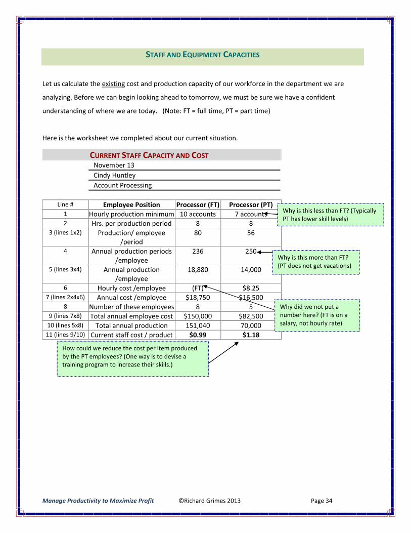
STAFF AND EQUIPMENT CAPACITIES
Let us calculate the existing cost and production capacity of our workforce in the department we are
analyzing. Before we can begin looking ahead to tomorrow, we must be sure we have a confident
understanding of where we are today. (Note: FT = full time, PT = part time)
Here is the worksheet we completed about our current situation.
CURRENT STAFF CAPACITY AND COSTNovember 13Cindy HuntleyAccount Processing
Line # Employee Position Processor (FT) Processor (PT)1 Hourly production minimum 10 accounts 7 accounts2 Hrs. per production period 8 8
3 (lines 1x2) Production/ employee/period
80 56
4 Annual production periods/employee
236 250
5 (lines 3x4) Annual production/employee
18,880 14,000
6 Hourly cost /employee (FT) $8.257 (lines 2x4x6) Annual cost /employee $18,750 $16,500
8 Number of these employees 8 59 (lines 7x8) Total annual employee cost $150,000 $82,500
10 (lines 5x8) Total annual production 151,040 70,00011 (lines 9/10) Current staff cost / product $0.99 $1.18
How could we reduce the cost per item producedby the PT employees? (One way is to devise atraining program to increase their skills.)
Why is this more than FT?(PT does not get vacations)
Why is this less than FT? (TypicallyPT has lower skill levels)
Why did we not put anumber here? (FT is on asalary, not hourly rate)
Manage Productivity to Maximize Profit ©Richard Grimes 2013 Page 35
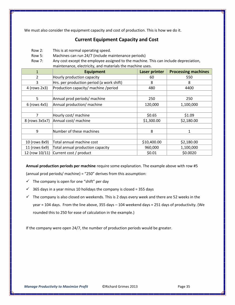
We must also consider the equipment capacity and cost of production. This is how we do it.
Current Equipment Capacity and Cost
Row 2: This is at normal operating speed.Row 5: Machines can run 24/7 (include maintenance periods)Row 7: Any cost except the employee assigned to the machine. This can include depreciation,
maintenance, electricity, and materials the machine uses.1 Equipment Laser printer Processing machines2 Hourly production capacity 60 5503 Hrs. per production period (a work shift) 8 8
4 (rows 2x3) Production capacity/ machine /period 480 4400
5 Annual prod periods/ machine 250 2506 (rows 4x5) Annual production/ machine 120,000 1,100,000
7 Hourly cost/ machine $0.65 $1.098 (rows 3x5x7) Annual cost/ machine $1,300.00 $2,180.00
9 Number of these machines 8 1
10 (rows 8x9) Total annual machine cost $10,400.00 $2,180.0011 (rows 6x9) Total annual production capacity 960,000 1,100,000
12 (row 10/11) Current cost / product $0.01 $0.0020
Annual production periods per machine require some explanation. The example above with row #5
(annual prod periods/ machine) = “250” derives from this assumption:
The company is open for one “shift” per day
365 days in a year minus 10 holidays the company is closed = 355 days
The company is also closed on weekends. This is 2 days every week and there are 52 weeks in the
year = 104 days. From the line above, 355 days – 104 weekend days = 251 days of productivity. (We
rounded this to 250 for ease of calculation in the example.)
If the company were open 24/7, the number of production periods would be greater.
Manage Productivity to Maximize Profit ©Richard Grimes 2013 Page 36
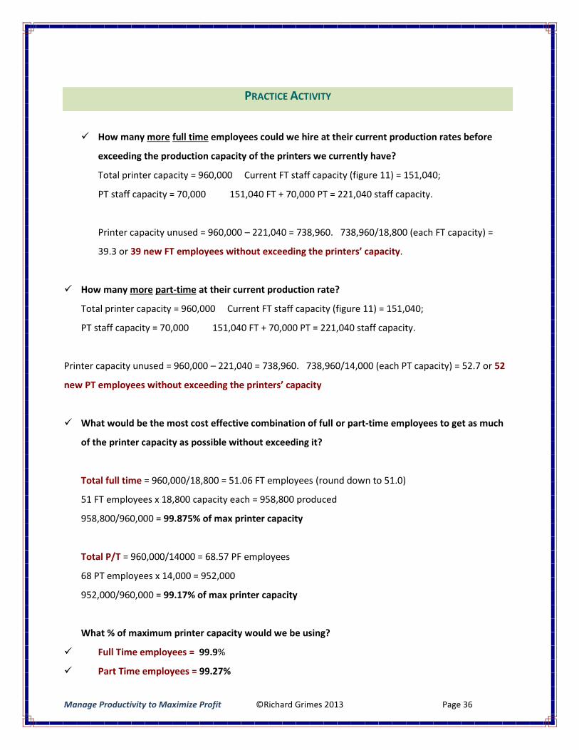
PRACTICE ACTIVITY
How many more full time employees could we hire at their current production rates before
exceeding the production capacity of the printers we currently have?
Total printer capacity = 960,000 Current FT staff capacity (figure 11) = 151,040;
PT staff capacity = 70,000 151,040 FT + 70,000 PT = 221,040 staff capacity.
Printer capacity unused = 960,000 – 221,040 = 738,960. 738,960/18,800 (each FT capacity) =
39.3 or 39 new FT employees without exceeding the printers’ capacity.
How many more part-time at their current production rate?
Total printer capacity = 960,000 Current FT staff capacity (figure 11) = 151,040;
PT staff capacity = 70,000 151,040 FT + 70,000 PT = 221,040 staff capacity.
Printer capacity unused = 960,000 – 221,040 = 738,960. 738,960/14,000 (each PT capacity) = 52.7 or 52
new PT employees without exceeding the printers’ capacity
What would be the most cost effective combination of full or part-time employees to get as much
of the printer capacity as possible without exceeding it?
Total full time = 960,000/18,800 = 51.06 FT employees (round down to 51.0)
51 FT employees x 18,800 capacity each = 958,800 produced
958,800/960,000 = 99.875% of max printer capacity
Total P/T = 960,000/14000 = 68.57 PF employees
68 PT employees x 14,000 = 952,000
952,000/960,000 = 99.17% of max printer capacity
What % of maximum printer capacity would we be using?
Full Time employees = 99.9%
Part Time employees = 99.27%
Manage Productivity to Maximize Profit ©Richard Grimes 2013 Page 37
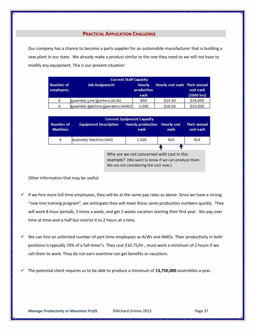
PRACTICAL APPLICATION CHALLENGE
Our company has a chance to become a parts supplier for an automobile manufacturer that is building a
new plant in our state. We already make a product similar to the one they need so we will not have to
modify any equipment. This is our present situation:
Other information that may be useful:
If we hire more full time employees, they will be at the same pay rates as above. Since we have a strong
“new hire training program”, we anticipate they will meet those same production numbers quickly. They
will work 8-hour periods, 5 times a week, and get 2 weeks vacation starting their first year. We pay over
time at time-and-a-half but restrict it to 2 hours at a time.
We can hire an unlimited number of part-time employees as ALWs and AMOs. Their productivity in both
positions is typically 70% of a full-timer’s. They cost $10.75/hr., must work a minimum of 2 hours if we
call them to work. They do not earn overtime nor get benefits or vacations.
The potential client requires us to be able to produce a minimum of 13,750,000 assemblies a year.
Why are we not concerned with cost in thisexample? (We want to know if we can produce them.We are not considering the cost now.)
Manage Productivity to Maximize Profit ©Richard Grimes 2013 Page 38
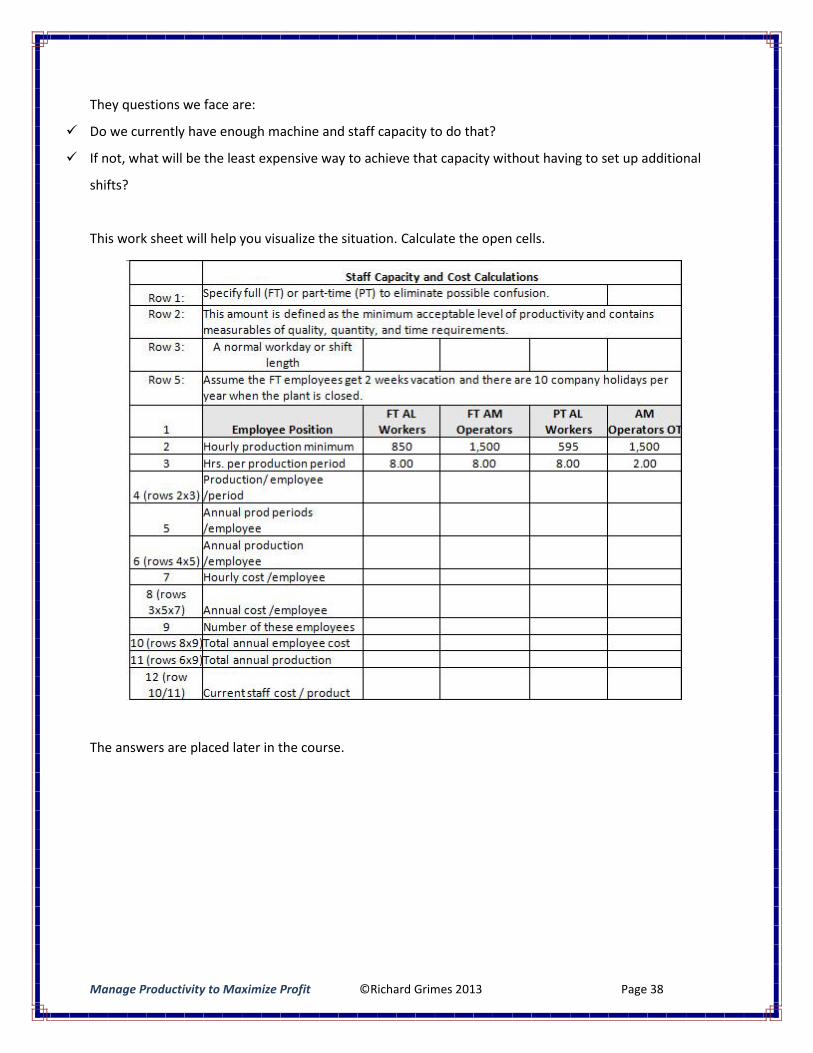
They questions we face are:
Do we currently have enough machine and staff capacity to do that?
If not, what will be the least expensive way to achieve that capacity without having to set up additional
shifts?
This work sheet will help you visualize the situation. Calculate the open cells.
The answers are placed later in the course.
Manage Productivity to Maximize Profit ©Richard Grimes 2013 Page 39
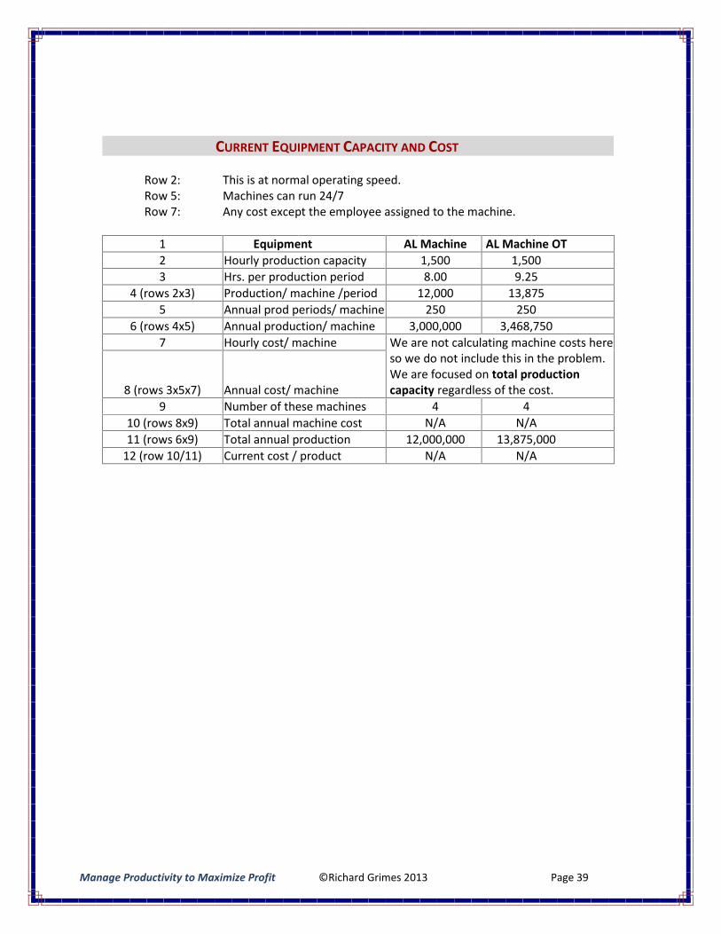
CURRENT EQUIPMENT CAPACITY AND COST
Row 2: This is at normal operating speed.Row 5: Machines can run 24/7Row 7: Any cost except the employee assigned to the machine.
1 Equipment AL Machine AL Machine OT2 Hourly production capacity 1,500 1,5003 Hrs. per production period 8.00 9.25
4 (rows 2x3) Production/ machine /period 12,000 13,8755 Annual prod periods/ machine 250 250
6 (rows 4x5) Annual production/ machine 3,000,000 3,468,7507 Hourly cost/ machine We are not calculating machine costs here
so we do not include this in the problem.We are focused on total productioncapacity regardless of the cost.8 (rows 3x5x7) Annual cost/ machine
9 Number of these machines 4 410 (rows 8x9) Total annual machine cost N/A N/A11 (rows 6x9) Total annual production 12,000,000 13,875,000
12 (row 10/11) Current cost / product N/A N/A
Manage Productivity to Maximize Profit ©Richard Grimes 2013 Page 40
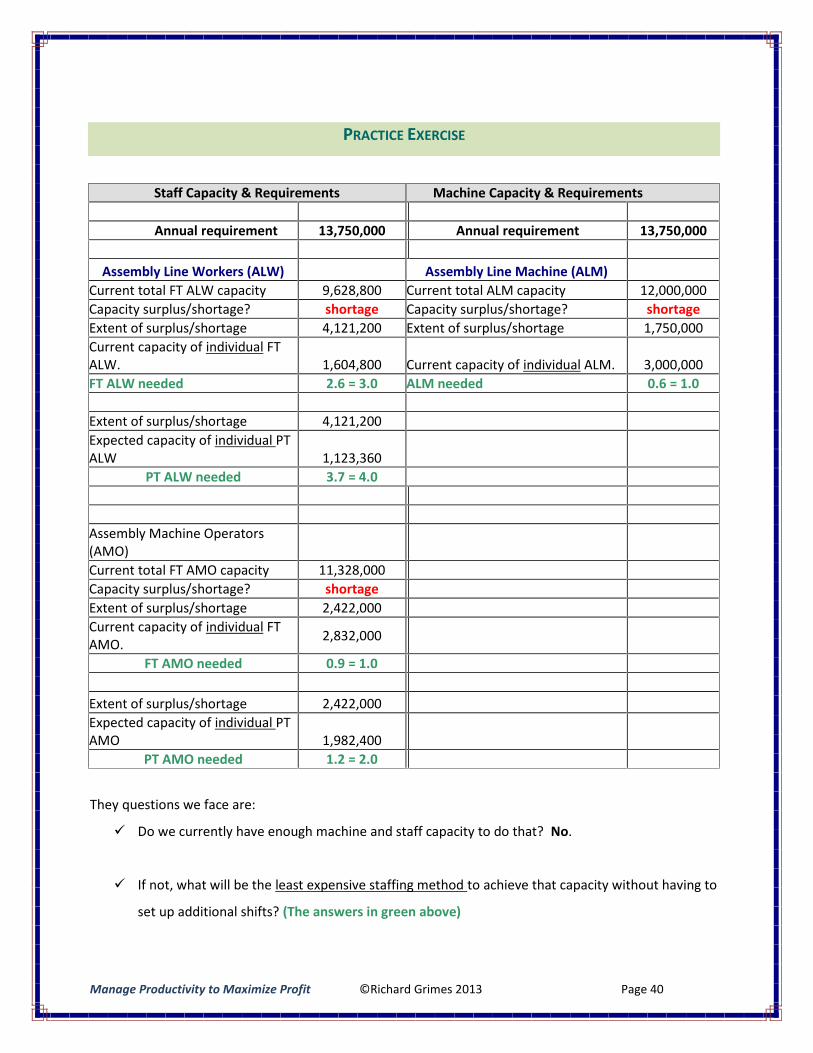
PRACTICE EXERCISE
Staff Capacity & Requirements Machine Capacity & Requirements
Annual requirement 13,750,000 Annual requirement 13,750,000
Assembly Line Workers (ALW) Assembly Line Machine (ALM)Current total FT ALW capacity 9,628,800 Current total ALM capacity 12,000,000Capacity surplus/shortage? shortage Capacity surplus/shortage? shortageExtent of surplus/shortage 4,121,200 Extent of surplus/shortage 1,750,000Current capacity of individual FTALW. 1,604,800 Current capacity of individual ALM. 3,000,000FT ALW needed 2.6 = 3.0 ALM needed 0.6 = 1.0
Extent of surplus/shortage 4,121,200Expected capacity of individual PTALW 1,123,360
PT ALW needed 3.7 = 4.0
Assembly Machine Operators(AMO)Current total FT AMO capacity 11,328,000Capacity surplus/shortage? shortageExtent of surplus/shortage 2,422,000Current capacity of individual FTAMO. 2,832,000
FT AMO needed 0.9 = 1.0
Extent of surplus/shortage 2,422,000Expected capacity of individual PTAMO 1,982,400
PT AMO needed 1.2 = 2.0
They questions we face are:
Do we currently have enough machine and staff capacity to do that? No.
If not, what will be the least expensive staffing method to achieve that capacity without having to
set up additional shifts? (The answers in green above)
Manage Productivity to Maximize Profit ©Richard Grimes 2013 Page 41
BREAK EVEN ANALYSIS
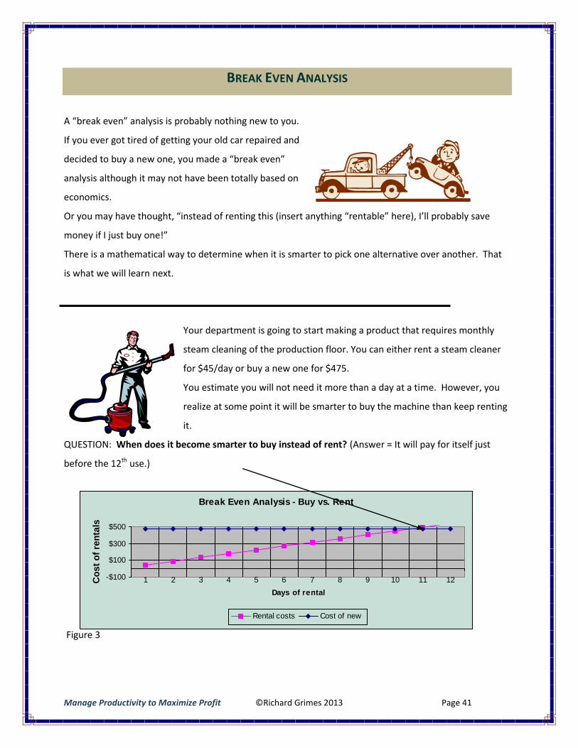
A “break even” analysis is probably nothing new to you.
If you ever got tired of getting your old car repaired and
decided to buy a new one, you made a “break even”
analysis although it may not have been totally based on
economics.
Or you may have thought, “instead of renting this (insert anything “rentable” here), I’ll probably save
money if I just buy one!”
There is a mathematical way to determine when it is smarter to pick one alternative over another. That
is what we will learn next.
Your department is going to start making a product that requires monthly
steam cleaning of the production floor. You can either rent a steam cleaner
for $45/day or buy a new one for $475.
You estimate you will not need it more than a day at a time. However, you
realize at some point it will be smarter to buy the machine than keep renting
it.
QUESTION: When does it become smarter to buy instead of rent? (Answer = It will pay for itself just
before the 12th use.)
Figure 3
Break Even Analysis - Buy vs. Rent
-$100
$100
$300
$500
1 2 3 4 5 6 7 8 9 10 11 12Days of rental
Cos
t of r
enta
ls
Rental costs Cost of new
Manage Productivity to Maximize Profit ©Richard Grimes 2013 Page 42
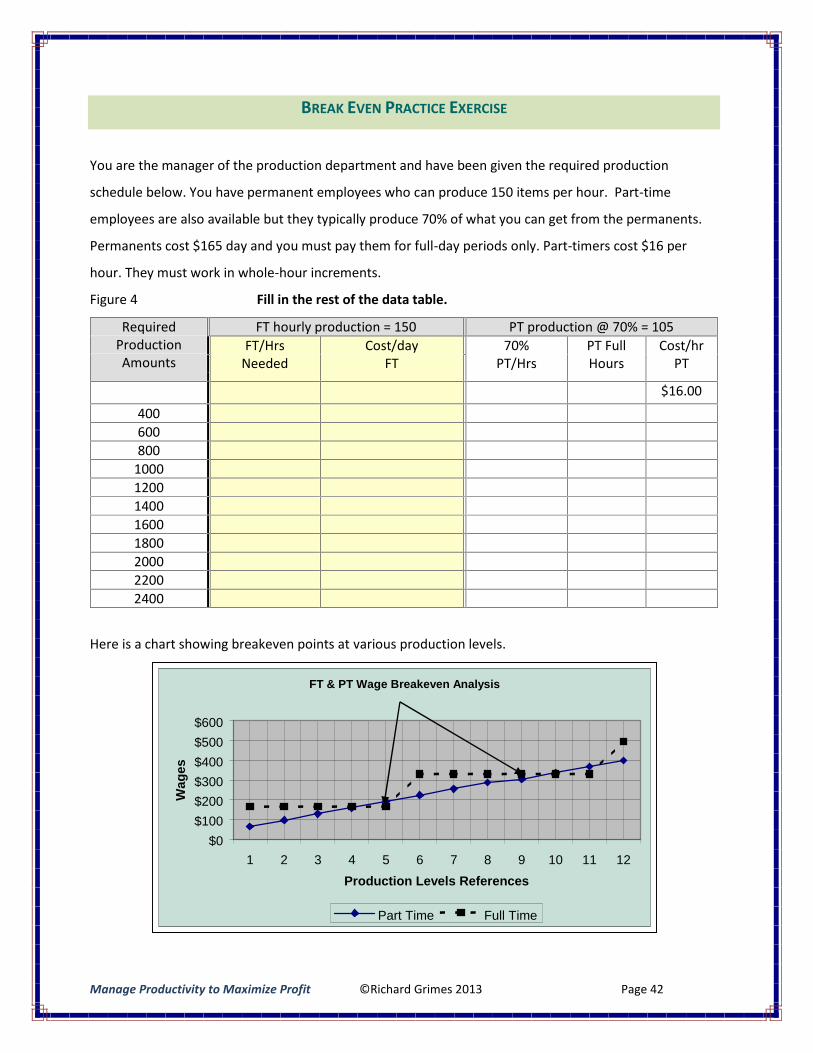
BREAK EVEN PRACTICE EXERCISE
You are the manager of the production department and have been given the required production
schedule below. You have permanent employees who can produce 150 items per hour. Part-time
employees are also available but they typically produce 70% of what you can get from the permanents.
Permanents cost $165 day and you must pay them for full-day periods only. Part-timers cost $16 per
hour. They must work in whole-hour increments.
Figure 4 Fill in the rest of the data table.
Here is a chart showing breakeven points at various production levels.
RequiredProductionAmounts
FT hourly production = 150 PT production @ 70% = 105FT/Hrs
NeededCost/day
FT70%
PT/HrsPT FullHours
Cost/hrPT
$16.00400600800
10001200140016001800200022002400
FT & PT Wage Breakeven Analysis
$0$100$200$300$400$500$600
1 2 3 4 5 6 7 8 9 10 11 12Production Levels References
Wag
es
Part Time Full Time
Manage Productivity to Maximize Profit ©Richard Grimes 2013 Page 43
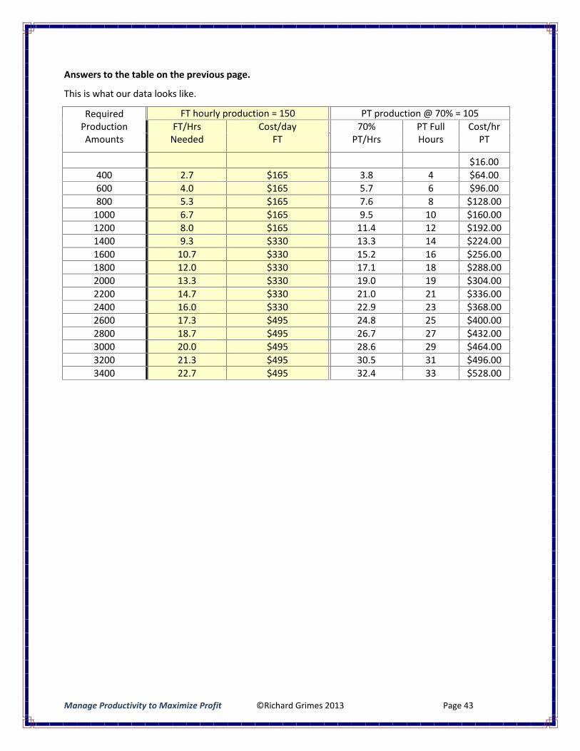
Answers to the table on the previous page.
This is what our data looks like.
RequiredProductionAmounts
FT hourly production = 150 PT production @ 70% = 105FT/Hrs
NeededCost/day
FT70%
PT/HrsPT FullHours
Cost/hrPT
$16.00400 2.7 $165 3.8 4 $64.00600 4.0 $165 5.7 6 $96.00800 5.3 $165 7.6 8 $128.00
1000 6.7 $165 9.5 10 $160.001200 8.0 $165 11.4 12 $192.001400 9.3 $330 13.3 14 $224.001600 10.7 $330 15.2 16 $256.001800 12.0 $330 17.1 18 $288.002000 13.3 $330 19.0 19 $304.002200 14.7 $330 21.0 21 $336.002400 16.0 $330 22.9 23 $368.002600 17.3 $495 24.8 25 $400.002800 18.7 $495 26.7 27 $432.003000 20.0 $495 28.6 29 $464.003200 21.3 $495 30.5 31 $496.003400 22.7 $495 32.4 33 $528.00
Manage Productivity to Maximize Profit ©Richard Grimes 2013 Page 44
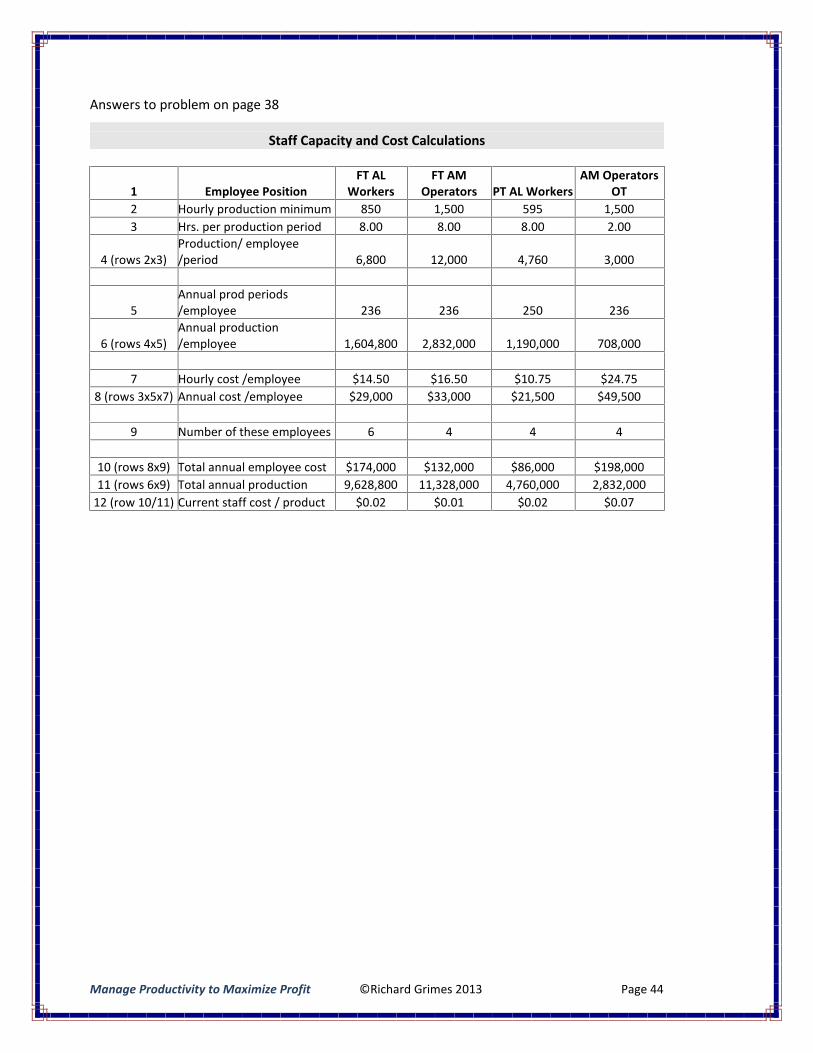
Answers to problem on page 38
Staff Capacity and Cost Calculations
1 Employee PositionFT AL
WorkersFT AM
Operators PT AL WorkersAM Operators
OT2 Hourly production minimum 850 1,500 595 1,5003 Hrs. per production period 8.00 8.00 8.00 2.00
4 (rows 2x3)Production/ employee/period 6,800 12,000 4,760 3,000
5Annual prod periods/employee 236 236 250 236
6 (rows 4x5)Annual production/employee 1,604,800 2,832,000 1,190,000 708,000
7 Hourly cost /employee $14.50 $16.50 $10.75 $24.758 (rows 3x5x7) Annual cost /employee $29,000 $33,000 $21,500 $49,500
9 Number of these employees 6 4 4 4
10 (rows 8x9) Total annual employee cost $174,000 $132,000 $86,000 $198,00011 (rows 6x9) Total annual production 9,628,800 11,328,000 4,760,000 2,832,000
12 (row 10/11) Current staff cost / product $0.02 $0.01 $0.02 $0.07
Manage Productivity to Maximize Profit ©Richard Grimes 2013 Page 45
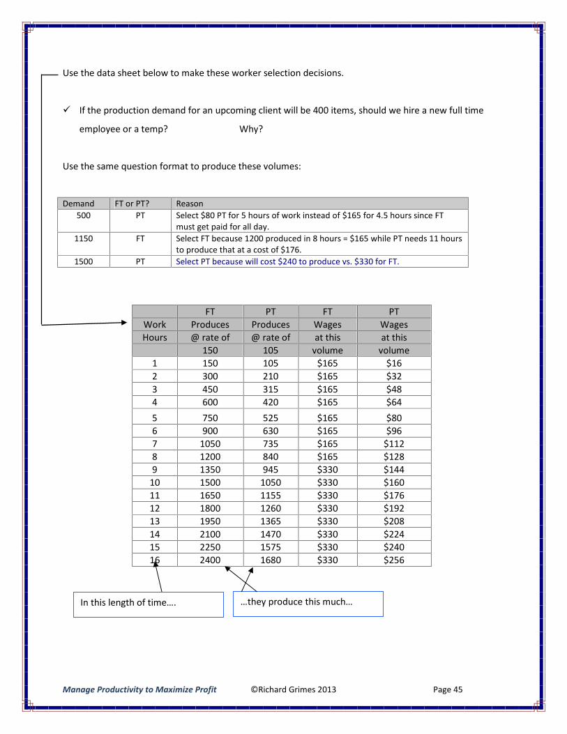
Use the data sheet below to make these worker selection decisions.
If the production demand for an upcoming client will be 400 items, should we hire a new full time
employee or a temp? Why?
Use the same question format to produce these volumes:
Demand FT or PT? Reason500 PT Select $80 PT for 5 hours of work instead of $165 for 4.5 hours since FT
must get paid for all day.1150 FT Select FT because 1200 produced in 8 hours = $165 while PT needs 11 hours
to produce that at a cost of $176.1500 PT Select PT because will cost $240 to produce vs. $330 for FT.
FT PT FT PTWork Produces Produces Wages WagesHours @ rate of @ rate of at this at this
150 105 volume volume1 150 105 $165 $162 300 210 $165 $323 450 315 $165 $484 600 420 $165 $645 750 525 $165 $806 900 630 $165 $967 1050 735 $165 $1128 1200 840 $165 $1289 1350 945 $330 $144
10 1500 1050 $330 $16011 1650 1155 $330 $17612 1800 1260 $330 $19213 1950 1365 $330 $20814 2100 1470 $330 $22415 2250 1575 $330 $24016 2400 1680 $330 $256
…they produce this much…In this length of time….
Manage Productivity to Maximize Profit ©Richard Grimes 2013 Page 46
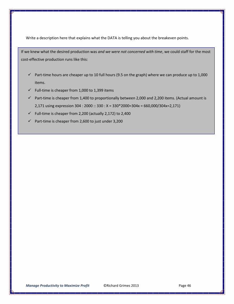
Write a description here that explains what the DATA is telling you about the breakeven points.
If we knew what the desired production was and we were not concerned with time, we could staff for the most
cost-effective production runs like this:
Part-time hours are cheaper up to 10 full hours (9.5 on the graph) where we can produce up to 1,000
items.
Full-time is cheaper from 1,000 to 1,399 items
Part-time is cheaper from 1,400 to proportionally between 2,000 and 2,200 items. (Actual amount is
2,171 using expression 304 : 2000 :: 330 : X = 330*2000=304x = 660,000/304x=2,171)
Full-time is cheaper from 2,200 (actually 2,172) to 2,400
Part-time is cheaper from 2,600 to just under 3,200
If we were concerned with time, then we would focus on that and not the costs.
Manage Productivity to Maximize Profit ©Richard Grimes 2013 Page 47
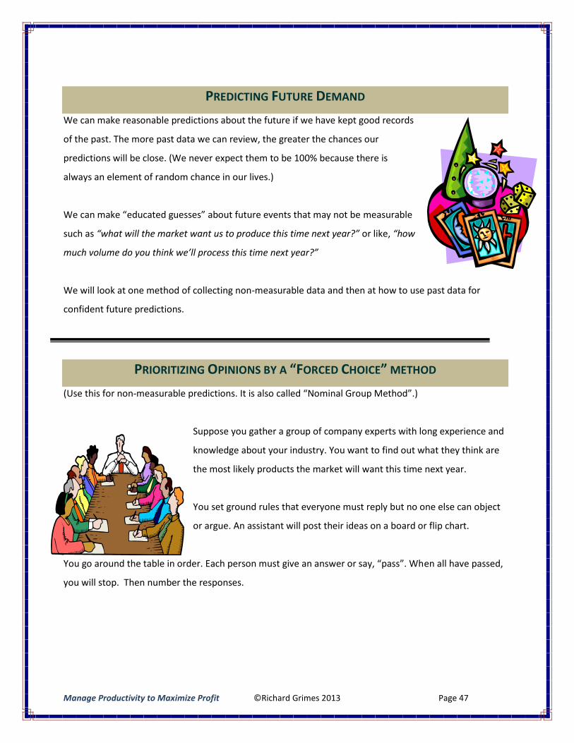
PREDICTING FUTURE DEMAND
We can make reasonable predictions about the future if we have kept good records
of the past. The more past data we can review, the greater the chances our
predictions will be close. (We never expect them to be 100% because there is
always an element of random chance in our lives.)
We can make “educated guesses” about future events that may not be measurable
such as “what will the market want us to produce this time next year?” or like, “how
much volume do you think we’ll process this time next year?”
We will look at one method of collecting non-measurable data and then at how to use past data for
confident future predictions.
PRIORITIZING OPINIONS BY A “FORCED CHOICE” METHOD
(Use this for non-measurable predictions. It is also called “Nominal Group Method”.)
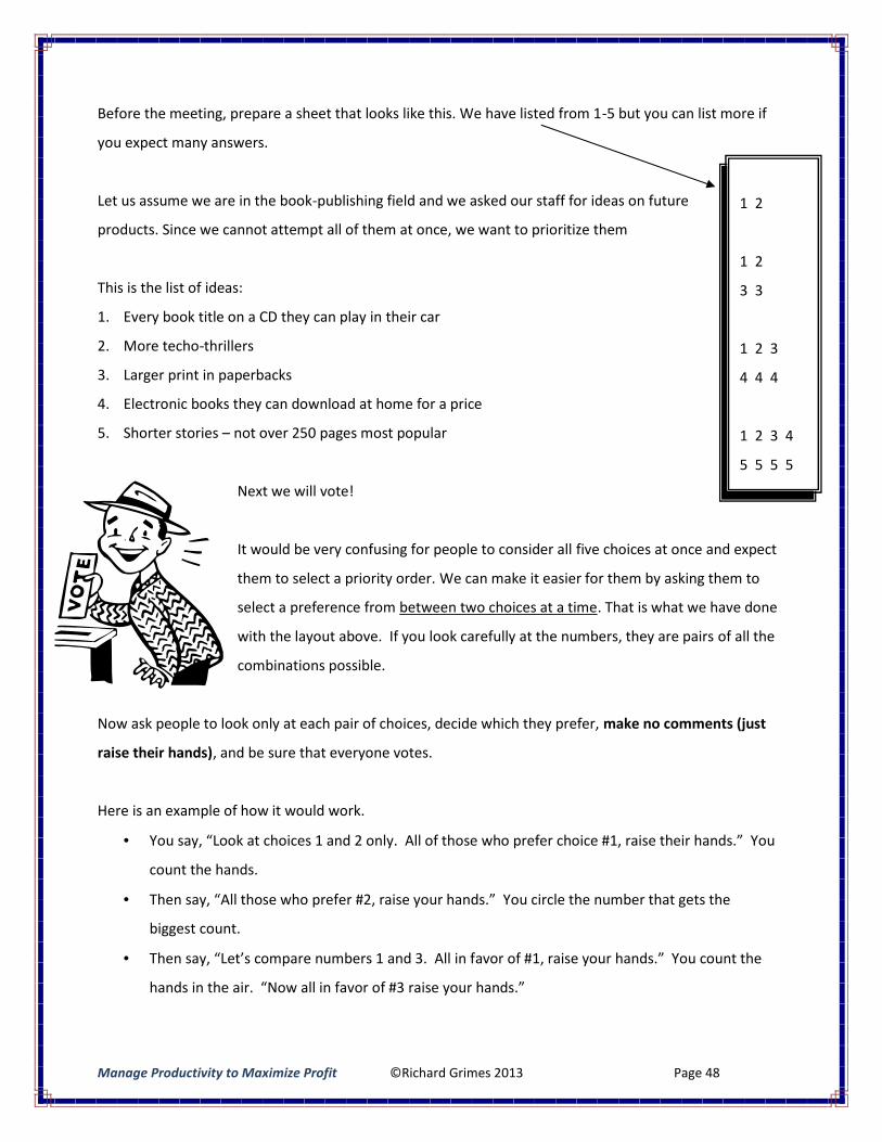
Suppose you gather a group of company experts with long experience and
knowledge about your industry. You want to find out what they think are
the most likely products the market will want this time next year.
You set ground rules that everyone must reply but no one else can object
or argue. An assistant will post their ideas on a board or flip chart.
You go around the table in order. Each person must give an answer or say, “pass”. When all have passed,
you will stop. Then number the responses.
Manage Productivity to Maximize Profit ©Richard Grimes 2013 Page 48
1 2
1 2
3 3
1 2 3
4 4 4
1 2 3 4
5 5 5 5
Before the meeting, prepare a sheet that looks like this. We have listed from 1-5 but you can list more if
you expect many answers.
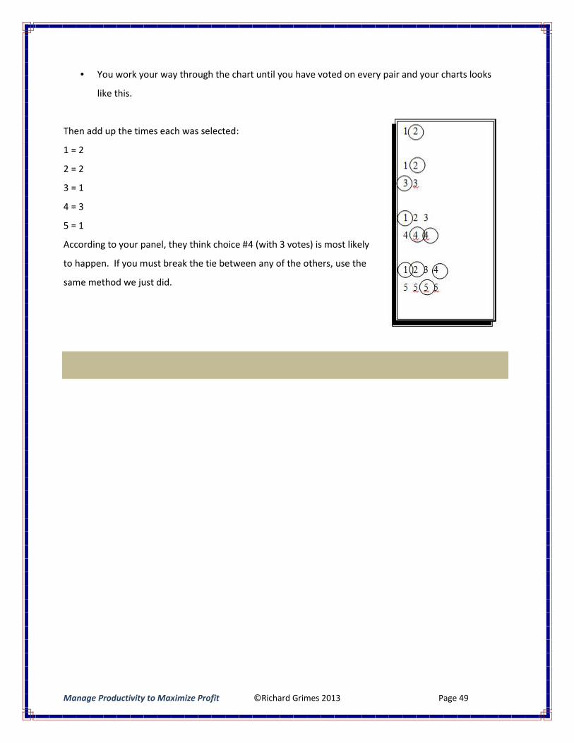
Let us assume we are in the book-publishing field and we asked our staff for ideas on future
products. Since we cannot attempt all of them at once, we want to prioritize them
This is the list of ideas:
1. Every book title on a CD they can play in their car
2. More techo-thrillers
3. Larger print in paperbacks
4. Electronic books they can download at home for a price
5. Shorter stories – not over 250 pages most popular
Next we will vote!
It would be very confusing for people to consider all five choices at once and expect
them to select a priority order. We can make it easier for them by asking them to
select a preference from between two choices at a time. That is what we have done
with the layout above. If you look carefully at the numbers, they are pairs of all the
combinations possible.
Now ask people to look only at each pair of choices, decide which they prefer, make no comments (just
raise their hands), and be sure that everyone votes.
Here is an example of how it would work.
You say, “Look at choices 1 and 2 only. All of those who prefer choice #1, raise their hands.” You
count the hands.
Then say, “All those who prefer #2, raise your hands.” You circle the number that gets the
biggest count.
Then say, “Let’s compare numbers 1 and 3. All in favor of #1, raise your hands.” You count the
hands in the air. “Now all in favor of #3 raise your hands.”
Manage Productivity to Maximize Profit ©Richard Grimes 2013 Page 49
You work your way through the chart until you have voted on every pair and your charts looks
like this.
Then add up the times each was selected:
1 = 2
2 = 2
3 = 1
4 = 3
5 = 1
According to your panel, they think choice #4 (with 3 votes) is most likely
to happen. If you must break the tie between any of the others, use the
same method we just did.
Manage Productivity to Maximize Profit ©Richard Grimes 2013 Page 50
MEASURABLE FORECASTING METHODS
We will look at some simple but powerful methods of predicting future
measurable trends.
Remember that measurable predictions are based on past data while non-
measurable predictions are usually “best guess” thoughts based on
experience and educated opinion.
We will look at four prediction methods and you will quickly understand
when to use each.
SIMPLE AVERAGE (“SA”)
This is what we used in grade school to determine how we would do on the
next report card.
Although the report card was in our future, it only told us about our past.
For example, if we received these scores on our weekly tests, 72, 84, 85, 88,
91, and 94 over the past six weeks, we would add them up (514), divide by 6
(the number of scores), and expect an average grade of 86 (85.66) on our
report card.
Look at our scores. Do you see a trend over the past six weeks? What is it? [Steadily increasing]
Grades over 6 weeks - simple average
7284 85 88 91 94
5060708090
100
1 2 3 4 5 6
Week Number
Tes
t Sc
ores
“86” average
Manage Productivity to Maximize Profit ©Richard Grimes 2013 Page 51
Predicting the 7th weekly grade
5060708090
100
1 2 3 4 5 6 7
Week Number
Test
Sco
res
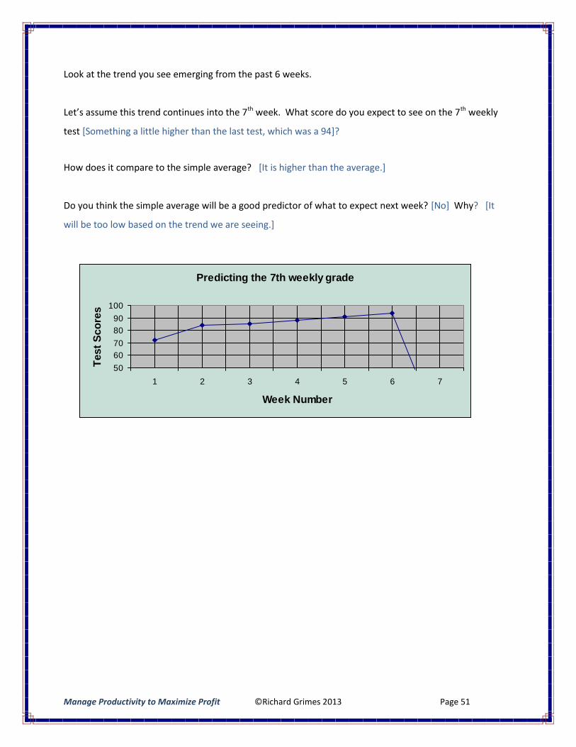
Look at the trend you see emerging from the past 6 weeks.
Let’s assume this trend continues into the 7th week. What score do you expect to see on the 7th weekly
test [Something a little higher than the last test, which was a 94]?
How does it compare to the simple average? [It is higher than the average.]
Do you think the simple average will be a good predictor of what to expect next week? [No] Why? [It
will be too low based on the trend we are seeing.]
Manage Productivity to Maximize Profit ©Richard Grimes 2013 Page 52
Predicting the 7th weekly grade
80
85
90
95
100
1 2 3 4 5 6 7
Week Number
Test
Sco
res
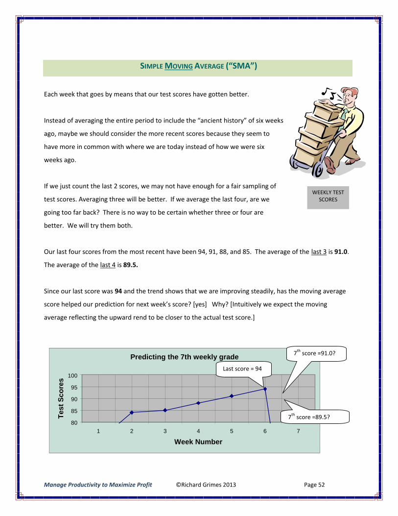
SIMPLE MOVING AVERAGE (“SMA”)
Each week that goes by means that our test scores have gotten better.
Instead of averaging the entire period to include the “ancient history” of six weeks
ago, maybe we should consider the more recent scores because they seem to
have more in common with where we are today instead of how we were six
weeks ago.
If we just count the last 2 scores, we may not have enough for a fair sampling of
test scores. Averaging three will be better. If we average the last four, are we
going too far back? There is no way to be certain whether three or four are
better. We will try them both.
Our last four scores from the most recent have been 94, 91, 88, and 85. The average of the last 3 is 91.0.
The average of the last 4 is 89.5.
Since our last score was 94 and the trend shows that we are improving steadily, has the moving average
score helped our prediction for next week’s score? [yes] Why? [Intuitively we expect the moving
average reflecting the upward rend to be closer to the actual test score.]
WEEKLY TESTSCORES
7th score =91.0?
Last score = 94
7th score =89.5?
Manage Productivity to Maximize Profit ©Richard Grimes 2013 Page 53
WEIGHTED MOVING AVERAGE (“WMA”)
We will leave the prediction about the 7th test grade alone for a few
minutes and recall another aspect of grade school, the dreaded
“SEMESTER PROJECT”.
The teacher would always say something like, “The semester project is
very important and your score on will be weighted 4 times as much (or
some amount that she decided) in relation to your test grades”.
This means that if you received a 93 on the semester project, she would
count it as four 93’s when she figured your semester grade.
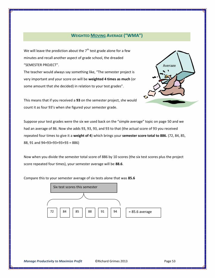
Suppose your test grades were the six we used back on the “simple average” topic on page 50 and we
had an average of 86. Now she adds 93, 93, 93, and 93 to that (the actual score of 93 you received
repeated four times to give it a weight of 4) which brings your semester score total to 886. (72, 84, 85,
88, 91 and 94+93+93+93+93 = 886)
Now when you divide the semester total score of 886 by 10 scores (the six test scores plus the project
score repeated four times), your semester average will be 88.6.
Compare this to your semester average of six tests alone that was 85.6
Six test scores this semester
72 84 85 88 91 94 = 85.6 average
Average
Manage Productivity to Maximize Profit ©Richard Grimes 2013 Page 54
Predicting the 7th weekly grade
80
85
90
95
100
1 2 3 4 5 6 7
Week Number
Test
Sco
res
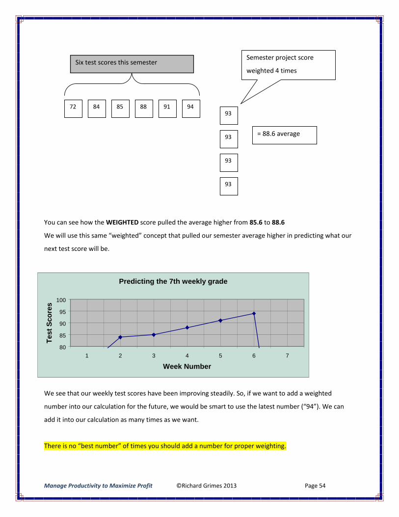
You can see how the WEIGHTED score pulled the average higher from 85.6 to 88.6
We will use this same “weighted” concept that pulled our semester average higher in predicting what our
next test score will be.
We see that our weekly test scores have been improving steadily. So, if we want to add a weighted
number into our calculation for the future, we would be smart to use the latest number (“94”). We can
add it into our calculation as many times as we want.
There is no “best number” of times you should add a number for proper weighting.
72 84 85 88 91 94
Six test scores this semester
93
93
93
93
= 88.6 average
Semester project score
weighted 4 times
Manage Productivity to Maximize Profit ©Richard Grimes 2013 Page 55
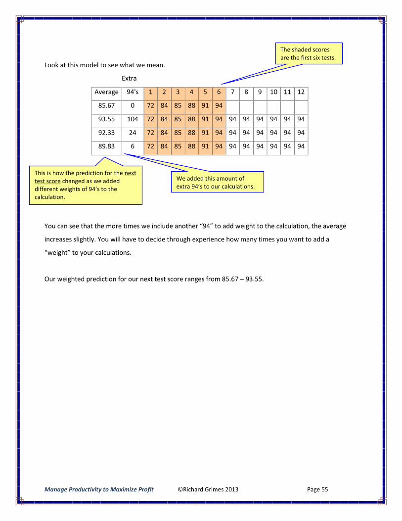
Look at this model to see what we mean.
Extra
Average 94's 1 2 3 4 5 6 7 8 9 10 11 12
85.67 0 72 84 85 88 91 94
93.55 104 72 84 85 88 91 94 94 94 94 94 94 94
92.33 24 72 84 85 88 91 94 94 94 94 94 94 94
89.83 6 72 84 85 88 91 94 94 94 94 94 94 94
You can see that the more times we include another “94” to add weight to the calculation, the average
increases slightly. You will have to decide through experience how many times you want to add a
“weight” to your calculations.
Our weighted prediction for our next test score ranges from 85.67 – 93.55.
We added this amount ofextra 94’s to our calculations.
The shaded scoresare the first six tests.
This is how the prediction for the nexttest score changed as we addeddifferent weights of 94’s to thecalculation.
Manage Productivity to Maximize Profit ©Richard Grimes 2013 Page 56
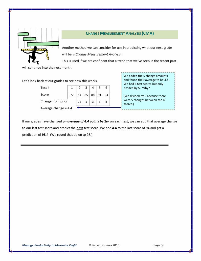
CHANGE MEASUREMENT ANALYSIS (CMA)
Another method we can consider for use in predicting what our next grade
will be is Change Measurement Analysis.
This is used if we are confident that a trend that we’ve seen in the recent past
will continue into the next month.
Let’s look back at our grades to see how this works.
Test # 1 2 3 4 5 6
Score 72 84 85 88 91 94
Change from prior 12 1 3 3 3
Average change = 4.4
If our grades have changed an average of 4.4 points better on each test, we can add that average change
to our last test score and predict the next test score. We add 4.4 to the last score of 94 and get a
prediction of 98.4. (We round that down to 98.)
We added the 5 change amountsand found their average to be 4.4.We had 6 test scores but onlydivided by 5. Why?
(We divided by 5 because therewere 5 changes between the 6scores.)
Manage Productivity to Maximize Profit ©Richard Grimes 2013 Page 57
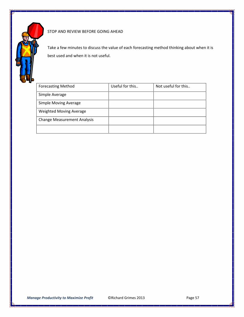
STOP AND REVIEW BEFORE GOING AHEAD
Take a few minutes to discuss the value of each forecasting method thinking about when it is
best used and when it is not useful.
Forecasting Method Useful for this.. Not useful for this..
Simple Average
Simple Moving Average
Weighted Moving Average
Change Measurement Analysis
Manage Productivity to Maximize Profit ©Richard Grimes 2013 Page 58
PREDICTING SEASONAL TRENDS
We look at predicting seasonal trends in a similar way that we look at predicting our next grade on a test.
We will use the holiday shopping season as an example.
Instead of looking at the previous months of this year to predict what kind of a holiday season we can
expect, we will look at the previous holiday seasons over the past few years to make a prediction.
There are conditions outside of our control, of course, such as the economy in general, the weather, and
possible shortages of a particular item that we must always consider in addition to the pure math data of
past seasons.
The point we want to make here is that we compare similar data when making a prediction of a future
measurable event. That is why we compare similar previous holiday seasons instead of previous months
on this year’s calendar.
Manage Productivity to Maximize Profit ©Richard Grimes 2013 Page 59
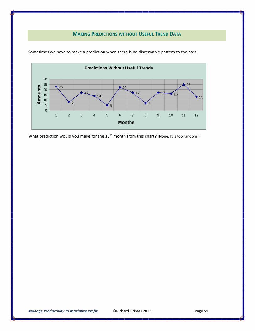
MAKING PREDICTIONS WITHOUT USEFUL TREND DATA
Sometimes we have to make a prediction when there is no discernable pattern to the past.
What prediction would you make for the 13th month from this chart? [None. It is too random!]
Predictions Without Useful Trends
23
8
1714
5
2217
7
17 16
25
13
05
1015202530
1 2 3 4 5 6 7 8 9 10 11 12
Months
Am
ount
s
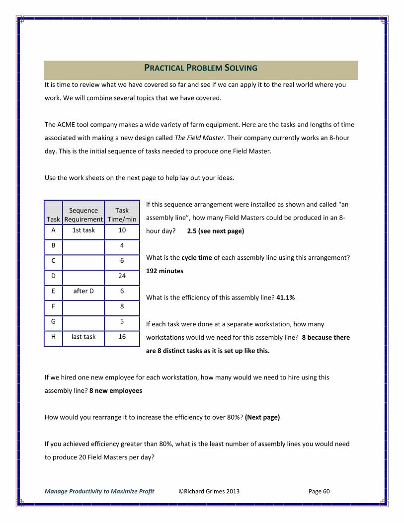
Manage Productivity to Maximize Profit ©Richard Grimes 2013 Page 60
PRACTICAL PROBLEM SOLVING
It is time to review what we have covered so far and see if we can apply it to the real world where you
work. We will combine several topics that we have covered.
The ACME tool company makes a wide variety of farm equipment. Here are the tasks and lengths of time
associated with making a new design called The Field Master. Their company currently works an 8-hour
day. This is the initial sequence of tasks needed to produce one Field Master.
Use the work sheets on the next page to help lay out your ideas.
If this sequence arrangement were installed as shown and called “an
assembly line”, how many Field Masters could be produced in an 8-
hour day? 2.5 (see next page)
What is the cycle time of each assembly line using this arrangement?
192 minutes
What is the efficiency of this assembly line? 41.1%
If each task were done at a separate workstation, how many
workstations would we need for this assembly line? 8 because there
are 8 distinct tasks as it is set up like this.
If we hired one new employee for each workstation, how many would we need to hire using this
assembly line? 8 new employees
How would you rearrange it to increase the efficiency to over 80%? (Next page)
If you achieved efficiency greater than 80%, what is the least number of assembly lines you would need
to produce 20 Field Masters per day?
TaskSequence
RequirementTask
Time/minA 1st task 10
B 4
C 6
D 24
E after D 6
F 8
G 5
H last task 16
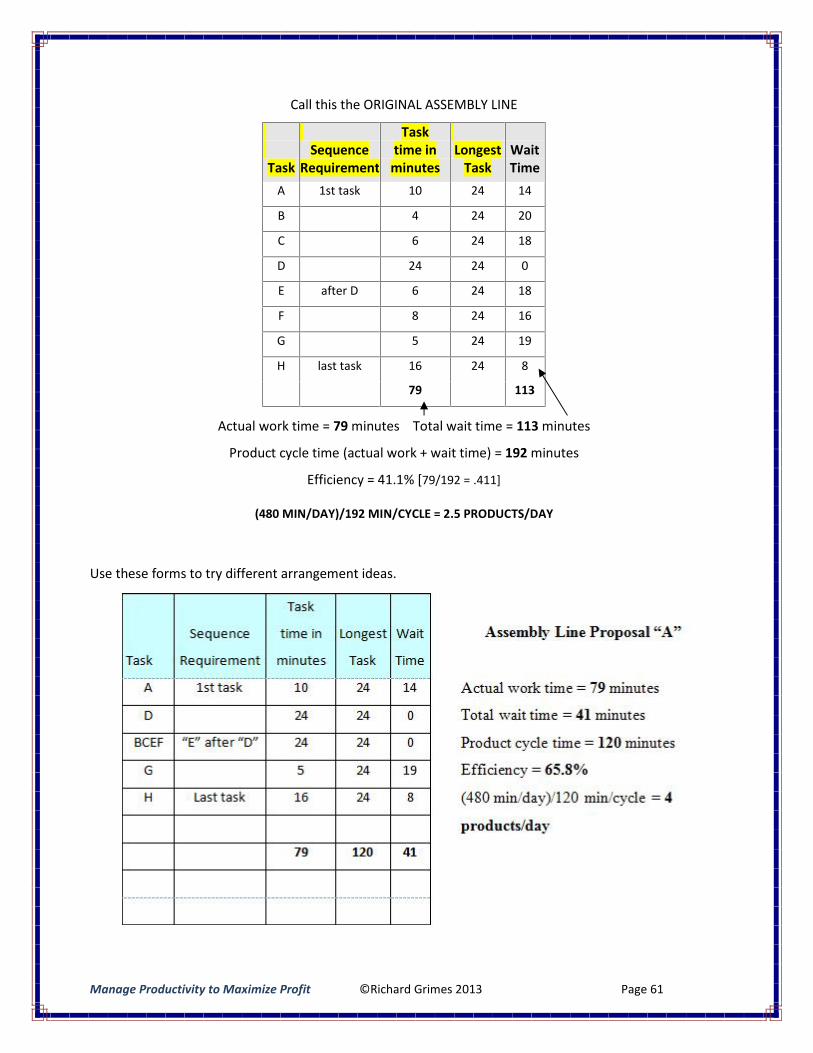
Manage Productivity to Maximize Profit ©Richard Grimes 2013 Page 61
Call this the ORIGINAL ASSEMBLY LINE
Actual work time = 79 minutes Total wait time = 113 minutes
Product cycle time (actual work + wait time) = 192 minutes
Efficiency = 41.1% [79/192 = .411]
(480 MIN/DAY)/192 MIN/CYCLE = 2.5 PRODUCTS/DAY
Use these forms to try different arrangement ideas.
TaskSequence
Requirement
Tasktime in
minutesLongest
TaskWaitTime
A 1st task 10 24 14
B 4 24 20
C 6 24 18
D 24 24 0
E after D 6 24 18
F 8 24 16
G 5 24 19
H last task 16 24 8
79 113
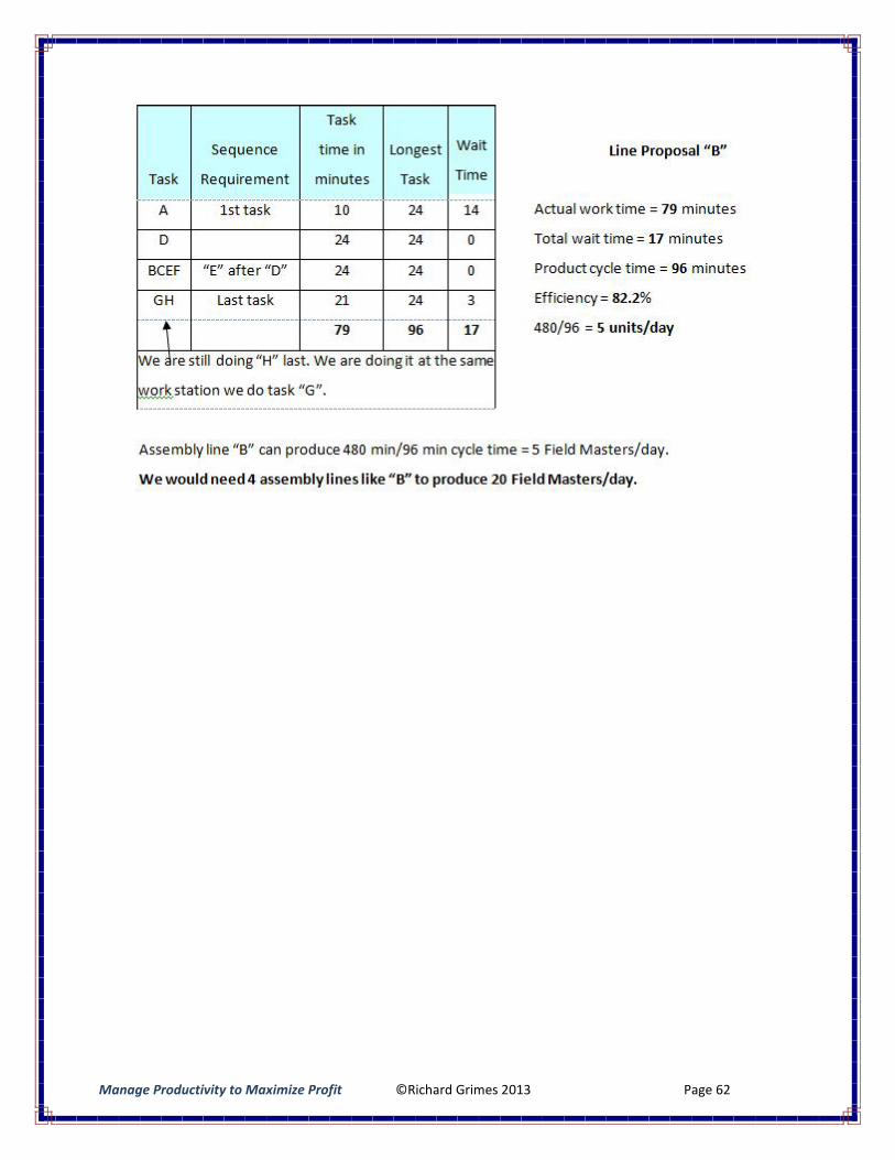
Manage Productivity to Maximize Profit ©Richard Grimes 2013 Page 62
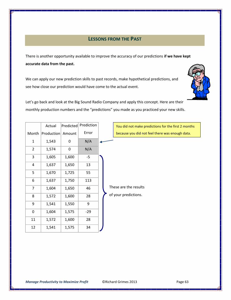
Manage Productivity to Maximize Profit ©Richard Grimes 2013 Page 63
LESSONS FROM THE PAST
There is another opportunity available to improve the accuracy of our predictions if we have kept
accurate data from the past.
We can apply our new prediction skills to past records, make hypothetical predictions, and
see how close our prediction would have come to the actual event.
Let’s go back and look at the Big Sound Radio Company and apply this concept. Here are their
monthly production numbers and the “predictions” you made as you practiced your new skills.
Month
Actual
Production
Predicted
Amount
Prediction
Error
1 1,543 0 N/A
2 1,574 0 N/A
3 1,605 1,600 -5
4 1,637 1,650 13
5 1,670 1,725 55
6 1,637 1,750 113
7 1,604 1,650 46
8 1,572 1,600 28
9 1,541 1,550 9
0 1,604 1,575 -29
11 1,572 1,600 28
12 1,541 1,575 34
These are the results
of your predictions.
You did not make predictions for the first 2 months
because you did not feel there was enough data.
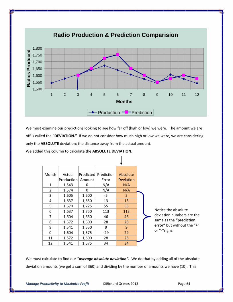
Manage Productivity to Maximize Profit ©Richard Grimes 2013 Page 64
We must examine our predictions looking to see how far off (high or low) we were. The amount we are
off is called the “DEVIATION.” If we do not consider how much high or low we were, we are considering
only the ABSOLUTE deviation; the distance away from the actual amount.
We added this column to calculate the ABSOLUTE DEVIATION.
We must calculate to find our “average absolute deviation”. We do that by adding all of the absolute
deviation amounts (we get a sum of 360) and dividing by the number of amounts we have (10). This
Month ActualProduction
PredictedAmount
PredictionError
AbsoluteDeviation
1 1,543 0 N/A N/A2 1,574 0 N/A N/A3 1,605 1,600 -5 54 1,637 1,650 13 135 1,670 1,725 55 556 1,637 1,750 113 1137 1,604 1,650 46 468 1,572 1,600 28 289 1,541 1,550 9 90 1,604 1,575 -29 29
11 1,572 1,600 28 2812 1,541 1,575 34 34
Radio Production & Prediction Comparision
1,500
1,550
1,600
1,650
1,700
1,750
1,800
1 2 3 4 5 6 7 8 9 10 11 12
Months
Rad
ios
Prod
uced
Production Prediction
Notice the absolutedeviation numbers are thesame as the “predictionerror” but without the “+”or “-“signs.
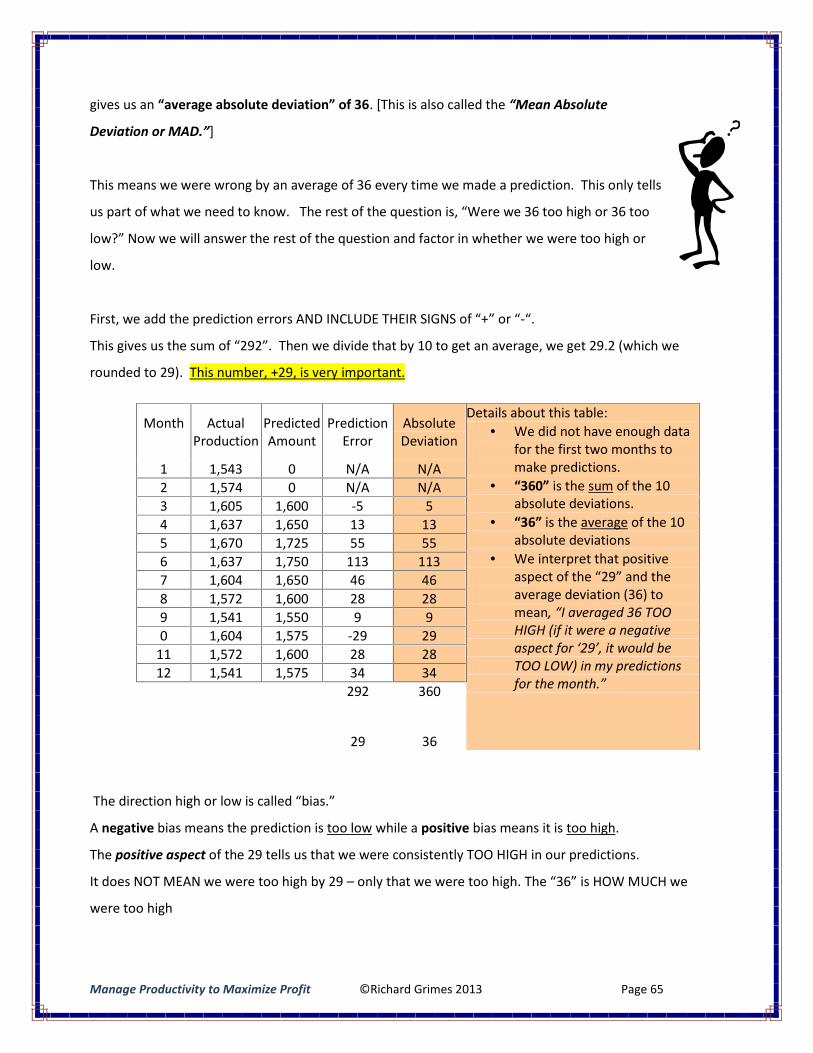
Manage Productivity to Maximize Profit ©Richard Grimes 2013 Page 65
gives us an “average absolute deviation” of 36. [This is also called the “Mean Absolute
Deviation or MAD.”]
This means we were wrong by an average of 36 every time we made a prediction. This only tells
us part of what we need to know. The rest of the question is, “Were we 36 too high or 36 too
low?” Now we will answer the rest of the question and factor in whether we were too high or
low.
First, we add the prediction errors AND INCLUDE THEIR SIGNS of “+” or “-“.
This gives us the sum of “292”. Then we divide that by 10 to get an average, we get 29.2 (which we
rounded to 29). This number, +29, is very important.
The direction high or low is called “bias.”
A negative bias means the prediction is too low while a positive bias means it is too high.
The positive aspect of the 29 tells us that we were consistently TOO HIGH in our predictions.
It does NOT MEAN we were too high by 29 – only that we were too high. The “36” is HOW MUCH we
were too high
Month ActualProduction
PredictedAmount
PredictionError
AbsoluteDeviation
Details about this table: We did not have enough data
for the first two months tomake predictions.
“360” is the sum of the 10absolute deviations.
“36” is the average of the 10absolute deviations
We interpret that positiveaspect of the “29” and theaverage deviation (36) tomean, “I averaged 36 TOOHIGH (if it were a negativeaspect for ‘29’, it would beTOO LOW) in my predictionsfor the month.”
1 1,543 0 N/A N/A2 1,574 0 N/A N/A3 1,605 1,600 -5 54 1,637 1,650 13 135 1,670 1,725 55 556 1,637 1,750 113 1137 1,604 1,650 46 468 1,572 1,600 28 289 1,541 1,550 9 90 1,604 1,575 -29 29
11 1,572 1,600 28 2812 1,541 1,575 34 34
292 360
29 36
Manage Productivity to Maximize Profit ©Richard Grimes 2013 Page 66
Review these terms and describe a situation where you would use them.
Simple Average [Finding the average of all sales prices of homes in a geographic area]
Simple Moving Average [Going back in three year increments to see if housing sales have
increased over a period of time in a geographic area.]
Weighted Moving Average [Giving more weight to most recent sales to predict near future sales
prices]
Change Measurement Analysis (If we can measure a steady change in sales prices, we can add
that change to the current year’s average and get a good prediction for next year.)
Using MAD and bias (MAD tells us the magnitude of error – bias tells us the direction high or low)
Nominal Group Method (Get most ideas from a group of people in a short time)
Which of these measuring methods are most responsive for making predictions when the past
has been steadily increasing or decreasing? (Change measurement analysis)
When the past has not been a steady trend either up or down? (None is good for random
events.)
Related Documents